A Neural Network model in stereovision matching

Pergamon

o893-6o8o(95)o~17-s

Neural Networks, Vol. 8, No. 5, pp. 805-813, 1995 Copyright © 1995 Elsevier Science Ltd

Printed in USA. All fights reserved 0893~/080/95 $9.50+ .00

CONTRIBUTED ARTICLE

A Neural Network Model in Stereovision Matching

JESOS M. CRUZ, 1 GONZALO PAJARES 2 AND JOAQUiN ARANDA 2

t Dpto. Informfitica y Autom/Rica, Facultad de CC Fisicas, U. Complutens¢, and 2Dpto. Inform/Ltica y Autom~tica, Facultad CC Fisicas, UNED

(Received 26 August 1994; accepted 9 January 1995)

Abstract--The paper outlines a method for solving the stereovision matching problem through a Neural Network approach based on self-organizing technique. The goal is to classify pairs of features (edge segments) as true or false matches; giving rise to two classes. Thus, the corresponding parameter vector from two component density fanctions, representing both classes and drawn as Normal densities, are to be estimated by using an unsupervised learning method. A three layer neural network topology implements the mixture denMty fanction and Bayes's rule, all required computations are realized with the simple "'sam of product'" units commonly used in connectionist models. The unsupervised learning method leads to a learning rule, while all applicable constraints from stereovision field yield an activation rule. A training process receives the samples to learn, and a matching process classifies the pairs. The method is illustrated with two images from an indoor scene.

Keywords--Neural Network, Unsupervised learning, Training, Stereovision, Matching, Self-organizing, Bayes strategy, Probability density function.

1. INTRODUCTION

This paper follows Specht (1990a, b) and Traven (1991) topology models and presents a three-layer Neural Network approach to the stereopsis correspondence problem, in which a pattern classification technique using unsupervised learning process is to be embedded, as in Duda and Hart (1973), Traven (1991), Morasso et al. (1993) or Kosko (1992).

A major portion of research efforts by the computer vision community has been directed towards the study of the three-dimensional (3-D) structure of objects using machine analysis of images Dhond and Aggarwal (1989). The analysis of video images in stereo has emerged as an important passive method for extracting the 3-D structure of a scene.

The basic principle involved in the recovery of depth using passive imaging is triangulation. In stereopsis triangulation needs to be achieved with the help of only the existing environmental illumina-

Acknowledgements: The authors wish to acknowledge Dr. S. Dormido, Head of Department of Infonn~tica y Autom~tica, CC Fisicas, LrNED, Madrid, for his support and encouragement. Part of this work has been performed under project CICYT TAP94- 0832-C02-01.

Requests for reprints should be sent to Prof. Jesfis M. de la Cruz, Dpto. Infornuitica y Automfitica, Facultad Ciencias Fisicas, Universidad Complutense, 28040 Madrid, Spain.

805

tion. Hence, a correspondence needs to be established between features from two images that correspond to some physical feature in space. Provided then, that the position of centers of projection, the effective local length, the orientation of the optical axis, and the sampling interval of each camera are known, the depth can be established using triangulation as drawn in Fu, Gonzfilez and Lee (1988).

Following the Barnard and Fischler (1982) terminology, we can view the problem of stereo analysis as consisting of the following steps: image acquisition, camera modeling, feature acquisition, image matching, depth determination and interpolation. The key step is that of image matching, that is, the process of identifying the corresponding points in two images that are cast by the same physical point in 3-D space. This paper is devoted solely to this problem. The matching is made difficult in part by changes in the images of the corresponding points due to different view points. The amount of change is dependent on the stereo angle.

Two types of techniques have been broadly used for stereo matching, Medioni and Nevatia (1985), area-based and feature-based. Area-based stereo techniques use correlation between brightness (intensity) patterns in the local neighborhood of a pixel in one image with brightness patterns in the local neighborhood in the other image, Grimson

806 J. M. Cruz, G. Pajares and J. Aranda

(1985), Khotanzad, Bokil and Lee (1993), Kim and Aggarwal (1987), Lutsiv and Novikova (1992), Marr et al. (1976, 1979, 1980, 1982), Rubio (1993) and Zhou and Chellappa (1982), where the number of possible matches becomes high, while feature-based methods use sets of pixels with similar attributes (edges), Ayache and Faverjon (1987), Hoff and Ahuja (1989), Kim, Choi and Park (1992), Medioni and Nevatia (1985) and Pajares et al. (1993). As shown in Medioni and Nevatia (1985), these latter methods lead to a sparse depth map only, leaving the rest of the surface to be reconstructed by interpolation; but they are faster than area-based methods, because there are many fewer points (features) to be considered. This research paper will use a feature- based method where edge segments are to be matched. Thus five attributes (module and direction gradient average, variance average, Laplace average and length) are to be computed for each edge segment.

Previous Neural Net approaches to stereopsis have been developed; the Marr-Poggio Cooperative Algorithm, Marr et al. (1976, 1979, 1982), can be regarded as a crude neural network approach with no embedded learning. Lutsiv and Novikova (1992) propose an exact neural implementation of the Marr-Poggio algorithm. A rather different approach is to formulate the correspondence problem as an optimization task followed by utilization of a neural net to perform the optimization. This is the approach taken by Nasrabadi and Choo (1992). O'Toole (1989) proposes a computational model to get the structure from stereo that develops smooth- ness constraints naturally by associative learning of a large number of examples of mappings from disparity data to surface depth data. This model computes local depth changes from point to point across the image, rather than finding absolute depth at these points. Thus, computation outputs are local and stringing them together yields a global perception. In Khotanzad, Bokil, and Lee (1993), two multilayer feed-forward nets are used to learn the mapping that retains correct matches between pixels. None of the typical constraints, such as uniqueness and continuity, are explicitly imposed, and all the applicable constraints are learned. The back-propagation learning rule and a training set are applied. Zhou and Chellappa (1992) propose an energy-minimization process in which the stereo matching problem is reformulated as a problem of minimizing an error function.

The research papers referred to above use area- based methods. In this paper a new view point is taken. A feature-based technique is implemented through a three-layer (input, hidden, output) neural network approach with the same topology as the one used in the Specht (1990a, b) and Traven (1991)

models. Thus, the stereovision correspondence problem is formulated as a pattern classification problem and an unsupervised learning rule must be incorporated. The learning rule uses the linear differential competitive learning law described in Kosko (1992), Duda and Hart (1973), Traven (1991), Morasso et al. (1993) and Hsieh and Chen (1993). The resulting neural network implements a mixture density function, Duda and Hart (1973). The hidden layer is the most important one, as it activates or inhibits its own neurons according to a winner and loser concept as described in Sacristan, Valderama, and Prrez-Vicente (1993), that leads to a lateral connection as in the Morasso model, Morasso et al. (1993).

A training process with embedded unsupervised learning and a streovision correspondence with feature matching are involved.

This paper is organized as follows: in Section 2 the stereovision correspondence problem is formulated as a pattern classification problem in which a multivariate mixture problem will be considered. Next, a derivation of the stochastic gradient descent procedure for solving it is presented by Duda and Hart (1973), Morasso et al. (1993) and Traven (1991); this procedure will be the learning rule. The relationship to artificial Neural Networks is described explicitly in Section 3. The performance of the method in a couple of four-dimensional density functions are illustrated in Section 4. Finally in Section 5, there is a discussion of some related topics.

2. THE STEREOVISION CORRESPONDENCE PROBLEM AS A PATTERN CLASSIFICATION

PROBLEM

From two images, left and right, a number of features are to be extracted. Here, we will extract edge segments. Five attributes are also to be computed from each edge segment (module and direction gradient, Laplacian, variance and length). Then a pair of edge segments from the left and right images will be matched, and a similarity measure must be defined. A difference in attributes will always be involved, in order to decide if such a pair is a True or False correspondence. Therefore, all pairs of features can be classified as true or false matches. The stereovision correspondence problem is now formulated as a pattern classification problem with two associated classes, w r as True and wF as False correspondences. A pair of edge segments is the sample to be classified as belonging to one of the classes, wr or wF, where, as it will be seen later, wr is playing the role of master while wr is playing the role of slave. A difference measurement vector, x, computed as a difference of attributes values for each segment, is associated with a pair. We must

Neural Network in Stereovision 807

clarify which pairs of features are to be classified as false correspondences. I f a pair is not classified as a True correspondence, it will be a False one, and therefore we will be the set complementary to wr. The problem should be restricted to classifying all pairs as belonging or not belonging to the wr class, rendering we unnecessary from here on. However, in stereovision the major problem is ambiguity, where a pair is really a false match, but the difference vector is not enough to take a clear decision. Feature pairs whose associated difference vector allows them to be classified without any doubt as false matches are to be discarded and rejected during the training process. The neural network must have the capability of rejecting such correspondences in order to exclude them, and therefore a lateral-connection between the T and F neurons is to be established, as seen below. The we class could be renamed Semi-False correspondences, but it will be referred to as False correspondences.

Assume x = {Xm, Xd, Xt, Xv} is a four-dimensional difference measurement vector, where its components are the corresponding differences for gradient module and direction, as computed in Leu and Yau (1991), and Laplacian and variance are computed as in Krotkov (1989).

Let x be a vector. The goal is to compute its associated probabilities in order to classify it as belonging to the wr or wF class. To do that, we start with an unlabeled set of samples, and therefore will be an unsupervised learning method.

2.1. Finite Mixture of Multivariate Densities

Following Duda and Har t (1973), we start by assuming that we know the complete probability structure for the problem with the sole exception of the values of some parameters. To be more specific, we make the following assumptions:

(1) The samples come from two known classes, wr and WF

(2) The a priori probabilities P ( w r ) and P(WF) are known. They are computed from the overlap rate: a segment from the left image and a segment from the right image overlap if by sliding one of them in a horizontal direction they are made to intersect, Medioni and Nevati (1985). The overlap rate is computed as a probability from the associated lengths. Such probabilities will be complementaries.

(3) The forms for the class-conditional probability densities p(x/wj, 6j) are known, j = T, F. With- out loss of generality, we suppose such densities function as normal densities, where 6j = (#j, Ej), with /z and E are the mean vector and the covariance matrix, respectively.

(4) All that is unknown are the values for the parameter vector #j, Ej.

Samples are assumed to be obtained by selecting a class Wy with probability P(wj) and then selecting an x according to the probability law p(x/wy, 6j) = N(x/wy, I% Ej). Thus, the probability density function for the samples is given by:

p(xlS) = ~ pCxlwj, 8j)e(wj) (1) j=F, T

A density function of this form is called a mixture density. The conditional densities probabilities p(x/wj , 6j) are the component densities, and the a priori probabilities P(wj) are the mixing parameters Duda and Har t (1973). Our basic goal will be to use samples drawn from this mixture density to estimate the unknown parameter vector 6. Once 6 is known, we can break the mixture down into its components. Then, when a difference vector x associated with a pair of features is presented to the neural network as an input, the pair will be classified as belonging to either the wr of the wF class, in accordance with network processing. An unsupervised learning approach is the key step to computing the unknown parameter vector 6. That will also be the learning rule during the network training process, as will be seen in the next section.

The unsupervised learning process is solved by the Maximum Likelihood approach in Duda and Hart (1973), Traven (1991), Hsieh and Chert (1993) and Juan and Vidal (1994). Another possible solution includes unsupervised Bayesian learning, as in Duda and Hart (1973), but this is beyond the scope of this work.

2.2. Maximum Likelihood Estimates

Suppose now, that we are given a set X = { x l , . . . , xn} of n unlabeled samples drawn independently from the mixture density eqn (1). The likelihood of the observed samples is by definition, Edwards (1972), the joint density:

p(XIr) = ~ p(xklr). (2) k = l

The maximum likelihood estimate is that value of 6 = (#, r,) that maximizes p(X/6). See Duda and Har t (1973) for an exhaustive treatment where all parameters to be estimated are uknown. Here, for greater ease, we only reproduce the resulting equations for the local-maximum-likelihood estimates #i, Ei, and P(wi), eqn (3)-(6).


1 n

P(w,) =- ~ i'(w, lxk, ~) /I k = |

~,_ E:=, P(w, lxk, $)xj, EL, P(w, lx~, ~)

Y]i =

n ^ E."(w~lxk, $)(xk - a,)(x~ - ~)' k=l

E:=, PCw, lx~, ~,)

(3)

P(w, lxk, ~) =

1~,l-'/2 e,~[-½ Cxk - ~,) '~; '(xk- ~,)] P(wi)

(4)

(5)

(6)

The hat symbol in the above equations indicate estimates, /zi is the mean and Ei is the covariance matrix. The system consisting of eqns (3)-(6) can be solved by iterative methods. In Traven (1991) a stochastic gradient descent solution that avoids singular solutions is exhaustively analyzed (see also Hsieh & Chen (1993) and Morasso et al. (1993)).

2.3 S tochas t i c Gradient Descen t So lu t ion

The expressions for #i and I:i in eqn (4) and eqn (5) are both of the form,

O~v = ~"]~k~l P (WIxk)O( xk) (7) N E~=, p(wlx~)

With an amount of algebraic manipulation, a recursive expression can be obtained as follows (see Traven (1991) for exhaustive treatment):

0s+t = 0M + ~ + , [0(xs÷l) - 0~];

with

p(wlx#+l) p(wlxN+l) (8) I"]N+I - - ~"~N+I ( S ~ - 1 ) p ( w ) " z_.k=l / , ( w l x k )

We can now specify explicit time update equations for both parameters, # and E, where the new value is obtained by adding to the old value a fraction of the difference between the sample and the old value. This will be the learning rule during network training, as we can see in the next section.

3. FEED-FORWARD ARTIFICIAL NEURAL NETWORK TOPOLOGY

The network topology is based on Specht (1990a, b), where a probabilistic neural network implementing a Parzen (1962) window is proposed, but only the model is to be used here.

As mentioned before, our basic goal will be to use unlabeled samples drawn from the mixture density eqn (1) to estimate the unknown parameter vector through eqns (3)-(6) leading to eqn (8). Once ~ is known, the mixture density function can be broken down into its components. Then, when a difference vector x associated with a pair of features is presented as an input to the neural network, it will be classified as belonging to either the wr or the wF class, in accordance with network processing. We can imagine the two component densities as playing the role of hidden categories from which we want to infer the true or false match.

The network is characterized by (i) a connection rule, (ii) an activation rule, and (iii) a learning rule, as defined in Morasso et al. (1993).

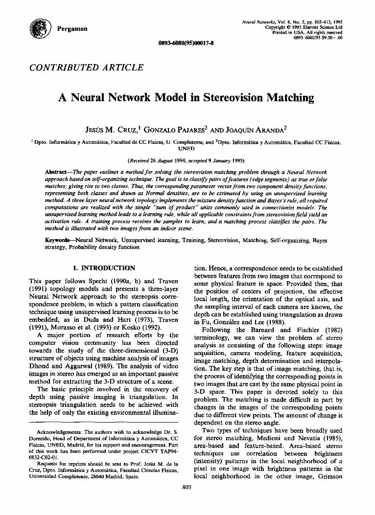
Responsibility for the connection rule is held by the three-layer network topology, shown in Figure 1. The network has" an input layer, a hidden layer and an output layer. An input layer consists of four neurons that are mere distribution units, Specht (1990a, b). They supply the input component values

I

DIFFERENCE COMPONENT MIXTURE C L R S S

VECTOR DENS IT IES DENS IT Y

x p ( x I ~ t , 6 t ) p ( x 16)

FIGURE 1. Organization for classification of edge segment pairs as true or false matches.


FIGURE 2. Diagram of training and matching procedures.

f rom a four-dimensional x input vector. Since there are two component densities in the mixture density function (1), the hidden layer has two neurons, named (T, F), associated with the wr and the wF pattern classes. Each hidden neuron receives, via its four connection synapses, the four x vector components and the corresponding attached mean vector #, the latter as an associated weight vector learned during the training process. Then each neuron computes a bounded output signal according to the general multivariate density component function eqn (9), Bendat and Piersol (1971). This generalized Gaussian output signal function defines the potential or radial basis function for the input activation vector x = (Xm, xa, xt, xv)eR 4, the covariance matrix ~, and the mean vector #i = ( # / , #~, #J, #~). Each radial basis function defines a spherical receptive field at R 4. The T or F neuron emits unity, or near unity, signals for any input activation vector x that fails in its receptive field. The mean vector /z centers the receptive field at R 4. The covariance matrix is a localization measure for it.

As we can see, the nonlinear operation used here is the function given by eqn (9), instead of the sigmoid activation function commonly used for back-propagation, Hush and H o m e (1992).

threshold (t2'), the T hidden neuron is inhibited but excites the F neuron, and finally, if the value is smaller than this second threshold, both neurons are inhibited and the considered pair of features is rejected, as it is clearly a false match and no additional computations are needed. From eqn (9), it is clear that the probability density function p(x /wi , 6i) is large when the embedded squared Mahalanobis distance, Duda and Hart (1973) dM= (Xk--[Li)t~'~l(xk--I~i) is small, so, in accordance with this criterion, the four-dimensional x difference vector whole space can be partitioned into three disjoint classes with two concentric hyper- spheres centered in the null vector and radii tl (inner hyper-sphere) and t2 (outer hyper-sphere). When the master neuron is activated, the x input difference vector falls into the inner hyper-sphere region, class war, but if the slave neuron is now activated, the corresponding x input difference vector falls into a region bounded by the inner and outer hyper-spheres, class wr, and when any neuron is activated, the x

, [, -.,,] v(~lw,, 6,) 47r2[~,ii/2 exp -~ ( x - - p , ) t ~ [ ' ( x

(9)

The output layer has a unique summation neuron that receives the two outputs from the hidden layer, with the associated a priori probabilities P(wj) as synapse weights. Lateral connection is also required, since it is needed during the activation process described below.

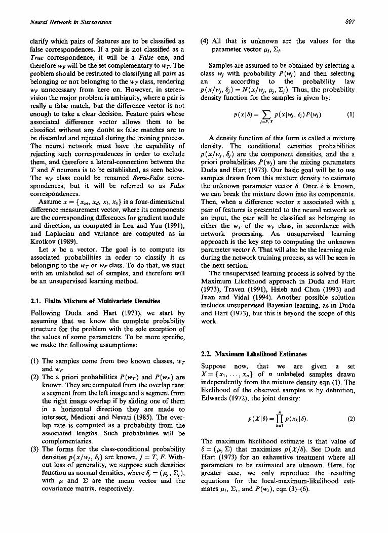
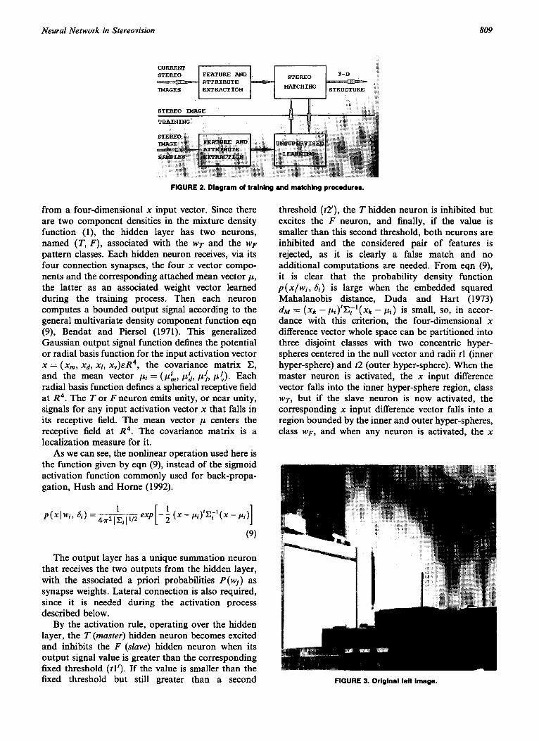
By the activation rule, operating over the hidden layer, the T (master) hidden neuron becomes excited and inhibits the F (slave) hidden neuron when its output signal value is greater than the corresponding fixed threshold (tl ') . If the value is smaller than the fixed threshold but still greater than a second FIGURE 3. Original left image.


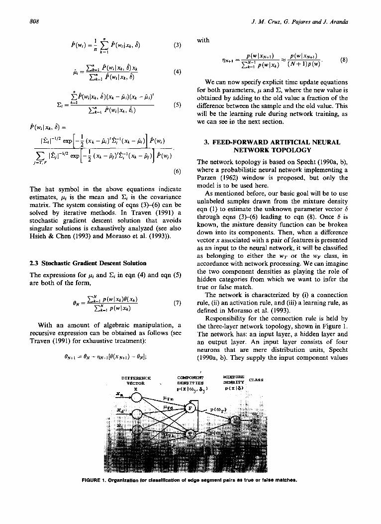
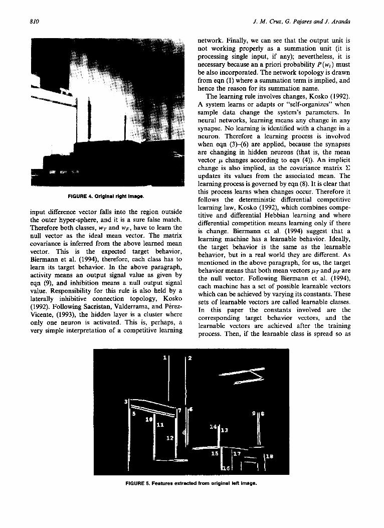
FIGURE 4. Original right Image.

input difference vector falls into the region outside the outer hyper-sphere, and it is a sure false match. Therefore both classes, wr and we, have to learn the null vector as the ideal mean vector. The matrix covariance is inferred from the above learned mean vector. This is the expected target behavior, Biermann et al. (1994), therefore, each class has to learn its target behavior. In the above paragraph, activity means an output signal value as given by eqn (9), and inhibition means a null output signal value. Responsibility for this rule is also held by a laterally inhibitive connection topology, Kosko (1992). Following Sacristan, Valderrama, and Prrez- Vicente, (1993), the hidden layer is a cluster where only one neuron is activated. This is, perhaps, a very simple interpretation of a competitive learning

network. Finally, we can see that the output unit is not working properly as a summation unit (it is processing single input, if any); nevertheless, it is necessary because an a priori probability P(wi) must be also incorporated. The network topology is drawn from eqn (1) where a summation term is implied, and hence the reason for its summation name.

The learning rule involves changes, Kosko (1992). A system learns or adapts or "self-organizes" when sample data change the system's parameters. In neural networks, learning means any change in any synapse. No learning is identified with a change in a neuron. Therefore a learning process is involved when eqn (3)-(6) are applied, because the synapses are changing in hidden neurons (that is, the mean vector # changes according to eqn (4)). An implicit change is also implied, as the covariance matrix updates its values from the associated mean. The learning process is governed by eqn (8). It is clear that this process learns when changes occur. Therefore it follows the deterministic differential competitive learning law, Kosko (1992), which combines competitive and differential Hebbian learning and where differential competition means learning only if there is change. Biermann et al. (1994) suggest that a learning machine has a learnable behavior. Ideally, the target behavior is the same as the learnable behavior, but in a real world they are different. As mentioned in the above paragraph, for us, the target behavior means that both mean vectors # r and #V are the null vector. Following Biermann et al. (1994), each machine has a set of possible learnable vectors which can be achieved by varying its constants. These sets of learnable vectors are called learnable classes. In this paper the constants involved are the corresponding target behavior vectors, and the learnable vectors are achieved after the training process. Then, if the learnable class is spread so as

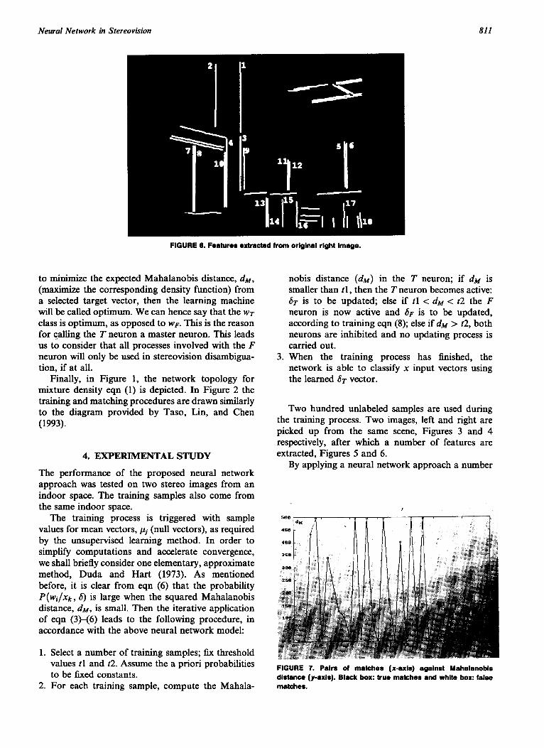
FIGURE 5. Features extracted from original left image.


1 I I 1 1 12 Ii' I_,,

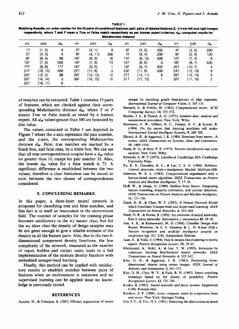
FIGURE 6. Features extracted from original right image.

to minimize the expected Mahalanobis distance, dM, (maximize the corresponding density function) from a selected target vector, then the learning machine will be called optimum. We can hence say that the wr class is optimum, as opposed to wF. This is the reason for calling the T neuron a master neuron. This leads us to consider that all processes involved with the F neuron will only be used in stereovision disamhigua- tion, if at all.

Finally, in Figure 1, the network topology for mixture density eqn (1) is depicted. In Figure 2 the training and matching procedures are drawn similarly to the diagram provided by Taso, Lin, and Chen (1993).

4. EXPERIMENTAL STUDY

The performance of the proposed neural network approach was tested on two stereo images from an indoor space. The training samples also come from the same indoor space.

The training process is triggered with sample values for mean vectors, #j (null vectors), as required by the unsupervised learning method. In order to simplify computations and accelerate convergence, we shall briefly consider one elementary, approximate method, Duda and Hart (1973). As mentioned before, it is clear from eqn (6) that the probability P(wi/xk, 6) is large when the squared Mahalanobis distance, dM, is small. Then the iterative application of eqn (3)-(6) leads to the following procedure, in accordance with the above neural network model:

1. Select a number of training samples; fix threshold values tl and t2. Assume the a priori probabilities to be fixed constants.

2. For each training sample, compute the Mahala-

.

nobis distance (dM) in the T neuron; if dM is smaller than tl, then the T neuron becomes active: 6r is to be updated; else if tl < dM < t2 the F neuron is now active and 6F is to be updated, according to training eqn (8); else if dM > t2, both neurons are inhibited and no updating process is carried out. When the training process has finished, the network is able to classify x input vectors using the learned 6r vector.

Two hundred unlabeled samples are used during the training process. Two images, left and right are picked up from the same scene, Figures 3 and 4 respectively, after which a number of features are extracted, Figures 5 and 6.

By applying a neural network approach a number

FIGURE 7. Pairs of matches (x-axis) against Mahalanobis distance (y-axis). Black box: true matches end white box: false matches.


TABLE 1 Matching Results; on: order number for Ihe 33 pairs of considered features; pair: pairs of labeled features (I, r) from left and right images

respectively, where T and F mean a True or False match respectively as par human expert criterion; dM: computed results for Mahalanobis distance

on pair dM on pair dM on pair dM on pair dM

1T (1, 2) 6 2T (2, 1) 0 3F (2, 5) 435 4F (3, 6) 500 5T (4, 3) 6 6F (4, 11) 336 7F (5, 4) 230 8F (5, 9) 126 9F (6, 4) 98 lOT (6, 9) 16 11F (6, 10) 500 12T (7, 4) 8

13F (7, 6) 500 14F (7, 9) 73 15T (8, 6) 3 16F (8, 7) 500 17F (8, 8) 177 18T (9, 5) 1 19F (9, 7) 402 20T (10, 7) 4 21F (10, 10) 500 22T (11, 8) 3 23F (11, 9) 500 24T (12, 10) 9 25F (12, 3) 98 26T (13, 12) 12 27T (14, 11) 9 28T (15, 13) 5 29T (16, 14) 3 30F (16, 15) 12 31T (17, 15) 1 32F (17, 16) 2 33T (18, 17) 6

o f ma tches can be extracted. Tab le 1 con ta ins 33 pa i r s o f fea tures , which are checked agains t thei r cor re- s p o n d i n g M a h a l a n o b i s d is tance dM, where T o r F means T r u e or False m a t c h as tested by a h u m a n exper t . Al l dM values grea te r t han 500 are b o u n d e d by this value.

The va lues con ta ined in Table 1 are dep ic ted in F igu re 7 where the x-axis represents the pa i r number , a n d the y-axis , the co r r e spond ing M a h a l a n o b i s d i s tance dM. Here , t rue matches are m a r k e d by a b l ack box , and false ones, by a white box. W e can see tha t all t rue cor respondences couples have a d ~ va lue no g rea te r t han 16, except for pa i r n u m b e r 32. Also , the lowest dM value for a false m a t c h is 73. A signif icant difference is es tabl i shed be tween the two values; therefore a c lear l imi ta t ion can be s ta ted to exist be tween the two classes o f co r re spondences cons idered .

5. C O N C L U D I N G REMARKS

In this pape r , a three- layer neural n e t w o r k is p r o p o s e d for classifying true and false matches , and this fact is in i tself an i nnova t ion in the s te reovis ion field. The n u m b e r o f samples for the t ra in ing phase becomes sa t i s fac tory in the w r m a s t e r class, b u t for the WF s lave c lass the dens i ty o f design samples m a y be n o t g rea t enough to give a rel iable es t imate o f the dens i ty in al l the fea ture pairs . Also, due to the two 4- d i m e n s i o n a l c o m p o n e n t densi ty funct ions , the low com plex i t y o f the ne twork , measured as the n u m b e r o f inpu t , h idden and o u t p u t units , leads to a full i m p l e m e n t a t i o n o f the mix ture densi ty func t ion wi th e m b e d d e d unsuperv ised learning.

F ina l ly , this m e t h o d can be app l ied wi th sat isfac- t o ry resul ts to es tabl ish matches between pa i r s o f fea tures when an env i ronmen t is u n k n o w n and no superv ised learn ing can be app l ied since no k n o w - ledge is p rev ious ly s tored.

REFERENCES

Ayache, N., & Faberjon, B. (1987) Efficient registration of stereo

images by matching graph descriptions of edge segments. International Journal of Computer Vision, 1, 107-131.

Barnard, S., & Fishier, M. (1982). Computational stereo. ACM Computing Surveys, 14, 553-572.

Bendat, J. S., & Piersol, A. G. (1971). Random data: analysis and measurement procedures. New York: Wiley.

Biermann, A. W., Gilbert, K. C., Fahmy, A. F., & Koster, B. (1994). On the errors that learning machines will make. International Journal Intelligent Systems, 9, 269-302.

Dhond, A. R., & Aggarwal, J. K. (1989). Structure from stereo---A review. IEEE Transactions on Systems, Man, and Cybernetics, 19, 1489-1510.

Duda, R. O., & Hart, P. E. (1973). Pattern classification andscene analysis. New York: Wiley.

Edwards, A. W. F. (1972). Likelihood. Cambridge, MA: Cambridge University Press.

Fu, K. S., Gonzailez, R. C., & Lee, C. S. G. (1988). Rob6tica: Control, deteccirn, visirn e inteligencia. Madrid: McGraw-Hill.

Grimson, W. E. L. (1985). Computational experiments with a feature-based stereo algorithm. IEEE Transactions on Pattern Analysis and Machine Intelligence, 7, 17-34.

Hoff, W., & Ahuja, N. (1989). Surface from Stereo: Integrating feature matching, disparity estimation, and contour detection. IEEE Transactions on Pattern Analysis and Machine Inteligence, 11, 121-136.

Hsieh, K. R., & Chert, W. T. (1993). A Neural Network Model which Combines Unsupervised and Supervised Learning. IEEE Transactions on Neural Networks, 4, 357-360.

Hush, D. R., & Home, B. (1992). An overview of neural networks, Part I: static networks, lnforrruitica y Automdtica 25, 19-36.

Jain, A. K., & Ramaswami, M. D. (1988). Classifier Design with Parzen Windows. In E. S. Geisema & L. N. Kanal (Eds.), Pattern recognition and artificial intelligence towards an integration (pp. 211-218). Amsterdam: Elsevier.

Juan, A., & Vidal, E. (1994). Fast K-means-like clustering in metric spaces. Pattern Recognition Letters, 15, 19-25.

Khotanzad, A., Bokil, A., & Lee, Y. W. (1993). Stereopsis by constraint learning feed-forward neural networks. 1EEE Transactions on Neural Networks, 4, 332-342.

Kim, D. H., & Aggarwal, J. K. (1987). Positioning three- dimensional objects using stereo images. IEEE Journal of Robotics and Automation, 3, 361-373.

Kim, D. H., Choi, W. Y., & Park, R. H. (1992). Stereo matching technique based on the theory of possibility. Pattern Recognition Letters, 13, 735-744.

Kosko, B. (1992). Neural networks and fuzzy systems. Englewood Cliffs: Prentice-Hall.

Krotkov, E. P. (1989). Active computer vision by cooperative focus and stereo. New York: Springer-Verlag.

Leu, J. G , & Yau, H. L. (1991). Detecting the dislocations in metal


crystals from microscope images. Pattern Recognition, 24, 41- 56.

Lutsiv, V. R., & Novikova, T. A. (1992). On the use of a neurocomputer for stereoimage processing. Pattern Recognition and Image Analysis, 2, 441 ~ .

M a r l D. (1982). Vision. San Francisco: Freeman. M a r l D., & Hildreth, E. (1980). Theory of edge detection.

Proceedings Royal Society of London, B207, 187-217. Marr, D., & Poggio, T. (1979). A computational theory of human

stereovision. Proceedings Royal Society of London, B207, 301- 328.

M a r l D., & Poggio, T. (1976). Cooperative computation of stereo disparity. Science, 194, 283-287.

Medioni, G., & Nevatia, R. (1985). Segment based stereo matching. Computer Vision, Graphics, and Image Processing, 31, 2-18.

Morasso, P., Barberis, L., Pagliano, S., & Vergano, D. (1993). Recognition experiments of cursive dynamic handwriting self- organizing networks. Pattern Recognition, 26, 451-460.

Nasrabadi, N. M., & Choo, C. Y. (1992). Hopfield; network for stereovision correspondence. IEEE Transactions on Neural Networks, 3, 123-125.

O'Toole, A. J. (1989). Structure from stereo by associative learning of the constraints. Perception, 18, 767-782.

Pajares, G., Pereira, R., Rives, J., & Diaz, J. A. (1993). Correspondencia difusa en visi6n estereosc6pica. In Barro, S., & Sobrino, A. (Eds.), I l l Congreso Espwiol sabre Tecnologias y I_,Jgica Fuzzy (pp. 303-310). Santiago de Compostela: Dpto. Electronica Computacion.

Parzen, E. (1962). On estimation of a probability density function and mode. Annals of Mathematieul Statistics, 33, 1065-1076.

Rubio, P. (1993). RP: un algoritmo eficiente para la bdsqueda de correspondencias en visibn estereoscbpica. Informdtica y Autonu~tica, 26, 5-15.

Sacrist/m, A., Valderrama, E., & P6rez-Vicente, C. (1993). Criterio de la medida de estabilidad para redes de aprendizaje competitivo, lnformdtica y Automfltica, 26, 28-36.

Specht, D. F. (1990a). Probabilistic neural networks. Neural Networks, 3, 109-118.

Specht, D. F. (1990b). Probabilistic neural networks and the polynomial adaiine as complementary techniques for classification. IEEE Transactions on Neural Networks, 1, 111-121.

Traven, H. G. C. (1991). A neural network approach to statistical pattern classification by semiparametric estimation of probability density functions. IEEE Transactions-Neural Networks, 2, 366-377.

Tsao, E. C. K., Lin, W. C., & Chen, C. T. (1993). Constraint satisfaction neural networks for image recognition. Pattern Recognition, 26, 553-567.

x

Xm, Xd, XI, Xv

P(wj) #j

Pro, Izd , ftl , Pv

r,j

= r,j)

pCx/wj,

N(xlwj, pj, ~j)

norN

X xj

0

~7

R 4

NOMENCLATURE

jth class of correspondences (True, False) 4-dimensional diffcrcncc measurement vector components of x (gradient modulc, gradicnt direction, laplace and variance) a priori probability mean vector representing the jth class components of p (gradient module, gradient dircction, Laplace and variance) covariancc matrix representing the jth class parameter vector rcprcscnting the jth class (to bc cstimatcd) probability of x given wj and 6j unknown Normal probability of x given wj and 6j unknown probability of x given number of unlabeled training sam- plcs sct of n unlabclcd samples jth clement of X joint density gcncric symbol for representing p and fraction of the difference bctwccn thc sample and the old value estimate of a 4-dimensional space

Documents

A Neural Network model in stereovision matching