Embed Size (px)
Citation preview

IMAGE MATCHING TECHNIQUES
Template matchingFrom Wikipedia, the free encyclopedia
Template matching[1] is a technique in digital image processing for finding small parts of an image which match a template image. It can be used in manufacturing as a part of quality control,[2] a way to navigate a mobile robot,[3] or as a way to detect edges in images.[4]
Contents 1 Approach 2 Feature-based approach 3 Template-based approach 4 Motion tracking and occlusion handling 5 Template-based matching and convolution 6 Implementation 7 Speeding up the Process 8 Improving the accuracy of the matching 9 Similar Methods 10 Examples of Use 11 See also 12 References 13 External links
Approach
This section is empty. You can help by adding to it. (March 2013)
Feature-based approachIf the template image has strong features, a feature-based approach may be considered; the approach may prove further useful if the match in the search image might be transformed in some fashion. [5] [6]
Template-based approachFor templates without strong features, or for when the bulk of the template image constitutes the matching image, a template-based approach may be effective. As aforementioned, since template-based template matching may potentially require sampling of a large number of points, it is possible to reduce the number of sampling points by reducing the resolution of the search and template images by the same factor and performing the operation on the resultant downsized

images (multiresolution, or Pyramid (image processing)), providing a search window of data points within the search image so that the template does not have to search every viable data point, or a combination of both.
Motion tracking and occlusion handlingIn instances where the template may not provide a direct match, it may be useful to implement the use of eigenspaces – templates that detail the matching object under a number of different conditions, such as varying perspectives, illuminations, color contrasts, or acceptable matching object “poses”.[7] For example, if the user was looking for a face, the eigenspaces may consist of images (templates) of faces in different positions to the camera, in different lighting conditions, or with different expressions.
It is also possible for the matching image to be obscured, or occluded by an object; in these cases, it is unreasonable to provide a multitude of templates to cover each possible occlusion. For example, the search image may be a playing card, and in some of the search images, the card is obscured by the fingers of someone holding the card, or by another card on top of it, or any object in front of the camera for that matter. In cases where the object is malleable or poseable, motion also becomes a problem, and problems involving both motion and occlusion become ambiguous.[8] In these cases, one possible solution is to divide the template image into multiple sub-images and perform matching on each subdivision.
Template-based matching and convolutionA basic method of template matching uses a convolution mask (template), tailored to a specific feature of the search image, which we want to detect. This technique can be easily performed on grey images or edge images. The convolution output will be highest at places where the image structure matches the mask structure, where large image values get multiplied by large mask values.
This method is normally implemented by first picking out a part of the search image to use as a template: We will call the search image S(x, y), where (x, y) represent the coordinates of each pixel in the search image. We will call the template T(x t, y t), where (xt, yt) represent the coordinates of each pixel in the template. We then simply move the center (or the origin) of the template T(x t, y t) over each (x, y) point in the search image and calculate the sum of products between the coefficients in S(x, y) and T(xt, yt) over the whole area spanned by the template. As all possible positions of the template with respect to the search image are considered, the position with the highest score is the best position. This method is sometimes referred to as 'Linear Spatial Filtering' and the template is called a filter mask.
For example, one way to handle translation problems on images, using template matching is to compare the intensities of the pixels, using the SAD (Sum of absolute differences) measure.

A pixel in the search image with coordinates (xs, ys) has intensity Is(xs, ys) and a pixel in the template with coordinates (xt, yt) has intensity It(xt, yt ). Thus the absolute difference in the pixel intensities is defined as Diff(xs, ys, x t, y t) = | Is(xs, ys) – It(x t, y t) |.
The mathematical representation of the idea about looping through the pixels in the search image as we translate the origin of the template at every pixel and take the SAD measure is the following:
Srows and Scols denote the rows and the columns of the search image and Trows and Tcols denote the rows and the columns of the template image, respectively. In this method the lowest SAD score gives the estimate for the best position of template within the search image. The method is simple to implement and understand, but it is one of the slowest methods.
ImplementationIn this simple implementation, it is assumed that the above described method is applied on grey images: This is why Grey is used as pixel intensity. The final position in this implementation gives the top left location for where the template image best matches the search image.
minSAD = VALUE_MAX;
// loop through the search imagefor ( int x = 0; x <= S_rows - T_rows; x++ ) { for ( int y = 0; y <= S_cols - T_cols; y++ ) { SAD = 0.0;
// loop through the template image
for ( int j = 0; j < T_cols; j++ ) for ( int i = 0; i < T_rows; i++ ) {
pixel p_SearchIMG = S[x+i][y+j]; pixel p_TemplateIMG = T[i][j];
SAD += abs( p_SearchIMG.Grey - p_TemplateIMG.Grey ); } // save the best found position if ( minSAD > SAD ) { minSAD = SAD; // give me min SAD

position.bestRow = x; position.bestCol = y; position.bestSAD = SAD; } }}
One way to perform template matching on color images is to decompose the pixels into their color components and measure the quality of match between the color template and search image using the sum of the SAD computed for each color separately.
Speeding up the ProcessIn the past, this type of spatial filtering was normally only used in dedicated hardware solutions because of the computational complexity of the operation,[9] however we can lessen this complexity by filtering it in the frequency domain of the image, referred to as 'frequency domain filtering,' this is done through the use of the convolution theorem.
Another way of speeding up the matching process is through the use of an image pyramid. This is a series of images, at different scales, which are formed by repeatedly filtering and subsampling the original image in order to generate a sequence of reduced resolution images.[10] These lower resolution images can then be searched for the template (with a similarly reduced resolution), in order to yield possible start positions for searching at the larger scales. The larger images can then be searched in a small window around the start position to find the best template location.
Other methods can handle problems such as translation, scale, image rotation and even all affine transformations.[11][12][13]
Improving the accuracy of the matchingImprovements can be made to the matching method by using more than one template (eigenspaces), these other templates can have different scales and rotations.
It is also possible to improve the accuracy of the matching method by hybridizing the feature-based and template-based approaches.[14] Naturally, this requires that the search and template images have features that are apparent enough to support feature matching.
Similar MethodsOther methods which are similar include 'Stereo matching', 'Image registration' and 'Scale-invariant feature transform'.
Examples of Use

Template matching has various applications and is used in such fields as face recognition (see facial recognition system) and medical image processing. Systems have been developed and used in the past to count the number of faces that walk across part of a bridge within a certain amount of time. Other systems include automated calcified nodule detection within digital chest X-rays.[15] Recently, this method was implemented in geostatistical simulation which could provide a fast algorithm.[16]
See also Facial recognition system Pattern recognition Computer vision Elastic Matching
References1. R. Brunelli, Template Matching Techniques in Computer Vision: Theory and Practice,
Wiley, ISBN 978-0-470-51706-2, 2009 ([1] TM book)2. Aksoy, M. S., O. Torkul, and I. H. Cedimoglu. "An industrial visual inspection system
that uses inductive learning." Journal of Intelligent Manufacturing 15.4 (August 2004): 569(6). Expanded Academic ASAP. Thomson Gale.
3. Kyriacou, Theocharis, Guido Bugmann, and Stanislao Lauria. "Vision-based urban navigation procedures for verbally instructed robots." Robotics and Autonomous Systems 51.1 (April 30, 2005): 69-80. Expanded Academic ASAP. Thomson Gale.
4. WANG, CHING YANG, Ph.D. "EDGE DETECTION USING TEMPLATE MATCHING (IMAGE PROCESSING, THRESHOLD LOGIC, ANALYSIS, FILTERS)". Duke University, 1985, 288 pages; AAT 8523046
5. Li, Yuhai, L. Jian, T. Jinwen, X. Honbo. “A fast rotated template matching based on point feature.” Proceedings of the SPIE 6043 (2005): 453-459. MIPPR 2005: SAR and Multispectral Image Processing.
6. B. Sirmacek, C. Unsalan. “Urban Area and Building Detection Using SIFT Keypoints and Graph Theory”, IEEE Transactions on Geoscience and Remote Sensing, Vol.47 (4), pp. 1156-1167, April 2009.
7. Luis A. Mateos, Dan Shao and Walter G. Kropatsch. Expanding Irregular Graph Pyramid for an Approaching Object. CIARP 2009: 885-891.
8. F. Jurie and M. Dhome. Real time robust template matching. In British Machine Vision Conference, pages 123–131, 2002.
9. Gonzalez, R, Woods, R, Eddins, S "Digital Image Processing using Matlab" Prentice Hall, 2004
10. E. H. Adelson, C. H. Anderson, J. R. Bergen, P. J. Burt and J. M. Ogden, Pyramid methods in image processing http://web.mit.edu/persci/people/adelson/pub_pdfs/RCA84.pdf
11. Yuan, Po, M.S.E.E. "Translation, scale, rotation and threshold invariant pattern recognition system". The University of Texas at Dallas, 1993, 62 pages; AAT EP13780

12. H. Y. Kim and S. A. Araújo, "Grayscale Template-Matching Invariant to Rotation, Scale, Translation, Brightness and Contrast," IEEE Pacific-Rim Symposium on Image and Video Technology, Lecture Notes in Computer Science, vol. 4872, pp. 100-113, 2007.
13. Korman S., Reichman D., Tsur G. and Avidan S., "FAsT-Match: Fast Affine Template Matching", CVPR2013.
14. C. T. Yuen, M. Rizon, W. S. San, and T. C. Seong. “Facial Features for Template Matching Based Face Recognition.” American J. of Engineering and Applied Sciences 3 (1): 899-903, 2010.
15. Ashley Aberneithy. "Automatic Detection of Calcified Nodules of Patients with Tuberculous". University College London, 2007
16. Tahmasebi, P., Hezarkhani, A., Sahimi, M., 2012, Multiple-point geostatistical modeling based on the cross-correlation functions, Computational Geosciences, 16(3):779-79742.
External links Template Matching in OpenCV Visual Object Recognition using Template Matching Rotation, scale, translation-invariant template matching demonstration program perspective-invariant template matching
Categories:
Image processing
Navigation menu Not logged in Talk Contributions Create account Log in
Article Talk
Read Edit View history
Main page Contents Featured content Current events Random article Donate to Wikipedia

Wikipedia store
Interaction
Help About Wikipedia Community portal Recent changes Contact page
Tools
What links here Related changes Upload file Special pages Permanent link Page information Wikidata item Cite this page
Print/export
Create a book Download as PDF Printable version
Languages
Italiano 日本語
Edit links
This page was last modified on 23 December 2015, at 09:46. Text is available under the Creative Commons Attribution-ShareAlike License;
additional terms may apply. By using this site, you agree to the Terms of Use and Privacy Policy. Wikipedia® is a registered trademark of the Wikimedia Foundation, Inc., a non-profit organization.
Privacy policy About Wikipedia Disclaimers Contact Wikipedia Developers Cookie statement

Mobile view
OpenCV-Python Tutorials latest
OpenCV-Python Tutorials o Introduction to OpenCV o Gui Features in OpenCV o Core Operations o Image Processing in OpenCV
Changing Colorspaces Image Thresholding Geometric Transformations of Images Smoothing Images Morphological Transformations Image Gradients Canny Edge Detection Image Pyramids Contours in OpenCV Histograms in OpenCV Image Transforms in OpenCV Template Matching
Goals

Theory Template Matching in OpenCV Template Matching with Multiple Objects Additional Resources Exercises
Hough Line Transform Hough Circle Transform Image Segmentation with Watershed Algorithm Interactive Foreground Extraction using GrabCut Algorithm
o Feature Detection and Description o Video Analysis o Camera Calibration and 3D Reconstruction o Machine Learning o Computational Photography o Object Detection o OpenCV-Python Bindings
Love Documentation? Come to the Write the Docs 2016 conference in Portland.
Docs » OpenCV-Python Tutorials » Image Processing in OpenCV » Template Matching Edit on GitHub

http://opencv-pythontutroals.readthedocs.org/en/latest/py_tutorials/py_imgproc/py_template_matching/py_template_matching.html
Template Matching
GoalsIn this chapter, you will learn
To find objects in an image using Template Matching You will see these functions : cv2.matchTemplate(), cv2.minMaxLoc()
TheoryTemplate Matching is a method for searching and finding the location of a template image in a larger image. OpenCV comes with a function cv2.matchTemplate() for this purpose. It simply slides the template image over the input image (as in 2D convolution) and compares the template and patch of input image under the template image. Several comparison methods are implemented in OpenCV. (You can check docs for more details). It returns a grayscale image, where each pixel denotes how much does the neighbourhood of that pixel match with template.
If input image is of size (WxH) and template image is of size (wxh), output image will have a size of (W-w+1, H-h+1). Once you got the result, you can use cv2.minMaxLoc() function to find where is the maximum/minimum value. Take it as the top-left corner of rectangle and take (w,h) as width and height of the rectangle. That rectangle is your region of template.
Note
If you are using cv2.TM_SQDIFF as comparison method, minimum value gives the best match.
Template Matching in OpenCVHere, as an example, we will search for Messi’s face in his photo. So I created a template as below:
We will try all the comparison methods so that we can see how their results look like:
import cv2import numpy as npfrom matplotlib import pyplot as plt

img = cv2.imread('messi5.jpg',0)img2 = img.copy()template = cv2.imread('template.jpg',0)w, h = template.shape[::-1]
# All the 6 methods for comparison in a listmethods = ['cv2.TM_CCOEFF', 'cv2.TM_CCOEFF_NORMED', 'cv2.TM_CCORR', 'cv2.TM_CCORR_NORMED', 'cv2.TM_SQDIFF', 'cv2.TM_SQDIFF_NORMED']
for meth in methods: img = img2.copy() method = eval(meth)
# Apply template Matching res = cv2.matchTemplate(img,template,method) min_val, max_val, min_loc, max_loc = cv2.minMaxLoc(res)
# If the method is TM_SQDIFF or TM_SQDIFF_NORMED, take minimum if method in [cv2.TM_SQDIFF, cv2.TM_SQDIFF_NORMED]: top_left = min_loc else: top_left = max_loc bottom_right = (top_left[0] + w, top_left[1] + h)
cv2.rectangle(img,top_left, bottom_right, 255, 2)
plt.subplot(121),plt.imshow(res,cmap = 'gray') plt.title('Matching Result'), plt.xticks([]), plt.yticks([]) plt.subplot(122),plt.imshow(img,cmap = 'gray') plt.title('Detected Point'), plt.xticks([]), plt.yticks([]) plt.suptitle(meth)
plt.show()
See the results below:
cv2.TM_CCOEFF
cv2.TM_CCOEFF_NORMED

cv2.TM_CCORR
cv2.TM_CCORR_NORMED
cv2.TM_SQDIFF

cv2.TM_SQDIFF_NORMED
You can see that the result using cv2.TM_CCORR is not good as we expected.
Template Matching with Multiple ObjectsIn the previous section, we searched image for Messi’s face, which occurs only once in the image. Suppose you are searching for an object which has multiple occurances, cv2.minMaxLoc() won’t give you all the locations. In that case, we will use thresholding. So in this example, we will use a screenshot of the famous game Mario and we will find the coins in it.
import cv2import numpy as npfrom matplotlib import pyplot as plt
img_rgb = cv2.imread('mario.png')img_gray = cv2.cvtColor(img_rgb, cv2.COLOR_BGR2GRAY)template = cv2.imread('mario_coin.png',0)w, h = template.shape[::-1]
res = cv2.matchTemplate(img_gray,template,cv2.TM_CCOEFF_NORMED)threshold = 0.8loc = np.where( res >= threshold)

for pt in zip(*loc[::-1]): cv2.rectangle(img_rgb, pt, (pt[0] + w, pt[1] + h), (0,0,255), 2)
cv2.imwrite('res.png',img_rgb)
Result:
Additional Resources
Exercises
© Copyright 2013, Alexander Mordvintsev & Abid K. Revision 43532856.
Built with Sphinx using a theme provided by Read the Docs. Read the Docs v: latest

http://opencv-python-tutroals.readthedocs.org/en/latest/py_tutorials/py_imgproc/py_template_matching/py_template_matching.html
Template MatchingGoalIn this tutorial you will learn how to:
Use the OpenCV function matchTemplate to search for matches between an image patch and an input image
Use the OpenCV function minMaxLoc to find the maximum and minimum values (as well as their positions) in a given array.
Theory
What is template matching?
Template matching is a technique for finding areas of an image that match (are similar) to a template image (patch).
How does it work?
We need two primary components:1. Source image (I): The image in which we expect to find a match to the template
image2. Template image (T): The patch image which will be compared to the template
image
our goal is to detect the highest matching area:

To identify the matching area, we have to compare the template image against the source image by sliding it:
By sliding, we mean moving the patch one pixel at a time (left to right, up to down). At each location, a metric is calculated so it represents how “good” or “bad” the match at that location is (or how similar the patch is to that particular area of the source image).
For each location of T over I, you store the metric in the result matrix (R). Each location in R contains the match metric:

the image above is the result R of sliding the patch with a metric TM_CCORR_NORMED. The brightest locations indicate the highest matches. As you can see, the location marked by the red circle is probably the one with the highest value, so that location (the rectangle formed by that point as a corner and width and height equal to the patch image) is considered the match.
In practice, we use the function minMaxLoc to locate the highest value (or lower, depending of the type of matching method) in the R matrix.
Which are the matching methods available in OpenCV?
Good question. OpenCV implements Template matching in the function matchTemplate. The available methods are 6:
1. method=CV_TM_SQDIFF
2. method=CV_TM_SQDIFF_NORMED
3. method=CV_TM_CCORR
4. method=CV_TM_CCORR_NORMED
5. method=CV_TM_CCOEFF
where

6. method=CV_TM_CCOEFF_NORMED
Code What does this program do?
o Loads an input image and a image patch (template)o Perform a template matching procedure by using the OpenCV function
matchTemplate with any of the 6 matching methods described before. The user can choose the method by entering its selection in the Trackbar.
o Normalize the output of the matching procedureo Localize the location with higher matching probabilityo Draw a rectangle around the area corresponding to the highest match
Downloadable code: Click here Code at glance:
#include "opencv2/highgui/highgui.hpp"#include "opencv2/imgproc/imgproc.hpp"#include <iostream>#include <stdio.h>
using namespace std;using namespace cv;
/// Global VariablesMat img; Mat templ; Mat result;char* image_window = "Source Image";char* result_window = "Result window";
int match_method;int max_Trackbar = 5;
/// Function Headersvoid MatchingMethod( int, void* );
/** @function main */int main( int argc, char** argv ){ /// Load image and template img = imread( argv[1], 1 ); templ = imread( argv[2], 1 );
/// Create windows namedWindow( image_window, CV_WINDOW_AUTOSIZE );

namedWindow( result_window, CV_WINDOW_AUTOSIZE );
/// Create Trackbar char* trackbar_label = "Method: \n 0: SQDIFF \n 1: SQDIFF NORMED \n 2: TM CCORR \n 3: TM CCORR NORMED \n 4: TM COEFF \n 5: TM COEFF NORMED"; createTrackbar( trackbar_label, image_window, &match_method, max_Trackbar, MatchingMethod );
MatchingMethod( 0, 0 );
waitKey(0); return 0;}
/** * @function MatchingMethod * @brief Trackbar callback */void MatchingMethod( int, void* ){ /// Source image to display Mat img_display; img.copyTo( img_display );
/// Create the result matrix int result_cols = img.cols - templ.cols + 1; int result_rows = img.rows - templ.rows + 1;
result.create( result_rows, result_cols, CV_32FC1 );
/// Do the Matching and Normalize matchTemplate( img, templ, result, match_method ); normalize( result, result, 0, 1, NORM_MINMAX, -1, Mat() );
/// Localizing the best match with minMaxLoc double minVal; double maxVal; Point minLoc; Point maxLoc; Point matchLoc;
minMaxLoc( result, &minVal, &maxVal, &minLoc, &maxLoc, Mat() );
/// For SQDIFF and SQDIFF_NORMED, the best matches are lower values. For all the other methods, the higher the better if( match_method == CV_TM_SQDIFF || match_method == CV_TM_SQDIFF_NORMED ) { matchLoc = minLoc; } else { matchLoc = maxLoc; }
/// Show me what you got rectangle( img_display, matchLoc, Point( matchLoc.x + templ.cols , matchLoc.y + templ.rows ), Scalar::all(0), 2, 8, 0 ); rectangle( result, matchLoc, Point( matchLoc.x + templ.cols , matchLoc.y + templ.rows ), Scalar::all(0), 2, 8, 0 );
imshow( image_window, img_display ); imshow( result_window, result );
return;

}
Explanation1. Declare some global variables, such as the image, template and result matrices, as well as
the match method and the window names:2. Mat img; Mat templ; Mat result;3. char* image_window = "Source Image";4. char* result_window = "Result window";5.6. int match_method;7. int max_Trackbar = 5;8. Load the source image and template:9. img = imread( argv[1], 1 );10. templ = imread( argv[2], 1 );11. Create the windows to show the results:12. namedWindow( image_window, CV_WINDOW_AUTOSIZE );13. namedWindow( result_window, CV_WINDOW_AUTOSIZE );14. Create the Trackbar to enter the kind of matching method to be used. When a change is
detected the callback function MatchingMethod is called.15. char* trackbar_label = "Method: \n 0: SQDIFF \n 1: SQDIFF NORMED \n 2:
TM CCORR \n 3: TM CCORR NORMED \n 4: TM COEFF \n 5: TM COEFF NORMED";16. createTrackbar( trackbar_label, image_window, &match_method,
max_Trackbar, MatchingMethod );17. Wait until user exits the program.18. waitKey(0);19. return 0;20. Let’s check out the callback function. First, it makes a copy of the source image:21. Mat img_display;22. img.copyTo( img_display );23. Next, it creates the result matrix that will store the matching results for each template
location. Observe in detail the size of the result matrix (which matches all possible locations for it)
24. int result_cols = img.cols - templ.cols + 1;25. int result_rows = img.rows - templ.rows + 1;26.27. result.create( result_rows, result_cols, CV_32FC1 );28. Perform the template matching operation:29. matchTemplate( img, templ, result, match_method );
the arguments are naturally the input image I, the template T, the result R and the match_method (given by the Trackbar)
30. We normalize the results:31. normalize( result, result, 0, 1, NORM_MINMAX, -1, Mat() );32. We localize the minimum and maximum values in the result matrix R by using
minMaxLoc.33. double minVal; double maxVal; Point minLoc; Point maxLoc;34. Point matchLoc;35.36. minMaxLoc( result, &minVal, &maxVal, &minLoc, &maxLoc, Mat() );

the function calls as arguments:
o result: The source arrayo &minVal and &maxVal: Variables to save the minimum and maximum values
in resulto &minLoc and &maxLoc: The Point locations of the minimum and maximum
values in the array.o Mat(): Optional mask
37. For the first two methods ( CV_SQDIFF and CV_SQDIFF_NORMED ) the best match are the lowest values. For all the others, higher values represent better matches. So, we save the corresponding value in the matchLoc variable:
38. if( match_method == CV_TM_SQDIFF || match_method == CV_TM_SQDIFF_NORMED )
39. { matchLoc = minLoc; }40. else41. { matchLoc = maxLoc; }42. Display the source image and the result matrix. Draw a rectangle around the highest
possible matching area:43. rectangle( img_display, matchLoc, Point( matchLoc.x + templ.cols ,
matchLoc.y + templ.rows ), Scalar::all(0), 2, 8, 0 );44. rectangle( result, matchLoc, Point( matchLoc.x + templ.cols ,
matchLoc.y + templ.rows ), Scalar::all(0), 2, 8, 0 );45.46. imshow( image_window, img_display );47. imshow( result_window, result );
Results1. Testing our program with an input image such as:
and a template image:

2. Generate the following result matrices (first row are the standard methods SQDIFF, CCORR and CCOEFF, second row are the same methods in its normalized version). In the first column, the darkest is the better match, for the other two columns, the brighter a location, the higher the match.
3. The right match is shown below (black rectangle around the face of the guy at the right). Notice that CCORR and CCDEFF gave erroneous best matches, however their normalized version did it right, this may be due to the fact that we are only considering the “highest match” and not the other possible high matches.

Help and FeedbackYou did not find what you were looking for?
Ask a question on the Q&A forum. If you think something is missing or wrong in the documentation, please file a bug report.
Table Of Contents
Template Matching o Goal o Theory

What is template matching? How does it work? Which are the matching methods available in OpenCV?
o Code o Explanation o Results
Previous topic
Back Projection
Next topic
Finding contours in your image
This Page
Show Source
index next | previous | OpenCV 2.4.12.0 documentation » OpenCV Tutorials » imgproc module. Image Processing »
© Copyright 2011-2014, opencv dev team. Last updated on Apr 12, 2016. Created using Sphinx 1.2.3.

http://docs.adaptive-vision.com/current/studio/machine_vision_guide/TemplateMatching.html
Template MatchingIntroduction
Template Matching is a high-level machine vision technique that identifies the parts on an image that match a predefined template. Advanced template matching algorithms allow to find occurrences of the template regardless of their orientation and local brightness.
Template Matching techniques are flexible and relatively straightforward to use, which makes them one of the most popular methods of object localization. Their applicability is limited mostly by the available computational power, as identification of big and complex templates can be time-consuming.
ConceptTemplate Matching techniques are expected to address the following need: provided a reference image of an object (the template image) and an image to be inspected (the input image) we want to identify all input image locations at which the object from the template image is present. Depending on the specific problem at hand, we may (or may not) want to identify the rotated or scaled occurrences.
We will start with a demonstration of a naive Template Matching method, which is insufficient for real-life applications, but illustrates the core concept from which the actual Template Matching algorithms stem from. After that we will explain how this method is enhanced and extended in advanced Grayscale-based Matching and Edge-based Matching routines.
Naive Template Matching
Imagine that we are going to inspect an image of a plug and our goal is to find its pins. We are provided with a template image representing the reference object we are looking for and the input image to be inspected.

Template image Input image
We will perform the actual search in a rather straightforward way – we will position the template over the image at every possible location, and each time we will compute some numeric measure of similarity between the template and the image segment it currently overlaps with. Finally we will identify the positions that yield the best similarity measures as the probable template occurrences.
Image Correlation
One of the subproblems that occur in the specification above is calculating the similarity measure of the aligned template image and the overlapped segment of the input image, which is equivalent to calculating a similarity measure of two images of equal dimensions. This is a classical task, and a numeric measure of image similarity is usually called image correlation.
Cross-Correlation
Image1 Image2 Cross-Correlation194047802331689024715810
The fundamental method of calculating the image correlation is so called cross-correlation, which essentially is a simple sum of pairwise multiplications of corresponding pixel values of the images.
Though we may notice that the correlation value indeed seems to reflect the similarity of the images being compared, cross-correlation method is far from being robust. Its main drawback is that it is biased by changes in global brightness of the images - brightening of an image may sky-rocket its cross-correlation with another image, even if the second image is not at all similar.
Normalized Cross-Correlation

Image1 Image2 NCC-0.4170.5530.844
Normalized cross-correlation is an enhanced version of the classic cross-correlation method that introduces two improvements over the original one:
The results are invariant to the global brightness changes, i.e. consistent brightening or darkening of either image has no effect on the result (this is accomplished by subtracting the mean image brightness from each pixel value).
The final correlation value is scaled to [-1, 1] range, so that NCC of two identical images equals 1.0, while NCC of an image and its negation equals -1.0.
Template Correlation Image
Let us get back to the problem at hand. Having introduced the Normalized Cross-Correlation - robust measure of image similarity - we are now able to determine how well the template fits in each of the possible positions. We may represent the results in a form of an image, where brightness of each pixels represents the NCC value of the template positioned over this pixel (black color representing the minimal correlation of -1.0, white color representing the maximal correlation of 1.0).
Template image Input image Template correlation image
Identification of Matches
All that needs to be done at this point is to decide which points of the template correlation image are good enough to be considered actual matches. Usually we identify as matches the positions that (simultaneously) represent the template correlation:
stronger that some predefined threshold value (i.e stronger that 0.5)

locally maximal (stronger that the template correlation in the neighboring pixels)
Areas of template correlation above 0.75
Points of locally maximal template correlation
Points of locally maximal template correlation above 0.75
Summary
It is quite easy to express the described method in Adaptive Vision Studio - we will need just two built-in filters. We will compute the template correlation image using the ImageCorrelationImage filter, and then identify the matches using ImageLocalMaxima - we just need to set the inMinValue parameter that will cut-off the weak local maxima from the results, as discussed in previous section.
Though the introduced technique was sufficient to solve the problem being considered, we may notice its important drawbacks:
Template occurrences have to preserve the orientation of the reference template image. The method is inefficient, as calculating the template correlation image for medium to
large images is time consuming.
In the next sections we will discuss how these issues are being addressed in advanced template matching techniques: Grayscale-based Matching and Edge-based Matching.
Grayscale-based Matching, Edge-based Matching

Grayscale-based Matching is an advanced Template Matching algorithm that extends the original idea of correlation-based template detection enhancing its efficiency and allowing to search for template occurrences regardless of its orientation. Edge-based Matching enhances this method even more by limiting the computation to the object edge-areas.
In this section we will describe the intrinsic details of both algorithms. In the next section (Filter toolset) we will explain how to use these techniques in Adaptive Vision Studio.
Image Pyramid
Image Pyramid is a series of images, each image being a result of downsampling (scaling down, by the factor of two in this case) of the previous element.
Level 0 (input image) Level 1 Level 2
Pyramid Processing
Image pyramids can be applied to enhance the efficiency of the correlation-based template detection. The important observation is that the template depicted in the reference image usually is still discernible after significant downsampling of the image (though, naturally, fine details are lost in the process). Therefore we can identify match candidates in the downsampled (and therefore much faster to process) image on the highest level of our pyramid, and then repeat the search on the lower levels of the pyramid, each time considering only the template positions that scored high on the previous level.
At each level of the pyramid we will need appropriately downsampled picture of the reference template, i.e. both input image pyramid and template image pyramid should be computed.
Level 0 (template reference image) Level 1 Level 2
Grayscale-based Matching
Although in some of the applications the orientation of the objects is uniform and fixed (as we have seen in the plug example), it is often the case that the objects that are to be detected appear

rotated. In Template Matching algorithms the classic pyramid search is adapted to allow multi-angle matching, i.e. identification of rotated instances of the template.
This is achieved by computing not just one template image pyramid, but a set of pyramids - one for each possible rotation of the template. During the pyramid search on the input image the algorithm identifies the pairs (template position, template orientation) rather than sole template positions. Similarly to the original schema, on each level of the search the algorithm verifies only those (position, orientation) pairs that scored well on the previous level (i.e. seemed to match the template in the image of lower resolution).
Template image Input image Results of multi-angle matching
The technique of pyramid matching together with multi-angle search constitute the Grayscale-based Template Matching method.
Edge-based Matching
Edge-based Matching enhances the previously discussed Grayscale-based Matching using one crucial observation - that the shape of any object is defined mainly by the shape of its edges. Therefore, instead of matching of the whole template, we could extract its edges and match only the nearby pixels, thus avoiding some unnecessary computations. In common applications the achieved speed-up is usually significant.
Grayscale-based Matching:
Edge-based Matching:
Different kinds of template pyramids used in Template Matching algorithms.
Matching object edges instead of an object as a whole requires slight modification of the original pyramid matching method: imagine we are matching an object of uniform color positioned over uniform background. All of object edge pixels would have the same intensity and the original algorithm would match the object anywhere wherever there is large enough blob of the appropriate color, and this is clearly not what we want to achieve. To resolve this problem, in Edge-based Matching it is the gradient direction (represented as a color in HSV space for the illustrative purposes) of the edge pixels, not their intensity, that is matched.

Filter ToolsetAdaptive Vision Studio provides a set of filters implementing both Grayscale-based Matching and Edge-based Matching. For the list of the filters see Template Matching filters.
As the template image has to be preprocessed before the pyramid matching (we need to calculate the template image pyramids for all possible rotations), the algorithms are split into two parts:
Model Creation - in this step the template image pyramids are calculated and the results are stored in a model - atomic object representing all the data needed to run the pyramid matching.
Matching - in this step the template model is used to match the template in the input image.
Such an organization of the processing makes it possible to compute the model once and reuse it multiple times.
Available Filters
For both Template Matching methods two filters are provided, one for each step of the algorithm.
Grayscale-based Matching Edge-based Matching
Model Creatio
n:
Matching:
Please note that the use of CreateGrayModel and CreateEdgeModel filters will only be necessary in more advanced applications. Otherwise it is enough to use a single filter of the Matching step

and create the model by setting the inGrayModel or inEdgeModel parameter of the filter. For more information see Creating Models for Template Matching.
The main challenge of applying the Template Matching technique lies in careful adjustment of filter parameters, rather than designing the program structure.
Advanced Application Schema
There are several kinds of advanced applications, for which the interactive GUI for Template Matching is not enough and the user needs to use the CreateGrayModel or CreateEdgeModel filter directly. For example:
1. When creating the model requires non-trivial image preprocessing.2. When we need an entire array of models created automatically from a set of images.3. When the end user should be able to define his own templates in the runtime application
(e.g. by making a selection on an input image).
Schema 1: Model Creation in a Separate Program
For the cases 1 and 2 it is advisable to implement model creation in a separate Task macrofilter, save the model to an AVDATA file and then link that file to the input of the matching filter in the main program:
Model Creation: Main Program:

When this program is ready, you can run the "CreateModel" task as a program at any time you want to recreate the model. The link to the data file on the input of the matching filter does not need any modifications then, because this is just a link and what is being changed is only the file on disk.
Schema 2: Dynamic Model Creation
For the case 3, when the model has to be created dynamically, both the model creating filter and the matching filter have to be in the same task. The former, however, should be executed conditionally, when a respective HMI event is raised (e.g. the user clicks an ImpulseButton or makes some mouse action in a VideoBox). For representing the model, a register of EdgeModel? type should be used, that will store the latest model (another option is to use LastNotNil filter).

Here is an example realization with the model being created from a predefined box on an input image when a button is clicked in the HMI:
Model Creation

Height of the Pyramid
The inPyramidHeight parameter determines the number of levels of the pyramid matching and should be set to the largest number for which the template is still recognizable on the highest pyramid level. This value should be selected through interactive experimentation using the diagnostic output diagPatternPyramid (Grayscale-based Matching) or diagEdgePyramid (Edge-based Matching).
In the following example the inPyramidHeight value of 4 would be too high (for both methods), as the structure of the template is entirely lost on this level of the pyramid. Also the value of 3 seem a bit excessive (especially in case of Edge-based Matching) while the value of 2 would definitely be a safe choice.
Level 0 Level 1 Level 2 Level 3 Level 4
Grayscale-based Matching
(diagPatternPyramid):
Edge-based Matching(diagEdgePyramid):
Angle Range
The inMinAngle, inMaxAngle parameters determine the range of template orientations that will be considered in the matching process. For instance (values in brackets represent the pairs of inMinAngle, inMaxAngle values):
(0.0, 360.0): all rotations are considered (default value) (-15.0, 15.0): the template occurrences are allowed to deviate from the reference template
orientation at most by 15.0 degrees (in each direction) (0.0, 0.0): the template occurrences are expected to preserve the reference template
orientation
Wide range of possible orientations introduces significant amount of overhead (both in memory usage and computing time), so it is advisable to limit the range whenever possible.
Edge Detection Settings (only Edge-based Matching)

The inEdgeMagnitudeThreshold, inEdgeHysteresis parameters of CreateEdgeModel filter determine the settings of the hysteresis thresholding used to detect edges in the template image. The lower the inEdgeMagnitudeThreshold value, the more edges will be detected in the template image. These parameters should be set so that all the significant edges of the template are detected and the amount of redundant edges (noise) in the result is as limited as possible. Similarly to the pyramid height, edge detection thresholds should be selected through interactive experimentation using the diagnostic output diagEdgePyramid - this time we need to look only at the picture at the lowest level.
(15.0, 30.0) - excessive amount of noise (40.0, 60.0) - OK (60.0, 70.0) - significant edges
lost
The CreateEdgeModel filter will not allow to create a model in which no edges were detected at the top of the pyramid (which means not only some significant edges were lost, but all of them), yielding an error in such case. Whenever that happens, the height of the pyramid, or the edge thresholds, or both, should be reduced.
Matching
The inMinScore parameter determines how permissive the algorithm will be in verification of the match candidates - the higher the value the less results will be returned. This parameter should be set through interactive experimentation to a value low enough to assure that all correct matches will be returned, but not much lower, as too low value slows the algorithm down and may cause false matches to appear in the results.
Tips and Best Practices
How to Select a Method?
For vast majority of applications the Edge-based Matching method will be both more robust and more efficient than Grayscale-based Matching. The latter should be considered only if the template being considered has smooth color transition areas that are not defined by discernible edges, but still should be matched.
Previous: Shape Fitting Next: Local Coordinate Systems
This article is valid for version 4.3.1
©2007-2016 Future Processing
https://en.wikipedia.org/wiki/Image_processing
Image processingFrom Wikipedia, the free encyclopedia
In imaging science, image processing is processing of images using mathematical operations by using any form of signal processing for which the input is an image, a series of images, or a video, such as a photograph or video frame; the output of image processing may be either an image or a set of characteristics or parameters related to the image.[1] Most image-processing techniques involve treating the image as a two-dimensional signal and applying standard signal-processing techniques to it. Images are also processed as three-dimensional signals where the third-dimension being time or the z-axis.
Image processing usually refers to digital image processing, but optical and analog image processing also are possible. This article is about general techniques that apply to all of them. The acquisition of images (producing the input image in the first place) is referred to as imaging.[2]
Closely related to image processing are computer graphics and computer vision. In computer graphics, images are manually made from physical models of objects, environments, and lighting, instead of being acquired (via imaging devices such as cameras) from natural scenes, as in most animated movies. Computer vision, on the other hand, is often considered high-level image processing out of which a machine/computer/software intends to decipher the physical contents of an image or a sequence of images (e.g., videos or 3D full-body magnetic resonance scans).
In modern sciences and technologies, images also gain much broader scopes due to the ever growing importance of scientific visualization (of often large-scale complex scientific/experimental data). Examples include microarray data in genetic research, or real-time multi-asset portfolio trading in finance.
References1. Rafael C. Gonzalez; Richard E. Woods (2008). Digital Image Processing. Prentice Hall.
pp. 1–3. ISBN 978-0-13-168728-8.2. Joseph P. Hornak, Encyclopedia of Imaging Science and Technology (John Wiley &
Sons, 2002) ISBN 97804713327633. http://www.disi.unige.it/person/RovettaS/rad/image-processing-wikipedia-book.pdf
https://sisu.ut.ee/imageprocessing/book/1

1. Introduction to image processing Image processing is a method to perform some operations on an image, in order to get an enhanced image or to extract some useful information from it. It is a type of signal processing in which input is an image and output may be image or characteristics/features associated with that image. Nowadays, image processing is among rapidly growing technologies. It forms core research area within engineering and computer science disciplines too.
Image processing basically includes the following three steps:
Importing the image via image acquisition tools; Analysing and manipulating the image; Output in which result can be altered image or report that is based on image analysis.
There are two types of methods used for image processing namely, analogue and digital image processing. Analogue image processing can be used for the hard copies like printouts and photographs. Image analysts use various fundamentals of interpretation while using these visual techniques. Digital image processing techniques help in manipulation of the digital images by using computers. The three general phases that all types of data have to undergo while using digital technique are pre-processing, enhancement, and display, information extraction.
In this lecture we will talk about a few fundamental definitions such as image, digital image, and digital image processing. Different sources of digital images will be discussed and examples for each source will be provided. The continuum from image processing to computer vision will be covered in this lecture. Finally we will talk about image acquisition and different types of image sensors.
http://www.uttv.ee/naita?id=20081
http://youtu.be/FPNGPHkXybo?list=UU-ETlxdihAaw8Pn6_Zz10lg
Further details on why we need digital image processing have been discussed in another presentation which was hold in January 2014. In order to access the video of that presentation please click here.
Lecture_01.ppt 3.81 MB
Printer-friendly version

Sisu@UT
http://www.engineersgarage.com/articles/image-processing-tutorial-applicationsSkip to main content
Search form
Search
Home Insight EG Labs Articles Invention Stories Forum STORE Knowledge Base Contribute Advertise Contact Us
Arduino Projects | Raspberry Pi | Electronic Circuits | AVR | PIC | 8051 | Electronic Projects
Introduction to Image ProcessingTable of Contents:
1. Introduction to Image Processing2. Applications 3. Research & future
What is Image Processing?
Image processing is a method to convert an image into digital form and perform some operations on it, in order to get an enhanced image or to extract some useful information from it. It is a type of signal dispensation in which input is image, like video

frame or photograph and output may be image or characteristics associated with that image. Usually Image Processing system includes treating images as two dimensional signals while applying already set signal processing methods to them.
It is among rapidly growing technologies today, with its applications in various aspects
of a business. Image Processing forms core research area within engineering and
computer science disciplines too.
Image processing basically includes the following three steps.
· Importing the image with optical scanner or by digital photography.
· Analyzing and manipulating the image which includes data compression and image
enhancement and spotting patterns that are not to human eyes like satellite
photographs.
· Output is the last stage in which result can be altered image or report that is based on
image analysis.
Purpose of Image processing
The purpose of image processing is divided into 5 groups. They are:
1. Visualization - Observe the objects that are not visible.
2. Image sharpening and restoration - To create a better image.
3. Image retrieval - Seek for the image of interest.
4. Measurement of pattern – Measures various objects in an image.
5. Image Recognition – Distinguish the objects in an image.
Types

The two types of methods used for Image Processing are Analog and Digital Image
Processing. Analog or visual techniques of image processing can be used for the hard
copies like printouts and photographs. Image analysts use various fundamentals of
interpretation while using these visual techniques. The image processing is not just
confined to area that has to be studied but on knowledge of analyst. Association is
another important tool in image processing through visual techniques. So analysts apply
a combination of personal knowledge and collateral data to image processing.
Digital Processing techniques help in manipulation of the digital images by using
computers. As raw data from imaging sensors from satellite platform contains
deficiencies. To get over such flaws and to get originality of information, it has to
undergo various phases of processing. The three general phases that all types of data
have to undergo while using digital technique are Pre- processing, enhancement and
display, information extraction.

Log in or register to post comments 230158 reads
Comments
hello friends,in the keil 3
Submitted by Kunal on Mon, 02/05/2011 - 17:45
hello friends,

in the keil 3 software debuging time i found this type of error (for storing a value to a particular address):
"error 65: access violation at C:0x0004:no 'execute/read' permission"
if there is a solution then please tell me..
Log in or register to post comments
sorry i dont no
Submitted by ajay on Wed, 04/05/2011 - 14:37
sorry i dont no
Log in or register to post comments
put the problem in forum
Submitted by Samual Machado on Thu, 05/05/2011 - 19:27
put the problem in forum section of the site
hope you will get the right solution..
Log in or register to post comments
i think u r trying to access
Submitted by narayan gour on Fri, 06/02/2015 - 12:15
i think u r trying to access code section memory location which may or may not be in use ...if u r trying to to access data section memory location than put "D" instead of "C" ..u will not get this error ...
Log in or register to post comments
wide applications!
Submitted by kaushil on Sat, 14/05/2011 - 19:59
wide applications!
Log in or register to post comments
very dificult language to

Submitted by shareh on Mon, 16/05/2011 - 12:03
very dificult language to understand.....I need it 4 ma project....more content (if possible) will help me ....thnx if managed !
Log in or register to post comments
For Image Processing there is
Submitted by Manish T I on Fri, 07/09/2012 - 00:11
For Image Processing there is an open online community
www.iprg.co.in
Log in or register to post comments
Pages

We promise not to send you spam.
User login
E-mail *
Password *
Create new account Request new password
Featured Arduino ProjectsGetting Started with Arduino
LCD Arduino Interfacing
Xbee Arduino Interfacing
Interface GPS with Arduino
Interface SD Card with Arduino
Call using Keyboard, GSM & Arduino
SPI Module of Arduino

... more arduino projects
TI Reference Design Library
Featured Designs
Space-optimized DC/DC Inverting Power Module Reference Design with Minimal BOM Count
High Light-Load Efficient 120VAC Input, 25W/5VDC Reference Design with 4 POL Outputs
Smartwatch Battery Management Solution Reference Design

For more designs, check out TI Reference Design Library
Active forum topics 8:1 mux in 8051 alp and 8051C project Basic Video Recording Device regarding PIC mc based project
More
Featured Raspberry Pi ProjectsHow to Load Ubuntu on Raspberry Pi
How to Configure Raspberry Pi
How to use Alarm Signal in Raspberry Pi
How to Get GUI on Raspberry Pi
Playing Snake Game using Raspberry Pi Game Pad
How to Use Raspberry Pi as a Game Server

... more raspberry pi projects
Related ContentContent based Image Retrieval (CBIR) using MATLAB Pulse Code Modulation and Line Coding Techniques using MATLAB Arduino Modelling in MATLAB-Simulink Home Automation using Arduino and MATLAB Traffic Surveillance System using MATLAB and Arduino
Copyright © 2012 EngineersGarage. All rights reserved. Privacy Policy | Refund Policy | About Us
https://en.wikipedia.org/wiki/Medical_image_computing
Medical image computingFrom Wikipedia, the free encyclopedia
Medical image computing (MIC) is an interdisciplinary field at the intersection of computer science, data science, electrical engineering, physics, mathematics and medicine. This field develops computational and mathematical methods for solving problems pertaining to medical images and their use for biomedical research and clinical care.
The main goal of MIC is to extract clinically relevant information or knowledge from medical images. While closely related to the field of medical imaging, MIC focuses on the computational analysis of the images, not their acquisition. The methods can be grouped into several broad categories: image segmentation, image registration, image-based physiological modeling, and others.
Contents 1 Data forms 2 Segmentation 3 Registration 4 Visualization 5 Atlases
o 5.1 Single templateo 5.2 Multiple templates
6 Statistical analysis o 6.1 Group analysiso 6.2 Classification

o 6.3 Clusteringo 6.4 Shape analysiso 6.5 Longitudinal studies
7 Image-based physiological modelling 8 Mathematical methods in medical imaging 9 Modality specific computing
o 9.1 Diffusion MRIo 9.2 Functional MRI
10 Software 11 Additional notes 12 See also 13 References 14 Journals on medical image computing
Data formsMedical image computing typically operates on uniformly sampled data with regular x-y-z spatial spacing (images in 2D and volumes in 3D, generically referred to as images). At each sample point, data is commonly represented in integral form such as signed and unsigned short (16-bit), although forms from unsigned char (8-bit) to 32-bit float are not uncommon. The particular meaning of the data at the sample point depends on modality: for example a CT acquisition collects radiodensity values, while a MRI acquisition may collect T1 or T2-weighted images. Longitudinal, time-varying acquisitions may or may not acquire images with regular time steps. Fan-like images due to modalities such as curved-array ultrasound are also common and require different representational and algorithmic techniques to process. Other data forms include sheared images due to gantry tilt during acquisition; and unstructured meshes, such as hexahedral and tetrahedral forms, which are used in advanced biomechanical analysis (e.g., tissue deformation, vascular transport, bone implants).
Segmentation
A T1 weighted MR image of the brain of a patient with a meningioma after injection of a MRI contrast agent (top left), and the same image with the result of an interactive segmentation overlaid in green (3D model of the segmentation on the top right, axial and coronal views at the bottom).

Segmentation is the process of partitioning an image into different segments. In medical imaging, these segments often correspond to different tissue classes, organs, pathologies, or other biologically relevant structures.[1] Medical image segmentation is made difficult by low contrast, noise, and other imaging ambiguities. Although there are many computer vision techniques for image segmentation, some have been adapted specifically for medical image computing. Below is a sampling of techniques within this field; the implementation relies on the expertise that clinicians can provide.
Atlas-Based Segmentation: For many applications, a clinical expert can manually label several images; segmenting unseen images is a matter of extrapolating from these manually labeled training images. Methods of this style are typically referred to as atlas-based segmentation methods. Parametric atlas methods typically combine these training images into a single atlas image,[2] while nonparametric atlas methods typically use all of the training images separately.[3] Atlas-based methods usually require the use of image registration in order to align the atlas image or images to a new, unseen image.
Shape-Based Segmentation: Many methods parametrize a template shape for a given structure, often relying on control points along the boundary. The entire shape is then deformed to match a new image. Two of the most common shape-based techniques are Active Shape Models [4] and Active Appearance Models.[5] These methods have been very influential, and have given rise to similar models.
Image-Based segmentation: Some methods initiate a template and refine its shape according to the image data while minimizing integral error measures, like the Active contour model and its variations.[6]
Interactive Segmentation: Interactive methods are useful when clinicians can provide some information, such as a seed region or rough outline of the region to segment. An algorithm can then iteratively refine such a segmentation, with or without guidance from the clinician. Manual segmentation, using tools such as a paint brush to explicitly define the tissue class of each pixel, remains the gold standard for many imaging applications. Recently, principles from feedback control theory have been incorporated into segmentation, which give the user much greater flexibility and allow for the automatic correction of errors.[7]
However there are some other classification of image segmentation methods which are similar to above categories. Moreover, we can classify another group as “Hybrid” which is based on combination of methods.[8]
Registration

CT image (left), PET image (center) and overlay of both (right) after correct registration.
Image registration is a process that searches for the correct alignment of images.[9][10][11][12] In the simplest case, two images are aligned. Typically, one image is treated as the target image and the other is treated as a source image; the source image is transformed to match the target image. The optimization procedure updates the transformation of the source image based on a similarity value that evaluates the current quality of the alignment. This iterative procedure is repeated until a (local) optimum is found. An example is the registration of CT and PET images to combine structural and metabolic information (see figure).
Image registration is used in a variety of medical applications:
Studying temporal changes. Longitudinal studies acquire images over several months or years to study long-term processes, such as disease progression. Time series correspond to images acquired within the same session (seconds or minutes). They can be used to study cognitive processes, heart deformations and respiration.
Combining complementary information from different imaging modalities. An example is the fusion of anatomical and functional information. Since the size and shape of structures vary across modalities, it is more challenging to evaluate the alignment quality. This has led to the use of similarity measures such as mutual information.[13]
Characterizing a population of subjects. In contrast to intra-subject registration, a one-to-one mapping may not exist between subjects, depending on the structural variability of the organ of interest. Inter-subject registration is required for atlas construction in computational anatomy.[14] Here, the objective is to statistically model the anatomy of organs across subjects.
There are several important considerations when performing image registration:
The transformation model. Common choices are rigid, affine, and deformable transformation models. B-spline and thin plate spline models are commonly used for parameterized transformation fields. Non-parametric or dense deformation fields carry a displacement vector at every grid location; this necessitates additional regularization constraints. A specific class of deformation fields are diffeomorphisms, which are invertible transformations with a smooth inverse.
The similarity metric. A distance or similarity function is used to quantify the registration quality. This similarity can be calculated either on the original images or on features extracted from the images. Common similarity measures are sum of squared distances

(SSD), correlation coefficient, and mutual information. The choice of similarity measure depends on whether the images are from the same modality; the acquisition noise can also play a role in this decision. For example, SSD is the optimal similarity measure for images of the same modality with Gaussian noise.[15] However, the image statistics in ultrasound are significantly different from Gaussian noise, leading to the introduction of ultrasound specific similarity measures.[16] Multi-modal registration requires a more sophisticated similarity measure; alternatively, a different image representation can be used, such as structural representations.[17]
The optimization procedure. Either continuous or discrete optimization is performed. For continuous optimization, gradient-based optimization techniques are applied to improve the convergence speed.
Visualization
Volume rendering (left), axial cross-section (right top), and sagittal cross-section (right bottom) of a CT image of a subject with multiple nodular lesions (white line) in the lung.
Visualization plays several key roles in Medical Image Computing. Methods from scientific visualization are used to understand and communicate about medical images, which are inherently spatial-temporal. Data visualization and data analysis are used on unstructured data forms, for example when evaluating statistical measures derived during algorithmic processing. Direct interaction with data, a key feature of the visualization process, is used to perform visual queries about data, annotate images, guide segmentation and registration processes, and control the visual representation of data (by controlling lighting rendering properties and viewing parameters). Visualization is used both for initial exploration and for conveying intermediate and final results of analyses.
The figure "Visualization of Medical Imaging" illustrates several types of visualization: 1. the display of cross-sections as gray scale images; 2. reformatted views of gray scale images (the sagittal view in this example has a different orientation than the original direction of the image acquisition; and 3. A 3D volume rendering of the same data. The nodular lesion is clearly visible in the different presentations and has been annotated with a white line.
Atlases
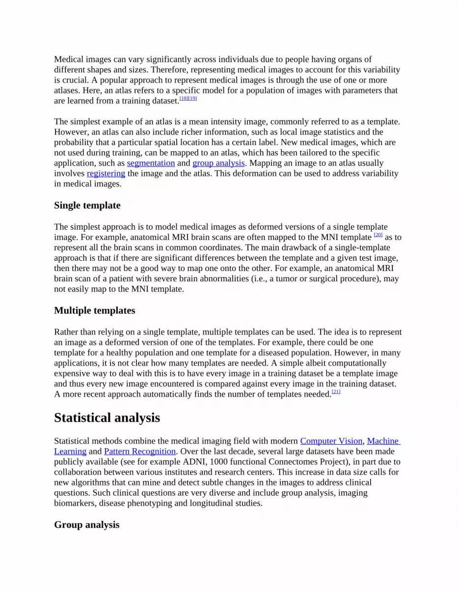
Medical images can vary significantly across individuals due to people having organs of different shapes and sizes. Therefore, representing medical images to account for this variability is crucial. A popular approach to represent medical images is through the use of one or more atlases. Here, an atlas refers to a specific model for a population of images with parameters that are learned from a training dataset.[18][19]
The simplest example of an atlas is a mean intensity image, commonly referred to as a template. However, an atlas can also include richer information, such as local image statistics and the probability that a particular spatial location has a certain label. New medical images, which are not used during training, can be mapped to an atlas, which has been tailored to the specific application, such as segmentation and group analysis. Mapping an image to an atlas usually involves registering the image and the atlas. This deformation can be used to address variability in medical images.
Single template
The simplest approach is to model medical images as deformed versions of a single template image. For example, anatomical MRI brain scans are often mapped to the MNI template [20] as to represent all the brain scans in common coordinates. The main drawback of a single-template approach is that if there are significant differences between the template and a given test image, then there may not be a good way to map one onto the other. For example, an anatomical MRI brain scan of a patient with severe brain abnormalities (i.e., a tumor or surgical procedure), may not easily map to the MNI template.
Multiple templates
Rather than relying on a single template, multiple templates can be used. The idea is to represent an image as a deformed version of one of the templates. For example, there could be one template for a healthy population and one template for a diseased population. However, in many applications, it is not clear how many templates are needed. A simple albeit computationally expensive way to deal with this is to have every image in a training dataset be a template image and thus every new image encountered is compared against every image in the training dataset. A more recent approach automatically finds the number of templates needed.[21]
Statistical analysisStatistical methods combine the medical imaging field with modern Computer Vision, Machine Learning and Pattern Recognition. Over the last decade, several large datasets have been made publicly available (see for example ADNI, 1000 functional Connectomes Project), in part due to collaboration between various institutes and research centers. This increase in data size calls for new algorithms that can mine and detect subtle changes in the images to address clinical questions. Such clinical questions are very diverse and include group analysis, imaging biomarkers, disease phenotyping and longitudinal studies.
Group analysis

In the Group Analysis, the objective is to detect and quantize abnormalities induced by a disease by comparing the images of two or more cohorts. Usually one of these cohorts consist of normal (control) subjects, and the other one consists of abnormal patients. Variation caused by the disease can manifest itself as abnormal deformation of anatomy (see Voxel-based morphometry). For example, shrinkage of sub-cortical tissues such as the Hippocampus in brain may be linked to Alzheimer's disease. Additionally, changes in biochemical (functional) activity can be observed using imaging modalities such as Positron Emission Tomography.
The comparison between groups is usually conducted on the voxel level. Hence, the most popular pre-processing pipeline, particularly in neuroimaging, transforms all of the images in a dataset to a common coordinate frame via (Medical Image Registration) in order to maintain correspondence between voxels. Given this voxel-wise correspondence, the most common Frequentist method is to extract a statistic for each voxel (for example, the mean voxel intensity for each group) and perform statistical hypothesis testing to evaluate whether a null hypothesis is or is not supported. The null hypothesis typically assumes that the two cohorts are drawn from the same distribution, and hence, should have the same statistical properties (for example, the mean values of two groups are equal for a particular voxel). Since medical images contain large numbers of voxels, the issue of multiple comparison needs to be addressed,.[22][23] There are also Bayesian approaches to tackle group analysis problem.[24]
Classification
Although group analysis can quantify the general effects of a pathology on an anatomy and function, it does not provide subject level measures, and hence cannot be used as biomarkers for diagnosis (see Imaging Biomarkers). Clinicians, on the other hand, are often interested in early diagnosis of the pathology (i.e. classification,[25][26]) and in learning the progression of a disease (i.e. regression [27]). From methodological point of view, current techniques varies from applying standard machine learning algorithms to medical imaging datasets (e.g. Support Vector Machine [28]), to developing new approaches adapted for the needs of the field.[29] The main difficulties are as follows:
Small sample size (Curse of Dimensionality): a large medical imaging dataset contains hundreds to thousands of images, whereas the number of voxels in a typical volumetric image can easily go beyond millions. A remedy to this problem is to reduce the number of features in an informative sense (see dimensionality reduction). Several unsupervised and semi-/supervised,[29][30][31][32] approaches have been proposed to address this issue.
Interpretability: A good generalization accuracy is not always the primary objective, as clinicians would like to understand which parts of anatomy are affected by the disease. Therefore, interpretability of the results is very important; methods that ignore the image structure are not favored. Alternative methods based on feature selection have been proposed,.[30][31][32][33]
Clustering
Image-based pattern classification methods typically assume that the neurological effects of a disease are distinct and well defined. This may not always be the case. For a number of medical

conditions, the patient populations are highly heterogeneous, and further categorization into sub-conditions has not been established. Additionally, some diseases (e.g., Autism Spectrum Disorder (ASD), Schizophrenia, Mild cognitive impairment (MCI)) can be characterized by a continuous or nearly-continuous spectra from mild cognitive impairment to very pronounced pathological changes. To facilitate image-based analysis of heterogeneous disorders, methodological alternatives to pattern classification have been developed. These techniques borrow ideas from high-dimensional clustering [34] and high-dimensional pattern-regression to cluster a given population into homogeneous sub-populations. The goal is to provide a better quantitative understanding of the disease within each sub-population.
Shape analysis
Shape Analysis is the field of Medical Image Computing that studies geometrical properties of structures obtained from different imaging modalities. Shape analysis recently become of increasing interest to the medical community due to its potential to precisely locate morphological changes between different populations of structures, i.e. healthy vs pathological, female vs male, young vs elderly. Shape Analysis includes two main steps: shape correspondence and statistical analysis.
Shape correspondence is the methodology that computes correspondent locations between geometric shapes represented by triangle meshes, contours, point sets or volumetric images. Obviously definition of correspondence will influence directly the analysis. Among the different options for correspondence frameworks we can find: Anatomical correspondence, manual landmarks, functional correspondence (i.e. in brain morphometry locus responsible for same neuronal functionality), geometry correspondence, (for image volumes) intensity similarity, etc. Some approaches, e.g. spectral shape analysis, do not require correspondence but compare shape descriptors directly.
Statistical analysis will provide measurements of structural change at correspondent locations.
Longitudinal studies
In longitudinal studies the same person is imaged repeatedly. This information can be incorporated both into the image analysis, as well as into the statistical modeling.
In longitudinal image processing, segmentation and analysis methods of individual time points are informed and regularized with common information usually from a within-subject template. This regularization is designed to reduce measurement noise and thus helps increase sensitivity and statistical power. At the same time over-regularization needs to be avoided, so that effect sizes remain stable. Intense regularization, for example, can lead to excellent test-retest reliability, but limits the ability to detect any true changes and differences across groups. Often a trade-off needs to be aimed for, that optimizes noise reduction at the cost of limited effect size loss. Another common challenge in longitudinal image processing is the, often unintentional, introduction of processing bias. When, for example, follow-up images get registered and resampled to

the baseline image, interpolation artifacts get introduced to only the follow-up images and not the baseline. These artifact can cause spurious effects (usually a bias towards overestimating longitudinal change and thus underestimating required sample size). It is therefore essential that all time points get treated exactly the same to avoid any processing bias.
Post-processing and statistical analysis of longitudinal data usually requires dedicated statistical tools such as repeated measure ANOVA or the more powerful linear mixed effects models. Additionally, it is advantageous to consider the spatial distribution of the signal. For example cortical thickness measurements will show a correlation within-subject across time and also within a neighborhood on the cortical surface - a fact that can be used to increase statistical power. Furthermore, time-to-even (aka survival) analysis is frequently employed to analyze longitudinal data and determine significant predictors.
Image-based physiological modellingTraditionally, medical image computing has seen to address the quantification and fusion of structural or functional information available at the point and time of image acquisition. In this regard, it can be seen as quantitative sensing of the underlying anatomical, physical or physiological processes. However, over the last few years, there has been a growing interest in the predictive assessment of disease or therapy course. Image-based modelling, be it of biomechanical or physiological nature, can therefore extend the possibilities of image computing from a descriptive to a predictive angle.
According to the STEP research roadmap,[35][36] the Virtual Physiological Human (VPH) is a methodological and technological framework that, once established, will enable the investigation of the human body as a single complex system. Underlying the VPH concept, the International Union for Physiological Sciences (IUPS) has been sponsoring the IUPS Physiome Project for more than a decade,.[37][38] This is a worldwide public domain effort to provide a computational framework for understanding human physiology. It aims at developing integrative models at all levels of biological organization, from genes to the whole organisms via gene regulatory networks, protein pathways, integrative cell functions, and tissue and whole organ structure/function relations. Such an approach aims at transforming current practice in medicine and underpins a new era of computational medicine.[39]
In this context, medical imaging and image computing play, and will continue to play, an increasingly important role as they provide systems and methods to image, quantify and fuse both structural and functional information about the human being in vivo. These two broad research areas include the transformation of generic computational models to represent specific subjects, thus paving the way for personalized computational models.[40] Individualization of generic computational models through imaging can be realized in three complementary directions:
definition of the subject-specific computational domain (anatomy) and related subdomains (tissue types);
definition of boundary and initial conditions from (dynamic and/or functional) imaging; and

characterization of structural and functional tissue properties.
In addition, imaging also plays a pivotal role in the evaluation and validation of such models both in humans and in animal models, and in the translation of models to the clinical setting with both diagnostic and therapeutic applications. In this specific context, molecular, biological, and pre-clinical imaging render additional data and understanding of basic structure and function in molecules, cells, tissues and animal models that may be transferred to human physiology where appropriate.
The applications of image-based VPH/Physiome models in basic and clinical domains are vast. Broadly speaking, they promise to become new virtual imaging techniques. Effectively more, often non-observable, parameters will be imaged in silico based on the integration of observable but sometimes sparse and inconsistent multimodal images and physiological measurements. Computational models will serve to engender interpretation of the measurements in a way compliant with the underlying biophysical, biochemical or biological laws of the physiological or pathophysiological processes under investigation. Ultimately, such investigative tools and systems will help our understanding of disease processes, the natural history of disease evolution, and the influence on the course of a disease of pharmacological and/or interventional therapeutic procedures.
Cross-fertilization between imaging and modelling goes beyond interpretation of measurements in a way consistent with physiology. Image-based patient-specific modelling, combined with models of medical devices and pharmacological therapies, opens the way to predictive imaging whereby one will be able to understand, plan and optimize such interventions in silico.
Mathematical methods in medical imagingA number of sophisticated mathematical methods have entered medical imaging, and have already been implemented in various software packages. These include approaches based on partial differential equations (PDEs) and curvature driven flows for enhancement, segmentation, and registration. Since they employ PDEs, the methods are amenable to parallelization and implementation on GPGPUs. A number of these techniques have been inspired from ideas in optimal control. Accordingly, very recently ideas from control have recently made their way into interactive methods, especially segmentation. Moreover, because of noise and the need for statistical estimation techniques for more dynamically changing imagery, the Kalman filter [41] and particle filter have come into use. A survey of these methods with an extensive list of references may be found in.[42]
Modality specific computingSome imaging modalities provide very specialized information. The resulting images cannot be treated as regular scalar images and give rise to new sub-areas of Medical Image Computing. Examples include diffusion MRI, functional MRI and others.
Diffusion MRI

A mid-axial slice of the ICBM diffusion tensor image template. Each voxel's value is a tensor represented here by an ellipsoid. Color denotes principal orientation: red = left-right, blue=inferior-superior, green = posterior-anterior
Diffusion MRI is a structural magnetic resonance imaging modality that allows measurement of the diffusion process of molecules. Diffusion is measured by applying a gradient pulse to a magnetic field along a particular direction. In a typical acquisition, a set of uniformly distributed gradient directions is used to create a set of diffusion weighted volumes. In addition, an unweighted volume is acquired under the same magnetic field without application of a gradient pulse. As each acquisition is associated with multiple volumes, diffusion MRI has created a variety of unique challenges in medical image computing.
In medicine, there are two major computational goals in diffusion MRI:
Estimation of local tissue properties, such as diffusivity; Estimation of local directions and global pathways of diffusion.
The diffusion tensor,[43] a 3 × 3 symmetric positive-definite matrix, offers a straightforward solution to both of these goals. It is proportional to the covariance matrix of a Normally distributed local diffusion profile and, thus, the dominant eigenvector of this matrix is the principal direction of local diffusion. Due to the simplicity of this model, a maximum likelihood estimate of the diffusion tensor can be found by simply solving a system of linear equations at each location independently. However, as the volume is assumed to contain contiguous tissue fibers, it may be preferable to estimate the volume of diffusion tensors in its entirety by imposing regularity conditions on the underlying field of tensors.[44] Scalar values can be extracted from the diffusion tensor, such as the fractional anisotropy, mean, axial and radial diffusivities, which indirectly measure tissue properties such as the dysmyelination of axonal fibers [45] or the presence of edema.[46] Standard scalar image computing methods, such as registration and segmentation, can be applied directly to volumes of such scalar values. However, to fully exploit the information in the diffusion tensor, these methods have been adapted to account for tensor valued volumes when performing registration [47][48] and segmentation.[49][50]
Given the principal direction of diffusion at each location in the volume, it is possible to estimate the global pathways of diffusion through a process known as tractography.[51] However, due to the relatively low resolution of diffusion MRI, many of these pathways may cross, kiss or fan at a single location. In this situation, the single principal direction of the diffusion tensor is not an appropriate model for the local diffusion distribution. The most common solution to this problem is to estimate multiple directions of local diffusion using more complex models. These include mixtures of diffusion tensors,[52] Q-ball imaging,[53] diffusion spectrum imaging [54] and fiber

orientation distribution functions,[55][56] which typically require HARDI acquisition with a large number of gradient directions. As with the diffusion tensor, volumes valued with these complex models require special treatment when applying image computing methods, such as registration [57][58][59] and segmentation.[60]
Functional MRI
Functional magnetic resonance imaging (fMRI) is a medical imaging modality that indirectly measures neural activity by observing the local hemodynamics, or blood oxygen level dependent signal (BOLD). fMRI data offers a range of insights, and can be roughly divided into two categories:
Task related fMRI is acquired as the subject is performing a sequence of timed experimental conditions. In block-design experiments, the conditions are present for short periods of time (e.g., 10 seconds) and are alternated with periods of rest. Event-related experiments rely on a random sequence of stimuli and use a single time point to denote each condition. The standard approach to analyze task related fMRI is the general linear model (GLM) [61]
Resting state fMRI is acquired in the absence of any experimental task. Typically, the objective is to study the intrinsic network structure of the brain. Observations made during rest have also been linked to specific cognitive processes such as encoding or reflection. Most studies of resting state fMRI focus on low frequency fluctuations of the fMRI signal (LF-BOLD). Seminal discoveries include the default network,[62] a comprehensive cortical parcellation,[63] and the linking of network characteristics to behavioral parameters.
There is a rich set of methodology used to analyze functional neuroimaging data, and there is often no consensus regarding the best method. Instead, researchers approach each problem independently and select a suitable model/algorithm. In this context there is a relatively active exchange among neuroscience, computational biology, statistics, and machine learning communities. Prominent approaches include
Massive univariate approaches that probe individual voxels in the imaging data for a relationship to the experiment condition. The prime approach is the general linear model (GLM) [61]
Multivariate- and classifier based approaches, often referred to as multi voxel pattern analysis or multi-variate pattern analysis probe the data for global and potentially distributed responses to an experimental condition. Early approaches used support vector machines (SVM) to study responses to visual stimuli.[64] Recently, alternative pattern recognition algorithms have been explored, such as random forest based gini contrast [65] or sparse regression and dictionary learning [66]
Functional connectivity analysis studies the intrinsic network structure of the brain, including the interactions between regions. The majority of such studies focus on resting state data to parcelate the brain [63] or to find correlates to behavioral measures.[67] Task specific data can be used to study causal relationships among brain regions (e.g., dynamic causal mapping (DCM) [68]).

When working with large cohorts of subjects, the normalization (registration) of individual subjects into a common reference frame is crucial. A body of work and tools exist to perform normalization based on anatomy (FSL, FreeSurfer, SPM). Alignment taking spatial variability across subjects into account is a more recent line of work. Examples are the alignment of the cortex based on fMRI signal correlation,[69] the alignment based on the global functional connectivity structure both in task-, or resting state data,[70] and the alignment based on stimulus specific activation profiles of individual voxels.[71]
SoftwareSoftware for medical image computing is a complex combination of systems providing IO, visualization and interaction, user interface, data management and computation. Typically system architectures are layered to serve algorithm developers, application developers, and users. The bottom layers are often libraries and/or toolkits which provide base computational capabilities; while the top layers are specialized applications which address specific medical problems, diseases, or body systems.
Additional notesMedical Image Computing is also related to the field of Computer Vision. An international society, the MICCAI society represents the field and organizes an annual conference and associated workshops. Proceedings for this conference are published by Springer in the Lecture Notes in Computer Science series.[72] In 2000, N. Ayache and J. Duncan reviewed the state of the field.[73]
See also
Medical portal
Imaging informatics Neuroimaging software
References1. Forghani, M.; Forouzanfar, M.; Teshnehlab, M. (2010). "Parameter optimization of
improved fuzzy c-means clustering algorithm for brain MR image segmentation". Engineering Applications of Artificial Intelligence 23 (2): 160–168.
2. J Gee, M Reivich, R Bajcsy (1993). "Elastically Deforming a Three-Dimensional Atlas to Match Anatomical Brain Images". Journal of Computer Assisted Tomography 17 (1): 225–236. doi:10.1097/00004728-199303000-00011.
3. MR Sabuncu, BT Yeo, K Van Leemput, B Fischl, P Golland (June 2010). "A Generative Model for Image Segmentation Based on Label Fusion". IEEE Transactions on Medical Imaging 29 (10): 1714–1729. doi:10.1109/TMI.2010.2050897. PMC 3268159. PMID 20562040.

4. Cootes TF, Taylor CJ, Cooper DH, and Graham J (1995). "Active shape models-their training and application". Computer vision and image understanding (San Diego: Academic Press, c1995-) 61 (1): 38–59. doi:10.1006/cviu.1995.1004.
5. Cootes, T.F. and Edwards, G.J. and Taylor, C.J. (2001). "Active appearance models". Pattern Analysis and Machine Intelligence, IEEE Transactions on (IEEE) 23 (6): 681–685. doi:10.1109/34.927467.
6. R. Goldenberg, R. Kimmel, E. Rivlin, and M. Rudzsky (2001). "Fast geodesic active contours" (PDF). IEEE Transactions on Image Processing 10 (10): 1467–1475. doi:10.1109/83.951533.
7. Karasev, P., Kolesov I., Chudy, K. Vela, P., and Tannenbaum, A. (2011). "Interactive MRI segmentation with controlled active vision". Proceedings of the Conference on Decision and Control.
8. Ehsani Rad, Abdolvahab; Mohd Rahim Mohd Shafry; Rehman Amjad; Altameem Ayman; Saba Tanzila (May 2013). "Evaluation of Current Dental Radiographs Segmentation Approaches in Computer-aided Applications". IETE Technical Review 30 (3): 210. doi:10.4103/0256-4602.113498.
9. Lisa Gottesfeld Brown (1992). "A survey of image registration techniques". ACM Computing Surveys 24 (4): 325–376. doi:10.1145/146370.146374.
10. J. Maintz and M. Viergever (1998). "A survey of medical image registration". Medical Image Analysis 2 (1): 1–36. doi:10.1016/S1361-8415(01)80026-8. PMID 10638851.
11. J. Hajnal, D. Hawkes, and D. Hill (2001). Medical Image Registration. Baton Rouge, Florida: CRC Press.
12. Barbara Zitová, Jan Flusser (2003). "Image registration methods: a survey". Image Vision Comput. 21 (11): 977–1000. doi:10.1016/S0262-8856(03)00137-9.
13. J. P. W. Pluim, J. B. A. Maintz, and M. A. Viergever (2003). "Mutual information based registration of medical images: A survey". IEEE Trans. Med. Imaging 22 (8): 986–1004. doi:10.1109/TMI.2003.815867. PMID 12906253.
14. Grenander, Ulf and Miller, Michael I. (1998). "Computational anatomy: an emerging discipline". Q. Appl. Math. LVI (4): 617–694.
15. P. A. Viola (1995). Alignment by Maximization of Mutual Information (Thesis). Massachusetts Institute of Technology.
16. C. Wachinger, T. Klein, N. Navab (2011). "Locally adaptive Nakagami-based ultrasound similarity measures". Ultrasonics 52 (4): 547–554. doi:10.1016/j.ultras.2011.11.009. PMID 22197152.
17. C. Wachinger, N. Navab (2012). "Entropy and Laplacian images: structural representations for multi-modal registration". Medical Image Analysis 16 (1): 1–17. doi:10.1016/j.media.2011.03.001. PMID 21632274.
18. M. De Craene and A. B. d Aische and B. Macq and S. K. Warfield. "Multi-subject registration for unbiased statistical atlas construction". Proceedings of Medical Image Computing and Computer-Assisted Intervention 2004.
19. C. J. Twining and T. Cootes and S. Marsland and V. Petrovic and R. Schestowitz and C. Taylor. "A unified information-theoretic approach to groupwise non-rigid registration and model building". Proceedings of Information Processing in Medical Imaging 2005.
20. "The MNI brain and the Talairach atlas" .

21. M. Sabuncu and S. K. Balci and M. E. Shenton and P. Golland (2009). "Image-driven Population Analysis through Mixture Modeling". IEEE Transactions in Medical Imaging 28 (9): 1473–1487. doi:10.1109/TMI.2009.2017942.
22. J. Ashburner and K.J. Friston (2000). "Voxel-Based Morphometry – The Methods". NeuroImage 11 (6): 805–821. doi:10.1006/nimg.2000.0582. PMID 10860804.
23. C. Davatzikos (2004). "Why voxel-based morphometric analysis should be used with great caution when characterizing group differences,". NeuroImage 23 (1): 17–20. doi:10.1016/j.neuroimage.2004.05.010. PMID 15325347.
24. K.J. Friston, W.D. Penny, C. Phillips, S.J. Kiebel, G. Hinton, and J. Ashburner (2002). "Classical and Bayesian Inference in Neuroimaging: Theory". NeuroImage 16 (2): 465–483. doi:10.1006/nimg.2002.1090. PMID 12030832.
25. Yong Fan, Nematollah Batmanghelich, Chris M. Clark, Christos Davatzikos, the Alzheimer’s Disease Neuroimaging Initiative, Spatial patterns of brain atrophy in MCI patients, identified via high-dimensional pattern classification, predict subsequent cognitive decline. (2008). "Spatial patterns of brain atrophy in MCI patients, identified via high-dimensional pattern classification, predict subsequent cognitive decline". NeuroImage 39 (4): 1731–1743. doi:10.1016/j.neuroimage.2007.10.031. PMC 2861339. PMID 18053747.
26. Rémi Cuingnet and Emilie Gerardin and Jérôme Tessieras and Guillaume Auzias and Stéphane Lehéricy and Marie-Odile Habert and Marie Chupin and Habib Benali and Olivier Colliot (2011). "The Alzheimer's Disease Neuroimaging Initiative, Automatic classification of patients with Alzheimer's disease from structural MRI: A comparison of ten methods using the ADNI database". NeuroImage 56 (2): 766–781. doi:10.1016/j.neuroimage.2010.06.013.
27. Y. Wang and Y. Fan and P. Bhatt P and C. Davatzikos (2010). "High-dimensional pattern regression using machine learning: from medical images to continuous clinical variables". NeuroImage 50 (4): 1519–35. doi:10.1016/j.neuroimage.2009.12.092. PMC 2839056. PMID 20056158.
28. Benoît Magnin and Lilia Mesrob and Serge Kinkingnéhun and Mélanie Pélégrini-Issac and Olivier Colliot and Marie Sarazin and Bruno Dubois and Stéphane Lehéricy and Habib Benali (2009). "Support vector machine-based classification of Alzheimer's disease from whole-brain anatomical MRI". Neuroradiology 51 (2): 73–83. doi:10.1007/s00234-008-0463-x. PMID 18846369.
29. N.K. Batmanghelich and B. Taskar and C. Davatzikos (2012). "Generative-discriminative basis learning for medical imaging". IEEE Trans Med Imaging 31 (1): 51–69. doi:10.1109/TMI.2011.2162961. PMC 3402718. PMID 21791408.
30. Glenn Fung and Jonathan Stoeckel (2007). "SVM feature selection for classification of SPECT images of Alzheimer's disease using spatial information". Knowledge and Information Systems 11 (2): 243–258. doi:10.1007/s10115-006-0043-5.
31. R. Chaves and J. Ramírez and J.M. Górriz and M. López and D. Salas-Gonzalez and I. Álvarez and F. Segovia (2009). "SVM-based computer-aided diagnosis of the Alzheimer's disease using t-test NMSE feature selection with feature correlation weighting". Neuroscience Letters 461 (3): 293–297. doi:10.1016/j.neulet.2009.06.052. PMID 19549559.
32. yanxi liu and leonid teverovskiy and owen carmichael and ron kikinis and martha shenton and cameron s. carter and v. andrew stenger and simon davis and howard

aizenstein and james t. becker (2004). "discriminative mr image feature analysis for automatic schizophrenia and alzheimer's disease classification". Medical image computing and computer-assisted intervention – miccai.
33. Savio A., Graña M. (2013). "Deformation based feature selection for Computer Aided Diagnosis of Alzheimer’s Disease". Expert Systems with Applications 40 (5): 1619–1628. doi:10.1016/j.eswa.2012.09.009. ISSN 0957-4174.
34. R. Filipovych and S. M. Resnick and C. Davatzikos (2011). "Semi-supervised cluster analysis of imaging data". NeuroImage 54 (3): 2185–2197. doi:10.1016/j.neuroimage.2010.09.074. PMC 3008313. PMID 20933091.
35. STEP research roadmap . europhysiome.org36. J. W. Fenner, B. Brook, G. Clapworthy, P. V. Coveney, V. Feipel, H. Gregersen, D. R.
Hose, P. Kohl, P. Lawford, K. M. McCormack, D. Pinney, S. R. Thomas, S. Van Sint Jan, S. Waters, and M. Viceconti (2008). "The EuroPhysiome, STEP and a roadmap for the virtual physiological human". Philos. Trans. A 366 (1878): 2979–2999. Bibcode:2008RSPTA.366.2979F. doi:10.1098/rsta.2008.0089. PMID 18559316.
37. J. B. Bassingthwaighte (2000). "Strategies for the Physiome Project". Ann. Biomed. Eng. 28 (8): 1043–1058. doi:10.1114/1.1313771. PMC 3425440. PMID 11144666.
38. P. J. Hunter and T. K. Borg (2003). "Integration from proteins to organs: The Physiome Project". Nat. Rev.Mol. Cell Biol. 4 (3): 237–243. doi:10.1038/nrm1054. PMID 12612642.
39. R. L.Winslow, N. Trayanova, D. Geman, and M. I. Miller (2012). "Computational medicine: Translating models to clinical care". Sci. Trans. Med. 4 (158): 158rv11. doi:10.1126/scitranslmed.3003528. PMC 3618897. PMID 23115356.
40. N. Ayache, J.-P. Boissel, S. Brunak, G. Clapworthy, G. Lonsdale, J. Fingberg, A. F. Frangi,G.Deco, P. J. Hunter, P.Nielsen,M.Halstead, D. R. Hose, I. Magnin, F. Martin-Sanchez, P. Sloot, J. Kaandorp, A. Hoekstra, S. Van Sint Jan, and M. Viceconti (2005) "Towards virtual physiological human: Multilevel modelling and simulation of the human anatomy and physiology". Directorate General INFSO & Directorate General JRC, White paper
41. Boulfelfel D., Rangayyan R.M., Hahn L.J., Kloiber R., Kuduvalli G.R. (1994). "Restoration of single photon emission computed tomography images by the Kalman filter". IEEE Transactions on Medical Imaging 13 (1): 102–109. doi:10.1109/42.276148.
42. Angenent, S. , Pichon, E., and Tannenbaum, A. (2006). "Mathematical methods in medical image processing". Bulletin of the AMS 43 (3): 365–396. doi:10.1090/S0273-0979-06-01104-9.
43. P Basser, J Mattiello, D LeBihan (January 1994). "MR diffusion tensor spectroscopy, imaging". Biophysical Journal 66 (1): 259–267. doi:10.1016/S0006-3495(94)80775-1. PMC 1275686. PMID 8130344.
44. P Fillard, X Pennec, V Arsigny, N Ayache (2007). "Clinical DT-MRI estimation, smoothing,, fiber tracking with log-Euclidean metrics". IEEE Transactions on Medical Imaging 26 (11): 1472–1482. doi:10.1109/TMI.2007.899173. PMID 18041263.
45. S-K Song, S-W Sun, M Ramsbottom, C Cheng, J Russell, A Cross (November 2002). "Dysmyelination Revealed through MRI as Increased Radial (but Unchanged Axial) Diffusion of Water". NeuroImage 13 (3): 1429–1436. doi:10.1006/nimg.2002.1267.
46. P Barzo, A Marmarou, P Fatouros, K Hayasaki, F Corwin (December 1997). "Contribution of vasogenic and cellular edema to traumatic brain swelling measured by

diffusion-weighted imaging". Journal of Neurosurgery 87 (6): 900–907. doi:10.3171/jns.1997.87.6.0900. PMID 9384402.
47. D Alexander, C Pierpaoli, P Basser (January 2001). "Spatial transformation of diffusion tensor magnetic resonance images". IEEE Transactions on Medical Imaging 20 (11): 1131–1139. doi:10.1109/42.963816. PMID 11700739.
48. Y Cao, M Miller, S Mori, R Winslow, L Younes (June 2006). "Diffeomorphic Matching of Diffusion Tensor Images". Proceedings of IEEE Computer Society Conference on Computer Vision, Pattern Recognition (CVPR), Workshop on Mathematical Methods in Biomedical Image Analysis (MMBIA 2006). New York. pp. 67–67. doi:10.1109/CVPRW.2006.65.
49. Z Wang, B Vemuri (October 2005). "DTI segmentation using an information theoretic tensor dissimilarity measure". IEEE Transactions on Medical Imaging 24 (10): 1267–1277. doi:10.1109/TMI.2005.854516. PMID 16229414.
50. Melonakos, J., Pichon, E., Angenent, S., and Tannenbaum, A. (2008). "Finsler active contours". IEEE Trans. PAMI 30 (3): 412–423. doi:10.1109/TPAMI.2007.70713.
51. S Mori, B Crain, V Chacko, P van Zijl (February 1999). "Three-dimensional tracking of axonal projections in the brain by magnetic resonance imaging". Annals of Neurology 45 (2): 265–269. doi:10.1002/1531-8249(199902)45:2<265::AID-ANA21>3.0.CO;2-3. PMID 9989633.
52. D Tuch, T Reese, M Wiegell, N Makris, J Belliveau, V Wedeen (October 2002). "High angular resolution diffusion imaging reveals intravoxel white matter fiber heterogeneity". Magnetic Resonance in Medicine 48 (4): 577–582. doi:10.1002/mrm.10268. PMID 12353272.
53. D Tuch (December 2004). "Q-ball imaging". Magnetic Resonance in Medicine 52 (6): 1358–1372. doi:10.1002/mrm.20279. PMID 15562495.
54. V Wedeen, P Hagmann, W-Y Tseng, T Reese (December 2005). "Mapping complex tissue architecture with diffusion spectrum magnetic resonance imaging". Magnetic Resonance in Medicine 64 (6): 1377–1386. doi:10.1002/mrm.20642. PMID 16247738.
55. K Jansons, D Alexander (July 2003). "Persistent angular structure: new insights from diffusion magnetic resonance imaging data". Proceedings of Information Processing in Medical Imaging (IPMI) 2003, LNCS 2732. pp. 672–683. doi:10.1007/978-3-540-45087-0_56.
56. J-D Tournier, F Calamante, D Gadian, A Connelly (2007). "Direct estimation of the fiber orientation density function from diffusion-weighted MRI data using spherical deconvolution". NeuroImage 23 (3): 1176–1185. doi:10.1016/j.neuroimage.2004.07.037. PMID 15528117.
57. X Geng, T Ross, W Zhan, H Gu, Y-P Chao, C-P Lin, G Christensen, N Schuff, Y Yang (July 2009). "Diffusion MRI Registration Using Orientation Distribution Functions". Proceedings of Information Processing in Medical Imaging (IPMI) 2009, LNCS 5636. pp. 626–637. doi:10.1007/978-3-642-02498-6_52.
58. P-T Yap, Y Chen, H An, Y Yang, J Gilmore, W Lin, D Shen (2011). "SPHERE: SPherical Harmonic Elastic REgistration of HARDI data". NeuroImage 55 (2): 545–556. doi:10.1016/j.neuroimage.2010.12.015. PMC 3035740. PMID 21147231.
59. P Zhang, M Niethammer, D Shen, P-T Yap (2012). "Large Deformation Diffeomorphic Registration of Diffusion-Weighted Images". Proceedings of Medical Image Computing and Computer-Assisted Intervention (MICCAI).

60. M Descoteaux, R Deriche (September 2007). "Segmentation of Q-Ball Images Using Statistical Surface Evolution". Proceedings of Medical Image Computing and Computer-Assisted Intervention (MICCAI) 2007, LNCS 4792. pp. 769–776. doi:10.1007/978-3-540-75759-7_93.
61. Friston, K., Holmes, A., Worsley, K., Poline, J., Frith, C., Frackowiak, R.; et al. (1995). "Statistical parametric maps in functional imaging: a general linear approach". Hum Brain Mapp 2 (4): 189–210. doi:10.1002/hbm.460020402.
62. Buckner, R. L., Andrews-Hanna, J. R., and Schacter, D. L. (2008). "The brain's default network: anatomy, function, and relevance to disease". Annals of the New York Academy of Sciences 1124: 1–38. Bibcode:2008NYASA1124....1B. doi:10.1196/annals.1440.011. PMID 18400922.
63. Yeo, B. T. T., Krienen, F. M., Sepulcre, J., Sabuncu, M. R., Lashkari, D., Hollinshead, M., Roffman, J. L., Smoller, J. W., Zöllei, L., Polimeni, J. R., Fischl, B., Liu, H., and Buckner, R. L. (2011). "The organization of the human cerebral cortex estimated by intrinsic functional connectivity". J Neurophysiol 106 (3): 1125–65. doi:10.1152/jn.00338.2011. PMC 3174820. PMID 21653723.
64. J. V. Haxby, M. I. Gobbini, M. L. Furey, A. Ishai, J. L. Schouten, and P. Pietrini (2001). "Distributed and overlapping representations of faces and objects in ventral temporal cortex". Science 293 (5539): 2425–30. Bibcode:2001Sci...293.2425H. doi:10.1126/science.1063736. PMID 11577229.
65. Langs, G., Menze, B. H., Lashkari, D., and Golland, P. (2011). "Detecting stable distributed patterns of brain activation using Gini contrast". NeuroImage 56 (2): 497–507. doi:10.1016/j.neuroimage.2010.07.074. PMC 3960973. PMID 20709176.
66. Varoquaux, G., Gramfort, A., Pedregosa, F., Michel, V., and Thirion, B. (2011). "Multi-subject dictionary learning to segment an atlas of brain spontaneous activity". Inf Process Med Imaging. pp. 562–73.
67. van den Heuvel, M. P., Stam, C. J., Kahn, R. S., and Hulshoff Pol, H. E. (2009). "Efficiency of functional brain networks and intellectual performance". J Neurosci 29 (23): 7619–24. doi:10.1523/JNEUROSCI.1443-09.2009. PMID 19515930.
68. Friston, K. (2003). "Dynamic causal modelling". NeuroImage 19 (4): 1273–1302. doi:10.1016/S1053-8119(03)00202-7. PMID 12948688. |first2= missing |last2= in Authors list (help); |first3= missing |last3= in Authors list (help)
69. Sabuncu, M. R., Singer, B. D., Conroy, B., Bryan, R. E., Ramadge, P. J., and Haxby, J. V. (2010). "Function-based Intersubject Alignment of Human Cortical Anatomy". Cerebral Cortex 20 (1): 130–140. doi:10.1093/cercor/bhp085. PMC 2792192. PMID 19420007.
70. Langs, G., Lashkari, D., Sweet, A., Tie, Y., Rigolo, L., Golby, A. J., and Golland, P. (2011). "Learning an atlas of a cognitive process in its functional geometry". Inf Process Med Imaging. pp. 135–46.
71. Haxby, J. V., Guntupalli, J. S., Connolly, A. C., Halchenko, Y. O., Conroy, B. R., Gobbini, M. I., Hanke, M., and Ramadge, P. J. (2011). "A common, high-dimensional model of the representational space in human ventral temporal cortex". Neuron 72 (2): 404–416. doi:10.1016/j.neuron.2011.08.026. PMC 3201764. PMID 22017997.
72. Lecture Notes in Computer Science 1496. 1998. doi:10.1007/BFb0056181.73. JS Duncan, N Ayache (2000). "Medical image analysis: Progress over two decades and
the challenges ahead". Pattern Analysis and Machine Intelligence 22: 85–106. doi:10.1109/34.824822.

Journals on medical image computing Medical Image Analysis (MedIA) ; also the official journal of the MICCAI Society, a
premier conference for medical image computing IEEE Transactions on Medical Imaging (IEEE TMI) Medical Physics Journal of Digital Imaging (JDI) ; the official journal of the Society of Imaging
Informatics Computerized Medical Imaging and Graphics Journal of Computer Aided Radiology and Surgery BMC Medical Imaging
In addition the following journals occasionally publish articles describing methods and specific clinical applications of medical image computing or modality specific medical image computing
Radiology the official journal of the Radiological Society of North America NeuroImage Journal of Magnetic Resonance Imaging (JMRI) Magnetic Resonance in Medicine (MRM) Journal of Computer Assisted Tomography (JCAT) Human Brain Mapping
Categories:
Medical technology Medical imaging Health informatics
Navigation menu Not logged in Talk Contributions Create account Log in
Article Talk
Read Edit View history
Main page Contents

Featured content Current events Random article Donate to Wikipedia Wikipedia store
Interaction
Help About Wikipedia Community portal Recent changes Contact page
Tools
What links here Related changes Upload file Special pages Permanent link Page information Wikidata item Cite this page
Print/export
Create a book Download as PDF Printable version
Languages
Add links
This page was last modified on 5 April 2016, at 01:28. Text is available under the Creative Commons Attribution-ShareAlike License;
additional terms may apply. By using this site, you agree to the Terms of Use and Privacy Policy. Wikipedia® is a registered trademark of the Wikimedia Foundation, Inc., a non-profit organization.
Privacy policy About Wikipedia Disclaimers Contact Wikipedia Developers