A new achievement scalarizing function based on parameterization in multiobjective optimization

OR Spectrum (2012) 34:69–87DOI 10.1007/s00291-010-0224-1

REGULAR ARTICLE

A new achievement scalarizing function basedon parameterization in multiobjective optimization

Yury Nikulin · Kaisa Miettinen ·Marko M. Mäkelä

Published online: 11 August 2010© Springer-Verlag 2010

Abstract This paper addresses a general multiobjective optimization problem. Oneof the most widely used methods of dealing with multiple conflicting objectivesconsists of constructing and optimizing a so-called achievement scalarizing func-tion (ASF) which has an ability to produce any Pareto optimal or weakly/properlyPareto optimal solution. The ASF minimizes the distance from the reference point tothe feasible region, if the reference point is unattainable, or maximizes the distanceotherwise. The distance is defined by means of some specific kind of a metric intro-duced in the objective space. The reference point is usually specified by a decisionmaker and contains her/his aspirations about desirable objective values. The classicalapproach to constructing an ASF is based on using the Chebyshev metric L∞. Anotherpossibility is to use an additive ASF based on a modified linear metric L1. In this paper,we propose a parameterized version of an ASF. We introduce an integer parameterin order to control the degree of metric flexibility varying from L1 to L∞. We provethat the parameterized ASF supports all the Pareto optimal solutions. Moreover, wespecify conditions under which the Pareto optimality of each solution is guaranteed.An illustrative example for the case of three objectives and comparative analysis ofparameterized ASFs with different values of the parameter are given. We show thatthe parameterized ASF provides the decision maker with flexible and advanced tools

Y. Nikulin (B) · M. M. MäkeläDepartment of Mathematics, University of Turku, 20014 Turku, Finlande-mail: [email protected]

M. M. Mäkeläe-mail: [email protected]

K. MiettinenDepartment of Mathematical Information Technology, University of Jyväskylä,40014 Jyväskylä, Finlande-mail: [email protected]

123

70 Y. Nikulin et al.

to detect Pareto optimal points, especially those whose detection with other ASFs isnot straightforward since it may require changing essentially the reference point orweighting coefficients as well as some other extra computational efforts.

Keywords Multiobjective optimization · Achievement function · Parameterization ·Pareto optimal solutions · Multiple criteria decision making

1 Introduction

Many real-life optimization problems can hardly be considered as properly formu-lated without taking into account their multiple objective nature. This fact commonlyaccepted by many experts explains a permanently growing interest in the area ofmultiobjective optimization. Considering multiple conflicting objectives is advanta-geous in comparison with optimizing one single objective only. It is well known thata solution which is optimal with respect to one single objective may be arbitrarilybad with respect to other objectives and thus will be unacceptable for the decisionmaker (DM). While optimizing one objective usually leads to one optimal solution,multiobjective optimization involves dealing with a set of Pareto optimal solutions(alternatives) that provide different trade-offs between several conflicting objectives.Usually these objectives represent various interests. For example, for some transpor-tation problems one goal may be oriented on passenger comfort while another onemay represent convenience for the transport company. Thus, finding a compromisebetween several goals may positively influence interests of all participants involved.The primary goal of multiobjective optimization is to optimize simultaneously severalconflicting objectives in order to find Pareto optimal solutions acceptable for the DM.Optimality is usually understood in the sense of Pareto optimality, but other optimalityprinciples (lexicographic, Smale, Slater, Geoffrion, Borwein, Condorcet etc., see, e.g.Sawaragi et al. 1985) can also be used.

In multiobjective optimization, vectors are regarded as optimal if their componentscannot be improved without deteriorating the others. This concept was first introducedby Pareto (1909). The Pareto optimality principle generally describes an equilibriumsituation such that the value of no objective for any Pareto optimal solution can beimproved without getting the value of another objective deteriorated.

There is a large variety of methods suggested for solving multiobjective optimiza-tion problems (see, e.g., Ehrgott 2000; Miettinen 1999; Sawaragi et al. 1985; Steuer1986). Many of these methods are based on a scalarization approach. Via scalariza-tion, the problem is transformed into a single objective optimization problem involvingpossibly some parameters or additional constraints. In most scalarizing functions, addi-tional information is requested from the DM about her/his individual preferences andfurther taken into consideration. After the scalarization phase, the widely developedtheory and methods of single objective optimization are available.

Multiobjective optimization methods utilize different scalarizing functions in dif-ferent ways. The input requested from the DM may consist of trade-off information,marginal rates of substitution or desirable objective function values (see ++e.g. Luqueet al.). Furthermore, the scalarization may be performed once or repeatedly as a part

123

A new achievement scalarizing function 71

of an iterative process. When methods are introduced in the literature, the optimalityof the results produced is usually proved. On the other hand, it is not so common tojustify why some specific form of scalarization is used. The choice of the particularscalarization approach has to be done very carefully, since different scalarizationstypically produce different Pareto optimal solutions.

One of the most widely used approaches of dealing with multiple conflicting objec-tives involves constructing and optimizing a so-called achievement scalarizing func-tion (ASF) (Miettinen 1999; Wierzbicki 1980, 1986b) which has an ability to produceany (properly) Pareto optimal or weakly Pareto optimal solution. The ASF minimizesthe distance from the reference point (specified by the DM) to the feasible region, ifthe reference point is unattainable, or maximizes the distance otherwise. The distanceis defined by means of some appropriate metric introduced in the objective space. Theclassical approach to constructing an ASF is based on using Chebyshev L∞ and linearL1 metrics (see, e.g. Miettinen 1999).

Our work is inspired by Ruiz et al. (2008) where an achievement scalarizing func-tion based on using a modified linear metric was proposed. As it was truly noticedRuiz et al. (2008), there might be some situations where the DM may want to minimizenot the maximal unwanted deviation from the reference point, but the weighted sumof unwanted deviations instead. We enhance this idea of Ruiz et al. (2008) by assum-ing that the DM’s wishes can be even more complicated involving more advancedscalarization mechanisms. So, in our paper we extend some general ideas of Ruizet al. (2008) and propose a parameterized version of an ASF. We introduce an integerparameter in order to control the degree of metric flexibility varying from L1 to L∞.We prove that the parameterized ASF is able to detect any Pareto optimal solutions.Moreover, we specify conditions under which the Pareto optimality of each solutionproduced by the parameterized ASF is guaranteed.

The paper is organized as follows: Sect. 2 is devoted to the main definitions andconcepts. In Sect. 3 we briefly give a description for a class of methods based onthe concept of a reference point. In Sect. 4 we propose a new approach to creatingan achievement scalarizing function which is based on parameterization. Theoreticaljustification of the approach is given. An illustrative example for the case of a three-dimensional objective space is presented in Sect. 5. Final remarks and open questionsare presented in Sect. 6.

2 Preliminaries and basic definitions

Let X be an arbitrary set of feasible solutions or a set of decision vectors. Let a vectorvalued function f : X → Rm consisting of m ≥ 2 objective functions be defined onthe set of feasible solutions:

f (x) = ( f1(x), f2(x), . . . , fm(x)).

Without loss of generality we assume that every objective function is subject to beminimized on the set of feasible solutions:

fi (x) −→ minx∈X

, i ∈ Nm = {1, 2, . . . , m}.

123


Further, throughout the paper we will refer to Rm as an objective space and vectorf (x) as an objective vector.

We also assume that

(i) every objective function fi is a lower semicontinuous function;(ii) X is a nonempty compact set.

We denote by

Mi (X) = arg minx∈X

fi (x), i ∈ Nm

a set of minima of the i-th objective function.Evidently, if

m∩i=1

Mi (X) �= ∅,

then there exists at least one solution which delivers a minimum for all objectives.Such a solution can be called an ideal solution. An optimization problem which doesnot contain ideal solutions is called non-degenerate and objectives are at least partlyconflicting. Simultaneous optimization of several objectives for non-degenerate mul-tiobjective optimization problems is not a straightforward task, and we need to defineoptimality for such problems. In what follows, we consider non-degenerate problems.

The following definition formalizes the concept of Pareto optimality:

Definition 1 A decision vector x∗ ∈ X is Pareto optimal if there does not exist anotherx ∈ X such that fi (x) ≤ fi (x∗) for all i ∈ Nm and f j (x) < f j (x∗) for at least oneindex j .

We can denote the set of Pareto optimal decision vectors as Pm(X). Furthermore,the set { f (x) ∈ Rm : x ∈ Pm(X)} is called the Pareto frontier. For two vectorsa, b ∈ Rm , we write a ≤ b if ai ≤ bi for all i ∈ Nm . Then we say that one vectora dominates another vector b if a ≤ b and a �= b. Thus, the set of Pareto optimalsolutions is simply a subset of feasible solutions whose images are non-dominated inthe objective space.

The optimality in a multiobjective case can be introduced in different ways. Thefollowing definition was firstly proposed by Slater (1950):

Definition 2 A decision vector x ∈ X is weakly Pareto optimal if there does not existanother x ∈ X such that fi (x) < fi (x) for all i ∈ Nm .

We can denote the set of weakly Pareto optimal decision vectors or Slater set asSlm(X). For two vectors a, b ∈ Rm , we write a < b if ai < bi for all i ∈ Nm . Thenwe say that one vector a strictly dominates another vector b if ai < bi for all i ∈ Nm .Thus, the set of weakly Pareto optimal solutions is a subset of feasible solutions whoseimages are strictly non-dominated in the objective space. An objective vector f (x)

is (weakly) Pareto optimal if the corresponding decision vector x is (weakly) Paretooptimal.

Under the assumptions (i)–(ii) mentioned earlier in the problem formulation, weknow that the set of Pareto optimal solutions is non-empty, i.e., there always exists at

123


least one Pareto optimal solution (see Sawaragi et al. 1985, Corollary 3.2.1). Obviously,the set of Pareto optimal solutions is a subset of weakly Pareto optimal solutions.

Even though the concept of Pareto optimality corresponds to the intuitive ideaof a compromise and rational behavior of the DM, we deal with both Definitions 1and 2 because weakly Pareto optimal solutions are sometimes computationally moreconvenient to produce than Pareto optimal solutions.

Lower and upper bounds on objective values of all Pareto optimal solutions are givenby the ideal and nadir objective vectors f I and f N , respectively. The componentsfi of the ideal (nadir) objective vector f I = ( f I

1 , . . . , f Im) ( f N = ( f N

1 , . . . , f Nm ))

are obtained by minimizing (maximizing) each of the objective functions individuallysubject to the set of Pareto optimal solutions:

f Ii = min

x∈Pm (X)fi (x), i ∈ Nm,

f Ni = max

x∈Pm (X)fi (x), i ∈ Nm .

For calculating the ideal objective vector, minimization over the set of Pareto opti-mal solutions can be replaced by minimization over the set of all feasible solutions.Such a replacement allows to calculate the ideal objective vector without havingexplicit information about the entire Pareto optimal set. Due to this, in fact, the conceptof an ideal objective vector coincides with the concept of an ideal solution introducedearlier. Unfortunately, calculating the nadir objective vector is not that simple. Theupper bounds of the Pareto optimal set, that is, the components of a nadir objectivevector f N are hard to compute for problems with more than two objectives. The nadirobjective vector can, however, be estimated from a payoff table, but this estimationmight be not very reliable (see, e.g. Miettinen 1999). Recently, some approaches havebeen proposed as efficient approximation techniques to obtain a good approximationof the nadir objective vector (see, e.g. Deb and Miettinen 2010).

Sometimes, a vector strictly better than f I is required. This vector is called a uto-pian objective vector and denoted by f U . In practice, the components of the utopianobjective vector are calculated by subtracting some small positive scalar from thecomponents of the ideal objective vector:

f U = f I − ε · 1(m),

where 1(m) is an m-dimensional vector of all ones and ε is a small positive parameter.There exists a large variety of methods proposed to deal with problems involv-

ing multiple objectives. As mentioned in the introduction, a widely used approachfor solving multiobjective optimization problems is scalarization, that is, convertingthe multiple objectives together with possible preference information into one scalar-ized objective. Two major requirements are set for a scalarization function in order toprovide method completeness (Sawaragi et al. 1985):

• it should be able to cover the entire set of Pareto optimal solutions, and• every solution found by means of scalarization should be (weakly) Pareto optimal.

123


The mechanism of scalarization is a key issue behind many different methods formultiobjective optimization reported in the literature.

The simplest approach is a linear scalarization, also known as the weighting method(Miettinen 1999; Steuer 1986). This scalarization satisfies the two aforementionedrequirements for convex optimization problems, but not for nonconvex and discreteunsupported cases. A major incremental complication of these cases is that not allPareto optimal solutions are reachable as optimal solutions by means of linear scalar-ization. Such solutions are referred to as unsupported solutions in the literature (see,e.g. Steuer 1986).

A scalarization approach which is applicable for both convex and nonconvex prob-lems is the minimization of some sort of distance from an ideal solution. As we alreadymentioned earlier, in the case of conflicting objectives, the ideal objective vector is notfeasible, but it can serve as a reference point, with a goal to find solutions which are asclose as possible to the ideal values with respect to the chosen distance measure. Anexample of this approach is the so-called compromise programming, also known as amethod of global criterion, where the L p metric (1 ≤ p ≤ ∞) can be used to measurethe distance. If weighting coefficients are used in the metric, we get a so-called methodof weighted metrics or weighted compromise programming. The two requirements seton scalarization functions are satisfied only if L∞, that is, the Chebyshev metric isused with the utopian objective vector as a reference point. For more advanced detailson properties of compromise programming and L p problems, see Miettinen (1999)and references therein.

The usage of compromise programming has some limitations. One of the mostimportant restrictions is that the usage of the ideal objective vector does not incorpo-rate the preference information. To enable the DM’s preferences to be included, onecan use a reference point consisting of aspiration levels instead of the ideal objectivevector. If we ask the DM to specify the reference point, we can take her/his preferencesinto account and hopefully generate more satisfactory solutions. The reference pointreflects the DM’s estimations about the desirable objective values. However, if weallow the DM to set the reference point, we must replace the L p metrics as distancemeasures by achievement scalarizing functions. In this way we can guarantee thatthe method works for both achievable and inachievable reference points Miettinen(1999).

In what follows, we concentrate on reference point-based scalarizing functions.

3 Reference point-based approaches and achievement scalarizing functions

In reference point based methods (see, e.g. Wierzbicki 1980, 1986b, 1999), the DMspecifies a reference point f R consisting of desirable or reasonable aspiration levelsf Ri for each objective function fi , i ∈ Nm . This reference point only indicates what

kind of objective function values the DM prefers.Achievement scalarizing functions (ASFs) have been introduced by Wierzbicki

(1980). The scalarized problem is given by

minx∈X

sR( f (x)). (1)

123


Certain properties of ASFs guarantee that problem (1) yields Pareto optimalsolutions.

Definition 3 Wierzbicki (1986b) An ASF sR : Rm → R is said to be

1. Increasing,if for any y1, y2 ∈ Rm, y1

i ≤ y2i for all i ∈ Nm , then sR(y1) ≤ sR(y2).

2. Strictly increasing,if for any y1, y2 ∈ Rm, y1

i < y2i for all i ∈ Nm , then sR(y1) < sR(y2).

3. Strongly increasing,if for any y1, y2 ∈Rm, y1

i ≤ y2i for all i ∈ Nm and y1 �= y2, then sR(y1)<sR(y2).

Obviously, any strongly increasing ASF is also strictly increasing, and any strictlyincreasing ASF is also increasing. The following theorems define necessary and suf-ficient conditions for an optimal solution of (1) to be (weakly) Pareto optimal:

Theorem 1 Wierzbicki (1986a,b)

1. Let sR be strongly (strictly) increasing. If x∗ ∈ X is an optimal solution of problem(1), then x∗ is (weakly) Pareto optimal.

2. If sR is increasing and the solution of (1) x∗ ∈ X is unique, then x∗ is Paretooptimal.

Theorem 2 Miettinen (1999) If sR is strictly increasing and x∗ ∈ X is weakly Paretooptimal, then it is a solution of (1) with f R = f (x∗) and the optimal value of sR iszero.

The advantage of ASFs is that any (weakly) Pareto optimal solution can be obtainedby moving the reference point only. It was shown in Wierzbicki (1986a) that the solu-tion of an ASF depends Lipschitz continuously on the reference point. In general,ASFs are conceptually very appealing to generate Pareto optimal solutions, and theyovercome most of the difficulties arising with other methods (Miettinen 1999) in theclass of methods for generating Pareto optimal solutions.

The most well-known strictly increasing ASF is of Chebyshev type:

s∞R ( f (x), λ) = max

i∈Nmλi ( fi (x) − f R

i ), (2)

where λ is m-vector of non-negative coefficients used for scaling purposes, that is, fornormalizing objective functions of different magnitudes.

Note that here we do not use absolute value because we want to ensure that (weakly)Pareto optimal solutions are produced independently of the attainability or unattain-ability of the reference point. Indeed, we are in fact seeking for solutions which eitherminimize the distance from the reference point to the feasible region, if the referencepoint is unattainable, or maximize the distance otherwise.

The most well-known strongly increasing ASF is of augmented Chebyshev type:

s∞+1R ( f (x), λ) = ρ

∑

i∈Nm

λi ( fi (x) − f Ri ) + max


i ), (3)

where ρ > 0 is a small parameter.

123


Note that (3) can be viewed as a parameterized version of s∞R with a continuous

parameter ρ > 0. While the main term maxi∈Nm λi ( fi (x) − f Ri ) produces weakly

Pareto optimal solutions, the augmented term ρ∑


i ) is used at thesame time to guarantee proper Pareto optimality of the obtained solutions (for the def-inition of proper Pareto optimality see, e.g. Miettinen 1999). In terms of Wierzbicki(1977), functions (2) and (3) are called order-representing and order-approximationfunctions, respectively. There are many variants and refinements of these ASFs whichhave been designed to guarantee Pareto optimality (Kaliszewski 1994; Miettinen andMäkelä 2002).

Among others, some questions concerning ASFs based on the L1 metric arediscussed in Ruiz et al. (2008) and an additive ASF based on the L1 metric is proposedas

s1R( f (x), λ) =

∑

i∈Nm

λi | fi (x) − f Ri |. (4)

It is evident that

s∞+1R ( f (x), λ) = ρ s1

R( f (x), λ) + s∞R ( f (x), λ)

in the case where the reference point dominates or is equal to the ideal solution.Notice that (4) requires the reference point not to be strictly dominated by any

feasible point in order to work properly. However, even in the case of non-dominatedreference point, the solution produced may be not the best one due to excessive penali-zation of “good” (negative) deviations (for more details see Fig. 2 in Ruiz et al. (2008)).Penalizing “good” deviations makes no sense unless the reference point is attainable.To overcome the last-mentioned drawback, a modified additive ASF based on the L1metric is proposed in Ruiz et al. (2008) in the following form:

s1R( f (x), λ) =

∑

i∈Nm

max [λi ( fi (x) − f Ri ), 0]. (5)

Note that s1R( f (x), λ) ≥ 0. This function is still sensitive to the location of the ref-

erence point (i.e. being nondominated by any feasible point); however, it maintainsa better penalization mechanism. Indeed, it allows penalizing “bad” (positive) devia-tions from the reference point but at the same time forbids penalizing “good” (negative)deviation.

The following properties of s1R( f (x), λ) were proved in Ruiz et al. (2008).

Theorem 3 Ruiz et al. (2008) Given problem (1) with ASF defined by (5), let f R bea reference point such that f R is not dominated by an objective vector of any feasiblesolution of problem (1). Also assume λi > 0 for all i ∈ Nm. Then any optimal solutionof problem (1) is a weakly Pareto optimal solution.

It is easy to see by checking the proof in Ruiz et al. (2008) (see Theorem 2) thatthe result stated above is also valid in the case if the reference point is not strictly

123


dominated by an objective vector of any feasible solution of problem (1), i.e., if thereexist no feasible x ∈ X with fi (x) < f R

i for all i ∈ Nm .

Theorem 4 Ruiz et al. (2008) Given problem (1) with ASF defined by (5) and anyreference point f R, assume λi > 0 for all i ∈ Nm. Then among the optimal solutionsof problem (1) there exists at least one Pareto optimal solution. If the optimal solutionof problem (1) is unique, then it is Pareto optimal.

Based on the above results, we may conclude that s1R( f (x), λ) is sensitive to the

correct choice of the reference point f R , i.e., some sort of underestimation of aspi-ration levels is required from the DM to guarantee weak Pareto optimality. In casewe want to guarantee Pareto optimality, an augmentation term can be used as in (3).Notice that earlier we mentioned ASFs that work for any kind of reference point,whereas s1

R( f (x), λ) is sensitive to the choice of a reference point. The assumptionthat the reference point should not be dominated by an objective vector of any feasiblesolution is the price the DM has to pay if (s)he wants to minimize the aggregateddeviations from the reference point. Nevertheless, the good fact about s1

R( f (x), λ) isthat, under the same set of weighting coefficients, it allows producing solutions whichare significantly different from those produced by “classical” ASFs. These solutionsrepresent a different preference structure and therefore could be a good alternative tothose solutions obtained based on s∞

R ( f (x), λ).In the following section we introduce a parameterized ASF, depending on a param-

eter q ∈ Nm , whose extreme cases coincide with s1R( f (x), λ) for q = 1, and

s∞R ( f (x), λ) for q = m, respectively.

4 Parameterized achievement scalarizing functions

In this section we extend ideas of Ruiz et al. (2008) by introducing a parameterizationbased on the notion of embedded subsets. We introduce an integer parameter q ∈ Nm

in order to control the degree of metric flexibility varying from L1 to L∞.Let I q be a subset of Nm of cardinality q. A parameterized ASF is defined as

follows:

sqR( f (x), λ) = max

I q⊆Nm : |I q |=q

{∑

i∈I q

max [λi ( fi (x) − f Ri ), 0]

}, (6)

where q ∈ Nm and λ = (λ1, . . . , λm), λi > 0, i ∈ Nm . Notice that

• for q ∈ Nm : sqR( f (x), λ) ≥ 0;

• for q = 1: s1R( f (x), λ) = max

i∈Nmmax [λi ( fi (x) − f R

i ), 0] ∼= s∞R ( f (x), λ);

• for q = m: smR ( f (x), λ) = ∑

i∈Nm

max [λi ( fi (x) − f Ri ), 0] = s1

R( f (x), λ).

Here, “∼=” means equality in the case where there exist no feasible solutions x ∈ Xwhich strictly dominate the reference point, i.e., such that fi (x) < f R

i for all i ∈ Nm .

123


The problem to be solved is

minx∈X

sqR( f (x), λ). (7)

It is obvious that using problem (7), every feasible solution of the multiobjectiveproblem (including Pareto optimal) is supported. Indeed, given any x ∈ X , the ref-erence point f R = f (x) and a vector of weighting coefficients λ > 0, the optimalsolution to problem (7) is x with the optimal value of sq

R( f (x), λ) equals zero. Thus,the first of the two requirements, mentioned in Sect. 2, holds.

For any x ∈ X , denote Ix = {i ∈ Nm : f Ri ≤ fi (x)}. The following result is

analogous to Theorem 3:

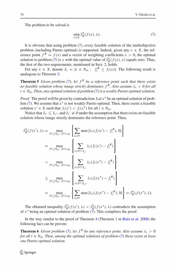
Theorem 5 Given problem (7), let f R be a reference point such that there existsno feasible solution whose image strictly dominates f R. Also assume λi > 0 for alli ∈ Nm. Then, any optimal solution of problem (7) is a weakly Pareto optimal solution.

Proof The proof will be given by contradiction. Let x∗ be an optimal solution of prob-lem (7). We assume that x∗ is not weakly Pareto optimal. Then, there exists a feasiblesolution x ′ ∈ X such that fi (x ′) < fi (x∗) for all i ∈ Nm .

Notice that Ix ′ ⊆ Ix∗ , and Ix ′ �= ∅ under the assumption that there exists no feasiblesolution whose image strictly dominates the reference point. Then,

sqR( f (x ′), λ) = max

I q⊆Nm : |I q |=q

{∑

i∈I q

max [λi ( fi (x ′) − f Ri ), 0]

}

= maxI q⊆Nm : |I q |=q

⎧⎨

⎩∑

i∈I q∩Ix ′λi ( fi (x ′) − f R

i )

⎫⎬

⎭

< maxI q⊆Nm : |I q |=q

⎧⎨

⎩∑

i∈I q∩Ix ′λi ( fi (x∗) − f R

i )

⎫⎬

⎭

≤ maxI q⊆Nm : |I q |=q

⎧⎨

⎩∑

i∈I q∩Ix∗λi ( fi (x∗) − f R

i )

⎫⎬

⎭


{∑

i∈I q

max [λi ( fi (x∗) − f Ri ), 0]

}= sq

R( f (x∗), λ).

The obtained inequality sqR( f (x ′), λ) < sq

R( f (x∗), λ) contradicts the assumptionof x∗ being an optimal solution of problem (7). This completes the proof.

In the way similar to the proof of Theorem 4 (Theorem 1 in Ruiz et al. 2008) thefollowing fact can be proven:

Theorem 6 Given problem (7), let f R be any reference point. Also assume λi > 0for all i ∈ Nm. Then, among the optimal solutions of problem (7) there exists at leastone Pareto optimal solution.

123


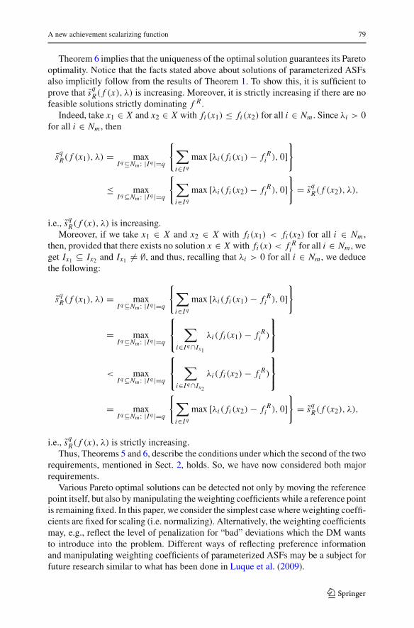
Theorem 6 implies that the uniqueness of the optimal solution guarantees its Paretooptimality. Notice that the facts stated above about solutions of parameterized ASFsalso implicitly follow from the results of Theorem 1. To show this, it is sufficient toprove that sq

R( f (x), λ) is increasing. Moreover, it is strictly increasing if there are nofeasible solutions strictly dominating f R .

Indeed, take x1 ∈ X and x2 ∈ X with fi (x1) ≤ fi (x2) for all i ∈ Nm . Since λi > 0for all i ∈ Nm , then

sqR( f (x1), λ) = max

I q⊆Nm : |I q |=q

{∑

i∈I q

max [λi ( fi (x1) − f Ri ), 0]

}

≤ maxI q⊆Nm : |I q |=q

{∑

i∈I q

max [λi ( fi (x2) − f Ri ), 0]

}= sq

R( f (x2), λ),

i.e., sqR( f (x), λ) is increasing.

Moreover, if we take x1 ∈ X and x2 ∈ X with fi (x1) < fi (x2) for all i ∈ Nm ,then, provided that there exists no solution x ∈ X with fi (x) < f R

i for all i ∈ Nm , weget Ix1 ⊆ Ix2 and Ix1 �= ∅, and thus, recalling that λi > 0 for all i ∈ Nm , we deducethe following:

sqR( f (x1), λ) = max

I q⊆Nm : |I q |=q

{∑

i∈I q

max [λi ( fi (x1) − f Ri ), 0]

}


⎧⎨

⎩∑

i∈I q∩Ix1

λi ( fi (x1) − f Ri )

⎫⎬

⎭

< maxI q⊆Nm : |I q |=q

⎧⎨

⎩∑

i∈I q∩Ix2

λi ( fi (x2) − f Ri )

⎫⎬

⎭


{∑

i∈I q

max [λi ( fi (x2) − f Ri ), 0]

}= sq

R( f (x2), λ),

i.e., sqR( f (x), λ) is strictly increasing.

Thus, Theorems 5 and 6, describe the conditions under which the second of the tworequirements, mentioned in Sect. 2, holds. So, we have now considered both majorrequirements.

Various Pareto optimal solutions can be detected not only by moving the referencepoint itself, but also by manipulating the weighting coefficients while a reference pointis remaining fixed. In this paper, we consider the simplest case where weighting coeffi-cients are fixed for scaling (i.e. normalizing). Alternatively, the weighting coefficientsmay, e.g., reflect the level of penalization for “bad” deviations which the DM wantsto introduce into the problem. Different ways of reflecting preference informationand manipulating weighting coefficients of parameterized ASFs may be a subject forfuture research similar to what has been done in Luque et al. (2009).

123


Parameterized ASFs can be potentially used either for some particular values of qor for all q ∈ Nm simultaneously. The simplest but the most computationally demand-ing way is to calculate ASFs for all q ∈ Nm . Since the solution of a problem witha smaller q-value unlikely provides any help for the solution of the problem with alarger q-value and vice versa, it seems realistic to use parallel computation for thesepurposes. The choice of a particular q-value can be done if some extra information isavailable (at least locally) about the shape of the Pareto frontier as well as the shapeof the R-level set (i.e. a set of points for which the distance from the reference pointis equal to R in terms of the corresponding ASF) of the parameterized ASF for thegiven q-value. In general, getting such information may be a very complicated task andpractically can be potentially fulfilled under strong assumptions like, e.g., objectivefunctions convexity etc.

Notice also that the choice of parameter q affects directly the shape of R-levelthat may vary from being sharp in the case of s1

R( f (x), λ) to linearly flat as in thecase of sm

R ( f (x), λ). This helps the ASF to penetrate into the areas where lots ofnon-supported solutions are accumulated.

As in the case with the additive ASF s1R( f (x), λ) developed in Ruiz et al. (2008), the

parameterized ASF sqR( f (x), λ) inherits the similar limitation: one has to keep always

in mind that the reference point should not be strictly dominated by some feasiblepoint. However, if this is the case, the point which strictly dominates the referencepoint could be easily detected, and the problem can be overcame as pointed out inRuiz et al. (2008).

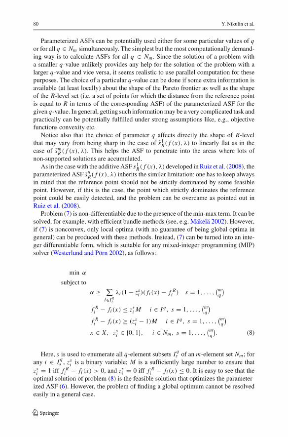
Problem (7) is non-differentiable due to the presence of the min-max term. It can besolved, for example, with efficient bundle methods (see, e.g. Mäkelä 2002). However,if (7) is nonconvex, only local optima (with no guarantee of being global optima ingeneral) can be produced with these methods. Instead, (7) can be turned into an inte-ger differentiable form, which is suitable for any mixed-integer programming (MIP)solver (Westerlund and Pörn 2002), as follows:

min α

subject to

α ≥ ∑

i∈I qs

λi (1 − zsi )( fi (x) − f R

i ) s = 1, . . . ,(m

q

)

f Ri − fi (x) ≤ zs

i M i ∈ I q , s = 1, . . . ,(m

q

)

f Ri − fi (x) ≥ (zs

i − 1)M i ∈ I q , s = 1, . . . ,(m

q

)

x ∈ X, zsi ∈ {0, 1}, i ∈ Nm, s = 1, . . . ,

(mq

). (8)

Here, s is used to enumerate all q-element subsets I qs of an m-element set Nm ; for

any i ∈ I qs , zs

i is a binary variable; M is a sufficiently large number to ensure thatzs

i = 1 iff f Ri − fi (x) > 0, and zs

i = 0 iff f Ri − fi (x) ≤ 0. It is easy to see that the

optimal solution of problem (8) is the feasible solution that optimizes the parameter-ized ASF (6). However, the problem of finding a global optimum cannot be resolvedeasily in a general case.

123


This mixed-integer programming model contains 4 · (mq

)constraints, so one may

expect the increase of computational time while(m

q

)grows up. A large number of

constraints can be efficiently treated by a MIP solver if the constraint propagationmechanisms (see, e.g. Rossi et al. 2006) are incorporated. Instead, solvers not assum-ing differentiability can be used.

Despite increasing computational efforts, the parameterized ASFs present a newapproach (based on parameterization) how to generate systematically different ASFswhich may potentially produce different solutions with different q-values. Furtherunderstanding of how different q-values produce different shapes of R-level sets mayshed extra light on the practical application of the parameterized ASFs. This could bea challenging and promising topic for further research. In the next section, we lightlytreat this and other questions for the simplest case with three objective functions.

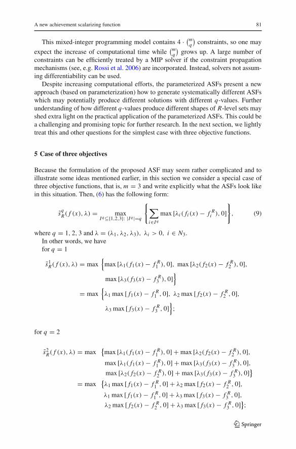
5 Case of three objectives

Because the formulation of the proposed ASF may seem rather complicated and toillustrate some ideas mentioned earlier, in this section we consider a special case ofthree objective functions, that is, m = 3 and write explicitly what the ASFs look likein this situation. Then, (6) has the following form:

sqR( f (x), λ) = max

I q⊆{1,2,3}: |I q |=q

{∑

i∈I q

max [λi ( fi (x) − f Ri ), 0]

}, (9)

where q = 1, 2, 3 and λ = (λ1, λ2, λ3), λi > 0, i ∈ N3.In other words, we havefor q = 1

s1R( f (x), λ) = max

{max [λ1( f1(x) − f R

1 ), 0], max [λ2( f2(x) − f R2 ), 0],

max [λ3( f3(x) − f R3 ), 0]

}

= max{λ1 max [ f1(x) − f R

1 , 0], λ2 max [ f2(x) − f R2 , 0],

λ3 max [ f3(x) − f R3 , 0]

};

for q = 2

s2R( f (x), λ) = max

{max [λ1( f1(x) − f R

1 ), 0] + max [λ2( f2(x) − f R2 ), 0],

max [λ1( f1(x) − f R1 ), 0] + max [λ3( f3(x) − f R

3 ), 0],max [λ2( f2(x) − f R

2 ), 0] + max [λ3( f3(x) − f R3 ), 0]}

= max{λ1 max [ f1(x) − f R

1 , 0] + λ2 max [ f2(x) − f R2 , 0],

λ1 max [ f1(x) − f R1 , 0] + λ3 max [ f3(x) − f R

3 , 0],λ2 max [ f2(x) − f R

2 , 0] + λ3 max [ f3(x) − f R3 , 0]};

123


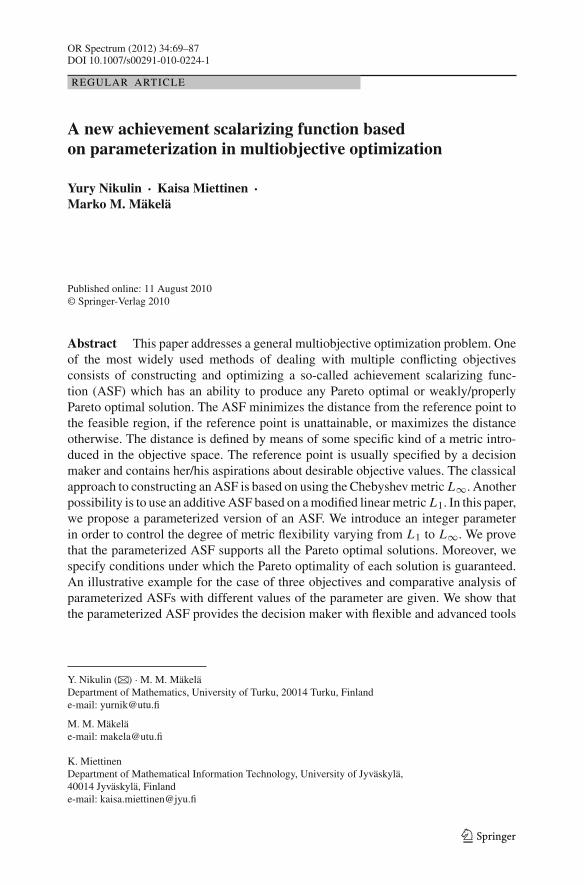
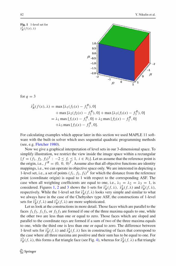
Fig. 1 1-level set fors1

R( f (x), λ)

for q = 3

s3R( f (x), λ) = max [λ1( f1(x) − f R

1 ), 0]+ max [λ2( f2(x) − f R

2 ), 0] + max [λ3( f3(x) − f R3 ), 0]

= λ1 max [ f1(x) − f R1 , 0] + λ2 max [ f2(x) − f R

2 , 0]+λ3 max [ f3(x) − f R

3 , 0].

For calculating examples which appear later in this section we used MAPLE 11 soft-ware with the built-in solver which uses sequential quadratic programming methods(see, e.g. Fletcher 1980).

Now we give a graphical interpretation of level sets in our 3-dimensional space. Tosimplify illustration, we restrict the view inside the image space within a rectangular{ f = ( f1, f2, f3)

T : −2 ≤ fi ≤ 1, i ∈ N3}. Let us assume that the reference point isthe origin, i.e., f R = (0, 0, 0)T . Assume also that all objective functions are identitymappings, i.e., we can operate in objective space only. We are interested in depicting a1-level set, i.e., a set of points ( f1, f2, f3)

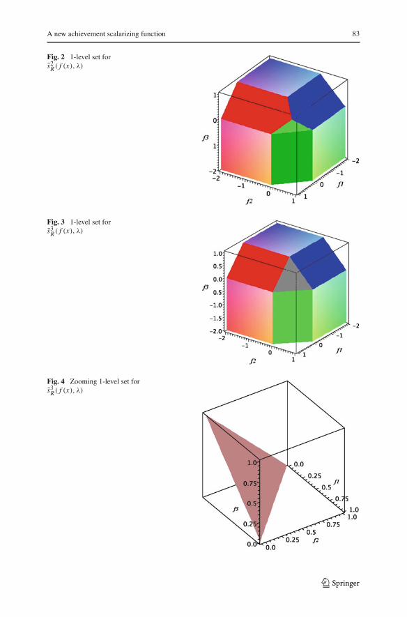
T for which the distance from the referencepoint (coordinate origin) is equal to 1 with respect to the corresponding ASF. Thecase when all weighting coefficients are equal to one, i.e., λ1 = λ2 = λ3 = 1, isconsidered. Figures 1, 2 and 3 shows the 1-sets for s1

R( f, λ), s2R( f, λ) and s3

R( f, λ),respectively. While the 1-level set for s1

R( f, λ) looks very simple and similar to whatwe always have in the case of the Chebyshev type ASF, the constructions of 1-levelsets for s2

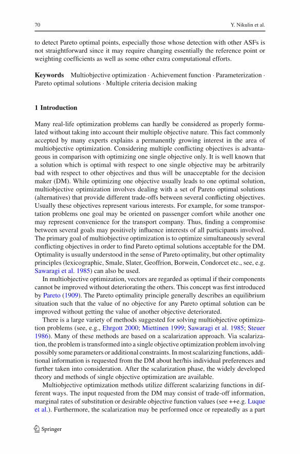
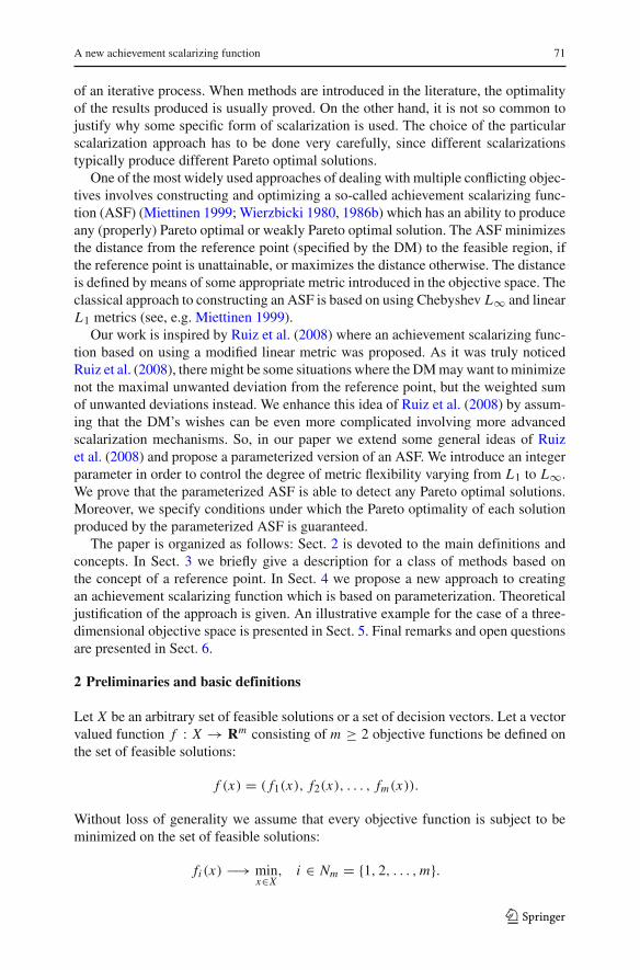
R( f, λ) and s3R( f, λ) are more sophisticated.

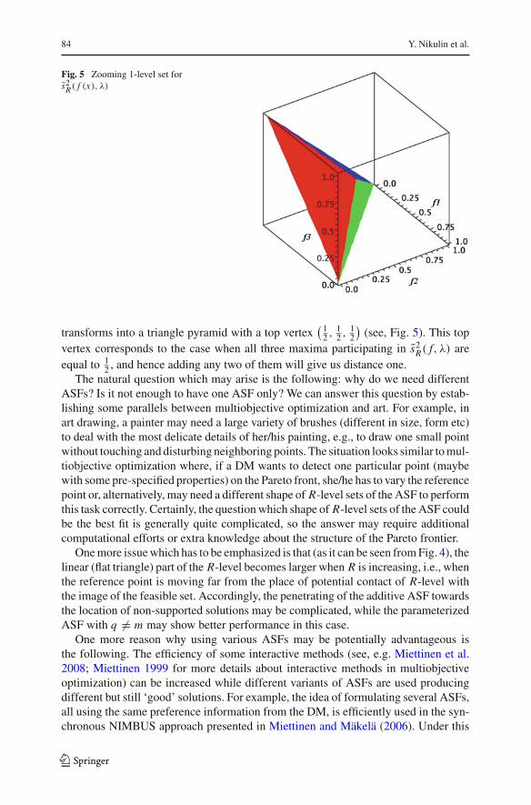
Let us look at the constructions in more detail. Those faces which are parallel to thefaces f1 f2, f1 f3, or f2 f3 are formed if one of the three maxima equals to one, whilethe other two are less than one or equal to zero. Those faces which are sloped andparallel to the coordinate rays are formed if a sum of two of the three maxima equalsto one, while the third one is less than one or equal to zero. The difference between1-level sets for s2

R( f, λ) and s3R( f, λ) lies in constructing of faces that correspond to

the case where all three maxima are positive and their sum has to be equal to one. Fors3

R( f, λ), this forms a flat triangle face (see Fig. 4), whereas for s2R( f, λ) a flat triangle

123



R( f (x), λ)


R( f (x), λ)

Fig. 4 Zooming 1-level set fors3

R( f (x), λ)

123


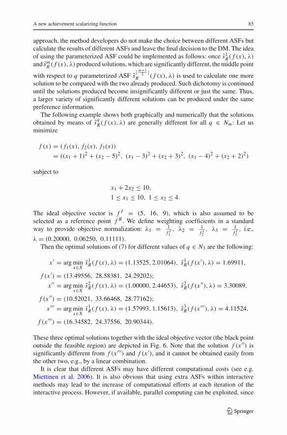
Fig. 5 Zooming 1-level set fors2

R( f (x), λ)

transforms into a triangle pyramid with a top vertex( 1

2 , 12 , 1

2

)(see, Fig. 5). This top

vertex corresponds to the case when all three maxima participating in s2R( f, λ) are

equal to 12 , and hence adding any two of them will give us distance one.

The natural question which may arise is the following: why do we need differentASFs? Is it not enough to have one ASF only? We can answer this question by estab-lishing some parallels between multiobjective optimization and art. For example, inart drawing, a painter may need a large variety of brushes (different in size, form etc)to deal with the most delicate details of her/his painting, e.g., to draw one small pointwithout touching and disturbing neighboring points. The situation looks similar to mul-tiobjective optimization where, if a DM wants to detect one particular point (maybewith some pre-specified properties) on the Pareto front, she/he has to vary the referencepoint or, alternatively, may need a different shape of R-level sets of the ASF to performthis task correctly. Certainly, the question which shape of R-level sets of the ASF couldbe the best fit is generally quite complicated, so the answer may require additionalcomputational efforts or extra knowledge about the structure of the Pareto frontier.

One more issue which has to be emphasized is that (as it can be seen from Fig. 4), thelinear (flat triangle) part of the R-level becomes larger when R is increasing, i.e., whenthe reference point is moving far from the place of potential contact of R-level withthe image of the feasible set. Accordingly, the penetrating of the additive ASF towardsthe location of non-supported solutions may be complicated, while the parameterizedASF with q �= m may show better performance in this case.

One more reason why using various ASFs may be potentially advantageous isthe following. The efficiency of some interactive methods (see, e.g. Miettinen et al.2008; Miettinen 1999 for more details about interactive methods in multiobjectiveoptimization) can be increased while different variants of ASFs are used producingdifferent but still ‘good’ solutions. For example, the idea of formulating several ASFs,all using the same preference information from the DM, is efficiently used in the syn-chronous NIMBUS approach presented in Miettinen and Mäkelä (2006). Under this

123


approach, the method developers do not make the choice between different ASFs butcalculate the results of different ASFs and leave the final decision to the DM. The ideaof using the parameterized ASF could be implemented as follows: once s1

R( f (x), λ)

and smR ( f (x), λ) produced solutions, which are significantly different, the middle point

with respect to q parameterized ASF s� m+1

2 �R ( f (x), λ) is used to calculate one more

solution to be compared with the two already produced. Such dichotomy is continueduntil the solutions produced become insignificantly different or just the same. Thus,a larger variety of significantly different solutions can be produced under the samepreference information.

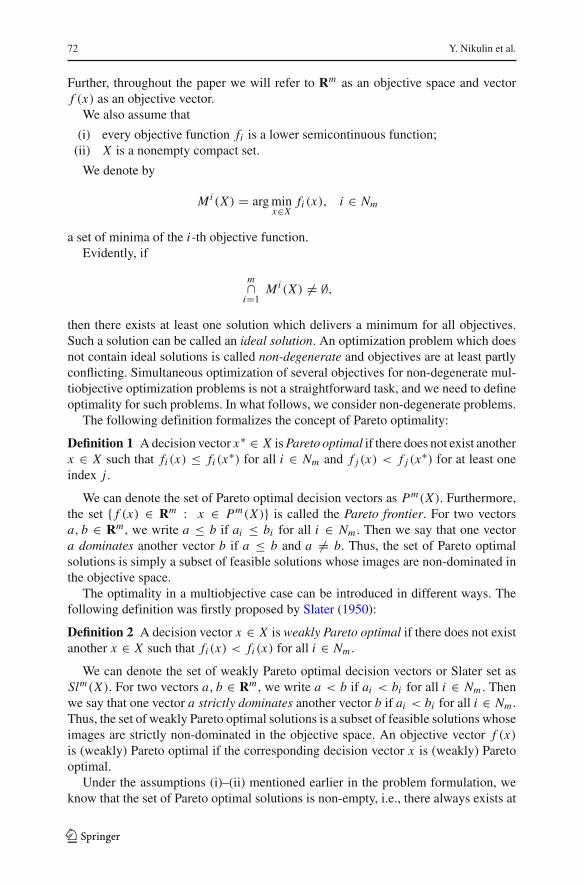
The following example shows both graphically and numerically that the solutionsobtained by means of sq

R( f (x), λ) are generally different for all q ∈ Nm : Let usminimize

f (x) = ( f1(x), f2(x), f3(x))

= ((x1 + 1)2 + (x2 − 5)2, (x1 − 3)2 + (x2 + 3)2, (x1 − 4)2 + (x2 + 2)2)

subject to

x1 + 2x2 ≤ 10,

1 ≤ x1 ≤ 10, 1 ≤ x2 ≤ 4.

The ideal objective vector is f I = (5, 16, 9), which is also assumed to beselected as a reference point f R . We define weighting coefficients in a standardway to provide objective normalization: λ1 = 1

f I1, λ2 = 1

f I2, λ3 = 1

f I3, i.e.,

λ = (0.20000, 0.06250, 0.11111).

Then the optimal solutions of (7) for different values of q ∈ N3 are the following:

x ′ = arg minx∈X

s1R( f (x), λ) = (1.13525, 2.01064), s1

R( f (x ′), λ) = 1.69911,

f (x ′) = (13.49556, 28.58381, 24.29202);x ′′ = arg min

x∈Xs2

R( f (x), λ) = (1.00000, 2.44653), s2R( f (x ′′), λ) = 3.30089,

f (x ′′) = (10.52021, 33.66468, 28.77162);x ′′′ = arg min

x∈Xs1

R( f (x), λ) = (1.57993, 1.15613), s3R( f (x ′′′), λ) = 4.11524,

f (x ′′′) = (16.34582, 24.37556, 20.90344).

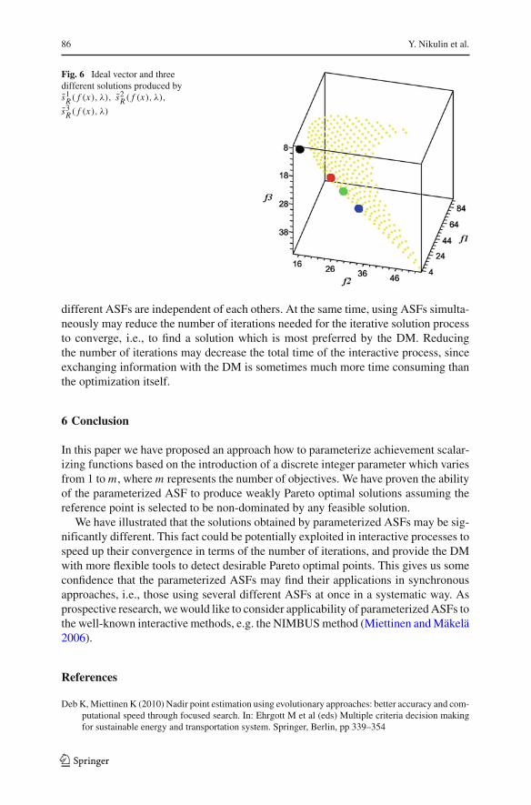
These three optimal solutions together with the ideal objective vector (the black pointoutside the feasible region) are depicted in Fig. 6. Note that the solution f (x ′′) issignificantly different from f (x ′′′) and f (x ′), and it cannot be obtained easily fromthe other two, e.g., by a linear combination.

It is clear that different ASFs may have different computational costs (see e.g.Miettinen et al. 2006). It is also obvious that using extra ASFs within interactivemethods may lead to the increase of computational efforts at each iteration of theinteractive process. However, if available, parallel computing can be exploited, since

123


Fig. 6 Ideal vector and threedifferent solutions produced bys1

R( f (x), λ), s2R( f (x), λ),

s3R( f (x), λ)

different ASFs are independent of each others. At the same time, using ASFs simulta-neously may reduce the number of iterations needed for the iterative solution processto converge, i.e., to find a solution which is most preferred by the DM. Reducingthe number of iterations may decrease the total time of the interactive process, sinceexchanging information with the DM is sometimes much more time consuming thanthe optimization itself.

6 Conclusion

In this paper we have proposed an approach how to parameterize achievement scalar-izing functions based on the introduction of a discrete integer parameter which variesfrom 1 to m, where m represents the number of objectives. We have proven the abilityof the parameterized ASF to produce weakly Pareto optimal solutions assuming thereference point is selected to be non-dominated by any feasible solution.

We have illustrated that the solutions obtained by parameterized ASFs may be sig-nificantly different. This fact could be potentially exploited in interactive processes tospeed up their convergence in terms of the number of iterations, and provide the DMwith more flexible tools to detect desirable Pareto optimal points. This gives us someconfidence that the parameterized ASFs may find their applications in synchronousapproaches, i.e., those using several different ASFs at once in a systematic way. Asprospective research, we would like to consider applicability of parameterized ASFs tothe well-known interactive methods, e.g. the NIMBUS method (Miettinen and Mäkelä2006).

References

Deb K, Miettinen K (2010) Nadir point estimation using evolutionary approaches: better accuracy and com-putational speed through focused search. In: Ehrgott M et al (eds) Multiple criteria decision makingfor sustainable energy and transportation system. Springer, Berlin, pp 339–354

123


Ehrgott M (2000) Multicriteria optimization. Springer, BerlinFletcher R (1980) Practical methods of optimization. Wiley, New YorkKaliszewski I (1994) Quantitative Pareto analysis by cone separation technique. Kluwer Academic

Publishers, DordrechtLuque M, Miettinen K, Eskelinen P, Ruiz F (2009) Incorporating preference information in interactive

reference point methods for multiobjective optimization. Omega 37:450–462Luque M, Ruiz F, Miettinen K (2009) Global formulation for interactive multiobjective optimization, OR

Spectrum. doi:10.1007/s00291-008-0154-3Miettinen K (1999) Nonlinear multiobjective optimization. Kluwer Academic Publishers, BostonMiettinen K, Ruiz F, Wierzbicki AP (2008) Introduction to multiobjective optimization: interactive

approaches. In: Branke J et al (eds) Multiobjective optimization interactive and evolutionaryapproaches. Lecture Notes in computer science, vol 5252. Springer, Berlin, pp 27–58

Miettinen K, Mäkelä MM (2006) Synchronous approach in interactive multiobjective optimization. Eur JOper Res 170(3):909–922

Miettinen K, Mäkelä MM (2002) On scalarizing functions in multiobjective optimization. OR Spectr24:193–213

Miettinen K, Mäkelä MM, Kaario K (2006) Experiments with classification-based scalarizing functions ininteractive multiobjective optimization. Eur J Oper Res 175(2):931–947

Mäkelä MM (2002) Survey of bundle methods for nonsmooth optimization. Optim Methods Softw 17(1):1–20

Pareto V (1909) Manuel d’ecoonomie politique. Qiard, ParisRossi F, van Beek P, Walsh T (eds) (2006) Handbook of constraint programming. ElsevierRuiz F, Luque M, Miguel F, del Mar Muñoz M (2008) An additive achievement scalarizing function for

multiobjective programming problems. Eur J Oper Res 188(3):683–694Sawaragi Y, Nakayama H, Tanino T (1985) Theory of multiobjective optimization. Academic Press,

OrlandoSlater M (1950) Lagrange multipliers revisited. Cowles Commission Discussion Paper: Mathematics 403Steuer R (1986) Multiple criteria optimization: theory, computation and application. Wiley, New YorkWesterlund T, Pörn R (2002) Solving pseudo-convex mixed-integer optimization problems by cutting plane

techniques. Optim Eng 3:253–280Wierzbicki AP (1977) Basic properties of scalarizing functionals for multiobjective optimization. Optimi-

zation 8:55–60Wierzbicki AP (1980) The use of reference objectives in multiobjective optimization. In: Fandel G,

Gal T (eds) Multiple criteria decision making theory and applications. MCDM theory and appli-cations proceedings. Lecture notes in economics and mathematical systems, vol 177. Springer, Berlin,pp 468–486

Wierzbicki AP (1986a) A methodological approach to comparing parametric characterizations of efficientsolutions. In: Fandel G et al (eds) Large-scale modelling and interactive decision analysis. Lecturenotes in economics and mathematical systems, vol 273. Springer, Berlin, pp 27–45

Wierzbicki AP (1986b) On the completeness and constructiveness of parametric characterizations to vectoroptimization problems. OR Spectr 8:73–87

Wierzbicki AP (1999) Reference point approaches. In: Gal T et al (eds) Multicriteria decision making:advances in MCDM models, algorithms, theory, and applications. Kluwer, Boston, pp 1–39

123

http://dx.doi.org/10.1007/s00291-008-0154-3

Documents

A new achievement scalarizing function based on parameterization in multiobjective optimization