Embed Size (px)
Citation preview

Multiobjective Simulation Optimisation in Software ProjectManagement
Mercedes Ruiz∗
Dept of Computer ScienceThe University of Cádiz
11002 Cádiz, [email protected]
Daniel Rodríguez∗
Dept of Computer ScienceUniversity of Alcalá
28871 Alcalá de Henares,Madrid, Spain
[email protected]é C. Riquelme
Dept of Computer ScienceThe University of Seville
41012 Seville, [email protected]
Rachel HarrisonSchool of Technology
Oxford Brookes UnivesityOxford OX33 1HX, UK
ABSTRACT• Background: Traditionally, simulation has been used
by project managers in optimising decision making.However, current simulation packages only include sim-ulation optimisation which consider a single objective(or multiple objectives combined into a single fitnessfunction). Although useful, such single optimisationapproaches do not seem to be enough in a field such assoftware project management where the optimisationof several conflicting objectives is a frequent task.
• Aim: This paper aims to describe an approach thatconsists of using multiobjective optimisation techniquesvia simulation in order to help software project man-agers find the best values for initial team size andschedule estimates for a given project so that cost, timeand productivity are optimised.
• Method: Using a System Dynamics (SD) simulationmodel of a software project, the sensitivity of the out-put variables regarding productivity, cost and scheduleusing different initial team size and schedule estima-tions is determined. The generated data is combinedwith a well-known multiobjective optimisation algo-rithm, called NSGA-II, to find optimal solutions forthe output variables, i.e., development time, cost andproductivity.
• Results: The NSGA-II algorithm was able to quicklyconverge to a set of optimal solutions (Pareto front)
∗Part of this work was carried out while visiting OxfordBrookes University
composed of multiple and conflicting variables from amedium size software project simulation model.
• Conclusions: Multiobjective optimisation and SD sim-ulation modeling are complementary techniques thatcan generate the Pareto front needed by project man-agers for decision making. Furthermore, visual repre-sentations of such solutions in two or three dimensionsare intuitive and can help project managers in theirdecision making process.
Categories and Subject DescriptorsI.2 [Artificial Intelligence]: Problem solving, control, meth-ods and search—Heuristic Methods; I.6 [Simulation andModeling]: Simulation Output Analysis; D.2.9 [SoftwareEngineering]: Management—Cost estimation, productiv-ity, time estimation
General TermsManagement
KeywordsSoftware Project Management, Simulation Optimisation, Mul-tiobjective Genetic Algorithms, NSGA-II
1. INTRODUCTIONProject managers face multiple and conflicting decisions dur-ing the execution of a project in order to successfully developit within the specified time span, budget and quality.
Among the decisions that need to be made in a softwaredevelopment project, estimating not only the average teamsize but the initial team size needed to develop the projectcan be placed among the most influential decisions regardingthe productivity of the team and, eventually, the cost andtime required to carry out the project.
Project team size has drawn a lot of attention over the years.Basically, large teams have been considered ineffective whilesmall teams are perceived as better at delivering results.
Brooks [7] already claimed in 1975 that assigning more pro-grammers to a project running behind schedule will make iteven later, due to the time required for the new program-mers to learn about the project, as well as the increasedcommunication overhead. Furthermore, team size does notremain stable throughout the project lifecycle. On the con-trary, project planning needs to determine the initial teamsize and the policies and schedule required to add or removepeople to or from the initial team. Accordingly to Brooks,the loss of productivity suffered when staff are added directlyaffects key project performance indicators such as schedule,quality and cost.
Therefore, project managers need reliable ways to decideabout the effects of their decisions regarding the rate ofchange in development teams on the software products, pro-jects and processes in general. From the pioneering appli-cation of Forrester’s System Dynamics (SD) simulation ap-proach to software project modeling by Abdel-Hamid andMadnick [1], SD simulation modeling has been applied tomany aspects of software development and management.Simulation enables project managers to build and run themodels to better understand the implications of candidateproject strategies and decisions.
However, a simple evaluation of the simulation outputs of amodel is often not enough to determine the best decisionsthat maximise project performance. Usually, a more ex-ploratory and in-depth study is required to determine themost suitable combination of decisions that lead the bestproject results. Simulation optimisation can be defined asthe process of finding the best values of some decision vari-ables for a system where the performance is evaluated basedon the output of a simulation model of this system [20].Currently, simulation optimisation functionalities are oftenfound as part of simulation packages, being the metaheuris-tics approach among the most used methods for simulationoptimisation. Metaheuristic techniques are a family of ap-proximate (stochastic) optimisation algorithms that searchiteratively in the solution space for a good enough solution.
However, while the approaches already implemented in thesimulation packages often provide robust results when fo-cussing on finding the optimal solution for an given objec-tive, they do not usually provide the functionality of mul-tiobjective optimisation, that is, simultaneously optimisingtwo or more conflicting objectives. For instance, Vensim c⃝1,claimed to be the most used simulation tool for softwareproject simulation modelling [25] uses the Powell hill climb-ing algorithm to search through the parameter space lookingfor the largest cumulative payoff. The payoff function is auser-defined function that is maximised or minimised andgroups together the simultaneous objectives of the modeluser. AnylogicTM2 is a new tool in the arena of softwareproject simulation. It uses the built-in OptQuestR⃝ opti-miser to search for the best solution, given the objectivefunction, constraints, requirements, and parameters that canbe varied. Once again, it is the user who needs to provide asingle objective function for maximisation or minimisation.Since software project management is a field where optimis-
1http://www.vensim.com/2http://www.xjtek.com/
ing conflicting objectives is one of the most frequent tasksthat project managers need to face, it would be interestingto provide them with this facility.
This paper describes an approach that consists of using amultiobjective optimisation technique based on genetic algo-rithms for simulation optimisation in order to help softwareproject managers to find the best values for initial team sizeand time estimates for a given project so that cost, time andproductivity are optimised.
The phases carried out in this work are as follows. First,we developed a SD simulation model based on the litera-ture and previous work. Second, we generated a databasewith all possible inputs combinations of the simulation runs.Although, in theory, the multiobjective genetic algorithmshould call the simulation tool (i.e., the model correspondsto the fitness function) as many times as necessary whileconverges to the optimum values, this is not possible dueto licence issues. Therefore, in the process of generatingthe database with input and output results, we have prob-ably executed the simulation tool many more times thanreally necessary. Third, we ran several executions of the thegenetic algorithm with different multi-objectives as well asconstraints obtained from the sensitivity analysis performedin the SD model.
The rest of this paper is structured as follows. Section 2 cov-ers the background, Section 3 describes the SD model builtto simulate a software project. Next, we describe the appli-cation of a multiobjective optimisation algorithm based ongenetic algorithms with the simulation model in Section 4.Finally, Section 5 provides some conclusions and future re-search directions.
2. BACKGROUNDAbdel-Hamid and Madnick [1, 2] developed a highly aggre-gated simulation model of software project dynamics. Theadvantage of using System Dynamics is that one can ex-periment with different management policies before, duringand after the execution of a project (post-mortem analysis)without additional cost. Among other things, their modelwas used to analyse Brooks’ law applying different staffingpolicies on cost and schedule in a specific project, the NASADE-A project. The authors conclude that adding more peo-ple to a late project always causes it to become more costlybut does not always cause it to complete later. In this case,Brooks’ law holds when the time to complete is less than 30days (which would correspond to a project of approximatelly24KDSI, 2,220 Person-days and 380 days).
The application of metaheuristic techniques to Software En-gineering problems has generated a research field known asSearch Based Software Engineering (SBSE) [13, 12]. So far,SBSE has been majoritarily applied to software testing prob-lems [18] but it is been increasingly applied to other softwareengineering problems such as project management. For ex-ample, in Software Project Staffing, Di Penta et al. [9, 4]analysed the Brooks’ law using genetic algorithms. Albaand Chicano [3] have applied genetic algorithms as a tech-nique to optimise people allocation to software developmenttasks. Zhang et al. [26] and Saliu and Ruhe [21] have appliedmetaheristic techniques in the next release problem, etc.
However, although simulation optimisation has been a pro-ductive topic of research in other fields, not many appli-cations can be found in the field of software project man-agement. Hanne and Nickel [11] considered the problemof planning inspections and other tasks within a softwaredevelopment project with respect to the objectives of qual-ity, project duration, and costs. They built a discrete-eventsimulation model comprising the phases of coding, inspec-tion, test, and rework and formalised the problem of projectscheduling as a multiobjective simulation optimisation prob-lem. Di Penta et al. [5] shows how search-based optimisa-tion techniques can be combined with a queuing simulationmodel to address the problems of allocating resources to asoftware project and assigning tasks to teams.
As in the example above, most of the applications of sim-ulation optimisation that can be found in the field of soft-ware project management use the discrete-event paradigm asthe simulation approach. However, there are some applica-tions of simulation optimisation using the System Dynamicssimulation approach. For instance, Ng [19] reported an ap-proach for integrating simulation and optimisation of SystemDynamics models using Matlab and Simulink and demon-strated how to combine genetic algorithms, fuzzy logic ex-pert input and System Dynamics modelling for improvingdecision-making. They applied their approach in the classi-cal market growth model. Kremmel et al. [15] developed aSystem Dynamics simulation model to analyse the dynam-ics of city problems and city development under three typesof policy interventions. They used genetic algorithms formaximising the benefits of policy decision making.
There are also some studies for optimising agent-based sim-ulation models. Better et al. [6] describes work on progressconsisting of incorporating advanced data mining techniquesto identify relevant system inputs and to analyse the waythese inputs interact within the system. The approach isapplied in an agent-based simulation model for market re-search that works at both the consumer and the companylevel.
3. SIMULATION MODEL FOR SOFTWAREPROJECT MANAGEMENT
The simulation model has been built followings Law’s method-ology [16]. This section describes the model according toKellner’s proposal for simulation model description [14].
3.1 Model Purpose and ScopeThe purpose of a simulation model can be described as thekey questions the model has to address. In our case, thepurpose of the simulation model is to help analyse the ef-fect of uncertainty of both the schedule estimate and theinitial team size of a software project on the key indicatorsof project success, namely time, cost and productivity. De-termining the model scope is also an important issue, sincethe scope needs to be large enough to fully address the keyquestions posed. For the purpose of this work, the scope ofthe model is a software development project with a mediumtime-span and just of one project team.
We next sumarise the most important input and output vari-ables.
3.2 Output VariablesThe output variables are the information elements neededto answer the key questions that were specified along withthe purpose of the model. For the purpose of this study, wewill need the following outputs of the model:
• Project End (Time): The final time of the project.
• Cumulative Cost (Cost): The final cost of the project.
• Productivity (Prod): The average productivity reachedby the team through the project lifecycle. This is cal-culated as the ratio between size (Function Points -FP-in this case) and the Project End (time taken to finishthe project).
Other output variables that are helpful for analysis duringthe simulation timeframe are the following:
• Fraction Complete: The percentage of project comple-tion at any time of the simulation.
• Effective Workforce: The effective work rate performedby the team.
3.3 Input ParametersThe input parameters to include in the model depend on theresult variables desired and the process abstraction identi-fied. To simulate a software project different input param-eters are required, each of them customising the simulationmodel to both the features of the project and the organisa-tion.
In our case, the model built provides input parameters todescribe the features of the project under development suchas the initial estimations of size and time, the quality leveldesired, the initial team size and its composition, the maxi-mum workforce allowed, the wage rate, etc. In addition, themodel also provides a set of input parameters to customisethe model to the features of the organisation developing theproject. Among these features, the following ones can behighlighted: hiring and dismissals delays, average time tooverwork, the effect of fatigue on product quality and teamproductivity, etc.
For the sake of clarity, we will only describe here the inputparameters that allow us to model decision making regardingthe purpose of this study, that is, the initial team size and itscomposition, together with the initial estimations of projectsize and time to develop.
• Initial Novice Workforce (NoviceWf): The initial num-ber of novice personnel allocated to the project.
• Initial Experienced Workforce (ExpWf): The initialnumber of experienced personnel allocated to the project.
• Project Size (Size): The estimate of project size (weconsider Function Points -FP -[17] as a measure of thesize).
• Scheduled Time (SchldT ime): The estimate of projectschedule.
3.4 Process AbstractionWhen developing a simulation model, it is necessary to iden-tify the key elements of the process, their interrelationshipsand behaviour, for inclusion in the model. The focus needsto be on those aspects of the process that are especially rel-evant to the purpose of the model and are believed to affectthe result variables. The model developed is structured inthree main subsystems:
• Development : This subsystem models the software de-velopment process excluding requirements, operationand maintenance.
• Team management : This deals with hiring, training,assimilation and transfer of the human resources. Itincludes Brooks’ Law to model training and communi-cation overhead due to team size.
• Control and Planning : This subsystem provides theinitial project estimates and models how and underwhat circumstances they will be revised through thesoftware project life cycle.
Under the System Dynamics simulation approach, all sys-tems, no matter how complex, consist of networks of feed-back loops, and all dynamics arise from the interaction ofthese loops with one another. Therefore, much of the workwhen building a System Dynamics model is discovering andrepresenting the feedback loops, which along with stock andflow structures, time delays, and nonlinearities, determinethe dynamics of a system. For the purpose of this study, thesimulation model built consists of a network 77 interactingfeedback loops and 89 equations.
3.5 Sensitivity Experiment of the ModelUsing the model described, we design a scenario for sim-ulation and analysis of the sensitivity of the main outputvariables to the variation of the main input parameters.
Let us assume that the project size has been estimated as500FP and that from the organisation historical data, thetime required to develop a FP is 2 days. Therefore, thetime scheduled for this project should be approximately 50months. Let us also assume that in this particular projectthere are some new aspects that lead to the project managerto some uncertainty regarding the time estimation and thenumber of personnel that should be allocated for the initialteam for this project.
In this context, a sensitivity experiment carried out with thesimulation model can help the project manager to visualisethe effect that under- or overestimating the project schedule,as well as the initial team size and composition betweennovice and experience personnel can have over the projectfinal outcome.
Table 1 collects the values of the control parameters for thesensitivity experiment. In the experiment, the simulationmodel is run to obtain a database with all the output corre-sponding to each possible combination of the input param-eters that control de experiment. Considering the sentivity
Table 1: Control Parameters for Sensitivity Exper-iment
Input parameter Range Step
Initial Novice Workforce [0-10] 1Initial Experienced Workforce [2-10] 1Scheduled Completion Time [45-80] 5
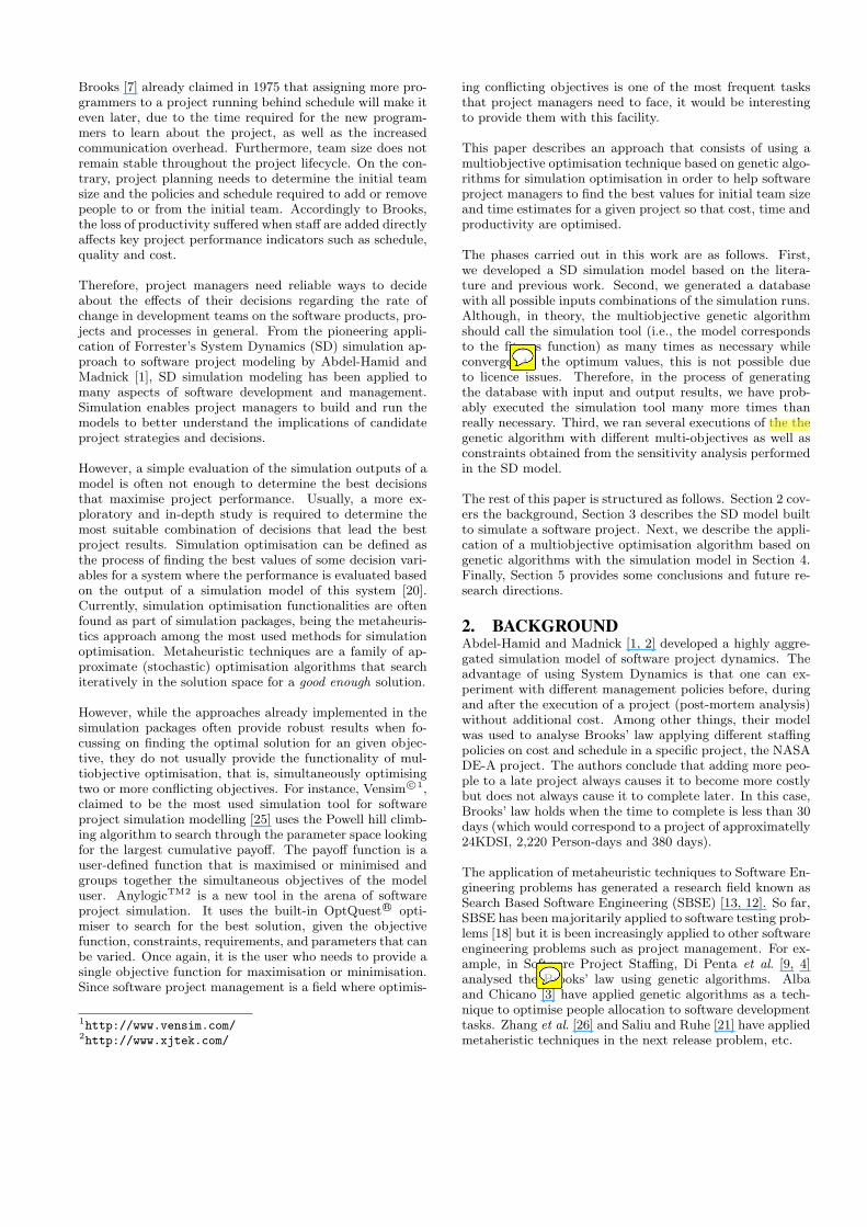
Figure 1: Sensitivity of the output variable Fraction-Complete
analysis, we are assuming that the minimum size of the de-velopment team is two experienced people. The number ofexperienced people can rise from 2 up to 10. Regarding theinitial number of new personnel in the project, the valueswill varied from 0 to 10. These restrictions will lead to de-signing a development team whose initial size is no largerthan 20 people. As for the time estimates, the experimentallows for a range starting with 45 and up to 80 months.
Figure 1 shows the sensitivity of the output variable Frac-tionComplete. When this output variable reaches one itmeans that the project is already finished since 100% of thetasks pending has been developed. According to this exper-iment, the final schedule of the project is within the rangefrom 44 to 81 months.
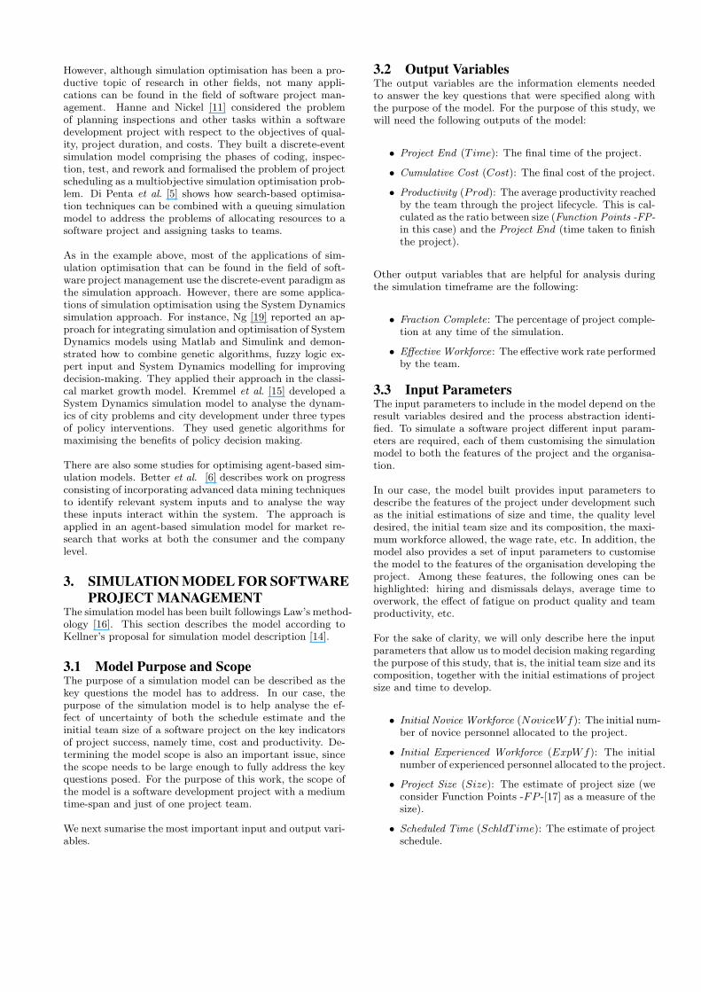
Figure 2 shows the sensitivity of the output variable Effec-tiveWorkforce. This output variable represents the effectivework rate the development team is able to achieve at everymoment of each simulated project. It results from calculat-ing the real productivity of each particular team taking intoaccount their training and communication overheads.
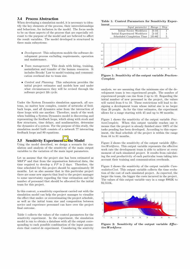
Figure 3 shows the sensitivity of the output variable Cum-mulativeCost. This output variable collects the time evolu-tion of the cost of each simulated project. As expected, thelarger the team, the bigger the costs incurred in the project.The values of this output variable vary in a range $992K to$2,551K.
Figure 2: Sensitivity of the output variable Effec-tiveWorkforce
Figure 3: Sensitivity of the output variable Cummu-lativeCost
Among the many managerial decisions that need to be madein a software project, personnel related factors are amongthe ones affecting the productivity most [23]. This raisesthe concern about empirical evidence about the relationshipsbetween project attributes, productivity and staffing levelsthat can help optimise managerial decisions. Concretely,regarding the team size it is commonly acknowledged thatthe time spent in communication among team members in-creases with the size of the team. Project team size thereforeaffects schedule decisions, which are also acknowledged as animportant factor in project success [24]. Furthermore, teamsize is important when making decisions about the struc-ture of teams and the eventual partitioning of projects intosmaller sub-projects. If an optimal team size could be found,then the decomposition of projects into smaller pieces be-comes a key management practice with direct implicationsin the decision of distributing project teams.
3.6 Simulation OptimisationOnce the sensitivity of the output variables of the modelhas been determined, the next step for the project managershould be to use the model in order to decide what valuesof the input parameters optimise the key project indicators.Current simulation tools provide their users with simulationoptimisation but only for a single fitness function. That is,all the objectives need to be aggregated together to forma single objective or a scalar fitness function which is thentreated by some classical techniques, mostly simulated an-nealing and scatter search.
This approach brings problems regarding how to normalise,prioritise and weight the different objectives in the globalfitness function. In software project management it is alsousual that conflicting objectives interact with each other innonlinear ways. Therefore, finding an adequate function be-comes the critical point in this approach since the set ofsolutions produced is highly dependent upon the functionselected and the weights assigned.
In this study, we use the optimisation module built in AnylogicTM
to optimise simulation output. We next show and discussthe results obtained in single and multiobjective simulationoptimisation.
1. Single objective optimisation.
In single objective optimisation, the tool finds the val-ues of the input parameters that maximise or minimisea single output variable.
Table 2 shows the values of the input parameters that
Table 2: Input Parameter Values for Single Objec-tive Optimisation
Output Input ParametersNoviceWf ExpWf SchldT ime
Cost $992K 0 10 80SchldT ime 44.75 3 10 40
Prod 11.47 3 10 40
optimise each single output variable according to thedifferent optimisation experiments carried out usingthe simulation framework.
It can be seen that the initial team size and the sched-uled completion time vary depending on the objectiveone wants to achieve. Typically, this is not a very re-alistic situation in software project management, sinceproject managers would be interested in the combi-nation of input parameters that lead to the projectwith the maximum productivity and the minimum costand time. Therefore, a multiobjective optimisation isneeded.
2. Multiobjective simulation optimisation.
When using current simulation frameworks for simula-tion optimisation such as AnylogicTM, it is necessaryto aggregate all the objectives into a single fitness func-tion. This fitness function is then maximised or min-imised, depending on the user request, mainly usingscatter search.
The simplest way to do this is to bundle all the objec-tives into a single fitness function using a linear func-tion. For the purpose of this study, it was assumedthat the project cost is the main objective driver andso different weights were used to determine how thetwo other objectives were related to the driving objec-tive (Eq. 1).
Fitness(i) = CummCost(i)
+1
weightT ime(i)· TimeProjEnds(i)
+1
weightProd(i)· Prod(i)
The optimisation experiments carried out with the tooldetermined that the values of input parameters thatoptimise this fitness function are 10 experienced per-sonnel, none of the novice personnel and 80 months(SchldT ime).
The optimisation module of AnylogicTM concludes thatno matter the weights, for a linear fitness function adevelopment team formed by ten experienced peopleand a time estimate of 80 months is the best configu-ration possible to maximise productivity and minimis-ing cost and development time. However, we have justseen that this combination of input parameters min-imises cost, but does not minimise time or maximisesproductivity.
In the following section, we will apply and discuss theapplication of multi-objective optimisation techniques.
4. APPLYING NSGA-II TO THE SIMULA-TION DATA
As stated previouly, there are a large number of problemswithin the software engineering discipline that can be solvedwith metaheuristic techniques. In turn, there are multiplemetaheuristic techniques available, and Multi-objective Op-timisation problems (MOP) are those that involve multipleand conflicting objective functions. MOP is also known asMultiple Criterion Decision Making (MCDM) in other fieldssuch as in operation research. In general, the solutions forMOP are defined using the Pareto front, which can be for-mally defined as follows.
Given the minimisation of the n components fk, k = 1, . . . , n,of a vector function f of a vector variable x in D, i.e., f(x) =(f1(x), . . . , fn(x)) and subject to inequality and equalityconstraints (gj(x) ≥ 0, j = 1, . . . , J and hk(x) = 0, k =1, . . . ,K).
A vector u = {u1, . . . , uk} dominates a vector v = {v1, . . . , vk},denoted by u ≼ v if u is partially less than v, i.e., ∀i ∈{1, . . . , k}, ui ≤ vi ∧ ∃i ∈ {1, . . . , k} : ui < vi (assuming theobjective is always to minimise).
The set of non-dominated decision vectors, also known asPareto-optimal, constitute the Pareto front, i.e., a set ofsolutions for which no objective can be improved withoutworsening at least one of the other objectives.
In this work, as multiobjective algorithm, we applied theNon-dominated Sorting Genetic Algorithm-II (NSGA-II) de-veloped by Deb et al. [8] as an extension of an earlier pro-posal by Srinivas and Deb [22]. The NSGA-II is a compu-tationally efficient algorithm even with a large number ofobjectives and population size.
The population individuals are evaluated (assigned fitnessvalues) in relation to how close they are to the Pareto frontand a crowding measure. The fitness value according to itsnon-domination rank is calculated as follows. The Paretofront is Rank 1. If we calculate a new Pareto front remov-ing individuals in Rank 1, individuals in the new Paretofront form Rank 2, etc . Thus, individuals in lower ranksare given higher fitness values (as we are minimising). TheNSGA-II algorithm also considers the sparsity (density) ofthe individuals belonging to the same rank using a crowd-ing measure (the Manhattan distance among individuals),with the idea of promoting diversity within the ranks (thelarger the sparcity, the better). In addition, the NSGA-IIincludes elitism in order to maintain the best solutions fromthe Pareto front found.
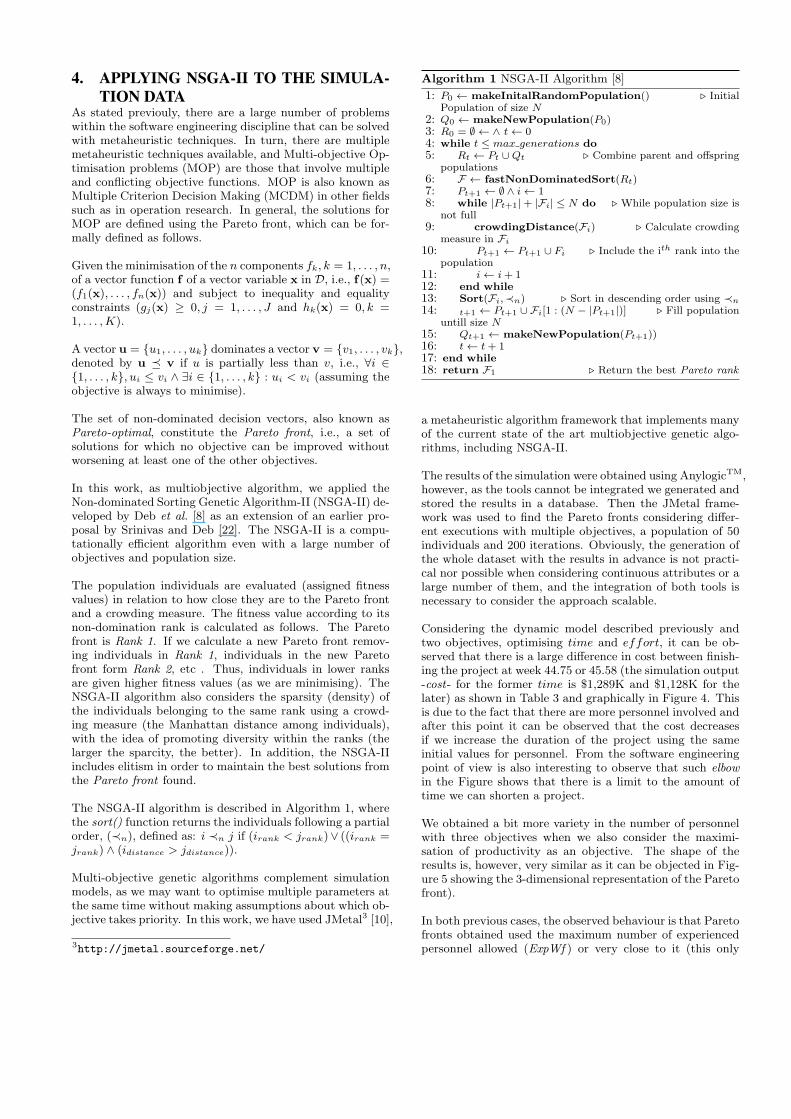
The NSGA-II algorithm is described in Algorithm 1, wherethe sort() function returns the individuals following a partialorder, (≺n), defined as: i ≺n j if (irank < jrank)∨ ((irank =jrank) ∧ (idistance > jdistance)).
Multi-objective genetic algorithms complement simulationmodels, as we may want to optimise multiple parameters atthe same time without making assumptions about which ob-jective takes priority. In this work, we have used JMetal3 [10],
3http://jmetal.sourceforge.net/
Algorithm 1 NSGA-II Algorithm [8]
1: P0 ← makeInitalRandomPopulation() ◃ InitialPopulation of size N
2: Q0 ← makeNewPopulation(P0)3: R0 = ∅ ← ∧ t← 04: while t ≤ max generations do5: Rt ← Pt ∪Qt ◃ Combine parent and offspring
populations6: F ← fastNonDominatedSort(Rt)7: Pt+1 ← ∅ ∧ i← 18: while |Pt+1|+ |Fi| ≤ N do ◃ While population size is
not full9: crowdingDistance(Fi) ◃ Calculate crowding
measure in Fi
10: Pt+1 ← Pt+1 ∪ Fi ◃ Include the ith rank into thepopulation
11: i← i+ 112: end while13: Sort(Fi,≺n) ◃ Sort in descending order using ≺n
14: t+1 ← Pt+1 ∪ Fi[1 : (N − |Pt+1|)] ◃ Fill populationuntill size N
15: Qt+1 ← makeNewPopulation(Pt+1))16: t← t+ 117: end while18: return F1 ◃ Return the best Pareto rank
a metaheuristic algorithm framework that implements manyof the current state of the art multiobjective genetic algo-rithms, including NSGA-II.
The results of the simulation were obtained using AnylogicTM,however, as the tools cannot be integrated we generated andstored the results in a database. Then the JMetal frame-work was used to find the Pareto fronts considering differ-ent executions with multiple objectives, a population of 50individuals and 200 iterations. Obviously, the generation ofthe whole dataset with the results in advance is not practi-cal nor possible when considering continuous attributes or alarge number of them, and the integration of both tools isnecessary to consider the approach scalable.
Considering the dynamic model described previously andtwo objectives, optimising time and effort, it can be ob-served that there is a large difference in cost between finish-ing the project at week 44.75 or 45.58 (the simulation output-cost- for the former time is $1,289K and $1,128K for thelater) as shown in Table 3 and graphically in Figure 4. Thisis due to the fact that there are more personnel involved andafter this point it can be observed that the cost decreasesif we increase the duration of the project using the sameinitial values for personnel. From the software engineeringpoint of view is also interesting to observe that such elbowin the Figure shows that there is a limit to the amount oftime we can shorten a project.
We obtained a bit more variety in the number of personnelwith three objectives when we also consider the maximi-sation of productivity as an objective. The shape of theresults is, however, very similar as it can be objected in Fig-ure 5 showing the 3-dimensional representation of the Paretofront).
In both previous cases, the observed behaviour is that Paretofronts obtained used the maximum number of experiencedpersonnel allowed (ExpWf ) or very close to it (this only
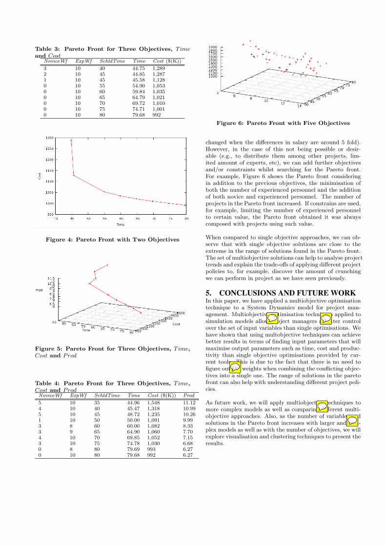
Table 3: Pareto Front for Three Objectives, Timeand Cost
NoviceWf ExpWf SchldTime Time Cost ($(K))
3 10 40 44.75 1,2892 10 45 44.85 1,2871 10 45 45.58 1,1280 10 55 54.90 1,0530 10 60 59.84 1,0350 10 65 64.79 1,0210 10 70 69.72 1,0100 10 75 74.71 1,0010 10 80 79.68 992
Figure 4: Pareto Front with Two Objectives
Figure 5: Pareto Front for Three Objectives, Time,Cost and Prod
Table 4: Pareto Front for Three Objectives, Time,Cost and ProdNoviceWf ExpWf SchldTime Time Cost ($(K)) Prod
5 10 35 44.96 1,548 11.124 10 40 45.47 1,318 10.995 10 45 48.72 1,235 10.261 10 50 50.00 1,091 9.993 8 60 60.00 1,082 8.333 9 65 64.90 1,060 7.704 10 70 69.85 1,052 7.153 10 75 74.78 1,030 6.680 8 80 79.69 993 6.270 10 80 79.68 992 6.27
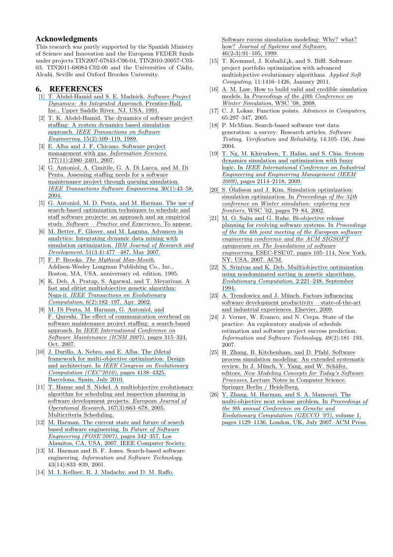
Figure 6: Pareto Front with Five Objectives
changed when the differences in salary are around 5 fold).However, in the case of this not being possible or desir-able (e.g., to distribute them among other projects, lim-ited amount of experts, etc), we can add further objectivesand/or constraints whilst searching for the Pareto front.For example, Figure 6 shows the Pareto front consideringin addition to the previous objectives, the minimisation ofboth the number of experienced personnel and the additionof both novice and experienced personnel. The number ofprojects in the Pareto front increased. If constrains are used,for example, limiting the number of experienced personnelto certain value, the Pareto front obtained it was alwayscomposed with projects using such value.
When compared to single objective approaches, we can ob-serve that with single objective solutions are close to theextreme in the range of solutions found in the Pareto front.The set of multiobjective solutions can help to analyse projecttrends and explain the trade-offs of applying different projectpolicies to, for example, discover the amount of crunchingwe can perform in project as we have seen previously.
5. CONCLUSIONS AND FUTURE WORKIn this paper, we have applied a multiobjective optimisationtechnique to a System Dynamics model for project man-agement. Multiobjective optimisation techniques applied tosimulation models allow project managers a better controlover the set of input variables than single optimisations. Wehave shown that using multobjective techniques can achievebetter results in terms of finding input parameters that willmaximise output parameters such as time, cost and produc-tivity than single objective optimisations provided by cur-rent tools. This is due to the fact that there is no need tofigure out the weights when combining the conflicting objec-tives into a single one. The range of solutions in the paretofront can also help with understanding different project poli-cies.
As future work, we will apply multiobjective techniques tomore complex models as well as comparing different multi-objective approaches. Also, as the number of variables andsolutions in the Pareto front increases with larger and com-plex models as well as with the number of objectives, we willexplore visualisation and clustering techniques to present theresults.
AcknowledgmentsThis research was partly supported by the Spanish Ministryof Science and Innovation and the European FEDER fundsunder projects TIN2007-67843-C06-04, TIN2010-20057-C03-03, TIN2011-68084-C02-00 and the Universities of Cadiz,Alcala, Seville and Oxford Brookes University.
6. REFERENCES[1] T. Abdel-Hamid and S. E. Madnick. Software Project
Dynamics: An Integrated Approach. Prentice-Hall,Inc., Upper Saddle River, NJ, USA, 1991.
[2] T. K. Abdel-Hamid. The dynamics of software projectstaffing: A system dynamics based simulationapproach. IEEE Transactions on SoftwareEngineering, 15(2):109–119, 1989.
[3] E. Alba and J. F. Chicano. Software projectmanagement with gas. Information Sciences,177(11):2380–2401, 2007.
[4] G. Antoniol, A. Cimitile, G. A. Di Lucca, and M. DiPenta. Assessing staffing needs for a softwaremaintenance project through queuing simulation.IEEE Transactions Software Engineering, 30(1):43–58,2004.
[5] G. Antoniol, M. D. Penta, and M. Harman. The use ofsearch-based optimization techniques to schedule andstaff software projects: an approach and an empiricalstudy. Software – Practice and Experience, To appear.
[6] M. Better, F. Glover, and M. Laguna. Advances inanalytics: Integrating dynamic data mining withsimulation optimization. IBM Journal of Research andDevelopment, 51(3.4):477 –487, May 2007.
[7] F. P. Brooks. The Mythical Man-Month.Addison-Wesley Longman Publishing Co., Inc.,Boston, MA, USA, anniversary ed. edition, 1995.
[8] K. Deb, A. Pratap, S. Agarwal, and T. Meyarivan. Afast and elitist multiobjective genetic algorithm:Nsga-ii. IEEE Transactions on EvolutionaryComputation, 6(2):182–197, Apr. 2002.
[9] M. Di Penta, M. Harman, G. Antoniol, andF. Qureshi. The effect of communication overhead onsoftware maintenance project staffing: a search-basedapproach. In IEEE International Conference onSoftware Maintenance (ICSM 2007), pages 315–324,Oct. 2007.
[10] J. Durillo, A. Nebro, and E. Alba. The jMetalframework for multi-objective optimization: Designand architecture. In IEEE Congress on EvolutionaryComputation (CEC’2010), pages 4138–4325,Barcelona, Spain, July 2010.
[11] T. Hanne and S. Nickel. A multiobjective evolutionaryalgorithm for scheduling and inspection planning insoftware development projects. European Journal ofOperational Research, 167(3):663–678, 2005.Multicriteria Scheduling.
[12] M. Harman. The current state and future of searchbased software engineering. In Future of SoftwareEngineering (FOSE’2007), pages 342–357, LosAlamitos, CA, USA, 2007. IEEE Computer Society.
[13] M. Harman and B. F. Jones. Search-based softwareengineering. Information and Software Technology,43(14):833–839, 2001.
[14] M. I. Kellner, R. J. Madachy, and D. M. Raffo.
Software rocess simulation modeling: Why? what?how? Journal of Systems and Software,46(2-3):91–105, 1999.
[15] T. Kremmel, J. Kubalı£¡k, and S. Biffl. Softwareproject portfolio optimization with advancedmultiobjective evolutionary algorithms. Applied SoftComputing, 11:1416–1426, January 2011.
[16] A. M. Law. How to build valid and credible simulationmodels. In Proceedings of the 40th Conference onWinter Simulation, WSC ’08, 2008.
[17] C. J. Lokan. Function points. Advances in Computers,65:297–347, 2005.
[18] P. McMinn. Search-based software test datageneration: a survey: Research articles. SoftwareTesting, Verification and Reliability, 14:105–156, June2004.
[19] T. Ng, M. Khirudeen, T. Halim, and S. Chia. Systemdynamics simulation and optimization with fuzzylogic. In IEEE International Conference on IndustrialEngineering and Engineering Management (IEEM2009), pages 2114–2118, 2009.
[20] S. Olafsson and J. Kim. Simulation optimization:simulation optimization. In Proceedings of the 34thconference on Winter simulation: exploring newfrontiers, WSC ’02, pages 79–84, 2002.
[21] M. O. Saliu and G. Ruhe. Bi-objective releaseplanning for evolving software systems. In Proceedingsof the the 6th joint meeting of the European softwareengineering conference and the ACM SIGSOFTsymposium on The foundations of softwareengineering, ESEC-FSE’07, pages 105–114, New York,NY, USA, 2007. ACM.
[22] N. Srinivas and K. Deb. Muiltiobjective optimizationusing nondominated sorting in genetic algorithms.Evolutionary Computation, 2:221–248, September1994.
[23] A. Trendowicz and J. Munch. Factors influencingsoftware development productivity – state-of-the-artand industrial experiences. Elsevier, 2009.
[24] J. Verner, W. Evanco, and N. Cerpa. State of thepractice: An exploratory analysis of scheduleestimation and software project success prediction.Information and Software Technology, 49(2):181–193,2007.
[25] H. Zhang, B. Kitchenham, and D. Pfahl. Softwareprocess simulation modeling: An extended systematicreview. In J. Munch, Y. Yang, and W. Schafer,editors, New Modeling Concepts for Today’s SoftwareProcesses, Lecture Notes in Computer Science.Springer Berlin / Heidelberg.
[26] Y. Zhang, M. Harman, and S. A. Mansouri. Themulti-objective next release problem. In Proceedings ofthe 9th annual Conference on Genetic andEvolutionary Computation (GECCO ’07), volume 1,pages 1129–1136, London, UK, July 2007. ACM Press.


