Molecular Ecology (2007)

16

, 2031–2043 doi: 10.1111/j.1365-294X.2007.03293.x

© 2007 The AuthorsJournal compilation © 2007 Blackwell Publishing Ltd

Blackwell Publishing Ltd

A new individual-based spatial approach for identifying genetic discontinuities in natural populations

S . MANEL,

*

F . BERTHOUD,

†

E . BELLEMAIN,

*

M. GAUDEUL,

*

G . LUIKART,

*

J . E . SWENSON,

‡

L . P . WAITS ,

§

P . TABERLET

*

and INTRABIODIV CONSORTIUM

1

*

Laboratoire d’Ecologie Alpine, CNRS UMR 5553, Université Joseph Fourier, BP 53, F-38041 Grenoble Cedex 9, France,

†

Laboratoire de Physique et Modélisation des Milieux Condensés, Maison des Magistères, CNRS, BP 166, F-38042 Grenoble Cedex, France,

‡

Department of Ecology and Natural Resource Management, Norwegian University of Life Sciences, Post Box 5003, NO-1432 Ås, Norway, and Norwegian Institute for Nature Research Tungasletta 2, NO-7485 Trondheim, Norway,

§

Department of Fish and Wildlife Resources, University of Idaho, Moscow, ID 83844-1136, USA

Abstract

The population concept is central in evolutionary and conservation biology, but identify-ing the boundaries of natural populations is often challenging. Here, we present a newapproach for assessing spatial genetic structure without the

a priori

assumptions on thelocations of populations made by adopting an individual-centred approach. Our method isbased on assignment tests applied in a moving window over an extensively sampled studyarea. For each individual, a spatially explicit probability surface is constructed, showingthe estimated probability of finding its multilocus genotype across the landscape, andidentifying putative migrants. Population boundaries are localized by estimating the meanslope of these probability surfaces over all individuals to identify areas with geneticdiscontinuities. The significance of the genetic discontinuities is assessed by permutationtests. This new approach has the potential to reveal cryptic population structure and toimprove our ability to understand gene flow dynamics across landscapes. We illustrate ourapproach by simulations and by analysing two empirical datasets: microsatellite data of

Ursus arctos

in Scandinavia, and amplified fragment length polymorphism (AFLP) data of

Rhododendron ferrugineum

in the Alps.

Keywords

: assignment test, genetic discontinuity, moving windows, multilocus genotype, spatialgenetics

Received 24 September 2006; revision accepted 9 January 2007

Introduction

Delineating populations is a crucial first step for assessingevolutionary processes (e.g. local adaptation, gene flow) andfor the preservation of biodiversity (e.g. identification ofmanagement units). The definition of a population remainsan area of active discussion (Waples & Gaggiotti 2006).Here, we present a new approach that combines largemolecular datasets, assignment tests and spatial movingwindow analysis to identify population boundaries.

Classical population genetic analyses consist of samplinggroups of individuals from predefined populations, andthen estimating allele frequencies and parameters, such as

genetic distance and

F

-statistics (Weir & Cockerham 1984;Nei 1987). For more continuously distributed popula-tions, individuals are at risk of being grouped somewhatarbitrarily using unproven criteria, such as habitat charac-teristics, morphological differences, geographical distance,or political boundaries (Pritchard

et al

. 2000). Also, classicalpopulation genetic analyses do not utilize the full discri-minatory power of multilocus data (Waser & Strobek 1998).

Aspatial Bayesian clustering methods (Pritchard

et al

.2000; Corander

et al

. 2003) have emerged as a popular newtool for defining populations using multilocus genotypedata. When the genetic structure coincides with the geography,using spatial information might increase the power ofdetecting genetic discontinuities. However, using spatialmethods to localize genetic discontinuities among individualsremains rare in the field of population genetics (e.g.Barbujani

et al

. 1989; Bocquet-Appel & Bacro 1994; Sokal

1

Annexe 1Correspondence: Dr Stéphanie Manel, Fax: +33 476 51 42 79;E-mail: stephanie.manel@ujf-grenoble.fr

2032

S . M A N E L

E T A L .

© 2007 The AuthorsJournal compilation © 2007 Blackwell Publishing Ltd

& Thomson 1998; Manel

et al

. 2003; Coulon

et al

. 2006).Perhaps one of the major reasons is the lack of availabledatasets with both genetic and geographical coordinateinformation, but this limitation has now been removed.New spatial Bayesian clustering algorithms (e.g. Guillot

et al

.2005; Corander

et al

. 2006; François

et al

. 2006) indirectlyidentify genetic boundaries at an individual level. Analternative and complementary approach is to look directlyfor zones of sharp change in genetic data (Legendre & Legendre2006). Two main approaches are available to achieve thisgoal: the Monmonier algorithm (Monmonnier 1973; Manni

et al

. 2004; Miller 2005) based on genetic distance analysisand the ‘wombling’ method (Womble 1951; Barbujani

et al

.1989) based on the analysis of allele frequencies.

Here, we introduce a new approach that uses individualgenotypes and their geographical co-ordinates to identifypopulations. This new approach has the potential to revealgenetic discontinuities and identify migrants without priorassumptions about population boundaries. Our methoddoes not group individuals

a priori

into perceived popula-tions, but rather adopts a spatial approach by using a ‘movingwindow’ placed across points of a grid map to identify popu-lation boundaries from the inferred genetic discontinuities.

We illustrate and validate this new approach usingsimulations and two empirical datasets from two types ofmolecular marker systems. Our first dataset encompasses18 microsatellites loci from 964 brown bear (

Ursus arctos

)samples collected across Scandinavia. The second datasetcontains 382 samples of the shrub

Rhododendron ferrugineum

sampled over the entire European Alps, and genotyped at123 polymorphic AFLP markers.

Materials and methods

Description of the method

Our approach applies an assignment test locally withina moving window over the entire sampled area (Paetkau

et al

. 1995; Rannala & Mountain 1997). Thus, a probabilitymap is constructed for each individual, showing the estimatedprobability of finding its multilocus genotype at eachpoint of a grid across the landscape. The local variation ofprobability between adjacent points is used to calculate aslope at each point of the grid across the landscape. Eachmap reveals the most likely region of origin of the individual(i.e. area with the highest probabilities), and also highlightsareas where the probability rapidly declines (greatest slope).The mean slopes calculated for all the individual probabilitymaps are used to identify population genetic discontinuitiesand thus putative population boundaries.

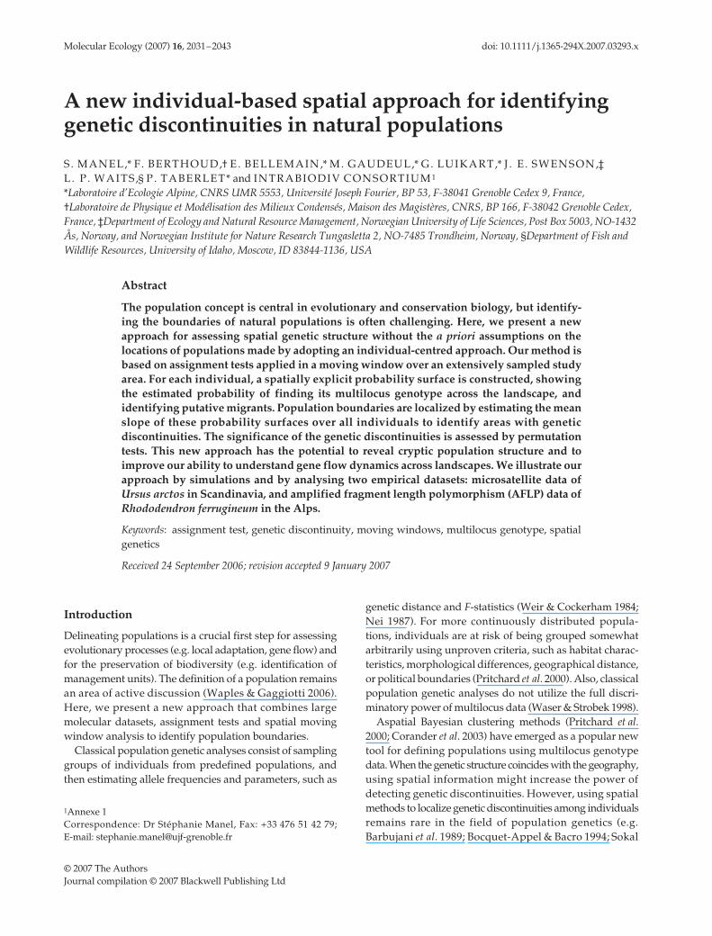
Data analysis consisted of three main steps. First, for eachindividual, we constructed a map showing the probabilityof finding its multilocus genotype at each of many pointsacross the landscape (Fig. 1). Points were distributed

on a grid with a distance

d

between adjacent points. Thealgorithm consisted of: (i) removing the individual to beassigned; (ii) computing allele frequencies using individualswithin a window of radius

R

around each point of the grid;(iii) computing the logarithm of the probability (log-likelihood) that the individual multilocus genotype occursin the area around each point of the grid, based on theBayesian assignment method of Rannala & Mountain (1997);and (iv) graphically representing the log-likelihood valuesin each point. The graphical representation consists of acircle, whose size corresponds to the magnitude of thelog-likelihood. To avoid imprecise estimates of allelefrequencies, we considered only windows with morethan

n

min

individuals (

n

min

= 20 for the simulations and thebrown bear dataset;

n

min

= 10 for the

R. ferrugineum

dataset).Missing data are allowed in the model by omitting missingloci when calculating individual probabilities (Pritchard

et al

. 2000). The appropriate values of

d

and

R

have to bedetermined by the user and will vary by species dependingon density, home range size and dispersal ability.

Second, we identified the geographical zones of highestgenetic change (discontinuity) for all individuals. Suchdiscontinuities represent putative population boundaries.For each individual and for each point of the grid, we esti-mated the slope of the likelihood function. For each pointof the grid, the slope was estimated as the mean absolutevalue of the difference between the likelihood value at thepoint considered and the eight adjacent points (if available).This resulted in a map of slopes of the likelihood functionfor each individual. In the final step, all individual slopemaps were combined to produce the final map, where theslopes values at each point of the grid corresponds to themean slopes values estimated over all individuals.

The significance of the mean slope values was estimatedthrough a randomization test (Sokal & Rohlf 1981; MonteCarlo procedure). Null distributions of mean slopes wereconstructed for each point of the grid. Individual locationswere randomised with respect to individual genotypes.Mean slopes for each point of the grid were estimatedfor each randomised data set. On the basis of the resultingdistribution of mean slopes for each point of the grid, wedecide whether the mean slope observed for the analyseddata deviated less or more than the distribution at a level

α

(e.g.

α

= 0.05).The probability maps, the identification of genetic dis-

continuities and their significance were conducted using a

c

++

computer program (available upon request) and theGIS software

arcview

(version 3.1). A fully implemented,user-friendly program is in development.

Simulations

Microsatellite genotypes were simulated with the program

easypop

(Balloux 2001) using the following parameters:

I D E N T I F Y I N G G E N E T I C D I S C O N T I N U I T I E S

2033

© 2007 The AuthorsJournal compilation © 2007 Blackwell Publishing Ltd

random mating, same number of males and females ineach population, same migration scheme, low migrationrate (0.00001), free recombination between loci andKAM mutation model. Individual spatial coordinateswere independently generated using the software

r

(

r

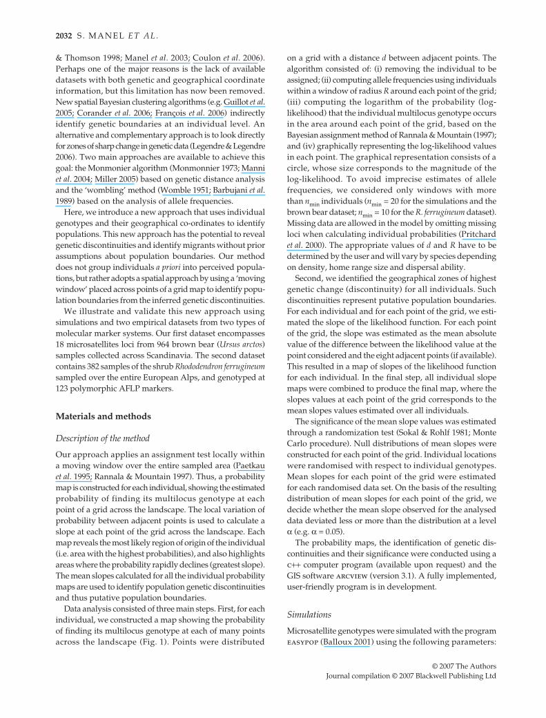
Development Core Team 2004) with the objective ofcreating three scenarios differing in spatial distributionand genetic structure (Fig. 2). Each scenario was replicated10 times, but only one repetition is shown. First, onepopulation (1000 individuals and 20 loci) was generatedwith a spatially continuous distribution and no geneticboundary (Fig. 2a). Second, the same population was thendistributed into two spatially separated subpopulationsbut with no genetic boundary (Fig. 2b). Finally, two geneti-cally differentiated populations (300 individuals each, 20loci,

F

ST

= 0.1) were generated and uniformly distributedin space (Fig. 2c). The uniform distributions were chosen inorder to obtain two populations with similar mean x-values,but different mean y-values.

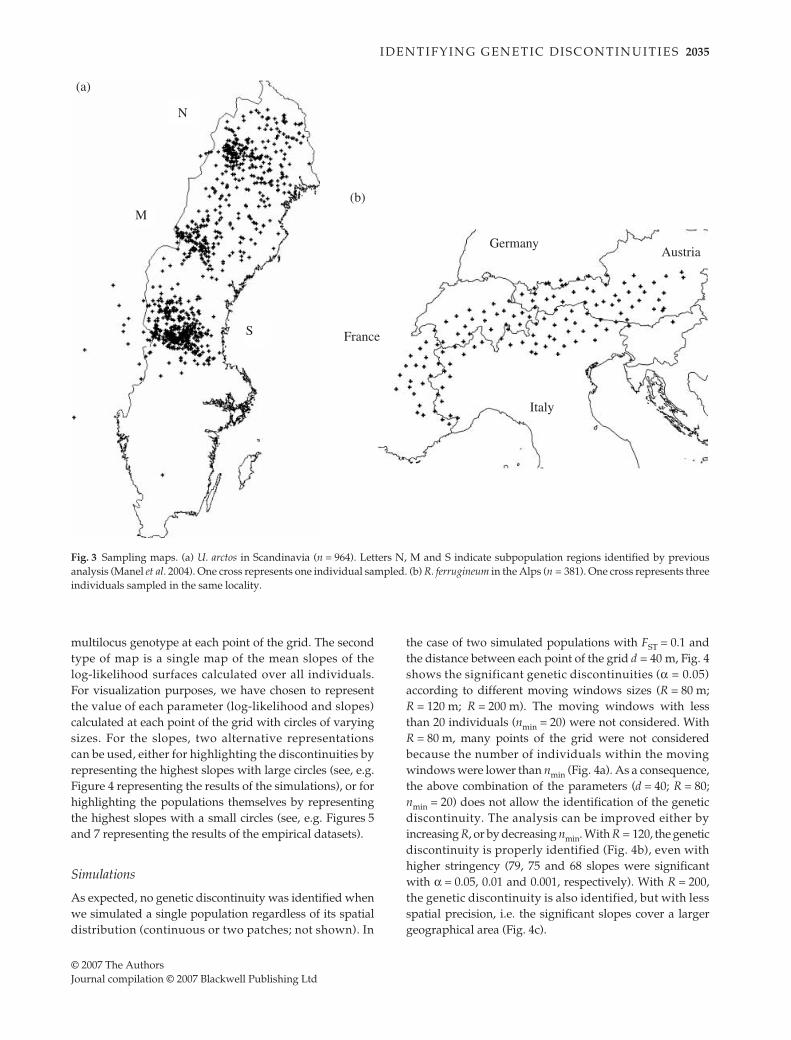
Brown bears (Ursus arctos) in Scandinavia

We used a dataset consisting of 18 microsatellite loci geno-typed for 964 brown bears distributed over

c

. 200 000 km

2

in Sweden (Waits

et al

. 2000; Bellemain 2004) (Fig. 3a). The18 microsatellite loci (G1A, G1D, G10B, G10C, G10L, G10P,G10X, G10H, G10O, G10J, Mu05, Mu10, Mu15, Mu23,Mu50, Mu51, Mu59, Mu61) were described in Waits

et al

. (2000). The error rate per locus for this dataset wasestimated to be 0.008 (Bonin

et al

. 2004).We analysed three datasets: the entire dataset com-

prising the 964 individuals, the 517 males and the 447 females.The parameters

d

and

R

were set at 50 and 120 km, respec-tively. Only windows containing at least 20 individualswere considered. The value of

d

was chosen in relation tothe size and the shape of the sampled area and the densityof the sampling. The value of

R

was chosen to insure thateach moving window would contain enough individualsto obtain reliable estimate allele frequencies. This value of

Fig. 1 Steps in the method used to generate one individual probability map. (a) Geographical distribution of the samples (small blackcrosses). (b) A grid (black dots) covers the sampling area, and the first individual to be analysed is chosen (large black cross). (c) Allelefrequencies are estimated within the window (black circle) centred around the first point of the grid. (d) The log-likelihood of the chosenindividual is estimated, and represented on the map by grey circles scaled to the size of the likelihood value. (e) The window moves to the nextpoint of the grid. (f) (g) (h) log-likelihoods are estimated and represented on the map for the next points of the grid. If the moving window doesnot encompass enough individuals (n = 20) to precisely estimate allele frequencies, the log-likelihood is not estimated for that grid point.

2034

S . M A N E L

E T A L .

© 2007 The AuthorsJournal compilation © 2007 Blackwell Publishing Ltd

R

produced 100 windows with a minimum of 20 individualswhere the slope is calculated.

A subset of these data (366 bears) was previously analysedusing a classical approach (

F

ST

and assignment tests), groupingindividuals into four putative populations correspondingto areas with a high density of females (Waits

et al

. 2000).A second study based on the analysis of the same 366 multi-locus genotypes, but using a Bayesian clustering approachwithout

a priori

population definition (Pritchard

et al

. 2000),identified only three main genetic groups (Manel

et al

. 2004).

Rhododendron ferrugineum in the Alps

Leaf samples of

R. ferrugineum

were collected during summer2004 across the entire European Alps (latitude: 44

°

48

′

to 48

°

36

′

; longitude: 5

°

20

′

to 15

°

40

′

). A 12

′

latitude

×

20

′

longitude (

c

. 23 km

×

25 km) grid was adopted and threeplants were sampled in every other cell (Fig. 3b), resultingin a total of 381 samples (127 cells) distributed over

c

. 171 350 km

2

. Because vegetative growth is extensive in

R. ferrugineum

, sampled plants were chosen at least 10 mapart to avoid sampling several ramets of a single genet.Samples were immediately dried in silica gel and preservedat room temperature. AFLP data were generated using a

protocol inspired from Vos

et al

. (1995). After electrophoresison an ABI 3100 automated sequencer, 123 polymorphicAFLP markers were manually scored as present/absent usingthe

genographer

software (http://hordeum.oscs.montana.edu/genographer/). An error rate per locus of 0.013 was estimatedby duplicating analyses for 46 random samples.

Binary AFLP data were then recoded as suggested byEvanno

et al

. (2005). Because dominant homozygotes andheterozygotes cannot be distinguished, marker presencewas recoded as 1 –9 and the absence as 0 0, where 1 indicatespresence of the band,

−

9 indicates a missing data and 0 absenceof the band.

d

and

R

were set at 25 and 50 km, respectively.For the AFLP dataset, we used only windows containing atleast 10 individuals. The value of

d

(25 km) is directly relatedto the size of the sampling grid (23km

×

25km). The value of

R

(50 km) was chosen to insure that enough individuals (atleast 10) are in the windows to calculate allele frequencies.

Results

Visualization of the results on maps

Our new method produces two types of maps. The first maprepresents the log-likelihood of observing an individual’s

Fig. 2 Spatial representation of the threesimulated scenarios. (a) One populationuniformly distributed; 1000 individuals,20 loci. (b) One population distributeduniformly in two separate patches; 1000individuals, 20 loci. (c) Two geneticallydifferentiated populations (20 loci, FST = 0.1)uniformly distributed. The uniform distri-butions were chosen in order to obtain twopopulations with similar mean x-values,but different mean y-values. Populationone: black dots; population two: grey dots.The values on the axes follow an arbitrarycoordinate system.

I D E N T I F Y I N G G E N E T I C D I S C O N T I N U I T I E S

2035

© 2007 The AuthorsJournal compilation © 2007 Blackwell Publishing Ltd

multilocus genotype at each point of the grid. The secondtype of map is a single map of the mean slopes of thelog-likelihood surfaces calculated over all individuals.For visualization purposes, we have chosen to representthe value of each parameter (log-likelihood and slopes)calculated at each point of the grid with circles of varyingsizes. For the slopes, two alternative representationscan be used, either for highlighting the discontinuities byrepresenting the highest slopes with large circles (see, e.g.Figure 4 representing the results of the simulations), or forhighlighting the populations themselves by representingthe highest slopes with a small circles (see, e.g. Figures 5and 7 representing the results of the empirical datasets).

Simulations

As expected, no genetic discontinuity was identified whenwe simulated a single population regardless of its spatialdistribution (continuous or two patches; not shown). In

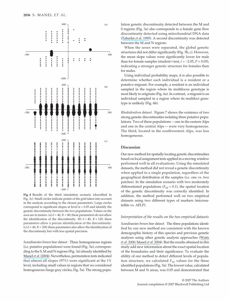
the case of two simulated populations with

F

ST

= 0.1 andthe distance between each point of the grid

d

= 40 m, Fig. 4shows the significant genetic discontinuities (

α

= 0.05)according to different moving windows sizes (

R =

80 m;

R

= 120 m;

R

= 200 m). The moving windows with lessthan 20 individuals (

n

min

= 20) were not considered. With

R

= 80 m, many points of the grid were not consideredbecause the number of individuals within the movingwindows were lower than

n

min

(Fig. 4a)

.

As a consequence,the above combination of the parameters (

d

= 40; R = 80;nmin = 20) does not allow the identification of the geneticdiscontinuity. The analysis can be improved either byincreasing R, or by decreasing nmin. With R = 120, the geneticdiscontinuity is properly identified (Fig. 4b), even withhigher stringency (79, 75 and 68 slopes were significantwith α = 0.05, 0.01 and 0.001, respectively). With R = 200,the genetic discontinuity is also identified, but with lessspatial precision, i.e. the significant slopes cover a largergeographical area (Fig. 4c).

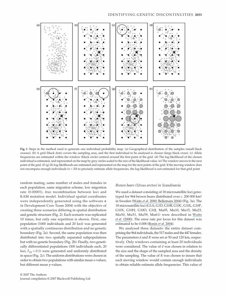
Fig. 3 Sampling maps. (a) U. arctos in Scandinavia (n = 964). Letters N, M and S indicate subpopulation regions identified by previousanalysis (Manel et al. 2004). One cross represents one individual sampled. (b) R. ferrugineum in the Alps (n = 381). One cross represents threeindividuals sampled in the same locality.

2036 S . M A N E L E T A L .

© 2007 The AuthorsJournal compilation © 2007 Blackwell Publishing Ltd

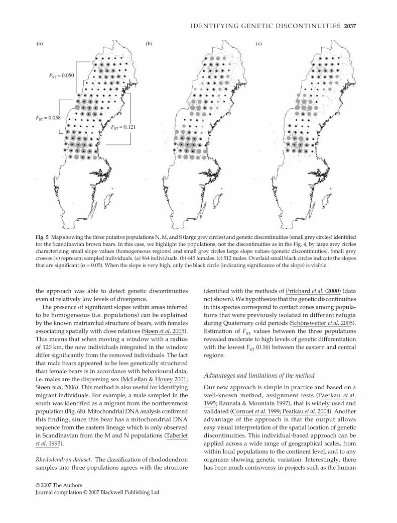
Scandinavian brown bear dataset. Three homogeneous regions(i.e. putative populations) were found (Fig. 5a), correspon-ding to the S, M and N regions (Fig. 3a) already identified byManel et al. (2004). Nevertheless, permutation tests indicatedthat almost all slopes (97%) were significant at the 1%level, including small values in regions that we consideredhomogeneous (large grey circles, Fig. 5a). The strong popu-

lation genetic discontinuity detected between the M andS regions (Fig. 3a) also corresponds to a female gene flowdiscontinuity detected using mitochondrial DNA data(Taberlet et al. 1995). A second discontinuity was detectedbetween the M and N regions.

When the sexes were separated, the global geneticstructures did not differ significantly (Fig. 5b, c). However,the mean slope values were significantly lower for malethan for female samples (student t-test, t = −2.05, P < 0.05),indicating a stronger genetic structure for females thanfor males.

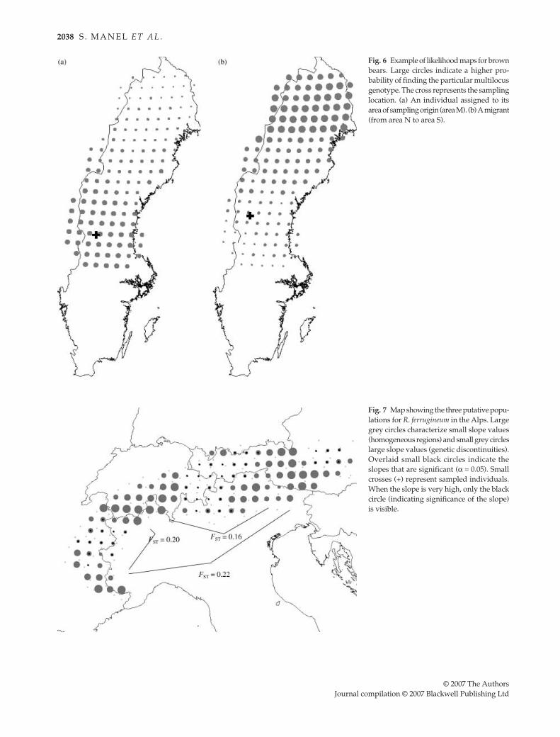
Using individual probability maps, it is also possible todetermine whether each individual is a resident or aputative migrant. For example, a resident is an individualsampled in the region where its multilocus genotype ismost likely to originate (Fig. 6a). In contrast, a migrant is anindividual sampled in a region where its multiloci geno-type is unlikely (Fig. 6b).

Rhododendron dataset. Figure 7 shows the existence of twostrong genetic discontinuities isolating three putative popu-lations. Two of these populations — one in the eastern Alpsand one in the central Alps — were very homogeneous.The third, located in the southwestern Alps, was lesshomogeneous.

Discussion

Our new method for spatially locating genetic discontinuitiesbased on local assignment tests applied in a moving windowperformed well in all evaluations. Using the simulateddatasets, the method did not reveal a genetic discontinuitywhen applied to a single population, regardless of thegeographical distribution of the samples (i.e. one vs. twopatches). In the simulation scenario with two moderatelydifferentiated populations (FST = 0.1), the spatial locationof the genetic discontinuity was correctly identified. Inaddition, the method performed well on two empiricaldatasets using two different types of markers (microsa-tellite vs. AFLP).

Interpretation of the results on the two empirical datasets

Scandinavian brown bear dataset. The three populations identi-fied by our new method are consistent with the knowndemographic history of this species and previous geneticanalyses using other genetic analysis approaches (Waitset al. 2000; Manel et al. 2004). But the results obtained in thisstudy add new information about the exact spatial locationof the boundaries and their significance. To evaluate theability of our method to detect different levels of popula-tion structure, we calculated FST values for the threeidentified populations (Fig. 5a). The lowest value, calculatedbetween M and N areas, was 0.05 and demonstrated that

Fig. 4 Results of the third simulation scenario (described inFig. 2c). Small circles indicate points of the grid taken into accountin the analysis according to the chosen parameters. Large circlescorrespond to significant slopes at level α = 0.05 and identify thegenetic discontinuity between the two populations. Values on theaxes are in meters. (a) d = 40, R = 80; these parameters do not allowthe identification of the discontinuity. (b) d = 40, R = 120; theseparameters allow a precise identification of the discontinuity.(c) d = 40, R = 200; these parameters also allow the identification ofthe discontinuity but with less spatial precision.

I D E N T I F Y I N G G E N E T I C D I S C O N T I N U I T I E S 2037

© 2007 The AuthorsJournal compilation © 2007 Blackwell Publishing Ltd

the approach was able to detect genetic discontinuitieseven at relatively low levels of divergence.

The presence of significant slopes within areas inferredto be homogeneous (i.e. populations) can be explainedby the known matriarchal structure of bears, with femalesassociating spatially with close relatives (Støen et al. 2005).This means that when moving a window with a radiusof 120 km, the new individuals integrated in the windowdiffer significantly from the removed individuals. The factthat male bears appeared to be less genetically structuredthan female bears is in accordance with behavioural data,i.e. males are the dispersing sex (McLellan & Hovey 2001;Støen et al. 2006). This method is also useful for identifyingmigrant individuals. For example, a male sampled in thesouth was identified as a migrant from the northernmostpopulation (Fig. 6b). Mitochondrial DNA analysis confirmedthis finding, since this bear has a mitochondrial DNAsequence from the eastern lineage which is only observedin Scandinavian from the M and N populations (Taberletet al. 1995).

Rhododendron dataset. The classification of rhododendronsamples into three populations agrees with the structure

identified with the methods of Pritchard et al. (2000) (datanot shown). We hypothesize that the genetic discontinuitiesin this species correspond to contact zones among popula-tions that were previously isolated in different refugiaduring Quaternary cold periods (Schönswetter et al. 2005).Estimation of FST values between the three populationsrevealed moderate to high levels of genetic differentiationwith the lowest FST (0.16) between the eastern and centralregions.

Advantages and limitations of the method

Our new approach is simple in practice and based on awell-known method, assignment tests (Paetkau et al.1995; Rannala & Mountain 1997), that is widely used andvalidated (Cornuet et al. 1999; Peatkau et al. 2004). Anotheradvantage of the approach is that the output allowseasy visual interpretation of the spatial location of geneticdiscontinuities. This individual-based approach can beapplied across a wide range of geographical scales, fromwithin local populations to the continent level, and to anyorganism showing genetic variation. Interestingly, therehas been much controversy in projects such as the human

Fig. 5 Map showing the three putative populations N, M, and S (large grey circles) and genetic discontinuities (small grey circles) identifiedfor the Scandinavian brown bears. In this case, we highlight the populations, not the discontinuities as in the Fig. 4, by large grey circlescharacterizing small slope values (homogeneous regions) and small grey circles large slope values (genetic discontinuities). Small greycrosses (+) represent sampled individuals. (a) 964 individuals. (b) 445 females. (c) 512 males. Overlaid small black circles indicate the slopesthat are significant (α = 0.05). When the slope is very high, only the black circle (indicating significance of the slope) is visible.

2038 S . M A N E L E T A L .

© 2007 The AuthorsJournal compilation © 2007 Blackwell Publishing Ltd

Fig. 6 Example of likelihood maps for brownbears. Large circles indicate a higher pro-bability of finding the particular multilocusgenotype. The cross represents the samplinglocation. (a) An individual assigned to itsarea of sampling origin (area M). (b) A migrant(from area N to area S).

Fig. 7 Map showing the three putative popu-lations for R. ferrugineum in the Alps. Largegrey circles characterize small slope values(homogeneous regions) and small grey circleslarge slope values (genetic discontinuities).Overlaid small black circles indicate theslopes that are significant (α = 0.05). Smallcrosses (+) represent sampled individuals.When the slope is very high, only the blackcircle (indicating significance of the slope)is visible.

I D E N T I F Y I N G G E N E T I C D I S C O N T I N U I T I E S 2039

© 2007 The AuthorsJournal compilation © 2007 Blackwell Publishing Ltd

genome diversity project, as to which sampling strategy toadopt: a systematic sampling using a grid or a samplingonly of populations identified a priori (Cavalli-Sforza et al.1991; Greely 2001). Our results illustrate that a systematicsampling on a grid or evenly spaced sampling is efficientfor identifying spatial patterns of genetic diversity. Thisapproach will be especially useful when studying largecontinuous populations with no obvious boundaries orwith cryptic barriers to gene flow. However it requires acontinuous, evenly spaced sampling and multiple geneticmarkers to provide enough resolution to assign individualsto a sampling region with confidence. The importance ofcontinuous, evenly spaced sampling in landscape studiesthat seek to detect the spatial location of populationboundaries was also noted by Guillot et al. (2005).

The results of our method were mainly influenced by thesize of the windows, R. For a fixed value of d, increasing Rdecreases the precision of the localization of the boundary:for example if d = 40 m and R = 240 m, the boundary wouldbe identified at a precision of ± 260 m (R + d/2). Thusresearchers will want to use the smallest possible value ofR. However, as R decreases it becomes more difficult tomaintain enough individuals in a window for accuratelyestimating allele frequencies. In the case of R. ferrugineum,the low minimum number of individuals per windows (10)was compensated by a relatively high number of markers(i.e. 123). This choice influences the accuracy of the locationand the time of computing. Implementation of the methodrequires finding the optimal balance between R (radiusof the windows) and d (distance between adjacent pointsof the grid) to identify zones of sharp discontinuitieswith meaningful geographical precision. Nevertheless, themethod is robust when using different values for themoving window and grid sizes, because it always locatesthe discontinuities (i.e. the discontinuities are always atthe same place, but are detected less accurately). Finally, thechoice of R and d will depend on the study organism andthe density of sampling and requires multiple iterations ofattempts.

In summary, our method first produces likelihood mapsfor each individual. These maps allow the identification ofmigrants, corresponding to the individuals that weresampled far from the area where their multilocus geno-types are more likely. For example, the examination of thedistribution of geographical distances between individualsand their ‘windows’ with largest assignment probabilitiesshould provide valuable data about the dispersion distances.Second, the approach can identify the geographical loca-tion of genetic discontinuities from multilocus genotypesand individual geographical locations and adds a new toolfor addressing the first step of landscape genetics (Manelet al. 2003). It can be used to detect conservation units byidentifying cryptic genetic boundaries when individualsare continuously distributed across space. Its main advan-

tages come from its ease of implementation and from thesimplicity of the theory behind assignment tests. It is lesssophisticated than the recent spatial Bayesian clusteringmethod introduced by Guillot et al. (2005) and Coranderet al. (2006) where the spatial organization of populations ismodelled through the coloured Voronoi tesselation. Ournew approach and the two previous methods differ fromWombling (Womble 1951) in that they use multilocus datainstead of analysing each allele separately. They also differfrom Monmonier algorithm (Monmonier 1973), becausethis is a distance-based method that is generally applied atthe population level. These methods have never beenthoroughly compared, and the next step will therefore beto assess their relative performance in identifying geneticdiscontinuities and population boundaries in a spatialcontext.

Once a genetic discontinuity has been detected, anexciting new research direction will be to determine theunderlying explanatory variables by overlaying spatialmaps of genetic variation onto maps of environmentalvariables and exploiting spatial statistics and GIS (e.g.Manel et al. 2003; Spear et al. 2005). Such approaches havemany applications in expanding our fundamental know-ledge of ecology, evolution, behaviour and landscape levelprocesses. There is clearly great potential in this analyticalapproach and much need for further development andvalidation of individual-based geographical approaches inpopulation genetics.

Acknowledgements

We thank J. Hogg and M. Schwartz for helpful discussions andcomments on the manuscript. This study was supported by theUniversity Joseph Fourier (Grenoble), the Centre National de laRecherche Scientifique, the Swedish Environmental ProtectionAgency, the Norwegian Directorate for Nature Management, theResearch Council of Norway, the Swedish Association forHunting and Wildlife Management, and the WWF-Sweden. Mostof the computations were performed at the LPM2C.

References

Balloux F (2001) easypop (version 1.7) a computer program for thesimulation of population genetics. Journal of Heredity, 92, 301–302.

Barbujani G, Oden NL, Sokal R (1989) Detecting regions of abruptchange in maps of biological variables. Systematic Zoology, 38,376–389.

Bellemain E (2004) Genetics of the Scandinavian Brown Bear:Implications for Biology and Conservation. PhD Dissertation,Agricultural University of Norway, Ås, Norway.

Bocquet-Appel JP, Bacro JN (1994) Generalized wombling.Systematic Biology, 43, 442–448.

Bonin A, Bellemain E, Eidesen PB et al. (2004) How to track andassess genotyping errors in population genetic studies. MolecularEcology, 13, 3261–3273.

Cavalli-Sforza LL, Wilson AC, Cantor CR et al. (1991) Call fora world-wide survey of human genetic diversity: a vanishing

2040 S . M A N E L E T A L .

© 2007 The AuthorsJournal compilation © 2007 Blackwell Publishing Ltd

opportunity for the human genome project. Genomics, 11, 490–491.

Corander J, Waldmann P, Sillanpa MJ (2003) Bayesian analysis ofgenetic differentiation between populations. Genetics, 163, 367–374.

Corander J, Marttinen P, Sirén J, Tang J (2006) BAPS: BayesianAnalysis of Population Structure, Manual v, 4.1. Available at:http://www.rni.helsinki.fi/ ∼jic/bapspage.html.

Cornuet J-M, Piry S, Luikart G et al. (1999) New methods employingmultilocus genotypes to select or exclude populations as originsof individuals. Genetics, 153, 1989–2000.

Coulon A, Guillot G, Cosson J-F et al. (2006) Genetic structure isinfluenced by landscape features: empirical evidence from a reddeer population. Molecular Ecology, 15, 1669–1679.

Evanno G, Regnaut S, Goudet J (2005) Detecting the number ofclusters of individuals using the software structure: a simula-tion study. Molecular Ecology, 14, 2611–2620.

François O, Ancelet S, Guillot G (2006) Bayesian clustering usinghidden Markov random fields in spatial population genetics.Genetics, 4, 805–816.

Greely HT (2001) Human genome diversity: what about the otherhuman genome project? Nature Reviews Genetics, 2, 222–227.

Guillot G, Estoup A, Mortier F, Cosson J (2005) A spatial statisticalmodel for landscape genetics. Genetics, 170, 1261–1280.

Legendre P, Legendre L (2006) Numerical Ecology. Elsevier,Amsterdam, p. 853.

Manel S, Schwartz M, Luikart G, Taberlet P (2003) Landscapegenetics: combining landscape ecology and population genetics.Trends in Ecology and Evolution, 18, 189–197.

Manel S, Bellemain E, Swenson J, François O (2004) Assumed andinferred spatial structure of populations: the Scandinavianbrown bears revisited. Molecular Ecology, 13, 1227–1331.

Manni F, Guerard E, Heyer E (2004) Geographic patterns of genetic,morphologic and linguistic variation: how barriers can be detectedby using Monmonier’s algorithm. Human Biology, 76, 173–190.

McLellan BN, Hovey FW (2001) Natal dispersal of grizzly bears.Canadian Journal of Zoology, 79, 838–844.

Miller MP (2005) alleles in space (ais): computer software forthe joint analysis of interindividual spatial and genetic informa-tion. Journal of Heredity, 96, 722–724.

Monmonnier M (1973) Maximum–difference barriers: an alter-native numerical regionalization method. Geographical Analysis,3, 245–261.

Nei M (1987) Molecular Evolutionary Genetics. Columbia UniversityPress, New York.

Paetkau D, Calvert W, Stirling I, Strobeck C (1995) Microsatelliteanalysis of population structure in Canadian polar bears.Molecular Ecology, 4, 347–354.

Peatkau D, Slades R, Burdens M, Arnaud E (2004) Genetic assign-ment methods for the direct, real-time estimation of migrationrate: a simulation-based exploration of accuracy and power.Molecular Ecology, 13, 55–65.

Pritchard JK, Stephens M, Donnelly P (2000) Inference of popula-tion structure using multilocus genotype data. Genetics, 155,945–959.

Rannala B, Mountain JL (1997) Detecting immigration by usingmultilocus genotypes. Proceedings of the National Academy ofSciences USA, 94, 9197–9201.

Schönswetter P, Stehlik I, Holderegger R, Tribsch A (2005)Molecular evidence for glacial refugia of mountain plants in theEuropean Alps. Molecular Ecology, 14, 3547–3555.

Sokal RR, Rohlf FJ (1981) Biometry. The Principles and Practice ofStatistics in Biological Research. Freeman WH and Company, SanFransisco.

Sokal RR, Thomson BA (1998) Spatial genetic structure of humanpopulations in Japan. Human Biology, 70, 1–22.

Spear SF, Peterson CR, Matocq MD, Storfer A (2005) Landscapegenetics of the blotched tiger salamander (Ambystoma tigrinummelanostictum). Molecular Ecology, 14, 2553–2564.

Støen OG, Bellemain E, Sæbø S, Swenson JE (2005) Kin-relatedspatial structure in brown bears Ursus arctos. Behavioural Ecologyand Sociobiology, 59, 191–197.

Støen O-G, Zedrosser A, Sæbo S, Swenson JE (2006) Natal dispersalin expanding brown bear Ursus arctos populations. OecologiaDOI 1007.

Taberlet P, Swenson JE, Sandegren F, Bjärvall A (1995) Localizationof a contact zone between two highly divergent mitochondrialDNA lineages of the brown bear (Ursus arctos) in Scandinavia.Conservation Biology, 9, 1255–1261.

Vos P, Hagers R, Bleeker M et al. (1995) aflp: new technique forDNA fingerprinting. Nucleic Acid Research, 23, 4407–4414.

Waits LP, Taberlet P, Swenson JE, Sandegren F, Franzén R (2000)Nuclear DNA microsatellite analysis of genetic diversityand gene flow in the Scandinavian brown bear (Ursus arctos).Molecular Ecology, 9, 421–431.

Waples R, Gaggiotti O (2006) What is a population? An empiricalevaluation of some genetic methods for identifying the numberof gene pools and their degree of connectivity. Molecular Ecology,15, 1419–1439.

Waser PM, Strobek C (1998) Genetic signatures of interpopulationdispersal. Trends in Ecology and Evolution, 13, 43–44.

Weir BS, Cockerham CC (1984) Estimating F-statistics for theanalysis of population structure. Evolution, 38, 1358–1370.

Womble WH (1951) Differential systematics. Science, 114, 315–322.

This work has been done in collaboration with different researchers.Stéphanie Manel and Lisette Waits are interested in developingspatial analysis in population genetics (i.e. landscape genetics).Françoise Berthoud is a computer scientist that helped in thedevelopment of the C++ program. Pierre Taberlet and GordonLuikart are interested in population genetics and molecular tools.Pierre Taberlet is the leader of the European project that providedthe Rhododendron datasets. Jon Swenson is the scientific leaderof the Scandinavian brown bear research project. Eva Bellermainis a postdoctoral researcher interested in population genetics andevolution. Myriam Gaudeul is interested in various aspects ofplant evolutionary biology, including biogeography and populationgenetics.

I D E N T I F Y I N G G E N E T I C D I S C O N T I N U I T I E S 2041

© 2007 The AuthorsJournal compilation © 2007 Blackwell Publishing Ltd

Annexe 1

IntraBioDiv Consortium

The IntraBioDiv Consortium is composed of membersof the IntraBioDiv project, as well as additional scientists,botanical experts, and technical assistants who participatedto this project in relation with the official contractors andsubcontractors.

The project has been supported financially by the EuropeanCommission, under the Six Framework Programme.Acronym: IntraBioDivTitle: Tracking surrogates for intraspecific biodiversity:towards efficient selection strategies for the conservationof natural genetic resources using comparative mappingand modelling approaches.Reference: GOCE-CT-2003-505376Duration: 1st January 2004–31st December 2006Coordinator: Pierre TaberletScientistsWolfgang AHLMER6

Paolo AJMONE MARSAN2

Nadir ALVAREZ3

Enzo BONA9

Maurizio BOVIO9

El¿bieta CIESLAK12

Gheorghe COLDEA11

Licia COLLI2

Vasile CRISTEA11

Jean-Pierre DALMAS8

Thorsten ENGLISCH4

Luc GARRAUD8

Myriam GAUDEUL1

Ludovic GIELLY1

Felix GUGERLI5

Walter GUTERMANN4

Rolf HOLDEREGGER5

Nejc JOGAN7

Alexander A. KAGALO18

Gra¿yna KORBECKA12

Philippe KÜPFER3

Benoît LEQUETTE14

Dominik Roman LETZ10

Stéphanie MANEL1

Guilhem MANSION3

Karol MARHOLD10

Fabrizio MARTINI9

Zbigniew MIREK12

Riccardo NEGRINI2

Harald NIKLFELD4

Fernando NIÑO13

Massimiliano PATRINI2

Ovidiu PAUN4

Marco PELLECCHIA2

Giovanni PERICO9

Halina PIEKOS-MIRKOWA12

Peter POSCHLOD6

Filippo PROSSER16

Mihai PUSCAS11

Micha3 RONIKIER12

Patrizia ROSSI15

Martin SCHEUERER6

Gerald SCHNEEWEISS4

Peter SCHÖNSWETTER4

Luise SCHRATT-EHRENDORFER4

Fanny SCHÜPFER3

Alberto SELVAGGI17

Katherina STEINMANN5

Pierre TABERLET1

Conny THIEL5

Andreas TRIBSCH4

Marcela VAN LOO4

Manuela WINKLER4

Thomas WOHLGEMUTH5

Tone WRABER7

Niklaus ZIMMERMANN5

Botanical expertsGabriel ALZIAR14

Carlo ARGENTI16

Tinka BACIC7

Jean-Eric BERTHOUSE14

Alessio BERTOLLI16

Enrico BRESSAN9

François BRETON14

Massimo BUCCHERI9

Sonia D’ANDREA17

Sergio DANIELI9

Rosanna DE MATTEI17

Thierry DELAHAYE8

Roberto DELLA VEDOVA17

Cédric DENTANT8

Alessandra DI TURI17

Wolfgang DIEWALD6

Rolland DOUZET1

Constantin DRAGULESCU11

Philippe DRUART3

Siegrun ERTL4

Delphine FALLOUR-RUBIO14

Gino FANTINI9

Paolo FANTINI15

Germano FEDERICI9

Franco FENAROLI9

Viera FERÁKOVÁ10

Roberto FERRANTI9

Francesco FESTI16

Bozo FRAJMAN7

Jean-Claude GACHET14

Bruno GALLINO17

2042 S . M A N E L E T A L .

© 2007 The AuthorsJournal compilation © 2007 Blackwell Publishing Ltd

Federica GIRONI9

Gheorghe GROZA11

Andreas HILPOLD19

Catherine JOLLIBERT14

Denis JORDAN8

Thomas KIEBACHER19

Michael KLEIH9

Michel LAMBERTIN14

Cesare LASEN9

Petra MAIR19

Luca MANGILI9

Diego MARANGONI17

Carlo & Marisa MARCONI9

Hugues MERLE8

Marco MERSCHEL6

Henri MICHAUD8

Luca MISERERE17

Gian Paolo MONDINO17

Patrik MRÁZ10

Benoît OFFERHAUS14

Adrian OPREA11

Marziano PASCALE17

Roberto PASCAL17

Giorgio PERAZZA16

Marián PERNY10

Jean-Louis POLIDORI14

Guy REBATTU14

Jean-Pierre ROUX8

Ioan SÂRBU11

Silvio SCORTEGAGNA16

Paola SERGO9

Natalia SKIBITSKA18

Adriano SOLDANO17

Jean-Marie SOLICHON14

Simona STRGULC KRAJSEK7

Nadiya SYTSCHAK18

Zbigniew SZELAG12

Filippo TAGLIAFERRI9

Peter TURIS10

Tudor-Mihai URSU11

Jérémie VAN ES8

Jean-Charles VILLARET8

£ukasz WILK12

Technical assistantsSarah BOUDON13

Sabine BRODBECK5

Véronique FINIELS8

Jean-Michel GENIS8

Hanna KUCIEL12

Philippe LAGIER-BRUNO8

Chritian MIQUEL1

Virgile NOBLE8

Tjasa POGACNIK LIPOVEC7

Delphine RIOUX1

Dirk SCHMATZ5

Ivan VALKO10

Stéphanie ZUNDEL1

AcknowledgmentsChristian BOUCHER14

Jean-Marie CEVASCO14

Guillaume CHAUDE14

Dominique CHAVY14

Bruno CUERVAN14

Gil DELUERMOZ14

Daniel DEMONTOUX14

Laurence FOUCAULT14

Jean-Félix GANDIOLI14

Ernest GRENIER14

Emmanuel ICARDO14

Zoltan JABLONOVSKI11

Vincent KULESZA14

Mihai MICLÃUS11

Monique PERFUS14

Daniel REBOUL14

Alain ROCCHIA14

Jean-Pierre ROUX14

Robert SALANON14

Addresses of the Institutions (contractors and subcontractors)1 Laboratoire d’Ecologie Alpine, CNRS UMR 5553,

Université Joseph Fourier, BP 43,F-38041 Grenoble Cedex 9, France

2 Istituto di ZootecnicaUniversità Cattolica del S. Cuorevia E. Parmense, 84I-29100 Piacenza, Italy

3 Laboratoire de Botanique EvolutiveUniversité de Neuchâtel11, rue Emile-ArgandCH-2007 Neuchâtel, Switzerland

4 Department of BiogeographyInstitute of Botany, University of ViennaRennweg 14,A-1030 Vienna, Austria

5 Swiss Federal Research Institute WSLEcological GeneticsZuercherstrasse 111CH-8903 Birmensdorf, Switzerland

6 University of RegensburgInstitute of BotanyD-93040 Regensburg, Germany

7 Univerza v LjubljaniOddelek za biologijo BFVecna pot 111SI-1000 Ljubljana, Slovenia

8 Conservatoire Botanique National Alpin — CBNADomaine de CharanceF-05000 Gap, France

I D E N T I F Y I N G G E N E T I C D I S C O N T I N U I T I E S 2043

© 2007 The AuthorsJournal compilation © 2007 Blackwell Publishing Ltd

9 Dipartimento di BiologiaUniversità di TriesteVia L. Giorgieri 10I-34127 Trieste, Italy

10 Institute of Botany of Slovak Academy of Sciences,Department of Vascular Plant Taxonomy,

Dúbravská cesta 14,SK-845 23 Bratislava, Slovakia

11 Institutul de Cercetari BiologiceStr. Republicii nr. 48400015 Cluj-Napoca, Romania

12 Institute of BotanyPolish Academy of SciencesLubicz 46PL-31-512 Kraków, Poland

13 Medias-France/IRDCNES – BPi 210218, Av. Edouard BelinF-31401 Toulouse Cedex 9, France

14 Parc national du Mercantour23 rue d’Italie, BP 1316F-06006 Nice Cedex 1, France

15 Parco Naturale Alpi MarittimeCorso Bianco 5I-12010 Valdieri (CN) Italy

16 Museo CivicoLargo S. Caterina 41,I-38068 Rovereto, Italy

17 Istituto per le Piante da Legno e l’Ambientec.so Casale, 476I-10132 Torino, Italy

18 Institute of Ecology of the Carpathians N.A.S. ofUkraine, 4 Kozelnitska str.,

79026 Lviv, Ukraine19 Naturmuseum Südtirol, Museo Scienze Naturali Alto

AdigeBindergasse 1I-39100 Bozen/Bolzano, Ital