A Pieri rule for skew shapes

Sami H. Assaf1

Department of Mathematics, Massachusetts Institute of Technology, Cambridge, MA 02139,

USA

Peter R. W. McNamara

Department of Mathematics, Bucknell University, Lewisburg, PA 17837, USA

Abstract

The Pieri rule expresses the product of a Schur function and a single row Schurfunction in terms of Schur functions. We extend the classical Pieri rule byexpressing the product of a skew Schur function and a single row Schur functionin terms of skew Schur functions. Like the classical rule, our rule involves simpleadditions of boxes to the original skew shape. Our proof is purely combinatorialand extends the combinatorial proof of the classical case.

Keywords: Pieri rule, skew Schur functions, Robinson-Schensted2000 MSC: 05E05, 05E10, 20C30

1. Introduction

The basis of Schur functions is arguably the most interesting and impor-tant basis for the ring of symmetric functions. This is due not just to theirelegant combinatorial definition, but more broadly to their connections to otherareas of mathematics. For example, they are intimately tied to the cohomologyring of the Grassmannian, and they appear in the representation theory of thesymmetric group and of the general and special linear groups.

It is therefore natural to consider the expansion of the product sλsµ of twoSchur functions in the basis of Schur functions. The Littlewood–Richardson rule[11, 19, 24, 25], which now comes in many different forms ([22] is one startingpoint), allows us to determine this expansion. However, more basic than theLittlewood–Richardson rule is the Pieri rule, which gives a simple, beautiful andmore intuitive answer for the special case when µ = (n), a partition of length1. Though we will postpone the preliminary definitions to Section 2 and thestatement of the Pieri rule to Section 3, stating the rule in a rough form will

Email addresses: sassaf@math.mit.edu (Sami H. Assaf), peter.mcnamara@bucknell.edu(Peter R. W. McNamara)

1Supported by NSF Postdoctoral Fellowship DMS-0703567

Preprint submitted to Journal of Combinatorial Theory, Series A April 28, 2010

arX

iv:0

908.

0345

v2 [

mat

h.C

O]

26

Apr

201

0

give its flavor. For a partition λ and a positive integer n, the Pieri rule statesthat sλsn is a sum of Schur functions sλ+ , where λ+ is obtainable by addingcells to the diagram of λ according to a certain simple rule. The Pieri rule’sprevalence is highlighted by its adaptions to many other settings, includingSchubert polynomials [8, 10, 13, 20, 26], LLT polynomials [5], Hall–Littlewoodpolynomials [14], Jack polynomials [9, 21], and Macdonald polynomials [4, 12].

It is therefore surprising that there does not appear to be a known adaption ofthe Pieri rule to the most well-known generalization of Schur functions, namelyskew Schur functions. We fill this gap in the literature with a natural extensionof the Pieri rule to the skew setting. Reflecting the simplicity of the classicalPieri rule, the skew Pieri rule states that for a skew shape λ/µ and a positiveinteger n, sλ/µsn is a signed sum of skew Schur functions sλ+/µ− , where λ+/µ−

is obtainable by adding cells to the diagram of λ/µ according to a certain simplerule. Our proof is purely combinatorial, using a sign-reversing involution thatreflects the combinatorial proof of the classical Pieri rule. After reading anearlier version of this manuscript, which included an algebraic proof of the casen = 1 due to Richard Stanley, Thomas Lam provided a complete algebraic proofof our skew Pieri rule.

It is natural to ask if our skew Pieri rule can be extended to give a “skew”version of the Littlewood–Richardson rule, and we include such a rule as aconjecture in Section 6. This conjecture has been proved by Lam, Aaron Lauveand Frank Sottile in [7] using Hopf algebras. It remains an open problem tofind a combinatorial proof of the skew Littlewood–Richardson rule.

The remainder of this paper is organized as follows. In Section 2, we give thenecessary symmetric function background. In Section 3, we state the classicalPieri rule and introduce our skew Pieri rule. In Section 4, we give a varia-tion from [17] of the Robinson–Schensted–Knuth algorithm, along with relevantproperties. This algorithm is then used in Section 5 to define our sign-reversinginvolution, which we then use to prove the skew Pieri rule. We conclude in Sec-tion 6 with two connections to the Littlewood–Richardson rule. Lam’s algebraicproof appears in Appendix Appendix A.

2. Preliminaries

We follow the terminology and notation of [12, 22] for partitions and tableaux,except where specified. Letting N denote the nonnegative integers, a partitionλ of n ∈ N is a weakly decreasing sequence (λ1, λ2, . . . λl) of positive integerswhose sum is n. It will be convenient to set λk = 0 for k > l. We also let∅ denote the unique partition with l = 0. We will identify λ with its Youngdiagram in “French notation”: represent the partition λ by the unit square cellswith top-right corners (i, j) ∈ N × N such that 1 ≤ i ≤ λj . For example, thepartition (4, 2, 1), which we abbreviate as 421, has Young diagram

.

2

Define the conjugate or transpose λt of λ to be the partition with λi cells incolumn i. For example, 421t = 3211. For another partition µ, we write µ ⊆ λwhenever µ is contained within λ (as Young diagrams); equivalently µi ≤ λi forall i. In this case, we define the skew shape λ/µ to be the set theoretic differenceλ−µ. In particular, the partition λ is the skew shape λ/∅. We call the number ofcells of λ/µ its size, denoted |λ/µ|. We say that a skew shape forms a horizontalstrip (resp. vertical strip) if it contains no two cells in the same column (resp.row). A k-horizontal strip is a horizontal strip of size k, and similarly for verticalstrips. For example, the skew shape 421/21 is a 4-horizontal strip:

.

With another skew shape σ/τ , we let (λ/µ) ∗ (σ/τ) denote the skew shapeobtained by positioning λ/µ so that its bottom right cell is immediately aboveand left of the top left cell of σ/τ . For example, the horizontal strip 421/21above could alternatively be written as (21/1) ∗ (2) or as (1) ∗ (31/1).

A Young tableau of shape λ/µ is a map from the cells of λ/µ to the posi-tive integers. A semistandard Young tableau (SSYT) is such a filling which isweakly increasing from left-to-right along each row and strictly increasing upeach column, such as

1 2 73 3 55

.

The content of an SSYT T is the sequence π such that T has πi cells with entryi; in this case π = (1, 1, 2, 0, 2, 0, 1).

We let Λ denote the ring of symmetric functions in the variables x =(x1, x2, . . .) over Q, say. We will use three familiar bases from [12, 22] for Λ:the elementary symmetric functions eλ, the complete homogeneous symmetricfunctions hλ and, most importantly, the Schur functions sλ. The Schur func-tions form an orthonormal basis for Λ with respect to the Hall inner productand may be defined in terms of SSYTs by

sλ =∑

T∈SSYT(λ)

xT , (2.1)

where the sum is over all SSYTs of shape λ and where xT denotes the mono-mial xπ1

1 xπ22 · · · when T has content π. Replacing λ by λ/µ in (2.1) gives the

definition of the skew Schur function sλ/µ, where the sum is now over all SSYTsof shape λ/µ. For example, the SSYT shown above contributes the monomialx1x2x

23x

25x7 to s431/1.

3. The skew Pieri rule

The celebrated Pieri rule gives an elegant method for expanding the productsλsn in the Schur basis. This rule was originally stated in [15] in the setting

3

of Schubert Calculus. Recall that the single row Schur function sn equals thecomplete homogeneous symmetric function hn. Recall also the involution ω onΛ, which may be defined by sending the Schur function sλ to sλt or equiva-lently by sending hk to ek. Thus the Schur function s1n equals the elementarysymmetric function en, where 1n denotes a single column of size n.

Theorem 3.1 ([15]). For any partition λ and positive integer n, we have

sλsn = sλhn =∑

λ+/λ n-hor. strip

sλ+ , (3.1)

where the sum is over all partitions λ+ such that λ+/λ is a horizontal strip ofsize n.

Applying the involution ω to (3.1), we get the dual version of the Pieri rule:

sλs1n = sλen =∑

λ+/λ n-vert. strip

sλ+ , (3.2)

where the sum is now over all partitions λ+ such that λ+/λ is a vertical stripof size n.

A simple application of Theorem 3.1 gives

s322s2 = s3222 + s3321 + s4221 + s432 + s522,

as represented diagrammatically in Figure 1.

+= + + +

Figure 1: The expansion of s322s2 by the Pieri rule.

Given the simplicity of (3.1), it is natural to hope for a simple expressionfor sλ/µsn in terms of skew Schur functions. This brings us to our main result.

Theorem 3.2. For any skew shape λ/µ and positive integer n, we have

sλ/µsn = sλ/µhn =

n∑k=0

(−1)k∑

λ+/λ (n−k)-hor. strip

µ/µ− k-vert. strip

sλ+/µ− , (3.3)

where the second sum is over all partitions λ+ and µ− such that λ+/λ is ahorizontal strip of size n− k and µ/µ− is a vertical strip of size k.

4

Observe that when µ = ∅, Theorem 3.2 specializes to Theorem 3.1. Again,we can apply the ω transformation to obtain the dual version of the skew Pierirule.

Corollary 3.3. For any skew shape λ/µ and any positive integer k, we have

sλ/µs1n = sλ/µen =

n∑k=0

(−1)k∑

λ+/λ (n−k)-vert. strip

µ/µ− k-hor. strip

sλ+/µ− ,

where the sum is over all partitions λ+ and µ− such that λ+/λ is a vertical stripof size n− k and µ/µ− is a horizontal strip of size k.

Example 3.4. A direct application of Theorem 3.2 gives

s322/11s2 = s3222/11 + s3321/11 + s4221/11 + s432/11 + s522/11

− s3221/1 − s332/1 − s422/1 + s322,

as represented diagrammatically in Figure 2.

+

+

= + + +

Figure 2: The expansion of s322/11s2 by the skew Pieri rule.

As (3.3) contains negative signs, our approach to proving Theorem 3.2 will beto construct a sign-reversing involution on SSYTs of shapes of the form λ+/µ−.We will then provide a bijection between SSYTs of shape λ+/µ− that are fixedunder the involution and SSYTs of shape (λ/µ) ∗ (n). The result then followsfrom the fact that s(λ/µ)∗(n) = sλ/µsn.

4. Row insertion

In order to describe our sign-reversing involution, we will need the Robinson–Schensted–Knuth (RSK) row insertion algorithm on SSYTs [16, 18, 3]. For athorough treatment of this algorithm along with many applications, we recom-mend [22]. In fact, we will use an analogue of the algorithm for SSYTs of skewshape from [17]. There, row insertion comes in two forms, external and inter-nal row insertion. External row insertion, which we now define, is just like theclassical RSK insertion.

5

Definition 4.1. Let T be an SSYT of arbitrary skew shape and choose apositive integer k. Define the external row insertion of k into T , denoted T ←0

k, as follows: if k is weakly larger than all entries in row 1 of T , then add k tothe right end of the row and terminate the process. Otherwise, find the leftmostcell in row 1 of T whose entry, say k′, is greater than k. Replace this entry byk and then row insert k′ into T at row 2 using the procedure just described.Repeat the process until some entry comes to rest at the right end of a row.

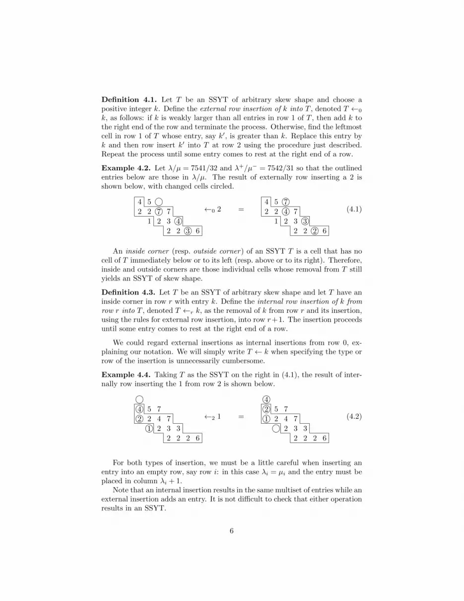
Example 4.2. Let λ/µ = 7541/32 and λ+/µ− = 7542/31 so that the outlinedentries below are those in λ/µ. The result of externally row inserting a 2 isshown below, with changed cells circled.

4 5 ○2 2 7○ 7

1 2 3 4○2 2 3○ 6

←0 2 =4 5 7○2 2 4○ 7

1 2 3 3○2 2 2○ 6

(4.1)

An inside corner (resp. outside corner) of an SSYT T is a cell that has nocell of T immediately below or to its left (resp. above or to its right). Therefore,inside and outside corners are those individual cells whose removal from T stillyields an SSYT of skew shape.

Definition 4.3. Let T be an SSYT of arbitrary skew shape and let T have aninside corner in row r with entry k. Define the internal row insertion of k fromrow r into T , denoted T ←r k, as the removal of k from row r and its insertion,using the rules for external row insertion, into row r+1. The insertion proceedsuntil some entry comes to rest at the right end of a row.

We could regard external insertions as internal insertions from row 0, ex-plaining our notation. We will simply write T ← k when specifying the type orrow of the insertion is unnecessarily cumbersome.

Example 4.4. Taking T as the SSYT on the right in (4.1), the result of inter-nally row inserting the 1 from row 2 is shown below.

○4○ 5 7

2○ 2 4 7

1○ 2 3 3

2 2 2 6

←2 1 =

4○5 72○2 4 71○

○ 2 3 3

2 2 2 6

(4.2)

For both types of insertion, we must be a little careful when inserting anentry into an empty row, say row i: in this case λi = µi and the entry must beplaced in column λi + 1.

Note that an internal insertion results in the same multiset of entries while anexternal insertion adds an entry. It is not difficult to check that either operationresults in an SSYT.

6

We will also need to invert row insertions, again for skew shapes and follow-ing [17].

Definition 4.5. Let T be an SSYT of arbitrary skew shape and choose anoutside corner c of T , say with entry k. Define the reverse row insertion ofc from T , denoted T → c, by deleting c from T and reverse inserting k intothe row below, say row r, as follows: if r = 0, then the procedure terminates.Otherwise, if k is weakly smaller than all entries in row r, then place k at theleft end of row r and terminate the procedure. Otherwise, find the rightmostcell in row r whose entry, say k′, is less than k. Replace this entry by k andthen reverse row insert k′ into row r − 1 using the procedure just described.

Example 4.6. In (4.1), reverse row insertion of the cell containing the circled7 from the SSYT T on the right results in the SSYT on the left, and similarlyin (4.2) for the circled 4.

As with row insertion, it follows from the definition that the resulting arraywill again be an SSYT. Observe that the first type of termination mentionedin Definition 4.5 corresponds to reverse external row insertion, and we then saythat k lands in row 0. The second type of termination corresponds to reverseinternal row insertion, and we then say that k lands in row r. In both cases, wewill call the entry k left at the end of the procedure the final entry of T → c.The following lemma, which follows immediately from Definitions 4.1, 4.3 and4.5, formalizes the bijectivity of row and reverse row insertion.

Lemma 4.7. Let T be an SSYT of skew shape.

a. If S is the result of T ← k for some positive integer k, then S → c resultsin T , where c is the unique non-empty cell of S that is empty in T .

b. If S is the result of T → c for some removable cell c of T and the finalentry k of T → c lands in row r ≥ 0, then S ←r k results in T .

For both row insertion and reverse row insertion, we will often want to trackthe cells affected by the procedure. Therefore define the bumping path of therow insertion T ← k (resp. the reverse bumping path of a reverse row insertionT → c) to be the set of cells in T , as well as those empty cells, where the entriesdiffer from the corresponding entries in T ← k (resp. T → c). The cells of thebumping paths for row insertion and reverse row insertion are circled in (4.1)and (4.2). Note that the fact that the bumping path and reverse bumping pathare equal in each of these examples is a consequence of Lemma 4.7.

It is easy to see that the bumping paths always move weakly right from topto bottom in the case of column-strict tableaux. The following bumping lemmawill play a crucial role in defining our sign-reversing involution and in provingits relevant properties.

Lemma 4.8. Let T be an SSYT of skew shape and let k, k′ be positive integers.Let B be the bumping path of T ← k and let B′ be the bumping path of (T ←k)← k′.

7

a. If B is strictly left of B′ in any row r, then B is strictly left of B′ inevery row they both occupy. Moreover, the top cells of B and B′ form ahorizontal strip.

b. If both row insertions are external, then B is strictly left of B′ in everyrow they both occupy if and only if k ≤ k′.

c. Suppose C ′ is the reverse bumping path of T → c′ with final entry k′ andC is the reverse bumping path of (T → c′) → c with final entry k. If c isstrictly left of c′, then C is strictly left of C ′ in every row they both occupy.If, in addition, both reverse row insertions land in row 0, then k ≤ k′.

Proof. For general i, let Bi (resp. B′i) be the cell of B (resp. B′) in row i, saywith entry bi in T (resp. b′i in T ← k).

(a) Suppose Br is strictly left of B′r for some r for which Br+1 and B′r+1

both exist. Then br will occupy the cell Br+1 in T ← k, and since b′r ≥ br,B′r+1 will be strictly right of Br+1. To show that Br−1 is strictly left of B′r−1assuming both exist, let c denote the cell that is empty in T but non-emptyin T ← k and let c′ denote the cell that is empty in T ← k but not in (T ←k) ← k′. By Lemma 4.7(a), B (resp. B′) is also the reverse bumping path of(((T ← k) ← k′) → c′) → c (resp. ((T ← k) ← k′) → c′). We know that br−1will occupy the cell Br in (T ← k) ← k′ while b′r−1 will occupy the cell B′r,implying br−1 ≤ b′r−1. As a result, considering the reverse row insertions of c′

and then c, we deduce that Br−1 is strictly left of B′r−1.Now consider the top cells Br and B′s of B and B′ respectively. Since Br is

the top cell of B, we know that it is at the right end of row r. When s ≥ r, weknow that B′r is strictly right of Br. But then B′r is empty in T ← k and so wemust have s = r. We conclude that s ≤ r and the result follows.

(b) If k ≤ k′, then B1 is strictly left of B′1. If k > k′, then B1 is weakly rightof B′1. The result now follows from (a).

(c) Letting T ′ denote (T → c′) → c, Lemma 4.7 implies that C equals thebumping path B of T ′ ← k while C ′ equals the bumping path B′ of (T ′ ← k)←k′. Applying (a), it suffices to show that C is strictly left of C ′ in some rowwhich they both occupy. Consider row r, the top row of C ′. Since c is strictlyleft of c′, either C and C ′ have no rows in common, in which case the result istrivial, or else C has a cell in row r. When we choose the elements of C, wehave already performed the reverse row insertion T → c′. In particular, the cellc′ is empty. Therefore, C must be strictly left of C ′ in row r, as required. Thesecond assertion now follows by applying (b) to these new B and B′.

To foreshadow the role of Lemma 4.8 in the following section, we give a proofof the classical Pieri rule using this result.

Proof of Theorem 3.1. The formula is proved if we can give a bijection betweenSSYTs of shape λ ∗ (n) and SSYTs of shape λ+ such that λ+/λ is a horizontalstrip of size n. Let k1 ≤ · · · ≤ kn be entries of (n) from left to right. Re-peated applications of (a) and (b) of Lemma 4.8 ensure that row inserting theseentries into an SSYT of shape λ will add a horizontal strip of size n to λ. By

8

Lemma 4.7, this establishes a bijection where the inverse map is given by reverserow inserting the cells of λ+/λ from right to left.

5. A sign-reversing involution

Throughout this section, fix a skew shape λ/µ. We will be interested inSSYTs of shape λ+/µ−, where we always assume that λ+/λ is a horizontal strip,µ/µ− is a vertical strip, and |λ+/λ| + |µ/µ−| = n. Our goal is to construct asign-reversing involution on SSYTs whose shapes take the form λ+/µ−, suchthat the fixed points are in bijection with SSYTs of shape (λ/µ) ∗ (n).

Our involution is reminiscent of the proof of the classical Pieri rule given inSection 4. By Lemma 4.7, reverse row insertion gives a bijective correspondenceprovided we record the final entry and its landing row. Our strategy, then, isto reverse row insert the cells of λ+/λ from right to left, recording the entriesas we go. If at some stage we land in row r ≥ 1, we will then re-insert allthe previous final entries. More formally, we have the following definition of adownward slide of T .

Definition 5.1. Let T be an SSYT of shape λ+/µ−. Define the downward slideof T , denoted D(T ), as follows: construct T → c1 where c1 is the rightmost cellof λ+/λ, and let k1 denote the final entry. If k1 lands in row 0, then continue withc2 the second rightmost cell of λ+/λ and k2 the final entry of (T → c1) → c2.Continue until the first time km lands in row r ≥ 1 and set m′ = m− 1, or setm = m′ = |λ+/λ| if no such km exists. Then D(T ) is given by

(· · · (((· · · (T → c1)→ c2 · · · )→ cm)← km′) · · · )← k1.

Example 5.2. With T shown on the left below, we exhibit the construction ofD(T ) in two steps. We find that m = 4 and the middle SSYT shows the resultof (((T → c1)→ c2)→ c3)→ c4. The entries that land in row 0 are recorded inthe dashed box. Then the SSYT on the right is D(T ). The significance of thecircles will be explained later.

9

3 5○ 7 7

2 2○ 3 4

1○ 2 2 3 6○ 1 2 2 5

9

3

2 5 7 7

2 2 3 4

1 2 2 3 6

1 2 5

9

3 5 7

2 3 4 7

2 2 2 3 6

1 1 2 2 5

(5.1)

Alternatively, if T is the SSYT shown on the left below, we find that m = 3 andthat all three final entries land in row 0. Then m′ = |λ+/λ| and Lemma 4.7ensures that D(T ) = T . Below in the middle, we have shown ((T → c1) →c2)→ c3. The position of the dashed box is intended to be suggestive: togetherwith the entries in the outlined shape, we see that we have an SSYT of shape

9

(λ/µ) ∗ (n) = (653/21) ∗ (3).

2

5

6

1 3 3

4

1 1

3 7

2 3 3

2 5 6

1 3 3 4

1 1 3 7

2 3 3

2

5

6

1 3 3

4

1 1

3 7

2 3 3

The final reverse bumping path in a downward slide will play an importantrole in the sign-reversing involution. Therefore, with notation as in Defini-tion 5.1, if m < |λ+/λ|, then we refer to the reverse bumping path of km as thedownward path of T . The cells of the downward path of T are circled above. Saythat the downward path of T exits right if its bottom cell (which may be empty)is strictly below the bottom cell µ/µ−. Our terminology is justified since onecan show that the exits right condition is equivalent to the bottom cell of thedownward path being weakly right of the bottom cell of µ/µ−. The importanceof the exits right condition is revealed by the following result.

Proposition 5.3. Suppose T is an SSYT of shape λ+/µ− such that the down-ward path of T , if it exists, exits right. Then D(T ) is an SSYT of shape λ′/µ′,where λ′/λ (resp. µ/µ′) is a horizontal (resp. vertical) strip.

Proof. First observe that if T has no downward path, then D(T ) = T and clearlyhas the required shape. Otherwise, using the notation from Definition 5.1, foreach 1 ≤ i < m, ci has a reverse bumping path leading down to the first row.Therefore by Lemma 4.8(c), the reverse bumping path of ci lies strictly rightof that of and ci+1, and ki+1 ≤ ki for 1 ≤ i < m − 1. After the last reverserow insertion, which is along the downward path, a cell containing km is addedto the left end of a row strictly below the bottom cell of µ/µ−. Thus µ/µ′ isindeed a vertical strip. By (a) and (b) of Lemma 4.8, since km−1 ≤ · · · ≤ k1,reinserting these entries adds a horizontal strip, so it remains to show that thecell added when inserting km−1 lies strictly right of those cells of λ+/λ that werenot moved under the downward slide. This will be the case if the cell addedwhen inserting km−1 lies weakly right of cm. Indeed, the bumping path of km−1will either be the reverse bumping path of cm−1 or it will have been affected bythe changes on the downward path and so will intersect the downward path. Inthe former case the bumping path will end with the addition of cm−1, while inthe latter it ends with the addition of cm, as required.

Supposing D(S) = T with T 6= S, the next step is to invert the downwardslides for such T . Since any such T necessarily has µ− 6= µ, the idea is tointernally row insert the bottom cell of µ/µ−. However, before doing this wemust reverse row insert certain cells of λ+/λ, as in a downward slide. To describewhich cells to reverse insert, we define the upward path of T to be the bumpingpath that would result from internal row insertion of the entry in the bottomcell of µ/µ−. Roughly, we will reverse row insert anything that is weakly rightof this upward path.

10

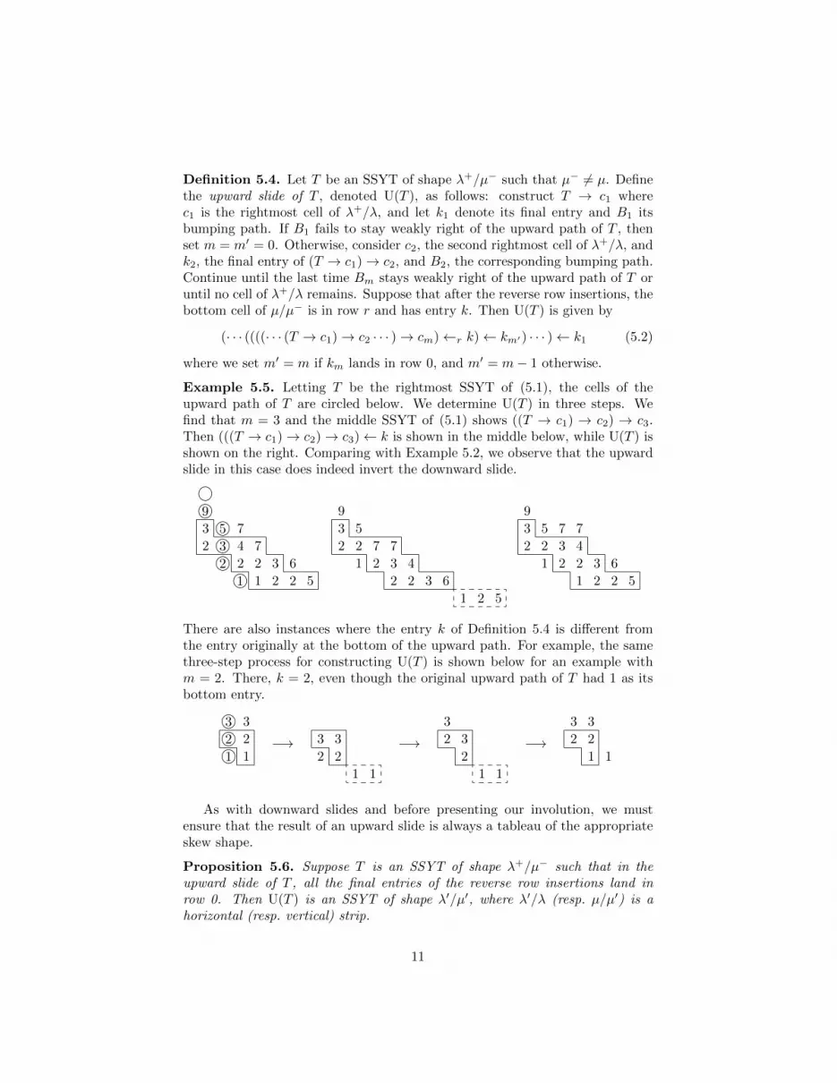
Definition 5.4. Let T be an SSYT of shape λ+/µ− such that µ− 6= µ. Definethe upward slide of T , denoted U(T ), as follows: construct T → c1 wherec1 is the rightmost cell of λ+/λ, and let k1 denote its final entry and B1 itsbumping path. If B1 fails to stay weakly right of the upward path of T , thenset m = m′ = 0. Otherwise, consider c2, the second rightmost cell of λ+/λ, andk2, the final entry of (T → c1)→ c2, and B2, the corresponding bumping path.Continue until the last time Bm stays weakly right of the upward path of T oruntil no cell of λ+/λ remains. Suppose that after the reverse row insertions, thebottom cell of µ/µ− is in row r and has entry k. Then U(T ) is given by

(· · · ((((· · · (T → c1)→ c2 · · · )→ cm)←r k)← km′) · · · )← k1 (5.2)

where we set m′ = m if km lands in row 0, and m′ = m− 1 otherwise.

Example 5.5. Letting T be the rightmost SSYT of (5.1), the cells of theupward path of T are circled below. We determine U(T ) in three steps. Wefind that m = 3 and the middle SSYT of (5.1) shows ((T → c1) → c2) → c3.Then (((T → c1)→ c2)→ c3)← k is shown in the middle below, while U(T ) isshown on the right. Comparing with Example 5.2, we observe that the upwardslide in this case does indeed invert the downward slide.

○9○3 5○ 7

2 3○ 4 7

2○ 2 2 3 6

1○ 1 2 2 5

9

3 5

2 2 7 7

1 2 3 4

2 2 3 6

1 2 5

9

3 5 7 7

2 2 3 4

1 2 2 3 6

1 2 2 5

There are also instances where the entry k of Definition 5.4 is different fromthe entry originally at the bottom of the upward path. For example, the samethree-step process for constructing U(T ) is shown below for an example withm = 2. There, k = 2, even though the original upward path of T had 1 as itsbottom entry.

3○ 3

2○ 2

1○ 1−→ 3 3

2 2

1 1

−→3

32

2

1 1

−→3 3

2 2

1 1

As with downward slides and before presenting our involution, we mustensure that the result of an upward slide is always a tableau of the appropriateskew shape.

Proposition 5.6. Suppose T is an SSYT of shape λ+/µ− such that in theupward slide of T , all the final entries of the reverse row insertions land inrow 0. Then U(T ) is an SSYT of shape λ′/µ′, where λ′/λ (resp. µ/µ′) is ahorizontal (resp. vertical) strip.

11

Proof. If none of the reverse bumping paths B1, . . . , Bm in the upward slideof T intersect the upward path, then inserting the bottom cell of the upwardpath into the row above will follow the upward path. So applying U to T willsimply amount to row insertion along the upward path, with any movementalong the Bi being inverted in the course of applying U. Thus, with notation asin Definition 5.4, we can assume that Bm intersects the upward path of T , whereBm is the last reverse bumping path that stays weakly right of the upward pathof T . Note that by Lemma 4.8(c), no other reverse bumping path Bm′ withm′ < m can intersect the upward path. When k is internally inserted into T ,it will follow the upward path of T until it intersects Bm from which time itwill follow Bm, ultimately adding cm back to the tableau. Next inserting kmwill result in a bumping path B′m following Bm until one row below the pointof intersection. Note that B′m cannot intersect the bottom cell of the upwardpath, since that cell is now empty. Therefore, in the row of the bottom cell ofthe upward path, B′m is strictly right of the upward path. Thus we can applyLemma 4.8(a) to deduce that B′m will necessarily remain strictly right of thebumping path for k. Finally, by Lemma 4.8(c), we have that km ≤ · · · ≤ k1.Thus, by (a) and (b) Lemma 4.8, inserting the remaining entries still results inthe addition of a horizontal strip.

Our involution will consist of either applying a downward slide or an upwardslide. The decision for which slide to apply is roughly based on which of thedownward path of T or the upward path of T lies further to the right.

Definition 5.7. Consider the set of SSYTs T of shape λ+/µ− such that thatλ+/λ is a horizontal strip and µ/µ− is a vertical strip. Define a map φ on suchT by

φ(T ) =

D(T ) if T has no upward path or

the downward path of T exists and exits right,

U(T ) otherwise.

Theorem 5.8. The map φ defines an involution on the set of SSYTs with shapesof the form λ+/µ− where λ+/λ is a horizontal strip and µ/µ− is a vertical strip.

Proof. We refer the reader to Examples 5.2 and 5.5 for illustrations of the ideasof the proof.

First suppose that φ(T ) = D(T ). By Definition 5.7, the first way in whichthis can happen is if T has neither an upward path nor a downward path. Thiscorresponds to the case m′ = m in Definition 5.1 which, by Lemma 4.7(b),results in φ(T ) = D(T ) = T , trivially an involution.

Therefore, assume the downward path of T exists and exits right, so byProposition 5.3, φ(T ) has the required shape. Moreover, since D(T ) adds acell to µ/µ−, φ(T ) must have an upward path. Suppose cell cm is at the topof the downward path of T . It follows from Lemma 4.8 that all cells strictlyright of cm and above λ in T have reverse bumping paths strictly right of thedownward path of T and, by definition of the downward path, their reverse row

12

insertions all land in row 0. For any cell c strictly left of cm in T , Lemma 4.8(c)implies that the reverse bumping path of c in T must remain strictly left ofthe downward path of T , and this property persists in φ(T ). Therefore eitherφ(T ) has no downward path or the downward path does not exit right, and soφ(φ(T )) = U(D(T )).

To show that U(D(T )) = T , first consider D applied to T . After reverserow inserting along the reverse bumping paths including the downward path,suppose we have arrived at an SSYT S. We next row insert the final entrieskm−1, . . . , k1 of Definition 5.1. These new bumping paths may have been af-fected by the changes on the downward path but, as shown in the proof ofProposition 5.3, the bumping path B of km−1 still lies weakly right of thedownward path. Next, we consider the application of U to D(T ) and observethat, since the downward path of T exits right, it shares a bottom cell with theupward path of D(T ). Thus the upward path must stay weakly left of the down-ward path and, in particular, B lies weakly right of the upward path. Moreover,B corresponds to the Bm of Definition 5.4 since, as mentioned in the previousparagraph, reverse bumping paths further left will have a bottom cell that isstrictly left of the bottom cell of the upward path. A key idea is now evident:after we perform the first part of U by applying the reverse row insertions, wewill return to the SSYT S. Therefore, the rest of the application of U to D(T )will invert the reverse row insertions from the application of D to T , as required.

Next, suppose φ(T ) = U(T ). By Definition 5.7, T has an upward path andeither has no downward path or the downward path does not exit right. So, thedownward path, if it exists, does not stay weakly right of the upward path. Inparticular, all the final entries of the reverse row insertions in the upward slideland in row 0. So by Proposition 5.6, φ(T ) has the required shape.

If none of the reverse bumping paths B1, . . . , Bm in the upward slide of Tintersect the upward path then, as we observed in the proof of Proposition 5.6,applying U to T will simply amount to row insertion along the upward path,with any movement along the Bi being inverted in the course of applying U.In particular, the upward path of T will become the downward path of U(T )and hence it exits right. Again, the downward path of U(T ) will not intersectthe other reverse bumping paths of U(T ), which will still be B1, . . . , Bm. Soapplying D to U(T ) will simply amount to the reverse row insertion along thedownward path. Thus φ(φ(T )) = D(U(T )) = T .

On the other hand, if Bm from Definition 5.4 intersects the upward path,we know from the proof of Proposition 5.6 that internally inserting the bottomentry k of the upward path into the row above will eventually follow Bm andall other insertions will have bumping paths B′m, B

′m−1, . . . , B

′1 strictly to the

right. Therefore this bumping path for k will become the downward path ofU(T ) and again it clearly exits right. Thus when we apply D to U(T ), wewill first reverse row insert along the B′i and then invert the changes causedby the internal insertion of k. As a result, when we complete the D operationby reinserting the final entries of B′m, B

′m−1, . . . , B

′1, the bumping paths will be

the same as the original reverse bumping paths when we applied U to T . Thusφ(φ(T )) = D(U(T )) = T .

13

We now have all the ingredients needed to prove the skew Pieri rule.

Proof of Theorem 3.2. Using the expansion of sλ+/µ− in terms of SSYTs as in(2.1), observe that if φ(T ) 6= T , then the T and φ(T ) occur with different signs inthe right-hand side of (3.3). Since φ clearly preserves the monomial associatedto an SSYT, the monomials corresponding to T and φ(T ) in the right-handside of (3.3) will cancel out. Because sλ/µsn = s(λ/µ)∗(n), it remains to showthat there is a monomial-preserving bijection from fixed points of φ to SSYTsof shape (λ/µ) ∗ (n).

Note that T is a fixed point of φ only if T has neither an upward path nora downward path. This happens if and only if µ− = µ and when reverse rowinserting the cells of λ+/λ from right to left, every final entry lands in row 0.In particular, the entries of T remaining after reverse row inserting the cellsof λ+/λ form an SSYT of shape λ/µ. Say the final entries of the reverse rowinsertions are kn, . . . , k1 in the order removed. By Lemma 4.8(c), since λ+/λ isa horizontal strip, we have k1 ≤ · · · ≤ kn and so these entries form an SSYTof shape (n). By Lemma 4.7, this process is invertible and therefore establishesthe desired bijection.

6. Concluding remarks

6.1. Littlewood–Richardson fillings

We proved Theorem 3.2 by working with SSYTs. In particular, we showedthat the two sides of (3.3) were equal when expanded in terms of monomials.Alternatively, we could consider the expansions of both sides of (3.3) in terms ofSchur functions. The Littlewood–Richardson rule states that the coefficient ofsν in the expansion of any skew Schur function sλ/µ is the number of Littlewood–Richardson fillings (LR-fillings) of shape λ/µ and content ν. (The interestedreader unfamiliar with LR-fillings can find the definition in [22].) It is not hardto check that our maps D and U send LR-fillings to LR-fillings, and bumpingwithin LR-fillings has some nice properties. For example, the entries along a(reverse) bumping path are always 1, 2, . . . , r from bottom to top for some r.

However, we chose to give our proof in terms of SSYTs because one doesnot need to invoke the power of the Littlewood–Richardson rule to prove theclassical Pieri rule, and we wanted the same to apply to the skew Pieri rule.

6.2. The bigger picture

We would like to conclude by asking if the skew Pieri rule can be shownto be a special case of a larger framework. For example, [2] and [6] both givegeneral setups that might be relevant. It would be of obvious interest if theseframeworks or any others in the literature could be used to rederive the skewPieri rule.

In a similar spirit, we close with a conjectural rule for the product sλ/µsσ/τ ,which has now been proved by Lam, Lauve and Sottile in [7]. This rule gives theskew Pieri rule when σ/τ = (n) and gives the classical Littlewood–Richardson

14

rule when µ = τ = ∅. The Littlewood–Richardson rule can itself be used toevaluate the general product sλ/µsσ/τ , but our rule will be different in that, likethe skew Pieri rule, we will be adding boxes to both the inside and outside ofλ/µ.

As before, fix a skew shape λ/µ, and suppose we have a skew shape λ+/µ−

such that λ+ ⊇ λ and µ− ⊆ µ. We no longer require that λ+/λ (resp. µ/µ−) isa horizontal (resp. vertical) strip. We will need a few new definitions that arevariants of those that arise in the Littlewood–Richardson rule. Let T+ be anSSYT of shape λ+/λ and let T− be a filling of µ/µ−. We let T− be an anti-semistandard Young tableau (ASSYT), meaning that the entries of T− strictlydecrease from left-to-right along rows, and weakly decrease up columns. Whenλ/µ = 7541/33 and λ+/µ− = 9953/1, an example of a pair (T−, T+) with theabove-stated properties is

5 6

3

2 4

1 4 4 55

3

3 1

2

. (6.1)

The reverse reading word of the pair (T−, T+) is the sequence of entriesobtained by first reading the entries of T− from bottom-to-top along its columns,starting with rightmost column and moving left, followed by reading the entriesof T+ from right-to-left along its rows, starting with the bottom row and movingupwards. The reverse reading word of the example above is 21335425441365. Aword w is said to be Yamanouchi if, in the first j letters of w, the number ofoccurrences of i is no less than the number of occurrences of i+ 1, for all i andj. For a partition τ , a word w is said to be τ -Yamanouchi if it is Yamanouchiwhen prefixed by the following concatenation: τ1 1’s, followed by τ2 2’s, andso on. The reverse reading word of (6.1) is certainly not Yamanouchi but is5321-Yamanouchi.

For a proof of the following conjecture, see Theorem 6 and Remark 7 in [7].

Conjecture 6.1. For any skew shapes λ/µ and σ/τ ,

sλ/µsσ/τ =∑

T−∈ASSYT(µ/µ−)

T+∈SSYT(λ+/λ)

(−1)|µ/µ−|sλ+/µ− ,

where the sum is over all ASSYTs T− of shape µ/µ− for some µ− ⊆ µ, andSSYTs T+ of shape λ+/λ for some λ+ ⊇ λ, with the following properties:

◦ the combined content of T− and T+ is the component-wise difference σ−τ ,and

◦ the reverse reading word of (T−, T+) is τ -Yamanouchi.

For example, to the product s7541/33 s755431/5321, the pair (T−, T+) of (6.1)contributes −s9953/1. Note that when µ = τ = ∅, Conjecture 6.1 is exactly the

15

classical Littlewood–Richardson rule. If instead σ/τ = (n), then all the entriesof T− and T+ must be 1’s, and the skew Pieri rule results.

Another interesting special case of Conjecture 6.1 is when σ/τ is a horizontalstrip with row lengths ρ = σ− τ from bottom to top, with ρ a partition. In thiscase, sσ/τ = hρ, while the τ -Yamanouchi property is trivially satisfied for any(T−, T+) with content σ−τ . Conjecture 6.1 then gives the following expressionfor the product sλ/µhρ for any skew shape λ/µ and partition ρ:

sλ/µhρ =∑

T−∈ASSYT(µ/µ−)

T+∈SSYT(λ+/λ)

(−1)|µ/µ−|sλ+/µ− ,

where the sum is over all ASSYTs T− of shape µ/µ− for some µ− ⊆ µ, andSSYTs T+ of shape λ+/λ for some λ+ ⊇ λ, such that the combined contentof T− and T+ is ρ. Observe that this result follows directly from repeatedapplications of the skew Pieri rule.

7. Acknowledgments

We are grateful to a number of experts for informing us that they too weresurprised by the existence of the skew Pieri rule, and particularly to RichardStanley for providing an algebraic proof of the n = 1 case that preceded ourcombinatorial proof. We are also grateful to Thomas Lam for extending Stan-ley’s proof to the general case and for his willingness to append his proof tothis manuscript. This research was performed while the second author wasvisiting MIT, and he thanks the mathematics department for their hospitality.Conjecture verification was performed using [1, 23].

Appendix A. An algebraic proof (by Thomas Lam)

Let 〈., .〉 : Λ × Λ → Q denote the (symmetric, bilinear) Hall inner product.For f ∈ Λ, we let f⊥ : Λ→ Λ denote the adjoint operator to multiplication byf , so that 〈fg, h〉 = 〈g, f⊥h〉 for g, h ∈ Λ.

Proposition Appendix A.1. For n ≥ 1, and f, g ∈ Λ, we have

f h⊥n (g) =

n∑k=0

(−1)kh⊥n−k(e⊥k (f)g). (A.1)

Proof. We shall use the formula [12, 2.6′], for n ≥ 1

n∑i=0

(−1)ieihn−i = 0 (A.2)

and [12, Example I.5.25(d)]

h⊥n (fg) =

n∑i=0

h⊥n−i(f)h⊥i (g). (A.3)

16

In the following we shall use the fact that the map Λ → EndQ(Λ) given byf → f⊥ is a ring homomorphism [12, Example I.5.3]. Starting from the right-hand side of (A.1) and using (A.3) we have

n∑k=0

(−1)kh⊥n−k(e⊥k (f)g) =

n∑k=0

(−1)kn−k∑j=0

h⊥j (e⊥k (f))h⊥n−k−j(g).

Under the substitution n− k = j + i, the right-hand side becomes

n∑i=0

(−1)n−i

n−i∑j=0

(−1)j(h⊥j e⊥n−j−i)(f)

h⊥i (g). (A.4)

Since∑n−ij=0(−1)j(h⊥j e

⊥n−j−i)(f) = 0 for n− i > 0 using (A.2)⊥, but is equal to

f for n = i, we see that (A.4) reduces to f h⊥n (g).

Proof of Theorem 3.2. It is well known (see [12, I.(4.8), I.(5.1)] or [22, Corollary7.12.2, (7.60)]) that for two partitions λ and µ, we have 〈sλ, sµ〉 = δλ,µ ands⊥µ sλ = sλ/µ, where sλ/µ = 0 if µ 6⊆ λ. Let g ∈ Λ. We calculate

〈sλ/µhn, g〉 = 〈sλ/µ, h⊥n g〉 = 〈s⊥µ sλ, h⊥n g〉 = 〈sλ, sµh⊥n g〉

= 〈sλ,n∑k=0

(−1)kh⊥n−k(e⊥k (sµ)g)〉

by Proposition Appendix A.1. Using the Pieri rule (Theorem 3.1), this amountsto ⟨

n∑k=0

(−1)k∑

λ+/λ (n−k)-hor. strip

µ/µ− k-vert. strip

sλ+/µ− , g

⟩.

Since the Hall inner product is non-degenerate, we obtain (3.3).

[1] Anders S. Buch. Littlewood–Richardson calculator, 1999.Available from http://www.math.rutgers.edu/~asbuch/lrcalc/.

[2] Sergey Fomin. Schur operators and Knuth correspondences. J. Combin.Theory Ser. A, 72(2):277–292, 1995.

[3] Donald E. Knuth. Permutations, matrices, and generalized Youngtableaux. Pacific J. Math., 34:709–727, 1970.

[4] Tom H. Koornwinder. Self-duality for q-ultraspherical polynomials associ-ated with root system an. Unpublished manuscript.http://staff.science.uva.nl/~thk/art/informal/dualmacdonald.

pdf, 1988.

[5] Thomas Lam. Ribbon tableaux and the Heisenberg algebra. Math. Z.,250(3):685–710, 2005.

17

[6] Thomas Lam. A combinatorial generalization of the boson-fermion corre-spondence. Math. Res. Lett., 13(2-3):377–392, 2006.

[7] Thomas Lam, Aaron Lauve, and Frank Sottile. Skew Littlewood–Richardson rules from Hopf algebras. Preprint. http://arxiv.org/abs/0908.3714, 2009.

[8] Alain Lascoux and Marcel-Paul Schutzenberger. Polynomes de Schubert.C. R. Acad. Sci. Paris Ser. I Math., 294(13):447–450, 1982.

[9] Michel Lassalle. Une formule de Pieri pour les polynomes de Jack. C. R.Acad. Sci. Paris Ser. I Math., 309(18):941–944, 1989.

[10] Cristian Lenart and Frank Sottile. A Pieri-type formula for the K-theoryof a flag manifold. Trans. Amer. Math. Soc., 359(5):2317–2342 (electronic),2007.

[11] D.E. Littlewood and A.R. Richardson. Group characters and algebra. Phi-los. Trans. Roy. Soc. London, Ser. A, 233:99–141, 1934.

[12] I. G. Macdonald. Symmetric functions and Hall polynomials. Oxford Math-ematical Monographs. The Clarendon Press Oxford University Press, NewYork, second edition, 1995. With contributions by A. Zelevinsky, OxfordScience Publications.

[13] Laurent Manivel. Fonctions symetriques, polynomes de Schubert et lieux dedegenerescence, volume 3 of Cours Specialises [Specialized Courses]. SocieteMathematique de France, Paris, 1998.

[14] A. O. Morris. A note on the multiplication of Hall functions. J. LondonMath. Soc., 39:481–488, 1964.

[15] Mario Pieri. Sul problema degli spazi secanti. Rend. Ist. Lombardo (2),26:534–546, 1893.

[16] G. de B. Robinson. On the Representations of the Symmetric Group. Amer.J. Math., 60(3):745–760, 1938.

[17] Bruce E. Sagan and Richard P. Stanley. Robinson–Schensted algorithmsfor skew tableaux. J. Combin. Theory Ser. A, 55(2):161–193, 1990.

[18] C. Schensted. Longest increasing and decreasing subsequences. Canad. J.Math., 13:179–191, 1961.

[19] M.-P. Schutzenberger. La correspondance de Robinson. In Combinatoireet representation du groupe symetrique (Actes Table Ronde CNRS, Univ.Louis-Pasteur Strasbourg, Strasbourg, 1976), pages 59–113. Lecture Notesin Math., Vol. 579. Springer, Berlin, 1977.

[20] Frank Sottile. Pieri’s formula for flag manifolds and Schubert polynomials.Ann. Inst. Fourier (Grenoble), 46(1):89–110, 1996.

18

[21] Richard P. Stanley. Some combinatorial properties of Jack symmetric func-tions. Adv. Math., 77(1):76–115, 1989.

[22] Richard P. Stanley. Enumerative combinatorics. Vol. 2, volume 62 of Cam-bridge Studies in Advanced Mathematics. Cambridge University Press,Cambridge, 1999.

[23] John R. Stembridge. SF, posets and coxeter/weyl.Available from http://www.math.lsa.umich.edu/~jrs/maple.html.

[24] Glanffrwd P. Thomas. Baxter algebras and Schur functions. PhD thesis,University College of Swansea, 1974.

[25] Glanffrwd P. Thomas. On Schensted’s construction and the multiplicationof Schur functions. Adv. in Math., 30(1):8–32, 1978.

[26] Rudolf Winkel. On the multiplication of Schubert polynomials. Adv. inAppl. Math., 20(1):73–97, 1998.

19