Continuous Aerodynamic Modelling of Entry Shapes

Continuous Aerodynamic Modelling of Entry Shapes

Dominic Dirkx� and Erwin Mooijy

Delft University of Technology, Delft, 2600 AA, The Netherlands

During the conceptual design phase of a re-entry vehicle, the vehicle shape can be variedand its impact on performance evaluated. To this end, the continuous modeling of theaerodynamic characteristics as a function of the shape is useful in exploring the full designspace. Local inclination methods for aerodynamic analysis have proven su�ciently accuratefor use at such a design stage, but manual selection of methods over the vehicle is ine�cientfor the exploration of a large number of design possibilities. This paper describes the modelof an aerodynamic analysis code, written for use in conceptual vehicle shape optimization,which includes an automatic method selection algorithm. Panel shielding is also includedin the analysis code to allow for the analysis of more complex geometries. The modelsused for the shape and aerodynamics are described and results for the Space Shuttle andApollo are compared to wind tunnel data. They show an accuracy of better than 15% formost cases, which is su�cient for the use in conceptual design. Panel shielding is shownto be important in the prediction of control derivatives at low angle of attack, as well asthe prediction of lateral stability derivatives. Finally, a simple guidance algorithm is usedto assess the impact of the errors in the aerodynamic coe�cients on the vehicle heat loadand ground track length. Both show discrepancies of less than 10%.

Nomenclature

A = Area [m2]Cp = Pressure coe�cient [-]CD = Drag coe�cient [-]CL = Lift coe�cient [-]Cm = Pitch moment coe�cient [-]cref = Moment reference length [m]D = Drag [N]fc(t) = Cubic bridging polynomial [-]g = Acceleration due to gravity [m]h = Altitude [m]ki = method selection parameter (i = 1::9)[-]L = Length [m]M = Mach number [-]m = Mass [kg]qc = Convective heat rate [W/m2]R = Radius [m]r = Distance to moment reference point [m]Sref = Moment reference area [m2]T = Temperature [m]V = Velocity [m/s]�Graduate Student. Currently: Researcher, Faculty of Aerospace Engineering, [email protected] Professor, Faculty of Aerospace Engineering, [email protected], Senior member AIAA.

1 of 24

American Institute of Aeronautics and Astronautics

AIAA Atmospheric Flight Mechanics Conference08 - 11 August 2011, Portland, Oregon

AIAA 2011-6575

Copyright © 2011 by D. Dirkx and E. Mooij. Published by the American Institute of Aeronautics and Astronautics, Inc., with permission.

Dow

nloa

ded

by T

EC

HN

ISC

HE

UN

IVE

RSI

TE

IT D

EL

FT o

n Fe

brua

ry 1

7, 2

015

| http

://ar

c.ai

aa.o

rg |

DO

I: 1

0.25

14/6

.201

1-65

75

� = Angle of attack [rad]� = Sideslip angle [rad]� = Shock angle [rad]�bf = Body ap de ection [rad]�e = Elevon de ection [rad] = Ratio of speci�c heats [-] = Flight-path angle [rad]� = Latitude [rad]� = Lateral panel inclination [rad]� = Panel inclination angle [rad]�c = Cone half angle [rad]� = Wing sweep angle [rad]� = Density [kg/m3]� = Bank angle [rad]� = Longitude [rad]� = Heading angle [rad]!P = Central body angular rate [rad/s]

Subscripts:

cog = Center of gravityR = In inertial Earth-�xed frames = At stagnation point

I. Introduction

During the conceptual design stage of re-entry vehicles, the design parameters are varied to gain knowledgeof their e�ect on the vehicle’s overall performance and its capability to ful�ll the design requirements.One of the de�ning characteristics of an entry vehicle is its shape, as this shape will largely de�ne theaerothermodynamic characteristics of the vehicle. Since aerothermodynamic challenges, such as vehicleheating remain one of the most di�cult problems in atmospheric re-entry, an exploration of the possibleshapes for a vehicle early in the design is advisable. It is advantageous to use a continuous model for theanalysis, so that one is not limited to the analysis and comparison of a limited number of shapes,1 but isinstead free to analyze any shape in the design space. This paper will discuss a simpli�ed aerodynamicmodel, which is to be used in a vehicle-optimization e�ort. The optimization is to be carried out on botha capsule-shaped vehicle described in this paper, as well as a freeform winged fuselage entry vehicle usingspline surfaces.2

The validation of the aerodynamics code through comparison with Apollo and Space-Shuttle wind-tunneldata will be used here to assess the accuracy of the methodology that is used. The e�ect that the di�erenceswill have on vehicle trajectories will also be adressed, to assess the capability of the aerodynamic models toproperly predict the vehicles’ performance criteria in an optimization loop. The de�nition of the shapes isdiscussed in Section II, followed by the de�nition of the aerothermodynamic models in Section III. SectionIV will show the comparison between the calculated and measured aerodynamic coe�cients of Apollo andthe Shuttle, and give a discussion of the discrepancies that are observed. The trajectory and guidancemodels are described in Section V, whereas Section VI will show the impact of the aerothermodynamicdiscrepancies on the resulting trajectories. Finally, Section VII will conclude the paper with conclusions andrecommendations for future work.

2 of 24


Dow

nloa

ded

by T

EC

HN

ISC

HE

UN

IVE

RSI

TE

IT D

EL

FT o

n Fe

brua

ry 1

7, 2

015

| http

://ar

c.ai

aa.o

rg |

DO

I: 1

0.25

14/6

.201

1-65

75

(a) (b)

Figure 1. Schematic representation of capsule re-entry vehicle shape4 a) Vehicle parameters b) Division in analyticalshapes

II. Geometry De�nition

The de�nition and parametrization of the vehicle shape is the starting point of the analysis of the problem.Numerous possibilities exist for de�ning vehicle shapes, where in this context the continuous variation of alimited number of parameters on which it is to be based is crucial. In the optimization, two cases will betreated, one describing analytical shape de�nitions and one using freeform spline de�nitions. The formerof these will be used for the validation of the aerodynamics model in this article, while the latter will beconsidered in future work. For validation of the code for a lifting entry vehicle, a Space-Shuttle mesh willbe used, which is independent of the shape parametrization that will be used in the optimization.

II.A. Capsule Shape

A number of vehicle shapes can be de�ned by a combination of analytical surfaces. An example of this in aframework similar to the one discussed here is found in literature.3 The analytical shape that will be usedin this study is shown in Fig. 1. This is a parametrization of, among others, the Apollo capsule. As can beseen, it consists of four matched analytical geometries, a sphere segment, a torus segment, a conical frustumand a spherical segment. Although no unique set of parameters exists for de�ning this shape, the requirednumber of parameters for de�ning it is �ve. Since the shape is axisymmetric, the full surface geometry isde�ned by the cross-section shown. The parameters which are chosen for the shape de�nition are:

� Nose radius RN

� Side radius RS

� Rear cone half-angle �c

� Mid radius Rm

� Rear conical part length Lc

The parameter Lc is chosen here, instead of the capsule length L, due to the simplicity of the constraint onit from other vehicle parameters. This will be advantageous in the optimization process. The cross-sectionsof the constituent analytical shapes can be seen from Fig. 1(b). The relations between the parameters ofthe capsule and the parameters of the analytical shapes can be derived by simple geometrical relations.

When generating a capsule shape, the constraints on the parameters are inter-dependent. That is, inaddition to constraints imposed on each variable a priori, the choice of RN and �c in uence the availablechoices of Rm and Lc. When generating the variables in the order described above, the following constraints

3 of 24


Dow

nloa

ded

by T

EC

HN

ISC

HE

UN

IVE

RSI

TE

IT D

EL

FT o

n Fe

brua

ry 1

7, 2

015

| http

://ar

c.ai

aa.o

rg |

DO

I: 1

0.25

14/6

.201

1-65

75

Figure 2. Space Shuttle wireframe model from Langley Wireframe Geometry Standard, note the di�erence in theformation of fusiform and planar geometries.5

.

are to be observed:

Rm < RN (1)

Lc <Rm �RS (1� cos �c)

tan �c(2)

In addition to the external geometry of the vehicle, the capsule’s center of mass is important for deter-mining the vehicle’s performance. Its position is parametrized by two variables, i.e., its position along thevehicle centerline and the o�set from this centerline.

II.B. Surface Mesh

For the aerodynamic analysis described in the next section, a panelled surface mesh is required. The geometryinput �le format that is used is the Langley Wireframe Geometry Format (LaWGS).5 It bases the de�nitionof a wireframe on a discrete number of points which make up an object. The entire con�guration can thenbe de�ned from an arbitrary number of these objects. Objects may be de�ned in a (right-handed Cartesian)global coordinate system, or a local coordinate system, where the speci�cation of the translation and rotationfrom the local to global coordinate system must be given. In addition, a mirror symmetry about the xy-,xz- or yz-plane may be de�ned in either local or global coordinates for an object.

A single object is composed of a number of contours, which are in turn composed of a number of points,where the number of points on each contour must be equal. By connecting each point to both neighbouringpoints on the same contour and connecting points with the same indices on subsequent contours, a wireframeof quadrilaterals is obtained. An example of a resulting wireframe for the Space Shuttle is shown in Fig. 2.

Although not required for the �le format, a guideline, which is later exploited in the aerodynamics code(see Section III.B), is to de�ne parts as either ’fusiform’ or ’planar’. The former includes fuselages, etc., andthe latter includes wings, vertical and horizontal stabilizers, etc. The distinction between these two types ofgeometries can be seen in Fig. 2, where the di�erent orientations of the contours on the wings, ap and tailversus the fuselage are clearly indicated.

III. Aerothermodynamics

The aerothermodynamic e�ect on a re-entry vehicle in hypersonic ow is characterized by the aerodynamicforces and moments, as well as the heating over the vehicle. For use in trajectory simulation, a database ofcoe�cients as a function of freestream Mach number M , angle of attack � and sideslip angle � is generated,and these values are interpolated to yield a data point at a particular ight condition during integration.

For a complete aerothermodynamic analysis, the prediction of pressure, friction and heating on the surfaceshould be performed in unison, as these e�ects are strongly coupled in hypersonic ow. To perform suchan analysis would require the use of a Computational Fluid Dynamics (CFD) tool, which numerically solves

4 of 24


Dow

nloa

ded

by T

EC

HN

ISC

HE

UN

IVE

RSI

TE

IT D

EL

FT o

n Fe

brua

ry 1

7, 2

015

| http

://ar

c.ai

aa.o

rg |

DO

I: 1

0.25

14/6

.201

1-65

75

the (chemically reacting) Navier Stokes equations. Such an analysis would require a prohibitive amount oftime in the context of the vehicle optimization work, however, since aerodynamic coe�cients are requiredfor all attitudes and Mach numbers that occur during the re-entry of each of the vehicle con�gurations tobe analyzed. Depending on the exact number of trajectory integrations during the optimization, as well asthe total number of Mach numbers and attitude angles at which coe�cients are determined, aerodynamiccoe�cients for 105-107 cases will need to be computed. Obviously, this is infeasible in a reasonable amountof time using a Navier-Stokes solver, or even an Euler solver.

For this reason, a set of simple analysis methods for hypersonic ow are used in this study, notablylocal inclination methods. The rationale behind these methods, as well as their implementation, will bedescribed in Section III.A. An algorithm for the selection of the applicable aerodynamic method per vehiclepart is discussed in Section III.B. A method that has been used in the past as a modi�cation of the localinclination methods is discussed in Section III.C. Finally, the heating analysis, which in this study is limitedto stagnation-point heating, is given in Section III.D.

A �rst version of software was developed in the framework of the open source software project SpaceTrajectory Analysis (STA)6 as the Re-entry Aerodynamics Module (RAM). This version includes the methodselection algorithm, but does not include the panel shielding or the ability to determine control derivatives.

The local inclination methods produce only a pressure distribution on the vehicle. The viscous e�ect onthe aerodynamic forces and moments will be neglected in this study. Additionally, the ow will be assumedto be a continuum throughout the entry. The methods described in the next section will be used to calculatepressure coe�cients Cp on each of the vehicle panels.

III.A. Local Inclination Methods

An important set of force estimation methods in hypersonic ow is formed by the so-called local inclinationmethods, which require only the angle � by which the surface is (locally) inclined w.r.t. the free stream ow to produce a pressure coe�cient. Although such methods are obviously highly simpli�ed, reasonableresults can be obtained by using them. Due to this combination of simplicity and reasonable validity, thistype of method �nds wide use in conceptual design7{11 and are very well suited to use in conceptual designoptimization. The long heritage has also made them well documented. An excellent introduction is given inliterature,12 with their formulation and implementation extensively discussed in manuals for previous codesusing such methods.13{15 Generally, two classes of methods are used, one for the windward side and one forthe leeward side. The leeward side methods are also applied to ’shielded’ sections. Shielding occurs whena vehicle is oriented to the ow in such a manner that a part of it is ’shielded’ from the oncoming ow byanother part of it. In such cases, the windward surface-inclination method should be applied only to thesurface the ow encounters �rst, the second part should use an appropriate leeward method.

The most basic inclination method for the estimation of the aerodynamic forces and moments on ahypersonic body is the Newtonian method. This method assumes that, upon hitting a surface, the owloses its component normal to the surface while retaining all of its tangential motion. The assumptions ofNewtonian ow lead to the following relation for the local pressure coe�cient:

Cp = 2 sin2 � (3)

A modi�cation of this method that is typically used involves an additional physical consideration of supersonic ow, namely the loss of total pressure over a shock wave. Including the loss of total pressure will increasethe physical justi�cation of the model. The model, which is obtained is termed the Modi�ed Newtonianmethod, the pressure coe�cient it produces is:

Cp = Cp;s sin2 � (4)

where Cp;s is the stagnation point pressure coe�cient.The modi�ed Newtonian method assumes that that all streamlines have passed through a normal shock

wave. Although this assumption will in general be true for only a very select number of streamlines, Fig.3(a) gives an indication as to why this assumption can be assumed valid as a �rst-order approximation overa larger region. Here, the stagnation pressure coe�cient that occurs after passing through an oblique shockwave is plotted. It can be seen that the ’correct’ value of Cp;s varies very little over the range 40� < � < 90�.For low shock angles (and therefore low inclination angles), however, the value of Cp;s increases very quickly.

5 of 24


Dow

nloa

ded

by T

EC

HN

ISC

HE

UN

IVE

RSI

TE

IT D

EL

FT o

n Fe

brua

ry 1

7, 2

015

| http

://ar

c.ai

aa.o

rg |

DO

I: 1

0.25

14/6

.201

1-65

75

(a) (b)

Figure 3. a) Ratio of post-shock total pressure to freestream pressure, = 1:4 b) E�ect of local inclination method onpressure prediction, = 1:4

For the cases of low inclination angles, where the ow has typically (but not necessarily) passed through alow-angle shock wave, di�erent local inclination methods are typically used. The two most popular methods,the Tangent Wedge and Tangent Cone methods,13 liken the local ow to that of an equivalent wedge orcone. Although the cone and wedge will (for su�ciently low cone and wedge angles) have an attached noseshock, these methods have also seen use in predicting the pressure on the rear part of a blunt nosed shape,which will have a detached shock. This is due to the fact that for such a case, as for instance a vehiclefuselage, the shock angle of the shock for which the ow impacting a surface at these low inclination regionhas passed through will be similar to that which it would have passed through had there been an attachedshock. Even though the ow�eld behind the shock will be di�erent in the two cases and the development ofthe boundary and entropy layer will di�er, using these methods can still produce results which are superiorto those produced by the (Modi�ed) Newtonian method, and are therefore useful in a conceptual designstage. Pressure coe�cients for the three methods discussed are shown in Fig. 3(b). It can be seen that thegeneral trend with inclination angle is similar for all methods, but the scale of the results di�er.

For the determination of the expansion pressure coe�cient of the vehicle, a di�erent method must beused. A lower bound for the pressure coe�cient is taken as the vacuum pressure coe�cient:

Cp;vac = � 2 M21

(5)

However, since there will be some ow on the rear of the vehicle due to, for instance, ow recirculation, thiswill underpredict the occuring pressure. An empirical correlation, which is sometimes used, is:

Cp = � 1M1

(6)

Another method that can be used is Prandtl-Meyer expansion from the point of � = 0 onwards. This methodis slightly more complex than the above methods, because it is also a function of the inclination angle �.

In general, di�erent methods are applicable for low and high hypersonic Mach numbers, the details ofthis will be described in Section III.B. To have a database of aerodynamic coe�cients that is continuousin M , a bridging between the low and high hypersonic aerodynamic coe�cients is employed, in a similarfashion to what is sometimes employed for the transitional region between rare�ed and continuum ow. Acubic bridging polynomial fc(t), with t running from 0 to 1, is used. To match both the values and theslopes of the coe�cients at the boundaries of the bridging domain, fc(t) is chosen to be:

fc(t) = �2t3 + 3t2 (7)

6 of 24


Dow

nloa

ded

by T

EC

HN

ISC

HE

UN

IVE

RSI

TE

IT D

EL

FT o

n Fe

brua

ry 1

7, 2

015

| http

://ar

c.ai

aa.o

rg |

DO

I: 1

0.25

14/6

.201

1-65

75

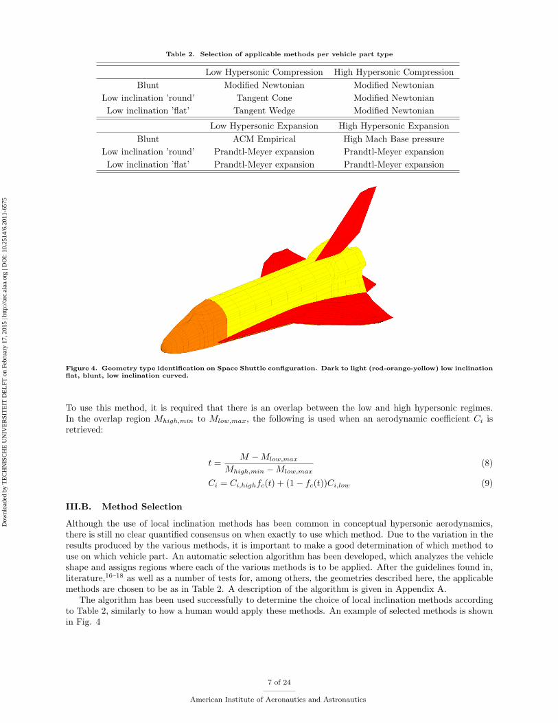
Table 2. Selection of applicable methods per vehicle part type

Low Hypersonic Compression High Hypersonic CompressionBlunt Modi�ed Newtonian Modi�ed Newtonian

Low inclination ’round’ Tangent Cone Modi�ed NewtonianLow inclination ’ at’ Tangent Wedge Modi�ed Newtonian

Low Hypersonic Expansion High Hypersonic ExpansionBlunt ACM Empirical High Mach Base pressure

Low inclination ’round’ Prandtl-Meyer expansion Prandtl-Meyer expansionLow inclination ’ at’ Prandtl-Meyer expansion Prandtl-Meyer expansion

Figure 4. Geometry type identi�cation on Space Shuttle con�guration. Dark to light (red-orange-yellow) low inclination at, blunt, low inclination curved.

To use this method, it is required that there is an overlap between the low and high hypersonic regimes.In the overlap region Mhigh;min to Mlow;max, the following is used when an aerodynamic coe�cient Ci isretrieved:

t =M �Mlow;max

Mhigh;min �Mlow;max(8)

Ci = Ci;highfc(t) + (1� fc(t))Ci;low (9)

III.B. Method Selection

Although the use of local inclination methods has been common in conceptual hypersonic aerodynamics,there is still no clear quanti�ed consensus on when exactly to use which method. Due to the variation in theresults produced by the various methods, it is important to make a good determination of which method touse on which vehicle part. An automatic selection algorithm has been developed, which analyzes the vehicleshape and assigns regions where each of the various methods is to be applied. After the guidelines found in,literature,16{18 as well as a number of tests for, among others, the geometries described here, the applicablemethods are chosen to be as in Table 2. A description of the algorithm is given in Appendix A.

The algorithm has been used successfully to determine the choice of local inclination methods accordingto Table 2, similarly to how a human would apply these methods. An example of selected methods is shownin Fig. 4

7 of 24


Dow

nloa

ded

by T

EC

HN

ISC

HE

UN

IVE

RSI

TE

IT D

EL

FT o

n Fe

brua

ry 1

7, 2

015

| http

://ar

c.ai

aa.o

rg |

DO

I: 1

0.25

14/6

.201

1-65

75

(a) (b)

Figure 5. Shadowing of Space Shuttle panels, � = 30�, � = 2�, a) Shadowed fraction per panel b) Panel type, green =compression, blue = expansion

III.C. Panel Shielding

For complex geometries with protrusions such as wings, vertical stabilizer(s) or a body ap, the concept ofpanel shielding can become important in determining the aerodynamic coe�cients. For the standard localinclination methods, any panel with a positive inclination angle is treated as a compression panel. Whentwo panels are (partially) behind one another, though, this assumption needs to be revised. When a givenfreestream streamline is extended through the vehicle geometry and intersects multiple panels with positiveinclination, it is obvious that it will only have the true compression e�ect on one of these panels. This canbe clari�ed by considering the Newtonian method, which is based on the loss of momentum normal to thewall and realizing that a given ow volume can only lose this momentum once.

To account for this e�ect an algorithm has been used,13 by which all combinations of panels are analyzedand the occurrence and size of overlapping regions are determined. The algorithm is capable of quicklydiscarding the possibility of shielding when comparing two panels to increase computational e�ciency. Theprocedure described there proved to be insu�cient for the comparison of two panels where vertices of thetwo panels that are being compared coincide or if a vertex of one panel is on the side of the other. Criteriato account for these cases have been implemented and tested in the analysis code. The exact procedure willnot be explained in detail here for the sake of brevity.

As can be imagined, the computational e�ort required for the shielding analysis can be signi�cant, as itrequires each combination of panels to be analyzed, so that the computational time will increase with n2,whereas determining the pressures on the panels using the local inclination methods only takes computationaltime on the order of n. For this reason, it should only be used when it is expected to have an importantin uence on the results in question.

Due to the limited usefulness and the high computational cost, the calculation of multiple shielding,where one panel is shielded by more than one panel, is not considered here. Although this will cause someerrors in the results, the occurrence of such a case has proven to be rare, so that the in uence is negligible.An example of the panel-shadowing determination is shown in Fig. 5, where the shadowed fraction of eachShuttle panel is shown, along with a �gure showing which panel is a compression surface, and which is anexpansion surface.

III.D. Heating Analysis

The aerodynamic heating of entry vehicles poses a serious design challenge due to the high heat uxes thatare reached during re-entry. For a detailed analysis of hypersonic heating over a full con�guration, CFD or

8 of 24


Dow

nloa

ded

by T

EC

HN

ISC

HE

UN

IVE

RSI

TE

IT D

EL

FT o

n Fe

brua

ry 1

7, 2

015

| http

://ar

c.ai

aa.o

rg |

DO

I: 1

0.25

14/6

.201

1-65

75

(a) (b)

(c) (d)

Figure 6. Aerodynamic coe�cients for Apollo command capsule a) Drag coe�cient b) Lift coe�cient c) Momentcoe�cients d)Lift over Drag

experimental data are required, which is not feasible for this project. Instead, a number of (semi-)empiricalcorrelations, which have been extensively used in conceptual vehicle design, will be employed here. Thefollowing relation is used for convective heating at a stagnation point:

qc;s = k�N1V N2 (10)

where the values of k, N1 and N2 that are used in literature vary somewhat. The values used here, assuminglaminar ow conditions, are N1 = 0:5 and N2 = 3.19 For k the following relation is used:

k =1:83 � 10�4

pRn

�1� Tw

Taw

�(11)

where Rn is the nose radius, Tw the wall temperature and Taw the adiabatic wall temperature. As a �rstapproximation, the cold wall approximation can be used, so that Tw=Taw � 0 is assumed.

IV. Aerodynamic Veri�cation and Validation

The aerodynamic coe�cients produced by the methods described in Section III.B are compared to avail-able aerodynamic databases and the in uence on the discrepancies is analyzed.

9 of 24


Dow

nloa

ded

by T

EC

HN

ISC

HE

UN

IVE

RSI

TE

IT D

EL

FT o

n Fe

brua

ry 1

7, 2

015

| http

://ar

c.ai

aa.o

rg |

DO

I: 1

0.25

14/6

.201

1-65

75

IV.A. Apollo

The geometry of the Apollo capsule has been modelled according to the parametrization given in SectionII.A, with the parameters taken from literature4 to be the following:

RN = 4:694 m, Rm = 1:956 m, RS = 0:196 m, �c = 33�, Lc = 2:662 m

Aerodynamic coe�cients were then generated and compared to the data from wind-tunnel testing.20 Thereference quantities used in this reference, as well as here are:

Sref = 39:441 m2, cref = 3:9116 m, rcog = (1:0367; 0; 0:1369) m

where the axes are de�ned as in Fig. 1.Figs. 6(a) - 6(b) show the longitudinal translational coe�cients of the Apollo capsule compared to the

wind-tunnel results. It can be seen that the results coincide reasonably well with the wind tunnel data.The most important di�erence between the two is the over-prediction at M = 10. At this Mach numberthe contribution of the expansion is minimal. This is due to the fact that the vacuum pressure coe�cientis very close to zero and the expansion pressure coe�cient will therefore not di�er from 0 by much, sothat the results are almost fully de�ned by the compression pressure distribution. From Fig. 3(b), it canbe seen that the Modi�ed Newtonian method gives the lowest value of the pressure coe�cient at a giveninclination angle of the methods used. Since this method is used on all compression surfaces at M = 10and still produces an axial force which is too high, this indicates that no suitable local inclination methodexists which can produce su�ciently low results here. This could be the result of the fact that stream-linesthat pass through a shock wave of inclination angle somewhat lower than 90� (which will be the case forthe detached bow shock) results in a lower stagnation pressure coe�cient. This will in turn result in a lowerpressure coe�cient. This e�ect has not been included in the code, but could be part of future work. Thee�ect of this can be seen to be acceptable, though. Although not included in this paper, it was observedthat the aerodynamic coe�cients for the EXPERT21 capsule di�ered by a greater amount, most likely dueto a related phenomenon.

The moment coe�cients for the Apollo capsule are shown in Fig. 6(c). It can be seen that the resultscoincide very well with the wind tunnel data. In this study, since attitude propagation is not included andonly vehicle trim is considered to determine the attitude, it is important that the trimmed � and consequentL=D are well predicted. From the �gure, it can be seen that the value of �trim is o� by about 1� for M1 = 10and 0:1� for M1 = 3. The resulting errors in L=D are � 10% in both cases. These discrepancies are morethan acceptable for a conceptual design e�ort, and their in uence on the trajectories of the capsule will bediscussed in Section VI.

(a) (b)

Figure 7. Lift and drag coe�cients produced for the Space Shuttle with and without shadowing compared to windtunnel data

10 of 24


Dow

nloa

ded

by T

EC

HN

ISC

HE

UN

IVE

RSI

TE

IT D

EL

FT o

n Fe

brua

ry 1

7, 2

015

| http

://ar

c.ai

aa.o

rg |

DO

I: 1

0.25

14/6

.201

1-65

75

(a) (b)

Figure 8. Moment coe�cients for the Space Shuttle a) Results generated here with and without shadowing comparedto wind tunnel data b) Wind tunnel data compared to ight data22

(a) (b)

(c)

Figure 9. Stability derivatives produced for the Space Shuttle with and without shadowing compared to wind-tunneldata

11 of 24


Dow

nloa

ded

by T

EC

HN

ISC

HE

UN

IVE

RSI

TE

IT D

EL

FT o

n Fe

brua

ry 1

7, 2

015

| http

://ar

c.ai

aa.o

rg |

DO

I: 1

0.25

14/6

.201

1-65

75

IV.B. Space Shuttle

A geometry mesh for the Space Shuttle, modi�ed to be compatible with the method selection algorithmhas been used to generate aerodynamic coe�cients. The resulting coe�cients were then compared to thoseobtained from wind tunnel data.23 Although these data are known to contain some discrepancies when com-pared to ight data, they comprise a comprehensive and consistent set of data that can be used to comparethe coe�cients generated here at more data points than could be done using only ight data. The referencequantities of the coe�cients are:

Sref = 249:441 m2, cref = 12:0579 m, rcog = (21:356; 0; 0:8224) m

with the Orbiter nose as origin, positive x-direction rearwards and positive z-direction upwardsThe analysis is performed using the default method-selection criteria given in Section III.B. When

comparing the lift and drag coe�cients, it can be seen that the method described here predicts the correctcoe�cients quite well. In addition, for low Mach numbers where a non-Newtonian method is used as thecompression method, the accuracy of the method selection yields results which are clearly superior to amodi�ed Newtonian approach, showing that the approach taken here will be useful for the calculation ofthe translational motion of the Space Shuttle. The e�ect of shadowing on the longitudinal force coe�cientsappears to be minimal, however.

The moment coe�cients di�er more strongly from the database values, as was to be expected frominformation from literature.12 However, it would be advisable to perform a more in-depth analysis of theactual ight data from the Space Shuttle, since there is a known discrepancy in the wind tunnel data, givinga consistent underprediction in the moment coe�cients at high Mach numbers. This e�ect has been studiedin detail22 and a build-up of the actual moment coe�cient is shown here in Fig. 8(b). Since the resultsproduced in the present study show an over-prediction of the coe�cients at � > 20�, they may approximatethe actual coe�cients more closely than can be seen from the �gures here. The e�ect of shadowing is morenoticeable here, with questionable in uence on the accuracy of the results.

The stability derivatives of the lateral coe�cients for small sideslip angles, which are important in theanalysis of the vehicle stability during re-entry can be seen in Figs. 9. Here, the e�ect of the shadowing canbe seen very clearly, in the case of the side force and yaw moment, they cause the trend of the coe�cients tobe followed quite closely, as opposed to the case without shadowing, where no such trend can be observed.The o�set between the wind tunnel data and the results that include shadowing can be explained by thefact that the hard distinction between shadowing and no shadowing will not be quite as abrubt in reality.The streamlines ow which passes over the vehicle’s edges will de ect and in uence the external ow. Inaddition, vortices will form at these positions, further in uencing the ow �eld.

In the case of the roll-moment derivative shown in Fig. IV.A, the in uence of the shadowing is not quiteas clearly positive, causing the coe�cients to be somewhat underpredicted instead of overpredcited in mostcases. This will, however, make for a more conservative estimate of the vehicle stability.

For the control increments, proper prediction of the pitch-moment increments is the primary objectivefor this study, since these values determine the de ection of the control surfaces to trim the vehicle. Theresulting lift and drag increments can constitute � 10 % of the total lift and drag and should not be neglected,though. The control derivatives shown in Figs. 10-12 indicate that the predictions for the elevon incrementsare reasonably good, with lift increments having the lowest accuracy, showing di�erences of up to about0.01.

The body ap increments shown in Figs. 13-15 show greater discrepancies, however, for positive de ec-tions. This can be caused by a number of factors. Firstly, for low de ection angles, the body ap will befully engulfed in the fuselage boundary layer, reducing the body ap e�ectiveness. For higher de ectionangles, though, the compression shock which will occur on the ramp between the fuselage and shock wave,which will cause an increase in surface pressure on the body ap. This e�ect is not observed as strongly onthe elevon, however, where a similar ramp e�ect is expected to occur. Due to the smaller size of the wings,however, the boundary layer will be less thick on the elevons, reducing its e�ect on the control increments.Since a positive body ap de ection is required for Space Shuttle trim, these errors in the moment incrementprediction will result in an over-prediction of the required body ap de ection. The e�ect on the performanceof the Shuttle will be discussed in the next section.

Concluding, it can be said that the longitudinal force coe�cients show excellent agreement with wind-tunnel data. The pitch moment coe�cients are reasonably well predicted, but show substantial discrepancies

12 of 24


Dow

nloa

ded

by T

EC

HN

ISC

HE

UN

IVE

RSI

TE

IT D

EL

FT o

n Fe

brua

ry 1

7, 2

015

| http

://ar

c.ai

aa.o

rg |

DO

I: 1

0.25

14/6

.201

1-65

75

(a) (b)

Figure 10. Elevon moment increments produced for the Space Shuttle compared to wind-tunnel data

(a) (b)

Figure 11. Elevon drag increments produced for the Space Shuttle compared to wind-tunnel data

(a) (b)

Figure 12. Elevon ap lift increments produced for the Space Shuttle compared to wind-tunnel data

13 of 24


Dow

nloa

ded

by T

EC

HN

ISC

HE

UN

IVE

RSI

TE

IT D

EL

FT o

n Fe

brua

ry 1

7, 2

015

| http

://ar

c.ai

aa.o

rg |

DO

I: 1

0.25

14/6

.201

1-65

75

(a) (b)

Figure 13. Body ap moment increments produced for the Space Shuttle compared to wind-tunnel data

(a) (b)

Figure 14. Body ap drag increments produced for the Space Shuttle compared to wind-tunnel data

(a) (b)

Figure 15. Body ap lift increments produced for the Space Shuttle compared to wind-tunnel data

14 of 24


Dow

nloa

ded

by T

EC

HN

ISC

HE

UN

IVE

RSI

TE

IT D

EL

FT o

n Fe

brua

ry 1

7, 2

015

| http

://ar

c.ai

aa.o

rg |

DO

I: 1

0.25

14/6

.201

1-65

75

in some regions. In order to properly predict the side force and yaw moment coe�cients, using shadowing isnecessary, although this slightly decreases the accuracy of the yaw moment coe�cients. Elevon incrementsare better predicted than body ap increments. The body ap moment and lift increments show the highestdeviations, especially at high angles of attack and Mach numbers.

V. Flight Mechanics

In order to analyze the in uence of the di�erences between the coe�cients generated here and the windtunnel data, 3DOF trajectories for an Apollo-shaped capsule and a Space-Shuttle shaped winged entry vehicleare generated using both databases. Section V.A will describe the assumptions on the re-entry environmentand Section V.B will describe the guidance algorithms that are used for the entries.

V.A. Environment Model

The force models, which are included in the analysis, are limited to the aerodynamic force and a simpli�edgravity �eld model. This model includes the central gravity term, as well as the J2 term. Since onlyunpowered entries are considered, no thrust force is required for the model. Other perturbative forces areneglected as their in uence is limited in an entry trajectory, and the errors induced by their neglectionsare only small compared to errors due to inaccuracies in the aerodynamic coe�cients. Integration of theequations of motion will be performed in inertial Earth-centered coordinates. The resultant equations ofmotion can be found in, for instance,24

For the determination of the atmospheric properties the 1976 Standard Atmosphere25 will be used, sothat the atmospherics characteristics are a function of altitude only. No wind model is included, so that theatmosphere is assumed to rotate with the Earth.

The trajectory will be propagated until M1 = 3 is reached, since below this Mach number, the aerody-namic coe�cients which are calculated can no longer assumed to be valid.

For the de�ntion of the guidance algorithm discussed in the following section, simpli�ed equations for thetime derivative of the velocity and ight path angle are used. A spherical Earth with only a central gravityterm is assumed. The centrifugal term due to the Earth’s rotation is neglected, but the Coriolis term isincluded, as it has an appreciable in uence in the hypersonic phase. Although its magnitude becomes lowerthan that of the centrifugal term for low velocities, such velocities will not be encountered for the trajectoriesgenerated here, since Mmin = 3. The resulting equations become26 :

dV

dt= ��SCDV

2

2m� g sin (12)

Vd

dt=�SCLV

2

2mcos� �

�g � V 2

r

�cos + 2!PV cos � sin� (13)

V.B. Guidance and control approach

To limit the computational time required for the trajectory calculation, targeting of a landing site or TAEMinterface is not foreseen to be used in the present work. Instead, entry conditions will be speci�ed, while theend conditions will be kept free. A trajectory optimization is deemed infeasible, since this would require anoptimization for each of the vehicle shapes which is generated. Since the optimization of a single trajectorycan be rather time-consuming, such an approach is unlikely to be cost-e�ective here.

The guidance and control approach di�ers between the ballistic and winged entry vehicles. For theballistic vehicle, trimmed conditions will be assumed, so that:

�tr = �jCm=0 (14)

For symmetric vehicles with the center of gravity on the centerline, this will result in � = 0. For an o�setcenter of gravity, as was the case for, for instance, the Apollo capsule, the trimmed angle of attack willbe non-zero. Since the moment coe�cient curve is a function of Mach number, the trimmed angle will be(lightly) dependent on Mach number. Since the trajectory propagation is 3 DOF, the time-dependent processby which the capsule changes attitude is not analyzed, but is assumed to be instantaneous. Considering theminor changes in angle of attack that are expected to occur, this is not expected to seriously in uence theresults, assuming vehicle stability. Attitude stability of the vehicle is important, however, as instability will

15 of 24


Dow

nloa

ded

by T

EC

HN

ISC

HE

UN

IVE

RSI

TE

IT D

EL

FT o

n Fe

brua

ry 1

7, 2

015

| http

://ar

c.ai

aa.o

rg |

DO

I: 1

0.25

14/6

.201

1-65

75

make it unlikely for the vehicle to retain its trimmed conditions throughout the ight. For this reason, thefollowing condition will be imposed on the capsule:

Cm� j�=�tr < 0 (15)

Whether this relation is ful�lled or not depends on the location of the center of gravity with respect to thecenter of pressure. Since the center of gravity is not known exactly from only the vehicle’s shape, somevariability in internal mass distribution could be used in order to produce a stable vehicle. A good criterionfor static stability will be further investigated in future work. As dynamic derivatives are not determined inthe analysis, dynamic stability will be assumed for all shapes. The bank angle of the capsule is determinedby imposing _ < 0, which is derived from Eq. (13) as follows:

cos� =m

L

�g

�1� V 2

V 2c

�cos � 2!PV cos � sin�

�(16)

The winged vehicle shapes will be guided to y a maximum time at a given reference stagnation pointheat rate qc;s;ref , which can be seen as a typical mission pro�le for a class of experimental vehicles. Suchan approach was found in literature27 and it, as well as a variant of it, are considered here. This approachhas the virtue of allowing much of the guidance law to be expressed analytically. For the �rst portion of thetrajectory, the vehicle is commanded to y at maximum angle of attack to minimize the maximum stagnation-point heat rate. After the heating peak, the heat-rate tracking is activated when qc;s;ref is reached, whichwill guide the vehicle to maintain a constant heat rate. If the heat rate at the heating peak is smaller thanqc;s;ref , the heat rate at the heating peak will be tracked. A similar approach could be used at the end ofthe trajectory to maintain constant dynamic pressure, as both rely (approximately) on keeping the followingterm:

K = �V n (17)

constant, where n � 6 (exact value depends on the choice of model, see Eq. (10)) for constant heat rate andn = 2 for constant dynamic pressure. This leads to the following relation:

dV

dt= � 1

n

V

�

d�

dt(18)

Two approaches to enforce this are considered, with the latter derived as a variant of the former:

1. Modulate � to cause the drag to be such that Eq. (18) is enforced by using Eq. (13). Set � to valueof�LD

�max

to maximize range.27

2. Modulate � to cause the drag to be such that Eq. (18) is enforced by using Eq. (12). The bank angleis modulated to enforce Eq. (16).

For the latter of these, a deviation in � at the initiation of the tracking of K will cause deviations in thevalue that is to be tracked, whereas deviations in will cause this in the case of the former of the guidanceschemes. The mismatch of at the initiation of the guidance algorithm has been found to cause much greaterdiscrepancies than mismatches in � due to the fact that � can be changed more rapidly than , relative tothe size of the respective errors, which are expected to occur. Although this error could be handled by usinga PI controller to steer the vehicle to the proper heat-rate tracking, this would require automatic generationof the control gains for each of the randomly generated entry shapes in case of shape optimization. Thismakes the guidance algorithm less suitable to be included in the inner loop of such an optimization. For thisreason, the value of K is to be tracked by the former of the methods given.

To prevent the vehicle from skipping before it has reached the heat-rate peak, bank modulation to enforceEq. (16) is used when the lift term becomes dominant in Eq. (13)

Neglecting the centrifugal term due to the rotation of the Earth and latitudinal dependency of thegravitational acceleration, this leads to the following relation for the drag:

DK=const =mV

n�

d�

dt�mg sin (19)

From the aerodynamic database that is created and the ight conditions, this value of the drag can bematched to a required angle of attack. A maximum angle of attack rate will be imposed to avoid discontinu-ities in the angle of attack. The winged vehicle shapes that are to be analyzed will have active pitch control

16 of 24


Dow

nloa

ded

by T

EC

HN

ISC

HE

UN

IVE

RSI

TE

IT D

EL

FT o

n Fe

brua

ry 1

7, 2

015

| http

://ar

c.ai

aa.o

rg |

DO

I: 1

0.25

14/6

.201

1-65

75

(a) (b)

(c) (d)

Figure 16. Re-entry trajectory pro�le of capsule shape a) Lift over drag and trimmed angle of attack, b) Bank anglec) Stagnation point heat rate and total g-load d) Altitude

capability by the use of a body ap and elevons. Since only symmetric (� = 0) entries are considered, theyaw and roll moments will be zero by virtue of the vehicle symmetry w.r.t. the vertical center plane. Theguidance scheme will attempt to trim the pitch moment by body ap and elevon de ections. First, trim byonly the body ap is attempted. If this fails, the elevons are also used.

VI. Trajectory results

This section will describe the calculated entry trajectories of an Apollo-shaped capsule and a Space-Shuttle shaped lifting entry vehicles. The results obtained here are not meant to resemble the actual entrypro�les of these two vehicles, but are instead used to assess the in uence of errors in the aerodynamicson trajectory simulation, using assumptions and a guidance law similar to what can be used in a shape-optimization process.

The trajectories were integrated using a Runge-Kutta 4th-order �xed step size integrator with a step sizeof 0.1 s.

VI.A. Capsule shape trajectory

Fig. 16 shows the entry trajectory of the capsule, using the following initial conditions:

h = 120 km, � = 225:5�, � = �23:75�, VR = 7.63 km/s, = �4�, � = 49:6�, m = 4532 kg.

It can be seen from Fig. 16(a) that the trimmed angle of attack remains approximately constant for theinitial part of the re-entry, owing to the near Mach number independence of the modi�ed Newtonian methodat these Mach numbers. The gradual increase in the value of �, and resultant decrease in L=D, is due to the

17 of 24


Dow

nloa

ded

by T

EC

HN

ISC

HE

UN

IVE

RSI

TE

IT D

EL

FT o

n Fe

brua

ry 1

7, 2

015

| http

://ar

c.ai

aa.o

rg |

DO

I: 1

0.25

14/6

.201

1-65

75

Table 3. Comparison of results for performance criteria of Apollo to be used in optimization

Wind tunnel Local inclination % Percentage di�erenceStagnation point heat load 49.232 MJ/m2 53.06 MJ/m2 -7.2056

Ground track length 1425.6 km 1430.2 km +0.3242

bridging between the low and high hypersonic regime for the aerodynamic coe�cients. Additionally, for the�nal part of the entry, where the coe�cients are calculated for low hypersonic speeds only, the Mach numberindependence is no longer present, since it no longer holds at these low velocities. This leads to the observedbehavior that the trimmed angle of attack changes more substantially for M < 10 than M > 10. It shouldbe noted, however, that the change in trimmed angle of attack is larger when using the local inclinationmethods than when using the wind-tunnel data. The di�erence in L=D between the two cases is roughlyconstant (�0.03) over all angles of attack, though. This di�erence is likely to be acceptable for a conceptualdesign stage, as will be discussed shortly.

Bank-angle modulation can be seen to be required during part of the entry in Fig. 16(b). In the absenceof this modulation, a small skip in the trajectory was observed, although not su�ciently large to exit thenoticeable atmosphere. Additionally, the absence of limits on the attitude angles and angular rates can beseen to be justi�ed, since there are no apparent discontinuities in the bank angle.

The �gures show that the trajectories produced using the wind-tunnel coe�cients and the ones generatedhere are very similar, as was to be expected from the discussion in the previous section. Since the L=D issomewhat overpredicted, the vehicle’s range and stagnation-point heat load (integrated heat ux) are alsooverpredicted. However, comparing these values, shown in Table 3, implies that the results are of su�cientaccuracy to be useful in a conceptual design study. The error in the vehicle’s range is very small, owing tothe limited lifting capability of the vehicle. The error in stagnation point heat load, although substantiallyhigher than for the range is still at an acceptaible low at about 7.5 % for a conceptual study.

VI.B. Shuttle shape trajectory

Fig. 17 shows the trajectory of the Space Shuttle geometry using the guidance algorithm discussed in sectionV.B. The following initial conditions are used:

h = 120 km, � = 225:5�, � = �23:75�, VR = 7.63 km/s, = �1:5�, � = 49:6�, m = 75000 kg

The following constraints are imposed on the attitude angles:

10� < � < 40�, j _�j < 2�=s, j�j < 80�:

It can be clearly seen that the heat rate, which is set at a reference value of 500 kW/m2, is properlytracked, even without the inclusion of control gains. This indicates that it is likely that the guidance schemecan be applied to a generic vehicle without the trajectory being sensitive to the gains. This makes thecomparison between various entry shapes more fair, since the control gains will not positively or negativelyin uence the performance of di�erent shapes.

In addition, it can be seen that the heat-rate tracking stops being possible once � reaches 10�, since atthis point the drag required for constant heat rate becomes so low that it is impossible for the vehicle toattain. Also, it can be seen that the bank-angle modulation successfully prevents the vehicle from skippingout of the atmosphere before the heat-rate peak.

As can be seen from Fig. 17(b), the body ap is capable of trimming the Shuttle throughout most of theentry, as was to be expected. The correspondence to the actual de ections during the initial phase of theSTS-1 entry are reasonable, as can be observed from Fig. 18. Due to the di�erent control schemes used inactual ight and the simulations here, the correspondence only occurs at high Mach numbers, where the �pro�le is similar (� constant at 40�). Although it may appear curious that trim is achieved by a downwardde ection of the body ap, which will cause a negative pitch moment increment, in light of Fig. 8, this isdue to di�erent centers of gravity during the wind-tunnel tests and re-entry. In the wind-tunnel tests, thecenter of gravity is approximately 24 inches more forward then during the entry of STS-1.28 This changecauses the center of pressure to lie in front of the center of gravity, instead of behind, as was the case during

18 of 24


Dow

nloa

ded

by T

EC

HN

ISC

HE

UN

IVE

RSI

TE

IT D

EL

FT o

n Fe

brua

ry 1

7, 2

015

| http

://ar

c.ai

aa.o

rg |

DO

I: 1

0.25

14/6

.201

1-65

75

(a) (b)

(c) (d)

(e)

Figure 17. Space Shuttle re-entry trajectory pro�le a) Angles of attack and bank, b) Control surface de ections c) Liftover drag d) Stagnation point heat rate and total g-load e) Altitude

19 of 24


Dow

nloa

ded

by T

EC

HN

ISC

HE

UN

IVE

RSI

TE

IT D

EL

FT o

n Fe

brua

ry 1

7, 2

015

| http

://ar

c.ai

aa.o

rg |

DO

I: 1

0.25

14/6

.201

1-65

75

Table 4. Comparison of results for performance criteria of the Space Shuttle to be used in optimization

Wind tunnel Local inclination % Percentage di�erenceStagnation point heat load 698.9 MJ/m2 762.9 MJ/m2 +9.160

Ground track length 9608km 10288 km +7.0776

(a) (b)

Figure 18. Selected re-entry conditions for STS-1 and STS-228 a) Angle-of-attack pro�le, b) Control-surface de ections

the wind tunnel tests, causing a positive untrimmed pitch moment.The relatively large discrepancy in the behavior of the control-surface de ections for the two simulations

is caused by the stacking of a number of errors. Namely, the over-prediction of the pitch moment at moderateangles of attack, along with the under-prediction of the body ap e�ectiveness, cause the required control-surface de ections to show large di�erences during the nose-down maneuver. This is especially noticeableafter the nose-down maneuver is initiated. Before this occurs, when � = 40� and the Mach number is high,the pitch moment di�erence is relatively small. This is also due to the fact that the angle-of-attack andbank-angle pro�les have not begun to show di�erent behavior yet in this region. After the initiation of thenose-down maneuver, though, the lower angle of attack causes the in uence of the control surface de ectionson L=D to increase, in turn di�erently a�ecting the trajectories of the vehicle. This can be well seen in theL=D curves of the two vehicles, which coincide well up until about Mach 16, at which � � 20�.

The e�ect on the performance criteria is shown in Table 4. Despite the discrepacies in the L=D curves,the di�erence in the ground track length is limited to about 7.5%. The error in the stagnation-point heatload, although higher, is also an acceptably low at 10%. This shows that despite the complexity of theSpace-Shuttle shape and the resulting errors in the aerodynamic coe�cients, vehicle performance is stillpredicted to a level of accuracy acceptable at an early design stage.

VII. Conclusions and Recommendations

It has been shown that the aerodynamic models that have been implemented can predict the aerodynamicforces and moments for both ballistic and winged entry shapes su�ciently well for use in a conceptual designstage. The largest di�erences were observed for downward de ections of the Space-Shuttle body ap, dueto the complex and highly inviscid ow, which will occur in this region. Prediction of the Space Shuttlemoment coe�cient was also less than satisfactory. This was also the case for the wind-tunnel data, however,as they showed a large discrepancy with ight data. A method of automatically analyzing a vehicle shapeand selecting aerodynamic analysis methods is described, and is shown to select methods satisfactorily. Theuse of shielding of compression panels was shown to have limited in uence on the body-force and -momentcoe�cients. The results for the body ap at low angles of attack, as well as the lateral stability derivatives, arestrongly a�ected, though, with positive in uence with the exception of the prediction of Cl� . The trajectoryanalyses using simple guidance algorithms of a Space-Shuttle and Apollo shape were performed using both

20 of 24


Dow

nloa

ded

by T

EC

HN

ISC

HE

UN

IVE

RSI

TE

IT D

EL

FT o

n Fe

brua

ry 1

7, 2

015

| http

://ar

c.ai

aa.o

rg |

DO

I: 1

0.25

14/6

.201

1-65

75

wind tunnel and results generated here, and both the ground-track length and the stagnation-point heat loaddi�ered by less than 10%. This indicates the usefullness of the methods described in a conceptual designe�ort and shape optimization.

The methodology described here can be used for vehicle-shape optimization of either a capsule-shapedvehicle or a lifting entry vehicle. Both the aerothermodynamic characteristics and the vehicle trajectory willbe generated using the methods described here.

Appendix A: Method Selection Algorithm

The method selection is performed per vehicle part and a single method per part is selected. If necessary,a part can be split into two parts on each of which a method is then selected. The criterion for determiningwhether a part is blunt or not is di�erent for fusiform and planar parts (see Section II.B), since for a fusiformpart it will typically involve the analysis of a nose and for a planar part of a leading edge. For both criteria,however, only the front most contour on the part is analyzed for bluntness determination. The averageinclination �� over a contour with n panels is weighted by the panel areas, so:

�� = �A1n

nXi=0

��iAi

�=

1n2

nXi=0

Ai

! nXi=0

��iAi

�!(20)

For a fusiform part, the most forward contour (denoted by a 0 subscript) must satisfy the followingcriterion:

��0 > k1 (21)

Values for k1, as well as the other parameters on which the algorithm is based, are given in Table 5.For a planar part, the panels of the most forward contour are analyzed separately and a single panel is

determined to be blunt if:�i > k2 (22)

The contribution of a single panel to the bluntness of the entire contour is determined by its lateral extent.That is, its extent in longitudinal direction is neglected to scale the in uence according to the number ofstreamlines that would impact the panel (in the Newtonian approximation). The relevant panel length Lp;ifor a panel becomes (see Fig. 19(a) ):

Lp;i =

s�yi+1;j+1 + yi+1;j

2� yi;j+1 + yi;j

2

�2

+�zi+1;j+1 + zi+1;j

2� zi;j+1 + zi;j

2

�2

(23)

The following summation over all blunt panels (according to Eq. (22)) is then performed to obtain the bluntfraction of the contour:

nblunt =

Pi:�i>k2

Li

nPi=0

Li

(24)

The part is considered blunt if:nblunt > k3 (25)

Since the inviscid pressure far downstream of a blunt nose will be similar to that which is experienced if thegeometry had a sharp nose (see previous section), these two cases will be treated similarly.

A blunt part is split if the downstream sections of the part have a su�ciently low inclination for asu�ciently large fraction to warrant the use of di�erent methods on the two sections of the part. Thiscriterion is quanti�ed by �nding the front-most lateral contour on which the following is satis�ed:

ilow = mini

� ��i < k4

�(26)

where, for a planar part, only panels on those longitudinal contours that were determined to have a bluntpanel on lateral contour 0 are considered. In addition, for planar parts, the average is computed weighted byLi. The part is not split immediately at this point, instead, it is checked whether the part of the vehicle tothe rear of the vehicle is su�ciently large to warrant the split. In addition, non-blunt parts are analyzed by

21 of 24


Dow

nloa

ded

by T

EC

HN

ISC

HE

UN

IVE

RSI

TE

IT D

EL

FT o

n Fe

brua

ry 1

7, 2

015

| http

://ar

c.ai

aa.o

rg |

DO

I: 1

0.25

14/6

.201

1-65

75

(a) (b)

Figure 19. Schematic representation of a) Panel indices b) Lateral panel inclination angle �

Table 5. Choice of coe�cients for method selection algorithm

Parameter Valuek1 45�

k2 30k3 35�

k4 30�

k5 1.2k6 40k7 45�

k8 0.4k9 45�

methods for which it is assumed that the shock wave is attached at the nose. As discussed in the previoussection, being ’su�ciently far’ downstream of the detached nose shock makes this approximation reasonable.For these reasons, the average x-value of the contour where the part is to be split is determined as:

�xsplit = �xlow + k5 (�xlow � �x0) (27)

Taking the bu�er region size as a fraction of the blunt front of the part.All of the above assumes a convex vehicle part, i.e. ��i is continuously decreasing with i. For, for instance,

a Space Shuttle geometry, this assumption is invalidated by the presence of the front windows and enginenacelles. For this reason, a convexity check is included for the split point determination. If a convexity isfound at contour for which:

�x < k6L (28)

where L denotes the part length, a relevant convexity is identi�ed. This criterion allows for including thefront windows, but ignoring the nacelles in the split determination in the case of the Shuttle. If a convexitysatisfying this criterion is found, the split is delayed until after this convexity.

Following the determination of blunt parts and any necessary splitting, the remaining non-blunt partsare further analyzed to determine whether to identify the part as ’ at’ or ’curved’. A �rst check, which isconsidered here to be a su�cient, but not a necessary condition for ’ atness’ of a single lateral contour, isthe following (see Fig. 19(b)):

mini;jj�i � �j j < k7 (29)

which indicates that the maximum change in lateral angle is su�ciently small over the whole part. This isnot a necessary condition, however, as a wing or cube should also not be identi�ed as round. To this end, acondition is included which analyzes the change in � between each two consecutive panels and determines thelateral contour to be ’ at’ if this change is su�ciently small on a su�cient number of panels on the lateralcontour. The following derivative is used:�

d�

dL

�� i+1 � �i

12

Pni=1 Li

Li+1 � Li(30)

22 of 24


Dow

nloa

ded

by T

EC

HN

ISC

HE

UN

IVE

RSI

TE

IT D

EL

FT o

n Fe

brua

ry 1

7, 2

015

| http

://ar

c.ai

aa.o

rg |

DO

I: 1

0.25

14/6

.201

1-65

75

where the normalization of the denominator is performed to make the criterion independent of the total sizeof the lateral contour. The following is a criterion for ’ atness’ over two panels:�

d�

dL

�i

< k8 (31)

The following is then used to determine the atness of a lateral contour:

nflat =

P8i:( d�dL )

i<k2

Li

nPi=1

Li

(32)

nflat < k9 (33)

This last criterion is then used to determine the atness of a lateral contour. An entire part is then consideredblunt if this criterion, averaged over the entire part, is satis�ed. It must be noted that the algorithm is stilldependent on 9 parameters, for which an in-depth study of the sensitivity has not yet been performed. Table5 gives a list of parameters which have been shown to perform well for a variety of geometries, however.

References

1Sudmeijer, K. and Mooij, E., \Shape Optimisation for a Small Experimental Re-entry Module," AIAA/AAAF 11thInternational Space Planes and Hypersonic Systems and Technology Conference, 2002.

2Farin, R., Curves and Surfaces for Computer Aided Geometric Design, A Practical Guide, Academic Press Inc., 3rd ed.,2003.

3Huertas, I., Mollmann, C., Weikert, S., and Martinez Barrio, A., \Re-entry Vehicle Design by Multidisciplinary optimi-sation in ASTOS," 4th International Conference on Astrodynamics Tools and Techniques, 2010.

4Hirschel, E. and Weiland, C., Selected Aerothermodynamic Design Problems of Hypersonic Flight Vehicles, Springer-Verlag/AIAA, 2009.

5Craidon, C., \A Description of the Langley Wireframe Geometry Standard (LaWGS) Format, ," Tech. Rep. TM 85767,NASA, 1985.

6Ortega, G., Erb, S., Lopez, C., Laurel, C., Bueskens, C., Mooij, E., Laurel, F., Fliege, J., Giron-Sierra, J., Nunes Vicente,L., Burchell, M., Ruckmann, J., Gerdts, M., Lavagna, M., Soares Gil, P., and Martinez, R., \STA, the Space Trajectory AnalysisProject," 4th International Conference on Astrodynamics Tools and Techniques, 2010.

7Shaughnessy, J., Pinckney, S., and McMin, J., \Hypersonic Vehicle Simulation Model: Winged-Cone Con�guration,"Tech. Rep. TM-102610, NASA, 1990.

8Maughmer, M., Ozoroski, L., Ozoroski, T., and Straussfogel, D., \Prediction of Forces and Moments for Flight VehicleControl E�ectors - Final Report Part I: Validation for Predicting Hypersonic Vehicle Control Forces and Moments," Tech. Rep.CR-186571, NASA, 1990.

9Theisinger, J. and Braun, R., \Multi-Objective Hypersonic Entry Aeroshell Shape Optimization," Journal of Spacecraftand Rockets, Vol. 46, No. 5, 2009, pp. 957{966.

10Kinney, D., \Aero-Thermodynamics for Conceptual Design," 42nd AIAA Aerospace Sciences Meeting and Exhibit , No.AIAA-2004-31, 2004.

11Cruz, C. and White, A., \Prediction of High-Speed Aerodynamic Characteristics Using the Aerodynamic PreliminaryAnalysis System," AIAA 7th Applied Aerodynamics Conference, 1989.

12Anderson, J., Hypersonic and High-Temperature Gas Dynamics, AIAA Education Series, 2nd ed., 2006.13Gentry, A., Smyth, D., and Oliver, W., The Mark IV Supersonic-Hypersonic Arbitrary Body Program, Volume II -

Program Formulation, 1973.14Bonner, E., Clever, W., and Dunn, K., Aerodynamic preliminary analysis system 2. Part 1: Theory, NASA-CR-165627 ,

1981.15Hoeijmakers, H., Sudmeijer, K., and Wegereef, J., \Hypersonic Aerothermodynamic Module for the NLRAERO Pro-

gram," Tech. rep., Delft University of Technology, 1996.16Maughmer, M., Ozoroski, L., Straussfogel, D., and Long, L., \Validation of Engineering Methods for Predicting Hyper-

sonic Vehicle Control Forces and Moments," Journal of Guidance, Control and Dynamics, Vol. 16, No. 4, 1993, pp. 762{782.17Moore, M. and Williams, J., \Aerodynamic Prediction Rationale for Analyses of Hypersonic Con�gurations," 27th

Aerospace Sciences Meeting, 1989.18Gomez, G., \In uence of Local Inclination Methods on the S/HABP Aerodynamic Analysis Tool," Tech. Rep. EWP

1793, esa, 1990.19Tauber, M., Menees, G., and Adelman, H., \Aerothermodynamics of Transatmospheric vehicles," Journal of Aircraft ,

Vol. 24, No. 9, 1987, pp. 594{602.20Anonymous, \Aerodynamic Data Manual for Project Apollo," Tech. Rep. NAS 9-159 (U), North American Aviation,

1965.

23 of 24


Dow

nloa

ded

by T

EC

HN

ISC

HE

UN

IVE

RSI

TE

IT D

EL

FT o

n Fe

brua

ry 1

7, 2

015

| http

://ar

c.ai

aa.o

rg |

DO

I: 1

0.25

14/6

.201

1-65

75

21Massobrio, F., Viotto, R., Serpico, M., Sansone, A., Caporicci, M., and Muylaert, J.-M., \EXPERT: An atmosphericre-entry testbed," Acta Astronautica, Vol. 60, No. 12, 2007, pp. 974{985.

22Maus, J., Gri�tj, B., and Szerna, K., \Hypersonic Mach Number and Real Gas E�ects on Space Shuttle Orbiter Aero-dynamics," Journal of Spacecraft and Rockets, Vol. 21, No. 2, 1983, pp. 136{141.

23Anonymous, \Aerodynamic Design Data Book, Volume1, Orbiter Vehicle, STS-1," Tech. Rep. SD72-SH-0060, RockwellInternational, 1965.

24Vinh, N., Busemann, A., and Culp, R., Hypersonic and Planetary Entry Flight Mechanics, The University of MichiganPress, 1980.

25NOAA/NASA, \US Standard Atmosphere, 1976," Tech. rep., U.S. Government Printing O�ce, 1976.26Mooij, E., Aerospace Plane Flight Dynamics: Analysis of Guidance and Control Concepts , Ph.D. thesis, TU Delft, 1998.27Mooij, E. and H�anninen, P., \Distributed Global Trajectory Optimization of a Moderate Lift-to-Drag Re-entry Vehicle,"

AIAA Guidance, Navigation and Control Conference, No. AIAA 2009-5770, 2009.28Underwood, J. and Cooke, D., \A Preliminary Correlation of the Orbiter Stability and Control Aerodynamics from the

�rst two Space Shuttle Flights (STS-1 & 2) with Pre ight Predictions," 12th Aerodynamic Testing Conference, No. AIAA82-0564, 1982.

24 of 24


Dow

nloa

ded

by T

EC

HN

ISC

HE

UN

IVE

RSI

TE

IT D

EL

FT o

n Fe

brua

ry 1

7, 2

015

| http

://ar

c.ai

aa.o

rg |

DO

I: 1

0.25

14/6

.201

1-65

75

Documents

Continuous Aerodynamic Modelling of Entry Shapes