Embed Size (px)
Citation preview

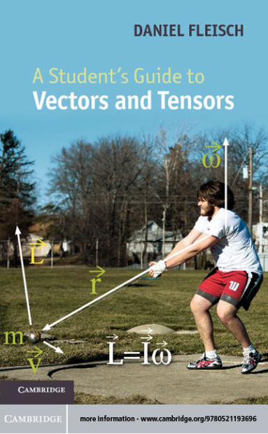
A Student’s Guide to Vectors and Tensors
Vectors and tensors are among the most powerful problem-solving tools available,with applications ranging from mechanics and electromagnetics to general relativity.Understanding the nature and application of vectors and tensors is critically importantto students of physics and engineering.
Adopting the same approach as in his highly popular A Student’s Guide toMaxwell’s Equations, Fleisch explains vectors and tensors in plain language. Writtenfor undergraduate and beginning graduate students, the book provides a thoroughgrounding in vectors and vector calculus before transitioning through contra andcovariant components to tensors and their applications. Matrices and their algebra arereviewed on the book’s supporting website, which also features interactive solutions toevery problem in the text, where students can work through a series of hints or chooseto see the entire solution at once. Audio podcasts give students the opportunity to hearimportant concepts in the book explained by the author.
D A N I E L FL E I S C H is a Professor in the Department of Physics at WittenbergUniversity, where he specializes in electromagnetics and space physics. He is theauthor of A Student’s Guide to Maxwell’s Equations (Cambridge University Press,2008).

A Student’s Guide to Vectorsand Tensors
DANIEL A. FLEISCH
C AMBRIDGE UNIVERSITY PRESS
Cambridge, New York, Melbourne, Madrid, Cape Town,Singapore, Sao Paulo, Delhi, Tokyo, Mexico City
Cambridge University PressThe Edinburgh Building, Cambridge CB2 8RU, UK
Published in the United States of America by Cambridge University Press, New York
www.cambridge.orgInformation on this title: www.cambridge.org/9780521171908
c© D. Fleisch 2012
This publication is in copyright. Subject to statutory exceptionand to the provisions of relevant collective licensing agreements,no reproduction of any part may take place without the written
permission of Cambridge University Press.
First published 2012
Printed in the United Kingdom at the University Press, Cambridge
A catalog record for this publication is available from the British Library
ISBN 978-0-521-19369-6 Hardback
ISBN 978-0-521-17190-8 Paperback
Additional resources for this publication at www.cambridge.org/9780521171908
Cambridge University Press has no responsibility for the persistence oraccuracy of URLs for external or third-party internet websites referred to
in this publication, and does not guarantee that any content on suchwebsites is, or will remain, accurate or appropriate.
Contents
Preface page viiAcknowledgments x
1 Vectors 11.1 Definitions (basic) 11.2 Cartesian unit vectors 51.3 Vector components 71.4 Vector addition and multiplication by a scalar 111.5 Non-Cartesian unit vectors 141.6 Basis vectors 201.7 Chapter 1 problems 23
2 Vector operations 252.1 Scalar product 252.2 Cross product 272.3 Triple scalar product 302.4 Triple vector product 322.5 Partial derivatives 352.6 Vectors as derivatives 412.7 Nabla – the del operator 432.8 Gradient 442.9 Divergence 462.10 Curl 502.11 Laplacian 542.12 Chapter 2 problems 60
3 Vector applications 623.1 Mass on an inclined plane 623.2 Curvilinear motion 72
v
vi Contents
3.3 The electric field 813.4 The magnetic field 893.5 Chapter 3 problems 95
4 Covariant and contravariant vector components 974.1 Coordinate-system transformations 974.2 Basis-vector transformations 1054.3 Basis-vector vs. component transformations 1094.4 Non-orthogonal coordinate systems 1104.5 Dual basis vectors 1134.6 Finding covariant and contravariant components 1174.7 Index notation 1224.8 Quantities that transform contravariantly 1244.9 Quantities that transform covariantly 1274.10 Chapter 4 problems 130
5 Higher-rank tensors 1325.1 Definitions (advanced) 1325.2 Covariant, contravariant, and mixed tensors 1345.3 Tensor addition and subtraction 1355.4 Tensor multiplication 1375.5 Metric tensor 1405.6 Index raising and lowering 1475.7 Tensor derivatives and Christoffel symbols 1485.8 Covariant differentiation 1535.9 Vectors and one-forms 1565.10 Chapter 5 problems 157
6 Tensor applications 1596.1 The inertia tensor 1596.2 The electromagnetic field tensor 1716.3 The Riemann curvature tensor 1836.4 Chapter 6 problems 192
Further reading 194Index 195
Preface
This book has one purpose: to help you understand vectors and tensors so thatyou can use them to solve problems. If you’re like most students, you firstencountered vectors when you took a course dealing with mechanics in highschool or college. At that level, you almost certainly learned that vectors aremathematical representations of quantities that have both magnitude and direc-tion, such as velocity and force. You may also have learned how to add vectorsgraphically and by using their components in the x-, y- and z-directions.
That’s a fine place to start, but it turns out that such treatments only scratchthe surface of the power of vectors. You can harness that power and make itwork for you if you’re willing to delve a bit deeper – to see vectors not justas objects with magnitude and direction, but rather as objects that behave invery predictable ways when viewed from different reference frames. That’sbecause vectors are a subset of a larger class of objects called “tensors,” whichmost students encounter much later in their academic careers, and which havebeen called “the facts of the Universe.” It is no exaggeration to say that ourunderstanding of the fundamental structure of the universe was changed for-ever when Albert Einstein succeeded in expressing his theory of gravity interms of tensors.
I believe, and I hope you’ll agree, that tensors are far easier to understandif you first establish a stronger foundation in vectors, one that can help youcross the bridge between the “magnitude and direction” level and the “facts ofthe Universe” level. That’s why the first three chapters of this book deal withvectors, the fourth chapter discusses coordinate transformations, and the lasttwo chapters discuss higher-order tensors and some of their applications.
One reason you may find this book helpful is that if you spend a few hourslooking through the published literature and on-line resources for vectors andtensors in physics and engineering, you’re likely to come across statementssuch as these:
vii
viii Preface
“A vector is a mathematical representation of a physical entity characterizedby magnitude and direction.”
“A vector is an ordered sequence of values.”“A vector is a mathematical object that transforms between coordinate
systems in certain ways.”“A vector is a tensor of rank one.”“A vector is an operator that turns a one-form into a scalar.”You should understand that every one of these definitions is correct, but
whether it’s useful to you depends on the problem you’re trying to solve.And being able to see the relationship between statements like these shouldprove very helpful when you begin an in-depth study of subjects that useadvanced vector and tensor concepts. Those subjects include Mechanics,Electromagnetism, General Relativity, and others.
As with most projects, a good first step is to make sure you understand theterminology that will be used to attack the problem. For that reason, Chapter 1provides the basic definitions you’ll need to begin understanding vectors andtensors. And if you’re ready for more-advanced definitions, you can find thoseat the beginning of Chapter 5.
You may be wondering how this book differs from other texts that deal withvectors and/or tensors. Perhaps the most important difference is that approx-imately equal weight is given to vector and tensor concepts, with one entirechapter (Chapter 3) devoted to selected vector applications and another chapter(Chapter 6) dedicated to example tensor applications.
You’ll also find the presentation to be very different from that of other books.The explanations in this book are written in an informal style in which math-ematical rigor is maintained only insofar as it doesn’t obscure the underlyingphysics. If you feel you already have a good understanding of vectors andmay need only a quick review, you should be able to skim through Chapters 1through 3 very quickly. But if you’re a bit unclear on some aspects of vectorsand how to apply them to problems, you may find these early chapters quitehelpful. And if you’ve already seen tensors but are unsure of exactly what theyare or how to apply them, then Chapters 4 through 6 may provide some insight.
As a student’s guide, this book comes with two additional resourcesdesigned to help you understand and apply vectors and tensors: an interactivewebsite and a series of audio podcasts. On the website, you’ll find the com-plete solution to every problem presented in the text in interactive format –that means you’ll be able to view the entire solution at once, or ask for a seriesof helpful hints that will guide you to the final answer. So when you see a state-ment in the text saying that you can learn more about something by lookingat the end-of-chapter problems, remember that the full solution to every one

Preface ix
of those problems is available to you. And if you’re the kind of learner whobenefits from hearing spoken words rather than just reading text, the audiopodcasts are for you. These MP3 files walk you through each chapter of thebook, pointing out important details and providing further explanations of keyconcepts.
Is this book right for you? It is if you’re a science or engineering studentand have encountered vectors or tensors in one of your classes, but you’renot confident in your ability to apply them. In that case, you should read thebook, listen to the accompanying podcasts, and work through the examplesand problems before taking additional classes or a standardized exam in whichvectors or tensors may appear. Or perhaps you’re a graduate student strugglingto make the transition from undergraduate courses and textbooks to the more-advanced material you’re seeing in graduate school – this book may help youmake that step.
And if you’re neither an undergraduate nor a graduate student, but a curi-ous young person or a lifelong learner who wants to know more about vectors,tensors, or their applications in Mechanics, Electromagnetics, and General Rel-ativity, welcome aboard. I commend your initiative, and I hope this book helpsyou in your journey.
Acknowledgments
It was a suggestion by Dr. John Fowler of Cambridge University Press that gotthis book out of the starting gate, and it was his patient guidance and unflag-ging support that pushed it across the finish line. I feel very privileged to haveworked with John on this project and on my Student’s Guide to Maxwell’sEquations, and I acknowledge his many contributions to these books. A projectlike this really does take a village, and many others should be recognized fortheir efforts. While pursuing her doctorate in Physics at Notre Dame Univer-sity, Laura Kinnaman took time to carefully read the entire manuscript andmade major contributions to the discussion of the Inertia tensor in Chapter 6.Wittenberg graduate Joe Fritchman also read the manuscript and made helpfulsuggestions, as did Carnegie-Mellon undergraduate Wyatt Bridgeman. CarrieMiller provided the perspective of a Chemistry student, and her husband Jor-dan Miller generously shared his LaTeX expertise. Professor Adam Parker ofWittenberg University and Daniel Ross of the University of Wisconsin did theirbest to steer me onto a mathematically solid foundation, and Professor MarkSemon of Bates College has gone far beyond the role of reviewer and deservescredit for rooting out numerous errors and for providing several of the betterexplanations in this work. I alone bear the responsibility for any remaininginconsistencies or errors.
I also wish to acknowledge all the students who have taken a class fromme during the two years it took me to write this book. I very much appreciatetheir willingness to share their claim on my time with this project. The greatestsacrifice has been made by the unfathomably understanding Jill Gianola, whogracefully accommodated the expanding time and space requirements of mywriting.
x
1
Vectors
1.1 Definitions (basic)
There are many ways to define a vector. For starters, here’s the most basic:
A vector is the mathematical representation of a physical entity that may becharacterized by size (or “magnitude”) and direction.
In keeping with this definition, speed (how fast an object is going) is not rep-resented by a vector, but velocity (how fast and in which direction an object isgoing) does qualify as a vector quantity. Another example of a vector quantityis force, which describes how strongly and in what direction something is beingpushed or pulled. But temperature, which has magnitude but no direction, is nota vector quantity.
The word “vector” comes from the Latin vehere meaning “to carry;” it wasfirst used by eighteenth-century astronomers investigating the mechanism bywhich a planet is “carried” around the Sun.1 In text, the vector nature of anobject is often indicated by placing a small arrow over the variable representingthe object (such as �F), or by using a bold font (such as F), or by underlining(such as F or F∼). When you begin hand-writing equations involving vectors,
it’s very important that you get into the habit of denoting vectors using one ofthese techniques (or another one of your choosing). The important thing is nothow you denote vectors, it’s that you don’t simply write them the same wayyou write non-vector quantities.
A vector is most commonly depicted graphically as a directed line seg-ment or an arrow, as shown in Figure 1.1(a). And as you’ll see later in thissection, a vector may also be represented by an ordered set of N numbers,
1 The Oxford English Dictionary. 2nd ed. 1989.
1
2 Vectors
(b)(a)
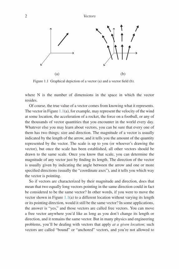
Figure 1.1 Graphical depiction of a vector (a) and a vector field (b).
where N is the number of dimensions in the space in which the vectorresides.
Of course, the true value of a vector comes from knowing what it represents.The vector in Figure 1.1(a), for example, may represent the velocity of the windat some location, the acceleration of a rocket, the force on a football, or any ofthe thousands of vector quantities that you encounter in the world every day.Whatever else you may learn about vectors, you can be sure that every one ofthem has two things: size and direction. The magnitude of a vector is usuallyindicated by the length of the arrow, and it tells you the amount of the quantityrepresented by the vector. The scale is up to you (or whoever’s drawing thevector), but once the scale has been established, all other vectors should bedrawn to the same scale. Once you know that scale, you can determine themagnitude of any vector just by finding its length. The direction of the vectoris usually given by indicating the angle between the arrow and one or morespecified directions (usually the “coordinate axes”), and it tells you which waythe vector is pointing.
So if vectors are characterized by their magnitude and direction, does thatmean that two equally long vectors pointing in the same direction could in factbe considered to be the same vector? In other words, if you were to move thevector shown in Figure 1.1(a) to a different location without varying its lengthor its pointing direction, would it still be the same vector? In some applications,the answer is “yes,” and those vectors are called free vectors. You can movea free vector anywhere you’d like as long as you don’t change its length ordirection, and it remains the same vector. But in many physics and engineeringproblems, you’ll be dealing with vectors that apply at a given location; suchvectors are called “bound” or “anchored” vectors, and you’re not allowed to

1.1 Definitions (basic) 3
relocate bound vectors as you can free vectors.2 You may see the term “sliding”vectors used for vectors that are free to move along their length but are not freeto change length or direction; such vectors are useful for problems involvingtorque and angular motion.
You can understand the usefulness of bound vectors if you think about anapplication such as representing the velocity of the wind at various points inthe atmosphere. To do that, you could choose to draw a bound vector at eachpoint of interest, and each of those vectors would show the speed and directionof the wind at that location (most people draw the vector with its tail – the endwithout the arrow – at the point to which the vector is bound). A collection ofsuch vectors is called a vector field; an example is shown in Figure 1.1(b).
If you think about the ways in which you might represent a bound vector,you may realize that the vector can be defined simply by specifying the startand end points of the arrow. So in a three-dimensional Cartesian coordinatesystem, you only need to know the values of x , y, and z for each end of thevector, as shown in Figure 1.2(a) (you can read about vector representation innon-Cartesian coordinate systems later in this chapter).
Now consider the special case in which the vector is anchored to the originof the coordinate system (that is, the end without the arrowhead is at the pointof intersection of the coordinate axes, as shown in Figure 1.2(b).3 Such vectorsmay be completely specified simply by listing the three numbers that representthe x-, y-, and z-coordinates of the vector’s end point. Hence a vector anchoredto the origin and stretching five units along the x-axis may be represented as
(a) (b)
(0, 0, 0)
x
y
z (xend – xstart,yend – ystart,zend – zstart)
(xend, yend, zend)
(xstart, ystart, zstart)x
y
z
Figure 1.2 A vector in 3-D Cartesian coordinates.
2 Mathematicians don’t have much use for bound vectors, since the mathematical definition of avector deals with how it transforms rather than where it’s located.
3 The vector shown in Figure 1.2 (a) can be shifted to this location by subtracting xstart , ystart ,and zstart from the values at each end.
4 Vectors
(5,0,0). In this representation, the values that represent the vector are called the“components” of the vector, and the number of components it takes to definea vector is equal to the number of dimensions in the space in which the vectorexists. So in a two-dimensional space a vector may be represented by a pairof numbers, and in four-dimensional spacetime vectors may appear as lists offour numbers. This explains why a horizontal list of numbers is called a “rowvector” and a vertical list of numbers is called a “column vector” in computerscience. The number of values in such vectors tells you how many dimensionsthere are in the space in which the vector resides.
To understand how vectors are different from other entities, it may help toconsider the nature of some things that are clearly not vectors. Think about thetemperature in the room in which you’re sitting – at each point in the room,the temperature has a value, which you can represent by a single number. Thatvalue may well be different from the value at other locations, but at any givenpoint the temperature can be represented by a single number, the magnitude.Such magnitude-only quantities have been called “scalars” ever since W.R.Hamilton referred to them as “all values contained on the one scale of progres-sion of numbers from negative to positive infinity.”4 Thus
A scalar is the mathematical representation of a physical entity that may becharacterized by magnitude only.
Other examples of scalar quantities include mass, charge, energy, and speed(defined as the magnitude of the velocity vector). It is worth noting that thechange in temperature over a region of space does have both magnitude anddirection and may therefore be represented by a vector, so it’s possible to pro-duce vectors from groups of scalars. You can read about just such a vector(called the “gradient” of a scalar field) in Chapter 2.
Since scalars can be represented by magnitude only (single numbers)and vectors by magnitude and direction (three numbers in three-dimensionalspace), you might suspect that there are other entities involving magnitude anddirections that are more complex than vectors (that is, requiring more numbersthan the number of spatial dimensions). Indeed there are, and such entities arecalled “tensors.”5 You can read about tensors in the last three chapters of thisbook, but for now this simple definition will suffice:
4 W.R. Hamilton, Phil. Mag. XXIX, 26.5 As you can learn in the later portions of this book, scalars and vectors also belong to the class
of objects called tensors but have lower rank, so in this section the word “tensors” refers tohigher-rank tensors.
1.2 Cartesian unit vectors 5
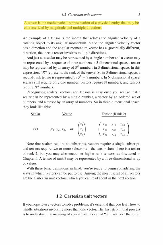
A tensor is the mathematical representation of a physical entity that may becharacterized by magnitude and multiple directions.
An example of a tensor is the inertia that relates the angular velocity of arotating object to its angular momentum. Since the angular velocity vectorhas a direction and the angular momentum vector has a (potentially different)direction, the inertia tensor involves multiple directions.
And just as a scalar may be represented by a single number and a vector maybe represented by a sequence of three numbers in 3-dimensional space, a tensormay be represented by an array of 3R numbers in 3-dimensional space. In thisexpression, “R” represents the rank of the tensor. So in 3-dimensional space, asecond-rank tensor is represented by 32 = 9 numbers. In N-dimensional space,scalars still require only one number, vectors require N numbers, and tensorsrequire NR numbers.
Recognizing scalars, vectors, and tensors is easy once you realize that ascalar can be represented by a single number, a vector by an ordered set ofnumbers, and a tensor by an array of numbers. So in three-dimensional space,they look like this:
Scalar Vector Tensor (Rank 2)
(x) (x1, x2, x3) or
⎛⎝x1
x2
x3
⎞⎠
⎛⎝ x11 x12 x13
x21 x22 x23
x31 x32 x33
⎞⎠
Note that scalars require no subscripts, vectors require a single subscript,and tensors require two or more subscripts – the tensor shown here is a tensorof rank 2, but you may also encounter higher-rank tensors, as discussed inChapter 5. A tensor of rank 3 may be represented by a three-dimensional arrayof values.
With these basic definitions in hand, you’re ready to begin considering theways in which vectors can be put to use. Among the most useful of all vectorsare the Cartesian unit vectors, which you can read about in the next section.
1.2 Cartesian unit vectors
If you hope to use vectors to solve problems, it’s essential that you learn how tohandle situations involving more than one vector. The first step in that processis to understand the meaning of special vectors called “unit vectors” that often
6 Vectors
1 2 y
1
2
z
1
2x
ijk
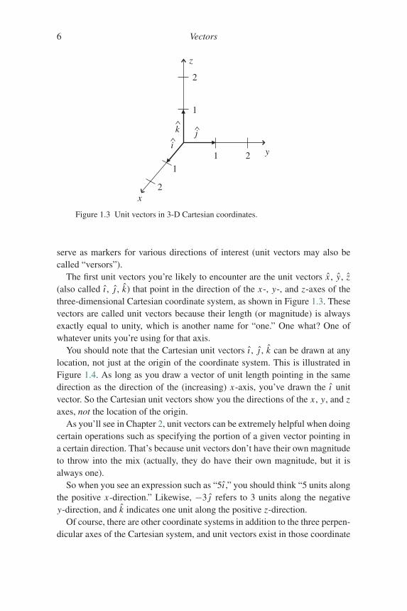
Figure 1.3 Unit vectors in 3-D Cartesian coordinates.
serve as markers for various directions of interest (unit vectors may also becalled “versors”).
The first unit vectors you’re likely to encounter are the unit vectors x , y, z(also called ı , j , k) that point in the direction of the x-, y-, and z-axes of thethree-dimensional Cartesian coordinate system, as shown in Figure 1.3. Thesevectors are called unit vectors because their length (or magnitude) is alwaysexactly equal to unity, which is another name for “one.” One what? One ofwhatever units you’re using for that axis.
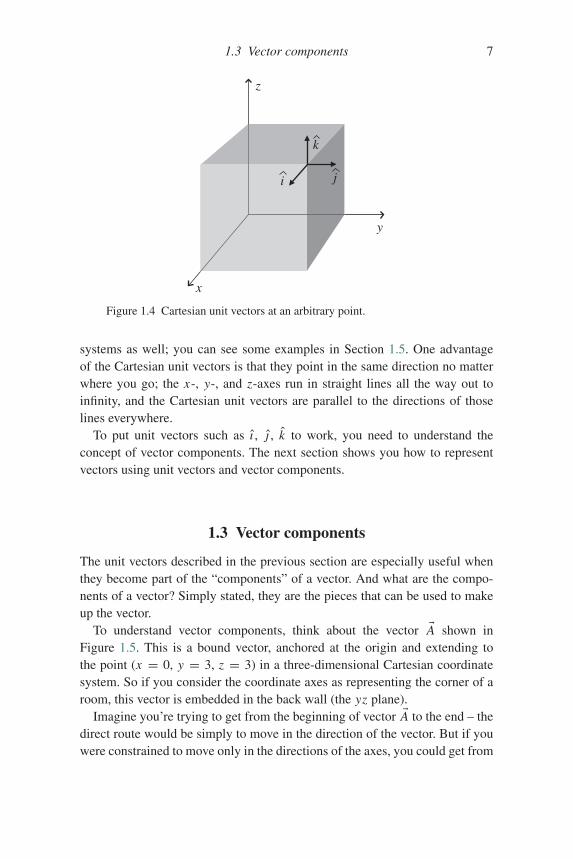
You should note that the Cartesian unit vectors ı , j , k can be drawn at anylocation, not just at the origin of the coordinate system. This is illustrated inFigure 1.4. As long as you draw a vector of unit length pointing in the samedirection as the direction of the (increasing) x-axis, you’ve drawn the ı unitvector. So the Cartesian unit vectors show you the directions of the x , y, and zaxes, not the location of the origin.
As you’ll see in Chapter 2, unit vectors can be extremely helpful when doingcertain operations such as specifying the portion of a given vector pointing ina certain direction. That’s because unit vectors don’t have their own magnitudeto throw into the mix (actually, they do have their own magnitude, but it isalways one).
So when you see an expression such as “5ı ,” you should think “5 units alongthe positive x-direction.” Likewise, −3j refers to 3 units along the negativey-direction, and k indicates one unit along the positive z-direction.
Of course, there are other coordinate systems in addition to the three perpen-dicular axes of the Cartesian system, and unit vectors exist in those coordinate
1.3 Vector components 7
x
y
z
i j
k
Figure 1.4 Cartesian unit vectors at an arbitrary point.
systems as well; you can see some examples in Section 1.5. One advantageof the Cartesian unit vectors is that they point in the same direction no matterwhere you go; the x-, y-, and z-axes run in straight lines all the way out toinfinity, and the Cartesian unit vectors are parallel to the directions of thoselines everywhere.
To put unit vectors such as ı , j , k to work, you need to understand theconcept of vector components. The next section shows you how to representvectors using unit vectors and vector components.
1.3 Vector components
The unit vectors described in the previous section are especially useful whenthey become part of the “components” of a vector. And what are the compo-nents of a vector? Simply stated, they are the pieces that can be used to makeup the vector.
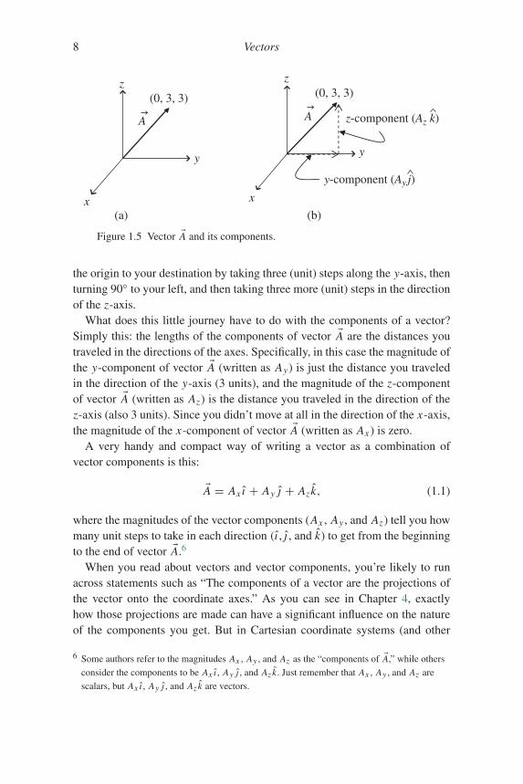
To understand vector components, think about the vector �A shown inFigure 1.5. This is a bound vector, anchored at the origin and extending tothe point (x = 0, y = 3, z = 3) in a three-dimensional Cartesian coordinatesystem. So if you consider the coordinate axes as representing the corner of aroom, this vector is embedded in the back wall (the yz plane).
Imagine you’re trying to get from the beginning of vector �A to the end – thedirect route would be simply to move in the direction of the vector. But if youwere constrained to move only in the directions of the axes, you could get from
8 Vectors
(a) (b)
A
x
y
z(0, 3, 3)
A
x
y
z(0, 3, 3)
z-component (Az k)
y-component (Ay j)
Figure 1.5 Vector �A and its components.
the origin to your destination by taking three (unit) steps along the y-axis, thenturning 90◦ to your left, and then taking three more (unit) steps in the directionof the z-axis.
What does this little journey have to do with the components of a vector?Simply this: the lengths of the components of vector �A are the distances youtraveled in the directions of the axes. Specifically, in this case the magnitude ofthe y-component of vector �A (written as Ay) is just the distance you traveledin the direction of the y-axis (3 units), and the magnitude of the z-componentof vector �A (written as Az) is the distance you traveled in the direction of thez-axis (also 3 units). Since you didn’t move at all in the direction of the x-axis,the magnitude of the x-component of vector �A (written as Ax ) is zero.
A very handy and compact way of writing a vector as a combination ofvector components is this:
�A = Ax ı + Ay j + Azk, (1.1)
where the magnitudes of the vector components (Ax , Ay , and Az) tell you howmany unit steps to take in each direction (ı ,j , and k) to get from the beginningto the end of vector �A.6
When you read about vectors and vector components, you’re likely to runacross statements such as “The components of a vector are the projections ofthe vector onto the coordinate axes.” As you can see in Chapter 4, exactlyhow those projections are made can have a significant influence on the natureof the components you get. But in Cartesian coordinate systems (and other
6 Some authors refer to the magnitudes Ax , Ay , and Az as the “components of �A,” while others
consider the components to be Ax ı , Ay j , and Azk. Just remember that Ax , Ay , and Az are
scalars, but Ax ı , Ay j , and Azk are vectors.
1.3 Vector components 9
Light raysperpendicularto x-axis
Shadow castby vector A on y-axis
Light raysperpendicularto y-axis
(b)(a)
Shadow castby vector Aon x-axis
xθ
y
x
y
A
A
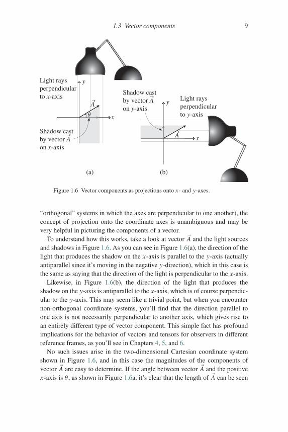
Figure 1.6 Vector components as projections onto x- and y-axes.
“orthogonal” systems in which the axes are perpendicular to one another), theconcept of projection onto the coordinate axes is unambiguous and may bevery helpful in picturing the components of a vector.
To understand how this works, take a look at vector �A and the light sourcesand shadows in Figure 1.6. As you can see in Figure 1.6(a), the direction of thelight that produces the shadow on the x-axis is parallel to the y-axis (actuallyantiparallel since it’s moving in the negative y-direction), which in this case isthe same as saying that the direction of the light is perpendicular to the x-axis.
Likewise, in Figure 1.6(b), the direction of the light that produces theshadow on the y-axis is antiparallel to the x-axis, which is of course perpendic-ular to the y-axis. This may seem like a trivial point, but when you encounternon-orthogonal coordinate systems, you’ll find that the direction parallel toone axis is not necessarily perpendicular to another axis, which gives rise toan entirely different type of vector component. This simple fact has profoundimplications for the behavior of vectors and tensors for observers in differentreference frames, as you’ll see in Chapters 4, 5, and 6.
No such issues arise in the two-dimensional Cartesian coordinate systemshown in Figure 1.6, and in this case the magnitudes of the components ofvector �A are easy to determine. If the angle between vector �A and the positivex-axis is θ , as shown in Figure 1.6a, it’s clear that the length of �A can be seen
10 Vectors
as the hypotenuse of a right triangle. The sides of that triangle along the x- andy-axes are the components Ax and Ay . Hence by simple trigonometry you canwrite:
Ax = | �A| cos(θ),
Ay = | �A| sin(θ),(1.2)
where the vertical bars on each side of �A signify the magnitude (length)of vector �A. Notice that so long as you measure the angle θ from thepositive x-axis in the direction toward the positive y-axis (that is, counter-clockwise in this case), these equations will give the correct sign for the x- andy-components no matter which quadrant the vector occupies.
For example, if vector �A is a vector with a length of 7 meters pointing in adirection 210◦ counter-clockwise from the +x-axis, the x- and y-componentsare given by Eq. 1.2 as
Ax = | �A| cos(θ) = 7m cos 210◦ = −6.1 m,
Ay = | �A| sin(θ) = 7m sin 210◦ = −3.5 m.(1.3)
As expected for a vector pointing down and to the left from the origin, bothcomponents are negative.
It’s equally straightforward to find the length and direction of a vector ifyou’re given the vector’s Cartesian components. Since the vector forms thehypotenuse of a right triangle with sides Ax and Ay , the Pythagorean theoremtells you that the length of �A must be
| �A| =√
A2x + A2
y, (1.4)
and from trigonometry
θ = arctan
(Ay
Ax
), (1.5)
where θ is measured counter-clockwise from the positive x-axis in a right-handed coordinate system. If you try this with the components of vector �Afrom Eq. 1.3 and end up with a direction of 30◦ rather than 210◦, rememberthat unless you have a four-quadrant arctan function on your calculator, youmust add 180◦ to the angle whenever the denominator of the expression (Ax inthis case) is negative.
Once you have a working understanding of unit vectors and vector compo-nents, you’re ready to do basic vector operations. The entirety of Chapter 2 isdevoted to such operations, but two of them are needed for the remainder of thischapter. For that reason, you can read about vector addition and multiplicationby a scalar in the next section.
1.4 Vector addition and multiplication by a scalar 11
1.4 Vector addition and multiplication by a scalar
If you’ve read the previous section on vector components, you’ve already seentwo vector operations in action. Those two operations are the addition of vec-tors and multiplication of a vector by a scalar. Both of these operations areused in the expansion of a vector in terms of vector components as in Eq. 1.1from Section 1.3:
�A = Ax ı + Ay j + Azk.
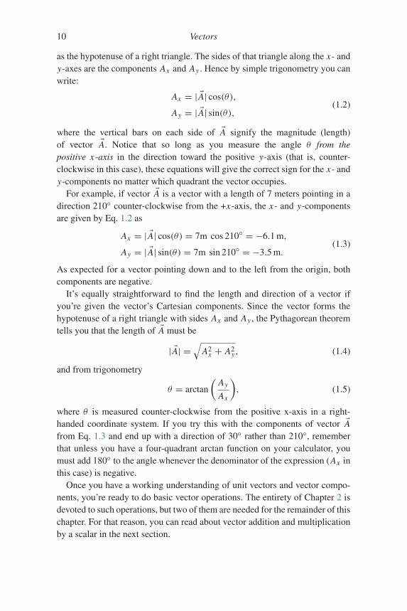
In each of these terms, the unit vector (ı , j , or k) is being multiplied by ascalar (Ax , Ay , or Az), and you already know the effect of that: it producesa new vector, in the same direction as the unit vector, but longer than unityby the value of the component (or shorter if the magnitude of the componentis between zero and one). So multiplying a vector by any positive scalar doesnot change the direction of the vector, but only scales the length of the vector.Hence, 5 �A is a vector in exactly the same direction as �A, but with length fivetimes that of �A, as shown in Figure 1.7(a). Likewise, multiplying �A by (1/2)produces a vector that points in the same direction as �A but is only half as long.So the vector component Ax ı is a vector in the ı direction, but with length Ax
units (since ı has a length of one unit).There is a caveat that goes with the “changes length, not direction” rule
when multiplying a vector by a scalar: if the scalar is negative, then thevector is reversed in direction in addition to being scaled in length. Thusmultiplying vector �B by −2 produces the new vector −2 �B, and that vectoris twice as long as �B and points in the opposite direction to �B, as shown inFigure 1.7(b).
The other operation going on in Eq. 1.1 is vector addition, and you alreadyhave an idea of what that means if you recall Figure 1.5 and the process ofgetting from the beginning of vector �A to the end. In that process, the quantity
5A
(½)A
(a) (b)
–2B
B
A
Figure 1.7 Multiplication of a vector by a scalar.
12 Vectors
Ay j represented not only the number of steps you took, but also the directionin which you took them. Likewise, the quantity Azk represented the numberof steps you took in a different direction. The fact that these two quanti-ties include directional information means that you cannot simply add themtogether algebraically; you must add them “as vectors.”
To accomplish vector addition graphically, you simply imagine moving onevector (without changing its length or direction) so that its tail is at the headof the other vector. The sum is then determined by making a new vector thatbegins at the start of the first vector and terminates at the end of the secondvector. You can do this graphically, as in Figure 1.5(b), where the tail of vectorAzk is placed at the head of vector Ay j , and the sum is the vector from thebeginning of Ay j to the end of Azk.
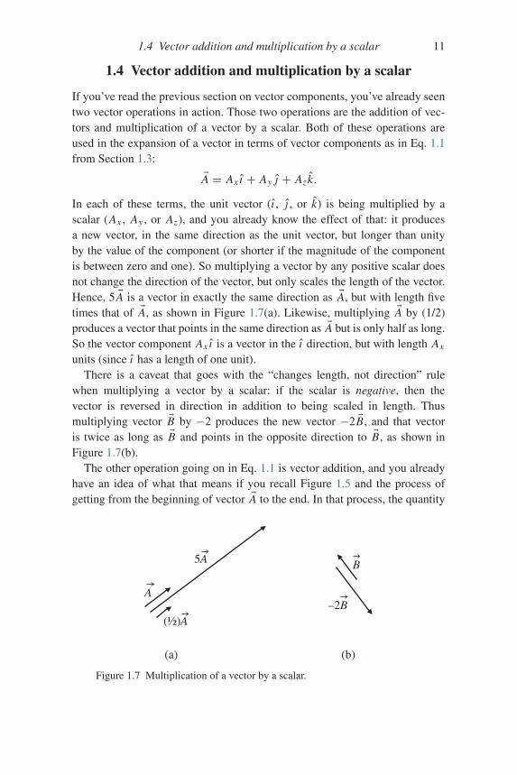
This graphical “head-to-tail” approach to vector addition works for any vec-tors (and any number of vectors), not just two vectors that are perpendicular toone another (as Ay j and Azk were). An example of this is shown in Figure 1.8.To graphically add the two vectors �A and �B in Figure 1.8(a), you simply imag-ine moving one of the two vectors so that its tail is at the position of the othervector’s head (it doesn’t matter which vector you choose to move; the resultwill be the same). This is illustrated in Figure 1.8(b), in which vector �B hasbeen displaced so that its tail is at the head of vector �A. The sum of these twovectors (called the “resultant” vector �C = �A + �B) is the vector that extendsfrom the beginning of �A to the end of �B.
Knowing how to add vectors graphically means you can always determinethe sum of two or more vectors simply using a ruler and a protractor; just drawthe vectors head-to-tail (being careful to maintain each vector’s length and
(a) (b)
B (displaced)
x
y
B
Ax
y
A
C
A + B
B
Figure 1.8 Graphical addition of vectors.
1.4 Vector addition and multiplication by a scalar 13
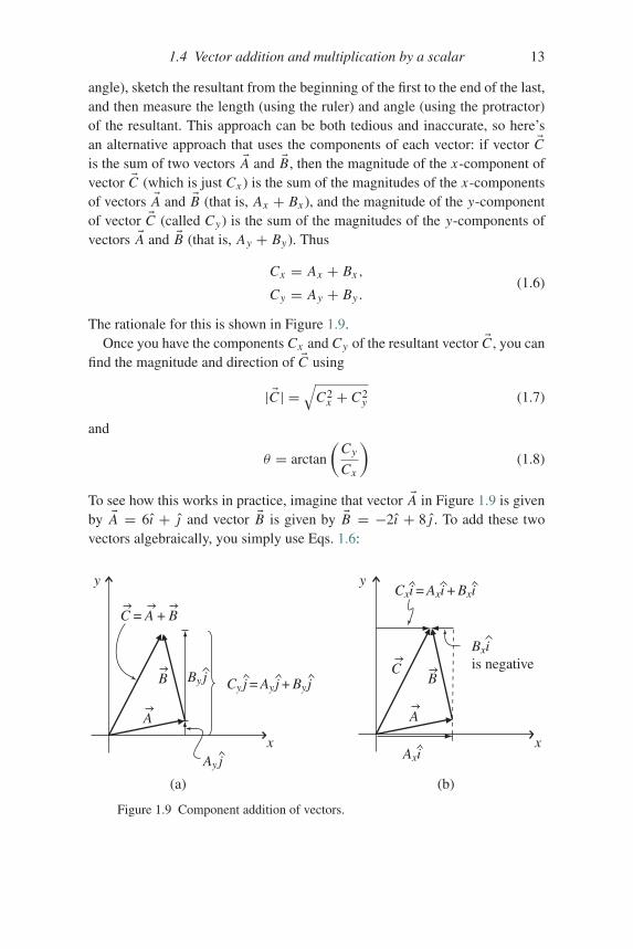
angle), sketch the resultant from the beginning of the first to the end of the last,and then measure the length (using the ruler) and angle (using the protractor)of the resultant. This approach can be both tedious and inaccurate, so here’san alternative approach that uses the components of each vector: if vector �Cis the sum of two vectors �A and �B, then the magnitude of the x-component ofvector �C (which is just Cx ) is the sum of the magnitudes of the x-componentsof vectors �A and �B (that is, Ax + Bx ), and the magnitude of the y-componentof vector �C (called Cy) is the sum of the magnitudes of the y-components ofvectors �A and �B (that is, Ay + By). Thus
Cx = Ax + Bx ,
Cy = Ay + By .(1.6)
The rationale for this is shown in Figure 1.9.Once you have the components Cx and Cy of the resultant vector �C , you can
find the magnitude and direction of �C using
| �C| =√
C2x + C2
y (1.7)
and
θ = arctan
(Cy
Cx
)(1.8)
To see how this works in practice, imagine that vector �A in Figure 1.9 is givenby �A = 6ı + j and vector �B is given by �B = −2ı + 8j . To add these twovectors algebraically, you simply use Eqs. 1.6:
(a) (b)
C = A + B
B
x
y
x
y
Ay j
Cy j = Ayj + ByjBy j
A
Axi
Bxiis negative
A
BC
Cxi = Axi + Bxi
Figure 1.9 Component addition of vectors.
14 Vectors
Cx = Ax + Bx = 6+ (−2) = 4,
Cy = Ay + By = 1+ 8 = 9,
so �C = 4ı + 9j . If you wish to know the magnitude of �C , you can just plugthe components into Eq. 1.7 to get
| �C | =√
C2x + C2
y =√
42 + 92
= √16+ 81 = 9.85.
And the angle that �C makes with the positive x-axis is given by Eq. 1.8:
θ = arctan
(Cy
Cx
)
= arctan
(9
4
)= 66.0◦.
With the basic operations of vector addition and multiplication of a vectorby a scalar in hand, you’re ready to begin thinking about the more advanceduses of vectors. But you’re also ready to attack a variety of problems involvingvectors, and you can find a set of such problems at the end of this chapter.7
1.5 Non-Cartesian unit vectors
The three straight, mutually perpendicular axes of the Cartesian coordinate sys-tem are immensely useful for a variety of problems in physics and engineering.Some problems, however, are much easier to solve in other coordinate systems,often because the axes of those systems more closely align with the directionsover which one or more of the parameters relevant to the problem remain con-stant or vary in a predictable manner. The unit vectors of such non-Cartesiancoordinate systems are the subject of this section, and transformations betweencoordinate systems are discussed in Chapter 4.
As described earlier, it takes exactly N numbers to unambiguously representany location in a space of N dimensions, which means you have to specifythree numbers (such as x , y, and z) to designate a location in our Universeof three spatial dimensions. However, on the two-dimensional surface of theEarth (ignoring height variation for the moment) it takes only two numbers(latitude and longitude, for example) to designate a specific point. And one ofthe few benefits to living on a long, infinitely thin island is that you can set
7 Remember that full solutions are available on the book’s website.
1.5 Non-Cartesian unit vectors 15
up a rendezvous using only a single number to describe the location (“I’ll bewaiting for you at 3.75 kilometers”).
Of course, numbers define locations only after you’ve defined the coordi-nate system that you’re using. For example, do you mean 3.75 kilometers fromthe east end of the island or from the west end? In every space of 1, 2, 3, ormore dimensions, you can devise an infinite number of coordinate systems tospecify locations in that space. In each of those coordinate systems, at eachlocation there’s one direction in which one of the coordinates is increasingthe fastest, and if you lay a vector with length of one unit in that direction,you’ve defined a coordinate unit vector for that system. So in the Cartesiancoordinate system, the ı unit vector shows you the direction in which thex-coordinate increases, the j unit vector shows you the direction in which they-coordinate increases, and the k unit vector shows you the direction in whichthe z-coordinate increases. Other coordinate systems have their own coordinateunit vectors, as well.
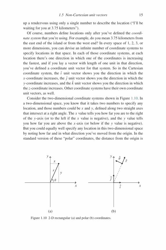
Consider the two-dimensional coordinate systems shown in Figure 1.10. Ina two-dimensional space, you know that it takes two numbers to specify anylocation, and those numbers could be x and y, defined along two straight axesthat intersect at a right angle. The x value tells you how far you are to the rightof the y-axis (or to the left if the x value is negative), and the y value tellsyou how far you are above the x-axis (or below if the y value is negative).But you could equally well specify any location in this two-dimensional spaceby noting how far and in what direction you’ve moved from the origin. In thestandard version of these “polar” coordinates, the distance from the origin is
x
yr
x
y y
x
(a) (b)
θ
θ
j
r
i
Figure 1.10 2-D rectangular (a) and polar (b) coordinates.
16 Vectors
called r and the direction is specified by giving the angle θ measured counter-clockwise from the positive x-axis.
It’s easy enough to figure out one set of coordinates if you know the others;for example, if you know the values of x and y, you can find r and θ using
r =√
x2 + y2
θ = arctan( y
x
).
(1.9)
Likewise, if you have the values of r and θ , you can find x and y using
x = r cos(θ)
y = r sin(θ).(1.10)
For the point shown in Figure 1.10, if the values of x and y are 4 cm and 9 cm,then r has a value of approximately 9.85 cm and θ has a value of 66.0◦. Clearly,whether you write (x, y) = (4 cm, 9 cm) or (r, θ) = (9.85 cm, 66.0◦), you’rereferring to the same location; it’s not the point that’s changed, it’s only thepoint’s coordinates that are different.
And if you choose to use the polar coordinate system to represent the point,do unit vectors exist that serve the same function as ı and j in Cartesian coor-dinates? They certainly do, and with a little logic you can figure out whichdirection they must point. After all, you know that the unit vector ı shows youthe direction of increasing x and the unit vector j shows you the direction ofincreasing y, but now you’re using r and θ instead of x and y. So it seemsreasonable that the unit vector r at any location should point in the direction ofincreasing r , and the unit vector θ should point in the direction of increasing θ .For the point shown in Figure 1.10, that means that r should point up and to theright, in the direction of increasing r if θ is held constant. At that same point,θ should point up and to the left, in the direction of increasing θ if r is heldconstant. These polar unit vectors are shown for one point in Figure 1.10(b).
An important consequence of this definition is that the directions of r and θwill be different at different locations. They’ll always be perpendicular to oneanother, but they will not point in the same directions as they do for the pointin Figure 1.10. The dependence of the polar unit vectors on position can beseen in the following relations:
r = cos(θ)ı + sin(θ)j
θ = − sin(θ)ı + cos(θ)j .(1.11)
So if θ = 0 (which means your location is on the +x-axis), then r = ı andθ = j . But if θ = 90◦ (so your location is on the +y-axis), then r = j andθ = −ı .
1.5 Non-Cartesian unit vectors 17
Does this dependence on position mean that these unit vectors are not “real”vectors? That depends on your definition of a real vector. If you define a vectoras a quantity with magnitude and direction, the polar unit vectors do meetyour definition. But they do not meet the definition of free vectors described inSection 1.1, since they may not be moved without changing their direction.
This means that if you express a vector in polar coordinates and thentake the derivative of that vector, you’ll have to account for the change inthe unit vectors, as well. That’s one of the advantages offered by Cartesiancoordinates – the unit vectors do not change no matter where you go in thespace.
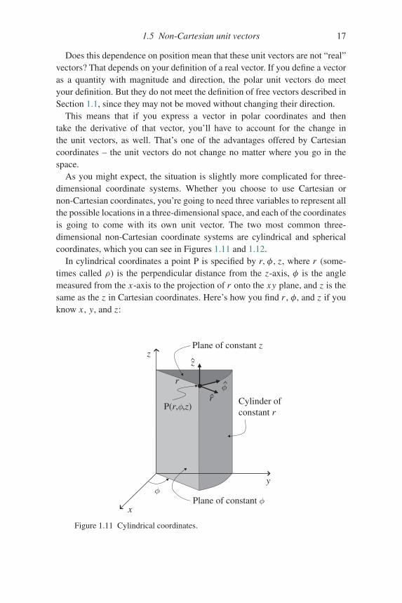
As you might expect, the situation is slightly more complicated for three-dimensional coordinate systems. Whether you choose to use Cartesian ornon-Cartesian coordinates, you’re going to need three variables to represent allthe possible locations in a three-dimensional space, and each of the coordinatesis going to come with its own unit vector. The two most common three-dimensional non-Cartesian coordinate systems are cylindrical and sphericalcoordinates, which you can see in Figures 1.11 and 1.12.
In cylindrical coordinates a point P is specified by r, φ, z, where r (some-times called ρ) is the perpendicular distance from the z-axis, φ is the anglemeasured from the x-axis to the projection of r onto the xy plane, and z is thesame as the z in Cartesian coordinates. Here’s how you find r , φ, and z if youknow x , y, and z:
Cylinder ofconstant r
P(r,φ,z)
Plane of constant z
Plane of constant φ
z
x
yφ
r
r
z
φ
Figure 1.11 Cylindrical coordinates.
18 Vectors
Plane ofconstant φ
Sphere ofconstant r
Cone ofconstant θ
θ
φy
x
zP(r,θ,φ)
r
θ
φ
ρ
Figure 1.12 Spherical coordinates.
r =√
x2 + y2
φ = arctan( y
x
)z = z.
(1.12)
And if you have the values of r , φ, and z, you can find x , y, and z using
x = r cos(φ)
y = r sin(φ)
z = z.
(1.13)
A vector at the point P is specified in cylindrical coordinates in terms ofthree mutually perpendicular components with unit vectors perpendicular tothe cylinder of radius r , perpendicular to the plane through the z-axis at angleφ, and perpendicular to the xy plane at distance z. As in the Cartesian case,each cylindrical coordinate unit vector points in the direction in which thatparameter is increasing, so r points in the direction of increasing r , φ pointsin the direction of increasing φ, and z points in the direction of increasing z.The unit vectors (r , φ, z) form a right-handed set, so if you point the fingersof your right hand along r and push it into φ with your right palm, your rightthumb will show you the direction of z.
1.5 Non-Cartesian unit vectors 19
The following equations relate the Cartesian to the cylindrical unit vectors:
r = cos(φ)ı + sin(φ)j
φ = − sin(φ)ı + cos(φ)j
z = z.
(1.14)
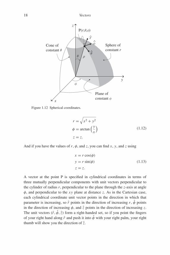
In spherical coordinates a point P is specified by r, θ, φ where r representsthe distance from the origin, θ is the angle measured from the z-axis towardthe xy plane, and φ is the angle measured from the x-axis (or xz plane) to theconstant-φ plane containing point P. With the z-axis up, θ is sometimes calledthe zenith angle and φ the azimuth angle. You can determine the sphericalcoordinates r , θ , and φ, from x , y, and z using the following equations:
r =√
x2 + y2 + z2
θ = arccos
(z√
x2 + y2 + z2
)
φ = arctan( y
x
).
(1.15)
And you can find x , y, and z from r , θ , and φ using:
x = r sin(θ) cos(φ)
y = r sin(θ) sin(φ)
z = r cos(θ).
(1.16)
In spherical coordinates, a vector at the point P is specified in terms of threemutually perpendicular components with unit vectors perpendicular to thesphere of radius r , perpendicular to the plane through the z-axis at angle φ,and perpendicular to the cone of angle θ . The unit vectors (r , θ , φ) form aright-handed set, and are related to the Cartesian unit vectors as follows:
r = sin(θ) cos(φ)ı + sin(θ) sin(φ)j + cos(θ)k
θ = cos(θ) cos(φ)ı + cos(θ) sin(φ)j − sin(θ)k
φ = − sin(φ)ı + cos(φ)j .
(1.17)
You may be asking yourself “Do I really need all these different unit vec-tors?” Well, need may be a bit strong, but your life will certainly be easierif you’re trying to describe motion along a line of constant longitude on aspherical planet (the θ direction) or the direction of a magnetic field around a
20 Vectors
current-carrying wire (the φ direction). You’ll find some examples of that inthe problems at the end of this chapter.
1.6 Basis vectors
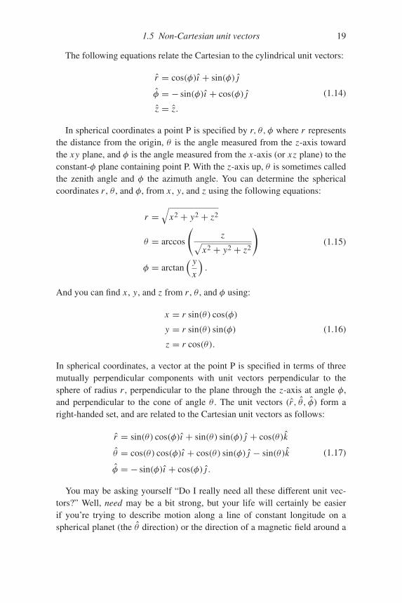
If you think about the unit vectors ı , j , and k and vector components such asAx ı , Ay j , and Azk, you may realize that any vector in our three-dimensionalCartesian coordinate system can be made up of three components, each onetelling you how many steps to take in the direction of one of the coordi-nate axes. Since those steps may be large or small, in the positive or negativedirection, you can reach any point in the space containing these vectors. Littlewonder, then, that ı , j , and k are one example of “basis vectors” in this space;combined with appropriate magnitudes, they form the basis of any vector inthe space.
And you don’t need to use only these particular vectors to make up anyvector in this space – you can easily imagine using three vectors that are twiceas long as the unit vectors ı , j , and k, as shown in Figure 1.13(a). Althoughthe vector components would change if you switched to these longer basisvectors, you’d have no trouble using them to make up any vector within thespace. Specifically, if the unit vectors were twice as long, the values of Ax , Ay ,and Az would have to be only half as big to reach a given point in space.
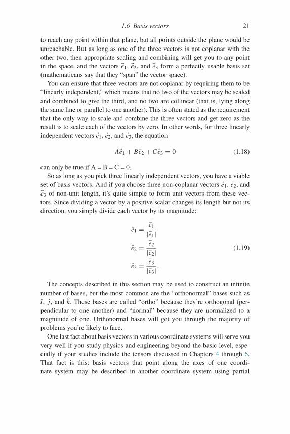
You might even think of using three non-orthogonal, non-unit vectors suchas the vectors �e1, �e2, and �e3 in Figure 1.13(b) as your basis vectors. Of course,if you were to select three coplanar vectors (that is, vectors lying in the sameplane), you’d quickly find that scaling and combining those vectors allows you
(a)
1
21
2
1
e3
x
y
z
1
21
2
1
2k
x
y
z
2i
2j
(b)
e2e1
Figure 1.13 Alternative basis vectors.
1.6 Basis vectors 21
to reach any point within that plane, but all points outside the plane would beunreachable. But as long as one of the three vectors is not coplanar with theother two, then appropriate scaling and combining will get you to any pointin the space, and the vectors �e1, �e2, and �e3 form a perfectly usable basis set(mathematicans say that they “span” the vector space).
You can ensure that three vectors are not coplanar by requiring them to be“linearly independent,” which means that no two of the vectors may be scaledand combined to give the third, and no two are collinear (that is, lying alongthe same line or parallel to one another). This is often stated as the requirementthat the only way to scale and combine the three vectors and get zero as theresult is to scale each of the vectors by zero. In other words, for three linearlyindependent vectors �e1, �e2, and �e3, the equation
A�e1 + B�e2 + C�e3 = 0 (1.18)
can only be true if A = B = C = 0.So as long as you pick three linearly independent vectors, you have a viable
set of basis vectors. And if you choose three non-coplanar vectors �e1, �e2, and�e3 of non-unit length, it’s quite simple to form unit vectors from these vec-tors. Since dividing a vector by a positive scalar changes its length but not itsdirection, you simply divide each vector by its magnitude:
e1 = �e1
|�e1|e2 = �e2
|�e2|e3 = �e3
|�e3| .
(1.19)
The concepts described in this section may be used to construct an infinitenumber of bases, but the most common are the “orthonormal” bases such ası , j , and k. These bases are called “ortho” because they’re orthogonal (per-pendicular to one another) and “normal” because they are normalized to amagnitude of one. Orthonormal bases will get you through the majority ofproblems you’re likely to face.
One last fact about basis vectors in various coordinate systems will serve youvery well if you study physics and engineering beyond the basic level, espe-cially if your studies include the tensors discussed in Chapters 4 through 6.That fact is this: basis vectors that point along the axes of one coordi-nate system may be described in another coordinate system using partial
22 Vectors
derivatives.8 Specifically, imagine that you’re converting from spherical torectangular coordinates. The basis vector along the original spherical (r ) axiscan be written in the Cartesian (x , y, and z) system as
�er = ∂x
∂rı + ∂y
∂rj + ∂z
∂rk
= sin θ cosφ ı + sin θ sinφ j + cos θ k.
Likewise, the �eθ and �eφ basis vectors can be written as
�eθ = ∂x
∂θı + ∂y
∂θj + ∂z
∂θk
= r cos θ cosφ ı + r cos θ sinφ j − r sin θ k,
�eφ = ∂x
∂φı + ∂y
∂φj + ∂z
∂φk
= −r sin θ sinφ ı + r sin θ cosφ j .
Notice that these basis vectors are not all unit vectors (because their magni-tudes are not all equal to one), nor do they all have the same dimensions (�er
is dimensionless, but �eθ and �eφ have dimensions of length). Neither of thesecharacteristics disqualifies these as basis vectors, and you can always turn theminto unit vectors by dividing by their magnitudes (take a look at the problemsat the end of this chapter and their on-line solutions if you want to see how thisworks).
In general, if the coordinates of the original system are called x1, x2, and x3
(these were r , θ , and φ in the example just discussed), and the coordinates ofthe new system are called x ′1, x ′2, and x ′3 (these were x , y, and z in the example),then the basis vectors along the original coordinate axes can be written in thenew system as
�e1 = ∂x ′1∂x1�e ′1 +
∂x ′2∂x1�e ′2 +
∂x ′3∂x1�e ′3,
�e2 = ∂x ′1∂x2�e ′1 +
∂x ′2∂x2�e ′2 +
∂x ′3∂x2�e ′3,
�e3 = ∂x ′1∂x3�e ′1 +
∂x ′2∂x3�e ′2 +
∂x ′3∂x3�e ′3.
(1.20)
In other words, the partial derivatives∂x ′1∂x1�e ′1,
∂x ′2∂x1�e ′2, and
∂x ′3∂x1�e ′3 are the compo-
nents of the first original (unprimed) basis vector expressed in the new (primed)
8 If you’re not familiar with partial derivatives or need a refresher, you’ll find one in the nextchapter.
1.7 Chapter 1 problems 23
coordinate system. For this reason, you’ll find that some authors define basisvectors in terms of partial derivatives.
These relationships will prove to be extremely valuable in the study ofcoordinate-system transformation and tensor analysis, so file them away if yourstudies include those topics.
1.7 Chapter 1 problems
1.1 (a) If | �B| = 18 m and �B points along the negative x-axis, what are Bx
and By?(b) If Cx = −3 m/s and Cy = 5 m/s, find the magnitude of �C and the
angle that �C makes with the positive x-axis.1.2 Vector �A has magnitude of 11 m/s2 and makes an angle of 65 degrees
with the positive x-axis, and vector �B has Cartesian components Bx = 4m/s2 and By = −3 m/s2. If vector �C = �A + �B,(a) Find the x- and y-components of �C ;(b) What are the magnitude and direction of �C?
1.3 Imagine that the y-axis points north and the x-axis points east.(a) If you travel a distance r = 22 km in a straight line from the origin in a
direction 35 degrees south of west, what is your position in Cartesian(x, y) coordinates?
(b) If you travel 6 miles due south from the origin and then turn west andtravel 2 miles, how far from the origin and in what direction is yourfinal position?
1.4 What are the x- and y-components of the polar unit vectors r and θ when(a) θ = 180 degrees?(b) θ = 45 degrees?(c) θ = 215 degrees?
1.5 Cylindrical coordinates(a) If r = 2 meters, φ = 35 degrees, and z = 1 meter, what are x , y, and
z?(b) If (x, y, z) = (3, 2, 4) meters, what are (r, φ, z)?
1.6 (a) In cylindrical coordinates, show that r points along the x-axisif φ = 0.
(b) In what direction is φ if φ = 90 degrees?1.7 (a) In spherical coordinates, find x , y, and z if r = 25 meters, θ = 35
degrees, and φ= 110 degrees.(b) Find (r, θ, φ) if (x, y, z) = (8, 10, 15) meters.
24 Vectors
1.8 (a) For spherical coordinates, show that θ points along the negativez-axis if θ = 90 degrees.
(b) If φ also equals 90 degrees, in what direction are r and φ?1.9 As you can read in Chapter 3, the magnetic field around a long, straight
wire carrying a steady current I is given in spherical coordinates by theexpression �B = μ0 I
2πR φ, where μ0 is a constant and R is the perpendiculardistance from the wire to the observation point. Find an expression for �Bin Cartesian coordinates.
1.10 If �e1 = 5ı − 3j + 2k, �e2 = j − 3k, and �e3 = 2ı + j − 4k, what are theunit vectors e1, e2, and e3?
2
Vector operations
If you were tracking the main ideas of Chapter 1, you should realize thatvectors are representations of physical quantities – they’re mathematical toolsthat help you visualize and describe a physical situation. In this chapter, youcan read about a variety of ways to use those tools to solve problems. You’vealready seen how to add vectors and how to multiply vectors by a scalar (andwhy such operations are useful); this chapter contains many other “vector oper-ations” through which you can combine and manipulate vectors. Some of theseoperations are simple and some are more complex, but each will prove usefulin solving problems in physics and engineering. The first section of this chapterexplains the simplest form of vector multiplication: the scalar product.
2.1 Scalar product
Why is it worth your time to understand the form of vector multiplicationcalled the scalar or “dot” product? For one thing, forming the dot productbetween two vectors is very useful when you’re trying to find the projectionof one vector onto another. And why might you want to do that? Well, youmay be interested in knowing how much work is done by a force acting on anobject. The first instinct of many students is to think of work as “force timesdistance” (which is a reasonable starting point). But if you’ve ever taken acourse that went a bit deeper than the introductory level, you may rememberthat the definition of work as force times distance applies only to the specialcase in which the force points in exactly the same direction as the displacementof the object. In the more general case in which the force acts at some angle tothe direction of the displacement, you have to find the component of the forcealong the displacement. That’s one example of exactly what the dot productcan do for you, and you’ll find more in the problems at the end of this chapter.
25
26 Vector operations
How do you go about computing the dot product between two vectors? Well,if you know the Cartesian components of each vector (call the vectors �A and�B), you can use
�A ◦ �B = Ax Bx + Ay By + Az Bz . (2.1)
Or if you know the angle θ between the vectors,
�A ◦ �B = | �A|| �B| cos θ, (2.2)
where | �A| and | �B| represent the magnitude (length) of the vectors �A and �B.1
Note that the dot product between two vectors gives a scalar result (just a singlevalue, no direction).
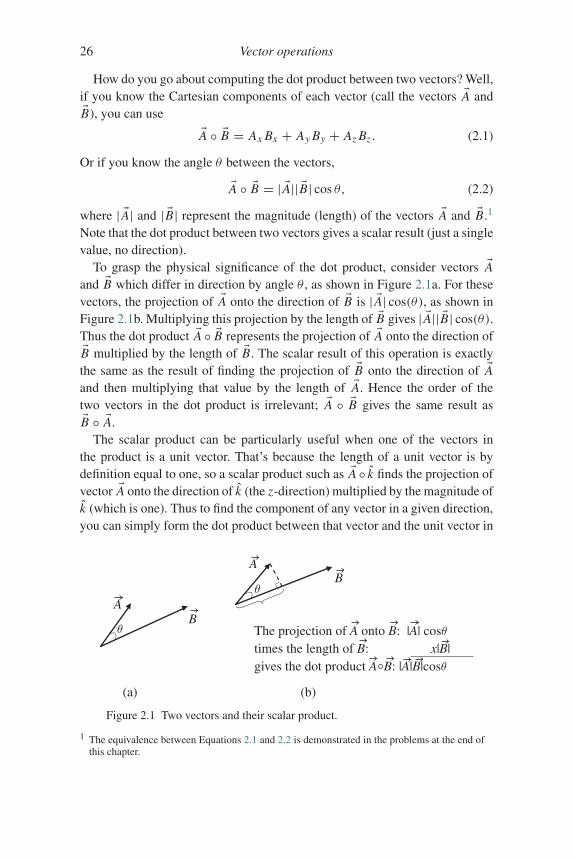
To grasp the physical significance of the dot product, consider vectors �Aand �B which differ in direction by angle θ , as shown in Figure 2.1a. For thesevectors, the projection of �A onto the direction of �B is | �A| cos(θ), as shown inFigure 2.1b. Multiplying this projection by the length of �B gives | �A|| �B| cos(θ).Thus the dot product �A ◦ �B represents the projection of �A onto the direction of�B multiplied by the length of �B. The scalar result of this operation is exactlythe same as the result of finding the projection of �B onto the direction of �Aand then multiplying that value by the length of �A. Hence the order of thetwo vectors in the dot product is irrelevant; �A ◦ �B gives the same result as�B ◦ �A.
The scalar product can be particularly useful when one of the vectors inthe product is a unit vector. That’s because the length of a unit vector is bydefinition equal to one, so a scalar product such as �A ◦ k finds the projection ofvector �A onto the direction of k (the z-direction) multiplied by the magnitude ofk (which is one). Thus to find the component of any vector in a given direction,you can simply form the dot product between that vector and the unit vector in
Bθ The projection of A onto B: |A| cosθ
times the length of B: x|B|gives the dot product A B: |A|B|cosθ
A
AB
(b)(a)
θ
Figure 2.1 Two vectors and their scalar product.
1 The equivalence between Equations 2.1 and 2.2 is demonstrated in the problems at the end ofthis chapter.
2.2 Cross product 27
the desired direction. It’s quite likely you’ll come across problems in physicsand engineering in which you have a vector ( �A) and you wish to know thecomponent of that vector that’s perpendicular to a specified surface; if youknow the unit normal vector (n) for the surface, the scalar product �A ◦ n givesyou that perpendicular component of �A.
The scalar product is also useful in finding the angle between two vectors.To understand how that works, consider the two expressions for the dot productgiven in Eqs. 2.1 and 2.2. Since
�A ◦ �B = | �A|| �B| cos θ = Ax Bx + Ay By + Az Bz, (2.3)
then dividing both sides by the product of the magnitudes of �A and �B gives
cos(θ) = Ax Bx + Ay By + Az Bz
| �A|| �B|or
θ = arccos
(Ax Bx + Ay By + Az Bz
| �A|| �B|). (2.4)
So if you wish to find the angle between two vectors �A = 5ı − 2j + 4k and�B = 3ı + j + 7k, you can use Eq. 2.4 to find
θ = arccos
((5)(3)+ (−2)(1)+ (4)(7)√
(5)2 + (−2)2 + (4)2√(3)2 + (1)2 + (7)2)
= arccos
(41√
45√
59
)= 37.3◦.
One final note about the scalar product: any unit vector dotted with itselfgives a result of 1 (since, for example, ı ◦ ı = |ı ||ı | cos(0◦) = (1)(1)(1) = 1),and the dot product between two different orthogonal unit vectors gives a resultof zero (since, for example, ı ◦ j = |ı ||j | cos(90◦) = (1)(1)(0) = 0).
2.2 Cross product
Another way to multiply two vectors is to form the “cross product” betweenthem. Unlike the dot product, which gives a scalar result, the cross prod-uct results in another vector. Why bother learning this form of vectormultiplication? One reason is that the cross product is just what you need whenyou’re trying to find the result of certain physical processes, such as applying aforce at the end of a lever arm or firing a charged particle into a magnetic field.
28 Vector operations
Computing the cross product between two vectors is only slightly more com-plicated than finding the dot product. If you know the Cartesian componentsof both vectors, the cross product is given by
�A × �B = (Ay Bz − Az By)ı
+ (Az Bx − Ax Bz)j
+ (Ax By − Ay Bx )k, (2.5)
which can be written as
�A × �B =∣∣∣∣∣∣
ı j kAx Ay Az
Bx By Bz
∣∣∣∣∣∣ . (2.6)
If you haven’t seen determinants before and you need some help getting fromEq. 2.6 to Eq. 2.5, you can find an explanation of how this works on the book’swebsite.
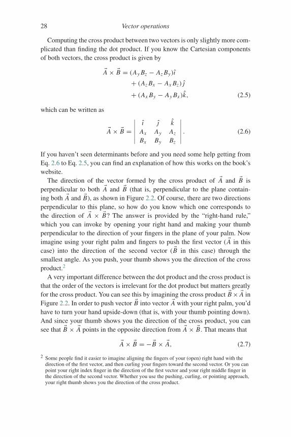
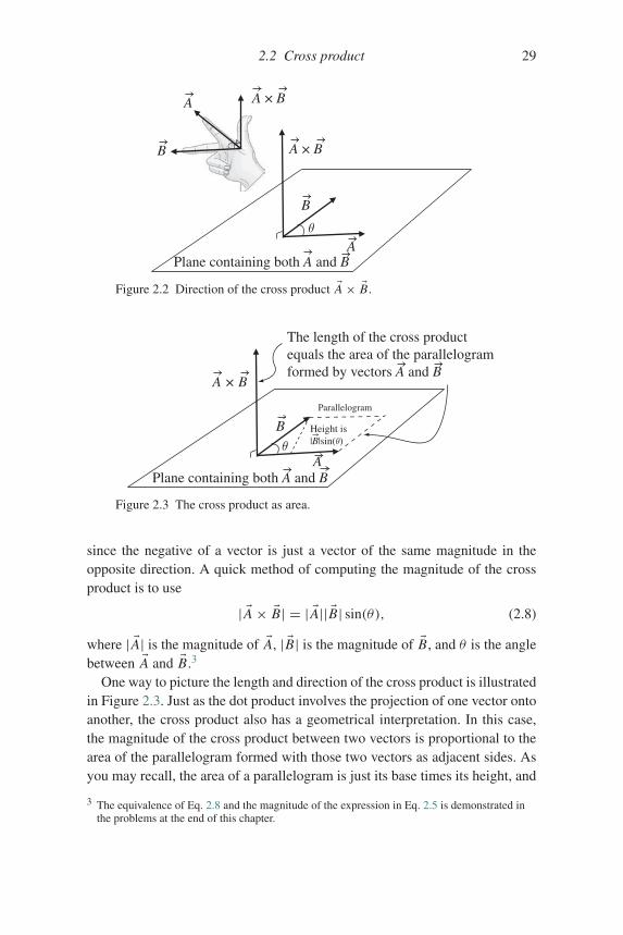
The direction of the vector formed by the cross product of �A and �B isperpendicular to both �A and �B (that is, perpendicular to the plane contain-ing both �A and �B), as shown in Figure 2.2. Of course, there are two directionsperpendicular to this plane, so how do you know which one corresponds tothe direction of �A × �B? The answer is provided by the “right-hand rule,”which you can invoke by opening your right hand and making your thumbperpendicular to the direction of your fingers in the plane of your palm. Nowimagine using your right palm and fingers to push the first vector ( �A in thiscase) into the direction of the second vector ( �B in this case) through thesmallest angle. As you push, your thumb shows you the direction of the crossproduct.2
A very important difference between the dot product and the cross product isthat the order of the vectors is irrelevant for the dot product but matters greatlyfor the cross product. You can see this by imagining the cross product �B× �A inFigure 2.2. In order to push vector �B into vector �A with your right palm, you’dhave to turn your hand upside-down (that is, with your thumb pointing down).And since your thumb shows you the direction of the cross product, you cansee that �B × �A points in the opposite direction from �A × �B. That means that
�A × �B = − �B × �A, (2.7)
2 Some people find it easier to imagine aligning the fingers of your (open) right hand with thedirection of the first vector, and then curling your fingers toward the second vector. Or you canpoint your right index finger in the direction of the first vector and your right middle finger inthe direction of the second vector. Whether you use the pushing, curling, or pointing approach,your right thumb shows you the direction of the cross product.
2.2 Cross product 29
A
A × B
Plane containing both A and B
A
B
B
A × B
θ
Figure 2.2 Direction of the cross product �A × �B.
B
The length of the cross productequals the area of the parallelogramformed by vectors A and B
Parallelogram
A × B
Height is|B|sin(θ)
APlane containing both A and B
θ
Figure 2.3 The cross product as area.
since the negative of a vector is just a vector of the same magnitude in theopposite direction. A quick method of computing the magnitude of the crossproduct is to use
| �A × �B| = | �A|| �B| sin(θ), (2.8)
where | �A| is the magnitude of �A, | �B| is the magnitude of �B, and θ is the anglebetween �A and �B.3
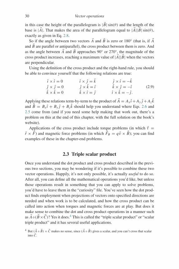
One way to picture the length and direction of the cross product is illustratedin Figure 2.3. Just as the dot product involves the projection of one vector ontoanother, the cross product also has a geometrical interpretation. In this case,the magnitude of the cross product between two vectors is proportional to thearea of the parallelogram formed with those two vectors as adjacent sides. Asyou may recall, the area of a parallelogram is just its base times its height, and
3 The equivalence of Eq. 2.8 and the magnitude of the expression in Eq. 2.5 is demonstrated inthe problems at the end of this chapter.
30 Vector operations
in this case the height of the parallelogram is | �B| sin(θ) and the length of thebase is | �A|. That makes the area of the parallelogram equal to | �A|| �B| sin(θ),exactly as given in Eq. 2.8.
So if the angle between two vectors �A and �B is zero or 180◦ (that is, if �Aand �B are parallel or antiparallel), the cross product between them is zero. Andas the angle between �A and �B approaches 90◦ or 270◦, the magnitude of thecross product increases, reaching a maximum value of | �A|| �B|when the vectorsare perpendicular.
Using the definition of the cross product and the right-hand rule, you shouldbe able to convince yourself that the following relations are true:
ı × ı = 0 ı × j = k j × ı = −kj × j = 0 j × k = ı k × j = −ık × k = 0 k × ı = j ı × k = −j .
(2.9)
Applying these relations term-by-term to the product of �A = Ax ı+ Ay j+ Azkand �B = Bx ı + By j + Bzk should help you understand where Eqs. 2.6 and2.5 come from (and if you need some help making that work out, there’s aproblem on this at the end of this chapter, with the full solution on the book’swebsite).
Applications of the cross product include torque problems (in which �τ =�r × �F) and magnetic force problems (in which �FB = q �v × �B); you can findexamples of these in the chapter-end problems.
2.3 Triple scalar product
Once you understand the dot product and cross product described in the previ-ous two sections, you may be wondering if it’s possible to combine these twovector operations. Happily, it’s not only possible, it’s actually useful to do so.After all, you can define all the mathematical operations you’d like, but unlessthose operations result in something that you can apply to solve problems,you’d have to leave them in the “curiosity” file. You’ve seen how the dot prod-uct finds employment when projections of vectors onto specified directions areneeded and when work is to be calculated, and how the cross product can becalled into action when torques and magnetic forces are at play. But does itmake sense to combine the dot and cross product operations in a manner suchas �A◦( �B× �C)? Yes it does.4 This is called the “triple scalar product” or “scalartriple product” and it has several useful applications.
4 But ( �A ◦ �B)× �C makes no sense, since ( �A ◦ �B) gives a scalar, and you can’t cross that scalarinto �C .
2.3 Triple scalar product 31
The mathematics of this operation are straightforward; you know that
�B × �C = (ByCz − BzCy)ı
+ (BzCx − Bx Cz)j
+ (Bx Cy − ByCx )k, (2.10)
and from Eq. 2.1 you also know that
�A ◦ �B = Ax Bx + Ay By + Az Bz,
so combining the dot and cross product gives
�A ◦( �B × �C) = Ax (ByCz − BzCy)
+ Ay(BzCx − Bx Cz)
+ Az(Bx Cy − ByCx ). (2.11)
A handy way to write this is
�A ◦( �B × �C) =
∣∣∣∣∣∣Ax Ay Az
Bx By Bz
Cx Cy Cz
∣∣∣∣∣∣ . (2.12)
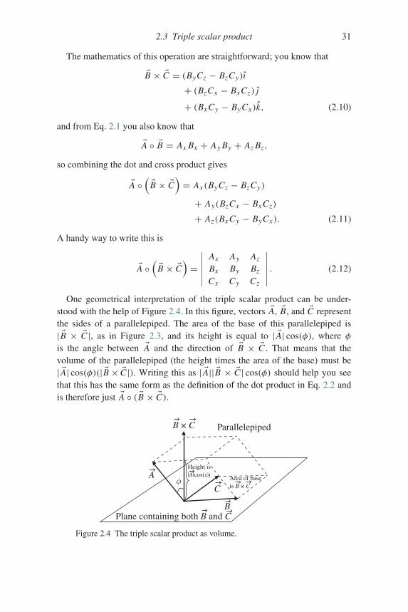
One geometrical interpretation of the triple scalar product can be under-stood with the help of Figure 2.4. In this figure, vectors �A, �B, and �C representthe sides of a parallelepiped. The area of the base of this parallelepiped is| �B × �C |, as in Figure 2.3, and its height is equal to | �A| cos(φ), where φis the angle between �A and the direction of �B × �C . That means that thevolume of the parallelepiped (the height times the area of the base) must be| �A| cos(φ)(| �B× �C |). Writing this as | �A|| �B × �C | cos(φ) should help you seethat this has the same form as the definition of the dot product in Eq. 2.2 andis therefore just �A ◦ ( �B × �C).
Plane containing both B and C
Parallelepiped
Height is|A|cos(φ)
B × C
A Area of baseis B × C
B
Cφ
Figure 2.4 The triple scalar product as volume.
32 Vector operations
Hence the triple scalar product �A◦( �B× �C)may be interpreted as the volumeof the parallelepiped formed by vectors �A, �B, and �C . You should note that thetriple product will give a positive result so long as the vectors �A, �B, and �Cform a right-handed system (that is, pushing �A into �B with the palm of yourright hand gives a direction onto which �C projects in a positive sense (likewisefor pushing �B into �C and pushing �C into �A).
Seeing the relationship between the triple scalar product of three vectors andthe volume formed by those vectors makes it easy to understand why the triplescalar product may be used as a test to determine whether three vectors arecoplanar (that is, whether all three lie in the same plane). Just imagine howthe parallelepiped in Figure 2.4 would look if vectors �A, �B, and �C were allin the same plane. In that case, the height of the parallelepiped would be zeroand the projection of �A onto the direction of �B × �C would be zero, whichmeans the triple product �A ◦ ( �B × �C) would have to be zero. Stated anotherway, if the projection of �A onto the direction of �B × �C is not zero, then �Acannot lie in the same plane as �B and �C . Thus
�A ◦ ( �B × �C) = 0 (2.13)
is both a necessary and a sufficient condition for vectors �A, �B, and �C to becoplanar.
Equating �A ◦ ( �B× �C) to the volume of the parallelepiped formed by vectors�A, �B, and �C should also help you see that any cyclic permutation of the vectors
(such as �B ◦ ( �C × �A) or �C ◦ ( �A × �B)) gives the same result for the triplescalar product, since the volume of the parallelepiped is the same in each ofthese cases. Some authors describe this as the ability to interchange the dotand the cross without affecting the result (since ( �A × �B) ◦ �C is the same as�C ◦ ( �A × �B)).
One application in which the triple scalar product finds use is the determi-nation of reciprocal vectors, as explained in the sections in Chapter 4 dealingwith covariant and contravariant components of vectors.
2.4 Triple vector product
The triple scalar product described in the previous section is not the only use-ful way to multiply three vectors. An operation such as �A × ( �B × �C) (calledthe “triple vector product”) comes in very handy when you’re dealing withcertain problems involving angular momentum and centripetal acceleration.Unlike the triple scalar product, which produces a scalar result (since the sec-ond operation is a dot product), the triple vector product yields a vector result
2.4 Triple vector product 33
(since both operations are cross products). You should note that �A × ( �B × �C)is not the same as ( �A× �B)× �C ; the location of the parentheses matters greatlyin the triple vector product. The triple vector product is somewhat tedious tocalculate by brute force, but thankfully a simplified expression exists:
�A × ( �B × �C) = �B( �A ◦ �C)− �C( �A ◦ �B). (2.14)
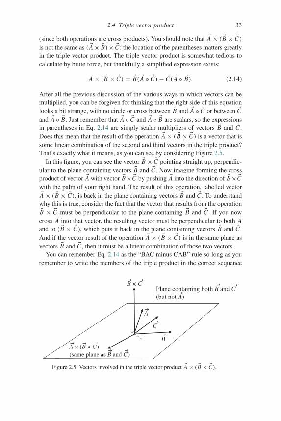
After all the previous discussion of the various ways in which vectors can bemultiplied, you can be forgiven for thinking that the right side of this equationlooks a bit strange, with no circle or cross between �B and �A ◦ �C or between �Cand �A ◦ �B. Just remember that �A ◦ �C and �A ◦ �B are scalars, so the expressionsin parentheses in Eq. 2.14 are simply scalar multipliers of vectors �B and �C .Does this mean that the result of the operation �A × ( �B × �C) is a vector that issome linear combination of the second and third vectors in the triple product?That’s exactly what it means, as you can see by considering Figure 2.5.
In this figure, you can see the vector �B × �C pointing straight up, perpendic-ular to the plane containing vectors �B and �C . Now imagine forming the crossproduct of vector �A with vector �B× �C by pushing �A into the direction of �B× �Cwith the palm of your right hand. The result of this operation, labelled vector�A × ( �B × �C), is back in the plane containing vectors �B and �C . To understand
why this is true, consider the fact that the vector that results from the operation�B × �C must be perpendicular to the plane containing �B and �C . If you nowcross �A into that vector, the resulting vector must be perpendicular to both �Aand to ( �B × �C), which puts it back in the plane containing vectors �B and �C .And if the vector result of the operation �A × ( �B × �C) is in the same plane asvectors �B and �C , then it must be a linear combination of those two vectors.
You can remember Eq. 2.14 as the “BAC minus CAB” rule so long as youremember to write the members of the triple product in the correct sequence
Plane containing both B and C(but not A)
A × (B × C)(same plane as B and C)
B × C
B
C
A
Figure 2.5 Vectors involved in the triple vector product �A × ( �B × �C).
34 Vector operations
( �A, �B, �C) with the parentheses around the last two vectors. To see where thiscomes from, you can simply use the definition of the cross product (Eq. 2.6) towrite
�A × ( �B × �C) =∣∣∣∣∣∣
ı j kAx Ay Az
( �B × �C)x ( �B × �C)y ( �B × �C)z
∣∣∣∣∣∣ . (2.15)
And from Equation 2.5 you know that
�B × �C = (ByCz − BzCy)ı
+ (BzCx − Bx Cz)j
+ (Bx Cy − ByCx )k. (2.16)
Substituting these terms into Eq. 2.15 gives
�A × ( �B × �C) =∣∣∣∣∣∣
ı j kAx Ay Az
(ByCz − BzCy) (BzCx − Bx Cz) (Bx Cy − ByCx )
∣∣∣∣∣∣ .(2.17)
Multiplying this out looks ugly at first:
�A × ( �B × �C) = [Ay(Bx Cy − ByCx )− Az(BzCx − Bx Cz)]ı+ [Az(ByCz − BzCy)− Ax (Bx Cy − ByCx )]j+ [Ax (BzCx − Bx Cz)− Ay(ByCz − BzCy)]k. (2.18)
But a little rearranging gives
�A × ( �B × �C) = (AyCy + AzCz)(Bx ı)− (Ay By + Az Bz)(Cx ı)
+ (AzCz + Ax Cx )(By j )− (Az Bz + Ax Bx )(Cy j )
+ (Ax Cx + AyCy)(Bzk)− (Ax Bx + Ay By)(Czk), (2.19)
which still isn’t pretty, but it does hold some promise. That promise can berealized by adding nothing to each row of Eq. 2.19. Nothing, that is, in thefollowing form:
Ax Bx Cx (ı)− Ax Bx Cx (ı) Add this to the top row;
Ay ByCy(j )− Ay ByCy(j ) Add this to the middle row;
Az BzCz(k)− Az BzCz(k) Add this to the bottom row.
2.5 Partial derivatives 35
These additions make Eq. 2.19 a good deal more friendly:
�A × ( �B × �C)= (Ax Cx + AyCy + AzCz)(Bx ı)− (Ax Bx + Ay By + Az Bz)(Cx ı)
+ (Ax Cy + AyCy + AzCz)(By j )− (Ax Bx + Ay By + Az Bz)(Cy j )
+ (Ax Cx + AyCy + AzCz)(Bzk)− (Ax Bx + Ay By + Az Bz)(Czk).
Or
�A × ( �B × �C) = (Ax Cx + AyCy + AzCz)(Bx ı + By j + Bzk)
− (Ax Bx + Ay By + Az Bz)(Cx ı + Cy j + Czk).
But Bx ı + By j + Bzk is just the vector �B, Cx ı + Cy j + Czk is the vector �C ,and the other two terms fit the definition of dot products (Eq. 2.1). Thus
�A × ( �B × �C) = ( �A ◦ �C) �B − ( �A ◦ �B) �C= �B( �A ◦ �C)− �C( �A ◦ �B).
2.5 Partial derivatives
Once you understand the basic vector operations of dot, cross, and tripleproducts, it’s a small step to more advanced vector operations such as gradient,divergence, curl, and the Laplacian. But these are differential vector operations,so before you can make that step, it’s important for you to understand the dif-ference between ordinary derivatives and partial derivatives. This is worth yourtime and effort because differential vector operations have many applicationsin diverse areas of physics and engineering.
You probably first encountered ordinary derivatives when you learned howto find the slope of a line (m = dy
dx ) or how to determine the speed of anobject given its position as a function of time (vx = dx
dt ). Happily, partialderivatives are based on the same general concepts as ordinary derivatives, butextend those concepts to functions of multiple variables. And you should neverhave any doubt as to which kind of derivative you’re dealing with, becauseordinary derivatives are written as d
dx or ddt and partial derivatives are written as
∂∂x or ∂
∂t .As you may recall, ordinary derivatives come about when you’re interested
in the change of one variable with respect to another. For example, you mayencounter a variable y which is a function of another variable x (which meansthat the value of y depends on the value of x). This can be written as y = f (x),where y is called the “dependent variable” and x is called the “independent
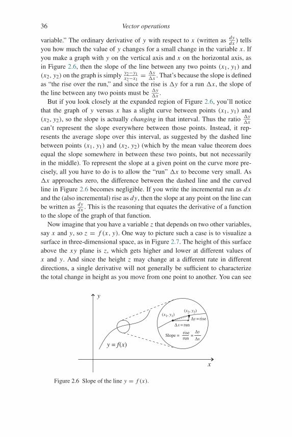
36 Vector operations
variable.” The ordinary derivative of y with respect to x (written as dydx ) tells
you how much the value of y changes for a small change in the variable x . Ifyou make a graph with y on the vertical axis and x on the horizontal axis, asin Figure 2.6, then the slope of the line between any two points (x1, y1) and(x2, y2) on the graph is simply y2−y1
x2−x1= y
x . That’s because the slope is definedas “the rise over the run,” and since the rise is y for a run x , the slope ofthe line between any two points must be y
x .But if you look closely at the expanded region of Figure 2.6, you’ll notice
that the graph of y versus x has a slight curve between points (x1, y1) and(x2, y2), so the slope is actually changing in that interval. Thus the ratio y
xcan’t represent the slope everywhere between those points. Instead, it rep-resents the average slope over this interval, as suggested by the dashed linebetween points (x1, y1) and (x2, y2) (which by the mean value theorem doesequal the slope somewhere in between these two points, but not necessarilyin the middle). To represent the slope at a given point on the curve more pre-cisely, all you have to do is to allow the “run” x to become very small. Asx approaches zero, the difference between the dashed line and the curvedline in Figure 2.6 becomes negligible. If you write the incremental run as dxand the (also incremental) rise as dy, then the slope at any point on the line canbe written as dy
dx . This is the reasoning that equates the derivative of a functionto the slope of the graph of that function.
Now imagine that you have a variable z that depends on two other variables,say x and y, so z = f (x, y). One way to picture such a case is to visualize asurface in three-dimensional space, as in Figure 2.7. The height of this surfaceabove the xy plane is z, which gets higher and lower at different values ofx and y. And since the height z may change at a different rate in differentdirections, a single derivative will not generally be sufficient to characterizethe total change in height as you move from one point to another. You can see
y
x
y = f(x)
Slope =riserun
=
(x1, y1)(x2, y2)
Δy = riseΔx = run
Δy
Δx
Figure 2.6 Slope of the line y = f (x).
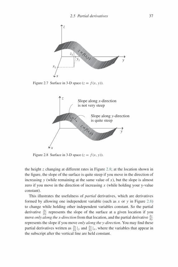
2.5 Partial derivatives 37
z
x
yy1
x1
z1
z = f(x,y)
Figure 2.7 Surface in 3-D space (z = f (x, y)).
z
x
y
z = f(x,y)
Slope along x-directionis not very steep
Slope along y-directionis quite steep
Figure 2.8 Surface in 3-D space (z = f (x, y)).
the height z changing at different rates in Figure 2.8; at the location shown inthe figure, the slope of the surface is quite steep if you move in the direction ofincreasing y (while remaining at the same value of x), but the slope is almostzero if you move in the direction of increasing x (while holding your y-valueconstant).
This illustrates the usefulness of partial derivatives, which are derivativesformed by allowing one independent variable (such as x or y in Figure 2.8)to change while holding other independent variables constant. So the partialderivative ∂z
∂x represents the slope of the surface at a given location if youmove only along the x-direction from that location, and the partial derivative ∂z
∂yrepresents the slope if you move only along the y-direction. You may find thesepartial derivatives written as ∂z
∂x |y and ∂z∂y |x , where the variables that appear in
the subscript after the vertical line are held constant.
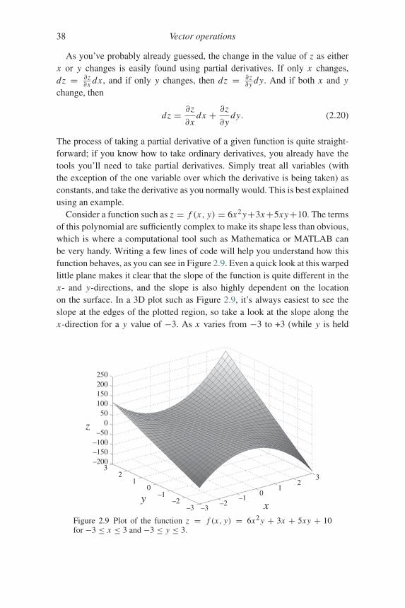
38 Vector operations
As you’ve probably already guessed, the change in the value of z as eitherx or y changes is easily found using partial derivatives. If only x changes,dz = ∂z
∂x dx , and if only y changes, then dz = ∂z∂y dy. And if both x and y
change, then
dz = ∂z
∂xdx + ∂z
∂ydy. (2.20)
The process of taking a partial derivative of a given function is quite straight-forward; if you know how to take ordinary derivatives, you already have thetools you’ll need to take partial derivatives. Simply treat all variables (withthe exception of the one variable over which the derivative is being taken) asconstants, and take the derivative as you normally would. This is best explainedusing an example.
Consider a function such as z = f (x, y) = 6x2 y+3x+5xy+10. The termsof this polynomial are sufficiently complex to make its shape less than obvious,which is where a computational tool such as Mathematica or MATLAB canbe very handy. Writing a few lines of code will help you understand how thisfunction behaves, as you can see in Figure 2.9. Even a quick look at this warpedlittle plane makes it clear that the slope of the function is quite different in thex- and y-directions, and the slope is also highly dependent on the locationon the surface. In a 3D plot such as Figure 2.9, it’s always easiest to see theslope at the edges of the plotted region, so take a look at the slope along thex-direction for a y value of −3. As x varies from −3 to +3 (while y is held
250200150100500
–50z
–100–150–200
32
10
–1–2y
x–3 –3–2
–10
12
3
Figure 2.9 Plot of the function z = f (x, y) = 6x2 y + 3x + 5xy + 10for −3 ≤ x ≤ 3 and −3 ≤ y ≤ 3.
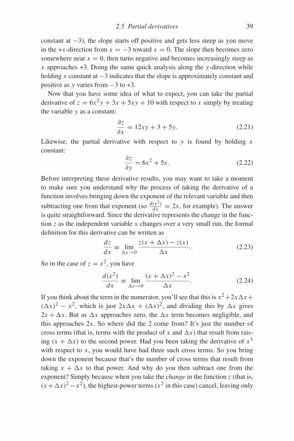
2.5 Partial derivatives 39
constant at −3), the slope starts off positive and gets less steep as you movein the +x-direction from x = −3 toward x = 0. The slope then becomes zerosomewhere near x = 0, then turns negative and becomes increasingly steep asx approaches +3. Doing the same quick analysis along the y-direction whileholding x constant at−3 indicates that the slope is approximately constant andpositive as y varies from −3 to +3.
Now that you have some idea of what to expect, you can take the partialderivative of z = 6x2 y + 3x + 5xy + 10 with respect to x simply by treatingthe variable y as a constant:
∂z
∂x= 12xy + 3+ 5y. (2.21)
Likewise, the partial derivative with respect to y is found by holding xconstant:
∂z
∂y= 6x2 + 5x . (2.22)
Before interpreting these derivative results, you may want to take a momentto make sure you understand why the process of taking the derivative of afunction involves bringing down the exponent of the relevant variable and then
subtracting one from that exponent (so d(x2)dx = 2x , for example). The answer
is quite straightforward. Since the derivative represents the change in the func-tion z as the independent variable x changes over a very small run, the formaldefinition for this derivative can be written as
dz
dx≡ limx→0
z(x +x)− z(x)
x. (2.23)
So in the case of z = x2, you have
d(x2)
dx≡ limx→0
(x +x)2 − x2
x. (2.24)
If you think about the term in the numerator, you’ll see that this is x2+2xx+(x)2 − x2, which is just 2xx + (x)2, and dividing this by x gives2x +x . But as x approaches zero, the x term becomes negligible, andthis approaches 2x . So where did the 2 come from? It’s just the number ofcross terms (that is, terms with the product of x and x) that result from rais-ing (x + x) to the second power. Had you been taking the derivative of x3
with respect to x , you would have had three such cross terms. So you bringdown the exponent because that’s the number of cross terms that result fromtaking x + x to that power. And why do you then subtract one from theexponent? Simply because when you take the change in the function z (that is,(x+x)2− x2), the highest-power terms (x2 in this case) cancel, leaving only
40 Vector operations
terms of one lower power (x1 in this case). It’s a bit laborious, but the same
analysis can be applied to show that d(x3)dx = 3x2 and that d(xn)
dx = nxn−1.So that’s why you bring down the exponent and subtract one, but what does
it mean when you take derivatives and get answers such as Eqs. 2.21 and 2.22?It simply means that the slope varies with direction and location on the sur-face z. So, for example, the slope along the x-direction at location (−3,2) is12xy+ 3+ 5y= 12(−3)(2)+ 3+ 5(2) = −59, while at the same location theslope along the y-direction is 6x2 + 5x = 6[(−3)2] + 5(−3) = 39.
You can do a rough check on your calculated partial derivative in Eq. 2.21by inserting the value of −3 for y to see that the slope of z at this value of y is12(x)(−3) + 3 + 5(−3) = −36x − 12. Thus as you move in the x-directionat y = −3, the slope should vary from +96 at x = −3, to zero at x = −1/3,and down to −120 at x = +3. This is consistent with the quick analysis of theslope after Figure 2.9.
Likewise, Eq. 2.22 tells you that the slope of z in the y-direction at x = −3 isconstant and positive, also consistent with the behavior expected from a quickanalysis of the shape of the function z.
And just as you can take “higher order” ordinary derivatives such asd
dx (dzdx )= d2z
dx2 and ddy (
dzdy )= d2z
dy2 , you can also take higher-order partial deriva-
tives. So for example ∂∂x (
∂z∂x )= ∂2z
∂x2 tells you the change in the x-direction slope
of z as you move along the x-direction, and ∂∂y (
∂z∂y )= ∂2z
∂y2 tells you the changein the y-direction slope as you move along the y-direction.
It’s important for you to realize that an expression such as ∂2z∂x2 is the
derivative of a derivative, which is not the same as ( ∂z∂x )
2, which is the squareof a first derivative. That’s easy to verify for the example given above, in
which ∂z∂x = 12xy + 3 + 5y. In that case, ∂2z
∂x2 = 12y, whereas ( ∂z∂x )
2 =(12xy + 3+ 5y)2. By convention the order of the derivative is always writtenbetween the “d” or “∂” and the function, as d2z or ∂2z, so be sure to lookcarefully at the location of superscripts when you’re dealing with derivatives.
You may also have occasion to use “mixed” partial derivatives such as∂∂x (
∂z∂y ) = ∂2z
∂x∂y . If you’ve been tracking the discussion of partial derivatives as
slopes of functions in various directions, you can probably guess that ∂2z∂x∂y rep-
resents the change in the y-direction slope as you move along the x-direction,
and ∂2z∂y∂x represents the change in the x-direction slope as you move along
the y-direction. Thankfully, for well-behaved5 functions these expressions are
5 What exactly is a “well-behaved” function? Typically this means any function that iscontinuous and has continuous derivatives over the region of interest.
2.6 Vectors as derivatives 41
interchangeable, so you can take the partial derivatives in either order. You caneasily verify this for the example given above by comparing ∂
∂y of Eq. 2.21
with ∂∂x of Eq. 2.22 (the result is 12x + 5 in both cases).
There’s another widely used aspect of partial derivatives you should makesure you understand, and that’s the chain rule. Up to this point, we’ve beendealing with functions such as z = f (x, y) without considering the fact thatthe variables x and y may themselves be functions of other variables. It’s com-mon to call these other variables u and v and to allow both x and y to dependon one or both of u and v. You may encounter situations in which you knowthe variation in u and v, and you want to know how much your function z willchange due to those changes. In such cases, the chain rule for partial derivativesgives you the answer:
∂z
∂u= ∂z
∂x
∂x
∂u+ ∂z
∂y
∂y
∂u, (2.25)
and∂z
∂v= ∂z
∂x
∂x
∂v+ ∂z
∂y
∂y
∂v. (2.26)
The chain rule is a concise expression of the fact that z depends on both xand y, and since both x and y may change if u changes, the change in z withrespect to u is the sum of two terms. The first term is the change in x due tothe change in u ( ∂x
∂u ) times the change in z due to that change in x ( ∂z∂x ), and the
second term is the change in y due to the change in u ( ∂y∂u ) times the change
in z due to that change in y ( ∂z∂y ). Adding those two terms together gives you
Eq. 2.25, and the same reasoning applied to changes in z caused by changes inv leads to Eq. 2.26.
2.6 Vectors as derivatives
In many texts dealing with vectors and tensors, you’ll find that vectors areequated to “directional derivatives” and that partial derivatives such as ∂
∂x and∂∂y are referred to as basis vectors along the coordinate axes.
To understand this correspondence between vectors and derivatives, con-sider a path such as that shown in Figure 2.10. You can think of this as apath along which you’re travelling with velocity �v; for simplicity imaginethat this path lies in the xy plane. Now imagine that you’re keeping track oftime as you move, so you assign a value (such as the t values shown in thefigure) to each point on the curve. By marking the curve with values, you have
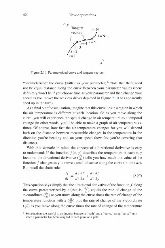
42 Vector operations
y
x
t = 1t = 2
t = 3
t = N
t = N–1
Tangentvectors
t = 4 t = 5
Figure 2.10 Parameterized curve and tangent vectors.
“parameterized” the curve (with t as your parameter).6 Note that there neednot be equal distance along the curve between your parameter values (theredefinitely won’t be if you choose time as your parameter and then change yourspeed as you move; the reckless driver depicted in Figure 2.10 has apparentlysped up in the turn).
As a final bit of visualization, imagine that this curve lies in a region in whichthe air temperature is different at each location. So as you move along thecurve, you will experience the spatial change in air temperature as a temporalchange (in other words, you’ll be able to make a graph of air temperature vs.time). Of course, how fast the air temperature changes for you will dependboth on the distance between measurable changes in the temperature in thedirection you’re heading and on your speed (how fast you’re covering thatdistance).
With this scenario in mind, the concept of a directional derivative is easyto understand. If the function f (x, y) describes the temperature at each x, ylocation, the directional derivative ( d f
dt ) tells you how much the value of thefunction f changes as you move a small distance along the curve (in time dt).But recall the chain rule:
d f
dt= dx
dt
∂ f
∂x+ dy
dt
∂ f
∂y. (2.27)
This equation says simply that the directional derivative of the function f alongthe curve parameterized by t (that is, d f
dt ) equals the rate of change of thex-coordinate ( dx
dt ) as you move along the curve times the rate of change of the
temperature function with x ( ∂ f∂x ) plus the rate of change of the y-coordinate
( dydt ) as you move along the curve times the rate of change of the temperature
6 Some authors are careful to distinguish between a “path” and a “curve,” using “curve” onlywhen a parameter has been assigned to each point on a path.
2.7 Nabla – the del operator 43
function with y ( ∂ f∂y ). But ( dx
dt ) is just vx , the x-component of your velocity, and
( dydt ) is vy , the y-component of your velocity. And since you know that your
velocity is a vector that is always tangent to the path on which you’re moving,you can consider the directional derivative d f
dt to be a vector with directiontangent to the curve and with length equal to the rate of change of f with t(that is, the time rate of change of the air temperature).
Now here’s the important concept: since f can be any function, you canwrite Eq. 2.27 as an “operator” equation (that is, an equation waiting to be feda function on which it can operate):
d
dt= dx
dt
∂
∂x+ dy
dt
∂
∂y. (2.28)
The trick to seeing the connection between derivatives and vectors is to viewthis equation as a vector equation in which
Vector = x-component · x basis vector+ y-component · y basis vector.
Comparing this to Eq. 2.28, you should be able to see that the directionalderivative operator d
dt represents the tangent vector to the curve, the dxdt and
dydt terms represent the x- and y-components of that vector, and the operators∂∂x and ∂
∂y represent the basis vectors in the direction of the x and y coordinateaxes.
Of course, it’s not just air temperature that can be represented by f (x, y);this function can represent anything that is spatially distributed in the regionaround your curve. So f (x, y) could represent the height of the road, the qual-ity of the scenery, or any other quantity that varies in the vicinity of your curve.Likewise, you could have chosen to parameterize your path with markers otherthan time; had you assigned a value s or λ to each point on your path, thedirectional derivative d
ds or ddλ would still represent the tangent vector to the
curve, dxds or dx
dλ would still represent the x-component of that vector, and dyds
or dydλ would still represent the y-component of that vector.If you plan to proceed on to the study of tensors, you will find that under-
standing this relationship between basis vectors along the coordinate axes andpartial derivatives is of significant value.
2.7 Nabla – the del operator
The partial derivatives discussed in the previous section can be put to use ina wide range of problems, and when you come across such problems youmay find that they involve equations that contain an inverted upper case delta
44 Vector operations
wearing a vector hat ( �∇). This symbol represents a vector differential operatorcalled “nabla” or “del,” and its presence instructs you to take derivatives of thequantity on which the operator is acting. The exact form of those derivativesdepends on the symbol following the del operator, with �∇( ) signifying gradi-ent, “ �∇◦” signifying divergence, “ �∇×” indicating curl, and ∇2( ) signifyingthe Laplacian. Each of these operations is discussed in later sections; for nowwe’ll just consider what an operator is and how the del operator can be writtenin Cartesian coordinates.
Like all good mathematical operators, del is an action waiting to happen.Just as √ tells you to take the square root of anything that appears under its
roof, �∇ is an instruction to take derivatives in three directions. Specifically, inCartesian coordinates
�∇ ≡ ı∂
∂x+ j ∂
∂y+ k
∂
∂z, (2.29)
where ı , j , and k are the unit vectors in the direction of the Cartesiancoordinates x , y, and z.
This expression may appear strange, since in this form it’s lacking anythingon which it can operate. However, if you follow the del with a scalar or vectorfield, you can extract information about how those fields change in space. Inthis context, “field” refers to an array or collection of values defined at variouslocations. A scalar field is specified entirely by its magnitude at these locations:examples of scalar fields include the air temperature in a room and the heightof terrain above sea level. A vector field is specified by both magnitude anddirection at various locations: examples include electric, magnetic, and gravi-tational fields. Specific examples of how the del operator works on scalar andvector fields are given in the following sections.
2.8 Gradient
When the del operator �∇ is followed by a scalar field, the result of the opera-tion is called the gradient of the field. What does the gradient tell you about ascalar field? Two important things: the magnitude of the gradient indicates howquickly the field is changing over space, and the direction of the gradient indi-cates the direction in which the field is increasing most quickly with distance.So although the gradient operates on a scalar field, the result of the gradientoperation is a vector, with both magnitude and direction. Thus, if the scalarfield represents terrain height, the magnitude of the gradient at any location
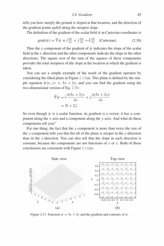
2.8 Gradient 45
tells you how steeply the ground is sloped at that location, and the direction ofthe gradient points uphill along the steepest slope.
The definition of the gradient of the scalar fieldψ in Cartesian coordinates is
grad(ψ) = �∇ψ ≡ ı ∂ψ∂x + j ∂ψ∂y + k ∂ψ
∂z (Cartesian). (2.30)
Thus the x-component of the gradient of ψ indicates the slope of the scalarfield in the x-direction and the other components indicate the slope in the otherdirections. The square root of the sum of the squares of these componentsprovides the total steepness of the slope at the location at which the gradient istaken.
You can see a simple example of the result of the gradient operator byconsidering the tilted plane in Figure 2.11(a). This plane is defined by the sim-ple equation ψ(x, y) = 5x + 2y, and you can find the gradient using thetwo-dimensional version of Eq. 2.30:
�∇ψ = ı∂(5x + 2y)
∂x+ j ∂(5x + 2y)
∂y
= 5ı + 2j .
So even though ψ is a scalar function, its gradient is a vector; it has a com-ponent along the x-axis and a component along the y-axis. And what do thesecomponents tell you?
For one thing, the fact that the x-component is more than twice the size ofthe y-component tells you that the tilt of the plane is steeper in the x-directionthan in the y-direction. You can also tell that the slope in each direction isconstant, because the components are not functions of x or y. Both of thoseconclusions are consistent with Figure 2.11(a).
(a)
–0.6–0.4 –0.2 0 0.2 0.4 0.6
–0.6
–0.4
–0.2
0
0.2
0.4
0.6
x
Top viewSide view
2520151050
–5–10–15–20–25
32
1 0–1
y x–2–3 –3 –2 –1 0 1 2 3
(b)
y
Figure 2.11 Function ψ = 5x + 2y and the gradient and contours of ψ .
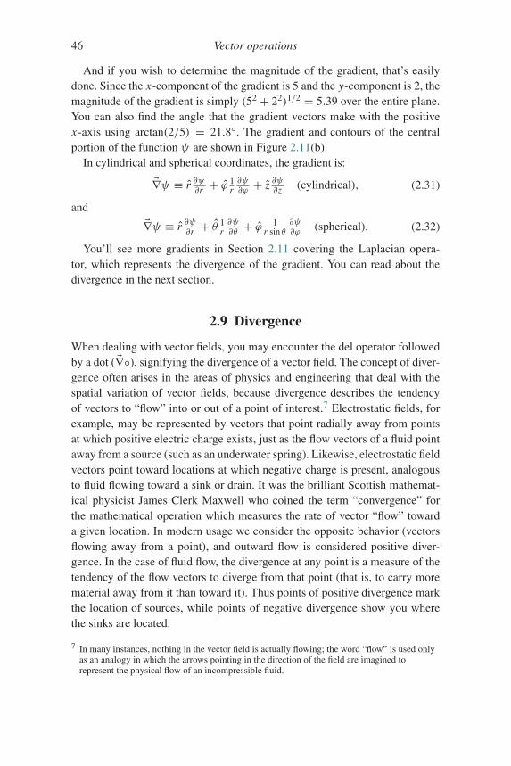
46 Vector operations
And if you wish to determine the magnitude of the gradient, that’s easilydone. Since the x-component of the gradient is 5 and the y-component is 2, themagnitude of the gradient is simply (52 + 22)1/2 = 5.39 over the entire plane.You can also find the angle that the gradient vectors make with the positivex-axis using arctan(2/5) = 21.8◦. The gradient and contours of the centralportion of the function ψ are shown in Figure 2.11(b).
In cylindrical and spherical coordinates, the gradient is:
�∇ψ ≡ r ∂ψ∂r + ϕ 1
r∂ψ∂ϕ+ z ∂ψ
∂z (cylindrical), (2.31)
and
�∇ψ ≡ r ∂ψ∂r + θ 1
r∂ψ∂θ+ ϕ 1
r sin θ∂ψ∂ϕ
(spherical). (2.32)
You’ll see more gradients in Section 2.11 covering the Laplacian opera-tor, which represents the divergence of the gradient. You can read about thedivergence in the next section.
2.9 Divergence
When dealing with vector fields, you may encounter the del operator followedby a dot ( �∇◦), signifying the divergence of a vector field. The concept of diver-gence often arises in the areas of physics and engineering that deal with thespatial variation of vector fields, because divergence describes the tendencyof vectors to “flow” into or out of a point of interest.7 Electrostatic fields, forexample, may be represented by vectors that point radially away from pointsat which positive electric charge exists, just as the flow vectors of a fluid pointaway from a source (such as an underwater spring). Likewise, electrostatic fieldvectors point toward locations at which negative charge is present, analogousto fluid flowing toward a sink or drain. It was the brilliant Scottish mathemat-ical physicist James Clerk Maxwell who coined the term “convergence” forthe mathematical operation which measures the rate of vector “flow” towarda given location. In modern usage we consider the opposite behavior (vectorsflowing away from a point), and outward flow is considered positive diver-gence. In the case of fluid flow, the divergence at any point is a measure of thetendency of the flow vectors to diverge from that point (that is, to carry morematerial away from it than toward it). Thus points of positive divergence markthe location of sources, while points of negative divergence show you wherethe sinks are located.
7 In many instances, nothing in the vector field is actually flowing; the word “flow” is used onlyas an analogy in which the arrows pointing in the direction of the field are imagined torepresent the physical flow of an incompressible fluid.
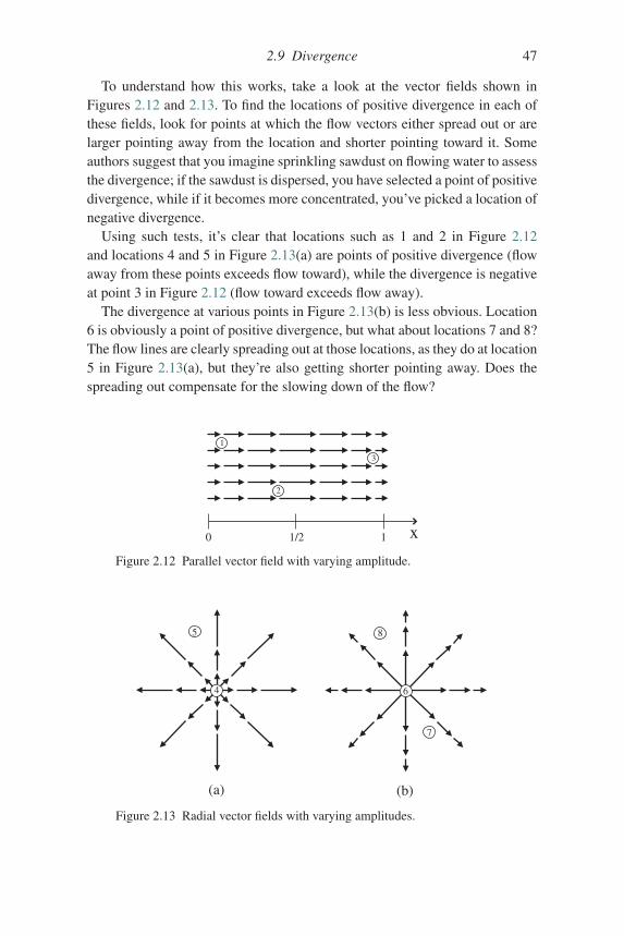
2.9 Divergence 47
To understand how this works, take a look at the vector fields shown inFigures 2.12 and 2.13. To find the locations of positive divergence in each ofthese fields, look for points at which the flow vectors either spread out or arelarger pointing away from the location and shorter pointing toward it. Someauthors suggest that you imagine sprinkling sawdust on flowing water to assessthe divergence; if the sawdust is dispersed, you have selected a point of positivedivergence, while if it becomes more concentrated, you’ve picked a location ofnegative divergence.
Using such tests, it’s clear that locations such as 1 and 2 in Figure 2.12and locations 4 and 5 in Figure 2.13(a) are points of positive divergence (flowaway from these points exceeds flow toward), while the divergence is negativeat point 3 in Figure 2.12 (flow toward exceeds flow away).
The divergence at various points in Figure 2.13(b) is less obvious. Location6 is obviously a point of positive divergence, but what about locations 7 and 8?The flow lines are clearly spreading out at those locations, as they do at location5 in Figure 2.13(a), but they’re also getting shorter pointing away. Does thespreading out compensate for the slowing down of the flow?
1
2
3
x0 1/2 1
Figure 2.12 Parallel vector field with varying amplitude.
4 6
7
5 8
(a) (b)
Figure 2.13 Radial vector fields with varying amplitudes.
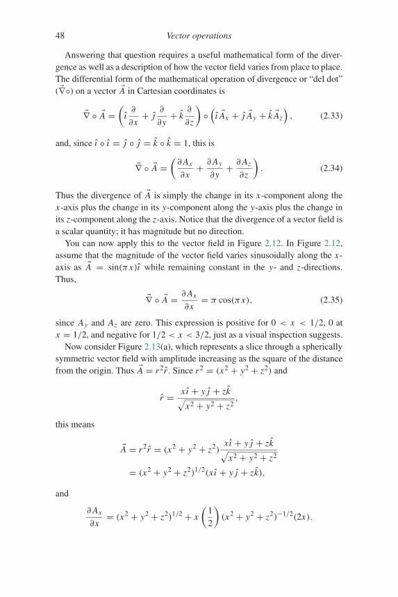
48 Vector operations
Answering that question requires a useful mathematical form of the diver-gence as well as a description of how the vector field varies from place to place.The differential form of the mathematical operation of divergence or “del dot”( �∇◦) on a vector �A in Cartesian coordinates is
�∇ ◦ �A =(
ı∂
∂x+ j ∂
∂y+ k
∂
∂z
)◦(
ı �Ax + j �Ay + k �Az
), (2.33)
and, since ı ◦ ı = j ◦ j = k ◦ k = 1, this is
�∇ ◦ �A =(∂Ax
∂x+ ∂Ay
∂y+ ∂Az
∂z
). (2.34)
Thus the divergence of �A is simply the change in its x-component along thex-axis plus the change in its y-component along the y-axis plus the change inits z-component along the z-axis. Notice that the divergence of a vector field isa scalar quantity; it has magnitude but no direction.
You can now apply this to the vector field in Figure 2.12. In Figure 2.12,assume that the magnitude of the vector field varies sinusoidally along the x-axis as �A = sin(πx)ı while remaining constant in the y- and z-directions.Thus,
�∇ ◦ �A = ∂Ax
∂x= π cos(πx), (2.35)
since Ay and Az are zero. This expression is positive for 0 < x < 1/2, 0 atx = 1/2, and negative for 1/2 < x < 3/2, just as a visual inspection suggests.
Now consider Figure 2.13(a), which represents a slice through a sphericallysymmetric vector field with amplitude increasing as the square of the distancefrom the origin. Thus �A = r2r . Since r2 = (x2 + y2 + z2) and
r = xı + yj + zk√x2 + y2 + z2
,
this means
�A = r2r = (x2 + y2 + z2)xı + yj + zk√x2 + y2 + z2
= (x2 + y2 + z2)1/2(xı + yj + zk),
and
∂Ax
∂x= (x2 + y2 + z2)1/2 + x
(1
2
)(x2 + y2 + z2)−1/2(2x).
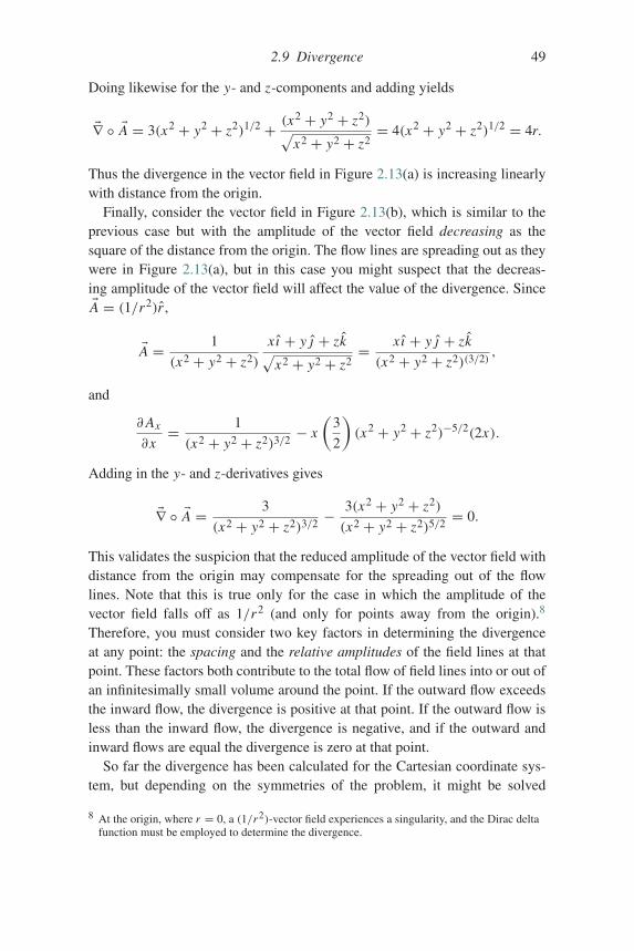
2.9 Divergence 49
Doing likewise for the y- and z-components and adding yields
�∇ ◦ �A = 3(x2 + y2 + z2)1/2 + (x2 + y2 + z2)√x2 + y2 + z2
= 4(x2 + y2 + z2)1/2 = 4r.
Thus the divergence in the vector field in Figure 2.13(a) is increasing linearlywith distance from the origin.
Finally, consider the vector field in Figure 2.13(b), which is similar to theprevious case but with the amplitude of the vector field decreasing as thesquare of the distance from the origin. The flow lines are spreading out as theywere in Figure 2.13(a), but in this case you might suspect that the decreas-ing amplitude of the vector field will affect the value of the divergence. Since�A = (1/r2)r ,
�A = 1
(x2 + y2 + z2)
xı + yj + zk√x2 + y2 + z2
= xı + yj + zk
(x2 + y2 + z2)(3/2),
and
∂Ax
∂x= 1
(x2 + y2 + z2)3/2− x
(3
2
)(x2 + y2 + z2)−5/2(2x).
Adding in the y- and z-derivatives gives
�∇ ◦ �A = 3
(x2 + y2 + z2)3/2− 3(x2 + y2 + z2)
(x2 + y2 + z2)5/2= 0.
This validates the suspicion that the reduced amplitude of the vector field withdistance from the origin may compensate for the spreading out of the flowlines. Note that this is true only for the case in which the amplitude of thevector field falls off as 1/r2 (and only for points away from the origin).8
Therefore, you must consider two key factors in determining the divergenceat any point: the spacing and the relative amplitudes of the field lines at thatpoint. These factors both contribute to the total flow of field lines into or out ofan infinitesimally small volume around the point. If the outward flow exceedsthe inward flow, the divergence is positive at that point. If the outward flow isless than the inward flow, the divergence is negative, and if the outward andinward flows are equal the divergence is zero at that point.
So far the divergence has been calculated for the Cartesian coordinate sys-tem, but depending on the symmetries of the problem, it might be solved
8 At the origin, where r = 0, a (1/r2)-vector field experiences a singularity, and the Dirac deltafunction must be employed to determine the divergence.
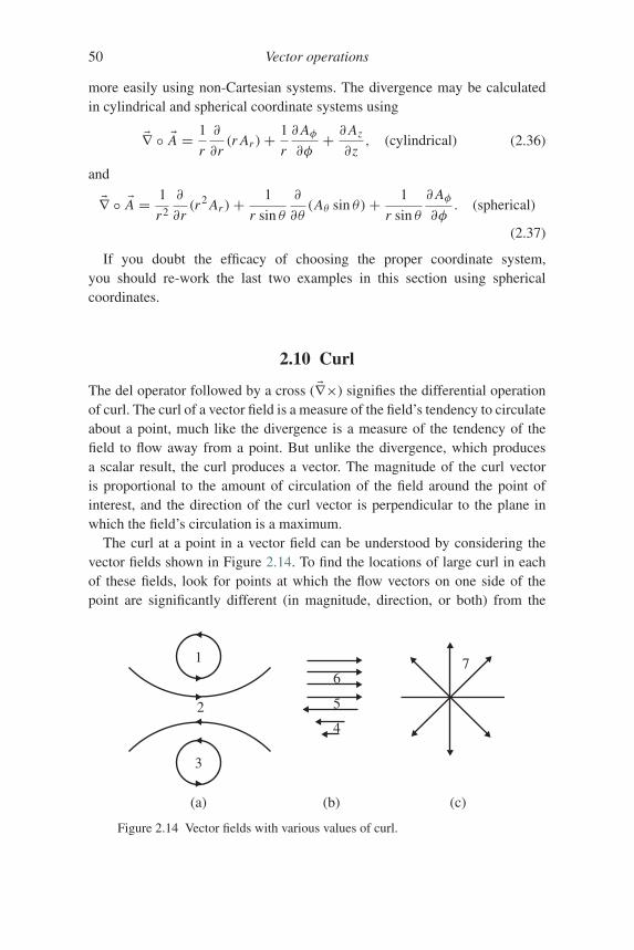
50 Vector operations
more easily using non-Cartesian systems. The divergence may be calculatedin cylindrical and spherical coordinate systems using
�∇ ◦ �A = 1
r
∂
∂r(r Ar )+ 1
r
∂Aφ∂φ+ ∂Az
∂z, (cylindrical) (2.36)
and
�∇ ◦ �A = 1
r2
∂
∂r(r2 Ar )+ 1
r sin θ
∂
∂θ(Aθ sin θ)+ 1
r sin θ
∂Aφ∂φ
. (spherical)
(2.37)
If you doubt the efficacy of choosing the proper coordinate system,you should re-work the last two examples in this section using sphericalcoordinates.
2.10 Curl
The del operator followed by a cross ( �∇×) signifies the differential operationof curl. The curl of a vector field is a measure of the field’s tendency to circulateabout a point, much like the divergence is a measure of the tendency of thefield to flow away from a point. But unlike the divergence, which producesa scalar result, the curl produces a vector. The magnitude of the curl vectoris proportional to the amount of circulation of the field around the point ofinterest, and the direction of the curl vector is perpendicular to the plane inwhich the field’s circulation is a maximum.
The curl at a point in a vector field can be understood by considering thevector fields shown in Figure 2.14. To find the locations of large curl in eachof these fields, look for points at which the flow vectors on one side of thepoint are significantly different (in magnitude, direction, or both) from the
1
3
(a) (b) (c)
5
4
7
2
6
Figure 2.14 Vector fields with various values of curl.
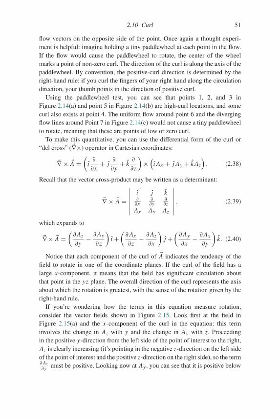
2.10 Curl 51
flow vectors on the opposite side of the point. Once again a thought experi-ment is helpful: imagine holding a tiny paddlewheel at each point in the flow.If the flow would cause the paddlewheel to rotate, the center of the wheelmarks a point of non-zero curl. The direction of the curl is along the axis of thepaddlewheel. By convention, the positive-curl direction is determined by theright-hand rule: if you curl the fingers of your right hand along the circulationdirection, your thumb points in the direction of positive curl.
Using the paddlewheel test, you can see that points 1, 2, and 3 inFigure 2.14(a) and point 5 in Figure 2.14(b) are high-curl locations, and somecurl also exists at point 4. The uniform flow around point 6 and the divergingflow lines around Point 7 in Figure 2.14(c) would not cause a tiny paddlewheelto rotate, meaning that these are points of low or zero curl.
To make this quantitative, you can use the differential form of the curl or“del cross” ( �∇×) operator in Cartesian coordinates:
�∇ × �A =(
ı∂
∂x+ j ∂
∂y+ k
∂
∂z
)×(
ı Ax + j Ay + k Az
). (2.38)
Recall that the vector cross-product may be written as a determinant:
�∇ × �A =
∣∣∣∣∣∣∣ı j k∂∂x
∂∂y
∂∂z
Ax Ay Az
∣∣∣∣∣∣∣ , (2.39)
which expands to
�∇ × �A =(∂Az
∂y− ∂Ay
∂z
)ı +
(∂Ax
∂z− ∂Az
∂x
)j +
(∂Ay
∂x− ∂Ax
∂y
)k. (2.40)
Notice that each component of the curl of �A indicates the tendency of thefield to rotate in one of the coordinate planes. If the curl of the field has alarge x-component, it means that the field has significant circulation aboutthat point in the yz plane. The overall direction of the curl represents the axisabout which the rotation is greatest, with the sense of the rotation given by theright-hand rule.
If you’re wondering how the terms in this equation measure rotation,consider the vector fields shown in Figure 2.15. Look first at the field inFigure 2.15(a) and the x-component of the curl in the equation: this terminvolves the change in Az with y and the change in Ay with z. Proceedingin the positive y-direction from the left side of the point of interest to the right,Az is clearly increasing (it’s pointing in the negative z-direction on the left sideof the point of interest and the positive z-direction on the right side), so the term∂Az∂y must be positive. Looking now at Ay , you can see that it is positive below
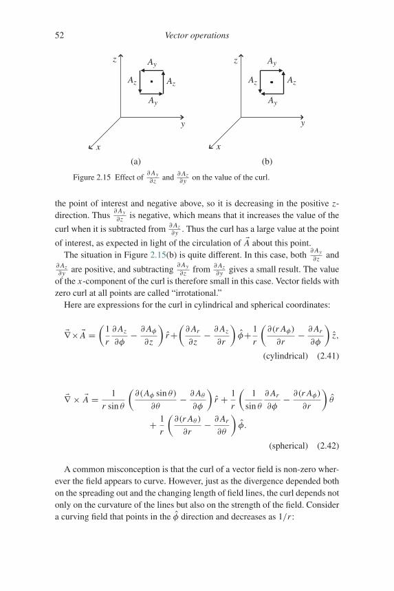
52 Vector operations
x
y
zz
x
y
(b)
Ay Ay
AyAy
AzAz Az Az
(a)
Figure 2.15 Effect of∂Ay∂z and ∂Az
∂y on the value of the curl.
the point of interest and negative above, so it is decreasing in the positive z-direction. Thus ∂Ay
∂z is negative, which means that it increases the value of the
curl when it is subtracted from ∂Az∂y . Thus the curl has a large value at the point
of interest, as expected in light of the circulation of �A about this point.The situation in Figure 2.15(b) is quite different. In this case, both ∂Ay
∂z and∂Az∂y are positive, and subtracting ∂Ay
∂z from ∂Az∂y gives a small result. The value
of the x-component of the curl is therefore small in this case. Vector fields withzero curl at all points are called “irrotational.”
Here are expressions for the curl in cylindrical and spherical coordinates:
�∇× �A =(
1
r
∂Az
∂φ− ∂Aφ
∂z
)r+(∂Ar
∂z− ∂Az
∂r
)φ+ 1
r
(∂(r Aφ)
∂r− ∂Ar
∂φ
)z,
(cylindrical) (2.41)
�∇ × �A = 1
r sin θ
(∂(Aφ sin θ)
∂θ− ∂Aθ∂φ
)r + 1
r
(1
sin θ
∂Ar
∂φ− ∂(r Aφ)
∂r
)θ
+ 1
r
(∂(r Aθ )
∂r− ∂Ar
∂θ
)φ.
(spherical) (2.42)
A common misconception is that the curl of a vector field is non-zero wher-ever the field appears to curve. However, just as the divergence depended bothon the spreading out and the changing length of field lines, the curl depends notonly on the curvature of the lines but also on the strength of the field. Considera curving field that points in the φ direction and decreases as 1/r :
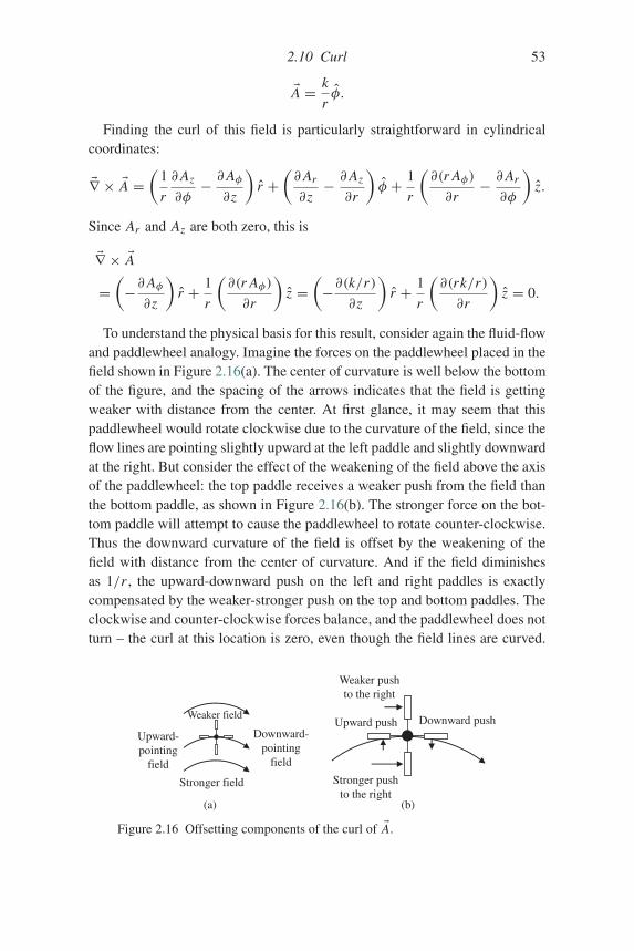
2.10 Curl 53
�A = k
rφ.
Finding the curl of this field is particularly straightforward in cylindricalcoordinates:
�∇ × �A =(
1
r
∂Az
∂φ− ∂Aφ
∂z
)r +
(∂Ar
∂z− ∂Az
∂r
)φ + 1
r
(∂(r Aφ)
∂r− ∂Ar
∂φ
)z.
Since Ar and Az are both zero, this is
�∇ × �A=(−∂Aφ∂z
)r + 1
r
(∂(r Aφ)
∂r
)z =
(−∂(k/r)
∂z
)r + 1
r
(∂(rk/r)
∂r
)z = 0.
To understand the physical basis for this result, consider again the fluid-flowand paddlewheel analogy. Imagine the forces on the paddlewheel placed in thefield shown in Figure 2.16(a). The center of curvature is well below the bottomof the figure, and the spacing of the arrows indicates that the field is gettingweaker with distance from the center. At first glance, it may seem that thispaddlewheel would rotate clockwise due to the curvature of the field, since theflow lines are pointing slightly upward at the left paddle and slightly downwardat the right. But consider the effect of the weakening of the field above the axisof the paddlewheel: the top paddle receives a weaker push from the field thanthe bottom paddle, as shown in Figure 2.16(b). The stronger force on the bot-tom paddle will attempt to cause the paddlewheel to rotate counter-clockwise.Thus the downward curvature of the field is offset by the weakening of thefield with distance from the center of curvature. And if the field diminishesas 1/r , the upward-downward push on the left and right paddles is exactlycompensated by the weaker-stronger push on the top and bottom paddles. Theclockwise and counter-clockwise forces balance, and the paddlewheel does notturn – the curl at this location is zero, even though the field lines are curved.
Weaker field
Stronger field
(a) (b)
Upward-pointing
field
Downward-pointing
field
Weaker pushto the right
Stronger pushto the right
Upward push Downward push
Figure 2.16 Offsetting components of the curl of �A.
54 Vector operations
For this 1/r field, the curl is zero everywhere except at the center of curvature(where a singularity exists and must be handled using the delta function).
2.11 Laplacian
Once you know that the gradient operates on a scalar function and produces avector and that the divergence operates on a vector and produces a scalar, it’snatural to wonder whether these two operations can be combined in a mean-ingful way. As it turns out, the divergence of the gradient of a scalar functionφ, written as �∇ ◦ ( �∇φ), is one of the most useful mathematical operations inphysics and engineering. This operation, usually written as ∇2φ (but some-times as �φ), is called the “Laplacian” in honor of Pierre-Simon Laplace, thegreat French mathematician and astronomer.
Before trying to understand why the Laplacian operator is so valuable,you should begin by recalling the operations of gradient and divergence inCartesian coordinates:
Gradient:
�∇φ = ı∂φ
∂x+ j ∂φ
∂y+ k
∂φ
∂z. (2.43)
Divergence:
�∇ ◦ �A = ∂Ax
∂x+ ∂Ay
∂y+ ∂Az
∂z. (2.44)
Since the x-component of the gradient of φ is ∂φ∂x , the y-component of the gra-
dient of φ is ∂φ∂y , and the z-component of the gradient of φ is ∂φ
∂z , the divergenceof the vector produced by the gradient is
�∇ ◦ �∇φ = ∇2φ = ∂2φ
∂x2+ ∂
2φ
∂y2+ ∂
2φ
∂z2. (2.45)
Just as the gradient ( �∇), divergence ( �∇◦), and curl ( �∇×) representdifferential operators, so too the Laplacian (∇2) is an operator waiting to befed a function. As you may recall, the gradient operator tells you the direc-tion of greatest increase of the function (and how steep the increase is), thedivergence tells you how strongly a vector function “flows” away from a point(or toward that point if the divergence is negative), and the curl tells you howstrongly a vector function tends to circulate around a point. So what does theLaplacian, the divergence of the gradient, tell you?
If you write the Laplacian operator as ∇2 = ∂2
∂x2 + ∂2
∂y2 + ∂2
∂z2 , it shouldhelp you see that this operator finds the change in the change of the function
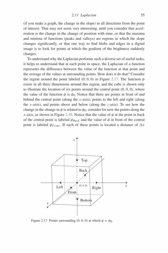
2.11 Laplacian 55
(if you make a graph, the change in the slope) in all directions from the pointof interest. That may not seem very interesting, until you consider that accel-eration is the change in the change of position with time, or that the maximaand minima of functions (peaks and valleys) are regions in which the slopechanges significantly, or that one way to find blobs and edges in a digitalimage is to look for points at which the gradient of the brightness suddenlychanges.
To understand why the Laplacian performs such a diverse set of useful tasks,it helps to understand that at each point in space, the Laplacian of a functionrepresents the difference between the value of the function at that point andthe average of the values at surrounding points. How does it do that? Considerthe region around the point labeled (0, 0, 0) in Figure 2.17. The function φexists in all three dimensions around this region, and the cube is shown onlyto illustrate the location of six points around the central point (0, 0, 0), wherethe value of the function φ is φ0. Notice that there are points in front of andbehind the central point (along the x-axis), points to the left and right (alongthe y-axis), and points above and below (along the z-axis). To see how thechange in the change in φ is related to φ0, consider for now the points along thex-axis, as shown in Figure 2.18. Notice that the value of φ at the point in backof the central point is labeled φBack and the value of φ in front of the centralpoint is labeled φFront . If each of these points is located a distance of x
x
y
z
(0, 0, 0)Right
Top
LeftFront
Bottom
Back
Figure 2.17 Points surrounding (0, 0, 0) at which φ = φ0.
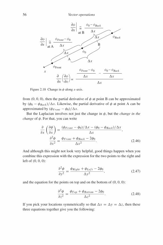
56 Vector operations
x
= ~
=~
A
Bat A
at B
=
∂x
∂φ φ0 – φBack
Δx
Δx φBack
φ0Δx
Δx
φFront
–φFront – φ0
Δx
φ0 – φBack
Δx
Δx
∂x
∂φ
∂x
∂φ∂x
∂
φFront – φ0
Δx
Figure 2.18 Change in φ along x-axis.
from (0, 0, 0), then the partial derivative of φ at point B can be approximatedby (φ0 − φBack)/x . Likewise, the partial derivative of φ at point A can beapproximated by (φFront − φ0)/x .
But the Laplacian involves not just the change in φ, but the change in thechange of φ. For that, you can write
∂
∂x
(∂φ
∂x
)= (φFront − φ0)/x − (φ0 − φBack)/x
x,
∂2φ
∂x2= φFront + φBack − 2φ0
x2. (2.46)
And although this might not look very helpful, good things happen when youcombine this expression with the expression for the two points to the right andleft of (0, 0, 0):
∂2φ
∂y2= φRight + φLe f t − 2φ0
y2, (2.47)
and the equation for the points on top and on the bottom of (0, 0, 0):
∂2φ
∂z2= φT op + φBottom − 2φ0
z2. (2.48)
If you pick your locations symmetrically so that x = y = z, then thesethree equations together give you the following:
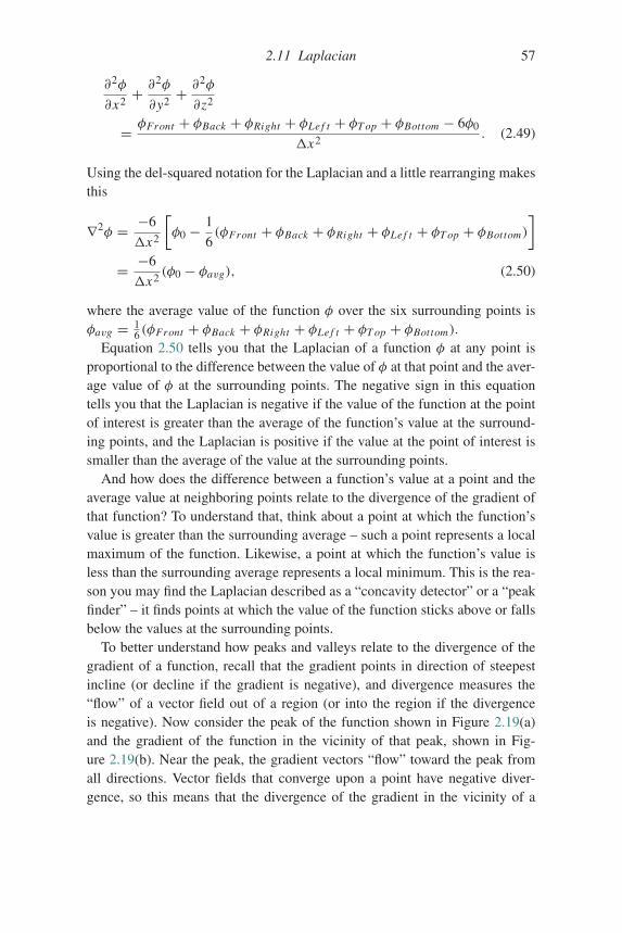
2.11 Laplacian 57
∂2φ
∂x2+ ∂
2φ
∂y2+ ∂
2φ
∂z2
= φFront + φBack + φRight + φLe f t + φT op + φBottom − 6φ0
x2. (2.49)
Using the del-squared notation for the Laplacian and a little rearranging makesthis
∇2φ = −6
x2
[φ0 − 1
6(φFront + φBack + φRight + φLe f t + φT op + φBottom)
]
= −6
x2(φ0 − φavg), (2.50)
where the average value of the function φ over the six surrounding points isφavg = 1
6 (φFront + φBack + φRight + φLe f t + φT op + φBottom).Equation 2.50 tells you that the Laplacian of a function φ at any point is
proportional to the difference between the value of φ at that point and the aver-age value of φ at the surrounding points. The negative sign in this equationtells you that the Laplacian is negative if the value of the function at the pointof interest is greater than the average of the function’s value at the surround-ing points, and the Laplacian is positive if the value at the point of interest issmaller than the average of the value at the surrounding points.
And how does the difference between a function’s value at a point and theaverage value at neighboring points relate to the divergence of the gradient ofthat function? To understand that, think about a point at which the function’svalue is greater than the surrounding average – such a point represents a localmaximum of the function. Likewise, a point at which the function’s value isless than the surrounding average represents a local minimum. This is the rea-son you may find the Laplacian described as a “concavity detector” or a “peakfinder” – it finds points at which the value of the function sticks above or fallsbelow the values at the surrounding points.
To better understand how peaks and valleys relate to the divergence of thegradient of a function, recall that the gradient points in direction of steepestincline (or decline if the gradient is negative), and divergence measures the“flow” of a vector field out of a region (or into the region if the divergenceis negative). Now consider the peak of the function shown in Figure 2.19(a)and the gradient of the function in the vicinity of that peak, shown in Fig-ure 2.19(b). Near the peak, the gradient vectors “flow” toward the peak fromall directions. Vector fields that converge upon a point have negative diver-gence, so this means that the divergence of the gradient in the vicinity of a
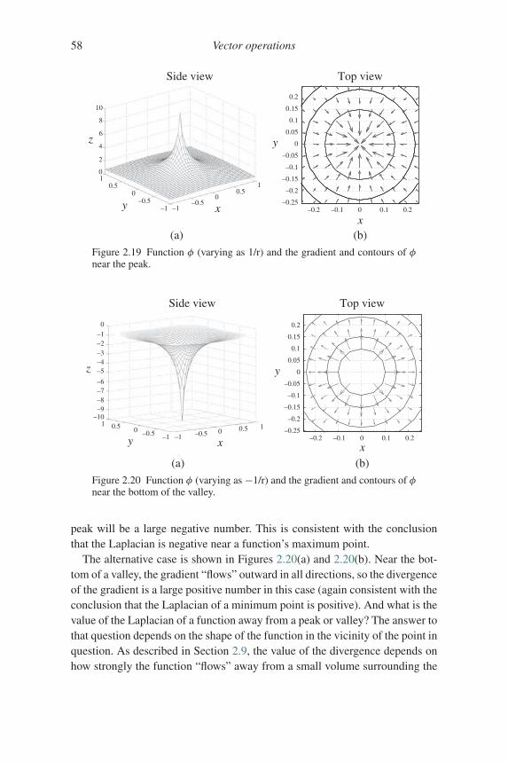
58 Vector operations
(a)
–0.2 –0.1 0 0.1 0.2–0.25
–0.2
–0.15
–0.1
–0.05
0
0.05
0.1
0.15
0.2
x
y
Top viewSide view
10
8
6
4
2
01
0.50
–0.5–1 –1
–0.50
x
z
y0.5
1
(b)
Figure 2.19 Function φ (varying as 1/r) and the gradient and contours of φnear the peak.
Side view
z
0.51–10–9–8–7–6
–5–4–3–2–10
0 –0.5 –1y –1 –0.5 0
x0.5 1
–0.2 –0.1 0 0.1 0.2–0.25
–0.2
–0.15
–0.1
–0.05
0
0.05
0.1
0.15
0.2
x
y
Top view
(b)(a)
Figure 2.20 Function φ (varying as −1/r) and the gradient and contours of φnear the bottom of the valley.
peak will be a large negative number. This is consistent with the conclusionthat the Laplacian is negative near a function’s maximum point.
The alternative case is shown in Figures 2.20(a) and 2.20(b). Near the bot-tom of a valley, the gradient “flows” outward in all directions, so the divergenceof the gradient is a large positive number in this case (again consistent with theconclusion that the Laplacian of a minimum point is positive). And what is thevalue of the Laplacian of a function away from a peak or valley? The answer tothat question depends on the shape of the function in the vicinity of the point inquestion. As described in Section 2.9, the value of the divergence depends onhow strongly the function “flows” away from a small volume surrounding the
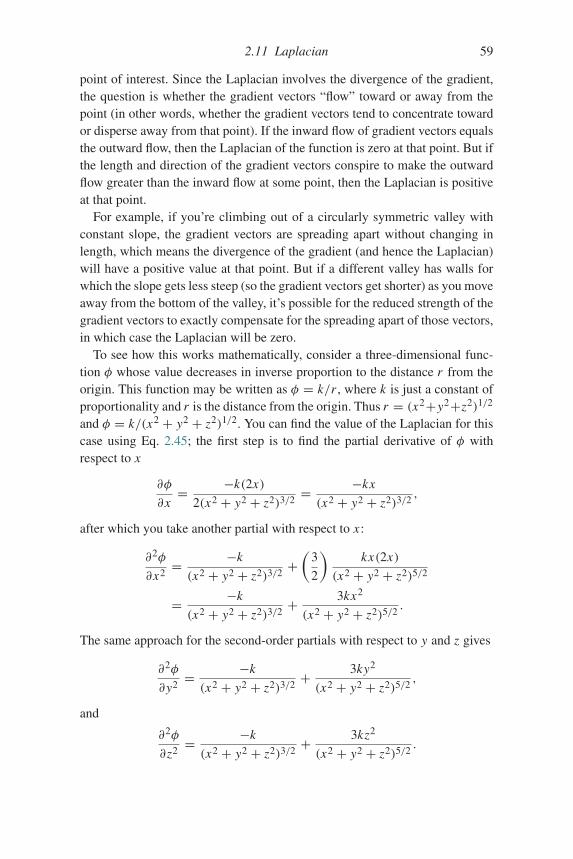
2.11 Laplacian 59
point of interest. Since the Laplacian involves the divergence of the gradient,the question is whether the gradient vectors “flow” toward or away from thepoint (in other words, whether the gradient vectors tend to concentrate towardor disperse away from that point). If the inward flow of gradient vectors equalsthe outward flow, then the Laplacian of the function is zero at that point. But ifthe length and direction of the gradient vectors conspire to make the outwardflow greater than the inward flow at some point, then the Laplacian is positiveat that point.
For example, if you’re climbing out of a circularly symmetric valley withconstant slope, the gradient vectors are spreading apart without changing inlength, which means the divergence of the gradient (and hence the Laplacian)will have a positive value at that point. But if a different valley has walls forwhich the slope gets less steep (so the gradient vectors get shorter) as you moveaway from the bottom of the valley, it’s possible for the reduced strength of thegradient vectors to exactly compensate for the spreading apart of those vectors,in which case the Laplacian will be zero.
To see how this works mathematically, consider a three-dimensional func-tion φ whose value decreases in inverse proportion to the distance r from theorigin. This function may be written as φ = k/r , where k is just a constant ofproportionality and r is the distance from the origin. Thus r = (x2+y2+z2)1/2
and φ = k/(x2 + y2 + z2)1/2. You can find the value of the Laplacian for thiscase using Eq. 2.45; the first step is to find the partial derivative of φ withrespect to x
∂φ
∂x= −k(2x)
2(x2 + y2 + z2)3/2= −kx
(x2 + y2 + z2)3/2,
after which you take another partial with respect to x :
∂2φ
∂x2= −k
(x2 + y2 + z2)3/2+(
3
2
)kx(2x)
(x2 + y2 + z2)5/2
= −k
(x2 + y2 + z2)3/2+ 3kx2
(x2 + y2 + z2)5/2.
The same approach for the second-order partials with respect to y and z gives
∂2φ
∂y2= −k
(x2 + y2 + z2)3/2+ 3ky2
(x2 + y2 + z2)5/2,
and
∂2φ
∂z2= −k
(x2 + y2 + z2)3/2+ 3kz2
(x2 + y2 + z2)5/2.
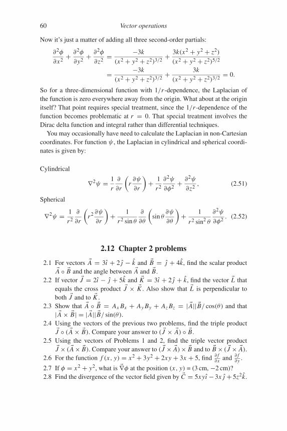
60 Vector operations
Now it’s just a matter of adding all three second-order partials:
∂2φ
∂x2+ ∂
2φ
∂y2+ ∂
2φ
∂z2= −3k
(x2 + y2 + z2)3/2+ 3k(x2 + y2 + z2)
(x2 + y2 + z2)5/2
= −3k
(x2 + y2 + z2)3/2+ 3k
(x2 + y2 + z2)3/2= 0.
So for a three-dimensional function with 1/r -dependence, the Laplacian ofthe function is zero everywhere away from the origin. What about at the originitself? That point requires special treatment, since the 1/r -dependence of thefunction becomes problematic at r = 0. That special treatment involves theDirac delta function and integral rather than differential techniques.
You may occasionally have need to calculate the Laplacian in non-Cartesiancoordinates. For function ψ , the Laplacian in cylindrical and spherical coordi-nates is given by:
Cylindrical
∇2ψ = 1
r
∂
∂r
(r∂ψ
∂r
)+ 1
r2
∂2ψ
∂φ2+ ∂
2ψ
∂z2, (2.51)
Spherical
∇2ψ = 1
r2
∂
∂r
(r2 ∂ψ
∂r
)+ 1
r2 sin θ
∂
∂θ
(sin θ
∂ψ
∂θ
)+ 1
r2 sin2 θ
∂2ψ
∂φ2. (2.52)
2.12 Chapter 2 problems
2.1 For vectors �A = 3ı + 2j − k and �B = j + 4k, find the scalar product�A ◦ �B and the angle between �A and �B.
2.2 If vector �J = 2ı − j + 5k and �K = 3ı + 2j + k, find the vector �L thatequals the cross product �J × �K . Also show that �L is perpendicular toboth �J and to �K .
2.3 Show that �A ◦ �B = Ax Bx + Ay By + Az Bz = | �A|| �B/ cos(θ) and that| �A × �B| = | �A|| �B/ sin(θ).
2.4 Using the vectors of the previous two problems, find the triple product�J ◦ ( �A × �B). Compare your answer to ( �J × �A) ◦ �B.
2.5 Using the vectors of Problems 1 and 2, find the triple vector product�J × ( �A× �B). Compare your answer to ( �J × �A)× �B and to �B× ( �J × �A).
2.6 For the function f (x, y) = x2 + 3y2 + 2xy + 3x + 5, find ∂ f∂x and ∂ f
∂y .
2.7 If φ = x2 + y2, what is �∇φ at the position (x, y) = (3 cm, −2 cm)?2.8 Find the divergence of the vector field given by �C = 5xyı − 3x j + 5z2k.
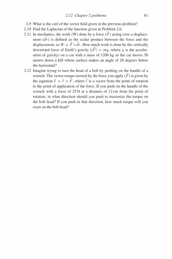
2.12 Chapter 2 problems 61
2.9 What is the curl of the vector field given in the previous problem?2.10 Find the Laplacian of the function given in Problem 2.6.2.11 In mechanics, the work (W) done by a force ( �F) acting over a displace-
ment ( �dr ) is defined as the scalar product between the force and thedisplacement, so W = �F ◦ �dr . How much work is done by the verticallydownward force of Earth’s gravity (| �F | = mg, where g is the acceler-ation of gravity) on a car with a mass of 1200 kg as the car moves 50meters down a hill whose surface makes an angle of 20 degrees belowthe horizontal?
2.12 Imagine trying to turn the head of a bolt by pushing on the handle of awrench. The vector torque exerted by the force you apply ( �F) is given bythe equation �τ = �r × �F , where �r is a vector from the point of rotationto the point of application of the force. If you push on the handle of thewrench with a force of 25 N at a distance of 12 cm from the point ofrotation, in what direction should you push to maximize the torque onthe bolt head? If you push in that direction, how much torque will youexert on the bolt head?
3
Vector applications
The real value of understanding vectors and how to manipulate them becomesclear when you realize that your knowledge allows you to solve a variety ofproblems that would be much more difficult without vectors. In this chapter,you’ll find detailed explanations of four such problems: a mass sliding downan inclined plane, an object moving along a curved path, a charged particlein an electric field, and a charged particle in a magnetic field. To solve theseproblems, you’ll need many of the vector concepts and operations described inChapters 1 and 2.
3.1 Mass on an inclined plane
Consider the delivery woman pushing a heavy box up the ramp to her deliverytruck, as illustrated in Figure 3.1. In this situation, there are a number of forcesacting on the box, so if you want to determine how the box will move, you needto know how to work with vectors. Specifically, to solve problems such as this,you can use vector addition to find the total force acting on the box, and thenyou can use Newton’s Second Law to relate that total force to the accelerationof the box.
To understand how this works, imagine that the delivery woman slips off theside of the ramp, leaving the box free to slide down the ramp under the influ-ence of gravity. For starters, pretend that the ramp is so slippery that frictionbetween the bottom of the box and the ramp surface is negligible (so the coef-ficient of friction is effectively zero). How fast will the box be moving when itreaches the bottom of the ramp? Perhaps more importantly, on what does thatspeed depend?
Whenever you approach a problem like this, it’s a good idea to beginby drawing a diagram that shows all the forces acting on the box. Such a
62
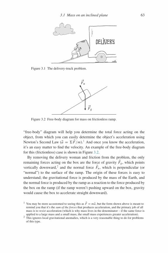
3.1 Mass on an inclined plane 63
Figure 3.1 The delivery-truck problem.
Fn
Fg
Figure 3.2 Free-body diagram for mass on frictionless ramp.
“free-body” diagram will help you determine the total force acting on theobject, from which you can easily determine the object’s acceleration usingNewton’s Second Law (�a = �F/m).1 And once you know the acceleration,it’s an easy matter to find the velocity. An example of the free-body diagramfor this (frictionless) case is shown in Figure 3.2.
By removing the delivery woman and friction from the problem, the onlyremaining forces acting on the box are the force of gravity �Fg , which pointsvertically downward,2 and the normal force �Fn , which is perpendicular (or“normal”) to the surface of the ramp. The origin of these forces is easy tounderstand; the gravitational force is produced by the mass of the Earth, andthe normal force is produced by the ramp as a reaction to the force produced bythe box on the ramp (if the ramp weren’t pushing upward on the box, gravitywould cause the box to accelerate straight downward).
1 You may be more accustomed to seeing this as �F = m�a, but the form shown above is meant toremind you that it’s the sum of the forces that produces acceleration, and the primary job of allmass is to resist acceleration (which is why mass lives in the denominator – if the same force isapplied to a large mass and a small mass, the small mass experiences greater acceleration).
2 This ignores local gravitational anomalies, which is a very reasonable thing to do for problemsof this type.
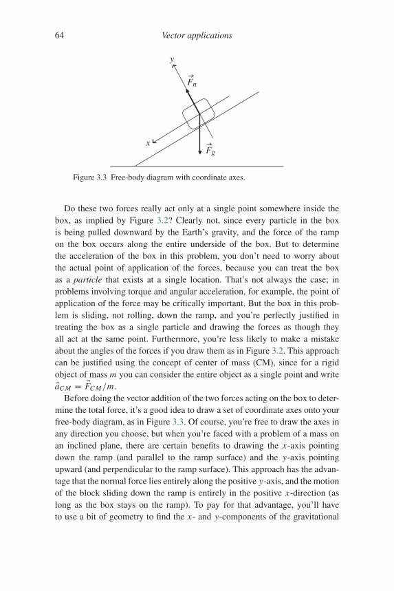
64 Vector applications
Fn
Fg
y
x
Figure 3.3 Free-body diagram with coordinate axes.
Do these two forces really act only at a single point somewhere inside thebox, as implied by Figure 3.2? Clearly not, since every particle in the boxis being pulled downward by the Earth’s gravity, and the force of the rampon the box occurs along the entire underside of the box. But to determinethe acceleration of the box in this problem, you don’t need to worry aboutthe actual point of application of the forces, because you can treat the boxas a particle that exists at a single location. That’s not always the case; inproblems involving torque and angular acceleration, for example, the point ofapplication of the force may be critically important. But the box in this prob-lem is sliding, not rolling, down the ramp, and you’re perfectly justified intreating the box as a single particle and drawing the forces as though theyall act at the same point. Furthermore, you’re less likely to make a mistakeabout the angles of the forces if you draw them as in Figure 3.2. This approachcan be justified using the concept of center of mass (CM), since for a rigidobject of mass m you can consider the entire object as a single point and write�aC M = �FC M/m.
Before doing the vector addition of the two forces acting on the box to deter-mine the total force, it’s a good idea to draw a set of coordinate axes onto yourfree-body diagram, as in Figure 3.3. Of course, you’re free to draw the axes inany direction you choose, but when you’re faced with a problem of a mass onan inclined plane, there are certain benefits to drawing the x-axis pointingdown the ramp (and parallel to the ramp surface) and the y-axis pointingupward (and perpendicular to the ramp surface). This approach has the advan-tage that the normal force lies entirely along the positive y-axis, and the motionof the block sliding down the ramp is entirely in the positive x-direction (aslong as the box stays on the ramp). To pay for that advantage, you’ll haveto use a bit of geometry to find the x- and y-components of the gravitational
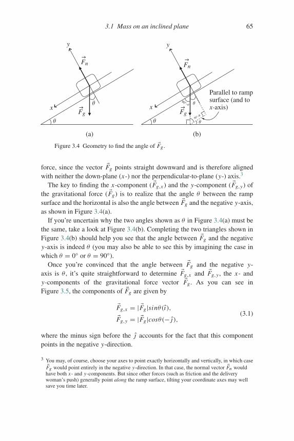
3.1 Mass on an inclined plane 65
θ θ
θθ θ
y
x
y
x
Parallel to rampsurface (and tox-axis)
(b)(a)
Fn
Fg Fg
Fn
90°–θ
90°–θ
Figure 3.4 Geometry to find the angle of �Fg .
force, since the vector �Fg points straight downward and is therefore alignedwith neither the down-plane (x-) nor the perpendicular-to-plane (y-) axis.3
The key to finding the x-component ( �Fg,x ) and the y-component ( �Fg,y) ofthe gravitational force ( �Fg) is to realize that the angle θ between the rampsurface and the horizontal is also the angle between �Fg and the negative y-axis,as shown in Figure 3.4(a).
If you’re uncertain why the two angles shown as θ in Figure 3.4(a) must bethe same, take a look at Figure 3.4(b). Completing the two triangles shown inFigure 3.4(b) should help you see that the angle between �Fg and the negativey-axis is indeed θ (you may also be able to see this by imagining the case inwhich θ = 0◦ or θ = 90◦).
Once you’re convinced that the angle between �Fg and the negative y-axis is θ , it’s quite straightforward to determine �Fg,x and �Fg,y , the x- andy-components of the gravitational force vector �Fg . As you can see inFigure 3.5, the components of �Fg are given by
�Fg,x = | �Fg|sinθ(ı),
�Fg,y = | �Fg|cosθ(−j ), (3.1)
where the minus sign before the j accounts for the fact that this componentpoints in the negative y-direction.
3 You may, of course, choose your axes to point exactly horizontally and vertically, in which case�Fg would point entirely in the negative y-direction. In that case, the normal vector �Fn would
have both x- and y-components. But since other forces (such as friction and the deliverywoman’s push) generally point along the ramp surface, tilting your coordinate axes may wellsave you time later.
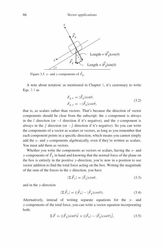
66 Vector applications
Length = |Fg|cos(θ)
Length = |Fg|sin(θ)
Fn
θ
θ
y
x Fg
Figure 3.5 x- and y-components of �Fg .
A note about notation: as mentioned in Chapter 1, it’s customary to writeEqs. 3.1 as
Fg,x = | �Fg|sinθ,
Fg,y = −| �Fg|cosθ,(3.2)
that is, as scalars rather than vectors. That’s because the direction of vectorcomponents should be clear from the subscript: the x-component is alwaysin the ı direction (or −ı direction if it’s negative), and the y-component isalways in the j direction (or −j direction if it’s negative). So you can writethe components of a vector as scalars or vectors, as long as you remember thateach component points in a specific direction, which means you cannot simplyadd the x- and y-components algebraically, even if they’re written as scalars.You must add them as vectors.
Whether you write the components as vectors or scalars, having the x- andy-components of �Fg in hand and knowing that the normal force of the plane onthe box is entirely in the positive y-direction, you’re now in a position to usevector addition to find the total force acting on the box. Writing the magnitudeof the sum of the forces in the x-direction, you have
| �Fx | = | �Fg|sinθ, (3.3)
and in the y-direction
| �Fy | = (| �Fn| − | �Fg|cosθ). (3.4)
Alternatively, instead of writing separate equations for the x- andy-components of the total force, you can write a vector equation incorporatingboth:
�F = (| �Fg|sinθ)i + (| �Fn| − | �Fg|cosθ) j, (3.5)
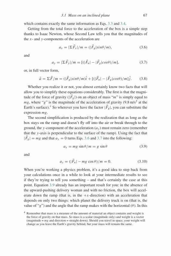
3.1 Mass on an inclined plane 67
which contains exactly the same information as Eqs. 3.3 and 3.4.Getting from the total force to the acceleration of the box is a simple step
thanks to Isaac Newton, whose Second Law tells you that the magnitudes ofthe x- and y-components of the acceleration are
ax = | �Fx |/m = (| �Fg|sinθ/m), (3.6)
and
ay = | �Fy |/m = [(| �Fn| − | �Fg|cosθ)/m], (3.7)
or, in full vector form,
�a = �F/m = (| �Fg|sinθ/m)i + [(| �Fn| − | �Fg|cosθ)/m] j . (3.8)
Whether you realize it or not, you almost certainly know two facts that willallow you to simplify these equations considerably. The first is that the magni-tude of the force of gravity (| �Fg|) on an object of mass “m” is simply equal tomg, where “g” is the magnitude of the acceleration of gravity (9.8 m/s2 at theEarth’s surface).4 So wherever you have the factor | �Fg|, you can substitute theexpression mg.
The second simplification is produced by the realization that as long as thebox stays on the ramp and doesn’t fly off into the air or break through to theground, the y-component of the acceleration (ay) must remain zero (rememberthat the y-axis is perpendicular to the surface of the ramp). Using the fact that| �Fg| = mg and that ay = 0 turns Eqs. 3.6 and 3.7 into the following:
ax = mg sin θ/m = g sin θ (3.9)
and
ay = (| �Fn| − mg cos θ)/m = 0. (3.10)
When you’re working a physics problem, it’s a good idea to step back fromyour calculations once in a while to look at your intermediate results to seeif they’re trying to tell you something – and that’s certainly the case at thispoint. Equation 3.9 already has an important result for you: in the absence ofthe upward-pushing delivery woman and with no friction, the box will accel-erate down the ramp (that is, in the +x-direction) with an acceleration thatdepends on only two things: which planet the delivery truck is on (that is, thevalue of “g”) and the angle that the ramp makes with the horizontal (θ). In this
4 Remember that mass is a measure of the amount of material an object contains and weight isthe force of gravity on that mass. So mass is a scalar (magnitude only) and weight is a vector(magnitude = mg and direction = straight down). Should you travel in space, your weight willchange as you leave the Earth’s gravity behind, but your mass will remain the same.
68 Vector applications
case, just as for a freely falling object, the mass of the box does not affect itsacceleration.5
Since the sine of the ramp angle can never be greater than one, Eq. 3.9 alsotells you that the magnitude of the acceleration of the object (g sin θ ) can neverbe greater than g, the accleration of gravity. It can, of course, be equal to g ifsin θ = 1. But this would mean that θ would have to be 90◦ (since sin 90◦ = 1),in which case the ramp would be exactly vertical. In such cases, you no longerhave an object sliding down a ramp, you have an object falling next to a wall.
There’s also good information lurking in Eq. 3.10, but you have to think a bitto see it. According to this equation, the y-component of the box’s accelerationis equal to the difference between the magnitude of the normal force (| �Fn|) andthe y-component of the gravitational force (mg cos θ ). But since you know thatin this problem the box remains on the ramp and the y-acceleration is thereforezero, you can use Eq. 3.10 to determine the magnitude of the normal force.Since
ay = (| �Fn| − mg cos θ)/m = 0,
then
| �Fn| = mg cos θ. (3.11)
So the normal force depends on the weight of the object (mg) and the cosineof the ramp angle (θ ). Understanding this will help you avoid a common pit-fall for students who know that the normal force is the reaction force producedon the object by the ramp, and who then mistakenly conclude that the normalforce must always equal the weight of the object (mg). That line of reason-ing only works for horizontal surfaces, because for any inclined surface, it’sonly the component of the object’s weight that’s perpendicular to the surfacethat produces the reaction force we call the normal force. That perpendicu-lar component of the object’s weight is shown in Figure 3.5 to be mg cos θ ,which spans the range from mg (when θ = 0◦, meaning the ramp is horizontaland bears the full weight of the object) to zero (when θ = 90◦, meaning theramp is vertical and bears none of the object’s weight). In all other cases, themagnitude of the normal force will have a value between 0 and mg.
If you’re wondering why you should bother finding �Fn if you’re only inter-ested in the x-component of the acceleration, the answer is that you may not
5 But doesn’t the Earth pull harder on a more-massive object? Yes it does, but a more-massiveobject also resists acceleration more than a less-massive object. Since gravitational mass(which determines how strongly gravity pulls on an object) has the same value as inertial mass(which determines how strongly the object resists acceleration), the result is that all objects fallfreely (or slide freely down frictionless ramps) with an acceleration that does not depend ontheir mass.
3.1 Mass on an inclined plane 69
care about �Fn for the frictionless case (unless you’re worried about your rampbreaking), but you’ll definitely need �Fn when friction exists between the rampsurface and the bottom of the box.
With the magnitude of the down-ramp component of the acceleration (ax )available from Eq. 3.9, all that remains is for you to find the speed of thebox at the bottom of the ramp. Finding speed from acceleration turns out tobe quite straightforward, especially when the acceleration is constant (as it isin this case), provided that you’re in possession of either one of two piecesof information: the time the box takes to reach the bottom of the ramp, or(more likely), the distance from the box’s starting point to the bottom of theramp. You’ll also need the initial speed, which you can generally discern fromthe initial conditions, and which you can take to be zero in this case. As youmay remember from kinematics, the final speed of an object moving in thex-direction with initial speed vx,ini tial undergoing constant accleration ax overtime t is given by
vx, f inal = vx,ini tial + ax t, (3.12)
or, if you know d , the distance in the positive x-direction over which theacceleration occurs,
(vx, f inal)2 = (vx,ini tial)
2 + 2ax d. (3.13)
Using the expression for acceleration from Eq. 3.9, this becomes
(vx, f inal)2 = (0)2 + 2 (g sin θ) d
or
vx, f inal =√
2 (g sin θ) d. (3.14)
So, for example, a box sliding down a 2 m ramp with an angle of 30◦ to thehorizontal on the surface of the Earth will be moving at a speed of
vx, f inal =√
2[(9.8m/s2) sin 30◦
]2m = 4.4m/s (3.15)
when it reaches the bottom of the ramp. If you’re curious about how long ittakes the box to travel the 2 m down the ramp under these conditions, you canplug this value for the final speed into Eq. 3.12 and solve for t , which turns outto be about 0.9 s in this case.
Stripping away effects such as friction is often a good way to learn the fun-damentals of a problem, but if you’ve ever encountered a ramp outside ofphysics texts, there’s a good chance you had to deal with friction. Happily,once you understand how to use vectors, including friction in the “box on a
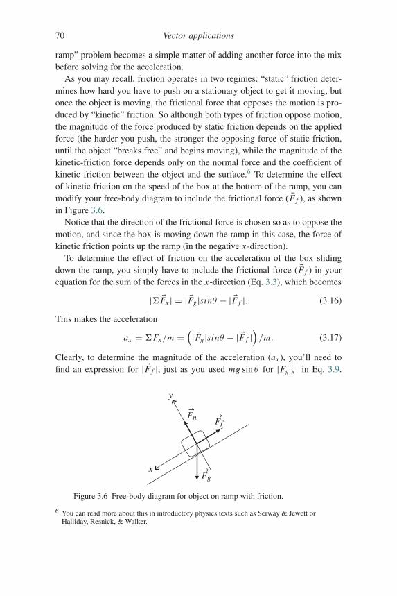
70 Vector applications
ramp” problem becomes a simple matter of adding another force into the mixbefore solving for the acceleration.
As you may recall, friction operates in two regimes: “static” friction deter-mines how hard you have to push on a stationary object to get it moving, butonce the object is moving, the frictional force that opposes the motion is pro-duced by “kinetic” friction. So although both types of friction oppose motion,the magnitude of the force produced by static friction depends on the appliedforce (the harder you push, the stronger the opposing force of static friction,until the object “breaks free” and begins moving), while the magnitude of thekinetic-friction force depends only on the normal force and the coefficient ofkinetic friction between the object and the surface.6 To determine the effectof kinetic friction on the speed of the box at the bottom of the ramp, you canmodify your free-body diagram to include the frictional force ( �F f ), as shownin Figure 3.6.
Notice that the direction of the frictional force is chosen so as to oppose themotion, and since the box is moving down the ramp in this case, the force ofkinetic friction points up the ramp (in the negative x-direction).
To determine the effect of friction on the acceleration of the box slidingdown the ramp, you simply have to include the frictional force ( �F f ) in yourequation for the sum of the forces in the x-direction (Eq. 3.3), which becomes
| �Fx | = | �Fg|sinθ − | �F f |. (3.16)
This makes the acceleration
ax = Fx/m =(| �Fg|sinθ − | �F f |
)/m. (3.17)
Clearly, to determine the magnitude of the acceleration (ax ), you’ll need tofind an expression for | �F f |, just as you used mg sin θ for |Fg,x | in Eq. 3.9.
y
x
Fn Ff
Fg
Figure 3.6 Free-body diagram for object on ramp with friction.
6 You can read more about this in introductory physics texts such as Serway & Jewett orHalliday, Resnick, & Walker.
3.1 Mass on an inclined plane 71
Fortunately, that’s easy to do, because the magnitude of the force of kineticfriction is simply the product of the magnitude of the normal force (| �Fn|) andthe coefficient of kinetic friction (μk):
| �F f | = μk | �Fn|. (3.18)
You also know from Eq. 3.11 that | �Fn| = mg cos θ , so
ax = (mg sin θ − μk mg cos θ) /m
= (g sin θ − μk g cos θ) . (3.19)
Comparing this expression for the acceleration of the box to the accelerationin the frictionless case (Eq. 3.9), you’ll be happy to note that the term due togravity (g sin θ ) is exactly the same in both cases, and the term due to friction(μk g cos θ ) is subtracted from the gravity term. This means that the acceler-ation of the box will be made smaller by the frictional force. So in the caseconsidered previously of a box sliding down a 2 m ramp that makes an angleof 30◦ with the horizontal, if the coefficient of kinetic friction between the boxand the ramp is 0.4, the speed of the box at the bottom of the ramp will bereduced to
vx, f inal =√
2[(9.8m/s2) sin 30◦ − (0.4)(9.8m/s2) cos 30◦
]2m
= 2.5m/s. (3.20)
There is one aspect of Eq. 3.19 that may worry you: what if the second termis larger than the first? For any angle between 0◦ and 45◦, the cosine is biggerthan the sine, so if the coefficient of kinetic friction (μk) is sufficiently large,this equation predicts that the acceleration will be in the negative x-direction,meaning the box will acclerate up the ramp even if no one is pushing on it.As physicists like to say, “That’s not physical,” meaning that this result contra-dicts other well-established laws of physics (conservation of energy comes tomind in this case). So where have we gone wrong in our analysis? We haven’t,really, you just need to think carefully about the initial assumptions. One ofthose assumptions was that the box is travelling down the ramp, which is whywe drew the frictional force pointing up the ramp in our free-body diagram(Figure 3.6). But if the ramp isn’t very steep and the coefficient of frictionbetween the box and the ramp is sufficiently large, the down-ramp componentof the force of gravity will not be strong enough to overcome the frictionalforce, and the box will not slide down the ramp.7 So there’s nothing wrong
7 You can determine whether the box will move by comparing the maximum static frictionalforce (which is just the product of the coefficient of static friction and the normal force) to thesum of the x-components of all the other forces.
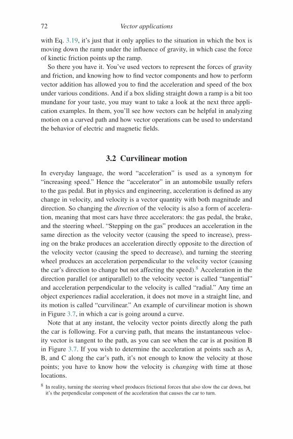
72 Vector applications
with Eq. 3.19, it’s just that it only applies to the situation in which the box ismoving down the ramp under the influence of gravity, in which case the forceof kinetic friction points up the ramp.
So there you have it. You’ve used vectors to represent the forces of gravityand friction, and knowing how to find vector components and how to performvector addition has allowed you to find the acceleration and speed of the boxunder various conditions. And if a box sliding straight down a ramp is a bit toomundane for your taste, you may want to take a look at the next three appli-cation examples. In them, you’ll see how vectors can be helpful in analyzingmotion on a curved path and how vector operations can be used to understandthe behavior of electric and magnetic fields.
3.2 Curvilinear motion
In everyday language, the word “acceleration” is used as a synonym for“increasing speed.” Hence the “accelerator” in an automobile usually refersto the gas pedal. But in physics and engineering, acceleration is defined as anychange in velocity, and velocity is a vector quantity with both magnitude anddirection. So changing the direction of the velocity is also a form of accelera-tion, meaning that most cars have three accelerators: the gas pedal, the brake,and the steering wheel. “Stepping on the gas” produces an acceleration in thesame direction as the velocity vector (causing the speed to increase), press-ing on the brake produces an acceleration directly opposite to the direction ofthe velocity vector (causing the speed to decrease), and turning the steeringwheel produces an acceleration perpendicular to the velocity vector (causingthe car’s direction to change but not affecting the speed).8 Acceleration in thedirection parallel (or antiparallel) to the velocity vector is called “tangential”and acceleration perpendicular to the velocity is called “radial.” Any time anobject experiences radial acceleration, it does not move in a straight line, andits motion is called “curvilinear.” An example of curvilinear motion is shownin Figure 3.7, in which a car is going around a curve.
Note that at any instant, the velocity vector points directly along the paththe car is following. For a curving path, that means the instantaneous veloc-ity vector is tangent to the path, as you can see when the car is at position Bin Figure 3.7. If you wish to determine the acceleration at points such as A,B, and C along the car’s path, it’s not enough to know the velocity at thosepoints; you have to know how the velocity is changing with time at thoselocations.8 In reality, turning the steering wheel produces frictional forces that also slow the car down, but
it’s the perpendicular component of the acceleration that causes the car to turn.
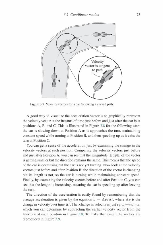
3.2 Curvilinear motion 73
A
B
C
Velocityvector is tangent
to path
Figure 3.7 Velocity vectors for a car following a curved path.
A good way to visualize the acceleration vector is to graphically representthe velocity vector at the instants of time just before and just after the car is atpositions A, B, and C. This is illustrated in Figure 3.8 for the following case:the car is slowing down at Position A as it approaches the turn, maintainingconstant speed while turning at Position B, and then speeding up as it exits theturn at Position C.
You can get a sense of the acceleration just by examining the change in thevelocity vectors at each position. Comparing the velocity vectors just beforeand just after Position A, you can see that the magnitude (length) of the vectoris getting smaller but the direction remains the same. This means that the speedof the car is decreasing but the car is not yet turning. Now look at the velocityvectors just before and after Position B: the direction of the vector is changingbut its length is not, so the car is turning while maintaining constant speed.Finally, by examining the velocity vectors before and after Position C, you cansee that the length is increasing, meaning the car is speeding up after leavingthe turn.
The direction of the acceleration is easily found by remembering that theaverage acceleration is given by the equation �a = �v/t , where �v is thechange in velocity over timet . That change in velocity is just �v f inal−�vini tial ,which you can determine by subtracting the earlier velocity vector from thelater one at each position in Figure 3.8. To make that easier, the vectors arereproduced in Figure 3.9.
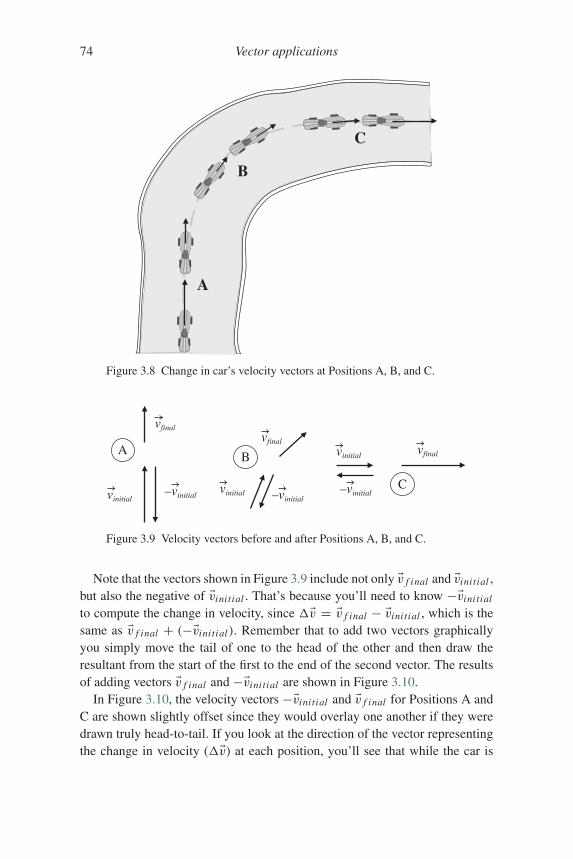
74 Vector applications
A
B
C
Figure 3.8 Change in car’s velocity vectors at Positions A, B, and C.
A B
C
vfinal
–vinitial
vfinalvfinalvinitial
vinitialvinitial –vinitial
–vinitial
Figure 3.9 Velocity vectors before and after Positions A, B, and C.
Note that the vectors shown in Figure 3.9 include not only �v f inal and �vini tial ,but also the negative of �vini tial . That’s because you’ll need to know −�vini tial
to compute the change in velocity, since �v = �v f inal − �vini tial , which is thesame as �v f inal + (−�vini tial). Remember that to add two vectors graphicallyyou simply move the tail of one to the head of the other and then draw theresultant from the start of the first to the end of the second vector. The resultsof adding vectors �v f inal and −�vini tial are shown in Figure 3.10.
In Figure 3.10, the velocity vectors −�vini tial and �v f inal for Positions A andC are shown slightly offset since they would overlay one another if they weredrawn truly head-to-tail. If you look at the direction of the vector representingthe change in velocity (�v) at each position, you’ll see that while the car is
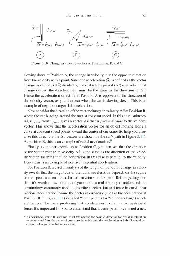
3.2 Curvilinear motion 75
vfinalvfinal
vfinal
–vinitial –vinitial
Δv = vfinal – vinitial
A B C
–vinitial
Δv = vfinal – vinitial Δv = vfinal – vinitial
Figure 3.10 Change in velocity vectors at Positions A, B, and C.
slowing down at Position A, the change in velocity is in the opposite directionfrom the velocity at this point. Since the acceleration (�a) is defined as the vectorchange in velocity (�v) divided by the scalar time period (t) over which thatchange occurs, the direction of �a must be the same as the direction of �v.Hence the acceleration direction at Position A is opposite to the direction ofthe velocity vector, as you’d expect when the car is slowing down. This is anexample of negative tangential acceleration.
Now consider the direction of the vector change in velocity�v at Position B,where the car is going around the turn at constant speed. In this case, subtract-ing �vini tial from �v f inal gives a vector �v that is perpendicular to the velocityvector. This shows that the acceleration vector for an object moving along acurve at constant speed points toward the center of curvature (to help you visu-alize this direction, the�v vectors are shown on the car’s path in Figure 3.11).At position B, this is an example of radial acceleration.9
Finally, as the car speeds up at Position C, you can see that the directionof the vector change in velocity �v is the same as the direction of the veloc-ity vector, meaning that the accleration in this case is parallel to the velocity.Hence this is an example of positive tangential acceleration.
For Position B, a careful analysis of the length of the vector change in veloc-ity reveals that the magnitude of the radial acceleration depends on the squareof the speed and on the radius of curvature of the path. Before getting intothat, it’s worth a few minutes of your time to make sure you understand theterminology commonly used to describe acceleration and force in curvilinearmotion. Acceleration toward the center of curvature (such as the acceleration atPosition B in Figure 3.11) is called “centripetal” (for “center-seeking”) accel-eration, and the force producing that acceleration is often called centripetalforce. It’s important for you to understand that a centripetal force is not a new
9 As described later in this section, most texts define the positive direction for radial accelerationto be outward from the center of curvature, in which case the acceleration at Point B would beconsidered negative radial acceleration.
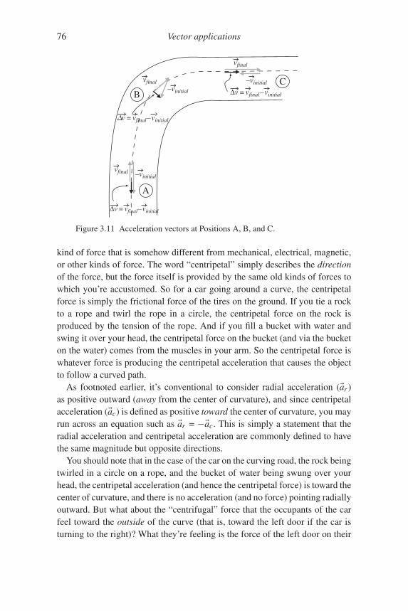
76 Vector applications
A
BC
Δv = vfinal–vinitial
Δv = vfinal–vinitial
Δv = vfinal–vinitial
vfinal
vfinal
–vinitial
–vinitial–vinitial
vfinal
Figure 3.11 Acceleration vectors at Positions A, B, and C.
kind of force that is somehow different from mechanical, electrical, magnetic,or other kinds of force. The word “centripetal” simply describes the directionof the force, but the force itself is provided by the same old kinds of forces towhich you’re accustomed. So for a car going around a curve, the centripetalforce is simply the frictional force of the tires on the ground. If you tie a rockto a rope and twirl the rope in a circle, the centripetal force on the rock isproduced by the tension of the rope. And if you fill a bucket with water andswing it over your head, the centripetal force on the bucket (and via the bucketon the water) comes from the muscles in your arm. So the centripetal force iswhatever force is producing the centripetal acceleration that causes the objectto follow a curved path.
As footnoted earlier, it’s conventional to consider radial acceleration (�ar )as positive outward (away from the center of curvature), and since centripetalacceleration (�ac) is defined as positive toward the center of curvature, you mayrun across an equation such as �ar = −�ac. This is simply a statement that theradial acceleration and centripetal acceleration are commonly defined to havethe same magnitude but opposite directions.
You should note that in the case of the car on the curving road, the rock beingtwirled in a circle on a rope, and the bucket of water being swung over yourhead, the centripetal acceleration (and hence the centripetal force) is toward thecenter of curvature, and there is no acceleration (and no force) pointing radiallyoutward. But what about the “centrifugal” force that the occupants of the carfeel toward the outside of the curve (that is, toward the left door if the car isturning to the right)? What they’re feeling is the force of the left door on their
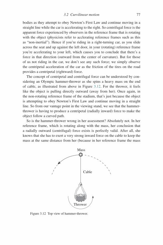
3.2 Curvilinear motion 77
bodies as they attempt to obey Newton’s First Law and continue moving in astraight line while the car is accelerating to the right. So centrifugal force is theapparent force experienced by observers in the reference frame that is rotatingwith the object (physicists refer to acclerating reference frames such as thisas “non-inertial”). Hence if you’re riding in a right-turning car, as you slideacross the seat and up against the left door, in your (rotating) reference frameyou’re accelerating to your left, which causes you to conclude that there’s aforce in that direction (outward from the center of curvature). But for thoseof us not riding in the car, we don’t see any such force; we simply observethe centripetal acceleration of the car as the friction of the tires on the roadprovides a centripetal (rightward) force.
The concept of centripetal and centrifugal force can be understood by con-sidering an Olympic hammer-thrower as she spins a heavy mass on the endof cable, as illustrated from above in Figure 3.12. For the thrower, it feelslike the object is pulling directly outward (away from her). Once again, inthe non-rotating reference frame of the stadium, that’s just because the objectis attempting to obey Newton’s First Law and continue moving in a straightline. So from our vantage point in the viewing stand, we see that the hammer-thrower is having to produce a centripetal (radially inward) force to make theobject follow a curved path.
So is the hammer-thrower wrong in her assessment? Absolutely not. In herreference frame, which is rotating along with the mass, her conclusion thata radially outward (centrifugal) force exists is perfectly valid. After all, sheknows that she has to exert a very strong inward force on the cable to keep themass at the same distance from her (because in her reference frame the mass
Thrower
Cable
Mass
Figure 3.12 Top view of hammer-thrower.
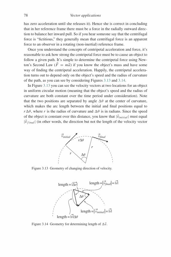
78 Vector applications
has zero acceleration until she releases it). Hence she is correct in concludingthat in her reference frame there must be a force in the radially outward direc-tion to balance her inward pull. So if you hear someone say that the centrifugalforce is “fictitious,” they generally mean that centrifugal force is an apparentforce to an observer in a rotating (non-inertial) reference frame.
Once you understand the concepts of centripetal acceleration and force, it’sreasonable to ask how strong the centripetal force must be to cause an object tofollow a given path. It’s simple to determine the centripetal force using New-ton’s Second Law ( �F = m�a) if you know the object’s mass and have someway of finding the centripetal acceleration. Happily, the centripetal accelera-tion turns out to depend only on the object’s speed and the radius of curvatureof the path, as you can see by considering Figures 3.13 and 3.14.
In Figure 3.13 you can see the velocity vectors at two locations for an objectin uniform circular motion (meaning that the object’s speed and the radius ofcurvature are both constant over the time period under consideration). Notethat the two positions are separated by angle θ at the center of curvature,which makes the arc length between the initial and final positions equal torθ , where r is the radius of curvature and θ is in radians. Since the speedof the object is constant over this distance, you know that |�vini tial | must equal|�v f inal | (in other words, the direction but not the length of the velocity vector
r
r
rΔθ
Δθ
vfinalvinitial
Figure 3.13 Geometry of changing direction of velocity.
length = vfinal = |v|length = |Δv|
length = vinitial = |v|
length = |v|Δθ
Δθ
Figure 3.14 Geometry for determining length of �v.
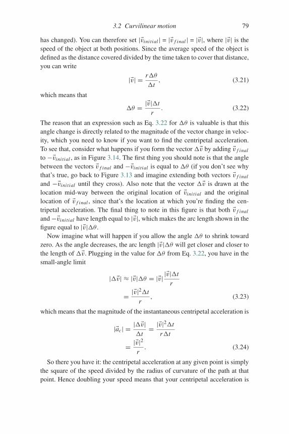
3.2 Curvilinear motion 79
has changed). You can therefore set |�vini tial | = |�v f inal | = |�v|, where |�v| is thespeed of the object at both positions. Since the average speed of the object isdefined as the distance covered divided by the time taken to cover that distance,you can write
|�v| = rθ
t, (3.21)
which means that
θ = |�v|t
r. (3.22)
The reason that an expression such as Eq. 3.22 for θ is valuable is that thisangle change is directly related to the magnitude of the vector change in veloc-ity, which you need to know if you want to find the centripetal acceleration.To see that, consider what happens if you form the vector�v by adding �v f inal
to −�vini tial , as in Figure 3.14. The first thing you should note is that the anglebetween the vectors �v f inal and −�vini tial is equal to θ (if you don’t see whythat’s true, go back to Figure 3.13 and imagine extending both vectors �v f inal
and −�vini tial until they cross). Also note that the vector �v is drawn at thelocation mid-way between the original location of �vini tial and the originallocation of �v f inal , since that’s the location at which you’re finding the cen-tripetal acceleration. The final thing to note in this figure is that both �v f inal
and−�vini tial have length equal to |�v|, which makes the arc length shown in thefigure equal to |�v|θ .
Now imagine what will happen if you allow the angle θ to shrink towardzero. As the angle decreases, the arc length |�v|θ will get closer and closer tothe length of �v. Plugging in the value for θ from Eq. 3.22, you have in thesmall-angle limit
|�v| ≈ |�v|θ = |�v| |�v|t
r
= |�v|2t
r, (3.23)
which means that the magnitude of the instantaneous centripetal acceleration is
|�ac| = |�v|t= |�v|
2t
rt
= |�v|2
r. (3.24)
So there you have it: the centripetal acceleration at any given point is simplythe square of the speed divided by the radius of curvature of the path at thatpoint. Hence doubling your speed means that your centripetal acceleration is
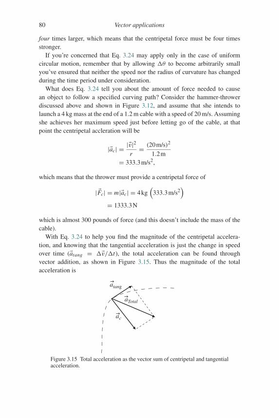
80 Vector applications
four times larger, which means that the centripetal force must be four timesstronger.
If you’re concerned that Eq. 3.24 may apply only in the case of uniformcircular motion, remember that by allowing θ to become arbitrarily smallyou’ve ensured that neither the speed nor the radius of curvature has changedduring the time period under consideration.
What does Eq. 3.24 tell you about the amount of force needed to causean object to follow a specified curving path? Consider the hammer-throwerdiscussed above and shown in Figure 3.12, and assume that she intends tolaunch a 4 kg mass at the end of a 1.2 m cable with a speed of 20 m/s. Assumingshe achieves her maximum speed just before letting go of the cable, at thatpoint the centripetal accleration will be
|�ac| = |�v|2
r= (20m/s)2
1.2m= 333.3m/s2,
which means that the thrower must provide a centripetal force of
| �Fc| = m|�ac| = 4kg(
333.3m/s2)
= 1333.3N
which is almost 300 pounds of force (and this doesn’t include the mass of thecable).
With Eq. 3.24 to help you find the magnitude of the centripetal accelera-tion, and knowing that the tangential acceleration is just the change in speedover time (�atang = �v/t), the total acceleration can be found throughvector addition, as shown in Figure 3.15. Thus the magnitude of the totalacceleration is
atang
ac
aTotal
Figure 3.15 Total acceleration as the vector sum of centripetal and tangentialacceleration.
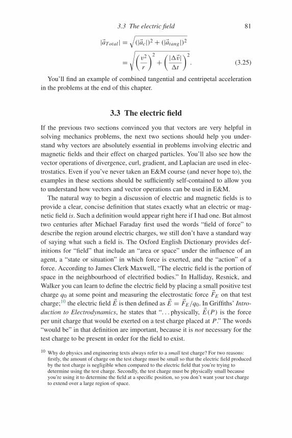
3.3 The electric field 81
|�aT otal | =√(|�ac|)2 + (|�atang|)2
=√(
v2
r
)2
+( |�v|t
)2
. (3.25)
You’ll find an example of combined tangential and centripetal accelerationin the problems at the end of this chapter.
3.3 The electric field
If the previous two sections convinced you that vectors are very helpful insolving mechanics problems, the next two sections should help you under-stand why vectors are absolutely essential in problems involving electric andmagnetic fields and their effect on charged particles. You’ll also see how thevector operations of divergence, curl, gradient, and Laplacian are used in elec-trostatics. Even if you’ve never taken an E&M course (and never hope to), theexamples in these sections should be sufficiently self-contained to allow youto understand how vectors and vector operations can be used in E&M.
The natural way to begin a discussion of electric and magnetic fields is toprovide a clear, concise definition that states exactly what an electric or mag-netic field is. Such a definition would appear right here if I had one. But almosttwo centuries after Michael Faraday first used the words “field of force” todescribe the region around electric charges, we still don’t have a standard wayof saying what such a field is. The Oxford English Dictionary provides def-initions for “field” that include an “area or space” under the influence of anagent, a “state or situation” in which force is exerted, and the “action” of aforce. According to James Clerk Maxwell, “The electric field is the portion ofspace in the neighbourhood of electrified bodies.” In Halliday, Resnick, andWalker you can learn to define the electric field by placing a small positive testcharge q0 at some point and measuring the electrostatic force �FE on that testcharge;10 the electric field �E is then defined as �E = �FE/q0. In Griffiths’ Intro-duction to Electrodynamics, he states that “. . . physically, �E(P) is the forceper unit charge that would be exerted on a test charge placed at P .” The words“would be” in that definition are important, because it is not necessary for thetest charge to be present in order for the field to exist.
10 Why do physics and engineering texts always refer to a small test charge? For two reasons:firstly, the amount of charge on the test charge must be small so that the electric field producedby the test charge is negligible when compared to the electric field that you’re trying todetermine using the test charge. Secondly, the test charge must be physically small becauseyou’re using it to determine the field at a specific position, so you don’t want your test chargeto extend over a large region of space.
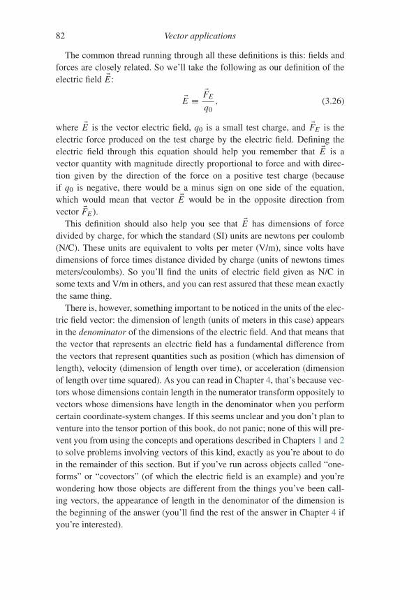
82 Vector applications
The common thread running through all these definitions is this: fields andforces are closely related. So we’ll take the following as our definition of theelectric field �E :
�E ≡ �FE
q0, (3.26)
where �E is the vector electric field, q0 is a small test charge, and �FE is theelectric force produced on the test charge by the electric field. Defining theelectric field through this equation should help you remember that �E is avector quantity with magnitude directly proportional to force and with direc-tion given by the direction of the force on a positive test charge (becauseif q0 is negative, there would be a minus sign on one side of the equation,which would mean that vector �E would be in the opposite direction fromvector �FE ).
This definition should also help you see that �E has dimensions of forcedivided by charge, for which the standard (SI) units are newtons per coulomb(N/C). These units are equivalent to volts per meter (V/m), since volts havedimensions of force times distance divided by charge (units of newtons timesmeters/coulombs). So you’ll find the units of electric field given as N/C insome texts and V/m in others, and you can rest assured that these mean exactlythe same thing.
There is, however, something important to be noticed in the units of the elec-tric field vector: the dimension of length (units of meters in this case) appearsin the denominator of the dimensions of the electric field. And that means thatthe vector that represents an electric field has a fundamental difference fromthe vectors that represent quantities such as position (which has dimension oflength), velocity (dimension of length over time), or acceleration (dimensionof length over time squared). As you can read in Chapter 4, that’s because vec-tors whose dimensions contain length in the numerator transform oppositely tovectors whose dimensions have length in the denominator when you performcertain coordinate-system changes. If this seems unclear and you don’t plan toventure into the tensor portion of this book, do not panic; none of this will pre-vent you from using the concepts and operations described in Chapters 1 and 2to solve problems involving vectors of this kind, exactly as you’re about to doin the remainder of this section. But if you’ve run across objects called “one-forms” or “covectors” (of which the electric field is an example) and you’rewondering how those objects are different from the things you’ve been call-ing vectors, the appearance of length in the denominator of the dimension isthe beginning of the answer (you’ll find the rest of the answer in Chapter 4 ifyou’re interested).
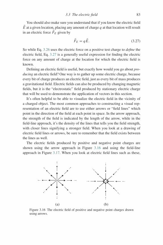
3.3 The electric field 83
You should also make sure you understand that if you know the electric field�E at a given location, placing any amount of charge q at that location will result
in an electric force �FE given by
�FE = q �E . (3.27)
So while Eq. 3.26 uses the electric force on a positive test charge to define theelectric field, Eq. 3.27 is a generally useful expression for finding the electricforce on any amount of charge at the location for which the electric field isknown.
Defining an electric field is useful, but exactly how would you go about pro-ducing an electric field? One way is to gather up some electric charge, becauseevery bit of charge produces an electric field, just as every bit of mass producesa gravitational field. Electric fields can also be produced by changing magneticfields, but it is the “electrostatic” field produced by stationary electric chargethat will be used to demonstrate the application of vectors in this section.
It’s often helpful to be able to visualize the electric field in the vicinity ofa charged object. The most common approaches to constructing a visual rep-resentation of an electric field are to use either arrows or “field lines” whichpoint in the direction of the field at each point in space. In the arrow approach,the strength of the field is indicated by the length of the arrow, while in thefield-line approach, it’s the density of the lines that tells you the field strength,with closer lines signifying a stronger field. When you look at a drawing ofelectric field lines or arrows, be sure to remember that the field exists betweenthe lines as well.
The electric fields produced by positive and negative point charges areshown using the arrow approach in Figure 3.16 and using the field-lineapproach in Figure 3.17. When you look at electric field lines such as these,
+
(a)
_
(b)
Figure 3.16 The electric field of positive and negative point charges drawnusing arrows.
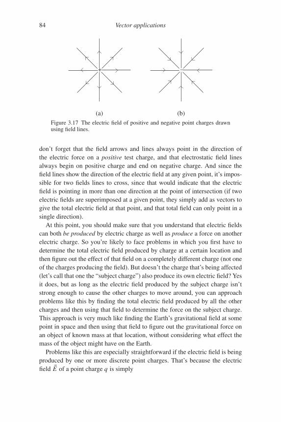
84 Vector applications
+
(a)
–
(b)
Figure 3.17 The electric field of positive and negative point charges drawnusing field lines.
don’t forget that the field arrows and lines always point in the direction ofthe electric force on a positive test charge, and that electrostatic field linesalways begin on positive charge and end on negative charge. And since thefield lines show the direction of the electric field at any given point, it’s impos-sible for two fields lines to cross, since that would indicate that the electricfield is pointing in more than one direction at the point of intersection (if twoelectric fields are superimposed at a given point, they simply add as vectors togive the total electric field at that point, and that total field can only point in asingle direction).
At this point, you should make sure that you understand that electric fieldscan both be produced by electric charge as well as produce a force on anotherelectric charge. So you’re likely to face problems in which you first have todetermine the total electric field produced by charge at a certain location andthen figure out the effect of that field on a completely different charge (not oneof the charges producing the field). But doesn’t the charge that’s being affected(let’s call that one the “subject charge”) also produce its own electric field? Yesit does, but as long as the electric field produced by the subject charge isn’tstrong enough to cause the other charges to move around, you can approachproblems like this by finding the total electric field produced by all the othercharges and then using that field to determine the force on the subject charge.This approach is very much like finding the Earth’s gravitational field at somepoint in space and then using that field to figure out the gravitational force onan object of known mass at that location, without considering what effect themass of the object might have on the Earth.
Problems like this are especially straightforward if the electric field is beingproduced by one or more discrete point charges. That’s because the electricfield �E of a point charge q is simply
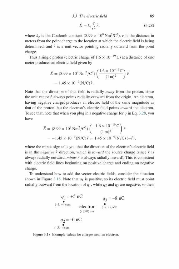
3.3 The electric field 85
�E = keq
r2r , (3.28)
where ke is the Coulomb constant (8.99 × 10⁹ Nm2/C2), r is the distance inmeters from the point charge to the location at which the electric field is beingdetermined, and r is a unit vector pointing radially outward from the pointcharge.
Thus a single proton (electric charge of 1.6 × 10⁻¹⁹ C) at a distance of onemeter produces an electric field given by
�E = (8.99× 10⁹ Nm2/C2)
(1.6× 10⁻¹⁹C
(1 m)2
)r
= 1.45× 10⁻⁹(N/C) r .
Note that the direction of that field is radially away from the proton, sincethe unit vector r always points radially outward from the origin. An electron,having negative charge, produces an electric field of the same magnitude asthat of the proton, but the electron’s electric field points toward the electron.To see that, note that when you plug in a negative charge for q in Eq. 3.28, youhave
�E = (8.99× 10⁹ Nm2/C2)
(−1.6× 10⁻¹⁹ C
(1 m)2
)r
= −1.45× 10⁻⁹(N/C) r = 1.45× 10⁻⁹(N/C)(−r),
where the minus sign tells you that the direction of the electron’s electric fieldis in the negative r direction, which is toward the source charge (since r isalways radially outward, minus r is always radially inward). This is consistentwith electric field lines beginning on positive charge and ending on negativecharge.
To understand how to add the vector electric fields, consider the situationshown in Figure 3.18. Note that q1 is positive, so its electric field must pointradially outward from the location of q1, while q2 and q3 are negative, so their
q1 = +5 nC
q2 = –6 nC
q3 = –8 nC
electron(–5, +4) cm
(–5, –4) cm
(+7, +2) cm(0,0) cm
Figure 3.18 Example values for charges near an electron.
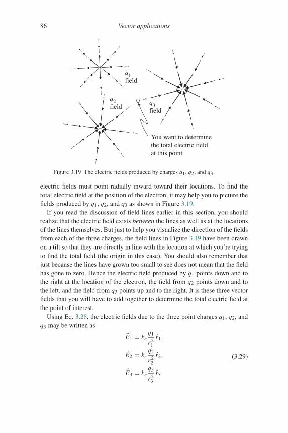
86 Vector applications
_
+
-
q1field
q2field
q3field
You want to determinethe total electric fieldat this point
Figure 3.19 The electric fields produced by charges q1, q2, and q3.
electric fields must point radially inward toward their locations. To find thetotal electric field at the position of the electron, it may help you to picture thefields produced by q1, q2, and q3 as shown in Figure 3.19.
If you read the discussion of field lines earlier in this section, you shouldrealize that the electric field exists between the lines as well as at the locationsof the lines themselves. But just to help you visualize the direction of the fieldsfrom each of the three charges, the field lines in Figure 3.19 have been drawnon a tilt so that they are directly in line with the location at which you’re tryingto find the total field (the origin in this case). You should also remember thatjust because the lines have grown too small to see does not mean that the fieldhas gone to zero. Hence the electric field produced by q1 points down and tothe right at the location of the electron, the field from q2 points down and tothe left, and the field from q3 points up and to the right. It is these three vectorfields that you will have to add together to determine the total electric field atthe point of interest.
Using Eq. 3.28, the electric fields due to the three point charges q1, q2, andq3 may be written as
�E1 = keq1
r21
r1,
�E2 = keq2
r22
r2,
�E3 = keq3
r23
r3.
(3.29)
3.3 The electric field 87
Of course, you know from Figure 3.19 that these three electric fields do notpoint in the same direction. That’s because the unit vector r1 points radiallyoutward from the location of charge q1, and r2 and r3 point radially outwardfrom q2 and q3, respectively. This means you can’t add the three electric fieldsalgebraically; to find the total field you must use vector addition. You’ll findan example of the vector addition of electric fields in the problems at the endof this chapter and the on-line solutions.
As you might suspect, it’s not just the simple operations of vector additionand multiplication by a scalar that find use in electrostatics. If you followedthe discussion of the divergence operation in Chapter 2, you may be wonder-ing about the divergence of the electrostatic fields produced by a point charge(Figures 3.16 and 3.17). In fact, one of the fundamental laws of electrostaticsis Gauss’s Law for electric fields, the differential form of which is
�∇ ◦ �E = ρ/ε0, (3.30)
where ρ represents the volume electric charge density (coulombs per cubicmeter) and ε0 is the vacuum permittivity of free space (8.85×10⁻¹² Nm2/C2).
Gauss’s Law for electric fields tells you that electric field lines diverge fromany location at which positive charge exists (positive ρ) and converge uponany location at which negative charge is present (negative ρ). This explains theanalogy between the “flow” of electrostatic field lines and the flow of a fluid.In this analogy, positive charge acts as the “source” of electrostatic field linesin the same sense as a faucet acts as the source of fluid, and negative chargeacts as a “sink” of electrostatic field lines just as a drain does for fluid.
Note what happens when you take the divergence of the electric field of apoint charge (this is most easily done in spherical coordinates):
�∇ ◦ �E = 1
r2
∂
∂r(r2 Er ) = 1
r2
∂
∂r
(r2ke
q
r2
)= 1
r2
∂
∂r(keq) = 0.
This is consistent with the worked example in Chapter 2 showing that thedivergence of any radial vector field is zero if the amplitude of the field fallsoff as 1/r2. Zero, that is, at all locations except where r = 0, the location ofthe source of the field. Thus Gauss’s Law tells you that electrostatic field linesdiverge only from those locations at which positive electric charge exists, andconverge only on those locations at which negative charge exists.
You can gain additional understanding of the behavior of the electrostaticfield by considering the curl of �E for a point charge. Since Eθ and Eφ are bothzero, the curl in spherical coordinates becomes
88 Vector applications
�∇ × �E = 1
r
1
sin θ
∂Er
∂φθ + 1
r
(−∂Er
∂θ
)φ
= 1
r
1
sin θ
∂
∂φ
(keq
r
)θ + 1
r
[− ∂
∂θ
(keq
r
)]φ
= 0.
This is not a surprising result in light of the radial nature of the electrostaticfield of a point charge.
As mentioned in Chapter 2, vector fields with zero curl are called irro-tational, and such fields have several important properties. One of thoseproperties arises from the fact that the curl of a gradient is always zero: anirrotational vector field may always be written as the gradient of a scalar field.
In the case of electrostatic fields, the electric field may be written as the gra-dient of the scalar electric potential (usually written as φ or V ). By convention,the electric field is written as the negative gradient of the scalar potential, soyou’re likely to see this relationship written as
�E = −�∇V, (3.31)
where V is the scalar electric potential with units of Nm/C (equivalent to joulesper coulomb or volts).
Since the electric field is the negative of the change in electric potentialwith distance, moving along an electric field line in the direction it’s pointingmeans that you’re moving toward a region of lower electric potential. Likewise,moving in the opposite direction (opposite to the direction of the field) takesyou into a region of higher potential, and moving perpendicular to the fieldlines results in no change in potential. Hence the “equipotential” surfaces arealways perpendicular to the electric field lines.
Another differential vector operation useful in electrostatics is the Laplacian(∇2). Recall that the Laplacian involves the second spatial derivative, specif-ically the divergence of the gradient. Since the electrostatic field �E may bewritten as the negative of the gradient of the scalar potential V , taking thedivergence of the electric field gives:
�∇ ◦ �E = �∇ ◦ (−�∇V ) = −∇2V . (3.32)
Since Gauss’s Law says that the divergence of the electrostatic field must equalρ/ε0, this means
∇2V = −ρ/ε0. (3.33)
This is known as Poisson’s Equation. Since the Laplacian finds peaks and val-leys of a function (locations at which the value of the function differs from the
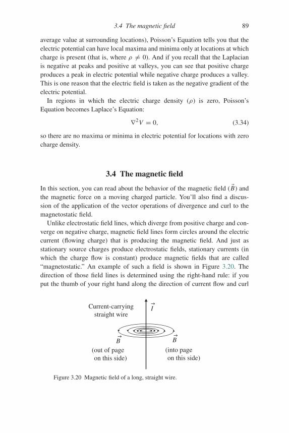
3.4 The magnetic field 89
average value at surrounding locations), Poisson’s Equation tells you that theelectric potential can have local maxima and minima only at locations at whichcharge is present (that is, where ρ �= 0). And if you recall that the Laplacianis negative at peaks and positive at valleys, you can see that positive chargeproduces a peak in electric potential while negative charge produces a valley.This is one reason that the electric field is taken as the negative gradient of theelectric potential.
In regions in which the electric charge density (ρ) is zero, Poisson’sEquation becomes Laplace’s Equation:
∇2V = 0, (3.34)
so there are no maxima or minima in electric potential for locations with zerocharge density.
3.4 The magnetic field
In this section, you can read about the behavior of the magnetic field ( �B) andthe magnetic force on a moving charged particle. You’ll also find a discus-sion of the application of the vector operations of divergence and curl to themagnetostatic field.
Unlike electrostatic field lines, which diverge from positive charge and con-verge on negative charge, magnetic field lines form circles around the electriccurrent (flowing charge) that is producing the magnetic field. And just asstationary source charges produce electrostatic fields, stationary currents (inwhich the charge flow is constant) produce magnetic fields that are called“magnetostatic.” An example of such a field is shown in Figure 3.20. Thedirection of those field lines is determined using the right-hand rule: if youput the thumb of your right hand along the direction of current flow and curl
I
B
Current-carryingstraight wire
(out of page on this side)
(into page on this side)
B
Figure 3.20 Magnetic field of a long, straight wire.
90 Vector applications
your fingers (like you’re grabbing the current), the magnetic field points in thedirection of your curled fingers. So if you were to reverse the direction of thatcurrent flow, the magnetic field lines would still form circles around the cur-rent, but the magnetic field lines would point in the opposite direction (as youcan tell by observing the direction of your curled fingers when your thumbpoints in the opposite direction).
You can tell by the spacing of the field lines in Figure 3.20 that the strengthof the magnetic field is decreasing as the distance from the current increases.For a thin wire of infinite length carrying current I , the vector magnetic fieldis given by the equation
�B = μ0 I
2πrφ, (3.35)
where μ0 is a constant called the magnetic permeability of free space, r isthe distance from the wire to the point at which the magnetic field is beingdetermined, and φ is the cylindrical-coordinate unit vector that points in thedirection circulating around the wire. The standard (SI) unit of magnetic fieldis the tesla (T).
Comparing the magnetic field lines around an electric current to the vectorfields with various values of divergence and curl discussed in Chapter 2, youmay have already guessed that magnetic fields fit into the “low divergence,high curl” category. Recall that electric field lines originate on positive chargeand terminate on negative charge, and it is only at the location of those chargesthat the divergence of the electrostatic field is non-zero. And since magneticfield lines circulate back onto themselves rather than diverging from and con-verging upon specific locations, it’s reasonable to expect small values for thedivergence of the magnetic field. In fact, the divergence of the magnetic field( �B) is exactly zero, as indicated by Gauss’s Law for magnetic fields:
�∇ ◦ �B = 0. (3.36)
You can verify this for the magnetic field of a long, straight wire by taking thedivergence of the field in Eq. 3.35:
�∇ ◦ �B = 1
r sin θ
∂Bφ∂φ= 1
r sin θ
∂
∂φ
(μ0 I
2πr
)= 0.
As you might expect from the discussion of curl in Chapter 2, the magneticfield around a current-carrying wire has zero curl:
3.4 The magnetic field 91
�∇ × �B =(−∂Bφ∂z
)r + 1
r
(∂(r Bφ)
∂r
)z
=[− ∂∂z
(μ0 I
2πr
)]r + 1
r
[∂
∂r
(rμ0 I
2πr
)]z
= 0.
As in the case of the divergence of the electric field, which has a non-zero valueonly at locations at which charge exists, the only locations at which the curl ofthe magnetic field is non-zero are locations at which current exists (that is, atthe singularity point r = 0).
Other uses of vectors and vector operations come about when you considerthe force ( �FB) produced by a magnetic field ( �B) on a moving electric charge(q). This force is given by the vector equation
�FB = q �v × �B, (3.37)
where �v is the velocity of the charged particle with respect to the magneticfield. The magnitude of the force is readily found using the definition of themagnitude of the vector cross product (| �A × �B| = | �A|| �B| sin θ ):
| �FB | = q|�v|| �B| sin θ, (3.38)
where θ is the angle between vector �v and vector �B.Examined carefully, Eqs. 3.37 and 3.38 can tell you a great deal about how
magnetic fields affect charged particles. Compare these equations to Eq. 3.27( �FE = q �E), and note that there are similarities and differences betweenelectric and magnetic forces:
• Similarity: Both are directly proportional to the amount of charge (q);• Similarity: Both are directly proportional to the field strength ( �E or �B);• Difference: The velocity (�v) of the particle appears in the magnetic
equation;• Difference: The magnetic force depends on the angle between the velocity
and the magnetic field;• Difference: The magnetic force is perpendicular to both the velocity and the
magnetic field.
The similarities seem reasonable: both electric and magnetic forces arestronger if the fields are stronger and if the amount of charge is greater. Also,charges with opposite signs feel forces in opposite directions. The first listeddifference (the fact that the magnetic force depends on the velocity of the parti-cle) has the interesting consequence that a charged particle at rest with respect
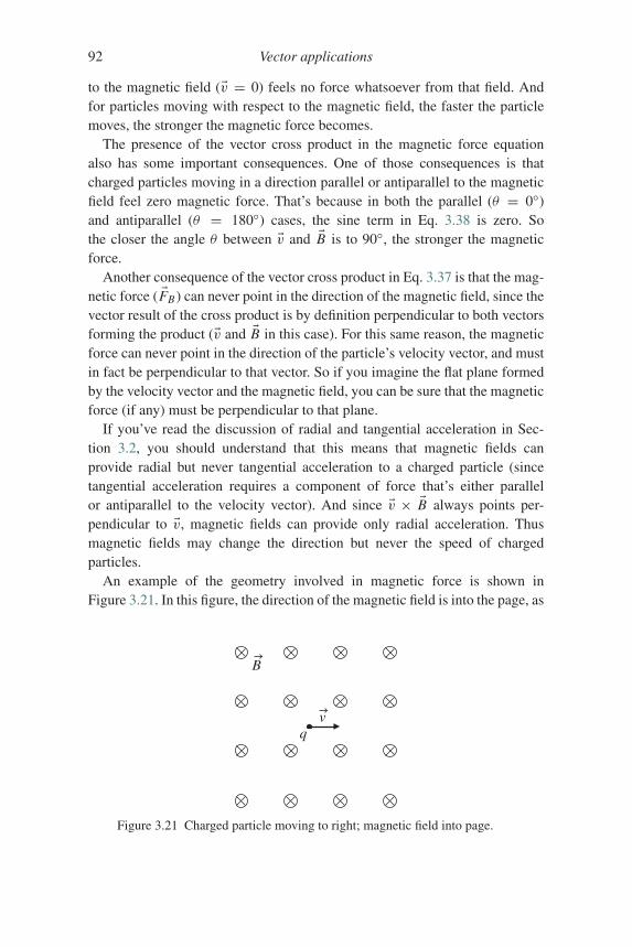
92 Vector applications
to the magnetic field (�v = 0) feels no force whatsoever from that field. Andfor particles moving with respect to the magnetic field, the faster the particlemoves, the stronger the magnetic force becomes.
The presence of the vector cross product in the magnetic force equationalso has some important consequences. One of those consequences is thatcharged particles moving in a direction parallel or antiparallel to the magneticfield feel zero magnetic force. That’s because in both the parallel (θ = 0◦)and antiparallel (θ = 180◦) cases, the sine term in Eq. 3.38 is zero. Sothe closer the angle θ between �v and �B is to 90◦, the stronger the magneticforce.
Another consequence of the vector cross product in Eq. 3.37 is that the mag-netic force ( �FB) can never point in the direction of the magnetic field, since thevector result of the cross product is by definition perpendicular to both vectorsforming the product (�v and �B in this case). For this same reason, the magneticforce can never point in the direction of the particle’s velocity vector, and mustin fact be perpendicular to that vector. So if you imagine the flat plane formedby the velocity vector and the magnetic field, you can be sure that the magneticforce (if any) must be perpendicular to that plane.
If you’ve read the discussion of radial and tangential acceleration in Sec-tion 3.2, you should understand that this means that magnetic fields canprovide radial but never tangential acceleration to a charged particle (sincetangential acceleration requires a component of force that’s either parallelor antiparallel to the velocity vector). And since �v × �B always points per-pendicular to �v, magnetic fields can provide only radial acceleration. Thusmagnetic fields may change the direction but never the speed of chargedparticles.
An example of the geometry involved in magnetic force is shown inFigure 3.21. In this figure, the direction of the magnetic field is into the page, as
B
vq
Figure 3.21 Charged particle moving to right; magnetic field into page.
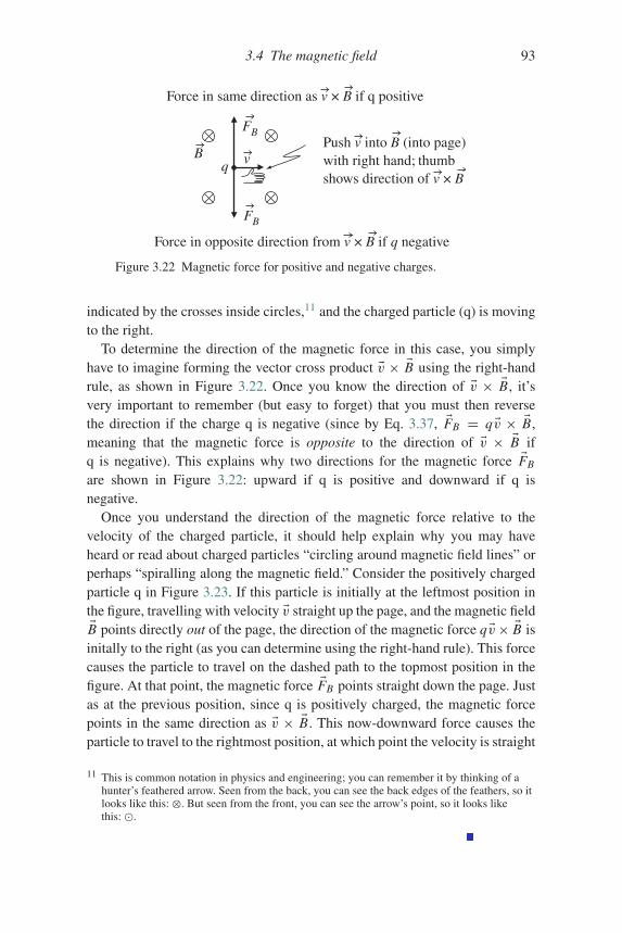
3.4 The magnetic field 93
B vq
Force in same direction as v × B if q positive
Force in opposite direction from v × B if q negative
Push v into B (into page)with right hand; thumbshows direction of v × B
FB
FB
Figure 3.22 Magnetic force for positive and negative charges.
indicated by the crosses inside circles,11 and the charged particle (q) is movingto the right.
To determine the direction of the magnetic force in this case, you simplyhave to imagine forming the vector cross product �v × �B using the right-handrule, as shown in Figure 3.22. Once you know the direction of �v × �B, it’svery important to remember (but easy to forget) that you must then reversethe direction if the charge q is negative (since by Eq. 3.37, �FB = q �v × �B,meaning that the magnetic force is opposite to the direction of �v × �B ifq is negative). This explains why two directions for the magnetic force �FB
are shown in Figure 3.22: upward if q is positive and downward if q isnegative.
Once you understand the direction of the magnetic force relative to thevelocity of the charged particle, it should help explain why you may haveheard or read about charged particles “circling around magnetic field lines” orperhaps “spiralling along the magnetic field.” Consider the positively chargedparticle q in Figure 3.23. If this particle is initially at the leftmost position inthe figure, travelling with velocity �v straight up the page, and the magnetic field�B points directly out of the page, the direction of the magnetic force q �v× �B isinitally to the right (as you can determine using the right-hand rule). This forcecauses the particle to travel on the dashed path to the topmost position in thefigure. At that point, the magnetic force �FB points straight down the page. Justas at the previous position, since q is positively charged, the magnetic forcepoints in the same direction as �v × �B. This now-downward force causes theparticle to travel to the rightmost position, at which point the velocity is straight
11 This is common notation in physics and engineering; you can remember it by thinking of ahunter’s feathered arrow. Seen from the back, you can see the back edges of the feathers, so itlooks like this: ⊗. But seen from the front, you can see the arrow’s point, so it looks likethis: �.
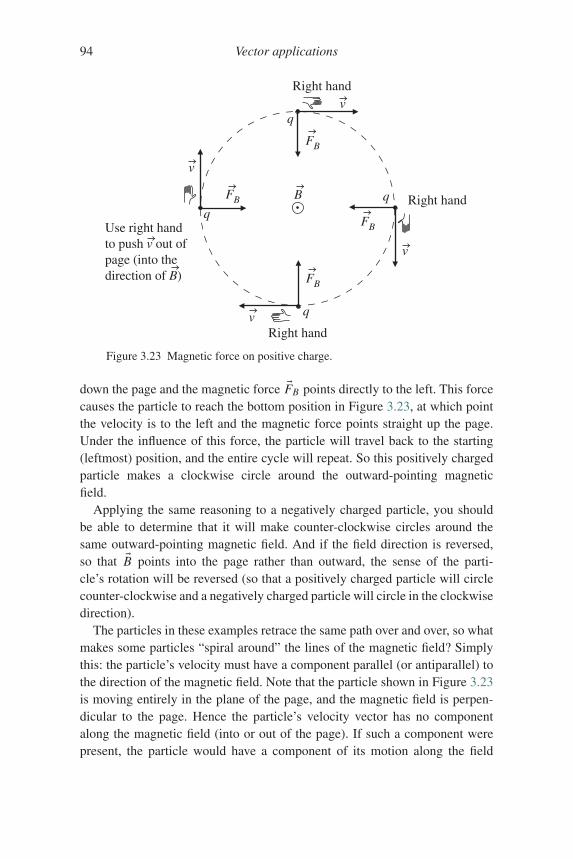
94 Vector applications
FB
v
Use right handto push v out ofpage (into thedirection of B)
Right hand
Right hand
Right hand
q
q
q
q
B
FB
FB
FB
v
v
v
Figure 3.23 Magnetic force on positive charge.
down the page and the magnetic force �FB points directly to the left. This forcecauses the particle to reach the bottom position in Figure 3.23, at which pointthe velocity is to the left and the magnetic force points straight up the page.Under the influence of this force, the particle will travel back to the starting(leftmost) position, and the entire cycle will repeat. So this positively chargedparticle makes a clockwise circle around the outward-pointing magneticfield.
Applying the same reasoning to a negatively charged particle, you shouldbe able to determine that it will make counter-clockwise circles around thesame outward-pointing magnetic field. And if the field direction is reversed,so that �B points into the page rather than outward, the sense of the parti-cle’s rotation will be reversed (so that a positively charged particle will circlecounter-clockwise and a negatively charged particle will circle in the clockwisedirection).
The particles in these examples retrace the same path over and over, so whatmakes some particles “spiral around” the lines of the magnetic field? Simplythis: the particle’s velocity must have a component parallel (or antiparallel) tothe direction of the magnetic field. Note that the particle shown in Figure 3.23is moving entirely in the plane of the page, and the magnetic field is perpen-dicular to the page. Hence the particle’s velocity vector has no componentalong the magnetic field (into or out of the page). If such a component werepresent, the particle would have a component of its motion along the field
3.5 Chapter 3 problems 95
lines while also circling around them. In that case, the circular path shown inFigure 3.23 would move into or out of the paper over time, and the circle wouldbecome a spiral. The magnetic field has no effect on the velocity component(v||) parallel or antiparallel to the field (since there’s no magnetic force in thatdirection), so the speed with which the particle moves along the field line isconstant as long as no other forces are acting.
3.5 Chapter 3 problems
3.1 Solve the box-on-a-ramp problem (that is, find the acceleration ofthe box) for the frictionless case using a Cartesian coordinate systemfor which the y-axis points vertically upward and the x-axis pointshorizontally to the right.
3.2 The maximum force of static friction is μs �Fn , where μs is the coefficientof static friction and �Fn is the normal force. How big must the coefficientof static friction μs be to prevent a box of mass m from sliding down aramp inclined 20 degrees from the horizontal?
3.3 If a delivery woman pushes a box of mass m up a 2 m ramp with a forceof 10 N, how fast is the box moving at the top of the ramp if the rampangle to the horizontal is 25 degrees and the coefficient of kinetic frictionis 0.33?
3.4 If the hammer-thrower shown on the cover of this book wishes tolaunch a hammer of mass 7.26 kg on a cable of length 1.22 m with aspeed of 22 m/s, what is the magnitude of the centripetal force he mustsupply?
3.5 Imagine a Formula 1 car going around a curve with radius of 10 m whileslowing from a speed of 180 mph to 120 mph in 2 s. What are the magni-tude and direction of the car’s acceleration at the instant the car’s speedis 150 mph?
3.6 If three electric charges q1, q2, and q3 have the values and locationsshown in Figure 3.18, find the electric field they produce at the origin(x = 0, y = 0), then use your value of the field to determine the electricforce on an electron at that location.
3.7 If the vector electric field �E in some region is given in spherical coordi-nates by 5
r r + 2r sin θ cosφ θ − 1
r sin θ cosφ φ (N/C), what is the volumecharge density ρ in that region?
3.8 If the scalar electric potential V in some region is given in cylindricalcoordinates by V (r, φ, z) = r2sinφ e−3/z , what is the electric field �E inthat region?
96 Vector applications
3.9 For the scalar electric potential V of Problem 3.8, use Poisson’s Equationto find volume charge density ρ in that region.
3.10 Find the magnitude and direction of the magnetic force on a chargedparticle with charge −4 nC and velocity �v = 2.5 × 10⁴ ı + 1.1 × 10⁴ j
(m/s) if the magnetic field in the region is given by �B = 1.2× 10⁻³ ı +5.6× 10⁻³ j − 3.2× 10⁻³ k (T).
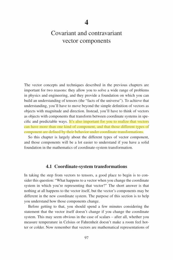
4
Covariant and contravariantvector components
The vector concepts and techniques described in the previous chapters areimportant for two reasons: they allow you to solve a wide range of problemsin physics and engineering, and they provide a foundation on which you canbuild an understanding of tensors (the “facts of the universe”). To achieve thatunderstanding, you’ll have to move beyond the simple definition of vectors asobjects with magnitude and direction. Instead, you’ll have to think of vectorsas objects with components that transform between coordinate systems in spe-cific and predictable ways. It’s also important for you to realize that vectorscan have more than one kind of component, and that those different types ofcomponent are defined by their behavior under coordinate transformations.
So this chapter is largely about the different types of vector component,and those components will be a lot easier to understand if you have a solidfoundation in the mathematics of coordinate-system transformation.
4.1 Coordinate-system transformations
In taking the step from vectors to tensors, a good place to begin is to con-sider this question: “What happens to a vector when you change the coordinatesystem in which you’re representing that vector?” The short answer is thatnothing at all happens to the vector itself, but the vector’s components may bedifferent in the new coordinate system. The purpose of this section is to helpyou understand how those components change.
Before getting to that, you should spend a few minutes considering thestatement that the vector itself doesn’t change if you change the coordinatesystem. This may seem obvious in the case of scalars – after all, whether youmeasure temperature in Celsius or Fahrenheit doesn’t make a room feel hot-ter or colder. Now remember that vectors are mathematical representations of
97
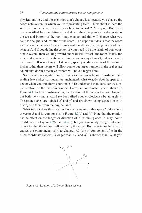
98 Covariant and contravariant vector components
physical entities, and those entities don’t change just because you change thecoordinate system in which you’re representing them. Think about it: does thesize of a room change if you tilt your head to one side? Clearly not. But if youuse your tilted head to define up and down, then the points you designate asthe top and bottom of the room may change, and this will change what youcall the “height” and “width” of the room. The important idea is that the roomitself doesn’t change (it “remains invariant”) under such a change of coordinatesystem. And if you define the center of your head to be the origin of your coor-dinate system, then walking toward one wall will “offset” the room (that is, thex , y, and z values of locations within the room may change), but once againthe room itself is unchanged. Likewise, specifying dimensions of the room ininches rather than meters will allow you to put larger numbers in the real-estatead, but that doesn’t mean your room will hold a bigger sofa.
So if coordinate-system transformations such as rotation, translation, andscaling leave physical quantities unchanged, what exactly does happen to avector when you transform coordinates? To understand that, consider the sim-ple rotation of the two-dimensional Cartesian coordinate system shown inFigure 4.1. In this transformation, the location of the origin has not changed,but both the x- and y-axis have been tilted counter-clockwise by an angle θ .The rotated axes are labeled x ′ and y′ and are drawn using dashed lines todistinguish them from the original axes.
What impact does this rotation have on a vector in this space? Take a lookat vector �A and its components in Figure 4.2(a) and (b). Note that the rotationhas no effect on the length or direction of �A (at first glance, �A may look abit different in Figure 4.2(a) and 4.2(b), but you can verify using a ruler andprotractor that the vector itself is exactly the same). But the rotation has clearlycaused the components of �A to change: A′x (the x ′-component of A in thetilted coordinate system) is longer than Ax , and A′y is shorter than Ay . If you
y′ y
x
x′θ
θ
Figure 4.1 Rotation of 2-D coordinate system.
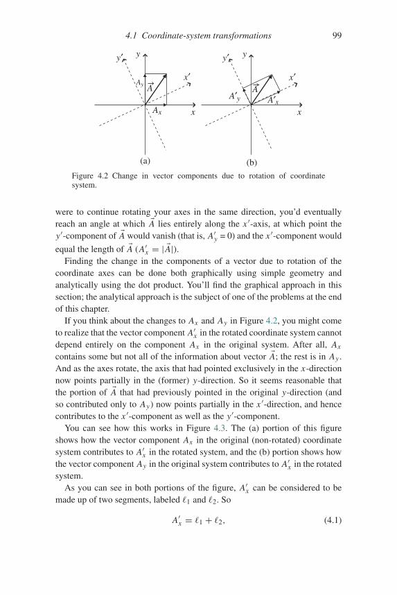
4.1 Coordinate-system transformations 99
y′ y
x
x′
y′ y
x
x′
A′A′A
(a) (b)
AAy
Ax
y x
Figure 4.2 Change in vector components due to rotation of coordinatesystem.
were to continue rotating your axes in the same direction, you’d eventuallyreach an angle at which �A lies entirely along the x ′-axis, at which point they′-component of �A would vanish (that is, A′y = 0) and the x ′-component would
equal the length of �A (A′x = | �A|).Finding the change in the components of a vector due to rotation of the
coordinate axes can be done both graphically using simple geometry andanalytically using the dot product. You’ll find the graphical approach in thissection; the analytical approach is the subject of one of the problems at the endof this chapter.
If you think about the changes to Ax and Ay in Figure 4.2, you might cometo realize that the vector component A′x in the rotated coordinate system cannotdepend entirely on the component Ax in the original system. After all, Ax
contains some but not all of the information about vector �A; the rest is in Ay .And as the axes rotate, the axis that had pointed exclusively in the x-directionnow points partially in the (former) y-direction. So it seems reasonable thatthe portion of �A that had previously pointed in the original y-direction (andso contributed only to Ay) now points partially in the x ′-direction, and hencecontributes to the x ′-component as well as the y′-component.
You can see how this works in Figure 4.3. The (a) portion of this figureshows how the vector component Ax in the original (non-rotated) coordinatesystem contributes to A′x in the rotated system, and the (b) portion shows howthe vector component Ay in the original system contributes to A′x in the rotatedsystem.
As you can see in both portions of the figure, A′x can be considered to bemade up of two segments, labeled �1 and �2. So
A′x = �1 + �2, (4.1)
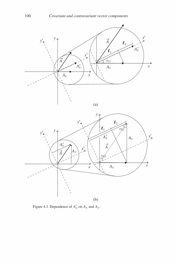
100 Covariant and contravariant vector components
y′ y
x
x′A
Ax
Ax
Ax′
x
(a)
y′ y
x
x′A
Ay
Ay
Ax
1
A ′
y
y′
x
x′
A
(b)
x
A ′x
A ′x
A ′x
α11
α12
α12
1
2
2
Figure 4.3 Dependence of A′x on Ax and Ay .
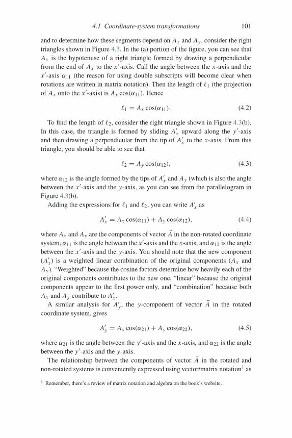
4.1 Coordinate-system transformations 101
and to determine how these segments depend on Ax and Ay , consider the righttriangles shown in Figure 4.3. In the (a) portion of the figure, you can see thatAx is the hypotenuse of a right triangle formed by drawing a perpendicularfrom the end of Ax to the x ′-axis. Call the angle between the x-axis and thex ′-axis α11 (the reason for using double subscripts will become clear whenrotations are written in matrix notation). Then the length of �1 (the projectionof Ax onto the x ′-axis) is Ax cos(α11). Hence
�1 = Ax cos(α11). (4.2)
To find the length of �2, consider the right triangle shown in Figure 4.3(b).In this case, the triangle is formed by sliding A′x upward along the y′-axisand then drawing a perpendicular from the tip of A′x to the x-axis. From thistriangle, you should be able to see that
�2 = Ay cos(α12), (4.3)
where α12 is the angle formed by the tips of A′x and Ay (which is also the anglebetween the x ′-axis and the y-axis, as you can see from the parallelogram inFigure 4.3(b).
Adding the expressions for �1 and �2, you can write A′x as
A′x = Ax cos(α11)+ Ay cos(α12), (4.4)
where Ax and Ay are the components of vector �A in the non-rotated coordinatesystem, α11 is the angle between the x ′-axis and the x-axis, and α12 is the anglebetween the x ′-axis and the y-axis. You should note that the new component(A′x ) is a weighted linear combination of the original components (Ax andAy). “Weighted” because the cosine factors determine how heavily each of theoriginal components contributes to the new one, “linear” because the originalcomponents appear to the first power only, and “combination” because bothAx and Ay contribute to A′x .
A similar analysis for A′y , the y-component of vector �A in the rotatedcoordinate system, gives
A′y = Ax cos(α21)+ Ay cos(α22), (4.5)
where α21 is the angle between the y′-axis and the x-axis, and α22 is the anglebetween the y′-axis and the y-axis.
The relationship between the components of vector �A in the rotated andnon-rotated systems is conveniently expressed using vector/matrix notation1 as
1 Remember, there’s a review of matrix notation and algebra on the book’s website.
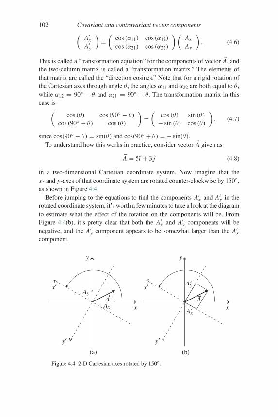
102 Covariant and contravariant vector components(A′xA′y
)=(
cos (α11) cos (α12)
cos (α21) cos (α22)
)(Ax
Ay
). (4.6)
This is called a “transformation equation” for the components of vector �A, andthe two-column matrix is called a “transformation matrix.” The elements ofthat matrix are called the “direction cosines.” Note that for a rigid rotation ofthe Cartesian axes through angle θ , the angles α11 and α22 are both equal to θ ,while α12 = 90◦ − θ and α21 = 90◦ + θ . The transformation matrix in thiscase is(
cos (θ) cos (90◦ − θ)cos (90◦ + θ) cos (θ)
)=(
cos (θ) sin (θ)− sin (θ) cos (θ)
), (4.7)
since cos(90◦ − θ) = sin(θ) and cos(90◦ + θ) = − sin(θ).To understand how this works in practice, consider vector �A given as
�A = 5ı + 3j (4.8)
in a two-dimensional Cartesian coordinate system. Now imagine that thex- and y-axes of that coordinate system are rotated counter-clockwise by 150◦,as shown in Figure 4.4.
Before jumping to the equations to find the components A′x and A′y in therotated coordinate system, it’s worth a few minutes to take a look at the diagramto estimate what the effect of the rotation on the components will be. FromFigure 4.4(b), it’s pretty clear that both the A′x and A′y components will benegative, and the A′y component appears to be somewhat larger than the A′xcomponent.
y′
y
x′Ay
Ax
Ax
y′
y
x′A ′
A ′
Ax
(b)(a)
y
x
Figure 4.4 2-D Cartesian axes rotated by 150◦.
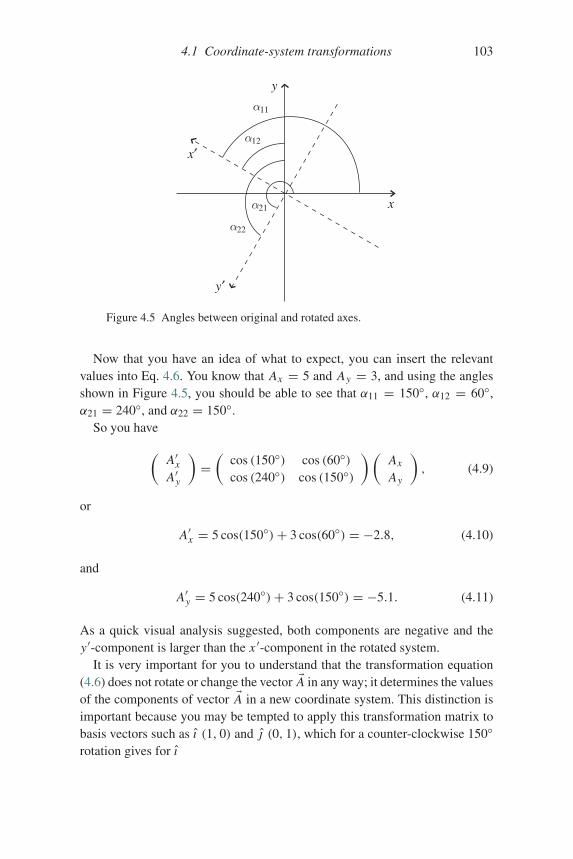
4.1 Coordinate-system transformations 103
y′
α22
α21
α12
α11
y
x′
x
Figure 4.5 Angles between original and rotated axes.
Now that you have an idea of what to expect, you can insert the relevantvalues into Eq. 4.6. You know that Ax = 5 and Ay = 3, and using the anglesshown in Figure 4.5, you should be able to see that α11 = 150◦, α12 = 60◦,α21 = 240◦, and α22 = 150◦.
So you have
(A′xA′y
)=(
cos (150◦) cos (60◦)cos (240◦) cos (150◦)
)(Ax
Ay
), (4.9)
or
A′x = 5 cos(150◦)+ 3 cos(60◦) = −2.8, (4.10)
and
A′y = 5 cos(240◦)+ 3 cos(150◦) = −5.1. (4.11)
As a quick visual analysis suggested, both components are negative and they′-component is larger than the x ′-component in the rotated system.
It is very important for you to understand that the transformation equation(4.6) does not rotate or change the vector �A in any way; it determines the valuesof the components of vector �A in a new coordinate system. This distinction isimportant because you may be tempted to apply this transformation matrix tobasis vectors such as ı (1, 0) and j (0, 1), which for a counter-clockwise 150◦rotation gives for ı
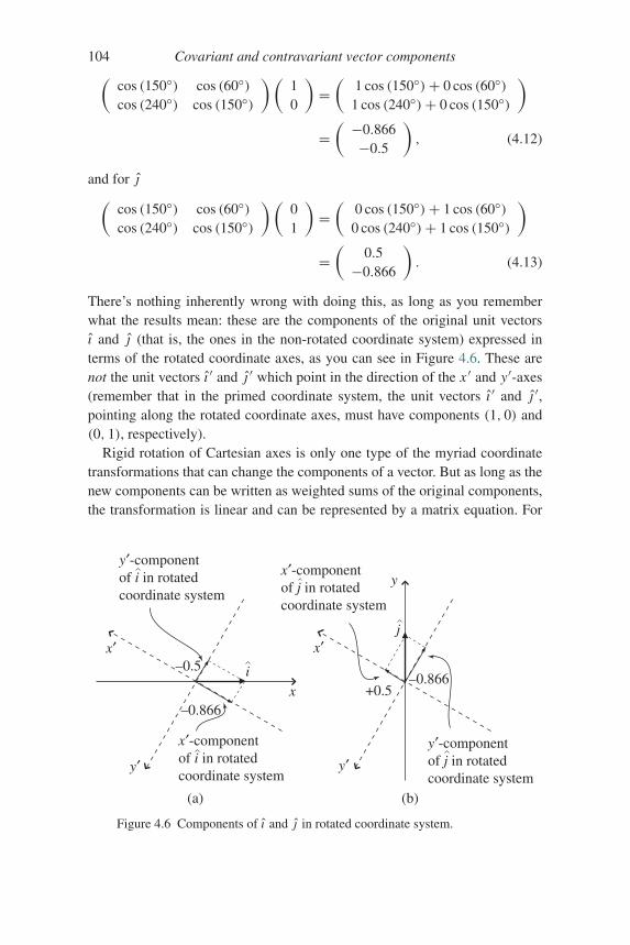
104 Covariant and contravariant vector components(cos (150◦) cos (60◦)cos (240◦) cos (150◦)
)(10
)=(
1 cos (150◦)+ 0 cos (60◦)1 cos (240◦)+ 0 cos (150◦)
)
=( −0.866−0.5
), (4.12)
and for j(cos (150◦) cos (60◦)cos (240◦) cos (150◦)
)(01
)=(
0 cos (150◦)+ 1 cos (60◦)0 cos (240◦)+ 1 cos (150◦)
)
=(
0.5−0.866
). (4.13)
There’s nothing inherently wrong with doing this, as long as you rememberwhat the results mean: these are the components of the original unit vectorsı and j (that is, the ones in the non-rotated coordinate system) expressed interms of the rotated coordinate axes, as you can see in Figure 4.6. These arenot the unit vectors ı ′ and j ′ which point in the direction of the x ′ and y′-axes(remember that in the primed coordinate system, the unit vectors ı ′ and j ′,pointing along the rotated coordinate axes, must have components (1, 0) and(0, 1), respectively).
Rigid rotation of Cartesian axes is only one type of the myriad coordinatetransformations that can change the components of a vector. But as long as thenew components can be written as weighted sums of the original components,the transformation is linear and can be represented by a matrix equation. For
y′
x′
x
y′
y
x′
(b)(a)
i–0.5
–0.866+0.5
–0.866
j
y′-componentof i in rotatedcoordinate system
y′-componentof j in rotatedcoordinate system
x′-componentof j in rotatedcoordinate system
x′-componentof i in rotatedcoordinate system
Figure 4.6 Components of ı and j in rotated coordinate system.
4.2 Basis-vector transformations 105
reasons that will become clear when you read Section 4.3 of this chapter, suchtransformations of vector components are called “inverse” or “passive” trans-formations, which means the matrix equation of such a transformation willlook like this:⎛
⎝ Components ofsame vector
in new system
⎞⎠ =
⎛⎝ Inverse
transformationmatrix
⎞⎠⎛⎝ Components of
vector inoriginal system
⎞⎠ .(4.14)
At this point, you may be wondering how you might go about transform-ing the unit vectors of the original (non-rotated) system (that is, ı and j ) intothe unit vectors of the primed (rotated) system (ı ′ and j ′). That’s a differentquestion, because you’re no longer asking, “Given the components of a vectorin one coordinate system, how do I find the components of that same vectorin a different coordinate system?” Instead, you’re asking, “How do I change agiven vector (in this case, a unit vector in one coordinate system) into a differ-ent vector (the unit vector in a different coordinate system)?” That question isaddressed in the next section.
4.2 Basis-vector transformations
The previous section illustrated what happens to the components of a vectorwhen the two-dimensional Cartesian axes are rotated, and the results are notsurprising: the components of the vector referenced to the new (rotated) axesare different from the components referenced to the original (non-rotated) axes.More specifically, the new components are weighted linear combinations of theoriginal components.
Now here’s a very important point: as your studies carry you along thepath from vectors to tensors, you will undoubtedly run across discussions of“covariant” and “contravariant” vector components.2 In those discussions, youmay see words to the effect that covariant components transform in the sameway as basis vectors (“co” ≈ “with”), and contravariant components trans-form in the opposite way to basis vectors (“contra” ≈ “against”). As you’llsee later in this chapter, there’s plenty of truth in that description, but there’salso a major pitfall. That’s because the “transformation” of basis vectors usu-ally refers to the conversion of the basis vectors in the original (non-rotated)coordinate system to the different basis vectors which point along the coordi-nate axes in the new (rotated) system, whereas the “transformation” of vector
2 These components are identical in the Cartesian coordinate systems considered so far.
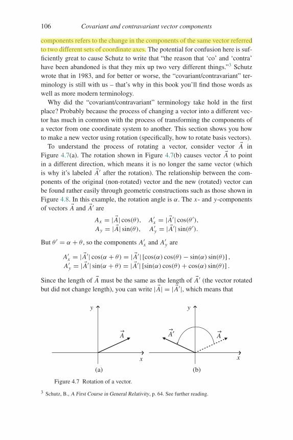
106 Covariant and contravariant vector components
components refers to the change in the components of the same vector referredto two different sets of coordinate axes. The potential for confusion here is suf-ficiently great to cause Schutz to write that “the reason that ‘co’ and ‘contra’have been abandoned is that they mix up two very different things.”3 Schutzwrote that in 1983, and for better or worse, the “covariant/contravariant” ter-minology is still with us – that’s why in this book you’ll find those words aswell as more modern terminology.
Why did the “covariant/contravariant” terminology take hold in the firstplace? Probably because the process of changing a vector into a different vec-tor has much in common with the process of transforming the components ofa vector from one coordinate system to another. This section shows you howto make a new vector using rotation (specifically, how to rotate basis vectors).
To understand the process of rotating a vector, consider vector �A inFigure 4.7(a). The rotation shown in Figure 4.7(b) causes vector �A to pointin a different direction, which means it is no longer the same vector (whichis why it’s labeled �A′ after the rotation). The relationship between the com-ponents of the original (non-rotated) vector and the new (rotated) vector canbe found rather easily through geometric constructions such as those shown inFigure 4.8. In this example, the rotation angle is α. The x- and y-componentsof vectors �A and �A′ are
Ax = | �A| cos(θ), A′x = | �A′| cos(θ ′),Ay = | �A| sin(θ), A′y = | �A′| sin(θ ′).
But θ ′ = α + θ , so the components A′x and A′y are
A′x = | �A′| cos(α + θ) = | �A′| [cos(α) cos(θ)− sin(α) sin(θ)] ,A′y = | �A′| sin(α + θ) = | �A′| [sin(α) cos(θ)+ cos(α) sin(θ)] .
Since the length of �A must be the same as the length of �A′ (the vector rotatedbut did not change length), you can write | �A| = | �A′|, which means that
y
x
A
y
x
(b)(a)
AA′
Figure 4.7 Rotation of a vector.
3 Schutz, B., A First Course in General Relativity, p. 64. See further reading.
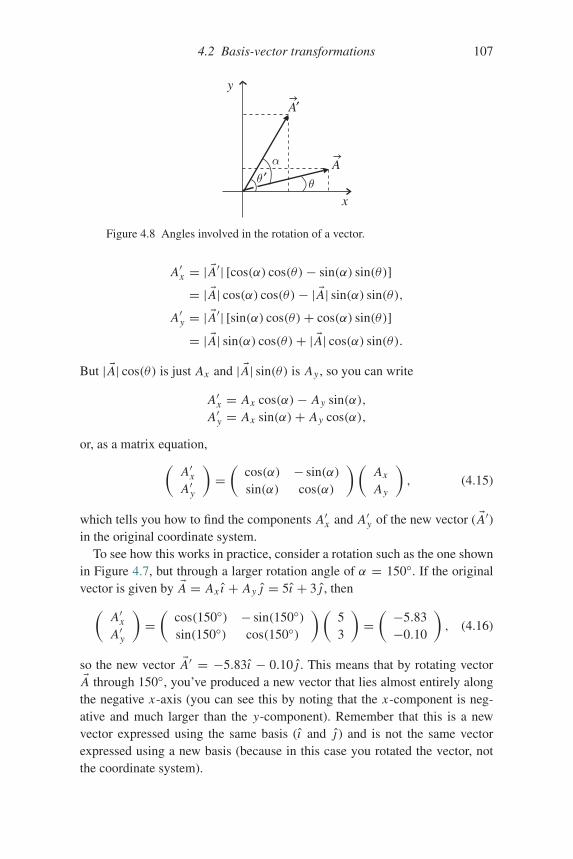
4.2 Basis-vector transformations 107
y
x
A
A′
θ ′ θ
α
Figure 4.8 Angles involved in the rotation of a vector.
A′x = | �A′| [cos(α) cos(θ)− sin(α) sin(θ)]
= | �A| cos(α) cos(θ)− | �A| sin(α) sin(θ),
A′y = | �A′| [sin(α) cos(θ)+ cos(α) sin(θ)]
= | �A| sin(α) cos(θ)+ | �A| cos(α) sin(θ).
But | �A| cos(θ) is just Ax and | �A| sin(θ) is Ay , so you can write
A′x = Ax cos(α)− Ay sin(α),A′y = Ax sin(α)+ Ay cos(α),
or, as a matrix equation,(A′xA′y
)=(
cos(α) − sin(α)sin(α) cos(α)
)(Ax
Ay
), (4.15)
which tells you how to find the components A′x and A′y of the new vector ( �A′)in the original coordinate system.
To see how this works in practice, consider a rotation such as the one shownin Figure 4.7, but through a larger rotation angle of α = 150◦. If the originalvector is given by �A = Ax ı + Ay j = 5ı + 3j , then(
A′xA′y
)=(
cos(150◦) − sin(150◦)sin(150◦) cos(150◦)
)(53
)=( −5.83−0.10
), (4.16)
so the new vector �A′ = −5.83ı − 0.10j . This means that by rotating vector�A through 150◦, you’ve produced a new vector that lies almost entirely along
the negative x-axis (you can see this by noting that the x-component is neg-ative and much larger than the y-component). Remember that this is a newvector expressed using the same basis (ı and j ) and is not the same vectorexpressed using a new basis (because in this case you rotated the vector, notthe coordinate system).
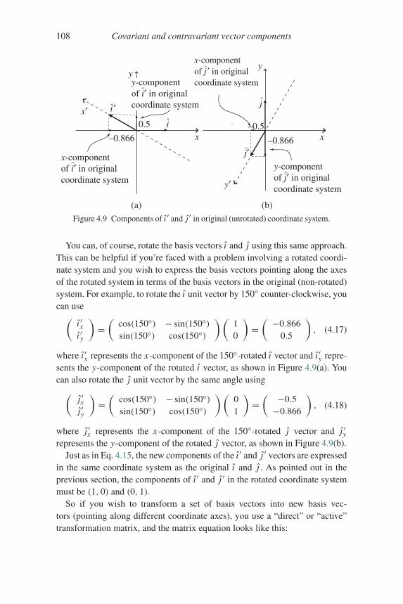
108 Covariant and contravariant vector components
x′
x
y′
y
(b)(a)
i0.5
–0.866–0.5
–0.866
j
x-componentof i′ in originalcoordinate system
x-componentof j ′ in originalcoordinate system
y-componentof j′ in originalcoordinate system
y
i ′
x
j′
y-componentof i′ in originalcoordinate system
Figure 4.9 Components of ı ′ and j ′ in original (unrotated) coordinate system.
You can, of course, rotate the basis vectors ı and j using this same approach.This can be helpful if you’re faced with a problem involving a rotated coordi-nate system and you wish to express the basis vectors pointing along the axesof the rotated system in terms of the basis vectors in the original (non-rotated)system. For example, to rotate the ı unit vector by 150◦ counter-clockwise, youcan use(
ı ′xı ′y
)=(
cos(150◦) − sin(150◦)sin(150◦) cos(150◦)
)(10
)=( −0.866
0.5
), (4.17)
where ı ′x represents the x-component of the 150◦-rotated ı vector and ı ′y repre-sents the y-component of the rotated ı vector, as shown in Figure 4.9(a). Youcan also rotate the j unit vector by the same angle using(
j ′xj ′y
)=(
cos(150◦) − sin(150◦)sin(150◦) cos(150◦)
)(01
)=( −0.5−0.866
), (4.18)
where j ′x represents the x-component of the 150◦-rotated j vector and j ′yrepresents the y-component of the rotated j vector, as shown in Figure 4.9(b).
Just as in Eq. 4.15, the new components of the ı ′ and j ′ vectors are expressedin the same coordinate system as the original ı and j . As pointed out in theprevious section, the components of ı ′ and j ′ in the rotated coordinate systemmust be (1, 0) and (0, 1).
So if you wish to transform a set of basis vectors into new basis vec-tors (pointing along different coordinate axes), you use a “direct” or “active”transformation matrix, and the matrix equation looks like this:
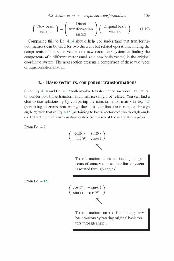
4.3 Basis-vector vs. component transformations 109
(New basis
vectors
)=⎛⎝ Direct
transformationmatrix
⎞⎠( Original basis
vectors
). (4.19)
Comparing this to Eq. 4.14 should help you understand that transforma-tion matrices can be used for two different but related operations: finding thecomponents of the same vector in a new coordinate system or finding thecomponents of a different vector (such as a new basis vector) in the originalcoordinate system. The next section presents a comparison of these two typesof transformation matrix.
4.3 Basis-vector vs. component transformations
Since Eq. 4.14 and Eq. 4.19 both involve transformation matrices, it’s naturalto wonder how those transformation matrices might be related. You can find aclue to that relationship by comparing the transformation matrix in Eq. 4.7(pertaining to component change due to a coordinate-axis rotation throughangle θ ) with that of Eq. 4.15 (pertaining to basis-vector rotation through angleθ ). Extracting the transformation matrix from each of those equations gives:
From Eq. 4.7: (cos(θ) sin(θ)− sin(θ) cos(θ)
)
↖Transformation matrix for finding compo-nents of same vector as coordinate systemis rotated through angle θ
From Eq. 4.15: (cos(θ) − sin(θ)sin(θ) cos(θ)
)
↖Transformation matrix for finding newbasis vectors by rotating original basis vec-tors through angle θ
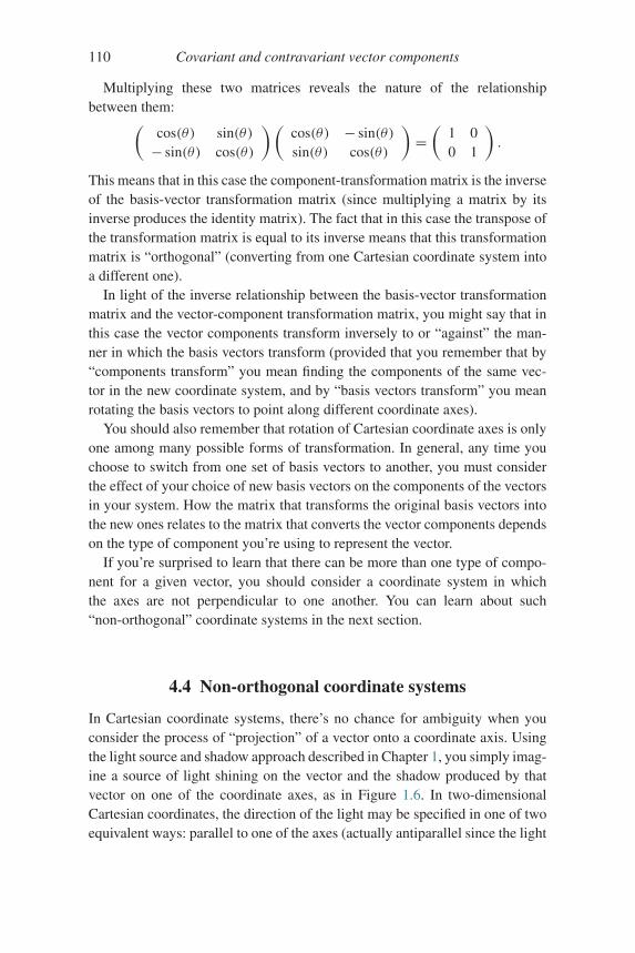
110 Covariant and contravariant vector components
Multiplying these two matrices reveals the nature of the relationshipbetween them:(
cos(θ) sin(θ)− sin(θ) cos(θ)
)(cos(θ) − sin(θ)sin(θ) cos(θ)
)=(
1 00 1
).
This means that in this case the component-transformation matrix is the inverseof the basis-vector transformation matrix (since multiplying a matrix by itsinverse produces the identity matrix). The fact that in this case the transpose ofthe transformation matrix is equal to its inverse means that this transformationmatrix is “orthogonal” (converting from one Cartesian coordinate system intoa different one).
In light of the inverse relationship between the basis-vector transformationmatrix and the vector-component transformation matrix, you might say that inthis case the vector components transform inversely to or “against” the man-ner in which the basis vectors transform (provided that you remember that by“components transform” you mean finding the components of the same vec-tor in the new coordinate system, and by “basis vectors transform” you meanrotating the basis vectors to point along different coordinate axes).
You should also remember that rotation of Cartesian coordinate axes is onlyone among many possible forms of transformation. In general, any time youchoose to switch from one set of basis vectors to another, you must considerthe effect of your choice of new basis vectors on the components of the vectorsin your system. How the matrix that transforms the original basis vectors intothe new ones relates to the matrix that converts the vector components dependson the type of component you’re using to represent the vector.
If you’re surprised to learn that there can be more than one type of compo-nent for a given vector, you should consider a coordinate system in whichthe axes are not perpendicular to one another. You can learn about such“non-orthogonal” coordinate systems in the next section.
4.4 Non-orthogonal coordinate systems
In Cartesian coordinate systems, there’s no chance for ambiguity when youconsider the process of “projection” of a vector onto a coordinate axis. Usingthe light source and shadow approach described in Chapter 1, you simply imag-ine a source of light shining on the vector and the shadow produced by thatvector on one of the coordinate axes, as in Figure 1.6. In two-dimensionalCartesian coordinates, the direction of the light may be specified in one of twoequivalent ways: parallel to one of the axes (actually antiparallel since the light
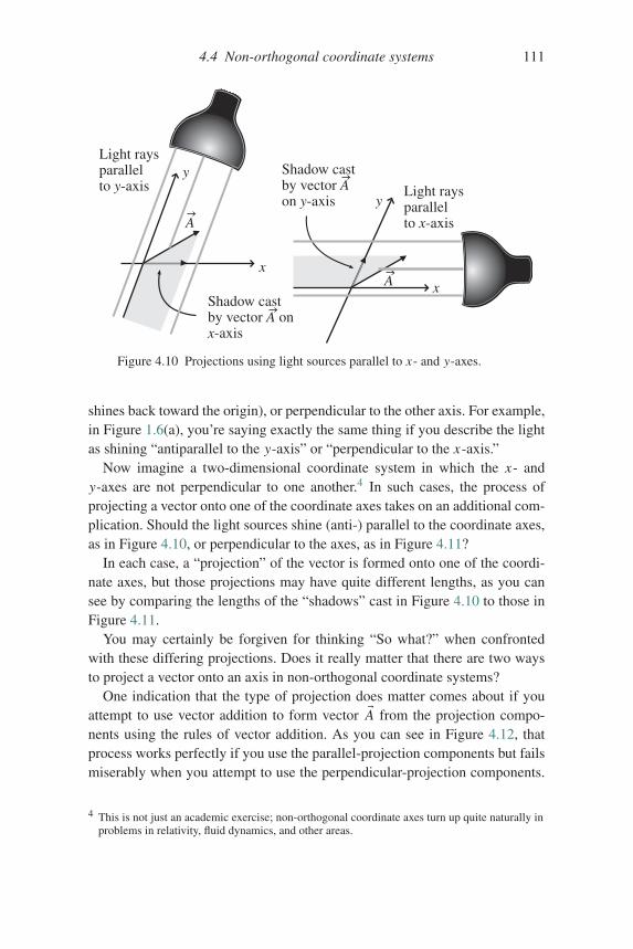
4.4 Non-orthogonal coordinate systems 111
Light raysparallelto y-axis Light rays
parallelto x-axis
Shadow castby vector A onx-axis
Shadow castby vector Aon y-axis
x
y
y
xA
A
Figure 4.10 Projections using light sources parallel to x- and y-axes.
shines back toward the origin), or perpendicular to the other axis. For example,in Figure 1.6(a), you’re saying exactly the same thing if you describe the lightas shining “antiparallel to the y-axis” or “perpendicular to the x-axis.”
Now imagine a two-dimensional coordinate system in which the x- andy-axes are not perpendicular to one another.4 In such cases, the process ofprojecting a vector onto one of the coordinate axes takes on an additional com-plication. Should the light sources shine (anti-) parallel to the coordinate axes,as in Figure 4.10, or perpendicular to the axes, as in Figure 4.11?
In each case, a “projection” of the vector is formed onto one of the coordi-nate axes, but those projections may have quite different lengths, as you cansee by comparing the lengths of the “shadows” cast in Figure 4.10 to those inFigure 4.11.
You may certainly be forgiven for thinking “So what?” when confrontedwith these differing projections. Does it really matter that there are two waysto project a vector onto an axis in non-orthogonal coordinate systems?
One indication that the type of projection does matter comes about if youattempt to use vector addition to form vector �A from the projection compo-nents using the rules of vector addition. As you can see in Figure 4.12, thatprocess works perfectly if you use the parallel-projection components but failsmiserably when you attempt to use the perpendicular-projection components.
4 This is not just an academic exercise; non-orthogonal coordinate axes turn up quite naturally inproblems in relativity, fluid dynamics, and other areas.
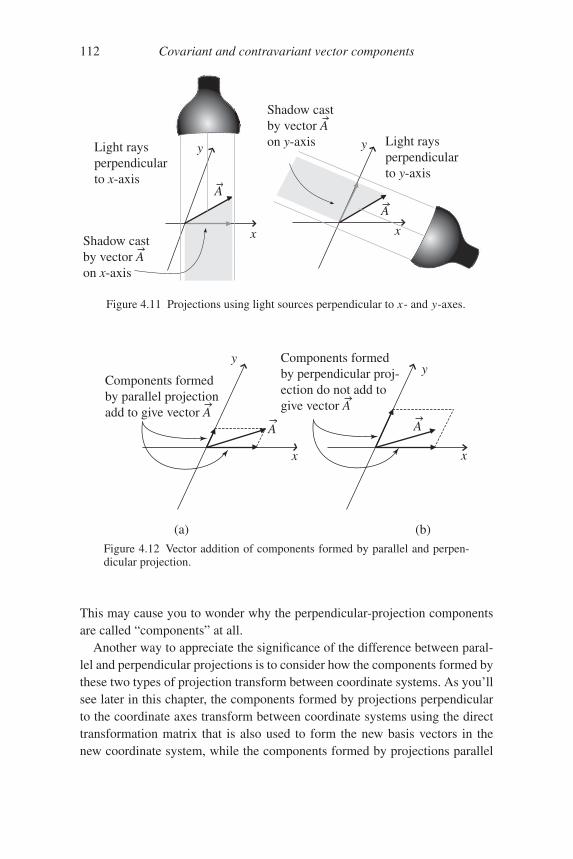
112 Covariant and contravariant vector components
Light raysperpendicularto x-axis
Light raysperpendicularto y-axis
Shadow castby vector Aon x-axis
Shadow castby vector Aon y-axis
A
A
y
x x
y
Figure 4.11 Projections using light sources perpendicular to x- and y-axes.
x
y
A
Components formedby parallel projectionadd to give vector A
x
y
A
Components formedby perpendicular proj-ection do not add togive vector A
(b)(a)
Figure 4.12 Vector addition of components formed by parallel and perpen-dicular projection.
This may cause you to wonder why the perpendicular-projection componentsare called “components” at all.
Another way to appreciate the significance of the difference between paral-lel and perpendicular projections is to consider how the components formed bythese two types of projection transform between coordinate systems. As you’llsee later in this chapter, the components formed by projections perpendicularto the coordinate axes transform between coordinate systems using the directtransformation matrix that is also used to form the new basis vectors in thenew coordinate system, while the components formed by projections parallel
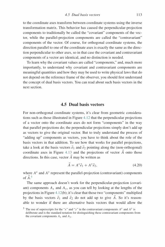
4.5 Dual basis vectors 113
to the coordinate axes transform between coordinate systems using the inversetransformation matrix. This behavior has caused the perpendicular-projectioncomponents to traditionally be called the “covariant” components of the vec-tor, while the parallel-projection components are called the “contravariant”components of the vector. Of course, for orthogonal coordinate systems, thedirection parallel to one of the coordinate axes is exactly the same as the direc-tion perpendicular to other axes, so in that case the covariant and contravariantcomponents of a vector are identical, and no distinction is needed.
To learn why the covariant values are called “components,” and, much moreimportantly, to understand why covariant and contravariant components aremeaningful quantities and how they may be used to write physical laws that donot depend on the reference frame of the observer, you should first understandthe concept of dual basis vectors. You can read about such basis vectors in thenext section.
4.5 Dual basis vectors
For non-orthogonal coordinate systems, it’s clear from geometric considera-tions such as those illustrated in Figure 4.12 that the perpendicular projectionsof a vector onto the coordinate axes do not form “components” in the waythat parallel projections do; the perpendicular projections simply don’t add upas vectors to give the original vector. But to truly understand the process of“adding up” components as vectors, you have to think about the role of thebasis vectors in that addition. To see how that works for parallel projections,take a look at the basis vectors �e1 and �e2 pointing along the (non-orthogonal)coordinate axes in Figure 4.13 and the projections of vector �A onto thosedirections. In this case, vector �A may be written as
�A = Ax �e1 + Ay �e2, (4.20)
where Ax and Ay represent the parallel-projection (contravariant) componentsof �A.5
The same approach doesn’t work for the perpendicular-projection (covari-ant) components Ax and Ay , as you can tell by looking at the lengths of theprojections in Figure 4.12(b); it’s clear that those two “components” multipliedby the basis vectors �e1 and �e2 do not add up to give �A. So it’s reason-able to wonder if there are alternative basis vectors that would allow the
5 The use of superscripts for the “x” and “y” in the contravariant components Ax and Ay isdeliberate and is the standard notation for distinguishing these contravariant components fromthe covariant components Ax and Ay .
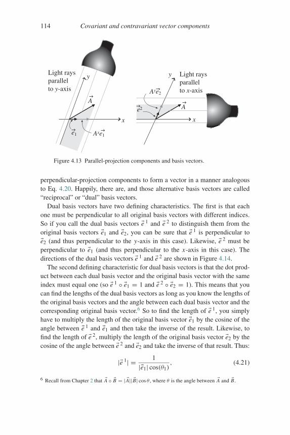
114 Covariant and contravariant vector components
Light raysparallelto y-axis
Light raysparallelto x-axis
y
xx
AA
Axe1
Aye2
e1
e2
y
Figure 4.13 Parallel-projection components and basis vectors.
perpendicular-projection components to form a vector in a manner analogousto Eq. 4.20. Happily, there are, and those alternative basis vectors are called“reciprocal” or “dual” basis vectors.
Dual basis vectors have two defining characteristics. The first is that eachone must be perpendicular to all original basis vectors with different indices.So if you call the dual basis vectors �e 1 and �e 2 to distinguish them from theoriginal basis vectors �e1 and �e2, you can be sure that �e 1 is perpendicular to�e2 (and thus perpendicular to the y-axis in this case). Likewise, �e 2 must beperpendicular to �e1 (and thus perpendicular to the x-axis in this case). Thedirections of the dual basis vectors �e 1 and �e 2 are shown in Figure 4.14.
The second defining characteristic for dual basis vectors is that the dot prod-uct between each dual basis vector and the original basis vector with the sameindex must equal one (so �e 1 ◦ �e1 = 1 and �e 2 ◦ �e2 = 1). This means that youcan find the lengths of the dual basis vectors as long as you know the lengths ofthe original basis vectors and the angle between each dual basis vector and thecorresponding original basis vector.6 So to find the length of �e 1, you simplyhave to multiply the length of the original basis vector �e1 by the cosine of theangle between �e 1 and �e1 and then take the inverse of the result. Likewise, tofind the length of �e 2, multiply the length of the original basis vector �e2 by thecosine of the angle between �e 2 and �e2 and take the inverse of that result. Thus:
|�e 1| = 1
|�e1| cos(θ1), (4.21)
6 Recall from Chapter 2 that �A ◦ �B = | �A|| �B| cos θ , where θ is the angle between �A and �B.
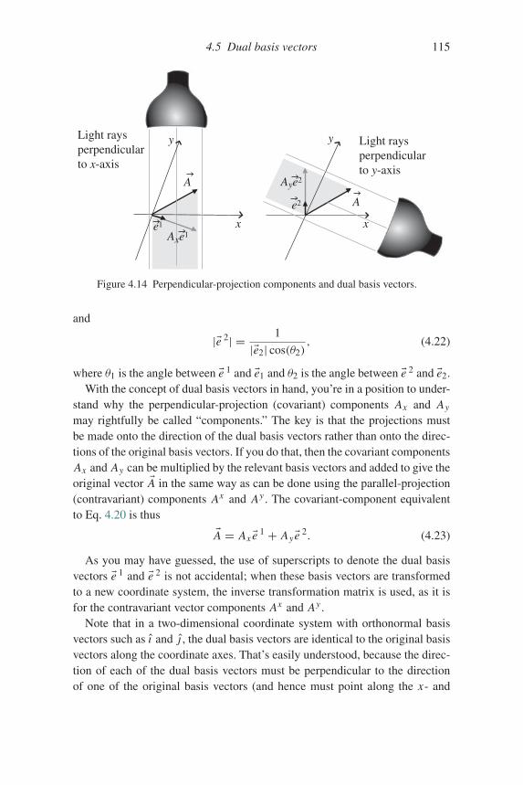
4.5 Dual basis vectors 115
Light raysperpendicularto x-axis
Light raysperpendicularto y-axis
y
A
x xe1
A
Aye2
e2
y
Axe1
Figure 4.14 Perpendicular-projection components and dual basis vectors.
and
|�e 2| = 1
|�e2| cos(θ2), (4.22)
where θ1 is the angle between �e 1 and �e1 and θ2 is the angle between �e 2 and �e2.With the concept of dual basis vectors in hand, you’re in a position to under-
stand why the perpendicular-projection (covariant) components Ax and Ay
may rightfully be called “components.” The key is that the projections mustbe made onto the direction of the dual basis vectors rather than onto the direc-tions of the original basis vectors. If you do that, then the covariant componentsAx and Ay can be multiplied by the relevant basis vectors and added to give theoriginal vector �A in the same way as can be done using the parallel-projection(contravariant) components Ax and Ay . The covariant-component equivalentto Eq. 4.20 is thus
�A = Ax �e 1 + Ay �e 2. (4.23)
As you may have guessed, the use of superscripts to denote the dual basisvectors �e 1 and �e 2 is not accidental; when these basis vectors are transformedto a new coordinate system, the inverse transformation matrix is used, as it isfor the contravariant vector components Ax and Ay .
Note that in a two-dimensional coordinate system with orthonormal basisvectors such as ı and j , the dual basis vectors are identical to the original basisvectors along the coordinate axes. That’s easily understood, because the direc-tion of each of the dual basis vectors must be perpendicular to the directionof one of the original basis vectors (and hence must point along the x- and
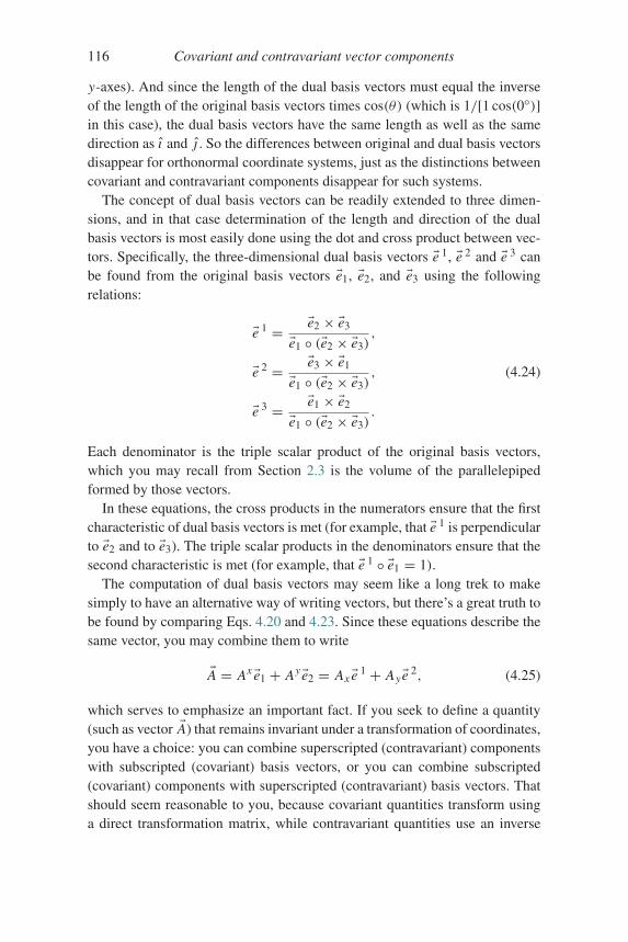
116 Covariant and contravariant vector components
y-axes). And since the length of the dual basis vectors must equal the inverseof the length of the original basis vectors times cos(θ) (which is 1/[1 cos(0◦)]in this case), the dual basis vectors have the same length as well as the samedirection as ı and j . So the differences between original and dual basis vectorsdisappear for orthonormal coordinate systems, just as the distinctions betweencovariant and contravariant components disappear for such systems.
The concept of dual basis vectors can be readily extended to three dimen-sions, and in that case determination of the length and direction of the dualbasis vectors is most easily done using the dot and cross product between vec-tors. Specifically, the three-dimensional dual basis vectors �e 1, �e 2 and �e 3 canbe found from the original basis vectors �e1, �e2, and �e3 using the followingrelations:
�e 1 = �e2 × �e3
�e1 ◦ (�e2 × �e3),
�e 2 = �e3 × �e1
�e1 ◦ (�e2 × �e3),
�e 3 = �e1 × �e2
�e1 ◦ (�e2 × �e3).
(4.24)
Each denominator is the triple scalar product of the original basis vectors,which you may recall from Section 2.3 is the volume of the parallelepipedformed by those vectors.
In these equations, the cross products in the numerators ensure that the firstcharacteristic of dual basis vectors is met (for example, that �e 1 is perpendicularto �e2 and to �e3). The triple scalar products in the denominators ensure that thesecond characteristic is met (for example, that �e 1 ◦ �e1 = 1).
The computation of dual basis vectors may seem like a long trek to makesimply to have an alternative way of writing vectors, but there’s a great truth tobe found by comparing Eqs. 4.20 and 4.23. Since these equations describe thesame vector, you may combine them to write
�A = Ax �e1 + Ay �e2 = Ax �e 1 + Ay �e 2, (4.25)
which serves to emphasize an important fact. If you seek to define a quantity(such as vector �A) that remains invariant under a transformation of coordinates,you have a choice: you can combine superscripted (contravariant) componentswith subscripted (covariant) basis vectors, or you can combine subscripted(covariant) components with superscripted (contravariant) basis vectors. Thatshould seem reasonable to you, because covariant quantities transform usinga direct transformation matrix, while contravariant quantities use an inverse
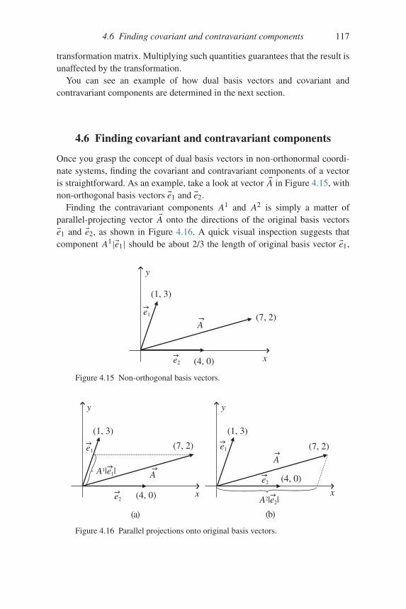
4.6 Finding covariant and contravariant components 117
transformation matrix. Multiplying such quantities guarantees that the result isunaffected by the transformation.
You can see an example of how dual basis vectors and covariant andcontravariant components are determined in the next section.
4.6 Finding covariant and contravariant components
Once you grasp the concept of dual basis vectors in non-orthonormal coordi-nate systems, finding the covariant and contravariant components of a vectoris straightforward. As an example, take a look at vector �A in Figure 4.15, withnon-orthogonal basis vectors �e1 and �e2.
Finding the contravariant components A1 and A2 is simply a matter ofparallel-projecting vector �A onto the directions of the original basis vectors�e1 and �e2, as shown in Figure 4.16. A quick visual inspection suggests thatcomponent A1|�e1| should be about 2/3 the length of original basis vector �e1,
y
x
(1, 3)
(7, 2)
(4, 0)
e1
A
e2
Figure 4.15 Non-orthogonal basis vectors.
y
x
(1, 3)
(7, 2)
(4, 0)
e1
y
x
(1, 3)
(7, 2)
A1|e1|(4, 0)
(a) (b)
e1
e2
e2
A
A
A2|e2|
Figure 4.16 Parallel projections onto original basis vectors.
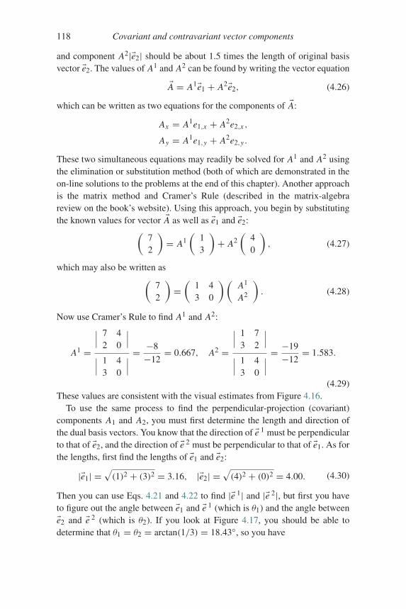
118 Covariant and contravariant vector components
and component A2|�e2| should be about 1.5 times the length of original basisvector �e2. The values of A1 and A2 can be found by writing the vector equation
�A = A1�e1 + A2�e2, (4.26)
which can be written as two equations for the components of �A:
Ax = A1e1,x + A2e2,x ,
Ay = A1e1,y + A2e2,y .
These two simultaneous equations may readily be solved for A1 and A2 usingthe elimination or substitution method (both of which are demonstrated in theon-line solutions to the problems at the end of this chapter). Another approachis the matrix method and Cramer’s Rule (described in the matrix-algebrareview on the book’s website). Using this approach, you begin by substitutingthe known values for vector �A as well as �e1 and �e2:(
72
)= A1
(13
)+ A2
(40
), (4.27)
which may also be written as(72
)=(
1 43 0
)(A1
A2
). (4.28)
Now use Cramer’s Rule to find A1 and A2:
A1 =
∣∣∣ 7 42 0
∣∣∣∣∣∣ 1 4
3 0
∣∣∣= −8
−12= 0.667, A2 =
∣∣∣ 1 73 2
∣∣∣∣∣∣ 1 4
3 0
∣∣∣= −19
−12= 1.583.
(4.29)These values are consistent with the visual estimates from Figure 4.16.
To use the same process to find the perpendicular-projection (covariant)components A1 and A2, you must first determine the length and direction ofthe dual basis vectors. You know that the direction of �e 1 must be perpendicularto that of �e2, and the direction of �e 2 must be perpendicular to that of �e1. As forthe lengths, first find the lengths of �e1 and �e2:
|�e1| =√(1)2 + (3)2 = 3.16, |�e2| =
√(4)2 + (0)2 = 4.00. (4.30)
Then you can use Eqs. 4.21 and 4.22 to find |�e 1| and |�e 2|, but first you haveto figure out the angle between �e1 and �e 1 (which is θ1) and the angle between�e2 and �e 2 (which is θ2). If you look at Figure 4.17, you should be able todetermine that θ1 = θ2 = arctan(1/3) = 18.43◦, so you have
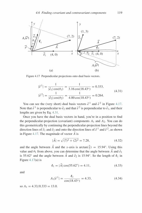
4.6 Finding covariant and contravariant components 119
y
x x
(7, 2)
(4, 0)e2
A
y
(1, 3)
(7, 2)
(b)(a)
(4, 0)
e1
e2e2
e1 e1
AA1|e1|
A2|e2|
θ
θ2
1
2
1
Figure 4.17 Perpendicular projections onto dual basis vectors.
|�e 1| = 1
|�e1| cos(θ1)= 1
3.16 cos(18.43◦)= 0.333,
|�e 2| = 1
|�e2| cos(θ2)= 1
4.00 cos(18.43◦)= 0.264.
(4.31)
You can see the (very short) dual basis vectors �e 1 and �e 2 in Figure 4.17.Note that �e 1 is perpendicular to �e2 and that �e 2 is perpendicular to �e1, and theirlengths are given by Eq. 4.31.
Once you have the dual basis vectors in hand, you’re in a position to findthe perpendicular-projection (covariant) components A1 and A2. You can dothis geometrically by continuing the perpendicular-projection lines beyond thedirection lines of �e1 and �e2 and onto the direction lines of �e 1 and �e 2, as shownin Figure 4.17. The magnitude of vector �A is
| �A| =√(7)2 + (2)2 = 7.28, (4.32)
and the angle between �A and the x-axis is arctan( 27 ) = 15.94◦. Using this
value and θ1 from above, you can determine that the angle between �A and �e1
is 55.62◦ and the angle between �A and �e2 is 15.94◦. So the length of �1 inFigure 4.17(a) is
�1 = | �A| cos(55.62◦) = 4.11, (4.33)
and
A1|�e 1| = �1
cos(18.43◦)= 4.33, (4.34)
so A1 = 4.33/0.333 = 13.0.
120 Covariant and contravariant vector components
Using the same approach to find A2 from Figure 4.17(b) gives
�2 = | �A| cos(15.94◦) = 7.00, (4.35)
and
A2|�e 2| = �2
cos(18.43◦)= 7.38, (4.36)
so A2 = 7.38/0.264 = 28.0.These results serve as a reminder that when you use non-normalized basis
vectors (that is, basis vectors with magnitude not equal to one), you cannotequate the lengths of the projections onto the coordinate axes with the valueof a vector’s components. That’s because those projections are the products ofthe components with the magnitudes of the basis vectors.
If you prefer the algebraic approach to finding A1 and A2, you can do thatby proceeding as you did for A1 and A2, although in this case you begin with
�A = A1�e 1 + A2�e 2, (4.37)
and then substitute the known values for vector �A as well as the x- and y-components of the dual basis vectors �e 1 and �e 2:
e 1x = |�e 1| cos(90◦) = 0.000, e 2
x = |�e 2| cos(360◦ − 18.43◦) = 0.250,e 1
y = |�e 1| sin(90◦) = 0.333, e 2y = |�e 2| sin(360◦ − 18.43◦) = −0.083.
So (72
)= A1
(0
0.333
)+ A2
(0.25−0.083
). (4.38)
As before, this may be written as(72
)=(
0 0.250.333 −0.083
)(A1
A2
). (4.39)
Again using Cramer’s Rule to solve for A1 and A2 gives
A1 =
∣∣∣ 7 0.252 −0.083
∣∣∣∣∣∣ 0 0.25
0.333 −0.083
∣∣∣= −1.081
−0.083= 13.0,
A2 =
∣∣∣ 0 70.333 2
∣∣∣∣∣∣ 0 0.25
0.333 −0.083
∣∣∣= −2.331
−0.083= 28.0, (4.40)
as expected from the geometric approach.
4.6 Finding covariant and contravariant components 121
A simpler approach to finding the contravariant and covariant componentsof a vector once you have both the original and dual basis vectors in hand is touse these relations:
A1 = �A ◦ �e1 = Ax e1,x + Aye1,y A2 = �A ◦ �e2 = Ax e2,x + Aye2,y,
(4.41)and
A1 = �A ◦ �e 1 = Ax e1x + Aye1
y A2 = �A ◦ �e 2 = Ax e2x + Aye2
y . (4.42)
In the current example, this approach gives the covariant components as
A1 = (7, 2) ◦ (1, 3) = (7)(1)+ (2)(3) = 13,
A2 = (7, 2) ◦ (4, 0) = (7)(4)+ (2)(0) = 28,
and
A1 = (7, 2) ◦ (0, 0.333) = (7)(0)+ (2)(0.333) = 0.666,
A2 = (7, 2) ◦ (0.250,−0.083) = (7)(0.250)+ (2)(−0.083) = 1.58,
in agreement with the geometric and matrix-algebra approaches taken above.It’s important for you to realize that what you’ve just found are the parallel-
projection (contravariant) and perpendicular-projection (covariant) compo-nents of vector �A with respect to the original basis vectors �e1 and �e2 and thedual basis vectors �e 1 and �e 2. So does that mean that �A is a covariant vector ora contravariant vector?
The answer is neither (or both, if you prefer); it’s not the vector itself thatis contravariant or covariant, it’s the set of components that you form throughits parallel or perpendicular projections. As you read the literature on tensors,you’re very likely to run into expressions such as “the contravariant vector�A” or “the covariant vector �B,” and what the author generally means is that
the contravariant components of vector �A and the covariant components ofvector �B are being used for the problem (perhaps because they’re simpler).But you can be sure that like all vectors, �A and �B both have contravariant andcovariant components, and you can find them using the techniques describedin this section.7
And if you’re wondering why you might want to go through the effort offinding those components, rest assured that the payoff is worth the effort. Toappreciate the value of that payoff, you’ll have to begin thinking of vectors notjust as arrows with a certain length and pointing in a specified direction, butrather as members of a class of objects called tensors that have very predictable
7 In Chapter 5, you can learn to move between contravariant and covariant components using themetric tensor.
122 Covariant and contravariant vector components
(and useful) properties under transformation of coordinates. In that view, thevectors you’ve been dealing with up to this point have all been tensors of rankone. Seeing them as such, and understanding what that means, will be madea great deal easier through the use of a notation called “index notation” anda convention known as the “Einstein summation convention.” You can readabout index notation and the summation convention in the next section.
4.7 Index notation
You’ve seen the first glimmerings of index notation in the earlier section ofthis chapter describing coordinate transformations. As you may recall, theangles between the transformed (rotated) coordinate axes and the original(non-rotated) axes of a two-dimensional coordinate system were called α11,α12, α21, and α22. These angles could just as well have been designated αx ′x ,αx ′y , αy′x , and the like, but there are several good reasons to use the index num-bers 1, 2, and 3 rather than the letters x , y, and z to refer to coordinate axesand vector components. One of those reasons is that many problems in physicsand engineering involve a number of dimensions greater than 3, and althougheveryone agrees that “4” comes after “3,” a consensus hasn’t been reached onwhat comes after “z.” Another reason is that index notation enables the greatconvenience of the summation convention that you can read about later in thissection.
Using index notation, the coordinates of a point in three-dimensionalspace are written as (x1, x2, x3) or (x1, x2, x3) rather than (x, y, z), andthe components of a vector are written as (A1, A2, A3) or (A1, A2, A3)
rather than (Ax , Ay, Az) or (Ax , Ay, Az). This system is easily extended toN-dimensional space, in which the coordinates become (x1, x2, . . . , xN ) or(x1, x2, . . . , x N ) and the vector components become (A1, A2, . . . , AN ) or(A1, A2, . . . , AN ).
Applying this notation to the equation for the transformation of contravariantvector components produced by a rotation of two-dimensional axes, Eq. 4.6becomes (
A′1
A′2
)=(
cos (α11) cos (α12)
cos (α21) cos (α22)
)(A1
A2
). (4.43)
In three dimensions, this is⎛⎜⎝ A
′1
A′2
A′3
⎞⎟⎠ =
⎛⎝ cos (α11) cos (α12) cos (α13)
cos (α21) cos (α22) cos (α23)
cos (α31) cos (α32) cos (α33)
⎞⎠⎛⎝ A1
A2
A3
⎞⎠ . (4.44)
4.7 Index notation 123
Designating the elements of the transformation matrix a11, a12, a13, and soforth allows you to write Eq. 4.44 as
A′1 = a11 A1 + a12 A2 + a13 A3,
A′2 = a21 A1 + a22 A2 + a23 A3,
A′3 = a31 A1 + a32 A2 + a33 A3,
(4.45)
or
A′1 =
3∑j=1
a1 j A j ,
A′2 =
3∑j=1
a2 j A j ,
A′3 =
3∑j=1
a3 j A j .
(4.46)
Allowing “i” to stand for any of the indices 1, 2, or 3 makes this:
A′i =
3∑j=1
ai j A j . i = 1, 2, 3 (4.47)
As a final simplification, whenever an index appears twice in the same term,once as a superscript and once as a subscript (as “ j” does in Eq. 4.47), you canomit the summation symbol and write simply
A′i = ai j A j , (4.48)
in which the reader knows to sum over the repeated index ( j in this case).Such repeated indices are often called “dummy” indices, since any letter maybe used for that index and the result will be the same.8 It was Albert Einsteinwho first suggested this summation convention, which he jokingly called his“great discovery in mathematics.”9 Whatever you call it, this idea certainly hassaved a lot of ink and time since Einstein proposed it in 1916.
Before moving on, you should take a careful look at Eq. 4.48 and makesure you understand that these few symbols mean exactly the same thing asthe many terms in the three separate equations of Eq. 4.45. They tell you that
8 Unlike the repeated “dummy” indices which indicate summation, i is called a “free” index andno summation is implied.
9 Pais, A. 1983, Subtle Is the Lord: The Science and the Life of Albert Einstein, OxfordUniversity Press, Oxford.
124 Covariant and contravariant vector components
each component in the primed coordinate system is a weighted linear combi-nation of the components in the original (unprimed) coordinate system, withthe transformation matrix elements (ai j ) providing the weighting factors foreach term.
And if you want to know the exact meaning of each of those factors inthe transformation of covariant and contravariant vector components, the nextsection will help with that.
4.8 Quantities that transform contravariantly
With the convenience of index notation and the summation convention at yourdisposal, you should be ready to take the next step in the transition from think-ing of vectors as quantities with magnitude and direction to understanding whyvectors belong to the class of objects known as tensors. That step begins byasking the question of how a differential element of length d�s transforms fromone coordinate system to another.
In general, the equations relating the coordinates in one system to those inanother do not involve simple linear combinations of coordinate values. Forexample, in transforming from spherical (r, θ, φ) to Cartesian (x, y, z) coordi-nates, it’s not possible to write equations such as x = a11r + a12θ + a13φ,because x depends on the product of r with the sine of θ and the cosineof φ. And y and z have similar non-linear relationships to the sphericalcoordinates.
If, however, you ask how the differentials of x , y, and z (that is, dx , dy, anddz) depend on the differentials of r , θ , and φ (that is, dr , dθ , and dφ), you’llfind that on this infinitesimally small scale, dx does depend linearly on dr , dθ ,and dφ (as do dy and dz). So you are able to write
dx = a11dr + a12dθ + a13dφ, (4.49)
and likewise for dy and dz.For any two coordinate systems in which a linear relationship exists between
differential length elements, writing the equations which transform betweenthe systems is straightforward. If you call the differentials of one coordinatesystem dx , dy, and dz and the other coordinate system dx ′, dy′, and dz′,the transformation equations from the unprimed to the primed systems comedirectly from the rules of partial differentiation, as shown in the left columnbelow:
4.8 Quantities that transform contravariantly 125
dx ′ = ∂x ′
∂xdx + ∂x ′
∂ydy + ∂x ′
∂zdz ⇒ dx
′1 = ∂x′1
∂x1dx1 + ∂x
′1
∂x2dx2 + ∂x
′1
∂x3dx3,
dy′ = ∂y′
∂xdx + ∂y′
∂ydy + ∂y′
∂zdz ⇒ dx
′2 = ∂x′2
∂x1dx1 + ∂x
′2
∂x2dx2 + ∂x
′2
∂x3dx3,
dz′ = ∂z′
∂xdx + ∂z′
∂ydy + ∂z′
∂zdz ⇒ dx
′3 = ∂x′3
∂x1dx1 + ∂x
′3
∂x2dx2 + ∂x
′3
∂x3dx3.
(4.50)
Using the index-notation approach of substituting x1, x2, and x3 for x , y,and z results in the column shown on the right.10 Putting this into matrixnotation gives
⎛⎜⎝ dx
′1
dx′2
dx′3
⎞⎟⎠ =
⎛⎜⎜⎜⎜⎜⎜⎜⎜⎜⎜⎝
∂x′1
∂x1
∂x′1
∂x2
∂x′1
∂x3
∂x′2
∂x1
∂x′2
∂x2
∂x′2
∂x3
∂x′3
∂x1
∂x′3
∂x2
∂x′3
∂x3
⎞⎟⎟⎟⎟⎟⎟⎟⎟⎟⎟⎠
⎛⎝ dx1
dx2
dx3
⎞⎠ , (4.51)
or, using individual equations with summation symbols
dx′1 =
3∑j=1
∂x′1
∂x jdx j , dx
′2 =3∑
j=1
∂x′2
∂x jdx j , dx
′3 =3∑
j=1
∂x′3
∂x jdx j .
If you now allow the letter i to represent each of the numerical values of theindex (1, 2, and 3), this can be written as
dx′i =
3∑j=1
∂x′i
∂x jdx j . (4.52)
Since the j index is repeated, a final simplification results from the Einsteinsummation convention, allowing you to write
dx′i = ∂x
′i
∂x jdx j . (4.53)
So index notation has allowed the expression in Eq. 4.50, consisting of threeequations with three terms in each, to be written as this single equation. Moreimportantly, the form of this equation will help you understand why differentiallength elements (dxi ) are considered to be contravariant quantities.
10 Superscripts are used for the indices because differential length elements transform ascontravariant quantities, as described later in this section.
126 Covariant and contravariant vector components
To gain that understanding, it’s useful to recall Eq. 4.48 from the previoussection:
A′i = ai j A j ,
which tells you that the components of a vector in the primed (transformed)coordinate system are the weighted linear combination of the componentsof that same vector in the unprimed (original) coordinate system. And theweighting factors ai j are the elements of the transformation matrix.
Now compare Eq. 4.53 to Eq. 4.48. On the left side of both equations,a primed quantity (dx
′i or A′i ) with free index i appears. On the right
side, both equations contain the product of a factor with free index i and
dummy index j ( ∂x′i
∂x j or ai j ) with the left-side quantity unprimed and with
dummy index j (dx j or A j ). And you know that the factor ai j in Eq. 4.48represents the elements of a transformation matrix for contravariant vectorcomponents between the unprimed and the primed coordinate systems. So
it seems reasonable to conclude that the ∂x′i
∂x j terms in Eq. 4.53 can beseen as the elements of the transformation matrix for the differential lengthelements.
So instead of looking at Eq. 4.53 as simply the index-notation version of thechain rule, you should see it as a transformation equation that takes differentiallength elements from the unprimed to the primed coordinate system (just asEq. 4.48 does for the contravariant components of vector �A).
And here’s the important insight: the ∂x′i
∂x j terms are not only the ele-ments of a transformation matrix from the unprimed to the primed coordinatesystem, they’re also the components of the basis vectors tangent to the orig-inal (unprimed) coordinate axes, expressed in the new (primed) coordinatesystem.11
Furthermore, you know that basis vectors tangent to the original coordinateaxes are the covariant basis vectors described earlier. And since contravariantvector components combine with covariant basis vectors to produce invariantquantities, differential length elements must transform as contravariant vectorcomponents. This is the reason that the indices are written as superscripts inEqs. 4.51 through 4.53; the differential length element is the “prototype” ofcontravariant vector components.
Using index notation and representing the components of the basis vec-
tors as ∂x′i
∂x j , you should now understand why the transformation equation for
contravariant components of vector �A is often written as
11 If you’re wondering how partial derivatives can represent basis vectors, you should reviewSection 2.6 of Chapter 2.
4.9 Quantities that transform covariantly 127
A′i = ∂x
′i
∂x jA j . (4.54)
Many authors present this as the definition of contravariant components.To see how this notation works in practice, consider the transformation
from polar (r, θ ) to two-dimensional Cartesian (x, y) coordinates. In this case,x′1= x , x
′2= y, x1= r , and x2= θ , and you know that x = r cos(θ) andy= r sin(θ). So what are the weighting factors (that is, the elements of thetransformation matrix) in this case? Taking the appropriate derivatives, youfind that
∂x′1
∂x1= ∂x
∂r= cos(θ),
∂x′2
∂x1= ∂y
∂r= sin(θ), (4.55)
∂x′1
∂x2= ∂x
∂θ= −r sin(θ),
∂x′2
∂x2= ∂y
∂θ= r cos(θ). (4.56)
Are these really the components of the tangent vectors to the original (r, θ )coordinate axes (that is, are they pointing along those axes)? You can see thatthey are by writing these terms as components in the primed coordinate system(Cartesian in this case):
�e1 = ∂x′1
∂x1ı + ∂x
′2
∂x1j = cos(θ)ı + sin(θ)j , (4.57)
�e2 = ∂x′1
∂x2ı + ∂x
′2
∂x2j = −r sin(θ)ı + r cos(θ)j . (4.58)
The first of these expressions is a vector pointing radially outward (along ther -direction in polar coordinates) and the second is a vector pointing perpendic-ular to the radial direction (along the θ -direction).12 This demonstrates that thepartial derivatives in Eq. 4.53 do indeed represent components of the original(unprimed) covariant basis vectors expressed in the new (primed) coordinatesystem.
4.9 Quantities that transform covariantly
If the differential length element of the previous section serves as the “proto-type” for quantities that transform as contravariant vector components, youmay be wondering if there’s a similar “prototype” for covariant quantities.You can answer that question by considering a quantity such as the changein temperature with distance (degrees per meter) over some region, whichyou may recognize from Chapter 2 as the gradient of that quantity. Unlike
12 These basis vectors can be understood in terms of the non-Cartesian unit vectors discussed inSection 1.5 of Chapter 1.
128 Covariant and contravariant vector components
the differential length element, which has dimensions directly related to thecoordinate dimensions, quantities such as the gradient have dimensions thatinclude the inverse of the coordinate dimensions (per unit length rather thanlength in the case of spatial coordinates). This dimensional consideration sug-gests that the gradient may be a good candidate for the prototype of quantitiesthat transform as covariant vector components. And index notation makes thiseasy to see.
Imagine a scalar quantity such as temperature or density whose value atvarious positions is given by the function f (x, y, z); the rate of change ofthat quantity is ∂ f
∂x in the x-direction, ∂ f∂y in the y-direction, and ∂ f
∂z in the z-direction. It’s reasonable to ask how these rates of change vary if the coordinatesystem is changed. To answer that question, you can proceed as we did for thedifferential length element, using the chain rule for partial derivatives and thenemploying index notation as follows:
∂ f
∂x ′= ∂ f
∂x
∂x
∂x ′+ ∂ f
∂y
∂y
∂x ′+ ∂ f
∂z
∂z
∂x ′
⇒ ∂ f
∂x ′1= ∂ f
∂x1
∂x1
∂x ′1+ ∂ f
∂x2
∂x2
∂x ′1+ ∂ f
∂x3
∂x3
∂x ′1,
∂ f
∂y′= ∂ f
∂x
∂x
∂y′+ ∂ f
∂y
∂y
∂y′+ ∂ f
∂z
∂z
∂y′
⇒ ∂ f
∂x ′2= ∂ f
∂x1
∂x1
∂x ′2+ ∂ f
∂x2
∂x2
∂x ′2+ ∂ f
∂x3
∂x3
∂x ′2,
∂ f
∂z′= ∂ f
∂x
∂x
∂z′+ ∂ f
∂y
∂y
∂z′+ ∂ f
∂z
∂z
∂z′
⇒ ∂ f
∂x ′3= ∂ f
∂x1
∂x1
∂x ′3+ ∂ f
∂x2
∂x2
∂x ′3+ ∂ f
∂x3
∂x3
∂x ′3.
As before, you can write this as a matrix equation
⎛⎜⎜⎜⎜⎜⎜⎜⎜⎜⎝
∂ f
∂x ′1
∂ f
∂x ′2
∂ f
∂x ′3
⎞⎟⎟⎟⎟⎟⎟⎟⎟⎟⎠=
⎛⎜⎜⎜⎜⎜⎜⎜⎜⎜⎜⎝
∂x1
∂x ′1∂x2
∂x ′1∂x3
∂x ′1
∂x1
∂x ′2∂x2
∂x ′2∂x3
∂x ′2
∂x1
∂x ′3∂x2
∂x ′3∂x3
∂x ′3
⎞⎟⎟⎟⎟⎟⎟⎟⎟⎟⎟⎠
⎛⎜⎜⎜⎜⎜⎜⎜⎜⎜⎝
∂ f
∂x1
∂ f
∂x2
∂ f
∂x3
⎞⎟⎟⎟⎟⎟⎟⎟⎟⎟⎠, (4.59)
4.9 Quantities that transform covariantly 129
or as individual equations using the summation symbol:
∂ f
∂x ′1=
3∑j=1
∂x j
∂x ′1∂ f
∂x j,
∂ f
∂x ′2=
3∑j=1
∂x j
∂x ′2∂ f
∂x j,
∂ f
∂x ′3=
3∑j=1
∂x j
∂x ′3∂ f
∂x j.
Once again employing i as the free index gives
∂ f
∂x ′i=
3∑j=1
∂x j
∂x ′i∂ f
∂x j, (4.60)
and the Einstein summation convention simplifies this to
∂ f
∂x ′i= ∂x j
∂x ′i∂ f
∂x j. (4.61)
Comparing this to the equivalent expression for the differential length element(Eq. 4.53) suggests that once again the vector components in the primed coor-dinate system are the weighted linear combination of the components in theoriginal coordinate system. But in this case the elements of the transformationmatrix ( ∂x j
∂x ′i ) are the inverse of those in the transformation of the differen-
tial length elements (which are ∂x′i
∂x j ). And just as in that case the ∂x′i
∂x j termsrepresent the components of vectors that point along the original coordinateaxes, in this case the ∂x j
∂x ′i terms represent the components of vectors thatare perpendicular to the original coordinate surfaces. Hence in this case theweighting factors are the components of the (contravariant) dual basis vectors,which means that the components of the gradient vector transform as covari-ant components. Of course, for orthonormal coordinate systems the lengthsand directions of the original and dual basis vectors are exactly the same, andthere is no difference between the covariant and contravariant vector com-ponents. In non-orthonormal coordinate systems, this distinction is criticallyimportant.
Again using index notation and representing the dual basis vectors as ∂x j
∂x ′i ,you probably won’t find it surprising that many authors define the covari-ant components of vector �A as components that transform according to theequation
A′i =∂x j
∂x ′iAi . (4.62)
At this point you should be convinced that vectors are more than just lit-tle arrows with magnitude and direction; they’re quantities that transform incertain ways between coordinate systems. Specifically, every vector has bothcontravariant and covariant components that transform in predictable ways.
130 Covariant and contravariant vector components
The contravariant components vary in the opposite manner to the basis vec-tors pointing along the original coordinate axes, and the covariant componentsvary in the same manner as those basis vectors. Most importantly, by combin-ing the vector’s contravariant components with the original basis vectors, orby combining the vector’s covariant components with the dual basis vectors,the resulting quantity (the vector itself) remains invariant under all coordinatetransformations. It is this characteristic that qualifies vectors to join the ranksof tensors.
Understanding the distinction between contravariant and covariant vectorcomponents is extremely helpful in understanding tensors, because vectors aretensors. Specifically, since all the components of a vector can be delineatedusing only a single index, vectors are tensors of rank one. Under this definition,scalars are tensors of rank zero, since scalars are single numbers and requireno index at all. And of what use are tensors of rank two and higher? You’llencounter those in Chapter 5.
4.10 Chapter 4 problems
4.1 Write the inverse transformation matrix for a 70◦ rotation of the 2-DCartesian coordinate axes and the indirect transformation matrix for therotation of a vector through an angle of 70◦ degrees. Show that theproduct of these two transformation matrices is the identity matrix.
4.2 Use the inverse transformation matrix from Problem 4.1 to find thecomponents of vector �A = 2ı + 5.5j in the rotated coordinate system.
4.3 Use the direct transformation matrix from Problem 4.1 to rotate the origi-nal coordinate basis vectors ı and j by 70◦, so they point along the rotatedaxes.
4.4 Use a direct transformation matrix to rotate vector �A from Problem 4.2through an angle of −70◦, and compare the x- and y-components ofthe rotated vector (in the original coordinate system) to the x ′- andy′-components of the unrotated vector in the rotated coordinate system.
4.5 Use the dot product of the original vector �A with the rotated basis vectors( �A ◦ ı ′ and �A ◦ j ′) to find the components of �A in the rotated coordinatesystem.
4.6 For vector �A = −5ı+6j and basis vectors �e1 = ı+2j and �e2 = −2ı−j ,find the contravariant components �A1 and �A2.
4.7 Find the dual basis vectors �e 1 and �e 2 for the basis vectors �e1 and �e2 ofProblem 4.6.
4.8 Find the covariant components �A1 and �A2 for vector �A of Problem 4.6.
4.10 Chapter 4 problems 131
4.9 Use the subsitution method and the elimination method to solve the twosimultaneous equations that result from vector Eq. 4.26.
4.10 Show that the elements of the Cartesian-to-polar transformation matrixare the components of the basis vectors tangent to the original (Cartesian)coordinate axes.
5
Higher-rank tensors
The previous chapter contains several ideas that are important to a fullunderstanding of tensors. The first is that any vector may be represented bycomponents that transform between coordinate systems in one of two ways.“Covariant” components transform in the same manner as the original basisvectors pointing along the coordinate axes, and “contravariant” componentstransform in the inverse manner of those basis vectors.1 The second main ideais that coordinate basis vectors are tangent to the coordinate axes, and thatthere also exist reciprocal or dual basis vectors that are perpendicular to thecoordinate axes; these dual basis vectors transform inversely to the coordinatebasis vectors. The third idea is that combining contravariant components withoriginal basis vectors and combining covariant components with dual basisvectors produces a result that is invariant under coordinate transformation. Thatresult is the vector itself, and the vector is the same no matter which coordinatesystem you use for its components.
This chapter extends the concepts of covariance and contravariance beyondvectors and makes it clear that scalars and vectors are members of the class ofobjects called “tensors.”
5.1 Definitions (advanced)
In the basic definitions of Chapter 1, scalars, vectors, and tensors were definedby the number of directions involved: zero for scalars, one for vectors, andmore than one for tensors.2 Now that you’ve seen the concepts of components,basis vectors, and the transformation properties of each, you’re in a position
1 The prototype of a vector expressed in contravariant components is the displacement vector,and the prototype of a vector expressed in covariant components is the gradient vector.
2 Note that specifying one direction in 3-dimensional space requires two angles.
132
5.1 Definitions (advanced) 133
to understand the more-advanced definitions of scalars, vectors, and tensors.Specifically:
A scalar is a single value with no directional indicator that represents aquantity that does not vary as the coordinate system is changed.
So for a scalar with value φ in one coordinate system and value φ′ in anothercoordinate system, you can be certain that the quantity represented by φ (com-bined with the relevant unit) and φ′ (combined with its unit) is the same nomatter which system you use to represent it. Thus 1 inch and 2.54 centimetersrepresent the same quantity of length.
A vector is an array of three values (in 3-D space) called “vector compo-nents” that combine with directional indicators (“basis vectors”) to form aquantity that does not vary as the coordinate system is changed.
So vector �A represents the same entity whether it is expressed using contravari-ant components Ai or covariant components Ai :
�A = Ai �ei = Ai �e i ,
where �ei represents a covariant basis vector and �e i represents a contravariantbasis vector.
In transforming between coordinate systems, a vector with contravariantcomponents A j in the original (unprimed) coordinate system and contravariantcomponents A
′i in the new (primed) coordinate system transforms as
A′i = ∂xi ′
∂x jA j ,
where the ∂xi ′∂x j terms represent the components in the new coordinate system
of the basis vectors tangent to the original axes.Likewise, for a vector with covariant components A j in the original
(unprimed) coordinate system and covariant components A′i in the new(primed) coordinate system, the transformation equation is
A′i =∂x j
∂xi ′ A j ,
where the ∂x j
∂xi ′ terms represent the components in the new coordinate systemof the (dual) basis vectors perpendicular to the original axes.
134 Higher-rank tensors
A tensor of rank n is an array of 3n values (in 3-D space) called “tensor com-ponents” that combine with multiple directional indicators (basis vectors) toform a quantity that does not vary as the coordinate system is changed.
From this definition, you can see that a second-rank tensor has 32 = 9 compo-nents in three-dimensional space. Note that a tensor of rank 0 is a scalar and atensor of rank 1 is a vector.
There is no standard notation for tensors; you may see a tensor represented
with double overhead arrows (such as ��T ) or with a tilde or two-directional
arrow above or below (such as T ,←→T or T←→). Many authors don’t bother with
arrows or tildes and represent tensors simply by writing the letter signifying thetensor with “placeholder” indices to indicate the contravariant and covariantrank of the tensor (such as T i j or T a
b ).
5.2 Covariant, contravariant, and mixed tensors
You should by this point understand that the expression
A′i = ∂xi ′
∂x jA j (5.1)
presents the contravariant components of vector �A in the transformed (primed)coordinate system (A
′i ) as a weighted sum of the components of �A in the origi-
nal (unprimed) coordinate system (A j ). The weighting factors ( ∂xi ′∂x j ) are simply
the elements of the transformation matrix from the unprimed to the primedcoordinate systems, and those elements represent the components of the basisvectors tangent to the original coordinate axes. With that understanding, atensor expression such as
A′i j = ∂xi ′
∂xk
∂x j ′
∂xlAkl (5.2)
should have some recognizable elements. As you can probably surmise, inthis expression A
′i j are the contravariant tensor components in the new coor-dinate system, Akl are the contravariant tensor components in the original
coordinate system, and ∂xi ′∂xk as well as ∂x j ′
∂xl are elements of the transforma-tion matrix between the original and new coordinate systems. And just as inEq. 5.1, the elements of the direct transformation matrix also represent thebasis vectors tangent to the original coordinate axes. But in the vector expres-sion Eq. 5.1 each component pertains to a single basis vector, whereas the
5.3 Tensor addition and subtraction 135
components in the tensor expression Eq. 5.2 pertain to two basis vectors. Thisshould seem reasonable to you, since the basic definitions in Chapter 1 statethat vectors involve a single direction while higher-rank tensors involve two ormore directions.
The vector Eq. 5.1 involves contravariant components (as indicated by theuse of superscripted indices in A
′i and A j ), but you know that an equivalentexpression exists for the covariant components:
A′i =∂x j
∂xi ′ A j . (5.3)
In this equation, the covariant components of vector �A in the transformed(primed) coordinate system (A′i ) are expressed as a weighted sum of the covari-ant components of �A in the original (unprimed) coordinate system (A j ). In this
case, the weighting factors ( ∂x j
∂xi ′ ) are the elements of the inverse transformationmatrix from the unprimed to the primed coordinate systems, and those ele-ments represent the dual basis vectors perpendicular to the original coordinateaxes.
Extending this to a second-rank tensor gives a transformation equation suchas this:
A′i j =∂xk
∂xi ′∂xl
∂x j ′ Akl . (5.4)
In this expression, A′i j are the covariant tensor components in the new coordi-nate system, Akl are the covariant tensor components in the original coordinatesystem, and ∂xk
∂xi ′ as well as ∂xl
∂x j ′ are elements of the transformation matrixbetween the original and new coordinate systems. And much as in Eq. 5.3,the elements of the transformation matrix represent the dual basis vectorsperpendicular to the original coordinate axes.
As you may have anticipated, another possibility exists for second-ranktensors:
A′ij =
∂xi ′
∂xk
∂xl
∂x j ′ Akl , (5.5)
in which the tensor ��A is represented by one contravariant and one covariantindex; each uses the transformation matrix appropriate for its type.
5.3 Tensor addition and subtraction
As you may recall from Section 1.4, two or more vectors can be added simplyby adding their corresponding components. Hence a single vector equationsuch as
136 Higher-rank tensors
�C = �A + �B, (5.6)
actually consists of three equations (in three-dimensional space), since eachcomponent of the resultant vector �C must be the sum of the correspondingcomponents of vectors �A and �B:
Cx = Ax + Bx ,
Cy = Ay + By,
Cz = Az + Bz .
(5.7)
Higher-order tensors can be added using the same process, provided that thetensors to be added have the same structure (that is, they are the same order andhave the same number of covariant indices and the same number of contravari-ant indices). The result of tensor addition is also a tensor, and the resultanttensor has the same structure as each of the tensors that are added:
Ci j = Ai j + Bi j ,
Ci j = Ai j + Bi j ,
Cij = Ai
j + Bij .
(5.8)
Note that each of these expressions represents more than one equation; theexact number depends on the number of values that each index may take on.Note also that you can add tensors with any number of covariant and con-travariant indices, as long as the tensors being added have the same number ofeach type of index.
To see that the result of adding two tensors fits the definition of a tensor, con-sider how the tensor components Ai
j and Bij transform to another coordinate
system:
A′kl =
∂x′k
∂xi
∂x j
∂xl ′ Aij ,
B′kl =
∂x′k
∂xi
∂x j
∂xl ′ Bij .
(5.9)
Hence
A′kl + B
′kl =
∂x′k
∂xi
∂x j
∂x ′lAi
j +∂x′k
∂xi
∂x j
∂x ′lBi
j
= ∂x′k
∂xi
∂x j
∂x ′l(Ai
j + Bij ).
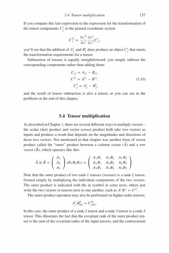
5.4 Tensor multiplication 137
If you compare this last expression to the expression for the transformation ofthe tensor components Ci
j to the primed coordinate system
C′kl =
∂x′k
∂xi
∂x j
∂x ′lCi
j ,
you’ll see that the addition of Aij and Bi
j does produce an object Cij that meets
the transformation requirements for a tensor.Subtraction of tensors is equally straightforward; you simply subtract the
corresponding components rather than adding them:
Ci j = Ai j − Bi j ,
Ci j = Ai j − Bi j ,
Cij = Ai
j − Bij ,
(5.10)
and the result of tensor subtraction is also a tensor, as you can see in theproblems at the end of this chapter.
5.4 Tensor multiplication
As described in Chapter 2, there are several different ways to multiply vectors –the scalar (dot) product and vector (cross) product both take two vectors asinputs and produce a result that depends on the magnitudes and directions ofthose two vectors. Not mentioned in that chapter was another form of vectorproduct called the “outer” product between a column vector ( �A) and a rowvector ( �B), which operates like this:
�A ⊗ �B =⎛⎝ A1
A2
A3
⎞⎠ (B1 B2 B3) =
⎛⎝ A1 B1 A1 B2 A1 B3
A2 B1 A2 B2 A2 B3
A3 B1 A3 B2 A3 B3
⎞⎠ .
Note that the outer product of two rank-1 tensors (vectors) is a rank-2 tensor,formed simply by multiplying the individual components of the two vectors.The outer product is indicated with the ⊗ symbol in some texts; others justwrite the two vectors or tensors next to one another, such as Ai B j = Ci j .
The outer-product operation may also be performed on higher-order tensors:
Aij Bk
lm = Cikjlm .
In this case, the outer product of a rank-2 tensor and a rank-3 tensor is a rank-5tensor. This illustrates the fact that the covariant rank of the outer-product ten-sor is the sum of the covariant ranks of the input tensors, and the contravariant
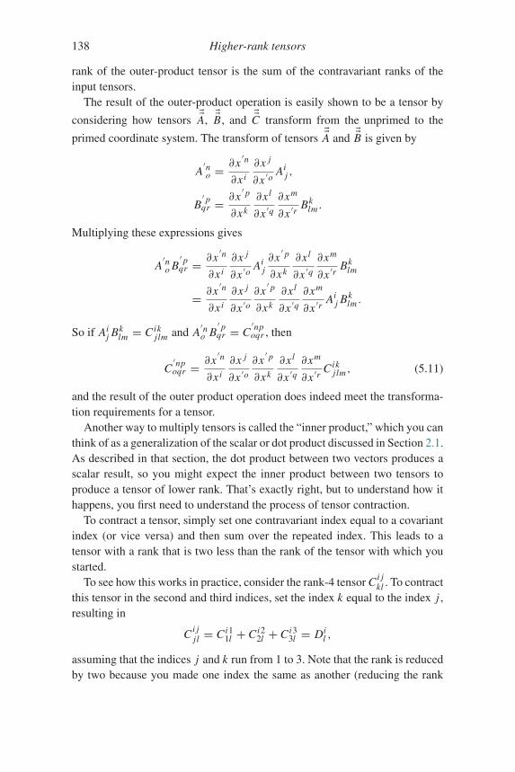
138 Higher-rank tensors
rank of the outer-product tensor is the sum of the contravariant ranks of theinput tensors.
The result of the outer-product operation is easily shown to be a tensor by
considering how tensors ��A, ��B, and ��C transform from the unprimed to the
primed coordinate system. The transform of tensors ��A and ��B is given by
A′no =
∂x′n
∂xi
∂x j
∂x ′oAi
j ,
B′ pqr = ∂x
′ p
∂xk
∂xl
∂x ′q∂xm
∂x ′rBk
lm .
Multiplying these expressions gives
A′no B′ pqr = ∂x
′n
∂xi
∂x j
∂x ′oAi
j∂x′ p
∂xk
∂xl
∂x ′q∂xm
∂x ′rBk
lm
= ∂x′n
∂xi
∂x j
∂x ′o∂x′ p
∂xk
∂xl
∂x ′q∂xm
∂x ′rAi
j Bklm .
So if Aij Bk
lm = Cikjlm and A
′no B
′ pqr = C
′npoqr , then
C′npoqr = ∂x
′n
∂xi
∂x j
∂x ′o∂x′ p
∂xk
∂xl
∂x ′q∂xm
∂x ′rCik
jlm, (5.11)
and the result of the outer product operation does indeed meet the transforma-tion requirements for a tensor.
Another way to multiply tensors is called the “inner product,” which you canthink of as a generalization of the scalar or dot product discussed in Section 2.1.As described in that section, the dot product between two vectors produces ascalar result, so you might expect the inner product between two tensors toproduce a tensor of lower rank. That’s exactly right, but to understand how ithappens, you first need to understand the process of tensor contraction.
To contract a tensor, simply set one contravariant index equal to a covariantindex (or vice versa) and then sum over the repeated index. This leads to atensor with a rank that is two less than the rank of the tensor with which youstarted.
To see how this works in practice, consider the rank-4 tensor Ci jkl . To contract
this tensor in the second and third indices, set the index k equal to the index j ,resulting in
Ci jjl = Ci1
1l + Ci22l + Ci3
3l = Dil ,
assuming that the indices j and k run from 1 to 3. Note that the rank is reducedby two because you made one index the same as another (reducing the rank
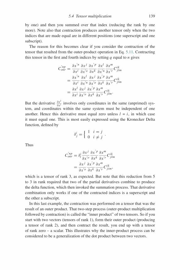
5.4 Tensor multiplication 139
by one) and then you summed over that index (reducing the rank by onemore). Note also that contraction produces another tensor only when the twoindices that are made equal are in different positions (one superscript and onesubscript).
The reason for this becomes clear if you consider the contraction of thetensor that resulted from the outer-product operation in Eq. 5.11. Contractingthis tensor in the first and fourth indices by setting q equal to n gives
C′nponr = ∂x
′n
∂xi
∂x j
∂x ′o∂x′ p
∂xk
∂xl
∂x ′n∂xm
∂x ′rCik
jlm
= ∂x′n
∂xi
∂xl
∂x ′n∂x j
∂x ′o∂x′ p
∂xk
∂xm
∂x ′rCik
jlm
= ∂xl
∂xi
∂x j
∂x ′o∂x′ p
∂xk
∂xm
∂x ′rCik
jlm .
But the derivative ∂xl
∂xi involves only coordinates in the same (unprimed) sys-tem, and coordinates within the same system must be independent of oneanother. Hence this derivative must equal zero unless l = i , in which caseit must equal one. This is most easily expressed using the Kronecker Deltafunction, defined by
δij =
{ 1 i = j0 i �= j
.
Thus
C′nponr = δi
l∂x j
∂x ′o∂x′ p
∂xk
∂xm
∂x ′rCik
jlm
= ∂x j
∂x ′o∂x′ p
∂xk
∂xm
∂x ′rCik
jim,
which is a tensor of rank 3, as expected. But note that this reduction from 5to 3 in rank required that two of the partial derivatives combine to producethe delta function, which then invoked the summation process. That derivativecombination only works if one of the contracted indices is a superscript andthe other a subscript.
In this last example, the contraction was performed on a tensor that was theresult of an outer product. That two-step process (outer-product multiplicationfollowed by contraction) is called the “inner product” of two tensors. So if youstart with two vectors (tensors of rank 1), form their outer product (producinga tensor of rank 2), and then contract the result, you end up with a tensorof rank zero – a scalar. This illustrates why the inner-product process can beconsidered to be a generalization of the dot product between two vectors.
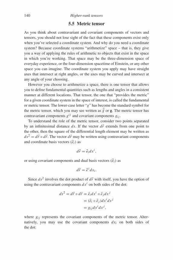
140 Higher-rank tensors
5.5 Metric tensor
As you think about contravariant and covariant components of vectors andtensors, you should not lose sight of the fact that these components exist onlywhen you’ve selected a coordinate system. And why do you need a coordinatesystem? Because coordinate systems “arithmetize” space – that is, they giveyou a way of applying the rules of arithmetic to objects that exist in the spacein which you’re working. That space may be the three-dimension space ofeveryday experience, or the four-dimension spacetime of Einstein, or any otherspace you can imagine. The coordinate system you apply may have straightaxes that intersect at right angles, or the axes may be curved and intersect atany angle of your choosing.
However you choose to arithmetize a space, there is one tensor that allowsyou to define fundamental quantities such as lengths and angles in a consistentmanner at different locations. That tensor, the one that “provides the metric”for a given coordinate system in the space of interest, is called the fundamentalor metric tensor. The lower-case letter “g” has become the standard symbol forthe metric tensor, which you may see written as ��g or g. The metric tensor hascontravariant components gi j and covariant components gi j .
To understand the role of the metric tensor, consider two points separatedby an infinitesimal distance ds. If the vector d�r extends from one point tothe other, then the square of the differential length element may be written asds2 = d�r ◦ d�r . The vector d�r may be written using contravariant componentsand coordinate basis vectors (�ei ) as
d�r = �ei dxi ,
or using covariant components and dual basis vectors (�ei ) as
d�r = �e i dxi .
Since ds2 involves the dot product of d�r with itself, you have the option ofusing the contravariant components dxi on both sides of the dot:
ds2 = d�r ◦ d�r = �ei dxi ◦ �e j dx j
= (�ei ◦ �e j )dxi dx j
= gi j dxi dx j ,
where gi j represents the covariant components of the metric tensor. Alter-natively, you may use the covariant components dxi on both sides ofthe dot:
5.5 Metric tensor 141
ds2 = d�r ◦ d�r = �e i dxi ◦ �e j dx j
= (�e i ◦ �e j )dxi dx j
= gi j dxi dx j ,
where gi j represents contravariant components of the metric tensor. A thirdoption is to use contravariant components on one side of the dot and covariantcomponents on the other:
ds2 = �ei dxi ◦ �e j dx j
= (�ei ◦ �e j )dxi dx j
= dxi dx j .
Note that in this case no metric tensor is needed, since the definition of dualbasis vectors ensures that �ei ◦ �e j equals one if i = j and zero if i �= j .
Whether ds2 is written as gi j dxi dx j , gi j dxi dx j , or dxi dx j , you can besure of one thing: the distance between two points must be the same no matterwhich coordinate system you employ, whether you use contravariant, covari-ant, or mixed components. Hence it must be the job of the metric tensor ��gand its components gi j and gi j to turn the product of incremental coordinatechanges expressed in either contravariant or covariant components into theinvariant distance between points. This is the rationale behind the statementthat the metric tensor “provides the geometry” of the space.
The geometry of vectors entails use of lengths and angles, so it’s usefulto understand the role of the metric tensor in defining the length of a vectorsuch as �A and the angle between two vectors �A and �B. Just as the incrementaldistance ds can be found by dotting the separation vector d�r into itself, thelength of vector �A can be found from �A ◦ �A. And there’s more than one wayto do that.
One option is to use only the contravariant components of �A:
| �A| =√ �A ◦ �A = √Ai �ei ◦ A j �e j
=√(�ei ◦ �e j )Ai A j =
√gi j Ai A j .
Another option is to use only covariant components:
| �A| =√ �A ◦ �A = √Ai �e i ◦ A j �e j
=√(�e i ◦ �e j )Ai A j =
√gi j Ai A j .
And the final option is to use mixed components:
142 Higher-rank tensors
| �A| =√ �A ◦ �A = √Ai �ei ◦ A j �e j
=√(�ei ◦ �e j )Ai A j =
√Ai A j .
As in the case of d�r , the metric tensor ensures that the length of vector �A isinvariant.
To understand the role of the metric tensor in providing a consistent defini-tion of angles, consider the dot product �A◦ �B. Once again, there are alternativeways of writing this product, and this means that the angle between �A and �Bcan be written in the following equivalent ways:
cos θ = �A ◦ �B| �A|| �B|= gi j Ai B j√
gi j Ai A j√
gi j Bi B j
= Ai B j√Ai Ai
√Bi Bi
= gi j Ai B j√gi j Ai A j
√gi j Bi B j
.
This explains why you’re likely to run into the statement that the metric tensor“provides a dot product” for a space – if you know how to find the dot product,you can define lengths and angles.
To see the tensor nature of the metric tensor, consider the transformation ofthe contravariant components of the incremental separation vector d�r :
dx′i = ∂x
′i
∂x jdx j .
This means that the square of the incremental length (ds2) becomes:
ds2 =[∂x′1
∂x1
∂x′1
∂x1+ ∂x
′2
∂x1
∂x′2
∂x1+ ∂x
′3
∂x1
∂x′3
∂x1
]dx1dx1
+[∂x′1
∂x2
∂x′1
∂x2+ ∂x
′2
∂x2
∂x′2
∂x2+ ∂x
′3
∂x2
∂x′3
∂x2
]dx2dx2
+[∂x′1
∂x3
∂x′1
∂x3+ ∂x
′2
∂x3
∂x′2
∂x3+ ∂x
′3
∂x3
∂x′3
∂x3
]dx3dx3
+[∂x′1
∂x1
∂x′1
∂x2+ ∂x
′2
∂x1
∂x′2
∂x2+ ∂x
′3
∂x1
∂x′3
∂x2
]dx1dx2
5.5 Metric tensor 143
+[∂x′1
∂x2
∂x′1
∂x1+ ∂x
′2
∂x2
∂x′2
∂x1+ ∂x
′3
∂x2
∂x′3
∂x1
]dx2dx1
+[∂x′1
∂x1
∂x′1
∂x3+ ∂x
′2
∂x1
∂x′2
∂x3+ ∂x
′3
∂x1
∂x′3
∂x3
]dx1dx3
+[∂x′1
∂x3
∂x′1
∂x1+ ∂x
′2
∂x3
∂x′2
∂x1+ ∂x
′3
∂x3
∂x′3
∂x1
]dx3dx1
+[∂x′1
∂x2
∂x′1
∂x3+ ∂x
′2
∂x2
∂x′2
∂x3+ ∂x
′3
∂x2
∂x′3
∂x3
]dx2dx3
+[∂x′1
∂x3
∂x′1
∂x2+ ∂x
′2
∂x3
∂x′2
∂x2+ ∂x
′3
∂x3
∂x′3
∂x2
]dx3dx2. (5.12)
This daunting expression becomes far more tractable if you realize that eachbracketed term involves the sum of the partial derivatives of each of the trans-formed coordinates (x
′1, x′2, and x
′3) taken with respect to two of the originalcoordinates (x1, x2, and x3). More specifically, each of the three terms withineach bracket is a product of the components of the basis vectors tangent to the
original axes (recall that ∂x′1
∂xi , ∂x′2
∂xi , and ∂x′3
∂xi are the components in the trans-formed coordinate system of the basis vector tangent to the i th original axis).
If you assign the bracketed terms to the variable g with two subscriptsdenoting the axes with respect to which the derivatives are taken, you willhave
g11 =[∂x′1
∂x1
∂x′1
∂x1+ ∂x
′2
∂x1
∂x′2
∂x1+ ∂x
′3
∂x1
∂x′3
∂x1
],
g22 =[∂x′1
∂x2
∂x′1
∂x2+ ∂x
′2
∂x2
∂x′2
∂x2+ ∂x
′3
∂x2
∂x′3
∂x2
],
g33 =[∂x′1
∂x3
∂x′1
∂x3+ ∂x
′2
∂x3
∂x′2
∂x3+ ∂x
′3
∂x3
∂x′3
∂x3
],
g12 =[∂x′1
∂x1
∂x′1
∂x2+ ∂x
′2
∂x1
∂x′2
∂x2+ ∂x
′3
∂x1
∂x′3
∂x2
],
g13 =[∂x′1
∂x1
∂x′1
∂x3+ ∂x
′2
∂x1
∂x′2
∂x3+ ∂x
′3
∂x1
∂x′3
∂x3
],
g23 =[∂x′1
∂x2
∂x′1
∂x3+ ∂x
′2
∂x2
∂x′2
∂x3+ ∂x
′3
∂x2
∂x′3
∂x3
],
144 Higher-rank tensors
and since the order of multiplication is irrelevant, g21 = g12, g31 = g13, andg32 = g23. Substituting these into Eq. 5.12, the expression for ds2 becomes
ds2 = g11dx1dx1 + g22dx2dx2 + g33dx3dx3 + g12dx1dx2 + g21dx2dx1
+ g13dx1dx3 + g31dx3dx1 + g23dx2dx3 + g32dx3dx2.
This can be further simplified using index notation and the summationconvention:
ds2 = gi j dxi dx j . (5.13)
The gi j term in this equation meets all the requirements of a second-ranktensor, but it’s not just any tensor. Because it relates the coordinate differentialsin various directions to a quantity that is invariant across all coordinate trans-formations, it’s no wonder that this tensor is called the metric or fundamentaltensor.
To understand what’s so fundamental about this tensor, recall that the partialderivatives that make up the elements of gi j also represent the components ofthe basis vectors tangent to the original coordinate axes:
�e1 =(∂x′1
∂x1,∂x′2
∂x1,∂x′3
∂x1
),
�e2 =(∂x′1
∂x2,∂x′2
∂x2,∂x′3
∂x2
), (5.14)
�e3 =(∂x′1
∂x3,∂x′2
∂x3,∂x′3
∂x3
).
And since
gi j =[∂x′1
∂xi
∂x′1
∂x j+ ∂x
′2
∂xi
∂x′2
∂x j+ ∂x
′3
∂xi
∂x′3
∂x j
], (5.15)
another way to represent the metric tensor is gi j = �ei ◦ �e j (the inner productof the basis vectors tangent to the coordinate axes). Since the inner productinvolves the projection of one vector onto the direction of another and scalesas the length of those two vectors, the elements of gi j specify the relationshipsbetween the coordinate axes. Those relationships are determined by the shapeof the coordinate space.
The nature of the metric tensor can be readily understood by considering atransformation from spherical polar (r, θ, φ) to Cartesian (x, y, z) coordinates.In this case
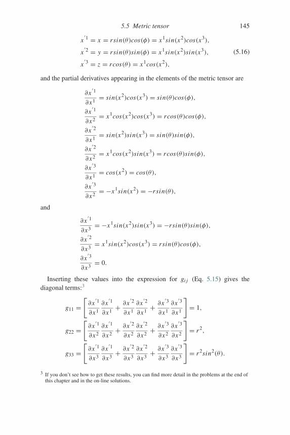
5.5 Metric tensor 145
x′1 = x = rsin(θ)cos(φ) = x1sin(x2)cos(x3),
x′2 = y = rsin(θ)sin(φ) = x1sin(x2)sin(x3),
x′3 = z = rcos(θ) = x1cos(x2),
(5.16)
and the partial derivatives appearing in the elements of the metric tensor are
∂x′1
∂x1= sin(x2)cos(x3) = sin(θ)cos(φ),
∂x′1
∂x2= x1cos(x2)cos(x3) = rcos(θ)cos(φ),
∂x′2
∂x1= sin(x2)sin(x3) = sin(θ)sin(φ),
∂x′2
∂x2= x1cos(x2)sin(x3) = rcos(θ)sin(φ),
∂x′3
∂x1= cos(x2) = cos(θ),
∂x′3
∂x2= −x1sin(x2) = −rsin(θ),
and
∂x′1
∂x3= −x1sin(x2)sin(x3) = −rsin(θ)sin(φ),
∂x′2
∂x3= x1sin(x2)cos(x3) = rsin(θ)cos(φ),
∂x′3
∂x3= 0.
Inserting these values into the expression for gi j (Eq. 5.15) gives thediagonal terms:3
g11 =[∂x′1
∂x1
∂x′1
∂x1+ ∂x
′2
∂x1
∂x′2
∂x1+ ∂x
′3
∂x1
∂x′3
∂x1
]= 1,
g22 =[∂x′1
∂x2
∂x′1
∂x2+ ∂x
′2
∂x2
∂x′2
∂x2+ ∂x
′3
∂x2
∂x′3
∂x2
]= r2,
g33 =[∂x′1
∂x3
∂x′1
∂x3+ ∂x
′2
∂x3
∂x′2
∂x3+ ∂x
′3
∂x3
∂x′3
∂x3
]= r2sin2(θ).
3 If you don’t see how to get these results, you can find more detail in the problems at the end ofthis chapter and in the on-line solutions.
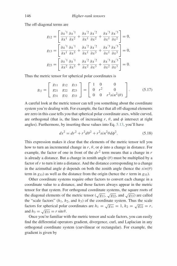
146 Higher-rank tensors
The off-diagonal terms are
g12 =[∂x′1
∂x1
∂x′1
∂x2+ ∂x
′2
∂x1
∂x′2
∂x2+ ∂x
′3
∂x1
∂x′3
∂x2
]= 0,
g13 =[∂x′1
∂x1
∂x′1
∂x3+ ∂x
′2
∂x1
∂x′2
∂x3+ ∂x
′3
∂x1
∂x′3
∂x3
]= 0,
g23 =[∂x′1
∂x2
∂x′1
∂x3+ ∂x
′2
∂x2
∂x′2
∂x3+ ∂x
′3
∂x2
∂x′3
∂x3
]= 0.
Thus the metric tensor for spherical polar coordinates is
gi j =⎡⎣ g11 g12 g13
g21 g22 g23
g31 g32 g33
⎤⎦ =
⎡⎣ 1 0 0
0 r2 00 0 r2sin2(θ)
⎤⎦ . (5.17)
A careful look at the metric tensor can tell you something about the coordinatesystem you’re dealing with. For example, the fact that all off-diagonal elementsare zero in this case tells you that spherical polar coordinate axes, while curved,are orthogonal (that is, the lines of increasing r , θ , and φ intersect at rightangles). Furthermore, by inserting these values into Eq. 5.13, you’ll have
ds2 = dr2 + r2dθ2 + r2sin2θdφ2. (5.18)
This expression makes it clear that the elements of the metric tensor tell youhow to turn an incremental change in r , θ , or φ into a change in distance. Forexample, the factor of one in front of the dr2 term means that a change in ris already a distance. But a change in zenith angle (θ ) must be multiplied by afactor of r to turn it into a distance. And the distance corresponding to a changein the azimuthal angle φ depends on both the zenith angle (hence the sin(θ)term in g33) as well as the distance from the origin (hence the r term in g33).
Other coordinate systems require other factors to convert each change in acoordinate value to a distance, and those factors always appear in the metrictensor for that system. For orthogonal coordinate systems, the square roots ofthe diagonal elements of the metric tensor (
√g11,√
g22, and√
g33) are calledthe “scale factors” (h1, h2, and h3) of the coordinate system. Thus the scalefactors for spherical polar coordinates are h1 = √g11 = 1, h2 = √g22 = r ,and h3 = √g33 = r sin θ .
Once you’re familiar with the metric tensor and scale factors, you can easilyfind the differential operators gradient, divergence, curl, and Laplacian in anyorthogonal coordinate system (curvilinear or rectangular). For example, thegradient is given by
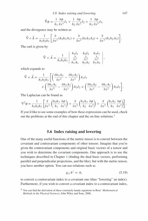
5.6 Index raising and lowering 147
�∇φ = 1
h1
∂φ
∂x1e1 + 1
h2
∂φ
∂x2e2 + 1
h3
∂φ
∂x3e3,
and the divergence may be written as
�∇ ◦ �A = 1
h1h2h3
[∂
∂x1(h2h3 A1)+ ∂
∂x2(h1h3 A2)+ ∂
∂x3(h1h2 A3)
].
The curl is given by
�∇ × �A = 1
h1h2h3
∣∣∣∣∣∣h1e1 h2e2 h3e3∂
∂x1∂
∂x2∂
∂x3
h1 A1 h2 A2 h3 A3
∣∣∣∣∣∣ ,which expands to
�∇ × �A = 1
h1h2h3
[(∂h3 A3
∂x2− ∂h2 A2
∂x3
)h1e1
+(∂h1 A1
∂x3− ∂h3 A3
∂x1
)h2e2 +
(∂h2 A2
∂x1− ∂h1 A1
∂x2
)h3e3
].
The Laplacian can be found as
∇2φ= 1
h1h2h3
[∂
∂x1
(h2h3
h1
∂φ
∂x1
)+ ∂
∂x2
(h1h3
h2
∂φ
∂x2
)+ ∂
∂x3
(h1h2
h3
∂φ
∂x3
)].
If you’d like to see some examples of how these expressions can be used, checkout the problems at the end of this chapter and the on-line solutions.4
5.6 Index raising and lowering
One of the many useful functions of the metric tensor is to convert between thecovariant and contravariant components of other tensors. Imagine that you’regiven the contravariant components and original basis vectors of a tensor andyou wish to determine the covariant components. One approach is to use thetechniques described in Chapter 4 (finding the dual basis vectors, performingparallel and perpendicular projections, and the like), but with the metric tensor,you have another option. You can use relations such as
gi j A j = Ai (5.19)
to convert a contravariant index to a covariant one (thus “lowering” an index).Furthermore, if you wish to convert a covariant index to a contravariant index,
4 You can find the derivation of these extremely handy equations in Boas’ MathematicalMethods in the Physical Sciences, John Wiley and Sons, 2006.
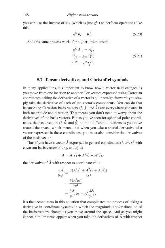
148 Higher-rank tensors
you can use the inverse of gi j (which is just gi j ) to perform operations likethis:
gi j Bi = B j . (5.20)
And this same process works for higher-order tensors:
gi j Aik = A jk ,
Cijk = g jsCis
k ,
T i jk = gil T jkl .
(5.21)
5.7 Tensor derivatives and Christoffel symbols
In many applications, it’s important to know how a vector field changes asyou move from one location to another. For vectors expressed using Cartesiancoordinates, taking the derivative of a vector is quite straightforward: you sim-ply take the derivative of each of the vector’s components. You can do thatbecause the Cartesian basis vectors (ı , j , and k) are everywhere constant inboth magnitude and direction. That means you don’t need to worry about thederivatives of the basis vectors. But as you’ve seen for spherical polar coordi-nates, the basis vectors (r , θ , and φ) point in different directions as you movearound the space, which means that when you take a spatial derivative of avector expressed in these coordinates, you must also consider the derivativesof the basis vectors.
Thus if you have a vector �A expressed in general coordinates x1, x2, x3 withcovariant basis vectors �e1, �e2, and �e3 as
�A = A1 �e1 + A2 �e2 + A3 �e3,
the derivative of �A with respect to coordinate x1 is
∂ �A∂x1= ∂(A1 �e1 + A2 �e2 + A3 �e3)
∂x1
= ∂(Ai �ei )
∂x1
= ∂Ai
∂x1�e1 + Ai ∂ �ei
∂x1.
It’s the second term in this equation that complicates the process of taking aderivative in coordinate systems in which the magnitude and/or direction ofthe basis vectors change as you move around the space. And as you mightexpect, similar terms appear when you take the derivatives of �A with respect
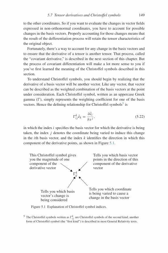
5.7 Tensor derivatives and Christoffel symbols 149
to the other coordinates. So if you want to evaluate the changes in vector fieldsexpressed in non-orthonormal coordinates, you have to account for possiblechanges in the basis vectors. Properly accounting for those changes means thatthe result of the defferentiation process will retain the tensor characteristics ofthe original object.
Fortunately, there’s a way to account for any change in the basis vectors andto ensure that the derivative of a tensor is another tensor. That process, calledthe “covariant derivative,” is described in the next section of this chapter. Butthe process of covariant differentiation will make a lot more sense to you ifyou’ve first learned the meaning of the Christoffel symbols described in thissection.
To understand Christoffel symbols, you should begin by realizing that thederivative of a basis vector will be another vector. Like any vector, that vectorcan be described as the weighted combination of the basis vectors at the pointunder consideration. Each Christoffel symbol, written as an uppercase Greekgamma (�), simply represents the weighting coefficient for one of the basisvectors. Hence the defining relationship for Christoffel symbols5 is
�ki j �ek = ∂�ei
∂x j, (5.22)
in which the index i specifies the basis vector for which the derivative is beingtaken, the index j denotes the coordinate being varied to induce this changein the i th basis vector, and the index k identifies the direction in which thiscomponent of the derivative points, as shown in Figure 5.1.
This Christoffel symbol givesyou the magnitude of onecomponent of thederivative vector
Tells you which basis vectorpoints in the direction of thiscomponent of the derivativevector
Tells you which basisvector’s change isbeing considered
Tells you which coordinateis being varied to cause achange in the basis vector
Γkij
Figure 5.1 Explanation of Christoffel symbol indices.
5 The Christoffel symbols written as �ki j are Christoffel symbols of the second kind; another
form of Christoffel symbol (the “first kind”) is described in most General Relativity texts.
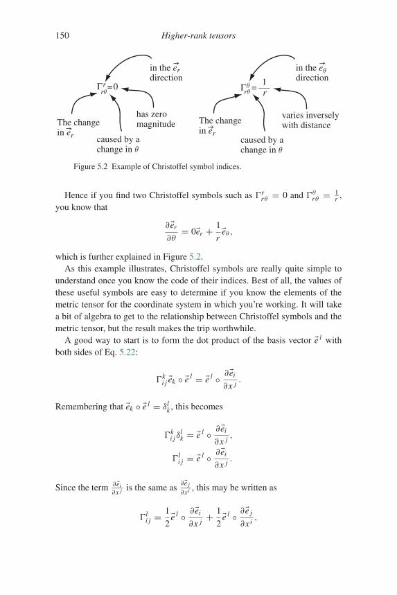
150 Higher-rank tensors
has zeromagnitude
caused by achange in θ
rθΓr =0
in the erdirection
The changein er
1r
varies inverselywith distance
caused by achange in θ
The changein er
Γθ =
in the eθdirection
rθ
Figure 5.2 Example of Christoffel symbol indices.
Hence if you find two Christoffel symbols such as �rrθ = 0 and �θrθ = 1
r ,you know that
∂�er
∂θ= 0�er + 1
r�eθ ,
which is further explained in Figure 5.2.As this example illustrates, Christoffel symbols are really quite simple to
understand once you know the code of their indices. Best of all, the values ofthese useful symbols are easy to determine if you know the elements of themetric tensor for the coordinate system in which you’re working. It will takea bit of algebra to get to the relationship between Christoffel symbols and themetric tensor, but the result makes the trip worthwhile.
A good way to start is to form the dot product of the basis vector �e l withboth sides of Eq. 5.22:
�ki j �ek ◦ �e l = �e l ◦ ∂�ei
∂x j.
Remembering that �ek ◦ �e l = δlk , this becomes
�ki jδ
lk = �e l ◦ ∂�ei
∂x j,
�li j = �e l ◦ ∂�ei
∂x j.
Since the term ∂�ei∂x j is the same as
∂�e j
∂xi , this may be written as
�li j =
1
2�e l ◦ ∂�ei
∂x j+ 1
2�e l ◦ ∂�e j
∂xi,
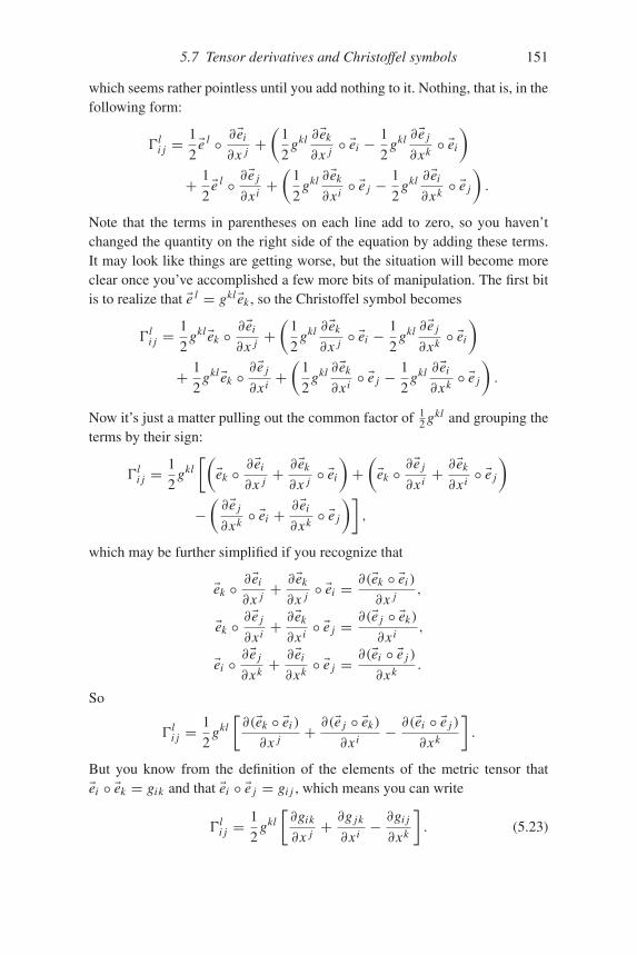
5.7 Tensor derivatives and Christoffel symbols 151
which seems rather pointless until you add nothing to it. Nothing, that is, in thefollowing form:
�li j =
1
2�e l ◦ ∂�ei
∂x j+(
1
2gkl ∂�ek
∂x j◦ �ei − 1
2gkl ∂�e j
∂xk◦ �ei
)
+ 1
2�e l ◦ ∂�e j
∂xi+(
1
2gkl ∂�ek
∂xi◦ �e j − 1
2gkl ∂�ei
∂xk◦ �e j
).
Note that the terms in parentheses on each line add to zero, so you haven’tchanged the quantity on the right side of the equation by adding these terms.It may look like things are getting worse, but the situation will become moreclear once you’ve accomplished a few more bits of manipulation. The first bitis to realize that �e l = gkl �ek , so the Christoffel symbol becomes
�li j =
1
2gkl �ek ◦ ∂�ei
∂x j+(
1
2gkl ∂�ek
∂x j◦ �ei − 1
2gkl ∂�e j
∂xk◦ �ei
)
+ 1
2gkl �ek ◦ ∂�e j
∂xi+(
1
2gkl ∂�ek
∂xi◦ �e j − 1
2gkl ∂�ei
∂xk◦ �e j
).
Now it’s just a matter pulling out the common factor of 12 gkl and grouping the
terms by their sign:
�li j =
1
2gkl
[(�ek ◦ ∂�ei
∂x j+ ∂�ek
∂x j◦ �ei
)+(�ek ◦ ∂�e j
∂xi+ ∂�ek
∂xi◦ �e j
)
−(∂�e j
∂xk◦ �ei + ∂�ei
∂xk◦ �e j
)],
which may be further simplified if you recognize that
�ek ◦ ∂�ei
∂x j+ ∂�ek
∂x j◦ �ei = ∂(�ek ◦ �ei )
∂x j,
�ek ◦ ∂�e j
∂xi+ ∂�ek
∂xi◦ �e j = ∂(�e j ◦ �ek)
∂xi,
�ei ◦ ∂�e j
∂xk+ ∂�ei
∂xk◦ �e j = ∂(�ei ◦ �e j )
∂xk.
So
�li j =
1
2gkl
[∂(�ek ◦ �ei )
∂x j+ ∂(�e j ◦ �ek)
∂xi− ∂(�ei ◦ �e j )
∂xk
].
But you know from the definition of the elements of the metric tensor that�ei ◦ �ek = gik and that �ei ◦ �e j = gi j , which means you can write
�li j =
1
2gkl
[∂gik
∂x j+ ∂g jk
∂xi− ∂gi j
∂xk
]. (5.23)
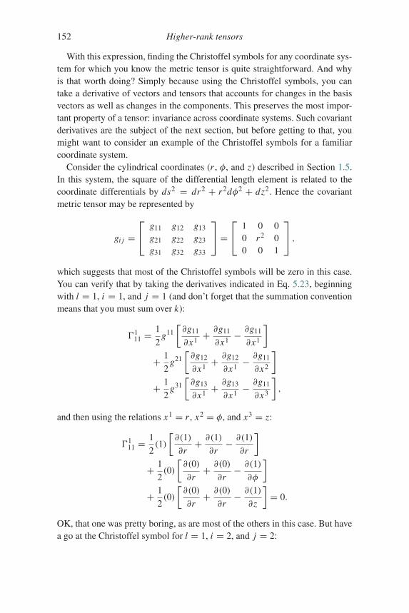
152 Higher-rank tensors
With this expression, finding the Christoffel symbols for any coordinate sys-tem for which you know the metric tensor is quite straightforward. And whyis that worth doing? Simply because using the Christoffel symbols, you cantake a derivative of vectors and tensors that accounts for changes in the basisvectors as well as changes in the components. This preserves the most impor-tant property of a tensor: invariance across coordinate systems. Such covariantderivatives are the subject of the next section, but before getting to that, youmight want to consider an example of the Christoffel symbols for a familiarcoordinate system.
Consider the cylindrical coordinates (r , φ, and z) described in Section 1.5.In this system, the square of the differential length element is related to thecoordinate differentials by ds2 = dr2 + r2dφ2 + dz2. Hence the covariantmetric tensor may be represented by
gi j =⎡⎣ g11 g12 g13
g21 g22 g23
g31 g32 g33
⎤⎦ =
⎡⎣ 1 0 0
0 r2 00 0 1
⎤⎦ ,
which suggests that most of the Christoffel symbols will be zero in this case.You can verify that by taking the derivatives indicated in Eq. 5.23, beginningwith l = 1, i = 1, and j = 1 (and don’t forget that the summation conventionmeans that you must sum over k):
�111 =
1
2g11
[∂g11
∂x1+ ∂g11
∂x1− ∂g11
∂x1
]
+ 1
2g21
[∂g12
∂x1+ ∂g12
∂x1− ∂g11
∂x2
]
+ 1
2g31
[∂g13
∂x1+ ∂g13
∂x1− ∂g11
∂x3
],
and then using the relations x1 = r , x2 = φ, and x3 = z:
�111 =
1
2(1)
[∂(1)
∂r+ ∂(1)
∂r− ∂(1)
∂r
]
+ 1
2(0)
[∂(0)
∂r+ ∂(0)
∂r− ∂(1)
∂φ
]
+ 1
2(0)
[∂(0)
∂r+ ∂(0)
∂r− ∂(1)
∂z
]= 0.
OK, that one was pretty boring, as are most of the others in this case. But havea go at the Christoffel symbol for l = 1, i = 2, and j = 2:
5.8 Covariant differentiation 153
�122 =
1
2g11
[∂g21
∂x2+ ∂g21
∂x2− ∂g22
∂x1
]
+ 1
2g21
[∂g22
∂x2+ ∂g22
∂x2− ∂g22
∂x2
]
+ 1
2g32
[∂g23
∂x2+ ∂g23
∂x2− ∂g22
∂x3
],
which is:
�122 =
1
2(1)
[∂(0)
∂φ+ ∂(0)
∂φ− ∂r2
∂r
]
+ 1
2(0)
[∂r2
∂φ+ ∂r2
∂φ− ∂r2
∂φ
]
+ 1
2(0)
[∂(0)
∂φ+ ∂(0)
∂φ− ∂r2
∂z
],
or
�122 =
1
2(1)[0+ 0− 2r ] + 0+ 0 = −r.
Now you’re getting somewhere. And exactly where is that? Just rememberthe meaning of a Christoffel symbol, and you’ll see that this result means thatthe change in the covariant �φ basis vector as you move in the φ direction hasa component in the −�r direction that increases directly with distance from theorigin.
A similar analysis shows that �212 = �2
21 = 1/r , which are the only othernon-zero Christoffel symbols for the cylindrical coordinate system.6 If youdon’t see how to get that result, take a look at the problems at the end of thischapter and the on-line solutions.
5.8 Covariant differentiation
With Christoffel symbols in hand, you have a way of differentiating a vector orhigher-order tensor that includes the effect of changes (if any) in the magnitudeand direction of the basis vectors used to expand that vector or tensor. This typeof derivative is called the “covariant” derivative, and it finds application notonly in the Euclidean space in which many engineering and physics problemsare worked, but also in the curved Riemanian space of General Relativity.
In Euclidean space, two vectors at different locations may be compared andcombined by dragging one of the vectors to the location of the other without6 Note that the symmetry of the metric tensor means that Christoffel symbols of this type are
symmetric in the two lower indices.
154 Higher-rank tensors
changing its magnitude or its direction. If the vector is expanded using Carte-sian coordinates, such “parallel transport” is accomplished simply by keepingeach of its components the same (because the Cartesian basis vectors have thesame magnitude and direction everywhere). But if the vector is expressed innon-Cartesian coordinates, the length and direction of the basis vectors may bedifferent at the two locations. In such cases, the covariant derivative providesa means of parallel-transporting one of the vectors to the location of the other.
The situation is more complicated for curved spaces. You can find the detailsof the use of the covariant derivative in curved spaces in Chapter 6, but fornow you can understand the role of the covariant derivative by considering atwo-dimensional spherical surface embedded in a three-dimensional Euclideanspace. Imagine a series of tangent planes just touching the sphere at each loca-tion, and picture a vector lying in one of those tangent planes. If that vector ismoved to a different location on the sphere while holding its direction constant(as viewed in the larger three-dimensional space), it will not lie in the tangentplane at the new location (you can think of the vector as “sticking out” ofthe two-dimensional space of the sphere). In such cases, the covariant deriva-tive serves to project the derivative of the vector into the tangent space of thesphere.
You should also note that the covariant differentiation process producesa result that retains the properties of a tensor, which means that the resulttransforms between coordinate systems according to the rules of tensortransformation.
To understand how the process of covariant differentiation works, considerthe vector �A = A1 �e1 + A2 �e2 + A3 �e3 and its derivatives
∂ �A∂x j= ∂(A1 �e1 + A2 �e2 + A3 �e3)
∂x j
= ∂(Ai �ei )
∂x j
= ∂Ai
∂x j�ei + Ai ∂ �ei
∂x j.
Now replace the partial derivative in the second term with the Christoffel-symbol definition (Eq. 5.22):
∂ �A∂x j= ∂Ai
∂x j�ei + Ai (�k
i j �ek).
Since the indices i and k in the second term are both dummy indices by thesummation rule, you can switch them and then extract the common factor thatis now the basis vector �ei :
5.8 Covariant differentiation 155
∂ �A∂x j= ∂Ai
∂x j�ei + Ak(�i
k j �ei )
=(∂Ai
∂x j+ Ak�i
k j
)�ei .
The covariant derivative is defined as the combination of the two terms insidethe parentheses. Common notation for the covariant derivative is to use a semi-colon (;) in front of the index with respect to which the covariant derivative isbeing taken ( j in this case). Thus you’re likely to see the components of thecovariant derivative defined as
Ai; j ≡
∂Ai
∂x j+ Ak�i
k j . (5.24)
A similar analysis leads to the covariant derivative of a vector expandedusing covariant coefficients:
Ai; j ≡ ∂Ai
∂x j− Ak�
ki j . (5.25)
Note that the term involving Christoffel symbols is subtracted in this case.To make the meaning of Eqs. 5.24 and 5.25 more explicit, consider the
covariant derivative of vector �A with respect to φ in cylindrical coordinates(so x1 = r , x2 = φ, and x3 = z). Setting j = 2 in Eq. 5.24 (since we’reinterested in the covariant derivative with respect to φ),
Ar;φ =
∂Ar
∂φ+ Ar�r
rφ + Aφ�rφφ + Az�r
zφ
= ∂Ar
∂φ+ 0+ Aφ(−r)+ 0,
which says that a change in the r -component of vector �A caused by a changein φ is caused both by a change in Ar with φ and by a change in the basisvectors which causes a portion of �A that was originally in the φ-direction tonow point in the −r -direction. Likewise, for the change in Aφ as the value ofφ is changed,
Aφ;φ =∂Aφ
∂φ+ Aφ�φrφ + Ar�
φφφ + Az�
φzφ
= ∂Aφ
∂φ+ Ar
(1
r
)+ 0+ 0.
Thus∂ �A∂φ=(∂Ar
∂φ− r Aφ
)�er +
(∂Aφ
∂φ+ 1
rAr)�eφ.
The process of covariant differentiation can also be applied to higher-order tensors. As you might expect, this simply requires the addition of a
156 Higher-rank tensors
Christoffel-symbol term for each contravariant index, and the subtraction ofa Christoffel-symbol term for each covariant index. Hence
Ai j;k =
∂Ai j
∂xk+ Al j�i
lk + Ail�jlk,
Bi j ;k = ∂Bi j
∂xk− Bl j�
lik − Bil�
ljk,
Cij ;k =
∂Cij
∂xk+ Cl
j�ilk − Ci
l�ljk .
5.9 Vectors and one-forms
If you look up the subject of tensors in recently published physics texts, espe-cially those dealing with General Relativity, you may be surprised to find littlemention of contravariant and covariant components in favor of terms such as“covectors” and “one-forms.” Have you wasted your time struggling to under-stand complicated concepts and terminology that have now become obsolete?I obviously don’t think so, or I wouldn’t have devoted so many pages to thedevelopments of the last two chapters. Instead, I believe there’s value in seeingthe “traditional” presentation as well as the “modern” approach, because thedifferences arise from perspective rather than from the core concepts. But thosedifferent perspectives do lead to very different terminology, and the purpose ofthis section is to provide a short introduction to that terminology.
The first thing to understand is that the traditional approach tends to treatcontravariant and covariant components as representations of the same object,whereas in the modern approach objects are classified either as “vectors” oras “one-forms” (also called “covectors”). In the modern terminology, vectorstransform as contravariant quantities, and one-forms transform as covariantquantities. Quantities with dimension of length in the numerator (such asvelocity, with units that include “meters per”) fit naturally into the vectorcategory; quantities with dimension of length in denominator (such as the gra-dient of a scalar field, with units that include “per meter”) fit naturally into theone-form category.
In illustrations involving vectors and one-forms, vectors are represented asarrows and one-forms are represented as small sections of surfaces, as shownin Figure 5.3. As indicated in the figure, for vectors the angle of the arrowshows direction and the length of the arrow shows the magnitude. For one-forms, surfaces are aligned normal to the direction and the spacing betweensurfaces is inversely proportional to the magnitude. This means that vectorswith greater magnitude are represented by longer arrows, while one-forms ofgreater magnitude are represented by closer spacing.
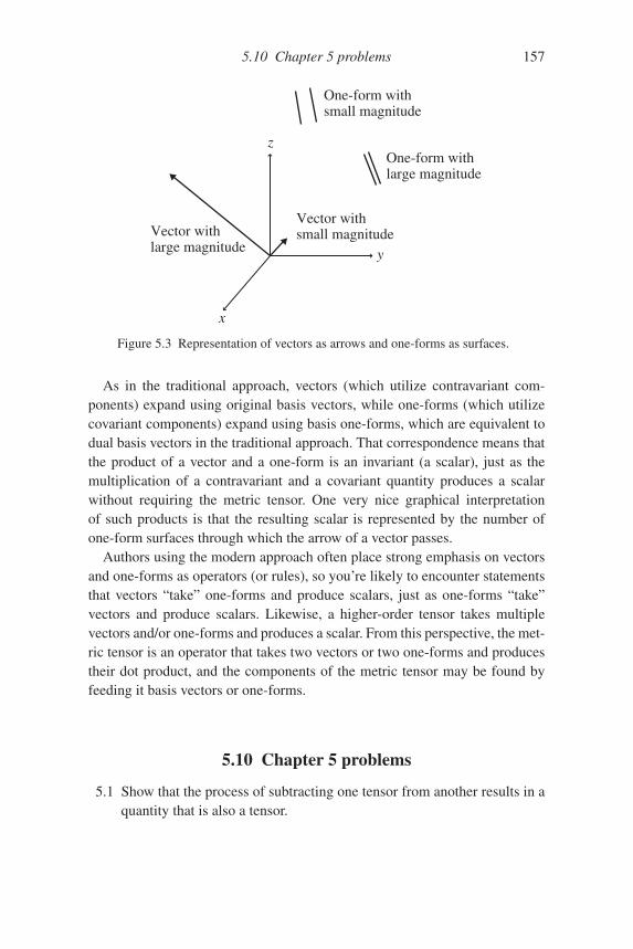
5.10 Chapter 5 problems 157
x
y
z
One-form withsmall magnitude
One-form withlarge magnitude
Vector withlarge magnitude
Vector withsmall magnitude
Figure 5.3 Representation of vectors as arrows and one-forms as surfaces.
As in the traditional approach, vectors (which utilize contravariant com-ponents) expand using original basis vectors, while one-forms (which utilizecovariant components) expand using basis one-forms, which are equivalent todual basis vectors in the traditional approach. That correspondence means thatthe product of a vector and a one-form is an invariant (a scalar), just as themultiplication of a contravariant and a covariant quantity produces a scalarwithout requiring the metric tensor. One very nice graphical interpretationof such products is that the resulting scalar is represented by the number ofone-form surfaces through which the arrow of a vector passes.
Authors using the modern approach often place strong emphasis on vectorsand one-forms as operators (or rules), so you’re likely to encounter statementsthat vectors “take” one-forms and produce scalars, just as one-forms “take”vectors and produce scalars. Likewise, a higher-order tensor takes multiplevectors and/or one-forms and produces a scalar. From this perspective, the met-ric tensor is an operator that takes two vectors or two one-forms and producestheir dot product, and the components of the metric tensor may be found byfeeding it basis vectors or one-forms.
5.10 Chapter 5 problems
5.1 Show that the process of subtracting one tensor from another results in aquantity that is also a tensor.
158 Higher-rank tensors
5.2 Find the elements of the metric tensor for spherical coordinates byforming the dot products of the relevant basis vectors.
5.3 Show how the derivatives given after Eq. 5.16 lead to the elements of themetric tensor for spherical polar coordinates (Eq. 5.17).
5.4 Use the scale factors for spherical polar coordinates to verify the expres-sions given in Chapter 2 for the gradient, divergence, curl, and Laplacianin spherical coordinates.
5.5 Show that for cylindrical coordinates (r, φ, z) the Christoffel symbols�2
12 and �221 are equal to 1/r .
5.6 Find gi j , the inverse of the spherical metric tensor gi j .5.7 Use gi j to raise the indices of the vector Ai = (1, r2sinθ, sin2θ).5.8 On the two-dimensional surface of a sphere of radius R, the square of
the differential length element is given by ds2 = R2dθ2 + R2sin2θdφ2.Find the metric tensor gi j and its inverse gi j for this case.
5.9 What are the Christoffel symbols for the 2-D spherical surface ofProblem 5.8?
5.10 Show that the covariant derivative of the metric tensor equals zero.
6
Tensor applications
This chapter provides examples of how to apply the tensor concepts containedin Chapters 4 and 5, just as Chapter 3 provided examples of how to applythe vector concepts presented in Chapters 1 and 2. As in Chapter 3, the intentfor this chapter is to include more detail about a small number of selectedapplications than can be included in the chapters in which tensor concepts arefirst presented.
The examples in this chapter come from the fields of Mechanics, Elec-tromagnetics, and General Relativity. Of course, there’s no way to compre-hensively cover any significant portion of those fields in one chapter; theseexamples were chosen only to serve as representatives of the types of tensorapplication you’re likely to encounter in those fields.
6.1 The inertia tensor
A very useful way to think of mass is this: mass is the characteristic of matterthat resists acceleration. This means that it takes a force to change the velocityof any object with mass. You may find it helpful to think of moment of inertiaas the rotational analog of mass. That is, moment of inertia is the characteristicof matter that resists angular acceleration, so it takes a torque to change theangular velocity of an object.
Many students find that rotational motion is easier to understand by keepingthe relationships between translational and rotational quantities in mind. Sowhere translational motion dealt with position (x), velocity (�v), and accelera-tion (�a), rotational motion has the analogous quantities of angle (θ ), angularvelocity ( �ω), and angular acceleration (�α). There are rotational analogs formany other quantities; the translational quantities of force ( �F), mass (m), andmomentum ( �p) have the rotational equivalents of torque (�τ ), moment of inertia(I ), and angular momentum ( �L).
159
160 Tensor applications
As you may also recall, several of the equations relating various translationalquantities have direct parallels in rotational motion. So the rotational equiva-lent of Newton’s Second Law ( �F = m�a) is �τ = I �α.1 And whereas translationalmomentum is related to mass and velocity by �p = m�v, you probably learnedthat angular momentum is related to moment of inertia and angular velocity byLz = Iω.
When first presenting these relationships, most texts restrict the motion toplanar rotation of a single particle to keep things simple. So when you think ofthe relationship between linear and angular velocity, you may think of some-thing like v = ωr . And if Lz = mvr , then Lz = mr2ω. Taking mr2 as themoment of inertia (I ) of a single particle, this becomes Lz = Iω. But the vand the ω in those equations can’t really be velocities, since they’re writtenas scalars rather than vectors, and that z subscript on the angular momentumseems to be trying to tell you something.
It is. It’s telling you that you’re using an equation for one component of theangular momentum (the z-component in this case), and this pertains to a singleparticle moving about the origin in the xy plane. So these equations aren’twrong, they just have limited application. Specifically, they apply to cases ofplanar motion about the z-axis.
The more-general relationship between the vectors that represent velocity,angular velocity, and position is this:
�v = �ω × �r , (6.1)
in which the cross represents the vector cross product described in Chapter 2.And the equations relating angular momentum to linear momentum, linearvelocity, and mass are
�L = �r × �p= �r × (m�v)= m�r × �v.
(6.2)
Before delving more deeply into these equations, you should consider theimplications of the (planar-motion) equation that says that the moment ofinertia of a single particle is Iparticle = mr2. One important idea in thisequation is that the moment of inertia of a particle depends not only on itsmass, but also on the location of that mass – specifically, the distance (r ) ofthe mass from the axis of rotation. Thus the moment of inertia of an extendedobject made up of many particles must depend not only on the object’s mass,
1 Or, if you prefer the more-general form of Newton’s Second Law ( �F = d �pdt ), the analogous
rotational relationship is �τ = d �Ldt .
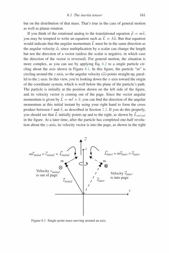
6.1 The inertia tensor 161
but on the distribution of that mass. That’s true in the case of general motionas well as planar rotation.
If you think of the rotational analog to the translational equation �p = m�v,you may be tempted to write an equation such as �L = I �ω. But that equationwould indicate that the angular momentum �L must be in the same direction asthe angular velocity �ω, since multiplication by a scalar can change the lengthbut not the direction of a vector (unless the scalar is negative, in which casethe direction of the vector is reversed). For general motion, the situation ismore complex, as you can see by applying Eq. 6.2 to a single particle cir-cling about the axis shown in Figure 6.1. In this figure, the particle “m” iscircling around the z-axis, so the angular velocity ( �ω) points straight up, paral-lel to the z-axis. In this view, you’re looking down the x-axis toward the originof the coordinate system, which is well below the plane of the particle’s path.The particle is initially at the position shown on the left side of the figure,and its velocity vector is coming out of the page. Since the vector angularmomentum is given by �L = m�r × �v, you can find the direction of the angularmomentum at this initial instant by using your right hand to form the crossproduct between �r and �v, as described in Section 2.2. If you do this properly,you should see that �L initially points up and to the right, as shown by �Linitial
in the figure. At a later time, after the particle has completed one-half revolu-tion about the z-axis, its velocity vector is into the page, as shown in the right
y
z
ω
mm
rlater
Velocity vlateris into page
Llater = mrlater × vlatermrinitial × vinitial = Linitial
Velocity vinitialis out of page
rinitial
Figure 6.1 Single point mass moving around an axis.
162 Tensor applications
portion of the figure. At that later instant, the cross product between �r and �vmeans that the direction of the angular momentum vector �L is up and to theleft, as shown by �Llater .
So not only is the angular-momentum vector �L not parallel to the angular-velocity vector �ω, the direction of the �L is changing as the particle movesaround the axis, while the direction of �ω remains fixed along the z-axis.
Under these circumstances, you clearly cannot use a scalar value for themoment of inertia to relate the angular momentum to the angular velocitythrough an equation such as �L = I �ω. A scalar moment of inertia simply isn’tcapable of relating a vector in one direction to a different vector in anotherdirection. But if you’ve followed the developments of Chapters 4 and 5, you’realready familiar with a type of object that is capable of taking in a vector (suchas �ω) and producing another vector (such as �L) that points in a different direc-tion. That object is a tensor. So although you may have initially learned aboutthe moment of inertia as a scalar value in the case of planar motion aboutthe origin, you should now understand why more-general problems require amore-powerful approach, and that involves the representation of inertia as atensor rather than a scalar.
You may be thinking that simply by adding another particle of equal massat the same distance on the other side of the z-axis, you could produce anadditional bit of angular momentum that would add to the angular momentumof the original mass. In that case, the total angular momentum would indeedpoint straight up the z-axis, in exactly the same direction as the angular veloc-ity. So you may suspect that the relationship between the angular momentumand the angular velocity (and hence the nature of the inertia tensor) depends onthe symmetry of the object. That suspicion is correct, as you’ll see when youexamine the components of the inertia tensor.
You can begin to understand the components of the inertia tensor by firstwriting the tensor equation relating angular momentum to angular velocity:
�L = ��I �ω, (6.3)
and then using the definition of angular momentum:
�L = �r × �p= �r × (m�v)= m�r × �v= m�r × ( �ω × �r).
The triple vector product in this expression can be simplified using the “BACminus CAB” rule described in Section 2.4, giving
6.1 The inertia tensor 163
�L = m[ �ω(�r ◦ �r)− �r(�r ◦ �ω)].This is a usable expression for the angular momentum of a single particle,
and you can modify it for use with multiple masses simply by summing (or fora continuous object by integrating) over all the masses. Thus the expressionyou’ll most often encounter will probably look something like this:
�L =∑
i
mi [ �ω(�ri ◦ �ri )− �ri (�ri ◦ �ω)], (6.4)
where the index i denotes each element of mass of the object.To see the moment of inertia in this expression, first expand the position
vector as �ri = xi ı + yi j + zi k and the angular velocity vector as �ω = ωx ı +ωy j+ωz k (note that the angular velocity �ω is the same for every mass elementin a rigid body, so it’s not necessary to write �ωi ). Thus the expression forangular momentum is
�L =∑
i
mi [ �ω(xi ı + yi j + zi k) ◦ (xi ı + yi j + zi k)
− �ri (xi ı + yi j + zi k) ◦ (ωx ı + ωy j + ωz k)],and performing the dot products gives
�L =∑
i
mi [ �ω(x2i + y2
i + z2i )− �ri (xiωx + yiωy + ziωz)].
Since the x-component of �ω is ωx and the x-component of �ri is xi , the x-component of the angular momentum can be written
Lx =∑
i
mi [ωx (x2i + y2
i + z2i )− xi (xiωx + yiωy + ziωz)]
=∑
i
mi [ωx x2i + ωx y2
i + ωx z2i − x2
i ωx − xi yiωy − xi ziωz]
=∑
i
mi [ωx (y2i + z2
i )− xi yiωy − xi ziωz].
The y- and z-components come out as
L y =∑
i
mi [ωy(x2i + z2
i )− yi xiωx − yi ziωz],
Lz =∑
i
mi [ωz(x2i + y2
i )− zi xiωx − zi yiωy].
These three equations for the components of angular momentum ( �L) may bewritten as a single matrix equation:
164 Tensor applications⎛⎝Lx
L y
Lz
⎞⎠ =
⎛⎝∑
i mi (y2i + z2
i ) −∑
i mi xi yi −∑i mi xi zi
−∑i mi yi xi∑
i mi (x2i + z2
i ) −∑
i mi yi zi
−∑i mi zi xi −∑i mi zi yi∑
i mi (x2i + y2
i )
⎞⎠⎛⎝ωx
ωy
ωz
⎞⎠ .
(6.5)
The elements of the center matrix represent the components of the inertia ten-
sor ( ��I ). Note that the dimensions of each element are mass times distancesquared (SI units of kg m2), just as in the case of scalar moment of inertia.
In some texts, you’ll find the elements of the inertia tensor written assomething like
Iab = mi (δabr2i − rarb),
which are the same elements as shown in Eq. 6.5.The diagonal elements of the inertia tensor are called “moments of inertia”
and the off-diagonal elements are called “products of inertia.” To understandthe physical meaning of each of these elements, recall that the moment ofinertia characterizes an object’s tendency to resist angular acceleration. Thatresistance depends not only on the object’s mass, but on the distribution of thatmass relative to the axis of rotation.
Each term Iab tells you how much angular momentum in the a-directionis produced by rotation about the b-axis. So I11 = Ixx tells you how muchangular momentum the object produces in the x-direction due to rotation aboutthe x-axis. And I23 = Iyz tells you how much angular momentum the objectproduces in the y-direction due to rotation about the z-axis.
How those off-diagonal terms come about is explained below, but youshould first take a look at the diagonal terms. In the expression for Ixx , foreach element of mass (mi ), the element’s mass is multiplied by the square ofthe distance from the x-axis (y2
i + z2i ). So this is just the three-dimensional ver-
sion of the equation you may have learned for planar rotation that says that themoment of inertia of a particle is I = mr2, where r is the particle’s distancefrom the axis of rotation. Looking down the diagonal of the inertia tensor, yousee the contribution to the x-component of angular momentum due to rotationabout the x-axis, the contribution to the y-component of angular momentumdue to rotation about the y-axis, and the contribution to the z-component ofangular momentum due to rotation about the z-axis. The bottom line is that dis-tributions of mass that are symmetric about each axis contribute to the diagonalterms of the moment of inertia matrix.
The off-diagonal elements of the inertia tensor are somewhat different. InIyz , for each element of mass (mi ), the element’s mass is multiplied by theproduct of the element’s y- and z-coordinates (yi zi ). As explained above, this
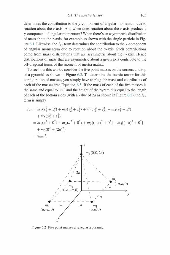
6.1 The inertia tensor 165
determines the contribution to the y-component of angular momentum due torotation about the z-axis. And when does rotation about the z-axis produce ay-component of angular momentum? When there’s an asymmetric distributionof mass about the z-axis, for example as shown with the single particle in Fig-ure 6.1. Likewise, the Ixy term determines the contribution to the x-componentof angular momentum due to rotation about the y-axis. Such contributionscome from mass distributions that are asymmetric about the y-axis. Hencedistributions of mass that are asymmetric about a given axis contribute to theoff-diagonal terms of the moment of inertia matrix.
To see how this works, consider the five point masses on the corners and topof a pyramid as shown in Figure 6.2. To determine the inertia tensor for thisconfiguration of masses, you simply have to plug the mass and coordinates ofeach of the masses into Equation 6.5. If the mass of each of the five masses isthe same and equal to “m” and the height of the pyramid is equal to the lengthof each of the bottom sides (with a value of 2a as shown in Figure 6.2), the Ixx
term is simply
Ixx = m1(y21 + z2
1)+ m2(y22 + z2
2)+ m3(y23 + z2
3)+ m4(y24 + z2
4)
+ m5(y25 + z2
5)
= m1(a2 + 02)+ m2(a
2 + 02)+ m3[(−a)2 + 02] + m4[(−a)2 + 02]+ m5(0
2 + (2a)2)
= 8ma2,
y
x
z
m1(a,a,0)
m2
m3(–a,–a,0)
m4(a,–a,0)
m5 (0,0,2a)
a
2a
a
a
a
(–a,a,0)
Figure 6.2 Five point masses arrayed as a pyramid.
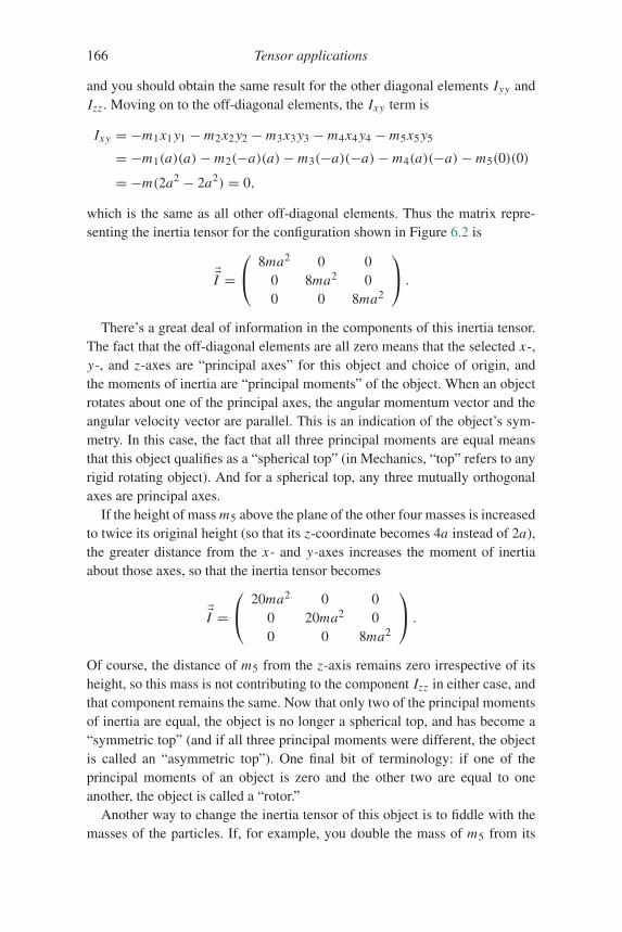
166 Tensor applications
and you should obtain the same result for the other diagonal elements Iyy andIzz . Moving on to the off-diagonal elements, the Ixy term is
Ixy = −m1x1 y1 − m2x2 y2 − m3x3 y3 − m4x4 y4 − m5x5 y5
= −m1(a)(a)− m2(−a)(a)− m3(−a)(−a)− m4(a)(−a)− m5(0)(0)
= −m(2a2 − 2a2) = 0,
which is the same as all other off-diagonal elements. Thus the matrix repre-senting the inertia tensor for the configuration shown in Figure 6.2 is
��I =⎛⎝ 8ma2 0 0
0 8ma2 00 0 8ma2
⎞⎠ .
There’s a great deal of information in the components of this inertia tensor.The fact that the off-diagonal elements are all zero means that the selected x-,y-, and z-axes are “principal axes” for this object and choice of origin, andthe moments of inertia are “principal moments” of the object. When an objectrotates about one of the principal axes, the angular momentum vector and theangular velocity vector are parallel. This is an indication of the object’s sym-metry. In this case, the fact that all three principal moments are equal meansthat this object qualifies as a “spherical top” (in Mechanics, “top” refers to anyrigid rotating object). And for a spherical top, any three mutually orthogonalaxes are principal axes.
If the height of mass m5 above the plane of the other four masses is increasedto twice its original height (so that its z-coordinate becomes 4a instead of 2a),the greater distance from the x- and y-axes increases the moment of inertiaabout those axes, so that the inertia tensor becomes
��I =⎛⎝ 20ma2 0 0
0 20ma2 00 0 8ma2
⎞⎠ .
Of course, the distance of m5 from the z-axis remains zero irrespective of itsheight, so this mass is not contributing to the component Izz in either case, andthat component remains the same. Now that only two of the principal momentsof inertia are equal, the object is no longer a spherical top, and has become a“symmetric top” (and if all three principal moments were different, the objectis called an “asymmetric top”). One final bit of terminology: if one of theprincipal moments of an object is zero and the other two are equal to oneanother, the object is called a “rotor.”
Another way to change the inertia tensor of this object is to fiddle with themasses of the particles. If, for example, you double the mass of m5 from its
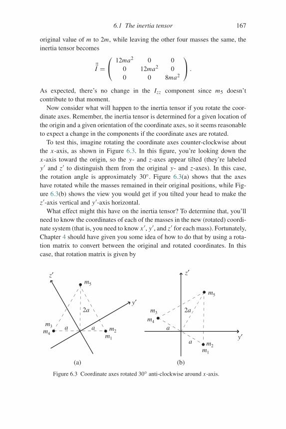
6.1 The inertia tensor 167
original value of m to 2m, while leaving the other four masses the same, theinertia tensor becomes
��I =⎛⎝ 12ma2 0 0
0 12ma2 00 0 8ma2
⎞⎠ .
As expected, there’s no change in the Izz component since m5 doesn’tcontribute to that moment.
Now consider what will happen to the inertia tensor if you rotate the coor-dinate axes. Remember, the inertia tensor is determined for a given location ofthe origin and a given orientation of the coordinate axes, so it seems reasonableto expect a change in the components if the coordinate axes are rotated.
To test this, imagine rotating the coordinate axes counter-clockwise aboutthe x-axis, as shown in Figure 6.3. In this figure, you’re looking down thex-axis toward the origin, so the y- and z-axes appear tilted (they’re labeledy′ and z′ to distinguish them from the original y- and z-axes). In this case,the rotation angle is approximately 30◦. Figure 6.3(a) shows that the axeshave rotated while the masses remained in their original positions, while Fig-ure 6.3(b) shows the view you would get if you tilted your head to make thez′-axis vertical and y′-axis horizontal.
What effect might this have on the inertia tensor? To determine that, you’llneed to know the coordinates of each of the masses in the new (rotated) coordi-nate system (that is, you need to know x ′, y′, and z′ for each mass). Fortunately,Chapter 4 should have given you some idea of how to do that by using a rota-tion matrix to convert between the original and rotated coordinates. In thiscase, that rotation matrix is given by
y′
z′
m1
m2
m3m4
m5
2a
a a
y′
z′
m1
m2
m3
m4
m5
2a
a
a
(a) (b)
Figure 6.3 Coordinate axes rotated 30◦ anti-clockwise around x-axis.
168 Tensor applications⎛⎝ x ′
y′z′
⎞⎠ =
⎛⎝ 1 0 0
0 cos θ sin θ0 − sin θ cos θ
⎞⎠⎛⎝ x
yz
⎞⎠ . (6.6)
If you go back to the original masses (all five masses equal to mass m)and original height of m5 (which is 2a above the xy plane) and then apply thisrotation, you should find the following values for the components of the matrixrepresenting the inertia tensor:
��I =⎛⎝ 8ma2 0 0
0 8ma2 00 0 8ma2
⎞⎠ .
If you’re suprised to find that there’s no change from the original inertia ten-sor (the one without the rotation), remember that the symmetry of this objectmakes it a spherical top, which means that any set of three orthogonal axes willbe principal axes. So tilting the axes should not have caused any change in theinertia tensor.
That sounds reasonable enough, but if you compare the location of themasses in Figure 6.3 to the single-mass case shown in Figure 6.1, doesn’t italso seem reasonable to expect that m5 will produce a component of angularmomentum in the −y-direction (as the single mass did in Figure 6.1)?
Yes, it does. And, in fact, mass m5 does indeed produce a component ofangular momentum in the −y-direction. To demonstrate that, just set the otherfour masses to zero and calculate the inertia tensor for m5 alone (don’t forgetthat the coordinate axes are rotated). You should get
��I =⎛⎝ 4ma2 0 0
0 3ma2 −1.73ma2
0 −1.73ma2 ma2
⎞⎠ .
So there it is: Iyz (which represents the y-component of angular momentumproduced by rotation around the z-axis) is clearly not zero. But why did youget zero for all the off-diagonal elements when you first calculated the inertiatensor for the pyramid with tilted coordinate axes? The answer is that the otherfour masses also have something to say about the inertia tensor. To isolate theircontribution to Iyz , try setting the mass of m5 to zero and leaving the other fourmasses equal to m. The inertia tensor should then be
��I =⎛⎝ 4ma2 0 0
0 5ma2 1.73ma2
0 1.73ma2 7ma2
⎞⎠ .
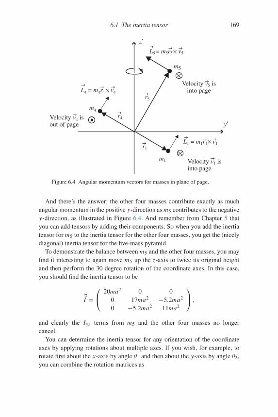
6.1 The inertia tensor 169
y′
z′
m1
r1
m4
m5
r5
r4Velocity v4 isout of page
L4 = m4r4× v4
Velocity v1 isinto page
Velocity v5 isinto page
L1 = m1r1× v1
L5= m5r5× v5
Figure 6.4 Angular momentum vectors for masses in plane of page.
And there’s the answer: the other four masses contribute exactly as muchangular momentum in the positive y-direction as m5 contributes to the negativey-direction, as illustrated in Figure 6.4. And remember from Chapter 5 thatyou can add tensors by adding their components. So when you add the inertiatensor for m5 to the inertia tensor for the other four masses, you get the (nicelydiagonal) inertia tensor for the five-mass pyramid.
To demonstrate the balance between m5 and the other four masses, you mayfind it interesting to again move m5 up the z-axis to twice its original heightand then perform the 30 degree rotation of the coordinate axes. In this case,you should find the inertia tensor to be
��I =⎛⎝ 20ma2 0 0
0 17ma2 −5.2ma2
0 −5.2ma2 11ma2
⎞⎠ ,
and clearly the Iyz terms from m5 and the other four masses no longercancel.
You can determine the inertia tensor for any orientation of the coordinateaxes by applying rotations about multiple axes. If you wish, for example, torotate first about the x-axis by angle θ1 and then about the y-axis by angle θ2,you can combine the rotation matrices as
170 Tensor applications⎛⎝ x ′
y′z′
⎞⎠ =
⎛⎝ cos θ2 0 sin θ2
0 1 0− sin θ2 0 cos θ2
⎞⎠⎛⎝ 1 0 0
0 cos θ1 sin θ1
0 − sin θ1 cos θ1
⎞⎠⎛⎝ x
yz
⎞⎠ ,(6.7)
which in the case of two 30 degree rotations (first about the x-axis and thenabout the y-axis) gives a combined rotation matrix of⎛
⎝ x ′y′z′
⎞⎠ =
⎛⎝ 0.866 −0.25 4.33
0 0.866 0.5−0.5 −0.433 0.75
⎞⎠⎛⎝ x
yz
⎞⎠ . (6.8)
If you leave m5 at height 4a and then apply this rotation to the coordinates,the inertia tensor becomes
��I =⎛⎝ 17.8ma2 2.6ma2 3.9ma2
2.6ma2 17ma2 −4.5ma2
3.9ma2 −4.5ma2 13.3ma2
⎞⎠ . (6.9)
You can perform a quick check on your calculation by verifying that thecoordinate-axis rotation has changed neither the trace nor the determinant ofthe matrix.2
Instead of finding the new coordinates of each mass in the rotated system,an alternative approach allows you to find the inertia tensor for rotated coordi-nates directly. That approach is to apply a “similarity transform” to the originalinertia tensor. Here’s how that works: the angular momentum is related tothe inertia tensor and angular velocity in the original (unrotated) coordinatesystem as
�L = ��I �ω,and you rotate the coordinates by applying a rotation matrix R (which may bethe product of several rotation matrices). You can therefore write
�L ′ = R �L = R( ��I �ω).And since the product of any matrix and its inverse is just the identity matrix,you can insert the term R−1 R in front of �ω:
�L ′ = R �L = R ��I (R−1 R) �ω= (R ��I R−1)R �ω.
But R �ω is just �ω′, so
�L ′ = (R ��I R−1) �ω′.2 The matrix review on the book’s website explains how to do these calculations.
6.2 The electromagnetic field tensor 171
Thus the expression (R ��I R−1) relates angular momentum to angular veloc-ity in the rotated coordinate system, which means that this expression is theinertia tensor in that system. So instead of calculating the new coordinates foreach mass and plugging them into the equation for the inertia tensor, you caninstead simply apply the rotation matrix and its inverse to the matrix represent-ing the inertia tensor directly (but remember that the sequence matters whenyou’re doing matrix multiplication).
Using this approach, the process looks like this:
��I ′ =⎛⎝ 0.866 −0.25 4.33
0 0.866 0.5−0.5 −0.433 0.75
⎞⎠⎛⎝ 20ma2 0 0
0 20ma2 00 0 8ma2
⎞⎠
×⎛⎝ 0.866 −0.25 4.33
0 0.866 0.5−0.5 −0.433 0.75
⎞⎠−1
=⎛⎝ 17.8ma2 2.6ma2 3.9ma2
2.6ma2 17ma2 −4.5ma2
3.9ma2 −4.5ma2 13.3ma2
⎞⎠ ,
which is identical to the result obtained by inserting the rotated coordinatesinto the inertia tensor.
If you’ve studied matrix algebra, you may be wondering about the possibil-ity of finding the principal axes and principal moments by manipulating thematrix representing the inertia tensor into a diagonal form. That is certainlypossible, and you can read about doing that using eigenvectors and eigenvalueson this book’s website.
And if you’re able by visual inspection to determine the angles of rotationneeded to align the axes with the symmetries of the object, you can use thesimilarity transform approach to diagonalize the inertia matrix. You can seehow that works by looking at the problems at the end of this chapter and theon-line solutions.
6.2 The electromagnetic field tensor
One of the defining characteristics of our modern world is the availabil-ity of broadband communication channels which allow near-instantaneoustransfer of information over great distances without the need for physical con-nection. The technology used in this communication descends directly fromthe equations synthesized by Scotsman James Clerk Maxwell in the 1860s,
172 Tensor applications
now called “Maxwell’s Equations.” In view of the impact of electromagnetictelecommunications on our lives, it’s not surprising that in 2004 the readers ofPhysics World voted Maxwell’s Equations to be the “greatest equations” everdeveloped.
The four vector equations that have come to be called Maxwell’s Equationsare Gauss’s Law for electric fields, Gauss’s Law for magnetic fields, Faraday’sLaw, and the Ampere–Maxwell Law, each of which may be written in inte-gral or differential form. The integral forms describe the behavior of electricand magnetic fields over surfaces or around paths, while the differential formsapply to specific locations. The differential forms are most relevant to the vec-tor and tensor operations discussed in this book, involving the scalar product,divergence, curl, and partial derivatives discussed in Chapter 2. They’re alsoclosely related to the subject of this section, the electromagnetic field-strengthtensor.
The differential forms of Maxwell’s Equations are usually written as
Gauss’s Law for electric fields: �∇ ◦ �E = ρ
ε0,
Gauss’s Law for magnetic fields: �∇ ◦ �B = 0,
Faraday’s Law: �∇ × �E = −∂ �B∂t,
Ampere–Maxwell Law: �∇ × �B = μ0 �J + μ0ε0∂ �E∂t.
In order to understand the electromagnetic tensor, you may find it helpful tobriefly review the meaning of each of these equations.3
�∇ ◦ �E = ρε0
Gauss’s Law for electric fields states that the divergence ( �∇◦) of the electricfield ( �E) at any location is proportional to the electric charge density (ρ) atthat location. That’s because electrostatic field lines begin on positive chargeand end on negative charge (hence the field lines tend to diverge away fromlocations of positive charge and converge toward locations of negative charge).
�∇ ◦ �B = 0
Gauss’s Law for magnetic fields tells you that the divergence ( �∇◦) of themagnetic field ( �B) at any location must be zero. This is true because thereis apparently no isolated “magnetic charge” in the universe, so magnetic fieldlines neither diverge nor converge.
3 Complete descriptions may be found in any introductory electromagnetics text.
6.2 The electromagnetic field tensor 173
�∇ × �E = − ∂ �B∂t
Faraday’s Law indicates that the curl ( �∇×) of the electric field ( �E) at any loca-tion is equal to the negative of the time rate of change of the magnetic field atthat location. That’s because a changing magnetic field produces a circulatingelectric field.
�∇ × �B = μ0 �J +μ0ε0∂ �E∂t
Ampere’s Law, as modified by Maxwell, tells you that the curl ( �∇×) of themagnetic field ( �B) at any location is proportional to the electric current density( �J ) plus the time rate of change of the electric field at that location. This isthe case because a circulating magnetic field is produced both by an electriccurrent and by a changing electric field.
Note that Maxwell’s Equations relate the spatial behavior of fields to thesources of those fields. Those sources are electric charge (with density ρ)appearing in Gauss’s Law for electric fields, electric current (with density �J )appearing in the Ampere–Maxwell Law, changing magnetic field (with time
derivative ∂ �B∂t ) appearing in Faraday’s Law, and changing electric field (with
time derivative ∂ �E∂t ) appearing in the Ampere–Maxwell Law.
One additional equation is needed to fully characterize electromagneticinteractions. That equation is called the “continuity equation,” usually writtenlike this:
∂ρ
∂t= −�∇ ◦ �J ,
where ρ is the density of electric charge and �J is the current density.The continuity equation tells you that the time rate of change of the density
of electric charge ( ∂ρ∂t ) equals the negative of the divergence of the electric
current density ( �∇◦ �J ). That’s because negative divergence means convergence,and if the convergence of the current density �J is positive at a point, then morepositive charge must be arriving at that location than is being carried away. Ifthat’s happening, then the density of positive charge at that point must increase(meaning that ∂ρ
∂t will be positive in this case).As valuable as Maxwell’s Equations are individually, the real power of these
equations is realized by combining them together to produce the wave equa-tion. Taking the curl of both sides of Faraday’s Law and inserting the curl of �Bfrom the Ampere–Maxwell Law results in the equation
∇2 �E = μ0ε0∂2 �E∂t2
, (6.10)
174 Tensor applications
where ∇2() = �∇ ◦ �∇() is the vector form of the Laplacian operator.4 Thisequation applies to regions in which the charge density (ρ) and the currentdensity ( �J ) are both zero.
You can find a similar equation for the magnetic field by taking the curl ofboth sides of the Ampere–Maxwell Law and then inserting the curl of �E fromFaraday’s Law. This gives
∇2 �B = μ0ε0∂2 �B∂t2
. (6.11)
It’s instructive to compare Eqs. 6.10 and 6.11 to the general equation for apropagating wave:
∇2 �A = 1
v2
∂2 �A∂t2
, (6.12)
where v is the speed of propagation of the wave. Note the 1/v2 term, whichleads to the conclusion that the velocity of an electromagnetic wave dependsonly on the electric permittivity (ε0) and magnetic permeability (μ0) of freespace (specifically, μ0ε0 = 1/v2, or v = 1/
√μoε0 = 3 × 10⁸ m/s). Most
importantly, that velocity is completely independent of the motion of theobserver. It was this feature of electromagnetic waves that put Albert Einsteinonto the path that eventually led to the Theory of Special Relativity.
To arrive at the Theory of Special Relativity, Einstein held fast to twopostulates. Those postulates are:
1) The laws of physics must be the same in all inertial (that is, non-accelerating) frames of reference.
2) The speed of light in a vacuum is constant and does not depend on themotion of the source or observer.
Steadfast faithfulness to these postulates even in the face of counter-intuitiveconclusions allowed Einstein to see that distances in space and intervals of timeare not absolute but depend on the relative motion of the observer. Additionally,space and time are not separate but are linked together into four-dimensionalspacetime, and it is the four-dimensional spacetime interval that is invariantacross all inertial reference frames.
To understand Einstein’s approach, consider the two Cartesian referenceframes shown in Figure 6.5. As indicated by the arrow in the figure, the primedreference frame is moving with velocity �v in the positive x-direction. Using thetraditional Galilean approach, the coordinate (x , y, and z) and time (t) values
4 If you’d like to see the details of the derivation of the electromagnetic-wave equation, you’llfind them in the on-line solutions to the problems at the end of this chapter.
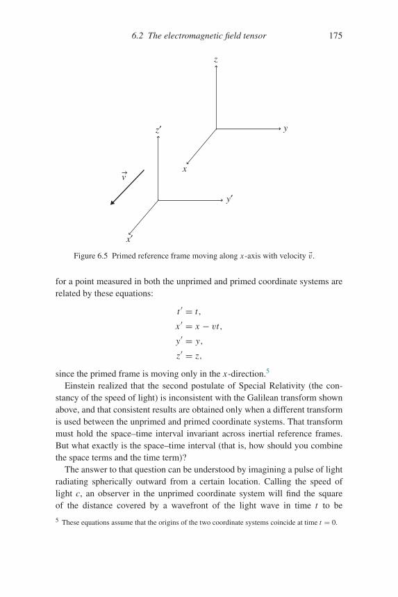
6.2 The electromagnetic field tensor 175
x
y
z
x′
y′
z′
v
Figure 6.5 Primed reference frame moving along x-axis with velocity �v.
for a point measured in both the unprimed and primed coordinate systems arerelated by these equations:
t ′ = t,
x ′ = x − vt,
y′ = y,
z′ = z,
since the primed frame is moving only in the x-direction.5
Einstein realized that the second postulate of Special Relativity (the con-stancy of the speed of light) is inconsistent with the Galilean transform shownabove, and that consistent results are obtained only when a different transformis used between the unprimed and primed coordinate systems. That transformmust hold the space–time interval invariant across inertial reference frames.But what exactly is the space–time interval (that is, how should you combinethe space terms and the time term)?
The answer to that question can be understood by imagining a pulse of lightradiating spherically outward from a certain location. Calling the speed oflight c, an observer in the unprimed coordinate system will find the squareof the distance covered by a wavefront of the light wave in time t to be
5 These equations assume that the origins of the two coordinate systems coincide at time t = 0.
176 Tensor applications
x2 + y2 + z2 = ct2. Likewise, an observer in the primed coordinate systemwill write this as x ′2 + y′2 + z′2 = ct ′2. But by the second postulate of specialrelativity, the speed of light must be the same for all observers. So
ct2 − x2 − y2 − z2 = ct ′2 − x ′2 − y′2 − z′2,
which indicates that the sign of the time term must be opposite to the sign ofthe spatial terms if the speed of light is to be the same for all observers. Ofcourse, the negative sign could equally well be attached to the time term (aslong as the spatial terms were made positive), and you’ll find some texts usingthat convention.
The combination of one time and three spatial coordinates into a single“four-vector” is best expressed using index notation:
x0 = ct,
x1 = x,
x2 = y,
x3 = z,
in which the speed of light (c) is used in the time term to ensure that all fourcoordinates have dimensions of length.
Using this notation, the space–time interval (ds) can be written as
(ds)2 = (dx0)2 − (dx1)2 − (dx2)2 − (dx3)2.
This interval is the space–time equivalent of distance (ds2 = dx2+dy2+dz2)in three-dimensional space.
Transformations that preserve the invariance of the space–time intervalacross inertial reference frames are called “Lorentz transforms” after the Dutchphysicist Hendrik Lorentz. For motion in +x-direction with speed v, theLorentz transformation is
x ′0 = γ (x0 − βx1),
x ′1 = γ (x1 − βx0),
x ′2 = x2,
x ′3 = x3,
where
β = |v|c,
and
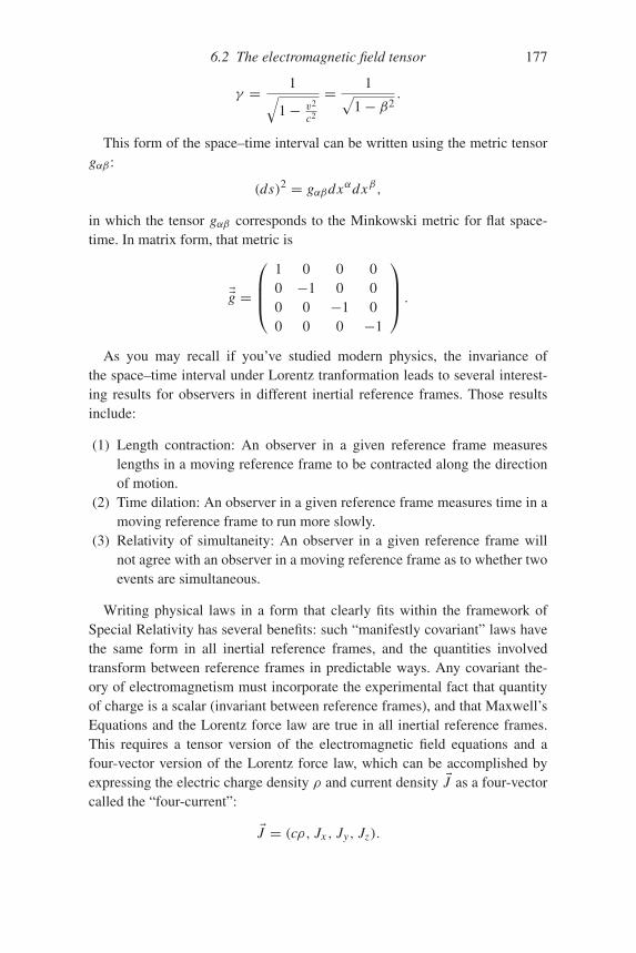
6.2 The electromagnetic field tensor 177
γ = 1√1− v2
c2
= 1√1− β2
.
This form of the space–time interval can be written using the metric tensorgαβ :
(ds)2 = gαβdxαdxβ,
in which the tensor gαβ corresponds to the Minkowski metric for flat space-time. In matrix form, that metric is
��g =
⎛⎜⎜⎝
1 0 0 00 −1 0 00 0 −1 00 0 0 −1
⎞⎟⎟⎠ .
As you may recall if you’ve studied modern physics, the invariance ofthe space–time interval under Lorentz tranformation leads to several interest-ing results for observers in different inertial reference frames. Those resultsinclude:
(1) Length contraction: An observer in a given reference frame measureslengths in a moving reference frame to be contracted along the directionof motion.
(2) Time dilation: An observer in a given reference frame measures time in amoving reference frame to run more slowly.
(3) Relativity of simultaneity: An observer in a given reference frame willnot agree with an observer in a moving reference frame as to whether twoevents are simultaneous.
Writing physical laws in a form that clearly fits within the framework ofSpecial Relativity has several benefits: such “manifestly covariant” laws havethe same form in all inertial reference frames, and the quantities involvedtransform between reference frames in predictable ways. Any covariant the-ory of electromagnetism must incorporate the experimental fact that quantityof charge is a scalar (invariant between reference frames), and that Maxwell’sEquations and the Lorentz force law are true in all inertial reference frames.This requires a tensor version of the electromagnetic field equations and afour-vector version of the Lorentz force law, which can be accomplished byexpressing the electric charge density ρ and current density �J as a four-vectorcalled the “four-current”:
�J = (cρ, Jx , Jy, Jz).
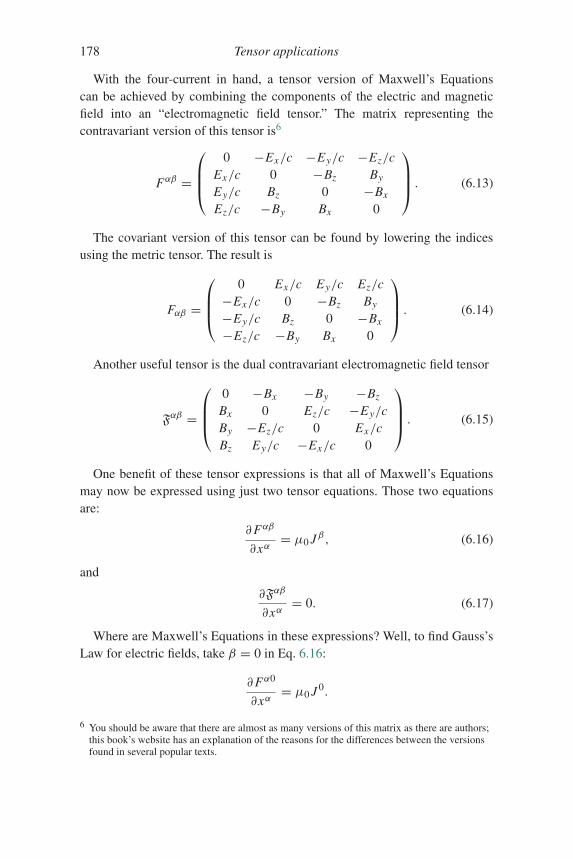
178 Tensor applications
With the four-current in hand, a tensor version of Maxwell’s Equationscan be achieved by combining the components of the electric and magneticfield into an “electromagnetic field tensor.” The matrix representing thecontravariant version of this tensor is6
Fαβ =
⎛⎜⎜⎝
0 −Ex/c −Ey/c −Ez/cEx/c 0 −Bz By
Ey/c Bz 0 −Bx
Ez/c −By Bx 0
⎞⎟⎟⎠ . (6.13)
The covariant version of this tensor can be found by lowering the indicesusing the metric tensor. The result is
Fαβ =
⎛⎜⎜⎝
0 Ex/c Ey/c Ez/c−Ex/c 0 −Bz By
−Ey/c Bz 0 −Bx
−Ez/c −By Bx 0
⎞⎟⎟⎠ . (6.14)
Another useful tensor is the dual contravariant electromagnetic field tensor
Fαβ =
⎛⎜⎜⎝
0 −Bx −By −Bz
Bx 0 Ez/c −Ey/cBy −Ez/c 0 Ex/cBz Ey/c −Ex/c 0
⎞⎟⎟⎠ . (6.15)
One benefit of these tensor expressions is that all of Maxwell’s Equationsmay now be expressed using just two tensor equations. Those two equationsare:
∂Fαβ
∂xα= μ0 Jβ, (6.16)
and
∂Fαβ
∂xα= 0. (6.17)
Where are Maxwell’s Equations in these expressions? Well, to find Gauss’sLaw for electric fields, take β = 0 in Eq. 6.16:
∂Fα0
∂xα= μ0 J 0.
6 You should be aware that there are almost as many versions of this matrix as there are authors;this book’s website has an explanation of the reasons for the differences between the versionsfound in several popular texts.
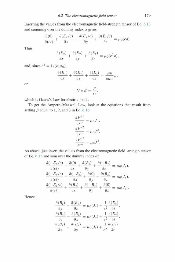
6.2 The electromagnetic field tensor 179
Inserting the values from the electromagnetic field-strength tensor of Eq. 6.13and summing over the dummy index α gives
∂(0)
∂(ct)+ ∂(Ex/c)
∂x+ ∂(Ey/c)
∂y+ ∂(Ez/c)
∂z= μ0(cρ).
Thus∂(Ex )
∂x+ ∂(Ey)
∂y+ ∂(Ez)
∂z= μ0(c
2ρ),
and, since c2 = 1/(ε0μ0),
∂(Ex )
∂x+ ∂(Ey)
∂y+ ∂(Ez)
∂z= μ0
ε0μ0ρ,
or
�∇ ◦ �E = ρ
ε0,
which is Gauss’s Law for electric fields.To get the Ampere–Maxwell Law, look at the equations that result from
setting β equal to 1, 2, and 3 in Eq. 6.16:
∂Fα1
∂xα= μ0 J 1,
∂Fα2
∂xα= μ0 J 2,
∂Fα3
∂xα= μ0 J 3.
As above, just insert the values from the electromagnetic field-strength tensorof Eq. 6.13 and sum over the dummy index α:
∂(−Ex/c)
∂(ct)+ ∂(0)
∂x+ ∂(Bz)
∂y+ ∂(−By)
∂z= μ0(Jx ),
∂(−Ey/c)
∂(ct)+ ∂(−Bz)
∂x+ ∂(0)
∂y+ ∂(Bx )
∂z= μ0(Jy),
∂(−Ez/c)
∂(ct)+ ∂(By)
∂x+ ∂(−Bx )
∂y+ ∂(0)
∂z= μ0(Jz).
Hence
∂(Bz)
∂y− ∂(By)
∂z= μ0(Jx )+ 1
c2
∂(Ex )
∂t,
∂(Bx )
∂z− ∂(Bz)
∂x= μ0(Jy)+ 1
c2
∂(Ey)
∂t,
∂(By)
∂x− ∂(Bx )
∂y= μ0(Jz)+ 1
c2
∂(Ez)
∂t.
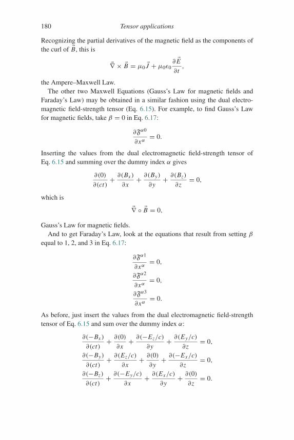
180 Tensor applications
Recognizing the partial derivatives of the magnetic field as the components ofthe curl of �B, this is
�∇ × �B = μ0 �J + μ0ε0∂ �E∂t,
the Ampere–Maxwell Law.The other two Maxwell Equations (Gauss’s Law for magnetic fields and
Faraday’s Law) may be obtained in a similar fashion using the dual electro-magnetic field-strength tensor (Eq. 6.15). For example, to find Gauss’s Lawfor magnetic fields, take β = 0 in Eq. 6.17:
∂Fα0
∂xα= 0.
Inserting the values from the dual electromagnetic field-strength tensor ofEq. 6.15 and summing over the dummy index α gives
∂(0)
∂(ct)+ ∂(Bx )
∂x+ ∂(By)
∂y+ ∂(Bz)
∂z= 0,
which is
�∇ ◦ �B = 0,
Gauss’s Law for magnetic fields.And to get Faraday’s Law, look at the equations that result from setting β
equal to 1, 2, and 3 in Eq. 6.17:
∂Fα1
∂xα= 0,
∂Fα2
∂xα= 0,
∂Fα3
∂xα= 0.
As before, just insert the values from the dual electromagnetic field-strengthtensor of Eq. 6.15 and sum over the dummy index α:
∂(−Bx )
∂(ct)+ ∂(0)
∂x+ ∂(−Ez/c)
∂y+ ∂(Ey/c)
∂z= 0,
∂(−By)
∂(ct)+ ∂(Ez/c)
∂x+ ∂(0)
∂y+ ∂(−Ex/c)
∂z= 0,
∂(−Bz)
∂(ct)+ ∂(−Ey/c)
∂x+ ∂(Ex/c)
∂y+ ∂(0)
∂z= 0.
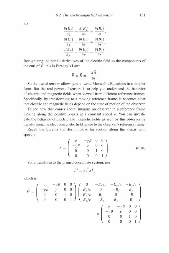
6.2 The electromagnetic field tensor 181
So∂(Ey)
∂z− ∂(Ez)
∂y= ∂(Bx )
∂t,
∂(Ez)
∂x− ∂(Ex )
∂z= ∂(By)
∂t,
∂(Ex )
∂y− ∂(Ey)
∂x= ∂(Bz)
∂t.
Recognizing the partial derivatives of the electric field as the components ofthe curl of �E , this is Faraday’s Law:
�∇ × �E = −∂ �B∂t.
So the use of tensors allows you to write Maxwell’s Equations in a simplerform. But the real power of tensors is to help you understand the behaviorof electric and magnetic fields when viewed from different reference frames.Specifically, by transforming to a moving reference frame, it becomes clearthat electric and magnetic fields depend on the state of motion of the observer.
To see how that comes about, imagine an observer in a reference framemoving along the positive x-axis at a constant speed v. You can investi-gate the behavior of electric and magnetic fields as seen by this observer bytransforming the electromagnetic field tensor to the observer’s reference frame.
Recall the Lorentz transform matrix for motion along the x-axis withspeed v:
A =
⎛⎜⎜⎝
γ −γβ 0 0−γβ γ 0 0
0 0 1 00 0 0 1
⎞⎟⎟⎠ . (6.18)
So to transform to the primed coordinate system, use
��F ′ = A ��F AT ,
which is
��F ′ =
⎛⎜⎜⎝
γ −γβ 0 0−γβ γ 0 0
0 0 1 00 0 0 1
⎞⎟⎟⎠⎛⎜⎜⎝
0 −Ex/c −Ey/c −Ez/cEx/c 0 −Bz By
Ey/c Bz 0 −Bx
Ez/c −By Bx 0
⎞⎟⎟⎠
×
⎛⎜⎜⎝
γ −γβ 0 0−γβ γ 0 0
0 0 1 00 0 0 1
⎞⎟⎟⎠.
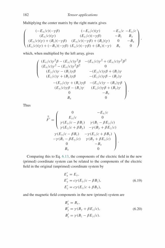
182 Tensor applications
Multiplying the center matrix by the right matrix gives⎛⎜⎜⎝
(−Ex/c)(−γβ) (−Ex/c)(γ ) −Ey/c −Ez/c(Ex/c)(γ ) (Ex/c)(−γβ) −Bz By
(Ey/c)(γ )+ (Bz)(−γβ) (Ey/c)(−γβ)+ (Bz)(γ ) 0 −Bx
(Ez/c)(γ )+ (−By)(−γβ) (Ez/c)(−γβ)+ (By)(−γ ) Bx 0
⎞⎟⎟⎠ ,
which, when multiplied by the left array, gives⎛⎜⎜⎝(Ex/c)γ 2β − (Ex/c)γ 2β −(Ex/c)γ 2 + (Ex/c)γ 2β2
(Ex/c)γ 2 − (Ex/c)γ 2β2 0(Ey/c)γ − (Bz)γβ −(Ey/c)γβ + (Bz)γ
(Ez/c)γ + (By)γβ −(Ez/c)γβ − (By)γ
−(Ey/c)γ + (Bz)γβ −(Ez/c)γ − (By)γβ
(Ey/c)γβ − (Bz)γ (Ez/c)γβ + (By)γ
0 −Bx
Bx 0
⎞⎟⎟⎠ .
Thus
��F ′ =
⎛⎜⎜⎝
0 −Ex/cEx/c 0
γ (Ey/c − βBz) γ (Bz − βEy/c)γ (Ez/c + βBy) −γ (By + βEz/c)
γ (Ey/c − βBz) −γ (Ez/c + βBy)
−γ (Bz − βEy/c) γ (By + βEz/c)0 −Bx
Bx 0
⎞⎟⎟⎠ .
Comparing this to Eq. 6.13, the components of the electric field in the new(primed) coordinate system can be related to the components of the electricfield in the original (unprimed) coordinate system by
E ′x = Ex ,
E ′y = cγ (Ey/c − βBz),
E ′z = cγ (Ez/c + βBy),
(6.19)
and the magnetic field components in the new (primed) system are
B ′x = Bx ,
B ′y = γ (By + βEz/c),
B ′z = γ (Bz − βEy/c).
(6.20)
6.3 The Riemann curvature tensor 183
This is a profound result, since it indicates that the existence of electric andmagnetic fields depends on the motion of the observer.
To understand the implications of these results, consider the case in whichEx = Ey = Ez = 0 but one or more components of �B are non-zero (thisoccurs, for example, when a long, straight wire carries a steady electric cur-rent). This means that an observer in the unprimed coordinate system seesa magnetic field but no electric field. However, transforming to the primedcoordinate system, Eqs. 6.19 and 6.20 tell you that an observer in the primedcoordinate system sees both electric and magnetic fields (since in this caseE ′y = −cγβBz and E ′z = cγβBy). So does the magnetic field exist or not?The answer depends on the motion of the observer.
Now consider a case in which Bx = By = Bz = 0 but one or morecomponents of �E are non-zero in the unprimed system (for example, an elec-tric charge at rest in the unprimed system). For this case, an observer in theprimed system does see a magnetic field with components B ′y = γβEz/c andB ′z = −γβEy/c (this makes sense, since the observer in the primed systemsees a moving electric charge, which is an electric current, and electric currentsproduce magnetic fields). Cases such as these explain the reasoning behind thestatement that electric and magnetic fields “have no independent existence.”
The problems at the end of this chapter will give you an idea of the relativemagnitudes of fields seen by an observer at rest and a second observer movingat a significant fraction of the speed of light.
6.3 The Riemann curvature tensor
In the decade after publishing his Theory of Special Relativity in 1905, AlbertEinstein turned his attention to what he called a “deficiency” in classicalmechanics: the lack of an explanation for the precise equality of inertial andgravitational mass. An object’s inertial mass determines its resistance to accel-eration, and its gravitational mass determines its response to a gravitationalfield. The equality of these differently defined masses cannot be explainedby classical mechanics, and Einstein’s scientific instincts told him that theresolution of this deficiency could be achieved by “an extension of the prin-ciple of relativity to spaces of reference which are not in uniform motionrelative to one another.”7 He applied the word “General” to this extension ofhis theory of relativity because this new theory would not be restricted to thenon-accelerating reference frames of Special Relativity.7 A. Einstein, The Meaning of Relativity.
184 Tensor applications
Early in his work on the General Theory, Einstein constructed a Gedanken-experiment (that is, a mental exercise) in which he imagined a group of objectswith different mass far away from the Earth and from all other masses – youcan think of this as a bunch of rocks far out in space. The behavior of theseobjects is observed from two reference systems, one of which is called sys-tem K and is “inertial” or non-accelerating with respect to the rocks. The othersystem, called system K′, is in uniform acceleration with respect to the first.For an observer in the K′ system, the objects all accelerate in the same direc-tion (opposite to the direction of the acceleration of the K′ system) and atthe same rate (equal to the rate of acceleration of the K′ system). Seeing allobjects accelerating in the same direction and at the same rate, that observerwould be entirely justified in concluding that the acceleration of the objectsis produced by an external gravitational field and that the K′ system is at rest.Einstein realized that both the K and the K′ systems are valid frames of refer-ence, and he termed the complete equivalence of such systems the “principleof equivalence.”
Einstein’s next step was to overlay the z′-axis of K′ system with the z-axisof the K system and then to allow the K′ system to rotate about the z′-axiswith uniform angular speed (recall that a rotating object experiences centripetalacceleration, so rotation makes K′ an accelerated system). If system K′ werenot rotating, the size of objects and rate of time flow measured in the K and K′systems would be the same. But when system K′ is rotating, objects at rest inK′ will be moving when measured in the K system and will therefore experi-ence length contraction and time dilation, and the amount of contraction anddilation will depend on the location of the objects (since objects farther fromthe rotation axis will have higher velocity). Since the principle of equivalencedemands that an accelerated system and a system at rest in a gravitational fieldare equivalent, Einstein was forced to conclude that length contraction andtime dilation could also be produced by gravity, or as he put it “the gravita-tional field influences and even determines the metrical laws of the space–timecontinuum.”
Those metrical laws are expressed using tensors, so the General Theoryof Relativity relies on tensor formulation of physical laws and on conceptsdescribed in earlier chapters, such as the metric tensor, Christoffel symbols,and covariant derivatives. The most important tensor in General Relativity isthe Riemann curvature tensor, sometimes called the Riemann–Christoffel ten-sor after the nineteenth-century German mathematicians Bernhard Riemannand Elwin Bruno Christoffel. The importance of this tensor stems from thefact that non-zero components are the hallmark of curvature; the vanishing of
6.3 The Riemann curvature tensor 185
the Riemann tensor is both a necessary and a sufficient condition for Euclidean(flat) space.
Most texts use one of two ways to derive the Riemann curvature tensor:parallel transport or the commutator of the covariant derivative. To understandthe parallel-transport approach, you should first understand that “parallel trans-port” refers to a method of moving a vector around a space while keeping thelength and direction of the vector the same. In Cartesian flat space, makingsure the vector’s magnitude and direction don’t change is straightforward –just move the vector around without allowing the x-, y-, or -z components tochange. If the components don’t change, then the length and the direction ofthe vector don’t change, and this satisfies the requirements of parallel transport.
In curved spaced, the situation is more complex. For one thing, “pointingin the same direction” becomes more difficult to define. Consider the two-dimensional space that is the surface of the Earth (and pretend for the momentthat it’s perfectly smooth). Imagine a vector that is initially at the equator (saya bit north of Quito, Ecuador) and is pointing due north, directly along themeridian line. Now imagine transporting that vector toward the north pole,all the while making sure it remains pointed exactly along the meridian line.Remember, the entire space is the surface of the Earth, so the vector mustremain tangent to the surface (that is, locally horizontal) as you move it. If youcontinue moving your vector along the meridian line and pass over the NorthPole and then “down” the other side of the Earth, you will eventually reach theequator again somewhere near the middle of Indonesia. Your vector will stillbe pointing along the meridian, but now it will be pointing south. So althoughyou’ve kept your vector pointing “in the same direction” (that is, along themeridian) over the entire trip, it’s gone from pointing north to pointing south.
Now imagine making another trip, also starting with a north-pointing vectorat the equator near Quito, but this time moving along the equator instead ofover the North Pole. Once again, as you move you make sure that your vectorcontinues to point north (along the local meridian). After a long journey, youarrive in the middle of Indonesia, but this time you find that your vector ispointing north. Hence the direction of the vector at the end of the journeydepends on the path taken, even though you used parallel transport in eachcase. And whenever the result of parallel transport is a change in the directionof a vector, you can be sure you’re dealing with a curved space.
This raises a larger issue: it’s not possible to add, subtract, multiply, or inany way compare vectors at different locations – you have to transport one ofthe vectors to the location of the other before you can perform such operations.That’s no problem in flat space, because you can parallel-transport a vector toany other location simply by keeping its coefficients constant (ensuring that the
186 Tensor applications
vector’s length is constant and that it remains pointed in the same direction).But while “pointed in the same direction” is easily defined at different locationsin flat space, you’ve just seen that this phrase is problematic in curved space.Hence a more-general definition of parallel transport is required.
In that definition, “parallel transport” is defined as transport for which thecovariant derivative is zero. Remember that the covariant derivative is the com-bination of two terms, the first of which is the usual partial derivative, and thesecond of which involves a Christoffel symbol. As described in Section 5.7in Chapter 5, the purpose of that second term is to account for changes inthe basis vectors. Holding the covariant derivative at zero while transporting avector around a small loop is one way to derive the Riemann tensor.8
The Riemann curvature tensor falls naturally out of the commutator of thecovariant derivative of a vector. In this usage, “commutator” refers to the dif-ference that results from performing two operations first in one order and thenin the reverse order. So if one operator is denoted by A and another operatorby B, the commutator is defined as [AB] = AB−BA. Thus if the sequence ofthe two operations has no impact on the result, the commutator has a value ofzero.
To get to the Riemann tensor, the operation of choice is covariant differenti-ation. That’s because in a flat space the order of covariant differentiation makesno difference, so the commutator must yield zero. Any non-zero result ofapplying the commutator to covariant differentiation can therefore be attributedto the curvature of the space.
To begin this process, take the covariant derivative of vector Vα first withrespect to xβ :
Vα;β = ∂Vα∂xβ− �σαβVσ . (6.21)
Now call this result Vαβ and take another covariant derivative (this time withrespect to xγ ):
Vαβ;γ = ∂Vαβ∂xγ
− �ταγ Vτβ − �ηβγ Vαη. (6.22)
Substituting the expression from Eq. 6.21 into this equation gives
Vαβ;γ = ∂2Vα∂xγ ∂xβ
− ∂�σαβ
∂xγVσ − �σαβ
∂Vσ∂xγ
− �ταγ(∂Vτ∂xβ− �στβVσ
)
− �ηβγ(∂Vα∂xη− �σαηVσ
). (6.23)
8 You can find the details in Schutz, A First Course in General Relativity, Cambridge UniversityPress, 2009.
6.3 The Riemann curvature tensor 187
It’s not easy to see the physical significance in this expression, but rememberhow you got here: first by finding the incremental change in Vα as you take asmall step in the xβ -direction, and then finding the change in that quantity asyou take a small step in the xγ -direction. And now you’re going to compare theresult of these two operations with the result you get when you take the stepsin reverse order – from the same starting point, you’ll first find the incrementalchange in Vα as you take a small step in the xγ -direction, after which you’llfind the change in that quantity as you take a small step in the xβ -direction.
To take the covariant derivatives in the opposite order, differentiate first withrespect to xγ :
Vα;γ = ∂Vα∂xγ− �σαγ Vσ . (6.24)
Call this result Vαγ and take another covariant derivative (this time with respectto xβ ):
Vαγ ;β = ∂Vαγ∂xβ
− �ταβVτγ − �ηγβVαη. (6.25)
As before, you can substitute the expression from Eq. 6.24 into this equationto get
Vαγ ;β = ∂2Vα∂xβ∂xγ
− ∂�σαγ
∂xβVσ − �σαγ
∂Vσ∂xβ
− �ταβ(∂Vτ∂xγ− �στγ Vσ
)
− �ηγβ(∂Vα∂xη− �σαηVσ
). (6.26)
In flat space, the order of covariant differentiation should make no differ-ence, so Eq. 6.26 should be identical to Eq. 6.23. Any differences betweenthese equations can therefore be attributed to the curvature of the space.Examining these two equations term by term, the first terms are equal:
∂2Vα∂xγ ∂xβ
= ∂2Vα∂xβ∂xγ
,
(these terms are equal because the order of normal partial derivatives doesnot matter). Hence these terms cancel in the commutator. Now comparing thesecond terms,
−∂�σαβ
∂xγVσ �= −
∂�σαγ
∂xβVσ ,
so these terms do not cancel one another. Comparing the third term of Eq. 6.23to the fourth term of Eq. 6.26, they’re found to be equal:
188 Tensor applications
−�σαβ∂Vσ∂xγ= −�ταβ
∂Vτ∂xγ
,
because the symbols used for dummy indices (σ and τ ) are irrelevant. Thefourth term of Eq. 6.23 equals the third term of Eq. 6.26:
−�ταγ∂Vτ∂xβ= −�σαγ
∂Vσ∂xβ
,
for the same reason. The fifth terms are not equal:
�ταγ �στβVσ �= �ταβ�στγ Vσ .
But the sixth terms are equal:
−�ηβγ∂Vα∂xη= −�ηγβ
∂Vα∂xη
,
because Christoffel symbols are symmetric in their lower indices. The seventhterms are equal for the same reason:
�ηβγ �
σαηVσ = �ηγβ�σαηVσ .
So when the commutator AB−BA is formed, most of the terms cancel out,but the second and fifth terms remain after subtraction. Those terms are
Vαβ;γ − Vαγ ;β = −∂�σαβ
∂xγVσ +
∂�σαγ
∂xβVσ + �ταγ �στβVσ − �ταβ�στγ Vσ
=(∂�σαγ
∂xβ− ∂�
σαβ
∂xγ+ �ταγ �στβ − �ταβ�στγ
)Vσ .
(6.27)
The terms within the parentheses define the Riemann curvature tensor:
Rσαβγ ≡∂�σαγ
∂xβ− ∂�
σαβ
∂xγ+ �ταγ �στβ − �ταβ�στγ . (6.28)
If you’re wondering why the curvature tensor involves the derivative ofChristoffel symbols, consider this: in any space, you can always define a coor-dinate system for which the Christoffel symbols are all zero at some point. Butunless the space is flat, the Christoffel symbols will not be zero at all otherlocations, which means that the partial derivatives of the Christoffel symbolswill not be zero. So a necessary and sufficient condition for flat space is that
Rσαβγ = 0. (6.29)
Another tensor related to the Riemann curvature tensor is the Ricci ten-sor, which you can find by contracting the Riemann tensor along the σ and βindices. In four dimensions, this is
Rαγ ≡ Rσασγ = R1α1γ + R2
α2γ + R3α3γ + R4
α4γ . (6.30)
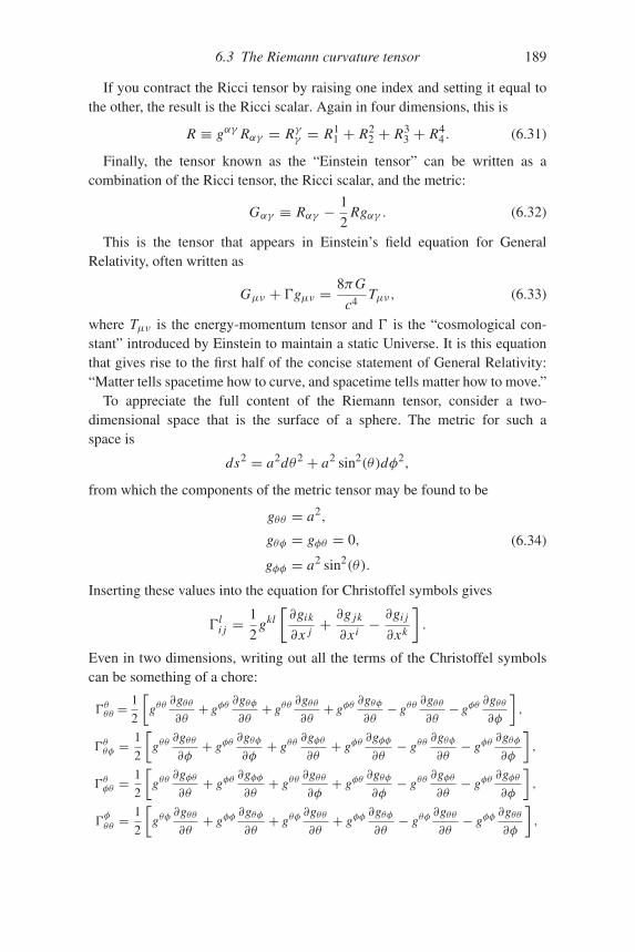
6.3 The Riemann curvature tensor 189
If you contract the Ricci tensor by raising one index and setting it equal tothe other, the result is the Ricci scalar. Again in four dimensions, this is
R ≡ gαγ Rαγ = Rγγ = R11 + R2
2 + R33 + R4
4 . (6.31)
Finally, the tensor known as the “Einstein tensor” can be written as acombination of the Ricci tensor, the Ricci scalar, and the metric:
Gαγ ≡ Rαγ − 1
2Rgαγ . (6.32)
This is the tensor that appears in Einstein’s field equation for GeneralRelativity, often written as
Gμν + �gμν = 8πG
c4Tμν, (6.33)
where Tμν is the energy-momentum tensor and � is the “cosmological con-stant” introduced by Einstein to maintain a static Universe. It is this equationthat gives rise to the first half of the concise statement of General Relativity:“Matter tells spacetime how to curve, and spacetime tells matter how to move.”
To appreciate the full content of the Riemann tensor, consider a two-dimensional space that is the surface of a sphere. The metric for such aspace is
ds2 = a2dθ2 + a2 sin2(θ)dφ2,
from which the components of the metric tensor may be found to be
gθθ = a2,
gθφ = gφθ = 0,
gφφ = a2 sin2(θ).
(6.34)
Inserting these values into the equation for Christoffel symbols gives
�li j =
1
2gkl
[∂gik
∂x j+ ∂g jk
∂xi− ∂gi j
∂xk
].
Even in two dimensions, writing out all the terms of the Christoffel symbolscan be something of a chore:
�θθθ =1
2
[gθθ
∂gθθ∂θ+ gφθ
∂gθφ∂θ+ gθθ
∂gθθ∂θ+ gφθ
∂gθφ∂θ− gθθ
∂gθθ∂θ− gφθ
∂gθθ∂φ
],
�θθφ =1
2
[gθθ
∂gθθ∂φ+ gφθ
∂gθφ∂φ+ gθθ
∂gφθ∂θ+ gφθ
∂gφφ∂θ− gθθ
∂gθφ∂θ− gφθ
∂gθφ∂φ
],
�θφθ =1
2
[gθθ
∂gφθ∂θ+ gφθ
∂gφφ∂θ+ gθθ
∂gθθ∂φ+ gφθ
∂gθφ∂φ− gθθ
∂gφθ∂θ− gφθ
∂gφθ∂φ
],
�φθθ =
1
2
[gθφ
∂gθθ∂θ+ gφφ
∂gθφ∂θ+ gθφ
∂gθθ∂θ+ gφφ
∂gθφ∂θ− gθφ
∂gθθ∂θ− gφφ
∂gθθ∂φ
],
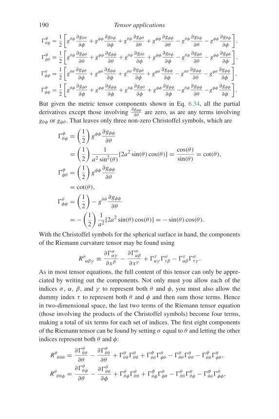
190 Tensor applications
�φθφ =
1
2
[gθφ
∂gθθ∂φ+ gφφ
∂gθφ∂φ+ gθφ
∂gφθ∂θ+ gφφ
∂gφφ∂θ− gθφ
∂gθφ∂θ− gφφ
∂gθφ∂φ
],
�φφθ =
1
2
[gθφ
∂gφθ∂θ+ gφφ
∂gφφ∂θ+ gθφ
∂gθθ∂φ+ gφφ
∂gθφ∂φ− gθφ
∂gφθ∂θ− gφφ
∂gφθ∂φ
],
�θφφ =1
2
[gθθ
∂gφθ∂φ+ gφθ
∂gφφ∂φ+ gθθ
∂gφθ∂φ+ gφθ
∂gφφ∂φ− gθθ
∂gφφ∂θ− gφθ
∂gφφ∂φ
],
�φφφ =
1
2
[gθφ
∂gφθ∂φ+ gφφ
∂gφφ∂φ+ gθφ
∂gφθ∂φ+ gφφ
∂gφφ∂φ−gθφ
∂gφφ∂θ−gφφ
∂gφφ∂φ
].
But given the metric tensor components shown in Eq. 6.34, all the partialderivatives except those involving ∂gφφ
∂θare zero, as are any terms involving
gθφ or gφθ . That leaves only three non-zero Christoffel symbols, which are
�φθφ =
(1
2
)gφφ
∂gφφ∂θ
=(
1
2
)1
a2 sin2(θ)[2a2 sin(θ) cos(θ)] = cos(θ)
sin(θ)= cot(θ),
�φφθ =
(1
2
)gφφ
∂gφφ∂θ
= cot(θ),
�θφφ =(
1
2
)− gθθ
∂gφφ∂θ
= −(
1
2
)1
a2[2a2 sin(θ) cos(θ)] = − sin(θ) cos(θ).
With the Christoffel symbols for the spherical surface in hand, the componentsof the Riemann curvature tensor may be found using
Rσαβγ ≡∂�σαγ
∂xβ− ∂�
σαβ
∂xγ+ �ταγ �στβ − �ταβ�στγ .
As in most tensor equations, the full content of this tensor can only be appre-ciated by writing out the components. Not only must you allow each of theindices σ , α, β, and γ to represent both θ and φ, you must also allow thedummy index τ to represent both θ and φ and then sum those terms. Hencein two-dimensional space, the last two terms of the Riemann tensor equation(those involving the products of the Christoffel symbols) become four terms,making a total of six terms for each set of indices. The first eight componentsof the Riemann tensor can be found by setting σ equal to θ and letting the otherindices represent both θ and φ:
Rθθθθ =∂�θθθ
∂θ− ∂�
θθθ
∂θ+ �θθθ�θθθ + �φθθ�θφθ − �θθθ�θθθ − �φθθ�θφθ ,
Rθθθφ =∂�θθφ
∂θ− ∂�
θθθ
∂φ+ �θθφ�θθθ + �φθφ�θφθ − �θθθ�θθφ − �φθθ�θφφ,
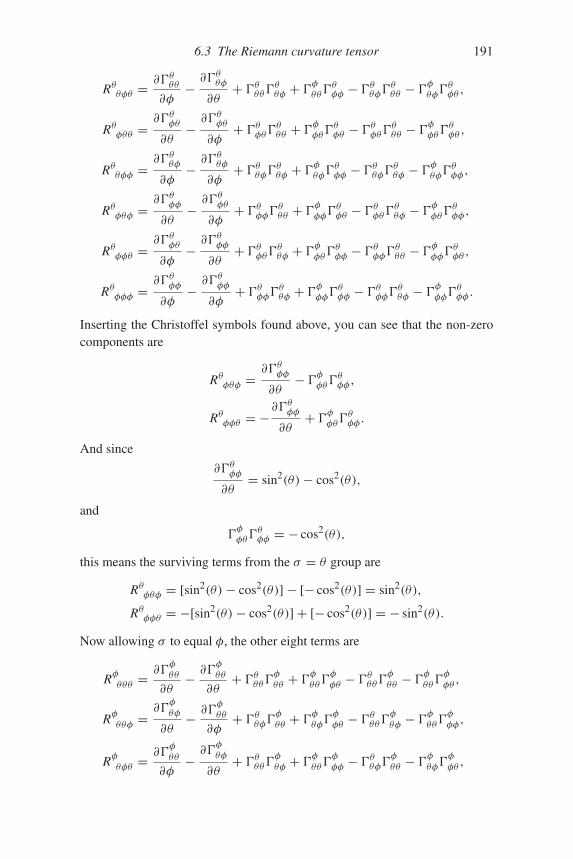
6.3 The Riemann curvature tensor 191
Rθθφθ =∂�θθθ
∂φ− ∂�
θθφ
∂θ+ �θθθ�θθφ + �φθθ�θφφ − �θθφ�θθθ − �φθφ�θφθ ,
Rθφθθ =∂�θφθ
∂θ− ∂�
θφθ
∂φ+ �θφθ�θθθ + �φφθ�θφθ − �θφθ�θθθ − �φφθ�θφθ ,
Rθθφφ =∂�θθφ
∂φ− ∂�
θθφ
∂φ+ �θθφ�θθφ + �φθφ�θφφ − �θθφ�θθφ − �φθφ�θφφ,
Rθφθφ =∂�θφφ
∂θ− ∂�
θφθ
∂φ+ �θφφ�θθθ + �φφφ�θφθ − �θφθ�θθφ − �φφθ�θφφ,
Rθφφθ =∂�θφθ
∂φ− ∂�
θφφ
∂θ+ �θφθ�θθφ + �φφθ�θφφ − �θφφ�θθθ − �φφφ�θφθ ,
Rθφφφ =∂�θφφ
∂φ− ∂�
θφφ
∂φ+ �θφφ�θθφ + �φφφ�θφφ − �θφφ�θθφ − �φφφ�θφφ.
Inserting the Christoffel symbols found above, you can see that the non-zerocomponents are
Rθφθφ =∂�θφφ
∂θ− �φφθ�θφφ,
Rθφφθ = −∂�θφφ
∂θ+ �φφθ�θφφ.
And since
∂�θφφ
∂θ= sin2(θ)− cos2(θ),
and
�φφθ�
θφφ = − cos2(θ),
this means the surviving terms from the σ = θ group are
Rθφθφ = [sin2(θ)− cos2(θ)] − [− cos2(θ)] = sin2(θ),
Rθφφθ = −[sin2(θ)− cos2(θ)] + [− cos2(θ)] = − sin2(θ).
Now allowing σ to equal φ, the other eight terms are
Rφθθθ =∂�
φθθ
∂θ− ∂�
φθθ
∂θ+ �θθθ�φθθ + �φθθ�φφθ − �θθθ�φθθ − �φθθ�φφθ ,
Rφθθφ =∂�
φθφ
∂θ− ∂�
φθθ
∂φ+ �θθφ�φθθ + �φθφ�φφθ − �θθθ�φθφ − �φθθ�φφφ,
Rφθφθ =∂�
φθθ
∂φ− ∂�
φθφ
∂θ+ �θθθ�φθφ + �φθθ�φφφ − �θθφ�φθθ − �φθφ�φφθ ,
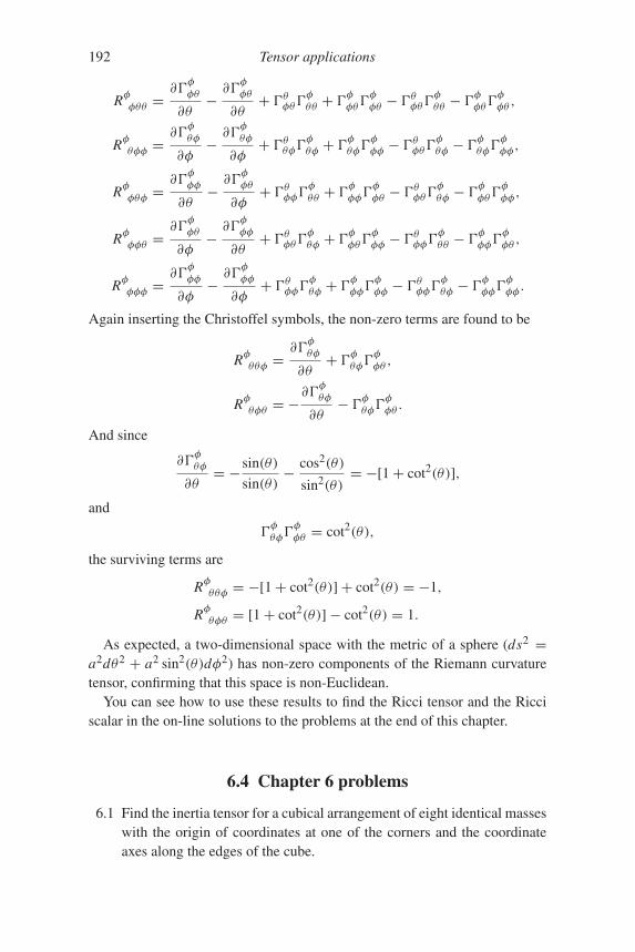
192 Tensor applications
Rφφθθ =∂�
φφθ
∂θ− ∂�
φφθ
∂θ+ �θφθ�φθθ + �φφθ�φφθ − �θφθ�φθθ − �φφθ�φφθ ,
Rφθφφ =∂�
φθφ
∂φ− ∂�
φθφ
∂φ+ �θθφ�φθφ + �φθφ�φφφ − �θφθ�φθφ − �φθφ�φφφ,
Rφφθφ =∂�
φφφ
∂θ− ∂�
φφθ
∂φ+ �θφφ�φθθ + �φφφ�φφθ − �θφθ�φθφ − �φφθ�φφφ,
Rφφφθ =∂�
φφθ
∂φ− ∂�
φφφ
∂θ+ �θφθ�φθφ + �φφθ�φφφ − �θφφ�φθθ − �φφφ�φφθ ,
Rφφφφ =∂�
φφφ
∂φ− ∂�
φφφ
∂φ+ �θφφ�φθφ + �φφφ�φφφ − �θφφ�φθφ − �φφφ�φφφ.
Again inserting the Christoffel symbols, the non-zero terms are found to be
Rφθθφ =∂�
φθφ
∂θ+ �φθφ�φφθ ,
Rφθφθ = −∂�
φθφ
∂θ− �φθφ�φφθ .
And since
∂�φθφ
∂θ= − sin(θ)
sin(θ)− cos2(θ)
sin2(θ)= −[1+ cot2(θ)],
and
�φθφ�
φφθ = cot2(θ),
the surviving terms are
Rφθθφ = −[1+ cot2(θ)] + cot2(θ) = −1,
Rφθφθ = [1+ cot2(θ)] − cot2(θ) = 1.
As expected, a two-dimensional space with the metric of a sphere (ds2 =a2dθ2 + a2 sin2(θ)dφ2) has non-zero components of the Riemann curvaturetensor, confirming that this space is non-Euclidean.
You can see how to use these results to find the Ricci tensor and the Ricciscalar in the on-line solutions to the problems at the end of this chapter.
6.4 Chapter 6 problems
6.1 Find the inertia tensor for a cubical arrangement of eight identical masseswith the origin of coordinates at one of the corners and the coordinateaxes along the edges of the cube.
6.4 Chapter 6 problems 193
6.2 How would the moment of inertia tensor of Problem 6.1 change if one ofthe eight masses is removed?
6.3 Find the moment of inertia tensor for the arrangement of masses of Prob-lem 6.2 if the coordinate system is rotated by 20 degrees about one ofthe coordinate axes (do this by finding the locations of the masses in therotated coordinate system).
6.4 Use the similarity-transform approach to verify the moment of inertiatensor you found in Problem 6.3.
6.5 Show how the vector wave equation results from taking the curl of bothsides of Faraday’s Law and inserting the curl of the magnetic field fromthe Ampere–Maxwell Law.
6.6 If an observer in one coordinate system measures an electric field of5 volts per meter in the z-direction and zero magnetic field, what electricand magnetic fields would be measured by a second observer moving at1/4 the speed of light along the x-axis?
6.7 If an observer in one coordinate system measures a magnetic field of 1.5tesla in the z-direction and zero electric field, what electric and magneticfields would be measured by a second observer moving at 1/4 the speedof light along the x-axis?
6.8 Show that �E ◦ �B is invariant under Lorentz transformation.6.9 The differential line element in 2-D Euclidean space may be expressed
in polar coordinates as ds2 = dr2 + r2dθ2. Show that the Riemanncurvature tensor equals zero in this case, as it must for any flat space.
6.10 Find the Ricci tensor and scalar for the 2-sphere of Section 6.3.
Further reading
Arfken, G. and Weber, H., Mathematical Methods for Physicists, Elsevier AcademicPress 2005.
Boas, M., Mathematical Methods in the Physical Sciences, John Wiley and Sons 2006.Borisenko, A. and Tarapov, I., Vector and Tensor Analysis, Dover Press 1979.Carroll, S., Spacetime and Geometry: An Introduction to General Relativity, Benjamin-
Cummings 2003.Einstein, A., The Meaning of Relativity, Princeton University Press 2004.Griffiths, D., Introduction to Electrodynamics, Benjamin-Cummings 1999.Jackson, J., Classical Electrodynamics, John Wiley and Sons 1999.Lieber, L., The Einstein Theory of Relativity, Paul Dry Books 2008.Matthews, P., Vector Calculus, Springer-Verlag 1998.McMahon, D., Relativity Demystified, McGraw-Hill 2006.Morse, P. and Feshbach, H., Methods of Theoretical Physics, McGraw-Hill 1953.Schutz, B., A First Course in General Relativity, Cambridge University Press 2009.Spiegel, M., Vector Analysis, McGraw-Hill 1959.Stroud, K., Vector Analysis, Industrial Press 2005.
194
Index
acceleration, 72acceleration of gravity, 67active transformation, 108Ampere–Maxwell Law, 173angular momentum, 160angular velocity, 160arithmetized space, 140asymmetric top, 166
BAC minus CAB rule, 33, 162basis vectors, 20
as partial derivatives, 23dual, 113orthonormal, 21
basis-vector transformation, 105bound vectors, 2
Cartesian coordinatesunit vectors, 5
center of mass, 64centrifugal force, 76centripetal acceleration, 75centripetal force, 76chain rule, 41, 42Christoffel, Elwin Bruno, 184Christoffel symbols, 148column vectors, 4commutator, 186continuity equation, 173convergence, 46coordinate-system transformation, 97cosmological constant, 189Coulomb constant, 85covariant differentiation, 153, 186
notation, 155
covectors, 156Cramer’s Rule, 118, 120cross product, 27curl, 50curvilinear motion, 72cylindrical coordinates, 17
unit vectors, 19
del cross, 51del dot, 48del operator, 43differential length element, 140direct transformation, 108direction cosines, 102directional derivative
as tangent vector, 43directional derivatives, 41divergence, 46
of gradient, 54dot product, 25dual basis vectors, 113dual contravariant electromagnetic field tensor,
178
Einstein, Albert, 123, 174, 183Einstein summation convention, 123Einstein tensor, 189electric field, 81electric force, 83electric potential, 88electromagnetic field tensor, 171, 178electromagnetic wave equation, 174electrostatic field, 83equipotential surfaces, 88Euclidean space, 185
195
196 Index
Faraday’s Law, 173field
definition, 81electric, 81electrostatic, 46, 83irrotational, 52, 88magnetic, 89magnetostatic, 89scalar, 44vector, 44
field lines, 83four-current, 177four-dimensional spacetime, 174four-vector, 176free vectors, 2free-body diagram, 63friction, 69frictional force, 70
Galilean transformation, 175Gauss’s Law
for electric fields, 87, 172for magnetic fields, 90, 172
General Relativity, 183gradient, 44
inclined plane, 62index notation, 122index raising and lowering, 147inertia tensor, 159, 164inertial reference frame, 184inner product, 138inverse transformation, 105irrotational fields, 52, 88
kinetic friction, 70Kronecker Delta function, 139
Laplace, Pierre-Simon, 54Laplace’s Equation, 89Laplacian, 54
as difference from surrounding points, 57as divergence of gradient, 54as peak finder, 57
length contraction, 177linearly independent vectors, 21Lorentz, Hendrik, 176Lorentz transform, 176Lorentz transformation matrix, 181
magnetic field, 89
magnetic force, 91magnetostatic field, 89manifest covariance, 177Maxwell, James Clerk, 46, 81, 171Maxwell’s Equations, 172
tensor form, 178metric tensor, 140
notation, 140Minkowski metric, 177moment of inertia
for a single particle, 160moments of inertia, 164
nabla, 43Newton, Isaac, 67Newton’s Second Law, 63non-Cartesian coordinate systems
cylindrical coordinates, 17polar coordinates, 15spherical coordinates, 19
non-Cartesian coordinatesunit vectors, 14
non-orthogonal coordinate systems, 110normal force, 63
one-forms, 156operator, 44operator equation, 43ordinary derivatives, 35orthogonal transformation, 110outer product, 137
parallel projection, 111parallel transport, 154, 185parameterized curve, 42partial derivatives, 35
as basis vectors, 23as slope, 37chain rule, 41higher-order, 40mixed, 40notation, 35
passive transformation, 105perpendicular projection, 112Poisson’s Equation, 88polar coordinates, 15
unit vectors, 16principal axes, 166principal moments, 166principle of equivalence, 184products of inertia, 164
Index 197
Pythagorean theorem, 10
radial acceleration, 72reciprocal basis vectors, 114relativity of simultaneity, 177Ricci scalar, 189Ricci tensor, 188Riemann, Bernhard, 184Riemann curvature tensor, 183right-hand rule, 28rotor, 166row vectors, 4
scalar, 4definition, 4, 133field, 44Ricci, 189
scalar product, 25scalar triple product, 30scale factors, 146similarity transform, 170sliding vectors, 3space–time interval, 176Special Relativity, 174spherical coordinates, 19
unit vectors, 19spherical top, 166static friction, 70summation convention, 123symmetric top, 166
tangential acceleration, 72tensor, 4
addition and subtraction, 135definition, 5, 134derivatives, 148Einstein, 189electromagnetic field, 171, 178higher-rank, 132inertia, 159, 164inner product, 138metric, 140multiplication, 137notation, 134rank, 5Ricci, 188Riemann curvature, 183
test charge, 82
time dilation, 177top, 166transformation
basis-vector, 105coordinate-system, 97direct or active, 108equation, 102inverse or passive, 105matrix, 102orthogonal, 110
triple scalar product, 30, 116triple vector product, 32
unit vectorsCartesian, 5non-Cartesian, 14
vector, 1addition, 11
graphical, 12using components, 13
as an ordered set, 3as derivative, 41basis, 2bound, 2column, 4components, 4, 7
covariant and contravariant, 97, 105definition, 1, 133field, 44free, 2graphical depiction, 1linearly independent, 21multiplication by a scalar, 11notation, 1outer product, 137row, 4sliding, 3unit
Cartesian, 5non-Cartesian, 14
vector components, 4, 7as projections onto coordinate axes, 8
vector field, 3versors, 6
weighted linear combination, 101work, 25

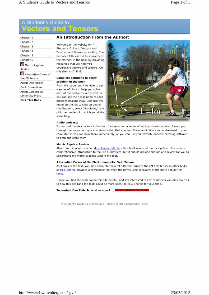
An Introduction From the Author:
Welcome to the website for A
Student’s Guide to Vectors and
Tensors, and thanks for visiting. The
purpose of this site is to supplement
the material in the book by providing
resources that will help you
understand vectors and tensors. On
this site, you’ll find:
Complete solutions to every
problem in the book
From this page, you’ll be able to get
a series of hints to help you solve
each of the problems in the text, or
you can see the full solution to each
problem straight away. Just use the
menu on the left to click on one of
the Chapters, select “Problems,” and
pick the problem for which you’d like
some help.
Audio podcasts
For each of the six chapters in the text, I’ve recorded a series of audio podcasts in which I walk you
through the major concepts contained within that chapter. These audio files can be streamed to your
computer so you can hear them immediately, or you can use your favorite podcast-catching software
to grab and store them.
Matrix Algebra Review
Also from this page, you can download a .pdf file with a brief review of matrix algebra. This is not a
comprehensive introduction to the use of matrices, but it should provide enough of a review for you to
understand the matrix algebra used in the text.
Alternative Forms of the Electromagnetic Field Tensor
As it says in the text, you may encounter several different forms of the EM field tensor in other texts,
so this .pdf file provides a comparison between the forms used in several of the more popular EM
texts.
I hope you find the material on this site helpful, and I’m interested in any comments you may have as
to how this site (and the text) could be more useful to you. Thanks for your time.
To contact Dan Fleisch, send an e-mail to
A Student’s Guide to Vectors and Tensors ©2011 Cambridge Press
Chapter 1
Chapter 2
Chapter 3
Chapter 4
Chapter 5
Chapter 6
Matrix Algebra
Review
Alternative forms of
the EM tensor
About Dan Fleisch
Book Corrections
About Cambridge
University Press
BUY This Book
Page 1 of 1A Student's Guide to Vectors and Tensors
23/05/2012http://www4.wittenberg.edu/sgvt/
Corrections
A list of corrections for the printed edition. Updated May 6, 2012.
Chapter 1
Chapter 2
Chapter 3
Chapter 4
Chapter 5
Chapter 6
Matrix Algebra
Review
Alternative forms of
the EM tensor
About Dan Fleisch
Book Corrections
About Cambridge
University Press
BUY This Book
Page 1 of 4A Student's Guide to Vectors and Tensors
23/05/2012http://www4.wittenberg.edu/sgvt/corrections.shtml
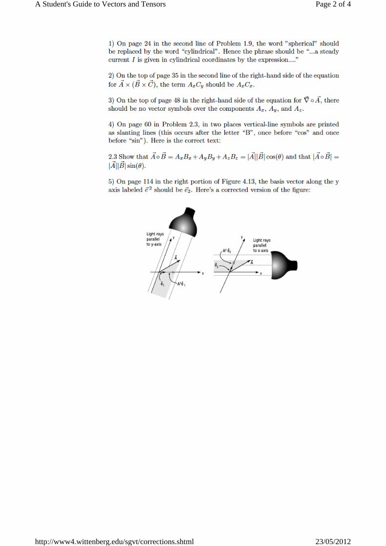
Page 2 of 4A Student's Guide to Vectors and Tensors
23/05/2012http://www4.wittenberg.edu/sgvt/corrections.shtml
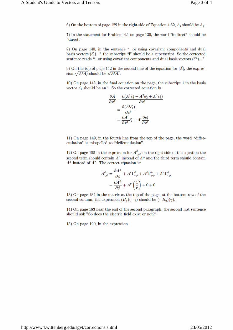
Page 3 of 4A Student's Guide to Vectors and Tensors
23/05/2012http://www4.wittenberg.edu/sgvt/corrections.shtml
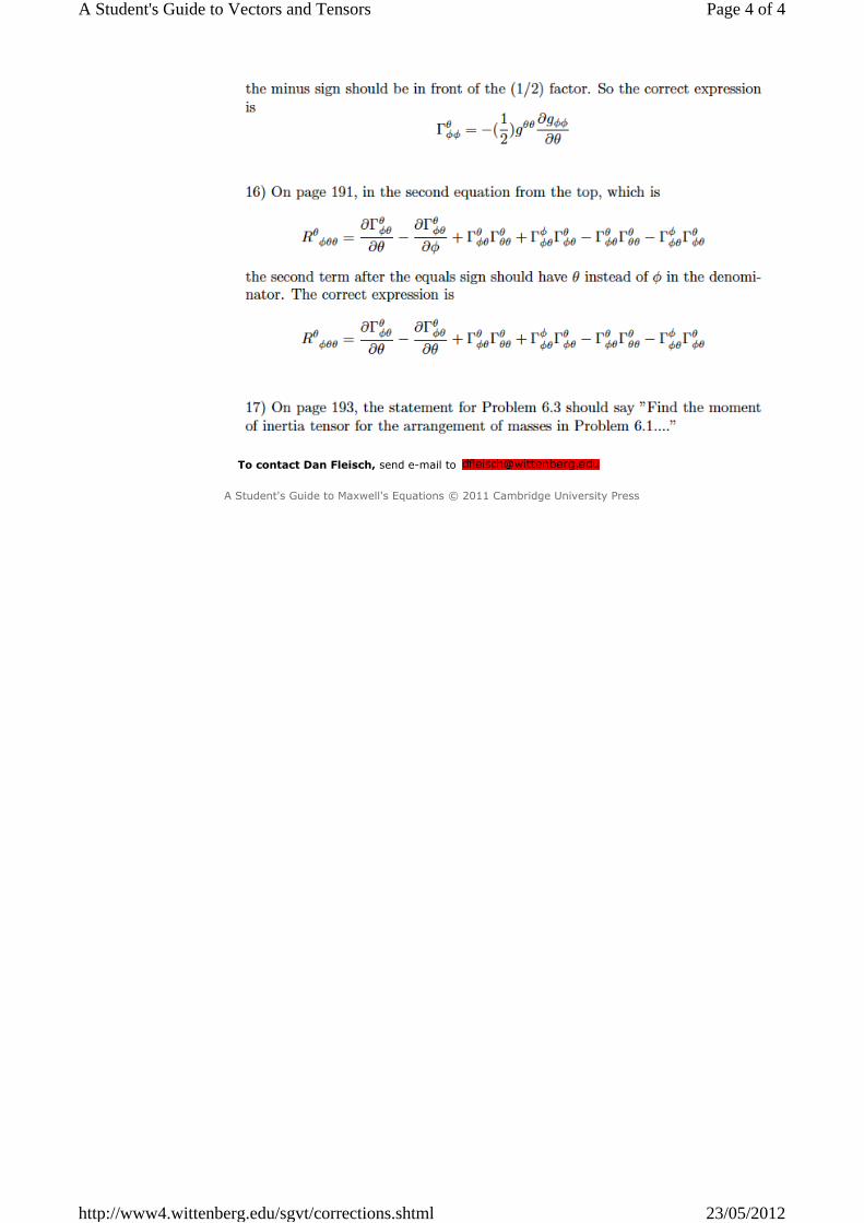
To contact Dan Fleisch, send e-mail to
A Student's Guide to Maxwell's Equations © 2011 Cambridge University Press
Page 4 of 4A Student's Guide to Vectors and Tensors
23/05/2012http://www4.wittenberg.edu/sgvt/corrections.shtml