Embed Size (px)
Citation preview

APPENDIX A
TENSORS, TENSOR PRODUCTS AND TENSOR OPERATIONS IN THREE-DIMENSIONS
A.I Vectors and vector operations
The purpose of this section is to summarize some basic properties of vectors and vector operations. Complete descriptions of linear vector spaces can be found in standard texts on linear algebra (Noble, 1969) and a more complete summary of the use of vectors in continuum mechanics can be found in (Sokolnikoff, 1964). For the present purpose it is sufficient to recall that a vector in three-dimensional space is usually identified with an
arrow connecting two points in space. This arrow has a magnitude and a specific direction.
Fig. A.I.l Parallelogram rule of vector addition.
Some basic vector operations can be summarized as follows. If a,b are two vectors, then the quantity
c=a+b, (A. 1.1)
is also a vector which is defined by the parallelogram law of addition (see Fig. A.I.l). Furthermore, the operations
a+b=b+a (a+b)+c=a+(b+c)
aa=aa a-b=b-a
a-(b+c)=a-b+a-c a(a-b)=(aa)-b
axb=-bxa
ax(b+c)=axb+axc
a(axb)=(aa)xb
(commutative law) , (associative law) , (multiplication by a real number) , (commutative law) , (distributive law) ,
(associative law) , (lack of commutativity) , (distributive law) ,
(associative law) , (A.I.2)
are satisfied for all vectors a,b,c and all real numbers a, where a - b denotes the dot product (or scalar product), and a x b denotes the cross product (or vector product) between the vectors a and b.
429
APPENDIX A
TENSORS, TENSOR PRODUCTS AND TENSOR OPERATIONS IN THREE-DIMENSIONS
A.I Vectors and vector operations
The purpose of this section is to summarize some basic properties of vectors and vector operations. Complete descriptions of linear vector spaces can be found in standard texts on linear algebra (Noble, 1969) and a more complete summary of the use of vectors in continuum mechanics can be found in (Sokolnikoff, 1964). For the present purpose it is sufficient to recall that a vector in three-dimensional space is usually identified with an
arrow connecting two points in space. This arrow has a magnitude and a specific direction.
R p.:: Fig. A.I.l Parallelogram rule of vector addition.
Some basic vector operations can be summarized as follows. If a,b are two vectors, then the quantity
c=a+b, (A. 1.1)
is also a vector which is defined by the parallelogram law of addition (see Fig. A.I.l). Furthermore, the operations
a+b=b+a (a+b)+c=a+(b+c)
aa=aa a-b=b-a
a-(b+c)=a-b+a-c a(a-b)=(aa)-b
axb=-bxa
ax(b+c)=axb+axc
a(axb)=(aa)xb
(commutative law) , (associative law) , (multiplication by a real number) , (commutative law) , (distributive law) ,
(associative law) , (lack of commutativity) , (distributive law) ,
(associative law) , (A.I.2)
are satisfied for all vectors a,b,c and all real numbers a, where a - b denotes the dot product (or scalar product), and a x b denotes the cross product (or vector product) between the vectors a and b.
429

430 APPENDIX A
A.2 Tensors as linear operators
Scalars (or real numbers) are referred to as tensors of order zero, and vectors are
referred to as tensors of order one. Here, higher order tensors are defined inductively starting with the notion of a vector.
Tensor of Order M: The quantity T is called a tensor of order two (or a second order tensor) if it is a linear operator whose domain is the space of all vectors v and whose
range Tv or vT is a vector. Similarly, the quantity T is called a tensor of order three if it
is a linear operator whose domain is the space of all vectors v and whose range Tv or vT is a tensor of order two. Consequently, by induction, the quantity T is called a tensor of
order M (M~l) if it is a linear operator whose domain is the space of all vectors v and
whose range Tv or vT is a tensor of order (M-I). Since T is a linear operator, it satisfies
the following rules
T(v + w) = Tv + Tw , a(Tv) = (aT)v = T(av) ,
(v + w)T = vT + wT , a(vT) = (av)T = (vT)a , (A.2.1)
where v,w are arbitrary vectors and a is an arbitrary scalar. Notice that the tensor T can
be operated upon on its right [e.g. (A.2.1)l,2l or on its left [e.g. (A.2.1»),4l and that in general, operation on the right and on the left is not commutative
Tv ;f. vT (Lack of commutativity in general) . (A.2.2)
Zero Tensor of Order M: The zero tensor of order M is denoted by OeM) and is a linear operator whose domain is the space of all vectors v and whose range O(M-J) is the
zero tensor of order M-I.
OeM) v = v OeM) = O(M-I) . (A.2.3) Notice that these tensors are defined inductively starting with the known properties of the
real number 0, which is the zero tensor 0(0) of order O. Often, for simplicity in writing a tensor equation, the zero tensor of any order is denoted by the symbol O.
Addition and Subtraction: The usual rules of addition and subtraction of two tensors A and B apply only when the two tensors have the same order. It should be emphasized that tensors of different orders cannot be added or subtracted.
A.3 Tensor products (special case)
In order to define the operations of tensor product, dot product, and juxtaposition for
general tensors, it is convenient to first consider the definitions of these properties for
special tensors. Also, the operations of left and right transpose of the tensor product of a
string of vectors will be defined. It will be seen later that the operation of dot product is
defined to be consistent with the usual notion of the dot product as an inner product
because it is a positive definite operation. Consequently, the dot product of a tensor with
itself yields the square of the magnitude of the tensor. Also, the operation of
juxtaposition is defined to be consistent with the usual procedures for matrix
multiplication when two second order tensors are juxtaposed.
430 APPENDIX A
A.2 Tensors as linear operators
Scalars (or real numbers) are referred to as tensors of order zero, and vectors are referred to as tensors of order one. Here, higher order tensors are defined inductively starting with the notion of a vector.
Tensor of Order M: The quantity T is called a tensor of order two (or a second order tensor) if it is a linear operator whose domain is the space of all vectors v and whose range Tv or vT is a vector. Similarly, the quantity T is called a tensor of order three if it is a linear operator whose domain is the space of all vectors v and whose range Tv or vT is a tensor of order two. Consequently, by induction, the quantity T is called a tensor of order M (M~I) if it is a linear operator whose domain is the space of all vectors v and whose range Tv or vT is a tensor of order (M-I). Since T is a linear operator, it satisfies
the following rules T(v + w) = Tv + Tw , a(Tv) = (aT)v = T(av) ,
(v + w)T = vT + wT , a(vT) = (av)T = (vT)a , (A.2.I)
where v,w are arbitrary vectors and a is an arbitrary scalar. Notice that the tensor T can be operated upon on its right [e.g. (A.2.1)J,2] or on its left [e.g. (A.2.I)3,4] and that in general, operation on the right and on the left is not commutative
Tv '# vT (Lack of commutativity in general) . (A.2.2) Zero Tensor of Order M: The zero tensor of order M is denoted by OeM) and is a
linear operator whose domain is the space of all vectors v and whose range O(M-I) is the
zero tensor of order M-I. OeM) v = v OeM) = O(M-I) . (A.2.3)
Notice that these tensors are defined inductively starting with the known properties of the real number 0, which is the zero tensor 0(0) of order O. Often, for simplicity in writing a tensor equation, the zero tensor of any order is denoted by the symbol O.
Addition and Subtraction: The usual rules of addition and subtraction of two tensors A and B apply only when the two tensors have the same order. It should be emphasized that tensors of different orders cannot be added or subtracted.
A.3 Tensor products (special case)
In order to define the operations of tensor product, dot product, and juxtaposition for
general tensors, it is convenient to first consider the definitions of these properties for special tensors. Also, the operations of left and right transpose of the tensor product of a string of vectors will be defined. It will be seen later that the operation of dot product is
defined to be consistent with the usual notion of the dot product as an inner product because it is a positive definite operation. Consequently, the dot product of a tensor with
itself yields the square of the magnitude of the tensor. Also, the operation of juxtaposition is defined to be consistent with the usual procedures for matrix
multiplication when two second order tensors are juxtaposed.

TENSORS 431
Tensor Product (Special Case): The tensor product operation is denoted by the symbol
® and it is defined so that for an arbitrary vector v, the quantity (a I ®a2) is a second order tensor satisfying the relations
(a l ®a2)v=a l (a2 ·v) , v(a l ®a2)=(v·a l )a2 . (A.3.1)
Similarly, the quantity (a l ®a2®a3) is a third order tensor satisfying the relations
(a l ®a2®a3) v = (al®a2) (a3 • v) , v (a l ®a2®a3) = (v· a l ) (a2®a3) . (A.3.2)
For convenience in generalizing these ideas, let A be a special tensor of order M which is formed by the tensor product of a string of M (M~2) vectors (a l ,a2,a3, ... ,aM), and let B
be a special tensor of order N which is formed by the tensor product of a string of N
(N~2) vectors (b l ,b2,b3, ... ,bN) so that
A = (a l ®a2®a3® ... ®aM), B = (b l ®b2®b3® ... ®bN) , (A.3.3)
and for definiteness take M:.:;N. (A.3.4)
It then follows that A satisfies the relations
Av = (a l ®a2® ... ®aM) v = (a l ®a2® ... ®aM_I ) (aM· v),
vA = v (a l ®a2® ... ®aM) = (v· a l ) (a2®a3® ... ®aM) . (A.3.S)
Notice that when v operates on either the right or left side of A, it has the effect of
forming the scalar product with the vector in the string closest to it, and it causes the result A v or v A to have order one less than the order of A since one of the tensor products is
removed. The remaining vectors in the string of tensor products are unaltered. Dot Product (Special Case): The dot product operation between two vectors can be
generalized to an operation between two tensors of any orders. For example, the dot product between two second order tensors can be written as
(a l ®a2)· (b l ®b2) = (a l • bl) (a2 • b2) ,
(A.3.6)
and the dot product between a second order tensor and a third order tensor can be written
as
(a l ®a2)· (b l ®b2®b3) = (a l • bl) (a2 • b2) b 3 '
(b l ®b2®b3)· (a l®a2) = bl (b2 • al) (b3 • a2) .
Also, the dot product between two third order tensors can be written as
(a l ®a2®a3) • (b l ®b2®b3) = (a l • bl) (a2 • b2) (a3 • b3) ,
(b l ®b2®b3)· (a l ®a2®a3) = (b l • a l ) (b2 • a2) (b3 • a3) ,
(A.3.7)
(A.3.8)
and the dot product between a second order tensor and a fourth order tensor can be
written as
(a l ®a2)· (b l ®b2®b3®b4) = (a l • bl) (a2 • b2) (b3®b4) ,
(b l ®b2®b3®b4)· (a l ®a2) = (b l ®b2) (b3 • al) (b4 • a2)· (A.3.9)
This dot product operation can be generalized for special tensors of any orders like A
and B by carefully examining examples (A.3.7) and (A.3.9). These examples indicate
TENSORS 431
Tensor Product (Special Case): The tensor product operation is denoted by the symbol
® and it is defined so that for an arbitrary vector v, the quantity (a I ®a2) is a second order tensor satisfying the relations
(a l ®a2)v=a l (a2 ·v) , v(a l ®a2)=(v·a l )a2 . (A.3.1)
Similarly, the quantity (a l ®a2®a3) is a third order tensor satisfying the relations
(a l ®a2®a3) v = (al®a2) (a3 • v) , v (a l ®a2®a3) = (v· a l ) (a2®a3) . (A.3.2)
For convenience in generalizing these ideas, let A be a special tensor of order M which is formed by the tensor product of a string of M (M~2) vectors (a l ,a2,a3, ... ,aM), and let B
be a special tensor of order N which is formed by the tensor product of a string of N
(N~2) vectors (b l ,b2,b3, ... ,bN) so that
A = (a l ®a2®a3® ... ®aM), B = (b l ®b2®b3® ... ®bN) , (A.3.3)
and for definiteness take M:.:;N. (A.3.4)
It then follows that A satisfies the relations
Av = (a l ®a2® ... ®aM) v = (a l ®a2® ... ®aM_I ) (aM· v),
vA = v (a l ®a2® ... ®aM) = (v· a l ) (a2®a3® ... ®aM) . (A.3.S)
Notice that when v operates on either the right or left side of A, it has the effect of
forming the scalar product with the vector in the string closest to it, and it causes the result A v or v A to have order one less than the order of A since one of the tensor products is
removed. The remaining vectors in the string of tensor products are unaltered. Dot Product (Special Case): The dot product operation between two vectors can be
generalized to an operation between two tensors of any orders. For example, the dot product between two second order tensors can be written as
(a l ®a2)· (b l ®b2) = (a l • bl) (a2 • b2) ,
(b l ®b2)· (al®a2) = (b l • al) (b2 • a2) , (A.3.6)
and the dot product between a second order tensor and a third order tensor can be written
as
(a l ®a2)· (b l ®b2®b3) = (a l • bl) (a2 • b2) b 3 '
(b l ®b2®b3)· (a l®a2) = b l (b2 • al) (b3 • a2) .
Also, the dot product between two third order tensors can be written as
(a l ®a2®a3) • (b l ®b2®b3) = (a l • bl) (a2 • b2) (a3 • b3) ,
(b l ®b2®b3)· (a l ®a2®a3) = (b l • a l ) (b2 • a2) (b3 • a3) ,
(A.3.7)
(A.3.8)
and the dot product between a second order tensor and a fourth order tensor can be
written as
(a l ®a2)· (b l ®b2®b3®b4) = (a l • bl) (a2 • b2) (b3®b4) ,
(b l ®b2®b3®b4)· (a l ®a2) = (b l ®b2) (b3 • al) (b4 • a2)· (A.3.9)
This dot product operation can be generalized for special tensors of any orders like A
and B by carefully examining examples (A.3.7) and (A.3.9). These examples indicate

432 APPENDIX A
that the dot product between tensors of different orders does not necessarily commute, whereas the dot product of two tensors of the same order does commute.
A • B :;t B • A for M<N , A· B = B • A for M=N . (A.3.1O) Moreover, it can be seen that the tensor of smallest order controls the outcome of the dot product operation. Specifically, in (A.3.7), the second order tensor (a,®a2) appears on
the left of the third order tensor (b, ®b2®b3). Since (a, ®a2) is a second order tensor this causes only the first two vectors on the left of (b, ®b2®b3) to form inner products
with a, and a2. Similarly, since (a,®a2) appears on the right side of (b,®b2®b3) in
(A.3.7)2' this causes only the first two vectors on the right of (b, ®b2®b3) to form inner products with a, and a2.
In general, the dot product A • B of the special tensors defined in (A.3.3) is a tensor of order IM-NI. Furthermore, in view of the restriction (A.3.4), only the first M vectors of
B closest to A will form inner products with the vectors of A. It is also important to note that the order of the strings of vectors in the inner products remains the same as that in the
tensors. Specifically, for the dot product A • B the first vector on the left side of A forms an inner product with the first vector on the left side of B and so forth. Whereas,
for the dot product B • A the last vector on the right side of A forms an inner product with the last vector on the right side of B.
Cross Product (Special Case): The cross product operation between two vectors can
be generalized to an operation between two tensors of any orders. For example, the cross
product between two second order tensors can be written as
(a,®a2) x (b,®b2) = (a, x b,)®(a2 x b2) ,
(A.3.II)
and the cross product between a second order tensor and a third order tensor can be
written as
(a,®a2) x (b,®b2®b3) = (a, x b,)®(a2 x b2)®b3 '
(b,®b2®b3) x (a,®a2) = b,®(b2 x a,)®(b3 x a2) . (A.3.12)
Also, the cross product between two third order tensors can be written as (a , ®a2®a3) x (b,®b2®b3) = (a, x b,)®(a2 x b2)®(a3 x b3) ,
(b,®b2®b3) x (a,®a2®a3) = (b, x a,)®(b2 x a2)®(b3 x a3) , (A.3.l3)
and the cross product between a second order tensor and a fourth order tensor can be
written as
(a,®a2) x (b,®b2®b3®b4) = (a, x b,)®(a2 x b2)®(b3®b4) ,
(b,®b2®b3®b4) x (a,®a2) = (b,®b2)®(b3 x a,)®(b4 x a2). (A.3.l4)
This cross product operation can be generalized for special tensors of any orders like A and B by carefully examining examples (A.3.l2) and (A.3.14). These examples indicate
that the cross product between tensors of different orders does not necessarily commute,
whereas the cross product of two tensors of the same order will commute if the order is
even, and it will be changed in sign if the order is odd. A x B :;t B x A for M<N ,
432 APPENDIX A
that the dot product between tensors of different orders does not necessarily commute, whereas the dot product of two tensors of the same order does commute.
A • B :;t B • A for M<N , A· B = B • A for M=N . (A.3.1O) Moreover, it can be seen that the tensor of smallest order controls the outcome of the dot
product operation. Specifically, in (A.3.7), the second order tensor (a,®a2) appears on
the left of the third order tensor (b, ®b2®b3). Since (a, ®a2) is a second order tensor
this causes only the first two vectors on the left of (b, ®b2®b3) to form inner products
with a, and a2. Similarly, since (a,®a2) appears on the right side of (b,®b2®b3) in
(A.3.7)2' this causes only the first two vectors on the right of (b, ®b2®b3) to form inner products with a, and a2.
In general, the dot product A • B of the special tensors defined in (A.3.3) is a tensor of order IM-NI. Furthermore, in view of the restriction (A.3.4), only the first M vectors of
B closest to A will form inner products with the vectors of A. It is also important to note that the order of the strings of vectors in the inner products remains the same as that in the
tensors. Specifically, for the dot product A • B the first vector on the left side of A forms an inner product with the first vector on the left side of B and so forth. Whereas,
for the dot product B • A the last vector on the right side of A forms an inner product with the last vector on the right side of B.
Cross Product (Special Case): The cross product operation between two vectors can
be generalized to an operation between two tensors of any orders. For example, the cross
product between two second order tensors can be written as
(a,®a2) x (b,®b2) = (a, x b,)®(a2 x b2) ,
(b,®b2) x (a,®a2) = (b, x a,)®(b2 x a2) , (A.3.II)
and the cross product between a second order tensor and a third order tensor can be
written as (a,®a2) x (b,®b2®b3) = (a, x b,)®(a2 x b2)®b3 '
(b,®b2®b3) x (a,®a2) = b,®(b2 x a,)®(b3 x a2) . (A.3.12)
Also, the cross product between two third order tensors can be written as (a , ®a2®a3) x (b,®b2®b3) = (a, x b,)®(a2 x b2)®(a3 x b3) ,
(b,®b2®b3) x (a,®a2®a3) = (b, x a,)®(b2 x a2)®(b3 x a3) , (A.3.l3)
and the cross product between a second order tensor and a fourth order tensor can be
written as
(a,®a2) x (b,®b2®b3®b4) = (a, x b,)®(a2 x b2)®(b3®b4) ,
(b,®b2®b3®b4) x (a,®a2) = (b,®b2)®(b3 x a,)®(b4 x a2). (A.3.l4)
This cross product operation can be generalized for special tensors of any orders like A and B by carefully examining examples (A.3.l2) and (A.3.14). These examples indicate
that the cross product between tensors of different orders does not necessarily commute,
whereas the cross product of two tensors of the same order will commute if the order is
even, and it will be changed in sign if the order is odd. A x B :;t B x A for M<N ,

TENSORS 433
A x B = B x A for M=N (even order) ,
A x B = - B x A for M=N (odd order) . (A.3.1S) Moreover, it can be seen that the tensor of smallest order controls the outcome of the
result of the cross product operation. Also, since the cross product of two vectors is a
vector, it is necessary to retain the tensor product operators in the examples (A.3.11)
(A.3.14).
In general, the cross product A x B of the special tensors defined in (A.3.3) is a tensor
of order N which is equal to the order of the highest order tensor B. Furthermore, in
view of the restriction (A.3.4), only the first M vectors of B closest to A will form cross
products with the vectors of A. It is also important to note that the order of the strings of
vectors in these cross products remains the same as that in the tensors. Specifically, for
the cross product A x B, the first vector on the left side of A forms a cross product with
the first vector on the left side of B and so forth. Whereas, for the cross product B x A,
the last vector on the right side of A forms a cross product with the last vector on the right
side of B. Juxtaposition (Special Case): The operation of juxtaposition is indicated when two
special tensors are placed next to each other without an operator between them. For
examples
(a l ®a2)(b l ®b2) = (a2 - b l ) (a l ®b2) ,
(a I ®a2)(b I ®b2®b3) = (a2 - b I) (a I )®(b2®b3) ,
(b l ®b2®b3)(a l ®a2) = (b3 - a l ) (b l ®b2)®(a2) ,
(a l ®a2®a3)(b l ®b2®b3) = (a3 - b l ) (a l ®a2)®(b2®b3) (A.3.l6)
It can be seen that the juxtaposition operation causes only one of the vectors in each tensor
(the vectors closest to each other) to be connected by the inner product. The remaining
vectors form a string of vectors connected by tensor products. The order of these vectors in the string is the same as their order in the juxtaposition operation. The order of the
resulting tensor is the sum of the orders of the two tensors placed in juxtaposition minus two.
In general, the juxtaposition AB of the special tensors defined in (AS) is a tensor of
order (M+N-2) which is given by
AB = (al®a2®a3® ... ®aM)(bl®b2®b3® ... ®bN)
= (aM - b l ) (al®a2®a3®···®aM_I)®(b2®b3®···®bN)· (A.3.17)
Thus, the juxtaposition operation is not commutative if anyone of the tensors A or B is
of higher order than one AB:;tBA. (A.3.IS)
Since only the closest vectors are connected by the inner product, it follows that the
juxtaposition of any order tensor A with a vector v, is the same as the dot product of the
two tensors
Av=A-v, vA=v-A. (A.3.l9)

434 APPENDIX A
Consequently, the juxtaposition of two vectors is the same as the dot product between them so that this is a special case when the juxtaposition operation commutes
a, b, = a, • b, = b,a, . (A.3.20) In spite of the validity of this result, the dot product between two vectors will usually be
expressed explicitly instead of through the juxtaposition operation.
Transpose (Special Case): The transpose of the second order tensor (a, ®a2) is
defined by
(A.3.21)
Note that the effect of the transpose operation is merely to change the order of the vectors in the tensor product. This transpose operation can be generalized for higher order
tensors, for higher order transpose operations, and for left and right transpose operations. Once the left transpose operation is admitted, it is easy to see that a quantity like A TB cannot be interpreted uniquely if the left and right transpose operations are both denoted
by a superposed (T). In particular, it would not be clear if the transpose operation were
applied to the right of A or the left of B. For this reason, the left transpose operation will
be denoted by a superposed (LT) on the left of the tensor. Thus, for example
LT(a,®a2) = (a2®a,) = (a,®a2)T , (A.3.22)
which indicates that for second order tensors there is no distinction between the left and
right transposes. These transpose operations can be applied to higher order tensors by generalizing the
following examples
LT(a,®a2®a3) = (a2®a,)®a3 ' LT(a,®a2®a3®a4) = (a2®a,)®(a3®a4) ,
(a , ®a2®a3)T = a,®(a3®a2) , (a,®a2®a3®a4)T = (a,®a2)®(a4®a3) . (A.3.23)
Here, the parentheses are included to emphasize that these transpose operators influence only the order of the two vectors in the string closest to the operator. In this regard, it is
possible to define transpose operators of order M~2 by L T(M) and T(M) such that they interchange the order of two sets of M vectors in the tensor product B of a string of N vectors. Since the special tensor B has to contain at least two sets of M vectors, it follows that the transpose operator of order M can be applied only to tensors of order
N~2M. For examples
LT(2)(a,®a2®a3®a4) = (a3®a4)®(a,®a2) ,
LT(2)(a,®a2®a3®a4®aS) = (a3®a4)®(a,®a2)®aS '
(a,®a2®a3®a4)T(2) = (a3®a4)®(a,®a2) ,
(a,®a2®a3®a4®as)T(2) = a,®(a4®aS)®(a2®a3) . (A.3.24)
Notice that for these second order transpose operators, only the four vectors closest to the
operators are influenced and that the order of the vectors in each of the two sets of two
vectors are not changed.
434 APPENDIX A
Consequently, the juxtaposition of two vectors is the same as the dot product between
them so that this is a special case when the juxtaposition operation commutes
a, b, = a, • b, = b,a, . (A.3.20) In spite of the validity of this result, the dot product between two vectors will usually be
expressed explicitly instead of through the juxtaposition operation.
Transpose (Special Case): The transpose of the second order tensor (a, ®a2) is
defined by
(a,®a2)T = (a2®a,) . (A.3.21)
Note that the effect of the transpose operation is merely to change the order of the vectors in the tensor product. This transpose operation can be generalized for higher order
tensors, for higher order transpose operations, and for left and right transpose operations.
Once the left transpose operation is admitted, it is easy to see that a quantity like A TB cannot be interpreted uniquely if the left and right transpose operations are both denoted
by a superposed (T). In particular, it would not be clear if the transpose operation were
applied to the right of A or the left of B. For this reason, the left transpose operation will be denoted by a superposed (LT) on the left of the tensor. Thus, for example
LT(a,®a2) = (a2®a,) = (a,®a2)T , (A.3.22)
which indicates that for second order tensors there is no distinction between the left and
right transposes. These transpose operations can be applied to higher order tensors by generalizing the
following examples
LT(a,®a2®a3) = (a2®a,)®a3 ' LT(a,®a2®a3®a4) = (a2®a,)®(a3®a4) ,
(a , ®a2®a3)T = a,®(a3®a2) , (a,®a2®a3®a4)T = (a,®a2)®(a4®a3) . (A.3.23)
Here, the parentheses are included to emphasize that these transpose operators influence only the order of the two vectors in the string closest to the operator. In this regard, it is
possible to define transpose operators of order M~2 by L T(M) and T(M) such that they interchange the order of two sets of M vectors in the tensor product B of a string of N vectors. Since the special tensor B has to contain at least two sets of M vectors, it follows that the transpose operator of order M can be applied only to tensors of order
N~2M. For examples
LT(2)(a,®a2®a3®a4) = (a3®a4)®(a,®a2) ,
LT(2)(a,®a2®a3®a4®aS) = (a3®a4)®(a,®a2)®aS '
(a,®a2®a3®a4)T(2) = (a3®a4)®(a,®a2) ,
(a,®a2®a3®a4®as)T(2) = a,®(a4®aS)®(a2®a3) . (A.3.24)
Notice that for these second order transpose operators, only the four vectors closest to the
operators are influenced and that the order of the vectors in each of the two sets of two
vectors are not changed.

TENSORS 435
A.4 Indicial notation
Quantities written in indicial notation will have a finite number of indices attached to
them. Since the number of indices can be zero, a scalar with no index can also be considered to be written in index notation. The language of index notation is quite simple
because only two types of indices can appear in any term. Either the index is a free· index
or it is a repeated index. Also, a simple summation convention will be defined which
applies only to repeated indices. These two types of indices and the summation
convention are defined as follows. Free Indices: Indices that appear only once in a given term are known as free indices.
When the free index is a Latin letter, the index will take the values (1,2,3), whereas when
it is a Greek letter, it will take only the values (1,2). For example, i and a are free indices
in the following expressions
e i =(e l ,e2 ,e3), gi=(gl,g2,g3)' gi=(gl,g2,g3) (i=I,2,3),
ea=(e l ,e2) , aa=(a l ,a2) , aa=(a l ,a2) (a=I,2), (A.4.I)
For general curvilinear coordinates it is necessary to distinguish between indices used as
subscripts for covariant quantities, and indices used as superscripts for contravariant quantItIes. Whereas, for rectangular Cartesian coordinates the base vectors ei are
orthonormal constant vectors and the distinction between covariant and contravariant quantities disappears so that all indices can be written as subscripts.
Repeated Indices: Indices that appear twice in a given term are known as repeated
indices. For example, i and j are free indices and m and n are repeated indices in the following expressions
ai bj cm T mn dn , Aimn Bjmn , Aim n Bt n . (A.4.2)
It is important to emphasize that in the language of indicial notation, an index can never appear more than twice in any term. Also, for curvilinear coordinates one of the repeated indices is a subscript and the other is a superscript.
Einstein Summation Convention: When an index appears as a repeated index in a term, that index is understood to take on the values (1,2,3) for Latin indices or (1,2) for Greek indices and the resulting terms are summed. Thus, for example,
vi g - vi g + v2 g + v3 g v gi - v gl + v g2 + v g3 i- I 2 3' i-I 2 3'
va a = v I a + v2 a v aa = val + v a2 a I 2' a I 2'
gi0gi = gl0g 1 + g20g2 + g30 g3 . (A.4.3)
Because of this summation convention, repeated indices are also known as dummy
indices since their replacement by any other letter (of the same type, Latin or Greek) not
appearing as a free index and also not appearing as another repeated index, does not
change the meaning of the term in which they occur. For examples,
vi g. = vj g. a· b ca = a· bR c~ (A.4.4) I J' I a It-"
TENSORS 435
A.4 Indicial notation
Quantities written in indicial notation will have a finite number of indices attached to
them. Since the number of indices can be zero, a scalar with no index can also be considered to be written in index notation. The language of index notation is quite simple
because only two types of indices can appear in any term. Either the index is a free index
or it is a repeated index. Also, a simple summation convention will be defined which
applies only to repeated indices. These two types of indices and the summation
convention are defined as follows. Free Indices: Indices that appear only once in a given term are known as free indices.
When the free index is a Latin letter, the index will take the values (1,2,3), whereas when
it is a Greek letter, it will take only the values (1,2). For example, i and a are free indices
in the following expressions
e i =(e l ,e2 ,e3), gi=(gl,g2,g3)' gi=(gl,g2,g3) (i=I,2,3),
ea=(e l ,e2) , aa=(a l ,a2) , aa=(a l ,a2) (a=I,2), (A.4.I)
For general curvilinear coordinates it is necessary to distinguish between indices used as
subscripts for covariant quantities, and indices used as superscripts for contravariant quantItIes. Whereas, for rectangular Cartesian coordinates the base vectors ei are
orthonormal constant vectors and the distinction between covariant and contravariant quantities disappears so that all indices can be written as subscripts.
Repeated Indices: Indices that appear twice in a given term are known as repeated
indices. For example, i and j are free indices and m and n are repeated indices in the following expressions
ai bj cm T mn dn , Aimn Bjmn , Aim n Bt n . (A.4.2)
It is important to emphasize that in the language of indicial notation, an index can never appear more than twice in any term. Also, for curvilinear coordinates one of the repeated indices is a subscript and the other is a superscript.
Einstein Summation Convention: When an index appears as a repeated index in a term, that index is understood to take on the values (1,2,3) for Latin indices or (1,2) for Greek indices and the resulting terms are summed. Thus, for example,
vi g - vi g + v2 g + v3 g v gi - v gl + v g2 + v g3 i- I 2 3' i-I 2 3'
Va a = v I a + v2 a v aa = val + v a2 a I 2' a I 2'
gi0gi = gl0g 1 + g20g2 + g30 g3 . (A.4.3)
Because of this summation convention, repeated indices are also known as dummy
indices since their replacement by any other letter (of the same type, Latin or Greek) not
appearing as a free index and also not appearing as another repeated index, does not
change the meaning of the term in which they occur. For examples,
vi gi = vj gj , ai baca = ai b~ c~ . (A.4.4)

436 APPENDIX A
It is important to emphasize that the same free indices must appear in each term in an equation so that for example, the free index i in (A.4.4)2 must appear on each side of the
equality. Kronecker Delta: Using the fact that the contravariant base vectors gi defined by
(2.1.10) are reciprocal vectors of the covariant base vectors gi defined by (2.1.5), it
follows that the Kronecker delta symbols o! and Oij are defined by . . {I if i = j . . {I if i = j
0iJ = gi • gJ = 0 i f i i:- j Olj = gl • gj = 0 i f i i:- j (A.4.5)
Since the Kronecker deltas vanish unless i=j, they exhibit the following exchange
properties
(A.4.6)
Notice that the Kronecker symbol can be removed by replacing the repeated index j in
(A.4.6) by the free index i. In view of the definitions of base tensors and components of tensors discussed in
section 2.2, it follows that the Kronecker delta symbols are used in calculating the dot
product between two vectors a and b, since
a = a· gi = ai g. b = b. gi = bi g. I I ' I I '
a • b = a· gi • bi g. = a· (gi • g.) bi = a· oi. bi = a. bi I J I J I J I'
a. b = ai g. • b· gj = ai (g. • gj) b· = ai oj b· = ai b· (A.4.7) I J I J I J I
Permutation symbol: The permutation symbols fijk and £ijk are defined by
£ijk = gi X gj • gk = gl/2 eijk ' fijk = gi x gj • gk = g-1/2 eijk , (A.4.8)
where the scalar g 112 is defined by (2.1.6) and the alternating symbols eijk and eijk are defined in terms of the right-handed orthonormal base vectors ei of a rectangular
Cartesian coordinate system by the equations
e"k = eijk = e· x e· • ek IJ I J '
{I if (i,j,k) are an even permutation of (1,2,3)
eijk = -1 if (i,j ,k) are an odd permutation of (1,2,3) o if at least two of (i,j,k) have the same value
(A.4.9)
From the definition (A.4.9), it appears that the permutation symbols can be used in
calculating the vector product between two vectors. To this end, it is necessary to prove
that
(A.4.10)
Proof: Since gi x gj is a vector in Euclidean 3-Space for each choice of the values of i and j, and since gk forms a complete basis for that space, it follows that gi x gj can be
represented as a linear combination of the base vectors gk such that
g.xg.=A"kgk (A.4.11) I J IJ ' where the components Aijk need to be determined. In particular, by taking the dot
product of (A.4.11) with gk and using the definition (A.4.8) it can be shown that
436 APPENDIX A
It is important to emphasize that the same free indices must appear in each term in an equation so that for example, the free index i in (A.4.4)2 must appear on each side of the
equality. Kronecker Delta: Using the fact that the contravariant base vectors gi defined by
(2.1.10) are reciprocal vectors of the covariant base vectors gi defined by (2.1.5), it
follows that the Kronecker delta symbols o! and Oij are defined by . . {I if i = j . . {I if i = j
0iJ = gi • gJ = 0 i f i i:- j , Olj = gl • gj = 0 i f i i:- j (A.4.5)
Since the Kronecker deltas vanish unless i=j, they exhibit the following exchange
properties
0ij Vj = (Olj Vj , 02j Vj' 03j Vj) = (vI' v2 ' v3) = Vi '
oi.vj=(ol.vj o2.vj o3. vj)=(v' v2 v3)=vi J J' J ' J " , (A.4.6)
Notice that the Kronecker symbol can be removed by replacing the repeated index j in
(A.4.6) by the free index i. In view of the definitions of base tensors and components of tensors discussed in
section 2.2, it follows that the Kronecker delta symbols are used in calculating the dot
product between two vectors a and b, since
a = a· gi = ai g. b = b. gi = bi g. I I ' I I '
a • b = a· gi • bi g. = a· (gi • g.) bi = a· oi. bi = a. bi I J I J I J I'
a· b = ai gi • bj gj = ai (gi • gj) bj = ai 0ij bj = ai bi (A.4.7)
Permutation symbol: The permutation symbols fijk and £ijk are defined by
£ijk = gi X gj • gk = g 112 eijk ' fijk = gi x gj • gk = g-1I2 eijk , (A.4.8)
where the scalar g 112 is defined by (2.1.6) and the alternating symbols eijk and eijk are defined in terms of the right-handed orthonormal base vectors ei of a rectangular
Cartesian coordinate system by the equations
e"k = eijk = e· x e· • ek IJ I J '
{I if (i,j,k) are an even permutation of (1,2,3)
eijk = -1 if (i,j,k) are an odd permutation of (1,2,3) o if at least two of (i,j,k) have the same value
(A.4.9)
From the definition (A.4.9), it appears that the permutation symbols can be used in
calculating the vector product between two vectors. To this end, it is necessary to prove
that k . . "k
gi x gj = £ijk g , gl X gJ = £IJ gk (A.4.10)
Proof: Since gi x gj is a vector in Euclidean 3-Space for each choice of the values of i and j, and since gk forms a complete basis for that space, it follows that gi x gj can be
represented as a linear combination of the base vectors gk such that
gixgj=Aijkgk, (A.4.11)
where the components Aijk need to be determined. In particular, by taking the dot
product of (A.4.11) with gk and using the definition (A.4.8) it can be shown that

TENSORS 437
C--k = g- x g- • gk = A-- gm. gk = A- Omk = A-- k (A.4.12) IJ I 1 IJm IJm IJ ' which proves the result (A.4.lO) I' A similar proof can be provided for the result (A.4.10)2' Now, using (A.4.1O) it follows that the cross product between the vectors a and b can be represented in the forms
a x b = (al gi) x (hi gj) = (gi x gj) ai hi = Cijk ai hi gk ,
a x b = (ai gi) x (bj gj) = (gi X gj) ai bj = cijk ai bj gk (A.4.l3)
Contraction: Contraction is the process of setting two free indices in a given expression equal to the same repeated index, together with the implied summation convention. For
example, the free indices i,j in 0ij and Oij can be contracted upon to obtain
0ii = Oil + 022 + ol = 3 , Oij = Oil + 022 + 033 = 3 . (A.4.l4)
Note that contraction on the set of 9=32 quantities Tij or Tij can be performed by
multiplying them by the Kronecker delta to obtain
(A.4.IS)
A.S Tensors products (general case)
Base Tensors and Tensors: Section 2.2 shows how base tensors of any order can be
defined using the tensor products of the covariant base vectors gi and the contravariant base vectors g i. Section 2.2 also shows how the covariant, contravariant, and mixed
components of a tensor can be defined. For example, let A be a second order tensor and
B be a third order tensor defined by
A = Aij (gi®gj) = Aij (gi®gj) = Aij (gi®gj) = Aij (gi®gj) , - - k k - - -k-
B = Bijk (gl®gJ®g ) = Bij (gl®gJ®gk) = BiJ (gl®gj®gk) --k -- k - - k
= BIJ (gi®gj®gk) = B\ (gi®gj®g ) = Bljk (gi®gJ®g ) - k - - - k
= Blj (gi®gJ®gk) = Bi\ (gl®gj®g ) . (A.S.l)
Higher order tensors can be defined in an obvious manner. Since the components of these tensors can be arbitrary real numbers, these expressions
represent general tensors of order two and three. In particular, it should be recognized that a general second order tensor A cannot necessarily be expressed as the tensor product
of two vectors a and b, as was done in discussing the special cases of the tensor
operations.
Using the fact that components of a tensor are unaffected by the various tensor
operations, it is rather straight forward to generalize the tensor operations defined in
section A.3 for general tensors. For simplicity, the tensors A and B defined in (A.S.l)
will be used for specific examples. However, since each tensor can be represented in
terms of its covariant, contravariant, and mixed components, only a few possible
representations of these examples will be exhibited.
Tensor Product (General Case): The tensor product A®B of A and B can be written as
TENSORS 437
Eijk = gi x gj • gk = Aijm gm • gk = Aijm 8mk = Aijk ' (AA.12)
which proves the result (AA.lO) I. A similar proof can be provided for the result (AA.IO)2. Now, using (AA.lO) it follows that the cross product between the vectors a
and b can be represented in the forms
a x b = (ai gi) x (bi gj) = (gi x gj) ai bl = Eijk ai bi gk
a x b = (ai gi) x (bj gj) = (gi X gj) ai bj = Eijk ai bj gk (AA.13)
Contraction: Contraction is the process of setting two free indices in a given expression
equal to the same repeated index, together with the implied summation convention. For
example, the free indices i,j in 8ij and 8ij can be contracted upon to obtain
8ii =811 +822 +8l=3 , ~j=811 +822 +833 =3 . (AA.14)
Note that contraction on the set of 9=32 quantities Tij or Tij can be performed by
multiplying them by the Kronecker delta to obtain Tj 8i. = Ti Ti 8j = Ti.
I J I' J I I (AA.IS)
A.S Tensors products (general case)
Base Tensors and Tensors: Section 2.2 shows how base tensors of any order can be
defined using the tensor products of the covariant base vectors gi and the contravariant base vectors g i. Section 2.2 also shows how the covariant, contravariant, and mixed
components of a tensor can be defined. For example, let A be a second order tensor and
B be a third order tensor defined by
A = Aij (gi®gj) = Aij (gi®gj) = Aij (gi®gj) = Aij (gi®gj) , . . k k·· ·k·
B = Bijk (gl®gJ®g ) = Bij (gl®gJ®gk) = BiJ (gl®gj®gk) ··k .. k· . k
= B'J (gi®gj®gk) = B\ (gi®gj®g ) = B'jk (gi®gJ®g ) . k' .. k
= B'j (gi®gJ®gk) = Bi\ (gl®gj®g ) . (A.5.I)
Higher order tensors can be defined in an obvious manner. Since the components of these tensors can be arbitrary real numbers, these expressions
represent general tensors of order two and three. In particular, it should be recognized
that a general second order tensor A cannot necessarily be expressed as the tensor product of two vectors a and b, as was done in discussing the special cases of the tensor
operations. Using the fact that components of a tensor are unaffected by the various tensor
operations, it is rather straight forward to generalize the tensor operations defined in
section A.3 for general tensors. For simplicity, the tensors A and B defined in (A.S.I)
will be used for specific examples. However, since each tensor can be represented in
terms of its covariant, contravariant, and mixed components, only a few possible
representations of these examples will be exhibited.
Tensor Product (General Case): The tensor product A®B of A and B can be written
as

438 APPENDIX A
A®B = Aij Bqrs (gi®gj)®(gq®gr®gs) = Aij Bqrs (gi®gj)®(gq®gr®gs) . (A.S.2)
Dot Product (General Case): The dot products A • Band B • A of A and B can be written as
A • B = A. B (gi®gj) • (gq®gr®gs) = A. B giq gjr gS U q~ U q~
= A. Bij gS = Aqr B gS IJ S qrs'
B • A = Bqrs Aij (gq®gr®gs) • (gi®gj) = Bqrs Aij (gq) gri gsj
= BArs gq = B ij A· gq (A S 3) qrs q IJ • . .
Cross Product (General Case): The cross products A x Band B x A of A and B can
be written as
A x B = Aij Bqrs (gi®gj) x (gq®gr®gs) = Aij Bqrs (gixgq)®(gjxgr)®gS
= A. B £iqm £jrn (g ®g ®gS) IJ qrs m n '
B x A =Bqrs Aij (gq®gr®gs) x (gi®gj) = Bqrs Aij gq®(grxgi)®(gsxgj)
= B A· trim £sjn (gq®g ®g ) (A S 4) qrs IJ m n . . .
Juxtaposition (General Case): The juxtapositions AB and BA of A and B can be written as
AB = Aij Bqrs (gi®gj)(gq®gr®gs) = Aij Bqrs gjq gi®(gr®gs)
= Aij Wrs gi®(gr®gs) = Aiq Bqrs gi®(gr®gs) ,
BA = Bqrs Aij (gq®gr®gs)(gi®gj) = Bqrs Aij gSi (gq®gr)®gj
= B N· (gq®gr)®gj = B i A. (gq®gr)®gj (A.S.S) qrs J qr IJ .
Transpose of a Tensor: The transpose operations AT, L T A, B T, and L TB can be
written as
AT = (Aij gi®gj? = Aij (gi®gj) T = Aij (gj®gi) = L T A ,
AT = (Aij gi®gj)T = Aij (gi®gj? = Aij (gj®gi) = LT A,
BT = (Bqrs gq®gr®gs)T = Bqrs (gq®gr®gs)T = Bqrs gq®(gs®gr) ,
BT = (Bq/ gq®gr®gs)T = Bq/ (gq®gr®gs)T = Bq/ gq®(gs®gr) ,
LTB = LT(B gq®gr®gs) = B LT(gq®gr®gs) = B (gr®gq)®gS, qrs qrs qrs
LTB = LT(Bqrs gq®gr®gs) = B\s LT(gq®gr®gs) = Bqrs (gr®gq)®gs. (AS.6)
In particular, notice that the transpose operation does not change the order of the indices
of the components of the tensor, but merely changes the order of the base vectors. Using
these results, it can be shown for a second order tensor A and an arbitrary vector v that
Av=vAT, vA=ATv. (A.S.7)
Recalling that the components of a tensor are unaffected by the transpose operation,
higher order transpose operations can be expressed as natural generalizations of results
like (A.3.24). For example, let T be a fifth order tensor defined by
T = Tijkmn (gi®gj®gk®gm®gn) = Tijkmn (gi®gj®gk®gm®gn)' (A.5.8)
438 APPENDIX A
A®B = Aij Bqrs (gi®gj)®(gq®gr®gs) = Aij Bqrs (gi®gj)®(gq®gr®gs) . (A.S.2)
Dot Product (General Case): The dot products A • Band B • A of A and B can be written as
A • B = A. B (gi®gj) • (gq®gr®gs) = A. B giq gjr gS U q~ U q~
= A. Bij gS = Aqr B gS IJ S qrs'
B • A = Bqrs Aij (gq®gr®gs) • (gi®gj) = Bqrs Aij (gq) gri gsj
= Bqrs NS gq = Bqij Aij gq . (A.S.3)
Cross Product (General Case): The cross products A x Band B x A of A and B can
be written as
A x B = Aij Bqrs (gi®gj) x (gq®gr®gs) = Aij Bqrs (gixgq)®(gjxgr)®gS
= A. B £iqm £jrn (g ®g ®gS) IJ qrs m n '
B x A =Bqrs Aij (gq®gr®gs) x (gi®gj) = Bqrs Aij gq®(grxgi)®(gsxgj)
= Bqrs Aij trim £sjn (gq®gm®gn) . (A.S.4)
Juxtaposition (General Case): The juxtapositions AB and BA of A and B can be written as
AB = Aij Bqrs (gi®gj)(gq®gr®gs) = Aij Bqrs gjq gi®(gr®gs)
= Aij Wrs gi®(gr®gs) = Aiq Bqrs gi®(gr®gs) ,
BA = Bqrs Aij (gq®gr®gs)(gi®gj) = Bqrs Aij gSi (gq®gr)®gj
= Bqrs N j (gq®gr)®gj = Bq/ Aij (gq®gr)®gj . (A.S.S)
Transpose of a Tensor: The transpose operations AT, L T A, B T, and L TB can be
written as
AT = (Aij gi®gj? = Aij (gi®gj) T = Aij (gj®gi) = L T A ,
AT = (Aij gi®gj)T = Aij (gi®gj? = Aij (gj®gi) = LT A,
BT = (Bqrs gq®gr®gs)T = Bqrs (gq®gr®gs)T = Bqrs gq®(gs®gr) ,
BT = (Bq/ gq®gr®gs)T = Bq/ (gq®gr®gs)T = Bq/ gq®(gs®gr) ,
LTB = LT(B gq®gr®gs) = B LT(gq®gr®gs) = B (gr®gq)®gS, qrs qrs qrs
LTB = LT(Bqrs gq®gr®gs) = B\s LT(gq®gr®gs) = Bqrs (gr®gq)®gs. (AS.6)
In particular, notice that the transpose operation does not change the order of the indices
of the components of the tensor, but merely changes the order of the base vectors. Using
these results, it can be shown for a second order tensor A and an arbitrary vector v that
Av=vAT, vA=ATv. (A.S.7)
Recalling that the components of a tensor are unaffected by the transpose operation,
higher order transpose operations can be expressed as natural generalizations of results
like (A.3.24). For example, let T be a fifth order tensor defined by
T = Tijkmn (gi®gj®gk®gm®gn) = Tijkmn (gi®gj®gk®gm®gn)' (A.5.8)

TENSORS 439
Then, the second order transpose operations T(2) and LT(2) applied to T can be written
as
TT(2) = (Tijkmn gi®gj®gk®gm®gn)T(2) = Tijkmn (gi®gj®gk®gm®gn)T(2)
= Tijkmn gi®(gm®gn)®(gj®gk) ,
TT(2) = (Tijk mn gi®gj®gk®gm®gn)T(2) = Tijk mn (gi®gj®gk®gm®gn)T(2)
= Tijk mn gi®(gm®gn)®(gj®gk) ,
LT(2)T = LT(2)(Tijkmn gi®gj®gk®gm®gn) = Tijkmn LT(2)(gi®gj®gk®gm®gn)
= Tijkmn (gk®gm)®(gi®gh®gn ,
L T(2)T = LT(2)(Tijk mn gi®gj®gk®gm ®gn) = Tijk mn LT(2)(gi®gj®gk®gm ®gn)
= Tijk mn (gk®gm)®(gi®gj)®gn . (A.S.9)
Identity Tensor of Order 2M: The identity tensor of order 2M (M21) is denoted by
1(2M) and is a tensor that has the property that the dot product of 1(2M) with an arbitrary
tensor A of order M yields the result A such that
1(2M) - A = A - 1(2M) = A . (A.S.IO)
Letting (i,j ... s,t) be a string of M indices, it follows that 1(2M) admits a number of
representations which include
1(2M) = (gi®gj® ... ®gs®gt)®(gi®gj® ... ®gS®gt) ,
1(2M) = (gi®gj® ... ®gS®gt)®(gi®gj® ... ®gs®gt) ,
1(2M) = (gi®gj® ... ®gS®gt)®(gi®gj® ... ®gs®gt)
1(2M) = (gi®gj® ... ®gs®gt)®(gi®gj® ... ®gS®gt) , (A.S.II)
where summation over repeated indices is implied. Since the second order identity tensor
appears often in continuum mechanics, it is convenient to denote it by 1 instead of 1(2).
In view of (A.S.II), it follows that the second order identity 1 can be represented by
1 = gi®gi = gi®gi . (A.S.12)
Also, the various components of 1 can be written as
gij = 1 - (gi®gj), gij = 1 - (gi®gj)' 8ij = 1 - (gi®gj), 8ij = 1 - (gi®gj) . (A.5.l3)
Zero Tensor of Order M: Since all components of the zero tensor of order Mare 0,
and since the order of the tensors in a given equation will usually be obvious from the
context, the symbol 0 is used to denote the zero tensor of any order.
Lack of Commutativity: Note that in general, the operations of tensor product, dot
product, cross product, and juxtaposition are not commutative so the order of these
operations must be preserved. Specifically, it follows that
A®B;t:B®A, A-B;t:B-A, AxB;t:BxA, AB ;t: BA . (A.S.14)
Permutation Tensor: The permutation tensor E is a third order tensor that can be
defined such that for any two vectors a and b
(a®b)-E =E-(a®b)=axb (A.S.lS)
Moreover, it can be shown that for any vector c
E - (a®b<Xlc) = a X h - {'
TENSORS 439
Then, the second order transpose operations T(2) and LT(2) applied to T can be written
as
TT(2) = (Tijkmn gi®gj®gk®gm®gn)T(2) = Tijkmn (gi®gj®gk®gm®gn)T(2)
= Tijkmn gi®(gm®gn)®(gj®gk) ,
TT(2) = (Tijk mn gi®gj®gk®gm®gn)T(2) = Tijk mn (gi®gj®gk®gm®gn)T(2)
= Tijk mn gi®(gm®gn)®(gj®gk) ,
LT(2)T = LT(2)(Tijkmn gi®gj®gk®gm®gn) = Tijkmn LT(2)(gi®gj®gk®gm®gn)
= Tijkmn (gk®gm)®(gi®gj)®gn ,
L T(2)T = L T(2)(Tijk mn gi®gj®gk®gm ®gn) = Tijk mn LT(2)(gi®gj®gk®gm ®gn)
= Tijk mn (gk®gm)®(gi®gj)®gn . (A.S.9)
Identity Tensor of Order 2M: The identity tensor of order 2M (M~I) is denoted by
1(2M) and is a tensor that has the property that the dot product of 1(2M) with an arbitrary
tensor A of order M yields the result A such that
1(2M) • A = A • 1(2M) = A . (A.5.IO)
Letting (i,j ... s,t) be a string of M indices, it follows that 1(2M) admits a number of
representations which include
1(2M) = (gi®gj® ... ®gs®gt)®(gi®gj® ... ®gS®gt) ,
1(2M) = (gi®gj® ... ®gS®gt)®(gi®gj® ... ®gs®gt) ,
1(2M) = (gi®gj® ... ®gS®gt)®(gi®gj® ... ®gs®gt) ,
1(2M) = (gi®gj® ... ®gs®gt)®(gi®gj® ... ®gS®gt) , (A.S.II)
where summation over repeated indices is implied. Since the second order identity tensor
appears often in continuum mechanics, it is convenient to denote it by 1 instead of 1(2).
In view of (A.S.II), it follows that the second order identity 1 can be represented by
1 = gi®gi = gi®gi . (A.5.12)
Also, the various components of 1 can be written as
gij = 1 • (gi®gj), gij = I· (gi®gj)' 0ij = 1 ° (gi®gh, Oij = 1 ° (gi®gj) . (A.S.13)
Zero Tensor of Order M: Since all components of the zero tensor of order Mare 0,
and since the order of the tensors in a given equation will usually be obvious from the context, the symbol 0 is used to denote the zero tensor of any order.
Lack of Commutativity: Note that in general, the operations of tensor product. dot
product, cross product, and juxtaposition are not commutative so the order of these
operations must be preserved. Specifically, it follows that
A®B:tB®A, AoB:tBoA, AxB:tBxA, AB :t BA . (A.S.14)
Permutation Tensor: The permutation tensor £ is a third order tensor that can be
defined such that for any two vectors a and b
(a®b)o£ =£o(a®b)=axb (A.S.IS)
Moreover, it can be shown that for any vector c £o(a®b<X>c)=axboC' (A " 1 h\

440 APPENDIX A
Thus, with the help of the definitions (A.4.8) it follows that £ijk are the covariant components and £IJk are the contravariant components of e so that
£ijk = e • (gi®gj®gk) , e = £ijk (gi®gj®gk) ,
£ijk = e • (gi®gj®gk) , e = £ijk (gi®gj®gk) . (A.S.17)
Hierarchy of Tensor Operations: To simplify the notation and reduce the need for
using parentheses to clarify mathematical equations, it is convenient to define the
hierarchy of the tensor operations according to Table A.S.I, with level I operations being
performed before level 2 operations and so forth. Also, as is usual, the order in which
operations in the same level are performed is determined by which operation appears in
the most left-hand position in the equation.
Level Tensor Operation
I Left Transpose (L T) and Right Transpose (T)
2 Juxtaposition and Tensor product (®)
3 Cross product (x)
4 Dot product (.)
5 Addition and Subtraction
Table A.S.l Hierarchy of tensor operations
A.6 Tensor transformation relations
From a physical point of view it is obvious that a reasonable mathematical
representation of any physical law cannot depend on arbitrary mathematical choices. In
particular, it cannot depend on the choice of the specific coordinate system with respect to
which this law is expressed. For this reason, it is essential to formulate physical laws
using mathematical quantities which themselves are automatically independent of the
particular choice of coordinate system. Tensors have this mathematical property and thus
are essential in continuum mechanics.
Although the tensor T is a mathematical quantity that is independent of the particular
choice of coordinate system, it is important to emphasize that the components of the
tensor T depend explicitly on the choice of the coordinate system. Moreover, it is clear
from equations like (2.2.4) and (2.2.5), that the covariant, contravariant and mixed
components of T also depend on the particular choice of the base tensors used to
determine them.
To make this dependence on the choice of the coordinate system more clear, let S'l be
another set of coordinates which are related to Si by a one-to-one invertible mapping such
that
(A.6.1)
Now, the covariant base vectors g'i and contravariant base vectors g'i associated with the
new coordinates S,i are defined by
440 APPENDIX A
Thus, with the help of the definitions (A.4.8) it follows that £ijk are the covariant components and £IJk are the contravariant components of £ so that
£ijk = £ • (gi(8)g/9gk) , £ = £ijk (gi(8)gj(8)gk) ,
£ijk = £ • (gi(8)gj(8)gk) , £ = £ijk (gi(8)gj(8)gk) . (A.5.17)
Hierarchy of Tensor Operations: To simplify the notation and reduce the need for using parentheses to clarify mathematical equations, it is convenient to define the
hierarchy of the tensor operations according to Table A.5.1, with level I operations being
performed before level 2 operations and so forth. Also, as is usual, the order in which operations in the same level are performed is determined by which operation appears in
the most left-hand position in the equation.
Level Tensor Operation
I Left Transpose (L T) and Right Transpose (T)
2 Juxtaposition and Tensor product (8)
3 Cross product (x)
4 Dot product (.)
5 Addition and Subtraction
Table A.5.1 Hierarchy of tensor operations
A.6 Tensor transformation relations
From a physical point of view it is obvious that a reasonable mathematical representation of any physical law cannot depend on arbitrary mathematical choices. In particular, it cannot depend on the choice of the specific coordinate system with respect to which this law is expressed. For this reason, it is essential to formulate physical laws
using mathematical quantities which themselves are automatically independent of the particular choice of coordinate system. Tensors have this mathematical property and thus are essential in continuum mechanics.
Although the tensor T is a mathematical quantity that is independent of the particular
choice of coordinate system, it is important to emphasize that the components of the tensor T depend explicitly on the choice of the coordinate system. Moreover, it is clear
from equations like (2.2.4) and (2.2.5), that the covariant, contravariant and mixed
components of T also depend on the particular choice of the base tensors used to
determine them. To make this dependence on the choice of the coordinate system more clear, let 8 ,i be
another set of coordinates which are related to 81 by a one-to-one invertible mapping such
that
8'i = e'i (8j , t) , e i = e i (8'j, t) (A.6.1)
Now, the covariant base vectors gi and contravariant base vectors gO! associated with the
new coordinates 8'i are defined by

TENSORS 441
(A.6.2)
Consequently, with the help of the chain rule of differentiation it can be shown that ae.i . ae,j· ae'j . ae j .
gi = ae,j gj , g'l = ae.i gJ , gj = ae j gj , gl = ae'j g'J (A.6.3)
In particular, notice that the index in the numerator of the partial derivative is a
contravariant index and the index in the denominator ofthe partial derivative is a covariant
index. Also, notice that if the primed coordinate is a free index, then it has the same
character (covariant or contravariant) as the primed base vector (A.6.3),,2' Moreover,
notice that if the primed index is a repeated index, then it has the opposite character from
the primed base vector (A.6.3)3,4' Using these relations, it can also be shown that ae,j· aej . aej = g'l • gj , ae'j = gl .~' . (A.6.4)
By definition [(2.2.1) and (2.2.2)], the components Vj or vj of the vector v are
determined by taking the dot product of v with the base vectors gj or gj
v· = v • g. vj = v • gj v = v· gj = vj g. I I ' 'I I . (A.6.S)
Similarly, the components vi or v,j ofv with respect to the new base vectors gi or g,j are
defined such that v~ = v • g~ v,j = v • g,j v = v~ g,j = v,j g~
1 I ' '1 1 • (A.6.6)
However, since v can be expressed in terms of either the primed or the unprimed base
vectors, it follows that the primed and unprimed components must be related. In
particular, using the expressions (A.6.3) it can be shown that aej . ae,j· ae'j . ae j .
v~ = -- v· V'I =-- vJ v· =-- v~ VI = -- v'J (A.6.7) I ae,j J' aej 'I ae j J' ae'j .
Similarly, the components of a general tensor T are defined by the dot product of T
with the base tensors so that for example
Tjjk...rst = T • gj®g/~gk® ... ®gr®gs®gt ,
T = Tjjk...rst (gj®gj®gk® ... ®gr®gs®gt) ,
T'jjk...rst = T. gi®gj®gk® ... ®g'r®g's®g't ,
T = T'jjk ... rst (g,j®g,j®g'k® ... ®g~®g~®g;) . (A.6.8)
Again, since T can be expressed in terms of either the primed or the unprimed base
vectors, it follows that the primed and unprimed components must be related so that with
the help of (A.6.3), it can be shown that
T'.. rst = aea aeb aec
IJk... aO'j ae'j ae,j
ae'r ae's ae't ------ T def aed aee ae[ abc ...
aO'a ae'b ae'c aer aes aet T .. rst =-- -- -- -- -- -- T' def
IJk... ae j ae.i aek ... ae'd ae'e ae'[ abc ... (A.6.9)
TENSORS 441
ax* gi = ae,j ,
g,j. g! = oj· J J
(A.6.2)
Consequently, with the help of the chain rule of differentiation it can be shown that
ae.i . ae'i. ae'j . aei . g!=-. g., g'!=-. gJ, g.=-. g!, gl=-. g'J
I ae'! J a9J I ael J ae'J (A.6.3)
In particular, notice that the index in the numerator of the partial derivative is a
contravariant index and the index in the denominator of the partial derivative is a covariant
index. Also, notice that if the primed coordinate is a free index, then it has the same
character (covariant or contravariant) as the primed base vector (A.6.3)(,2. Moreover,
notice that if the primed index is a repeated index, then it has the opposite character from
the primed base vector (A.6.3)3,4. Using these relations, it can also be shown that ae,j· aei . -. = g'l • g. , -. = gl • I!,' • (A.6.4) aeJ J ae'J c:J
By definition [(2.2.1) and (2.2.2)], the components vi or vj of the vector v are
determined by taking the dot product of v with the base vectors gi or gi
vi = v • gi ' vi = v • gi , v = vi gi = vi gi . (A.6.S)
Similarly, the components vi or v'i ofv with respect to the new base vectors gi or g'i are
defined such that v! = V • g! v'i = v • g,j v = v! g'i = v'i g! I I ' I I (A.6.6)
However, since v can be expressed in terms of either the primed or the unprimed base
vectors, it follows that the primed and unprimed components must be related. In
particular, using the expressions (A.6.3) it can be shown that ae.i . ae,j. ae'j . ae j .
v! = -- v· V'I =-- vJ v· =-- v! VI = -- v'J (A 6 7) I ae'i J' aej 'I aei J' ae'j . . .
Similarly, the components of a general tensor T are defined by the dot product of T with the base tensors so that for example
Tjjk ... rst = T • gi®g/~gk® ... ®gr®gs®gt ,
T = Tjjk ... rst (gj®gj®gk® ... ®gr®gs®gt) ,
T'ijk ... rst = T. gi®gj®gic® ... ®g'r®g's®g't ,
T = T'ijk ... rst (g'i®g,j®g'k® ... ®g~®g~®gD . (A.6.8)
Again, since T can be expressed in terms of either the primed or the unprimed base
vectors, it follows that the primed and unprimed components must be related so that with
the help of (A.6.3), it can be shown that
T'.. rst = aea aeb aec IJk... a9'i ae'j ae,j
ae'r ae's ae't ----- T def
... aed aee aef abc ...
ae~ ae~ ae~ aer aes aet . T .. rst= _____ ... --- T' def IJk... aei ae.i aek ae'd ae'e ae'f abc ...
(A.6.9)

442 APPENDIX A
A.7 Additional definitions and results
Properties of the dot product: For later convenience it is useful to discuss some properties of the dot product between second order tensors. To this end, let a, b be general vectors and A, B, C, D be general second order tensors. It then can be shown
that
a· Bb = BTa· b = B • a®b , A a • Bb = a • A TBb = BT A a • b = A TB • a®b , A. I = AT. I ,
A • B = AB T • I = B T A • I = B T • AT = AT. B T ,
A· BCD = BTA· CD, A· BCD = AD""· BC, A· BCD = BTADT • C ,(A.7.1)
Symmetric: A second order tensor A is said to be symmetric if
AT=A. (A.7.2)
It then follows that the components of A are related to those of A T by the following
expressions
A = Aij (gi®gj) = Aij (gi®gj) = Aij (gi®gj) = Aij (gi®gj) , T .... ". ,
A = Aij (gJ®gl) = AlJ (gj®gi) = AiJ (gj®gl) = Alj (gJ®gi) ,
A \ = AT • (gi®gj) = Aji ' A Tij = AT • (gi®gj) = Aji ,
A Tij = AT. (gi®gj) = Aji ' ATij = AT • (gi®gj) = Aji .
Skew-Symmetric: A second order tensor A is said to be skew-symmetric if
(A.7.3)
AT=-A. (A.7.4)
It then follows that the components of A are related to those of AT by the following expressions
A \ = Aji = - Aij , A II = A22 = A33 = 0 ,
ATij=Aji=_Aij, All =A22 =A33 =O . (A.7.S)
It can also be shown that since a skew-symmetric tensor A has only three independent components, it is possible to define an axial vector 0> such that for any vector v
I 0>=-'2 £·A , A=-£o>, Av=o>xv . (A.7.6)
Symmetric and skew-symmetric parts of a tensor: An arbitrary second order tensor A
can be uniquely separated into the sum of its symmetric part Asym and its skew
symmetric part Askew such that A = Asym + Askew '
1 1 Asym = '2 (A + AT) = Aslm ' Askew = '2 (A - AT) = - Ask~w' (A.7.7)
U sing the properties of the dot product (A. 7.1) it can be shown that the symmetric and
skew-symmetric parts of A are orthogonal to each other since
A • A - AT. A T - - A • A - 0 (A 7 8) sym skew - sym skew - sym skew -. . .
This means that (A.7.7)1 separates A into two orthogonal tensors. Trace: The trace of a second order tensor A is defined as the dot product of A with the
second order identity tensor I trA=A·I. (A.7.9)
442 APPENDIX A
A.7 Additional definitions and results
Properties of the dot product: For later convenience it is useful to discuss some
properties of the dot product between second order tensors. To this end, let a, b be general vectors and A, B, C, D be general second order tensors. It then can be shown that
a· Bb = BTa· b = B • a®b , A a • Bb = a • A TBb = BT A a • b = A TB • a®b , A. I = AT. I ,
A • B = AB T • I = B T A • I = B T • AT = AT. B T ,
A·BCD=BTA·CD, A·BCD=AD'i·BC, A.BCD=BTADT·C,(A.7.1)
Symmetric: A second order tensor A is said to be symmetric if AT =A . (A.7.2)
It then follows that the components of A are related to those of AT by the following expressions
A = Aij (gi®gj) = Aij (gi®g) = Aij (gi®gj) = Aij (gi®gj) , T .... ... .
A = Aij (gJ®gl) = NJ (gj®gi) = AiJ (gj®gl) = N j (gJ®gi) ,
A \ = AT • (gi®gj) = Aji ' A Tij = AT • (gi®gj) = Aji ,
A Tij = AT • (gi®gj) = Aji ' ATij = AT • (gi®gj) = A/ . (A.7.3)
Skew-Symmetric: A second order tensor A is said to be skew-symmetric if AT=-A. (A.7.4)
It then follows that the components of A are related to those of AT by the following expressions
A \ = Aji = - Aij , A II = A22 = A33 = 0 ,
ATij=Aji=_Aij, All =A22 =A33 =O . (A.7.S)
It can also be shown that since a skew-symmetric tensor A has only three independent components, it is possible to define an axial vector 0> such that for any vector v
1 0>=-2E.A, A=-EO>, Av=o>xv. (A.7.6)
Symmetric and skew-symmetric parts of a tensor: An arbitrary second order tensor A
can be uniquely separated into the sum of its symmetric part Asym and its skew
symmetric part Askew such that A = Asym + Askew '
Asym = !(A + AT) = Aslm ' Askew = !(A - AT) = - ASk!w (A.7.7)
U sing the properties of the dot product (A. 7.1) it can be shown that the symmetric and
skew-symmetric parts of A are orthogonal to each other since
Asym • Askew = Aslm • Ask~w = - Asym • Askew = 0 . (A.7.S)
This means that (A.7.7)1 separates A into two orthogonal tensors.
Trace: The trace of a second order tensor A is defined as the dot product of A with the
second order identity tensor I
trA=A·I. (A.7.9)

TENSORS 443
Using the representations (A.7.3) it can be shown that A. I = A· gij = Aij g .. = Ai = Ai. (A.7.1O)
IJ IJ 1 1
Deviatoric tensor: The second order tensor A is said to be deviatoric if its trace vanishes
(A.7.11) Spherical and deviatoric parts of a tensor: An arbitrary second order tensor A can also
be uniquely separated into the sum of its spherical part (A I) and its deviatoric part A'
such that
(A.7.12)
Moreover, it is obvious from (A.7.12) that the spherical and deviatoric parts of A are orthogonal to each other since
(A I)· A' = 0 . (A.7.13) This means that (A.7.12)1 separates A into two orthogonal tensors.
Polar decomposition theorem: An arbitrary nonsingular second order tensor F (det F;<,:O) can be uniquely decomposed into the juxtaposition of an orthogonal rotation tensor R and two positive definite symmetric tensors M and N such that
F = RM = NR , RTR = RRT = I , MT = M = (FTF) 112 , M· (v®v) > 0 for v ;<': 0 ,
NT = N = (FFT) 112 , N· (v®v) > 0 for v ;<': 0 , (A.7.14)
where v is an arbitrary nonzero vector. Moreover, if the determinant of F is positive,
then R is a proper orthogonal tensor with detF>O ~ detR=+1 . (A.7.1S)
The proof of this theorem can be found in (Malvern, 1969). An additional property of nonsingular tensors: It can be shown that for an arbitrary
nonsingular second order tensor F and arbitrary vectors a and b Fax Fb = (det F) F-T(axb) . (A.7.16)
This result can be proved by first noting that the vector F-T (axb) is orthogonal to both
the vectors Fa and Fb F-T(axb)· Fb = (axb)· F-IFb = (axb)· b = 0 ,
F-T(axb)· Fa = (axb)· F-IFa = (axb) • a = 0 ,
so that the vector (Fax Fb) must be parallel to the vector F-T(axb)
Fax Fb = a F-T(axb) .
(A.7.17)
(A.7.18)
Moreover, since the left-hand side of (A.7.18) is a linear function of both a and b, the
scalar a cannot depend on either a or b. It also follows that for an arbitrary vector c a(axb·c)=FaxFb·Fc. (A.7.19)
Now, the proof can be completed by using the rectangular Cartesian base vectors ei and
by taking a=e I' b=e2' and c=e3 to shown that a = det F = Fel x Fe2 • Fe3 . (A.7.20)
TENSORS 443
Using the representations (A.7.3) it can be shown that
A· I = Aij gij = Aij gij = Aii = Aii (A.7.1O)
Deviatoric tensor: The second order tensor A is said to be deviatoric if its trace vanishes
A·I=O. (A.7.11) Spherical and deviatoric parts of a tensor: An arbitrary second order tensor A can also
be uniquely separated into the sum of its spherical part (A I) and its deviatoric part A' such that
A = A I + A' , A = ~ (A • I) , A'· I = 0 . (A.7.12)
Moreover, it is obvious from (A.7.12) that the spherical and deviatoric parts of A are orthogonal to each other since
(A I)· A' = 0 . (A.7.13) This means that (A.7.12)1 separates A into two orthogonal tensors.
Polar decomposition theorem: An arbitrary nonsingular second order tensor F (det F;t:O) can be uniquely decomposed into the juxtaposition of an orthogonal rotation tensor R and two positive definite symmetric tensors M and N such that
F = RM = NR , RTR = RRT = I , MT = M = (FTF)1/2 , M. (v®v) > 0 for v;t: 0 ,
NT = N = (FFT) 1/2 , N. (v®v) > 0 for v ;t: 0 , (A.7.14)
where v is an arbitrary nonzero vector. Moreover, if the determinant of F is positive, then R is a proper orthogonal tensor with
detF>O ~ detR=+1. (A.7.15) The proof of this theorem can be found in (Malvern, 1969).
An additional property of nonsingular tensors: It can be shown that for an arbitrary nonsingular second order tensor F and arbitrary vectors a and b
Fax Fb = (det F) F-T(axb) . (A.7.16) This result can be proved by first noting that the vector F-T(axb) is orthogonal to both the vectors Fa and Fb
F-T(axb)· Fb = (axb)· F-IFb = (axb) • b = 0 ,
F-T(axb). Fa = (axb)· F-IFa = (axb)· a = 0 ,
so that the vector (Fax Fb) must be parallel to the vector F-T(axb)
Fax Fb = a F-T(axb) .
(A.7.17)
(A.7.18)
Moreover, since the left-hand side of (A.7.18) is a linear function of both a and b, the scalar a cannot depend on either a or b. It also follows that for an arbitrary vector e
a (axb· e) = Fax Fb· Fe . (A.7.19) Now, the proof can be completed by using the rectangular Cartesian base vectors ei and by taking a=e l , b=e2, and e=e3 to shown that
a = det F = Fe l x Fe2 • Fe3 . (A.7.20)

444 APPENDIX A
Eigenvalues, eigenvectors and principal invariants of a real second order tensor: The vector v is said to be an eigenvector of a real second order tensor T with the associated eigenvalue a if
Tv = a v . (A.7.21) It follows that the characteristic equation for determining the three values of the eigenvalue a is given by
det (T - a I) = - a3 + I((T) a2 - 12(T) a + 13(T) = 0 , (A.7.22)
where the principal invariants 1(, 12, 13 of T are determined by the expressions
I((T) = Tel, 12(T) = ~ [(T e 1)2 - T e TT] , 13(T) = det T. (A.7.23)
For a general nonsymmetric tensor T, the eigenvalues and eigenvectors can have complex
values. However, if T is symmetric, then the three roots {a (,a2,a3) of the cubic equation (A.7.22) for a are real and can be ordered so that
(A.7.24)
Also, the associated eigenvectors {p (,P2,P3) are real linearly independent vectors which can be normalized to form a right-handed orthonormal set. Moreover, T can be represented in the spectral form
T = a( p(®p( + a 2 P2®P2 + a3 P3®P3 (A.7.2S)
In the remainder of this section attention will be confined to this symmetric case. In order to determine explicit expressions for the eigenvalues, it is noted that the
characteristic equation of a deviatoric tensor is a cubic equation in standard form since the first invariant I( of a deviatoric tensor vanishes. Moreover, using the fact that T can be separated into its spherical part T I and its deviatoric part T' such that
1 T=TI+T' , T="3(TeI) , T'eI= 0 , (A.7.26)
it follows that when v is an eigenvector of T it is also an eigenvector of T' T' v = (T - T I) v = (a - T) v = a' v ,
with the associated eigenvalue a' related to a by a = a' + T .
(A.7.27)
(A.7.28) Thus, the values of a can be deduced by solving the simpler problem for the values of a' using the characteristic equation
a2 det (T' - cr'I) = - (a,)3 + a'(f) + 13 = 0 , (A.7.29)
where ae and 13 are invariants of T' defined by
cr~ = & T' e T' = - 3 12(T') , 13 = det T' = 13(T') (A.7.30)
Note that if ae vanishes, then T' vanishes so that from (A.7.29), a' vanishes and
(A.7.28) indicates that there is only one distinct eigenvalue a=T. (A.7.31)
On the other hand, if ae does not vanish, (A.7.29) can be divided by (ai3)3 to obtain
444 APPENDIX A
Eigenvalues. eigenvectors and principal invariants of a real second order tensor: The vector v is said to be an eigenvector of a real second order tensor T with the associated eigenvalue 0' if
Tv=O'v. (A.7.21) It follows that the characteristic equation for determining the three values of the eigenvalue 0' is given by
det (T - 0' I) = - 0'3 + II(T) 0'2 - 12(T) 0' + 13(T) = 0 • (A.7.22)
where the principal invariants II' 12, 13 of T are determined by the expressions
II(T)=Tel , 12(T)=~ [(Tel)2_TeTT] , 13(T)=detT. (A.7.23)
For a general nonsymmetric tensor T, the eigenvalues and eigenvectors can have complex
values. However, if T is symmetric, then the three roots {O' 1'0'2'0'3} of the cubic equation (A.7.22) for 0' are real and can be ordered so that
0' I ;?: 0'2 ;?: 0'3 . (A.7.24)
Also, the associated eigenvectors {p I ,P2,P3} are real linearly independent vectors which can be normalized to form a right-handed orthonormal set. Moreover, T can be represented in the spectral form
T = 0'1 PI®PI + 0'2 P2®P2 + 0'3 P3®P3 (A.7.25)
In the remainder of this section attention will be confined to this symmetric case. In order to determine explicit expressions for the eigenvalues, it is noted that the
characteristic equation of a deviatoric tensor is a cubic equation in standard form since the first invariant II of a deviatoric tensor vanishes. Moreover, using the fact that T can be separated into its spherical part T I and its deviatoric part T' such that
T=TI+T' , T=~(Tel) , T'el= 0 , (A.7.26)
it follows that when v is an eigenvector of T it is also an eigenvector of T' T' v = (T - T I) v = (0' - T) v = 0" V ,
with the associated eigenvalue 0" related to 0' by 0' = 0" + T
(A.7.27)
(A.7.28) Thus, the values of 0' can be deduced by solving the simpler problem for the values of 0"
using the characteristic equation 0'2
det (T' - 0"1) = - (0',)3 + 0"( ; ) + 13 = 0 , (A.7.29)
where O'e and 13 are invariants of T' defined by
O'~ = ~ T' e T' = - 3 I2(T') , 13 = det T' = 13(T') (A.7.30)
Note that if O'e vanishes, then T' vanishes so that from (A.7.29), 0" vanishes and
(A.7.28) indicates that there is only one distinct eigenvalue 0' = T . (A.7.31)
On the other hand, if O'e does not vanish, (A.7.29) can be divided by (O'i3)3 to obtain

1\
where the invariant J 3 is defined by
TENSORS
1\ 27J3 J --3 - 2 3 . ae
445
(A.7.32)
(A.7.33)
Now, the solution of (A.7.32) can easily be obtained using the trigonometric form 1\ 1t 1t
sin 3~ = - J 3 ' - 6 :5 ~ :5 6" '
where the eigenvalues a'l ' a2 ,a3 are automatically ordered so that
a'l 2:a2 2:a3 . (A.7.35)
Then, the three values of a are be calculated using (A. 7 .28).
Furthermore, if T is the stress tensor, then ~ is related to the Lode angle (Hill, 1971,
p. 18; Vyalov, 1986, sec. 3.4), and the values of ~ can be used to identify three states of
deviatoric stress denoted by: triaxial compression (TXC); torsion (TOR); and triaxial
extension (TXE); and defined by
1t 1t ~ = 6 for (TXC) , ~ = 0 for (TOR) , ~ = -6 for (TXE) . (A.7.36)
TENSORS
1\
(30"',y (30"'] 1\ O"e) - 3 O"e - 2 J 3 = 0 ,
where the invariant J 3 is defined by 1\ 27J3 J --3 - 2 3 .
O"e
445
(A.7.32)
(A.7.33)
Now, the solution of (A.7.32) can easily be obtained using the trigonometric form
1\ 1t 1t sin 3~ = - J 3 ' - 6" :s; ~ :s; 6" '
20"e 1t 20"e 20"e 1t 0"'1 = TCOS (6" + ~) 0"2 = T sin (~) 0"3 = - TCOS (6" -~), (A.7.34)
where the eigenvalues 0"'1 ,0"2,0"3 are automatically ordered so that
0"'1 ~0"2 ~0"3 . (A.7.35)
Then, the three values of 0" are be calculated using (A.7.28).
Furthermore, if T is the stress tensor, then ~ is related to the Lode angle (Hill, 1971,
p. 18; Vyalov, 1986, sec. 3.4), and the values of ~ can be used to identify three states of
deviatoric stress denoted by: triaxial compression (TXC); torsion (TOR); and triaxial
extension (TXE); and defined by
1t 1t ~=6" for(TXC), ~=O for (TOR) , ~=-6" for(TXE). (A.7.36)

APPENDIX B
SUMMARY OF TENSOR OPERATIONS IN SPECIFIC COORDINATE SYSTEMS
B.t Cylindrical polar coordinates
Fig. B.1.1 Definition of cylindrical polar coordinates.
The right -handed orthononnal base vectors {er, ee' ez} associated with the cylindrical polar coordinates {r, e, z} are defined in tenns of the fixed base vectors e i of a
rectangular Cartesian coordinate system by the equations
er = e/e) = cos eel + sin e e2 ' ee = ee(e) = - sin eel + cos e e2 '
(B. 1.1)
where er and ee lie in the e l-e2 plane and the angle e is measured counterclockwise from
the e I direction (see Fig. B.1.1). Also, the position vector x * of a point in the threedimensional space can be represented in the form
x* = r er(e) + z ez . (B.1.2)
Since the objective of this appendix is to present fonnulas for derivatives of tensors expressed in tenns of these coordinates, it is necessary to first record the derivatives of
the base vectors der dee -=e -=-e de e' de r
(B.1.3)
Also, by taking e i to be general curvilinear coordinates (not necessarily convected
coordinates) and setting
ei = {r , e , z} , (B.1.4)
it follows that the covariant base vectors gi' the contravariant vectors gi and the scalar g 1/2 are given by
447
APPENDIX B
SUMMARY OF TENSOR OPERATIONS IN SPECIFIC COORDINATE SYSTEMS
B.t Cylindrical polar coordinates
z
~~-----r-- .--e2 K
e l
Fig. B.1.1 Definition of cylindrical polar coordinates.
The right -handed orthononnal base vectors {er, ee' ez} associated with the cylindrical polar coordinates {r, e, z} are defined in tenns of the fixed base vectors e i of a rectangular Cartesian coordinate system by the equations
er = e/e) = cos eel + sin e e2 ' ee = ee(e) = - sin eel + cos e e2 '
ez = e3 ' (B. 1.1)
where er and ee lie in the e l-e2 plane and the angle e is measured counterclockwise from
the e I direction (see Fig. B.1.1). Also, the position vector x * of a point in the threedimensional space can be represented in the form
x* = r er(e) + z ez . (B.1.2)
Since the objective of this appendix is to present fonnulas for derivatives of tensors expressed in tenns of these coordinates, it is necessary to first record the derivatives of
the base vectors der dee -=e -=-e de e' de r
dez = 0 de
(B.1.3)
Also, by taking e i to be general curvilinear coordinates (not necessarily convected
coordinates) and setting
ei = {r, e ,z} , (B.1.4)
it follows that the covariant base vectors gi' the contravariant vectors gi and the scalar g 1/2 are given by
ax* ax* I g I = dr = er ' g I = er ' g2 = ae = r ee ' g2 = r ee '
447

448 APPENDIX B
(B.1.5)
Next, let f, v and T be, respectively, scalar, vector and second order tensor functions of {r,e,z}. Furthermore, let v and T be expressed in terms of their physical components
by v = V r er + ve ee + v z ez '
T = Trr (er®er) + Tre (er®ee) + Trz (er®ez)
+ Ter (ee®er) + Tee (ee®ee) + Tez (ee®ez)
+ Tzr (ez®er) + Tze (ez®ee) + Tzz (ez®ez)
Then, the gradient operator can be expressed as * df 1 df df
grad f = dr er + r de ee + dz ez
* dVr 1 [dVr] dVr grad v = Tr(er®er)+ r de - ve (er®ee) + Tz(er®ez)
dVe 1 [dVe] dVe + Tr(ee®er) + r ae + Vr (ee®ee) + Tz(ee®ez)
dVz 1 dVz dVz + Tr(ez®er) + r ae-(ez®ee) + dz(ez®ez) ,
the divergence operator can be expressed as . * dV r 1 [dVe ] dV z
dlV V = ~ + - - + vr +""\""""" , ar r de az
. * [dTrr 1 dTre dTrz Trr - Tee] dlV T = ........-- + --- +""""'C"" + e ar r de az r r
[ dT er 1 dT ee dT ez T er + T re ] + .......,- +---+~ + ee ar r de az r
[ dTzr 1 dTze dTzz Tzr] + ---;-:- +--- +""""'"i:""" + - e ar r de az r Z'
the curl operator can be expressed as * [ 1 dV z dVe ] [ dV r dV z ]
curl v = - - - --c- er + ~ -~ ee r de az az ar
+ [ dVe + ve _ .!. dV r ] e Tr r r de Z
and the Laplacian operator can be expressed as
*2 . * * d2f I df I d2f d2f V f= dlV (grad f) =- +- ""I": +- - +-
dr2 r ar r2 de2 dZ2
(8.1.6)
(B.1.7)
(B.1.8)
(B.1.9)
(8.l.l0)
448 APPENDIX B
dX* g3 = dz = ez ' g3 = ez ' gl/2 = r . (B.I.S)
Next, let f, v and T be, respectively, scalar, vector and second order tensor functions
of {r,e,z}. Furthermore, let v and T be expressed in terms of their physical components
by v = V r er + ve ee + v z ez '
T = Trr (er®er) + Tre (er®ee) + Trz (er®ez)
+ Ter (ee®er) + Tee (ee®ee) + Tez (ee®ez)
+ Tzr (ez®er) + Tze (ez®ee) + Tzz (ez®ez)
Then, the gradient operator can be expressed as * df 1 df df
grad f = dr er + r de ee + dz ez
* dVr 1 [dVr] dVr grad v = Tr(er®er)+ r de - ve (er®ee) + Tz(er®ez)
dVe 1 [dVe] dVe + Tr(ee®er) + r ae + Vr (ee®ee) + Tz(ee®ez)
dVz 1 dVz dVz + Tr(ez®er) + r ae-(ez®ee) + dz(ez®ez) ,
the divergence operator can be expressed as . * dV r 1 [dVe ] dV z
dlV V = ~ + - - + vr +""\""""" , ar r de az
. * [dTrr 1 dTre dTrz Trr - Tee] dlV T = ........-- + --- +""""C"" + e ar r de az r r
[ dT er 1 dT ee dT ez T er + T re ] + .......,- +---+~ + ee ar r de az r
[ dTzr 1 dTze dTzz Tzr] + ---;-:- +--- +""""'"i:""" + - e ar r de az r z'
the curl operator can be expressed as * [ 1 dV z dVe ] [ dV r dV z ]
curl v = - - - --c- er + ~ -~ ee r de az az ar
[ dVe vel dV r ] + --c-+---- e
ar r r de Z
and the Laplacian operator can be expressed as
*2 . * * d2f I df I d2f d2f V f= dlV (grad f) =- +- dr +- - +-
dr2 r r r2 de2 dZ2
(B.1.6)
(B.1.7)
(B.1.8)
(B.1.9)
(B.l.lO)

COORDINATE SYSTEMS 449
B.2 Spherical polar coordinates
The right-handed orthonormal base vectors {er ,ee ,eq,} associated with the spherical
polar coordinates {r, 0, <!>} are defined in terms of the fixed base vectors ej of a
rectangular Cartesian coordinate system by the equations
er = erCO,<!» = sinO (cos<!> el + sin<!> e2) + cosO e3 '
ee = ee(O,<!» = cosO (cos<!> e l + sin<!> e2) - sinO e3 '
eq, = eq,(<!» = - sin<!> e l + cos<!> e2 ' (B.2.1)
where the angle <!> is measured in the horizontal plane counterclockwise from the e I
direction to the vertical plane which includes the position vector (see Fig. B.2.1), and 0 is
the acute angle measured from the vertical direction e3 to the position vector. Also, the
position vector x * of a point in the three-dimensional space can be represented in the form
x* = r er(O,<!» (B.2.2)
Fig. B.2.1 Definition of spherical polar coordinates.
Since the objective of this appendix is to present formulas for derivatives of tensors expressed in terms of these coordinates, it is necessary to first record the derivatives of
the base vectors aer aer . -ao- = ee ' -a<!>- = smO eq, ,
aee aee - = - e - = cosO e ao r' a<!> q, ,
aep = 0 ao '
ae .:::II>. = - sinO e - cosO ee
a<!> r (B.2.3)
Also, by taking Oi to be general curvilinear coordinates (not necessarily convected
coordinates) and setting
(8.2.4)
it follows that the covariant base vectors gi' the contravariant vectors gi and the scalar gll2 are given by
COORDINATE SYSTEMS 449
B.2 Spherical polar coordinates
The right-handed orthonormal base vectors {er ,ee ,e<l>} associated with the spherical
polar coordinates {r, e, Ij>} are defined in terms of the fixed base vectors ei of a rectangular Cartesian coordinate system by the equations
er = erCe,lj» = sine (coslj> el + sinlj> e2) + cose e3 '
ee = ee(e,lj» = cose (coslj> el + sinlj> e2) - sine e3 '
e<l> = e<l>(lj» = - sinlj> e l + coslj> e2 ' (B.2.1)
where the angle Ij> is measured in the horizontal plane counterclockwise from the e I direction to the vertical plane which includes the position vector (see Fig. B.2.1), and e is
the acute angle measured from the vertical direction e3 to the position vector. Also, the
position vector x * of a point in the three-dimensional space can be represented in the form
x* = r er(e,lj» . (B.2.2)
Jr
e l
* x
.. e2
Fig. 8.2.1 Definition of spherical polar coordinates.
Since the objective of this appendix is to present formulas for derivatives of tensors expressed in terms of these coordinates, it is necessary to first record the derivatives of
the base vectors:. aee aee e ae oer . _ = _ e , _ = cos e<l> ' _r = e , - = sme e<l> ae r alj> ae e alj>
aep = 0 , aep = _ sine er - cose ee ae alj>
(B.2.3)
Also, by taking e i to be general curvilinear coordinates (not necessarily convected
coordinates) and setting
ei = {r, e ,Ij>} , (B.2.4)
it follows that the covariant base vectors gi' the contravariant vectors gi and the scalar gl/2 are given by
ax* ax* 1 g I = dr = er ' g I = er ' g2 = ae = r ee ' g2 = r ee '

450 APPENDIX B
dx * . e 3 1 1/2 2· e g1 = - = r Sin em , g = -- em ,g = r Sin . . d<j> 't' r sine 't'
(B.2.5)
Next, let f, v and T be, respectively, scalar, vector and second order tensor functions
of {r,e,<j>}. Furthermore, let v and T be expressed in terms of their physical components
by
(B.2.6)
the divergence operator can be expressed as
. * oVr 2vr love ve cote I oVp dlV V= -r::- +- +- - + +--,
or r r oe r r sine o<j> . '" [OTrr 1 oTre 1 oTrp 2Trr-Tes-T<I><I>+Trscote]
dlV T = ~ + - -- + -- + -- e or r oe r sine o<j> r r
[OT Sr 1 oT ss 1 oT Sp 2T Sr + T rS+(T SS-T <I><I»cote ] + ---;::- + - -- + -- + -- eS
or r oe r sine o<j> r
+ [o;pr +1.. oTpS +_1_ ~ + 2Tpr+Trp+(Tps+Tsp)Cote] e r r oe r sine o<j> r <I>
(B.2.8)
the curl operator can be expressed as
'" [I oVp vpcote I OVS] curl v = - + - -- - e
r oe r r sine o<j> r
+ [ _1_ OV r _ 0;<1> _ ~ ] es + [ OV S + v S _ 1.. ov r ] e r sine o<j> r r dr r r oe <I>
(B.2.9)
and the Laplacian operator can be expressed as
*2 . * * 02f 2 of I 02f cote af a2f v f= dlv (grad f)=- +- "'i":" +- - +-- -- + -~-or2 r or r2 oe2 r2 ae r2sin2e 0<j>2
(B.2.IO)
450 APPENDIX B
g" = dx * = r sine e , g3 = -~- e , g 112 = r2 sine . . d<j) <\> r sme <\>
(B.2.5)
Next, let f, v and T be, respectively, scalar, vector and second order tensor functions of {r,e,<j)}. Furthermore, let v and T be expressed in terms of their physical components
by v=vrer+Veee+v<\>e<\> '
T = Trr (er®er) + Tre (er®ee) + Tr<\> (er®e<\»
+ T er (ee®er) + Tee (ee®ee) + T e<\> (ee®e<\»
+ T<\>r (e<\>®er) + T<\>e (e<\>®ee) + T<\><\> (e<\>®e<\»
Then, the gradient operator can be expressed as * df I df I df
grad f = "'C e + - - e + -- - e or r r de e r sine d<j) <\>
(B.2.6)
* dv r I [dV r] I [dV r ] grad 'v = Tr(er®er)+ - --ve (er®ee)+-.- --v<\>sinS (er®e<\»
r r dS r smS d<j)
dVe 1 [dVe] I [dVe ] + Tr(ee®er)+ - - + vr (ee®ee) + -.- - - v<\> cosS (ee®e<\»
r r dS r smS d<j)
d;<I> I dV<I> I dV<I> + (e<\>®er) + - (e<\>®ee) + -.- [ + vr sinS + ve cosS ] (e<\>®e<\»
r r dS r smS d<j) (B.2.7)
the divergence operator can be expressed as
. * dVr 2vr I dYe ve cotS I dV<I> dlV v = """i':'" + - + - - + +--
or r r dS r r sinS d<j) ,
. '" [dTrr 1 dTre 1 dTr<l> 2Trr-Tee-T<I><I>+TrecotS] dlV T= -..,-- +- -- +-- + e
or r dS r sinS d<j) r r
[dT er 1 dT ee 1 dT e<l> 2T er + T re+(T ee-T <I><I»cotS ] + ......,.--+---+-- + e
or r dS r sine d<j) r e
+ [d~<I>r +.!.. dT<I>e +_1_ ~ + 2T<I>r+Tr<l>+(T<I>e+Te<l»CotS] e r r dS r sinS d<j) r <\>
(B.2.8)
the curl operator can be expressed as
* [I dV<I> v<I>cotS 1 dVe] curl v = - + - -- - e
r dS r r sinS d<j) r
+ [ _1_ dv r _ d; <I> _ ~ ] ee + [ dVe + ve _ .!.. dv r ] e r sine d<j) r r dr r r dS <\>
(B.2.9)
and the Laplacian operator can be expressed as
V*2f = div*(grad* f) = d2f + ~ df +.!.... d2f + cotS df + __ 1_ d2f dr2 r dr r2 dS2 r2 dS r2sin2S d<j)2
CB,2.10)

EXERCISES
In the following, the number of a typical exercise problem is denoted by E2.3-2,
which indicates that it is the second exercise related to section 2.3.
Exercises for Chapter 2
Section 2.1 E2.1-1 Show that the expressions (2.1.16) satisfy the equations (2.l.l1).
Section 2.2 E2.2-1 Derive the expressions (B 1.S) for the covariant vectors gi' the contravariant
vectors gi, and the scalar gll2 associated with cylindrical polar coordinates.
E2.2-2 Using the representation (B1.6)1 for the vector v in terms of its physical components in a cylindrical polar coordinate system, derive expressions for its covariant
components Vi and its contravariant components vi.
E2.2-3 Using the representation (B 1.6)2 for the tensor T in terms of its physical
components in the cylindrical polar coordinate system, derive expressions for its covariant components Tij , its contravariant components Tij, and its mixed components Tij and Tij.
E2.2-4 Derive the expressions (B2.S) for the covariant vectors gj' the contravariant vectors gi, and the scalar gl/2 associated with spherical polar coordinates.
E2.2-S Using equations (A.7.19) and (A.7.20) it can be shown that the determinant of a second order tensor T satisfies the equation
(a x b· c) det T = Ta x Tb • Tc ,
for any vectors a, band c. With the help of this result, prove that
g 112 det T = £ijk Ti I Tj2 T k3 = g-1I2 det (Tij) , det (Tij ) = eijk Ti I Tj2 T k3 '
g 112 det T = £jjk Ti I Tj2 Tk3 = g 112 det (Tij) , det (Tij) = eijk Ti I Tj2 Tk3 ,
E2.2-6 Show that the results in exercise E2.2-S can be rewritten in the alternative
forms
det T = det (Tij) (g I xg2 • g3) (g I xg2 • g3) = det (Tij) (g I xg2 • g3) (g I xg2 • gj) ,
det T = det (Tij) (glxg2 • gj) (glxg2 • g3) = det (Tij) (glxg2 • g3) (glxg2 • gj) .
E2.2-7 Using the representation I = gij gi®gj = gij gi®gj for the second order
identity tensor and using the formulas of exercise E.2.2-S, prove that
det (gij) = g , det (gij) = g-I .
E2.2-8 Consider the simple shearing deformation characterized by
x* = (X+ 'Y Y) e l + Y e2 + Z e3 ' 81 = (X,Y,Z) ,
where 'Y is a constant. Show that
4S1
EXERCISES
In the following, the number of a typical exercise problem is denoted by E2.3-2,
which indicates that it is the second exercise related to section 2.3.
Exercises for Chapter 2
Section 2.1 E2.1-1 Show that the expressions (2.1.16) satisfy the equations (2.l.l1).
Section 2.2 E2.2-1 Derive the expressions (B 1.S) for the covariant vectors gi' the contravariant
vectors gi, and the scalar gll2 associated with cylindrical polar coordinates.
E2.2-2 Using the representation (B 1.6) I for the vector v in terms of its physical components in a cylindrical polar coordinate system, derive expressions for its covariant
components Vi and its contravariant components vi.
E2.2-3 Using the representation (B 1.6)2 for the tensor T in terms of its physical components in the cylindrical polar coordinate system, derive expressions for its covariant
components Tij , its contravariant components Tij, and its mixed components Tij and Tij. E2.2-4 Derive the expressions (B2.S) for the covariant vectors gj' the contravariant
vectors gi, and the scalar gl/2 associated with spherical polar coordinates.
E2.2-S Using equations (A.7.19) and (A.7.20) it can be shown that the determinant of a second order tensor T satisfies the equation
(a x b· c) det T = Ta x Tb • Tc ,
for any vectors a, band c. With the help of this result, prove that
g 112 det T = £ijk Ti I Tj2 T k3 = g-1I2 det (Tij) , det (Tij ) = eijk Ti I Tj2 T k3 '
g 112 det T = £jjk Ti I Tj2 Tk3 = g 112 det (Tij) , det (Tij) = eijk Ti I Tj2 Tk3 ,
E2.2-6 Show that the results in exercise E2.2-S can be rewritten in the alternative
forms
det T = det (Tij) (g I xg2 • g3) (g I xg2 • g3) = det (Tij) (g I xg2 • g3) (g I xg2 • gj) ,
det T = det (Tij) (glxg2 • gj) (glxg2 • g3) = det (Tij) (glxg2 • g3) (glxg2 • gj) .
E2.2-7 Using the representation I = gij gi®gj = gij gi®gj for the second order
identity tensor and using the formulas of exercise E.2.2-S, prove that
det (gij) = g , det (gij) = g-I .
E2.2-8 Consider the simple shearing deformation characterized by
x* = (X+ 'Y Y) e l + Y e2 + Z e3 ' 81 = (X,Y,Z) ,
where 'Y is a constant. Show that
4S1

452 EXERCISES
g, =e, ' g2=ye, +e2 ' g3=e3 ' g1l2= 1,
g' e, - y e2 , g2 = e2 ' g3 = e3 '
and sketch the vectors g" g2' g', g2 in the e,-e2 plane. Section 2.3
E2.3-1 Using the representation (B2.6), for the vector v, derive the expressions (B2.7)2 for grad* v and (B2.8), for div * v in spherical polar coordinates.
E2.3-2 Derive the expression (B2.l0) for the Laplacian of a scalar f in spherical polar coordinates.
E2.3-3 Prove the validity of the equation
(g 112 gj)'j = 0
E2.3-4 Using the representation (B2.6)2 for the second order tensor T and the expression (2.3.16), derive the expression CB2.8)2 for div * T in spherical polar
coordinates. E2.3-5 Consider the axial shearing deformation in cylindrical polar coordinates which
is characterized by the coordinates and position vectors
Si = { R , 8 , Z} , r = R , S = 8 , z = Z + Y R ,
X*=Re/8)+Ze3 , x*=Re/S)+[Z+yR]e3 ,
where y is a constant. Using the expression (2.3.8), show that the deformation gradient F* can be represented in the form
F* = I + y Ce3®er) .
Also, show that the right Cauchy-Green deformation tensor C* =F*TF* is given by
C* = I + y2 e/~ger + y (er®e3 + e3®er) .
In particular, notice that even though the coordinates {r, S,z} are linear functions of the reference coordinates {R,8,Z), the deformation is inhomogeneous since F* and C* depend on S through the base vector er.
E2.3-6 Consider simple torsion of a cylindrical bar which is characterized by the coordinates and position vectors
Si = { R , 8 , Z} , r = R , S = 8 + y Z, z = Z ,
X* = R er(8) + Z e3 ' x* = R e/S) + Z e3 '
where y is a constant. Using the expression C2.3.8), show that the deformation gradient I F* can be represented in the form
F* = e/S)®erC8) + eeCS)®eeC8) + e3®e3 + y R eeCS)®e3 .
Also, show that the right Cauchy-Green deformation tensor C* =F*TF* is given by
C* = I + Cy R)2 e3®e3 + y R [ee(8)®e3 + e3®ee(8)] .
In particular, note that since S:;t8, the directions erCS) and ee(S) are different from er(8) and ee(S). Also, note that the deformation is not homogeneous since F* and C* depend
on the coordinates. E2.3-7 Let fbe a scalar function of the convected coordinates Si. The Laplacian of f
with respect to the reference configuration is denoted by the symbol V2f and is defined by
452 EXERCISES
g, =e, ' g2=ye, +e2 ' g3=e3 ' g1l2= 1,
g' e, - y e2 , g2 = e2 ' g3 = e3 '
and sketch the vectors g" g2' g', g2 in the e,-e2 plane. Section 2.3
E2.3-1 Using the representation (B2.6), for the vector v, derive the expressions (B2.7)2 for grad* v and (B2.8), for div* v in spherical polar coordinates.
E2.3-2 Derive the expression (B2.l0) for the Laplacian of a scalar f in spherical polar coordinates.
E2.3-3 Prove the validity of the equation
(g 112 gj)'j = 0
E2.3-4 Using the representation (B2.6)2 for the second order tensor T and the expression (2.3.16), derive the expression CB2.8)2 for div * T in spherical polar
coordinates. E2.3-5 Consider the axial shearing deformation in cylindrical polar coordinates which
is characterized by the coordinates and position vectors
Si = { R , 8 , Z} , r = R , S = 8 , z = Z + Y R ,
X*=Re/8)+Ze3 , x*=Re/S)+[Z+yR]e3 ,
where y is a constant. Using the expression (2.3.8), show that the deformation gradient F* can be represented in the form
F* = I + y Ce3®er) .
Also, show that the right Cauchy-Green deformation tensor C* =F*TF* is given by
C* = I + y2 e/~ger + y (er®e3 + e3®er) .
In particular, notice that even though the coordinates {r, S,z} are linear functions of the reference coordinates {R,8,Z), the deformation is inhomogeneous since F* and C* depend on S through the base vector er.
E2.3-6 Consider simple torsion of a cylindrical bar which is characterized by the coordinates and position vectors
Si = { R , 8 , Z} , r = R , S = 8 + y Z, z = Z ,
X* = R er(8) + Z e3 ' x* = R e/S) + Z e3 '
where y is a constant. Using the expression C2.3.8), show that the deformation gradient I F* can be represented in the form
F* = e/S)®erC8) + eeCS)®eeC8) + e3®e3 + y R eeCS)®e3 .
Also, show that the right Cauchy-Green deformation tensor C* =F*TF* is given by
C* = I + Cy R)2 e3®e3 + y R [ee(8)®e3 + e3®ee(8)] .
In particular, note that since S:;t8, the directions erCS) and ee(S) are different from er(8) and ee(S). Also, note that the deformation is not homogeneous since F* and C* depend
on the coordinates. E2.3-7 Let fbe a scalar function of the convected coordinates Si. The Laplacian of f
with respect to the reference configuration is denoted by the symbol V2f and is defined by

EXERCISES
'12f= Div* (Grad* t)
Show that '12f can be written in the form '12f= G- 1/2 [G I12 f. Gij] .
'l 'J
453
E2.3-8 Show that for rectangular Cartesian coordinates with Gi=ei, the Laplacian of fin E2.3.7 can be rewritten in the form
Section 2.4
'12f= f·· 'JJ
E2.4-1 Using the expressions (2.4.9), prove that the covariant derivatives of the
metrics gij and gij vanish
gijlm = 0 , gijlm = 0 .
E2.4-2 Using the result of problem E2.4-1 and the equation giklj + gkjli - gijlk = 0 ,
prove that the Christoffel symbol rij~ can be expressed in the form
r m I [ ] km ij. = 2" gik'j + gkj'i - gij'k g ,
which is a function of the metric only. This means that the notion of covariant
differentiation (2.4.9) is valid in a general Riemannian space where the metric gij is
specified as a function of the coordinates, but a positiQll vector x * leading to the base
vectors gi=x \ does not necessarily exist.
Exercises for Chapter 3
Section 3.2 E3.2-1 Prove the validity of equation (3.2.18). E3.2-2 Prove the validity of equation (3.2.22).
Section 3.4 E3.4-1 Prove the validity of the expression (3.4.7).
Section 3.5 E3.5-1 Prove the validity of the expressions (3.5.7). E3.5-2 Prove the validity of the expressions (3.5.8). E3.5-3 Prove the validity of the expressions (3.5.9).
Section 3.6 E3.6-1 Derive the equation (3.6.3).
Section 3.8 E3.8-1 Derive an expression for the constraint response f* associated with the
constraint (3.8.2).
Section 3.10 E3.10-1 Prove that H* in (3.11.4) is an orthogonal tensor.
Section 3.11 E3.11-1 Derive an expression for the material derivative ofB*'.
E3.11-2 Prove the validity of the restriction (3.11.18).
EXERCISES
'12f= Div* (Grad* t)
Show that '12f can be written in the form '12f= G- 1/2 [G I12 f. Gij] .
'l 'J
453
E2.3-8 Show that for rectangular Cartesian coordinates with Gi=ei, the Laplacian of fin E2.3.7 can be rewritten in the form
Section 2.4
'12f= f·· 'JJ
E2.4-1 Using the expressions (2.4.9), prove that the covariant derivatives of the
metrics gij and gij vanish gij = 0 g.. - 0 1m ' 1Jlm - .
E2.4-2 Using the result of problem E2.4-1 and the equation giklj + gkjli - gijlk = 0 ,
prove that the Christoffel symbol f iJ·m can be expressed in the form I .
fir = 2' [ gik'j + gkj'i - gij'k ] gkm ,
which is a function of the metric only. This means that the notion of covariant
differentiation (2.4.9) is valid in a general Riemannian space where the metric gij is
specified as a function of the coordinates, but a positiQll vector x * leading to the base
vectors gi=x \ does not necessarily exist.
Exercises for Chapter 3
Section 3.2 E3.2-1 Prove the validity of equation (3.2.18). E3.2-2 Prove the validity of equation (3.2.22).
Section 3.4 E3.4-1 Prove the validity of the expression (3.4.7).
Section 3.5 E3.5-1 Prove the validity of the expressions (3.5.7).
E3.5-2 Prove the validity of the expressions (3.5.8). E3.5-3 Prove the validity of the expressions (3.5.9).
Section 3.6 E3.6-1 Derive the equation (3.6.3).
Section 3.8 E3.8-1 Derive an expression for the constraint response f* associated with the
constraint (3.8.2).
Section 3.10 E3.10-1 Prove that H* in (3.11.4) is an orthogonal tensor.
Section 3.11 E3.11-1 Derive an expression for the material derivative ofB*'.
E3.11-2 Prove the validity of the restriction (3.11.18).

454 EXERCISES
Section 3.12 E3.12-1 Explain why the result (3.12.9) depends on the symmetry of K~jkl . E3.12-2 Starting with (3.12.13), prove the validity of(3.12.14).
Section 3.13 E3.13-1 Rederive the equation for gl/2 in (3.13.5).
E3.13-2 Rederive the equation for p in (3.13.6).
Section 3.14 E3.14-1 Show that the stresses (3.14.8) satisfy the equations of equilibrium.
E3.14-2 Show that the constants a~2' a~3' a;3 associated with rigid body rotations do not influence the strains.
Section 3.15 E3.15-1 Starting with the displacements (3.15.1), derive the expressions (3.15.2) for
the stresses. E3.15-2 Rederive the boundary conditions (3.15.4). E3.15-3 Rederive the expressions (3.15.11) for the moments.
Section 3.16 E3.16-1 Starting with the displacements (3.16.1), derive the expressions (3.16.2) for
the stresses. E3.16-2 Prove the validity of the expressions (3.16.3) for the vibrational frequencies.
Section 3.17 E3.17-1 Starting with the displacements (3.17.2), derive the expressions (3.17.4) for
the stresses. E3.17-2 Prove the validity of the expression (3.17.5) for the natural frequency.
Section 3.18 E3.18-1 Show that the stresses (3.18.2) satisfy the equations of equilibrium. E3.18-2 Starting with the displacements (3.18.4), derive the expressions (3.18.2) for
the stresses. Section 3.19
E3.19-1 Show that the stresses (3.19.5) satisfies the equations of equilibrium. E3.19-2 Starting with the displacements (3.19.10), derive the expression (3.19.5) for
the stress.
Section 3.20 E3.20-1 Rederive the equation of motion (3.20.3).
Exercises for Chapter 4
Section 4.1 E4.I-l Show that the reciprocal vectors in (4.1.5) satisfy the conditions (2.3.3)3.
E4.1-2 Rederive the expression for G I/2 in (4.1.16).
Section 4.2 E4.2-1 Prove the validity of equation (4.2.11).

EXERCISES 455
E4.2-2 The second fundamental form baB which characterizes the curvature of the surface x(Sa,t), is defined in terms of the tangent vectors aa and the unit normal vector
a3 by the expression baB = a3 • aa'B .
Prove that baB is symmetric (baB = bBa) and that baB can also be determined by the
equations baB = - a 3'a • aB .
Furthermore, it is recalled that the Gaussian curvature K and the mean curvature H of a
surface are defined by b I I b22 - b 12 b 12 K = ---:....:...-..:::=-----:.=--= a ll a22 - a l2a l2
where aaB is the metric defined by
H - laaB b , - 2 aB '
aaB = aa. aB
E4.2-3 Consider a right circular cylindrical surface characterized by
x(Sa) = r er(S) + z e3 ' Sa = (S , z) ,
where r is a constant. Show that
a I = r ee ' a2 = e3 ' a3 = er ' a 112 = r I
b I I = - r , b 12 = b22 = 0, K = 0 , H = - 2r '
where K and H are defined in exercise E4.2-2.
E4.2-4 Consider axisymmetric deformation of a circular cylindrical membrane
characterized by
Show that
1/2 = [I {dr }2] 112 dz , a + dr, z dS2
d2r
I dz2 H=- + -----
2r[1+{~~}2]112 2[1+{~~}2]312'
where K and H are defined in exercise E4.2-2.
E4.2-5 Consider axisymmetric deformation of a circular membrane characterized by
x = r(SI) er(S) + z(r) e3 ' S2 = S .
Show that
EXERCISES 455
E4.2-2 The second fundamental form baB which characterizes the curvature of the
surface x(8a ,t), is defined in terms of the tangent vectors aa and the unit normal vector
a 3 by the expression baB = a3 • aa'B .
Prove that baB is symmetric (baB = bBa) and that baB can also be determined by the
equations baB = - a 3'a • aB .
Furthermore, it is recalled that the Gaussian curvature K and the mean curvature H of a
surface are defined by b I I b22 - b 12 b 12
K =---.:...:...-::~~-=--= a ll a22 - a l2a l2
H = ~aaB baB '
where aaB is the metric defined by aaB = aa. aB
E4.2-3 Consider a right circular cylindrical surface characterized by
x(8a ) = r e r(8) + z e3 ' 8a = (8 , z) ,
where r is a constant. Show that
a I = r ee ' a2 = e3 ' a 3 = er ' a 112 = r I
b I I = - r , b 12 = b22 = 0, K = 0 , H = - 2r '
where K and H are defined in exercise E4.2-2.
E4.2-4 Consider axisymmetric deformation of a circular cylindrical membrane
characterized by
Show that
x = r(z) er(8) + z(82) e3 ' 8 1 = 8
dr ] dz - -e +e - , a l = r ee ' a2 - [dz r 3 d82
dr e r - -e a3 = dz 3
[1+{~~}2]1/2 , a 1/2 = [1+{dr}2]ll2r dz
dz d82 '
b ll =_ r ---[1+{~~}2]112 ' b l2 =0 ,
{~}2 d2r 2-
b22 = d8 dz2
[1+{~~}2]112 '
d2r d2r
I dz2 H=- + -----
2r[1+{~~}2]112 2[1+{~~}2]312' K = _ dz2
r [1+{~~}2]2 '
where K and H are defined in exercise E4.2-2.
E4.2-5 Consider axisymmetric deformation of a circular membrane characterized by
x = r(8 1) er(8) + z(r) e3 ' 82 = 8 .
Show that

456 EXERCISES
where K and H are defined in exercise E4.2-2.
E4.2-6 Using the fact that aO" are biorthogonal to the vectors a~ and a3' prove that
aO"'a = - (a~'a • aO") a~ - (a3'a • aO") a3 . Section 4.3
E4.3-1 Rederive the expressions in (4.3.12). E4.3-2 Rederive the expressions in (4.3.15). E4.3-3 Rederive the expression for n* in (4.3.21). E4.3-4 Prove the validity of equation (4.3.25).
E4.3-5 Prove the validity of equation (4.3.39). Section 4.4
E4.4-1 Prove the validity of equation (4.4.14). E4.4-2 Prove the validity of equation (4.4.19)3. E4.4-3 Prove the validity of equation (4.4.22). E4.4-4 Prove the validity of equation (4.4.26) I. E4.4-5 Prove the validity of equation (4.4.28). E4.4-6 Prove the validity of equation (4.4.34)1. E4.4-7 Consider an isotropic plate of constant reference thickness H which is
subjected to uniform uniaxial tension T on its top and bottom surfaces. For this case, the position vector x * and the three-dimensional stress tensor T* are given by
x*=be l e l +be2e2+ce3e3 ' T*=Te3®e3 '
where band c are constants determining the stretches of line elements in the plane of the
plate and in the thickness directions, respectively. Next, neglect body force, assume
equilibrium, and use the definitions (3.2.34), (4.3.24), (4.3.34), (4.3.38), (4.3.15) and
(4.3.36) to show that
t*a = 0 , t*3 = b2T e3 ' ta = 0 , t3 = b2HT e3 '
rna = 0 b = 0 m b3 = b2HT e 'c 'C 3 '
456 EXERCISES
[ dz] dr a, = er + -d e3 - , a2 = r ee '
r de' dz
- (if e r + e 3 a3 [1+{dz}2]"2 ' a'/2 = [1+{dz}2]'12 dr dr dr r-de' '
{~}2 d2z
b" = de' dr2
[1 + { ~~} 2] '/2 , b'2 = 0 ,
dz r -
b22 = dr
[1+{~~} 2] '12 '
d2z dz
H = dr2 + dr , 2 [ 1 + { dz } 2] 3/2 2r[ 1 + { dz } 2] 1/2
dr dr
where K and H are defined in exercise E4.2-2.
{dz} d2z
K= dr dr2
[1+{~~}2f '
E4.2-6 Using the fact that aO" are biorthogonal to the vectors a~ and a3' prove that
aO"'a = - (a~'a • aO") a~ - (a3'a • aO") a3 . Section 4.3
E4.3-1 Rederive the expressions in (4.3.12). E4.3-2 Rederive the expressions in (4.3.15). E4.3-3 Rederive the expression for n* in (4.3.21). E4.3-4 Prove the validity of equation (4.3.25).
E4.3-5 Prove the validity of equation (4.3.39). Section 4.4
E4.4-1 Prove the validity of equation (4.4.14). E4.4-2 Prove the validity of equation (4.4.19)3' E4.4-3 Prove the validity of equation (4.4.22). E4.4-4 Prove the validity of equation (4.4.26) ,. E4.4-5 Prove the validity of equation (4.4.28). E4.4-6 Prove the validity of equation (4.4.34),. E4.4-7 Consider an isotropic plate of constant reference thickness H which is
subjected to uniform uniaxial tension T on its top and bottom surfaces. For this case, the position vector x * and the three-dimensional stress tensor T* are given by
* , 2 3 * x =be e, +be e2 +ce e3 ' T =Te3@e3 '
where band c are constants determining the stretches of line elements in the plane of the
plate and in the thickness directions, respectively. Next, neglect body force, assume
equilibrium, and use the definitions (3.2.34), (4.3.24), (4.3.34), (4.3.38), (4.3.15) and
(4.3.36) to show that
t*a = 0 , t*3 = b2T e3 ' ta = 0 , t3 = b2HT e3 '
rna = 0 b = 0 m b3 = b2HT e 'c 'C 3 '

EXERCISES 457
and that the equations of equilibrium (4.4.35) are satisfied. In particular, notice the importance of the presence of t3 in the balance of director momentum. Section 4.5
E4.5-1 Prove the validity of equation (4.5.6)2' Section 4.6
E4.6-1 Prove the validity of equation (4.6.2). E4.6-2 Prove the validity of equation (4.6.3).
E4.6-3 Prove the validity of equation (4.6.5).
E4.6-4 Prove the validity of equation (4.6.12).
E4.6-5 Prove the validity of equation (4.6.17).
Section 4.7 E4.7-1 Prove the validity of (4.7.3).
E4.7-2 Prove the validity of (4.7.7).
Section 4.8 E4.8-1 Prove the validity of (4.8.10).
Section 4.9 E4.9-1 Starting with FF-I =1, prove the validity of (4.9.6)2'
E4.9-2 Prove the validity of (4.9.24).
E4.9-3 Prove the validity of (4.9.28).
E4.9-4 Rederive the expressions (4.9.31).
Section 4.11 E4.11-1 Prove the validity of (4.11.5)3' E4.11-2 Prove the validity of (4.11.16).
E4.11-3 Prove the validity of (4.11.22)3' E4.11-4 Prove the validity of the expression for t i in (4.11.28)3'
Section 4.12 E4. 12-1 Rederive the expanded form of the strain energy (4.12.15).
Section 4.13 E4.13-1 Starting with FF-I =1, prove the validity of the expression for F- 1 in
(4.13.5). E4.13-2 Prove the validity of the expression for p in (4.13.6).
Section 4.14 E4.14-1 Show that the expressions (4.14.15) and (4.14.23) satisfy the equilibrium
equations (4.14.10). E4.14-2 Use the displacements (4.14.19) to derive the strains (4.14.21).
E4.14-3 Rederive the expressions (4.14.30).
Section 4.15 E4. 15-1 Prove the validity of (4.15.4).
E4.15-2 Prove the validity of (4.15.6).
E4.15-3 Prove the validity of (4.15.20).
EXERCISES 457
and that the equations of equilibrium (4.4.35) are satisfied. In particular, notice the importance of the presence of t3 in the balance of director momentum.
Section 4.5 E4.5-1 Prove the validity of equation (4.5.6)2'
Section 4.6 E4.6-1 Prove the validity of equation (4.6.2). E4.6-2 Prove the validity of equation (4.6.3).
E4.6-3 Prove the validity of equation (4.6.5).
E4.6-4 Prove the validity of equation (4.6.12).
E4.6-5 Prove the validity of equation (4.6.17).
Section 4.7 E4.7-1 Prove the validity of (4.7.3).
E4.7-2 Prove the validity of (4.7.7).
Section 4.8 E4.8-1 Prove the validity of (4.8.10).
Section 4.9 E4.9-1 Starting with FF-I=I, prove the validity of (4.9.6)2'
E4.9-2 Prove the validity of (4.9.24).
E4.9-3 Prove the validity of (4.9.28).
E4.9-4 Rederive the expressions (4.9.31).
Section 4.11 E4.11-1 Prove the validity of (4.11.5)3' E4.11-2 Prove the validity of (4.11.16).
E4.11-3 Prove the validity of (4.11.22)3' E4.11-4 Prove the validity of the expression for t i in (4.11.28)3'
Section 4.12 E4. 12-1 Rederive the expanded form of the strain energy (4.12.15).
Section 4.13 E4.13-1 Starting with FF-I =1, prove the validity of the expression for F- 1 in
(4.13.5). E4.13-2 Prove the validity of the expression for p in (4.13.6).
Section 4.14 E4.14-1 Show that the expressions (4.14.15) and (4.14.23) satisfy the equilibrium
equations (4.14.10). E4.14-2 Use the displacements (4.14.19) to derive the strains (4.14.21).
E4.14-3 Rederive the expressions (4.14.30).
Section 4.15 E4. 15-1 Prove the validity of (4.15.4).
E4.15-2 Prove the validity of (4.15.6).
E4.15-3 Prove the validity of (4.15.20).

458 EXERCISES
Section 4.16 E4.16-1 Prove the validity of (4.16.7). E4.16-2 Rederive the expressions (4.16.9). E4.16-3 Prove the validity of (4.16.12).
Section 4.17 E4.17-1 Rederive the expressions (4.17.10). E4.17-2 Prove the validity of the frequencies (4.17.12).
Section 4.18 E4.18-1 Rederive the expressions (4.18.5). E4.18-2 Prove the validity of (4.18.6).
Section 4.20 E4.20-1 Rederive the expressions (4.20.7). E4.20-2 Show that (4.20.12) can be rearranged into the forms (4.20.13).
Section 4.21 E4.21-1 Prove the validity of (4.21.7).
Section 4.22 E4.22-1 Rederive the expressions (4.22.4). E4.22-2 Rederive the expressions (4.22.9). E4.22-3 Rederive the expressions (4.22.12).
E4.22-4 Show that (4.22.18) predict the correct displacement field for homogeneous deformations. Section 4.23
E4.23-1 Rederive the equations of motion in (4.23.2). Section 4.24
E4.24-1 Rederive the expressions (4.24.3). E4.24-2 Use the displacements (4.24.4) to derive the strains (4.24.5). E4.24-3 Use the displacements (4.24.8) to derive the constitutive responses (4.24.9).
Section 4.25 E4.25-1 Calculate the value of p associated with the strain energy function (4.25.10). E4.25-2 Show that if 1=1, then the value ofp in E4.25-1 does not vanish and that it is
dependent on the inhomogeneous strains PC(. E4.25-3 Explain the motivation for specifying v* in (4.15.25) by the value (4.25.12)
for an incompressible shell.
Section 4.26 E4.26-1 Prove the validity of equations (4.26.7) and (4.26.8).
E4.26-2 Prove the validity of equation (4.26.11) and (4.26.12). E4.26-3 Prove the validity of equations (4.26.13) and (4.26.14).
Section 4.28 E4.28-1 Compare the order of the equations of motion (4.28.3) for a generalized
membrane with the order of those of a general shell.
458 EXERCISES
Section 4.16 E4.16-1 Prove the validity of (4.16.7).
E4.16-2 Rederive the expressions (4.16.9). E4.16-3 Prove the validity of (4.16.12).
Section 4.17 E4.17-1 Rederive the expressions (4.17.10). E4.17-2 Prove the validity of the frequencies (4.17.12).
Section 4.18 E4.18-1 Rederive the expressions (4.18.5). E4.18-2 Prove the validity of (4.18.6).
Section 4.20 E4.20-1 Rederive the expressions (4.20.7). E4.20-2 Show that (4.20.12) can be rearranged into the forms (4.20.13).
Section 4.21 E4.21-1 Prove the validity of (4.21.7).
Section 4.22 E4.22-1 Rederive the expressions (4.22.4). E4.22-2 Rederive the expressions (4.22.9). E4.22-3 Rederive the expressions (4.22.12). E4.22-4 Show that (4.22.18) predict the correct displacement field for homogeneous
deformations. Section 4.23
E4.23-1 Rederive the equations of motion in (4.23.2). Section 4.24
E4.24-1 Rederive the expressions (4.24.3). E4.24-2 Use the displacements (4.24.4) to derive the strains (4.24.5). E4.24-3 Use the displacements (4.24.8) to derive the constitutive responses (4.24.9).
Section 4.25 E4.25-1 Calculate the value of p associated with the strain energy function (4.25.10). E4.25-2 Show that if 1=1, then the value ofp in E4.25-1 does not vanish and that it is
dependent on the inhomogeneous strains Pcx. E4.25-3 Explain the motivation for specifying v* in (4.15.25) by the value (4.25.12)
for an incompressible shell.
Section 4.26 E4.26-1 Prove the validity of equations (4.26.7) and (4.26.8).
E4.26-2 Prove the validity of equation (4.26.11) and (4.26.12). E4.26-3 Prove the validity of equations (4.26.13) and (4.26.14).
Section 4.28 E4.28-1 Compare the order of the equations of motion (4.28.3) for a generalized
membrane with the order of those of a general shell.
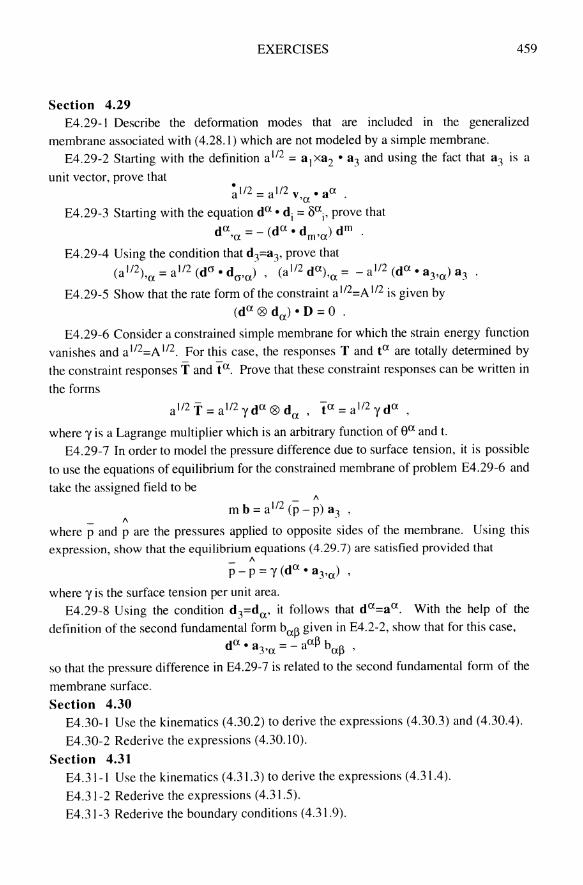
EXERCISES 459
Section 4.29 E4.29-1 Describe the defonnation modes that are included in the generalized
membrane associated with (4.2S.1) which are not modeled by a simple membrane.
E4.29-2 Starting with the definition a 1/2 = a l xa2 • a3 and using the fact that a3 is a
unit vector, prove that
~1/2 = a l12 v'o:. aO: .
E4.29-3 Starting with the equation dO:· d j = 80: j , prove that
dO:,o: = - (dO:· dm,o:) d m .
E4.29-4 Using the condition that d 3=a3, prove that
(a I/2 ) = a l12 (dO". d ) (a 1/2 dO:) = - a l/2 (dO:· a ) a '0: 0"'0: "0: 3 '0: 3
E4.29-5 Show that the rate form of the constraint a II2=A 112 is given by
(dO: ® do:) • D = 0 .
E4.29-6 Consider a constrained simple membrane for which the strain energy function
vanishes and a 1/2=A 1/2. For this case, the responses T and to: are totally detennined by
the constraint responses T and to:. Prove that these constraint responses can be written in
the forms
a l12 T = a l/2 ydO: ® do: ' to: = a l12 ydO: ,
where y is a Lagrange multiplier which is an arbitrary function of eo: and t.
E4.29-7 In order to model the pressure difference due to surface tension, it is possible
to use the equations of equilibrium for the constrained membrane of problem E4.29-6 and
take the assigned field to be
- 1\
- 1\
mb=a I/2 (p-p)a3 '
where p and p are the pressures applied to opposite sides of the membrane. Using this
expression, show that the equilibrium equations (4.29.7) are satisfied provided that 1\
p -p = Y (dO:· a 3,0:) ,
where y is the surface tension per unit area.
E4.29-S Using the condition d 3=do:, it follows that dO:=aO:. With the help of the
definition of the second fundamental form bo:J) given in E4.2-2, show that for this case, dO: • a = - ao:J) b
3'0: 0:J) ,
so that the pressure difference in E4.29-7 is related to the second fundamental fonn of the
membrane surface.
Section 4.30 E4.30-1 Use the kinematics (4.30.2) to derive the expressions (4.30.3) and (4.30.4).
E4.30-2 Rederive the expressions (4.30.10).
Section 4.31 E4.31-1 Use the kinematics (4.31.3) to derive the expressions (4.31.4).
E4.31-2 Rederive the expressions (4.31.5).
E4.31-3 Rederive the boundary conditions (4.31.9).
EXERCISES 459
Section 4.29 E4.29-1 Describe the defonnation modes that are included in the generalized
membrane associated with (4.2S.1) which are not modeled by a simple membrane. E4.29-2 Starting with the definition a"2 = a lxa2 0 a3 and using the fact that a3 is a
unit vector, prove that ~ 1/2 = a 112 v 0 aa
'a E4.29-3 Starting with the equation da 0 d j = 8a j , prove that
da'a = - (da 0 dm'a) d m .
E4.29-4 Using the condition that d3=a3, prove that
(a I/2 ) =all2(daod ) (a I/2 d a ) = -aI/2(daoa )a 'a a'a "a 3'a 3 E4.29-5 Show that the rate form of the constraint a 1/2=A 112 is given by
(da ® da ) 0 D = 0 .
E4.29-6 Consider a constrained simple membrane for which the strain energy function vanishes and a 1/2=A 1/2. For this case, the responses T and t a are totally determined by
the constraint responses T and tao Prove that these constraint responses can be written in
the forms
a l12 T = a l/2 yda ® da ' t a = a l/2 yda ,
where y is a Lagrange multiplier which is an arbitrary function of Sa and t.
E4.29-7 In order to model the pressure difference due to surface tension, it is possible
to use the equations of equilibrium for the constrained membrane of problem E4.29-6 and
take the assigned field to be "
- " m b = a ll2 (p - p) a3 '
where p and p are the pressures applied to opposite sides of the membrane. Using this expression, show that the equilibrium equations (4.29.7) are satisfied provided that
" p - p = y (da 0 a 3'a) ,
where y is the surface tension per unit area. E4.29-S Using the condition d 3=da , it follows that da=aa. With the help of the
definition of the second fundamental form baf3 given in E4.2-2, show that for this case, da 0 a = - aaf3 b 3'a af3 '
so that the pressure difference in E4.29-7 is related to the second fundamental fonn of the
membrane surface.
Section 4.30 E4.30-l Use the kinematics (4.30.2) to derive the expressions (4.30.3) and (4.30.4).
E4.30-2 Rederive the expressions (4.30.10).
Section 4.31 E4.31-l Use the kinematics (4.31.3) to derive the expressions (4.3\.4).
E4.3l-2 Rederive the expressions (4.3\.5).
E4.3l-3 Rederive the boundary conditions (4.3\.9).
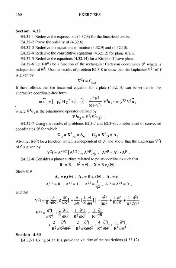
460 EXERCISES
Section 4.32 E4.32-1 Rederive the expressions (4.32.3) for the linearized strains. E4.32-2 Prove the validity of (4.32.6). E4.32-3 Rederive the equations of motion (4.32.9) and (4.32.10). E4.32-4 Rederive the constitutive equations (4.32.12) for plane strain. E4.32-5 Rederive the equations (4.32.14) for a Kirchhoff-Love plate. E4.32-6 Let f(aa) be a function of the rectangular Cartesian coordinates a i which is
independent of a3. Use the results of problem E2.3-8 to show that the Laplacian '12f of f is given by
'12f = f,aa .
It then follows that the linearized equation for a plate (4.32.14) can be written in the alternative coordinate-free form
00 [ * * - II] f.l*H3 4 33 200
m u 3 = - Po H g + P - P - V u3 + m y' V u 3 ' 6(l-v*)' .
where '14u3 is the biharmonic operator defined by '14u3 = '12('12u3) .
E4.32-7 Using the results of problems E2.3-7 and E2.3-8, consider a set of convected
coordinates a i for which
Ga=X*,a=Aa' G3 =X*'3=A3'
Also, let f(aa) be a function which is independent of a3 and show that the Laplacian '12f
of f is given by
E4.32-8 Consider a planar surface referred to polar coordinates such that
8 1 = R , a2 = e , X = R er(e) .
Show that
Al = e/e) , A2 = R ee(e) , A3 = e3 '
A 1/2 = R , A I I = 1 A 22 = _1_ A 12 = A 21 = 0 , R2 ' ,
and that
'12f = l [ a {R af} + ~ {l~}] = a2f + l af + _1 a2f R dR dR ae Rae aR2 RdR R2 ae2 '
a4f 2 a3f I a2f I af '14f = aR4 + R aR3 - R2 aR2 + R3 dR
2 a4f 2 a3f 4 a2f 1 a4f + -----+---+--- . R2 aR2ae2 R3 aRae2 R4 ae2 R4 ae4
Section 4.33 E4.32-1 Using (4.33.10), prove the validity of the restrictions (4.33.12).
460 EXERCISES
Section 4.32 E4.32-1 Rederive the expressions (4.32.3) for the linearized strains. E4.32-2 Prove the validity of (4.32.6).
E4.32-3 Rederive the equations of motion (4.32.9) and (4.32.10).
E4.32-4 Rederive the constitutive equations (4.32.12) for plane strain.
E4.32-5 Rederive the equations (4.32.14) for a Kirchhoff-Love plate. E4.32-6 Let f(aa) be a function of the rectangular Cartesian coordinates a i which is
independent of a3. Use the results of problem E2.3-8 to show that the Laplacian '12f of f
is given by
'12f = f,aa .
It then follows that the linearized equation for a plate (4.32.14) can be written in the alternative coordinate-free form
*H3 00 [ * * - II] f.l 4 33 200
m u 3 = - Po H g + P - P - V u3 + m y' V u 3 ' 6(l-v*)' .
where '14u3 is the biharmonic operator defined by '14u3 = '12('12u3)
E4.32-7 Using the results of problems E2.3-7 and E2.3-8, consider a set of convected
coordinates a i for which
Ga=X*,a=Aa' G3 =X*'3=A3'
Also, let f(aa) be a function which is independent of a3 and show that the Laplacian '12f
of f is given by n2f=A-II2[All2f AaP] Aap=AaoAP v 'u'~ , .
E4.32-8 Consider a planar surface referred to polar coordinates such that
8 1 = R , a2 = e , X = R er(e) .
Show that
Al = e/e) , A2 = R ee(e) , A3 = e3 '
A 1/2 = R A I I = 1 , A 22 = _1 A 12 = A 21 = 0 , R2 ' ,
and that
'12f=l[a {R af} +~{l~}]= a2f +laf +_1 a2f R dR dR ae Rae aR2 RdR R2 ae2 '
a4f 2 a3f I a2f I af '14f = aR4 + R aR3 - R2 aR2 + R3 dR
2 a4f 2 a3f 4 a2f 1 a4f + -----+---+--- .
R2 aR2ae2 R3 aRae2 R4 ae2 R4 ae4
Section 4.33 E4.32-1 Using (4.33.10), prove the validity of the restrictions (4.33.12).

EXERCISES
Exercises for Chapter 5
Section 5.1 ES.l-l Rederive the expression for G 112 in (S.1.1S).
Section 5.2 ES.2-1 Using the definition (S.2.S), sketch the projection d 1 of the director d 1.
ES.2-2 Prove the validity of (S.2.14).
Section 5.3 ES.3-1 Prove the validity of (S.3.14).
ES.3-2 Rederive the expression (S.3.16).
ES.3-3 Rederive the expression (S.3.2S).
ES.3-4 Rederive the expression (S.3.32).
ES.3-S Starting with (S.3.38), rederive the equation (S.3.39).
ES.3-6 Rederive the expression (S.6.9).
Section 5.6 ES.6-1 Rederive the expression (S.6.9).
ES.6-2 Rederive the expression (S.6.10).
Section 5.7 ES.7-1 Prove the validity of (S.7.3).
ES. 7 -2 Prove the validity of (S.7 .8).
Section 5.8 ES.8-1 Prove the validity of (S.8.1O).
Section 5.9 ES.9-1 Rederive the constraint (S.9.S).
ES.9-2 Rederive the constraint (S.9.9).
ES.9-3 Rederive the constraint responses (S.9.23). ES.9-4 Starting with (S.9.31), rederive the expressions (S.9.32).
Section 5.11 ES.ll-l Prove the validity of (S.I1.S).
ES.II-2 Prove the validity of (S.I1.17). ES.11-3 Prove the validity of (S.ll.28).
Section 5.12 ES.12-1 Rederive the expanded form of the strain energy (S.12.12).
Section 5.13
461
ES.13-1 Starting with FF-l=I, prove the validity of the expression for F-1 in (S.13.S).
ES.13-2 Prove the validity of the expression for pin (S.13.6).
Section 5.14 ES.14-1 Show that the expressions (S.14.17) and (S.14.2S) satisfy the equilibrium
equations (S.14.12). ES.14-2 Use the displacements (S.14.21) to derive the strains (S.14.23).
EXERCISES
Exercises for Chapter 5
Section 5.1 ES.1-1 Rederive the expression for GII2 in (S.1.1S).
Section 5.2 ES.2-1 Using the definition (S.2.S), sketch the projection d l of the director d l .
ES.2-2 Prove the validity of (S.2.14).
Section 5.3 ES.3-1 Prove the validity of (S.3.14). ES.3-2 Rederive the expression (S.3.16).
ES.3-3 Rederive the expression (S.3.2S).
ES.3-4 Rederive the expression (S.3.32).
ES.3-S Starting with (5.3.38), rederive the equation (S.3.39).
ES.3-6 Rederive the expression (S.6.9).
Section 5.6 ES.6-1 Rederive the expression (S.6.9).
ES.6-2 Rederive the expression (S.6.10).
Section 5.7 ES.7-1 Prove the validity of (S.7.3).
ES.7-2 Prove the validity of (S.7.8).
Section 5.8 ES.8-1 Prove the validity of (S.8.1O).
Section 5.9 ES.9-1 Rederive the constraint (S.9.S).
ES.9-2 Rederive the constraint (S.9.9).
ES.9-3 Rederive the constraint responses (S.9.23). ES.9-4 Starting with (S.9.31), rederive the expressions (S.9.32).
Section 5.11 ES.ll-l Prove the validity of (S.I1.S).
ES.II-2 Prove the validity of (S.11.17).
ES.II-3 Prove the validity of (S.11.28).
Section 5.12 ES.12-1 Rederive the expanded form of the strain energy (S.12.12).
Section 5.13
461
ES.13-1 Starting with FF-I=I, prove the validity of the expression for F-I in
(S.13.S). ES.13-2 Prove the validity of the expression for pin (S.13.6).
Section 5.14 ES.14-1 Show that the expressions (S.14.17) and (S.14.2S) satisfy the equilibrium
equations (S.14.12). ES.14-2 Use the displacements (S.14.21) to derive the strains (S.14.23).

462 EXERCISES
ES.14-3 Rederive the expressions (S.14.32).
Section 5.15 ES.lS-l Sketch the deformation described by the displacements (S.IS.I).
ES.1S-2 Prove the validity of (S.lS.3).
ES.1S-3 Prove the validity of (S.lS.8).
Section 5.16 ES.16-1 Sketch the deformation described by the displacements (S.16.1). ES.16-2 Prove the validity of (S.16.3).
ES.16-3 Prove the validity of (S.16.9).
Section 5.17 ES.17 -I Use the displacements (S.17.8) to derive the results (S.17.9).
Section 5.18 ES.18-1 Use the displacements (S.18.7) to derive the results (S.18.8) and (S.18.1O).
Section 5.19 ES.19-1 Use the displacements (S.19.7) to derive the results (S.19.9).
Section 5.21 ES.21-1 Use the displacements (S.2l.8) to derive the results (S.21.11).
ES.21-2 Rederive the equations of motion (S.2l.12). ES.21-3 Show that (S.2l.13) predict the correct displacement field for homogeneous
deformations. Section 5.22
ES.22-1 Rederive the equation of motion (S.22.4).
Section 5.23 ES.23-1 Rederive the expressions (S.23.4).
ES.23-2 Use the displacements (S.23.S) to derive the strains (S.23.6).
ES.23-3 Use the strains (S.23.6) to derive the constitutive responses (S.23.7).
Section 5.24 ES.24-1 Calculate the value of p associated with the strain energy function (S.24.8).
Section 5.25 ES.2S-1 Prove the validity of equations (S.2S.7) and (S.2S.9).
ES.2S-2 Prove the validity of equations (S.2S.12) and (S.2S.13).
ES.2S-3 Prove the validity of equations (S.2S.14) and (S.2S.IS).
Section 5.27 ES.27-1 Rederive the constitutive responses (S.27.2).
Section 5.28 ES.28-1 Rederive the equations of motion (S.28.6).
ES.28-2 Rederive the expressions (S.28.7) for the constraint responses. ES.28-3 Use the strain energy function (S.28.18) to derive the expressions (S.28.20).
ES.28-4 Rederive the expressions (S.28.28) for the linearized theory.
ES.28-S Rederive the equations of motion (S.28.33).

EXERCISES 463
E5.28-6 Neglect assigned fields and determine the dispersion relationship for the differential equation associated with u\ in (5.28.33). Section 5.29
E5.29-1 Use the sLain energy function (5.29.9) to rederive the expressions (5.29.11). E5.29-2 Use the kinematics (5.29.17) to rederive the constitutive responses (5.29.21).
E5.29-3 Rederive the equations of motion (5.29.22). Section 5.31
E5.31-1 Rederive the equations (5.31.3).
E5.31-2 Let the total strain energy of the string 'llbe defined by
'll=fPLds,
where L is the strain energy per unit mass of the string. Next, define the rate of material
dissipation 'D per unit present arclength by the formula
f 'D ds = 'W - ~ - ,u ~ 0 , p
where 'Wand J(are given by (5.31.7). Using these expressions, show that 'Dbecomes
-'D=T-D-pL.
E5.31-3 Using the form (5.31.11) for the strain energy function and the results
(5.31.3), show that 'Din E5.31-2 can be written in the form
aL d3®d3 'D = [ T - P A aA {~}] - D .
For an elastic string, the rate of dissipation 'D vanishes for all motions and it can be shown using the usual argument that
aL {d3®d3 } T=PA aA ~ ,
where use has been made of the form (5.31.9) for T. E5. 31-4 Using the form (5.31.11) for the strain energy function and the results
(5.31.3), show that'D in E5.31-2 can be written in the alternative form
'D = [ T - P A aL I] - D . aA
For an elastic string, the rate of dissipation 'D vanishes for all motions and it is tempting to conclude that the coefficient of D in this expression vanishes. To understand why this
conclusion is incorrect, it is necessary to note that D is not a general symmetric three
dimensional tensor. To this end, let da be vectors that are orthogonal to d 3 such that d j
forms a right -handed triad. Show, that the components of D relative to these base vectors
have the properties that
Da~ = D - (da®d~) = 0 .
It therefore follows that only three of the components of the coefficient of D appear
explicitly in the expression for the rate of dissipation 'D. In other words, no information can be obtained about the components of the coefficient of D that do not appear explicitly
in this expression for 'D.
EXERCISES 463
E5.28-6 Neglect assigned fields and detennine the dispersion relationship for the differential equation associated with u l in (5.28.33). Section 5.29
E5.29-1 Use the sLain energy function (5.29.9) to rederive the expressions (5.29.11). E5.29-2 Use the kinematics (5.29.17) to rederive the constitutive responses (5.29.21).
E5.29-3 Rederive the equations of motion (5.29.22). Section 5.31
E5.31-1 Rederive the equations (5.31.3).
E5.31-2 Let the total strain energy of the string'll be defined by
'l1=fpIds,
where I is the strain energy per unit mass of the string. Next, define the rate of material
dissipation 1) per unit present arclength by the formula
f 0 0
1) ds = W - 'l( - 'l1 ? 0 , p
where Wand 'l(are given by (5.31.7). Using these expressions, show that 1) becomes o
1)=ToD-pI
E5.31-3 Using the form (5.31.11) for the strain energy function and the results
(5.31.3), show that 1) in E5.31-2 can be written in the form
aI d3®d3 1) = [ T - P A - {--}] 0 D .
aA d33 For an elastic string, the rate of dissipation 1) vanishes for all motions and it can be shown using the usual argument that
aI {d3®d3} T=PA- --- ,
aA d33 where use has been made of the form (5.31.9) for T.
E5.31-4 Using the form (5.31.11) for the strain energy function and the results (5.31.3), show that 1) in E5.31-2 can be written in the alternative form
aI 1)=[T-pA-I]°D.
aA For an elastic string, the rate of dissipation 1) vanishes for all motions and it is tempting to conclude that the coefficient of D in this expression vanishes. To understand why this
conclusion is incorrect, it is necessary to note that D is not a general symmetric three
dimensional tensor. To this end, let da be vectors that are orthogonal to d 3 such that d j
forms a right -handed triad. Show, that the components of D relative to these base vectors
have the properties that
Da~ = D 0 (da®d~) = 0 .
It therefore follows that only three of the components of the coefficient of D appear
explicitly in the expression for the rate of dissipation 1). In other words, no information can be obtained about the components of the coefficient of D that do not appear explicitly
in this expression for 1).

464 EXERCISES
Section 5.32 E5.32-1 Prove the validity of the results (5.32.5). E5.32-2 Prove the validity of the results (5.32.8). E5.32-3 Prove the validity of the results (5.32.10).
Section 5.33 E5.33-1 Use the kinematics (5.33.2) to rederive the results (5.33.3). E5.33-2 Use the results (5.33.3) to rederive the constitutive responses (5.33.4). E5.33-3 Use the results (5.33.4) to rederive the equations of motion (5.33.8). E5.33-4 Use the results (5.33.4) to rederive the equations of motion (5.33.9). E5.33-5 Use the results (5.33.4) to rederive the equations of motion (5.33.11). E5.33-6 Use the results (5.33.16) to rederive the buckling equation (5.33.18).
Section 5.34 E5.34-1 Prove the validity of (5.34.13). E5.34-2 Use the strain energy function (5.34.9) to prove the validity of (5.34.16). E5.34-3 Use the results (5.34.16) to prove the validity of (5.34.18).
Section 5.35 E5.35-1 Use (5.35.10) to prove the validity of the restrictions (5.35.12).
Exercises for Chapter 6
Section 6.3 E6.3-1 Prove the validity of (6.3.11) and (6.3.18). E6.3-2 Prove the validity of (6.3.20) and (6.3.21).
Section 6.4 E6.4-1 Rederive the reduced form (6.4.8) of the balance of angular momentum.
Section 6.6 E6.6-1 Prove the validity of (6.6.4).
Section 6.7 E6.7-1 Rederive the equation (6.7.3).
E6.7-2 Prove the validity of (6.7.7).
Section 6.9 E6.9-1 Prove the validity of (6.9.20). E6.9-2 Prove the validity of (6.9.23) and (6.9.24). E6.9-3 Use (6.9.26) to prove the validity of (6.9.25).
Section 6.13 E6.13-1 Starting with FF- 1 =1, prove the validity of the expressIOn for F- 1 in
(6.13.5). E6.13-2 Prove the validity of the expression for p in (6.13.6).
Section 6.14 E6.14-1 Use the displacements (6.14.20) to derive the expressions (6.14.21).
E6.14-2 Rederive the expressions (6.14.24).
464 EXERCISES
Section 5.32 E5.32-1 Prove the validity of the results (5.32.5).
E5.32-2 Prove the validity of the results (5.32.8).
E5.32-3 Prove the validity of the results (5.32.10). Section 5.33
E5.33-1 Use the kinematics (5.33.2) to rederive the results (5.33.3).
E5.33-2 Use the results (5.33.3) to rederive the constitutive responses (5.33.4).
E5.33-3 Use the results (5.33.4) to rederive the equations of motion (5.33.8).
E5.33-4 Use the results (5.33.4) to rederive the equations of motion (5.33.9).
E5.33-5 Use the results (5.33.4) to rederive the equations of motion (5.33.11). E5.33-6 Use the results (5.33.16) to rederive the buckling equation (5.33.18).
Section 5.34 E5.34-1 Prove the validity of (5.34.13).
E5.34-2 Use the strain energy function (5.34.9) to prove the validity of (5.34.16).
E5.34-3 Use the results (5.34.16) to prove the validity of (5.34.18). Section 5.35
E5.35-1 Use (5.35.10) to prove the validity of the restrictions (5.35.12).
Exercises for Chapter 6
Section 6.3 E6.3-1 Prove the validity of (6.3.11) and (6.3.18). E6.3-2 Prove the validity of (6.3.20) and (6.3.21).
Section 6.4 E6.4-1 Rederive the reduced form (6.4.8) of the balance of angular momentum.
Section 6.6 E6.6-1 Prove the validity of (6.6.4).
Section 6.7 E6.7-1 Rederive the equation (6.7.3).
E6.7-2 Prove the validity of (6.7.7).
Section 6.9 E6.9-1 Prove the validity of (6.9.20).
E6.9-2 Prove the validity of (6.9.23) and (6.9.24).
E6.9-3 Use (6.9.26) to prove the validity of (6.9.25).
Section 6.13 E6.13-1 Starting with FF-1 =1, prove the validity of the expression for F-I in
(6.13.5). E6.13-2 Prove the validity of the expression for p in (6.13.6).
Section 6.14 E6.14-1 Use the displacements (6.14.20) to derive the expressions (6.14.21). E6.14-2 Rederive the expressions (6.14.24).

EXERCISES
Exercises for Chapter 7
Section 7.2 E7.2-1 Rederive the expressions (7.2.4). E7.2-2 Rederive the expressions (7.2.8). E7.2-3 Prove the validity of the expressions (7.2.13). E7.2-4 Prove the validity of the equations of motion (7.2.20).
Section 7.3 E7.3-l Rederive the equation (7.3.8). E7.3-2 Rederive the equations (7.3.20).
Section 7.4
465
E7.4-1 Show that the expressions (7.4.39) satisfy the equations of motion (7.4.15). E7.4-2 Rederive the expression (7.4.43) for the rate of work. E7.4-3 Show that IPa vanish for homogeneous deformation.
Section 7.S E7.5-1 Rederive the expression (7.5.39) for the rate of work. E7.5-2 Show that the expressions (7.5.41) satisfy the equations of motion (7.5.16).
Section 7.6 E7.6-1 Rederive the expression (7.6.39) for the rate of work. E7.6-2 Show that the expressions (7.6.42) satisfy the equations of motion (7.6.16).
Exercises for Appendix A EA-l Prove the validity of the equations (A.4.8). EA-2 Prove the validity of the equations (A.4.1 0).
EXERCISES
Exercises for Chapter 7
Section 7.2 E7.2-1 Rederive the expressions (7.2.4). E7.2-2 Rederive the expressions (7.2.8). E7.2-3 Prove the validity of the expressions (7.2.13). E7.2-4 Prove the validity of the equations of motion (7.2.20).
Section 7.3 E7.3-1 Rederive the equation (7.3.8). E7.3-2 Rederive the equations (7.3.20).
Section 7.4
465
E7.4-1 Show that the expressions (7.4.39) satisfy the equations of motion (7.4.15). E7.4-2 Rederive the expression (7.4.43) for the rate of work. E7.4-3 Show that If3a vanish for homogeneous deformation.
Section 7.5 E7.5-1 Rederive the expression (7.5.39) for the rate of work. E7.5-2 Show that the expressions (7.5.41) satisfy the equations of motion (7.5.16).
Section 7.6 E7.6-1 Rederive the expression (7.6.39) for the rate of work. E7.6-2 Show that the expressions (7.6.42) satisfy the equations of motion (7.6.16).
Exercises for Appendix A EA-I Prove the validity of the equations (A.4.8).
EA-2 Prove the validity of the equations (A.4.1 0).

ACKNOWLEDGMENTS
The author would like to acknowledge a.M. O'Reilly and G. Schajer for helpful discussions, and B. Nadler and E. Tufekci for proof reading some parts of the manuscript at various stages of its development. During my sabbatical in 1996-1997, the University of British Columbia in Vancouver provided a wonderful atmosphere for beginning writing this book. Also, the Fund for Promotion of Research at Technion provided some financial support and the Faculty of Mechanical Engineering at Technion provided the academic freedom and support to pursue my research interests in Cosserat theory.
REFERENCES
The numbers in square brackets at the end of each reference indicate the sections where the reference is referred to in the test.
Alehossein, H. and Muhlhaus, H.B. (1994). "Computer modelling of comminuting granular media", Proceedings of the 1 st Congress on Computing in Civil Engineering Part 1, Publ. by ASCE, New, 660-667. [1.1]
Antman, S.S. (1972). The theory of rods, In S. Flugge's Handbuch der Physik, Vol. VIal2, (ed. C. Truesdell), Springer-Verlag, Berlin, 641-703. [1.1, 1.2,5.28,5.34]
Antman, S.S. (1995). Nonlinear problems of elasticity, Applied Mathematical Sciences 107, Springer-Verlag, Berlin. [1.1, 1.2,4.30,5.28,5.33]
Antman, S.S. and Jordan, K.B. (1975). "Qualitative aspects of the spatial deformation of non-linearly elastic rods", Proc. Roy. Soc. Edinburgh 73A, 85-105. [5.34]
Atkin, R.J. and Fox, N. (1980). An introduction to the theory of elasticity. Longman, New York. [3.11]
Axelrad, E.L. (1987). Theory of flexible shells. Vol. 28 in North-Holland Series in Applied Mathematics and Mechanics. Elsevier Science, Amsterdam. [1.2]
Bathe, K.J. (1982). Finite element procedures in engineering analysis. Prentice-Hall,
New Jersey. [7.1] Becker, E.B., Carey, G.F. and aden, J.T. (1981). Finite elements: an introduction.
volume I. Prentice-Hall, New Jersey. [7.1] Biezeno, C.B. and Grammel, R. (1954). Engineering dynamics - Volume III Steam
turbines. Blackie & Son Limited, London. [7.3] Cairns, D.S., Ilcewicz, L.B., Walker, T. and Minguet, P.J. (1995). "Fracture scaling
parameters of inhomogeneous microstructure in composite structures", Composites Sci. and Tech. 53, 223-231. [1.1]
467
ACKNOWLEDGMENTS
The author would like to acknowledge a.M. O'Reilly and G. Schajer for helpful discussions, and B. Nadler and E. Tufekci for proof reading some parts of the manuscript at various stages of its development. During my sabbatical in 1996-1997, the University of British Columbia in Vancouver provided a wonderful atmosphere for beginning writing this book. Also, the Fund for Promotion of Research at Technion provided some financial support and the Faculty of Mechanical Engineering at Technion provided the academic freedom and support to pursue my research interests in Cosserat theory.
REFERENCES
The numbers in square brackets at the end of each reference indicate the sections where the reference is referred to in the test.
Alehossein, H. and Muhlhaus, H.B. (1994). "Computer modelling of comminuting granular media", Proceedings of the 1 st Congress on Computing in Civil Engineering Part 1, Publ. by ASCE, New, 660-667. [1.1]
Antman, S.S. (1972). The theory of rods, In S. Flugge's Handbuch der Physik, Vol. VIal2, (ed. C. Truesdell), Springer-Verlag, Berlin, 641-703. [1.1, 1.2,5.28,5.34]
Antman, S.S. (1995). Nonlinear problems of elasticity, Applied Mathematical Sciences 107, Springer-Verlag, Berlin. [1.1, 1.2,4.30,5.28,5.33]
Antman, S.S. and Jordan, K.B. (1975). "Qualitative aspects of the spatial deformation of non-linearly elastic rods", Proc. Roy. Soc. Edinburgh 73A, 85-105. [5.34]
Atkin, RJ. and Fox, N. (1980). An introduction to the theory of elasticity. Longman, New York. [3.11]
Axelrad, E.L. (1987). Theory of flexible shells. Vol. 28 in North-Holland Series in Applied Mathematics and Mechanics. Elsevier Science, Amsterdam. [1.2]
Bathe, K.J. (1982). Finite element procedures in engineering analysis. Prentice-Hall,
New Jersey. [7.1] Becker, E.B., Carey, G.F. and aden, J.T. (1981). Finite elements: an introduction,
volume I. Prentice-Hall, New Jersey. [7.1] Biezeno, C.B. and Gramme!, R (1954). Engineering dynamics - Volume III Steam
turbines. Blackie & Son Limited, London. [7.3] Cairns, D.S., Ilcewicz, L.B., Walker, T. and Minguet, P.J. (1995). "Fracture scaling
parameters of inhomogeneous microstructure in composite structures", Composites Sci. and Tech. 53, 223-231. [1.1]
467

468 REFERENCES
Carey, G.F. and Oden, J.T. (1983). Finite elements: a second course, Volume II. Prentice-Hall, New Jersey. [7.1]
Carey, G.F. and Oden, J.T. (1984). Finite elements: computational aspects, Volume III. Prentice-Hall, New Jersey. [7.1]
Calladine, c.R. (1983). Theory of shell structures. Cambridge University Press, Cambridge. [1.2]
Cheng, Z.Q. and He, L.H. (1995). "Micropolar elastic fields due to a spherical
inclusion", Int. J. Engn. Sci. 33, 389-397. [1.1] Cohen, H. (1981). "Pseudo-rigid bodies", Utilitas Math. 20, 221-247. [1.1]
Cohen, H. and Mac Sithigh, G.P. (1993). "Plane motions of elastic pseudo-rigid bodies: an example", J. Elasticity 32,51-59. [6.1]
Cohen, H. and Mac Sithigh, G.P. (1994). "Impulsive motions of elastic pseudo-rigid bodies II: further results and examples", J. Elasticity 34, 149-166. [6.1]
Cohen, H. and Mac Sithigh, G.P. (1996). "Collisions of pseudo-rigid bodies: A Brachtype treatment", Int. J. Engng. Sci. 34,249-256. [6.1]
Cohen, H. and Muncaster, RG. (1984). "The dynamics of pseudo-rigid bodies: general
structure and exact solutions", J. Elasticity 14, 127-154. [1.1]
Cohen, H. and Muncaster, R.G. (1988). Theory of pseudo-rigid bodies. Springer,
Berlin. [1.1] Cohen, H. and Sun, Q.-X. (1991). "Snapping of an elastic pseudo-rigid body", Int. J.
Solids Structures 28, 807-818. [6.1]
Cosserat, E. and F. (1909). "Theorie des corps deformables". Paris. vi+226pp. = Appendix, pp. 953-1173 of Chwolson's Traite de Physique, 2nd ed., Paris. Also in translated form, "Theory of deformable bodies", NASA TT F-l1, 561 (Washington, D.C.). Clearinghouse for U.S. Federal Scientific and Technical Information, Springfield, Virginia. [Preface, 1.1]
Craine, RE. and Newman, M.G. (1996). "Modelling creep failure in welded plates under uniaxial loading", J. Strain Anal. Engn. Design 31, 117-124. [1.1]
Darlow, M.S. (1989). Balancing of high-speed machinery. Springer-Verlag, New
York. [7.3]
De Borst, R (1991). "Simulation of strain localization: a reappraisal of the Cosserat
continuum", Engineering Computations 8,317-332. [1.1]
Desai, C.S. (1979). Elementary finite element method. Prentice-Hall, New Jersey.
[7.1]
Duhem, P. (1893). "Le potentiel thermodynamique et la pression hydrostatic", Ann.
Ecole Norm. 10, 187-230. [1.1]
Ericksen, J. L. (1961). "Conservation laws for liquid crystals", Trans. Soc. Rheol. 5, 23-34. [1.1]
Ericksen, J. L. (1970). "Simpler static problems in nonlinear theories of rods", Int. 1.
Solids Structures 6,371-377. [5.34]
468 REFERENCES
Carey, G.F. and Oden, J.T. (1983). Finite elements: a second course, Volume II. Prentice-Hall, New Jersey. [7.1]
Carey, G.F. and Oden, J.T. (1984). Finite elements: computational aspects, Volume III. Prentice-Hall, New Jersey. [7.1]
Calladine, c.R. (1983). Theory of shell structures. Cambridge University Press, Cambridge. [1.2]
Cheng, Z.Q. and He, L.H. (1995). "Micropolar elastic fields due to a spherical inclusion", Int. J. Engn. Sci. 33, 389-397. [1.1]
Cohen, H. (1981). "Pseudo-rigid bodies", Utilitas Math. 20, 221-247. [1.1]
Cohen, H. and Mac Sithigh, G.P. (1993). "Plane motions of elastic pseudo-rigid bodies: an example", J. Elasticity 32,51-59. [6.1]
Cohen, H. and Mac Sithigh, G.P. (1994). "Impulsive motions of elastic pseudo-rigid bodies II: further results and examples", J. Elasticity 34, 149-166. [6.1]
Cohen, H. and Mac Sithigh, G.P. (1996). "Collisions of pseudo-rigid bodies: A Brach
type treatment", Int. J. Engng. Sci. 34,249-256. [6.1] Cohen, H. and Muncaster, RG. (1984). "The dynamics of pseudo-rigid bodies: general
structure and exact solutions", J. Elasticity 14, 127-154. [1.1]
Cohen, H. and Muncaster, R.G. (1988). Theory of pseudo-rigid bodies. Springer, Berlin. [1.1]
Cohen, R and Sun, Q.-X. (1991). "Snapping of an elastic pseudo-rigid body", Int. J.
Solids Structures 28, 807-818. [6.1]
Cosserat, E. and F. (1909). "Theorie des corps deformables". Paris. vi+226pp. = Appendix, pp. 953-1173 of Chwolson's Traite de Physique, 2nd ed., Paris. Also in translated form, "Theory of deformable bodies", NASA TT F-l1, 561 (Washington,
D.C.). Clearinghouse for U.S. Federal Scientific and Technical Information, Springfield, Virginia. [Preface, 1.1]
Craine, RE. and Newman, M.G. (1996). "Modelling creep failure in welded plates under uniaxial loading", J. Strain Anal. Engn. Design 31, 117-124. [1.1]
Darlow, M.S. (1989). Balancing of high-speed machinery. Springer-Verlag, New
York. [7.3]
De Borst, R (1991). "Simulation of strain localization: a reappraisal of the Cosserat
continuum", Engineering Computations 8,317-332. [1.1]
Desai, C.S. (1979). Elementary finite element method. Prentice-Hall, New Jersey.
[7.1]
Duhem, P. (1893). "Le potentiel thermodynamique et la pression hydrostatic", Ann. Ecole Norm. 10, 187-230. [1.1]
Ericksen, J. L. (1961). "Conservation laws for liquid crystals", Trans. Soc. Rheol. 5, 23-34. [1.1]
Ericksen, J. L. (1970). "Simpler static problems in nonlinear theories of rods", Int. 1.
Solids Structures 6,371-377. [5.34]

REFERENCES 469
Ericksen, J.L. and Truesdell C. (1958). "Exact theory of stress and strain in rods and shells", Arch. Ration. Mech. Anal. 1, 295-323. [1.1]
Eringen, A.c. (1967). Mechanics of continua, John Wiley & Sons, New York. [2.1]
Eringen, A.c. and Suhubi, E. S. (1964). "Nonlinear theory of simple micro-elastic solids - I", Int. J. Engng. Sci. 2, 189-203. [1.1]
Flory, P.J. (1961). Thermodynamic relations for high elastic materials. Trans. Faraday Soc. 57,829-838. [3.11]
Flugge, W. (1973). Stresses in shells. 2nd Ed., Springer-Verlag, Berlin. [1.2]
Gladwell, G.M.L (1998). Private communication. [3.15]
Gol'denveizer, A.L. (1961). Theory of elastic thin shells (translation from the 1953
Russian ed.). Pergamon Press, Oxford. [1.2]
Graff, K.F. (1975). Wave motion in elastic solids, Ohio State University Press. [5.27,
5.28, 5.33, 7.3]
Green, A.E. (1959). "The equilibrium of rods", Arch. Ration. Mech. Anal. 3, 417-421.
[1.1 ]
Green, A.E., and Adkins, J.E. (1960). Large elastic deformations and nonlinear continuum mechanics, Oxford University Press. [3.10]
Green, A.E., Knops, R.J. and Laws, N. (1968). "Large deformations, superposed
small deformations and stability of elastic rods", Int. J. Solids Structures 4, 555-577.
[5.13]
Green, A.E. and Naghdi, P.M. (1971). "On superposed small deformations on a large
deformation of an elastic Cosserat surface", J. Elasticity 1, 1-17. [4.13]
Green, A.E. and Naghdi, P.M. (1979a). "On thermal effects in the theory of shells",
Proc. Royal Soc. London A365, 161-190. [1.2]
Green, A.E. and Naghdi, P.M. (1979b). "On thermal effects in the theory of rods", Int. 1. Solids Structures 15, 829-853. [1.2]
Green, A.E. and Naghdi, P.M. (1982). "A theory of laminated composite plates", 1M A J. Appl. Math. 29, 1-23. [4.14,4.15,5.14]
Green, A.E. and Naghdi, P.M. (1983). "On electromagnetic effects in the theory of shells
and plates", Phil. Trans. Royal Soc. London A309, 559-610. [1.1]
Green, A.E. and Naghdi, P.M. (1985). "Electromagnetic effects in the theory of rods",
Phil. Trans. Royal Soc. LondonA314, 311-352. [1.1]
Green, A.E. and Naghdi, P.M. (1991). "A thermomechanical theory of a Cosserat point
with application to composite materials", Q. J. Mech. and Appl. Math. 44, 335-355.
[I.l, 1.2, 6.2]
Green, A.E. and Naghdi, P.M. (1996). "On thermomechanical formulation of theories of
continuous media", Nonlinear effects in fluids and solids, (edited by M.M. Carroll
and M. Hayes), Plenum Press, New York, 161-187. [1.1, 1.2]
Green, A.E., Naghdi, P.M., and Trapp, J.A. (1970). "Thermodynamics of a continuum
with internal constraints", Int. J. Engng. Sci. 8, 891-908. [3.8]
REFERENCES 469
Ericksen, J.L. and Truesdell C. (1958). "Exact theory of stress and strain in rods and shells", Arch. Ration. Mech. Anal. 1,295-323. [1.1]
Eringen, A.c. (1967). Mechanics of continua, John Wiley & Sons, New York. [2.1]
Eringen, A.c. and Suhubi, E. S. (1964). "Nonlinear theory of simple micro-elastic
solids - I", Int. 1. Engng. Sci. 2, 189-203. [1.1]
Flory, P.J. (1961). Thermodynamic relations for high elastic materials. Trans. Faraday
Soc. 57,829-838. [3.11]
Flugge, W. (1973). Stresses in shells. 2nd Ed., Springer-Verlag, Berlin. [1.2]
Gladwell, G.M.L (1998). Private communication. [3.15]
Gol'denveizer, A.L. (1961). Theory of elastic thin shells (translation from the 1953
Russian ed.). Pergamon Press, Oxford. [1.2]
Graff, K.F. (1975). Wave motion in elastic solids, Ohio State University Press. [5.27,
5.28, 5.33, 7.3]
Green, A.E. (1959). "The equilibrium of rods", Arch. Ration. Mech. Anal. 3, 417-421.
[1.1]
Green, A.E., and Adkins, J.E. (1960). Large elastic deformations and nonlinear
continuum mechanics, Oxford University Press. [3.10]
Green, A.E., Knops, R.J. and Laws, N. (1968). "Large deformations, superposed
small deformations and stability of elastic rods", Int. 1. Solids Structures 4, 555-577.
[5.13]
Green, A.E. and Naghdi, P.M. (1971). "On superposed small deformations on a large
deformation of an elastic Cosserat surface", 1. Elasticity 1,1-17. [4.13]
Green, A.E. and Naghdi, P.M. (1979a). "On thermal effects in the theory of shells",
Proc. Royal Soc. London A365, 161-190. [1.2]
Green, A.E. and Naghdi, P.M. (1979b). "On thermal effects in the theory of rods", Int.
1. Solids Structures 15, 829-853. [1.2] Green, A.E. and Naghdi, P.M. (1982). "A theory of laminated composite plates", IMA
1. Appl. Math. 29, 1-23. [4.14,4.15,5.14]
Green, A.E. and Naghdi, P.M. (1983). "On electromagnetic effects in the theory of shells
and plates", Phil. Trans. Royal Soc. London A309, 559-610. [1.1]
Green, A.E. and Naghdi, P.M. (1985). "Electromagnetic effects in the theory of rods",
Phil. Trans. Royal Soc. London A314, 311-352. [1.1]
Green, A.E. and Naghdi, P.M. (1991). "A thermomechanical theory of a Cosserat point
with application to composite materials", Q.l. Mech. and Appl. Math. 44, 335-355.
[1.1, 1.2, 6.2]
Green, A.E. and Naghdi, P.M. (1996). "On thermomechanical formulation of theories of
continuous media", Nonlinear effects in fluids and solids, (edited by M.M. Carroll
and M. Hayes), Plenum Press, New York, 161-187. [1.1, 1.2]
Green, A.E., Naghdi, P.M., and Trapp, J.A. (1970). "Thermodynamics of a continuum
with internal constraints", Int. 1. Engng. Sci. 8, 891-908. [3.8]

470 REFERENCES
Green, A.E., Naghdi, P.M., and Wenner, M.L. (1974a). "On the theory of rods - Part I: Derivations from the three-dimensional equations", Pmc. Royal Soc. London A337, 451-483. [l.l]
Green, A.E., Naghdi, P.M., and Wenner, M.L. (1974b). "On the theory of rods - Part
II: Developments by direct approach", Proc. Royal Soc. London A337, 485-507.
[l.l, 5.12, 5.14, 5.15]
Hill, R. (1971). The mathematical theory of plasticity, Oxford University Press, Oxford. [A]
Huebner, K.H. (1975). The finite element method for engineers, John Wiley, New
York. [7.1]
Hughes, T.1.R. (1987). The finite element method: linear static and dynamic finite
element analysis. Prentice-Hall, New Jersey. [7.1]
Hutchinson, J.R. and Zillmer, S.D. (1983). "Vibration of a free rectangular
parallelepiped", ASME 1. Appl. Mech. 50, 123-130. [3.17] Iordache, M.M. and Willam, K. (1995). "Elastoplastic bifurcation in Cosserat continua",
Proceedings of the 10th Conference on Engineering Mechanics, in Proceedings of Engineering Mechanics Part 1. Pub!. by ASCE, New York, 525-528. [l.l]
Kolsky, H. (1963). Stress waves in solids, Dover, New York. [7.3,7.4]
Kraus, H. (1967). Thin elastic shells. An introduction to the theoretical foundations and the analysis of their static and dynamic behavior. John Wiley, New York.
[ 1.2] Lakes, R. (1993). "Strongly Cosserat elastic lattice and foam materials for enhanced
toughness", Cellular Polymers 12,17-30. [1.1] Lakes, R.S., Nakamura, S., Behiri, J.e. and Bonfield, W. (1990). "Fracture mechanics
of bone with short cracks", 1. of Biomechanics 23,967-975. [1.1]
Lekhnitskii, S.G. (1963). Theory of elasticity of an anisotropic elastic body, Holden
Day, San Francisco. [3.14,3.15] Libai, A. and Simmonds, J.G. (1988). The nonlinear theory of elastic shells - one
spatial dimension, Academic Press, Boston. [1.2]
Libai, A. and Simmonds, J.G. (1998). The nonlinear theory of elastic shells,
Cambridge University Press, Cambridge. [1.2]
Love, A.E.H. (1944). A treatise on the mathematical theory of elasticity, fourth
edition, Dover, New York. [4.21,4.23,5.34]
Lu, e.L. and Perkins, N.e. (1994). "Nonlinear spatial equilibria and stability of cables
under uni-axial torque and thrust", ASME 1. Appl. Mech. 61, 879-886. [5.34]
Malvern, L.E. (1969). Introduction to the mechanics of a continuous medium,
Prentice-Hall, New Jersey. [2.1, A.7]
Marshall, J.S. and Naghdi, P.M. (1989a). "A thermodynamical theory of turbulence,
Part I: Basic developments", Phil. Trans. Royal Soc. London A327, 415-448. [1.1]

REFERENCES 471
Marshall, J.S. and Naghdi, P.M. (I 989b). "A thermodynamical theory of turbulence,
Part II: Determination of constitutive coefficients and illustrative examples", Phil. Trans. Royal Soc. London A327, 449-475. [l.l]
Marshall, J.S., Naghdi, P.M. and Srinivasa, A.R. (1991). "A macroscopic theory of
microcrack growth in brittle materials", Phil. Trans. Royal Soc. London A335, 455-
485. [l.l]
Meseguer, J. and Perales, J.M. (1992). "Non steady phenomena in the vibration of
viscous, cylindrical, long liquid bridges", Microgravity Sci. Tech. 5, 69-72. [l.l]
Mindlin, R.D. (1951). "Influence of rotary inertia and shear on flexural vibration of
isotropic, elastic plates", ASME 1. Appl. Mech. 18,31-38. [4.12]
Mollmann, H. (1981). Introduction to the theory of thin shells. John Wiley, New
York. [1.2]
Muncaster, R.G. (1984a). "Invariant manifolds in mechanics I: the general construction
of coarse 'heories from fine theories", Arch. Ration. Mech. Anal. 84, 353-373. [l.l]
Muncaster, RG. (1984b). "Invariant manifolds in mechanics II: zero-dimensional elastic
bodies with directors", Arch. Ration. Mech. Anal. 84, 375-392. [1.1]
Naghdi, P.M. (1972). The theory of plates and shells, In S. Flugge's Handbuch der
Physik, Vol. VIal2, (ed. C. Truesdell), Springer-Verlag, Berlin, 425-640. [1.1, 1.2,
2.1,4.9,4.13,4.32]
Naghdi, P.M. (1979). "Fluid jets and fluid sheets: a direct formulation", Proceedings of
the 12th Symposium on Naval Hydrodynamics, National Academy of Sciences,
Washington, D.C., 500-515. [1.1]
Naghdi, P.M. (1982). "Finite deformation of elastic rods and shells", Proceedings of the
IUTAM Symposium on Finite Elasticity (Bethlehem, PA), Edited by D. E. Carlson
and R. T. Shield, Martinus Nijhoff Pub., The Hague. 47-103. [1.1,4.2,5.2,6.2]
Naghdi, P.M., and Rubin, M.B. (1984). "Constrained theories of rods", 1. Elasticity 14, 343-361. [5.2, 5.9]
Naghdi, P.M., and Rubin, M.B. (1989). "On the significance of normal cross-sectional
extension in beam theory with application to contact problems", Int. 1. Solids
Structures 25, 249-265. [5.14] Naghdi, P.M., and Rubin, M.B. (1995). "Restrictions on nonlinear constitutive
equations for elastic shells", 1. Elasticity 39,133-163. [1.2, 4.2, 4.11, 4.13, 4.22,
6.11 ]
Naghdi, P.M. and Srinivasa, A.R. (l993a). "A dynamical theory of structured solids,
Part I: Basic developments", Phil. Trans. Royal Soc. London A345, 425-458. [1.1]
Naghdi, P.M. and Srinivasa, A.R. (l993b). "A dynamical theory of structured solids,
Part II: Special constitutive equations and special cases of the theory", Phil. Trans.
Royal Soc. London A345, 459-476. [l.l]
Niordson, F.I. (1985). Shell theory. Vol. 29 in North-Holland Series in Applied
Mathematics and Mechanics. Elsevier Science, Amsterdam. [1.2]
Noble, B. (1969). Applied linear algebra. Prentice Hall, New Jersey. [A. 1 ]

472 REFERENCES
Novozhilov, V.V. (1959). The theory of thin shells (transl. from the 1951 Russian ed.). P. Noordhoof Ltd, Groningen. [1.2]
Ogden, R.W. (1997). Non-linear elastic deformations, Dover, New York. [3.11]
Reddy, J.N. (1985). An introduction to the finite element method. McGraw-Hili, New York. [7.1]
Reissner, E. (1945). "The effect of transverse shear deformation on the bending of elastic plates", ASME J. Appl. Mech. 12,69-77. [4.12]
Rubin, M.B. (I 985a). "On the theory of a Cosserat point and its application to the
numerical solution of continuum problems", ASME J. Appl. Mech. 52, 368-372.
[1.1,6.1,7.1]
Rubin, M.B. (l985b). "On the numerical solution of one-dimensional continuum
problems using the theory of a Cosserat point", ASME J. Appl. Mech. 52, 373-378.
[1.1,6.1,7.1]
Rubin, M.B. (1986). "Free vibration of a rectangular parallelepiped using the theory of a
Cosserat point", ASME J. Appl. Mech. 53,45-50. [1.1,3.16,4.19,6.1,6.8,6.15]
Rubin, M.B. (l987a). "On the numerical solution of nonlinear string problems using the
theory of a Cosserat point", Int. 1. Solids Structures 23, 335-349. [1.1, 1.2, 4.19,
6.1,7.1,7.3]
Rubin, M.B. (1987b). "On the numerical solution of spherically symmetric problems
using the theory of a Cosserat surface", Int. J. Solids Structures 23, 335-349. [1.1,
4.14,6.1,7.1,7.2]
Rubin, M.B. (1987c). "An elastic-viscoplastic model exhibiting continuity of solid and
fluid states", Int. J. Engng. Sci. 25, 1175-1191. [3.11] Rubin, M.B. (1987d). "On the singular nature of linearization of certain constrained
theories of shells", J. Appl. Mech. 54,472-474. [4.9,5.28]
Rubin, M.B. (1995). "Numerical solution of two- and three-dimensional
thermomechanical problems using the theory of a Cosserat point", J. of" Math. and Physics (ZAMP) 46,308-334. [1.1, 1.2,6.1]
Rubin, M.B. (1996). "Restrictions on nonlinear constitutive equations for elastic rods", J.
Elasticity 44, 9-36. [1.2, 5.2, 4.14, 5.11, 5.12, 5.14, 5.28, 6.11]
Rubin, M.B. (1997). "An intrinsic formulation for nonlinear elastic rods", lilt. 1. Solids
Structures 34,4191-4212. [5.34]
Rubin, M.B. (2000). "Numerical solution procedures for nonlinear elastic rods using the
theory of a Cosserat point", To appear in the Int. 1. Solids Structures. [1.2,7.4]
Rubin, M.B. and Gottlieb, O. (1996). "Numerical solutions of forced vibration and
whirling of a nonlinear string using the theory of a Cosserat point", 1. of" Sound and
Vibration 197,85-101. [7.1,7.3]
Slawianowski, J.J. (1974). "Analytical mechanics of finite homogeneous strains", Arch.
Mech. 26, 569-587. [1.1]
Slawianowski, J.1. (1975). "Newtonian dynamics of homogeneous strains", Arch.
Mech. 27, 93-102. [1.1]
472 REFERENCES
Novozhilov, V.V. (1959). The theory of thin shells (transl. from the 1951 Russian ed.). P. Noordhoof Ltd, Groningen. [1.2]
Ogden, R.W. (1997). Non-linear elastic deformations, Dover, New York. [3.11]
Reddy, J.N. (1985). An introduction to the finite element method. McGraw-Hili, New York. [7.1]
Reissner, E. (1945). "The effect of transverse shear deformation on the bending of elastic plates", ASME J. Appl. Mech. 12,69-77. [4.12]
Rubin, M.B. (I 985a). "On the theory of a Cosserat point and its application to the
numerical solution of continuum problems", ASME J. Appl. Mech. 52, 368-372. [1.1,6.1,7.1]
Rubin, M.B. (l985b). "On the numerical solution of one-dimensional continuum
problems using the theory of a Cosserat point", ASME J. Appl. Mech. 52, 373-378.
[1.1,6.1,7.1]
Rubin, M.B. (1986). "Free vibration of a rectangular parallelepiped using the theory of a
Cosserat point", ASME J. Appl. Mech. 53,45-50. [1.1,3.16,4.19,6.1,6.8,6.15] Rubin, M.B. (l987a). "On the numerical solution of nonlinear string problems using the
theory of a Cosserat point", Int. 1. Solids Structures 23, 335-349. [1.1, 1.2, 4.19,
6.1,7.1,7.3] Rubin, M.B. (1987b). "On the numerical solution of spherically symmetric problems
using the theory of a Cosserat surface", Int. J. Solids Structures 23, 335-349. [1.1,
4.14,6.1,7.1,7.2]
Rubin, M.B. (1987c). "An elastic-viscoplastic model exhibiting continuity of solid and fluid states", Int. J. Engng. Sci. 25, 1175-1191. [3.11]
Rubin, M.B. (1987d). "On the singular nature of linearization of certain constrained theories of shells", J. Appl. Mech. 54,472-474. [4.9,5.28]
Rubin, M.B. (1995). "Numerical solution of two- and three-dimensional
thermomechanical problems using the theory of a Cosserat point", J. of" Math. and Physics (ZAMP) 46,308-334. [1.1, 1.2,6.1]
Rubin, M.B. (1996). "Restrictions on nonlinear constitutive equations for elastic rods", J.
Elasticity 44, 9-36. [1.2, 5.2, 4.14, 5.11, 5.12, 5.14, 5.28, 6.11]
Rubin, M.B. (1997). "An intrinsic formulation for nonlinear elastic rods", lilt. 1. Solids
Structures 34,4191-4212. [5.34]
Rubin, M.B. (2000). "Numerical solution procedures for nonlinear elastic rods using the
theory of a Cosserat point", To appear in the Int. 1. Solids Structures. [1.2,7.4]
Rubin, M.B. and Gottlieb, O. (1996). "Numerical solutions of forced vibration and
whirling of a nonlinear string using the theory of a Cosserat point", 1. of" Sound and
Vibration 197,85-101. [7.1,7.3] Slawianowski, J.J. (1974). "Analytical mechanics of finite homogeneous strains", Arch.
Mech. 26, 569-587. [1.1]
Slawianowski, J.1. (1975). "Newtonian dynamics of homogeneous strains", Arch.
Mech. 27, 93-102. [1.1]

REFERENCES 473
Slawianowski, J.J. (1982). "The mechanics of the homogeneously-deformable body. Dynamical models with high symmetries", Z. Angew. Math. Mech. 62, 229-240.
[1.1 ]
Simo, J.e. and Fox, D.O. (1989). "On a stress resultant geometrically exact shell model.
Part I: Formulation and optimal parameterization", Camp. Meth. Appl. Mech. Engn. 72, 267-304. [1.1]
Simo, J.e., Fox, D.O. and Rifai, M.S. (1989). "On a stress resultant geometrically exact
shell model. Part II: The linear theory; computational aspects", Camp. Meth. Appl.
Mech. Engn. 73, 53-92. [1.1]
Simo, J.e., Rifai, M.S. and Fox, D.O. (1990). "On a stress resultant geometrically exact
shell model. Part IV: Variable thickness shells with through-the-thickness stretching",
Camp. Meth. Appl. Mech. Engn. 81, 91-126. [1.1,4.9]
Sokolnikoff, 1.S. (1964). Tensor analysis - Theory and applications to geometry and
mechanics o.f continua, John Wiley & Sons, New York. [2.1 ,AI]
Sokolnikoff, 1.S. (1956). Mathematical theory of elasticity, McGraw-Hili, New York.
[4.9, 4.17, 4.22, 4.28, 7.2]
Strang, G. and Fix, GJ. (1973). An analysis of the finite element method, Prentice
Hall, New Jersey. [7.1]
Suhubi, E.S. (1968). "On the foundation of the theory of rods", Int. 1. Engng. Sci. 6,
169-191. [1.1]
Suhubi, E.S. and Eringen, Ae. (1964). "Nonlinear theory of micro-elastic solids - II",
Int. 1. Engng. Sci. 2, 389-404. [1.1, 4.9]
Sulem, J. and Vardoulakis, 1. (1990). "Bifurcation analysis of the triaxial test on rock
specimens. A theoretical model for shape and size effect", Acta Mechanica 83, 195-
212. [1.1]
The MathWorks Inc., (1996). MATLAB 5.2.0, Natick, Massachusetts. [7.3,7.4] Timoshenko, S. (1921). "On the correction for shear of the differential equations for
transverse vibrations of prismatic bars", Phil. Mag. 41, 744-746. [5.28]
Timoshenko, S. and Gere, J.M. (1961). Theory of elastic stability, 2nd ed., McGraw
Hill, New York. [5.33]
Timoshenko, S. and Goodier, J.N. (1951). Theory of elasticity, 2nd ed., McGrawHill, New York. [3.15, 4.20]
Timoshenko, S. and Woinowsky-Kreiger, W. (1959). Theory ()f plates and shells, 2nd
ed., McGraw-Hill, New York. [1.2]
Toupin, R.A. (1964). "Theories of elasticity with couple-stress", Arch. Ration. Meek
Anal. 17,85-112. [1.1]
Truesdell, e. and Toupin, R. (1960). The classical field theories. In Handbuch der
Physik. Vol. IIIII (edit. by S. Flugge), pp. 226-793. Springer-Verlag, Berlin. [1.2]
Truesdell, e. and Noll, W. (1965). The non-linear field theories of mechanics. In
Handbuch der Physik. Vol. IIII3 (edit. by S. Flugge). Springer-Verlag, Berlin. [1.2]

474 REFERENCES
Vardoulakis, I. (1989). "Shear-banding and liquefaction in granular materials on the basis of a Cosserat continuum theory", Ingenieur-Archiv 59, 106-113. [1.1 J
Villaggio, P. (1997). Mathematical models for elastic structures, Cambridge
University Press, Cambridge. [1.1 J
Vyalov, S.S. (1986). Rheological fundamentals of soil mechanics, Elsevier,
Amsterdam. [AJ Watkins, B.a. (1969). Introduction to control systems, Macmillan, New York. [6.3J
Whitman, A.B. and DeSilva, C.N. (1974). "An exact solution in a nonlinear theory of rods",l. Elasticity 4,265-280. [5.34J
Zienkiewicz, O.c. and Taylor, R.L. (1989). The finite element method, volume 1,
basic formulation and linear problems. McGraw-Hill, New York. [7.1 J
Zienkiewicz, O.c. and Taylor, R.L. (1991). The finite element method, volume 2,
solid and fluid mechanics, dynamics and non-linearity. McGraw-Hill, New York.
[7.1 J
474 REFERENCES
Vardoulakis, I. (1989). "Shear-banding and liquefaction in granular materials on the basis of a Cosserat continuum theory", Ingenieur-Archiv 59, 106-113. [1.1 J
Villaggio, P. (1997). Mathematical models for elastic structures, Cambridge
University Press, Cambridge. [1.1J
Vyalov, S.S. (1986). Rheological fundamentals of soil mechanics, Elsevier,
Amsterdam. [AJ Watkins, B.a. (1969). Introduction to control systems, Macmillan, New York. [6.3J
Whitman, A.B. and DeSilva, C.N. (1974). "An exact solution in a nonlinear theory of rods",l. Elasticity 4,265-280. [5.34J
Zienkiewicz, O.c. and Taylor, R.L. (1989). The finite element method, volume 1,
basic formulation and linear problems. McGraw-Hill, New York. [7.1 J
Zienkiewicz, O.c. and Taylor, R.L. (1991). The finite element method, volume 2,
solid and fluid mechanics, dynamics and non-linearity. McGraw-Hill, New York.
[7.1 J

INDEX
Anisotropic material, for three-dimensions, 38,44,46,52
for shells, 97,108,173
for rods, 212,224
for points, 325,334 A veraged form of linear momentum,
for three-dimensions, 37 for shells, 84,86 for rods, 200,202
for points, 317,318 numerical solutions, 380,397,
412,422
Balance laws
Angular momentum for three-dimensions, 1,6,22,26,
32,37,41 for shells, 1,6,86,88,91,96,
97,102
for rods, 1,6,202,205-207,210-
212,218 for points, 1,6,318-321,323-
325,330 numerical solutions, 380-382,396,
398,399,412-414,422,423 exercises, 464
Director momentum for three-dimensions, 1,6,38
for shells, 1,6,80,84,86,88,91,92
95 for rods, 1,6,197,200,202,204,
206,207,210
for points, 1,6,315,317-321,323
numerical solutions, 356,360,380,
381,398,408,413,422
exercises, 457
Linear momentum
475
for three-dimensions, 1,6,21,22,
26,32,33,36-38,56,57 for shells, 1,6,81,84,86-88,91
95,96,120
for rods, 1,6,198,200-204,207, 210,211,220,225,234,235
for points, \ ,6,316,317 -321,323, 324,332,335,339,339
numerical solutions, 356,360,380,
381,396,397,412,413,421, 422
Base tensors, 13-15,17,436,437,
440,441
Base vectors, 4,5,11-17,435-438,440,
441,443, 447,449, 452,453,463 Beam, 4,191
Bending for three-dimensions, 57
for shells, 121,179
for rods, 235,295,298,300,301 numerical solutions, 368,369,405,
406 Bernoulli-Euler rods, 8,219,220,277-
281,288,290,292,293,299,303,304, 306,307
Biharmonic operator, 460 Binormal vector, 304-307
Biorthogonal, 13,456
Body force
for three-dimensions, 21,22,27 ,28,
31,33,55
for shells, 82,84-86,88
for rods, 198,200-202,204,225
for points, 316-3\8,320,335 Boundary conditions
for three-dimensions, 42-44
INDEX
Anisotropic material, for three-dimensions, 38,44,46,52
for shells, 97,108,173
for rods, 212,224
for points, 325,334 A veraged form of linear momentum,
for three-dimensions, 37 for shells, 84,86 for rods, 200,202
for points, 317,318
numerical solutions, 380,397, 412,422
Balance laws
Angular momentum for three-dimensions, 1,6,22,26,
32,37,41 for shells, 1,6,86,88,91,96,
97,102
for rods, 1,6,202,205-207,210-
212,218 for points, 1,6,318-321,323-
325,330 numerical solutions, 380-382,396,
398,399,412-414,422,423 exercises, 464
Director momentum for three-dimensions, 1,6,38
for shells, 1,6,80,84,86,88,91,92
95 for rods, 1,6,197,200,202,204,
206,207,210
for points, 1,6,315,317-321,323
numerical solutions, 356,360,380,
381,398,408,413,422
exercises, 457
Linear momentum
475
for three-dimensions, 1,6,21,22, 26,32,33,36-38,56,57
for shells, 1,6,81,84,86-88,91
95,96,120
for rods, 1,6,198,200-204,207, 210,211,220,225,234,235
for points, \ ,6,316,317 -321,323, 324,332,335,339,339
numerical solutions, 356,360,380,
381,396,397,412,413,421, 422
Base tensors, 13-15,17,436,437,
440,441
Base vectors, 4,5,11-17,435-438,440,
441,443, 447,449, 452,453,463 Beam, 4,191
Bending for three-dimensions, 57
for shells, 121,179
for rods, 235,295,298,300,301 numerical solutions, 368,369,405,
406 Bernoulli-Euler rods, 8,219,220,277-
281,288,290,292,293,299,303,304, 306,307
Biharmonic operator, 460 Binormal vector, 304-307
Biorthogonal, 13,456
Body force
for three-dimensions, 21,22,27 ,28,
31,33,55
for shells, 82,84-86,88
for rods, 198,200-202,204,225
for points, 316-3\8,320,335 Boundary conditions
for three-dimensions, 42-44
476
for shells, 103,104,106-108 for rods, 207,219,220,222,223
for points, 333 Buckling, 117,232,293
Cauchy-Green deformation tensor, 39
for three-dimensions, 39
for shells, 98
for rods, 214
for points, 326 Cauchy stress, 7,22,26,33,38,
40,41
Christoffel symbols, 4,5,17,18,453
Circular cylinder
for three-dimensions, 67,68 for shells, 147,149
for rods, 260
Components Contravariant, 4,13-15,18,440,451
Covariant, 13-15,18,440,451
Constraints for three-dimensions, 40-43,70
for shells, 100-106 for rods, 216-222 for points, 328-333
Contact force for three-dimensions, 27,28,34 for shells, 82,84-86,88,98,172 for rods, 199-202,204,213,277 for points, 317,318,320, numerical solutions,
Convected coordinate, 25,77,192,313
Covariant derivative, 453
Cross product, 9,429,432,433,437-440
Cube for three-dimensions, 65
for shells, 136 for rods, 250
for points, 345
Curvature
for shells
Gaussian, 141,149,455
INDEX
Mean, 141,149,455 for rods, 8,215,224,256,304-306
Cylindrical polar coordinates, 5,447 Damping,
for three-dimensions, 69-71
for shells, 187-189
for rods, 309-310 for points, 351-353
numerical solutions, 394,400,415, 424
Deviatoric tensor, 443
Dilatational deformation
for three-dimensions, 22,31,70 for shells, 162,189 for rods, 310
for points, 353
numerical solutions, 400,415,424
Direct approach for shells, 2,87-92 for rods, 2,204-207
for points, 2,319-321
Director inertia coefficients for shells, 81,84,87,136,137,142
149,185 for rods, 198,20 1,203,204,221,
248-251,256,262 for points, 316-321,333,341,342,
344-346 numerical solutions, 356,382,398,
406,413,422
Director vectors
for shells, 1,77,88,172
for rods, 1,194,204,288
for points, 1,313,314,319
numerical solutions, 379,380,395,
407,411,419,420,426
Dissipation inequality
for three-dimensions, 69
for shells, 187
for rods, 309
for points, 351
476
for shells, 103,104,106-108 for rods, 207,219,220,222,223
for points, 333
Buckling, 117,232,293
Cauchy-Green deformation tensor, 39
for three-dimensions, 39
for shells, 98
for rods, 214 for points, 326
Cauchy stress, 7,22,26,33,38,
40,41
Christoffel symbols, 4,5,17,18,453
Circular cylinder for three-dimensions, 67,68 for shells, 147,149
for rods, 260
Components
Contravariant, 4,13-15,18,440,451 Covariant, 13- I 5, I 8,440,451
Constraints for three-dimensions, 40-43,70
for shells, 100-106 for rods, 216-222 for points, 328-333
Contact force for three-dimensions, 27,28,34 for shells, 82,84-86,88,98,172 for rods, 199-202,204,213,277 for points, 3 I 7,3 I 8,320,
numerical solutions,
Convected coordinate, 25,77,192,313
Covariant derivative, 453
Cross product, 9,429,432,433,437-440
Cube for three-dimensions, 65
for shells, 136
for rods, 250 for points, 345
Curvature
for shells
Gaussian, 141,149,455
INDEX
Mean, 141,149,455 for rods, 8,215,224,256,304-306
Cylindrical polar coordinates, 5,447 Damping,
for three-dimensions, 69-71
for shells, 187-189
for rods, 309-310
for points, 351-353
numerical solutions, 394,400,415, 424
Deviatoric tensor, 443
Dilatational deformation for three-dimensions, 22,31,70 for shells, 162,189 for rods, 310
for points, 353
numerical solutions, 400,415,424
Direct approach for shells, 2,87-92
for rods, 2,204-207 for points, 2,319-321
Director inertia coefficients for shells, 81,84,87,136,137,142
149,185 for rods, 198,201,203,204,221,
248-251,256,262 for points, 316-321,333,341,342,
344-346 numerical solutions, 356,382,398,
406,413,422
Director vectors
for shells, 1,77,88,172
for rods, 1,194,204,288
for points, 1,313,314,319
numerical solutions, 379,380,395.
407,411,419,420,426 Dissipation inequality
for three-dimensions, 69
for shells, 187
for rods, 309
for points, 351

numerical solutions, 380,396,411, 421
Distortional deformation for three-dimensions, 50,70
for shells, 177,189
for rods, 310
for points, 352,353
numerical solutions, 400,415,424
Divergence theorem, 24 Dot product, 9,429-434,436,438-442
Elastic material for three-dimensions, 38-40,70 for shells, 97-100,108-113,188 for rods, 212-216,224-229,309
for points, 325-328,334-336,352 numerical solutions, 404,405,410,
419
Elastic moduli, 53 Elastica, 304,308 Eulerian description, 20,21
Free vibrations for three-dimensions, 65,68,69,71
for shells, 147,148,156,187,189
for rods, 260,309,310
for points, 345,351,353 numerical solutions, 387,400,415,
424 Galerkin method
for shells, 127,128,136,142 for rods, 241,242,248,249,255
for points, 342,345 numerical solutions, 356,378,379,
387,395,406,410,418,419
Generalized plane stress, 106,171,174,
175,185
Geometric torsion, 304,305
Homogeneous deformation for three-dimensions, 56
for shells, 79,80
for rods, 196
for points, 311,312,315
INDEX
numerical solutions, Hyperelastic material, 2
Incompressible for three-dimensions, 40,41,50 for shells, 162,163,175,179
for rods, 265
for points, 347
numerical solutions, 373-377
exercises, 458 Indicial notation, 435-437
Inextensible, 41,304
Inhomogeneous deformation for three-dimensions, 39,57,60
477
for shells, 111,121,140,141,189
for rods, 227,232,235,254,255,310 for points, 328 numerical solutions, 356,396,400,
404-406
exercises, 452 Inhomogeneous material
for three-dimensions, 38,47
for shells, 97, III
for rods, 213,227 Inhomogeneous shear, 245,246
Initial conditions for three-dimensions, 43 for shells, 106,107 for rods, 222 for points, 333,334
Inner product, 13,430,432,433 Intrinsic, 303,304,308 Intrinsic director couples
for shells, 85,86,88
for rods, 201,202,204
for points, 317,318,320,334
numerical solutions, 382,398,413,
417,422,426
Invariance under SRBM
for three-dimensions, 27 -34,35-37,
70
for shells, 92-93,95-97,188
numerical solutions, 380,396,411, 421
Distortional deformation for three-dimensions, 50,70 for shells, 177,189
for rods, 310
for points, 352,353
numerical solutions, 400,415,424
Divergence theorem, 24 Dot product, 9,429-434,436,438-442
Elastic material for three-dimensions, 38-40,70 for shells, 97-100,108-113,188
for rods, 212-216,224-229,309
for points, 325-328,334-336,352 numerical solutions, 404,405,410,
419
Elastic moduli, 53 Elastica, 304,308 Eulerian description, 20,21
Free vibrations for three-dimensions, 65,68,69,71
for shells, 147,148,156,187,189
for rods, 260,309,310
for points, 345,351,353 numerical solutions, 387,400,415,
424 Galerkin method
for shells, 127,128,136,142 for rods, 241,242,248,249,255 for points, 342,345 numerical solutions, 356,378,379,
387,395,406,410,418,419
Generalized plane stress, 106,171,174,
175,185
Geometric torsion, 304,305
Homogeneous deformation for three-dimensions, 56
for shells, 79,80
for rods, 196
for points, 311,312,315
INDEX
numerical solutions, Hyperelastic material, 2
Incompressible for three-dimensions, 40,41,50 for shells, 162,163,175,179
for rods, 265
for points, 347
numerical solutions, 373-377
exercises, 458 Indicial notation, 435-437
Inextensible, 41,304
Inhomogeneous deformation for three-dimensions, 39,57,60
477
for shells, 111,121,140,141,189
for rods, 227,232,235,254,255,310 for points, 328
numerical solutions, 356,396,400,
404-406
exercises, 452 Inhomogeneous material
for three-dimensions, 38,47
for shells, 97, III
for rods, 213,227 Inhomogeneous shear, 245,246
Initial conditions for three-dimensions, 43 for shells, 106,107 for rods, 222 for points, 333,334
Inner product, 13,430,432,433
Intrinsic, 303,304,308 Intrinsic director couples
for shells, 85,86,88
for rods, 201,202,204
for points, 317,318,320,334
numerical solutions, 382,398,413,
417,422,426
Invariance under SRBM
for three-dimensions, 27 -34,35-37,
70 for shells, 92-93,95-97,188
478
for rods, 207-208,210-212,310 for points, 321-322,323-325,352 numerical solutions,
Inverse, 16,19 Isochoric, 4 I ,
Isochoric vibrations for three-dimensions, 65 for shells, 136 for rods, 250 for points, 345
Isotropic material for three-dimensions, 45,47-50,52-
54,57,60,63 for shells, 115,116,128,133,161-163,188 for rods, 231,242,247,265-266 for points, 337,346-347,352 numerical solutions, 405
Kinetic energy for three-dimensions, 34 for shells, 86,87 for rods, 202,203 for points, 3 I 8,319 numerical solutions, 383,399,414,
423 Kirchhoff-Love, 103,104,477,460 Lagrangian description, 20,21 Laplacian operator, 448,450,452,453,
460 Linear operators, 430
Material damping, see Damping
Material description, 20 Material point
for three-dimensions, 11,15,19,20
for shells, 74,78 for rods, 191, I 95 for points, 312,313,314 numerical solutions, 380,396,411,
421 Material symmetry, 44-47
INDEX
Mechanical power for three-dimensions, 34-35 for shells, 93-95 for rods, 208-210 for points, 322-323
numerical solutions, 383,399,4 I 4, 423
Membrane
Generalized, 170-171,366-374,377, 378,458,459
Simple, 172-175,459 Membrane-like shell, 170- I 71 ,366-368,
370-374,377,378 Mooney-Rivlin material, 50,405 Neo-Hookean material, 50 Normal cross-sectional extension, 194,
216,219,221,272,273,277,278,283, 288
Normal cross-sectional shear
deformation, 194,216,217,219,272, 273,277 ,278,283,288
Normal extension, 168,184, I 85 Normal vector
for three-dimensions, 24 for shells, 74,77,89,455 for curves, 304
Orthotropic material for three-dimensions, 46,47,52,57,
60,63,66 for shells, 115,116,121,129,134,179
for rods, 231,235,243,245,247,251 for points, 337,340
Physical components, 15,448,450,451 Piola-Kirchhoff stress
for three-dimensions, 40 for shells, 214
for rods, 214 for points, 327
Plane strain for three-dimensions, 68 for shells, 143,147
478
for rods, 207-208,210-212,310 for points, 321-322,323-325,352
numerical solutions,
Inverse, 16,19
Isochoric, 4 I ,
Isochoric vibrations for three-dimensions, 65 for shells, 136
for rods, 250
for points, 345
Isotropic material for three-dimensions, 45,47-50,52-
54,57,60,63 for shells, 115,116,128,133,161-
163,188 for rods, 231,242,247,265-266
for points, 337,346-347,352
numerical solutions, 405 Kinetic energy
for three-dimensions, 34
for shells, 86,87
for rods, 202,203 for points, 3 I 8,319 numerical solutions, 383,399,414,
423 Kirchhoff-Love, 103,104,477,460
Lagrangian description, 20,21 Laplacian operator, 448,450,452,453,
460 Linear operators, 430
Material damping,
see Damping
Material description, 20
Material point for three-dimensions, 11,15,19,20
for shells, 74,78
for rods, 191,195
for points, 312,313,314 numerical solutions, 380,396,411,
421 Material symmetry, 44-47
INDEX
Mechanical power
for three-dimensions, 34-35
for shells, 93-95 for rods, 208-210
for points, 322-323
numerical solutions, 383,399,4 I 4,
423 Membrane
Generalized, 170-171,366-374,377, 378,458,459
Simple, 172-175,459
Membrane-like shell, 170- I 71 ,366-368, 370-374,377,378
Mooney-Rivlin material, 50,405
Neo-Hookean material, 50 Normal cross-sectional extension, 194,
216,219,221,272,273,277,278,283,
288 Normal cross-sectional shear
deformation, 194,216,217,219,272, 273,277 ,278,283,288
Normal extension, 168,184, I 85
Normal vector for three-dimensions, 24 for shells, 74,77,89,455
for curves, 304 Orthotropic material
for three-dimensions, 46,47,52,57, 60,63,66
for shells, 115,116,121,129,134,179
for rods, 231,235,243,245,247,251 for points, 337,340
Physical components, 15,448,450,451 Piola-Kirchhoff stress
for three-dimensions, 40
for shells, 214
for rods, 214
for points, 327
Plane strain
for three-dimensions, 68
for shells, 143,147

for rods, 256,260 Plate, 4,73 Point-like structure, 1,2,311 Present configuration
for three-dimensions, 15,19,20
for shells, 77,78,80
for rods, 194,195,197,204
for points,313-315,319
Rate of deformation tensor, 30,42
Rate of work for three-dimensions, 34,35
for shells, 86,87,93 for rods, 202,203
for points, 318 numerical solutions, 383,386,399,
403,414,416,417,423,425,426 Reciprocal vectors, 13,74,75,77,79
Rectangular parallelepiped for three-dimensions, 57,60,63,66
for shells, 134
for rods, 248 for points, 327,333,340,347
Reference configuration for three-dimensions, 15,19,20
for shells, 73,74,77,78,80
for rods, 191,193,195,197 for points, 312-315,321
Reference curve, 193, Reference point, 312 Reference surface, 77,79 Resultant force
for shells, 84,107
for rods, 222,223,281,285
Resultant moments (couples)
for shells, 107,132
for rods, 222,223,281,285
Rod-like structure, 191-193,195,197,
204
Rotary inertia, 282,287,296,303
Scalar product, 429,431 Second fundamental form, 455,459
INDEX 479
Serret-Frenet triad, 304 Shear deformation
for shells, 101-103,121 for rods, 194,216,217,219,236
Shearing vibrations
for three-dimensions, 63 for shells, 134,247 for points, 340
Shell-like structure, 73,77 ,78,80,87 Skew-symmetric tensor, 442
Small strain theory
for three-dimensions, 51 for shells, 113 for rods, 229
for points, 336 Sphere, 142,152,155,156,157,378
Spherical polar coordinates, 5,449
Spherical shell, 149,175,356,357,366-374,377,378
Spherically symmetric,
Spin tensor, 30 SRBM, see Superposed Rigid Body
Motions
Strain energy function for three-dimensions, 2,8,38-40,
46,44-50 for shells, 2,97-100,108-116,161-
163 for rods, 2,212-216,224-232,265-
266 for points, 2,325-328,334-336,346-
347
numerical solutions, 358,365,367-369,382-383,386,399,404,414,
415,423,425
Stress vector, 22,32,33
Stretch, 78,176,279,280
Stretch tensors
for three-dimensions, 39
for shells, 98 for rods, 214
for rods, 256,260 Plate, 4,73
Point-like structure, 1,2,311 Present configuration
for three-dimensions, 15,19,20
for shells, 77,78,80
for rods, 194,195,197,204
for points,313-315,319
Rate of deformation tensor, 30,42
Rate of work for three-dimensions, 34,35
for shells, 86,87,93
for rods, 202,203 for points, 318
numerical solutions, 383,386,399, 403,414,416,417,423,425,426
Reciprocal vectors, 13,74,75,77,79
Rectangular parallelepiped for three-dimensions, 57,60,63,66
for shells, 134
for rods, 248 for points, 327,333,340,347
Reference configuration for three-dimensions, 15,19,20
for shells, 73,74,77,78,80
for rods, 191,193,195,197 for points, 312-315,321
Reference curve, 193, Reference point, 312 Reference surface, 77,79 Resultant force
for shells, 84,107 for rods, 222,223,281,285
Resultant moments (couples)
for shells, 107,132
for rods, 222,223,281,285
Rod-like structure, 191-193,195,197,
204
Rotary inertia, 282,287,296,303
Scalar product, 429,431 Second fundamental form, 455,459
INDEX 479
Serret-Frenet triad, 304 Shear deformation
for shells, 101-103,121 for rods, 194,216,217,219,236
Shearing vibrations
for three-dimensions, 63
for shells, 134,247
for points, 340
Shell-like structure, 73,77,78,80,87
Skew-symmetric tensor, 442 Small strain theory
for three-dimensions, 51 for shells, 113
for rods, 229 for points, 336
Sphere, 142,152,155,156,157,378
Spherical polar coordinates, 5,449 Spherical shell, 149,175,356,357,366-
374,377,378
Spherically symmetric,
Spin tensor, 30 SRBM, see Superposed Rigid Body
Motions Strain energy function
for three-dimensions, 2,8,38-40, 46,44-50
for shells, 2,97-100, 108-116,161-
163 for rods, 2,212-216,224-232,265-
266 for points, 2,325-328,334-336,346-
347
numerical solutions, 358,365,367-
369,382-383,386,399,404,414,
415,423,425
Stress vector, 22,32,33
Stretch,78,176,279,280
Stretch tensors
for three-dimensions, 39 for shells, 98
for rods, 214

480
for points, 326
String
Generalized, 287-288
Simple, 288-290
Superimposed deformations
for three-dimensions, 54-57
for shells, 117-121
for rods, 232-235
for points, 337-340
Superposed Rigid Body Motions (SRBM)
for three-dimensions, 27-34 for shells, 92-93
for rods, 207-208
for points, 321-322 Symmetric tensor, 442 Tangential shear, see Shear deformation
for rods Tensor, 430 Tensor product, 9,430-431
Tensor transformation relations, 440-
441
INDEX
Timoshenko beam, 297-299 Timoshenko rods, 283-287
Torsion
for three-dimensions, 60-63,445,452
for shells, 129-134
for rods, 243-245
numerical solutions, 405,406
Traction vector, see Stress vector
Transpose, 434,438-440
Transverse loading, 290-293
Transverse shear, see Shear deformation for shells
Unimodular tensor, 49 Vector, 429
Vector product, Weight
for three-dimensions, 66-67
for shells, 137-140,158-161 for rods, 251-254,262-265
480
for points, 326
String Generalized,287-288
Simple, 288-290
Superimposed deformations
for three-dimensions, 54-57
for shells, 117 -12l for rods, 232-235
for points, 337-340 Superposed Rigid Body Motions
(SRBM)
for three-dimensions, 27-34 for shells, 92-93 for rods, 207-208
for points, 321-322 Symmetric tensor, 442
Tangential shear, see Shear deformation
for rods
Tensor, 430 Tensor product, 9,430-431
Tensor transformation relations, 440-
441
INDEX
Timoshenko beam, 297-299 Timoshenko rods, 283-287
Torsion
for three-dimensions, 60-63,445,452 for shells, 129-134
for rods, 243-245
numerical solutions, 405,406
Traction vector, see Stress vector
Transpose, 434,438-440 Transverse loading, 290-293 Transverse shear, see Shear deformation
for shells
Unimodular tensor, 49 Vector, 429
Vector product, Weight
for three-dimensions, 66-67
for shells, 137-140,158-161 for rods, 251-254,262-265
Mechanics
SOLID MECHANICS AND ITS APPLICATIONS Series Editor: G.M.L. Gladwell
Aims and Scope of the Series
The fundamental questions arising in mechanics are: Why?, How?, and How much? The aim of this series is to provide lucid accounts written by authoritative researchers giving vision and insight in answering these questions on the subject of mechanics as it relates to solids. The scope of the series covers the entire spectrum of solid mechanics. Thus it includes the foundation of mechanics; variational formulations; computational mechanics; statics, kinematics and dynamics of rigid and elastic bodies; vibrations of solids and structures; dynamical systems and chaos; the theories of elasticity, plasticity and viscoelasticity; composite materials; rods, beams, shells and membranes; structural control and stability; soils, rocks and geomechanics; fracture; tribology; experimental mechanics; biomechanics and machine design.
1. R.T. Haftka, Z. Giirdal and M.P. Kamat: Elements of Structural Optimization. 2nd rev.ed., 1990 ISBN 0-7923-0608-2
2. 1.1. Kalker: Three-Dimensional Elastic Bodies in Rolling Contact. 1990 ISBN 0-7923-0712-7 3. P. Karasudhi: Foundations of Solid Mechanics. 1991 ISBN 0-7923-0772-0 4. Not published 5. Not published. 6. J.F. Doyle: Static and Dynamic Analysis of Structures. With an Emphasis on Mechanics and
Computer Matrix Methods. 1991 ISBN 0-7923-1124-8; Pb 0-7923-1208-2 7. 0.0. Ochoa and J.N. Reddy: Finite Element Analysis of Composite Laminates.
ISBN 0-7923-1125-6 8. M.H. Aliabadi and D.P. Rooke: Numerical Fracture Mechanics. ISBN 0-7923-1175-2 9. J. Angeles and C.S. L6pez-Cajun: Optimization of Cam Mechanisms. 1991
ISBN 0-7923-1355-0 10. D.E. Grierson, A. Franchi and P. Riva (eds.): Progress in Structural Engineering. 1991
ISBN 0-7923-1396-8 11. R.T. Haftka and Z. Giirdal: Elements of Structural Optimization. 3rd rev. and expo ed. 1992
ISBN 0-7923-1504-9; Pb 0-7923-1505-7 12. J.R. Barber: Elasticity. 1992 ISBN 0-7923-1609-6; PbO-7923-161O-X 13. H.S. Tzou and G.L. Anderson (eds.): Intelligent Structural Systems. 1992
ISBN 0-7923-1920-6 14. E.E. Gdoutos: Fracture Mechanics. An Introduction. 1993 ISBN 0-7923-1932-X 15. J.P. Ward: Solid Mechanics. An Introduction. 1992 ISBN 0-7923-1949-4 16. M. Farshad: Design and Analysis of Shell Structures. 1992 ISBN 0-7923-1950-8 17. H.S. Tzou and T. Fukuda (eds.): Precision Sensors, Actuators and Systems. 1992
ISBN 0-7923-2015-8 18. J.R. Vinson: The Behavior of Shells Composed of Isotropic and Composite Materials. 1993
ISBN 0-7923-2113-8 19. H.S. Tzou: Piezoelectric Shells. Distributed Sensing and Control of Continua. 1993
ISBN 0-7923-2186-3 20. W. Schiehlen (ed.): Advanced Multibody System Dynamics. Simulation and Software Tools.
1993 ISBN 0-7923-2192-8 21. C.-W. Lee: Vibration Analysis of Rotors. 1993 ISBN 0-7923-2300-9 22. D.R. Smith: An Introduction to Continuum Mechanics. 1993 ISBN 0-7923-2454-4 23. G.M.L. Gladwell: Inverse Problems in Scattering. An Introduction. 1993 ISBN 0-7923-2478-1

Mechanics
SOliD MECHANICS AND ITS APPLICATIONS Series Editor: G.M.L. Gladwell
24. G. Prathap: The Finite Element Method in Structural Mechanics. 1993 ISBN 0-7923-2492-7 25. J. Herskovits (ed.): Advances in Structural Optimization. 1995 ISBN 0-7923-2510-9 26. M.A. Gonzalez-Palacios and J. Angeles: Cam Synthesis. 1993 ISBN 0-7923-2536-2 27. W.S. Hall: The Boundary Element Method. 1993 ISBN 0-7923-2580-X 28. J. Angeles, G. Hommel and P. Kovacs (eds.): Computational Kinematics. 1993
ISBN 0-7923-2585-0 29. A. Curnier: Computational Methods in Solid Mechanics. 1994 ISBN 0-7923-2761-6 30. D.A. Hills and D. Nowell: Mechanics of Fretting Fatigue. 1994 ISBN 0-7923-2866-3 31. B. Tabarrok and F.P.J. Rimrott: Variational Methods and Complementary Formulations in
Dynamics. 1994 ISBN 0-7923-2923-6 32. E.H. Dowell (ed.), E.F. Crawley, H.C. Curtiss Jr., D.A. Peters, R. H. Scanlan and F. Sisto: A
Modern Course in Aeroelasticity. Third Revised and Enlarged Edition. 1995 ISBN 0-7923-2788-8; Pb: 0-7923-2789-6
33. A. Preumont: Random Vibration and Spectral Analysis. 1994 ISBN 0-7923-3036-6 34. J.N. Reddy (ed.): Mechanics of Composite Materials. Selected works of Nicholas J. Pagano.
1994 ISBN 0-7923-3041-2 35. A.P.S. Selvadurai (ed.): Mechanics of Po roe las tic Media. 1996 ISBN 0-7923-3329-2 36. Z. Mr6z, D. Weichert, S. Dorosz (eds.): Inelastic Behaviour of Structures under Variable
Loads. 1995 ISBN 0-7923-3397-7 37. R. Pyrz (ed.): IUTAM Symposium on Microstructure-Property Interactions in Composite
Materials. Proceedings of the IUTAM Symposium' held in Aalborg, Denmark. 1995 ISBN 0-7923-3427-2
38. M.I. Friswell and J.E. Mottershead: Finite Element Model Updating in Structural Dynamics. 1995 ISBN 0-7923-3431-0
39. D.F. Parker and A.H. England (eds.): IUTAM Symposium on Anisotropy, Inhomogeneity and Nonlinearity in Solid Mechanics. Proceedings of the IUTAM Symposium held in Nottingham, U.K. 1995 ISBN 0-7923-3594-5
40. J.-P. Merlet and B. Ravani (eds.): Computational Kinematics '95. 1995 ISBN 0-7923-3673-9 41. L.P. Lebedev, 1.1. Vorovich and G.M.L. Gladwell: Functional Analysis. Applications in Mech-
anics and Inverse Problems. 1996 ISBN 0-7923-3849-9 42. J. Mencik: Mechanics of Components with Treated or Coated Surfaces. 1996
ISBN 0-7923-3700-X 43. D. Bestle and W. Schiehlen (eds.): IUTAM Symposium on Optimization of Mechanical Systems.
Proceedings of the IUTAM Symposium held in Stuttgart, Germany. 1996 ISBN 0-7923-3830-8
44. D.A. Hills, P.A. Kelly, D.N. Dai and A.M. Korsunsky: Solution of Crack Problems. The Distributed Dislocation Technique. 1996 ISBN 0-7923-3848-0
45. V.A. Squire, R.J. Hosking, A.D. Kerr and PJ. Langhorne: Moving Loads on Ice Plates. 1996 ISBN 0-7923-3953-3
46. A. Pineau and A. Zaoui (eds.): IUTAM Symposium on Micromechanics of Plasticity and Damage of Multiphase Materials. Proceedings of the IUTAM Symposium held in Sevres, Paris, France. 1996 ISBN 0-7923-4188-0
47. A. Naess and S. Krenk (eds.): IUTAM Symposium on Advances in Nonlinear Stochastic Mechanics. Proceedings of the IUTAM Symposium held in Trondheim, Norway. 1996
ISBN 0-7923-4193-7 48. D. Ie~an and A. Scalia: Thermoelastic Deformations. 1996 ISBN 0-7923-4230-5

Mechanics
SOUD MECHANICS AND ITS APPLICATIONS Series Editor: G.M.L. Gladwell
49. J.R. Willis (ed.): IUTAM Symposium on Nonlinear Analysis of Fracture. Proceedings of the IUTAM Symposium held in Cambridge, U.K. 1997 ISBN 0-7923-4378-6
50. A. Preumont: Vibration Control of Active Structures. An Introduction. 1997 ISBN 0-7923-4392-1
51. G.P. Cherepanov: Methods of Fracture Mechanics: Solid Matter Physics. 1997 ISBN 0-7923-4408-1
52. D.H. van Campen (ed.): IUTAM Symposium on Interaction between Dynamics and Control in Advanced Mechanical Systems. Proceedings of the IUTAM Symposium held in Eindhoven, The Netherlands. 1997 ISBN 0-7923-4429-4
53. N.A. Fleck and A.C.F. Cocks (eds.): IUTAM Symposium on Mechanics of Granular and Porous Materials. Proceedings of the IUTAM Symposium held in Cambridge, U.K. 1997
ISBN 0-7923-4553-3 54. J. Roorda and N.K. Srivastava (eds.): Trends in Structural Mechanics. Theory, Practice, Edu-
cation. 1997 ISBN 0-7923-4603-3 55. Yu.A. Mitropolskii and N. Van Dao: Applied Asymptotic Methods in Nonlinear Oscillations.
1997 ISBN 0-7923-4605-X 56. C. Guedes Soares (ed.): Probabilistic Methodsfor Structural Design. 1997
ISBN 0-7923-4670-X 57. D. Fran~ois, A. Pineau and A. Zaoui: Mechanical Behaviour of Materials. Volume I: Elasticity
and Plasticity. 1998 ISBN 0-7923-4894-X 58. D. Fran~ois, A. Pineau and A. Zaoui: Mechanical Behaviour of Materials. Volume II: Visco-
plasticity, Damage, Fracture and Contact Mechanics. 1998 ISBN 0-7923-4895-8 59. L.T. Tenek and J. Argyris: Finite Element Analysis for Composite Structures. 1998
ISBN 0-7923-4899-0 60. Y.A. Bahei-El-Din and G.J. Dvorak (eds.): IUTAM Symposium on Transformation Problems
in Composite and Active Materials. Proceedings of the IUTAM Symposium held in Cairo, Egypt. 1998 ISBN 0-7923-5122-3
61. I.G. Goryacheva: Contact Mechanics in Tribology. 1998 ISBN 0-7923-5257-2 62. O.T. Bruhns and E. Stein (eds.): IUTAM Symposium on Micro- and Macrostructural Aspects
of Thermoplasticity. Proceedings of the IUTAM Symposium held in Bochum, Germany. 1999 ISBN 0-7923-5265-3
63. F.C. Moon: IUTAM Symposium on New Applications of Nonlinear and Chaotic Dynamics in Mechanics. Proceedings of the IUTAM Symposium held in Ithaca, NY, USA. 1998
ISBN 0-7923-5276-9 64. R. Wang: IUTAM Symposium on Rheology of Bodies with Defects. Proceedings of the IUTAM
Symposium held in Beijing, China. 1999 ISBN 0-7923-5297-1 65. Yu.l. Dimitrienko: Thermomechanics of Composites under High Temperatures. 1999
ISBN 0-7923-4899-0 66. P. Argoul, M. Fremond and Q.S. Nguyen (eds.): IUTAM Symposium on Variations of Domains
and Free-Boundary Problems in Solid Mechanics. Proceedings of the IUTAM Symposium held in Paris, France. 1999 ISBN 0-7923-5450-8
67. F.J. Fahy and W.G. Price (eds.): IUTAM Symposium on Statistical Energy Analysis. Proceedings of the IUTAM Symposium held in Southampton, U.K. 1999 ISBN 0-7923-5457-5
68. H.A. Mang and F.G. Rammerstorfer (eds.): IUTAM Symposium on Discretization Methods in Structural Mechanics. Proceedings of the IUTAM Symposium held in Vienna, Austria. 1999
ISBN 0-7923-5591-1

Mechanics SOUD MECHANICS AND ITS APPLICATIONS
Series Editor: G.M.L. Gladwell
69. P. Pedersen and M.P. Bends0e (eds.): IUTAM Symposium on Synthesis in Bio Solid Mechanics. Proceedings of the IUTAM Symposium held in Copenhagen, Denmark. 1999
ISBN 0-7923-5615-2 70. S.K. Agrawal and B.C. Fabien: Optimization of Dynamic Systems. 1999
ISBN 0-7923-5681-0 71. A. Carpinteri: Nonlinear Crack Models for Nonmetallic Materials. 1999
ISBN 0-7923-5750-7 72. F. Pfeifer (ed.): IUTAM Symposium on Unilateral Multibody Contacts. Proceedings of the
IUTAM Symposium held in Munich, Germany. 1999 ISBN 0-7923-6030-3 73. E. Lavendelis and M. Zakrzhevsky (eds.): IUTAMllFToMM Symposium on Synthesis ofNon
linear Dynamical Systems. Proceedings of the IUTAMllFToMM Symposium held in Riga, Latvia. 2000 ISBN 0-7923-6106-7
74. J.-P. MerIet: Parallel Robots. 2000 ISBN 0-7923-6308-6 75. 76. 77. 78. S.D. Akbarov and A.N. Guz: Mechanics of Curved Composites. 2000 ISBN 0-7923-6477-5 79. M.B. Rubin: Cosserat Theories: Shells, Rods and Points. 2000 ISBN 0-7923-6489-9
Kluwer Academic Publishers - Dordrecht / Boston / London
Mechanics SOliD MECHANICS AND ITS APPLICATIONS
Series Editor: G.M.L. Gladwell
69. P. Pedersen and M.P. Bends0e (eds.): IUTAM Symposium on Synthesis in Bio Solid Mechanics. Proceedings of the IUTAM Symposium held in Copenhagen, Denmark. 1999
ISBN 0-7923-5615-2 70. S.K. Agrawal and B.C. Fabien: Optimization o/Dynamic Systems. 1999
ISBN 0-7923-5681-0 71. A. Carpinteri: Nonlinear Crack Models/or Nonmetallic Materials. 1999
ISBN 0-7923-5750-7 72. F. Pfeifer (ed.): IUTAM Symposium on Unilateral Multibody Contacts. Proceedings of the
IUTAM Symposium held in Munich, Germany. 1999 ISBN 0-7923-6030-3 73. E. Lavendelis and M. Zaknhevsky (eds.): IUTAMllFToMM Symposium on Synthesis o/Non
linear Dynamical Systems. Proceedings of the IUTAMlIFfoMM Symposium held in Riga, Latvia. 2000 ISBN 0-7923-6106-7
74. J.-P. MerIet: Parallel Robots. 2000 ISBN 0-7923-6308-6 75. 76. 77. 78. S.D. Akbarov and A.N. Guz: Mechanics o/Curved Composites. 2000 ISBN 0-7923-6477-5 79. M.B. Rubin: Cosserat Theories: Shells, Rods and Points. 2000 ISBN 0-7923-6489-9
Kluwer Academic Publishers - Dordrecht / Boston / London

Mechanics
FLUID MECHANICS AND ITS APPLICATIONS Series Editor: R. Moreau
Aims and Scope of the Series
The purpose of this series is to focus on subjects in which fluid mechanics plays a fundamental role. As wen as the more traditional applications of aeronautics, hydraulics, heat and mass transfer etc., books wiII be published dealing with topics which are currently in a state of rapid development, such as turbulence, suspensions and multiphase fluids, super and hypersonic flows and numerical modeIling techniques. It is a widely held view that it is the interdisciplinary subjects that will receive intense scientific attention, bringing them to the forefront of technological advancement. Fluids have the ability to transport matter and its properties as wen as transmit force, therefore fluid mechanics is a subject that is particularly open to cross fertilisation with other sciences and disciplines of engineering. The subject of fluid mechanics wiII be highly relevant in domains such as chemical, metanurgical, biological and ecological engineering. This series is particularly open to such new multidisciplinary domains.
1. M. Lesieur: Turbulence in Fluids. 2nd rev. ed., 1990 ISBN 0-7923-0645-7 2. O. Metais and M. Lesieur (eds.): Turbulence and Coherent Structures. 1991
ISBN 0-7923-0646-5 3. R. Moreau: Magnetohydrodynamics. 1990 ISBN 0-7923-0937-5 4. E. Coustols (ed.): Turbulence Control by Passive Means. 1990 ISBN 0-7923-1020-9 5. A.A. Borissov (ed.): Dynamic Structure of Detonation in Gaseous and Dispersed Media. 1991
ISBN 0-7923-1340-2 6. K.-S. Choi (ed.): Recent Developments in Turbulence Management. 1991 ISBN 0-7923-1477-8 7. E.P. Evans and B. Coulbeck (eds.): Pipeline Systems. 1992 ISBN 0-7923-1668-1 8. B. Nau (ed.): Fluid Sealing. 1992 ISBN 0-7923-1669-X 9. T.K.S. Murthy (ed.): Computational Methods in Hypersonic Aerodynamics. 1992
ISBN 0-7923-1673-8 10. R. King (ed.): Fluid Mechanics of Mixing. Modelling, Operations and Experimental Tech-
niques.1992 ISBN 0-7923-1720-3 11. Z. Han and X. Yin: Shock Dynamics. 1993 ISBN 0-7923-1746-7 12. L. Svarovsky and M.T. Thew (eds.): Hydroclones. Analysis and Applications. 1992
ISBN 0-7923-1876-5 13. A. Lichtarowicz (ed.): Jet Cutting Technology. 1992 ISBN 0-7923-1979-6 14. F.T.M. Nieuwstadt (ed.): Flow Visualization and Image Analysis. 1993 ISBN 0-7923-1994-X 15. A.J. Saul (ed.): Floods and Flood Management. 1992 ISBN 0-7923-2078-6 16. D.E. Ashpis, T.B. Gatski and R. Hirsh (eds.): Instabilities and Turbulence in Engineering
Flows. 1993 ISBN 0-7923-2161-8 17. R.S. Azad: The Atmospheric Boundary Layer for Engineers. 1993 ISBN 0-7923-2187-1 18. F.T.M. Nieuwstadt (ed.): Advances in Turbulence IV. 1993 ISBN 0-7923-2282-7 19. K.K. Prasad (ed.): Further Developments in Turbulence Management. 1993
ISBN 0-7923-2291-6 20. Y.A. Tatarchenko: Shaped Crystal Growth. 1993 ISBN 0-7923-2419-6 21. J.P. Bonnet and M.N. Glauser (eds.): Eddy Structure Identification in Free Turbulent Shear
Flows. 1993 ISBN 0-7923-2449-8 22. R.S. Srivastava: Interaction of Shock Waves. 1994 ISBN 0-7923-2920-1 23. J.R. Blake, 1.M. Boulton-Stone and N.H. Thomas (eds.): Bubble Dynamics and Interface
Phenomena. 1994 ISBN 0-7923-3008-0
Mechanics
FLUID MECHANICS AND ITS APPLICATIONS Series Editor: R. Moreau
Aims and Scope of the Series
The purpose of this series is to focus on subjects in which fluid mechanics plays a fundamental role. As wen as the more traditional applications of aeronautics, hydraulics, heat and mass transfer etc., books will be published dealing with topics which are currently in a state of rapid development, such as turbulence, suspensions and multiphase fluids, super and hypersonic flows and numerical modelling techniques. It is a widely held view that it is the interdisciplinary subjects that will receive intense scientific attention, bringing them to the forefront of technological advancement. Fluids have the ability to transport matter and its properties as wen as transmit force, therefore fluid mechanics is a subject that is particularly open to cross fertilisation with other sciences and disciplines of engineering. The subject of fluid mechanics will be highly relevant in domains such as chemical, metanurgical, biological and ecological engineering. This series is particularly open to such new multidisciplinary domains.
1. M. Lesieur: Turbulence in Fluids. 2nd rev. ed., 1990 ISBN 0-7923-0645-7 2. O. Metais and M. Lesieur (eds.): Turbulence and Coherent Structures. 1991
ISBN 0-7923-0646-5 3. R. Moreau: Magnetohydrodynamics. 1990 ISBN 0-7923-0937-5 4. E. Coustols (ed.): Turbulence Control by Passive Means. 1990 ISBN 0-7923-1020-9 5. A.A. Borissov (ed.): Dynamic Structure of Detonation in Gaseous and Dispersed Media. 1991
ISBN 0-7923-1340-2 6. K.-S. Choi (ed.): Recent Developments in Turbulence Management. 1991 ISBN 0-7923-1477-8 7. E.P. Evans and B. Coulbeck (eds.): Pipeline Systems. 1992 ISBN 0-7923-1668-1 8. B. Nau (ed.): Fluid Sealing. 1992 ISBN 0-7923-1669-X 9. T.K.S. Murthy (ed.): Computational Methods in Hypersonic Aerodynamics. 1992
ISBN 0-7923-1673-8 10. R. King (ed.): Fluid Mechanics of Mixing. Modelling, Operations and Experimental Tech-
niques.1992 ISBN 0-7923-1720-3 11. Z. Han and X. Yin: Shock Dynamics. 1993 ISBN 0-7923-1746-7 12. L. Svarovsky and M.T. Thew (eds.): Hydroclones. Analysis and Applications. 1992
ISBN 0-7923-1876-5 13. A. Lichtarowicz (ed.): Jet Cutting Technology. 1992 ISBN 0-7923-1979-6 14. F.T.M. Nieuwstadt (ed.): Flow Visualization and Image Analysis. 1993 ISBN 0-7923-1994-X 15. A.J. Saul (ed.): Floods and Flood Management. 1992 ISBN 0-7923-2078-6 16. D.E. Ashpis, T.B. Gatski and R. Hirsh (eds.): Instabilities and Turbulence in Engineering
Flows. 1993 ISBN 0-7923-2161-8 17. R.S. Azad: The Atmospheric Boundary Layer for Engineers. 1993 ISBN 0-7923-2187-1 18. F.T.M. Nieuwstadt (ed.): Advances in Turbulence IV. 1993 ISBN 0-7923-2282-7 19. K.K. Prasad (ed.): Further Developments in Turbulence Management. 1993
ISBN 0-7923-2291-6 20. Y.A. Tatarchenko: Shaped Crystal Growth. 1993 ISBN 0-7923-2419-6 21. J.P. Bonnet and M.N. Glauser (eds.): Eddy Structure Identification in Free Turbulent Shear
Flows. 1993 ISBN 0-7923-2449-8 22. R.S. Srivastava: Interaction of Shock Waves. 1994 ISBN 0-7923-2920-1 23. J.R. Blake, I.M. Boulton-Stone and N.H. Thomas (eds.): Bubble Dynamics and Interface
Phenomena. 1994 ISBN 0-7923-3008-0

Mechanics
FLUID MECHANICS AND ITS APPLICATIONS Series Editor: R. Moreau
24. R. Benzi (ed.): Advances in Turbulence V. 1995 ISBN 0-7923-3032-3 25. B.I. Rabinovich, V.G. Lebedev and A.I. Mytarev: Vortex Processes and Solid Body Dynamics.
The Dynamic Problems of Spacecrafts and Magnetic Levitation Systems. 1994 ISBN 0-7923-3092-7
26. P.R. Voke, L. Kleiser and J.-P. Chollet (eds.): Direct and Large-Eddy Simulation I. Selected papers from the First ERCOFfAC Workshop on Direct and Large-Eddy Simulation. 1994
ISBN 0-7923-3106-0 27. J.A. Sparenberg: Hydrodynamic Propulsion and its Optimization. Analytic Theory. 1995
ISBN 0-7923-3201-6 28. J.F. Dijksman and G.D.C. Kuiken (eds.): IUTAM Symposium on Numerical Simulation of
Non-Isothermal Flow of Viscoelastic Liquids. Proceedings of an IUTAM Symposium held in Kerkrade, The Netherlands. 1995 ISBN 0-7923-3262-8
29. B.M. Boubnov and G.S. Golitsyn: Convection in Rotating Fluids. 1995 ISBN 0-7923-3371-3 30. S.I. Green (ed.): Fluid Vortices. 1995 ISBN 0-7923-3376-4 31. S. Morioka and L. van Wijngaarden (eds.): IUTAM Symposium on Waves in Liquid/Gas and
Liquid/Vapour Two-Phase Systems. 1995 ISBN 0-7923-3424-8 32. A. Gyr and H.-W. Bewersdorff: Drag Reduction of Turbulent Flows by Additives. 1995
ISBN 0-7923-3485-X 33. Y.P. Golovachov: Numerical Simulation of Viscous Shock Layer Flows. 1995
ISBN 0-7923-3626-7 34. J. Grue, B. Gjevik and J.E. Weber (eds.): Waves and Nonlinear Processes in Hydrodynamics.
1996 ISBN 0-7923-4031-0 35. P.W. Duck and P. Hall (eds.): IUTAM Symposium on Nonlinear Instability and Transition in
Three-Dimensional Boundary Layers. 1996 ISBN 0-7923-4079-5 36. S. Gavrilakis, L. Machiels and P.A. Monkewitz (eds.): Advances in Turbulence VI. Proceedings
of the 6th European Turbulence Conference. 1996 ISBN 0-7923-4132-5 37. K. Gersten (ed.): IUTAM Symposium on Asymptotic Methods for Turbulent Shear Flows at
High Reynolds Numbers. Proceedings of the IUTAM Symposium held in Bochum, Germany. 1996 ISBN 0-7923-4138-4
38. J. Verhas: Thermodynamics and Rheology. 1997 ISBN 0-7923-4251-8 39. M. Champion and B. Deshaies (eds.): IUTAM Symposium on Combustion in Supersonic Flows.
Proceedings of the IUTAM Symposium held in Poitiers, France. 1997 ISBN 0-7923-4313-1 40. M. Lesieur: Turbulence in Fluids. Third Revised and Enlarged Edition. 1997
ISBN 0-7923-4415-4; Pb: 0-7923-4416-2 41. L. Fulachier, J.L. Lumley and F. Anselmet (eds.): IUTAM Symposium on Variable Density Low
Speed Turbulent Flows. Proceedings of the IUTAM Symposium held in Marseille, France. 1997 ISBN 0-7923-4602-5
42. B.K. Shivamoggi: Nonlinear Dynamics and Chaotic Phenomena. An Introduction. 1997 ISBN 0-7923-4772-2
43. H. Ramkissoon, IUTAM Symposium on Lubricated Transport of Viscous Materials. Proceed-ings of the IUTAM Symposium held in Tobago, West Indies. 1998 ISBN 0-7923-4897-4
44. E. Krause and K. Gersten, IUTAM Symposium on Dynamics of Slender Vortices. Proceedings of the IUTAM Symposium held in Aachen, Germany. 1998 ISBN 0-7923-5041-3
45. A. Biesheuvel and GJ.F. van Heyst (eds.): In Fascination of Fluid Dynamics. A Symposium in honour of Leen van Wijngaarden. 1998 ISBN 0-7923-5078-2

Mechanics FLUID MECHANICS AND ITS APPLICATIONS
Series Editor: R. Moreau
46. U. Frisch (ed.): Advances in Turbulence VII. Proceedings of the Seventh European Turbulence Conference, held in Saint-Jean Cap Ferrat, 30 June-3 July 1998. 1998 ISBN 0-7923-5115-0
47. E.F. Toro and J.F. Clarke: Numerical Methods for Wave Propagation. Selected Contributions from the Workshop held in Manchester, UK. 1998 ISBN 0-7923-5125-8
48. A. Yoshizawa: Hydrodynamic and Magnetohydrodynamic Turbulent Flows. Modelling and Statistical Theory. 1998 ISBN 0-7923-5225-4
49. T.L. Geers (ed.): IUTAM Symposium on Computational Methods for Unbounded Domains. 1998 ISBN 0-7923-5266-1
50. Z. Zapryanov and S. Tabakova: Dynamics of Bubbles, Drops and Rigid Particles. 1999 ISBN 0-7923-5347-1
51. A. Alemany, Ph. Marty and J.P. Thibault (eds.): Transfer Phenomena in Magnetohydrodynamic and Electroconducting Flows. 1999 ISBN 0-7923-5532-6
52. J.N. SI1lrensen, E.J. Hopfinger and N. Aubry (eds.): IUTAM Symposium on Simulation and Identification of Organized Structures in Flows. 1999 ISBN 0-7923-5603-9
53. G.E.A. Meier and P.R. Viswanath (eds.): IUTAM Symposium on Mechanics of Passive and Active Flow Control. 1999 ISBN 0-7923-5928-3
54. D. Knight and L. Sakell (eds.): Recent Advances in DNS and LES. 1999 ISBN 0-7923-6004-4 55. P. Orlandi: Fluid Flow Phenomena. A Numerical Toolkit. 2000 ISBN 0-7923-6095-8 56. M. Stanislas, J. Kompenhans and J. Westerveel (eds.): Particle Image Velocimetry. Progress
towards Industrial Application. 2000 ISBN 0-7923-6160-1 57. H.-C. Chang (ed.): IUTAM Symposium on Nonlinear Waves in Multi-Phase Flow. 2000
ISBN 0-7923-6454-6
Kluwer Academic Publishers - Dordrecht / Boston / London

ICASEILaRC Interdisciplinary Series in Science and Engineering
1. J. Buckmaster, T.L. Jackson and A. Kumar (eds.): Combustion in High-Speed Flows. 1994 ISBN 0-7923-2086-X
2. M.Y. Hussaini, T.B. Gatski and T.L. Jackson (eds.): Transition, Turbulence and Combustion. Volume I: Transition. 1994
ISBN 0-7923-3084-6; set 0-7923-3086-2 3. M.Y. Hussaini, T.B. Gatski and T.L. Jackson (eds.): Transition, Turbulence and
Combustion. Volume II: Turbulence and Combustion. 1994 ISBN 0-7923-3085-4; set 0-7923-3086-2
4. D.E. Keyes, A. Sameh and V. Venkatakrishnan (eds): Parallel Numerical Algorithms. 1997 ISBN 0-7923-4282-8
5. T.G. Campbell, R.A. Nicolaides and M.D. Salas (eds.): Computational Electromag-netics and Its Applications. 1997 ISBN 0-7923-4733-1
6. V. Venkatakrishnan, M.D. Salas and S.R. Chakravarthy (eds.): Barriers and Chal-lenges in Computational Fluid Dynamics. 1998 ISBN 0-7923-4855-9
KLUWER ACADEMIC PUBLISHERS - DORDRECHT / BOSTON / LONDON