Embed Size (px)
Citation preview
JOURNAL OF GEOPHYSICAL RESEARCH, VOL. 106, NO. D1, PAGES 134%1363, JANUARY 16, 2001
A study of the importance of initial conditions for photochemical oxidant modeling
Erik Berge Norwegian Meteorological Institute, Oslo, Norway
Ho-Chun Huang and Julius Chang Atmospheric Sciences Research Center, University at Albany, State University of New York, Albany
Tsun-Hsien Liu
Graduate Institute of Environmental Engineering, National Taiwan University, Taipei, Taiwan
Abstract. We present a study of the impact of initial concentrations on the modeling of photochemical oxidants. A simple impact model is employed, and an impact factor is defined which describes the ratio between the initial concentration and the time-dependent model concentration. The calculations have been carded out with data from a box model and a
comprehensive three-dimensional (3-D) model. Results are for three different sites in the California San Joaquin Valley. By using data from the chemical box model a very active chemistry and rather high concentrations are obtained since no transport processes are included. The impact of the initial concentrations is small already after 24 hours of model integration under such conditions. Results from the more realistic 3-D data show that the impact factor is reduced to less than 10% within the planetary boundary layer after 48 hours for nearly all chemical components studied. An exception is the sum of selected grouped species of Ox + NO2 + NO3 + N205 + mlqo3 q' PAN (sum of reservoir species for 03) which is not below 10% before approximately after 3 days at the two least polluted sites. In the free troposphere the impact factors of the initial concentrations are large even after 3 days for paraffin, ethene, and isoprene. For selected grouped species of Ox + NO2 and Ox + NO2 + NO3 + N205 + HNO3 + PAN, large impact factors are still found after 3 days. The large impact of the initial concentrations in the free troposphere strongly complicates any model evaluation by use of measurements.
1. Introduction
During the last 10 to 20, years considerable attention has been devoted to understand the formation of ozone and other
photochemical oxidants in the troposphere. Ozone plays a key role in the tropospheric chemistry, but at elevated levels this gas may also be harmful to humans and plants [Skarby and Sellden, 1984; Worm Health Organization (WHO), 1996; Beck et al., 1998]. Significant attention has lately also been placed on the role of ozone as a greenhouse gas [Hauglustaine et al., 1994; Wang et al., 1995]. Spatial and temporal ozone measurements [e.g., Scheel et al., 1997], which together with three-dimensional atmospheric transport and chemical models [e.g. Chang et al., 1987; Carmichael et al., 1991; Venkatram et al., 1992; Hass et al., 1993; Chang et al., 1997; Moussiopoulos et al., 1997] are essential tools for understanding the behavior of ozone and other photooxidants.
A three-dimensional air quality model contains a set of chemical species mass conservation equations which
•Now at Illinois State Water Survey, Champaign, Illinois.
Copyright 2001 by the American Geophysical Union.
Paper number 2000JD900227. 0148-0227/01/2000JD900227509.00
describes the time evolution of chemical species in the atmosphere. In order to solve this set of equations, proper choices of initial and boundary conditions are needed. Ideally, initial and boundary conditions should be determined based on observations. However, such high-resolution observations are generally not available, and therefore initial and boundary values must be specified based on other sources of information. It is obvious that model studies of photooxidants pertained to a limited region and over a limited time period to some degree will be affected by the assumed initial and boundary conditions. The extent of influence will be most profound shortly after the model simulation has been initiated and close to the model boundaries. However, the impact of, for example, the initial concentrations could depend on several factors. If a chemical species is rapidly produced and consumed by emissions, deposition, and chemical reactions, the initial signal is expected to diminish after a short time period, and the simulations will only reflect processes as described by the model. However, with only small source terms the signal of the initial value may be carded on for a rather long time in the model. When a model is evaluated against measurements, it is essential to know by how much the simulations are affected by the initial value.
The importance of the initial conditions, although not systematically studied, has been recognized by comprehensive
1347
1348 BERGE ET AL.: A STUDY OF THE IMPORTANCE OF INITIAL CONDITIONS
three-dimensional regional or urban scale modeling system. The models typically assume a "spin-up" time in order to avoid any influence from the initial conditions. For example, regional models such as the Regional Acid Deposition Model (RADM) [Chang et al., 1987], the SARMAP Air Quality Model (SAQM) [Chang et al., 1997], and the European Regional Acid Deposition (EURAD) model [Hass et al., 1993] assume 48 hours spin-up time, while the urban scale air pollution model, European Zooming Model (EZM), of Moussiopoulos et al. [1997] employs a spin-up time of 72 hours. Brost [1988] investigated the sensitivity of the RADM model to several of the model assumptions among which he also studied the initial conditions. Several of his simulations
indicated that the initial conditions were unimportant after 48- 72 hours for a few of the key chemical species.
Although presumably a reasonable spin-up time is included in the above mentioned model systems, no systematic quantification of how important the initial concentrations are for the various chemical species is available. The main aims of this study are to present a method for investigating the impact of the initial conditions on ozone and several of its key chemical precursors, and to give examples of applications to photochemical oxidant modeling. Our approach will be the following: First, we will present a simple, but general mathematical method on calculating impact factors of the initial conditions. Second, we will select key chemical species and groups of species relevant for ozone formation. We will then further calculate the impact factors and estimate spin-up times using data from a chemical box model and a three- dimensional model with environmentally realistic data. In our approach we have selected to study how emissions and the chemical source and loss terms modify the influence of the initial conditions as time evolves. A comprehensive study of the importance of the initial conditions would have to cover an analysis of how all chemical and physical processes influence the initial conditions, including a comparison with the effects of the boundary conditions. However, a complex analysis to isolate any individual impact from a nonlinear interaction between model processes would be required. Such a comprehensive study is beyond the scope of the present analysis.
The boundary condition problem will not be addressed in this study. A quantification of the impact of the boundary values in the same modeling area and episode as analyzed in this study is under preparation by Liu et al. [2000]. In that study the degree of influence of the boundary conditions due to modification of local characteristics such as emission along
the pathway and the lifetime of the chemical component are discussed. The data set chosen for this study is taken from a high ozone concentration episode of the California San Joaquin Valley, United States.
2. Methods
2.1. Simple Impact Model
The time evolution of the concentration C of a chemical
species i may be described by the equation
dG(t) = Si (t) - ai (t)Ci (t) (1)
dt
where &(t) is the production term including chemical production and/or emission and Li(t)=ai(t)C•(t) is the loss term
including the chemical reaction loss and/or dry deposition. Equation (1) is a linear differential equation of first order and the general solution is given by equation (A2) of the appendix. The discretized solution of equation (A2) is also presented in the appendix.
Equation (A2) is a tool for analyzing how the initial conditions influence the concentrations as time develops from the beginning of a model simulationß In order to elucidate closer the impact of the initial concentration we define an impact factor F by t
-l a, (t')dt'
Fi(t) = (Co)ie o (2) ß
C/(t)
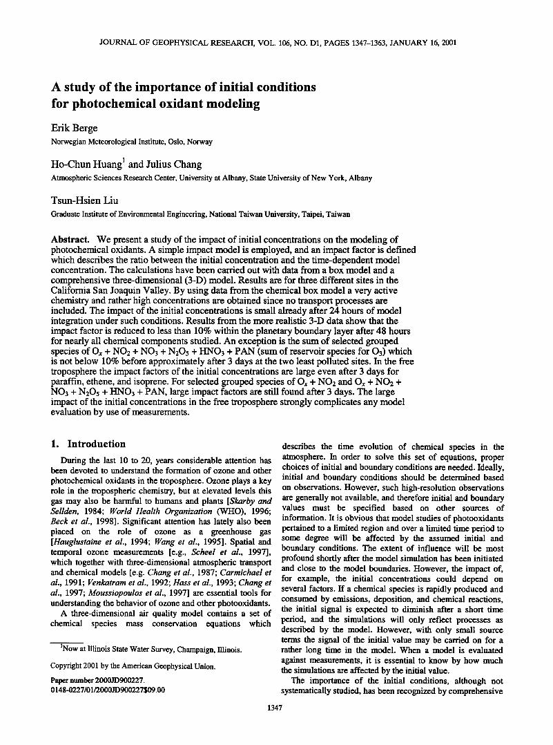
As a first approach to the interpretation of equation (2) we illustrate in Figures la and lb how C(t) and F(t) will develop in time for three different cases with constant source and sink
terms. In all three cases we assume that ct=l.16 10 -s s 4 which corresponds to a lifetime of 24 hours, and we solve the equation for a 24 hour period. In the first case the source term S equals zero. In the second case S equals the loss term, while in the third case S is about 10 times larger than the loss term. F will in the first case equal unity since C(t) is only a function of the decay of the initial condition. The solution is therefore always dependent on the initial condition. In the second case the concentration is constant since the sources
and sinks balance, hence the impact factor is reduced to 1/e within 24 hours, that is, the lifetime of the component. In the third case the sources of the chemical species are very large, and the importance of the initial condition for the modeled concentration is reduced rapidly. Already after approximately 4 hours the ratio F is less than 1/e.
From the above example we understand that F gives a quantitative measure of how much the initial conditions affect the predicted concentrations as a function of time. This will be the basis for the discussion of the impact of the initial conditions in this paper. One other important reason for selecting this impact model is that equation (1) has a simple solution that can easily be discretized and interpreted (see the appendix).
It should be noted that in the special case of &=0 (F remains equal to one as in case 2 in Figure 1) the species concentrations could sometimes approach zero within a short time through rapid reaction with other species. Such a small concentrations would then have little influence on other
species. Although the impact factor equals one, the influence of the initial concentrations could in such particular cases be of little chemical importance. Therefore, in the case of impact factor remaining equal to one for the whole period, the time series of species concentration should also be examined to determine the impact on solution from initialization. This is the case in a few examples as described in section 4.2.
We will in the remaining parts of this study employ the simple impact model (equation (2)) in the case of time- dependent source and loss terms. Thus C•(t) has to be solved by employing equation (A5).
2.2. Selection of Chemical Species
We have employed the Carbon Bond IV (CBM4) chemical mechanism as described by Gary et al. [1989] to study the impact of the initial concentrations. Our version of the CBM4 mechanism is presented by Chang et al. [1997], and it is slightly modified as compared to Gary et al. [1989]. The
BERGE ET AL.: A STUDY OF THE IMPORTANCE OF INITIAL CONDITIONS 1349
a b
o
o o
/ /
/ /
/ /
/ /
/ /
/ /
/
\ \
\ \
0 õ '10 '1õ •0 0 õ '10 '1õ
'l'irne (h) 'l'irne
Figure 1. Development of the (a) concentration and the (b) impact factor with c•=l.16x10 's s '• for $=0 (1), S=o: (2), and S=10xo: (3).
CBM4 mechanism contains a total of 72 reactions. It includes
two alkane classes (methane and lumped paraffin), three alkene classes (ethylene, lumped olefin, and isoprene), three aromatics classes (toulene, cresol, and xylene), and two aldehyde classes (formaldehyde and higher aldehydes). All reactions are listed in Table 1.
As discussed in the previous section, the impact factor will depend on the magnitudes of St(t) and •(t). The chemical productions and losses can be obtained directly form the numerical routine that solves the gas-phase chemistry. However, null cycles with no net chemical production or loss are not necessarily of any importance for the impact of the initial concentrations. For example, ozone is during daytime photolyzed by reactions (J2) and (J3) (see Table 1) to produce either singlet-D ozone atom in the exited state (O(•D)) or triplet-P ozone atom in the base state (O(3p)). O(•D) is rapidly transformed to O(3p) which regenerates 0 3 through reaction R1. These reactions would have no net effect on the initial 03 concentrations unless other sources and sinks could modify the starting value. A net sink of ozone would be through reaction of O(•D) with water (reaction (R8)) to form the hydroxyl radical [SeinfeM and Pandis, 1998]. We now may
define O,• and disregard all internal reactions between the three components 03, O(•D), and O(3p) (see Table 2 for the definition of Ox and the source and sink terms included in this group).
The basic photochemical cycle of NO2, NO, and O3 at wavelengths less than 424 nm [Seinfeld and Pandis, 1998] is represented by the reactions (reaction numbers are taken from Table 1 and 3, rate constants, equilibrium constants, and rate constant expressions are further given for some of the reactions in Table 4-6)
(J1) NO 2 + hv --) NO + 0
(R1) O+O•_ +M-->O3 +M
(R2) 03 + NO •> NO 2 + 02 .
The steady state ozone concentration, [O3]ss (only considering the basic photochemical cycle), can be expressed by [O3]ss = (/•[NO2])/k2[NO]) where j• is the photolysis rate of reaction (J1) and k2 is the reaction rate of reaction (R2). We observe that NO2 is a reservoir gas for 03 through these reactions and
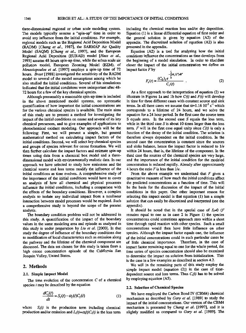
Table 1. Photochemical Reactions
Reaction No. Photochemical Reactions
(J1) NO2 (J2) 03 (J3) 03 (J4) HONO (J5) NO3 (J6) H202 (J7) HCHO
(JS)
(J9) (J10) (Jll)
HCHO
ALD2 OPEN MGLY
h¾
hv ) NO + O3p hv ) O•D + 02 hv ) O3p + 02 hv ) HO + NO hv ) 0.89 NO2 + 0.89 O3p + 0.11 NO hv ) 2HO
> CO
hv,202 ) 2 HO2 + CO
hv,202 hv > HCHO + XO2 + CO + 2 HO2 hv ) C203 + CO + HO2
) C203 + CO + HO2
Photolysis Rate s 4 (Noon Maximum)
5.43x10 '3 2.12x10 '• 2.88x10 '4 1.06x 10 '3 0.18 5.33x10 '6 3.38x10 '•
1.81x10 '•
3.29x 10 '6 1.37x10 '4 1.46x10 '4
1350 BERGE ET AL.: A STUDY OF THE IMPORTANCE OF IN1TIAL CONDITIONS
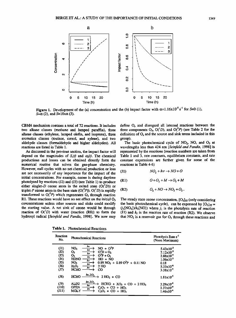
Table 2. Single Species or Groups of Species for Initial Concentration Analysis
Group of Species Source Reactions
Ox = 03+ O(•D)+ O(3p) (J 1), (J5)
Ox + NO2
NOy = NO + NO2 + NO3 + 2(N205) + HONO + HNO4 + HNO3 + PAN
TOC = 2ALD2 + HCHO + 3OPEN + PAR + 2ETH + 2OLE + 5ISO + 2PAN + 7TOL + 8XYL + 7CRES + 2MGLY
HCHO
PAR ETH ISO
Experimental group
(Ox + NO2)net = Ox + NO: + NO3 + N205 + HNO4 + PAN
(JS), (R11), (R15-16), (R19-20), (R23), (R25-26), (R38), (R40), (R51), (R56), (R69)
(R38), (R39), (R41-R43), (R45), (R56), (R57)
(J9), (R38), (R41-43), (R48-54), (R62- 63), (R66-67)
(R48), (R61), (R65), (R67) (R65-67)
(R16), (R19), (R20), (R22-23), (R38), (R40), (R56), (R69)
Loss Reactions
(R2-6), (R8-10), (R33), (R35), (R48), (R50), (R52), (R54), (R63), (R65), (R67)
(R3-4), (R6), (R8), (R6), (R8-10), (R13), (R17), (R21), (R24), (R33), (R35), (R39), (R47-48), (R50), (R52), (R54), (R60), (R63), (R65), (R67)
(R47), (R56), (R60), (R68), (R71)
(J7-J 11), (R32-37), (R40), (R44), (R48), (R50), (R52), (R54-55), (R58-59), (R61-67)
(J7-8), (R32-34)
(R44-45), (R49-51) (R52-54) (R65-68)
(R12), (R14), (R17), (R21), (R34), (R33), (R35), (R37), (R39), (R47-48), (R50), (R54), (R59), (R60), (R63), (R65), (R67-68)
that, in general, the sum of 03 + NO2 should be considered to be a better indicator of the importance of the initial concentrations for ozone itself as time evolves in a model
simulation. Reactions (J1), R(1), and (R2) are therefore not included as sources or sinks for the grouped species O• + NO2 given in Table 2. The main source reaction for O• + NO2 is the hydroperoxyl (HO2) or peroxy radical (RO2) reaction with NO, which converts NO to NO2 without consuming 03. HO2 and RO2 are generated during daytime through the reaction of hydrocarbons with the OH radical [Seinfeld and Pandis, 1998].
We have included NOy, the sum of all inorganic nitrogen components plus PAN, which only has loss reactions. Furthermore, we also include the single NMVOC formaldehyde (HCHO), lumped paraffin (PAR), ethylene (ETH) and isoprene (ISO) and TOC (total carbon) which is the sum of all NMVOCs. The selected hydrocarbons represent a wide range in reactivities, emission strengths, and importance for the ozone production under different environmental conditions. We also note that there are no
source reactions of isoprene as was the case for NOy. An experimental group (O,, + NO2)net is also added (see Table 2). A further reasoning for why we have selected this group is given in section 4.3.
Any chemical mechanism other than the CBM4 could also be employed to the impact model and the selected grouped species. However, for some of the grouped species listed above, the combination of reactions may be different since individual species may involve a different number of reactions when changing from one chemical mechanism to another.
3. Chemical Modeling
3.1. Description of the Box Model and the Three-Dimensional Model
A box model represents a closed system where chemical reactions are performed with an initial mixture of air parcel.
Box model simulations can also include emissions and dry deposition to study the impact due to explicit source or sink term. In this study a box model of a horizontal dimension of 12 km by 12 km and a vertical extent of 60 m is used. The emissions are assumed to be well mixed within this box. In order to quantify the impact of initial conditions on pure chemistry we carried out box model runs as a first step.
For the three-dimensional simulations we have employed the SARMAP Air Quality Model (SAQM). The model originates from the Regional Acid Deposition Model version 2 (RADM2) [Chang et al., 1987]. A detailed description of the SAQM model, including a specification of the boundary conditions, is given by Chang et al. [1997]. Here we only give an overview of the most important model features. The model is formulated in a non-hydrostatic o coordinate system and the meteorological data are derived from the Pennsylvania State/National Center for Atmospheric Research (NCAR) Mesoscale Model version 5 (MM5) nonhydrostatic meteorological model [Seamann et al., 1995]. The model is for this particular study operated on 12 km x 12 km horizontal resolution with 15 layers in the vertical with a domain size of approximately 400 km x 480 km (see Figure 2). The model includes features such as both one-way and two-way nesting, telescoping techniques, a surface layer submodel, a new advection scheme as compared to the RADM2 model, and updated dry deposition velocities. The numerical algorithm in solving the gas-phase chemistry (chemical solver) is a modified version of the Hertel solver [Hertel et al., 1993] obtained from Huang [1999]. This numerical solver is also used for the box model calculations. In the present approach, no nesting was employed.
3.2. Description of the Input Data to the Impact Model
The impact model (equation (2)) requires source S and sink terms c• together with the initial concentrations Co. Two different methods are utilized to obtain these three categories of input data. First, a box model is run to acquire the data.
BERGE ET AL.' A STUDY OF THE IMPORTANCE OF INITIAL CONDITIONS 1351
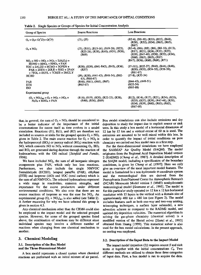
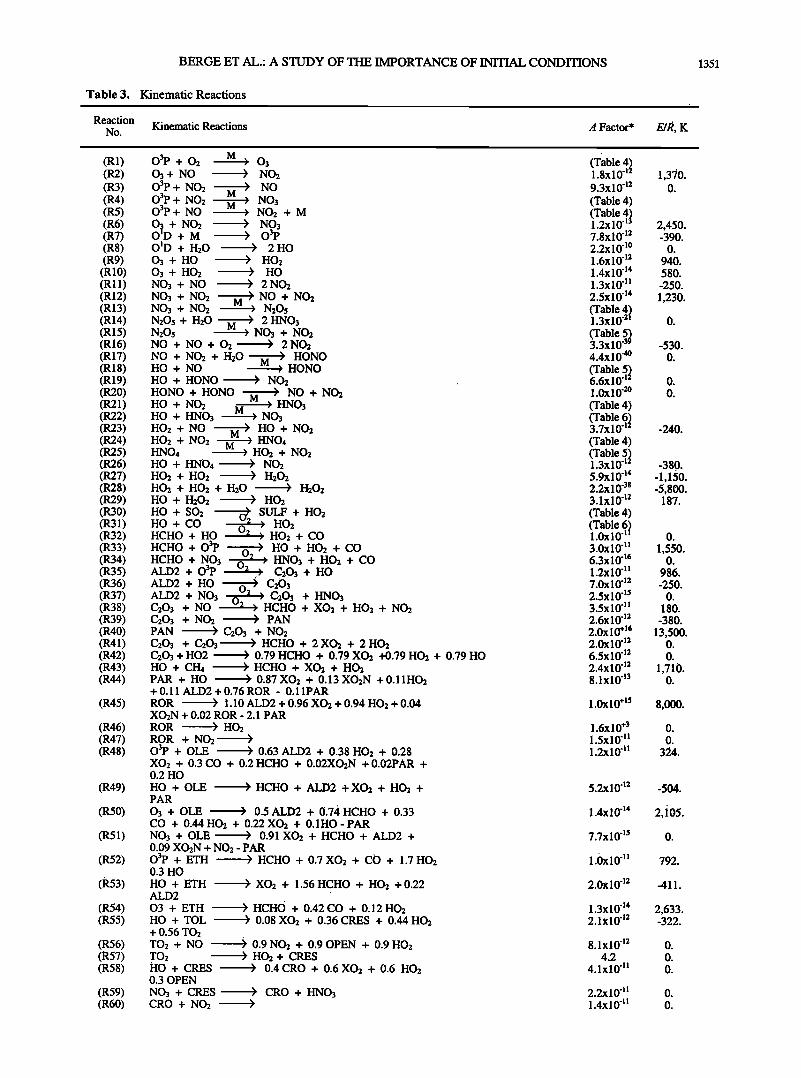
Table 3. Kinematic Reactions
Reaction Kinematic Reactions
No. A Factor*
(R1) (R2) (R3) (R4) (R5) (R6) (R7) (R8) (R9) (R10) (Rll) (R12) (R13) (R!4) (R15) (R16) (R17) (R18) (R19) (R20) (R21) (R22) (R23) (R24) (R25) (R26) (R27) (R28) (R29) (R30) (R31) (R32) (R33) (R34) (R35) (R36) (R37) (R38) (R39) (R40) (R41) (R42) (R43) (R44)
(R45)
(R46) (R47) (R48)
(R49)
(R50)
(R51)
(R52)
(R53)
(R54) (R55)
(R56) (R57) (R58)
(R59) (R60)
M O3p + 02 03+ NO O3p + NO2 O3p + NO2 O3p + NO O +NO2 O{D + M O'D + H20 03 + HO 03 + HO2 NO3 + NO
NO3 + NO2 M NO3 + NO2 N20• + H20 N20• M NO + NO + O2
03 NO2 NO
NO3 NO2 + M NO3 O3p
2 HO HO2 HO
2NO2 NO + NO2 N205 2 HNO3
NO3 + NO2 ) 2NO2
NO + NO2 + H20 ) HONO HO + NO M ) HONO HO + HONO ) NO2
HONO + HONO M ) NO + NO2 HO + NO2 M ) HNO3 HO + HNO3 ) NO3
HO2 + NO M ) HO + NO2 HO2 + NO2 M ) HNO4 HNO4 ) HO2 + NO2 HO + HNO4 ) NO2 HO2 + HO2 ) H202 HO2 + HO2 + H20 ) H202 HO + H202 ) HO2
HO + SO2 ' 4 SULF + HO2 HO + CO > HO2 02 HCHO + HO > HO2 + CO
HCHO + O3P 02 ))HO + HO2 + CO HCHO + NO3 02 HNO3 + HO2 + CO ALD2 + O3P ) C203 + HO
ALD2 + HO 02 )) C203 ALD2 + NO3 02 C203 + HNO3 C203 4. NO ) HCHO + XO2 + HO2 + NO2 C203 4. NO2 ) PAN PAN > C203 4' NO2 C203 + C203 ) HCHO + 2 XO2 + 2 HO2 C203 + HO2 ) 0.79 HCHO + 0.79 XO2 +0.79 HO2 + 0.79 HO HO + CH4 ) HCHO + XO2 + HO2 PAR + HO ) 0.87 XO2 + 0.13 XO2N + 0.11HO2 + 0.11 ALD2 + 0.76 ROR - 0.11PAR
ROR ) 1.10 ALD2 + 0.96 XO2 + 0.94 HO2 + 0.04 XO2N + 0.02 ROR- 2.1 PAR ROR ) HO2 ROR + NO2 ) O3P + OLE ) 0.63 ALD2 + 0.38 HO2 + 0.28 XO2 + 0.3 CO + 0.2 HCHO + 0.02XO2N + 0.02PAR + 0.2 HO
HO + OLE ) HCHO + ALD2 + XO2 + HO2 + PAR
03 + OLE ) 0.5 ALD2 + 0.74 HCHO + 0.33 CO + 0.44 HO2 + 0.22 XO2 + 0.1HO- PAR NO3 + OLE ) 0.91XO2 + HCHO + ALD2 + 0.09 XO2N + NO2 - PAR O3P + ETH ) HCHO + 0.7 XO2 + CO + 1.7 HO2 0.3 HO HO + ETH ALD2 03 + ETH HO + TOL
+ 0.56 TO2 TO2 + NO TO2 HO + CRES 0.3 OPEN
NO3 + CRES CRO + NO2
) XO2 + 1.56 HCHO + HO2 + 0.22
' ) HCHO + 0.42 CO + 0.12 HO2 ' ) 0.08 XO2 + 0.36 CRES + 0.44HO2
) 0.9 NO2 + 0.9 OPEN + 0.9 HO2 ) HO2 + CRES
) 0.4CRO + 0.6XO2 + 0.6
> CRO + HNO3 >
(Table 4) 1.8x1042 9.3X1042 (Table 4) (Table 4,} 1.2x10"' 7.8x1042 2.2x10⁴ø 1.6x1042 1.4x1044 1.3x10⁴• 2.5x1044 (Table 4,•} 1.3x10"'
(Table 3.3x10-"' 4.4x10 -4ø (Table 6.6x10"' 1.0x 10 '2ø (Table 4) (Table 6,• 3.7x10"'
(Table 4) (Table 1.3x10"' 5.9x10 -v* 2.2x 10 3.1x10 -12 (Table 4) (Table 6,} 1.0xl 0"' 3.0x10⁴• 6.3x10⁴• 1.2x10⁴• 7.0x1042 2.5x10⁴• 3.5x10⁴• 2.6x1042 2.0x10 +• 2.0xl 042 6.5x1042 2.4x1042 8.1x1043
1.0xl 0 +•:s
1.6x10 +3 1.5x10"' 1.2x10⁴•
5.2X10 '12
1.4x10⁴•
7.7x10⁴•
1.0x10⁴•
2.0x 10'•2
1.3x10⁴'• 2.1x1042
8.1x1042 4.2
4.1x1041
2.2x10 -'• 1.4x10⁴•
E/R, K
1,370. 0.
2,450. -390.
0. 940. 580. -250.
1,230.
0.
-530. 0.
0. 0.
-240.
-380.
-1,150. -5,800.
187.
0.
1,550. 0.
986. -250.
0. 180.
-380.
13,500. 0. 0.
1,710. 0.
O. 0.
324.
2,105.
792.
-411.
2,633. -322.
1352 BERGE ET AL.: A STUDY OF TI-IE IMPORTANCE OF INITIAL CONDITIONS
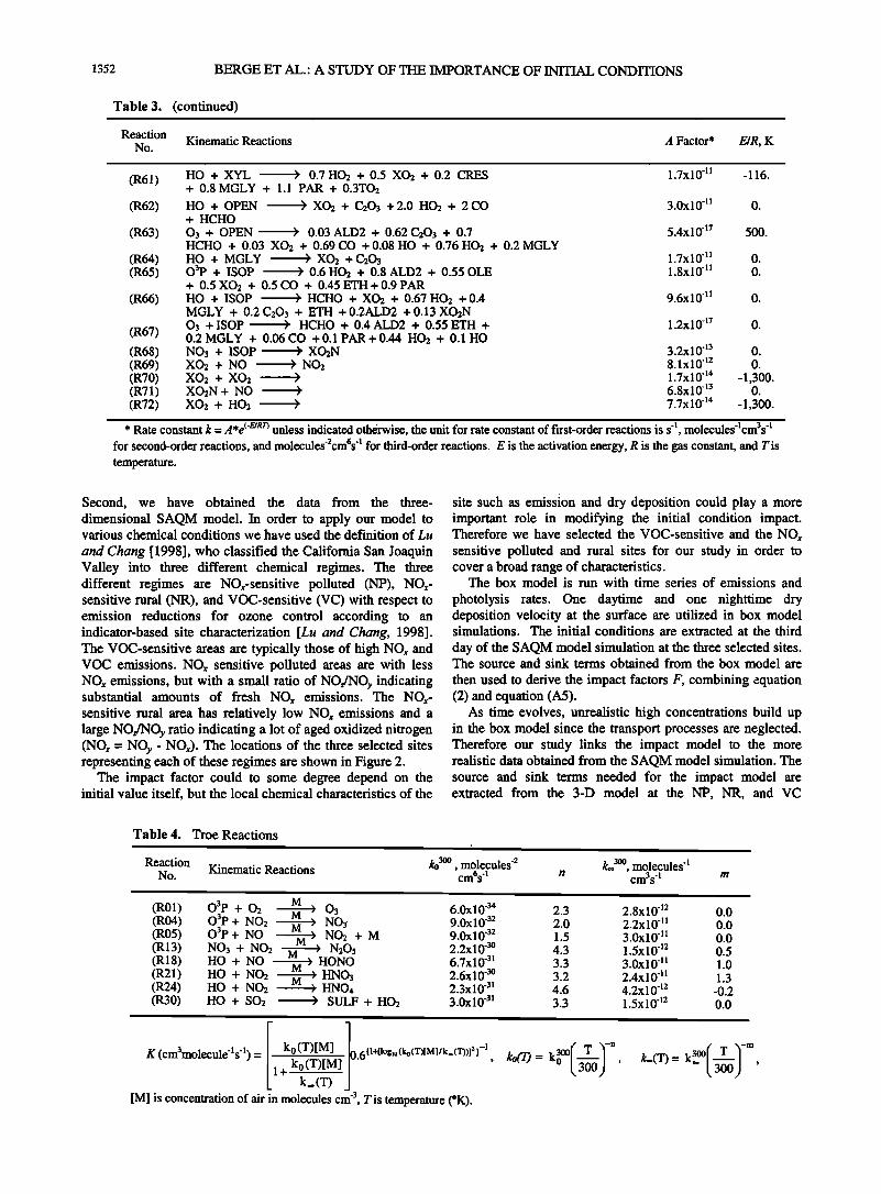
Table 3. (continued)
Reaction Kinematic Reactions
No. A Factor* E/R, K
(R61)
(R62)
(R63)
(R64) (R65)
(R66)
(R67)
(R68) (R69) (R70) (R71) (R72)
HO + XYL ) 0.7HO2 + 0.5 XO2 + 0.2 CRES + 0.8 MGLY + 1.1 PAR + 0.3TO2
HO + OPEN ) XO2 -I- C203 -I-2.0 HO2 + 2 CO + HCHO
03 + OPEN ) 0.03 ALD2 + 0.62 C203 -I- 0.7 HCHO + 0.03 XO2 + 0.69 CO +0.08 HO + 0.76 HO2 + 0.2 MGLY HO + MGLY ) go2 -I-C203 O3p + ISOP ) 0.6 HO2 + 0.8 ALD2 + 0.55 OLE + 0.5 XO2 + 0.5 CO + 0.45 ETH + 0.9 PAR HO + ISOP ) HCHO + XO2 + 0.67 HO2 + 0.4 MGLY + 0.2 C203 -I- ETH +0.2ALD2 +0.13 XO2N 03 + ISOP ) HCHO + 0.4 ALD2 + 0.55 ETH + 0.2 MGLY + 0.06 CO + 0.1 PAR + 0.44 HO2 + 0.1 HO NO3 + ISOP ) XO2N go2 + NO ) NO2 XO2 + XO2 > XO2N + NO ) XO2 + HO2
1.7x10 ']] -116.
3.0x10⁴] 0.
5.4x1047 500.
1.7x10⁴] 0. 1.8x10⁴] 0.
9.6x10⁴] 0.
1.2x1047 0.
3.2x1043 0. 8.1x10 '12 0. 1.7x 10 -]4 - 1,300. 6.8x1043 0. 7.7x1044 -1,300.
* Rate constant k = A*e (4r/at) unless indicated otherwise, the unit for rate constant of first-order reactions is s 4, molecules4cm3s 4 for second-order reactions, and molecules-2cmts 4 for third-order reactions. E is the activation energy, R is the gas constant, and T is temperature.
Second, we have obtained the data from the three- dimensional SAQM model. In order to apply our model to various chemical conditions we have used the definition of Lu
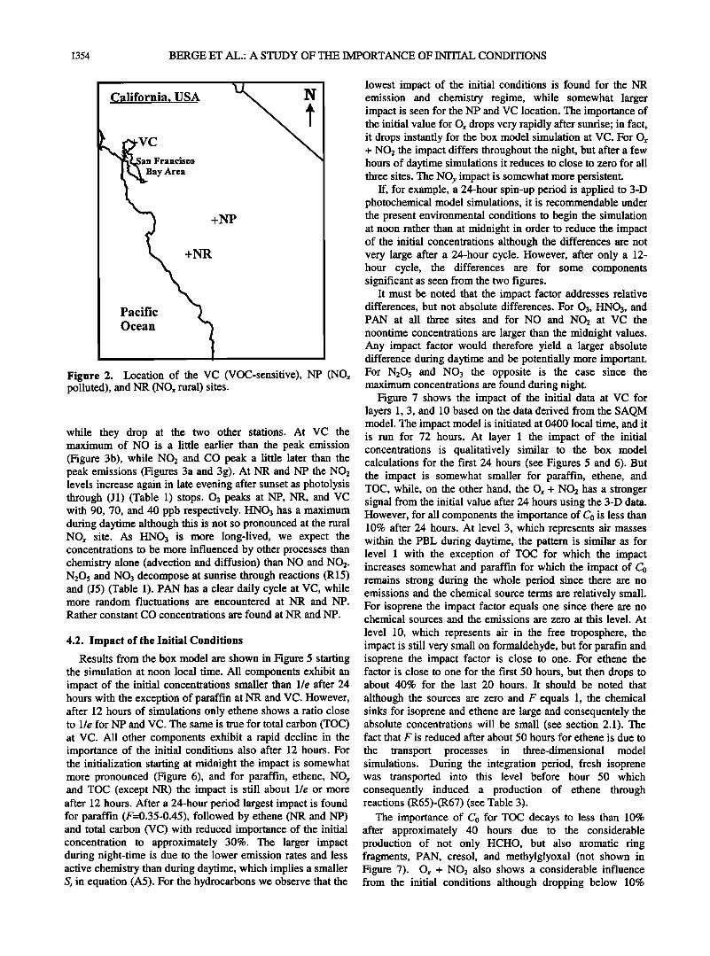
and Chang [1998], who classified the California San Joaquin Valley into three different chemical regimes. The three different regimes are NOx-sensitive polluted (NP), NOr- sensitive rural (N-R), and VOC-sensitive (VC) with respect to emission reductions for ozone control according to an indicator-based site characterization [Lu and Chang, 1998]. The VOC-sensitive areas are typically those of high NOr and VOC emissions. NOx sensitive polluted areas are with less NOx emissions, but with a small ratio of NOJNOy indicating substantial amounts of fresh NO• emissions. The NOx- sensitive rural area has relatively low NO• emissions and a large NOJlqOy ratio indicating a lot of aged oxidized nitrogen (NOz = NO• - NO•). The locations of the three selected sites representing each of these regimes are shown in Figure 2.
The impact factor could to some degree depend on the initial value itself, but the local chemical characteristics of the
site such as emission and dry deposition could play a more important role in modifying the initial condition impact. Therefore we have selected the VOC-sensitive and the NO• sensitive polluted and rural sites for our study in order to cover a broad range of characteristics.
The box model is run with time series of emissions and
photolysis rates. One daytime and one nighttime dry deposition velocity at the surface are utilized in box model simulations. The initial conditions are extracted at the third
day of the SAQM model simulation at the three selected sites. The source and sink terms obtained from the box model are
then used to derive the impact factors F, combining equation (2) and equation (A5).
As time evolves, unrealistic high concentrations build up in the box model since the transport processes are neglected. Therefore our study links the impact model to the more realistic data obtained from the SAQM model simulation. The source and sink terms needed for the impact model are extracted from the 3-D model at the NP, NR, and VC
Table 4. Troe Reactions
Reaction No. Kinematic Reactions ko 3øø ' molecules -2 ko? ø, molecules ']
cmts 4 n cm3s. l
(R01) O3p + 02 • 03 (R04) O3p + NO2 • NO3 (R05) O3p + NO • NO2 + M (R13) NO3 + NO2 M ) (R18) HO + NO M N205 M • ) HONO (R21) HO + NO2 HNO3 (R24) HO + NO2 ) HNO4 (R30) HO + SO2 ) SULF + HO2
6.0xl 0 '34 2.3 2.8x 10 '12 0.0 9.0X 10 '32 2.0 2.2x 10⁴] 0.0 9.0x10 '32 1.5 3.0x10⁴] 0.0 2.2x 10 '3o 4.3 1.5x 10 ']2 0.5 6.7x 10 '3] 3.3 3.0x 10⁴] 1.0 2.6xl 0 '3o 3.2 2.4xl 04] 1.3 2.3x 10 '3] 4.6 4.2x 10 ']2 -0.2 3.0x 10 '31 3.3 1.5x 10 ']2 0.0
3 I 1 K (cm molecule' s' ) = kø(T)[M] (kø(T)[MI/k-(T))12}-I k 0(T)[M]' '611+[]øg'ø 1+• k,(T)
[M] is concentration of air in molecules cm -3, T is temperature (øK).
k3OO ( T ,•-n 0 , k•(T): ,• [,3-•) '
BERGE ET AL.: A STUDY OF THE IMPORTANCE OF INITIAL CONDITIONS 1353
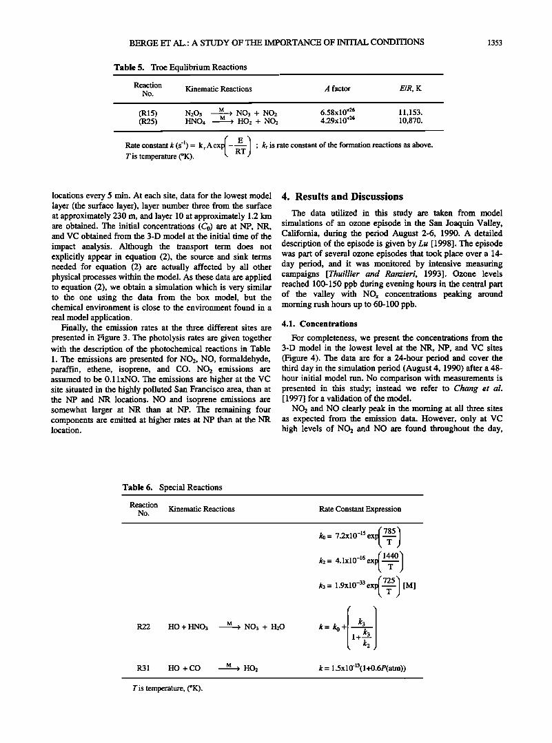
Table 5. Troe Equlibrium Reactions
Reaction Kinematic Reactions A factor E/R, K No.
(R15) N205 M > NO3 + NO2 6.58x10 +26 11,153. (R25) HNO4 M > HO2 + NO2 4.29x10 +26 10,870.
Rate constant k (s 'l) = krA ex - ß kr is rate constant of the formation reactions as above. T is temperature (øK).
locations every 5 min. At each site, data for the lowest model layer (the surface layer), layer number three from the surface at approximately 230 m, and layer 10 at approximately 1.2 km are obtained. The initial concentrations (Co) are at NP, NR, and VC obtained from the 3-D model at the initial time of the
impact analysis. Although the transport term does not explicitly appear in equation (2), the source and sink terms needed for equation (2) are actually affected by all other physical processes within the model. As these data are applied to equation (2), we obtain a simulation which is very similar to the one using the data from the box model, but the chemical environment is close to the environment found in a
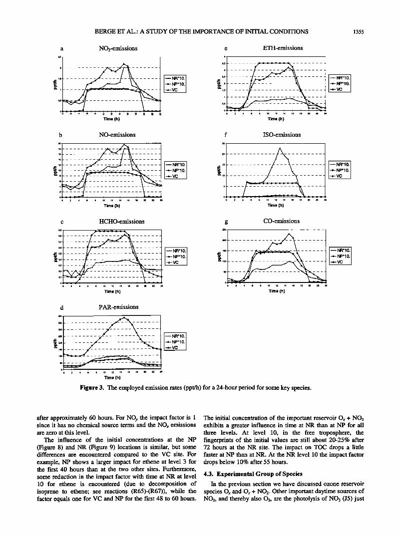
real model application. Finally, the emission rates at the three different sites are
presented in Figure 3. The photolysis rates are given together with the description of the photochemical reactions in Table 1. The emissions are presented for NO2, NO, formaldehyde, paraffin, ethene, isoprene, and CO. NO2 emissions are assumed to be 0.1 lxNO. The emissions are higher at the VC site situated in the highly polluted San Francisco area, than at the NP and NR locations. NO and isoprene emissions are somewhat larger at NR than at NP. The remaining four components are emitted at higher rates at NP than at the NR location.
4. Results and Discussions
The data utilized in this study are taken from model simulations of an ozone episode in the San Joaquin Valley, California, during the period August 2-6, 1990. A detailed description of the episode is given by Lu [ 1998]. The episode was part of several ozone episodes that took place over a !4- day period, and it was monitored by intensive measuring campaigns [Thuillier and Ranzieri, 1993]. Ozone levels reached 100-150 ppb during evening hours in the central part of the valley with NO,• concentrations peaking around morning rush hours up to 60-100 ppb.
4.1. Concentrations
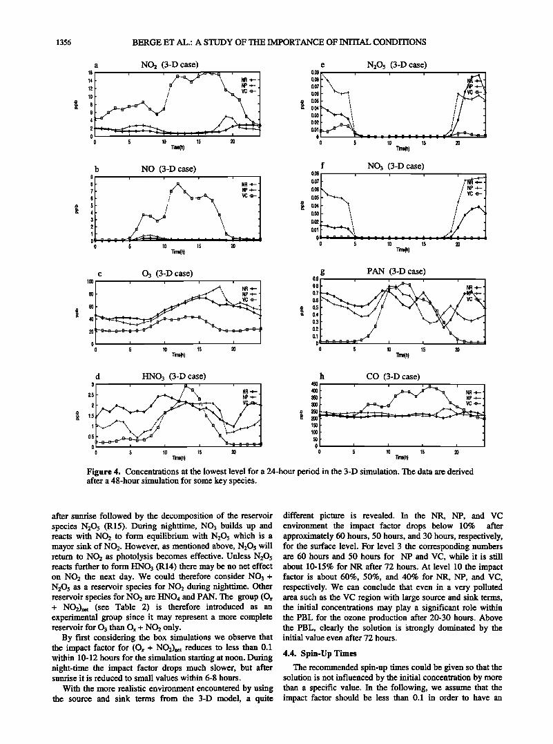
For completeness, we present the concentrations from the 3-D model in the lowest level at the NR, NP, and VC sites (Figure 4). The data are for a 24-hour period and cover the third day in the simulation period (August 4, 1990) after a 48- hour initial model run. No comparison with measurements is presented in this study; instead we refer to Chang et al. [ 1997] for a validation of the model.
NO2 and NO clearly peak in the morning at all three sites as expected from the emission data. However, only at VC high levels of NO2 and NO are found throughout the day,
Table 6. Special Reactions
Reaction Kinematic Reactions
No.
R22 HO q-HNO3 M > NO3 q- H20
R31 HO + CO
Rate Constant Expression
f 1440'•
('725'1
k3= 1.9xlO -33 ex••j [M]
•=•o + l+k3
J
M > H02 k = 1.5x10'13(l+0.6P(atm))
Tis temperature, (øK).
1354 BERGE ET AL.: A STUDY OF TI-IE IMPORTANCE OF INITIAL CONDITIONS
ß ß
+NP
Pacific ).•
Ocean • Figure 2. Location of the VC (VOC-sensitive), NP (NO,• polluted), and NR (NOx rural) sites.
while they drop at the two other stations. At VC the maximum of NO is a little earlier than the peak emission (Figure 3b), while NO2 and CO peak a little later than the peak emissions (Figures 3a and 3g). At NR and NP the NO2 levels increase again in late evening after sunset as photolysis through (J1) (Table 1) stops. 03 peaks at NP, NR, and VC with 90, 70, and 40 ppb respectively. HNO3 has a maximum during daytime although this is not so pronounced at the rural NOx site. As HNO3 is more long-lived, we expect the concentrations to be more influenced by other processes than chemistry alone (advection and diffusion) than NO and NO•. N•O5 and NO3 decompose at sunrise through reactions (R15) and (J5) (Table 1). PAN has a clear daily cycle at VC, while more random fluctuations are encountered at NR and NP. Rather constant CO concentrations are found at NR and NP.
4.2. Impact of the Initial Conditions
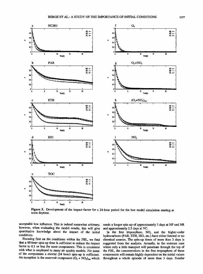
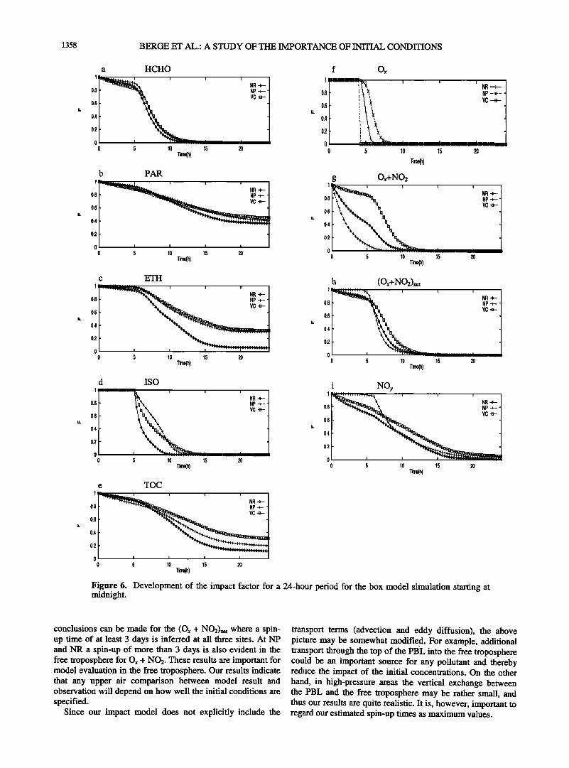
Results from the box model are shown in Figure 5 starting the simulation at noon local time. All components exhibit an impact of the initial concentrations smaller than 1/e after 24 hours with the exception of paraffin at NR and VC. However, after 12 hours of simulations only ethene shows a ratio close to 1/e for NP and VC. The same is true for total carbon (TOC) at VC. All other components exhibit a rapid decline in the importance of the initial conditions also after 12 hours. For the initialization starting at midnight the impact is somewhat more pronounced (Figure 6), and for paraffin, ethene, NOy and TOC (except NR) the impact is still about 1/e or more after 12 hours. After a 24-hour period largest impact is found for paraffin (F=0.35-0.45), followed by ethene (NR and NP) and total carbon (VC) with reduced importance of the initial concentration to approximately 30%. The larger impact during night-time is due to the lower emission rates and less active chemistry than during daytime, which implies a smaller Si in equation (A5). For the hydrocarbons we observe that the
lowest impact of the initial conditions is found for the NR emission and chemistry regime, while somewhat larger impact is seen for the NP and VC location. The importance of the initial value for Ox drops very rapidly after sunrise; in fact, it drops instantly for the box model simulation at VC. For Ox + NO• the impact differs throughout the night, but after a few hours of daytime simulations it reduces to close to zero for all three sites. The NOy impact is somewhat more persistent.
If, for example, a 24-hour spin-up period is applied to 3-D photochemical model simulations, it is recommendable under the present environmental conditions to begin the simulation at noon rather than at midnight in order to reduce the impact of the initial concentrations although the differences are not very large after a 24-hour cycle. However, after only a 12- hour cycle, the differences are for some components significant as seen from the two figures.
It must be noted that the impact factor addresses relative differences, but not absolute differences. For 03, HNO3, and PAN at all three sites and for NO and NO• at VC the noontime concentrations are larger than the midnight values. Any impact factor would therefore yield a larger absolute difference during daytime and be potentially more important. For N205 and NO3 the opposite is the case since the maximum concentrations are found during night.
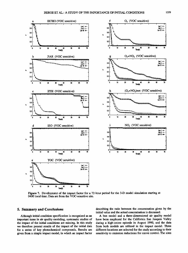
Figure 7 shows tb.e impact of the initial data at VC for layers 1, 3, and 10 based on the data derived from the SAQM model. •he impact model is initiated at 0400 local time, and it is run for 72 hours. At layer 1 the impact of the initial concentrations is qualitatively similar to the box model calculations for the first 24 hours (see Figures 5 and 6). But the impact is somewhat smaller for paraffin, ethene, and TOC, while, on the other hand, the Ox + NO• has a stronger signal from the initial value after 24 hours using the 3-D data. However, for all components the importance of Co is less than 10% after 24 hours. At level 3, which represents air masses within the PBL during daytime, the pattern is similar as for level 1 with the exception of TOC for which the impact increases somewhat and paraffin for which the impact of Co remains strong during the whole period since there are no emissions and the chemical source terms are relatively small. For isoprene the impact factor equals one since there are no chemical sources and the emissions are zero at this level. At
level 10, which represents air in the free troposphere, the impact is still very small on formaldehyde, but for parafin and isoprene the impact factor is close to one. For ethene the factor is close to one for the first 50 hours, but then drops to about 40% for the last 20 hours. It should be noted that
although the sources are zero and F equals i, the chemical sinks for isoprene and ethene are large and consequentely the absolute concentrations will be small (see section 2.1). The fact that F is reduced after about 50 hours for ethene is due to
the transport processes in three-dimensional model simulations. During the integration period, fresh isoprene was transported into this level before hour 50 which consequently induced a production of ethene through reactions (R65)-(R67) (see Table 3).
The importance of Co for TOC decays to less than 10% after approximately 40 hours due to the considerable production of not only HCHO, but also aromatic ring fragments, PAN, cresol, and methylglyoxal (not shown in Figure 7). Ox + NO2 also shows a considerable influence from the initial conditions although dropping below 10%
BERGE ET AL.: A STUDY OF THE IMPORTANCE OF INITIAL CONDITIONS 1355
a NO2-emissions ETH-emissions
2
o,s
o:
Time {h)
-- NR*10. I ---- NP*10. ß --*- VC
e
3,5.
3'
0,s
0
-- NR* 10. I --- NP*I 0. I --*- ¾C I
...............
2 4 6 8 10 12 14 16 18 20 22 24
Time (h)
b
2O.--
16.
14'--
12.
..
•'.
2.
0
NO-emissions
-- NR*10. I I-'- NP*10.
............. I '-*- ¾c
2 4 6 8 10 12 14 16 18 20 22 24
Time (h)
f ISO-emissions
...........
2 4 e e 10 12 14 16 te 2o 22 24
Time (h)
-- NR*10. I ---- NP*10. ß -*- VC
c HCHO-emissions g CO-emissions
•, _ ---- NP*I 0. I ---- NP*I 0. _ -,- vc J • ,oo --- vc
o o _-!- 0 2 4 6 e 10 12 14 16 18 20 22 24 0 2 4 e e 10 12 14 16 te 20 22 24
Time (h) Time (h)
d
o
o 2
PAR-emissions
-.- NF" o. I -,- ¾C I
4 6 6 10 12 14 16 16 2O 22 24
Time (h)
Figure 3. The employed emission rates (ppt/h) for a 24-hour period for some key species.
after approximately 60 hours. For NOy the impact factor is 1 since it has no chemical source terms and the NOx emissions are zero at this level.
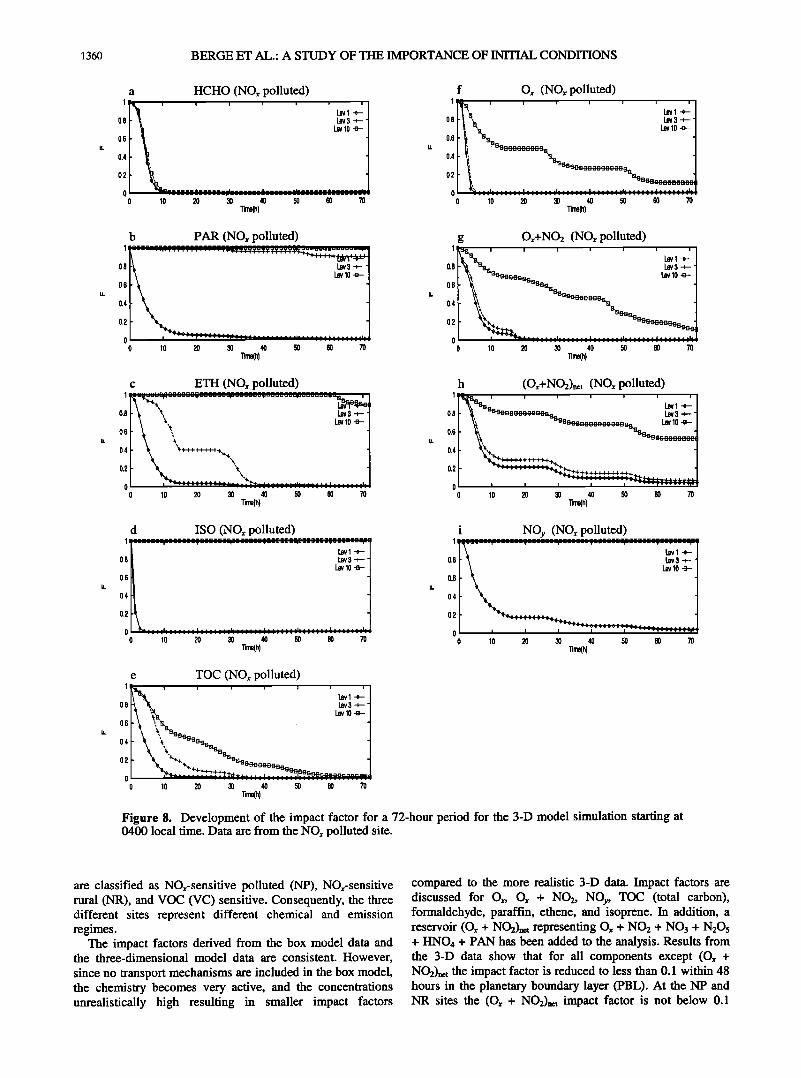
The influence of the initial concentrations at the NP
(Figure 8) and NR (Figure 9) locations is similar, but some differences are encountered compared to the VC site. For example, NP shows a larger impact for ethene at level 3 for the first 40 hours than at the two other sites. Furthermore,
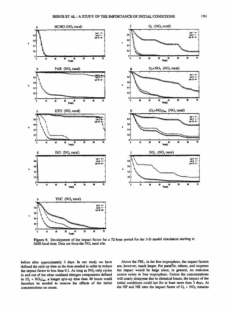
some reduction in the impact factor with time at NR at level 10 for ethene is encountered (due to decomposition of isoprene to ethene; see reactions (R65)-(R67)), while the factor equals one for VC and NP for the first 48 to 60 hours.
The initial concentration of the important reservoir Ox + NO2 exhibits a greater influence in time at NR than at NP for all three levels. At level 10, in the free troposphere, the fingerprints of the initial values are still about 20-25% after 72 hours at the NR site. The impact on TOC drops a little faster at NP than at NR. At the NR level 10 the impact factor drops below 10% after 55 hours.
4.3. Experimental Group of Species
In the previous section we have discussed ozone reservoir species O• and O• + NO2. Other important daytime sources of NO2, and thereby also 03, are the photolysis of NO3 (J5) just
1356 BERGE ET AL.: A STUDY OF THE IMPORTANCE OF INITIAL CONDITIONS
a NO2 (3-D case)
14 NR -e--
12 ? •,•a VC -a- 10 /
6 4
2 '/
0 5 10 15 20 •me(h)
e N205 (3-D case) 0.09, , • , ,
0.08 l",• 0.07 I" '", 0.08 I' '+"'+'"+ o.o5
0.04•_ 0.03 0.02 0.01
0 5 10 15 20 'rime(h)
b NO (3-D case) 9 i i i i
87 • NR-e-
/
0 5 10 15 •h)
f NO3 (3-D case)
.... ;.,=1
o.o4 '",,, 0.03
...... :: : .... ..&... 0 5 10 15 20
Time(h)
c 03 (3-D case)
' ' ' .+...,k, ' NR -+- / .... e-'•"' ", NP +"1
I I I I I
0 5 10 15 20 Tin•h)
g PAN (3-D case) 0.9 / ' ' ' '
0.7 ",,._.• • -*--.
0.6 0.5 • 0.4 I' "'"'+-"+/' ? "'. '•"+' /"• ...... -'1'
0 5 10 15 20 •m•)
d HNO3 (3-D case) 3 i i i i
/% ,,-.- '•) / " NP .-*--' . ,•
2 - •': "N
1. I ", . o.s •_.,=._e ' '"•' "ax,,..+-"
0 5 10 15 20 Tirne(•)
h CO (3-D case) 450 i i i i 400 a/a'"s• .+_ = ,,.,,
0 5 10 15 20 T•e(h)
Figure 4. Concentrations at the lowest level for a 24-hour period in the 3-D simulation. The data are derived after a 48-hour simulation for some key species.
after sunrise followed by the decomposition of the reservoir species N2Os (R15). During nighttime, NO3 builds up and reacts with NO2 to form equilibrium with N2Os which is a mayor sink of NO2. However, as mentioned above, N205 will return to NO2 as photolysis becomes effective. Unless N205 reacts further to form HNO3 (R14) there may be no net effect on NO2 the next day. We could therefore consider NO3 + N2Os as a reservoir species for NO2 during nighttime. Other reservoir species for NO2 are HNO4 and PAN. The group (O,, + NO2)net (see Table 2) is therefore introduced as an experimental group since it may represent a more complete reservoir for 03 than O,, + NO2 only.
By first considering the box simulations we observe that the impact factor for (O,, + NO2)net reduces to less than 0.1 within 10-12 hours for the simulation starting at noon. During night-time the impact factor drops much slower, but after sunrise it is reduced to small values within 6-8 hours.
With the more realistic environment encountered by using the source and sink terms from the 3-D model, a quite
different picture is revealed. In the NR, NP, and VC environment the impact factor drops below 10% after approximately 60 hours, 50 hours, and 30 hours, respectively, for the surface level. For level 3 the corresponding numbers are 60 hours and 50 hours for NP and VC, while it is still about 10-15% for NR after 72 hours. At level 10 the impact factor is about 60%, 50%, and 40% for NR, NP, and VC, respectively. We can conclude that even in a very polluted area such as the VC region with large source and sink terms, the initial concentrations may play a significant role within the PBL for the ozone production after 20-30 hours. Above the PBL, clearly the solution is •trongly dominated by the initial value even after 72 hours.
4.4. Spin-Up Times
The recommended spin-up times could be given so that the solution is not influenced by the initial concentration by more than a specific value. In the following, we assume that the impact factor should be less than 0.1 in order to have an
BERGE ET AL.: A STUDY OF THE IMPORTANCE OF INITIAL CONDITIONS 1357
a HCHO
0.8 NR • $ NP +- O. VC -a-
0.4
0'20I" ....•777:'. ????T7777777..•. •m.•:::::.•_.:. .... 0 5 10 15 2o
Time(h)
f Ox 1• i i i i
::. vc -•- 0.6
u. 0.4 0 5 10 15 20
'lime(h)
b PAR.
ii I i i i i I NR-*- / NP +-'1
I I
5 10 15 2O
Time(h)
g Ox+NO•_ i i i i I
NR+-/ NP•- 1
0 5 10 15 2O
•me(h)
c ETH
i I i i j NR -e-- tip +-
I I I I .... '1'
0 5 10 15 2o
Tim(h)
h (Ox+NO2)net i i i I
ß NR -*- / , NP •" 1
::::::_:::• vc • ß , .... , -:-_-:_----_
0 5 10 15 2o
Time(h)
d ISO
1[• , , , ,
I NR 0.8 • NP +-. o.s 0.2
0 5 10 15 2o 0 'lime(h)
i NOy
' ' ' ' NP +-.
_.
5 10 15 20 Time(h)
e TOC
NR•-/ NP •-1
I I I I I
0 5 10 15 2o
Time(h)
Figure 5. Development of the impact factor for a 24-hour period for the box model simulation starting at noon daytime.
acceptable low influence. This is indeed somewhat arbitrary; needs a longer spin-up of approximately 3 days at NP and NR however, when evaluating the model results, this will give and approximately 2.5 days at VC. quantitative knowledge about the impact of the initial conditions.
Focusing first on the conditions within the PBL, we find that a 48-hour spin-up time is sufficient to reduce the impact factor to 0.1 or less for most components. This is consistent with what is employed in many air quality models. For some of the components a shorter (24 hour) spin-up is sufficient. An exception is the reservoir component (O,• + NO2)nc t which
In the free troposphere, NOy and the higher-order hydrocarbons (PAR, ETH, ISO, etc.) have either limited or no chemical sources. The spin-up times of more than 3 days is suggested from the analysis. Actually, in the extreme case where only a little transport will penetrate through the top of the PBL, the concentrations in the free troposphere of these components will remain highly dependent on the initial values throughout a whole episode of more than 3 days. Similar
1358 BERGE ET AL.' A STUDY OF TIlE IMPORTANCE OF INITIAL CONDITIONS
a HCHO
,• ' ' ' NR
0 5 10 15 2o Time(h)
1
0.8
0.6
0.4
0.2
o o
b PAR
NR --e-/ NP +-.-I
I I I I
5 10 15 2O Time(h)
f
/ i•-x NR --•
0.8 I' "P--*--
"0.4 •,• 0.2 or :::::::::::::::::::::::::::::::::::::::::::::
0 5 10 15 20
Ti•h)
• O•+NO• 1 i i i i
0.6 .
,, 0 5 10 15 20
•m(h)
c ETH
1 l----•' -' ' ''•••••a. ' ' ' ,R-e-[
o't { 0.
I I
0 5 10 15 2o
Time(h)
d ISO
•,*, NR -e-
0.8 ß •a.'•,•,k NP .+-- •. •,, vc •
0.6 k •,,, 0.2
0 ß i .......... ::_•7.------•_----,_•--;;; ------ 0 5 10 15 2o
Tim(h)
e TOC
0.8 NP +-'1
0.4 %'•
0 L t • o 5 lO 15 20
Time(h)
h (Ox+NO2)net 1 :•-;.;.;'::;;;; ;N,•, , , ,
0.8 NP -+'-' VC -a-
0 5 10 15 20
Time(h)
i NOy 1 •;;;; •r•-,++• , , ' I
•%•• \ NR -,- / 0.8 •'e',e,e,e••• NP -',---'1 0.6
0.4
0.2
0 I I I ' ..,•'w-=-•.•; ;_.=-•'-5-'-•• o 5 10 15 2O
Time(h)
Figure 6. Development of the impact factor for a 24-hour period for the box model simulation starting at midnight.
conclusions can be made for the (Ox + NO2)net where a spin- up time of at least 3 days is inferred at all three sites. At NP and NR a spin-up of more than 3 days is also evident in the free troposphere for Ox + NO2. These results are important for model evaluation in the free troposphere. Our results indicate that any upper air comparison between model result and observation will depend on how well the initial conditions are specified.
Since our impact model does not explicitly include the
transport terms (advection and eddy diffusion), the above picture may be somewhat modified, For example, additional transport through the top of the PBL into the free troposphere could be an important source for any pollutant and thereby reduce the impact of the initial concentrations. On the other hand, in high-pressure areas the vertical exchange between the PBL and the free troposphere may be rather small, and thus our results are quite realistic. It is, however, important to regard our estimated spin-up times as maximum values.
BERGE ET AL.: A STUDY OF THE IMPORTANCE OF INITIAL CONDITIONS 1359
a HCHO (VOC sensitive) '1 n,.• I '1 ' I I [ ' I '
•i' Levl -e- 0.8 Lev3 -+--. Lev10 -a-
O.
- 0 10 20 30 40 50 60 70
'nine(h)
f O,• (VOC sensitive) l[!,a , , , ' , , , ,
a Lev10 -a- 0.6 t •
0.2 • 0 10 • • g • • 70
•(h)
b PAR (VOC sensitive)
[ "•"'++%++++•.. Lev 1 -*- I 0.8 I{ '•'+'+'+++++.. Lev 3 +-1
0.4
0.2
0 0 10 2o 3o 4o 5o 6o 70
'nine(h)
g Ox+NO2 (VOC sensitive)
I "•+.'"'a Levl --e- l 0.8I• • 'a Lev3 -+---[
0 10 2O 3O 40 50 60 70 nine(h)
c ETH (VOC sensitive)
0.8• • "•V 3 -+-- 1 o, t
o ::::::::::::::::::::::::::::::::::: 0 10 2o 3o 4o 5o 6o 70
Time(h)
h (O,•+NO2)net (VOC sensitive) l•sa.. , ' ' ..... I
IN•, =a Levl -e-I 0.8 F •&. %s<,_ Lev 3 +-. q
', •o• • 10 •
o lO • • • • • 7o •m(h)
d ISO (VOC sensitive) 1 ======================================================
* i•.vl •- 0.8 Lev3 .+-.
Lev10 -a- 0.6
0.4
02
0 -::00: 0 10 20 3o 40 5o 6o 70
Time(h)
i NOy (VOC sensitive)
o.8 :.
• •10 • 06 ß
0.2
I •+• .... /
0 10 • • • • • •(h)
e TOC (VOC sensitive) 1 "]dl•i• ' , i i i i ! i
0.8[ 0.tl o.21'
0 10 • • 40 • m 70 •h)
Figure 7. Development of the impact factor for a 72-hour period for the 3-D model simulation starting at 0400 local time. Data are from the VOC-sensitive site.
5. Summary and Conclusions
Although initial condition specification is recognized as an important issue in air quality modeling, systematic studies of the impact of the initial conditions are missing. In this study we therefore present results of the impact of the initial data for a series of key photochemical compounds. Results are given from a simple impact model, in which an impact factor
describing the ratio between the concentration given by the initial value and the actual concentration is discussed.
A box model and a three-dimensional air quality model have been employed for the California San Joaquin Valley during a high-ozone episode in August 1990, and the data from both models are utilized in the impact model. Three different locations are selected for the study according to their sensitivity to emission reductions for ozone control. The sites
1360 BERGE ET AL.' A STUDY OF Tt• IMPORTANCE OF INITIAL CONDITIONS
a HCHO (NO,• polluted) 1 i i !
Lev1 0.8 Lev3 '+"1
Lev10 -a-
0.6
0.4
0.2
0 - '-= ..... * ...... !11"- :::::-'-::::::-;-• 0 10 2o 3o 4o 50 6o 7o
Time(h)
f Ox (NOx polluted)
a,. Levl -e- • Lev3 -+---
0'SL• %.% Lev 10 -a- • , ø'21 •,, %•o• o l • ..................................................
0 10 2o 3o 4o 50 60 70 Time(h)
b PAR (NOx polluted)
0,2
0 10 • • • • • 70 •(h)
g Ox+NO2 (NOx polluted)
1T• ...... Lvl -,:/ 0.8 •-• as_ Lev 3 +-- -I
o lO • • • • m • •(h)
c ETH (NO• polluted) ::::::::::::::::::::::::::::::::::::::::::::::::::::
I\ '•, 0.8 }- • •, Lev 3 -+-- 1
o.,t '.,,, .v,o.- t ", '1
0 10 20 30 40 50 6o 70 Xirne(h)
h (Ox+NO2)net (NOx polluted) 1 In- i i i i , i i
0.8 •- •t, "'•aeeeoeeeOe-E•a.% Lev 3 +--
0 • • • • • • ---• ....... •, o lO • • 4o • • •
•(h)
d ISO (NOx polluted) 1 ::::::::::::::::::::::::::::::::::::::::::::::
Levl --e- 0.8 Lev3 +--
Lev10 -a-
0.6
0.4
0 10 20 30 4o 50 6o 7o Time(h)
i NOy (NO,• polluted) .... I ....... 'r ...... '"1 ....... •' ...... ,-1-
Levl -*- Lev3 -+--
Lev10 -e--
0 10 2o 3o 40 50 6o 70 Time(h)
e TOC (NOx polluted)
1•'t• ...... 0.8 I-\ •. Lev 3 -+----I
L•vlø •- / o.61- •, ,, '• I\ 1
0 10 20 30 40 50 60 70 time(h)
Figure 8. Development of the impact factor for a 72-hour period for the 3-D model simulation starting at 0400 local time. Data are from the NOx polluted site.
are classified as NOx-sensitive polluted (NP), NOx-sensitive rural (NR), and VOC (VC) sensitive. Consequently, the three different sites represent different chemical and emission regimes.
The impact factors derived from the box model data and the three-dimensional model data are consistent. However,
since no transport mechanisms are included in the box model, the chemistry becomes very active, and the concentrations unrealistically high resulting in smaller impact factors
compared to the more realistic 3-D data. Impact factors are discussed for O,, O,• + NO2, NOy, TOC (total carbon), formaldehyde, paraffin, ethene, and isoprene. In addition, a reservoir (O,• + NO•)=t representing O,• + NO2 + NO3 + N205 + HNO4 + PAN has been added to the analysis. Results from the 3-D data show that for all components except (Ox + NO2)net the impact factor is reduced to less than 0.1 within 48 hours in the planetary boundary layer (PBL). At the NP and NR sites the (Ox + NO2)=t impact factor is not below 0.1
BERGE ET AL.: A STUDY OF TttE IMPORTANCE OF INmAL CONDITIONS 1361
a HCHO (NO,• rural)
0.8 ' Lev3 -+--1 I•v10 -a-
0.8 i:
0.4 ',
0'20 • -''--'-'-'-•-'-'-'-'-'-'-": i ---'-'':''-- 0 10 20 30 40 50 60 70
•me(h)
b PAR (NO,• rural)
0.2
0 10 • • • •)
c ETH (NO,• rural) • •,i :;•, :: :,:: :...0..•.•,•..0___, _ .', ' '1
0.8 I- •, '+, Lev 3 q--- 1 I X. X LevlO•../
ø.'I \ ', "1 , \
01 :::::::::::::::::::::::::::::::::: 0 10 20 30 40 50 60 70
•me(,)
d ISO (NO,• rural) ::::::::::::::::::::::::::::::::::::::::::::::::::::
•v3 -+--. LevlO
10 20 30 40 50 60 70 Time(h)
f O,• (NO,• rural)
0.8 I' •, -'u.., Uv3 -- 1
0.6 0 10 • • 40 • • 70
•m(h)
g O,•+NO2 (NO,• rural) 1 mI. i i i i i i i
0.8 Levl -e- •, 8a'aoa•ae6 Lev 3 -*--- 1 '1 /
0 10 2o 3o 4o 50 6o 70 Time(h)
h (O,•+NO2)•, (NO,• rural)
,,o [ •,-•...-,•.0.-.o...._ •vl -,- /
u.z r •::::::::-- o I • i • • i t
o lo • • • • • 7o •(h)
i NOy (NO• rural) ::::::::::::::::::::::::::::::::::::::::::::::::::: ••_ Lev 1
',+, Lev 3 -+--- ,+,+_•q.+++++.+_•,+. Lev 10 -a-
• •'4'4'+4'q-I'-t'q'++4-: :; :: •e 0 10 20 30 40 50 60 70
e TOC (NO,• rural)
1 •. ...... LevlZ 0.81'\ "• Lev 3 -+---
0 10 20 3o 40 50 6o 70 Time(h)
Figure 9. Development of the impact factor for a 72-hour period for the 3-D model simulation starting at 0400 local time. Data are from the NOx rural site.
before after approximately 3 days. In our study we have defined the spin-up time as the time needed in order to reduce the impact factor to less than 0.1. As long as NO2 only cycles in and out of the other oxidized nitrogen components defined in (Ox + NO2)net, a longer spin-up time than 48 hours could therefore be needed to remove the effects of the initial concentrations on ozone.
Above the PBL, in the free troposphere, the impact factors are, however, much larger. For paraffin, ethene, and isoprene the impact would be large since, in general, no emission source exists in free troposphere. Unless the concentrations will nearly disappear due to chemical losses, the impact of the initial conditions could last for at least more than 3 days. At the NP and NR sites the impact factor of O, + NO2 remains
1362 BERGE ET AL.: A STUDY OF THE IMPORTANCE OF INrI7AL CONDITIONS
above 0.1 for more than 3 days, and for (O,• + NO2)net the impact is even stronger. This would require spin-up times well above 3 days. The active chemistry at the VC location, which is close to San Francisco, reduces the impact factors of O,• + NO2 and (O,• + NO2)net somewhat compared to the other sites. The large impact factors in the free troposphere strongly complicate any model evaluation by use of measurements in the upper air. Finally, it is important to notice that our estimates of impact factors and spin-up times will represent tipper limits since the effects of transport processes are not included explicitly into the impact model.
In forthcoming studies it is recommended to extend the present methodology to include effects of the transport terms explicitly. It is also recommended to study the impact of the boundary conditions which could also be of large significance specially for small modeling domains. Altogether, this may give further insight into the importance of the externally specified concentrations on air quality modeling.
Appendix The time evolution of the initial concentration is described
by the first-order linear differential equation
dC(t) dt
• = S(t) - c•(t)C(t) (A1)
where C is the concentration of a chemical species, S(t) and L(t) = a'(t)C(t) are the source and sink terms, respectively, and a(t) is the time-dependent loss rate coefficient. If we assume that the initial concentration C(t=-0) = Co, then the solution of equation (A1) may be written
a(t ')dt a(t ')dt' _ I a(t ") dt" C(t) = C0e 0 + e 0 ls(t')e0 dt' (A2)
where t' and t" are dummy integration variables. In order to evaluate the time evolution of C(t) on a computer we have discretized equation (A2). We now define C, as the concentration after n time steps with length At. C, may then be expressed by
aiAt aiAt n • ajAt Cn = C0 e i=• + e i=• {ZSi(e j:• )At}. (A3)
i=l
The second term on the right-hand side of equation (A3) can be expanded in the following way:
n i
- y• aiAt n •ajAt e i=• [ESi (ej=• )At = e -(a• +a: + .... +a•)at { [Slea•at ]At
i=l
= e-(a• +a 2 + .... +an)At { [Slea•At ]At
+ [S2 e(a• +a2)At ]At
+ [Sne(al +a2 + .... +an)At ]At}
= [S 1 . e-(a: +% + .... +a n)AtAt]
+ [S2 e-(a3 +a4 + .... +an)AtAt ] + ..
.. + [Sn_le-anAtAt] +SnAt (A4)
which then gives the final discretized solution of equation (A2)
i
-y• aiAt n-1 - • a jAt Cn =C0 e i=l +{(ZSi e i:m )At+SnAt}. (A5)
i=l
Acknowledgments. One of the authors, Dr. Erik Berge, would like to acknowledge the Atmospheric Research Sciences Center, University at Albany, State University of New York for hosting him for a one year scientific visit during which this research was carried out.
References
Beck, J., M. Krzyzanowski, F. de Leeuw, and M. Tombrou, Tropospheric ozone in Europe's Environment: The Second Assessment, chap. 5, pp. 94-108, Eur. Environ. Agency, Copenhagen, Denmark., 1998.
Brost, R. A., The sensitivity of input parameters of atmospheric concentrations simulated by a regional chemical model. J. Geophys. Res., 93, 2371-2387, 1988.
Carmichael, G. R., L. K. Peters, and R. D. Saylor, The STEM-II regional acid deposition and photochemical oxidant model: An overview of model development and applications, Atmos. Environ., Part A, 25, 2077-2090, 1991.
Chang, J. S., R. A. Brost, I. S. A. Isaksen, P. Madronich, W. R. Stockwell and C. J. Walcek, A three-dimensional eulerian acid deposition model: Physical concepts and formulation. J. Geophys. Res., 92, 14,681-14,700, 1987.
Chang, J. S., J. Shengxin, L. Yonghong, M. Beauharnois, C-H. Lu, H.-C. Huang, S. Tanrikulu and J. DaMassa, The SARMAP air quality model, final report, Air Resour. Board, Calif. Environ. Prot. Agency, Sacramento, 1997.
Gary, M.H., G. Z. Whitten, J.P. Killus, and M. C. Dodge, A photochemical kinetics mechanism for urban and regional computer modeling. d. Geophys., Res., 94, 12,925-12,956, 1989.
Hass, H., A. Ebel, H. Feldmann, H. J. Jakobs and M. Memmesheimer, Evaluation studies with a regional chemical transport model (EURAD) using air quality data from the EMEP monitoring network. Atmos. Environ., Part A, 27, 867-887, 1993.
Hauglustaine, D. A., C. Granier, G. P. Brasseur, and G. Megie, The importance of atmospheric chemistry in the calculation of radiative forcing of the climate system. J. Geophys. Res., 99, 1173-1186, 1994.
Hertel, O., R. Berkowicz, J. Christensen, and O. Hov, Test of two numericl schemes for use in atmospheric transport-chemistry models, Atmos. Environ., Part A, 27, 2591-2611, 1993.
Huang, H.-C., The evaluation and development of efficient gas-phase chemistry modeling technique in air quality model, Ph.D. thesis, State Univ. of N.Y. at Albany, 1999.
Liu, T.-H., F.-T. Jeng, H.-C. Huang, E. Berge, and J. S. Chang, Influences of initial conditions and boundary conditions on regional and urban scale eulerian air quality transport model simulations, Chemosphere Global Change Sci., in press, 2000.
Lu, C.-H., Regional-scale oxidant formation: Analysis of rural and urban coupling, Ph.D. thesis, State Univ. of N.Y. at Albany, 1998.
Lu, C.-H., and J. S. Chang, On the indicator-based approach to assess ozone sensitivities and emission features, d. Geophys. Res., 103, 3453-3462, 1998.
Moussiopoulos, N., P. Sahm, R. Kunz, T. V0gele, C. Schneider, and C. Kessler, High resolution simulations of the wind flow and the ozone formation during the Heilbronn ozone experiment. Atmos. Environ., 31, 3177-3186, 1997.
Scheel, H.E., et al., Spatial and temporal variability of ozone over Europe, in Tropospheric Ozone Research, edited by O. Hov, pp. 35-64, Springer-Verlag, New York, 1997.
BERGE ET AL.: A STUDY OF • IMPORTANCE OF INITIAL CONDITIONS 1363
Seamann, N.L., D. R. Stauffer and A.M. Lario-Gibbs, A multiscale four-dimensional data assimilation system applied to the San Joaquin Valley during SARMAP, part 1, Modeling design and basic performance characteristics, J. Appl. Meteorol., 34, 1739- 1761, 1995.
Seinfeld, J. H., and S. N. Pandis, Atmospheric Chemistry and Physics: From Air Pollution to Climate Change, Wiley- Interscience, New York, 1998.
Skarby, L., and G. Sellden, The effects of ozone on crops and forests,. Ambio, 13, 68-72, 1984.
Thuillier, R. H., and A. Ranzieri, SARMAP - Lessons learned, paper presented at Specialty Conference on Regional Photochemical Measurement and Modeling Studies, Air and Waste Manage. Assoc., San Diego, Calif., Nov. 8-12, 1993.
Venkatram, A., P. K. Karamchandani, G. Kuntasal, P. K. Misra, and D. L. Davies, The development of the acid deposition and oxidant model (ADOM), EnvircJn. Pollut. 75, 189-198, 1992.
Wang, W.-C., X.-Z. Liang, M.P. Dudek, D. D. Polland, and S. L.
Thompson, Atmospheric ozone as a climate gas, Atmos. Res., 37, 247-256, 1995.
World Health Organization (WHO), Update and revisions of the WHO air quality guidelines for Europe: Classical air pollutants; ozone and other photochemical oxidants, Eur. Cent. for Environ. and Health, Bilthoven, Netherlands, 1996.
E. Berge, Norwegian Meteorological Institute, P.O. Box 43, N- 0313, Oslo, Norway. ([email protected]).
J. Chang, Atmospheric Sciences Research Center, University at Albany, State University of New York, 251 Fuller Rd., Albany, NY 12203.
H.-C. Huang, Illinois State Water Survey, 2204 Griffith Dr., Champaign, IL 61820-7495.
T.-H. Liu, Graduate Institute of Environmental Engineering, National Taiwan University, 71 Chou-San Road, Taipei, Taiwan.
(Received October 13, 1999; revised April 3, 2000; accepted April 5, 2000.)


