AC Signal Processing

AC Signal Processing

History

No discussion of AC Signal analysis is complete without mention of Jean

Baptiste Joseph Fourier, the 18th century mathematician whose work has beenhonored by giving his name to the mathematical methods based on conjectureshe made in his study of the conduction of heat: The Fourier Series and Fourier

Transform[1]. Fourier's conjecture was that virtually any function could berepresented as a summed series of sines and cosines, something that, withsuitable restrictions (see Johan Dirichlet), is assumed as a given by engineersand mathematicians of today. The validity of this conjecture was by no meansobvious to mathematicians of Fourier's time. There was considerable doubt as

to whether the series would actually converge.[2] However, in 1900, a young(19 years old) mathematician, [Lipót Fejér], in writing his doctoral thesis,realized that if the Fourier Series was cast in the form of the means of the sineand cosine functions, then the series could be shown to converge. Certainconditions still applied of course (limitations on discontinuities, therequirement of periodicity - or at least the ability to pretend periodicity bymeans of repetition), but for the most part, almost all functions describingnatural phenomena are valid candidates for analysis using Fourier methods.

The Fourier Transform for the Mathematically Gifted

One who is interested in the Fourier methods would typically pick up any oneof the excellent textbooks on the subject and begin to read up on themathematics, only to be frustrated by encountering something like this

and

on the first page[3]. This is the classic Fourier Forward/Reverse Transform pair.The accompanying explanation is often in mathematical terms that are difficultfor non-mathematicians to deal with. Gifted mathematicians can stop here -they already have the thing figured out.

� � � �

The Fourier Transform for the Not so Mathematically Gifted

For the rest of us, the truth is that it takes a great deal of study andintellectual effort to gain an intuitive feel for the subtle meaning of these twointegrals. While they may be elegant and complete, they often leave theinexperienced with a feeling of wondering exactly why, or how, the wholething works. There are very few (if any) sources that convey, at least toamateurs, a deeper sense of exactly why Fourier analysis works. For this, oneneeds to do a bit of homework on their own. Fortunately, a great deal of insightcan be had using only high school level math: algebra, trigonometry and a bitof introductory calculus.

While the discussion that follows is mathematically correct in essence, it is byno means rigorous. It's purpose after all, is to clarify the workings of theFourier Transform, in particular as it applies to the analysis of AC waveforms,

not to replace formal textbooks on Fourier Methods[4].

Necessary Mathematical Background

There are only a few well known and relatively simple bits of math that will berequired. These are:

Basic Algebra. This really requires no additional comments.

The Sine[5] and Cosine[5] Functions. Since, for all practical purposes,

Fourier deals with functions that are periodic[6], it should come as nosurprise that sine and cosine functions would be involved. Here is a oneperiod plot of these functions:

The idea here is to remind us that the only di�erence between the sine and

cosine functions is a simple shift of ✁ ✂ / 2 along the abscissa[7]. The axes haveno labels at this point - on purpose, since the function itself is dimensionless.Later on we'll scale the axes to put time on the abscissa and some measuredquantity like voltage or current on the ordinate. We'll also be using a fewcommon relationships between these functions:

1. The Tangent function. While typically thought of as a trigonometricfunction in it's own right, it is far more useful to define it in terms of thesine and cosine functions:

2. A Fundamental Identity. Everyone knows this one:

3. Sum of angles formulas. Everyone has to learn these in high school andprobably forgets them almost immediately. They are stated here forreference:

4. The forms in which ✄ and ☎ are equal are also useful:

Simple Integrals. While some may consider integral calculus beyond highschool math, in fact almost all high school curricula include someelementary calculus, at least for some of the students. We're only going tobe using one integral that may go a bit beyond this minimal treatment,that being the integral defining the mean of an arbitrary function, f(u):

All this integral says is that we can get the average height by dividing thearea under some bounded segment of a curve by its width. This isintuitively obvious for shapes like squares, rectangles and triangles. It's

really cool that it's also true for any arbitrary function that can beintegrated.

The Concept of Orthogonality. The concept of Orthogonal functions istossed about in many math texts as though everyone on the planet is bornwith an inherent knowledge of orthogonality. Yet the vast majority ofpeople I encounter have never even heard of the concept - some havenever even heard the word. Geometrically, it refers to right angles andhas been abstracted to functions in the sense that the product of twofunctions that are orthogonal to each other will always be exactly zero.Working from the geometrical concept, the simplest pair of orthogonalfunctions are the x and y axes of the Cartesian coordinate system, x=0and y=0, the product of which is clearly zero. While x=0 and y=0 arereally boring orthogonal functions, it turns out that sin(x) and cos(x) arealso orthogonal functions under the right circumstances. This is muchmore interesting and will be critical to understanding the operation of theFourier Transform.

Notes

� [Fourier, J.B.J. The Analytical Theory of Heat. 1822.] (Trans., 1878, byAlexander Freeman from Théorie analytique de la chaleur.)

1.

� That is, whether the series of sines could actually be made to equal theoriginal function.

2.

� A small apology is in order here. For the sake of making a point, I havepresented the Fourier integrals. However, the FFT and its relatives arereally based on the Fourier Series. More about this shortly.

3.

� If rigor is what you need, there are many fine texts that discuss Fouriermethods in more rigorous mathematical terms. In my opinion, for sheerunderstandability alone, the best of these is the Ramirez book: The FFT:Fundamentals and Concepts, Robert W. Ramirez. Prentice-Hall, Inc.,Englewood Cliffs, N.J. 1985.

4.

�5.1 5.2 See these references for a more complete mathematical definition

of the [sine] and [cosine] functions.5.

� Meaning, specifically, repeating over and over again in time.6.� The conventional x-axis. See [Cartesian Coordinate System] for a morecomplete discussion.

7.

Copyright© 2007, Stephen R. Besch, Ph.D.

The Fourier Series

A Formal Definition of the Fourier Series

Here is a more formal statement of the Fourier Series, written only in terms of

the sine function:

The Fourier Series only considers integer harmonics of a fundamental

frequency, �[1]

and I'm ignoring negative frequencies[2]

. Note the nature of the

series. Each term is a sine wave with it's own unique amplitude (An) and phase

(✁n). The first term represents zero frequency - that is, it is the DC component

of the signal. It is in fact, identical to the mean. The second term is the

fundamental frequency. This is the frequency that corresponds to the effective

periodicity of the signal being analyzed. Finally, for true generality, we need to

sum up an infinite number of frequencies. Interestingly, it turns out that for

most practical purposes, we really need only a few frequencies to get a rather

good approximation of f(t). A good thing too, otherwise the FFT, in which the

number of harmonics is strictly limited by the number of samples of f(t), would

be of only limited usefulness!

A Simple Modification of the Fourier Series

If we were constructing a waveform de Novo from known sine waves, then the

above statement of the Fourier series would be ideal: it is intuitively simple

and straightforward. However, it will become increasingly inconvenient to

leave phase expressed explicitly in the equation. The very simple reason for

this is that we don't know the phases of the frequency components of unknown

waveforms and we will need some means of discovering them. A simple

application of the formula for sin(✂ + ✄) will let us resolve this dilemma nicely:

But, by de�nition, for any single component, ✁n is a constant, so we can write

this in the simpler form:

where:

an = Ansin(✁n)

bn = Ancos(✁n)

an and bn are typically referred to as the "real" and "imaginary" parts of each

frequency component[3]

. Once we have an's and bn's for each frequency, it's

relatively easy to recover An's and ✁'s. First, square both an and bn and add

them together:

but, since cos2(✁n) + sin

2(✁n) = 1,

, or, more conventionally,

Finding ✁n is even easier. Simply divide an by bn:

, or simply,

, which is usually stated as

Periodicity

Before moving on, a little bit needs to be said about periodicity. Oftentimes, a

question comes up about using Fourier methods on "non-periodic" signals. The

initial assumption is that the lack of obvious periodicity is a problem which

rules out the use of Fourier methods. The truth is, that it is a problem, but it

doesn't rule out using Fourier. There are 2 ways out of this dilemma. First, the

most general technique (and least attainable) is to make the period an infinite

interval, under which conditions all signals are periodic. While one cannot

really reach infinity, it is possible to come close enough to permit analysis of

many signals. Second, the most attainable, but less general, technique is to

impose periodicity by chopping the signal up into periodic chunks and

analyzing these chunks. In fact, we have no choice but to do this when

sampling data[4]

. The problems arising from these tricks are that distortions

are introduced into the results. Much has been written on this subject - all of

which is beyond the scope, or requirements, of this monograph.

Why Fourier?

So, what exactly is the point of claiming that any periodic wave is made up of

the sum of a lot of sine waves? Well, if this is true, then we can, according to

Fourier, disassemble that wave into its component sine waves, recovering in

the process the amplitudes and phases of each component. It is very common

to want to know how much of a particular frequency is contained in some

signal. The common AM radio is a classic example of this - the sound you hear

is directly related to the amplitude of the radio station's carrier frequency is

arriving at the antenna - and, it arrives amidst a virtual cacophony of other

frequencies. If you want to listen you had better be able to extract the

amplitude of that frequency from the mess. It makes no difference that the AM

radio uses non-numerical techniques to do this. The principle is identical.

Oftentimes, the signal being analyzed is digitally sampled, as is the case with

the CVC7000. We use a sinusoidal current of a known frequency to excite the

conductivity chamber and recover the small, somewhat noisy voltage that

results. In order to determine the resistance of the chamber, we need to

precisely determine the amplitude of that voltage and the amplitudes of the

first few of its harmonics. Fourier methods are ideal for this. The question is,

how does it work?

Summary

Our goal then is to be able to extract the component sine amplitudes and

phases from some arbitrary periodic waveform, that is, the an's and bn's for all

of the waveform's frequency components. If we can do this, we will have

defined that specific Fourier Series which uniquely and completely represents

that waveform. We will do this using the properties of sine and cosine

functions. The challenge is to explain how and why. In order to do this, we

need to explore some very interesting properties of sines and cosines.

Notes

� Strictly speaking, the frequencies do not need to be integral multiples

of the fundamental. In fact, the Fourier transform pair given in the

introduction (Fourier Transform Pair) requires that the integral be taken

over all frequencies. In the limit, as the fundamental frequency

approaches 0, the Fourier Series and the Fourier Integral converge. The

problem is that since the integral is taken over all time, there really is no

period and in this sense the integral is not suitable for analysis of periodic

signals. In fact, strict adherence to theory prohibits its use for periodic

signals. Thus the integral is used for mathematical analysis of functions

and non-periodic signals, whereas the series is used for analysis periodic

signals. Hence the use of the series in the FFT.

1.

� Largely because negative frequencies are an intuitive mess. They are

somewhat of a mathematical curiosity and we don't need them for any real

world data analysis. The negative frequency spectrum is always a mirror

reflection of the positive spectrum, each representing exactly half the

total amplitude. Just bear this in mind if comparing the equations given

here with those given in textbooks on Fourier methods.

2.

� The explanation for this comes at the end in the Fourier Afterword.3.

� This is in fact the equivalent of multiplying the signal with a square

wave, and consequently, the resulting Fourier transform will be the sum

of the transform of the square wave and the "sampled" part of the signal.

4.


Sine Properties

Introduction

It isn't terribly obvious, but extracting the amplitude and phase of anycomponent of a complex wave requires multiplying that wave by sine andcosine functions. Perhaps the genius of Fourier was that he recognized thisand extrapolated the concept to his contention that all periodic waves must be

composed of component sine waves[1]. The task at hand is to illustrate whysuch products extract amplitudes and phases. For this, we examine severalsine product functions.

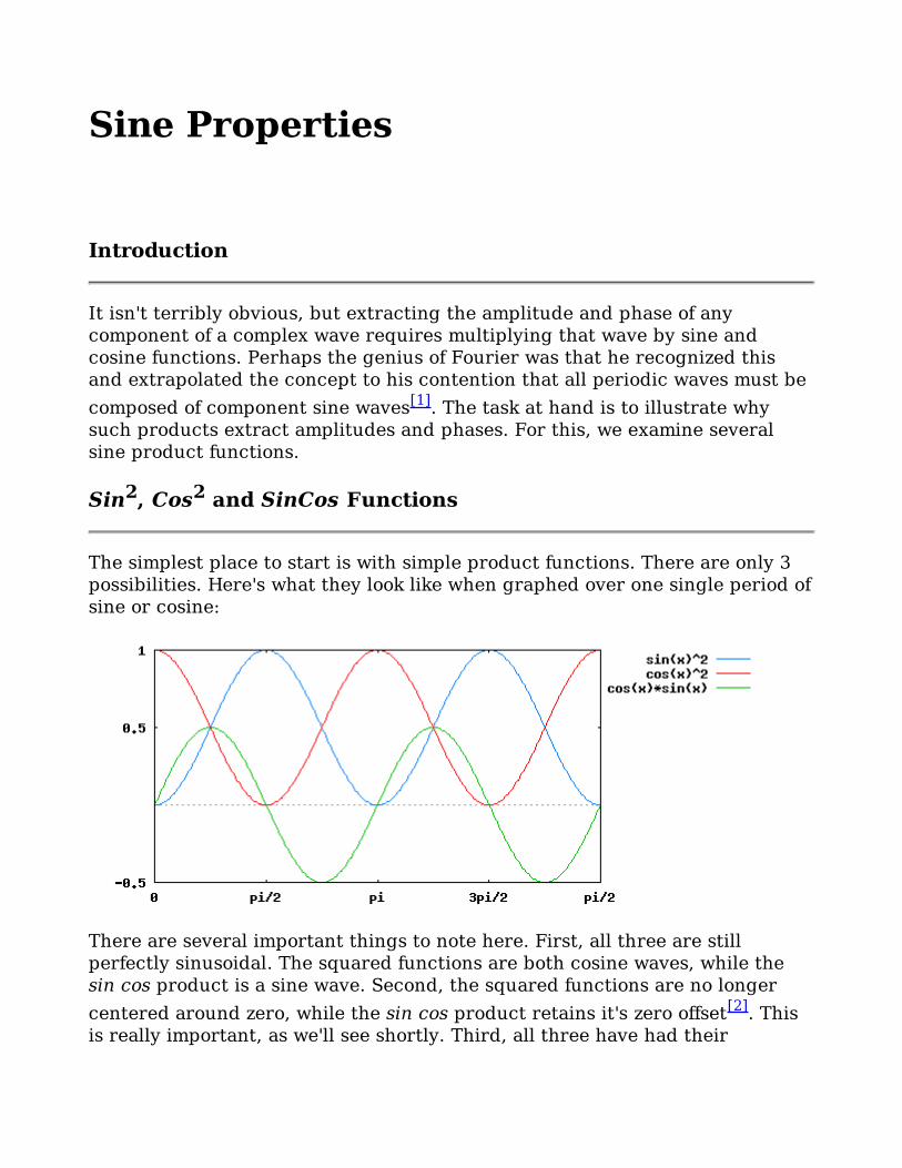
Sin2, Cos2 and SinCos Functions

The simplest place to start is with simple product functions. There are only 3possibilities. Here's what they look like when graphed over one single period ofsine or cosine:

There are several important things to note here. First, all three are stillperfectly sinusoidal. The squared functions are both cosine waves, while thesin cos product is a sine wave. Second, the squared functions are no longer

centered around zero, while the sin cos product retains it's zero offset[2]. Thisis really important, as we'll see shortly. Third, all three have had their

amplitudes reduced, by exactly a factor of 2. Finally, all are doubled infrequency. A rather interesting side effect of the multiplication. We can get allthis directly from the math by rearranging the double angle formulae:

which gives ,

which gives , and

which gives

Fejér Redux

While it should already be apparent from the above graph and the relatedfunctions, reinforcing the significance of Fejér's conjecture is a worthwhilegesture at this point. His contention was that basing the Fourier coefficients(i.e., the an's and bn's of the Fourier Series) on the mean values of product

functions would produce more robust convergence. This is illustrated clearlyin the graph. Let's look at this more formally. Pick any one frequencycomponent from our unknown waveform. Call it component n, of frequency �.

For the time being, let's ignore all the other frequencies in our waveform[3].We'll just pretend that they don't exist. Our chosen � has an amplitude An and

a phase ✁n. We already know that our selected frequency component can be

broken up into sine and cosine sub-components and this suggests that we form

two independent products: multiply our component, in turn, times unity

amplitude sine and cosine waves of the same, identical frequency. Notice what

happens. The sine product gives us , while the

cosine product give us . We can clearly see

that the mean of the sin cos products are zero[4]

. To find the mean of the

non-zero part, we need to integrate[5]

. We have the following 2 equations:

and

Which we can easily integrate by substituting the equations for sin2 and cos

2

from above:

and

Again, because we know that the mean value of the sine and cosine functionsare zero, these both simplify to:

and

That is,

and

Now, I've played a few dirty tricks on you. First, when I wrote the integrals

above, I set the limits to be from 0 to 2� / ✁[6]. If you've followed everything so

far, you should have expected that the limits would be . The point is thatthe mean of any sine or cosine cycle is exactly the same as any other, so we getthe same answer over one cycle as we do over all cycles, it's just a lot easier to

do the integral. Second. I've introduced two new variables, [7], andthese require some explanation. We've been talking about some hypotheticalunknown waveform. However, that waveform must really exist sometime,somewhere if we are going to work with it. In fact, there are 2 such waveforms.One lives in the data set that we collect from some real measurement and storeaway somewhere in the computer. The other lives in the set of equations thatcomprise the Fourier Series we are attempting to build up. The trick is makingthose the same.

That's where come in. They represent the amplitudes of thefrequency components of the real data. We generate them by physicallymultiplying sine and cosine functions together with and our waveform, point

by point, and then taking the average of each to get the mean sine product (

) and the mean cosine product ( ) for each frequency. The an's and bn's, on

the other hand, represent the cosine and sine amplitudes of the frequencycomponents of the Fourier Series we are trying to find. The last set ofequations listed above tells us the relationship between the real datacomponents and the components of the Fourier series. As such, we can use thecalculated data to determine the an's and bn's, and from these, we can compute

the amplitude and phase of each component.

It's difficult to over stress the importance of this point. The entire basis of theFourier Transform derives from this simple fact: That the amplitude of anyfrequency component present in a periodic waveform can be extracted merelyby multiplying that waveform first by a sine wave of that frequency andaveraging, then by a cosine wave of that frequency and averaging. What's leftis to show why we can - indeed that we can - ignore the other frequency

components.

Notes

� After all, one can argue that if some portion of a waveform may beremoved by extracting the component at one frequency, then whatever isleft would be further reduced with removal of more frequencies, untilsuch point is reached that nothing at all would be left - if only asu✁ciently large number of frequencies could be removed.

1.

� And zero mean! This is an excellent example of the orthogonality of sineand cosine functions: the mean of the product is exactly zero.

2.

� We'll get to those shortly anyway.3.� While we could easily prove this, for the sake of expediency, I am goingto simply accept what my eyes tell me to be true. It's an interestingexercise to show that this is in fact the case. Please feel welcome to try.

4.

� Well, we could also just infer the result we get here from thehalf-amplitude means seen in the graphs of the squared functions. I don'tdo this here because I need to illustrate the integration for later and I alsoneed to use this to introduce another concept. Read on.

5.

� That is, exactly one period of the frequency ✂. In reality, I need tocompute the integral over the full period of the fundamental.Nevertheless, I get the same answer in the presently discussed cases. Thedifference comes in when I consider other frequencies. For now, just trustthat the answer will be the same when I integrate over a full cycle of thefundamental, which I must do to cancel contributions from any otherfrequencies which may be present.

6.

� The exponent is to remind us that these represent the mean of thesquared sine and cosine functions, not that the variable is itself squared.

7.


Harmonic Properties

Introduction

Up to now, we have looked at result of sine and cosine products when the

frequencies are the same. However, when we multiply our unknown waveform

by the sine or cosine of some frequency, we are multiplying all of the frequency

components in our waveform by that sine or cosine. If we are really to believe

that this process extracts only the amplitude and phase of that one specific

frequency, then we need to show that the mean of the product of a sine or

cosine wave with a sine or cosine wave of any other frequency will be exactly

equal to zero. In other words, mean sine and cosine products must be

orthogonal for all cases except when the frequencies are the same.

First and Second Harmonic Products

The series of graphs below show the 4 possible cases of having a first harmonic

multiplied by a second harmonic.

While it is somewhat more difficult in some of these cases to see how symmetry

indicates that there will be a zero mean (that is, that the net area under each

curve is zero), after a little study, it becomes quite obvious. Nevertheless, it is

interesting to prove mathematically that this is true in at least one of these

cases. I'll choose the one that is the least easy to see from simple observation:

. First, just write the integral. As before, we only need to

compute for one period, since, by definition, all remaining periods must be

identical[1]

:

The left hand side ( ) is named in a manner analogous to the naming of the

sine square and cosine squared integrals. Note that I've also omitted reference

to which component this might be (i.e., there are no "n" subscripts and �t is

simply given as x[2]

). It doesn't matter which component, it only matters that it

is some component and its second harmonic: it could be the first and second

harmonics or the 10th

and 20th

harmonics. It matters not. To solve this, we

again fall back on substitution using one of the double angle formulas (

):

If we recall that the derivative of cos(x) is -sin(x)[3]

, then we see that

This allows direct solution of the above integral as

,

which evaluates nicely to zero.

The remaining three cases can be evaluated in an identical manner, showing

that indeed, all cases evaluate to zero. Although the math gets increasingly

tedious, one can show that exactly the same thing happens for higher and

higher harmonics. However, rather than taking this piecemeal approach, lets

go for broke and see if we can show that the mean of all sine-cosine products

with non-identical frequencies will always evaluate exactly to zero.

Notes

� The function wouldn't be periodic if this were not the case!1.

� We are free to leave out any speci✁c reference to time or frequency here

as long as we integrate over a full cycle of the lower frequency, that is,

from 0 to 2✂.

2.

� Which still, I believe, does not violate my assertion that we would

require only high school level mathematics.

3.


Orthogonality Revisited

Introduction

Our goal here is simple. We would like to show that the contention that the

phase and amplitude of some frequency component in a complex periodic wave

can be recovered from the mean sine and cosine products at that frequency. To

do this, we must be convinced that any other frequency components present in

the waveform will have no effect on the recovered phase and amplitude. What

this boils down to is finding the solutions to a few generalized integrals.

Specifically, we need to show that:

where:

a and b are two frequencies such that .

P is some suitably chosen period[1]

.[2]

are the double frequency mean sine and cosine

products.

I will only solve the first of these integrals in detail. Solutions for the remaining

three are found using an identical technique and will be cited without

derivation.

Solving the integral.

Unlike with the earlier integrals, it is not immediately obvious how to proceed

with this integral. However, the product suggests that the

solution lies somewhere in the formula for cos(a+b). Indeed, after a little

experimentation, one discovers that subtracting cos(a-b) from cos(a+b)

suggests a solution:

Making this substitution:

Which can be integrated immediately to:

or simply,

What Does It All Mean?

While it may not be immediately apparent, this is a very important result. Let's

try to disassemble this equation to see why. First, note that the numerators of

both terms are simple sine functions. Their maximum/minimum values are by

definition . This permits a very simple conclusion when the period (P) is

very large: the mean value of the sine product approaches zero. In fact, if we

extend this all the way to infinity, then we in fact will always have a mean that

is exactly zero for any product other than sin2

(i.e., when we multiply by sin(f)

to extract the phase and amplitude for frequency f[3]

. This means that the

signal we are looking at doesn't even have to be periodic over infinite time[4]

!)

What about periodic signals though? By definition, in any periodic waveform,

all frequency components that are present must be harmonics of the

fundamental frequency. That is, exactly an integer multiple of cycles must fit

into the period of the fundamental frequency. Think what it means if this were

not the case for some frequency in our signal. The very next period of the

fundamental would contain a different part of this rogue frequency - that is,

this period would be different from the last one. This would therefore not be a

periodic waveform! We might be able to make it periodic by using a different

(lower) fundamental frequency, but as it stands, it would not be periodic[5]

If we have (or assume) periodicity, then we can rewrite our solution in terms of

the fundamental frequency. f:

Where:

mf = a and nf = b

m and n are both integers

Because of the periodic nature of the sine function, the mean over any full

cycle is the same: regardless of frequency or phase, it is exactly zero. Since

m-n and m+n must be integers, if we let P be exactly one cycle of the

fundamental frequency, 2� / f, then sin((m ✁ n)2�) and sin((m + n)2�) will also

be exactly zero. The importance of this is hard to overestimate. It means that

we can make practical use of Fourier's method to analyze periodic

waveforms with the only overhead being that we must compute the

integrals of the sine and cosine products of the waveform over at least

one period of the fundamental frequency.

That one Last Thing.

I said above that I would give the solutions to all 4 of the integrals mentioned

in the introduction. So, to make things complete, here they are, without any

further comment:

Notes

� This will usually be the period of our chosen fundamental frequency.1.

� Again, the naming here is analogous to the sin2

and cos2

integrals.

However, the sine-sine and cosine-cosine products are shown as

rather than with a superscript 2, the idea being to convey the

notion that these are products of sines and cosines at 2 different

frequencies.

2.

� A word of caution: You can't get to the sin2

case from this equation

simply by setting the two frequencies equal. Setting a=b produces an

undefined result in the first term since a-b sits in the denominator. The

problem is that having a=b violates one of the assumptions that was

implicitly made when writing the integral. For the equal frequency case,

you have to refer back to the integrals written using the double angle

formulae.

3.

� Providing, of course that we are willing to deal with the rather

irritating little fact of having to compute for an infinitely long time!

4.

� We can also just tolerate any rogue frequencies, assuming that our

waveform is periodic enough. These effects of this will be discussed

shortly.

5.


Non-periodicity

Introduction

We should take a bit of time to explore what happens when we have some

frequencies in our sample waveform that don't quite fit the criteria of being an

integer harmonic of the fundamental frequency. The truth is that this is rather

inevitable. Aside from the fact that it's nearly impossible to sample even well

defined periodic waveforms precisely enough to include exact integer numbers

of periods[1]

, there are also those inevitable gremlins that creep into our signal

as noise. Noise comes in a disturbing number of varieties: high frequency

leakage of the many electromagnetic signals permeating our space, slow drift

from thermal and other vagaries of the electronics, broadband noise generated

by the very components that make up the electronics, etc. It is ever present

and unavoidable - it can only be reduced, never eliminated. If it is low enough

in frequency, relative to the frequencies of interest, it can sometimes be

removed by lumping it together with the DC component of the signal[2][3]

, but

in any case, it's really still there - we have just found a way to effectively ignore

it. The question then is: What happens to the noise in a more general sense?

Another look at

Let's drag out that integral we just finished with:

However, to keep the argument simple and clear, we'll look at only one

frequency (a) which must be a harmonic of the fundamental - in fact, it might

just as well be the fundamental - which we will normalize to 1 Hz. Then we can

simply integrate a single period of 2�. The the other frequency (b) must then

be a non-integer multiple of the fundamental, which we'll call ✁ to avoid

ambiguity with the non-normalized frequency[4]

:

If we simplify this using , and

remembering that sin(2�) = 0 and cos(2�) = 1, then we have:

, or, combining terms:

By definition, ✁ cannot be an integer and therefore ;sin(2�✁) cannot be zero.

Without belaboring the point too much, the major take home is that almost all

extraneous frequency components that are present in an otherwise periodic

waveform will not produce zero means under multiplication by sines[5]

which

are harmonics of our fundamental frequency. Thus, the cardinal assumption of

the Fourier Series for our periodic waveform is false. That is, we have assumed

that the only non-zero means are the sin2

and cos2

means that we use to

compute the coefficients of the Fourier series. However, when we actually

compute the sine and cosine products for each harmonic, every extraneous

frequency in the waveform will make some additional contribution to the mean

value. In other words, the energy in the noise will leak into the coefficients for

the legitimate harmonic terms in the series.

While this sounds bad, in practice we are not left completely without recourse.

First, some of the noise frequencies are close enough to real harmonics of our

waveform that they predominantly show up being added into those

components. As long as those components are not interesting to us, then no

harm is done. However, some components of the noise will inevitably fall at or

near components in which we are interested, resulting in real reduction of the

net signal to noise ratio. In fact, we cannot distinguish these noise components

from our signal at all - well, not quite. We do have at least one other trick at

our disposal.

Noise is, by definition, random. It therefore makes a different contribution to

each subsequent period of our fundamental waveform. This is our second point.

In almost all cases, we can extend our waveform to include more than one

complete period[6]

simply by sampling for a longer period of time. Some of

what's added in one period gets subtracted in the next[7]

. If we look at a large

enough number of cycles, we can reduce noise to an almost arbitrary extent[8]

.

Notes

� This is an interesting topic in and of itself. It results in the introduction

of discontinuities at the ends of the sampled waveform. Mathematically, it

is rather like multiplying your true signal with a square wave whose

period is the sampling window width. In fact, the Fourier series of a

square wave shows up in the Fourier series of your signal. While a

discussion of this is outside the intent of this monograph, whole textbooks

have been written on the subject. I refer you to those for further details.

The Ramirez book is quite good in this regard.

1.

� Note that any "DC" offsets in our signal are not to be considered noise.

This is a real component of the signal and shows up as the very first term

in the Fourier series.

2.

� Better yet, it we happen to know the frequency of the noise, then we

can force it to appear at DC by means of intentional aliasing - i.e.

sampling at exactly the noise frequency!

3.

� Given that we have normalized the fundamental to 1 Hz, ✁ simply

reflects the second frequency normalized by f, that is, ✁=b/f.

4.

� The same thing is obviously true of the cosine products.5.

� That is, we can artificially lower the fundamental frequency.6.

� Another way of looking at this is that by lengthening the sampling

period (i.e., lower and lower fundamental frequency) we can include more

and more possible frequencies as legitimate harmonics, which will now

properly accept their own share of the total waveform.

7.

� Well, there are caveats. If one could sample for the hypothetical infinite

period, then noise is at least put in it's place. That is to say that all of the

energy in the signal that is made up by noise will at least appear in the

right place in the spectrum, rather than being added into other frequency

components. However, the part that falls at the same place as our signal

will still be irritating us. It's just that usually there is so little noise at any

one specific frequency that we care less and less about it. While we can't

sample for an infinite period, usually we can sample for long enough to

achieve useful results.

8.


Fourier Afterword

Imaginary Numbers

Let's have another look at the Fourier transform pair given in the introduction:

and

Two things stand out on closer inspection. First, it's written in terms of an

exponential (eu), and second, the exponential has an imaginary variable ( �

j2✁ft)[1]

. On the other hand, we've written the series in terms of a sum of sines

and cosines, with no imaginary part at all:

Certainly, some kind of resolution must be made before finishing this topic.

Taylor Series

Keeping with the high school math paradigm[2]

, let's write the Taylor's series

for each of our culprit functions. These are commonly known and should

already be familiar to most readers:

The series for ex

is tantalizingly close to being the sum of sin(x) and cos(x). It's

just those nasty negative signs that are getting in the way. However, if we

make the argument to the exponential imaginary,

Remembering that , then this becomes:

Which is exactly the sum of cos(x) and j sin(x):

This is in fact Euler's formula. If we rewrite the transform integral in terms of

the sine and cosine,

the result looks remarkably similar to the Fourier series as stated above. In

fact, the series is usually written with the imaginary operator, which allows the

coefficients of each term to be given as a single complex number equal to an �

jbn.

Notes

✁ Note the use of j for the imaginary operator. It turns out that

engineering people prefer the use of j, but mathematicians prefer the use

of i. While i may appear more natural - and indeed is probably more

familiar to the average reader - the conflicting use of i to mean electrical

current causes considerable confusion. For this reason, the traditional use

of j is adhered to in this document.

1.

✁ Well, I learned about Taylor's series in high school.2.


Documents

AC Signal Processing