arX

iv:1

103.

4023

v1 [

stat

.ML

] 2

1 M

ar 2

011

Additive Kernels for Gaussian Process Modeling

N. Durrande∗‡, D. Ginsbourger†, O. Roustant ∗

January 12, 2010

Abstract

Gaussian Process (GP) models are often used as mathematical ap-proximations of computationally expensive experiments. Provided thatits kernel is suitably chosen and that enough data is available to obtaina reasonable fit of the simulator, a GP model can beneficially be usedfor tasks such as prediction, optimization, or Monte-Carlo-based quantifi-cation of uncertainty. However, the former conditions become unrealisticwhen using classical GPs as the dimension of input increases. One popularalternative is then to turn to Generalized Additive Models (GAMs), re-lying on the assumption that the simulator’s response can approximatelybe decomposed as a sum of univariate functions. If such an approach hasbeen successfully applied in approximation, it is nevertheless not com-pletely compatible with the GP framework and its versatile applications.The ambition of the present work is to give an insight into the use ofGPs for additive models by integrating additivity within the kernel, andproposing a parsimonious numerical method for data-driven parameterestimation. The first part of this article deals with the kernels naturallyassociated to additive processes and the properties of the GP models basedon such kernels. The second part is dedicated to a numerical procedurebased on relaxation for additive kernel parameter estimation. Finally, theefficiency of the proposed method is illustrated and compared to otherapproaches on Sobol’s g-function.

keyword Kriging, Computer Experiment, Additive Models, GAM, MaximumLikelihood Estimation, Relaxed Optimization, Sensitivity Analysis

∗CROCUS - Ecole Nationale Superieure des Mines de St-Etienne29 rue Ponchardier - 42023 St Etienne, France

†Institute of Mathematical Statistics and Actuarial Science, University of Berne,Alpeneggstrasse 22 - 3012 Bern, Switzerland,

‡Corresponding author: durrande@emse.fr

1

1 Introduction

The study of numerical simulators often deals with calculation intensive com-puter codes. This cost implies that the number of evaluations of the numericalsimulator is limited and thus many methods such as uncertainty propagation,sensitivity analysis, or global optimization are unaffordable. A well known ap-proach to circumvent time limitations is to replace the numerical simulator bya mathematical approximation called metamodel (or response surface or sur-rogate model) based on the responses of the simulator for a limited numberof inputs called the Design of Experiments (DoE). There is a large number ofmetamodels types and among the most popular we can cite regression, splines,neural networks... In this article, we focus on a particular type of metamodel:the Kriging method, more recently referred to as Gaussian Process modeling[11]. Originally presented in spatial statistics [2] as an optimal Linear Unbi-ased Predictor (LUP) of random processes, Kriging has become very popularin machine learning, where its interpretation is usually restricted to the conve-nient framework of Gaussian Processes (GP). Beyond the LUP —which thenelegantly coincides with a conditional expectation—, the latter GP interpreta-tion allows indeed the explicit derivation of conditional probability distributionsfor the response values at any point or set of points in the input space.

The classical Kriging method faces two issues when the number of dimen-sions d of the input space D ⊂ R

d becomes high. Since this method is basedon neighborhoods, it requires an increasing number of points in the DoE tocover the domain D. The second issue is that the number of anisotropic kernelparameters to be estimated increases with d so that the estimation becomes par-ticularly difficult for high dimensional input spaces [3, 4]. An approach to getaround the first issue is to consider specific features lowering complexity suchas the family of Additive Models. In this case, the response can approximatelybe decomposed as a sum of univariate functions:

f(x) = µ+

d∑

i=1

fi(xi), (1)

where µ ∈ R and the fi’s may be non-linear. Since their introduction by Stonesin 1985 [5], many methods have been proposed for the estimation of additivemodels. We can cite the method of marginal integration [6] and a very popularmethod described by Hastie and Tibshirani in [8, 7]: the GAM backfitting algo-rithm. However, those methods do not consider the probabilistic framework ofGP modeling and do not usually provide additional information such as the pre-diction variance. Combining the high-dimensional advantages of GAMs with theversatility of GPs is the main goal of the present work. For the study functionsthat contain an additive part plus a limited number of interactions, an extensionof the present work can be found in the recent paper of T. Muehlenstaedt [1].

The first part of this paper focuses on the case of additive Gaussian Pro-cesses, their associated kernels and the properties of associated additive kriging

2

models. The second part deals with a Relaxed Likelihood Maximization (RLM)procedure for the estimation of kernel parameters for Additive Kriging models.Finally, the proposed algorithm is compared with existing methods on a wellknown test function: the Sobol’s g-function [9]. It is shown within the latterexample that Additive Kriging with RLM outperforms standard Kriging andproduce similar performances as GAM. Due to its approximation performanceand its built-in probabilistic framework both demonstrated later in this arti-cle, the proposed Additive Kriging model appears as a serious and promisingchallenger among additive models.

2 Towards Additive Kriging

2.1 Additive random processes

Lets first introduce the mathematical construction of an additive GP. A functionf : D ⊂ R

d −→ R is additive when it can be written f(x) =∑di=1 fi(xi), where

xi is the i-th component of the d-dimensional input vector x and the fi’s arearbitrary univariate functions. Let us first consider two independent real-valuedfirst order stationary processes Z1 and Z2 defined over the same probabilityspace (Ω,F , P ) and indexed by R, so that their trajectories Zi(.;ω) : x ∈ R −→Zi(x;ω) are univariate real-valued functions. Let Ki : R × R −→ R be theirrespective covariance kernels and µ1, µ2 ∈ R their means. Then, the processZ := Z1 + Z2 defined over (Ω,F , P ) and indexed by R

2, and so that

∀ω ∈ Ω ∀x ∈ R2 Z(x;ω) = Z1(x1;ω) + Z2(x2;ω), (2)

has mean µ = µ1 + µ2 and kernel K(x,y) = K1(x1, y1) +K2(x2, y2). Followingequation 2, the latter sum process clearly has additive paths. In this document,we call additive any kernel of the form K : (x,y) ∈ R

d × Rd −→ K(x,y) =

∑di=1Ki(xi, yi) where the Ki’s are semi-positive definite (s.p.d.) symmetric

kernels over R× R. Although not commonly encountered in practice, it is wellknown that such a combination of s.p.d kernels is also a s.p.d. kernel in thedirect sum space [11]. Moreover, one can show that the paths of any randomprocess with additive kernel are additive in a certain sens:

Proposition 1. Any (square integrable) random process Zx possessing an ad-ditive kernel is additive up to a modification. In essence, it means that thereexists a process Ax which paths are all additive, and such that ∀x ∈ X, P(Zx =Ax) = 1.

The proof of this property is given in appendix for d = 2. For d = n

the proof follows the same pattern but the notations are more cumbersome.Note that the class of additive processes is not actually limited to processeswith additive kernels. For example, let us consider Z1 and Z2 two correlatedGaussian processes on (Ω,F , P ) such that the couple (Z1, Z2) is Gaussian. ThenZ1(x1) + Z2(x2) is also a Gaussian process with additive paths but its kernelis not additive. However, in the next section, the term additive process willalways refer to GP with additive kernels.

3

2.2 Invertibility of covariance matrices

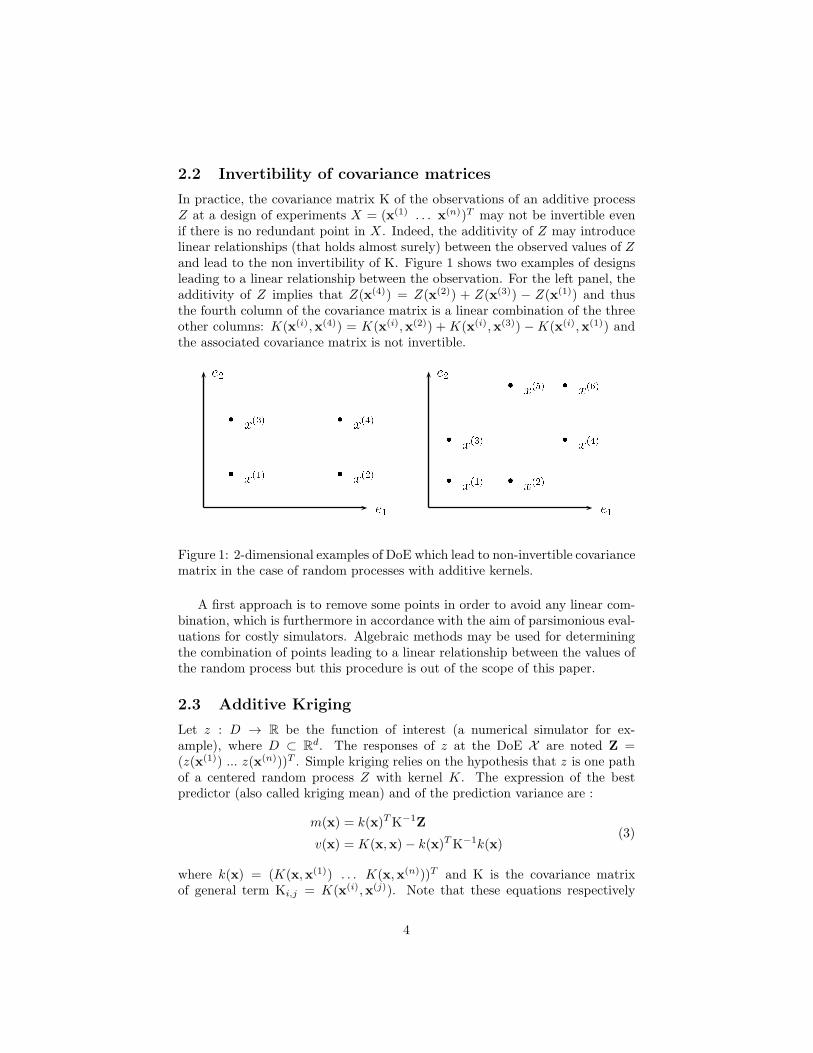
In practice, the covariance matrix K of the observations of an additive processZ at a design of experiments X = (x(1) . . . x(n))T may not be invertible evenif there is no redundant point in X . Indeed, the additivity of Z may introducelinear relationships (that holds almost surely) between the observed values of Zand lead to the non invertibility of K. Figure 1 shows two examples of designsleading to a linear relationship between the observation. For the left panel, theadditivity of Z implies that Z(x(4)) = Z(x(2)) + Z(x(3)) − Z(x(1)) and thusthe fourth column of the covariance matrix is a linear combination of the threeother columns: K(x(i),x(4)) = K(x(i),x(2)) +K(x(i),x(3)) −K(x(i),x(1)) andthe associated covariance matrix is not invertible.

Figure 1: 2-dimensional examples of DoE which lead to non-invertible covariancematrix in the case of random processes with additive kernels.

A first approach is to remove some points in order to avoid any linear com-bination, which is furthermore in accordance with the aim of parsimonious eval-uations for costly simulators. Algebraic methods may be used for determiningthe combination of points leading to a linear relationship between the values ofthe random process but this procedure is out of the scope of this paper.

2.3 Additive Kriging

Let z : D → R be the function of interest (a numerical simulator for ex-ample), where D ⊂ R

d. The responses of z at the DoE X are noted Z =(z(x(1)) ... z(x(n)))T . Simple kriging relies on the hypothesis that z is one pathof a centered random process Z with kernel K. The expression of the bestpredictor (also called kriging mean) and of the prediction variance are :

m(x) = k(x)TK−1Z

v(x) = K(x,x)− k(x)TK−1k(x)(3)

where k(x) = (K(x,x(1)) . . . K(x,x(n)))T and K is the covariance matrixof general term Ki,j = K(x(i),x(j)). Note that these equations respectively

4

correspond to the conditional expectation and variance in the case of a GP withknown kernel. In practice, the structure of k is supposed known (e.g. power-exponential or Matern families) but its parameters are unknown. A commonway to estimate them is to maximize the likelihood of the kernel parametersgiven the observations Z [12, 11].

Equations 3 are valid for any s.p.d kernel, thus they can be applied with additivekernels. In this case, the additivity of the kernel implies the additivity of thekriging mean: for example in dimension 2, for K(x,y) = K1(x1, y1)+K2(x2, y2)we have

m(x) = (k1(x1) + k2(x2))T (K1 +K2)

−1Z

= k1(x1)T (K1 +K2)

−1Z+ k2(x2)T (K1 +K2)

−1Z

= m1(x1) +m2(x2).

(4)

Another interesting property concerns the variance: v can be null at points thatdo not belong to the DoE. Let us consider a two dimensional example wherethe DoE is composed of the 3 points represented on the left pannel of figure 1:X = x(1) x(2) x(3). Direct calculations presented in Appendix B shows thatthe prediction variance at the point x(4) is equal to 0. This particularity followsfrom the fact that the value of the additive process are known almost surely atthe point x(4) based on the observations at X . In the next section, we illustratethe potential of Additive Kriging on an example and propose an algorithm forparameter estimation.

2.4 Illustration and further consideration on a 2D exam-ple

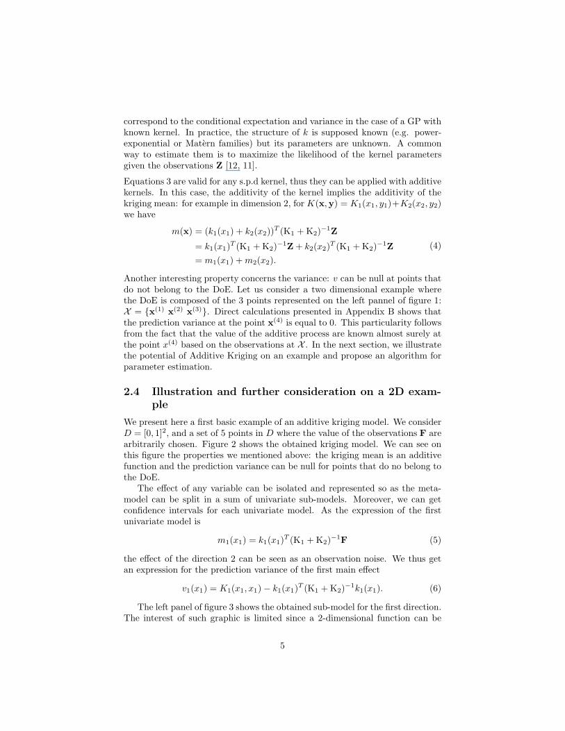
We present here a first basic example of an additive kriging model. We considerD = [0, 1]2, and a set of 5 points in D where the value of the observations F arearbitrarily chosen. Figure 2 shows the obtained kriging model. We can see onthis figure the properties we mentioned above: the kriging mean is an additivefunction and the prediction variance can be null for points that do no belong tothe DoE.

The effect of any variable can be isolated and represented so as the meta-model can be split in a sum of univariate sub-models. Moreover, we can getconfidence intervals for each univariate model. As the expression of the firstunivariate model is

m1(x1) = k1(x1)T (K1 +K2)

−1F (5)

the effect of the direction 2 can be seen as an observation noise. We thus getan expression for the prediction variance of the first main effect

v1(x1) = K1(x1, x1)− k1(x1)T (K1 +K2)

−1k1(x1). (6)

The left panel of figure 3 shows the obtained sub-model for the first direction.The interest of such graphic is limited since a 2-dimensional function can be

5

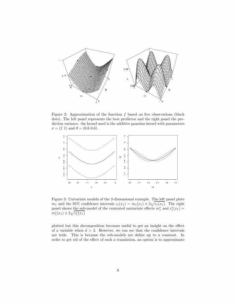
Figure 2: Approximation of the function f based on five observations (blackdots). The left panel represents the best predictor and the right panel the pre-diction variance. the kernel used is the additive gaussian kernel with parametersσ = (1 1) and θ = (0.6 0.6).

Figure 3: Univariate models of the 2-dimensional example. The left panel plotsm1 and the 95% confidence intervals c1(x1) = m1(x1) ± 2

√

v1(x1). The rightpanel shows the sub-model of the centrated univariate effects m∗

1 and c∗1(x1) =m∗

1(x1)± 2√

v∗1(x1)

plotted but this decomposition becomes useful to get an insight on the effectof a variable when d > 2. However, we can see that the confidence intervalsare wide. This is because the sub-models are define up to a constant. Inorder to get rid of the effect of such a translation, an option is to approximate

6

Zi(xi)−∫

Zi(si)dsi conditionally to the observations:

m∗

i (xi) = E

[

Zi(xi)−

∫

Zi(si)dsi

∣

∣

∣

∣

Z(X) = Y

]

v∗i (xi) = var

[

Zi(xi)−

∫

Zi(si)dsi

∣

∣

∣

∣

Z(X) = Y

] (7)

The expression of m∗

i (xi) is straightforward whereas v∗i (xi) requires more cal-culations which are given in Appendix C.

m∗

i (xi) = mi(xi)−

∫

mi(si)dsi

v∗i (xi) = vi(xi)− 2

∫

Ki(xi, si)dsi + 2

∫

ki(xi)TK−1ki(si)dsi

+

∫∫

Ki(si, ti)dsidti −

∫∫

ki(ti)TK−1ki(si)dsidti

(8)

The benefits of using m∗

i and v∗i and then to define the sub-models up to aconstant can be seen on the right panel of figure 3. At the end, the probabilisticframework gives an insight on the error of the metamodel but also of each sub-model.

3 Parameter estimation

3.1 Maximum likelihood estimation (MLE)

MLE is a standard way to estimate covariance parameters and it is covered indetail in the literature [11, 13]. Let Y be a centered additive Process and ψi =σ2

i , θi with i ∈ 1, . . . , d the parameters of the univariate kernels. Accordingto the MLE methodology, the best values ψ∗

i for the parameters ψi are thevalues maximizing the likelihood of the observations Y:

L(ψ1, . . . , ψd) :=1

(2π)n/2

det(K(ψ))1/2

exp

(

−1

2YTK(ψ)−1Y

)

(9)

where K(ψ) = K1(ψ1)+ · · ·+Kd(ψd) is the covariance matrix depending on theparameters ψi. The latter maximization problem is equivalent to the usuallypreferred minimization of

l(ψ1, . . . , ψd) := log(det(K(ψ))) + YTK(ψ)−1Y (10)

Obtaining the optimal parameters ψ∗

i relies on the succesful use of a non-convexglobal optimization routine. This can be severely hindered for large values of dsince the search space of kernel parameters becomes high dimensional. One wayto cope with this issue is to separate the variables and split the optimizationinto several low-dimensional subproblems.

7

3.2 The Relaxed Likelihood Maximization algorithm

The aim of the Relaxed Likelihood Maximization (RLM) algorithm is to treatseparately the optimization in each direction. In this way, RLM can be seenas a cyclic relaxation optimization procedure [14] with initial values of the pa-rameters σ2

i set to zero. As we will see, the main originality here is to considera kriging model with an observation noise variance τ2 that fluctuates duringthe optimization. This parameter account for the metamodel error (if the func-tion is not additive for example) but also for the inaccuracy of the intermediatevalues of σi and θi.

The first step of the algorithm is to estimate the parameters of the kernel K1.The simplification of the method is to consider that all the variations of Y inthe other directions can be summed up as a white noise. Under this hypothesis,l depends on ψ1 and τ :

l(ψ1, τ) = log(det(K1(ψ1) + τ2Id)) +YT (K1(ψ1) + τ2Id)−1Y (11)

Then, the couple ψ∗

1 , τ∗ that maximizes l(ψ1, τ) can be obtained by numerical

optimization.The second step of the algorithm consists in estimating ψ2, with ψ1 fixed to ψ∗

1 :

ψ∗

2 , τ∗ =argmax

ψ2,τ(l(ψ∗

1 , ψ2, τ)), with

l(ψ∗

1 , ψ2, τ) =log(det(K1(ψ∗

1) + K2(ψ2) + τ2Id))+

YT (K1(ψ∗

1) + K2(ψ2) + τ2Id)−1Y

(12)

This operation can be repeated for all the directions until the estimation ofψd. However, even if all the parameters ψi have been estimated, it is fruitful tore-estimate them such that the estimation of the parameter ψi can benefit of thevalues ψ∗

j for j > i. Thus, the algorithm is composed of a cycle of estimationsthat treat each direction one after each other:

RLM Algorithm :

1. Initialize the values σ(0)i = 0 for i ∈ 1, . . . , d

2. For k from 1 to number of iteration do3. For l from 1 to d do4. ψ

(k)l , τ (k) = argmin

ψl,τ(lc(ψ

(k)1 , . . . , ψ

(k)l−1, ψl, ψ

(k−1)l+1 , . . . , ψ

(k−1)d , τ))

5. End For6. End For

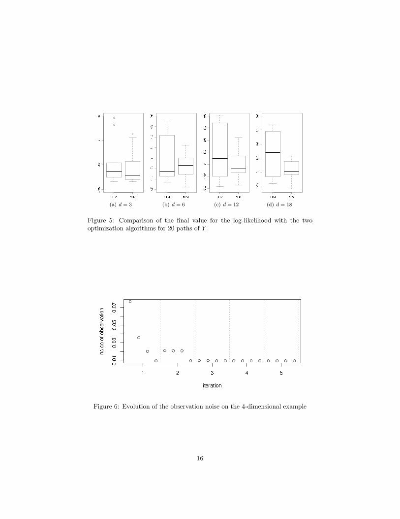
τ is a parameter tuning the fidelity of the metamodel since for τ = 0 thekriging mean interpolates the data. In practice, this parameter is decreasing atalmost each new estimation. Depending on the observations and on the DoE,τ converges either to a constant or to zero (cf. the g-function example andfigure 6). When zero is not reached, τ2 should correspond to the part of thevariance that cannot be explained by the additive model. Thus, the comparison

8

between τ2 and the σ2i allows us to quantify the degree of additivity of the

objective function according to the metamodel.

This procedure of estimation is not meant to be applied for kernels that are notadditive. The method developed by Welch for tensor product kernels in [10] hassimilarities since it corresponds to a sequential estimation of the parameters.One interesting feature of Welch’s algorithm is to choose at each step the bestsearch direction for the parameters. The RLM algorithm could easily be adaptedin a similar way to improve the quality of the results but the correspondingadapted version would be much more time consuming.

4 Comparison between the optimization’s meth-

ods

The aim of this section is to compare the RLM algorithm to the Usual Like-lihood Maximization (ULM). The test functions that are considered are pathsof an additive GP Y with Gaussian additive kernel K. For this example, theparameters of K are fixed to σi = 1, θi = 0.2 for i ∈ 1 . . . d but those values aresupposed to be unknown.Here, 2 × d + 1 parameters have to be estimated: d for the variances, d forthe range and 1 for the noise variance τ2. For ULM, they are estimated si-multaneously, whereas the RLM is a 3-dimensional optimization at each step.In both cases, we use the L-BFGS-B method of the function optim with the R

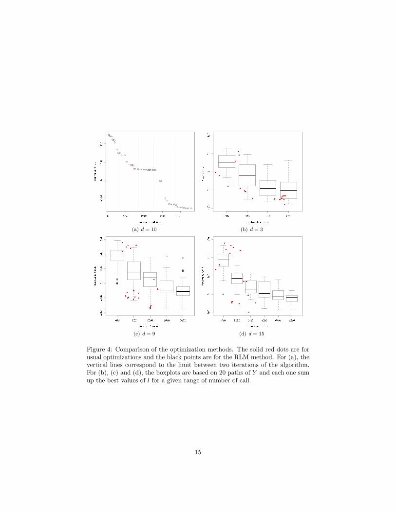
software. To judge the effectiveness of the algorithms, we compare here the bestvalue found for the log-likelihood l to the computational budget (the numberof call to l) required for the optimization. As the optim function returns thenumber nc of call to l and the best value bv at the end of each optimization,we obtain for the MLE on one path of Y one value of nc and bv for ULM andnb iteration× d values of nv and bv for RLM since there is one optimization ateach step of each iteration.The panel (a) of figure 4 presents the results for the two optimizations on apath of a GP for d = 5. On this example, we can see that ULM needs 1500 callsto the log-likelihood before convergence whereas RLM requires much more callsbefore convergence. However, the result of the two methods are similar for 1500calls but the result of RLM after 5000 calls is substantially improved. In orderto get more robust results we simulate 20 paths of Y and we observe the globaldistribution of the variables nv and bv. Furthermore, we study the evolutionof the algorithm performances when the dimension increases choosing variousvalues for the parameter d from 3 to 18 with a Latin Hypercube (LH) Designwith maximin criteria [13] containing 10× d points. We observe on the panels(b), (c) and (d) of figure 4 that optimization with the RLM requires more callsto the function l, but this method appears to be more efficient and robust thanULM. Those results are stressed by figure 5 where the final best value of RLMand ULM are compared. This figure also shows that the advantage of usingRLM comes bigger when d is getting larger.

9

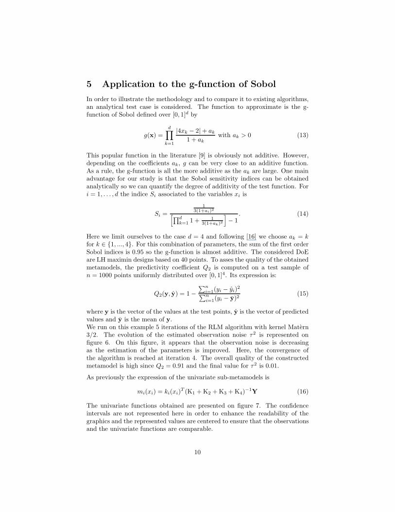
5 Application to the g-function of Sobol

In order to illustrate the methodology and to compare it to existing algorithms,an analytical test case is considered. The function to approximate is the g-function of Sobol defined over [0, 1]d by

g(x) =

d∏

k=1

|4xk − 2|+ ak

1 + akwith ak > 0 (13)

This popular function in the literature [9] is obviously not additive. However,depending on the coefficients ak, g can be very close to an additive function.As a rule, the g-function is all the more additive as the ak are large. One mainadvantage for our study is that the Sobol sensitivity indices can be obtainedanalytically so we can quantify the degree of additivity of the test function. Fori = 1, . . . , d the indice Si associated to the variables xi is

Si =

13(1+ai)2

[

∏dk=1 1 +

13(1+ak)2

]

− 1. (14)

Here we limit ourselves to the case d = 4 and following [16] we choose ak = k

for k ∈ 1, ..., 4. For this combination of parameters, the sum of the first orderSobol indices is 0.95 so the g-function is almost additive. The considered DoEare LH maximin designs based on 40 points. To asses the quality of the obtainedmetamodels, the predictivity coefficient Q2 is computed on a test sample ofn = 1000 points uniformly distributed over [0, 1]4. Its expression is:

Q2(y, y) = 1−

∑ni=1(yi − yi)

2

∑ni=1(yi − y)2

(15)

where y is the vector of the values at the test points, y is the vector of predictedvalues and y is the mean of y.We run on this example 5 iterations of the RLM algorithm with kernel Matern3/2. The evolution of the estimated observation noise τ2 is represented onfigure 6. On this figure, it appears that the observation noise is decreasingas the estimation of the parameters is improved. Here, the convergence ofthe algorithm is reached at iteration 4. The overall quality of the constructedmetamodel is high since Q2 = 0.91 and the final value for τ2 is 0.01.

As previously the expression of the univariate sub-metamodels is

mi(xi) = ki(xi)T (K1 +K2 +K3 +K4)

−1Y (16)

The univariate functions obtained are presented on figure 7. The confidenceintervals are not represented here in order to enhance the readability of thegraphics and the represented values are centered to ensure that the observationsand the univariate functions are comparable.

10

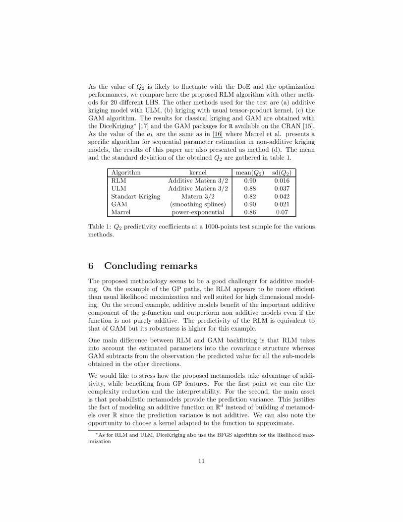
As the value of Q2 is likely to fluctuate with the DoE and the optimizationperformances, we compare here the proposed RLM algorithm with other meth-ods for 20 different LHS. The other methods used for the test are (a) additivekriging model with ULM, (b) kriging with usual tensor-product kernel, (c) theGAM algorithm. The results for classical kriging and GAM are obtained withthe DiceKriging∗ [17] and the GAM packages for R available on the CRAN [15].As the value of the ak are the same as in [16] where Marrel et al. presents aspecific algorithm for sequential parameter estimation in non-additive krigingmodels, the results of this paper are also presented as method (d). The meanand the standard deviation of the obtained Q2 are gathered in table 1.

Algorithm kernel mean(Q2) sd(Q2)RLM Additive Matern 3/2 0.90 0.016ULM Additive Matern 3/2 0.88 0.037Standart Kriging Matern 3/2 0.82 0.042GAM (smoothing splines) 0.90 0.021Marrel power-exponential 0.86 0.07

Table 1: Q2 predictivity coefficients at a 1000-points test sample for the variousmethods.

6 Concluding remarks

The proposed methodology seems to be a good challenger for additive model-ing. On the example of the GP paths, the RLM appears to be more efficientthan usual likelihood maximization and well suited for high dimensional model-ing. On the second example, additive models benefit of the important additivecomponent of the g-function and outperform non additive models even if thefunction is not purely additive. The predictivity of the RLM is equivalent tothat of GAM but its robustness is higher for this example.

One main difference between RLM and GAM backfitting is that RLM takesinto account the estimated parameters into the covariance structure whereasGAM subtracts from the observation the predicted value for all the sub-modelsobtained in the other directions.

We would like to stress how the proposed metamodels take advantage of addi-tivity, while benefiting from GP features. For the first point we can cite thecomplexity reduction and the interpretability. For the second, the main assetis that probabilistic metamodels provide the prediction variance. This justifiesthe fact of modeling an additive function on R

d instead of building d metamod-els over R since the prediction variance is not additive. We can also note theopportunity to choose a kernel adapted to the function to approximate.

∗As for RLM and ULM, DiceKriging also use the BFGS algorithm for the likelihood max-imization

11

At the end, the proposed methodology is fully compatible with Kriging-basedmethods and its versatile applications. For example, one can choose a wellsuited kernel for the function to approximate or use additive kriging for high-dimensional optimization strategies relying on the expecting improvement cri-teria.

References

[1] T. Muehlenstaedt, O. Roustant, L. Carraro, S. Kuhnt, Data-driven Krigingmodels based on FANOVA-decomposition. Technical report. 201

[2] N. Cressie, Statistics for Spatial Data, Wiley Series in Probability andMathematical Statistics, 1993.

[3] K.-T. Fang, R. Li, A. Sudjianto, Design and modeling for computer exper-iments, Chapman & Hall, 2006.

[4] A. OHagan, Bayesian analysis of computer code outputs: A tutorial, Reli-ability Engineering and System Safety 91.

[5] C. Stone, Additive regression and other nonparametric models, The annalsof Statistics, Vol. 13, No. 2. (1985) 689–705.

[6] W. Newey, Kernel estimation of partial means and a general variance esti-mator, Econometric Theory (1994) 233–253.

[7] T. Hastie, R. Tibshirani, Generalized Additive Models, Monographs onStatistics and Applied Probability, 1990.

[8] A. Buja, T. Hastie, R .Tibshirani, Linear Smoothers and Additive Models,The Annals of Statistics, Vol. 17, No. 2. (1989), 453–510.

[9] A. Saltelli, K. Chan, E. Scott, Sensitivity analysis, Wiley Series in Proba-bility and Statistics, 2000.

[10] W. J. Welch, R. J. Buck, J. Sacks, H. P. Wynn, T. J. Mitchell, M. D.Morris, Screening, predicting, and computer experiments, Technometrics34 (1992) 15–25.

[11] C. Rasmussen, C. Williams, Gaussian Processes for Machine Learning, MITPress, 2006.

[12] D. Ginsbourger, D. Dupuy, A. Badea, O. Roustant, L. Carraro, A noteon the choice and the estimation of kriging models for the analysis of de-terministic computer experiments, Applied Stochastic Models for Businessand Industry 25 (2009) 115 –131.

[13] T. J. Santner, B. Williams, W. Notz, The Design and Analysis of ComputerExperiments, Springer-Verlag, 2003.

12

[14] M. Minoux, Mathematical Programming: Theory and Algorithm, JohnWiley & Sons, 1986.

[15] R Development core team, R: A Language and Environment for StatisticalComputing, http://www.R-project.org, 2010.

[16] A. Marrel, B. Iooss, F. Van Dorpe, E. Volkova, An efficient methodology formodeling complex computer codes with gaussian processes, ComputationalStatistics and Data Analysis, 52 52 (2008) 4731–4744.

[17] O. Roustant, D. Ginsbourger, Y. Deville, The DiceKriging package:kriging-based metamodeling and optimization for computer experiments,in: Book of abstract of the R User Conference. Package available atwww.dice-consortium.fr, 2009.

Appendix A: Proof of proposition 1 for d = 2

Let Z be a random process indexed by R2 with kernel K(x,y) = K1(x1, y1) +

K2(x2, y2), and ZT the random process defined by ZT (x1, x2) = Z(x1, 0) +Z(0, x2) − Z(0, 0). By construction, the paths of ZT are additive functions.In order to show the additivity of the paths of Z, we will show that ∀x ∈R

2, P(Z(x) = ZT (x)) = 1. For the sake of simplicity, the three terms ofvar[Z(x) − ZT (x)] = var[Z(x)] + var[ZT (x)] − 2cov[Z(x), ZT (x)] are studiedseparately:

var[Z(x)] = K(x,x)

var[ZT (x)] = var[Z(x1, 0) + Z(0, x2)− Z(0, 0)]

= var[Z(x1, 0)] + var[Z(0, x2)] + 2cov[Z(x1, 0), Z(0, x2)]

+ var[Z(0, 0)]− 2cov[Z(x1, 0), Z(0, 0)]− 2cov[Z(0, x2), Z(0, 0)]

= K1(x1, x1) +K2(0, 0) +K1(0, 0) +K2(x2, x2) +K(0, 0)

+ 2 (K1(x1, 0) +K2(0, x2))− 2 (K1(x1, 0) +K2(0, 0))

− 2 (K1(0, 0) +K2(x2, 0))

= K1(x1, x1) +K2(x2, x2) = K(x,x)

cov[Z(x), ZT (x)] = cov[Z(x1, x2), Z(x1, 0) + Z(0, x2)− Z(0, 0)]

= K1(x1, x1) +K2(x2, 0) +K1(x1, 0) +K2(x2, x2)

−K1(x1, 0)−K2(x2, 0)

= K1(x1, x1) +K2(x2, x2) = K(x,x)

Those three equations implies that var[Z(x) − ZT (x)] = 0, ∀x ∈ R2. Thus,

P(Z(x) = ZT (x)) = 1 and there exists a modification of Z with additive paths.

13

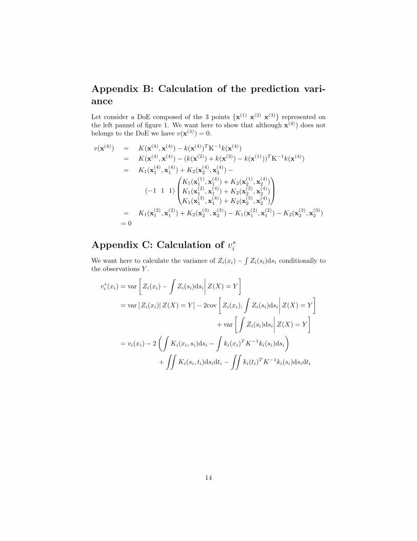
Appendix B: Calculation of the prediction vari-ance

Let consider a DoE composed of the 3 points x(1) x(2) x(3) represented onthe left pannel of figure 1. We want here to show that although x(4)) does notbelongs to the DoE we have v(x(4)) = 0.

v(x(4)) = K(x(4),x(4))− k(x(4))TK−1k(x(4))

= K(x(4),x(4))− (k(x(2)) + k(x(3))− k(x(1)))TK−1k(x(4))

= K1(x(4)1 ,x

(4)1 ) +K2(x

(4)2 ,x

(4)2 )−

(−1 1 1)

K1(x(1)1 ,x

(4)1 ) +K2(x

(1)2 ,x

(4)2 )

K1(x(2)1 ,x

(4)1 ) +K2(x

(2)2 ,x

(4)2 )

K1(x(3)1 ,x

(4)1 ) +K2(x

(3)2 ,x

(4)2 )

= K1(x(2)1 ,x

(2)1 ) +K2(x

(3)2 ,x

(3)2 )−K1(x

(2)1 ,x

(2)1 )−K2(x

(3)2 ,x

(3)2 )

= 0

Appendix C: Calculation of v∗i

We want here to calculate the variance of Zi(xi) −∫

Zi(si)dsi conditionally tothe observations Y .

v∗i (xi) = var

[

Zi(xi)−

∫

Zi(si)dsi

∣

∣

∣

∣

Z(X) = Y

]

= var [Zi(xi)|Z(X) = Y ]− 2cov

[

Zi(xi),

∫

Zi(si)dsi

∣

∣

∣

∣

Z(X) = Y

]

+ var

[∫

Zi(si)dsi

∣

∣

∣

∣

Z(X) = Y

]

= vi(xi)− 2

(∫

Ki(xi, si)dsi −

∫

ki(xi)TK−1ki(si)dsi

)

+

∫∫

Ki(si, ti)dsidti −

∫∫

ki(ti)TK−1ki(si)dsidti

14

(a) d = 10 (b) d = 3

(c) d = 9 (d) d = 15

Figure 4: Comparison of the optimization methods. The solid red dots are forusual optimizations and the black points are for the RLM method. For (a), thevertical lines correspond to the limit between two iterations of the algorithm.For (b), (c) and (d), the boxplots are based on 20 paths of Y and each one sumup the best values of l for a given range of number of call.

15

(a) d = 3 (b) d = 6 (c) d = 12 (d) d = 18

Figure 5: Comparison of the final value for the log-likelihood with the twooptimization algorithms for 20 paths of Y .

Figure 6: Evolution of the observation noise on the 4-dimensional example

16

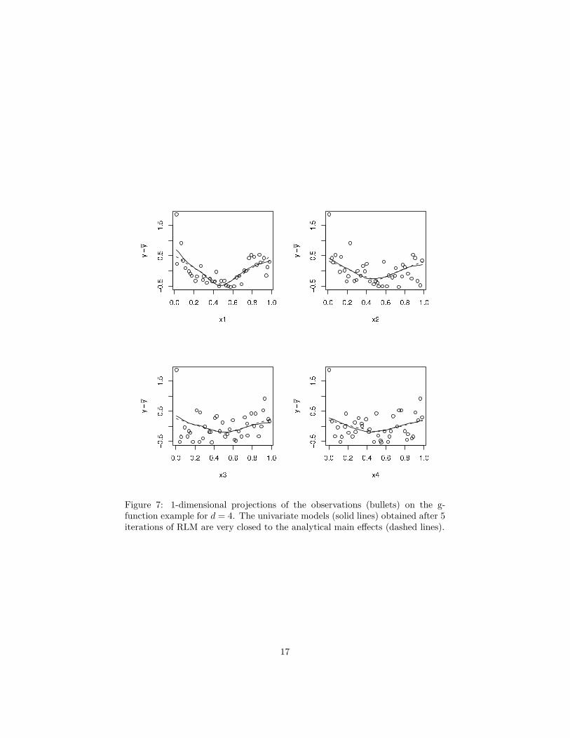
Figure 7: 1-dimensional projections of the observations (bullets) on the g-function example for d = 4. The univariate models (solid lines) obtained after 5iterations of RLM are very closed to the analytical main effects (dashed lines).

17