Advanced Control of Ethylene to Butene-1 Dimerization Reactor

Automatic Control and System Engineering, 1, 34:52, 2004

Advanced Control of Ethylene to Butene-1

Dimerization Reactor

Emad Ali* and Khalid Al-humaizi

Chemical Engineering Department, King Saud University

P.O.Box 800, Riyadh 11421, Saudi Arabia

Fax no.: ++(9661) 467-8770

Phone no.: ++(9661) 467-6871

Email address: [email protected]

Abstract

Butene-1 is produced from ethylene by dimerization reaction in a CSTR. Due to the

exothermic reaction, serious temperature runaway occurs in the reactor. Therefore, it is

important to stabilize the reaction temperature in order to maintain good quality product and

safe operation. Temperature stabilization is also essential for maintaining optimal operation

of high ethylene conversion and desired butene-1 yield in the face of plant upsets. The

objective of this paper is, thus, to study the simulated implementation of nonlinear control

algorithms such as Fuzzy Logic Control (FLC), Globally Linearizing Control (GLC) and

Nonlinear Model Predictive Control (NLMPC) algorithms for temperature stabilization of

such a reactor to maintain favorable ethylene conversion and butene-1 yield conditions. The

simulation results revealed the capability of all the proposed control algorithms to stabilize

such a reactor with some differences in their performance. In addition, the performance of the

nonlinear controllers outperforms that of the standard PI algorithm in terms of providing

higher yield and shorter settling time during disturbances. However, careful tuning of the

parameters of these controllers is necessary without which very aggressive or even unstable

closed-loop performance will be obtained.

Keywords: Ethylene dimerization, Temperature stabilization, Fuzzy logic control, Globally

linearizing control, Model predictive control

1


Introduction

One of the most economic methods for producing butene-1 is the catalytic

dimerization of ethylene. The reaction usually takes place at moderate pressure (20-30 psia)

and temperature (50-60 oC). The catalyst used in the reaction is a homogeneous titanium-

based catalyst, which leads to a high dimerization activity and excellent selectivity to butene-

1. The industrial ethylene dimerization reactor operates in a liquid phase at bubble point

conditions. Fresh ethylene and homogenous catalyst are fed continuously to the reactor

where the exothermic reaction is removed by means of an external cooler. The cooler is

installed on the recycle pipelines. The recycle returns portion of the product back to the

reactor.

The ethylene dimerization process is strongly nonlinear and very sensitive to external

disturbances. Thermal runway risks are very common because the main reaction is highly

exothermic and its rate increases rapidly with temperature. The side reactions produce

heavier oligmers such as hexene and octene that might cause continuous fouling of the

overall system of the reactor, recycle loop and heat exchangers. According to industrial

practice, extreme regular monitoring of the process variables is necessary. Trabzoni (1998)

has developed a mathematical model for this unit to study the static and dynamic behavior of

such a reactor. The steady state analysis of the model shows that the system can exhibit a

unique steady state and a multiplicity in the form of S shape (hysteresis). Generally,

exothermic polymerization reactions with recycle are well known for reactor temperature

instability (Dadebo, et. al., 1997; Luyben, 1998). In fact, phases of variation such as

persistent oscillation and/or runway of the dimerization reactor temperature are reported

(Braunschweig et. al., 1990; Trabzoni, 1998). In fact, our previous work (Ali and Alhumaizi,

2000; and Alhumaizi, 2000) confirmed that the desired operating condition of maximum

butene-1 yield occurs at an open-loop periodically unstable point. For this reason, control of

the reactor temperature is essential for stable operations. In addition, good temperature

control is important to maintain the process around the optimum conditions of maximum

yield and to minimize large duration of off-specs products. The main objective of this paper

is, thus, to design and test a good temperature controller.

Because the process is highly unstable, achieving a good control performance or even

stable feedback response is a challenging task. Careful control design and tuning are essential

2


in this case to attain such control objectives. In fact, our earlier work (Ali and Alhumaizi,

2000) showed that implementation of a standard proportional-integral (PI) control algorithm

and similarly a linear model predictive control algorithm can provide excellent control

performance only at small magnitude for the disturbance. At large values for the disturbance,

a multi-input multi-output (MIMO) control scheme, specifically 2x2 control loops, was found

necessary to stabilize the reactor. However, the control performance was very sluggish. In

addition, tuning of the MIMO scheme turned to be a difficult task. For these reasons non-

linear control algorithms will be applied to control the reactor. Specifically, Fuzzy Logic

Control (Lee, 1990a, 1990b), Globally Linearizing Controller (Kravaris et. al., 1989) and

Nonlinear Model Predictive Controller (Ali and Zafiriou, 1993) will be used in this paper.

Fuzzy logic control is based on the original work of Zadeh (1965) on fuzzy set theory.

Its first implementation to control physical processes was proposed by Mamdani (1974,

1977). Since then several other applications were reported (Bernard, 1988; Kishimoto et. al.,

1989; Parekh et. al., 1994; Rhinehart et. al., 1996; Inmdar and Chiu, 1997; and Garrido et. al.,

1997). Recently, FLC received more interest due to its successful application to important

industrial systems (Rao, et. al., 1999). Since FLC is a nonlinear controller and can adapt itself

to changing situations, it can outperform conventional PI controllers for unstable dynamics

and nonlinear systems. In contrast to model-based controllers, FLC is known as a knowledge-

based controller that does not require a mathematical model of the process at any stage of the

controller design and implementation. In many cases, the phenomenological model of the

control process may not exist or may be too expensive in terms of computer processing

power and memory, and a system based on rules of human knowledge may be more effective.

In this case, FLC is a simple alternative to model-based advanced controllers.

Globally linearizing controller is introduced first by Kravaris and Chung (1987) and

belongs to a family of nonlinear control algorithms that uses the nonlinear model directly in

the synthesis of the control law. It is also known as nonlinear internal model control

(Kulkarni et. al., 1991; Patwardhan and Madhavan, 1998; Kendi and Doyle, 1998; Economu

and Morari, 1986; Henson and Seborg, 1991; and Hu and Rangaiah, 1999), sometimes as

output feedback control (Ramirez, 1999; Kumar and Daoutidis, 1995; and Alvarez, 1996) or

input/output linearizing control (Alvarez et. al., 1994; Soroush and Kravaris, 1992). Most of

these algorithms are based on the differential geometry technique and require analytical

expression for the process model usually in the form of state space. Several simulated

3


implementation on nonlinear unstable models revealed the success of such a controller, which

makes it suitable for our specific case. However, unlike other model-based controllers, GLC

law formulation depends on the explicit analytical expression of the process model. This

situation presents a barrier, which hindered the GLC implementation to real industrial control

problems.

The nonlinear model predictive control belongs to the family of model predictive

controllers (MPC). The MPC algorithms differ from the other advanced controllers in that a

dynamic optimization problem is solved on-line each control execution. The original MPC

uses a linear model in the form of step response and is known as dynamic matrix control

(Cutler and Ramaker, 1979). Other generations of MPC were developed such as generalized

predictive control (Clarke et. al., 1987) and quadratic dynamic matrix control (Garcia and

Morshedi, 1986). Due to the MPC appealing features such as constraints handling and

superiority for processes with large number of manipulated and controlled variables, it

became the most widely used control system in the chemical industries (Qin and Badgwell,

1996; Morari and Lee, 1999). This success has lead to the extension of MPC to consider

nonlinear models for the online prediction (Ali and Zafiriou, 1993; Biegler and Rawlings,

1991). Review of the nonlinear MPC theory and its industrial applications has been reported

(Henson, 1998; Qin and Badgwell, 2000).

Therefore, the specific objective of this paper is to investigate the simulated

implementation of FLC, GLC and NLMPC to stabilize the dimerization reactor. The paper is

organized as follows. The following section presents the mathematical model for the

dimerization reactor and its cooling system followed by a section devoted for the open-loop

analysis of the model. The fourth section discusses the control objectives of the dimerization

reactor. The following three sections are devoted for the development of the proposed

nonlinear controllers. The eighth section is devoted for illustrative closed-loop simulations.

The last section offers the final conclusions.

Reactor Model

The dimerization reactor considered in this study is assumed to be a liquid phase perfectly

mixed reactor, i.e. no mass transfer limitation is considered in this system. Schematic of the

process is depicted in Figure 1. The liquid is homogenized by a high re-circulation rate

4


around the reactor through a heat exchange used to remove the high exothermic heat of

reaction. The model uses the Homo- and Co-polymerization mechanisms suggested by

Galtier et. al. (1988). The reaction kinetics for the initiation, propagation and termination

stages of the ethylene dimerization are given elsewhere (Ali and Alhumaizi, 2000).

Based on the above assumptions and the assumed reaction kinetics, the resulted dynamic

model of the dimerization process is as follows (Ali and Alhumaizi, 2000):

])[( 44444244442244 KCbKCaKCbCaCbVCQ

dtdCV ++++−−β−=

(1)

)]()([ 642224222222 KKKCbKKKCaVCQFC

dtdCV f +++++−β−=

(2)

)]()()[( 4244642224422 KKCbKKKCbKCaCaVKQFKdtdKV f ++++++−β−=

(3)

))()(()()()1()( 2412 HrHrVTTCQTTCQTTCFdtdTCV rprRprfpffp Δ−+Δ−+−ρ−−ρβ−+−ρ=ρ (4)

)()()1( cavRavRpR

pc TTUATTCQdt

dTCV −−−ρβ−=ρ

(5)

])([ 2442244222222 KCbCbCaCaKCaVKQ

dtdKV +++−+β−=

(6)

])([ 44444222222244 KCaKCbCbCaKCaVKQ

dtdKV +++−+β−=

(7)

)][ 24462242266 KCaKCbKCaVKQ

dtdK

V +−+β−= (8)

where

2coc

cavTT

T+

=

2R

RavTTT +

=

The dynamic of the outlet temperature of the coolant fluid is not included and

alternatively it is obtained by solving the steady-state equation:

5


)()( cavRavchccow TTAUTTWCp −=− (9)

In this case, W (Coolant flow rate) and F (Gases feed flow rate) are used as forcing inputs.

The kinetic parameters, i.e., ai and bi, used in this study are based on the rate constants

obtained by Galtier, et. al. (1988), and Woo et. al. (1991), and are given elsewhere (Ali and

Alhumaizi, 2000). The definition of the process states and the various process parameters in

the above equations is given in the nomenclature. Table 1 shows the numerical values of the

design parameters for the dimerization reactor system. The original model of the dimerization

process contains two additional states (Trabzoni, 1998). The two states, which represent the

hexene and octene concentrations, are not included in this paper for simplicity. This

assumption is valid since the above eight states are independent of the omitted ones.

It should be noted that, in the above model, arithmetic temperature average as driving

force for heat transfer is used instead of log-mean temperature differences. The reason behind

this treatment is to simplify the GLC scheme design. As will be shown later, the GLC design

is based on solving the model equations for the design variable. Therefore, the solution

becomes straight forward when the design variables appear linearly in the model equations.

Open-loop Analysis

Our previous open-loop bifurcation analysis (Ali and Alhumaizi, 2000), revealed the

existence of a trade-off between conversion and selectivity (yield), which is clear in Figure 2.

It can be seen that as the feed flow rate F increases, the conversion increases while the yield

decreases and vise verse. For this reason it is recommended to operate the plant around a

favorable operating point that corresponds to F = 4x10-3 m3/s, which corresponds to 95.7%

conversion and 69.6% yield. This point also corresponds to a practical temperature operation,

which has to be around the heavy mixture bubble point of 67 oC. Table 2 lists the process

parameters at this favorable operating point. Nevertheless, as the open–loop response shown

in Figure 3 indicates, the desired operating point is unstable. The stable regions for this

process are economically unacceptable. For example, as shown in Figure 2 a stable region

exists at high throughput, i.e., high F, but, in the same time, at low yield and selectivity.

Another stable region is located at very low F, which corresponds to a high selectivity but

low conversion and production rate. This region is not shown in the figure. Therefore, there is

6


a potential for utilizing a good control design to stabilize the reactor around the desired open-

loop unstable point.

Control Objective

The main control objective of such a process is the stabilization of the reactor

temperature. This is essential to secure safe plant operation and to deliver a good quality

product. It is also desirable to maintain optimal operation of high ethylene conversion and

desired butene-1 yield as given in Table 2 in the face of plant upsets. In practice, the coolant

feed temperature, Tc, is one possible source of disturbances to the process, which may cause

thermal runaway due to temperature instability and consequently loss of conversion and/or

yield. The upset in Tc is chosen for demonstration purposes and is considered to simulate an

unknown unmeasured disturbance that creates a temperature excursion situation. For this

reason, the closed-loop simulations in this paper focus on temperature stabilization and

maintaining desired yield in the face of upsets in Tc. In this case, the controlled variable

would be the reactor temperature, (T), and the butene concentration at the outlet stream, (C4).

In due course, the suitable manipulated variables (MV) are the coolant flow rate, W, and the

feed flow rate F. Single-input single-output (SISO), multi-input single output (MISO) and

MIMO control schemes will be examined for this control problem. For the SISO case, the

controlled variable is the reactor temperature and the manipulated variable is the coolant flow

rate. The MIMO scheme is carried out in a decentralized form where T is regulated via W and

C4 via F. In the MISO scheme, the two manipulated variables, i.e., W and F, will be driven by

the same error signal, which is the deviation of T from its set point. The selection of these

particular manipulated variables and their pairing procedure are based on our earlier work

(Ali and Alhumaizi, 2000) which includes detailed analysis for designing the control

structure of the dimerization reactor. In the simulation section, a sampling rate of 0.1 hr will

be used, which is more realistic for practical applications.

Fuzzy Logic Control Algorithm The basic FLC loop is shown in Figure 4. It consists of three major sequential steps,

namely Fuzzification, Inference engine and Defuzzification. In the following subsections, the

development and design of each step is discussed in detail. Hereafter, by input we mean

controller input, i.e. error and/or error velocity signal and by output we mean the controller

output, i.e. manipulated variable.

7


Fuzzification:

The input signal of the controller, which is a real-value variable also known as crisp

value, is fed to the fuzzifier. In the fuzzifier, the crisp value is converted as a member of a

finite number of fuzzy sets. Therefore, the process of fuzzification is simply mapping, i.e.

checking the value of the input signal (member) against each fuzzy set to determine its degree

of membership (belongingness). The fuzzy set is usually represented as a membership

function as shown in figure 5. The membership function can have any symmetrical geometric

shape and is graded between 0 and 1. The fuzzy sets in Figure 5 are identified by linguistic

names such as Large Positive (LP), Small Positive (SP), Zero (ZE), Small Negative (SN),

Large Negative (LN) and they are labeled as μ1, μ2, μ3, μ4 and μ5, respectively. Usually,

finite number of overlapping membership functions (fuzzy sets) can be used to span the

possible range of the process variable. The overall span (domain of a specific variable) is

known as the universe of discourse.

Common difficulties exist in this step. The selection of the shape and number of the

membership functions, the location of their center, i.e. where the fuzzy set has a maximum

value, and the size of the universe of discourse is not straight forward. Moreover, the

common FLC design involves at least three different groups of fuzzy sets, each of which

corresponds, to a different process variable. For example one group is used for the error

signal, e, another for the velocity of error signal, Δe, and another for the controller’s output

(manipulated variable), u. The latter is used in the defuzzification step. In this paper we try

to overcome the above problems. First we use only one group of fuzzy sets for all the three

process variables. To achieve this, the universe of discourse is unified so that it spans the

interval [-1, +1]. In this case, the value of each process variable should be scaled properly to

fit the specific interval. This idea of normalizing the fuzzy set domain is proposed by Qin and

Borders, 1994. Discussion of the scaling procedure is given under the tuning section.

Secondly, Gaussian and sigmoidal shapes are considered for the membership functions.

Gaussian shape is selected because it is a continuous function and can be easily expressed by

an analytical formula. Continuity of the Gaussian functions produces smoother control

output. Usually to symmetrically span the input domain, odd number of fuzzy sets should be

designed. Increasing the numbers of the fuzzy sets creates smoother output. However, this

8


will be at the expense of increasing the number of control rules leading to more complicated

design procedure and tuning. Therefore, five such functions are used here as shown in Figure

5, which found, with the aid of Gaussian functions, sufficient to provide smooth output at

reasonable number of fuzzy rules.

In this work, two variables are fuzzified, which are the error (e) and the error velocity

(Δe). Therefore, in this controller phase, the membership degree of a specific input value, i.e.

e or Δe, over all fuzzy sets can be determined directly from Figure 5.

Inference Engine:

Inference engine is the heart of the FLC algorithm where the control action is

formulated. Specifically, it describes the output of the controller for all input signals

combination. It consists of several fuzzy set rules represented by conditional statements in the

form of IF-Then rules as shown in Table 3 (Yen and Langari, 1999). The collection of all

rules is called Rule Base. Generation of such rules is another difficult part of the FLC design.

In this paper, we choose to design the rule base according to desired response of the

process because it the most intuitive for many control practitioners. The rule base for a

generic feedback response as listed in Table 3 is used here. Note that the AND command is a

common fuzzy rule operation, which mathematically implies the minimum of two values.

Note that the first index of μ is the label for the membership function. The second index

indicates the rule number.

At this phase of the controller algorithm, given a value for the input signal, the degree

of fulfillment of each rule in the rule base set is determined. The degree of fulfillment of the

rule base is known as the conclusion or the result of the rule base. The process in which these

conclusions are calculated is known as inference. Due to overlapping membership functions,

some of the rule conclusions may have a zero value and some a non-zero value. Membership

function for the output with a non-zero degree of fulfillment is considered fired. In standard

FLC algorithms, the fired functions are clipped or scaled and then copied to a temporary

template. All fired sets are then combined using superimposing technique. The combined set

is known as the inferred controller output. Figure 6 shows an example of three combined

active fuzzy sets.

9


Defuzzification:

In this step, the combined output fuzzy sets (inferred output from the previous step)

are then converted (defuzzified) into a single crisp value. The calculated crisp value is the

numerical value for the manipulated variable. Defuzzification is thus equivalent to finding

the weighted average value for the combined sets. In standard FLC applications, the

combined set is a new geometric shape, say μout (Figure 6). Hence, finding a weighted

average is similar to determining the geometric center. One way is by calculating the center

of area (COA) (Yen and Langari, 1999). The discretized form of COA can be written as:

∑∑

∑∑

= =

= =

μ

δμ=Δ

R f

R f

n

j

n

iijij

n

j

n

iijiij

A

Au

1 1,,

1 1,,

(10)

Where nf is the number of output membership functions and equals 5 in this paper, nR is the

number of rules and equals 25 in this paper, which is the maximum possible number to cover

all eventualities created by the 5 output membership functions. δi is value for the location of

the center of μi.. The value of δi is pre-calculated and fixed as shown in figure 5. A is nR x nf

pre-calculated matrix, which identifies which membership function is included in each Rule.

For example, row 1 of matrix A, which is assigned for Rule 1, contains 1 at the first column

and zeros elsewhere. The same logic is carried out over the remaining rows.

It should be emphasized that the control output, Δu computed by Eq. 10 is taken in the

velocity form. Velocity form is more suitable for non-linear systems. In non-linear systems,

the new equilibrium value for u, denoted as uss, that brings the output to the desired steady

state value may not be known beforehand. Thus, it is difficult to locate uss in the universe of

discourse as the center for the ZE membership function. However, when Δu is used, zero

value will always be the equilibrium point around which ZE can be built.

Tuning method:

10


Tuning a fuzzy linguistic controller to changing process and environment dynamics can

be accomplished in several different ways:

- Adjusting the membership functions.

- Changing the finite set of values describing the universe of discourse.

- Reformulating the finite set of control rules in the knowledge base (inference engine).

However, these procedures are cumbersome. In addition, there are no clear guidelines on

how these procedures affect the closed-loop response. In this paper, we adopt a simpler

method. The scaling factors for the input and output signals are used as the tuning

parameters. As will be seen in the examples, these factors have direct and clear effect on the

closed-loop response. These factors are used to scale the process variables so that they fit the

universe of discourse domain used in Figure 5. Specifically, the scaling factors for the error,

error velocity, and output velocity are se = a/sp, sde = b/sp and sdu = cΔum respectively. For

servo control problems, sp is the difference between the set point and the initial steady state

value for the controlled variable. For regulatory control problem, sp is the set point value.

Δum is the difference between the maximum and minimum allowable values for the

manipulated variable. Therefore, a, b, and c are the tuning parameters. Changing the value of

a, b, or c is equivalent to stretching or expanding the universe of discourse of the fuzzy sets

shown in Figure 5. Conceptually, this is similar to the first two tuning guidelines mentioned

above.

FLC algorithm:

The following steps explain the FLC control algorithm used in this paper.

Set a=b=c=1.At any sampling time, k do:

Step1: scale the error and the error velocity signals (e (k), Δe (k)) via multiplying them with

se and sde.

Step2: Compute the degree of membership of e(k) and Δe(k) to the five membership

functions shown in Figure 5.

Step3: Calculate the conclusions of the Rule base as given in Table 3.

Step4: Calculate the control action using equation 10. Scale the computed value by

multiplying with sdu.

Step 5: Implement the control action, set k=k+1 and go back to step 1

11


If the control performance is poor, adjust the value of a, b, or c. We have found that

increasing the value of a increases the speed of response and eliminates offset. Increasing the

value of c penalizes the manipulated variable moves, thus introduces stabilizing effect.

The main advantage of FLC, besides being a nonlinear controller, is its independence

on process model as the latter is expensive or difficult to obtain. The drawback of such

algorithm arises from the complexity of designing the fuzzy sets and the fuzzy rules. This is

because these sets and rules are usually built based on heuristic and engineering knowledge.

Globally Linearizing Control Algorithm

This approach uses an explicit process model usually in the form of state space to

derive analytical nonlinear control law. Geometric theory, specifically Lie derivatives, is used

to determine the relative order of the process model (Kravaris and Kantor, 1990). The relative

order is basically the number of times that the output must be differentiated till the

manipulated variable appears explicitly in the observed state equation. The obtained equation

is then solved for the manipulated variable such that the closed-loop response tracks a certain

desired closed-loop behavior. The desired trajectory must possess an order equals to or

greater than the relative order.

SISO control scheme

The manipulated variable (W) does not appear explicitly in the state equation for T,

i.e. equation (4). In due course, the differential equation for T can be differentiated once

generating a second order differential equation for T. The ordinary differential equation

(ODE) for TR (Equation (5)) can then be inserted into the resulted second-order ODE in order

to incorporate W explicitly into the equation. The process in this case is said to have a

relative order of two. Consequently, a second or higher order reference trajectory should be

designed for the output. Alternatively, the relative order can be reduced to one and thus, a

first order reference trajectory can be sufficient. This can be achieved by writing the overall

energy balance:

Hrpccopwrfpffp VRTTCFTTWCTTCFdtdTCV +−ρ−−−−ρ=ρ )()()(

(11)

12


where RH = r2(−ΔH1)+ r4(-ΔH2) . Solving the above equation for the manipulated variable

(W) gives:

( )[ ]Hrrfffccopw

VRTTCpTTCpFTCpVTTC

W +−ρ−−ρ+ρ−−

= )()()(

1 &

(12)

Hence, a second order reference trajectory for the output can be selected as:

∫ −+−τ=t

spi

sp dtTTkTTT0

11 )()(&

(13)

Here τ1 and ki1 are tuning parameters. The integral action is incorporated to eliminate

steady state offset. Equation (12) and equation (13) comprise the SISO GLC control law for

the temperature loop.

MIMO control structure:

Beside the above control loop, there will be another loop relating C4 with F. Clearly

F appears explicitly in equation (1) and equation (4). However, W appears only in the overall

energy balance equation. Thus, the 2x2 system is partially decoupled. Assuming total

decoupling, and noting that F = Qβ, equation (1) can be solved for F giving:

[ ] 44444424444224 / )( CVKCbKCaKCbCaCbCF ++++−+−= & (14)

Since the second loop has a relative order of one, a second order reference trajectory

for the second output can be used as follows:

∫ −+−τ=t

spi

sp dtCCkCCC0

4424424 )()(&

(15)

Equation (14) and (15) comprise the GLC law for the second loop. τ2 and ki2 are the

corresponding adjustable parameters. When the MIMO structure is employed in total de-

coupling fashion, equations 12 to 15 are solved independently, i.e. F is fixed in equation (12).

13


On the other hand, when the MIMO scheme is employed in partial de-coupling fashion,

equation (14) and (15) are solved first and then the resulted value for F is substituted in

equation (12).

MISO control structure:

The MISO scheme consist of one controlled output, which is the reactor temperature

(T) and two manipulated variables namely; the feed flow rate F and the cooling flow rate W.

Apparently, both manipulated variables appear explicitly in the overall energy balance

[equation (11)]. The latter can be written as follows:

21 α+α=−ρ WFVRTCV Hp& (16)

Because the above equation has two unknowns, one possible solution is the least squares

solution:

][22

21

1Hp RTCVF −ρ

α+α

α= &

(17)

][22

21

2Hp RTCVW −ρ

α+α

α= &

(18)

Equation (17) and (18) along with equation (13) comprise the MISO control law. This control

scheme has only one set of tuning parameters, i.e. τ1 and ki1. However, since the two

variables are of different order of magnitude, a proper scaling should be used. Consequently,

α1 and α2 are scaled through pre-multiplied them by the corresponding maximum value of F

and W respectively. Therefore, before implementing the value of F and W calculated from

equation (17) and (18), they should be re-multiplied by the scaling factor to retrieve their raw

values. The MISO control scheme based on the least-squares solution does not necessarily

provide the best dynamic response however; it is simply an intuitive attempt to improve the

feedback performance.

The GLC scheme is illustrated via the block diagram shown in Figure 7. In this paper,

we consider practical implementation schemes. We consider that the plant states are partially

measured. Therefore, a parallel model observer should be used to estimate the other

14


unmeasured plant states as shown in figure 7. In this case, the feedback signal is the

difference between the plant measurement and the model output. In addition, the model states

that represent the unmeasured plant states are fed to the nonlinear controller. Moreover, the

control law (Eqns 12-18) represented by the block called “nonlinear control” contains several

unmeasured model parameters. Consequently, the effect of some degree of uncertainty in

these parameters should be also investigated. It should be noted that the above control laws

are implemented in a discrete-time formulation, thus, the integral is approximated

numerically by summation.

Robustness of the GLC algorithm is addressed here through simple feedback

compensation (Hu and Rangaiah, 1999). Generally, the GLC algorithm, like other model-

based algorithms, performs well when the model is perfect. However, the performance may

degrade substantially or even becomes unstable in the presence of model uncertainty. This

situation lead the researcher to incorporate parameters and state estimation techniques (Tracy

and McGregor, 1997; Assala et. al., 1997; and Soroush, 1997). However, this issue is out of

the scope of this paper. Alternatively, simple state resetting through standard disturbance (or

model-plant mismatch) estimation is used. This simple treatment is found sufficient. The

model states are reset every sampling time by adding to them the following estimate of

model-plant mismatch:

Di(k) = ypi(k) – ymi(k), i = 1, ny (19)

Where k is the sampling instant, and ny is the number of outputs. yp denotes the

measured output and ym is the corresponding model output. In practice, yp is obtained from

plant measurement, however, in this paper it is obtained from numerical integration of the

process model. Similarly, ym is obtained from the numerical integration of the process model.

The process model is the set of ODE’s (Equation 1-8). In order to simulate model-plant

mismatch, some of the model parameters have different values when used to obtain yp than

when used to obtain ym. The difference in these values will be discussed in the next section

when GLC implementation is discussed.

The advantage of GLC methods is the ability to deliver perfect control and globally

stable response if the model is perfect. The disadvantages include the requirement of a

15


special model form such as state space equations. In this case all model parameters and states

appear in the control law. Therefore, robustness is an important issue especially in the

presence of errors in the model parameters and states.

Non-linear MPC algorithm

In this paper the structure of the MPC version developed by Ali and Zafiriou (1993)

that utilizes directly the nonlinear model for output prediction is used. A usual MPC

formulation solves the following on-line optimization:

)( )()(( 21

M

1=i

2P

1=i)(),....,(min

1−+++

ΔΔΛ+−Γ ∑∑

−+ikikik

tutututRty

Mkk

(20)

subject to

)( BtUC kT ≤Δ

(21)

For nonlinear MPC the predicted output, y over the prediction horizon P is obtained by the

numerical integration of:

y=g(x)

tuxfdtdx ),,(=

(22)

(23)

from tk up to tk+P where x and y represent the states and the output of the model

respectively. The symbols || . || denotes the Euclidean norm, k is the sampling instant, Γ and

Λ are diagonal weight matrices and R is the desired output trajectory. ΔU(tk)=[Δu(tk) …

Δu(tk+M-1)]T is a vector of M future changes of the manipulated variable vector u that are to

be determined by the on-line optimization. The control horizon (M) and the prediction

horizon (P) are used to adjust the speed of the response and hence to stabilize the feedback

behavior. Γ is usually used for trade-off between different controlled outputs. Λ, on the other

hand, is used to penalize different inputs and thus to stabilize the feedback response.

16


The usual implementation of MPC involves numerical integration of the model state

equations over the prediction horizon P to obtain the future output behavior. Then, the

objective function (Eq. 20) is solved on-line to determine the optimum value of ΔU(k). Only

the current value of Δu, which is the first element of ΔU(k), is implemented on the plant. At

the next sampling instant, the whole procedure is repeated. There are two methods of solution

of the NLMPC optimization problems. The sequential solution iteratively solves the ODE's

as an inner loop to evaluate the objective function. The simultaneous solution transforms the

ODEs to algebraic equations which are solved as nonlinear equality constraints. The first

approach is adopted here. It should be noted that NLMPC is not restricted to a special type of

nonlinear models. Black box models can also be used.

A disturbance estimate (or model-plant mismatch), as defined by equation (19),

should also be added to y in Equation (23) or alternatively it can be absorbed in R(tk+1). In

the standard MPC implementation, the disturbance is assumed constant over the prediction

horizon, and is set equal to the difference between plant and model outputs at present time, k

. The function of the ‘’additive’’ constant disturbance in the model prediction is to introduce

integral action and thus removes steady state offset in the presence of model uncertainty or

unmeasured disturbances. For unstable processes, improving the model prediction by the

additive constant disturbance is not enough solely. In fact, state estimator and/or parameter

estimation should be used in conjunction with the additive corrections.

The original NLMPC algorithm (Ali and Zafiriou, 1993) is equipped with Kalman

filtering to improve the controller performance for open-loop unstable processes. Kalman

filtering requires repeated solution of Riccati differential equations, which may not converge

if the original nonlinear model is highly unstable (Ali and Elnashaie, 1997). Alternatively, the

Kalman filter gain is estimated by solving a small-size optimization problem (Ali and

Elnashaie, 1997). However, like other state observers, the proposed observer is stable only

for bounded input. In this particular application, the input to the proposed state estimator

(modified Kalman Filter), which is the model-plant mismatch, is sometimes unbounded. This

situation leads to unsatisfactory application of the proposed state observer. As intuitive

remedy, the model states are updated by simply adding to them, the estimate of model-plant

mismatch (Equation 19). This is exactly the same procedure used in the GLC algorithm. It

17


should be noted that this is done in addition to the output correction mentioned in the

beginning of the previous paragraph.

In addition to the general features of the MPC mentioned in the introduction section,

NLMPC is more suitable for highly nonlinear processes. The main drawback of such a

scheme is the computational effort and time needed to solve the optimization problem. The

performance and stability of the algorithm depends on good tuning. Robustness in the face of

modeling errors can be improved by incorporating state and/or parameter estimation

techniques.

Closed-loop simulations

PI controller

The results in this section are adopted from our earlier work (Ali and Alhumaizi,

2000). It is reproduced here for comparison purposes. The PI setting values are determined

by continuous cycling method as reported in (Ali and Alhumaizi, 2000). Simulation of the

SISO control problem for +4oC and +6 oC step changes in Tc using the PI control is shown in

Figure 8. As shown in the figure, for +4oC upset the reactor temperature is well maintained at

its set point. It is obvious that by regulating the reactor temperature, the reaction yield,

represented by the C4 response, is also kept at the desired favorable set points of 69.6%. The

PI settings for this case are kc = -1000 kg/s.oC and τI = 10 ks. However, at an upset of

magnitude of +6 oC in Tc, more amount of coolant is needed to remove the heat of reaction

leading to saturation of the coolant flow rate. This degrades the closed-loop performance. A

loss in the yield is also observed. The PI controller gain in this case is the same as before,

however the integral time (τI) is re-tuned for stability by trial-and-error to 100 ks.

Another way to deal with the case of rejecting +6 oC change in Tc is to use a MIMO

control structure. The solid lines in Figure 9 illustrate the effect of employing the MIMO

control scheme to handle such challenging problem. The corresponding PI settings are kc = [-

1000 kg/s.oC, -5x10-7 (m3/s)/(mole/m3)] and τI = [2000 s, 0 s]. In this case, the MIMO

scheme managed to perfectly regulate the first controlled variable, T while the second

controlled variable C4, suffers from an offset of -73 mole/m3. Our investigations observed

that any attempt to reduce the offset would create persistent oscillatory response for the

reactor temperature. Moreover, tuning of the MIMO scheme is difficult due to the strong

18


interaction behavior. In fact, the disturbance causes the reactor temperature to increase

rapidly. As a result the first control loop will increase W till it brings the temperature back.

During the temperature excursion, the reaction activity diminishes causing sharp drop in the

yield. The latter causes the second control loop to reduce the feed rate in order to recover the

yield. However, because C4 has very slow dynamic compared to the reactor temperature, it

takes longer time for the yield to recover. If the settings of the second loop are tuned to

produce faster response, then adverse effect will be introduced in the first loop. This will

cause undesirable behavior in the temperature loop as mentioned earlier.

Alternatively a MISO PI scheme can be used. In due course, the temperature will be

controlled by both W and F simultaneously in a split range mode. It should be noted that 90%

of the error signal will be used to actuate W and the rest to actuate F. The split range ratio is

used only in the PI controller and is chosen mainly to avoid over utilization of both MVs and

secondly to give more weight to the coolant flow. Tuning will be easier because interaction is

not involved. In addition, the higher degree of freedom can help to perfectly control the

reactor temperature. This will also bring the response of C4 to the corresponding steady state

value (desired set point). This is evident from the dashed lines shown in Figure 9. Obviously,

less overshoot in the reactor temperature response and less offset (-26 mole/m3) in the yield

response are observed. In fact, since both W and F are used to regulate the reactor

temperature, they managed to minimize the temperature overshoot. This in turn minimized

the reduction in yield. The PI settings used are kc = [-1000 kg/s.oC, 0.002 m3/s.oC] and τI =

[100 ks, 50 ks].

Fuzzy Logic Controller

The above SISO, MISO and MIMO control problems are re-tested using the FLC

algorithm. Regarding the SISO case, Figure 10 demonstrates the closed loop response to two

step changes in Tc of +4 and +6 oC, respectively. For both cases, a = 1, b = 10 and c = 105 are

used. As the figure illustrates, a perfect disturbance rejection without offset is obtained for

the first case, i.e. ΔTc = +4 oC. For the larger disturbance case, i.e., ΔTc = +6 oC, poor

performance, which seems worse than that for the PI algorithm, is obtained. The poor

temperature control is associated with a loss in the yield, which is not shown in figure 10 for

simplicity. The SISO FLC performance can be made less aggressive through tuning.

However, the closed-loop response will eventually oscillate due to input saturation. The SISO

PI response also oscillates if aggressive values for the tuning parameters are used or if longer

19


simulation time is used in Figure 8. Anyhow, further improvement in the FLC performance is

not possible in this case because the loss in performance is due to input constraints.

Building upon the poor performance faced in the SISO case at large upset in the inlet

cooler temperature, a MIMO FLC scheme is examined. In this case, a decentralized control

system similar to that used in the PI algorithm is also used here. The result of the closed loop

response is shown in Figure 11 by the solid lines. For the first loop, a = 1, b = 100, and c =

105 are used, while a = 1, b = 3x103 and c = 1x10-5 are used for the second loop. Tuning is

found to be a cumbersome task due to the strong cross interaction. Nevertheless, the obtained

closed loop response is reasonable as perfect control of T and minor offset in C4 (-67

mole/m3) are observed. Small reduction in the feed flow rate was necessary to reduce offset

in the yield, but was not good enough. Further tuning was found not helpful. On the other

hand implementation of the MISO control structure provided excellent offset-free response as

shown in Figure 11 by the dashed line. The FLC tuning parameters are the same as in the

MIMO case except that c for the second loop is re-adjusted to 1x10-4. The only reported

advantage of the FLC is that its resulted performance for the MISO case outperforms that

obtained by the PI algorithm. However, the MISO FLC is superior to the MIMO FLC in the

sense of less offset in the yield response. This situation is attributed to the strong cross-lop

interaction. In the MIMO case, tuning the second control loop to reduce offset in the yield

would require less fresh feed flow. Alteration of the fresh feed flow introduces disturbance to

the first control loop leading to temperature runaway and consequently unstable process

behavior. Moreover, it is found that tuning the FLC parameters for the MIMO case is as

difficult as that for the MIMO PI algorithm.

Globally linearizing controller

The GLC algorithm is also tested for the same control objective in SISO, MIMO and

MISO modes. In the following applications, the reactor temperature and the butene

concentration states are assumed measured, while the rest are unmeasured. Therefore, in the

GLC control law (Eqns 12-18), the plant states are used for the measured states and the

model states for the unmeasured ones. The values of the model states are obtained by direct

integration of the process model equations. The values of the plants states are supposed to be

obtained from the plant measurement, however in this paper they are obtained from

integration of the process plant equations. The latter is exactly the same as the model

20


equation except in two aspects. First, the values of the process parameter values may differ as

indicated later. Second, the upsets in the cooler inlet temperature affect only the plant

equations but not the model equations. This procedure reflects the actual application in

practice. Therefore, in all the following simulations the reaction rate constant a2 and a4 of the

model are assumed 30% less than those of the plant. The overall heat transfer coefficient (U)

of the model is assumed 20% higher than that of the plant. The measured states are T and C4

while the unmeasured states are the catalyst concentrations, i.e. K, K2, K4 and K6. Note that

all aforementioned states are utilized in the GLC control law. The idea of incorporating

parametric errors and unmeasured states is to introduce model-plant mismatch and hence test

the robustness of the GLC algorithm. For this reason, the standard disturbance estimation, i.e.

model states resetting, proposed earlier is incorporated in the control algorithm.

Figure 12 shows the closed loop response for ΔTc = +4 oC using the SISO GLC

algorithm. The GLC parameters are τ = 1 s-1 and ki = 0.01 s-2. As figure 12 demonstrates,

GLC was able to stabilize the reactor temperature in that case and consequently to maintain a

proper butene yield. However, at ΔTc = +6 oC, the reactor temperature suffers from higher

overshoot and steady state offset. As a result, a loss of butene yield is observed (Fig. 12). The

reason for temperature offset is input saturation. Although, the coolant flow rate is not

completely saturated, any attempt to remove the offset through controller tuning results in

excessive oscillation. It should be noted that the adjustable parameter ki is re-tuned for the

last case to 5x10-4 s-2 to preserve stability. It is worth to mention that the GLC performance

without model state resetting is not shown here for simplicity. The reason for exclusion is

that the feedback response without state resetting does not differ than those shown in figure

12 except of minute periodic spikes produced by the effect of parametric modeling errors.

To overcome the loss of controllability in the SISO case, a MIMO GLC scheme is

examined for the ΔTc = +6 oC case. Figure 13 depicts the result for this case. The values for

the GLC tuning parameters are τ1 = 1 s-1, ki1 = 5x10-4 s-2, τ2 = 10-4 s-1 and ki2 = 0 s-2. As figure

13 shows, with the model state resetting is incorporated in the GLC law, very successful

closed loop response for both T and C4 is obtained. The second control law is only

implemented after twice the process time constant, i.e., 10 hrs, has elapsed. This is to ensure

that the reactor temperature has been stabilized. If the second control law is implemented at

zero time, poor performance will result due to strong interaction. It should be noted that the

21


response of both T and C4 suffer from slight offset of 0.1 oC and –74 mole/m3, respectively.

Our simulation revealed the existence of trade off between the performances of the two loops.

When τ1 is tuned to eliminate the offset in T, steady state noise is produced in butene (C4 )

response. On the other hand, when τ2 is tuned to eliminate offset in C4, larger offset is

produced in T response.

As expected, implementation of the MISO control scheme delivered improved

performance compared to that obtained using the MIMO scheme as shown by the dashed

lines in Figure 13. The offset in C4 is further reduced to –7 mole/m3. The GLC parameters are

τ = 1 s-1 and ki = 1x10-4 s-2. Note that both control loops are activated at zero time, i.e. no

time delay is introduced in the second loop as in the MIMO case. Overall, the GLC algorithm

illustrated some merit over the PI algorithm, but at the expense of additional effort associated

with designing the GLC algorithm. Note that the GLC algorithm requires developing and

utilizing a process model.

NLMPC controller:

In all the following simulations, the same model parameter alterations employed in

the GLC controller is also considered here. The purpose is to test the robustness of the model-

based controllers in the presence of modeling errors. The NLMPC performance is tuned by

trial and error according to general guidelines. In general, increasing P improves stability and

robustness of the response. Increasing λ penalizes the corresponding input moves creating

slower and more stable response. The weighting matrix Γ, is used primarily for scaling in the

multivariable case; it permits the assignment of more or less weight to the objective of

reducing the predicted error for the individual output variables.

The solid line of Figure 14 demonstrates the response of the dimerizarion process to

step change of +4oC in Tc using SISO NLMPC algorithm. Note the model state T is re-set

using the estimated modeling error (Eqn 19) as discussed earlier. The tuning parameter

values for this case are M = 1, P = 11 and λ = 0.008. As expected, perfect rejection of the

effect of the disturbances is obtained. However, at an upset of +6oC in Tc , the closed-loop

response for the reactor temperature suffers from a temperature offset due to the effect of

input saturation as shown in Figure 14 by the dashed line. This situation created a larger

22


steady state offset for the yield. The tuning parameter values for this case are M = 1, P = 15

and λ = 0. Further performance improvement through controller tuning is found useless.

The dashed line in Figure 15 shows the feedback response for an upset of +6oC in Tc

using NLMPC with MISO scheme. The tuning parameters are M = 1, P = 20, Λ =

diag[0,10]. Like the other algorithms, improved closed-loop response is observed.

Specifically –9 mole/m3 offset in C4 is obtained. The solid line in Figure 15 illustrates the

feedback response for an upset of +6oC in Tc using NLMPC with MIMO scheme. The tuning

parameters for this case are M = 1, P = 22. Λ= diag[0,10] and Γ = diag[1,0.01]. Interestingly,

unlike the other algorithms the NLMPC response in the MIMO case outperforms that of the

MISO case in the sense of less offset in C4 (-4 mole/m3). In addition, the reactor temperature

response had the lowest overshoot over all other algorithms. Inferiority of the MIMO scheme

of the other control algorithms is attributed to the fact that they operate in a decentralized

structure. Therefore, the function of the additional control loop, more specifically the

additional degree of freedom, F, is devoted for regulating the butene concentration only.

Perfect control of the additional loop may not be satisfied unless the reactor temperature is

well stabilized and is offset free. The MIMO structure in the NLMPC algorithm operates in a

fully multivariable fashion, which is one of the advantages of such an algorithm. With special

adjustment of the output weights, Γ, more weight can be given to the most important

variable, i.e. the reactor temperature in this case. However, we should admit here that tuning

the MIMO NLMPC is a difficult task due to the internal instability augmented with the

strong cross-loop interaction. Careful procedure should be used when fine-tuning the

NLMPC. Large changes in the tuning parameters create unsatisfactory performances and

unpredictable effect on the response. This behavior does not provide a meaningful guideline

on how to further fine-tune the feedback performance. Our experience in this problem

indicates that stepwise and infinitesimal changes should be adopted for fine tuning the

NLMPC especially in the MIMO case.

It can be argued that a better state estimation or disturbance prediction technique is

required to enhance the NLMPC feedback performance. Our simulations revealed that the

performance can not be improved even when the disturbance is treated as fully measured and

that no parametric errors exist. By fully measured disturbance we mean that the upset in Tc

affects both the model and plant, this is also known as feed-forward compensation. In this

23


case, the NLMPC performance with feed-forward and without modeling errors should

outperform that with any optimal state or disturbance estimator. This is because simulation

using feed-forward and perfect model makes the model states exactly equal the plant states.

Overall analysis:

Table 4 summarizes some performance criteria for the four tested control algorithms.

The selected performance criteria are the offset in yield presented by the absolute deviation

of steady state butene concentration from its set point, the overshoot in reactor temperature

presented by the maximum value achieved during simulation and the settling time for the

reactor temperature. The settling time is defined as the first time at which the temperature

response reaches its final static value. The offset in the reactor temperature is not included in

the comparison because the offset in C4/yield is considered more important. According to the

results reported in table 4, the SISO structure has the worst performance for all control

algorithms and that the MISO structure has the best performance for all cases except for

NLMPC. For the latter, the MIMO structure delivered the best performance over all control

strategies and implementation schemes. However, some other practical comparison issues

might be considered. For example, the PI and FLC algorithms do not require a process

model. Tuning of the PI and the NLMPC are somewhat difficult especially for the MIMO

case.

In all the simulations shown previously, offset was observed in the C4 response.

However, this is not attributed to poor design or to improper handling of modeling error

because some the strategies are model free. In the model-based controllers, perfect models

were tested, but offset was still observed. Therefore, possible explanation of the poor

performance in some cases is the difficulty of the control problem and tuning. Generally,

perfect control of the reactor temperature is essential to stabilize the reactor and to maintain

the yield because the latter is strongly affected by the temperature. The coolant flow, W

affects the temperature directly and the yield indirectly through the temperature. In the model

used here, the catalyst feed flow is related to the total feed flow, F. Therefore, the total feed

has dual effect and cross-loop interaction. Dual effect means that F has simultaneous positive

and negative effect on the reactor temperature. Cross interaction means that F has opposite

24


effect on the reactor temperature and on the yield. For example, increasing F will help in

reducing the temperature because the gas flow acts like a cooling medium. In the same time,

the increase in F will propagate the catalyst flow leading to a higher reaction activity. This

situation will escalate the temperature. Note also that increasing F will decrease the yield.

Decreasing F will create exactly the opposite effect. It should be noted though, that the

thermal effect of F due to reaction activity is more dominant than that due to heat transfer.

According to the strong interaction discussed above, it is difficult to maintain the

MIMO control objective unless a fully-coupled multivariable controller is used. This explains

the superiority of NLMPC in this case. However, some offset in the yield was still observed

in the MIMO NLMPC. This is because tuning was extremely difficult due to internal

instability as mentioned earlier. On the other hand, one would expect the MISO scheme to

control T perfectly because the cross-loop interaction does not exist. This was found true for

all cases. However, offset-free response for the yield is not guaranteed because its control

loop is open. Therefore, the resulted C4 response depends on the behavior of the feed flow.

The process is highly unstable, has limitation on the coolant flow rate and has input

multiplicity as discussed in (Al-humaizi 2000). These conditions make it very difficult to

bring the response to the desired steady state. Therefore, because of input multiplicity and the

way each controller is tuned, the controlled process may converge at different steady states.

Any attempt to further tune any of these controllers, unstable performance may occur.

Conclusions

Our previous closed loop analysis using a first-principle model for the ethylene to

butene-1 dimerization reactor revealed the necessity for a better control design. For this

purpose nonlinear control strategies such as fuzzy logic, globally linearizing control and non-

linear model predictive control algorithms were tested for possible stabilization of such a

reactor. Application of SISO FLC, GLC and NLMPC algorithms revealed the ability to

stabilize the reactor at a low upset in the coolant temperature. At high upsets, saturation of

the coolant flow rate occurs degrading the controller performance. This founding is in

agreement with that obtained previously. The limitation of the SISO scheme is not related to

the control algorithm neither to controller tuning, but rather to the controllability of the

process.

25


Therefore, MIMO and MISO control schemes were tried. In fact, the simulations

illustrated that improved control performance can be obtained using the MISO scheme for the

PI, FLC and GLC algorithms. On the other hand, the MIMO scheme provided better results

when used with the NLMPC algorithm. However, the MIMO scheme suffered from tuning

difficulties due to cross loop interaction, which made maintaining both outputs very difficult.

A situation gave the MISO scheme more advantage. The inferiority of the MIMO scheme to

the MISO scheme when used with the FLC and GLC algorithms depends on the de-coupling

nature of those specific control algorithms. Nevertheless, the overall feedback performance of

the proposed nonlinear control algorithms was almost comparable to each other and

outperforms that obtained using the PI algorithm. The improvement measure is based on the

faster settling time for the reactor temperature and on the less offset in the butene yield

26


Nomenclature

a Tuning parameter for the FLC algorithm

aj Rate constant for jth reaction, (m3/mole s).

A Constant matrix for the FLC defuzzification law

Ac Cooler area for heat transfer (m2)

b Tuning parameter for the FLC algorithm

B Constant vector of lower and upper bounds

bj Rate constant for jth reaction, (m3/mole s).

C Constant matrix for linear constraints

Cp, Cpf, Cpw Heat capacity of reactor mixture, feed and water respectively, (cal/gm, oC)

C4, C2 Butene-1 and ethylene concentrations, (mole/m3)

c Tuning parameter for the FLC algorithm

D Disturbance estimates

F Reactor fresh feed, (m3/s)

k Sampling time, (hr)

kc Proportional gain

ki Adjustable parameter for the GLC algorithm

K, K2, K4, K6 Catalyst, and catalyst activator for C2, C4 and C6 (mole/m3)

Kf Catalyst concentration at the fresh feed (mole/m3)

Q Reactor product volumetric flow rate (m3/s)

M Control horizon

nR, nf, ny Number of FLC rules, FLC fuzzy sets and controlled outputs respectively

P Prediction horizon

R Vector of set point

ri rates of chain initiation and propagation for ith reaction (mole/m3 s)

Tc, Tco Inlet and outlet coolant temperature respectively, (oC)

Tf ,Tr Reactor feed and reference temperature respectively, (oC)

T, TR Reactor and recycle temperature respectively (oC)

t, tk Time and time at sampling point k

u Vector of manipulated variables

U Vector of M future values of u

Uh Heat transfer coefficient (cal /m2 s oC)

27


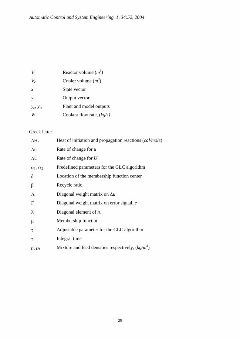
V Reactor volume (m3)

Vc Cooler volume (m3)

x State vector

y Output vector

yp, ym Plant and model outputs

W Coolant flow rate, (kg/s)

Greek letter

ΔΗr Heat of initiation and propagation reactions (cal/mole)

Δu Rate of change for u

ΔU Rate of change for U

α1, α2 Predefined parameters for the GLC algorithm

δ Location of the membership function center

β Recycle ratio

Λ Diagonal weight matrix on Δu

Γ Diagonal weight matrix on error signal, e

λ Diagonal element of Λ

μ Membership function

τ Adjustable parameter for the GLC algorithm

τΙ Integral time

ρ, ρf Mixture and feed densities respectively, (kg/m3)

28


References

1. Alhumaizi, K. I. “Stability Analysis of the Ethylene Dimerization Reactor for the

Selective Production of Butene-1”, IChemE, 78, 492-498 (2000).

2. Ali, E. and K. Alhumaizi, “Temperature Control of Ethylene to Butene-1

Dimerization Reactor”, Ind. Eng. Chem. Res., 39, 1320-1329 (2000).

3. Ali, E.; and E. Zafiriou, “Optimization-Based Tuning of Model Predictive Control

with State Estimation” J. Proc. Cont, 3, 97-108 (1993).

4. Ali, E. and S. Elnashaie, ``Non-linear Model Predictive Control of Industrial Type

IV Fluid Catalytic Cracking (FCC) Units for Maximum Yield``, Ind. & Eng. Chem.

Res., 36, 389-398 (1997).

5. Alvarez, J., R. Suarez and A. Sanchez, “Semiglobal Nonlinear Control Based on

Complete Input/Output Linearization and its Application to the Start-up of a

Continuous Polymerization Reactor”, Chem. Eng. Sci., 49, 3617-3630 (1994).

6. Alvarez, J. “Output-Feedback Control of Nonlinear Plants”. AIChE J., 42, 2540-2554

(1996).

7. Assala, N., F. Viel, and J. P. Gauthier, “Stabilization of Polymerization CSTR Under

Input Constraints” Comp. Chem. Eng., 21, 501-509 (1997).

8. Bernard, J. A. “Use of Rule-Based System for Process Control”, IEEE Control

System Magazine, 8, 3-13 (1988).

9. Biegler, L. T., and J. B. Rawlings, "Optimization Approach to Nonlinear Model

Predictive Control", in proceedings of CPC IV, 543-571 (1991).

10. Braunschweig, S.; Galtier, P.; and Glaize, Y. “ALEXIP”, Revue De Einstitut

Francais Du Petorle, 47, 375-383 (1990).

11. Clarke, D. W., Mohtadi, C., and P.S. Tuffs, "Generalized Predictive Control- Part I:

the basic algorithm", Automatica, 23, 137-148, (1987).

12. Cutler, C.R., and B. L. Ramaker, "Dynamic Matrix Control- A Computer Control

Algorithm", AIChE 86th National Meeting, Houston, TX (1979).

13. Dadebo, S.; M. Bell; P. Mclellan; and K. McAuley, “Temperature Control of

Industrial Gas Phase Polyethylene Reactors”, J. Proc. Cont., 7, 83-96 (1997).

14. Economu, C. G., and M. Morari, “Internal Model Control. 5. Extension to Nonlinear

Systems”. Ind. Eng. Chem. Process Des. Dev., 25, 403-411 (1986).

15. Galtier, P. A.; A. A. Forestiere; Y. H. Glaize; and J. P. Wauquire “Mathematical

Modeling of Ethylene Oligomerization”, Chem. Eng. Sci., 43, 1855-1860 (1988).

29


16. Garcia, C.E., and M. Morshedi, "Quadratic Programming Solution of Dynamic

Matrix Control (QDMC)", Chem. Eng. Comm.., 46, 73-87 (1986).

17. Garrido, R., M. Adroer, and M. Pocj, “Wastewater Neutralization Control Based on

Fuzzy Logic Simulation Results”, Ind. Eng. Chem. Res., 36, 1665-1674 (1997).

18. Henson, M. "Nonlinear Model Predictive Control: Current Status and Future

Directions", Comp. Chem. Eng., 23, 187-202, (1998).

19. Henson, M. A., D. E. Seborg, “An Internal Model Control Strategy for Nonlinear

Systems”, AIChE J., 37, 1065-1081 (1991).

20. Hu, Q., and G. P Rangaiah, “Adaptive Internal Model Control for Nonlinear

Processes”, Chem. Eng. Sci. 54, 1205-1220 (1999).

21. Hu, Q. and G. P. Rangaiah, “A Time Delay Compensation Strategy for Uncertain

Single-Input Single-Output Nonlinear Processes”, Ind. Eng. Chem. Res., 38, 4309-

4316 (1999).

22. Inamdar, S. R.and M S. Chiu, “Fuzzy Logic Control of an Unstable Biological

Reactor”, Chem. Eng. Technol. 20, 414-418 (1997).

23. Kendi, T. A., and F. J. Doyle III, “Nonlinear Internal Model Control for Systems

with Measured Disturbances and Input Constraints”, Ind. Eng. Chem. Res., 37, 489-

505 (1998).

24. Kishimoto, M., T. Yoshida and M. Young, “Application of Fuzzy Expert System to

Fermentation Process”, IFAC Workshop PCPI, Osaka, Japan, 2, (1989).

25. Kravaris, C. and C.B. Chung, “Nonlinear State Feedback Synthesis by Global

Input/Output Linearization”, AIChE J., 33, 225-235 (1987).

26. Kravaris, C., R. A. Wright, and J.F. Carrier, “Nonlinear Controllers for Trajectory

Tracking in Batch Processes”, Comp. Chem. Eng., 13, 73-82 (1989).

27. Kravaris, C. and C. Kantor, “Geometric Methods for Nonlinear Process Control: 1.

Background”, Ind. Eng. Chem. Res., 29, 2295-2310 (1990).

28. Kulkarni, B. D., S. S. Tambe, N. V. Shukla, and P. B. Deshpande, “Nonlinear pH

Control”, Chem. Eng. Sci., 46, 995-1003 (1991).

29. Kumar, A. and P. Daoutidis, “Feedback Control of Nonlinear Differential-Algebraic-

Equation Systems”, AIChE J., 41, 619-636 (1995).

30. Lee, C.C., “Fuzzy Logic in Control Systems: Fuzzy Logic Controller – Part I”, IEEE

Trans. on Sys. Man. And Cybernetics, 20, 404-418 (1990a).

30


31. Lee, C.C., “Fuzzy Logic in Control Systems: Fuzzy Logic Controller – Part II”,

IEEE Trans. on Sys. Man. and Cybernetics, 20, 419-435 (1990b).

32. Luyben, W. “Tuning Temperature Controllers on Open-loop Unstable Reactors”,

Ind. Eng. Chem. Res., 37, 4322-4331 (1998).

33. Mamdani, E. H., “Application of Fuzzy Algorithms for Control of Simple Dynamic

Plants”, IEE Proceed., 121(3), 585-588 (1974).

34. Mamdani, E. H., “Application of Fuzzy Logic to Approximate Reasoning Using

Linguistic Synthesis, IEEE Trans. on Computers, C26(12), 1182-1191, (1977).

35. Morari, M. and J. Lee, “Model Predictive Control: Past, Present and Future", Comp.

Chem. Eng., 21, 667-682 (1999).

36. Parekh, M. and M. Desai, H. H. Lee and R. R. Rhinehart, “Inline Control of

Nonlinear pH Neutralization Based on Fuzzy Logic”, IEEE Transaction on

Components, Packaging and Mfg. Tech. Part A 17, 192-201 (1994)

37. Patwardhan, S. C. and K. P. Madhavan, “Nonlinear Internal Model Control Using

Quadratic Prediction Models”, Comp. Chem. Eng., 22, 587-601 (1998).

38. Qin, S. J. and T. A. Badgwell, "An Overview of Industrial Model Predictive Control

Technology", Chem. Process Control, Jan, 1-31, (1996).

39. Qin, S.J. and T.A. Badgwell. "An Overview of Nonlinear Model Predictive Control

Applications", In Nonlinear Model Predictive Control, edited by F. Allgower and A.

Zheng, Birkhauser, Switzerland, (2000)

40. Qin, S.J. and G. Borders, "A Multiregion Fuzzy Logic Controller for Nonlinear

Process Control", IEEE Trans. on Fuzzy Systems, 2, 74-81, (1994)

41. Ramirez, J. A. “Robust PI Stabilization of a Class of Continuously Stirred-Tank

Reactors”, AIChE J., 45, 1992-2000 (1999).

42. Rao, A., V.K. Jayaraman, B.D. Kulkarni, S. Japanwala and P. Shevgaonkar,

“Improved Controller Performance with Simple Fuzzy Rules”, Hydrocarbon

Processing, May, 97-100 (1999).

43. Rhinehart, R. R., H. H. Lee and P. Murugan, “Improve Process Control Using Fuzzy

Logic”, Chem. Eng. Progress, 91(11), 60-65 (1996).

44. Soroush, M., and C. Kravaris, “Discrete-Time Nonlinear Controller Synthesis by

Input/Output Linearization”, AIChE, 38, 1923-1945 (1992).

45. Soroush, M. “Nonlinear State-Observer Design with Application to Reactors”,

Chem. Eng. Sci., 52, 387-404 (1997).

31


46. Trabzoni, F. “Modeling and Simulation of An Ethylene Dimerization Reactor

Dynamics”, Msc. Thesis, Chemical Engineering Dept., King Saud University,

Riyadh, Saudi Arabia, 1998.

47. Tracy, C. P. and J. F. McGregor, “Nonlinear Adaptive Temperature Control of

Multi-Product, Semi-batch Polymerization Reactors”, Comp. Chem. Eng., 21, 1395-

1409 (1997).

48. Woo, T.W.; and S. I. Woo, “Kinetics Study of Ethylene Dimerization Catalyzed

Over Tu(O-nC4H9)4/AlEt3”, Journal of Catalyst, 132, 68-78 (1991).

49. Yen, J. and Langari, R. Fuzzy Control, Prentice Hall, New Jersey, 1999.

50. Zadeh, L. A., “Fuzzy Sets”, Information Control, 8, 330-353 (1965).

32


Figure captions

Figure 1: Schematic of the Dimerization reaction process

Figure 2: Steady state bifurcation diagram

Figure 3: Open-loop simulation of the reactor temperature for two values of Tc.

Figure 4: Block diagram of the FLC algorithm.

Figure 5: Gaussian fuzzy set used in this paper Figure 6: Example of clipped output membership function Figure 7: Block diagram for the GLC algorithm Figure 8: Closed loop response to step changes in Tc: +4 oC (solid), +6 oC (dashed) using SISO PI control algorithm. Figure 9: Closed loop response to step change in Tc of +6 oC using PI control algorithm, Dashed line: MISO scheme, solid line: MIMO scheme. Figure 10: Closed loop response to step changes in Tc using SISO FLC algorithm, (a,b): ΔTc = +4 oC, (c,d): ΔTc = +6 oC Figure 11: Closed loop response to step change in Tc of +6 oC using FLC algorithm. MIMO (solid), MISO (dashed) Figure 12: Closed loop response to step changes in Tc using SISO GLC algorithm: +4 oC (solid), +6 oC (dashed). Figure 12: Closed loop response to step changes in Tc using SISO GLC algorithm: +4 oC (solid), +6 oC (dashed). Figure 14: Closed loop response to step change in Tc of +4 oC (solid), +6oC (dashed) using SISO NLMPC. Figure 15: Closed loop response to step change in Tc of +6 oC using MISO NLMPC (dashed), MIMO NLMPC (solid).

33


Table 1: Dimerization reactor design parameters

Cp = 0.55 cal/g.oC

Cpf = 0.55 cal/g.oC

C2f = 25000 mole/ m3

Kf = 1.25 mole/ m3

−ΔHr1 = - 25000 cal/mole

−ΔHr2 = - 25000 cal/mole

Vc = 50 m3 ρ = 500 kg/ m3 V = 500 m3

Tr = 25 oC UA = 27500 cal/mole s Cpw = 1.0 cal/g.oC

Table 2: Favorable operating condition

Variable W

(kg/s)

F X1000

(m3/s)

β Tf

(oC)

Kf

(mole/m3)

T, TR

(oC)

C2

(mole/m3)

C4

(mole/m3)

Value 500 4.0 0.02 30.0 1.25 67, 43 1065 8700

34


Table 3: Rule base, mathematical representation no. Fuzzy rule Results (Conclusion) R1 R2 R3 R4

If e is LP & Δe is LP then Δu is LP If e is SP & Δe is SP then Δu is SP If e is SN & Δe is SN then Δu is SN If e is LN & Δe is LN then Δu is LN

μ1,1(Δu) = min (μ1(e),μ1(Δe)) μ2,2(Δu) = min (μ2(e),μ2(Δe)) μ4,3(Δu) = min (μ4(e),μ4(Δe)) μ5,4(Δu) = min (μ5(e),μ5(Δe))

R5 R6 R7 R8

If e is LP & Δe is ZE then Δu is SP If e is SP & Δe is ZE then Δu is SP If e is SN & Δe is ZE then Δu is SN If e is LN & Δe is ZE then Δu is SN


R9 R10 R11 R12

If e is LP & Δe is SN then Δu is ZE If e is SP & Δe is SN then Δu is ZE If e is SN & Δe is SP then Δu is ZE If e is LN & Δe is SP then Δu is ZE


R13 R14 R15 R16

If e is LP & Δe is SP then Δu is LP If e is SP & Δe is LP then Δu is LP If e is SN & Δe is LN then Δu is LN If e is LN & Δe is SN then Δu is LN


R17 R18 R19 R20

If e is LP & Δe is LN then Δu is SN If e is SP & Δe is LN then Δu is SN If e is SN & Δe is LP then Δu is SP If e is LN & Δe is LP then Δu is SP


R21 If e is ZE & Δe is ZE then Δu is ZE μ3,21(Δu) = min (μ3(e),μ3(Δe)) R22 R23

If e is ZE & Δe is LN then Δu is SN If e is ZE & Δe is LP then Δu is SP

μ4,22(Δu) = min (μ3(e),μ5(Δe)) μ2,23(Δu) = min (μ3(e),μ1(Δe))

R24 R25

If e is ZE & Δe is SN then Δu is ZE If e is ZE & Δe is SP then Δu is ZE

μ3,24(Δu) = min (μ3(e),μ4(Δe)) μ3,25(Δu) = min (μ3(e),μ2(Δe))

35


Table 4: performance comparison for the tested controllers for ΔTc = + 6 oC

Algorithm Structure Overshoot (oC) Settling time (hr) Offset (mole/m3)

PI

SISO

MISO

MIMO

73.3

69.4

73.2

50

30

8

143

26

73

FLC

SISO

MISO

MIMO

Oscillatory

69.6

73.5

Oscillatory

5

8

Oscillatory

0

67

GLC

SISO

MISO

MIMO

73.9

68.8

73.9

19

5

12

74

7

74

NLMPC

SISO

MISO

MIMO

72.2

68.8

68.2

19

4.5

4.5

71

9

4

36


F, TfEthyleneCatalyst

Q, TEthylene

Butene, C6, C8

βQ, T

(1-β)Q, T

TR

W, Tc

W, Tco

Figure 1: Schematic of the Dimerization reaction process

37


1 3 5 7F x1000 (m3/s)

0

70

140

T (o C

)1 3 5 7

F x1000 (m3/s)

0.0

0.5

1.0

Sel

ectiv

ity

0.1

0.6

1.0

Yie

ld

0.8

0.9

1.0

Con

vers

ion

HPHP

HP

HP

Figure 2: Steady state bifurcation diagram

38


0 50

Time (hr)100

0

250

500

750

T (o C

)

Tc = 4 oCTc = 0 oC

Figure 3: Open-loop simulation of the reactor temperature for two values of Tc.

39


DefuzzifierInferenceEngineFuzzifier Processer

+_

yu

Fuzzy Logic control Block

Figure 4: Block diagram of the FLC algorithm

40


-1.5 -1.0 -0.5 0.0 0.5 1.0 1.5Process variable (e, Δe, Δu)

LPSPZESNLN

Figure 5: Gaussian fuzzy set used in this paper

41


μout

Universe of Discourse for u

Figure 6: Example of clipped output membership function

42


PlantNonlinearControl

Model+

-

+

_

yp

ym

u

x

er

Figure 7: Block diagram for the GLC algorithm

43


66.0

70.0

74.0

T (o C

)

0 25 50Time (hr)

200

800

1400

W (k

g/s)

8500

8650

8800

C 4 (

mol

e/m

3 )

0 25Time (hr)

502.00

4.00

6.00

F x1

000

(m3 /s

)

Figure 8: Closed loop response to step changes in Tc: +4 oC (solid), +6 oC (dashed) using SISO PI control algorithm.

44


64.00

69.00

74.00

T (o C

)

0 25 50Time (hr)

200

800

1400

W (k

g/s)

8600

8675

8750

C 4 (m

ole/

m3 )

0 25Time (hr)

503.20

3.61

4.02

F x1

000

(m3 /s

)

Figure 9: Closed loop response to step change in Tc of +6 oC using PI control algorithm, Dashed line: MISO scheme, solid line: MIMO scheme.

45


0 10 20Time (hr)

66.8

67.0

67.2

T (o C

)

0 10Time(hr)

20200

800

1400

W (k

g/s)

0 25 50Time (hr)

66.0

70.0

74.0

T (o C

)

0 25Time (hr)

50500

950

1400

W (k

g/s)

(a) (b)

(c)(d)

Figure 10: Closed loop response to step changes in Tc using SISO FLC algorithm, (a,b): ΔTc

= +4 oC, (c,d): ΔTc = +6 oC

46


8600

8700

8800

C 4 (m

ole/

m3 )

66.0

70.0

74.0

T (o C

)

0 25Time (hr)

503.00

3.55

4.10

F x1

000

(m3 /s

)

0 25 50Time (hr)

200

800

1400

W (k

g/s)

Figure 11: Closed loop response to step change in Tc of +6 oC using FLC algorithm. MIMO (solid), MISO (dashed)

47


0 25Time (hr)

502.00

4.00

6.00

F x1

000

(m3 /s

)

66.0

70.0

74.0

T (o C

)

8620

8660

8700

8740

C 4 (m

ole/

m3 )

0 25 50Time (hr)

300

700

1100

1500

W (k

g/s)

Figure 12: Closed loop response to step changes in Tc using SISO GLC algorithm: +4 oC (solid), +6 oC (dashed).

48


0 25Time (hr)

503.00

4.00

5.00

F x1

000

(m3 /s

)

0 25 50Time (hr)

200

600

1000

1400

W (k

g/s)

8620

8690

8760C 4

(mol

e/m

3 )

66.0

69.0

72.0

75.0

T (o C

)

Figure 13: Closed loop response to step change in Tc of +6 oC using MIMO (solid), MISO

(dashed) GLC algorithms.

49


66.00

70.00

74.00

T (o

C)

8600

8700

8800C 4

(mol

e/m

3 )

0 25 50Time (hr)

200

800

1400

W (k

g/s)

0 25Time (hr)

503.00

4.00

5.00

F x1

000

(m3 /s

)

Figure 14: Closed loop response to step change in Tc of +4 oC (solid), +6oC (dashed) using SISO NLMPC.

50


66

67

68

69

T (o

C)

8650

8700

8750

C 4 (m

ole/

m3 )

0 25 50

Time (hr)

500

800

1100

1400

W (k

g/s)

0 25

Ti50

me (hr)

3.4

3.9

4.4

F x1

000

(m3 /s

)

Figure 15: Closed loop response to step change in Tc of +6 oC using MISO NLMPC (dashed), MIMO NLMPC (solid).

51

Documents

Advanced Control of Ethylene to Butene-1 Dimerization Reactor