Advanced Prototypes of the Aerosol Limb

Imager

A dissertation submitted to the

College of Graduate and Postdoctoral Studies

in partial fulfillment of the requirements

for the degree of Doctor of Philosphy

in the Department of Physics and Engineering Physics

University of Saskatchewan

Saskatoon

By

Matthew N. Kozun

©Matthew N. Kozun, April 2022. All rights reserved.

Unless otherwise noted, copyright of the material in this thesis

belongs to the author.

Permission to Use

In presenting this dissertation in partial fulfillment of the requirements for a Postgraduate

degree from the University of Saskatchewan, I agree that the Libraries of this University may

make it freely available for inspection. I further agree that permission for copying of this

dissertation in any manner, in whole or in part, for scholarly purposes may be granted by the

professor or professors who supervised my dissertation work or, in their absence, by the Head

of the Department or the Dean of the College in which my dissertation work was done. It

is understood that any copying or publication or use of this dissertation or parts thereof for

financial gain shall not be allowed without my written permission. It is also understood that

due recognition shall be given to me and to the University of Saskatchewan in any scholarly

use which may be made of any material in my dissertation.

Requests for permission to copy or to make other uses of materials in this dissertation in

whole or part should be addressed to:

Head of the Department of Physics and Engineering Physics

116 Science Place

University of Saskatchewan

Saskatoon, Saskatchewan

Canada

S7N 5E2

OR

Dean

College of Graduate and Postdoctoral Studies

University of Saskatchewan

116 Thorvaldson Building, 110 Science Place

Saskatoon, Saskatchewan S7N 5C9 Canada

i

Abstract

Over the past decades, the call for global monitoring of aerosol has amplified to better

understand its role in climate change. The Canadian Space Agency has identified targeted

program funding for mission development to address this call. The Aerosol Limb Imager, or

ALI, is a candidate remote sensing instrument that will provide this monitoring.

ALI is a Canadian developed atmospheric remote sensing instrument specifically designed

to be sensitive to aerosol and clouds from the mid-troposphere through the stratosphere. An

orbital-based viewing platform is necessary to realize global coverage. This work presents the

development of two sub-orbital prototype instruments that inform the design of a satellite

instrument.

The first ALI prototype presented is a technology demonstration aimed at validating the

performance of state-of-the-art optical technologies on a high-altitude balloon observatory.

The instrument pairs an extended range acousto-optic tunable filter with a liquid crystal

polarization rotator to capture spectrally resolved polarimetric imagery of the atmospheric

limb. These technologies provide the capability to extract particle size information from

the sampled radiance and to identify cloud structures. The instrument met performance

expectations from a balloon platform in 2018.

The ALI elegant breadboard is the latest hardware development and is designed to mea-

sure scattered sunlight from a high-altitude aircraft. An aircraft platform offers a varying

spatial scene, which is analogous to the variation observed from orbit. Along-track sampling

and signal-to-noise requirements are met with a state-of-the-art large-aperture acousto-optic

tunable filter. The optical design surrounding the filter is equally advanced, incorporating

diamond-turned mirrors and precision optical alignment. The ALI elegant breadboard is

being assembled to meet a flight opportunity on the NASA ER-2 observatory in late 2022.

The insight and experience gained through the development of these two prototypes are

paramount to the design of a future satellite-based sensor. Teams from the Canadian Space

Agency, a Canadian University consortium and industry partners have assembled to ensure

that ALI is the right instrument to address a global need. If selected for a satellite mission,

ALI will fuel new research into how aerosol shapes climate and the health of the planet.

ii

Acknowledgements

The activities completed to write this dissertation have allowed me to travel to several

traditional indigenous territories. I’d like to honour and pay respect to the indigenous an-

cestors and communities whose lands were occupied for this work. Most of the work was

performed on Treaty 6 territory and the homeland of the Metis, and on the traditional un-

ceded territory of the Algonquin Anishnaabeg people. Flight opportunities were realized in

Treaty 9 territory and the traditional and current territory of the Arrente people.

This work was made possible through the financial support of the Canadian Space Agency’s

Flights and Fieldwork for the Advancement of Science and Technology funding initiative and

the Space Technology Development Program, as well as through the generous support of the

University of Saskatchewan.

I am lucky to have built a vast base of support from family and friends over the several

years needed to complete this work. I thank them all for their endless encouragement, whether

from the start of my academic career or only in the final years. I thank this group also for

providing an outlet to take a break from this work to cultivate important relationships that

will last a lifetime.

Finally, I wish to extend my sincerest thanks to Professor Adam Bourassa and Professor

Doug Degenstein for their endless support through this work. I owe a great debt of gratitude

for their insight, guidance, and mentorship through this work and most of my academic

career. Paul Loewen has also played an important role by sharing his wisdom and talents

with me over several years, for which I am truly grateful. I am endlessly thankful that the

closure of my academic chapter has not coincided with the closure of our work relationship,

and I look forward to continued collaboration with these three incredible scientists in the

years to come.

iii

For Eloise

iv

Contents

Permission to Use i

Abstract ii

Acknowledgements iii

Contents v

List of Tables viii

List of Figures ix

List of Abbreviations xv

1 Introduction 1

2 Background 42.1 Stratospheric Aerosol . . . . . . . . . . . . . . . . . . . . . . . . . . . . . . . 4

2.1.1 Transport Mechanisms . . . . . . . . . . . . . . . . . . . . . . . . . . 52.1.2 Stratospheric Aerosol Processes . . . . . . . . . . . . . . . . . . . . . 62.1.3 Climate Impacts of Stratospheric Aerosol . . . . . . . . . . . . . . . . 7

2.2 Instrumentation for Stratospheric Aerosol Measurement . . . . . . . . . . . . 82.2.1 In Situ Measurement . . . . . . . . . . . . . . . . . . . . . . . . . . . 92.2.2 Lidar Instruments . . . . . . . . . . . . . . . . . . . . . . . . . . . . . 92.2.3 Occultation Instruments . . . . . . . . . . . . . . . . . . . . . . . . . 102.2.4 Limb Viewing Instruments . . . . . . . . . . . . . . . . . . . . . . . . 12

2.3 Radiative Transfer and Aerosol Properties . . . . . . . . . . . . . . . . . . . 142.3.1 Atmospheric Scattering . . . . . . . . . . . . . . . . . . . . . . . . . . 142.3.2 Radiative Transfer . . . . . . . . . . . . . . . . . . . . . . . . . . . . 202.3.3 Retrieval Method . . . . . . . . . . . . . . . . . . . . . . . . . . . . . 232.3.4 Retrieval of Aerosol Properties . . . . . . . . . . . . . . . . . . . . . . 25

2.4 Project Motivation . . . . . . . . . . . . . . . . . . . . . . . . . . . . . . . . 282.5 Advanced Remote Sensing Techniques . . . . . . . . . . . . . . . . . . . . . 29

2.5.1 Imaging Optics . . . . . . . . . . . . . . . . . . . . . . . . . . . . . . 292.5.2 Novel Atmospheric Spectral Filtering . . . . . . . . . . . . . . . . . . 332.5.3 Liquid Crystal Technology . . . . . . . . . . . . . . . . . . . . . . . . 442.5.4 ALI Version 1 . . . . . . . . . . . . . . . . . . . . . . . . . . . . . . . 46

3 Methods 483.1 High-Level Instrument Requirements . . . . . . . . . . . . . . . . . . . . . . 483.2 Optical Design . . . . . . . . . . . . . . . . . . . . . . . . . . . . . . . . . . 49

3.2.1 Technology Trades . . . . . . . . . . . . . . . . . . . . . . . . . . . . 49

v

3.2.2 AOTF Modelling . . . . . . . . . . . . . . . . . . . . . . . . . . . . . 513.2.3 Design Trades . . . . . . . . . . . . . . . . . . . . . . . . . . . . . . . 573.2.4 Optical Specification . . . . . . . . . . . . . . . . . . . . . . . . . . . 66

3.3 Opto-Mechanical Design . . . . . . . . . . . . . . . . . . . . . . . . . . . . . 683.4 Laboratory Methods . . . . . . . . . . . . . . . . . . . . . . . . . . . . . . . 70

3.4.1 Spectral Characterization . . . . . . . . . . . . . . . . . . . . . . . . 713.4.2 Image Detector Characterization . . . . . . . . . . . . . . . . . . . . 74

3.5 Pre-flight Simulation . . . . . . . . . . . . . . . . . . . . . . . . . . . . . . . 763.5.1 Selection of Balloon Flight Wavelength Channels . . . . . . . . . . . 77

4 AMulti-Spectral Polarimetric Imager for Atmospheric Profiling of Aerosoland Thin Cloud: Prototype Design and Sub-Orbital Performance 794.1 Abstract . . . . . . . . . . . . . . . . . . . . . . . . . . . . . . . . . . . . . . 804.2 Introduction . . . . . . . . . . . . . . . . . . . . . . . . . . . . . . . . . . . . 81

4.2.1 Stratospheric Aerosol Remote Sensing . . . . . . . . . . . . . . . . . 814.2.2 Early ALI Prototype . . . . . . . . . . . . . . . . . . . . . . . . . . . 844.2.3 Design Improvements . . . . . . . . . . . . . . . . . . . . . . . . . . . 854.2.4 Acousto-Optic Technology . . . . . . . . . . . . . . . . . . . . . . . . 854.2.5 Liquid Crystal Polarization Rotator . . . . . . . . . . . . . . . . . . . 88

4.3 Advanced ALI Prototype . . . . . . . . . . . . . . . . . . . . . . . . . . . . . 894.3.1 Instrument Design . . . . . . . . . . . . . . . . . . . . . . . . . . . . 894.3.2 Characterization and Calibration . . . . . . . . . . . . . . . . . . . . 954.3.3 Instrument Simulation Model . . . . . . . . . . . . . . . . . . . . . . 105

4.4 Stratospheric Balloon Demonstration Flight . . . . . . . . . . . . . . . . . . 1084.4.1 Flight Description . . . . . . . . . . . . . . . . . . . . . . . . . . . . . 1084.4.2 Balloon Measurements . . . . . . . . . . . . . . . . . . . . . . . . . . 1084.4.3 Instrument Model Validation . . . . . . . . . . . . . . . . . . . . . . 111

4.5 Conclusion . . . . . . . . . . . . . . . . . . . . . . . . . . . . . . . . . . . . . 1124.6 Data Availability . . . . . . . . . . . . . . . . . . . . . . . . . . . . . . . . . 113

5 Adaptation of the Polarimetric Multi-Spectral Aerosol Limb Imager forHigh Altitude Aircraft and Satellite Observations 1145.1 Abstract . . . . . . . . . . . . . . . . . . . . . . . . . . . . . . . . . . . . . . 1155.2 Introduction . . . . . . . . . . . . . . . . . . . . . . . . . . . . . . . . . . . . 1155.3 Instrument Design . . . . . . . . . . . . . . . . . . . . . . . . . . . . . . . . 117

5.3.1 Spectral and Polarization Selection . . . . . . . . . . . . . . . . . . . 1185.3.2 Reflective Design . . . . . . . . . . . . . . . . . . . . . . . . . . . . . 1205.3.3 ALI EBB . . . . . . . . . . . . . . . . . . . . . . . . . . . . . . . . . 121

5.4 Instrument Performance . . . . . . . . . . . . . . . . . . . . . . . . . . . . . 1215.4.1 MTF and Vertical Resolution . . . . . . . . . . . . . . . . . . . . . . 1225.4.2 SNR . . . . . . . . . . . . . . . . . . . . . . . . . . . . . . . . . . . . 1275.4.3 Stray Light . . . . . . . . . . . . . . . . . . . . . . . . . . . . . . . . 131

5.5 Adaptation for Satellite Based Remote Sensing . . . . . . . . . . . . . . . . . 1355.6 Conclusion . . . . . . . . . . . . . . . . . . . . . . . . . . . . . . . . . . . . . 137

vi

6 Conclusion and Outlook 1396.1 Outlook Towards Orbital Operation . . . . . . . . . . . . . . . . . . . . . . . 141

References 144

Appendix A ALI V2 Optical Design Source Code 157

Appendix B ALI V2 Bill of Materials 162

vii

List of Tables

3.1 Summary of optical layout trade off implications . . . . . . . . . . . . . . . . 59

4.1 TEAF—10-0.5-1.5-MSD-ER AOTF Properties . . . . . . . . . . . . . . . . . 904.2 Raptor Owl 640 Detector Properties . . . . . . . . . . . . . . . . . . . . . . 924.3 Instrument Model Properties . . . . . . . . . . . . . . . . . . . . . . . . . . . 107

5.1 List of manufacturing and build tolerances. . . . . . . . . . . . . . . . . . . . 127

B.1 ALI V2 Bill of Materials . . . . . . . . . . . . . . . . . . . . . . . . . . . . . 163

viii

List of Figures

2.1 Viewing geometry for solar occultation measurements. The instrument makesdirect line of sight measurements at different points in its orbit during a localsunrise to sample various layers of the atmosphere. . . . . . . . . . . . . . . 11

2.2 Viewing geometry for limb viewing measurements. The instrument field ofview is centred on the sunlit portion of the atmosphere to measure sunlightthat is scattered by particles in that atmosphere. Multiple scattering eventsare likely, including scattering from the surface of the Earth. . . . . . . . . . 13

2.3 Mie scattering phase functions for three wavelengths and four particle sizes,[Matzler, 2002]. The wavelength dependent refractive index of H2SO4 is used,with mλ=1000 = 1.361+ i4.534E−7. Radiation is incident from the left in eachexample, and a tendency to scatter in the forward direction (along θ = 0) isobserved, with a stronger response as the particle size increases. . . . . . . . 17

2.4 Modelled sensitivity of aerosol retrieval vectors to particle size distributions.(a) Three aerosol size distributions at 22.5 km, highlighting two unimodaldistributions with differing mean particle radii, and a bimodal distributionrepresenting a post-volcanic activity atmosphere. Each size distribution gen-erates a common retrieval vector at 750 nm. (b) Retrieval vectors as a functionof wavelength for the three size distributions. Reproduced with permission ofthe author, [Rieger et al., 2014]. . . . . . . . . . . . . . . . . . . . . . . . . . 28

2.5 Image formation of point source, P, through an ideal lens. . . . . . . . . . . . 30

2.6 Image formation of a point source, P, through a physical lens. (a) Rays andsampled wavefronts traced from the source P to the image P’. (b) Magnifiedview of a single wavefront showing deviation from a spherical shape. (c) 2Dspot diagram of rays traced through the lens system to a screen placed at thefocus, P’. (d) Point spread function displaying energy distribution includingimpacts of diffraction. . . . . . . . . . . . . . . . . . . . . . . . . . . . . . . 33

2.7 Transfer of object modulation through an optical system. (a) Low-frequencymodulation is efficiently transferred, with high contrast between bright anddark regions. The brightness in the image is shown in red. (b) High-frequencymodulation is less efficiently transferred, with more energy from the brightregions registering in the dark regions in the image. The contrast between thebright and dark regions is reduced as shown in the red line. . . . . . . . . . . 34

2.8 Optical propagation at angle θ with respect to optical axis. (a) Intersectionof orthogonal polarization states with refractive index ellipsoid. (b) Ordinaryand extraordinary refractive index as a function of incidence angle with respectto the optical axis. . . . . . . . . . . . . . . . . . . . . . . . . . . . . . . . . 37

2.9 Slowness curves for shear and longitudinal acoustic waves in TeO2. . . . . . . 39

2.10 Momentum matching criterion on a wave vector diagram for a non-collinearAOTF. . . . . . . . . . . . . . . . . . . . . . . . . . . . . . . . . . . . . . . . 41

ix

2.11 Application of an AOTF on unpolarized broadband signal. Four distinctbeams exit the AOTF, identified by their polarization state and diffractionorder. . . . . . . . . . . . . . . . . . . . . . . . . . . . . . . . . . . . . . . . 42

2.12 Three thermotropic mesogen arrangements. (a) Smectic. (b) Nematic. (c)Cholesteric or twisted-nematic. [Litster and Birgeneau, 1982] . . . . . . . . . 45

2.13 Optical activity within a twisted-nematic liquid crystal cell. (a) In the relaxedstate, the mesogen director undergoes a 90 twist over the length of the cell.The linear polarization state of an optical wave follows the rotation. (b) Themesogen directors align to an applied electric field between the plates housingthe cell, removing the optical activity and allowing the optical wave to passthrough unaffected. . . . . . . . . . . . . . . . . . . . . . . . . . . . . . . . . 46

2.14 Optical layout of ALI V1. Elements 1 and 2 comprise an afocal telescope.Elements 3 and 5 are linear polarizing filters around the AOTF, Element 4.Element 6 is a singlet to focus wave fronts onto the image sensor, Element 7. 47

3.1 AOTF model geometry adapted with permission from [Zhao et al., 2014] ©The Optical Society. Three optical surfaces define how an optical signal entersthe AOTF, diffracts at the acoustic column (or passes through if momentummatching is not met), and then refracts out of the AOTF at a wedged interface. 52

3.2 Ray tracing phase matching condition for the second surface. Adapted withpermission from [Zhao et al., 2014] © The Optical Society. . . . . . . . . . . 54

3.3 Overlapping wave vector surfaces for tracing acousto-optic diffraction undermomentum mismatching condition. The intersection of ordinary wave vec-tor surface and extraordinary wave vector surface translated by momentummatching acoustic wave vector is determined using numerical methods. . . . 57

3.4 Two standard methods of using an AOTF in an optical system. Ray bundlefields are differentiated by colour. (a) Confocal or telecentric layout, withfocused rays reaching the AOTF. Two optical fields, identified by colour, arefocused to a small region on the face of the AOTF. Note that the focal planeis commonly within the AOTF in this layout. (b) Afocal telescopic layout,with collimated rays reaching the AOTF. Two fields enter the AOTF in twodistinct directions, filling the aperture of the AOTF. . . . . . . . . . . . . . . 58

3.5 Lateral chromatic aberration caused by telecentric AOTF layout. (a) Thechromatic focal plane shift caused by AOTF crystal dispersion. (b) Simulationof image plane shift for best focus. (c) Spot size at common image focal plane. 60

3.6 Reduced spectral resolution caused by telecentric AOTF layout. (a) Diffractedwavelength described as a function of incidence angle onto AOTF. Three cen-tral wavelength tunings are displayed across ALI spectral range. (b) Compar-ison of telescopic (collimated input) and telecentric (focused input) spectralresolutions over ALI wavelength range. . . . . . . . . . . . . . . . . . . . . . 61

x

3.7 Optical effects caused by noncritical phase matching in telescopic layout. (a)Distortion caused by acousto-optic interaction. The central wavelength expe-riences the nominal change in angle between the incident and diffracted beam,shown as a null field change. All other fields experience a differing amountof change between incidence and diffracted beams, resulting in the displayeddistortion. (b) Transmission gradients occur for three sampled wavelengthchannels. The gradient falls out of the wavelength dependence of the AOTFtransmission function. . . . . . . . . . . . . . . . . . . . . . . . . . . . . . . 63

3.8 Optical effects caused by the momentum matching condition in the telescopiclayout. (a) Diffracted field shift as a function of incident angle and wavelength.(b) Average image shift over wavelength with respect to the 500 nm channelimage shift. (c) Field-dependent magnification of the 500 nm channel. (d)Field averaged magnification over wavelength. . . . . . . . . . . . . . . . . . 64

3.9 Angular broadening caused by acousto-optic image blur compared againstRayleigh criterion. . . . . . . . . . . . . . . . . . . . . . . . . . . . . . . . . 65

3.10 Input telescope design option using (a) refractive optical elements or (b) re-flective optical elements. . . . . . . . . . . . . . . . . . . . . . . . . . . . . . 67

3.11 Optical layout of ALI V2. Elements 3 and 4 are the afocal telescope forFOV mapping. Elements 1, 2, 5 and 6 are the LCR, LPF, AOTF and LPFrespectively, providing polarization and spectral filtering. Elements 7 and 8are fold mirrors to reduce the footprint, leading to the imaging optics describedby 9. Finally, the image sensor ends the optical chain at Element 10. . . . . 69

3.12 ALI V2 opto-mechanical solution. (a) Interior opto-mechanical solution show-ing optics assembled on three optical breadboards, with COTS mounts formirrors, lenses and other optical components. (b) ALI V2 optical enclosure. 71

3.13 Method for finding central diffracted wavelength from a discrete wavelengthsampled spectrum. (a) Sample spectrum measured with AOTF tuning fre-quency f = 92 MHz. (b) Test of symmetry of central lobe. (c) Assessment ofgoodness-of-fit parameters to estimate central wavelength. . . . . . . . . . . 73

3.14 Histogram of pixel counts for a 100 ms exposure time in front of a uniformillumination source, with an average of half-well illumination. . . . . . . . . . 75

3.15 Flat field calibration. (a) Uniform field illumination measurement at 1100nm. (b) Optical footprint plot on imaging lens 1 showing signs of clipping forextreme fields. . . . . . . . . . . . . . . . . . . . . . . . . . . . . . . . . . . 77

3.16 Absorption cross sections of several key atmospheric species, normalized forclarity. Sampled measurement spectra for 25 selected wavelength channels areoverlaid to compare measured bandpasses with expected atmospheric features. 78

4.1 Limb scatter viewing geometry. Multiple scattering events are shown withphotons scattering into the FOV of the instrument [Bourassa et al., 2008b].Adapted with permission from J Quant Spectrosc Radiat Transf. 109 (2008).Copyright 2007, Elsevier Ltd. . . . . . . . . . . . . . . . . . . . . . . . . . . 83

xi

4.2 Momentum matching criterion on a wave vector diagram for a non-collinearAOTF, with axes normalized to the magnitude of the optical wave vector. Thered curve shows the refractive index of the ordinary polarization state over allincident angles, and the blue curve represents that of the extraordinary state.

Bragg diffraction is shown between the incident optical wave vector,−→ki , the

acoustic wave vector,−→Ka and the diffracted optical wave vector,

−→kd. . . . . . 86

4.3 AOTF diffracting unpolarized light. The broadband undiffracted beam expe-riences double refraction due to the crystal birefringence. Narrow band filter-ing produces two first order diffraction beams, paired to the two undiffractedbeams. No higher diffraction orders exist due to the sinusoidal nature of theacoustic wave within the AOTF. . . . . . . . . . . . . . . . . . . . . . . . . . 87

4.4 Wavelength distribution across detector in telescopic layout for filtering at1000 nm. The marker sizes indicate the relative spectral transmission withinthe bandpass, dictated by momentum mismatch at these wavelengths. . . . . 91

4.5 ALI V2 instrument layout. (a) Optical layout as designed in CODE V. (b)Opto-mechanical model designed primarily with COTS components. . . . . 97

4.6 Frequency tuning curve measurements. (a) Optical layout for tuning curvemeasurement. (b) Sample spectra used to determine tuning curve. (c) Wave-length tuning curve as a function of applied frequency. Note the smooth jointbetween the two transducers at the change over frequency of 100 MHz. . . . 99

4.7 AOTF bandpass as a function of wavelength. The discontinuity at 920 nm isa result of different transducer interaction lengths. . . . . . . . . . . . . . . . 100

4.8 Internal diffraction efficiency measurements. (a) Sample spectra showing ab-sence of diffracted signal, described in generic pixel count digital numbers, DN.S0 is the full 0th order spectrum with the tuning frequency amplitude set to0 W. SP is once again the 0th order spectrum but with the tuning frequencyamplitude set to maximize diffraction. (b) IDE over wavelength range. . . . 102

4.9 Characterization of ALI polarization tuning. This is a full instrument char-acterization, including all optical elements in ALI. (a) Wavelength dependentpolarization response. The spread seen in the LCR Off measurements is a re-sult of the twisted nematic cell LCR, which is only optimized over a narrowerbandwidth than the ALI spectral range. (b) Coefficients for ALI Mueller ma-trices. The effect of the narrow optimized bandwidth is once again seen in thevariation of the g12 and g13 curves when the LCR is off. . . . . . . . . . . . . 104

4.10 Sample measurement taken from 4841’39.8“N, 8348’17.3”W, altitude 36.6km, at 12:55:14 UTC on 08/26/2018 . Solar Zenith Angle = 36.8. Wavelengthchannel 1025 nm, LCR off. . . . . . . . . . . . . . . . . . . . . . . . . . . . 109

4.11 Level 1 data product from multi-spectral scan #10, Measurements taken near4841’39.8“N, 8348’17.3”W, altitude 36.6 km, between 12:54:30 and 12:58:30UTC. Solar Zenith Angle near 37 (a) LCR off. (b) LCR on. (c) Ratio of LCRoff to LCR on. . . . . . . . . . . . . . . . . . . . . . . . . . . . . . . . . . . . 110

4.12 Comparison of modelled and measured instrument response at 20 km. . . . . 112

xii

5.1 Spectral and polarization filtering performed by the SPS subassembly. (a) SPSresponse with an unpowered LCR. The atmospheric linear polarization state isrotated by 90 before passing the first linear polarizer. Spectral filtering resultsin a second 90 rotation, so the second linear polarizer filters out the broadbandsignal. Originally horizontally polarized signal is filtered through the SPS.(b) SPS response with a powered LCR. The atmospheric linear polarizationstate passes the LCR unchanged before the first linear polarizer. Spectralfiltering and the second polarizer allow originally vertically polarized signal tobe filtered through the SPS. . . . . . . . . . . . . . . . . . . . . . . . . . . . 119

5.2 Spectral and Polarization subassembly. (a) Standard view. (b) Exploded View.120

5.3 ALI EBB Optical Layout. (a) Top view of input telescope and first periscopefold. The input aperture is in the upper left of the frame. (b). Secondperiscope fold, SPS and camera TMA. (c) Side view of ALI EBB showing twohorizontal optical planes. (d) Isometric view of ALI EBB. Input aperture isin the center left of the frame. . . . . . . . . . . . . . . . . . . . . . . . . . 122

5.4 ALI EBB Optomechanical design. (a) Input optics subassembly. (b) Periscopesubassembly. (c) Camera TMA subassembly. (d) ALI EBB Assembly. Inputoptics chassis acts as an optical bench for the other subassemblies, includingthe SPS shown in Figure 5.2. Note that an additional baffle hood (not shown)is added around the periscope and SPS to shield these from the surroundings. 123

5.5 Optical modulation transfer function of nominal ALI EBB optical design. Thedetector cutoff spatial frequency is 33.3 cycles/mm. Solid lines represent theMTF for select fields over the FOV. . . . . . . . . . . . . . . . . . . . . . . . 124

5.6 Limb viewing geometry. The vertical field of view has several lines of sight,based on pixel binning. Each line of sight makes a measurement at a uniquetangent height. . . . . . . . . . . . . . . . . . . . . . . . . . . . . . . . . . . 125

5.7 Relationship between the PSF FWHM and vertical resolution in the atmo-spheric limb from a flight altitude of 22 km. (a) The nominal vertical res-olution is displayed for various field and wavelength combinations based onthe 50% encircled energy of the ALI optical design. (b) Vertical resolutioncalculated from 1σ tolerance analysis of encircled energy . . . . . . . . . . . 126

5.8 STOP analysis results. (a) Finite element model of ALI EBB shows the nodaldisplacements under the hot operating condition of +40C. These distortionsare used to build a representative optical model. (b) Vertical resolution esti-mated from the hot and cold operating case optical models, using the describedmethod to convert PSF FWHM to vertical resolution. . . . . . . . . . . . . 128

5.9 ALI EBB transmission. Spectral curves are generated using reflectance of 9silver coated mirrors, transmission properties of polarizing filters and rotators,and diffraction efficiency of the AOTF. The mirrors have different reflectioncoefficients for S and P polarization states, which has a small impact on thetransmission depending on the LCR state modelled. . . . . . . . . . . . . . . 129

xiii

5.10 Simulated signal to noise ratio for ALI EBB under two aerosol loading con-ditions. (a) “Clear” case with contributions from Rayleigh scattering, Ozoneabsorption and background aerosol levels. (b) “Signal Enhanced” case withcontributions from Rayleigh scattering, Ozone absorption and aerosol loadingsimilar to that which followed the Nabro eruption in 2011 as well as thick, lowaltitude cloud coverage. SNR=200 threshold is marked in thick blue. . . . . 130

5.11 Stray light PST simulation covering vertical and horizontal fields extendingbeyond the designed field of view with monochromatic input. We find ap-proximately 3 orders of attenuated magnitude for in-band, in-field stray lightsignal, and roughly 6 orders for out-of-band, in-field stray light signal. Thecontributions from outside the field of view all exhibit more than 6 orders ofmagnitude of attenuation. . . . . . . . . . . . . . . . . . . . . . . . . . . . . 133

5.12 Mathematical model of broadband 0th order stray light compared to simulatedsignal levels. The simulated levels have been normalized to show the roughorder of magnitude of attenuation of the 0th order beam that is expected toreach the detector. The minimum signal profile across all wavelength channelsis calculated and reduced by a factor of 200 to simulate the SNR requirement.The 0th contribution falls below this level for all tangent heights. . . . . . . . 134

5.13 Optical design for ALI to meet requirements for orbital aerosol retrieval. Thisdesign highlights similar features to the EBB, with a telescopic input assembly,an SPS, periscope and an imaging assembly. . . . . . . . . . . . . . . . . . . 136

xiv

List of Abbreviations

2D 2 Dimensional

A-CCP Aerosol and Cloud, Convection and Precipitation

ALI Aerosol Limb Imager

ALI V1 Aerosol Limb Imager Version 1

ALI V2 Aerosol Limb Imager Version 2

ALI EBB Aerosol Limb Imager Elegant BreadBoard

AO Acousto-Optic

AOTF Acousto-Optic Tunable Filter

CALIOP Cloud-Aerosol LIdar with Orthogonal Polarization

CLAES Cryogenic Limb Array Etalon Spectrometer

CN Condensation Nuclei

COTS Commercial Off The Shelf

CSA Canadian Space Agency

EBB Elegant BreadBoard

ESA European Space Agency

FWHM Full Width at Half Maximum

FOV Field of View

GOMOS Global Ozone Monitoring by Occulation of Stars

HALOE HALogen Occultation Experiment

LC Liquid Crystal

LCR Liquid Crystal polarization Rotator

LPF Linear Polarizing Filter

MART Multiplicative Algebraic Reconstruction Technique

MTF Modulation Transfer Function

NASA National Aeronautics and Space Administration

NIR Near Infrared

OMPS-LP Ozone Mapping and Profiler Suite - Limb Profiler

xv

OSIRIS Optical Spectrograph and InfraRed Imaging System

PCW Prospective Central Wavelength

PMT PhotoMultiplier Tube

PSF Point Spread Function

SAGE Stratospheric Aerosol and Gas Experiment

SAM Stratospheric Aerosol Measurement

SCHIAMACHY SCanning Imaging Absorption SpectroMeter for Atmospheric

CHartographY

SHOW Spatial Heterodyne Observations of Water

SNR Signal-to-Noise Ratio

SOFIE Solar Occultation For Ice Experiment

SPS Spectral and Polarization Selection

SWIR Short-Wave Infrared

TRL Technology Readiness Level

WOPC Wyoming’s Optical Particle Counter

UTLS Upper Troposphere/Lower Stratosphere

xvi

Chapter 1

Introduction

The dynamics of particles in the atmosphere influence the climate experienced on Earth,

the health of humans and the health of the natural environment. Particles of different types

interact with solar radiation and each other through processes that seek an unreachable state

of equilibrium. This balance is consistently perturbed by planetary motion, natural geological

processes, and most notably in recent centuries, the activity of developing human society.

The anthropological mark on Earth is continuously spreading, from urbanization and

deforestation, to the collapse of terrestrial and aquatic ecosystems, and to the loss of

freshwater stores in polar latitudes [Lawrence and Vandecar, 2015, Morecroft et al., 2019,

Moritz et al., 2002]. These changes continue to put pressure on inhabited regions of the

planet, leading to greater demand for resources, which in turn impacts the health of the

planet through negative feedback.

The overall health of the environment is increasingly being supervised through remote

sensing applications. Of these applications, atmospheric monitoring offers an important

tool for the indirect sampling of the composition of the atmosphere [Yang et al., 2013,

Li et al., 2011, Karl et al., 2010]. The composition of essential climate variables, including

carbon dioxide, methane and ozone can be inversely inferred from measurements of sunlight

as it passes through the atmosphere [Buchwitz et al., 2015, Hollmann et al., 2013]. Addi-

tionally, the signatures of aerosol on solar spectral transmission play a role in understanding

environmental health. Understanding the distribution and concentration of these particles

helps link climate affecting interactions like cloud formation, global cooling and ozone loss

[Robock and Mao, 1995, Aquila et al., 2013].

The inference of aerosol concentration and distribution is inherently complicated due

to several microphysical properties of the particles. With a broad spectral signature, spe-

1

cialized inversion techniques are required to definitively extract these particle properties

[Rieger et al., 2019, Zawada et al., 2018]. Furthermore, the fine vertical variation in aerosol

distribution impacts the capability of current generation remote sensors to adequately mea-

sure stratospheric aerosol for climate modelling [Andersson et al., 2015, Boucher et al., 2013].

This work describes the development of a new atmospheric remote sensor specifically de-

signed to perform the high-resolution monitoring of stratospheric aerosol requested by the

science community. The Aerosol Limb Imager (ALI) is a passive, solid-state, polarimet-

ric imaging spectrometer designed to measure scattered sunlight in the atmosphere. The

designed viewing geometry allows for continuous atmospheric sampling from an orbital plat-

form, aimed at providing global coverage with unprecedented temporal resolution. The

implied retrieval technique builds on a legacy of Canadian-produced analytical methods,

developed for the extraction of ozone concentration profiles from the Optical Spectrograph

and Infrared Imaging System, and extended to additional atmospheric species like nitrogen

dioxide and stratospheric aerosol. Support from the Canadian Space Agency for this in-

strument development represents continued efforts towards the goal of ensuring “Canada’s

leadership in acquiring and using space-based data to support science excellence, innovation

and economic growth” [Canadian Space Agency, 2019].

The fundamental principles governing this thesis work are described in Chapter 2. A

review of stratospheric aerosol properties and processes is presented, with a description of

scattering and radiative transfer in the atmosphere. The current state of stratospheric aerosol

monitoring is addressed, with a description of key technologies used to date. Following, a

description of a novel technology is presented, describing the pairing of acousto-optic and

liquid crystal technology to provide spectral and polarimetric filtering.

The key methods applied to the design and characterization of the ALI instruments are

discussed in Chapter 3. Here, the high-level design requirements are established to provide

a basis for the design choices made. A trade-off study is outlined to address key instrument

parameters, including a justification for the technological choices and the first-order optical

layout selection. A mathematical model of the acousto-optic interaction is described, which

is critical for completing several of the trade-off studies. Details are then provided about the

laboratory methods utilized to aid in designing and characterizing the optical unit.

2

The subsequent chapters of this thesis are two published manuscripts, with summaries

provided to link the described topics to the broader context of this work. The first manuscript

contained in Chapter 4 discusses the second prototype of ALI, featuring an extended spectral

range and new dual-polarization measurement capabilities. This prototype of ALI was tested

onboard a stratospheric balloon platform and presents the first documented two-dimensional

spectral and polarization resolved images of the upper troposphere/lower stratosphere. This

paper validates the capabilities of the technology choices for capturing the required atmo-

spheric signals. Chapter 5 details the significant improvements achieved by adapting an

orbital-based approach to instrument design for an ALI elegant breadboard. Here, custom

precision optics are prescribed to meet the spatial resolution targets for ALI. Furthermore,

improved throughput is achieved using a state-of-the-art large aperture acousto-optic tunable

filter to reduce exposure time requirements for atmospheric measurement. This facilitates

imaging from a mobile platform, nominally a high altitude aircraft like the NASA ER-2 Air-

borne Science Aircraft. This elegant breadboard flight campaign will simulate orbital-based

measurements with spatial variation between images. The motivation of this portion of this

work is to increase the technology readiness level of ALI to better demonstrate its suitability

for a space flight. Finally, Chapter 6 provides conclusions for this work and a summary of

necessary steps for ALI to reach the ultimate goal of orbital observation.

3

Chapter 2

Background

The composition of particles in the atmosphere affects the transmission of solar radiation

near the Earth. Quantities and distributions of various atomic and molecular compounds

influence the radiative and chemical balance in the atmosphere, which in turn influence

the climate experienced on Earth. This chapter addresses details related specifically to

stratospheric aerosol in the atmosphere, discussing climate effects, measurement techniques,

and the impacts on the radiation balance. Finally, the use of novel optical technology for

remote sensing of stratospheric aerosol is discussed.

2.1 Stratospheric Aerosol

Stratospheric aerosol is predominantly composed of aqueous sulfuric acid (H2SO4–H2O), in

the region 15-25 km above the earth [Junge et al., 1961]. This region was first probed in

1959, discovering that the density of particles ranging from 0.1-1.0 µm peaked at an altitude

of 20 km [Junge and Manson, 1961]. This aerosol layer has been referred to as the “Junge

Layer” following these findings, with its base near the tropopause.

The stable nature of the stratosphere allows for relatively long residence times of strato-

spheric aerosol. An inversion at the tropopause leads to increasing temperature with alti-

tude, which prevents the thermally driven vertical transport of air parcels that is common

in the troposphere. This can lead to stratospheric residence times on the order of years

[Telegadas and List, 1969].

Aerosol in the Junge layer can be disturbed by natural phenomena, which dynamically

change the composition of the layer. During quiescent periods, the layer is made of sulfur-

bearing particles, meteoric dust and non-sulfur-bearing aerosol, but can be disturbed by

4

increased sulfur loading, smoke and ash. The latter constituents can enter the stratosphere

during large-scale wildfire events, like those experienced in British Columbia, Canada in 2017

[Thomas et al., 2017]. Wildfires of this magnitude can lead to climate impacts comparable to

that of volcanic eruptions [Bourassa et al., 2019]. Although volcanic activity has historically

played the greatest role in the stratospheric aerosol dynamics, the prevalence of wildfires

globally is expected to increase [Liu et al., 2010], suggesting increased interest in monitoring

wildfire plumes. The following discussion will focus primarily on sulfur-based stratospheric

aerosol, however.

2.1.1 Transport Mechanisms

Under typical circumstances, stratospheric aerosol precursors originate in the troposphere

and are transported into the stratosphere by one of several pathways. These include quasi-

isentropic transport into the extratropical lowermost stratosphere, cross-isentropic exchange

into the tropical stratosphere by radiative ascent, or direct injection by overshooting con-

vection in the tropics [Kremser et al., 2016]. All three of these mechanisms bring precursor

gasses into the stratosphere at low to low-mid latitude. Although the composition and distri-

bution are ever-changing, the previous conditions establish what is known as the background

aerosol layer.

Extraordinary events can also result in increased sulfur loading in the stratosphere.

The Asian monsoon anticyclone is identified as a pathway for aerosol precursors from Asia

into the stratosphere [Randel et al., 2010]. This event also brings additional loading into

the upper troposphere, resulting in the Asian tropopause aerosol layer [Vernier et al., 2011,

Thomason and Vernier, 2013]. However, the most dynamic event that disrupts the back-

ground aerosol layer is the direct stratospheric injection of sulfur by volcanic eruptions. The

convective eruption columns can lead to extremely fast conversion of sulfur dioxide (SO2)

into aerosol, which can quickly change the loading levels. Eruptions like El Chichon in 1983

and Mount Pinatubo in 1991 injected aerosol that stayed in the stratosphere for years and

eventually spread over both hemispheres [Robock, 2000].

Although the stratosphere is a vertically stable region of the atmosphere, transport along

latitude lines is rapid due to strong zonal winds. Altitude and latitude mixing does however

5

occur as a result of Brewer-Dobson circulation [Holton et al., 1995, Butchart, 2014]. This

circulation pattern draws tropical stratospheric air to higher altitudes before directing it

poleward. At high latitude, the circulation brings the air parcels back down to lower altitudes,

causing a latitudinal distribution of tropical originating aerosol. This circulation pattern

is related to the long residence times aerosol particles achieve in the stratosphere when

injected in the tropics, with much shorter residence for those injected from mid-high latitudes

[Holton et al., 1995].

2.1.2 Stratospheric Aerosol Processes

Macroscopic properties of the aerosol layer like the concentration and size distribution are

governed by five key processes [Seinfeld and Pandis, 2006]. The formation of stratospheric

aerosol is the result of nucleation. In the abundance of water vapour, sulfuric acid (H2SO4)

forms aerosol through binary homogeneous nucleation [Vehkamaki et al., 2002], acting as

the main source for new stratospheric aerosol. Once established, the particles may undergo

condensational growth in the presence of additional H2SO4 and H2O through heteromolecular

condensation [Stauffer et al., 1973]. The particle size distribution is further influence by

coagulation, occurring when established aerosol particles collide and form larger particles

[Hamill et al., 1977]. Aerosol sinks come primarily from two processes: sedimentation and

evaporation. Sedimentation occurs when particles reach low enough altitudes that they cross

the tropopause and are lost due to the dynamic nature of the troposphere [Junge et al., 1961].

Conversely, evaporation occurs through the upwelling of aerosol to higher altitudes caused by

Brewer-Dobson circulation, bringing the liquid particles to regions with temperatures high

enough to evaporate into gas once again. These gases are circulated to high latitudes where

a drop in altitude often leads to recondensation of the sulfur precursors.

Maintenance of the Junge layer must begin with sulfur-rich precursor compounds that

are transported into the stratosphere. During volcanically inactive periods, the predominant

precursors are carbonyl sulfide (OCS), SO2 and H2SO4. Both OCS and SO2 oxidize in the

stratosphere to form H2SO4, which condense into aerosol in the presence of water vapour.

Roughly 25% of the sulfur residing in the stratosphere is in the form of H2SO4–H2O aerosol

droplets [SPARC, 2006].

6

Sulfur and aerosol in the stratosphere play a role in the depletion of ozone in the atmo-

sphere [Solomon, 1999]. The presence of sulfur accelerates heterogeneous chemical reactions,

affecting midaltitude ozone [Fahey et al., 1993, Mills et al., 1993]. Furthermore, at high lat-

itude, H2SO4–H2O form polar stratospheric clouds. These clouds lead to chlorine activating

reactions, which further deplete ozone [Solomon, 1999].

2.1.3 Climate Impacts of Stratospheric Aerosol

The presence of aerosol in the atmosphere (both tropospheric and stratospheric) disrupts and

dictates the transmission of solar radiation, which in part dictates the weather that is expe-

rienced on Earth. Additionally, stratospheric aerosol can contribute to climate change. The

magnitude of the climate impacts is related to the amount of scattering that occurs, which is

a strong function of size distribution and concentration [Pinto et al., 1989, Lacis et al., 1992].

The most influential and direct process that stratospheric aerosol has on climate is the

increase in planetary albedo as it causes an increase in radiation scattering away from the

Earth. Additionally, the presence of aerosol in regions with water vapour promotes cloud

formation with the aerosol acting as nucleation sites, which also increases scattering away

from the Earth [Le Treut et al., 1998]. The nucleation of clouds at these altitudes impact

both temperature and precipitation patterns, but hold much uncertainty in the dynamics

of the interactions [Boucher et al., 2013, Zelinka et al., 2016, Zelinka et al., 2020]. Both of

these processes result in a cooling effect on Earth’s climate. Conversely, the aerosol layer

also has the effect of scattering thermal radiation from the Earth back toward it through

the greenhouse effect, causing a warming effect. Ultimately, the net radiative forcing caused

by stratospheric aerosol is negative, with the cooling effects exceeding the warming one

[Lacis et al., 1992, Valero and Pilewskie, 1992]. This net cooling effect is characteristic of

aerosol in all regions of the atmosphere but is most notable in the stratosphere due to the

long residence time in the Junge layer.

When the Junge layer is disrupted by direct injection of precursor gasses by volcanic erup-

tions, the size distribution of stratospheric aerosol is disrupted, leading to variations in climate

[Hegerl et al., 2007]. The 1991 eruption of Mount Pinatubo is a case study that featured sev-

eral notable phenomena which are key to understanding the role of stratospheric aerosol on cli-

7

mate. This eruption ejected ash and sulfur to altitudes of 35 km, increasing the stratospheric

sulfur loading by a factor of 30-60 [Mccormick et al., 1995, Sheng et al., 2015]. The resulting

aerosol was detectable until 1995, which highlights the long-lasting influence an eruption of

this magnitude can have. At its peak, the net radiative forcing from the increased loading was

4 W/m2, which is comparable to the forcing that would occur from doubling atmospheric CO2

[Cess et al., 1993]. In the months following the eruption, temperatures near the Earth’s sur-

face dropped by 0.4C [Thompson et al., 2009] and the net cooling exceeded anthropogenic

greenhouse warming for the next 18 months [Soden et al., 2002]. Although Pinatubo is

a notable example, these large-scale events only occur on average once every 30-50 years

[Masson-Delmotte et al., 2013, Deligne et al., 2010]. However, smaller eruptions with higher

frequency can sustain stratospheric aerosol concentration enhancements[Solomon et al., 2011].

Small volcanic events can lead to an appreciable change in surface temperature, but there

remains much uncertainty related to the magnitude of radiative forcing that these events

provide through scattering processes. This uncertainty stems from unknown concentration

and size distribution in aerosol loading following these events, coupled with the related high-

altitude cloud feedback processes. This has been speculated as a reason for discrepancies

between climate models and measurements [Santer et al., 2017].

2.2 Instrumentation for Stratospheric Aerosol Measure-

ment

The stratospheric aerosol record has been maintained through consistent measurement by a

series of instruments over the past several decades. Ground-based observation with lidars

starting in the 1960s has persisted through the years, but several new technologies including

in situ and remote sensing instruments have evolved to provide global coverage. All the

measurement methods described utilize the optical scattering properties of aerosol, which

will be described in Section 2.3.

8

2.2.1 In Situ Measurement

The most direct method for measuring properties of stratospheric aerosol is through in situ

measurements. These measurements describe the size distribution of aerosol. Three primary

data sets compose much of the in situ measurement record, spanning from the mid 20th

century to the present. One of these sets comes from the University of Wyoming’s Optical

Particle Counters (WOPCs) and Condensation Nuclei (CN) counters, which are balloon-

borne instruments first flown in 1971 [Deshler et al., 2019].

These WOPCs measure forward scattered signal from a broadband incandescent source at

25, using two photomultiplier tubes (PMT) in a dark field sampling region. The symmetry of

these two PMTs limits dark field noise, as a particle is only counted if each PMT is triggered.

This method is sensitive to particles with radii in the range of 0.15-0.3 µm. Continued

development of the WOPCs increased the measured scattering angle to 40, which allows

for measurement of particles from 0.15-10 µm. The particle concentration is determined by

counting voltage pules on the PMT and converting them to a concentration based on the

flow rate into the counter. The size distribution is assessed by comparing the magnitude of

the voltage pulses against a calibration with known particle size and index of refraction.

During volcanically quiescent periods, particles with radii less than 0.05 µm dominate the

background size distribution of stratospheric aerosol [Deshler et al., 2003]. This is below the

measurement threshold of WOPCs. To extend the sampling range of WOPCs, CN counters

are utilized to grow these particles to measurable sizes. The particles are exposed to a super-

saturated region of ethylene glycol vapour, which condenses on the particles before entering

the dark field sampling region of a WOPCs [Campbell and Deshler, 2014]. The combination

of WOPC and CN measurements have offered localized long-term concentration monitoring.

These have facilitated the development of an algorithm to fit particle concentration profiles

to unimodal and/or bimodal lognormal size distributions [Deshler et al., 2003].

2.2.2 Lidar Instruments

Lidar measurement of stratospheric aerosol requires the use of pulsed lasers. The measure-

ment method developed soon after this technology developed [Fiocco and Grams, 1964]. The

9

ground-based technique involves measuring the backscattered signal from a laser pulse di-

rected upward from the Earth. The backscattered signal strength and the time it takes

to return indicate the scattering particles in the air parcel above, with a typical vertical

resolution of 75 m [Jager, 2005].

The measured backscatter coefficient is used to infer the aerosol extinction coefficient,

which is necessary for radiative transfer calculations. An extinction-to-backscatter ratio is

used to map these measurements. Confirmation of this ratio relies on additional technologies,

including in situ measurements [Jager and Deshler, 2002] or remote sensing measurements

[Antuna et al., 2002]. Beyond the extinction coefficient, particle size and number density

information may be extracted using lasers at several wavelengths [Post, 1996]. Furthermore,

sampling two crossed polarization channels of backscattered signal enables the identification

of cloud structures in the optical path.

The network of ground-based lidars provides a low-cost and low-maintenance solution for

long-term monitoring of aerosol. However, limited spatial coverage is available, based on the

stationary nature of these observatories. Furthermore, tropospheric conditions can greatly

inhibit these instruments from probing the stratosphere, depending on the optical depth of

the column above the laser.

Lidar monitoring is also possible from satellite platforms, as demonstrated with the Cloud-

Aerosol Lidar with Orthogonal Polarization (CALIOP) [Winker et al., 2010]. Satellite-based

lidar measurement allows for global coverage while avoiding measuring through the tropo-

sphere, which may contain clouds and tropospheric aerosol. However, low signal levels require

vertical and horizontal spatial averaging, and temporal averaging on the order of weeks, re-

ducing the vertical resolution of space-based lidar to 500 m.

2.2.3 Occultation Instruments

The earliest and most implemented method for satellite-based remote sensing of stratospheric

aerosol is occultation, typically solar-based. Solar occultation measurements make direct line

of sight measurements of the sun through the atmosphere to assess the attenuation through

its layers, shown in Figure 2.1. The native quantity measured is transmission profiles, which

are used to retrieve aerosol extinction.

10

Figure 2.1: Viewing geometry for solar occultation measurements. The instrumentmakes direct line of sight measurements at different points in its orbit during a localsunrise to sample various layers of the atmosphere.

Solar occultation from orbit is a powerful and reliable measurement technique because

each atmospheric sample collected comes with an instrument calibration sample when the

instrument can view the sun from above the atmosphere. This occurs at the end of each

local sunrise or the start of each sunset sample measurement. However, the requirement

to sample through the atmosphere limits the number of measurements to 28-30, per day

depending on season and orbit. Furthermore, the technique depends on an assumption of

horizontal homogeneity along the optical path length through the atmosphere. To achieve

1 km sampling from 10 km to 40 km vertical range, this optical path length extends 1200

km.

The most notable series of instruments employing solar occultation is the Stratospheric

Aerosol and Gas Experiment (SAGE). This series includes flights of the Stratospheric

Aerosol Measurement II (SAM II, 1978-1993), SAGE (1979-1981), SAGE II (1984-2005),

SAGE III/M3M (2002-2005) and SAGE III/ISS (2017-present), the last of which is presently

operating on the International Space Station.

The SAGE progeny consists of grating spectrometers that measure spectrally resolved sig-

nal from the ultraviolet to the near-infrared region. Early generations contained individual

wavelength channels, starting with four on SAGE [World Meteorological Organization, 1986]

11

and then seven on SAGE II [Mauldin et al., 1985]. SAGE III imposed an architecture change

to implement a CCD instead of individual wavelength channels, and achieves 1-2 nm resolu-

tion from 290-1040 nm, and features a photodiode to measure 1550 nm [Cisewski et al., 2014].

The change in architecture allows SAGE III to capture additional lunar occultation measure-

ments.

The robustness of the occultation measurement record has influenced additional instru-

mentation beyond the SAGE series, with novel differences for each. These instruments do

not necessarily target stratospheric aerosol as their primary observable species, but often

target related atmospheric species. These include the mid-wave and long-wave infrared ob-

serving Halogen Occultation Experiment (HALOE) [Russell III et al., 1993] and Cryogenic

Limb Array Etalon Spectrometer (CLAES) [Roche et al., 1993], the stellar occulting Global

Ozone Monitoring by Occulation of Stars (GOMOS) [Bertaux et al., 2010] and the higher

altitude observing Solar Occultation For Ice Experiement (SOFIE) [Gordley et al., 2009].

2.2.4 Limb Viewing Instruments

The final commonly used method for remote stratospheric aerosol observation is by limb

scattered radiation measurement. This technique orients the remote sensing instrument to

observe the sunlit portion of the atmosphere, without the sun in the field of view. The

geometry is captured in Figure 2.2.

This remote sensing technique offers a significant improvement in spatial sampling when

compared to an occultation method because the only requirement is the observation of a sunlit

portion of the atmosphere. Although select sensitivities occur for certain solar geometries, a

sun-synchronous orbit can offer ample observation opportunities within a single orbit, nearing

a 100% duty cycle in a near-terminator orbit.

The trade-off associated with the increased spatial sampling is that the retrieval method

of atmospheric species from the limb viewing geometry is more challenging. In the case of

occultation, the attenuation of light scattered out of or absorbed along the line of sight is

measured, and contributions scattered into the line of sight are negligible. Conversely, in

the limb viewing geometry, the measured radiance relies on these scattering events, which

can occur in several scattering categories. In the simplest form, these events occur when

12

Figure 2.2: Viewing geometry for limb viewing measurements. The instrument fieldof view is centred on the sunlit portion of the atmosphere to measure sunlight thatis scattered by particles in that atmosphere. Multiple scattering events are likely,including scattering from the surface of the Earth.

radiation is scattered off a particle directly into the line of sight of the instrument. Beyond

this, reflections can occur from the surface of the Earth back into the atmosphere, where

they may scatter into the line of sight. Alternatively, radiation may scatter off two or more

particles in the atmosphere into the line of sight. Further combinations of these multiple

scattering events are also possible, which requires a detailed radiative transfer model to

perform retrieval techniques to determine the atmospheric state.

The Optical Spectrograph and InfraRed Imaging System (OSIRIS) is a limb viewing imag-

ing spectrometer that makes Earth observations through the ultraviolet/visible/near-infrared

spectrum [Llewellyn et al., 2004]. OSIRIS is a single line of sight imager with a wider hor-

izontal field of view (FOV) than vertical. The line of sight is scanned in the atmosphere

from 7-100 km and collects spectra covering 280-810 nm, achieving along-track sampling of

∼600 km. The scanning action occurs as the satellite platform nods during orbit, allow-

ing vertical profile sampling. Similarly, the SCanning Imaging Absorption SpectroMeter for

Atmospheric CHartographY (SCIAMACHY) is an imaging spectrometer that achieves verti-

cal profile sampling using a scan mirror [Bovensmann et al., 1999]. The Ozone Mapping and

13

Profiler Suite - Limb Profiler (OMPS-LP) further improved the functionality of the limb view-

ing geometry by capturing three vertical profiles simultaneously via vertical slits (unlike to

the horizontal slit in OSIRIS) [Flynn et al., 2006]. The vertical imaging capability through a

single slit allows for rapid sampling in the along-track direction, achieving a spatial resolution

of ∼125 km, allowing for tomographic retrieval of stratospheric aerosol [Zawada et al., 2018].

ALI is designed to measure limb scattered radiance, with the advantage of continuous vertical

sampling through two-dimensional (2D) imaging.

2.3 Radiative Transfer and Aerosol Properties

The techniques described for measuring and monitoring stratospheric aerosol all require an

understanding of the scattering properties of aerosol. These optical properties are fundamen-

tal to calibrating the PMTs in WOPCs, quantifying the attenuation along occultation path

lengths, and modelling multiple scattering events in the atmospheric limb.

2.3.1 Atmospheric Scattering

If diffraction effects are neglected, an electromagnetic plane wave will propagate in a uniform

direction, and cannot be detected from the side. Generally speaking, this occurs to sunlight

as it propagates through the solar system near the Earth (at a distance far enough from the

sun to behave like a plane wave rather than a spherical wave).

When radiation from the sun interacts with the densifying particle volume near the

Earth’s surface, the propagation is affected by the presence of atoms and molecules. This

interaction, known as scattering, is characterized by the wavelength of the radiation, the size

and shape of the scattering particle and the complex refractive index of the particle. Atmo-

spheric scattering is typically characterized by elastic scattering, where little energy transfer

is experienced between the electromagnetic wave and the particle. Instead, the energy is

absorbed by electrons in the particle then immediately re-emitted, often in a new direction

but with the same wavelength. Mie theory describes the absorption and scattering of light

by spherical particles by numerically solving Maxwell’s equations at a spherical boundary

[Mie, 1908, Bohren and Huffman, 1998]. Here, a dimensionless size parameter is defined:

14

α =πDp

λ, (2.1)

where Dp is the particle diameter and λ is the radiation wavelength. This parameter defines

three dominate scattering regimes that occur in the atmosphere:

• α ≪ 1 Rayleigh scattering

• α ≃ 1 Mie scattering

• α ≫ 1 Non-selective scattering

Each of these scattering regimes hold unique properties defining the way that the radia-

tion is re-emitted from the particle. These properties include responses to polarization and

wavelength and can result in significantly different angular distributions of emitted radiation.

A scalar scattering event from a single particle is dominated by two properties: the scattering

cross-section and the scattering phase function.

The likelihood that incident radiation will interact with a particle is quantified by the

scattering cross section, σ. This quantity is not strictly defined by the geometric cross section

of a particle, although the units are common between these two quantities. The scattering

cross section may be much larger or smaller than the geometric cross section, depending on

the scattering regime, and typically displays strong spectral dependence. This quantity can

be conceptualized as the probability that a single particle will scatter a photon incident on

a 1 cm2 area.

The scattering phase function, P , represents the angular distribution that incident radi-

ation may be scattered into, which is a function of scattering angle, θ, size parameter, α,

and normalized refractive index, m. Here, the refractive index of the particle is normalized

by the refractive index of the surrounding medium, which in the case of air is nearly 1. The

scattering phase function is described as

P (θ, α,m) =F (θ, α,m)∫ π

0F (θ, α,m) sin θdθ

, (2.2)

where F (θ, α,m) is the intensity scattered into angle θ. The scattering phase function

should therefore be interpreted as a probability distribution of a photon scattering into

an infinitesimal angular range, dθ, that is centered on θ. Note that the assumption of

15

a spherical particle means the azimuthal dependence is removed from the phase function

[Seinfeld and Pandis, 2006].

The Earth’s atmosphere is composed predominately of nitrogen, oxygen, argon and car-

bon dioxide, with trace gas species making up less than 1% of the volume of dry air. These

constituents have diameters in the range of a few tenths of a nanometer, which is orders of

magnitude smaller than the peak solar wavelength, near 500 nm. This leads to Rayleigh

scattering, the most common process that occurs in the atmosphere. This scattering regime

takes its name from Lord Rayleigh, who studied the interaction in terms of molecular oscil-

lators [Strutt, 1871]. In this regime, a closed-form analytic solution can be found using Mie

theory to describe the scattering, in terms of both the cross section and phase function.

The Rayleigh cross section is

σRay =

(2π5D6

p

λ4

)∣∣∣∣m2 − 1

m2 + 2

∣∣∣∣, (2.3)

and the phase function is

PRay(θ) =

(3

16π

)(1 + cos2 θ). (2.4)

This cross section reveals a λ−4 dependence, resulting in significantly more scattering in the

blue end of the visible spectrum than in the red end. This results in the blue sky observed

in Earth’s atmosphere. Signal captured in remote sensing measurements of the atmosphere

is dominated by this form of scattering.

The next larger category of particles is those with diameters approximately equal to the

wavelength of the radiation. Stratospheric aerosol is an example of this type of scattering

species in the atmosphere, with typical diameters of 0.1-1.0 µm. A closed-form solution

does not exist in this regime, and a numerical solution is required consisting of Legendre

polynomials and Bessel functions. Figure 2.3 shows the phase function for three near-infrared

(NIR) wavelengths interacting with four spheres of H2SO4, each with different diameters in

the Mie regime.

The smallest particle diameter in Figure 2.3 shows a phase function reminiscent of the

underlying (1+cos2 θ) shape characteristic of Rayleigh scattering. However, a larger fraction

of the energy is scattered into the forward direction. As the particle size continues to increase,

a larger portion of the energy is scattered in the forward direction, especially at longer

16

Figure 2.3: Mie scattering phase functions for three wavelengths and four particlesizes, [Matzler, 2002]. The wavelength dependent refractive index of H2SO4 is used,with mλ=1000 = 1.361+i4.534E−7. Radiation is incident from the left in each example,and a tendency to scatter in the forward direction (along θ = 0) is observed, with astronger response as the particle size increases.

17

wavelengths. This behaviour is observed when soot and ash from forest fires are present in

the atmosphere, giving the sky a reddish glow.

The final elastic scattering regime occurs when the particle size parameter greatly exceeds

1. Non-selective, or geometric, scattering occurs when the particle size is much greater than

the radiation wavelength. Under this condition, the macroscopic behaviours of scattering (re-

flection and/or refraction) dominate the interaction and the geometry of the particle becomes

important. Under these conditions, the scattering phase function becomes independent of

the scattering angle, polarization state or wavelength. All radiation is scattered uniformly

away from the particle, as implied by the term non-selective. This scattering regime is char-

acteristic of water droplets in cloud formations, which are transparent to visible wavelengths.

The independence from wavelength and scattering angle causes the bright white appearance

of cloud structures in the sky.

Polarized Scattering

Although sufficient for several applications, the description provided of the three primary

atmospheric scattering regimes is incomplete without addressing the polarization response

of these scattering scenarios. This response can be interrogated using Stokes vectors and

Mueller matrices.

The four-element Stokes vector, I, fully describes the polarization information for a select

source. The vector is described as

I =

I

Q

U

V

. (2.5)

Here, I describes the total radiance, Q represents the degree of linear polarization along the

vertical/horizontal axes, U is the degree of linear polarization along the diagonal/antidiagonal

axes, and V describes the degree of circular polarization.

Each scattering event imparts a polarization attribute to the scattered light. These at-

tributes may be described by Mueller matrices acting on an incident Stokes vector, described

as a scattering matrix, P(θ), where the first matrix element is the phase function described

18

for scalar scattering. The scattering event and Stokes vector are not necessarily defined in

the same coordinate frame, so rotation matrices, L(ϕ), are required, where ϕ is the rotation

angle between the two frames. The scattered Stokes vector is

Iscatt = L(ϕ)P(θ)L(−ϕ)I. (2.6)

The Rayleigh-Gans approximation describes the scattering matrix for small particles

(α ≪ 1) [Mishchenko et al., 2002]:

P(θ)Ray =3

4

1 + cos2 θ −1 + cos2 θ 0 0

−1 + cos2 θ 1 + cos2 θ 0 0

0 0 2 cos θ 0

0 0 0 2 cos θ

. (2.7)

Equation 2.7 shows that the polarization state of Rayleigh scattered light changes depending

on the scattering angle. For instance, for randomly polarized incident signal (I = 1, Q =

V = C = 0), the scattered signal will be randomly polarized for θ = 0 and θ = 180, but

linearly polarized for θ = 90 and θ = 270. Also note that the total scattered radiance is

characterized by a (1 + cos2(θ)) term, as seen in Equation 2.4.

As noted previously, a closed-form solution using Mie theory does not exist to describe

scattering when α ≃ 1. Hence, a closed-form for the scattering matrix cannot be found

[Bohren and Huffman, 1998]. However, for isotropic spherical particles like stratospheric

aerosol, symmetry leads to matrices in the form

P(θ) =

P11(θ) P12(θ) 0 0

P12(θ) P11(θ) 0 0

0 0 P33(θ) P34(θ)

0 0 −P34(θ) P33(θ)

. (2.8)

A combination of the phase matrices for both Rayleigh and Mie scattering are responsible for

the polarization signatures of stratospheric aerosol. The radiance from the sun is randomly

polarized and is typically scattered by the Rayleigh background collection of particles. This

19

scattering event imparts a Rayleigh polarization feature on the scattered field. This feature is

then modified by additional scattering events, like those from aerosol interactions, imparting

the Mie polarization features onto the field.

The composition of particles in Earth’s atmosphere affects the way that solar radiation

travels through it. Macroscopically, the transmitted radiance is a function of several factors,

including the number of particles, particle refractive index and path length through the at-

mosphere. The unique composition of trace gasses and particles impart identifiers onto the

transmitted spectrum, based on unique spectral absorption and emission characteristics in

their scattering cross-section. Additionally, the polarization state is influenced by particle

composition. The radiative transfer equation describes how radiation interacts with the at-

mosphere and transmits through it. The impacts of stratospheric aerosol on this transmission

can be difficult to isolate, and therefore inverse methods to retrieve aerosol properties are

not straightforward. Here, the radiative transfer equation is developed, a simple but effec-

tive retrieval technique is identified, and the specific application for stratospheric aerosol is

described.

2.3.2 Radiative Transfer

Spectral radiance, I(r, Ω), describes the power measured by an optical sensor from an emit-

ting surface area. It is described in space as a function of reference position, r, and unit

propagation vector, Ω, which is in the opposite direction of the sensor surface normal. The

magnitude of measured radiance is derived from the radiant flux density, which is described

by the optical energy, dE, per unit time, dt, per unit area, dA, that is emitted from a surface

in a wavelength range from (λ,λ+dλ). The radiant flux density is scaled by a 1/ cos(θ) factor

when viewed at an angle θ from the surface normal and is measured over a small solid angle,

dΩ. The radiance is described by

I(r, Ω) =dE(r)

dt dA dλ dΩ cos(θ). (2.9)

The optical energy is described by the number of photons emitted. Therefore, the units of

radiance are

[I(r, Ω)] =photons

s cm2 nm sterad. (2.10)

20

For atmospheric radiative transfer, the propagation of radiance from one point to another

is parameterized over an optical path, s. The transport of radiation is assumed to be in a

straight line when refraction effects are negated (which is typically appropriate for Earth’s

atmosphere), so the point r can be described relative to an observing point, ro, as

r = ro + Ω s. (2.11)

Radiance may also be parameterized by the optical path as I(s), rather than reference posi-

tion vector and direction vectors.

As radiation propagates through a medium, it is attenuated according to the Beer-

Lambert Law. Here, the radiance is attenuated over a small path length, ds, by the particle

number density, ni, and the probability of interaction, or particle cross-section, σi. The

subscript i represents a single particle species. The change in radiance is written as

dI(s)

ds= −I(s)

∑i

niσi. (2.12)

The effect of all particle species is summed. This quantity is called extinction,

k(s) =∑i

niσi. (2.13)

Extinction is often described in terms of scattering and absorbing components,

k(s) = kscat(s) + kabs(s). (2.14)

A useful quantity, optical depth, may be defined over a path length with uniform extinc-

tion,

τ(s) = −k(s) s. (2.15)

Rearranging terms in Equation 2.12, and making substitutions for the extinction and optical

depth based on definition yields,

dI(s)

I(s)= dτ(s). (2.16)

21

This differential equation may be solved to find how the radiance at a point, I(s), is attenu-

ated along the path to an observation point, I(0), through the optical depth,

I(0) = I(s)e−τ(s), (2.17)

where the optical depth at the observation point is zero. This solution to the Beer-Lambert

Law forms one of the primary terms in the radiative transfer equation, describing radiation

losses along a path. The remaining term is responsible for describing radiation scattered into

the optical path and is a function of a source term, J . The source term is once again related

to extinction, however, to be a source, only the scattering component of extinction, kscat(s),

is applicable. The addition of a source term implies that the radiance at a single point along

the path may be influenced by all other points in the atmosphere. The source term, J(s, Ω),

represents radiance coming from all directions scattered into the propagation direction and

is written as

J(s, Ω) =kscatt(s)

k(s)

∫4π

I(s, Ω′)p(s,Θ)dΩ. (2.18)

Here, Ω′ highlights that diffuse radiance from all directions may be scattered into the prop-

agation direction. The term p(s,Θ) is a weighted average phase function for all scattering

particles, and describes the probability of scattering per unit solid angle from direction Ω′

into Ω, with a defined scattering angle, Θ. When combining the result of the Beer-Lambert

law and the effect of the source term, the radiative transfer equation is written as

I(0) = I(s)e−τ(s) +

∫ 0

s

k(s′)J(s′, Ω′)e−τ(s′)ds′. (2.19)

Up to this point, the radiative transfer problem has only treated scalar radiance defini-

tions, and ignored the polarized nature of atmospheric scattering. The vector description of

the radiative transfer equation closely resembles Equations (2.18) and (2.19):

J(s, Ω) =kscatt(s)

k(s)

∫4π

Iscatt(s, Ω′(θ, ϕ))dΩ, (2.20)

I(0) = I(s)e−τ(s) +

∫ 0

s

k(s′)J(s′, Ω)e−τ(s′)ds′. (2.21)

22

Recall the definition of Iscatt from Equation (2.6), which contains rotation matrices, L(±ϕ),

a scattering matrix, P(θ), and a Stokes vector, I. J(s, Ω) is now also described as a Stokes

vector.

Both the scalar and vector definitions of the radiative transfer equation display the re-

cursive nature of radiative transfer, where the integral term in the source term requires the

calculation of radiance coming from an infinite number of points in an infinite number of

directions, and each of these radiance calculations requires the same integral over another

infinite number of directions. Each recursive step represents an additional scattering event

in the atmosphere. Practically, the contribution of higher-order scattering events tails off,

and fewer than 10 steps are typically required [Bourassa et al., 2008b].

The nature of Earth’s atmosphere, with several particle species, relatively long path

lengths, and highly variable density distribution, require specialized platforms to model the

radiative transfer. SASKTRAN is one such model that solves the radiative transfer problem,

which pairs well with limb viewing instruments [Bourassa et al., 2008b]. The viewing require-

ments for this branch of remote sensing instruments require explicit inclusion of the source

term, and multiple scattering events. SASKTRAN allows for the inversion of remotely sensed

observations for the retrieval of atmospheric properties in both scalar and vector definitions.

2.3.3 Retrieval Method

The problem of atmospheric modelling often comes down to an inversion problem when uti-

lizing remote sensing measurements. In this case, the target quantities are not explicitly

sampled but must be inferred from another measurable quantity. For instance, the num-

ber density of a scattering particle, like stratospheric aerosol, must be inferred from the

magnitudes of spectrally sampled radiance measurements.

The SASKTRAN platform consists of three primary modules: Engine, Geometry and

Atmosphere. The engine is the component that performs radiance calculations and has been

under constant development since the early 1990s. Several engine options exist to calculate

the radiance, including the original successive orders (SO) engine [Bourassa et al., 2008b],

its successor the high resolution (HR) engine [Zawada et al., 2015], the Monte Carlo (MC)

engine [Zawada et al., 2015], and others.

23

The geometry module is used to model the specific relation between observation positions

and the sun. The geometry module established lines of sight, which represent the optical

paths that the radiance propagates along towards the remote sensor. It defines angular

relationships between radiance propagation vectors which are required to calculate phase

function contributions, for example.

The final component, atmosphere, is the most dynamic element of SASKTRAN. This

module represents the atmospheric state that will be modelled by the platform. This state

describes the composition of the atmosphere, including which particle species are included

in a simulation, how the species are distributed both vertically and horizontally, and the

amount of ground reflectance (or albedo) that is simulated.

To use SASKTRAN, all three modules must be defined with a minimum set of parameters.

Typically, the HR engine is defined, as it is the primary engine product. The geometry

module may be defined using properties such as modified Julian date (to describe the position

of the sun) and the observer position in latitude, longitude and altitude, plus the “look

direction” of the observer. Finally, the atmospheric state must be assigned, which may be

done with the assistance of defined climatologies. For instance, the MSIS90 climatology

supports temperature and pressure identifiers, which may be used to set the number density

of typical atmospheric species.

A common retrieval technique used with the SASKTRAN framework is a multiplicative

algebraic reconstruction technique (MART). This technique is used to retrieve oxygen, ozone

and stratospheric aerosol properties from limb scattered measurements [Degenstein et al., 2004,

Degenstein et al., 2009, Bourassa et al., 2007, Bourassa et al., 2012b]. The MART defines a

retrieval vector, y, which is intended to be sensitive only to the property that is targeted by

the retrieval. For instance, ozone displays strong absorption in the Chappuis band (400-650

nm). Following [Degenstein et al., 2009], a retrieval vector may be defined using radiance

observations at the two extremes of this band (identified as reference wavelengths), and one

in the middle (identified as the absorption wavelength),

yobs = ln

√I(λref1)I(λref2)

I(λabs). (2.22)

Here, the radiance at the two reference wavelengths should not be strongly influenced by the

24

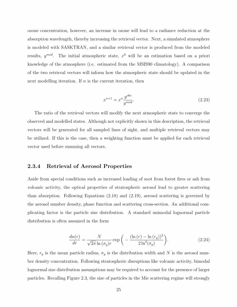
ozone concentration, however, an increase in ozone will lead to a radiance reduction at the

absorption wavelength, thereby increasing the retrieval vector. Next, a simulated atmosphere

is modeled with SASKTRAN, and a similar retrieval vector is produced from the modeled

results, ymod. The initial atmospheric state, x0 will be an estimation based on a priori

knowledge of the atmosphere (i.e. estimated from the MSIS90 climatology). A comparison

of the two retrieval vectors will inform how the atmospheric state should be updated in the

next modelling iteration. If n is the current iteration, then

xn+1 = xn yobs

ymod. (2.23)

The ratio of the retrieval vectors will modify the next atmospheric state to converge the

observed and modelled states. Although not explicitly shown in this description, the retrieval

vectors will be generated for all sampled lines of sight, and multiple retrieval vectors may

be utilized. If this is the case, then a weighting function must be applied for each retrieval

vector used before summing all vectors.

2.3.4 Retrieval of Aerosol Properties

Aside from special conditions such as increased loading of soot from forest fires or ash from

volcanic activity, the optical properties of stratospheric aerosol lead to greater scattering

than absorption. Following Equations (2.18) and (2.19), aerosol scattering is governed by

the aerosol number density, phase function and scattering cross-section. An additional com-

plicating factor is the particle size distribution. A standard unimodal lognormal particle

distribution is often assumed in the form

dn(r)

dr=

N√2π ln (σg)r

exp

(− (ln (r) − ln (rg))

2

2 ln2(σg)

). (2.24)

Here, rg is the mean particle radius, σg is the distribution width and N is the aerosol num-

ber density concentration. Following stratospheric disruptions like volcanic activity, bimodal

lognormal size distribution assumptions may be required to account for the presence of larger

particles. Recalling Figure 2.3, the size of particles in the Mie scattering regime will strongly

25

impact the scattering phase function. Errors in the assumed particle distribution will there-

fore manifest errors in the phase function.

Several retrieval methods have been developed to measure stratospheric aerosol extinction

coefficient, including the OSIRIS Version 5 Data Product [Bourassa et al., 2012a]. This data

product uses SASKTRAN’s flagship remote sensing instrument, OSIRIS, described in Section

2.2.4. The Version 5 extinction retrieval algorithm is a modification to a previous algorithm

developed by [Bourassa et al., 2007], with improvements coming from the inclusion of forward

modeled calculation of the radiance of the Rayleigh atmosphere, improvements to effective

albedo retrieval, and normalization of the retrieval vector to improve signal to noise. The

previous algorithm defined a retrieval vector

yj = ln

(I(j, λ2)

I(j, λ1)

), (2.25)

where I(j, λ) represents a normalized radiance at tangent altitude j and wavelength λ

[Bourassa et al., 2007]. In the published data product, λ1 = 470 nm and λ2 = 750 nm.

The tangent altitude radiance is normalized by the radiance at a higher reference tangent

altitude at the same wavelength. The tangent altitude normalization removes the need for

an absolute calibration, and also reduces the sensitivity to effective albedo.

The retrieval vector is modified in Version 5 to remove sensitivity to the dominant

Rayleigh scattering, particularly at low tangent altitudes. The Rayleigh contribution is

simulated in an aerosol free atmosphere, then used to normalize the retrieval vector,

yj = ln

(I(j, λ2)

I(j, λ1)

)− ln

(IRay(j, λ2)

IRay(j, λ1)

). (2.26)

This normalization helps to linearize the retrieval vector dependence on aerosol loading. The

retrieval vector is further modified to include a high altitude geometric mean normalization

rather than single high altitude normalization, which improves the signal-to-noise ratio.

The limitation to this approach is that it requires an assumed particle size distribution

(rg = 80 nm and σg = 1.6 in this case) to calculate the phase function. [Rieger et al., 2014]

investigate the validity of the ascribed phase functions by comparing intersecting measure-

ments from the ascending and descending track of OSIRIS. These intersection points are

26

measurements of common atmospheric states with different scattering angles. Differences in

the retrieved aerosol extinction indicate errors in the phase function, caused by an incorrect

particle size distribution. Comparing retrieved extinction in the tropics from the ascending

and descending nodes over several years highlights a systematic offset, likely pointing to an

incorrect particle size distribution assumption.

[Rieger et al., 2014] further develop the retrieval technique by investigating the sensitivity

of the retrieval vector to particle size. Although minimally, the 470 nm radiance is noted

to be influenced by aerosol, so it is not entirely insensitive to the particle size assumptions.

Therefore, the 470 nm normalization is removed from the retrieval vector.

In this 2014 study, three particle size distributions are defined that produce a common

retrieval vector at 750 nm, shown in Figure 2.4a. The size distributions represent a bimodal

distribution to simulate volcanic conditions, the Version 5 unimodal distribution, and a uni-

modal distribution with an effective radius to match the bimodal distribution. The retrieval

vector is then calculated over a wider spectrum for these three distributions, displayed in

Figure 2.4b. These vectors show little difference for wavelengths shorter than 800 nm, and

improved particle size sensitivity at longer wavelengths, highlighted by the separation of the

measurement vectors at long wavelengths. This is a key finding to identify the need for

near-infrared spectral measurements to retrieve both extinction and particle size content.

Advances to the retrieval technique are under continued investigation, with improve-

ments made to the selection of retrieval vectors as well as the inversion technique. The

current Version 7 OSIRIS data product for instance utilizes a selection of wavelengths and a

Levenberg-Marquardt procedure to update atmospheric state vectors, which minimizes bias

due to uncertainty in particle size [Rieger et al., 2019]. This continued retrieval development

has run in parallel to the development of aerosol sensing instrumentation. It has capitalized

on the features of existing instruments but has also identified opportunities for improvements

in the succeeding generation.

27

Figure 2.4: Modelled sensitivity of aerosol retrieval vectors to particle size distribu-tions. (a) Three aerosol size distributions at 22.5 km, highlighting two unimodal dis-tributions with differing mean particle radii, and a bimodal distribution representing apost-volcanic activity atmosphere. Each size distribution generates a common retrievalvector at 750 nm. (b) Retrieval vectors as a function of wavelength for the three sizedistributions. Reproduced with permission of the author, [Rieger et al., 2014].

2.4 Project Motivation

The goal of this work is to advance the design of ALI to fill the current opening in stratospheric

aerosol monitoring remote sensors. This development requires the expansion of the spectral

range from visible to NIR wavelengths to address the size distribution sensitivity in aerosol

retrievals. Additionally, polarization sensitivity is imperative in the next generation designs

for high altitude cloud identification to facilitate linking aerosol-cloud interactions.

Satellite-based instruments require several years of development from grassroots proto-

types to flight-qualified operational units. Standard practices in the space sector are out-

lined by operating procedures, hardware development plans and review processes defined by

organizations like the Canadian Space Agency (CSA), the National Aeronautics and Space

Administration (NASA), the European Space Agency (ESA) and several other national orga-

nizations. One of the most concise descriptions of the hardware development plan is NASA’s

roadmap of Technology Readiness Levels (TRLs) [Shea, 2017]. This work is focused on im-

28

proving the TRL of the Aerosol Limb Imager through hardware development for sub-orbital

platforms.

2.5 Advanced Remote Sensing Techniques

The several examples cited in section 2.2 have sustained a continuous stratospheric aerosol

record since the 1970s, with continuous global coverage beginning with the first satellite-based

remote sensors. Several of these instruments are designed specifically to target stratospheric

aerosol measurements, while others have adaptable capabilities as secondary functions. The

catalogue of remote sensors contains a vacancy for an instrument to capture continuous

global coverage with high spatial and temporal resolution. These targets are limited by the

technologies used in past and current generations of remote sensing instruments.

To fill this vacancy, a new instrument concept has been developed to specifically target

some of the shortcomings of current instrumentation. The Aerosol Limb Imager began fea-

sibility studies in the early 2010s and has continued to evolve towards a viable candidate for

a satellite mission within the next 10 years. The instrument is designed to capture multi-

spectral, 2D images of limb scattered sunlight and is the focus of the remainder of this work.

Optical concepts are first discussed, addressing image formation and limitations of physical

optical elements. These limitations result in degradation of image quality, which can be

characterized by aberration theory and quantified by performance metrics like spot size, en-

circled energy and modulation transfer function. These concepts are only briefly summarized

as they are well studied and documented [Born and Wolf, 2013, Hecht, 2017, Smith, 2008].

Next, acousto-optics, an electro-optical technique is examined to identify how spectrally re-

solved 2D images can be captured from a remote sensing platform. A discussion of a second

electro-optic technique, liquid crystal polarization modulation, is also presented, followed by

a discussion of the historical developments of ALI.

2.5.1 Imaging Optics

A point source, P, radiates through a uniform medium as a diverging spherical wave with

maxima separated by the wavelength, shown in Figure 2.5. These maxima, or wavefronts,

29

are captured at a specific moment in time and drawn as thin black lines. At the interface

between two media, the wave will refract according to Snell’s law. An ideal lens, with a

radius of curvature and an appropriately higher refractive index than the surrounding media,

will refract the spherical wave at different moments in time as it propagates, forming a plane

wave within the interior of the lens. As this plane wave continues to propagate rightward, it

once again reaches a media interface, and the plane wave is refracted at different moments

in time, forming a converging spherical wave. The point where the wavefronts converge, P’,

is a focused image of the point source. P and P’ are optical conjugates.

The process of focusing a point source through an ideal lens can be expanded to multiple

sources, each emitting a unique set of spherical wavefronts. Each source will have a single

optical conjugate, related to the longitudinal and transverse position of the source with

respect to the lens and its optic axis. Sources with a common longitudinal distance from the

lens will ideally focus on a plane, often described as an image plane. This leads to the concept

of optical image formation, in which a series of point sources from an extended object are

focused through an optical system to form an image in conjugate space.

Figure 2.5: Image formation of point source, P, through an ideal lens.

A mathematical formulism for wavefront propagation in an optical system is challenging,

however, it is greatly simplified by introducing the concept of optical rays. Rays are drawn

perpendicular to the wavefronts, shown in blue in Figure 2.5. These rays originate and diverge

from the source, P, and then converge at the focus, P’. Geometric optics is based on tracing

30

rays through an optical system. The technique is used for the initial layout of an optical

system as well as first-order error assessment.

Physical optics impose limitations on the reshaping of wavefronts, leading to optical

aberrations. Aberrations are the result of constraints in lens material selection and surface

shaping. Surface shaping can also limit the performance of reflective optical elements like

mirrors, which are analogous to lenses in many ways. Optical aberrations are character-

ized by the distance the ray is from the rotation axis of the optical element, r, and the

angle at which the rays strike the surface, h. The five primary transverse aberrations, re-

ferred to as Seidel aberrations, are spherical (proportional to r3), coma (proportional to r2h),

astigmatism (proportional to rh2), Petzval curvature (proportional to rh2), and distortion

(proportional to h3). Some of these Seidel aberrations also have longitudinal components

with slightly different dependencies. The result of these and higher-order aberrations is the

spatial broadening of energy distribution at the focus, P’. Figure 2.6a displays a geomet-

ric ray trace from a monochromatic point source, through a real lens to the focus. Select

wavefronts are highlighted. Figure 2.6b shows a single wavefront with a spherical wavefront

overlaid to highlight the difference in shape resulting from transmission through a physical

optical element. Finally, Figure 2.6c shows the distribution of rays as observed on a screen

placed at the focus of the lens from a geometric ray trace. The optical energy is distributed

over a finite area rather than focused to a single point, as was described for the ideal lens

case.

There are additional factors that also affect the concentration of rays at the focus. The

first is diffraction caused by the physical size of the imaging optic. Diffraction is quantified

by a Fourier transform related to the optical aperture and the wavelength of the source. For

example, an infinite distance point source passing through a circular aperture has a well-

defined diffraction limit described by the Airy disk [Airy, 1835]. In fact, diffraction occurs

for an ideal lens modelled with a finite size as well. Figure 2.6d displays the point spread

function (PSF) representing the physical propagation of wavefronts through a finite-sized real

lens. Here, the energy distribution is shown to be similar to that in Figure 2.6c, but in this

case, includes the impacts of diffraction.

The PSF is a useful analytic tool because it can be convolved with an object scene to

31

estimate the imaging performance of an optical system. Furthermore, it lends itself to a

convenient proxy, the encircled energy, to quantify the point source image quality. The

encircled energy describes the diameter of a circle that is required to capture a specified

percentage of the total optical energy. For instance, a perfect Airy disk contains 83.9% of the

optical energy within the central lobe of the pattern. This means the 83.9% encircled energy

for an ideal lens is encircled by a diameter of 2.44λ × f/#, where f/# is the ratio of the

system focal length to pupil diameter. The encircled energy is a particularly helpful metric

for assessing image quality when performing a Monte Carlo tolerance analysis to estimate

the performance of an optical system with realistic manufacturing and build tolerances.

A second significant factor that limits the size of a focused spot is related to the wavelength-

dependent refractive index of materials used for refractive optics. All physical sources have

a finite spectral bandwidth, which will inherently focus at different distances from the lens.

This leads to a wavelength-dependent broadening of the spot on a static image plane. The

magnitude of this broadening, described as chromatic defocus, can be reduced through the

addition of new lenses of different materials to find a balance in the spectral divergence for

each lens. These chromatic effects are not seen in reflective optical systems because the laws

governing reflection are achromatic.

Similar to the description for an ideal lens, the focusing of wavefronts through a physical

optic can also be expanded to an extended object to form an image. Here, however, the

extended point sources will each experience different amounts of optical aberration, depending

on their position with respect to the lens, and therefore each features a specific PSF. A tool

called the modulation transfer function (MTF) is used to quantify how the PSF redistributes

energy in the image plane over an extended object. To calculate the MTF at spatial frequency

f , a sinusoidal scene is imaged through the optical system, where the PSF redistributes signal

from the bright part of the scene into the dark parts through a convolution. A sinusoid is

selected for this metric because Fourier analysis shows that any scene can be represented by

sinusoidal spatial frequencies. The MTF is calculated using the bright (Imax) and dark (Imin)

parts of the image as:

MTF (f) =(Imax − Imin)

(Imax + Imin). (2.27)

32

Figure 2.6: Image formation of a point source, P, through a physical lens. (a) Raysand sampled wavefronts traced from the source P to the image P’. (b) Magnified viewof a single wavefront showing deviation from a spherical shape. (c) 2D spot diagramof rays traced through the lens system to a screen placed at the focus, P’. (d) Pointspread function displaying energy distribution including impacts of diffraction.

Figure 2.7 shows a representation of the MTF calculation for two object scenes with

differing frequencies on the left. The modulation is transferred through the optical system

and captured in the image. The low-frequency modulation (Figure 2.7a) is transferred more

efficiently than the high-frequency modulation (Figure 2.7b). The red lines in each plot

highlight the contrast in the respective images, with greater contrast seen in the low-frequency

case. Typically, contrast greater than 0.1 is required to resolve image information, but this

is application-specific [Smith, 1998].

2.5.2 Novel Atmospheric Spectral Filtering

Standard spectral filtering techniques implemented in previous aerosol measurement instru-

mentation cannot meet the goals of ALI. Grating spectrometers restrict spatial resolution

to only a single direction; transmission filters limit spectral selection flexibility and imaging

33

Figure 2.7: Transfer of object modulation through an optical system. (a) Low-frequency modulation is efficiently transferred, with high contrast between bright anddark regions. The brightness in the image is shown in red. (b) High-frequency modula-tion is less efficiently transferred, with more energy from the bright regions registeringin the dark regions in the image. The contrast between the bright and dark regions isreduced as shown in the red line.

duty cycle. Here, a novel use for acousto-optic tunable filter (AOTF) technology has been

identified to perform solid-state, multi-spectral imaging. The acousto-optic (AO) interaction

is governed by the propagation of acoustic and optical waves through certain materials, the

most effective being crystals which exhibit optical birefringence.

Optical Waves in Crystal Structures

The propagation of optical waves through birefringent crystals relies on the characteristics

of the lattice structure of the atoms. This has been well characterized for several materials

[Newnham, 2005]. Tellurium dioxide (TeO2) is a common AO material with a Tetragonal

422 crystal class, which exhibits uniaxial birefringence, meaning it shows symmetry about a

single rotation axis.

The optical anisotropic nature of TeO2 arises from the electrical dipoles established within

the medium, which induces a directional dependence on the electrical permitivity, ϵ. For most

34

materials, ϵ is a scalar value, but in this case it is a second rank tensor,

ϵ =

ϵ11 ϵ12 ϵ13

ϵ21 ϵ22 ϵ23

ϵ31 ϵ32 ϵ33

. (2.28)

The orientation of this tensor with respect to the crystal can be selectively chosen to

eliminate all elements except for the diagonal. The tensor leads to loci of two orthogonal

wave vectors, ko and ke [Korpel, 1996]. This is observed by starting with two of Maxwell’s

equations:

∇× E = −dBdt

, (2.29)

∇×H =dDdt

. (2.30)

Assuming a plane wave oscillating according to ej(ωt−k·R), and recalling that B = µoH in

material free from magnetic permeability, Equations (2.29) and (2.30) may be simplified to

k × E = ωµoH (2.31)

and

k ×H = −ωD. (2.32)

Eliminating H and applying a× (b× c) = (a · c)b− (a · b)c yields:

(k · E)k − (k · k)E = −ω2µoD. (2.33)

Recall also that D = ϵE , where ϵ is the tensor from Equation (2.28). The orientation of the

tensor is chosen to align with the Cartesian crystal symmetry axes, resulting in

ϵ = ϵ0

n2x 0 0

0 n2y 0

0 0 n2z

. (2.34)

Equation (2.33) can be expressed as a set of linear equations in E as

35

(βn2

x − k2y − k2

z) kxky kxkz

kxky (βn2y − k2

x − k2z) kykz

kxkz kykz (βn2z − k2

x − k2y)

Ex

Ey

Ez

= 0, (2.35)

where

β = µ0ϵ0ω2. (2.36)

Nontrivial solutions are found when the determinant of the 3 × 3 matrix equals zero, ex-

pressed as

β2−β

(−k2x − k2

y

n2z

+−k2

x − k2z

n2y

+−k2

y − k2z

n2x

)+

(k2x

n2yn

2z

+k2y

n2xn

2z

+k2z

n2xn

2y

)(k2

x+k2y+k2

z) = 0. (2.37)

The uniaxial property of TeO2 implies that the refractive indices about two of these axes

are the same. Defining nx = ny = no as the “ordinary” refractive index and nz = ne as the

“extraordinary” refractive index, the expression factors into

(k2x

n2o

+k2y

n2o

+k2z

n2o

− β

)(k2x

n2e

+k2y

n2e

+k2z

n2o

− β

)= 0. (2.38)

Equation (2.38) is used to describe two elliptical surfaces in k space, which bound the wave

vector of a specific frequency. Equating the first factor to zero traces a spherical boundary for

the wave vector, regardless of the direction of k. Equating the second to zero, however, traces

an ellipsoid symmetric about the Z-axis. This solution space implies that any direction of

propagation has two allowable wave vector solutions. The first solution is the same regardless

of propagation direction, and the second varies with direction. These solutions describe the

ordinary and extraordinary polarization states, respectively.

To better illustrate this point, a refractive index ellipsoid for a uniaxial material is drawn

in Figure 2.8a where nx = ny = no and nz = ne. A wave propagates in the YZ plane in the

direction of the wave normal, sp, at an angle, θ, with respect to the optic axis of the material

(defined as the z-axis). The refractive index for this wave is defined by the intersection of the

ellipsoid with a vector normal to sp. Equation (2.38) described two solutions for k, the first

of which is bound by a sphere with refractive index described by no. This assigns the first

36

refractive index solution to the XY plane, shown as point “a”, the ordinary refractive index.

The second solution, with an orthogonal polarization to the first, intersects with the ellipsoid

on an elliptical boundary which depends on θ. The second point, “b”, offers the refractive

index of the extraordinary polarization. A plot of the loci of the ordinary and extraordinary

refractive indices as a function of angle from 0 to 2π is shown in Figure 2.8b. The ordinary

refractive index, na, is constant with θ, but the refractive index of the extraordinary wave,

nb, varies from no to ne based on the ellipse [Yariv, 1991]

1

nb(θ)=

cos2(θ)

n2o

+sin2(θ)

n2e

. (2.39)

(a) (b)

Figure 2.8: Optical propagation at angle θ with respect to optical axis. (a) Intersectionof orthogonal polarization states with refractive index ellipsoid. (b) Ordinary andextraordinary refractive index as a function of incidence angle with respect to theoptical axis.

Multiplying the indices in Figure 2.8b by the magnitude of the free space wave vector

will define ko and ke. Generating similar plots for the wave vectors is essential later for

illustrating the Bragg diffraction criterion that defines the AOTF interaction.

37

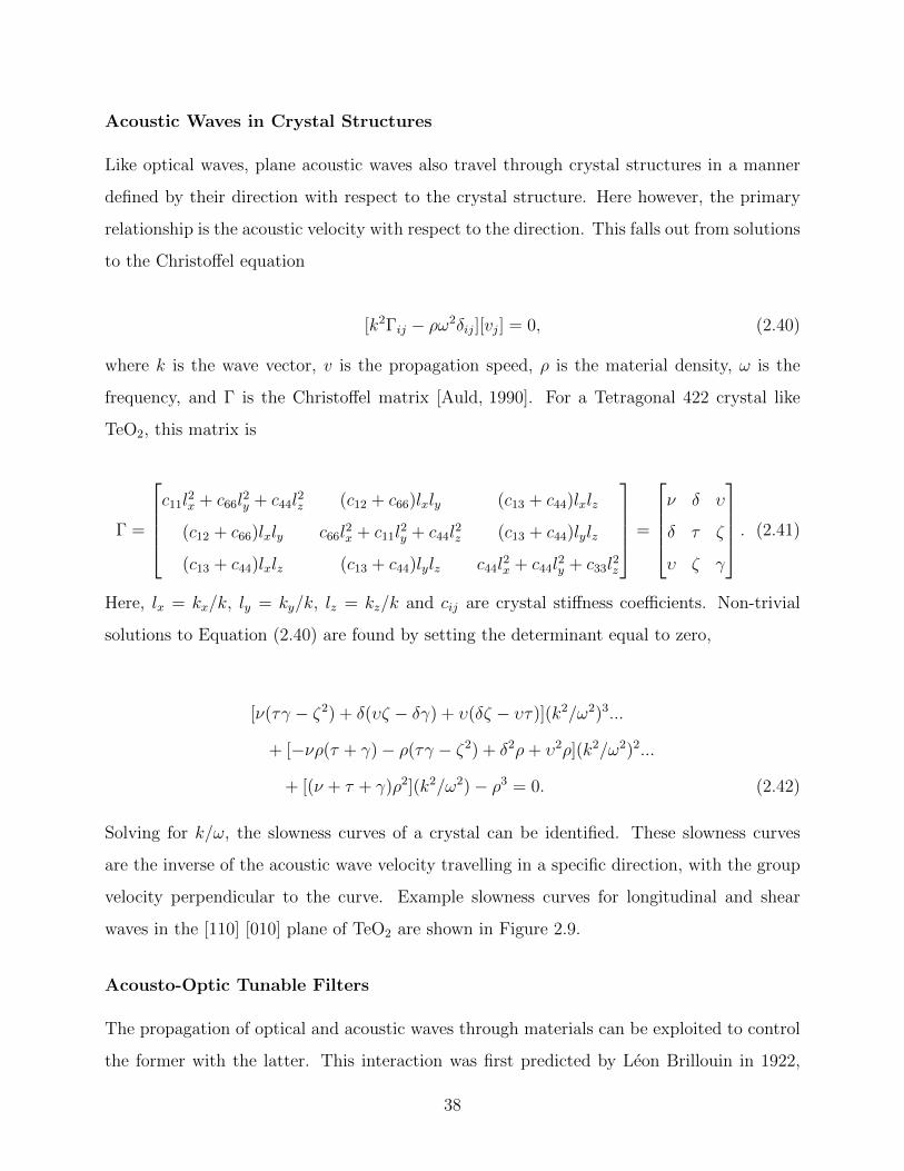
Acoustic Waves in Crystal Structures

Like optical waves, plane acoustic waves also travel through crystal structures in a manner

defined by their direction with respect to the crystal structure. Here however, the primary

relationship is the acoustic velocity with respect to the direction. This falls out from solutions

to the Christoffel equation

[k2Γij − ρω2δij][vj] = 0, (2.40)

where k is the wave vector, v is the propagation speed, ρ is the material density, ω is the

frequency, and Γ is the Christoffel matrix [Auld, 1990]. For a Tetragonal 422 crystal like

TeO2, this matrix is

Γ =

c11l

2x + c66l

2y + c44l

2z (c12 + c66)lxly (c13 + c44)lxlz

(c12 + c66)lxly c66l2x + c11l

2y + c44l

2z (c13 + c44)lylz

(c13 + c44)lxlz (c13 + c44)lylz c44l2x + c44l

2y + c33l

2z

=

ν δ υ

δ τ ζ

υ ζ γ

. (2.41)

Here, lx = kx/k, ly = ky/k, lz = kz/k and cij are crystal stiffness coefficients. Non-trivial

solutions to Equation (2.40) are found by setting the determinant equal to zero,

[ν(τγ − ζ2) + δ(υζ − δγ) + υ(δζ − υτ)](k2/ω2)3...

+ [−νρ(τ + γ) − ρ(τγ − ζ2) + δ2ρ + υ2ρ](k2/ω2)2...

+ [(ν + τ + γ)ρ2](k2/ω2) − ρ3 = 0. (2.42)

Solving for k/ω, the slowness curves of a crystal can be identified. These slowness curves

are the inverse of the acoustic wave velocity travelling in a specific direction, with the group

velocity perpendicular to the curve. Example slowness curves for longitudinal and shear

waves in the [110] [010] plane of TeO2 are shown in Figure 2.9.

Acousto-Optic Tunable Filters

The propagation of optical and acoustic waves through materials can be exploited to control

the former with the latter. This interaction was first predicted by Leon Brillouin in 1922,

38

Figure 2.9: Slowness curves for shear and longitudinal acoustic waves in TeO2.

through a demonstration of light scattering within a medium caused by an acoustic wave

travelling through it [Brillouin, 1922]. Several decades later, this phenomenon was formally

described as the interaction between planar sound waves and light and named the AO effect

identified previously [Korpel and Poon, 1980].

The AO effect is induced in transparent materials by a periodic variation of the refrac-

tive index. This variation is introduced by the elasto-optic effect when high frequency stress

causes compression and relaxation of the material [Chang, 1981]. Stress may be applied by

bonding piezoelectric transducers to the material and applying a potential difference. The

interaction of light with this region of periodic variation leads to AO diffraction, which is

like the interaction of light with a transmission grating [Chang, 1977]. This AO diffrac-

tion was first demonstrated in a water cell in 1955, then with anisotropic materials in 1967

[Rosenthal, 1955, Dixon, 1967]. The most favourable of these materials are those with high

densities and slow acoustic speeds, such as quartz (SiO2), lithium niobate (LiNbO3) and

TeO2 [Bei et al., 2004].

39

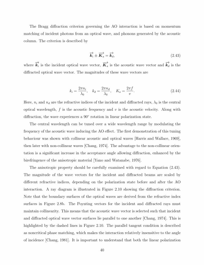
The Bragg diffraction criterion governing the AO interaction is based on momentum

matching of incident photons from an optical wave, and phonons generated by the acoustic

column. The criterion is described by

−→ki ±

−→Ka =

−→kd, (2.43)

where−→ki is the incident optical wave vector,

−→Ka is the acoustic wave vector and

−→kd is the

diffracted optical wave vector. The magnitudes of these wave vectors are

ki =2πni

λ0

, kd =2πnd

λ0

, Ka =2πf

v. (2.44)

Here, ni and nd are the refractive indices of the incident and diffracted rays, λ0 is the central

optical wavelength, f is the acoustic frequency and v is the acoustic velocity. Along with

diffraction, the wave experiences a 90 rotation in linear polarization state.

The central wavelength can be tuned over a wide wavelength range by modulating the

frequency of the acoustic wave inducing the AO effect. The first demonstration of this tuning

behaviour was shown with collinear acoustic and optical waves [Harris and Wallace, 1969],

then later with non-collinear waves [Chang, 1974]. The advantage to the non-collinear orien-

tation is a significant increase in the acceptance angle allowing diffraction, enhanced by the

birefringence of the anisotropic material [Yano and Watanabe, 1976].

The anisotropic property should be carefully examined with regard to Equation (2.43).

The magnitude of the wave vectors for the incident and diffracted beams are scaled by

different refractive indices, depending on the polarization state before and after the AO

interaction. A ray diagram is illustrated in Figure 2.10 showing the diffraction criterion.

Note that the boundary surfaces of the optical waves are derived from the refractive index

surfaces in Figure 2.8b. The Poynting vectors for the incident and diffracted rays must

maintain collinearity. This means that the acoustic wave vector is selected such that incident

and diffracted optical wave vector surfaces lie parallel to one another [Chang, 1974]. This is

highlighted by the dashed lines in Figure 2.10. The parallel tangent condition is described

as noncritical phase matching, which makes the interaction relatively insensitive to the angle

of incidence [Chang, 1981]. It is important to understand that both the linear polarization

40

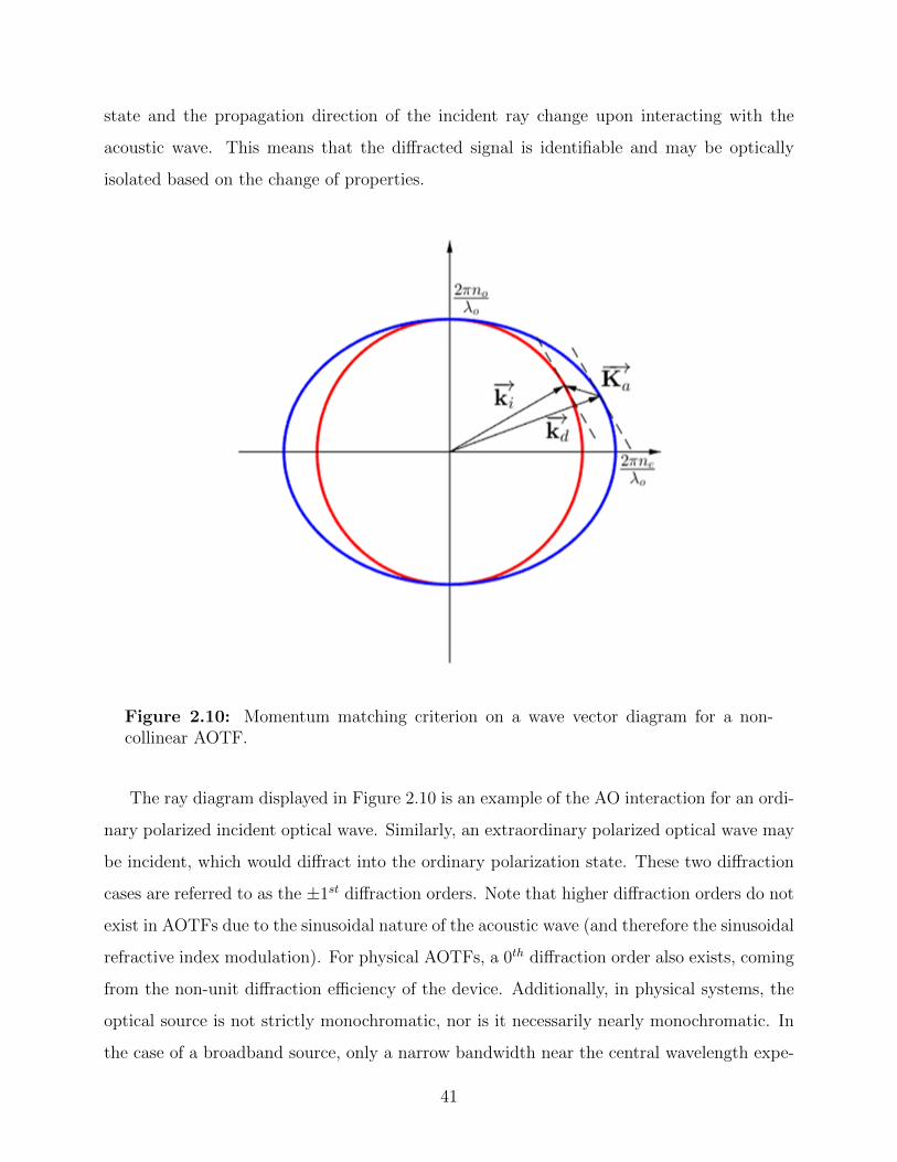
state and the propagation direction of the incident ray change upon interacting with the

acoustic wave. This means that the diffracted signal is identifiable and may be optically

isolated based on the change of properties.

Figure 2.10: Momentum matching criterion on a wave vector diagram for a non-collinear AOTF.

The ray diagram displayed in Figure 2.10 is an example of the AO interaction for an ordi-

nary polarized incident optical wave. Similarly, an extraordinary polarized optical wave may

be incident, which would diffract into the ordinary polarization state. These two diffraction

cases are referred to as the ±1st diffraction orders. Note that higher diffraction orders do not

exist in AOTFs due to the sinusoidal nature of the acoustic wave (and therefore the sinusoidal

refractive index modulation). For physical AOTFs, a 0th diffraction order also exists, coming

from the non-unit diffraction efficiency of the device. Additionally, in physical systems, the

optical source is not strictly monochromatic, nor is it necessarily nearly monochromatic. In

the case of a broadband source, only a narrow bandwidth near the central wavelength expe-

41

riences diffraction. The rays from beyond this bandwidth will transmit through, unaffected

by the acoustic wave, and therefore exist as additional 0th order signal. Figure 2.11 shows

the nominal operation of an AOTF on an unpolarized broadband source.

Figure 2.11: Application of an AOTF on unpolarized broadband signal. Four distinctbeams exit the AOTF, identified by their polarization state and diffraction order.

The function of an AOTF on unpolarized broadband signal highlights the capability of

this technology to perform spectral filtering. The narrow bandwidth experiencing the AO

interaction is illustrated with red rays. The interaction occurs on both the ordinary and

extraordinary polarization states of the incident signal, and the ±1st order diffracted beams

diverge from one another. This leaves the 0th order to propagate between these diffracted

beams, but it too experiences a polarization-dependent separation based on the birefringence

of the crystal.

A common method to utilize an AOTF for spectral filtering is to employ two linear

polarizing filters. The first filter is placed ahead of the AOTF and is aligned such that it only

transmits either the ordinary or extraordinary polarization state, as defined by the crystal

orientation. This first polarizing filter eliminates one of the undiffracted beams and one of

the 1st order beams. The second polarizing filter is placed after the AOTF, and is cross

aligned with the first. Due to the change in polarization state during the AO interaction,

this second filter eliminates the second undiffracted beam, and only passes a single 1st order

state, thus providing narrow-band spectral filtering.

42

The specific properties of the narrow band filtering fall out from both the momentum

matching condition for a specific crystal geometry, as well as the geometry of the transducer

bonded to the crystal. Specifically, recalling the wave vector illustration in Figure 2.10,

the relationship between the acoustic frequency, fa, and the diffracted wavelength can be

extracted under the assumption of small birefringence. This relationship can be approximated

as

fa =

(v∆n

λ0

)√sin4 θi + sin2 2θi. (2.45)

Here, ∆n is the birefringence and θi is the angle of the incident wave vector with respect to

the optical axis [Chang, 1974]. The bandpass response is described by

T (λ0) = Tosinc2(σL), (2.46)

where To is the peak transmission, L is the interaction length and σ is the momentum

mismatch parameter [Chang, 1975]. The peak transmission is a function of the AO figure of

merit, M2, and the acoustic power density, Pd, per

To = sin2

(π

2λ20

M2PdL2

)1/2

. (2.47)

Finally, the full width at half maximum (FWHM) of the bandpass response can be esti-

mated from Equation (2.46) when σL ≈ 0.44. The FWHM is

∆λ =0.9λ2

0

bL sin2 θo, (2.48)

where b is the dispersion constant [Chang, 1975]. The AOTF properties described in Equa-

tions (2.45) through (2.48) lead to trade-offs between diffraction efficiency, the bandwidth

of the filtered signal, power requirements and acoustic frequency selection. It is worth not-

ing that the sidelobes in the sinc2 bandpass response may be suppressed using transducer

amplitude apodization [Chang and Katzka, 1978].

43

2.5.3 Liquid Crystal Technology

Liquid crystals (LCs) are a classification of materials that exist in a state similar to both

crystalline solids and liquid states. The classification is based primarily on the order that

the molecules feature.

Classically, crystal solids are defined as either atomic solids (metals) or molecular solids

(ice crystals). In the first case, the primary bonds holding the individual atomic components

together are ionic or covalent. In the second case, the individual molecular components are

bound by secondary bonds, which are not as strong as the ones holding the atoms together

in the molecule, but still feature strong bond enthalpies. As a result, the structure of both

of these crystal types is very well defined, with no degrees of freedom for either rotational or

translational order. Crystals may therefore be classified based on the properties of order that

they feature, such as unit cells and lattice translation vectors. Liquids on the other hand

do not feature these same strong bonds between individual components and display multiple

orders of freedom in both translation and rotation for the components.

Liquid crystals are composed of molecular components called mesogens with secondary

bonds tying the mesogens together. They have fluidlike properties, however, the mesogens

are arranged with structural order [De Gennes and Prost, 1993]. Liquid crystals are grouped

into three types: thermotropic, lyotropic and polymeric. Mesogens of the first type establish

their order based on the entropy of the system, ranging from the most ordered arrangements

(smectic) to least ordered (nematic) as entropy increases. Once a high enough entropy is

reached, the order of the mesogens breaks and the material takes on a strictly fluidlike

behaviour. Thermotropic liquid crystals may also be influenced by external electromagnetic

fields, which is described following.

Two types of mesogens exist, based on the structure of the molecule. These are rod-

like “calamitic” mesogens, and disc-like “discotic” mesogens. The former are of current

interest, specifically those which are anisotropic. These calamitic mesogens typically arrange

themselves so that there exists some alignment along their long axis. The average direction

of the long axis is described as a director. Three examples of mesogen arrangements are

shown in Figure 2.12.

44

(a) (b) (c)

Figure 2.12: Three thermotropic mesogen arrangements. (a) Smectic. (b) Nematic.(c) Cholesteric or twisted-nematic. [Litster and Birgeneau, 1982]

The arrangement in Figure 2.12a is described as smectic. This classification contains as

many as 9 subclassifications, but generally exhibit a layered translational order as well as

strong rotational order exhibited by aligned directors in each layer. The nematic classification

illustrated in Figure 2.12b shows a reduction in the translational order of the mesogens, with

mesogens existing outside of defined layers, caused by an increase in entropy. The director

however is common over the entire volume. Finally, Figure 2.12c shows the cholesteric, or

twisted-nematic arrangement. Here, the mesogens once again feature a layered order, how-

ever, each layer defines a unique director, which is rotated a uniform amount with respect to

the previous layer, with a pitch roughly on the order of microns [Litster and Birgeneau, 1982].

The scale of the rotating director and the anisotropic nature of twisted-nematic liquid

crystals offer a desirable method for controlling or altering the polarization state of light.

As described previously, the electric dipoles established within a birefringent material can

influence an optical wave passing through, with distinct impacts attributed to the polarization

state of the wave. In this case, the rotating director influences a rotation in the linear

polarization state of light as it passes through, with a rotation angle nearly equal to the

rotation of the director. This response is presented in Figure 2.13a, where liquid crystals

are sandwiched between two transparent plates. Qualitatively, this optical response is very

similar to that of a birefringent wave plate. However, the unique quality of these twisted-

nematic liquid crystals is that the director responds to an electric field that may be applied

across the cell if the two plates are transparent yet electrically conductive. This causes the

directors in all layers to align such that both optical polarization states behave as ordinary

45

polarized waves passing through the material (the propagation direction is aligned with the

optical axis of the mesogens), thus removing the optical activity displayed in the twisted

state, shown in Figure 2.13b [Schadt and Helfrich, 1971].

(a) (b)

Figure 2.13: Optical activity within a twisted-nematic liquid crystal cell. (a) In therelaxed state, the mesogen director undergoes a 90 twist over the length of the cell.The linear polarization state of an optical wave follows the rotation. (b) The mesogendirectors align to an applied electric field between the plates housing the cell, removingthe optical activity and allowing the optical wave to pass through unaffected.

The electro-optic element depicted in Figure 2.13 is called a Liquid Crystal polarization

Rotator (LCR). As with the previously described birefringent materials used in AOTFs, the

ordinary and extraordinary refractive indices of the mesogens have a wavelength dependence.

This means that a specified LCR cell width can be optimized for a single monochromatic

wavelength, and any additional wavelengths will experience a polarization rotation not ex-

actly equal to 90 [Gooch and Tarry, 1974]. This results in a slightly elliptical polarization

state.

2.5.4 ALI Version 1

The first generation of the ALI instrument (ALI V1) was designed and tested between 2011-

2014 [Elash et al., 2016, Elash, 2016]. This instrument laid the groundwork for the develop-

ments that are discussed in this work.

ALI V1 was based on the concepts described in Sections 2.5.1 and 2.5.2. It was a multi-

spectral imager operating over the 650-1000 nm spectral range. A transmissive optical chain

46

channeled scattered sunlight through an AOTF and imaged it on a charge-coupled device

image sensor. The optical layout of ALI V1 is presented in Figure 2.14.

Figure 2.14: Optical layout of ALI V1. Elements 1 and 2 comprise an afocal telescope.Elements 3 and 5 are linear polarizing filters around the AOTF, Element 4. Element 6is a singlet to focus wave fronts onto the image sensor, Element 7.

The operational performance of ALI V1 was tested on board a stabilized, high-altitude

balloon platform from Timmins, Ontario in the fall of 2014. This flight represented the first

demonstration of atmospheric limb scattered images captured with AOTF spectral filtering.

This important proof-of-concept experiment validates the ability of this technology to cap-

ture level 0 data products for the retrieval of stratospheric aerosol properties in the upper

troposphere and lower stratosphere of the atmosphere.

The following chapters describe the work completed to advance the TRL of the ALI

concept. These efforts specifically focus on hardware development to improve the optical

performance of ALI, tailored to several measurement platforms that progress towards the

operating conditions for a satellite mission. A review of the methods used for the design and

preparation for flight is presented in the following chapter.

47

Chapter 3

Methods

3.1 High-Level Instrument Requirements

The discussion of stratospheric aerosol remote sensors has highlighted the need for new instru-

mentation with long-term, global monitoring capabilities achieving high spatial and temporal

resolution. The proof-of-concept demonstration of ALI V1 has positioned the instrument to

fulfill this need.

The conceptual requirements for ALI are:

• Narrow band spectral filtering across the visible to near infrared spectrum.

• Polarization detection in two orthogonal linear states.

• 2 dimensional image capture with fine vertical resolution.

• Utilization of the limb viewing geometry for sub-orbital demonstration with orbital

analogs.

This chapter discusses the adaptation of this concept to a realized instrument, highlight-

ing the optical design activities and the key trade-off studies that have guided the next

generations of ALI. These activities are key for both the second balloon-borne version of

ALI (ALI V2) and an elegant breadboard version set to fly on a high altitude aircraft (ALI

EBB). A discussion of characterization techniques is presented, motivated specifically by the

preparation for the sub-orbital demonstration of ALI V2 on a high-altitude balloon platform.

48

3.2 Optical Design

3.2.1 Technology Trades

The conceptual instrument requirements are first addressed by selecting the appropriate

technologies to best meet their needs. Each of the first three requirements leads to a unique

technology selection, although the requirements themselves are not mutually exclusive. Two

primary technology trade studies are summarized to justify the technologies selected for

instrument realization.

Spectral Filtering

Spectral filtering may be achieved through classical optical techniques such as diffrac-

tion gratings or optical filters. The former has been demonstrated for atmospheric re-

mote sensing in instruments like OSIRIS [Llewellyn et al., 2004] and the SAGE instruments

[World Meteorological Organization, 1986, Mauldin et al., 1985]. Although this technique

achieves fine spectral resolution, it does not lend itself to 2D imaging. This is because the

spectral separation is achieved through an angular broadening of the optical signal, thereby

washing out the spatial resolution in at least one axis.

The alternate classical approach for spectral filtering using optical filters is effectively the

obverse of a diffraction grating approach. These filters are capable of operating over reason-

able fields of view to maintain 2D imaging capabilities, as demonstrated on the Hubble Space

Telescope [Turner-Valle et al., 2004] and for the Near Infrared Imager and Slitless Spectro-

graph on the James Webb Space Telescope [Doyon et al., 2012]. However, the selection of

discrete filtering wavebands makes this technology rigid in terms of spectral filtering mobility.

Furthermore, the use of optical filters necessarily requires a mechanism capable of moving

each filter into the optical path of the instrument, impacting temporal resolution.

Acousto-optic technology, described in Section 2.5.2 strikes a balance between these two

techniques. The tunable nature of AOTF devices is complimentary to continuous spectral dis-

persion of a grating (albeit with coarser spectral resolution) while preserving the angular regis-

tration required for 2D imaging. AOTFs are an emerging technology for several space-based

49

applications, including planetary and natural satellite spectroscopy [Korablev et al., 2018]

and Earth observation [Dekemper et al., 2012]. Therefore, an AOTF is selected for further

technology development for ALI.

Polarimetry Mechanism

The polarization effects of an AOTF must be considered when selecting a technology to

capture orthogonal polarization states. Once again, classical optical techniques may be used

to perform the polarization selection, however, they come at a cost for sub-orbital/orbital

remote sensors.

Figure 2.11 highlighted that unpolarized signal entering into an AOTF will be diffracted

into two 1st orders. Theoretically, this provides the capabilities that are sought for cloud

discrimination. However, the relatively high dispersion of AO materials coupled with the

momentum matching criterion means that the direction of these two 1st order beams will

wander as the wavelength is tuned. This is an undesirable characteristic because it will

significantly change the field of view captured for each tuned wavelength (both for the ALI

application and several other AOTF uses). To compensate for this wander, a wedge is

often cut into the exit face of the AOTF to balance the inherent dispersion and momentum

matching condition. This balance can only be struck for one of the two 1st order beams

however and exaggerates the wander for the second. This explains the use of linear polarizing

filters (LPF) that are typically placed in front of and behind an AOTF, as they act to reduce

stray light passing through the optical system.

With the assumption of a LPF preceding the AOTF, a classical solution to alter the linear

polarization state into the filter would be to use a set of half-wave plates. These plates rely on

birefringent materials which retard the phase of the polarization state aligned to a specific

crystal axis. Choosing an appropriate thickness (half of a specific wavelength), the linear

polarization state of transmitted light can be rotated 90. This rotation is specific to a single

wavelength, and additional wavelengths adopt an elliptical profile unless multiple waveplates

are used. To utilize this technology, a rotation mechanism is required to either rotate the

wave plate about its normal axis (rotation by 45) or to rotate the wave plate(s) into and

out of the optical path. Although viable options exist for both, these impact the temporal

50

resolution of the instrument in much the same way optical filters would have impacted the

spectral filtering design trade.

A preferable alternative to a wave plate solution is to utilize a liquid crystal polarization

rotator described in Section 2.5.3. Although these too suffer from a wavelength-dependent

ellipticity in the outgoing polarization state, their solid-state operation is preferable for sub-

orbital platforms. They require reduced volume, mass and power when compared to a rota-

tion mechanism, while also featuring significantly faster switching speeds. A LCR is a new

addition to ALI V2 and ALI EBB as it was not used in the previous ALI V1 design.

3.2.2 AOTF Modelling

The previous chapter highlighted the theory and principles that govern the operation of an

AOTF. These principles can be applied to generate a mathematical model to assess the

operation of an AOTF [Zhao et al., 2014, Poon, 2006]. For this work, a model is developed

based on the one presented by [Zhao et al., 2014] to aid in the design of ALI. The model

uses the geometry of the AOTF crystal to assess how optical rays of various wavelengths will

travel through the AOTF as it is tuned to near by central wavelengths. The geometry used

for the model is described in Figure 3.1.

The formulism set out in [Zhao et al., 2014] is closely followed in this model, but deviates

in the approach to handling phase-mismatching condition. An analytic solution to the phase-

matching condition is determined, then a numerical method is used to assess the mismatching

cases for several fields and wavelengths.

The model decomposes the function of an AOTF into three processes, described by three

surfaces. This method is translatable to several ray-tracing software packages like CODE V

or Zemax, as each primarily uses surface-to-surface propagation for design and analysis. The

model calculates direction cosines for rays between each surface, described as (Li,Mi, Ni),

where i is the index of the previous surface. The incident ray is indexed 0. The model

requires two coordinate frames, the global XYZ frame and the crystal X’Y’Z’ frame.

51

Figure

3.1:

AO

TF

mod

elge

omet

ryad

apte

dw

ith

per

mis

sion

from

[Zh

aoet

al.,

2014

]©

Th

eO

pti

cal

Soci

ety.

Th

ree

opti

cal

surf

aces

defi

ne

how

anop

tica

lsi

gnal

ente

rsth

eA

OT

F,

diff

ract

sat

the

acou

stic

colu

mn

(or

pas

ses

thro

ugh

ifm

omen

tum

mat

chin

gis

not

met

),an

dth

enre

frac

tsou

tof

the

AO

TF

ata

wed

ged

inte

rfac

e.

52

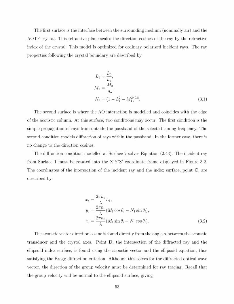
The first surface is the interface between the surrounding medium (nominally air) and the

AOTF crystal. This refractive plane scales the direction cosines of the ray by the refractive

index of the crystal. This model is optimized for ordinary polarized incident rays. The ray

properties following the crystal boundary are described by

L1 =L0

no

,

M1 =M0

no

,

N1 = (1 − L21 −M2

1 )0.5. (3.1)

The second surface is where the AO interaction is modelled and coincides with the edge

of the acoustic column. At this surface, two conditions may occur. The first condition is the

simple propagation of rays from outside the passband of the selected tuning frequency. The

second condition models diffraction of rays within the passband. In the former case, there is

no change to the direction cosines.

The diffraction condition modelled at Surface 2 solves Equation (2.43). The incident ray

from Surface 1 must be rotated into the X’Y’Z’ coordinate frame displayed in Figure 3.2.

The coordinates of the intersection of the incident ray and the index surface, point C, are

described by

xc =2πno

λL1,

yc =2πno

λ(M1 cos θi −N1 sin θi),

zc =2πno

λ(M1 sin θi + N1 cos θi). (3.2)

The acoustic vector direction cosine is found directly from the angle α between the acoustic

transducer and the crystal axes. Point D, the intersection of the diffracted ray and the

ellipsoid index surface, is found using the acoustic vector and the ellipsoid equation, thus

satisfying the Bragg diffraction criterion. Although this solves for the diffracted optical wave

vector, the direction of the group velocity must be determined for ray tracing. Recall that

the group velocity will be normal to the ellipsoid surface, giving

53

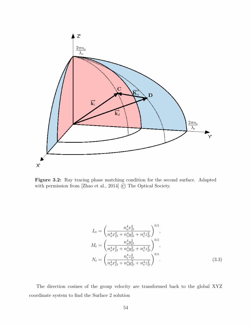
Figure 3.2: Ray tracing phase matching condition for the second surface. Adaptedwith permission from [Zhao et al., 2014] © The Optical Society.

Lt =

(n4ox

2D

n4ox

2D + n4

oy2D + n4

ez2D

)0.5

,

Mt =

(n4oy

2D

n4ox

2D + n4

oy2D + n4

ez2D

)0.5

,

Nt =

(n4ez

2D

n4ox

2D + n4

oy2D + n4

ez2D

)0.5

. (3.3)

The direction cosines of the group velocity are transformed back to the global XYZ

coordinate system to find the Surface 2 solution

54

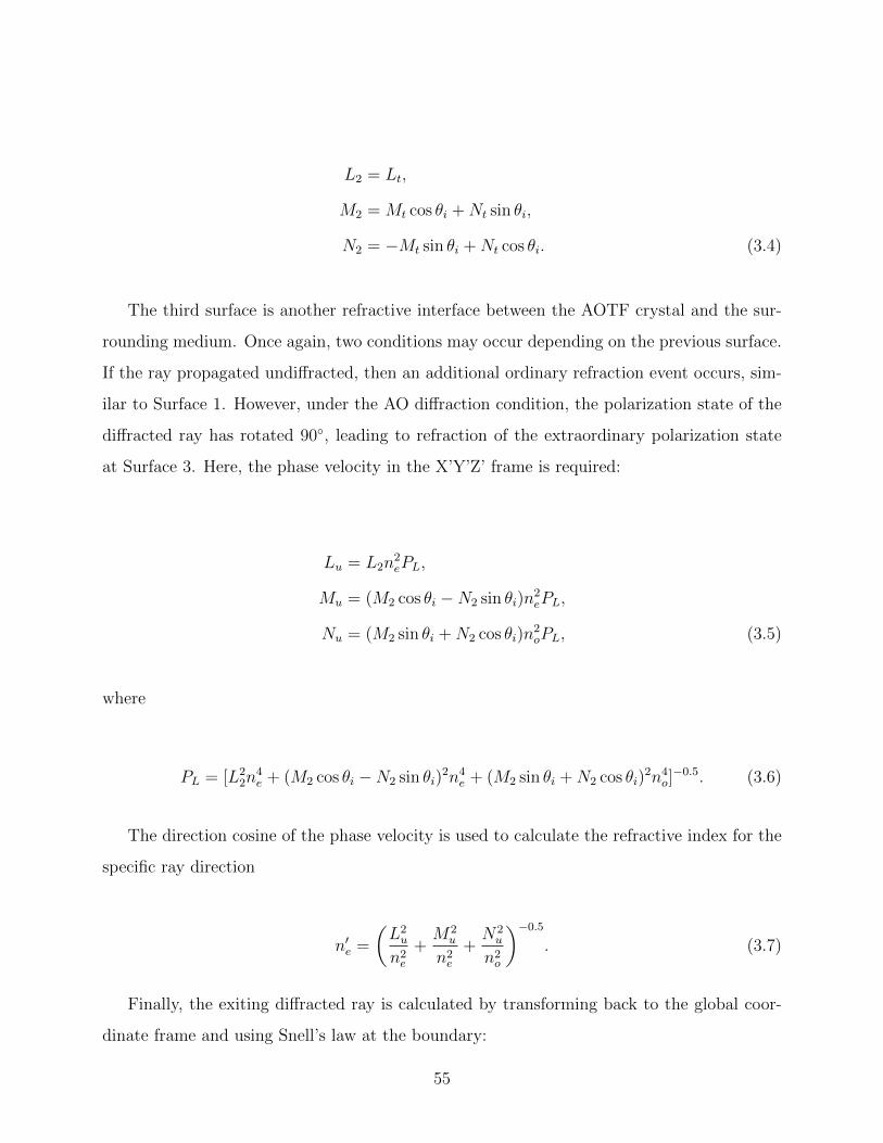
L2 = Lt,

M2 = Mt cos θi + Nt sin θi,

N2 = −Mt sin θi + Nt cos θi. (3.4)

The third surface is another refractive interface between the AOTF crystal and the sur-

rounding medium. Once again, two conditions may occur depending on the previous surface.

If the ray propagated undiffracted, then an additional ordinary refraction event occurs, sim-

ilar to Surface 1. However, under the AO diffraction condition, the polarization state of the

diffracted ray has rotated 90, leading to refraction of the extraordinary polarization state

at Surface 3. Here, the phase velocity in the X’Y’Z’ frame is required:

Lu = L2n2ePL,

Mu = (M2 cos θi −N2 sin θi)n2ePL,

Nu = (M2 sin θi + N2 cos θi)n2oPL, (3.5)

where

PL = [L22n

4e + (M2 cos θi −N2 sin θi)

2n4e + (M2 sin θi + N2 cos θi)

2n4o]

−0.5. (3.6)

The direction cosine of the phase velocity is used to calculate the refractive index for the

specific ray direction

n′e =

(L2u

n2e

+M2

u

n2e

+N2

u

n2o

)−0.5

. (3.7)

Finally, the exiting diffracted ray is calculated by transforming back to the global coor-

dinate frame and using Snell’s law at the boundary:

55

L3 = Lun′e,

M3 = [Mu cos (θi + β) + Nu sin (θi + β)]n′e cos β

− 1 − L2u − [Mu cos (θi + β) + Nu sin (θi + β)]2n′

e20.5 sin β,

N3 = [Mu cos (θi + β) + Nu sin (θi + β)]n′e sin β

− 1 − L2u − [Mu cos (θi + β) + Nu sin (θi + β)]2n′

e20.5 cos β. (3.8)

The direction cosines (L0,M0, N0), (L1,M1, N1), (L2,M2, N2), and (L3,M3, N3) describe

the propagation direction of the phase matched ray diffracted by an AOTF. This equation

set is used both in MATLAB for numerical computing and CODE V for optical design and

analysis.

As noted, the method for handling the momentum mismatching condition used in this

work differs from the one described in [Zhao et al., 2014]. Here, a numerical approach is taken

specifically to understand the trade-offs involved in AOTF implementation. Therefore, the

momentum mismatching condition is only utilized while performing analysis with MATLAB

and does not require implementation in CODE V, which would necessitate the described

analytical approach.

The solution to the momentum matched condition has described the acoustic wave vector

that results in AO diffraction at the desired central wavelength. To solve the mismatch

condition for several directions, the extraordinary wave vector surface for nearby wavelengths

is translated along the acoustic vector. This translation causes an intersection between the

two wave surfaces, as highlighted in Figure 3.3. To find the intersection, cross sections parallel

to the Y’/Z’ plane are assessed and a binary search is used to locate the two intersection

points.

The set of intersection points is first used to describe the incident ray directions that

meet the momentum mismatching condition for the specific wavelength by drawing rays to

the intersecting curve on the ordinary wave vector surface.

The set of all intersection points is then translated along the reverse of the acoustic

wave vector and the surface tangent for each point is calculated to describe the propagation

direction of the diffracted rays. The incident rays are then defined to have the same group

56

velocity, described as noncritical phase matching, which offsets the momentum mismatch.

This describes pairs of incident and diffracted rays (and wave vectors) for a wavelength near

the centrally tuned wavelength.

Figure 3.3: Overlapping wave vector surfaces for tracing acousto-optic diffraction un-der momentum mismatching condition. The intersection of ordinary wave vector surfaceand extraordinary wave vector surface translated by momentum matching acoustic wavevector is determined using numerical methods.

3.2.3 Design Trades

The key technologies identified in the above trades have sustained persistent technology de-

velopment to improve their respective TRLs in both ALI V2 and ALI EBB. These technolo-

gies come with flexibility in their implementation, which requires additional design trade-off

studies to determine the most applicable implementation for ALI. The most notable of these

design trades is the use of the AOTF in either collimated or imaging space within ALI.

57

AOTF Optical Layout

The wide angular aperture achieved with non-collinear AOTFs allows for two primary meth-

ods of use in an optical system. The AOTF can either perform its interaction on bundles

of collimated signal, filling an angular aperture or on focused bundles of signal, with an

F-number paired to the AOTF acceptance angle. The two cases are shown in Figure 3.4

(a)

(b)

Figure 3.4: Two standard methods of using an AOTF in an optical system. Raybundle fields are differentiated by colour. (a) Confocal or telecentric layout, with fo-cused rays reaching the AOTF. Two optical fields, identified by colour, are focused toa small region on the face of the AOTF. Note that the focal plane is commonly withinthe AOTF in this layout. (b) Afocal telescopic layout, with collimated rays reachingthe AOTF. Two fields enter the AOTF in two distinct directions, filling the apertureof the AOTF.

The telecentric (Figure 3.4a) and telescopic (Figure 3.4b) layout each come with unique

drawbacks, which generates an important trade study to be considered. The primary disad-

vantages, as well as associated causes, are highlighted in Table 3.1.

The dispersion of the AOTF crystal material affects the spatial resolution of the device

when used in the telecentric layout. This is described as longitudinal chromatic aberration.

The refractive index of the material changes with wavelength, which changes the position of

the focal plane within the AOTF, shown in Figure 3.5a. As this position changes, so too

does the focus position on the image sensor following the AOTF.

The flow-down impacts of this chromatic aberration are assessed using a simple optical

model with ideal lenses in front of and behind the AOTF crystal. The lens in front produces

58

Table 3.1: Summary of optical layout trade off implications

Cause Telecentric Telescopic

Dispersion in AOTF Reduced spatial resolution N/A

Noncritical phase Reduced spectral resolution Spectral gradient

matching Non-uniform image illumination

Momentum matching N/A Image shift

condition Wavelength dependent magnification

Acousto-optic blur N/A Reduced spatial resolution

a chromatic focal plane within the AOTF, with the 1000 nm focus located at the center of

the crystal body. The second lens refocuses the 1000 nm internal focal plane onto an imaging

screen. Rays of several wavelengths within the ALI spectral range are traced through this

optical system, in two cases. For the first case, the image plane is moved to minimize the

spot size, and this focus shift is plotted in Figure 3.5b. This plot shows that the image

plane requires nearly 400 µm of range to properly focus the entire spectral range. The use

of a focusing mechanism is not feasible for all systems, however. In the second case, the

image plane is optimized for 1000 nm, and the resulting spot sizes of several spectral samples

are plotted, shown in Figure 3.5c. There is a significant amount of defocus as the sampled

wavelength moves away from 1000 nm. This defocus may be slightly reduced by optimal

selection of refractive focusing optics, however, the wide wavelength range of ALI makes this

challenging and likely impossible to eliminate.

Noncritical phase matching also leads to limitations of the telecentric layout. Equation

(2.48) describes the bandwidth as a function of several factors, including incident angle,

θi. The telecentric layout has a range of incident angles filling the optical aperture, thus

deteriorating the spectral resolution.

The AOTF model is used to calculate the incident angles for wavelengths within the

expected bandwidth at several wavelength channels across the spectral range. Three sample

wavelength channels are shown in Figure 3.6a. These diffraction wavelength maps describe

the relationship between the incidence angle (described horizontally and vertically along

the X and Y axes) and the diffracted wavelength (described by the colour bar). A strong

59

(a)(b)

(c)

Figure 3.5: Lateral chromatic aberration caused by telecentric AOTF layout. (a) Thechromatic focal plane shift caused by AOTF crystal dispersion. (b) Simulation of imageplane shift for best focus. (c) Spot size at common image focal plane.

wavelength gradient is evident in the horizontal direction, with a weaker vertical structure.

The bounds of these plots are set to 5 x 5 to represent the approximate full acceptance angle

of a typical AOTF, which will describe the cone of fields entering the AOTF in a telecentric

layout.

The maximum and minimum wavelengths that are diffracted within the cone are used

to describe the “cone bandwidth”. This bandwidth sets the bounds on a boxcar function

in the spectral domain to convolve with measured spectral point spread functions from an

AOTF. The FWHM of the convolution describes the spectral resolution of the AOTF in the

telecentric layout. This telecentric bandwidth is compared against the measured bandwidth

in a telescopic layout in Figure 3.6b. The spectral resolution of the telecentric layout is 3.5

to 7.0 nm wider than the telescopic layout across all channels.

The wavelength distribution over incident angle caused by noncritical phase matching

60

(a)

(b)

Figure 3.6: Reduced spectral resolution caused by telecentric AOTF layout. (a)Diffracted wavelength described as a function of incidence angle onto AOTF. Threecentral wavelength tunings are displayed across ALI spectral range. (b) Comparison oftelescopic (collimated input) and telecentric (focused input) spectral resolutions overALI wavelength range.

plays a significant role in the performance of an AOTF in the telescopic layout as well. Each

field filling the AOTF will have a unique central wavelength diffracted due to changes in the

incident optical wave vector directions and the common acoustic wave vector. Therefore,

once the fields are imaged following the AOTF, a spectral gradient like the ones in Figure

3.6a will occur on the image sensor. Although this figure shows the diffracted wavelength

as a function of incident angle, the distribution as a function of diffracted angle is similar.

The difference however occurs as a result of distortion picked up through the AO interaction.

The distortion for the 1000 nm wavelength channel is displayed in Figure 3.7a. Here, the

difference in incident and diffracted angle with respect to the central wavelength is displayed

61

showing the magnitude and direction of the distortion, all as a function of incident direction

and wavelength. Beyond the spectral gradient and distortion, a transmission gradient is also

expected, caused by the finite bandwidth of the AOTF, described in Equation (2.46). Figure

3.7b shows that the gradient primarily affects the highest and lowest vertical incident angles

in the horizontal direction that diffracts the longest wavelengths in the passband.

An additional consequence of the telescopic layout is an image shift and wavelength-

dependent magnification coming from the momentum matching condition described in Equa-

tion (2.43). With a fixed acoustic angle and AO materials with strong dispersion, the diffrac-

tion angle of the on-axis ray (and all others) will necessarily change as the tuning frequency

is adjusted.

In the previous case study, an assessment of the performance of individual wavelength

channels in isolation was conducted to investigate optical aberrations over the field of view.

Now, an inter-channel assessment will look at how differently each channel behaves with

respect to one another in the telescopic layout.

The AOTF model is used to find the incident and diffracted pairs similar to the previous

exercise. In this case, however, a uniform set of incident angles is tested for each wavelength

(as opposed to the previous case where uniform wavelength sampling was selected over the

bandpass with varying incident angles). With this simulation set, a wavelength channel

comparison can be made for the diffraction angle over incidence angle, displayed in Figure

3.8a. The diffracted rays generally display a leftward shift in the chosen reference frame.

The primary influence of the shift is the AO interaction, with only a small spectral variation.

However, greater chromatic variance occurs from dispersion in the AOTF material. The

wedge cut into the crystal is specifically designed to reduce the chromatic factor, but full

spectral compensation is unachievable. Figure 3.8b quantifies the spectral image shift with

respect to the 500 nm channel. Note that this channel experiences an average 2.83 angular

change between the incident and diffracted rays over the field of view.

The same incident and diffracted pairs are used to assess the magnification of the diffracted

rays. Here, the magnitude of the diffracted angle (less the full field of view average) is com-

pared against the magnitude of the incident angle. Figure 3.8c shows the field response for

the 500 nm channel. The largest change in magnification occurs along the vertical axis, where

62

(a)

(b)

Figure 3.7: Optical effects caused by noncritical phase matching in telescopic layout.(a) Distortion caused by acousto-optic interaction. The central wavelength experiencesthe nominal change in angle between the incident and diffracted beam, shown as a nullfield change. All other fields experience a differing amount of change between incidenceand diffracted beams, resulting in the displayed distortion. (b) Transmission gradientsoccur for three sampled wavelength channels. The gradient falls out of the wavelengthdependence of the AOTF transmission function.

63

the diffracted angle magnitudes are smaller than the incident magnitudes. This leads to a

reduction in image size along this axis. Along the horizontal axis, however, the diffracted

angles are positively magnified, but by a smaller margin. The field of view averaged magni-

fication across the spectral range is summarized in Figure 3.8d, where only a small spectral

response is displayed.

(a) (b)

(c)(d)

Figure 3.8: Optical effects caused by the momentum matching condition in the tele-scopic layout. (a) Diffracted field shift as a function of incident angle and wavelength.(b) Average image shift over wavelength with respect to the 500 nm channel imageshift. (c) Field-dependent magnification of the 500 nm channel. (d) Field averagedmagnification over wavelength.

The final important implication to address in the telescopic layout is the spatial broad-

ening that occurs due to diffraction of the acoustic beam, known as acousto-optic blur. As

the acoustic column travels through the AO material, it diverges due to diffraction. This

acoustic diffraction is the same phenomenon that leads to the finite bandpass of the diffracted

64

wavelength channel [Suhre et al., 1992]. The diffraction angle broadening and bandwidth is

expressed as

∆θd∆λ

=

(∆n

noλo

)(sin4 θi + sin2 2θi)

0.5. (3.9)

The angular broadening occurs in the direction of the acoustic interaction [Zhao et al., 2017].

This angular broadening is of course tied closely to the ultimate spatial broadening that oc-

curs upon imaging the diffracted signal. The measured bandpass displayed in Figure 3.6b

is once again utilized to estimate the broadening caused by acousto-optic blur. Here, the

incidence angle is θi = 29.65. Figure 3.9 shows that the broadening is roughly 3× larger

than the Rayleigh angular resolution limit for a 10 mm diameter optic.

Figure 3.9: Angular broadening caused by acousto-optic image blur compared againstRayleigh criterion.

The several aberrations imparted by the two AOTF optical layouts are difficult to com-

pare directly because there is only minor alignment of aberrations between the two design

options. However, a qualitative assessment can help to delineate which aberrations will be

most impactful on the image quality.

The reduced spectral resolution in the telecentric layout and the spectral gradient in the

telescopic layout, both caused by noncritical phase matching, are both tolerable and can

be characterized during instrument commissioning. The broad nature of aerosol scattering

65

implies that high spectral resolution is not a critical design driver of ALI. Similarly, the non-

uniform image illumination is also manageable with appropriate flat field characterization.

Similarly, the spectral image shift and magnification changes in the telescopic layout can be

addressed with full-field image characterization. This leaves only the reduction in spatial

resolution caused by AOTF dispersion in the telecentric case and the reduction caused by

acousto-optic blur in the telescopic case. The upper hand here is given to the telescopic case

because the acousto-optic blur is only unidirectional. With the appropriate orientation of

the AOTF, this can be set to affect only the horizontal spatial resolution, therefore leaving

the vertical resolution unaffected. This is a desirable alternative for ALI, where fine vertical

resolution is required and horizontal pixel binning is anticipated. Therefore, the telescopic

layout is selected for the ALI design.

3.2.4 Optical Specification

The optical design of ALI was optimized using the ray-tracing package CODE V. This soft-

ware package is an industry-standard for the design and optimization of optical systems, with

advanced features for beam propagation through non-sequential systems, tolerance analysis

and image simulation. This tool also allows the user to define non-linear and/or user-defined

behaviours to optical surfaces, providing a necessary interface to implement the AOTF model

described in Section 3.2.2.

The optical design is divided into three primary subsystems: an input telescope to collect

signal from the atmospheric limb and redistribute it to be accepted by the AOTF, the AOTF

and polarization filtering elements, and finally an imaging system to capture the filtered signal

on a sensor.

The telescopic layout chosen in the design trade requires a mapping of the instrument field

of view to the acceptance angle of the AOTF. The specification for the AOTF for ALI V2

describes a ±2 acceptance angle. However, the geometry shown in Figure 2.2 requires a 6

FOV to measure from a balloon altitude of 40 km to the surface of the Earth. To achieve this

mapping while preserving the etendue, an afocal telescope with 0.66× angular magnification

was required. Two layouts were designed, featuring either refractive or reflective optics,

shown in Figure 3.10a and Figure 3.10b respectively. The qualities of these two types of

66

systems were weighed to determine the most appropriate choice. While the ease of alignment

of the refractive elements would have been beneficial, the wide spectral range could not be

easily accommodated by glass elements. The reflective solution requires tighter alignment

tolerances to maintain image quality, however, the performance of reflective optics is invariant

of wavelength (if we omit diffraction effects, which affect both designs). Furthermore, the

reflective design offers an intermediate focus, which allows for a field stop to be installed.

The reflective design was selected.

(a) (b)

Figure 3.10: Input telescope design option using (a) refractive optical elements or (b)reflective optical elements.

The telescope is a reflective analog to a Keplerian refractor, featuring two positive focal

length elements with a separation equal to the sum of both focal lengths. The mirrors

selected are off-axis parabolic mirrors with focal lengths of 50.8 mm and 76.2 mm, offering

1.5× spatial magnification (and 0.66× angular magnification). The 10 mm aperture of the

AOTF was placed at the exit pupil of the telescope, allowing an instrument aperture to be

defined at the start of the optical chain, facilitating the use of a baffle for out-of-field stray

light suppression.

The subsystem responsible for polarization and spectral filtering is composed of the AOTF

and LCR described previously, as well as a set of LPFs. The LCR came first in the chain,

with its optical axis aligned at 45 with respect to the horizon. This rotated the horizontally

polarized limb signal into the vertical orientation following the LCR. Following this element,

the first LPF was oriented to pass vertically polarized signal, thus eliminating one of two

states from propagating further along the optical path. The crystal axis of the following

67

AOTF was designed to diffract this vertically polarized signal. Finally, an LPF followed the

AOTF to block the 0th order signal that passes the AOTF.

The final subsystem is responsible for imaging the fields exiting the AOTF onto the

image sensor. The sensor selected for ALI V2 was a Raptor Owl 640 Vis-InGaAs sensor,

with 640 × 512 pixels and 15 µm pitch. The effective focal length to map the 4 FOV to

9.6 mm image sensor is 137 mm. Unlike the telescope subsystem, where a simple ratio of two

reflective optics was required, the imaging subsystem does not have the same flexibility to use

only reflective optics, specifically if choosing those that are commercial off-the-shelf (COTS)

parts. Therefore, a refractive design was iterated, starting from a well-defined Cooke triplet,

but deviating to allow for one plano surface on each element, thereby reducing aberration

correction. A solution is optimized to utilize three COTS lenses.

The complete optical ray trace is displayed in Figure 3.11. The complete CODE V source

code to generate this ray trace is found in Appendix A.

3.3 Opto-Mechanical Design

The use of COTS optical elements was a beneficial choice because there are several standard

COTS mounting options for these pieces. Based on the alignment requirements, appropriate

mounting solutions were found for the input telescope and back-end imaging system. The

bill of materials for the ALI V2 build is provided in Appendix B.

The common optical plane for the major subassemblies provided flexibility in selecting an

optical bench to base the opto-mechanical design around. Standard optical breadboards from

Thorlabs, with 25 mm mounting grids were selected for their versatility and size availability.

Three breadboards were selected: the first was used to mount the input telescope and spectral

and polarizing filter elements, the second for the imaging system and detector, and a large

breadboard to mount the first two.

The tight alignment requirements for the input telescope stems from the need to match

the focus points of the two mirrors to within 100 µm. ULTIMA kinematic mounts with

3 degrees of freedom were selected to position these two mirrors, covering the tip, tilt and

piston degrees. X and Y centering was achieved by adjusting the position of the second mirror

68

Figure 3.11: Optical layout of ALI V2. Elements 3 and 4 are the afocal telescope forFOV mapping. Elements 1, 2, 5 and 6 are the LCR, LPF, AOTF and LPF respectively,providing polarization and spectral filtering. Elements 7 and 8 are fold mirrors to reducethe footprint, leading to the imaging optics described by 9. Finally, the image sensorends the optical chain at Element 10.

with respect to the first on the breadboard using a pedestal clamp. Finally, the clocking of

the mirrors was achieved by rotating the mirror mount in the kinematic mounts. The mirrors

were aligned using the two parallel laser input method [Lee, 1992].

The AOTF was installed following the input telescope on the same optical breadboard.

The position of the AOTF defines the exit pupil of the telescope, which in turn defines a

location for the input aperture. A stray light baffle was designed to instigate at least three

reflections for out of field rays before passing the aperture. Each allowed reflection is off a

diffuse black baffle vane, reducing the optical power by roughly 90% per reflection.

The LCR and input LPF were the last elements that were assembled on the first optical

breadboard. These elements were housed in optical tubes from Thorlabs, with retaining

69

rings to secure the final aligned position. Rotational alignment was chosen to align with the

AOTF crystal geometry. A diffracted signal was monitored through the AOTF as the LPF

was positioned. The LCR was then oriented 45 with respect to the LPF to facilitate the 90

polarization plane rotation in its unpowered state.

The back-end imaging system following the AOTF was constructed on a second bread-

board to accommodate the diffraction angle through the AOTF. The lenses for this system

were once again mounted in optical tubes from Thorlabs. These tubes were threaded through

their inner bore, so retaining rings could be rotated to adjust the spacing between the lenses

to aid in focus alignment. Precision spacers were used between the second two lenses, and

the first was positioned to achieve the best focus. The detector was mounted to the end of

the optical tube. Two mounted plano mirrors were also included to fold the optical chain

to reduce the overall length. Finally, the second LPF was installed and aligned to pass the

diffracted signal from the AOTF. The two smaller optical breadboards were mounted on the

largest and secured to achieve the best alignment between the front end and back end optics.

A light-tight enclosure was built around the optical bench to achieve signal isolation

and thermal insulation. The enclosure consisted of two nested boxes, with an insulating

medium filling the space between the boxes. These boxes were made of folded aluminum

sheets, with thermal and electrical isolation standoffs used to separate the boxes. A thermal

strap was attached to the detector to aid in thermal regulation, and several temperature

sensors were secured to elements within the opto-mechanical design. Figure 3.12a shows the

opto-mechanical design and Figure 3.12b displays the final enclosure of the instrument.

3.4 Laboratory Methods

Several standard optical laboratory methods and practices were used during the build and

test phases of ALI V2. Furthermore, several standard optical ground support equipment

(OGSE) pieces were used for these processes, including a vibration isolated optics table,

a Horiba iHR320 imaging spectrometer with InGaAs and Silicon detectors, an integrating

sphere, a broadband collimator, a shear plate interferometer, laser sources, spectral emission

lamps, broadband lamps, optical targets, and miscellaneous optical hardware for prototyping

70

(a) (b)

Figure 3.12: ALI V2 opto-mechanical solution. (a) Interior opto-mechanical solutionshowing optics assembled on three optical breadboards, with COTS mounts for mirrors,lenses and other optical components. (b) ALI V2 optical enclosure.

and assembly.

A selection of methods used in the laboratory is described in further detail. These methods

are unique to the technologies used in ALI and warrant further investigation beyond an

understanding of standard practices.

3.4.1 Spectral Characterization

Much of the AOTF characterization was performed using a Horiba iHR320 imaging spectrom-

eter. This metrology instrument has an adjustable slit at the focus of a parabolic collimating

mirror, a programmable rotating diffraction grating, and an imaging mirror. The diffracted

spectrum is imaged onto an imaging array in either one or two dimensions.

Central Wavelength Characterization

The spectrum diffracted through the AOTF in the telescopic layout was imaged onto the

spectrometer slit and captured to locate the central wavelength as a function of tuning

frequency.

Sidelobe suppression of the AOTF transducer, coupled with the non-ideal performance of

71

the acoustic source, and minor off-axis alignment of a diverging source resulted in AOTF

diffracted spectra that did not display nominal sinc2 behaviour as predicted by Equa-

tion (2.46). Typically, a blue shift occured with larger side lopes appearing on the shorter

wavelength side of the central lobe. Therefore, a novel goodness-of-fit approach was adopted

to identify the central diffracted wavelength of the AOTF, rather than a sinc2 fit.

To locate the central wavelength, the relative symmetry of the central lobe was utilized.

The peak wavelength sampled by the spectrometer was first identified from a measured

spectrum. The spectral resolution of the spectrometer was much finer than the spectral

bandpass of the AOTF, so there was little concern about identifying a peak far away from

the true central lobe peak when accounting for measurement noise. An example spectrum,

measured at 92 MHz is displayed in Figure 3.13a. Here, the full measured spectral sample is

shown, with the central lobe highlighted and the peak sampled wavelength identified.

A window was defined around the peak sampled wavelength with 10 sampled wavelengths

on either side. The size of this window changed depending on the width of the central lobe,

however, a total of 21 samples was used in the 92 MHz case.

Each wavelength in this window was assessed as the “prospective central wavelength”

(PCW). The central lobe was folded back onto itself about this PCW to compare the sym-

metry between the two sides, as shown in Figure 3.13b. A least-squares fit was applied to

each set of points to establish common sampling along each side of the PCW. The cumulative

difference between these two fits was archived as the goodness-of-fit parameter. The PCW

nearest to the true central wavelength had the smallest goodness-of-fit parameter.

Finally, the goodness-of-fit parameters were plotted as a function of PCW in Figure 3.13c.

Here, a local minimum was identified. Another least square fit was applied to each side of the

minimum to find the intersection of these fits. This intersection point describes the central

diffracted wavelength, λ0.

This method was applied across all tested acoustic frequencies to determine the central

wavelengths used in the frequency-wavelength tuning relation described later in Section 4.3.2

72

(a)

(b)

(c)

Figure 3.13: Method for finding central diffracted wavelength from a discrete wave-length sampled spectrum. (a) Sample spectrum measured with AOTF tuning frequencyf = 92 MHz. (b) Test of symmetry of central lobe. (c) Assessment of goodness-of-fitparameters to estimate central wavelength.

73

3.4.2 Image Detector Characterization

Several characterization tests were performed to understand the performance of the detector

used in ALI. These tests started with an investigation of valid detector pixels, followed by a

dark current characterization and a flat field test over select wavelength channels.

Dark Current

Dark current is an intrinsic property of photosensitive devices. It is a small measure of current

in each pixel, resulting from reverse saturation current and leakage current, which registers

as detector counts as the image is read off of the detector. Dark current is influenced strongly

by temperature because it is the result of the thermal excitation of electrons to high energy

states. Longer exposure times allow more charge to build up as a result of dark current,

leading to larger dark counts on the detector, even in the absence of any photons.

The dark current response of ALI was measured at various exposure times to find time-

dependent masks to remove dark current from measurements. An internal thermoelectric

cooler (TEC) in the ALI detector maintains a constant operating temperature for the focal

plane array, which negates the need to also perform temperature-dependent calibration.

Valid Pixels

A study of valid pixels was needed to identify detector pixels that were either running hot

(accumulating current too quickly and saturating prematurely) or those that were inactive

or dead. Hot pixels typically showed the maximum detector count, in this case, 214, and

dead pixels often to showed counts near the dark current threshold. This test was performed

by placing the detector in front of a uniform source and capturing various exposure times.

These images were analyzed to identify which pixels fit into the categories of hot or dead.

A histogram of the pixel counts from one example image is shown in Figure 3.14. This

image capture had an exposure time of 100 ms and a source radiance set to fill pixels to

approximately half of the well depth. The histogram shows that 99.98% of the pixels were

valid, with most of the remainder being dead pixels, and only a small portion being hot. The

dead and hot pixels were excluded from all image analyses.

74

Figure 3.14: Histogram of pixel counts for a 100 ms exposure time in front of auniform illumination source, with an average of half-well illumination.

Flat Field

The final image detector characterization performed was a flat field measurement across

the spectral range. The flat field calibration was used to correct for pixel non-uniformity

across the image plane. Each pixel displayed a slightly different response to uniform field

illumination (highlighted by the broad valid pixel distribution in Figure 3.14). Furthermore,

instrument artifacts may have also influenced illumination across the image plane. A prime

example for ALI was the angular response of the AOTF, which shows degrading diffraction

efficiency as the angle of incidence into the instrument increases, highlighted in Figure 3.7b.

The measurements for the flat field calibration were captured by placing ALI in front

of an integrating sphere. An integrating sphere is a piece of OGSE specially designed to

provide uniform illumination over all fields of view. The interior of the sphere was coated

with a nearly Lambertian, white coating, which influences several diffuse scattering events.

An internal source is baffled with similarly coated vanes, preventing direct illumination of

the exit aperture. When used as an optical source, an integrating sphere achieves uniform

illumination regardless of incidence angle, which is critical for flat field calibration.

75

Figure 3.15a shows an example of a flat field calibration measurement captured at 1100

nm. Under ideal imaging conditions, the entire image would show uniform illumination (with

the exception of hot and dead pixels identified earlier). However, we see an illumination

gradient caused primarily by the AOTF. Several measurements were made with uniform,

calibrated radiance and varying exposure times to find linear equations to describe the rate

of count accumulation on the detector. These rates were used to generate flat field calibration

masks that may be applied to each measurement. Note that the position of the AOTF was

optimized to provide the highest flat field sensitivity to the upper portion of the vertical

FOV, representing higher tangent altitudes. This is the region where the signal levels are

lowest, so the improved performance was useful for maximizing the signal-to-noise ratio at

these altitudes.

An important instrument artifact was identified through the flat field calibration. The

gradient in Figure 3.15a is also influenced by clipping at the most extreme fields. The lens

diameter of the first imaging lens was selected to accommodate ±3 in either the X or Y

dimension only. The error however is that the FOV is square, so the diameter should have

been large enough to accommodate ϕ =√

32 + 32 = 4.243. Therefore, clipping occured,

reducing signal levels in each corner of the image. This is displayed in the optical footprint

plot shown in Figure 3.15b, where the shapes of the ray bundles from several fields are

imposed on the clear aperture of the lens. This error was identified after the design and

instrument build was completed, and could not be easily remedied. Fortuitously, this optical

element is located in collimated space, so only decreased throughput was experienced, as

opposed to absolute throughput loss.

3.5 Pre-flight Simulation

The SASKTRAN simulation environment was used for stratospheric balloon mission plan-

ning. A detailed instrument model was built in MATLAB to simulate the performance of

ALI using spectral scenes generated using SASKTRAN. Further details on this process are

described in Section 4.3.3. However, before this simulation was possible, appropriate wave-

length channels had to be selected.

76

(a) (b)

Figure 3.15: Flat field calibration. (a) Uniform field illumination measurement at1100 nm. (b) Optical footprint plot on imaging lens 1 showing signs of clipping forextreme fields.

3.5.1 Selection of Balloon Flight Wavelength Channels

SASKTRAN allows access to many atmospheric species climatologies to simulate the effect

of unique absorption cross sections in the atmosphere. Several key species are identified that

are expected to have significant spectral impacts over the spectral range of ALI. HITRAN

was used to extract O2, CO2, CH4, and H2O cross sections, the Labow climatology was

used for O3 and the Burrows climatology finds the NO2 cross sections [Gordon et al., 2017,

Labow et al., 2015, Burrows et al., 1998]. These cross sections are normalized and plotted

in Figure 3.16. Spectral regions with high-density cross section features were avoided when

selecting the wavelength channels to measure during the ALI flight. We found specifically

that NO2 and O3 dominate the low end of the ALI spectral region, and CH4 and H2O

obscure regions around 1150 nm and 1400 nm. Most other regions were relatively free of

strong features, so 25 spectral channels were selected, within a nominal 25 nm interval. The

measured spectra for these sampled spectral channels are also highlighted in Figure 3.16.

Many additional characterization and calibration tests were performed on ALI before the

flight, all further detailed in Section 4.3.2. The next chapter presents a published manuscript

that provides greater detail into the ALI V2 design, characterization and flight.

77

Figure 3.16: Absorption cross sections of several key atmospheric species, normalizedfor clarity. Sampled measurement spectra for 25 selected wavelength channels are over-laid to compare measured bandpasses with expected atmospheric features.

78

Chapter 4

A Multi-Spectral Polarimetric Imager for

Atmospheric Profiling of Aerosol and Thin

Cloud: Prototype Design and Sub-Orbital

Performance

The design trades and principles described previously have been implemented to build

the second generation of the ALI instrument. This manuscript provides further details into

key advances made to the optical design to improve the measurement capabilities.

The attributes that set ALI V2 apart from its predecessor are a three-fold set of im-

provements. These include expanding the spectral measurement range, added capability

to capture two nearly orthogonal polarization states and space-simulated packaging. The

improved spectral range is driven by the desire to measure spectral channels longer than

1200 nm, which is critical to better understand the particle size distribution of stratospheric

aerosol [Rieger et al., 2014]. This improvement is made possible by adding a second AOTF

channel, in the form of a dual transducer device. Additionally, a specialized detector is se-

lected which extends the typical short-wave infrared (SWIR) photosensitivity of InGaAs to

include mid-visible wavelengths. Polarimetric measurements are facilitated by the use of a

liquid crystal polarization rotator, and reflective optics are designed to reduce the instrument

volume.

ALI V2 has been designed, built and tested in the Institute of Space and Atmospheric

Studies optics lab and then tested from a sub-orbital platform in both Alice Springs, Australia

and Timmins, Ontario. The first flight from Alice Springs experienced a critical detector

power failure that prevented any measurements from being collected. However, the ther-

79

mal regulation system performed as expected, and the power monitoring system suggested

that all other electrical components operated as expected. The secondary flight produced

a novel measurement set of polarization and spectrally resolved, two-dimensional limb scat-

tered measurements. This image set validated the pre-flight simulations with respect to

optical throughput, which is a key performance indicator for the operation of ALI.

This manuscript has been published in Review of Scientific Instrument, and unless oth-

erwise stated the version presented here is unchanged. The layout of figures and equations

and the format of cross-references has been modified to match that of the overall document.

Kozun, M. N., Bourassa, A. E., Degenstein, D. A., & Loewen, P. R. (2020). A multi-

spectral polarimetric imager for atmospheric profiling of aerosol and thin cloud: Prototype de-

sign and sub-orbital performance. Rev. Sci. Instrum. 91 (10), 103106. doi:10.1063/5.0016129.

4.1 Abstract

We report on the development of a novel multi-spectral polarimetric imager for atmospheric

remote sensing of aerosol and cloud properties. The instrument concept, called the Aerosol

Limb Imager (ALI) is ultimately intended for satellite measurements from low Earth orbit. It

utilizes a coupling of a dual transducer acousto-optic tunable filter and a liquid crystal rotator

to provide dual linear polarization observations over a wide spectral range covering 600-

1500 nm. In the limb, or side-viewing, geometry, these measurements provide capability to

resolve vertical and horizontal distributions of aerosol and cloud properties such as extinction

coefficient, optical depth, and particle distribution parameters. Here we present the design

and performance of an ALI prototype. Lab characterization of the instrument is used to

develop a mathematical instrument model to predict signal levels under various atmospheric

conditions. Results from a sub-orbital flight of the ALI prototype on a stabilized high-

altitude stratospheric balloon gondola are presented that show the first known polarimetric,

multi-spectral images of the limb radiance. The signal levels obtained agree reasonably well

with those predicted by the instrument model using radiative transfer calculations for typical

atmospheric conditions.

80

4.2 Introduction

The Aerosol Limb Imager (ALI) is an atmospheric remote sensing instrument designed at

the University of Saskatchewan in collaboration with the Canadian Space Agency and Hon-

eywell Aerospace. The instrument, which is a type of multi-spectral polarimetric imager, has

been developed to measure the vertical profile of atmospheric scattered sunlight to retrieve

high spatial resolution stratospheric aerosol and thin cloud parameters, including extinction

coefficient and particle size. This is achieved with a novel coupling of a liquid crystal po-

larization rotator and a large aperture acousto-optic tunable filter, which allows for rapid

two dimensional imaging of multi-spectral bands at orthogonal polarization states with no

moving parts. The eventual goal is the realization of the ALI instrument on a satellite

platform in low Earth orbit where it will enable nearly global daily coverage of aerosol and

thin cloud measurement in the upper troposphere and stratosphere. Canada has proposed

ALI as a contributed instrument as a potential part of a future NASA satellite mission be-

ing currently developed by the “Aerosol, and Cloud, Convection, and Precipitation” study

to fulfill recommendations from the recent “Decadal Strategy for Earth Observation from

Space” [National Academies of Sciences Engineering and Medicine, 2018].

4.2.1 Stratospheric Aerosol Remote Sensing

The target geophysical parameters of the ALI instrument are vertically resolved profiles of

aerosol extinction, particle size information, and thin cloud properties in the upper tropo-

sphere and stratosphere. Aerosol in the stratosphere is typically formed by the nucleation

and condensation of sulphur bearing gases into liquid droplets of hydrated sulphuric acid.

Due to the scattering of incoming solar radiation, the impact of aerosol in the stratosphere

is a net cooling effect at the Earth’s surface, with a cooling efficiency dependent upon their

size distribution and concentration [Kiehl and Briegleb, 1993].

Stratospheric aerosol typically resides in a layered region 15-25 km above the surface

of the Earth. Various transport mechanisms assist precursor gas molecules in crossing the

tropopause where nucleation mechanisms initiate and maintain a background level aerosol

concentration [Kremser et al., 2016]. However, this can be strongly perturbed by explosive

81

volcanic eruptions that can directly inject sulphur bearing precursor gases into the strato-

sphere [Robock, 2000]. Additionally, aerosol generated by intense pyro-convective forest fires

is becoming increasingly important and frequent with several large events observed in re-

cent years including in Canada in 2017 [Bourassa et al., 2019], and in Australia in 2020

[Pickrell, 2019]. The stable nature of the stratosphere allows the injected or nucleated aerosol

to remain in the stratosphere for months to years, and to spread across the global atmosphere

and thus impact climate [Robock, 2000]. The ”persistently variable” nature of the aerosol

layer [Solomon et al., 2011], and recent findings that show a potentially large impact from

aerosol in the lowermost stratosphere [Andersson et al., 2015] motivate detailed global ob-

servations to further our understanding of the climate impact. Thin, high altitude cirrus

are composed of water ice crystals with complex particle shapes, and have a wide range of

optical depths and a high frequency of occurrence with strong seasonality. The interaction of

near-by aerosol and the representation of cirrus clouds is a challenge in climate models and

leads to one of the larger uncertainties in climate prediction [Patnaude and Diao, 2020].

The ALI instrument has been developed to utilize a remote sensing technique called limb

scattering where spectral observations of the vertical profile of scattered sunlight are used to

retrieve profiles of atmospheric composition. The Optical Spectrograph and InfraRed Imaging

System (OSIRIS) was the first satellite instrument to utilize the limb scatter viewing geom-

etry to measure aerosol in the stratosphere [Bourassa et al., 2007, Bourassa et al., 2008a].

The viewing geometry is shown in Figure 4.1. Photons scattered through interactions with

molecules, aerosol and cloud particles in the atmosphere are measured by the satellite in-

strument and resolved spectrally. Scattering occurs either due to direct scattering from the

sun into the line of sight, or through multi-scattering events. These multi-scattering events

can include reflections from the surface of the Earth, and higher order scattering events in

the atmosphere [Bourassa et al., 2008b]. The amount of scattering depends on the density

profiles of various absorbing or scattering molecules and aerosol and cloud particles. Thus

in simple terms, a measurement of scattered sunlight allows for the retrieval of these density

profiles, or in the case of aerosol, the extinction coefficient profile [Bourassa et al., 2007].

Due to the increasing optical depth of the atmosphere at shorter wavelengths, the retrieval

is only possible at stratospheric altitudes for wavelengths greater than 600 nm. Furthermore,

82

Figure 4.1: Limb scatter viewing geometry. Multiple scattering events are shown withphotons scattering into the FOV of the instrument [Bourassa et al., 2008b]. Adaptedwith permission from J Quant Spectrosc Radiat Transf. 109 (2008). Copyright 2007,Elsevier Ltd.

measurements of wavelength channels longer than 1200 nm are required to derive information

on the particle size distribution [Rieger et al., 2014, Malinina et al., 2019].

While previous and current limb scatter instruments in orbit are traditional grating or

prism spectrometers [Bovensmann et al., 1999, Flynn et al., 2006], the ALI instrument is a

multi-spectral imager designed specifically to optimize the aerosol measurement by taking

two dimensional spatial images of the atmospheric limb with a narrow spectral passband

that is successively scanned across a wide spectral range. This method is favourable because

it allows for high resolution imaging to sample the fine spatial structure of aerosol in the

atmosphere. The trade-off of reduced spectral sampling and resolution is justified because

of the broadband nature of aerosol scattering. A second unique feature of the instrument,

which does not exist in any current limb viewing satellite instrument, is the capability to

explicitly measure orthogonal linear polarization (LP) states. This measurement will be

used to discriminate aerosol and cloud in the measurements in a similar fashion to a lidar

measurement where the radiative signature of liquid aerosol can be isolated from that of ice

clouds by analysing the depolarization ratio of the backscattered signal [Winker et al., 2010].

83

4.2.2 Early ALI Prototype

Previous work on an early prototype of ALI was to show the proof-of-concept for the use of

an imaging Acousto-Optic Tunable Filter (AOTF) to measure the signatures of stratospheric

aerosol in the atmosphere in the limb scatter measurement geometry from a stratospheric

balloon test platform [Elash et al., 2016]. This early prototype operated over a limited wave-

length range of 650-1000 nm with a tunable bandpass no larger than 6 nm. This provided

sufficient resolution to capture the characteristic broadband scattering from aerosol at se-

lected wavelength channels that avoid contamination from molecular absorption and emission

bands from trace gas species. A 6 degree square field of view provided the angular range

required to image the atmospheric limb. This field of view covers a range from the horizontal

at a balloon altitude of 35 km to a line-of-sight tangent to the surface of the Earth.

The version 1 prototype (ALI V1) was designed using commercial off the shelf (COTS)

parts, with the acknowledgement that optical performance would not be entirely optimized

(see details in [Elash et al., 2016]). The critical element in the design was the 10 mm x 10

mm imaging quality AOTF produced by Brimrose Corporation of America (model number

TEAF—10-0.6-1.0-MSD). Specific parameters of this device, namely wavelength range and

acceptance angle, drove the optical design. Additionally, a COTS silicon based detector

was selected to align with the wavelength range of the AOTF, which also drove the optical

design. The optical design consists of three singlets. The first two form an afocal telescope

used to redistribute the instrument field of view into the acceptance angle of the AOTF.

The final singlet is used to image the diffracted signal onto the detector. The optical design

also included two orthogonally mounted broadband LP filters (pre- and post-AOTF) and a

front-end baffle to help mitigate stray light.

The opto-mechanical design was also primarily based on COTS parts, with minimal cus-

tom machined parts. The optical components were mounted using an optical cage system

from ThorLabs, and arranged in a linear chain on an optical rail. The footprint of ALI V1

was not a critical design driver, because the balloon platform for the experiment did not have

highly limiting requirements. An insulated aluminum case was built around the optical unit,

and the instrument was mounted on an aluminum base plate. A 3 degree wedge mount was

84

built to interface the base plate to the deck of the stratospheric balloon gondola. The wedge

was required to orient the field-of-view of the instrument to the atmospheric limb between

the balloon altitude and the Earth’s surface.

From a stratospheric balloon flight in 2014, this prototype successfully demonstrated the

capability to capture high quality spectral limb radiance images. Images were captured over

13 wavelength channels with various solar viewing geometries and show both vertical and

horizontal structures in the atmosphere at the target spatial resolutions. These images were

used to successfully retrieve stratospheric aerosol extinction coefficient profiles that showed

reasonable agreement with nearly coincident satellite observations [Elash et al., 2016].

4.2.3 Design Improvements

In this work we further develop the ALI instrument concept as a future satellite instrument

that can meet the driving scientific observation requirement for stratospheric aerosol and thin

cirrus observation. Three specific improvements beyond the early prototype are highlighted

in this design:

• Extension of the wavelength range to 600 - 1500 nm to provide aerosol particle size dis-

tribution information using a dual transducer AOTF; we incorporate detailed physical

modelling of the AOTF filtering process in order to characterize nonidealities of the

device.

• Addition of a LP selection mechanism to observe two orthogonal LP states and provide

aerosol/cloud discrimination capability; we use a novel combination of a liquid crys-

tal rotator coupled to the AOTF and characterize the performance of the system by

measurement of the system Mueller matrix.

• Implementation of a folded, reflective optical design which reduces the footprint, min-

imizes chromatic aberration, and provides additional stray light rejection.

4.2.4 Acousto-Optic Technology

The central technology in the ALI instrument design is the AOTF. These devices provide

fast wavelength tuning over a large wavelength range without the use of mechanically moving

85

Figure 4.2: Momentum matching criterion on a wave vector diagram for a non-collinear AOTF, with axes normalized to the magnitude of the optical wave vector.The red curve shows the refractive index of the ordinary polarization state over allincident angles, and the blue curve represents that of the extraordinary state. Bragg

diffraction is shown between the incident optical wave vector,−→ki , the acoustic wave

vector,−→Ka and the diffracted optical wave vector,

−→kd.

parts. This is an advantage for satellite based instruments because it reduces the likelihood

of failure due to mechanical wear. The acousto-optic (AO) effect is characterized by the

Bragg diffraction criterion based on a momentum matching condition between photons and

phonons. This condition is described by

−→ki ±

−→Ka =

−→kd, (4.1)

where−→ki is the incident optical wave vector,

−→Ka is the acoustic wave vector and

−→kd is

the diffracted optical wave vector. Along with diffraction, the wave may also experience

retardation or a polarization rotation during the AO interaction. The momentum matching

criterion for ordinary polarized incident light is displayed in Figure 4.2.

This geometry represents the non-collinear momentum matching that emerges from cer-

tain anisotropic materials [Chang, 1974]. Under Bragg diffraction, the Poynting vectors of

86

Figure 4.3: AOTF diffracting unpolarized light. The broadband undiffracted beamexperiences double refraction due to the crystal birefringence. Narrow band filteringproduces two first order diffraction beams, paired to the two undiffracted beams. Nohigher diffraction orders exist due to the sinusoidal nature of the acoustic wave withinthe AOTF.

the incident and diffracted rays must be parallel and are defined normal to the index curves

(identified by the dashed tangent lines). The Bragg diffraction criterion dictates a number

of important properties of the AOTF, including the tuning relationship between the acous-

tic frequency, fa, to the optical wavelength, λo, the peak transmission, To, and the optical

bandpass, ∆λ, described in Equations (4.2) through (4.4).

fa =

(v∆n

λo

)√sin4 θo + sin2 2θo, (4.2)

To = sin2

(π

2λ2o

M2PdL2

)1/2

, (4.3)

∆λ =0.9λ2

o

bL sin2 θo. (4.4)

In the previous equations, v is the acoustic speed in the material, ∆n is the birefringence,

λo is the diffracted central wavelength, θo is the angle of the incident wave, M2 is the acousto-

optic figure of merit, Pd is the power density, L is the interaction length and b is the dispersion

constant, all described in [Chang, 1974] and [Chang, 1975].

The functionality of an AOTF is displayed in Figure 4.3 with unpolarized incident light.

87

An important consequence to consider with non-collinear devices is that two first diffrac-

tion orders occur, defined as ±1st order. These first order diffraction beams have opposite

LP states. The undiffracted beams are denoted 0th order. Note that higher diffraction orders

are suppressed due to the sinusoidal nature of the acoustic wave.

4.2.5 Liquid Crystal Polarization Rotator

It has been noted earlier that linearly polarized atmospheric scattering measurements are use-

ful for isolating clouds from stratospheric aerosol signals. The inherent LP filtering effect of a

non-collinear AOTF means that a single incident LP state should be chosen for optimization.

Pairing a twisted nematic liquid crystal cell with an AOTF allows for an additional LP state

to be captured depending on the state of the cell. The application of a voltage across a twisted

nematic cell affects the optical activity within the medium [Schadt and Helfrich, 1971]. In

a relaxed state, the liquid crystals are arranged in a pattern parallel to the cell walls but

with differing directions that result in a 90 twist. This twist causes the LP plane of incident

light to also rotate 90. However, when a voltage is applied across the cell, the electric field

causes the liquid crystals to align with the field. Under these conditions, the polarization

state of passing light is not rotated. The rotation in the relaxed state is wavelength depen-

dent. This means that the length of the cell allows only a single wavelength to rotate by

90, and all other wavelengths end up having an elliptical polarization state upon leaving

the crystal [Gooch and Tarry, 1974]. By placing such a cell in front of an AOTF, the LP

state that is incident upon the cell and nominally diffracted by the AOTF can be selected.

The coupling of these two devices for multi-spectral, dual polarization measurements without

moving parts is a novel application for atmospheric remote sensing from space. Although

this instrumental concept has been reported in recent work [Li et al., 2015], we believe this

is the first sub-orbital implementation and demonstration for atmospheric remote sensing.

Implementation details are discussed in the following section.

88

4.3 Advanced ALI Prototype

4.3.1 Instrument Design

Extended Wavelength Range

Spectral filtering is achieved using a TEAF—10-0.5-1.5-MSD-ER AOTF from Brimrose Cor-

poration of America. This AOTF differs from the one used in the previous ALI prototype

in that it is a dual transducer AOTF operating over two frequency ranges, which provides

an extended wavelength tuning range. The transducer on a typical AOTF has a limited

frequency response, typically tuning over one optical octave. This dual transducer type of

AOTF includes two transducers bonded to the acousto-optic crystal that are responsive over

different frequency ranges, thus increasing the range of optical frequencies that will meet the

diffraction criteria. The properties of this AOTF are shown in Table 4.1.

There are two methods of coupling light into an AOTF, either using a telescopic or

telecentric layout. The difference between these two is that the AO interaction occurs on

collimated light in the telescopic layout, or on focused light in the telecentric case. Each

comes with a unique trade-off. For the telescopic case, a wavelength gradient exists over

the fields diffracted by the AOTF. For the telecentric case, a chromatic defocus occurs. The

impact of this is that only a single wavelength channel will be properly focused by the imaging

system following the AOTF, unless active focus compensation is involved.

The telescopic layout is selected for ALI, because the spectral scattering signature of

stratospheric aerosol is very broad compared to the expected field gradient. In this work

we have estimated this gradient by modelling the momentum matching condition for various

fields based on the crystal structure of the AOTF. The method is a modification of the

approach described by [Zhao et al., 2014] for tracing rays through an AOTF. The method

begins by identifying the acoustic vector for on-axis Bragg diffraction at a specific tuned

wavelength, like that shown in Figure 4.2. This vector is then positioned to fit between the

refractive index ellipses of the ordinary and extraordinary states of TeO2 for wavelengths near

the tuned wavelength. The position on these ellipses indicates the propagation direction of

the incident and diffracted rays. By tracing the group velocity vector to the exit surface

89

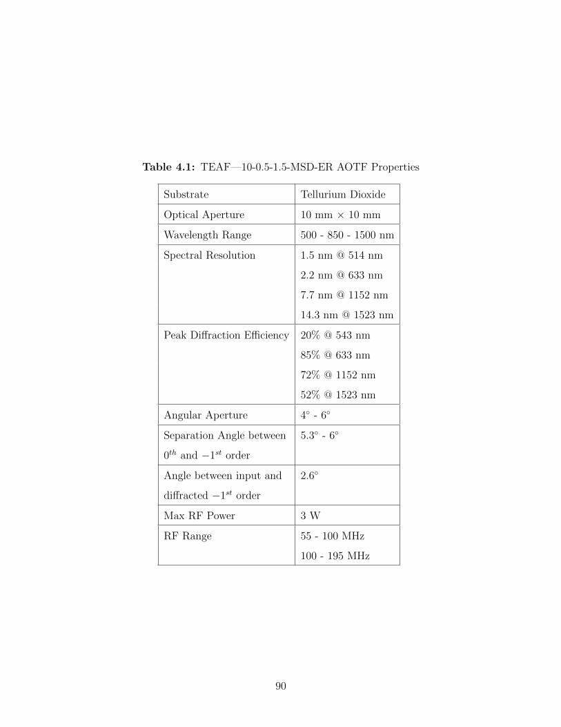
Table 4.1: TEAF—10-0.5-1.5-MSD-ER AOTF Properties

Substrate Tellurium Dioxide

Optical Aperture 10 mm × 10 mm

Wavelength Range 500 - 850 - 1500 nm

Spectral Resolution 1.5 nm @ 514 nm

2.2 nm @ 633 nm

7.7 nm @ 1152 nm

14.3 nm @ 1523 nm

Peak Diffraction Efficiency 20% @ 543 nm

85% @ 633 nm

72% @ 1152 nm

52% @ 1523 nm

Angular Aperture 4 - 6

Separation Angle between 5.3 - 6

0th and −1st order

Angle between input and 2.6

diffracted −1st order

Max RF Power 3 W

RF Range 55 - 100 MHz

100 - 195 MHz

90

Figure 4.4: Wavelength distribution across detector in telescopic layout for filteringat 1000 nm. The marker sizes indicate the relative spectral transmission within thebandpass, dictated by momentum mismatch at these wavelengths.

of the AOTF, and applying the appropriate refraction, we can determine the propagation

direction for wavelengths within the bandpass of the AOTF. Figure 4.4 shows the wavelength

distribution mapped onto a 9.6 mm by 7.68 mm image plane using an ideal singlet with a

137 mm focal length. The range of wavelengths displayed is based on the bandwidth at the

tuned frequency. The size of the gradient is found to be comparable to the tuned bandwidth,

resulting in a negligible impact on the retrieval of aerosol and cloud information.

The extended spectral range is a challenge at the detector level as typically Si is used for

visible wavelengths and InGaAs is used for near infrared beyond 1000 nm. For this design, we

selected a “vis-doped” Raptor Owl 640 VIS-SWIR InGaAs detector. The spectral response

of this detector is much wider than that of a standard InGaAs detector, with responsivity

down to 400 nm. However, the quantum efficiency is below 50% for wavelengths shorter than

800 nm. The reduction in quantum efficiency is compensated for by a significant increase

in scattered sunlight in the visible spectrum compared the near infrared. The detector

91

Table 4.2: Raptor Owl 640 Detector Properties

Sensor Type InGaAs PIN-Photodiode

Active Pixels 640 × 512

Pixel Pitch 15 µm × 15 µm

Active Area 9.6 mm × 7.68 mm

Spectral Response 400 - 1700 nm

Readout Noise (RMS) 174 electrons (typical in Low Gain)

Well Depth 650,000 electrons (Low Gain)

Dark Current (e−/pix/s) <28,000 @ 15C

TE Cooling Active

Digital Output Format 14 bit Camera Link

specification is listed in Table 4.2.

Polarization Selection

The birefringent nature of the TeO2 crystal in the AOTF results in significant angular sep-

aration between the diffraction orders once rays exit the device. Coupling this with the

highly dispersive properties of the material leads to wavelength dependent beam wander if

the output face of the crystal is parallel to the input. To suppress this wander, the crystal is

cut with a wedge at the output face to optimize the wavelength dependent refraction, which

maintains a uniform direction for one diffracted polarization state across all wavelengths.

Therefore, only the signal that is linearly polarized along the ordinary axis of the crys-

tal is uniformly transmitted through the AOTF and measured [Yano and Watanabe, 1976,

Suhre and Theodore, 1996].

As shown in Figure 4.3, randomly polarized signal entering the AOTF is separated into

four directions based on polarization state and wavelength. To reduce stray light contami-

nation from the unwanted signals out of the AOTF, LP filters are placed on either side of

it. Glan-Taylor type LP filters are selected for their broadband operation. The input LP

filter (LPF1) is aligned such that the signal passing the element is aligned with the ordinary

axis of the AOTF, thus eliminating the extraordinary polarized beam and the resulting −1st

92

diffracted beam in Figure 4.3. This polarizer is placed early in the optical chain for two rea-

sons: to filter the polarization state from the atmosphere prior to reflections off the telescope

mirrors and to reduce the signal reaching the mirrors, which limits stray light scattering. This

attenuates the signal aligned with the extraordinary axis of the crystal per the extinction

ratio of the polarizer, which is on the order of 20000:1.

The output LP filter (LPF2) is aligned orthogonal to LPF1 in order to pass signal along

the extraordinary axis of the AOTF, i.e. the signal diffracted by the AOTF. The undiffracted

0th order signal contains most of the broadband atmospheric signal, but because this beam

does not undergo the acousto-optic interaction, its polarization state is unchanged as it passes

the AOTF and is significantly attenuated by LPF2. It is important to note however that the

total radiance of the broadband signal is several orders of magnitude larger than the diffracted

narrow band signal, so the filtering from LPF1 and LPF2 acts to bring the diffracted and

undiffracted signals to comparable order.

An additional property to be exploited is the angular separation between the 0th and −1st

orders, which is greater than 5. The clear aperture of the output polarizer is centered about

the diffracted signal, providing significant vignetting of the 0th order path. Furthermore,

the optical path length between the AOTF and the imaging optics is maximized using fold

mirrors to increase lateral displacement between the paths and prevent the 0th order path

from reaching the imaging optics.

The novel dual polarization capability of this instrument capitalizes on the LP operation

of the AOTF. A liquid crystal polarization state rotator (LCR) is placed ahead of LPF1 in

the optical chain. The LCR acts on the polarization state of incident light by rotating it

approximately 90. This interaction has a wavelength dependence and is tuned for only a

subset region of the entire instrument bandwidth, so the rotation does not perfectly reach

90 for all wavelengths.

Folded Optical Layout

A folded optical layout comes with several advantages, including reduced aberration, footprint

and stray light. Two off axis parabolic mirrors are used as the front-end telescope. These

mirrors reduce chromatic aberration of the input signal before the AO interaction. The use of

93

mirrors also reduces the footprint of the telescope, which would require a long optical chain

if lenses were used.

The test environment for ALI is on the deck of a stratospheric balloon payload, imaging

the atmosphere from approximately 35 km above the surface of the Earth using the limb

scatter viewing geometry. Under these conditions, the full field of view from the instrument

horizontal to the surface of the Earth is approximately 6. With ALI suspended in an

upper layer of the atmosphere, measurements of the radiance scattered from the volume of

atmosphere in front of and below the balloon deck are captured. In the limb scatter viewing

geometry, ALI measures photons that have been scattered from any point in the illuminated

atmosphere within its field of view. Table 4.1 shows that the maximum acceptance cone

angle of the AOTF is 4, so the two mirrors must accommodate this angular reduction. The

telescope mirrors produce an intermediate image, so a field stop is placed here to reject out

of field rays. Additionally, an external baffle is designed to precede the telescope to further

limit these rays from striking the first mirror to contain stray light.

The back-end imaging optics must map the acceptance angle of the AOTF to the dimen-

sions of the detector. This requires a focal length of 137 mm on the imaging optics. A triplet

is designed based loosely on the Cooke triplet format. Here refractive imaging elements are

used for several reasons. The achromatic nature of the front end optics of ALI are disrupted

by the AOTF, and the off the shelf availability is far greater for refractive elements. These

three lenses are housed in a lens tube, following two enclosed fold mirrors to extend the

optical path length following the AOTF, which allows for the residual undiffracted beam to

be blocked by the lens tubes. These efforts are made to reduce the stray light reaching the

detector.

Optical Design

The optical layout was designed using CODE V software. Three special user-defined sur-

faces are used to simulate the interaction of the AOTF, based on the method described by

[Zhao et al., 2014]. The first of these surfaces is used to model refraction of the ordinary po-

larized beam, while setting a flag to identify rays that are entering the AOTF from outside the

acceptance angle. The second simulates the AO interaction, using a list of crystallographic

94

properties that are described in a text file. A linked MATLAB script is used to calculate the

acoustic walk-off angle and acoustic wave vector to improve the model [Poon, 2006]. Rays are

finally traced to the final surface, where extraordinary refraction occurs based on the crystal

geometry. Standard ray tracing algorithms are used for all other optical surfaces. All optical

elements aside from the AOTF are COTS components. Figure 4.5a shows the final optical

layout of ALI. The stray light baffle defines the aperture of the system, with the LCR and

LPF1 immediately following. These elements select the atmospheric polarization state to be

measured. Following this is the telescope, comprised of two off axis parabolic mirrors, which

is used to map the instrument aperture to the AOTF aperture at the telescope exit pupil.

Following the AOTF is LPF2, aligned orthogonal to the first. Two flat fold mirrors elongate

the optical path length while reducing the footprint of the instrument. Finally, a triplet is

used to focus the diffracted signal onto the detector. COTS opto-mechanical components are

selected to hold the selected optics, shown in Figure 4.5b.

4.3.2 Characterization and Calibration

Following assembly, the instrument underwent a characterization and calibration campaign.

Instrument characterization took the form of assessing the optical response of individual

components and/or the optical system to electrical inputs. An example of a characteriza-

tion is the frequency-wavelength tuning response to relate the input acoustic frequency to

the diffracted optical wavelength channel. The characterization responses are required for

development of an instrument simulation model, described later. System level calibration ac-

tivities, like the flat field calibration, were also performed. These calibrations are necessary

to generate Level 1 data products from the instrument measurements for aerosol property

retrieval.

95

96

Figure

4.5:

AL

IV

2in

stru

men

tla

you

t.(a

)O

pti

cal

layo

ut

asd

esig

ned

inC

OD

EV

.(b

)O

pto

-mec

han

ical

mod

eld

esig

ned

pri

mar

ily

wit

hC

OT

Sco

mp

onen

ts.

97

Frequency-Wavelength Tuning

The wavelength diffracted by the AOTF is determined by the frequency of the acoustic

wave propagating through the crystal in a defined direction. The relationship between the

wavelength and frequency is known as the tuning curve. The tuning curve of the AOTF

used in ALI is measured by scanning frequencies in 0.2 or 0.4 MHz steps across the designed

frequency range of 50 - 200 MHz. The AOTF is placed between crossed polarizers, with a

broadband light source with low divergence filling the aperture. The diffracted spectrum is

measured with a HORIBA iHR320 spectrometer and either a CCD or InGaAs imaging array.

The optical set up is shown in Figure 4.6a. Typical normalized spectra from various tuning

frequencies are shown in Figure 4.6b.

The central wavelength of the diffraction peak is calculated using curve fitting to a good-

ness of fit parameter. The coefficients of determination for the curve fitting exceeded 0.997.

Figure 4.6c shows the tuning curve for the AOTF. The inverse relationship between frequency

and wavelength means the low frequency transducer diffracts wavelengths longer than 920

nm, and the high frequency transducer diffracts wavelengths below 920 nm.

Bandpass

The bandpass of the AOTF is found using the same spectra used to calculate the tuning

curve. The FWHM is extracted from the normalized spectra. Figure 4.7 shows a best fit

theoretical bandpass predicted by Equation (4.4) and the measured bandpass.

We see two distinct regions in the bandpass relationship, separated at 920 nm, which

correspond to the two transducer frequency ranges. The difference in interaction length of

the transducers leads to this step change. Differences between the measured and theoretical

bandpass are within 1.5 nm, and are the result of a non-zero frequency bandwidth applied

for each sample, non-zero divergence of the incident signal, and uncertainty in the AOTF

geometry, each of which are not characterized in this paper. Rather, the measured bandpass

is directly incorporated into the instrument simulation model described in section 2.3.

98

Figure 4.6: Frequency tuning curve measurements. (a) Optical layout for tuning curvemeasurement. (b) Sample spectra used to determine tuning curve. (c) Wavelengthtuning curve as a function of applied frequency. Note the smooth joint between the twotransducers at the change over frequency of 100 MHz.

99

Figure 4.7: AOTF bandpass as a function of wavelength. The discontinuity at 920nm is a result of different transducer interaction lengths.

Internal Diffraction Efficiency

The internal diffraction efficiency (IDE) of the AOTF is a measure of the fraction of passing

light that is diffracted at a specific tuning frequency. It does not consider Fresnel or other

losses occurring at the medium interfaces of the TeO2 crystal. Measuring the IDE requires a

similar optical set up to the one used for the tuning curve measurements, but with the AOTF

rotated such that the undiffracted 0th order signal passing through the AOTF is imaged onto

the spectrometer entrance slit. Additionally, the polarizer following the AOTF is rotated

such that it also transmits light polarized along the ordinary axis of the AOTF.

The IDE is calculated by measuring three spectra in this configuration, shown in Figure

4.8a. The first measurement made is with the source lamp turned off to capture the dark

current signal on the detector. The next spectrum is the full 0th order signal with the tuning

frequency amplitude set to 0 W, denoted S0. The last spectrum is the 0th order signal

with the tuning frequency powered to maximize diffraction, denoted SP . This amplitude of

the powered RF signal is approximately 3 W across all frequencies for this AOTF. The SP

100

spectrum closely resembles the S0 spectrum for wavelengths outside of the bandpass, and

drops away within the bandpass. This is because this signal has been diffracted away from

the entrance slit of the spectrometer and is no longer imaged. The dark current is subtracted

from the remaining two spectra to give S ′0 and S ′

P . The IDE is then defined as

IDE(λ) = max

(S ′0 − S ′

P

S ′0

). (4.5)

Figure 4.8b shows the IDE of the AOTF as a function of central wavelength. The sampling

used for the IDE characterization is the same as that used for the tuning curves.

The IDE of the AOTF is once again a function of tuning frequency. Equation (4.3) shows

that the peak transmission of the AOTF is related to the power density, which is strongly

dependent upon the responsivity of the transducers to a selected frequency. The efficiency

drops off significantly as we approach the extremes of the transducer responsivities. This

explains the decline in IDE near 850 nm. We also note the severe drop in IDE at the far

edges of the spectral range near 500 nm and 1600 nm.

Uncertainty in the IDE measurement comes from the dispersive nature of the TeO2 crystal,

as well as the variation in diffraction acceptance angle. The dispersion requires realignment

of the source, collimating optics and AOTF as the wavelength is scanned, to ensure the 0th

order signal at the tuned central wavelength has normal incidence with the imaging optics.

The non-zero divergence of the collimated input coupled with the variation in acceptance

angle leads to a variation in coupling into the spectrometer over the wavelength range.

Polarization Tuning

The liquid crystal polarization rotator in ALI provides polarization selection capabilities to

the instrument, but other optical elements also manipulate the polarization state being mea-

sured. These elements include the telescope and fold mirrors, the two LP filters that precede

the telescope and follow the AOTF, as well as the AOTF itself. Therefore, we must charac-

terize this manipulation in terms of Mueller matrices, which depend upon tuning frequency

and LCR state. These matrices operate on the Stokes vectors describing incident light, de-

fined as S =[I Q U V

]T. It is not necessary to calculate all 16 elements of the Mueller

matrix for two reasons. The first is that the contribution to the total radiance from circu-

101

Figure 4.8: Internal diffraction efficiency measurements. (a) Sample spectra showingabsence of diffracted signal, described in generic pixel count digital numbers, DN. S0 isthe full 0th order spectrum with the tuning frequency amplitude set to 0 W. SP is onceagain the 0th order spectrum but with the tuning frequency amplitude set to maximizediffraction. (b) IDE over wavelength range.

102

larly polarized light is insignificant in the atmosphere. The V term is neglected in the Stokes

vector, meaning the last column of the matrix is unnecessary [Hansen and Travis, 1974].

Furthermore, the detector in ALI measures the total radiance incident at the detector plane,

Imeas, so the first three elements of the top row of the Mueller matrix are all that is required

[Mclinden et al., 2011]. The measured radiance can therefore be expressed as

Imeas = f(λ)[1 g12 g13

] [Iin Qin Uin

]T, (4.6)

where f(λ) is the wavelength dependent transmission of the instrument that is characterized

in the next subsection and g12 and g13 are the second and third elements of the top row of

the system Mueller matrix. To determine the g12 and g13 parameters, a LP filter is placed

at an angle α between an unpolarized broadband source and ALI. The measured signal is

expressed in the form

Imeas ∝[1 g12 g13

]1 cos 2α sin 2α

cos 2α cos2 2α cos 2α sin 2α

sin 2α cos 2α sin 2α sin2 2α

1

0

0

(4.7a)

∝ 1 + g12 cos 2α + g13 sin 2α (4.7b)

The 3 × 3 matrix in Equation (4.7a) describes the Mueller matrix of a LP filter. The constants

g12 and g13 are determined by making measurements with various polarizer rotation angles,

α, and using a curve fitting method to match the form of Equation (4.7b). Figure 4.9a

displays normalized measurements made with an external LP filter, which have curves fitted

to determine the required constants for the specific wavelength and LCR state. Figure 4.9b

shows the g12 and g13 parameters for select wavelengths across the operating range. The ideal

response would be that of a linear polarization in each of two orthogonal states, i.e. (g12, g13)

equal to (1,0) for LCR Off, and equal to (-1,0) for LCR On. While this behavior is generally

observed, substantial variation from the ideal case is observed for g13 when the LCR is off,

and for g12 at the longest wavelengths when the LCR is off. This is due to the nature of

the twisted nematic cell polarization rotator, which is optimized only for a bandwidth much

narrower than our measurement range. These observations are used directly in the instrument

simulation model in Section 2.4 as they are an important aspect of characterization of the

response for the aerosol and cloud information retrieval.

103

Figure 4.9: Characterization of ALI polarization tuning. This is a full instrumentcharacterization, including all optical elements in ALI. (a) Wavelength dependent po-larization response. The spread seen in the LCR Off measurements is a result of thetwisted nematic cell LCR, which is only optimized over a narrower bandwidth than theALI spectral range. (b) Coefficients for ALI Mueller matrices. The effect of the narrowoptimized bandwidth is once again seen in the variation of the g12 and g13 curves whenthe LCR is off.

104

Flat Field and Absolute Calibration

A flat field calibration is performed to account for imaging sensitivity variations across the

ALI field of view. Variations in sensitivity arise from several sources, including non-uniform

response of the detector, variation in path length through the LCR, reduced AOTF diffraction

efficiency with increasing incidence angle, and slight vignetting at the AOTF aperture from

misalignment with the exit pupil of the telescope. A flat field calibration mask is applied to

each pixel for each wavelength channel and LCR state. The calibration masks are measured

using a calibrated broadband signal and an integrating sphere. The calibration masks then

convert dark corrected pixel counts into radiance in units of photons · cm−2 · sr−1 · s−1.

4.3.3 Instrument Simulation Model

The performance of ALI is simulated using a mathematical instrument model developed in

MATLAB. This instrument model is used to estimate the performance under a predicted

test environment, and is necessary to estimate exposure times to achieve signal-to-noise

ratio requirements. It can also be used as a tool to run simulation aerosol retrievals to

estimate performance under various solar geometries. The model treats the instrument as

a linear system, where the input, S, is a spectral radiance profile represented by Stokes

vectors with units [photons · cm−2 · sr−1 · nm−1 · s−1]. The output from the system, O,

is the expected detector count digital number (DN) per second that ALI would measure in

[DN· s−1]. This model is based upon optical material properties, optical design parameters

and select characterized responses described above. All parameters used in the model are

wavelength dependent, and therefore we will omit explicitly describing each parameter as a

function of wavelength.

The passive transmission, Tp, through the instrument is first calculated based on physical

properties of the optical components. Refractive components are considered independently,

and the transmission is calculated based on indices of refraction, Fresnel reflection coeffi-

cients on uncoated surfaces, and internal transmittance scaled to the center thickness of each

element. Reflection coefficients are estimated for the reflecting surfaces based on the average

incident angle on the element. The passive transmission is on the order of 19% - 36% over

105

the wavelength range.

The performance of the AOTF is simulated based on the internal diffraction efficiency

measurements presented in Figure 4.8b. Similarly, the performance of the detector is sim-

ulated by the quantum efficiency, QE [e− · photon−1], provided by the manufacturer. The

performance of the detector is dominated by high responsivity in the NIR region, with reason-

able performance from 600 - 900 nm. Additionally, the electron well depth in low gain is used

to determine the conversion factor from electrons to DN , CDN . The polarization response is

modelled using the g12 and g13 parameters derived from the characterization measurements.

Specific optical design properties are also included in this model. The effective area, Aeff ,

of the aperture is calculated using the magnification of the telescope and the aperture area

of the AOTF. Additionally, the instantaneous field of view is calculated based on the focal

length of the imaging optics and the detector pixel size, which in turn is used to find the

solid angle, SApix, each pixel sees. The final remaining parameter required by the model

is the bandpass, BP , shown in Figure 4.7 as measured in the lab. The spectra used to

calculate the bandpass are multiplied by a high spectral resolution input radiance spectrum

and integrated over wavelength to account for the spectral resolution of the instrument. The

simulation model can be summarized mathematically as,

O = Tp · IDE ·QE · C−1DN · Aeff · SApix ·

∫BP ·

[1 g12 g13

]Sdλ. (4.8)

The terms in Equation (4.8) are summarized in Table 4.3, with associated parame-

ter value ranges. This instrument model is used to estimate exposure times based on

typical input radiance profiles as calculated by the radiative transfer model SASKTRAN

[Bourassa et al., 2008b]. This radiative transfer code is used to estimate solar scattering

based on defined properties of a spherical atmosphere. These properties include profile distri-

butions of atmospheric gasses, trace gasses, clouds and aerosol. The code estimates scattered

radiance by tracing rays from a defined solar position into the atmosphere, and models mul-

tiple scattering and ground reflection events into a defined line of sight. Typical estimates

of late summer mid-latitude atmospheric properties are used to estimate the radiance that is

scattered into the ALI field of view as it measures from a 35 km balloon float altitude above

Timmins, Canada in August[Hedin, 1991, Labow et al., 2015, Thomason et al., 2018].

106

Table 4.3: Instrument Model Properties

Symbol Parameter Value

Tp Passive Transmission 0.19 − 0.36

IDE Internal Diffraction 0.1 − 0.9

Efficiency

QE Quantum Efficiency 0.1 - 0.81 e−1 · photon −1

C−1DN Electron to DN 36.68 e− · DN−1

Conversion Factor

Aeff Effective Aperture 0.444 cm2

SApix Pixel Solid Angle 8.54 ×10−8 sr

BP Bandpass 2 - 13 nm

S Spectral Radiance 1011 - 1014

photons · cm−2 · sr−1 · nm−1 · s−1

g12 Mueller matrix element ≈ 1 or -1

g13 Muller matrix element -0.5 to 0.5

107

4.4 Stratospheric Balloon Demonstration Flight

4.4.1 Flight Description

ALI was tested in its designed environment in August, 2018 from Timmins, Canada. The

instrument was carried on board the CARMEN gondola as part of a stratospheric balloon

campaign led by the Canadian Space Agency and the Centre national d’etudes spatiales. The

10.5-hour flight provided 3 hours of atmospheric illumination where images were captured

at stable float altitude of 37 km above the Earth. Throughout this observation period, the

instrument repeatedly performed multi-spectral observation, capturing images at 24 tuned

wavelength channels for both LP states. Wavelength channels were selected to avoid strong

absorbing features in the atmosphere caused by trace gasses like CH4, CO2, H2O, NO2, O2

and O3 [Gordon et al., 2017].

4.4.2 Balloon Measurements

A full frame sample image captured during the flight is displayed in Figure 4.10. The only

corrections applied to this image are the removal of dark current and the conversion from

vertical pixel numbers to tangent altitudes. In this image, we observe fine cloud structure

below 12 km. We also see a region of increased signal level between 12.5-25 km, which

highlights the scattering due to aerosol.

The Level 0 images captured during the flight are processed using the calibrations de-

scribed in the previous section. A dark current correction is first applied, then the flat field

calibration masks are used to convert the detector counts into units of radiance. The field

of view properties and viewing geometry are used to relate pixel rows to tangent altitudes.

Finally, the center ten columns are averaged to generate Level 1 radiance profiles. Figure

4.11 shows radiance profiles captured in Scan #10 from the flight.

The behaviour of the calibrated radiance observations highlights many features that val-

idate the performance of the instrument. We observe in the region above 12.5 km an ex-

ponential decay in radiance, corresponding to the typical atmospheric density profile. We

also notice specifically at longer wavelengths, a deviation from this exponential decay occurs

108

Figure 4.10: Sample measurement taken from 4841’39.8“N, 8348’17.3”W, altitude36.6 km, at 12:55:14 UTC on 08/26/2018 . Solar Zenith Angle = 36.8. Wavelengthchannel 1025 nm, LCR off.

109

Figure 4.11: Level 1 data product from multi-spectral scan #10, Measurements takennear 4841’39.8“N, 8348’17.3”W, altitude 36.6 km, between 12:54:30 and 12:58:30UTC. Solar Zenith Angle near 37 (a) LCR off. (b) LCR on. (c) Ratio of LCR offto LCR on.

110

between 12.5-25 km. As stated earlier, this indicates the presence of stratospheric aerosol

in the sampled atmosphere. Furthermore, we see that as the channel increases, the radiance

decreases. This is typical of an atmosphere exhibiting Rayleigh (molecular) and Mie (aerosol)

scattering. The ratio of the two polarization states measured at each channel is shown in

panel (c). We see a step change in the ratio at 12 km, corresponding to cloud coverage as we

saw in Figure 4.10. Below 12 km, the ratio of the polarization states approaches 1, caused

by the unpolarized nature of cirrus cloud scattering.

The slight increase in radiance at the highest measured altitudes suggests that there

is some stray light contamination occurring. This issue is seen most clearly in the longer

wavelength channel measurements, resulting from the wavelength dependence of Rayleigh

scattering. It should however be noted that the strong increases in radiance for the 1250 nm

and 1275 nm profiles are related to singlet delta oxygen emission, which peaks in a layer in

the upper stratosphere [Noxon and Jones, 1962], rather than stray light.

4.4.3 Instrument Model Validation

Measurements from the balloon flight are used to validate the instrument model de-

scribed previously. Aerosol concentrations are extracted from the GloSSAC climatology

[Thomason et al., 2018], along with other typical atmospheric state parameters to generate

polarized radiance profiles with SASKTRAN. These profiles are used to solve Equation (4.8).

Figure 4.12 compares the measured and modelled instrument performance.

The modelled instrument response uses the 50th percentile aerosol concentration from the

GloSSAC climatology. Error bounds on the modelled response are generated using the 10th

and 90th percentile concentrations. We find relatively good agreement between the measured

response within the range of the modelled response. This is not meant to be a precise

calculation as the atmospheric state is unknown; this shows that with typical atmospheric

parameters, the instrument simulation model is able to quantitatively predict reasonable

signal levels. As noted previously, singlet delta oxygen emission near 1270 nm results in an

under predicted response for nearby channels. Additionally, we see that the 950 nm channel

is impacted by H2O absorption [Buning-Pfaue, 2003], resulting in an over prediction of the

response. We also note a region of over prediction for channels below 900 nm, which is likely

111

Figure 4.12: Comparison of modelled and measured instrument response at 20 km.

related to the quantum efficiency of the instrument detector.

4.5 Conclusion

A new prototype of the ALI instrument has been built and characterized. This prototype

offers several improvements over its predecessor. The folded optical design reduces the overall

instrument footprint, while offering improved chromatic performance. The spectral sensitiv-

ity is also greatly improved through the use of a dual channel AOTF, extending from the

visible to NIR spectrum. This sensitivity to wavelength channels longer than 1200 nm will

allow for greater insight into microphysics properties of aerosol distributions. Lastly, the

pairing of a LCR with an AOTF offers exciting opportunities to study interactions between

cloud and aerosol structures.

The advanced ALI prototype has been successfully deployed on a stratospheric balloon

platform to capture multi-spectral images from a 37 km float altitude. Measurements from

this flight represent some of the first spectrally resolved, polarized images in the limb viewing

112

geometry. Measurements of the 20 km tangent altitude have been compared against modelled

results with aerosol concentrations predicted by the GloSSAC climatology to validate the

predicted signal levels of the instrument.

Continued instrument development is planned to increase throughput to allow the ALI

instrument to meet driving scientific requirements of resolution and signal to noise from a

low Earth orbit satellite. These additional instrument studies will increase the technology

readiness level of ALI for the eventual realization of orbital based remote sensing.

4.6 Data Availability

The data that support the findings of this study are available from the corresponding author

upon reasonable request.

113

Chapter 5

Adaptation of the Polarimetric Multi-Spectral

Aerosol Limb Imager for High Altitude Air-

craft and Satellite Observations

The initial ALI prototypes have demonstrated the measurement of spectrally resolved two-

dimensional images with fine vertical resolution using acousto-optic technology. Furthermore,

pairing this technology with a liquid crystal device has added the capability to measure a

second polarization state in the limb scattered viewing geometry. This manuscript furthers

the ALI development to demonstrate its capabilities on a moving platform, which better

simulates the ultimate orbital platform required for global monitoring.

The ALI elegant breadboard has been funded through the Space Technology Development

Program from the Canadian Space Agency. Research and hardware development for this

prototype is led by this work, and represents a collaborative effort between the University

of Saskatchewan and Honeywell Aerospace. The instrument is designed to be flown on an

aircraft, nominally NASA’s ER-2 High Altitude laboratory. This platform will provide a

spatially varying image scene, which is much different from the static scenes captured by

the previous balloon missions. Improved spectral throughput is required to accommodate

this change in the image scene, so a state-of-the-art 20 mm × 20 mm AOTF is baselined in

the design. This AOTF aperture size offers a four-fold increase in throughput compared to

the predecessor designs and is necessary to achieve signal-to-noise ratio and spatial sampling

requirements for the mission.

The design of the ALI EBB highlights further advancement towards an orbital-based

design, featuring methods and approaches typical of space instruments. These include en-

114

hanced thermal regulation and characterization, improved optical prescription requirements

and build tolerancing and detailed stray light analysis. The manuscript concludes by detailing

design modifications to make the instrument suitable for the space environment.

This manuscript has been published in Applied Optics, and unless otherwise stated the

version presented here is unchanged. The layout of figures and equations and the format of

cross-references has been modified to match that of the overall document.

Kozun, M. N., Bourassa, A. E., Degenstein, D. A., Haley C. S., Zheng, S. H. (2021).

Adaptation of the polarimetric multi-spectral Aerosol Limb Imager for high altitude aircraft

and satellite observation. Appl. Opt. 60, 4325-4334. doi:10.1364/AO.419249.

5.1 Abstract

An elegant breadboard prototype of the Aerosol Limb Imager (ALI) has been developed to

meet key performance parameters that will meet requirements for the retrieval of aerosol from

the upper troposphere and stratosphere from limb scattered sunlight radiance measurements.

Similar in concept to previous high altitude balloon based generations, this instrument pairs a

liquid crystal polarization rotator with an acousto-optic tunable filter to capture polarimetric

multi-spectral images of the atmospheric limb. This design improves the vertical resolution,

signal to noise ratio and athermalization, all of which will facilitate observation from a moving

high altitude aircraft platform, which provides an analogous platform to the spatially varying

measurements that would be made from a satellite. Finally, a preliminary design is presented

for a satellite-based generation of ALI.

5.2 Introduction

The Aerosol Limb Imager (ALI) is a multi-spectral, dual-polarization, imaging system being

developed as a future satellite instrument through a collaboration between the Canadian

Space Agency, the University of Saskatchewan, and Honeywell Aerospace. This imager is

used to measure the spectrum of scattered sunlight from an atmospheric limb viewing, or

side-viewing, geometry. Spectrally resolved images with high vertical and horizontal spatial

115

resolution are obtained using an acousto-optic tunable filter (AOTF) operating over a wave-

length range from 500-1500 nm. Dual linear polarization states are captured by coupling

a liquid crystal polarization rotator (LCR) to the AOTF. Rapid cycling of the polarization

and wavelength selection along the satellite track allows ALI to capture fine cloud structures

and aerosol distributions with retrieved properties like aerosol extinction with unprecedented

resolution from a passive sensor.

Recently, prototype models of the instrument concept were developed and success-

fully tested onboard high altitude balloon platforms. The first generation, detailed in

[Elash et al., 2016], used a fully refractive design and was limited to a spectral range of

600-1000 nm and a single linear polarization state. A more advanced prototype that demon-

strated the dual polarization capability and greatly extended the spectral range to 600-1500

nm is presented in [Kozun et al., 2020]. This instrument also advanced the optical design to

utilize folded, reflective optics. These prototype models demonstrated the feasibility of the

multi-spectral and dual polarization concept for cloud and aerosol but, by design, did not

attempt to reach the signal level and image quality needed to meet scientific requirements

from low Earth orbit.

In this work we present the optical design and modelled performance for an ALI instru-

ment that is specifically motivated by compliance to scientific requirements. This optical

design, which was funded through the Canadian Space Agency’s Space Technology Devel-

opment Program is referred to as the Elegant Bread-Board (EBB) model. As part of the

program to advance the technological readiness of the instrument, the instrument is targeted

for a test flight on the NASA ER-2 aircraft. The instrument will be installed in a forward

facing wing pod on the aircraft to make along-track measurements. This is a similar viewing

geometry that that used by the Spatial Heterodyne Observations of Water instrument flight

in 2017 [Langille et al., 2019]. The satellite based requirements are mapped to requirements

for the aircraft viewing geometry, which leads to an optical design unique to this platform,

but not drastically different from that needed for an orbital instrument. Further, methods

and procedures typical of orbital applications are implemented throughout the design and

build of the instrument in anticipation of a future satellite model.

This paper describes the requirements set for the design of the ALI EBB and highlights the

116

key subsystems designed to meet these requirements. Special attention is given to the Spectral

and Polarization Selection (SPS) subassembly. Next, an overview of the optical analysis is

presented to justify the instrument performance both under nominal design conditions but

also with allocations for manufacturing and build tolerances and environmental conditions.

We will focus primarily on the vertical resolution and signal to noise ratio (SNR) expectations,

as these are key performance indicators for this project, with attention also focused on the

stray light performance. Finally, the EBB design is compared to a preliminary design for a

satellite platform to highlight similarities in the design and build approach.

5.3 Instrument Design

The requirements for the ALI EBB have been substantially refined beyond those used to

design the first two prototypes. Increased focus on key imaging parameters such as verti-

cal resolution and SNR are described to meet the specific science objectives. The driving

instrument design requirements are:

• Capability to measure limb radiance on the tangent of the atmospheric limb from the

surface to the aircraft flight altitude.

– Cross-track Field of View (FOV) to match the vertical FOV.

• Along-Track multi-spectral sampling every 48 seconds/every 10 km.

– 11 horizontally polarized wavelength samples spaced evenly between 500 nm and

1500 nm.

– 3 vertically polarized wavelength samples at 750, 1020 and 1500 nm.

– 1 zeroth order measurement with AOTF off for stray light measurement.

• Vertical altitude resolution < 100 m.

• Signal to noise ratio of the horizontal linear polarization state > 200 over all wavelength

channels.

• Boresight stability of less than 10 arcseconds over an operating temperature range of

-15°C to +40°C.

• Spectral resolution of 1.2% of the central wavelength with tuning stability within one

117

tenth of the spectral resolution over an operating temperature range of -15°C to +40°C.

• Stray light suppression for all first-order sources to maintain SNR of > 200.

5.3.1 Spectral and Polarization Selection

ALI achieves linear polarization state dependent multi-spectral imaging by pairing an AOTF

with a twisted nematic liquid crystal polarization rotator. A LCR from ArcOptix S.A. is

selected for the ALI EBB. The optical activity of an LCR is controlled by applying or re-

moving a bias voltage across the cell. In the unpowered, relaxed state, the linear polarization

state of transmitted light is rotated by a nominal angle, 90 for ALI. However, when a volt-

age is applied, the liquid crystal molecules align with the electric field and do not affect

the polarization state of the light passing through [Schadt and Helfrich, 1971]. The spectral

performance of the LCR is limited in comparison to the full spectral range of ALI, with only

a subset of wavelength channels being rotated by 90. Outside of this performance range,

non-ideal but characterizable polarization effects are experienced. This does not limit the

performance of ALI over the wavelength range.

An AOTF is a solid-state device offering tunable narrow band wavelength filtering when

the Bragg diffraction criterion is met between incident photons and tuned phonons within

specific crystals. Non-collinear AOTF devices allow for acceptance angles as large as 8

with full angular separation between the diffracted and unfiltered, 0th order, signals passing

through. Optical birefringence of the substrate is necessary for this angular separation and

facilitates a 90 rotation of the incident linear polarization state. Further details about

AOTFs are found in [Chang, 1974, Chang, 1975].

The AOTF selected for the ALI EBB is a 20 mm × 20 mm TeO2 device fabricated by

Brimrose Corporation of America. The device uses a dual transducer design to provide an

extended operational wavelength range. The first transducer operates from 50 MHz to 100

MHz, resulting in diffraction over the 850 nm to 1500 nm range, the second transducer

responds to 100 MHz to 200 MHz, diffracting the remaining 500 nm to 850 nm range.

The LCR and AOTF are incorporated into a single subassembly to mature its design and

characterization independent of the rest of the ALI EBB. This unit is called the Spectral

and Polarization Selection subassembly. The SPS also contains crossed linear polarizing

118

filters, placed before and after the AOTF, to select only a single input polarization state and

to attenuate the 0th order that passes through. These are “Outrageously Wide Lambda”

polarizers from Meadowlark Optics performing from 300-2700 nm. The operation of the SPS

is shown in Figure 5.1. The input linear polarizer is aligned to the ordinary polarization

axis of the AOTF, and the output linear polarizer is aligned with the extraordinary axis,

in order to pass the spectrally filtered signal. In Figure 5.1a, the LCR is in its unpowered

state, which rotates the input polarization state by 90. This means that the signal that was

horizontally polarized in the atmosphere will pass through the first linear polarizer and be

spectrally filtered by the AOTF. In Figure 5.1b however, the LCR is in its powered state, so

it does not affect the passing polarization state. Here, the vertically polarized component of

the atmospheric signal passes through and interacts with the AOTF.

Figure 5.1: Spectral and polarization filtering performed by the SPS subassembly.(a) SPS response with an unpowered LCR. The atmospheric linear polarization stateis rotated by 90 before passing the first linear polarizer. Spectral filtering results ina second 90 rotation, so the second linear polarizer filters out the broadband signal.Originally horizontally polarized signal is filtered through the SPS. (b) SPS responsewith a powered LCR. The atmospheric linear polarization state passes the LCR un-changed before the first linear polarizer. Spectral filtering and the second polarizerallow originally vertically polarized signal to be filtered through the SPS.

As discussed earlier, the Bragg diffraction criteria in non-collinear AOTFs is met by

matching optical wave vectors in birefringent materials to an applied acoustic wave vector.

The acoustic wave vector is defined by elastic properties within the medium, which are shown

119

to be temperature dependent [Silvestrova et al., 1987]. Temperature changes of an AOTF

can therefore affect the tuning relationship between applied acoustic frequency and diffracted

wavelength, as well as total diffraction efficiency [Mantsevich et al., 2015]. Therefore, the

temperature of the SPS subassembly is actively maintained at approximately 22C using a

thermoelectric cooler, with feedback coming from temperature sensors placed on the SPS.

The structure of the SPS is primarily made of aluminum, with titanium flexures used for

mounting to the EBB structure. An aluminum heat shunt is used to draw heat away from

the SPS and EBB. The SPS subassembly design is presented in Figure 5.2.

Figure 5.2: Spectral and Polarization subassembly. (a) Standard view. (b) ExplodedView.

5.3.2 Reflective Design

The ALI EBB optical design is presented in Figure 5.3. All optical elements aside from

the SPS are reflecting elements, primarily to achieve highly achromatic performance. The

mirrors are single point diamond turned surfaces made of 6061-T651 Aluminum alloy. These

mirrors provide athermal performance with low surface roughness.

The front-end telescope, shown in Figure 5.3a, is designed with two matched off-axis

120

parabolic mirrors and a planar fold mirror acting as a field stop at the common focus,

which limits out of field stray light from propagating through the telescope. Unlike previous

generations, no magnification is required from this telescope, because both the vertical FOV

and the AOTF acceptance angle are 5.

A common axis three mirror anastigmat (TMA) is used for imaging the filtered beam

from the SPS, displayed in Figure 5.3b. The primary and tertiary mirrors have a common

vertex, so both can be cut on the same diamond lathe configuration, aiding in alignment.

This imaging system is paired to a Raptor Owl 640 camera, which incorporates a visible

extended InGaAs detector with responsivity from 400–1700 nm.

A two-mirror periscope is designed to pair the input telescope to the SPS. Although

this periscope provides no optical improvements, it folds the optical plane up and over itself

to reduce the structural footprint, seen in Figure 5.3c. Additionally, the periscope provides

compensation degrees of freedom for aligning the front and back end systems. The full optical

ray trace is finally shown in Figure 5.3d.

5.3.3 ALI EBB

The opto-mechanical structure of the ALI EBB is made of 6061-T651 Aluminum alloy. The

major structural components of the EBB are designed to be monolithic, to minimize struc-

tural interfaces. Conventional machining is used for all components, except for mirror in-

terface pads which are diamond turned to reduce distortion of the mirrors upon torquing.

The input telescopic optics chassis is the largest and most robust structure, and serves as

an optical bench for the entire instrument. The opto-mechanical design of the ALI EBB is

shown in Figure 5.4.

5.4 Instrument Performance

The performance of the ALI EBB is assessed according to several optical and mechanical

criteria, related primarily to the key requirements highlighted previously.

121

Figure 5.3: ALI EBB Optical Layout. (a) Top view of input telescope and firstperiscope fold. The input aperture is in the upper left of the frame. (b). Secondperiscope fold, SPS and camera TMA. (c) Side view of ALI EBB showing two horizontaloptical planes. (d) Isometric view of ALI EBB. Input aperture is in the center left ofthe frame.

5.4.1 MTF and Vertical Resolution

Two key imaging performance parameters that are assessed are the modulation transfer

function (MTF) and the encircled energy as it relates to resolution at the atmospheric limb.

The MTF of the ALI EBB optical design is shown in Figure 5.5. The InGaAs detector has

15 µm pixels, so the cutoff spatial frequency with dual pixel binning is 33.3 cycles/mm. Hence,

we present the MTF to a maximum spatial frequency slightly above the cutoff frequency. For

each wavelength, the diffraction limit is drawn with a dashed line, and the simulated MTF

for various fields are shown in solid lines. The system performs near the diffraction limit over

all wavelengths and fields. We also note good contrast, with an MTF greater than 0.6 for

spatial frequencies up the detector cutoff.

122

Figure 5.4: ALI EBB Optomechanical design. (a) Input optics subassembly. (b)Periscope subassembly. (c) Camera TMA subassembly. (d) ALI EBB Assembly. Inputoptics chassis acts as an optical bench for the other subassemblies, including the SPSshown in Figure 5.2. Note that an additional baffle hood (not shown) is added aroundthe periscope and SPS to shield these from the surroundings.

To estimate the instantaneous vertical resolution, the spatial response of the image cap-

tured by the detector is first estimated. The point spread function (PSF) is modelled as

a Gaussian with a variable full width half max (FWHM). This is convolved with a boxcar

function representing a single 15 µm pixel, which describes the spatial resolution in image

space.

The image space spatial resolution is next mapped into the atmospheric object space in

the limb viewing geometry, shown in Figure 5.6. Assuming a 22 km flight altitude, the center

of the vertical field of view strikes a tangent altitude height of 11 km at a distance of 374.9

123

Figure 5.5: Optical modulation transfer function of nominal ALI EBB optical design.The detector cutoff spatial frequency is 33.3 cycles/mm. Solid lines represent the MTFfor select fields over the FOV.

km from the instrument. At this distance, the instantaneous field of view of a pixel represents

a vertical distance of 63.9 m. This scaling factor is used to map the variable image space

spatial resolution into an atmospheric vertical resolution, shown as a solid line in Figure 5.7a.

To model the instrument performance, the image space spatial resolution is simulated

with ray tracing software. The FWHM of the PSF is equated to the 50% encircled energy for

various wavelengths and fields in the ALI optical model. The corresponding vertical resolution

for sampled fields and wavelengths are highlighted in Figure 5.7a. The 50% encircled energy

metric is selected because it provides the ability to compare the encircled energy between

the nominal design, the thermally distorted design and the assumed as-built performance

based on part manufacturing and build tolerance simulations. These three conditions all help

124

Figure 5.6: Limb viewing geometry. The vertical field of view has several lines ofsight, based on pixel binning. Each line of sight makes a measurement at a uniquetangent height.

estimate the expected instrument performance. The 50% encircled energy for all wavelengths

and fields is below 8.5 µm for the nominal design, which translates to a vertical resolution

less than 67.2 m, shown in Figure 5.7a. A tolerance analysis using manufacturing and build

tolerances listed in Table 5.1 is used to calculate a 1σ change in the 50% encircled energy.

The corresponding vertical resolution is shown in Figure 5.7b.

There is a significant wavelength dependence in the vertical resolution, but also a field

dependence, which is less obvious in Figure 5.7b. The wavelength response is driven by

diffraction effects. The field dependence is a result of the off-axis nature of the camera

TMA with a gradient observed in the off-axis direction, which is particularly sensitive to

tip and tilt of the camera TMA mirrors. An additional effect which impacts spatial res-

olution in AOTFs is image blur caused by divergence of the acoustic beam as it travels

through the finite sized TeO2 crystal [Sivanayagam and Findlay, 1984]. This divergence

changes the properties of the momentum matching condition in the direction of the diffrac-

tion [Gupta and Voloshinov, 2007, Suhre and Gupta, 2005]. The diffraction direction of the

AOTF has been aligned with the cross-track dimension of the atmospheric limb. The impact

on the vertical resolution is shown to be minimal and therefore does not impact this analysis

[Zhang et al., 2016]. The worst-case vertical resolution we expect to see at 1500 nm is 86 m,

125

Figure 5.7: Relationship between the PSF FWHM and vertical resolution in theatmospheric limb from a flight altitude of 22 km. (a) The nominal vertical resolutionis displayed for various field and wavelength combinations based on the 50% encircledenergy of the ALI optical design. (b) Vertical resolution calculated from 1σ toleranceanalysis of encircled energy

below the 100 m requirement.

The athermalization of the ALI EBB is tested using Structural Thermal Optical Perfor-

mance (STOP) analysis. A finite element model of the ALI EBB is generated, and envi-

ronmental heat loads are applied. It is assumed that the aircraft accommodation structure

will maintain the operational temperature range of -15C to +40C. Representative heat

loads are applied to the SPS and camera to induce thermal gradients to simulate operating

conditions. The thermal results are mapped onto a structural node mesh to evaluate the

distortions experienced by each optical element. The resulting structural distortions for the

hot operating case are shown in Figure 5.8a. Finally, the nodal distortions are used to dis-

tort the optical model, and the resulting performance is evaluated. Figure 5.8b displays the

vertical resolution predicted under the described thermal loading cases. When compared to

Figure 5.7a, we find only a small variation in the vertical resolution under thermal loading,

which validates the athermal optical design.

126

Table 5.1: List of manufacturing and build tolerances.

Tolerance Type Value

Radius (mm) 0.025

Power (fringes @ 632.8 nm) 3.000

Irregularity (fringes @ 632.8 nm) 1.000

Refractive index 0.0005

Abbe number 0.005

Center thickness & airgap (mm) 0.050

Centering displacement (mm) 0.025

5.4.2 SNR

The retrieval of aerosol properties from atmospheric limb sounding images requires a signal to

noise ratio of 200 or better. To validate the SNR, a mathematical model is used to estimate

the performance of the instrument under variable atmospheric conditions. This model is

based primarily on the optical design characteristics, theoretical diffraction efficiency of the

AOTF and properties of the imaging detector. The assumptions for the SNR model are:

• f/4.35

• Theoretical optical transmission

• 15 µm pixel size

• Quantum efficiency described by Raptor Owl 640 datasheet

• Readout noise of 195 e−

• Electronics noise of 10 e− RMS/px

• Dark current of 100 e−/px/s

• 14 bit analog-to-digital conversion

• Off-chip horizontal binning

• 50 ms single frame exposure time, with 11 frames co-added

The modelled optical transmission is based on standard reflectance curves for protected

silver coated diamond turned aluminum mirrors, with consideration to polarization and in-

127

Figure 5.8: STOP analysis results. (a) Finite element model of ALI EBB shows thenodal displacements under the hot operating condition of +40C. These distortions areused to build a representative optical model. (b) Vertical resolution estimated from thehot and cold operating case optical models, using the described method to convert PSFFWHM to vertical resolution.

cident angle. Transmission curves for the linear polarizing filters and LCR are also included,

as well as the expected diffraction efficiency of the AOTF. The transmission of ALI is shown

in Figure 5.9. The shape of the transmission curve is dominated by the diffraction efficiency

of the dual transducer AOTF, producing a local maximum for each transducer. The diffrac-

tion efficiency drops significantly near the transducer cutoff frequency, which translates to a

wavelength near 820 nm.

The optical signal is calculated in electrons for each pixel using the camera equation

[Klein, 1986] and the optical system efficiency:

Spx =πI(λ)ADε(λ)∆λ(λ)∆t

4(f/#)2 + 1. (5.1)

Here, I(λ) is the input radiance in units of photons/cm2/s/sr/nm at the center wavelength

λ. AD is the pixel area, ε(λ) is the optical system efficiency, which includes the transmission

and detector quantum efficiency, ∆λ(λ) is the optical bandwidth of the AOTF and ∆t is the

exposure time.

128

Figure 5.9: ALI EBB transmission. Spectral curves are generated using reflectanceof 9 silver coated mirrors, transmission properties of polarizing filters and rotators, anddiffraction efficiency of the AOTF. The mirrors have different reflection coefficients forS and P polarization states, which has a small impact on the transmission dependingon the LCR state modelled.

Noise is calculated as

Npx =√

Spx + Dpx + N2ro + N2

elec + N2dig, (5.2)

where Dpx is the pixel dark current, Nro is the RMS readout noise, Nelec is the RMS electronics

noise and Ndig is the digitization noise. The SNR is calculated as Spx/Npx. Off-chip binning

modifies the SNR by the square root of the binning factor. Here, the horizontal field of

view is binned into 1 bins, comprised of 102 pixels. The exposure times are set to capture

15 wavelength/polarization/calibration measurements per 10 km along track at an aircraft

speed of 0.21 km/s.

The input radiance for the SNR calculation is produced by the SASKTRAN radiative

transfer model [Bourassa et al., 2008b]. Two atmospheric conditions are tested, the first

being a “clear” case including only effects from Rayleigh scattering, ozone and background

aerosol levels, with a solar zenith angle of 60, solar scattering angle of 90 and albedo

of 0.3. The second case is a “signal enhanced” case, with aerosol loading similar to that

129

seen following the Nabro eruption in 2011 [Bourassa et al., 2012b], thick low altitude cloud

coverage, and albedo of 1. The SNR for 14 polarization and wavelength channel pairs are

shown in Figure 5.10.

Figure 5.10: Simulated signal to noise ratio for ALI EBB under two aerosol load-ing conditions. (a) “Clear” case with contributions from Rayleigh scattering, Ozoneabsorption and background aerosol levels. (b) “Signal Enhanced” case with contribu-tions from Rayleigh scattering, Ozone absorption and aerosol loading similar to thatwhich followed the Nabro eruption in 2011 as well as thick, low altitude cloud coverage.SNR=200 threshold is marked in thick blue.

The SNR requirement is met for all horizontal wavelength channels except at the longest

wavelength at the highest tangent heights. This suggests that vertical binning may be re-

quired in some cases in order to achieve the desired SNR. Note also that the SNR requirement

only applies to the horizontal polarization state, as the vertical wavelength samples will be

used for discrimination of ice clouds rather than aerosol property retrieval.

130

5.4.3 Stray Light

The narrow wavelength channel filtering of ALI makes it sensitive to stray light, requiring

detailed stray light modelling. The stray light sources are categorized as either in-band or

out-of-band based on their spectral features. The interaction at the AOTF differentiates

these two sources.

The in-band contribution is diffracted through the AOTF and therefore propagates within

the field of view of the detector following the SPS. This signal, referred to as the science signal,

is susceptible to scattering dominated by the surface roughness and cleanliness of the optical

surfaces. In this case, surface scattering from all surfaces, including those before the AOTF,

are critical to monitor.

Out-of-band stray light is dominated by the 0th order signal that passes through the AOTF

undiffracted. This signal contains significantly more spectral bandwidth and is not affected

by the diffraction efficiency of the AOTF. Although this signal is heavily attenuated by the

second linear polarizer, the total integrated signal remains on a similar order of magnitude

as the diffracted signal, and therefore needs to be managed appropriately within the camera

TMA to reduce stray light contamination.

Two methods of stray light assessment are used. The first method is a Monte Carlo ray

trace method using TracePro. This method is useful for validating stray light contributions

through direct path analysis and monochromatic Point Source of Transmission (PST) anal-

ysis, as well as assessing ghosting in the SPS. The second method is a mathematical model

used to simulate stray light contamination from the 0th order signal passing through the SPS.

Monte Carlo Ray Trace

The structural model of the EBB shown in Figure 5.4 is imported into TracePro, where

appropriate optical properties are applied to all surfaces. For the direct ray path analysis,

all surfaces are either perfect specular mirrors, perfect transmitters or perfect absorbers. For

the ghost analysis and PST modelling, mirror surfaces are modelled with reflectivity typical

of protected silver and with reflected scattering defined by the RMS surface roughness of

9 nm. The ABg scattering model is used to define the BRDF of these surfaces. Similarly,

131

uncoated transmissive surfaces have transmission and reflection coefficients defined by the

Fresnel equations, and scattering based on 2 nm RMS surface roughness. Non-optical surfaces

have properties typical of bead-blasted black anodized aluminum [Marshall et al., 2014].

The direct ray path analysis is a reverse ray tracing technique that validates that no direct

lines of sight to the detector or AOTF from outside of the field of view exist. Baffle vanes

are strategically placed throughout the optical structure to limit these lines of sight, and an

input baffle is included. This test validates that only fields within ±2.5 reach the input

to the AOTF through the entrance aperture, and only fields within ±2.5 of the nominal

diffracted beam reach the detector after propagating through the AOTF.

Ghosting analysis focuses specifically on the planar surfaces of the SPS. The broadband

nature of ALI requires uncoated transmissive elements to be used. With several closely spaced

flat surfaces, the likelihood of ghost production is unavoidable, however the AOTF, LCR,

input polarizing filter and output polarizing filter are all tilted with respect to one another

to minimize ghosts from reaching the detector from either the 0th order or the science path.

PST analysis shows well behaved performance over several tested fields in the vertical

and horizontal direction with respect to the boresight. Monochromatic PST tests are run

for the desired science path signal, scattered science path signal and 0th order scattered

signal at discrete wavelengths. Figure 5.11 shows that the specular signal PST drops off

beyond the designed FOV, and the scattered science path signal PST is more than 3 orders

of magnitude lower than the specular signal. This scattering is dominated by the first mirror

in the optical system, which may scatter light directly into the FOV of the AOTF. Finally,

the 0th order PST is more than 6 orders of magnitude lower than the specular science path

and is dominated primarily by scattering from mirrors within the Camera TMA.

Mathematical Model

The narrow bandwidth filtering provided by the AOTF requires special attention to the

broadband 0th order signal that passes through the AOTF undiffracted, which is not captured

in the monochromatic PST simulation presented previously. The attenuation of the two

crossed polarizers in the SPS drastically reduces the 0th order signal level, but the integrated

spectral power is of a similar order to that of the diffracted science signal.

132

Figure 5.11: Stray light PST simulation covering vertical and horizontal fields extend-ing beyond the designed field of view with monochromatic input. We find approximately3 orders of attenuated magnitude for in-band, in-field stray light signal, and roughly 6orders for out-of-band, in-field stray light signal. The contributions from outside thefield of view all exhibit more than 6 orders of magnitude of attenuation.

The separation between the science path and 0th order path is 6.3-7.3. This is larger

than the 5 field of view, which limits the chance of specular signal from the 0th order landing

on the detector. However, this signal does still have a direct view factor onto the primary

camera TMA mirror, leading to three opportunities for scattering into the FOV:

1. Scattering from the primary into the detector FOV,

2. Specular reflection from the primary and scattering from the secondary into the detector

FOV,

3. Specular reflections from the primary and secondary and scattering from the tertiary

into the detector FOV.

The total integrated scatter (TIS) for mirror surfaces with 9 nm RMS surface roughness

is used to characterize the stray light impact of each of these scattering cases. The TIS is

calculated as

TIS(λ) =

(4πσ

λ

)2

, (5.3)

133

where σ is the surface roughness. The largest TIS is 0.0512 at 500 nm.

An attenuation factor is calculated for the 0th order under the three cases, using the

illumination areas of the science path and 0th order on each mirror in the TMA. This factor

is the product of the ratios of these areas, Apri, Asec and Ater, the solid angle of the detector

at the scattering surface as a ratio of a full hemisphere, SA, and the TIS. The attenuation

factors for the three scattering cases at 500 nm are 3.9 × 10−4, 2.8 × 10−3 and 3.9 × 10−6

respectively.

To quantify the magnitude of the 0th order stray light contribution, a similar model to

the one described by the SNR calculation is developed to approximate relative intensities

for various wavelength channels. This model uses the contrast ratios of the linear polarizers,

the overall instrument transmission, and attenuation factors with wavelength dependence.

Figure 5.12 shows the contribution of the 0th order beam relative to the normalized expected

filtered signal levels at several wavelength channels. The integrated 0th order scattering levels

fall below the modelled SNR requirement for all wavelength channels and tangent altitudes.

Figure 5.12: Mathematical model of broadband 0th order stray light compared tosimulated signal levels. The simulated levels have been normalized to show the roughorder of magnitude of attenuation of the 0th order beam that is expected to reach thedetector. The minimum signal profile across all wavelength channels is calculated andreduced by a factor of 200 to simulate the SNR requirement. The 0th contribution fallsbelow this level for all tangent heights.

134

5.5 Adaptation for Satellite Based Remote Sensing

The eventual goal of the ALI instrument is to contribute to the global aerosol record from

a satellite platform, with the EBB representing a necessary development model to increase

the technology readiness level of the instrument. As noted, the methods and procedures for

the design, build and alignment of the EBB are aligned with those required for an orbital

instrument. Beyond these processes, the requirements for the ALI EBB are adapted from

preliminary scientific requirements for a satellite-based ALI. The key requirements include:

• Capability to measure limb radiance on the tangent of the atmospheric limb from the

surface to 40 km.

– Cross-track FOV of 5 with a goal of 8.

• Along-track multi-spectral sampling every 50 km with 15 wavelength/polarization chan-

nel cadence.

• Low altitude vertical resolution better than 250 m for tangent altitudes below 22 km,

with a goal of better than 100 m.

• High altitude vertical resolution scaling from 250 m to a maximum of 3 km for altitudes

above 22 km, with a goal of a 1 km maximum at the highest altitudes.

• Signal to Noise ratio for the horizontal linear polarization state > 200.

A fundamental difference between the EBB and satellite-based instrument is the field of

view requirement. The EBB has common vertical and cross-track FOV specifications, so

rotationally symmetric optics are implemented in the optical design. The vertical sampling

requirements from a 600 km orbit are met with approximately 1 vertical FOV, while main-

taining 5 in the cross-track direction. This requires anamorphic imaging optics paired with

a high aspect ratio detector, which provides 300 km cross-track imaging at the tangent point.

An additional challenge when viewing from orbit over the larger tangent altitude range is

the dynamic range required, which scales logarithmically with tangent altitude. A gradient

neutral density filter is proposed with the highest optical depth targeting the lowest tangent

altitudes. A preliminary layout for a satellite-based design is shown in Figure 5.13.

In the satellite layout, the two parabolic mirrors (a and d) in the telescope are offset and

the fold (b) is moved away from the field stop. This has left room for a transmissive gradient

135

Figure 5.13: Optical design for ALI to meet requirements for orbital aerosol retrieval.This design highlights similar features to the EBB, with a telescopic input assembly,an SPS, periscope and an imaging assembly.

136

neutral density filter which will be mounted in a field stop (c). This stop will define the

anamorphic field of view. The telescope is followed by an SPS layout once again utilizing

an AOTF, LCR and linear polarizing filters (e). Here, the periscope has been rotated to

keep the full optical system in a single plane (f). Finally, an anamorphic imaging assembly

is designed with vertical and horizontal focal lengths of 188 mm and 141 mm respectively (g

and h). Two fold mirrors (i and j) are included to optimize the detector location (k). This

design is under continued development for a prospective future aerosol sensing mission.

5.6 Conclusion

The Aerosol Limb Imager has been designed as an Elegant Bread-Board to operate from a

high altitude aircraft, using practices and procedures typical of an orbital mission. Building

on the legacy of previous design architectures, this EBB represents an athermalized, nearly

fully reflective instrument that will perform from a flight altitude of 22 km. A large aperture

AOTF is paired directly with a liquid crystal polarization rotator and linear polarizing filters

to comprise the spectral and polarization selection subassembly. This SPS subassembly is

thermally stabilized to reduce temperature dependent wavelength drift in the spectral channel

sampling.

The enlarged AOTF aperture helps boost the SNR of the ALI EBB far beyond the

levels that the previous generations of the instrument achieved. At the reported levels, the

system can operate from a mobile platform, which is key for assessing the distribution of

aerosol and clouds over large horizontal distances. This platform provides a spatially varying

scene analogous to one observed from orbit. This, combined with the large improvements

in imaging capability make ALI a strong candidate to offer high quality vertical profiles,

suitable for resolving fine structures in the atmosphere. Continued development and testing

in a suborbital campaign will elevate the technology readiness level of ALI in order to become

a viable global monitoring sensor for an upcoming satellite mission, with continued design

work progressing to meet this goal.

137

Funding

Canadian Space Agency (9F063-140572/023/MTB, 9F063-160953/008/MTB).

Disclosures

The authors declare no conflicts of interest.

Data Availability

Data underlying the results presented in this paper are not publicly available at this time

but may be obtained from the authors upon reasonable request.

138

Chapter 6

Conclusion and Outlook

Monitoring essential climate variables will remain an important method of survey-

ing climate change in the coming decades. National and international organizations like

the CSA, ESA and NASA have identified the value in dedicating resources to measur-

ing these variables from remote sensing platforms, enabling the scientific community a

global outlook on patterns and processes in the atmosphere. The dedication of these

agencies is exemplified in the current efforts to include ALI as part of a Canadian con-

tribution to NASA’s Aerosol and Cloud, Convection and Precipitation (A-CCP) mission

[National Academies of Sciences Engineering and Medicine, 2018].

ALI builds on a long legacy of atmospheric monitoring tools developed in Canada, includ-

ing MOPITT, ACE-FTS, OSIRIS and more [Drummond and Mand, 1996, Bernath, 2001,

Llewellyn et al., 2004]. The expertise gained through these instruments by both Canadian

academic and industrial institutions facilitates the development of new ideas to meet the

evolving challenges described by climate scientists. ALI specifically has grown from a lab-

oratory prototype concept to an elegant breadboard ready to perform orbit-simulated mea-

surement and retrievals.

The first version of ALI contributed an important proof-of-concept for using an AOTF

based multi-spectral imager for limb viewing remote sensing. The work performed by

[Elash et al., 2016] laid the groundwork for the instrument advancements described in this

work.

The successor, ALI V2, expands the instrument capabilities in three key areas; extension

of the spectral range, the addition of a second linear polarization state measurement and

additional packaging flexibility through a catadioptric optical system [Kozun et al., 2020].

Expanding the spectral range ALI meets the requirement to capture the short wave in-

139

frared spectrum for particle size discrimination. The scattering properties of stratospheric

aerosol limit the ability to extract particle size information from the visible spectrum. This

means that current generation retrievals require assumptions of the particle size distribution

to retrieve other aerosol properties like extinction. The retrieval vectors used in the retrieval

method are shown to be sensitive to particle size for wavelengths longer than 1200 nm. Wa-

ter vapour, however, influences the nearby spectral range of roughly 1350-1400 nm, meaning

particle size information must be gathered from spectral channels longer than 1400 nm. This

aligns well with current InGaAs sensing technology, with an upper spectral cut-off near 1700

nm. Furthermore, advances in this technology have extended the lower sensing cut-off to

around 400 nm (with reduced quantum efficiency). This means that visible-extended In-

GaAs technology is the ideal candidate to meet the extended spectral range of ALI. Paired

with this, current state-of-the-art AOTF’s feature two piezo-transducers, expanding the typ-

ical diffraction range from one octave to two. ALI V2 features a spectral sensitivity range

from 500-1500 nm based on the dual transducer AOTF selection.

Cloud structures in the upper troposphere and stratospheric aerosol distributions contain

several similarities. Therefore, the spectral scattering structures of one may be mistaken for

the other. However, the sizes of the scattering particles in clouds are much larger than visible

and NIR wavelengths, leading to non-selective scattering. This scattering regime does not

depend on the linear polarization of the incident radiation, which contrasts the Mie scattering

regime that defines aerosol scattering. The added capability of linear polarization selection

in ALI V2 allows for cloud identification in the atmospheric scene. This capability is demon-

strated in the measurement set captured from the 2018 balloon campaign. This identification

is fundamental for further investigation into cloud-aerosol interactions and feedbacks.

Finally, the packaging flexibility allowed for a necessary volume reduction for ALI V2.

The feasibility of this instrument rests primarily on the optical performance, however, volume

constraints are typically a limitation of satellite-based instrumentation. The reflective front

end design and the addition of fold mirrors aided not only in the volume reduction but also

in reducing chromatic aberration over the relatively large spectral range.

The flight of ALI V2 offers the first published example of spectral and polarization-

resolved measurements of the atmospheric limb. The response of the instrument aligns well

140

with the modelled performance, validating the design process adopted for the optical system.

The ALI elegant breadboard design deviated from the previous prototypes in that a

satellite-based approach was adopted. This started from the initial optical design, which

utilizes optimized reflective surfaces to improve imaging performance. These surfaces are

single-point diamond-turned optics made of aluminum 6061 alloy, which feature minimal

surface form errors, low surface scattering, and high precision alignment interfaces. Fur-

thermore, monolithic machined aluminum chassis are used as the opto-mechanical structure

for the optics. Thermal isolation and temperature control of the spectral and polariza-

tion selection mechanism provide athermal performance over a wide operating temperature

[Kozun et al., 2021].

The anticipated test environment for the ALI EBB is from a high altitude aircraft cov-

ering low to mid-latitudes. This aircraft achieves a flight altitude range of 18 km to 21

km. Although lower than the balloon platform, this test environment will offer spatially

varying atmospheric scenes, which are unattainable from the balloon observatory. This spa-

tial variation in the along-track direction will simulate the varying imagery that would be

captured from a satellite platform. This demanding environment requires increased optical

throughput to maintain signal-to-noise ratio requirements for aerosol property retrievals. To

accommodate this, the limiting aperture of the ALI EBB has an area 4× larger than that of

the predecessors. The performance models suggest that the EBB will achieve the SNR re-

quirements over nearly all spectral channels and tangent altitudes, with post-process binning

required under select circumstances.

6.1 Outlook Towards Orbital Operation

The path towards an orbital flight opportunity takes years and sometimes decades of develop-

ment and prototyping before an instrument is launched into space. It relies on collaboration

between academic and industry partners, and in Canada is often facilitated by the CSA. The

CSA provides funding for grassroots and technology development studies, both of which have

been demonstrated in the framework of ALI.

The earliest ALI prototypes were developed through the Flights and Fieldwork for the

141

Advancement of Science and Technology program from the CSA, to support University lead

research projects to advance the capabilities and technologies of the Canadian space sector.

Next, the Space Technology Development Program funded both the development of the ALI

EBB and the concept design study for a preliminary layout of a satellite-based design, both

presented in Chapter 5. These programs have supported the development of breakthrough

technologies, and have provided opportunities to enhance technology readiness in anticipation

of a future space mission.

The ALI concept has continued development beyond the work presented, in parallel

streams of hardware development and scientific modelling and simulation. The hardware

activities are twofold, both in further ALI EBB development for a high altitude aircraft

flight, as well as a hardware feasibility study. These activities are expected to address several

priorities described by Environment and Climate Change Canada and the Canadian Gov-

ernment and have taken place after the publication of the manuscript presented in Chapter

5.

The accommodation of the ALI EBB onto an aircraft platform is in the bidding stage at

the time of writing. Upon contract award, the activity will consist of the development of the

electrical and software systems to control the developed ALI EBB, as well as the mechanical

accommodation of all related hardware into an ER-2 wing superpod. The intended flight

campaign will also include the Spatial Heterodyne Observations of Water (SHOW) elegant

breadboard, where the fields of view of the two instruments will overlap to simultaneously

retrieve aerosol and water vapour content from a common atmospheric parcel. The aircraft

campaign is targeted for fall 2022.

The second activity is a feasibility study of the ALI instrument for inclusion on NASA’s

A-CCP mission. This activity, described as a Phase 0 study, has been focused on furthering

the conceptual development of ALI, as well as program planning and cost scheduling. The

study has been strongly informed by the previous ALI design activities, with a focus on

reducing risk and achieving technology readiness level advancement. The current Phase 0

concept has been informed by the technology challenges observed in the ALI EBB program

and has notably changed the optical architecture to include two single-transducer AOTFs

and both Silicon and InGaAs based detector plane arrays. These types of informed design

142

decisions are critical for the future success of the ALI satellite design, validating the need for

the early technology development presented in this work.

The accompanying modelling and simulation work is led primarily by the ALI science

team and is focused on synergies between ALI, other Canadian remote sensors, and the base-

line technologies identified for the A-CCP mission. This work includes developing the ALI

processing pipeline to process raw measurement data to a level 2 data product describing

aerosol properties. Details from the Phase 0 concept are used for modelling the perfor-

mance of this processing pipeline, and in turn, the results are used to inform trades in the

Phase 0 design. Additionally, this activity targets updating the retrieval methods to incor-

porate short wave infrared wavelength channels for additional particle parameter sensitivity,

and tomographic techniques to utilize the cross-track field of view available from ALI. The

high-altitude aircraft flight described above will offer the first opportunity to test these new

retrieval techniques.

The latest ALI activities have laid a framework to achieve an instrument launch in early

2029. Following a traditional multi-phase development approach accompanied by parallel

technology development, a breadboard of the satellite platform design will be built and

tested by early 2024 to reach TRL 4. TRL 6 and higher will be achieved with a qualification

model by the end of 2026, and finally a protoflight model with be prepared for testing and

flight by early 2028. The current projected budget leading up to launch is on the order of

40M CAD. Further efforts are also underway to identify cost-saving approaches utilizing a

“New Space” approach of accelerated development time, reduced validation and higher risk

acceptance. This secondary effort is anticipated to reduce cost by as much as 80%, and

will be managed by a University-led consortium with guidance from the CSA. Regardless of

the trajectory chosen, a promising future exists for ALI as it helps shape the landscape for

Canada’s role in global climate monitoring.

143

References

[Airy, 1835] Airy, G. B. (1835). On the diffraction of an object-glass with circular aperture.Transactions of the Cambridge Philosophical Society, 5:283.

[Andersson et al., 2015] Andersson, S. M., Martinsson, B. G., Vernier, J.-P., Friberg, J.,Brenninkmeijer, C. A., Hermann, M., Van Velthoven, P. F., and Zahn, A. (2015). Signifi-cant radiative impact of volcanic aerosol in the lowermost stratosphere. Nature communi-cations, 6:7692.

[Antuna et al., 2002] Antuna, J. C., Robock, A., Stenchikov, G. L., Thomason, L. W., andBarnes, J. E. (2002). Lidar validation of SAGE II aerosol measurements after the 1991Mount Pinatubo eruption. Journal of Geophysical Research: Atmospheres, 107(D14).

[Aquila et al., 2013] Aquila, V., Oman, L. D., Stolarski, R., Douglass, A. R., and Newman,P. A. (2013). The response of ozone and nitrogen dioxide to the eruption of mt. pinatubo atsouthern and northern midlatitudes. Journal of the Atmospheric Sciences, 70(3):894–900.

[Auld, 1990] Auld, B. A. (1990). Acoustic fields and waves in solids. R.E. Krieger, Malabar,Fla., 2nd ed. edition.

[Bei et al., 2004] Bei, L., Dennis, G. I., Miller, H. M., Spaine, T. W., and Carnahan, J. W.(2004). Acousto-optic tunable filters: fundamentals and applications as applied to chemicalanalysis techniques. Progress in Quantum Electronics, 28(2):67–87.

[Bernath, 2001] Bernath, P. (2001). Atmospheric Chemistry Experiment (ACE): AnOverview, pages 147–161. Springer Netherlands.

[Bertaux et al., 2010] Bertaux, J. L., Kyrola, E., Fussen, D., Hauchecorne, A., Dalaudier, F.,Sofieva, V., Tamminen, J., Vanhellemont, F., Fanton d’Andon, O., Barrot, G., Mangin,A., Blanot, L., Lebrun, J. C., Perot, K., Fehr, T., Saavedra, L., Leppelmeier, G. W., andFraisse, R. (2010). Global ozone monitoring by occultation of stars: an overview of GOMOSmeasurements on ENVISAT. Atmospheric Chemistry and Physics, 10(24):12091–12148.

[Bohren and Huffman, 1998] Bohren, C. F. and Huffman, D. R. (1998). Absorption andscattering of light by small particles. John Wiley & Sons, Ltd.

[Born and Wolf, 2013] Born, M. and Wolf, E. (2013). Principles of optics: electromagnetictheory of propagation, interference and diffraction of light. Elsevier.

[Boucher et al., 2013] Boucher, O., Randall, D., Artaxo, P., Bretherton, C., Feingold, G.,Forster, P., Kerminen, V.-M., Kondo, Y., Liao, H., Lohmann, U., Rasch, P., Satheesh,

144

S. K., Sherwood, S., Stevens, B., and Zhang, X. Y. (2013). Clouds and aerosols. CambridgeUniversity Press, Cambridge, UK.

[Bourassa et al., 2007] Bourassa, A. E., Degenstein, D. A., Gattinger, R. L., and Llewellyn,E. J. (2007). Stratospheric aerosol retrieval with optical spectrograph and infrared imag-ing system limb scatter measurements. Journal of Geophysical Research: Atmospheres,112(D10).

[Bourassa et al., 2008a] Bourassa, A. E., Degenstein, D. A., and Llewellyn, E. J. (2008a).Retrieval of stratospheric aerosol size information from OSIRIS limb scattered sunlightspectra. Atmospheric Chemistry and Physics, 8(21):6375–6380.

[Bourassa et al., 2008b] Bourassa, A. E., Degenstein, D. A., and Llewellyn, E. J. (2008b).SASKTRAN: A spherical geometry radiative transfer code for efficient estimation of limbscattered sunlight. Journal of Quantitative Spectroscopy and Radiative Transfer, 109(1):52– 73.

[Bourassa et al., 2012a] Bourassa, A. E., Rieger, L. A., Lloyd, N. D., and Degenstein, D. A.(2012a). Odin-OSIRIS stratospheric aerosol data product and SAGE III intercomparison.Atmospheric Chemistry and Physics, 12(1):605–614.

[Bourassa et al., 2019] Bourassa, A. E., Rieger, L. A., Zawada, D. J., Khaykin, S., Thoma-son, L. W., and Degenstein, D. A. (2019). Satellite limb observations of unprecedentedforest fire aerosol in the stratosphere. Journal of Geophysical Research: Atmospheres,124(16):9510–9519.

[Bourassa et al., 2012b] Bourassa, A. E., Robock, A., Randel, W. J., Deshler, T., Rieger,L. A., Lloyd, N. D., Llewellyn, E. J. T., and Degenstein, D. A. (2012b). Large volcanicaerosol load in the stratosphere linked to Asian monsoon transport. Science, 337(6090):78.

[Bovensmann et al., 1999] Bovensmann, H., Burrows, J. P., Buchwitz, M., Frerick, J., Noel,S., Rozanov, V. V., Chance, K. V., and Goede, A. P. H. (1999). SCIAMACHY: Missionobjectives and measurement modes. Journal of the Atmospheric Sciences, 56(2):127–150.

[Brillouin, 1922] Brillouin, L. (1922). Diffusion de la lumiere et des rayons x par un corpstransparent homogene - influence de l’agitation thermique. Ann. Phys., 9(17):88–122.

[Buchwitz et al., 2015] Buchwitz, M., Reuter, M., Schneising, O., Boesch, H., Guerlet, S.,Dils, B., Aben, I., Armante, R., Bergamaschi, P., Blumenstock, T., et al. (2015). Thegreenhouse gas climate change initiative (ghg-cci): Comparison and quality assessment ofnear-surface-sensitive satellite-derived co2 and ch4 global data sets. Remote Sensing ofEnvironment, 162:344–362.

[Buning-Pfaue, 2003] Buning-Pfaue, H. (2003). Analysis of water in food by near infraredspectroscopy. Food Chemistry, 82(1):107 – 115.

[Burrows et al., 1998] Burrows, J. P., Dehn, A., Deters, B., Himmelmann, S., Richter, A.,Voigt, S., and Orphal, J. (1998). Atmospheric remote-sensing reference data from GOME:

145

Part 1. temperature-dependent absorption cross-sections of NO2 in the 231–794 nm range.Journal of Quantitative Spectroscopy and Radiative Transfer, 60(6):1025–1031.

[Butchart, 2014] Butchart, N. (2014). The Brewer-Dobson circulation. Reviews of geophysics,52(2):157–184.

[Campbell and Deshler, 2014] Campbell, P. and Deshler, T. (2014). Condensation nucleimeasurements in the midlatitude (1982–2012) and Antarctic (1986–2010) stratosphere be-tween 20 and 35 km. Journal of Geophysical Research: Atmospheres, 119(1):137–152.

[Canadian Space Agency, 2019] Canadian Space Agency (2019). Exploration, imagination,innovation: a new space strategy for Canada. Monograph. https://www.asc-csa.gc.ca/pdf/eng/publications/space-strategy-for-canada.pdf, Catalogue number: ST99-60/2019F-PDF.

[Cess et al., 1993] Cess, R., Zhang, M., Potter, G., Gates, W., Taylor, K., Colman, R.,Fraser, J., Mcavaney, B., Dazlich, D., Randall, D., Del Genio, A., Lacis, A., Esch, M.,Roeckner, E., Galin, V., Hack, J., Kiehl, J., Ingram, W., Le Treut, H., Lli, Z., Liang,X., Wang, W., and Mahfouf (1993). Uncertainities in carbon dioxide radiative forcingin atmospheric general circulation models. Science (Washington, D.C.); (United States),262(5137).

[Chang, 1974] Chang, I. C. (1974). Noncollinear acousto-optic filter with large angular aper-ture. Applied Physics Letters, 25(7):370–372.

[Chang, 1975] Chang, I. C. (1975). Analysis of the noncollinear acousto-optic filter. Elec-tronics Letters, 11(25):617–618.

[Chang, 1977] Chang, I. C. (1977). Tunable acousto-optic filters: An overview. OpticalEngineering, 16(5).

[Chang, 1981] Chang, I. C. (1981). Acousto-optic tunable filters. Optical Engineering,20(6):824 – 829.

[Chang and Katzka, 1978] Chang, I. C. and Katzka, P. (1978). Tunable acousto-optical filterswith apodized acoustical excitation (A). Journal of the Optical Society of America (1917-1983), 68:1449.

[Cisewski et al., 2014] Cisewski, M., Zawodny, J., Gasbarre, J., Eckman, R., Topiwala, N.,Rodriguez-Alvarez, O., Cheek, D., and Hall, S. (2014). The Stratospheric Aerosol andGas Experiment (SAGE III) on the International Space Station (ISS) Mission. In Sensors,Systems, and Next-Generation Satellites XVIII, volume 9241, pages 59 – 65. InternationalSociety for Optics and Photonics, SPIE.

[De Gennes and Prost, 1993] De Gennes, P.-G. and Prost, J. (1993). The physics of liquidcrystals, volume 83. Oxford university press.

[Degenstein et al., 2009] Degenstein, D. A., Bourassa, A. E., Roth, C. Z., and Llewellyn,E. J. (2009). Limb scatter ozone retrieval from 10 to 60 km using a multiplicative algebraicreconstruction technique. Atmospheric Chemistry and Physics, 9(17):6521–6529.

146

[Degenstein et al., 2004] Degenstein, D. A., Llewellyn, E. J., and Lloyd, N. D. (2004). To-mographic retrieval of the oxygen infrared atmospheric band with the OSIRIS infraredimager. Canadian Journal of Physics, 82(7):501–515.

[Dekemper et al., 2012] Dekemper, E., Loodts, N., Van Opstal, B., Maes, J., Vanhellemont,F., Mateshvili, N., Franssens, G., Pieroux, D., Bingen, C., Robert, C., et al. (2012).Tunable acousto-optic spectral imager for atmospheric composition measurements in thevisible spectral domain. Applied optics, 51(25):6259–6267.

[Deligne et al., 2010] Deligne, N. I., Coles, S. G., and Sparks, R. S. J. (2010). Recurrencerates of large explosive volcanic eruptions. Journal of Geophysical Research: Solid Earth,115(B6).

[Deshler et al., 2003] Deshler, T., Hervig, M. E., Hofmann, D. J., Rosen, J. M., and Liley,J. B. (2003). Thirty years of in situ stratospheric aerosol size distribution measurementsfrom Laramie, Wyoming (41°N), using balloon-borne instruments. Journal of GeophysicalResearch: Atmospheres, 108(D5).

[Deshler et al., 2019] Deshler, T., Luo, B., Kovilakam, M., Peter, T., and Kalnajs, L. E.(2019). Retrieval of aerosol size distributions from in situ particle counter measurements:Instrument counting efficiency and comparisons with satellite measurements. Journal ofGeophysical Research: Atmospheres, 124(9):5058–5087.

[Dixon, 1967] Dixon, R. (1967). Acoustic diffraction of light in anisotropic media. IEEEJournal of Quantum Electronics, 3(2):85–93.

[Doyon et al., 2012] Doyon, R., Hutchings, J. B., Beaulieu, M., Albert, L., Lafreniere, D.,Willott, C., Touahri, D., Rowlands, N., Maszkiewicz, M., Fullerton, A. W., Volk, K., Mar-tel, A. R., Chayer, P., Sivaramakrishnan, A., Abraham, R., Ferrarese, L., Jayawardhana,R., Johnstone, D., Meyer, M., Pipher, J. L., and Sawicki, M. (2012). The JWST FineGuidance Sensor (FGS) and Near-Infrared Imager and Slitless Spectrograph (NIRISS).In Space Telescopes and Instrumentation 2012: Optical, Infrared, and Millimeter Wave,volume 8442, pages 1005 – 1017. International Society for Optics and Photonics, SPIE.

[Drummond and Mand, 1996] Drummond, J. R. and Mand, G. (1996). The measurementsof pollution in the troposphere (mopitt) instrument: Overall performance and calibrationrequirements. Journal of Atmospheric and Oceanic Technology, 13(2):314–320.

[Elash, 2016] Elash, B. J. (2016). The Aerosol Limb Imager. PhD thesis, University ofSaskatchewan.

[Elash et al., 2016] Elash, B. J., Bourassa, A. E., Loewen, P. R., Lloyd, N. D., and Degen-stein, D. A. (2016). The aerosol limb imager: acousto-optic imaging of limb-scattered sun-light for stratospheric aerosol profiling. Atmospheric Measurement Techniques, 9(3):1261–1277.

[Fahey et al., 1993] Fahey, D. W., Kawa, S. R., Woodbridge, E. L., Tin, P., Wilson, J. C.,Jonsson, H. H., Dye, J. E., Baumgardner, D., Borrmann, S., Toohey, D. W., Avallone,

147

L. M., Proffitt, M. H., Margitan, J., Loewenstein, M., Podolske, J. R., Salawitch, R. J.,Wofsy, S. C., Ko, M. K. W., Anderson, D. E., Schoeber, M. R., and Chan, K. R. (1993).In situ measurements constraining the role of sulphate aerosols in mid-latitude ozone de-pletion. Nature, 363(6429):509.

[Fiocco and Grams, 1964] Fiocco, G. and Grams, G. (1964). Observations of the aerosollayer at 20 km by optical radar. Journal of the Atmospheric Sciences, 21(3):323–324.

[Flynn et al., 2006] Flynn, L. E., Seftor, C. J., Larsen, J. C., and Xu, P. (2006). The OzoneMapping and Profiler Suite in Earth Science Satellite Remote Sensing: Vol. 1: Scienceand Instruments, pages 279–296. Springer Berlin Heidelberg, Berlin, Heidelberg.

[Gooch and Tarry, 1974] Gooch, C. H. and Tarry, H. A. (1974). Optical characteristics oftwisted nematic liquid-crystal films. Electronics Letters, 10(1):2–4.

[Gordley et al., 2009] Gordley, L. L., Hervig, M. E., Fish, C., Russell, J. M., Bailey, S., Cook,J., Hansen, S., Shumway, A., Paxton, G., Deaver, L., Marshall, T., Burton, J., Magill, B.,Brown, C., Thompson, E., and Kemp, J. (2009). The solar occultation for ice experiment.Journal of Atmospheric and Solar-Terrestrial Physics, 71(3):300–315.

[Gordon et al., 2017] Gordon, I., Rothman, L., Hill, C., Kochanov, R., Tan, Y., Bernath, P.,Birk, M., Boudon, V., Campargue, A., Chance, K., Drouin, B., Flaud, J.-M., Gamache, R.,Hodges, J., Jacquemart, D., Perevalov, V., Perrin, A., Shine, K., Smith, M.-A., Tennyson,J., Toon, G., Tran, H., Tyuterev, V., Barbe, A., Csaszar, A., Devi, V., Furtenbacher, T.,Harrison, J., Hartmann, J.-M., Jolly, A., Johnson, T., Karman, T., Kleiner, I., Kyuberis,A., Loos, J., Lyulin, O., Massie, S., Mikhailenko, S., Moazzen-Ahmadi, N., Muller, H.,Naumenko, O., Nikitin, A., Polyansky, O., Rey, M., Rotger, M., Sharpe, S., Sung, K.,Starikova, E., Tashkun, S., Auwera, J. V., Wagner, G., Wilzewski, J., Wcis lo, P., Yu,S., and Zak, E. (2017). The HITRAN2016 molecular spectroscopic database. Journal ofQuantitative Spectroscopy and Radiative Transfer, 203:3 – 69.

[Gupta and Voloshinov, 2007] Gupta, N. and Voloshinov, V. B. (2007). Development andcharacterization of two-transducer imaging acousto-optic tunable filters with extended tun-ing range. Appl. Opt., 46(7):1081–1088.

[Hamill et al., 1977] Hamill, P., Toon, O. B., and Kiang, C. S. (01 Jul. 1977). Microphys-ical processes affecting stratospheric aerosol particles. Journal of Atmospheric Sciences,34(7):1104 – 1119.

[Hansen and Travis, 1974] Hansen, J. E. and Travis, L. D. (1974). Light scattering in plan-etary atmospheres. Space Science Review, 16:527–610.

[Harris and Wallace, 1969] Harris, S. E. and Wallace, R. W. (1969). Acousto-optic tunablefilter. Journal of the Optical Society of America, 59(6):744.

[Hecht, 2017] Hecht, E. (2017). Optics. Pearson Education.

148

[Hedin, 1991] Hedin, A. E. (1991). Extension of the MSIS thermosphere model into the mid-dle and lower atmosphere. Journal of Geophysical Research: Space Physics, 96(A2):1159–1172.

[Hegerl et al., 2007] Hegerl, G. C., Crowley, T. J., Allen, M., Hyde, W. T., Pollack, H. N.,Smerdon, J., and Zorita, E. (15 Feb. 2007). Detection of human influence on a new,validated 1500-year temperature reconstruction. Journal of Climate, 20(4):650 – 666.

[Hollmann et al., 2013] Hollmann, R., Merchant, C. J., Saunders, R., Downy, C., Buchwitz,M., Cazenave, A., Chuvieco, E., Defourny, P., de Leeuw, G., Forsberg, R., et al. (2013).The esa climate change initiative: Satellite data records for essential climate variables.Bulletin of the American Meteorological Society, 94(10):1541–1552.

[Holton et al., 1995] Holton, J. R., Haynes, P. H., McIntyre, M. E., Douglass, A. R., Rood,R. B., and Pfister, L. (1995). Stratosphere-troposphere exchange. Reviews of geophysics,33(4):403–439.

[Junge et al., 1961] Junge, C. E., Chagnon, C. W., and Manson, J. E. (01 Feb. 1961). Strato-spheric aerosols. Journal of Atmospheric Sciences, 18(1):81 – 108.

[Junge and Manson, 1961] Junge, C. E. and Manson, J. E. (1961). Stratospheric aerosolstudies. Journal of Geophysical Research, 66(7):2163–2182.

[Jager, 2005] Jager, H. (2005). Long-term record of lidar observations of the stratosphericaerosol layer at Garmisch-Partenkirchen. Journal of Geophysical Research: Atmospheres,110(D8).

[Jager and Deshler, 2002] Jager, H. and Deshler, T. (2002). Lidar backscatter to extinction,mass and area conversions for stratospheric aerosols based on midlatitude balloonbornesize distribution measurements. Geophysical Research Letters, 29(19):35–1–35–4.

[Karl et al., 2010] Karl, T., Diamond, H., Bojinski, S., Butler, J., Dolman, H., Haeberli,W., Harrison, D., Nyong, A., Rosner, S., Seiz, G., et al. (2010). Observation needs for cli-mate information, prediction and application: Capabilities of existing and future observingsystems. Procedia Environmental Sciences, 1:192–205.

[Kiehl and Briegleb, 1993] Kiehl, J. T. and Briegleb, B. P. (1993). The relative roles ofsulfate aerosols and greenhouse gases in climate forcing. Science, 260(5106):311–314.

[Klein, 1986] Klein, M. V. (1986). Optics. Wiley, New York, second edition.

[Korablev et al., 2018] Korablev, O. I., Belyaev, D. A., Dobrolenskiy, Y. S., Trokhimovskiy,A. Y., and Kalinnikov, Y. K. (2018). Acousto-optic tunable filter spectrometers in spacemissions. Appl. Opt., 57(10):C103–C119.

[Korpel, 1996] Korpel, A. (1996). Acousto-optics, volume 57. CRC Press.

[Korpel and Poon, 1980] Korpel, A. and Poon, T.-C. (1980). Explicit formalism for acousto-optic multiple plane-wave scattering. Journal of the Optical Society of America, 70(7):817.

149

[Kozun et al., 2021] Kozun, M. N., Bourassa, A. E., Degenstein, D. A., Haley, C. S., andZheng, S. H. (2021). Adaptation of the polarimetric multi-spectral aerosol limb imager forhigh altitude aircraft and satellite observations. Appl. Opt., 60(15):4325–4334.

[Kozun et al., 2020] Kozun, M. N., Bourassa, A. E., Degenstein, D. A., and Loewen, P. R.(2020). A multi-spectral polarimetric imager for atmospheric profiling of aerosol and thincloud: Prototype design and sub-orbital performance. Review of Scientific Instruments,91(10):103106.

[Kremser et al., 2016] Kremser, S., Thomason, L. W., von Hobe, M., Hermann, M., Deshler,T., Timmreck, C., Toohey, M., Stenke, A., Schwarz, J. P., Weigel, R., Fueglistaler, S.,Prata, F. J., Vernier, J.-P., Schlager, H., Barnes, J. E., Antuna-Marrero, J.-C., Fairlie,D., Palm, M., Mahieu, E., Notholt, J., Rex, M., Bingen, C., Vanhellemont, F., Bourassa,A., Plane, J. M. C., Klocke, D., Carn, S. A., Clarisse, L., Trickl, T., Neely, R., James,A. D., Rieger, L., Wilson, J. C., and Meland, B. (2016). Stratospheric aerosol-observations,processes, and impact on climate. Reviews of Geophysics, 54(2):278–335.

[Labow et al., 2015] Labow, G. J., Ziemke, J. R., McPeters, R. D., Haffner, D. P., and Bhar-tia, P. K. (2015). A total ozone-dependent ozone profile climatology based on ozonesondesand Aura MLS data. Journal of Geophysical Research: Atmospheres, 120(6):2537–2545.

[Lacis et al., 1992] Lacis, A., Hansen, J., and Sato, M. (1992). Climate forcing by strato-spheric aerosols. Geophysical Research Letters, 19(15):1607–1610.

[Langille et al., 2019] Langille, J., Letros, D., Bourassa, A., Solheim, B., Degenstein, D.,Dupont, F., Zawada, D., and Lloyd, N. D. (2019). Spatial heterodyne observations ofwater (SHOW) from a high-altitude airplane: characterization, performance, and firstresults. Atmospheric Measurement Techniques, 12(1):431–455.

[Lawrence and Vandecar, 2015] Lawrence, D. and Vandecar, K. (2015). Effects of tropicaldeforestation on climate and agriculture. Nature climate change, 5(1):27–36.

[Le Treut et al., 1998] Le Treut, H., Forichon, M., Boucher, O., and Li, Z.-X. (1998). Sulfateaerosol indirect effect and CO2 greenhouse forcing equilibrium response of the LMD GCMand associated cloud feedbacks. Journal of Climate, 11(7):1673–1684.

[Lee, 1992] Lee, Y. H. (1992). Alignment of an off-axis parabolic mirror with two parallelHe-Ne laser beams. Optical Engineering, 31(11):2287 – 2292.

[Li et al., 2011] Li, J., Wang, M.-H., and Ho, Y.-S. (2011). Trends in research on globalclimate change: A science citation index expanded-based analysis. Global and PlanetaryChange, 77(1-2):13–20.

[Li et al., 2015] Li, K., Wang, Z., Yang, C.-Q., Zhang, R., Wang, Y.-L., and Song, Y.-P.(2015). A new technique of full polarization hyperspectral imaging based on acousto-optictunable filter and liquid crystal variable retarder. Acta Physica Sinica -Chinese Edition-,64.

150

[Litster and Birgeneau, 1982] Litster, J. D. and Birgeneau, R. J. (1982). Phases and phasetransitions. Physics Today, 35(5):26–33.

[Liu et al., 2010] Liu, Y., Stanturf, J., and Goodrick, S. (2010). Trends in global wildfirepotential in a changing climate. Forest Ecology and Management, 259(4):685–697.

[Llewellyn et al., 2004] Llewellyn, E. J., Lloyd, N. D., Degenstein, D. A., Gattinger, R. L.,Petelina, S. V., Bourassa, A. E., Wiensz, J. T., Ivanov, E. V., McDade, I. C., Solheim,B. H., McConnell, J. C., Haley, C. S., von Savigny, C., Sioris, C. E., McLinden, C. A.,Griffioen, E., Kaminski, J., Evans, W. F., Puckrin, E., Strong, K., Wehrle, V., Hum, R. H.,Kendall, D. J., Matsushita, J., Murtagh, D. P., Brohede, S., Stegman, J., Witt, G., Barnes,G., Payne, W. F., Piche, L., Smith, K., Warshaw, G., Deslauniers, D. L., Marchand, P.,Richardson, E. H., King, R. A., Wevers, I., McCreath, W., Kyrola, E., Oikarinen, L.,Leppelmeier, G. W., Auvinen, H., Megie, G., Hauchecorne, A., Lefevre, F., de La Noe,J., Ricaud, P., Frisk, U., Sjoberg, F., von Scheele, F., and Nordh, L. (2004). The OSIRISinstrument on the odin spacecraft. Canadian Journal of Physics, 82(6):411–422.

[Malinina et al., 2019] Malinina, E., Rozanov, A., Rieger, L., Bourassa, A., Bovensmann,H., Burrows, J. P., and Degenstein, D. (2019). Stratospheric aerosol characteristics fromspace-borne observations: extinction coefficient and angstrom exponent. Atmospheric Mea-surement Techniques, 12(7):3485–3502.

[Mantsevich et al., 2015] Mantsevich, S., Korablev, O., Kalinnikov, Y., Ivanov, A., and Kise-lev, A. (2015). Wide-aperture TeO2 AOTF at low temperatures: Operation and survival.Ultrasonics, 59:50–58.

[Marshall et al., 2014] Marshall, J. L., Williams, P., Rheault, J.-P., Prochaska, T., Allen,R. D., and DePoy, D. L. (2014). Characterization of the reflectivity of various blackmaterials. 9147.

[Masson-Delmotte et al., 2013] Masson-Delmotte, V., Schulz, M., Abe-Ouchi, A., Beer, J.,Ganopolski, J., Gonzalez Rouco, J. F., Jansen, E., Lambeck, K., Luterbacher, J., Naish,T., Osborn, T., Otto-Bliesner, B., Quinn, T., Ramesh, R., Rojas, M., Shao, X., and Tim-mermann, A. (2013). Information from paleoclimate archives, pages 383–464. CambridgeUniversity Press, Cambridge, UK.

[Matzler, 2002] Matzler, C. (2002). MATLAB functions for Mie scattering and absorption,Version 2.

[Mauldin et al., 1985] Mauldin, L. E. I., Zaun, N. H., Jr., M. P. M., Guy, J. H., and Vaughn,W. R. (1985). Stratospheric Aerosol And Gas Experiment II Instrument: A FunctionalDescription. Optical Engineering, 24(2):307 – 312.

[Mccormick et al., 1995] Mccormick, M. P., Thomason, L. W., and Trepte, C. R. (1995).Atmospheric effects of the Mt Pinatubo eruption. Nature, 373(6513):399.

151

[Mclinden et al., 2011] Mclinden, C., McConnell, J., Strong, K., McDade, I., Gattinger, R.,King, R., Solheim, B., Llewellyn, E., and Evans, W. (2011). The impact of the OSIRIS grat-ing efficiency on radiance and trace-gas retrievals. Canadian Journal of Physics, 80:469–481.

[Mie, 1908] Mie, G. (1908). Contributions to the optics of turbid media, particularly ofcolloidal metal solutions. Annalen der Physik, Leipzig, 25(3):377–445.

[Mills et al., 1993] Mills, M. J., Langford, A. O., O’ Leary, T. J., Arpag, K., Miller, H. L.,Proffitt, M. H., Sanders, R. W., and Solomon, S. (1993). On the relationship betweenstratospheric aerosols and nitrogen dioxide. Geophysical Research Letters, 20(12):1187–1190.

[Mishchenko et al., 2002] Mishchenko, M. I., Travis, L. D., and Lacis, A. A. (2002). Scatter-ing, absorption, and emission of light by small particles. Cambridge university press.

[Morecroft et al., 2019] Morecroft, M. D., Duffield, S., Harley, M., Pearce-Higgins, J. W.,Stevens, N., Watts, O., and Whitaker, J. (2019). Measuring the success of climate changeadaptation and mitigation in terrestrial ecosystems. Science, 366(6471):eaaw9256.

[Moritz et al., 2002] Moritz, R. E., Bitz, C. M., and Steig, E. J. (2002). Dynamics of recentclimate change in the arctic. Science, 297(5586):1497–1502.

[National Academies of Sciences Engineering and Medicine, 2018] National Academies ofSciences Engineering and Medicine (2018). Thriving on Our Changing Planet: A DecadalStrategy for Earth Observation from Space. The National Academies Press, Washington,DC.

[Newnham, 2005] Newnham, R. E. (2005). Properties of materials : anisotropy, symmetry,structure. Oxford University Press, Oxford ; New York.

[Noxon and Jones, 1962] Noxon, J. F. and Jones, A. V. (1962). Observation of the (0,0)Band of the (1∆g - 3 Σ −

g ) System of Oxygen in the Day and Twilight Airglow. Nature,196:157–158.

[Patnaude and Diao, 2020] Patnaude, R. and Diao, M. (2020). Aerosol indirect effectson cirrus clouds based on global aircraft observations. Geophysical Research Letters,47(10):e2019GL086550.

[Pickrell, 2019] Pickrell, J. (2019). Massive Australian blazes will ‘reframe our understandingof bushfire’. Science, 366(6468):937–937.

[Pinto et al., 1989] Pinto, J. P., Turco, R. P., and Toon, O. B. (1989). Self-limiting phys-ical and chemical effects in volcanic eruption clouds. Journal of Geophysical Research:Atmospheres, 94(D8):11165–11174.

[Poon, 2006] Poon, T.-C. (2006). Engineering optics with Matlab. World Scientific, Singapore; Hong Kong.

152

[Post, 1996] Post, M. J. (1996). A graphical technique for retrieving size distribution parame-ters from multiple measurements: Visualization and error analysis. Journal of Atmosphericand Oceanic Technology, 13(4):863 – 873.

[Randel et al., 2010] Randel, W., Park, M., Emmons, L., Kinnison, D., Bernath, P., Walker,K., Boone, C., and Pumphrey, H. (2010). Asian monsoon transport of pollution to thestratosphere. Science, 328(5978):611–613.

[Rieger et al., 2014] Rieger, L. A., Bourassa, A. E., and Degenstein, D. A. (2014). Strato-spheric aerosol particle size information in Odin-OSIRIS limb scatter spectra. AtmosphericMeasurement Techniques, 7(2):507–522.

[Rieger et al., 2019] Rieger, L. A., Zawada, D. J., Bourassa, A. E., and Degenstein, D. A.(2019). A multiwavelength retrieval approach for improved OSIRIS aerosol extinctionretrievals. Journal of Geophysical Research: Atmospheres, 124(13):7286–7307.

[Robock, 2000] Robock, A. (2000). Volcanic eruptions and climate. Reviews of Geophysics,38(2):191–219.

[Robock and Mao, 1995] Robock, A. and Mao, J. (1995). The volcanic signal in surfacetemperature observations. Journal of Climate, 8(5):1086–1103.

[Roche et al., 1993] Roche, A. E., Kumer, J. B., Mergenthaler, J. L., Ely, G. A., Uplinger,W. G., Potter, J. F., James, T. C., and Sterritt, L. W. (1993). The cryogenic limb arrayetalon spectrometer (CLAES) on UARS: Experiment description and performance. Journalof Geophysical Research: Atmospheres, 98(D6):10763–10775.

[Rosenthal, 1955] Rosenthal, A. H. (1955). Color control by ultrasonic wave gratings. Journalof the Optical Society of America, 45(9):751.

[Russell III et al., 1993] Russell III, J. M., Gordley, L. L., Park, J. H., Drayson, S. R., Hes-keth, W. D., Cicerone, R. J., Tuck, A. F., Frederick, J. E., Harries, J. E., and Crutzen,P. J. (1993). The halogen occultation experiment. Journal of Geophysical Research: At-mospheres, 98(D6):10777–10797.

[Santer et al., 2017] Santer, B. D., Fyfe, J. C., Pallotta, G., Flato, G. M., Meehl, G. A.,England, M. H., Hawkins, E., Mann, M. E., Painter, J. F., Bonfils, C., Cvijanovic, I.,Mears, C., Wentz, F. J., Po-Chedley, S., Fu, Q., and Zou, C.-Z. (2017). Causes of differencesin model and satellite tropospheric warming rates. Nature Geoscience, 10(7).

[Schadt and Helfrich, 1971] Schadt, M. and Helfrich, W. (1971). Voltage-dependent opticalactivity of a twisted nematic liquid crystal. Applied Physics Letters, 18(4):127–128.

[Seinfeld and Pandis, 2006] Seinfeld, J. H. and Pandis, S. N. (2006). Atmospheric chemistryand physics : from air pollution to climate change, chapter 15, pages 691–719. John Wiley& Sons, Ltd, Hoboken, N.J., second edition.

[Shea, 2017] Shea, G. (2017). NASA Systems Engineering Handbook Revision 2.

153

[Sheng et al., 2015] Sheng, J., Weisenstein, D. K., Luo, B., Rozanov, E., Stenke, A., Anet, J.,Bingemer, H., and Peter, T. (2015). Global atmospheric sulfur budget under volcanicallyquiescent conditions: Aerosol-chemistry-climate model predictions and validation. Journalof Geophysical Research: Atmospheres, 120(1):256–276.

[Silvestrova et al., 1987] Silvestrova, I. M., Pisarevskii, Y. V., Senyushenkov, P. A., Krupny,A. I., Voszka, R., Foldvari, I., and Janszky, J. (1987). Temperature dependence of elasticproperties of paratellurite. physica status solidi (a), 101(2):437–444.

[Sivanayagam and Findlay, 1984] Sivanayagam, A. and Findlay, D. (1984). High resolutionnoncollinear acoustooptic filters with variable passband characteristics: design. Appl. Opt.,23(24):4601–4608.

[Smith, 1998] Smith, G. H. (1998). Practical computer-aided lens design. Willmann-Bell,Incorporated.

[Smith, 2008] Smith, W. J. (2008). Modern optical engineering: the design of optical systems.McGraw-Hill Education.

[Soden et al., 2002] Soden, B. J., Wetherald, R. T., Stenchikov, G. L., and Robock, A.(2002). Global cooling after the eruption of Mount Pinatubo: a test of climate feedbackby water vapor. Science (New York, N.Y.), 296(5568):727.

[Solomon, 1999] Solomon, S. (1999). Stratospheric ozone depletion: A review of conceptsand history. Reviews of Geophysics, 37(3):275–316.

[Solomon et al., 2011] Solomon, S., Daniel, J. S., Neely, R. R., Vernier, J.-P., Dutton, E. G.,and Thomason, L. W. (2011). The persistently variable background stratospheric aerosollayer and global climate change. Science, 333(6044):866–870.

[SPARC, 2006] SPARC (2006). SPARC Assessment of Stratospheric Aerosol Properties(ASAP). Technical report, SPARC.

[Stauffer et al., 1973] Stauffer, D., Mohnen, V., and Kiang, C. (1973). Heteromolecular con-densation theory applied to particle growth. Journal of Aerosol Science, 4(6):461–471.

[Strutt, 1871] Strutt, H. J. (1871). XV. On the light from the sky, its polarization andcolour. The London, Edinburgh, and Dublin Philosophical Magazine and Journal of Sci-ence, 41(271):107–120.

[Suhre et al., 1992] Suhre, D. R., Gottlieb, M. S., Taylor, L. H., and Melamed, N. T. (1992).Spatial resolution of imaging noncollinear acousto-optic tunable filters. Optical Engineer-ing, 31(10):2118 – 2121.

[Suhre and Gupta, 2005] Suhre, D. R. and Gupta, N. (2005). Acousto-optic tunable filtersidelobe analysis and reduction with telecentric confocal optics. Appl. Opt., 44(27):5797–5801.

[Suhre and Theodore, 1996] Suhre, D. R. and Theodore, J. G. (1996). White-light imagingby use of a multiple passband acousto-optic tunable filter. Appl. Opt., 35(22):4494–4501.

154

[Telegadas and List, 1969] Telegadas, K. and List, R. J. (1969). Are particulate radioactivetracers indicative of stratospheric motions? Journal of Geophysical Research (1896-1977),74(6):1339–1350.

[Thomas et al., 2017] Thomas, J. L., Polashenski, C. M., Soja, A. J., Marelle, L., Casey,K. A., Choi, H. D., Raut, J.-C., Wiedinmyer, C., Emmons, L. K., Fast, J. D., Pelon, J.,Law, K. S., Flanner, M. G., and Dibb, J. E. (2017). Quantifying black carbon depositionover the Greenland ice sheet from forest fires in Canada. Geophysical Research Letters,44(15):7965–7974.

[Thomason et al., 2018] Thomason, L. W., Ernest, N., Millan, L., Rieger, L., Bourassa,A., Vernier, J.-P., Manney, G., Luo, B., Arfeuille, F., and Peter, T. (2018). A globalspace-based stratospheric aerosol climatology: 1979–2016. Earth System Science Data,10(1):469–492.

[Thomason and Vernier, 2013] Thomason, L. W. and Vernier, J.-P. (2013). Improved SAGEII cloud/aerosol categorization and observations of the Asian tropopause aerosol layer:1989-2005. Atmospheric Chemistry and Physics, 13(9):4605–4616.

[Thompson et al., 2009] Thompson, D. W. J., Wallace, J. M., Jones, P. D., and Kennedy,J. J. (2009). Identifying signatures of natural climate variability in time series of global-mean surface temperature: Methodology and insights. Journal of Climate, 22(22):6120 –6141.

[Turner-Valle et al., 2004] Turner-Valle, J. A., Sullivan, J., Mentzell, J. E., and Woodruff,R. A. (2004). Wide Field Camera 3 instrument optical design for the Hubble Space Tele-scope. In Optical, Infrared, and Millimeter Space Telescopes, volume 5487, pages 317 –329. International Society for Optics and Photonics, SPIE.

[Valero and Pilewskie, 1992] Valero, F. P. J. and Pilewskie, P. (1992). Latitudinal survey ofspectral optical depths of the Pinatubo volcanic cloud-derived particle sizes, columnar massloadings, and effects on planetary albedo. Geophysical Research Letters, 19(2):163–166.

[Vehkamaki et al., 2002] Vehkamaki, H., Kulmala, M., Napari, I., Lehtinen, K. E. J., Timm-reck, C., Noppel, M., and Laaksonen, A. (2002). An improved parameterization for sulfuricacid–water nucleation rates for tropospheric and stratospheric conditions. Journal of Geo-physical Research: Atmospheres, 107(D22).

[Vernier et al., 2011] Vernier, J. Thomason, L. W., and Kar, J. (2011). CALIPSO detectionof an asian tropopause aerosol layer. Geophysical Research Letters, 38(7):n/a–n/a.

[Winker et al., 2010] Winker, D., Pelon, J., A. Coakley Jr, J., Ackerman, S., Charlson, R.,Colarco, P., Flamant, P., Fu, Q., M. Hoff, R., Kittaka, C., Kubar, T., Le Treut, H.,Mccormick, M., Megie, G., Poole, L., Powell, K., Trepte, C., Vaughan, M., and Wielicki,B. (2010). The CALIPSO mission: A global 3D view of aerosols and clouds. Bulletin ofthe American Meteorological Society, 91.

155

[World Meteorological Organization, 1986] World Meteorological Organization (1986). At-mospheric Ozone, 1985: Assessment of Our Understanding of the Processes ControllingIts Present Distribution and Change, volume 1. National Aeronautics and Space Admin-istration.

[Yang et al., 2013] Yang, J., Gong, P., Fu, R., Zhang, M., Chen, J., Liang, S., Xu, B., Shi,J., and Dickinson, R. (2013). The role of satellite remote sensing in climate change studies.Nature climate change, 3(10):875–883.

[Yano and Watanabe, 1976] Yano, T. and Watanabe, A. (1976). Acoustooptic TeO2 tunablefilter using far-off-axis anisotropic Bragg diffraction. Appl. Opt., 15(9):2250–2258.

[Yariv, 1991] Yariv, A. (1991). Optical electronics. Saunders College Publishing.

[Zawada et al., 2015] Zawada, D. J., Dueck, S. R., Rieger, L. A., Bourassa, A. E., Lloyd,N. D., and Degenstein, D. A. (2015). High-resolution and Monte Carlo additions to theSASKTRAN radiative transfer model. Atmospheric Measurement Techniques, 8(6):2609–2623.

[Zawada et al., 2018] Zawada, D. J., Rieger, L. A., Bourassa, A. E., and Degenstein, D. A.(2018). Tomographic retrievals of ozone with the OMPS Limb Profiler: algorithm descrip-tion and preliminary results. Atmospheric Measurement Techniques, 11(4):2375–2393.

[Zelinka et al., 2020] Zelinka, M. D., Myers, T. A., McCoy, D. T., Po-Chedley, S., Caldwell,P. M., Ceppi, P., Klein, S. A., and Taylor, K. E. (2020). Causes of higher climate sensitivityin CMIP6 models. Geophysical Research Letters, 47(1):e2019GL085782.

[Zelinka et al., 2016] Zelinka, M. D., Zhou, C., and Klein, S. A. (2016). Insights from arefined decomposition of cloud feedbacks. Geophysical Research Letters, 43(17):9259–9269.

[Zhang et al., 2016] Zhang, R., Li, K., Chen, Y., Wang, Y., and Wang, Z. (2016). Imageprocessing method to improve aotf spectral resolution and spatial resolution. Journal ofModern Optics, 63(21):2203–2210.

[Zhao et al., 2014] Zhao, H., Li, C., and Zhang, Y. (2014). Three-surface model for the raytracing of an imaging acousto-optic tunable filter. Applied Optics, 53.

[Zhao et al., 2017] Zhao, H., Wang, Z., Jia, G., Zhang, Y., and Xu, Z. (2017). Chromaticaberrations correction for imaging spectrometer based on acousto-optic tunable filter withtwo transducers. Opt. Express, 25(20):23809–23825.

156

Chapter A

ALI V2 Optical Design Source Code

RDM;LEN ”VERSION: 11 .5 LENS VERSION: 87 Creat ion Date : 01−Jan−2016”

TITLE ’1500 ’

EPD 6.666

DIM M

WL 1500.0 1250 .0 1000 .0 750 .0 500 .0

REF 1

WTW 1 0 0 0 0

INI ’ ’

XAN 0.0 0 .0 0 .0 3 .0 −3.0

YAN 0.0 3 .0 −3.0 0 .0 0 .0

WTF 1.0 1 .0 1 .0 1 .0 1 .0

VUX 0.0 0 .0 0 .0 0 .0 0 .0

VLX 0 .0 0 .0 0 .0 0 .0 0 .0

VUY 0.0 0 .0 0 .0 0 .0 0 .0

VLY 0 .0 0 .0 0 .0 0 .0 0 .0

PRV

PWL 1500.0 1250 .0 1000 .0 750 .0 500 .0

’ TeO2 o ’ 2.190611109079129 2.196602667409352&

2.20792408767 2.23378993087695&

2.321183938029447

END

SO 0.0 0 .1 e14

157

S 0 .0 75 .0

S 0 .0 9.999999950385273

THC 0

S 0 .0 2 .0 SILICA SPECIAL

SLB ”LCR”

CIR 8 .9

S 0 .0 10 .0

SLB ”LCR out”

CIR 8 .9

S 0 .0 21 .0 SILICA SPECIAL

SLB ”Gt”

CIR 6.35

S 0 .0 50 .0

SLB ”GT out”

CIR 6.35

S −101.6 −50.8 REFL

SLB ”M1”

CIR 25 .4

ADY 42.08409794

CON

K −1.0

XDE 0 . 0 ; YDE −42.08409794; ZDE 0 .0

CUM 0 . 0 ; THM 4.0

S 0 .0 −76.2

S 152 .4 50 .0 REFL

SLB ”M2”

CIR 25 .4

ADY −63.12614691

CON

K −1.0

158

DAR

XDE 0 . 0 ; YDE 0 . 0 ; ZDE 0 .0

CUM 0 . 0 ; THM 2.0

S 0 .0 0 .0

STO

XDE 0 . 0 ; YDE −63.12614691; ZDE 0 .0

S 0 .0 20 .0 ’ TeO2 o ’

SLB ”AOTFIn”

REX 6 . 0 ; REY 6 .0

XDE 0 . 0 ; YDE 0 . 0 ; ZDE 0 .0

S 0 .0 0 .0

SLB ”AOTFout”

REX 6 . 0 ; REY 6 .0

DIF GRT

GRO 1 . 0 ; GRS 0.014507159326053

GRX 0 . 0 ; GRY 1 . 0 ; GRZ 0 .0

DAR

XDE 0 . 0 ; YDE 0 . 0 ; ZDE 0 .0

ADE 7 . 3 2 ; BDE 0 . 0 ; CDE 0 .0

S 0 .0 60 .0

XDE 0 . 0 ; YDE 0 . 0 ; ZDE 0 .0

ADE −2.8; BDE 0 . 0 ; CDE 0 .0

S 0 .0 21 .0 SILICA SPECIAL

SLB ”GT2”

CIR 6.35

S 0 .0 20 .0

SLB ”GT2out”

S 0 .0 −101.6 REFL

SLB ”Fold1”

REX 1 2 . 5 ; REY 17.675

159

BEN

XDE 0 . 0 ; YDE 0 . 0 ; ZDE 0 .0

ADE 4 5 . 0 ; BDE 0 . 0 ; CDE 0 .0

CUM 0 . 0 ; THM 2.0

S 0 .0 0 .0

S 0 .0 28 .0973 REFL

SLB ”Fold2”

REX 1 2 . 5 ; REY 17.675

BEN

XDE 0 . 0 ; YDE 0 . 0 ; ZDE 0 .0

ADE 4 5 . 0 ; BDE 0 . 0 ; CDE 0 .0

CUM 0 . 0 ; THM 2.0

S 43 .4 3 .9 CAF2 SCHOTT

SLB ”LA5817”

CIR 12 .7

S 0 .0 19.5296381641621

SLB ”L1out”

CIR 12 .7

S −51.50000000000001 4 .0 NBK7 SCHOTT

SLB ”LC1120”

CIR 12 .7

S 0 .0 1.38618162709587

SLB ”L2out”

CIR 12 .7

S 65.09999999999999 3 .3 CAF2 SCHOTT

SLB ”LA5012”

CIR 12 .7

S 0 .0 105.179607368821

SLB ”L3out”

CIR 12 .7

160

SI 0 .0 −1.70495816634074

CIR 9 .6

ZOO 5

ZOO TIT

TIT Z1 ”1500”

TIT Z2 ”1250”

TIT Z3 ”1000”

TIT Z4 ”750”

TIT Z5 ”500”

ZOO WTW W1 1 0 0 0 0

ZOO WTW W2 0 1 0 0 0

ZOO WTW W3 0 0 1 0 0

ZOO WTW W4 0 0 0 1 0

ZOO WTW W5 0 0 0 0 1

ZOO REF 1 2 3 4 5

ZOO GRS S12 0.014507159326053 0.012000697388874 0.009469420336054&

0.006887136222235 0.004165499726183

ZOO RSC S12 100 100 100 100 100

GO

DLG S7 0 .03

DLG S9 0 .03

FRW 632.8

DER VAL I1 0.02295562413705749

GO

161

Chapter B

ALI V2 Bill of Materials

162

Table B.1: ALI V2 Bill of Materials

Assembly Item Vendor Part Number

Instrument Outer Enclosure Protocase Custom part

Top Level

Instrument Inner Enclosure Protocase Custom part

Top Level

Instrument Mounting Hardware McMaster-Carr Various

Top Level

Instrument Baffle Department of Physics Custom part

Top Level Machine Shop

Instrument Insulation Lowes 96554

Top Level

Instrument Thermal Spacers McMaster-Carr 92273A140

Top Level

Instrument Black Out Foil Thorlabs BKF12

Top Level

Instrument Large Optical Breadboard Thorlabs MB3045

Top Level

Input Telescope Mirror Edmund Optics 69-165

Input Telescope Mirror Edmund Optics 69-167

Input Telescope Mirror Adaptors Edmund Optics 47-112

Input Telescope Window Thorlabs WG12012

Input Telescope Pedestal Base Thorlabs BE1/M

Input Telescope Pedestal Thorlabs RS05P4M

Input Telescope Kinematic Mount Newport U300-A3K

Input Telescope Optical Breadboard Thorlabs MB1545/M

163

Assembly Item Vendor Part Number

Spectral/ AOTF Brimrose Corp. TEAF 10-0.5-1.5-MSD-ER

Polarization of America

Spectral/ Polarizer Edmund Optics 89-548

Polarization

Spectral/ LCR Meadowlark LTN-200-875-UNC

Polarization Optics

Spectral/ AOTF Base Thorlabs UBP2/M

Polarization Plate

Spectral/ Slotted Tube Thorlabs SM2L20C

Spectral/ Tube Thorlabs SM2AD1.5

Polarization Adapter SM1A2

Spectral/ Tube Thorlabs SM2T2

Polarization Coupler

Imaging Channel Lens Thorlabs LA5012

Imaging Channel Lens Thorlabs LA5817

Imaging Channel Lens Thorlabs LC1120

Imaging Channel Detector Raptor Photonics OWL1.7-VS-CL-640

Imaging Channel Garolite McMaster Carr 9910T65

Imaging Channel Mounting Base Thorlabs BA1S/M

Imaging Channel Post Holder Thorlabs PH30V/M

Imaging Channel Optical Posts Thorlabs TR20V/M

TR30V/M

Imaging Channel Right Angle Brackets Thorlabs AB90G

Imaging Channel C Mount Adaptor Thorlabs SM1A9

Imaging Channel Lens Tube Thorlabs SM1L10

Imaging Channel Tube Coupler Thorlabs SM1T2

Imaging Channel Slotted Tubes Thorlabs SM1L30C

Imaging Channel Lens Spacer Thorlabs SM1S20

Imaging Channel Fold Mirror Thorlabs CCM1-P01/M

164