Advances in Geotechnical Engineering

TRANSPORTATION RESEARCH

RECORD No. 1369

Soils, Geology, and Foundations

Advances in Geotechnical Engineering

A peer-reviewed publica.tion of the Transportation Research Board

TRANSPORTATION RESEARCH BOARD NATIONAL RESEARCH COUNCIL

NATIONAL ACADEMY PRESS WASHINGTON, D.C. 1992

Transportation Research Record 1369 Price: $24.00

Subscriber Category IHA soils, geology, and foundations

TRB Publications Staff Director of Reports and Editorial Services: Nancy A. Ackerman Senior Editor: Naomi C. Kassabian Associate Editor: Alison G. Tobias Assistant Editors: Luanne Crayton, Norman Solomon,

Susan E. G. Brown Graphics Coordinator: Terri Wayne Office Manager: Phyllis D. Barber Production Assistant: Betty L. Hawkins

Printed in the United States of America

Library of Congress Cataloging-in-Publication Data National Research Council. Transportation Research Board.

Advances in geotechnical engineering. p. cm.-(Transportation research record ISSN 0361-1981;

no. 1369) "A peer-reviewed publication of the Transportation Research

Board." ISBN 0-309-05410-9 1. Roads-Foundations. 2. Soil stabilization. 3. Soil

consolidation. 4. Engineering geology. I. National Research Council (U.S.). Transportation Research Board. II. Series: Transportation research record; 1369. TE7.H5 no. 1369 [TE210] 388 s-dc20 [624.7'3]

92-40597 CIP

Sponsorship of Transportation Research Record 1369

GROUP 2-DESIGN AND CONSTRUCTION OF TRANSPORTATION FACILITIES Chairman: Charles T. Edson, New Jersey Department of

Transportation

Soil Mechanics Section Chairman: Michael G. Katona, Tyndall Air Force Base

Committee on Transportation Earthworks Chairman: Richard P. Long, University of Connecticut Loren R. Anderson, Arnold Aronowitz, Jerome A. Dimaggio, Said M. Easa, Eugene C. Geiger, Raymond L. Gemme, John B. Gilmore, Robert D. Holtz, flan Juran, Philip C. Lambe, Victor A. Modeer, Jr., K. Jeff Nelson, T. Skep Nordmark, Subal K. Sarkar, Cliff J. Schexnayder, Walter C. Waidelich

Committee on Subsurface Soil-Structure Interaction Chairman: Thomas D. O'Rourke, Cornell University George Abdel-Sayed, Arnold Aronowitz, Baidar Bakht, Sangchul Bang, Timothy J. Beach, Mike Bealey, J. Michael Duncan, Lester H. Gabriel, James B. Goddard, William A. Grottkau, John Owen Hurd, fey K. Jeyapalan, Michael G. Katona, Kenneth K. Kienow, Richard W. Lautensleger, L. R. Lawrence, Donald Ray McNeal, Samuel C. Musser, James C. Schluter, Raymond B. Seed, Ernest T. Selig, H. J. Siriwardane, Mehdi S. Zarghamee

Committee on Mechanics of Earth Masses and Layered Systems Chairman: Tien H. Wu, Ohio State University Walter R. Barker, Richard D. Barksdale, Richard J. Bathurst, Joseph A. Caliendo, Umakant Dash, Deborah J. Goodings, John S. Horvath, Mary E. Hynes, flan Juran, Glen E. Miller, Gerald P. Raymond, Harry E. Stewart, Harvey E. Wahls, John L. Walkinshaw

Committee on Geosynthetics Chairman: Robert K. Barrett, Colorado Department of Highways Tony M. Allen, Richard D. Barksdale, Richard J. Bathurst, Ryan R. Berg, Robert G. Carroll, Jr., Barry R. Christopher, Jerome A. Dimaggio, Graham R. Ford, Stephen M. Gale, Deborah J. Goodings, S. S. Dave Guram, Gary L. Hoffman, Robert D. Holtz, Robert M. Koerner, Larry Lockett, James H. Long, Verne C. McGuffey, R. Gordon McKeen, Bernard Myles, Malcolm L. Steinberg, John E. Steward, Steve L. Webster, Jonathan T. H. Wu, David C. Wyant

Geology and Properties of Earth Materials Section Chairman: Robert D. Holtz, University of Washington

Committee on Soil and Rock Properties Chairman: Mehmet T. Tumay, National Science Foundation Robert C. Bachus, S. S. Bandy, Roy H. Borden, David J. Elton, Kenneth L. Fishman, Paul M. Griffin, Robert D. Holtz, An-Bin Huang, Mary E. Hynes, Steven L. Kramer, Rodney W. Lentz, Emir Jose Macari, Paul W. Mayne, Kenneth L. McManis, Victor A. Modeer, Jr., Priscilla P. Nelson, Norman I. Norrish, Sibel Pamukcu, Carl D. Rascoe, Peter K. Robertson, James J. Schnabel, Kaare Senneset, Timothy D. Stark, Recep Yilmaz

Committee on Physicochemical Phenomena in Soils Chairman: John J. Bowders, Jr., West Virginia University Yalcin B. Acar, Roy H. Borden, Karen S. Henry, Richard H. Howe, Robert Johnson, Rodney W. Lentz, Milton W. Meyer, Harold W. Olsen, Mumtaz A. Usmen, Anwar E. Z. Wissa, Thomas F. Zimmie

G. P. Jayaprakash, Transportation Research Board staff

Sponsorship is indicated by a footnote at the end of each paper. The organizational units, officers, and members are as of December 31, 1991.

Transportation Research Record 1369

Contents

Foreword

Performance of Wick Drains at Windsor, Connecticut Richard P. Long and Leo L. Fontaine

Application of a. Test Fill at a Layered Clay Site Scott A. Ashford and Sandra L. Madsen

Centrifugal Modeling 'Of Consolidation Phenomena F. C. Townsend

Erosion Resistance of Compacted Soils G. ]. Hanson

Frost Effects in Soil-Steel Bridges George Abdel-Sayed and Nabil Ghobrial

Investigation of Soil Nailing Systems S. Bang, C. K. Shen,]. Kim, and P. Kroetch

Field Experiments on Soils Reinforced with Multioriented Geosynthetic Inclusions Evert C. Lawton and Nathaniel S. Fox

Geogrids as a Rehabilitation Remedy for Asphaltic Concrete Pavements Malcolm L. Steinberg

v

1

I 8 I

1 17

26

31

37

44

54

Resilient Testing of Soils Using Gyratory Testing Machine K. P. George DISCUSSION, Waheed Uddin, 71 AUTHOR'S CLOSURE, 71

Characterization of Saturated Granular Bases Under Repeated Loads Lutfi Raad, George H. Minassian, and Scott Gartin

Characterization of Resilient Modulus of Compacted Subgrade Soils Using Resonant Column and Torsional Shear Tests Dong-Soo Kim and Kenneth H. Stakoe II DISCUSSION, Waheed Uddin, 90 AUTHORS' CLOSURE, 91

Update on In Situ Testing for Ground Modification Techniques Joseph P. Welsh

Ground Improvement and Testing of Random Fills and Alluvial Soils Upul D. Atukorala, Dharma Wijewickreme, and Richard C. Butler

Verification of Surface Vibratory Compaction of Sand Deposit Robert Alperstein

Effect of Freeze-Thaw on the Hydraulic Conductivity of Three Compacted Clays from Wisconsin Majdi A. Othman and Craig H. Benson

Freeze/Thaw Effects on the Hydraulic Conductivity of Compacted Clays Christine M. LaPlante and Thomas F. Zimmie

Effects of Desiccation on the Hydraulic Conductivity Versµs Void Ratio Relationship for a Natural Clay Dixie L. Shear, Harold W. Olsen, and Karl R. Nelson

63

73

83

92

98

108

118

126

130

Foreword

The 17 papers included in this Record contain information on advances in geotechnical engineering. The scope of the papers varies widely, and they are grouped into several general topics. Some papers provide insights on consolidation that are based on observation and . testing; others discuss practical aspects of use of reinforcements to improve the performance of slopes, fills, and pavements. Other general topics include resilient modulus testing procedures, in situ testing of improved ground, and geoenvironmental properties of soil and rock.

v

TRANSPORTATION RESEARCH RECORD 1369

Performance of Wick Drains at Windsor, Connecticut

RICHARD P. LONG AND LEO L. FONTAINE

Reconstruction of highways in Windsor, Connecticut, required fills to separate Route I-91 from I-291. To keep this ~roject on schedule the consolidation and settlement of the underlymg varved clay wa; accelerated with vertical drains. The _soi~ ~rofile and properties are described and the predicted ?ehav1?r is illustrated. The field data included settlement observations, p1ezometer readings, and inclinometer measurements. The settl~ment observations and the piezometer readings are analyzed, mdependent of laboratory data, for coefficient of consolidation and total settlement. The analytical techniques are presented. The analyzed results compare with predicted values.

Reconstruction of the highways in Windsor, Connecticut, required several new features. A limited access highway_ r~pla~es the existing roadway to develop Route 1-291. The ongmal mterchange between 1-91 and I-291 was inadequate for the new arrangement. The new alignment elevates the grade of 1-291, to cross over 1-91 and local roads, with a series of structures and fills. The separation of these roadways required many large fills over deep clay deposits. To complete the project in the specified 4-year period, vertical drains were needed to accelerate the consolidation process so primary compression settlements and some secondary compression settlement could occur before paving began. The work p.resented here analyzes the field data associated with these settlements and compares them with design parameters and predictions.

SUBSURFACE PROFILE

The earth materials in this area occur in five distinct layers as shown in Figure 1. The site is underlain by sedimentary bedrock that supports a dense glacial till. The major deposit affecting settlements is the varved clay above the till, which is covered with a layer of dense silt. A layer of sand rests on top of the silt at most locations.

The most important geological feature in the history of the area is Lake Hitchcock. This lake formed behind a natural dam at the present location of Rocky Hill, Connecticut, during the glacial age of the late Pleistocene era. The glacier's advance carved deeply into the present Connecticut River Valley, and the shrinking ice sheet formed a reservoir behind the dam. The yearly cycle of sediment deposition started in the warming periods of spring, when the annual snowmelt increased the flow of water bringing new sediment. During the high flow periods the coarser particles· settled out. Later in

R. P. Long, University of Connecticut, S~orrs, Conn. 06269-3?30. L. L. Fontaine, Department of Transportation, State of Connecticut, Wethersfield, Conn.

100

80

z 60 0 i== <( 40 > w _J 20 w

0

(20)

126 127

~VAR.CLAY

128 129 130

BASELINE 1-291 - BEDROCK rn TILL:

~GR.SILT [2] BR.SAND

131

FIGURE 1 Soil profile, 1-291, Windsor, Connecticut.

each year, as the average daily temperature dropped, the flow reduced, allowing the finer particles to settle. The varves are generally 0.1 to 1.5 in. thick. The coarse varves contain silt with some fine sand and usually have a relatively high horizontal permeability.

Lake Hitchcock extended as far north as Lyme, New Hampshire, and existed for 2,000 to 3,000 years, allowing a clay stratum between 50 and 150 ft thick to form in some parts of the deposit. The natural dam was breached about 11,000 years ago, draining· the lake. Since the draining of Lake Hitchcock, the Connecticut River has been the dominant geological factor in the area.

ENGINEERING CHARACTERISTICS OF THE VARVED CLAY

Some properties for the varved clay in this area, including moisture content, stress history, and undrained strength, are shown in Figure 2 as reported from several geotechnical investigations (1 ,2) .. Predictions of rate and amount of settlement for this area were made from these studies. The combined subsurface investigations included 339 borings and laboratory testing of the soil properties. The upper fine sand layer varies in thickness between 0 and 15 ft; the silt layer varies between the same thicknesses and is dense. The maximum thickness of the clay in this area is 95 ft. The laboratory testing measured Atterburg limits, consolidation characteristics, and strength properties. The varves varied in thi~kne~s between 0.1 and 0.8 in. The coefficient of consolidation m the vertical direction varied from a value of 0.1 ft2/day i~ the

2 TRANSPORTATION RESEARCH RECORD 1369

WATER CONTENT, LL, PL EFFECTIVE STRESS HISTORY UNDRAINED STRENGTH

··-.._ o-PRECONSOLIDATION

PRESSURE

20· 0 0 'b 0 -----0 0 oo 0 0

0 -----0 0 0

0 0 0 Q> 0 40.

0 0 0 0 0

g 0 0 0 :I: I-

60· 0..

0 ·9

0

w 0 0 0

----0 0 0

0 0 0 80.

o- LAB VANE

100. 0

- o - TRIAXIAL

PL LL o:wc INITIAL OVERBURpEN

20 40 2 4 400 800

(%) (tsf) Su (psf)

FIGURE 2 Varved clay properties, 1-291, Windsor, Connecticut.

normally consolidated range to 0.9 ft2/day in the overconsolidated range. The coefficient of secondary compression for the samples tested fell into the range 0.0025 to 0.0082, measured as strain per log cycle. The undrained strength of the samples varied between 400 and 1,000 lb/ft2

• Permeability of the clay was not measured in the laboratory. Values of horizontal to vertical permeability reported in the literature range between 4.5 and 14 for Connecticut Valley varved clays (3). However, the apparent coefficients of consolidation backfigured from field data indicate significantly higher values of horizontal permeability ( 4).

INSTRUMENTATION OF THE FOUNDATION AND CONSTRUCTION OF THE FILL

Instrumentation

The work reported here is primarily from the approach fill at the western abutment shown in Figure 3. The fill was built to

-a height of 30 ft including 3 ft of surcharge in approximately 40 days. The fill lies east of Pine Lane, north of Wolcott Ave., and west of the proposed abutment as shown in Figure 3. This figure is a plan of the settlement platforms, inclinometers, and piezometers. Two inclinometers, of the Sinco type, were installed on the eastern and western edges of the fill to monitor movements of the underlying soil. Groundwater levels were monitored through the inclinometer casings. Two clusters of pneumatic piezometers were used. The western group, labeled PZ-8a, b, and c, were installed at depths of 28.5, 53.3, and 78.5 ft, respectively; the eastern group, called PZ-9a, b, c, and d, were placed at depths of 25, 40, 55, and 70 ft. The settlements were monitored through observations

on seven platforms: SP-31, 33, 34, 35, 36, 37, and 39: Each settlement platform consisted of a 2.5-in.-diameter steel pipe attached to a 3 x 3 ft wood base.

Drain Specification and Installation

Wick drains were installed on a triangular pattern with spacings varying from 6 to 12 ft under the fill. The closer spacing was used under the footprint of the proposed structure including retaining walls. A brand of wick drain was not spec-

PROPOSED ABUTMENT LOCATION

FIGURE 3 Plan of instrumentation.

Long and Fontaine

ified. The generic specifications, included in special provisions of the contract, stated that the drain had to consist of a plastic core wrapped in a geotextile having a permeability of at least 6.0 x 10- 4 ft/min, a.free surface of 72 in. 2/ft of length, and a free volume greater than 7.56 in. 3/ft of length. The crosssectional area of the mandrel of installation had to be less than 7 in.2

• The type of wick drain chosen by the contractor was Alidrain.

Each wick was to be within 6 in. of its plan location, and a vertical tolerance of 1 in. in 1 ft was specified. The wicks could not be installed by impact driving of the mandrel and were assumed to reach the bottom of the clay when the mandrel, pushing the wick through the clay, could penetrate no further.

A 2-ft-thick sand blanket was placed to handle the drainage from the wicks. The sand blanket had an undulated surface. The contractor's machinery could not hold the specified vertical tolerance when working on the steeper portions of the surface. The area was leveled with additional fill to facilitate installation of the, drains. The additional fill increased the linear feet of wick installed. The location for each wick was determined by survey after the fill was leveled and marked with a small flag. A second problem was the resistance of the dense silt about the clay of the penetration of the mandrel. Each location of wick drain was first penetrated by a rod that was vibrated to top of clay. Once the silt was thus loosened, the wicks were easily installed.

The bottom of each wick was secured to the level of deepest mandrel penetration with a steel pin. On the average, about 100 wicks were installed each day. The rate was not affected by the depth of the clay. A total of 1.4 million linear ft of drain was installed.

Fill Placement

To ensure enough time for the settlement without causing construction delays, the area analyzed in this study was filled first. When the fill reached a height of 20 ft, the stability was monitored, as is CONNDOT practice, by comparing each increase of excess pore pressure with the corresponding increase of fill height. Lateral movements were monitored with the inclinometer readings.

SETTLEMENT CHARACTERISTICS-EXPECTED AND OBSERVED

Design Predictions

Design calculations, assuming one-dimensional compression, indicated settlements between 12 and 18 in. for the fill on this project. To have construction proceed smoothly, the waiting period to limit postconstruction settlements was not to exceed 18 months. Vertical drains were used because the time to achieve the necessary settlement without them was estimated to be 5 to 6 years on the basis of a vertical coefficient of consolidation of 1 ft2/day and double drainage. Stability concerns, the proximity of existing roadways, and interference

3

with proposed construction next to the site negated the use of large surcharges to reduce the waiting period.

The best estimates of the amount and rate of settlement for this fill are shown in Figure 4. The solid lines show the predicted behavior with vertical drains. The predicted curves shown in Figure 4 include only consolidation settlements. Initial settlements were not computed specifically, because experience has shown that the one-dimensional compression computations yield a settlement that is as great as the field values of initial plus consolidation settlement. The time axis in Figure 4 does not extend into the period of secondary compression.

Observations

Piezometers

No prediction of initial excess pore pressures was made before construction began. The piezometers were read daily from the time the fill reached a height of 20 ft until it reached its surcharged height. After the fill was completed, readings were taken weekly until the changes between successive readings were negligible. Piezometer readings with depth at five dif-

en w I () z :::::.. 1-z w :::? w s CJ)

(5)

(10)

(15)

(20)

... ·· . ... ········· .... ...

--- -- -

...... .. : ...... ~ ... = .. ::.,, ... .

10 30 50 70 90 110 130

20 40 60 80 100 120

TIME (DAYS)

EST. SET. RANGE SP-31 SP-33 SP-34

SP-35 SP-36 SP-37

FIGURE 4 Predicted and observed settlement versus time.

4

ferent times are plotted in Figures 5 and 6. Figure 5 shows the pore pressures at PZ-8. The pore pressures at this location show little influence of vertical drainage. The pore pressures from PZ-9, shown in Figure 6, appear to show more influence of vertical drainage. This may be due to a difference in clay thickness. Both sets of piezometers showed little change in pore pressure after 130 days, which was used as an estimate of the end of primary compression.

Settlements

Figure 4 shows both predicted and observed settlements. The predictions were made using radial dissipation of pore pressures neglecting any vertical drainage. The waiting period allowed settlement observations to be made during both primary and secondary compression. The observed settlements up to 130 days are shown in Figure 4. From Figure 4, the observed settlements occur somewhat faster than predicted and are mostly within the predicted range.

Plots such as Figure 4 indicate general agreement between prediction and observation. However, specific consolidation

PZ BA @28.5' 20 [email protected]' [email protected]'

40

!;: ~

~ 60

80

r

! r

,_;r I -,-

d i 1 5 10 15 20

EXCESS PORE PRESSURE (FT)

t= time from start of fllllng

t;,;:40 days

t=50days

t=70days

t=90 days

t=120 days

FIGURE 5 Plot of excess pore pressures with depth at various times for PZ-8.

PZ9A@25' 25 PZ98@40' PZ9C@55' PZ9D@70'

40

~ ~ fri Q

55

5 10 15 20 EXCESS PORE PRESSURE (FT)

t=40 days

t=50days

t=70days

t=90days

t=120 days

t= ~-from lllaltof filling

FIGURE 6 Plot of excess pore pressures with depth at various times for PZ-9.


properties from the field data are required to improve the accuracy of predictions on future projects involving the varved clays along the Connecticut River Valley.

DATA ANALYSIS

General

The techniques to analyze settlement and piezometer data have been published in detail elsewhere (5). A brief description of the procedures will be given here. These techniques are independent of laboratory data. The consolidation and settlement properties backfigured from the field data can be used to check the accuracy of the properties measured in the laboratory and their application in conventional design methods.

During filling, the load is changing, and the observed settlements may be due to increases in both initial and consolidation settlements. After filling is complete, the changes in observed settlements are due to changes in the percent consolidation, and the data can be analyzed for an apparent coefficient of consolidation and the total settlement. The total settlement is defined as the initial plus consolidation settlement. The backfigured apparent coefficient of consolidation in the radial direction includes any effects of pore pressure dissipation in the vertical direction. Knowing the ratio of horizontal to vertical permeability, the consolidation coefficients in the vertical and radial directions can be estimated ( 6). The analysis usually begins by assuming constant soil properties and using the equal strain theory of Barron (7). If the properties vary with level of effective stress, there are techniques for handling these cases when the settlement data are accurate enough to define the variation ( 8 ,9).

Piezometer data can be analyzed for coefficient of consolidation using the same basic theory (7). A manipulation of the basic equation for pore pressure dissipation with time derives a relation that can be used to analyze for cases showing a decrease in the coefficient of consolidation.

Pore Pressures

The dissipation of excess pore pressures at a point, for a soil having constant properties, can be described using the following equation (7):

u - = A exp ( - Lt) Uo

which can be written

ln (u) = ln (B) - (Lt)

where

u = the excess pore pressure at time t, u0 = the initial excess pore pressure, and

A and B = constants.

(1)

(2)

Long and Fontaine

Or

-~ L - F(n) R~

n2 F(n) = n2 _

1 ln (n)

F(n) = ln (n) - 0.74

and

3n2 - 1 4n2

(3)

(4)

(5)

(6)

where Re is the effective radius of the area serviced by the vertical drain and Rw is the equivalent radius of the vertical drain.

Equation 2 indicates that a plot of the natural logarithm of the excess pore pressure versus time yields a straight line for a clay that has a constant coefficient of consolidation and radial drainage. If the plot is concave upward, the coefficient of consolidation may be decreasing with time or the dissipation of pore pressures in the vertical direction may be affecting the readings. When conditions indicate that the curvature is due to a decreasing coefficient of consolidation, the following equation can be used to compute the instantaneous C, (JO):

du - =-Lu dt

(7)

To use Equation 7, the excess pore pressure versus time curve must be analyzed for slope at a selected time, which is then used with the values of the pore pressure at the same time to compute L. The value of the coefficient of consolidation at that time can then be computed from L with Equation 3. By repeating this process throughout the range of interest, the variation of the coefficient of consolidation can be determined.

The radius serviced by each drain was taken as 0.53 times the triangular spacing of the drains (5). The equivalent radius of the drain requires some consideration. The theory was derived on the basis of a circular drain. The wick drain is

5

closer to a rectangular shape; therefore an approximation is _required. Several methods have been suggested, but the method that appears to give the closest approximation is the following (11):

R = w + b w 4 (8)

where w is the width of the wick drain and bis its thickness. The excess pore pressures and their times of observation

were first fitted with a polynomial curve using the program POLYMATH (12). Values of du/dt and u were computed from the best fit equation and used according to Equations 2 and 7. Piezometer data plotted according to Equation 2 showed a slight curvature upward but were fitted with the best fit straight line to get an average C, during the observation period. Analysis according to Equation 7 showed the variation in the coefficient of consolidation.

The results of the analysis by Equation 2 are given in Table 1. The results of the analysis by Equation 7 are given in Table 2. These tables indicate that the values from Equation 2 are approximate average values of the results by Equation 7.

Settlement

The settlement data are plotted in Figure 4. Filling of the area required about 38 days. The observed settlements, after the filling and assuming that the properties are constant, can be described by the following equation (5 ,6):

S = S1 + Sc exp ( - Lt) (9)

where

S = observed settlements, St total settlement = S; + Sc, S; = initial settlement, and Sc = consolidation settlement.

Equation 9 can be used in several ways (5). When the soil properties are known to be constant, the data can be fitted to Equation 9 directly using a computer program for nonlinear equations (11). Alternatively, taking the derivative of Equa-

TABLE 1 Coefficients of Consolidation Analyzed from Piezometer Data (Assuming Constant Properties)

Elev. Piez. Clay No. Bound

(ft) TOJ2 Bott

Sb -9 +75

9b -20 +75

9c -20 +75

Elev. of Piez.

(ft)

-45

-55

-40

Cr Piez.

(ft2/day)

0.21

0.25

0.24

Drain Spacing

(ft)

6

6

6

Closest Set. Pl

No.

34

36

36

(ft2/day)

0.45

0.34

0.34

6

TABLE 2 Coefficients of Consolidation Analyzed from Piezometer Data (Assuming Varying Properties)

Cr (ft2 /day)

Piez. No. Time days PZ-8b PZ-9b PZ-9c

50 0.36 0.41 0.39 60 0.30 0.35 0.32 70 0.23 0.28 0.25 80 0.20 0.23 0.21 90 0.17 0.18 0.21

100 0.15 0.18 o. 21 110 0.14 0.18 0.21 120 0.08 0.12 0.15

tion 9 results in an equation that can be written

In ( ~D ~ C - (Lt) (10)

where C is a constant. Plots of In (dS/dt) versus tare a straight line When the soil

properties are constant. If the plot represented by Equation 10 is concave upward due to a decrease of Cr with time, there is a possibility of determining the range of Cr from the settlement data (8,9,12). This method was tried, but the data did not yield a consistently converging solution. A best fit straight line was made using Equation 10 and the slope of the line used to compute C"


Another method of analyzing settlement data is to plot successive settlements, as Pn versus Pn_ 1 , observed at equal time intervals (5 ,13). It can be shown that a plot of these observations follows the equation

(11)

where

In (m) = F(~fR~ (12)

Settlement data were analyzed by Equations 9, 10, and 11. The results are given in Table 3, and the results by the three methods compare.

Secondary Compression

Observations continued for more than 1 year, but primary compression was essentially complete at the end of 150 days. The observations beyond primary were used to compute the coefficient of secondary compression according to the expression

(13)

where h is the thickness of the clay layer and Cs is the coefficient of secondary compression.

The field values of Cs are given in Table 4.

TABLE 3 Results of Analysis of Data from Settlement Platforms

Set. Plat. No.

31

33

34

35

36

37

Cr (ft2/day) Drain Spacing (Eq.8) (Eq. 9) (Eq.10)

(ft) 12 1.37 1.19 1. 29

6 0.28 0.29 0.30

6 0.34 0.56 0.41

6 0.35 0.28 0.34

6 0.25 0.26 0.25

10 0.45 0.39 0.61

TABLE 4 Coefficients of Secondary Compression

Set Pl No.

31 33 34 35 36 37 39

Drain Spacing

(ft) 12 6 6 6 6 10 6

Total Obs.Set. Set. @ 150 d.

(ft) (ft) 0.81 0.78

1. 78 1. 70

0.91 0.91

1.35 1.31

1.51 1.45

0.87 o. 72

(strain/log cycle) 0.006 0.007 0.003 0.007 0.006 0.006 0.005

Long and Fontaine

COMPARISON OF RESULTS AND PREDICTIONS

The results given in Tables 1, 2, and 3 show that the analyses yield consistent results for both the piezometer and the settlement data. The C, values from the settlement platforms are slightly larger than from the piezometers because the settlement observations are more strongly influenced by consolidation in the vertical direction than the piezometers near the center of the clay layer. The C, values are toward the low end of the values expected from the laboratory program. This may be due to smear around the drains at the time of installation. ·

The settlements are consistent with the location of the platforms in the fill. The magnitudes of settlement found by the approaches used here are consistent with the observed values at the end of primary consolidation. Most of the observed primary settlements fell within the estimates of 12 to 18 in.

The values of Cs are given in Table 4 and are within the range predicted from laboratory testing.

CONCLUSIONS

1. The coefficient of consolidation decreased somewhat during the time of observations, but the analysis techniques yielded reasonable values of the consolidation properties of the varved clay.

2. The laboratory test program yielded good design parameters for estimating total settlements.

3. The effectiveness of the wick drains in varved clay is somewhat reduced by smear.

4. The values of the consolidation and settlement properties, backfigured from the field data, will allow better predictions of field behavior on future projects with similar stratigraphy.

ACKNOWLEDGMENT

The authors thank the Soil and Foundations Division of CONNDOT and H. W. Lochner for making available the

7

data that were analyzed here. The assistance of M. Cutlip with some of the analytical techniques is also appreciated.

REFERENCES

1. Preliminary Soil and Foundation Report for Interstate Routes 291 and 91, Windsor, CT. Project 164-118. Storch Engineers, 1966.

2. Connecticut I-91, Laboratory Testing. Geotechnical Engineers, May 24, 1983.

3. C. C. Ladd and A. E. Z. Wissa. Geology and Engineering Properties of Connecticut Valley Varved Clays with Special Reference to Embankment Construction. Research Report R70-56. Soils Publication 264. Massachusetts Institute of Technology, Cambridge, 1970.

4. R. P. Long, K. A. Healy, and P. J. Carey. Field Consolidation of Varved Clay. Research Report JHR 78-113. Department of Civil Engineering, University of Connecticut, Storrs, 1978.

5. R. P. Long. Techniques of Backfiguring Consolidation Parameters from Field Data. In Transportation Research Record 1277, TRB, National Research Council, Washington, D.C., 1990, pp. 71-79.

6. R. P. Long and P. J. Carey. Analysis of Settlement Data from Sand Drained Areas. In Transportation Research Record 678, TRB, National Research Council, Washington, D.C., 1978, pp. 36-40.

7. R. A. Barron. Consolidation of Fine-Grained Soils by Drain Wells. ASCE Trans, Vol. 113, 1948, pp. 718-742.

8. R. L. Schiffman. Field Applications of Soil Conditions Under Time-Dependent Loading and Varying Permeability. Transportation Research Bulletin 248, National Research Council, Washington, D.C., 1960, pp. 1-25.

9. R. P. Long and W. H. Hover. Performance of Sand Drains in a Tidal Marsh. Proc., International Conference on Case Histories in Geotechnical Engineering. Vol. III, St. Louis, Mo., 1984, pp. 1235-1244.

10. D. P. Nicholson and R. J. Jardine. Performance of Vertical Drains at Queenborough Pass. In Vertical Drains (I. R. Wood, ed.). Thomas Telford Ltd., London, 1982, pp. 67-90.

11. J. J. Rixner, S. R. Kraemer, and A. D. Smith. Prefabricated Vertical Drains. FHW A/RD-86/168. Federal Highway Administration, U.S. Department of Transportation, 1986.

12. M. B. Cutlip. Gauss-Newton Method of Nonlinear Estimation. Department of Chemical Engineering, University of Connecticut, Storrs.

13. A. Asaoka. Observational Procedure of Settlement Prediction. Soils and Foundations, Vol. 18, No. 4, 1978, pp. 88-101.

Publication of this paper sponsored by Committee on Transportation Earthworks.


Application of a Test Fill at a Layered Clay Site

SCOTT A. ASHFORD AND SANDRA L. MADSEN

Settlement estimates can often dictate structure type selection and construction scheduling in the design of multispan highway structures. At layered clay sites where several different clays exist, the uncertainties associated with estimating settlement rate and magnitude can lead to excess conservatism in the design of these structures. A case history in which a 35-ft-high test fill was used to refine settlement estimates for a 2-mi-long freeway realignment is presented. The soil profile consisted of alternating layers of normally consolidated and overconsolidated clay. How settlement properties of individual soil units were backcalculated using the results of several types of instrumentation is described. The resulting soil model was used to develop preload and surcharge recommendations for the abutments of 13 multispan structures. The test fill eliminated excess conservatism in the settlement estimates for design and allowed the project to continue on its fasttrack design and construction schedule.

An important geotechnical consideration for designing multispan highway structures is settlement. Long-term settlement of a structure can result in high maintenance costs, and excessive differential settlement between spans can cause structural distress. Design estimates of settlement rate and magnitude can dictate construction schedule and structure type selection. Often preloading abutments before structure construction is necessary, and the preload may contain a surcharge load in excess of the final embankment load to facilitate settlement.

At layered clay sites, the uncertainties associated with estimating settlement rate and magnitude can lead to overly conservative recommendations for design. Some of these uncertainties can be overcome at layered clay sites through the use of a test fill. For the Great America Parkway and State Route 237 Realignment (GAP) project, a combination of large fills, layered normally consolidated clay, and a fast-track schedule led to the construction of a test fill to refine estimates of settlement rate and magnitude.

The GAP project consists of constructing nearly 2 mi of new six-lane freeway on the margins of San Francisco Bay, just north of San Jose, California. The realigned freeway must cross several creeks, local streets, and a railroad. The proposed construction consists of a series of 13 multispan bridge structures connected by fills up to 35 ft high and 400 ft wide at the base. Fills of this size, involving 1.5 million yd3 of material, were unprecedented in the area. A site plan and profile are shown in Figure 1.

The remainder of this paper discusses the investigation used to estimate the settlement of the bridge structures due to the

CHZM HILL, 6425 Christie Avenue, Suite 500, Emeryville, Calif. 94608.

large fills and, in particular, how a test fill was used to reduce uncertainties in the settlement estimates and enable the project to proceed economically with design.

SOIL CONDITIONS

To a depth of several hundred feet the soil along the alignment consists predominantly of alternating deposits of Pleistocene alluvium and older bay mud, though a desiccated crust of younger bay mud is present. The stress history of the Pleistocene deposits varies greatly because of periodic flooding and desiccation.

Soil conditions along the alignment were studied through an extensive field exploration and laboratory testing program. The field program consisted of nearly 50 soil borings, more than 70 cone and piezo-cone penetrometer tests ( CPTs), groundwater monitoring, test pit logging, field vane testing, and geophysical logging. Laboratory soil testing included a large number of index tests, 70 consolidation tests, and a variety of strength tests.

On the basis of this effort, the soil below the alignment was found to consist primarily of heavily overconsolidated clay interbedded with some slightly overconsolidated clay lilyers, all with moderate plasticity. These slightly overconsolidated layers, which may enter virgin compression upon loading, will be referred to as normally consolidated in this paper. The clay was divided into soil "units" on the basis of the results of consolidation tests and CPT data, as well as appearance, plasticity, strength, and geologic history. The characteristics associated with each soil unit are given in Table 1. The same units were present in layers of different thicknesses across the entire site. Figure 1 shows the soil profile as it varied along the alignment. The normally consolidated clay emphasized in the figure is actually composed of three separate soil units (3D, 4A, and 5A).

The stress history of the normally consolidated clay layers was critical in estimating settlements. In these soil layers, the preconsolidation pressure (Pc) of the soil could not be precisely defined, despite laboratory consolidation testing specifically designed to do so. These tests included reduced load increments near Pc to better define the break from recompression to virgin compression. Casagrande's construction (1) was primarily used to estimate Pc from the laboratory data, and Schmertmaim's method (2) was used to reconstruct field curves.

The difficulty in estimating the precise Pc was primarily due to two factors. First, even for a normally consolidated soil, the preconsolidation pressure is relatively high at depths of

Ashford and Madsen 9

REALIGNED ROUTE 237

Embankment, typ

200

FIGURE 1 Site plan and profile and generalized subsurface profile.

TABLE 1 Soil Unit Properties

Soil Saturated Natural Liquid

Unit Unit Weight (psf) Water Content(%) Limit

118 34 49

3A 120 33 34

3B 120 32 42

3C 130 22 42

30 123 29 40

3E 123 29 45

4A 125 27 41

48 127 26 41

5A 123 28 32

5B 126 26 52

6 130 22 39

131 21 42

130 22 NTa

a "NT' indicates not tested.

50 to 150 ft. Small variations on a typical plot of void ratio ( e) and log of pressure (log P) result in differences of a few thousand pounds per square foot in Pc. Second, even with great care, the sample disturbance and stress relief associated with sampling from those depths result in somewhat rounded e-log P curves.

These two factors, in combination with the layered soil profile, lead to wide data scatter for the estimate of PC" The precise value of Pc is important because if varied slightly, settlement estimates changed drastically. Reductions of less than 15 percent in Pc, which approaches the accuracy of the computational method, more than doubled the estimated settlement because the soil entered virgin compression.

Just as important, or even more so for construction scheduling, the rate of settlement was also uncertain. Initial estimates of settlement period ranged from 1 to 5 years for the 2 to 4 ft of estimated settlement. This range in estimated

Plasticity Void

Index Ratio cc Consistency

26 0.93 0.30 Very Stiff

21 0.90 0.38 Finn to Stiff


23 0.60 0.26 Very Stiff


20 0.70 0.26 Stiff to Very Stiff


19 0.71 0.26 Stiff to Hard

15 0.77 0.26 Stiff to Very Stiff

24 0.72 0.33 Very Stiff to Hard

17 0.60 0.25 Hard

20 0.59 0.28 Hard

NT 0.60 0.25 Hard

settlement rate was large because it was difficult to accurately determine the factors that control it. The settlement rate was determined using the consolidation characteristics of the soil, the state of stress, and the location of drainage layers. None of these factors could be established with enough accuracy to reduce the estimated range of settlement rate.

The uncertainties in determining Pc and in establishing settlement rates led to initially conservative settlement estimates for design. However, the long preload period and magnitude of long-term settlement associated with these initial estimates made potential project costs increase substantially.

TEST FILL

To economically design and construct the project, the estimates of settlement rate and magnitude needed to be refined

10

by reducing the uncertainties. It did not appear that these estimates could be improved using the results of additional laboratory tests. Therefore, a 350-ft by 300-ft by 35-ft-high test fill was built to confirm and refine the estimates of settlement rate and magnitude. This approach allowed the project to proceed on a reasonable schedule using the engineer's best estimate of settlement on the basis of the available laboratory and field data, while accepting the possibility of redesign if these estimates were not confirmed by the test fill. Without the test fill, much more conservative settlement estimates would have been used in the design because of the uncertainty in the consolidation parameters exhibited by the laboratory tests.

Ideally, the stress distribution beneath the test fill should be identical to distribution beneath a typical proposed freeway section. The size of the test fill was, however, limited by budget and space constraints. Therefore, the test fill was designed so that the stress distribution beneath its center would be similar to the stress distribution beneath the proposed structure abutments, as shown in Figure 2.

80

160

240

;: ~ :r: .... a.

320 w 0

400

480

560

i i

i i i i ; ; ; ; ; ; ; ; ; ; ; i

- CENTER OF TEST FILL ·-· CENTER OF HIGHEST PROPOSED ABUTMENT

1000 2000 3000 4000

CHANGE IN STRESS DUE TO EMBANKMENT LOAD. (PSFl

FIGURE 2 Comparison of stress distribution.


INSTRUMENTATION

The purpose of the instrumentation was to yield enough data to backcalculate settlement properties for each of the different soil units. Four types of instrumentation were installed: surface settlement risers, Sondex settlement systems, extensometers, and pore-pressure transducers. The configuration and instrumentation of the test fill are shown in Figure 3. Instrumentation for the test fill was installed just before construction of the test fill.

Ten surface settlement risers were installed to measure original ground surface settlement with time. Each settlement riser was constructed of a %-in. ductile iron pipe attached to a wooden platform resting on a bed of sand at the original ground surface. A 1 Y2-in. outer casing was used to protect the riser from downdrag of the surrounding fill (3). The risers were extended up in 5-ft segments as the test fill was placed. Original ground surface settlement was monitored by horizontal and vertical survey of the top of the riser. The horizontal survey was used to correct for nonverticality.

Thne Sondex settlement systems ( 4) were installed to a depth vi 140 ft to monitor the variation of settlement within each soil unit over time. The Sondex system consists of a sensing probe and a series of metal rings fixed at regular 5-ft intervals to flexible corrugated polyethylene pipe. The corrugated pipe was grouted into a borehole using a cementbentonite grout with a stiffness similar to that of the surrounding soil. As soil settled within the upper 140 ft, the flexible pipe compressed in proportion to the settlement, thus changing the location of the metal rings. The depths of the metal rings were determined by lowering the sensing probe through the pipe. By comparing the depths of the rings at later times with the initial readings, settlement with depth and time was determined.

Two extensometers were installed to monitor settlement below 180 ft over time (4). Each extensometer consists of a %-in. stainless steel reference rod, a protective ABS plastic pipe casing, and a hydraulic anchor. The reference rods extended from the ground surface to a depth of approximately 180 ft and were supported at the bottom of the borehole by the hydraulic anchor. The protective pipe, which fit closely around the reference rod, was grouted into the borehole using a cement-bentonite grout. The protective pipe prevented soil downdrag on the rod by sliding down with the soil; three slip couplings attached to the pipe each provided approximately 12 in. of movement. Settlement below 180 ft was determined by surveying the top of the reference rod.

Three sets of five pneumatic pore-pressure transducers were installed at depths from 30 to 180 ft. They were installed to monitor changes in pore water pressure over time in an effort to better define the end of primary consolidation. A mandrel was used to push the transducers into the soil at the bottom of a borehole. The borehole above the transducer was filled with a cement-bentonite grqut. Pore pressures were recorded pneumatically from the ground surface.

As shown in Figure 3, most of the instruments were located in one of three locations, which are referred to as instrument clusters. The first cluster was in the center of the test fill, the second at the middle of the west side, and the third at the southwest corner. Instruments were installed in clusters to

Ashford and Madsen 11

50' -50' 250' I .. + ..

~ 0 I :=c ,.. "'

~ SP-6 f2> 0 ~

S-1 ~

• SP-7

0 ,..

PLAN OF PROOF FILL

SECTION CA\ L E G E N 0

Q 140 ft. SONDEX UNIT

0 180 ft. EXTENSOMETER

6 PORE PRESSURE CLUSTER WITH 5 TRANSDUCERS BETWEEN 30 AND 190 ft. BELOW EXISTING GROUND

• SURFACE SETTLEMENT RISERS

FIGURE 3 Plan and section of test fill.

collect different types of measurements within similar soil conditions and.stress regimes.

SUMMARY OF MONITORED SETTLEMENT

A baseline set of instrumentation readings was obtained before construction began. Monitoring was performed weekly during the 2-month construction period and then gradually

decreased in frequency. Monitoring continued for 12 months. The surface settlement riser data are shown in Figures 4 and 5. A summary of the Sondex data is shown in Figures 6, 7, and 8.

The surface risers and the Sondex were the most useful in monitoring the consolidation of the test fill. After 7 months, measurements from both sets of instruments began to level off at approximately 1.5 feet. The total settlement measured by the Sondex was 1 to 3 in. less than that measured by the

12

o.o~----~o:::::::::<>.<>~~

-0.2 ' -0.4 ~

'b*·ao Q; -0.6 .coL 0 a ~ '1~ 'a........_a-a

• -0.8 l +'C ~*"' OJ -1.0 0 ,, E °\~0_ ~ -1.2 O SP-6 o~~:::!!! +' llE SP-7 0-o 8l -1.4

-1.6

-1.8

6 SP-8

a SP-9

<> SP-10

10 100 Time. Days

1000 . 10000

FIGURE 4 Surface settlement over time-settlement risers, center, test fill.

a; -0.6 OJ

'+--0.8

~ -1.0

~-I 2 .., . .., 8l -1.4

-1.6

-1.8

OSP-1

* SP-2

6 SP-3

a SP-4

<> SP-5

10 100 Time. Days

1000 10000

FIGURE 5 Surface settlement over time-settlement risers, west end, test fill.

0.0 ~----~~0,0000-------------i -.........a ~~~<> o-o-o....o

-0.2 "' 6t~,<> -0.4 a\ h., '<>-o,<>

.., ~ 't>-z:. ~ -0.6 \ 'z:.-z:,

...; -0.8 \ c ~ ~ -I 0 a, OJ • a......._

~ -I .2 settlement between depths °'a Ol .

CJ) -1.4 a - 2 and 140 feet

-1.6

- I .8 0

0

- 25 and 140 feat

- 50 and 140 feet

- 75 and 140 feet

10 100 Time. Days

1000 10000

FIGURE 6 Settlement over time-Sondex Sl, center, test fill.


sett 1 amen t bet ween depths

a - 2 and 140 feet

-1.6 6 - 25 and 140 feet

<> - 50 end 140 feet -1.8

O - 75 and 140 feet

10 100 Time. Days

1000 10000

FIGURE 7 Settlement over time-Sondex S2, west side, test fill.

0.0

-0.2

-0.4 .., ~ -0.6

...; -0.8 c ~ -1.0

~ -1.2 OJ

CJ) -1.4

-1.6

-1.8

I

eat ti emant between depths

a - 2 and 140 feet

6 - 25 and 140 feat

o- 50 and 140 feet

O - 75 and 140 feet

10 100 Time. Days

1000

FIGURE 8 Settlement over time-Sondex S3, southwest corner, test fill.

. 10000

surface risers, indicating that some settlement did occur below 140 ft.

Though no instruments were completely lost to damage, two systems, the extensometer and the pore pressure transducer, did not yield useful results. The extensometer data

. indicated that unreasonably high settlements occurred below a depth of 180 ft (nearly 1 ft). This is probably due to incomplete anchoring at the base of the reference rod. Difficulties were experienced in activating the hydraulic anchors during installation. Incomplete anchoring may have allowed the rodanchor assembly to creep downward under the weight of the system. Other causes for the unreasonably high settlement readings may have been transfer of downdrag forces to the reference rod due to inoperative slip couples on the protective casing or bending of the extensometer system in the borehole because the cement-bentonite grout may have been too weak.

Although the pore pressure transducers (PPTs) appeared to function properly, they showed very little change with time, indicating either that buildup in pore water pressure was very small or th~t any buildup of the pore water pressure dissipated rather quickly. The absence of substantial excess pore water pressures may indicate that the PPTs were either installed in

Ashford and Madsen

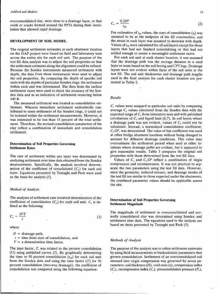
overconsolidated clay, were close to a drainage layer, or that voids or cracks formed around the PPTs during their installation that allowed rapid drainage.

DEVELOPMENT OF SOIL MODEL

The original settlement estimates at each abutment location on the GAP project were based on field and laboratory tests across the entire site for each soil unit. The purpose of the test fill data analysis was to adjust the soil properties so that the settleme.nt estimates along the alignment could be refined. Because the Sondex instruments measured settlement with depth, the data from those instruments were used to adjust the soil properties. By comparing the depth of specific soil units with the depths of particular Sondex rings, the settlement within each unit was determined. The data from the surface settlement risers were used to check the accuracy of the Sondex data and as an indication of settlement occurring below 140 ft.

The measured settlement was treated as consolidation settlement. Whereas immediate settlement undoubtedly contributed to some settlement of the Sondex rings, it could not be isolated within the settlement measurements. However, it was estimated to be less than 15 percent of the total settlement. Therefore, the revised consolidation parameters of the clay reflect a combination of immediate and consolidation settlement.

Determination of Soil Properties Governing Settlement Rates

The rate of settlement within any layer was determined by analyzing settlement over time data obtained from the Sondex measurements. Specifically, the analysis involved determination of the coefficient of consolidated ( Cv) for each soi.I layer. Equations presented by Terzaghi and Peck were used as the basis for analysis (5).

Method of Analysis

The analyses of settlement rate involved determination of the coefficient of consolidation ( Cv) for each soil unit. Cv is defined as the following:

D 2T c =-v t

where

D = drainage path, t = time from start of consolidation, and

T = a dimensionless time factor.

(1)

The time· factor, T, was related to the percent consolidation (U) using published curves (5). By graphically determining the time to 50 percent consolidation (t50) for each soil unit from the Sondex data and using .the time factor (T) for 50 percent consolidation (two-way drainage), the coefficient of consolidation was computed using the following equation:

13

C = 0.2D2

v tso (2)

For estimation of t50 values, the start of consolidation (t0) was assumed to be at the midpoint of the fill construction, and the strain in each layer was assumed to decrease with depth. Values of t50 were calculated for all soil layers except for those layers that had not finished consolidating or that had not settled enough to create a meaningful settlement curve.

.For each soil unit at each cluster location, it was assumed that the drainage path was the average distance to a sand layer or seam based on the soil boring and CPT logs. Drainage layers were not evident within three of the soil units at the test fill. The soil unit thicknesses and drainage path lengths used in the final analysis for each cluster location are presented in Table 2.

Results

Cv values were assigned to particular soil units by comparing average Cv values calculated from the Sondex data with the expected range of Cv from laboratory tests and with published correlations of Cv and liquid limit (6,7). In soil layers where a drainage path was not evident, values of Cv could not be calculated. Instead, a normalized consolidation coefficient, C) D 2

, was determined. The value of this coefficient was used at other bridge abutment locations without being changed to account for different drainage conditions. This value may overestimate the settlement period when used at other locations where drainage paths are. evident, but it appeared to give reasonable results. Table 3 compares the original soil properties with those determined from the test fill data.

Values of Cv and C)D2 reflect a combination of virgin compression and recompression. It was not practical to separate the two parameters using the test fill data. However, since the geometry, induced stresses, and drainage modes of the test fill are similar to those expected under the abutments, the combined parameter values should be applicable across the site.

Determination of Soil Properties Governing Settlement Magnitude

The magnitude of settlement in overconsolidated and normally consolidated clay was determined using Sonde~ and settlement riser data. The equations used in the analysis are based on those presented by Terzaghi and Peck (5).

Methods of Analysis

The purpose of the analysis was to refine settlement estimates by using field measurements to backcalculate parameters that govern consolidation. Settlement of an overconsolidated soil stressed into virgin compression was governed by' seven parameters: soil thickness (H), void ratio (e), compression index (Cc), recompression index.(C), preconsolidation pressure (Pc),


TABLE 2 Soil Unit Thickness and Drainage Path at Cluster Locations

Center West Side Southwest Corner

Soil Thickness Drainage Soil Thickness Drainage Soil Thickness Drainage

Type (ft) ' Path (fl) Type (ft) Path (ft) Type (ft) Path (ft)

2 6.0 6 2 6.5 6.5 2 6.5 6.5

3A 4.0 4 3A 4.0 4 3A 4.0 4

SAND 3.0 1 3B 5.0 2.5 3B 5.0 10

3B 6.0 2.S SAND 4.0 3B 6.0 10

3B 7.0 6 3B s.o 3C 20.0 ND

3C 14.0 NDa 3C 17.0 ND 30 12.0 ND

30 13.0 ND 30 s.o ND 3E 20.0 ND

3E 18.0 ND 3E 23.0 ND SAND s.o SAND 6.0 SAND 6.0 4A 16.0

4A 12.0 4A 2S.O lS SAND 10.0

4B 16.0 16 4B s.o s SA 22.0 10

SA 19.0 15 SA 20.0 16 SB 7S.O 20

SB 79.0 20 58 76.0 15 SAND 13.0 1

SAND 13.0 1 SAND 13.0 1 S8 S2.0 30

SB S2.0 20 S8 S2.0 30 6 . 10.0 10

6 10.0 10 6 10.0 10 SAND 2S

SAND 25.0 SAND 2S.O 6 3S lS

6 30.0 lS 6 3S.O 15 7 14S.O 30

14S.O 30 7 14S.O 30 8 20 50

20.0 so 8 20.0 so a "ND" indicates drainage path was not detennined for soil layer.

TABLE 3 Comparison of Original and Revised Properties

c. {ft2/yr) CjD2 (I/yr)

Soil

Unit Original 8 Revised

3-26 80

3A 28-61 76

38 11-lSO 80

3C NAb NA 1.8

30 NA NA 1.8

3E NA NA 1.8

4A 8-200 37

48 7-54 60

5Ad 27-77 37

58 7-260 so 6 310 so

9 50

none 50

an_n indicates range of values from laboratory test. hNA indicates not applicable. CNR indicates not revised. dunit SA did not undergo virgin compression.

initial overburden pressure (P;), and final overburden pressure (P1):

( Cr pc Cc fl)

Settlement = H 1 + e log P; + 1 + e log pc (3)

To improve the accuracy of the settlement estimates, the most reliable parameters for calculating settlement were identified and then considered constants. The compression index (Cc) and e were assumed to be determined accurately through laboratory tests. The final overburden pressure (P1) and the initial overburden pressure (P;) were easily computed. The remaining parameters, Cr and Pc, appear to be the least reliable and, therefore, were backcalculated using the test fill data.

C, pc {ps0

Original Revised Original Revised

O.Q25 0.048 4460 NRC

0.034 0.036 6000 NR

0.021 0.046 3SOO 3SOO

O.QIS 0.017 10000 NR

O.Q28 0.030 4600 5900

O.Q25 0.043 8320 NR

O.Q2S 0.022 8200 8200 .

0.026 0.029 14000 NR

0.020 0.017 8250 10700

. 0.024 0.026 20000 NR

O.Q25 0.012 32000 NR

0.028 0.017 35000 NR

O.Q25 O.OZS 40000 NR

Parameter Revision of Overconsolidated Soil For those soils that did not go into virgin compression, the consolidation equation was reduced to the follo\\'.ing:

Settlement H(_£_10 fl) 1 + e g P;

(4)

The recompression index, Cn was easily backcalculated at each instrument cluster for each soil unit using Equation 4. The settlement was determined from the Sondex data, the void ratio was determined iri the laboratory, and the other parameters in the equation. were known: Since these soils did not enter virgin compression, calculation of Pc was not possible (or necessary) from the data.

Ashford and Madsen

In some of the deep overconsolidated soil layers, the Sondex did not register settlement. However, since the Sondex may not accurately measure small displacements, settlement was assumed to occur in those layers on the basis of the surface risers. Cr for the deep overconsolidated layers, including the layers that lie below the Sondex base, was determined using laboratory data in addition to experience gained from the other units. This was thought to be conservative, since values of Cr determined in the laboratory were found to be higher than values calculated using field measurements.

Parameter Revision for Normally Consolidated Soil To determine the consolidation parameters of soil that went into virgin compression, Cr was assumed to be both more predictable and less critical to settlement estimates than Pc The ratio of the recompression index (determined as described previously) to the compression index (measured in the laboratory) in the overconsolidated shallow soils varied from 1/10 to V1. On the basis of those data, Cr was assumed in the normally consolidated soil to be Y10 Cc. Using this assumption, values of Pc for each soil unit could be backcalculated from the settlement measurements at each cluster since all other parameters in Equation 3 were known.

Final Revision The accuracy of the backcalculated Cr and Pc was checked by running consolidation analyses for each of the three cluster locations, each having a different stress regime. If the average absolute difference between the measured and calculated settlement within any layer for the three clusters was more than 25 percent, Cr or Pc was altered and the settlement recalculated ·until the average absolute difference was within 25 percent. Since cumulative differences within clusters tended to be compensating, absolute values were used in developing the model in an effort to more closely match the in situ soil properties.

Secondary Compression The duration of monitoring since the completion of primary consolidation was too short to make any reasonable judgment on the magnitude of secondary compression. In the absence of field data, estimates of secondary compression were based on laboratory test results and published values (6,7).

Results

A summary of the original and revised properties is presented in Table 3. For the overconsolidated soil units; the value of Cr was typically increased from the values originally estimated from laboratory data, though no trends were a~parent. The preconsolidation pressure for the normally consolidated soil units was increased from zero to 30 percent over 'the values developed from laboratory data. This confirmed that all of the normally consolidated soil units were slightly overconsolidated.

Comparison of Settlement Estimates

A comparison of the original and revised settlement estimates at the center of the test fill, along with the measured settle-

15

0.0 .------------------------, o--....... o~ -0.2 "\.

-0.4 °\ a; -0.6 00

ID ~' 't- -0.8 \ "" +' \ 0 '" ~ORIGINAL ESTIMATE

~ -1.0 \bo V ID \ \ ~MEASURED (SP-6) ::; -1.2 ' o"'-.. +' REVISED ESTIMATE~.' '( Q 0 '

c9l -1.4 . """'

-1.6 ',---~ -1.8 '~------

10 100 Time. Oo!:JS

1000

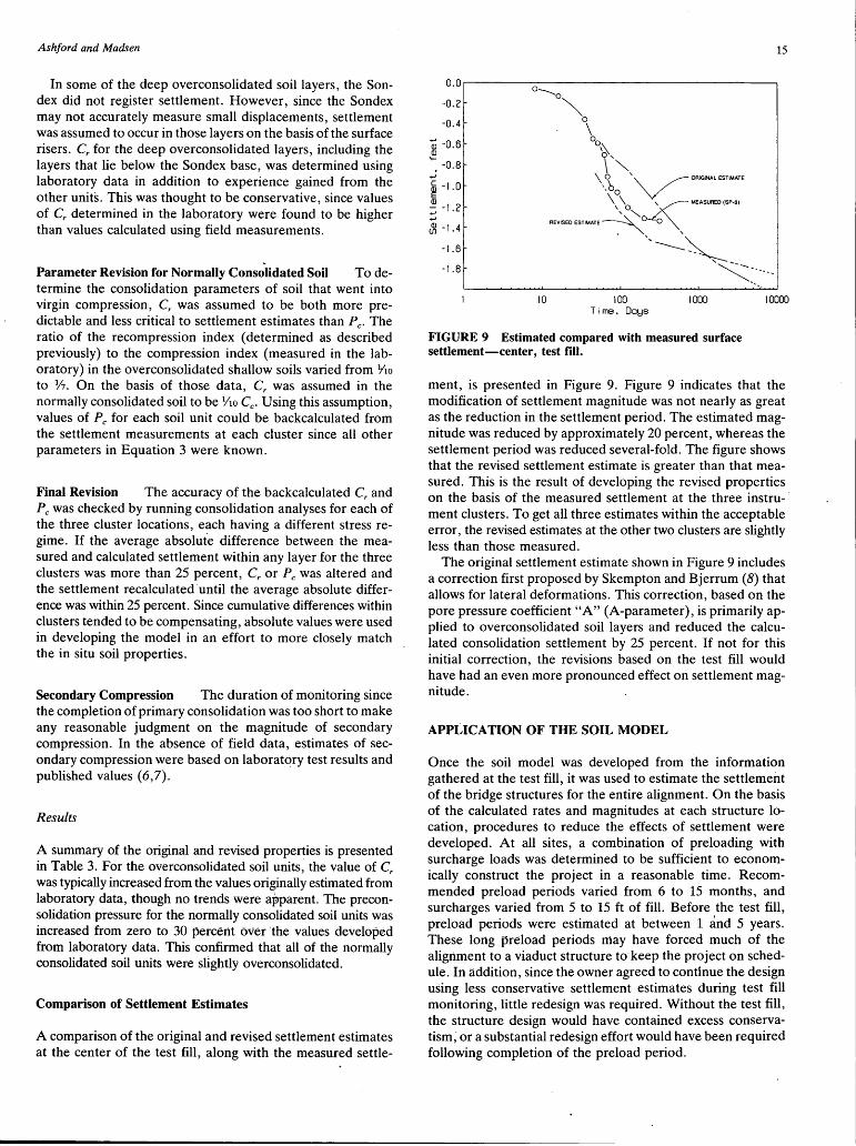
FIGURE 9 Estimated compared with measured surface settlement-center, test fill.

10000

ment, is presented in Figure 9. Figure 9 indicates that the modification of settlement magnitude was not nearly as great as the reduction in the settlement period. The estimated magnitude was reduced by approximately 20 percent, whereas the settlement period was reduced several-fold. The figure shows that the revised settlement estimate is greater than that measured. This is the result of developing the revised properties on the basis of the measured settlement at the three instru- · ment clusters. To get all three estimates within the acceptable error, the revised estimates at the other two clusters are slightly less than those measured.

The original settlement estimate shown in Figure 9 includes a correction first proposed by Skempton and Bjerrum (8) that allows for lateral deformations. This correction, based on the pore pressure coefficient "A" (A-parameter), is primarily applied to overconsolidated soil layers and reduced the calculated consolidation settlement by 25 percent. If not for this initial correction, the revisions based on the test fill would have had an even more pronounced effect on settlement magnitude.

APPLICATION OF THE SOIL MODEL

Once the soil model was developed from the information gathered at the test fill, it was used to estimate the settlement of the bridge structures for the entire alignment. On the basis of the calculated rates and magnitudes at each structure location, procedures to reduce the effects of settlement were developed. At all sites, a combination of preloading with surcharge loads was determined to be sufficient to economically construct the project in a reasonable time. Recommended preload periods varied from 6 to 15 months, and surcharges varied from 5 to 15 ft of fill. Before the test fill, preload periods were estimated at between 1 ~nd 5 years. These long preload periods may have forced much of the alignment to a viaduct structure to keep the project on schedule. In addition, since the owner agreed to continue the design using less conservative settlement estimates during test fill monitoring, little redesign was required. Without the test fill, the structure design would have contained excess conservatism~ or a substantial redesign effort would have been required following completion of the preload period.

16

CONCLUSIONS

1. Use of test fill can be an economical way to eliminate excess conservatism in settlement estimates where soil properties are uncertain. With adequate instrumentation soil properties for individual soil layers can be backcalculated.

2. In layered soil profiles, it is critical to monitor settlement with depth if properties are to be backcalculated. With only surface data, it would not have been possible to differentiate behavior between units. This would have prevented extrapolation of the information to other sites along the alignment, where different stress distributions and unit thicknesses were present.

3. Multiple types of instrumentation installed in different stress regimes proved very useful in developing the soil model. The different instruments complemented each other and provided independent checks. The three instrument clusters with different stres~ regimes provided three independent checks for the soil model.

4. The A-parameter correction factor suggested by Skempton and Bjerrum brought the initially estimated consolidation closer to that measured. It seems appropriate to consider its use on projects in which no test fill is used.


REFERENCES

1. A. Casagrande. The Determination of the Pre-Consolidated Load and Its Practical Significance. Proc., First International Conference on Soil Mechanics, Vol. 3, Cambridge, Mass., 1936, pp. 60-64.

2. J. H. Schmertmann. Estimating the True Consolidation Behavior of Clay from Laboratory Test Results. Proceedings of the American Society of Civil Engineers, Vol. 79, Separate 311, 1953.

3. Method of Installation and Use of Embankment Settlement Devices, California Test 112. Standard Test Methods, Vol. 1, California Department of Transportation, 1978.

4. J. Dunnicliff. Geotechnical Instrumentation for Monitoring Field Performance. John Wiley and Sons, Inc., New York, 1988.

5. K. Terzaghi and R. B. Peck. Soil Mechanics in Engineering Practice (2nd ed.). John Wiley and Sons, Inc., New York, 1967.

6. J.M. Duncan and A. L. Buchignani. An Engineering Manual for Settlement Studies. Geotechnical Engineering Report, University of California, Berkeley, 1976.

7. Design Manual 7.01, Soil Mechanics. Naval Facilities Engineering Command, U.S. Department of the Navy, 1986.

8. A. W. Skempton and L. Bjerrum. A Contribution to the Settlement Analysis of Foundations on Clay. Geotechnique, Vol. 7, No. 4, 1957' pp. 168-178.

Publication of this paper sponsored by Committee on Transportation &~~~ .

TRANSPORTATION RESEARCH RECORD 1369 17

Centrifugal Modeling of Consolidation Phenomena

F. c. TOWNSEND

Geotechnical centrifugal modeling is a technique whereby centrifugal accelerations are used to create prototype stresses within a small-scale model. Diminishing prototype geometry drainage path lengths in the model also permit rapid simulation of large prototype time frames. Centrifugal modeling of consolidation behavior is reviewed. Centrifugal modeling examples presented are large strain (self-weight) consolidation of reclamation schemes involving waste clays, determination of consolidation behavior parameters, observation of consolidation behavior, and computer model verification. The reviews indicate that centrifugal modeling is a feasible technique for assessing geotechnical problems involving consolidation.

Traditional design and analysis of geotechnical engineering problems are based on small-scale laboratory tests or in situ test correlations to develop parameters for material behavior, which are then used in various analytical solutions. The analytical techniques currently used include conventional 1-D Terzaghi theory and 2-D and 3-D finite element methods and finite difference approache·s. The validity of these techniques must be verified to ensure that limitations of small-scale laboratory tests used to define soil properties are adequate. In addition, mathematical modeling to produce the observed laboratory or field response. is difficult because the behavior of soils is greatly influenced by factors such as (a) water content, density, and soil structure; (b) previous stress history; (c) stresses imposed by boundary conditions; and (d) a nonlinear, hysteritic, and time-dependent behavior. Since it is virtually impossible to evaluate all these effects in laboratory tests or by means of nonlinear mathematical models or analytical techniques, the unknown degree of uncertainty must be covered by safety factors or overly conservative estimates of soil properties.

The various limitations of precise design and analysis techniques make full-scale testing attractive; however, because of the large soil masses and weights of material required to include gravity forces, and time frame involved, full-scale tests are seldom performed to evaluate consolidation behavior. Consequently, soil modeling, in a manner that includes gravity force, offers an attractive and needed verification method.

BASIC CENTRIFUGAL MODELING THEORY

The basic concept of centrifuge model testing is to create a scale model similar in geometry, material properties, and boundary conditions to the full-scale prototype, and to subject

University of Florida, Gainesville, Fla. 32611.

the scale mpdel to an acceleration such that the increase in self-weight stresses matches those at corresponding points in the prototype. Thus applying Newton's second law (F = ma), the stress (]" simply becomes the force F divided by the area A or(]" = FIA and(]" = FIA = ma/A.

Since m = Wig, where W = weight and g = gravity, then (]" = Wa/Ag. Considering that unit weight 'Y = weight volume = W/Ah, where h = height of material, then(]" = -yAha/Ag = -yhalg. At the earth's surface a = g, and thus (]" = -yh, which is the familiar equation for vertical geostatic stresses in a horizontal soil deposit. If we wish to model this soil deposit by a scale of n (i.e., hln), then(]" = -yhalng, and we see that the stress is only l/nth of the prototype. Therefore to achieve similitude, the acceleration must be increased by a factor of n, such that(]" = -yhnalng = -yhalg. Thus, the first law of centrifugal modeling may be stated as follows:

If soils with identical friction, cohesion, and density are formed into two geometrically similar bodies, one of a prototype of full scale and one a model of llnth, arid if the llnth scale model is accelerated so that the self-weight increases n times, the stresses at corresponding points are then similar.

If one considers _dissipation of pore water pressure,

where

tP = time. in prototype, T = time factor, h thickness of layer, and

cv = coefficient of consolidation.

In the case of a model of l/nth scale tm = T(h/n)2/cv, where tm = time in model, then tm = Vn2

• Thus the second law of centrifugal modeling can be stated as follows:

Once the excess pore pressure distribution has been made to correspond in model and prototype, all subsequent primary flow processes of pore water are correctly modelled after time tm in the model that is less than time tP in the prototype in the ratio of the square of the scale factor n. (1)

From these considerations, centrifugal modeling is most attractive for examining consolidation phenomena. For example, a l/lOOth scale model at 100 g models time as 1 min = 6.9 prototype days or 52.6 min = 1 year prototype.

18

OBJECTIVE

The objective of this paper is to review and examine centrifugal modeling of consolidation behavior.

Centrifugal modeling is becoming more in vogue with over 50 geotechnical modeling centrifuges worldwide. At this time centrifugal modeling appears akin to numerical modeling of two decades ago. It is a feasible technique for examining geotechnical problems but has not entered the mainstream of geotechnical engineering.

LARGE STRAIN (SELF-WEIGHT) CONSOLIDATION

Reclamation schemes involving dredged materials, mine waste clays, and so forth require predictions of consolidation rates and final consolidation levels for estimating storage capacities of contaminant areas or for considering alternative disposal techniques (e.g., sand/clay mixes, surcharge capping, or stage

· filling). Current large strain computer programs can predict some boundary conditions (homogeneous deposits, uniform surcharges) but are limited when considering nonuniform (layered) deposits and stage filling (2). In addition, input parameter determination for such soft soils req·uires specialized laboratory testing (e.g., slurry columns, CRS slurry consolidometers, and pump flow).

Bloomquist and Townsend (3) provide one of the few centrifuge-numerical model prototype verifications for a waste phosphatic clay. In the study, a "modeling of models" centrifuge test series at 40, 60, and 80 g replicating the same prototype was performed to ascertain the time scaling ex-

22

It-!?

"' 20 UJ ~ ::::> ...J 0 > >-ca 18 I-z UJ I-z 0 u 16 VJ 0

...J 0 VJ

I .--1··'

A: I

~ i.

6

+. ~

14 >- •i <( ...J u


ponent. Although pore pressure dissipation scales as n2 , sedimentation scales as n. Thus for cases where sedimentation/ consolidation occurs, the exponent varies between ·i.o and 2.0. These centrifuge results in Figure 1 show the time scaling exponent for solids contents (srbetween 14 percent (e = 16) and 20 percent (e = 11) [e = G(l - s)/s]. Using these centrifugal test-devised exponents, a comparison was made with a 2. 79- x 4.27-m metal prototype tank test that self-weight consolidated from an initial solids content of 12.6 to 21.2 percent over a 403-day period. Using Somogyi's finite strain consolidation program ( 4), a numerical prediction was also made. These comparisons are shown in Figure. 2 and reveal an excellent agreement.

Centrifuge to Obtain Consolidation Properties

Large deformation (finite strain) self-weight consolidation equations (5 ,6) differ from Terzaghi consolidation in that k, mv, and layer thickness are not constant during consolidation. Therefore, nonlinear cr-e and k-e relationships are required as input for computer codes.

Takada and Mikasa (7) used centrifugal modeling to obtain these nonlinear relationships. In their tests 30-cm-diameter by 100-cm-thick specimens of clay at different water contents but approximately twice their liquid limit were "cured" several days at 1 g to minimize "hindered settling" before accelerating at 150 g for 1,000 to 5,000 min. By monitoring the specimen surface settling rate (s) for different e0 values, from

Mikasa's theory (6) k = ~ -yj-y a k-e relationship as shown n . in Figure 3 was obtained. Upon stopping the centrifuge, an

• +,,. ~-

.,,-·I

~,._ .. ~-·

12J-~~---~~~--~~__....~~~-t--~~--t-~~~-+-~---

l. 0 i.2 1. 4 1.6 1.8 2.0 2.2

ACCELERATION LEVEL EXPONENT

FIGURE 1 Time scale exponent versus solids content (3).

Townsend 19

22

• 21 • • • • 20 • ••

N • ....: . .. z 19 w I- • z 0

~ u 18 Ul 0 .... •• ...J 17 0 Ul

>- • LEGEND < 16 • • PROTOTYPE TANK TEST ...J u

CENTl=llFUGE MODEL w ,,. • l.:) • SOMOGYI PROGRAM < JS a:: w > < ,

14 • 13 ·-Go 12.6

7. J Ho 20. 75 FT

12 0 JOO 200 300 400 500

PROTOTYPE ELAPSED TIME. DAYS

FIGURE 2 Comparisons of prototype tank test, centrifugal model, and numerical prediction (3).

e 13

11 Oedoaeter Selfveight

test consolidation Hanko I 0 n ( lSOg) t:.. (lg)

Hanko II • • (lOOg) I 4)1Ji

I I

b. ~~ .,,/11·,J

/ )(

Hanko II W0 •149:t

/ •"' 10-S

le (cm/sec)

FIGURE 3 Permeability versus void ratio (7).

w (%)

~{! I

I 400

300

200

100

undisturbed 5-cm soil column was sampled throughout the specimen length using a thin-walled tube, and water content determinatio_ns were made for every! 2- to 3-mm slice. The effective overburden pressure P' was obtained by integrating n-y' from the specimen surface to a specific depth. Thus values of e-log P' relationships as presented in Figure 4 were obtained. This relationship is not unique for very low P' values.

· To circumvent the multiplicity of centrifuge tests using Takada and Mikasa's approach, the University of Florida (UF) used

· an approach based on measurements of. por@, pressure and void ratio with depth and time during a centrifuge test (8). The void i;-atio values were obtained by using small individual

5-cm-diameter subsample tubes and periodically stopping the centrifuge, removing a tube to determine the water content distribution. The permeability values were calculated from the pore pressure measurements. Figures 5 and 6 present the e-log P' and e-log k relationships for centrifuge tests on a waste phosphatic clay as compared with 1 g constant rate of deformation consolidometer (CRD) tests. The compressibility curves show good agreement for the virgin zone of the curve, particularly when the slower deformation rate is used for the CRD test. Unfortunately, the centrifuge permeability values are a half order of magnitude greater than the CRD tests, which is probably due to difficulties in measuring pore pressures along the side of the centrifuge container.

Phenomenological Observations

Townsend et al. (9 ,10) used centrifugal modeling to evaluate disposal schemes to enhance densification/consolidation phosphatic waste clays and thus reduce storage area. Specifically, (a) use of flocculents, (b) sand/clay mixes, and (c) surcharging were investigated by centrifuge models. It was deemed that centrifugal modeling would be easier than numerical modeling in determining how waste clays responded to these treatments due to the difficulty and uncertainties of input parameters for the latter. Figure 7 shows the flocculent effectiveness in increasing the sedimentation rate. Although 1-g bench tests (not shown) suggested that flocculents were not beneficial and the final solids content achieved is reduced because of the formation of large floes, the centrifuge tests belie this conclusion and show final solids contents only slightly lower than un-

12

.01 .1 1 W(:C)

5 e 4 r-~~..-~...---"""T"--.,......._...~~~...-~...--.-......... -.-P"""'l"''T"'l"'~~--.,....__,,...."T""""WlSO

3

2

Oedcmeter W0 •120%

FIGURE 4 Void ratio-log P relationships (7).

c

.... 00-1 Si=l5.3% 0.02 nl•in ... 00-3 Si=l6. 2% 0. DOB aa/ain c l:T-1 51=15. 7% o = B09 o l:T-2 Si=l6. 0% o = 609

16

u

12

0 ...., 10 0

a:: -0

·;; >

or lower water content

.... am-1

.. l:RD-3 c l:T-1 o l:T-2

test

Si=l5. 3% 0. 02 1111/ain 51=16. 2% 0. DOB 11111/min 51=15. 71. 0 a B09 51=16. 0% 0 = 609

120

90

4-t-~~~~~"T"TT~--.----.~~~...-~~~.-.-~....-r-~~~-.-. 4-t-~-.---.--.--.-.-.-......-~~~--.-.-.-.-......-~~.--..-r-r~..--~---.~~......-M

IE-3 IE-2 IE-I IE 0 Effective Stress Cpsi)

FIGURE 5 Compressibility relationships (1 psi = 6.9 kPa) (8).

6

8

,~ r-:... -~ --- ............ :--"""

~ r .........

...: 10 z

!'-... .........

0.25 KG/HT

r--.., ~ z 12 c:::J u Vl 14 Cl

~ r----._

?

' ..... ~

1 .........

'~

........ ~i--

...J Cl 0. 50 KG/tlT Vl 16 w <..:> <

18 ~ w > <

20

22

24

26 .1

.... ~

IE-4 IE-3 IE-2 IE-I IE 0 Permeability (ft/day)

FIGURE 6 Permeability relationships (1 ft/day = 3.53 x 10-6

m/sec) (8).

CENTRIFUGE TEST RESULTS SAMPLE ACC. INITIAL HT.

POL YHALL I 082 60 C 10. 0 CM

I I I

!'-.. 0.00 KG/HT

"~,.. ~ /

~ I\ ~"'- I"'~

!'-... ,N~ "r--. ' .... ~

' ' ~ ...__ -i-...

~ -i-...... -......,...._

10 100 1000

ELAPSED MODEL TI ME. MIN D· FIGURE 7 Effect of Polyhall flocculent on solids content (10).

Townsend

40 TEST DESJCNATJON1 KC:B0-0/6 CJ6% !n!Ual ela aol!da I 40-JOO aand>

~ s0 = 16.0 %

~ H0

= 6.0 CH

~ ..J ~ 35tt-~-+~~-+--loor~+-~.......-ll--~-+~~-+-~~-+-~~

~

2so~~~-"-~~"--~~~~-41.--~--1.s~~-'-~~-'-~---'e

SANO/C:LAY RATJO Ho-HF

Percent reduc:t1on 1n height (~ X 100)

FIGURE 8 Percent reduction in height versus sand/clay ratio (9).

treated nonflocculated (dosage = 0. 00 kg/MT) solids contents. When the agglomerated floes are subjected to field stress conditions, they collapse, but they never achieve higher solids contents than untreated clay. Thus treatment with flocculents gains sedimentation rates at the expense of lower solids contents or increased storage areas.

One disposal scheme is to mix trailings sands with the waste clays, thereby increasing the unit weight and subsequent consolidation. Figure 8 shows that an optimum sand/clay mix ratio (SCR) exists at 1:1 = 2:1, and that SCRs greater than 3:1 produce less consolidation. This observation is attributed to interference by the sand grains at higher SCRs preventing

21

densification of the waste clay within the sand matrix. (One concern in these model tests was segregation of the sand particles due to centripetal forces invalidating the models. This was avoided by maintaining a sufficient clay viscosity.)

Surcharging waste clay ponds by flowing a sand/clay cap onto the pond's surface to increase effective stresses was a "mixed bag." Several considerations for applying this scenario were apparent: (a) bearing capacity of the underlying clay sufficient to support the surcharge, (b) field considerations of actually placing a surcharge on very soft clays, (c) large time frames required for consolidation because of impeded drainage from crusting at the sand cap interface, and (d) the occupation of disposal space by an incompressible cap. Figure 9 compares the effects of an SCR surcharge cap in a 6-m waste clay pond at= 24 percent solids over which a 3.2-m surcharge is placed. Although the 6:1, 3:1, and 1:1 SCR mixes produced increasing solids contents of 35.2, 32.2, and 31.5 percent, respectively, in the underlying clay, this increase in solids content did not translate into considerable reductions in interface height because of the incompressibility of the sand.

Croce et al. (11) used seven centrifugal model tests to evaluate the influence of vertical sand drains on consolidation behavior. The prototype modeled was a single drained 7 .5-m clay deposit into which 1.9_.m-diameter drains were placed on a 10.1-m spacing. Three successive 1.8-m sand fills ('y = 18.3 kN/m3

) would be placed on the clay surface .. The model tests were reduced to a single equal strain consolidometer cylinder with an equivalent "diameter of 11.4 mas shown in Figure 10. Vertical, radial, or combined flow conditions could be imposed on the model. Figure 11 and Table 1 present the settlement-time results and show that the final observed settlements are in agreement with those calculated from odometer tests. (The scatter was explained by initial height variations.) Traditionally, the combined degree of consolidation is estimated as urx = 1 - (1 - u R)(l - Ux) using superposition of Terzaghi's theory. Thus cv was evaluated by fitting the log

TEST DESIGNATION1 KCB0-7.5/4.0

31

30

·I- 29 ll-

w u < 28 ll-0: w I-:s

27 w n. >-I-0 I- 26 0 0: n. ll-0 25 I-J: t..:I

w 24 J:

23

....__ t----

.• 1:1 .__• ------ ~--

, ___ _,_

~ - -•- -!._ r--. • 3:1 l----

~ ~ r-..._ "ll r--.r--. A 6:1 I-. l "i.. ' I ,_ ---....,!'-..

"'' r--.1---~ !'-.·~ ~ ~

""" ~ ~ f'.-

" f'._f'-11

~ L-. -l·-

"'f'.- --~ " r-.." ' ~ I' I'

-~'-

r~ ~ ~ "' -~ -

~ ~[' r-.1• ~-

~[' .._,_ --r-.. 14

~ !"- ~I'

"

22 JO JOO 1000 JOOOO

ELAPSED MODEL TI ME, MIN

FIGURE 9 Prototype interface versus model time for 4-cm cap (9).

22

-.. ~

i::: Q) .. Q) ~ ~ ~ Q)

Ul

3

2 -+-+----"--+I

1-H~===:~n

11.40 cm ·I FIGURE 10 Sand drain model apparatus: 1, porous (or impervious disc); 2, porous (or impervious disc); 3, load pressure; 4, L VDT; 5, back pressure; 6, loading ram with convoluted rubber membrane; 7, piston; 8, clay sample; 9, differential pressure transducers (11).

Tiae (days) 01 10 100

• • +: •• • • 0.1 • • •

• • ·:. 0.2

• 0.3 • • 0.4 • • • • •

1000

I ca> !

I

o.s I

..... f + ••

I I • • •• 0.6 i • •·

Computed I •+ •• 0.7 Settle-at

~··· 0.8 • 0 • (b)

0.1

0.2

0.3

0

0.1

0.2

FIGURE 11 Settlements versus prototype time (11).


TABLE 1 Model Tests (11)

Pore Hei9ht (cm! Sym- Test Water Initial Step

bol Flow 1

• Vert • 7.47 6.87

• 2 Vert • 7.57 6.79

.& 3 Rad. 7.20 6.54

.... 4 Rad. 7.58 6.86

• 5 Comb. 7.43 6.71

+ 6 Comb. 7. 43 6.71

* 7 Comb. 7.12 6.54

Tiae (days)

1 10 100 0

0.2

0.4

0.6

0.8

1.0

~ 0 c:I GI El 0.2 GI .... ~ ~ 0.4 GI tlJ

Cw 0.6 0

GI 0.8 e

tn GI 1.0 Q

FIGURE 12 Analysis of combined flow settlements (see Table 1) (11).

Step Step

2 3

6.52 6.32

6.49 6.27

6.26 6.06

6.59 6. 39.

6.39 6.20

6.39 6.20

6.25 6.08

1000

(b)

settlement data, while c,, was fitted using Barron's th€oty (12) . Figure 12 shows an analysis of combined flow settlements and reveals that the calculated rate of settlement (Curve 4) is always faster than the measured (Curve 3); thus linear superposition overpredicts settlement rates. (Curves 1 and 2 of Figure 12 are for radial or vertical flow only, respectively.)

Computer Model Verification

Mitchell and Liang (13) conducted a "modeling of models" test series using accelerated levels of 75 to 97 g of an

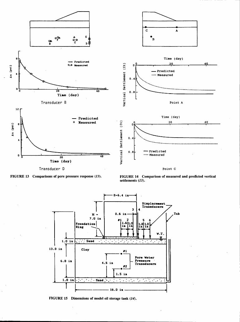
... GI .e :s <I

... GI .e

8

4

0 0

12

8

4

~ B

oC6 F

A 00 c

E

D

- Predicted o,a Measured

Tiae (day)

Transducer B

40

Predicted

20 Tiae (day)

Transducer D

o Measured

40

...

... r:: CD E CD

...... ... ... CD (/)

...... lO u

·.-4 ... I-< CD >

...

... r:: CD E CD ...... ... ... CD (/)

...... lO u

·.-4 ... I-< CD >

c

00

0.4 .......... _

• B

A

Time (day)

20

-Predicted ·--- Measured

40

······-.... ___ _

------··-··---------. ----------------------0.8

Point A

Time (day)

00~-----------------~20 ________ ""'T"" ________ 4~0----~

·· ... .. 0. 4 . •· •.

······-··----- ---------------------------------------~-----o. a - Predicted

--·- Measured

Point C

FIGURE 13 Comparisons of pore pressure response (13). FIGURE 14 Comparison of measured and predicted vertical settlements (13).

13.0

H • 7.0 in

Foundation I Ring

r--o-6.4 Displace-nt Transducers

3 4

0.6 in

#1 2 1.6 1.0 in in

5 1.0 1.0 in in

L ~ W.T. t---=--:---~;====z~..__.____._~

1. 0 iD -~ ; · : .: Sand · · · · . · ~,.: · . · . -. . in ~t--..._C_l_a_y ______ _._ __ _._ ............ ___ #_1.;........;_~----~----;....;~

f •J Pore Water 6. 0 in Pressure

_i___t--------------

4

--·

5

.__

1

_·n ___ l_._:_'_i: _____ T_r_a_n_s_d_u_c_•_rs ______ -f

1 • 0 in . : . · . ~ . : . Sand • · • • · ·.

~I·-------- 16.0 in ----------et~ FIGURK15 Dimensions of model oil storage tank (14).

Tub

24

(/)

a.

Q) s... ::::i (/)

U'I (1J s...

0....

Q) s... 0

0....

20

18

16

14

12

10

8

6

4

2

0


Centrifuge Test 11 Centrifuge Test 12 Finite Eleaent Analysis

0 2000 4000 6000 8000 10000 12000 14000

TIHE (sec)

FIGURE 16 Pore pressure response to loading and unloading (14).

A u r:I ....

-.... Ill ~

;::~ 2.o~t----...

a------.~-------------.---~ : '. l

7200

0.02

0.04

0.06

0.08

0 1800

1800

3600

TIME 3600

5400 9000

(sec) 5400 7200 9000

a ----........ --------.--------~ 0.02

0.04

0.06

a~--...... ---..---....... ---...... --..... 0.02

0.04

0.06

OE''***~ ... ~ : ; ; 0.02 •11d1 .... fill 11111 I I I

a. 04 I Centrifuge # 1 OEDT #6 Centrifuge 112 Finite Element Analysis

FIGURE 17 Surface settlements during loading and unloading (14).

embankment-type soil structure to evaluate a two-dimensional ·FEM consolidation program, CON2D. The prototype condition modeled was essentially a single drained kaolinite clay deposit 10 m (33 ft) thick overlain by a 3.4-m (11-ft) sand blanket upon which was placed a sand embankment 4.6 m (15 ft) high with 2.5:1 slopes. Figure 13 presents the measured

and predicted pore pressures versus time using a time-scaling of n2 • The comparison shows that both the initial loading increment and subsequent rate of dissipation are closely predicted. A comparison of several vertical settlement locations in Figure 14 shows that the immediate settlements were underpredicted in areas near the toe and overpredicted beneath the central portions of the embankment.

Shen et al. (14) performed centrifugal model tests at 60 g of a prototype oil storage tank 9.8 m (32 ft) in diameter fo"unded on a soft double-drained kaolinite deposit 9.1 m (30 ft) thick as shown in Figure 15. Testing consisted of loading (filling) and unloading (draining) the storage tank. Numerical modeling used a bounding surface plasticity model involving 18 input parameters, which had been incorporated into 2-D and 3-D FEM codes. Figure 16 presents the model time pore pressure predictions, whereas Figure 17 presents the surface settlements. As can be seen the agreements are good.

CONCLUSIONS

Centrifugal modeling is a powerful technique for assessing consolidation phenomena in that prototype geostatic stresses are applied to the soil, and the reduced model geometry accelerates pore pressure dissipation and thus consolidation time. The technique is applicable for assessing behavior such as· sand drains, self-weight consolidation, and consolidation of flocculated soils. The technique also provides a feasible method for verifying numerical computer codes and assumptions.

REFERENCES

1. G. I. Pokrovsky and I. S. Fedorov. Studies of Soil Pressure Reformations by Means of a Centrifuge. Proc., First International. Conference on Soil Mechanics and Foundation Engineering, Vol. 1, No. 70, 1936.

2. F. C. Townsend. SOA: Large Strain Consolidation Predictions.

Townsend

Journal of Geotechnical Engineering, ASCE, Vol. 119, No. 2, Feb. 1990, pp. 222-243.

3. D. Bloomquist and F. C. Townsend. Centrifugal Modeling of Phosphatic pay Consolidation. Sedimentation/Consolidation Models: Predictions and Validation, ASCE, 1984, pp. 565-580.

4. F. Somogyi. Analysis and Prediction of Phosphatic Clay Consolidation: Implementation Package. Florida Institute of Phosphate Research, Bartow, 1979.

5. R. E. Gibson, G. L. England, and M. J. L. Hussy. Theory of One-Dimensional Consolidation of Saturated Clays. Geotechnique, Vol. 17, 1967, pp. 261-273.

6. M. Mikasa. The Consolidation of Soft Clay-A New Consolidation Theory and Its Application. Kajima Shuppon-Kai, 1963.

7. N. Takada and M. Mikasa. Determination of Consolidation Parameters by Self-Weight Consolidation Tests in Centrifuge. ASTM STP 892 Consolidation of Soils: Testing and Evaluation, 1985, pp. 548-566.

8. R. E. Martinez, D. Bloomquist, M. C. McVay, and F. C. Townsend. Consolidation Properties of Slurried Soils. Soil Properties Evaluation from Centrifugal Models and Field Performance. ASCE Geot Spec Publ 17, 1988, pp. 1-14.

9. F. C. Townsend, M. C. McVay, D. Bloomquist, and S. A.

25

McClimans. Clay Waste Pond Reclamation by Sand/Clay Mix or Capping. Journal of'Geotechnical Engineering, Vol. -115, No. 11, Nov. 1989, pp. 1647-1666.

10: F. C. Townsend, D. Bloomquist, and S. A. McClimans. Evaluation of Reclamation Schemes by Centrifugal Modelling. Flocculation, Sedimentation and Consolidation, 1985, pp. 471-487.

11. P. Croce, H.-Y. Ko, R. L. Schiffman, and D. Znidarcic. The Influence of Vertical Drains or Consolidation. Centrifuge 88, A. A. Balkema, 1988, pp. 171-180.

12. R. A. Barron. Consolidation of Fine-Grained Soils by Drain Wells. Transactions, ASCE, Vol. 113, pp. 718-754.

13. J. K. Mitchell and R. Y. K. Liang. Centrifugal Evaluation of a Time-Dependent Numerical Model for Soft Clay Deformations. ASTM STP 892 Consolidation of Soils: Testing and Evaluation, pp. 567-592.

14. C. K. Shen, J. Sohn, K. Mish, V. N. Kaliakin, and L. R. Hewmann. Centrifuge Consolidation Study for Purposes of Plasticity Theory Validation. ASTM STP 892 Consolidation of Soils: Testing and Evaluation, pp. 593-609.



Erosion Resistance of Compacted Soils

G. J. HANSON

There has been recent interest in overflow erosion on overtopped earth embankments, which are typically constructed from compacted cohesive soils. A study of the effects of compaction density and moisture content on the erosion resistance of a soil material is presented. Four soil materials were tested using a laboratory submerged jet testing apparatus. The results of the laboratory testing were used to quantify the changes in erosion resistance due to changes in compaction density and moisture content. Increases in compaction moisture content were observed to result in increased resistance to erosion. Increases in density at a constant moisture content were also observed to result in increased resistance to erosion. Proper control of these factors during embankment construction could make a difference in performan~e.

There has been recent interest in the overflow erosion on overtopped earth embankments for such applications as dams, levees, and highway and railroad fills, which is evidenced by the number of studies in this area (1-4). When embankments are overtopped by floodwater, erosion damage can be significant, involving economic as well as safety concerns. Powledge et al. (J) identified several factors as having a strong influence on the initiation and rate of erosion. Two of the factors identified were the type of material and the density of the fill. Clopper and Chen (2) concluded that soil type and compaction affect the erosion rates and patterns of erosion on embankments.

The objective of this study was to analyze the changes in the erosion resistance of compacted soils. This paper discusses the results of submerged jet tests conducted on four cohesive soils, comparing changes in resistance·ofthe soils at equivalent hydraulic stress and varying compaction moisture contents and compaction efforts.

BACKGROUND

Compaction and Erosion Resistance

The nature and magnitude of compaction has a significant impact on the engineering behavior of the soil material. Therefore, the engineer must conduct compaction tests to determine the properties desired for the specific construction application of interest. The most-common type of compaction test is the standard Proctor, which consists of placing soil in a mold and dropping a hammer on the soil from a specified distance a specified number of times. Compaction tests of this nature for samples at various moisture contents, w, result in a compaction curve in which the dry density, 'Yct, increases to a peak and then decreases. The dry density and compaction moisture content at the peak dry density are the maximum

Water Conservation Structures Laboratory, USDA, Stillwater, Okla.

dry density and optimum moisture content, respectively. Maximum dry density and optimum moisture content are relative, not absolute, terms, being dependent on the compaction effort and method. The portion of the curve that is less than the optimum moisture content is referred to as the dry side, and that portion that is greater than the optimum moisture content is referred to as the wet side. A discussion of the effects of compaction on the engineering behavior of soils is given by Lambe (5) and Barden and Sides (6). These investigators proposed conceptual models to explain the nature of the clay structure as a result of compaction. Lambe (5) proposed a microscale model in which orientation of the individual clay particles depends on the compaction effort and compaction moisture content. The soil structure changes from a flocculated structure to an oriented ·structure as the moisture content is increased at a constant compaction effort. Barden and Sides ( 6) proposed a macroscale structure in which the soil consists of particle clusters called macropeds. In this conceptual model, changes in the macroped interaction change with compaction moisture content at a given compaction effort. At low compaction moisture contents the macropeds have high strength and resist compaction effort without much distortion and remain relatively independent. As the compaction moisture content increases, the soil changes to a state in which the macropeds are distorted during compaction, filling the pore spaces. In this process the macropeds lose their individuality. Both models explain the observed changes in the engineering behavior of compacted soils. Paaswell (7), in his discussions on the state of the art of the mechanics and causes of cohesive soil erosion, pointed out that the physical structure of a compacted cohesive soil material plays a major role in erosion resistance. This structure is influenced by the compaction effort, compactiqn mo.isture content, and the method of compaction. One of the engineering properties that changes with compaction moisture content- and compaction effort is the soil swell. The soil swell, upon wetting, is greater for a soil compacted on the dry side of optimum than on the wet side of optimum. If erosion is considered a surface phenomenon, swelling can only have an adverse effect on the resistance to erosion (7). Therefore, a soil compacted on the dry side of optimum is anticipated to erode more than a soil compacted on the wet side of optimum.

The effect of compaction on the erosion resistance of soils has been investigated in a number of studies (8-14). The results of these studies have not been altogether conclusive. Three of the studies did not investigate the effects of compaction moisture content, but rather the effects of increased density (8,10,12). These studies concluded that increases in compacted density resulted in increased resistance to erosion. Two other studies observed the effects of compaction moisture content at a constant compaction effort (9,13) .. Enger (9)

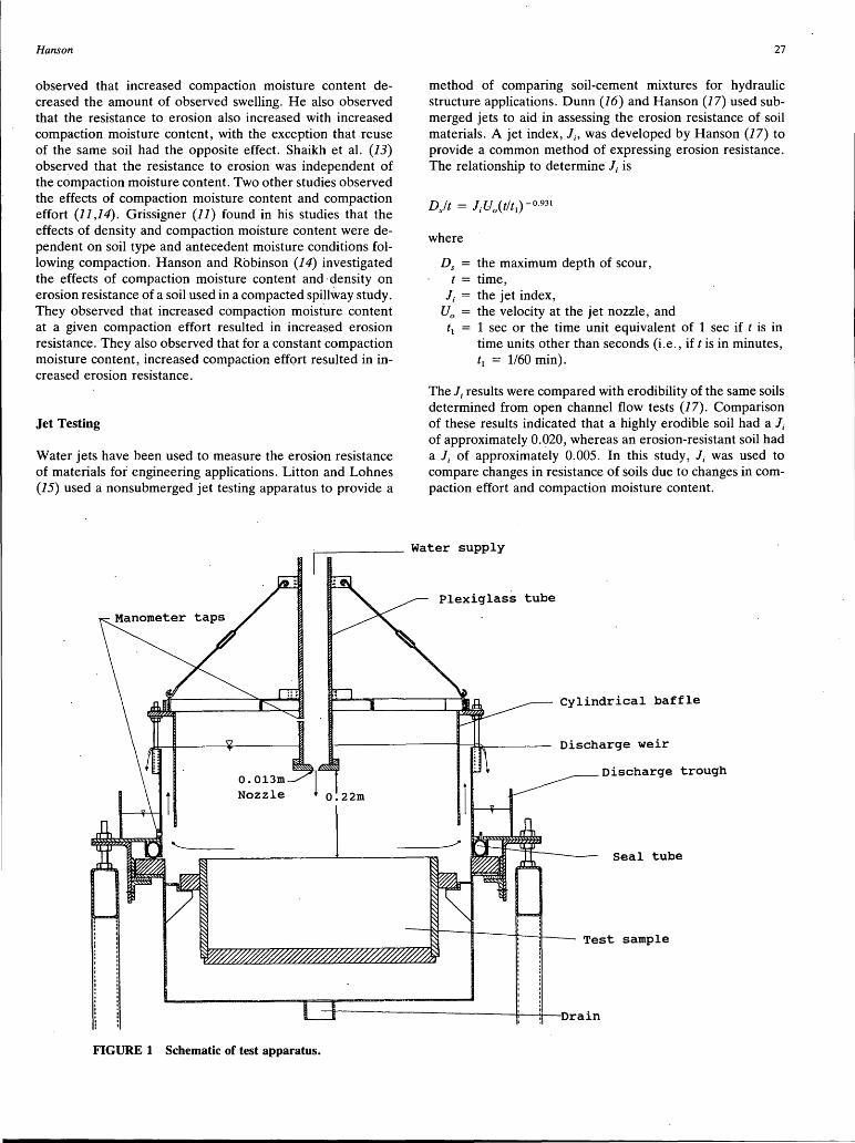
Hanson

observed that increased compaction moisture content decreased the amount of observed swelling. He also observed that the resistance to erosion also increased with increased compaction moisture content, with the exception that reuse of the same soil had the opposite effect. Shaikh et al. (13) observed that the resistance to erosion was independent of the compaction moisture content. Two other studies observed the effects of compaction moisture content and compaction effort (11,14). Grissigner (11) found in his studies that the effects of density and compaction moisture content were dependent on soil type and antecedent moisture conditions following compaction. Hanson and Robinson (14) investigated the effects of compaction moisture content and· density on erosion resistance of a soil used in a compacted spillway study. They observed that increased compaction moisture content at a given compaction effort resulted in increased erosion resistance. They also observed that for a constant compaction moisture content, increased compaction effort resulted in increased erosion resistance.

Jet Testing

Water jets have been used to measure the erosion resistance of materials for engineering applications. Litton and Lohnes (15) used a nonsubmerged jet testing apparatus to provide a

27

method of comparing soil-cement mixtures for hydraulic structure applications. Dunn (16) and Hanson (17) used submerged jets to aid in assessing the erosion resistance of soil materials. A jet index, l;, was developed by Hanson (17) to provide a common method of expressing erosion resistance. The relationship to determine l; is

where

Ds = the maximum depth of scour, t = time,

l; the jet index, U0 the velocity at the jet nozzle, and t1 1 sec or the time unit equivalent of 1 sec if t is in

time units other than seconds (i.e., if tis in minutes, !1 = 1/60 min).

The l; results were compared with erodibility of the same soils determined from open channel flow tests (17). Comparison of these results indicated that a highly erodible soil had a l; of approximately 0.020, whereas an erosion-resistant soil had a l; of approximately 0.005. In this study, l; was used to compare changes in resistance of soils due to changes in compaction effort and compaction moisture content.

~~~~~~ water supply

Plexiglass tube

cylindrical baffle

Discharge weir

Discharge trough

Seal tube

Test sample

FIGURE 1 Schematic of test apparatus.

28

TEST METHODS AND SPECIMEN PREPARATION

Erosion tests were concluded using a laboratory submerged jet testing apparatus as described by Hanson and Robinson (14). Circular soil samples were placed in a tank and slid under the jet apparatus. The soil samples are- 0.44 m in diameter and 0.19 min height, with a volume of 0.028 m3

• Water was fed under a constant head of 0.91 m, U0 = 4.2 m/sec, through a rounded nozzle 13 mm diameter at a set height, 0.22 m, above an originally level bed of prepared soil. A schematic of the test apparatus is shown in Figure 1. The course of scour with time was measured with a pin profiler. Profiles were measured at set time intervals ranging over the test duration. of 0 to 240 min.

Soil samples for laboratory submerged jet testing were prepared by dynamic compaction. Dynamic compaction was attained by dropping a 79.4-kg hammer 0.30 m and controlling the number of blows. The soils were compacted in three layers using from 1 to 24 blows per layer with the compaction effort varying 0.26 to 6.15 kg-cm/cm3 respectively. The compaction effort of ASTM Standard Designation D698 is comparable at 6.05 kg-crn/cm3 • Moisture content was also controlled at the time of compaction. The moisture content, w, was determined by the weight of water divided by the weight of solid in the soil element. The dry density, -yd, was determined by the weight of solid in the soil element divided by the total volume occupied by the entire element. The samples were then wetted for a period of 20 hr before jet testing.

Four soil materials were used in testing, ranging from a rionplastic sandy loam to a clay loam having a plasticity index of 18 as indicated in Table 1. The gradations of the soil materials are shown in Figure 2. ·

TABLE 1 Soil Classification

Physical properties

Liquid limit Plastic limit Plasticity Index u.s.c. AS.C.

ASTM-

Soil A

21 17 4

CL-ML sandy loam

Soil B

37 19 18 CL

clay loam

Silt

Soil C Soil E

26 23 20 14 6 9

CL-ML CL loam sandy-clay loam

Clay 100 i-.-.-......-~:=;~---.-........... ..,.......-,...--.--,...---y-rT"T""i,...+--..-.-..----;

..... Q)

c

80

i.:L 60 +-' c Q)

~ Q) 40

0....

20

o - Soil A • - Soil B v - Soil C ~ - Soil E

0 '-'--'--'--'-'-'-·-'-~--'-''-'--'--'----L.-'--'--'---1...L.'-'--'--'-.___._~~

1 0. 1 0.01 0.001

Grain Diameter, mm

FIGURE 2 Soil gradation curves.


TEST RESULTS

Soil Materials A, C, and E were dynamically compacted at equivalent compaction efforts, 6.15 kg-crn/cm3 at various compaction moisture contents. The maximum depth of scour versus time for Soil Material A at various moisture contents is shown in Figure 3. There is a dramatic decreas~ in scour observed with increases in compaction moisture contents. A display of the test results to determine the I; is shown in Figure 4. A comparison of the moisture-density curve and the re-

.............

E u

'--'

CIJ

0

25

20

15

10

5

3 o -w=9.3%, ')'d=1.73 g/cm

3 • -w=10.0%,f'd=1.75 g/cm

3 v -w=11.9%,f'd=1.79 g/cm

3 T -w=13.0%,f'd=1.82 g/cm

3 o -w=14.1%,f'd=1.85 g/cm

3 • -w=15.1%,f'd=1.83 g/cm

o ____ ..__ _ __. __ __._ __ _._ __ _._ __ _.._ _ ___. 0 2000 4000 6000· 8000 10000 12000 14000

Time (sec)

FIGURE 3 Maximum depth of scour for different compaction moisture contents of Soil Material A at a constant compactive effort versus erosion testing time.

............. u Q) Cf)

...........

E u

'--' ........,

........... CIJ

0

0. 04 r.::====::i::::=====::r::::====:::i::====:::::r:::::::::;3:;:::::::;---i----,

o -w=9.3%, f'd=1.73 g/cm3

• -w=10.0%,f'd=1.75 g/cm

0.03

0.02

o.oi

3 v -w=11.9%,f'd=1.79 g/cm

3 T -w=13.0%,f'd=1.82 g/cm

3 o -w=14.1%,f'd=1.85 g/cm

3 • -w= 15.1 %,yd= 1.83 g/cm

0.2 0.4 0.6 0.8 1.0 -0.931

U0(t/t

1) (cm/sec)

1.2

FIGURE 4 The slope of each line represents the}; for each· sample of Soil Material A tested.

Hanson

0.03

(a) 0.02

J. I

0.01

0 0.00 1.90

~ Soil A s Energy input 6.15 kg-cm/cm J

0 24 Blows per layer .......... 1.85 bl)

"d ("-...

>.. 1.80 +'

rn c Q)

0 1.75

>. L

0

1.70 8 10 12 14 16 18

Moisture content, w %

FIGURE 5 Influence of the compaction moisture content on the erosion resistance of Soil Material A: (a) l; versus the compaction moisture content; (b) dry density versus the compaction moisture content.

suiting l; for Soils A, C; and Eis shown in Figures 5, 6, and 7 respectively. There is a consistent trend with each soil material displaying a decrease in the l; with an increase in compaction moisture content indicating an increase in erosion resistance with increases in compaction moisture content. The erosion resistance of Soil Material A shows significant sensitivity to changes in compaction moisture content, whereas Soil Material C in contrast is much less sensitive. The l; for Soil A at w = 10 percent was greater than 0.02, indicating a low resistance to erosion. The l; for Soil A at w = 15 percent was less than 0.005, indicating a high resistance to erosion. It may be concluded that in all cases, within a workable compaction moisture content range for the soils tested, there was an increase in erosion resistance with an increase in compaction moisture content.

Another question that was addressed in testing is the significance of compaction effort or density. To investigate this, Soils A, B, C, and E were compacted to various densities at 15.0, 17.0. 15.2, and 13.2 percent moisture contents, respectively. The results are shown in Figure 8. Increases in density reduced the l; significantly. The resistance of Soil Material B increased significantly from 1.3 g/cm3 to 1.5 g/cm3 and showed only minor increases with greater densities. The results show that increased density as a result of increased compaction

29

0.03

(a) 0.02

J. I

0.01

0.00 L-~~---1~~~--L~~~---L..~~~--'-~~~~ 1.85 .--~~--...~~~--.-~~~-.-......-~---,...--~~---.

~ s 0

.......... 1.80 bl)

"d ("-...

>.. 1.75 ~ rn c Q)

0 1.70

>. L

0

1.65 10

Soil C 3

Energy input 6.15 kg-cm/cm 24 Blows per layer (b)

12 14 16 18 20


FIGURE 6 Influence of the compaction moisture content on the erosion resistance of Soil Material C: (a)]; versus the compaction moisture content; (b) dry density versus the compaction moisture content.

effort has a beneficial effect on_the soil's resistance. If a certain level of resistance is desired, compaction effort may be adjusted accordingly.

DISCUSSION AND CONCLUSIONS

There may be significant benefits to controlled compaction of embankments for improving erosion resistance of the compacted cohesive soil material. Test results using l; as an indicator of changes in erosion resistance of a soil show that compaction effort and moisture content have a significant effect. Increases in compaction effort and compaction moisture content increased the soil materials' resistance to erosion. The soil erosion resistance was observed to vary in sensitivity to increases in compaction moisture content. Therefore, some soils may require more stringent moisture specifications at the time of compaction than others. The soils tested also indicated that if surface detachment is the only soil property of interest there may be cases where increased compaction effort beyond_ a certain level will provide only minimal improvement. The use of compaction becomes even more complicated realizing that compacted soils are expected to maintain these properties throughout the life of the structure. Change in resistance of

30

(a)

0.02

J. I

0.01

0.00 2.00

t'J

E () 1.95

' bD

"C

<""" 1.90

>.. ....... rn c Q) 1.85

0

>-I...

0 1.80

8 10 12 14 16


FIGURE 7 Influence of the compaction moisture content on the erosion resistance of Soil Material E: (a)]; versus the compaction moisture content; (b) dry density versus the compaction moisture content.

0.030 0 -Soil A, w=15.0%

• -Soil 8, w=17.0% 0.025 "' -Soil c, w=15.2%

"' -Soil E, w=13.2%

0.020

J. 0.015 I

0.010

0.005

0.000

18

1.2 1.4 1.6 1.8 2.0

Dry Density, I'd g/ cm 3

FIGURE 8 ]; versus the dry density for Soil Materials A, B, C, and E at constant moisture contents of 15.0, 17 .0, 15.2, and 13.2 percent, respectively.

a soil with time, particularly as the antecedent moisture condition changes, requires further investigation. Another area requiring investigation is the effects of the freeze-thaw cycle on the erosion resistance of compacted soils.

The purpose of this study was to investigate the influence of density and moisture content on the resistance to erosion


of the soil materials tested. The maximum compactive effort used in this study is comparable with the industry standard ASTM Standard Designation D698. The advantage of this type of testing procedure is that specific environmental and design conditions may be addressed by conducting specific tests.

REFERENCES

1. G. R. Powledge, D. C. Ralston, P. Miller, Y. H. Chen, P. E. Clopper, and D. M. Temple. Mechanics of Overflow Erosion on Embankments. I: Research Activities. Journal of Hydraulic Engineering, ASCE, Vol. 115, No. 8, Aug. 1989, pp. 1040-1055.

2. P. E. Clopper and Y. H. Chen. Minimizing Embankment Damage During Overtopping Flow. Report FHW A-RD-88-181. FHW A, U.S. Department of Transportation, 1988.

3. Y. H. Chen and B. A. Anderson. Methodology for Estimating Embankment Damage Caused by Flood Overtopping. In Transportation Research Record 1151, TRB, National Research Council, Washington, D.C., 1987, pp. 1-15 .

4. H. Y. Ko, R. J. Dunn, and E. Simantob. Study of Embankment Performance During Overtopping and Throughflow. Miscellaneous Paper CL-89-5. USACE, Waterways Experiment Station, 1989.

5. T. W. Lambe. The Structure of Compacted Clay. lour. Soil Mech. and Found. Div., Proc. ASCE, Vol. 84, No. SM2, May 1958.

6. L. Barden and G. R. Sides. Engineering Behavior and Structure of Cqmpacted Clay. lour. Soil Mech. and Found. Div., Proc. ASCE, Vol. 96, No. 4, July 1970, pp. 1171-1197.

7. R. E. Paaswell. Causes and Mechanisms of Cohesive Soil Erosion: The State of the Art. In Special Report 135: Soil Erosion: Causes and Mechanisms; Prevention and Control, HRB National Research Council, Washington, D.C., 1973, pp. 52-74.

8. J.M. Laflen and R. P. Beasley. Effects of Compaction on Critical Tractive Forces in Cohesive Soils. Research Bulletin 749. Agricultural Experiment Station, University of Missouri, Columbia, 1960.

9. P. F. Enger, Canal Erosion and Tractive Force Study-Analyses of Data Taken on Boundary Shear Flume. Hydraulic Branch Report Hyd-532. Bureau of Reclamation, Denver, Colo., 1964.

10. W. M. Lyle and E. T. Smerdon. Relation of Compaction and Other Soil Properties to Erosion Resistance of Soils. Transactions of the ASAE, Vol. 8, No. 3, 1965, pp. 419-422.

11. E. H. Grissinger. Resistance of Selected Clay Systems to Erosion by Water. Water Resources Research, Vol. 2, No. 1, 1966, pp. 131-138.

12. E. 0. Kuti and C. Yen. Scouring of Cohesive Soils. Journal of Hydraulic Research, Vol. 3, No. 3, 1976, pp. 195-206.

13. A. Shaikh, J. F. Ruff, and S. R. Abt. Effects of Salts on Erosion Rate of Unsaturated Compacted Montmorillonite Clays. In Transportation Research Record 1151, TRB, National Research Council, Washington, b.C., 1987, pp. 32-38.

14. G. J. Hanson and K. M. Robinson. Compacted Spillway: Comparison of Field Experience and Jet Index Results. ASAE Paper 912054. St. Joseph, Mich., 1990.

15. L. L. Litton and R. A. Lohnes. Attrition Rates of Soil-Cement Subjected to Water Jets. In Transportation Research Record 941, TRB, National Research Council, Washington, D.C., 1983, pp. 18-23.

16. I. S. Dunn. Tractive Resistance of Cohesive Channels. Journal of the Soil Mechanics and Foundations Division, ASCE, Vol. 85, No. 3, pp. 1-24.

17. G. J. Hanson. Development of a Jet Index To Characterize Erosion Resistance of Soils in Earthen Spillways. Transactions of the ASAE, Vol. 34, No. 5, 1991, pp. 2015-2020.



Frost Effects in Soil-Steel Bridges

GEORGE ABDEL-SAYED AND NABIL GHOBRIAL

The durability of soil-steel structures may be governed by the frost effects in the soil backfill and under the invert. The mechanics of frost action and its harmful effects on conduits, especially pipe arches carrying water, are discussed. The present OHBD code and AASHTO specifications need to be revised to avoid placing frost-susceptible soil within the depth of frost penetration through the backfill, and the bedding should be provided with enough depth to avoid frost upheaval in the case of frostsusceptible native soil. Water seepage should also be prevented through the bedding to avoid infiltration of fine particles, which could change the character of clean granular soil under the invert into frost-susceptible soil.

The durability of soil-steel structures may be governed by frost effects because of the forces induced on the conduit walls and their surrounding soil or because of the change in bearing capacity or the mechanical properties of the soil through the freeze-thaw cycles.

.Frost effects are usually considered to be important criteria in the design of roads. They should also be eliminated or taken into consideration in the·· design of soil-steel bridges. This fact is emphasized with the recent reports of distress conditions for a number of soil-steel bridges (J ,2). The authors have also observed upheaval of the invert and bolt tearing at the haunches in a few pipe arches in Ontario (3). These distresses are believed to be caused mainly by frost effects.

This paper examines the possible effects of frost action on soil-steel structures. It also examines the present OHBD code and the AASHTO specifications from the point of view of frost action and suggests possible code changes and backfill material modification to improve the durability of the structures.

FREEZING AND THAWING EFFECTS

Freezing

When a freezing front advances through soil, water may either be expelled or attracted to the freezing front depending on the soil type, stress level; and rate of freezing (4). The geotechnical implications of this phenomenon are as follows.

1. If water is expelled by an advancing freezing front, the soil is classified as frost nonsusceptible. Herein, po~itive excess pore pressure can be generated in the case of blocked

·. drainage, leading to a decrease in the effective stress and accordingly to a decrease in the stiffness of the soil.

Department of Civil and Environmental Engineering, University of Windsor, Windsor, Ontario, Canada N9B 3P4.

2. If water is attracted to the freezing front, the soil is classified as frost susceptible. This phenomenon is also known as ice segregation, in which water is drawn from unfrozen soil to the freezing front, where it attaches to form layers of .ice, forcing soil particles apart and causing the soil surface to heave. Without physical restraint there is no apparent limit to the amount of heaving that may occur. Where restraint is present in the form of a building load, heaving pressures may or may not overcome the restraint.

Mechanism of Frost Action

The propagation of ice between the soil particles depends on pore size, that is, the smaller the pores and channels between pores, the lower is the temperature necessary before the ice front can advance. This provides means for supercooling the pore water beneath an actively growing ice lens. The subsequent release of energy in such a system creates a moisture suction gradient, which induces a moisture flow to the ice front and also develops a positive pressure to raise the overburden pressure and provide a space for the ice lens. Silt is the most favorable soil size for the frost heaving, since the particles are small enough to provide a comparatively high capillary rise, whereas the pores are large enough to allow a quick flow of moisture. Therefore silty soils are the most frostsusceptible soils.

Heaving Pressure

Heaving pressure is the pressure developed upon the freezing of soil when the soil is restrained from displacement. According to Burn (5) there is no apparent limit to the amount of heaving pressure that may occur upon the frost action in soil. However, the formation of ice lenses in a freezing soil can be arrested if the frost heaving pressure is counteracted by an equal or greater external pressure. Therefore, it is important in the design to be able to predict the magnitude of heaving pressure generated by the formation of ice lenses in soils upon freezing. Such pressure has been reported by Moore (1), who noticed a. decrease in the horizontal dimension and an increase in the vertical dimension in few soil-steel structures.

Research on heaving pressures associated with the formation of ice lenses in soils indicates that the magnitude of the heaving pressure is governed by (a) the geometry of the icewater interface, which involves a double curvature of ice front into the voids and around the adjacent particles (i.e., both particles and pore size distribution); and (b) the degree of restraint on the soil's displacements. Everett and Haynes (6)

32

developed the following equation for calculating the heaving pressure:

(1)

where

dP = heaving pressure, criw = interfacial energy between ice and water (20 ergs/

cm2);

riw = radius of curvature of meniscus passing through ap. erture in close-packed spheres,

·r = the radius of the spheres (using the grain size analysis), and

B = .!...., (experimentally determined, B = 5.6). riw

Penner (7) confirmed Equation 1 by measuring the pressure resulting from ice lens growth on pads of glass beads, unconsolidated material.

Span = 186 in


Heave pressure may overcome the restraint of the conduit, especially at the invert of pipe arches, were the soil pressure is low due to the large curvature of the conduit's invert. Also, the heave pressure could become considerably high if (a) the bedding soil is susceptible or changes with time to become susceptible to frost action, or ( b) the depth of bedding is less than the frost penetration and is placed above native frostsusceptible soil.

To examine and qualitatively demonstrate the effect of heave pressure at the invert, a pipe arch is analyzed considering an upward pressure of 4 psi. This loading represents the excess of heave pressure over the pressure at the invert due to dead load. The analysis has been conducted by treating the conduit as a frame on elastic supports; representing soil with coefficients of reaction kn = E' IR in the direction perpendicular to the wall and ks = .2kn in the tangential direction. In these equations E' is the modulus of soil reaction assumed at 6,000 psi and R is the local radius of curvature of the conduit wall (8). The analysis shows considerable bending moments developed at the invert and haunches when considering the effect of such uplift forces (see Figure 1 b).

122 H

normal spring supports

H = 121 i

4 psi excess heave pressure (BJ

tangential spring supports

O Bending moment dra\lll on t.hc tension side, Units are in lb. in/in. (bl

FIGURE 1 (a) Model for conduit analysis; (b) bending moment induced by heave pressure at the invert. Span D8 = 186 in.; rise = 121 in.; radius at crown Re = 92 in., at invert Ri = 252 in., at haunch Rh = 31 in.; and heave pressure = 4 psi.

706

Abdel-Sayed and Ghobrial

Depth of Frost Penetration

The depth of frost penetration is governed by the duration and degree of cooling of the air at the surface of the soil. This is usually expressed as the freezing index (FI),_ which is the cumulative total of degree-days of air temperature below freezing. A map showing the local FI has been published by Armstrong and Csathy (9).

An analytical formula has been developed oy Stefan to calculate the depth of frost penetration (10). Also, a "design curve" has been developed experimentally by the U.S. Corps of Engineers showing a linear relation between the depth of frost penetration, d, and FI, which can be expressed as follows:

d = 0.0015(FI) (2a)

where dis in meters and FI is in degrees-days Celsius, or

d = 0.035(FI) (2b)

where d is in inches and FI is in degrees-days Fahrenheit.

Thawing

Toward the end of winter or in early spring, upon thawing, the water released from the ice lenses causes local oversaturation until the excess water can be drained from the thawed zone. However, thawing commences from the inside surface of the conduit and progresses outward to the soil, while the nonthawed soil traps the excess water around the conduit. The increase of the water content of the soil causes a decrease in the soil density, and the induced high pore water pressure causes reduction of the shear strength of the soil. Therefore, loss of bearing capacity has been observed during thawing. The general behavior during a 1-year period has been reported by Jessenberger and Carbee (11), whose findings show that for soil tested under an arbitrary pressure of 0.83 psi, a reduction took place in the bearing capacity even for soil with 0, 2.0, or 6 percent of particles finer than 0.02 mm. Even for these so-called "frost nonsusceptible" soils,· a reduction of 30 percent has been recorded, whereas red_uctions of 70 percent or more have been observed for frost-susceptible soil.

The loss of bearing capacity or the stiffness of the soil at the haunch is qualitatively demonstrated in Figure 2, which shows the bending moment induced in the conduit wall as a result of reduced stiffness of the soil at the haunches. Herein, the conduit outlined in Figure la is analyzed under dead load considering a loss of 40 percent of the force carried by the spring supports at the haunches. This leads to ari increase in the bending moment in the conduit wall, especially in the vicinity of the haunch (Figure 2). This effect is similar to the effect of relax~tion or consolidation of the soil behind the haunch.

A test has also been conducted to simulate the effect of ice melting (i.e., reduction in soil stiffness) behind the haunches. A model was built of corrugated aluminum plate with a thickness of 1 mm and depth of corrugation of 6 mm (see Figure 3). ~ix wooden rods were placed behind each of the haunches during construction. They were to be removed later, simu-

798

# Rending moment drawn on the tension side, Units are in lb. in/in.

710

FIGURE 2 Bending moment induced by loss of .soil support (stiffness) at the haunches. Spring supports at haunch reduced by 40 percent. Span DH = 186 in.; rise = 121 in.; radius at er.own Re = 92 in., at invert R; = 252 in., at haunch Rh = 31 in.

33

lating loss of soil compaction (or st"iffness) due to ice melting behind the haunches. Measurements were take~ for strains and displacements of the model under loading· at the embankment, before and after partial pulling of the rods. Details of these measurements are given by Abdel-Sayed and Ghobrial (3). Figure 4 shows the effects of loss of soil support at the haunches of the conduit. Herein, a load of 13 kN is applied through a rigid I beam and is considered to act uniformly over the length of the I beam (i.e., the width of the testing box). The induced deflection before pulling any of the dowels (i.e., before any loss of soil compaction behind the haunches) is shown by A, Figure 4. The deflection shape remained unchanged·, whereas its magnitude increased considerably after pulling three, six, and nine dowels (Curves B, C, and D, respectively) .. This figure demonstrates the effect of frost action, which could lead to loss of consolidation of the soil behind the haunches. It shows that a small displacement at the haunch causes considerably magnified deflection at the crown as well as the corresponding bending moments.

IDENTIFICATION OF FROST-SUSCEPTIBLE SOILS

Frost action is a dynamic unsteady state process. Its nature is complex and involves a number of interrelated variables. It may be impossible to predict the exact effects of frost; however, the relative potential of frost to affect soil-steel

34

ZJO mm

600 mm

• • • •••


i -4 200 mm

1- I

:~oo mm L rno mm

if---------------2700 mr:1

FIGURE 3 Model tested to simulate loss of soil support behind the haunches.

FIGURE 4 Deflection of model as related to loss of soil support behind the haunches. Deflection measured under a load of 13 kN: A, before pulling any dowels; B, after pulling three dowels from each side; C, after pulling five dowels from each side; and D, after pulling six dowels from each side.

structures could be estimated by studying the various factors that aid in its development.

Haley and Kapler (12) reported the results of tests that have been performed to determine the effects of individual factors considered to influence ice segregation in soils. Tests ha_ve been conducted on a large number of natural soils obtained from several locations and on specimens prepared by blending soil fractions in proportions to give desired investigational gradations. The test data .show the following main characteristics:

1. The intensity of ice segregation in soils depends not only on the percentage oJ fine grains but also on the grain size distribution. or physical-chemical properties of these fines.

2. In well-graded frost-susceptible gravelly soils, the intensity of ice segregation increases moderately with initial density up to approximately 95 percent of modified AASHO density, above which there is a decrease in ice segregation with increase in density.

3. The intensity of ice segregation in soils is decreased appreciably by an increase in overburden pressure, all other factors, such as rate of frost penetration, being equal.

4. The intensity of ice segregation in a frost-susceptible soil varies directly with the initial degree of saturation, where water is available only by withdrawal of a portion of that existing in the voids of the soil underlying the surface of freezing.

Whereas each of these criteria makes it possible to diagnose the frost susceptibility of a particular soil, it remains practically impossible to indicate the degree of frost susceptibility or its intensity.

Different frost criteria are used to identify and evaluate the frost susceptibility of soils. The most acknowledged definition is, according to Casagrande (13), "Under natural freezing conditions and with sufficient water supply (from ground water) one should expect considerable ice segregation in nonuniform soils containing more than 3% of grains smaller than 0.02 mm, and in very uniform soils containing more than 10% smaller than 0.02 mm."

FROST EFFECTS ON SOIL-STEEL STRUCTURES

· The following is a numerical example to qualitatively illustrate the frost effects on a soil-steel structure. Herein, a pipe arch is considered with a span S = 3.12 m and height H = 2.05 m (Figure 5).

A depth of soil cover, D = 1.2 m, and a soil unit weight, -y = 17 .2 kN/m, are assumed. According to the ring compression theory the soil pressures P at any point around the conduit are shown in Figure 5 as computed by. the following equation:

p ·= -yDS 2R

(3)

where R is the radius of curvature at the point under consideration. Herein, let us assume two kinds of soil backfill. Soil

Abdel-Sayed and Ghobrial

~

v = li'.2 kN/1:1 ..

35

l iOO rn·1

20. 6'' Kps .CL 0 psi)

2:0~0 r.1r.1

7 .2 Kpa ( 1.01•. psi)

( lO.:" psi)

3120 mm

FIGURES Example of a pipe arch showing earth pressure under dead load.

A is a well-graded soil with 3 percent by weight finer than 0.02 mm. According to the gradation characteristics, the effective diameter would be about 0.045 mm. Thus, a heaving pressure of 20 kPa (2.9 psi) is obtained from Equation 1. Soil B has 15 percent by weight finer than 0.02 mm and an effective diameter of 0.011 mm. Thus the heaving pressure is 84.0 kPa (12.15 psi). Therefore, the behavior at the invert and haunches can be analyzed as follows:

• Invert: It is assumed that the soil pressure shown in Figure 5 does not cause bending moment to the bottom plate. Yet, the soil pressure at the invert is 7 .2 kPa (i.e., less than the heaving pressure of both Soils A and B). Therefore, the bottom plate will be subjected to bending moment during freezing period. Moreover, the soil underneath the conduit may heave toward the center of the conduit, uplifting the bottom plate in winter and causing oversaturation during thawing.

• Haunches: In the case of Soil A, the soil pressure at the comer plate is 70.45 kPa [i.e., larger than the heaving pressure (20 kPa)]. Therefore, it is expected that the ice lenses cease to grow, and the soil at the comer will not be subjected to frost action. However, at Point A" just above the joint, this condition could be reversed, and.an inward displacement may occur at this point.

In the case of Soil B the heaving pressure is 84 kPa, which is larger than the soil pressure at the comer plate. Therefore, the soil may heave toward the corner plate, causing moment and displacement in the comer plate and also providing more space for ice lenses to form.

Moreover, the ice lenses may grow in the direction of the native soil. This may cause displacement toward the native soil, which deforms permanently under pressure. Thus after thawing, the density and stiffness of the backfill will be reduc~d.

FROST SUSCEPTIBILITY OF SOIL-STEEL STRUCTURES

It is always recomm~nded that clean granular soils be used for backfill. They are expected to be nonsusceptible to frost action. Also, the soil envelope is usually under pressure, which reduces its susceptibility to frost action. However, the frost effect should be examined in soil-steel structures because of the following:

1. Backfill material: According to the present AASHTO specification, the backfill soil should conform to one of the following soil classifications: "for heights of fill less than 3400 mm, A-1, A-3, A-2-4, and A-2-5, and for heights of fill of 3400 mm or more, A-1 and A-3." The code does not specify a limit for the percentage of the fine material. For example, Soil A-1 could have up to 25 percent silt and/or clay; also, Soils A-2-4 and A-2-5 could have up to 35 percent, which make them very frost susceptible and prone to the loss of bearing capacity, especially since frost susceptibility increases With the high degree of compaction that is usually performed around the culvert.

Moreover, the present OHBD code specifies two soil groups according to the grain size (coarse, medium, and fine) without limiting the percentage of the fine materials. For example, most of the soils in Group "II have at least 12 percent silt and/ or clay. If any of these soils were well graded, the percentage of the fine materials should not exceed 3 percent to avoid frost action problems.

Since the fine materials govern the frost susceptibility of the soil, their content must be specified in the codes. Casagrande's criterion is believed to be the most reliable one; it is followed for road construction by most state and provincial highway departments.

36

2. Depth of bedding: The present AASHTO specification and the OHBD code do not specify any thickness for the bedding or the backfill underneath the conduit. If the frost penetration depth is greater than the specified thickness of the backfill, the regular soil, which could be silty soil (frost susceptible), will freeze, forming ice lenses and high pressure on the conduit, and it may lose its supporting capacity during thawing. To avoid such troubles, the backfill material and the bedding soil must be non-frost-susceptible soil and must extend to at least the frost penetration depth.

Furthermore, granular soil placed for bedding and under the haunch may be subjected to water flow in two directions and to the possibility of infiltration of fine soil particles because of (a) water flow along the axis of the conduit, especially in the case of conduits with no end treatment (this could lead to considerable silt infiltration, especiillly in sand bedding near the inlet, and may explain the end uplift that was observed in a few conduits in Ontario), and (b) lateral water flow due to the freezing of fully saturated granular soil adjacent to the conduit wall and the reverse at thawing.

3. Soil material of the embankment: The present codes do not specify any soil group for the part of the embankment above the minimum depth of cover. However, the embankment material may affect the backfill material around the culvert. For example, the backfill around one of the culverts in Pennsylvania (14) had a low percentage of fine material, which made it non-frost-susceptible soil, but the embankment material above that culvert had about 57 percent clay and silt by weight. It is possible that these fine materials penetrate into the backfill around the culvert, changing it to frost-susceptible soil. .

4. Construction technique: The present codes do not specify a certain compaction or construction technique to avoid the accumulation of fine materials in layers within the layered backfill. However, a thin layer of silt or clay could be accumulated during dumping and compaction of the backfill, which could be very detrimental. Beskow (15) stated, "In sands, if an ever so thin layer of fine material, silt, fine silt, or clay seam exists, an appreciable ice layer can form under favorable circumstances." Whereas the sand may appear at the surface to be non-frost-heaving soil, the existence of a thin layer of fine silt may make it strongly frost-heaving soil.

5. Poor construction practice: Some of the conduits may be built with "dirty" sand and gravel. It has been reported by Beskow (15) that adding a small amount ·of clay to the sand causes the mixture to become frost susceptible. He reported that 5 percent clay (corresponding to 2V2 percent dry substance) causes a noticeable effect, 10 percent a considerable effect, and 20 percent very large effects. In the meantime bore tests in the backfill adjacent to pipe-arch bridges that are in distress ( 14) show the dominant character of the backfill to be "loose brown silty sand and gravel with occasional clayey silt lump." This leads to the unfortunate conclusion that many conduits have been or may be built with frost-susceptible soil.

RECOMMENDATIONS

As discussed, the durability of soil-steel structures can be enhanced by avoiding the frost effects as follows:


· l. Non-frost-susceptible soil should be provided at the sides and invert of the conduit with a depth equal to or more than the frost penetration. This would require the delete of the listed silty sand or silty gravel soil which is allowed at the present in the OHBDC as well as the use of A-2-4 and A-2-4 from the AASHTO specifications. This may also require the excavation of native soil and its replacement with non-frostsusceptible granular soil under the invert.

2. Graded filter should be used or the embankment material should be selected such that no fine particles can be washed down and induce fine particle sedimentation in the backfill around the conduit.

3. Head walls should be provided, especially at the entrance of waterway conduits to avoid infiltration of fine particles under the invert.

4. Cement-modified soil may be used in the absence of non- . frost-susceptible soil near the site of construction. Such treatmen~, in which 1 to 4 percent of portland cement is mixed with the soil, could change the soil characteristic and change it to non-frost-susceptible soil.

REFERENCES

1. R. C. Moore. Observed Signs of Distress in Soil-Steel Structures. Proc., 2nd International Conference on Short and Medium Span Bridges, Ottawa, Canada, 1986.

2. B. Bakht and A. C. Agarwal. On Distress in Pipe-Arches. Canadian Journal of Civil Engineering, Vol. 15, 1988, pp. 589-595.

3. G. Abdel-Sayed and N. Ghobrial. Investigation of Soil-Steel Structures in Distress and Recommendations for Repair. Report 22-39, Industrial Research Institute of the University of Windsor, Windsor, Ontario, Canada, 1991.

4. E. C. McRoberts and N. R. Morgenstern. Pore Water Expulsion During Freezing. Canadian Geotechnical Journal, Vol. 12, 1975, pp. 130-144.

5. K. N. Bum. Frost Action and Foundation. Canadian Building Digest, 1976.

6. D. H. Everrett and J.M. Haynes. Capillary Properties of Some Model Pore System with Special to Frost Damage. RI LEM Bull. New Series No. 27, 1965, pp. 31-38.

7. E. Penner. Heaving Pressure in Soils During Unidirectional Freezing. Canadian Geotechnical Journal, Vol. 4, 1967.

8. N. Ghobrial and G. Abdel-Sayed. Inelastic Buckling of Soil-Steel Structures. Transportation Research Record 1008, TRB, National Research Council, Washington, D.C., 1985, pp. 7-14. ·

9. M. D. Armstrong and T. I. Csathy. Frost Design Practice in Canada. In Highway Research Record 33, HRB, National Research Council, Washington, D.C., 1963.

10. A. R. Jumikis. Introduction to Soil Mechanics. Rutgers University Press, New Brunswick, N.J., 1967.

11. H. L. Jessenberger and D. L. Carbee. Influence of Frost Action on Bearing Capacity of Soils. Highway Research Record 304, HRB, National Research Council, Washington, D.C., 1968.

12. J. F. Haley and C. W. Kapler. Cold-Room Studies of Frost Action in Soils. In Special-Report 2, HRB, National Research Council, Washington, D.C., 1952, pp. 246-267.

13. A. Casagrande. Discussion on Frost Heaving. HRB Proc., Vol. 11, Part 1, 1932, pp. 168-172.

14. 'E.T. Selig, C. W. Lockhart, and R. W. Lautensleger. Measured Performance of Newtown Creek Culvert. Journal of the Geotechnical Engineering Division, ASCE, Sept. 1979.·

15. G. Beskow. Soil Freezing and Frost Heaving with Special Application to Roads and Railways. Technological Institute, Northwestern University, Evanston, Ill., 1935.

Publication of this paper sponsored by Committee on Subsurface Soi/Structure Interaction.


Investigation of Soil Nailing Systems

S. BANG, c. K. SHEN, J. KIM, AND P. KROETCH

Benefits of using the soil nailing system in reinforcing slopes and excavations have been widely known among geotechnical engineers and proven very effective. The soil nailing syste~ essentially modifies the strength characteristics of weaker soil adjacent to slopes and excavations, thereby allowing safe construction without endangering stability. An analytical formulation for the design of a soil nailing system based on two-dimensional plane strain limiting equilibrium is presented. Various design parameters such as soil type, depth of excavation, geometry of the nails, spacing of the nails, variation of ground surface, layered soil profile, inclined panel facing wall, and various loading conditions are included. An analytical parametric study to identify the effects of several pertinent parameters on the overall factor of safety of the soil nailing system has also been conducted. and the results are included.

An in situ lateral earth support system, known as the· soil nailing system, has been introduced and widely adopted in practice in recent years and summarized by Mitchell (1). In this technique, the native soil adjacent to the slope or excavation is strengthened by a series of grouted anchors so that it can remain stable at depths that would normally require the installation of a lateral support system. This method requires no pile driving; therefore, it produces less noise and vibratio"n during construction than typical conventional lateral support systems. The details of the soil nailing system as well as its advantages over conventional lateral earth support systems are described elsewhere (1-3).

An extensive study of the soil nailing system including the design and analysis methods have been conducted by the writers and published elsewhere ( 4-6). However, the original design formulation is limited in its applicability, since it only considers a vertical cut on a level ground surface with constant nail length. This study expands the original formulation by including random ground surface geometry, variable nail length, multiple layered soil profile, various loading conditions, and inclined panel facing wall. In addition, the factor of safety is calculated by comparing the components of total resisting force and total driving force along the direction of driving force. Details of the analytical formulation are explained, and effects of several parameters on the overall stability of the soil nailing system are discussed.

BACKGROUNp

Several design methods have been developed during the last two decades. These design procedures involve different definitions of factor of safety and various assumptions regarding

S. Bang, J. Kim, and P. Kroetch, South Dakota School of Mines and Technology, 501 E. St. Joseph, Rapid City, S.Dak. 57701. C. K. Shen, Hong Kong University of Science and Technology.

the failure mechanism, the types of soil-reinforcement interaction, and the resisting force calculation in the reinforcing nails. A good summary is provided by Juran et al. (7).

All the available design methods can be divided into two general groups: the local stability approach and the global stability approach.

The first approach is based on the analysis of the local equilibrium condition of the active zone, which is bounded by the assumed failure surface. Assumptions involved in this approach are that the failure is caused by a progressive breakage or slippage of the reinforcing nails and that, at failure, the shear strength of the soil is fully mobilized along the entire assumed failure surface. Solution of this approach involves determining the locus and the values of maximum tensile force, shear force, and bending moment in each reinforcing nail ( 7). An example of this is a kinematic limit design method of soil nailing systems recently developed by Juran et al. (7). This method is intended to estimate the local stability of the soil mass near the nail.

The second approach is based on the consideration of the nailed soil structure and its surroundings. A classical slope stability analysis method is usually adopted to evaluate the factor of safety with respect to the global failure (i.e., sliding, overtUrning, etc.) by taking into consideration the tensile, shearing, and pullout resistance of the reinforcing nails crossing the assumed failure surface.

Many methods are currently available for the design of soil nailing systems [e.g., methods developed by Gassler and Gudehus (8), Schlosser (2), Shen et al. (1), etc.]. Most of them are based on limiting equilibrium analysis. However, definitions of factor of safety, failure mechanism, soilreinforcement interaction, and resisting forces provided by reinforcing nails in each of the methods are not the same.

The limiting equilibrium analysis is best suited for analyzing the global stability instead of the local stability of individual components of the soil nailing system. Therefore, the use of limiting equilibrium analysis for the determination of nail dimensions may not yield reliable results.

LIMITING EQUILIBRIUM FORMULATION

The proposed limiting equilibrium approach is based on the assumption that the failure surface can be represented by a parabolic curve passing through the toe of the wall. This assumption has been derived from the results of finite element study of in situ reinforced soil ( 4). The potential failure surface identified from the finite element study passes more or less th.rough the toe of the wall and forms a curved surface as it propagates upward. Centrifuge model study has also been performed to validate this assumption (6). A classical method


y

1------ A<H + Hs) Ar<H + Hs)

x2 A2 <H + Hs)

SOIL LAYER I

x rDUNDATION SOIL

FIGURE 1 Assumed potential failure surface.

of equilibrium analysis is then used to evaluate the stability of the soil nailing system by considering the contribution of the nails to overall stability. The tensile forces developed in the reinforcing nails are divided into tangential and normal components along the failure plane. These force components are then included in the force equilibrium equations. The maximum tensile stress in each reinforcing nail is calculated and compared with the tensile strength of the nails to identify the possibility of nail yielding. The overall minimum factor of safety is then obtained by considering a series of failure surfaces.

Figure 1 shows the assumed potential failure surface and geometric parameters associated with it. The point at which the parabola intersects the ground surface is determined by the value A. Term AT describes the parabola that intersects tpe end of the uppermost nail. In this formulation, it is assumed that soil layers are horizontal and the nails are inclined at the same angle.

Figure 2 shows a free body diagram in which the failure surface extends beyond the reinforced soil zone. The tangential forces S2 and S3 developed along the potential failure surface are assumed to be parallel to the corresponding chords.

The equilibrium equations of Element 1 (reinforced soil zone) yield the following:

where

W1 = weight of Element 1, S1 = tangential force between Elements 1 and 2, a 3 = inclination angle of Force S2 , and kh = horizontal body force coefficient.

The equilibrium equations of Element 2 produce

(1)

(2)

(3)

EleMent (Rein f orcecD

FIGURE 2 Free body diagram.

E ler1en.t 2· CUnreinforceci)

(4)

where W2 is the weight of Element 2 and a 5 is the inclination angle of Force S3 •

Elements 1 and 2 may have different factors of safety because of different inclination angles of the potential failure surface at the base of each element. To overcome this discrepancy, the following steps have been taken to estimate the overall factor of safety. First, the total driving force, SD, is found by adding the individual element driving forces vectorially considering the directions of the forces.

where

s DX = S2COS 0'.3 + S3COS 0'.5

SDY = S2 sin a 3 + S3sin a 5

(5)

(6)

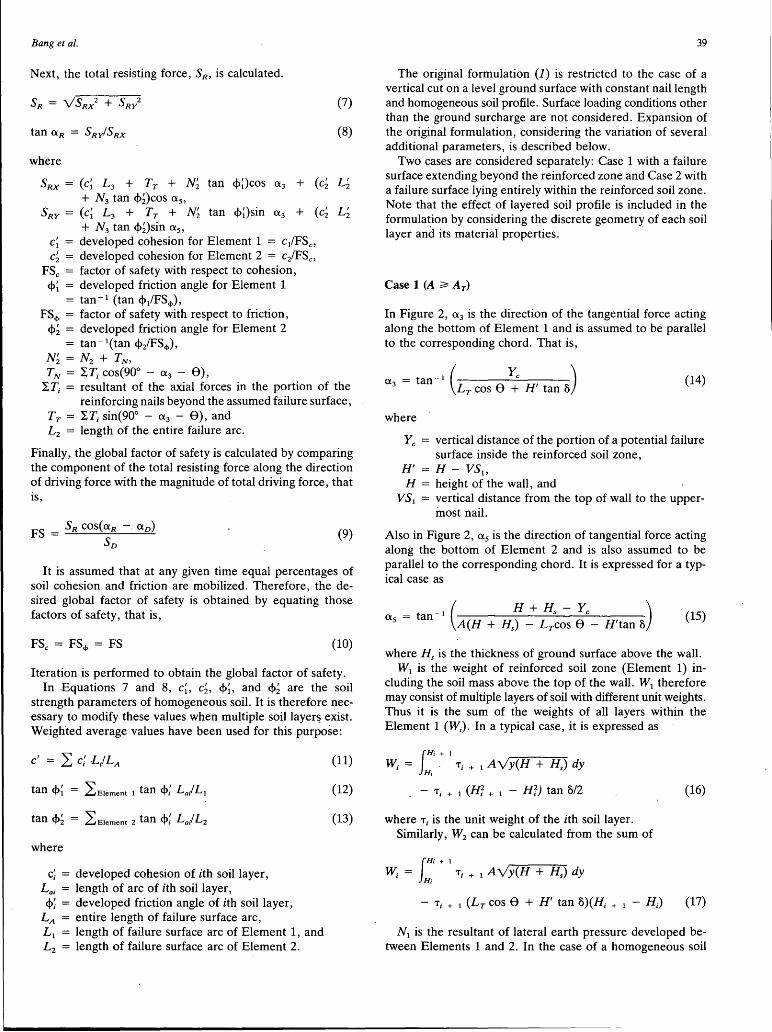
Bang et al.

Next, the total resisting force, SR, is calculated.

where

(7)

(8)

SRx = (c~ L 3 + Tr + N~ tan cf>~)cos 0'.3 + (c~ L~ + N 3 tan cf>~)cos 0'.5 ,

SRY = (c~ L 3 + Tr + N~ tan cf>~)sin 0'.3 + (c~ L~ + N3 tan cf>~)sin 0'.5 ,

c~ = developed cohesion for Element 1 = c/FS0

c~ = developed cohesion for Element 2 = cifFSe, FSe = factor of safety with respect to cohesion,

cf>~ = developed friction angle for Element 1 = tan - 1 (tan cf>/FS<I>),

FS<I> = factor of safety with respect to friction, ct>; = developed friction angle for Element 2

= tan- 1(tan cf>2/FS<1>), N; = N2 + TN, TN = "i.T; cos(90° - 0'.3 - 8),

!. T; = resultant of the axial forces in the portion of the reinforcing nails beyond the assumed failure surface,

Tr = "i.T; sin(90° - a 3 - 8), and L 2 = length of the entire failure arc.

Finally, the global factor of safety is calculated by comparing the component of the total resisting force along the direction of driving force with the magnitude of total driving force, that is,

FS = SR cos(O'.R -. O'.D) SD

(9)

It is assumed that at any given time equal percentages of soil cohesion and friction are mobilized. Therefore, the desired global factor of safety is obtained by equating those factors of safety, that is,

FSe = FS<I> = FS (10)

Iteration is performed to obtain the global factor of safety. In Equations 7 and 8, c~, c;, cf>~, and ct>; are the soil

strength parameters of homogeneous soil. It is therefore necessary to modify these values when multiple soil layer51 exist. Weighted average values have been used for this purpose:

where

c~ = developed cohesion of ith soil layer, L 0 ; = length of arc of ith soil layer,

cf>~ = developed friction angle of ith soil layer; LA = entire length of failure surface arc, L 1 = length of failure surface arc of Element 1, and L2 = length of failure surface arc of Element 2.

(11)

(12)

(13)

39

The original formulation (J) is restricted to the case of a vertical cut on a level ground surface with constant nail length and homogeneous soil profile. Surface loading conditions other than the ground surcharge are not considered. Expansion of the original formulation, considering the variation of several additional parameters, is described below.

Two cases are considered separately: Case 1 with a failure surface extending beyond the reinforced zone and Case 2 with a failure surface lying entirely within the reinforced soil zone. Note that the effect of layered soil profile is included in the formulation by considering the discrete geometry of each soil layer and its material properties.

Case 1 (A ~ Ar)

In Figure 2, 0'.3 is the direction of the tangential force acting along the bottom of Element 1 and is assumed to be parallel to the corresponding chord. That is,

( Ye ) O'. = tan- 1

3 Lr cos 8 + H' tan 8 (14)

where

Ye = vertical distance of the portion of a potential failure surface inside the reinforced soil zone,

H' = H - VS 1 ,

H = height of the wall, and VS1 = vertical distance from the top of wall to the upper

inost nail.

Also in Figure 2, 0'.5 is the direction of tangential force acting along the bottom of Element 2 and is also assumed to be parallel to the corresponding chord. It is expressed for a typical case as

_ 1 ( H + Hs - Ye ) O'. =tan 5 A(H + Hs) - Lrcos 8 - H'tan 8 . (15)

where Hs is the thickness of ground surface above the wall. W1 is the weight of reinforced soil zone (Element 1) in

cluding the soil mass above the top of the wall. W1 therefore may consist of multiple layers of soil with different unit weights. Thus it is the sum of the weights of all layers within the Element 1 (W;). In a typical case, it is expressed as

lHi +I

W; = H; · T; + 1 A y'y(H + Hs) dy

. - T; + 1 (ffl + 1 - Hf) tan 8/2 (16)

where T; is the unit weight of the ith soil layer. Similarly, W2 can be calculated from the sum of

lHi +I

W; = Hi T; + 1 Av'y(H + Hs) dy

- T; + 1 (Lr cos 8 + H' tan 8)(H; + 1 - H;) (17)

N 1 is the resultant of lateral earth pressure developed between Elements 1 and 2. In the case of a homogeneous soil

40

layer of height H, N1 is expressed as

(18)

where K is the lateral earth pressure coefficient. At-rest lateral earth pressure coefficient, K 0 , has been used

to describe the force N 1 •

For a multiple layered soil profile, soil layers that lie above the layer in question are represented by an equivalent surcharge load in calculating the resultant ·force. Term N 1 is therefore the sum of the resultant forces from each. layer:

(19)

where N; is the resultant of the ith layer.

The difference between Cases 1 and 2 is the expression of x-directional coordinate of the interface of Elements 1 and 2. In Case 1, the x-coordinate of the interface of Elements 1 and 2 is (Lr cos 8 + H' tan&), which is the x-coordinate of the end of the uppermost nail. But in Case ·2, the interface lies at the intersection between the failure surface and the uppermost nail. The x-coordinate of the intersection between the failure surface and the upper most nail, Xe, is expressed as

X< ~ 1/2[-A' (H + H,)tan e +

v'A 4 (H + H5 )2 tan2 0 + 4A2(H + Hs)H' (1 + tanStane)J (20)

Therefore, if (Lrcos 8 + H'tan &) is replaced by Xe in the solution of Case 1, the solution of Case 2 is obtained.

Calculation of Tensile Force in Nails

In this formulation, the developed nail force can be calculated in two ways. One approach assumes that the nail force is proportional to the overburden. However, because of possible soil arching, especially in dense cohesionless soils, the developed forces within the same length nails may remain more or less constant beyond a certain depth. For this reason, the analysis method allows an alternative method of estimating the nail ~xial force (i.e., by specifying the axial force per unit length. of the nail). Described below is the calculation of the nail axial force when it is proportional to the depth.

The frictional resistance of each reinforcing nail is expressed as

where

D = bore hole diameter, Le = effective length of the reinforcing nails,

tan <f>' = developed frictional coefficient,

(21)


crn = average normal stress, HS = horizontal spacing of the hails, and

c' = developed cohesion.

From the theory of elasticity,

<Tn = (cry cos2 8 - crx sin2 8)/(cos28

+ sin28 tan<f>') (22)

where

cry = overburden acting at the middle of the effective nail length,

crx = Kcry, 8 = nail inclination angle to the horizontal, and K = coefficient of lateral earth pressure.

Nail Length

The nail length can be described in several different ways. Two possible descriptions of nail length variation are considered in this formulation: linear variation and step variation. Figure 3 shows how these two descriptions can be applied.

In the case of linear variation of nail length (at depth of d;), L; is calculated by Equation 23 for Lr > L 8 and by Equation 24 for Lr< L 8 .

Hs

(a)

Hs

SET

(b)

FIGURE 3 Description of nail length: (a) linear variation, (b) step variation.

Bang et al.

where

Lr = length of the uppermost nail, L 8 = length of the lowermost nail, . Z 8 = depth to the lowermost nail from the top of panel

facing wall, vsl = depth to the uppermost nail from the top of panel

facing wall, and d; = depth to ith nail from the top of panel facing wall.

When step variation of nail length is used, the number of nail sets having the same length, the same number of nails in each set, and the nail length in each set are specified as part of the input.

Effective Length

Le is the effective length of the nail that lies beyond the assumed failure surface.

[x; - (H - d;)tan &]/cos 8 (25)

where

L; = length of the nail at depth of d;, d; = depth to ith nail from the top of panel facing wall, & = wall inclination angle to the vertical,

8 .= nail inclination angle to the horizontal, and X; = x-coordinate of intersection poi_nt between the ith nail

and failure surface 1/z {-A2(H + Hs)tan8 + [A 4 (H + Hs)2 tan28 + 4~2(H + Hs)(H - d;) (1 + tan 8 tan &)]112

}

Stress aY

Term aY is the resultant of overburden including the surcharge load acting at the middle length of Le. Actually, the stress is distributed along the entire effective length whose variation depends on the geometry of the ground surface and the surcharge load. However, aY is obtained from the sum of overburden due to all soil layers arid equivalent uniform surcharge load:

where

'T; = unit weight of ith soil layers, Z; = thickness of ith soil layers,

(26)

qe = transformed equivalent uniform surcharge load, and z; = distance measured from the ground surface to the

center of the contact length of ith nail.

Loading Conditions ..

It is assumed that the effect of vertical concentrated point loads is the same as increasing the weights of W1 and W2 with

41

increase in lateral stress calculated by Boussinesq's equation (9) of two-dimensional line load. The distributed surcharge increases the vertical stress as well as the lateral stress as defined by the lateral earth pressure coefficient. The effect of earthquake-induced loading is simulated by a pseudostatic analysis (i.e., by the equivalent horizontal acceleration coefficient).

S1)cos a 3 - (N1 + kh W1)sin a 3

S1)sin a 3 + (N1 + kh W1)cos a 3

N 3 (W2 + S1)cos as + (N1 - kh W2)sin as

S3 (W2 + S1)sin as - (N1 - kh W2)cos as

PARAMETRIC STUDY

(27)

The effects of reinforcing nail properties including the spacing, length, and inclination angle on the global stability are briefly discussed _below. Also included are the effects of panel facing wall inclination angle, layered soil profile, and pseudostatic earthquake load. Table 1 gives the variations of geometric and material parameters used in the parametric study.

Spacing and Length of Nails

The factor ·of safety decreases dramatically as the horizontal spacing of nails ii;icreases (Figure 4). When the nail length is 20 ft, which is relatively small compared with the height of panel facing wall (50 ft), the factors of safety are much lower than those calculated for longer nails. This is primarily because the contribution of shorter nails to the overall stability

TABLE 1 Geometric and Material Parameters Used

Height of the wall:

Facing wall inclination angle:

Diameter of the bore hole:

Diameter of the nails:

Spacing of the nails:

Length of the nails:

Yield strength of the nails:

Inclination angle of the nails:

Soil unit weight:

Soil frictio~- angle:

Soil cohesion:

Earthquake coefficient:

Slope of backfill surface:

Lateral earth pressure coefficient:

50 ft.

0 - 40° (0)

4 in.

1 in.

2 - 7 ft. (5)

20 - 60 ft. (40)

30 - 80 ksi (30)

0 - 40° (15)

100 - 125 pcf (100)

5 - 40° (30)

0.5 - 2 ksf (1)

0 - 0.6 (0)

oo

1 - sin¢

Numbers in parentheses are the standard values used

in the parametric study.

42

4.5

4.0 - L=20 FT

>- L=40 FT 1--w 3.5 L=60 FT LL <(

~ U)

3.0 LL 0

0::: 2.5 0 1-- 2.0 ~.~ u <( LL

1.5

1.0 2 3 4 5 6 7

NAIL SPACING (ft)

FIGURE 4 Effect of nail spacing~

is relatively small. When the nail length is 20 ft, slippage is the dominant failure mechanism, whereas breakage is dominant when the nail lengths are 40 ft and 60 ft. The curves become flatter as the spacing of nails incre.ases because the contribution of nail tensile forces to the global stability again becomes smaller.

Increasing the nail length is equivalent to increasing the contact length between the nails and the surrounding soil. This causes a direct increase in developed nail tensile force.' Figure 5 shows the effect of length of reinforcing nails to the overall factor of safety with various spacings of the nails. When the nail length changes from 20 ft to 60 ft, the factor of safety increases by 0.3 to 1.0. Because of the yielding of nails the factor of safety becomes constant with further increases in nail length assuming the cross section and strength of the nails remain the same.

Nail Inclination Angle

The effect of nail inclination angle is shown in Figure 6. The largest factor of safety occurs at a nail inclination angle of approximately 5 to 20 degrees regardless of the nail spacing. This finding confirms the previous result of the optimum nail

2.4

2.2 -S=4 FT

>- - S=S FT 1-- _..__ S=6 FT w 2.0 LL <( U)

1.8 LL 0

0::: 1.6 0 1--u <(

1.4 LL

1.2

1 . 0 L-~-___.L--L---'---'---.l..-~--20 25 30 35 40 45 50 55 60

NAIL LENGTH (ft)

FIGURE 5 Effect of nail length.


2.0

- L=40 FT

>- L=50 FT 1-- 1.9 L=60 FT w LL <( l/)

LL 1.8 0

0::: 0 1--u 1.7 <( LL

.6 0 5 10 15 20 25 30 35 40

NAIL INCLINATION (deg)

FIGURE 6 Effect of nail inclination angle.

inclination angle obtained by the writers that was based on simple analytical calculation (3).

Inclination Angle of Panel Facing Wall

Increasing the inclination angle of the panel facing wall corresponds to increasing the effective nail length of a given nail and to decreasing the driving forces. Therefore increasing the inclination angle results in increasing the factor of safety. As the panel facing wall inclination angle increases from 0 to 40 · degrees, the factor of safety increases almost linearly by approximately 85 percent regardless of the soil strength parameters (Figure 7).

Layered Soil Profile

It is assumed that the developed tensile force is proportional to the overburden, the shear strength of soil, and the contact length between the soil and the nails. Therefore, the tensile stress tends to become larger in nails loc~ted near the bottom of the excavation. This indirectly indicates that the stability of the reinforced soil is primarily influenced by the shear strength of the soil layer near the bottom of excavation rather than that near the top if nail force is proportional to the overburden (Figure 8).

>-1--. w LL <( U)

LL 0

0::: 0 1--u <( LL

3.0

2.8 - <!> =5 DEG. C=2000 PSF -.- <!> =40 DEG, C=500 PSF

2.6

2.4

2.2

2.0

1.8

1.6

1 . 4 L-~---'----'----'---'---.l..-__JL----' 0 5 1 0 1 5 2 0 2 5 30 35 40

WALL INCLINATION .(deg)

FIGURE 7 Effect of panel facing wall inclination.

Bang et al.

>-f-w LL <( tfl

LL 0

0::: 0 f-u <( LL

1.3

1.2 f =:= C1 = 500 PSF, C2 = 2000 PSF I C1 = 2000 PSF, C 1 = 500 PSF

1.1 ___-6--·---A---.a.---

1.0

0.9

0.8

~ -0.7 30 40 50 60 70 80

YEILD STRENGTH (ksi) C 1 = Cohesion of lower soil layer C2 = Cohesion of upper soil layer

FIGURE 8 Effect of layered soil profile.

>fw LL <( tfl

2.1

1.8

.5 ""-

- C= 1000 PSF C=2000 PSF

LL 0

0::: ~.

~. ~.

0 fu <(

.2

LL 0.9 ---------. -----. -----0.6 '--~-'-~~.L-~__J_~~-'--~-'-~--' 0.0 0.1 0.2 0.3 0.4 0.5 0.6

EARTHQUAKE COEFFICIENT

FIGURE 9 Effect of earthquake load.

Earthquake Load

Earthquake loads increase the driving force and reduce the resisting force simultaneously. Therefore the effect of earthquake loads is rather significant (Figure 9). As the horizontal coefficient of acceleration increases from 0 to 0.6, the factor of safety decreases by 50 percent.

CONCLUSIONS

This paper presents the limit equilibrium formulation for the design of a soil nailing system. It expands the original formulation by including the layered soil profile, variable nail length, inclined panel facing wall, random ground surface geometry, ground surcharge, and earthquake loading. The definitions of factor of safety, failure mechanism, and soilreinforcement interaction remain the same as in the previous formulation. The limiting equilibrium method of analysis is intended to estimate the overall stability of the soil nailing wall against sliding.

A preliminary parametric study to identify the effects of several design parameters on the overall stability has been carried out and the following conclusions have been reached:

43

1. The nail spacing and length have profound effects on global stability.

2. There is an optimum nail inclination angle, approximately 5 to 20 degrees to the horizontal.

3. The factor of safety is approximately linearly proportional to the inclination angle of the panel facing wall.

4. When the soil is layered, the stability of the soil nailing system is primarily influenced by the soil properties located near the bottom, assuming that the nail axial force is proportional to the overburden.

5. Earthquake loading has a rather significant effect. As the coefficient of horizontal acceleration increases from 0 to 0.6, the factor of safety decreases by as much as 50 percent.

Several recommendations for further study have been identified as a result of this study:

1. The effect of corrosion should be considered for longterm stability analysis.

2. Additional extensive parametric study considering much wider variation is necessary to obtain more detailed quantitative information regarding the effects of design parameters to the global stability of the soil nailing system.

3. The soil-nail interaction behavior needs to be studied in detail so that the correct stress transfer mechanism is modeled in the analysis.

4. The developed analytical formulation and its results need to be verified through detailed experimental scale model or field testing of the soil nailing system.

REFERENCES

1. C. K. Shen, L. R. Herrmann, K. M. Rornstad, S. Bang, Y. S. Kirn, and J. S. DeNatale. An In Situ Earth Reinforcement Lateral Support System. Report 81-03. University of California, Davis, 1981.

2. J. K. Mitchell. Reinforcement of Earth Slopes and Embankments. TRB, National Research Council, Washington, D.C., 1987.

3. S. Bang, C. K. Shen, and K. M. Rornstad. Analysis of an EarthReinforcing System for Deep Excavation. In Transportation Research Record 749, TRB, National Research Council, Washington, D.C., 1980.

4. C. K. Shen, S. Bang, and L. R. Herrmann. Ground Movement Analysis of an Earth Support System. ASCE, Vol. 107, GT12, Dec. 1981.

5. C. K. Shen, S. Bang, K. M. Rornstad, L. Kulchin, and J. S. DeNatale. Field Measurements of an Earth Support System. ASCE, Vol. 107, GT12, Dec. 1981.

6. C. K. Shen, Y. S. Kirn, S. Bang, and J. F. Mitchell. Centrifuge Modelling of Lateral Earth Support. ASCE, Vol. 108, GT9, 1982.

7. I. Juran, G. Baudrand, K. Farrag, and V. Elias. Kinematic Limit Analysis for Design of Soil-Nailed Structures. Journal of Geotechnical Engineering, Vol. 116, No. 1, Jan. 1990.

8. G. Gassler and C. Gudehus. Soil Nailing-Some Aspects of a New Technique. Proc., 10th International Conference on Soil Mechanics and Foundation Engineering, Vol. 3, Stockholm, Sweden, 1981.

9. B. M. Das. Principles of Geotechnical Engineering (2nd ed.). PWSKent, 1990.

Publication of this paper sponsored by Committee on Mechanics of Earth Masses and Layered Systems.


Field Experiments on Soils Reinforced with Multioriented Geosynthetic Inclusions

EVERT C. LAWTON AND NATHANIEL S. Fox

Results and· conclusions determined from field experiments performed to evaluate the practical aspects of reinforcing cohesionless soils with multioriented geosynthetic inclusions are described. The multioriented elements were generally similar in size and configuration to toy jacks. Experiments conducted included California bearing ratio, resistance to compaction, rutting, and trafficability tests. Substantial increases in stiffness and strength were obtained by reinforcing cohesionless soils with multioriented in· clusions. Multioriented elements also proved useful in reducing rutting and providing increased mobility and trafficability in soft and loose soils.

Results and conclusions from field experiments performed on comparable unreinforced and reinforced soils to evaluate the practical aspects of reinforcing cohesionless soils with multioriented inclusions are presented in this paper. The multioriented reinforcing elements were generally similar in shape and size to toy jacks. Comparable unreinforced and reinforced soils consisted of small-scale fills compacted with the same equipment and energy and with the same number and thickness of lifts.

The goals of this study were to determine the following characteristics of compacted and in situ soils reinforced with multioriented inclusions: improvement in bearing resistance, resistance to compaction caused by the reinforcement, effectiveness in increasing the trafficability characteristics of soft or loose soils, and usefulness in extricating vehicles immobilized in loose sand. The results from field experiments conducted to achieve these goals are presented in the following section. Further details can be found elsewhere (1).

FIELD EXPERIMENTS

Reinforcing Elements

The multioriented elements consisted of six stems emanating from a central hub, with an enlarged head attached to four of the six stems (Figure 1). Manufacturing limitations did not permit heads on the other two stems. These multioriented elements will be called "jacks" for brevity.

The jacks were cast in a specially designed, two-cavity injection mold. Two prototypes were manufactured using dif-

E. C. Lawton, Department of Civil Engineering, University of Utah, Salt Lake City, Utah 84112. N. S. Fox, GEOPIERS International Corporation, 4635 Riveredge Cove, Lithonia, Ga. 30058.

ferent polypropylenes-a homopolymer polypropylene 20 melt (Type 1 jack) and a copolymer polypropylene with 2.3 percent polyethylene (Type 2 jack). Typical properties indicated by the manufacturers are given in Table 1. On the basis of the given properties and posttesting viewing of jacks in the laboratory (2), Type 1 jacks were found to be stiffer, stronger, and more ductile in both bending and tension than Type 2 jacks. The surfaces of Type 1 jacks were somewhat rougher than the surfaces of Type 2 jacks, although the surfaces of both types of jacks were relatively smooth.

For comparative purposes, polypropylene fibers were used as reinforcement in CBR tests and resistance to compaction studies. These collated, fibrillated fibers were 0.5 in. long with a specific gravity of 0.91, a tensile modulus of elasticity of 500 ksi, and an effective diameter of approximately 0.006 in.

In the resistance to compaction and trafficability tests, biaxial polypropylene geogrid with nominal aperture dimensions of 1.0 by 1.3 in., a minimum open area of 70 percent, and a tensile modulus (Geosynthetics Research Institute GGl-87) of 14,000 lb/ft was also studied. A nonwoven geotextile was used in the trafficability tests.

Soils

The trafficability tests were performed on a dune sand (median size, D50 = 0.017 in.; uniformity coefficient, Cu = 1.8) near Albany, Georgia. All other field experiments were conducted at a site near Atlanta, Georgia, where the in situ oil was residual silty micaceous sand (D50 = 0.019 in.; Cu = 4.6). The Unified Soil Classification System designation for both soils is SP (poorly graded sand).

California Bearing Ratio Tests

The CBR test was chosen as the primary experimental method because it is essentially a small-scale bearing test, both stiffness and strength data can be obtained, and the reaction load required to perform the test is substantially less than that for the plate bearing test. Although it is recognized that there are scale effects related to the small piston diameter, which will be discussed in detail in a subsequent section, the qualitative relationships determined from comparisons between unreinforced and reinforced fills, as well as between different

Lawton and Fox

Note: All oliMensions o.re in inches.

114 ~

r- 3/16

.(b)

CD

' .......

351

FIGURE 1 Geometry and dimensions of multioriented inclusions: (a) plan view of four stems with heads; (b) plan view of two stems with heads and two stems without heads (rotated 90 degrees).

T 1

reinforced samples, provide useful information. Field CBR tests were performed on small-scale fills constructed using silty micaceous sand as the matrix soil. On the basis of previous laboratory results (2), a minimum of 200 jacks/ft2 per reinforcing layer was used in layered reinforced fills. Randomly reinforced soil was produced by mixing the jacks or fibers

45

with soil in a 4.0-ft3 concrete mixer. Both the jacks and the fibers mixed well with the soil using this method. The observation that the fibers mixed well with the soil was somewhat surprising in light of the difficulties in mixing fibers with soil described by others (3-5).

Two compactors were used to prepare the test pads for testing-a vibratory plate compactor and a pneumatic impact tamper. In most layered reinforced sections the jacks were placed on the surface of the previously compacted lift of unreinforced soil and the next layer of loose soil was placed before compaction. In some instances the jacks were "prestressed" by placing them loosely on the surface of the previously compacted soil lift and then pressing them partially into the underlying soil by one or two passes of the vibratory compactor before placing the next loose soil lift. The ascompacted thicknesses of the unreinforced and reinforced soil lifts (1.5 to 3.0 in.) were smaller than normally would be constructed in practice because of the low compactive effort of the compactors (compared with compaction rollers) and the small diameter (1.95 in.) of the CBR piston. That is, the

. depth of influence beneath a loaded area is typically between one and four times its diameter. Therefore, use of larger soil lifts in the layered reinforcement sections would have resulted in the reinforcement having little influence on the CBR results and would not have modeled typical bearing situations where ratios of bearing area width to lift thickness are generally greater than 0.5 and often much higher.

The CBR tests were conducted with the loading press attached to the frame of a 3.5-ton truck. In all tests the surcharge load (10 lb) and penetration rate (0.05 in./min) were the same.

Four test pads were constructed for the CBR tests as described in Table 2. The first two pads were constructed in mounds above the existing groqnd surface. Because of difficulties in controlling the lift thicknesses and widths when the fill was constructed in narrow mounds, the last two test pads were constructed in shallow excavated trenches. In each test pad separate sections were constructed in which the nominal thicknesses of the lifts were the same but reinforcement was varied.

Results

In general, only qualitative analyses of the stress-penetration results will be made in this section. CBR values for all tests can be found elsewhere (1 ) .

Two CBR tests were conducted in each section of Test Pads 1 and 2 to determine the reproducibility of results. The stress-

TABLE 1 Typical Properties of Materials Used in Manufacturing Specially Designed Multioriented Inclusions

Property

Specific Gravity Melt Flow Rate (g/10 min.) Tensile Strength at Yield (ksi) Elongation at Yield (%) Flexural Modulus (ksi) Notched Izod Impact Strength

at 23° c (ft-lb/in.)

Inclusion Designation

Type 1

0.903 18.0 5.050 11 250

0.7

Type 2

0.902 19.5 3.050 10 155

2.0


TABLE 2 Details of Test Pads for CBR Testing: (a) Dimensions; (b) Compaction and Reinforcement

(a)

Test Pad

1 2 3 4

Fill Type

Mound Mound Trench Trench

Sections

No.

2 2 5 6

Width (in.)

16 16 18 18

Length (ft)

3 3 2 2

Soil Lifts

No.

3 3 3 2

As-compacted Thicknessesa

2.0, 1.5, 1.5 2.0, 1.5, 1.5 2.0, 1.5, 1.5 3 .o, 3. 0

ain order of construction (bottom-first, top-last)

(b)

Test Sec-Pad tion Methodb Energyc

Heavy 7 passes 3 passes 7 pai;;ses 7 passes 7 passes 7 passes 7 passes 7 pass_gs 1 passh 1 pass

Type 1 Type 1 None None None Fibers Type 1 Type 1 Type 2 Fibers Type 1 None

Orientation

Layered Layered

Layered Layeredg Layeredg Layeredg Random Random

Locatione

1. 5, 3. o in. 1. 5, 3. o in.

1. 5, 3. o in. 1. 5, 3. o in. 1. 5, 3. o in. 1. 5, 3. o in. Top lift Top lift

Amountf

200 jsf 200 jsf

.375 psf 200 jsf 300 jsf 200 jsf VF=3.6% VF=4.1%

1 1 2 2 3 3 3 3 3 4 4 4 4 4 4

A B A B A B c D E A B c D E F

P.I.T. V.P.C. V.P.C. V.P.C. V.P.C. V.P.C. V.P.C. V.P.C. V.P.C. V.P.C. V.P.C. V.P.C. V.P.C. P.I.T. P.I.T.

1 pass~ 1 pas~ Hea~ Heavy--

Type 2 , Layered Type 2 Random None

Surf ace Top lift

500 jsf VF=4.1%

bP.I.T. pneumatic impact tamper; V.P.C. = vibratory plate compactor ~Number of passes listed are per lift

Types 1 and 2 refer to jacks ~Values for layered reinforcement refer to depths below top surface Jsf = jacks per square foot; psf = pounds per square foot;

VF = volume fraction = volume of reinforcement / total volume gEach layer prestressed by two passes of V.P.C. hBottom lift was unreinforced and was compacted by 7 passes of V.P.C.; values given are for top lift

penetration curves for each original test and its repeat test are similar (Figure 2). For the two sections in Test Pad 1 reinforced with layered jacks, a comparison of the stresspenetration curves suggests that a stronger reinforced soil was produced by using the impact tamper than by using the vibratory plate. This is also indicated by the soil dry densities (excluding the volume and weight of the reinforcement) calculated from samples taken from the two sections-103.5 pcf at a water content (w) of 10.3 percent for heavy compaction from the impact tamper and 96.4 pcf at w = 10.6 percent for seven passes of the vibratory plate. The stiffnesses of the two reinforced soils were approximately the same. Most of the . subsequent sections were compacted with the vibratory plate because of the greater ease in controlling and identifying the · compactive effort.

Increasing the number of passes per lift from three to seven produced a stronger and stiffer unreinforced soil (Figure 2). This is expected and is attributable to the higher dry density produced by greater compactive effort (102.0 pcf for seven passes and 100.4 pcf for three passes). A comparison of the reinforced and unreinforced curves for the soil compacted with seven passes of the plate shows a substantial improvement in strength and greater stiffness for the reinforced soil

at penetrations greater than about 0.1 in., and approximately the same stiffness at lower penetrations.

In Test Pad 3, reinforcement was placed in layers, and layers of jacks were prestressed before placing the next lift of soil. During repetitive passes of the compactor in the fiberreinforced section, fibers migrated upward through the soil lift and created spalling along the surface of the soil lift. It can be seen in Figure 3 that the addition of jacks strengthened and stiffened the soil. The fiber-reinforced soil, however, was less stiff than the unreinforced soil at low penetrations ( < 0.23 in.), but stiffer at higher penetrations. The fiberreinforced soil appears to have been strongest, although the test on it was not completed because of equipment problems.

Increasing the areal density of Type 1 jacks from 200/ft2 to 300/ft2 produced a considerable increase in strength, but the stiffness at low penetrations was decreased because of rearrangement of the jacks within the reinforcement layer during loading .. This loss of stiffness was minimized, however, by prestressing the jacks before placement of the next soil lift. The soil reinforced with Type 2 jacks was stronger than the soil reinforced with Type 1 jacks at the same areal density of 200/ft2 • This result contrasts with that demonstrated in the laboratory CBR experiments for nonprestressed jacks and

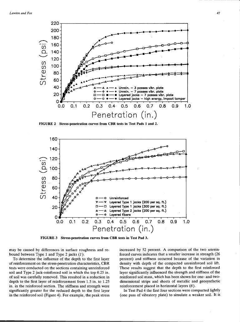
Lawton and Fox

220

200

180 ~

Cf) 160

Q_ 140 ""--"

120 Cf)

100 Cf)

Q) 80 L

+-' 60 Cf)

40

20

0 0.0

.......... .- -·-·-·-·-·-·-··-·-·-·-· /o...-o-o -o--D

/

,,...- ..._a--a--0 ·-·-_,.,_-0__...--o--u- --·-·-·-~ ·-·-·

CY _ri--c -·-·-·-,._/a-;_.-• .P1ou • ...-

•/ ~__.__._._._.__._._._.

•o-~::::::~::::;;·-- .... '

'$•.,.,.,... A-A-A-A-• ¥ . -·-•-4-•-6=11'-&-•-&-. ·-·-· 6-6-

-·-·- _6_6_ ......... -6-6

...... 6-6-6 •

6...-6...- 6 - 6 • - • Unrein. - 3 passes vibr. plate

6 6 O - o • - • Unrein. - 7 passes vibr. plate o - o • - • Layered jacks - 7 passes vibr. plate o - o • - • Layered jacks - high energy, impact tamper

0.1 0.2 0.3 0.4 0.5 0.6 0.7 0.8 0.9 1.0

Penetration (in.) FIGURE 2 Stress-penetration curves from CBR tests in Test Pads 1 and 2.

160

140

~ 120 (/)

o.._ 100 "'-.-/

(/) 80 (/) Q) 60 L

-+-' (f) 40

20

o-o v-v 0-0

Unreinforced Layered Type 1 jacks (200 per sq. ft.) Layered Type 1 jacks (300 per sq. ft.)

6 - 6 Layered Type 2 jacks (200 per sq. ft.) <> - <> Layered fibers

0----.---.,.--.---.---.--..---.---...--.--.-----.--------------.....-----1

0.0 0.1 0.2 0.3 0.4 0.5 0.6 0.7 0.8 0.9 1.0

Penetration (in.) FIGURE 3 Stress-penetration curves from CBR tests in Test Pad 3.

47

may be caused by differences in surface roughness and rebound between Type 1 and Type 2 jacks (1 ).

To determine the influence of the depth to the first layer of reinforcement on the stress-penetration characteristics, CBR tests were conducted on the sections containing unreinforced soil and Type 2 jack-reinforced soil in which the top 0.25 in. of soil was carefully removed. This resulted in a reduction in depth to the first layer of reinforcement from 1.5 in. to 1.25 in. in the reinforced section. The stiffness and strength were significantly greater for the reduced depth to the first layer in the reinforced soil (Figure 4). For example, the peak stress

increased by 52 percent. A comparison of the two unreinforced curves indicates that a smaller increase in strength (26 percent) and stiffness occurred because of the variation in density with depth of the compacted unreinforced soil lift. These results suggest that the depth to the first reinforced layer significantly influenced the strength and stiffness of the reinforced soil mass, which has been shown for one- and twodimensional strips and sheets of metallic and geosynthetic reinforcement placed in horizontal layers (6).

In Test Pad 4 the first four sections were compacted lightly (one pass of vibratory plate) to simulate a weaker soil. It is

48

220

200

180 ,,--....

160 (/) Q_ 140

'--' 120 (/) (/) 100 Q) 80 L

+J 60. (f)

40

0.1 0.2 0.3 0.4 0.5 0.6

Penetration


0.7 0.8 0.9 1.0

(in.) FIGURE 4 Stress-penetration curves from CBR tests in Test Pad 3 for varying depth to first layer of reinforcement.

clear in Figure 5 that the inclusion of layered and random jacks substantially increased both the stiffness and strength of the reinforced soil compared with the unreinforced soil. The jacks placed on the surface of the compacted soil and then prestressed produced a significantly greater strength and stiffness increase than the random jacks. The fiber-reinforced soil was less stiff than the unreinforced soil at low penetrations ( < 0.08 in.), but stiffer at higher penetrations. The peak stress for the fiber-reinforced soil was approximately the same as for the soil with layered jacks on the surface, but the jackreinforced soil was stiffer at low penetrations.

It can be seen in Figure 6 that the randomly reinforced jack soil compacted heavily with the impact tamper had a substantially higher peak stress than the unreinforced soil but was slightly more compressible at low penetrations ( < 0.15 in.). ·

Resistance to Compaction Tests

To assess the resistance to compaction provided by various types of reinforcement, additional experiments were con-

180

~ 160

Cf) 140

o - o Unreinforced 6 -· 6 Layered Type 2 jacks (500 per sq. ft. on surface; prestressed) v - v Random Type 1 jacks (Volume Fraction == 4.1 X) <> -· <> Random Fibers (Vol. Fraction = 3.6X) /<>-<>

6.,,,-6 /<>

3120

Cf) 100 Cf)

,4/ / f o-<> v-v-v-v-

6 / v-v ........

60

I <> v..,.,.... 6

6 / ~v-v/ , <> v-

6 / v ........ I v,.,,,-l _...e$-V./' -o-O_o--0

6 v-8 _o-o--<> 40 / vvvv <>/ -o-<>-o

6 vv 0 <> -o-o-0 20 vv 88000-0-

0

(]) 80 L

+-' (f)

~eeoe o---.----~...--.---.~...--.---.~...--.---.~------...~ ........ ---...~..------1

0.0 0.1 0.2 0.3 0.4 0.5 0.6

Penetration 0.7

(in.) 0.8 0.9 1.0

FIGURES Stress-penetration curves from CBR tests in Test Pad 4 (vibratory compaction).

Lawton and Fox 49

• - • Unreinforced

300- • - • Random Type 2 jacks (Volume Fraction = 4.1 ~) .._/ ·-·-·~ /·-·-..,,,,,,,..-· ·-· .._/ .,,,,,,,,..

.,,,,,,,,..

~

• UJ 250-o_

..,,,,,,,,,.. / •-·-•-o . ·-·-·-

.........._,, 200-

UJ UJ 150-Q)

/ ·-·-. ·-·-·-L

-+-' 100-(f) .f·

.t 50~ .f•'

t{.&'

0 f

/ .,.,..-·-. ·-· .. .,.,. •••

0.0 0.1 0.2 0.3 0.4 0.5 0.6 0.7 0.8 0.9 1.0

Penetration (in.) FIGURE 6 Stress-penetration curves from CBR tests in Test Pad 4 (impact compaction).

ducted at the same site. A test pad 18 in. wide by 6 in. deep by 15 ft long was constructed in an excavated trench in two 3.0-in.-thick lifts. The bottom lift was unreinforced and was compacted by seven passes of the vibratory plate. The top lift was divided into fifteen 1.0-ft.-long sections. The first five sections consisted of (a) unreinforced soil, (b) one layer of 570 jacks covering the entire area (380 jacks/ft2) at a depth of 3.0 in., (c) 600 random jacks within the matrix soil (volume fraction = 10.1 percent), (d) 0.68 lb of random fibers within the matrix soil (volume fraction = 3.2 percent), and (e) geogrid placed at a depth of 3.0 in. These five sections were repeated two more times. The first five sections were com-

110 0-0 Unreinforced ,,..........

105 '-I-- - A-A Layered Jacks u 0-O Random Jacks

3100 -""'O ('.. 95

JI JI--------0

0 ~ 90 +J 0--..._

0 Ul c 85 Cl)

- A A .

0 80 . -

c 75 0 ------<> - <>

70 I

pacted by 1 pass of the vibratory plate, the second five sections by 5 passes, and the third five sections by 15 passes. In the layered jack sections, the jacks were not prestressed before placing the loose soil for the top lift.

The average soil dry density of each section determined from two dfive tube samples (ASTM D-2937) are plotted in Figure 7 as a function of the number of passes of the vibratory plate compactor. The soil dry density should have increased with the number of passes, but only three of the five curves meet this expectation. This apparent inconsistency was caused by elements extending outside the sample tube, which made trimming the samples difficult and required an estimation of

<>- <> Random Fibers JI-JI Geogrid

n .. I'

: ]

I

0 5 10 15

Number of Passes of Vibratory Plate FIGURE 7 Results from resistance to compaction tests.

50

the volume of partial elements extending outside the tube. However, the general trend of resistance to compaction developed by each reinforced method can be seen in Figure 7. The random fibers, even though placed in a much smaller volume than the jacks, created the greatest resistance to compaction, followed in descending order by layered jacks and random jacks. Layered jacks resisted compaction more than random jacks as a result of rebound of the layered jacks upon removal of the compactive energy and little interaction between random jacks and soil because of the smooth surface of the jacks. The geogrid improved compaction of the soil primarily by vertical confinement, thereby increasing the soil dry density above that for the unreinforced soil. The average percent difference in the reinforced soil dry density compared with the unreinforced soil dry density was - 21 percent for random fibers, -10 percent for layered jacks, - 6 percent for random jacks, and + 3 percent for geogrid.

Rutting Tests

Following an intensive rainfall, the effectiveness of using jacks to support construction traffic in wet soil conditions was evaluated. A particularly soft and wet location on the site was selected for testing. First, an area approximately 3 ft wide by 10 ft long was raked to a depth of 6 in. to homogenize the wet soil. Two pads of Type 1 jacks, each pad containing 900 jacks in an area 18 in. square (400 jacks/ft2), were then placed on the surface of the prepared area approximately 7 ft apart. One of the jack pads was tamped lightly to prestress the jacks. The area between the pads remained unreinforced. A 3.5-ton truck was driven across the prepared area through the center of the pads for a total of 10 passes.

The depths of ruts created in the two reinforced pads and in the unreinforced area were measured at the deepest part for 1, 2, and 10 passes of the truck. Because the top surfaces of the pads were uneven, a range in depth of rutting was measured for the jack pads.

The results of the rutting tests, which are summarized in Table 3, clearly indicate that the jacks substantially reduced the depth of rutting compared with the unreinforced soil. For example, compared with the unreinforced soil, the loosely placed jacks reduced the maximum depth of rutting for one pass of the truck from 2.2 in. to 0.6 to 0.8 in., a reduction of 64 to 73 percent. The tamped jacks reduced the depth of rutting for one pass by 82 to 91 percent. For 10 passes of the truck, the maximum depth of rutting was reduced by 51 to 57 percent for the loosely placed jacks and 75 to 80 percent for the tamped jacks.

TABLE 3 Results of Rutting Tests

Maximum Depth of Rut (in.)

Loosely Lightly No. of Placed Tamped Passes Unrein- Type 1 Type 1 of Truck forced Jacks Jacks

1 2.2 0.6 - 0.8 0.2 - 0.4 2 3.0 0.8 - 1.0 0.3 - 0.5 10 3.5 1.5 - 1. 7 0.7 - 0.9


Trafficability Tests in Dune Sand

The use of jacks to support vehicles and extricate immobilized vehicles in loose uniform sands was evaluated at a natural sand dune area in Albany, Georgia. This area of deep aeolian sands is well known to local developers and citizens as an area that will not support vehicles or structures and that cannot be adequately densified by normal compaction methods. Several tests were performed and are described below.

Extrication of Immobilized Vehicle

A jeep-type vehicle was driven off the paved roadway into an area of especially loose sand and became immobilized several times, sinking to depths ranging from 8 to 20 in. At a depth of 8 in., a pad of jacks with an average thickness equal to two elements was placed behind the traction wheels, and the vehicle was put into reverse and easily became dislodged.

Extrication of the vehicle for an embedded depth of 18 in. was much more difficult. Only after placing pads of jacks behind and in front of each traction wheel, and rocking the vehicle back and forth, did the vehicle become dislodged. Several schemes for extricating the vehicle were attempted for an embedment depth of 20 in., including increasing the thickness of the jack pads and using geogrid in place of the jacks, with no success. The vehicle had to be removed by chain and hoist.

Trafficability Tests

Trafficability tests were conducted in an area where the vehicle was not immobilized but was making ruts averaging 4. 75 in. deep in the unstabilized sand. A variety of stabilizing methods were studied using jacks, geotextile, geogrid, and combinations thereof. The methods used and the results obtained are summarized in Table 4.

For the various methods in which the reinforcing elements were placed on the surface of the in situ sand, a composite system composed of layered jacks on top of geogrid proved the best in terms of both initial rutting and repetitive loading. In this synergistic composite system, the jacks anchored the geogrid, preventing it from being displaced, while the geogrid anchored the jacks by resisting longitudinal, lateral, and downward movements of the jacks during loading. Layered jacks by themselves were moderately successful in reducing rutting and improving trafficability under repeated loads. When placed on the surface, neither geogrid nor geotextile was effective in reducing rutting. This ineffectiveness was caused by sliding of the material along the ground surface during loading because of lack of confinement.

In tests where the reinforcement was buried beneath a thin (1 to 2 in.) layer of sand, two systems were best for reducing initial rutting-geotextile alone and composite geogrid/jacks. Under repetitive loads, the composite geogrid/jacks system was somewhat better in providing firm and stable support: The addition of jacks beneath the geotextile produced no additional support beyond that provided by the geotextile alone. In all instances, burying the reinforcement beneath a

Lawton and Fox

TABLE 4 Details and Results from Trafficability Tests

Reinforcement

Orien-Test Type tat ion Location

1 None

Amount

Depth of Initial Rutting (in.)

4.75

51

Comments

Loose dune sand

2 Jacks Layered Surface 2 elements thick

3.0 Jacks were displaced longitudinally and laterally

3 Jacks Layered Surface 3 elements thick

3.5 Jacks were displaced longitudinally and laterally

4 Jacks Layered 2 in. deep trench; 3 elements 1-2 in. sand cover thick

2.75 Firmer than jacks on surface

5 Geotextile Horiz. Surface 1 sheet 4.75 Geotextile was pushed and displaced by wheels

6 Geotextile Horiz. Surface; 1-2 in. 1 sheet 1. 0 Good performance under repeated loads sand cover

7 Geogrid Horiz. surface 1 strip 4.75 Geogrid slid on surface as vehicle moved over it

8 Geogrid Horiz. Surface; 1-2 in. 1 strip 2.5 Fair performance under repeated loads sand cover

9 Jacks/ geotextile

Layered/ Horiz.

Jacks on surface; 2 ele. thk. 3.0 No improvement over jacks alone (Test 3) geotextile on jacks 1 sheet

10 Jacks/ geotextile

Layered/ Horiz.

Same as 9 except 2 ele. thk. 1. 0 No improvement over buried geotextile alone (Test 6) 1-2 in. sand cover 1 sheet

11 Geogrid/ jacks

Horiz./ Layered

Geogrid on surface 1 strip 2.25 Very good performance under repeated loads Jacks on geogrid 2 ele. thk.

12 Geogrid/ jacks

Horiz./ Layered

Same as 11 except 1 strip 1. 0 Excellent (best) performance under repeated loads 1-2 in. sand cover. 2 ele. thk.

thin layer of sand produced better stabilization compared with the same reinforcement placed on the surface. This result is attributable to the confinement provided by the overburden.

OTHER CONSIDERATIONS

Scale Effects

Because the CBR tests were not full-scale tests, some scale effects must be considered in evaluating the obtained results. The primary problems related to scale effects concern the small diameter of the CBR piston (1. 95 in.) relative to (a) the size of the jacks (= 1.0 in.), (b) the depth to the first layer of reinforcement, and ( c) typical widths of actual bearing areas (e.g., approximately 1 to 2 ft for wheel loads and ;;:::: 3 ft for footings). Regarding the size of the jacks, typical rules dictate that the diameter of the piston should have been more than six times the largest particle size, rather than twice the size as in these CBR tests.

Whether the use of CBR tests to determine stress-: penetration characteristics overestimates or underestimates the improvement obtained from the incorporation of jacks on or within the soil is not readily apparent, and is clearly a function of many parameters. These parameters include the width of the bearing area, the magnitude of the applied load, the amount and orientation of the reinforcement (layered or random jacks in this case), and the depth to the first layer of reinforcement.

For random jacks, the location of the piston relative to the locations of the adjacent jacks would probably affect the stresspenetration results. For example, the results would probably be different if the piston were placed directly over a jack near the surface than if it were placed between jacks that were located at some depth in the layer. The results for either condition would vary from the "average" results of all possible conditions. An estimate of the degree of variation of the results could have been obtained from multiple testing in each test pad section. This was not done in this study because of time and budgetary restrictions. However, the fact that improvements in both stiffness and strength were noted in all three instances where tests were conducted on soils containing random jacks suggests that some improvement was obtained by including the jacks.

For CBR tests conducted on soils containing layered jacks, the effect of the small piston diameter to element width ratio was prob~bly less pronounced. For the five test sections in which the first layer was located at a depth of 1.5 in., the diameter of the zone of influence would have been approximately 3.5 in. (assuming an approximate 2:1 stress distribution with depth), which would have involved the interaction of at least 10 jacks in the upper portion of the reinforcement layer (assuming each jack occupies an area of 1 in.2, which is an overestimate because of overlapping among the jacks). Because the reinforcing effect in layered jacks is derived from a combination of bearing resistance as the lower jacks are pushed into the soil, interlocking among adjacent jacks, and

52

confinement of the soil above the first layer, the results for similar stress conditions under a larger loaded area would probably be at least qualitatively comparable to those obtained in these tests.·

The scale effect caused by the small diameter of the piston compared with practical load-bearing areas is a more difficult issue to address. Even in homogeneous sand, the relationship between stiffness and width of loaded area is not clear-cut. This was demonstrated by Kogler (7), who studied the relationship between width of square footing and settlement under the same applied stress and found that settlement was a minimum for a width (B) of about 0.7 ft, increased rapidly with decreasing width below 0. 7 ft, and increased gradually with increasing B above 0. 7 ft. This unusual relationship is related to two contrasting components of settlement: (a) compression beneath the central portion of the footing, which approximates one-dimensional compression and is essentially independent of the horizontal pressures, and (b) lateral yielding near the edge of the loaded area, which depends significantly on the confining pressure. As the width of the loaded area increases, the percentage of the loaded area beneath which compression occurs increases, resulting in a tendency

· toward decreased stiffness. However, the depth of influence and the average confining pressure also increase with increasing B, resulting in a tendency toward increased stiffness. Kogler's results suggest that CBR tests in sands substantially underestimate the stiffness of the soil for most practical bearing widths. Similar analyses indicate that peak strength is also underestimated in the CBR test.

In soils with randomly oriented jacks, the CBR test probably underestimates the stiffness in a magnitude comparable to that for unreinforced sands. The jacks are relatively rigid structural elements that increase the stiffness by bearing against soil in the direction of deformation. This passive resistance is greater than that developed by the soil alone in shearing resistance. The overall result is increased stiffness regardless of the mechanism of deformation (vertical compression or lateral yielding).

The results from CBR tests in soils with layered jacks also are likely to underestimate the stiffness and strength of these composite soils. Layered jacks reinforce the soil primarily by reducing compression in the vertical direction (via bearing and interlocking as described previously) and secondarily by limiting lateral yielding via the undulating surface of the jack layer. With increasing bearing width, a greater percentage of settlement occurs as vertical compression, so layered jacks should be stiffer for practical bearing widths than for the CBR piston under comparable conditions. The ratio of the bearing width to the depth of the first layer of reinforcement is also a critical factor, as has been shown in research on horizontal continuous reinforcement (6).

In summary, it appears that the CBR tests underestimate the stiffness and strength of both unreinforced and jackreinforced soils compared with practical bearing conditions. Although a complex theoretical analysis can be undertaken, the relative magnitudes of the underestimation can only be ascertained by conducting field experiments at full-scale bearing widths. Because this was not feasible in this research program, only qualitative comparisons can be made. It appears, however, that the qualitative comparisons are useful despite the inherent scale effects.


Cost and Practicability

The usefulness of any technology depends not only on its technical feasibility but also on its affordability. It is difficult to assess the affordability of this technology at the present early stage of development. Only two prototypical jacks have been manufactured to date-both essentially the same except for their material properties. Because of manufacturing difficulties and funding limitations, the jacks used in this study were deficient in many respects from the initial design prepared by the authors. Desired characteristics not incorporated

.. by the initial prototypes include thinner stems for a more efficient element (same reinforcing capability at a lower volume), rougher surfaces to promote greater soil-jack interaction, heads on all six stems to produce greater interlocking, and stronger and stiffer geosynthetic materials.

The total cost per jack (excluding the cost of manufacturing the injection mold) in this study was approximately $0.18. This high unit cost was caused by the low volume of jacks manufactured (6,000) and the small injection mold, which only produced two jacks at a time. At these unit costs, jacks are obviously not competitive with alternate reinforcing methods or select sand and gravel. However, with a full production injection mold, it is estimated that the unit cost of the jacks could be reduced to about $0.001 to $0.005. At this cost the jacks could be competitive in certain situations. Alternative methods for manufacturing the jacks more economically may be feasible and should be investigated. At this stage of development it is impossible to estimate the in-place cost of the jack-reinforced systems because additional research is needed to further refine the product and determine its applications and limitations. Methods for large-scale mixing and placement of jacks also need to be identified and developed. Other characteristics of the jacks that need to be evaluated in terms of their influence on effectiveness of jacks as reinforcement include overall size and configuration, size and shape of heads and stems, and material properties in terms of durabil~ty and strength. Full-scale field tests in all anticipated applications must be conducted to assess the effectiveness and affordability of jacks.

SUMMARY AND CONCLUSIONS

In this i~itial field study of a new technology, the primary objective was to determine the technical feasibility of improving the engineering characteristics of cohesionless soils by incorporating multioriented reinforcing elements (jacks) on or within in situ or fill soils. CBR, resistance to compaction, rutting, and trafficability tests were conducted. The following general results and conclusions were determined:

1. Results from CBR tests indicate that for the same method of compaction and compactive effort, the inclusion of jacks in either layered or random orientation generally improved the strength and stiffness of the soil.

2. Random fibers created the greatest resistance to compaction, followed in descending order by layered jacks and random jacks. Geogrid improved compaction by confining the soil.

Lawton and Fox

3. Jacks placed on the surface of a wet silty sand reduced the rutting deformations for both single and multiple passes of a truck.

4. Jacks were used in a dune sand to reduce rutting substantially and to extricate vehicles that had become immobilized by placing jacks in pads behind or in front of the embedded wheels. Rutting deformations were significantly reduced by placing a thin layer of sand on top of the layered jacks rather than having the jack~ exposed. The most effective means of stabilizing the sand for repetitive vehicular traffic was a composite system· wherein layered jacks were placed on geogrid.

5. In general, ultimate strength increases produced by fiberreinforced soils were comparable with those developed for jack-reinforced soils. However, considerably greater deformation was required to mobilize the reinforcing effect in fiberreinforced soils, suggesting that fiber-reinforced soils may be less suitable for situations where settlement or deformation of the soil controls the design. The stiffness of fiber-reinforced soils under low stresses was typically less than the comparable unreinforced soil, whereas layered jack-reinforced soils were generally stiffer than the unreinforced soil under all stress levels tested.

Although the results from this preliminary small-scale field study suggest that multioriented inclusions may have several potential uses, additional research and development is neededparticularly full-scale field tests associated with potential applications-before this technology can be considered practicable for commercial usage!

53

ACKNOWLEDGMENTS

This research was funded by a Phase I Small Business Innovative Research grant from the National Science Foundation.

REFERENCES

1. N. S. Fox and E. C. Lawton. Cohesionless Soil and Small Discontinuous Reinforcing Elements in Composite Engineering Material. Final Report. National Science Foundation, Dec. 1990, 130 pp.

2. E. C. Lawton, M. V. Khire, and N. S. Fox. Reinforcement of Soils by Discontinuous Multi-Oriented Geosynthetic Inclusions. Journal of Geotechnical Engineering, ASCE, Vol. 118, Nq. 9, Sept. 1992.

3. D. R. Freitag. Soil Randomly Reinforced with Fibers. Journal of Geotechnical Engineering, ASCE, Vol. 112, No. 8, Aug. 1986, pp. 823-826.

4. D. H. Gray and T. Al-Refeai. Behavior of Fabric Versus FiberReinforced Sand. Journal of Geotechnical Engineering, ASCE, Vol. 112, No. 8, Aug. 1986, pp. 804-820.

5. J. M. Hoover et al. Performance of Randomly Oriented, FiberReinforced Roadway Soils: A Laboratory and Field Investigation. Final Report. Iowa DOT Project HR-211, Dec. 1982, 306 pp.

6. J. Binquet and K. L. Lee. Bearing Capacity Tests on Reinforced Earth Slabs. Journal of the Geotechnical Engineering Division, ASCE, Vol. 101, No. 12, Dec. 1975, pp. 1241-1255.

7. F. Kogler. Discussion: Soil Mechanics Research. Transactions, ASCE, Vol. 98, 1933, pp. 299-301.

Publication of this paper sponsored by Committee on Geosynthetics.


Geogrids as a Rehabilitation Remedy for Asphaltic Concrete Pavements

MALCOLM L. STEINBERG

Rutting and shoving of asphaltic concrete pavements extend from streets in front of the White House across the country. Frequent practice has been to remove and ~epl~ce the paveme~t. Rotomilling the displaced material, relaymg it, and overlaymg the lanes is another remedy. On multilane highways, overlaying both lanes with asphaltic concrete is frequently done. Studies have indicated that the outside lanes receive several more equivalent axle loads than the inside lanes. This is reflected by their increas~d distress and rutting. The Texas State Department of Highways and Public Transportation's El Paso District is testing a different solution. The outside lane was provided with additional reinforcement using geogrids on a rehabilitation project on Interstate Highway 10. Sections received various quantities of asphaltic concrete overlays. The rotomilled geogrid sections failed. The other sections including another geogrid are serving well.

Rutting and shoving of asphalt concrete pavements extend from the streets in front of the White House across the country. Frequent practice has been to remove and replace the offending pavement. Rotomilling the displaced material, relaying it, and overlaying the lanes with more asphaltic concrete is another remedy. Common practice on multilane highways is to overlay the lanes with another course of asphaltic concrete. Recent studies on the Interstate system indicated that the outside lanes received two to six times the single-axle equivalent loads as the inside ones; yet rehabilitation projects often add another course of asphaltic concrete to both lanes. The Texas State Department of Highways and Public Transportation (SDHPT) El Paso District 24 sought another solution. The first step was a literature search.

LITERATURE SEARCH

Reinforcement of flexible pavement structures using various material has existed for many years. In the 1930s cotton was used. Later, the material of choice was reinforcing steel. In 1980 with the introduction of a new type of high-strength polymer geogrid known as Tensar, another option became available. In 1983, Halim et al. (1) presented results of cooperative laboratory testing by Canada's Royal Military College, the Ontario Ministry of Transportation, and Waterloo University. They concluded that substantial savings of asphalt paving thickness, double the number of load repetitions to failure, plus fatigue cracking reduction could be achieved using the geogrid.

Kennepohl and Kamel (2) reviewed the many attempts to

Texas Department of Transportation, P.O. Box 102~8, El Paso, Tex. 79994-0278. Current affiliation: Steinberg and Associates, 1201 Prospect Street, El Paso, Tex. 79902.

reinforce asphaltic concrete. Efforts to increase longevity and satisfactory performance were suffering from asphalt's lower ultimate tensile strengths compared with its compressive strengths. Reinforcement is desired to increase the tensile strength, provide longer fatigue life, and reduce material cost. The geogrids provided a recommended solution to strengthening asphaltic pavement structures. Geogrids were seen as offering considerable potential in pavement design processes.

Brown (3) reported investigation of permanent deformation development and reflective cracking in asphalt pavements using an AR-1 geogrid. Responses showed the geogrid significantly increased rutting resistance. The manufacturer published a manual in January 1985 (4). Placement methods on asphalt, concrete, and granular material methods for dealing with faults are clearly explained.

Kennepohl et al. (5) presented results of full-scale test models at Canada's Royal Military College and the University of Waterloo showing that the geogrid-reinforced sections carried three times the number of loads before reaching 1-in. rut depth, compared with the unreinforced ones.

Lytton (6) tested asphalt beams with and without geogrid. The tests were conducted at varying temperatures, crack openings, load cycles, overlay thicknesses, and with and without crack seals. The tests indicated that an overlay with a geogrid and a seal coat will last four times longer than a nonreinforced overlay. It was observed that as the daily temperature range increases, the days of overlay life decrease. Brown (7) found that placing an AR-1 at the bottom of an asphalt base increases the layer life by a factor of 10. The report concluded that where rutting is a problem, geogrid reinforcement should be considered as a solution.

Though geogrids are manufactured by others, Tensar reports were the only ones found in this search.

BACKGROUND

After the literature search and discussions, SDHPT planned an experimental rehabilitation project on Interstate Highway 10 in Hudspeth County 25 mi east of El Paso. The average daily traffic (ADT) on this four-lane divided highway with heavy truck volumes was 8,000 vehicles per day (vpd). Several sections would receive geogrid reinforcement in the outside lanes along with overlays of asphaltic concrete pavement (ACP). Other sections would receive varying quantities of ACP. The existing section was built as a four-lane divided highway on 6 in. of soil cement, 6 in. of flexible base, 3 in. of asphaltstabilized base, and an ACP of 165 lb/yd2 • A safety shoulder widening project added 3 in. of asphalt-stabilized base and 165 lb/yd2 ACP (Figure 1).

Steinberg 55

<i. 12' 10· Lane

~--1651/SY. AC.P. 38' Wide

3" Asph. Stab. Base - 38'Wide 1651/S'l AC.P. • 24' Wide

3· Asph. Stab. Base - 24' Wide

I

5· Flex Base .__ ____________________ __,--- 5· Soil Cement

Milepost 62.0 • 63.0

FIGURE 1 Existing section.

The first mile of the new section would receive 110 lb/yd2

ACP with a shoulder seal. The second mile would have 220 lb/yd2 with shoulder seals. The third mile would have Vz-mi sections where the geogrids would be placed in the outside lanes. The first half included salvaging and replacing approximately 4Vz in. of material in the outside travel lane, a width of 12 ft. The material was to be stockpiled and a geogrid, an SS-I or equal, placed at the 4Vz-in. depth. The milled material was to be placed and compacted on top of the grid in two equal lifts. A seal coat would be applied on the outside lane, and an ACP overlay of 165 lb/yd2 would cover the existing pavement width, with a shoulder seal to finish the operation (Figure 2). The next :Y2 mi had an AR-1 geogrid or equal on the outside lane's existing pavement with a seal coat followed by a 165 lb/yd2 overlay and a shoulder seal (Figure 3).

4' 12·

FHW A recommended the addition of a fourth mile to the project. The first Vz mi would salvage and replace the 4Vz-in. depth of material in the outside lane, return the milled material compacted in two lifts, seal it, and place 165 lb/yd2 ACP (Figure 4). The final Vz mi would have a seal coat on the outside travel lane, 165 lb/yd2 of ACP, and the shoulder seals (Figure 5).

The estimated cost of the project bid items totaled $615,438 (Tables 1 and 2). Bids were opened May 5, 1988. The Yantis Corporation was the apparent low bidder for $656,978.

CONSTRUCTION

From June 13 to 24, 1988, a Bomag recycler rotomilled the first 1,300 ft of the eastbound outside travel lane that was to

12' 1651/SY. AC.P.

"4--.+,.._------1.,.. ____ _..,.__~-+--.-. Overlay

Symmetrical About, It IH-10

Geog rid Reinfortement (SS1 or Equal)----.J


FIGURE 2 First half of third 1-mi section.

12·

Salvage and Replace Material Approx. 4 112· Deep

and Regular Shoulder Seal Coat

12' 16511/SY. A.C.P.

~-+14------w .... -----.++---1'--f-...i. Overlay 4' 12'

Symmetrical About.It. IH-10

Seal Coat


FIGURE 3 Second half of third 1-mi section.


12'

Seal Coat

12'

Milepost 66.0 - 66.5

FIGURE 4 First half of fourth 1-mi section.


4' 12'

Seal Coat


FIGURE 5 Second half of fourth 1-mi section.

Geogrid Reinforcement (AR-1 or Equal)

Salvage and Replace Material Approx. 4 112· Deep

and Regular Shoulder Seal Coat

165#/SY. A.C.P. Overlay and Regular Shoulder Seal Coat

165#/SY. A.C.P. Overlay and Regular Shoulder Seal Coat

Steinberg 57

TABLE 1 IH-10 Geogrids Estimates

Estimated Item Rate Quantity Bid To cal

Asphaltic Concrete

Aggregate Type D (ton) Varies 13,930 31.70 S441,581 Asphalt (ton) 810 31.70 25,677

Seal Coat

Aggregate Type B Gr 3 11110 s~ 657 40.0 26,280 PreCoat (G)

Asphalt AC 3, 5, 10 0.35/SY 39,424 1.00 39,424 gal.

Geogrid

AR-1 7,040 3.50 24,640 SS-1 7,040 2.50 17,600

Salvaging and Replacing 14,080 2.80 39,424 Base (SY)

aseai Coat Rates Aggregate - 1/110 SY Travel Lanes - l CY/100 SY Shoulder Asphalt - 0.35 Gal/SY Travel Lanes - 0.45 Gal/SY

TABLE 2 Costs

Rate Cosr/Square Yard (.S)

110 LB/SY 1.74 220 LB/SY 3.48 165 LB/SY 2.65

AR-1 3.50 165 LB/SY 2.65 = S6.15

SS-1 2.50 165 LB/SY 2.65 = .S7.95

Rotomilled 2.80

Seal Coat 0.35 Gal/SY @ 1 0.35 1 CY/110 SY@ 40/CY 0.36

0.71

receive the geogrid. This was followed by similar sections on the east- and westbound lanes. The milled material was windrowed on the adjacent paved shoulder.

The Tensar geogrid fabric, an SS-1, was placed on the eastbound lane beginning June 30. The geogrid corporation personnel were present, and procedures outlined in its publication for installation were followed. Tensioning bars were placed through both ends of the geogrid roll. The beginning of the

roll was nailed to the surface with a 22-caliber power hammer. At the other end, a chain connected the tensioning bar to a Dynamometer, a come-along,. and then to a pickup truck. The truck supplied most of the required tension to the geogrid. The geogrid was nailed at the far end and at intermediate points to secure the tension that had been achieved.

After the grid placement, a maintainer, a water truck, a pneumatic roller, and a vibratory roller were used to place the milled· material in two equal lifts and compact it. The material was in a very tight condition. Seal coating of the milled material began on June 30. The seal was not sticking to the replaced milled material. On completion of the seal coat operation, placement of the ACP began. The trucks delivering ~he ACP and the asphalt paving machine caused considerable amounts of the seal coat to pull up as they passed over it. Later, large sections of the ACP became loose on the eastbound rotomilled sections. By July 14, the condition of these pavement sections was considered severe and hazardous to the traveling public. Traffic was detoured off the sections. A field change was prepared to provide a safe solution for the traffic. The rotomilled material was removed along with the geogrid, the seal coat, and the ACP. In their place, 41/2 in. of black base, topped by an AR-1, a seal coat, and 165 lb/yd2 of ACP, was placed. On the FHWA section, the same work was done, except no geogrid was added.

The field change included three new bid items: (a) removal of existing base and/or asphalt surfacing, (b) asphalt (AC) base, and ( c) asphalt (TY C). The field change provided negotiated prices for the new items and for increased quantities at the original bid prices for asphalt (TY D), asphalt (AC), barricades, signs and traffic handling, and geogrid rein-

58

forcing (TY AR-1). The field change indicated a net overrun of $178,033.

Work began on the field change items on July 15, on the eastbound lane and then on the westbound lanes. The contractor during this period continued work on other contact items. With the geogrid representative present, the AR-1 was placed on the existing pavement and tensioned as required. Seal coat was applied over the AR-1, followed by the ACP over the full pavement width. The shoulder seal completed that phase of the rehabilitation. Where the geogrid was too close to the finish surface, it popped through the ACP. These faults were easily remedied. The ACP over the fault was removed, approximate 6-in. squares were cut in the geogrid, and the geogrid was then nailed back in place, followed by the addition of ACP and compaction. These areas have behaved well for more than 3 years after the remedial efforts.

The rehabilitation project was completed on August 12, 1988. The final estimate totaled $812,277.51, a $155,299 increase from the low bid.

OBSERVATIONS AND DISCUSSION

This project is part of the annual highway performance monitoring system (HPMS) and the pavement evaluation study (PES). Profilometer readings, part of these studies, are taken in a moving vehicle and computer-reduced to serviceability indices. A perfectly smooth pavement would result in a serviceability index (SI) of 5. Descending Sis indicate an increasingly rough pavement. The outside lanes in both direc-


tions on this project were measured. Generally between 1983 and 1986, before the treatment, eastbound lane (EBL) Sis decreased (Table 3). No westbound lane (WBL) readings are on record in 1986, but the trend from 198.3 to 1984 was down. With the rehabilitation work in summer 1988, Sis trended upward; however, the readings in December 1990 reflected a downward movement to levels below those registered in

. 1983 (Table 4). On both the EBL and WBL, the 110-lb/yd2

overlay section had the better Sis. The AR:r section secured to the existing pavement, followed by the 165 lb/yd2 and the black base, with the 165-lb/yd2 segments, were close behind.

The PES also provided evaluations of rutting and raveling/ patching. This information is provided in 2-mi sections, which creates some interpretative challenges since the geogrid test sections were in Yi-mi lengths (Tables 5 and 6).

The rutting tabulation (Table 5) shows three number sets for each test. They indicate the area damaged by the rut. The first number set indicates a rutted area of 1 to 25 percent, the second 26 to 50 percent, and the third more than 50 percent. Within each set, the number 1 indicates a rut depth of Vi to 1 in., and the ·number 2 a rut depth in excess of 1 in. Between 1983 and 1987, there was a general increase in rut areas and depth. After the rehabilitation project, rutting indicated a slight decrease in the first survey in December 1988. The 1990 results indicate an increase in rutting and its depths. On both lanes, it appears that between MPs 64 and 66 the rutting condition was the least bad. Between these MPs were the 220 lb/yd2 overlay and the geogrid test sections. At the other ends were the 1-mi sections where no work was done. The AR-1 geogrid section was within the least-rutted area ..

TABLE 3 IH-10 Serviceability Indices, Eastbound Lane

Tre:ianent 6-7/88

No Work

Milepost

62.0

62.5

63.0

110 LB Overlay 63.5

64.0

220 LB Overlay 64.5

B tack Base/ AR-1 165 LB Overlay

AR-1 +165 LB Overlay

Black Base 165 LB Overlay

165 LB Overlay

65.0

65.5

66.0

66.5

67.0

12/83 10/84

4.1 4.0

4.3 4.2

4.6 4.4

4.5 4.4

4.4 4.5

4.5 4.5

4.5 4.6

4.5 4.5

4.5 4.5

4.4 4.5

12/86 12/88 12/89 12/90

3.6 3.9 3.3 3.4

3.9 4.3 3.3 3.6

4.2 4.7 4.2 4.1

4.3 4.6 4.6 4.0

4.2 4.6 4.6 3.9

4.4 3.9 4.0 3.1

4.5 4.0 3.3 3.4

4.0 4.1 4.3 3.8

4.2 4.2 4.3 4.0

4.2 4.2 4.4 3.5

59

TABLE 4 IH-10 Serviceability Indices, Westbound Lane

Treaanent 6-7/88 Milepost 12/83 10/84 12/86 12/88 12189 12/90

61.0 2.7

62.0 4.1 4.1 NIA 3.9 2.9 3.1

No Work 62.5 4.4 3.8 3.9 3.8 2.9

63.0 4.2 4.0 4.3 4.2 3.5

110 LB Overlay 63.5 4.5 4.1 4.2 4.3 4.0

64.0 4.5 4.2 4.0 3.9 3.7

220 LB Overlay 64.5 4.5 4.2 4.0 3.9 3.4

65.0 Black Base/ AR-1 4.3 4.1 4.1 4.1 3.5 165 LB Overlay

65.5 AR-1 +165 LB 4.5 3.9 4.3 4.4 3.9

Overlay 66.0

Black Base 165 LB 4.6 4.3 4.1 4.3 3.9 Overlay

66.5 165 LB Overlay 4.4 4.4 4.2 3.9 3.5

67.0

TABLE 5 IH-10 Geogrids-Rutting, Percent Area

Milepost 83

Easlbound Lane 62-64 0--0-0 64-66 0-0-0 ~ 0-0-0

w estbowxi Lane 62-64 64-66 ~

Percent Area Key 1 1-25 Key2 26-50 Key 3 >50

0-0-0 0-0-0 0-0-0

Depth l/2"-1" = 1 >l" = 2

84

0-1-0 0-0-0 0-0-0

0-0-1 0-0-1 0-0-1

Rutting and shoving of IH-10 ACPs in El Paso and Hudspeth counties continued to cause ~oncern. In late 1990, it was decided to make further investigation r'eadings transversely of the pavement section at Y4-mi intervals. The Barnhart bar permitted these quick, accurate, and safe measurements.

This latest survey and the average end area calculations provide additional material to evaluate the effectiveness of the geogrid project. The EBL provides the most ·apparent

85

2-0-0 1-0-0 0-1-0

1-0-0 1-0-0 0-1-0

86 87 88 89 90

NIA 0-2-0 2-0-0 1-0-0 0-0-1 NIA 0-0-1 0-0-0 1-0-0 1-0-0 NIA 2-0-0 0-2-0 0-2-0 0-0-1

0-1-0 0-1-0 0-0-1 2-0-0 0-1-0 0-1-0 0-1-0 0-0-0 2-0-0 0-1-0 1-0-0 0-1-0 0-0-1 0-2-0 0-2-0

values (Table 7). The 110-lblyd2 overlay and the AR-1 section secured fo the existing pavement with the 165 lblyd2 had the low rutting values.

A letter from the geogrid producers, received after project bid opening, suggested that a .spreader box or asphalt paver be used to place the milled material on the roadway. Concern was raised that a grader or similar equipment could damage the grid in the placement operation. They later noted that

60

TABLE 6 IH-10 Geogrid-Raveling/Patching

Milepost 83

Eastbound Lane 62-64 ()...()..0 64-66 '0-0-0 66-68 0-0-0

Westbound Lane 62-64 0-0-0 64-66 ()...()..0 66-68 ()...()..0

Percent Area Key 1 1-25 Key2 26-50 Key3 >50

TABLE 7 IH-10 Geogrids

Milepost

62.00 62.25 62.50 62.75 63.00 63.25 63.50 63.75 64.00 64.25 64.50 64.75 65.00 65.25 65.50 65.75 66.00 66.25 66.50 66.75 67.00 67.25 67.50 67.75

Cross Ref ere.nee to

Figures

3

4

5

6

7

8

9

84 85 86

0--0--0 2-0-0 NIA 0--0--0 1-0-0 NIA 0--0--0 0-1-0 N/A

1-0-0 1-0-0 1-0-0 0--0--0 1-0-0 0-0--0 0-0-0 0-0--0 0-0--0

Action

No Work No Work No Work No Work

110 LB/SY llOLB/SY 110LB/SY 110 LB/SY 220 LB/SY 220LB/SY 220 LB/SY 220 LB/SY

BB/AR-1/165 LB/SY BB/AR-1/165 LB/SY

AR-1/165 LB/SY AR-1/165 LB/SY

BB/165 LB/SY BB/165 LB/SY

165 LB/SY 165 LB/SY NoWorlc


87 88 89 90

0-0--0 ()...()..0 0-0-0 ()...()..0 0-0--0 ()...()..0 0-0-0 0-0-0 0-0-0 0-0-0 0-0-0 ()...()..0

1-0-0 1-0-0 1-0-0 1-0-0 0-0--0 0-0-0 0-0-0 0-0-0 0-0--0 Q-0..0 Q-0..0 0-0-0

Average End Area (Sq. Ft)

Eastbound Westbound Lane Lane

0.41 0.10 0.00 0.15 0.09 0.08 0.53 0.04 0.09 0.00 0.00 0.00 0.01 0.00 0.05 0.00 0.00 0.00 0.03 0.00 0.09 0.04 0.03 0.13 0.13 0.05 0.10 0.0 0.00 0.00 0.02 0.02 O.Q7 0.01 0.03 0.00 0.07 0.00 0.00 0.06 0.00 0.01

the milled material was not binding and that compaction results were viewed as unsatisfactory. Additional observation stated the geogrid rolls are manufactured in straight sections. Placing the geogrid on a horizontal curve can cause wrinkling, as experienced on this project, but could be remedied by additional tacking of the material to the support surface.

OTHER STATES' EXPERIENCES

Additional information on geogrid experiences was received from three other states. The Maine Department of Transportation's Research and Development Section reported using these·materials since 1976 (8). In June 1984, AR-1 Tensar

Steinberg

geogrid and a Bates "terra firma" were used where both lanes were rutted, drainage of the silty subgrade was poor, and the road was frequently closed during thaw conditions. A 1988 report indicated that the test sections were generally in good condition. Some signs of rutting were noted in the northbound lane right wheelpath in the Bates area. ·

The Minnesota Department of Transportation reported on three January 1985 geofabric tests (9). Two used Glasgrid on TH 20 and TH 95, and both had installation problems. The third test involved a Tensar. No paving problems were experienced, but the missing protection from the seal coat areas was considered a potential cause of concern. The report observed that Tensar did not seem suited for large-scale projects, because the tensioning operation did not have appropriate equipment, and the use of the strain gauges caused delays.

The New Mexico State Highway and Transportation Department (NMSHT) reported on four geogrid projects in intradepartment correspondence. Two used Glasgrid and two used Tensar AR-1 placed on State Road 44 near Nageezi in October 1985. A slight advantage could be seen for the geogrid. The second NMSHT Tensar project was on ramp on the Frontier interchange of Interstate 40 near Santa Rosa. The project manager concluded that the operation, done in July 1988, was a success but took too long.

Three other reports of early geogrid placements were received and offered encouragement on the use of the material (10-12).

The failure of the rotomilled section led to a thorough review by Wood et al. (13). Addition of virgin aggregates appears to be a standard practice. Water was considered important to cold in-place recycling (CIR). All have constraints of no rain or immediate forecast of rain. PennDOT recommends a double surface treatment for a pavement with an ADT of 1,500 or less, a hot mix wearing surface for ADTs of 1,501 to 3,000, and no CIR with ADTs over 3,000 or with heavy truck traffic. The states that used CIR consider it promising. Mix design, field control, and when the roadway is ready for traffic are considered major problems. Cost savings are reported.

Rotomilling has been the subject of many other studies and reports. One by Kennedy et al. (14) summarizes major considerations. Basic failure causes were aggregates, and the resulting aggregate/asphalt combinations were highly susceptible to moisture damage, ineffective antistripping and "overasphalted" pavement sections.

CONCLUSION

The concept of strengthening existing ACPs .that are experiencing rutting and shoving is a worthwhile goal. This Interstate Highway 10 rehabilitation project compared the results of a variety of overlay quantities including sections using two types of geogrids in the distressed outside lanes. The first cost of the rehabilitation indicated the 110-lb/yd2 overlay was the least expensive. Tests indicated that it performed as well as or better than any other combination used.

The geogrid was placed beneath the .rotomilled material that· was relaid without additives or heat in the section that failed shortly after traffic used that lane. The SS-1 grid is heat sensitive, requiring insulation from a seal coat. It is believed

61

that the geogrid was not a factor in the section failing. The reuse of rotomilled material has many potential advantages. However, there are many documented projects that failed despite intensive prior testing, use of additives, and other rehabilitative measures.

The AR-1 geogrid with greater heat resistance capabilities functioned well. This conclusion is based on a review of the Sis and the end areas. It can be viewed as one way to strengthen an existing ACP suffering distress. If only one lane suffers distress, rather than adding material to all adjacent lanes, this may provide a long-term economic and environmental solution. Over decades, ACPs have been reinforced with a variety of materials. The polypropylene geogrid, after a decade of testing in the laboratory and field, holds great promise. It could provide long life of project economies when incorporated into construction of new roadways. Geogrids are seen as possible enhancements to the construction and rehabilitation of ACPs in an economical and conservationist effort.

ACKNOWLEDGMENTS

The author acknowledges Kathleen Jones, Joe M. Battle, and Rebecca Grado of Texas DOT; Lyn Antoniotti and Mike Gray of the Center for Transportation Research, University of Texas at Austin; Maine DOT; New Mexico DOT; and Minnesota DOT.

REFERENCES

1. A. G. Abdel Halim, R. Haas, and W. A. Phang. Geogrid Reinforcement of Flexible Pavements and Verification of Elastic

· Theory. In Transportation Research Record 949, TRB, National Research Council, Washington, D.C., 1983.

2. G. J. A. Kennepohl and W. I. Kamel. Construction of Tensar Reinforcement of Asphalt Pavement. Proceedings of Conference sponsored by Science and Engineering Research Council and Netlon Ltd., London, March 1984.

3. S. F. Brown. Tensar Reinforcement of Asphalt-Laboratory Studies. Presented at the Symposium on Asphalt Polymer Grid Reinforcement in Civil Engineering for the Institute of Civil Engineers, London, March 1984.

4. Tensar AR-1 Installations for Asphalt Pavement Reinforcements. The Tensar Corporation, Morrow, Ga., Jan. 1985.

5. G. J. A. Kennepohl, N. I. Kamel, J. Walls, and R. Haas. Geogrid Reinforcement of Flexible Pavements, Design Basis and Field Trials. Proc. Association of Asphalt Paving Technologists, Feb. 1985.

6. R. L. Lytton. Reinforcing Grids for Asphalt Overlays for the Tensar Corporation. Texas Transportation Institute, College Station, Tex., Feb. 1985.

7. S. F. Brown. The Use of Polymer Grids for Improved Asphalt Performance. Presented at the 3rd Eurobitume Symposium, The Hague; Netherlands, Sept. 1985.

8. Experimental Construction Report 84B: Use of Tensar and Bates Terra Firma for Subgrade Stabilization. State of Maine, Department of Transportation, Technical Service Division, Research and Development Section, Augusta, Maine, 1987.

9. Contact Report-Reflective Crack Study and Update. Minnesota Department of Transportation, Physical Research Section, Minneapolis, Minn., 1984.

10. C. C. Bowman. Subbase Reinforcement-Geogrid Provides Structural Support, Expedites Construction. Geotechnical Fabrics Report, May/June 1987.

11. B. C. J. Chaddock. Deformation of Road Foundations with Geogrid Reinforcement. Research Report 140. Department of Trans-

62

port, Transportation and Road Research Laboratory, Crowthorne, England, 1988.

12. N. C. Polysou and G. A. Lachmuth. Tensar Reinforced Roadway Structure. Geotechnical and Materials Engineering Branch, Ministry of Transport, Vancouver, British Columbia, Canada.

13. L. E. Wood, T. D. White, and T. B. Nelson. Current Practice of Cold In-Place Recycling of Asphalt Pavements. Presented at 67th Annual Meeting ·of the Transportation Research Board, Washington, D.C., 1988.


14. T. W. Kennedy, R. B. McGennis, and F. L. Roberts. Investigation of Premature Distress in Conventional Asphalt Materials on Interstate 10 at Columbus, Texas. Research Report 313-1. Austin: Center for Transportation Research, The University of Texas, Austin, 1982.

Publication of this paper sponsored by Committee on Geosynthetics.


Resilient Testing of Soils Using Gyratory Testing Machine

K. P. GEORGE

Characterization of soils in terms of resilient behavior is gaining support because of its ready application in mechanistic analysis of pavements and· in designing soil-structure systems. Resilient modulus (Mr) determination, using AASHTO T274-82, has been generally viewed as a complex and time-consuming test. An alternative procedure using the U.S. Army Corps of Engineers Gyratory Testing Machine (GTM) is investigated. Study shows that GTM, developed originally for the design of bituminous mixtures and subsequently used for density control of base and subgrade soils, is likely to be a feasible alternative for resilient modulus testing. The development of the GTM test procedure is described, with special focus on simulating conditions resulting from a moving load. The stress path of GTM loading is compared . with that under a passing loaded vehicle to show that the GTM simulates field stress conditions. With due consideration to sample confinement in the mold, a revised equation for kneading resilient modulus, Mrb is derived. For validating the test procedure, six subgrade soils and three subbase materials are investigated using the GTM and the repeated load triaxial device, and the results are analyzed with respect to material characteristics as well as test variables. Fines content, uniformity coefficient, and stress state (bulk stress) are shown to affect the Mrk of soils. The test variables investigated include the stress state of the sample and moisture content during compaction, the latter showing very little effect on the modulus. The important role of sample gyration (shear stress reversal) on kneading modulus is illustrated by the test results. Also included is a regression model for predicting kneading resilient modulus.

In the revised AASHTO Guide (1) the resilient modulus, M,, was selected to replace the soil support value used in the previous editions of the guide. Resilient modulus is defined to include the recoverable part of the strain only, that is,

(1)

where

ad = deviator stress = a 1 - a 3 = principal stress difference, and

Ear = resilient (recoverable) axial straim

The repeated load triaxial (RL T) test proposed for determining Mr (AASHTO T274-82) is relatively complex; accordingly, highway agencies have sought other test methods. Diametral testing procedure, an alternative used in experiments by the Oregon DOT (2), has been found adequate for use with cohesive soils but is not recommended for use with noncohesive soils. After a careful study of the literature te•

Civil Engineering Department, The University of Mississippi, University, Miss. 38677.

view, the researcher initiated this study to assess whether the U.S. Army Corps of Engineers Gyratory Testing Machine (GTM), developed originally for the design of bituminous mixtures and later used successfully for density control of base and subgrade soils, is a feasible alternative for resilient modulus testing. The GTM is described elsewhere (3).

OBJECTIVE AND SCOPE

The overall objective was to develop the GTM to perform resilient testing of soils. A basic requirement was that the test should capture the stresses/strains resulting from a moving load. The extent to which sample confinement in the GTM mold affects the kneading resilient modulus was investigated. The result is a revised equation for the kneading resilient modulus. The validity of the GTM test in characterizing subgrade soils was also investigated.

In developing the test procedure, the researcher instrumented the conventional GTM equipment to accommodate repeated loads and to sense and simultaneously record the stress and deformation in the sample. Compaction stresses as well as wheel load stresses in typical pavement subgrade were analyzed for selecting stress state and gyration angle in the GTM sample. Stress paths of both traversing load and the GTM test sample were prepared, a procedure that helped the author to select the test parameter. The test parameters were validated by performing kneading resilient modulus testing on a range of soils: six subgrade soils and three subbase materials. Using this data base, the author derived and substantiated a statistical model for predicting Mrk· Note that resilient modulus determined in GTM is designated as "kneading resilient modulus," Mrk·

GTM

The GTM, a combination kneading compaction, "dynamic consolidation," and shear testing machine, is a rather realistic simulator of abrasion effects caused by repetitive stress and intergranular movement within the mass of material (pavement or base) in a flexible pavement structure. Figure 1 is a schematic side view section of the gyrating mechanism. Mold A, containing a test specimen, is clamped in position in the flanged mold chuck B. Vertical pressure on the test specimen is maintained by upper ram E and lower ram F, acting against head G and base H, respectively. Head G acts against roller bearing and is free to slip, while base His fixed. A gyratory

64

FIGURE 1 Gyratory testing machine.

motion is imparted to mold chuck B by rollers C and D as they travel around the flanged portion of the chuck. Roller C is adjustable in elevation to permit setting any desired gyratory angle (degree of shear strain). The recording mechanism I, Figure 1, shows gyratory motion or shear strain. This recording, referred to as a gyrograph, is a direct indicator of plasticity. A detailed explanation of this aspect of the machine (i.e., the gyrograph recording) is beyond the scope of this discussion except to point out that it will predict any instability that might result in either the pavement base or subgrade caused by the development of excess pore pressure.

How GTM Simulates Passing Wheel Loads

For GTM to be a viable test device, it is imperative that the stress state in the GTM sample simulate the passing of a loaded vehicle. When a moving load traverses a road, the subgrade experiences transient displacements, as shown in Figure 2. The shear stress reversal, when a moving load approaches the element in relation to when leaving the element, needs to be simulated in the test procedure.

Vehicle Motion --------------------->

Position A Position 8 Position C

Q Q Q

D D \D 8-A 8 - 8 8 - c

• Element B - A shows deformation at position B when the vehicle is

at position A

FIGURE 2 Stress reversal at Position Bas the vehicle traverses from A to C.

Road

Surface

b.

4

3 •.-! lfJ P4 2

rii 1 lfJ Q) ~

..+-) 0

lfJ.

~ -1

ro Q) -2

..c: lfJ.

-3

-4 0.0 0.5


a.

1.0

z

x

y

1.5 2.0 2.5 3.0 3.5 4.0 4.5 5.0

Time, seconds

FIGURE 3 (a) Coordinate references system used in the finite element analysis. (b) Variation of Tz.r (with initial deflection in the xz-plane) during one revolution.

Stress State in GTM Sample

In the GTM test, the soil sample is confined in a steel mold and is subjected to a repeated axial stress as well as reversal of shear stresses. Whereas the axial repeated stress is iapplied at a frequency of 1 Hz with a 4-sec rest period, the frequency of the roller carriage and, in turn, gyratory displacement is 0.2 Hz. In other words, when the roller carriage rotates through one full cycle (2'TI' radians) the shear stresses ,.xz and Tyz at ai.ly point undergo nearly sinusoidal variation as shown in Figure 3. This plot is compiled from a finite element analysis of a sample (with the tacit assumption of elastic behavior of GTM sample) laterally deformed by 0.1 degree and gyrated with a frequency of 0.2 Hz. The GTM can be programmed to simulate the transient stresses generated under a moving load.

Comparison of Stress Paths

The stress path in p-q space of the GTM sample is compared with that of the passing vehiclular load in Figure 4. Note p = VJ (o-1 + o-2 + o-3), known as the mean normal stress, and q = Vi (o-1 - o-3), designated as the deviatoric stress. Also shown in Figure 4 is the stress path generated in a conventional repeated load triaxial test. Typical stress values used to graph the three stress paths are as follows:

1. GTM sample gyrated at 0.1 degree and subjected to a cyclic load pulsating between 10 and 20 psi,

George

14

12

2

2

D GTM Loading

x 9000-lb Single Tire Loading

o Triaxial Loading

4 6 8 10 12 Mean Normal Stress (p ), psi

A

14

FIGURE 4 Stress paths for three load modes: (a) repeated loss stress pulse 10 psi/20 psi in the GTM, (b) 9000-lb single-tire load on 9-in.-thick pavement, and (c) triaxial sample repeated load stress pulse 3 psi/15 psi. Note: Point A on GTM stress path corresponds to peak load, about 1 sec after loading starts, and B to 1.6 sec after loading starts.

2. Stress state resulting from a 9-kip single tire (100 psi tire pressure) traversing a pavement 9 in. thick underlain by a subgrade (E = 10,000 psi), and

3. RLT sample subjected to a confining pressure of 3 psi and subsequently subjected to a cycle load between 3 and 15 psi.

In graphing the GTM stress path, the gyration-induced axial and shear stresses are taken into account. The unloading stress path for the field stress state is qualitative at best. In graphing the unload paths it is premised that for a given vertical stress, the horizontal stress will be larger during unloading than during the original loading. Although not conclusively demonstrated, there are indications that during cyclic loading and unloading the lateral stress ratio alternates approximately between K0 and 1/ K 0 , where K 0 is the coefficient of earth pressure at rest (4). As a compromise, however, the unloading lateral stress is assumed equal to the low value of cyclic stress (but not less than K 0 a ip), a tacit assumption made to graph the GTM unload stress paths in Figure 4. Note that a 1P is the high value of cyclic stress.

When one compares the stress paths of the three loading states, the slope of the GTM stress path resembles the field stress path, even though their magnitudes are different. Iii addition, in both cases the loading and the unloading paths are homologous, a fact that gives credence to the belief that the GTM is able to simulate the stress reversal phenomenon. The research recommends that, in future GTM tests, the stress level be lowered, which was not feasible in the current setup.

DEVELOPMENT OF RESILIENT MODULUS TESTING USING GTM

The gyratory repeated load test procedure envisioned in this study had to be developed and standardized. Because sample compaction is performed in the GTM, a compaction proce-

65

dure must be in place before the repeated load test can be conducted. The compaction pressure and the gyration angle are chosen to simulate the state of the soil material during field densification, for example, roller compaction. Since the resilient behavior of a soil is controlled by stress state, among other'factors, the stress levels during modulus testing should correspond to those anticipated under the passing of a loaded vehicle. The test procedure calls for compacting coarse and fine grain soils, respectively, at 50 and 70 psi vertical pressure. Regardless of soil type, the gyration angle is set at 0.5 degrees. Because the resilient test pressure is lower than the compacting pressure, a 2-hr waiting period to allow for the sample rebound is also programmed in the test procedure. Resilient deformation is measured at three levels of cyclic pressure: 10 psi/20 psi, 15 psi/25 psi, and 25 psi/35 psi, all at the 0.1-degree gyration angle, which then will be followed by a 10 psi/20 psi pressure test at 0-degree gyration angle. A step~by-step procedure of the test adopted in the study is given elsewhere (5).

Instrumentation of G TM

The GTM, modified as an integral part of this study, not only compacts the soil to a user input density (AASHTO T99 density, for example) but also performs repeated load test in the samples confined in the steel mold. Samples 4 in. in diameter and 2.5 in. high are used in the GTM for resilient testing. The equipment modifications were extensive and focused in two areas-repeated load testing and data acquisition:

1. A system to measure specimen height, gyration angle, ram pressure, and sample deformation, both compression and rebound, during repetitive load pulse;

2. A three-channel strip chart recorder to record any three of the four attributes in Item 1; and

3. A computer-based controller and data acquisition system and the associated software for data reduction.

Equation for Kneading Resilient Modulus

In the GTM, the sample, after being compacted in the mold, is subjected to a stress pulse, with a peak value smaller than the compaction pressure. The implication of this large compaction stress is that the sample tends to retain large lateral stress and continues to do so during the loading and unloading segments of the repeated stress pulse. Accordingly, a tacit assumption is made that the frictional resistance in the mold during loading and unloading is identical. An expression for the recoverable strain, Ein is as follows:

. = (1 + v)(l - 2v) ( . _ ~ !!_t) E,, E(l - v) a,, 3 R

where

v = Poisson's ratio, E = modulus (psi),

air = rebound stress in the axial direction (psi), h = height of sample (in.), R = radius of sample (in.), and f = fully mobilized frictional resistance (psi).

(2)

66

TABLE 1 Soil Characteristics

Atterberg Limits Location Passing #200

Soil No. Hwy/County Sieve,% LL

2 US98/Forrest & Perry 19 0

3 MS7 /Yalobu.sha 26 22

4 US49/Sunflower 70 32

5 US49 /Sunflower 89 40

6 US61/Coahoma 97 70

7 US78/Benton & Union 51 26

8* US98/Forrest & Perry 23 0

9* MS7 /Yalobusha 12 0

10· US98/Forrest 10 0

*subbase material I lb/cu.ft = 0.157 kN/m3

The maximum frictional resistance is developed at the bottom of the mold where the slippage is maximum with zero resistance at the top where the deformation is negligible.

To mini_mize the wall friction effect, the mold is lightly oiled; accordingly, f ~ 0. Therefore, Equation 2, upon being transposed, becomes

E or Mrk = CTir (1 + v)(l 2v) Eir (1 - v)

(3)

Recognizing how important is Poisson's ratio in Equation 3, the author undertook a review of the literature using the following recommended values: sand, 0.25; sandy/silty/clay, 0.35; and clay, 0.40. This recommendation is based on a statistical analysis of the data assembled from the literature, the details of which are presented elsewhere (5). On the basis of the findings of this analysis, an appropriate Poisson's ratio is assigned to each soil. They are given in Table 1.

GYRATORY RESILIENT MODULUS TESTING

Experimental Test Program

Six different subgrade soils covering a wide range of soils in the state of Mississippi were selected for resilient modulus determination. Three Class C subbase materials were also included in the testing program. All of the nine soil materials have been used recently in pavement construction. Dynaflect deflections were obtained on five of these pavements at various stages of construction, making it possible to backcalculate the in situ modulus of each layer. Table 1 gives the index properties and classification symbols of nine soil materials. A range of different gradations is represented, as indicated in Table 1.

The experiment design called for performing three series of testing: Three or more samples from each soil at optimum moisture and AASHTO T99 (standard Proctor) density composed Series 1. Series 2 is similar to Series 1 except that the samples are compacted to "equilibrium density." Equilibrium density is accomplished in "fully compacted condition" of the material when subjected to kneading pressure at the respective vertical stress and gyration angle. A material attains fully

PI

NP

4

13

18

39

7

NP

NP

NP


Proctor Test Data Soil Classification Maxm. Optimum Density, Moisture Poisson's Ratio lb/cu.ft % AASHTO/Unified

122.4 10.4 SP-SM/A-3 0.25

120.2 11.9 SM-SC/A-2-4 0.30

116.9 15.1 CL/A-6(7) 0.35

110.3 15.7 CL/A-6(16) 0.35

97.5 23.0 CH/A-7-5(45) 0.40

123.3 11.5 ML-CL/A-4(1) 0.30

122.9 10.7 SM/A-2 0.25

111.7 10.8 SP-SM/A-2 0.25

119.9 9.5 SP-SM/A-3 0.25

compacted condition provided the next 100 revolutions cause an increase in density of 1 lb/ft3 or less (6). How moisture affects M,k is studied by testing a third series in which each soil is tested at AASHTO density and moisture above and below optimum moisture. · The effect of state of stress in the sample on M,k is inves

tigated by including a range of stresses in the testing program. Accordingly, M,k values are determined in all of the samples at three stress pulses: 10 psi/20 psi, 15 psi/25 psi, and 25 psi/ 35 psi. Gyration angle is set at 0.1 degree for all stress combinations listed. Following the combinations mentioned, the gyration angle in each test is brought to zero and tested at 10 psi/20 psi stress pulse. The latter tests simply determine the confined resilient modulus of the material for the purpose of comparison. When switching from one stress pulse to the next, the sample is conditioned ( 40 cycles) at the desired setting before recording the data in the ensuing 10 cycles.

Data Analysis

A brief discussion of error analysis, including the statistical methods used to compile the data, is presented first, followed by a discussion of the results.

Uncertainty Analysis of Experimental Data

The total error of M,k determination comprises bias error and precision error. A regimented calibration schedule of the L VDT as well as the pressure transducers has helped to minimize the bias error. What remains is the random error or the precision error. On the basis of numerous repeated measurements, appropriate values of precision limits have been chosen: ± 1 psi on pressure measurement and ± 0.00016 in. on deformation measurement. Using the data reduction equation (Equation 3), the uncertainty in each M,k determination is calculated to be ± 2,400 psi. This value is judged to be high considering that M,k values generally fall in the range of 5,000 tQ 20,000 psi. The experimental design, calling for a minimum of three replicated samples with three or more observations of each sample, has the objective of reducing the test variation to tolerable levels.

George

Data Reduction Procedure

In the main experiment (Series 1 and 2), not less than three samples were tested, with three or more observations of each sample. In other experiments, the testing program was scaled down both in number of samples and number of observations. The data reduction starts with applying Chauvenet's criterion for statistically rejecting "wild" readings from the sample measurements of three or more. Following this procedure, an analysis of variance (ANOVA) provides a basis for estimating the variation within groups as opposed to variation between groups. The F-test is subsequently used to test the hypothesis that all of the groups (three or more in the first and second test series) do not belong to the same population. In the event that the hypothesis is accepted, a technique known as least significant difference is used to isolate the outlier group, if any, from the sample population. Data from each soil are scrutinized in two steps (as detailed above) and then analyzed. The results are discussed in the following sections.

Discussion of Kneading Resilient Modulus Results

To what extent Mrk of soils is affected by soil characteristics or test variables· is discussed in the ensuing sections.

Soil Gradation

The kneading resilient modulus increases with (a) a decrease in the finer fraction of soil (PF, passing No. 200 sieve), (b) an increase in uniformly coefficient (UC) of soil (see Table 2), and (c) an increase in UC/PF ratio. Column 7 of Table 2 is obtained by averaging the Mrk values of not less than three samples, each providing four kneading moduli at 10 psi/20 psi stress pulse. That the resilient modulus in fine-grained soils decreases with fines content has been observed in previous RLT studies, for example, Drumm et al. (7).

67

Moduli at AASHTO and Equilibrium Densities

The summary results in Table 2 indicate that the Mrk values at equilibrium densities are for the most part (except in Soils 3 and 5) lower than those at the AASHTO densities despite the fact that equilibrium .densities exceed their AASHTO counterpart, though by only one or two units. The decrease in modulus may be traced, in part, to the relatively large number of gyratory revolutions (see Column 6 of Table 2) required to attain the so-called equilibrium density. It may be that soils subjected to repetitious shear deformation tend to become plastic or show strain softening behavior. Therefore, any attempt to attain higher densities by reworking the soil with accompanying large displacement should be discouraged.

Modulus Influenced by Stress State

The effect of stress state on Mrk is investigated in the second series of tests, where samples tested at 10 psi/20 psi are retested at higher stress levels 15 psi/25 psi and 25 psi/35 psi while keeping the cyclic deviator stress constant at 10 psi. Typical results of Mrk versus bulk stress, 0, given in Table 3 indicate that Mrk increases as expected with 0 for all the soils, including both cohesionless and cohesive soils.

Effect of Moisture on Mrk

Modulus results of each soil at AASHTO dry density and at OMC, dry and wet of OMC, are given in Table 4. Whether the three groups of moduli are statistically different is indicated in the sixth column of the table. The results do not conclusively show that moisture significantly affects kneading resilient modulus of soils. This finding deviates from other results (8,9) indicating that moisture exerts a strong influence on modulus determined in the RL T device-on the dry side

TABLE 2 Kneading Resilient Modulus Related to Percent Passing No. 200 Sieve (Ascending Order)

Soil Group Soil No.

(1) (2)

10

9

Coarse· 2 Grained

8

3

7

Fine- 4

Grained

5

6

! lb/cu.ft = 0.157 kN/m3

1 psi = 6.894 kPa

Uniformly UC/PF Ratio Coefficient (UC)

(3) (4)

7 0.70

155 12.92

130 6.84

> 110 4.78

160 6.15

>38 0.75

>16 0.23

>7 0.08

>2 0.02

Density Chuck Revolutions to Kneading Resilient Mode, lb/cu.ft. Attain Density (average) Modulus, PSI

(5) (6) (7)

AASHTO, 119.9 96 15,780 Equilibrium, 121.3 200 10,610







AASHTO, 110.3 138 6,330 Equilibrium, 11 1.4 132 8,720



TABLE 3 Kneading Resilient Modulus Influenced by Stress State (Bulk Stress = a 1 + a 2 + a 3)

Kneading Resilient Modulus, PSI

Soil Group Soil No. Stress State, psi Bulk Stress, psi Gyration Angle, 0.1 degree Gyration Angle, zero degree

(1) (2) (3)

10/20* Fine- 4 15/25

Grained 25/35

10/20 6 15/25

25/35

10/20 Coarse- 8 15/25 Grained 25/35

10/20 9 15/25

25/35

•(ow pressure/high pressure during repeated load sequence 1 psi = 6.894 kPa

(4)

35 50 80

35 50 80

35 50 80

35 50 80

AASHTO Equilibrium AASHTO Equilibrium Density Density Density Density

(5) (6) (7) (8)

9110 8220 13890 14300 11360 10450 11420 11370

7630 7130 13350 14050 7500 7920 9020 9220

16210 13380 29860 30110 16720 14590 18770 15850

16610 15470 28210 27390 17430 15550 18760 17120

TABLE 4 Kneading Resilient Modulus Determined at Dry- and Wet-of-Optimum (Load Pulse 20 psi/10 psi)

Classification Soil Kneading Resilient Modulus, psi/Compaction Moisture, % Difference Between by Use

(I)

Subgrade

Subbase

·optimum moisture content 1 psi = 6.894 kPa

No.

(2)

2

3

4

5

6

7

8

9

10

Dry ofOMc· (3)

15460/9.4

12910/10.9

8590/13.1

7110/13.7

7420/21.0

5700/11.2

15170/9.7

11650/9.8

12000/8.5

of optimum modulus increases significantly and vice versa. In discussing this phenomenon Fredlund et al. (9) used the concept of matrix suction as a surrogate for degree of saturation and reported that modulus increases with matrix suction. If the moisture in the GTM sample was varied over a large range, for example 20 to 30 percent of OMC, Mrk might have shown a similar trend, perhaps of a lesser order than what Fredlund et al. observed.

Why is the GTM modulus not significantly affected by minor variation in moisture, like the RLT modulus? One fundamental difference between GTM and RL T devices is that the sample is not gyrated in the latter (that is, no shear strain reversal). Because the GTM sample is kneaded during modulus testing, the air-water interface is continually changing; this action causes matrix suction to be relatively small. Accordingly, minor moisture changes have an insignificant effect on matrix suction and, in turn, on kneading modulus. Considering this result, one may expect moisture-related moduli variation to be minimal in the GTM.

Angle of Gyration (Shear Strain) on Kneading Resilient Modulus

The researcher recommended that GTM modulus tests be conducted at a 0.1-degree (1,700-µrad) gyration angle induc-

Moduli in

OMC Wet ofOMC Columns 3, 4 and 5

(4) (5) (6)

16150/10.4 14250/11.4 not significant

12840/11.9 13630/12.9 not significant

9110/15.1 6890/17.1 not significant

6330/15.7 7800/17.7 not significant

7630/23.0 10630/25.0 significant

11110/13.0 5500/14.3 significant

16210/10.7 13470/11.7 not significant

16610/10.8 13120/11.8 significant

15780/9.5 13,ooo / 10.8 significant

ing cyclic shear stresses ('Tzx and 'Tzy• Figure 3) at 0.2 Hz. To determine the effect of this cyclic shear stress on the modulus, the samples included in Series 1, 2, and 3 are also tested at 0-degree angle (no kneading), and the results are compared in Table 3 (Columns 5 and 7, and 6 and 8). The results are convincing that the modulus increases under a no-kneading condition (or simple confined compression). Depending on the soil type, the increase in confined modulus can be anywhere from 50 to 80 percent.

The effect of shear stress (strain) reversal on stiffness of soil and susceptibility to liquefaction has been well documented in the literature (10). Analyzing in situ results, May and Witczak (11) concluded that in situ effective modulus of granular material is a function of not only the stress state but also the magnitude of the shear strain induced in that layer by the surface loading. At low levels of shear strain, the effective in situ modulus is much larger than at higher levels of shear strain.

The decrease in resilient modulus with gyration angle can be attributed to the nonlinear constitutive stress-strain relationship of soils. The explanation offered here invokes the Duncan-Chang nonlinear stress-strain model (12). According to them, the modulus at any given deviatoric stress, o-1 - o-3 ,

can be related to the initial tangent modulus, Ei, as follows:

(4)

George

where

'a(0"1 - <73) d 1 d . . Et = A , mo u us at eviatonc stress 0"1 - 0"3 ; LJ.f1

(<71 - 0"3)f Rt= ;

(<71 - 0"3)ult

c = cohesion; cf> angle of internal friction; and Ej = initial tangent modulus.

In a confined sample, if the maximum principal stress is 0"1 ,

the minimum principal stress, 0"3 , is K 0 0"1 , both of which will be changed (<71 increases and 0"3 decreases) owing to the shear stress induced by sample gyration. Modified by the deviator stress, ( O" 1 - O" 3) in the gyrated sample is larger than that in a simply confined state. The enhanced (<71 - <73) as well as the smaller 0"3 decreases Et in Equation 4, thus confirming the experimental observations.

Prediction of Mrk from Test Variables and Soil Characteristics

After testing a range of subgrade and subbase materials, it would be instructive to formulate a model for predicting Mrk

of soils, preferably using basic soil characteristics and test variables. Not only will an equation prove useful to agencies in preliminary design calculations, but it also helps to delineate the most critical explanatory variables (in some sense, sensitivity analysis of the model) that determines kneading resilient modulus of soils.

The factors that affect resilient modulus may be divided into two categories: material and test variables. Important material variables include dry unit weight, degree of saturation/moisture content, aggregate gradation, uniformity coefficient, fines content, and Atterberg limits. Among the test variables, confining stress, number of loadings, and stress state/deviatoric stress have the greatest effect on resilient modulus. In the GTM sample, because confining stress, O"c,

is related to vertical stress (O"c = K0 <71), the effect of O"c can be only indirectly related to resilient modulus.

Using those variables, a regression equation with Mrk as the dependent variable is developed. A multivariate statistical

69

analysis-specifically, a backward stepwise selection procedure-was adopted in which the independent variables were removed from the model one at a time starting with the variable with the least statistical significance. The resulting model, as in Equation 5, yields a coefficient of determination, R 2 = 0.89.

9.447576 - 0.007381PF ·

+ 0.022538UC/PF + 0.00469340 (5)

where

Mrk kneading resilient modulus (psi), PF = percent finer than No. 200 sieve,

UC/PF = ratio of uniformity coefficient and percent fines, and

0 = bulk stress = 0"1 + 0"2 + 0"3,

in which 0"1, 0"2 , and 0"3 = maximum, intermediate, and minimum principal stress (psi), respectively.

In view of the relatively high R2, a recommendation is in

order here that the model can provide a satisfactory prediction of resilient modulus of soils and warrant consideration in selecting preliminary input values in the revised AASHTO pavement design procedure.

Repeated Load Triaxial Test Results

For comparison, the nine soils were tested in triaxial mode (three or more samples for each soil) using the AASHTO T274 procedure. The averaged resilient modulus, after applying Chauvenet's criterion, is given in Table 5. As expected, coarse-grained soils exhibit larger values than the fine-grained counterpart. For comparison purposes, the moduli of soils tested in this research are predicted using empirical equations of other researchers. Columns 6, 7, and 8 of Table 5, respectively, give resilient moduli calculated using the empirical equations of ·carmichael and Stuart (13), Drumm et al. (7), and Elliot et al. (14). Recognizing that the experimental precision is ± 2,400 psi, the equations of Carmichael and Stuart predict the moduli of coarse-grained soils rather well. Of the four fine-grained soils, only Soil 7 modulus agrees with that

TABLE 5 RL T Resilient Modulus of Nine Soils Compared with Those of Other Researchers

Soil Soil Number/ Percent Atterberg RL T Resilient Modulus, psi Group Classification Passing #200 (PF) Limits

Repeated Load Charmichael et al. Drumm et al. (1) Elliot et al. (.HJ Triaxial (.Ll.) od = 8 psi

(1) (2) (3) LL (4) PI (5) (6) (7) (8)

10/A-3 10 0 NP 20,340* 22,580

9/A-2 12 0 NP 21,260* 21,770

2/A-3 19 0 NP 17,500* 21,550 Coarse-Grained 8/A-2 23 0 NP 23,830* 21,220

3/A-2-4 26 22 4 17,870* 20,680

7/A-4(1) 51 26 7 17,700** 16,230 4,000 7,160

Fine- 4/A-6(7) 70 32 13 13,470** 9,490 10,290 5,950

Grained 5/A-6(16) 89 40 18 11,400** 4,120 10,850 6,910

6/A-7-5(45) 97 70 39 16,610·· 25,310 17,920 9,660

•Resilient modulus at bulk stress 40 psi ••Resilient modulus at deviatoric stress 10 psi and confining pressure 3 psi

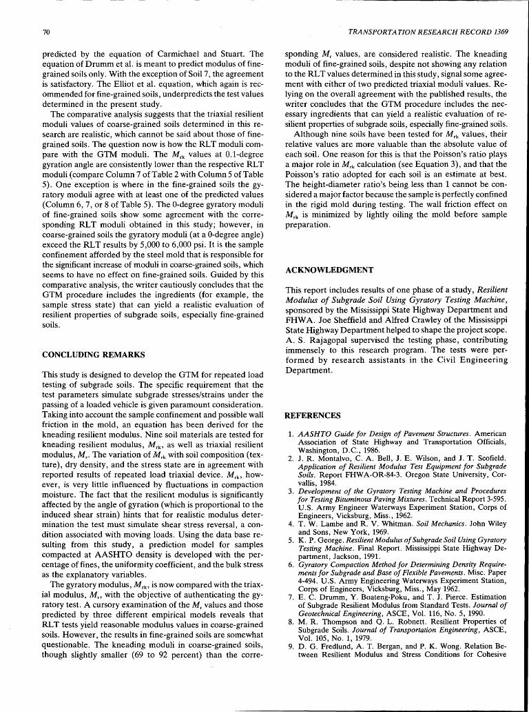
70

predicted by the equation of Carmichael and Stuart. The equation of Drumm et al. is meant to predict modulus of finegrained soils only. With the exception of Soil 7, the agreement is satisfactory. The Elliot et al. equation, which again is recommended for fine-grained soils, underpredicts the test values determined in the present study.

The comparative analysis suggests that the triaxial resilient moduli values of coarse-grained soils determined in this research are realistic, which cannot be said about those of finegrained soils. The question now is how the RLT moduli compare with the GTM moduli. The Mrk values at 0.1-degree gyration angle are consistently lower than the respective RL T moduli (compare Column 7 of Table 2 with Column 5 of Table 5). One exception is where in the fine-grained soils the gyra tory moduli agree with at least one of the predicted values (Column 6, 7, or 8 of Table 5). The 0-degree gyratory moduli of fine-grained soils show some agreement with the corresponding RLT moduli obtained in this study; however, in coarse-grained soils the gyratory moduli (at a 0-degree angle) exceed the RLT results by 5,000 to 6,000 psi. It is the sample confinement afforded by the steel mold that is responsible for the significant increase of moduli in coarse-grained soils, which seems to have no effect on fine-grained soils. Guided by this comparative analysis, the writer cautiously concludes that the GTM procedure includes the ingredients (for example, the sample stress state) that can yield a realistic evaluation of resilient properties of subgrade soils, especially fine-grained soils.

CONCLUDING REMARKS

This study is designed to develop the GTM for repeated load testing of subgrade soils. The specific requirement that the test parameters simulate subgrade stresses/strains under the passing of a loaded vehicle is given paramount consideration. Taking into account the sample confinement and possible wall friction in the mold, an equation has been derived for the kneading resilient modulus. Nine soil materials are tested for kneading resilient modulus, Mrk' as well as triaxial resilient modulus, Mr. The variation of Mrk with soil composition (texture), dry density, and the stress state are in agreement with reported results of repeated load triaxial device. Mrk• however, is very little influenced by fluctuations in compaction moisture. The fact that the resilient modulus is significantly affected by the angle of gyration (which is proportional to the induced shear strain) hints that for realistic modulus determination the test must simulate shear stress reversal, a condition associated with moving loads. Using the data base resulting from this study, a prediction model for samples compacted at AASHTO density is developed with the percentage of fines, the uniformity coefficient, and the bulk stress as the explanatory variables.

The gyratory modulus, Mrk' is now compared with the triaxial modulus, Mn with the objective of authenticating the gyratory test. A cursory examination of the Mr values and those predicted by three different empirical models reveals that RL T tests yield reasonable modulus values in coarse-grained soils. However, the results in fine-grained soils are somewhat questionable. The kneading moduli in coarse-grained soils, though slightly smaller (69 to 92 percent) than the corre-


sponding Mr values, are considered realistic. The kneading moduli of fine-grained soils, despite not showing any relation to the RL T values determined in this study, signal some agreement with either of two predicted triaxial moduli values. Relying on the overall agreement with the published results, the writer concludes that the GTM procedure includes the necessary ingredients that can yield a realistic evaluation of resilient properties of subgrade soils, especially fine-grained soils.

Although nine soils have been tested for Mrk values, their relative values are more valuable than the absolute value of each soil. One reason for this is that the Poisson's ratio plays a major role in Mrk calculation (see Equation 3), and that the Poisson's ratio adopted for each soil is an estimate at best. The height-diameter ratio's being less than 1 cannot be considered a major factor because the sample is perfectly confined in the rigid mold during testing. The wall friction effect on Mrk is minimized by lightly oiling the mold before sample preparation.

ACKNOWLEDGMENT

This report includes results of one phase of a study, Resilient Modulus of Subgrade Soil Using Gyratory Testing Machine, sponsored by the Mississippi State Highway Department and FHW A. Joe Sheffield and Alfred Crawley of the Mississippi State Highway Department helped to shape the project scope. A. S. Rajagopal supervised the testing phase, contributing immensely to this research program. The tests were performed by research assistants in the Civil Engineering Department.

REFERENCES

1. AASHTO Guide for Design of Pavement Structures. American Association of State Highway and Transportation Officials, Washington, D.C., 1986.

2. J. R. Montalvo, C. A. Bell, J. E. Wilson, and J. T. Scofield. Application of Resilient Modulus Test Equipment for Subgrade Soils. Report FHWA-OR-84-3. Oregon State University, Corvallis, 1984.

3. Development of the Gyratory Testing Machine and Procedures for Testing Bituminous Paving Mixtures. Technical Report 3-595. U.S. Army Engineer Waterways Experiment Station, Corps of Engineers, Vicksburg, Miss., 1962.

4. T. W. Lambe and R. V. Whitman. Soil Mechanics. John Wiley and Sons, New York, 1969.

5. K. P. George. Resilient Modulus of Subgrade Soil Using Gyratory Testing Machine. Final Report. Mississippi State Highway Department, Jackson, 1991.

6. Gyratory Compaction Method for Determining Density Requirements for Sub grade and Base of Flexible Pavements. Misc. Paper 4-494. U.S. Army Engineering Waterways Experiment Station, Corps of Engineers, Vicksburg, Miss., May 1962.

7. E. C. Drumm, Y. Boateng-Poku, and T. J. Pierce. Estimation of Subgrade Resilient Modulus from Standard Tests. Journal of Geotechnical Engineering, ASCE, Vol. 116, No. 5, 1990.

8. M. R. Thompson and Q. L. Robnett. Resilient Properties of Subgrade Soils. Journal of Transportation Engineering, ASCE, Vol. 105, No. 1, 1979.

9. D. G. Fredlund, A. T. Bergan, and P. K. Wong. Relation Between Resilient Modulus and Stress Conditions for Cohesive

George

Subgrade Soils. In Transportation Research Record 642, TRB, National Research Council, Washington, D.C., 1977.

10. A. Casagrande, Liquefaction and Cyclic Deformation of SandsA Critical Review. Harvard Soil Mechanics Series No. 88. Harvard University, Cambridge, Mass., 1976.

11. R. W. May and M. W. Witczak. Effective Granular Modulus to Model Pavement Responses. In Transportation Research Record 810, TRB, National Research Council, Washington, D.C., 1981.

12. J. M. Duncan and C. Y. Chang. Nonlinear Analysis of Stress and Strain in Soils. Journal of Soil Mechanics and Foundation Division, ASCE, Vol. 96, No. 5, 1970.

13. R. F. Carmichael and E. Stuart. Predicting Resilient Modulus: A Study To Determine the Mechanical Properties of Subgrade Soils. In Transportation Research Record 1043, TRB, National Research Council, Washington, D.C., 1985.

14. R. P. Elliot, S. I. Thornton, K. Y. Foo, K. W. Siew, and R. Woodbridge. Resilient Properties of Arkansas Subgrades. TRC-94. Arkansas Highway and Transportation Research Center, 1988.

DISCUSSION

WAHEED UDDIN Department of Civil Engineering, The University of Mississippi, University, Miss. 38677.

The use of Gyratory Testing Machine (GTM) for laboratory characterization of resilient modulus (Mr) of granular material and cohesive subgrade soils will provide a practical and relatively simple-to-use alternative to more complex triaxial testing procedures (AASHTO T274-82 and SHRP-LTPP Protocol P46-1989). The author and the sponsors of the research study are commended for taking initiative in this direction. The author's final report on this research study (1) also includes a comparison with the backcalculated moduli that further supports the GTM alternative.

Table 6 (1) gives the Mr values determined by the GTM method and the subgrade moduli backcalculated from the Dynaflect deflection basins measured at these test sites and analyzed by the MODULUS (2) and FPEDDl (3) programs. It is interesting to note the following:

1. Both backcalculation programs give comparable results (see Columns 4 and 5 of Table 6). These backcalculated moduli are generated by the two computer programs by matching measured with theoretical deflections. The FPEDDl program does not require any user input to generate seed moduli.

2. The backcalculated moduli (without correction for nonlinear behavior) are significantly higher, on the order of 80

TABLE 6 Comparison of Laboratory Resilient Moduli with Backcalculated Moduli for Various Roadbed Soils (I)

Soil No.

Kr, psi !bmaflect Daskcalcul~ted Mogul! Qlii FPEDDl I FPEDDl MODULUS

(GTM, at 0.1°) Corrected I Uncorrected Column l 2 3 4

10 15. 780 17, 980 28 ,000 28. 230

16, 150 15, 820 24, 750 25 ,030

12,840 12, 940 25,820 24,420

4 9 ,110 8, 360 16. 370 16 ,000

6,330 9,280 17,630 17,330

71

to 200 percent, than the GTM resilient moduli. In the case of Soil 5, the backcalculated moduli are about three times higher than the laboratory GTM resilient modulus.

3. The final solution of the FPEDDl program is a set of effective in situ moduli after correction for nonlinear behavior of both the unbound granular base/subbase layer and subgrade. These corrected moduli are shown in Column 3 of Table 6.

4. The corrected FPEDDl moduli (Column 3) and the GTM resilient moduli (Column 2) compare very well; the difference is generally less than 10 percent. The only exception is Soil 5, for which the corrected FPEDDl modulus is about 1.5 times higher than the GTM resilient modulus.

Overall, these results indicate the strong need of applying correction to the backcalculated moduli for nonlinear behavior of unbound pavement layers and roadbed soils. The results further provide evidence that the self-iterative nonlinear algorithm of the FPEDDl program is a practical approach to backcalculating effective in situ nonlinear moduli for these unbound pavement materials and soils.

The FPEDDl and RPEDDl programs apply correction for nonlinear behavior using the strain-softening models derived from earthquake engineering studie~ (3). The recent work at the University of Texas at Austin ( 4) supports this approach, in which normalized modulus versus strain relationships developed by conducting series of resonant column, torsional shear, and resilient modulus tests show approximately the same strain-softening pattern as that used in the FPEDDl and RPEDDl programs. Further laboratory work using repeated triaxial testing is in progress at The University of Mississippi, and falling weight deflectometer tests are also planned at these selected test sites. The MODULUS and FPEDDl programs will be used again to analyze the deflection basins. The author is encouraged to present the result of these ongoing and planned studies to benefit the pavement community.

REFERENCES

1. K. P. George. Resilient Modulus of Sub grade Soils Using Gyratory Testing Machine. Final Report. MississiRpi Highway Department, Dec. 1991. ·

2. Y. J. Chou and R. L. Lytton. Accuracy and Consistency of Backcalculated Pavement Layer Moduli. In Transportation Research Record 1293, TRB, National Research Council, Washington, D.C., 1991, pp. 72-85.

3. W. Uddin, A. H. Meyer, W. R. Hudson, and K. H .. Stokoe II. Project-Level Structural Evaluation Based on Dynamic Deflections. In Transportation Research Record 1007, TRB, National Research Council, Washington, D.C., 1985, pp. 37-45.

4. D.-S. Kim and K. H. Stokoe II. Characterization of Resilient Modulus of Compacted Subgrade Soils Using Resonant Column and Torsional Shear Test. Presented at the 71st Annual Meeting of the Transportation Research Board, Washington, D.C., 1992.

AUTHOR'S CLOSURE

The discussant brings out a very significant aspect of backcalculating moduli values from deflection data. Citing the

72

author's results, the discussant makes a valid observation that the backcalculated moduli of unbound materials, including roadbed soils, should be corrected for nonlinear behavior. That the kneading resilient moduli agree with the corrected backcalculated moduli gives credence to the gyratory resilient modulus test, in which the soil sample is subjected to shear stress reversal. What is important in the resilient modulus test would be to program the loading sequence in such a manner


that both normal and shear stresses undergo reversal during each loading.

The opinions, findings, and conclusions expressed in this report are those of the author and not necessarily those of the Mississippi State Highway Department or FHWA. This does not constitute a standard, specification, or regulation.

Publication of this paper sponsored by Committee on Soil and Rock Properties.


Characterization of Saturated Granular Bases Under Repeated Loads

LUTFI RAAD, GEORGE H. MINASSIAN, AND SCOTT GARTIN

The behavior of typical granular materials with different gradation was investigated under saturated, undrained, repeated triaxial loading conditions. Of particular interest is the comparative behavior of open-graded and dense-graded base courses and the influence of fines content on the dynamic response. The effect of aggregate gradation on the cyclic stress-strain behavior, pore pressure, damping, resilient modulus, compressibility, and permeability is investigated. Results indicate that saturated granular materials will develop excess pore water pressure under undrained repeated triaxial loading. This could lead to a decrease in resilient modulus and a potential increase in volume compressibility. Open-graded aggregates are more resistant to pore pressure buildup than dense-graded aggregates and are therefore less likely to induce damage in pavements under saturated conditions. In this respect, the estimated damage per repetition could be as much as 70 to 100 times more for pavements with densegraded bases.

It is estimated that more than 90 percent of the major pavements in the United States are periodically exposed to surface water infiltration resulting in saturation and flooding of underlying pavement layers (1). Cedergren (2) used data from several field test sections and estimated that relative damage for wet sections varies from 5 to 70,000 tim~s in comparison with dry sections. According to Markow (3), pavement wett~ng and subsequent drying are associated with the following periods:

1. The time during rainfall in which the pavement sublayers may be increasing in moisture content and could possibly reach saturation;

2. The time during which the sublayers are sufficiently wet or saturated to influence material properties, structural response, and performance; and

3. The time during which any excess moisture, not significantly affecting pavement behavior, is drained off.

Estimates of pavement wetness duration can be determined using data and relationships presented by Markow (3) and Moulton (4). Results show that, for a variation of base permeability in the range of 10 ft/day and 1,000 ft/day, the period of excessive moisture during which pavement performance could be adversely affected ranges between 1 and 28 days. Other field· data (J) show that the period of saturation following a rain can range from 5 to 20 days, except for pave-

L. Raad and G. H. Minassian, University of Alaska Fairbanks, Fairbanks, Alaska 99775. S. Gartin, Materials Section, Alaska Department of Transportation and Public Facilities, Anchorage, Alaska 99507.

ments with excellent drainage properties. During saturation, pavement sublayers could experience excess pore water pressure as a result of repeated traffic loads. An increase in pore water pressure reduces the effective stresses and, consequently, the strength and stiffness of the underlying soil layers. Consolidation settlement could result as the excess pore water pressure dissipates following a sequence of repeated loads. In recent years, more states have built permeable base pavements, which allow rapid drainage of infiltrated moisture. Performance data nationwide indicate that properly designed and constructed permeable bases significantly reduce pumping, faulting, and pavement cracking (5). Laboratory studies on pavement models reported by Dempsey ( 6) conclude that open-graded unbound granular bases are much less susceptible to pumping and channeling. Additional analyses performed by Raad (7) on dynamic pore water pressure generation and dissipation in granular pavement layers support such findings.

OBJECTIVES

Although a qualitative assessment of the behavior of saturated unbound granular layers in pavements has started to emerge, a mechanistic evaluation is essentially lacking. This study evaluates the behavior of saturated unbound granular bases under repeated triaxial load conditions. Specifically, the dynamic response of saturated granular base materials under controlledstrain repeated triaxial loading conditions will be investigated. The test aggregate gradations vary from open graded to dense graded. The influence of gradation on cyclic stress-strain behavior, pore pressure generation, damping, resilient modulus, and volume compressibility will be determined.

LABORATORY INVESTIGATION

Materials

Four materials (Gl-G4), representing a range of gradation from open graded to dense graded, were used. All aggregates were crushed sedimentary river deposits· of igneous origin. A summary of aggregate type, gradation, classification, dry density, compaction moisture content, permeability, and volume compressibility associated with excess pore pressure dissipation is presented in Table 1. A comparison of the grain size distribution is shown in Figure 1.

TABLE 1 Summary of the Properties of Tested Aggregates

Aggregate T~~e

Sieve G1 G2

3/4" 100 100 3/8" 50 70 #4 8 40 #8 5 23 #40 0 10 #200 0 0

Yd(pcf) 106.9 120.7 m(%) 4.08 4.34

Kr (cm/sec) 0.00333 0.00107

Kc (cm/sec) 0.0227 0.0104

K..., (cm/sec) 0.0087 0.0033

m., 3.77 x 10·3 27.6 x 10·3

AASHTO A-1-a A-1-a A-1-a Classification

Unified GP GW Classification

Note: yd = dry density m = compaction moisture content Kr= permeability as measured in the triaxial set-up

. Kc = permeability as measured using constant head permeability test Kav =average permeability (i.e., logarithmic average of Kr and Kc)

G3 G4

100 100 72 65 51 50 36 34 16 20 0 10

121.9 121.4 3.99 4.05

0.00075 0.00061

0.Q114 0.00094

0.0029 0.00076

3.51 x 10·3 5.98 x 10·3

A-1-a A-1-a

GW GP-GM

m., = volume compressibility associated with excess pore pressure dissipation

-- G1

100

90

80

70

" z 60 u; UJ 50 < D..

';I. 40

30 t--20

IO

0 0.01

- - - G2

..,., __ .,,,,. __ --

0.1

--· G3

DIAMETER (mm)

FIGURE 1 Gradations of aggregates used in the study.

-··- G4

10 100

Raad et al.

Specimen Preparation

Cylindrical specimens, 4 in. in diameter and 8 in. high, were prepared using vibratory compaction. Specimens were compacted in four layers, each subjected to 0.92 psi surcharge and vibrated at 60 Hz for 45 sec using a vibrating table. A 0.035-in.-thick rubber membrane was used to encase the compacted specimen. Before mixing and compaction, the portion of the specimen retained on the No. 8 sieve was soaked for 24 hr to attain a saturated surface dry condition. This procedure facilitated the back-water pressure saturation of the specimen required in the saturated undrained repeated load testing phase.

Resilient Testing

The compacted specimen was tested to determine the stressdependent resilient modulus relationship under repeated triaxial loading conditions. The specimen was subjected to the required confining pressure using water as a confining medium. Repeated deviator stress pulses were applied using MTS closedloop hydraulic testing equipment. Specimen conditioning and resilient testing were performed according to AASHTO Method T274-82. Following that, the specimen was subjected to a controlled-strain repeated load testing under a confining pressure of 5 psi, using the same cyclic strain that would be used after saturation during undrained loading. This allows a comparison of resilient modulus values under controlled-stress and controlled-strain loading conditions.

Saturation and Permeability Testing

After the completion of resilient testing, the specimen was subjected to a flow of carbon dioxide gas under 1 psi pressure for a period of 1 hr. This was followed by gradual backpressuring of deaired water through the specimen, which would help dissolve the carbon dioxide and achieve a high degree of saturation. During the saturation process, an effective confining pressure of 5 psi was maintained (i.e., the difference between the cell pressure and the back-water pressure was kept at 5 psi). Saturation was assumed to be complete when a (3 value (the ratio of the change in pore water pressure to the change in cell pressure) of 0.94 or larger was attained. After saturation, the specimen's permeability was determined for three different hydraulic head values, and the average permeability was reported. Permeability was also determined in a constant-head permeability setup according to AASHTO Method T215-70.

Controlled-Strain Repeated Load Testing

Controlled-strain undrained repeated load triaxial tests were conducted on saturated specimens under an initial effective 5 psi confining pressure. Each specimen was tested under a given controlled-strain haversine pulse having a duration of 0.10 sec and a frequency of 60 cpm. The peak cyclic strain value used in these tests varied between 0.05 and 1.0 percent. The applied strain cycles were repeated until the specimen

75

liquefied (i.e., the average excess pore water pressure in a given loading cycle became equal to the initial effective confining pressure) or until the total number of strain applications reached 1,500. Stresses, strains, and pore water pressure were monitored during the controlled-strain testing phase. At the end of this phase, the specimen w~s allowed to drain until an effective confining pressure of 5 psi was attained, and the volume compressibility associated with the corresponding pore pressure dissipation was measured.

RESULTS

Cyclic Stress-Strain and Damping Characteristics

The mechanistic behavior of the aggregates under repeated triaxial loading can best be illustrated through the variation of stress-strain characteristics with the number of strain repetitions. A schematic representation of the stresses and strains during a given cycle is presented in Figure 2. A typical variation of the stress-strain curve with number of repetitions is shown for Aggregate G3 when subjected to repeated strain cycles of amplitude equal to 0 .25 percent (Figure 3). The cyclic stress-strain loop seems to stabilize with number of load repetitions for the moist condition (i.e., as compacted moisture content), whereas in the case of saturated undrained loading, the stress-strain loops tend to "collapse," indicating significant softening. This is shown further in Figures 4 and 5 where a significant decrease in deviator stress, total strain modulus, and resilient modulus occurs with increasing number of repetitions. This is caused by the increase in pore pressure ratio (i.e., the ratio of excess pore water pressure in the specimen to the initial applied effective pressure), thereby resulting in

rn rn w a: Im

OA • INITIAL EFFECTIVE CONFINING PRESSURE

AB • APPLIED CYCLIC STRAIN

AF • PERMANENT STRAIN

BF • RESILIENT STRAIN

AC • PEAK DEVIATOR STRESS

SLOPE OF AQ • TOTAL STRAIN MODULUS

SLOPE OF FQ .. RESILIENT STRAIN MODULUS

D G

STRAIN

FIGURE 2 Stress-strain loop.

76

40

MOIST I 35

'iii 30 ~ .s 25

tn 20 r tn w a: 15

I-tn

10

5

0 0.00 0.05 0.10 0.15 0.20 0.25 0.30

AXIAL STRAIN (%)

40

35 SATURATED

30 ·; .s 25

tn 20 tn w a: 15 I-tn

10

5

0 0.00 0.05 0.10 0.15 0.20 0.25 0.30

AXIAL STRAIN (%)

FIGURE 3 Cyclic stress-strain behavior of Aggregate G3.

'iii .s tn tn w a: I-tn

a: 0 I-< > w c

0 j:: < a: w a: :::> tn tn w a: Q,

w a: 0 Q.

30

25

20

15

10

5

1.00

O.BO

0.60

0.40

0.20

0.00 0

7

NUMBER OF REPETITIONS

~ ~

// //

v /

5 10 15 20 25 30


FIGURE 4 Variation of deviator stress and pore pressure ratio with number of repetitions for Aggregate G3 (saturated condition).


'iii .s tn :::> ~a; c'tl o~ ~5

i-E z w ::i tij w a:

15

12

9

6

3

0 0

25

20

\ ~~

5

15 I\

~ 1---.....

~ I---_ v--....

10 15 20


10 ~ ..._.

5

0 0 5

~ ~

~ . .

10 15 20


25

...

25

FIGURE 5 Variation of total strain modulus and resilient modulus with number of repetitions for Aggregate G3 (saturated condition).

-

30

30

a decrease in effective stresses and gradual softening and collapse of the stress-strain curve .

Damping in soils is the energy lost during a complete cycle of applied shear stresses ( 8 ,9). The energy loss is equal to the area enclosed by the cyclic shear stress-shear strain loop. The damping ratio reflects the damping characteristics of a soil and could be used for dynamic response analysis of pavements. With reference to Figure 2, the damping ratio is given by

D _ .! area of Loop ADEF - 'TT area of AGB

(1)

The variation of damping with number of repetitions is illustrated for Aggregate G3 and strain level 0.25 percent in Figure 6. In the case of moist aggregate, the damping response remains a relatively stable response under repeated loads. This was typical for all the aggregates tested. However, under saturated conditions, an unstable response seems to be associated with a critical pore pressure ratio in the range of 0.60 to 0. 70. For the higher values, the stress-strain loop would collapse with increasing repetitions, leading in many cases to unstable response of damping and resilient behavior. In general, the gradation of the aggregates and the degree of saturation do not seem to have a significant effect on the damping ratio. However, the cyclic strain level seems to have the predominant influence. An increase in cyclic strain from 0.05 to 0.5 percent will result in an average increase in damping ratio from about 3 to 15 percent. This is smaller than the damping

Raad et al.

1.00

0 0.80 MOIST

j:: < a: 0.60

0 z a: 0.40 L

~ < c

0.20

' 0.00

0 50 100 150


1.00

0 0.80

SATURATED

j:: < a: 0.60

0 z a: 0.40 ~ < c

0.20

0.00 0 5 10 15 20 25


FIGURE 6 Variation of damping ratio with number of repetitions for Aggregates G3.

200

30

ratio reported for sands by Seed and Idriss (8). For the same range of cyclic strains, the ratio for sand varies, on the average, between 12 and 22 percent.

Pore Pressure Generation

The generation of excess pore water pressure of saturated granular layers could be a major cause of fast deterioration

········· G1 -- G2

1.00

0 0.80 j::

4( a: w 0.60 a: ::::> 0 0 w

0.40 a: 0..

w a: 0 0.20 0..

0.00 10

77

of pavement structures. This could be related to the following failure mechanisms:

1. An increase in pore pressure reduces strength and stiffness of the underlying granular layers and results in increased surface deflections and loss of pavement service?.bility.

2. In the case where pore pressure ratio increases and reaches unity, liquefaction will occur and result in the possible pumping of underlying soil through pavement cracks and joints. Excess pore water pressure could also be a major cause of channeling and erosion as reported by Dempsey ( 6).

3. The dissipation of excess pore water pressure results in the settlement of granular layers, causing additional loss of pavement support and surface cracking.

A comparison of pore pressure ratio increase for all aggregates (Figure 7) illustrates the superior behavior of opengraded Base Gl compared with G2, G3, and G4. The pore pressure ratio reaches unity and causes liquefaction in all aggregates except G 1, where the rate of pore pressure development decreases with number of repetitions and the pore pressure ratio remained well below unity even after 1,500 repetitions. Note that in Aggregate G4, with 10 percent fines content, the rate of pore pressure increase is generally greater than in Aggregate G3, with similar gradation but with no fines. In both aggregates, however, the number of repetitions required to cause liquefaction remains essentially the same.

The influence of cyclic strain level on pore pressure development is shown in Figures 8 and 9. Results indicate that, for all values of cyclic strains, Aggregate Gl is more resistant to the development of pore pressure compared with other more densely graded aggregates. In other words, for the same cyclic strain level, it would require more cyclic strain repetitions to achieve the same pore pressure ratio for G 1 aggregate than the rest of the tested aggregates. An increasing fines content generally increases the rate of pore pressure generation, particularly for cyclic strains that are smaller than 0.10 percent (Figure 9).

--- G3

.. ·"

100

-··- G4

0.25° CYCLIC STRAIN

, ..... ····· ...

1000 10000


FIGURE 7 Variation of pore pressure ratio with number of repetitions.

78

G1 AGGREGATE

1.00 - 0.055%

0 j:

0.80 - - • 0.1 CJ(, < a: w -- 0.25% a: o.so I ::::J en en I ....... 0.5% w 0.40~ a: 11.

w -·- 0.73% a: 0

0.20

11. -· 0.91%

0.00 10 100 1000 10000


G2 AGGREGATE

1.00 - 0.0.55%

0 j:

- - • 0.09% < a: w -- 0.25% a: 0.60 ::::J en en ....... 0.35% w 0.40 a: 11.

w -·- 0.72% a: 0.20 0 11.

-· 0.92% 0.00

10 100 1000 10000


FIGURE 8 Variation of pore pressure ratio with number of repetitions for Aggregates Gland G2.

The relative performance of the various granular bases under saturated conditions could be estimated by comparing the percent damage induced for a given load repetition. In this case the pavement damage associated with a pore pressure ratio equal to 0.60 was considered. Damage induced was assumed to be linear with load repetitions as proposed by Miner's damage theory. The percent damage caused per load repetition for different strain levels is summarized in Table 2. Aggregate G 1 has the lowest damage factors. They ranged between 0.1and0.5 percent for Aggregate Gland 10 percent and 35 percent for the more dense-graded Aggregates G3 and G4.


Q3 AGGREGATE

1.00

0 j:

0.80 < - 0.052% a: w a: 0.60 - - • 0.1 % ::::J en en w 0.40 a:

-- 0.25%

11.

w ....... 0.5% a: 0.20 0 11.

0.00 1 10 100 1000


Q4 AGGREGATE

1.00

0 j:

0.80 < - 0.052% a: w a: 0.60

- - • 0.1 % ::::J en en w 0.40 a:

-- 0.25%

11.

w ....... 0.5% a: 0.20 0 11.

0.00 10 100 1000


FIGURE 9 Variation of pore pressure ratio with number of repetitions for Aggregates G3 and G4.

Permeability and Compressibility

The influence of base permeability on the drainage of granular layers in pavement structures has been recognized by a number of investigators (1-3 ,5). An increase in base permeability can significantly decreas·e the drainage time and therefore reduce the exposure of the pavement to additional load repetitions during the period of base soaking. This would decrease the pavement damage associated with excess moisture conditions. However, under dynamic loading conditions, dissipation of the excess pore pressure generated in the granular base depends on both its permeability and compressibility.

TABLE 2 Percent Damage per Repetition for the Tested Aggregates

Damage per Repetition (%)

Aggregate Type Cyclic Strain 0.25% Cyclic Strain 0.50%

G1 00.10 00.50

G2 00.17 04.00

G3 10.00 35.00

G4 15.00 20.00

Raad et al.

This can be illustrated by exammmg the following onedimensional equation for pore pressure generation and dissipation (7,10):

au K a2u aue dN - = ---- + --at 'YJflv azi aN dt

where

'Yw = density of water, u = average cyclic excess pore water pressure, K = permeability,

mv = compressibility'

(2)

aue ·aN = rate of generation of excess pore water pressure under

undrained loading conditions, and dN --;Ji = frequency of load applications.

The right-hand side of the equation represents the sum of contributions of two components: (a) the pore pressure gen-

. aue dN d (b) h d" . . erat10n term, - -d , an t e pore pressure 1ss1pation aN t

K a2u term, -- --;:;;.

"f.Jflv aL-The ratio Klmv is a parameter that influences the dynamic

pore pressure dissipation. A higher Kand a lower mv would reduce the time required for dynamic pore pressure dissipation in the granular layer.

Permeability values for the aggregates used in this study are summarized in Table 1. Permeability measurements using the triaxial test setup yielded lower values than those obtained using the constant head apparatus. This could probably be attributed to the higher effective confining pressure applied on the specimens in the triaxial cell. The logarithmic average of the measured permeability values ranges from 0.87 x 10- 2

cm/sec for Aggregate Gl to 0.76 x 10-3 cm/sec for Aggregate G4.

Volume compressibility, mv, associated with the dissipation of excess pore water pressure, depends on the pore pressure ratio and cyclic strain level (Figure 10). For pore pressure

+ G1 t::. G2

:a 0.80 :::::: c ·a-..! 0.60

> t: ~ _JN

0.40 - I mw Ci)-UJ w 0.20 m: ..,..

D. 2 0 0.00 0

0.00 0.20 0.40

79

ratios less than 0.60, mv maintains essentially a constant value. However, for higher pore pressure ratios, mv increases and reaches a maximum value for pore pressure ratio equal to 1. This is consistent with similar findings by Seed et al. (11). Furthermore, the limited data obtained in this study indicate that for a pore pressure ratio equal to 1, higher cyclic strains will result in higher values of mv. Maximum measured compressibility values are summarized in Table 1. Well-graded aggregates, G2 and G3, have lower compressibility than opengraded aggregate, Gl. However, Aggregate G4, with 10 percent fines, maintains the highest compressibility.

Resilient Properties

Results of the variation of resilient modulus, MR, with the applied stress state expressed in terms of the sum of principal stresses 8 are shown in Figures 11 and 12. In this case, the relationship is defined as MR = ken, where k and n are material parameters. As expected, the most dense-graded aggregate, G3, exhibits the highest resilient modulus, whereas the open-graded aggregate, Gl, has the lowest. For example, assuring a 8 of 30 psi, the resilient modulus of Gl is 18,000 psi compared with 26,000 psi for G3, an increase of about 44 percent. These modulus values, however, were determined for moist-when-compacted specimen conditions. Under saturated undrained loading conditions, the resilient modulus decreases as a result of the increase in pore water pressure and the corresponding decrease in effective stresses. Such a decrease is illustrated by the variation of modular ratio with respect to pore pressure ratio (Figures 13 and 14). The modular ratio is defined as the ratio of the resilient modulus under saturated undrained loading to the resilient modulus for moistcompacted conditions, under the same cyclic strain level.

Although the variation of the resilient modulus with applied stress for the moist-compacted condition depends on aggregate gradation, the modular ratio decreases with increase in pore pressure ratio, and this decrease is essentially similar for all aggregate gradations considered.

In pavement design, the mechanistic evaluation of the granular layers is often needed. Mechanistic design procedures use limiting criteria in terms of pavement response parameters

o G3 D G4

.. + j

+ + ll

..,..

!::, !::,

0.60 0.80 1.00

PORE PRESSURE RA TIO

FIGURE 10 Compressibility versus pore pressure ratio.

80

+ CONTROLLED STRESS

G1 AGGREGATE

A CONTROLLED STRAIN

n = 0.805

DRY DENSITY = 107.4 pcf

MOISTURE CONTENT = 3.86%

1000'--~~~~~~~~-~~~-'-~~-~~-'-~~~

10 100

SUM OF PRINCIPAL STRESSES (psi)

G2 AGGREGATE

+ CONTROLLED A CONTROLLED STRESS STRAIN

·m 100000~~~~~~~~~~~~~~~~~~~~-, E: rn ::J ...J ::J 0 ~ 10000

.... z w :::i u; w a:

10

n = 0.741

DRY DENSITY = 120.9- pcf



FIGURE 11 Resilient moduli for Aggregates Gland G2.

100

to minimize the damage induced by repeated traffic loads. Although the development of these criteria for saturated granular bases is beyond the scope of this paper, the following general approach could be considered:

1. Determine the duration and frequency of occurrence for periods that correspond to near-saturation conditions in the pavement.

2. Estimate traffic loading and repetitions within each period.

3. Determine the resilient modulus of the granular layers by using the appropriate modular ratio (Figures 13 and 14).

4. Compute stresses and strains in the granular layer and apply limiting criteria to estimate critical number of load repetitions.

5. Use the reduced resilient modulus (Step 3) to determine the stresses and strains on the underside of the pavement surface layer and assess its fatigue behavior.

SUMMARY AND CONCLUSIONS

An attempt has been made to study the behavior of typical granular materials with different gradations under saturated undrained repeated triaxial loading conditions. Of particular interest is the comparative behavior of open-graded and dense-

10


+ CONTROLLED STRESS

G3 AGGREGATE

A CONTROLLED STRAIN

K = 4551.34

n = 0.515




+ CONTROLLED STRESS

G4 AGGREGATE

A CONTROLLED STRAIN

n = 0.819



100

1000~~~~~~...._~~-~~~~-~~~~~~~~

10 100


FIGURE 12 Resilient moduli for Aggregates G3 and G4.

graded base courses and the influence of fines content on the dynamic response. The influence of gradation on cyclic stFessstrain behavior, pore pressure generation, damping, resilient modulus, compressibility, and permeability was determined. Limiting criteria expressed in terms of repeated resilient strains and stresses and the allowable number of load repetitions were developed to pro•lide an improved mechanistic evaluation of saturated unbound granular layers in pavement structures. Results of this study lead to the following conclusions:

1. DynamiC loading of saturated granular layers induces excess pore pressure, thereby reducing the effective stresses and the corresponding frictional resistance in these layers.

2. Aggregate gradation has a major influence on the excess pore pressure generated. Open-graded aggregates with permeability greater than 8 x 10- 3 cm/sec seem to be more resistant to pore pressure generation than dense-graded and less permeable aggregates.

3. Volume compressibility depends on excess pore pressure generated during a dynamic loading sequence. However, for pore pressure ratios less than 0.60, the compressibility remains essentially unchanged. The most influential gradation component on compressibility is percent fines (i.e., percent passing No. 200 sieve). For example, Aggregate G4 with 10 percent fines has a maximum compressibility of 6 x 10-3 in2/lb compared with 3.5 x 10-3 in2/lb for Aggregate G3, which

Raad et al.

0 j::: < a: a: < .J ::::> Q 0 ~

::r-,...

1.00 :

I o.5o I

I

G1 AGGREGATE

0.00 L_.._ _ __._ __ __l___~-~-0.00 0.10 0.20 0.30 0.40 0.50 0.60


G2 AGGREGATE

2.00

I 0 1•0[ j::: < a: l

a: < .J

I ::::> Q I 0 050 I ~

I 0.00

0.00 0.10 0.20 0.30 0.40 0.50 0.60


0.70 0.80

0.70 0.80

FIGURE 13 Change of modular ratio with pore pressure ratio for Aggregates Gland G2.

has similar gradation but no fines. A higher compressibility indicates larger settlement of pavement layers after the dissipation of excess pore pressure.

4. The damping ratio for all aggregates tested increases with increasing cyclic strain and varies on the average between 3 and 15 percent, independent of degree of saturation and gradation.

5. The resilient modulus decreases with increasing pore pressure ratio. The decrease is similar for all gradations considered and varies essentially between 0 and 70 percent.

6. The open-graded aggregate seems to resist higher stresses and strains associated with a given number of load repetitions compared with other more dense-graded aggregates. In this respect, the estimated damage per repetition, under saturated conditions, could be as much as 70 to 100 times more for pavements with dense-graded bases than those with opengraded bases.

ACKNOWLEDGMENTS

This study is part of Project INE90.ll, Pavement Drainage Systems for Alaskan Highways and Airfields. This project is sponsored by the Alaska Department of Transportation and

2.00

0 1.50 j::: < a: a: 1.00 < .J ::::> Q 0 ~

0.00 0.00 0.10

2.00

0 1.50 j::: < a: a: 1.00 < ...I ::::> Q 0 ~ 0.50

0.00 0.00 0.10

G3 AGGREGATE

0.20 0.30 0.40 0.50 0.60


G4 AGGREGATE

0.20 0.30 0.40 0.50 0.60


0.70

0.70

l I

81

0.80

0.80

FIGURE 14· Change of modular ratio with pore pressure ratio for Aggregates G3 and G4.

Public Facilities (AKDOT&PF). The excellent cooperation and continuous support of AKDOT &PF Research Section is greatly appreciated.

REFERENCES

1. H. R. Cedregren, J. H. Arman, and K. H. O'Brien. Development of Guidelines for the Design of Subsurface Drainage Systems for Highway Pavement Structural Sections. Report FHW A-RD-73-14. Federal Highway Administration, U.S. Department of Transportation, 1973.

2. H. R. Cedergren. Drainage of Highway and Airfield Pavements. John Wiley and Sons, New York, 1974.

3. M. J. Markow. Simulating Pavement Performance Under Various Moisture Conditions. In Transportation Research Record 849, TRB, National Research Council, Washington, D.C., 1982, pp. 24-29.

4. L. K. Moulton. Highway Subdrainage Design. Report FHW ATS-80-224. Federal Highway Administration, U.S. Department of Transportation, 1980. ·

5. D. M. Mathis. Permeable Base Design and Construction. Fourth International Conference on Concrete Pavement Design and Rehabilitation, Purdue University, 1989, pp. 663-669.

6. B. J. Dempsey. Laboratory and Field Studies of Channeling and Pumping. In Transportation Research Record 849, TRB, National Research Council, Washington, D.C., 1982, pp. 1-12.

7. L. Raad. Pumping Mechanisms of Foundation Soils Under Rigid

82

Pavements. In Transportation Research Record 849, TRB, National Research Council, Washington, D.C., 1982, pp. 29-37.

8. H. B. Seed and I. M. Idriss. Soil Moduli and Damping Factors for Dynamic Response Analysis. Report EERC-70-10. Earthquake Engineering Research Center, University of California, Berkeley, 1970.

9. B. 0. Hardin and V. P. Drnevich. Shear Modulus and Damping in Soils: Design Equations and Curves. Journal of the Soil Mechanics and Foundations Division, ASCE 98 (SM7), pp. 667-692.

10. P. P. Martin and H.B. Seed. APOLLO: A Computer Program for the Analysis of Pore Pressure Generation and Dissipation in Horizontal Sand Layers During Cyclic or Earthquake Loading. Report UCB/EERC-78/21. University of California, Berkeley, 1978.


11. H. B. Seed, P. P. Martin, and J Lysmer. The Generation and Dissipation of Pore Water Pressure During Soil Liquefaction. Earthquake Engineering Research Center, University of California, Berkeley, 1975.

The contents of this paper reflect the views of the authors, who are responsible for the facts and accuracy of the data presented herein. The contents do not necessarily reflect the official views and po.licies of the Alaska Department of Transportation and Public Facilities. This paper does not constitute a standard, specification, or regulation.



Characterization of Resilient Modulus of Compacted Subgrade Soils Using Resonant Column and Torsional Shear Tests

DoNG-Soo K1M AND KENNETH H. STOKOE II

Both resonant column (RC) and torsional shear (TS) tests were performed at small (below 0.001 percent) to intermediate (below 0.1 percent) strain levels to investigate the effects of variables such as strain amplitude, loading frequency, and number of cycles of loading on the resilient modulus (MR) of compacted subgrade soils. Plasticity index (PI) was found to be an important variable in evaluating these effects, with the majority of the tests performed on cohesive subgrade soils compacted at optimum moisture content. Resilient moduli determined by RC, TS, and MR tests compare well when measurements are compared at the same strain amplitude, time of confinement, and excitation frequency. Elastic threshold strains were determined for the compacted subgrade soils. At cyclic strains below the elastic threshold strain, resilient modulus of a given soil is independent of strain amplitude and is the maximum value measured. At cyclic strains above the elastic threshold strain, MR decreases as strain amplitude increases. The elastic threshold strains of compacted cohesive soils ranged from 0.0008 to 0.0048 percent as Pl varied from 4 to 52 percent. Both RC and TS tests accurately measured resilient moduli below the elastic threshold strain. On the other hand, MR equipment could not be used in this strain range because of the lack of resolution. Resilient modulus was found to increase as loading frequency increased, even below the elastic threshold. Moduli obtained from RC, TS, and MR tests agreed well at strains above about 0.01 percent once the effect of frequency was taken into account. Modulus reduction curves showing the variation in normalized modulus, resilient modulus divided by the small-strain resilient modulus, versus strain amplitude correlate well with plasticity index.

In 1986 AASHTO adopted the use of resilient modulus (MR) in the design of pavement structures. In the laboratory, MR testing has been developed to determine resilient modulus of subgrade soils (J). In the field, nondestructuve testing methods such as the dynaflect, falling weight deflectometer, and spectral analysis of surface waves have been developed for evaluation of MR of pavement material~. However, different testing techniques are likely to have different applied stress (or strain) levels and different loading frequencies, and the response of pavement materials can be affected by these variables. Therefore, the effects of strain amplitudes (or nonlinear behavior) and loading frequencies on the stiffness of pavement materials need to be considered, and measured values

D.-S. Kim, Department of Civil and Environmental Engineering, Polytechnic University, Brooklyn, N.Y. 11201. K. H. Stokoe II, Department of Civil Engineering, The University of Texas at Austin, Austin, Tex. 78712-1076.

should be adjusted to the strain amplitudes and frequencies where the actual system is working.

It has long been recognized that all subgrade soils exhibit nonlinear behavior at strains above about 0.001 percent (2). The axial strain levels encountered in pavement subgrades generally range from small ( < 10- 3 percent) to intermediate ( < 10- 1 percent) levels (3). However, most MR testing equipment cannot accurately measure moduli at axial strains smaller than about 0.01 percent because of the limitation in resolution of transducers and the compliance of the system itself (4,5). Therefore, the complete stress-strain behavior of subgrade soils over a strain range from small to intermediate strains is not generally obtained in MR testing unless the soils are very stiff.

To investigate the effects of strain amplitude, loading frequency, and number of loading cycles on the resilient modulus of subgrade soils at small to intermediate strains, both resonant column (RC) and torsional shear (TS) tests were performed on the same specimen. RC tests were performed over strains between 10-4 percent and 10- 1 percent, and the complete modulus-strain behavior was obtained. The effect of frequency was also investigated at two strain levels: a smallstrain level of about 0.0007 percent and an intermediate strain level of about 0.007 percent. TS tests were also used in this evaluation. Finally, plasticity index (PI) was investigated as one variable in defining the effects of strain amplitude, frequency, and number of loading cycles on MR of compacted subgrade soils. Modulus reduction curves, showing Young's modulus at a given strain amplitude divided by Young's modulus at small strains (E/Emax) versus strain amplitude were developed. The trend in the modulus reduction curves with PI was also investigated. In this case, Young's modulus, E, was assumed to be equivalent to MR.

TEST EQUIPMENT AND MEASUREMENT TECHNIQUES

Torsional Resonant Column Test

Resonant column equipment of the torsional fixed-free type was used. In the fixed-free resonant column test, the bottom end of the specimen is rigidly fixed against rotation at the base pedestal while the top (free end) is connected to a drive

84

system that is used to excite and monitor torsional motion, as shown in Figure la.

The basic operational principle is to vibrate the cylindrical specimen in first-mode torsional motion. Once first mode is established, measurements of the resonant frequency and amplitude of vibration are made as shown in Figure lb. These measurements are then combined with equipment characteristics and specimen size to calculate shear wave velocity (Vs), shear modulus ( G), and shearing strain amplitude ( 'Y) ( 6).

One-dimensional wave propagation in a circular rod is ased to analyze the dynamic response of the specimen. The basic data-reduction equation is expressed as follows:

where

I mass moment of inertia of the specimen, I

0 = mass moment of inertia of drive system,

wr = resonant circular frequency, L = length of the specimen, and

Vs = shear wave velocity.

a) Specimen in the Resonant Column Apparatus

(1)

Coil Support System

(The Resonant Column and Torsional Shear Apparatus is One Piece of Equipment Operated Either at Resonance, Resonant Column, or in Slow Cyclic Loading, Torsional Shear)

> E

I /lo =(CO r ·LI V5 ) tan (ro r' LI Y5 )

:; 0.. 80 :; 0

..... Q)

0 E e 40 Q)

u u u <

0 35 40 45

G =PY/ E = 2 (l+u) G Ar~Y Ea=Y/(l+u)

50 Frequency, f, Hz

55

b) Typical Frequency Response Curve

FIGURE 1 Fixed-free resonant column test and an associated frequency response curve ..

60


Once the value of shear wave velocity is determined from Equation 1, shear modulus (G) oi the specimen can be calculated from

G = pV~ (2)

where p is the mass density. The shearing strain ( 'Y) is calculated from the peak rotation of the top of the specimen at 0.80 times the radius of the solid sample (7,8).

Standard procedures followed in relating cyclic triaxial and resonant column results were also used to relate MR and RC results. For cyclic triaxial and RC results, Young's modulus, E, and axial strain, Ea, are taken to be compatible with shear modulus, G, and shearing strain, 'Y (9) through

E = 2G(l + v)

and

Ea -y/(1 + v)

Proximitor Probe

Slow Cyclic Torsional Excitation

(3)

(4)

Coil Support System

a) Specimen in the Torsional Shear Apparatus

(The Resonant Column and Torsional Shear Apparatus is One Piece of Equipment Operated Either at Resonance, Resonant Column, or in Slow Cyclic Loading, Torsional Shear)

G= 't/Y E=2(l+u)G Ea =Y /(1 +u)

b) Measurement of Shear Modulus from Hysteresis Loop

FIGURE 2 Torsional shear apparatus and an associated hysteresis loop.

Kim and Stokoe

where v is Poisson's ratio. In MR testing, E and MR are assumed equal. Therefore, MR is simply inserted in Equation 3 for E. In applying these equations, the material is assumed to be homogeneous and isotropic. Values for Poisson's ratio of the compacted cohesive soils tested in this work were not measured but were assumed to be 0.45 and to be independent of excitation frequency. This value was selected because the cohesive soils were nearly saturated and Poisson's ratio most likely fell within the range of 0.40 to 0.50. As a result, the assumption of 0.45 causes less than a 5 percent error in using Equations 3 and 4.

Torsional Shear Test

The TS test is another method of determining shear and Young's moduli with the same equipment used in resonant column testing but operating it in a different manner. In this test, a cyclic torsional force with a given frequency, generally below 10 Hz, is applied at the top of the specimen while the bottom is held fixed, as shown in Figure 2a. Instead of determining a resonant frequency, the stress-strain hysteresis loop is determined from measuring the torque-twist response to the specimen. Proximeters are used to measure the angle of twist while the voltage applied to the coils is calibrated to yield torque. Shear modulus (G) is calculated from the slope of a line through the endpoints of the hysteresis loop as shown in Figure 2b. Thus, the shear modulus is calculated from

G = -r/-y (5)

Shearing strain amplitude is calculated at 0.80 times the radius of the specimen, just as in resonant column tests. Once G and 'Y are determined, Young's modulus and axial strain can be determined using Equations 3 and 4.

TEST MATERIALS AND SAMPLE PREPARATION

Test Materials

Ten disturbed subgrade soils were gathered from across the state of Texas. The Texas State Department of Highways and Public Transportation helped collect the samples from subgrades of actual pavement projects that have already been constructed and put into operation. Table 1 presents the basic properties of the test soils. Plasticity index (PI) was investigated to evaluate its importance as a correlation parameter.

Sample Preparation

Compacted subgrade specimens were prepared following Tex-101-E-part II "Preparation of Soil and Flexible Base Materials for Testing" (10). Test Method Tex-101-E is in close agreement with AASHTO Designation T 146-86 and T 87-86.

To prepare the sample, the soil was first air dried. The soil was then placed in a 20-rpm mixer and mixed with the proper amount of distilled water to create the design water content. The kneading compaction method was. used to compact the samples to a diameter of 4 in. (10.2 cm) and a height of 6 in.

85

TABLE 1 Summary of Properties of Subgrade Soils Collected Around Texas

Opnmum Sample Total Disttict Passing Moisture Moisture Unit

Soil County AASIITO No. 200 Liquid Plasticity Content Content Wt. ID Highway Class. (%) Limit Index (%) (%) (nrf\

14 I Travis A-7-6 87.3 56 29 19.3 19.3 112.7

Mooac-183 21

2 Starr A-4 34.9 25 10 10.6 10.5 129.8 FM75S

:> 3 Hockley A-6 100 30 IS 12.7 12.8 131.4

US62 4

4 Potter A-6 100 37 20 16.S 22.0 123.4 Sour951

4 5 Gray A-7-6 100 52 34 19.2 22.2 120.6

SH70

' 6 Lubbock A-4 91 20 4 10.6 13.0 132.2 FM835

:.l.U 7 Jasper A-7-6 100 79 S2 19.9 20.0 123.1

FM2S2 2U

8 Jefferson A-7-6 96 S4 36 18.0 10.2 120.6 US69

7 9 Tom Green A-7-6 98 S8 40 20.1 20.0 12S.4

US67 8

10 Haskell A-7-6 97 SI 29 16.2 16.4 125.2 Abilene

(15.2 cm). Five layers were used, and the compaction effort specified in Test Method Tex-113-E was applied. The samples were prepared at optimum, wet of optimum, and dry of optimum moisture contents. The "dry" and "wet" samples were prepared to achieve 95 percent of the maximum dry density. However, samples compacted at dry of optimum were very difficult to trim, which resulted in samples at optimum and wet of optimum being the ones on which most testing was performed.

After compacting the soil specimens, they were carefully extruded out of the steel mold using the hydraulic extruder. The samples were usually trimmed by hand to 2.0 in. (5.1 cm) in diameter and 4.0 in. (10.2 cm) in height. Trimmed samples were wrapped and stored in the moisture room for about 5 days before they were removed for setup and testing.

TESTING PROCEDURES

Before testing, each specimen was grouted to the top cap and base pedestal using a thin layer of hydrostone paste manufactured by U.S. Gypsum. Grouting had the beneficial result of achieving the fixed-free boundary condition in the RC and TS tests. An external rubber membrane was placed on the specimen immediately after grouting and sealed to the top cap and bottom pedestal with 0-rings. The sample-cement connections were allowed to cure overnight before testing.

Six days after compaction, both RC and TS tests were performed on the same specimen under an isotropic confining pressure of 6 psi. Only one pressure was used because the main goal of this study was to evaluate the influence of strain amplitude and loading frequency on MR. In addition, all specimens were compacted, which resulted in overconsolidating the cohesive soils. Overconsolidated cohesive soils exhibit only a small influence of confining pressure on stiffness (2); therefore, this effect was not studied further.

The series of RC and TS tests is shown in Figure 3. Initially the change in the low-amplitude shear modulus (at 'Y < 0.001 percent) with confinement time (usually 1 hr) was defined in

86

y

••

LA-RC HA-TS LA-RC* HA-RC

rest period

LA-RC = low-amplitude resonant column test (at y < 0.0001 %).

HA-TS = high-amplitude torsional shear tests; 10 loading cycles are applied during each constant-amplitude test; amplitude of successive test is approximately doubled each time.

LA-RC* = low-amplitude resonant column test; compare modulus with value before HA-TS; HA-RC tests not started until low-amplitude modulus equals value before HA-TS tests.

HA-RC = high-amplitude resonant column tests; amplitude of successive test is approximately doubled each time.

•• Check the effect of loading frequency at shearing strains of 0.001 % and 0.01 %.

FIGURE 3 Typical series of cyclic tests used to investigate the resilient modulus of compacted subgrade soils at a 0 = 6 psi.

the RC test. A series of high-amplitude TS tests was then performed. The TS tests were conducted at 0.5 Hz. To investigate the effect of loading frequency on modulus, loading frequencies were changed at shearing strain amplitudes of about 0.001 and 0.01 percent. Typical loading frequencies used in this study were 0.05, 0.1, 0.5, 1, 5, and 10 Hz. After completion of high-amplitude TS testing, the low-amplitude shear modulus was again measured in the RC test and compared with the value before high-amplitude TS testing. Sometimes, the low-amplitude shear modulus decreased because of cyclic degradation. However, a rest period following highamplitude testing allowed the stiffness to regain with time at constant confinement. Once the low-amplitude modulus had regained to the previous value, high-amplitude RC testing was performed with increasing strain amplitudes.

TEST RESULTS

Effect of Strain Amplitude on Stiffness of Compacted Subgrade Soils

Typical variations in Young's modulus with axial strain determined by RC and TS tests are shown in Figure 4. Shear moduli and shearing strains obtained from both tests were converted to the equivalent Young's moduli and axial strains using Equations 3 and 4. For strain levels below about 0.003 percent, moduli determined by the RC and TS tests are independent of strain amplitude. In this strain range, the behavior of soil is elastic (or proportional). The upper bound strain of this range is defined as an elastic threshold strain,

.fij Q.

~

fl)

:I :; ,, 0

~ fl)

~~ :I 0

;;....

25000


Soil #10 Age= 6days O'o = 6 psi

D TS Test (0.5 Hz)

/l,. RCTest

15000 .____.__. ........................ ..._~.._ ............................... ~...__-£-L..L. .... ~

16 4 10- 3 162

101

Axial Strain , £8 , %

FIGURE 4 Typical variation in Young's modulus with axial strain for a compacted subgrade as determined by resonant column and torsional shear tests.

Ete. Above the elastic threshold, moduli determined by both RC and TS tests decrease as strain amplitude increases. As shown in Figure 4, RC and TS tests can be performed at small to intermediate strains, resulting in a more complete picture of the modulus strain behavior from the proportional range to the nonlinear range than is presently possible with typical MR equipment.

Moduli determined by the RC test are larger than those obtained by the TS test over the whole strain range. In the RC test, moduli at small strains were measured at a loading frequency of about 90 Hz, whereas corresponding values in the TS test were obtained at 0.5 Hz. Generally, the stiffness of cohesive soil increases with increasing loading frequency. Therefore, the moduli difference between the two types of tests can be explained mainly by the difference in loading frequency (as discussed in more detail later). For these soils, number of loading cycles had very little effect on the moduli, especially for soils compacted at the optimum moisture content.

Effect of Frequency on Stiffness of Compacted Subgrade Soils

To investigate the effect of loading frequency on stiffness, the variation in Young's modulus of compacted subgrade soil with loading frequency is plotted at axial strain amplitudes of 0.0007 and 0.007 percent in Figure 5a. Moduli from the RC tests are also included. The modulus of this compacted subgrade soil increases almost linearly as a function of the logarithm of loading frequency.

To quantify the influence of loading frequency on stiffness, Young's modulus was normalized by the value of Young's modulus at a loading frequency of 0.5 Hz. Typical normalized behavior is plotted in Figure 5b. This normalization was done

Kim and Stokoe

·c;; Q,, .. ~

i :; ,, e

:"i! Gil -, = ~

32000

26000

20000 -2

10

Soil #10 Age= 6 days cr0 = 6 psi

0 f.a- 0.0007 %

A f.a- 0.001 %

Loading Frequency, f, Hz

a.) Variation in Young's Modulus with frequency

1.1

1.0

0.9

Soil #10 Age= 6days ~ =6psi

EI E(0.5Hz) = 1.00 + 7.1 lE-2 •LOO(Freq.)

fa=0.007% 0.8 L.-_,__l-J.Jl....U.L"'-~..L...L.L.U.~-.L......L..JU,,l.U.U..----JL.....1-.......,..L.LIM

10-2 10-1 10 ° 101

10 2

Loading Frequency, Hz

b.) Variation in normalized Young's Mcxlulus with frequency

FIGURES Typical variation in moduli with frequency for a compacted subgrade soil as determined by resonant column and torsional shear tests.

for an axial strain amplitude of 0.007 percent. By performing least-squares curve fitting on these data, the fitting curve yields the effect of loading frequency on stiffness, which is 7.1 percent per log cycle of loading frequency~

Correlation of the effect of loading frequency on the stiffnesses of compacted subgrade soils with Pl at different strain amplitudes is presented in Figure 6. The open symbols represent testing at a strain amplitude of 0.0007 percent, and the solid symbols represent the results at a strain amplitude of 0.007 percent. The best-fit curve is plotted with a solid line approximately in the middle of the data band. The effect of frequency on compacted subgrade soils increases with increasing Pl and ranges from 4.5 and 8.4 percent. In addition,

10

Comg~~ Submde Swb - D t 8 s Cl> .s ~ 6

...: ~

I! ~ 4 t' = ~ = t" 2

D Ea= 0.0007% ~

~= 6 psi • fa=0.007%

0 0 20 40

Plasticity Index, %

FIGURE 6 Variation in the effect of loading frequency on the stiffness of compacted subgrade soils with PI at axial strain amplitudes of 0.0007 and 0.007 percent.

87

60

it appears that strain amplitude has little influence ·on the frequency effect.

Comparison Between MR, RC, and TS Tests

To determine the capability of the testing equipment, several comparisons of results between MR, RC, and TS tests were made. MR tests were performed by following the recommendations published by Strategic Highway Research Program (SHRP) Protocol P-46 (11). Details of the resilient modulus tests are described by -pezo (4). To make this comparison, moduli obtained with the RC and TS tests were converted to equivalent resilient moduli using Equations 3 and 4. In addition, the moduli were finally adjusted to an excitation frequency of 10 Hz, which is the primary loading frequency in the M.R measurement. Figure 7 shows the typical variation in

40000

Soil #1 Age=6Days

• 0'0 = 6psi ·1 Dt:l~ ~ A lSI i:;i;;i ~, !f = 30000

~ WI

·11i1 D RC Test (adjusted to 10 Hz) a D

~ A TS Test (10 Hz)

• MR Test (10 Hz)

20000 l(f4

Axial Strain, £8 , %

FIGURE 7 Comparison of MR values of compacted subgrade soil determined by RC, TS, and MR tests (5).

88

resilient modulus with axial strain as determined by the three different testing methods. Moduli obtained from the RC and TS tests overlap nicely, with values from the MR test showing that RC and TS tests can be used in determining resilient modulus of subgrade soils provided the effect of loading frequency is considered. MR testing equipment could not be used to measure moduli at axial strains smaller than about 0.01 percent, and thus the elastic threshold strain could not be defined.

Effect of PI on Normalized Behavior of Compacted Subgrade Soils

Since Young's modulus in the small-strain region (Emax) as well as moduli at larger strains were measured, normalized modulus reduction curve, E/Emax versus log E, could be developed. The RC test is important in these measurements because it can generate higher strains at the same applied torque than the TS test because of dynamic magnification. Therefore, the RC test was used to investigate the normalized behavior of compacted subgrades over a wide range of strain amplitudes.

Normalized modulus reduction curves for the compacted subgrade soils are shown in Figure 8. Figure 8a presents the

i.e

~ I ' ~ 1.0 ' -.Qea· tne1· oH M'l s .dJ '-

~ • • ., oa&!a . .,.

= 0.8 .. ~ - .. , '8 a #1--29% •• 0 ~ A #2--10% a rn • -ci> 0.6 .. • r:: #3--15% .·{~

::I • #7--52% Q > • #8--36% l 0.4 ...

0 #9--40% RC Test at OMC

I -==·· #10--29% Conf. Pressure=6psi

"" 0.2 . I . I

Q z -4 -3 -2 10 10 10 10

Axial Strain, £a, %

a) At Optimum Moisture Content

. I ' 1.0 - Ao •e •9 Aa •a •• 0 .A

0 a

0.8 - a -0 .A

0.6 - 0 a A

.sm!:::£l D #4--20% 0

0.4 - A #5--34% 0 #6--4% RC Test at WET

Conf. Pressure=6psi 0.2 - I - I • •

-4 -3 -2 10 10 10 10

Axial Strain, £8, %

b) At Wet of Optimum

FIGURE 8 Variation in normalized modulus reduction curves with PI for compacted subgrade soils.

-1

-1


variation of normalized modulus reduction curves of subgrade soils compacted at optimum moisture content, and Figure Sb presents those results of subgrade soils compacted at wet of optimum (95 percent of maximum dry density). The range of PI of the samples is 4 to 52 percent. Soil 6 (PI = 4 percent), which is the least plastic soil, exhibits nonlinear behavior beginning at a strain amplitude of about 0.0008 percent, and Soil 7 (PI = 52 percent), the most plastic soil, exhibits nonlinear behavior beginning at strains of about 0.005 percent. These results show how the E/Emax versus log E curve shifts toward increasing elastic threshold strains as soil plasticity increases. Therefore, it can be concluded that PI of the soil is an important variable in evaluating the nonlinear behavior of (compacted) subgraded soils. Vucetic and Dobry (12) have shown the small effect of PI on the location of the normalized shear modulus reduction curve, G/Gmax versus log -y, and Kokusho et al. (13) have demonstrated that, even for large overconsolidation ratios (OCRs), the value of OCR has practically no effect on the position of the G/Gmax versus log -y curve.

To fit these test data, a Ramberg-Osgood (R-0) fitting method was used (4,8). The R-0 fitting equation can be written as

E = EI . E + c (EI . E )R (6)

where E' = E/Emax = normalized Young's modulus and C and Rare the R-0 parameters. Equation 6 can be rewritten as

E . (1- E') = c . (E' . E)R (7)

By taking the logarithm of both sides, Equation 7 yields

log [E · (1 - E')] = log C + R · log (E' · E) (8)

Using a least-squares curve fitting, the R-0 parameter R is directly determined from the slope, and the parameter C is calculated from the intercept. In using this approach, normalized Young's moduli larger than 0.99 are deleted from the fitting process.

The R-0 parameters, C and R, were determined for each sample, and the values are given in Table 2. Correlation of R-0 parameters with PI for the subgrade soils compacted at optimum moisture content was determined using linear regression, and the variation of the general normalized curves with PI is plotted in Figure 9. Using the curves in Figure 9, once the small-strain modulus (Emax) of compacted subgrade soils is obtained from field seismic methods, it is possible to predict the strain-dependent behavior of subgrades using the normalized curve at the given Pl.

To determine the influence of PI on the elastic threshold strain, the R-0 curve-fitting method was also used. The elastic threshold strain is defined as the point where E/Emax is 0. 98, and the associated values of Ete are given in Table 2. The

Kim and Stakoe

TABLE 2 Summary of Ramberg-Osgood Parameters and Elastic Threshold Strains for Compacted Subgrade Soils#

Plasticity Sample

Sample Index Condition• R

ID (%)

soil#l 29 OMC 2.4968

soil#2 10 OMC 2.3448

soil#3 15 OMC 2.4252

soil#4 20 WET 2.6321

soil#5 34 WET 2.5715

soil#6 4 WET 2.3883

soil#? 52 OMC 2.5627

soil#8 36 OMC 2.3626

soil#9 40 OMC 2.4771

soil #10 29 OMC 2.4820

# All of the tests were performed at confining pressure of 6 psi. • OMC =Compacted Optimum Moisture Content

Wet= Compacted Wet of Optimum

Compacted Subgrade Soils

at Optimum Moisture Content

Elastic

c Threshold

(%)

38530 0.0045

58076 0.0011

102612 0.0014

174100 0.0040

71203 0.0048

155131 0.0008

65811 0.0048

17611 0.0031

34324 0.0043

49534 0.0035

0.2 L-_4__..__ ................ ~ ........ _3_..__ ........................ .....__2~ ....... - ................ - -1

10 10 10 10

Axial Strain,Ea , %

FIGURE 9 Variation in normalized Young's modulus with PI for compacted subgrade soils at optimum moisture content.

10-t

10-2

10-3

10-4 0

Compacted Subgrade Soils

20

e -5 1.632 ft= 0.0007 + 1.05•10 •Pl

EI Emax = 0.98 at Optimum Moisture Content

40

Plasticity Index, %

FIGURE 10 Variation in elastic threshold strain with PI of compacted subgrade soils at optimum moisture content.

89

variation in elastic threshold strain of compacted subgrade soils at the optimum moisture contents with PI is shown in Figure 10. The elastic threshold increases with increasing PI. The elastic threshold strain ranges between 0.0008 and 0.0048 percent when PI varies from 4 to 52 percent.

CONCLUSIONS

Resilient modulus of compftcted subgrade soils was investigated using RC and TS tests. The following conclusions can be drawn from this study:

1. An elastic threshold strain can be defined below which resilient moduli of compacted subgrade soils are independent of strain amplitude. Above the elastic threshold strain, moduli decrease as strain amplitude increases. The elastic threshold strain increases with increasing PI of the soil. Elastic threshold strains for the cohesive soils ranged from 0.0008 to 0.0048 percent as PI varied from 4 to 52 percent.

2. The resilient modulus of compacted subgrade soils increases linearly as a function of the logrithm of loading frequency. The effect of frequency on resilient modulus increases as PI increases. The effect of frequency ranged from 4.5 to 8.4 percent per log cycle of loading frequency as PI varied from 4 to 52 percent.

3. Resilient modulus can be measured at small (below 0.001 percent) to intermediate (below 0.1 percent) strains using RC and TS tests, whereas MR testing generally produces reliable measurements at strains above about 0.01 percent. Moduli obtained from RC, TS, and MR tests agreed well at strains above about 0.01 percent, provided the effect of frequency on stiffness was considered in the comparison. Therefore, RC and TS tests can also be used to determine resilient modulus over a wide range of strain amplitudes.

4. Normalized modulus (E/Emax) versus strain curves move to increasing strains as the PI of cohesive soils increases. Correlation curves between normalized modulus and PI for cohesive soils compacted at optimum moisture contents are presented. Once the small-strain modulus (Emax) of a given soil is obtained from field seismic measurements, it is possible to predict the strain-dependent behavior of the subgrade soil using the normalized curve at the given PI as is often done in geotechnical earthquake engineering.

ACKNOWLEDGMENTS

This work was supported by the Texas State Department of Highways and Public Transportation. The authors express their appreciation for this support. In addition, the authors thank W. Ronald Hudson and Rafael Pezo for their assistance.

REFERENCES

1. Resilient Modulus of Subgrade Soils. AASHTO T274-82. AASHTO, 1986, pp. 1157-1177.

2. B. 0. Hardin and V. P. Dmevich. Shear Modulus and Damping in Soils: Measurement and Parameter Effects. Journal of Soil Mechanics and Foundation Division, ASCE, Vol. 98, No. SM6, June 1972, pp. 603-624.

90

3. D.-W. Chang, J. M. Roesset, and K. H. Stokoe II. Nonlinear Effects in Falling Weight Deflectometer Tests. Presented at 71st Annual Meeting of the Transportation Research Board, Washington, D.C., 1992.

4.· R. F. Pezo. Development of Reliable Resilient Modulus Test for Subgrade and Subbase Materials for Use in Routine Pavem~nt Design. Ph.D. Dissertation. The University of Texas at Austm, Austin, 1991.

5. R. F. Pezo, D. S. Kim, K. H. Stokoe II, and W. R. Hudson. Developing a Reliable Resilient Modulus Testing System. Presented at the 70th Annual Meeting of the Transportation Research Board, Washington, D.C., 1991.

6. Standard Test Methods for Modulus and Damping of Soils by the Resonant-Column Method. 1987 Annual Book of Standards, Vol. 04.08 Soil and Rock; Building Stones. American Society for Testing and Materials, ASTM D4015-87, pp. 507-525.

7. A. T. F. Chen and K. H. Stokoe II. Interpretation of Strain Dependent Modulus and Damping from Torsional Shear Tests. Report USGS-GD-769-002. United States Geological Survey, 1979, 46 pp.

8. D. S. Kim. Deformational Characteristics of Soils at Small to Intermediate Strain from Cyclic Tests. Ph.D. Dissertation. The University of Texas at Austin, Austin, 1991, 340 pp.

9. M. L. Silver and T. K. Park. Testing Procedure Effects on Dynamic Soil Behavior. Journal of the Geotechnical Ettgineering Division, ASCE, Vol. 101, No. GTlO, Oct. 1975, pp. 1061-1083.

10. Manual of Testing Procedures, Texas Highway Department, Vol. 1. Jan. 1983.

11. Resilient Modulus of Unbound Granular Base, Subbase Materials and Subgrade Soils. Strategic Highway Research Program Protocol P-46, UG07, SS07, 1989.

12 M. Vucetic and R. Dobry. Effect of Soil Plasticity on Cyclic Response. Journal of the Geotechnical Engineering Division, ASCE, Vol. 117, No. 1, Jan. 1991, pp. 89-107.

13. T. Kokusho, Y. Yoshida, and Y. Esashi. Dynamic Properties of Soft Clay for Wide Strain Range. Soils and Foundations, JSSMFE, Vol. 22, No. 4, Dec. 1982, pp. 1-18.

DISCUSSION

WAHEED UDDIN Department of Civil Engineering, The University of Mississippi, University, Miss. 38677.

The authors are commended for conducting and reporting the results of acceptable and proven laboratory seismic testing techniques of the resonant column and torsional shear tests and comparing these with the resilient modulus (M,) results of the repeated load triaxial using the SHRP-LTPP protocol. The paper provides new insight for laboratory characterization of resilient properties of cohesive subgrade soils and indicates the need for high-resolution instrumentation capable of generating strain-softening M, relationships similar to those shown in Figures 7 and 8 for the resonant column and torsional shear tests.

The following observations and discussion are offered with the view of encouraging the use of the developments in earthquake engineering where the in situ moduli determined from field seismic tests are corrected for strain-softening behavior, a highly recommended concept for calculating nonlinear moduli of soils (1-4).

1. M, results from all three types of tests agree fairly well at and above 0.01 percent strain levels, as shown in Figures 7 and 8 of the paper.

0 _g ~ ~ 0.4 33 -0 -0


Ranges in values from severa I investigators

~ ~ 0.2 1..-----~----+-----+:""6',~~--4

Shear Strain, Y, percent

FIGURE 11 Typical reduction of normalized shear modulus with shearing strain amplitude presented by Seed and Idriss (2).

2. There is a critical threshold strain level below which the normalized modulus is independent of strain amplitude and corresponds to the maximum modulus value.

3. The authors agree with the strain softening behavior (Figure 11) used for dynamic response analysis in earthquake engineering (2).

4. The low amplitude strain level test results presented by the authors show that below 0.01 percent strain amplitude the M, results from the triaxial testing equipment (customarily used by the pavement community) could not be obtained because of the inadequacy of the instrumentation.

5. Low amplitude strain levels are also implied during nondestructive testing (NDT) of pavements using the Dynaflect, falling weight deflectometer (FWD), Road Rater, and spectralanalysis-of-surface-wave (SASW) method (3-5).

6. It is expected that the moduli calculated from the lightload Dynaflect and SASW seismic testing in the field are maximum moduli because these correspond to the elastic strain level below 0.005 percent strain amplitude or below the critical strain level, whereas the same may not be true for relatively heavy NDT devices or for truck loading where the strain amplitude is expected to be in the range of 0.001to1 percent.

7. Therefore, the strain-softening models, as shown in Figure 11 and presented by the authors in Figure 8, can be used to correct the NDT in situ moduli for nonlinear behavior. This behavior is exhibited by cohesive soils as well as granular material.

I first recognized the importance of the strain-softening behavior of unbound granular pavement layers and roadbed soils in early 1980s and developed an equivalent linear analysis procedure to correct the effective in situ Young's moduli of these layers backcalculated from the Dynaflect data. The equivalent linear analysis procedure used the normalized modulus versus strain amplitude relationships shown in Figure 12 and typical relationships of elastic parameters similar to Equations 3 and 4. The equivalent linear analysis is equally applicable to other NDT deflection equipment and the SASW method. My equivalent linear analysis procedure is incorporated in the FPEDDl and RPEDDl backcalculation programs (3).

On the basis of the excellent dynamic laboratory tests data presented by the authors and this discussion, there seems to be a strong need to extend this initiative in the following areas:

Kim and Stokoe

>C 1.0 0 E ~ (.!) 0.8

"' :;, :;

~ 0.6

c ~ 0.4 en ~ C1J

~0.2 0 E C5

....... , ', Curve A - CLAYS

', Stokoe & Lodde (1978)

< Curve B - SANDS '

_,.,, \ Seed & Idriss (1970) '\

\ \

z OL_--~--:~::-:-~~--:::-::-::--~~--::::-7~~~--;-~ 0.0001 0.001 0.01 0.1 LO

Single-Amplitude Shearing Strain in percent

FIGURE 12 Strain-softening models used in the FPEDDl and RPEDDl programs to calculate nonlinear moduli of unbound granular pavement layers and roadbed soils (3).

1. Improve the M, triaxial test equipment to make accurate and precise measurement of resilient moduli in the low strain amplitude range of 0.001 percent and below.

2. Conduct a series of tests on different soil types using the resonant column techniques and SHRP-LTPP M, protocol at varying confining pressures and develop the strain-softening relationships that can be used to derive typical curves for both unbound granular base/subbase materials and roadbed soils.

3. Conduct the preceding test program for undisturbed and disturbed samples extracted from a few SHRP-LTPP test sections located in different environmental regions of the United States. This will provide strain-softening models for use in calculating nonlinear FWD moduli.

91

REFERENCES

1. B. O. Hardin and V. P. Drnevich. Shear Modulus and Damping in Soils: Design Equations and Curves. Journal of SMF Div., ASCE, Vol. 98, No. SM7, July 1972, pp. 667-692.

2. H. B. Seed and .I. M. Idriss. Soil Moduli and Damping Factors for Dynamic Response Analysis. Repor~ EERC ~0-10: Earthquake Engineering Research Center, University of Cahforma, Berkeley, 1970.

3. W. Uddin, A. H. Meyer, W. R. Hudson, and K. H. Stokoe II. Project-Level Structural Evaluation Based on Dynamic D~flections. In Transportation Research Record 1007, TRB, National Research Council, Washington, D.C., 1985, pp. 37-45.

4. W. Uddin. Recent Advances in Nondestructive Dynamic Testing and Evaluation Methods. Proc., 8th Asian Regional Conference on Soil Mechanics and Foundation Engineering, Vol. 2, Kyoto, Japan, 1987. .

5. S. Nazarian and K. H. Stokoe II. Use of Surface Waves m Pavement Evaluation. In Transportation Research Record 1070, TRB, National Research Council, Washington, D.C., 1986, pp. 132-144.

AUTHORS' CLOSURE

We thank the discussant for his fine discussion of our paper. We agree with his comments and observations about smallstrain moduli and the relationship between small-strain moduli (at strains less than about 0.001 percent) and nonlinear behavior exhibited by soils at larger strains. As the profession comes to understand the importance of small-strain moduli that can be measured in the field and in the laboratory, improvements will occur in the design, analysis, and testing of pavement systems.



Update on In Situ Testing for Ground Modification Techniques

JOSEPH P. WELSH

In situ testing has played a major role in the growth of ground modification in the United States. If the in-place soil is inadequate for construction, the engineering profession is frequently designing for the ground to be modified, rather than using a deep foundation that bypasses the inadequate soil or removing and replacing the problem soil. There has been little change in the status of in situ testing for ground modification for construction purposes. However, a new field of environmental geotechnical engineering has developed, bringing with it a need for testing of the modified ground for existing and emerging technologies. Recommendations for additional research and development in the area of in situ testing for ground modification are included.

Ground modification is the in-place controlled processing of existing materials to form part of a geotechnical construction system. This paper discusses how in situ testing has assisted the rapid growth of ground modification techniques in the United States. Well-defined quality assurance/quality control programs, backed up by appropriate in situ testing techniques, are now possible. Design engineers can now determine minimum settlements or maximum relative density criteria, prepare plans and specifications, and, by in situ testing, ascertain that the soil has been adequately treated to meet these requirements. Ground modification contractors using in situ testing are now able to determine when specifications are met and revise their construction procedures, when necessary.

An overview is given of the current status of some ground modification techniques including Dynamic Deep Compaction; vibrocompaction; vibroreplacement; vibrodisplacement; and cement, chemical, compaction, and jet grouting. Limitations regarding specific ground modification techniques and in situ testing are discussed and recommendations for future research needs are presented. Soil Improvement-A Ten Year Update (1) is a report of the ASCE Geotechnical Engineering Division's Committee on Placement and Improvement of Soils. These ground modification and many other techniques and in situ tests are included along with 10 major case histories on soil improvement. This is still a good, current reference for professionals contemplating designing or constructing with ground modification technologies.

IN SITU TESTING

Standard Penetration Testing

Standard penetration testing is the technique most commonly used to determine initial soil properties at a site. However,

Hayward Baker Inc., 1875 Mayfield Road, Odenton, Md. 21113.

unless continuous standard penetration tests are specified, thin strata may be missed, which could influence the method selected for improving the soil. The initial N value, the type of material to be treated, the depth of treatment specified, the elevation of the groundwater, and so forth, are all factors to be considered in determining the possibility and ground modification method of reaching the specified N value criteria. The standard penetration test samples should have sieve analyses performed, particularly if the three most silt- and clay-sensitive techniques (vibrocompaction, chemical grouting, and compaction grouting) are contemplated.

Cone Penetration Testing

Cone penetration testing presents a continuous soil profile with relative strength parameters. On critical, large projects, specialty ground modification contractors have supplemented the design soils reports by using cone penetration testing before, during, and after soil improvement. Spacings as close as a 50-ft square grid pattern have been used. The before testing vividly points out abnormalities of the site and allows the specialty contractor to plan the soil improvement program. The testing during the actual work gives assurance that the planned program is succeeding and indicates whether changes in spacing, additional energy input, or localized retreatment are necessary. The after-treatment cone penetration tests verify the success of the program. However, even in granular formations, a time lag has been noted in the improvement in the cone tip resistance reading (2-5). The cone testing apparatus, added to conventional drilling rigs, is limited by the reaction weight of the rig, which is normally less than 10 tons; this has hampered penetration to the required depth, particularly after soil improvement has been accomplished. Electric Dutch Cone rigs are available with reaction weights of 23 tons that have been able to penetrate over 80 ft in densified granular soils where the cone tip resistance has uniformly exceeded 150 tsf.

Dilatometer

The flat plate dilatometer (5 ,6) is an innovative technique and an excellent supplement to cone penetration testing, particularly for critical structures where differential settlement is the main criterion. Results from the dilatometer are expressed in terms of the three index parameters: material index, I0 ,

related to the soil type; horizontal stress index, K0 , related to in situ K0 , coefficient of earth pressure at rest; and dila-

Welsh

tometer modulus, E 0 , a parameter related to soil stiffness. Quantitative estlimates of K0 , Su (undrained strength), 0 (friction angle for sands), OCR ( overconsolidation ratio), and M (the constrained modulus) can be obtained from the empirical correlation with the dilatometer's I0 , K0 , and E0 . Sometimes, the strata are so densified that the DMT blade cannot be pushed by a drill rig. Then preboring is performed down to the specific zone to be tested rather than continuous testing from the surface as done prior to densification.

Pressuremeter Test

The pressuremeter test has extensive application for ground improvement evaluation, offering the advantage that estimates can be made of the lateral stress, the moduli, and the shear strength (7).

GROUND MODIFICATION TECHNIQUES

Dynamic Compaction

Dropping weights onto the ground from various heights for soil improvements is called dynamic compaction, pounding, dynamic consolidations, and so forth and has a long historic background, with reports of the Romans using this method. The first documented project in the United States was in 1871, when a cannon was filled with lead and used to densify the soil beneath the foundations of the Saint George Mormon Temple, St. George, Utah (8). The late L. Menard's publication in 1975 (9) rekindled interest in this technique. However, through the late 1970s there was relatively limited use of dynamic compaction in the United States. This is demonstrated by the absence of relevant case histories in the ASCE's 1976 Bicentennial Report on Soil Improvement, History, Capabilities and Outlook (10) and the few case histories in Mitchell's 1981 "Soil Improvement-State of the Art Report" (11). In the 1980s, however, over 250 projects were performed in the United States, due to the economy of this technique and the capability of assessing the improvement of the soil by in situ testing. The publication by Lukas (12) in July 1986 for the Federal Highway Administration has increased the use of this system for highway construction. Some of the major contributions of Lukas's publication are as follows:

1. The grain size grouping of soils into three zones depending on their suitability for improvement by dynamic compaction;

2. The applied energy requirements in tonne-m/m3 , depending on the type of deposit being improved; and

3. The upper bound test values for standard penetration test, cone preparation test, and pressuremeter test after dynamic compaction.

Current practice in the United States involves the use of weights between 8 and 20 tons dropped from heights of up to 100 ft with a single line attachment from specially modified cranes. Some of the limitations of dynamic compaction have

93

been the safety problems involved with dropping weights from these heights, flying debris, the damage that can be caused by the shear, compression and Raleigh waves generated by this technique, and the limit in the depth of influence obtainable by"this method. Menard's original proposition, that the depth of influence is equal to the square root of the weight times the height of drop, has been modified by Leonards et al. (13), Lukas (12), and other authors. Current practice is to use a modification factor, varying between 0.3 and 0. 7 depending on the soil type, to determine the predicted depth of influence.

The uses of dynamic compaction will continue to grow, primarily because of the relative economy of this method with cost conventionally starting at $1.00/ft2 of surface area densified, coupled with the relative speed with which this ground modification technique can be performed.

Dynamic compaction for improving nonhomogeneous fill, such as sanitary landfills, mine spoils, and building debris, will require better in situ testing methods. Standard penetration testing, cone penetration testing, pressuremeter, and dilatometer are of limited use in these materials, in the writer's opinion. One method that needs additional research and development for testing of nonhomogeneous fill is shear wave velocity, using the weight as the energy source and placing transducers around the site and monitoring before and after the de.nsification. This would allow a determination of the relative cross site improvement, which then could be correlated with the potential site settlement characteristics.

Vibrocompaction, Vibroreplacement, and Vibrodisplacement

The vibrosystems use a depth vibrator to densify granular soils horizontally. The vibrator is a hollow steel tube containing an eccentric weight mounted on a vertical axis that produces horizontal vibrations. The most recent equipment innovation is the use of vibrators to produce higher centrifugal forces so the probes can be spaced further apart, thus making greater economy possible. The vibrocompaction system was first developed in Germany in the 1930s, and its first commercial application in the United States was in Cape May, New Jersey, in 1948. Vibrocompaction improves the density of loose sands as long as the sands do not contain more than 12 percent silt or 3 percent clays. The vibrations liquify and realign the sand grains, causing a densification of the sand. Additional sand could be added around the perimeter of the vibrator, or the entire site could be dropped as the densification takes place.

The next major development of the vibrosystems was vibroreplacement, or stone columns, where the addition of stone backfill around the vibrator was used to treat nonhomogeneous strata, with the sands being densified and cohesive soil replaced and reinforced. The jetting action of the vibrator in the installation process washed out the cohesive material, which was replaced by stone around the perimeter, and diameters 3 to 4 ft were created by a single probe. Because of potential environmental problems with the fines-laden jetting water being disbursed across a site, a dry, bottom-feed method, labeled vibrodisplacement, was developed to place the stone at the tip of the vibrator. Its first major project in the United

94

States was the Steel Creek Dam (14,15). The use of the vibrosystem to improve sites is well documented in the literature. One major publication (16), sponsored by the Federal Highway Administration, gave more confidence to designers of stone columns for highway construction. These columns of stone could density loose granular soils (reducing the risk of liquefaction), could treat mix granular and cohesive strata, and reduce the total and differential settlement under highways, bridge approaches, and so forth. The vibrodisplacement method now can accomplish the same objectives but with more concern for the environment.

In situ testing of granular soil, improved by the vibrocompaction system using the standard penetration test and the cone penetration test, is a common and reliable engineering practice. However, when soils are replaced or displaced by stone backfill, a hybrid system is created. Priebe (17) and others give criteria for designing this hybrid system, and load tests have proven to be an accurate method of verifying design assumptions.

A symposium (Design, Construction and Testing of Deep Foundation Improvements: Stone Columns and Other Related Techniques) sponsored by ASTM was held in Las Vegas, Nevada, on January 25, 1990. Many of the 22 papers presented describe the testing and instrumentation of stone columns. The proceedings were published in 1991 (18) and are required reading for consultants contemplating ground modification by the use of stone columns.

Grouting

Grouting can generally be described as the injection of pumpable materials into a soil or rock formation to change the physical characteristics of the formation. The five types of grouting generally recognized and their methods are shown in Figure 1.

Slurry Grouting-Intrusion

Although the oldest form of goruting, in situ testing methods for slurry grouting are still primitive, as are some of the other

Chemical Grout (Permeation)

Slurry Grout (Intrusion)

Jet Grout (Replacement)

FIGURE 1 Five types of grouting.

Compaction Grout (Displacement)

Fracture Grout (Fracture)


fundamentals of this type of grouting. The second century of slurry grouting has seen the beginning of computerization, while the debate continues as to the correct water/cement ratio, the proper drilling method, the proper pumping pressure, and so forth (19,20). The basic issues remain. How does the particular grout travel through the rock or soil, and when is a formation adequately grouting to satisfy the project requirements? Preliminary research has shown that, with the use of acoustic emission, it is feasible to plot where the grout is traveling through the medium (21,22). More development in this area is needed. Acoustic emission can also detect when hydrofracturing occurs in formations being drilled and grouted. In addition to being a useful safety tool for new and existing structures, particularly dams, this technique can allow sitespecific group pressure to be used rather than relying on rules of thumb.

The introduction of the finer-grind cements into the industry (23-25) gives another tool for better grouting of fractures, fissures, and seams in rock and for penetrating finer granular soils.

Compaction Grouting- Displacement

Compaction grouting is the only ground modification technique developed in the United States. It uses low-slump grout under high pressure to density soil, and its success depends on keeping the bulb of grout intact to density and displace soils. In addition to arresting ongoing foundation settlement and controlling settlements caused by soft ground tunneling (26), there is a growing use of compaction grouting for preconstruction site improvement and treating liquefiable soils (27,28). Similar to other ground modification techniques that use inclusions to density soils, testing in the center of the grid pattern can show the degree of improvement, but the results will be conservative. Better testing methods are needed to evaluate the soil-grout hybrid created. Byle et al. (29) describe how this in situ testing method was used on one project.

Chemical Grouting-Permeation

In the 1970s the potential cost savings of using chemical grouts for stabilizing granular soils for subway construction encouraged the funding of federal research. As a direct result of this research, the mechanics of fluid grout permeating i~to granular soils are the best researched of all grouting types. In underpinning a portion of the Pittsburgh subway, crosshole shear wave velocity and crosshole radar testing for quality control were successfully used (30).

Jet Grouting-Replacement

There are three main types of jet grouting: single rod, double rod, and triple rod. Single rod horizontally injects cement into a formation to form a soil-cement matrix as strong as the weakest strata it encounters; the double rod uses an air sheath to protect the slurry and permit a larger diameter to be created; and the triple rod system uses horizontal, high-pressure water jets protected by air to remove soils and replaces it

Welsh

with Soilcrete, a designed cementitious material injected vertically through the center rod at relatively low pressure. This system has been used commercially in Japan since the early 1970s, moved into Europe in the late 1970s, and was introduced in the United States in the early 1980s. Its uses in the United States have been mainly for underpinning, excavation support, and groundwater control (31,32), with the majority of the work being accomplished since 1987.

Soilcrete differs with each type of jet grouting, the characteristics of the cement grout injected, the rate of withdrawal, and the rate of rotation of the rods, the type of soil being treated, the groundwater, and so forth. Most testing has been performed by placing jet grouting elements adjacent to the site of the proposed project and by excavating and sampling these elements to determine diameters, strengths, and permeability. This, coupled with in-place sampling of the injected grout and waste, has determined which modifications to perform for the actual program.

COMBINING GROUND MODIFICATION TECHNIQUES

Because each ground modification technique has its advantages and limitations and specific cost and time considerations, more and more construction projects are being performed by combining ground modification techniques to take advantage of the technical and economic advantages of each. Typical case histories follow.

St. John River Power Park, Jacksonville, Florida

The ground modification for this 20-acre site combined dynamic compaction and compaction grouting to improve the up to 55 ft of loose sand over limestone (22). In addition to extensive standard penetration tests, over 80,000 linear ft of electric Dutch cone tests and 500 dilatometer tests were performed.

K-D Tool Company, Waterboro, South Carolina

To allow the loose sand underneath an existing building to take the dynamic and static loads necessary for a relocated die forge operation, compaction grouting was used to improve the overall density of the soils in the affected area. Then chemical grouting was used for soil strength improvement and water control purposes beneath the four die forge hammers. Resonant column tests were performed to find the range of achievable shear moduli and crosshole seismic tests before and after the grouting to ascertain the soil improvement (33,34). The vibration measurements, made 2 and 14 months after the hammers were in operation, were in the range predicted during design, and no adverse settlement was noted.

Steel Creek's Dam Foundation, Department of Energy's Savannah River Plant

This 2,000-ft-long embankment dam, which rises 85 ft above the original streambed, required extensive foundation treat-

95

ment before dam construction. This included a slurry concrete cutoff wall to a depth of 140 ft, extensive cement grouting of the calcareous bedrock beneath the dam, and dynamic compaction of the 200 ,OO-ft2 valley floor using both a 19-ton weight and a 32-ton free-fall system to densify the loose sands. Extensive cone penetrometer and standard penetration tests verified that the average effective depth of treatment was 33 ft. At certain locations this then required stone columns to be placed to a depth of 60 ft by preaugering through the dynamically compacted sand and placing stone columns by the dry, bottom-feed method. The loose soils on both abutments were also densified by this vibrodisplacement technique (14).

U.S. Navy's Trident Facility at St. Mary's, Georgia

A detailed performance specification was prepared for soil densification for settlement control as well as for prevention of liquefaction from both earthquake and blast possibilities. A combination of dynamic compaction, vibrocompaction, vibroreplacement, and compaction grouting was used to densify the soil.. Before densification, electric dutch cone and dilatometer tests gave a profile of each of the sites. Then a decision was made to which densification method to use on this lump sum contract. After densification, testing was performed to verify that the specified results were obtained or to indicate where additional densification was necessary (35).

RESEARCH AND DEVELOPMENT NEEDS

The following are four areas where additional research and development in situ testing are required for modified ground.

1. Fills: More and more highways and other structures are being built over sanitary landfills, construction, and miscellaneous fills. In the writer's opinion there is no adequate method of testing these heterogenous fill materials and determining their properties before, during, or after ground modification.

2. Ground modification by inclusions: Many of the ground modification techniques require inclusions of an engineered material into an unsuitable soil to improve the soil. These methods include vibrocompaction, vibroreplacement, dynamic compaction (when stone is driven into the ground), and all grouting methods (slurry, chemical, compaction, jet, and fracture). Current in situ testing methods measure the improvement in the existing ground normally at a location furthest from the points of the inclusion and in effect monitoring the weakest point in the improved soil strata. This leads to conservative design, which could be made more economical if in situ testing methods were developed to monitor the hybrid soil-inclusion system.

3. Postconstruction monitoring: Soils beneath foundations are modified to meet specific criteria such as minimum settlement, density, and so forth, and in seismic zones, protection from liquefaction. However, in the United States it is rare for the designer to provide monitoring or in situ testing to determine the lifetime movement of the improved soil or the effects on the improved soil from an earthquake. Economical in situ testing and monitoring methods are needed for foun-

96

dations built on improved soil for the life of the structure and the effects of natural phenomena, such as earthquakes.

4. Remediation: As the geotechnical engineering and construction practice moves ahead in remediation of contaminated soil and rock, many new ground modification techniques are being developed for cleaning up the environment, such as in situ vitrification, in situ vapor stripping, electric kinetics, in situ solidification, in situ stabilization, in situ fixation, freezing, bioremediation, pump and treat, surfactant flushing, and so forth. The environmental geotechnical community has a major thrust in development of ground modification techniques that can treat or remove the contaminants to a level set by regulations. However, little research and development has been done on these in situ techniques and how the contaminant and its removal affects the soil properties before, during, and after regulatory cleanup.

SUMMARY

Each ground modification project that uses proper in situ testing and reports the results expands the profession's knowledge of these techniques.

CONCLUSION

The greater acceptance by the consulting engineer of newer methods of in situ testing, particularly cone penetration testing, dilatometer, acoustic emission, and crosshole shear wave velocity, has prompted the growth of the ground modification industry.

Currently in the design of a foundation, if soil conditions dictate other than a conventional spread footing, the engineer can design a deep foundation or a system to modify the ground that lets the client realize possible savings in construction costs and time. The client has to assume an active role as part of the decision-making team, beginning with the initial decision to spend additional funds for the costs of in situ testing to establish the feasibility of ground modification.

The consultant must keep abreast of current technology so that criteria can be established to determine whether modified soil has met project requirements. Knowledge of all in situ testing methods and required test results is needed to determine testing feasibility and applications of ground modification methods.

REFERENCES

1. Soil Improvement-A Ten Year Update. Proceedings of a Symposium Sponsored by the Committee on Placement and Improvement of Soils, Geotechnical Engineering Division, ASCE. Geotechnical Special Publication No. 12 (J. P. Welsh, ed.), ASCE, New York, 1987.

2. J. K. Mitchell and Z. V. Solymar. Time Dependent Strength Gain in Freshly Deposited or Densified Sand. Journal of Geotechnical Engineering, ASCE, Vol. 110, No. 11, Nov. 1984, pp. 1559-1576.

3. J. K. Mitchell. Practical Problems from Surprising Soil Behavior. Journal of Geotechnical Engineering, ASCE, Vol. 112, No. 3, 1986, pp. 255-289.

4. J. K. Mitchell and J.P. Welsh. Soil Improvement by Combining


Methods. Proc., Twelfth International Conference on Soil Mechanics and Foundation Engineering, Rio de Janeiro, Brazil, 1989, pp. 1393-1396.

5. J. Schmertmann, W. Baker, R. Gupta, and K. Kessler. CPT/DMT Quality Control at a Power Plant. Geotechnical Special Publication No. 6 (S. P. Clemence, ed.), ASCE, New York, 1986, pp. 985-1001.

6. S. Marchetti. In Situ Test by Flat Dilatometer. Journal of the Geotechnical Engineering Division, ASCE, Vol. 106, No. GT3, March 1980, pp. 299-321.

7. J. K. Mitchell. Ground Improvement Evaluation by In Situ Tests. Geotechnical Special Publication No. 6 (S. P. Clemence, ed.), ASCE, New York, 1986, pp. 221-236.

8. N. B. Lundwall. The Saint George Temple, Temples of the Most High. Chapter 111. Bookcraft, Salt Lake City, Utah, 1968.

9. L. Menard and Y. Broise. Theoretical and Practical Aspects of Dynamic Consolidation. Geotechnique, Vol. 15, No. 1, March 1975, pp. 3-18.

10. Soil Improvement, History, Capabilities, and Outlook. Report by the Committee on Placement and Improvement of Soils, Geotechnical Engineering Division, ASCE, New York, 1978, 182 pp.

11. J. K. Mitchell. Soil Improvement-State of the Art Report. Proc., Tenth International Conference on Soil Mechanics and Foundation Engineering, Stockholm, Sweden, June 1981, pp. 509-565.

12. R. G. Lukas. Dynamic Compaction for Highway Construction, Vol. 1: Design and Construction Guideline. Report FHW NRD-86/133. Federal Highway Administration, U.S. Department of Transportation, 1986, 241 pp.

13. · G. A. Leonards, W. A. Cutter, and R. D. Holtz. Dynamic Compaction of Granular Soils. Journal of the Geotechnical Engineering Division, ASCE, Vol. 106, No. GTl, Jan. 1980, pp. 35-44.

14. G. V. Castro, T. 0. Keller, and J. H. Roger. Ground Modification Test Program for Steel Creek Dam. Geotechnical Special Publication No. 12 (J. P. Welsh, ed.), ASCE, New York, 1987, pp. 136-166.

15. T. Dobson. Case Histories of the Vibro Systems To Minimize the Risk of Liquefaction. Geotechnical Special Publication No. 12 (J.P. Welsh, ed.), ASCE, 1987, pp. 167-183.

16. R. D. Barksdale and R. C. Bachus. Design and Construction of Stone Columns, Vol. 1. FHWNRD-83/26. Federal Highway Administration, U.S. Department of Transportation, 1983, 210 pp.

17. H. Priebe. Vibro Replacement-Design Criteria and Quality Control. In Deep Foundation Improvement: Design, Construction and Testing, STP 1089, ASTM, Philadelphia, Pa., 1991, pp. 62-72.

18. M. I. Esrig and R. C. Bachus. Deep Foundation Improvements: Design Construction and Testing. Papers from Symposium on Design, Construction and Testing of Deep Foundation Improvements Stone Columns and Other Related Technique, STP 1089, Philadelphia, Pa., 1991.

19. D. U. Deere and G. Lombardi. Grout Slurries-Thick or Thin. In Issues in Dam Grouting (W. H. Baker, ed.), ASCE, New York, 1985, pp. 156-164.

20. A. C. Houlsby. Cement Grouting: Water Minimizing Practices. In Issues in Dam Grouting (W. H. Baker, ed.), ASCE, New York, 1985, pp. 34-75.

21. R. M. Koerner, J. D. Leaird, and J.P. Welsh. Use of Acoustic Emissions as a Non-Destructive Method to Monitor Grouting. Innovative Cement Grouting. SP-83, ACI, Detroit, Mich. 1984, pp. 85-102.

22. R. M. Koerner, R. N. Sands, andJ. D. Leaird. Acoustic Emission Monitoring of Grout Movement. In Issues in Dam Grouting (W. H. Baker, ed.), ASCE, New York, 1985, pp. 149-155.

23. W. J. Clarke. Performance Characteristics of Microfine Cement. ASCE, New York, 1984.

24. D. W. Moller, H. L. Minch, and J.P. Welsh. Ultrafine Cement Pressure Grouting To Control Ground Water in Fractured Granite Rock. Innovative Cement Grouting. SP-83. ACI, Detroit, Mich. 1984.

25. S. Zebovitz, R. J. Krizek, and D. H. Atmatzidis. Injection of Fine Sands with Very Fine Cement Grout. Journal of Geotechnical Engineering, ASCE, Vol. 115, No. 12, Dec. 1989, pp. 1717-1733.

Welsh

26. E. J. Cording, W. H. Baker, and H. H. Macpherson. Compaction Grouting To Control Movements During Tunnelling. Underground Space, Vol. 7, Pergamon Press, Ltd., 1983, pp. 205-212.

27. J. P. Welsh. Sinkhole Rectification by Compaction Grouting. Geotechnical Special Publication 14 (N. Sitar, ed.), ASCE, New York, 1988, pp. 115-132.

28. J. R. Salley, B. Foreman, J. Henry, W. H. Baker. Compaction Grout Test Program-West Pinnapolis Dam. Soil Improvement-A Ten Year Update, Geotechnical Special Publication No. 12 (J. P. Welsh, ed.), ASCE, New York, 1987, pp. 245-269.

29. M. J. Byle, P. M. Blakita, and E. Winter. Seismic Testing for Evaluation of Deep Foundation Improvement by Compaction Grouting. Deep Foundation Improvement: Design, Construction, and Testing (ASTM STP 1089) (M. I. Esrig and R. C. Bachus, eds.), ASTM, Philadelphia, Pa., 1991, pp. 234-247.

30. W. C. Parish; W. H. Baker, and R. M. Rubright. Underpinning with Chemical Grout. Civil Engineering, ASCE, New York, Aug. 1983.

31. G. K. Burke, L. F. Johnsen, and R. A. Heller. Jet Grouting for Underpinning and Excavation Support. Proc., Foundation En-

97

gineering: Current Principles and Practices (F. H. Kulhawy, ed.), ASCE, New York, 1989, pp. 291-300.

32. G. K. Burke and J. P. Welsh. Jet Grouting-Uses for Soil Improvement. Geotechnical Special Publication No. 27 (F. G. McLean, D. A. Campbell, and D. W. Harris, eds.), ASCE, New York, 1991, pp. 334-345.

33. A. Partos, R. D. Woods, and J. P. Welsh. Soil Modification for Relocated Die Forging Operations. Grouting in Geotechnical Engineering, ASCE, New York, 1982, pp. 938-958.

34. R. D. Woods and A. Partos. Control of Soil Improvement by Crosshole Testing. Proc., Tenth International Conference on Soil Mechanics and Foundation Engineering, Stockholm, Sweden, 1981, pp. 793-796.

35. J. D. Hussin and S. S. Ali. Soil Densification at the Trident Submarine Facility. Geotechnical Special Publication No. 12 (J. P. Welsh, ed.), ASCE, New York, 1987, pp. 215-231.



Ground Improvement and Testing of Random Fills and Alluvial Soils

UPUL D. ATUKORALA, DHARMA WIJEWICKREME, AND

RICHARD c. BUTLER

Case histories of ground improvement are presented ~o.r three sites located along the coastal margin of southwest Bntish Columbia a zone of moderate to high seismic risk. Materials consisting ~f random fills and unconsolidated alluvi~l soils ha~e been improved to reduce settl~ments_, inc~ease b~anng ca~ac1~y, and provide adequate protection agamst hq':1efact1on f~r se1sm1c l~ading. Two of the sites were treated us1?g dynamic_ co~pactI~n, whereas ground improvement at one site was earned ~ut usmg vibroreplacement techniques. The ~egree o~ groun? 1~provement achieved has been assessed usmg a vanety of m situ penetration resistance methods including SPT, electronic CPT methods with dynamic pore pressure measurements, Becker penetration tests, and pressuremeter testing. At one o~ the sites, postc~mstruction settlement measurements were earned out over a penod of 4 months to assess the effectiveness of the treatment program and in situ test data.

For satisfactory performance of foundations, the supporting soils must be capable of carrying the applied loads with tolerable deformations. With the ever-increasing demand for land, sites that do not have naturally occurring competent bearing strata at shallow depth are being treated by some form of ground improvement to permit suitable development with conventional foundation support. In areas of high seismicity, such as the west coast of Canada, protection against liquefaction of foundation soils is an added requirement in foundation design. Limited by the mountainous terrain of the region, most otherwise desirable sites are located near the shoreline and frequently consist of loose, unconsolidated granular soils of variable composition with groundwater levels close to the surface. Many of these areas have been filled in the past by random, often coarse soils or construction debris placed or end dumped with little or no control or compaction. Even those granular soils that perform satisfactorily for static loads generally perform poorly under earthquake shaking, with resulting risk of liquefaction-induced loss of support, excessive deformations, and failure. Ground improvement methods have been used at many such sites to enhance the performance of these soils and fills under both static and seismic loading conditions. The three sites presented as case histories have been identified as A, B, and C. At Sites A and B, the uppermost layer and bearing stratum consists of coarse granular soils and random fills. Ground improvement by densification has been carried out using dynamic compaction. The overburden soils at Site C consist of sands, silts, and silty sands. Ground improvement has been achieved using vibroreplacement methods.

Golder Associates, Ltd., Vancouver, British Columbia, Canada.

Following completion of ground improvement treatment, the strucures at these sites were constructed using conventional shallow foundations, or at Site C, shallow foundations plus pile support under several concentrated column loads.

GROUND IMPROVEMENT METHODS

The suitability of a particular ground improvement method depends on a number of factors including but not limited to the type of soil, depth of treatment required, site location, environmental concerns, and site access restrictions. Of the various ground improvement methods available, dynamic compaction and vibroreplacement have been successfully used at the three sites reported in this paper. A brief description of each technique is presented herein for completeness.

Dynamic Compaction

Dynamic compaction is a method of ground improvement in which poor foundation soils are densified by the systematic application of very high energy impact loadings using steel or concrete tamper weights typically weighing 10 to 20 tonnes, dropped from heights of up to 40 m but most commonly limited to 10 to 25 m by practical and economic considerations with respect to the lifting equipment. The high impact loading induces large shock waves that penetrate the underlying soils to considerable depths, inducing restructuring and densification of granular soil. Fills consisting of mixtures of gravel, sand, silt, and clay; hydraulically placed sand fills; and most natural granular soils with a clay fraction less than 15 percent respond favorably to dynamic compaction. The presence of coarse cobble- or boulder-size particles or construction debris up to 1 m in diameter is not normally a significant restriction on the suitability of this technique. Natural soils with more than 50 percent passing the 0.075-mm (USS200) sieve and clay fraction in excess of 15 percent show little or no improvement with dynamic compaction (1).

The compaction effort imparted by the impact loading is usually computed in terms of energy per unit area (i.e., Tm/m2 and for most applications ranges from about 100 T-m/m2

to in excess of 400 T-m/m2. The maximum depth of influence, dmruo has been found to be proportional to the square root of the energy applied and is given by

dmax = C • (WH)I/2 (1)

Atukorala et al.

where

W = weight (tonnes), H = free fall (m), and C = coefficient dependent on a number of factors, in

cluding the soil type and stratigraphic features, efficiency or energy loss of lifting/tamping equipment, the ratio of mass to surface area of the weight, and the method of application of energy.

Typically, C is close to 0.5, although variations on the order of +0.25 have been reported.

Noise generated by the tamper impacts is generally muffled and not environmentally objectionable. In cases where direct impact occurs onto coarse materials, both the potential for increased noise and, more important, possible projection of surface particles due to air pressure outflow around the edge of the tamper may require provision for safety screening of fencing around the treatment area. The most frequently encountered limitation in the use of dynamic compaction methods is the potential risk of ground vibrations being induced beyond the treatment area that are sufficient to be unacceptably irritating to persons and, less commonly, potentially damaging to nearby structures. ·

Vibroprocesses

The improvement of foundation soils by the use of deep vibratory techniques forms one of the most frequently used methods of ground improvement. This technique involves the use of a large, downhole poker type vibrator, operating at frequencies ranging from 20 to 50 Hz with up to 125 kW (165 hp) of energy. The vibrations are induced by rotating eccentric weights mounted on a shaft driven by an electric motor located within the casing. The vibrator probe is advanced to the maximum depth of treatment required, typically using water jetting, and occasionally air, to aid in penetration. Densification is achieved as the vibrator probe is extracted at a controlled rate to permit compaction of the soil, often aided by water injection. The current drawn by the motor is generally used as a field guide of the densification achieved.

In granular soils having less than 20 percent fines passing the 0.075-mm (USS200) sieve, the vibroprocess is generally referred to as vibrocompaction. The natural soils or fill being densified may be used as backfill or ground surface may be allowed to subside as the volume of the underlying soil decreases because of densification.

In finer-grained silt or clayey soils, the amount of densification that can be achieved is generally limited. In these cases, the vibroprocess is referred to as vibroreplacement, where essentially the same equipment and procedures are used except that select gravel or coarse sand is used as backfill to fill the void created during installation of the probe and any densification of the surrounding soil. This select backfill forms "stone columns" within the overall treated soil mass that increase the bearing capacity and provide rapid dissipation of pore water pressure through shorter drainage paths.

The spacing and pattern of the probe installations are selected to achieve the desired densification of granular soils. Similarly, the spacing of stone column vibroreplacement

99

installations is selected to provide the added strength or stiffness.

VERIFICATION TESTING

In situ verification testing is normally carried out on completion of ground improvement treatment or at specific stages during such treatment. Typically, verification testing uses the same geotechnical drilling, sampling, or probing techniques as that carried out during the initial geotechnical investigation or preconstruction assessment of the site to permit a direct comparison of the change in conditions resulting from treatment. In some instances, additional in situ testing, pressuremeter testing for example, is carried out either after or both before and after ground improvement treatment when specific bearing capacity and settlement criteria must be achieved.

However, differing investigation and testing techniques must often be used to achieve the desired verification while accommodating the soil or fill conditions and characteristics at specific sites. At Site A, because of the very coarse granular soils at this site, Becker penetration testing (BPT) was considered the most suitable means of assessing the penetration resistance of soils. The Becker percussion drill rig consists of a double acting ICE-180 type diesel hammer that is capable of delivering 11 kJ (15,000 ft-lb) per blow. The penetration resistance is measured in terms of the number of blows required to advance a closed-end 140-mm nominal diameter double-walled steel casing over an incremental distance of 300 mm. Although correlations have been proposed (2) between BPT values and the conventional SPT values to compute settlements beneath the tank foundations, settlement measurements have also been taken during initial operation of the SC tanks as further verification of improvement.

At Site B, the densification effort has been evaluated by comparing both standard penetration test data and pressuremeter moduli and limit pressures measured with depth. A Menard type pressuremeter was used, which was inflated inside a special 125-mm-diameter protective steel split casing.

At Site C, treated using the vibroreplacement technique, the improvement effort has been evaluated by comparing the pre- and posttreatment electric cone penetration (CPT) resistance measurements with depth.

SITES, SOIL CONDITIONS, AND TREATMENT PROGRAM

The following summarizes site and subsurface characteristics, the foundation design requirements, selection, and installation of the ground improvement treatments at the three sites.

Site A

Site A is located on a small deltaic and shoreline deposit in southwest British Columbia where two new secondary clarifier (SC) tanks, each approximately 70 m in diameter, were constructed as part of the modernization ad expansion program of an existing pulp mill. The two SC tanks were located side by side, separated by about 10 m, and consisted of 0.3-

100

m-thick grade-supported floor slabs that were conical in shape. The outer walls were 5.5 m high and supported on perimeter ring foundations. The height of fluid retained inside these tanks varies between about 7 .3 m at the center to about 4.5 m at the outside walls. The structural design of the foundations imposed stringent differential settlement criteria of 25 mm across the diameter of tanks with not more than 6 mm over a 6-m distance locally.

Soil Conditions

The southern SC tank and a portion of the northern tank were located within an old bay area east of the existing pulp mill as shown in Figure 1. The site grade was raised 2 to 6 m by placing granular fill from excavations carried out in other parts of the mill site. Part of this fill supporting the SC tanks was placed under water by end dumping. In situ penetration resistance measurements carried out subsequent to end dumping indicated that the fills were in a loose state of compaction and likely to induce excessive ground settlements.


To the north, the site consists of a cobble and boulder layer of 6 to 8 m in thickness overlying an extensive deposit of compact, medium to coarse, angular alluvial sand. On the basis of BPT results obtained within the cobble and boulder layer, the density of this layer has been inferred to be compact with possible loose zones, in which the cobbles and boulders are embedded within a loose sand matrix. These loose zones were also expected to produce settlements in excess of the acceptable values when subject to the design foundation loads.

Treatment Program

Ground improvement was considered necessary to achieve the required settlement characteristics as well as to provide adequate resistance to liquefaction of the foundation soils in the event of a major earthquake. Ground improvement techniques that involve penetration of a probe as in vibrocompaction, compaction grouting, and jet grouting were considered inapplicable for this site because of the difficulties anticipated in penetrating the cobble and bouldery stratum.

0

LEGEND:

S 1 Settlement Plate Location

FORMER BAY

SCALE 50 100 metres

FIGURE 1 Location of SC tanks before site upgrading.

Atukorala et al.

Dynamic compaction was selected as the most suitable method of ground densification in view of the cobble and bouldery stratum, reasonable thickness of material requiring treatment, and since the site was located in an area having no existing structures housing vibration-sensitive equipment.

Dynamic compaction was carried out over the plan area and 8 m beyond the perimeter of the SC tank foundations. Primary densification points were located at a center-to-center spacing of 6 m arranged in a square grid pattern. Approximately 220 T-m/m2 of energy was imparted at these compaction points by dropping a 20-tonne weight over a height of about 26 m. Approximately seven to eight drops were recorded at each location, resulting in craters that were 0.5 to 1.5 m deep. The secondary densification points were located at the centers of the primary points.

Site B

Site B is located north of the Burrard Inlet in Vancouver, British Columbia, where an extensive office building up to six stories in height has been constructed. The structural loadings at major foundations impose bearing pressures up to 300 kPa with the exception of some peripheral footings where a design bearing pressure of 200 kPa was designated. The structural design required that the total settlements of the footings be limited to 20 mm and the differential settlement between any two adjacent columns be limited to 10 mm (1 in 1,300).

Soil Conditions

A major portion of the site is located within land reclaimed by uncontrolled filling of the tidal area of the Burrard Inlet over a period of many years. The site was generally flat. Along the southern boundary of the site, the fills were retained by a sheetpile bulkhead anchored to concrete deadmen.

Site investigation revealed that most of the site was underlain by heterogeneous fill material, which varied in composition from silty sand and gravel to sandy silt, with extensive local zones of coarse construction fragments, and large cobble or boulder sizes near surface. In general, the fill thickness increased from some 2 m at the northern boundary to as much as 10 m near the southern boundary. Generally, the upper 1 m of the fill was compact, and the remainder varied from very. loose to dense with SPT values ranging from 1 to 8 blows/0.3 m. Bay bottom deposits consisting of very loose to loose silt and sand up to 2 m thick with SPT values varying from 1 to about 12 blows/0.3 were encountered below these fills in certain areas within the south portion of the site. The generally loose fills and bay bottom sediments were in turn underlain by compact to dense sand and gravel beach sediments containing shell fragments, organics, occasional cobbles, and a trace of silt, typically less than 5 m thick with SPT values in excess of about 25 blows/0.3 m. The beach sediments in the south and the fill in the north rest on a thick and extensive deposit of randomly stratified dense to very dense glacial drift, with SPT values in excess of 100 blows/0.3 m. The groundwater level was located at a depth of some 1 to 2 m below ground surface.

101

On the basis of the SPT values and gradation data, it was concluded that much of the fill, the bay bottom deposits, and loose zones of the beach deposits would have a high probability of liquefaction if subject to a design earthquake firm ground acceleration of 0.16 g. Liquefaction of soils at this site was expected to induce loss of bearing capacity, excessive total settlements of the foundations, and risk of large horizontal ground movements or failure toward the nearby harbor shoreline.

Treatment Program

To improve the foundation performance for static loading, permitting use of shallow foundations, and to provide an adequate factor of safety against liquefaction, ground improvement using dynamic compaction was selected, taking into consideration the presence of coarse materials detrimental to other ground improvement methods even though this work was to be carried out adjacent to a major transit exchange, which had to be maintained in operation throughout the treatment program. Dynamic compaction was carried out using tampers weighing 18 tonnes dropped from heights of up to 28 m. An 11-tonne tamper was used for low-energy ironing applications.

The average settlement of the site induced by dynamic compaction was on the order of 0.55 m, equivalent to an average vertical strain of about 8 percent within the compressible strata. Because of the presence of existing structures as well as business uses and transit operations, ground vibration measurements were determined throughout the course of the treatment. All ground vibrations at off-site structures or other vibration-sensitive facilities were significantly below a value of 50 mm/sec, normally considered to be the upper ~afe limit of vibration velocity to limit risk of structural damage.

Site C

Site C is located within the floodplain, close to the confluence of two mountain rivers in southwest British Columbia north of Vancouver, where an aquatic center covering a plan area of 45 m by 55 m was to be constructed immediately adjacent to an existing recreation center and arena. The aquatic center was to house a swimming pool about 500 m2 with a maximum depth of 3.5 m. The average column loads imposed by the structure are generally less than 450 kN with the exception of two columns located close to the swimming pool imposing loads up to 2200 kN per column. The lighter columns are to be supported on shallow spread footings, whereas the heavier columns are to be supported at a depth of about 4 m below pool deck level.

Soil Conditions

On the basis of a field investigation carried out during the initial design phase, which consisted of a series of shallow test pits, sampled boreholes, and dynamic cone penetration tests, the soil conditions at the site were inferred to consist of loose to compact sand and gravel fill about 1 m thick, overlying 5.5

102

to 6 m of very loose to loose sand and silty sand with interbedded thin layers of silt and significant wood or organic fragments both within the granular soils and as thin layers or lenses. Compact to dense layered sands, gravels, and cobbles underlie these upper soils to depths in excess of 10 m below ground surface. The overall site is generally flat with groundwater table within 1.5 m of original ground surface.

The site is located within Seismic Zone 3 of the current (1985) Canadian and British Columbia building codes with a design ground acceleration level of 0.14 g. Liquefaction potential assessment indicated that the very loose to loose sand and silty sand interbedded with sandy silt having a high probability of liquefaction during the design earthquake. The risks of liquefaction-induced loss of bearing capacity, excessive total settlements of the foundations, and large horizontal ground movements were considered unacceptable for this public building.

Treatment Program

Several forms of ground improvement were considered during design (i.e., dynamic compaction, compaction piles, and vibroreplacement). Dynamic compaction was eliminated because of the high probability of excessive and damaging ground vibrations at the existing and adjoining arena structure. Costbenefit considerations indicated that ground improvement at

2

4

6

8

"' ~ 10 a; E I

J: ~ 12 w 0

14

16

18

20

22

BECKER PENETRATION TEST - N Value Blows/0.3 m

50 100 150 Soil Stratigraphy

Coarse SAND & GRAVEL.

COBBLES & BOULDERS.

Medium to coarse

Pre-Compaction Resistance SAND. some gravel.

(Northern SCJ

(a)

"'


this site could be best achieved by the vibroreplacement "stone column" method. Vibroreplacement treatment to depths of up to 10 m below ground surface was selected, covering the entire building plan and up to 8 m outside the perimeter of the structure. The timber piles supporting the heavily loaded central columns were driven to the dense granular soils strata about 10 m below ground surface following vibroreplacement treatment.

Vibroreplacement columns were put down on a 2.5-m equilateral triangular grid pattern using a vibratory probe with a rated energy of 125 kW (65 hp). Stone columns were installed to a depth of 8 m. The average amperage buildup was between

· 180 and 220 A, and the stone consumption was on the order of 1.5 to 2 tonnes per linear meter of "stone column."

On the basis of vibration monitoring carried out during treatment, the maximum measured velocities within the adjacent arena building were less than 7 mm/sec when operations were carried out up to 6 m from the existing structure.

VERIFICATION TESTING

Site A

Figure 2 shows the pre- and postdensification BPT results at selected locations within the SC foundations. The comparisons indicate that measurable and often significant ground

BECKER PENETRATION TEST - N Value Blows/0.3 m

50 100 150

4

6

8 ';f l!Jr Post-Compaction Resistance

Soil Stratigraphy

SAND & GRAVELS FILL

deposited under water

_5!_ l

May4.

1988

~ 10

'f/Jlt! <Southern SCJ

E I

J: ~ 12 w 0

14

16

18

20

22

Pre-Compaction Resistance (Southern SC)

(b)

Medium to coarse SAND, some gravel.

FIGURE 2 Comparison of pre- and postcompaction BPT N-value profiles at the SC tank sites.

Atukorala et al.

50

20

10

5

/ /

/

• Maximum observed depth of influence / / • Influence oreater than depth tested

/ &40

/f21 / / / /

/•91~ / 64 .. I 3{.; •5y 35 / / SITE B

7 0 &8/ 2 /

2~ 'a~ I i..J1861l']41 25 /

2~r.•& ~"": I / ,A •19166 /

SITEA

103

,,(~o 13 11V

4f/ 2 •44 /

/ /~· / /~fu· /

// /.,....Voma1t=0.8(WHJ 0 ·5

/43 .A /

2

//' "--omax = 0.5 (WH) 0 ·5

// /

)(

0

0.5 //1 / ~Dma1t = 0.3(WH) 0 ·5

/ 30/

/ / / / / / E

0

0.2 / /

/ •28

/ /

/

414 570 0.1--~~~~--''--~~~~--"~~~~~~~~-"'~~-'-~~~~~~

0.1 10 100 1000 10,000

ENERGY PER BLOW= WH (tonne -meters)

FIGURE 3 Trend between apparent maximum depth of influence and energy per blow (3). (Numerals refer to sources of data.)

improvement has been achieved to depths of 9 to 12 m below ground surface. Figure 3 shows the imparted energy per tamper drop versus the depth of improvement anticipated on the basis of published correlations (3). The depth of influence inferred based on BPT data is in good agreement with these results.

As part of the postconstruction monitoring program, a series of eight settlement points was installed at the outer ring walls during foundation construction. Four settlement points were installed at diametrically opposite locations in each tank. The locations of the settlement plates Sl through SB are shown in Figure 1.

The maximum settlements recorded over a period of 4 months of operation of the SC tanks are summarized in Table 1.

TABLE 1 Summary of Settlements

Location Settlement after 120 days (mm)

South SC Tanlc SI 3.6 S2 8.1 S3 7.8 S4 5.7

North SC Tank S5 6.0 S6 4.5 S7 2.4 S8 2.4

Settlements of about 8 mm were measured at two settlement points, S2 and S3 on the southern SC tank, which is located within the former bay area, underlain by the greatest thickness of end-dumped fill. At the northern tank, the maximum measured settlements were 6 mm or less. Overall, the measured settlements were within the limits required for structural considerations and provide additional confirmation of the effectiveness of the dynamic compaction ground improvement in reducing postconstruction settlements to acceptable levels.

Site B

The degree of densification achieved by dynamic compaction was verified by carrying out a series of standard penetration tests as well as pressuremeter (Menard) tests. Figure 4 compares SPT values obtained with depth before and after dynamic compaction. The penetration resistance of soil within the upper 10 m of the site has achieved the design values, with the upper portion of the fills having been densified well in excess. of that required for resistance to liquefaction.

Comparison of the pre- and postcompaction pressuremeter moduli and limit pressures shown in Figure 5 indicates a trend similar to that of the SPT values and typical of that observed for dynamic compaction ground improvement. As shown, the posttreatment moduli or SPT values increase with depth to a

"' Q) ._ -Cl)

E I

:I: t-Q. w 0

N-VALUES (uncorrected) Blows/0.3m

00 10 20 30 40 50 60 70 80

6 2

• 6 • 4 •

• 6

8 - • 10

14

•

•

Design criteria for liquefaction resistance

6 BH 102 -~ Dynamic Consolidation

• BH309 - Attm Dynamic Consolidation

90 100

•

Soil Stratigraphy at BH 102

SAND & GRAVEL, SILT

occasional cobbles, boulders

and pockets of organics .

Silty SAND & SAND &

GRAVE!-. occ. cobbles

& boulders.

Stratified SAND, GRAVEL

& SILT, occ. cobbles

& boulders.

FIGURE 4 Comparison of pre- and postcompaction SPT values (Site B).

2 2.3.-- --- ---

' ' ' •. 9j

3 u{ I I I

I BEFORE O.C.

" 3.8( , (8 BOREHOLES>

4.8\ \ .. 5

/

)8.4

~ /

ti 3.5(

E I

I 6 4.31j

J: I ..... I a. I w I 0 7 4.2 I

I I I I I

8 6.1} I

4.7<

' 9 ' 6.8\,

10 8.1\ 15.2

' ' \ 11 8.71

0 10 20 30

PRESSURE LIMIT - bars

(a)

2

3

" .,, Gl

~ 5 E I

J: ..... 6 a. w 0

7

8

9

10

11

40

-----24·--------\ I

291 I

34\ i I 1 BEFORE O.C.

25!,, <e BOREHOLES>

',)59

so( I I I

46} I I I I

I

as'- __

---..... --- ........ --;·170

99/ I

I

78/ I I I I

63.' ·75

,,../' /

,,"'

AFTER O.C. ( 10 BOREHOLES>

238

0 100 200 300 PRESSUREMETER MODULUS - bars

(b)

FIGURE 5 Comparison of pre- and postcompaction pressuremeter moduli and limit pressures (Site B).

Atukorala et al.

maximum value at 2 to 4 m and then decrease gradually with depth to nominal improvement at the depth of maximum influence, 9 to 11 m. This depth of maximum improvement was achieved using an average tamper impact energy of about 415 tonne-m per impact. Backcalculation indicates that the coefficient C varies from 0.44 to 0.54, which is consistent with the relationship shown in Figure 3.

Analysis of the pressuremeter data confirmed that the required allowable bearing capacity of 300 kPa had been achieved, whereas the predicted settlements using this information indicated that postcompaction settlements would generally meet the specified limit. The assessment of liquefaction resistance of the site after dynamic compaction also indicated that an acceptable factor of safety against liquefaction had been achieved for the design earthquake.

CONE BEARING qc (BAR)

105

Site C

Typical penetration resistance variations observed for standard penetration tests and electrical cone penetration tests carried out before vibroreplacement are shown in Figure 6. A cone tip bearing ratio, qc/N, ranging from 3 to 4 is considered representative for the soil types at the site. The CPT is a continuous logging test and, being able to reflect the nature of a soil in terms of friction ratio, indicated the presence of thicker layers of silts compared with those indicated by the SPT sampling, which was carried out at approximately 1.5-m intervals of depth. The CPT tip bearing profile required to provide the desired level of protection against liquefaction is also shown in Figure 6. This criterion applies to that portion of the predominantly sandy subsoils with less than 20 percent

0 250 Soil Stratigraphy o+---_..--~-----__,--~-------t

0

FRICTION RATIO Rf 00

2.5

-"' Q) ~ -Q)

E -:::i::: ..... a.. w 0

5

iO

~ qc inferred from

• l SPT values I

' \jqc profile required to prevent lique faction

' \ \ \

' \ I •

•

t~ __ .._ __________ _..__..._ ..... _.__...

Loose to compact SAND & GRAVEL

(FILL)

Very loose to loose. SAND and silty

SAND with

interbedded thin

layers of soft silt.

Compact to very dense SAND,

GRAVEL and

COBBLES.

FIGURE 6 Pretreatment penetration resistance variations (Site C).

0+-_..._ ...... ____ .__-1

106

c;; ~ a; .§ I t-0.. w 0

10

CONE BEARING QC (BAR)

250

15,-----------LEGEND:

Before Treatment

After Treatment


FRICTION RATIO Rt (I)

0 2.5 0-........ ...._--.....

5

~-~=-

10 "'?

15------

FIGURE 7 Comparison of pre- and posttreatment penetration resistance (Site C).

passing the 0.075-mm sieve, defined as those strata having a friction ratio less than 0. 75 percent.

Figure 7 shows the typical CPT profiles after vibroreplacement compared with typical pretreatment CPT data. The postimprovement tests were carried out at the approximate centroid of the triangular grid. As indicated, the predominantly granular soils (friction ratio of 0.75 or less) show large increases in cone bearing, meeting the requirements for resistance to liquefaction and improved bearing capacity. Some but generally limited improvement in cone bearing was recorded within those layers having high friction ratios that are considered to have high silt content. As shown, improvement is limited to the 7- to 8-m depth of vibroreplacement treatment. Although the high silt content layers are not considered to represent a significant risk of liquefaction, the limited densification of the silty strata confirms the suitability of the stone column vibroreplacement method to provide additional stiff-

ness and load-carrying capacity through these fine-grained layers.

SUMMARY

Dynamic compaction and vibroprocesses form viable means of enhancing the foundation performance of granular soils consisting of random fills and alluvial soils as illustrated by the three case histories described. In situ verification testing has been carried out using a number of different testing methods. These methods were selected for each specific site taking into consideration both the constraints due to the soil conditions, such as the presence of coarse materials, and the design and performance requirements to be established.

Given the heterogeneous and often variable subsoil conditions both with depth and areal extent, use of continuous

Atukorala et al.

profiling in situ test methods is recommended in all cases to permit correlation between individual tests such as SPT or pressuremeter testing. Equally important, similar test methods should be used before and after ground improvement treatment to permit rapid and direct comparison of results.

REFERENCES

1. J.C. Dumas and N. F. Beaton. Dynamic Compaction, Suggested Guidelines for Planning-For Specifying-For Controlling (undated).

107

2. H. B. Seed and L. F. Harder. Development of Correlations Between Corrected SPT and Becker Penetration Resistance for Becker Drill Rig Used at FMC Site. B. C. Hydro and Power Authority, Vancouver, British Columbia, Canada, 1986.

3. P. W. Mayne, J: S. Jones, and J. C. Dumas. Ground Response to Dynamic Compaction. ASCE Geotechnical Engineering Journal, Vol. 110, No. 6, 1984, pp. 757-774.



Verification of Surface Vibratory Compaction of Sand Deposit

ROBERT ALPERSTEIN

A site in Rhode Island underlain by loose to dense sand was to accommodate the construction of a submarine assembly building (SAB). The SAB was a one-story, 90-ft-high, steel frame industrial building with column spacings of approximately 75 by 205 ft. Maximum design column loads were approximately 1,600 kips. Inside the building were computer-controlled welding machine fixtures used to assemble the submarine bodies with precision tolerances. The fixtures were about 55 ft in diameter. Differential settlement tolerances of the welding machine fixtures were very small, whereas settlement tolerances of the building were consistent with flexible steel frame construction. Standard penetration test N-values in the sand deposit were generally higher than 15 blows/ft. Howeve.r, within a depth of 0 to 10 ft below proposed footing grades, some areas exhibited N-values as low as 4blows/ft. After evaluating several foundation schemes, spread footings (designed for 3 TSF) were selected to support the building. The footings would bear on a natural sand subgrade densified to a depth of about 6 ft by multiple passes of heavy vibratory rollers. The feasibility of subgrade densification was verified by a field test section using standard penetration tests, cone penetration tests, and plate load tests. Production densification was verified by cone penetration testing. The engineering evaluation, the field test section, and production verification test results are described.

During the late 1970s and 1980s, the nation strengthened its military forces. This included increasing the number of submarines in our arsenaJ. To accomplish this submarine assembly buildings (SABs) and related facilities were constructed.

The SAB considered in this paper is a one-story, 90-ft-high, steel frame industrial building occupying about 283,000 ft2. The building is about 615 by 460 ft in plan dimensions and composed of three modules, each 205 by 460 ft in plan and housing 12 single-cylinder assembly fixtures. A building foot-print is shown in Figure 1. .

Column pairs supporting the structure are spaced on a 75-x 205-ft grid. Maximum combined load per column pair is approximately 1,600 kips. Allowable differential settlements are about 11/2 in. because of the relatively long span between column supports. Allowable total settlements are about twice the allowable differential settlement. Each cylinder assembly fixture occupies a 55-ft-diameter circula~ area, with the following nonsimultaneous loadings: vertical loads, 500 kips;· lateral load, 200 kips; radial tensions, 410 kips; moments, 2,600 kip-ft; torsion, 1,800 kip-ft; and moving vertical load, 800 kips.

The specified allowable differential settlement is less than % in. across the fixture diameter. Details of the various loading conditions are described by Cuoco et al. (1).

RA Consultants, Glen Rock, N.J.

Investigations were conducted to determine subsurface conditions and develop recommendations for foundation support for the structure located on a site in Rhode Island. This paper describes the investigations, evaluations, foundation recommendations, and verification of site densification that allowed the use of spread footing foundations for the SAB structure. The evaluations described herein were accomplished in 1978. The intent is to present a case study showing the selection of foundation type and verification of subgrade densification that was necessary for the success of the selected foundation.

SITE CONDITIONS

Site Description

Several one-story warehouses occupied portions of the building site area. The sit~ sloped gently towards the northeast from el 22.0 ft (local datum), to about el 14.0 ft.

Pertinent Geology

Overburden

Soil _deposits were .encountered (as described later) from the ground surface to depths averaging about 60 ft below original grades. These deposits are of the Pleistocene Age and consist mainly of fine sands and silt. The fin~ sands are likely icecontact deposits (kames and kame terrace deposits) that were deposited between or beneath stagnant ice masses during the later stages of retreat of the Wisconsin glacier. The silt is probably the result of periods of quiescence following summer flooding.

Glacial till underlying the silt stratum is a result of the action of the advancing and retreating glacial ice as it picked up and then redeposited soil and rock particles. The till is a dense heterogenous mixture of boulder, cobbles, gravel, sand, silt, and clay.

Bedrock

Underlying the Pleistocene deposits are metamorphosed quartzfeldspar sandstone, conglomerate, and phyllite.

Subsurface Investigation

Subsurface conditions in the building area were investigated during the design phase with 34 borings. Observation wells

~B-201

I I I I I

~B-206

~B-216

N ROAD

LEGEND: ~ a-201 SOIL BORING a NUMBER

FIGURE 1 Plan of SAB and boring locations.

3 MODULES

[,--PROPOSED BUILDING I LINE

_ B-229 B 215 ~ ~B-204

~B-218

(

I I ~B-214 I

NOTES:

0

FUTURE MODULE

50 100

SCALE IN FEET

1.) OBSERVATION WELLS WERE INSTALLED AT BH-1, BH-2, BH-3, BH-4, BH-6 AND BH-7.

2.) SEE FIGURES 2 AND 3 FOR GENERA -LIZED PROFILES ALONG SECTION A AND B.

110

were installed in six borings. Additional borings were drilled in possible future expansion areas. The locations of the borings and observation wells are shown in Figure 1.

Bedrock was cored in selected borings using BX- or NXsize double-tube core barrels, generally to depths of at least 10 ft below the rock surface. These data were necessary for the evaluation of deep foundations.

Generalized subsurface conditions at the site are shown in Figures 2 and 3. The descriptions of soil strata given below are based on visual soil classifications and laboratory test data.

Fill

The fill is a fine to coarse sand of variable density. It contains varying percentages of silt and gravel and is classified SP to SM. The boundary between the fill and the underlying natural sand was difficult to identify in the boreholes because the fill and sand were similar in grain size and color. 1'his stratum varied in thickness from about 2 ft to about 4Yz ft.

t20

tlO

0

tJ -10 w IJ...

~ -20

~ I-

~ -30 w __J w

-40

-60

73%

98% 97% BEDROCK: Metamorphosed 97%

90% sandstone

NOTES: I. STRATA BOUNDARIES BETWEEN BORINGS ARE

INFERRED FOR THE PURPOSE OF VISUALIZATION.

2. NX AND BX CORE BARRELS USED FOR ROCK CORING. RQD SHOWN ONLY FOR NX CORE.

3. SEE FIGURE I FOR SECTION LOCATIONS.

FIGURE 2 Generalized Subsurface Section A-A.


Gray to Brown Fine Sand, Trace to Some Silt (SP to SM)

This stratum of highly variable density,· as indicated by variations in N-values, is believed to be glacially derived as discussed earlier. Its high density at varying depths may be due to the compacting effect of rapidly flowing streams. Its contrasting low density may be due to the variable energy involved in this type of deposition, because the position of stream channels, the amount of flow, and flow velocities were all variable with time. Its thickness varied from about 40 to 60 ft. The N-values in this layer varied in the extreme from 4 to greater than 100. Thin silt layers occasionally were encountered within the sand stratum. Grain-size distributions of soil samples obtained at various depths are shown in Figure 4.

Gray to Dark Gray Nonplastic Silt (ML)

This stratum underlying the fine sand stratum is also believed to be glacially derived. Its thickness varied from 0

BH-6 s-211

78% BEDROCK :Metamorphosed (38) 63%

LEGEND:

sandstone (10) 50% RQD

BH-3 BORING

t20

tlO

0

1-

-10 ~ IJ...

~

-20 z 0 j:: ct

-30 ~

-50

-GO

__J w

23 STANDARD PENETRATION RESISTANCE

~ .SAMPLE LOCATION

(BLOWS PER FOOT)

~ GROUNDWATER LEVEL AT OBSERVATION WELLS

(40): R Q DI% (40) 50% ROCK CORE RECOVERY

Alperstein

t20

tlO

0

I-IJ.J IJ.J -10 u..

~

z -20 Q I-ct > IJ.J -' -30 IJ.J

-40

-50

-so

NOTES:

H-

93%

92%

BH-8

(61)

RQD 69%

I. STRATA BOUNDARIES BETWEEN BORINGS ARE INFERRED FOR THE PURPOSE OF VISUALIZATION.

2. NX AND BX CORE BARRELS USED FOR ROCK CORING. RQ D SHOWN ONLY FOR NX CORE.

3. SEE FIGURE I FOR SECTION LOCATIONS.

FIGURE 3 Generalized Subsurface Section B-B.

I-:c: 52 w 3:

~ CD

(.!)

:z: u; en ~ a_

~ 100

U.S.

10 GRAIN SIZE

CURVE# I 2 3 4 5 6 7

1.0 0.1 IN MILLIMETERS

DEPTH(FO 5-7

10-12 15-17 ~-26 30-32 50-52 65-67

FIGURE 4 Grain size distributions.

0.01

BH-1

100+ 453

t20

tlO

0

1-IJ.J

-10 ~ ~ z

-20 0 I<{

> IJ.J -'

-30' UJ

~~~~SAL (70) 81% -40

0 BEDROO<:Metomorphosed63

) 940~0 85 :lo Sandstone ( " RQD -50

-so

LEGEND: BH-4 BORING

23 STANDARD PENETRATION RESISTANCE (BLOWS PER FOOT) ~ SAMPLE LOCATION

~ GROUNDWATER LEVEL AT OBSERVATION WELLS

(40): R Q DI% (40) 50% ROCK CORE RECOVERY

111

to 14 ft. Occasionally, this stratum was interlayered with fine sand.

Six "undisturbed" samples of the silt (ML) were obtained (using a 3-in.-diameter Osterberg piston sampler) for laboratory compressibility testing because of concern that this stratum could affect shallow foundations.

Gray to Dark Gray Gravel, Some Coarse to Fine Sand, Silt, and Boulders (GM)

This stratum underlies the silt or the fine sand layer and is believed to be a glacial till. Its thickness varies from 0 to 16 ft. The N-values in this layer vary in the extreme from 12 to more than 100 with most values in excess of 35.

Bedrock

The bedrock consists mainly of interlayered quartz-feldspar sandstone, conglomerate, and phyllite. The top of bedrock

112

within the site, as indicated by the borings, varies from el -28.0 to el -55.0.

Groundwater

The groundwater level, based on six observations wells, varied from el 9.0 to 11. 7.

SELECTION OF SUITABLE FOUNDATIONS

The selection of the most suitable foundation system is based on the tolerance of the structure and equipment fixtures to settlement and on the compressibility of the subsoils. The structural engineer indicated that the steel-framed structure, with bay dimensions of 75112 by 205 ft, could tolerate total settlements of about 2 to 3 in. and differential settlements of about 11/2 in. between column pairs.

Cylinder-assembly fixtures ·had to be treated as a "machine tool," according to its manufacturer. No out-of-plane settlements were tolerable, and only small differential settlements (about 1/4 in.) between adjacent parts and between the column posts and the adjacent circular area were acceptable. Rotations of the column posts were unacceptable.

Spread Footings

The most significant stratum affecting the choice of foundation was the fine sand (SP to SM). This stratum is extremely variable, exhibiting both low ( 4) and high (100 +) N-values. The variable N-values are indicative of variable density and compressibility. Untreated, this stratum was judged unsuitable to support the heavy column and equipment loads. Treatment was deemed necessary to reduce the lateral variability

0

4

8

<>-- __ - --

FIGURE 5 Consolidation tests on silt.


in soil properties and decrease the compressibility within a depth of about 50 percent of the footing widths. Since the extent of the areas exhibiting low N-values could not be accurately defined, the treatment was required over the entire area supporting foundations.

D'Appolonia et al. (2), Forssblad (3), Moorhouse and Baker (4), and others indicated that compaction at the ground surface with heavy vibratory rollers could be effective in densifying loose sand deposits to limited depths. The densification reduces the compressibility and the variability of the deposit. Surface compaction had been found to be effective to a maximum depth of about 7 ft. Thus, excavating the column areas to about el 12 ft and then compacting with about eight passes of a vibratory roller having a minimum weight of 12 tons was expected to produce a densified granular mat about 7 ft thick. This mat would support spread footings designed for a net bearing value of 3 t/ft2 •

The compressibility of the silt stratum underlying the SP to SM sand was evaluated on the basis of both N-values and the results of the laboratory consolidation tests (Figure 5) on relatively undisturbed samples. The two methods of evaluation gave similar indications of compressibility. Settlement analyses indicated that if the column loads were supported well above the top of the silt in a relatively competent stratum (at least 15 ft above the top of the silt), settlements resulting from one-dimensional compression of the silt were likely to range between about % and 1/2 in.

Estimated postconstruction settlements with the above densification procedure ranged from about% to 21/2 in. (including settlement of the silt stratum). The maximum footing size was approximately 16 ft square. Settlement estimates were based on the settlement coefficient (SNIP) versus footing width presented by Schultze and Sherif (5) and variations of N-values versus elevation as shown in Figure 6 for the southeast quadrant of the site.

Sch_ultze and Sherif (5) summarized the commonly used methods of estimating settlements on sands at that time (1970).

...._....__

10 100

UV ( t/ft.2)

Alperstein

N, BLOWS I FT. 0 40 80

• • • • . ... • • • • • J • .. ~~ ••

0

I-LL..

..... ~ .. . .. ~ -:: . • • •4 t

z 0

•• • • I-<t >

!.r• • UJ _J • w

-20

• • • 4~

• • • •

•

• •

•

• ••

• • • • • • • •

~

•• LEGEND:

• •

-· • •• •

• •

•

Lt.

e SAND • SILT A TILL

• •

19

• '

!IOOtl

• , . • •

• I I I l • • I • • •

• ...

FIGURE 6 N-values versus elevation-southeast quadrant.

The summary indicated that a three-fold difference in estimated settlements could result depending on the method used. Therefore, the choice in method is highly subjective. The author used Schmertmann's ( 6) method, which was the most conservative one considered by Schultze and Sherif (5) for a 16-ft-wide footing. The point of this discussion is that for most practical projects wide variation in available methodology and wider variations in field data are the norm. Engineering judgment is required in selecting the approach to the project. Judgment is usually developed by experience on actual projects or by reviewing published case studies containing sufficient detail.

The cylinder assembly fixtures, if supported in the same manner as described above for the structure, were expected to experience settlements of about % to 1 % in. with differential settlements of up to about % in. The amount of outof-plane settlement and the amount of fixture column rotation could not be estimated reliably. The estimated settlements could have been reduced somewhat by reducing the bearing pressures. Piers drilled into bedrock were selected to support the fixtures.

Deep Foundations

Deep foundations, including various types of piles and drilled piers, were considered as alternatives to shallow foundations as described earlier. Since this paper is concerned with ver-

113

ification of support for shallow foundations, the discussion of deep foundations is omitted. ·

Required Construction Monitoring

A limited field test section to verify the feasibility of surface densification and a construction monitoring program were deemed necessary because of uncertainties in potential densification results as discussed later. The field test section was to verify that densification could be accomplished to an acceptable depth. The production construction subgrade monitoring program was to verify that densification was being achieved as a routine aspect of construction. Both of these programs were no more elaborate in concept than a conventional pile load test program and inspection of pile driving operations for a pile-supported foundation.

FIELD TEST PROGRAM

The field test program was deemed necessary because successful foundation performance depended on (a) elimination of loose and highly compressible zones from immediately beneath the footings and ( b) a relatively uniform and dense granular mat to help minimize differential settlements. Also, the success of surface compaction depends on specific conditions at the site (e.g., groundwater, .grain size of the soil, localized soil layering, characteristics of compactor, and other unknown factors) that can only be evaluated by a field test.

The verification consisted of the evaluation of the depth of densification, the relative amount of densification, and the relative uniformity of the densification. Experience indicated that N-values could be anomalous. Therefore several types of testing were used for the feasibility evaluation.

A 100- x 20-ft test section, as shown in Figure 7a, was chosen within the southeastern quadrant of the proposed building area. The entire test section was excavated to a depth of 2Y2 ft; resulting in an average test section elevation of 13 ± or about 1 ft above groundwater level.

The southeast quadrant was selected because the results of the boring program carried out during the geotechnical investigation seemed to indicate that the loosest near-surface soil conditions existed in this area. This "indication" was recognized as a possible misrepresentation of actual conditions, since the geology of the area suggested no differences from one portion of the site to the other. Nevertheless, this portion of this site was selected because it was potentially the most critical area. /

Description of Verification Tests

As shown in Figure 7b, the test section was divided into three major areas, identified as A, B, and C, and a fourth minor area, Aux. Three plate bearing tests (one in each of Areas A, B, and C) were performed before densification, and three tests were performed after densification. Three test borings were drilled before densification in the test section (one each at Areas A, B, and C) and three after densification. A fourth boring to a depth of 71/z ft was added in the field when the

114

r---------Ci ~ I I I I

:---PROPOSED---t ,,_ J BUILDING h ~ r ,_

LI µ "' 1 I

rJ g-120' " LI 100' ::-'I , I I FIELD TEST SECTIOU~ I (See Figure 78) I L----------J

"N" ROAD -i-- -OH IQO 2QO

SCALE IN FEET

A

LEGEND:

0 Q


5' 10' 5'

r:---,

r···· ·····~ *".J_ l·A· A\1£ I. . ;I I 0 'I I ~ I "-----

·-A----

r---, I I I • I

BEFORE AFTER ~ . l ..... -A..~ TEST BORING 0 • CONE 6. • I I . ·

1 6 It::,, PLATE BEARING D • I O I

I L---

0 5' 10'

4' 9' 4'

B

FIGURE 7 Test section-(a) location, (b) plan.

near surface N-values in B-2 appeared low, possibly because of drilling techniques. Three cone penetration tests were performed in each of the Test Areas A, B, and C before densification. The cone penetration tests were located approximately 2 to 3 ft from the test boring. After densification, three additional cone penetration tests were performed in each of the three Test Areas A, B, and C. The cone penetration tests were located around each boring. The auxiliary area was used for performing only cone penetration tests, one before densification and a second after densification. The locations of all these tests are shown in Figure 7b, and brief descriptions of the test procedures follow.

Test Borings

The test borings were drilled using rotary drilling techniques with recirculating bentonite drilling mud and an Acker AD-11 truck-mounted rig. Standard penetration tests (SPTs) were performed in each of the borings in accordance with ASTM D 1586-67. The SPT was conducted continuously for the first 10-ft depth interval. At greater depths, the tests were conducted at 5-ft intervals. The maximum boring depth was 20 ft. SPT results are shown in Figure 8.

Cone Penetration Tests

The cone penetration tests were conducted using an electrical static cone penetrometer with a cone having 60-degree tip and 10-cm2 base area. The cone was pushed hydraulically by the Acker AD-11 drilling rig at a uniform rate in the range of about 2 to 2.5 cm/sec. The cone point resistance was monitored by a waterproof, full-bridged strain gauge load cell (capacity 6,000 lb) housed in a stainless steel casing. Standard EW drill rods were used for pressing the cone into the ground. In some cases, where the maximum rig reaction was reached at a depth less than 15 ft, additional penetration was accomplished by mud drilling to clean out the hole before advancing the cone. In this way friction on the rods was eliminated. The maximum depth of the cone penetration tests was 20 ft. The strain signals were transmitted to a small electronics package containing a bridge balancing circuit and power supply through a shielded electrical cable. The signals were recorded continuously as cone resistance on one channel of a two-channel strip chart recorder. Depending on the actual cone resistan~e recorded, the range of scale settings on the strip chart recorder was appropriately adjusted to produce data portrayed suitable for interpretation. The results of the cone penetration tests are shown in Figure 9.

Alperstein

0

2

f-w w 4 LL.

:I: f-a.. w Cl

6

8

0

BEFORE 0 6 D

N (BLOWS/FT)

20

AFTER

• .&

• FIGURE 8 Test section results-SPT.

Qc(t/ft 2 )

I- 2 LL._

:I: I-a.. w Cl

4

6

BEFORE AFTER

0 • 6 .& D •

FIGURE 9 Test section results-CPT.

40

115

Plate Bearing Tests

The plate bearing tests were conducted in 30- x 30-in. handdug pits. A 24- x 24- x 1-in.-thick steel plate was placed at elevation 11 ± under 12- x 12- x 1-in.-thick and 18- x 18-x 1-in. thick steel plates to minimize deflection of the plate under load. The tests were performed in general accordance with the procedures given in ASTM D 1194-72. Each test was carried to a maximum load of 7.2 k/ft2 (1.2 x design bearing value of 6.0 k/ft2), applied in five equal load increments. Each load increment was maintained until the rate of settlement was small, usually less than 0.001 in., in 10 min. After reaching and holding the maximum load, the unloading was accomplished in three equal decrements. The load was applied through a calibrated 20-ton hydraulic jack. Reaction was provided by two metal boxes, each filled with 20 kips of lead and mounted on a girder weighing 5 kips as reaction frame. Settlement (deformation) measurements were made using four dial gauges mounted at the four plate corners. The gauges had a least count of 0.001 in. and measurements were documented at 1-min to 5-min intervals. In all other details, the tests and documentation thereof were performed in accordance with ASTM procedures. The results of the tests are shown in Figure 10.

Compaction of Test Subgrade

Upon completion of the three types of "before densification" tests, the entire test subgrade was cleaned, leveled, and graded with a D7E Caterpillar to an average elevation of 12.8. The test area was then compacted with eight passes of a heavy Ingersoll-Rand SP-60 DD drum drive self-propelled vibratory compactor with a 100-in. drum width and 60-in. drum diameter, delivering an applied force of 83,100 lb per impact and having a static weight of 24,130 lb (at drum).

z

Q) 0.2

0.4

FIGURE 10

BEFORE

0 6 D

PIA LB/FT 2

4000

--0---

AFTER

• .&

• Test section results-PL T.

8000


TABLE 1 Before and After Compaction Soil Parameters

Before <Average>

qc (t/ft2) 55±

N 10±

qc/N 5.5 (4-6)

E (t/ft2) 224

E/qc 4

E/N 22

The compactor was operated at a frequency of 25 Hz and at a uniform travel speed of 2 mph, except for the last two passes when, due to trafficability difficulty, the speed was increased to 3 mph. Upon increasing the travel speed, no further difficulties were encountered. Spot level readings taken before and after compaction indicated that the subgrade settled about 3Yz in. because of compaction activities. This suggests about a 5 percent average increase in density over a 7-ft thickness. The three series of "after densification" tests were then commenced arid completed over the next few days.

Test Results

The "before" and "after" test results from the test boririgs, cone penetration tests, and the plate bearing tests are presented in Figures 8, 9, and 10, respectively. These tests show that (with the exception of the borings in Section B) a su.bstantial increase in soil resistance to penetration occurred after densification to a depth of about 6 to 7 ft. In most cases the penetration resistance almost doubled after densification was achieved. Although the borings in Area B did not indicate that compaction had been achieved, both the plate load tests and the cone penetration tests indicated substantial densification.

The plate load test data shown in Figure 10 are a direct indication of the compressibility of the approximately 4-ftthick zone immediately below the 2-ft-square test plates. The before and after tests indicate that the average compressibility within this zone was reduced by about 60 percent by the densification. The estimated settlements at the design loads (after compaction) were about 0.15 in. The actual foundations were to be much larger than 2 ft square and the stressed zone beneath them would extend well below the densified depth.

Evaluation of the before and after plate load test data, the densification suggested by spot survey, the cone penetration and boring data, and the proposed structure and fixture foundations indicated that the settlement estimates stated earlier were reasonable and prudent. From these series of tests results apd analyses, it was concluded that the subsoils to a depth of about 6 ft (corresponding to about elevation 6) were densified to the extent anticipated. The compaction effort had little, if any, effect in the upper 6-in. to 1-ft depth zone and had a maximum beneficial effect between the depths of about 2 to 4 ft. The vibratory compactor used in this study was not capable of densifying the loose zones occasionally encountered below about elevation 5.5 (corresponding to a depth of 7 ft) mostly in Test Area B. Such loose zones were not encountered

After AfterLBefore <Average> Ratio

110± 2

22± 2

5± 1

369 1. 65

3.3± 0.8

17 0.8

in other test areas. However, this type of variability is typical of that encountered in the original subsurface investigation. One purpose of the field densification program was to eliminate this variability from the shallow zone immediately below the footings. The remaining deeper loose zones were considered in previous evaluations in estimating settlement and differential settlement.

The ratio of cone resistance to N-value qc/N is useful in converting from one test to the other and is believed to be a function of soil type. Alperstein and Leifer (7) summarized qc/N presented by several investigators and reported for fine sand (SP-SM) that qc/ N varied from 3 to 6. The data in Figures 8 and 9 indicate that qc/ N for this site was about 5 before and after compaction, well within the 3 to 6 correlation.

Table 1 gives a comparison of before and after average soil properties. Clearly, the penetration resistances (qc and N) doubled and Young's modulus increased by 65 percent. Possibly, the higher penetration resistance increase compared to modulus increase results from an increase in lateral stresses as well as densification ( 8). The ratio qc/ N remained essentially constant at a value consistent with that reported in the literature. Significantly, the before and after ratio of E/qc was significantly higher than assumed during design ( 6). Therefore, the earlier settlement estimates were considered prudent, because a conservative modulus was originally used. Also, the relationship between E and N is consistent with data reported by Wrench and Nowatski (9) some 7 years after the information presented herein was developed.

CONSTRUCTION VERIFICATION PROGRAM

The construction verification program was performed during December 1978 and January 1979 using the same equipment and procedures as with the test section.

Frequency and Depth of Testing

The frequency of testing was one cone penetration sounding (or one boring) at each major column location and one at the center of each fixture.

Ninety cone penetration tests and _10 borings with standard penetration tests were performed as part of the construction monitoring program. The cone penetration tests and standard penetration tests were performed after eight passes of the SP-60DD vibratory roller. Generally, the depth of cone penetration after densification was terminated at 7 .0 ft. The SPT

Alperstein

CONE PENETRATION RESISTANCE,8c, tsf

0 40 80 120 160 ACCEPTABLE(TYP.) 84 %

2 -'

::c I-a... w Cl

6

FIGURE 11 Typical production test results.

was conducted continuously to maximum depths of 6.5 to 8.0 ft.

Test Results and Criteria for Acceptability

The criteria for acceptability of the field densification procedure were based on the "minimum envelope" results from the field test section. The minimum envelope for the cone penetration tests performed after densification gc(MIN) is shown in Figure 9; the minimum envelope for the standard penetration tests performed after densification N(MIN) is shown in Figure 8. In most cases the observed penetration resistance during production exceeded the minimum envelopes and was considered acceptable. Approximately 84 percent of the production test results were considered acceptable. The remaining 16 percent were considered originally to be either marginal or unacceptable. Figure 11 shows typical "acceptable" and "unacceptable" results.

Where tests typified on Figure 11 failed to meet the established criteria (marginal or unacceptable), the actual differences between the observed resistances and the minimum envelope were usually quite small. Therefore rerolling (minimum of eight additional passes with the SP-60DD) of the surface was the required corrective action.

The production tests show that a substantial increase in soil resistance to penetration occurred after densification to a depth of about 6 to 7 ft and that densification was achieved to the extent anticipated.

CONCLUSIONS

The following conclusions are drawn from the data and discussion:

1. Eight passes of the SP-60DD vibratory roller were successful in densifying the sand subgrade to a depth of approximately 7 ft.

117

2. A test section demonstrated the potential success of the vibratory densification method and showed the applicability of three verification techniques-cone penetration sounding, standard penetration test, and plate load tests.

3. Production verification using cone penetration soundings and SPT occasionally was successful. Verification criteria were based on the test section results.

4. Postconstruction settlements were not measured. However, the facility has been used for many years without complaints by the owner. This suggests that the foundation treatments are successful.

ACKNOWLEDGMENTS

The author acknowledges Lev Zetlin Associates, Inc., who were responsible for the overall design and engineering of the facility, for permission to publish this paper. The author was responsible for the geotechnical aspects of this project as an Associate and head of the New York City office ofWoodwardClyde Consultants. Woodward-Clyde Consultants' permission to publish this paper is also acknowledged.

REFERENCES

1. D. A. Cuoco, L. M. Joseph, R. L. Tomasetti, and E. Veliasakis. Finite Element Analysis of Caisson-Structure and Soil-Structure Interaction. Preprint 80-144. ASCE Convention and Exposition, Portland, Oreg., April 14-18, 1980.

2. D. J. D'Appolonia, R. V. Whitman, and E. D'Appolonia. Sand Compaction with Vibratory Rollers. Journal of the Soil Mechanics and Foundations Division, Proceedings ASCE, Vol. 95, No. SMl, Jan. 1969.

3. L. Forssblad. Investigations of Soil Compaction by Vibration. ACTA Polytechnic Scandinavia, Series C:34, 1965.

4. D. C. Moorhouse and G. L. Baker. Sand Densification by Heavy Vibratory Compactor. Journal of the Soil Mechanics and Foundations Division, Proceedings ASCE, Vol. 95, No. SM4, July 1969.

5. E. Schultze and G. Sherif. Prediction of Settlements from Evaluated Settlement Observations for Sand. Proc. 8th International Conference on Soil Mechanics and Foundation Engineering, Vol. I, Part 3, Moscow, 1973, pp. 225-231.

6. J. H. Schmertmann. Static Cone To Compute Static Settlement over Sand. Journal of the Soil Mechanics and Foundations Division, Proceedings ASCE, Vol. 96, No. SM3, March 1970.

7. R. Alperstein and S. A. Leifer. Site Investigation with Static Cone Penetrometer. Journal of the Geotechnical Division, Proceedings ASCE, Vol. 102, No. GT5, May 1976.

8. S. R. Huntsman, J. K. Mitchell, L. Klejbuk, Jr., and S. B. Shirde. Lateral Stress Measurement During Cone Penetration. Use of In Situ Tests in Geotechnical Engineering. ASCE Geotechnical Special Publication 6, 1986. pp. 617-634.

9. B. P. Wrench and E. A. Nowatski. A Relationship Between Deformation Modulus and SPT N for Gravels. Use of In Situ Tests in Geotechnical Engineering, ASCE Geotechnical Special Publication 6, 1986, pp. 1163-1177.



Effect of Freeze-Thaw on the Hydraulic Conductivity of Three Compacted Clays from Wisconsin

MAJDI A. OTHMAN AND CRAIG H. BENSON

A laboratory testing program that was conducted to evaluate how freeze-thaw affects the hydraulic conductivity of three compacted clays is described. A parametric study was conducted to evaluate how the rate of freezing, temperature of freezing, dimensionality of freezing, and number of freeze-thaw cycles affect changes in hydraulic conductivity. The influence of molding water content, compactive effort, and state of stress has also been evaluated. Although the soils used in this study are of different mineralogical composition and geologic origin, the results show that freezethaw has a similar effect on their hydraulic conductivity. In particular, an increase in hydraulic conductivity of one to two orders of magnitude occurs because of freeze-thaw. Physical observations have shown that freeze-thaw causes cracks that act as conduits for flow and hence results in increased hydraulic conductivity. The study has shown that changes in hydraulic conductivity are independent of molding water contents in excess of optimum, but that increases in compactive effort reduce, albeit slightly, the increase in hydraulic conductivity. Results of the study also show that a single freeze-thaw cycle can result in large increases in hydraulic conductivity, but increases in hydraulic conductivity cease after three cycles of freeze-thaw. Conditions during freezethaw have also been found to influence the change in hydraulic conductivity. In particular, greater changes in hydraulic conductivity occur at greater rates of freezing and lower freezing temperatures.

-Engineers are often confronted with remediating sites con-taminated with hazardous materials such as chemical compounds from tank-truck or railroad car spills, mixed wastes generated by maintenance facilities, or hydrocarbons that have leaked from underground storage tanks. Because they have low hydraulic conductivity, earthen barriers constructed with compacted clay are often used as caps at contaminated sites to control infiltration and prevent the spread of pollutants. Earthen barriers are also used in waste containment structures. For example, they are used as liners for landfills, storage ponds, and sewage lagoons.

In cold regions, unprotected earthen barriers are subjected to freeze-thaw in the winter months. During freeze-thaw, the growth of ice lenses and the development of pore water suctions result in changes in soil structure that can have a deleterious effect on the ability of the soil to act as a hydraulic barrier. In particular, the hydraulic conductivity can increase one to two orders of magnitude (1 ,2). An investigation by Chamberlin et al. (J) has shown that freeze-thaw causes crack-

Department of Civil and Environmental Engineering, University of Wisconsin-Madison, Madison, Wis. 53706.

ing and degradation of the soil fabric, which results in the increase in hydraulic conductivity.

Numerous factors can affect the freeze-thaw process and the resultant changes in hydraulic conductivity. In this paper, a parametric study is described that was conducted to evaluate how compaction conditions (water content and compactive effort), freezing variables (freezing rate and ultimate temperature), and state of stress affect changes in hydraulic conductivity. Tests were conducted on three soils of different plasticity index to determine whether the changes were dependent on soil type.

BACKGROUND

When a soil freezes, free water in the pores and water adsorbed on soil particles change to ice. During this process, the water expands approximately 9 percent because of the opening of the lattice of its hexagonal crystal structure. Redistribution of water may also occur in the soil as a result of suctions developed during the growth of ice lenses. More details regarding the freezing process can be found elsewhere (3,4).

The expansion occurring during the phase change and the redistribution of water can exert considerable pressures on adjacent soil particles. As a result, the peds consolidate and ice-filled cracks form in the soil mass (5 ,6). When the ice melts, pores and cracks that were filled with ice become large voids filled with water. If these voids are continuous throughout a soil, then its hydraulic conductivity may increase substantially.

Experiments on Natural Soils

The formation of cracks during freeze-thaw in naturally deposited soils has been observed by Chamberlin and Gow (7). They examined thin sections of frqzen sedimented silt and clay and found horizontal ice lenses perpendicular to the direction of freezing and vertical ice-filled shrinkage cracks that were linked to form columns with polygonal cross sections. Chamberlin and Gow conducted hydraulic conductivity tests on these soils in specially .prepared consolidometers. They found that the hydraulic conductivity increased 10 to 100 times after freeze-thaw and attributed the increase in hydraulic conductivity to the cracks formed during freeze-thaw.

Othman and Benson

Experiments on Compacted Clays

Recently, two experimental studies have been published that were conducted to evaluate the effect of freeze-thaw on the hydraulic conductivity of compacted clays (1,2). Chamberlin et al. (1) compacted five days at optimum water content and measured their hydraulic conductivity in a consolidometer. The specimens were frozen from bottom to top with free access to water (an "open system" for freeze-thaw). Freezethaw was continued for 15 cycles and hydraulic conductivity was measured after thawing at selected cycles.

For four of the clays, the hydraulic conductivity increased one to two orders of magnitude. The increases were larger during the first few cycles and ceased after about nine cycles. Chamberlin et al. (1) attributed the increases in hydraulic conductivity to macroscopic horizontal and vertical cracks that were formed during freeze-thaw. Each of these clays was classified as CL in the Unified Soil Classification System (USCS). The fifth clay, which was classified as CH, did not show an increase in hydraulic conductivity when frozen and thawed.

Zimmie and La Plante (2) investigated the effect of freezethaw on the hydraulic conductivity of compacted Niagara clay (also a CL). The specimens had no access to water; hence freeze-thaw occurred in a "closed system." After a specified number of cycles of freeze-thaw, the specimens were thawed in a flexible-wall permeameter and then permeated. Like Chamberlin et al. (1 ), Zimmie and La Plante measured increases in hydraulic conductivity of one to two orders of magnitude. They also found that similar hydraulic conductivities were obtained with one- and three-dimensional freeze-thaw and suggested that drier soils undergo greater changes in hydraulic conductivity.

Implications for Earthen Barriers

The findings of Chamberlin et al. (1) and Zimmie and La Plante (2) suggest that the performance of an earthen barrier may be compromised if it is exposed to freeze-thaw. It is not clear, however, whether their findings are representative of field conditions. Differences between conditions in the laboratory and in the field, such as rate of freezing, temperature of freezing, and state of stress may magnify or reduce the change in hydraulic conductivity. In this paper, a study is described that was conducted to evaluate these factors.

TABLE 1 Characteristics of Soils Used in Study

Optimum Soil uses LL(%) Pl(%) Water

Classification Content (%)a A CL 34 16 16.0 B CL 42 22 18.5 c CH 84 60 26.0

a Standard Proctor b Percentage Passing No. 200 Sieve

119

SOIL CHARACTERISTICS

Three clayey soils excavated from sites in southern Wisconsin were used in the study. Table 1 is a summary of pertinent index properties of the three soils. Soils A and B are glacial clays of low to moderate plasticity. Soil C is a residual clay of high plasticity. All of the soils have a particle size distribution with at least 71 percent passing the No. 200 sieve and clay contents (5µm fraction) exceeding 58 percent.

Compaction tests were conducted on each soil. Before compaction, the soil was air dried and broken down to particle sizes smaller than the No. 4 sieve. Tap water was then added to the soil to achieve the desired water contents. The soils were then sealed in plastic bags and allowed to hydrate for 3 days. Compaction curves corresponding to standard (ASTM D698) and modified Proctor (ASTM D1557) compactive efforts are shown in Figure 1.

The compacted specimens were permeated in flexible-wall permeameters in accordance with ASTM D5084. However, backpressure was not used. The permeant was deaired 0.005 N CaS04 • Tests were conducted at an effective stress of 21 kPa and a hydraulic gradient in the range of 13 to 18. Tests were terminated after the hydraulic conductivity became steady and inflow equaled outflow. Graphs of hydraulic conductivity as a function of water content and compactive effort are shown in Figure 1. For each soil, hydraulic conductivities less than 1 x 10- 7 cm/sec were obtained when compacted wet of optimum.

PROCEDURES FOR FREEZE-THAW

Closed Versus Open System

Because increases in hydraulic conductivity induced by freezethaw appear to be caused by cracks formed during freezing, it is plausible to expect that greater access to water may result in more ice lensing and greater changes in hydraulic conductivity. However, the studies by Chamberlin et al. (1) and Zimmie and La Plante (2), conducted in open and closed systems, respectively, show similar changes in hydraulic conductivity. Apparently, at high water contents (and degree of saturation) ordinarily used to compact earthen barriers, sufficient water is available to form ice lenses that crack the soil and cause increases in hydraulic conductivity. Hence, from a practical perspective, the difference between open and closed systems does not appear significant. For the study described herein, tests were conducted in a closed system.

Maximum 5µm Clay Activity Dry Unit P2oob Fraction (Pl/2µm) Wt (kN/m3)a (%) {%} 18.0 85 58 0.36 16.8 99 77 0.41 14.7 71 5e 1.43


Open Symbol = Standard Proctor Solid Symbol = Modified Proctor

0 10-5 10-s 10-s Q)

~

~ Soil B SoilC

.3. 10-6 10-6 10-6

~ ·s; ti 10-1 10-7 10-1 ::J

"O c:

~ 0

(..) 10-8 10-e 10-e

.Q :; £!!

"O 10-9 10-9 10-9 >. I 8 12 16 20 24 8 12 16 20 24 15 20 25 30 35

{a)

20 20 17

;:;- Soil B E 19 19

SoilC

z 16 ~

E 18 18 Cl 15

"Ci)

3: 17 17

·c: 14 ::> 16 16 ~ Cl

15 15 13

8 12 16 20 24 8 12 16 20 24 15 20 25 30 35

Water Content(%) Water Content (%) Water Content (%) (b)

FIGURE 1 Hydraulic conductivity-water content curves (a) and compaction curves (b)

for Soils A, B, and C.

Three-Dimensional Freeze-Thaw

Specimens were subjected to one-.and three-dimensional freezethaw to determine whether simpler three-dimensional tests result in the same hydraulic conductivities as more realistic onedimensional tests. Specimens subjected to three-dimensional freeze-thaw were sealed with two layers of plastic wrap to prevent desiccation. For rapid freeze-thaw, specimens were placed in a freezer with only the plastic wrapping. If the freezing rate was to be reduced, fiberglass insulation was wrapped around the specimen.

Multiple specimens compacted under essentially identical conditions were frozen concurrently. One of the specimens was instrumented with thermocouples to monitor temperature. The other specimens were used for hydraulic conductivity measurements. Thermocouples were also placed in the freezer to ensure that the air temperature was uniform. A specimen was subjected to a freeze-thaw cycle by cooling it from room temperature ( = 20°C) to the ambient temperature of the freezer and then warming it back to room temperature.

One-Dimensional Freeze-Thaw

Specimens subjected to one-dimensional freeze-thaw were sealed in the same manner that was used for specimens frozen three-dimensionally. To promote one-dimensional freezing, the specimens were wrapped in a cylinder of fiberglass and subjected to a temperature gradient. The temperature gradient was created by placing a source of heat at the bottom of the specimen as shown in Figure 2. A heating pad sandwiched between two 0.05-m-thick sheets o~ Styrofoam was used to provide the source of heat.

Compacted Soil Specimen

Heating Pad

FIGURE 2 Apparatus for onedimensional freeze-thaw.

Finite element analyses of heat transfer and several preliminary experiments were used to determine the thickness of insulation and temperature of the heating pad that would yield one-dimensional freeze-thaw for a wide variety of temperatures in the freezer. From these experiments, the insulation thickness was selected as 7 cm and the initial temperature of the heating pad was 37°C.

Figure 3 shows a typical temperature profile obtained by monitoring thermocouples at the top, bottom, and center of a specimen of Soil A. The thermocouples placed at the "middle-center" and "middle-out" of the specimen show that freezing occurs one-dimensionally, whereas the thermocouples located at the top and bottom show that a vertical gradient in temperature exists.

Comparison of One- and Three-Dimensional Tests

To compare one- and three-dimensional freeze-thaw, specimens were compacted 4 percent wet of optimum water content with standard Proctor effort. This water content and effort

Othman and Benson 121

30

--Top

2: 20 ----- Bottom

-o- Middle-Center

~ 10 - Middle-out Top :::J

~ Middle-Out Middle-Center Q) 0 a.

E Q) Bottom t- -10

-20 .___...__.....__~__.._~__,_~~....__~_, 0 1000 2000 3000 4000 5000

Time (min)

FIGURE 3 Freezing curve and schematic showing location of thermocouples in a specimen during one-dimensional freeze-thaw.

are typically used for compaction of earthen barriers (8). Specimens were then subjected to one-: and three-dimensional freeze-thaw. To eliminate· confounding effects, the rate and temperature of freezing were held constant. The rate of freezing, Rr. was defined as

R = Lmax f !:l.t (1)

where Lmax is the greatest distance the freezing front must travel and !:l.t is the time required to lower the temperature at this point from 0°C to the ambient temperature of the freezer (Tr).

The hydraulic conductivity of the specimens is shown in Figure 4; the median of five replicate tests was used to determine each point on the graph to avoid ambiguities caused by scatter. Figure 4 shows that one- and three-dimensional freeze-thaw result in essentially the same hydraulic conductivity. Because the hydraulic conductivities for one- and threedimensional freeze-thaw are essentially the same, the simpler and faster procedures for three-dimensional freeze-thaw were used in the remainder of the study.

Figure 4 also shows that large changes in hydraulic conductivity occurred when the soil was frozen and thawed. Vis-

10-s

0 <1> (/) 10-s E ~ .&!-·s: t5

:::::> 'O c: 0

(.)

• S:? 'S ~ 'O >.

A .A oilC I 10-9

0 2 3 4 5

Number of Freeze-Thaw Cycles

FIGURE 4 Comparison of hydraulic conductivities for one- and three-dimensional freeze-thaw.

6

ual observations of the compacted specimens revealed a network of cracks that formed throughout the specimens (Figure 5b). When the specimens were split open after permeation, the surfaces of the cracks were laden with water. Similar free water was not observed in the matrix between the cracks. On the basis of these observations, the. writers believe that the formation of cracks during freeze-thaw is the primary cause of the increase in hydraulic conductivity.

RESULTS OF PARAMETRIC STUDY

Comparison of Soils A, B, and C

Chamberlin et al. (1) found that changes in hydraulic conductivity were large for four clays of low plasticity and nonexistent for a clay of high plasticity. One explanation of this behavior is that highly plastic clays tend to have a greater amount of adsorbed water because of the presence of more active clay minerals and hence have less water available for the formation of ice lenses. This explanation is supported in concept by experiments conducted by Tsytovich (3). By changing pore fluid chemistry, Tsytovich (3) showed that increasing the amount of adsorbed water can significantly reduce the amount of cracking and frost heave in clays.

Soils A, B, and C, which differ in composition (e.g., Pl, activity), were compared to determine whether clays of different composition exhibit different changes in hydraulic conductivity when frozen and thawed. Specimens were compacted 3 to 4 percent wet of optimum and then subjected to three-dimensional freeze-thaw. Figure 6 shows hydraulic conductivity as a function of number of freeze-thaw cycles for the three soils. For all three soils, the hydraulic conductivity increased by a factor of 100 or more, with the greatest change occurring in the first cycle. Furthermore, changes ceased after three cycles .

Soil C, a CH, underwent the greatest change in hydraulic conductivity, but its final hydraulic conductivity was essentially the same as the final hydraulic conductivities of Soils A and B ( = 2 x 10- 6 cm/sec). This is in direct contrast to the results obtained by Chamberlin et al. (1 ). The CH soil they tested showed no change in hydraulic conductivity. Apparently, for the soils used in this study, the differences in composition did not have a significant effect on the hydraulic . conductivity after freeze-thaw.

122

FIGURE 5 Specimen (a) before and (b) after freeze-thaw.

0 Q) (/) e s ~ ·:; u :l "C c 0 ()

.2 :5 ~ "C >-::c

10-s

10-9

0

•

2 3

•

D SoilA

• Soil B A SoilC

4 5

Number. Of Freeze-Thaw Cycles

6

FIGURE 6 Comparison of hydraulic conductivities of Soils A, B, and C after freeze-thaw.

Molding Water Content

Zimmie and La Plante (2) found greater hydraulic conductivities after freeze-thaw for specimens compacted at lower water contents. To determine whether a similar effect occurred for the soils used in this study, specimens were compacted at optimum water content and 4 percent wet of optimum to bracket molding water contents typically specified for construction of earthen barriers (8). The specimens were then subjected to three-dimensional freeze-thaw.


Table 2 summarizes the hydraulic conductivities of Soils A, B, and C compacted at optimum and 4 percent wet of optimum water content before and after freeze-thaw. i:<or all three soils_, the hydraulic conductivity after freeze-thaw was essentially the same for both water contents(= 4 x 10- 6 cm/sec). For typical molding water contents, it appears that differences in water content are not large enough to cause significant differences in the effects of freeze-thaw for these soils.

Compactive Effort

The effect of compactive effort on the increase in hydraulic conductivity was also evaluated to determine whether .increases in density achieved with higher compactive effort would prevent increases in hydraulic conductivity. Broderick and Daniel (9) have shown that modified Proctor effort can be

TABLE 2 Comparison of Effect of Freeze-Thaw on Hydraulic Conductivity at Two Molding Water Contents

Hydraulic Conductivity (cm/sec)a

Soil Optimum Water Content

A 3.5 x 10-6

B 5.0 x 10-6

c 3.0 x 10-6 Average 3.8 x 1 o-6 a Note: Rt= 2x10-6 mis; Tt = -1aoc

4% Wet of Optimum

4.0 x 10-6

1.2 x 10-6

5.5 x 10-6 3.6 x 10-6

Othman and Benson 123

TABLE 3 Comparison of Hydraulic Conductivities for Standard and Modified Proctor Effort

H~draulic Conductivit~ ~cm/s~a

Water Content = 16.5% Water Content = 20% Soil A Std. Proctor Mod. Proctor Std. Proctor Mod. Proctor No Freeze-Thaw 1 x 10-8 5 x 10-9 1 x 10-8 5 x 10-9 3 Cycles of Freeze-Thaw 4 x 10-6 6 x 10-7 4 x 10-6 1 x 1 o-6

Water Content = 18.5 % Water Content = 20.5% SoilB Std. Proctor Mod. Proctor Std. Proctor Mod. Proctor No Freeze-Thaw 4 x 10-8 3 x 10-9 1 x 10-a 7 x 10-9 3 Cycles of Freeze-Thaw 6 x 10-6 1 x 10-6 1 x 10-6 1 x 10-6

Water Content = 26 % Water Content = 30% SoilC Std. Proctor Mod. Proctor Std. Proctor Mod. Proctor No Freeze-Thaw 2 x 10-a 2 x 10-9 3 Cycles of Freeze-Thaw 3 X' 1 o-6 3 x 10-7

a Note: Rt = 2x10-6 mis; Tt = -1 aoc

used to prevent cracking and increases in hydraulic conductivity of compacted clays that often occur during permeation with strong organic chemicals. They concluded that particles are unable to move at increased densities, and therefore cracks are unable to form.

To determine whether compactive effort had a similar beneficial effect for freeze-thaw, specimens were compacted with modified Proctor effort at molding water contents corresponding to standard Proctor optimum and 2 to 4 percent wet of standard Proctor optimum. The specimens were then subjected to three cycles of three-dimensional freeze-thaw and afterwards permeated in flexible-wall permeameters.

Table 3 gives the results of the hydraulic conductivity tests. Specimens compacted with modified Proctor effort had slightly lower hydraulic conductivity after freeze-thaw than samples compacted with standard Proctor effort. Apparently, specimens compacted with modified Proctor compactive effort are slightly more resistant to changes in hydraulic conductivity than the specimens compacted using standard Proctor effort. Nevertheless, the change in hydraulic conductivity was still large(~ two orders of magnitude) even When modified Proctor effort was used.

Rate of Freezing

As ice lenses nucleate in the pores of a freezing soil, suctions develop that draw water toward the growing ice crystal (JO). At greater rates of freezing, the rate of growth of ice lenses increases, larger suctions develop, and, as a result, more frost damage occurs. These effects have been documented in research on frost heaving. For example, Penner (11) has shown that the rate and magnitude of heave increase as the rate of freezing increases because larger ice lenses are formed. Thus, it might be expected that the change in hydraulic conductivity depends on the rate of freezing.

To evaluate the effect of rate of freezing, specimens were frozen three-dimensionally at various rates of freezing. The

8 x 10-9 6x 10-9

6 x 10-6 2 x 10-7

rate of freezing was controlled by varying the thickness of insulation. Specimens were subjected to rates of freezing of 2 x 10- 6 m/sec (fast), 4 x 10-7 m/sec (moderate), and 2.6 x 10- 7 m/sec (slow). For the slow rate, tests were conducted only on Soil A because of the number of specimens and length of time required to conduct the tests.

Figure 7 shows hydraulic conductivity for fast, moderate, and slow freezing as a function of number of freeze-thaw cycles. The rate of freezing has a significant effect on how freeze-thaw changes hydraulic conductivity. For fast freezethaw, the hydraulic conductivity increased by a factor of 300, whereas for moderate freeze-thaw the increase was only about a factor of 60. No difference was observed, however, between moderate and slow freezing. Visual observations of the specimens showed that rapid freezing resulted in a more dense network of cracks than slow freezing and hence had greater hydraulic conductivity.

Fast Mod. Slow

• 0 x Soil A

• 0 Soil B A /:,,. SoilC

10-9...._~--~~....._~~---~---'-~~ ........ ~----' 0 2 3 4 5

Number of Freeze-Thaw Cycles

FIGURE 7 Effect of rate of freezing on hydraulic · conductivity.

6


25

20 • Cooling Curve (a}

15 Freezing Temperatures

6 10

~ 5 ~ ::::> 0 16 (ii -5 0.. E -10 Q)

I--15

-20

-25 0 L--........ -'-__. _ _,___,___._......__,___.,__,

0 200 400 600 800 1000 -25 -20 -15 -10 -5 0

Time (min) Freezing Temperature {°C)

FIGURE 8 Freezing curve (a) and hydraulic conductivity as a function of temperature of freezing (b).

A practical implication of these results is that tests used to evaluate the effects of freeze-thaw should be performed at rates of freezing that are expected in the field. Tests conducted at rates that are too fast will probably yield conservative hydraulic conductivities but may also lead to incorrect conclusions regarding the actual performance of an earthen barrier.

Temperature of Freezing

When the temperature of soil drops below 0°C, the water in the pores begins to freeze. Because of the thermodynamic equilibrium between the solid, water, ice, and air, unfrozen water still exists at temperatures below 0°C (10,12). As the temperature is lowered further, more of the water becomes ice. Hence, if the formation of cracks caused by the growth of ice lenses is the primary cause of increases in hydraulic conductivity, then it is expected that hydraulic conductivity depends on the temperature of freezing.

To examine the influence of temperature of freezing, specimens of Soils A, B, and C were subjected to three-dimensional freeze-thaw. At temperatures of -l°C, -9°C, -1S°C, and - 23°C, specimens were removed from the freezer and allowed to warm at room temperature. Figure Sa shows these temperatures on the freezing curve. The highest temperature ( -1°C) corresponds to near complete freezing of free water; lower temperatures correspond to increasing amounts of freezing of adsorbed water (4).

Figure Sb is a graph of hydraulic conductivity as a function of temperature of freezing. It shows that hydraulic conductivity increases slightly as temperature of freezing is lowered. However, the difference between hydraulic conductivities of specimens frozen at -1°C and - 23°C is small. Furthermore, the change in hydraulic conductivity due to temperature of freezing is very small compared with the change in hydraulic conductivity that occurs when the free water simply undergoes a change of phase. Apparently, the freezing of free water causes the most significant change in soil structure.

State of Stress

If the changes in hydraulic conductivity that occur because of freeze-thaw are caused by the formation of cracks and reorientation of particles, it is expected that the state of stress imposed on the soil may affect hydraulic conductivity. Boynton and Daniel (13) observed significant decreases in hydraulic conductivity with increasing levels of effective stress for compacted clays that were cracked by desiccation.

To examine whether hydraulic conductivity after freezethaw is affected by effective stress, a specimen of Soil B was subjected to five cycles of three-dimensional freeze-thaw (Rf = 2 x 10-6 m/sec, Tf = - lS0 C). Afterwards, the specimen was placed in a flexible-wall permeameter and cons_olidated to effective stresses of 14, 70, and 210 kPa. After each increment of effective stress, the hydraulic conductivity was measured.

Figure 9 shows hydraulic conductivity as a function of effective stress for Soil B. Two curves are shown. The upper

0 ~ Q)

~ 10·6 \ , /reeze-Thaw _£.

~ " :~ 'd, 0 10·1 ::::>

"'O '-..... c:

............ 0 () ...........

. Q 10·8 'S - '.0 ~

"'O >-

:I: 10·9

No F eeze-Thaw

0 50 100 150 200

Effective Stress (kPa)

FIGURE 9 Influence of effective stress on hydraulic conductivity.

250

Othman and Benson

curve corresponds to a specimen subjected to five cycles of freeze-thaw; the lower curve corresponds to an identical specimen that was not subjected to freeze-thaw. Figure 9 shows that hydraulic conductivity decreases as the effective stress increases for both specimens. For the specimen exposed to freeze-thaw, however, much larger reductions in hydraulic conductivity occurred. The likely cause of this greater reduction in hydraulic conductivity is the closing of cracks (such as those shown in Figure 5b) that act as conduits for rapid flow. At high effective stress, however, the specimen subjected to freeze-thaw still had larger hydraulic conductivity than the specimen never frozen.

The sensitivity of hydraulic conductivity to effective stress has important ramifications. For earthen barriers used for liners in landfills, exposure to freeze-thaw will result in only temporary increases in hydraulic conductivity, provided a sufficient depth of waste is placed on the liner. For conditions where lower stress occurs, such as caps, liners for lagoons, and side slopes of landfill liners, changes in hydraulic conductivity are likely to be permanent.

SUMMARY

From the parametric study described in this paper, the following conclusions can be drawn:

1. For the clays used in this study, freeze-thaw resulted in an increase in hydraulic conductivity of one to two orders of magnitude. Similar changes have been observed by other investigators.

2. Significant changes in hydraulic conductivity (an order of magnitude or more) can occur in a single cycle of freezethaw. Increases in hydraulic conductivity cease after three to five cycles.

3. For the soils in this study, which range in plasticity index from 16 to 60 and differ in geologic origin, nearly identical hydraulic conductivities ( = 3 x 10-6 cm/sec) were obtained after three to five cycles of freeze-thaw.

4. Hydraulic conductivity after freeze-thaw did not depend on molding water content in the range of typical water contents used for compacted earthen barriers (0 to 4 percent wet of optimum). Increases in compactive effort reduced the increase in hydraulic conductivity caused by freeze-thaw. The reduction was small, however, and hydraulic conductivities in excess of 1 x 10- 1 cm/sec still occurred at high effort.

5. The rate and temperature of freezing affect the change in hydraulic conductivity. Faster rates and lower temperatures resulted in greater increases in hydraulic conductivity.

6. State of stress has a significant influence on how freezethaw affects hydraulic conductivity. As the effective stress is increased, the hydraulic conductivity decreases substantially, an effect probably caused by the closing of cracks. However,

125

even at high stress (200 kPa), the hydraulic conductivity was greater for soil frozen and thawed than for soil never frozen.

ACKNOWLEDGMENT

Financial support for this research was provided by the Graduate School at the University of Wisconsin-Madison. This support is gratefully acknowledged. Thanks are also expressed to Lorraine Loken, who typed the manuscript. Appreciation is also expressed to John Trast, Jason Kraus, and Xiaodong Wang, who assisted in the laboratory.

REFERENCES

1. E. J. Chamberlin, I. lskander, and S. E. Hunsiker. Effect of Freeze-Thaw on the Permeability and Macrostructure of Soils. Proc., International Symposium on Frozen Soil Impacts on Agricultural, Range, and Forest Lands, Spokane, Wash., March 21-22, 1990, pp. 145-155.

2. T. F. Zimmie and C. La Plante. The Effect of Freeze-Thaw Cycles on the Permeability of a Fine-Grained Soil. Proc., 22nd Mid-Atlantic Industrial Waste Conference, Philadelphia, Pa., July 24-27, 1990, pp. 580-593.

3. N. A. Tsytovich. The Mechanics of Frozen Ground. McGrawHill, New York, 1975.

4. N. A. Lundarini. Heat Transfer in Cold Climates. Litton Educational Publishing, New York, 1981.

5. E. J.Chamberlin and S. E. Blouin. Freeze-Thaw Enhancement of the Drainage and Consolidation of Fine-Grained Dredged Material in Confined Disposal Areas. CRREL Final Report, U.S. Army Cold Regions Research and Engineering Laboratory, Hanover, N.H., 1976.

6. B. D. Alkire and J. M. Morrison. Changes in Soil Structure due to Freeze-Thaw and Repeated Loading. In Transportation Research Record 918, TRB, National Research Council, Washington, D.C., 1982, pp. 15-22.

7. E. J. Chamberlin and A. J. Gow. Effect of Freezing and Thawing on the Permeability and Structure of Soils. Engineering Geology, No. 13, 1979, pp. 73-92.

8. D. E. Daniel and C. H. Benson. Water Content-Density Criteria for Compacted Soil Liners. Journal of Geotechnical Engineering, ASCE, Vol. 116, No. 12, 1990, pp. 1811-1830.

9. G. Broderick and D. Daniel. Stabilizing Compacted Clay Against Chemical Attack. Journal of Geotechnical Engineering, ASCE, Vol. 116, No. 10, 1990, pp. 1549-1567.

10. R. Koopmans and R. Miller. Soil Freezing and Soil Water Characteristic Curves. Proc., Soil Science Society of America, Vol. 30, No. 6, 1966, pp. 680-685.

11. E. Penner. The Importance of Freezing Rate in Frost Action in Soils. Proc., American Society for Testing and Materials, Vol. 60, 1960, pp. 1151-1165.

12. P. B. Black and A. R. Tice. Comparison of Soil Freezing Curve and Soil Water Curve Data for Windsor Sandy Loam. Water Resources Research, Vol. 25, No. 10, 1989, pp. 2205-2210.

13. S. Boynton and D. Daniel. Hydraulic Conductivity Tests on Compacted Clay. Journal of Geotechnical Engineering, ASCE, Vol. 111, No. 4, 1985, pp. 465-478.



Freeze/Thaw Effects on the Hydraulic Conductivity of Compacted Clays

CHRISTINE M. LAPLANTE AND THOMAS F. ZIMMIE

A series of clay samples molded at differing water contents was subjected to one-dimensional freezing and thawing, and the changes in permeability (hydraulic conductivity) were determined with respect ~o the number of freeze/thaw cycles. Triaxial permeability tests were performed at chamber pressures of 69 kPa (10 psi), resulting in observed increases in permeability of about one order of magnitude (a factor of 10), from 10-s cm/sec to 10-1 cin/sec. The maximum permeability changes occurred in les~ than 10 freeze/thaw cycles. Permeability tests were also performed at various chamber pressures to determine the permeability-effective stress relationship. Permeability changes due to freezing and thawing are greatest at low effective stresses and decrease with increasing effective stress. The results can have important implications for landfill cover and liner design. The clay barrier for a cover system remains at a relatively low effective stress. Test results indicate that a permeability change of about two orders of magnitude can be expected because of freezing and thawing. Thus, the clay barrier in the cover system must be protected from freezing and thawing. Clay liners subjected to freezing and thawing, for example after construction and before waste placement, will show the same increase in permeability as for cover material. However, as the waste is ·placed, and hence the effective stress increased, the clay permeability will decrease. If sufficient waste, cover, and overburden material are placed on the clay liner, the permeability can decrease to an acceptable value.

Safe solid waste disposal methods are a major environmental concern. Disposal of waste in specially designed landfills appears to be a necessary and feasible way to deal with solid waste. However, many unanswered questions exist with respect to the reliability of landfill liners and cover systems in minimizing or eliminating leachate entering the environment (i.e., escaping from the landfill).

Many factors influence proper landfill liner and cover system operations. Several of these factors can be controlled with proper construction and design considerations. Suggested liner and cover system designs can be found in numerous publications [e.g., that of the Environmental Protection Agency (EPA) (J)]. An important area of concern is the performance of the impermeable barrier layer located within both the cover and liner systems. This layer consists of a low permeability soil material, most commonly clay. Current design guidelines state that this layer must have a maximum permeability of 1 x 10-7 cm/sec (2). This paper is concerned with maintaining the required permeability in the barrier layer after it has been subjected to freeze/thaw cycling effects.

Civil and Environmental Engineering Department, Rensselaer Polytechnic Institute, Troy, N.Y. 12180.

TEST PROGRAM

Two distinctly different clay soil types were subjected to a varied number of freeze/thaw cycles. Table 1 gives the results of typical soil classification tests. The Niagara clay is from western New York State in the vicinity of Niagara Falls, and the Brown clay is from eastern New York State near Albany. The Niagara clay is a fine-grained silty clay classified as CL, and the Brown clay is a high-plasticity fat clay classified as CH [Unified Soil Classification System (3)].

The soil samples were frozen and thawed one-dimensionally (lD) as well as three-dimensionally (3D). Since the freezing front penetrates soil in the field from the surface downward (i.e., lD), fundamental research dealing with freeze/thaw effects must duplicate the in situ lD freeze/thaw process. The lD freezing process is time-consuming when simulated in the laboratory relative to 3D freezing; therefore, 3D freezing was also used. Although a detailed comparison of lD with 3D freezing is beyond the scope of this paper, the results indicate that for all practical purposes the end results (changes in permeability) are similar ( 4). This has important implications for routine testing, standardization of test procedures, and similar activities, since 3D testing is much faster and simpler than lD testing.

All soil specimens tested were 10.2 cm (4 in.) long and 7.6 cm (3 in.) in diameter. The specimens were prepared using the standard Proctor compaction technique. Each specimen was prepared in the 10.2 cm (4 in.) polyvinyl chloride (PVC) mold. For the Niagara clay the specimens were prepared at molded water content ranges of dry of optimum (13.5 to 14.5 percent), optimum (16 to 17 percent), and wet optimum (18.5 to 19.5 percent). Figure 1 shows the Proctor results for the Niagara clay. Specimens were molded at dry densities representing 95 percent compaction and moisture contents of approximately 3 percent wet or dry of optimum. Also shown in Figure 1 is the natural (before freezing) permeability with

TABLE 1 Soil Characteristics

NIAGARA CLAY BROWN CLAY

Plastic Limit: 19.8 26.0 Liquid Limit: 38.6 60.0 Plasticity Index: 18.8 34.0 Optimum Water Content: 16.5 31.0 Clay Content: 50% NA Silt Content: 40% NA

LaPlante and Zimmie

114

112

L:' 110 u ......... m 6108 >..... ~ 106 ..... 0

~ 104 0

102

100--. ........................... __....,,......._ .................. ""T'"'"I .......................... .._..,...._ ................. ....__

10 1 2 1 4 16 18 20 22 WATER CONTENT ~)

56

o+-.-.......... ..,....,....,....,....,....,....,....,....,....,..,..-rT""T""T""T""T""T""T""T""T"T",,-,....,

10 12 14 16 18 20 22 WATER CONTENT ~)

FIGURE 1 Natural permeability and dry density versus water content.

respect to water content curve. All specimens had natural permeabilities in the 10-s cm/sec range. The Brown clay exhibited similar results. For the Brown clay, water content ranges used for specimen preparation were 30.5 to 31.5 percent for the optimum specimens and 34.5 to 35.5 percent for the wet of optimum specimens. The dry of optimum state was not tested. The decreased workability, large clods, and cracks of the material molded dry of optimum prevented the formation of intact test specimens (i.e, the specimens collapsed).

Permeability tests were performed using flexible wall, backpressure, triaxial permeability apparatus. Additional testing details, test results, and procedures can be found elsewhere ( 4); a more extensive discussion of equipment details and experimental procedures is given by LaPlante and Thomas (5).

Further permeability tests were performed on the Niagara clay to evaluate the effect of effective stress on the permeability, and as a result, the effect of effective stress on the observed changes in permeability due to freezing and thawing. Samples of the Niagara clay were tested and subjected to various chamber pressures typical for liners and covers. Test

127

conditions were chosen to represent typical landfill construction practices for liners and covers. The samples were molded wet of optimum, and both unfrozen soil and soil subjected to 19 freeze/thaw cycles were tested. The 19 freeze/thaw cycles ensured that the maximum permeability change due to freeze/thaw conditions was reached. This research as well as that of Chamberlain et al. ( 6) indicates that the maximum permeability changes due to freeze/thaw effects occur within the first 10 cycles .

RESULTS AND DISCUSSION

Previous research studies indicate a definite increase in the permeability of compacted clays due to the freezing and thawing process. Observed permeability changes vary between one and two orders of magnitude (4,6). As shown in Figures 2 and 3 the two clays depicted in this study exhibit between 1 and 1 Vz orders of magnitude increases in the natural permeability due to freeze/thaw cycling effects. The amount of increase appears to be correlated with the molding water content, which in turn can be related to the soil dry density. Extensive research has been done correlating permeability and molded water content for unfrozen soil. Increases in compacted moisture content result in marked decreases in permeability until the minimum value of permeability occurs at a moisture content slightly wet of the optimum water content (7,8). Both the Niagara clay and the Brown clay tested in this study exhibited this typical behavior. The Niagara clay molded dry of optimum, and thus at the lowest dry density, exhibited the largest change in permeability (1 V2 orders of magnitude). The optimum and wet of optimum samples exhibited approximately one order of magnitude change in increased permeability due to freeze/thaw effects, relative to the natural unfrozen permeability. A similar relationship is shown in Figure 3 for the Brown clay optimum and wet of optimum sam-

10 -s a

U-10-- a • .. ........ E ...0- 0 8 u

~ 6 - --

~ 10 -J 0 O/_.... ~ _, y~

6

ii ~ w :2 ai:: D DRY ~ 10 -e o OPTIMUM

• wn

10-•+.--_,_ ..... ~ __ _.... .................................................................... ~ 0 5 10 15 20 25 JO 35

NUMBER or FREEZE/THAW CYCLES

FIGURE 2 Summary of the lD freeze/thaw cycle effects on Niagara clay.

128

-u

10 ...

: 10 -7

......... E u -

0

•WET 0 OPTIMUM

10-t-+-_._.._,._....._.,....,,_,.. ____ ......,,...... ____ ......,,......._.. __ ............. _,

0 10 15 20 NUMBER OF CYCLES

FIGURE 3 Summary of the lD freeze/thaw cycle effects on Brown clay.

25

pies. Research performed on uranium mill tailings covers by Chamberlain et al. ( 6) indicated permeability increases for the compacted clays tested of approximately two orders of magnitude due to freeze/thaw effects. All samples tested were molded at about their optimum water contents.

The clays in both studies were different, and thus the differences may simply be due to clay type. In addition, Chamberlain et al. used lD consolidometer permeameters in their research, which did not allow for the application of backpressure. Thus, the larger apparent changes in permeability may be due to saturation effects. However, the applied effective stresses used in both studies differed, and this may be the most important reason for observed differences in permeability changes. This will be discussed further later. Chamberlain used an effective stress of about 14 kPa (2 psi) representing about 0.6 m (2 ft) of overburden, a reasonable stress for cover material. The applied effective stress (referred to as chamber pressure, although it is actually the difference between chamber pressure and back pressure in the triaxial apparatus) used in this study for the testing of the Niagara and Brown clays was 69 kPa (10 psi), representing about 3 m (10 ft) of overburden material, a rather large effective stress for landfill cover soil.

It is well known that permeability is dependent on void ratio or effective consolidation stress. The relation between permeability and void ratio, or between permeability and effective stress, is generally linear when presented on a semilogarithmic plot (3 ,9).

Figure 4 shows the results of permeability tests performed on the Niagara clay using varied effective stresses. Both the frozen and nonfrozen soil exhibit a linear relationship between chamber pressure and permeability, as expected. As the chamber pressure increases the permeability decreases.

These results are consistent with the void ratio-permeability plots of soils depicted by Lambe and Whitman (3) discussed previously.

"' 0

10 -&


--~:. I •

I

~ ---- ......

: 10 _, -........... -~ E 0 .._...

>-1-:J Cii c( w 2 e:i 10 -B

a..

•Frozen 4 Natural

1Q-9-n-TT1r-TT.,,..,rrr"T'T'"rrr"T""rrrT"T'T'"T"'T'"'l"T'T'"T"nn-T"T"T"1r-r-r.,.......,r-i-r.,...,....,...,..,......,

0 5 10 15 20 25 CHAMBER PRESSURE (Effective Stress) (psi)

FIGURE 4 Effect of freeze/thaw cycling on the permeability of Niagara clay molded wet of optimum in the permeability versus chamber pressure plane.

The frozen soil exhibits a bit more scatter than the unfrozen soil. However, this appears to be due to normal test deviation. The conclusions are not altered whether one fits a straight line to the test results, a smooth curve through the test points, or a series of straight lines connecting the test points (Figure 4).

CONCLUSIONS

Clays molded at dry of optimum water contents generally exhibit a large amount of cracks and clods compared with samples molded at optimum or wet of optimum water contents. Thus, one may wish to conclude that dry of optimum clays will exhibit the largest permeability changes due to freezing and thawing, as observed with the Niagara clay (Figure 2). One may also conclude that since dry of optimum clays contain less water than clays at optimum moisture content, and are less saturated, they should show a lower increase in permeability due to freezing and thawing. However, with the limited amount of data available at this time, any such generalizations are premature. Further research to quantify the magnitude of the change in permeability due to freezing and thawing with respect to molding water content appears warranted.

As already noted, Chamberlain et al. (6) observed about two orders of magnitude change in permeability for the clays tested, using about 14 kPa (2 psi) effective vertical stress. In this research, about one order of magnitude increase in permeability was observed, using an effective stress (chamber pressure) of 69 kPa (10 psi). If the straight lines for both the frozen and unfrozen Niagara clay (Figure 4) are extended back to 14 kPa (2 psi), a permeability change of almost two orders of magnitude is indicated. These results are consistent with the results of Chamberlain et al. ( 6). It is clear that the effective stress must be considered when discussing absolute

LaPlante and Zimmie

values of permeability as well as changes in permeability due to freeze/thaw effects. This can have important implications when dealing with landfill cover and liner design.

An effective stress of 14 kPa (2 psi) is representative of about 0.6 m (2 ft) of soil. A minimum 2-ft barrier protection layer is often required over the clay cover layer for municipal landfills (10). Also, regulation and guidance documents usually stipulate that the impermeable barrier layer must not exceed a maximum permeability of 1 x 10- 7 cm/sec for covers and liners (2 ,10). On the basis of the results shown in Figure 4·, the permeability of the Niagara clay soil cover could become unacceptable within the first winter season. The choice of a winter season is based on the Northeast region, where well over 10 freeze/thaw cycles can typically be experienced (11).

It appears that low-permeability clay barriers used for landfill covers must be protected from deleterious freezing and thawing effects to maintain the integrity of the cover. Similar concerns exist for landfill liners that are subjected to freezing conditions during construction and initial waste placement. Before waste placement, overburden pressures can vary because of landfill liner design. Standard design practices usually place a minimum of 24 in. of material over the low-permeability soil (i.e., clay) layer for single and double composite liner systems (J). As mentioned pre~iously, this overburden material represents an effective stress of approximately 2 psi and a permeability increase of about two orders of magnitude when subjected to at least 10 freeze/thaw cycles.

In contrast to landfill covers, liners undergo increased overburden pressures due to waste placement and eventually cover installation. On the basis of the results shown in Figure 4, one might say that a healing process takes place with respect to permeability as the effective stress increases. With the introduction of waste materials the clay liner will regain a portion of its lost permeability (i.e., the permeability decreases). For the Niagara clay shown in Figure 4, a chamber pressure of approximately 21 psi would be required to restore the clay liner to an acceptable permeability of 1 x 10-7 cm/sec after it has been subjected to a winter season (or more than about 10 freeze/thaw cycles). This pressure is equivalent to about 21 ft of soil material or 60 ft of waste. The calculation for depth of waste is based on a waste density of 50 lb/cf of well-

129

compacted residential landfilled waste (12, chapter 4). In highly populated areas this depth of waste can easily be reached within 1 year. Thus, on the basis of this example, the effects on the liner due to freeze/thaw conditions could be eliminated within the first year of landfill operation.

REFERENCES

1. U.S. Environmental Protection Agency. Advanced Landfill Design, Construction and Closure Seminar (2nd ed.). State University of New York at Albany, Albany, Aug. 1990.

2. Geosynthetic Design Guidance for Hazardous Waste Landfill Cells and Surface Impoundments. EPA/600/2-871097. U.S. Environmental Protection Agency, 1987.

3. W. T. Lambe and R. V. Whitman. Soil Mechanics. John Wiley and Sons, Inc., New York, 1969.

4. T. F. Zimmie, C. M. LaPlante, and D. L. Bronson. The Effects of Freezing and Thawing on Landfill Covers and Liners. Proc., Third International Symposium on Cold Regions Heat Transfer, Fairbanks, Alaska, 1991, pp. 363-371.

5. C. M. LaPlante and M. B. Thomas. The Effect of Freeze/Thaw Cycles on the Permeability of Niagara Clay. Master of Engineering thesis. Rensselaer Polytechnic Institute, Troy, N.Y., 1989.

6. E. Chamberlain, I. Iskandar, and S. E.· Hunsicker. Effects of Freeze/Thaw Cycles on the Permeability and Macrostructure of Soils. Frozen Soil International Symposium, Spokane, Wash., March 1990.

7. T. W. Lambe. Soil Stabilization. In Foundation Engineering (G. A. Leonards, ed.), McGraw Hill, New York, 1962, pp. 351-437.

8. J. K. Mitchell, D. R. Hooper, and R. G. Campanella. Permeability of Compacted Clay. Journal of the Soil Mechanics and Foundation Engineering Division, ASCE, Vol. 91, No. SM4, July 1965, pp. 41-65.

9. T. F. Zimmie, J. S. Doynow, and J. T. Wardell. Permeability Testing of Soils for Hazardous Waste Disposal Sites. Proc., Tenth International Conference on Soil Mechanics and Foundation Engineering, Stockholm, Sweden, June 1981.

10. 6 NYCRR Part 360 Solid Waste Management Facilities. New York State Department of Environmental Conservation, Albany, 1988.

11. G. F. Sowers. Introductory Soil Mechanics and Foundations; Geotechnica/ Engineering (fourth ed.). MacMillan Publishing Co., Inc., New York, 1979, pp. 137-143.

12. G. Tchobanoglous, H. Theisen, and R. Eliassen. Solid Wastes: Engineering Principles and Management Issues. McGraw-Hill, Inc., New York, 1977.

Publication of this paper sponsored by Committee on Physicochemical Phenomena in Soils.


Effects of Desiccation on the Hydraulic Conductivity Versus Void Ratio Relationship for a Natural Clay

DIXIE L. SHEAR, HAROLD W. OLSEN, AND KARL R. NELSON

Undisturbed and reconstituted specimens of a soft gray Pleistocene clay were subjected to various degrees of desiccation, resaturated, and then tested to determine their hydraulic conductivity (k) versus void ratio (e) relationships. The log k versus e relationships for all of the specimens have a common shape that is characterized by a steep slope at high void ratios and a much flatter slope at lower void ratios. Desiccation affected primarily the magnitude, and not the shape, of the log k versus e relationships. With increasing degrees of desiccation, the relationships were displaced in the direction of increasing hydraulic conductivity. The desiccation-induced changes for the undisturbed specimens were greater than those exhibited by the reconstituted specimens. These characteristics of the log k versus e relationships can be explained in terms of the cluster model of clay fabric. At high void ratios, the steep slope of the log k versus e relationship is dominated by reductions in the sizes of the macropores surrounding the clusters. At lower void ratios, the increasing relative importance of pore-size reductions within the clusters is reflected in the decreasing slope of the log k versus e relationship. The generally higher hydraulic conductivity values with increasing degrees of desiccation in both the undisturbed and reconstituted samples reflect desiccation-induced shrinkage of clusters.

The macroscopic effects of desiccation on fine-grained soils are well known. In nature, near-surface materials are often overconsolidated, and very fine-grained clays such as smectite develop large cracks and fissures in response to desiccation.

The microscopic responses of soil fabric to desiccation are less well known due to the limitations of existing methods for observing these effects. Existing data show that remolded materials undergo greater shrinkage than undisturbed materials during desiccation because the pore sizes are smaller in the remolded materials (1). Pore-size distribution studies using mercury intrusion porosimetry show that oven drying has large effects on both the size of macropores surrounding soil aggregates and the size of micropores within aggregates (2 ,3).

The question arises whether air drying significantly affects the fabric of fine-grained materials. This paper presents new evidence concerning the effects of desiccation induced by air drying on the hydraulic conductivity (k) versus void ratio (e) relationship for a natural clay and shows how these effects can be attributed to fabric changes induced by desiccation. These effects have the potential to damage the integrity of

D. L. Shear, USPCI, 5665 Flatiron Parkway, Boulder, Colo. 80301. H. W. Olsen, Branch of Geologic Risk Assessment, U.S. Geological Survey, Box 25046, Mail Stop 966, Denver, Colo. 80225. K. R. Nelson, Department of Engineering, Colorado School of Mines, Golden, Colo. 80401.

clay liners and covers used for liquid retention structures and waste containment facilities.

EXPERIMENTS·

Material Properties and Specimen Preparation

The natural clay used in this investigation was obtained with a Shelby tube sampler from a depth of 15 to 17 ft in the Talbot Formation at Carroll Island, Maryland. This formation is a Pleistocene .coastal plain deposit of variable thickness that overlies pre-Cambrian rocks and Cretaceous formations ( 4). The material is a soft gray, slightly organic, and well-graded silty clay. It has a liquid limit of 34.8 percent, a plastic limit of 24.0 percent, a plasticity index of 10.8 percent, a clay-size fraction of 22 percent, a specific gravity of 2. 73, and a natural void ratio of 0.86.

Undisturbed specimens were trimmed from the main sample to a diameter of 2Y2 in. and height of approximately Y2 in. A stainless steel cutter and a Teflon-lined stainless steel ring, which served as the fixed ring apparatus during consolidation testing, were used. The initial sample height, diameter, and water content (indicated by the trimmings) were recorded. Each specimen was placed on a porous stone in a ceramic dish and sealed with plastic film. A small puncture was made in the center of the plastic, through which slow, uniform desiccation of the clay specimen was assumed to have occurred. The clay was permitted to air dry to a preselected water content. Sample height, diameter, and water content were again recorded to reflect the desiccation-induced changes in soil phase relationships.

The reconstituted specimens were prepared from air-dried trimmings of the main sample. These trimmings were broken down to a grain size passing through a #40 standard sieve, rewetted with distilled water, and mixed to form a viscous slurry. The slurry was placed under a vacuum to aid in saturation and eliminate air. voids, and then carefully poured into a Teflon-lined stainless steel ring. Upper and lower porous stones and filter paper were used to confine the slurry solids but allow excess pore water to drain freely. The slurry was uniaxially compressed at a constant rate to a precalculated height and water content that reflected an initial void ratio similar to that of the undisturbed specimens. When this initial, reconstituted state was achieved, each sample was trimmed and permitted to desiccate in the same manner described for the undisturbed materials.

Shear et al.

TABLE 1 Water Contents and Void Ratios of the Test Specimens

Test Specimens Before Desiccation After Desiccation Change

(w%) (e) (w%) (e) (~w%)

Undisturbed U-1 31 0.95 31 0.95 0 U-2 30 0.84 25 0.78 5 U-3 29 0.85 11 0.79 18 U-4 30 0.84 7 0.77 23

Reconstituted R-1 34 0.87 34 0.87 0 R-2 30 0.81 21 0.70 9 R-3 31 0.83 18 0.68 13 R-4 30 0.88 9 0.74 21 R-5 32 0.86 6 0.71 26

Four undisturbed and five reconstituted specimens were prepared and air dried to varying degrees of desiccation. Table 1 gives, for each of the specimens, the water content (w) and void ratio (e) before and after desiccation, and the change in water content (~w) during desiccation.

Experimental System and Procedures

The specimens were tested in a recently developed (5 ,6) volume-controlled apparatus for simultaneous direct measurement of one-dimensional consolidation and hydraulic conductivity, shown in Figure 1. This apparatus consists of an Anteus (use of trade names in this report is for descriptive purposes only and does not imply endorsement by the U.S. Geological Survey) one-dimensional backpressure oedometer equipped with two flow pumps. One pump (F) transmits fluid to the load pressure cliamber (L) and thereby provides a means to consolidate a test specimen (S) at a constant rate of volume change, which is commonly referred to as a constantrate-of-deformation (CRD) test. The second flow pump (P) controls pore-fluid movement across the base of the specimen and thereby provides a means to conduct constant-flow hydraulic conductivity tests simultaneously with a CRD consolidation test.

Figure 2 shows a typical time history for a test, taken from an actual analog strip chart recording. The variations in effective stress, base pore pressure, and void ratio are plotted separately. The specimen was first equilibrated under a small and constant seating load for more than 12 hr. The void ratio initially decreased slightly and then remained almost constant. Hydraulic conductivity was measured periodically by withdrawing pore fluid from the base of the specimen at a constant rate and monitoring the induced pore-pressure changes at the base of the specimen. Following this initial period, the specimen was consolidated at a constant rate of deformation until the total elapsed time reached about 65 hr. The upper graph shows the buildup of vertical effective stress with time, and the middle graph shows the consolidation-induced pore pressure at the base of the specimen, designated as the "compression baseline." Superimposed hydraulic conductivity tests are reflected in periodic changes in base pore pressure from the compression baseline that were induced by withdrawing pore fluid from the base of the sample at a constant rate. When compression was terminated, the base pore pressure returned to zero, and the vertical effective stress decayed somewhat, apparently because of some combination of secondary

131

DAPR

Air Pressure

APR Q

F

p

FIGURE 1 Diagram of a backpressured consolidometer (J) equipped for constant-flow hydraulic conductivity measurements on a volume-controlled specimen (S). One flow pump (F) controls the specimen volume by infusing or withdrawing fluid h:ito the hydraulic loading chamber (L). The thickness of the sample is monitored by a linear variable differential transducer (K), and the effective stress is monitored by a differential pressure transducer (N) in terms of the pressure difference between the loading chamber (L) and the backpressure chamber (C). A second flow pump (P) infuses or withdraws fluid across one end of the specimen (S) while flow across the opposite end moves to or from a pressure-controlled reservoir (R). The differential pressure transducer (M) monitors the pressure difference across the specimen. APR and DAPR are air pressure and differential air pressure regulators, respeetively. DAPR and the backpressure chamber (Q) provide a means of applying an initial seating load on the specimen.

compression and equipment compliance. During rebound, the effective stress decreased with time (Figure 2 upper), and the rebound-induced change in base pore pressure, designated as the rebound baseline in Figure 2 (middle), was negative. The changes in base pore pressure induced by superimposed constant-flow hydraulic conductivity tests were clearly evident.

RESULTS

The measured log k versus e relationships for the undisturbed and reconstituted specimens are presented in Figures 3 and 4, respectively. In both figures, each specimen is designated by its water content after desiccation. Increasing degrees of desiccation are characterized by decreasing water content values, compared with the initial water contents of the specimens before desiccation, which were shown in Table 1 to be on the order of 30 percent. Also shown in each figure is a line labeled "K C Equation." These lines show the variation of hydraulic conductivity with void ratio predicted by the Kozeny-Carman equation assuming all factors have arbitrary constant values

500

·;; A. 400

.5 fl)

300 fl) a> ... -(/) CD 200 > ;: u CD = w 100

0

0 20 40 60 80 100

Time in hours

0.60 -;; A.

0.40 .5 ! 0.20 :I fl) ., a> 0.0 ... D.

CD ... -0.20 0 D. CD

-0.40 fl) • m Reboun! baseline

-0.60

0 20 40 60 80 100

Time in hours

1.0

0.90

0 ;: 0.80 al IC .,, 0 0.70 >

0.60

0.50

0 20 40 60 80 100

Time in hours

FIGURE 2 Time history of simultaneous constant-flow hydraulic conductivity and continuous-loading compressibility measurements in the one-dimensional consolidometer shown in Figure 1.

en 1 o· 4

e u

.5 1 o· 5

>a -·; ::: u :I 1 o· 6 ,, c 0 0

.!:! 1 0· 1

'5 as .. ,, >a

1 o·B ::c 0.4 0.5 0.6 0.7 0.8 0.9

Void Ratio

FIGURE 3 Log k versus e relationships for undisturbed specimens. The curve for each specimen is designated by the water content of the specimen after desiccation.

.!! E u .5 ~ ·; ::: u :I 'O c 0 0

.!:! '5 as .. ,, >a ::c 1 o·B

0.4 0.5 0.6 0.7 0.8

Void Ratio

FIGURE 4 Log k versus e relationships for reconstituted specimens. The curve for each specimen is designated by the water content of the specimen after desiccation.

.!! E u

.5 >a -·;: ::: u :I ,, c 0 0

.!:! '5 t! ,, >a ::c

Undi~turbed - -j - · Recohstituted , , : ::: ~~~~~~~l-~~~t~~~--~r;~~~r~~ ~~~~

l /: /! 1 o·7 r 1 / / i : --------r:·---T--------1--- -- -r- ----1 o·B

0.9

0.4 0.5 0.6 0.7 0.8 0.9

Void Ratio

FIGURE 5 Comparison of ranges between upper and lower bounds of log k versus e relationships for the undisturbed and reconstituted specimens.

Shear et al.

except void ratio. This equation is

k-(1)(-1 )(-e) µ koT2S2o 1 + e

where

k = hydraulic conductivity, µ = viscosity, -y = density of the pore fluid,

k0 = shape factor, T = tortuosity of the pore space,

(1)

S0 = specific surface area per unit volume of particles, and e = void ratio.

All of the log k versus e relationships have a common shape that is characterized by a steep slope at high void ratios and a much flatter slope at lower void ratios. The pronounced change in slope of these relationships and the discrepancies between these slopes and that predicted by the KozenyCarman equation are well-known characteristics that have been observed in numerous previom; studies, as discussed later in this paper.

The influence of desiccation appears to be twofold. First, the position of the log k versus e plots for individual specimens changes; however, the overall shape of each plot remains the same. Second, the general trend of the individual curve shift is toward increasing magnitudes of hydraulic conductivity, in accordance with increasing desiccation state in each specimen suite. Exceptions to these trends involve one undisturbed specimen designated with a water content of 7 percent and two reconstituted specimens designated with water contents of 9 and 34 percent.

Figure 5 compares the overall magnitudes of the desiccation effects on the undisturbed and reconstituted specimens. The width of the band between the upper and lower bounds for the undisturbed specimens is more than twice that for the reconstituted specimens. This difference in bandwidth reflects primarily a difference in the lower bounds of hydraulic conductivity values of the undesiccated specimens of both undisturbed and reconstituted materials. In contrast, there is little difference between the upper bounds of hydraulic conductivity values for the desiccated specimens of both undisturbed and reconstituted materials.

DISCUSSION OF RESULTS

It has long been recognized that large discrepancies occur between measured and theoretical k versus e relationships in fine-grained soils (7-10). These discrepancies arise for theoretical relationships derived from capillary tube models of porous media that assume that the pores are uniform in size. The most widely known of these relationships is the KozenyCarman equation, which was introduced as Equation 1 and plotted in Figures 3 and 4.

Figure 6 shows these discrepancies with data published by Olsen (JO) and reproduced by Mitchell (J). The discrepancies are expressed in terms of the ratio of the measured to predicted hydraulic conductivities; the latter were calculated from Equation 1. A horizontal line on this graph represents the

133

0.1 L-L..L..L..L..L..L....L...JL....L...J'-L-1--'-L....1-J.....l-J..J-L.J-L..L-L..L-L..l-L...l-L...L..1....L..L-..L..l...J....J....W

0.1 0.2 0.3 0.4 0.5 0.6 0.7 0.8 0.9

Porosity

FIGURE 6 Ratio of measured and predicted hydraulic conductivities (JO).

specific case in which the rate of change of hydraulic conductivity with porosity is the same for both measured and predicted values. During compression at high porosities (or void ratios), hydraulic conductivity decreases more rapidly with decreasing porosity than is· predicted by Equation 1. Conversely, for compression at very low porosities, hydraulic conductivity decreases less rapidly than predicted by Equation 1. Note that the same behavior occurs for a variety of clays and pore fluids. The discrepancies in Figure 6 for porosities greater than about 0.4 (e = 0.67) have the same characteristics as those in Figure 3 and 4. The data in Figure 6 for porosities less than about 0.4 (e = 0.67) were obtained at much higher effective stresses than were used to obtain the data in Figures 3 and 4. Therefore, the characteristics of the discrepancies at low porosities in Figure 6 do not appear in Figures 3 and 4.

The fundamental cause of these discrepancies was identified as unequal pore sizes by Olsen in 1962 (10). Figure 7 shows the fabric model Olsen introduced to differentiate pore space into macropores surrounding clusters of particles and micropores within the clusters. Because fluid flow through soil pores is proportional to the fourth power of the pore radii, flow through the micropores is negligible compared with flow through the macropores.

Olsen's explanation for the discrepancies also required the assumption that during compression at high void ratios, the macropore sizes are reduced by rearrangement of the clusters, whereas the micropore sizes within the clusters are unaffected. At lower void ratios, after the clusters have been rearranged into a state of minimum packing,. compression reduces both the macropore and micropore sizes. Figure 8 shows these changes in the macropore and micropore sizes as follows. The abscissa shows the total void ratio, eT, and the ordinate shows the macropore and micropore components of the total void ratio in terms of the intercluster void ratio, eP, and the cluster void ratio, ec. With decreasing values of total void ratio, the cluster void ratio remains constant until its intercluster void ratio decreases to a value of 0.43, which is the void ratio for the densest possible packing of uniform-sized spheres. Below this critical void ratio, Figure 8 shows compression occurring

134

Micropores within clusters of particles

Macropores between clusters of particles

FIGURE 7 Cluster model (10).

both within and between the clusters. In relation to Figures 3, 4, and 6, the very rapid decrease in log k versus e at the highest void ratios corresponds with compression involving only the macropores between clusters. At lower void ratios, the less rapid decrease in log k versus e reflects a decreasing rate of volume change in the macropores because part of the volume change involves compression of the clusters.

tn 0 ·.::: ftS a: "O

~ ... ~ :::s

C3 a!. CD -.5 "O c m ...

1.6

1.2

0.8

s tn 0.4 :::s

C3

0.0

/

0.0 0.4 0.8


During the last two decades, mercury intrusion porosimetry and electron microscopy studies have confirmed that the hydraulic conductivity of clays is governed by their pore-size distributions (11). These studies have also shown that clay pores are distributed among macropores surrounding assemblages of particles, minipores within aggregations of particle groups, and micropores between adjacent particles. Figure 9 is a recently published illustration (12) of the widely quoted fabric model derived from electron microscopy studies by Collins and McGown in 1974 (13). The particle assemblages in this model correspond to the clusters in Olsen's model. In Collins and McGown's model the macropores that govern hydraulic flow exist between particle assemblages. Much smaller pores exist within the assemblages, including micropores between individual particles and minipores between particle groups. In Olsen's model the macropores governing hydraulic flow existing between the clusters are designated as intercluster pores. The smaller micropores and minipores within the clusters are referred to as intracluster pores.

More recent electron microscopy and mercury intrusion porosimetry studies support the assumption in Figure 8 that the intracluster void ratio remains constant during compression at high void ratios. These studies show that the volume decrease during consolidation of soft clays is due to changes in the volume of the largest existing pores; only minor to negligible changes in the micropores have been observed (3,12 ,14-16).

Desiccation influences the position of the log k versus e relationships in Figure 3 to 5. It is recognized that the capillary forces induced by desiccation increase in magnitude with decreasing pore size. In the cluster model, desiccation causes shrinkage of the clusters, and increasing degrees of desiccation

Minimum Void Ratio For Solid Spheres = 0.43

/ /

/

+/ /

lntet-c1uster Vold Ratio, e P /

Cluster Void Ratio, e c

1.2 1.6

Total Void Ratio, e T

FIGURE 8 Assumed relationships between total (eT), cluster (ec), and intercluster (ep) void ratios for two specimens having different initial cluster void ratios when consolidated from a slurry (10).

Shear et al.

Primary structural element with micropores between individual particles

Group of primary structural elements with micropores between elements

Assemblage of assemblages. of groups with macropores between assemblages

Connector assemblage between assemblages of groups

FIGURE 9 Fabric elements and pore types, interpreted from Collins and McGown (13) by Griffiths and Joshi (12).

cause decreasing magnitudes of cluster void ratios. When the log k versus e curves in either Figure 3 or Figure 4 are compared at the same total void ratio, the more desiccated specimens have smaller cluster void ratios and larger intercluster void ratios. Therefore, the more desiccated specimens have larger macropores and higher hydraulic conductivities. This trend is clearly evident in Figure 3 and appears to a lesser extent in Figure 4. In Figure 5, the range in values, or bandwidth, is small for the reconstituted specimens. Because the specimens were prepared from air-dried materials, the primary effects of desiccation took place before these specimens were tested. In contrast, the wide bandwidth for the undisturbed specimens reflects the full range of desiccation effects.

The data presented in Figures 3 and 4 include some inconsistencies with the trends described for the undisturbed specimen designated with a water content of 7 percent and for the reconstituted specimens designated with water contents of 9 and 34 percent. Whether these foconsistencies are due to variability of the materials in the test specimens or to fabric complexities not recognized in the cluster model has yet to be determined.

CONCLUSIONS

Undisturbed and reconstituted specimens of a soft gray Pleistocene clay were subjected to various degrees of desiccation, resaturated, and then tested to determine their hydraulic conductivity (k) versus void ratio (e) relationships. The log k verus e relationships for all of the specimens exhibited pronounced curvature in the direction of decreasing rates of change in log k with decreasing void ratios. Desiccation affected primarily the magnitude, and not the shape, of the log k versus e relationships. With increasing degrees of desiccation, the relationships were displaced in the direction of increasing hydraulic conductivity. The desiccation-induced changes for the undisturbed specimens were greater than those exhibited by the reconstituted specimens.

These characteristics of the log k versus e relationships can be explained in terms of the cluster model of clay fabric. At

135

high void ratios, the steep slope of the log k versus e relationship is dominated by reductions in the sizes of the macropores surrounding the clusters. At lower void ratios, the increasing relative importance of pore-size reductions within the clusters is reflected in the decreasing slope of the log k versus e relationship. The generally higher hydraulic conductivity values with increasing degrees of desiccation in both the undisturbed and reconstituted samples reflect desiccationinduced shrinkage of clusters. This process modifies the poresize distribution by reducing the proportion of the void space in the micropores within clusters compared with the void space in the macropores between clusters. This mechanism also accounts for the generally higher hydraulic conductivity values in the reconstituted samples, because they were prepared from air-dried materials.

REFERENCES

1. J. K. Mitchell. Fundamentals of Soil Behavior. John Wiley and Sons, New York, 1976, 450 pp.

2. S. Diamond. Pore Size Distribution in Clays. Clays and Clay Minerals, Vol. 18, 1970, pp. 7-23.

3. P. Delage and G. LeFebvre. Study of the Structure of a Sensitive Champlain Clay and Its Evolution During Consolidation. Canadian Geotechnical Journal, Vol. 21, 1984, pp. 21-35.

4. R. R. Bennett and R. R. Meyer. Geology and Ground-Water Resources of the Baltimore Area, In Bulletin No. 4, Department of Geology, Mines, and Water Resources, Board of Natural Resources, State of Maryland, 1952, pp. 24-72.

5. J. D. Gill. Simultaneous Measurement of Compressibility and Hydraulic Conductivity Using Volume-Controlled Methods. M.S. thesis. Colorado School of Mines, Golden, Colo. 1989, 184 pp.

6. J. D. Gill, H. W. Olsen, and K. R. Nelson. Volume-Controlled Approach for Direct Measurement of Compressibility and Hydraulic Conductivity. Proc., Geotechnical Engineering Congress 1991, ASCE Geotechnical Special Publication 27, 1991, pp. 1100-1111.

7. C. Terzaghi. Principles of Soil Mechanics: III-Determination of Permeability of Clay. Engineering News Record, Vol. 95, 1925, pp. 832-836.

8. H. H. Macey. Clay-Water Relationships and the Internal Mechanism of Drying. Transactions, British Ceramic Society, Vol. 41, 1942, pp. 73-121.

9. A. S. Michaels and C. S. Lin. The Permeability of Kaolinite. Industrial and Engineering Chemistry, Vol. 46, 1954, pp. 1239-1246.

10. H. W. Olsen. Hydraulic Flow Through Saturated Clays. Proc., Ninth National Conference on Clays and Clay Minerals, 1962, pp. 131-161.

11. I. Garcia-Bengochea, C. W. Lovell, and A. G. Altshaeffl. Pore Distribution and Permeability of Silty Clays. Journal of the Geotechnical Engineering Division, American Society of Civil Engineers, Vol. 105, No. GT7, 1979, pp. 839-855.

12. F. J. Griffiths and R. C. Joshi. Clay Fabric Response to Consolidation. Applied Clay Science, Vol. 5, 1990, pp. 37-66.

13. K. Collins and A. McGown. The Form and Function of Microfabric Features in a Variety of Natural Soils. Geotechnique, Vol. 24, 1974, pp. 223-254.

14. P. Delage. Microstructure and Compressibility of Some Eastern Canadian Sensitive Soft Clays. Proc. , International Symposium on Geotechnical Engineering of Soft Soils, Mexico, Vol. 1, 1987, pp. 33-38. ,

15. F. J. Griffiths and R. C. Joshi. Change in Pore-Size Distribution due to Consolidation of Clays. Geotechnique, Vol. 39, 1989, pp. 159-167.

16. T. S. Nagaraj, A. Vatsala, and B. R. Srinivasa Murthy. Discussion of Change in Pore Size Distribution due to Consolidation of Clays, F. J. Griffiths and R. C. Joshi, Geotechnique, Vol. 40, No. 2; 1990, pp. 303-309.

Publication of this paper. sponsored by Committee on Soil and Rock Properties.

Documents

Advances in Geotechnical Engineering