Embed Size (px)
Citation preview

Advances in Science, Technology &Engineering Systems Journal
V O L U M E 3 - I S S U E 3 | M A Y - J U N E 2 0 1 8
www.astesj.comISSN: 2415-6698

EDITORIAL BOARD Editor-in-Chief
Prof. Passerini Kazmerski University of Chicago, USA
Editorial Board Members
Prof. Rehan Ullah Khan Qassim University, Saudi Arabia
Prof. María Jesús Espinosa Universidad Tecnológica Metropolitana, Mexico
Dr. Hongbo Du Prairie View A&M University, USA
Dr. Nguyen Tung Linh Electric Power University, Vietnam
Tariq Kamal University of Nottingham, UK
Sakarya University, Turkey
Dr. Mohmaed Abdel Fattah Ashabrawy Prince Sattam bin Abdulaziz University, Saudi Arabia
Mohamed Mohamed Abdel-Daim Suez Canal University, Egypt
Dr. Omeje Maxwell Covenant University, Nigeria
Prof. Majida Ali Abed Meshari Tikrit University Campus, Iraq
Dr. Heba Afify MTI university, Cairo, Egypt
Regional Editors
Dr. Hung-Wei Wu Kun Shan University, Taiwan
Dr. Maryam Asghari Shahid Ashrafi Esfahani, Iran
Dr. Shakir Ali Aligarh Muslim University, India
Dr. Ahmet Kayabasi Karamanoglu Mehmetbey University, Turkey
Dr. Ebubekir Altuntas Gaziosmanpasa University, Turkey
Dr. Sabry Ali Abdallah El-Naggar Tanta University, Egypt
Mr. Aamir Nawaz Gomal University, Pakistan
Dr. Gomathi Periasamy Mekelle University, Ethiopia
Dr. Walid Wafik Mohamed Badawy National Organization for Drug Control and Research, Egypt
Dr. Shagufta Haneef Aalborg University, Denmark
Dr. Gomathi Periasamy Mekelle University, Ethiopia
Dr. Walid Wafik Mohamed Badawy National Organization for Drug Control and Research, Egypt
Aamir Nawaz Gomal University, Pakistan
Abdullah El-Bayoumi Cairo University, Egypt
Ayham Hassan Abazid Jordan university of science and technology, Jordan
Dr. Abhishek Shukla R.D. Engineering College, India

Editorial
dvances in Science, Technology and Engineering Systems Journal (ASTESJ) is an online-only journal
dedicated to publishing significant advances covering all aspects of technology relevant to the physical science and engineering communities. The journal regularly publishes articles covering specific topics of interest.
Current Issue features key papers
related to multidisciplinary domains involving complex system stemming from numerous disciplines; this is exactly how this journal differs from other interdisciplinary and multidisciplinary engineering journals. This issue contains 22 accepted papers in Electrical domain.
Editor-in-chief
Prof. Passerini Kazmersk
A

ADVANCES IN SCIENCE, TECHNOLOGY AND ENGINEERING SYSTEMS JOURNAL
Volume 3 Issue 3 May-June 2018
CONTENTS Experimental Results and Numerical Simulation of the Target RCS using Gaussian Beam Summation Method Ghanmi Helmi, Khenchaf Ali, Pouliguen Philippe, Leye Papa Oussmane
01
A Comparison of MIMO Tuning Controller Techniques Applied to Steam Generator Sergio Federico Yapur, Eduardo Jos´e Adam
07
Design of True Random Numbers Generators with Ternary Physical Unclonable Functions Bertrand Francis Cambou
15
Performance improvement of a wind energy system using fuzzy logic based pitch angle control Kanasottu Anil Naik, Chandra Prakash Gupta, Eugene Fernandez
30
Using Input Impedance to Calculate the Efficiency Numerically of Series-Parallel Magnetic Resonant Wireless Power Transfer Systems Thabat Thabet, John Woods
38
A Cyber-Vigilance System for Anti-Terrorist Drives Based on an Unmanned Aerial Vehicular Networking Signal Jammer for Specific Territorial Security Dhiman Chowdhury, Mrinmoy Sarkar, Mohammad Zakaria Haider
43
EAES: Extended Advanced Encryption Standard with Extended Security Abul Kalam Azad, Md. Yamin Mollah
51
Effects of Cinnamon on Diabetes Yusra Hussain, Munawar Ali, Faizan Ghani, Muhammad Imran, Aamira Hashmi, Wajahat Hussain, Muhammad Hashim Raza
57
Effects of Dielectric Properties of the Material located inside Multimode Applicator on Microwave Efficiency Sofiya Ali Mekonnen, Sibel Yenikaya, Gökhan Yenikaya, Güneş Yilmaz
61
Revealing Strengths, Weaknesses and Prospects of Intelligent Collaborative e-Learning Systems Amal Asselman, Azeddine Nasseh, Souhaib Aammou
67
Towards Process Standardization for Requirements Analysis of Agent-Based Systems Khaled Slhoub, Marco Carvalho
80

Evaluating the effect of Locking on Multitenancy Isolation for Components of Cloud-hosted Services Laud Charles Ochei, Christopher Ifeanyichukwu Ejiofor
92
Effect of Risperidone with Ondansetron to Control the Negative and Depressive Symptoms in Schizophrenia Sara Mubeen, Hafiz Muhammad Mudassar Aslam, Muhammad Tamour Danish, Muhammad Imran, Aamira Hashmi, Muhammad Hashim Raza
100
Weight Parameters and Green Tea Effect; A Review Yusra Hussain, Faizan Ghani, Munawar Ali, Muhammad Imran, Aamira Hashmi, Wajahat Hussain, Muhammad Hashim Raza
104
Learning Personalization Based on Learning Style instruments Alzain Alzain, Steve Clark, Gren Ireson, Ali Jwaid
108
An enhanced Biometric-based Face Recognition System using Genetic and CRO Algorithms Ola Surakhi, Mohammad Khanafseh, Yasser Jaffal
116
Experimental Software Solution for Estimation of Human Body Height using Homography and Vanishing point(s) Ondrej Kainz, Maroš Lukáč, Miroslav Michalko, František Jakab
125
A Method for Generating, Evaluating and Comparing Various System-level Synthesis Results in Designing Multiprocessor Architectures Peter Arato, Gyorgy Racz
129
A New Study Performance Control of PMSMs: Validity Abacus Approach Sabrine Jebri, Khaled Nouri
142
Automating Hostel Telephone Systems Rohan Prabhu Murje, Bhaskar Rishab, Krishna Gopalrao Jorapur, MuccatiraThimmaiah Karumbaiah, Muddenahalli Nagendrappa Thippeswamy
147
A Survey on Parallel Multicore Computing: Performance & Improvement Ola Surakhi, Mohammad Khanafseh, Sami Sarhan
152
Fuzzy Logic Based Selective Harmonic Elimination for Single Phase Inverters Zeynep Bala Duranay, Hanifi Guldemir
161

www.astesj.com 1
Experimental Results and Numerical Simulation of the Target RCS using Gaussian Beam Summation Method
Corresponding Author*, GHANMI Helmi1, KHENCHAF Ali1, POULIGUEN Philippe2, LEYE Papa Oussmane1
1Lab-STICC UMR CNRS 6285, ENSTA Bretagne, 29806, Brest, France 2French General Directorate for Armament (DGA), 75509, Paris, France
A R T I C L E I N F O A B S T R A C T Article history: Received: 04 April, 2018 Accepted: 18 April, 2018 Online: 07 May, 2018
This paper presents a numerical and experimental study of Radar Cross Section (RCS) of radar targets using Gaussian Beam Summation (GBS) method. The purpose GBS method has several advantages over ray method, mainly on the caustic problem. To evaluate the performance of the chosen method, we started the analysis of the RCS using Gaussian Beam Summation (GBS) and Gaussian Beam Launching (GBL), the asymptotic models Physical Optic (PO), Geometrical Theory of Diffraction (GTD) and the rigorous Method of Moment (MoM). Then, we showed the experimental validation of the numerical results using experimental measurements which have been executed in the anechoic chamber of Lab-STICC at ENSTA Bretagne. The numerical and experimental results of the RCS are studied and given as a function of various parameters: polarization type, target size, Gaussian beams number and Gaussian beams width.
Keywords : Radar Cross Section(RCS) Gaussian Beam Summation (GBS) Gaussian Beam Launching (GBL) Geometrical Theory of Diffraction (GTD) Physical Optic (PO) Method of Moment (MoM)
1. Introduction
In the radar frequency domain, both asymptotic and rigorousmethods have been developed to model the variations of the RCS of canonical and complex targets. The rigorous methods such as Method of Moment (MoM) are based on an integral formulation, and they are served to validate the new asymptotic approaches. The asymptotic methods as Physical Optic (PO) and Geometrical Theory of Diffraction (GTD) reduce the operation number of solving of high-frequency equations as for large objects [1-3]. The asymptotic methods using the hypothesis of locally plane wave and high-frequency approximation are based on the principle of rays. The application of these methods in a complex propagation scenario is often limited by the transaction between highlighted and shadowed region and the caustic problem (except the PO method). To overcome this problem, we will apply an asymptotic technique based on Gaussian beams and we will study the RCS variation of different radar targets. The used Gaussian method named Gaussian Beam summation (GBS) has been the subject of research for several years. In fact, the solutions of Maxwell’s
equations and Helmholtz’s wave equation as single Gaussian beams were developed in the sixties. Afterward, Babich and Pankratova have proposed a mathematical study of the integral Gaussian beams where they describe them as a representation of a scalar wave field [4-9]. This integral has been used for a mathematical study of the Green’s function discontinuities in the mixed problem for the wave equation. The Gaussian Beam summation as an asymptotic approach for computing high-frequency wave fields has been developed by V. Cerveny [7] and M.M. Popov [8]. The summation of Gaussian beams allowssolving some critical points of the asymptotic ray methods such asthe problems related to the evaluation of wave field in singularareas.
The main goal of this work is to simulate and analyze the RCS variations of canonical and complex targets using GBS method and validate the numerical simulation results by experimental measurements. Therefore, this paper is organized as follows: Section 2 shows the physical principle and the mathematical formulation of the GBS and GBL methods. Section 3, illustrates the numerical and experimental results of RSC of different radar targets. The final section presents conclusions and future research.
ASTESJ
ISSN: 2415-6698
*GHANMI Helmi, ENSTA Bretagne 29806 Brest, France, +33 (0) 2 98 34 87 08& [email protected]
Advances in Science, Technology and Engineering Systems Journal Vol. 3, No.3, 01-06 (2018)
www.astesj.com
Special Issue on Advancement in Engineering Technology
https://dx.doi.org/10.25046/aj030301

G. Helmi et al. / Advances in Science, Technology and Engineering Systems Journal Vol. 3, No. 3, 01-06 (2018)
www.astesj.com 2
2. Formulation and analysis of Gaussian Beam Methods
2.1. Formulation of GBS method
V. Cerveny and M.M. Popov [7-9] have developed a new technique for calculation of wave fields in high-frequency approximation. This technique is called Gaussian Beam Summation. In the GBS method, the total final field in any observation point outcomes from a set of rays that passed through his vicinity. According to V. Cerveny [7], [9-10] and M.M. Popov [8], [11], the general procedure of the GBS method consists of two compatible steps. Firstly, we derive a Gaussian beam propagating along the ray for each selected ray. Each Gaussian beam has its own contribution to the receiver. In the final step, we sum all contributions over all rays [7-9].
Before showing the basic formulation of the GBS method, we must describe the assumptions that were used to establish this formulation. We’ve started by considering a homogeneous and isotropic medium with an electromagnetic wave propagating (with a propagation velocity v) in this medium which is being excited by a point source. Then, we’ve supposed that some wave’s process is described by the Helmholtz’s wave equation and the point source is positioned in the origin. After that, we’ve solved the Helmholtz’s equation in the neighborhood of rays.
Figure 1: Geometric configuration and coordinate parameters: a point M
situated in the plane Σ⊥ perpendicular and crossing Ω at point S. The point M is located in the vicinity of ray Ω and it ray-centered coordinates are q1, q2, and s.
The center point O is at s=s0.
Figure 1 presents the ray-centered coordinate system (s, q1, q2) used to formulate the equation (1) of the Gaussian beam amplitude u(s, q1, q2, t). This coordinate system is connected to any selected ray Ω. As a function of the local coordinates and at the receiver point, the solution of the Helmholtz equation as a solitary Gaussian beam is given by (1) [8].
( ) [ ] ( ) ( )
( )
12
11 2
1, , , expdet 2
T
s
vu s q q t j t s q P Q qQ
dssv
ω τ
τ
−
= ⋅ − − − ⋅ ⋅ ⋅
=
∫
(1)
In (1) τ(s) is the travel time from the source along the selected ray, v is the propagation velocity, qT represents the transpose of the vector, the quantities Q and P are 2 x 2 matrix called “dynamic quantities” satisfying the system ODE (2) in variations, called “dynamic ray tracing equations” (DRT) [11], [15].In a homogeneous medium with wave speed equal to the celerity c, the DRT equations can be written as:
0;. ==dsdPandPc
dsdQ (2)
The system of differential equations (2), is solved by introducing initial conditions specified at an arbitrary point (s = s0) on the central ray. The initial conditions are also related to three other conditions along the whole rays [12]. These conditions are:
• Even though P and Q are not symmetrical the (P×Q-1) must be symmetric matrix;
• Im(P×Q-1) is a positive-definite matrix; • (det[Q]≠ 0);
To find the initial values for Q and P, we use Hill’s [13] initial data for the Green’s function.
0
20 ;.;.. ssandI
cjPI
cQ r ===
ωω (3)
In (3), ω0 is the initial half beam width at the frequency f = ωr/2π, I is the identity matrix (2×2). Using the initial conditions in (3), we can find the general solution of (2), and can be written as follows:
( ) IcjPandIssj
cQ r .;....
0
20 =
−+=
ωω (4)
In the case of homogeneous media, by using (4) in (1), we return to the representation of the amplitude u of the Gaussian beam in 3D:
( ) ( ) ( ) ( )
( )
−+−
++
−+=
0
20
22
21
020
23
21
...21exp.
..,,
ssc
jc
qqsjssj
cqqsuωω
τωωω
(5)
Using the geometrical configuration illustrated in Figure 1, and introducing the spherical coordination system (r, θ, φ), we can deduce the following factor (in 6) as a function of the distance (r) between the transmitter and the receiver:
( ) ( )ϕϕ cos.;sin. 022
21 rssandrqq =−=+ (6)
Finally, to calculate the full amplitude (uGBS) at the receiver we must use an integral formulation as shown in (7). This integral will be calculated on all Gaussian beams described by their characteristic angle (δ) from the source:
( ). 1 2, , .GBS s dq qu uϕδ
ϕ δ= Φ∫
(7)
Where, Φφ is a quantity, generally complex-valued, which remains constant along the considered ray but may differ from ray to ray. It is called complex weight function. And the function uφ(s, q1, q2) is the Gaussian beam connected with the ray.
In (7) the domain δ is centered on the central ray, it delimits the beams propagating in the vicinity of the central ray, chosen in such way that the Gaussian beam uφ(s,q1,q2) outside this domain do not contribute effectively to the wave field. δ is a cone with a vertex angle φ.
[ ]πϑϑϕϕδ 2,0,..sin ∈= ddd (8)
G. Helmi et al. / Advances in Science, Technology and Engineering Systems Journal Vol. 3, No. 3, 01-06 (2018)
www.astesj.com 3
For a homogeneous medium, on an observation point (M) the ray asymptotic solution of the Helmholtz equation is given by the following equation:
( )
= r
cj
rMu ..exp.
..41 ωπ
(9)
The GBS integral, in (7), may be evaluated asymptotically using the saddle-point method. Thus, this result must coincide with the above ray asymptotic solution in the regular region [12], [17]. Matching both asymptotic solution of (7) and (9) we can determine the complex weight function Φφ. Integral (7) is evaluated by numerical quadrature with regular increment Δφ. The equation (10) is used for the numerical computation.
( ) ( ) kk
N
kkk uMu ϕϕπ ϕϕ ∆Φ= ∑
=
.sin....21
(10)
After the formulation of the scattered filed using GBS method ((7) and (10)), we will analyze the influence of the main parameters of the Gaussian beam on the variation on the field amplitude. Then, we will compare the solution based on Gaussian beam with the analytical solution given by (9).
2.2. Analysis of GBS method
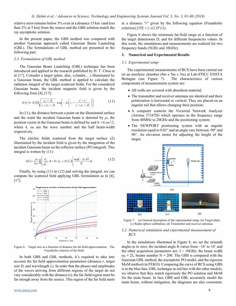
Figure 2 compares the amplitude of field calculated by GBS method and ray asymptotic solution of the Helmholtz equation. This simulation (Figure 2) has been realized as a function of the distance (r in km) from the source to the receiver. The frequency equal to 10GHz, the beam width (ω0) equal to 18λ (where λ is the wavelength) and the values of beams number (N) are : 133, 200, 400 and 600. Magenta, red, green, blue and lines correspond to the GBS solution for different beams number, respectively 133, 200, 400 and 600 over which the summation is down. The black line represents the ray asymptotic solution. We can observe, that the beam density in the vicinity of the central ray offers satisfactory accuracy. In fact, when the number of the beams is more than 200, the GBS and the ray asymptotic are in good agreement. So, as with the usual techniques of ray tracing, a high beam density (200 for this case) is necessary for high accuracy.
Figure 2: Comparison between the ray asymptotic solution and GBS method
for beam number N=133, 200, 400, 600 and beam width is 18λ.
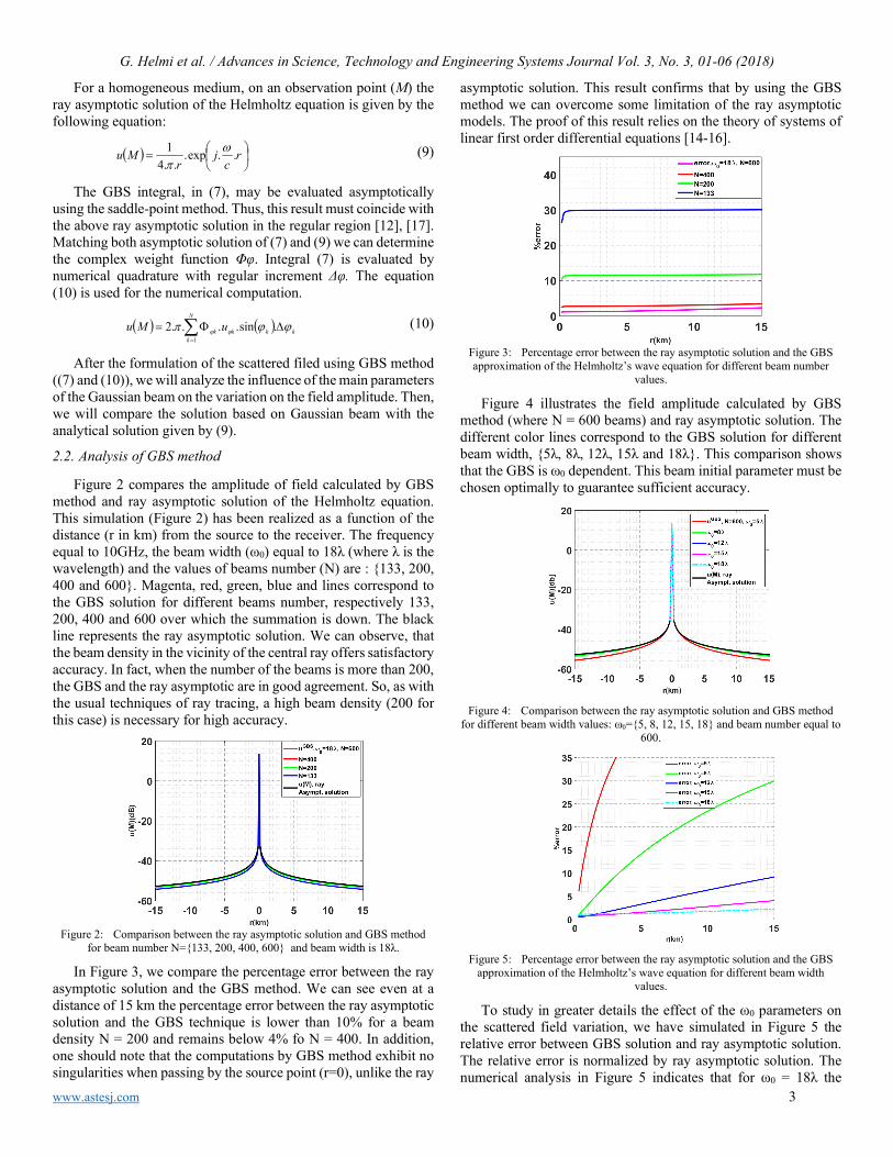
In Figure 3, we compare the percentage error between the ray asymptotic solution and the GBS method. We can see even at a distance of 15 km the percentage error between the ray asymptotic solution and the GBS technique is lower than 10% for a beam density N = 200 and remains below 4% fo N = 400. In addition, one should note that the computations by GBS method exhibit no singularities when passing by the source point (r=0), unlike the ray
asymptotic solution. This result confirms that by using the GBS method we can overcome some limitation of the ray asymptotic models. The proof of this result relies on the theory of systems of linear first order differential equations [14-16].
Figure 3: Percentage error between the ray asymptotic solution and the GBS approximation of the Helmholtz’s wave equation for different beam number
values.
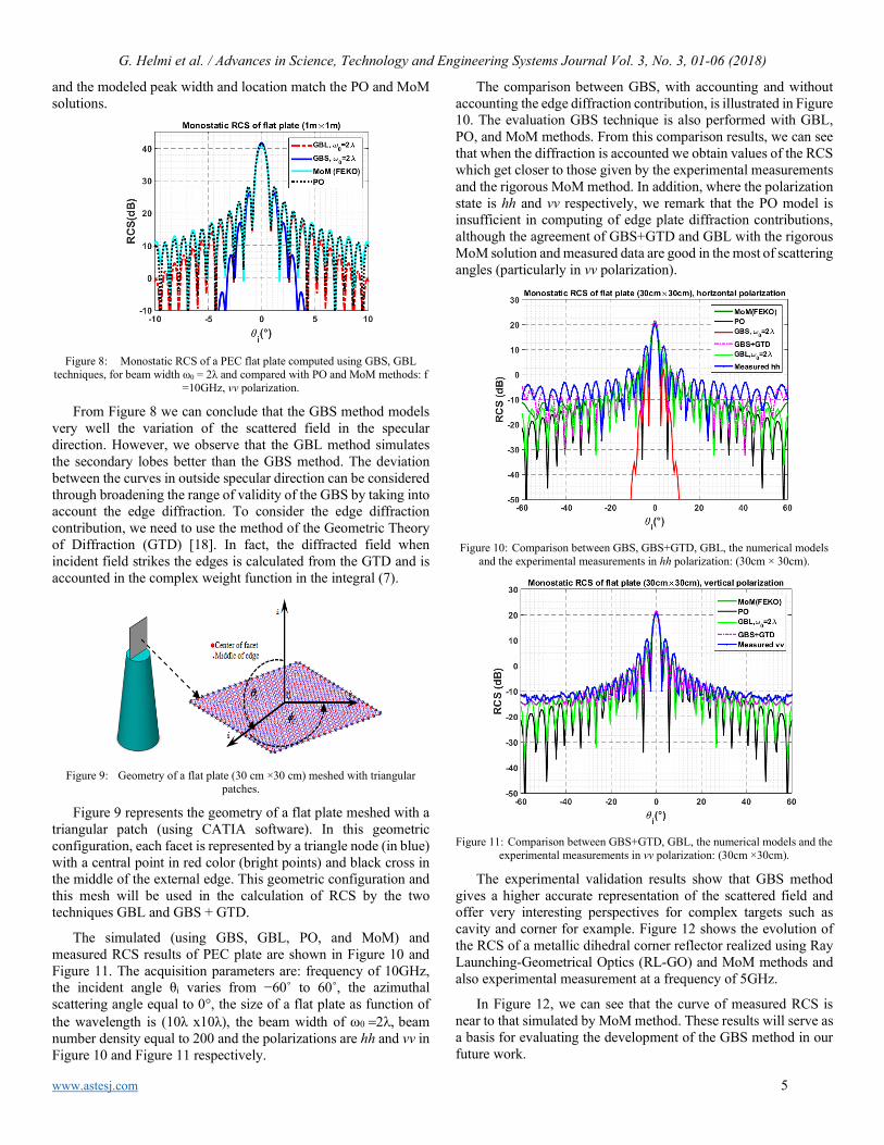
Figure 4 illustrates the field amplitude calculated by GBS method (where N = 600 beams) and ray asymptotic solution. The different color lines correspond to the GBS solution for different beam width, 5λ, 8λ, 12λ, 15λ and 18λ. This comparison shows that the GBS is ω0 dependent. This beam initial parameter must be chosen optimally to guarantee sufficient accuracy.
Figure 4: Comparison between the ray asymptotic solution and GBS method
for different beam width values: ω0=5, 8, 12, 15, 18 and beam number equal to 600.
Figure 5: Percentage error between the ray asymptotic solution and the GBS
approximation of the Helmholtz’s wave equation for different beam width values.
To study in greater details the effect of the ω0 parameters on the scattered field variation, we have simulated in Figure 5 the relative error between GBS solution and ray asymptotic solution. The relative error is normalized by ray asymptotic solution. The numerical analysis in Figure 5 indicates that for ω0 = 18λ the
G. Helmi et al. / Advances in Science, Technology and Engineering Systems Journal Vol. 3, No. 3, 01-06 (2018)
www.astesj.com 4
relative error remains below 3% even at a distance 15 km (and less than 2% at 5 km) from the source and the GBS solution match the ray asymptotic solution.
In the present paper, the GBS method was compared with another Gaussian approach called Gaussian Beam Launching (GBL). The formulations of GBL method are presented in the following part.
2.3. Formulation of GBL method
The Gaussian Beam Launching (GBL) technique has been introduced and applied in the research published by H. T. Chou et al [17]. Consider a target (plate, disc, cylinder,…) illuminated by a Gaussian beam, the GBL method is applied to calculate the radiation integral of the target scattered fields. For the considered Gaussian beam, the incident magnetic field is given by the following form [4], [17]:
( ) ( )
++
++−
+++
=iii
iii
iii
iiiii jbz
yxzjkjbz
jbHrHρρ
ρ 22
.exp.0 (11)
In (11), the distance between a point on the illuminated surface and the waist the incident Gaussian beam is denoted by ρi, the position vector in the Gaussian beam is defined by and bi =k.ω0
2/2, where k, ω0 are the wave number and the half beam-width respectively.
The electric fields scattered from the target surface (Σ) illuminated by the incident field is given by the integration of the incident Gaussian beam on the reflector surface (PO integral). This integral is written by (11):
( ) ( )( ) ( )∫∫Σ
−
×××= ds
RRkjrHeRR
ZkjrE iiz
r
...exp..4. 0
επ (12)
Finally, by using (11) in (12) and solving the integral, we can compute the scattered field applying GBL formulation as in [4], [17].
Figure 6: Target size as a function of distance for far-field approximation: The
Fraunhofer criterion of far-field.
In both GBS and GBL methods, it’s required to take into account the far-field approximation parameters (distance r, target size D, and wavelength λ). In order that the phases and amplitudes of the waves arriving from different regions of the target do not vary considerably with the distance (r), the far-field region must be far enough away from the source. This region of the far field starts
at a distance "r" given by the following equation (Fraunhofer criterion) [19]: r ≥ ((2.D2)/λ).
Figure 6 shows the minimum far-field range as a function of the target dimensions D, and for different frequencies values. In this work, the simulations and measurements are realized for two frequency bands (5GHz and 10GHz).
3. Numerical and Experimental Results
3.1. Experimental setup
The experimental measurements of RCS have been carried out on an anechoic chamber (8m x 5m x 5m) at Lab-STICC ENSTA Bretagne (see Figure 7). The characteristics of various components of measurements system are:
• All walls are covered with absorbent material; • The transmitter and receiver antennas are identical and there
polarization is horizontal or vertical. They are placed on an angular rail that allows changing their position;
• A computer controls the Vectorial Network Analyzer (Anritsu 37347D) which operates in the frequency range from 40MHz to 20GHz and the positioning system;
• The NEWPORT positioning system with an angular resolution equal to 0.01° and an angle vary between -90° and 90°. An elevation motor for adjusting the height of the target;
(a)
(b)
(c)
(d)
Figure 7: (a) General description of the experimental setup, (b) Target plate, (c) Radar sphere calibration, (d) Transmitter and receiver antennas.
3.2. Numerical simulation and experimental measurement of RCS
In the simulations illustrated in Figure 8, we set the azimuth angles φi to zero; the incident angle θi varies from −10˚ to 10˚ and the other acquisition parameters are: f = 10GHz, the beam width ω0 = 2λ, beams number N = 200. The GBS is compared with the Gaussian GBL method, the asymptotic PO model, and the rigorous MoM method (in FEKO). Comparing the curve of RCS using GBS is in the blue line, GBL technique in red line with the other models; we observe that they match rigorously the PO solution and MoM for the main beam. In fact, GBS and GBL accurately model the main beam, without mitigation, the diagrams are also consistent,
G. Helmi et al. / Advances in Science, Technology and Engineering Systems Journal Vol. 3, No. 3, 01-06 (2018)
www.astesj.com 5
and the modeled peak width and location match the PO and MoM solutions.
Figure 8: Monostatic RCS of a PEC flat plate computed using GBS, GBL
techniques, for beam width ω0 = 2λ and compared with PO and MoM methods: f =10GHz, vv polarization.
From Figure 8 we can conclude that the GBS method models very well the variation of the scattered field in the specular direction. However, we observe that the GBL method simulates the secondary lobes better than the GBS method. The deviation between the curves in outside specular direction can be considered through broadening the range of validity of the GBS by taking into account the edge diffraction. To consider the edge diffraction contribution, we need to use the method of the Geometric Theory of Diffraction (GTD) [18]. In fact, the diffracted field when incident field strikes the edges is calculated from the GTD and is accounted in the complex weight function in the integral (7).
Figure 9: Geometry of a flat plate (30 cm ×30 cm) meshed with triangular
patches.
Figure 9 represents the geometry of a flat plate meshed with a triangular patch (using CATIA software). In this geometric configuration, each facet is represented by a triangle node (in blue) with a central point in red color (bright points) and black cross in the middle of the external edge. This geometric configuration and this mesh will be used in the calculation of RCS by the two techniques GBL and GBS + GTD.
The simulated (using GBS, GBL, PO, and MoM) and measured RCS results of PEC plate are shown in Figure 10 and Figure 11. The acquisition parameters are: frequency of 10GHz, the incident angle θi varies from −60˚ to 60˚, the azimuthal scattering angle equal to 0°, the size of a flat plate as function of the wavelength is (10λ x10λ), the beam width of ω0 =2λ, beam number density equal to 200 and the polarizations are hh and vv in Figure 10 and Figure 11 respectively.
The comparison between GBS, with accounting and without accounting the edge diffraction contribution, is illustrated in Figure 10. The evaluation GBS technique is also performed with GBL, PO, and MoM methods. From this comparison results, we can see that when the diffraction is accounted we obtain values of the RCS which get closer to those given by the experimental measurements and the rigorous MoM method. In addition, where the polarization state is hh and vv respectively, we remark that the PO model is insufficient in computing of edge plate diffraction contributions, although the agreement of GBS+GTD and GBL with the rigorous MoM solution and measured data are good in the most of scattering angles (particularly in vv polarization).
Figure 10: Comparison between GBS, GBS+GTD, GBL, the numerical models and the experimental measurements in hh polarization: (30cm × 30cm).
Figure 11: Comparison between GBS+GTD, GBL, the numerical models and the experimental measurements in vv polarization: (30cm ×30cm).
The experimental validation results show that GBS method gives a higher accurate representation of the scattered field and offer very interesting perspectives for complex targets such as cavity and corner for example. Figure 12 shows the evolution of the RCS of a metallic dihedral corner reflector realized using Ray Launching-Geometrical Optics (RL-GO) and MoM methods and also experimental measurement at a frequency of 5GHz.
In Figure 12, we can see that the curve of measured RCS is near to that simulated by MoM method. These results will serve as a basis for evaluating the development of the GBS method in our future work.

G. Helmi et al. / Advances in Science, Technology and Engineering Systems Journal Vol. 3, No. 3, 01-06 (2018)
www.astesj.com 6
Figure 12: RCS of rectangular dihedral corner reflector (f = 5GHz):
Experimental and numerical models.
4. Conclusion and future work
In this study, the RCS of radar targets has been investigated by using a new technique called Gaussian Beam Summation (GBS). In the GBS technique, the total field at the receiver is represented by the integral over all Gaussian beams propagating in the vicinity of the receiver. To study the performance of the chosen GBS method, we have carried out it theoretical formulation and we have study the influence main Gaussian parameters (beams width, the density of beams number) on the field amplitude. Then, we have introduced a numerical simulation of the RCS of a PEC plate using GBS method. The results obtained using GBS were compared with those simulated trough GBL, PO and MoM methods. In addition, we have presented the experimental measurements of RCS of canonical and complex targets. The results of RCS using GBS method were compared and validated by the experimental measurements.
The study of the RCS of different complex objects (including dihedral and trihedral corner reflector) using GBS method is one of the perspectives of the work presented in this paper.
Conflict of Interest
The authors declare no conflict of interest.
Acknowledgment
We would like to thank the DGA (Direction Générale de l’Armement, France)-MRIS for their support of the SOFAGEMM project, where this work is in progress. Acknowledgments are also addressed to Mr. Hervé TRÉBAOL (Specialized Instructor Mechanical Design in ENSTA Bretagne) for these collaborations with us.
References
[1] F.Weinmann, “Ray tracing with PO/PTD for RCS modeling of large complex objects,” IEEE Trans. Antennas and Propagation., 54( 6), 1797–1806, Jun. 2006. DOI: 10.1109/TAP.2006.875910
[2] R. Harrington, “Field computation by moment methods,” Wiley-IEEE Press, 1993.
[3] H. T. Chou and P. H. Pathak, “Uniform asymptotic solution for electromagnetic reflection and diffraction of an arbitrary Gaussian beam by a smooth surface with an edge,” Radio. Science., 32(14), 1319-1336, 1997. DOI: 10.1029/97RS00713
[4] P.O. Leye, A. Khenchaf, and P. Pouliguen, “The Gaussian Beam Summation and the Gaussian Launching Methods in Scattering Problem,” J. Elect.
Analysis and Applications., 8, 219-225, 2016. DOI: 〈10.4236/jemaa.2016.810020 〉
[5] H. Ghanmi, A. Khenchaf, P. Pouliguen and P. O. Leye, “Study of RCS of complex target: Experimental measurements and Gaussian beam summation method,” IEEE Conference on Antenna Measurements & Applications (CAMA), Tsukuba, pp. 196-199, 2017. DOI: 10.1109/CAMA.2017.8273399
[6] M. Katsav and E. Heyman, “Gaussian Beam Summation Representation of Beam Diffraction by an Impedance Wedge: A 3D Electromagnetic Formulation Within the Physical Optics Approximation,” IEEE Trans. Antennas Propagation., 60(12), pp. 5843-5858, 2012. DOI: 10.1109/TAP.2012.2207694
[7] V. Červený, “Summation of paraxial Gaussian beams and of paraxial ray approximations in inhomogeneous anisotropic layered structures,” Seismic waves. Complex 3-D Structures., 10, 121–159, 2000. https://doi.org/10.1111/j.1365-246X.2009.04442.x
[8] M. M. Popov, “A new method of computation of wave fields using Gaussian beams,” Wave Motion., 4, 85-97, 1982. https://doi.org/10.1016/0165-2125(82)90016-6
[9] V. Červený, “Expansion of a Plane Wave into Gaussian Beams,” Stidia geoph. And geod., 26, 120 - 131, 1982. DOI: 10.1007/BF01582305
[10] V. Červený, “Seismic Ray Theory,” Cambridge: Cambridge University Press, 2001.
[11] M. M. Popov, “New method of computation of wave fields in high-frequency approximation,” J. Soviet Math., 20(1) ,1869–1882, 1982. https://doi.org/10.1007/BF01119372
[12] V. Červený, “Gaussian beam synthetic seismograms,” Journal. Geoph., 58, 44-72, 1985.
[13] N. R. Hill, “Gaussian beam migration,” Geophysics, 55(11), 1416-1428, 1990. https://doi.org/10.1190/1.1442788
[14] V. Červený, «Computation of wave field in homogeneous media,» Geophys. J. R. astr. Soc., 70, 109-128, 1982. DOI: 10.1111/j.1365-246X.1982.tb06394.x
[15] B. S. White, A. Norris, A. Bayliss and R. Burridge, “Some remarks on the Gaussian beam summation method,” Geoph. J. Royal. Astro. Society., 89, 579-636 , 1987. https://doi.org/10.1111/j.1365-246X.1987.tb05184.x
[16] B. Bleistein, “Mathematics of Modeling, Migration and Inversion with Gaussian Beams,” Colorado, USA, 2008. DOI: 10.3997/2214-4609.201405084
[17] H. T. Chou, P. Pathak and R. J. Burkholder, “Novel Gaussian Beam Method for the Rapid Analysis of Large Reflector Antennas,” IEEE Trans. Antennas. Propagation., 49(16), 880-893, 2001. DOI: 10.1109/8.931145
[18] J. B. Keller, “Geometrical Theory of Diffraction,” J.Optical Society of America, 52, 116 - 130, 1962. https://doi.org/10.1364/JOSA.52.000116
[19] Warren L. Stutzman, Gary A. Thiele. “Antenna Theory and Design”. John Wileys & Sons, Inc., 1997.

Advances in Science, Technology and Engineering Systems JournalVol. 3, No. 3, 7-14 (2018)
www.astesj.comASTES JournalISSN: 2415-6698
A Comparison of MIMO Tuning Controller Techniques Ap-plied to Steam Generator
Sergio Federico Yapur*, Eduardo Jose Adam
Faculty de Chemical Engineering, National University of Litoral, 3000, Argentina
A R T I C L E I N F O A B S T R A C T
Article history:Received: 10 April, 2018Accepted: 27 April, 2018Online: 10 May. 2018
Keywords:Controller TuningMIMO Process ControlStructured H∞
This work presents a comparison between controller tuning methods fora multivariable steam generator. Controller tuning has a remarkableimpact on closed loop performance. Methods selected were Single-LoopTuning (SLT), Biggest Log Modulus Tuning (BLT), Sequential Return-Difference (SRD) and StructuredH∞ Synthesis (S-H∞). Method assess-ment takes into account set-point tracking, disturbance rejection, tuningeffort and stability.
1 Introduction
Several tuning techniques coexist nowadays for indus-trial controllers. Ranging from classical frequency do-main methods for single loops to state-space controllersynthesis, there is an ever-increasing number of designoptions. Nevertheless, some of these techniques yieldno practical value in industry. This is due to incon-venient implementation, computational complexityand the prior background knowledge required in somecases. Usually, these issues are dealt concurrently witha fast-paced industrial environment, where keepingproduction rates is mandatory. In addition, most in-dustries lack testing facilities or even a reliable processsimulator to study in detail different control schemes.Which is more, knowledge in advanced control theoryis rather rare among plant engineers.
This work is an overview of different tuning tech-niques which may be of industrial interest. Based ona real plant, it aims to provide insight into the possi-ble issues of simpler tuning methods, and the effortneeded to overcome these issues with more complextechniques. In this regard, four methods were selectedwith an increasing degree of complexity. To start withSLT, which is a basic Single Input Single Output (SISO)approach. In the second place, BLT method improvesclosed-loop stability, as proposed by Luyben [1]. Be-sides, SRD tuning takes into account loop interactionsto some degree. Finally, S-H∞ method belongs to thewell knownH∞ theory, which is a rigorous scheme forcontroller synthesis [2], [3].
It is straightforward that selected methods are quitedissimilar. This was purposely set, as the goal is to findthe method with a right trade-off between industrialneeds and tuning effort. For this purpose, it is mean-ingful to highlight advantages and drawbacks of eachprocedure. Although the analysis is subject to a par-ticular plant, it is still possible to arrive some generalconclusions.
Due to the hegemony of Proportional-Integral (PI)control in the industry [4], all of the controllers in thiswork belong to this type. Furthermore, using the samecontrol structure provides a common framework fortuning method comparison.
This paper is organized as follows. Section 2 de-scribes the problem under study. Section 3 examinesrelevant features of the steam generator model, andhow they may impact on control objectives. A reviewof selected tuning methods is presented in Section 4.Afterwards, Section 5 provides a discussion over per-formance results for each tuning procedure. Finally,conclusions are presented in Section 6.
2 System Under Study
A thermal power station must be able to alter its out-put to meet a varying load demand. At the core ofthis process lies a Steam Generator (SG). This deviceregulates steam feed to the turbine, which in turn isresponsible for electricity generation. A good trackingof reference command signals is essential for a properoperation. Equally important are plant stability and
*Corresponding Author: S. Yapur, Email: [email protected]
www.astesj.com 7
https://dx.doi.org/10.25046/aj030302

S.F. Yapur / Advances in Science, Technology and Engineering Systems Journal Vol. 3, No. 3, 7-14 (2018)
disturbance rejection. Each of these objectives impacton production costs and operational safety.
The steam generator model under study was origi-nally reported by Tan, Marquez and Chen [5], and laterstudied by Adam and Valsecchi [6]. This SG is part ofcogeneration systems of Syncrude Canada Ltd. inte-grated energy facility located in Mildred Lake plantsite, Canada. Although the model is a simplification, itretains the typical attributes of an SG. Some of theseare the multivariable nature and the presence of inte-grators in the MIMO transfer function.
The model is represented by a 3×3 transfer functionmatrix. The inputs variables are listed below
u1: Feed water flow rate (kg/s)
u2: Fuel flow rate (kg/s)
u3: Attemperator spray flow rate (kg/s)
While the output variables are
y1: Drum level (m)
y2: Drum pressure (MPa)
y3: Steam temperature (C)
Figure 1 shows a simplified diagram where thesevariables are indicated.
Figure 1: Steam generator diagram
Transfer function matrix is shown in (1), whereevery Gij represents the transfer function from inputvariable i to output variable j.
Gp =
G11 G12 G13G21 G22 G23G31 G32 G33
(1)
Explicitly, the transfer functions are given by the fol-lowing expressions
G11 =0.00025
(−800.0s2 + 260.0s+ 7.0
)s (1250.0s+ 21.0)
(2)
G12 =0.008 (775.0s − 8.0)s (2000.0s+ 43.0)
(3)
G13 = 0 (4)
G21 = −0.0000395s+ 0.018
(5)
G22 =0.00251s+ 0.0157
(6)
G23 =5880.0s2 + 2015.0s+ 9.0
(1.0 · 107) s2 + 352000.0s+ 1420.0(7)
G31 = − 1.0 (1180.0s − 139.0)(1.0 · 106) s2 + 18520.0s+ 91.0
(8)
G32 =89600.0s+ 220.0
200000.0s2 + 2540.0s+ 19.0(9)
G33 =29100.0s2 − 1215.0
50000.0s2 + 5380.0s+ 52.0(10)
2.1 Operating Point
The operative conditions that assure a proper func-tioning of the boiler system in steady state are thefollowing
u01u0
2u0
3
=
40.682.102
0.0
(11)
Whereas the corresponding output variables arey0
1y0
2y0
3
=
1.06.45
466.7
(12)
Notice that units for each variable were previouslydefined. Interestingly, attemperator spray flow rate isnormally zero. The reason is that the attemperator isused only for precise regulation of steam temperaturein transient states. Any other usage of this flow rateleads to higher operative costs.
2.2 Constraints
Plant control system is subject to the following limitconstraints
0 ≤ u1 ≤ 120
0 ≤ u2 ≤ 7
0 ≤ u3 ≤ 10
−0.017 ≤ u2 ≤ 0.017 (13)
It is worth noting that u01 in (11) is relatively small
compared with the magnitude limit in (13), so thislimit does not impose a hard constraint for design.However, this is not the case for u2, as limits for fuelflow rate have a remarkable impact on the system per-formance.
www.astesj.com 8
S.F. Yapur / Advances in Science, Technology and Engineering Systems Journal Vol. 3, No. 3, 7-14 (2018)
3 Preliminary Analysis
The following paragraphs outline preliminary resultsof the open loop SG model. A prior characterizationof the plant is advisable in order to achieve a bettercontrol design. This is due to the fact that it helps tobe aware of possible issues beforehand.
3.1 Open loop stability
Open loop stability constitutes an relevant feature interms of preliminary control design. In particular, anunstable plant leads to special considerations, both forcontrol tuning and plant operation. In this case, the SGmodel presents integrator modes in matrix elementsG11 and G12. Consequently, these elements are notBounded Input Bounded Output (BIBO) stable for theopen loop configuration [7]. Moreover, Gp is a singularmatrix in steady state.
3.2 Minimum Phase
It was found that the system is non minimum phasethrough evaluation of Smith-McMillan transmissionzeros [8], as some of the zeros revealed positive realpart. Therefore, an inverse response to certain in-put may occur. The presence of this phenomena canstrongly affect control system performance.
3.3 Interactions
Some common problems of multivariable control arisefrom interactions between inputs and outputs. Aproper identification of these enables to select the mosteffective input-output channels for control purposes.In this regard, a well-known analysis is the so-calledRelative Gain Array (RGA), originally proposed byBristol [9]. However, the presence of integral modesprevents from applying this method, as steady-stategains Kij are not defined. An alternative algorithm forcomputing RGA was proposed by Hu, Cai and Xiao[10]. This generalization of the original method is ca-pable of handling both integrator and differentiatormodes. According to the algorithm proposed by Hu,Cai and Xiao, RGA is equal to
RGA =
1.2423 −0.2423 0−0.2987 1.2184 0.08030.0564 0.0239 0.9197
(14)
The RGA matrix is only meaningful for steady-stateinteractions. This result confirms that input-outputpairing suggested by Tan and Marquez [5] is suitable.Therefore, controlling output i through input i givethe best results for every i = 1,2,3. On the other hand,RGA suggests that no severe interactions are present.This is essential in order to reach a good control systemperformance.
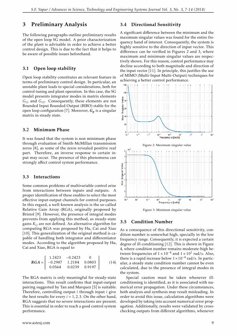
3.4 Directional Sensitivity
A significant difference between the minimum and themaximum singular values was found for the entire fre-quency band of interest. Consequently, the system ishighly sensitive to the direction of input vector. Thisdifference can be verified in Figures 2 and 3, wheremaximum and minimum singular values are respec-tively shown. For this reason, control performance maydecline according to both magnitude and direction ofthe input vector [11]. In principle, this justifies the useof MIMO (Multi-Input Multi-Output) techniques forachieving a better control performance.
Figure 2: Maximum singular value
Figure 3: Minimum singular value
3.5 Condition Number
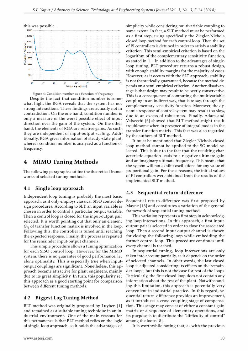
As a consequence of this directional sensitivity, con-dition number is somewhat high, specially in the lowfrequency range. Consequently, it is expected a certaindegree of ill-conditioning [12]. This is shown in Figure4, where condition number remains moderate-high be-tween frequencies of 1× 10⁻⁴ and 1× 101 rad/s. Also,there is a rapid increase below 1×10⁻⁴ rad/s. In partic-ular, a steady state condition number cannot be evencalculated, due to the presence of integral modes inthe system.
Special caution must be taken whenever ill-conditioning is identified, as it is associated with nu-merical error propagation. Under these circumstances,both analysis and synthesis may result misleading. Inorder to avoid this issue, calculation algorithms weredeveloped by taking into account numerical error prop-agation. Additionally, results were validated by cross-checking outputs from different algorithms, whenever
www.astesj.com 9
S.F. Yapur / Advances in Science, Technology and Engineering Systems Journal Vol. 3, No. 3, 7-14 (2018)
this was possible.
Figure 4: Condition number as a function of frequency
Despite the fact that condition number is some-what high, the RGA reveals that the system has notstrong interactions. These findings are actually not incontradiction. On the one hand, condition number isonly a measure of the worst possible effect of inputdirection over the gain of the system. On the otherhand, the elements of RGA are relative gains. As such,they are independent of input-output scaling. Addi-tionally, RGA gives information of steady-state plant,whereas condition number is analyzed as a function offrequency.
4 MIMO Tuning Methods
The following paragraphs outline the theoretical frame-works of selected tuning methods.
4.1 Single loop approach
Independent loop tuning is probably the most basicapproach, as it only employs classical SISO control de-sign procedures. According to SLT, an input variable ischosen in order to control a particular output variable.Then a control loop is closed for the input-output pairselected. It is worth pointing out that only an elementGij of transfer function matrix is involved in the loop.Following this, the controller is tuned until reachingthe expected response. Finally, the process is repeatedfor the remainder input-output channels.
This simple procedure allows a tuning optimizationfor each SISO control loop. However, for the MIMOsystem, there is no guarantee of good performance, letalone optimality. This is especially true when input-output couplings are significant. Nonetheless, this ap-proach became attractive for plant engineers, mainlydue to its great simplicity. In turn, this popularity setthis approach as a good starting point for comparisonbetween different tuning methods.
4.2 Biggest Log Tuning Method
BLT method was originally proposed by Luyben [1]and remained as a suitable tuning technique in an in-dustrial environment. One of the main reasons forthis permanence is that BLT method relies on the logicof single-loop approach, so it holds the advantages of
simplicity while considering multivariable coupling tosome extent. In fact, a SLT method must be performedas a first step, using specifically the Ziegler-Nicholsclosed loop method for each control loop. Then the setof PI controllers is detuned in order to satisfy a stabilitycriterion. This semi-empirical criterion is based on thelogarithm of the complementary sensitivity function,as stated in [1]. In addition to the advantages of single-loop tuning, BLT procedure returns a robust design,with enough stability margins for the majority of cases.However, as it occurs with the SLT approach, stabilityis not theoretically guaranteed, because the method de-pends on a semi-empirical criterion. Another disadvan-tage is that design may result to be overly conservative.This is a consequence of computing the multivariablecoupling in an indirect way, that is to say, through thecomplementary sensitivity function. Moreover, the dy-namic response of control system may result too slow,due to an excess of robustness. Finally, Adam andValsecchi [6] showed that BLT method might resulttroublesome when in presence of integral modes in thetransfer function matrix. This fact was also regardedby the authors of BLT method.
It must be mentioned that Ziegler-Nichols closedloop method cannot be applied to the SG model se-lected. This is due to the fact that the resulting char-acteristic equation leads to a negative ultimate gainand an imaginary ultimate frequency. This means thatthe system will not exhibit oscillations for any value ofproportional gain. For these reasons, the initial valuesof PI controllers were obtained from the results of theimplemented SLT method.
4.3 Sequential return-difference
Sequential return-difference was first proposed byMayne [13] and constitutes a variation of the generalframework of sequential tuning method.
This variation represents a first step in acknowledg-ing loop interactions. In this approach, a first input-output pair is selected in order to close the associatedloop. Then a second input-output channel is chosenfor closing the following loop while embedding theformer control loop. This procedure continues untilevery channel is reached.
In sequential tuning, loop interactions are onlytaken into account partially, as it depends on the orderof selected channels. In other words, the last closedloop is adjusted considering its effects on the remain-der loops; but this is not the case for rest of the loops.Particularly, the first closed loop does not contain anyinformation about the rest of the plant. Notwithstand-ing this limitation, this approach is potentially veryconvenient in industrial practice. In this regard, se-quential return-difference provides an improvement,as it introduces a cross-coupling stage of compensa-tion. This stage may consist of either a constant-gainmatrix or a sequence of elementary operations, andits purpose is to distribute the ”difficulty of control”among the loops [8].
It is worthwhile noting that, as with the previous
www.astesj.com 10
S.F. Yapur / Advances in Science, Technology and Engineering Systems Journal Vol. 3, No. 3, 7-14 (2018)
methods, sequential return-difference offers no guaran-tee of stability, nor even a good performance is assured.
4.4 StructuredH∞ method
Theory of H∞-control started with the work of Zames[14]. Since then, several methods were derived to syn-thesize controllers that achieve stabilization with guar-anteed performance. While some of these techniqueswere formulated in state-space representation, othersbelong to the frequency domain. In any case, they allfeature an optimization problem, by minimizing anH∞-type norm of a certain cost function.
Nonetheless, H∞ methods usually yield non struc-tured, high order controllers, even when some ofthese methods consider structured uncertainty, likeµ-synthesis. Non structured controllers are difficult toimplement in practice. Also, controller equation gen-erally lacks integral action [12]. To avoid these draw-backs, in this work we adopted the approach givenby Apkarian and Noll [2]. This is the first formula-tion suited to obtain structured controllers, such asPID, which have a straight industrial instrumentation.Hence this strategy is known as Structured-H∞ Syn-thesis. At the core of this method, minimization of anon smooth, non convex and discontinuous functionalmust be performed. This optimization is an NP-hardproblem, so it requires both computational power andattention to convergence issues, being these the maindisadvantages. Among the benefits, PID controllersare optimized, in contrast with classical theory, werecontrollers are simply tuned. Additionally, the result-ing controller stabilizes internally the control system[12]. Finally, this method admits constraints in thedesign problem, an important feature in practical ap-plications.
5 Results
5.1 Controller Parameters
Table 1 reports controller parameters obtained witheach of the methods previously introduced. Notice thatSLT gains are generally higher. This suggests a fasterdynamics, but also a less robust design. However, ro-bustness may be highly desirable in the presence ofloop interactions and process variability, just to namea few potential issues.
On the other hand, BLT method presents lowergains and higher integral time constants than SLT pro-cedure. This is expected, as BLT aims to improve ro-bustness by detuning SLT parameters.
A remarkable feature of SRD values is its parametervariability. Particularly, integral times differ up to fiveorders of magnitude. This might be possibly due tothe cross-coupling stage of compensation, which wasmentioned above.
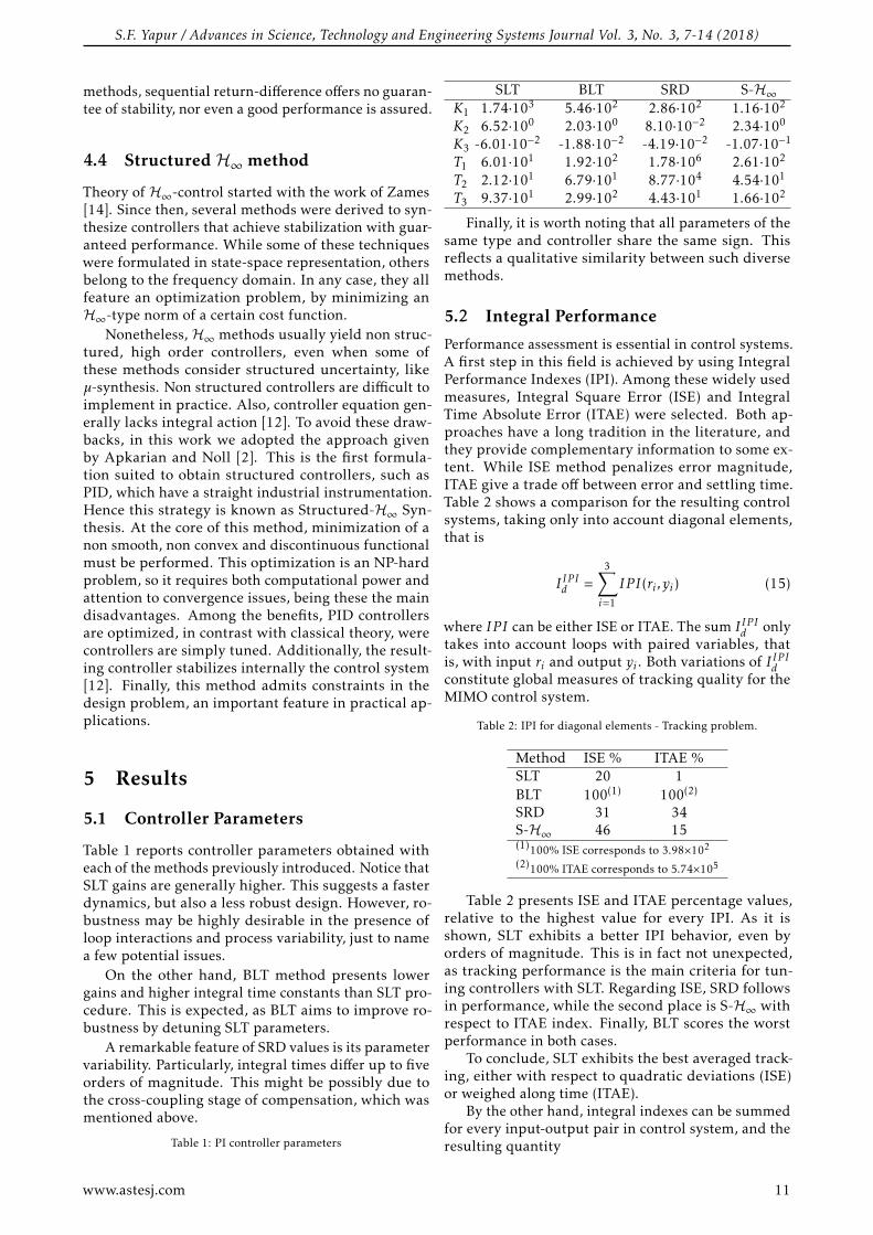
Table 1: PI controller parameters
SLT BLT SRD S-H∞K1 1.74·103 5.46·102 2.86·102 1.16·102
K2 6.52·100 2.03·100 8.10·10−2 2.34·100
K3 -6.01·10−2 -1.88·10−2 -4.19·10−2 -1.07·10−1
T1 6.01·101 1.92·102 1.78·106 2.61·102
T2 2.12·101 6.79·101 8.77·104 4.54·101
T3 9.37·101 2.99·102 4.43·101 1.66·102
Finally, it is worth noting that all parameters of thesame type and controller share the same sign. Thisreflects a qualitative similarity between such diversemethods.
5.2 Integral Performance
Performance assessment is essential in control systems.A first step in this field is achieved by using IntegralPerformance Indexes (IPI). Among these widely usedmeasures, Integral Square Error (ISE) and IntegralTime Absolute Error (ITAE) were selected. Both ap-proaches have a long tradition in the literature, andthey provide complementary information to some ex-tent. While ISE method penalizes error magnitude,ITAE give a trade off between error and settling time.Table 2 shows a comparison for the resulting controlsystems, taking only into account diagonal elements,that is
I IP Id =3∑i=1
IP I(ri , yi) (15)
where IP I can be either ISE or ITAE. The sum I IP Id onlytakes into account loops with paired variables, thatis, with input ri and output yi . Both variations of I IP Idconstitute global measures of tracking quality for theMIMO control system.
Table 2: IPI for diagonal elements - Tracking problem.
Method ISE % ITAE %SLT 20 1BLT 100(1) 100(2)
SRD 31 34S-H∞ 46 15(1)100% ISE corresponds to 3.98×10²
(2)100% ITAE corresponds to 5.74×10⁵
Table 2 presents ISE and ITAE percentage values,relative to the highest value for every IPI. As it isshown, SLT exhibits a better IPI behavior, even byorders of magnitude. This is in fact not unexpected,as tracking performance is the main criteria for tun-ing controllers with SLT. Regarding ISE, SRD followsin performance, while the second place is S-H∞ withrespect to ITAE index. Finally, BLT scores the worstperformance in both cases.
To conclude, SLT exhibits the best averaged track-ing, either with respect to quadratic deviations (ISE)or weighed along time (ITAE).
By the other hand, integral indexes can be summedfor every input-output pair in control system, and theresulting quantity
www.astesj.com 11
S.F. Yapur / Advances in Science, Technology and Engineering Systems Journal Vol. 3, No. 3, 7-14 (2018)
I IP Ia =3∑i=1
3∑j=1
IP I(ri , yj ) (16)
reveals information about disturbance rejection, as di-agonal integrals are negligible with respect to non di-agonal ones. Table 3 presents these data as percentages,relative to the highest value for every IPI.
Table 3: IPI for whole system - Disturbance rejection
Method ISE % ITAE %SLT 11 2BLT 100(1) 100(2)
SRD 20 21S-H∞ 3 5(1)100% ISE corresponds to 1.83×10⁷
(2)100% ITAE corresponds to 2.58×10⁸
Following Table 3, S-H∞method shows the best dis-turbance rejection under ISE criteria, while SLT holdsthe first place with respect to ITAE index. Once again,BLT method shows the worst performance.
5.3 Dynamic Response
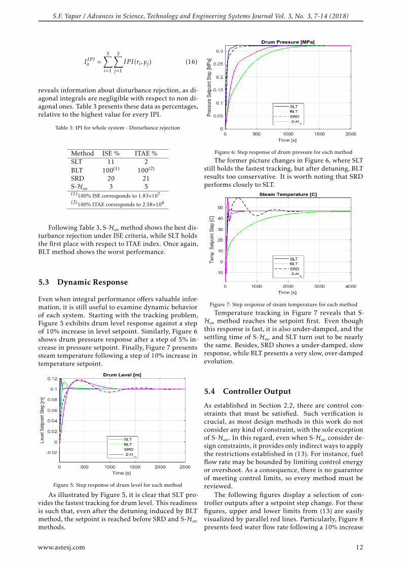
Even when integral performance offers valuable infor-mation, it is still useful to examine dynamic behaviorof each system. Starting with the tracking problem,Figure 5 exhibits drum level response against a stepof 10% increase in level setpoint. Similarly, Figure 6shows drum pressure response after a step of 5% in-crease in pressure setpoint. Finally, Figure 7 presentssteam temperature following a step of 10% increase intemperature setpoint.
Figure 5: Step response of drum level for each method
As illustrated by Figure 5, it is clear that SLT pro-vides the fastest tracking for drum level. This readinessis such that, even after the detuning induced by BLTmethod, the setpoint is reached before SRD and S-H∞methods.
Figure 6: Step response of drum pressure for each method
The former picture changes in Figure 6, where SLTstill holds the fastest tracking, but after detuning, BLTresults too conservative. It is worth noting that SRDperforms closely to SLT.
Figure 7: Step response of steam temperature for each method
Temperature tracking in Figure 7 reveals that S-H∞ method reaches the setpoint first. Even thoughthis response is fast, it is also under-damped, and thesettling time of S-H∞ and SLT turn out to be nearlythe same. Besides, SRD shows a under-damped, slowresponse, while BLT presents a very slow, over-dampedevolution.
5.4 Controller Output
As established in Section 2.2, there are control con-straints that must be satisfied. Such verification iscrucial, as most design methods in this work do notconsider any kind of constraint, with the sole exceptionof S-H∞. In this regard, even when S-H∞ consider de-sign constraints, it provides only indirect ways to applythe restrictions established in (13). For instance, fuelflow rate may be bounded by limiting control energyor overshoot. As a consequence, there is no guaranteeof meeting control limits, so every method must bereviewed.
The following figures display a selection of con-troller outputs after a setpoint step change. For thesefigures, upper and lower limits from (13) are easilyvisualized by parallel red lines. Particularly, Figure 8presents feed water flow rate following a 10% increase
www.astesj.com 12
S.F. Yapur / Advances in Science, Technology and Engineering Systems Journal Vol. 3, No. 3, 7-14 (2018)
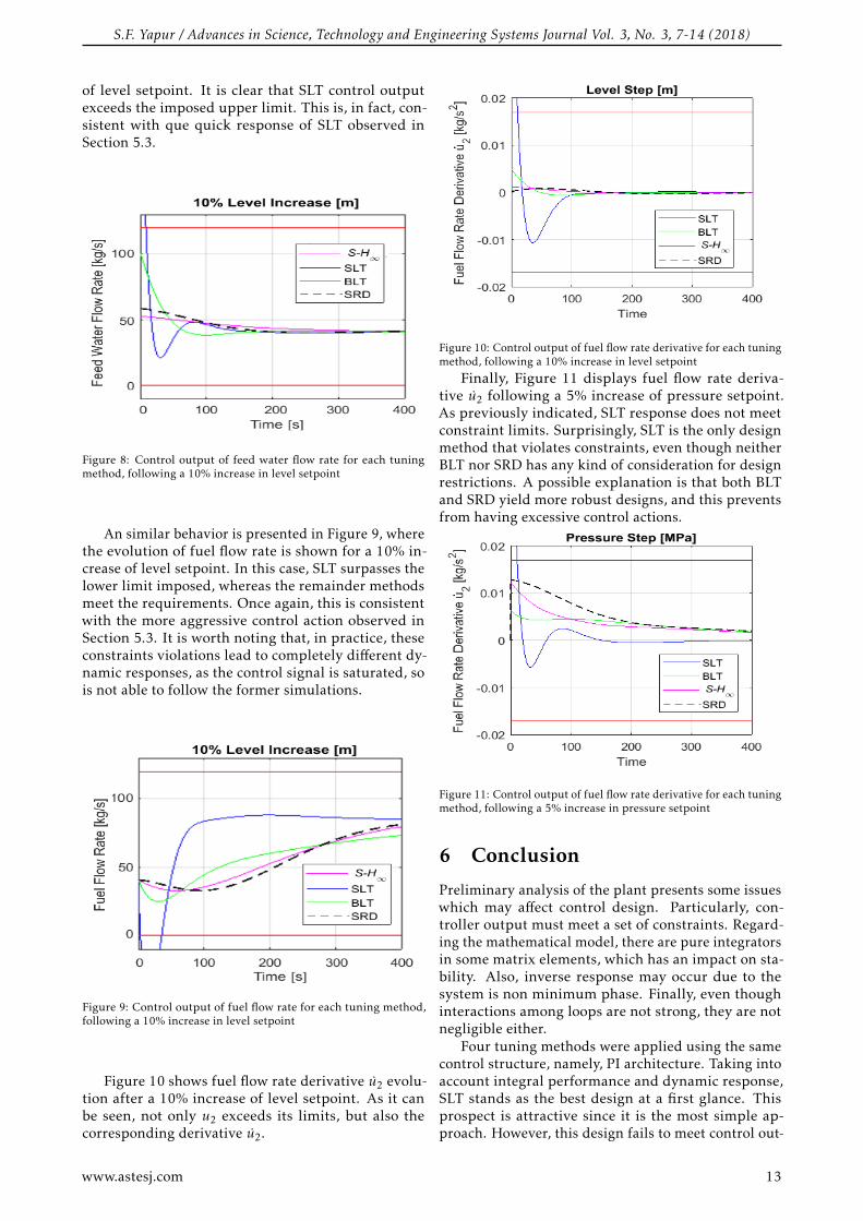
of level setpoint. It is clear that SLT control outputexceeds the imposed upper limit. This is, in fact, con-sistent with que quick response of SLT observed inSection 5.3.
Figure 8: Control output of feed water flow rate for each tuningmethod, following a 10% increase in level setpoint
An similar behavior is presented in Figure 9, wherethe evolution of fuel flow rate is shown for a 10% in-crease of level setpoint. In this case, SLT surpasses thelower limit imposed, whereas the remainder methodsmeet the requirements. Once again, this is consistentwith the more aggressive control action observed inSection 5.3. It is worth noting that, in practice, theseconstraints violations lead to completely different dy-namic responses, as the control signal is saturated, sois not able to follow the former simulations.
Figure 9: Control output of fuel flow rate for each tuning method,following a 10% increase in level setpoint
Figure 10 shows fuel flow rate derivative u2 evolu-tion after a 10% increase of level setpoint. As it canbe seen, not only u2 exceeds its limits, but also thecorresponding derivative u2.
Figure 10: Control output of fuel flow rate derivative for each tuningmethod, following a 10% increase in level setpoint
Finally, Figure 11 displays fuel flow rate deriva-tive u2 following a 5% increase of pressure setpoint.As previously indicated, SLT response does not meetconstraint limits. Surprisingly, SLT is the only designmethod that violates constraints, even though neitherBLT nor SRD has any kind of consideration for designrestrictions. A possible explanation is that both BLTand SRD yield more robust designs, and this preventsfrom having excessive control actions.
Figure 11: Control output of fuel flow rate derivative for each tuningmethod, following a 5% increase in pressure setpoint
6 Conclusion
Preliminary analysis of the plant presents some issueswhich may affect control design. Particularly, con-troller output must meet a set of constraints. Regard-ing the mathematical model, there are pure integratorsin some matrix elements, which has an impact on sta-bility. Also, inverse response may occur due to thesystem is non minimum phase. Finally, even thoughinteractions among loops are not strong, they are notnegligible either.
Four tuning methods were applied using the samecontrol structure, namely, PI architecture. Taking intoaccount integral performance and dynamic response,SLT stands as the best design at a first glance. Thisprospect is attractive since it is the most simple ap-proach. However, this design fails to meet control out-
www.astesj.com 13

S.F. Yapur / Advances in Science, Technology and Engineering Systems Journal Vol. 3, No. 3, 7-14 (2018)
put limits. For this reason, SLT turns out to be mislead-ing and must be discarded as a valid solution. By con-trast, BLT technique, which comes from detuning SLTparameters, achieves an excessive robustness. This isconfirmed with the slow dynamic responses of Figures6 and 7. In this way, only SRD and S-H∞ provide sat-isfactory designs. These two techniques imply similartuning effort, being SRD slightly more straightforwardbecause it has less possible tuning goals. Nonetheless,integral performance shows that S-H∞ outperformsSRD regarding setpoint tracking, as ITAE index dif-fers by an order of magnitude from that of SRD, whileISE indexes stay on the same order of magnitude forboth techniques. In addition, S-H∞ offers a superiordisturbance rejection than SRD for ISE as well as ITAEindexes.
Another reason for which S-H∞ turns out to be aconvincing option is that this method guarantees in-ternal stability. Even though no stability issues werepresented for this plant, it remains a desirable feature.
To sum up, S-H∞ yields the best design, justifyingthe additional computational cost and tuning effortthat it requires. Another useful conclusion is that it iseasy to misjudge the best design performance withouta careful analysis. Finally, it is worthwhile noting theimportance of considering constraints along the designprocess, in order to avoid further revisions. In fact,operative constraints are ubiquitous in every practicalsystem.
Conflict of Interest The authors declare no conflictof interest.
References[1] W. L. Luyben. Simple method for tuning siso controllers in mul-
tivariable systems. Ind. Eng. Chem. Process Des., 25:654–660,
1986.
[2] P. Apkarian and D. Noll. Nonsmooth H∞-synthesis. IEEETransactions of Automatic Control, 51:229–244, 2006.
[3] P. Apkarian and D. Noll. Structured H∞-control of infinitedimensional systems. International Journal of Robust and Non-linear Control, 2018.
[4] E. Adam. Instrumentacion y Control de Procesos: Notas de Clase.Universidad Nacional del Litoral, 2011.
[5] W. Tan and H. J. Marquez. Stabilizer design for industrial co-generation systems. Control Engineering Practice, 10:615–624,2002.
[6] E. J. Adam and C. J. Valsecchi. Multiloop control applied tointegrator mimo processes. XXII Interamerican Confederation ofChemical Engineering, page 18, 2006.
[7] D. Gu, P. Petkov, and M. Konstantinov. Robust Control Designwith Matlab. Springer, 2005.
[8] J. M. Maciejowski. Multivariable Feedback Design. Addison-Wesley, 1989.
[9] E. Bristol. On a new measure of interaction for multivari-able process control. IEEE Transactions on Automatic Control,11:133–134, 1966.
[10] W. Hu, W. Cai, and G. Xiao. Relative gain array for mimoprocesses containing integrators and/or differentiators. 11thInternational Conference on Control Automation Robotics andVision, 1:6, 2010.
[11] S. Skogestad and I. Postlethwaite. Multivariable Feedback Con-trol - Analysis and Design. Wiley, 1996.
[12] K. Zhou and J. C. Doyle. Essentials of Robust Control. PrenticeHall, 1999.
[13] D. Q. Mayne. The design of linear multivariable systems. Au-tomatica, 9:201–207, 1973.
[14] G. Zames. Feedback and optimal sensitivity: Model referencetransformations, multiplicative seminorms, and approximateinverses. IEEE Transactions on Automatic Control IEEE, 26:301–320, 1981.
www.astesj.com 14
www.astesj.com 15
Design of True Random Numbers Generators with Ternary Physical Unclonable Functions Bertrand Francis Cambou*
School of Informatics Computing and Cyber Systems, Northern Arizona University, Flagstaff, 86004, USA
A R T I C L E I N F O A B S T R A C T
Article history: Received: 06 April, 2018 Accepted: 02May, 2018 Online: 07 May, 2018
Memory based ternary physical unclonable functions contain cells with fuzzy states that are exploited to create multiple sources of physical randomness, and design true random numbers generators. A XOR compiler enhances the randomness of the binary data streams generated with such components, while a modulo-3 addition enhances the randomness of the native ternary data streams, also generated with the same method. Deviations from perfect randomness of these random numbers, in terms of probability to be non-random, was reported as low as 10-10 in the experimental section of this paper, which is considered as extremely random based on NIST criteria.
Keywords: Random numbers generators Physical unclonable functions Ternary states
Introduction
This paper is an extension of the work presented at the annual computing SAI conference, London, July 2017 [1]. The strengthening of cryptographic protocols with random numbers [2-4] is widely accepted as mandatory to secure networks of cyber physical systems (CPS). Both pseudo random numbers generators (PRNG) that use mathematical methods [5-8] and true random numbers generators (TRNG) that exploit physical elements [9-11] are mainstream. The randomness based on mathematical algorithms for PRNGs could be weak when crypto-analysts armed with powerful computers know the algorithms. Such algorithms can also consume too much computing power, which may be a problem for small internet of things (IoT) peripherals. The need to quantify the randomness of PRNG, and TRNG is of prime importance [12-15]. Physical Unclonable functions (PUF) can be valuable sources of natural randomness [16-17], they have been adopted for the design of true random number generators (TRNG). However, the randomness of the physical elements is not always acceptable when subjected to temperature changes, aging, electromagnetic interferences, and other parametric drifts. The PUFs can be too predictable in some circumstances, which is not necessarily conducive to the design of quality TRNGs that rely on physical randomness to generate a fresh random number at every query.
We are presenting how ternary PUFs contain fuzzy elements that are excellent sources of randomness. The method is based on the identification of the cells of memory based PUFs that are naturally unstable under repetitive queries. When tested, the fuzzy cells can switch back and forth randomly between “1” and
”0”, thereby generating random data streams. We are presenting three complementary elements: i) how a XOR data compiler, which process the data available
from multiple ternary cells, can create an extremely high level of randomness [18-21];
ii) how a probabilistic model allows the quantification of the level of randomness of the TRNG;
iii) how the method can be extended to the generation of native ternary random numbers with modulo-3 addition.
Designing a random number generator
2.1. Ternary physical unclonable functions
There is a growing interest in securing CPS’s with Physically Unclonable Functions (PUFs) to strengthen security when deployed in the cryptographic processes using a powerful set of physically derived cryptographic primitives [22-26]. PUFs act as virtual fingerprints for the hardware during the authentication processes to effectively block cyber thefts, Trojans, and malwares [27-34]. With error correcting methods, the PUFs can also generate cryptographic keys for symmetrical encryption schemes [35-36]. The inherent randomness, unclonability, secrecy, and physical nature of most PUFs makes it extremely hard to inspect during side channel attacks, or when lost to the enemy.
2.2. Quality considerations for PUFs
The PUFs, regardless of their design, must exhibit enough predictability overtime for reliable authentications, or encryption. The reference patterns of the PUFs that are
ASTESJ
ISSN: 2415-6698
*Bertrand Francis Cambou, Email : [email protected]
Advances in Science, Technology and Engineering Systems Journal Vol. 3, No. 3, 15-29 (2018)
www.astesj.com
Special Issue on Advancement in Engineering Technology
https://dx.doi.org/10.25046/aj030303
B.F. Cambou / Advances in Science, Technology and Engineering Systems Journal Vol. 3, No. 3, 15-29 (2018)
16
generated up front during the setup of protocol, called challenges, are compared over the life of the component with freshly generated patterns, called responses, during the authentication cycles. Quality PUFs need low challenge-response-pair (CRP) error rates, the intra-PUF challenge-response Hamming distance must be small enough to insure small level of false rejection rates (FRR). The PUF challenges should act as predictable “digital fingerprints” of the component, while the responses should be easily recognizable as a measurement of the same “digital fingerprints”. Error rates in the 3-7% range are usually acceptable when combined with error correcting techniques [35-36]. PUFs exploit the device-to-device randomness that is created during the manufacturing process of micro-components; it is desirable that the average inter-PUF hamming distance between different PUFs, divided by the length of the PUFs, should be in the 50% range to insure low level of false acceptance rates (FAR). This is achievable when the level of intra-PUF randomness, also called entropy, is high enough. PUFs with longer streams of bits have therefore higher entropy, and lower FAR. 128-bit CRPs, or higher, are usually required for this purpose.
Another important figure of merit for PUFs is the number of available CRP configurations for a unit. Strong PUFs, as opposed to weak PUFs, contains large quantities of possible CRPs that are addressable. For example, a ring oscillator PUF with 128 rings is a strong PUF. The number of possible pairing of two rings is N =1282 = 16,256. If the protocol use 128-bit long CRPs, the number of possible challenges of 2128, offers satisfactory entropy, and a low collision rate of the pairs. A memory PUF with random addressing capabilities is even stronger [36, 39-40]. For example, when the capacity of the memory is in the mega-byte range, millions of configurations are providing an entropy much higher than a 128-ring oscillator with “only” 16,256 possible configurations. Existing PUFs can have limitations, and lack of trustworthiness that could create a false sense of security. The signatures of PUFs are derived from intrinsic manufacturing variations, which could become predictable due fabrication excursions. Properties such as critical dimensions of printed structures, doping levels of semiconducting layers, and threshold voltages should make each device unique and identifiable from all other devices, abnormal operations during the manufacturing process could alter such randomness. When subject to changes related to temperature, voltage, EMI, aging, and other environmental factors these parameters can drift over time, the undesirable result, is weak PUFs with CRP error rates as high of 20%.
The main objective in designing ternary PUFs is to resolve some of these issues, and to reduce the CRP error rates by eliminating fuzzy CRPs during challenge generation. The figure of merit is to achieve trustworthy and robust intra-PUF CRP matching rates with low FRR during authentications, without increasing FAR during inter-PUF authentication of malicious challenges. The by-product of such design is the design of highly random TRNG with the fuzzy cells.
2.3. Memory based PUFs
The methods to design PUFs and TRNGs with SRAM memories have been published SRAM [36-38]. SRAM based PUFs have been successfully commercialized. When powered
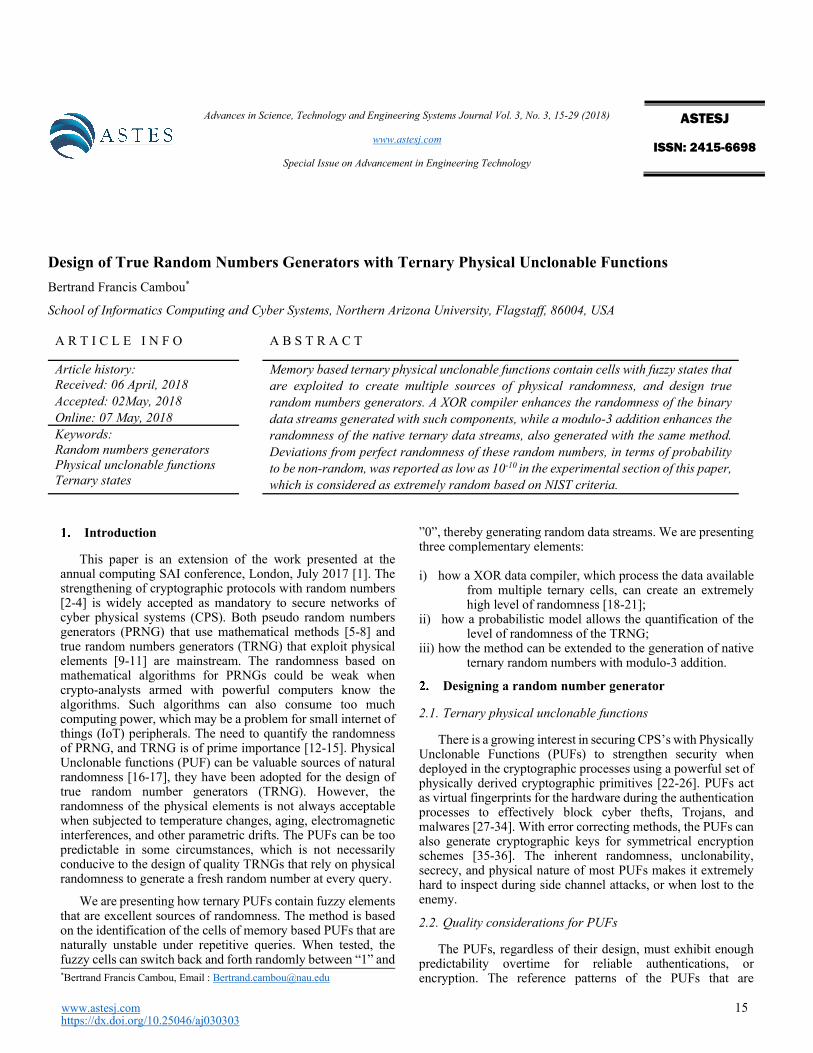
up, each SRAM cells naturally flip to store either a 0, or a 1. In most of the cases, arrays of SRAM cells return to a similar pattern characteristic, i.e. a similar finger print. SRAM based PUFs designed with this feature can be reliable, however heavy error correcting methods are usually needed. The SRAM based PUFs are not particularly immune to side channel attacks. Significant research efforts have been published regarding the design of PUFs with Flash RAMs [39-40], DRAMs [41-44], magnetic RAMs [45-46], and resistive RAMs [47-49]]. The cryptographic protocols leveraging memory PUFs are in general distinct from the ones developed with other mainstream PUFs such as ring oscillators, or gate delay arbiters. As shown in Fig. 1, the value of a parameter P is measured on each cell, and is compared with a threshold. The cells with parameter P below the threshold are “0”s, and are “1”s above the threshold. Examples of parameter P selected to design memory PUFs include: threshold voltages of Flash cells after fixed time programming; charges left on DRAM cells without refresh; high resistance value of MRAM cells after programming; and Vset of ReRAM cells.
Figure 1: Diagram explaining the design of memory based PUF with a
parameter P, and a threshold to sort out the states 0 and 1.
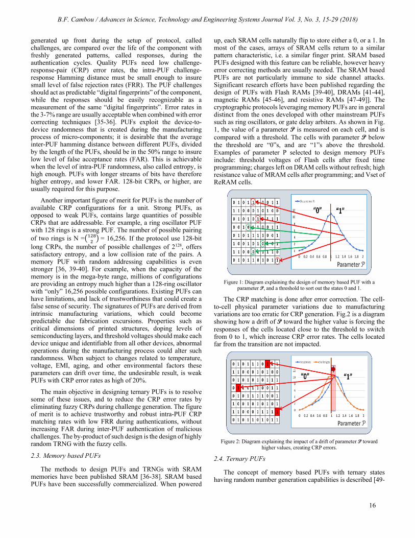
The CRP matching is done after error correction. The cell-to-cell physical parameter variations due to manufacturing variations are too erratic for CRP generation. Fig.2 is a diagram showing how a drift of P toward the higher value is forcing the responses of the cells located close to the threshold to switch from 0 to 1, which increase CRP error rates. The cells located far from the transition are not impacted.
Figure 2: Diagram explaining the impact of a drift of parameter P toward
higher values, creating CRP errors.
2.4. Ternary PUFs
The concept of memory based PUFs with ternary states having random number generation capabilities is described [49-
B.F. Cambou / Advances in Science, Technology and Engineering Systems Journal Vol. 3, No. 3, 15-29 (2018)
17
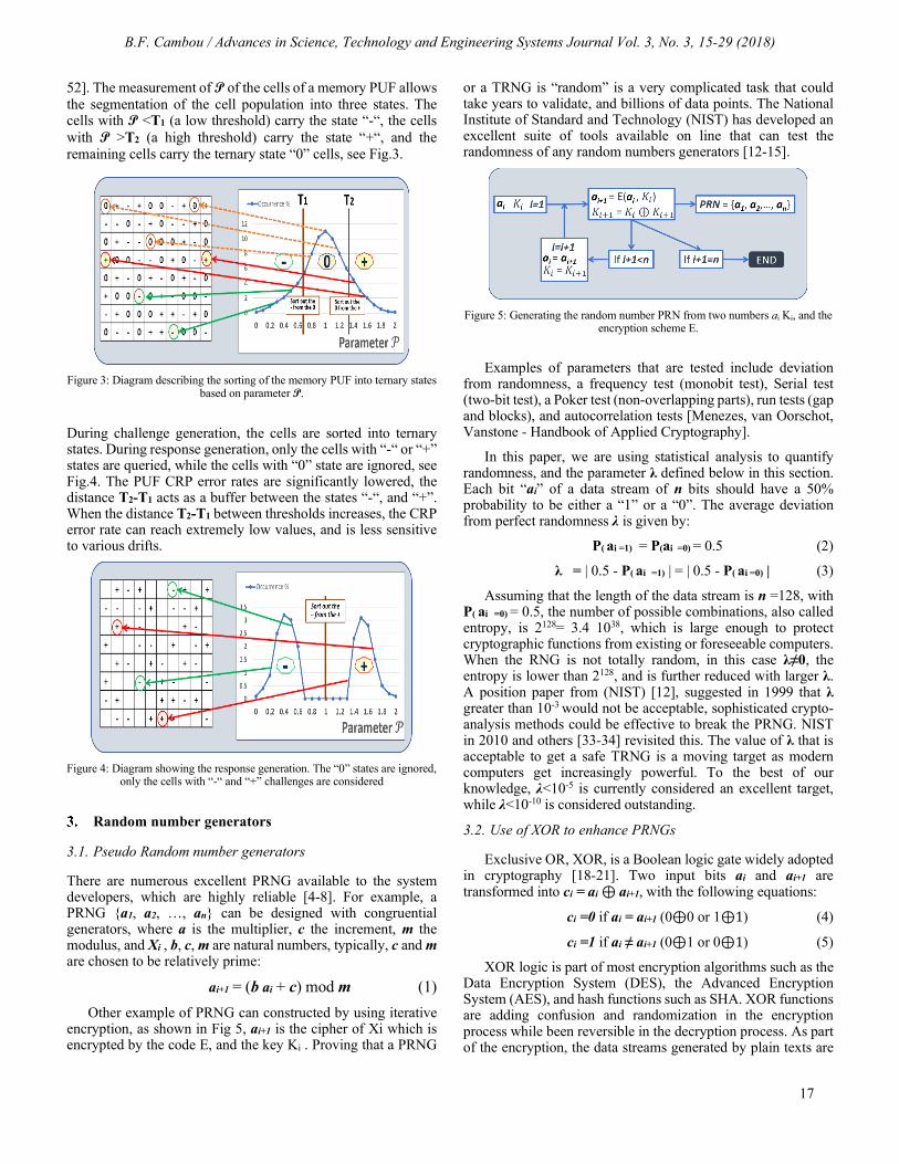
52]. The measurement of P of the cells of a memory PUF allows the segmentation of the cell population into three states. The cells with P <T1 (a low threshold) carry the state “-“, the cells with P >T2 (a high threshold) carry the state “+“, and the remaining cells carry the ternary state “0” cells, see Fig.3.
Figure 3: Diagram describing the sorting of the memory PUF into ternary states
based on parameter P.
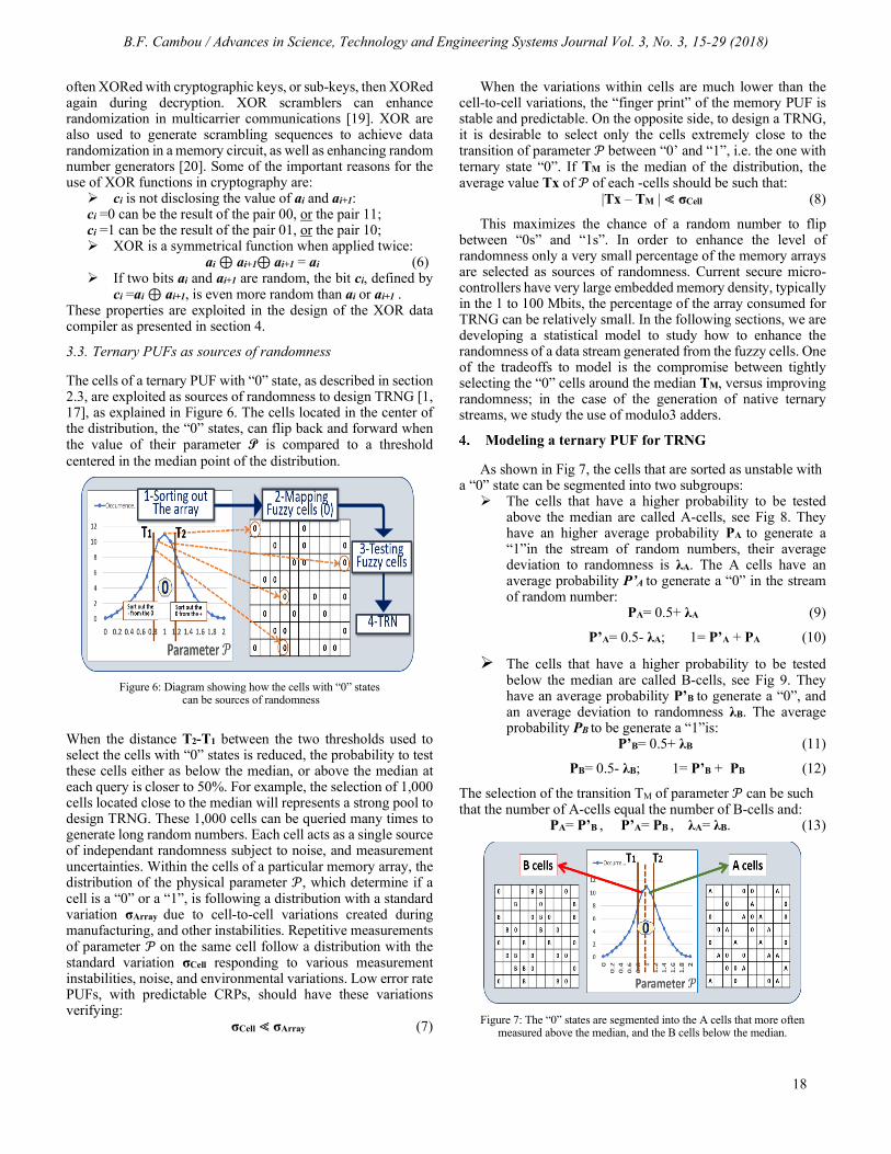
During challenge generation, the cells are sorted into ternary states. During response generation, only the cells with “-“ or “+” states are queried, while the cells with “0” state are ignored, see Fig.4. The PUF CRP error rates are significantly lowered, the distance T2-T1 acts as a buffer between the states “-“, and “+”. When the distance T2-T1 between thresholds increases, the CRP error rate can reach extremely low values, and is less sensitive to various drifts.
Figure 4: Diagram showing the response generation. The “0” states are ignored,
only the cells with “-“ and “+” challenges are considered
Random number generators
3.1. Pseudo Random number generators
There are numerous excellent PRNG available to the system developers, which are highly reliable [4-8]. For example, a PRNG a1, a2, …, an can be designed with congruential generators, where a is the multiplier, c the increment, m the modulus, and Xi , b, c, m are natural numbers, typically, c and m are chosen to be relatively prime:
ai+1 = (b ai + c) mod m (1) Other example of PRNG can constructed by using iterative encryption, as shown in Fig 5, ai+1 is the cipher of Xi which is encrypted by the code E, and the key Ki . Proving that a PRNG
or a TRNG is “random” is a very complicated task that could take years to validate, and billions of data points. The National Institute of Standard and Technology (NIST) has developed an excellent suite of tools available on line that can test the randomness of any random numbers generators [12-15].
Figure 5: Generating the random number PRN from two numbers ai Ki, and the
encryption scheme E.
Examples of parameters that are tested include deviation from randomness, a frequency test (monobit test), Serial test (two-bit test), a Poker test (non-overlapping parts), run tests (gap and blocks), and autocorrelation tests [Menezes, van Oorschot, Vanstone - Handbook of Applied Cryptography].
In this paper, we are using statistical analysis to quantify randomness, and the parameter λ defined below in this section. Each bit “ai” of a data stream of n bits should have a 50% probability to be either a “1” or a “0”. The average deviation from perfect randomness λ is given by:
P( ai =1) = P(ai =0) = 0.5 (2)
λ = | 0.5 - P( ai =1) | = | 0.5 - P( ai =0) | (3)
Assuming that the length of the data stream is n =128, with P( ai =0) = 0.5, the number of possible combinations, also called entropy, is 2128= 3.4 1038, which is large enough to protect cryptographic functions from existing or foreseeable computers. When the RNG is not totally random, in this case λ≠0, the entropy is lower than 2128, and is further reduced with larger λ. A position paper from (NIST) [12], suggested in 1999 that λ greater than 10-3 would not be acceptable, sophisticated crypto-analysis methods could be effective to break the PRNG. NIST in 2010 and others [33-34] revisited this. The value of λ that is acceptable to get a safe TRNG is a moving target as modern computers get increasingly powerful. To the best of our knowledge, λ<10-5 is currently considered an excellent target, while λ<10-10 is considered outstanding.
3.2. Use of XOR to enhance PRNGs
Exclusive OR, XOR, is a Boolean logic gate widely adopted in cryptography [18-21]. Two input bits ai and ai+1 are transformed into ci = ai ⊕ ai+1, with the following equations:
ci =0 if ai = ai+1 (0⊕0 or 1⊕1) (4)
ci =1 if ai ≠ ai+1 (0⊕1 or 0⊕1) (5)
XOR logic is part of most encryption algorithms such as the Data Encryption System (DES), the Advanced Encryption System (AES), and hash functions such as SHA. XOR functions are adding confusion and randomization in the encryption process while been reversible in the decryption process. As part of the encryption, the data streams generated by plain texts are
B.F. Cambou / Advances in Science, Technology and Engineering Systems Journal Vol. 3, No. 3, 15-29 (2018)
18
often XORed with cryptographic keys, or sub-keys, then XORed again during decryption. XOR scramblers can enhance randomization in multicarrier communications [19]. XOR are also used to generate scrambling sequences to achieve data randomization in a memory circuit, as well as enhancing random number generators [20]. Some of the important reasons for the use of XOR functions in cryptography are: ci is not disclosing the value of ai and ai+1: ci =0 can be the result of the pair 00, or the pair 11; ci =1 can be the result of the pair 01, or the pair 10; XOR is a symmetrical function when applied twice: ai ⊕ ai+1⊕ ai+1 = ai (6) If two bits ai and ai+1 are random, the bit ci, defined by
ci =ai ⊕ ai+1, is even more random than ai or ai+1 . These properties are exploited in the design of the XOR data compiler as presented in section 4.
3.3. Ternary PUFs as sources of randomness
The cells of a ternary PUF with “0” state, as described in section 2.3, are exploited as sources of randomness to design TRNG [1, 17], as explained in Figure 6. The cells located in the center of the distribution, the “0” states, can flip back and forward when the value of their parameter P is compared to a threshold centered in the median point of the distribution.
Figure 6: Diagram showing how the cells with “0” states
can be sources of randomness
When the distance T2-T1 between the two thresholds used to select the cells with “0” states is reduced, the probability to test these cells either as below the median, or above the median at each query is closer to 50%. For example, the selection of 1,000 cells located close to the median will represents a strong pool to design TRNG. These 1,000 cells can be queried many times to generate long random numbers. Each cell acts as a single source of independant randomness subject to noise, and measurement uncertainties. Within the cells of a particular memory array, the distribution of the physical parameter 𝒫𝒫, which determine if a cell is a “0” or a “1”, is following a distribution with a standard variation σArray due to cell-to-cell variations created during manufacturing, and other instabilities. Repetitive measurements of parameter 𝒫𝒫 on the same cell follow a distribution with the standard variation σCell responding to various measurement instabilities, noise, and environmental variations. Low error rate PUFs, with predictable CRPs, should have these variations verifying:
σCell ⪡ σArray (7)
When the variations within cells are much lower than the cell-to-cell variations, the “finger print” of the memory PUF is stable and predictable. On the opposite side, to design a TRNG, it is desirable to select only the cells extremely close to the transition of parameter 𝒫𝒫 between “0’ and “1”, i.e. the one with ternary state “0”. If TM is the median of the distribution, the average value Tx of 𝒫𝒫 of each -cells should be such that:
|Tx – TM | ⪡ σCell (8)
This maximizes the chance of a random number to flip between “0s” and “1s”. In order to enhance the level of randomness only a very small percentage of the memory arrays are selected as sources of randomness. Current secure micro-controllers have very large embedded memory density, typically in the 1 to 100 Mbits, the percentage of the array consumed for TRNG can be relatively small. In the following sections, we are developing a statistical model to study how to enhance the randomness of a data stream generated from the fuzzy cells. One of the tradeoffs to model is the compromise between tightly selecting the “0” cells around the median TM, versus improving randomness; in the case of the generation of native ternary streams, we study the use of modulo3 adders.
Modeling a ternary PUF for TRNG
As shown in Fig 7, the cells that are sorted as unstable with a “0” state can be segmented into two subgroups: The cells that have a higher probability to be tested
above the median are called A-cells, see Fig 8. They have an higher average probability PA to generate a “1”in the stream of random numbers, their average deviation to randomness is λA. The A cells have an average probability P’A to generate a “0” in the stream of random number:
PA= 0.5+ λA (9)
P’A= 0.5- λA; 1= P’A + PA (10)
The cells that have a higher probability to be tested below the median are called B-cells, see Fig 9. They have an average probability P’B to generate a “0”, and an average deviation to randomness λB. The average probability PB to be generate a “1”is:
P’B= 0.5+ λB (11)
PB= 0.5- λB; 1= P’B + PB (12)
The selection of the transition TM of parameter 𝒫𝒫 can be such that the number of A-cells equal the number of B-cells and:
PA= P’B , P’A= PB , λA= λB. (13)
Figure 7: The “0” states are segmented into the A cells that more often
measured above the median, and the B cells below the median.
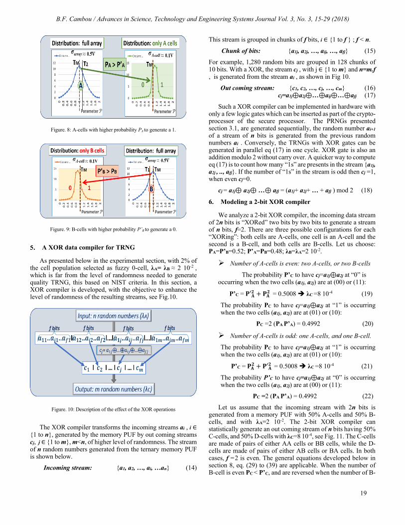
B.F. Cambou / Advances in Science, Technology and Engineering Systems Journal Vol. 3, No. 3, 15-29 (2018)
19
Figure. 8: A-cells with higher probability PA to generate a 1.
Figure. 9: B-cells with higher probability P’B to generate a 0.
A XOR data compiler for TRNG
As presented below in the experimental section, with 2% of the cell population selected as fuzzy 0-cell, λA= λB ≈ 2 10-2 , which is far from the level of randomness needed to generate quality TRNG, this based on NIST criteria. In this section, a XOR compiler is developed, with the objective to enhance the level of randomness of the resulting streams, see Fig.10.
Figure. 10: Description of the effect of the XOR operations
The XOR compiler transforms the incoming streams ai , i ∈ 1 to n, generated by the memory PUF by out coming streams cj, j ∈ 1 to m, m<n, of higher level of randomness. The stream of n random numbers generated from the ternary memory PUF is shown below.
Incoming stream: a1, a2, …, ai, …an (14)
This stream is grouped in chunks of f bits, i ∈ 1 to f ; f < n.
Chunk of bits: a1j, a2j, …, aij, …, afj (15)
For example, 1,280 random bits are grouped in 128 chunks of 10 bits. With a XOR, the stream cj , with j ∈ 1 to m and n=m.f , is generated from the stream ai , as shown in Fig 10.
Out coming stream: c1, c2, …, cj, …, cm (16) cj=a1j⊕a2j⊕…⊕aij⊕…⊕afj (17)
Such a XOR compiler can be implemented in hardware with only a few logic gates which can be inserted as part of the crypto-processor of the secure processor. The PRNGs presented section 3.1, are generated sequentially, the random number ai+1 of a stream of n bits is generated from the previous random numbers ai . Conversely, the TRNGs with XOR gates can be generated in parallel eq (17) in one cycle. XOR gate is also an addition modulo 2 without carry over. A quicker way to compute eq (17) is to count how many “1s” are presents in the stream a1j, a2j , .., afj. If the number of “1s” in the stream is odd then cj =1, when even cj=0.
cj = a1j⊕ a2j⊕ …⊕ afj = (a1j+ a2j+ … + afj ) mod 2 (18)
Modeling a 2-bit XOR compiler
We analyze a 2-bit XOR compiler, the incoming data stream of 2n bits is “XORed” two bits by two bits to generate a stream of n bits, f=2. There are three possible configurations for each “XORing”: both cells are A-cells, one cell is an A-cell and the second is a B-cell, and both cells are B-cells. Let us choose: PA=P’B=0.52; P’A=PB=0.48; λB=λA=2 10-2.
Number of A-cells is even: two A-cells, or two B-cells
The probability P’C to have cj=a1j⊕a2j at “0” is occurring when the two cells (a1j, a2j) are at (00) or (11):
P’C = 𝐏𝐏′𝐀𝐀𝟐𝟐 + 𝐏𝐏𝐀𝐀𝟐𝟐 = 0.5008 λC =8 10-4 (19)
The probability PC to have cj=a1j⊕a2j at “1” is occurring when the two cells (a1j, a2j) are at (01) or (10):
PC =2 (PA P’A) = 0.4992 (20)
Number of A-cells is odd: one A-cells, and one B-cell.
The probability PC to have cj=a1j⊕a2j at “1” is occurring when the two cells (a1j, a2j) are at (01) or (10):
P’C = 𝐏𝐏𝐀𝐀𝟐𝟐 + 𝐏𝐏′𝐀𝐀𝟐𝟐 = 0.5008 λC =8 10-4 (21)
The probability P’C to have cj=a1j⊕a2j at “0” is occurring when the two cells (a1j, a2j) are at (00) or (11):
PC =2 (PA P’A) = 0.4992 (22)
Let us assume that the incoming stream with 2n bits is generated from a memory PUF with 50% A-cells and 50% B-cells, and with λA=2 10-2. The 2-bit XOR compiler can statistically generate an out coming stream of n bits having 50% C-cells, and 50% D-cells with λC=8 10-4, see Fig. 11. The C-cells are made of pairs of either AA cells or BB cells, while the D-cells are made of pairs of either AB cells or BA cells. In both cases, f =2 is even. The general equations developed below in section 8, eq. (29) to (39) are applicable. When the number of B-cell is even PC < P’C, and are reversed when the number of B-

B.F. Cambou / Advances in Science, Technology and Engineering Systems Journal Vol. 3, No. 3, 15-29 (2018)
20
cell is odd PC > P’C. The deviation from randomness λC=8 10-4 is 25 times smaller than the deviation before the 3bit-XOR compilation, λA=2 10-2.
Figure. 11: Diagram showing a 2-bit XOR compiler.
Modeling a 3-bit XOR compiler
In this section we analyze a 3-bit XOR compiler, in which the incoming data stream of 3n bits is “XORed” three bits by three bits to generate a stream of n bits, f=3. We are again choosing the same example:
PA=P’B=0.52; P’A=PB=0.48; λB=λA=2 10-2.
There are four possible configurations for each “XORing”: three cells are A-cells, two cells are A-cells & one cell is B-cell, one cell is A-cell & two cells are B-cells, and finaly three cells are B-cells. Number of B-cells is even: three A-cells, A-cell & two
B-cells. The probability PC to have cj=a1j⊕a2j⊕a3j at “1” is occurring when the three cells (a1j, a2j, a3j) are at (111), (100), (010) or (001):
PC = 𝐏𝐏𝐀𝐀𝟑𝟑 + 3 𝐏𝐏𝐀𝐀𝐏𝐏′𝐀𝐀𝟐𝟐 = 0.500032 λC=3.2 10-5 (23)
The probability P’C to have cj=a1j⊕a2j⊕a3j at “0” is occurring when the three cells (a1j, a2j, a3j) are at (000), (110), (011) or (101):
P’C = 𝐏𝐏′𝐀𝐀𝟑𝟑 + 3 𝐏𝐏′𝐀𝐀𝐏𝐏𝐀𝐀𝟐𝟐 = 0.499968 (24)
Number of B-cells is odd: Three B-cells, B-cell & two A-cells. The probability P’C to have cj=a1j⊕a2j⊕a3j at “0” is occurring when the three cells (a1j, a2j, a3j) are at (000), (110), (011) or (101):
P’C = 𝐏𝐏𝐀𝐀𝟑𝟑 + 3 𝐏𝐏𝐀𝐀𝐏𝐏′𝐀𝐀𝟐𝟐 = 0.500032 λC=3.2 10-5 (25)
The probability P’C to have cj=a1j⊕a2j⊕a3j at “0” is occurring when the three cells (a1j, a2j, a3j) are at (000), (110), (011) or (101):
PC = 𝐏𝐏′𝐀𝐀𝟑𝟑 + 3 𝐏𝐏′𝐀𝐀𝐏𝐏𝐀𝐀𝟐𝟐 = 0.499968 (26)
Let us assume that the incoming stream with 3n bits is generated by a memory PUF having 50% A-cells, and 50% B-cells, and with λA=2 10-2. The 3-bit XOR compiler can statistically generate an out coming stream of 128 bits having 50% C-cells, and 50% D-cells with λC=3.2 10-5, see Fig. 12. The C-cells are made of triplets of either AAA cells, ABB cells BAB cells, or BBA cells. The D-cells are made of triplets of either AAB cells, ABA cells, BAA cells, or BBB cells.
In both cases, f=3 is odd. The general equations developed in the next section, eq. (29) to (38) are applicable. When the number of B-cells is even, PC < P’C, and are reversed when the number of B-cells is odd, PC > P’C. The resulting deviation from randomness, λc=3.2 10-5, is 25x25=625 times smaller than the deviation before the 3-XOR compilation, λA=2 10-2. It is interesting to notice that a 3-bits XOR data compiler needs only 50% more starting cells than a 2-bits compiler, and has a level of non-randomness 25 times lower.
Figure. 12: Diagram showing a 3-bits XOR compiler.
Modeling the XOR compiler in general terms
The goal is to develop a model that quantifies the effect of a XOR compiler, which enhance the level of randomization of a data stream, as a function of the size f of the chunk of incoming bits that are XORed together. The incoming stream a1, …, ai, …an has a deviation from randomness λA , and the out coming stream c1, c2, …, cj, …, cm has a deviation λC. This variation is obtained by computing PC, the probability for cj, to be a “1:
∣ λC ∣ = 1- PC (27)
The incoming random bits aij are generated from A-cells or B-cells of the ternary PUFs. As stated in section 4.1, the transition TM is selected in such a way that the probability to have an A-cell, and a B-cell is equal to 0.5. If each of the f long chunks have s A-cells and t B-cells with s+t=f. The numbers of possible combinations (f, s) is:
Cf,s = 𝐟𝐟𝐬𝐬 = f ! / s ! (f-s) ! (28):
1.1 All cells of chunk j are A-cells.
The probability of any of the A-cells of the stream to be a “1” is PA, and the probability to be a “0”is P’A. Both PA and P’A are following Bernoulli formula:
1= ∑ 𝐟𝐟𝐢𝐢 𝐏𝐏𝐀𝐀𝐢𝐢 𝐏𝐏′𝐀𝐀𝐟𝐟−𝐢𝐢𝐢𝐢=𝐟𝐟𝐢𝐢=𝟎𝟎 (29)
1=∑ [𝒊𝒊 mod2]𝐟𝐟𝐢𝐢𝐏𝐏𝐀𝐀𝐢𝐢 𝐏𝐏′𝐀𝐀𝐟𝐟−𝐢𝐢
𝒊𝒊=𝒇𝒇𝒊𝒊=𝟎𝟎 +∑ [𝒊𝒊 + 1mod2]𝐟𝐟𝐢𝐢𝐏𝐏𝐀𝐀
𝐢𝐢 𝐏𝐏′𝐀𝐀𝐟𝐟−𝐢𝐢𝒊𝒊=𝒇𝒇𝒊𝒊=𝟎𝟎
1= Pc + P’c (30)
The terms 𝐏𝐏𝐀𝐀𝐢𝐢 𝐏𝐏′𝐀𝐀𝐟𝐟−𝐢𝐢 of eq. (29) and (30) correspond to a configuration where i bits are “1s”, and f-i bits are “0”.
The probability PC, is the sum of all terms having i odd: i mod2 = 1 i+1 mod2 = 0 (31)
Pc = ∑ [𝒊𝒊 mod2]fi 𝐏𝐏𝐀𝐀𝐢𝐢 𝐏𝐏′𝐀𝐀𝐟𝐟−𝐢𝐢𝐢𝐢=𝐟𝐟
𝐢𝐢=𝟎𝟎 (32)
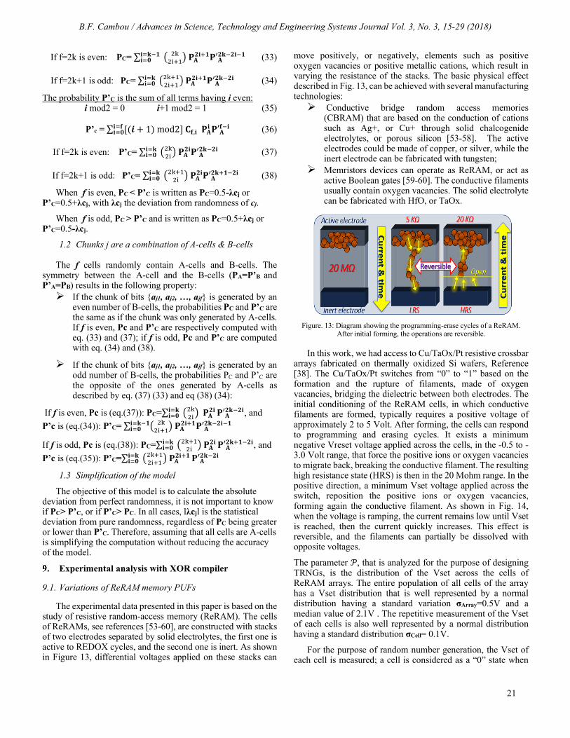
B.F. Cambou / Advances in Science, Technology and Engineering Systems Journal Vol. 3, No. 3, 15-29 (2018)
21
If f=2k is even: PC= ∑ 2k2i+1 𝐏𝐏𝐀𝐀𝟐𝟐𝐢𝐢+𝟏𝟏𝐏𝐏′𝐀𝐀𝟐𝟐𝟐𝟐−𝟐𝟐𝐢𝐢−𝟏𝟏𝐢𝐢=𝟐𝟐−𝟏𝟏
𝐢𝐢=𝟎𝟎 (33)
If f=2k+1 is odd: PC= ∑ 2k+12i+1 𝐏𝐏𝐀𝐀𝟐𝟐𝐢𝐢+𝟏𝟏𝐏𝐏′𝐀𝐀𝟐𝟐𝟐𝟐−𝟐𝟐𝐢𝐢𝐢𝐢=𝟐𝟐𝐢𝐢=𝟎𝟎 (34)
The probability P’C is the sum of all terms having i even: i mod2 = 0 i+1 mod2 = 1 (35)
P’c = ∑ [(𝒊𝒊 + 1) mod2] 𝐂𝐂𝐟𝐟,𝐢𝐢 𝐏𝐏𝐀𝐀𝐢𝐢 𝐏𝐏′𝐀𝐀𝐟𝐟−𝐢𝐢𝐢𝐢=𝐟𝐟
𝐢𝐢=𝟎𝟎 (36)
If f=2k is even: P’C= ∑ 2k2i 𝐏𝐏𝐀𝐀𝟐𝟐𝐢𝐢𝐏𝐏′𝐀𝐀𝟐𝟐𝟐𝟐−𝟐𝟐𝐢𝐢𝐢𝐢=𝟐𝟐𝐢𝐢=𝟎𝟎 (37)
If f=2k+1 is odd: P’C= ∑ 2k+12i 𝐏𝐏𝐀𝐀𝟐𝟐𝐢𝐢𝐏𝐏′𝐀𝐀𝟐𝟐𝟐𝟐+𝟏𝟏−𝟐𝟐𝐢𝐢𝐢𝐢=𝟐𝟐
𝐢𝐢=𝟎𝟎 (38)
When f is even, PC < P’C is written as PC=0.5-λcj or P’C=0.5+λcj, with λcj the deviation from randomness of cj.
When f is odd, PC > P’C and is written as PC=0.5+λcj or P’C=0.5-λcj.
1.2 Chunks j are a combination of A-cells & B-cells
The f cells randomly contain A-cells and B-cells. The symmetry between the A-cell and the B-cells (PA=P’B and P’A=PB) results in the following property: If the chunk of bits aj1, aj2, …, ajf is generated by an
even number of B-cells, the probabilities PC and P’C are the same as if the chunk was only generated by A-cells. If f is even, Pc and P’C are respectively computed with eq. (33) and (37); if f is odd, Pc and P’C are computed with eq. (34) and (38).
If the chunk of bits aj1, aj2, …, ajf is generated by an odd number of B-cells, the probabilities PC and P’C are the opposite of the ones generated by A-cells as described by eq. (37) (33) and eq (38) (34):
If f is even, Pc is (eq.(37)): PC=∑ 2k2i 𝐏𝐏𝐀𝐀𝟐𝟐𝐢𝐢 𝐏𝐏′𝐀𝐀𝟐𝟐𝟐𝟐−𝟐𝟐𝐢𝐢𝐢𝐢=𝟐𝟐𝐢𝐢=𝟎𝟎 , and
P’c is (eq.(34)): P’C= ∑ 2k2i+1 𝐏𝐏𝐀𝐀𝟐𝟐𝐢𝐢+𝟏𝟏𝐏𝐏′𝐀𝐀𝟐𝟐𝟐𝟐−𝟐𝟐𝐢𝐢−𝟏𝟏𝐢𝐢=𝟐𝟐−𝟏𝟏
𝐢𝐢=𝟎𝟎
If f is odd, Pc is (eq.(38)): PC=∑ 2k+12i 𝐏𝐏𝐀𝐀𝟐𝟐𝐢𝐢 𝐏𝐏′𝐀𝐀𝟐𝟐𝟐𝟐+𝟏𝟏−𝟐𝟐𝐢𝐢𝐢𝐢=𝟐𝟐𝐢𝐢=𝟎𝟎 , and
P’c is (eq.(35)): P’C=∑ 2k+12i+1 𝐏𝐏𝐀𝐀𝟐𝟐𝐢𝐢+𝟏𝟏 𝐏𝐏′𝐀𝐀𝟐𝟐𝟐𝟐−𝟐𝟐𝐢𝐢𝐢𝐢=𝟐𝟐𝐢𝐢=𝟎𝟎
1.3 Simplification of the model
The objective of this model is to calculate the absolute deviation from perfect randomness, it is not important to know if PC> P’C, or if P’C> PC. In all cases, lλcjl is the statistical deviation from pure randomness, regardless of PC being greater or lower than P’C. Therefore, assuming that all cells are A-cells is simplifying the computation without reducing the accuracy of the model.
Experimental analysis with XOR compiler
9.1. Variations of ReRAM memory PUFs
The experimental data presented in this paper is based on the study of resistive random-access memory (ReRAM). The cells of ReRAMs, see references [53-60], are constructed with stacks of two electrodes separated by solid electrolytes, the first one is active to REDOX cycles, and the second one is inert. As shown in Figure 13, differential voltages applied on these stacks can
move positively, or negatively, elements such as positive oxygen vacancies or positive metallic cations, which result in varying the resistance of the stacks. The basic physical effect described in Fig. 13, can be achieved with several manufacturing technologies: Conductive bridge random access memories
(CBRAM) that are based on the conduction of cations such as Ag+, or Cu+ through solid chalcogenide electrolytes, or porous silicon [53-58]. The active electrodes could be made of copper, or silver, while the inert electrode can be fabricated with tungsten;
Memristors devices can operate as ReRAM, or act as active Boolean gates [59-60]. The conductive filaments usually contain oxygen vacancies. The solid electrolyte can be fabricated with HfO, or TaOx.
Figure. 13: Diagram showing the programming-erase cycles of a ReRAM.
After initial forming, the operations are reversible.
In this work, we had access to Cu/TaOx/Pt resistive crossbar arrays fabricated on thermally oxidized Si wafers, Reference [38]. The Cu/TaOx/Pt switches from “0” to “1” based on the formation and the rupture of filaments, made of oxygen vacancies, bridging the dielectric between both electrodes. The initial conditioning of the ReRAM cells, in which conductive filaments are formed, typically requires a positive voltage of approximately 2 to 5 Volt. After forming, the cells can respond to programming and erasing cycles. It exists a minimum negative Vreset voltage applied across the cells, in the -0.5 to -3.0 Volt range, that force the positive ions or oxygen vacancies to migrate back, breaking the conductive filament. The resulting high resistance state (HRS) is then in the 20 Mohm range. In the positive direction, a minimum Vset voltage applied across the switch, reposition the positive ions or oxygen vacancies, forming again the conductive filament. As shown in Fig. 14, when the voltage is ramping, the current remains low until Vset is reached, then the current quickly increases. This effect is reversible, and the filaments can partially be dissolved with opposite voltages.
The parameter 𝒫𝒫, that is analyzed for the purpose of designing TRNGs, is the distribution of the Vset across the cells of ReRAM arrays. The entire population of all cells of the array has a Vset distribution that is well represented by a normal distribution having a standard variation σArray=0.5V and a median value of 2.1V . The repetitive measurement of the Vset of each cells is also well represented by a normal distribution having a standard distribution σCell= 0.1V.
For the purpose of random number generation, the Vset of each cell is measured; a cell is considered as a “0” state when
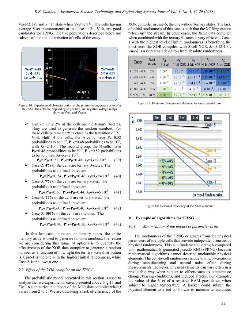
B.F. Cambou / Advances in Science, Technology and Engineering Systems Journal Vol. 3, No. 3, 15-29 (2018)
22
Vset<2.1V, and a “1” state when Vset>2.1V. The cells having average Vset measurements at or close to 2.1 Volt, are good candidates for TRNG. The five populations described below are subsets of the total distribution of cells of the array:
Figure. 14: Experimental characterization of the programming-erase cycles of a
ReRAM. The cells are responding to positive, and negative voltage ramps, showing Vset, and Vreset.
Case-1: Only 2% of the cells are the ternary 0-states. They are used to generate the random numbers. For these cells parameter 𝒫𝒫 is close to the transition of 2.1 Volt. Half of the cells, the A-cells, have PA=0.52 probabilities to be “1”, P’A=0.48 probabilities to be “0”, with λA=2 10-2. The second group, the B-cells, have PB=0.48 probabilities to be “1”, P’B=0.52 probabilities to be “0”, with λB=λA=2 10-2.
PA=P’B=0.52; P’A=PB=0.48; λB=λA=2 10-2 (39) Case-2: 4% of the cells are ternary 0-states. The
probabilities as defined above are: PA=P’B=0.54; P’A=PB=0.46; λB=λA=4 10-2 (40)
Case-3: 7% of the cells are ternary states. The probabilities as defined above are:
PA=P’B=0.56; P’A=PB=0.44; λB=λA=6 10-2 (41) Case-4: 11% of the cells are ternary states. The
probabilities as defined above are: PA=P’B=0.60; P’A=PB=0.40; λB=λA=1 10-1 (42)
Case-5: 100% of the cells are included. The probabilities as defined above are:
PA=P’B=0.90; P’A=PB=0.10; λB=λA=4 10-1 (43)
In this last case, there are no ternary states, the entire memory array is used to generate random numbers.The reason we are considering this range of options is to quantify the effectiveness of the XOR data compiler to generate a random number as a function of how tight the ternary state distribution is. Case-1 is the one with the highest initial randomness, while Case-5 is the lowest one.
9.2. Effect of the XOR compiler on the TRNG
The probabilistic model presented in this section is used to analyze the five experimental cases presented above. Fig 15. and Fig. 16 summarize the impact of the XOR data compiler when f varies from 2 to 5. We are observing a lack of efficiency of the
XOR compiler in case-5, the one without ternary states. The lack of initial randomness of this case is such that the XORing cannot “clean up” the stream. In other cases, the XOR data compiler when combined with the ternary 0-states is very efficient. Case-1 with the highest level of initial randomness is benefiting the most from the XOR compiler: with 5-cell XOR, λC=5.12 10-8, which is a very small deviation from absolute randomness.
Figure 15: Deviation from non-randomness by experimental case
Figure 16: Increased efficiency of the XOR compiler
Example of algorithms for TRNG
10.1. Minimization of the impact of parameter drifts
The randomness of the TRNG originates from the physical parameters of multiple cells that provide independent sources of physical randomness. This is a fundamental strength compared with mathematically generated pseudo RNG (PRNG) because mathematical algorithms cannot describe unclonable physical elements. The cell-to-cell randomness is due to micro-variations during manufacturing and natural noise effect during measurements. However, physical elements can vary often in a predictable way when subject to effects such as temperature change, biasing conditions, and induced attacks. For example, the value of the Vset of a resistive RAM goes down when subject to higher temperature. A hacker could submit the physical element to a hot air blower to increase temperature,
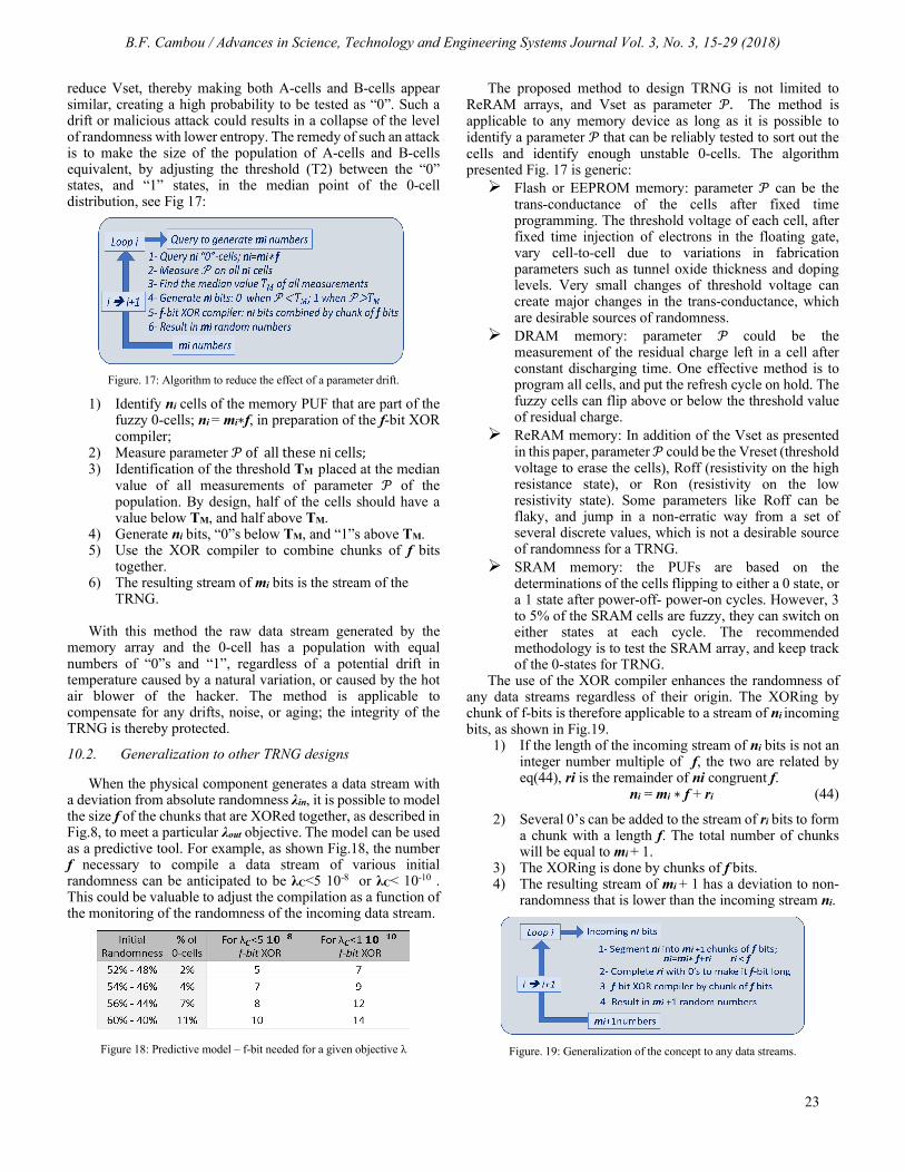
B.F. Cambou / Advances in Science, Technology and Engineering Systems Journal Vol. 3, No. 3, 15-29 (2018)
23
reduce Vset, thereby making both A-cells and B-cells appear similar, creating a high probability to be tested as “0”. Such a drift or malicious attack could results in a collapse of the level of randomness with lower entropy. The remedy of such an attack is to make the size of the population of A-cells and B-cells equivalent, by adjusting the threshold (T2) between the “0” states, and “1” states, in the median point of the 0-cell distribution, see Fig 17:
Figure. 17: Algorithm to reduce the effect of a parameter drift.
1) Identify ni cells of the memory PUF that are part of the fuzzy 0-cells; ni = mi∗f, in preparation of the f-bit XOR compiler;
2) Measure parameter 𝒫𝒫 of all these ni cells; 3) Identification of the threshold TM placed at the median
value of all measurements of parameter 𝒫𝒫 of the population. By design, half of the cells should have a value below TM, and half above TM.
4) Generate ni bits, “0”s below TM, and “1”s above TM. 5) Use the XOR compiler to combine chunks of f bits
together. 6) The resulting stream of mi bits is the stream of the
TRNG.
With this method the raw data stream generated by the memory array and the 0-cell has a population with equal numbers of “0”s and “1”, regardless of a potential drift in temperature caused by a natural variation, or caused by the hot air blower of the hacker. The method is applicable to compensate for any drifts, noise, or aging; the integrity of the TRNG is thereby protected.
10.2. Generalization to other TRNG designs
When the physical component generates a data stream with a deviation from absolute randomness λin, it is possible to model the size f of the chunks that are XORed together, as described in Fig.8, to meet a particular λout objective. The model can be used as a predictive tool. For example, as shown Fig.18, the number f necessary to compile a data stream of various initial randomness can be anticipated to be λC<5 10-8 or λC< 10-10 . This could be valuable to adjust the compilation as a function of the monitoring of the randomness of the incoming data stream.
Figure 18: Predictive model – f-bit needed for a given objective λ
The proposed method to design TRNG is not limited to ReRAM arrays, and Vset as parameter 𝒫𝒫. The method is applicable to any memory device as long as it is possible to identify a parameter 𝒫𝒫 that can be reliably tested to sort out the cells and identify enough unstable 0-cells. The algorithm presented Fig. 17 is generic: Flash or EEPROM memory: parameter 𝒫𝒫 can be the
trans-conductance of the cells after fixed time programming. The threshold voltage of each cell, after fixed time injection of electrons in the floating gate, vary cell-to-cell due to variations in fabrication parameters such as tunnel oxide thickness and doping levels. Very small changes of threshold voltage can create major changes in the trans-conductance, which are desirable sources of randomness.
DRAM memory: parameter 𝒫𝒫 could be the measurement of the residual charge left in a cell after constant discharging time. One effective method is to program all cells, and put the refresh cycle on hold. The fuzzy cells can flip above or below the threshold value of residual charge.
ReRAM memory: In addition of the Vset as presented in this paper, parameter 𝒫𝒫 could be the Vreset (threshold voltage to erase the cells), Roff (resistivity on the high resistance state), or Ron (resistivity on the low resistivity state). Some parameters like Roff can be flaky, and jump in a non-erratic way from a set of several discrete values, which is not a desirable source of randomness for a TRNG.
SRAM memory: the PUFs are based on the determinations of the cells flipping to either a 0 state, or a 1 state after power-off- power-on cycles. However, 3 to 5% of the SRAM cells are fuzzy, they can switch on either states at each cycle. The recommended methodology is to test the SRAM array, and keep track of the 0-states for TRNG.
The use of the XOR compiler enhances the randomness of any data streams regardless of their origin. The XORing by chunk of f-bits is therefore applicable to a stream of ni incoming bits, as shown in Fig.19.
1) If the length of the incoming stream of ni bits is not an integer number multiple of f, the two are related by eq(44), ri is the remainder of ni congruent f.
ni = mi ∗ f + ri (44)
2) Several 0’s can be added to the stream of ri bits to form a chunk with a length f. The total number of chunks will be equal to mi + 1.
3) The XORing is done by chunks of f bits. 4) The resulting stream of mi + 1 has a deviation to non-
randomness that is lower than the incoming stream ni.
Figure. 19: Generalization of the concept to any data streams.
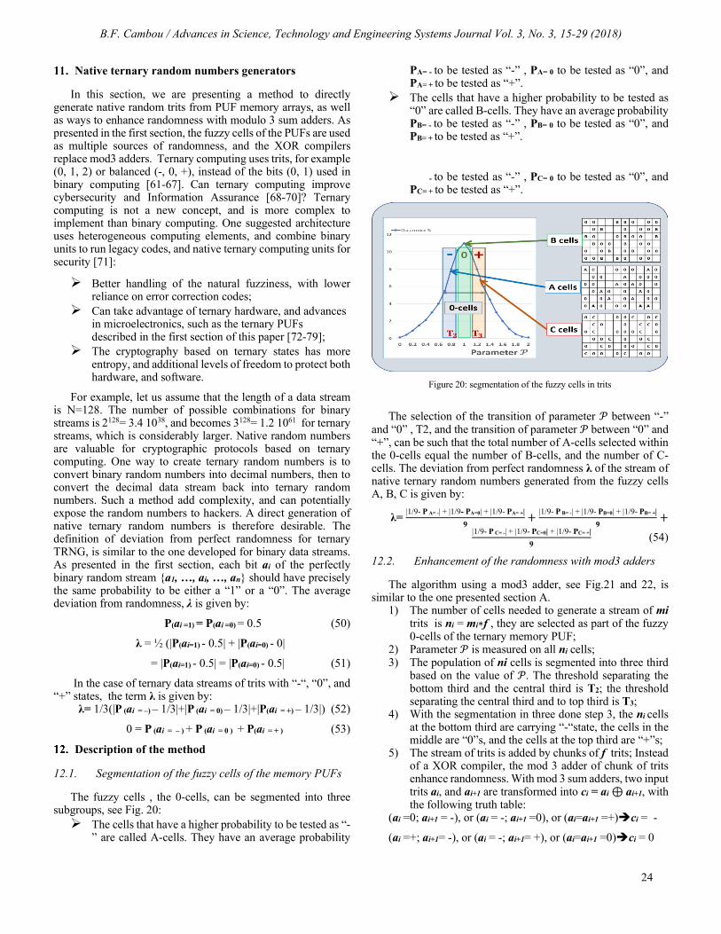
B.F. Cambou / Advances in Science, Technology and Engineering Systems Journal Vol. 3, No. 3, 15-29 (2018)
24
Native ternary random numbers generators
In this section, we are presenting a method to directly generate native random trits from PUF memory arrays, as well as ways to enhance randomness with modulo 3 sum adders. As presented in the first section, the fuzzy cells of the PUFs are used as multiple sources of randomness, and the XOR compilers replace mod3 adders. Ternary computing uses trits, for example (0, 1, 2) or balanced (-, 0, +), instead of the bits (0, 1) used in binary computing [61-67]. Can ternary computing improve cybersecurity and Information Assurance [68-70]? Ternary computing is not a new concept, and is more complex to implement than binary computing. One suggested architecture uses heterogeneous computing elements, and combine binary units to run legacy codes, and native ternary computing units for security [71]:
Better handling of the natural fuzziness, with lower reliance on error correction codes;
Can take advantage of ternary hardware, and advances in microelectronics, such as the ternary PUFs described in the first section of this paper [72-79];
The cryptography based on ternary states has more entropy, and additional levels of freedom to protect both hardware, and software.
For example, let us assume that the length of a data stream is N=128. The number of possible combinations for binary streams is 2128= 3.4 1038, and becomes 3128= 1.2 1061 for ternary streams, which is considerably larger. Native random numbers are valuable for cryptographic protocols based on ternary computing. One way to create ternary random numbers is to convert binary random numbers into decimal numbers, then to convert the decimal data stream back into ternary random numbers. Such a method add complexity, and can potentially expose the random numbers to hackers. A direct generation of native ternary random numbers is therefore desirable. The definition of deviation from perfect randomness for ternary TRNG, is similar to the one developed for binary data streams. As presented in the first section, each bit ai of the perfectly binary random stream a1, …, ai, …, an should have precisely the same probability to be either a “1” or a “0”. The average deviation from randomness, λ is given by:
P(ai =1) = P(ai =0) = 0.5 (50)
λ = ½ (|P(ai=1) - 0.5| + |P(ai=0) - 0|
= |P(ai=1) - 0.5| = |P(ai=0) - 0.5| (51)
In the case of ternary data streams of trits with “-“, “0”, and “+” states, the term λ is given by:
λ= 1/3(|P (ai = –) – 1/3|+|P (ai = 0) – 1/3|+|P(ai = +) – 1/3|) (52)
0 = P (ai = – ) + P (ai = 0 ) + P(ai = + ) (53)
Description of the method
12.1. Segmentation of the fuzzy cells of the memory PUFs
The fuzzy cells , the 0-cells, can be segmented into three subgroups, see Fig. 20: The cells that have a higher probability to be tested as “-
” are called A-cells. They have an average probability
PA= - to be tested as “-” , PA= 0 to be tested as “0”, and PA= + to be tested as “+”.
The cells that have a higher probability to be tested as “0” are called B-cells. They have an average probability PB= - to be tested as “-” , PB= 0 to be tested as “0”, and PB= + to be tested as “+”.
- to be tested as “-” , PC= 0 to be tested as “0”, and PC= + to be tested as “+”.
Figure 20: segmentation of the fuzzy cells in trits
The selection of the transition of parameter 𝒫𝒫 between “-” and “0” , T2, and the transition of parameter 𝒫𝒫 between “0” and “+”, can be such that the total number of A-cells selected within the 0-cells equal the number of B-cells, and the number of C-cells. The deviation from perfect randomness λ of the stream of native ternary random numbers generated from the fuzzy cells A, B, C is given by:
λ= |1/9- P A= -| + |1/9- PA=0| + |1/9- PA= +|9
+ |1/9- P B= -| + |1/9- PB=0| + |1/9- PB= +|9
+
|1/9- P C= -| + |1/9- PC=0| + |1/9- PC= +|9
(54)
12.2. Enhancement of the randomness with mod3 adders
The algorithm using a mod3 adder, see Fig.21 and 22, is similar to the one presented section A.
1) The number of cells needed to generate a stream of mi trits is ni = mi∗f , they are selected as part of the fuzzy 0-cells of the ternary memory PUF;
2) Parameter 𝒫𝒫 is measured on all ni cells; 3) The population of ni cells is segmented into three third
based on the value of 𝒫𝒫. The threshold separating the bottom third and the central third is T2; the threshold separating the central third and to top third is T3;
4) With the segmentation in three done step 3, the ni cells at the bottom third are carrying “-“state, the cells in the middle are “0”s, and the cells at the top third are “+”s;
5) The stream of trits is added by chunks of f trits; Instead of a XOR compiler, the mod 3 adder of chunk of trits enhance randomness. With mod 3 sum adders, two input trits ai, and ai+1 are transformed into ci = ai ⊕ ai+1, with the following truth table:
(ai =0; ai+1 = -), or (ai = -; ai+1 =0), or (ai=ai+1 =+)ci = -
(ai =+; ai+1= -), or (ai = -; ai+1= +), or (ai=ai+1 =0)ci = 0
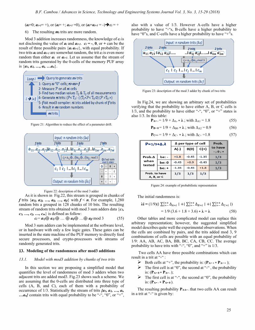
B.F. Cambou / Advances in Science, Technology and Engineering Systems Journal Vol. 3, No. 3, 15-29 (2018)
25
(ai=0; ai+1= +), or (ai= +; ai+1 =0), or (ai=ai+1 = -)ci = +
6) The resulting mi trits are more random.
Mod 3 addition increases randomness, the knowledge of ci is not disclosing the value of ai and ai+1. ci = -, 0, or + can be the result of three possible pairs ai ai+1, with equal probability. If two trits ai and ai+1 are somewhat random, the trit ci is even more random than either ai or ai+1. Let us assume that the stream of random trits generated by the 0-cells of the memory PUF array is a1, a2, …, ai, …an.
Figure 21: Algorithm to reduce the effect of a parameter drift.
Figure 22: description of the mod 3 adder
As it is shown in Fig.22, this stream is grouped in chunks of f trits a1j, a2j, …, aij, …, ajf with f < n. For example, 1,280 random bits a grouped in 128 chunks of 10 bits. The resulting stream of random trits obtained with mod 3 sum adders data c1, c2, …, cj, …, cm is defined as follow:
ci = a1j⊕ a2j ⊕ … ⊕ aij⊕ …⊕ ajf mod 3 (55)
Mod 3 sum adders can be implemented at the software level, or in hardware with only a few logic gates. These gates can be inserted in the state machine of the PUF memory to directly feed secure processors, and crypto-processors with streams of randomly generated trits.
Modeling of the randomness after mod3 additions
13.1. Model with mod3 addition by chunks of two trits
In this section we are proposing a simplified model that quantifies the level of randomness of mod 3 adders when two adjacent trits are added mod3. Fig.23 shows such a scheme. We are assuming that the 0-cells are distributed into three type of cells (A, B, and C), each of them with a probability of occurrence of 1/3. Statistically the stream of trits a1, a2, …, ai, …an contain trits with equal probability to be “-“, “0”, or “+”,
also with a value of 1/3. However A-cells have a higher probability to have “-“s, B-cells have a higher probability to have “0”s, and C-cells have a higher probability to have “+”s.
Figure 23: description of the mod 3 adder by chunk of two trits
In Fig.24, we are showing an arbitrary set of probabilities verifying that the probability to have either A, B, or C cells is 1/3, and the probability to have either “-“, “0”, or “+” states is also 1/3. In this table:
PA= - = 1/9 + ΔA- ∗ λ ; with ΔA1 = 1.8 (55)
PB= 0 = 1/9 + ΔB0 ∗ λ ; with ΔA2 = 0.9 (56)
PC=+ = 1/9 + ΔC+ ∗ λ ; with ΔC+ =1.8 (57)
Figure 24: example of probabilistic representation
The initial randomness is:
λi = (1/9)(∣ ∑ Δ𝐴𝐴=𝑖𝑖𝑖𝑖=+𝑖𝑖=− ∣ +∣ ∑ Δ𝐵𝐵=𝑖𝑖𝑖𝑖=+
𝑖𝑖=− ∣ +∣ ∑ Δ𝐶𝐶=𝑖𝑖𝑖𝑖=+𝑖𝑖=− ∣)
= 1/9 (3.6 + 1.8 + 3.6) ∗ λ = λ (58)
Other tables and more complicated model can replace this arbitrary representation; however, the suggested simplified model describes quite well the experimental observations. When the cells are combined by pairs, and the trits added mod 3, 9 combinations of cells are possible with an equal probability of 1/9: AA, AB, AC, BA, BB, BC, CA, CB, CC. The average probability to have trits with “-“, “0”, and “+” is 1/3.
Two cells AA have three possible combinations which can result in a trit at “-“ : Both cells at “+”, the probability is: (PA= + ∗ PA= + ); The first cell is at “0”, the second at “-“ , the probability
is: (PA= 0 ∗ PA= - ); The first cell is at “-“, the second at “0”, the probability
is: (PA= - ∗ PA= 0 ).
The resulting probability PAA= - that two cells AA can result in a trit at “-“ is given by:
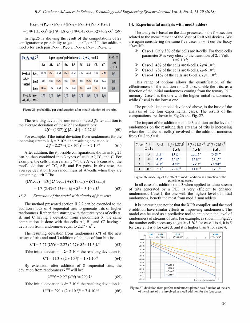
B.F. Cambou / Advances in Science, Technology and Engineering Systems Journal Vol. 3, No. 3, 15-29 (2018)
26
PAA= - =(PA= +∗ PA= +)+(PA=0 ∗ PA= -)+(PA= -∗ PA=0 )
=(1/9-1.35∗λ)2+2(1/9+1.8∗λ)(1/9-0.45∗λ)=1/27+0.2∗λ2 (59)
In Fig.25 is showing the result of the computations of 27 configurations: probability to get “-“, “0”, or “1” after addition mod 3 for each pair PAA= -, PAA= 0, PAA= +, PAB= -, PAB=0,…
Figure 25: probability per configuration after mod 3 addition of two trits.
The resulting deviation from randomness λ'f after addition is the average deviation of these 27 configurations:
λ'f = (1/27) ∑ |Δ . 𝝀𝝀2| ≈ 2.27 𝝀𝝀2 (60)
For example, if the initial deviation from randomness for the incoming stream is λi = 2 10-2; the resulting deviation is:
λ’f = 2.27 ∗( 2 ∗ 10-2)2 = 8.7 10-4 (61)
After addition, the 9 possible configurations shown in Fig.25 can be then combined into 3 types of cells A’, B’, and C. For example, the cells that are mainly “-“, the A’-cells consist of the mod3 additions of CC, AB, and BA pairs. In this case, the average deviation from randomness of A’-cells when they are containing a trit “-“is:
(λ’f A’= - )= 1/3(( λ’f CC= - ) + (λ’f AB= -) + (λ’f BA= -))
= 1/3 (2.43+2.43+4.46) ∗ 𝛌𝛌𝟐𝟐 = 3.10 ∗ 𝛌𝛌𝟐𝟐 (62)
13.2. Extension of the model with chunks of four trits
The method presented section II 2.2 can be extended to the addition mod3 of 4 sequential trits to generate trits of higher randomness. Rather than starting with the three types of cells A, B, and C having a deviation from randomness λ, the same computation is done with the cells A’, B’, and C’ having a deviation from randomness equal to 2.27 ∗ 𝛌𝛌2 .
The resulting deviation from randomness λ"f of the new stream of trits and mod 3 addition of chunks of four bits is:
λ"f = 2.27 (λ’f)2 = 2.27 (2.27)2 𝛌𝛌4≈ 11.3 𝛌𝛌4 (63)
If the initial deviation is λ= 2 10-2; the resulting deviation is:
λ”f = 11.3 ∗ (2 ∗ 10-2)4 = 1.81 10-6 (64)
By extension, after addition of 8 sequential trits, the deviation from randomness λ”” will be:
λ””f = 2.27 (λ”f) 2≈ 290 𝛌𝛌8 (65)
If the initial deviation is λ= 2 10-2; the resulting deviation is:
λ””f = 290 ∗ (2 ∗ 10-2)8 = 7.4 10-12 (66)
Experimental analysis with mod3 adders
The analysis is based on the data presented in the first section related to the measurement of the Vset of ReRAM devices. We are again considering the same five cases to sort out the fuzzy “0-cells”: Case-1: Only 2% of the cells are 0-cells. For these cells
parameter 𝒫𝒫 is very close to the transition of 2.1 Volt. λi=2 10-2;
Case-2: 4% of the cells are 0-cells. λi=4 10-2; Case-3: 7% of the cells are 0-cells. λi=6 10-2; Case-4: 11% of the cells are 0-cells. λi=1 10-1;
This range of options allows the quantification of the effectiveness of the addition mod 3 to scramble the trits, as a function of the initial randomness coming from the ternary PUF memory. Case-1 is the one with the higher initial randomness, while Case-4 is the lowest one.
The probabilistic model developed above, is the base of the analysis of the four experimental cases. The results of the computations are shown in Fig.26 and Fig. 27.
The impact of the addition modulo 3 addition on the level of randomness on the resulting data streams of trits is increasing when the number of cells f involved in the addition increases from f = 2 to f = 8.
Figure 26: modeling of the effect of mod 3 addition as a function of the
experimental cases. In all cases the addition mod 3 when applied to a data stream
of trits generated by a PUF is very efficient to enhance randomness. Case 1, the one with the highest level of initial randomness, benefit the most from mod 3 sum adders.
It is interesting to notice that the XOR compiler, and the mod 3 addition have similar effects in improving randomness. The model can be used as a predictive tool to anticipate the level of randomness of streams of trits. For example, as shown in Fig.27, the number cells necessary to get λ<5 10-6 for case 1 is 4, it is 5 for case 2, it is 6 for case 3, and it is higher than 8 for case 4.
Figure 27: deviation from perfect randomness plotted as a function of the size
of the chunk of trits involved in mod3 addition for the four cases.

B.F. Cambou / Advances in Science, Technology and Engineering Systems Journal Vol. 3, No. 3, 15-29 (2018)
27
Discussion and conclusion
The use of ternary PUFs to design TRNG, combined with a XOR compiler, or a modulo 3 addition has the following benefits: The cells with fuzzy behavior of a ternary PUF, the 0-
cells, can provide multiple sources of independent randomness. A memory arrays in the megabyte range can have a large quantity of such cells;
The randomness of the binary data streams extracted from the ternary 0-cells are enhanced by a XOR compiler. Based on a normal distribution of parameter 𝒫𝒫, the proposed statistical model can quantify the deviation from pure randomness of the TRNGs. It is possible to calculate f, the length of the XOR, to reach a desired level of non-randomness λf, as a function of the level of non-randomness λi of the incoming data stream extracted from the physical element.
The randomness of the ternary data streams extracted from the 0-cells can be enhanced by a modulo 3 adder. It is the possible to directly generate a stream of random trits without having to convert binary data streams into ternary data streams;
It is possible to anticipate, with the suggested probabilistic model, the minimum size of chunks of data f that need to be processed to reach the level of randomness λf. This is the case for the XOR compiler, and the mod 3 adder;
The proposed methodology minimizes sensitivity to parameter drifts such as temperature, aging, or biasing conditions. It is anticipated that the drifts should not materially degrade the quality of the TRNGs.
The hardware implementation of both the XOR compiler, and the mod 3 adder can use known commercial CMOS circuitry.
The method can reach NIST expectations in term of deviation from pure randomness of the TRNG, even if the randomness created by the PUF is weak.
The experimental section of this work, which is based on the measurements of the Vset of ReRAM cells, produced a distribution that is able to show enough randomness to generate random numbers. We noticed that the XOR data compiler is not effective when the initial data stream is not random. The model developed assumes that the initial random numbers generated from the 0-cells are symmetrically distributed between A-cells and B-cells.
Other statistical distributions beside the normal one are under consideration in our research effort. We are not anticipating that these improved statistical models will significantly change the outcome when only cells close to the median distribution are selected. This is not the case for wider distribution of the 0-cells away from the median.
Future work: The objective of this work was to develop TRNG for cryptographic protocols that can be embedded in the Internet of Things (IoT). The implementation of affordable sources of randomness to secure IoTs can benefit from the ease of use of ternary PUFs, which are tamper resistant. TRNGs are
essentials elements to encryption protocols involving PUF CRPs, and other cryptographic keys. We are studying the design of a prototype that incorporates the proposed TRNG scheme with various ReRAM arrays. The prototype is intended to automatically extract large quantities of PUF CRPs and random streams of bits, and trits. We intend to use the prototype to further validate our statistical models, and to leverage the tools developed by NIST that are available online to quantify the entropy, and the level of randomness of the TRNGs. The prototype should have the built-in flexibility to allow us to analyze multiple types of memory arrays, with different methods of fabrication.
We are interested in optimizing the randomness of the TRNG while reducing CRP error rates of the PUFs, and developing cryptographic protocols that leverage the combined capabilities. The method described in this paper can be used to the swarm dynamics generating true random noises [8], and other similar applications requiring TRNG. To accelerate the process to generate fresh random numbers on demand, the 0-cells can be tested in advance [80], and the data can be stored in the memory. The read time of a ReRAM is typically 10ns/bit, so we believe that the generation of the TRNG has the potential to be done at a rate of 100Mbit/s. The method presented in this paper can also be extended to n-value logic, for example quaternary logic (4 bits), pentagonal logic (5 bits), or hexagonal logic (6bits). In such cases the 0-cells are divided in n different type of cells, and the addition of chunk of n-bits is done modulo n.
Aknowledgment
Dr. Marius Orlowski from Virginia Tech produced, and characterized the metal oxide ReRAM samples [49]. These measurements were used to prepare the experimental analysis. Dr. Derek Sonderegger from the Department of Mathematics and Statistic of Northern Arizona University provided input for the development of the statistical model. The author is thanking both Dr. Donald Telesca from the US Air Force Research Labs for his support in this work.
References
[1] B. Cambou; A XOR data compiler combined with PUF for TRNG; SAI/IEEE computing conference, July 2017;
[2] C. Paar, and J. Pezl; Understanding Cryptography- A text book for students and practitioners; Spinger editions, 2011;
[3] C. P. Pfleeger, et al; Security in Computing; Fifth edition; Prentice Hall editions, 2015;
[4] R. Soorat; Hardware random number generation for cryptography; https://arxiv.org/pdf/1510.01234 , 2015;
[5] D. Glosemeyer, and B Knapp; Random Number Generation; Wolfram Mathematical Tutorial collection, 2008;
[6] M. Stipevic, et al; true random number generator; Open problems in Mathematics and computational science; pp.275-315, Springer, 2014;
[7] H. Katzgraber; Random Numbers in scientific computing: an introduction; Int. school comp. science, 2010, Oldenburg, Germany
[8] Y. Shang, and R. Bouffanais; “Influence of the number of topologically interacting neighbors on swarm dynamics”; Scientific Reports DOI: 10.1038/srep04184, 2015.
[9] Berndt Gammel, et al; Jul 2012; Random Generator configured to combine states of memory cells; US patent No 7,979,482 B2;
[10] Daniel E Holcomb, et al; Power up SRAM state as an identifying Fingerprint and Source of True Random Numbers; IEEE Trans. On Computers, 2009 Vol 58, issue No09 Sept;

B.F. Cambou / Advances in Science, Technology and Engineering Systems Journal Vol. 3, No. 3, 15-29 (2018)
28
[11] Sang-Yong Yoon, et al; Aug 2012; Method of operating nonvolatile memory devices storing randomized data generated by copyback operation; US patent No: 8990481 B2;
[12] J. Soto; Statistical testing of random number generators; 1999 – NIST; http://csrc.nist.gov/rng/rng5.html ;
[13] A. Rukhin, and all; A statistical Test Suite For Cryptographic Applications; NIST publication 800-22rev1a, April 2010.
[14] P. L’Ecuyer; Software for uniform random number generation: distinguishing the good from the bad; 2001 Simulation Conference;
[15] A. Rukhin, et all; A statistical test suite for random and PRNG for cryptographic applications; 2010, publication from NIST 800-22 rev 1a;
[16] A. Maiti, et al; PUF and TRNG: a compact and scalable implementation; GLSVLSI’09, May 2009, Boston;
[17] B. Cambou; Sept, 2015; Random numbers generator with ternary memory; US patent application 2017-0046129;
[18] G. Marsaglia; XOR shift RNG; Journal of Statistical software, 2003. [19] M. C Tzannes, A. Friedmann; Nov 2001; Randomization using an XOR
scrambler in multicarrier communications; US patent No 9191939 B2; [20] R. Davies; XOR and hardware random number generator;
http://www.robertnz.net/pdf/XOR2.pdf; February 2002; [21] B. Cambou; Data compiler for True Random Number Generation and
Related Methods; NAU disclosure D2017-03, Aug 2016; [22] Y. Gao, and all; Emerging Physical Unclonable Functions with
nanotechnologies; IEEE, DOI: 10.1109/ACCESS.2015.2503432; [23] N. Beckmann, et al; Hardware-based public-key cryptography with public
physically unclonable functions; in Information Hiding, New York, NY, USA: Springer-Verlag, 2009, pp. 206–220.
[24] Guajardo, J, et al; PUFs and PublicKey Crypto for FPGA IP Protection; Field Programmable Logic and Applications, 2007.
[25] David. Naccache and Patrice. Frémanteau; Aug. 1992; Unforgeable identification device, identification device reader and method of identification; Patent US5434917.
[26] Guajardo, J., et al; FPGA Intrinsic PUFs and Their Use for IP Protection; CHES, 2007;
[27] R. Pappu, B. Recht, J. Taylor, and N. Gershenfield; 20 Sept 2002; Physical one-way functions; Science. Vol 297 No5589 pp2026-2030.
[28] Yier Jin; Introduction to hardware security, Electronics 2015, 4, 763-784; doi:10.3390/electronics4040763.
[29] R. Maes; Physically Unclonable functions: constructions, properties, and applications; Doctoral thesis- Catholic University of Leuven, 2012;
[30] Herder, C., et al; "PUFs and Applications; A Tutorial." Proceedings of the IEEE 102, no. 8 (2014): 1126-1141;
[31] B. Gassend, et al; Silicon PUFs; CCS’ 2002; [32] B. Gassend; Physical random functions; M.S. thesis, Dept. Electr. Eng.
Comput. Sci., MA, USA, Massachusetts Inst. Tech.., Cambridge, 2003; [33] S. Katzenbeisser, et al; PUFs: myths, fact or busted? A security evaluation
of PUFs cast in silicon; CHES 2012; [34] Christian Krutzik; Jan 2015; Solid state drive Physical Unclonable
Function erase verification device and method; US Patent Application publication US 2015/0007337 A1
[35] H. Kang, Y. Hori, T. Katashita, M. Hagiwara, and K. Iwamura; Cryptographic Key Generation from PUF Data Using Efficient Fuzzy Extractors; in Proc. ICACT, 2014, pp.23–26.
[36] R. Maes, P. Tuyls and I. Verbauwhede, "A Soft Decision Helper Data Algorithm for SRAM PUFs," in 2009 IEEE International Symposium on Information Theory, 2009.
[37] Daniel E. Holcomb, Wayne P. Burleson, Kevin Fu; Nov 2008; Power-up SRAM state as an Identifying Fingerprint and Source of TRN; IEEE Trans. on Comp., vol 57, No 11.
[38] D. E. Holcomb, and all; Power-up SRAM state as an Identifying Fingerprint and TRN; IEEE Trans. Comp. Nov 2008;
[39] Pravin Prabhu, Ameen Akel, Laura M. Grupp, Wing-Kei S. Yu, G. Edward Suh, Edwin Kan, and Steven Swanson; June 2011; Extracting Device Fingerprints from Flash Memory by Exploiting Physical Variations; 4th int. conference on Trust and trustworthy computing;
[40] V.Zhirnov, et al; Chapter 26: Flash memories; Nanoelectronics and Information Technology; Rainer Waser editor, 2012 Wiley;
[41] T. A. Christensen, and all; PUF utilizing EDRAM memory cell capacitance variation; Patent: US 8,300,450B2; Oct, 2012;
[42] T. A. Christensen, J. E Sheets II; 2012; Implementing PUF utilizing EDRAM Memory Cell Capacitance Variation; US Patent 8,300,450 B2.
[43] K.K. Chang et al; Understanding Reduced-Voltage Operation in Modern DRAM Chips: Characterization, Analysis, and Mechanisms; Cornell Technical Library: 1705.102992, May 2017;
[44] U. Schroder, et al; Capacitor-based Random-Access Memories; Nanoelectronics and information technology; Wiley-vch, R. Waser editor, pp 635-654, 2012;
[45] Xiaochun Zhu, Steven Millendorf, Xu Guo, David M. Jacobson, Kangho Lee, Seung H. Kang, Matthew M. Nowak, Daha Fazla; March 2015; PUFs based on resistivity of MRAM magnetic tunnel junctions; Patents. US 2015/0071432 A1.
[46] Elena I. Vatajelu, Giorgio Di Natale, Mario Barbareschi, Lionel Torres, Marco Indaco, and Paolo Prinetto; July 2015; STT-MRAM-Based PUF Architecture exploiting Magnetic Tunnel Junction Fabrication-Induced Variability; ACM transactions.
[47] A. Chen; Comprehensive Assessment of RRAM-based PUF for Hardware Security Applications; IEDM IEEE; 2015;
[48] B.Cambou; Enhancing Secure Elements- Technology and Architecture; Springer Int. Publishing Foundations of Hardware IP Protection, 2017;
[49] B. Cambou, and M. Orlowski; PUF designed with ReRAM and ternary states; CISR 2016, April 2016, Oak ridge;
[50] D. Yamamoto, K. Sakiyama, K. Ohto, and M. Itoh; Uniqueness Enhancement of PUF Responses Based on the Locations of Random Outputting RS Latches; CHES 2011;
[51] B. Cambou; PUF generating systems and related methods; US patent disclosure No: 62/204912; Aug 2015;
[52] B. Cambou, and F. Afghah; PUF with Multi-states and Machine Learning; CryptArchi 2016
[53] Gilbert, Nad, et al. "A 0.6 V 8 pJ/write Non-Volatile CBRAM Macro Embedded in a Body Sensor Node for Ultra Low Energy Applications." VLSI Circuits (VLSIC), 2013 Symposium on. IEEE, 2013;
[54] M. N. Kozicki, M. Park, and M. Mitkova, “Nanoscale memory elements based on solid-state electrolytes," IEEE Trans. Nanotechnol, vol. 4, pp. 331-338, May 2005;
[55] M. N. Kozicki and M. Mitkova, "Mass transport in chalcogenide electrolyte films – materials and applications," J. of Non-Crystalline Solids, vol. 352, pp. 567-577, March 2006;
[56] Valov, R. Waser, J. R. Jameson and M. N. Kozicki, "Electrochemical metallization memories - Fundamentals, applications, prospects," Nanotechnology, vol. 22, p. 254003, June 2011;
[57] M. N. Kozicki, M. Balakrishnan, C. Gopalan, C. Ratnakumar, and M. Mitkova, “Programmable metallization cell memory based on Ag-Ge-S and Cu-Ge-S solid electrolytes," Proc. NVMTS, p. 8389, 2005;
[58] M. N. Kozicki, C. Gopalan, M. Balakrishnan, M. Park and M. Mitkova, "Nonvolatile memory based on solid electrolytes," in Proc. IEEE Non-Volatile Memory Technol. Symp., 2004;
[59] Gargi Ghosh and Marius Orlowski; 2015; Write and Erase Threshold Voltage Interdependence in Resistive Switching Memory Cells; IEEE trans. on Electron Devices, 62(9), pp. 2850-2857.
[60] P. R.Mickel, A. J. Lohn, B. J. Choi, J. J. Yang, M. X. Zhang, M. J. Marinella, C. D. James, and R. S. Williams, “A physical model of switching dynamics in tantalum oxide memristive devices,” Appl. Phys. Lett., vol. 102, p. 223502, 2013;
[61] M. Glusker, D.M. Hogan, and P. Vass; The ternary calculating machine of Thomas Fowler; IEEE Annals of the History of Computing, 2005;
[62] N.P. Brousentov, S.P. Maslov, J. Ramil Alvarez, and E.A. Zhogolev; Development of Ternary computers at Moscow State University; Russian Virtual Computer Museum; 1997-2017;
[63] G. Frieder; Ternary Computers, part 1: motivation for ternary computers; Micro 5 Conf. record of the 5th annual workshop on Microprogramming; 1972;
[64] S. Ahmad, M. Alam; Balanced Ternary Logic For improving Computing; IJCSIT, 2014;
[65] I. Profeanu; A ternary Arithmetic and Logic; WCE, June 2010; [66] M.G. Nektar, D.M. Hogan, P. Vass; The ternary calculating machine of
Thomas Fowler; IEEE Annals of the History of Computing, Aug 2005; [67] E.W. Dijkstra; Notes on structured programming; EWD 249 Technical
University, Eindhoven, Netherlands, 1969; [68] B. Cambou, P. Flikkema, J. Palmer, D. Telesca, C. Philabaum; Can
Ternary Computing Improve Information Assurance?; MDPI, Journal cryptography, Feb 2018;

B.F. Cambou / Advances in Science, Technology and Engineering Systems Journal Vol. 3, No. 3, 15-29 (2018)
29
[69] D.M. Miller, and M.A. Thornton; Multiple Valued Logic: Concepts and Representations; Synthesis Lectures on Digital Circuits and Systems; Morgan & Claypool Publishers, 2007;
[70] S. Ahmad, and M. Alam; Balanced Ternary Logic For improving Computing; IJCSIT, 2014;
[71] P.G. Flikkema and B. Cambou; Adapting Processor Architectures for the Periphery of the IoT Nervous System; IEEE 3rd World Forum on Internet of Things (WF-IoT), December 2016;
[72] H. Gundersen; Aspect of balanced ternary arithmetic implemented using CMOS recharged semi-floating gate device; thesis Oslo Univ. 2008;
[73] P.C. Balla, and A. Antoniou; Low Power Dissipation MOS Ternary Logic Family; IEEE J of Solid State Circuits, Oct 1984;
[74] P.C. Balla, A. Antoniou; Low Power Dissipation MOS Ternary Logic Family; IEEE J of Solid State Circuits, Oct 1984;
[75] X.W. Wu; CMOS Ternary Logic Circuits; IEE Proceedings, Feb 1990 [76] P. Nagaraju, et al; Ternary Logic Gates and Ternary SRAM
Implementation in VLSI; IJSR, Nov 2014; [77] N.P. Wanjari, S.P. Hajare; VLSI Design and Implementation of Ternary
Logic Gates and Ternary SRAM Cell; IJECSE, April 2013; [78] A. Srivastava, and K. Venkatapathy; Design and Implementation of a
Low Power Ternary Full Adder; VLSI design, vol 4, No.1, 1996; [79] N.P. Wanjari, and S.P. Hajare; VLSI Design and Implementation of
Ternary Logic Gates and Ternary SRAM Cell; IJECSE, April 2013; [80] Anuj Gupta, May 2005, Implementing Generic BIST for testing Kilo-Bit
Memories; Master Thesis No-6030402 Deemed University Patiala India

www.astesj.com 30
Performance improvement of a wind energy system using fuzzy logic based pitch angle control
Kanasottu Anil Naik*, Chandra Prakash Gupta, Eugene Fernandez
Department of Electrical Engineering, IIT Roorkee, 24767, India
A R T I C L E I N F O A B S T R A C T Article history: Received: 21 March, 2018 Accepted: 20 April, 2018 Online: 07 May, 2018
The pitch angle controller maintains the aerodynamic captured power at rated level when the wind speed is above the rated speed. Besides, it can also improve the transient stability occurring in the wind energy system (WES). This paper, therefore, proposes an effective pitch angle control strategy that can deliver the conditioned output power in windy condition and increase the transient stability capability in grid faults. A fuzzy logic method has employed to design the proposed control strategy, Moreover, in this paper some major factors that affect the transient stability have been investigated by deriving steady-state equivalent model of the wind energy system. The simulated results show that the proposed fuzzy logic based pitch angle controller is effective at conditioning the output power and complying with fault ride through requirements for WES in the power system.
Keywords : Fuzzy logic controller Pitch Angle controller Transient Stability Wind Energy System
1. Introduction
Transient stability enhancement of wind energy system using fuzzy logic based pitch angle controller is a topic of much interest in wind energy studies [1]. Wind energy is perhaps more economical and viable among the other renewable energy resources available for electric power generation. According to predictions it is estimated that, by 2020 wind energy will contributes to about 10 percentage of the world’s electricity [2]. While wind energy is free, its generation involves some operational issues. The main issue that arises is that wind speed is not constant, resulting in large fluctuations in the real power since the output power is proportional to the cube of the wind speed. Another issue of concern is that if a fault occurs in the power network then the induction generator that is generally used in a wind energy system (WES) will not be supplied with the necessary reactive power and this will result in rotor instability [3].
Pitch angle controller limit is one of the ways to regulate the speed of the wind turbine under varying wind speeds. This controller helps to maintain the aerodynamic power at rated value when the wind speed exceeds the rated wind speed. In some reported works [4-9], different methods have been proposed to design the pitch angle controller for regulating the active power at rated value and improve the power quality with frequent wind speed changes. Beside this, pitch angle controller is also employed to stabilize the WES under transient disturbances or faults. The transient stability analysis of a WES is important because of its impact on the utility grid. In the literature some researchers have
designed rotor speed control based pitch angle controller to enhance the transient stability [10-13].
Thus, the pitch angle control serves two purposes: In [4-9], they are used to regulate the generator output power at rated value for varying wind speeds while in [10-13], they are used for stabilizing the WES under transient disturbances or post fault operation. A study of the performance of the pitch controller in both these conditions is the subject of this paper. A pitch angle control strategy is proposed which is designed for improving the smoothing of power and transient stability behavior of the WES under disturbances or wind speed variations. Fuzzy logic technique has been employed for the pitch-angle controller design, as it reported best suited in comparison to other types of controllers.
The major contribution of this paper as follows: • Derived a steady-state equivalent model of the induction
generator using analytical approach. The mechanical torque versus rotor speed results were obtained under different pitch angle conditions.
• A fuzzy logic controller (FLC) based pitch angle control system (in power and speed control modes) has proposed, which can enhance the transient stability performance of the WES subjected to severe network disturbances (in speed control mode) and maintain the output power when the wind speed is higher than rated speed (in power control mode).
This paper is structured as follows: Section 2 discusses the system configuration, modeling of wind turbine and induction generator. In section 3, Pitch angle controller basic concept, proposed control strategy, and controller design (PI and fuzzy
ASTESJ
ISSN: 2415-6698
*Kanasottu Anil Naik, EED, IIT Roorkee, India, +919690314482, Email: [email protected]
Advances in Science, Technology and Engineering Systems Journal Vol. 3, No. 3, 30-37 (2018)
www.astesj.com
Special Issue on Advancement in Engineering Technology
https://dx.doi.org/10.25046/aj030304

K.A.Naik et al. / Advances in Science, Technology and Engineering Systems Journal Vol. 3, No. 3, 30-37 (2018)
www.astesj.com 31
logic) are discussed in detailed. The simulation results are discussed in section 4. Finally, important conclusions are drawn in section 5.
2. Modelling of Wind Energy System
2.1. Configuration of the studied system
A typical WES that is used for the present simulations consists of a 1.5 MW wind turbine driven induction generator (IG) as shown in Fig. 1. The stator winding of the IG is connected to the point of common coupling (PCC) through a step-up transformer (0.69/25kV) which exports power to the 120kV grid through step-up transformer (25/120kV) and a transmission line ( TL TLR jX+ ) operating at 120kV. The rotor of the IG is driven by a variable pitch wind turbine. A power factor correction capacitor ( C ) is connected to the low voltage terminal of the wind turbine generator. It provides required amount of reactive power to the IG for maintaining the terminal voltage. The design based parameters of the generator and wind turbine are given in Appendix-I.
Grid
Infinite bus
1km
25/120kV
PCC
0.69/25kV
1.5MW Wind Energy System
Pitch Controller
IG
Figure. 1. The studied grid-connected WES
2.2. Wind Turbine Modeling
The developed mechanical power of a typical wind turbine is directly proportional to the cube of wind speed as given:
31 ( , ) ( , )2m r p w p wP A C V C Pρ λ β λ β= = (1)
where, wP is available wind power, ρ is the air-density (kg/m3),
rA is the turbine swept area (m2) and can be written as 2rA Rπ= ,
wV is the wind speed (m/s) and pC is the power coefficient.
The typical wind turbine is characterized by the power coefficient ( pC ) which depends upon the ratio of rotor-tip speed ( λ ) and
blade pitch-angle ( β ). The power coefficient ( pC ) employed in this study is as follows [14]:
( )5 /6 4 3 2 1( , ) /ic
p iC c e c c c cλλ β λ β λ−= + − − + (2) where
31 1 0.035
0.008 1iλ β λ β= −
+ + (3)
The coefficients 6 1c c− are: 6 0.0068c = , 5 21c = , 4 5c = ,
3 0.4c = , 2 116c = and 1 0.5176c = and the tip-speed ratio (λ ) can be defined as:
tip speed of the blade wind speed w
r R
V
ωλ = = (4)
where, R is the radius of turbine rotor [m] and rω is rotor speed [rad/s] The mechanical power ( mP ) shown in equation (1) can be expressed as:
32 3 2 3
3
1 1( , ) ( , )2 2( , )
m p w p r
p r
RP R C V R C
C K
ρπ λ β ρπ λ β ωλ
λ β ω
= =
=
(5)
where, 3
212
RK Rρπλ
=
Hence, the mechanical torque output of induction generator (IG) can be derived as [15]:
( , )p wm
mr r
C PPTλ β
ω ω= = (6)
According to equations (1) – (4), for different values of pitch-angle ( β ), the power coefficient versus tip-speed ratio ( pC λ− ) curve for the studied system has been obtained as shown in Fig. 2. For different values of wind speed ( wV ), the turbine output power versus turbine speed characteristics is as shown in Fig. 3. The relation between mechanical torque ( mT ) and pitch angle
( β ) with respect to rotor speed ( rω ) as shown in Fig. 4 is obtained using information of Fig. 2 with Eqn. (6). As observed from equation (6), the mechanical power output ( mP ) of wind turbine depends upon power coefficient ( pC ) and the rotor speed
( rω ) of wind turbine. However, the turbine speed varies very little as the fixed speed cage generators have a speed variation range less than 1% [16]. Thus, variation of mechanical power depends mainly on the power coefficient ( , )pC λ β which varies with the
tip speed ratio ( )λ and pitch angle β . However, it may be observed that in transient disturbances, tip speed ratio variation is very small [17]. As a result, the mechanical torque mostly depends on the pitch angle ( β ). So, it can be noticed from Fig. 4, that the mechanical torque decreases, at the particular point onwards of rotor speed, as the pitch angle increases.
Figure. 2. Wind turbine pC λ− curve

K.A.Naik et al. / Advances in Science, Technology and Engineering Systems Journal Vol. 3, No. 3, 30-37 (2018)
www.astesj.com 32
Figure. 3. Turbine Power characteristics
( )rω
()
mT
0 0.5 1 1.50
0.2
0.4
0.6
0.8
1
Rotor speed
Mec
hani
cal t
orqu
e
Beta=0 degBeta=5 degBeta=10 degBeta=20 deg
Figure. 4. Mechanical torque versus rotor speed
2.3. Induction generator modeling
The employed test system shown in Fig. 1 can be modeled by the equivalent electrical circuit from induction generator (IG) to PCC is shown in Fig. 5. The steady state equivalent circuit of the IG is as shown Fig. 5 within the box enclosed by dotted lines.
Induction Generator
Transformer+Line
TR TjXSR SjX
MjX
RjX
RRs
CjX−
SI
mP
RIESVPCCV
MI
A
B
Figure. 5. Electrical equivalent of the test system
According to the IG equivalent circuit, the mathematical expression for stator terminal voltage ( SV ) of the IG is:
( )S S S SV I R jX E= + + (7) where, E is air gap magnetic field induction electro-magnetic-field (EMF) given by
M ME jI X= (8)
Where MX magnetizing reactance and MI is the exciting current
of the IG. Now the rotor current RI can be determined from
stator current SI after deducting MI as follows:
R S MI I I= − (9) and then the corresponding mechanical power input to the IG will be given by
23 Rm R
RP Is
=
(10)
where, RR and SR are the rotor and stator resistance, respectively and s is the slip which is less than zero for the IG. To understand the transient stability concept of the studied wind power system it is necessary to calculate the electrical torque of the generator using the electrical equivalent circuit of the system. The Thevenin equivalent circuit obtained from Fig. 5 from the point A and B is as shown in Fig. 6. Where, Thevenin equivalent voltage is:
1( )PCC C
THT T C
V jXVR jX jX
−=
+ − (11)
and the series parameters are: 1TH TR R= and 1TH T CX X X= −
1THR 1THjXSR SjX
MjX
RjX
RRs
SIRI
1THV
P
Q
Figure. 6. Reduced Equivalent circuit of the system
Again, applying the Thevenin concept to Fig. 6 at the point P and Q the further reduced equivalent circuit has been obtained as shown in Fig.8. The Thevenin equivalent voltage obtained as:
1
1 1
( )TH MTH
TH S TH S M
V jXVR R jX jX jX
=+ + + +
(12)
and the equivalent Thevenin resistance and reactance can be obtained as: 1TH TH SR R R= + and 1TH TH S MX X X X= + + .
THR THjXRjX
RRs
RI
THV
Figure. 7. Complete Reduced Equivalent circuit of the system
Finally, from the Fig.7, the rotor current can be computed as [18]:
( ) ( )2 2/TH
R
TH R TH R
VIR R s X X
=+ + +
(13)
From which, the generator electrical toque can be determined as:
( ) ( )
22
2 2/R R TH
e RTH R TH R
R R VT Is s R R s X X
= =+ + +
(14)
Generally, the slip ( s ) is defined as:
0 0.5 1
0
0.5
1 Max. power at base wind speed (14 m/s) and beta = 0 deg
6 m/s7.6 m/s
9.2 m/s
10.8 m/s
12.4 m/s
14 m/s
Turbine speed (p.u)
Turb
ine
outp
ut p
ower
(p.u
)

K.A.Naik et al. / Advances in Science, Technology and Engineering Systems Journal Vol. 3, No. 3, 30-37 (2018)
www.astesj.com 33
s r
s
s ω ωω−
= (15)
When the induction machine is operated as generator, the sign convention for the electrical ( eT ) and mechanical ( mT ) torques are reversed. Therefore, the mechanical-electrical equilibrium of the IG can be expressed as
( )12
re m
d T Tdt Hω
= − (16)
Eqn. (16) gives the information that during the network faults the electrical torque ( eT ) become zero since the voltage at the PCC is zero which causes the generator rotor speed to increase drastically leads to instability of the system. However, by increasing the pitch angle of wind turbine the mechanical toque ( mT ) can be decreased
(see Fig. 4) and thus, generator rotor speed ( rω ) can be limited/decreased to its normal value as given by Eqn. (16). Thus, the pitch angle controller plays an important role in the operation of a WES to improve the transient stability.
3. Pitch angle controller
The block diagram of a typical pitch-angle control system is shown in Fig. 8. When the wind speed crosses the rated wind speed ( wRV ), the pitch angle controller modifies the aerodynamic toque to maintain the generator output power at its rated value. The difference between the measured power ( gP ) and reference
power ( REFgP ) generates a control signal to the controller ( )C s ,
which regulates the output power accordance with error (ε ), by modifying the pitch angle. The pitch-angle control strategy mathematically can be expressed as:
( )REFg gc iP P
Pβ
ββ ∆= − +∆
(17)
where, P∆ and β∆ are small-signal state variables of
mechanical power and pitch angle, respectively, and iβ is the initial pitch-angle magnitude.
Pitch angle saturation
Rate limiter Pitch Servo
WIND
TURBINE
Figure. 8. The typical pitch-angle control system
The optimum pitch angle ( cβ ) from the controller ( )C s is used as reference to the pitch actuator/servo system. The purpose of the pitch servo is for the correct positioning of the blades. The first order transfer function of the electric or hydraulic pitch servo is as follows:
11 cT sβββ
+= (18)
The pitch angle ( β ) follows the reference pitch or optimum
pitch ( cβ ) by a first order lag with time constant Tβ , which is
dependent on the pitch actuator. In order to get the realistic response from the pitch control system, the pitch rate and the regulations range of pitch angle are set to 2 / sec± ° and 0 45° − ° , respectively.
As discussed earlier, the pitch angle controller is generally employed for control above rated wind speed where it regulates the generator output power. Besides, it can also be used to improve the transient stability of the WES. The next subsection discusses how the pitch angle controller can serve these tasks well.
3.1. Control Strategy implemented
The controller shown in Fig. 9 can be operated in two control modes (power and speed) in order to achieve above tasks effectively. The operating mode of the controller can be determined using selection switch. The controller works in power control mode with switch set to input 1 when the wind speed exceeds its rated speed to maintain the output power of the generator at rated value. However, for below rated wind speed controller not in operation where 0β = ° to extract the possible maximum wind power as governed by the Fig. 2. On the other hand, if the rotor speeds of induction generator increase to a threshold rotor speed ( TH
rω ) due to network disturbances, the controller input is set to input 2, as a result, it works in speed control mode where the transient stability enhancement is achieved with suitable pitch angle generation.
2
1
Control mode selection
switch
Pitch angle saturation
Rate limiter Pitch Servo
C(s)
Figure.9. A typical pitch angle controller in power and speed control modes
In order to achieve the effective performance of the wind energy system, the controller C(s) of pitch control system needs to be designed for effective control. 3.2. Proportional Integral (PI) controller
A PI controller was designed using the linearized model of the WES. The Ziegler-Nichols method is employed to determine the appropriate controller gain. When the wind speed is above the rated wind speed for the WES, the PI controller is used to regulate the output power at its rated value by setting a suitable valued pitch angle. Although, this method has a simple structure, good steady-state response and is easy to implement, it exhibits a poor transient response due to use of constant controller gains. Therefore, an alternative method for controller design is proposed using fuzzy logic. It has numerous advantages as fuzzy logic does not require a mathematical modeling of the system and is capable of handling irregularity /nonlinearity. In addition, they provide excellent dynamic responses.
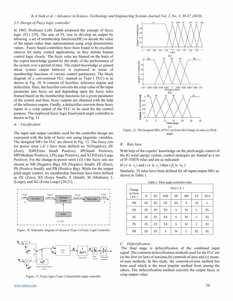
K.A.Naik et al. / Advances in Science, Technology and Engineering Systems Journal Vol. 3, No. 3, 30-37 (2018)
www.astesj.com 34
3.3. Design of Fuzzy logic controller
In 1965, Professor Lofti Zadeh proposed the concept of fuzzy logic (FL) [19]. The aim of FL was to develop an output by allowing a set of membership functions(MF) to decide the value of the inputs rather than representation using crisp deterministic values. Fuzzy based controllers have been found to be excellent choices for many control applications, as they imitate human control logic closely. The fuzzy rules are framed on the basis of the expert knowledge gained by the study of the performance of the system over a period of time. The expert knowledge so gained about system output behavior is expressed in terms of membership functions of various control parameters. The block diagram of a conventional FLC (named as Type-1 FLC) is as shown in Fig. 10. It consists of fuzzifier, inference engine and defuzzifier. Here, the fuzzifier converts the crisp value of the input parameter into fuzzy set and depending upon the fuzzy rules framed based on the membership functions for a given parameter of the system and then, fuzzy outputs are obtained with the help of the inference engine. Finally, a defuzzifier converts these fuzzy inputs to a crisp output of the FLC to be used for the control purpose. The employed fuzzy logic based pitch angle controller is shown in Fig. 11.
A. Fuzzification The input and output variables used for the controller design are expressed with the help of fuzzy sets using linguistic variables. The designed MFs for FLC are shown in Fig. 12. The fuzzy sets for power error ( ε ) have been defined as: N(Negative), ZE (Zero), XSP(Extra Small Positive), SP(Small Positive), MP(Medium Positive), LP(Large Positive), and XLP(Extra Large Positive). For the change-in-power error ( cε ) the fuzzy sets are chosen as NB (Negative Big), NS (Negative Small), ZE (Zero), PS (Positive Small), and PB (Positive Big). While for the output pitch-angle control, six membership functions have been defined as ZE (Zero), XS (Extra Small), S (Small), M (Medium), L (Large), and XL (Extra Large) [20,21].
Figure. 10. Schematic diagram of classical (Type-1) Fuzzy Logic Controller
2
1
Control mode selection
switch
Type-1
FLC
Pitch angle saturation
Rate limiter Pitch Servo
Figure. 11. Fuzzy logic (Type-1) based pitch angle controller
(a)
(b)
(c)
Figure. 12. The designed MFs of FLC (a) Error (b) Change in error (c) Pitch angle
B. Rule base
With help of the experts’ knowledge on the pitch-angle control of the IG wind energy system, control strategies are framed as a set of IF-THEN rules and are as indicated: If ( ε is 1x ) and ( cε is 1y ) then ( cβ is 1w ) Similarly, 35 rules have been defined for all input-output MFs as shown in Table 1.
Table.1. Pitch angle controller rules
Change in Error ( cε )
Error ( ε )
N ZE XSP SP MP LP XLP
NB ZE ZE ZE XS S M L
NS ZE ZE XS S M L XL
ZE ZE ZE XS S M L XL
PS ZE ZE XS S M L XL
PB ZE ZE S M L XL XL
C. Defuzzification The final stage is defuzzification of the combined input signal .The common defuzzification methods used for the FLC are (a) the first (or last) of maxima,(b) centroid-of-area and (c) mean-of-max methods. In this study, the centroid-of-area method has been used which is the most popular method from among the others. The defuzzification method converts the output fuzzy to crisp output value.
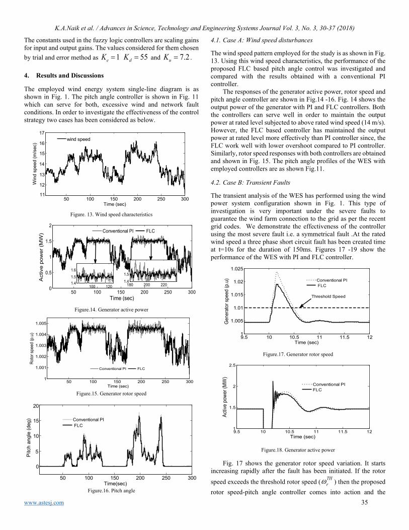
K.A.Naik et al. / Advances in Science, Technology and Engineering Systems Journal Vol. 3, No. 3, 30-37 (2018)
www.astesj.com 35
The constants used in the fuzzy logic controllers are scaling gains for input and output gains. The values considered for them chosen by trial and error method as 1eK = 55dK = and 7.2uK = . 4. Results and Discussions
The employed wind energy system single-line diagram is as shown in Fig. 1. The pitch angle controller is shown in Fig. 11 which can serve for both, excessive wind and network fault conditions. In order to investigate the effectiveness of the control strategy two cases has been considered as below.
Figure. 13. Wind speed characteristics
Figure.14. Generator active power
Figure.15. Generator rotor speed
Figure.16. Pitch angle
4.1. Case A: Wind speed disturbances
The wind speed pattern employed for the study is as shown in Fig. 13. Using this wind speed characteristics, the performance of the proposed FLC based pitch angle control was investigated and compared with the results obtained with a conventional PI controller.
The responses of the generator active power, rotor speed and pitch angle controller are shown in Fig.14 -16. Fig. 14 shows the output power of the generator with PI and FLC controllers. Both the controllers can serve well in order to maintain the output power at rated level subjected to above rated wind speed (14 m/s). However, the FLC based controller has maintained the output power at rated level more effectively than PI controller since, the FLC work well with lower overshoot compared to PI controller. Similarly, rotor speed responses with both controllers are obtained and shown in Fig. 15. The pitch angle profiles of the WES with employed controllers are as shown Fig.11.
4.2. Case B: Transient Faults
The transient analysis of the WES has performed using the wind power system configuration shown in Fig. 1. This type of investigation is very important under the severe faults to guarantee the wind farm connection to the grid as per the recent grid codes. We demonstrate the effectiveness of the controller using the most severe fault i.e. a symmetrical fault .At the rated wind speed a three phase short circuit fault has been created time at t=10s for the duration of 150ms. Figures 17 -19 show the performance of the WES with PI and FLC controller.
Figure.17. Generator rotor speed
Figure.18. Generator active power
Fig. 17 shows the generator rotor speed variation. It starts increasing rapidly after the fault has been initiated. If the rotor speed exceeds the threshold rotor speed ( TH
rω ) then the proposed rotor speed-pitch angle controller comes into action and the
50 100 150 200 250 3006
7
8
9
10
11
12
Time (sec)
Win
d sp
eed
(m/s
ec)
wind speed
14
15
16
17
13
12
11
50 100 150 200 250 3000
0.5
1
1.5
2
Time (sec)
Act
ive
pow
er (M
W)
Conventional PI FLC
100 1201.41.51.6
180 200 2201.41.51.6
50 100 150 200 250 3001
1.001
1.002
1.003
1.004
1.005
Time (sec)
Roto
r spe
ed (p
.u)
Conventional PI FLC
50 100 150 200 250 300
0
2
4
6
8
Time(sec)
Pitc
h an
gle
(deg
)
Conventional PI FLC
10
15
20
5
9.5 10 10.5 11 11.5 121
1.005
1.01
1.015
1.02
1.025
Time (sec)
Gen
erat
or s
peed
(p.u
)
Conventional PI FLC
Threshold Speed
9.5 10 10.5 11 11.5 121
1.5
2
2.5
Time (sec)
Activ
e po
wer (
MW
)
Conventional PIFLC

K.A.Naik et al. / Advances in Science, Technology and Engineering Systems Journal Vol. 3, No. 3, 30-37 (2018)
www.astesj.com 36
generator speed becomes stabilized with additional control using PI or FLC controllers. FLC shows better performance than the PI controller. The generator active power is shown in Fig. 18.
The pitch angle controller of the WT with PI and FLC is as shown in Fig. 19. It is noticed that for a large increase in pitch angle control the FLC controller decreases the mechanical torque and hence the rotor speed settles to a stable value.
Figure. 19. Pitch angle
Table 2. Comparison of ISE and ITAE for different controllers
Method ISE ITAE Conventional PI 113.90 23500
Fuzzy logic controller 88 17200
(a)
(b)
Figure. 20. Graphical representation of comparison of controller indices (a) ISE (b) ITAE
4.3. Controllers performance indices
Various controller performance indexes are available to estimate the controller performs improvement or degradation of the system such as Mean Relative Error (MRE), Integral Absolute Error (IAE), Integral Time Absolute Error (ITAE), Integral Square Error (ISE) and Integral Time Square Error (ITSE). To justify the
performance of the controllers properly, the most popularly used indices ISE and ITAE are adopted in this paper and defined as
2
0( )
TISE e t dt= ∫ (19)
0( )
TIATE t e t dt= ∫ (20)
Smaller the value of ISE and ITAE, better the controller performance. The quantitative results are presented in Table 2. It is observed from the Table 2 that the proposed FLC controller has minimum values of ISE and IATE compared to PI controller, therefore, the proposed controller exhibits better controlling performance. Moreover, the graphical representations of ISE and ITAE with both controllers are as shown in Fig. 20 (a) and (b), respectively.
5. Conclusion
This paper, proposes a fuzzy logic based novel pitch angle controller. It not only improves the quality of output power when the wind speed is above rated and high frequent but, can also improve the transient performance of the WES under faults. Two cases has been considered (wind speed disturbance and fault on the network) to demonstrate the effectiveness of the proposed controller. To show the superiority of the proposed controller, the results were compared with proportional-integral based pitch angle controller. It was found from the obtained results that the proposed fuzzy based novel control strategy exhibits superior response than PI based pitch angle controller.
Appendix-I
Table.3. SCIG generator parameters
Parameters Values
ratedP , ratedV 1.5 MW, 0.69 kV
,s rR R 0.004843 p.u., 0.004377 p.u.
,s rL L 0.1248 p.u., 0.1791p.u.
,mL H 6.77 p.u., 5.04 s
C 200 kVAR
Table.4.Wind turbine parameters
Parameters Values
Rated power 1.5 MW
Rotor diameter 64m
Number of blades 3
9.5 10 10.5 11 11.5 120
0.02
0.04
0.06
0.08
Time (sec)
Pitc
h an
gle
(deg
)
Conventional PI FLC
0
100
200
ISE
Fuzzy Logic ControllerConventional PI
0
20000
40000
ITAE
Fuzzy Logic ControllerConventional PI

K.A.Naik et al. / Advances in Science, Technology and Engineering Systems Journal Vol. 3, No. 3, 30-37 (2018)
www.astesj.com 37
Cut-in wind speed ( wCIV ) 4 m/s
Cut-out wind speed ( RV ) 25 m/s
Rated wind speed ( wRV ) 14 m/s
Generator SCIG
Conflict of Interest
The authors declare no conflict of interest.
References
[1] K. A. Naik and C. P. Gupta, “Transient stability enhancement of wind energy system using fuzzy logic based pitch angle controller,” 2017 4th IEEE Uttar Pradesh Section International Conference on Electrical, Computer and Electronics (UPCON), Mathura, 78-83 (2017). https://doi: 10.1109/UPCON.2017.8251026.
[2] The Global Wind Energy Council Belgium. http://www.gwec.net/global-Fig.s/wind-in-numbers/, (accessed 05.04.2017).
[3] O. Samuelsson, and S. Lindahl, “On speed stability”, Power Syst. IEEE Trans., 20: 1179-1180 (2005).
[4] M. B. Kadri and S. Khan, “Fuzzy adaptive pitch controller of a wind turbine,” 15th Int. Multitopic Conf. (INMIC), Islamabad, 105-110 (2012).
[5] Y. Mi, X. Bao, Y. Yang, H. Zhang and P. Wang, “The sliding mode pitch angle controller design for squirrel-cage induction generator wind power generation system,” Proceed. of the 33rd Chinese Control Conf., Nanjing, 8113-8117 ( 2014).
[6] Y. Mi, X. Bao, E. Jiang, W. Deng, J. Li, L. Ren, and P. Wang, “The pitch angle control of squirrel-cage induction generator wind power generation system using sliding mode control,” 16th European Conf. on Power Electronics and Appli., Lappeenranta, 1-10 (2014).
[7] M. Al-Saffar and P. Musilek, “Fuzzy logic controller for large, grid-integrated wind farm under variable wind speeds,” 17th International Scientific Conf. on Electric Power Engineering (EPE), Prague, 1-6 (2016).
[8] D. C. Vega, J. A. Marin and R. T. Sanchez, “Pitch angle controllers design for a horizontal axis wind turbine,” IEEE Int. Autumn Meeting on Power, Electronics and Computing (ROPEC), Ixtapa, 1-6 (2015).
[9] R. Sakamoto, T. Senjyo, T. Kaneko, N. Urasaki, T. Takagi and S. Sugimoto, “Output power levelling of wind turbine generator by pitch angle control using H-∞ control,” IEEE Pow. Syst. Conf. Expo., 1-6 (2006).
[10] J. Tamura, “Transient stability simulation of power system including wind generator by PSCAD/EMTDC,” IEEE Porto Power Tech Proceedings, vol.4, EMT-108, (2001).
[11] O. Wasynczuk, D.T. Man, J.P. Sullivan, “Dynamic behavior of a class of wind turbine generator during random wind fluctuations,” IEEE Trans. on Power Apparatus and Systems, 100: 2873-2845 (1981).
[12] S. M. Muyeen, M. Hasan Ali, R. Takahashi, T. Murata, J. Tamura, Y.Tomaki, A. Sakahara, and E. Sasano, “Transient Stability Analysis of Grid Connected Wind Turbine Generator System Considering Multi-Mass Shaft Modeling,” Electric Power Components And Systems, 34: 1121-1138 (2006).
[13] P. M. Anderson and A. Bose, “Stability simulation of wind turbine systems,” IEEE Trans. Power Apparatus and Systems, 102: 3791-3795 (1983).
[14] T. Ackerman, “Wind power in power system”, John Wiley & Sons. Ltd, (2005).
[15] R. Strzelecki and G. Benysek, “Power Electronics in Smart Electrical Energy Networks”, Springer, London, UK, (2008).
[16] B. Wu, Y. Lang, N. Zargari and S. Kouro, “Power conversion and control of wind energy systems”, John Wiley & Sons. Ltd, (2011).
[17] D. J. Trudnowski, A. Gentile, J. M. Khan, and E. M. Petritz, “Fixed-speed wind-generator and wind-park modeling for transient stability studies,” Power Syst. IEEE Trans. 19: 1911-1917 (2004).
[18] A. P. Grilo, A. Mota, L. T. M. Mota and W. Freitas, “An analytical method for analysis of large-disturbance stability of induction generators”, Power Syst. IEEE Trans. 22: 1861-1869 (2007).
[19] L. A. Zadeh, “Fuzzy sets”, Information and control, 8: 338-353 (1965).
[20] S. Z. Hassan, H. Li, T. Kamal, M. Q. Abbas, M. A. Khan and G. M. Mufti, "An intelligent pitch angle control of wind turbine," 2017 International Symposium on Recent Advances in Electrical Engineering (RAEE), Islamabad, 2017, pp. 1-6. doi: 10.1109/RAEE.2017.8246144
[21] S. Z. Hassan, H. Li, T. Kamal, M. Nadarajah and F. Mehmood, "Fuzzy embedded MPPT modeling and control of PV system in a hybrid power system," 2016 International Conference on Emerging Technologies (ICET), Islamabad, 2016, pp. 1-6. doi: 10.1109/ICET.2016.7813236

www.astesj.com 1
Using Input Impedance to Calculate the Efficiency Numerically of Series-Parallel Magnetic Resonant Wireless Power Transfer Systems
Thabat Thabet* 1, 2, John Woods1
1Essex University, School of Computer Science and Electronic Engineering, CO4 3SQ, UK
2Technical College of Mosul, Computer Engineering Department, Mosul, Iraq
A R T I C L E I N F O A B S T R A C T Article history: Received : 20 March, 2018 Accepted : 27 April, 2018 Online :7 May, 2018
Analysis of magnetic resonant wireless power transfer systems aims to achieve maximum efficiency of the power transfer. From the analysis we wish to derive the maximum power and the frequency at which this occurs. This paper presents a method to estimate these two required values and to achieve this requires the solution of the input impedance equation numerically. The frequency of the maximum efficiency is found when the imaginary of the input impedance is close to zero, and it could be different to the natural resonant frequency. We estimate the efficiency value which depends on the real value part of the input impedance. The proposed method has been applied to one of the four types of possible connections; a series-parallel (SP) connection although similar approaches could be applied to the others. In some cases the maximum efficiency shifts away from the resonant frequency. Therefore, this paper shows how to use the same equations to achieve maximum efficiency at resonance and suggests a design method to achieve this practically.
Keywords : wireless power transfer magnetic resonant maximum efficiency series-parallel connection SP input impedance
1. Introduction
This paper is an extension of work originally presented in 2017 IEEE International Conference on Circuits, System and Simulation [1]. Where the impact of connection type on the efficiency of magnetic resonant wireless power transfer systems is studied. There are four potential types of connection in the wireless system due to the resonance type in the transmitter and the receiver; they are: series-series (SS); series-parallel (SP); parallel-series (PS); and parallel-parallel (PP). The equivalent circuit of each type can be expressed by applying Kirchhoff’s law of voltage on each loop in the circuit producing a set of equations [1]. This is called the impedance matrix representation. The effect of changing the load resistor and the gap between the two coils is studied for each connection.
As a near field technology, magnetic resonant wireless power transfer systems can achieve high efficiency in specific conditions. Where the efficiency of the maximum transfer of power is affected by several factors; these are the resonant frequency, the
parameters of the coils (inductance, size, and shape), the distance between them and so the mutual inductance, the load resistor, and the connection type of the transmitter and the receiver [1],[2]. To improve the performance of the wireless system, it is important to calculate the efficiency and understand how it is affected by each factor.
Generally, there are two main methods to analyse the system. These methods are coupled mode theory (CMT) and circuit theory (CT) [3]. In the former method (CMT), the system can be described as differential equations [4], [5], [6]. However, according to [7] this method is complicated, undesirable and inconvenient. Therefore researchers tend to use the equivalent circuit for magnetic coupled systems.
The second method (CT) is more familiar to circuit designers than the coupled-mode theory used by the physicists. In this method, the magnetic coupling is represented as the mutual inductance between the two coils. The equivalent circuit of the wireless power transfer system can be formulated as a two port network, which can be represented by either impedance matrix or
ASTESJ
ISSN: 2415-6698
*Corresponding Author, [email protected]
Advances in Science, Technology and Engineering Systems Journal Vol. 2, No. 1, XX-YY (2018)
www.astesj.com
Special Issue on Multidisciplinary Sciences and Engineering
https://dx.doi.org/10.25046/aj030305

T. Thabet et al. / Advances in Science, Technology and Engineering Systems Journal Vol. 2, No. 1, XX-YY (2018)
www.astesj.com 2
scattering matrix [5]. Under this main concept of (CT), many researchers have used different modes with different names to study magnetic resonant wireless power transfer systems, such as magnetic resonant coupling (MRC) [7], [8], [9], and reflected load theory (RLT) [4], [10], [11], [12].
The (MRC) method is used to study magnetic resonant wireless power transfer systems by applying a scattering matrix [7], [8], [13]. They use this method because the practical measurement of scattering parameters is more convenient than other methods at high frequencies.
The (RLT) method is commonly used to analyse transformers by electrical engineers, and it can be used to analyse magnetic resonant wireless power transfer systems. The method states that the current in the transmitter coil is dependent on the load in the receiver coil, and the reflected load in the transmitter is not always the same as the actual load [4].
Starting with the impedance matrix representation to express the wireless system, this paper presents another mode to calculate the maximum efficiency of the transfer power and its associated frequency which can be different than the resonant frequency in some cases. Series-parallel type connection has been chosen to examine the method and calculate the required values. The paper also includes an explanation of the previous mode developed in [1]. The results of the two modes are compared in order to evaluate the new mode and show the differences in the calculation methods. 2. Theoretical Analysis
The transmitter of series-parallel magnetic resonant wireless power transfer system consists of a coil (L1) in serial with a capacitor (C1). While the receiver coil (L2) is in parallel with the capacitor (C2), as shown in Fig. 1. The two capacitors are chosen to make the two coils resonate at the same frequency. The voltage source (VS) of the system has an internal resistance of (RS); and RL is the load resistor. The circuit can be presented as follows:
𝑉𝑉𝑆𝑆00 =
𝑅𝑅𝑆𝑆 + 𝑋𝑋𝐿𝐿1 + 𝑋𝑋𝐶𝐶1 −𝑋𝑋𝑀𝑀 0−𝑋𝑋𝑀𝑀 𝑋𝑋𝐿𝐿2 + 𝑋𝑋𝐶𝐶2 −𝑋𝑋𝐶𝐶2
0 −𝑋𝑋𝐶𝐶2 𝑅𝑅𝐿𝐿 + 𝑋𝑋𝐶𝐶2 𝐼𝐼1𝐼𝐼2𝐼𝐼3 (1)
Where XL=2πfL and XC=1/2πfC; f is the frequency and fo is the selected frequency for resonance. Equation (1) can be rewritten in a different way.
[𝐼𝐼] = [𝑖𝑖𝑖𝑖𝑖𝑖 𝑍𝑍][𝑉𝑉] (2)
Through the following steps, the efficiency of the maximum transfer power can be found:
𝑃𝑃𝑜𝑜𝑜𝑜𝑜𝑜 = 𝐼𝐼32 𝑅𝑅𝐿𝐿 = (𝑖𝑖𝑖𝑖𝑖𝑖 𝑍𝑍(3,1) 𝑉𝑉𝑆𝑆)2𝑅𝑅𝐿𝐿 (3)
𝑃𝑃𝑖𝑖𝑖𝑖 = 𝑉𝑉𝑠𝑠𝑅𝑅𝑠𝑠+𝑅𝑅𝐿𝐿
2𝑅𝑅𝐿𝐿 (4)
𝑒𝑒𝑒𝑒𝑒𝑒 = 𝑖𝑖𝑖𝑖𝑖𝑖 𝑍𝑍(3,1)2 (𝑅𝑅𝑠𝑠 + 𝑅𝑅𝐿𝐿)2 ∗ 100% (5)
3. New Mode of Efficiency Calculation
Another way to calculate the efficiency is as follows:
𝑉𝑉𝑆𝑆 = 𝐼𝐼1 (𝑅𝑅𝑆𝑆 + 𝑍𝑍𝑖𝑖𝑖𝑖) (6)
It can be found from equation (2) that:
𝑖𝑖𝑖𝑖𝑖𝑖 𝑍𝑍(1,1) = 𝐼𝐼1𝑉𝑉𝑆𝑆
(7)
𝑍𝑍𝑖𝑖𝑖𝑖 = 1𝑖𝑖𝑖𝑖𝑖𝑖 𝑍𝑍(1,1)
− 𝑅𝑅𝑆𝑆 (8)
𝑍𝑍𝑖𝑖𝑖𝑖 = 𝑅𝑅𝑖𝑖𝑖𝑖 + 𝑗𝑗𝑋𝑋𝑖𝑖𝑖𝑖 (9)
Where Rin and Xin are the real and the imaginary parts of the input impedance, respectively.
Firstly, it is observed that maximum efficiency occurs when the imaginary part of the input impedance is equal to zero. Therefore, the frequency of maximum efficiency (even if it is different than the original resonant frequency) can be found from:
𝑋𝑋𝑖𝑖𝑖𝑖(𝑒𝑒) = 0 (10)
𝑋𝑋𝑖𝑖𝑖𝑖(𝑒𝑒) = 𝐴𝐴𝑒𝑒 + 𝐵𝐵𝑓𝑓
+ 𝐶𝐶𝑒𝑒3 + 𝐷𝐷𝑓𝑓3
(11)
The values of A, B, C, and D depend on the parameters of the circuit. It is apparent that the equation for Xin is complicated and does not have an analytic solution. Therefore, it has to be solved numerically in order to calculate the required frequency. The
∩
I1 I3
LM XC1
XC1
XC2
XC2 RL
RL
XL1-XLM XL2-XLM
XLM VS
VS
RS
RS
XL1 XL2
I2
Figure 1: Equivalent circuit of magnetic resonant coupling series-parallel antennas in two forms

T. Thabet et al. / Advances in Science, Technology and Engineering Systems Journal Vol. 2, No. 1, XX-YY (2018)
www.astesj.com 3
second step is to find the value of the maximum efficiency which is achieved by finding the real part Rin at that calculated frequency. The equivalent circuit in this stage is shown in Fig.2. Assuming maximum transfer of power the maximum efficiency (eff) is derived as:
𝑒𝑒𝑒𝑒𝑒𝑒 = 4 𝑅𝑅𝑆𝑆 𝑅𝑅𝑖𝑖𝑖𝑖(𝑅𝑅𝑆𝑆+𝑅𝑅𝑖𝑖𝑖𝑖)2
∗ 100% (12)
4. Results and Discussion
The representation of the series-parallel circuit is modelled in Matlab to calculate the mutual inductance and the efficiency of the two modes. To support the theoretical results, several experiments have been conducted. In this work a set of two circular pancake coils are used in all experiments as the primary and secondary. Each coil has 2.9 cm inner radius and 8 cm outer, with 17 turns and an inductance equal to 31.4µH. In addition to that, a set of capacitors equal to 185pF, tuned to work at 2.088MHz were connected to the coils in series in the transmitter and in parallel in the receiver.
4.1. Effect of Distance
Starting with a 50Ω load resistor, the efficiency is found at different gaps between the two coils 7 cm, 5 cm, and 2 cm. Figure 3 shows efficiency versus frequency calculated by equation (5). It is clear from the figure that the maximum efficiency increases and shifts away from the original resonant frequency for small gaps. The table contains the maximum efficiency and the associated frequency calculated by equations (10-12) for the same gaps between the two coils.
Table: Maximum efficiency and associated frequency calculated by the input impedance for the different cases
Gap (cm) 2 5 7 5 5 RL (Ω) 50 50 50 100 1k
f (Xin≈0) (MHz) 2.43 2.14 2.11 2.14 2.17 Rin (Xin≈0) (Ω) 13 2.35 0.87 4.7 45.77
effmax (%) 65.5 17.15 6.7 31.4 99.8
4.2. Effect of Load Resistor
Working on different load resistor values affects the efficiency of the wireless system. Figure 4 shows the system has high efficiency with small load at the same distance. In all cases there is a small shift in the maximum efficiency point compared to the resonant frequency.
In order to show the shift in maximum efficiency, the efficiency and input impedance curves including the real and the imaginary parts for the last case in the Table, all are shown in Fig. 5. The figure also defines the original resonant frequency at 2.088MHz.
RS
VS Zin = Rin Xin = 0
Figure 2: Equivalent circuit at the maximum transfer of power
Figure 3: Efficiency versus frequency at different gaps,
1.6 1.8 2 2.2 2.4 2.6 2.80
10
20
30
40
50
60
70
80
effic
ienc
y
frequency (MHz)
gap=7cmgap=5cmgap=2cm
Figure 4: Efficiency versus frequency at different RL, gap=5cm
1.6 1.8 2 2.2 2.4 2.6 2.80
20
40
60
80
100
effic
ienc
y
frequency (MHz)
RL=50RL=100RL=1k
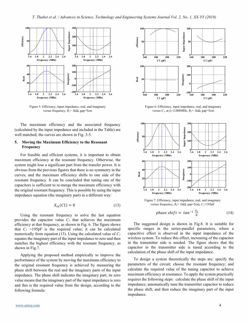
T. Thabet et al. / Advances in Science, Technology and Engineering Systems Journal Vol. 2, No. 1, XX-YY (2018)
www.astesj.com 4
The maximum efficiency and the associated frequency (calculated by the input impedance and included in the Table) are well matched; the curves are shown in Fig. 3-5.
5. Moving the Maximum Efficiency to the Resonant Frequency
For feasible and efficient systems, it is important to obtain maximum efficiency at the resonant frequency. Otherwise, the system might lose a significant part from the transfer power. It is obvious from the previous figures that there is no symmetry in the curves, and the maximum efficiency shifts to one side of the resonant frequency. It can be concluded that tuning one of the capacitors is sufficient to re-merge the maximum efficiency with the original resonant frequency. This is possible by using the input impedance equation (the imaginary part) in a different way:
𝑋𝑋𝑖𝑖𝑖𝑖(𝐶𝐶1) = 0 (13)
Using the resonant frequency to solve the last equation provides the capacitor value C1 that achieves the maximum efficiency at that frequency, as shown in Fig. 6. The figure shows that C1 =195pF is the required value; it can be calculated numerically from equation (13). Using the calculated value of C1 equates the imaginary part of the input impedance to zero and then matches the highest efficiency with the resonant frequency, as shown in Fig.7.
Applying the proposed method empirically to improve the performance of the system by moving the maximum efficiency to the original resonant frequency is achieved by measuring the phase shift between the real and the imaginary parts of the input impedance. The phase shift indicates the imaginary part; its zero value means that the imaginary part of the input impedance is zero and this is the required value from the design, according to the following formula:
𝑝𝑝ℎ𝑎𝑎𝑎𝑎𝑒𝑒 𝑎𝑎ℎ𝑖𝑖𝑒𝑒𝑖𝑖 = 𝑖𝑖𝑎𝑎𝑖𝑖−1 𝑋𝑋𝑐𝑐𝑅𝑅
(14)
The suggested design is shown in Fig.8. It is suitable for specific ranges in the series-parallel parameters, where a capacitive effect is observed in the input impedance of the wireless system. To reduce this effect, increasing of the capacitor in the transmitter side is needed. The figure shows that the capacitor in the transmitter side is tuned according to the calculation of the phase shift of the input impedance.
To design a system theoretically the steps are: specify the parameters of the circuit; choose the resonant frequency; and calculate the required value of the tuning capacitor to achieve maximum efficiency at resonance. To apply the system practically requires the following steps: calculate the phase shift of the input impedance; automatically tune the transmitter capacitor to reduce the phase shift; and then reduce the imaginary part of the input impedance.
1.6 1.8 2 2.2 2.4 2.60
50
100
effic
ienc
y
frequency (MHz)1.6 1.8 2 2.2 2.4 2.60
100
200
300
Inpu
t Im
peda
nce
frequency (MHz)
1.6 1.8 2 2.2 2.4 2.60
20
40
60
Rea
l
frequency (MHz)1.6 1.8 2 2.2 2.4 2.6
-200
-100
0
100
200Im
agin
ary
frequency (MHz)
Figure 5: Efficiency, input impedance, real, and imaginary versus frequency, RL= 1kΩ, gap=5cm
Figure 6: Efficiency, input impedance, real, and imaginary versus C1, at f0=2.088MHz, RL= 1kΩ, gap=5cm
160 180 200 2200
50
100
effic
ienc
y
C1 (pF)160 180 200 2200
50
100
Inpu
t Im
peda
nce
C1 (pF)
160 180 200 2200
50
100
Rea
l
C1 (pF)160 180 200 220
-100
0
100
200
Imag
inar
y
C1 (pF)
Figure 7: Efficiency, input impedance, real, and imaginary versus frequency, RL= 1kΩ, gap=5cm, C1=195pF
1.6 1.8 2 2.2 2.4 2.60
50
100
effic
ienc
y
frequency (MHz)1.6 1.8 2 2.2 2.4 2.60
100
200
300
Inpu
t Im
peda
nce
frequency (MHz)
1.6 1.8 2 2.2 2.4 2.60
20
40
60
Rea
l
frequency (MHz)1.6 1.8 2 2.2 2.4 2.6
-200
-100
0
100
200
Imag
inar
y
frequency (MHz)

T. Thabet et al. / Advances in Science, Technology and Engineering Systems Journal Vol. 2, No. 1, XX-YY (2018)
www.astesj.com 5
6. Conclusion
Having more than one mode to calculate efficiency is more convenient and allows results to be compared to one another.
The proposed method is a quick and simple mode to identify i) the maximum efficiency in a series-parallel wireless power transfer system and ii) the associated frequency. The idea is to equate the imaginary part of the input impedance with zero to find the frequency; and then calculate the maximum efficiency at that frequency from the real part.
Initially, the proposed method was applied to the series-parallel case. In our future work, this method can be applied on the other topologies of resonant wireless power systems.
This work markedly improves the efficiency of a series-parallel wireless system. The limitations of achieving this practically is limited to specific ranges of parameters where a capacitive effect is observed in the input impedance.
Conflict of Interest
The authors declare no conflict of interest.
References
[1] T. Thabet, and J. Woods, "Impact of connection type on the efficiency of wireless power transfer systems.", in 7th IEEE International Conference on Circuits, System and Simulation (ICCSS), 2017. https://doi.org/10.1109/CIRSYSSIM.2017.8023200
[2] T. Thabet, and J. Woods, “An Approach to Calculate the Efficiency for an N-Receiver Wireless Power Transfer System,” IJACSA, 6(9), 91-98, 2015. https://doi.org/10.14569/IJACSA.2015.060912
[3] X. Wei, Z. Wang, and H. Dai, “A critical review of wireless power transfer via strongly coupled magnetic resonances,” Energies, 7(7), 4316-4341, 2014. https://doi.org/10.3390/en7074316
[4] O. Rönnbäck, “Optimization of Wireless Power,” Master Thesis, Luleå University of Technology, 2013.
[5] A. Bodrov, and S.-K. Sul, "Analysis of wireless power transfer by coupled mode theory (CMT) and practical considerations to increase power transfer efficiency," InTech, 2012. https://doi.org/10.5772/25270
[6] H. Shim, J. Park, S. Nam, and B. Lee, "A criterion Proposed for Inductive Coupling and Magnetic Resonance Coupling in Wireless Power Transfer System." in 26th Asia-Pacific Microwave Conference (APMC), 2014. http://ieeexplore.ieee.org/document/7067678/
[7] T. Beh, M. Kato, T. Imura, and Y. Hori, “Wireless Power Transfer System via Magnetic Resonant Coupling at Fixed Resonance
Frequency―Power Transfer System Based on Impedance Matching―,” EVS-25 Shenzhen, China, 2010. https://pdfs.semanticscholar.org/7c5c/1dca95a922971ce5a7e28700876ff29b6448.pdf
[8] T. Imura, H. Okabe, and Y. Hori, "Basic experimental study on helical antennas of wireless power transfer for electric vehicles by using magnetic resonant couplings." in 5th IEEE Vehicle Power and Propulsion Conference, 2009. https://doi.org/10.1109/VPPC.2009.5289747
[9] T. C. Beh, M. Kato, T. Imura, S. Oh, and Y. Hori, “Automated impedance matching system for robust wireless power transfer via magnetic resonance coupling,” IEEE Transactions on Industrial Electronics, 60(9), 3689-3698, 2013. https://doi.org/10.1109/TIE.2012.2206337
[10] M. Kiani, U.-M. Jow, and M. Ghovanloo, “Design and optimization of a 3-coil inductive link for efficient wireless power transmission,” IEEE transactions on biomedical circuits and systems, 5(6), 579-591, 2011. https://doi.org/10.1109/TBCAS.2011.2158431
[11] M. Kiani, and M. Ghovanloo, “The circuit theory behind coupled-mode magnetic resonance-based wireless power transmission,” IEEE Transactions on Circuits and Systems I, 59(9), 2065-2074, 2012. https://doi.org/10.1109/TCSI.2011.2180446
[12] K. S. Kiran, S. Brahma, S. Parida, and R. Behera, "Analysis of inductive resonant coupled WPT system using Reflected Load Theory." in IEEE International Conference on Power Electronics, Drives and Energy Systems (PEDES), 2014. https://doi.org/10.1109/PEDES.2014.7041987
[13] T. Imura, and Y. Hori, “Maximizing air gap and efficiency of magnetic resonant coupling for wireless power transfer using equivalent circuit and neumann formula,” IEEE Transactions on Industrial Electronics, 58(10), 4746-4752, 2011. https://doi.org/10.1109/TIE.2011.2112317
AC Power Source
Microcontroller
Load Receiver Resonator
Transmitter Resonator
Phase Shift Calculator
Capacitor Tuning
Wireless Energy
Figure 8: Block diagram of the suggested design

Advances in Science, Technology and Engineering Systems JournalVol. 3, No. 3, 43-50 (2018)
www.astesj.comSpecial Issue on Multidisciplinary Sciences and Engineering
ASTES JournalISSN: 2415-6698
A Cyber-Vigilance System for Anti-Terrorist Drives Based onan Unmanned Aerial Vehicular Networking Signal Jammerfor Specific Territorial Security
Dhiman Chowdhury*,1, Mrinmoy Sarkar2, Mohammad Zakaria Haider3
1Electrical Engineering, University of South Carolina, SC 29208, U.S.A.2Electrical and Computer Engineering, North Carolina A & T State University, NC- 27411, U.S.A.3Electrical and Electronic Engineering, Bangladesh University of Engineering and Technology, Dhaka-1000,
Bangladesh
A R T I C L E I N F O A B S T R A C T
Article history:Received: 11 April, 2018Accepted: 02 May, 2018Online: 20 May, 2018
Keywords:Anti-terrorist driveBand-pass filterCyber-vigilance systemMotion controlNetworking signal jammerTerritorial securityUnmanned aerial vehicleVideo surveillance
During sudden anti-terrorist drives conducted by the law enforcementagencies, a localized cyber security system happens to be a special tacticto avert the unprecedented massacre and gruesome fatalities against theresidents of that area by disconnecting the affected territory from therest of the world; so that the militants and their outside accomplicescannot communicate with each other and also the terrorists cannot gothrough the ongoing apprehensive operation via wireless communica-tions. This paper presents a novel framework of an unmanned aerialvehicular networking signal jammer which is oriented to block incomingand outgoing signals of all frequencies transmitted from a specificallymarginalized territory scanned and explored by the aerial vehicle. Dur-ing such a cyber-vigilance operation, the aerial vehicle is equipped with atransmitter and an auto-tuning band-pass filter module with automaticregulation of center frequencies according to the surrounding networkingsignals, which are considered to be the suppressing noise parameters. Inorder to restrict the signal blocking operation within the militant hub,the aerial vehicle with the network terminator is controlled to navigatewithin a particular boundary of a residential area and its navigation iscontinuously mapped and stored for effective evacuation process directedto save the innocent stranded people. A very low frequency (VLF) metaldetector has been designed to trace the explosives and buried landminesinside the exploration arena. An algorithm for 3-D mapping of the metaltraces detected by the aerial navigator has been presented in this paper.Signal blocking, metal tracing and stable confined movements have beentested where the testbed is provided with signals of different frequenciesalong with variation in dimensions of the testing region to evaluate thereliability of the proposed framework.
1 Introduction
In order to commit crimes with ease and for ensuringtheir maximum safety with encrypted identity fromthe law enforcement personnel, the militants chooseplaces full of common people where the abodes are sub-urbs or localities with a dense population and residen-tial housing structures. During certain anti-militantdrives, the first and foremost security aspect is to evac-
uate the territory so that the innocent victims seizedin the attacked area remain unharmed and minimumhousehold materials are to be damaged. Due to theexposure of Internet and wireless communication pro-vision, the militants supposedly utilize networkingsignals and Internet facilities to penetrate the compre-hensive anti-terrorist operation and they often mate-rialize communication with their outside accomplicesto assist them to flee from the drive. If the terrorists
*University of South Carolina, SC 29208, Columbia, U.S.A., +19712050907 & [email protected]
www.astesj.com 43
https://dx.doi.org/10.25046/aj030306
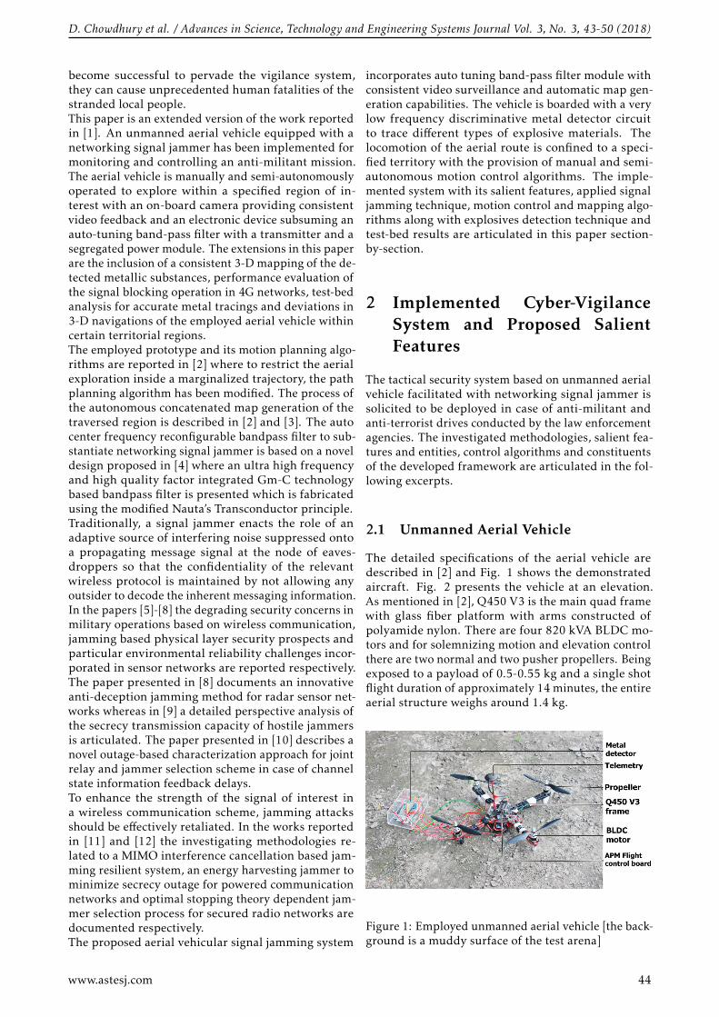
D. Chowdhury et al. / Advances in Science, Technology and Engineering Systems Journal Vol. 3, No. 3, 43-50 (2018)
become successful to pervade the vigilance system,they can cause unprecedented human fatalities of thestranded local people.This paper is an extended version of the work reportedin [1]. An unmanned aerial vehicle equipped with anetworking signal jammer has been implemented formonitoring and controlling an anti-militant mission.The aerial vehicle is manually and semi-autonomouslyoperated to explore within a specified region of in-terest with an on-board camera providing consistentvideo feedback and an electronic device subsuming anauto-tuning band-pass filter with a transmitter and asegregated power module. The extensions in this paperare the inclusion of a consistent 3-D mapping of the de-tected metallic substances, performance evaluation ofthe signal blocking operation in 4G networks, test-bedanalysis for accurate metal tracings and deviations in3-D navigations of the employed aerial vehicle withincertain territorial regions.The employed prototype and its motion planning algo-rithms are reported in [2] where to restrict the aerialexploration inside a marginalized trajectory, the pathplanning algorithm has been modified. The process ofthe autonomous concatenated map generation of thetraversed region is described in [2] and [3]. The autocenter frequency reconfigurable bandpass filter to sub-stantiate networking signal jammer is based on a noveldesign proposed in [4] where an ultra high frequencyand high quality factor integrated Gm-C technologybased bandpass filter is presented which is fabricatedusing the modified Nauta’s Transconductor principle.Traditionally, a signal jammer enacts the role of anadaptive source of interfering noise suppressed ontoa propagating message signal at the node of eaves-droppers so that the confidentiality of the relevantwireless protocol is maintained by not allowing anyoutsider to decode the inherent messaging information.In the papers [5]-[8] the degrading security concerns inmilitary operations based on wireless communication,jamming based physical layer security prospects andparticular environmental reliability challenges incor-porated in sensor networks are reported respectively.The paper presented in [8] documents an innovativeanti-deception jamming method for radar sensor net-works whereas in [9] a detailed perspective analysis ofthe secrecy transmission capacity of hostile jammersis articulated. The paper presented in [10] describes anovel outage-based characterization approach for jointrelay and jammer selection scheme in case of channelstate information feedback delays.To enhance the strength of the signal of interest ina wireless communication scheme, jamming attacksshould be effectively retaliated. In the works reportedin [11] and [12] the investigating methodologies re-lated to a MIMO interference cancellation based jam-ming resilient system, an energy harvesting jammer tominimize secrecy outage for powered communicationnetworks and optimal stopping theory dependent jam-mer selection process for secured radio networks aredocumented respectively.The proposed aerial vehicular signal jamming system
incorporates auto tuning band-pass filter module withconsistent video surveillance and automatic map gen-eration capabilities. The vehicle is boarded with a verylow frequency discriminative metal detector circuitto trace different types of explosive materials. Thelocomotion of the aerial route is confined to a speci-fied territory with the provision of manual and semi-autonomous motion control algorithms. The imple-mented system with its salient features, applied signaljamming technique, motion control and mapping algo-rithms along with explosives detection technique andtest-bed results are articulated in this paper section-by-section.
2 Implemented Cyber-VigilanceSystem and Proposed SalientFeatures
The tactical security system based on unmanned aerialvehicle facilitated with networking signal jammer issolicited to be deployed in case of anti-militant andanti-terrorist drives conducted by the law enforcementagencies. The investigated methodologies, salient fea-tures and entities, control algorithms and constituentsof the developed framework are articulated in the fol-lowing excerpts.
2.1 Unmanned Aerial Vehicle
The detailed specifications of the aerial vehicle aredescribed in [2] and Fig. 1 shows the demonstratedaircraft. Fig. 2 presents the vehicle at an elevation.As mentioned in [2], Q450 V3 is the main quad framewith glass fiber platform with arms constructed ofpolyamide nylon. There are four 820 kVA BLDC mo-tors and for solemnizing motion and elevation controlthere are two normal and two pusher propellers. Beingexposed to a payload of 0.5-0.55 kg and a single shotflight duration of approximately 14 minutes, the entireaerial structure weighs around 1.4 kg.
Figure 1: Employed unmanned aerial vehicle [the back-ground is a muddy surface of the test arena]
www.astesj.com 44
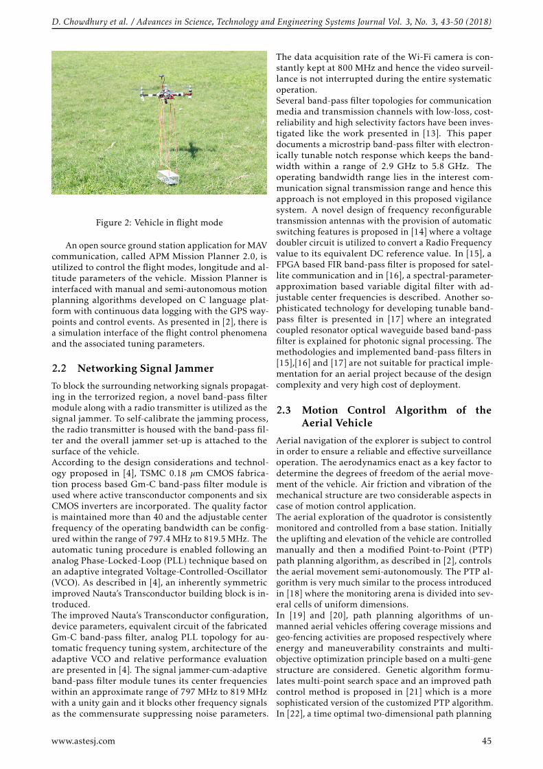
D. Chowdhury et al. / Advances in Science, Technology and Engineering Systems Journal Vol. 3, No. 3, 43-50 (2018)
Figure 2: Vehicle in flight mode
An open source ground station application for MAVcommunication, called APM Mission Planner 2.0, isutilized to control the flight modes, longitude and al-titude parameters of the vehicle. Mission Planner isinterfaced with manual and semi-autonomous motionplanning algorithms developed on C language plat-form with continuous data logging with the GPS way-points and control events. As presented in [2], there isa simulation interface of the flight control phenomenaand the associated tuning parameters.
2.2 Networking Signal Jammer
To block the surrounding networking signals propagat-ing in the terrorized region, a novel band-pass filtermodule along with a radio transmitter is utilized as thesignal jammer. To self-calibrate the jamming process,the radio transmitter is housed with the band-pass fil-ter and the overall jammer set-up is attached to thesurface of the vehicle.According to the design considerations and technol-ogy proposed in [4], TSMC 0.18 µm CMOS fabrica-tion process based Gm-C band-pass filter module isused where active transconductor components and sixCMOS inverters are incorporated. The quality factoris maintained more than 40 and the adjustable centerfrequency of the operating bandwidth can be config-ured within the range of 797.4 MHz to 819.5 MHz. Theautomatic tuning procedure is enabled following ananalog Phase-Locked-Loop (PLL) technique based onan adaptive integrated Voltage-Controlled-Oscillator(VCO). As described in [4], an inherently symmetricimproved Nauta’s Transconductor building block is in-troduced.The improved Nauta’s Transconductor configuration,device parameters, equivalent circuit of the fabricatedGm-C band-pass filter, analog PLL topology for au-tomatic frequency tuning system, architecture of theadaptive VCO and relative performance evaluationare presented in [4]. The signal jammer-cum-adaptiveband-pass filter module tunes its center frequencieswithin an approximate range of 797 MHz to 819 MHzwith a unity gain and it blocks other frequency signalsas the commensurate suppressing noise parameters.
The data acquisition rate of the Wi-Fi camera is con-stantly kept at 800 MHz and hence the video surveil-lance is not interrupted during the entire systematicoperation.Several band-pass filter topologies for communicationmedia and transmission channels with low-loss, cost-reliability and high selectivity factors have been inves-tigated like the work presented in [13]. This paperdocuments a microstrip band-pass filter with electron-ically tunable notch response which keeps the band-width within a range of 2.9 GHz to 5.8 GHz. Theoperating bandwidth range lies in the interest com-munication signal transmission range and hence thisapproach is not employed in this proposed vigilancesystem. A novel design of frequency reconfigurabletransmission antennas with the provision of automaticswitching features is proposed in [14] where a voltagedoubler circuit is utilized to convert a Radio Frequencyvalue to its equivalent DC reference value. In [15], aFPGA based FIR band-pass filter is proposed for satel-lite communication and in [16], a spectral-parameter-approximation based variable digital filter with ad-justable center frequencies is described. Another so-phisticated technology for developing tunable band-pass filter is presented in [17] where an integratedcoupled resonator optical waveguide based band-passfilter is explained for photonic signal processing. Themethodologies and implemented band-pass filters in[15],[16] and [17] are not suitable for practical imple-mentation for an aerial project because of the designcomplexity and very high cost of deployment.
2.3 Motion Control Algorithm of theAerial Vehicle
Aerial navigation of the explorer is subject to controlin order to ensure a reliable and effective surveillanceoperation. The aerodynamics enact as a key factor todetermine the degrees of freedom of the aerial move-ment of the vehicle. Air friction and vibration of themechanical structure are two considerable aspects incase of motion control application.The aerial exploration of the quadrotor is consistentlymonitored and controlled from a base station. Initiallythe uplifting and elevation of the vehicle are controlledmanually and then a modified Point-to-Point (PTP)path planning algorithm, as described in [2], controlsthe aerial movement semi-autonomously. The PTP al-gorithm is very much similar to the process introducedin [18] where the monitoring arena is divided into sev-eral cells of uniform dimensions.In [19] and [20], path planning algorithms of un-manned aerial vehicles offering coverage missions andgeo-fencing activities are proposed respectively whereenergy and maneuverability constraints and multi-objective optimization principle based on a multi-genestructure are considered. Genetic algorithm formu-lates multi-point search space and an improved pathcontrol method is proposed in [21] which is a moresophisticated version of the customized PTP algorithm.In [22], a time optimal two-dimensional path planning
www.astesj.com 45

D. Chowdhury et al. / Advances in Science, Technology and Engineering Systems Journal Vol. 3, No. 3, 43-50 (2018)
approach is documented along with obstacle avoid-ance provision. Several sophisticated motion controltechniques for unmanned aerial vehicles have beenarticulated in [23], [24] and [25].The basic control algorithm to decide the navigationtrajectory of the demonstrated aerial vehicle followsthe one presented in [2] with a modification of inser-tion of three dimensional movement within a boundedarena with limited specifications. The aerial vehicleis subject to scan the maximum coverage area of theregion of interest by moving from a point to its nearestpoint of exploration. The customized algorithm for theaerial motion control is presented in Algorithm 1.Apart form that GPS coordinates and orientation sen-sors embedded onto the vehicular structure enablesautomatic mapping of the stored position values of thenavigating and continuously moving quadrotor.
Algorithm 1 Algorithm for Motion Control
Array of X-axis coordinates of center of each grid→ XArray of Y-axis coordinates of center of each grid→ YArray of Z-axis coordinates of center of each grid→ ZDummy variables→ i, j,kMaximum index of X-array→ IMaximum index of Y-array→ JMaximum index of Z-array→ KCoordinates of the present grid→ x,y,zINITIALIZE:i← 0j← 0k← 0START:While (j < J)x← x[i]y← Y [j]y← Z[k]if j%2 = 0 theni← i + 1k← k + 1
elsei← i − 1k← k − 1
end ifif i = I and k = K theni← i − 1k← k − 1j← j + 1if i = −1 and k = −1 theni← i + 1k← k + 1j← j + 1
elseMove vehicle to (x,y,z) point
end ifend ifGoto START
2.4 Explosives Tracing and Detection
Algorithm 2 Algorithm for 3-D Mapping of the GPSTraces of Suspicious Metals
Array of (x,y,z) coordinates→ AcArray index→ IaState variable→ SaProgram variable→ CpSa← 0 ; no change in the present stateSa← 1 ; change in the present stateCp← 0 ; operation is being executedCp← 1 ; operation is being terminatedPresent location point→ (x,y,z)INITIALIZE:X←0 ; initial x-axis locationY←0 ; initial y-axis locationZ←0 ; initial z-axis (or elevated) locationIa← 0START:Read Saif Sa == 0 thenAc[Ia][0][0]← xAc[Ia][1][0]← yAc[Ia][1][1]← zIa← Ia + 1
end ifif Cp == 0 then
for m < 0;m < Ia;m←m+ 1 dox← Ac[m][0][0]y← Ac[m][1][0]z← Ac[m][1][1]x← x+ x0y← y + y0z← z+ z0x0← xy0← yz0← zplot (x,y,z) and connect with the previouspoints
end forend ifGoto START
The militants can bury improvised explosive de-vices and landmines in a terrorized area and such mal-practice can devastate the entire locality causing hugeholistic fatalities of the innocent people and their be-longings. To prevent such malicious activities the pro-posed aerial vehicle based vigilance system is providedwith a metal detector circuit module which is attachedto a downward inclined portion of the navigator tokeep the metal sensing circuitry close to the surface ofthe landscape. The metal detection technique and im-plemented sensing system follows the one presentedin [2] which contains a submersible monoloop coiland works on the principle of very low frequency elec-tromagnetic induction. The sensing frequency of thedetector is about 5.5 kHz which is suitable to detect theemanations from improvised ammos as they contain
www.astesj.com 46

D. Chowdhury et al. / Advances in Science, Technology and Engineering Systems Journal Vol. 3, No. 3, 43-50 (2018)
very less exposed metallic surface. The sensing depthpotential of the configuration is approximately 30 to35 cm being in elevation from the ground surface. Theexplorer can detect buried metals from a maximum of35 cm elevation height measured from the ground sur-face. The tracing and algorithm for simultaneous 2-Dmapping of the detected metal points in the exploredregion are described in [2]. In this paper, algorithmfor consistent 3-D mapping of the scanned surfacesand detected metals has been presented. In the flightmode, aerial vehicle sends (x,y,z) location coordinatesof the detected metals where the metal detecting cir-cuit senses the presence of any suspicious materialwithin a maximum depth potential of 35 cm above theground. Therefore, the z-location values do not exceed35 cm ground clearance where the x and y-locationvalues are confined within the testing territory. Algo-rithm 2 shows the implemented approach to map GPStraces of the metals.
3 Results and Analysis
The developed cyber-vigilance system is assessed indifferent test-beds to ensure the sustainability and re-liability of the aerial vehicle based networking signaljammer especially in case of accurate signal blockingactivities and stable aerial motion within a confinedterritory.
3.1 Evaluation of the Signal Blocking Phe-nomenon
The implemented security system is tested in differentenvironments with different frequency signals withco-existence of the communication signals of 2G, 3Gand 4G spectra and wide fidelity (Wi-Fi) and radiofrequency (RF) signals. With different combinationsof co-existing signals in an arena with a dimension of10m× 10m with a flight elevation height of 12m, eachtime the prototype is tested for 50 times for perfor-mance evaluation in terms of accurate blocking (%)and false blocking (%), which are enumerated in Table1. The evaluated percentages enlisted here are closeapproximated values.
Table 1: Evaluation of Accurate and False Signal Block-ing Phenomena
Test Signals BA(%) BF(%)2G 96 42G+ 3G 86 142G+ 3G+ 4G 85 152G + 3G + Wi −Fi(800MHz)
82 18
2G + 3G + 4G + Wi −Fi(800MHz)
79 21
2G + 3G + Wi −Fi(800MHz) +RF
78 22
2G + 3G + 4G + Wi −Fi(800MHz) +RF
75 25
Here BA and BF are the percent values of accurateand false blocking operations respectively and theseare determined as
BA =NBANT× 100% (1)
BF =NBFNT× 100% (2)
where NBA is the number of accurate blocking op-erations, NBF is the number of false blocking opera-tions and NT is the total number of testing operations[NT =NBA +NBF].The aerial vehicle is solicited to different elevationheights within a certain territorial boundary of 13.5m×13.5m and the accurate detection phenomenon istested for 50 consecutive times for each elevationwhere each time a composition of 2G + 3G + Wi −Fi(800MHz) signals is present there.
Figure 3: Evaluation of accurate blocking operation incase of different elevation heights
The performance evaluation of accurately blockingsignals for different elevation heights is presented inFig. 3.Likewise the accurate blocking operation of the signaljammer is tested for different two dimensional terri-tories with a constant elevation height of 12.5m for50 consecutive times. The performance evaluationof accurately blocking signals for different territorialboundaries for a constant elevation height is presentedin Fig. 4.
www.astesj.com 47

D. Chowdhury et al. / Advances in Science, Technology and Engineering Systems Journal Vol. 3, No. 3, 43-50 (2018)
Figure 4: Evaluation of accurate blocking operation incase of different territorial boundaries with a constantelevation height
3.2 Evaluation of the Accurate Metal Trac-ing Phenomenon
The aerial vehicle is tested for accurate tracing of (x,y)locations of the metals within the testing boundary.In this case, z-locations of the traces are constant for50 testing attempts. The vehicle in flight mode is con-trolled to navigate along a 350cm elevation height fromthe ground surface which is to be scanned to find metaltraces. The metal detector is attached to a platformapproximately 20cm underneath the main vehicularbody and hence the detector senses the metals froma ground clearance of 30cm. Fig. 5 presents the per-formance evaluation of accurate metal tracing of (x,y)locations within the testing arena.
Figure 5: Evaluation of accurate metal tracing for (x,y)locations with a constant z-location value in case ofdifferent test arenas
3.3 Evaluation of Deviations in Accelera-tion
According to [2], the navigation has been controlled insuch a manner that the vibration of the aerial structureremains within −3 cms−2 to +3 cms−2 along x and y-axis and −5 cms−2 to −15 cms−2 along z-axis. The lin-ear accelerometer shows some small deviations fromthe aforementioned standard range when the vehicleis in its flight mode. Fig. 6 presents the (x,y,z) devia-tions in acceleration of the vehicle. These have beenderived for 50 consecutive test runs and the values areapproximated from the accelerometer readings.
Figure 6: Evaluation of deviations of the vehicle inflight mode from the standard (x,y,z) acceleration val-ues
3.4 Evaluation of Stable Motion within aConfined Territory
The unmanned aerial vehicle is supposed to navigatewithin a confined region where the signal jammerblocks the networking signals with the provision ofvideo surveillance, map generation and metal detec-tion. The developed system is tested in terms of per-centage of accurate confinement to affirm its stableaerial exploration within a certain bounded area. Foreach different boundary limit, the vehicle is made toexplore for 20 times of assessment and the estimatedaccuracy of confinement in % is enlisted in Table 2.
Table 2: Evaluation of Accuracy of ConfinementTesting Arenas (m×m×m) CA (%)7× 5.5× 5 938.5× 6.3× 7.4 8911× 7.5× 9.8 8714× 9× 10.2 8216.7× 12.5× 13 79
HereCA =
NCNNTN
× 100% (3)
www.astesj.com 48

D. Chowdhury et al. / Advances in Science, Technology and Engineering Systems Journal Vol. 3, No. 3, 43-50 (2018)
where CA is the accuracy of confinement, NCN is thenumber of confined navigations and NTN is the num-ber of total navigations.
4 Conclusion
This paper articulates a novel aerial vehicle basedcyber-vigilance framework capable of networking sig-nal jamming retaliation against militants and terror-ists to corner them during an anti-terrorist drive. Theunconventional signal jammer consists of a auto tun-able band-pass filter module to block communicationsignals present in the examined area. This surveil-lance system provides an apprehensive security systemwhich is handy for saving innocent lives stranded ina terrorized region. The aerial prototype is equippedwith ammo detection module and has a unique fea-ture of automatic path mapping of the covered region.Accurate signal blocking operation, accurate metal de-tection, 3-D mapping of the metal traces and stableconfined motion with sustainable aerodynamic move-ment are the prominent features of the proposed work.The test results corroborate the efficacy and authentic-ity of the developed system for application in defensemissions and security drills.
References[1] D. Chowdhury, M. Sarkar, M. Z. Haider, S. A. Fattah and C.
Shahnaz, “Design and Implementation of a Cyber-VigilanceSystem for Anti-Terrorist Drives Based on an UnmannedAerial Vehicular Networking Signal Jammer for Specific Terri-torial Security” in Humanitarian Technology Conference (R10-HTC), Dhaka Bangladesh, 2017. https://doi.org/10.1109/R10-HTC.2017.8288995
[2] S. A. Fattah, M. Z. Haider, D. Chowdhury, M. Sarkar, R. I.Chowdhury, M. S. Islam, R. Karim, A. Rahi, and C. Shahnaz,“An aerial landmine detection system with dynamic path andexplosion mode identification features” in IEEE Global Hu-manitarian Technology Conference (GHTC), Seattle WA USA,2016. https://doi.org/10.1109/GHTC.2016.7857361
[3] S. A. Fattah, D. Chowdhury, M. Z. Haider, M. Sarkar, M.Refat, G. Rabbi, S. B. Masud, and C. Shahnaz, “Dynamicmap generating rescuer offering surveillance robotic sys-tem with autonomous path feedback capability” in IEEE Re-gion 10 Humanitarian Technology Conference (R10-HTC),Cebu City Philippines, 2015. https://doi.org/10.1109/R10-HTC.2015.7391872
[4] G. Zhiqiang, L. Zhiheng, H. Zhengxiong, Z. Yonglai, andZ. Xinyuan, “A uhf cmos gm-c bandpass filter and auto-matic tuning design” in Academic Symposium on Optoelec-tronics and Microelectronics Technology and 10th Chinese-Russian Symposium on Laser Physics and Laser Technolo-gyOptoelectronics Technology (ASOT), Harbin China, 2010.https://doi.org/10.1109/RCSLPLT.2010.5615323
[5] P. J. Nicholas, J. C. Tkacheff, and C. M. Kuhns, “Measuringthe operational impact of military SATCOM degradation” inWinter Simulation Conference (WSC), Washington DC USA,2016. https://doi.org/10.1109/WSC.2016.7822342
[6] Y. Zou, J. Zhu, X. Wang, and V. C. M. Leung, “Improv-ing physical-layer security in wireless communications us-ing diversity techniques” IEEE Netw., 29(1), 42–48, 2015.https://doi.org/10.1109/MNET.2015.7018202
[7] J. Zhu, Y. Zou, and B. Zheng, “Physical-layer se-curity and reliability challenges for industrial wire-less sensor networks” IEEE Acce., 5, 5313–5320, 2017.https://doi.org/10.1109/ACCESS.2017.2691003
[8] M. Nouri, M. Mivehchy, and M. F. Sabahi, “Novelanti-deception jamming method by measuring phasenoise of oscillators in lfmcw tracking radar sen-sor networks” IEEE Acce., 5, 11455–11467, 2017.https://doi.org/10.1109/ACCESS.2017.2655040
[9] C. Si, H. Sun, M. Sheng, X. Wang, and J. Li, “Phys-ical layer security with hostile jammers and eavesdrop-pers: Secrecy transmission capacity” in IEEE 27th AnnualInternational Symposium on Personal, Indoor, and Mo-bile Radio Communications (PIMRC), Valencia Spain, 2016.https://doi.org/10.1109/PIMRC.2016.7794718
[10] L. Wang, Y. Cai, Y. Zou, W. Yang, and L. Hanzo,“Joint relay and jammer selection improves the phys-ical layer security in the face of csi feedback de-lays” IEEE Trans. Vehi. Tech., 65(8), 6259–6274, 2016.https://doi.org/10.1109/TVT.2015.2478029
[11] Q. Yan, H. Zeng, T. Jiang, M. Li, Lou, and Y. T. Hou, “Jammingresilient communication using mimo interference cancella-tion” IEEE Trans. Info. Fore. and Secu., 11(7), 1486–1499,2016. https://doi.org/10.1109/TIFS.2016.2535906
[12] Q. Gao, Y. Huo, L. Ma, X. Xing, X. Cheng, T. Jing, and H.Liu,“Optimal stopping theory based jammer selection for se-curing cooperative cognitive radio networks” in IEEE GlobalCommunications Conference (GLOBECOM), Washington DCUSA, 2016. https://doi.org/10.1109/GLOCOM.2016.7842096
[13] M. A. Mutalib, Z. Zakaria, N. A. Shairi, and W. Y. Sam,“Design of microstrip bandpass filter with electronicallytunable notch response” in 26th International ConferenceRadioelektronika (RADIOELEKTRONIKA), Kosice Slovakia,2016. https://doi.org/10.1109/RADIOELEK.2016.7477380
[14] L. Hinsz and B. D. Braaten, “A frequency reconfigurabletransmitter antenna with autonomous switching capabili-ties” IEEE Trans. Ante. and Prop., 62(7), 3809–3813, 2014.https://doi.org/10.1109/TAP.2014.2316298
[15] V. Kumar, R. Mehra, and Shallu, “Reconfigurable bandpass filter using kaiser window for satellite communica-tion” in 2nd International Conference on Next GenerationComputing Technologies (NGCT), Dehradun India, 2016.https://doi.org/10.1109/NGCT.2016.7877451
[16] S. J. Darak, A. P. Vinod, E. M. K. Lai, J. Palicot, andH. Zhang, “Linear-phase vdf design with unabridgedbandwidth control over the nyquist band” IEEE Trans.Circ. and Syst. II: Expr. Brief., 61(6), 428–432, 2014.https://doi.org/10.1109/TCSII.2014.2319992
[17] C. Taddei, L. Zhuang, M. Hoekman, A. Leinse, R. Olden-beuving, P. van Dijk, and C. Roeloffzen, “Fully reconfigurablecoupled ring resonator-based bandpass filter for microwavesignal processing” in International Topical Meeting on Mi-crowave Photonics (MWP) and the 2014 9th Asia-Pacific Mi-crowave Photonics Conference (APMP), Sendai Japan, 2014.https://doi.org/10.1109/MWP.2014.6994485
[18] I. Khoufi, P. Minet, and N. Achir, “Unmanned aerial ve-hicles path planning for area monitoring” in InternationalConference on Performance Evaluation and Modeling inWired and Wireless Networks (PEMWN), Paris France, 2016.https://doi.org/10.1109/PEMWN.2016.7842902
[19] G. Gramajo and P. Shankar, “Path-planning for an un-manned aerial vehicle with energy constraint in a searchand coverage mission” in IEEE Green Energy and Sys-tems Conference (IGSEC), Long Beach CA USA, 2016.https://doi.org/10.1109/IGESC.2016.7790077
www.astesj.com 49

D. Chowdhury et al. / Advances in Science, Technology and Engineering Systems Journal Vol. 3, No. 3, 43-50 (2018)
[20] Y. Liu, R. Lv, X. Guan, and J. Zeng, “Path planning for un-manned aerial vehicle under geo-fencing and minimum safeseparation constraints” in 12th World Congress on Intelli-gent Control and Automation (WCICA), Guilin China, 2016.https://doi.org/10.1109/WCICA.2016.7578482
[21] J. Tao, C. Zhong, L. Gao, and H. Deng, “A study onpath planning of unmanned aerial vehicle based onimproved genetic algorithm” in 8th InternationalConference on Intelligent Human-Machine Systemsand Cybernetics (IHMSC), Hangzhou China, 2016.https://doi.org/10.1109/IHMSC.2016.182
[22] J. W. Yeol and Y. W. Hwang, “Parametrization of nonlineartrajectory for time optimal 2D path planning for unmannedaerial vehicles” in 2nd International Conference on Control,Automation and Robotics (ICCAR), Hong Kong China, 2016.https://doi.org/10.1109/ICCAR.2016.7486751
[23] F. Lazzari, A. Buffi, P. Nepa, and S. Lazzari, “Nu-merical Investigation of an UWB Localization Tech-nique for Unmanned Aerial Vehicles in Outdoor Sce-narios” IEEE Sens. Journal, 17(9), 2896–2903, 2017.https://doi.org/10.1109/JSEN.2017.2684817
[24] T. Lee, “Geometric Control of Quadrotor UAVsTransporting a Cable-Suspended Rigid Body” IEEETrans. Cont. Syst. Tech., 26(1), 255–264, 2018.https://doi.org/10.1109/TCST.2017.2656060
[25] L. L. Gomes, L. P. Leal, T. R. Oliveira, J. P. V. S. d. Cunha, andT. C. Revoredo, “Unmanned Quadcopter Control Using a Mo-tion Capture System” IEEE Latin America Trans., 14(8), 3606–3613, 2016. https://doi.org/10.1109/TLA.2016.7786340
www.astesj.com 50

www.astesj.com 51
EAES: Extended Advanced Encryption Standard with Extended Security
Abul Kalam Azad*, Md. Yamin Mollah
Computer Science and Telecommunication Engineering, Noakhali Science and Technology University, Noakhali-3814, Bangladesh
A R T I C L E I N F O A B S T R A C T Article history: Received: 29 March, 2018 Accepted: 24 April, 2018 Online :20 May, 2018
Though AES is the highest secure symmetric cipher at present, many attacks are now effective against AES too which is seen from the review of recent attacks of AES. This paper describes an extended AES algorithm with key sizes of 256, 384 and 512 bits with round numbers of 10, 12 and 14 respectively. Data block length is 128 bits, same as AES. But unlike AES each round of encryption and decryption of this proposed algorithm consists of five stages except the last one which consists of four stages. Unlike AES, this algorithm uses two different key expansion algorithms with two different round constants that ensure higher security than AES. Basically, this algorithm takes one cipher key and divides the selected key of two separate sub-keys: FirstKey and SecondKey. Then expand them through two different key expansion schedules. Performance analysis shows that the proposed extended AES algorithm takes almost same amount of time to encrypt and decrypt the same amount of data as AES but with higher security than AES.
Keywords: AES-256/384/512 EAES-256/384/512 Extended-AES Network Security
1. Introduction
Communications among individual or organizations are increasing day by day. Everyone wants to keep their private information secure from any type of threats or being lost. Cryptography achieves this goal to secure private information. Schemes are being developed rapidly and frequently for cryptography and attacks on those schemes are being developed often too. New attacks are being strong, effective and attenuating the security of existing cryptographic schemes.
Rijndael block cipher was proposed as AES by September 03, 1999 [1]. National Institute of Standards and Technology (NIST) announced Rijndael block cipher as AES by Federal Information Processing Standards Publication 197 (FIPS 197) by November 26, 2001. Several attacks were developed after the publication of AES that are threatening for AES but not practically successful on full AES. Until 2006, the best-known attacks were on 7 rounds, 8 rounds, and 9 rounds for 128-bit keys, 192-bit keys, and 256-bit keys respectively [2]. However, in the recent time, many attacks are close to successful on AES. For the reduced 8-round version of AES-128, the first known-key distinguishing attack was released as a preprint in November 2009 [3]. It works with a memory complexity of 232, and a time complexity of 248. In 2011
[4], the first key-recovery attack on full AES was developed. This biclique attack is four times faster than the brute force attack. It requires 2126.2, 2190.2 and 2254.6 operations to recover an AES-128, AES-192 and AES-256 key respectively. This result has been further improved to 2126.0, 2189.9 and 2254.3 operations for AES-128, AES-192 and AES-256 key respectively [5], which are the current best results in key recovery attack against AES.
As intended to develop AES with extended key sizes for more security against recently developed attacks by keeping the performance almost similar to that of AES. Thus proposed algorithm becomes more complex for Interpolation attack, Basic attack, and Square attack. Differential and Linear cryptanalysis will be inefficient for this algorithm too. Since this algorithm uses two different keys derived from one key, it will be more complex and impossible to crack in spite of having known plaintext-ciphertext pairs available. The throughput of the proposed algorithm is nearly similar to that of AES. It is shown that for a 100KB text file, encryption time taken by AES-128 is 0.100s where for EAES-256 it is the same amount of time. Performances of other versions of EAES are evaluated and they are effective too.
The rest of the paper is organized as follows: Section 2 briefly explain related research works, Section 3 describes the proposed EAES algorithm, Section 4 shows the performance analysis of
ASTESJ
ISSN: 2415-6698
*Abul Kalam Azad, Department of CSTE, NSTU, Email: [email protected]
Advances in Science, Technology and Engineering Systems Journal Vol. 3, No. 3, 51-56 (2018)
www.astesj.com
https://dx.doi.org/10.25046/aj030307

A. K. Azad et al. / Advances in Science, Technology and Engineering Systems Journal Vol. 3, No. 3, 51-56(2018)
www.astesj.com 52
EAES, Section 5 describes the strength of EAES against different types of attacks and Finally, Section 6 concludes the paper.
2. Background
After the proposal of AES encryption by Rijndael, a large number of research works has been done on it. An FPGA based architecture for a new version of 512-Bit Advanced Encryption Standard algorithm design and evaluation was proposed in [6]. It (AES-512) uses both input and key block size of 512-bits which makes it more resistant to cryptanalysis against the break of its security. Throughput increased by 230% when compared with the implementation of the original AES-128. But requires more control logic blocks (CLBs) in implementation prospect than existing AES.
An efficient parallel implementation and optimization of the Advanced Encryption Standard (AES) algorithm based on the Sunway TaihuLight was proposed in [7]. The Sunway TaihuLight is a China’s independently developed heterogeneous supercomputer [8] with peak performance over 100 Petaflops. Specifically, they expanded the scale to 1024 nodes and achieved the throughput of about 63.91 GB/s (511.28 Gbits/s). But with the increase of input data the throughput grows from quick to slow pattern.
A new efficient and novel approach to protect AES against differential power analysis was proposed in 2015 [9]. The implementation of this approach provides a significant improvement in strength against differential power analysis with a minimal additional hardware overhead. The efficiency of their proposed technique was verified by practical results obtained from real implementation on a Xilinx Spartan-II FPGA.
In 2016, an implementation of AES algorithm to overt fake keys against counter attacks was proposed [10]. An approach to overt the cryptographic key, when there is any counter attacks so-called side-channel attacks (SCAs) are applied in order to break the security of AES-128. Experimental results make sure the strength of the proposed approach to successfully hide the true cryptographic key. But it is more time consumptive than existing AES.
Constructing key dependent dynamic S-box for AES block cipher system was proposed in 2016 [11]. A new approach to generating dynamic S-box which was constructed centered on round key. Predefined static S-boxes pose a weak point for the attackers to analyze certain ciphertext pairs. The new S-boxes created were additionally dynamic, random and key dependent which attempts to escalate the complexity of the algorithm and furthermore mark the cryptanalysis more challenging. However, the performance in terms of time and power consumption is not examined and showed in this paper.
An implementation of AES-128 and AES-512 on Apple mobile processor [12] was proposed in 2017 that uses 512 bits of data block size using key sizes of 128, 192, 256, 512 and 1024 bits. However, again the performance degrades with the extension of key lengths.
3. Proposed Extended AES (EAES)
Advanced Encryption Standard (AES) is the most used and most secure algorithm at present among other symmetric cipher algorithms. But recently some sorts of attack such as biclique attack are threatening for AES. AES uses key sizes of 128 bits, 192 bits and 256 bits [13]. The authors have developed an algorithm almost similar to AES with some exceptions and double in key sizes (i.e., key sizes of 256, 384 and 512 bits) and highly secure than AES.
The proposed EAES algorithm has four parts: encryption, decryption, key division and key expansion. It takes plaintext block length of 128 bits as the existing AES. Every encryption and decryption process goes through several numbers of rounds according to their key sizes. This algorithm is named depending on its key lengths as EAES-256, EAES-384, and EAES- 512. Key sizes with corresponding round numbers are given in Table 1.
Table 1. Key sizes with corresponding round numbers of the cipher
Key Size ( bits/bytes/words ) Round Number ( Nr )
256/32/8 10
384/48/12 12
512/64/16 14
3.1. Key Division
This part of the algorithm takes a cipher key and divides it into two equal sub-keys in a simple way. The resulting two sub-keys are named FirstKey and SecondKey. Size of both sub-keys can be 128, 192 and 256 bits since the cipher key can be 256, 384 and 512 bits. FirstKey has byte values that are in odd positions in the cipher key and SecondKey has byte values that are in even positions in the cipher key. Figure 1 shows an example of this key division process where each letter is identified as a byte and the cipher key is 256 bits or 32 bytes.
Figure 1 Key division example of the cipher key expansion
Two different key expansions are used for two sub-keys. Since sub-key sizes are 128, 192 and 256 bits for cipher key sizes of 256, 384 and 512 bits respectively, the values of 𝑁𝑁𝑁𝑁 for both sub-keys will be same as defined in AES. Sub-key expansions can be described as follows:
1. At first, the sub-key is copied into the first 𝑁𝑁𝑁𝑁 words of the array of expanded sub-key. In other words, the first 𝑁𝑁𝑁𝑁 words of the expanded sub-key are filled with the sub-key which is also 𝑁𝑁𝑁𝑁 words long.

A. K. Azad et al. / Advances in Science, Technology and Engineering Systems Journal Vol. 3, No. 3, 51-56(2018)
www.astesj.com 53
2. Words in positions that are a multiple of 𝑁𝑁𝑁𝑁 go through a more complex function which is denoted by 𝑔𝑔.
3. Every following word w[i] is equal to the XOR of the previous word w[i – 1] and the word 𝑁𝑁𝑁𝑁 position earlier w[i – 𝑁𝑁𝑁𝑁]. Note that i starts with 1, not 0.
4. The complex function 𝑔𝑔 takes a single word or 4 bytes as input then passes it through the following three subsequent operations:
a. RotWord: If the sub-key is FirstKey, it performs a one-byte circular left shift on a word. This means an input word [B1, B2, B3, B4] transformed into [B2, B3, B4, B1]. If the sub-key is SecondKey, it performs a one-byte circular right shift on a word. This means an input word [B1, B2, B3, B4] transformed into [B4, B1, B2, B3].
b. SubWord: It performs a byte substitution on each byte of its input word using the S-box used for AES.
c. The result of operation b is XORed with a round constant Rcon[i]. The round constant is a word in which the first byte is different for different round values but the rightmost three bytes always remain constant. Round Constants are different for FirstKey and SecondKey. Rcon[i] values for FirstKey and SecondKey expansions are given in Table 2. For FirstKey expansion, the rightmost three bytes of the Round Constant are always 0. Rcon[i] = (RC[i], 0, 0, 0) with RC[1] = 1, RC[i] = 2 • RC[i – 1]. For SecondKey expansion, among the right most three bytes of the Round Constant, the first and third bytes are equal to hexadecimal value FF that means all bits of these two bytes are 1. The second byte is equal to 00 that means all bits of the second byte are 0. Rcon[i] = (RC[i], FF, 0, FF) with RC[1] = 1, RC[i] = 3 • RC[i – 1] = [2 ⊕ 1] • RC[i – 1] = (2 • RC[i – 1]) ⊕ RC[i – 1]. The symbol “ • ” denotes multiplication over the field 𝐺𝐺𝐺𝐺(28). The values of RC[i] in hexadecimal form are shown below where the value of “i” denotes round number.
5. If 𝑁𝑁𝑁𝑁 = 8 and (i – 4) is a multiple of 𝑁𝑁𝑁𝑁 then SubWord is applied to w[i – 1] prior to the XOR.
Table 2. Rcon[i] values for FirstKey and SecondKey expansion
i 1 2 3 4 5 6 7 8 9 10 11 12 13 14
RC[i] (for FirstKey) 01 02 04 08 10 20 40 80 1B 36 6C D8 AB 4D
RC[i] (for
SecondKey) 01 03 05 0F 11 33 55 FF 1A 2E 72 96 A1 F8
Two different complex functions𝑔𝑔 used in the expansions of FirstKey and SecondKey are shown in Figure 2.
Figure 2 Complex function g for a) FirstKey expansion and b) SecondKey
expansion
After successful expansion of the FirstKey and SecondKey, each of the expanded FirstKey and SecondKey has a total of 𝑁𝑁𝑁𝑁(𝑁𝑁𝑁𝑁 + 1) words. From these, every four words were used for each round. The expanded FirstKey and SecondKey of 𝑁𝑁𝑁𝑁(𝑁𝑁𝑁𝑁 +1) words are shown in Figure 3.
Figure 3 Expanded a) FirstKey and b) SecondKey
3.2. Encryption or Cipher
The encryption process takes the plaintext input into the state and passes it through a single stage at the beginning of the cipher named AddFirstRoundKey. Then the state passed through 𝑁𝑁𝑁𝑁 rounds to get the expected ciphertext as output. Each of first 𝑁𝑁𝑁𝑁 −1 rounds has five consecutive stages that are: SubBytes, AddSecondRoundKey, ShiftRows, MixColumns, and AddFirstRoundKey. The last round that means 𝑁𝑁𝑁𝑁th round has all four stages except the MixColumns stage. Figure 6 shows full encryption process with all 𝑁𝑁𝑁𝑁 rounds.
3.2.1 SubBytes, ShiftRows and MixColumns Transformation
These stages do the exact similar transformations as AES.
3.2.2 AddFirstRoundKey Transformation
In this stage, an 𝑁𝑁𝑁𝑁-word FirstRoundKey is added to the state by simple bitwise XOR operation. A FirstRoundKey is 𝑁𝑁𝑁𝑁 words length as the state. The FirstRoundKey is provided from the FirstKey expansion function that expands the 𝑁𝑁𝑁𝑁 words FirstKey into 𝑁𝑁𝑁𝑁(𝑁𝑁𝑁𝑁 + 1) words expanded FirstKey. This addition could be described as a column-wise addition of the state matrix and the FirstRoundKey. The following figure shows the addition of a column of four bytes of the state and a word of the FirstRoundKey, where i indicates the value𝑖𝑖 = (𝑁𝑁𝑁𝑁 × 𝑁𝑁𝑁𝑁). The lowest value of
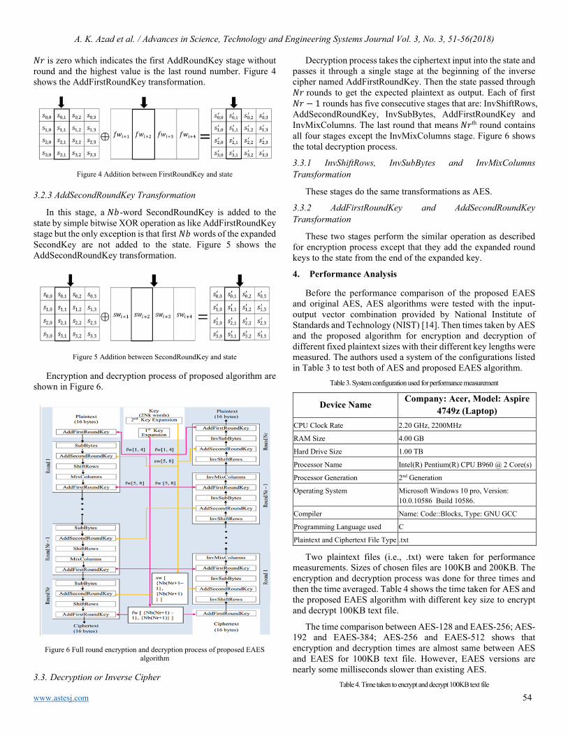
A. K. Azad et al. / Advances in Science, Technology and Engineering Systems Journal Vol. 3, No. 3, 51-56(2018)
www.astesj.com 54
𝑁𝑁𝑁𝑁 is zero which indicates the first AddRoundKey stage without round and the highest value is the last round number. Figure 4 shows the AddFirstRoundKey transformation.
Figure 4 Addition between FirstRoundKey and state
3.2.3 AddSecondRoundKey Transformation
In this stage, a 𝑁𝑁𝑁𝑁-word SecondRoundKey is added to the state by simple bitwise XOR operation as like AddFirstRoundKey stage but the only exception is that first 𝑁𝑁𝑁𝑁 words of the expanded SecondKey are not added to the state. Figure 5 shows the AddSecondRoundKey transformation.
Figure 5 Addition between SecondRoundKey and state
Encryption and decryption process of proposed algorithm are shown in Figure 6.
Figure 6 Full round encryption and decryption process of proposed EAES
algorithm
3.3. Decryption or Inverse Cipher
Decryption process takes the ciphertext input into the state and passes it through a single stage at the beginning of the inverse cipher named AddFirstRoundKey. Then the state passed through 𝑁𝑁𝑁𝑁 rounds to get the expected plaintext as output. Each of first 𝑁𝑁𝑁𝑁 − 1 rounds has five consecutive stages that are: InvShiftRows, AddSecondRoundKey, InvSubBytes, AddFirstRoundKey and InvMixColumns. The last round that means 𝑁𝑁𝑁𝑁th round contains all four stages except the InvMixColumns stage. Figure 6 shows the total decryption process.
3.3.1 InvShiftRows, InvSubBytes and InvMixColumns Transformation
These stages do the same transformations as AES.
3.3.2 AddFirstRoundKey and AddSecondRoundKey Transformation
These two stages perform the similar operation as described for encryption process except that they add the expanded round keys to the state from the end of the expanded key.
4. Performance Analysis
Before the performance comparison of the proposed EAES and original AES, AES algorithms were tested with the input-output vector combination provided by National Institute of Standards and Technology (NIST) [14]. Then times taken by AES and the proposed algorithm for encryption and decryption of different fixed plaintext sizes with their different key lengths were measured. The authors used a system of the configurations listed in Table 3 to test both of AES and proposed EAES algorithm.
Table 3. System configuration used for performance measurement
Device Name Company: Acer, Model: Aspire
4749z (Laptop) CPU Clock Rate 2.20 GHz, 2200MHz
RAM Size 4.00 GB
Hard Drive Size 1.00 TB
Processor Name Intel(R) Pentium(R) CPU B960 @ 2 Core(s)
Processor Generation 2nd Generation
Operating System Microsoft Windows 10 pro, Version: 10.0.10586 Build 10586.
Compiler Name: Code::Blocks, Type: GNU GCC
Programming Language used C
Plaintext and Ciphertext File Type .txt
Two plaintext files (i.e., .txt) were taken for performance measurements. Sizes of chosen files are 100KB and 200KB. The encryption and decryption process was done for three times and then the time averaged. Table 4 shows the time taken for AES and the proposed EAES algorithm with different key size to encrypt and decrypt 100KB text file.
The time comparison between AES-128 and EAES-256; AES-192 and EAES-384; AES-256 and EAES-512 shows that encryption and decryption times are almost same between AES and EAES for 100KB text file. However, EAES versions are nearly some milliseconds slower than existing AES.
Table 4. Time taken to encrypt and decrypt 100KB text file

A. K. Azad et al. / Advances in Science, Technology and Engineering Systems Journal Vol. 3, No. 3, 51-56(2018)
www.astesj.com 55
Alg. AES-128 AES-192 AES-256 EAES-256 EAES-384 EAES-512
Time(s)
Enc. Dec. Enc. Dec. Enc. Dec. Enc. Dec. Enc. Dec. Enc. Dec.
0.069 0.278 0.069 0.332 0.084 0.393 0.062 0.285 0.062 0.354 0.084 0.401
0.053 0.285 0.069 0.332 0.069 0.400 0.062 0.285 0.069 0.352 0.069 0.416
0.053 0.279 0.053 0.332 0.079 0.384 0.052 0.285 0.062 0.354 0.084 0.401 Average Time(s) 0.058 0.280 0.064 0.332 0.077 0.392 0.059 0.285 0.064 0.353 0.079 0.406
Table 5. Time taken to encrypt and decrypt 200KB text file
Alg AES-128 AES-192 AES-256 EAES-256 EAES-384 EAES-512
Time(s)
Enc. Dec. Enc. Dec. Enc. Dec. Enc. Dec. Enc. Dec. Enc. Dec.
0.100 0.554 0.147 0.670 0.132 0.791 0.100 0.599 0.115 0.707 0.147 0.809
0.100 0.577 0.100 0.693 0.138 0.793 0.100 0.601 0.122 0.707 0.138 0.817
0.084 0.583 0.122 0.664 0.131 0.791 0.100 0.602 0.125 0.702 0.131 0.822
Average Time(s) 0.095 0.571 0.123 0.676 0.134 0.792 0.100 0.600 0.120 0.705 0.139 0.816
Table 5 compares the time taken between AES-128 and EAES-256; AES-192 and EAES-384; AES-256 and EAES-512; and again shows that encryption and decryption times are almost same between AES and EAES for 200KB text file while EAES versions are some milliseconds slower than AES. Moreover, for a 200KB text file, the encryption and decryption time is clearly greater than the time taken for 100KB text file for all versions of AES and EAES as expected. Parallel Execution of AES-CTR Algorithm Using Extended Block Size [15] was proposed in 2011 that can be used to increase the performance of real-time uses of proposed EAES.
5. Strength of Proposed EAES Algorithm
The number of alternative keys and times taken by the brute-force attack to get the original cipher key are listed in Table 6. The authors have proposed an approach [16] that uses genetic algorithm and neural network in S-box. This feature can also be used to increase the security of proposed EAES.
Table 6. Average time required for exhaustive key search
Key Size (bits)
Number of Alternative keys
Time Required at 109 Decryption/Sec
Time Required at 1013 Decryption/Sec
256 2256≈ 1.2 × 1077 2255 ns = 1.8 × 1060 years 1.8 × 1056 years 384 2384≈ 3.9 × 10115 2383 ns = 6.2 × 1098 years 6.2 × 1094 years 512 2512≈ 1.34× 1077 2511 ns = 2.1 × 10137 years 2.1 × 10133 years
5.1 Strength Against Different Attacks
Several cryptanalysis attacks such as linear attack, algebraic attack, SAT-solver and hybrid attack, Side channel attack, distinguishing and related-keys attack revised in [17] and are very important for AES. EAES increases algorithm complexity and security against those attacks.
5.1.1 Biclique Attack
Still now, the best publicly known single-key attack on AES is biclique attack. It uses a computational complexity of 2126.1, 2189.7 and 2254.4 for AES-128, AES-192, and AES-256 respectively. It is the only publicly known single-key attack on AES that attacks the full number of rounds. Previous attacks have attacked round reduced variants (typically variants reduced to 7 or 8 rounds). This
attack is only theoretical but not practical because it’s high complexity as mentioned above. But it describes many safety margins of AES such as round numbers and key sizes. The proposed algorithm uses higher key sizes that are two times larger than AES which ensures more security for this type attack.
5.1.2 The Basic Attack
The authors placed a new stage between SubBytes and ShiftRows so that the algorithm becomes obsolete to basic attack. The scheme used for the basic attack will not be applicable for this algorithm. This extra stage of key addition ensures the nonlinearity of this algorithm.
5.1.3 The Square Attack
The “Square” attack utilizes the byte-oriented structure of Square cipher and is a dedicated attack on Square. This attack is also valid for AES, as AES inherits many properties from Square. The attack is independent of the multiplication polynomial of MixColumns, the key schedule and the specific choice of SubBytes and is also known as a chosen plaintext attack. It is faster than an exhaustive key search for AES versions of up to 6 rounds. However, no attacks faster than exhaustive key search have been found for 7 rounds or more. The proposed algorithm uses two different key schedules and two addition of cipher key that ensures high diffusion. So it ensures extra security to this algorithm.
5.1.4 Related-key Attacks
In this type of attacks, using a chosen relation, the cryptanalyst can do cipher operations with different unknown or partly unknown keys. The high diffusion and non-linearity key schedule of AES makes it very inviolable for this attack. The proposed algorithm uses two different key schedules with the same complexity as AES that ensures higher security than AES for this type of attack.
6. Conclusion
Security of this algorithm is higher than any other symmetric ciphers at present. In real life this algorithm can be implemented and used in applications like smart phone apps, real-time multimedia communication, and private network communications, SSL communications, ATMs etc with increased security than existing AES. The proposed algorithm is implemented using C programming language and then tested it with some plaintext blocks. It can also be easily implemented by other high level languages like C++, JAVA, C#, Python etc. The performance results are shown and compared with AES. Time consumptions were approximately same as AES but the security was higher than AES. This algorithm has just been developed, implemented and tested for performance analysis. The complexity and security of this algorithm have been evaluated theoretically. It is found that this algorithm is more secure than AES. But it is essential to analyze the result of the algorithm for various practical attacks. That defines the future works of the proposed algorithm.
References
[1] J. Daemen and V. Rijmen, "AES Proposal: Rijndael" in: Proc. first AES conference, 1998.

A. K. Azad et al. / Advances in Science, Technology and Engineering Systems Journal Vol. 3, No. 3, 51-56(2018)
www.astesj.com 56
[2] N. Ferguson, J. Kelsey, S. Lucks, B. Schneier, M. Stay, D. Wagner, D. Whiting, “Improved Cryptanalysis of Rijndael” Fast Software Encryption Lecture Notes in Computer Science, 213-230, 2001. https://doi.org/doi:10.1007/3-540-44706-7_15
[3] H. Gilbert, T. Peyrin, “Super-Sbox Cryptanalysis: Improved Attacks for AES-Like Permutations” Fast Software Encryption Lecture Notes in Computer Science, 365-383, 2010. https://doi.org/doi:10.1007/978-3-642-13858-4_21
[4] A. Bogdanov, D. Khovratovich, C. Rechberger, “Biclique Cryptanalysis of the Full AES” Lecture Notes in Computer Science Advances in Cryptology – ASIACRYPT 2011, 344-371, 2011. https://doi.org/doi:10.1007/978-3-642-25385-0_19
[5] B. Tao, H. Wu, “Improving the Biclique Cryptanalysis of AES” Information Security and Privacy Lecture Notes in Computer Science, 39-56, 2015. https://doi.org/doi:10.1007/978-3-319-19962-7_3
[6] A. Mohd, Y. Jararweh, L. Tawalbeh, “AES-512: 512-bit Advanced Encryption Standard algorithm design and evaluation” 7th International Conference on Information Assurance and Security (IAS), 2011. https://doi.org/doi:10.1109/isias.2011.6122835
[7] Y. Chen, K. Li, X. Fei, Z. Quan, K. Li, “Implementation and Optimization of AES Algorithm on the Sunway TaihuLight” 17th International Conference on Parallel and Distributed Computing, Applications and Technologies (PDCAT), 2016. https://doi.org/doi:10.1109/pdcat.2016.062
[8] “Sunway TaihuLight” - Wikipedia. (n.d.). Retrieved March 24, 2018, from https://en.wikipedia.org/wiki/Sunway_TaihuLight
[9] M. Masoumi, M. H. Rezayati, “Novel Approach to Protect Advanced Encryption Standard Algorithm Implementation Against Differential Electromagnetic and Power Analysis” IEEE Transactions on Information Forensics and Security, 10(2), 256-265, 2015. https://doi.org/doi:10.1109/tifs.2014.2371237
[10] S. Savitha, S. Yamuna, “Implementation of AES algorithm to overt fake keys against counter attacks” International Conference on Computer Communication and Informatics (ICCCI), 2016. https://doi.org/doi:10.1109/iccci.2016.7480017
[11] G. Manjula, H. S. Mohan, “Constructing key dependent dynamic S-Box for AES block cipher system” 2nd International Conference on Applied and Theoretical Computing and Communication Technology (iCATccT), 2016. https://doi.org/doi:10.1109/icatcct.2016.7912073
[12] S. Vatchara, K. Piromsopa, “An Implementation of AES-128 and AES-512 on Apple Mobile Processor” 14th International Conference on Electrical Engineering/Electronics, Computer, Telecommunications and Information Technology (ECTI-CON), 2017. https://doi.org/doi:10.1109/ ecticon.2017.8096255
[13] “Advanced encryption standard (AES)” 2001. https://doi.org/doi:10.6028/nist.fips.197
[14] M. J. Dworkin, “Recommendation for block cipher modes of operation” 2001. https://doi.org/doi:10.6028/nist.sp.800-38a
[15] N. Tran, M. Lee, S. hong, S. Lee, “Parallel Execution of AES-CTR Algorithm Using Extended Block Size” 14th IEEE International Conference on Computational Science and Engineering, 2011. https://doi.org/doi:10.1109/cse.2011.43
[16] K. Kalaiselvi, A. Kumar, “Enhanced AES Cryptosystem by Using Genetic Algorithm and Neural Network in S-Box” IEEE International Conference on Current Trends in Advanced Computing (ICCTAC), 2016, https://doi.org/doi:10.1109/icctac.2016.7567340
[17] D. M. Alghazzawi, S. H. Hasan, M. S. Trigui, “Advanced Encryption Standard - Cryptanalysis Research” International Conference on Computing for Sustainable Global Development (INDIACom), 2014, https://doi.org/doi:10.1109/indiacom.2014.6828045

www.astesj.com 57
Effects of Cinnamon on Diabetes
Yusra Hussain1, Munawar Ali2, Faizan Ghani3, Muhammad Imran*,4, Aamira Hashmi5, Wajahat Hussain6, Muhammad Hashim Raza4
1Mayo Hospital Lahore, 54000, Pakistan 2Bahawal Victoria Hospital, Bahawalpur, 63100, Pakistan 3District Headquarter Hospital, Toba Take Singh, 36050, Pakistan 4District Headquarter Hospital, Layyah, 31050, Pakistan 5District Headquarter Hospital, Muzaffargarh, 34200, Pakistan 6Tehsil Headquarter Hospital, Kallar Syedan, District Rawalpindi, 47520, Pakistan
A R T I C L E I N F O A B S T R A C T Article history: Received: 09 April, 2018 Accepted: 20 May, 2018 Online: 22 May, 2018
Diabetes is a condition of the body in which blood sugar level is higher than the normal average value. It is considered as a major cause of morbidity worldwide. According to the data reported in 2015,420 million people had diabetes worldwide, type 2 diabetes account for 85% of these cases. This shows 9.2% of the overall world population of adults is suffering from diabetes with their number increasing with every year. It occurs in both men and women equally, increasing the early death risk of the individual. A detailed review and analysis of research published in various publications and online research sites including; Pub Med, Web of Science, Biological, SciVerse Science Direct, CINAHL and The Cochrane Library. 4 Researches were selected on C. zeylanicum (two in-vitro, two in-vivo). But no human study was available. In-vitro C. zeylanicum showed potential to inhibit the enzyme pancreatic a-]amylase and a-glucosidase which in turn can reduce post prandial glucose absorption through the intestine, can also increase glucose uptake at cellular level membrane translocation of GLT-4. Increase metabolism of glucose and synthesis of glycogen and insulin release is stimulated as well. With potentially cause activity at insulin receptors. The favorable effects of C. zeylanicum in animals are diabetes related weight reduction, blood fasting glucose level was also reduced. LDL and HbA1c also show improvements. Cinnamomum zeylanicum shows various useful effects both in vitro and in vivo as a therapeutic agent for diabetes. Further study and research is needed to evaluate any unwanted effects.
Keywords: Diabetes Effects of Cinnamon
1. Introduction
All over the world, diabetes is the major cause of morbidity and mortality, around 350 million of the world population comprising of adults are suffering from it. According to a data published in the year 2012, it is expected that it will increase to double the value by the year 2030, while most of it is expected in countries with middle-level income such as Asia and Africa [1]. The total health care cost for the patients of diabetes reaches to 12% of the total expenditure in health care. The economic effect of this cost is important for the low and middle-income societies. Diabetes is a
disease which is a risk factor for a lot of life-threatening conditions such as cardiovascular and organ failure. 85% of the patients suffering from diabetes have type 2 diabetes having main features of insulin resistance, hyperinsulinaemia, b-cell dysfunction leading to b-cell failure. Currently pharmacological intervention is made to correct or modify the above conditions. Currently, in the USA 82% patients suffering from diabetes are on oral glycemic control or insulin while 18% are not taking any medications [2]. Studies on various aspects of medication and patient adherence has suggested that patients are usually not very adherent to using medicine leading to poor glycemic control and long-term complications. Some of the reasons for such behaviour is
ASTESJ
ISSN: 2415-6698
*Corresponding Author Muhammad Imran, DHQ Hospital, Layyah, Email: [email protected]
Advances in Science, Technology and Engineering Systems Journal Vol. 3, No. 3, 57-60 (2018)
www.astesj.com
https://dx.doi.org/10.25046/aj030308

Y. Hussain et al. / Advances in Science, Technology and Engineering Systems Journal Vol. 3, No. 3, 57-60 (2018)
www.astesj.com 58
hypoglycemia and complex drug regime. Lack of proper understanding of the disease and social believes [3].
Studies have also shown that 84% of the population living in non-developed countries believe in alternative and herbal medicine. Lack of better regime and methods to improve compliance has led to patients in both developed and underdeveloped parts of the world to rely on herbal and alternate methods. It is estimated that in underdeveloped > 85% and even in USA >70% of patients still rely on these alternate treatments.
Latest research on these various sources has proved them to be quite useful in overall glycemic control and metabolism of lipids, and capillary function [4].
The genus Cinnamon consists of 300 species and four of them are used to obtain “cinnamon spice”. (Cinnamomum zeylanicum) and (Cinnamomum aromaticum) are most widely used. Many beneficial effects of cinnamon such as anti-inflammation properties control of blood glucose, decreasing heart disease and decreasing cancer [5].
2. Materials and Methods
2.1. Literature search
Comprehensive analysis and reviewing of literature published on effects of C. zeylanicum on diabetes were considered and statement for systematic reviews of interventional studies was done. A detailed search was done on articles published on following databases; Pub Med, Web of Science (v.5.3), Biological Abstracts, SciVerse Scopus, SciVerse Science Direct, CINAHL and The Cochrane Library for studies published before 1 August 2011.
2.2. Data Collection
An analysis was done on the body clinical and biochemical parameters; Body weight, Blood fasting glucose, total cholesterol, high-density lipoprotein-cholesterol, triglycerides and insulin. Weight reduction and blood fasting glucose were estimated on the difference of values at the beginning and end of the experiment. On the other parameters the differences of the control and experiment groups were estimated at the end of experiment.
3. Results
While performing the search on the criteria following no. of articles were found on the data base. Pub Med (n = 24), Web of Science (n = 16), Biological Abstracts (n = 11), SciVerse Scopus (n = 30), Science Direct (n = 17) and CINHAL (n = 4). Four articles were selected in view of the research criteria [6]. Description of studies is shown in table.
3.1. In-vitro effects
A study which is done on a molecule, a cell or an organism in a test tube in a laboratory or any other place outside their normal biological environment is called in vitro studies.
Table 1: Description of the studies
S.No
Study design
Study description
Parameters
studied
CZ dose Subs. used
Refrence
s mg/kg
1
In vitro
Thailand
a-amylase and rat
intestine acetone Powder
(intestinal a-glucosidase)
Inhibitory act. On
intestinal a-
glucosidase&
pancreatic a-amylase
Not Applic
able
4 type of cinnamon(c.zeylanium)& acarbose.
[7]
2 In
vitro Chile
Porcine pancreatic
a-amylase,baker’s yeast a-glucosidase
phenolic content total,
inhibitory effect on
a-amylase,
a-glucosidase &ACE
Not Applic
able
C.zeylanicum &26 plant
extract [8]
3
In vivo
Saudi Arabia
Wistar rats: strep
inducediabetes
(n=45)healthy(11)
duration 21days
weigh of body, blood fasting glucose
HDL,TG,total
protein urea
blood, creatinine
, uric acid,
ALT,AST.
Not Applic
able
Nigella sa-tiva L &
C.zeylani-cum oils
[9]
4
In vivo & in vitro India
wistar rat: strep induce diabetes(n=20)healthy(6) duration 2 months
in vivo: weight of
body, intake of
fluid, blood fasting
glucose, HB1ac
insulin,LD50.
In vitro: pancreatic
insulin release,
Glycogen content, pyruvate kinase & phosphoe
nol, pyruvate
carboxykinase,
activity&mRNA level,
muscle GT4 level.
20
cinnamaldehyde
c.zeylanicm &
glibenclamide.
[10]

Y. Hussain et al. / Advances in Science, Technology and Engineering Systems Journal Vol. 3, No. 3, 57-60 (2018)
www.astesj.com 59
3.2. Regulation of enzymes of carbohydrate metabolism, glycolysis and gluconeogenesis
A study monitored the inhibitory action of cinnamon species (four types) on a-Glucosidase (intestine) and a-Amylase of the pancreas, while also studying the effect they produce in combination to acarbose. It was concluded that all the four types of cinnamon studies has an inhibitory effect on maltase, sucrose, and pancreatic a-amylase. A cinnamon named as Thai cinnamon extract had the most powerful and potent inhibitory effect on intestinal maltase [11]. C. zeylanicium had the most potent and strong inhibitory effect on intestinal sucrose and pancreatic a-amylase. With IC50 (max inhibitory concentration half) with values 0.44_0.02 and 1.21_0.02 mg⁄ ml, respectively. But this has a less effect on inhibition of pancreatic a-amylase, int. maltase, and int. Sucrose than acarbose. However when the cinnanmon extract was used in combination to acarbose the results were enhanced on all the three enzymes [11, 12]. A study shown C. zeylanicum extracts to have an a-glucosidase inhibition effects and it is dose dependent. (100% at 2.6 mg and 95% at 0.6 mg of dry sample) and a very strong inhibition effect on a-amylase (78%, 76% and 52% at 25 mg, 12.4 mg and 6 mg of dry sample, respectively) [8].
3.3. In-vivo effects
Study which is done on a living body either it is an organism or a cell is called in vivo, usually on animals which may also include human and plants are selected for such trails.
3.4. Decrease in level of LDL, HbA1c and insulin resistance
It is reported in a study, when a strep induce diabetic rat was evaluated it had a greater increase in LDL –cholesterol level in comparison to the control by about 64.6%. But when such rat was treated with the cinnamon extract it showed a significant (p<0.01) reduction in the level of LDL-cholesterol in comparison to the non-treated strep induce diabetic rate [9]. A trail was conducted to see the effect of cinnamon on the HbA1c level when treated with the cinnamon extracts, through the trail it was seen that the level of HBA1c is not changed in the healthy rats. (from 24_0.22 to 28_0.35 mmol ⁄ mol) however a very significant increase (P < 0.001) was noted in a non-treated rats (from 33_0.48 to 114_0.47 mmol ⁄mol). The increase of HbA1c in treated subjects showed a significant value [10].
3.5. Safety
It was also evaluated the safety factor of the extracts on the rats by evaluating the effect of 6 (100 mg⁄ kg), 12 (200 mg⁄ kg) and 24 (400 mg⁄ kg) times the effective dose (20 mg ⁄ kg) of cinnamon on healthy non diabetic rat. On the complete observation the rats showed no changes in their behavior. No death or ataxia was noted with similar excitement and nervousness than non-treated rats. Hepatic parameters i.e. ALT, AST, Bilirubin, Alk. phosphatase and Creatinine were in normal range throughout the study period. The insignificant changes were observed. But over-all safety of the cinnamon extracts was observed in the rats [10].
4. Discussion
Diabetes is a disease which affects a large population of the world. A large number of people whom suffer with this disease are also not show compliance to their treatments. A very major reason
for non-compliance on the treatment is the cultural believe in non-medicinal and herbal treatments. Cinnamon a medicinal herb is widely used for the treatment of diabetes. Above research trails performed comprehensive and systemic trails on effects of cinnamon on blood sugar levels and other body parameters showing some of the few effects. Reviewing the above trails shows C. zeylanicum extracts on diabetes rats has many beneficial effects both in vivo and vitro. C. zeylanicum shows some beneficial effects by lowering post prandial glucose absorption in intestine by inhibiting the enzymes involve in carbohydrate metabolism namely pan. A-amylase and a-glucosidase in rats.
Carbohydrate metabolism is a major step for intestinal glucose absorption, and by using regimes targeting the inhibition of this pathway, a lot of glucose lowering effects can be achieved. Which will over all improve the body sugar level and long/short term adverse effects of the disease. By improving over-all blood glucose levels long term complications like diabetic neuropathy and nephropathy can be prevented. In-vivo trails on diabetic rats also showed no significant adverse effect on organs such as liver and kidney providing a high therapeutic window for further interventions.
In addition to the glucose lowering effects of cinnamon, lipid lowering effects of cinnamon are also shown in detail in the above trails. The exact mechanism by which it is achieved in diabetic rats is not known but it is hypothesized to be the cinnamon high fiber content which in turn can reduce lipid intestinal absorption. Cinnamon also has a high anti-oxidant and a very high vitamin concentration which can also produce additive effect in lipid metabolism. Insulin itself can play a role in lipid metabolism so it can be estimated that consuming cinnamon can increase lipid metabolism due to its effect on insulin stimulation, as insulin stimulation is observed after administration of C. zeylanicum.
The attenuation of weight loss is also observed in diabetics with consumption of C. zeylanicum is probably due to better glycemic control achieve after therapy. The reduction in weight of the body of diabetic rat is due to catabolism of protein and fats because of insulin deficiency leading to muscular tissue proteolysis which in turn decrease protein content. Oral therapy with C. zeylanicum improves body weight in diabetic rats due to its effect on insulin stimulation. Apart of effects which are described above there are other very beneficial effects of C. zeylanicum, which can be very useful in overall improvement of the pathophysiology of diabetes. Phenol an important constituent of C. zeylanicum shows anti-oxidant properties in vitro which can be very useful in preventing the atherogenesis and may also prevent its progression.
C. zeylanicum has very potent anti-inflammatory effect both in vitro and in vivo which can be very beneficial in preventing the advancement of disease. (AGEs) Advanced glycation end-products are shown to be the major culprit for the pathological process of diabetes associated micro-vascular and macro-vascular complications, while Proanthocyanidins in cinnamon has an effect to prevent the formation of AGE, which in-turn can prevent a lot of major complications of diabetes and improving over-all health of patients and also improving their quality of life.
The effect of some plants having medicinal properties is also widely studied for the treatment of diabetes and has showed to be

Y. Hussain et al. / Advances in Science, Technology and Engineering Systems Journal Vol. 3, No. 3, 57-60 (2018)
www.astesj.com 60
very useful. A lot of conventional glucose lowering diabetic drugs are derivative of such medicinal plants. Metformin a very useful and effective oral Glucose lowering drug is an example of such efforts. It was developed as a Galega officinalis to treat diabetes. They have a very high concentration of guanidine, the hypoglycaemic component that leads to the development of metformin.
Up till now over 300 traditional treatments for diabetes have been reported but only a very small number is proven scientifically after medical evaluation and research. But a wide variety of such herbal treatments is available in the market for use and regularly used by the patients which need to be evaluated for their efficacy. These treatments are preferred by the patients. The major issue in using these alternate treatments is the lack of data supporting their benefits over side effects. Research and clinical trials are required for such herbal treatments as they can be very useful if properly used after meticulous trails and research. To properly evaluate their pharmacological properties and their toxic effects it is very important that animal model trails are conducted for their toxicity profile. By finding the effective component of these herbal treatments a very potent and effective medicine could be obtained, which will be beneficial for over-all health and reducing complications in diabetic patients.
By performing systemic reviews and analysis a gap between traditional (herbal) and allopathic medicine can be bridged. In combining the present knowledge while highlighting the areas which have potential for further research we can over-come the gap between the treatments of both traditional and allopathic ways. The above analysis has a lot of strengths and limitations. Strength includes that the analysis of some of the major research done in the field on all leading data resources are comprehensively analyzed and reviewed, and major effects are listed. While there are a few limitations as well such as un-ability to verify from the authors of the researches about the specific type of cinnamon used. But considering that all the researchers analyzed are from the countries where cinnamon is cultivated it is expected that they all use “True Cinnamon”. Heterogenicity is also present in different studies so to estimate the exact effect on Weight reduction (WR), Blood fasting glucose (BFG), Total cholesterol and LDL is not recorded. Heterogenicity is also present due to difference of sample size and the method which was used to induce diabetes in rats. Plus no study was there to evaluate the effect of Cinnamon on humans, therefore a lot of care and considerations are to be done when these results are to be applied on humans. But strong evidence is there which proves the efficacy of C. zeylanicum in diabetes, therefore research need to be done to evaluate its exact pharmacological benefit in humans.
5. Conclusion
The above review and analysis show that cinnamon C. zeylanicum has definitive beneficial effects both in vitro and in vivo for the treatment of diabetes. It can be efficacious for the better glycemic control, overall lipid profile, can decrease insulin reduction and can prevent long-term potentially dangerous complications associated with the disease. Plus, no significant side effect was shown. However further evaluation is required to show the exact therapeutically and pharmacological effects on human body and to establish its safety.
Conflict of Interest
The authors declare no conflict of interest.
References
[1] Cowie, C.C., Rust, K.F., Ford, E.S., Eberhardt, M.S., Byrd-Holt, D.D., Li, C., Williams, D.E., Gregg, E.W., Bainbridge, K.E., Saydah, S.H. and Geiss, L.S., 2009. Full accounting of diabetes and pre-diabetes in the US population in 1988–1994 and 2005–2006. Diabetes care, 32(2), pp.287-294.
[2] Wild, S., Roglic, G., Green, A., Sicree, R. and King, H., 2004. Global prevalence of diabetes: estimates for the year 2000 and projections for 2030. Diabetes care, 27(5), pp.1047-1053.
[3] Kahn, B.B., 1998. Type 2 diabetes: when insulin secretion fails to compensate for insulin resistance. Cell, 92(5), pp.593-596.
[4] Bhat, M., Zinjarde, S.S., Bhargava, S.Y., Kumar, A.R. and Joshi, B.N., 2011. Antidiabetic Indian plants: a good source of potent amylase inhibitors. Evidence-Based Complementary and Alternative Medicine, 2011.
[5] Sima, A.A., Kamiya, H. and Li, Z.G., 2004. Insulin, C-peptide, hyperglycemia, and central nervous system complications in diabetes. European journal of pharmacology, 490(1-3), pp.187-197.
[6] Saltiel, A.R. and Kahn, C.R., 2001. Insulin signalling and the regulation of glucose and lipid metabolism. Nature, 414(6865), p.799.
[7] Adisakwattana, S., Lerdsuwankij, O., Poputtachai, U., Minipun, A. and Suparpprom, C., 2011. Inhibitory activity of cinnamon bark species and their combination effect with acarbose against intestinal α-glucosidase and pancreatic α-amylase. Plant Foods for Human Nutrition, 66(2), pp.143-148.
[8] Ranilla, L.G., Kwon, Y.I., Apostolidis, E. and Shetty, K., 2010. Phenolic compounds, antioxidant activity and in vitro inhibitory potential against key enzymes relevant for hyperglycemia and hypertension of commonly used medicinal plants, herbs and spices in Latin America. Bioresource technology, 101(12), pp.4676-4689.
[9] Al-Logmani, A.S. and Zari, T.A., 2009. Effects of Nigella sativa L. and Cinnamomum zeylanicum Blume oils on some physiological parameters in streptozotocin-induced diabetic rats. Boletín latinoamericano y del caribe de plantas medicinales y aromáticas, 8(2).
[10] Anand, P., Murali, K.Y., Tandon, V., Murthy, P.S. and Chandra, R., 2010. Insulinotropic effect of cinnamaldehyde on transcriptional regulation of pyruvate kinase, phosphoenolpyruvate carboxykinase, and GLUT4 translocation in experimental diabetic rats. Chemico-biological interactions, 186(1), pp.72-81.
[11] World Health Organization. WHO Diabetes Fact Sheet. 2011[22 ⁄ 08 ⁄ 2011]; Available at http://www.who.int/mediacentre/factsheetsfs312/en/index.html Last accessed 22 August 2011.
[12] Wild, S., Roglic, G., Green, A., Sicree, R. and King, H., 2004. Global prevalence of diabetes: estimates for the year 2000 and projections for 2030. Diabetes care, 27(5), pp.1047-1053.

www.astesj.com 61
Effects of Dielectric Properties of the Material located inside Multimode Applicator on Microwave Efficiency
Sofiya Ali Mekonnen, Sibel Yenikaya*, Gökhan Yenikaya, Güneş Yılmaz
Department of Electrical-Electronics Engineering, Uludag University, 16059, Turkey.
A R T I C L E I N F O A B S T R A C T Article history: Received: 27 March, 2018 Accepted: 27 April, 2018 Online: 20 May, 2018
During microwave heating of materials, the efficiency of microwave heating depends on the materials’ dielectric property, shapes and sizes of the material, materials’ position inside the applicator, operating frequency, level of input power, specific heat capacity, number and position of waveguide over the applicator, size and geometry of applicator etc. This paper examines the effects of dielectric properties of the clay sample placed in the multimode applicator on the performance of microwave heating. The simulated and experimentally obtained results show that the variation in clay samples dielectric value creates variation in system efficiency inside the microwave applicator. Also placing another dielectric slab over the material to be heated affects the electric field distribution and system efficiency. Placing KESTAMID dielectric slab over the material improved the heating efficiency by 22%. COMSOL Multiphysics software was used to simulate and estimate the electric field distribution over the surface of the clay sample and inside the multimode applicator for different dielectric property clay samples. The simulated and experimentally obtained results are almost matched.
Keywords: Microwave heating Efficiency Electric field distribution Dielectric property Clay sample
1. Introduction
In recent days, microwave heating is gaining popularity as an alternative heating technique in many industries due to its high heating rates, significant energy saving, reduced processing time, selective and volumetric heating. Also microwave applications involve environmental friendly usage, safer handling and improved quality of materials etc [1,2]. Due to its various advantages, microwave has found applications in the drying of foods [3], drying of textiles[4], drying of zinc sulfate [5], recycling of polymeric materials [6], coal mining [7], vulcanizations of rubber[8,9], drying and sintering of ceramics [10], and drying of bagasse [11]. However, low heating efficiency is a limitation for microwave heating applications in practice.
High heating efficiency is one of the most desired characteristics for both industrial and domestic microwave ovens since electric energy is expensive and because low efficiencies indicate high power reflections, which might damage the magnetron. Also the quality of the processed material is determined by its heating efficiency. So far microwave heating efficiency is improved by matching the load through different methods like using external devices, such as tuners, stubs or irises,
feeding the applicator from more than one position [12], covering the sample material with dielectric multilayer [13] or by changing the position of the sample material inside multimode applicator [14]. However, the above mentioned techniques have their own limitation and difficulties in the overall cost of the system.
In microwave heating process, a number of factors are responsible for electric field distribution inside multimode microwave applicator. Among them samples’ location, dielectric property, sample size and shape, applicators’ size and its geometry, incident power and operating frequency are most important. In recent years, the effects of size, shape, applied power, operating frequency, samples’ location and dielectric properties have been studied both experimentally and numerically on microwave heating efficiency and it was found out that for each different sample, varied efficiency is obtained [15-18].
This paper is an extension of work presented in ELECO 2017 conference concerning the effects of dielectric properties of the clay sample placed in the multimode applicator on the performance of microwave heating [19]. The main goal of the extended version is to investigate the effects of dielectric property on the performance of microwave heating by increasing the number of sample dielectric materials and by placing a dielectric slab over the
ASTESJ
ISSN: 2415-6698
*Corresponding Author: Sibel Yenikaya, Email: [email protected]
Advances in Science, Technology and Engineering Systems Journal Vol. 3, No. 3, 61-66 (2018)
www.astesj.com
Special Issue on Multidisciplinary Sciences and Engineering
https://dx.doi.org/10.25046/aj030309
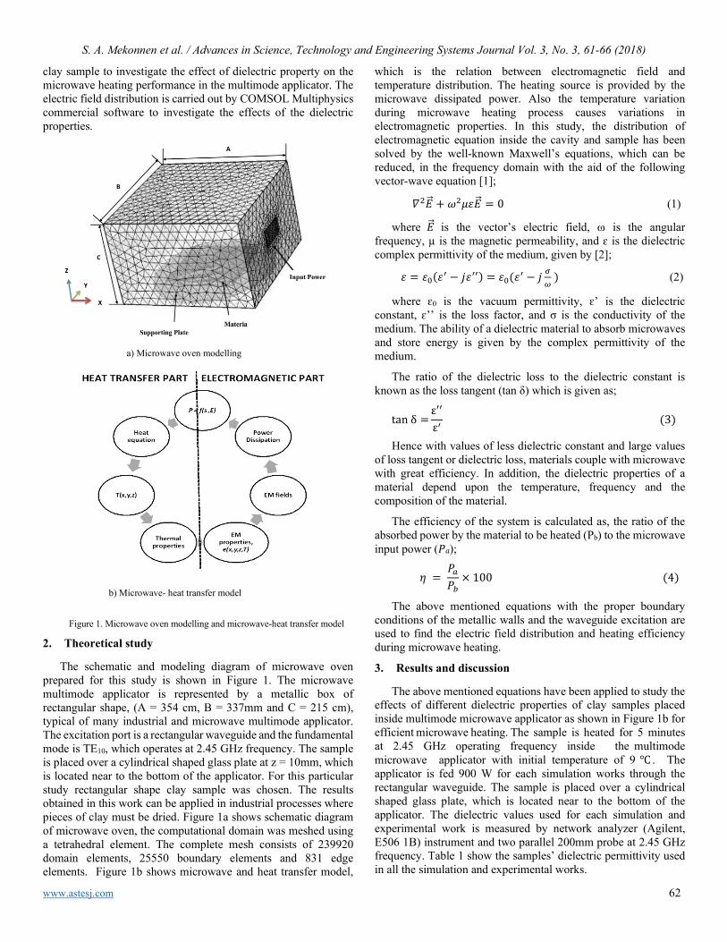
S. A. Mekonnen et al. / Advances in Science, Technology and Engineering Systems Journal Vol. 3, No. 3, 61-66 (2018)
www.astesj.com 62
clay sample to investigate the effect of dielectric property on the microwave heating performance in the multimode applicator. The electric field distribution is carried out by COMSOL Multiphysics commercial software to investigate the effects of the dielectric properties.
Figure 1. Microwave oven modelling and microwave-heat transfer model
2. Theoretical study
The schematic and modeling diagram of microwave oven prepared for this study is shown in Figure 1. The microwave multimode applicator is represented by a metallic box of rectangular shape, (A = 354 cm, B = 337mm and C = 215 cm), typical of many industrial and microwave multimode applicator. The excitation port is a rectangular waveguide and the fundamental mode is TE10, which operates at 2.45 GHz frequency. The sample is placed over a cylindrical shaped glass plate at z = 10mm, which is located near to the bottom of the applicator. For this particular study rectangular shape clay sample was chosen. The results obtained in this work can be applied in industrial processes where pieces of clay must be dried. Figure 1a shows schematic diagram of microwave oven, the computational domain was meshed using a tetrahedral element. The complete mesh consists of 239920 domain elements, 25550 boundary elements and 831 edge elements. Figure 1b shows microwave and heat transfer model,
which is the relation between electromagnetic field and temperature distribution. The heating source is provided by the microwave dissipated power. Also the temperature variation during microwave heating process causes variations in electromagnetic properties. In this study, the distribution of electromagnetic equation inside the cavity and sample has been solved by the well-known Maxwell’s equations, which can be reduced, in the frequency domain with the aid of the following vector-wave equation [1];
𝛻𝛻2𝐸𝐸 + 𝜔𝜔2𝜇𝜇𝜇𝜇𝐸𝐸 = 0 (1)
where 𝐸𝐸 is the vector’s electric field, ω is the angular frequency, µ is the magnetic permeability, and ɛ is the dielectric complex permittivity of the medium, given by [2];
𝜇𝜇 = 𝜇𝜇0(𝜇𝜇′ − 𝑗𝑗𝜇𝜇′′) = 𝜇𝜇0(𝜇𝜇′ − 𝑗𝑗 𝜎𝜎𝜔𝜔
) (2)
where ɛ0 is the vacuum permittivity, ɛ’ is the dielectric constant, ɛ’’ is the loss factor, and σ is the conductivity of the medium. The ability of a dielectric material to absorb microwaves and store energy is given by the complex permittivity of the medium.
The ratio of the dielectric loss to the dielectric constant is known as the loss tangent (tan δ) which is given as;
tan δ =ε′′
ε′ (3)
Hence with values of less dielectric constant and large values of loss tangent or dielectric loss, materials couple with microwave with great efficiency. In addition, the dielectric properties of a material depend upon the temperature, frequency and the composition of the material.
The efficiency of the system is calculated as, the ratio of the absorbed power by the material to be heated (Pb) to the microwave input power (𝑃𝑃𝑎𝑎);
𝜂𝜂 = 𝑃𝑃𝑎𝑎𝑃𝑃𝑏𝑏
× 100 (4)
The above mentioned equations with the proper boundary conditions of the metallic walls and the waveguide excitation are used to find the electric field distribution and heating efficiency during microwave heating.
3. Results and discussion
The above mentioned equations have been applied to study the effects of different dielectric properties of clay samples placed inside multimode microwave applicator as shown in Figure 1b for efficient microwave heating. The sample is heated for 5 minutes at 2.45 GHz operating frequency inside the multimode microwave applicator with initial temperature of 9 . The applicator is fed 900 W for each simulation works through the rectangular waveguide. The sample is placed over a cylindrical shaped glass plate, which is located near to the bottom of the applicator. The dielectric values used for each simulation and experimental work is measured by network analyzer (Agilent, E506 1B) instrument and two parallel 200mm probe at 2.45 GHz frequency. Table 1 show the samples’ dielectric permittivity used in all the simulation and experimental works.
a) Microwave oven modelling
b) Microwave- heat transfer model

S. A. Mekonnen et al. / Advances in Science, Technology and Engineering Systems Journal Vol. 3, No. 3, 61-66 (2018)
www.astesj.com 63
Table 1. Dielectric characteristics of the clay samples
ε' tan δ (10-3)
Sample 1 90 47.22
Sample 2 77.10 119.19
Sample 3 59.99 187.19
Sample 4 52.60 239.35
For this particular study, first, we used four different dielectric property values as shown in table 1 to investigate the effects of dielectric properties on the performance of microwave heating. Later, we investigated the influence of additional dielectric property value located inside multimode applicator on performance of microwave heating, which is located at the top side of sample material by using KESTAMID dielectric slab of 1 cm thickness. KESTAMIDs’ relative permittivity is εr = 3.7.
Microwave heating efficiency is greatly affected by geometry and size of the sample, its dielectric properties, operating frequency, applied power, its placement inside the applicator, size and geometry of the applicator. However, in this study we will observe and discuss only the effects of the samples’ dielectric properties while keeping the other factors constant for the entire simulation and experimental work.
The dielectric properties of the samples’ located inside the applicator influences the amount of the microwave power absorbed by the sample during its heating process. Dielectric properties of the material to be heated are functions of temperature, frequency and the composition of the material. The change of the dielectric properties with temperature influences the standing wave pattern inside the cavity and thus the microwave absorption. However, for this study we kept the effects of temperature and frequencies on dielectric properties of the sample constant for the purposes of simplicity in electromagnetic field and related calculations.
Figure 2a shows the electric field distribution over the clay sample 1 during microwave heating process for rectangular shaped sample. The simulation result show that the electric field intensity is stronger near to the top and bottom walls of the microwave applicator, and the weakest is located in the middle of the microwave applicator. This variation in electric field distribution leads to different microwave efficiency. From the simulation, the obtained absorbed power by the sample during microwave processing is 335.93 W. From this we calculated the efficiency of the system as η =37.33%.
To validate the simulated electric field distribution of clay samples, experimental works had been done to measure temperature distribution. A thermal fax paper was placed on the top of the sample before microwave heating and placed inside the applicator. Figure 2b shows the stain made by clay sample 1 during microwave heating. The stains obtained on the fax paper agree with the hot and cold spots generated during microwave heating. The temperature pattern over the samples was measured by the laser thermometer as shown in figure 2c.
Figure 2. Electric field distribution, Thermal fax paper stain and temperature
distribution of sample 1 (εr = 90-j4.25) during microwave drying.
Figure 2c represents temperature distribution pattern for sample 1, generally coincides with the simulated electric field distribution. For example, at the region of maximum electric field intensity on sample 1, V= 23.193 kV/m and 28.521 kV/m, the temperature that rises over sample 1 is also at the maximum; i.e., 61 and 67, respectively. Also for the other samples it shows that, at maximum electric field intensity region, the temperature rise is also maximum and at lower electric field region, the temperature rise is low. In the middle zone of the multimode applicator, the temperature rises of sample materials are lower. From the above experimental result, we can see clearly the direct relationship between the electric field intensity and temperature pattern, the temperature rise is affected by the sample’s dielectric properties, which also affected the system’s overall efficiency, and this validates our work.
Figure 3 shows the electric field and temperature distribution over the clay samples and inside multimode applicator during microwave heating process for rectangular shaped samples. Figure 3a shows electric field distribution over sample 2. The power absorbed by the sample is 380.34 W. From here the efficiency of the system is η = 42.31%. Figure 3b shows the temperature distribution pattern over sample 2. After the microwave heating, the minimum and maximum temperature over the heated material was measured as minimum temperature Tmin = 53 and maximum temperature Tmax=71 . The average temperature distribution was calculated as 62 .
Figure 4 shows the electric field and temperature distribution over the clay samples and inside multimode applicator during microwave heating process for rectangular shaped samples. Figure 4a shows electric field distribution over sample 3. The power absorbed by the sample 3 is 430.83 W. From this the calculated efficiency of the sample is 47.87%. Figure 4b shows the temperature distribution pattern over sample 3. After the microwave heating, the minimum and maximum temperature over the heated material was measured as minimum temperature Tmin
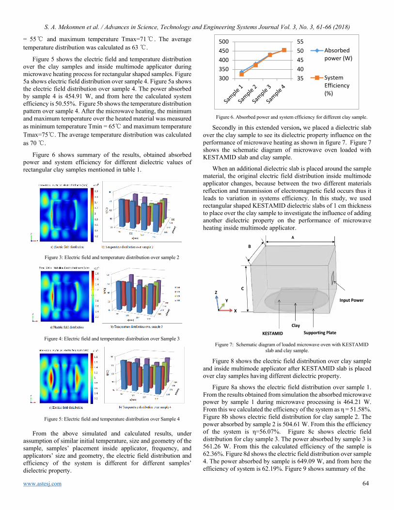
S. A. Mekonnen et al. / Advances in Science, Technology and Engineering Systems Journal Vol. 3, No. 3, 61-66 (2018)
www.astesj.com 64
= 55 and maximum temperature Tmax=71 . The average temperature distribution was calculated as 63 .
Figure 5 shows the electric field and temperature distribution over the clay samples and inside multimode applicator during microwave heating process for rectangular shaped samples. Figure 5a shows electric field distribution over sample 4. Figure 5a shows the electric field distribution over sample 4. The power absorbed by sample 4 is 454.91 W, and from here the calculated system efficiency is 50.55%. Figure 5b shows the temperature distribution pattern over sample 4. After the microwave heating, the minimum and maximum temperature over the heated material was measured as minimum temperature Tmin = 65 and maximum temperature Tmax=75. The average temperature distribution was calculated as 70 .
Figure 6 shows summary of the results, obtained absorbed power and system efficiency for different dielectric values of rectangular clay samples mentioned in table 1.
Figure 3: Electric field and temperature distribution over sample 2
Figure 4: Electric field and temperature distribution over Sample 3
Figure 5: Electric field and temperature distribution over Sample 4
From the above simulated and calculated results, under assumption of similar initial temperature, size and geometry of the sample, samples’ placement inside applicator, frequency, and applicators’ size and geometry, the electric field distribution and efficiency of the system is different for different samples’ dielectric property.
Figure 6. Absorbed power and system efficiency for different clay sample.
Secondly in this extended version, we placed a dielectric slab over the clay sample to see its dielectric property influence on the performance of microwave heating as shown in figure 7. Figure 7 shows the schematic diagram of microwave oven loaded with KESTAMID slab and clay sample.
When an additional dielectric slab is placed around the sample material, the original electric field distribution inside multimode applicator changes, because between the two different materials reflection and transmission of electromagnetic field occurs thus it leads to variation in systems efficiency. In this study, we used rectangular shaped KESTAMID dielectric slabs of 1 cm thickness to place over the clay sample to investigate the influence of adding another dielectric property on the performance of microwave heating inside multimode applicator.
Figure 7: Schematic diagram of loaded microwave oven with KESTAMID
slab and clay sample.
Figure 8 shows the electric field distribution over clay sample and inside multimode applicator after KESTAMID slab is placed over clay samples having different dielectric property.
Figure 8a shows the electric field distribution over sample 1. From the results obtained from simulation the absorbed microwave power by sample 1 during microwave processing is 464.21 W. From this we calculated the efficiency of the system as η = 51.58%. Figure 8b shows electric field distribution for clay sample 2. The power absorbed by sample 2 is 504.61 W. From this the efficiency of the system is η=56.07%. Figure 8c shows electric field distribution for clay sample 3. The power absorbed by sample 3 is 561.26 W. From this the calculated efficiency of the sample is 62.36%. Figure 8d shows the electric field distribution over sample 4. The power absorbed by sample is 649.09 W, and from here the efficiency of system is 62.19%. Figure 9 shows summary of the
3540455055
300350400450500
Absorbedpower (W)
SystemEfficiency(%)
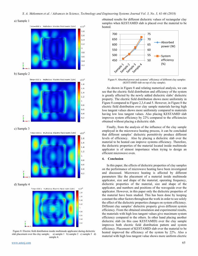
S. A. Mekonnen et al. / Advances in Science, Technology and Engineering Systems Journal Vol. 3, No. 3, 61-66 (2018)
www.astesj.com 65
Figure 8: Electric field distribution inside multimode applicator during dielectric
slab placement over the clay sample; a) sample 1 b) sample 2 c) sample 3 d) sample 4.
obtained results for different dielectric values of rectangular clay samples when KESTAMID slab is placed over the material to be heated.
Figure 9. Absorbed power and systems’ efficiency of different clay samples
(KESTAMID slab on top of clay sample).
As shown in Figure 8 and relating numerical analysis, we can see that the electric field distribution and efficiency of the system is greatly affected by the newly added dielectric slabs’ dielectric property. The electric field distribution shows more uniformity in Figure 8 compared to Figure 2,3,4 and 5. However, in Figure 8 the electric field distribution over clay sample materials having high loss tangent values shows more uniformity compared to materials having low loss tangent values. Also placing KESTAMID slab improves system efficiency by 22% compared to the efficiencies obtained without placing a dielectric slab.
Finally, from the analysis of the influence of the clay sample employed in the microwave heating process, it can be concluded that different samples’ dielectric permittivity produce different levels of efficiency. Also by placing a dielectric slab over the material to be heated can improve systems efficiency. Therefore, the dielectric properties of the material located inside multimode applicator is of utmost importance when trying to design an efficient microwave oven.
4. Conclusion
In this paper, the effects of dielectric properties of clay samples on the performance of microwave heating have been investigated and discussed. Microwave heating is affected by different parameters like the placement of a material inside multimode applicator, size and shape of the material, operating frequency, dielectric properties of the material, size and shape of the applicator, and numbers and positions of the waveguide over the applicator. However, in this paper only the dielectric properties of the material have been studied. This has been done by keeping constant the other factors throughout the work in order to see solely the effect of the dielectric properties changes on system efficiency. Different clay samples’ dielectric property gives different system efficiency. From the obtained simulation and experimental results, the materials with high loss tangent values give maximum system efficiency compared to the others. In other hand placing another dielectric slab (in this case KESTAMID) over the clay sample improves both electric field distribution pattern and system efficiency. Placement of KESTAMID slab over the material to be heated improved the efficiency of the system by 22%. Also a material with high loss tangent value shows more uniform electric
50
55
60
65
70
75
450
500
550
600
650
700
Absorbedpower (W)
Systemefficiency(%)
b) Sample 2
c) Sample 3
d) Sample 4
a) Sample 1

S. A. Mekonnen et al. / Advances in Science, Technology and Engineering Systems Journal Vol. 3, No. 3, 61-66 (2018)
www.astesj.com 66
field distribution compared to the others. However, different dielectric slab thickness also has an effect on the performance of the microwave heating; it will be considered in the future works.
Conflict of Interest
The authors declare no conflict of interest.
Acknowledgment
The authors are thankful to Assoc. Prof. Dr. Güray SALİHOĞLU of Uludag University (Department of Environmental Engineering) and Assoc. Prof. Dr. Filiz ALTAY of Istanbul Technical University.
References
[1] A. C. Metaxas, R. J. Meredith, Industrial Microwave Heating, Peter Peregrinus, 1983.
[2] David K. Cheng, Field and wave electromagnetics. John Wiley & Sons, Inc., 2009.
[3] H. Feng, Y. Yin, J. Tang, "Microwave Drying of Food and Agricultural Materials: Basics and Heat and Mass Transfer Modeling". Springer-Verlag, Food Eng Rev, 4(2), pp. 89-106, 2012. https://doi.org/10.1007/s12393-012-9048-x
[4] J. Vrba, M. Stejskal, M. Pourova, "Microwave drying machine for textile materials", in proceedings of the 2009 European Microwave Conference (EuMC), Rome, Italy, pp. 1121-1124, 2009. IEEEXplore, DOI: 10.23919/EUMC.2009.5296116.
[5] L, A Jermolovicius, J. T. Senise, R. B. D. Nascimento, "Microwave Drying of Zinc Sulfate", in 2007 SBMO/IEEE MTT-S International Microwave & Optoelectronics Conference, Brazil, pp. 284-286, 2007. IEEEXplore, DOI: 10.1109/IMOC.2007.4404264
[6] G. A. Morozov, O. G. Morozov, R. R. Samigullin, A. R. Nasibullin, "Application of Microwave Technologies for Increase of Efficiency of Polymeric Materials Recycling", 2011 VIII International Conference on Antenna Theory and Techniques (ICATT), Kyiv, Ukraine, pp. 321-323, 2011. IEEEXplore, DOI: 10.1109/ICATT.2011.6170771
[7] Y. Hong, Bai. Lin, H. Li, H. Dai, C. Zhu, H. Yao. "Three-dimensional simulation of microwave heating coal sample with varying parameters", Applied Thermal Engineering, Vol. 93, pp. 1145–1154, 2016. https://doi.org/10.1016/j.applthermaleng.2015.10.041.
[8] N. Makul, P. Rattanadecho, ''Microwave pre-curing of natural rubber-compounding using a rectangular wave guide", International Communications in Heat and Mass Transfer, Vol. 37, pp. 914–923, 2010. https://doi.org/10.1016/j.icheatmasstransfer.2010.03.001.
[9] U. Narumitbowonkul, P. Keangin, P. Rattanadecho, "Numerical and Experimental Analysis of Temperature Distribution and Electric Field in a Natural Rubber Glove during Microwave Heating", International Science Index, Mechanical and Mechatronics Engineering, 9(3), pp. 518-524, 2015. DOI: 10.1999/1307-6892/10000910.
[10] A. Esin, N. Mahmutyazıcıoğlu, S. Altıntaş, "Drying and Sintering of Ceramic Based Parts Using Microwave Heating", Key Engineering Materials, Vols. 264-268, pp. 731-734, 2004. https://doi.org/10.4028/www.scientific.net/KEM.264-268.731.
[11] S. K. Shah, M. A. Joshi, "Application of Microwave Heating In Vacuum for Bagasse Drying". Proceedings of the 2008 International Conference on Recent Advances in Microwave Theory and Applications, Jaipur, India, pp. 477-479, 2008. IEEEXplore, DOI: 10.1109/AMTA.2008.4763153.
[12] D. S. Rajpurohit, R. Chhibber, "Design Optimization of Two Input Multimode Applicator for Efficient Microwave Heating", International Journal of Advances in Microwave Technology (IJAMT), 1(3), pp. 68-73, 2016.
[13] J. Monzo-Cabrera, J. Escalante, A. Diaz-Morcillo, A. Martinez-Gonzalez, D. Sanchez-Hernandez, "Load matching in multimode microwave-heating applicators based on the use of dielectric layer moulding with commercial materials", Microwave Opt Technol Lett, 41(5), pp. 414–417, 2004. https://doi.org/10.1002/mop.20156.
[14] M. E. Requena-Perez, J. L. Pedreno-Molina, M. Pinzolas-Prado, J. Monzo-Cabrera, A. Diaz-Morcillo and D. Sinchez-Hernandez, "Load matching in multimode microwave-heating applicators by load location optimization", Proceedings of the 34th European Microwave Conference, , Amsterdam, The Netherlands, IEEE, Vol. 3: pp. 1549–1552, 2004. IEEEXplore, DOI: 10.1109/EUMC.2004.183902.
[15] J. L. Pedreno-Molina, J. Monzo-Cabrera, M. Pinzolas, "A new procedure for power efficiency optimization in microwave ovens based on thermographic
measurements and load location search", International Communications in Heat and Mass Transfer, 34(5), 564-569, 2009. https://doi.org/10.1016/j.icheatmasstransfer.2007.02.002
[16] I. A. Ali, "Effect of load on the heating efficiency and temperature uniformity in multimode cavity applicators", Taylor & Francis Group, journal of microwave power and electromagnetic energy, 50(2), pp. 123-137, 2016. http://dx.doi.org/10.1080/08327823.2016.1190170.
[17] G. Brodie, "The influence of load geometry on temperature distribution during microwave heating", Transactions of the ASABE (American Society of Agricultural and Biological Engineers), 51(4), pp. 1401-1413, 2008. DOI: 10.13031/2013.25224.
[18] W. Cha-um, P. Rattanadecho, W. Pakdee, "Experimental analysis of microwave heating of dielectric materials using a rectangular wave guide (MODE: TE10) (Case study: Water layer and saturated porous medium)", Experimental Thermal and Fluid Science, 33(3), pp. 472–481, 2009. https://doi.org/10.1016/j.expthermflusci.2008.11.008
[19] S. A. Mekonnen, S. Yenikaya, G. Yenikaya, G. Yılmaz, "Effects of sample's dielectric property on the performance of microwave heating", proceedings of 2017 10th International Conference on Electrical and Electronics Engineering (ELECO), Bursa, Turkey, pp. 1440 – 1443, 2017.

www.astesj.com 67
Revealing Strengths, Weaknesses and Prospects of Intelligent Collaborative e-Learning Systems
Amal Asselman*, Azeddine Nasseh, Souhaib Aammou
LIROSA, Faculty of Sciences, Abdelmalek Essaadi University, Tetouan, 93 000, MOROCCO
A R T I C L E I N F O A B S T R A C T Article history: Received: 09 April, 2018 Accepted: 02 May, 2018 Online: 20 May, 2018
The rapid evolution of Collaborative e-Learning Systems migrates to the use of new technologies such the artificial intelligence (AI). In this context, the role of AI in increasing the quality of learning and making it more productive, persistent and efficient. In addition, it can accomplish repetitive and complex tasks in record time and unmatched accuracy. These advantages offer the ability to interact with learners in an almost human way. This interaction could be made on the base of adaptive hypermedia techniques, Multi-agent Systems technology and a cognitive learner model. In this paper, we present and analyze some existing intelligent collaborative e-Learning systems on the basis of their various features such as collaboration features, intelligent actors’ interaction, adaptability measurement, cognitive student modeling, and security measurement. Our analysis aims to provide important information to researchers, educators and software developers of educational environments concerning strengths and weaknesses of those e-Learning systems. According to this study, we found that some collaborative e-Learning environments, even the use of the mentioned technologies, still poor in terms of the structure of human cognitive architecture aspects and the capacity to assess the help provided to learners. For these reasons, we present, in the end, some prospects in order to determine how we can improve these systems to stop the reasons of abandoning courses.
Keywords: Artificial intelligence Collaborative e-Learning Adaptive hypermedia techniques Cognitive user model Multi-agent Systems E-Learning systems
1. Introduction
The evolution of the Internet and the development of educational content have led to the emergence of a new mode of education called e-Learning (electronic learning). This mode is used in several areas including employee training follow-up or self-training. E-Learning tends to develop around the world following the evolution of new Information and Communications Technologies (ICT) in the educational field that allows him to have many advantages such as the ability to facilitate teaching, and the accessibility of educational resources. This mode of learning is based on remote access to the provision of educational resources and learning services. The online learning environments are recognized by a whole different set of appellation vary according to the tasks assigned to them. Those environments remain in constant evolution, we cite WBT (Web-Based Training), LMS (Learning Management System), LCMS (Learning Content
Management System) CLCS (Computer Support for Collaborative Learning), MOOC (Massive Open Online Course) etc.
Generally, the analysis of e-Learning systems based on their characteristics and functionalities [1] [2] mention that each of them is credited for enhancing the acquisition of learners. They offer them the opportunity to learn using a modern, fun, and interactive strategies that are completely different to traditional learning in which requires the memorization of a set of knowledge to better get them back on the day of examination. These programs also gives to the learner the choice of lessons that meet his needs without obligation to follow the lessons imposed by the teacher.
Despite all their benefits, these systems have recognized a major obstacle due to poor management of learning time and lack of orientation on the platform. In addition, the geographical dimension causes a difficult finding of available human accompanist in e-Learning environment during the whole day and throughout the learning period. Moreover the difficulty of finding always learners with the same profile available to collaborate. As a result, the learner can simply be lost depending on the huge number of resources and links. In fact, this eventually leads him to
ASTESJ
ISSN: 2415-6698
*Corresponding Author: Amal ASSELMAN, LIROSA, Faculty of Sciences, Abdelmalek Essaadi University, Tetouan, 93 000, MOROCCO E-mail : [email protected]
Advances in Science, Technology and Engineering Systems Journal Vol. 3, No. 3, 67-79 (2018)
www.astesj.com
Special Issue on Multidisciplinary Sciences and Engineering
https://dx.doi.org/10.25046/aj030310

A. Asselman et al. / Advances in Science, Technology and Engineering Systems Journal Vol. 3, No. 3, 67-79 (2018)
www.astesj.com 68
feel that online training is boring and decide automatically to drop out.
According to the reason mentioned before, several statistics [3] [4] [5] [6] have been realized showing us the number of students training leave, as example Figure 1 concerning “MITx course, 6.002x (Circuits and Electronics)” available on edX online learning platform [7]. This example indicates the number of learners participated during all phases of the training. It illustrates that there is a high drop-out rate appears from the first week. And after completing the 14 weeks of study, it remains a few of student arrive to accomplish this course. In terms of numbers, there are approximately just 4.6% of students have succeeded while the 95.4% withdrew.
Figure 1: Dropout rate among those who initially registered [7]
Consistent with this context and precisely with the accelerated development of information technologies as well as the trend towards the use of smart devices, the integration of artificial intelligence makes a great change in the society in the context of Collaborative e-Learning Systems. It remains as an appropriate solution to make educational system more productive, persistent and efficient [8]. It allows the creation and extension of various intelligent technologies such as adaptive hypermedia techniques, agent technology, and web services which makes e-Learning more effective and flexible. In the same case, the use of Multi-agent Systems (MAS) technology in the design and modeling process of learning environments has evolved spectacularly. It proved its ability in modeling the different actors of e-Learning systems and managing their interactions to meet their dynamic and execution needs by their innovative features like intelligence, autonomy, reactivity, social ability, and proactivity. However, even though there are collaborative e-Learning environments using the mentioned technologies, they have structured with a minimum of consideration the relevant aspects of human cognitive architecture, a low capacity to assess the help provided by learners and several other weaknesses.
This paper, as an extension of work originally presented in 15th International Conference on Emerging eLearning Technologies and Applications (ICETA) [9], is organized as follows. Section 2 presents general principles of collaborative online learning by presenting the different activities of e-Learning system’s actors as well as the interaction between them. Section 3 presents an overview of distributed artificial intelligence, multi-agent systems, and adaptive systems in order to indicate their importance for
improving the educational systems. Section 4 is based on an analysis presenting the advantages, the limitations of some existing agent-oriented collaborative learning system, and comparison between them on the basis of a multitude of criteria: collaboration features, intelligent actors interaction, adaptability measurement, cognitive student modeling, and security measurement. In the last, we will present certain recommendations in order to indicate how can improve these systems for stopping the main reason for drop-out.
2. Collaborative e-Learning Systems
2.1. Features and advantage of e-Learning
E-learning becomes an essential part of modern education that allows learners to consult the pedagogical content effectively everywhere and any time [2]. These contents are organized into modules that can be assembled into personalized training courses. Currently, many studies show that e-Learning training has better results compared to traditional classroom training. It is considered as an efficient and attractive way for computer education delivered or mediated a pedagogical content and learning experiences by means of digital technologies. These systems are recognized as a software environment designed, specifically, to meet the needs of distance education and to allow organizing the online content in which the authors have a simple interface to deposit their contents (within predefined themes and organized in categories). They can associate one or several downloadable files to their courses [2]. These systems are characterized by a number of advantages like:
• The ease of sharing, exchanging and using varied learning modalities (audio sequences, videos, animations, diagrams);
• Flexibility and adaptability according to learner availability (By providing training at any time or by allowing the learner to learn at his/her own pace and in an individualized way);
• The relative reduction of costs for learners and trainers (elimination of accommodation and travel costs) and increased accessibility of training.
E-Learning follows a new economic model of production in which a large number of people join with new communication tools. Learning is an active process where tutor plays a leading role in training to help advance learners by placing more emphasis on monitoring, accompanying rather than transferring expertise. The e-tutor occupies several goals, for example, he animates the group or the community of learners, he determines the most adapted training course to learners, he offers him the help in his first steps and he ensures the pedagogical follow-up of the training (personalized advice, analysis of the progression, answers to the questions of the learners). As in traditional learning systems, the teacher was previously the sole holder of knowledge. However, in modern e-Learning systems, his role is to facilitate learning by guiding learners to make good use of knowledge [10]. He can also observe the progress of student's activities in order to motivate and guide them during their prevent failure or abandonment. Moreover, the role of the learner is no longer similar to his / her role in traditional learning which is limited to the memorization and evaluation of his knowledge on the day of the exam, but he governs his process learning by transforming information into

A. Asselman et al. / Advances in Science, Technology and Engineering Systems Journal Vol. 3, No. 3, 67-79 (2018)
www.astesj.com 69
knowledge and creating interactions with other members of the group. Before learning, students set goals and learning tasks of the plan. During learning, they work together to accomplish tasks and monitor their progress. And after learning, they evaluate their performance and plan for future learning [1].
Online education systems revolve around a set of functionalities such as:
• Administrative management of the platform. It concerns the management of registration in training and the management of administrative data training.
• Creation of courses and training plans (creation of teaching scenarios, curricula, and preparation of the various evaluation tests) besides changing or add course content and activities, schedule management and training path planning.
• It allows classification, indexation, and administration of pedagogical materials. As well as consultation of educational content, individualization of learning and communication between trainers and learners and between learners.
• It determinate roles of trainers, groups of students and their access by specifying content types, communication modes, test types, and by facilitates communication with students or between them by messaging or forum.
• It authorizes creation and modification of individualized training paths as well as follow-up of the activities of learners on the platform (time spent online in the course notes, dialogues, work deposited on the platform...).
E-learning researchers aim to improve distance learning systems in two areas: organizationally and functionally. The first by taking note the standardization of self-training materials and a quality approach, providing training opportunities and broadening the prospects for dissemination to employees, suppliers, and customers [1]. The second by trying to personalize the learner's profile according to training, to reduce costs, to save time and to make learning more effective.
2.2. Definition and principles of collaborative learning
Since the evolution of the web, the semantic field of the word "collaboration" has evolved considerably. Several education experts point out that school is not just a place to learn facts. It is a place for a student to interact with one another and learn the basics of communication, etiquette, and respect for others. Actually, many studies have focused on the collaborative e-Learning system that is defined as the learning strategy where several learners interact with their partners, share ideas and help each other to achieve their common goals [11]. These educational environments are designed and dedicated to encouraging individual work and group work in various fields involving the domain of instruction. In the same context, Andrew Carnegie as an American Industrialist and philanthropist define collaborative work as follows:
“Teamwork is the ability to work together toward a common vision. The ability to direct individual accomplishment toward organizational objectives. It is the fuel that allows ordinary people to achieve extraordinary results”.
In collaborative e-Learning, actors can work together regardless of geographic location or time limitation. In other words, it provides learners with a great flexibility of time and place as well as excellent asynchronous interaction [12]. This mode of learning follows a learner-centered approach by involving new roles for teachers, accompanists, and learners. It can be reported that students can undertake problems that are more complicated and gain a better understanding of the material by working collaboratively [13]. For that, learning content is becoming increasingly hypermedia intelligent and collaborative, which allows placing initiative and power in the hands of learners to access the information. Moreover, this system makes the responsibility of collective and global learning. Indeed all members of the group stay in regular contact, each learner must participate in the group in an action to be realized, each member can contribute to the action of other members of the group to increase its performance. According to Walckiers and De Praetere in the case of collaborative work, there is no a priori distribution of roles: individuals are gradually subsumed into a group that becomes an entity in its own right [14].
Generally, Collaborative e-Learning provides functionalities essential in the educational process, such as real-time, as well as offline data and information gathering, analysis and distribution, embedded feedback, assessment, and collaboration. All of these functionalities are based on synchronous and asynchronous learning tools for interaction [15]. Where synchronous tools allow real-time communication between people remotely geographically: instant messaging, voice telephony, audio conferencing and video conferencing, etc. Indeed, the actors must be at the same time facing their respective computers. While asynchronous tools allow for time-and-space exchanges are e-mail, forum discussions, portfolio, wiki, and blog. In this type of system when a person sends a message, the receiver can read it for a few minutes, hours or days later.
Accordingly, Collaborative learning is a construct based on several sources. It feeds on the values of constructivism and relies on cognitive theories to explain the mechanisms of learning. For this reason, it promotes the integration of students in homogeneous groups which have the same profile and the common cultural and social aspects. This integration allows the development of critical thinking in the learner, as well as the emotional and pedagogical support of weak students. That can create for learners a source of motivation and consequently increase the communication skills, it can also support the realization of a continuous formative evaluation.
3. Artificial Intelligent technologies For Education
John McCarthy, an American computer and cognitive scientist pioneer and inventor, was known as the father of Artificial Intelligence (AI). The term AI was proposed, in 1956, by this person in Dartmouth Artificial Intelligence conference [16]. It was the first artificial intelligence conference organized to draw the talent and expertise of others interested in machine intelligence for a month of brainstorming. It refers to the ability to interact with the user and respond to their actions in a natural way [17]. It is recognized as a computer discipline that aims to model or simulate so-called intelligent human behaviors such as perception, memorization, decision-making, understanding, and learning [16].

A. Asselman et al. / Advances in Science, Technology and Engineering Systems Journal Vol. 3, No. 3, 67-79 (2018)
www.astesj.com 70
Among the areas where artificial intelligence is ready to make big changes is the field of education. The application of AI to eLearning content is not just a cost-saving solution; it also opens up a whole new way of looking at learning itself.
Several advanced research has been done in this area, particularly in the field of intelligent tutorial systems (ITS) so that research aims primarily at making learners benefit from technological advances in artificial intelligence. It can adapt educational software to student needs by putting more emphasis on certain subjects, repeating things that students haven’t mastered, and generally help students to work at their own pace [17]. AI will shift the role of the teacher to that of a facilitator so that teachers will supplement AI lessons, assist students who are struggling, and provide human interaction and hands-on experiences for students. AI-driven programs can give students and educators helpful feedback by allowing students to get the support they need and choose majors based on the areas they are doing well. And by providing for teachers ability to find areas where they can improve teaching for students who may be struggling with the subject. Data powered by AI can change how schools find, teach, and support students as well as it can point out places where courses need to improve. It also may change where students learn, who teaches them, and how they acquire basic skills [18]. Similarly, it is altering how can find and interact with information. In like manner, AI can make trial-and-error learning less intimidating in view of the idea of not knowing the answer or even failing is crippling. For this, artificial intelligence could help students learn in a relatively non-judgmental environment, especially when AI trainers can offer improvement solutions.
So, the use of artificial intelligence remains as an appropriate solution to make educational system more productive, persistent and efficient [8]. In order to achieve this intelligence, it must be aware of the user's objectives and knowledge for the purpose of designing adaptive educational intelligent systems. These systems try to help users during their learning by limiting the browsing space, suggesting the most relevant links to follow, or providing adaptation comments to visible links [19]. Add to that, integration of multi-agent systems offer an original approach to designing intelligent and collaborative systems. Multi-agent systems are characterized by the distribution of global control of the system, and by the presence of autonomous agents evolving in a shared and dynamic environment. They are more adapted to designing a learning environment where each member must manage and exchange knowledge, and collaborate with others to achieve its goals [15]. The fundamental aspects of these intelligent e-Learning systems are the ability of perception, inference, learning, reasoning, and knowledge-based systems [20], resulting from the integration of the agents’ cognitive architecture. This latter aims to treat the process of development and use of knowledge through the set of mechanisms of human cognition. In other words, it models specific tasks based on the simulation of human behavior to create a model able to understand, reason, and solve problems [21].
Due to the benefited of artificial intelligence, we will be interested in the modeling of intelligent behaviors that are the product of the cooperative activity between several agents in order to design an adaptive system respecting the personal needs of each learner and to have agents capable of interacting similarly to humans thanks to the integration of cognitive architecture.
3.1. Agent and Multi-Agent System in education
The design of a distance learning system involves a complex set of processes that are sometimes difficult to associate in a coherent and evolving system. Multi-agent systems (MAS) are proving to be relevant for solving these types of problems thanks to its great ability to structure knowledge transfer systems and open new perspectives of assistance to distance learning. MAS is currently considered as the most active research discipline which they relate to several areas, in particular of artificial intelligence, distributed computing systems, robotics and software engineering. These systems are made up of several flexible and autonomous entities interacting with each other and called agents. According to Ferber, a multi-agent system can be considered as a macro-system composed of autonomous agents that interact in a common environment in order to achieve a coherent collective activity [11].
In literature, the notion of agent remains relatively vague to define. It is found that several researchers have defined this concept in different ways. All of these definitions look the same, but they also differ according to the application context for which the agent is designed. According to Ferber, an agent is defined as a physical or virtual entity, autonomous, located in an environment, capable of acting in an environment, communicating with other agents, perceiving its environment, reproducing itself [11]. This definition is supported by Wooldridge [22] in which present an agent as computer system located in a certain environment capable of autonomously performing actions in that environment, achieve its goals. Another frequently cited definition is presented by Russel [23]; he provides that an agent is all that can be seen as perceiving its environment through sensors and acting on this environment through effectors. Generally, agents aim to reduce the complexity of problem-solving time by dividing it into sub-problems, each sub-problem is assigned to an independent intelligent agent called “resolver”. To achieve this, agents are organized, negotiated and coordinated for the purpose of resolving a common goal [24].
Generally, Educational area based on multi-agent systems presents a series of advantages for reason that these systems have inherited the traditional benefits of distributed resolution and artificial intelligence. Among which we can mention that intelligent systems are open, i.e. they have the ability to dynamically add or remove features or services in the agent system. It recognized a flexibility of the computer tool which aims to make the programming simpler, to change agents’ behavior, and to add or to delete possible actions. They also have the advantage of the decentralization of the agents which aims at allowing to support the individual failure of these elements as well as distributed problem solving where a problem can be broken down into subparts, each of which can be solved independently to arrive at a stable solution. Moreover the speed of execution where several agents can work at the same time for the resolution of a problem thanks to the parallelism of execution.
3.2. A required architecture for e-Learning system
In order to build an intelligent educational system that is able to minimize the intervention of a human in the execution of tasks, to facilitate localization and customization of appropriate e-learning resources, thus to promote collaboration in e-learning environments, as well as to be able to automate effectively learning
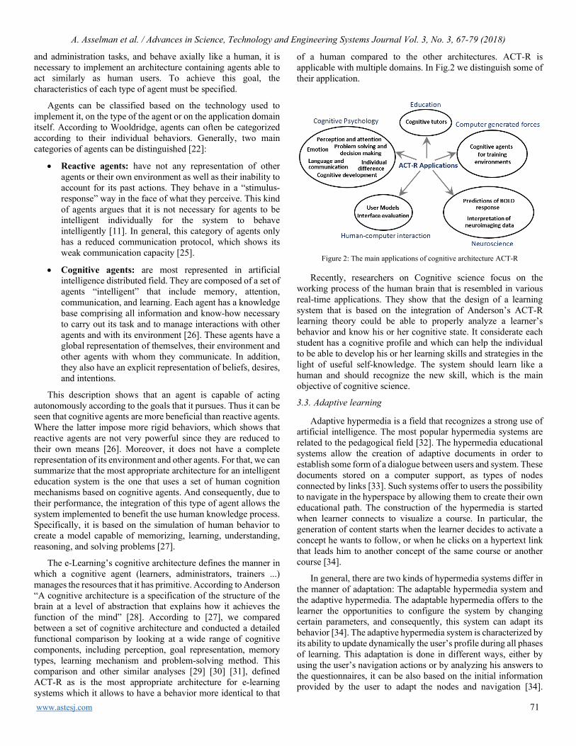
A. Asselman et al. / Advances in Science, Technology and Engineering Systems Journal Vol. 3, No. 3, 67-79 (2018)
www.astesj.com 71
and administration tasks, and behave axially like a human, it is necessary to implement an architecture containing agents able to act similarly as human users. To achieve this goal, the characteristics of each type of agent must be specified.
Agents can be classified based on the technology used to implement it, on the type of the agent or on the application domain itself. According to Wooldridge, agents can often be categorized according to their individual behaviors. Generally, two main categories of agents can be distinguished [22]:
• Reactive agents: have not any representation of other agents or their own environment as well as their inability to account for its past actions. They behave in a “stimulus-response” way in the face of what they perceive. This kind of agents argues that it is not necessary for agents to be intelligent individually for the system to behave intelligently [11]. In general, this category of agents only has a reduced communication protocol, which shows its weak communication capacity [25].
• Cognitive agents: are most represented in artificial intelligence distributed field. They are composed of a set of agents “intelligent” that include memory, attention, communication, and learning. Each agent has a knowledge base comprising all information and know-how necessary to carry out its task and to manage interactions with other agents and with its environment [26]. These agents have a global representation of themselves, their environment and other agents with whom they communicate. In addition, they also have an explicit representation of beliefs, desires, and intentions.
This description shows that an agent is capable of acting autonomously according to the goals that it pursues. Thus it can be seen that cognitive agents are more beneficial than reactive agents. Where the latter impose more rigid behaviors, which shows that reactive agents are not very powerful since they are reduced to their own means [26]. Moreover, it does not have a complete representation of its environment and other agents. For that, we can summarize that the most appropriate architecture for an intelligent education system is the one that uses a set of human cognition mechanisms based on cognitive agents. And consequently, due to their performance, the integration of this type of agent allows the system implemented to benefit the use human knowledge process. Specifically, it is based on the simulation of human behavior to create a model capable of memorizing, learning, understanding, reasoning, and solving problems [27].
The e-Learning’s cognitive architecture defines the manner in which a cognitive agent (learners, administrators, trainers ...) manages the resources that it has primitive. According to Anderson “A cognitive architecture is a specification of the structure of the brain at a level of abstraction that explains how it achieves the function of the mind” [28]. According to [27], we compared between a set of cognitive architecture and conducted a detailed functional comparison by looking at a wide range of cognitive components, including perception, goal representation, memory types, learning mechanism and problem-solving method. This comparison and other similar analyses [29] [30] [31], defined ACT-R as is the most appropriate architecture for e-learning systems which it allows to have a behavior more identical to that
of a human compared to the other architectures. ACT-R is applicable with multiple domains. In Fig.2 we distinguish some of their application.
Figure 2: The main applications of cognitive architecture ACT-R
Recently, researchers on Cognitive science focus on the working process of the human brain that is resembled in various real-time applications. They show that the design of a learning system that is based on the integration of Anderson’s ACT-R learning theory could be able to properly analyze a learner’s behavior and know his or her cognitive state. It considerate each student has a cognitive profile and which can help the individual to be able to develop his or her learning skills and strategies in the light of useful self-knowledge. The system should learn like a human and should recognize the new skill, which is the main objective of cognitive science.
3.3. Adaptive learning
Adaptive hypermedia is a field that recognizes a strong use of artificial intelligence. The most popular hypermedia systems are related to the pedagogical field [32]. The hypermedia educational systems allow the creation of adaptive documents in order to establish some form of a dialogue between users and system. These documents stored on a computer support, as types of nodes connected by links [33]. Such systems offer to users the possibility to navigate in the hyperspace by allowing them to create their own educational path. The construction of the hypermedia is started when learner connects to visualize a course. In particular, the generation of content starts when the learner decides to activate a concept he wants to follow, or when he clicks on a hypertext link that leads him to another concept of the same course or another course [34].
In general, there are two kinds of hypermedia systems differ in the manner of adaptation: The adaptable hypermedia system and the adaptive hypermedia. The adaptable hypermedia offers to the learner the opportunities to configure the system by changing certain parameters, and consequently, this system can adapt its behavior [34]. The adaptive hypermedia system is characterized by its ability to update dynamically the user’s profile during all phases of learning. This adaptation is done in different ways, either by using the user’s navigation actions or by analyzing his answers to the questionnaires, it can be also based on the initial information provided by the user to adapt the nodes and navigation [34].

A. Asselman et al. / Advances in Science, Technology and Engineering Systems Journal Vol. 3, No. 3, 67-79 (2018)
www.astesj.com 72
Moreover, the system can track and analyze the learner behavior and save it in a user model in order to adapt automatically the presentation consequently according to the characteristics of this model [35].
An educational hypermedia system is a system capable of adapting itself to the different characteristics of the students that are specified through a model. Brusilovsky [33] specifies that “Adaptive hypermedia systems are hypermedia systems which reflect some features of the user in a user model and use this model by adapting various visible aspects of a system to user”. Adaptive hypermedia aims to improve education systems by enhancing the assimilation of knowledge through the adaptation of links, content, and presentations to the user. These systems can considerably reduce the user’s path in hyperspace in order to avoid disorientation of user and the risk of misunderstanding the document.
An adaptive teaching system implements mechanisms that leverage on domain knowledge, learner knowledge, and knowledge about learning processes. This adaptive teaching offers approaches and personalized educational content. Usually, in order to increase the profitability of an educational application for a learner or a group of learners that have different profiles, it is obviously necessary to adapt the system according to learner goals, characteristics, and interests. This adaptation can be done in two ways: presentation adaptation and navigation adaptation. The first kind of adaptation makes it possible for each user to view a personalized page that is different from that of the others [11]. Where the navigation adaptation is interest in helping learners to find their self in hyperspace or to oblige them to use certain links rather than others in order to follow the most relevant path [19]. This phase involves changing the navigation structure or defining how this navigation structure will be presented to the user.
Learner modeling aims to give a complete and faithful description of all aspects of the user’s behavior. It represents the core of adaptive learning system. When a learner takes training in a distance learning session, the learner model evolves according to learners’ educational backgrounds and their responses [21]. This information can be directly entered by the learner (response to questions asked by the system), calculated from results of exercises or tests, or deduced from the learner’s behavior in terms of interaction with the system (navigation choice, document reading time, etc.). This model aims to present all the characteristics of learners helping to achieve adaptation [36]. Those characteristics are separated in learner model into two categories [26]: Domain Dependent Data and Domain Independent Data. The first reflects the status and level of knowledge and skills which student achieved in a certain subject and at the certain moment of time. This category is organized by a set of elements (concept, topic, subject…). The second includes information about the learner skills based on his behavior. This category may include generic information (demographic information, learner learning goals, interests, background and experience) and psychological information such as memory, perception, learning style and preferences, decision making abilities, critical thinking, analytical thinking for modeling cognitive aptitudes, and motivation, reflection, self-awareness, self-assessment, self-monitoring, self-regulation for modeling metacognitive affective features…) [31].
4. Analysis of Agent-Oriented Collaborative Learning System
4.1. Existing intelligent collaborative e-Learning system
Many multi-agent systems that focus on the collaborative e-Learning domain have been designed and implemented by integrating a wide range of functionalities. These systems offer an original approach to designing intelligent systems and provide an interesting solution for both problems of structuring and exploiting knowledge. Agent-oriented collaborative learning system offers many appropriate tools for designing a learning environment where each member must manage and exchange knowledge and then to collaborate with others in order to achieve its goals. The common goal of these systems is to improve the learning ability of the student/learner., among which we can distinguish. In the field of scientific research, there are several systems that meet these objectives. In this paragraph, we will present and analyze them it in order to clarify their strengths and limitations.
4.1.1. ALLEGRO
ALLEGRO is an intelligent environment [37]. This system offers flexibility, autonomy, and adaptability to the e-Learning environment base on MAS. It offers an individualized learning as well as CSCL (Computer Supported Collaborative Learning) which makes the system capable of supporting collaborative learning. This system is based on three theories of learning behaviorism, cognitivism, and historic-social.
This system has six types of artificial agent:
• Student Agent: aims to manage the learning student model and maintains individualized information about the apprentice.
• Tutor Agent: will guide the learning process, decides what action to teach, how and when, It tries to detect mistakes in the process of the apprentice, in addition, it offers suggestions, critics, and recommendations through the selection of the suitable pedagogical strategy. This agent aims to promote learner learning by asking Agent Diagnosis to send to the apprentice an appropriate evaluation according to its profile. Or by asking Expert Agent to offer certain knowledge to the learner according to the plan and its diagnosis.
• Diagnosis Agent: is responsible for filtering and classifying the knowledge level of the learner.
• Expert Agent: manages the content of the area or specific subject of learning and teaching. It sends knowledge to the apprentice when he asks for it or at the request of the Tutoring Agent.
• Collaboration Agent: aims to group the apprentices by study topics, profiles or behavior and that’s why it tries to find students who are interested in the same subject in order to create synchronous or asynchronous collaborative communication.
• Interface Agent: allows interaction between the user and the artificial agents. It allows the unfolding of knowledge and collaboration on the screen of the student.

A. Asselman et al. / Advances in Science, Technology and Engineering Systems Journal Vol. 3, No. 3, 67-79 (2018)
www.astesj.com 73
4.1.2. BAGHERA
BAGHERA is a platform for distance learning [38]. This platform has been implemented with the JATLite multi-agent application development environment. It proposes the basics of computer environments for human learning (EIAH) seen as an educational community made up of human and non-human agents who cooperate and work together to train students. Its functional objective is to construct a logical experimental, flexible, and adaptable platform for distance education. Its high-level MAS is used for collecting what is needed for its pedagogical behavior, while its lover level MAS is responsible to diagnose student’s conception. These diagnoses are based on the student’s action towards the Interface
In the environment, each apprentice is supported by three types of agents:
• Companion-Student Agent: aims to make the link with the rest of the system and the students. Also through this agent, the student can access his electronic binder and a specific graphical interface that will allow him to work on one of his exercises, save his work and request a verification of the proof he develops.
• Mediator Agent: Chooses an appropriate agent to send the student’s solutions for verification.
• Tutor Agent: He is an artificial designer. This agent is mandatory for every student registered in the system. When the teacher is absent, the tutor agent takes charge of the pedagogical follow-up for autonomous learning with regard to his student and the learning situation.
Similarly, the teacher is supported by two types of agents:
• Companion-Teacher agent: allows realizing the interface between the system and the teacher. It ensures the access of the teacher to his electronic locker. The teacher relies on the Companion-Teacher agent to connect with the students and other teachers who are available.
• Assistant Agent: The main function of this agent is to manage the teacher’s record that contains all the exercises. The agent also manages the distribution of these exercises. For this purpose, he distributes them to the tutor agents who then transmit them at the appropriate time in the electronic binders of their students.
4.1.3. I-MINDS
Intelligent Multi-agent Infrastructure for Distributed Systems (IMINDS) [39]. It provides a multi-agent infrastructure for Computer-Supported Collaborative Learning (CSCL) that is capable of monitoring and tracking both students and teacher activities and making decisions to support the users. This system allows the learner to learn, interact with other learners as well as with the tutor and it also allows it to form a group. I-MINDS provides standard online collaborative features. The infrastructure is also capable of machine learning, allowing the agents to improve their performance over time or to adapt to individual user behaviors [39]. In this system, intelligent agents interact to serve tutors and learners. I-MINDS provide collaboration in two principle manner: forum and whiteboard. During Forum
communication, student agents recognize some aspects of tracked behaviors including the number of messages each student contributed to the forum, the average length of each message, and the average quality of each message. Also during whiteboard collaboration, student agents track behaviors including the time that each student spent on the whiteboard and the tools (e.g., annotation, drawing, and eraser). This architecture provides to a teacher the ability to send their lectures directly from the classroom to the students via whiteboard technology. I-MINDS consists of three intelligent agents:
• Student Agent: manages the interaction channels among students and exchange information between the teacher and the students and the group agent. The student agent presents the learning material to the student. It can also assess and form a buddy group for the student that it serves. Other aspects of tracked behaviors include the number of messages each student contributed to the forum, the average length of each message, and the average quality of each message;
• Group Agent: is designed to encourage collaborative learning groups. It controls the students’ interactions to assess each student’s contribution as a group member.
• Teacher Agent: interacts with a teacher. It is responsible for disseminating information streams to student agents, maintaining profiles for all students, assessing the progress and participation of different students, ranking and filtering the questions asked by the students, and managing the progress of a classroom session.
4.1.4. MASCE
MASCE is the acronym of Multi-Agent System for Collaborative E-learning, it is a system described in [40]. It is intended in a blended learning to be used to support teaching and learning processes and also to encourage students to collaborate with peer to learn. The analysis and design phase of this system is done using Beliefs, Desires, Intentions-Agent Based Software Development (BDI-ASPD) to solve a particular problem in agent programming.
This system consists of three main intelligent agents:
• Student agent: helps the learning process of students. It provides the mechanism for initialized and update the student’s profile and preferences by tracking student behavior. During the learning process, once a student registers to follow a new course, a student agent dedicated to that course is created.
• Instructor agent: has the ability to interact with the students as well as allowing a group of students to work on the same assignment. It provides pedagogical materials when requested by Assistant Agent for distributing to students’ agents, evaluates the progress and participation of different students, and maintains course progress.
• Assistant agent: plays the most essential role in the proposed system. It is initialized as soon as any of the users start to use the system and acts as a mediator between Instructor Agents and Student Agent of a specific course.

A. Asselman et al. / Advances in Science, Technology and Engineering Systems Journal Vol. 3, No. 3, 67-79 (2018)
www.astesj.com 74
It can also track the user’s preferences in different areas then can nominee a peer for the user to get help.
MASCE allows the learner to review course materials, ask for help and evaluate the help provided to enable the system to have a list of best assistants [40]. Also, it allows students interacting with their tutors or the other learners using collaboration services provided: forums, wikis, blogs, chat rooms, e-mails. Hierarchical clustering algorithms are used for matching to find the best candidate helper for a peer according to the parameters collected by the system either from the user himself through a questionnaire or through user interaction with the system.
4.1.5. MAS-PLANG
MAS-PLANG is system that aims to offer characteristic of adaptability based on styles of learning for supporting distance adaptive education via the Web [41]. This system is based on the FIPA compliant multi-agent system, using Java, JavaScript Flash and XML languages. It provides content, navigation strategy, and navigation tools according to the students learning style. The environment is composed of two levels of agents: those of the higher level agent programmable (SONIA, Synthetic SMIT, Monitors, and Surfing), and the lower level (didactic agent, user).
• Sonia Agent: is a simple reflective agent that for its operation uses data for the tasks that the student or the professor wants it to carry out, as well as certain events happening in the learning environment.
• Navigation agent: organizes the navigation paths by direct interaction with databases and by communicating with the didactic agent and the user agent.
• Synthetic agent: presents the messages coming from other agents, in the form of suggestions or warnings when the student exhibits special behavior during the learning activity.
• Supervisor Agent: monitors the performance of JADE platform and other agents.
• User Agent: builds and maintains the student model.
• Didactic Agent: is based on information provided by the user agent to select the appropriate pedagogical strategies for the organization of the learning resources.
• Exercise Action Monitor: monitors the student during the exercise solving processes.
• General Action Monitor: monitors the action of its user and update the user agent.
• Pedagogic Agent: evaluates the pedagogic decision rules, whenever student interaction with materials.
• Controller Agent: Controls the operation of the agents that are assigned to the students or teacher during the learning session.
• Exercise Adapter Agent: Builds the exercise according to the requirement of the student.
4.1.6. SACA
SACA is a Collaborative Learning System based on Agents, it is developed by Lafifi [42]. Its role is to measure the degree of assimilation of knowledge by learners. The different pedagogical activities, including learning, evaluation and of course collaboration are all realized using artificial agents. The assistant agent of the learner can assist him in his learning task (history, statistics, etc.). For its part, the assessment officer takes charge of the process of assessing the degree of assimilation of the knowledge of his learner. In SACA, learner modeling aims to construct a student model based on the observation of its behavior vis-à-vis the interface of a computer system.
SACA is composed of a number of artificial agents:
• Assistant Learner Agent: provides the learner with an interface that facilitates the learning task. He holds the learner model of the student, his learning history and his collaboration and evaluation history. The student model provides the information needed to understand learner progress and increase his learning and collaboration opportunities.
• Pedagogical Agent: His role is to choose the pedagogical objectives to present to the learner by relying on the state of knowledge of the learner (student model), the final level to be reached (final profile) and the favorable educational strategy.
• Collaboration Agent or Mediator: This agent can support the collaborative process between learners (collaboration request, search for a collaborator, choice of collaboration tool, etc.). It can negotiate a possible collaboration with the collaborating agents (mediators) of the other learners.
• Evaluation Agent: aims to measure the level of knowledge of the learner by offering a set of exercises of different models and varying difficulties. He is asked to verify the acquisition, by the learner, of the knowledge of an educational objective of the subject to be taught.
4.2. Measurement criteria required for a system
4.2.1. Intelligent Agents Interaction in System
The emergence and development of digital communication tools, which use the Internet network, make possible a faster and more frequent interaction between the tutor and the learner or between the different learners. This interaction is essential to enhance learning communities that enable learners to develop interpersonal skills, and to investigate tacit knowledge shared by community members as well as a formal curriculum. It can deal with the possibility of interaction between humans and agents, checking the possibility of asking for help and collaborating with an appropriate group with a large number of varieties and format that include asynchronous and synchronous communication using text, audio, and video.
4.2.2. Adaptability Measurement of e-Learning Systems
According to the third section, in order to have an effective
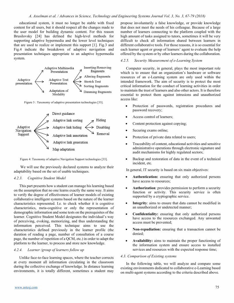
A. Asselman et al. / Advances in Science, Technology and Engineering Systems Journal Vol. 3, No. 3, 67-79 (2018)
www.astesj.com 75
educational system, it must no longer be stable with fixed content for all users, but it should respect all the changes made to the user model for building dynamic content. For this reason Brusilovsky [24] has defined the high-level methods for supporting adaptive hypermedia and the lower level techniques that are used to realize or implement this support [1]. Fig.3 and Fig.4 indicate the breakdown of adaptive navigation and presentation techniques appropriate to an adaptive hypermedia system.
Figure 3 : Taxonomy of adaptive presentation technologies [33].
Figure 4: Taxonomy of adaptive Navigation Support technologies [33].
We will use the previously declared systems to analyze their adaptability based on the set of usable techniques.
4.2.3. Cognitive Student Model
This part presents how a student can manage his learning based on the assumption that no one learns exactly the same way. It aims to verify the degree of effectiveness of learner models of existing collaborative intelligent systems based on the nature of the learner characteristics represented. I.e. to check whether it is cognitive characteristics, meta-cognitive or only the representation of demographic information and some tests on the prerequisites of the learner. Cognitive Student Model designates the individual’s way of perceiving, evoking, memorizing, and thus understanding the information perceived. This technique aims to use the characteristics defined previously in the learner profile (the duration of reading a page, number of consultation of a course page, the number of repetition of a QCM, etc.) in order to adapt the platform to the learner, to process and store new knowledge.
4.2.4. Learner /group of learners follow up
Unlike face-to-face learning spaces, where the teacher corrects at every moment all information circulating in the classroom during the collective exchange of knowledge. In distance learning environments, it is totally different, sometimes a student may
propose involuntarily a false knowledge, or provide knowledge that does not meet the needs of his colleague. Because of a large number of learners connecting to the platform coupled with the high amount of tasks assigned to tutors, sometimes it will be very difficult to check all information shared between learners in different collaborative tools. For those reasons, it is so essential for each learner agent or group of learners’ agent to evaluate the help offered by the system or by other learners during the collaboration.
4.2.5. Security Measurement of e-Learning System
Computer security, in general, plays the most important role which is to ensure that an organization’s hardware or software resources of an e-Learning system are only used within the intended framework. The aim of security is to protect the most critical information for the conduct of learning activities in order to maintain the trust of learners and also other actors. It is therefore essential to protect them against intrusions and unauthorized access like:
• Protection of passwords, registration procedures and password recovery;
• Access control of learners;
• Content protection against copying;
• Securing exams online;
• Protection of private data related to users;
• Traceability of content, educational activities and sensitive administrative operations through electronic signature and audit mechanisms for highly regulated sectors;
• Backup and restoration of data in the event of a technical incident, etc.
In general, IT security is based on six main objectives:
• Authentication: ensuring that only authorized persons have access to resources;
• Authorization: provides permission to perform a security function or activity. This security service is often supported by a cryptographic service.
• Integrity: aims to ensure that data cannot be modified in an unauthorized or undetected manner;
• Confidentiality: ensuring that only authorized persons have access to the resources exchanged. Any unwanted access must be prevented;
• Non-repudiation: ensuring that a transaction cannot be denied;
• Availability: aims to maintain the proper functioning of the information system and ensure access to installed services and resources with the expected response time;
4.3. Comparison of Existing systems
In the following table, we will analyze and compare some existing environments dedicated to collaborative e-Learning based on multi-agent systems according to the criteria described above.

A. Asselman et al. / Advances in Science, Technology and Engineering Systems Journal Vol. 3, No. 3, 67-79 (2018)
www.astesj.com 76
Table 1: Comparative measurements between existing intelligent collaborative systems
Measurements Systems ALLEGRO BAGHERA I-MIND MASCE MAS-PLANG SACA
Collaboration Tools
Synchronous Chat and video Conference Chat Chat rooms and
Whiteboards Chat Chat Chat
Asynchronous Email X Forum Email Email Email and
Forum
Intelligent actors Interaction
A student agent is interacting
with the Teacher tutor agent,
Collaborative agent and
Expert Agent
A student interacts with three
artificial agents: Companion, Tutor
and Mediator;
A teacher interacts with two artificial
agents: Companion and
Assistant
The student agent manages
the communication channels among
students and between the
teacher and the students
Each student is interacting with
the corresponding
Student Manager Agent that helps the
learning process of the student
Student interact with different
agents (SONIA, Monitoring agents,
programmed agents…)
Learner interacts with the Learner Assistant Agent
Teacher is interacting with a Teacher Assistant
Agent and Teacher’s Mediator Agent
Tutor is associated with a Tutor Agent
Adaptability Measurement
Navigation X Adaptive link annotation Guidance direct X Adaptive link
hiding Adaptive link
annotation
Presentation Inserting / Removing fragments
X X Inserting / Removing fragments
X X
Cognitive Student Model
Student model contemplates the learning
style, understanding of the subjects, limitations and
knowledge level of the
apprentice.
X X
MASCE makes it possible to
present relatively some
preferences such as cognitive
style (maximum numbers of concurrent
discussions)
X
In this system, the cognitive level
represents only the knowledge, and
moreover, it is the learner who must
manually choose his value (excellent,
good, average, etc.).
Learner /group of learners follow up X X
I-MINDS student agent evaluates and forms a peer
group (“buddy group”) for the student that it
serves
After each help session, each of the helper and
helpee are provided with an evaluation
form to evaluate his peer.
X X
Security Measurement
Authentication X
The application home page
requires users (student, teacher, or administrator) to login to access
their own interfaces
Student connect for each of the
classrooms using login and
password
Student logs to the system and is given a user
name and a password for
authentication in a specific course.
A student must be connected to the system to have access to revise some specific sections of the lesson, solve a
particular problem or enter the chat
room.
Learners, authors and tutors must
register before any effective use of the
system
Authorization X X X X X X
Integrity X X X X X X
Confidentiality X X X X X X
Non-repudiation X X X X X X
Availability X X X X X X

A. Asselman et al. / Advances in Science, Technology and Engineering Systems Journal Vol. 3, No. 3, 67-79 (2018)
www.astesj.com 77
4.4. Analysis and prospect for improvements
Reviewing the existing intelligent collaborative systems, we have seen that they have advantages as they have limits. But generally, we can see that they are hardly trying to solve the problem of students’ drop out through the integration of certain information and communication techniques to benefit from his strength. If we analyze the table above, we can mention that most of these systems are reinforced by the involvement of many collaborative tools, whether synchronous tools such as chat, or asynchronous tools like email, Whiteboard and forum discussion. Particularly, this can be retained as a great benefit in online learning systems, but this is not always the case. Indeed, the majority of these systems offer certain collaborative tools for learners to work in groups without verification whether this collaboration is beneficial and may meet the needs and preferences of the learner, thus, simply put two people in contact does not necessarily guarantee a good result. Therefore, collaborative tools can have adverse effects if the system does not control the learner behavior. In most cases, learners spend all their time communicating with other colleagues off the topic of learning. For this reason, the system must be managed against the misuse of collaboration tools so that it does not lose its educational value. Further, the majority of these systems are interested in collaborative learning in groups, but they have never analyzed how these groups should be constituted even there have been several studies conducted on the ideal size of the group, and methods of choosing members for regrouping.
As we have already shown in the third section of this article, the integration of agents in an e-Learning system suggests a very important improvement. It makes agents able to diminish and facilitate tasks to all human actors of learning platform. In order to have a more efficient learning environment, it is recommended to separate the tasks of different actors in the platform. I.e. it is better to have a system with multiple agents where everyone is responsible for specific tasks, instead of having, for example, one tutor or teacher agent who take overall responsibility for managing the whole system. So, in an e-Learning system, it’s better to separate the teacher role for two or more actors such as the pedagogical author and the expert author. Where the pedagogical author (or instructional designer) utilizes all the pedagogical design principles, models, and learning theories available to achieve pedagogical goals as he supports the management and development of e-Learning course content, the creation of storyboards, development compliance manuals, etc. While the expert author tries to define what needs to be added to the e-Learning course, and what can be put aside. Most of the time, a different expert author is used for each new e-Learning course. He usually works closely with the instructional designer to determine the key points and learning objectives of the course, as well as how the content will be delivered. Similarly to the tutor agent, it is necessary to separate the maximum tasks by creating specific agents such as the filtering agent that allows filtering multimedia documents stored in e-Learning system’s database in order to select an appropriate educational content adapted to the criteria specified in the student model. Or the technical assistant agent that is responsible for the good technical functioning, and the necessary updates in the learning environment. He must always be available
to help learners if they have a technical problem, or if they do not master the use of the computer tools.
From the table 1, we can observe that the personalization applied in these systems does not exceed more than one aspect of adaptation, i.e. they only adapt the navigation or the presentation of the interfaces. Moreover, they are limited to the use of just one adaptation technique, which is often inserting and removing fragment for presentation adaptation, and the adaptive annotation for navigation adaptation Indeed, this adaptation remains insufficient in the most existing systems and make their interfaces so very poor ergonomically. So we can summarize that there is a lack in the adaptation that should not be left behind.
This analyze, we noted that the problem of the lack of adaptation techniques used is not the only obstacle that interferes with the flexibility of adaptation of those systems, but there is also the lack of learner modeling. Most distance learning systems have been structured with a minimum of consideration of relevant aspects of human cognitive architecture [43]. Each of them does not perform any user model representations while others offer a limited learner model such as SACA for example. It deals only with the acquisition of learner’s knowledge whereas learner modeling is no longer limited to modeling knowledge but also the representation of psychological aspects such as information on the emotional state and emotions, the intentions of the learner. In this system, the cognitive aspects can only be dealt with a simple question asked to the user aiming to specify the level of mastery of concept taught. Before starting the learning activity, the learner must manually indicate his level of knowledge using a simple value (excellent, good, average ...), which is still irrelevant. For the above reasons, it’s important to think about improving existing systems or to design a new system based on cognitive modeling of the learner, i.e. it aims to represent as closely as possible all the cognitive and metacognitive aspects relating to the behaviors of a learner.
Not only misuse of cognitive student model but also the problem of helps evaluation by Learner agent or group of learner agent. We can distinguish that MASCE allows a learner to ask for help and to evaluate the help provided by another learner, and I-MINDS allows the teacher to monitor the activities of learners and groups. And both systems are used to evaluate learners. Unlike MASCE, I-MINDS offers users the possibility of forming a group [39]. However, the others do not offer any follow-up of learners.
Concerning the systems analyzed above, we can notice that the most of them lack the most basic conditions to prevent intruders. While the evolution of educational systems via the Internet currently is leading to a new concept of security threats against applications and users that affect e-Learning content design and tools. Besides that, even other systems that are partially secure, they only protect the authentication problem like MASCE, MAS-PLAN, and I-MINDS. Indeed, when designing a secure e-Learning system, designers must have a clear idea of the threats they must prevent, and the technical capabilities of the attackers to specify accordingly the preliminary steps required to secure the system [44]. They must take into consideration the identification verification of the student being assessed by ensuring that the person answering is the learner who must have passed the assessment and not another person. They must also protect the e-

A. Asselman et al. / Advances in Science, Technology and Engineering Systems Journal Vol. 3, No. 3, 67-79 (2018)
www.astesj.com 78
Learning systems, especially when passing evaluation, against nodes and links attacks which affects the availability of evaluation pages and other resources [44]. In the same way, the system must be protected by preventing unwanted access and theft of documents that reveal user privacy information. In addition, they must secure the evaluation procedures by ensuring that the learners did not have access to the assessment procedures before taking the exam. Indeed, in an e-Learning environment, depending on time zones, some students can take their exam in one country while others are still reviewing. This problem does not matter for environments that just have awareness training on a subject, but they are more important for certified training. And as a result, that will affect the reputation of the risky platform, and negatively affect the quality of the degrees acquired. For that, the most likely attacks for these systems should be described independently of the specific implementation, to help designers to eliminate or mitigate these attacks if possible in the design phase not waiting for actual attacks to occur.
5. Conclusion
According to the originality of solutions offered by adaptive multi-agent systems, recently, e-Learning researchers often use MAS to solve many problems as selecting autonomously the most suitable learning objects that meet students’ preferences, or collecting and processing learners’ data in order to monitor their progress, motivate and guide them, and avoid their abandonment. In this study, we present the interest of artificial intelligence in e-Learning system for the purpose of controlling the students’ dropout phenomenon. We analyzed some existing intelligent collaborative e-Learning based on various characters in order to determine their limits and propose some improvement that can make them more reliable for use.
In this paper which represent an analysis of some existing intelligent collaborative systems, we concluded that these systems are still in need of improvement at the level of integration of a powerful learner model. This model should not be limited to a simple collection of learner biographical information or an assessment of learner level knowledge, but it must also be able to represent psychological aspects such as information on affective state and emotions, learner intentions, as well as cognitive and metacognitive characteristics. We found also that the most of the analyzed systems do not offer any follow-up of learners. Moreover, the lack of the most basic conditions to prevent intruders even the other systems that are partially secure, they only protect the authentication problems.
References
[1]. CLARK, Ruth C. and MAYER, Richard E. E-learning and the science of instruction: Proven guidelines for consumers and designers of multimedia learning. John Wiley & Sons, 2016.
[2]. OYE, N. A., IAHAD, N., MADAR, M. J., and al. The impact of e-learning on students’ performance in tertiary institutions. International Journal of Computer Networks and Wireless Communications, 2012, vol. 2, no 2, p. 121-130.
[3]. BELANGER, Yvonne and THORNTON, Jessica. Bioelectricity: A quantitative approach Duke University’s first MOOC. 2013.
[4]. HALAWA, Sherif, GREENE, Daniel, and MITCHELL, John. Dropout prediction in MOOCs using learner activity features. Experiences and best practices in and around MOOCs, 2014, vol. 7, p. 3-12.
[5]. ONAH, Daniel FO, SINCLAIR, Jane, and BOYATT, Russell. Dropout rates of massive open online courses: behavioural patterns. EDULEARN14 proceedings, 2014, p. 5825-5834.
[6]. GÜTL, Christian, RIZZARDINI, Rocael Hernández, CHANG, Vanessa, and al. Attrition in MOOC: Lessons learned from drop-out students. In: International Workshop on Learning Technology for Education in Cloud. Springer, Cham, 2014. p. 37-48. https://doi.org/10.1007/978-3-319-10671-7_4
[7]. GEE, Sue. MITx-the fallout rate. Message posted, 2012, vol. 16. [8]. BARKLEY, Elizabeth F., CROSS, K. Patricia, and MAJOR, ClaireH.
Collaborative learning techniques: A handbook for college faculty. John Wiley & Sons, 2014.
[9]. ASSELMAN, Amal, NASSEH, Az-Eddine, and AAMMOU, Souhaib. Survey of intelligent collaborative E-learning systems. In: Emerging eLearning Technologies and Applications (ICETA), 2017 15th International Conference on. IEEE, 2017. p. 1-7. 10.1109/ICETA.2017.8102463
[10]. ZAPPAROLLI, Luciana Silva and STIUBIENER, Itana. FAG-a management support tool with BI techniques to assist teachers in the virtual learning environment Moodle. Advances in Science, Technology and Engineering Systems Journal, 2017, vol. 2, no 3, p. 587-597. 10.25046/aj020375
[11]. DE KOCH, Nora Parcus. Software engineering for adaptive hypermedia systems. Ph. DThesis, Verlag Uni-Druck, Munich, 2001.
[12]. JÄRVELÄ, Sanna, KIRSCHNER, Paul A., PANADERO, Ernesto, and al. Enhancing socially shared regulation in collaborative learning groups: designing for CSCL regulation tools. Educational Technology Research and Development, 2015, vol. 63, no 1, p. 125-142. https://doi.org/10.1007/s11423-014-9358-1
[13]. ROSCHELLE, Jeremy. Learning by collaborating: Convergent conceptual change. The journal of the learning sciences, 1992, vol. 2, no 3, p. 235-276. https://doi.org/10.1207/s15327809jls0203_1
[14]. WALCKIERS, Marc and DE PRAETERE, Thomas. L'apprentissage collaboratif en ligne, huit avantages qui en font un must. Distances and savoirs, 2004, vol. 2, no 1, p. 53-75. 10.3166/ds.2.53-75
[15]. MCLAREN, Bruce M., SCHEUER, Oliver, and MIKŠÁTKO, Jan. Supporting collaborative learning and e-Discussions using artificial intelligence techniques. International Journal of Artificial Intelligence in Education, 2010, vol. 20, no 1, p. 1-46.
[16]. MCCARTHY, John, MINSKY, Marvin L., ROCHESTER, Nathaniel, and al. A proposal for the dartmouth summer research project on artificial intelligence, august 31, 1955. AI magazine, 2006, vol. 27, no 4, p. 12.
[17]. RUSSELL, Stuart J. and NORVIG, Peter. Artificial intelligence: a modern approach. Malaysia; Pearson Education Limited,, 2016.
[18]. WENGER, Etienne. Artificial intelligence and tutoring systems: computational and cognitive approaches to the communication of knowledge. Morgan Kaufmann, 2014.
[19]. BRUSILOVSKY, Peter. Methods and techniques of adaptive hypermedia. User modeling and user-adapted interaction, 1996, vol. 6, no 2-3, p. 87-129. https://doi.org/10.1007/BF00143964
[20]. MIHALCA, Rodica, UTA, A., ANDREESCU, Anca, and al. Knowledge management in E-learning systems. Revista Informatica Economică, 2008, vol. 2, no 46, p. 60-65.
[21]. GHAHRAMANI, Zoubin. Probabilistic machine learning and artificial intelligence. Nature, 2015, vol. 521, no 7553, p. 452.
[22]. WOOLDRIDGE, Michael. An introduction to multiagent systems. John Wiley & Sons, 2009.
[23]. RUSSELL, Stuart and NORVIG, Peter. Intelligence artificielle: Avec plus de 500 exercices. Pearson Education France, 2010.
[24]. CHAIB-DRAA, Brahim, JARRAS, Imed, and MOULIN, Bernard. Systèmes multi-agents: principes généraux and applications. Principes and architectures des systèmes multi-agents, 2001.
[25]. LABIDI, Sofiane and LEJOUAD, Wided. De l'intelligence artificielle distribuée aux systèmes multi-agents. 1993. Thèse de doctorat. INRIA.
[26]. FERBER, Jacques. Les systèmes multi-agents: vers une intelligence collective. InterEditions, 1995.
[27]. ASSELMAN, Amal, AAMMOU, Souhaib, and NASSEH, Az-Eddine. Comparative study of cognitive architectures. International Research Journal of Computer Science (IRJCS), 2015, vol. 2, no 9.
[28]. ANDERSON, John R. How can the human mind occur in the physical universe?. Oxford University Press, 2009.
[29]. KOTSERUBA, Iuliia, GONZALEZ, Oscar J. Avella, and TSOTSOS, John K. A review of 40 years of cognitive architecture research: focus on perception, attention, learning and applications. arXiv preprint arXiv:1610.08602, 2016.
[30]. BISWAS, Pradipta and SPRINGETT, Mark. User Modeling. The Wiley Handbook of Human Computer Interaction, 2018, vol. 1, p. 143-169. https://doi.org/10.1002/9781118976005.ch8
[31]. VAN RIJN, Hedderik, JOHNSON, Addie, and TAATGEN, Niels. Cognitive user modeling. Handbook of human factors in web design, 2nd edn. CRC Press, New Yersey, 2011, p. 527-542. http://doi.org/doi:10.1201/b10855-34
[32]. BRUSILOVSKY, Peter and MILLÁN, Eva. User models for adaptive hypermedia and adaptive educational systems. In: The adaptive web. Springer

A. Asselman et al. / Advances in Science, Technology and Engineering Systems Journal Vol. 3, No. 3, 67-79 (2018)
www.astesj.com 79
Berlin Heidelberg, 2007, vol. 4321, p. 3-53. https://doi.org/10.1007/978-3-540-72079-9_1
[33]. BRUSILOVSKY, Peter. User modeling and user-adapted interaction. 2001. [34]. CHEN, Sherry Y. and MAGOULAS, George D. (ed.). Adaptable and
adaptive hypermedia systems. IGI Global, 2005. [35]. AL-AZAWEI, Ahmed and BADII, Atta. State of the art of learning styles-
based adaptive educational hypermedia systems (LS-BAEHSs). International Journal of Computer Science & Information Technology, 2014, vol. 6, no 3, p. 1. http://dx.doi.org/10.5121/ijcsit.2014.6301
[36]. KORB, Kevin B. and NICHOLSON, Ann E. Bayesian artificial intelligence. CRC press, 2010.
[37]. VICCARI, Rosa M., OVALLE, Demetrio A., and JIMÉNEZ, Jovani A. ALLEGRO: Teaching/learning multi-agent environment using instructional planning and cases-based reasoning (CBR). CLEI Electronic Journal, 2007, vol. 10, no 1, p. 1-20.
[38]. WEBBER, Carine, BERGIA, Loris, PESTY, Sylvie, and al. The Baghera project: a multi-agent architecture for human learning. In: Workshop-Multi-Agent Architectures for Distributed Learning Environments. In Proceedings International Conference on AI and Education. San Antonio, Texas. 2001.
[39]. SOH, Leen-Kiat, KHANDAKER, Nobel, and JIANG, Hong. IMINDS: a multiagent system for intelligent computer-supported collaborative learning and classroom management. International Journal of Artificial Intelligence in Education, 2008, vol. 18, no 2, p. 119-151.
[40]. MAHDI, Hani and ATTIA, Sally S. MASCE: a multi-agent system for collaborative e-learning. In: Computer Systems and Applications, 2008. AICCSA 2008. IEEE/ACS International Conference on. IEEE, 2008. p. 925-926. 10.1109/AICCSA.2008.4493647
[41]. PEÑA, Clara-Inés, MARZO, Jose-L., and DE LA ROSA, JosepLluis. Intelligent agents in a teaching and learning environment on the Web. In: Proceedings of the international conference on advanced learning technologies. Palmerston North, NZ: IEEE Learning Technology Task Force. 2002. p. 21-27.
[42]. LAFIFI, Yacine. SACA: un Système dApprentissage Collaboratif. 2007. Thèse de doctorat. PhD Thesis, Computer science department, University of Annaba, Algeria.
[43]. BALAŽ, Zdenko and PREDAVEC, Davor. Cognitive Cybernetics vs. Captology. Advances in Science, Technology and Engineering Systems Journal, 2017, vol. 2, no 6, p. 107. 10.25046/aj020614
[44]. NICKOLOVA, Maria and NICKOLOV, Eugene. Threat model for user security in e-learning systems. International Journal Information Technologies and Knowledge, 2007, vol. 1, no 1, p. 341-347.

Advances in Science, Technology and Engineering Systems JournalVol. 3, No. 3, 80-91 (2018)
www.astesj.comSpecial Issue on Multidisciplinary Sciences and Engineering
ASTES JournalISSN: 2415-6698
Towards Process Standardization for Requirements Analysisof Agent-Based Systems
Khaled Slhoub*, Marco Carvalho
Florida Institute of Technology, School of Computing, Florida, 32901, United States
A R T I C L E I N F O A B S T R A C T
Article history:Received: 18 April, 2018Accepted: 11 May, 2018Online: 31 May, 2018
Keywords:IEEE Std 830Agent-Oriented SpecificationAgent-Based SystemsMulti-Agent SystemsMASABSSoftware EngineeringSoftware Requirements Speci-ficationSRSSoftware StandardsSoftware Quality
The development of agent-based systems is negatively impacted by thelack of process standardization across the major development phases,such as the requirements analysis phase. This issue creates a key barrierfor agent technology stockholders regarding comprehending and ana-lyzing complexity associated with these systems specifications. Instead,such fundamental low-level infrastructure is loosely attended to in anad-hoc fashion, and important aspects of requirements analysis are oftenneglected altogether. The IEEE Std 830 model is a recommended practiceaimed at describing how to write better quality requirement specifica-tions of conventional software. Knowing that agent-based computing is anatural and logical evolution of the conventional approaches to softwaredevelopment, we believe that the requirements phase in agent-based sys-tems can benefit from applying the IEEE Std 830 model which results inhigh-quality and more accepted artifacts. This article provides a criteria-based evaluation that is derived from the software engineering bodyof knowledge guide to assessing the adoption degree of agent-orientedmethodologies to software requirements standards. Then, it proposes amodel-driven approach to restructuring and extending the IEEE Std 830-2009 standard model to specify requirements of agent-based systems. Toevaluate the applicability and usefulness of the updated model, we designa research study that allows practicing the model with simple real-worldproblem scenarios and conducting a summative survey to solicit feedbackon the model usages.
1 Introduction
This article is an extension of work initially presentedin 2017 at the IEEE 8th Annual Ubiquitous Computing,Electronics and Mobile Communication Conference(UEMCON) [1].
Agent-based systems (ABS) have proliferated in re-cent years into what is now one of the most activeresearch areas in computing. This intensity of inter-est is increased not only because these complex sys-tems impose a new promising means of developingsoftware, but also because the agent community hasbecome aware of the necessity to cast ABS as a softwareengineering paradigm (SE). This becomes importantin order to assist ABS development to be more formaland efficient. Agent-Oriented Software Engineering
(AOSE) is a new independent SE mainstream that aimsto either extend or adapt existing SE methodologies tofacilitate and improve the ABS complex development.SE practices have become a vital prerequisite of run-ning successful software products and have been ex-tensively used for decades to support the conventionalways of building software, such as object-oriented de-velopment which is currently the most popular pro-gramming paradigm [2].
Like other conventional software, software require-ments specification (SRS) is an essential aspect in agent-based systems, and numerous agent-oriented method-ologies demand it as an initial primary phase in theirdevelopment process life-cycles. SRS describes how anagent system is expected to behave and extends the re-
*Corresponding Author: Khaled Slhoub, Email: [email protected]
www.astesj.com 80https://dx.doi.org/10.25046/aj030311

K. Slhoub/ Advances in Science, Technology and Engineering Systems Journal Vol. 3, No. 3, 80-91 (2018)
quirements analysis phase to in-depth detail, detailedblueprints, used extensively by different stakehold-ers of agent systems. However, the complexity associ-ated with ABS development and its target applicationdomains often drives the complexity of ABS require-ments phase. This results in poor quality SRS artifactsthat have a genuine and significant negative impact onthe entire ABS development life-cycle and create fur-ther technical problems to the stakeholders. With theemergence of industry willingness for agent systems,there is a real demand to develop a high-quality agent-oriented specification in such a way that makes ABSdevelopment easier, more formal, more disciplined,and more accepted industry-wide.
Over the past three decades, software standardshave played a key role in improving quality of conven-tional software development. For instance, SE prac-tices like the UML modeling language and IEEE/ISOstandards have been widely used in the software in-dustry to formalize the entire software developmentlife-cycle. More specifically, the International Recom-mended Practice for Software Requirements Specifica-tions model (IEEE Std 830-2009) has been commonlyemployed to help developers toward constructing high-quality and well-organized SRS artifacts [3]. Agenttechnology as another approach for software devel-opment can undoubtedly benefit from the IEEE Std830-2009 model to standardize the SRS process whichwill mitigate the complexity of the requirements anal-ysis and, as a result, produce more accepted SRS ar-tifact. To do so, the IEEE Std 830-2009 model needsto be reconstructed and updated with new additionalextensions to make it more suitable to handle the nat-ural complexity of ABS and their target applicationdomains.
In the original work, the intent was to restructurethe IEEE Std 830-2009 model in such a way that makesit more suitable to handle ABS requirement specifi-cations. We first explored the requirement phases indifferent well-known AOSE methodologies, describedin [4], [5], and hence we identified five data modelswhich need to be specified and incorporated into theABS analysis process. Then, we checked the suitabilityof these data models according to the original IEEEStd 830-2009 sections and proposed rewriting somesubsections, extending others, and adding more newextensions to the IEEE Std 830-2009 model to comple-ment the process standardization in the ABS require-ment phase. In this extended article, we explain indetail evaluation criteria used to determine the cover-age degree of the agent-oriented methodologies withrespect to the requirement standards. Also, we conductan external evaluation study by asking participants togo through the updated model sections using a fewsimple real-world problem scenarios, and then take anonline survey to provide feedback on their experienceusing the updated model.
The rest of this paper is organized as follows: sec-tion 2 gives the necessary overview of software agent
concepts and goals, the agent-oriented specificationprocess with some related work, and the structure ofthe original IEEE Std 830-2009 standard model alongwith some related work. Section 3 presents an evalua-tion matrix used to asses the coverage degree of agent-oriented methodologies with respect to requirementstandards. Section 4 describes our proposed approachto restructuring the IEEE Std 830-2009 standard modelin such a way that makes it more capable to addressagent-oriented specification. Section 5 summarizes ourevaluation method and results for the updated IEEEStd 830-200 model. 6 concludes.
2 Background and Related Work
2.1 Agent-Based Systems: What and Why
Over the past two decades, computing systems have be-come more complex. There are several reasons behindsuch complexity. First, numerous computing systemsare now becoming concurrent and distributed. Theyare often configured and distributed over multiplelocations with the use of multiple networks, tens ofservers, and hundreds of different machines. Such sys-tems also comprise a considerable number of softwareapplications that extensively communicate with oneanother. Second, many computing systems operate indynamic environments which are flexible enough topermit unpredictable changes to their contents andsettings. Third, many computing systems now needto be continuously active and to provide services onan on-going basis [6]. Indeed, the explosive growthof the web and mobile technologies present a twofoldproblem in terms of the vast availability, wide variety,and heterogeneity of datasets [7]. Moreover, there hasbeen a natural tendency to rely more on technologyto resolve certain classes of complex real-world prob-lems. People want computer systems to do more forthem and, if possible, substitute them for performingcostly and complex tasks. More than this, consumersdemand systems to operate without their interventionand take the initiative when necessary. To do so, peoplebuild software components, known as agents, to acton behalf of users to achieve specific delegated goals.The intent is to develop sophisticated agents that are“capable of human-like reasoning and acting” [8], [9].
As a result of the above demands, new softwarecharacteristics and expectations have arisen and madecurrent software development paradigms strugglingto handle such complex development. These demandshave also triggered a need to focus more on devel-oping complex, real-time and distributed intelligentsystems. Thus, this has prompted researchers to lookfor some effective alternative approaches to addressthe new demands of software development. Currently,agent-based computing is becoming the most promis-ing development approach for handling such issues[5], [10], [11], [12], [13].
A software agent, another popular term used in-
www.astesj.com 81
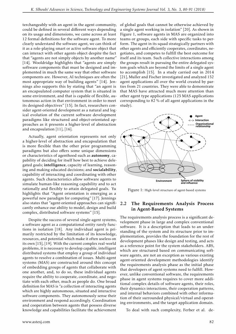
K. Slhoub/ Advances in Science, Technology and Engineering Systems Journal Vol. 3, No. 3, 80-91 (2018)
terchangeably with an agent in the agent community,could be defined in several different ways dependingon its usage and dimensions, we came across at least12 formal definitions for the software agent. To moreclearly understand the software agent, we can think ofit as a role-playing smart or active software object thatcan interact with other agents object despite the factthat “agents are not simply objects by another name”[14]. Wooldridge highlights that “agents are simplysoftware components that must be designed and im-plemented in much the same way that other softwarecomponents are. However, AI techniques are often themost appropriate way of building agents” [14]. Jen-nings also supports this by stating that “an agent isan encapsulated computer system that is situated insome environment, and that is capable of flexible, au-tonomous action in that environment in order to meetits designed objectives” [15]. In fact, researchers con-sider agent-oriented development as a natural and log-ical evolution of the current software developmentparadigms like structured and object-orientated ap-proaches as it presents a higher-level of abstractionand encapsulation [11], [16].
Actually, agent orientation represents not onlya higher-level of abstraction and encapsulation thatis more flexible than the other prior programmingparadigms but also offers some unique dimensionsor characteristics of agenthood such as autonomy, ca-pability of deciding for itself how best to achieve dele-gated goals; intelligence, capacity of learning, reason-ing and making educated decisions; and socialability,capability of interacting and coordinating with otheragents. Such characteristics allow software agents tosimulate human-like reasoning capability and to actrationally and flexibly to attain delegated goals. Yuhighlights that “Agent orientation is emerging as apowerful new paradigm for computing” [17]. Jenningsalso states that “agent-oriented approaches can signifi-cantly enhance our ability to model, design and buildcomplex, distributed software systems” [15].
Despite the success of several single-agent systems,a software agent as a computational entity rarely func-tions in isolation [18]. Any individual agent is pri-marily restricted by the limitation of its knowledge,resources, and potential which make it often useless onits own [15], [19]. With the current complex real-worldproblems, it is necessary to develop capable, intelligentdistributed systems that employ a group of individualagents to resolve a combination of issues. Multi-agentsystems (MAS) are constructed around this conceptof embedding groups of agents that collaborate withone another, and, to do so, these individual agentsrequire the ability to cooperate, coordinate, and nego-tiate with each other, much as people do. One broaddefinition for MAS is “a collection of interacting agentswhich are highly autonomous, situated and interactivesoftware components. They autonomously sense theirenvironment and respond accordingly. Coordinationand cooperation between agents that possess diverseknowledge and capabilities facilitate the achievement
of global goals that cannot be otherwise achieved bya single agent working in isolation” [20]. As shown inFigure 1, software agents in MAS are organized intoteams or groups, each side with specific tasks to per-form. The agent in its squad strategically partners withother agents and efficiently cooperates, coordinates, ne-gotiates, and competes to fulfill the best outcome foritself and its team. Such collective interactions amongthe groups result in pursuing the entire delegated sys-tem goals which are beyond the limits of a single agentto accomplish [15]. In a study carried out in 2014[21], Muller and Fischer investigated and analyzed 152agent applications all over the world created by par-ties from 21 countries. They were able to demonstratethat MAS have attracted much more attention thanother agent type applications (125 MAS applicationscorresponding to 82 % of all agent applications in thestudy).
Agent
Interaction Organizational relationship
Sphere of visibility and influence
Environment
Figure 1: High-level structure of agent-based systems
2.2 The Requirements Analysis Processin Agent-Based Systems
The requirements analysis process is a significant de-velopment phase in large and complex conventionalsoftware. It is a description that leads to an under-standing of the system and its structure prior to im-plementation, provides the foundation for the rest ofdevelopment phases like design and testing, and actsas a reference point for the system stakeholders. ABS,which are structured based on communicating soft-ware agents, are not an exception as various existingagent-oriented development methodologies identifythe requirements analysis phase as the initial phasethat developers of agent systems need to fulfill. How-ever, unlike conventional software, the requirementsphase in agent systems requires to cover more addi-tional complex details of software agents, their roles,their dynamics interactions, their cooperation patterns,and internal behaviors combined with other informa-tion of their surrounded physical/virtual and operat-ing environments, and the target application domain.
To deal with such complexity, Ferber et al. de-
www.astesj.com 82
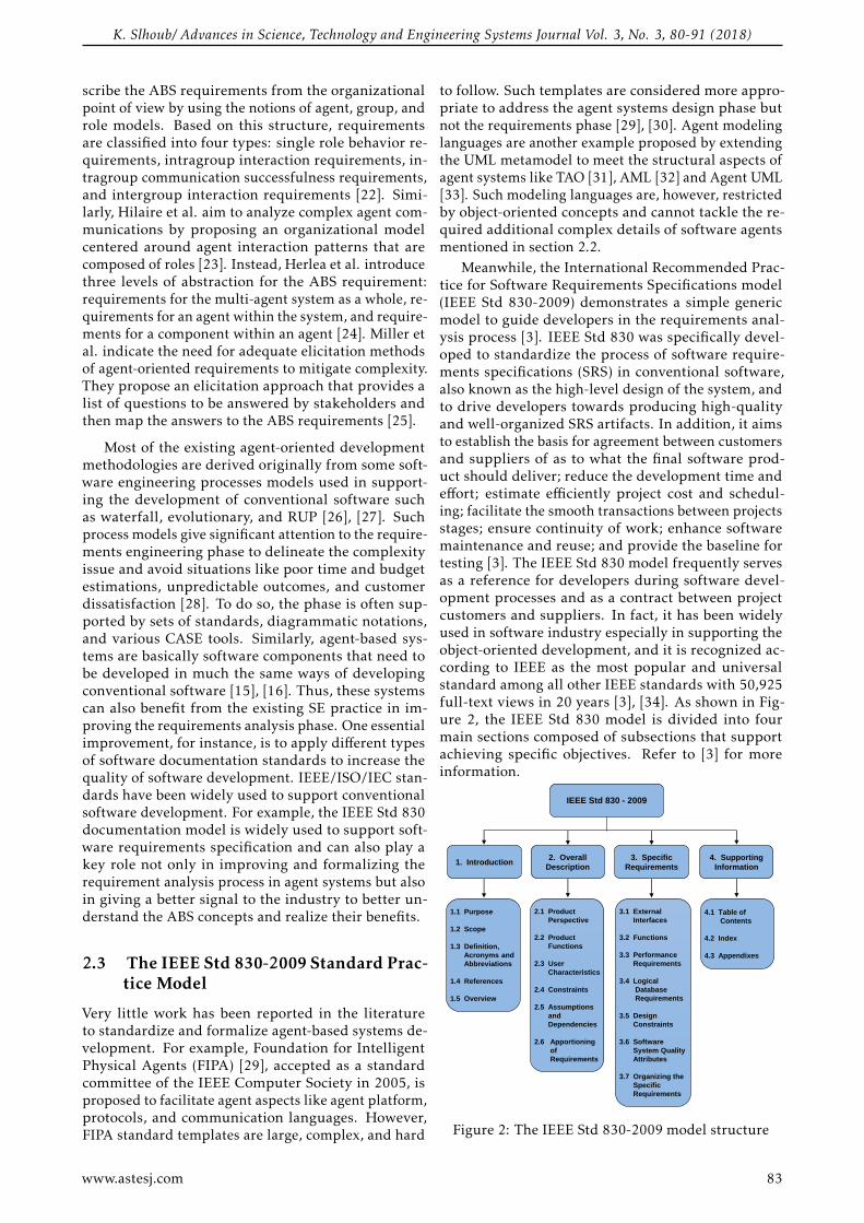
K. Slhoub/ Advances in Science, Technology and Engineering Systems Journal Vol. 3, No. 3, 80-91 (2018)
scribe the ABS requirements from the organizationalpoint of view by using the notions of agent, group, androle models. Based on this structure, requirementsare classified into four types: single role behavior re-quirements, intragroup interaction requirements, in-tragroup communication successfulness requirements,and intergroup interaction requirements [22]. Simi-larly, Hilaire et al. aim to analyze complex agent com-munications by proposing an organizational modelcentered around agent interaction patterns that arecomposed of roles [23]. Instead, Herlea et al. introducethree levels of abstraction for the ABS requirement:requirements for the multi-agent system as a whole, re-quirements for an agent within the system, and require-ments for a component within an agent [24]. Miller etal. indicate the need for adequate elicitation methodsof agent-oriented requirements to mitigate complexity.They propose an elicitation approach that provides alist of questions to be answered by stakeholders andthen map the answers to the ABS requirements [25].
Most of the existing agent-oriented developmentmethodologies are derived originally from some soft-ware engineering processes models used in support-ing the development of conventional software suchas waterfall, evolutionary, and RUP [26], [27]. Suchprocess models give significant attention to the require-ments engineering phase to delineate the complexityissue and avoid situations like poor time and budgetestimations, unpredictable outcomes, and customerdissatisfaction [28]. To do so, the phase is often sup-ported by sets of standards, diagrammatic notations,and various CASE tools. Similarly, agent-based sys-tems are basically software components that need tobe developed in much the same ways of developingconventional software [15], [16]. Thus, these systemscan also benefit from the existing SE practice in im-proving the requirements analysis phase. One essentialimprovement, for instance, is to apply different typesof software documentation standards to increase thequality of software development. IEEE/ISO/IEC stan-dards have been widely used to support conventionalsoftware development. For example, the IEEE Std 830documentation model is widely used to support soft-ware requirements specification and can also play akey role not only in improving and formalizing therequirement analysis process in agent systems but alsoin giving a better signal to the industry to better un-derstand the ABS concepts and realize their benefits.
2.3 The IEEE Std 830-2009 Standard Prac-tice Model
Very little work has been reported in the literatureto standardize and formalize agent-based systems de-velopment. For example, Foundation for IntelligentPhysical Agents (FIPA) [29], accepted as a standardcommittee of the IEEE Computer Society in 2005, isproposed to facilitate agent aspects like agent platform,protocols, and communication languages. However,FIPA standard templates are large, complex, and hard
to follow. Such templates are considered more appro-priate to address the agent systems design phase butnot the requirements phase [29], [30]. Agent modelinglanguages are another example proposed by extendingthe UML metamodel to meet the structural aspects ofagent systems like TAO [31], AML [32] and Agent UML[33]. Such modeling languages are, however, restrictedby object-oriented concepts and cannot tackle the re-quired additional complex details of software agentsmentioned in section 2.2.
Meanwhile, the International Recommended Prac-tice for Software Requirements Specifications model(IEEE Std 830-2009) demonstrates a simple genericmodel to guide developers in the requirements anal-ysis process [3]. IEEE Std 830 was specifically devel-oped to standardize the process of software require-ments specifications (SRS) in conventional software,also known as the high-level design of the system, andto drive developers towards producing high-qualityand well-organized SRS artifacts. In addition, it aimsto establish the basis for agreement between customersand suppliers of as to what the final software prod-uct should deliver; reduce the development time andeffort; estimate efficiently project cost and schedul-ing; facilitate the smooth transactions between projectsstages; ensure continuity of work; enhance softwaremaintenance and reuse; and provide the baseline fortesting [3]. The IEEE Std 830 model frequently servesas a reference for developers during software devel-opment processes and as a contract between projectcustomers and suppliers. In fact, it has been widelyused in software industry especially in supporting theobject-oriented development, and it is recognized ac-cording to IEEE as the most popular and universalstandard among all other IEEE standards with 50,925full-text views in 20 years [3], [34]. As shown in Fig-ure 2, the IEEE Std 830 model is divided into fourmain sections composed of subsections that supportachieving specific objectives. Refer to [3] for moreinformation.
IEEE Std 830 - 2009
1. Introduction2. Overall
Description
3. Specific
Requirements
4. Supporting
Information
1.1 Purpose
1.2 Scope
1.3 Definition,
Acronyms and
Abbreviations
1.4 References
1.5 Overview
2.1 Product
Perspective
2.2 Product
Functions
2.3 User
Characteristics
2.4 Constraints
2.5 Assumptions
and
Dependencies
2.6 Apportioning
of
Requirements
3.1 External
Interfaces
3.2 Functions
3.3 Performance
Requirements
3.4 Logical
Database
Requirements
3.5 Design
Constraints
3.6 Software
System Quality
Attributes
3.7 Organizing the
Specific
Requirements
4.1 Table of
Contents
4.2 Index
4.3 Appendixes
Figure 2: The IEEE Std 830-2009 model structure
www.astesj.com 83
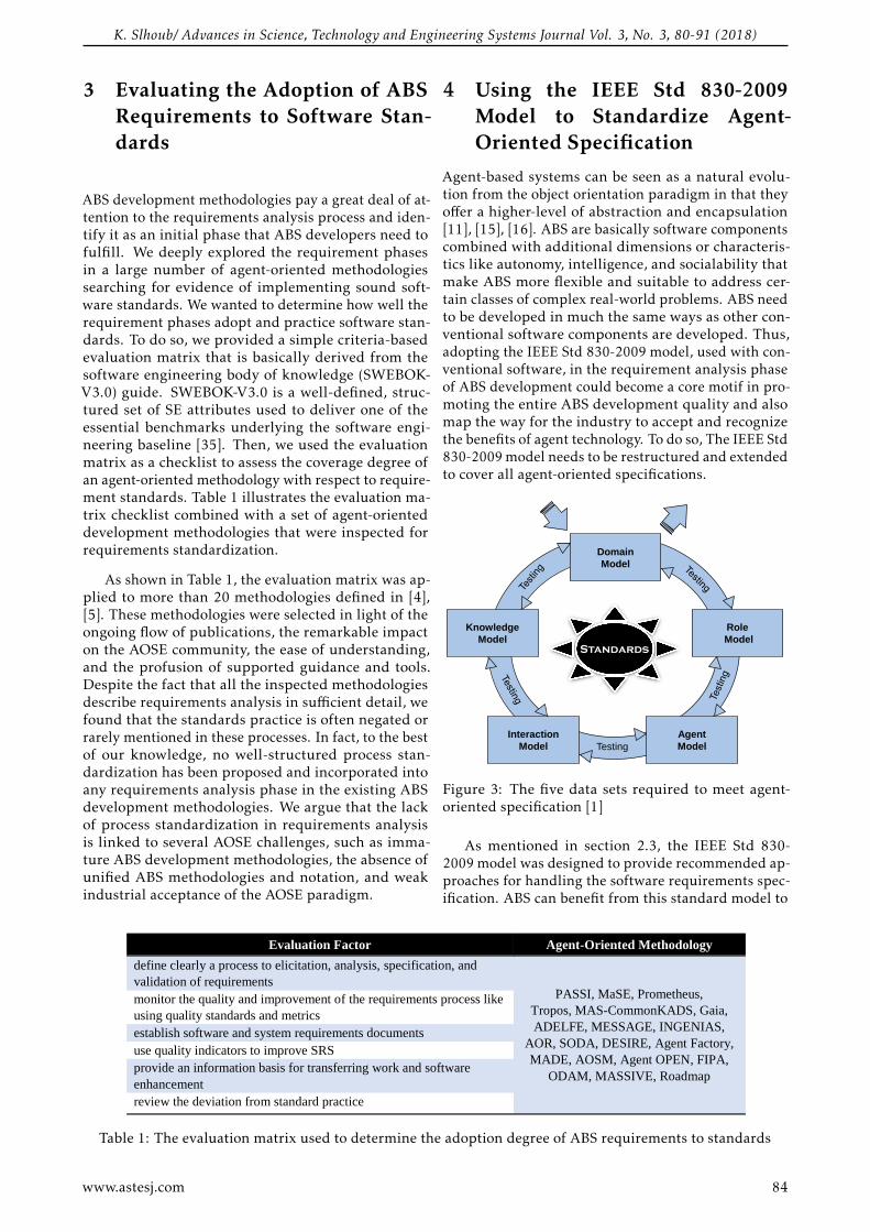
K. Slhoub/ Advances in Science, Technology and Engineering Systems Journal Vol. 3, No. 3, 80-91 (2018)
3 Evaluating the Adoption of ABSRequirements to Software Stan-dards
ABS development methodologies pay a great deal of at-tention to the requirements analysis process and iden-tify it as an initial phase that ABS developers need tofulfill. We deeply explored the requirement phasesin a large number of agent-oriented methodologiessearching for evidence of implementing sound soft-ware standards. We wanted to determine how well therequirement phases adopt and practice software stan-dards. To do so, we provided a simple criteria-basedevaluation matrix that is basically derived from thesoftware engineering body of knowledge (SWEBOK-V3.0) guide. SWEBOK-V3.0 is a well-defined, struc-tured set of SE attributes used to deliver one of theessential benchmarks underlying the software engi-neering baseline [35]. Then, we used the evaluationmatrix as a checklist to assess the coverage degree ofan agent-oriented methodology with respect to require-ment standards. Table 1 illustrates the evaluation ma-trix checklist combined with a set of agent-orienteddevelopment methodologies that were inspected forrequirements standardization.
As shown in Table 1, the evaluation matrix was ap-plied to more than 20 methodologies defined in [4],[5]. These methodologies were selected in light of theongoing flow of publications, the remarkable impacton the AOSE community, the ease of understanding,and the profusion of supported guidance and tools.Despite the fact that all the inspected methodologiesdescribe requirements analysis in sufficient detail, wefound that the standards practice is often negated orrarely mentioned in these processes. In fact, to the bestof our knowledge, no well-structured process stan-dardization has been proposed and incorporated intoany requirements analysis phase in the existing ABSdevelopment methodologies. We argue that the lackof process standardization in requirements analysisis linked to several AOSE challenges, such as imma-ture ABS development methodologies, the absence ofunified ABS methodologies and notation, and weakindustrial acceptance of the AOSE paradigm.
4 Using the IEEE Std 830-2009Model to Standardize Agent-Oriented Specification
Agent-based systems can be seen as a natural evolu-tion from the object orientation paradigm in that theyoffer a higher-level of abstraction and encapsulation[11], [15], [16]. ABS are basically software componentscombined with additional dimensions or characteris-tics like autonomy, intelligence, and socialability thatmake ABS more flexible and suitable to address cer-tain classes of complex real-world problems. ABS needto be developed in much the same ways as other con-ventional software components are developed. Thus,adopting the IEEE Std 830-2009 model, used with con-ventional software, in the requirement analysis phaseof ABS development could become a core motif in pro-moting the entire ABS development quality and alsomap the way for the industry to accept and recognizethe benefits of agent technology. To do so, The IEEE Std830-2009 model needs to be restructured and extendedto cover all agent-oriented specifications.
Domain
Model
Knowledge
Model
Role
Model
Agent
Model
Interaction
Model Testing
Standards
Figure 3: The five data sets required to meet agent-oriented specification [1]
As mentioned in section 2.3, the IEEE Std 830-2009 model was designed to provide recommended ap-proaches for handling the software requirements spec-ification. ABS can benefit from this standard model to
Evaluation Factor Agent-Oriented Methodology
define clearly a process to elicitation, analysis, specification, and
validation of requirements PASSI, MaSE, Prometheus,
Tropos, MAS-CommonKADS, Gaia,
ADELFE, MESSAGE, INGENIAS,
AOR, SODA, DESIRE, Agent Factory,
MADE, AOSM, Agent OPEN, FIPA,
ODAM, MASSIVE, Roadmap
monitor the quality and improvement of the requirements process like
using quality standards and metrics
establish software and system requirements documents
use quality indicators to improve SRS
provide an information basis for transferring work and software
enhancement
review the deviation from standard practice
Table 1: The evaluation matrix used to determine the adoption degree of ABS requirements to standards
www.astesj.com 84

K. Slhoub/ Advances in Science, Technology and Engineering Systems Journal Vol. 3, No. 3, 80-91 (2018)
shape and formalize the requirements analysis processin such a way that results in more accepted specifica-tion document. Thus, we attempt in this section tospecify ABS requirements by means of utilizing theIEEE Std 830-2009 model and proposing several newextensions to it. Accordingly, we first identified themain data models in the SRS process of ABS by in-vestigating the analysis processes in several differentAOSE development methodologies such as PASSI [36],ADELFE [37], MaSE [38], Gaia [39], and Tropos [40].Then, we checked the fitness of these data modelsaccording to the IEEE Std 830-2009 model. Conse-quently, we were able to identify the data models thatare not covered by the original IEEE Std 830-2009model and proposed rewriting some subsections, ex-tending others, and adding more new extensions to themodel that can facilitate the agent-oriented specifica-tion. Figure 3 illustrates the identified 5 data modelsthat carry the required information for specifying theABS requirements. The 5 data models are described inthe following list:
1. The Domain model is concerned with the anal-ysis of a specific real world that an agent-basedsystem is intended to work in and interact with.This model consists of three types of information:
• Operating Environment includes descrip-tions of the general characteristics of theoperating environment of ABS. Such envi-ronment provides the necessary infrastruc-ture in which agents deployed and live. Italso manages these agents while perform-ing their tasks and delivers the most cur-rent information about them. Moreover, itis responsible for providing the structure ofthe agent communication language and theagent semantic language.
• Physical/Virtual Environment includes de-scriptions of the world that software agentsperceive and interact with. ABS are oftenexecuted in challenging environments thatare dynamic, unpredictable, and unreliable.Such environments could be virtual like theweb world or physical like a self-driving carand a train control system.
• Application Domain includes informationabout the field in which the system oper-ates. Such information may involve certaindomain terminology or reference to domainconcepts and policies.
2. The Role model is concerned with describingthe ABS requirements in terms of agent tasksor services. Agents are the core actors that areresponsible for performing tasks and achievingdelegated goals. The descriptions may includeinformation about the role responsibilities, pre-requisites, and constraints.
3. The Agent model is concerned with identifyingand classifying agent types that are instantiated
later at ABS run-time, and it is directly linkedto the Role model. The Agent model should alsoinclude descriptions of characteristics for everyagent type which may include at least descrip-tions of the essential characteristics of agentssuch as autonomy, reactiveness, proactiveness,and socialability [15], [16].
4. The Interaction model is concerned with de-scribing the agents behavior in terms of cooper-ating, collaborating, negotiating with users, sys-tem resources, and other agents. It should alsospecify the agents messaging protocols and inter-action patterns along with the use of ontologiesor conceptual means for describing the messagecontents. For instance, an agent can request an-other agent to perform some action, and the otheragent may refuse or accept the request. It mayalso confirm to other agents that given proposi-tion is true.
5. The Knowledge model is concerned with de-scribing a repository of knowledge that agentsmay use to provide explanations, recovery in-formation, or optimize their performance. Forinstance, some agent types, like reflex agents andlearning agents, require some particular rules inorder perform actions, so such rules need to bespecified and stored in the system. The Knowl-edge model, also, should briefly describe agentarchitectures which underlying the concepts forbuilding rational agents and their characteris-tics. Such information is important to design anyagent-based system later. For instance, Belief-Desires-Intentions (BDI) architecture is probablythe best-known agent architecture that agentsrely on to reason about their actions [41].
After identifying the five main data models foragent-oriented specification, we carefully reviewed thefour main sections of the original IEEE Std 830-2009model to check the suitability of the 5 data models ac-cording to these sections. As a result, we were able topropose adding more new subsections, rewriting oth-ers, and extending other subsections to formulate theABS requirements specification. Figure 4 illustratesthe updated structure of the IEEE Std 830-2009 modelby highlighting the new and edited subsections. Also,full descriptions are provided for all new informationadded to the updated model as follows:
1. The first section “Introduction” contains subsec-tions that provide an overview of the entire SRSdocument, so we consider this information suit-able for the five data models of ABS [3]. We onlysuggest the following change in the followingsubsection:
• An existing subsection (1.5 Overview): thissubsection should provide a brief descrip-tion of the contents of the rest of SRS docu-ment, so it should also include a description
www.astesj.com 85

K. Slhoub/ Advances in Science, Technology and Engineering Systems Journal Vol. 3, No. 3, 80-91 (2018)
IEEE Std 830 - 2009
1. Introduction2. Overall
Description
3. Specific
Requirements
4. Supporting
Information
1.1 Purpose
1.2 Scope
1.3 Definition,
Acronyms and
Abbreviations
1.4 References
1.5 Overview
2.1 Product
Perspective
2.2 Domain
Perspective
2.3 Product
Functions
2.4 Agent
Perspective
2.5 User
Characteristics
2.6 Constraints
2.7 Assumptions
and
Dependencies
2.8 Apportioning
of
Requirements
3.1 Agent
Properties
3.2 External
Interfaces
3.3 Functions
3.4 Performance
Requirements
3.5 Logical
Database
Requirements
3.6 Design
Constraints
3.7 Software
System Quality
Attributes
3.8 Organizing the
Specific
Requirements
4.1 Table of
Contents
4.2 Index
4.3 Appendixes
Figure 4: The updated structure of the IEEE Std 830-2009 model [1]
of how analyses of the five ABS data mod-els are organized and presented in the SRSmodel.
2. The second section “Overall Description” con-tains subsections that describe the general fac-tors that could affect the product and its require-ments specifications [3]. We suggest the follow-ing changes to this section:
• A new defined subsection (2.2 Domain Per-spective): based on the provided descriptionof this section, the Domain model should bedescribed after (2.1 Product Perspective) foran organizational purpose. The domain ap-plication often has a great influence on ABS,ABS are considered as environment-drivenbusiness development. So, the potential fea-tures of the three sections of the Domainmodel are described in this subsection.
• An existing subsection (2.2 Product Func-tions): this subsection is renumbered to sub-section (2.3), and it is described in terms ofboth: the Role model and the user functions.Thus, it should provide a summary of thekey roles that agents in ABS will perform.Notice that this only include a high-levelsummary of the Role model that defines themajor functional roles for each listed agent.
• A new defined subsection (2.4 Agent Per-spective): based on the provided descrip-
tion of this section, the Agent model shouldbe summarized in section 2. It should in-clude a description that lists and definesthe potential software agent categories andtheir main characteristics.
• An existing subsection (2.6 Apportioningof Requirements): this subsection is renum-bered to subsection (2.8), and it should iden-tify functional agent roles and user func-tions that may be delayed until future ver-sions of the agent-based system.
3. The third section “Specific Requirement” con-tains subsections that describe in sufficient tech-nical details all ABS requirements. This includesall functional roles concerning all inputs andoutputs to/from the agent-based system and allrequired nonfunctional requirements [3]. Wesuggest the following changes to this section asfollows:
• A new defined subsection (3.1 Agent Prop-erties): this subsection should extend thesubsection (2.4 Agent Perspective). It isconcerned with agent properties/ dimen-sions to a level of sufficient detail that willhelp ABS designers to construct the internalstates for every agent type in ABS.
• An existing subsection (3.1 External Inter-faces): this subsection is renumbered to sub-section (3.2). One goal of the third section is
www.astesj.com 86
K. Slhoub/ Advances in Science, Technology and Engineering Systems Journal Vol. 3, No. 3, 80-91 (2018)
to provide detailed descriptions of softwareinterfaces. So, the Interaction model shouldbe described in this subsection in such a waythat presents communication mechanismsand messages between all agent types.
• An existing subsection (3.2 Functions): thissubsection is renumbered to subsection(3.3). It is concerned with all ABS require-ments specifications to a level of detail. Thisshould extend the subsection (2.2 ProductFunctions) and include sufficient detailedspecifications for every functional agentrole and user functions. Also, this sub-section should extend the subsection (2.4Agent Perspective) and include sufficientdetailed specifications of software agents. Itis critical also to explicitly link listed pro-posed agents to their functional roles. Anagent-role list is an effective technique touse here.
• An existing subsection (3.4 LogicalDatabase Requirements): this subsectionis renumbered to subsection (3.5). It isconcerned with any information that is tobe stored in a database. Thus, the knowl-edge model should be described in such away that shows how some types of agents,like the reflex and learning agents, can useit. Also, the agent architectures should bebriefly outlined in this subsection.
• An existing subsection (3.7 Organizing theSpecific Requirements): this subsection isrenumbered to subsection (3.8). The agent-oriented specification is detailed and tendsto be extensive. So, it is important to givespecial attention to organizing this informa-tion to ensure clarity and understandability.This section should include an additional or-ganization which organizing by agent class.Associated with each agent class is a set ofagent roles and characteristics.
4. The fourth section “Supporting Information”contains subsections that make the SRS docu-ment easier to use, for example, using the tableof contents, index, and appendixes [3]. We sug-gest no change to this section and consider thisinformation suitable for the five data models ofABS.
5 Evaluation Analysis
In the original published paper, we conducted twotypes of evaluation to assess the utility and effective-ness of the proposed restructured IEEE Std 830 model:1) we specified requirements of a small multi-agentsystem by using both the new proposed model and theoriginal model, and then we compared the outcomesof both models. 2) we used our proposed model tospecify requirements of some previous agent systems
that were already specified by using the original model,and we analyzed the outcomes of the different mod-els based on the SRS quality attributes described inthe IEEE Std 830-2009 model. Refer to [1] for moreinformation about both assessments.
This article summarizes results from an indepen-dent and external research study that was conductedto assess the suitability and validity of the updatedIEEE Std 830. The aim of the study was to determinewhether the updated model satisfies ABS requirementsspecification and to solicit feedback on any possiblemissing details or weaknesses in the model structure.Several experts in software engineering and agent-oriented systems were invited to participate in theresearch study. They were asked to go through theproposed model sections with a few simple real-worldproblem scenarios (requirements specification of a sim-ple small agent-based system: Item-Trading Agent-BasedSystem (ITABS) that enables users to create and em-ploy agents to act on behalf of them to trade items).Then, the participants conduct an online survey to pro-vide feedback on their experience using the proposedmodel in specifying ITABS. The survey consisted of 12statements as shown in Table 2. These statements wereorganized into 3 sets to determine participants’ accep-tance of the proposed model, their satisfaction with us-ing the various added and updated agent informationto the model, and the quality of the proposed model.The participants were asked to indicate their level ofagreement or disagreement with each statement. Wewere able to collect and analyze 13 responses from theparticipants as shown in the following charts.
In Figure 5, our concern was focused on whether ornot the participants think that the proposed standardsmodel is capable of specifying ABS requirements. Theparticipants were all in favor of the model as no onedisagreed with the statements S1 and S2.
In Figure 6, the participants provided their feed-back about the added and updated agent informationto the original IEEE Std 830 model. We believe thatthe existence of such information makes the IEEE Std830-2009 model more suitable to handle the agent-oriented specification. The positive responses actuallyconfirmed our belief as all participants agreed with thestatements S3 and S4, and only 4 persons disagreedwith the statement S5. The proposed model is requiredto briefly outline agent architectures which support theconcepts for building rational agents and their charac-teristics. This information is essential to start any ABSdesign later, but it seems that some participants dis-agree with referring to implementation details, like re-ferring to agent architectures in the requirement phase.
In Figure 7, the participants gave their opinionsabout the quality of the proposed model after using itin specifying small agent-based system requirements.They rated the model based on the IEEE seven qualityattributes of good software requirements, described inthe original IEEE Std 830 model, by indicating howwell they feel that the requirements meet the quality
www.astesj.com 87

K. Slhoub/ Advances in Science, Technology and Engineering Systems Journal Vol. 3, No. 3, 80-91 (2018)
S1 The updated IEEE 830 model helps the developers to identify an agent-based system to be developed
along with its requirements.
S2 The updated IEEE 830 model describes what the agent-based system will do and how it will be
expected to perform.
S3
Information regarding domain perspective which includes application domain, operating environment,
and physical/virtual environment needs to be specified in the IEEE 830 model and will be used to
build an agent-based system.
S4 Information regarding agent classification, characteristics, functions, and communications needs to be
specified in the IEEE 830 model and will be used to build an agent-based system.
S5 Information regarding agent architectures and agent repository of knowledge, if there's any, needs to
be briefly outlined in the IEEE 830 model and will be used to build an agent-based system.
S6 The functional requirements described in the model were unambiguous: there was only one
interpretation for every stated requirement.
S7 The functional requirements described in the model were complete: all significant requirements
concerning function, performance, interfaces, design constraints, and quality factors were included.
S8 The functional requirements described in the model were consistent: no subset of individual
requirements characteristics, actions, or terms conflicted.
S9 The functional requirements described in the model were verifiable (Testable): requirements were
stated in concrete terms that can be verified through testing or other objective means.
S10 The functional requirements described in the model were modifiable: the specification was structured
and annotated so that changes may be made easily, completely, and consistently.
S11 The functional requirements described in the model were traceable: the origin of each requirement
was clear and the format should aid in tracing forward and backward.
S12 The functional requirements described in the model were usable: the specifications should be useful
during development and in later identifying maintenance requirements and constraints.
0
1
2
3
4
5
6
7
8
9
10
11
12
13
S6 S7 S8 S9 S10 S11 S12
8
9
12
10
11
9
11
Participan
ts
Feedback
Table 2: The online survey statements given to the participants to scale
Strongly Disagree
Disagree
Agree
Strongly Agree
S1 S2
0 0
0 0
7
8
6
5
Par
tici
pan
ts
Feedback
Figure 5: The degree of acceptance of the updated IEEE Std 830-2009 model
attributes on a scale from Strongly Agree to StronglyDisagree. Generally, the responses were positive witha range from 62% to 93% of the participants agreed orstrongly agreed with each quality attribute applied tothe updated model.
Figure 8 represents a straightforward view thatonly illustrates the summary of users’ views whoagreed with each quality attributes applied to the pro-posed standard model.
6 Conclusion
A strong demand desires to apply agent-based sys-tems in complex and large real-world applications be-cause of their capability to act rationally and flexiblyto attain delegated goals. ABS development requiresthe inclusion of sound software engineering practices
in order to be more formal, efficient, and adopted inthe industry. Software standards as an SE key prac-tice are widely applied in the software industry tosupport the entire software development life-cycle.Based on our evaluation applied to a large numberof agent-oriented methodologies, we believe that nowell-structured process standardization has been pro-posed and incorporated into any requirements anal-ysis phase in the existing agent-oriented methodolo-gies.This paper addresses the process standardizationfor requirements specification of agent-based systemsby proposing a model-driven approach to restructureand update the IEEE Std 830-2009 model to make itmore suitable to handle the ABS requirement specifi-cations.
The updated IEEE Std 830-2009 model proposedadding new extensions and updating others in the orig-
www.astesj.com 88
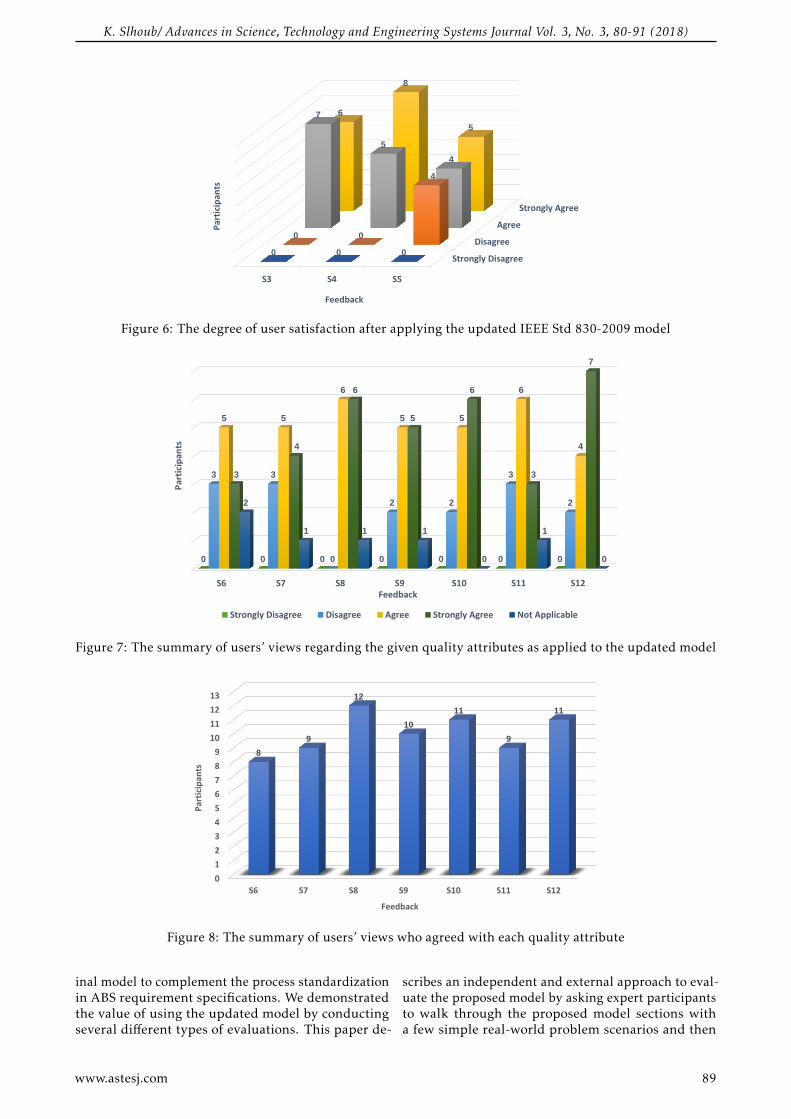
K. Slhoub/ Advances in Science, Technology and Engineering Systems Journal Vol. 3, No. 3, 80-91 (2018)
Strongly Disagree
Disagree
Agree
Strongly Agree
S3 S4 S5
0 0 0
0 0
4
7
5
4
6
8
5
Par
tici
pan
ts
Feedback
Figure 6: The degree of user satisfaction after applying the updated IEEE Std 830-2009 model
S6 S7 S8 S9 S10 S11 S12
0 0 0 0 0 0 0
3 3
0
2 2
3
2
5 5
6
5 5
6
4
3
4
6
5
6
3
7
2
1 1 1
0
1
0
Par
tici
pan
ts
Feedback
Strongly Disagree Disagree Agree Strongly Agree Not Applicable
Figure 7: The summary of users’ views regarding the given quality attributes as applied to the updated model
S1 The updated IEEE 830 model helps the developers to identify an agent-based system to be developed
along with its requirements.
S2 The updated IEEE 830 model describes what the agent-based system will do and how it will be
expected to perform.
S3
Information regarding domain perspective which includes application domain, operating environment,
and physical/virtual environment needs to be specified in the IEEE 830 model and will be used to
build an agent-based system.
S4 Information regarding agent classification, characteristics, functions, and communications needs to be
specified in the IEEE 830 model and will be used to build an agent-based system.
0
1
2
3
4
5
6
7
8
9
10
11
12
13
S6 S7 S8 S9 S10 S11 S12
8
9
12
10
11
9
11
Participan
ts
Feedback
Figure 8: The summary of users’ views who agreed with each quality attribute
inal model to complement the process standardizationin ABS requirement specifications. We demonstratedthe value of using the updated model by conductingseveral different types of evaluations. This paper de-
scribes an independent and external approach to eval-uate the proposed model by asking expert participantsto walk through the proposed model sections witha few simple real-world problem scenarios and then
www.astesj.com 89

K. Slhoub/ Advances in Science, Technology and Engineering Systems Journal Vol. 3, No. 3, 80-91 (2018)
take an online survey to provide feedback on theirexperience using the model. The feedback was very en-couraging as all participants agreed that the proposedmodel was capable of handling the ABS requirements,and were satisfied with using the model along withall updated and added agent information to it. Also,The summary of users’ views with respect to the givenquality attributes as applied to the updated modelwere positive and reflected how well the agent-orientedspecification in the updated model met these qualityattributes.
In the future, we plan to extend the updatedIEEE Std 830-2009 model to cover more specific sub-standards for every ABS data model we identified andfor every new central extension we added. This can bedone by studying what sub-standard information is re-quired to be specified in every extension. For instance,what ABS sub-standard information in the section 2.2domain perspective needs to be defined, or what sub-standard information should be included in the section3.1 Agent properties.
Conflict of Interest The authors declare no conflictof interest.
References[1] K. Slhoub, M. Carvalho, and W. Bond, “Recommended prac-
tices for the specification of multi-agent systems requirements,”in Ubiquitous Computing, Electronics and Mobile CommunicationConference (UEMCON), 2017 IEEE 8th Annual, pp. 179–185,IEEE, 2017. doi:10.1109/UEMCON.2017.8249021.
[2] B. Bauer and J. P. Muller, “Methodologies and modeling lan-guages,” Agent-based Software Development, pp. 77–131, 2004.
[3] IEEE, IEEE Recommended Practice for Software RequirementsSpecifications, vol. 2009. IEEE, 1998. doi:10.1109/IEEESTD.1998.88286.
[4] B. Henderson-Sellers, Agent-oriented methodologies. Idea GroupInc., 2005.
[5] O. Z. Akbari, “A survey of agent-oriented software engineeringparadigm: Towards its industrial acceptance,” InternationalJournal of Computer Engineering Research, vol. 1, no. 2, pp. 14–28, 2010.
[6] F. Zambonelli, N. R. Jennings, and M. Wooldridge, “Developingmultiagent systems: The Gaia methodology,” ACM Transactionson Software Engineering and Methodology (TOSEM), vol. 12,no. 3, pp. 317–370, 2003. doi:10.1145/958961.958963.
[7] Q. H. Mahmoud, “Software Agents: Characteristics and Classi-fication,” School of Computing Science, Simon Fraser University,pp. 1–12, 2000.
[8] M. Wooldridge and N. R. Jennings, “Pitfalls of agent-orienteddevelopment,” in Proceedings of the second international confer-ence on Autonomous agents, pp. 385–391, ACM, 1998. doi:10.1145/280765.280867.
[9] A. Sloman, “What sort of architecture is required for a human-like agent?,” in Foundations of rational agency, pp. 35–52,Springer, 1999. doi:10.1007/978-94-015-9204-8_3.
[10] F. Zambonelli and A. Omicini, “Challenges and research di-rections in agent-oriented software engineering,” AutonomousAgents and Multi-Agent Systems, vol. 9, no. 3, pp. 253–283, 2004.doi:10.1023/B:AGNT.0000038028.66672.1e.
[11] L. Padgham and J. Thangarajah, “Agent Oriented Software En-gineering: Why and How,” VNU Journal of Science: NaturalSciences and Technology, vol. 27, no. 3, pp. 190–204, 2011.
[12] S. Maalal and M. Addou, “A new approach of designing Multi-Agent Systems With a practical sample,” CoRR, vol. abs/1204.1,pp. 148–157, 2012.
[13] O. Shehory and A. Sturm, “A brief introduction toagents,” in Agent-Oriented Software Engineering: Reflectionson Architectures, Methodologies, Languages, and Frameworks,vol. 9783642544, pp. 3–11, Springer, 2014. doi:10.1007/978-3-642-54432-3_1.
[14] M. Wooldridge, “Agent-based software engineering,” IEEEProceedings-software, vol. 144, no. 1, pp. 26–37, 1997. doi:10.1049/ip-sen:19971026.
[15] N. R. Jennings, “On agent-based software engineering,” Arti-ficial Intelligence, vol. 117, no. 2, pp. 277–296, 2000. doi:10.1016/S0004-3702(99)00107-1.
[16] M. Wooldridge, An Introduction to MultiAgent Systems. Wiley,2nd ed., 2009.
[17] E. Yu, “Agent-oriented modelling: Software versus the world,”in Artificial Intelligence and Bioinformatics, vol. 2222, pp. 206–225, Springer, 2002. doi:10.1007/3-540-70657-7_14.
[18] Z. Ren and C. J. Anumba, “Multi-agent systems in construction-state of the art and prospects,” Automation in Construction,vol. 13, no. 3, pp. 421–434, 2004. doi:10.1016/j.autcon.2003.12.002.
[19] P. Bogg, G. Beydoun, and G. Low, “When to use a multi-agent system?,” vol. 5357 LNAI, pp. 98–108, Springer, 2008.doi:10.1007/978-3-540-89674-6_13.
[20] M. Dastani, “A survey of multi-agent programming languagesand frameworks,” in Agent-Oriented Software Engineering,vol. 9783642544, pp. 213–233, Springer, 2014. doi:10.1007/978-3-642-54432-3_11.
[21] J. P. Muller and K. Fischer, “Application impact of multi-agentsystems and technologies: A survey,” in Agent-Oriented Soft-ware Engineering, pp. 27–53, Springer, 2014. doi:10.1007/978-3-642-54432-3_3.
[22] J. Ferber, O. Gutknecht, C. M. Jonker, J. P. Muller, and J. Treur,“Organization models and behavioural requirements specifica-tion for multi-agent systems,” in Proceedings - 4th InternationalConference on MultiAgent Systems, ICMAS 2000, pp. 387–388,IEEE, 2000. doi:10.1109/ICMAS.2000.858488.
[23] V. Hilaire, A. Koukam, P. Gruer, and J. J.-P. Muller, “FormalSpecification and Prototyping of Multi-agent Systems,” in En-gineering Societies in the Agents World SE - 9, vol. 1972, pp. 114–127, Springer, 2000. doi:10.1007/3-540-44539-0_9.
[24] D. E. Herlea, C. M. Jonker, J. Treur, and N. J. E. Wijn-gaards, “Specification of bahavioural requirements within com-positional multi-agent system design,” vol. 1647, pp. 8–27,Springer, 1999. doi:10.1007/3-540-48437-X_2.
[25] T. Miller, B. Lu, L. Sterling, G. Beydoun, and K. Taveter,“Requirements elicitation and specification using the agentparadigm: The case study of an aircraft turnaround simula-tor,” IEEE Transactions on Software Engineering, vol. 40, no. 10,pp. 1007–1024, 2014. doi:10.1109/TSE.2014.2339827.
[26] P. Giorgini and B. Henderson-Sellers, Agent-Oriented Method-ologies: an Introduction. Idea Group Inc., 2005.
[27] L. Cernuzzi, M. Cossentino, and F. Zambonelli, “Process mod-els for agent-based development,” Engineering Applicationsof Artificial Intelligence, vol. 18, no. 2, pp. 205–222, 2005.doi:10.1016/j.engappai.2004.11.015.
[28] E. Ajith Jubilson, P. Joe Prathap, V. Vimal Khanna, P. Dhana-vanthini, W. Vinil Dani, and A. Gunasekaran, “An empiricalanalysis of agent oriented methodologies by exploiting the life-cycle phases of each methodology,” in Advances in IntelligentSystems and Computing, vol. 337, pp. 205–214, Springer, 2015.
[29] FIPA, “The standards organization for agents and multi-agentsystems,” 2005.
[30] P. Charlton, R. Cattoni, A. Potrich, and E. Mamdani, “Evalu-ating the FIPA standards and their role in achieving cooper-ation in multi-agent systems,” in Proceedings of the 33rd An-nual Hawaii International Conference on System Sciences, vol. 00,pp. 1–10, IEEE, 2000. doi:10.1109/HICSS.2000.926996.
www.astesj.com 90

K. Slhoub/ Advances in Science, Technology and Engineering Systems Journal Vol. 3, No. 3, 80-91 (2018)
[31] V. T. Da Silva and C. J. P. De Lucena, “Modeling multi-agent sys-tems,” Communications of the ACM, vol. 50, no. 5, pp. 103–108,2007. doi:10.1145/1230819.1241671.
[32] I. Trencansky and R. Cervenka, “Agent Modeling Lan-guage (AML): A comprehensive approach to modeling MAS,”INFORMATICA-LJUBLJANA-, vol. 29, no. 4, pp. 391–400, 2005.doi:10.1.1.60.8902.
[33] B. Bauer, J. P. Muller, and J. Odell, “Agent UML: A formalismfor specifying multiagent software systems,” International jour-nal of software engineering and knowledge engineering, vol. 11,no. 03, pp. 207–230, 2001. doi: 10.1142/S0218194001000517.
[34] A. Chikh and M. Aldayel, “Reengineering requirementsspecification based on IEEE 830 standard and traceabil-ity,” in Advances in Intelligent Systems and Computing,vol. 275 AISC, pp. 211–227, Springer, 2014. doi:10.1007/978-3-319-05951-8_21.
[35] P. Bourque and R. E. Fairley, Guide to the Software EngineeringBody of Knowledge (SWEBOK(R)): Version 3.0. Los Alamitos,CA, USA: IEEE Computer Society Press, 3rd ed., 2014.
[36] M. Cossentino and C. Potts, “PASSI: A process for specifyingand implementing multi-agent systems using UML,” RetrievedOctober, vol. 8, p. 2007, 2002.
[37] C. Bernon, M. Gleizes, S. Peyruqueou, and G. Picard, “ADELFE:A methodology for adaptive multi-agent systems engineer-ing,” in International Workshop on Engineering Societies in theAgents World, pp. 156–169, Springer Berlin Heidelberg, 2003.doi:10.1007/3-540-39173-8_12.
[38] M. Wood and S. Deloach, “An Overview of the MultiagentSystems Engineering Methodology,” in Proceedings - the FirstInternational Workshop on Agent-Oriented Software Engineering,vol. 1957, pp. 207–221, Springer, 2001.
[39] M. Wooldridge, N. R. Jennings, and D. Kinny, “The Gaiamethodology for agent-oriented analysis and design,” Au-tonomous Agents and multi-agent systems, vol. 3, no. 3, pp. 285–312, 2000. doi:10.1023/A:1010071910869.
[40] P. Bresciani, A. Perini, P. Giorgini, F. Giunchiglia, and J. My-lopoulos, “Tropos: An agent-oriented software developmentmethodology,” Autonomous Agents and Multi-Agent Systems,vol. 8, no. 3, pp. 203–236, 2004. doi:10.1023/B:AGNT.0000018806.20944.ef.
[41] M. Georgeff, B. Pell, M. Pollack, M. Tambe, and M. Wooldridge,“The Belief-Desire-Intention Model of Agency,” in InternationalWorkshop on Agent Theories, Architectures, and Languages, pp. 1–10, Springer, 1999. doi:10.1007/3-540-49057-4_1.
www.astesj.com 91
www.astesj.com 92
Evaluating the effect of Locking on Multitenancy Isolation for Components of Cloud-hosted Services
Laud Charles Ochei*,1, Christopher Ifeanyichukwu Ejiofor2
1School of Computing and Digital Media, Robert Gordon University, United Kingdom 2Department of Computer Science, University of Port Harcourt, Nigeria, [email protected]
ARTICLE INFO ABSTRACT
Article history: Received: 13 April, 2018 Accepted: 11 May, 2018 Online: 31 May, 2018
Multitenancy isolation is a way of ensuring that the performance, stored data volume and access privileges required by one tenant and/or component does not affect other tenants and/or components. One of the conditions that can influence the varying degrees of isolation is when locking is enabled for a process or component that is being shared. Although the concept of locking has been extensively studied in database management, there is little or no research on how locking affects multitenancy isolation and its implications for optimizing the deployment of components of a cloud-hosted service in response to workload changes. This paper applies COMITRE (Component-based approach to Multitenancy Isolation through Request Re-routing) to evaluate the impact of enabling locking for a shared process or component of a cloud-hosted application. Results show that locking has a significant effect on the performance and resource consumption of tenants especially for operations that interact directly with the local file system of the platform used on the cloud infrastructure. We also present recommendations for achieving the required degree of multitenancy isolation when locking is enabled for three software processes: continuous integration, version control, and bug tracking.
Keywords: Multitenancy Tenant Isolation Locking Cloud-hosted Service Cloud Patterns Software Process Bug Tracking
1. Introduction
Multitenancy (that is, an architectural practice of using a single instance of a service to serve multiple tenants) is a notable feature in many cloud-hosted services. Multiple users are usually expected to access a shared functionality or resource and so there is need to ensure that processes and data associated with a particular tenant and/or component does not affect others [1]. We refer to this concept as multitenancy isolation. Multitenancy isolation is a way of ensuring that the performance, stored data volume ad access privileges required by one tenant and/or component does not affect other tenants and/or components [1][2].
There are different or varying degrees of multitenancy isolation. For example, a higher degree of isolation would be imposed on a component that cannot be shared due to strict regulations than for a component that can be shared with minimal reconfiguration. A high degree of isolation implies that there is little or no interference between tenants when they are accessing a shared functionality/process or component of a cloud-hosted service, and
vice versa. We can achieve a high degree of isolation by duplicating a component (and its supporting resources) exclusively for one tenant.
One of the conditions that can influence the degree of isolation is when locking is enabled for the functionality/process or component that is being shared. Locking is a well-known concept used in database management to prevent data from being corrupted or invalidated when multiple users try to read or write to the database [3]. Any single user can only modify items in the database to which they have applied a lock that gives them exclusive access to the record until the lock is released. The concept of locking in database management is closely related to multitenancy isolation in the sense that both of them are used to prevent multiple users from performing conflicting operations on a shared process or component and can also be implemented at different or varying degrees. Despite this similarity, there is little or no research on how locking affects multitenancy isolation and its implications for optimizing the deployment for components of a cloud-hosted service in response to workload changes.
ASTESJ
ISSN: 2415-6698
*Corresponding Author: Laud Charles Ochei, Robert Gordon University E-mail : [email protected]
Advances in Science, Technology and Engineering Systems Journal Vol. 3, No. 3, 92-99 (2018)
www.astesj.com
Special Issue on Multidisciplinary Sciences and Engineering
https://dx.doi.org/10.25046/aj030312

L.C. Ochei et al. / Advances in Science, Technology and Engineering Systems Journal Vol. 3, No. 3, 92-99 (2018)
www.astesj.com 93
Motivated by this problem, this paper applies COMITRE (Component-based approach to Multitenancy Isolation through Request Re-routing) to evaluate the impact of enabling locking for a shared process or component of a cloud-hosted application. This paper addresses the following research question: “How can we evaluate the required degree of multitenancy isolation when locking is enabled on a shared process or component of a cloud-hosted service?” To the best of our knowledge, this study is the first to apply an approach for implementing the required degree of multitenancy isolation for a shared process or component of a cloud-hosted service when locking is enabled and to analyse its impact on the performance and resource consumption of tenants. In this study, we implemented multitenancy isolation based on three multitenancy patterns (i.e., shared component, tenant-isolated component, and dedicated component) to analyse the effect of the different degrees of isolation on performance and resource consumption of tenants when one of the tenants is exposed to high workload. The experiments were conducted using a cloud-hosted continuous integration system using Hudson as a case study deployed on a UEC private cloud. The results showed that when locking is enabled, it can have a significant effect on the performance and resource consumption of tenants especially for operations that interact directly with the local file system of the operating system or platform used on the cloud infrastructure.
The main contributions of the paper are:
1. Applying the COMITRE approach to empirically evaluate the required degree of multitenancy isolation for cloud-hosted software services when locking is enabled. 2. Presenting how locking is used in three different software processes (i.e., continuous integration, version control and bug tracking) to achieve multitenancy isolation, and its implication for optimal deployment of components. 3. Presenting recommendations and best practice guidelines for achieving multitenancy isolation when locking is enabled.
The rest of the paper is organised as follows: Section two discusses the relevance locking to multitenancy isolation for cloud-hosted services. Section three is the methodology, and Section four presents the results and discussion. The recommendations and limitations of the study are detailed in Section five and six respectively. Section seven concludes the paper with future work.
2. Relevance of Locking on Multitenancy Isolation for Cloud-Hosted Services
Multitenancy is an important cloud computing property where a single instance of an application is provided to multiple tenants, and so would have to be isolated from each other whenever there are workload changes. Just as multiple tenants can be isolated, multiple components being accessed by a tenant can also be isolated. We define “Multitenancy isolation” in this case as a way of ensuring that the required performance, stored data volume and access privileges of one component does not affect other
components of a cloud-hosted application being accessed by tenants.
When a component of a cloud-hosted application receives a high workload and there is little or no possibility of a significant influence on other tenants, we say that there is a high degree of isolation and vice versa. The varying degrees of multitenancy isolation, can be captured in three main cloud deployment patterns: (i) dedicated component, where components cannot be shared, although a component can be associated with either one tenant/resource or group of tenants/resources; (ii) tenant-isolated component, where components can be shared by a tenant or resource instance and their isolation is guaranteed; and (iii)shared component, where components can be shared with a tenant or resource instance and are unaware of other components.
Assuming that there is a requirement for a high degree of isolation between components, then components have to be duplicated for each tenant which leads to high resource consumption and running cost. A low degree of isolation may also be required, in which case, it might reduce resource consumption, and running cost, but there is a possibility of interference when workload changes and the application does not scale well.
Most of the widely used Global Software Development processes like continuous integration (for example, Hudson), version control (for example, with Subversion) and bug tracking (for example, with Bugzilla) implement some form of locking whether at the database level or filesystem level. In continuous integration for instance, locking can be used to block builds with either upstream or downstream dependencies from starting if an upstream/downstream project is in the middle of a build or in the build queue. Again, locking operations are also used in version control systems (e.g., subversion) and bug tacking systems (e.g., bugzilla) [3] [4] [5].
There are several research work on multitenancy isolation such as [6], [7] and [8]. However, none of these works have focused on the effect of locking on multitenancy isolation for components of a cloud-hosted service.
3. Evaluation
In the following, we present the experimental setup and the case study we have used in this study.
3.1. Applying COMITRE to Implement Multitenant Isolation
We applied COMITRE to evaluate multitenancy Isolation in a Version Control system. Fig. 1 shows the structure of COMITRE. It captures the essential properties required for the successful implementation of multitenancy isolation, while leaving large degrees of freedom to cloud deployment architects depending on the required degree of isolation between tenants. The actual implementation of the COMITRE is anchored on shifting the task of routing a request from the server to a separate component (e.g., Java class or plugin) at the application level of the cloud-hosted
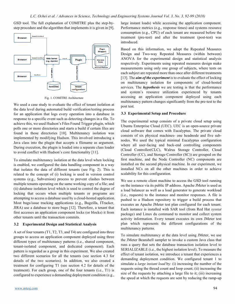
L.C. Ochei et al. / Advances in Science, Technology and Engineering Systems Journal Vol. 3, No. 3, 92-99 (2018)
www.astesj.com 94
GSD tool. The full explanation of COMITRE plus the step-by-step procedure and the algorithm that implements it is given in [9].
Fig. 1. COMITRE Architecture
We used a case study to evaluate the effect of tenant isolation at the data level during automated build verification/testing process for an application that logs every operation into a database in response to a specific event such as detecting changes in a file. To achieve this, we used Hudson’s Files Found Trigger plugin, which polls one or more directories and starts a build if certain files are found in those directories [10]. Multitenancy isolation was implemented by modifying Hudson. This involved introducing a Java class into the plugin that accepts a filename as argument. During execution, the plugin is loaded into a separate class loader to avoid conflict with Hudson’s core functionality [11].
To simulate multitenancy isolation at the data level when locking is enabled, we configured the data handling component in a way that isolates the data of different tenants (see Fig. 2). This is related to the concept of (i) locking is used in version control systems (e.g., Subversion) process to prevent clashes between multiple tenants operating on the same working copy of a file; and (ii) database isolation level which is used to control the degree of locking that occurs when multiple tenants or programs are attempting to access a database used by a cloud-hosted application. Most bugs/issue tracking applications (e.g., Bugzilla, ITracker, JIRA) use a database to store bugs [12]. Therefore, a tenant that first accesses an application component locks (or blocks) it from other tenants until the transaction commits.
3.2 Experimental Design and Statistical Analysis
A set of four tenants (T1, T2, T3, and T4) are configured into three groups to access an application component deployed using three different types of multitenancy patterns (i.e., shared component, tenant-isolated component, and dedicated component). Each pattern is regarded as a group in this experiment. We also created two different scenarios for all the tenants (see section 4.3 for details of the two scenarios). In addition, we also created a treatment for configuring T1 (see section 4.2 for details of the treatment). For each group, one of the four tenants (i.e., T1) is configured to experience a demanding deployment condition (e.g.,
large instant loads) while accessing the application component. Performance metrics (e.g., response times) and systems resource consumption (e.g., CPU) of each tenant are measured before the treatment (pre-test) and after the treatment (post-test) was introduced.
Based on this information, we adopt the Repeated Measures Design and Two-way Repeated Measures (within between) ANOVA for the experimental design and statistical analysis respectively. Experiments using repeated measures design make measurements using only one group of subjects, where tests on each subject are repeated more than once after different treatments [13]. The aim of the experiment is to evaluate the effect of locking on multitenancy isolation for components of cloud-hosted services. The hypothesis we are testing is that the performance and system’s resource utilization experienced by tenants accessing an application component deployed using each multitenancy pattern changes significantly from the pre-test to the post test.
3.3 Experimental Setup and Procedure
The experimental setup consists of a private cloud setup using Ubuntu Enterprise Cloud (UEC). UEC is an open-source private cloud software that comes with Eucalyptus. The private cloud consists of six physical machines- one headnode and five sub-nodes. We used the typical minimal Eucalyptus configuration where all user-facing and back-end controlling components (Cloud Controller(CLC), Walrus Storage Controller, Cloud Controller (CC), and Storage Controller (SC)) are grouped on the first machine, and the Node Controller (NC) components are installed on the second physical machine. In our experiment, we installed NCs on all the other machines in order to achieve scalability for this configuration.
We use a remote client machine to access the GSD tool running on the instance via its public IP address. Apache JMeter is used as a load balancer as well as a load generator to generate workload (i.e., requests) to the instance and monitor responses. A file is pushed to a Hudson repository to trigger a build process that executes an Apache JMeter test plan configured for each tenant. Each instance is installed with SAR tool (from Red Hat sysstat package) and Linux du command to monitor and collect system activity information. Every tenant executes its own JMeter test plan which represents the different configurations of the multitenancy patterns.
To simulate multitenancy at the data level using JMeter, we use the JMeter Beanshell sampler to invoke a custom Java class that runs a query that sets the database transaction isolation level to SERIALIZABLE (i.e., the highest isolation level). To measure the effect of tenant isolation, we introduce a tenant that experiences a demanding deployment condition. We configured tenant 1 to simulate a large instant load by: (i) increasing the number of the requests using the thread count and loop count; (ii) increasing the size of the requests by attaching a large file to it; (iii) increasing the speed at which the requests are sent by reducing the ramp-up
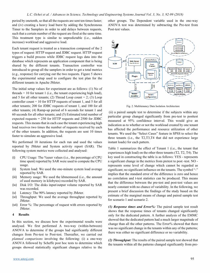
L.C. Ochei et al. / Advances in Science, Technology and Engineering Systems Journal Vol. 3, No. 3, 92-99 (2018)
www.astesj.com 95
period by onetenth, so that all the requests are sent ten times faster; and (iv) creating a heavy load burst by adding the Synchronous Timer to the Samplers in order to add delays between requests, such that a certain number of the request are fired at the same time. This treatment type is similar to unpredictable (i.e., sudden increase) workload and aggressive load.
Each tenant request is treated as a transaction composed of the 2 types of request: HTTP request and JDBC request. HTTP request triggers a build process while JDBC request logs data into the database which represents an application component that is being shared by the different tenants. Transaction controller was introduced to group all the samplers in order to get a total metrics (e.g., response) for carrying out the two requests. Figure 5 shows the experimental setup used to configure the test plan for the different tenants in Apache JMeter.
The initial setup values for experiment are as follows: (1) No of threads = 10 for tenant 1 (i.e., the tenant experiencing high load), and 5 for all other tenants; (2) Thread Loop count = 2; (3) Loop controller count = 10 for HTTP requests of tenant 1, and 5 for all other tenants; 200 for JDBC requests of tenant 1, and 100 for all other tenants; (4) Ramp-up period of 6 seconds for tenant 1 and 60 seconds for all other tenants; and (5) Estimated total number of expected requests = 250 for HTTP requests and 2500 for JDBC requests. This means that in each case the tenant experiencing high load receives two times the number of requests received by each of the other tenants. In addition, the requests are sent 10 times faster to simulate an aggressive load.
We performed 10 iterations for each run and used the values reported by JMeter and System activity report (SAR). The following system metrics were collected and analysed:
(i) CPU Usage: The %user values (i.e., the percentage of CPU time spent) reported by SAR were used to compute the CPU usage.
(ii) System load: We used the one-minute system load average reported by SAR.
(iii) Memory usage: We used the kbmemused (i.e., the amount of used memory in kilobytes) recorded by SAR.
(iv) Disk I/O: The disks input/output volume reported by SAR was recorded.
(v) Latency: The 90% latency reported by JMeter. (vi) Throughput: We used the average throughput reported by
JMeter. (vii) Error %: The percentage of request with errors reported by
JMeter.
4 Results
In this section, we discuss how the experimental results were analysed. We first performed A two-way (within-between) ANOVA to determine if the groups had significantly different changes from Pre-test to Post-test. Thereafter, we carried out planned comparisons involving the following: (i) a one-way ANOVA followed by Scheffe post hoc tests to determine which groups showed statistically significant changes relative to the
other groups. The Dependent variable used in the one-way ANOVA test was determined by subtracting the Pre-test from Post-test values.
Fig. 2. Multitenancy Data Isolation Architecture
(ii) a paired sample test to determine if the subjects within any particular group changed significantly from pre-test to posttest measured at 95% confidence interval. This would give an indication as to whether or not the workload created by one tenant has affected the performance and resource utilization of other tenants. We used the “Select Cases” feature in SPSS to select the three tenants (i.e., the T2,T3,T4 that did not experience large instant loads) for each pattern.
Table 1 summarizes the effect of Tenant 1 (i.e., the tenant that experiences high load) on the other three tenants (T2, T2, T4). The key used in constructing the table is as follows: YES - represents a significant change in the metrics from pretest to post -test. NO - represents some level of change which cannot be regarded as significant; no significant influence on the tenants. The symbol “-” implies that the standard error of the difference is zero and hence no correlation and t-test statistics can be produced. This means that the difference between the pre-test and post-test values are nearly constant with no chance of variability. In the following, we present a brief discussion the findings of the study based on the estimate of the marginal means of change and paired sample test for scenario 1 and scenario 2.
(1) Response times and Error%: The paired sample test result shows that the response times of tenants changed significantly only for the dedicated pattern. A further analysis of the EMMC showed that the dedicated pattern had a much larger magnitude of change than all the other patterns. The Error% showed that there was no significant change in the tenants within any of the patterns; there was either no significant difference or no variability.
(2) Throughput: The results of the paired sample test showed that the tenants within all the patterns changed significantly from pre-
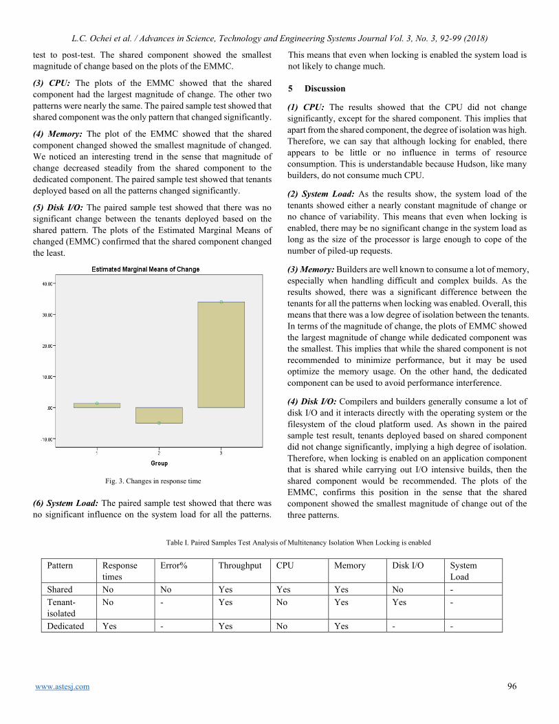
L.C. Ochei et al. / Advances in Science, Technology and Engineering Systems Journal Vol. 3, No. 3, 92-99 (2018)
www.astesj.com 96
test to post-test. The shared component showed the smallest magnitude of change based on the plots of the EMMC.
(3) CPU: The plots of the EMMC showed that the shared component had the largest magnitude of change. The other two patterns were nearly the same. The paired sample test showed that shared component was the only pattern that changed significantly.
(4) Memory: The plot of the EMMC showed that the shared component changed showed the smallest magnitude of changed. We noticed an interesting trend in the sense that magnitude of change decreased steadily from the shared component to the dedicated component. The paired sample test showed that tenants deployed based on all the patterns changed significantly.
(5) Disk I/O: The paired sample test showed that there was no significant change between the tenants deployed based on the shared pattern. The plots of the Estimated Marginal Means of changed (EMMC) confirmed that the shared component changed the least.
Fig. 3. Changes in response time
(6) System Load: The paired sample test showed that there was no significant influence on the system load for all the patterns.
This means that even when locking is enabled the system load is not likely to change much.
5 Discussion
(1) CPU: The results showed that the CPU did not change significantly, except for the shared component. This implies that apart from the shared component, the degree of isolation was high. Therefore, we can say that although locking for enabled, there appears to be little or no influence in terms of resource consumption. This is understandable because Hudson, like many builders, do not consume much CPU.
(2) System Load: As the results show, the system load of the tenants showed either a nearly constant magnitude of change or no chance of variability. This means that even when locking is enabled, there may be no significant change in the system load as long as the size of the processor is large enough to cope of the number of piled-up requests.
(3) Memory: Builders are well known to consume a lot of memory, especially when handling difficult and complex builds. As the results showed, there was a significant difference between the tenants for all the patterns when locking was enabled. Overall, this means that there was a low degree of isolation between the tenants. In terms of the magnitude of change, the plots of EMMC showed the largest magnitude of change while dedicated component was the smallest. This implies that while the shared component is not recommended to minimize performance, but it may be used optimize the memory usage. On the other hand, the dedicated component can be used to avoid performance interference.
(4) Disk I/O: Compilers and builders generally consume a lot of disk I/O and it interacts directly with the operating system or the filesystem of the cloud platform used. As shown in the paired sample test result, tenants deployed based on shared component did not change significantly, implying a high degree of isolation. Therefore, when locking is enabled on an application component that is shared while carrying out I/O intensive builds, then the shared component would be recommended. The plots of the EMMC, confirms this position in the sense that the shared component showed the smallest magnitude of change out of the three patterns.
Table I. Paired Samples Test Analysis of Multitenancy Isolation When Locking is enabled
Pattern Response
times Error% Throughput CPU Memory Disk I/O System
Load Shared No No Yes Yes Yes No - Tenant-isolated
No - Yes No Yes Yes -
Dedicated Yes - Yes No Yes - -
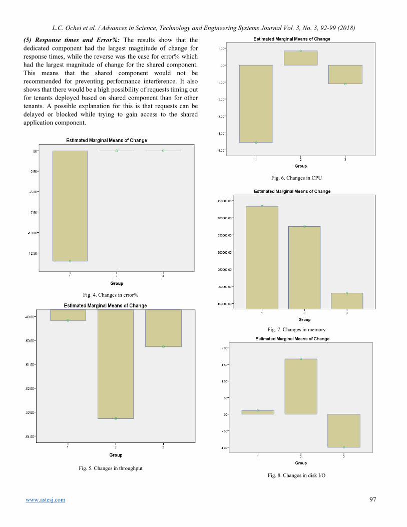
L.C. Ochei et al. / Advances in Science, Technology and Engineering Systems Journal Vol. 3, No. 3, 92-99 (2018)
www.astesj.com 97
(5) Response times and Error%: The results show that the dedicated component had the largest magnitude of change for response times, while the reverse was the case for error% which had the largest magnitude of change for the shared component. This means that the shared component would not be recommended for preventing performance interference. It also shows that there would be a high possibility of requests timing out for tenants deployed based on shared component than for other tenants. A possible explanation for this is that requests can be delayed or blocked while trying to gain access to the shared application component.
Fig. 4. Changes in error%
Fig. 5. Changes in throughput
Fig. 6. Changes in CPU
Fig. 7. Changes in memory
Fig. 8. Changes in disk I/O
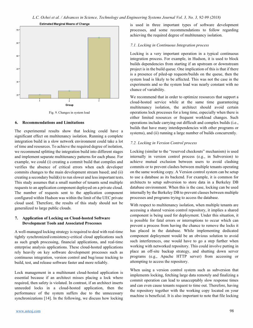
L.C. Ochei et al. / Advances in Science, Technology and Engineering Systems Journal Vol. 3, No. 3, 92-99 (2018)
www.astesj.com 98
Fig. 9. Changes in system load
6. Recommendations and Limitations
The experimental results show that locking could have a significant effect on multitenancy isolation. Running a complete integration build in a slow network environment could take a lot of time and resources. To achieve the required degree of isolation, we recommend splitting the integration build into different stages and implement separate multitenancy patterns for each phase. For example, we could (i) creating a commit build that compiles and verifies the absence of critical errors when each developer commits changes to the main development stream based; and (ii) creating a secondary build(s) to run slower and less important tests. This study assumes that a small number of tenants send multiple requests to an application component deployed on a private cloud. The number of requests sent to the application component configured within Hudson was within the limit of the UEC private cloud used. Therefore, the results of this study should not be generalized to large public clouds.
7. Application of Locking on Cloud-hosted Software Development Tools and Associated Processes
A well-managed locking strategy is required to deal with real-time tightly synchronized/consistency-critical cloud applications such as such graph processing, financial applications, and real-time enterprise analysis applications. These cloud-hosted applications rely heavily on key software development processes such as continuous integration, version control and bug/issue tracking to build, test, and release software faster and more reliably.
Lock management in a multitenant cloud-hosted application is essential because if an architect misses placing a lock where required, then safety is violated. In contrast, if an architect inserts unneeded locks in a cloud-hosted application, then the performance of the system suffers due to the unnecessary synchronizations [14]. In the following, we discuss how locking
is used in three important types of software development processes, and some recommendations to follow regarding achieving the required degree of multitenancy isolation.
7.1. Locking in Continuous Integration process
Locking is a very important operation in a typical continuous integration process. For example, in Hudson, it is used to block builds dependencies from starting if an upstream or downstream project is in the build queue. One implication of this is that if there is a presence of piled-up requests/builds on the queue, then the system load is likely to be affected. This was not the case in the experiments and so the system load was nearly constant with no chance of variability.
We recommend that in order to optimize resources that support a cloud-hosted service while at the same time guaranteeing multitenancy isolation, the architect should avoid certain operations lock processes for a long time, especially when there is either limited resources or frequent workload changes. Such operations include carrying out difficult and complex builds (i.e., builds that have many interdependencies with other programs or systems), and (ii) running a large number of builds concurrently.
7.2. Locking in Version Control process
Locking (similar to the “reserved checkouts” mechanism) is used internally in version control process (e.g., in Subversion) to achieve mutual exclusion between users to avoid clashing commits or to prevent clashes between multiple tenants operating on the same working copy. A Version control system can be setup to use a database as its backend. For example, it is common for architects to setup subversion to store data in a Berkeley DB database environment. When this is the case, locking can be used internally by the Berkeley DB to prevent classes between multiple processes and programs trying to access the database.
With respect to multitenancy isolation, when multiple tenants are accessing a shared version control repository, it implies a shared component is being used for deployment. Under this situation, it is possible for fatal errors or interruptions to occur which can prevent a process from having the chance to remove the locks it has placed in the database. While implementing dedicated component deployment would be an obvious solution to avoid such interferences, one would have to go a step further when working with networked repository. This could involve putting in place an off-site backup strategy, and shutting down server programs (e.g., Apache HTTP server) from accessing or attempting to access the repository.
When using a version control system such as subversion that implements locking, fetching large data remotely and finalizing a commit operation can lead to unacceptably slow response times and can even cause tenants request to time out. Therefore, having the repository together with the working copy located on your machine is beneficial. It is also important to note that file locking

L.C. Ochei et al. / Advances in Science, Technology and Engineering Systems Journal Vol. 3, No. 3, 92-99 (2018)
www.astesj.com 99
along with data compression are some of the operations that could consume resources, especially when accessing a shared repository from a client with a slow network and low bandwidth.
7.3. Locking in Bug tracking process
A bug tracking system is used to keep track of reported software bugs in software development projects. A major component of a bug tracking system is the storage component that records facts about known bugs. Depending on the type of storage component used to store bugs, locking can be used to prevent multiple tenants trying to access the bug data store.
Most bug and issue tracking systems (e.g., Bugzilla and JIRA) use a database to store bugs. Enabling locking on the bug database, for example, can also increase resource consumption (e.g., CPU, memory), especially when running long transactions, running complex transactions concurrently or transferring large bug attachments across a slow network connection.
8. Conclusion and Future Work
In this paper, we have presented the effect of locking on multitenancy isolation for components of a cloud-hosted service to contribute to literature on multitenancy isolation and cloud deployment of application components. The study revealed that when locking is enabled for components of a cloud-hosted service, it can have a significant impact on the performance and resource consumption of tenants especially for operations that interact directly with the local file system (e.g., FAT, NTFS, GoogleFS, HFS+) of the platform on which the service is hosted. One option we have recommended is to split a software process (e.g., a long build process) into separate phases and then implement different degrees of isolation for each phase.
We plan to apply our approach to implementing multitenancy isolation for a cloud-hosted service in a distributed scenario where locking is enabled for all or some of the components at different of the cloud stack. For example, in distributed bug tracking some bug trackers like Fossil and Veracity are either designed to use (or integrated with) distributed VC or CI systems, thus allowing bugs to be created automatically and inserted to the database at varying frequencies.
References [1] C. Fehling, F. Leymann, R. Retter, W. Schupeck, and P. Arbitter, Cloud
Computing Patterns. Springer, 2014. [2] E. Bauer and R. Adams, Reliability and availability of cloud computing. John
Wiley & Sons, 2012. [3] B. Collins-Sussman, B. Fitzpatrick, and M. Pilato, Version control with
subversion. O’Reilly, 2004. [4] M. Moser and T. O’Brien. The Hudson book. Oracle, Inc., USA. Online:
accessed in November, 2017 from http://www.eclipse.org/hudson/the-hudsonbook/book-hudson.pdf.
[5] Bugzilla.org. The bugzilla guide. The Mozilla Foundation. [Online: accessed in November, 2017 from http://www.bugzilla.org/docs/.
[6] R. Krebs, C. Momm, and S. Kounev, “Architectural concerns in multi-tenant saas applications.” CLOSER, vol. 12, pp. 426–431, 2012.
[7] S. Strauch, V. Andrikopoulos, F. Leymann, D. Muhler, “Esbmt: Enabling multi-tenancy in enterprise service buses,” CloudCom, vol. 12, pp. 456–463, 2012.
[8] S. Walraven, T. Monheim, E. Truyen, and W. Joosen, “Towards performance isolation in multi-tenant saas applications,” in Proceedings of the 7th Workshop on Middleware for Next Generation Internet Computing. ACM, 2012, p. 6.
[9] L. C. Ochei, J. Bass, and A. Petrovski, “Evaluating degrees of multitenancy isolation: A case study of cloud-hosted gsd tools,” in 2015 International Conference on Cloud and Autonomic Computing (ICCAC). IEEE, 2015, pp. 101–112.
[10] Hudson. Apache software foundation. [Online: accessed in January 2017 from http://wiki.hudsonci.org//display/HUDSON/Files+Found+Trigger].
[11] L. C. Ochei, A. Petrovski, and J. Bass, “Evaluating degrees of isolation between tenants enabled by multitenancy patterns for cloud-hosted version control systems (vcs),” International Journal of Intelligent Computing Research, vol. 6, Issue 3, pp. 601 – 612, 2015.
[12] Serrano, N. and Ciordia, I., 2005. Bugzilla, ITracker, and other bug trackers. IEEE software, 22(2), pp.11-13.
[13] Verma, J.P., 2015. Repeated measures design for empirical researchers. John Wiley & Sons.
[14] Demirbas, M., Tasci, S. and Kulkarni, S., 2012, July. Maestro: A cloud computing framework with automated locking. In Computers and Communications (ISCC), 2012 IEEE Symposium on (pp. 000833-000838). IEEE.

www.astesj.com 100
Effect of Risperidone with Ondansetron to Control the Negative and Depressive Symptoms in Schizophrenia
Sara Mubeen1, Hafiz Muhammad Mudassar Aslam2, Muhammad Tamour Danish3, Muhammad Imran*,4, Aamira Hashmi5, Muhammad Hashim Raza4
1Manawan Hospital, Lahore, 54000, Pakistan 2General Hospital, Lahore, 54000, Pakistan 3Basic Health Unit, Awan Chak 39, District Kasur, 55050, Pakistan 4District Headquarter Hospital, Layyah, 31050, Pakistan 5District Headquarter Hospital, Muzaffargarh, 34200, Pakistan
A R T I C L E I N F O A B S T R A C T Article history: Received: 08 April, 2018 Accepted: 24 May, 2018 Online: 31 May, 2018
To evaluate the effects of Ondansetron on the negative and depressive symptoms of patients with schizophrenia. A double-blind randomized control trial was conducted in 2016-17 in Lahore. 30 participants were included both in placebo and medicine group. The patients were assessed by using the Positive and Negative Syndrome Scale (PANSS) and Hamilton’s Rating Scale for Depression (HRSD) at baseline and at 12 weeks. The t-test and Chi square test were used to evaluate the data by using SPSS (version 21). The statistical significance was set at P<0.05. Ondansetron with risperidone has past impact on the negative symptoms as compared to placebo with risperidone (P=0.002). There was a significant difference between two groups after giving medicine and placebo as evaluated through WAIS-R scale. Ondansetron had significantly improved the visual memory that was based upon subsets of WAIS. Ondansetron has no role in the depressive symptoms (Effect size=0.15). Ondansetron can be used for the treatment of negative symptoms that are suffering from schizophrenia. It can be used as adjunctive therapy especially in cognitive impairment and negative symptoms.
Keywords: Schizophrenia Risperidone Depression Negative symptoms Ondansetron
1. Introduction
Schizophrenia is a mental disorder characterized by the separation of thought processes and poor emotional awareness. Schizophrenia contains negative and positive symptoms. It is probably one of the enfeebling disorders [1]. Schizophrenia is different in its all aspects whether it is in clinical forms, prognosis, and response to treatment. There are hypotheses suggesting that dysfunction of the neurotransmitters plays a unique role in the onset and progress of the disease [2]. Although positive symptoms that are hallucinations, disorganized speech, delusions and thought are common, the negative symptoms of schizophrenia that are emotional withdrawal, bad rapport, blunted affect, lack of spontaneity, difficulties in abstract thinking and conversational flow are often more prominent [3].
Cognitive impairment and negative symptoms are very important in impairment of occupation and social function [4]. Negative syndromes are diagnosed with interview-based measures, the Sans Assessment Scale (SANS) and Positive and Negative Syndrome Scale (PANSS). The negative symptoms are classified into 5 subscales: anhedonia, avolition, affective dullness, social isolation and alogia [5]. Main symptoms that are on negative side are often referred to as deficit disorder. Individuals with the deficit disorder have more cognitive deficits and poorer results than patients without it [6]. In spite of all the improvements in the treatment of schizophrenia, over the past decade, more researchers have been focusing on studying the negative symptoms of schizophrenia [7]. It is to be borne in mind that, apart from negative symptoms, depressive symptoms prevail in patients with schizophrenia [8].
The neurotransmitters involved in schizophrenia symptoms are dopamine, glutamate, gamma-aminobutyric acid, serotonin,
ASTESJ
ISSN: 2415-6698
*Corresponding Author: Muhammad Imran, District Headquarter Hospital Layyah, E-mail: [email protected]
Advances in Science, Technology and Engineering Systems Journal Vol. 3, No. 3, 100-103 (2018)
www.astesj.com
https://dx.doi.org/10.25046/aj030313

S. Mubeen1et al. / Advances in Science, Technology and Engineering Systems Journal Vol. 3, No. 3, 100-103 (2018)
www.astesj.com 101
acetylcholine and histamine. 5 hydroxytryptamine or serotonin was the first neurotransmitter to be studied in schizophrenia. Antipsychotics act on serotonin usually by inhibiting their resumption. Ondansetron is used for the treatment of schizophrenia as it is an antagonist of the serotonin 5-HT3 receptor [9]. Ondansetron is often used in conjunction with other medicines to treat nausea and vomiting caused by cancer chemo-radiotherapy, anxiety, depression, surgery and migraine Headache [10]. Ondansetron may be an option for the treatment of negative symptoms, taking into account the etiological hypotheses associated with neurotransmitters [9-12]. Ondansetron affects the serotonergic system over the 5 HT3 receptors and in animal models and alcoholics, regardless of their type Effect on drinking behavior, has reduced depressive symptoms [13,14], there may also be antidepressant activities in schizophrenic patients who have depressive symptoms, too. Results from experimental studies on the effects of Ondansetron on the negative symptoms of schizophrenia are scarce. We were unable to find studies investigating the antidepressant effects of Ondansetron in schizophrenia10. OCD and schizophrenia are somewhat clinically similar and are often comorbid [15,16]. On the other hand, there is some evidence on the Effect of Ondansetron on OCD [17]. There was found that Ondansetron plus risperidone is associated with a significantly larger improvement in the PANSS overall scale and subscales for negative symptoms and cognition than was risperidone plus placebo (P<0.001) [18]. The rationale of this study was to evaluate the effects of Ondansetron on the negative and depressive symptoms of patients with schizophrenia.
2. Methodology
A double-blind randomized controlled trial was conducted in one of the hospitals in Lahore. The study was approved by Ethical Committee of Services Hospital, Lahore. Duration of study was one year (2016-17). There were planned to enroll 30 patients were each group through purposive sampling [16]. Patients those are symptom-free from the psychotic episode since last two months were included in the study. Patients were included in the study after completion of DSM-IV-TR diagnosis, regardless of the type and stable phase of the schizophrenia. Schizophrenia was confirmed by three senior psychiatrists. Those patients who have cardiac and comorbid neurological disorder were excluded from the study. Patients having drug or alcohol dependency were also excluded from the study.
The first step of the study was to differentiate secondary symptoms from primary symptoms of the schizophrenia. Patients were evaluated through PANSS score before starting the treatment. Patients were evaluated through PANSS test after four weeks, those having no change >20% were selected for the study. To exclude the patients from major depression and to evaluate the effect of Ondansetron on the depressive syndrome, Hamilton’s Rating Scale for Depression (HRSD) was used.
Subjects were randomly selected through a simple random table after initial assessment and then divided into placebo and intervention group. All the patients were given risperidone with Ondansetron. Risperidone and Ondansetron were given to the patients for twelve weeks. Study population and staff were not aware of the placebo and intervention group. HRSD score, cognitive performance, and PANSS score were the outcome
variables. SPSS version 21 was used to analyze the data. The parametric and non-parametric test was used to evaluate the results of the study. T-test and chi-square test were used for the analysis of data while the effect of variables was assessed through repeated measure design.
3. Results
There were total 60 study participants (n=30 placebo group, n=30 in the intervention group). Almost 80% (48/60) completed the treatment course of 12 weeks. Among the control nd experimental group, the mean age of participants was 41.21 (CI: 37.43 to 43.26) and 36.61 years (CI: 34.02 to 39.20), respectively. Age and sex of the study participants described in table 1.
Table 1: Demographic variables in the experimental and placebo groups
Variables Experimental group
Placebo group P value
Frequency (Percentage)
Frequency (Percentage)
Age 20–40 17 (57%) 15 (50) 0.043 40–60 13 (43%) 15 (50) Sex Male 18 (60%) 20 (66.7%) 0.02 Female 12 (40%) 10 (33.3%)
To compare whether Ondansetron has a significant effect on the negative symptoms, both groups were compared at two different intervals and there was the difference between two groups. The t-test results showed that there was a significant difference between two groups. There was also examined the negative symptoms before and after treatment given. Spontaneity and flow of conversation was the only negative symptom was there was no significant difference as results revealed in the Wilcoxon test. Negative symptoms and improvement in them are shown in table 2. Table 2: Comparison of the effects of Ondansetron on different kinds of negative syndromes before and after the treatment in the experimental group by the Wilcoxon test
Negative syndromes Mean±SD Mean and difference
P value Before After
Blunted affect 4.21±0.85 3.11±6.22 1.1 <0.002 Emotional withdrawal
4.11±0.44 2.43±0.21 1.68 <0.003
Poor rapport 4.31±0.52 2.93±0.91 1.38 <0.001 Passive/apathetic social withdrawal
3.14±0.52 2.5±0.31 0.64 <0.005
Difficulty in abstract thinking
4.41±0.7 2.61±0.64 1.8 0.001
Lack of spontaneity and flow of conversation
3.71±0.72 3.43±0.47 0.28 0.31
Stereotyped thinking
3.93±0.55 3.44±0.78 0.49 <0.001
To assess the placebo and medicine group, the HRSD results were assessed and resulted showed that there were no positive effects on the depression syndromes. When HRSD scores were compared for two groups apropos through repeated measures analysis, results showed no significant difference. Before and after
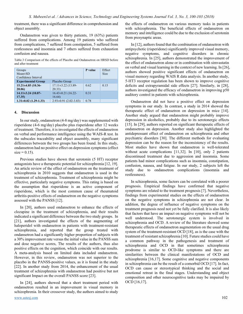
S. Mubeen1et al. / Advances in Science, Technology and Engineering Systems Journal Vol. 3, No. 3, 100-103 (2018)
www.astesj.com 102
treatment, there was a significant difference in comprehension and object assembly.
Ondansetron was given to thirty patients, 19 (63%) patients suffered from complications. Among 19 patients who suffered from complications, 7 suffered from constipation, 5 suffered from restlessness and insomnia and 7 others suffered from exhaustion confusion and nausea. Table.3 Comparison of the effects of Placebo and Ondansetron on HRSD before and after treatment
Groups Mean±SD Confidence Interval
P value Effect Size
Experimental Group Placebo Group 15.21±4.85 (10.36-20.06)
17.11±3.22 (13.89-20.33)
0.62 0.15
14.11±3.24 (10.87-17.35)
16.43±0.21 (16.22-16.64)
0.31
1.31±0.02 (1.29-1.33) 2.93±0.91 (2.02-3.83) 0.78
4. Discussion
In our study, ondansetron (4-8 mg/day) was supplemented with risperidone (4-6 mg/day) placebo plus risperidone after 12 weeks of treatment. Therefore, it is investigated the effects of ondansetron on verbal and performance intelligence using the WAIS-R test. In the subscales traceability and object assembly, many significant differences between the two groups has been found. In this study, ondansetron had no positive effect on depression symptoms (effect size = 0.15).
Previous studies have shown that serotonin (5 HT) receptor antagonists have a therapeutic potential for schizophrenia [12, 19]. An article review of the effect of ondansetron on the treatment of schizophrenia in 2010 suggests that ondansetron is used in the treatment of schizophrenia. Treatment of schizophrenia might be effective, particularly negative symptoms. This rating is based on the assumption that risperidone is an active component of risperidone, which is the most common cause of rheumatoid arthritis-positive effects of ondansetron on the negative symptoms assessed with the PANSS [12].
In [20], authors used ondansetron to enhance the effects of clozapine in the treatment of schizophrenia, and their results indicated a significant difference between the two study groups. In [21], authors investigated the effects of the augmenting of haloperidol with ondansetron in patients with treatment-resistant schizophrenia, and reported that the group treated with ondansetron had a significantly higher proportion of subjects with a 30% improvement rate versus the initial value in the PANSS sum and dose negative scores, The results of the authors, thus also positive effects on the cognition, which coincide with our results. A meta-analysis based on limited data included ondansetron. However, in this review, ondansetron was not superior to the placebo in the PANSS-positive values, as it is found in the study [22]. In another study from 2014, the enhancement of the usual treatment of schizophrenia with ondansetron had positive but not significant Impact on the overall PANSS score [23].
In [24], authors showed that a short treatment period with ondansetron resulted in an improvement in visual memory in schizophrenia. In their crossover study, the authors aimed to study
the effects of ondansetron on various memory tasks in patients with schizophrenia. The beneficial effects of ondansetron on memory and intelligence could be due to the exclusion of serotonin from presynaptic areas.
In [12], authors found that the combination of ondansetron with antipsychotic (risperidone) significantly improved visual memory, negative symptoms, and cognitive disorders in chronic schizophrenia. In [25], authors demonstrated the improvement of the effect of ondansetron alone or in combination with simvastatin on verbal and visual learning in the context of new learning. In [26], authors showed positive significant effects of ondansetron on visual memory regarding WAIS R data analysis. In another study, 5-HT3 receptor regulation has been shown to improve cognitive deficits and extrapyramidal side effects [27]. Similarly, in [28], authors investigated the efficacy of ondansetron in improving p50 auditory control in patients with schizophrenia.
Ondansetron did not have a positive effect on depression symptoms in our study. In contrast, a study in 2014 showed the therapeutic effect of ondansetron on depression in mice [14]. Another study argued that ondansetron might probably improve depression in alcoholics, probably due to its serotonergic effects [15]. In [29], authors reported on significant therapeutic effects of ondansetron on depression. Another study also highlighted the antidepressant effect of ondansetron on schizophrenia and other psychiatric disorders [30]. The different methods for evaluating depression can be the reason for the inconsistency of the results. Most studies have shown that ondansetron is well-tolerated without acute complications [11,32]. In [10], only 2 patients discontinued treatment due to aggression and insomnia. Some patients had minor complications such as insomnia, constipation, confusion, nausea, and fatigue. In our study, 2 subjects left the study due to ondansetron complications (insomnia and restlessness).
In schizophrenia, some factors can be correlated with a poorer prognosis. Empirical findings have confirmed that negative symptoms are related to the treatment prognosis [7]. Nevertheless, findings from experimental studies on the effects of ondansetron on the negative symptoms in schizophrenia are not clear. In addition, the degree of influence of negative symptoms on the treatment prognosis need not yet be fully clarified. It is also likely that factors that have an impact on negative symptoms will not be well understood. The serotonergic system is involved in schizophrenia and OCD. A review of the literature showed some therapeutic effects of ondansetron augmentation on the usual drug system of the treatment-resistant OCD [18], as is the case with the treatment of resistant schizophrenia [10]. Future studies could have a common pathway in the pathogenesis and treatment of schizophrenia and OCD in that sometimes schizophrenia prodrome is similar to OCD-like symptoms and there are similarities between the clinical manifestations of OCD and schizophrenia [16,17]. Some cognitive and negative components in schizophrenia can be the result of a comorbid OCD [17]. In fact, OCD can cause or stereotypical thinking and the social and emotional retreat in the final stages. Understanding and object composition and other neurocognitive tasks may be impaired by OCD [16,17].

S. Mubeen1et al. / Advances in Science, Technology and Engineering Systems Journal Vol. 3, No. 3, 100-103 (2018)
www.astesj.com 103
Although a standard treatment for schizophrenia has emerged, many unanswered questions remain. An important question is whether ondansetron is sufficient to reduce negative symptoms in schizophrenia.
The present study also underlines the importance of experimental studies to identify brain mechanisms involved in cognition and neuropathology of schizophrenia. The knowledge of negative symptoms in schizophrenia is increasing and the number of studies in this area has increased to understand the nature of schizophrenia as well as the possibilities of their treatment.
In the current study, there are a number of limitations, including the relatively small sample size, which excludes a generalizability of the results to other populations without further studies. A further limitation was the incomplete compliance with the CONSORT standard for reporting clinical trials [30].
5. Conclusion
The results of the current study showed that the administration of ondansetron significantly improved negative symptoms and cognitive disorders. These preliminary results suggest that ondansetron may play a role to improve the symptoms of people with Schizophrenia. The study results confirmed that ondansetron, as an additional treatment conventional therapy, is particularly in negative symptoms. There are limitations of the study as it has a small sample size. There is need of more studies should be conducted to support this study and there will be a good addition in the literature to give more confidence to the scientist to use this combination of medicines.
Conflict of Interest
The authors declare no conflict of interest.
References
[1] Martin, E. Concise Medical Dictionary. 8th ed. New York: Oxford University Press; 2010.
[2] Wong DF. Molecular Brain Imaging in Schizophrenia. In: Sadock BJ, Sadock VA, Ruiz P, Kaplan HI, editors. Kaplan & Sadock’s comprehensive textbook of psychiatry. 9th ed. Phiadilphia: Lippocott Williams and willkins; 2009. p. 1527.
[3] van Os J, Kapur S. Schizophrenia. Lancet. 2009;374:635 45. doi: 10.1016/ S0140 6736(09)60995 8. PubMed PMID: 19700006.
[4] Bowie CR, Harvey PD. Cognition in schizophrenia: impairments, determinants, and functional importance. Psychiatr Clin North Am. 2005;28:613 33, 26. doi: 10.1016/j.psc.2005.05.004. PubMed PMID: 16122570.
[5] Kirkpatrick B, Fischer B. Subdomains within the negative symptoms of schizophrenia: commentary. Schizophr Bull. 2006;32:246 9. doi: 10.1093/schbul/sbj054. PubMed PMID: 16492798; PubMed Central PMCID: PMC2632226.
[6] Stephen NL. Phenomenology of schizophrenia. In: In: Sadock BJ, Sadock VA, Ruiz P, Kaplan HI, editors. Kaplan & Sadock’s comprehensive textbook of psychiatry. Vol 2. Phiadilphia: Lippocott Williams and willkins; 2009. p. 1433 46.
[7] Makinen J, Miettunen J, Isohanni M, Koponen H. Negative symptoms in schizophrenia: a review. Nord J Psychiatry. 2008;62:334 41. doi: 10.1080/08039480801959307. PubMed PMID: 18752104.
[8] Castle DJ, Slott Jensen JK. Management of depressive symptoms in schizophrenia. Clin Schizophr Relat Psychoses. 2015;9:13 20. doi: 10.3371/CSRP.CAJE.103114. PubMed PMID: 25367164.
[9] Bennett AC, Vila TM. The role of ondansetron in the treatment of schizophrenia. Ann Pharmacother. 2010;44:1301 6. doi: 10.1345/aph.1P008. PubMed PMID: 20516364.
[10] Miyata K, Honda K. [Serotonin (5 HT) 3 receptors: antagonists and their pharmacological profiles]. Nihon Yakurigaku Zasshi. 1994;104:143 52. PubMed PMID: 7959407.
[11] Akhondzadeh S, Mohammadi N, Noroozian M, Karamghadiri N, Ghoreishi A, Jamshidi AH, et al. Added ondansetron for stable schizophrenia: a double blind, placebo controlled trial. Schizophr Res. 2009;107:206 12. doi: 10.1016/j.schres. 2008.08.004. PubMed PMID: 18789844.
[12] Lindenmayer JP, Bossie CA, Kujawa M, Zhu Y, Canuso CM. Dimensions of psychosis in patients with bipolar mania as measured by the positive and negative syndrome scale. Psychopathology. 2008;41:264 70. doi: 10.1159/000128325. PubMed PMID: 18441528.
[13] Gupta D, Radhakrishnan M, Kurhe Y. Ondansetron, a 5HT3 receptor antagonist reverses depression and anxiety like behavior in streptozotocin induced diabetic mice: possible implication of serotonergic system. Eur J Pharmacol. 2014;744:59 66. doi: 10.1016/j.ejphar.2014.09.041. PubMed PMID: 25284215.
[14] Johnson BA, Ait Daoud N, Ma JZ, Wang Y. Ondansetron reduces mood disturbance among biologically predisposed, alcohol dependent individuals. Alcohol Clin Exp Res. 2003;27:1773 9. doi: 10.1097/01. ALC.0000095635.46911.5D. PubMed PMID: 14634493.
[15] Bottas A, Cooke RG, Richter MA. Comorbidity and pathophysiology of obsessive compulsive disorder in schizophrenia: is there evidence for a schizo obsessive subtype of schizophrenia? J Psychiatry Neurosci. 2005;30:187 93. PubMed PMID: 15944743; PubMed Central PMCID: PMC1089779.
[16] Zink M. Comorbid Obsessive Compulsive Symptoms in Schizophrenia: Insight into Pathomechanisms Facilitates Treatment. Adv Med. 2014;2014:317980. doi: 10.1155/2014/317980. PubMed PMID: 26556409; PubMed Central PMCID: PMC4590963.
[17] Pittenger C, Bloch MH. Pharmacological treatment of obsessive compulsive disorder. Psychiatr Clin North Am. 2014;37:375 91. doi: 10.1016/j.psc.2014.05.006. PubMed PMID: 25150568; PubMed Central PMCID: PMC4143776.
[18] Samadi R, Soluti S, Daneshmand R, Assari S, Manteghi AA. Efficacy of Risperidone Augmentation with Ondansetron in the Treatment of Negative and Depressive Symptoms in Schizophrenia: A Randomized Clinical Trial. Iranian Journal of Medical Sciences. 2017;42(1):14-23.
[19] Briskin JK, Curtis JL. Augmentation of clozapine therapy with ondansetron. Am J Psychiatry. 1997;154:1171. PubMed PMID: 9247415.
[20] Zhang ZJ, Kang WH, Li Q, Wang XY, Yao SM, Ma AQ. Beneficial effects of ondansetron as an adjunct to haloperidol for chronic, treatment resistant schizophrenia: a double blind, randomized, placebo controlled study. Schizophr Res. 2006;88:102 10. doi: 10.1016/j.schres. 2006.07.010. PubMed PMID: 16959472.
[21] Kishi T, Mukai T, Matsuda Y, Iwata N. Selective serotonin 3 receptor antagonist treatment for schizophrenia: meta analysis and systematic review. Neuromolecular Med. 2014;16:61 9. doi: 10.1007/ s12017 013 8251 0. PubMed PMID: 23896722.
[22] Chaudhry IB, Husain N, Drake R, Dunn G, Husain MO, Kazmi A, et al. Add on clinical effects of simvastatin and ondansetron in patients with schizophrenia stabilized on antipsychotic treatment: pilot study. Ther Adv Psychopharmacol. 2014;4:110 6. doi: 10.1177/2045125313511487. PubMed PMID: 25057343; PubMed Central PMCID: PMC4107703.
[23] Levkovitz Y, Arnest G, Mendlovic S, Treves I, Fennig S. The effect of Ondansetron on memory in schizophrenic patients. Brain Res Bull. 2005;65:291 5. doi: 10.1016/j. brainresbull. 2003.09.022. PubMed PMID: 15811593.
[24] Deakin J, Chaudhry I, Parker A, Dunn G, Kazmi A, Drake R, et al. Therapeutic Trials of Minocycline, Ondansetron and Simvastatin in Schizophrenia. European Psychiatry. 2015;30:71.
[25] Mohammadi N, Noroozian M, Karamghadiri N, Akhondzadeh S. 5 HT3 antagonist for cognition improvement in schizophrenia: a double blind, placebo controlled trial. Basic Clin Neurosci. 2010;1:10 4.
[26] Shimizu S, Mizuguchi Y, Ohno Y. Improving the treatment of schizophrenia: role of 5 HT receptors in modulating cognitive and extrapyramidal motor functions. CNS Neurol Disord Drug Targets. 2013;12:861 9. PubMed PMID: 23844689.
[27] Adler LE, Cawthra EM, Donovan KA, Harris JG, Nagamoto HT, Olincy A, et al. Improved p50 auditory gating with ondansetron in medicated schizophrenia patients. Am J Psychiatry. 2005;162:386 8. doi: 10.1176/appi.ajp.162.2.386. PubMed PMID: 15677607.
[28] Piche T, Vanbiervliet G, Cherikh F, Antoun Z, Huet PM, Gelsi E, et al. Effect of ondansetron, a 5 HT3 receptor antagonist, on fatigue in chronic hepatitis C: a randomised, double blind, placebo controlled study. Gut. 2005;54:1169 73. doi: 10.1136/gut.2004.055251. PubMed PMID: 16009690; PubMed Central PMCID: PMC1774898.
[29] Bétry C, Etiévant A, Oosterhof C, Ebert B, Sanchez C, Haddjeri N. Role of 5 HT (3) Receptors in the Antidepressant Response. Pharmaceuticals. 2011;4:603 29. doi: 10.3390/ph 4040603. PubMed PMID: PMC4055881.
[30] Suvarna V. ‘Consort 2010: a standard for reporting clinical trials revised anew? Perspect Clin Res. 2010;1:87 9. PubMed PMID: 21814625; PubMed Central PMCID: PMC3146077.

www.astesj.com 104
Weight Parameters and Green Tea Effect; A Review
Yusra Hussain1, Faizan Ghani2, Munawar Ali3, Muhammad Imran*,4, Aamira Hashmi5, Wajahat Hussain6, Muhammad Hashim Raza4
1Mayo Hospital Lahore, 54000, Pakistan 2District Headquarter Hospital, Toba Take Singh, 36050, Pakistan 3Bahawal Victoria Hospital, Bahawalpur, 63100, Pakistan 4District Headquarter Hospital, Layyah, 31050, Pakistan 5District Headquarter Hospital, Muzaffargarh, 34200, Pakistan 6Tehsil Headquarter Hospital, Kallar Syedan, District Rawalpindi, 47520, Pakistan
A R T I C L E I N F O A B S T R A C T Article history: Received: 09 April, 2018 Accepted: 26 May, 2018 Online: 31 May, 2018
The objective was to review and add literature whether green tea is helpful for weight reduction. Reviewing the randomized, double-blind, placebo-controlled trials to compare green tea extracts for weight loss from various online sources including Ovid MEDLINE, PubMed, and Cochrane databases studies published in 2006, 2007 and 2008 in English language were considered. In each of the three studies, baseline measurements were taken and analyzed of the research participants. Measurements of total body weight, BMI with reference to age, hip and waist circumference were measured at the interval of 4 weeks i.e. 0 week (0 month), 4th week (1 month), 8th week (2 month), 12th week (3 month) were taken. All the research work analyzed and reviewed showed that a part of some minor changes no major changes were observed to prove the significance of green tea as a single agent for reducing weight. An increase in body energy expenditure was observed which leads to increase in appetite by the subjects but no adverse effects were noted. After detail review and analysis, the results showed that green tea have no significant effect on the weight reduction as a single agent.
Keywords : Green tea extract (GTE) Weight loss Weight reduction Overweight Obesity
1. Introduction
Obesity is a medical term defined as “having excessive amount of body fats leading to potentially hazardous health conditions”. Obesity in term of Body Mass Index (BMI) is defined as “body weight of a person divided by height square root”. A person will be overweight, if the average value of BMI is above 30 kg/m2, while normal average range of BMI is 25–30 kg/m2. Some Asian countries use even less than average value of range. Obesity has a potential hazard of causing serious medical conditions specially heart disease, diabetes type 2, obstructive sleep apnea, certain types of cancer, disorders of depression and osteoarthritis (OA) [1]. Most common cause of obesity is no physical activity, excessive eating of fatty food, and junk food, some people also have a genetic susceptibility of being obese. A few cases are caused primarily by genes, endocrine disorders, medicine or mental disorders. A misconception that obese people can gain more weight even with eating less is not correct. Rather people with more fats have high
body energy expenditure than a person who is of same age and height within a normal range of BMI, as an obese person needs to maintain more body mass. It can be prevented and treated with simple diet modifications in eating behavior and physical activity. Diet modifications such as less consumption of fats and high consumption of high fiber diet, and physical activity like regular exercise and walk can prevent and treat obesity [2]. Obesity is the major preventable cause of morbidity and complications which can lead to death world-wide. Its rate is increasing in adult and children day by day. In the year 2015, 650 million adult (12%) and 100 million children of the world population were obese. Obesity is more common in women than men. Authorities consider it as a major problem faced by people of 21 century and a major drawback from latest inventions [3]. Obesity is characteristic body change observed in high number in people of modern world (particularly in the western world), though it was seen as a symbol of wealth and prosperity at other times in history and still is considered at some parts of the world. In 2013, the American Medical Association classifies obesity as a disease requiring
ASTESJ
ISSN: 2415-6698
*Muhammad Imran, DHQ Hospital, Layyah, [email protected]
Advances in Science, Technology and Engineering Systems Journal Vol. 3, No. 3, 104-107 (2018)
www.astesj.com
https://dx.doi.org/10.25046/aj030314

Y. Hussain1et al. / Advances in Science, Technology and Engineering Systems Journal Vol. 3, No. 3, 104-107 (2018)
www.astesj.com 105
treatment [4]. Obesity, weight more than the average BMI accounts for a lot of hospital visits. In 2008, the report stated that the obesity alone account for over 8.1% of out- patient visits. The caring cost of such people takes a toll on the society. Researchers have suggested that these individual’s medical expense may have reached as high as $80 billion [5].
There are a few medications which are given to people with serious weight problem not controlled by eating habits and where the benefit out weights the risk involved; never the less medication have adverse effects that cannot be neglected. Also, non-FDA approved drugs are available in the market which has a lot of serious and potentially complicated side effects [6]. While there are a lot of different options in term of treatment, patients often want to have convenient, cost-effective and simple methods to aid their problem. Tea is historically used as a medication. Especially in Asian countries like China and Japan a lot of medicinal use of tea is described in details. Green tea contains two very important components which are often published as a solution for weight problems as green tea is a natural supplement if it could be the solution then it will be the safest and easiest way [7].
1.1. Objective
• The objective is to analyze effects of green tea for its effectiveness in weight reduction.
2. Methods
All the selected three studies meet the criteria of subjects as women and men, all having a high BMI and of the age group of 15- 40. Green tea extract was prepared in a capsule form. The treatment groups were compared to control groups given visually matched placebo. Parameters including weight, body mass index, circumference of waist, and circumference of hip measurement. The studies were double-blind, randomized, and placebo-controlled. In the study [8], which took place at Khon Kaen University in Thailand, selected participants were students of medicine faculty. All the participants in the research were fully informed about the detail of the study and their consent was taken. They were instructed to maintain their normal diet and daily habits as well as physical activity. A capsule was given to them to take one hour after each meal (Each capsule contain an extract obtained by boiling 5gm of green tea for a period of 15 min at 100 F). Time was specified in order to maintain the compliance by the participants.
First study reviewed was performed [9], in Maastricht University at Netherlands. In this research, selection of participants was done via an advertisement in the local newspaper to search for the willing participants for the trail. At first, subjects were instructed to make a chart of their daily food intake to measure the average amount caloric intake by the subjects. Than after calculating average caloric intake by each person they were told to keep their food intake in the range, and continue their daily routine.
Table 1: Demographics of included studies
S No Study Type # Pts Age (yrs.) Inclusion Criteria Exclusion Criteria W/D Interventions
1 [8] RCT 75 Males 35-55 Females post-Meno> 1 yr.
Male 35-55 yr. female post-meno>1yr History of metabolic disease/ Systemic disease
History of Prescribed medic-
-Regular exercise Ave-
energy expenditure daily > 8373.6 kJ/day
History of tea / caffeine
Allergic reactions
13 250 GTE CAPSULE TIB
after all 3
2 [9] RCT Double Blind, Placebo
Controlled
50 25-60 female (25-50) Overweight, BMI btw 20-35 kg/m2
initial screening
Health issues Heavy smokers regular medicines
use allergic heavy alcohol use caffeine
>250-450/day
1 GTE Capsule
3 [10] RCT Double Blind, Placebo
Controlled
150 15-55 Females(15-55yr) BMI> 28 kg/m2
cardiac disease endocrine problems pregnancy lactation
stroke/inability to exercise Weight control
management in 3 months Other condition unsuitable
as recommendation
2 GTE Capsule
Table 2- Efficacy of Green Tea Extract in Weight Reduction S No Study GTE group Reduction in Parameters Placebo group reduction in parameters p-value RRI ARI NNH
1 [8] 2.5 2.1 <0.05 0* 0* 0* 2 [9] 4.2 4.1 <0.001 0* 0* 0* 3 [10] 0.3 0.2 0.73 0.5 0.3 26

Y. Hussain1et al. / Advances in Science, Technology and Engineering Systems Journal Vol. 3, No. 3, 104-107 (2018)
www.astesj.com 106
Second study conducted [10], at The Taipei Hospital, Taiwan for one year. A trial on hundred subjects was done. After selection, subjects were given instructions about their eating habits and an informed consent was taken. A capsule was given to each subject and they were required to come after a month. Inclusion and exclusion criteria were followed by all three studies.
Finally, the third study reviewed [8], which included females with one year postmenopausal and male on an average age of 40-50 years old, with body mass index of 26 kg/m2 or greater. Subjects having a history of any metabolic or systemic disease or on daily medications, and energy expenditure greater than 8373.6 kJ/day, or specific history of tea and green tea hypersensitivity were not included.
In [9], the authors included females 18 to 50 years of age with a body mass index of 28 kg/m2 to 35 kg/m2. Initial screening was done and subjects who were of good health and no systemic and metabolic disease. Candidates with moderate tea and coffee intake and a minimum alcohol intake were selected. Females ages 14 -55 and a body mass index of 23 kg/m2 or greater were included in the Hsu et al study. Subjects with endocrine disease, heart disease, allergic or immunological diseases, high liver or renal profile values, pregnant women or lactating mothers, childbirth within six months, stroke history, inability to exercise were excluded.
All the articles searched for the review were published in peer-reviewed journals in English language. All literature searches were done using Ovid MEDLINE, PubMed, and Cochrane Databases. Inclusion and exclusion criteria selected for the analysis were POEM, randomized controlled trials, and studies published in 2005 or later. For statistics evaluation in the study p-value, relative risk increase (RRI), absolute risk increase (ARI), and numbers needed to harm (NNH) were used
2.1. Outcome Measured
The primary outcome of the studies showed a change in baseline parameters of weight in all three studies. Parameters of the body weight were defined as weight, body mass index, circumference of the waist, and circumference of the hip. Quantitative measurements were calculated in percent reduction of all the parameters at different time intervals throughout the trails. All the parameter measurements were standardized by measuring them in fasting state of the subject in all three studies. Secondary effects of the trail were also recorded as well. In [8], the authors measured level of hunger and the fullness on visual analog scales, resting energy expenditure and substrate oxidation, blood pressure and heart rate, urine VMA levels, and leptin levels. In [9], the authors measured systolic and diastolic blood pressure changes and also record changes in parameters of blood such as TG, LDL, HDL, leptin, and glucose levels. In [10], the authors measured hormone peptide levels throughout the trail including insulin, adiponectin, leptin, and ghrelin.
3. Results
The results concluded after the study was done on continuous data. The continuous data in [10], study can be converted to dichotomous form. The data obtained from the studies were presented and it was decided to treat analysis with exception of the participants who lost the follow ups. In [8], the authors reported
weight loss of 2.5 kg and 1.8 kg in the green tea extract and control groups, respectively. The p-value over time was statistically significant between groups (p < 0.05). During these studies, side effects were not seen in both controlled and experimental groups. Therefore, an exact value which can be harmful cannot be calculated. (Table 2). In [9], the authors reported weight reduction of 4.0 kg and 4.5 kg in green tea extract and control groups, respectively. The data for the study which was considered statistically significant is (p < 0.001). In the time period of study both groups had no adverse side effects, so no value can be calculated which may produce harm (Table 2).
In [10], the authors reported weight reduction of 0.2 kg and 0.1 kg in the GTE and control groups, respectively. The data was not statistically significant (p = 0.72). The absolute risk increase (ARI) was calculated to be 0.7% and the relative risk increase (RRI) was calculated to be 0.05%. In this study none of the subjects withdraw from the experiment but there were some subjects who observed side effects of the trial, therefore a number which can cause harm was also concluded. This study determined that the number needed to harm (NNH) was 25 patients using the dosage of 400 mg TID (Table 2).
One of the three trails showed subjects with mild adverse effect. In [10], 4 subjects experienced mild constipation and 2 experienced abdominal discomforts. Three subjects were found to experience mild nausea but no vomiting or other abnormalities were present in placebo treatment.
In all three trails, subjects were monitored in their special facilities where weight parameters were taken with accuracy and same measuring tools were used throughout screening days were also specified. In [8], the authors measured subject body weight parameters at weeks 0, 4, 8, and 12. In study [9], it had subjects to come on days 0, 12, 36, and 86. In study [10] it only measured the subjects on the initial day 0 and after 1 month. In [10], it also had subjects who missed the follow-up.
Tea has historic significance with green tea gaining wide popularity with its advertisement as a weight reducing agent. It is made from the leaves of Camellia sinensis. Camellia sinensis undergo very minimum oxidation in the process, containing two very important constituents: catethine polyphenol and caffeine, Catethine polyphenol is involved in inhibiting an enzyme catechol-o-methyl transferase (COMT) which in turn leads to enhanced action of catecholamines [11]. Caffeine is also involved in inhibiting phosphodiesterase induce degradation of Camp which causes an increased release of norepinephrine. Both caffeine and catethin polyphenol has potential to increase the energy expenditure which in turn can increase fat oxidation, leading to decrease in body weight. Catecholamines may also play an important role in satiety of the subject [12].
All the three studies used females as their primary subjects while [8], was the only study in which men were also in the their trail. All three studies used green tea in an extract capsule form. The specific timing and amount of extract used were slightly different. All placebos used are same and used a capsule of cellulose. In study [9], it also allowed their subjects to use caffeine during the trial period. The number of subjects used in all three studies was kept under hundred and trial lasted for about three

Y. Hussain1et al. / Advances in Science, Technology and Engineering Systems Journal Vol. 3, No. 3, 104-107 (2018)
www.astesj.com 107
months, while blinding was not compromised in all the three studies.
4. Conclusions
By reviewing all the three studies, it can be concluded that green tea does have some effect on weight reduction but it is not very significant plus significant variability between the intervention and placebo cannot be well defined. Green tea extract use was not harmful throughout the trail, further confirming the idea that it is not harmful to the body, but its weight reducing properties has to be further confirmed.
More research and investigation is also needed to determine the exact role of energy expenditure increase with the use of green tea. All the above three trails were done for a short duration of time. Trails are of long duration for further evaluation along with control of daily caloric intake and physical activity.
Long-term research with more participants and with better follow up protocols with exact statistics for this beneficial effect of green tea can be concluded, which would be of great help through a natural resource for weight reduction in overweight.
Conflict of Interest
The authors declare no conflict of interest.
References
[1] National Institutes of Health, National Heart LaBI, North American Association for the Study of Obesity. The practical guide: identification, evaluation, and treatment of overweight and obesity in adults.US Department of Health and Human Services, Public Health Service, National Institutes of Health, National Heart, Lung, and Blood Institute; 2000. NIH publication no. 00-4084.
[2] The Asia-Pacific Perspective Redefining Obesity; 2000. [3] Wing RR, Hill JO. Successful weight loss maintenance. Annu Rev Nutr
2001;21:323-41 [4] Action of the AMA House of Delegates 2013 Annual Meeting:
Recommendations in Report 3 of the Council on Science and Public Health Report Adopted, and Remainder of Report Filed.
[5] Obesity and Overweight. World Health Organization (WHO). 2010. Available at: http://www.who.int/dietphysicalactivity/publications/facts/obesity/en/. Accessed Sept 27, 2010.
[6] Overweight and Obesity. Centers for Disease Control. 2010. Available at: http://www.cdc.gov/obesity/recommendations.html. Accessed Sept 27, 2010.
[7] Cherry, D, Hing, E, Woodwell, D, et al. National Ambulatory Medical Care Survey: 2006 Summary. National Health Statistics Reports. 2008. Available at: http://www.cdc.gov/nchs/data/nhsr/nhsr003.pdf. Accessed Sept 28, 2010
[8] Auvichayapat P, Prapochanung M, Tunkamnerdthai O, et al. Effectiveness of green tea on weight reduction in obeseThais: A randomized, controlled trial. PhysiolBehav. 2008;93(3):486- 491.
[9] Diepvens K, Westerterp KR, Westerterp-Plantenga MS. Obesity and thermogenesis related to the consumption of caffeine, ephedrine, capsaicin and green tea. Am J Physiol Regul Integr Comp Physiol 2007;292:77–85.
[10] Hsu C, Tsai T, Kao Y, Hwang K, Tseng T, Chou P. Effect of green tea extract (GTE) on obese women: A randomized, double-blind, placebo-controlled clinical trial. Clinical Nutrition. 2008;27(3):363-370.
[11] Kovacs EM, Mela DJ. Metabolically active functional food ingredients for weight control. Obes Rev 2006;7:59-78.
[12] Chantre P, Lairon D. Recent findings of green tea extract AR 25 (Exolise) and its activity for the treatment of obesity. Phytomedicine 2002;9:3-8.

www.astesj.com 108
Learning Personalization Based on Learning Style instruments
Alzain Alzain*,1, Steve Clark1, Gren Ireson2, Ali Jwaid1
1School of Science and Technology, Nottingham Trent University, Clifton Campus NG11 8NS, Nottingham, United Kingdom 2School of Physics & Astronomy, University of Nottingham, University Park NG7 2RD, Nottingham, United Kingdom
A R T I C L E I N F O A B S T R A C T Article history: Received: 11 April, 2018 Accepted: 29 May, 2018 Online: 07 June, 2018
Adaptive education systems (AES) are considered one of the most interesting research topics in technology-based learning strategies. Since students have different abilities, needs and learning styles, we should fit the curriculum and teaching activities to these different learning styles. This study investigates the impact of using LAES (Libyan Adaptive Education System) on the performance of students. An ALSI (Arabic Learning Style Instrument) was integrated into the LAES system to investigate learning preferences of students. The student models are constructed according to the results obtained using this instrument (ALSI). Three experimental studies were then conducted to investigate the impact of the LAES system on the performance of students. The results reveal the students who have learnt using the LAES system were more successful than others who learnt without, in terms of the knowledge gained.
Keywords : Learning Style Learning Style Instruments Adaptive Education Systems
1. Introduction
This paper is an extension of work originally presented in the 2nd International Conference on Knowledge Engineering and Applications ICKEA 2017 [1]. Research on education has indicated that students have different learning preferences, abilities and needs, and learn in different ways. For example, learners with visual learning preference tend to obtain more knowledge from instructional materials that depend on visual forms of information, whereas the content will be more beneficial for the students with verbal preferences if these materials are represented using text and audio. Moreover, some learners tend to learn more through ‘doing’, whereas the others prefer to think and reflect. These learning preferences are often called learning styles [2].
Although it is argued that matching of teaching styles with the preferred learning styles of students will be quite useful to improve learning outcomes [2-5], it is quite clear that many researchers also believe that learners should know more details about their learning styles because this will help them to be more engaged, motivated and attracted in educational sessions [4, 6-8]. This study investigates empirically the effect of using adaptive education systems on the performance of student learning.
This article is organised as follows: the next section discusses the related work, where the Alzain model and ALSI instrument were selected to be integrated into the proposed system in order to profile learners; the structure of the proposed adaptive system is discussed in section 3; section 4 describes the methodology of the experiments as well as the research hypothesis; the results of our research are presented in section 5 and the conclusions are discussed in the last section.
2. Related Work
2.1. Adaptive Education Systems
Although learners have different learning preferences, goals, experiences and knowledge, the traditional education systems provide the same instructional materials for all students [9]. Therefore, in considering the individual differences between students, adaptive systems have been harnessed in the education field. The educational generation of adaptive systems is called Adaptive Learning Environment (ALE) or Adaptive Educational Hypermedia System (AEHS). These systems have been defined as “technological component of joint human–machine systems that can change their behavior to meet the changing needs of their users, often without explicit instructions from their users” [10]. This generation of educational systems can provide learners with instructional materials that are adapted especially to their learning
ASTESJ
ISSN: 2415-6698
*Alzain Alzain, Nottingham Trent University, Email: [email protected]
Advances in Science, Technology and Engineering Systems Journal Vol. 3, No. 3, 108-115 (2018)
www.astesj.com
Special Issue on Multidisciplinary Sciences and Engineering
https://dx.doi.org/10.25046/aj030315
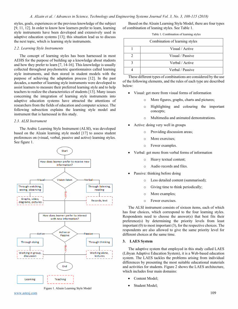
A. Alzain et al. / Advances in Science, Technology and Engineering Systems Journal Vol. 3, No. 3, 108-115 (2018)
www.astesj.com 109
styles, goals, experiences or the previous knowledge of the subject [9, 11, 12]. In order to know how learners prefer to learn, learning style instruments have been developed and extensively used in adaptive education systems [13]; this situation lead us to discuss the next topic, which is learning style instruments.
2.2. Learning Style Instruments
The concept of learning styles has been harnessed in most AEHS for the purpose of building up a knowledge about students and how they prefer to learn [7, 14-16]. This knowledge is usually collected throughout psychometric questionnaires called learning style instruments, and then stored in student models with the purpose of achieving the adaptation process [12]. In the past decades, a number of learning style instruments were developed to assist learners to measure their preferred learning style and to help teachers to realize the characteristics of students [13]. Many issues concerning the integration of learning style instruments into adaptive education systems have attracted the attentions of researchers from the fields of education and computer science. The following subsection explains the learning style model and instrument that is harnessed in this study.
2.3. ALSI Instrument
The Arabic Learning Style Instrument (ALSI), was developed based on the Alzain learning style model [17] to assess student preferences on (visual, verbal, passive and active) learning styles. See figure 1.
Figure 1. Alzain Learning Style Model
Based on the Alzain Learning Style Model, there are four types of combination of leaning styles. See Table 1.
Table 1. Combination of learning styles
Combination of learning styles
1 Visual / Active
2 Visual / Passive
3 Verbal / Active
4 Verbal / Passive
These different types of combinations are considered by the use of the following elements, and the rules of each type are described below:
• Visual: get more from visual forms of information
o More figures, graphs, charts and pictures;
o Highlighting and colouring the important concepts;
o Multimedia and animated demonstrations.
• Active: doing very well in groups
o Providing discussion areas;
o More exercises;
o Fewer examples.
• Verbal: get more from verbal forms of information
o Heavy textual content;
o Audio records and files.
• Passive: thinking before doing
o Less detailed content (summarised);
o Giving time to think periodically;
o More examples;
o Fewer exercises.
The ALSI instrument consists of sixteen items, each of which has four choices, which correspond to the four learning styles. Respondents need to choose the answer(s) that best fits their preference(s) by determining the priority levels from least important (0) to most important (3), for the respective choices. The respondents are also allowed to give the same priority level for different choices at the same time.
3. LAES System
The adaptive system that employed in this study called LAES (Libyan Adaptive Education System), it is a Web-based education system. The LAES tackles the problems arising from individual differences by presenting the most suitable educational materials and activities for students. Figure 2 shows the LAES architecture, which includes four main domains:
• Content Model;
• Student Model;
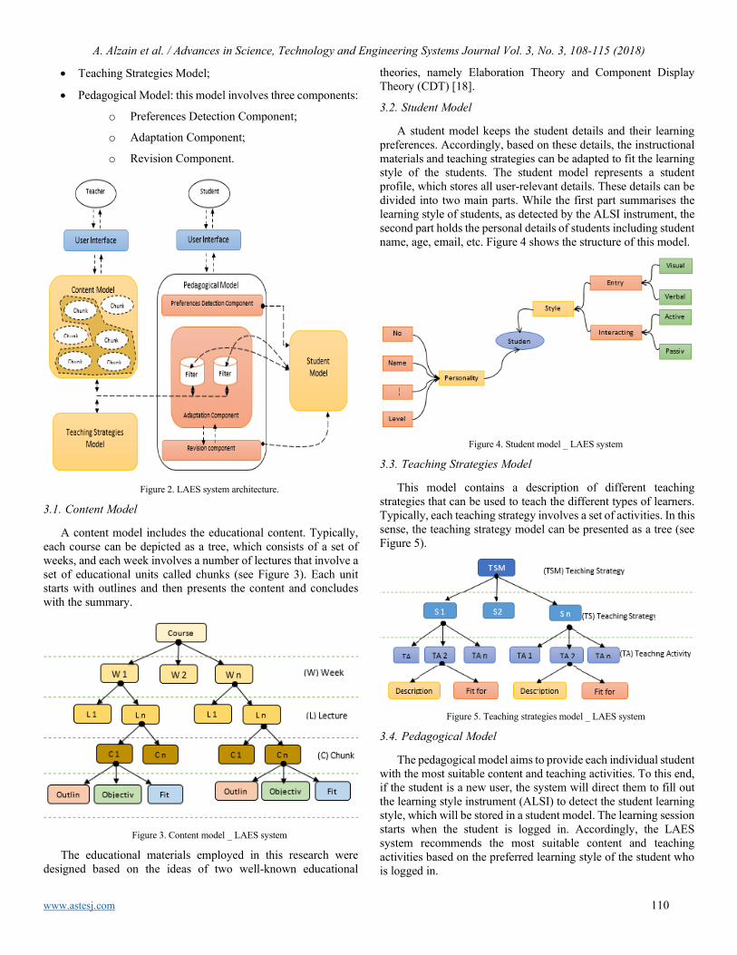
A. Alzain et al. / Advances in Science, Technology and Engineering Systems Journal Vol. 3, No. 3, 108-115 (2018)
www.astesj.com 110
• Teaching Strategies Model;
• Pedagogical Model: this model involves three components:
o Preferences Detection Component;
o Adaptation Component;
o Revision Component.
Figure 2. LAES system architecture.
3.1. Content Model
A content model includes the educational content. Typically, each course can be depicted as a tree, which consists of a set of weeks, and each week involves a number of lectures that involve a set of educational units called chunks (see Figure 3). Each unit starts with outlines and then presents the content and concludes with the summary.
Figure 3. Content model _ LAES system
The educational materials employed in this research were designed based on the ideas of two well-known educational
theories, namely Elaboration Theory and Component Display Theory (CDT) [18].
3.2. Student Model
A student model keeps the student details and their learning preferences. Accordingly, based on these details, the instructional materials and teaching strategies can be adapted to fit the learning style of the students. The student model represents a student profile, which stores all user-relevant details. These details can be divided into two main parts. While the first part summarises the learning style of students, as detected by the ALSI instrument, the second part holds the personal details of students including student name, age, email, etc. Figure 4 shows the structure of this model.
Figure 4. Student model _ LAES system
3.3. Teaching Strategies Model
This model contains a description of different teaching strategies that can be used to teach the different types of learners. Typically, each teaching strategy involves a set of activities. In this sense, the teaching strategy model can be presented as a tree (see Figure 5).
Figure 5. Teaching strategies model _ LAES system
3.4. Pedagogical Model
The pedagogical model aims to provide each individual student with the most suitable content and teaching activities. To this end, if the student is a new user, the system will direct them to fill out the learning style instrument (ALSI) to detect the student learning style, which will be stored in a student model. The learning session starts when the student is logged in. Accordingly, the LAES system recommends the most suitable content and teaching activities based on the preferred learning style of the student who is logged in.
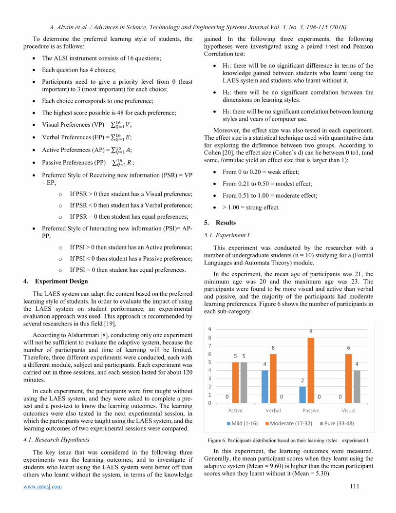
A. Alzain et al. / Advances in Science, Technology and Engineering Systems Journal Vol. 3, No. 3, 108-115 (2018)
www.astesj.com 111
To determine the preferred learning style of students, the procedure is as follows:
• The ALSI instrument consists of 16 questions;
• Each question has 4 choices;
• Participants need to give a priority level from 0 (least important) to 3 (most important) for each choice;
• Each choice corresponds to one preference;
• The highest score possible is 48 for each preference;
• Visual Preferences (VP) = ∑ 𝑉𝑉16𝑄𝑄=1 ;
• Verbal Preferences (EP) = ∑ 𝐸𝐸16𝑄𝑄=1 ;
• Active Preferences (AP) = ∑ 𝐴𝐴16𝑄𝑄=1 ;
• Passive Preferences (PP) = ∑ 𝑅𝑅16𝑄𝑄=1 ;
• Preferred Style of Receiving new information (PSR) = VP – EP;
o If PSR > 0 then student has a Visual preference;
o If PSR < 0 then student has a Verbal preference;
o If PSR = 0 then student has equal preferences;
• Preferred Style of Interacting new information (PSI)= AP-PP;
o If PSI > 0 then student has an Active preference;
o If PSI < 0 then student has a Passive preference;
o If PSI = 0 then student has equal preferences.
4. Experiment Design
The LAES system can adapt the content based on the preferred learning style of students. In order to evaluate the impact of using the LAES system on student performance, an experimental evaluation approach was used. This approach is recommended by several researchers in this field [19].
According to Alshammari [8], conducting only one experiment will not be sufficient to evaluate the adaptive system, because the number of participants and time of learning will be limited. Therefore, three different experiments were conducted, each with a different module, subject and participants. Each experiment was carried out in three sessions, and each session lasted for about 120 minutes.
In each experiment, the participants were first taught without using the LAES system, and they were asked to complete a pre-test and a post-test to know the learning outcomes. The learning outcomes were also tested in the next experimental session, in which the participants were taught using the LAES system, and the learning outcomes of two experimental sessions were compared.
4.1. Research Hypothesis
The key issue that was considered in the following three experiments was the learning outcomes, and to investigate if students who learnt using the LAES system were better off than others who learnt without the system, in terms of the knowledge
gained. In the following three experiments, the following hypotheses were investigated using a paired t-test and Pearson Correlation test:
• H1: there will be no significant difference in terms of the knowledge gained between students who learnt using the LAES system and students who learnt without it.
• H2: there will be no significant correlation between the dimensions on learning styles.
• H3: there will be no significant correlation between learning styles and years of computer use.
Moreover, the effect size was also tested in each experiment. The effect size is a statistical technique used with quantitative data for exploring the difference between two groups. According to Cohen [20], the effect size (Cohen’s d) can lie between 0 to1, (and some, formulae yield an effect size that is larger than 1):
• From 0 to 0.20 = weak effect;
• From 0.21 to 0.50 = modest effect;
• From 0.51 to 1.00 = moderate effect;
• > 1.00 = strong effect.
5. Results
5.1. Experiment I
This experiment was conducted by the researcher with a number of undergraduate students (n = 10) studying for a (Formal Languages and Automata Theory) module.
In the experiment, the mean age of participants was 21, the minimum age was 20 and the maximum age was 23. The participants were found to be more visual and active than verbal and passive, and the majority of the participants had moderate learning preferences. Figure 6 shows the number of participants in each sub-category.
Figure 6. Participants distribution based on their learning styles _ experiment I.
In this experiment, the learning outcomes were measured. Generally, the mean participant scores when they learnt using the adaptive system (Mean = 9.60) is higher than the mean participant scores when they learnt without it (Mean = 5.30).
0
4
2
0
56
8
65
0 0
4
0123456789
Active Verbal Passive Visual
Mild (1-16) Moderate (17-32) Pure (33-48)
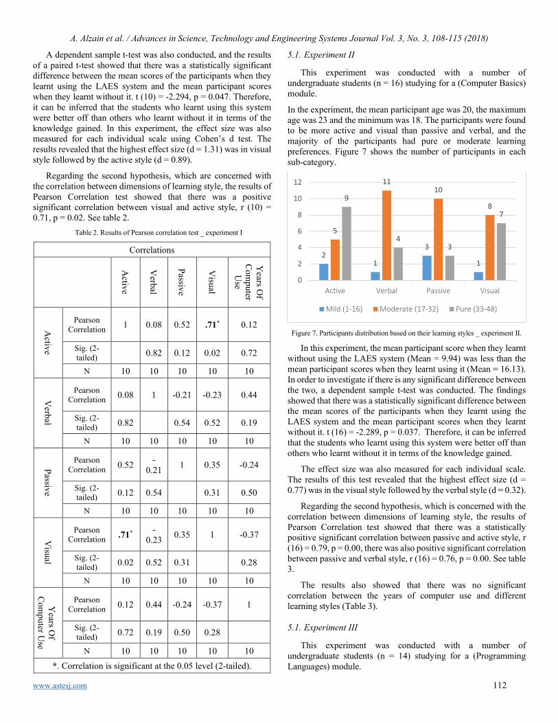
A. Alzain et al. / Advances in Science, Technology and Engineering Systems Journal Vol. 3, No. 3, 108-115 (2018)
www.astesj.com 112
A dependent sample t-test was also conducted, and the results of a paired t-test showed that there was a statistically significant difference between the mean scores of the participants when they learnt using the LAES system and the mean participant scores when they learnt without it. t (10) = -2.294, p = 0.047. Therefore, it can be inferred that the students who learnt using this system were better off than others who learnt without it in terms of the knowledge gained. In this experiment, the effect size was also measured for each individual scale using Cohen’s d test. The results revealed that the highest effect size (d = 1.31) was in visual style followed by the active style (d = 0.89).
Regarding the second hypothesis, which are concerned with the correlation between dimensions of learning style, the results of Pearson Correlation test showed that there was a positive significant correlation between visual and active style, r (10) = 0.71, p = 0.02. See table 2.
Table 2. Results of Pearson correlation test _ experiment I
Correlations
Active
Verbal
Passive
Visual
Years O
f C
omputer
Use
Active
Pearson Correlation 1 0.08 0.52 .71* 0.12
Sig. (2-tailed)
0.82 0.12 0.02 0.72
N 10 10 10 10 10
Verbal
Pearson Correlation 0.08 1 -0.21 -0.23 0.44
Sig. (2-tailed) 0.82 0.54 0.52 0.19
N 10 10 10 10 10
Passive
Pearson Correlation 0.52 -
0.21 1 0.35 -0.24
Sig. (2-tailed) 0.12 0.54 0.31 0.50
N 10 10 10 10 10 V
isual
Pearson Correlation .71* -
0.23 0.35 1 -0.37
Sig. (2-tailed) 0.02 0.52 0.31 0.28
N 10 10 10 10 10
Years O
f C
omputer U
se
Pearson Correlation 0.12 0.44 -0.24 -0.37 1
Sig. (2-tailed) 0.72 0.19 0.50 0.28
N 10 10 10 10 10 *. Correlation is significant at the 0.05 level (2-tailed).
5.1. Experiment II
This experiment was conducted with a number of undergraduate students (n = 16) studying for a (Computer Basics) module.
In the experiment, the mean participant age was 20, the maximum age was 23 and the minimum was 18. The participants were found to be more active and visual than passive and verbal, and the majority of the participants had pure or moderate learning preferences. Figure 7 shows the number of participants in each sub-category.
Figure 7. Participants distribution based on their learning styles _ experiment II.
In this experiment, the mean participant score when they learnt without using the LAES system (Mean = 9.94) was less than the mean participant scores when they learnt using it (Mean = 16.13). In order to investigate if there is any significant difference between the two, a dependent sample t-test was conducted. The findings showed that there was a statistically significant difference between the mean scores of the participants when they learnt using the LAES system and the mean participant scores when they learnt without it. t (16) = -2.289, p = 0.037. Therefore, it can be inferred that the students who learnt using this system were better off than others who learnt without it in terms of the knowledge gained.
The effect size was also measured for each individual scale. The results of this test revealed that the highest effect size (d = 0.77) was in the visual style followed by the verbal style (d = 0.32).
Regarding the second hypothesis, which is concerned with the correlation between dimensions of learning style, the results of Pearson Correlation test showed that there was a statistically positive significant correlation between passive and active style, r (16) = 0.79, p = 0.00, there was also positive significant correlation between passive and verbal style, r (16) = 0.76, p = 0.00. See table 3.
The results also showed that there was no significant correlation between the years of computer use and different learning styles (Table 3).
5.1. Experiment III
This experiment was conducted with a number of undergraduate students (n = 14) studying for a (Programming Languages) module.
21
3
1
5
1110
89
43
7
0
2
4
6
8
10
12
Active Verbal Passive Visual
Mild (1-16) Moderate (17-32) Pure (33-48)
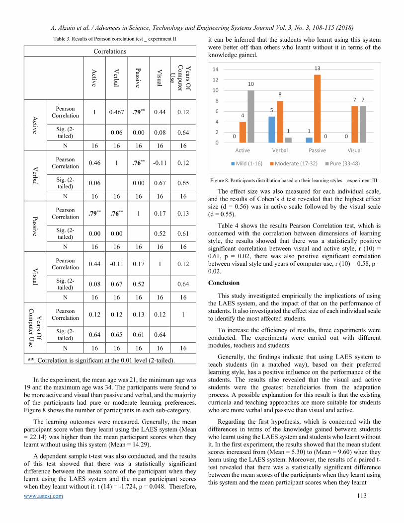
A. Alzain et al. / Advances in Science, Technology and Engineering Systems Journal Vol. 3, No. 3, 108-115 (2018)
www.astesj.com 113
Table 3. Results of Pearson correlation test _ experiment II
Correlations
Active
Verbal
Passive
Visual
Years O
f C
omputer
Use
Active
Pearson Correlation 1 0.467 .79** 0.44 0.12
Sig. (2-tailed)
0.06 0.00 0.08 0.64
N 16 16 16 16 16
Verbal
Pearson Correlation 0.46 1 .76** -0.11 0.12
Sig. (2-tailed) 0.06 0.00 0.67 0.65
N 16 16 16 16 16
Passive
Pearson Correlation .79** .76** 1 0.17 0.13
Sig. (2-tailed) 0.00 0.00 0.52 0.61
N 16 16 16 16 16
Visual
Pearson Correlation 0.44 -0.11 0.17 1 0.12
Sig. (2-tailed) 0.08 0.67 0.52 0.64
N 16 16 16 16 16
Years O
f C
omputer U
se
Pearson Correlation 0.12 0.12 0.13 0.12 1
Sig. (2-tailed) 0.64 0.65 0.61 0.64
N 16 16 16 16 16
**. Correlation is significant at the 0.01 level (2-tailed).
In the experiment, the mean age was 21, the minimum age was 19 and the maximum age was 34. The participants were found to be more active and visual than passive and verbal, and the majority of the participants had pure or moderate learning preferences. Figure 8 shows the number of participants in each sub-category.
The learning outcomes were measured. Generally, the mean participant score when they learnt using the LAES system (Mean = 22.14) was higher than the mean participant scores when they learnt without using this system (Mean = 14.29).
A dependent sample t-test was also conducted, and the results of this test showed that there was a statistically significant difference between the mean score of the participant when they learnt using the LAES system and the mean participant scores when they learnt without it. t (14) = -1.724, p = 0.048. Therefore,
it can be inferred that the students who learnt using this system were better off than others who learnt without it in terms of the knowledge gained.
Figure 8. Participants distribution based on their learning styles _ experiment III.
The effect size was also measured for each individual scale, and the results of Cohen’s d test revealed that the highest effect size (d = 0.56) was in active scale followed by the visual scale (d = 0.55).
Table 4 shows the results Pearson Correlation test, which is concerned with the correlation between dimensions of learning style, the results showed that there was a statistically positive significant correlation between visual and active style, r (10) = 0.61, p = 0.02, there was also positive significant correlation between visual style and years of computer use, r (10) = 0.58, p = 0.02.
Conclusion
This study investigated empirically the implications of using the LAES system, and the impact of that on the performance of students. It also investigated the effect size of each individual scale to identify the most affected students.
To increase the efficiency of results, three experiments were conducted. The experiments were carried out with different modules, teachers and students.
Generally, the findings indicate that using LAES system to teach students (in a matched way), based on their preferred learning style, has a positive influence on the performance of the students. The results also revealed that the visual and active students were the greatest beneficiaries from the adaptation process. A possible explanation for this result is that the existing curricula and teaching approaches are more suitable for students who are more verbal and passive than visual and active.
Regarding the first hypothesis, which is concerned with the differences in terms of the knowledge gained between students who learnt using the LAES system and students who learnt without it. In the first experiment, the results showed that the mean student scores increased from (Mean = 5.30) to (Mean = 9.60) when they learn using the LAES system. Moreover, the results of a paired t-test revealed that there was a statistically significant difference between the mean scores of the participants when they learnt using this system and the mean participant scores when they learnt
0
5
10
4
8
13
7
10
10
7
0
2
4
6
8
10
12
14
Active Verbal Passive Visual
Mild (1-16) Moderate (17-32) Pure (33-48)

A. Alzain et al. / Advances in Science, Technology and Engineering Systems Journal Vol. 3, No. 3, 108-115 (2018)
www.astesj.com 114
Table 4. Results of Pearson correlation test _ experiment III
without it (t (10) = 2.294, p = 0.047). That was also enhanced by the results of the second experiment, which revealed that the mean student scores increased from (Mean = 9.94) to (Mean = 16.13) when they learn using the LAES system. Moreover, the results of a paired t-test revealed that there was a statistically significant difference between the mean scores of the participants when they learnt using the LAES and the mean participant scores when they learnt without it (t (16) = 2.289, p = 0.037).
More encouraging results emerged from the third experiment where the findings showed that the mean student scores increased from (Mean = 14.29) to (Mean = 22.14) when they learn using the LAES system. Moreover, the results of a paired t-test revealed that there was a statistically significant difference between the mean scores of the participants when they learnt using the system and
the mean participant scores when they learnt without it (t (14) = -1.724, p = 0.048).
In general, the results revealed that the students had significantly higher learning outcomes when they used the LAES system to learn in a matched way. In addition, the (Cohen’s d) effect size was medium (from 0.51 to 1.00) [20].
These results reject the first hypothesis (H1), and prove that students who learnt using the ALSI system had significantly higher learning outcomes.
With reference to the second hypothesis, which is concerned with the correlation between dimensions of learning styles, the results were varied. While the first experiment revealed that there was a statistically positive significant correlation between visual and active styles, r (10) = 0.71, p = 0.02, the second experiment revealed that there was also a statistically positive significant correlation between passive and verbal styles, r (16) = 0.76, p = 0.00. Importantly, the results revealed that there was a statistically positive significant correlation between passive and active styles, r (16) = 0.79, p = 0.00. These results confirm that the dimensions of learning styles must not be treated as dichotomies (either/or options).
The results were also varied in terms of the third hypothesis, which is concerned with the correlation between the years of computer use and dimensions of learning styles. While the first two experiments revealed that there was no significant correlation between years of computer use and different learning styles, the third experiment revealed that there was a positive significant correlation between years of computer use and a visual learning style, r (14) = 0.58, p = 0.02.
References
[1] A. M. Alzain, S. Clark, G. Ireson and A. Jwaid, "LAES: An adaptive education system based on learners’ learning styles." in The 2nd International Conference on Knowledge Engineering and Applications, 2017, pp. 107.
[2] A. Franzoni-Velázquez, F. Cervantes-Pérez and S. Assar, "A Quantitative Analysis of Student Learning Styles and Teacher Teachings Strategies in a Mexican Higher Education Institution," Journal of Applied Research and Technology, vol. 10, pp. 289-308, 2012.
[3] A. M. Alzain, S. Clark and G. Ireson, "Libyan higher education system, challenges and achievements," in Engineering Education (ICEED), 2014 IEEE 6th Conference On, 2014, pp. 67-72.
[4] Richard M. Felder And Joni Spurlin, "Reliability and Validity of the Index of Learning Styles: a Meta-analysis," International Journal of Engineering Education, vol. 21, pp. 103 - 112, 2005.
[5] A. L. Franzoni, S. Assar, B. Defude and J. Rojas, "Student learning styles adaptation method based on teaching strategies and electronic media," in Advanced Learning Technologies, 2008. ICALT'08. Eighth IEEE International Conference On, 2008, pp. 778-782.
[6] Z. A. Akasah and M. Alias, "Emphasizing learning of the affective domain for the realization of the engineering learning outcomes," Cognition, vol. 7, pp. 9, 2010.
[7] H. M. Truong, "Integrating learning styles and adaptive e-learning system: current developments, problems and opportunities," Comput. Hum. Behav., vol. 55, pp. 1185-1193, 2016.
[8] M. T. Alshammari, "Adaptation Based On Learning Style And Knowledge Level In E-Learning Systems, Ph.D thesis," 2016.
[9] P. Brusilovsky, "Adaptive hypermedia. User Modeling and User Adapted Interaction," Ten Year Anniversary Issue (Alfred Kobsa, Ed.), vol. 11, pp. 87 - 110, 2001.
[10] K. M. Feigh, M. C. Dorneich and C. C. Hayes, "Toward a characterization of adaptive systems: a framework for researchers and system designers," Hum. Factors, vol. 54, pp. 1008-1024, Dec, 2012.
[11] P. Brusilovsky, "Methods and techniques of adaptive hypermedia," in Adaptive Hypertext and HypermediaAnonymous Springer, 1998, pp. 1-43.
Correlations
Active
Verbal
Passive
Visual
Years O
f C
omputer
Use
Active
Pearson Correlation 1 -0.05 0.12 .61* 0.38
Sig. (2-tailed)
0.86 0.67 0.02 0.18
N 14 14 14 14 14
Verbal
Pearson Correlation -0.05 1 0.33 -0.25 0.03
Sig. (2-tailed) 0.86 0.24 0.37 0.90
N 14 14 14 14 14
Passive
Pearson Correlation 0.12 0.33 1 -0.02 0.09
Sig. (2-tailed) 0.67 0.24 0.93 0.74
N 14 14 14 14 14
Visual
Pearson Correlation .61* -0.25 -0.02 1 .58*
Sig. (2-tailed) 0.02 0.37 0.93 0.02
N 14 14 14 14 14
Years O
f C
omputer U
se
Pearson Correlation 0.38 0.035 0.09 .58* 1
Sig. (2-tailed) 0.18 0.90 0.74 0.02
N 14 14 14 14 14 *. Correlation is significant at the 0.05 level (2-tailed).

A. Alzain et al. / Advances in Science, Technology and Engineering Systems Journal Vol. 3, No. 3, 108-115 (2018)
www.astesj.com 115
[12] N. Stash, "Incorporating cognitive/learning styles in a general-purpose adaptive hypermedia system," Dissertation Abstracts International, vol. 68, 2007.
[13] A. M. Alzain, G. Ireson, S. Clark and A. Jwaid, "Learning style instruments and impact of content: A qualitative study," in Sustainable Technologies (WCST), 2016 World Congress On, 2016, pp. 109-114.
[14] Ö Özyurt and H. Özyurt, "Learning style based individualized adaptive e-learning environments: Content analysis of the articles published from 2005 to 2014," Comput. Hum. Behav., vol. 52, pp. 349-358, 2015.
[15] S. Graf, T. Liu, N. Chen and S. J. Yang, "Learning styles and cognitive traits–Their relationship and its benefits in web-based educational systems," Comput. Hum. Behav., vol. 25, pp. 1280-1289, 2009.
[16] J. O. Liegle and T. N. Janicki, "The effect of learning styles on the navigation needs of Web-based learners," Comput. Hum. Behav., vol. 22, pp. 885-898, 2006.
[17] A. M. Alzain, S. Clark, G. Ireson and A. Jwaid, "A study of the reliability and validity of the first arabic learning styles instrument (ALSI)," in Sustainable Technologies (WCST), 2016 World Congress On, 2016, pp. 29-34.
[18] N. Al-Jojo, "Teacher assisting and subject adaptive material system: an Arabic adaptive learning environment, Ph.D. thesis," Teacher Assisting and Subject Adaptive Material System: An Arabic Adaptive Learning Environment, 2012.
[19] C. Mulwa, S. Lawless, M. Sharp and V. Wade, "The evaluation of adaptive and personalised information retrieval systems: a review," International Journal of Knowledge and Web Intelligence, vol. 2, pp. 138-156, 2011.
[20] L. Cohen, L. Manion and K. Morrison, Research Methods in Education. Routledge, 2013.

www.astesj.com 116
An enhanced Biometric-based Face Recognition System using Genetic and CRO Algorithms
Ola Surakhi*,1, Mohammad Khanafseh1 , Yasser Jaffal2
1University of Jordan, King Abdullah II School for Information Technology, Computer Science Department,11942, Jordan
2University of Kassel, Department of Technical Computer Science, Germany
A R T I C L E I N F O A B S T R A C T Article history: Received: 04 May, 2018 Accepted: 31 May, 2018 Online: 15 June, 2018
Face recognition is one of the most well-known biometric methods. It is a technique used for identifying individual from his face. The recognition process takes the face and compares it with the one stored in the database for recognizing it. Many methods were proposed to achieve that. In this paper, a new technique is proposed by using meta-heuristic algorithm. The algorithm is used to search for the best point in the image to be selected as a pivot, generate a vector of extracted features that are not necessary for the recognition and may reduce accuracy of it and evaluate the weight value for each area in the face image areas. A dataset with 371 images was used for evaluation. The results were conducted and compared with the original face recognition technique. That results show that proposed idea could enhance recognition by increasing accuracy up to 20% over original face recognition technique.
Keywords: Face Recognition Biometrics-based security Genetic algorithm CRO algorithm Optimization
1. Introduction
Recently, Face recognition has received a great attention in many fields from security, psychology, and image processing, to computer vision [1-5] because of its accuracy and low intrusiveness. It is one of the biometric techniques used for identification individuals by comparing face image with the ones stored in the database [6]. The process of face recognition can be divided into three stages: face detection, feature extraction and face recognition as shown in Figure 1
Face detection detects the existence of the face in an image by locating the position of it. Then, the features are extracted which is the most important step to recognize face. The face features are extracted to a vector, which is considered as a signature to the image. The features for each face are unique and used to discriminate between two individuals. Last, face recognition involves verification and identification. Verification compares the
face image to approve the request of individual, identification compares face image with the set of images stored in the database to identify it.
Many methods had been proposed before for face recognition such that Principal Component Analysis (PCA), Multi-linear Principal Component Analysis (MPCA) and Linear Discriminate Analysis (LDA) [8,9]. In [10], the authors proposed a new face recognition using genetic algorithm. The work compared with the Principal Component Analysis (PCA) and Linear Discriminate Analysis (LDA) algorithms for face recognition and analyzed the face recognition results using various databases such as ORL, UMIST and Indbase. The results clearly show that the recognition rate of Genetic algorithm is better than the PCA and LDA in case of ORL, UMIST and Indbase databases. In [11], the authors proposed a novel algorithm for recognizing human faces using Genetic Algorithms. The proposed method produces better result as compared to other techniques like PCA and LDA for one sample per person.
1.1. Face recognition system
For each image, there are more than 80 feature points on human face and one of these feature points must be elected as
ASTESJ
ISSN: 2415-6698
* Ola Surakhi, 1University of Jordan, Email: [email protected]
Advances in Science, Technology and Engineering Systems Journal Vol. 3, No. 3, 116-124 (2018)
www.astesj.com
Special Issue on Multidisciplinary Sciences and Engineering
https://dx.doi.org/10.25046/aj030316
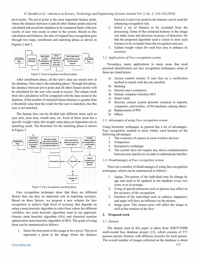
O. Surakhi et al. / Advances in Science, Technology and Engineering Systems Journal Vol. 3, No. 3, 116-124 (2018)
www.astesj.com 117
pivot point. The pivot point is the most important feature point, where the distance between it and all other feature points must be calculated and saved into database to be compared lately with new results of user who needs to enter to the system. Based on this calculation and features, the idea of original face recognition goes through two steps, enrollment and matching phase as shown in Figures 2 and 3.
Figure 2: Face recognition enrollment phase
After enrollment phase, all the user’s data are stored now in the database. Next step is the matching phase. Through this phase, the distance between pivot point and all other feature points will be calculated for the user who needs to access. The output result from this calculation will be compared with the data stored in the database. If the number of matched feature distance is greater than a threshold value then the result for this user is matched, else this user is not matched.
The human face can be divided into different areas such as eyes area, nose area, mouth area, etc. Each of these areas has a specific weight value; this weight value plays an important role in matching result. The flowchart for the matching phase is shown in Figure 3.
Figure 3: Face recognition matching phase
Face recognition technique show that there are different factors that can play an important role in matching accuracy. Based on these factors, we propose a new scheme for face recognition to achieve high level of accuracy that depends on using a meta heuristic algorithm to select best values for different variables; two meta heuristic algorithm used in our approach: Genetic meta heuristic algorithm (GA) and chemical reaction optimization meta heuristic algorithm (CRO). The goals of using them can be summarized as follows:
1. Select the best point in the image to be a pivot. The pivot represents a point in the image where the distance
between it and every point in the features can be used for enhancing recognition rate.
2. Select a set of features to be excluded from the processing. Some of the extracted features in the image can make noise and decrease accuracy of detection; for that the proposed algorithm used a vector to store such features to be excluded from the recognition process.
3. Update weight values for each face area to enhance its accuracy.
1.2. Applications of Face recognition system
Nowadays, many applications in many areas that need personal identification use face recognition techniques; some of these are listed below:
a) Access control system: It uses face as a verification method to match with the one enrolled.
b) Banking c) Internet and e-commerce d) Human computer interface HCI e) Smart cards f) Security camera system presents common in airports,
companies, universities, ATM machines, among others. g) Replacement of PIN h) Others
1.3. Advantages of using Face recognition system
Using biometric techniques in general has a lot of advantages. Face recognition method is most widely used because of the following advantages:
1. The existence of camera in most wireless devices 2. Uniqueness 3. Inexpensive technique 4. The system does not require any direct communication
between user and device in order to authenticate him/her.
1.4. Disadvantages of Face recognition system
There are a number of disadvantages of using face recognition techniques, which can be summarized as follows:
1. Aging: The picture of the individual may be change by age and need to be updated in the database every two years or so in average.
2. Using of special characters such as glasses may affect on the accuracy of the recognition.
3. Emotion of the individual such as sadness, happiness, and anger will have an influence on the picture.
4. Image pose: The camera pose will affect the image as well as the rotation of the face.
2. Proposed work
2.1. Dataset
The dataset used in this paper is taken from XM2VTSDB multi-modal face database project [12], which consists of 371 persons picture features with different sessions for each person. The overall number of images collected on the database is about

O. Surakhi et al. / Advances in Science, Technology and Engineering Systems Journal Vol. 3, No. 3, 116-124 (2018)
www.astesj.com 118
2360 different images for 371 persons. From each image we extracted 67 features. These collected images refer to different genders, males and females, with different ages and for different positions for each person. These images are taken over a period of four months. 2.2. Genetic algorithms
A Genetic algorithm, GA [13,14,15], is defined as the most powerful algorithm used to solve large problems where there are a large number of solutions and an optimization is needed to generate better solutions from them. The main components of the algorithm are:
1. An initial population for the solution 2. A fitness function to generate better solution
Each individual in the population is a numeric value with n bits that represents a solution to the problem. The individual in the GA is called chromosome, which is a sequence of 1’s and 0’s. In order to generate better solution from the population, GA runs a set of operations to optimize solution and gets better results for the problem as follows:
1. Evaluate fitness function for each individual. 2. Selection: The selection operator selects individuals
from the population with highest fitness value as a parent.
3. Crossover: This is the recombination operator, which allows individuals to exchange information and generate the offspring for the next population. The aim is to generate better offspring who is not identical to his parents but contains their traits. Three types of crossover can be used: one point, two point and uniform.
4. Mutation: Is making a change in some bits value of the chromosome in order to generate new better individual.
5. Update value of the fitness function for each individual. All the above three steps are repeated to a maximum number of iterations.
2.3. Chemical Reaction Optimization (CRO) Algorithm
Chemical Reaction Optimization (CRO) is a meta-heuristic algorithm inspired by the nature of chemical reactions [16]. It starts with initial molecules, and by doing a sequence of collisions where final product becomes in the stable state. The major difference between CRO algorithm and any other evolutionary techniques is that population size in the CRO may change after each iteration of the algorithm running, while in all other techniques, the population size is fixed and unchanged during execution. The basic unit in the CRO population is called molecule, which has a potential energy that is considered fitness function of the individual. Each molecule has a set of parameters like kinetic energy, molecule structure and more, some of them are important and some are less important depending on the problem.
In order to change on the molecule, a collision is made which could be either uni-molecule (one molecule) or inter-molecule
(two or more collide with each other). The aim is to transform into a stable product with minimal potential energy. The chemical reaction could be one of these types:
a. On-wall ineffective collision: This occurs when the molecule collides with the wall of container and then bounces. The transformation of the molecule structure can be represented as ω → ω-
b. Decomposition: This happens when the molecule hits in the wall and then decomposes into small parts. ω → ω1- + ω2
c. Inter-molecular ineffective collision: y happens when multi molecule collide with each other and then bounces away.
d. Synthesis: It is the opposite to the decomposition and happens when two or more molecules hit and combine together; ω1 + ω2 → ω-.
The steps of the algorithm can be summarized as shown below and the pseudo code is shown in Figure 4.
1. Starts with the initial population, which consists of a set of individuals where each one has a potential energy (PE). Some of the CRO parameters such that population size, number of iterations and buffer should be defined initially.
2. Apply chemical reaction to generate new reactants. 3. Update the potential energy. 4. Repeat steps till reaching termination condition.
Figure 4: pseudo code of the CRO algorithm
2.4. Proposed scheme
This paper proposes an enhancement version over available face recognition schemes using a meta-heuristic algorithm to achieve a high level of accuracy and less error-matching rate. The original face recognition system consists of two phases: enrollment and matching. The system depends mainly on choosing a point as a pivot point and then calculate the distance between it and other face features. The data is then stored as a vector in the database for each image. The second phase compares the values of the registered user with the data stored in the database for matching and authenticating individual.
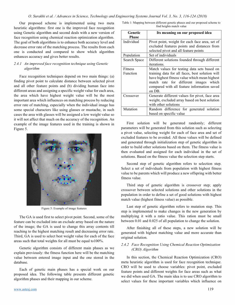
O. Surakhi et al. / Advances in Science, Technology and Engineering Systems Journal Vol. 3, No. 3, 116-124 (2018)
www.astesj.com 119
Our proposed scheme is implemented using two meta heuristic algorithms: first one is the improved face recognition using Genetic algorithm and second deals with a new version of face recognition using chemical reaction optimization algorithm. The goal of both algorithms is to enhance both accuracy level and decrease error rate of the matching process. The results from each one is conducted and compared to show which algorithm enhances accuracy and gives better results.
2.4.1 An improved face recognition technique using Genetic algorithm
Face recognition techniques depend on two main things: (a) finding pivot point to calculate distance between selected pivot and all other feature points and (b) dividing human face into different areas and assigning a specific weight value for each area, the area which have highest weight value will be the most important area which influences on matching process by reducing error rate of matching, especially when the individual image has some special characters like using glasses or mustache, in such cases the area with glasses will be assigned a low weight value so it will not affect that much on the accuracy of the recognition. An example of the image features used in the training is shown in Figure 5.
Figure 5: Example of image features
The GA is used first to select pivot point. Second, some of the
feature can be excluded into an exclude array based on the nature of the image; the GA is used to change this array contents till reaching to the highest matching result and decreasing error rate. Third, GA is used to select best weight value for each of the face areas such that total weights for all must be equal to100%.
Genetic algorithm consists of different main phases as we explain previously: the fitness function here will be the matching value between entered image input and the one stored in the database.
Each of genetic main phases has a special work on our proposed idea. The following table presents different genetic algorithm phases and their mapping in our scheme.
Table 1: Mapping between different genetic phases and our proposed scheme to find heights match value
Genetic Phase
Its meaning on our proposed idea
Individual Pivot point, weight for each face area, set of excluded features points and distances from selected pivot and all feature points
Population Set of individuals Search Space Different solutions founded through different
iterations. Fitness Function
Match values for testing data sets based on training data for all faces, best solution will have highest fitness value which mean highest match rate for different images which compared with all feature information saved on DB.
Crossover Generate different values for pivot, face area weight, excluded array based on best solution with other solutions
Mutation Random difference for generated solution based on specific value
First solution will be generated randomly; different
parameters will be generated from this solution such as selecting a pivot value, selecting weight for each of face area and set of excluded features to be avoided. All these values will be defined and generated through initialization step of genetic algorithm in order to build other solutions based on them. The fitness value is then evaluated and assigned for each individual in the set of solutions. Based on the fitness value the selection step starts.
Second step of genetic algorithm refers to selection step. Select a set of individuals from population with highest fitness value to be parents which will produce a new offspring with better fitness value.
Third step of genetic algorithm is crossover step; apply crossover between selected solutions and other solutions in the population in order to define a set of good solutions with highest match value (highest fitness value) as possible.
Last step of genetic algorithm refers to mutation step. This step is implemented to make changes in the new generation by multiplying it with a ratio value. This ration must be small between 0.01 and 0.025 of all population to change the solution.
After finishing all of these steps, a new solution will be generated with highest matching value and more accurate than original solution.
2.4.2 Face Recognition Using Chemical Reaction Optimization (CRO) Algorithm
In this section, the Chemical Reaction Optimization (CRO) meta heuristic algorithm is used for face recognition technique. CRO will be used to choose variables: pivot point, excluded feature points and different weights for face areas such as what we did when used GA. The main idea is to use CRO algorithm to select values for these important variables which influence on

O. Surakhi et al. / Advances in Science, Technology and Engineering Systems Journal Vol. 3, No. 3, 116-124 (2018)
www.astesj.com 120
matching results. CRO generates better solution after each iteration till reaching best one. Table 2 presents some of CRO scheme meanings and their mapping to our proposed technique.
Table 2: Mapping between chemical meaning and its meaning on face recognition.
Chemical Meaning
Its meaning on our proposed idea
Molecular Structure
Set of Solutions which found based on original solution
Potential Energy Important variables value: Pivot value, Exclude array values, Weights value for different face areas
Kinetic Energy Measure of tolerance to have a worse Solution
Number of Hits Total Number of iteration used for specific experiment.
Minimum Structure
Current Optimal value for Matching based on Different variables values
Synthesis Interaction, ω1 + ω2 → ω'
Two solutions with two Potential Energy combined with each other to select single solution with highest Potential energy which refers to highest match percent for all images.
Inter-molecule infective collision ω1 + ω2 → ω1' + ω2'.
Two solutions with two Potential energy will produce a single solution with highest Potential energy value. By combining different steps of both solutions as select best exclude array values from one solution with face area weight from other solution to have a solution with highest match percent for all faces.
Decomposition ω → ω1 + ω2
Single solution with specific potential energy will produce two new spate solutions with different potential energy for each by select some of main steps of match result from original solution and other steps will be selected randomly, so single solution will be divided to produce two single solution with j
On wall effective collision ω → ω'
Single solution will be combined with other random solution where each solution has its own potential energy to produce a new with different potential energy from original solution.
The proposed algorithm with CRO consists of a number of
steps. Each of these steps has its fitness function value to find best matching for face recognition.
First step is initialization for face recognition using CRO. Through first step, a random selection is used to select pivot point, excluded features array and areas weight. Then the fitness function value is evaluated for each solution. As mentioned before, after each iteration of CRO execution, the population size will be different. We used ‘parent size’ variable to express population size. After each iteration it refers to generation size which produce new different solutions with different matching value.
The kinetic energy value must be defined in this stage, and molecule value also which must be between 0 and 1. Pseudo code for Initialization phase is given in Figure 6.
Figure 6: Pseudo Code for Initialization phase
Second step of face recognition using CRO refers to iteration stage. The main goal here is to generate different solutions based on initial solution. The initial values are produced through initialization phase, and new generated solution must be compared with all other solutions. Some of these new solutions will be better than original solution. The potential energy is objective function or fitness function for generated solution. Through this stage, different molecules are selected based on the value of variable β, where the value of β will be selected randomly between “0” and “1”. As shown in Figure 7 for pseudo-code at line number 1, if the value of the variable β is larger than the value of the variable “molecule,” then one molecule will be selected. Otherwise, two molecules will be selected; each of them is a separate solution. The pseudo-code for second phase of Face recognition using CRO algorithm is given in Figure 7.
Figure 7: Pseudo code for second phase of Face recognition using CRO.
Third phase of face recognition using CRO refers to reaction phase, which is the final stage. When reaching to a specific value

O. Surakhi et al. / Advances in Science, Technology and Engineering Systems Journal Vol. 3, No. 3, 116-124 (2018)
www.astesj.com 121
and to number of predefined iterations, then this algorithm is stopped. Next, different solutions must be found and each of them has its potential energy which is number of matching faces. The output from this stage is the best solution, with highest objective function or matching value. This solution contains specific value for all variables: a pivot value, excluding feature points and weight values for all face areas. Number of selected solutions will lead to different interactions between molecules or solutions. When number of selected molecules is one, then the possibility of some interactions that depends on single molecule interaction will be as follows:
On-wall-infective collision: This interaction depends mainly on single molecule interaction with the wall of container which contains all different solutions. The output from this interaction is a new molecule with different structure produced ω → ω' as in [17]. Pseudo-code for on-wall effective collision through our proposed idea is shown in Figure 8.
Figure 8: Pseudo-code for on-wall effective collision
Second type of interaction refers to decomposition interaction. It deals with second interaction, which depends on single molecule with molecule containers. The difference here is that the output from this interaction is to divide the original molecule into two different molecules with same structure as follow: ω → ω1 + ω2. The pseudo-code for this interaction is shown in Figure 9.
If there are more than one molecule selected, the possibility for other interactions to occur between different selected molecules happens. These interactions between molecules are Synthesis interactions which happens when two molecules of solutions in our scheme interact with each other to generate new single solution from interacted solutions as follow: ω1 + ω2 → ω'.
3. Experimental Results
Both proposed ideas to enhance matching results for face recognition technique were implemented using java-programming language on Net Beans 8.1, through our implementation. We compared matching values of original face recognition algorithm with our proposed scheme. There are different results based on different parameter. First result deals
with face recognition using Genetic algorithm for different iterations with same generation size. Obtained results collected from implementing this approach were compared with results from original scheme of face recognition using same data sets as shown in Table 3.
Figure 9: The pseudo-code for this interaction
Pseudo-code for synthesis interaction is shown in Figure 10.
Figure 10: Pseudo-code for synthesis interaction
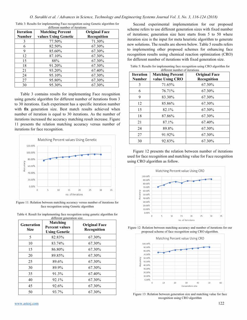
O. Surakhi et al. / Advances in Science, Technology and Engineering Systems Journal Vol. 3, No. 3, 116-124 (2018)
www.astesj.com 122
Table 3: Results for implementing Face recognition using Genetic algorithm for different number of iterations
Iteration Number
Matching Percent values Using Genetic
Original Face Recognition
3 77.50% 71.30% 6 82.50% 67.30% 9 85.60% 67.30% 12 87.10% 67.30% 15 88% 67.30% 18 91.20% 67.30% 21 93.20% 67.40% 24 95.10% 67.30% 27 95.80% 67.30% 30 95.30% 67.30%
Table 3 contains results for implementing Face recognition
using genetic algorithm for different number of iterations from 3 to 30 iterations. Each experiment has a specific iteration number with fix generation size. Best match results achieved when number of iteration is equal to 30 iterations. As the number of iterations increased the accuracy matching result increase. Figure 11 presents the relation matching accuracy versus number of iterations for face recognition.
Figure 11: Relation between matching accuracy versus number of iterations for
face recognition using Genetic algorithm
Table 4. Result for implementing face recognition using genetic algorithm for different generation size.
Generation Size
Matching Percent values Using Genetic
Original Face Recognition
5 82.83% 67.30% 10 83.74% 67.30% 15 86.80% 67.30% 20 89.85% 67.30% 25 89.6% 67.30% 30 89.9% 67.30% 35 91.3% 67.40% 40 92.1% 67.30% 45 92.6% 67.30% 50 93.7% 67.30%
Second experimental implementation for our proposed scheme refers to use different generation sizes with fixed number of iterations; generation size here starts from 5 to 50 where iteration size is the input for meta heuristic algorithm to generate new solutions. The results are shown below. Table 5 results refers to implementing other proposed schemes for enhancing face recognition results using chemical reaction optimization (CRO) for different number of iterations with fixed generation size.
Table 5: Results for implementing face recognition using CRO algorithm for different number of iterations
Iteration Number
Matching Percent value Using CRO
Original Face Recognition
3 71.65% 67.30% 6 76.71% 67.30% 9 83.30% 67.30% 12 85.86% 67.30% 15 82.1% 67.30% 18 87.86% 67.30% 21 87.1% 67.40% 24 89.8% 67.30% 27 91.92% 67.30% 30 92.83% 67.30%
Figure 12 presents the relation between number of iterations
used for face recognition and matching value for Face recognition using CRO algorithm as follow.
Figure 12: Relation between matching accuracy and number of iterations for our
proposed scheme of face recognition using CRO algorithm.
Figure 13: Relation between generation size and matching value for face
recognition using CRO algorithm
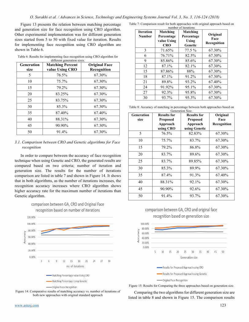
O. Surakhi et al. / Advances in Science, Technology and Engineering Systems Journal Vol. 3, No. 3, 116-124 (2018)
www.astesj.com 123
Figure 13 presents the relation between matching percentage and generation size for face recognition using CRO algorithm. Other experimental implementation was for different generation sizes started from 5 to 50 with fixed value for iteration. Results for implementing face recognition using CRO algorithm are shown in Table 6.
Table 6: Results for implementing face recognition using CRO algorithm for different generation sizes.
Generation size
Matching Percent value Using CRO
Original Face Recognition
5 76.5% 67.30% 10 75.7% 67.30% 15 79.2% 67.30% 20 83.25% 67.30% 25 83.75% 67.30% 30 85.3% 67.30% 35 87.40% 67.40% 40 88.31% 67.30% 45 90.90% 67.30% 50 91.4% 67.30%
3.1. Comparison between CRO and Genetic algorithms for Face
recognition
In order to compare between the accuracy of face recognition technique when using Genetic and CRO, the generated results are compared based on two criteria; number of iteration and generation size. The results for the number of iterations comparison are listed in table 7 and shown in Figure 14. It shows that in both algorithms, as the number of iterations increases, the recognition accuracy increases where CRO algorithm shows higher accuracy rate for the maximum number of iterations than Genetic algorithm.
Figure 14: Comparative results of matching accuracy vs. number of iterations of
both new approaches with original standard approach
Table 7: Comparison result for both approaches with original approach based on number of iterations
Iteration Number
Matching Percentage value Using
CRO
Matching Percentage
Using Genetic
Original Face
Recognition
3 71.65% 77.5 % 67.30% 6 76.71% 82.5% 67.30% 9 85.86% 85.6% 67.30% 12 87.1% 82.1% 67.30% 15 87.86% 88% 67.30% 18 87.1% 91.2% 67.30% 21 89.8% 93.2% 67.40% 24 91.92% 95.1% 67.30% 27 92.3% 95.8% 67.30% 30 93.7% 95.3% 67.30%
Table 8: Accuracy of matching in percentage between both approaches based on
Generation Size. Generation
size Results for Proposed Approach using CRO
Results for Proposed Approach
using Genetic
Original Face
Recognition
5 76.5% 82.83% 67.30%
10 75.7% 83.7% 67.30%
15 79.2% 86.8% 67.30%
20 83.7% 89.6% 67.30%
25 83.7% 89.85% 67.30%
30 85.3% 89.9% 67.30%
35 87.4% 91.3% 67.40%
40 88.31% 92.1% 67.30%
45 90.90% 92.6% 67.30%
50 91.4% 93.7% 67.30%
Figure 15: Results for Comparing the three approaches based on generation size.
Comparing the two algorithms for different generation size are listed in table 8 and shown in Figure 15. The comparison results

O. Surakhi et al. / Advances in Science, Technology and Engineering Systems Journal Vol. 3, No. 3, 116-124 (2018)
www.astesj.com 124
show that for bigger generation size the accuracy rate increases and CRO algorithm gives higher accuracy rate for the maximum generation size.
4. Results Discussion
The proposed work gives a new contribution in the face recognition technique which depend on three main criteria:
1. Selecting a pivot point. 2. Excluding some features into an exclude array base
on the nature of the image. 3. Dividing the face into areas and assign a weight for
each one. Two heuristic algorithms were used in order to select best
values for these variables, the Genetic and CRO. The aim of using such algorithm is to enhance searching results and get optimal solution. In our contribution, applying the heuristic algorithm on the face recognition technique gives more accurate results, as the algorithm searches for the best node in the image to be a pivot while the original technique select randomly a node as a pivot. The pivot node selected by the genetic and CRO is the node that is at the center of the image where we can evaluate distance between it and all other point in the image which will give an accurate estimation for the feature and thus will affect on the matching result and reduce error rate.
From the extracted features we can decide which features are important and which are not. For example, in the case where the image gas a special character like glasses the area around the eye will gives less matching results when it compared with the same image but without such glasses, so excluding this feature from the comparison will gives better result as shown previously.
By dividing the face image into a number of areas and assign a weight value for each one depending on the features for each area give a better accuracy for matching, some areas may be affected by different factors like brightness, shadow, etc. by assigning a low weight for those areas and higher value weight for the clear one affect much on the matching and increases accuracy.
The heuristic algorithms help on achieving that, as each algorithm depends on the number of iteration and generation size, the results show that as the number of iterations increase the matching accuracy increase as each algorithm training become near to its optimal solution. On the other hand, as the generation size increase the accuracy also increases, which means using more features and points from the image will increase matching results.
5. Conclusions
This paper presents a new methodology for face recognition by using two meta-heuristic algorithms: Genetic Algorithm (GA) and Chemical Reaction Optimization Algorithm (CRO). The aim of the proposed work is to enhance matching results for face recognition by increasing accuracy and decreasing error rate. Three criteria were taken into consideration throughout our work: the selection of the pivot point, excluding unnecessary features, dividing the face image into areas and assigning a weight value to
each area. The GA and CRO were used to implement these criteria and generate a best solution. A dataset of 371 images was used for the training and testing phases. The results for each run were compared with the original standard face recognition technique and showed that GA and CRO enhance matching face recognition by achieving more than 20% accuracy over original technique.
References
[1] Aoun, N.B.; Mejdoub, M.; Amar, C.B. Graph-based approach for human action recognition using spatio-temporal features. J. Vis. Commun. Image Represent. 2014, 25, 329–338.
[2] El’Arbi, M.; Amar, C.B.; Nicolas, H. Video watermarking based on neural networks. In Proceedings of the 2006 IEEE International Conference on Multimedia and Expo, Toronto, ON, Canada, 9–12 July 2006; pp. 1577–1580.
[3] El’Arbi, M.; Koubaa, M.; Charfeddine, M.; Amar, C.B. A dynamic video watermarking algorithm in fast motion areas in the wavelet domain. Multimed. Tools Appl. 2011, 55, 579–600.
[4] Wali, A.; Aoun, N.B.; Karray, H.; Amar, C.B.; Alimi, A.M. A new system for event detection from video surveillance sequences. In Advanced Concepts for Intelligent Vision Systems, Proceedings of the 12th International Conference, ACIVS 2010, Sydney, Australia, 13–16 December 2010; Blanc-Talon, J., Bone, D., Philips, W., Popescu, D., Scheunders, P., Eds.; Lecture Notes in Computer Science; Springer: Berlin/Heidelberg, Germany, 2010; Volume 6475, pp. 110–120.
[5] Koubaa,M.;Elarbi,M.;Amar,C.B.;Nicolas,H.Collusion,MPEG4compressionandframedroppingresistant video watermarking. Multimed. Tools Appl. 2012, 56, 281–301.
[6] M. S. Obaidat and N. Boudriga,” Security of e-Systems and Computer Networks, Cambridge University Press, 2007.
[7] Mejda Chihaoui *, Akram Elkefi, Wajdi Bellil and Chokri Ben Amar, “A Survey of 2D Face Recognition Techniques”, REGIM: Research Groups on Intelligent Machines, University of Sfax, National School of Engineers (ENIS), Sfax 3038, Tunisia; [email protected] (A.E.); [email protected] (W.B.); [email protected] (C.B.A.) * Correspondence: [email protected]; Tel.: +216-5460-1073
[8] D. Yi, Z. Lei, and S. Z. Li, “Towards pose robust face recognition,” in Computer Vision and Pattern Recognition (CVPR), 2013 IEEE Conference on. IEEE, 2013, pp. 3539–3545.
[9] N. Jindal and V. Kumar, “Enhanced face recognition algorithm using pca with artificial neural networks,” International Journal of Advanced Research in Computer Science and Software Engineering, vol. 3, no. 6, 2013.
[10] Pratibha Sukhija, Sunny Behal, Pritpal Singh, “Face Recognition System Using Genetic Algorithm”, International Conference on Computational Modeling and Security (CMS 2016).
[11] Ravi Subban, Dattatreya Mankame, Muthukumar Subramanyam,” Genetic Algorithm based Human Face Recognition”, Proc. of Int. Conf. on Advances in Communication, Network, and Computing, CNC
[12] https://personalpages.manchester.ac.uk/staff/timothy.f.cootes/data/xm2vts/xm2vts_markup.html.
[13] D.E. Goldberg, Genetic Algorithms in Search, Optimization & Machine Learning, Addison-Wesley, Reading, MA, 1989.
[14] John H. Holland ‘Genetic Algorithms’, Scientific American Journal, July 1992.
[15] KalyanmoyDeb, ‘An Introduction To Genetic Algorithms’, Sadhana, Vol. 24 Parts 4 And 5.
[16] A.Y.S. Lam, V.O.K. Li, "Chemical reaction optimization: a tutorial", Memetic Computing 4, 2012, pp. 3–17.
[17] Albert Y. S. Lam and Victor O. K. Li, Chemical reaction optimization: a tutorial, Memetic Computing, Vol. 4, No. 1, 2013.

www.astesj.com 125
Experimental Software Solution for Estimation of Human Body Height using Homography and Vanishing point(s)
Ondrej Kainz*, Maroš Lukáč, Miroslav Michalko, František Jakab
DCI, Faculty of Electrical Engineering and Informatics, Technical University of Košice, 042 00, Slovak Republic
A R T I C L E I N F O A B S T R A C T Article history: Received: 07 May, 2018 Accepted: 30 May, 2018 Online: 15 June, 2018
The principal goal of this paper is the development of the experimental software solution for the extraction of dimensional unit from the uncalibrated image. Existing techniques are analyzed and also partially utilized in presented approach as an aid in the extraction process. The design of two different approaches was proposed, these were later implemented and tested. Proposed methods cover utilization of homography matrix, vanishing points and vanishing line. Developed system allows to determine the dimension of any object in image based on the value of reference dimension. Proposed software solution was tested in laboratory and real-world environment.
Keywords: homography matrix vanishing line vanishing point
1. Introduction
The idea of computer machine being able to “see” is indeed intriguing. The very concept is the basis for computer vision and related image processing scientific field, having as an aim enabling the computer to detect and recognize the real-world by vision. This idea brings however many issues that have to be solved. On the other hand, it proves that some ideas and concepts are possible and can become reality.
Implementation of computer vision is part of our daily life. Millions of people utilize the social media services and add new images every moment. One of the areas of interest that is covered by computer vision is face detection. There is space for improvements even in this area, since many faces are often not being recognized due to multiple reasons, e.g. blurry image, small face etc., yet we can conclude that in general these algorithms are properly designed and work efficiently in most of the cases. Computer vision may be utilized also in the gaming industry by controlling of game environment through hand gestures or in virtual reality, which has potential of becoming vast part of this industry.
Extraction of dimensional units from the image belongs to the image processing. Two types of images may be considered, calibrated and uncalibrated. The first is the image with some prior information, i.e. camera intrinsic and extrinsic parameters. In the
second case, there is no such information and the only way is to process the information hidden within the pixels. In our research, we focus on the extraction from the uncalibrated image. Such extraction is more complex and hence different methods must be employed. Extraction of dimension from the image has multiple utilization, e.g. in security cameras or as additional parameters in person identification. Also, another method for such utilization is in the field of medicine, where dimensions may be used in anthropometry or for statistical purposes of changing population.
2. Approaches for the Extraction of Dimensions from Single Image
The overview of methods and approaches for the extraction of dimensional units from the images is presented in this part. As mentioned above, the image can be divided to two categories, calibrated and uncalibrated. Uncalibrated image is defined by [1] as image created by the optical device with unknown focal length, ratio, and principal point. Also, the position of camera in space is unknown, this covers its translation and rotation.
Many researches utilize estimation of dimension from the image for the reconstruction of scene captured in image or for creation of 3D models. Our solution is utilizing these principles, however only for the estimation of object’s size. Note that only single uncalibrated image is considered.
Authors of researches [1, 2] presume for image to be taken in perspective. Vanishing points and lines are largely utilized in this technique. Several definitions and mathematical proofs show the
ASTESJ
ISSN: 2415-6698
*Ondrej Kainz, DCI, FEEI, TUKE, Letna 9, 042 00 Kosice, Slovak republic, [email protected]
Advances in Science, Technology and Engineering Systems Journal Vol. 3, No. 3, 125-128 (2018)
www.astesj.com
https://dx.doi.org/10.25046/aj030317
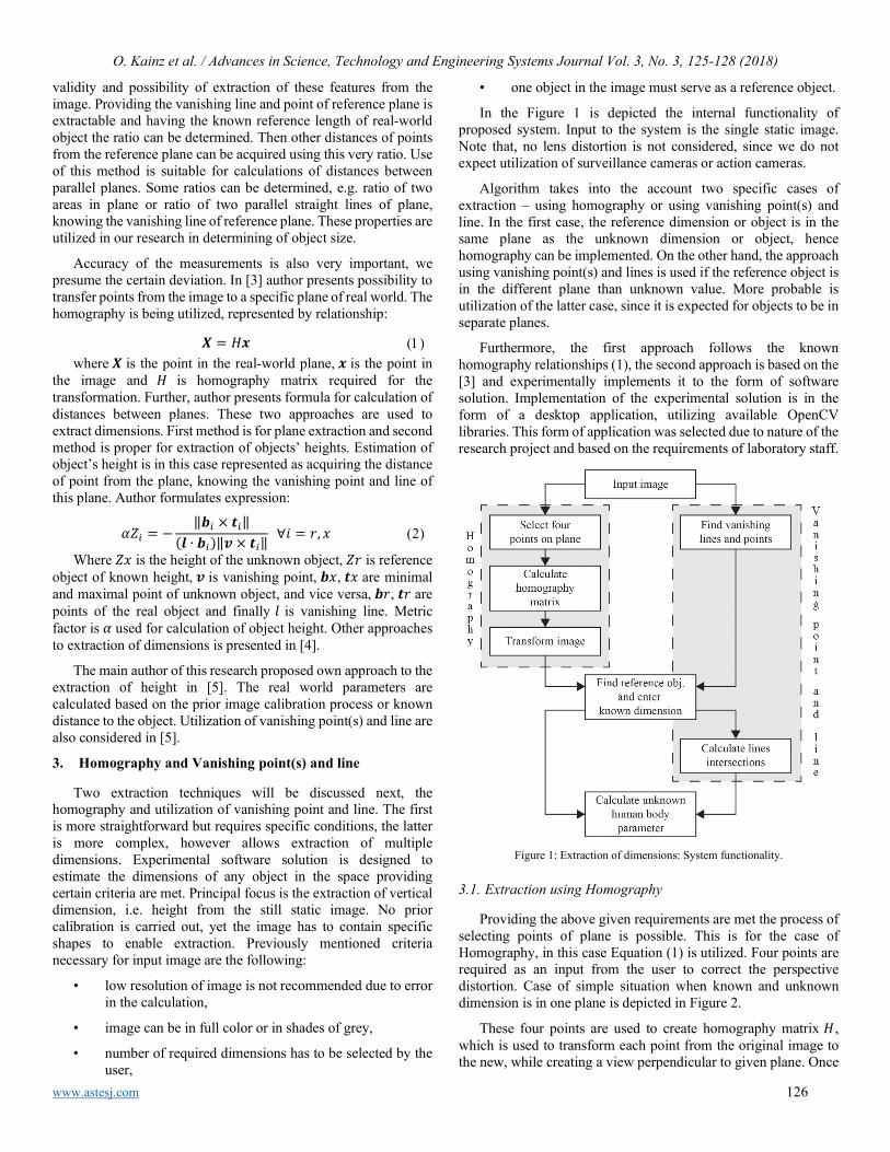
O. Kainz et al. / Advances in Science, Technology and Engineering Systems Journal Vol. 3, No. 3, 125-128 (2018)
www.astesj.com 126
validity and possibility of extraction of these features from the image. Providing the vanishing line and point of reference plane is extractable and having the known reference length of real-world object the ratio can be determined. Then other distances of points from the reference plane can be acquired using this very ratio. Use of this method is suitable for calculations of distances between parallel planes. Some ratios can be determined, e.g. ratio of two areas in plane or ratio of two parallel straight lines of plane, knowing the vanishing line of reference plane. These properties are utilized in our research in determining of object size.
Accuracy of the measurements is also very important, we presume the certain deviation. In [3] author presents possibility to transfer points from the image to a specific plane of real world. The homography is being utilized, represented by relationship:
𝑿𝑿 = 𝐻𝐻𝒙𝒙 (1) where 𝑿𝑿 is the point in the real-world plane, 𝒙𝒙 is the point in
the image and 𝐻𝐻 is homography matrix required for the transformation. Further, author presents formula for calculation of distances between planes. These two approaches are used to extract dimensions. First method is for plane extraction and second method is proper for extraction of objects’ heights. Estimation of object’s height is in this case represented as acquiring the distance of point from the plane, knowing the vanishing point and line of this plane. Author formulates expression:
𝛼𝛼𝑍𝑍𝑖𝑖 = −‖𝒃𝒃𝑖𝑖 × 𝒕𝒕𝑖𝑖‖
(𝒍𝒍 ∙ 𝒃𝒃𝑖𝑖)‖𝒗𝒗 × 𝒕𝒕𝑖𝑖‖ ∀𝑖𝑖 = 𝑟𝑟, 𝑥𝑥 (2)
Where 𝑍𝑍𝑥𝑥 is the height of the unknown object, 𝑍𝑍𝑟𝑟 is reference object of known height, 𝒗𝒗 is vanishing point, 𝒃𝒃𝑥𝑥, 𝒕𝒕𝑥𝑥 are minimal and maximal point of unknown object, and vice versa, 𝒃𝒃𝑟𝑟, 𝒕𝒕𝑟𝑟 are points of the real object and finally 𝑙𝑙 is vanishing line. Metric factor is 𝛼𝛼 used for calculation of object height. Other approaches to extraction of dimensions is presented in [4].
The main author of this research proposed own approach to the extraction of height in [5]. The real world parameters are calculated based on the prior image calibration process or known distance to the object. Utilization of vanishing point(s) and line are also considered in [5].
3. Homography and Vanishing point(s) and line
Two extraction techniques will be discussed next, the homography and utilization of vanishing point and line. The first is more straightforward but requires specific conditions, the latter is more complex, however allows extraction of multiple dimensions. Experimental software solution is designed to estimate the dimensions of any object in the space providing certain criteria are met. Principal focus is the extraction of vertical dimension, i.e. height from the still static image. No prior calibration is carried out, yet the image has to contain specific shapes to enable extraction. Previously mentioned criteria necessary for input image are the following:
• low resolution of image is not recommended due to error in the calculation,
• image can be in full color or in shades of grey,
• number of required dimensions has to be selected by the user,
• one object in the image must serve as a reference object.
In the Figure 1 is depicted the internal functionality of proposed system. Input to the system is the single static image. Note that, no lens distortion is not considered, since we do not expect utilization of surveillance cameras or action cameras.
Algorithm takes into the account two specific cases of extraction – using homography or using vanishing point(s) and line. In the first case, the reference dimension or object is in the same plane as the unknown dimension or object, hence homography can be implemented. On the other hand, the approach using vanishing point(s) and lines is used if the reference object is in the different plane than unknown value. More probable is utilization of the latter case, since it is expected for objects to be in separate planes.
Furthermore, the first approach follows the known homography relationships (1), the second approach is based on the [3] and experimentally implements it to the form of software solution. Implementation of the experimental solution is in the form of a desktop application, utilizing available OpenCV libraries. This form of application was selected due to nature of the research project and based on the requirements of laboratory staff.
Figure 1: Extraction of dimensions: System functionality.
3.1. Extraction using Homography
Providing the above given requirements are met the process of selecting points of plane is possible. This is for the case of Homography, in this case Equation (1) is utilized. Four points are required as an input from the user to correct the perspective distortion. Case of simple situation when known and unknown dimension is in one plane is depicted in Figure 2.
These four points are used to create homography matrix 𝐻𝐻 , which is used to transform each point from the original image to the new, while creating a view perpendicular to given plane. Once
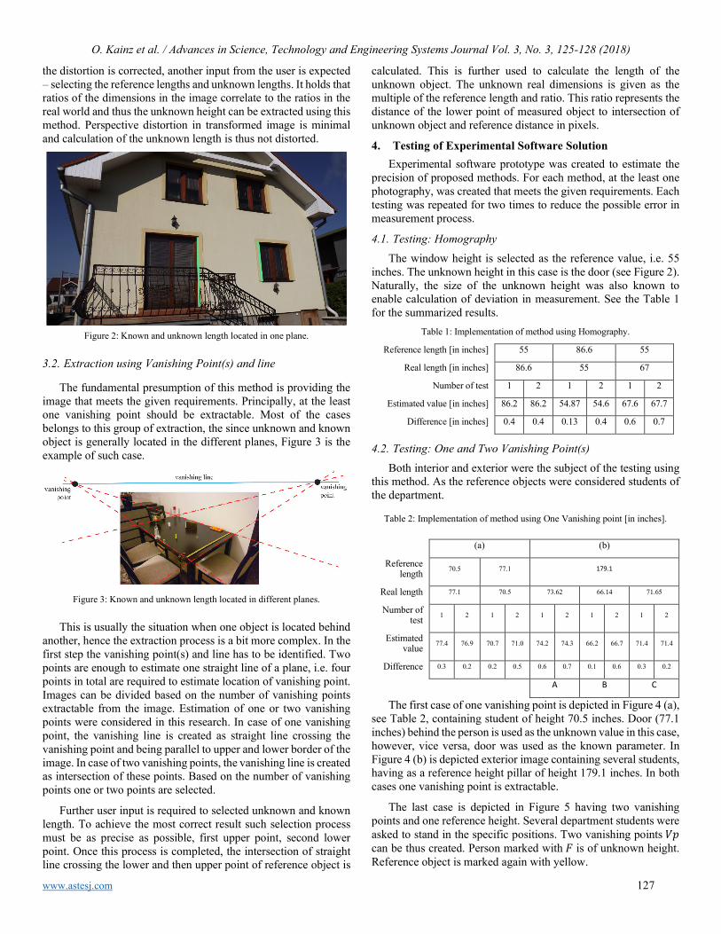
O. Kainz et al. / Advances in Science, Technology and Engineering Systems Journal Vol. 3, No. 3, 125-128 (2018)
www.astesj.com 127
the distortion is corrected, another input from the user is expected – selecting the reference lengths and unknown lengths. It holds that ratios of the dimensions in the image correlate to the ratios in the real world and thus the unknown height can be extracted using this method. Perspective distortion in transformed image is minimal and calculation of the unknown length is thus not distorted.
Figure 2: Known and unknown length located in one plane.
3.2. Extraction using Vanishing Point(s) and line
The fundamental presumption of this method is providing the image that meets the given requirements. Principally, at the least one vanishing point should be extractable. Most of the cases belongs to this group of extraction, the since unknown and known object is generally located in the different planes, Figure 3 is the example of such case.
Figure 3: Known and unknown length located in different planes.
This is usually the situation when one object is located behind another, hence the extraction process is a bit more complex. In the first step the vanishing point(s) and line has to be identified. Two points are enough to estimate one straight line of a plane, i.e. four points in total are required to estimate location of vanishing point. Images can be divided based on the number of vanishing points extractable from the image. Estimation of one or two vanishing points were considered in this research. In case of one vanishing point, the vanishing line is created as straight line crossing the vanishing point and being parallel to upper and lower border of the image. In case of two vanishing points, the vanishing line is created as intersection of these points. Based on the number of vanishing points one or two points are selected.
Further user input is required to selected unknown and known length. To achieve the most correct result such selection process must be as precise as possible, first upper point, second lower point. Once this process is completed, the intersection of straight line crossing the lower and then upper point of reference object is
calculated. This is further used to calculate the length of the unknown object. The unknown real dimensions is given as the multiple of the reference length and ratio. This ratio represents the distance of the lower point of measured object to intersection of unknown object and reference distance in pixels.
4. Testing of Experimental Software Solution Experimental software prototype was created to estimate the
precision of proposed methods. For each method, at the least one photography, was created that meets the given requirements. Each testing was repeated for two times to reduce the possible error in measurement process.
4.1. Testing: Homography The window height is selected as the reference value, i.e. 55
inches. The unknown height in this case is the door (see Figure 2). Naturally, the size of the unknown height was also known to enable calculation of deviation in measurement. See the Table 1 for the summarized results.
Table 1: Implementation of method using Homography.
Reference length [in inches] 55 86.6 55
Real length [in inches] 86.6 55 67
Number of test 1 2 1 2 1 2
Estimated value [in inches] 86.2 86.2 54.87 54.6 67.6 67.7
Difference [in inches] 0.4 0.4 0.13 0.4 0.6 0.7
4.2. Testing: One and Two Vanishing Point(s) Both interior and exterior were the subject of the testing using
this method. As the reference objects were considered students of the department.
Table 2: Implementation of method using One Vanishing point [in inches].
(a) (b)
Reference length 70.5 77.1 179.1
Real length 77.1 70.5 73.62 66.14 71.65
Number of test 1 2 1 2 1 2 1 2 1 2
Estimated value 77.4 76.9 70.7 71.0 74.2 74.3 66.2 66.7 71.4 71.4
Difference 0.3 0.2 0.2 0.5 0.6 0.7 0.1 0.6 0.3 0.2
A B C
The first case of one vanishing point is depicted in Figure 4 (a), see Table 2, containing student of height 70.5 inches. Door (77.1 inches) behind the person is used as the unknown value in this case, however, vice versa, door was used as the known parameter. In Figure 4 (b) is depicted exterior image containing several students, having as a reference height pillar of height 179.1 inches. In both cases one vanishing point is extractable.
The last case is depicted in Figure 5 having two vanishing points and one reference height. Several department students were asked to stand in the specific positions. Two vanishing points 𝑉𝑉𝑉𝑉 can be thus created. Person marked with 𝐹𝐹 is of unknown height. Reference object is marked again with yellow.

O. Kainz et al. / Advances in Science, Technology and Engineering Systems Journal Vol. 3, No. 3, 125-128 (2018)
www.astesj.com 128
Figure 4: Known and unknown length located in one plane.
Figure 5: Two vanishing points.
Last method contains the largest deviation from the real values, e.g. subject marked with B. Relative error in this case is up to 2%. For detailed outputs see Table 3.
Table 3: Implementation of method using Two Vanishing points [in inches].
Reference length 75.6
Real length 71.7 71.7 66.1 70.5 72.8 - 73.6
Estimated value 71.5 72.9 65.8 69.3 73.2 69.9 73.9
Difference 0.1 1.3 0.4 1.2 0.4 - 0.3
A B C D E F G
5. Testing of Experimental Software Solution
Large analysis of existing approaches in the extraction of length from uncalibrated images was carried out. Several approaches may be considered if the reference object is in the same plane as the unknown object. One of such approach is presented in this paper, i.e. correction of perspective distortion through the means of homography matrix.
Another situation consists of having reference object in different plane to unknown object. This case assumes utilization of vanishing point(s) and line. Specifically, the research was principally focused on the extraction of human body height. The outputs of the testing prove this method to be successful if deviation up to 2 percent is acceptable. These approaches have variety of use, in case of this research they were utilized to extract anthropometric parameters, mainly height was considered. However, as a part of another research other anthropometric parameters were extracted. Created software solution proved to be usable and reliable in estimation of object size from uncalibrated images.
In the future research, we plan to implement automatic detection of vanishing points and further automatic detection and recognition of reference object. Testing of image with and without lens distortion is considered. The extraction of heights can be also
extended to measure the human body parameters that can serve as an input to novel HBDF format proposed in [6].
Conflict of Interest
The authors declare no conflict of interest.
Acknowledgment
This publication is the result of the Project implementation: University Science Park TECHNICOM for Innovation Applications Supported by Knowledge Technology, Phase II., ITMS: 313011D232, supported by the Research & Inovation Operational Programme funded by the ERDF. We support research activities in Slovakia/This project is being co-financed by the European Union.
References
[1] A. Criminisi, Accurate visual metrology from single and multiple uncalibrated images, Distinguished Dissertation Series, London: Springer-Verlag, 2001.
[2] A. Criminisi, I. Reid, A. Zisserman, “Single View Metrology,” in International Journal of Computer Vision, 2001, vol. 40, no. 2, pp. 123-148.
[3] A. Criminisi, “Single-View Metrology: Algorithms and Applications,” in Proceedings of the 24th DAGM Symposium on Pattern Recognition, Zurich, CH, 2002, pp. 224-239.
[4] W. Guang-Hui, H. Zhan-Yi, W. Fu-Chao, “Single View Based Measurement on Space Planes,” in Journal of Computer Science and Technology, 2004, vol. 19, no. 3, pp. 374-382.
[5] O. Kainz, “Advanced Approaches in Identification the Anthropometric Features of Person in the Image,” PhD Thesis, Technical university of Kosice, 2018, pp. 1-117.
[6] O. Kainz, F. Jakab, R. Vápeník, and M. Michalko, “Human body description format,” in Computer Standards & Interfaces, vol. 58, pp. 118–125, May 2018.

www.astesj.com 129
A Method for Generating, Evaluating and Comparing Various System-level Synthesis Results in Designing Multiprocessor Architectures
Peter Arato*, Gyorgy Racz
Department of Control Engineering and Information Technology, Budapest University of Technology and Economics, 1117, Hungary
A R T I C L E I N F O A B S T R A C T Article history: Received: 08 May, 2018 Accepted: 02 June, 2018 Online: 15 June, 2018
Multiprocessing can be considered the most characteristic common property of complex digital systems. Due to the more and more complex tasks to be solved for fulfilling often conflicting requirements (cost, speed, energy and communication efficiency, pipelining, parallelism, the number of component processors, etc.), different types of component processors may be required by forming a so called Heterogeneous Multiprocessing Architecture (HMPA). The component processors of such systems may be not only general purpose CPUs or cores, but also DSPs, GPUs, FPGAs and other custom hardware components as well. Nevertheless, the system-level design process should be capable to handle the different types of component processors the same generic way. The hierarchy of the component processors and the data transfer organization between them are strongly determined by the task to be solved and by the priority order of the requirements to be fulfilled. For each component processor, a subtask must be defined based on the requirements and their desired priority orders. The definition of the subtasks, i.e. the decomposition of the task influences strongly the cost and performance of the whole system. Therefore, systematically comparing and evaluating the effects of different decompositions into subtasks may help the designer to approach optimal decisions in the system-level synthesis phase. For this purpose, the paper presents a novel method called DECHLS based on combining the decomposition and the modified high level synthesis algorithms. The application of the method is illustrated by redesigning and evaluating in some versions of two existing high performance practical embedded multiprocessing systems.
Keywords: system level synthesis, multiprocessor system, heterogeneous architectures, decomposition, high level synthesis, pipelining
1. Introduction and Related works
This paper is an extension of the work originally presented in IEEE System on Chip Conference 2017 [1]. This extension contains a more detailed explanation of the applied system level synthesis method. An additional practical benchmark is also solved and evaluated.
The system-level synthesis procedure of high-performance multiprocessor systems usually starts by some kind of a task description regarding the requirements and their desired priorities. The task description is usually formalized by a dataflow-like graph or by a high level programming language [2] [3]. To each component processor of the multiprocessor system, a subtask is assigned basically by intuition considering various special
requirements (communication cost, speed, pipelining, etc.). The definition of the subtasks, i.e. the decomposition of the task strongly influences the cost and performance of the whole multiprocessing system. Therefore, comparing and evaluating the effects of different task decompositions performed by applying systematic algorithms may help the designer to approach the optimal decisions in the system-level synthesis phase [4]. Our proposed method can also be considered a design space exploration as shown in [3-5]. In [5] the hardware-software partitioning problem is analyzed and various solutions are compared and evaluated. This approach refers formally only to special two-segment decompositions. These can be extended for multi-segment cases by utilizing several high performance heuristic algorithms [6], [7]. However, in case of such extensions for multiprocessing architectures [8], the decomposition algorithm and the calculation to find beneficial communication cost and time
ASTESJ
ISSN: 2415-6698
* Corresponding Author: Peter Arato, Email: [email protected]
Advances in Science, Technology and Engineering Systems Journal Vol. 3, No. 3, 129-141 (2018)
www.astesj.com
Special Issue on Multidisciplinary Sciences and Engineering
https://dx.doi.org/10.25046/aj030318
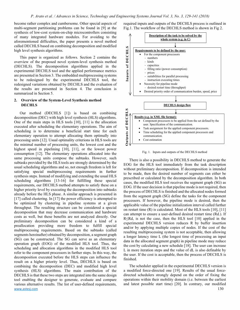
P. Arato et al. / Advances in Science, Technology and Engineering Systems Journal Vol. 3, No. 3, 129-141 (2018)
www.astesj.com 130
become rather complex and cumbersome. Other special aspects of multi-segment partitioning problems can be found in [9] at the synthesis of low-cost system-on-chip microcontrollers consisting of many integrated hardware modules. For avoiding to the aforementioned difficulties, the paper presents a novel method called DECHLS based on combining decomposition and modified high level synthesis algorithms.
This paper is organized as follows. Section 2 contains the overview of the proposed novel system-level synthesis method (DECHLS). The decomposition algorithms applied in the experimental DECHLS tool and the applied performance metrics are presented in Section 3. The embedded multiprocessing systems to be redesigned by the experimental DECHLS tool, the redesigned variations obtained by DECHLS and the evaluation of the results are presented in Section 4. The conclusion is summarized in Section 5.
2. Overview of the System-Level Synthesis method DECHLS
Our method (DECHLS [1]) is based on combining decomposition (DEC) with high level synthesis (HLS) algorithms. One of the main steps in HLS tools [10], [11] is the allocation executed after scheduling the elementary operations. The aim of scheduling is to determine a beneficial start time for each elementary operation to attempt allocating them optimally into processing units [12]. Usual optimality criterions in HLS tools are the minimal number of processing units, the lowest cost and the highest speed in pipelining [10], [11], or the lowest power consumption [12]. The elementary operations allocated into the same processing units compose the subtasks. However, such subtasks provided by the HLS tools are strongly determined by the usual scheduling algorithms and so, not enough freedom is left for satisfying special multiprocessing requirements in further synthesis steps. Instead of modifying and extending the usual HLS scheduling algorithms [13-16] for fulfilling these special requirements, our DECHLS method attempts to satisfy these on a higher priority level by executing the decomposition into subtasks already before the HLS phase. A similar approach is presented in [17] called clustering. In [17] the power efficiency is attempted to be optimized by clustering in pipeline systems at a given throughput. The resulting structure can be considered a special decomposition that may decrease communication and hardware costs as well, but these benefits are not analyzed directly. Our preliminary decomposition can be considered a kind of a preallocation providing more freedom to fulfill special multiprocessing requirements. Based on the subtasks (called segments hereinafter) obtained by decomposition, a segment graph (SG) can be constructed. The SG can serve as an elementary operation graph (EOG) of the modified HLS tool. Thus, the scheduling and allocation algorithms in the modified HLS tool refer to the component processors in further steps. In this way, the decomposition executed before the HLS steps can influence the result on a higher priority level. Thus, DECHLS is based on combining the decomposition (DEC) and modified high level synthesis (HLS) algorithms. The main contribution of the DECHLS is that these two steps are integrated into the same design tool enabling the designer to generate, evaluate and compare various alternative results. The list of user-defined requirements,
required inputs and outputs of the DECHLS process is outlined in Fig.1. The workflow of the DECHLS method is shown in Fig 2. Description of the task to be solved by the
whole system (e.g. in C)
Requirements to be defined by the user: • For the component processors
- numbers - kinds - capacities - filling ratio (power consumption) - prices - suitabilities for parallel processing - instruction executing times
• Necessity for pipeline mode - desired restart time (throughput)
• Desired priority order of communication burden, speed, price
DECHLS design flow
Results (e.g. in XML file format): • Component processors to be applied from the set defined by the
user. Specification of the communication. • Task assignment for the applied component processors. • Time scheduling for the applied component processors and
communication. • Cost estimation
Inp
uts
of
DE
CH
LS
O
utp
uts
of
DE
CH
LS
Fig. 1. Inputs and outputs of the DECHLS method
There is also a possibility in DECHLS method to generate the EOG for the HLS tool immediately from the task description without preliminary decomposition. If decomposition is intended to be made, then the desired number of segments can either be prescribed or calculated by the decomposition algorithm. In both cases, the modified HLS tool receives the segment graph (SG) as EOG. If the user decision is that pipeline mode is not required, then the process of DECHLS is finished and the allocated nodes formed from the segment graph (SG) define the tasks for the component processors. If however, the pipeline mode is desired, then the applicable value of the pipeline initialization interval called further on restart time (R) is calculated. Most of the HLS tools [10], [11] can attempt to ensure a user-defined desired restart time (Rd.). If R≤Rd, is not the case, then the HLS tool [10] applied in the experimental DECHLS version reduces R by buffer insertion and/or by applying multiple copies of nodes. If the cost of the resulting multiprocessing system is not acceptable, then allowing a longer latency time L (the longest time of processing an input data in the allocated segment graph) in pipeline mode may reduce the cost by calculating a new schedule [18]. The user can increase L in more iteration steps and the value of dL is also definable by the user. If the cost is acceptable, then the process of DECHLS is finished.
The scheduler applied in the experimental DECHLS version is a modified force-directed one [19]. Results of the usual force-directed schedulers strongly depend on the order of fixing the operations within their mobility domain (i.e. between the earliest and latest possible start time) [20]. In contrary, our modified
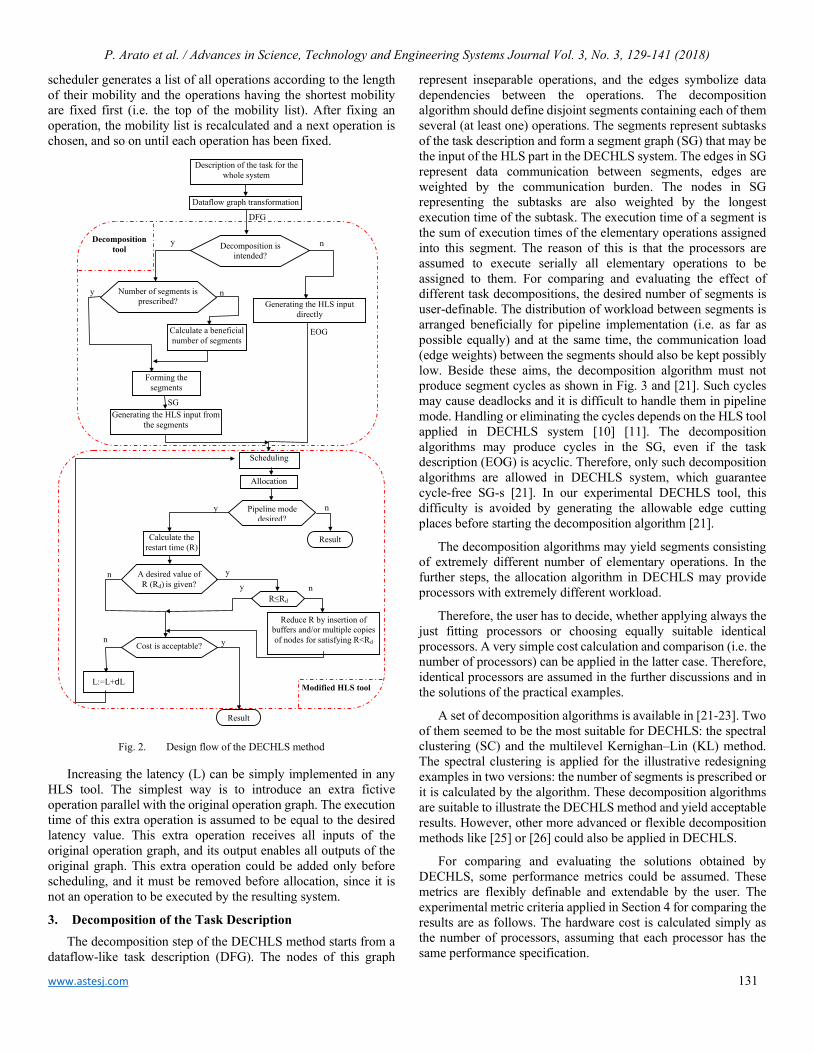
P. Arato et al. / Advances in Science, Technology and Engineering Systems Journal Vol. 3, No. 3, 129-141 (2018)
www.astesj.com 131
scheduler generates a list of all operations according to the length of their mobility and the operations having the shortest mobility are fixed first (i.e. the top of the mobility list). After fixing an operation, the mobility list is recalculated and a next operation is chosen, and so on until each operation has been fixed.
Decomposition is intended?
y
Number of segments is prescribed?
Forming the segments
Calculate a beneficial number of segments
Generating the HLS input directly
Generating the HLS input from the segments
Pipeline mode desired?
Calculate the restart time (R)
Scheduling
Allocation
R≤Rd
Result
n
n
y n
y
y n
A desired value of R (Rd) is given?
Result
Cost is acceptable? n y
y n
Reduce R by insertion of buffers and/or multiple copies of nodes for satisfying R<Rd
L:=L+dL
Decomposition tool
Modified HLS tool
Dataflow graph transformation
DFG
SG
EOG
Description of the task for the whole system
Fig. 2. Design flow of the DECHLS method
Increasing the latency (L) can be simply implemented in any HLS tool. The simplest way is to introduce an extra fictive operation parallel with the original operation graph. The execution time of this extra operation is assumed to be equal to the desired latency value. This extra operation receives all inputs of the original operation graph, and its output enables all outputs of the original graph. This extra operation could be added only before scheduling, and it must be removed before allocation, since it is not an operation to be executed by the resulting system.
3. Decomposition of the Task Description The decomposition step of the DECHLS method starts from a
dataflow-like task description (DFG). The nodes of this graph
represent inseparable operations, and the edges symbolize data dependencies between the operations. The decomposition algorithm should define disjoint segments containing each of them several (at least one) operations. The segments represent subtasks of the task description and form a segment graph (SG) that may be the input of the HLS part in the DECHLS system. The edges in SG represent data communication between segments, edges are weighted by the communication burden. The nodes in SG representing the subtasks are also weighted by the longest execution time of the subtask. The execution time of a segment is the sum of execution times of the elementary operations assigned into this segment. The reason of this is that the processors are assumed to execute serially all elementary operations to be assigned to them. For comparing and evaluating the effect of different task decompositions, the desired number of segments is user-definable. The distribution of workload between segments is arranged beneficially for pipeline implementation (i.e. as far as possible equally) and at the same time, the communication load (edge weights) between the segments should also be kept possibly low. Beside these aims, the decomposition algorithm must not produce segment cycles as shown in Fig. 3 and [21]. Such cycles may cause deadlocks and it is difficult to handle them in pipeline mode. Handling or eliminating the cycles depends on the HLS tool applied in DECHLS system [10] [11]. The decomposition algorithms may produce cycles in the SG, even if the task description (EOG) is acyclic. Therefore, only such decomposition algorithms are allowed in DECHLS system, which guarantee cycle-free SG-s [21]. In our experimental DECHLS tool, this difficulty is avoided by generating the allowable edge cutting places before starting the decomposition algorithm [21].
The decomposition algorithms may yield segments consisting of extremely different number of elementary operations. In the further steps, the allocation algorithm in DECHLS may provide processors with extremely different workload.
Therefore, the user has to decide, whether applying always the just fitting processors or choosing equally suitable identical processors. A very simple cost calculation and comparison (i.e. the number of processors) can be applied in the latter case. Therefore, identical processors are assumed in the further discussions and in the solutions of the practical examples.
A set of decomposition algorithms is available in [21-23]. Two of them seemed to be the most suitable for DECHLS: the spectral clustering (SC) and the multilevel Kernighan–Lin (KL) method. The spectral clustering is applied for the illustrative redesigning examples in two versions: the number of segments is prescribed or it is calculated by the algorithm. These decomposition algorithms are suitable to illustrate the DECHLS method and yield acceptable results. However, other more advanced or flexible decomposition methods like [25] or [26] could also be applied in DECHLS.
For comparing and evaluating the solutions obtained by DECHLS, some performance metrics could be assumed. These metrics are flexibly definable and extendable by the user. The experimental metric criteria applied in Section 4 for comparing the results are as follows. The hardware cost is calculated simply as the number of processors, assuming that each processor has the same performance specification.
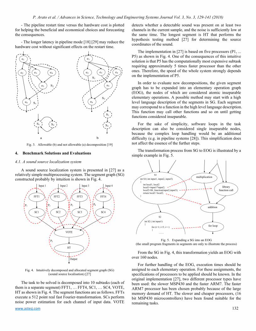
P. Arato et al. / Advances in Science, Technology and Engineering Systems Journal Vol. 3, No. 3, 129-141 (2018)
www.astesj.com 132
- The pipeline restart time versus the hardware cost is plotted for helping the beneficial and economical choices and forecasting the consequences.
- The longer latency in pipeline mode [18] [29] may reduce the hardware cost without significant effects on the restart time.
e1
e2 e3 e4
e5
e6
e1
e2 e3 e4
e5
e6 S1
S2
S1
S2
S2 S1
S1
S2
a b Fig. 3. Allowable (b) and not allowable (a) decomposition [19]
4. Benchmark Solutions and Evaluations
4.1. A sound source localization system
A sound source localization system is presented in [27] as a relatively simple multiprocessing system. The segment graph (SG) constructed probably by intuition is shown in Fig. 4.
FFT1
SC1
FFT2
SC2
VOTE
HT
Input 1 Input 2
Output
FFT3
SC3
Input 3
FFT4
SC4
Input 4
P1 P2 P3
P5
P4
Fig. 4. Intuitively decomposed and allocated segment graph (SG)
(sound source localisation) [27]
The task to be solved is decomposed into 10 subtasks (each of them is a separate segment) FFT1, … FFT4, SC1, … SC4, VOTE, HT as shown in Fig. 4. The segment functions are as follows. FFTs execute a 512 point real fast Fourier-transformation. SCs perform noise power estimation for each channel of input data. VOTE
detects whether a detectable sound was present on at least two channels in the current sample, and the noise is sufficiently low at the same time. The longest segment is HT that performs the hypothesis testing method [27] for determining the source coordinates of the sound.
The implementation in [27] is based on five processors (P1, ... P5) as shown in Fig. 4. One of the consequences of this intuitive solution is that P5 has the computationally most expensive subtask requiring approximately 5 times faster processor than the other ones. Therefore, the speed of the whole system strongly depends on the implementation of P5.
In order to evaluate new decompositions, the given segment graph has to be expanded into an elementary operation graph (EOG), the nodes of which are considered atomic inseparable elementary operations. A possible method may start with a high level language description of the segments in SG. Each segment may correspond to a function in the high level language description. This function may call other functions and so on until getting functions considered inseparable.
For the sake of simplicity, software loops in the task description can also be considered single inseparable nodes, because the complex loop handling would be an additional difficulty (e.g. in pipeline systems [28]). This simplification does not affect the essence of the further steps.
The transformation process from SG to EOG is illustrated by a simple example in Fig. 5.
int S1( int input1, input2, input3)
int local1, local2 local1=input1*input2; local2=lib_function(input2,input3); return local1+local2;
S1
int S2 ( int input1)
for (i=1; i<5; i++) ……
S2
multiplication
library function call
addition
for loop
Fig. 5. Expanding a SG into an EOG
(the small program fragments in segments are only to illustrate the process)
From the SG in Fig. 4, this transformation yields an EOG with over 160 nodes.
For further handling of the EOG, execution times should be assigned to each elementary operation. For these assignments, the specifications of processors to be applied should be known. In the original implementation [27], two different processor types have been used: the slower MSP430 and the faster ARM7. The faster ARM7 processor has been chosen probably because of the large memory demand of HT. The slower and cheaper processors, (16 bit MSP430 microcontrollers) have been found suitable for the remaining tasks.
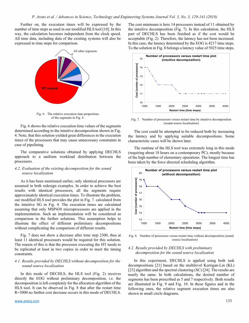
P. Arato et al. / Advances in Science, Technology and Engineering Systems Journal Vol. 3, No. 3, 129-141 (2018)
www.astesj.com 133
Further on, the execution times will be expressed by the number of time steps as used in our modified HLS tool [10]. In this way, the calculation becomes independent from the clock speed. All time data, including data of the existing systems will also be expressed in time steps for comparison.
HT segment
All other segments
Fig. 6. The relative execution time proportions
of the segments in Fig. 4.
Fig. 6 shows the relative execution time values of the segments determined according to the intuitive decomposition shown in Fig. 4. Note, that this solution yielded great differences in the execution times of the processors that may cause unnecessary constraints in case of pipelining.
The comparative solutions obtained by applying DECHLS approach to a uniform workload distribution between the processors.
4.2. Evaluation of the existing decomposition for the sound source localization
As it has been mentioned earlier, only identical processors are assumed in both redesign examples. In order to achieve the best results with identical processors, all the segments require approximately identical execution times. To illustrate the problem, our modified HLS tool provides the plot in Fig. 7. calculated from the intuitive SG in Fig. 4. The execution times are calculated assuming that only MSP430 microprocessors are applied in the implementation. Such an implementation will be considered as comparison in the further solutions. This assumption helps to illustrate the effect of different preliminary decompositions without complicating the comparison of different results.
Fig. 7 does not show a decrease after time step 2300, thus at least 11 identical processors would be required for this solution. The reason of this is that the processor executing the HT needs to be replicated at least in two copies in order to meet the timing constraints.
4.1. Results provided by DECHLS without decomposition for the sound source localization
In this mode of DECHLS, the HLS tool (Fig. 2) receives directly the EOG without preliminary decomposition, i.e. the decomposition is left completely for the allocation algorithm of the HLS tool. It can be observed in Fig. 8 that after the restart time R=3000 no further cost decrease occurs in this mode of DECHLS.
The cost minimum is here 14 processors instead of 11 obtained by the intuitive decomposition (Fig. 7). In this calculation, the HLS part of DECHLS has been finished as if the cost would be acceptable (Fig. 2). Therefore, the latency has not been increased. In this case, the latency determined by the EOG is 4217 time steps. To the solution in Fig. 8 belongs a latency value of 5025 time steps.
Fig. 7. Number of processors versus restart time by intuitive decomposition
(sound source localisation)
The cost could be attempted to be reduced both by increasing the latency and by applying suitable decompositions. Some characteristic cases will be shown later.
The runtime of the HLS tool was extremely long in this mode (requiring about 18 hours on a contemporary PC), mostly because of the high number of elementary operations. The longest time has been taken by the force directed scheduling algorithm.
Fig. 8. Number of processors versus restart time without decomposition (sound
source localisation)
4.2. Results provided by DECHLS with preliminary decomposition for the sound source localization
In this experiment, DECHLS is applied using both task decompositions [21] based on the multilevel Kerrigan-Lin (KL) [23] algorithm and the spectral clustering (SC) [24]. The results are nearly the same. In both calculations, the desired number of segments has been prescribed as 5 and 7 respectively. Both results are illustrated in Fig. 9 and Fig. 10. In these figures and in the following ones, the relative segment execution times are also shown in small circle diagrams.
Number of processors versus restart time plot(intuitive decomposition)
10
11
12
13
14
15
1000 1500 2000 2500 3000 3500 4000Restart time [time steps]
Cost
[num
ber o
f pro
cess
ors]
Number of processors versus restart time plot(without decomposition)
13
14
15
16
17
18
19
20
1000 1500 2000 2500 3000 3500 4000Restart time [time steps]
Cost
[num
ber o
f pro
cess
ors]
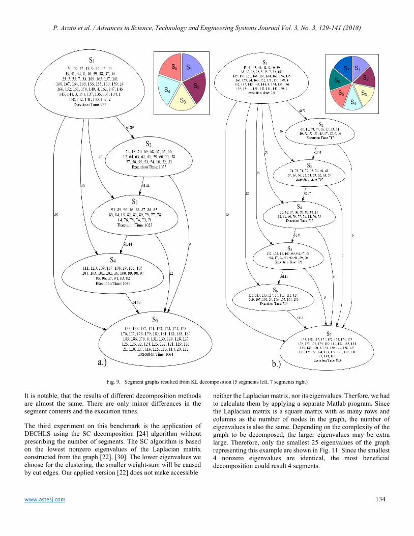
P. Arato et al. / Advances in Science, Technology and Engineering Systems Journal Vol. 3, No. 3, 129-141 (2018)
www.astesj.com 134
S1
S2
S2
S4
S5
S4
S3
S2
S1S5
a.)
S5
S6
S7
S4
S3
S2
S1 S7
S6
S4
S3
S2
S1
S5
b.)
Fig. 9. Segment graphs resulted from KL decomposition (5 segments left, 7 segments right)
It is notable, that the results of different decomposition methods are almost the same. There are only minor differences in the segment contents and the execution times.
The third experiment on this benchmark is the application of DECHLS using the SC decomposition [24] algorithm without prescribing the number of segments. The SC algorithm is based on the lowest nonzero eigenvalues of the Laplacian matrix constructed from the graph [22], [30]. The lower eigenvalues we choose for the clustering, the smaller weight-sum will be caused by cut edges. Our applied version [22] does not make accessible
neither the Laplacian matrix, nor its eigenvalues. Therfore, we had to calculate them by applying a separate Matlab program. Since the Laplacian matrix is a square matrix with as many rows and columns as the number of nodes in the graph, the number of eigenvalues is also the same. Depending on the complexity of the graph to be decomposed, the larger eigenvalues may be extra large. Therefore, only the smallest 25 eigenvalues of the graph representing this example are shown in Fig. 11. Since the smallest 4 nonzero eigenvalues are identical, the most beneficial decomposition could result 4 segments.
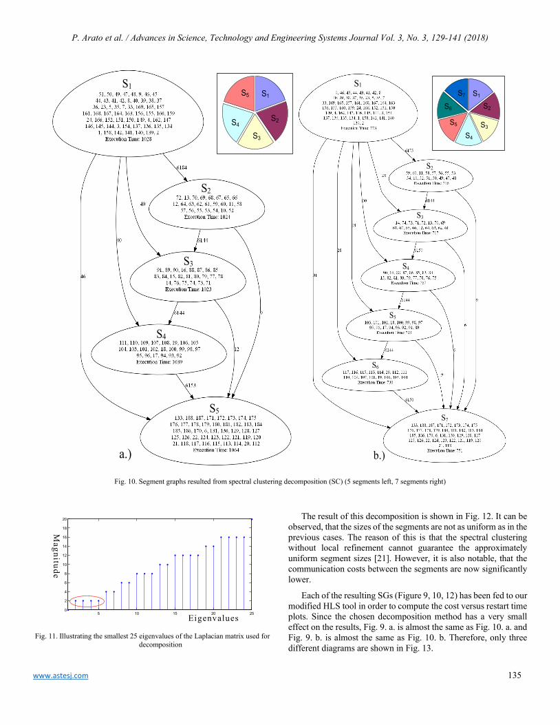
P. Arato et al. / Advances in Science, Technology and Engineering Systems Journal Vol. 3, No. 3, 129-141 (2018)
www.astesj.com 135
S1
S2
S3
S4
S5
S5 S1
S2
S3
S4
a.)
S1
S2
S3
S4
S5
S6
S7
S5
S1
S2
S3
S4
S6
S7
b.)
Fig. 10. Segment graphs resulted from spectral clustering decomposition (SC) (5 segments left, 7 segments right)
5 10 15 20 250
2
4
6
8
10
12
14
16
18
20
Eigenvalues
Magnitude
Fig. 11. Illustrating the smallest 25 eigenvalues of the Laplacian matrix used for
decomposition
The result of this decomposition is shown in Fig. 12. It can be observed, that the sizes of the segments are not as uniform as in the previous cases. The reason of this is that the spectral clustering without local refinement cannot guarantee the approximately uniform segment sizes [21]. However, it is also notable, that the communication costs between the segments are now significantly lower.
Each of the resulting SGs (Figure 9, 10, 12) has been fed to our modified HLS tool in order to compute the cost versus restart time plots. Since the chosen decomposition method has a very small effect on the results, Fig. 9. a. is almost the same as Fig. 10. a. and Fig. 9. b. is almost the same as Fig. 10. b. Therefore, only three different diagrams are shown in Fig. 13.
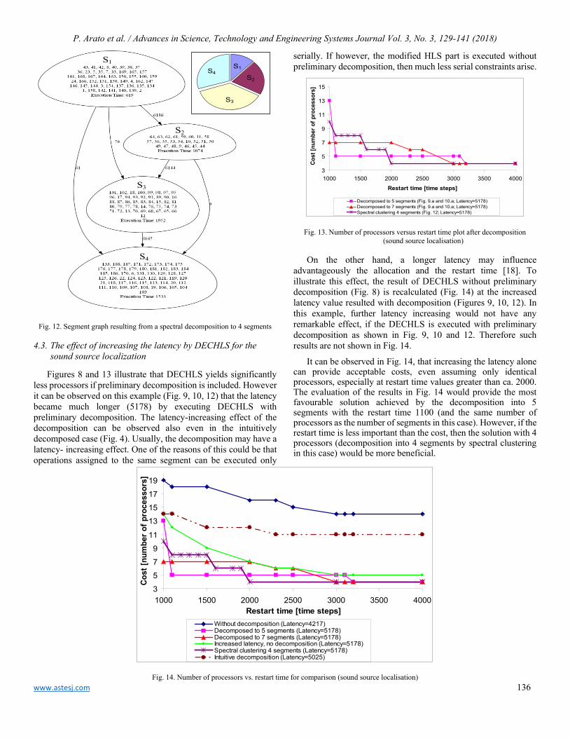
P. Arato et al. / Advances in Science, Technology and Engineering Systems Journal Vol. 3, No. 3, 129-141 (2018)
www.astesj.com 136
S1
S2
S3
S4
S1
S2
S3
S4
Fig. 12. Segment graph resulting from a spectral decomposition to 4 segments
4.3. The effect of increasing the latency by DECHLS for the sound source localization
Figures 8 and 13 illustrate that DECHLS yields significantly less processors if preliminary decomposition is included. However it can be observed on this example (Fig. 9, 10, 12) that the latency became much longer (5178) by executing DECHLS with preliminary decomposition. The latency-increasing effect of the decomposition can be observed also even in the intuitively decomposed case (Fig. 4). Usually, the decomposition may have a latency- increasing effect. One of the reasons of this could be that operations assigned to the same segment can be executed only
serially. If however, the modified HLS part is executed without preliminary decomposition, then much less serial constraints arise.
Fig. 13. Number of processors versus restart time plot after decomposition (sound source localisation)
On the other hand, a longer latency may influence advantageously the allocation and the restart time [18]. To illustrate this effect, the result of DECHLS without preliminary decomposition (Fig. 8) is recalculated (Fig. 14) at the increased latency value resulted with decomposition (Figures 9, 10, 12). In this example, further latency increasing would not have any remarkable effect, if the DECHLS is executed with preliminary decomposition as shown in Fig. 9, 10 and 12. Therefore such results are not shown in Fig. 14.
It can be observed in Fig. 14, that increasing the latency alone can provide acceptable costs, even assuming only identical processors, especially at restart time values greater than ca. 2000. The evaluation of the results in Fig. 14 would provide the most favourable solution achieved by the decomposition into 5 segments with the restart time 1100 (and the same number of processors as the number of segments in this case). However, if the restart time is less important than the cost, then the solution with 4 processors (decomposition into 4 segments by spectral clustering in this case) would be more beneficial.
Fig. 14. Number of processors vs. restart time for comparison (sound source localisation)
3
5
7
9
11
13
15
1000 1500 2000 2500 3000 3500 4000Restart time [time steps]
Cost
[num
ber o
f pro
cess
ors]
Decomposed to 5 segments (Fig. 9.a and 10.a; Latency=5178)Decomposed to 7 segments (Fig. 9.a and 10.a; Latency=5178)Spectral clustering 4 segments (Fig. 12; Latency=5178)
3579
11
13151719
1000 1500 2000 2500 3000 3500 4000Restart time [time steps]
Cost
[num
ber o
f pro
cess
ors]
Without decomposition (Latency=4217)Decomposed to 5 segments (Latency=5178)Decomposed to 7 segments (Latency=5178)Increased latency, no decomposition (Latency=5178)Spectral clustering 4 segments (Latency=5178)Intuitive decomposition (Latency=5025)
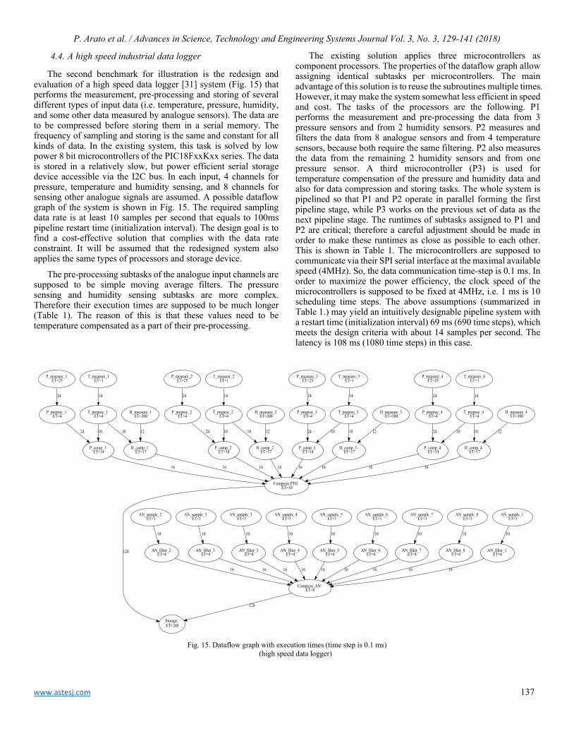
P. Arato et al. / Advances in Science, Technology and Engineering Systems Journal Vol. 3, No. 3, 129-141 (2018)
www.astesj.com 137
4.4. A high speed industrial data logger
The second benchmark for illustration is the redesign and evaluation of a high speed data logger [31] system (Fig. 15) that performs the measurement, pre-processing and storing of several different types of input data (i.e. temperature, pressure, humidity, and some other data measured by analogue sensors). The data are to be compressed before storing them in a serial memory. The frequency of sampling and storing is the same and constant for all kinds of data. In the existing system, this task is solved by low power 8 bit microcontrollers of the PIC18FxxKxx series. The data is stored in a relatively slow, but power efficient serial storage device accessible via the I2C bus. In each input, 4 channels for pressure, temperature and humidity sensing, and 8 channels for sensing other analogue signals are assumed. A possible dataflow graph of the system is shown in Fig. 15. The required sampling data rate is at least 10 samples per second that equals to 100ms pipeline restart time (initialization interval). The design goal is to find a cost-effective solution that complies with the data rate constraint. It will be assumed that the redesigned system also applies the same types of processors and storage device.
The pre-processing subtasks of the analogue input channels are supposed to be simple moving average filters. The pressure sensing and humidity sensing subtasks are more complex. Therefore their execution times are supposed to be much longer (Table 1). The reason of this is that these values need to be temperature compensated as a part of their pre-processing.
The existing solution applies three microcontrollers as component processors. The properties of the dataflow graph allow assigning identical subtasks per microcontrollers. The main advantage of this solution is to reuse the subroutines multiple times. However, it may make the system somewhat less efficient in speed and cost. The tasks of the processors are the following. P1 performs the measurement and pre-processing the data from 3 pressure sensors and from 2 humidity sensors. P2 measures and filters the data from 8 analogue sensors and from 4 temperature sensors, because both require the same filtering. P2 also measures the data from the remaining 2 humidity sensors and from one pressure sensor. A third microcontroller (P3) is used for temperature compensation of the pressure and humidity data and also for data compression and storing tasks. The whole system is pipelined so that P1 and P2 operate in parallel forming the first pipeline stage, while P3 works on the previous set of data as the next pipeline stage. The runtimes of subtasks assigned to P1 and P2 are critical; therefore a careful adjustment should be made in order to make these runtimes as close as possible to each other. This is shown in Table 1. The microcontrollers are supposed to communicate via their SPI serial interface at the maximal available speed (4MHz). So, the data communication time-step is 0.1 ms. In order to maximize the power efficiency, the clock speed of the microcontrollers is supposed to be fixed at 4MHz, i.e. 1 ms is 10 scheduling time steps. The above assumptions (summarized in Table 1.) may yield an intuitively designable pipeline system with a restart time (initialization interval) 69 ms (690 time steps), which meets the design criteria with about 14 samples per second. The latency is 108 ms (1080 time steps) in this case.
Fig. 15. Dataflow graph with execution times (time step is 0.1 ms)
(high speed data logger)
P_measure_1 ET=25
P_preproc_1 ET=4
24
H_measure_1 ET=300
H_comp_1 ET=17
12
T_measure_1 ET=1
T_preproc_1 ET=4
14
P_comp_1 ET=14
Compress PTH ET=10
16 16
24 10 10
P_measure_2 ET=25
P_preproc_2 ET=4
24
H_measure_2 ET=300
H_comp_2 ET=17
12
T_measure_2 ET=1
T_preproc_2 ET=4
14
P_comp_2 ET=14
16 16
24 10 10
P_measure_3 ET=25
P_preproc_3 ET=4
24
H_measure_3 ET=300
H_comp_3 ET=17
12
T_measure_3 ET=1
T_preproc_3 ET=4
14
P_comp_3 ET=14
16 16
24 10 10
P_measure_4 ET=25
P_preproc_4 ET=4
24
H_measure_4 ET=300
H_comp_4 ET=17
12
T_measure_4 ET=1
T_preproc_4 ET=4
14
P_comp_4 ET=14
16 16
24 10 10
Storage ET=248
128
AN_sample_1 ET=1
AN_sample_2 ET=1
AN_sample_3 ET=1
AN_sample_3 ET=1
AN_sample_4 ET=1
AN_sample_5 ET=1
AN_sample_6 ET=1
AN_sample_7 ET=1
AN_filter_1 ET=4
10
Compress_AN ET=8
16
AN_filter_2 ET=4
10
16
AN_filter_3 ET=4
10
16
AN_filter_3 ET=4
10
16
AN_filter_4 ET=4
10
16
AN_filter_5 ET=4
10
16
AN_filter_6 ET=4
10
16
AN_filter_7 ET=4
10
16
AN_sample_8 ET=1
AN_filter_8 ET=4
10
16
128

P. Arato et al. / Advances in Science, Technology and Engineering Systems Journal Vol. 3, No. 3, 129-141 (2018)
www.astesj.com 138
Table 1. Runtime calculation for an intuitive design
Name of task Execution time steps Total number Allocated to P1 Allocated to P2 Allocated to P3
AN_sample 1 8 0 8 0
AN_filter 4 8 0 8 0
P_measurement 25 4 3 1 0
H_measurement 300 4 2 2 0
T_measurement 1 4 0 4 0
P_comp 14 4 0 0 4
H_comp 17 4 0 0 4
P_preproc 4 4 3 1 0
T_preproc 4 4 0 4 0
Compress_PTH 10 1 0 0 1
Storage 248 1 0 0 1
Compress_AN 8 1 0 0 1
Total execution time (in time steps) 1766 687 689 390
4.5. Evaluation of the existing decomposition for the high speed data logger
A carefully designed intuitive solution that complies with all the constraints was presented in Subsection 4.6. The intuitive decomposition is done firstly based on the parameter values in Table 1. The resulting segment graph is shown in Fig. 16.
S1
S2
S3
Fig. 16. Segment graph of the existing solution
(high speed data logger)
In this implementation, the required number of processors is 3, the restart time is 690 time steps, and the latency is 1080 time steps. This intuitively designed system will be the basis for comparison.
4.6. Results provided by DECHLS without decomposition for the high-speed data logger
Fig. 15 shows that the dataflow graph has such a special structure in this case, which causes less than 4 processors, only if the latency is increased from 570 to above 1400 time steps. This
was calculated by the modified HLS tool. If the latency is increased to 1400 time steps (140 ms), then the solution is possible by applying 3 processors. However, this case requires a longer restart time, 1050 time steps (105 ms) than the prescribed value of 1000 (100 ms) given in Subsection 4.6.
4.7. Results provided by DECHLS with preliminary decomposition for the high-speed data logger
Without prescribing the number of segments, the DECHLS yields 4 segments (Fig. 17 a). For comparison, 3, 4, 5 and 6 segments were prescribed by applying both KL and spectral clustering (SC) methods. For the sake of simplicity, only the following three cases from these are illustrated:
• 3 segments, KL method (Fig. 17. b)
• 3 segments, spectral clustering method, shortest restart time with 3 processors (Fig. 17. c)
• 5 segments, KL method, longest restart time with 3 processors (Fig. 17. d)
In this example, the number of segments and the selected decomposition method had greater influence on the results than in the sound source localisation example.
It is also notable, that the solution with 4 segments has the shortest latency, but not the longest restart time. However, the solution yielding the shortest restart time does not result in the longest latency. All of the above-mentioned cases are illustrated in Fig. 18.
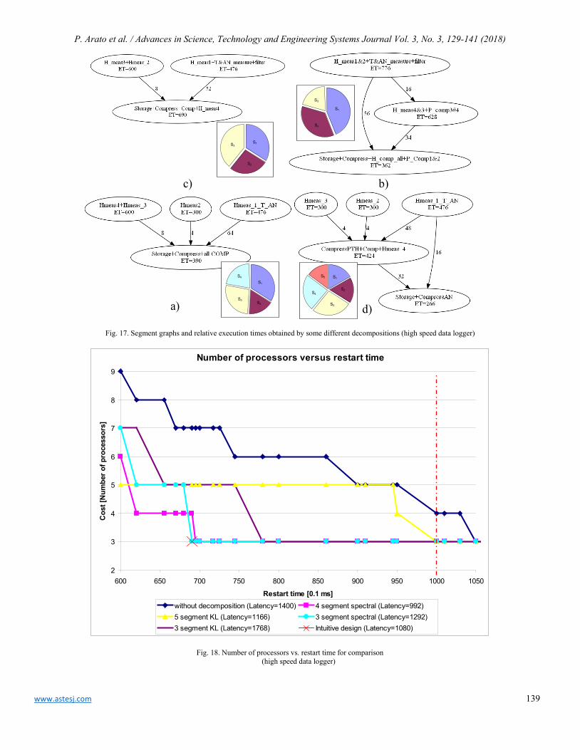
P. Arato et al. / Advances in Science, Technology and Engineering Systems Journal Vol. 3, No. 3, 129-141 (2018)
www.astesj.com 139
c) b)
S3
S2
S1
S1
S2
S3
S4
S3S2
S1
S5 S1
S2
S3
S4
a) d)
Fig. 17. Segment graphs and relative execution times obtained by some different decompositions (high speed data logger)
Fig. 18. Number of processors vs. restart time for comparison
(high speed data logger)
Number of processors versus restart time
2
3
4
5
6
7
8
9
600 650 700 750 800 850 900 950 1000 1050
Restart time [0.1 ms]
Cos
t [N
umbe
r of p
roce
ssor
s]
without decomposition (Latency=1400) 4 segment spectral (Latency=992)5 segment KL (Latency=1166) 3 segment spectral (Latency=1292)3 segment KL (Latency=1768) Intuitive design (Latency=1080)
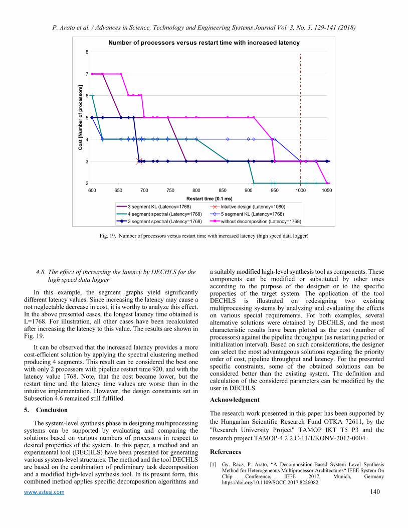
P. Arato et al. / Advances in Science, Technology and Engineering Systems Journal Vol. 3, No. 3, 129-141 (2018)
www.astesj.com 140
Fig. 19. Number of processors versus restart time with increased latency (high speed data logger)
4.8. The effect of increasing the latency by DECHLS for the high speed data logger
In this example, the segment graphs yield significantly different latency values. Since increasing the latency may cause a not neglectable decrease in cost, it is worthy to analyze this effect. In the above presented cases, the longest latency time obtained is L=1768. For illustration, all other cases have been recalculated after increasing the latency to this value. The results are shown in Fig. 19.
It can be observed that the increased latency provides a more cost-efficient solution by applying the spectral clustering method producing 4 segments. This result can be considered the best one with only 2 processors with pipeline restart time 920, and with the latency value 1768. Note, that the cost became lower, but the restart time and the latency time values are worse than in the intuitive implementation. However, the design constraints set in Subsection 4.6 remained still fulfilled.
5. Conclusion
The system-level synthesis phase in designing multiprocessing systems can be supported by evaluating and comparing the solutions based on various numbers of processors in respect to desired properties of the system. In this paper, a method and an experimental tool (DECHLS) have been presented for generating various system-level structures. The method and the tool DECHLS are based on the combination of preliminary task decomposition and a modified high-level synthesis tool. In its present form, this combined method applies specific decomposition algorithms and
a suitably modified high-level synthesis tool as components. These components can be modified or substituted by other ones according to the purpose of the designer or to the specific properties of the target system. The application of the tool DECHLS is illustrated on redesigning two existing multiprocessing systems by analyzing and evaluating the effects on various special requirements. For both examples, several alternative solutions were obtained by DECHLS, and the most characteristic results have been plotted as the cost (number of processors) against the pipeline throughput (as restarting period or initialization interval). Based on such considerations, the designer can select the most advantageous solutions regarding the priority order of cost, pipeline throughput and latency. For the presented specific constraints, some of the obtained solutions can be considered better than the existing system. The definition and calculation of the considered parameters can be modified by the user in DECHLS.
Acknowledgment
The research work presented in this paper has been supported by the Hungarian Scientific Research Fund OTKA 72611, by the "Research University Project" TAMOP IKT T5 P3 and the research project TAMOP-4.2.2.C-11/1/KONV-2012-0004.
References
[1] Gy. Racz, P. Arato, “A Decomposition-Based System Level Synthesis Method for Heterogeneous Multiprocessor Architectures“ IEEE System On Chip Conference, IEEE 2017, Munich, Germany https://doi.org/10.1109/SOCC.2017.8226082
Number of processors versus restart time with increased latency
2
3
4
5
6
7
8
600 650 700 750 800 850 900 950 1000 1050
Restart time [0.1 ms]
Cos
t [N
umbe
r of p
roce
ssor
s]
3 segment KL (Latency=1768) Intuitive design (Latency=1080)4 segment spectral (Latency=1768) 5 segment KL (Latency=1768)3 segment spectral (Latency=1768) without decomposition (Latency=1768)

P. Arato et al. / Advances in Science, Technology and Engineering Systems Journal Vol. 3, No. 3, 129-141 (2018)
www.astesj.com 141
[2] A. Gerstlauer, C. Haubelt, A. D. Pimentel, T. P. Stefanov, D. D. Gajski, J. Teich, “Electronic System-Level Synthesis Methodologies“, IEEE T COMPUT AID D., 28(10), 1517-1530, 2009
[3] R. Corvino, A. Gamatié, M. Geilen, L. Józwiak, “Design space exploration in application-specific hardware synthesis for multiple communicating nested loops“, in IEEE ICSAMOS, 128-135, 2012
[4] A. Carminati, R. S. de Oliveira, L. F. Friedrich, “Exploring the design space of multiprocessor synchronization protocols for real-time systems“, Journal of Systems Architecture (JSA), 60(3), 258-270, 2014. ISSN 1383-7621
[5] A. Cilardo, L. Gallo, N. Mazzocca, “Design space exploration for high-level synthesis of multi-threaded applications”, Journal of Systems Architecture (JSA), 59(10D), 1171-1183, 2013., ISSN 1383-7621
[6] P. Arató, Z. A. Mann, A. Orbán, “Finding optimal hardware/software partitions”, Formal Methods in System Design, 31(3), 241-263. 2007
[7] J. Wu, T. Srikanthan, G. Chen, “Algorithmic Aspects of Hardware/Software Partitioning: 1D Search Algorithms,” IEEE T. COMPUT., 59(4), 532-544, 2010. doi: 10.1109/TC.2009.173
[8] R. Ernst, J. Henkel, T. Benner, “Hardware-software cosynthesis for microcontrollers”, IEEE Design & Test of Computers, 10(4), 64-75, 1993.
[9] N. Govil, S. R. Chowdhury, “GMA: a high speed metaheuristic algorithmic approach to hardware software partitioning for Low-cost SoCs”, 2015 International Symposium on Rapid System Prototyping (RSP), Amsterdam, 2015.
[10] P. Arató, T. Visegrády, I. Jankovits, High Level Synthesis of Pipelined Datapaths, John Wiley & Sons, New York, ISBN: 0 471495582 4, 2001.
[11] W. Meeus, K. Van Beeck, T. Goedemé, J. Meel, D. Stroobandt, “An overview of today’s high-level synthesis tools”, Design Automation for Embedded Systems, 16(4), 31-51, 2012.
[12] T. Mukk, A. M. Rahmani, N. Dutt, “Adaptive-Reflective Middleware for Power and Energy Management in Many-Core Heterogeneous Systems”, International Symposium & Workshop on Many-Core Computing: Hardware and Software, Southampton, UK, 2018.
[13] P. Arató, Z. A. Mann, A. Orbán, “Time-constrained scheduling of large pipelined datapaths”, Journal of Systems Architecture (JSA), 51(12), 665-687, 2005.
[14] P. G. Paulin, J. P. Knight, “Force-directed scheduling for the behavioral synthesis of ASICs” IEEE T COMPUT AID D., 8(6), 661-679, 1989.
[15] M. Grajcar, “Genetic List Scheduling Algorithm for Scheduling and Allocation on a Loosely Coupled Heterogeneous Multiprocessor System”, 36th ACM/IEEE Conference on Design Automation, New Orleans, LA, USA, 1999.
[16] J-H. Ding, Y-T. Chang, Z-D. Guo, K-C. Li, Y-C. Chung, “An efficient and comprehensive scheduler on Asymmetric Multicore Architecture systems”, Journal of Systems Architecture, 60(3), 305-314, 2014, ISSN 1383-7621
[17] C-S. Lin, C-S. Lin, Y-S. Lin; P-A. Hsiung, C. Shih, “Multi-objective exploitation of pipeline parallelism using clustering, replication and duplication in embedded multi-core systems”, Journal of Systems Architecture (JSA), 59(10C), 1083-1094, 2013, ISSN 1383-7621
[18] Gy. Pilászy, Gy. Rácz, P. Arató, “The effect of increasing the latency time in High Level Synthesis”, Periodica Polytechnica Electrical Engineering, 58(2), 37-42, 2014. https://doi.org/10.3311/PPee.7024
[19] K. O'Neal, D. Grissom, P. Brisk, “Force-Directed List Scheduling for Digital Microfluidic Biochips”, IEEE/IFIP 20th International Conference on VLSI and System-on-Chip (VLSI-SoC), Santa Cruz, USA, 2012.
[20] P. G. Paulin, J. P. Knight, “Force-Directed Scheduling in Automatic Data Path Synthesis”, 24th Conference on Design Automation, New York, USA, 1987.
[21] P. Arató, D. Drexler, Gy. Rácz, “Analyzing the Effect of Decomposition Algorithms on the Heterogeneous Multiprocessing Architectures in System Level Synthesis” Buletinul Stiintific al Universitatii Politehnica din Timisoara Romania Seria Automatica si Calculatore / Scientific Buletin of Politechnica University of Timisoara Transactions on Automatic Control and Computer Science, 60(74) 39-46. 2015.
[22] B. Hendrickson, R. Leland, “The Chaco User’s Guide Version 2.0”, Technical Report SAND94-2692, 1994.
[23] B. Hendrickson, R. Leland, “A Multilevel Algorithm for Partitioning Graphs”, In Proc. Supercomputing '95. (Formerly, Technical Report SAND93-1301), 1993.
[24] B. Hendrickson, R. Leland, “An Improved Spectral Graph Partitioning Algorithm for Mapping Parallel Computations”, SIAM J. Sci. Stat. Comput., 16(2), 452-469, 1995.
[25] G. Karypis, V. Kumar, “Metis-unstructured graph partitioning and sparse matrix ordering system version 2.0”, 1995.
[26] A. Trifunovic, W. J. Knottenbelt, “Parkway 2.0: a parallel multilevel hypergraph partitioning tool”, Computer and Information Sciences-ISCIS 2004, Springer, 789-800. 2004.
[27] M. Goraczko, J. Liu, D. Lymberopoulos, “Energy-Optimal Software Partitioning in Heterogeneous Multiprocessor Embedded Systems”, DAC 2008., Anaheim, California, USA, 2008.
[28] G. Suba, “Hierarchical pipelining of nested loops in high-level synthesis”, Periodica Polytechnica Electrical Engineering, 58(3) 81-90, 2014. https://doi.org/10.3311/PPee.7610
[29] J. Subhlok, G. Vondran, “Optimal latency - throughput tradeoffs for data parallel pipelines”, 8th Annual ACM Symposium on Parallel Algorithms and Architectures, Padua, Italy, 1996.
[30] C. J. Alpert, A. B. Kahng, S.-Z. Yao, “Spectral partitioning with multiple eigenvectors”, Discrete Applied Mathematics, 90(1), 3-26, 1999.
[31] Project documentation of KMR_12-1-2012-0222 titled “The development of a complex monitoring system for fishing waters”

www.astesj.com 142
A New Study Performance Control of PMSMs: Validity Abacus Approach
Sabrine Jebri*, Khaled Nouri
Laboratoire de Systèmes Avancés (LSA), École Polytechnique de Tunisie, Université de Carthage, Tunisia
A R T I C L E I N F O A B S T R A C T Article history: Received: 30 May, 2017 Accepted: 02 June, 2018 Online: 18 June, 2018
This paper is an extension of work originally presented in conference name” Study Performance of Speed Tracking Control with Frequency and Amplitude Dependence”. Though many PMSMs (Permanent Magnet Synchronous Motor) control approach have already been published, little endeavors have been invested in the study of speed tacking control with frequency or amplitude dependence. The use of NDI (Nonlinear Dynamic Inversion) tracking control in versus amplitude and frequency dependence is the major focus of this paper. The proposed tracking control demonstrates that NDI control presents the ability to track the desired output with high precision. PMSM outputs are characterized at different amplitude and frequency. The speed and the direct current versus amplitude and frequency are successfully extracted. A mathematical (d-q) of the permanent magnet synchronous motor model is also presented. A comparative study between desired data and simulation results is conducted. Important to note, the proposed model and the simulation results reflect a successful agreement as far as a amplitude and frequency dependence is concerned. A new validity approach, namely "Validity Abacus" is proposed and discussed.
Keywords: Validity Abacus Approach NDIC PMSM Tracking Control Rotor Speed Direct Current Frequency and Amplitude Dependence Model
1. Introduction
In the electric drives systems, more than 70% of produced electrical energy is converted into mechanical energy. Therefore, a high energy efficiency of electric drives systems is demanded [1-2]. PMSMs (Permanent Magnet Synchronous Motors) gain more attention in variable speed drives due to their good efficiency, fast torque response, high power density, cooling, and lack of maintenance.
There are two types of PMSM: motors with surface mounted permanent magnets (SPMSM) and motors with internally mounted permanent magnets (IPMSM). The main difference between these two types is the existence of reluctant torque component which exists only in IPMSM due to the rotor salience [2]. The rotor of IPMSM has high mechanical strength and therefore this type of motor can operate in high speed drives [3-4].
Output tracking control has large applications in dynamic processes in industry, biology, and economics [5-6-7-8]. The most important objective of tracking control is to construct the output of the system, via a controller and track the output of a given reference model as close as possible [9].
In a PMSM system, there are wide quantities of the uncertainties and disturbances, unmodeled dynamics, friction force [10-11-12]. It will be very hard to limit these disturbances rapidly if adopting some classical control methods and also it is very difficult to solve the tracking control problem with these methods.
To circumvent some afore mentioned problems, an NDIC (Nonlinear Dynamic Inversion Control) was introduced, in which limit these disturbances rapidly and this approach solve the tracking control problem [1-2-13]. NDIC has been used for the study of direct current and speed tracking in PMSM, through this method, simulation results were obtained and compared. A performance study of this control technique was proposed and developed and a new validity study namely “Validity Abacus” is proposed in this work.
The present paper falls into five sections. It unfolds with a section about the PMSM control and NDIC approach. Section 2 characterize a (d-q) mathematical model of PMSMs and proposed an implementation of NDIC approach of the direct current and the speed tracking control of PMSM. Section 3 introduces the frequency and amplitude dependent model. Simulation results are discussed and conclusions comments are given respectively in sections 4 and 5.
ASTESJ
ISSN: 2415-6698
*Corresponding Author: Sabrine Jebri, Email: [email protected]
Advances in Science, Technology and Engineering Systems Journal Vol. 3, No. 3, 142-146(2018)
www.astesj.com
Special Issue on Multidisciplinary Sciences and Engineering
https://dx.doi.org/10.25046/aj030319

J. Sabrine et al. / Advances in Science, Technology and Engineering Systems Journal Vol. 3, No. 3, 142-146 (2018)
www.astesj.com 143
2. Preliminaries
In this section, some preliminaries are introduced, including PMSM (d-q) model and NDIC method, to propose a new tracking control approach.
2.1. Proposed Model
The important things are the design of tracking control systems to realize the variation speed and high precision motion. The PMSM electrical equations can be written in the (d-q) rotor flux reference [14-15] as following:
. 1 qsd d q d
d d d
pLRI I I uL L L
= − + Ω + (1)
. 1 qsq q d q
q d q q
pLR pI I I uL L L L
φ= − − Ω − Ω + (2)
. B 1 q T
p I CJ J Jφ
Ω = − Ω + (3)
Id and Iq: d and q axis stator currents.
Ω: rotor speed.
Ud and Uq: d and q stator voltages
2.2. NDIC Proposed Method
In this paper, the NDIC proposed approach will be used as a tracking controller for the direct current and the rotor speed of PMSMs to investigate its utility [1-16-17-18]. Figure 1 present the structure of the inverting law of the nonlinear dynamic inversion control approach.
Nonlinear PMSM
Model NDI Controller Reference Model
Id
Ω
Ud
Uq
Idd
Ωd
Idd ref
Ωd ref
Figure.1. Nonlinear Dynamic Inversion Control approach [1]
The control objective is to track a desired direct current (Idd) and speed (Ωd) with respectively the actual direct current (Id) and the rotor speed (Ω). The dynamic nonlinear model of the PMSM expressed in equations (1, 2 and 3) is taken in the following form:
.
. .1
. . .2
. .3 .
1 0( )
1( ) 0
( ) 0 0 B 1
qsd d q
d dd d
qsq q q dq d q q
q T
pLRI I IL Lx t I L
pLR px t I I I IL L L L
x tp I CJ J J
= − + Ω φ = = = − Ω − Ω + Ω φ Ω = − Ω +
1
2
( )( )
1 0 0
0 0 1
d
q
dd
q
U tU t
Iy I
Iy
= = Ω Ω
(4)
With:
1
2
3
d
q
x Ix Ix
= Ω
: is the state vector system
( )( )
d
q
U tU t
: is the input vector
1
2
dy Iy
= Ω
: is the output vector
[ ]2m( ) I sin( ) t 0,2 axdd tI t π= ∈ (5)
max( ) (1 exp(2 )) t d t t R= Ω − ∈Ω (6)
Using the nonlinear dynamic inversion proposed approach; the input can be obtained using the successive derived from the output. Then Ud(t) is expressed by equation 7.
.
11
1( ) ( ) ( )( )
dddu t I t tt
αβ
= − (7)
With:
1( ) qs
d q dd d
pLRt I IL L
α = − + Ω
(8)
and
1
1( )d
tL
β =
(9)
The input Uq(t) is expressed by equation (10):
2
..
2 22
1 B( ) ( ) ( ) ( )q Tu t t t Ct J
αβ
= Ω − − (10)
With: 22
22
B B ( )( ) ( ) (( ) ) ( )qsq d
q q d
p LRp pt I IJ J L J JL JL
φφ φα = − − − Ω − Ω (11)
and
2
f( )q
ptJL
β = (12)
3. Validity Abacus Approach
In order to validate the proposed nonlinear dynamic inversion approach, the following methodology is used in figure 2.
#first step: the mathematical nonlinear (d-q) model of PMSM is developed.
#Second step: this step consists in describing the frequency dependence of the speed tracking control model. In the third step, simulation results are compared to the desired model for both the direct current Idd and the speed Ωd.
# Third step: the errors between the desired data and the simulation results are computed. Based on these errors, discrepancies between them are depicted in order to finally judge on the correction of the model parameters. Figure 2 summarizes the previously presented steps respectively.
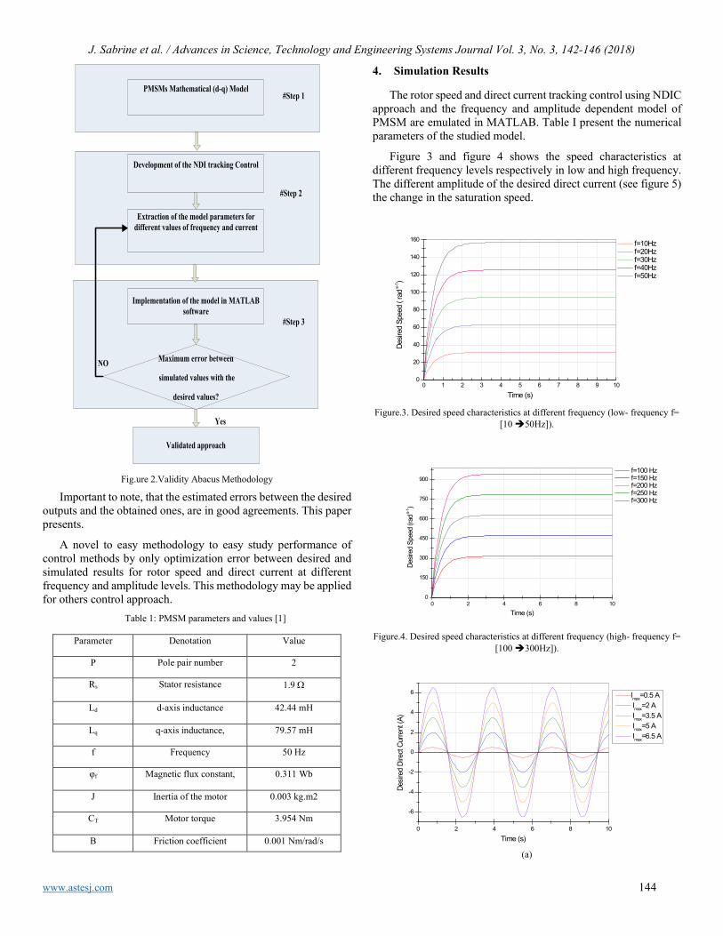
J. Sabrine et al. / Advances in Science, Technology and Engineering Systems Journal Vol. 3, No. 3, 142-146 (2018)
www.astesj.com 144
Validated approach
PMSMs Mathematical (d-q) Model
Development of the NDI tracking Control
Extraction of the model parameters for different values of frequency and current
Maximum error between
simulated values with the
desired values?
Implementation of the model in MATLAB software
#Step 1
#Step 2
#Step 3
Yes
NO
Fig.ure 2.Validity Abacus Methodology
Important to note, that the estimated errors between the desired outputs and the obtained ones, are in good agreements. This paper presents.
A novel to easy methodology to easy study performance of control methods by only optimization error between desired and simulated results for rotor speed and direct current at different frequency and amplitude levels. This methodology may be applied for others control approach.
Table 1: PMSM parameters and values [1]
Parameter Denotation Value
P Pole pair number 2
Rs Stator resistance 1.9 Ω
Ld d-axis inductance 42.44 mH
Lq q-axis inductance, 79.57 mH
f Frequency 50 Hz
φf Magnetic flux constant, 0.311 Wb
J Inertia of the motor 0.003 kg.m2
CT Motor torque 3.954 Nm
B Friction coefficient 0.001 Nm/rad/s
4. Simulation Results
The rotor speed and direct current tracking control using NDIC approach and the frequency and amplitude dependent model of PMSM are emulated in MATLAB. Table I present the numerical parameters of the studied model.
Figure 3 and figure 4 shows the speed characteristics at different frequency levels respectively in low and high frequency. The different amplitude of the desired direct current (see figure 5) the change in the saturation speed.
0 1 2 3 4 5 6 7 8 9 100
20
40
60
80
100
120
140
160 f=10Hz f=20Hz f=30Hz f=40Hz f=50Hz
Desir
ed S
peed
( ra
d s-1 )
Time (s)
Figure.3. Desired speed characteristics at different frequency (low- frequency f= [10 50Hz]).
0 2 4 6 8 100
150
300
450
600
750
900 f=100 Hz f=150 Hz f=200 Hz f=250 Hz f=300 Hz
Desir
ed S
peed
(rad
s-1 )
Time (s) Figure.4. Desired speed characteristics at different frequency (high- frequency f=
[100 300Hz]).
0 2 4 6 8 10
-6
-4
-2
0
2
4
6
Desir
ed D
irect
Curre
nt (A
)
Time (s)
Imax=0.5 A Imax=2 A Imax=3.5 A Imax=5 A Imax=6.5 A
(a)
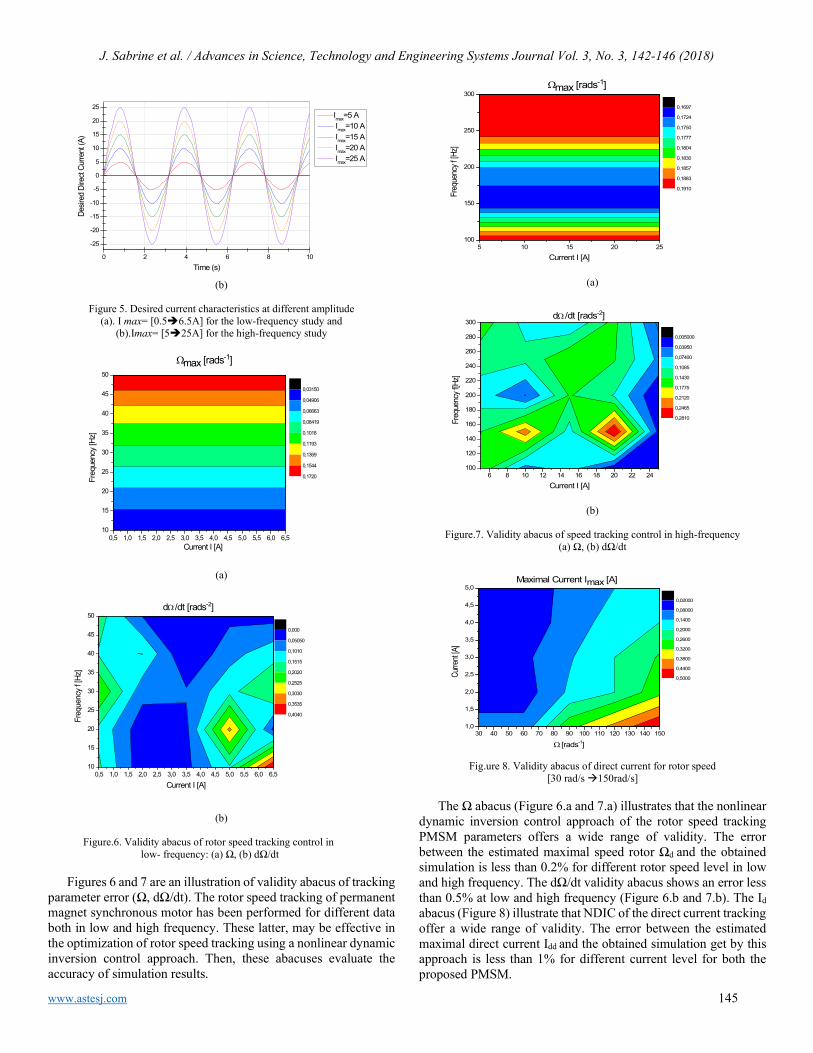
J. Sabrine et al. / Advances in Science, Technology and Engineering Systems Journal Vol. 3, No. 3, 142-146 (2018)
www.astesj.com 145
0 2 4 6 8 10
-25
-20
-15
-10
-5
0
5
10
15
20
25
Desir
ed D
irect
Curre
nt (A
)
Time (s)
Imax=5 A Imax=10 A Imax=15 A Imax=20 A Imax=25 A
(b)
Figure 5. Desired current characteristics at different amplitude (a). I max= [0.56.5A] for the low-frequency study and
(b).Imax= [525A] for the high-frequency study
0,5 1,0 1,5 2,0 2,5 3,0 3,5 4,0 4,5 5,0 5,5 6,0 6,510
15
20
25
30
35
40
45
50
Ωmax [rads-1]
Current I [A]
Freq
uenc
y [H
z]
0,03150
0,04906
0,06663
0,08419
0,1018
0,1193
0,1369
0,1544
0,1720
(a)
0,5 1,0 1,5 2,0 2,5 3,0 3,5 4,0 4,5 5,0 5,5 6,0 6,510
15
20
25
30
35
40
45
50dΩ /dt [rads-2]
Current I [A]
Freq
uenc
y f [H
z]
0,000
0,05050
0,1010
0,1515
0,2020
0,2525
0,3030
0,3535
0,4040
(b)
Figure.6. Validity abacus of rotor speed tracking control in low- frequency: (a) Ω, (b) dΩ/dt
Figures 6 and 7 are an illustration of validity abacus of tracking
parameter error (Ω, dΩ/dt). The rotor speed tracking of permanent magnet synchronous motor has been performed for different data both in low and high frequency. These latter, may be effective in the optimization of rotor speed tracking using a nonlinear dynamic inversion control approach. Then, these abacuses evaluate the accuracy of simulation results.
5 10 15 20 25100
150
200
250
300Ωmax [rads-1]
Current I [A]
Freq
uenc
y f [H
z]
0,1697
0,1724
0,1750
0,1777
0,1804
0,1830
0,1857
0,1883
0,1910
(a)
6 8 10 12 14 16 18 20 22 24100
120
140
160
180
200
220
240
260
280
300dΩ /dt [rads-2]
Current I [A]
Freq
uenc
y f[H
z]
0,005000
0,03950
0,07400
0,1085
0,1430
0,1775
0,2120
0,2465
0,2810
(b)
Figure.7. Validity abacus of speed tracking control in high-frequency (a) Ω, (b) dΩ/dt
30 40 50 60 70 80 90 100 110 120 130 140 1501,0
1,5
2,0
2,5
3,0
3,5
4,0
4,5
5,0Maximal Current Imax [A]
Ω [rads-1]
Curre
nt [A
]
0,02000
0,08000
0,1400
0,2000
0,2600
0,3200
0,3800
0,4400
0,5000
Fig.ure 8. Validity abacus of direct current for rotor speed
[30 rad/s 150rad/s]
The Ω abacus (Figure 6.a and 7.a) illustrates that the nonlinear dynamic inversion control approach of the rotor speed tracking PMSM parameters offers a wide range of validity. The error between the estimated maximal speed rotor Ωd and the obtained simulation is less than 0.2% for different rotor speed level in low and high frequency. The dΩ/dt validity abacus shows an error less than 0.5% at low and high frequency (Figure 6.b and 7.b). The Id abacus (Figure 8) illustrate that NDIC of the direct current tracking offer a wide range of validity. The error between the estimated maximal direct current Idd and the obtained simulation get by this approach is less than 1% for different current level for both the proposed PMSM.

J. Sabrine et al. / Advances in Science, Technology and Engineering Systems Journal Vol. 3, No. 3, 142-146 (2018)
www.astesj.com 146
The error is mainly due to the nonlinearity of PMSM model equations. Parameters error is less than 0.5% for different conditions. The obtained result proves the effectiveness of the control to ensure a rotor speed and direct current tracking. The abacus also helps the engineer to evaluate the simulation results accuracy of given devices. Various upshots and diverse validity abacus are satisfying so far. For a low and high frequency conditions, the proposed methodology is then adequate. Moreover, this model offers an efficient trade-off between ease and accuracy of speed tracking control study.
However, simulation errors cannot be avoided. They are calculated according to the rotor speed and the direct current at different frequency and amplitude. An error less than 0.5% is found for the permanent magnet synchronous motor model proposed. In addition to its precision, the suggested model has got a good convergence. Furthermore, the ease of use is one more advantage. It consists in both the facility of implementation using MATLAB and the simplicity in extracting PMSM model parameters. Moreover, the proposed algorithm, integrating the developed model, allows a better detection and adjustment of the outputs tracking control (using NDIC approach). In fact, in the case of poor design, the model replies routinely by detecting and tuning it. Nonlinear dynamic problems are, therefore, methodically avoided.
5. Conclusion
In this paper we have demonstrated that the PMSMs have the direct current and the rotor speed proportional to the frequency and amplitude. A mathematical nonlinear model of this motor is also proposed. The novel of this model is that it takes into account the design structure as well as frequency and amplitude parameters. The model validation is performed by comparing desired results with simulation. This model is run for a large range frequency and amplitude, and the simulation investigations show a good agreement with respect to the desired ones. These results are validated and. Future works concern the validation of the NDIC proposed approach associate the “Abacus Validity” approach others nonlinear systems.
References
[1] S. Jebri , K. Nouri and L. Bouslimi,” Study Performance of Speed Tracking Control with Frequency an Amplitude Dependence”IC_ASET, IEEE conferences Tunisia, Janvier 2017.
[2] S. Jebri ; H. Loussifi ; K. Nouri,” Two Mass Modeling and Nonlinear Dynamic Inversion of Motor Drive Systems”. Sciences and Techniques of Automatic Control and Computer Engineering, IEEE conf . July 2016.
[3] J. Hu, D. Dawson, and Y. Qian, “Position tracking control of an inductionmotor via partial state-feedback,” Automatica, vol. 31, pp. 989–1000, 1995.
[4] D. M. Dawson, Z. Qu, and J. J. Carroll, “Tracking control of rigid-link electrically-driven robot manipulators,” Int. J. Control, vol. 56, no. 5, pp. 991–1006, 1992.
[5] Z. Qu and J. Dorsey, “Robust tracking control of robots by a linear feedback law,” IEEE Trans. Autom. Control, vol. 36, no. 9, pp. 1081–1084, Sep. 1991.
[6] L. Benvenuti, M. D. Di Benedetto, and J. W. Grizzle, “Approximate output tracking for nonlinear nonminimum phase systems with an application to flight control,” Int. J. Robust Nonlinear Control, vol. 4, no. 3, pp. 397–414, 1994.
[7] F. Liao, J. L. Wang, and G. H. Yang, “Reliable robust flight tracking control: An LMI approach,” IEEE Trans. Control Syst. Technol., vol. 10, no. 1, pp. 76–89, Jan. 2002.
[8] N. C. Shieh, P. C. Tung, and C. L. Lin, “Robust output tracking control of a linear brushless DC motor with time-varying disturbances,” Inst. Elect. Eng. Proc. Elect. Power Appl., vol. 149, no. 1, pp. 39–45, 2002.
[9] G. Bartolini, A. Ferrara, and E. Usai, “Output tracking control of uncertain nonlinear second-order systems,” Automatica, vol. 33, no. 12, pp. 2203– 2212, 1997.
[10] X. Chen and C.-Y. Su, “Robust output tracking control for the systems with uncertainties,” Int. J. Syst. Sci., vol. 33, no. 4, pp. 247–257, 2002.
[11] P. Seiler and R. Sengupta, “An H∞ approach to networked control,” IEEE Trans. Autom. Control, vol. 50, no. 3, pp. 356–364, Mar. 2005.
[12] N. C. Shieh, K. Liang, and C. Mao, “Robust output tracking control of an uncertain linear system via a modified optimal linear-quadratic method,” J. Optim. Theory Appl., vol. 117, no. 3, pp. 649–659, 2003.
[13] D.Yang and J. Zhao,” H1 output tracking control for a class of switched LPV systems and its application to an aero-engine model” .International Journal of Robust and Nonlinear Control, September 2016.
[14] Y.Xin Li and G.Hong Yang,” Fuzzy Adaptive Output Feedback Fault-Tolerant Tracking Control of a Class of Uncertain Nonlinear Systems With Nonaffine Nonlinear Faults”IEEE Transactions on Fuzzy Systems .Vol.24, no: 1, Feb. 2016.
[15] B.A. Francis and W.M. “Wonham. The internal model principle of control theory”. Automatica, 12(5–E):457–465, 1976.
[16] M. Koç, J. Wang, T. Sun,” An Inverter Nonlinearity Independent Flux Observer for Direct Torque Controlled High Performance Interior Permanent Magnet Brushless AC Drives” IEEE Trans. Power Electron, Volume:PP , Issue: 99, February 2016.
[17] T. D. Do, S. Kwak, H. H. Choi, and J. W. Jung, “Suboptimal control scheme design for interior permanent magnet synchronous motors: An SDRE-based approach,” IEEE Trans. Power Electron., vol. 29, no. 6, pp. 3020–3031, Jun. 2014.
[18] K. Nouri, R. Dhaouadi, and N. B. Braiek, “A dynamic neural network based decoupled extended Kalman filter control applying to motor drive system,” 17ème Congrés Mondial IMACS, Calcul Scientifique, Mathématique Appliquées et Simulation, 2005
www.astesj.com 147
Automating Hostel Telephone Systems
Rohan Prabhu Murje, Bhaskar Rishab, Krishna Gopalrao Jorapur, MuccatiraThimmaiah Karumbaiah, Muddenahalli Nagendrappa Thippeswamy*
Department of Computer Science and Engineering, Nitte Meenakshi Institute of Technology, Yelahanka, Bengaluru, India-560064
A R T I C L E I N F O A B S T R A C T Article history: Received: 22 April, 2018 Accepted: 01 June, 2018 Online: 18 June, 2018
Residential schools can be a great place for students to learn and develop a different set of skills if the right environment is given to the child. Constant communication with parents can help the child to stay motivated and feel comfortable away from home, hence schools tend to provide various solutions to allow the student to communicate with their parents. The most common ways are using a coin booth or a common telephone. This process is very hectic as hundreds of student’s use this facility and these hundreds of calls have to be monitored individually so that no student would be getting into bad influence. In order to counter this problem, the entire process is automated in this paper. The proposed work also countered every small problem, such as unauthorized access, making calls to unauthorized numbers or exceeding the duration of call time allotted. In this paper, the digital lines are used to allow multiple calls and control these with the help of a Primary Rate Interface (PRI) card and an Electronic Private Automatic Branch Exchange (EPABX) system.
Keywords: Communication Digital lines EPABX systems PRI cards
1. Introduction
The business phone systems are more affordable due to the rise of cloud technology. This has transferred the telephone industry standards [1]. Automated phone systems can manage a high volume of callers and provide a method for filtering calls in a timely manner for small business [2]. The automation can save a substantial amount of time and money [2]. The number of parents opting for a residential school for their kids is on the rise, parents expect the right atmosphere for the students to develop. The schools do their best to provide the best facilities but often fail to monitor and control the usage of these facilities. One of the most common problems faced by the institutions is manually monitoring telephone facilities provided to the students. Parents often complain about students not contacting them on a regular basis. There are many other problems, for example, not everyone gets a chance to call; unlimited talk time calls are made to unauthorized people, and unauthorized access to the facility [3]. In order to counter all these problems, an automation solution which revolves around the automation of controlling and monitoring the calls that are made is proposed. It has pre-set numbers, pre-set call time, automated duration control and many other features which help in
reducing the amount of human intervention required. This is done by setting up a telephony network comprising of PRI lines, an interface card, an EPABX system and analogue phones. The back-end software controls the communication flow allowing us to manage and monitor every aspect, with minimal human intervention.
2. Related Work
The automatic voice responding system that uses the computer stored data is proposed in [4]. When a parent dialed the hostel phone number, they will get the answer in automatic stored voice form in this work. In [5], when a parent dialed the specified mobile number, they will get the student percentage attendance in voice form. Thus, parents can get their ward performance report from anywhere at any time.
As the rate at which residential institutions are growing, it is found that there is a greater need to automate the telephone calling system. It is necessary for a student to be in constant touch with his/her parents to remain motivated. The ability to quickly and efficiently manage hundreds of simultaneous calls is necessary in order to effectively manage the process [6].
ASTESJ
ISSN: 2415-6698
*Thippeswamy M.N., Department of Computer Science and Engineering, NitteMeenakshi Institute of Technology, Bengaluru, India-560064, 00919686329815, Email: [email protected]
Advances in Science, Technology and Engineering Systems Journal Vol. 3, No. 3, 147-151 (2018)
www.astesj.com
Special Issue on Multidisciplinary Sciences and Engineering
https://dx.doi.org/10.25046/aj030320

M.N. Thippeswamyet al. / Advances in Science, Technology and Engineering Systems Journal Vol. 3, No. 3, 147-151 (2018)
www.astesj.com 148
In this paper, different methods are explored that have been used over the years to provide this facility. In order to facilitate the calling process, one approach is to use coin phones. Here, each student can call their respective parents by inserting coins into the phone and making calls. This isn't feasible as there can be no control and monitoring of the system as the number of students increase. The other method that has been implemented is to allow only incoming calls using an analogue line connected to an analogue phone, the incoming call can be received by the student and the facility can be used.
The provision to block the call during the closed hours is provided, avoiding unauthorized access to the facilities. Though this system can address a lot of problems it cannot address some major issues like monitoring incoming calls, controlling the access and since analogue lines are used, only one call can be made/received at a time; hence, giving rise to a new problem of investment on analogue lines and cabling. Similar telephony systems are used for intra-communications within organizations, they use similar methods to allow intercom.
An EPABX system [7] with advance feature allows staff members to monitor the telephone usage and manage calls over a large organization. In this paper, analogue line is used instead of PRI lines [8]. Such systems are also used in a Call center where an Omni channel solution is required.
Compared to the existing system of telephone management, aproposed system uses PRI lines and a PRI interface card which is connected to the system, where the server controls the needs of the institution whereas generally there is no involvement of a local server providing this functionality. The systems are only used for intercom and other such facilities hence functions like pre-assigning call timings are not present.
3. Novel Contribution
This solution allows monitoring and control of a student’s telephone activities in the following ways: i. Pre-assigned call timings, the lines only open during this
time, hence avoiding unauthorized access. ii. Pre-assigned Phone numbers, Speed dial is set to these
telephone numbers, hence avoiding students calling other unknown numbers.
iii. Pre-assigned authorisation code, each student has an authorization code, which activates their account.
iv. Pre-assigned call duration, flexible call duration, admin can set call duration.
v. Automatic report generation, reports are sent every day to the administrator’s mail ID.
vi. Reports based on status of the call, reports based on call status, i.e. if a call is connected or dropped, can be generated.
vii. History of call log, complete call history of the student can be checked with few clicks.
viii. Flexible call charges, the management has the privileges to charge for the facility provided.
4. System Design
The system consists of different telephony hardware, this is put-together with backend software coded in asterisks and Hypertext Pre-processor (PHP). Also the system consists of database tables created in My Structured Query Language (MySQL). The main components of the system are PRI lines, PRI card, EPABX system and a local server. The telephone systems architecture consists of various hardware devices.
This software is built on controlling the PRI lines which can allow up to 30 simultaneous calls; this digital line is connected to the local server which consists of a PRI card. This card allows the PRI lines to be connected to the server (refer to Figure 7). In this paper, for the outgoing lines, an EPABX is used, which is a branch exchange device that helps to channel the outgoing calls. PRI line is also known as a T1 line, it is a multi-channel line. The feature of a call transferring and forwarding is another area enabling mobility of the users. Auto conferencing and automatic redialling of numbers found engaged on the first trial are some of the other advancements in the features of the EPBAX. An EPABX also checks the traffic and is also called as a switching system.
4.1. A brief functionality of each component:
• PRI Lines: PRI lines or primary interface lines are digital lines, which are a telecommunication standard that enables traditional phone lines to carry voice, data and video traffic, among others. A PRI line physically has only one line terminating on the interface but can allow us to send or receive 30 calls simultaneously. A PRI circuit consists of two pairs of copper lines terminating on a modem from a service provider premises to the customer premises. It uses multiplexing/de-multiplexing techniques to carry more than one channel in a single circuit. There are two common types of PRI lines used namely E1 and T1. The E1 type consists of 30 channels used mostly in India and Europe. Type T1 consists of 23/24 channels. T1 type is mostly used in the US. In this paper, the PRI E1 type is used.
• PRI interface cards: A PRI Card is used to connect PRI lines to IP PBX/ IP Telephony Server so that the entire Analog phones (extensions) can make outgoing calls or receive incoming calls using it. This is inserted in a local server in the Peripheral Component Interconnect (PCI) 3.3V/ PCI 5V/ PCI Express slots. These cards can have one slot, two slots or four slots.
• EPABX System:An EPABX system which is a branch exchange device that helps channeling the outgoing calls. It also controls the traffic and is also called a switching system.
• Analog Phones:The analogue phones allow speed dialing, hence it can serve the purpose of not allowing dialing of numbers and pre-assigning telephone numbers.
• Local Server:The local server consists of the software which controls communication. This software has the following modules.

M.N. Thippeswamyet al. / Advances in Science, Technology and Engineering Systems Journal Vol. 3, No. 3, 147-151 (2018)
www.astesj.com 149
o Student details:This module contains all the data of the students, it contains a database which stores the name, id, auth code and three pre-assigned telephone numbers.
o Verification module: This module contains the logic which verifies the authentication of the student. The number entered on the analog phone is matched with the authentication code present in the database; the student details present under the entered auth code is loaded onto the speed dial of the telephone.
o Balance account: Here all the students account balance is checked to see if an outgoing call can be made, if not then a voice over message is played alerting the user to recharge their account. After the call terminates the latest balance is updated to the database.
o Timings module: This module contains the assigned calling time. When the phone is accessed the timing, module is accessed and the time allotted is matched with the current time, if the there is a match between current time and opening time the user is allowed to use the facility else a voice over message alerts the user about the line being closed.
• System module:The system architecture consists of the above mentioned hardware. First, the PRI line is terminated at a Local Area Network (LAN) switch and a LAN cable is drawn to the local server which has a PRI card. In the local servers various modules are present. From the local server a branch exchange is used and then physical wiring is done to each room of the hostel which has a telephone.
5. Implementation and Results
The solution has been implemented using PHP as a front-end for the user interface and asterisks coding is used as a back-end to control the communication process. The implementation is performed by setting up telephony hardware as follows: the PRI line is terminated at the PRI interface card, which is present in our local server. In the local server the software to control and monitor the system is locally hosted. There are LAN connections between the local server and the EPABX system, from the EPABX system there are physical wiring to the hostel room where the phones are present.
This section shows the results that have been obtained from the implementation of this solution. The Figure (s) 1 – 6 are the results obtained for the proposed system.
The User Interface (UI) of the webpage is shown in Figure 1, which prompts the admin to login to the system. Upon successful login the admin can access different features present like the student details page depicted in Figure 2, here an authorization code is given to each student and their outgoing telephone numbers are assigned.
The next module is the timings module which is shown in Figure 3, here the admin can allot timings for outgoing and incoming calls for everyday of the week.
Figure 1: Shows the login page.
Figure 2: Represents the screen for entering student details.
Figure 3: Shows the call timing module.
Figure 4: Shows the recharge module of the software

M.N. Thippeswamyet al. / Advances in Science, Technology and Engineering Systems Journal Vol. 3, No. 3, 147-151 (2018)
www.astesj.com 150
To make an outgoing call the admin has to recharge the students account, this is depicted in Figure 4. Once an outgoing call is made and is disconnected the database is updated and reports are generated as seen in Figure 5 (a) and (b). These bills are generated based on the flexible call charges module, which allows the management to charge over the existing price, this module is depicted in Figure 6.
(a)
(b)
Figure 5: Shows the billing reports over a period of time.
6. Conclusion
This paper explains the working of a telephone system, which can help an institution tremendously by automating the control and monitoring of the process. This reduces the human effort that is required to monitor each and every call made by hundreds of students on a daily basis. This solution saves a lot of time and the effort required to monitor each and every call of hundreds of students. Reports are generated every day based on the status of the call, last call charge, total profits giving the management a bird's eye view of the process. Adding to the ease of control and monitoring it also gives the institution flexibility to charge per unit call for example, if the call provider charges Indian Rupees (INR) 1.0 per minute, the institution has options to charge INR 1.5 per minute, or INR 2.0 per minute or any amount they would want to. This solution would be beneficial for institutions with greater than hundred students who have taken residential facility from the school.
Figure 6: Shows the call charges module.
Conflict of Interest
The authors declare no conflict of interest.
References [1]. BT Prepare to Switch to an All IP Network by 2025, [online]
Available: http://www.sa1solutions.com/blog-bt-moving-ip-network.php. [2]. A. Smith, Automated Phone Systems: Identifying the Problem with yours
and how to turn the ship around, [Online] Available: https://www.theivrvoice.com/automated-phone-systems/
[3]. D. Kirk, How much is intelligent automation saving you, [online] Available:https://www.forbes.com.
[4]. I.J.Vinila, “Voice Response System for Parents of Hostel Students”, International Journal of Innovative Research in Computer and Communication Engineering, Vol. 4, Issue 5, May 2016.DOI: 10.15680/IJIRCCE.2016. 0405022
[5]. J. Patil and J. Barole, “Automatic Voice Responding System for Parents of Students”, International Journal of Innovative Research in Science, Engineering and Technology,Vol. 4, Issue 6, June 2015.
[6]. Hostel Telephone System, [online] Available:http://mipsoft.com/telephone.html
[7]. U. Nadeem. "The Functions of a PBX", [Online] Available: https://www.lifewire.com/functions-of-a-pbx-3426325
[8]. K. Rajesh, Telecom Trunk Lines: Difference Between Analog Line PRI/E1/T1 Digital-Line-GSM-Gateway, [online] Available: http://www.excitingip.com/2111/telecom-trunk-lines-difference-between-analog-line-prie1t1-digital-line-gsm-gateway/
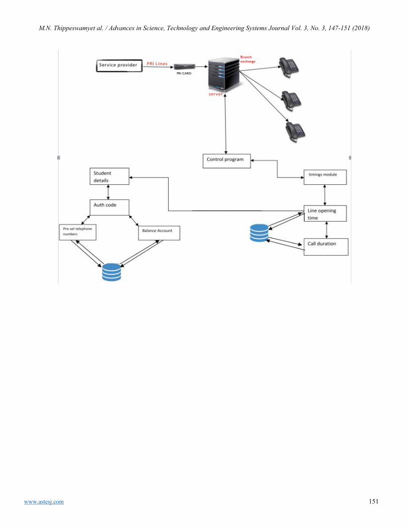
M.N. Thippeswamyet al. / Advances in Science, Technology and Engineering Systems Journal Vol. 3, No. 3, 147-151 (2018)
www.astesj.com 151
www.astesj.com 152
A Survey on Parallel Multicore Computing: Performance & Improvement
Ola Surakhi*, Mohammad Khanafseh, Sami Sarhan
University of Jordan, King Abdullah II School for Information Technology, Computer Science Department, 11942, Jordan
A R T I C L E I N F O A B S T R A C T Article history: Received: 18 May, 2018 Accepted: 11 June, 2018 Online: 26 June, 2018
Multicore processor combines two or more independent cores onto one integrated circuit. Although it offers a good performance in terms of the execution time, there are still many metrics such as number of cores, power, memory and more that effect on multicore performance and reduce it. This paper gives an overview about the evolution of the multicore architecture with a comparison between single, Dual and Quad. Then we summarized some of the recent related works implemented using multicore architecture and show the factors that have an effect on the performance of multicore parallel architecture based on their results. Finally, we covered some of the distributed parallel system concepts and present a comparison between them and the multiprocessor system characteristics.
Keywords: Distributed System Dual core Multicore Quad core
1. Introduction
Multicore is one of the parallel computing architectures which consists of two or more individual units (cores) that read and write CPU instruction on a single chip [1]. Multicore processor can run multiple instructions at the same time which increase speed of program execution and performance.
Original processor has one core, dual core processor has two cores, quad core processor has four cores, hexa core has six, octa core has eight, deca contains ten cores and so on. Gordon Moore predicted many that number of cores on the chip will be doubled once in every 18 months keeping in mind performance and cost which is known as Moore’s Law [2, 3, 4].
Each core in the multicore processor should not be necessarily faster than single core processor, but the overall performance of the multicore is better by handling many tasks in parallel [5].
The implementation of the multicore could be in different ways, homogeneous or heterogeneous depending on the application requirements. In the homogeneous architecture, all the cores are identical, and they break up the overall computations and run them in parallel to improve overall performance of the processor
[6]. The heterogenous cores have more than one type of cores, they are not identical, each core can handle different application. The later has better performance in terms of less power consumption as will be shown later [2].
In general, performance refers to the time needed to execute a given task, which in other words can be expressed as the frequency multiplied by the number of instructions executed per clock cycle as given in formula 1.
Performance = Instructions executed Per Clock Cycle * Frequency (1)
Both frequency and instruction per clock cycle are important to processor performance which can be increased by the increasing of these two factors. Unfortunately, high frequency has some implications on the power consumption.
The power problem is very important, while performance still desired as predictions from the ITRS Roadmap [7] predicting a need for 300x more performance by 2022 with a chip with 100x more cores than current one [8] as shown in Figure 1.
Power = Voltage2 * frequency (2)
The multicore processor designer should balance between power (which related to the voltage and frequency) and instructions per
ASTESJ
ISSN: 2415-6698
*Ola Surakhi, University of Jordan, Email: [email protected]
Advances in Science, Technology and Engineering Systems Journal Vol. 3, No. 3, 152-160 (2018)
www.astesj.com
https://dx.doi.org/10.25046/aj030321
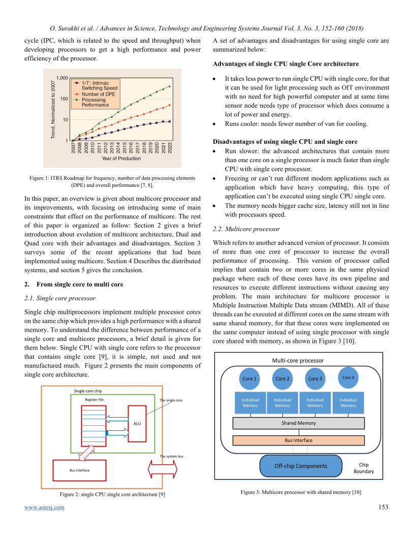
O. Surakhi et al. / Advances in Science, Technology and Engineering Systems Journal Vol. 3, No. 3, 152-160 (2018)
www.astesj.com 153
cycle (IPC, which is related to the speed and throughput) when developing processors to get a high performance and power efficiency of the processor.
Figure 1: ITRS Roadmap for frequency, number of data processing elements (DPE) and overall performance [7, 8].
In this paper, an overview is given about multicore processor and its improvements, with focusing on introducing some of main constraints that effect on the performance of multicore. The rest of this paper is organized as follow: Section 2 gives a brief introduction about evolution of multicore architecture, Dual and Quad core with their advantages and disadvantages. Section 3 surveys some of the recent applications that had been implemented using multicore. Section 4 Describes the distributed systems, and section 5 gives the conclusion.
2. From single core to multi core
2.1. Single core processor
Single chip multiprocessors implement multiple processor cores on the same chip which provides a high performance with a shared memory. To understand the difference between performance of a single core and multicore processors, a brief detail is given for them below. Single CPU with single core refers to the processor that contains single core [9], it is simple, not used and not manufactured much. Figure 2 presents the main components of single core architecture.
Bus interface
ALU
Register File
Single core chip
The single core
The system bus
Figure 2: single CPU single core architecture [9]
A set of advantages and disadvantages for using single core are summarized below:
Advantages of single CPU single Core architecture
• It takes less power to run single CPU with single core, for that it can be used for light processing such as OIT environment with no need for high powerful computer and at same time sensor node needs type of processor which does consume a lot of power and energy.
• Runs cooler: needs fewer number of van for cooling. Disadvantages of using single CPU and single core • Run slower: the advanced architectures that contain more
than one core on a single processor is much faster than single CPU with single core processor.
• Freezing or can’t run different modern applications such as application which have heavy computing, this type of application can’t be executed using single CPU single core.
• The memory needs bigger cache size, latency still not in line with processors speed.
2.2. Multicore processor
Which refers to another advanced version of processor. It consists of more than one core of processor to increase the overall performance of processing. This version of processor called implies that contain two or more cores in the same physical package where each of these cores have its own pipeline and resources to execute different instructions without causing any problem. The main architecture for multicore processor is Multiple Instruction Multiple Data stream (MIMD). All of these threads can be executed at different cores on the same stream with same shared memory, for that these cores were implemented on the same computer instead of using single processor with single core shared with memory, as shown in Figure 3 [10].
Off-chip Components
Bus Interface
Shared Memory
Core 1 Core 2 Core 3 Core 4
Multi-core processor
Chip Boundary
Individual Memory
Individual Memory
Individual Memory
Individual Memory
Figure 3: Multicore processor with shared memory [10]

O. Surakhi et al. / Advances in Science, Technology and Engineering Systems Journal Vol. 3, No. 3, 152-160 (2018)
www.astesj.com 154
Based on the idea of multicore processor which contains several processors ‘cores’ and packages inside single physical processor it increases overall performance of machine by allow more than one instruction to be executed at the same unit of time. As a result, simple multicore processors have better performance than complex single core processors [11].
Main advantages of multicore processor
• Allows cache coherency circuitry to operate at higher clock rate than is possible.
• Combining equivalent CPU on a single die can increase and improve the performance of cache snoop significantly.
• Many applications such as Customer Relationship Management, larger databases, Enterprise Resource Planning, e-commerce and virtualization can get a big benefit of multicore.
Multicore Challenges
There are a set of problems that arise when the multiple cores are implemented on a single chip [12]. Some of them are described below.
• Power and temperature problem, having multicores on the same chip will generates more heat and consumes more power than single CPU on a chip which can be solved by turning off unused cores to limit the amount of power.
• The need for enhancing in the interconnection network and bus network: managing the time required to handle memory requests to enhance speed and reducing communications between cores.
• The need of programming in parallel environment: the programmer needs to learn how to write a code for running a program on multicore instead of single core. As the total amount of cores on single chip is increasing as per Moore’s law, the quantity of parallelism should be doubled during development of the software.
• Denial of memory services, cores on the same chip share same the DRAM memory system and when multiple programs or branch of program run at multicore at the same time it will interfered with other memory access request.
• Multithread problem for multi core technology, starvation problem may occur if program developed to be run on a single thread while environment is multithread. This will cause a starvation where one thread is working, and others are idle.
• cache coherence problem, where different cores write and read on cache memory
There are different versions of multicore processor start from dual core technology [11], the CPU contains dual core, that is having two actual execution units on a single integrated circuit [9]. This refers to initial version of improvement of multicore technology
which has a lot of advantages and strongest point over old version of single core technology as it is easy for switching from single core processor to dual core processor with greater performance and low electrical costs comparing with single core technology. For everyone who can follow information technology industry knows that it is difficult and costs to increase the speed scale of clock rate for any processor, which means higher clock frequency and needs more heat. This will increase temperature of the chip which in turn needs to be cooling to reduce it [12]. In the dual core processor, the cores can execute programs in parallel which increase performance and at the same time the cores are not clocked at higher frequency which consumes more energy efficient. The design of the cores allows those who do not have any job (idle) to power down and when needed it can be powered up again which save power at all. The energy efficient performance for the dual core is shown in Figure 4, which shows how reduced clock frequency by five has more performance comparing with single core which consumes the same power but with maximum frequency.
Figure 4: Dual core processor at 20% reduced clock frequency effectively delivers 73% more performance while approximately using the same power as a single core processor at maximum frequency. [13,14]
Another advantage of using dual core processor rather than using single core processor refers to reducing the overall cost of processing, before dual core investment the users need to build dual processor units that had computing power same as single dual core processor with double cost of single computer with dual core.
Figure 5 presents the architecture of dual core processor that can execute different thread. Cores run without interference with each other.
As we have advantages for dual core technology there are disadvantages as follows
Some programs are not designed to run on more than one core, a single core processor will run such program faster than dual core. Running that programs on dual core will decrease performance.
If a single core CPU has a significantly greater clock speed than dual core CPU, then single core CPU can outperform dual core CPU.
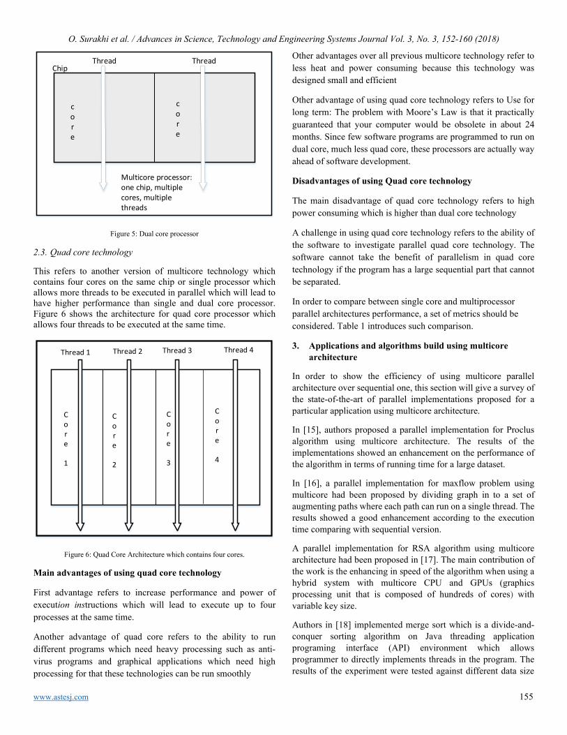
O. Surakhi et al. / Advances in Science, Technology and Engineering Systems Journal Vol. 3, No. 3, 152-160 (2018)
www.astesj.com 155
core
core
Thread ThreadChip
Multicore processor: one chip, multiple cores, multiple threads
Figure 5: Dual core processor
2.3. Quad core technology
This refers to another version of multicore technology which contains four cores on the same chip or single processor which allows more threads to be executed in parallel which will lead to have higher performance than single and dual core processor. Figure 6 shows the architecture for quad core processor which allows four threads to be executed at the same time.
Thread 1 Thread 2 Thread 3 Thread 4
Core
1
Core
2
Core 3
Core
4
Figure 6: Quad Core Architecture which contains four cores.
Main advantages of using quad core technology
First advantage refers to increase performance and power of execution instructions which will lead to execute up to four processes at the same time.
Another advantage of quad core refers to the ability to run different programs which need heavy processing such as anti-virus programs and graphical applications which need high processing for that these technologies can be run smoothly
Other advantages over all previous multicore technology refer to less heat and power consuming because this technology was designed small and efficient
Other advantage of using quad core technology refers to Use for long term: The problem with Moore’s Law is that it practically guaranteed that your computer would be obsolete in about 24 months. Since few software programs are programmed to run on dual core, much less quad core, these processors are actually way ahead of software development.
Disadvantages of using Quad core technology
The main disadvantage of quad core technology refers to high power consuming which is higher than dual core technology
A challenge in using quad core technology refers to the ability of the software to investigate parallel quad core technology. The software cannot take the benefit of parallelism in quad core technology if the program has a large sequential part that cannot be separated.
In order to compare between single core and multiprocessor parallel architectures performance, a set of metrics should be considered. Table 1 introduces such comparison.
3. Applications and algorithms build using multicore architecture
In order to show the efficiency of using multicore parallel architecture over sequential one, this section will give a survey of the state-of-the-art of parallel implementations proposed for a particular application using multicore architecture.
In [15], authors proposed a parallel implementation for Proclus algorithm using multicore architecture. The results of the implementations showed an enhancement on the performance of the algorithm in terms of running time for a large dataset.
In [16], a parallel implementation for maxflow problem using multicore had been proposed by dividing graph in to a set of augmenting paths where each path can run on a single thread. The results showed a good enhancement according to the execution time comparing with sequential version.
A parallel implementation for RSA algorithm using multicore architecture had been proposed in [17]. The main contribution of the work is the enhancing in speed of the algorithm when using a hybrid system with multicore CPU and GPUs (graphics processing unit that is composed of hundreds of cores) with variable key size.
Authors in [18] implemented merge sort which is a divide-and-conquer sorting algorithm on Java threading application programing interface (API) environment which allows programmer to directly implements threads in the program. The results of the experiment were tested against different data size

O. Surakhi et al. / Advances in Science, Technology and Engineering Systems Journal Vol. 3, No. 3, 152-160 (2018)
www.astesj.com 156
with different number of processors, and showed a good performance compared with sequential version.
In [19], authors implemented a parallel dynamic programming algorithm on multicore architecture in cognitive radio ad hoc networks (CRAHNs), the results showed a significant gain in terms of execution time.
In [20], authors implemented a parallel version of Breadth First Search (BFS) algorithm on multicore CPUs which show a great enhancing in the performance over current implementation as the size of the graph increases.
In [21], authors developed a parallel algorithm for the Euclidean Distance Map (EDM) which is a 2-D array and each element in it stores a value with its Euclidean distance between it and the nearest black pixel. The implementation was done on two parallel platforms multicore processors and GPU. The results showed an enhancing in the speed when using multicore platform for a specific input size 10000x10000 image size over GPU and sequential version
Authors in [22] implemented a sequential and parallel version of Viola-Joins face detection on multicore platform, the results that increasing number of cores for face detection in the image will increase speed up even though for big size image.
In [23], authors analyses the performance improvement of a parallel algorithm on multicore systems and show that a significant speed up achieved on multicore systems with the parallel algorithm.
In [24], authors mapped 4 implementations for Advanced Encryption Standard (AES) cipher algorithm on a fine-grained many-core system with eight cores online and six offline key expansions for a small design and 107 and 137 cores online and offline respectively for a largest design. The proposed design showed a higher throughput per unit of chip area and 8.2-18.1 times higher energy efficiency.
A summary for the results concluded from above mentioned works is shown in table2.
3.1. Discussion and Analysis
Many applications had been implemented in parallel using multicore platform to solve large and small problems as shown before. Some works implemented large algorithms in parallel such as Genetic [25], PSO [26], Tabu search algorithm [27] and more.
In order to evaluate the performance of such parallel implementations, there are some aspects that affect on the performance of the algorithms and need to be taken into consideration when evaluating parallel algorithm results. The main reason of using multicore architecture is to increase speed of the running program by dividing it into small pieces and run each piece independently on a single core. This means as many cores we have, will get faster execution! But it is not the proper
scenario that happens at real, adding more processors does not implies faster execution, as there are many other aspects that effect on the execution speed of the processor, like problem size, data input, communications between cores which is related to the interconnection network and computations needed on each core which is related to the problem. On the other hand, more cores on the processor need more power consumption which will reduce performance of the system which make companies like IBM, Intel to develop an enhanced version of the multicore chip that reduce power consumption.
The cache utilization in the multicore is shared between cores which increase cache access time, and this involve a higher percentage to access memory which in turn effects on the execution and performance. It can be reduced by implementing cache levels in a hierarchical design and including more cores in the processor which will decrease access time to the cache.
Degree of parallelism on each core allows instructions to run simultaneously to increase performance by increasing throughput. Pipelining is one of the techniques used to execute instructions in stages where number of instructions in the pipeline equal to number of stages. On the thread level, achieving parallelism is different here where program is divided into small pieces (threads) that run simultaneously in a synchronized manner such as Round Robin. The degree of parallelism could be decreased here when a starvation event happens where one thread take CPU time and keep all other waiting for execution which decrease performance.
Another problem that may happen here is Race condition when two threads need to access the same resource which also cause the system to get in to a deadlock.
Power, high power consumption causes the chip to have much heating and may be unreliable to do calculations and need much cooling. Many approaches had been used to reduce overheating in cores such as Stop & Go, Thread Migration(TM), and Dynamic Voltage and Frequency Scaling (DVFS) [28]. The main source that cause heating in the core is frequency which is not easy to optimize as it proportional to both performance and power.
Problem size, small input size leads to slowdown parallelism, because the communication will be high comparing to the computation done by each core. On the other hand, large input size may effect on the speed up and efficiency. As the problem size increases, the speed up and efficiency will increase to a specific limit depending on number of cores and cache size.
Many other aspects may effect on the performance of the multicore architecture, such as efficiency (keeping all cores busy during execution), architecture design issues, RAM size, parallel programming language, etc.
4. Distributed memory computers
It is a message-passing system where each processor has its own memory and all processors are connected by each other through a high-speed communication link. As each processor has its own
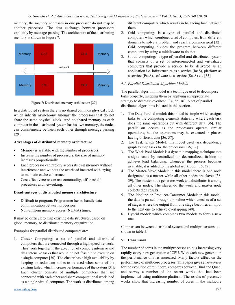
O. Surakhi et al. / Advances in Science, Technology and Engineering Systems Journal Vol. 3, No. 3, 152-160 (2018)
www.astesj.com 157
memory, the memory addresses in one processor do not map to another processor. The data exchange between processors explicitly by message-passing. The architecture of the distributing memory is shown in Figure 7.
Memory CPU CPU Memory
Memory MemoryCPU CPU
network
Figure 7: Distributed memory architecture [29]
In a distributed system there is no shared common physical clock which inherits asynchrony amongst the processors that do not share the same physical clock. And no shared memory as each computer in the distributed system has its own memory, the nodes can communicate between each other through message passing [29].
Advantages of distributed memory architecture
• Memory is scalable with the number of processors. • Increase the number of processors, the size of memory
increases proportionally. • Each processor can rapidly access its own memory without
interference and without the overhead incurred with trying to maintain cache coherence.
• Cost effectiveness: can use commodity, off-theshelf processors and networking.
Disadvantages of distributed memory architecture
• Difficult to program: Programmer has to handle data communication between processors.
• Non-uniform memory access (NUMA) times.
It may be difficult to map existing data structures, based on global memory, to distributed memory organization.
Examples for parallel distributed computers are:
1. Cluster Computing: a set of parallel and distributed computers that are connected through a high-speed network. They work together in the execution of compute intensive and data intensive tasks that would be not feasible to execute on a single computer [30]. The cluster has a high availability by keeping on redundant nodes to be used when some of the existing failed which increase performance of the system [31]. Each cluster consists of multiple computers that are connected with each other and share computational work load as a single virtual computer. The work is distributed among
different computers which results in balancing load between them.
2. Grid computing: is a type of parallel and distributed computers which combines a set of computers from different domains to solve a problem and reach a common goal [32]. Grid computing divides the program between different computers by using a middleware to do that.
3. Cloud computing: is type of parallel and distributed system that consists of a set of interconnected and virtualized computers that provide a service to be delivered as an application i.e. infrastructure as a service (IaaS), platform as a service (PaaS), software as a service (SaaS) etc [33].
4.1. Parallel Distributed Algorithm Models
The parallel algorithm model is a technique used to decompose tasks properly, mapping them by applying an appropriate strategy to decrease overhead [34, 35, 36]. A set of parallel distributed algorithms is listed in this section.
1. The Data-Parallel model: this model is simple which assigns tasks to the computing elements statically where each task does the same operations but with different data [36]. The parallelism occurs as the processors operate similar operations, but the operations may be executed in phases having different data [36, 37].
2. The Task Graph Model: this model used task dependency graph to map tasks to the processors [36, 37].
3. The Work Pool Model: is a dynamic mapping technique that assigns tasks by centralized or decentralized fashion to achieve load balancing. whenever the process becomes available, it is added to the global work pool [36, 37].
4. The Master-Slave Model: in this model there is one node designated as a master while all other nodes are slaves [38, 39]. The master node generates work and distributes it among all other nodes. The slaves do the work and master node collects then results.
5. The Pipeline or Producer-Consumer Model: in this model, the data is passed through a pipeline which consists of a set of stages where the output from one stage becomes an input to the next one to achieve overlapping [40].
6. Hybrid model: which combines two models to form a new one.
Comparison between distributed system and multiprocessors is shown in table 3.
5. Conclusion
The number of cores in the multiprocessor chip is increasing very rapidly every new generation of CPU. With each new generation the performance of it is increased. Many factors affect on the performance of multicore processor. This paper gives an overview for the evolution of multicore, compares between Dual and Quad, and survey a number of the recent works that had been implemented using multicore platform. The results of presented works show that increasing number of cores in the multicore

O. Surakhi et al. / Advances in Science, Technology and Engineering Systems Journal Vol. 3, No. 3, 152-160 (2018)
www.astesj.com 158
processors does not mean to get higher performance nor a speedup. The speed up of the system will be increased to a number of cores, where after that value the performance of the system will not be increased more.
Other factors have an influence on the efficiency and performance of multicore system such as RAM size, problem size, degree of parallelism, power and more as mentioned before.
A comparison between multiprocessor and distributed parallel system is made, it shows that distributed system is scalable, has a high degree of transparency but harder to be programmed, while multiprocessor system is not scalable, has a high degree of transparency and easy to be programmed.
As more applications and programs are developed to take advantage of multicore architecture, the designing and performance issues will be a challenge for most of the commercial industrial companies.
References [1] Lizhe Wang, Jie Tao, Gregor von Laszewski, Holger Marten. 2010,
“Multicores in Cloud Computing: Research Challenges for Applications”, Journal of Computers, Vol 5, No 6 (2010)
[2] Parkhurst, J., Darringer, J. & Grundmann, B. 2006, "From Single Core to Multi-Core: Preparing for a new exponential", Computer-Aided Design, 2006. ICCAD '06. IEEE/ACM International Conference on, pp. 67.
[3] Schaller, R.R. 1997, "Moore's law: past, present and future", Spectrum, IEEE, vol. 34, no. 6, pp. 52-59.
[4] Sodan, A., Machina, J., Deshmeh, A., Macnaughton, K. & Esbaugh, B. 2010, "Parallelism via Multithreaded and Multicore CPUs", Computer, vol. PP, no. 99, pp. 1-1.
[5] D. Geer, “Chip Makers Turn to Multicore Processors,” Computer, vol. 38, pp. 11-13, 05, 2005
[6] Blake, G., Dreslinski, R.G. & Mudge, T. 2009, "A survey of multicore processors", Signal Processing Magazine, IEEE, vol. 26, no. 6, pp. 26-37.
[7] International Technology Roadmap for Semiconductors, “International technology roadmap for semiconductors—System drivers,” 2007 [Online]. Available: http://www.itrs.net/Links/2007ITRS/2007_Chapters/2007_SystemDrivers.pdf
[8] Geoffrey Blake, Ronald G. Dreslinski, and Trevor Mudge, “A Survey of Multicore Processors “, IEEE SIGNAL PROCESSING MAGAZINE NOVEMBER 2009
[9] A. Vajda, Programming Many-Core Chips, Multi-core and Many-core Processor Architectures, DOI 10.1007/978-1-4419-9739-5_2, © Springer Science+Business Media, LLC 2011.
[10] IRakhee Chhibber, IIDr. R.B.Garg, Multicore Processor, Parallelism and Their Performance Analysis, International Journal of Advanced Research in Computer Science & Technology (IJARCST 2014).
[11] B. RAMAKRISHNA RAU AND JOSEPH A. FISHER, Instruction-Level Parallel Processing" History, Overview, and Perspective, Journal of Supercomputing, 7, 9-50 (1993) 1993 Kluwer Academic Publishers, Boston. Manufactured in The Netherlands
[12] Mark T. Chapman, “The Benefits of Dual-Core Processors in High-Performance Computing” , Supercharging your high-performance computing June 2005
[13] R. Ramanathan. Intel multi-core processors: Making the move to quad-core and beyond. Technology@Intel Magazine, Dec 2006.
[14] Balaji Venu, “Multi-core processors – An overview”, https://arxiv.org/ftp/arxiv/papers/1110/1110.3535.pdf
[15] M.Khanafseh, O.Surakhi & Y.Jaffal,“Parallel Implementation of "Fast algorithm for Project Clustering" on Multi Core Processor using Multi Threads”, Journal of Computer Science IJCSIS June 2017 Part I.pdf, (pp. 248-255)
[16] Mohammed Y. Alkhanafseh, Mohammad Qatawneh, Hussein A. al Ofeishat,” A Parallel Chemical Reaction Optimization Algorithm for MaxFlow Problem (pp. 19-32), Journal of Computer Science IJCSIS June 2017 Part I.pdf, Vol. 15 No. 6 JUN 2017
[17] Heba Mohammed Fadhil, Mohammed Issam Younis, “Parallelizing RSA Algorithm on Multicore CPU and GPU”, International Journal of Computer Applications (0975 – 8887) Volume 87 – No.6, February 2014
[18] Soha S. Zaghloul, PhD1, Laila M. AlShehri2, Maram F. AlJouie3, Nojood E. AlEissa4, Nourah A. AlMogheerah5, “Analytical and Experimental Performance Evaluation of Parallel Merge sort on Multicore System”, International Journal Of Engineering And Computer Science ISSN:2319-7242 Volume 6 Issue 6 June 2017, Page No. 21764-21773
[19] Badr Benmammar, Youcef Benmouna, Asma Amraoui, Francine Krief,” A Parallel implementation on a Multi-Core Architecture of a Dynamic Programming Algorithm applied in Cognitive Radio Ad hoc Networks”, International Journal of Communication Networks and Information Security (IJCNIS), Vol. 9, No. 2, August 2017
[20] Sungpack Hong , Tayo Oguntebi , Kunle Olukotun , “Efficient Parallel Graph Exploration on Multi-Core CPU and GPU” ,2011 International Conference on Parallel Architectures and Compilation Techniques.
[21] D.Man, K.Uda, H.Ueyama, Y.Ito, K.Nakano, “Implementation of Parallel Computation of Euclidean Distance Map in Multicore Processors and GPUs”, 2010 First International Conference on Networking and Computing
[22] Subhi A. Bahudaila and Adel Sallam M. Haider, “Performance Estimation of Parallel Face Detection Algorithm on Multi-Core Platforms”, Egyptian Computer Science Journal Vol. 40 No.2 May 2016, ISSN-1110-2586
[23] Sheela Kathavate, N.K. Srinath, “Efficiency of Parallel Algorithms on Multi Core Systems Using OpenMP”, International Journal of Advanced Research in Computer and Communication Engineering Vol. 3, Issue 10, October 2014
[24] M.Sambasiva Reddy, P.James Vijay, B.Murali Krishna, “Design and Implementation of Parallel AES Encryption Engines for Multi-Core Processor Arrays”, International Journal of Engineering Development and Research, 2014 IJEDR | Volume 2, Issue 4 | ISSN: 2321-9939
[25] A.J.Umbarkar,M.S.Joshi,Wei-ChiangHong, “Multithreaded Parallel Dual Population Genetic Algorithm (MPDPGA) for unconstrained function optimizations on multi-core system”, Applied Mathematics and Computation, Volume 243, 15 September 2014, Pages 936-949
[26] Abdelhak Bousbaci , Nadjet Kamel ,“A parallel sampling-PSO-multi-core-K-means algorithm using mapreduce”,Hybrid Intelligent Systems (HIS), 2014 14th International Conference on 14-16 Dec. 2014
[27] Ragnar Magnús Ragnarssona, Hlynur Stefánssona, Eyjólfur Ingi Ásgeirssona, “Meta-Heuristics in Multi-Core Environments”, Systems Engineering Procedia 1 (2011) 457–464
[28] Ransford Hyman Jr, “Performance Issues on Multi-Core Processors”. [29] Jelica ProtiC, Milo TomageviC, Veljko MilutinoviC, “A Survey of
Distributed Shared Memory Systems”, Proceedings of the 28th Annual Hawaii International Conference on System Sciences - 1995
[30] Brijender Kahanwal, Tejinder Pal Singh, “The Distributed Computing Paradigms: P2P, Grid, Cluster, Cloud, and Jungle”, International Journal of Latest Research in Science and Technology ISSN (Online):2278-5299 Vol.1,Issue 2 :Page No.183-187 ,July-August(2012)
[31] “Cluster Computing”, http://en.wikipedia.org/wiki/Cluster computing. [32] K. Krauter, R. Buyya, and M. Maheswaran, “A Taxonomy and Survey of
Grid Resource Management Systems for Distributed Computing”, Jr. of Software Practice and Experience, 32,(2), pp. 135-164, 2002.
[33] Seyyed Mohsen Hashemi, Amid Khatibi Bardsiri (MAY 2012) “Cloud Computing Vs. Grid Computing”, ARPN Journal of Systems and Software, VOL. 2, NO.5
[34] B Barney, Introduction to Parallel Computing, Retrieved from Lawrence Livermore National Laboratory: http://computing .IInl.govt/utorials/parallel comp/,2010
[35] I Ahmad, A Gafoor and G C Fox, Hierarchical Scheduling of Dynamic Parallel Computations on Hypercube Multicomputers, Journal of Parallel and Distributed Computing, 20, 19943, 17-329.
[36] A Grama, A Gupta, G Karypis and V Kumar, Introduction to Parallel Computing, Publisher: Addison Wesley, uJanuary 2003
[37] K Cristoph and K Jorg, Modles for Paralel Computing: Review and Perspectives, PARSMiteilungen 24, Dec. 2007, 13-29
[38] A Clamatis and A Corana, Performance Analysis of Task based Algorithms on Heterogeneous systems with message passing, In Proceedings Recent Advances in Parallel Virtual Machine and Message Passing Interface, 5th European PVM/MPI User’s Group Meeting, Sept 1998.
[39] D Gelernter, M R Jourdenais and Kaminsky, Piranha Scheduling: Strategies and Their Implementation, International Journal of Parallel Programming, Feb 1995, 23(1): 5-33
[40] S H Bokhari, Partitioning Problems in Parallel, Pipelined, and Distributed Computing, IEEE Transactions on Computers, January 1988, 37:8-57

O. Surakhi et al. / Advances in Science, Technology and Engineering Systems Journal Vol. 3, No. 3, 152-160 (2018)
www.astesj.com 159
Table 1: A comparison between Single core, Dual core and Quad core Difference criteria Single core Dual Core Quad Core Description Use Single Core processor
to process different operations, this type of processor used by many devices such as smartphones
Processor with two cores on a single integrated circuit, which acts as a single unit, each of these cores have a separated controller and cache which allow them to work faster.
Contains two dual core processor on a single chip, with all its property and performance.
Execution speed Runs slower based on sequential execution for tasks.
Perform tasks faster based on parallel execution for impendent tasks
One of the best systems of multi-tasking, based on that it can execute a lot of tasks while other systems start up.
Multi task possibility Possible by pre-emptive round robin scheduling
Possible Possible
Power usage Less Power Usage, to execute single core process processor take less power if comparing with others.
Wastes power more than single core because it need more cooling
Low battery life and can’t be used for battery powered devices.
Application support Word processing, surfing, browsing checking email, mobile applications, sensor applications and IOT devices
Flash-enabled web browsing.
Voice GPS systems and multi-player and video editing.
Parallel execution for tasks
Can execute other process while still work on first task but this depends on the application
It has two complete two execution units which can execute different instructions completely if there is no dependency
This architecture consists of two separated dual core which can execute double of what dual core can execute.
Need for cooling Using less power which produces less heat which means that no need for advance cooling
Need for cooling but not much cooling
Need for advance cooling which consume a lot of energy
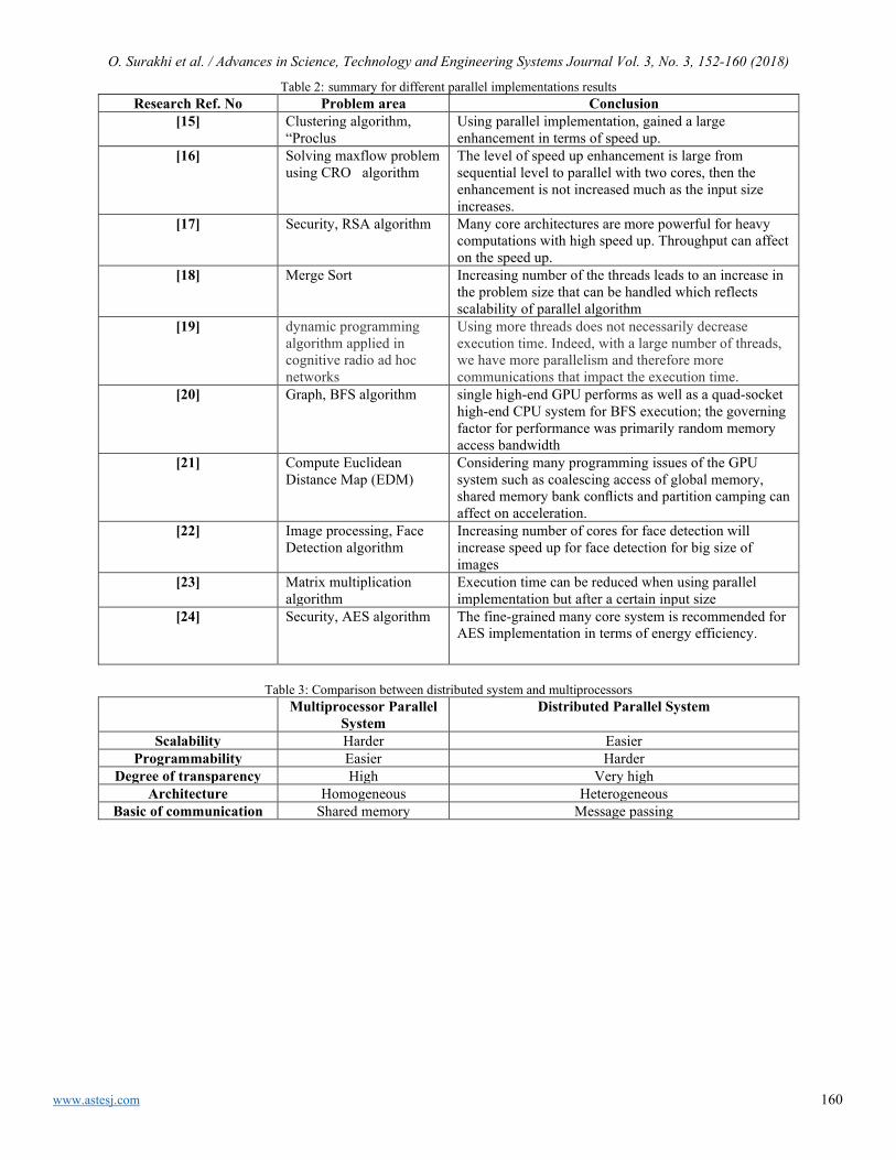
O. Surakhi et al. / Advances in Science, Technology and Engineering Systems Journal Vol. 3, No. 3, 152-160 (2018)
www.astesj.com 160
Table 2: summary for different parallel implementations results Research Ref. No Problem area Conclusion
[15] Clustering algorithm, “Proclus
Using parallel implementation, gained a large enhancement in terms of speed up.
[16] Solving maxflow problem using CRO algorithm
The level of speed up enhancement is large from sequential level to parallel with two cores, then the enhancement is not increased much as the input size increases.
[17] Security, RSA algorithm Many core architectures are more powerful for heavy computations with high speed up. Throughput can affect on the speed up.
[18] Merge Sort Increasing number of the threads leads to an increase in the problem size that can be handled which reflects scalability of parallel algorithm
[19] dynamic programming algorithm applied in cognitive radio ad hoc networks
Using more threads does not necessarily decrease execution time. Indeed, with a large number of threads, we have more parallelism and therefore more communications that impact the execution time.
[20] Graph, BFS algorithm single high-end GPU performs as well as a quad-socket high-end CPU system for BFS execution; the governing factor for performance was primarily random memory access bandwidth
[21] Compute Euclidean Distance Map (EDM)
Considering many programming issues of the GPU system such as coalescing access of global memory, shared memory bank conflicts and partition camping can affect on acceleration.
[22] Image processing, Face Detection algorithm
Increasing number of cores for face detection will increase speed up for face detection for big size of images
[23] Matrix multiplication algorithm
Execution time can be reduced when using parallel implementation but after a certain input size
[24] Security, AES algorithm The fine-grained many core system is recommended for AES implementation in terms of energy efficiency.
Table 3: Comparison between distributed system and multiprocessors
Multiprocessor Parallel System
Distributed Parallel System
Scalability Harder Easier Programmability Easier Harder
Degree of transparency High Very high Architecture Homogeneous Heterogeneous
Basic of communication Shared memory Message passing

www.astesj.com 161
Fuzzy Logic Based Selective Harmonic Elimination for Single Phase Inverters
Zeynep Bala Duranay *, Hanifi Guldemir
Firat University, Technology Faculty, Electrical-Electronics Engineering, 23119, Elazig, Turkey
A R T I C L E I N F O A B S T R A C T Article history: Received: 04 May, 2018 Accepted: 22 June, 2018 Online: 26 June, 2018
A selective harmonic elimination system using fuzzy logic for the elimination of high magnitude harmonics with frequencies close to fundamental in the output voltage of single phase inverters is presented. The system does not require look up tables for storage of the data as in traditional harmonic elimination methods. The input of the fuzzy system is the modulation index values. The output of the fuzzy system provides the switching angles which are further used to construct the switching signal for the switches in the inverter. With this fuzzy logic based selective harmonic elimination system, predetermined dominant low rank harmonics are successfully eliminated. Simulations are made with Matlab/Simulink and the results are presented which show the effectiveness of the presented harmonic elimination system.
Keywords: Fuzzy logic Harmonic analysis Harmonic elimination Inverter Pulse width modulation
1. Introduction
This paper is an extension of work originally presented in 2017 XXVI International Scientific Conference Electronics (ET) [1]. The use of power electronic devices in industrial and consumer applications has resulted nonlinear sinusoidal voltage and current to be drawn from the source. These nonlinear loads distort the sinusoidal form of the alternating current which results harmonics in the electrical system. The power quality of an electrical system is determined by its harmonic content. These harmonics may be classified as voltage or current harmonics. These harmonics can occur either supply or load. Current harmonics are generated by the harmonics of the source voltage which are depend on the type of the load connected to supply which can be resistive, inductive or capacitive. Nonlinear operation of power converters feeding loads cause harmonics to be produced in the load. These harmonics cause extra heating in transformers and motors.
Supply harmonics are produced by the source with nonsinusoidal voltage or current waveforms. Supply harmonics produce extra loss, cause electromagnetic interference and ripple torques in ac motors [2].
A pulse width modulated inverter which converts dc source to ac supply with desired voltage and frequency is used in many electrical devices such as uninterruptable power supplies (ups), switch mode power supplies(smps), machine drives. However, it
is seen that the output voltage of the inverters has higher harmonic content.
Among others [3-4], the pulse width modulation (pwm) technique is one of the commonly applied modulation strategy which controls the amplitude and frequency of the voltage produced by inverters.
Pwm techniques have been widely used in converter and inverter control where the switches are switched on and off number of times in each period. The controlled output signal is obtained by changing the width of these pulses.
Different pwm methods have been developed to suppress harmonics in converters and inverters. These techniques can be summarized as
• Carrieer based pwm
• Space vector pwm
• Third harmonic injection pwm
• Selective harmonic elimination pwm
One of the effective pwm method for the suppression of harmonics from the spectrum of the inverter output voltage is the selective harmonic elimination (SHE) technique [5-7].
The voltage or current waveform is represented by Fourier series expansion in SHE technique. The coefficients of the harmonics those will be eliminated are set to zero and the
ASTESJ
ISSN: 2415-6698
*Zeynep Bala Duranay, Firat University Electrical-Electronics Engineering 23119 Elazig Turkey, [email protected]
Advances in Science, Technology and Engineering Systems Journal Vol. 3, No. 3, 161-167 (2018)
www.astesj.com
Special Issue on Multidisciplinary Sciences and Engineering
https://dx.doi.org/10.25046/aj030322
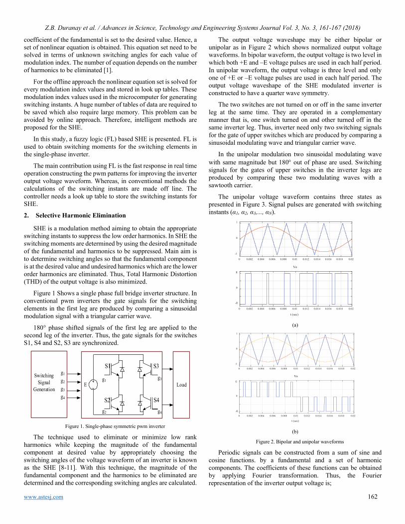
Z.B. Duranay et al. / Advances in Science, Technology and Engineering Systems Journal Vol. 3, No. 3, 161-167 (2018)
www.astesj.com 162
coefficient of the fundamental is set to the desired value. Hence, a set of nonlinear equation is obtained. This equation set need to be solved in terms of unknown switching angles for each value of modulation index. The number of equation depends on the number of harmonics to be eliminated [1].
For the offline approach the nonlinear equation set is solved for every modulation index values and stored in look up tables. These modulation index values used in the microcomputer for generating switching instants. A huge number of tables of data are required to be saved which also require large memory. This problem can be avoided by online approach. Therefore, intelligent methods are proposed for the SHE.
In this study, a fuzzy logic (FL) based SHE is presented. FL is used to obtain switching moments for the switching elements in the single-phase inverter.
The main contribution using FL is the fast response in real time operation constructing the pwm patterns for improving the inverter output voltage waveform. Whereas, in conventional methods the calculations of the switching instants are made off line. The controller needs a look up table to store the switching instants for SHE.
2. Selective Harmonic Elimination
SHE is a modulation method aiming to obtain the appropriate switching instants to suppress the low order harmonics. In SHE the switching moments are determined by using the desired magnitude of the fundamental and harmonics to be suppressed. Main aim is to determine switching angles so that the fundamental component is at the desired value and undesired harmonics which are the lower order harmonics are eliminated. Thus, Total Harmonic Distortion (THD) of the output voltage is also minimized.
Figure 1 Shows a single phase full bridge inverter structure. In conventional pwm inverters the gate signals for the switching elements in the first leg are produced by comparing a sinusoidal modulation signal with a triangular carrier wave.
180° phase shifted signals of the first leg are applied to the second leg of the inverter. Thus, the gate signals for the switches S1, S4 and S2, S3 are synchronized.
E
S3S1
S2 S4
g1
g2
g3
g4
LoadSwitching
SignalGeneration
g1
g2
g3
g4
Figure 1. Single-phase symmetric pwm inverter
The technique used to eliminate or minimize low rank harmonics while keeping the magnitude of the fundamental component at desired value by appropriately choosing the switching angles of the voltage waveform of an inverter is known as the SHE [8-11]. With this technique, the magnitude of the fundamental component and the harmonics to be eliminated are determined and the corresponding switching angles are calculated.
The output voltage waveshape may be either bipolar or unipolar as in Figure 2 which shows normalized output voltage waveforms. In bipolar waveform, the output voltage is two level in which both +E and –E voltage pulses are used in each half period. In unipolar waveform, the output voltage is three level and only one of +E or –E voltage pulses are used in each half period. The output voltage waveshape of the SHE modulated inverter is constructed to have a quarter wave symmetry.
The two switches are not turned on or off in the same inverter leg at the same time. They are operated in a complementary manner that is, one switch turned on and other turned off in the same inverter leg. Thus, inverter need only two switching signals for the gate of upper switches which are produced by comparing a sinusoidal modulating wave and triangular carrier wave.
In the unipolar modulation two sinusoidal modulating wave with same magnitude but 180° out of phase are used. Switching signals for the gates of upper switches in the inverter legs are produced by comparing these two modulating waves with a sawtooth carrier.
The unipolar voltage waveform contains three states as presented in Figure 3. Signal pulses are generated with switching instants (α1, α2, α3,..., αN).
(a)
(b)
Figure 2. Bipolar and unipolar waveforms
Periodic signals can be constructed from a sum of sine and cosine functions. by a fundamental and a set of harmonic components. The coefficients of these functions can be obtained by applying Fourier transformation. Thus, the Fourier representation of the inverter output voltage is;
0 0.002 0.004 0.006 0.008 0.01 0.012 0.014 0.016 0.018 0.02
-1
0
1
0 0.002 0.004 0.006 0.008 0.01 0.012 0.014 0.016 0.018 0.02
t (sec)
0
Vo
-E
E
0 0.002 0.004 0.006 0.008 0.01 0.012 0.014 0.016 0.018 0.02
-1
0
1
0 0.002 0.004 0.006 0.008 0.01 0.012 0.014 0.016 0.018 0.02
t (sec)
0
Vo
E
-E

Z.B. Duranay et al. / Advances in Science, Technology and Engineering Systems Journal Vol. 3, No. 3, 161-167 (2018)
www.astesj.com 163
𝑉𝑉0 = 𝑎𝑎0 + ∑ 𝐴𝐴𝑛𝑛∞𝑛𝑛=1 𝑐𝑐𝑐𝑐𝑐𝑐(𝑛𝑛𝑛𝑛𝑛𝑛) + ∑ 𝐵𝐵𝑛𝑛∞
𝑛𝑛=1 𝑐𝑐𝑠𝑠𝑛𝑛(𝑛𝑛𝑛𝑛𝑛𝑛) (1)
where
𝑎𝑎0 = 12𝜋𝜋 ∫ 𝑉𝑉0(𝑛𝑛)𝑑𝑑𝑛𝑛2𝜋𝜋
0 (2)
𝐴𝐴𝑛𝑛 = 4𝐸𝐸𝜋𝜋𝑛𝑛
[−∑ (−1)𝑛𝑛𝑁𝑁𝑖𝑖=1 𝑐𝑐𝑠𝑠𝑛𝑛𝑛𝑛𝛼𝛼𝑖𝑖] (3)
Due to odd and quarter wave symmetry, even harmonics do not exist in the output voltage waveform and Fourier coefficients An and a0 are equal to zero [12].
α1
α2
αΝ
π/2
π−α
Ν
π−α
2
π−α
1
3π/2
π−α
Ν
π−α
2
π−α
1
π+α
1
π+α
2
π+α
Ν
2π
V0
E
-E
. . . . . .
. . . . . .
Fundamental
Figure 3. Inverter output voltage
Only the odd harmonics with sine components exist in the output voltage, thus (1) can be written as:
𝑉𝑉0 = ∑ 𝐵𝐵𝑛𝑛∞𝑛𝑛=1 𝑐𝑐𝑠𝑠𝑛𝑛(𝑛𝑛𝑛𝑛𝑛𝑛) 𝑛𝑛 = 1, 3, 5, … ,∞) (4)
where Bn is the amplitude of the nth harmonic voltage and is given by
𝐵𝐵𝑛𝑛 = 4𝐸𝐸𝜋𝜋𝑛𝑛∑ [−(−1)𝑛𝑛𝑁𝑁𝑖𝑖=1 𝑐𝑐𝑐𝑐𝑐𝑐 (𝑛𝑛𝛼𝛼𝑖𝑖)] (5)
and
0 < 𝛼𝛼1 < 𝛼𝛼2 < ⋯ < 𝛼𝛼𝑁𝑁 < 𝜋𝜋2 (6)
E is the dc bus voltage, ω=2πf1, f1 is the frequency of the fundamental component and N is the number of switching angles per quarter cycle.
The goal of the SHE method is to determine the switching angles α1, α2,…,αN in the inverter output voltage so that the amplitudes of the harmonic components B3, B5,…,BN-1 are zero and the fundamental component B1 equal to the desired amplitude.
Applying the constraints defined above and using (5), the following equation set can be obtained
⎣⎢⎢⎢⎡𝐵𝐵1𝐵𝐵3𝐵𝐵5⋮𝐵𝐵𝑛𝑛⎦⎥⎥⎥⎤
=
⎣⎢⎢⎢⎡ cos(𝛼𝛼1) −cos(𝛼𝛼2) ⋯ ± cos(𝛼𝛼𝑛𝑛) cos(3𝛼𝛼1)cos(5𝛼𝛼1)
− cos(3𝛼𝛼2)− cos(5𝛼𝛼2)
⋯⋯
± cos(3𝛼𝛼𝑛𝑛)± cos(5𝛼𝛼𝑛𝑛)
⋮cos(𝑛𝑛𝛼𝛼1)
⋮−cos(𝑛𝑛𝛼𝛼2)
⋮⋯ ± cos(𝑛𝑛𝛼𝛼𝑛𝑛)⎦
⎥⎥⎥⎤
=
⎣⎢⎢⎢⎡4𝐸𝐸 𝜋𝜋⁄
00⋮0 ⎦
⎥⎥⎥⎤ (7)
where n=1, 3, 5… N and N is the number of pulse in every quarter cycle.
The first equation in this equation set is used to adjust the amplitude of the fundamental and the others are used for the suppression of harmonics.
Thus, N-1 harmonics can be eliminated by calculating N switching angles [13, 14].
If the amplitude of the fundamental component B1 need to be adjusted then
𝐵𝐵1 = 𝑚𝑚4𝐸𝐸𝜋𝜋
(8)
where m is the modulation index which is the ratio of fundamental to the maximum obtainable fundamental.
The set of nonlinear equations in (7) need to be solved using numerical methods [15, 16] to obtain the switching instants.
In this study, Newton-Raphson (NR) method, as in [17, 18] which is developed for the solution of nonlinear equations is used to solve the nonlinear equation set given in (7). The switching angles are obtained by a program developed in Matlab for solving the nonlinear algebraic transcendental equations. Solution obtained from NR is used to setup the input/output membership functions in the fuzzy controller. Table 1 lists the angles for different m values for 10 harmonics to be eliminated.
Table 1. Switching angles corresponding to modulation index
m 0.1 0.2 0.4 0.6 0.8 1 α1 14.793 14.578 14.109 13.587 12.997 12.093
α2 15.181 15.352 15.636 15.821 15.854 15.296
α3 29.607 29.195 28.298 27.295 26.138 24.287
α4 30.357 30.691 31.261 31.655 31.749 30.556
α5 44.450 43.876 42.633 41.232 39.571 36.681
α6 45.511 45.996 46.853 47.500 47.732 45.735
α7 59.335 58.645 57.170 55.509 53.478 49.375
α8 60.635 61.246 62.379 63.337 63.881 60.767
α9 74.268 73.518 71.947 70.215 68.082 62.457
α10 75.718 76.422 77.791 79.092 80.213 75.560
α11 89.249 88.495 86.967 85.372 83.569 75.996
3. Fuzzy Logic Controller
FL is a theory used to represent uncertain information. It is first formulated by Lotfi Zadeh in 1960s [19]. FL is a crisp model of a system. It uses rule base to convert crisp inputs to corresponding crisp output values. This technique has been successful especially when rules cannot be perfectly known and can be used in situations where the device cannot be described by mathematical models. Decision making capability of fuzzy logic controller (FLC) is achieved by human behavior.
Fuzzy systems provide a quick and approximate solution for complex systems which do not have exact mathematical model [20]. The real life and industrial applications of FL can be found in [21-23].
FL is realized in four steps which are the determination of fuzzy sets, definition of membership functions, construction of rules and defuzzification as shown in Figure 4.

Z.B. Duranay et al. / Advances in Science, Technology and Engineering Systems Journal Vol. 3, No. 3, 161-167 (2018)
www.astesj.com 164
Fuzzification is the first step in FL system. In this step, crisp input values are measured and converted to suitable linguistic variables using expert’s knowledge and experience.
The second step is the development of rule data base which defines the principles of the controller in terms of the relationship between input and output. This step is known as Inference Engine and supplies the required information for control rules
The last step is the conversion of the fuzzy outputs to control action which is called as Defuzzification which provides an actual control action.
Fuzzy Inference System Defuzzification
Fuzzification
Data Base
Input
Control Action
Decision
Figure 4. Block diagram of the FL system
Two types of fuzzy inference system which are Mamdami-type and Sugeno-type can be used. These types are differ according to the determination of outputs. Sugeno-type inference produces an output that is either constant or linear mathematical expression.
Due to the use of numerical values at the input and outputs, Sugeno-type fuzzy system is used for the implementation of the input and output data. Figure 5 shows the input membership function.
The outputs of the fuzzy control system which are the switching angles are computed for a given input which is the modulation index as shown in Figure 6.
The input data are represented by 10 membership functions. Because 10 harmonics are going to be eliminated which requires 11 switching angle thus 11 outputs each has 50 constant type membership functions for the representation of output data are used in the fuzzy system. Totally 104 rules are used between the input membership functions and output membership functions.
Figure 5. Input membership function
Figure 6. Fuzzy system
4. Switching Signal Generation
The switching instants corresponding to each m are determined by solving the nonlinear equation set for every value of m. These m and switching angles values are used in FLC. The m is used as the input to FLC and the output of this controller is the corresponding switching angles.
The switching instants obtained from FLC for a given m value are used as inputs for generation of switching signals.
As in traditional pwm methods, the switching angles produced by FL are compared with a timer content with specified frequency to produce pwm switching signals.
Figure 7 shows the generation of the switching signals for elimination of three harmonics i.e. N=4. In this system the switching angles are α1=23.56º, α2=39.26º, α3=48.96º and α4=89.20º. If the frequency is 50 Hz, the switching signals are obtained by comparing the timer content which is the triangular wave with the switching angles. Because of the symmetry, only the half period is given in this figure.
The Simulink block used to obtain the switching signals is shown in Figure 8.
The signals are constructed by comparison of switching instants with the sawtooth carrier and given to inverter switches as in Figure 9. Figure 10 represents a switching signals generation of 3 harmonic elimination.
180
135
90
45
T/2T/4
23.5
6
39.2
648
.96
89.2
090
.80
131.
0414
0.74
156.
44
S1Sw
itchi
ng S
igna
l
Switc
hing
Ang
le
23.5639.2648.96
89.2090.80
131.04140.74156.44
Switching Angle Figure 7. Switching signal generation for elimination of three harmonics
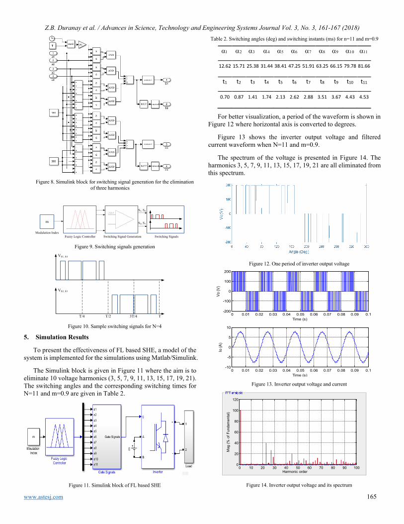
Z.B. Duranay et al. / Advances in Science, Technology and Engineering Systems Journal Vol. 3, No. 3, 161-167 (2018)
www.astesj.com 165
Figure 8. Simulink block for switching signal generation for the elimination
of three harmonics
m
Fuzzy Logic Controller Switching Signal Generation Switching SignalsModulation Index
S1, S4
S2, S3
Figure 9. Switching signals generation
3T/4 TT/4
VS2, S3
VS1, S4
T/2 Figure 10. Sample switching signals for N=4
5. Simulation Results
To present the effectiveness of FL based SHE, a model of the system is implemented for the simulations using Matlab/Simulink.
The Simulink block is given in Figure 11 where the aim is to eliminate 10 voltage harmonics (3, 5, 7, 9, 11, 13, 15, 17, 19, 21). The switching angles and the corresponding switching times for N=11 and m=0.9 are given in Table 2.
Figure 11. Simulink block of FL based SHE
Table 2. Switching angles (deg) and switching instants (ms) for n=11 and m=0.9
α1 α2 α3 α4 α5 α6 α7 α8 α9 α10 α11
12.62 15.71 25.38 31.44 38.41 47.25 51.91 63.25 66.15 79.78 81.66
t1 t2 t3 t4 t5 t6 t7 t8 t9 t10 t11
0.70 0.87 1.41 1.74 2.13 2.62 2.88 3.51 3.67 4.43 4.53
For better visualization, a period of the waveform is shown in Figure 12 where horizontal axis is converted to degrees.
Figure 13 shows the inverter output voltage and filtered current waveform when N=11 and m=0.9.
The spectrum of the voltage is presented in Figure 14. The harmonics 3, 5, 7, 9, 11, 13, 15, 17, 19, 21 are all eliminated from this spectrum.
Figure 12. One period of inverter output voltage
Figure 13. Inverter output voltage and current
Figure 14. Inverter output voltage and its spectrum
0 0.01 0.02 0.03 0.04 0.05 0.06 0.07 0.08 0.09 0.1-200
-100
0
100
200
Vo (V
)
Time (s)
0 0.01 0.02 0.03 0.04 0.05 0.06 0.07 0.08 0.09 0.1-10
-5
0
5
10
Io (A
)
Time (s)
0 10 20 30 40 50 60 70 80 90 1000
20
40
60
80
100
120
Harmonic order
Mag
(% o
f Fun
dam
enta
l)
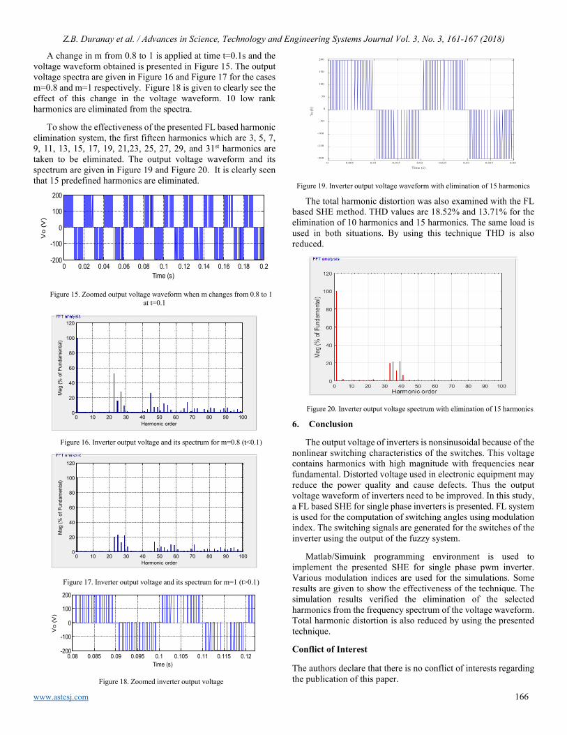
Z.B. Duranay et al. / Advances in Science, Technology and Engineering Systems Journal Vol. 3, No. 3, 161-167 (2018)
www.astesj.com 166
A change in m from 0.8 to 1 is applied at time t=0.1s and the voltage waveform obtained is presented in Figure 15. The output voltage spectra are given in Figure 16 and Figure 17 for the cases m=0.8 and m=1 respectively. Figure 18 is given to clearly see the effect of this change in the voltage waveform. 10 low rank harmonics are eliminated from the spectra.
To show the effectiveness of the presented FL based harmonic elimination system, the first fifteen harmonics which are 3, 5, 7, 9, 11, 13, 15, 17, 19, 21,23, 25, 27, 29, and 31st harmonics are taken to be eliminated. The output voltage waveform and its spectrum are given in Figure 19 and Figure 20. It is clearly seen that 15 predefined harmonics are eliminated.
Figure 15. Zoomed output voltage waveform when m changes from 0.8 to 1 at t=0.1
Figure 16. Inverter output voltage and its spectrum for m=0.8 (t<0.1)
Figure 17. Inverter output voltage and its spectrum for m=1 (t>0.1)
Figure 18. Zoomed inverter output voltage
Figure 19. Inverter output voltage waveform with elimination of 15 harmonics
The total harmonic distortion was also examined with the FL based SHE method. THD values are 18.52% and 13.71% for the elimination of 10 harmonics and 15 harmonics. The same load is used in both situations. By using this technique THD is also reduced.
Figure 20. Inverter output voltage spectrum with elimination of 15 harmonics
6. Conclusion
The output voltage of inverters is nonsinusoidal because of the nonlinear switching characteristics of the switches. This voltage contains harmonics with high magnitude with frequencies near fundamental. Distorted voltage used in electronic equipment may reduce the power quality and cause defects. Thus the output voltage waveform of inverters need to be improved. In this study, a FL based SHE for single phase inverters is presented. FL system is used for the computation of switching angles using modulation index. The switching signals are generated for the switches of the inverter using the output of the fuzzy system.
Matlab/Simuink programming environment is used to implement the presented SHE for single phase pwm inverter. Various modulation indices are used for the simulations. Some results are given to show the effectiveness of the technique. The simulation results verified the elimination of the selected harmonics from the frequency spectrum of the voltage waveform. Total harmonic distortion is also reduced by using the presented technique.
Conflict of Interest
The authors declare that there is no conflict of interests regarding the publication of this paper.
0 0.02 0.04 0.06 0.08 0.1 0.12 0.14 0.16 0.18 0.2-200
-100
0
100
200
Vo
(V)
Time (s)
0 10 20 30 40 50 60 70 80 90 1000
20
40
60
80
100
120
Harmonic order
Mag
(% o
f Fun
dam
enta
l)
0 10 20 30 40 50 60 70 80 90 1000
20
40
60
80
100
120
Harmonic order
Mag
(% o
f Fun
dam
enta
l)
0.08 0.085 0.09 0.095 0.1 0.105 0.11 0.115 0.12-200
-100
0
100
200
Vo
(V)
Time (s)
0 0.005 0.01 0.015 0.02 0.025 0.03 0.035 0.04
Time (s)
-200
-150
-100
-50
0
50
100
150
200
Vo (V
)

Z.B. Duranay et al. / Advances in Science, Technology and Engineering Systems Journal Vol. 3, No. 3, 161-167 (2018)
www.astesj.com 167
Acknowledgment
This research did not receive any specific grant from funding agencies in the public, commercial, or not-for-profit sectors.
References
[1] Z. B. Duranay, H. Guldemir, "Fuzzy Logic Based Harmonic Elimination in Single Phase Inverters" in XXVI International Scientific Conference Electronics, Sozopol Bulgaria, 2017. https://doi.org/10.1109/ET.2017.8124342
[2] O. Bouhali, M. Berkouk, B. Francois, C. Saudemont, S. Labiod, “Solving harmonics elimination problem in three-phase voltage controlled inverter using artificial neural networks” Journal of Electrical Systems, 1(1), 39-51, 2005.
[3] M. H. Rashid, Power Electronics Handbook: Devices, Circuits and Applications, Academic Press, 2010.
[4] N. Mohan, T. M. Undeland, W. P. Robbins, Power Electronics: Converters, Applications and Design, John Wiley & Sons Inc., 1995.
[5] E. Hendawi, “Single phase inverter with selective harmonics elimination pwm based on secant method” Int. Journal of Engineering Inventions, 4(12), 38-44, 2015.
[6] M. I. Jahmeerbacus, M. Sunassee, “Evaluation of Selective Harmonic Elimination and Sinusoidal PWM for Single-Phase Dc to Ac Inverters Under Dead-Time Distortion” in 23rd International Symposium on Industrial Electronics, Istanbul Turkey , 2014. https://doi.org/10.1109/ISIE.2014.6864658
[7] B. M. Saied, Q. M. Alias, A. S. AL-soufy, “Intelligent systems based selective harmonic elimination (she) for single phase voltage sourse inverter” Al Rafdain Enginering Journal, 16(3), 71-81, 2008.
[8] P. N. Enjeti, P. D. Ziogas, J. F. Lindsay, “Programmed pwm techniques to eliminate harmonics: a critical evaluation” IEEE Trans. Ind. Appl., 26(2), 302-316, 1990. https://doi.org/10.1109/28.54257
[9] M. S. A. Dahidah, V. G. Agelidis, “Non-symmetrical Selective Harmonic Elimination PWM Techniques: The Unipolar Waveform” in 38th IEEE Power Electronics Specialists Conference, Orlando FL USA, 2007. https://doi.org/10.1109/PESC.2007.4342290
[10] H. S. Patel, R. G. Hoft, “Generalized techniques of harmonic elimination and voltage control in thyristor inverters: part I harmonic elimination” IEEE Trans. Ind. Appl., IA-9(3), 310-317, 1973. https://doi.org/10.1109/TIA.1973.349908
[11] S. Tuncer, Y. Tatar, H. Guldemir, “A shepwm technique with constant v/f for multilevel inverters” Journal of Polytechnic, 8(2), 123-130, 2005.
[12] J. N. Chiasson, M. Tolbert, K. J. McKenzie, Z. Du, “A complete solution to the harmonic elimination problem” IEEE Trans. Power Electron., 19(2), 491-499, 2004. https://doi.org/10.1109/TPEL.2003.823207
[13] V. G. Agelidis, A. I. Balouktsis, M. S. A. Dahidah, “A five-level symmetrically defined selective harmonic elimination pwm strategy: analysis and experimental validation” IEEE Trans. Power Electron., 23(1), 19–26, 2008. https://doi.org/10.1109/TPEL.2007.911770
[14] F. G. Turnbull, “Selected harmonic reduction in static dc-ac inverters” IEEE Trans. Comm. Electron., CE-83(73), 374-378, 1964. https://doi.org/10.1109/TCOME.1964.6541241
[15] D. Czarkowski, D. V. Chudnovsky, G. V. Chudnovsky, I. W. Selesnick, “Solving the optimal pwm problem for single-phase inverters” IEEE Trans. Circuits-I, 49(4) , 465-475, 2002. https://doi.org/10.1109/81.995661
[16] J. Sun, I. Grotstollen, “Pulse Width Modulation Based on Real-Time Solution of Algebraic Harmonic Elimination Equations, Industrial Electronics” in 20th International Conference on Control and Instrumentation, Bologna Italy, 1994. https://doi.org/10.1109/IECON.1994.397753
[17] G. Carrara, S. Gardella, M. Marchesoni, R. Salutari, G. Sciutto, “A new multilevel pwm method: a theoretical analysis” IEEE Trans. Power Electron., 7(3), 497–505, 1992. https://doi.org/10.1109/63.145137
[18] D. Ahmadi, K. Zou, C. Li, Y. Huang, J. Wang, “A universal selective harmonic elimination method for high-power inverters” IEEE Trans. Power Electron., 26(10), 2743–2752, 2011. https://doi.org/10.1109/TPEL.2011.2116042
[19] L. A. Zadeh, “Fuzzy sets” Information and Control, 8, 338-353, 1965. https://doi.org/10.1016/S0019-9958(65)90241-X
[20] A. Kaur, A. Kaur, “Comparison of Mamdani-Type and Sugeno-Type fuzzy inference systems for air conditioning system” Int. J. of Soft Comp. and Eng., 2(2), 323-325, 2012.
[21] H. Singh, M. M. Gupta, T. Meitzler, et al. “Real-life applications of fuzzy logic” Advances in Fuzzy Systems, 2013, 1-3, 2013. http://dx.doi.org/10.1155/2013/581879.
[22] P. M. Larsen. “Industrial application of fuzzy logic control” International Journal of Man-Machine Studies. 12(1), 3-10, 1980. https://doi.org/10.1016/S0020-7373(80)80050-2.
[23] R. R.Yager, and L. A. Zadeh. “An introduction to fuzzy logic applications in intelligent systems”. Vol. 165. Springer Science & Business Media, 2012.


