Agricultural Price Distortion and Stabilization:

Stylized Facts and Hypothesis Tests

William A. Masters Professor of Agricultural Economics, Purdue University

wmasters@purdue.edu www.agecon.purdue.edu/staff/masters

Andres F. Garcia

PhD Candidate, Department of Agricultural Economics, Purdue University andres@purdue.edu

Forthcoming in Kym Anderson (ed.), Political Economy of Distortions to Agricultural Incentives. Washington, DC: The World Bank, 2009

– This draft revised August 31, 2008 – This paper is a product of a research project on Distortions to Agricultural Incentives, under the leadership of Kym Anderson and Will Martin of the World Bank’s Development Research Group, with funding from World Bank Trust Funds provided by the governments of Ireland, Japan, the Netherlands (BNPP) and the United Kingdom (DFID). Circulation of this draft is designed to promptly disseminate the findings of work in progress for comment before they are finalized. The views expressed are the authors’ alone and not necessarily those of the World Bank and its Executive Directors, nor the countries they represent, nor of the countries providing trust funds for this research project. The authors thank other project participants for sharing their data and for helpful suggestions at the World Bank Workshop on the Political Economy of Agricultural Policy, 23-24 May 2008.

Agricultural Price Distortion and Stabilization:

Stylized Facts and Hypothesis Tests

Introduction and summary

This paper describes agricultural policy choices and tests some predictions of major

political economy theories, exploiting the new Anderson et al. (2008a) dataset. We start

by establishing three broad stylized facts: the development paradox (governments tend to

tax agriculture in poorer countries, and subsidize it in richer ones), the prevalence of anti-

trade bias (governments tend to tax both imports and exports more than nontradables),

and the importance of resource abundance (governments tax more and subsidize less

where there is more land per capita). We then test a variety of political-economy

explanations, finding results consistent with hypothesized effects of rural and urban

constituents’ rational ignorance about small per-person effects, governance institutions’

control of rent-seeking by political leaders, governments’ revenue motive for taxation and

the role of time consistency in policy-making. Interestingly, we find that larger groups

obtain more favorable policies, suggesting that positive group size effects outweigh any

negative influence from more free-ridership. Some of these results add to the

explanatory power of our stylized facts, but others help explain them. A novel result is

that demographically driven entry of new farmers is associated with less favorable farm

policies, which is consistent with a model in which the arrival of new farmers erodes

policy rents and discourages political activity by incumbents. Another new result is that

governments achieve very little price stabilization relative to our benchmark estimates of

undistorted prices, and governments in the poorest countries have actually destabilized

domestic prices over the full span of our data. Price stability is often a stated goal of

policy, and would be predicted by status-quo bias or loss aversion, but the stockholding

or fiscal policies used to limit price changes are often unsustainable and prices tend jump

when the intervention ends.

2

Methodology

Following Anderson et al. (2008b), our principal measure of agricultural trade policy is a

tariff-equivalent “Nominal Rate of Assistance” (NRA), defined as:

f

fd

PPP

NRA−

≡ (1)

In equation (1), Pd is the observed domestic price in local currency for a given product,

country and year, and Pf is the estimated domestic price that would hold in the absence of

commodity-market or exchange-rate intervention. By definition, such an NRA would be

zero in a competitive free-trade regime, and is positive where producers are subsidized by

taxpayers or consumers. The NRA is negative where producers are taxed by trade policy,

for example through export restrictions or an overvalued exchange rate. In a few cases,

we use the absolute value of NRA in order to measure distortions away from competitive

markets, and where national-average NRAs are used they are value-weighted at the

undistorted prices.

The NRA results we use are based on the efforts of country specialists to obtain the best

possible data and apply appropriate assumptions about international opportunity costs and

transaction costs in each market. There is inevitably much measurement error, but by

covering a very large fraction of the world’s countries and commodities, over a very long

time period, we can detect patterns and trends that might otherwise remain hidden.

The Anderson et al. project was designed to measure policy effects on price levels. In

this paper we also use the data to measure policy effects on price variability from year to

year, by comparing the variability of domestic prices with the variability of estimated

free-trade prices, both expressed in natural logs. Ratio-detrending was used to remove

the time trend on prices, by regressing observed prices ( ) on time (t) as in equation OiP )ln(

3

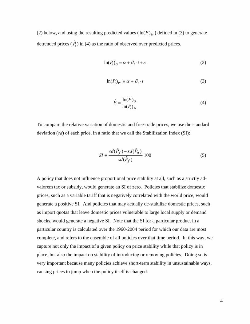
(2) below, and using the resulting predicted values ( ) defined in (3) to generate

detrended prices ( ) in (4) as the ratio of observed over predicted prices.

Pr)ln( iP

iP̂

εβα +t

ti

⋅+=P iOi )ln( (2)

Pi ⋅+≡ βαPr)ln( (3)

Pr)ln(

)ln(ˆi

Oii P

PP = (4)

To compare the relative variation of domestic and free-trade prices, we use the standard

deviation (sd) of each price, in a ratio that we call the Stabilization Index (SI):

100)⋅d

)ˆ(

ˆ()ˆ( −≡

f

f

Psd

PsdPsdSI (5)

A policy that does not influence proportional price stability at all, such as a strictly ad-

valorem tax or subsidy, would generate an SI of zero. Policies that stabilize domestic

prices, such as a variable tariff that is negatively correlated with the world price, would

generate a positive SI. And policies that may actually de-stabilize domestic prices, such

as import quotas that leave domestic prices vulnerable to large local supply or demand

shocks, would generate a negative SI. Note that the SI for a particular product in a

particular country is calculated over the 1960-2004 period for which our data are most

complete, and refers to the ensemble of all policies over that time period. In this way, we

capture not only the impact of a given policy on price stability while that policy is in

place, but also the impact on stability of introducing or removing policies. Doing so is

very important because many policies achieve short-term stability in unsustainable ways,

causing prices to jump when the policy itself is changed.

4

The NRA and SI estimates allow us to describe key stylized facts about policy choices,

and then test the degree to which the relationships implied by political economy models

actually fit the data. Our tests are all variations on equation (6):

εγβα +⋅+⋅+= ZXY (6)

In these tests, Y are the policy measures of interest (variously NRA at the country level,

NRA at product level, absolute value of NRA, or SI), X is a set of regressors that describe

stylized facts which could be explained by many different policymaking mechanisms

(income, direction of trade, resource abundance, continent dummies), and Z are

regressors that are associated with a specific mechanism hypothesized to cause the

policies we observe. Our tests aim to test the significance of introducing each variable in

Z when controlling for X, and to ask whether introducing Z explains the stylized facts

(that is, reduces the estimated value of β) or adds to them (that is, raises the equation’s

estimated R-squared without changing the estimated value of β), or perhaps adds no

additional significance at all. Regressors for X and Z are drawn from public data

disseminated by the World Bank, FAO, the Penn World Tables or others, as detailed in

Appendix Table A1.

The stylized facts of agricultural policy

Our dataset covers an extraordinary diversity of commodities and countries, with huge

variation in agricultural policies. In this section we explore a few key stylized facts, to

establish the background variation for which we will want to control when testing the

predictions of specific theories. A given theory could help explain these patterns, or

could fit the residual variation they leave unexplained. In either case, controlling for key

characteristics of commodities and countries allows us to test each theory’s explanatory

power in a simple, consistent framework.

The stylized facts we consider include the oldest and most general observations about

agricultural policy, linking policy choices to a commodity’s direction of trade, a

country’s real income per capita, and its endowment of farmland per capita. The

5

direction of trade might matter to the extent that agricultural trade policy is simply trade

policy, and so could be linked to a government’s more general anti-trade bias. A

country’s real income might matter to the extent that the role of agriculture changes with

economic growth, so that it is subject to the development paradox. Finally, land

abundance might matter because agriculture is a natural-resource intensive sector, and

could be subject to a natural resource effect. We address each of these in turn below.

The anti-trade bias of governments is among the first concerns of economics, dating back

to Adam Smith and David Ricardo who first described how restrictions on imports and

exports affect incentives for specialization. In this paper we capture anti-trade bias of

domestic instruments as well as trade restrictions, by linking measured NRAs to whether

a commodity is importable or exportable in a given country and year.

A second stylized fact is the development paradox, in which the governments of poorer

countries are typically observed to impose taxes on farm production, while governments

in richer countries typically subsidize it. The modern literature documenting this

tendency begins with Bale and Lutz (1981), and includes notable contributions from

Anderson and Hayami (1986), Lindert (1991), Krueger, Schiff and Valdes (1991) among

others. This pattern is paradoxical insofar as farmers are the majority and are poorer than

non-farmers in low income countries, whereas in high income countries farmers are a

relatively wealthy minority.

A third kind of pattern involves natural resource effects, whereby countries with a

greater resource rent available for extraction from a sector may be tempted to impose a

heavier tax burden on it. The political economy of resource taxation is often discussed

regarding oil and other mineral resources, as in Auty (2001); applications to agriculture

include McMillan and Masters (2003) and Isham et al. (2005). For our purposes, the

resource rent which may be available in agriculture is measured crudely here by arable

land area per capita, allowing us to ask whether more land-abundant countries tend to tax

the agricultural sector more (or subsidize it less), when controlling for both anti-trade bias

and the development paradox.

6

Note that anti-trade bias could help account for the development paradox, to the extent

that low-income countries tend to be net exporters of farm products while richer countries

tend to be net importers of them. And both could be driven by changes in the relative

administrative cost of taxation, insofar as a country’s income growth and capital

accumulation allows government to shift taxation from exports and imports (at the

expense of farms and farmers) to other things (at the expense of firms and their

employees). Thus we need to control for income when testing for anti-trade bias, and

control for anti-trade bias when testing for the development paradox, while controlling

for both of these when looking at resource effects.

To test the magnitude and significance of these patterns in the NRA data, we use data on

the direction of trade from our own database, and data on a country’s average income per

capita data from the Penn World Tables (2007). Income is defined here as real gross

domestic product in PPP prices, chain indexed over time in international dollars at year-

2000 prices. Finally, data on the agricultural sector’s land abundance comes from

FAOSTAT (2007), as the per-capita availability of arable land, defined as the area under

temporary crops, temporary meadows for mowing or pasture, land under market and

kitchen gardens and land temporarily fallow.

A graphical view

Our analysis of stylized facts begins with a graphical view of the data, focusing on the

development paradox and anti-trade bias across countries and regions. One way to test

for significant differences in NRAs across the income spectrum is to draw a smoothed

nonparametric regression line through the data, which then allows us to compare these

relationships across trade sectors. The general tendency of governments in poorer

countries to tax their farmers while governments in richer countries tend to subsidize

them is illustrated with smoothed lines in Figure 1, showing countries’ aggregate NRAs

relative to their level of real per-capita income in that year. These are weighted-average

7

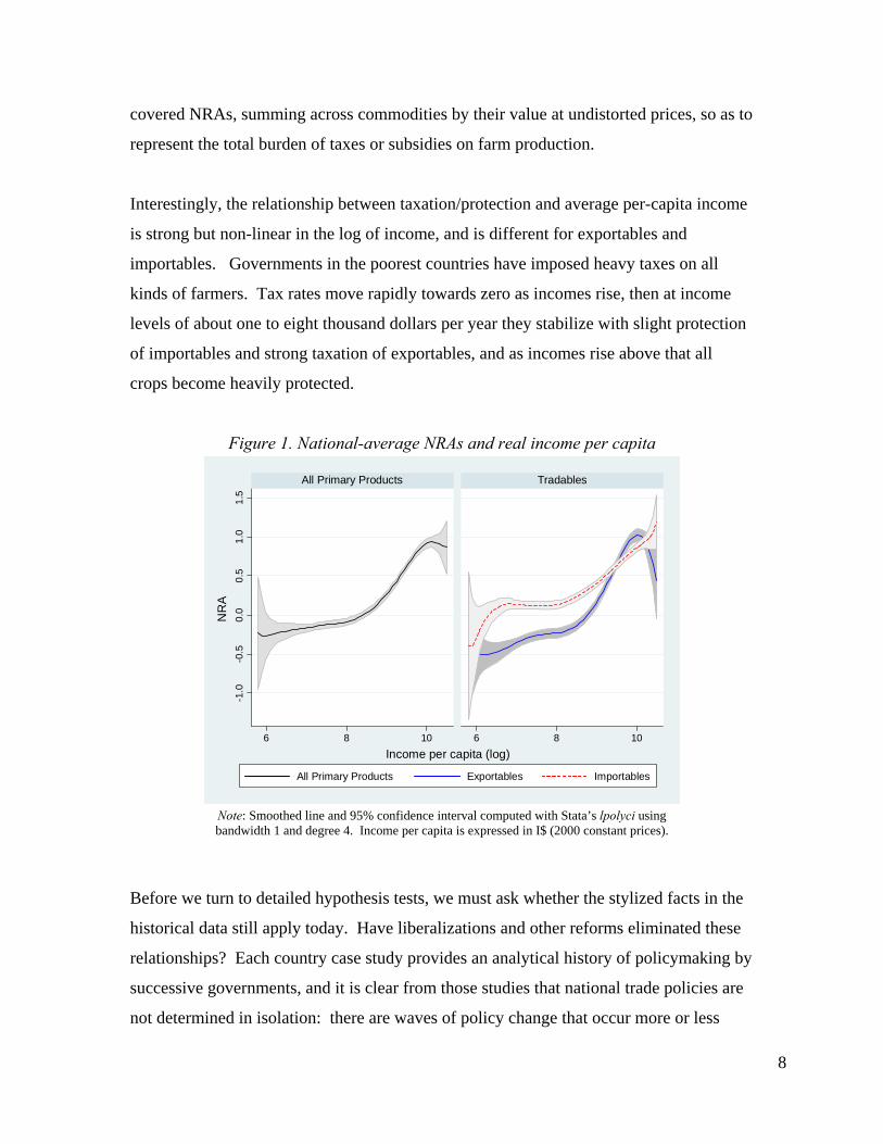
covered NRAs, summing across commodities by their value at undistorted prices, so as to

represent the total burden of taxes or subsidies on farm production.

Interestingly, the relationship between taxation/protection and average per-capita income

is strong but non-linear in the log of income, and is different for exportables and

importables. Governments in the poorest countries have imposed heavy taxes on all

kinds of farmers. Tax rates move rapidly towards zero as incomes rise, then at income

levels of about one to eight thousand dollars per year they stabilize with slight protection

of importables and strong taxation of exportables, and as incomes rise above that all

crops become heavily protected.

Figure 1. National-average NRAs and real income per capita

-1.0

-0.5

0.0

0.5

1.0

1.5

6 8 10 6 8 10

All Primary Products Tradables

All Primary Products Exportables Importables

NR

A

Income per capita (log)

Note: Smoothed line and 95% confidence interval computed with Stata’s lpolyci using bandwidth 1 and degree 4. Income per capita is expressed in I$ (2000 constant prices).

Before we turn to detailed hypothesis tests, we must ask whether the stylized facts in the

historical data still apply today. Have liberalizations and other reforms eliminated these

relationships? Each country case study provides an analytical history of policymaking by

successive governments, and it is clear from those studies that national trade policies are

not determined in isolation: there are waves of policy change that occur more or less

8

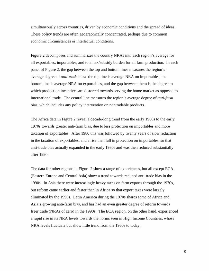
simultaneously across countries, driven by economic conditions and the spread of ideas.

These policy trends are often geographically concentrated, perhaps due to common

economic circumstances or intellectual conditions.

Figure 2 decomposes and summarizes the country NRAs into each region’s average for

all exportables, importables, and total tax/subsidy burden for all farm production. In each

panel of Figure 2, the gap between the top and bottom lines measures the region’s

average degree of anti-trade bias: the top line is average NRA on importables, the

bottom line is average NRA on exportables, and the gap between them is the degree to

which production incentives are distorted towards serving the home market as opposed to

international trade. The central line measures the region’s average degree of anti-farm

bias, which includes any policy intervention on nontradable products.

The Africa data in Figure 2 reveal a decade-long trend from the early 1960s to the early

1970s towards greater anti-farm bias, due to less protection on importables and more

taxation of exportables. After 1980 this was followed by twenty years of slow reduction

in the taxation of exportables, and a rise then fall in protection on importables, so that

anti-trade bias actually expanded in the early 1980s and was then reduced substantially

after 1990.

The data for other regions in Figure 2 show a range of experiences, but all except ECA

(Eastern Europe and Central Asia) show a trend towards reduced anti-trade bias in the

1990s. In Asia there were increasingly heavy taxes on farm exports through the 1970s,

but reform came earlier and faster than in Africa so that export taxes were largely

eliminated by the 1990s. Latin America during the 1970s shares some of Africa and

Asia’s growing anti-farm bias, and has had an even greater degree of reform towards

freer trade (NRAs of zero) in the 1990s. The ECA region, on the other hand, experienced

a rapid rise in its NRA levels towards the norms seen in High Income Countries, whose

NRA levels fluctuate but show little trend from the 1960s to today.

9

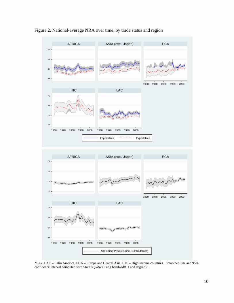
Figure 2. National-average NRA over time, by trade status and region

-10

12

-10

12

1960 1970 1980 1990 2000

1960 1970 1980 1990 2000 1960 1970 1980 1990 2000

AFRICA ASIA (excl. Japan) ECA

HIC LAC

Importables Exportables

-10

12

-10

12

1960 1970 1980 1990 2000

1960 1970 1980 1990 2000 1960 1970 1980 1990 2000

AFRICA ASIA (excl. Japan) ECA

HIC LAC

All Primary Products (incl. Nontradables)

Notes: LAC – Latin America, ECA – Europe and Central Asia, HIC – High income countries. Smoothed line and 95% confidence interval computed with Stata’s lpolyci using bandwidth 1 and degree 2.

10

The stylized facts: antitrade bias, the development paradox and resource abundance

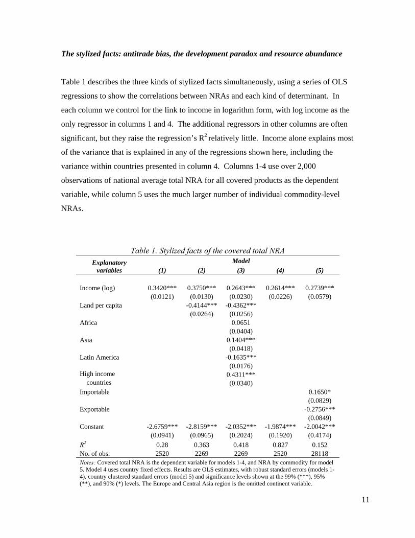
Table 1 describes the three kinds of stylized facts simultaneously, using a series of OLS

regressions to show the correlations between NRAs and each kind of determinant. In

each column we control for the link to income in logarithm form, with log income as the

only regressor in columns 1 and 4. The additional regressors in other columns are often

significant, but they raise the regression’s R2 relatively little. Income alone explains most

of the variance that is explained in any of the regressions shown here, including the

variance within countries presented in column 4. Columns 1-4 use over 2,000

observations of national average total NRA for all covered products as the dependent

variable, while column 5 uses the much larger number of individual commodity-level

NRAs.

Table 1. Stylized facts of the covered total NRA Explanatory

variables Model

(1) (2) (3) (4) (5) Income (log) 0.3420*** 0.3750*** 0.2643*** 0.2614*** 0.2739***

(0.0121) (0.0130) (0.0230) (0.0226) (0.0579) Land per capita -0.4144*** -0.4362***

(0.0264) (0.0256) Africa 0.0651

(0.0404) Asia 0.1404***

(0.0418) Latin America -0.1635***

(0.0176) High income 0.4311***

countries (0.0340) Importable 0.1650*

(0.0829) Exportable -0.2756***

(0.0849) Constant -2.6759*** -2.8159*** -2.0352*** -1.9874*** -2.0042***

(0.0941) (0.0965) (0.2024) (0.1920) (0.4174) R2 0.28 0.363 0.418 0.827 0.152 No. of obs. 2520 2269 2269 2520 28118 Notes: Covered total NRA is the dependent variable for models 1-4, and NRA by commodity for model 5. Model 4 uses country fixed effects. Results are OLS estimates, with robust standard errors (models 1-4), country clustered standard errors (model 5) and significance levels shown at the 99% (***), 95% (**), and 90% (*) levels. The Europe and Central Asia region is the omitted continent variable.

11

One of our stylized facts is that governments across the income spectrum tend to tax all

kinds of trade, thus introducing an anti-trade bias in favor of the home market. From

column 5, controlling for income the average NRA on an importable product is 16.5

percent higher and on an exportable it is 27.6 percent lower than it otherwise might be.

Most interestingly, LAC have NRAs that are a further 16 percent lower (column 3) than

those of other regions. Relative to Africa, Latin America and the omitted region (Eastern

Europe), Asia and the High Income Countries have unusually high NRAs when

controlling for their income level.

Trade policy and price stabilization

Trade policy often aims to stabilize domestic prices as well as change their level. As

detailed by Timmer (1989) and Dawe (2001) among others, stabilization of agricultural

product prices may be especially important for low-income countries, where food prices

have a large impact on consumer expenditure and farmgate prices have a large impact on

real incomes. In practice, however, while stockholding or variable-rate subsidies and

taxes can achieve stabilization in the short run, such effects may be offset by the jumps in

prices that occur when these policies are changed. Empirically the link between a

country’s income and the degree to which its trade policies actually stabilize prices is

shown in Table 2. As it happens, the estimated coefficient on income is positive and the

constant is negative: lower-income countries provide less stability. Less stabilization also

occurs in land-abundant countries, and for importables and exportables relative to

nontradables. Using column (4) as our preferred model, the estimated coefficients imply

that the crossover level of per-capita income below which governments have tended to

destabilize prices is $1,600 for importables and $2,400 for exportables. On average in

those countries, over the full period of our data, actual domestic prices have been less

stable than undistorted prices would have been.

12

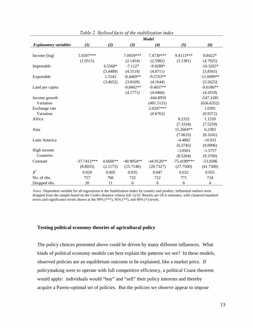
Table 2. Stylized facts of the stabilization index

Explanatory variables Model

(1) (2) (3) (4) (5) (6) Income (log) 5.6507*** 7.0059*** 7.4730*** 9.4113*** 8.8422*

(1.0515) (2.1454) (2.5982) (3.1381) (4.7925) Importable 6.5568* -7.1127 -9.4289* -10.3265*

(3.4489) (4.3119) (4.8711) (5.8565) Exportable 1.5545 -8.4469** -9.5703** -11.6999**

(3.4652) (3.8169) (4.1644) (5.5625) Land per capita -9.8402** -9.4037** -9.6186**

(4.1771) (4.0466) (4.2018) Income growth -444.8959 -547.3185

Variation (481.5131) (656.6352) Exchange rate 2.0297*** 1.0391

Variation (0.6763) (0.9372) Africa 8.2332 1.1559

(7.3334) (7.5259) Asia 15.2604** 6.2383

(7.0633) (8.3245) Latin America -4.4882 -10.931

(6.3745) (8.0996) High income -3.0503 -1.5757

Countries (8.5204) (9.3760) Constant -37.7412*** 4.6606** -40.9054** -44.9126** -75.4189*** -53.9286

(8.8035) (2.1175) (15.7140) (20.7327) (27.7500) (41.7300) R2 0.029 0.005 0.035 0.047 0.032 0.055 No. of obs. 757 766 722 722 771 724 Dropped obs. 20 11 6 6 6 4

Notes: Dependent variable for all regressions is the Stabilization Index by country and product. Influential outliers were dropped from the sample based on the Cook's distance criteria [(K-1)/N]. Results are OLS estimates, with clustered standard errors and significance levels shown at the 99% (***), 95% (**), and 90% (*) levels.

Testing political economy theories of agricultural policy

The policy choices presented above could be driven by many different influences. What

kinds of political economy models can best explain the patterns we see? In these models,

observed policies are an equilibrium outcome to be explained, like a market price. If

policymaking were to operate with full competitive efficiency, a political Coase theorem

would apply: individuals would “buy” and “sell” their policy interests and thereby

acquire a Pareto-optimal set of policies. But the policies we observe appear to impose

13

costs on some people that exceed their gains to others, so our explanations all involve one

or another mechanism that might prevent the competitive market sketched in Coase

(1960) from applying. Each model posits a specific mechanism which prevents losers

from buying out the gainers and thereby obtaining Pareto-improving reforms, and

suggests certain variables that might therefore be correlated with the particular policies

we observe. Identifying which kinds of political market failures have been most

important could help policymakers circumvent these constraints, through rules and other

interventions that help shift the political-economy equilibrium towards Pareto-improving

policy outcomes.

The following sections describe various possible mechanisms, drawing on the last half-

century of political economy modeling. The theories are well known so we describe

them only briefly, and focus on the empirical correlations between variables. Our results

are organized into two sets: regressions using aggregate national-average data are in

Table 3, and those using product-level data are in Table 4. Note that none of our tests

make any attempt to control for endogeneity. These are all exploratory regressions aimed

at establishing correlations, comparing a large number of competing hypotheses in a

common framework. Future work to test particular mechanisms would call for more

specialized models and datasets.

Explaining the data: six major political economy theories

The simplest kind of explanation for observed policies is rational ignorance, by which

individuals will not invest in learning or taking action about a policy if the policy’s cost

(or benefit) to them exceeds their cost of political organization. This mechanism could

help to explain why observed policies tend to generate highly concentrated gains that

provide substantial benefits to a few people, thereby motivating them to act politically

and obtain that policy. In many cases the gains come at the expense of others who, if the

cost per person is small, can be expected to remain on the sidelines. Such a focus on per-

capita incidence is associated with Anthony Downs (1957), and could be the most

14

powerful explanation for the patterns we observe. Influential applications to agriculture

include Anderson (1995), who demonstrated how the concentration of gains and losses

shifts during economic development.

Rational ignorance effects are tested in column 2 of Table 3, where the dependent

variable is the value-weighted average of all commodity NRAs for the country as a

whole, and the independent variable used to test for rational ignorance is its total cost

(benefit) per capita in that sector. This test is applicable only to observations with

positive total NRAs, so that a larger NRA imposes a greater cost (benefit) per urban

(rural) person. Results show a large and significant pattern: when costs (benefits) per

capita are larger, the percentage NRA levels are correspondingly smaller (higher).

Furthermore, the effect is larger for people living in urban areas, perhaps because city-

dwellers are more easily mobilized than their rural counterparts, when controlling for

other factors.

Column 3 of Table 3 tests a related but different explanation: the absolute size of each

group. This may influence outcomes through free-ridership, if individuals in larger

groups have more incentive to shirk as in Mancur Olson (1965). An opposite group-size

effect could arise if larger groups are more influential, perhaps because they can mobilize

more votes, political contributions, or other political forces. As it happens, column 3 of

Table 3 shows that larger groups do obtain more favorable policies, perhaps because all

of these groups are very large and have similar levels of free-ridership. Again the

magnitude is larger for urban people than for rural people, suggesting that on average an

additional urbanite has more political influence than an additional rural person.

Relative to the unconditional regression in column 1, the estimated coefficient on

national income is markedly lower when controlling for rational ignorance in (2), and

somewhat greater when controlling for group size in (3). In that sense, rational ignorance

helps to account for the development paradox, while group size is an additional influence;

these regressions are not necessarily comparable, however, because of differences in the

sample size.

15

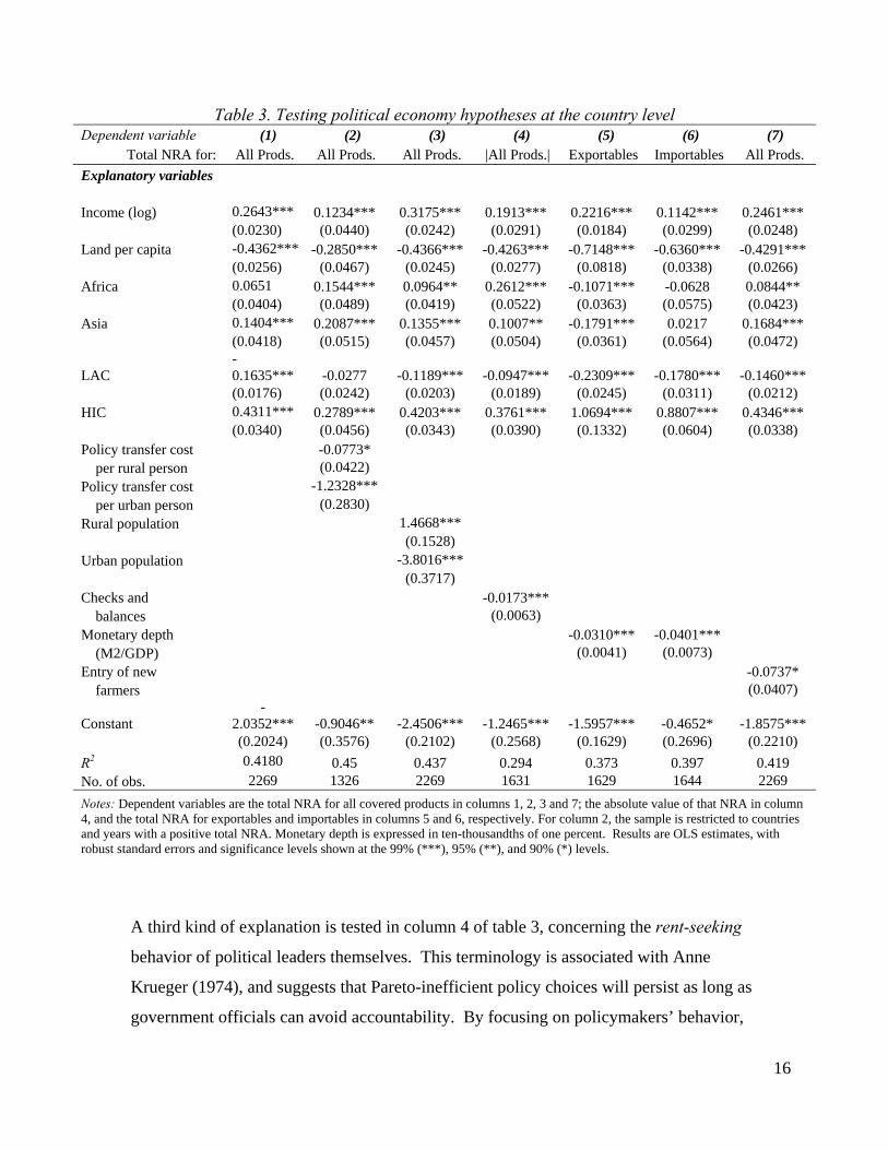
Table 3. Testing political economy hypotheses at the country level Dependent variable (1) (2) (3) (4) (5) (6) (7)

Total NRA for: All Prods. All Prods. All Prods. |All Prods.| Exportables Importables All Prods. Explanatory variables

Income (log) 0.2643*** 0.1234*** 0.3175*** 0.1913*** 0.2216*** 0.1142*** 0.2461*** (0.0230) (0.0440) (0.0242) (0.0291) (0.0184) (0.0299) (0.0248)

Land per capita -0.4362*** -0.2850*** -0.4366*** -0.4263*** -0.7148*** -0.6360*** -0.4291*** (0.0256) (0.0467) (0.0245) (0.0277) (0.0818) (0.0338) (0.0266)

Africa 0.0651 0.1544*** 0.0964** 0.2612*** -0.1071*** -0.0628 0.0844** (0.0404) (0.0489) (0.0419) (0.0522) (0.0363) (0.0575) (0.0423)

Asia 0.1404*** 0.2087*** 0.1355*** 0.1007** -0.1791*** 0.0217 0.1684*** (0.0418) (0.0515) (0.0457) (0.0504) (0.0361) (0.0564) (0.0472)

LAC -0.1635*** -0.0277 -0.1189*** -0.0947*** -0.2309*** -0.1780*** -0.1460*** (0.0176) (0.0242) (0.0203) (0.0189) (0.0245) (0.0311) (0.0212)

HIC 0.4311*** 0.2789*** 0.4203*** 0.3761*** 1.0694*** 0.8807*** 0.4346*** (0.0340) (0.0456) (0.0343) (0.0390) (0.1332) (0.0604) (0.0338)

Policy transfer cost -0.0773* per rural person (0.0422)

Policy transfer cost -1.2328*** per urban person (0.2830)

Rural population 1.4668*** (0.1528)

Urban population -3.8016*** (0.3717)

Checks and -0.0173*** balances (0.0063)

Monetary depth -0.0310*** -0.0401*** (M2/GDP) (0.0041) (0.0073)

Entry of new -0.0737* farmers (0.0407)

Constant -

2.0352*** -0.9046** -2.4506*** -1.2465*** -1.5957*** -0.4652* -1.8575*** (0.2024) (0.3576) (0.2102) (0.2568) (0.1629) (0.2696) (0.2210)

R2 0.4180 0.45 0.437 0.294 0.373 0.397 0.419 No. of obs. 2269 1326 2269 1631 1629 1644 2269 Notes: Dependent variables are the total NRA for all covered products in columns 1, 2, 3 and 7; the absolute value of that NRA in column 4, and the total NRA for exportables and importables in columns 5 and 6, respectively. For column 2, the sample is restricted to countries and years with a positive total NRA. Monetary depth is expressed in ten-thousandths of one percent. Results are OLS estimates, with robust standard errors and significance levels shown at the 99% (***), 95% (**), and 90% (*) levels.

A third kind of explanation is tested in column 4 of table 3, concerning the rent-seeking

behavior of political leaders themselves. This terminology is associated with Anne

Krueger (1974), and suggests that Pareto-inefficient policy choices will persist as long as

government officials can avoid accountability. By focusing on policymakers’ behavior,

16

the rent-seeking approach explains the observed pattern of policy intervention in terms of

the checks and balances that constrain policymakers differently across countries and

across sectors. The clear prediction is that governments facing more checks and balances

will choose policies that are closer to Pareto-optimality. In column 4 of Table 3, we test

this view using the absolute value of NRA as our dependent variable, and a variable for

“Checks and Balances” from the World Bank’s Database of Political Institutions (Beck et

al. 2008) as our measure of politicians’ power. Results are significant, suggesting that

after controlling for income, governments that impose more checks and balances on their

officials do have less distortionary policies.

Columns 5 and 6 of Table 3 tests a fourth type of model, in which observed policies may

be by-product distortions caused by policies chosen for other reasons, such as a revenue

motive or tax-base effects. Governments with a small nonfarm tax base may have a

stronger motive to tax agricultural imports and exports, or conversely governments with a

larger tax base may be less constrained by fiscal concerns and hence freer to pursue other

political goals. Here the variable we use to capture the extent of taxable activity is the

country’s monetary depth, as measured by the ratio of M2 to GDP. Since greater taxation

of trade is associated with negative NRAs for exportables but positive NRAs for

importables, this test is divided into two subsamples. What we find is that governments

in more monetized economies have lower levels of NRA in both samples: they tax

exportables more, and tax importables less. On average in our sample, import taxes are

associated with revenue motives (so they are smaller when other revenues are available),

but export taxes are not.

The four major theories described above are tested in Table 3 using data at the national

level, using value-weighted averages over all products; in the table below, we test two

additional kinds of theories that apply at the product level, with a much larger number of

observations. This is done for the fifth and sixth kinds of theory, namely time

consistency and status-quo bias.

17

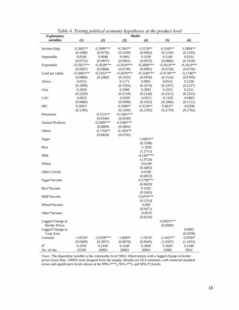
Table 4. Testing political economy hypotheses at the product level Explanatory

variables Model

(1) (2) (3) (4) (5) (6)

Income (log) 0.2605** 0.2989*** 0.2363** 0.2159** 0.3160** 0.2804** (0.1089) (0.0576) (0.1039) (0.0965) (0.1230) (0.1295)

Importable 0.0549 0.0048 -0.0061 0.1039 0.1106 0.0331 (0.0753) (0.0937) (0.0901) (0.0972) (0.0882) (0.1018)

Exportable -0.2921*** -0.3028*** -0.2918*** -0.2868*** -0.3614*** -0.3414*** (0.0697) (0.0868) (0.0749) (0.0805) (0.0728) (0.0756)

Land per capita -0.3066*** -0.3352*** -0.3478*** -0.3140*** -0.4738*** -0.1746** (0.0884) (0.1080) (0.1035) (0.0950) (0.1532) (0.0760)

Africa 0.0553 0.1171 0.0901 0.0554 0.1236 (0.1898) (0.1956) (0.1874) (0.2207) (0.2127)

Asia 0.2828 0.2998 0.2903 0.1833 0.2311 (0.2250) (0.2110) (0.2140) (0.2311) (0.2355)

LAC -0.0652 -0.0309 -0.0515 -0.1426 -0.0863 (0.0880) (0.0998) (0.1053) (0.1066) (0.1151)

HIC 0.2605* 0.3388** 0.3136** 0.4837* -0.0298 (0.1395) (0.1430) (0.1393) (0.2770) (0.1762)

Perennials -0.1315** -0.1492*** (0.0540) (0.0549)

Animal Products 0.2589*** 0.2580*** (0.0889) (0.0892)

Others -0.1764** -0.1956** (0.0820) (0.0795)

Sugar -1.0903** (0.5398)

Rice -1.1926 (1.2711)

Milk -4.1447*** (1.0724)

Wheat -0.6149 (0.4403)

Other Cereals 0.6198 (0.4822)

Sugar*Income 0.1790*** (0.0620)

Rice*Income 0.1502 (0.1663)

Milk*Income 0.5476*** (0.1214)

Wheat*Income 0.068 (0.0471)

Other*Income -0.0678 (0.0526)

Lagged Change in -0.0025*** Border Prices (0.0006)

Lagged Change in 0.0083 Crop Area (0.0358)

Constant -1.8516* -2.0109*** -1.6685* -1.5914* -2.1625** -2.0549* (0.9409) (0.3957) (0.8978) (0.8445) (1.0507) (1.1023)

R2 0.1950 0.2100 0.2240 0.2800 0.3020 0.1940 No. of obs. 25599 20063 20063 20063 15982 9932

Notes: The dependent variable is the commodity level NRA. Observations with a lagged change in border prices lower than -1000% were dropped from the sample. Results are OLS estimates, with clustered standard errors and significance levels shown at the 99% (***), 95% (**), and 90% (*) levels.

18

The first type of explanation tested at the product level involves time consistency and

commitment mechanisms. Such theories are associated with Kydland and Prescott

(1977), who show that current policy choices depend in part on how easily future

governments can change those policies. Without an institution for credible commitment,

introducing and sustaining a desirable policy may be impossible – particularly for

products that are more dependent on irreversible private investments. Differences across

products in the importance of irreversible investment thus allow us to test how much time

consistency matters: if products with irreversible investments attract high taxation, then

commitment devices that help governments maintain low taxes might be helpful. This

idea is applied to help explain agricultural policy in Africa by McMillan and Masters

(2003), who show that tree crops and other irreversible investments are more vulnerable

to high taxation and simultaneously attract less public services. A same effect holds in

these data: the results in columns 2 and 3 of Table 4 are consistent with such a time-

consistency effect, as perennials are taxed more than annuals. Other differences across

crops are also important. Column 4 of Table 4 shows that sugar and dairy are taxed more

than other commodities at low incomes, and then as income grows, policies switch

towards subsidization of these previously taxed commodities.

A sixth kind of political-economy mechanism is pure status-quo bias, in which political

leaders resist change as such, even if the change would be desirable in retrospect. Status

quo bias could lead policymakers to resist both random fluctuations and persistent trends,

even when accepting these changes would raise economic welfare. Several different

mechanisms have been proposed to explain why change would be resisted ex ante,

despite the desirability of reform ex post. An informal version of this idea that is specific

to policy-makers is described by Corden (1974) as a “conservative welfare function.” A

micro-foundation for this idea could be individual-level “loss aversion”, as formalized by

Kahneman and Tversky (1979): people systematically place greater value on losing what

they have than on gaining something else. Status quo bias can also arise for other

reasons: most notably, Fernandez and Rodrik (1991) show how Pareto-improving

reforms may lack political support if those who will lose know who they are, whereas

those who could gain do not yet know if they will actually benefit. If status-quo bias

19

leads policymakers to resist change in world prices, observed NRAs would be higher

after world prices have fallen. NRAs could also try to resist changes in crop profitability

more generally, and therefore be higher after acreage planted in that crop has fallen. We

test for both kinds of status quo bias in columns 5 and 6 of Table 4. With our usual

controls, we find support for status-quos bias in prices, as there is a negative correlation

between policies and lagged changes in world prices. However, there is no remaining

correlation between policies and lagged changes in crop area.

A new explanation: demographic influences on political pressures

The six political economy models tested above could all potentially explain the results we

observe, and are often mentioned in the political economy literature. A seventh kind of

explanation is more novel: it is based on exogenous but predictable changes in

employment that affect whether other people are likely to enter the sector in the future.

This could drive the level of political support in a dynamic political economy model,

where individuals’ incentives to invest in politics depend crucially on the probability of

others’ future entry to their sector and the resulting level of expected future rent

dissipation.

A forward-looking model of lobbying effort driven by the entry of new agents has been

suggested by Hillman (1982) and also Baldwin and Robert-Nicoud (2002), who used it to

help explain why governments protect declining industries. In their models, declining

industries invest more to seek policy-induced rents because their secular decline creates a

barrier to entry in the future. Agriculture experiences this kind of secular decline in its

labor force only after the “structural transformation turning point”, when total population

growth is slow enough and nonfarm employment is large enough for the absolute number

of farmers to decline (Tomich, Kilby and Johnston 1995). Before then, the number of

farmers is rising, whereas after that point the number of farmers falls or remains constant.

20

The secular rise and then fall in the number of farmers could help explain NRA levels, to

the extent that the entry of new farmers erodes policy rents obtained from lobbying. This

would discourage farmers from organizing politically as long as new farmers are entering

the sector, and facilitate organization once the entry of new farmers stops. Focusing on

this dynamic of entry, as opposed to the absolute size of the group, could help explain the

timing of transition from taxation to protection and also help explain the persistence of

protection even where agriculture is not a declining industry. In many industrialized

countries, for example, agricultural output grows but a fixed land area imposes a strong

barrier to the entry of new farmers, helping incumbent producers capture any policy rents

they may obtain through lobbying.

To test for an entry-of-new-farmers effect, we return to country-level data in Table 3,

where the last column tests for the correlation with NRA of an indicator variable set to

one if there is demographic entry of new farmers, defined as a year-to-year increase in the

“economically active population in agriculture” reported by the FAO. The variable is set

to zero when the number of farmers remains unchanged or declines. In column 7 of

Table 3, with our usual controls, observed policies remain less favorable to farmers as

long as the farm population is rising. This result is quite different from the predictions of

other models, and offers a potentially powerful explanation for the timing of policy

change and the difficulty of reform.

This previous section tested seven hypothesized mechanisms, using our generic stylized

facts as control variables. One important question is whether these mechanisms are

explaining the stylized facts, or adding to them. As it happens, the specific mechanism

mainly add to the explanatory power of our regressions: introducing them raises the

equations’ R-squared but does not reduce the magnitude or significance of the stylized

factors with respect to national income, land abundance, or the direction of trade. There

are, however, three important exceptions which account for some of the observed

correlation with income: these are the effect of peoples’ rational ignorance from having

larger transfers per person, the effect of a government’s revenue motive from having

greater monetary depth, and the effect on rent seeking behavior of having more checks

21

and balances in government. Variables specific to these effects capture a share of the

variance in NRAs that would otherwise be associated with per-capita income, suggesting

that they are among the mechanisms that might cause the development paradox, while

other results are additional influences on governments’ policy choices.

Conclusions

This paper uses results from a major new research project to test standard political-

economy theories of why governments intervene to influence agricultural prices. Our

key data source provides estimates for the tariff-equivalent effect on price of all types of

agricultural trade policies across 68 countries from 1955 through 2007. Policy impacts

are measured for 72 products, chosen to account for over 70 percent of agricultural value

added in each country, resulting in a total of over 25,000 distinct estimates from

particular products, country and year.

Our analysis begins by confirming three previously observed stylized facts: (i) a

consistent anti-trade bias in all countries, (ii) the development paradox of anti-farm bias

in poorer countries and pro-farm bias at higher incomes, and (iii) the resource abundance

effect towards higher taxation (or less subsidization) of agriculture in more land-abundant

countries. To explain these effects, we find strong support for a number of mechanisms

that could help explain government choices. Results support rational ignorance effects

as smaller per-capita costs (benefits) are associated with higher (lower) proportional

NRAs, particularly in urban areas. Results also support rent-seeking motives for trade

policy, as countries with fewer checks and balances on the exercise of political power

have smaller distortions, and we find support for time-consistency effects, as perennials

attract greater taxation than annuals. We find partial support for status-quo bias as

observed NRAs are higher after world prices have fallen but there is no correlation

between policies and lagged changes in crop area.

22

Three of our results run counter to much conventional wisdom. First, we support for a

revenue motive function of taxation only on importables, and the opposite effect on

exportables. Second, we find no support for the idea that larger groups of people will

have more free-ridership and hence less political success. Our results are consistent with

the alternative hypothesis of a group-size effect in which larger groups tend to be given

more favorable levels of NRA. Third, we find that governments in lower-income

countries actually destabilize domestic prices, relative to what they would be with freer

trade, over the full time period of our data. A given policy may achieve short-term

stability, but on average these policies are not (or perhaps cannot be) sustained, leading to

large price jumps when policies change.

An important novelty in our results is the finding that demographically-driven entry of

new farmers is associated with less favorable policies. This result is consistent with

models in which new entrants erode policy rents, making political organization depend

on barriers to entry that allow incumbents to capture the benefits of policy change.

Our data find robust support for some theories and not others, but none of our regressions

account for more than half of the variance across countries and over time. To explain the

remainder would require deeper analyses of policies’ institutional context in particular

countries and commodities, and further econometric tests. Such research will also point

the way towards improvements in data quality to reduce measurement error. Our

project’s methodology aimed for much more consistency in data sources, definitions and

assumptions than is usually possible to achieve over such a large sample, but the data are

inevitably noisy with important random and also systematic variance in our estimates.

We hope that future work will produce even more useful datasets, as well as further

analysis of the hypotheses tested here.

23

References cited Anderson, Kym, 1995. “Lobbying Incentives and the Pattern of Protection in Rich and Poor Countries”, Economic Development and Cultural Change, 43(2, January): 401-423. Anderson, Kym and Yujiro Hayami, 1986. The Political Economy of Agricultural Protection : East Asia in International Perspective. London and Boston: Allen & Unwin. Anderson, K., E. Jara, M. Kurzweil, D. Sandri and E. Valenzuela, 2008a. "Estimates of Distortions to Agricultural Incentives, 1955 to 2005", World Bank, Washington DC, pre-release October 2007 (public release to be posted at www.worldbank.org/agdistortions). Anderson, K., M. Kurzweil, W. Martin, D. Sandri and E. Valenzuela, 2008b, "Methodology for Measuring Distortions to Agricultural Incentives", Appendix 2 in Anderson, K. (ed.), "Distortions to Agricultural Incentives: Global Perspective", London: Palgrave Macmillan and Washington DC: World Bank, forthcoming. Auty, Richard M., ed. 2001. Resource Abundance and Economic Development, Oxford: Oxford University Press. Baldwin, Richard E. and Frederic Robert-Nicoud, 2002. "Entry and Asymmetric Lobbying: Why Governments Pick Losers." NBER Working Papers 8756, National Bureau of Economic Research. Bale, Malcolm D. and Ernst Lutz, 1981. “Price Distortions in Agriculture and Their Effects: An International Comparison.” American Journal of Agricultural Economics, 63 (1, Feb.): 8-22. Beck, Thorsten, Philip E. Keefer and George R. Clarke, 2008. Database of Political Institutions. Washington, DC: World Bank (http://go.worldbank.org/2EAGGLRZ40). Coase, Ronald, 1960. “The problem of social cost.” The Journal of Law & Economics, 3(1): 1-44. Corden, Max, 1974. Trade Policy and Economic Welfare, Oxford: Clarendon Press. Dawe, David, 2001. “How far down the path to free trade? The importance of rice price stabilization in developing Asia.” Food Policy, 26(2, April): 163-175. De Gorter, Harry and Jo Swinnen, 2002. “Political economy of agricultural policy,” in B. Gardner and G. Rausser, eds., Handbook of Agricultural Economics, vol. 2B (pp. 1893–1943). Downs, Anthony, 1957. “An economic theory of political action in a democracy.” Journal of Political Economy, 65(2): 135-150.

24

Fernandez, Raquel and Dani Rodrik, 1991. "Resistance to Reform: Status Quo Bias in the Presence of Individual-Specific Uncertainty," American Economic Review, 81(5): 1146-55. Hillman, Arye L., 1982. Declining industries and political-support protectionist motives. American Economic Review, 72(5): 1180–1187. Isham, Jonathan, Michael Woolcock, Lant Pritchett and Gwen Busby (2005), “The Varieties of Resource Experience: Natural Resource Export Structures and the Political Economy of Economic Growth.” The World Bank Economic Review 19(2):141-174. Kahneman, Daniel, and Amos Tversky, 1979. "Prospect Theory: An Analysis of Decision under Risk.", Econometrica, 47(2): 263-291. Krueger, Anne O., Maurice Shiff and Alberto Valdés, eds., 1991. Political Economy of Agricultural Pricing Policy, Johns Hopkins University Press, Baltimore. Krueger, Anne O., 1974. "The Political Economy of the Rent Seeking Society," American Economic Review, 64(June): 291-303. Kydland, Fynn E., and Edward C. Prescott, 1977. "Rules Rather than Discretion: The Inconsistency of Optimal Plans". Journal of Political Economy, 85(3): 473–492 Lindert, Peter, 1991. “Historical Patterns of Agricultural Policy,” chapter 2 in C.P. Timmer, ed., Agriculture and the State: Growth, Employment, and Poverty in Developing Countries. Ithaca: Cornell University Press. McMillan, Margaret S. and William A. Masters, 2003. “An African Growth Trap: Production Technology and the Time-Consistency of Agricultural Taxation, R&D and Investment.” Review of Development Economics 7 (2): 179–191. Olson, Mancur, 1965. The Logic of Collective Action, Harvard University Press, Cambridge. Timmer, C. Peter, 1989. “Food price policy: the rationale for government intervention,” Food Policy 14(1), 17-42. Tomich, Thomas, Peter Kilby and Bruce Johnston, 1995. Transforming Agrarian Economies: Opportunities Seized, Opportunities Missed. Ithaca: Cornell University Press.

25

26

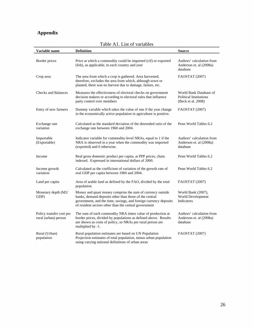
Appendix

Table A1. List of variables Variable name Definition Source

Border prices Price at which a commodity could be imported (cif) or exported (fob), as applicable, in each country and year

Authors’ calculation from Anderson et. al (2008a) database

Crop area The area from which a crop is gathered. Area harvested, therefore, excludes the area from which, although sown or planted, there was no harvest due to damage, failure, etc.

FAOSTAT (2007)

Checks and Balances Measures the effectiveness of electoral checks on government decision makers or according to electoral rules that influence party control over members

World Bank Database of Political Institutions (Beck et al. 2008)

Entry of new farmers Dummy variable which takes the value of one if the year change in the economically active population in agriculture is positive.

FAOSTAT (2007)

Exchange rate variation

Calculated as the standard deviation of the detrended ratio of the exchange rate between 1960 and 2004.

Penn World Tables 6.2

Importable (Exportable)

Indicator variable for commodity-level NRAs, equal to 1 if the NRA is observed in a year when the commodity was imported (exported) and 0 otherwise.

Authors’ calculation from Anderson et. al (2008a) database

Income Real gross domestic product per capita, at PPP prices, chain indexed. Expressed in international dollars of 2000.

Penn World Tables 6.2

Income growth variation

Calculated as the coefficient of variation of the growth rate of real GDP per capita between 1960 and 2004.

Penn World Tables 6.2

Land per capita Area of arable land as defined by the FAO, divided by the total population.

FAOSTAT (2007)

Monetary depth (M2/ GDP)

Money and quasi money comprise the sum of currency outside banks, demand deposits other than those of the central government, and the time, savings, and foreign currency deposits of resident sectors other than the central government

World Bank (2007), World Development Indicators

Policy transfer cost per rural (urban) person

The sum of each commodity NRA times value of production at border prices, divided by populations as defined above. Results are shown as costs of policy, so NRAs per rural person are multiplied by -1.

Authors’ calculation from Anderson et. al (2008a) database

Rural (Urban) population

Rural population estimates are based on UN Population Projection estimates of total population, minus urban population using varying national definitions of urban areas

FAOSTAT (2007)