Aio

GC

a

ARR1AA

KNHDS

1

dptsaRwt

2tltgiet

tpm

0h

Computers and Chemical Engineering 60 (2014) 364– 375

Contents lists available at ScienceDirect

Computers and Chemical Engineering

jo u r n al homep age : www.els evier .com/ locate /compchemeng

n active specification switching strategy that aidsn solving nonlinear sets and improves a VNS/TA hybridptimization methodology

. Robertson ∗, A. Geraili, M. Kelley, J.A. Romagnolihemical Engineering Department, Louisiana State University, Baton Rouge, LA, United States

r t i c l e i n f o

rticle history:eceived 14 June 2013eceived in revised form9 September 2013ccepted 1 October 2013

a b s t r a c t

A method to aid in convergence of nonlinear equations by relocating the solver is introduced. Deactivatingknown variables and activating intelligently chosen unknown variables at predicted values efficientlyformulates initial conditions. This repair strategy is integrated into an optimization procedure. The repairalgorithm has the ability to (1) relocate the solver for non-converged models caused by poor initialconditions and (2) utilize points formulated in relocating non-converged models caused by infeasible

vailable online xxx

eywords:onlinear set solutionsybrid metaheuristics

sets of decision variables as a perturbation phase of a stochastic optimization algorithm. To show theeffectiveness of the proposed repair strategy, a hybrid metaheuristic of a Variable Neighborhood Search(VNS) and Threshold Accepting (TA) is tested on the optimization of a large-scale industrial process, theprimary units of a crude oil refinery. The performance of the hybrid VNS/TA Metaheuristic with repair is

m wi

istillation optimizationtochastic optimization

compared to the algorith

. Introduction

Modern petroleum refining has become a competitive businessue to the deteriorating quality of crude oil coupled with tighterroduct specifications and more stringent environmental regula-ions. Refineries today receive shipments of crude from a variety ofources. These crude oils are of different quality and compositionnd usually blending can improve the economics of the refinery.efineries must deal with a dynamic schedule of incoming crudehich cause them to frequently change unit operating conditions

o reduce expenses.In a previous publication (Robertson, Palazoglu, & Romagnoli,

011), the integration of the production-layer scheduling problem,he crude oil unloading scheduling problem, and the operational-ayer process unit optimization problem of the main refinery units,he heat integration of the distillation units, was considered. Inte-rating tactical-layer decisions with the operational optimizations a dynamic optimization problem and was performed using mod-ling techniques. The need to create more robust optimizationechniques of crude oil refining operations is apparent.

Simulations are increasingly important in the field of optimiza-

ion as software becomes more specialized at accurately describingarticular processes. Engineers assigned to particular units are theost adept at modeling their units and can choose from a variety of

∗ Corresponding author. Tel.: +1 2252880210.E-mail address: gregory.m.robertson@gmail.com (G. Robertson).

098-1354/$ – see front matter © 2013 Elsevier Ltd. All rights reserved.ttp://dx.doi.org/10.1016/j.compchemeng.2013.10.002

thout the repair technique.© 2013 Elsevier Ltd. All rights reserved.

software to do so. In a competitive and evolving modeling softwarelandscape, software can have superior benefits in different areas.For example, Software A may have a better feed characterization toaid in a modeling a complex unit, where Software B is designed toconstruct models of large MILPs encountered in scheduling prob-lems. This makes optimization of simulations better suitable foran environment where multiple software types are specializedand communicate with one another. Tasks are specialized as well.The unit engineers can update simulations to incorporate processchanges and long-term dynamics using the same software config-uration.

Stochastic optimization is suitable for a real-world environmentwhere modeling and optimization tasks are specialized and multi-ple software types are integrated. When a process simulator is usedas part of the optimization strategy, as in our case, the optimizer isa separate entity that treats the model as a black box. The optimizersends a set of decision variables to the model and the model returnsvalues necessary to solve the objective function. For optimizationproblems to be solved analytically constraints must be included inthe objective function and an associated set of nonlinear equationssolved. In many real-world situations, the modeling equations areembedded in simulation software and cannot easily be extracted.Therefore, stochastic optimization is selected for problems in whichthe modeling constraints are distributed among software types and

are not expressed explicitly.

Stochastic optimization can exacerbate simulation convergenceissues. A converged solution is a solution in which all equations inthe model are satisfied. A set of decision variables generated by

Chemi

ascttimdiesoc

tvpstoisaeptVipttartAr

ractretpt

2

aimi

2

fouwast

G. Robertson et al. / Computers and

n optimizer can violate a constraint within the model when cho-en stochastically since the optimizer does not consider modelingonstraints. If the values of a set of decision variables are outsidehe convergence space, the model’s solver will not converge. Also,he solver may not converge if the optimizer makes large jumpsn the solution space. For a nonlinear set of equations to be solved,

odeling equations are typically solved through an iterative proce-ure. Despite advances of non-linear equation solvers, the solver’s

nitial condition strongly affects convergence. Typically, the mod-ling solver’s initial condition is the value of the previous pointolved. Therefore, increasing the solution space can help find globalptima; however, taking larger steps increases occurrences of non-onverging solutions by worsening the solver’s initial condition.

In this paper, a method to aid in convergence of nonlinear equa-ions by relocating the solver is introduced. Deactivating knownalues and activating intelligently chosen unknown variables atredicted values efficiently formulate initial conditions. This repairtrategy is integrated into an optimization procedure improvinghe procedure’s robustness. Many stochastic optimization meth-ds would suggest ignoring non-converged simulation models asnfeasible. The repair algorithm has the ability to (1) relocate theolver for non-converged models caused by poor initial conditionsnd (2) utilize points formulated in relocating non-converged mod-ls caused by infeasible sets of decision variables as a perturbationhase of a stochastic optimization algorithm. To show the effec-iveness of the proposed repair strategy, a hybrid metaheuristic of aariable Neighborhood Search (VNS) and Threshold Accepting (TA)

s tested on the optimization of a large-scale industrial process, therimary units of a crude oil refinery. The specification selection ofhe distillation model variables is illustrated. The performance ofhe hybrid VNS/TA Metaheuristic with repair is compared to thelgorithm without the repair technique. Results indicate that theepair strategy is able to improve the convergence of the distilla-ion models. Furthermore, embedding the strategy into the VNS/TAlgorithm improves VNS’s drawback of sensitivity to initial searchegion and allows for a larger range of solution space to be explored.

This paper is organized as follows: Section 2 outlines the generalepair procedure and incorporates the strategy into an optimizationlgorithm. Section 3 describes an industrial application, and dis-usses the implementation of the repair and optimization strategieso the application. Finally in Section 4, the optimization results withepair and without repair strategy are compared along with theffectiveness of the repair strategy. Appendix A contains a descrip-ion of the industrial application, formulation of the optimizationroblem, and notes on simulation and optimization implementa-ion.

. Methodology

In this section stochastic optimization methods are discussednd a hybrid metaheuristic algorithm is formulated. Convergencessues arising in Stochastic Global Optimization (SGO), such as

odel failing, are discussed. A repair strategy is introduced andntegrated into the optimization algorithm.

.1. TA/VNS Hybrid Metaheuristic

An optimization problem is typically modeled as an objectiveunction along with variable relationships and constraints. In anptimization problem, a set of decision variables (DV) is manip-lated to optimize (minimize or maximize) an objective function

hile other parameters are held constant. Among the constraints

re physically limiting constraints as well as relationship con-traints violated by a certain combination of decision variableshat can be more difficult to define in a mathematical model. In

cal Engineering 60 (2014) 364– 375 365

practical large-scale applications, models in simulation environ-ments are used to mimic complex processes behavior and areembedded into the optimization problem.

Metaheuristics is an emerging field of SGO. Metaheuristic meth-ods create a class of SGO techniques which has been successfullyapplied to many chemical processes and found to be superior(Rangaiah, 2010). Metaheuristics are solution methods of opti-mization problems that orchestrate an interaction between localimprovement procedures and higher-level strategies to create aprocess of escaping local optima and performing robust searchesof solution spaces. Hybrid metaheuristics take advantage of thestrengths of their individual metaheuristic components to betterexplore solution spaces. On the front of applications, metaheuristicsare used to find high-quality solutions to an ever-growing numberof complex, ill-defined real world problems. Metaheuristic appli-cations have greatly improved in the past two decades due to: (1)progress in mathematical theory and design, (2) rapid improve-ment in computer performances, and (3) better communication ofnew ideas and integration in widely used complex software.

Threshold Accepting (TA) is a metaheuristic derived from sim-ulated annealing (SA). Simulated annealing is an algorithm witha key feature of allowing objective worsening moves in hopes toescape local optima. Entire books have been devoted to its ori-gins and applications (Aarts & Korst, 1989; Aarts & Lenstra, 1997).The original criterion for allowing moves that worsen the objec-tive function is probabilistic and analogous to a process of physicalannealing in which a crystalline solid is heated and allowed tocool slowly until it achieves its most regular possible crystal lat-tice, minimizing free energy. Threshold accepting challenges theneed for a probabilistic criterion and simply uses a constant valuefor allowing moves which worsen the objective function (Dueck &Scheuer, 1990; Moscato & Fontanari, 1990). TA is a computation-ally efficient version of SA. Methods such as threshold accepting cansearch over larger solution spaces due to their ability to escape localoptima, which increases our chances of returning non-convergentsolutions.

Variable Neighborhood Search (VNS) was proposed byMladenovic and Hasen (1997). The basic idea of Variable Neighbor-hood Search is a systematic change of neighborhood both withina descent phase to find a local optima and a perturbation phase toget out of the local optima. It has proven to be successful in gen-erating good feasible solutions to continuous non-linear programs.VNS is based upon three facts: (1) a local minima with respect toone neighborhood structure is not necessarily one for another; (2)a global minima is a local minimum with respect to all possibleneighborhood structures; (3) for many problems, local minima withrespect to one or several neighborhoods are relatively close to eachother.

Intelligently choosing the neighborhoods searched can allowthe solver to search smaller spaces, reducing the non-convergedmodel runs from poor initial conditions and avoids combinationsthat violate constraints and therefore are infeasible. The optimizeris separate than the model so cannot explicitly consider the con-straints. To do so, the large solution space comprised of the DV’sphysical ranges, which the optimizer considers, is narrowed bysearching smaller sub-regions denoted as the neighborhoods of theVNS. To search smaller subsections of the space for a complex objec-tive function threshold accepting’s ability to escape local optimais utilized. After TA exploits a neighborhood, new subsections orneighborhoods are chosen to search in line with the reasoningof VNS in order to explore the domain. In order to escape localoptima, the search region is expanded after iterations where the

same optimum is found twice. Once the same optimum is found forsufficiently large neighborhood, the algorithm ends. In the contextof random search, objective worsening moves are allowed in thefirst step, vary the neighborhood structure which experiments are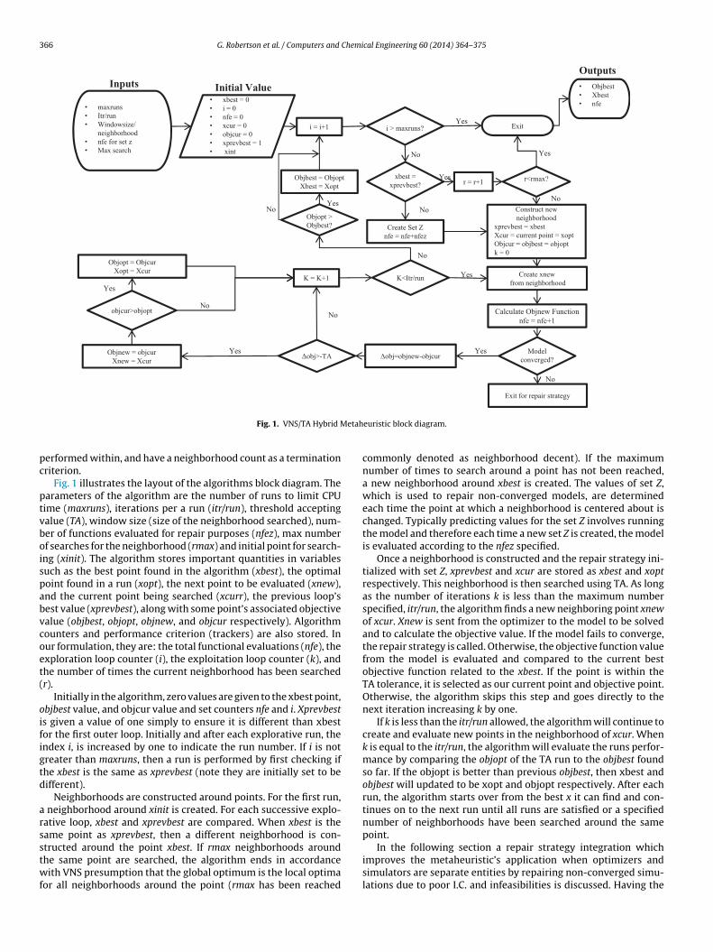

366 G. Robertson et al. / Computers and Chemical Engineering 60 (2014) 364– 375

Outputs• Objbest• Xbest• nfe• maxruns

• Itr/run• Windowsize/

neighborhood• nfe for set z• Max search

Inputs Initial Value• xbest = 0• i = 0• nfe = 0 • xcur = 0 • objcur = 0 • xprevbest = 1• xint

i = i+1 i > maxruns? Exit

xbest = xprevbest? r = r+1 r<rmax?

Create Set Znfe = nfe+nfez

Construct new neighborhood

xprevbest = xbestXcur = current point = xoptObjcur = objbest = objoptk = 0

Create xnewfrom neighborhood

Calculate Objnew Functionnfe = nfe+1

Model converged?

Exit for repair strategy

Δobj=objnew-objcurΔobj>-TAObjnew = objcurXnew = Xcur

objcur>objopt

Objopt = ObjcurXopt = Xcur

K = K+1 K<Itr/run

Objopt > Objbest?

Objbest = ObjoptXbest = Xopt

Yes

No Yes

No

Yes

No

Yes

NoNo

Yes

Yes

No

YesNo

Yes

No

etah

pc

ptvboispabvcoet(

oifigtd

arsstwf

Fig. 1. VNS/TA Hybrid M

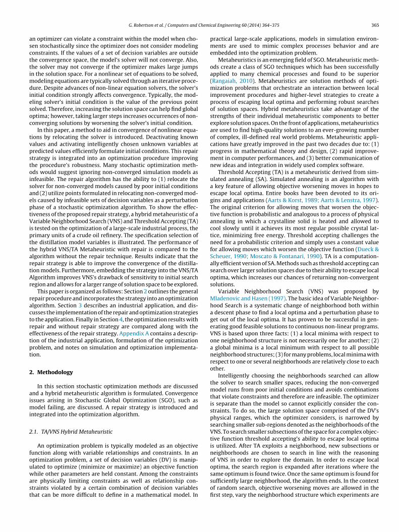
erformed within, and have a neighborhood count as a terminationriterion.

Fig. 1 illustrates the layout of the algorithms block diagram. Thearameters of the algorithm are the number of runs to limit CPUime (maxruns), iterations per a run (itr/run), threshold acceptingalue (TA), window size (size of the neighborhood searched), num-er of functions evaluated for repair purposes (nfez), max numberf searches for the neighborhood (rmax) and initial point for search-ng (xinit). The algorithm stores important quantities in variablesuch as the best point found in the algorithm (xbest), the optimaloint found in a run (xopt), the next point to be evaluated (xnew),nd the current point being searched (xcurr), the previous loop’sest value (xprevbest), along with some point’s associated objectivealue (objbest, objopt, objnew, and objcur respectively). Algorithmounters and performance criterion (trackers) are also stored. Inur formulation, they are: the total functional evaluations (nfe), thexploration loop counter (i), the exploitation loop counter (k), andhe number of times the current neighborhood has been searchedr).

Initially in the algorithm, zero values are given to the xbest point,bjbest value, and objcur value and set counters nfe and i. Xprevbests given a value of one simply to ensure it is different than xbestor the first outer loop. Initially and after each explorative run, thendex i, is increased by one to indicate the run number. If i is notreater than maxruns, then a run is performed by first checking ifhe xbest is the same as xprevbest (note they are initially set to beifferent).

Neighborhoods are constructed around points. For the first run, neighborhood around xinit is created. For each successive explo-ative loop, xbest and xprevbest are compared. When xbest is theame point as xprevbest, then a different neighborhood is con-

tructed around the point xbest. If rmax neighborhoods aroundhe same point are searched, the algorithm ends in accordanceith VNS presumption that the global optimum is the local optima

or all neighborhoods around the point (rmax has been reached

euristic block diagram.

commonly denoted as neighborhood decent). If the maximumnumber of times to search around a point has not been reached,a new neighborhood around xbest is created. The values of set Z,which is used to repair non-converged models, are determinedeach time the point at which a neighborhood is centered about ischanged. Typically predicting values for the set Z involves runningthe model and therefore each time a new set Z is created, the modelis evaluated according to the nfez specified.

Once a neighborhood is constructed and the repair strategy ini-tialized with set Z, xprevbest and xcur are stored as xbest and xoptrespectively. This neighborhood is then searched using TA. As longas the number of iterations k is less than the maximum numberspecified, itr/run, the algorithm finds a new neighboring point xnewof xcur. Xnew is sent from the optimizer to the model to be solvedand to calculate the objective value. If the model fails to converge,the repair strategy is called. Otherwise, the objective function valuefrom the model is evaluated and compared to the current bestobjective function related to the xbest. If the point is within theTA tolerance, it is selected as our current point and objective point.Otherwise, the algorithm skips this step and goes directly to thenext iteration increasing k by one.

If k is less than the itr/run allowed, the algorithm will continue tocreate and evaluate new points in the neighborhood of xcur. Whenk is equal to the itr/run, the algorithm will evaluate the runs perfor-mance by comparing the objopt of the TA run to the objbest foundso far. If the objopt is better than previous objbest, then xbest andobjbest will updated to be xopt and objopt respectively. After eachrun, the algorithm starts over from the best x it can find and con-tinues on to the next run until all runs are satisfied or a specifiednumber of neighborhoods have been searched around the samepoint.

In the following section a repair strategy integration whichimproves the metaheuristic’s application when optimizers andsimulators are separate entities by repairing non-converged simu-lations due to poor I.C. and infeasibilities is discussed. Having the

Chemical Engineering 60 (2014) 364– 375 367

an

2

npinbpameG

acastitpccoagoasrt

uodcswtt

2

crgadussnf

tsaXtfm

Evaluate Set X,Yi sets’ specifications are estimated,

y=0

i ≤ n

Activate Yii=i+1

YiConverge

?

Reactivate X

XConverge?

Exit repaired

Exit unrepaired(Infeasible point)

No

Yes

NoYes

No

Yes

G. Robertson et al. / Computers and

bility to repair non-converged simulations improves the robust-ess of the optimizer.

.2. Repair strategy

Modeling complex problems typically involves solving sets ofonlinear equations. Setting the problem up as an optimizationroblem and minimizing the error of the equations through an

terative procedure such as Newton Raphson best solves sets ofon-linear equations. Many variations of these procedures haveeen researched in order to improve the algorithms computationalerformance and reduce the sensitivity to initial conditions (suchs the Inside-Out algorithm). Although there have been improve-ents in the sensitivity to techniques which solve sets of nonlinear

quations, sensitivity to initial conditions are still an issue (Biegler,rossman, & Weseterberg, 1985).

In many cases the nonlinear set of equations has more vari-bles than equations and the modeler is interested in the modelonditions at a specific set of variables. The modeling equationsre solved by setting (giving values to) variables known as activepecifications. The set of active specifications are the same size ashe degrees of freedom of the problem. The active specification ofnterest to the modeler, X, may not be the easiest way of solvinghe set of equations. For example, calculating fluid properties atarticular temperatures usually takes one calculation; however,alculating the temperature at a vapor pressure is an iterative pro-ess (Antoine’s equation). There may be multiple different setsf active specifications, Y, which are easier to solve than X. Ourpproach will formulate new I.C.s, which can help attain conver-ence at non-converged specified values of set X, by using valuesbtained at solutions of the easier-to-converge sets Y. The vari-bles of all sets Yis which are not included in set X are denoted byet Z. The values in set Z must be predicted before beginning theepair algorithm. Fig. 2 illustrates the algorithm block diagram forhe proposed repair strategy.

The repair strategy tries to reach a solution at the specified val-es of X. If the model does not converge, an easier-to-solve set Yi,ut of a total of n, is activated at values from a number of pre-iction methods. If the model convergence at set Yi’s values, thisonverged point is used as the I.C. to the original set of D.V.s bywitching back to the set X. If it then converges, the set of D.V.s, X,as solved by changing the I.C. Once the algorithm has exhausted

he set of easier-to-converge sets, Yi’s, then the point is concludedo be infeasible.

.3. Repair strategy integrated into a stochastic algorithm

In the case of optimization, the variables of interest, set X, dis-ussed in Section 2.2 must include the set of decision variables. Theemaining DOF are chosen to meet constraints and ease of conver-ence criterion. The different sets of active specifications Y, whichre easier to solve than X, may not be composed of the originalecision variables of the optimization problem. These sets can besed to bring the non-converged points in X back to the solutionpace at the highest objective function value found during activepecification switching. However when evaluating a point to use asew I.C., we may serendipitously find that it has a higher objective

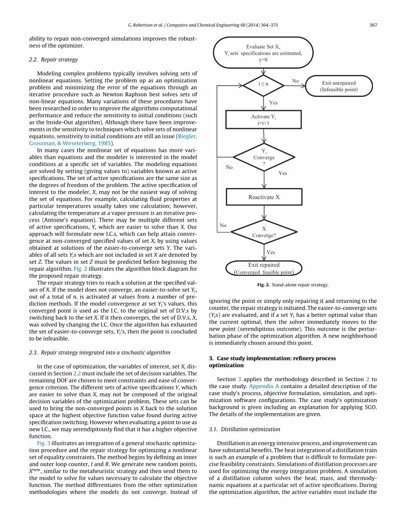
unction.Fig. 3 illustrates an integration of a general stochastic optimiza-

ion procedure and the repair strategy for optimizing a nonlinearet of equality constraints. The method begins by defining an innernd outer loop counter, I and R. We generate new random points,

new, similar to the metaheuristic strategy and then send them tohe model to solve for values necessary to calculate the objectiveunction. The method differentiates from the other optimization

ethodologies where the models do not converge. Instead of

(Converged feasible point)

Fig. 2. Stand-alone repair strategy.

ignoring the point or simply only repairing it and returning to thecounter, the repair strategy is initiated. The easier-to-converge sets(Yis) are evaluated, and if a set Yi has a better optimal value thanthe current optimal, then the solver immediately moves to thenew point (serendipitous outcome). This outcome is the pertur-bation phase of the optimization algorithm. A new neighborhoodis immediately chosen around this point.

3. Case study implementation: refinery processoptimization

Section 3 applies the methodology described in Section 2 tothe case study. Appendix A contains a detailed description of thecase study’s process, objective formulation, simulation, and opti-mization software configurations. The case study’s optimizationbackground is given including an explanation for applying SGO.The details of the implementation are given.

3.1. Distillation optimization

Distillation is an energy intensive process, and improvement canhave substantial benefits. The heat integration of a distillation trainis such an example of a problem that is difficult to formulate pre-cise feasibility constraints. Simulations of distillation processes are

used for optimizing the energy integration problem. A simulationof a distillation column solves the heat, mass, and thermody-namic equations at a particular set of active specifications. Duringthe optimization algorithm, the active variables must include the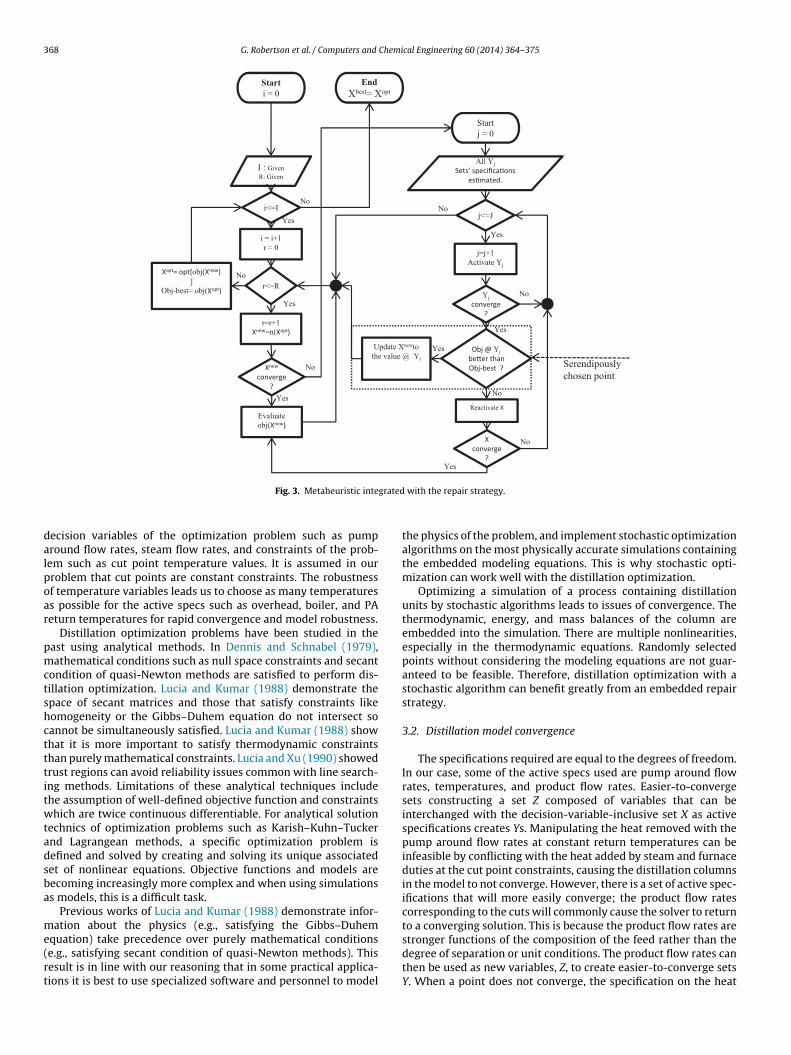

368 G. Robertson et al. / Computers and Chemical Engineering 60 (2014) 364– 375

Start= 0i

I : GivenR: Given

= i+1ir = 0

r<=R

r=r+1Xnew=n(Xopt)

Xnew

converge?

Evaluateobj(Xnew )

i<=I

Startj = 0

All YjSets’ specifica�ons

es�mated.

j<=J

j=j+1Activate Yj

Y

Yjconverge

?

@ YObj jbe�er than Obj-best ?

Reactivate X

Xconverge

?

Update XnewtoYthe value @ i

Xopt= opt[obj(Xnew )]

Obj-best= obj (Xopt)

EndXbest= Xopt

Serendipously chosen point

No

Yes

Yes

No

Yes

No

Yes

No

Yes

No

Yes

No

Yes

No

grated

dalpoar

pmctshctttitwtadsba

me(rt

Fig. 3. Metaheuristic inte

ecision variables of the optimization problem such as pumpround flow rates, steam flow rates, and constraints of the prob-em such as cut point temperature values. It is assumed in ourroblem that cut points are constant constraints. The robustnessf temperature variables leads us to choose as many temperaturess possible for the active specs such as overhead, boiler, and PAeturn temperatures for rapid convergence and model robustness.

Distillation optimization problems have been studied in theast using analytical methods. In Dennis and Schnabel (1979),athematical conditions such as null space constraints and secant

ondition of quasi-Newton methods are satisfied to perform dis-illation optimization. Lucia and Kumar (1988) demonstrate thepace of secant matrices and those that satisfy constraints likeomogeneity or the Gibbs–Duhem equation do not intersect soannot be simultaneously satisfied. Lucia and Kumar (1988) showhat it is more important to satisfy thermodynamic constraintshan purely mathematical constraints. Lucia and Xu (1990) showedrust regions can avoid reliability issues common with line search-ng methods. Limitations of these analytical techniques includehe assumption of well-defined objective function and constraintshich are twice continuous differentiable. For analytical solution

echnics of optimization problems such as Karish–Kuhn–Tuckernd Lagrangean methods, a specific optimization problem isefined and solved by creating and solving its unique associatedet of nonlinear equations. Objective functions and models areecoming increasingly more complex and when using simulationss models, this is a difficult task.

Previous works of Lucia and Kumar (1988) demonstrate infor-ation about the physics (e.g., satisfying the Gibbs–Duhem

quation) take precedence over purely mathematical conditionse.g., satisfying secant condition of quasi-Newton methods). Thisesult is in line with our reasoning that in some practical applica-ions it is best to use specialized software and personnel to model

with the repair strategy.

the physics of the problem, and implement stochastic optimizationalgorithms on the most physically accurate simulations containingthe embedded modeling equations. This is why stochastic opti-mization can work well with the distillation optimization.

Optimizing a simulation of a process containing distillationunits by stochastic algorithms leads to issues of convergence. Thethermodynamic, energy, and mass balances of the column areembedded into the simulation. There are multiple nonlinearities,especially in the thermodynamic equations. Randomly selectedpoints without considering the modeling equations are not guar-anteed to be feasible. Therefore, distillation optimization with astochastic algorithm can benefit greatly from an embedded repairstrategy.

3.2. Distillation model convergence

The specifications required are equal to the degrees of freedom.In our case, some of the active specs used are pump around flowrates, temperatures, and product flow rates. Easier-to-convergesets constructing a set Z composed of variables that can beinterchanged with the decision-variable-inclusive set X as activespecifications creates Ys. Manipulating the heat removed with thepump around flow rates at constant return temperatures can beinfeasible by conflicting with the heat added by steam and furnaceduties at the cut point constraints, causing the distillation columnsin the model to not converge. However, there is a set of active spec-ifications that will more easily converge; the product flow ratescorresponding to the cuts will commonly cause the solver to returnto a converging solution. This is because the product flow rates are

stronger functions of the composition of the feed rather than thedegree of separation or unit conditions. The product flow rates canthen be used as new variables, Z, to create easier-to-converge setsY. When a point does not converge, the specification on the heat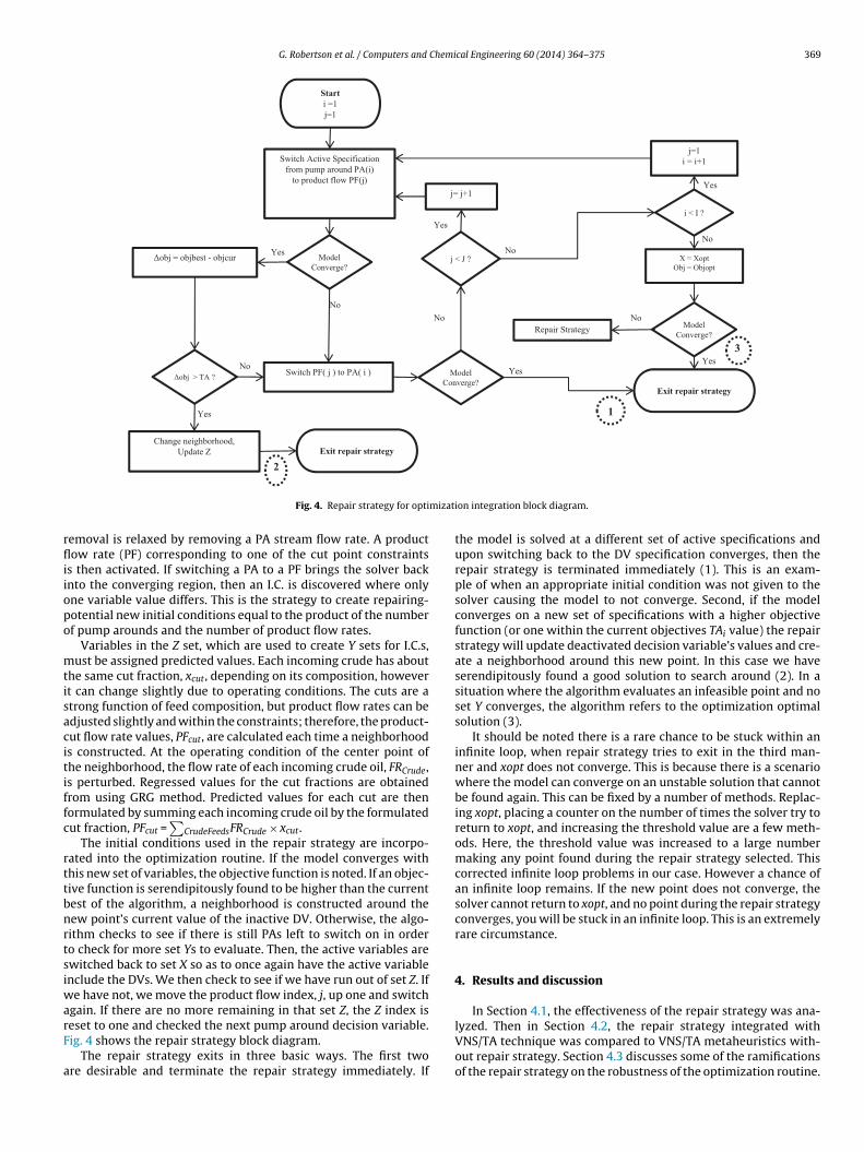

G. Robertson et al. / Computers and Chemical Engineering 60 (2014) 364– 375 369

Starti =1j=1

Switch Active Specification from pu mp around PA (i)

to product flo w PF (j)

Mod el Conv erg e?

Δob j > TA ?

Δob j = objbes t - objcu r

Chang e neighbo rhoo d, Update Z

Exit repair st rat egy

Switch PF( j ) to PA( i )

Mod el Converge?

Exit repair st rat egy

j= j+1

j < J ?

i < I ?

j=1i = i+1

X = XoptObj = Objop t

Mod el Conv erg e?

Repair Strategy

1

2

Yes

Yes

Yes

Yes

No

No

No

Yes

No

Yes

No

3

No

mizati

rfliiopo

mtisacitiffc

rttbnrtsiwarF

a

Fig. 4. Repair strategy for opti

emoval is relaxed by removing a PA stream flow rate. A productow rate (PF) corresponding to one of the cut point constraints

s then activated. If switching a PA to a PF brings the solver backnto the converging region, then an I.C. is discovered where onlyne variable value differs. This is the strategy to create repairing-otential new initial conditions equal to the product of the numberf pump arounds and the number of product flow rates.

Variables in the Z set, which are used to create Y sets for I.C.s,ust be assigned predicted values. Each incoming crude has about

he same cut fraction, xcut, depending on its composition, howevert can change slightly due to operating conditions. The cuts are atrong function of feed composition, but product flow rates can bedjusted slightly and within the constraints; therefore, the product-ut flow rate values, PFcut, are calculated each time a neighborhoods constructed. At the operating condition of the center point ofhe neighborhood, the flow rate of each incoming crude oil, FRCrude,s perturbed. Regressed values for the cut fractions are obtainedrom using GRG method. Predicted values for each cut are thenormulated by summing each incoming crude oil by the formulatedut fraction, PFcut =

∑CrudeFeedsFRCrude × xcut.

The initial conditions used in the repair strategy are incorpo-ated into the optimization routine. If the model converges withhis new set of variables, the objective function is noted. If an objec-ive function is serendipitously found to be higher than the currentest of the algorithm, a neighborhood is constructed around theew point’s current value of the inactive DV. Otherwise, the algo-ithm checks to see if there is still PAs left to switch on in ordero check for more set Ys to evaluate. Then, the active variables arewitched back to set X so as to once again have the active variablenclude the DVs. We then check to see if we have run out of set Z. If

e have not, we move the product flow index, j, up one and switchgain. If there are no more remaining in that set Z, the Z index is

eset to one and checked the next pump around decision variable.ig. 4 shows the repair strategy block diagram.

The repair strategy exits in three basic ways. The first twore desirable and terminate the repair strategy immediately. If

on integration block diagram.

the model is solved at a different set of active specifications andupon switching back to the DV specification converges, then therepair strategy is terminated immediately (1). This is an exam-ple of when an appropriate initial condition was not given to thesolver causing the model to not converge. Second, if the modelconverges on a new set of specifications with a higher objectivefunction (or one within the current objectives TAi value) the repairstrategy will update deactivated decision variable’s values and cre-ate a neighborhood around this new point. In this case we haveserendipitously found a good solution to search around (2). In asituation where the algorithm evaluates an infeasible point and noset Y converges, the algorithm refers to the optimization optimalsolution (3).

It should be noted there is a rare chance to be stuck within aninfinite loop, when repair strategy tries to exit in the third man-ner and xopt does not converge. This is because there is a scenariowhere the model can converge on an unstable solution that cannotbe found again. This can be fixed by a number of methods. Replac-ing xopt, placing a counter on the number of times the solver try toreturn to xopt, and increasing the threshold value are a few meth-ods. Here, the threshold value was increased to a large numbermaking any point found during the repair strategy selected. Thiscorrected infinite loop problems in our case. However a chance ofan infinite loop remains. If the new point does not converge, thesolver cannot return to xopt, and no point during the repair strategyconverges, you will be stuck in an infinite loop. This is an extremelyrare circumstance.

4. Results and discussion

In Section 4.1, the effectiveness of the repair strategy was ana-

lyzed. Then in Section 4.2, the repair strategy integrated withVNS/TA technique was compared to VNS/TA metaheuristics with-out repair strategy. Section 4.3 discusses some of the ramificationsof the repair strategy on the robustness of the optimization routine.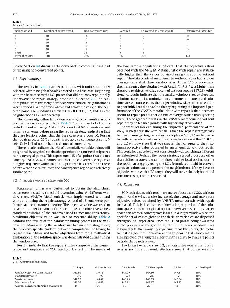

370 G. Robertson et al. / Computers and Chemical Engineering 60 (2014) 364– 375

Table 1Repair of base case results.

Neighborhood Number of points tested Non-converged runs Repaired Converged at alternative I.C. Determined infeasible

1 10 4 2 2 02 10 0 0 0 03 10 3 0 2 14 10 5 1 3 1

Fo

4

swudwtn

otitts

bncaps

4

pdwfmsMcdtret

t

TV

5 10 9

Total 50 21

Percent of total 100% 42%

inally, Section 4.4 discusses the draw back in computational loadf repairing non-converged points.

.1. Repair strategy

The results in Table 1 are experiments with points randomlyelected within neighborhoods centered on a base case. Beginningith the base case as the I.C., points that did not converge initiallynderwent the repair strategy proposed in Section 2.2. Ten ran-om points from five neighborhoods were chosen. Neighborhoodsere defined as a proportion above and below the value of the cen-

ered point. The window sizes were 0.05, 0.1, 0.15, 0.2, and 0.25 foreighborhoods 1–5 respectively.

The Repair Algorithm helps gain convergence of nonlinear setsf equations. As can be seen from Table 1 Column 3, 42% of all pointsested did not converge. Column 4 shows that 6% of points did notnitially converge before using the repair strategy, indicating thathey are feasible points that the base case was a poor I.C. Duringhe repair process, 22% of points were able to converge at some Yets. Only 14% of points had no chance of converging.

These results indicate that 6% of potentially valuable points wille ignored by a typical stochastic optimization routine that ignoreson-converged points. This represents 14% of all points that did notonverge. Also, 22% of points can enter the convergence region at

higher objective value than the optimizer has thus far or theseoints were able to return to the convergence region at a relativelyimilar point.

.2. Integrated repair strategy with SGO

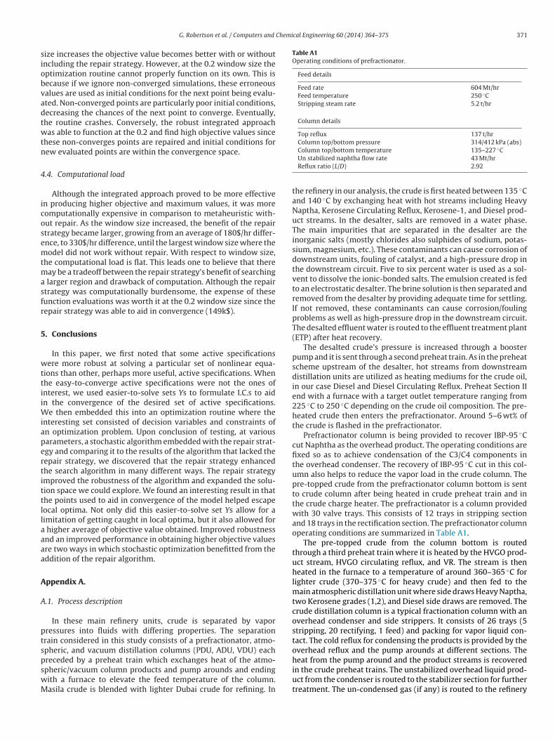
Parameter tuning was performed to obtain the algorithm’sarameters including threshold-accepting value. At different win-ow sizes, VNS/TA Metaheuristic was implemented with andithout utilizing the repair strategy. A total of 15 runs were per-

ormed at each parameter setting. The objective value was used toeasure the performance of the technique. The objective value’s

tandard deviation of the runs was used to measure consistency.aximum objective value was used to measure ability. Table 2

ontains the results of the parameter tuning process of the win-ow size. Manipulating the window size had an interesting effect;he problem-specific tradeoff between computation of having toepair infeasibilities and better objectives from more methodical

xploration of the solution space was demonstrated during tuninghe window size.

Results indicate that the repair strategy improved the consis-ency and amplitude of SGO method. A t-test on the means of

able 2NS/TA optimization results.

0.1 Repair 0.1 No Repair

Average objective value (k$/hr) 146.96 146.78

Standard deviation .46 .09

Maximum value 147.59 146.87

Minimum value 146.29 146.69

Average number of function evaluations 44 26

0 4 53 11 76% 22% 14%

the two sample populations indicates that the objective valuesobtained with the VNS/TA Metaheuristic with repair are statisti-cally higher than the values obtained using the routine withoutrepair. The data points of metaheuristic without repair had a loweraverage value at all three window sizes. At the 0.15 window size,the minimum value obtained with Repair (147.31) was higher thanthe average objective value obtained without repair (147.26). Addi-tionally, results indicate that the smaller window sizes explore lesssolution space during optimization and more non-converged solu-tions are encountered as the larger window sizes are chosen dueto poor initial conditions. One theory explaining the improved per-formance of the VNS/TA metaheuristic with repair is that it is moreuseful to repair points that do not converge rather than ignoringthem. These ignored points in the VNS/TA metaheuristic withoutrepair may be feasible points with higher objective values.

Another reason explaining the improved performance of theVNS/TA metaheuristic with repair is that the repair strategy mayhelp overcome getting caught in local optima. VNS/TA metaheuris-tic with repair obtained a maximum objective value at the 0.1, 0.15,and 0.2 window sizes that was greater than or equal to the max-imum objective value obtained by metaheuristic without repair.This could lead us to believe it consistently was searching a differentneighborhood. Perhaps the repair strategy served a purpose otherthan aiding in convergence; it helped exiting local optima duringthe repair strategy by using the I.C.s formulated to aid in conver-gence as points used to perturb the neighborhood. If they have anobjective value within TA range, they will move the neighborhoodthus increasing the area searched.

4.3. Robustness

SGO techniques with repair are more robust than SGOs withoutrepair. As the window size increased, the average and maximumobjective values obtained by VNS/TA metaheuristic with repairincreased. This is because searching a larger portion of the solu-tion space helps attain global optima; however, searching a largerspace can worsen convergence issues. In a larger window size, thespecific set of values given to the decision variables are dispersedthroughout a larger area. Since the I.C. of points being evaluatedis the previous converged point, the I.C. in larger window sizesis typically farther away. By repairing infeasible points, the meta-heuristic algorithm’s drawbacks due to poor initial search region

are improved by giving the algorithm the ability to evaluate pointsoutside the search region.

The largest window size, 0.2, demonstrates where the robust-ness is no more apparent. We have seen that as the window

0.15 Repair 0.15 No Repair 0.2 Repair 0.2 No Repair

147.59 147.26 147.87 N/A.28 .45 .7 N/A

148.29 148.29 149.06 N/A147.32 146.67 147.22 N/A

58 26 43 N/A

Chemical Engineering 60 (2014) 364– 375 371

siobvadtwtn

4

icosemtmasfr

5

wttiiWiapertittllaaaa

A

A

ptspswM

Table A1Operating conditions of prefractionator.

Feed details

Feed rate 604 Mt/hrFeed temperature 250 ◦CStripping steam rate 5.2 t/hr

Column details

Top reflux 137 t/hrColumn top/bottom pressure 314/412 kPa (abs)

◦

G. Robertson et al. / Computers and

ize increases the objective value becomes better with or withoutncluding the repair strategy. However, at the 0.2 window size theptimization routine cannot properly function on its own. This isecause if we ignore non-converged simulations, these erroneousalues are used as initial conditions for the next point being evalu-ted. Non-converged points are particularly poor initial conditions,ecreasing the chances of the next point to converge. Eventually,he routine crashes. Conversely, the robust integrated approachas able to function at the 0.2 and find high objective values since

hese non-converges points are repaired and initial conditions forew evaluated points are within the convergence space.

.4. Computational load

Although the integrated approach proved to be more effectiven producing higher objective and maximum values, it was moreomputationally expensive in comparison to metaheuristic with-ut repair. As the window size increased, the benefit of the repairtrategy became larger, growing from an average of 180$/hr differ-nce, to 330$/hr difference, until the largest window size where theodel did not work without repair. With respect to window size,

he computational load is flat. This leads one to believe that thereay be a tradeoff between the repair strategy’s benefit of searching

larger region and drawback of computation. Although the repairtrategy was computationally burdensome, the expense of theseunction evaluations was worth it at the 0.2 window size since theepair strategy was able to aid in convergence (149k$).

. Conclusions

In this paper, we first noted that some active specificationsere more robust at solving a particular set of nonlinear equa-

ions than other, perhaps more useful, active specifications. Whenhe easy-to-converge active specifications were not the ones ofnterest, we used easier-to-solve sets Ys to formulate I.C.s to aidn the convergence of the desired set of active specifications.

e then embedded this into an optimization routine where thenteresting set consisted of decision variables and constraints ofn optimization problem. Upon conclusion of testing, at variousarameters, a stochastic algorithm embedded with the repair strat-gy and comparing it to the results of the algorithm that lacked theepair strategy, we discovered that the repair strategy enhancedhe search algorithm in many different ways. The repair strategymproved the robustness of the algorithm and expanded the solu-ion space we could explore. We found an interesting result in thathe points used to aid in convergence of the model helped escapeocal optima. Not only did this easier-to-solve set Ys allow for aimitation of getting caught in local optima, but it also allowed for

higher average of objective value obtained. Improved robustnessnd an improved performance in obtaining higher objective valuesre two ways in which stochastic optimization benefitted from theddition of the repair algorithm.

ppendix A.

.1. Process description

In these main refinery units, crude is separated by vaporressures into fluids with differing properties. The separationrain considered in this study consists of a prefractionator, atmo-pheric, and vacuum distillation columns (PDU, ADU, VDU) each

receded by a preheat train which exchanges heat of the atmo-pheric/vacuum column products and pump arounds and endingith a furnace to elevate the feed temperature of the column.asila crude is blended with lighter Dubai crude for refining. In

Column top/bottom temperature 135–227 CUn stabilized naphtha flow rate 43 Mt/hrReflux ratio (L/D) 2.92

the refinery in our analysis, the crude is first heated between 135 ◦Cand 140 ◦C by exchanging heat with hot streams including HeavyNaptha, Kerosene Circulating Reflux, Kerosene-1, and Diesel prod-uct streams. In the desalter, salts are removed in a water phase.The main impurities that are separated in the desalter are theinorganic salts (mostly chlorides also sulphides of sodium, potas-sium, magnesium, etc.). These contaminants can cause corrosion ofdownstream units, fouling of catalyst, and a high-pressure drop inthe downstream circuit. Five to six percent water is used as a sol-vent to dissolve the ionic-bonded salts. The emulsion created is fedto an electrostatic desalter. The brine solution is then separated andremoved from the desalter by providing adequate time for settling.If not removed, these contaminants can cause corrosion/foulingproblems as well as high-pressure drop in the downstream circuit.The desalted effluent water is routed to the effluent treatment plant(ETP) after heat recovery.

The desalted crude’s pressure is increased through a boosterpump and it is sent through a second preheat train. As in the preheatscheme upstream of the desalter, hot streams from downstreamdistillation units are utilized as heating mediums for the crude oil,in our case Diesel and Diesel Circulating Reflux. Preheat Section IIend with a furnace with a target outlet temperature ranging from225 ◦C to 250 ◦C depending on the crude oil composition. The pre-heated crude then enters the prefractionator. Around 5–6 wt% ofthe crude is flashed in the prefractionator.

Prefractionator column is being provided to recover IBP-95 ◦Ccut Naphtha as the overhead product. The operating conditions arefixed so as to achieve condensation of the C3/C4 components inthe overhead condenser. The recovery of IBP-95 ◦C cut in this col-umn also helps to reduce the vapor load in the crude column. Thepre-topped crude from the prefractionator column bottom is sentto crude column after being heated in crude preheat train and inthe crude charge heater. The prefractionator is a column providedwith 30 valve trays. This consists of 12 trays in stripping sectionand 18 trays in the rectification section. The prefractionator columnoperating conditions are summarized in Table A1.

The pre-topped crude from the column bottom is routedthrough a third preheat train where it is heated by the HVGO prod-uct stream, HVGO circulating reflux, and VR. The stream is thenheated in the furnace to a temperature of around 360–365 ◦C forlighter crude (370–375 ◦C for heavy crude) and then fed to themain atmospheric distillation unit where side draws Heavy Naptha,two Kerosene grades (1,2), and Diesel side draws are removed. Thecrude distillation column is a typical fractionation column with anoverhead condenser and side strippers. It consists of 26 trays (5stripping, 20 rectifying, 1 feed) and packing for vapor liquid con-tact. The cold reflux for condensing the products is provided by theoverhead reflux and the pump arounds at different sections. The

heat from the pump around and the product streams is recoveredin the crude preheat trains. The unstabilized overhead liquid prod-uct from the condenser is routed to the stabilizer section for furthertreatment. The un-condensed gas (if any) is routed to the refinery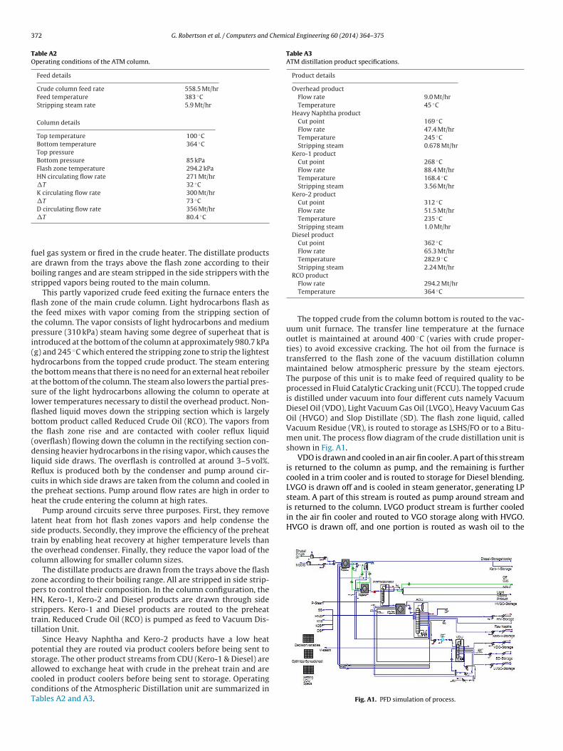

372 G. Robertson et al. / Computers and Chemical Engineering 60 (2014) 364– 375

Table A2Operating conditions of the ATM column.

Feed details

Crude column feed rate 558.5 Mt/hrFeed temperature 383 ◦CStripping steam rate 5.9 Mt/hr

Column details

Top temperature 100 ◦CBottom temperature 364 ◦CTop pressureBottom pressure 85 kPaFlash zone temperature 294.2 kPaHN circulating flow rate 271 Mt/hr�T 32 ◦CK circulating flow rate 300 Mt/hr�T 73 ◦CD circulating flow rate 356 Mt/hr

fabs

flttpi(htaslflbt(dlRcth

lsttc

zpHstt

psaccT

Table A3ATM distillation product specifications.

Product details

Overhead productFlow rate 9.0 Mt/hrTemperature 45 ◦C

Heavy Naphtha productCut point 169 ◦CFlow rate 47.4 Mt/hrTemperature 245 ◦CStripping steam 0.678 Mt/hr

Kero-1 productCut point 268 ◦CFlow rate 88.4 Mt/hrTemperature 168.4 ◦CStripping steam 3.56 Mt/hr

Kero-2 productCut point 312 ◦CFlow rate 51.5 Mt/hrTemperature 235 ◦CStripping steam 1.0 Mt/hr

Diesel productCut point 362 ◦CFlow rate 65.3 Mt/hrTemperature 282.9 ◦CStripping steam 2.24 Mt/hr

RCO product

is returned to the column. LVGO product stream is further cooledin the air fin cooler and routed to VGO storage along with HVGO.HVGO is drawn off, and one portion is routed as wash oil to the

�T 80.4 ◦C

uel gas system or fired in the crude heater. The distillate productsre drawn from the trays above the flash zone according to theiroiling ranges and are steam stripped in the side strippers with thetripped vapors being routed to the main column.

This partly vaporized crude feed exiting the furnace enters theash zone of the main crude column. Light hydrocarbons flash ashe feed mixes with vapor coming from the stripping section ofhe column. The vapor consists of light hydrocarbons and mediumressure (310 kPa) steam having some degree of superheat that is

ntroduced at the bottom of the column at approximately 980.7 kPag) and 245 ◦C which entered the stripping zone to strip the lightestydrocarbons from the topped crude product. The steam enteringhe bottom means that there is no need for an external heat reboilert the bottom of the column. The steam also lowers the partial pres-ure of the light hydrocarbons allowing the column to operate atower temperatures necessary to distil the overhead product. Non-ashed liquid moves down the stripping section which is largelyottom product called Reduced Crude Oil (RCO). The vapors fromhe flash zone rise and are contacted with cooler reflux liquidoverflash) flowing down the column in the rectifying section con-ensing heavier hydrocarbons in the rising vapor, which causes the

iquid side draws. The overflash is controlled at around 3–5 vol%.eflux is produced both by the condenser and pump around cir-uits in which side draws are taken from the column and cooled inhe preheat sections. Pump around flow rates are high in order toeat the crude entering the column at high rates.

Pump around circuits serve three purposes. First, they removeatent heat from hot flash zones vapors and help condense theide products. Secondly, they improve the efficiency of the preheatrain by enabling heat recovery at higher temperature levels thanhe overhead condenser. Finally, they reduce the vapor load of theolumn allowing for smaller column sizes.

The distillate products are drawn from the trays above the flashone according to their boiling range. All are stripped in side strip-ers to control their composition. In the column configuration, theN, Kero-1, Kero-2 and Diesel products are drawn through side

trippers. Kero-1 and Diesel products are routed to the preheatrain. Reduced Crude Oil (RCO) is pumped as feed to Vacuum Dis-illation Unit.

Since Heavy Naphtha and Kero-2 products have a low heatotential they are routed via product coolers before being sent totorage. The other product streams from CDU (Kero-1 & Diesel) arellowed to exchange heat with crude in the preheat train and are

ooled in product coolers before being sent to storage. Operatingonditions of the Atmospheric Distillation unit are summarized inables A2 and A3.

Flow rate 294.2 Mt/hrTemperature 364 ◦C

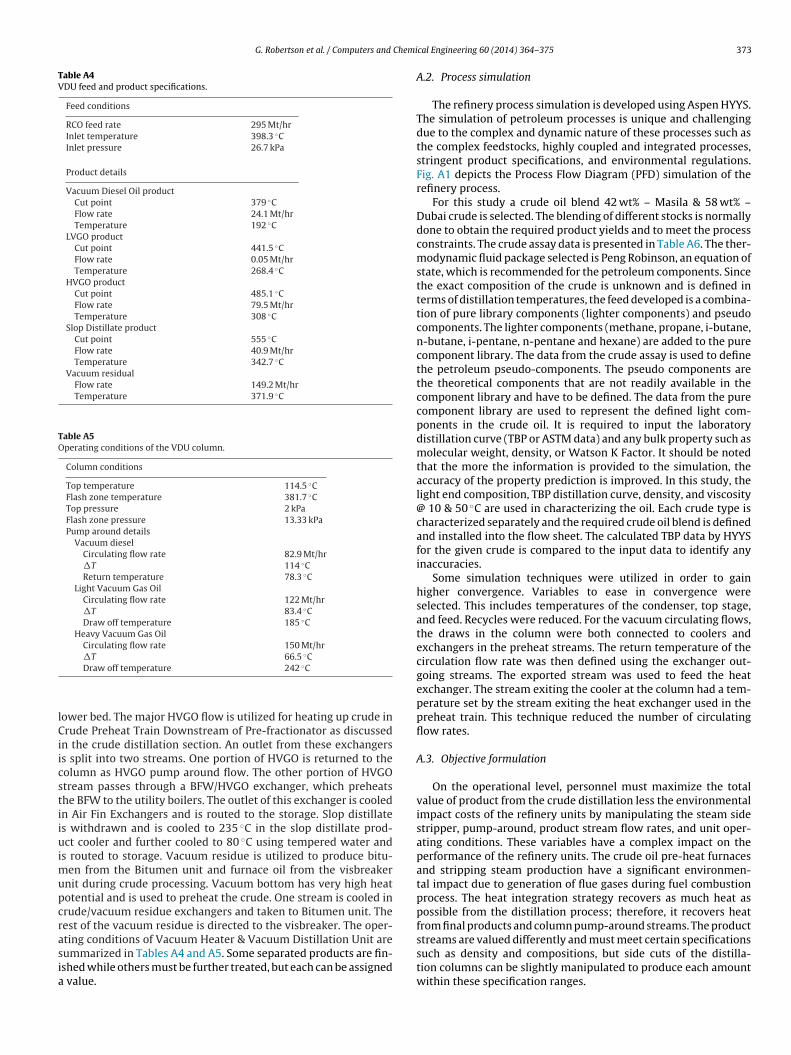
The topped crude from the column bottom is routed to the vac-uum unit furnace. The transfer line temperature at the furnaceoutlet is maintained at around 400 ◦C (varies with crude proper-ties) to avoid excessive cracking. The hot oil from the furnace istransferred to the flash zone of the vacuum distillation columnmaintained below atmospheric pressure by the steam ejectors.The purpose of this unit is to make feed of required quality to beprocessed in Fluid Catalytic Cracking unit (FCCU). The topped crudeis distilled under vacuum into four different cuts namely VacuumDiesel Oil (VDO), Light Vacuum Gas Oil (LVGO), Heavy Vacuum GasOil (HVGO) and Slop Distillate (SD). The flash zone liquid, calledVacuum Residue (VR), is routed to storage as LSHS/FO or to a Bitu-men unit. The process flow diagram of the crude distillation unit isshown in Fig. A1.

VDO is drawn and cooled in an air fin cooler. A part of this streamis returned to the column as pump, and the remaining is furthercooled in a trim cooler and is routed to storage for Diesel blending.LVGO is drawn off and is cooled in steam generator, generating LPsteam. A part of this stream is routed as pump around stream and

Fig. A1. PFD simulation of process.

G. Robertson et al. / Computers and Chemi

Table A4VDU feed and product specifications.

Feed conditions

RCO feed rate 295 Mt/hrInlet temperature 398.3 ◦CInlet pressure 26.7 kPa

Product details

Vacuum Diesel Oil productCut point 379 ◦CFlow rate 24.1 Mt/hrTemperature 192 ◦C

LVGO productCut point 441.5 ◦CFlow rate 0.05 Mt/hrTemperature 268.4 ◦C

HVGO productCut point 485.1 ◦CFlow rate 79.5 Mt/hrTemperature 308 ◦C

Slop Distillate productCut point 555 ◦CFlow rate 40.9 Mt/hrTemperature 342.7 ◦C

Vacuum residualFlow rate 149.2 Mt/hrTemperature 371.9 ◦C

Table A5Operating conditions of the VDU column.

Column conditions

Top temperature 114.5 ◦CFlash zone temperature 381.7 ◦CTop pressure 2 kPaFlash zone pressure 13.33 kPaPump around details

Vacuum dieselCirculating flow rate 82.9 Mt/hr�T 114 ◦CReturn temperature 78.3 ◦C

Light Vacuum Gas OilCirculating flow rate 122 Mt/hr�T 83.4 ◦CDraw off temperature 185 ◦C

Heavy Vacuum Gas OilCirculating flow rate 150 Mt/hr�T 66.5 ◦C

lCiicstiiuimupcrasia

streams are valued differently and must meet certain specifications

Draw off temperature 242 ◦C

ower bed. The major HVGO flow is utilized for heating up crude inrude Preheat Train Downstream of Pre-fractionator as discussed

n the crude distillation section. An outlet from these exchangerss split into two streams. One portion of HVGO is returned to theolumn as HVGO pump around flow. The other portion of HVGOtream passes through a BFW/HVGO exchanger, which preheatshe BFW to the utility boilers. The outlet of this exchanger is cooledn Air Fin Exchangers and is routed to the storage. Slop distillates withdrawn and is cooled to 235 ◦C in the slop distillate prod-ct cooler and further cooled to 80 ◦C using tempered water and

s routed to storage. Vacuum residue is utilized to produce bitu-en from the Bitumen unit and furnace oil from the visbreaker

nit during crude processing. Vacuum bottom has very high heatotential and is used to preheat the crude. One stream is cooled inrude/vacuum residue exchangers and taken to Bitumen unit. Theest of the vacuum residue is directed to the visbreaker. The oper-ting conditions of Vacuum Heater & Vacuum Distillation Unit are

ummarized in Tables A4 and A5. Some separated products are fin-shed while others must be further treated, but each can be assigned

value.

cal Engineering 60 (2014) 364– 375 373

A.2. Process simulation

The refinery process simulation is developed using Aspen HYYS.The simulation of petroleum processes is unique and challengingdue to the complex and dynamic nature of these processes such asthe complex feedstocks, highly coupled and integrated processes,stringent product specifications, and environmental regulations.Fig. A1 depicts the Process Flow Diagram (PFD) simulation of therefinery process.

For this study a crude oil blend 42 wt% – Masila & 58 wt% –Dubai crude is selected. The blending of different stocks is normallydone to obtain the required product yields and to meet the processconstraints. The crude assay data is presented in Table A6. The ther-modynamic fluid package selected is Peng Robinson, an equation ofstate, which is recommended for the petroleum components. Sincethe exact composition of the crude is unknown and is defined interms of distillation temperatures, the feed developed is a combina-tion of pure library components (lighter components) and pseudocomponents. The lighter components (methane, propane, i-butane,n-butane, i-pentane, n-pentane and hexane) are added to the purecomponent library. The data from the crude assay is used to definethe petroleum pseudo-components. The pseudo components arethe theoretical components that are not readily available in thecomponent library and have to be defined. The data from the purecomponent library are used to represent the defined light com-ponents in the crude oil. It is required to input the laboratorydistillation curve (TBP or ASTM data) and any bulk property such asmolecular weight, density, or Watson K Factor. It should be notedthat the more the information is provided to the simulation, theaccuracy of the property prediction is improved. In this study, thelight end composition, TBP distillation curve, density, and viscosity@ 10 & 50 ◦C are used in characterizing the oil. Each crude type ischaracterized separately and the required crude oil blend is definedand installed into the flow sheet. The calculated TBP data by HYYSfor the given crude is compared to the input data to identify anyinaccuracies.

Some simulation techniques were utilized in order to gainhigher convergence. Variables to ease in convergence wereselected. This includes temperatures of the condenser, top stage,and feed. Recycles were reduced. For the vacuum circulating flows,the draws in the column were both connected to coolers andexchangers in the preheat streams. The return temperature of thecirculation flow rate was then defined using the exchanger out-going streams. The exported stream was used to feed the heatexchanger. The stream exiting the cooler at the column had a tem-perature set by the stream exiting the heat exchanger used in thepreheat train. This technique reduced the number of circulatingflow rates.

A.3. Objective formulation

On the operational level, personnel must maximize the totalvalue of product from the crude distillation less the environmentalimpact costs of the refinery units by manipulating the steam sidestripper, pump-around, product stream flow rates, and unit oper-ating conditions. These variables have a complex impact on theperformance of the refinery units. The crude oil pre-heat furnacesand stripping steam production have a significant environmen-tal impact due to generation of flue gases during fuel combustionprocess. The heat integration strategy recovers as much heat aspossible from the distillation process; therefore, it recovers heatfrom final products and column pump-around streams. The product

such as density and compositions, but side cuts of the distilla-tion columns can be slightly manipulated to produce each amountwithin these specification ranges.

374 G. Robertson et al. / Computers and Chemical Engineering 60 (2014) 364– 375

Table A6Assay data for Dubai and Masila crude.

Properties Light end analysis TBP distillation

Component wt% vol% ◦C wt% vol%

Masila crudeDensity 15 ◦C (kg/m3) 874 Ethane 0.02 0.05◦ API 30 Propane 0.29 0.5 15 1.4 1.86Viscosity (cSt) at 10 ◦C 20 iso-butane 0.23 0.36 149 15.6 19.2Viscosity (cSt) at 50 ◦C 5.9 n-Butane 0.86 1.29 232 28.9 33.8Pour point (◦C) −30 342 48.6 53.9

362 53.4 58.5509 74.4 78.3550 79.3 82.7

Dubai crudeDensity 15 ◦C (kg/m3) 868 Ethane 0 0◦ API 31 Propane 0.05 0.09 15 0.39 0.3Viscosity (cSt) at 10 ◦C 22 iso-Butane 0.14 0.22 32 1.09 1.28Viscosity (cSt) at 50 ◦C 7.3 n-Butane 0.2 0.3 93 4.45 5.53Pour point (◦C) −9 149 12.4 14.9

182 17.7 20.8260 30.8 34.8371 52.8 56.9427 59.9 63.8

nsotomopuuomrat

prT9w

mPuIDe(Tf

P

T

Irrsp

The complex heat integration schemes and the interactiveature of the process due to the presence of pump-around andide-stripper distillation features make it difficult to operate at theptimal conditions and consequently create a difficult optimiza-ion problem. The huge capital expenditure involved in the refiningperations creates good opportunities for optimization. It is esti-ated that crude oil cost account for about 85–90% of the total

perating cost and therefore, a wide variety of crude blends arerocessed depending on the cost and demand of the various prod-cts. This change in feed composition often results in inferior crudenit performance and reduces the unit’s run length. Therefore, theptimal conditions vary depending on the crude selected and opti-izing the operation of the crude unit is essential to maximize a

efiner’s economics. In addition, recent crude oil price fluctuationsnd increased economic pressure further emphasize the impor-ance of optimizing crude unit performance.

The decision variables of the operational level optimizationroblem are the stripping steam mass flow rates, product flowates, pump around flow rates, and overhead column flow rates.he constraints are the quality parameters such as the ASTM D865% temperature of the product flows detailed in Section 3 alongith bounds on the decision variables.

Objective function. The goal in the operational planning level is toaximize operational revenue. Eq. (1) is the typical profit function,

F, which is equal to the revenue from the products, RP, minus thetility costs to produce them, UC, and the raw material costs, RM.

n refineries, the energy demand is met by burning side products.ue to rising global warming concerns and with implementation ofmissions trading programs (“cap and trade”), the triple bottom lineTBL) objective function given in Eq. (2) was used in our approach.he objective function used accounts for costs associated with theeed, products, utilities, and environmental effects.

F = RP − UC − RM (1)

BL = PF − SD − EC + SC (2)

n Eq. (2), EC is the cost required to comply with environmental

egulations such as permits, monitoring emissions, fines, etc. SCepresents the sustainable credits given to the processes that con-ume pollutants. SD represents the sustainable debits that penalizerocesses for producing pollutants (poll). In this study, sulphur

482 70.1 73.6538 78.1 81550 80.4 83.2

dioxide (SO2), carbon dioxide (CO2), and nitrogen oxides (NOx) arechosen as the environmental load. The plant requires electricity forthe condensers, steam for stripping, and heat for elevating feedsgenerating releases to the environment that are considered sub-stantial debits. A portion of the net energy required is obtained byusing the overhead gas of the PDU as the fuel in the furnace and thebalance is met from fuel oil. From the environmental loads analy-sis, it is evident that the use of fuel gas in the furnace reduces theemissions to a greater extent but at the same time reduces the quan-tity of the useful product having a negative impact on the columneconomics.

UC =∑

f

FDf × Ch +∑

c

CDc × Cc +∑

s

Qs × Cs (3)

RP =∑

p

PPp × Qp (4)

TEFO = (FHR + SHR) × �ce (5)

FHR =(∑

f FDf − FGEF)

�f(6)

SHR =(∑

sQs × SpecificHeat)

�b(7)

SD =∑

poll

(FGEF × Rpoll/duty + TEFO × Rpoll/duty) × Penaltypoll (8)

Eq. (3) calculates the utility costs as the sum of the total furnaceheating duties, FDf, over all furnaces f multiplied by the cost of heat-ing, Ch, the total condenser cooling duties, CDc, of all condensers cmultiplied by the cooling costs, Cc, and the steam flow rates, Qs,multiplied by the cost to produce steam, Cs. Eq. (4) is the revenueof products, RP, calculated as the multiplication of unit prices offinal products (PPp) and product flow rates (Qp), summed over all

products p.

In Table A7, pollution ratios are given as pollution amount pro-portional to the electricity produced if the fuel had been used tocreate electricity in a combustion engine. The available correlations

G. Robertson et al. / Computers and Chemi

Table A7Pollution ratios.

Environmental loads Fuel oil Fuel gas

CO2 (t/GWh) 657 439

re

dEmrFFflmQdTrabwtp

pttittittoiisflvalb

SO2 (kg/GWh) 1030 1NOx (kg/GWh) 988 1400

elate the amount of pollutants released by the fuel burned to thelectricity generated in combustion engines.

The theoretical electricity of fuel oil (TEFO) is the electricity pro-uced if the fuel oil used in the process is converted to electricity.q. (5) calculates TEFO by multiplying the fuel oil total heat require-ent by the combustion engine efficiency, �ce. The fuel oil heat

equirement is equal to the sum of the furnace heat requirement,HR, and the heat necessary to produce the steam, SHR (Eq. (6)). TheHR for the fuel oil is the total heater duty minus fuel gas enthalpyow, FGEF, divided by furnace efficiency, �f. Steam heat require-ents, SHR, is equal to the total mass flow rate of the steam streams,

s, over all steam streams s multiplied by the steam’s specific heativided by the boiler efficiency, �b, to produce the heat (Eq. (7)).his method of calculating the pollution loads by finding a theo-etical electricity production is due to the availability of pollutionmount/energy produced ratio data (Rpoll/duty) and can be replacedy simply inserting a ratio of pollution amount to fuel oil requiredhere that information is needed. The sustainable debits, SD, are

hen calculated as the pollutant amount multiplied by a pollutionenalty, calculated in Eq. (8).

In the optimization problem considered in this experiment, tem-erature profiles are kept relatively constant. For example, feedemperatures to the column, condenser temperatures and top stageemperatures are kept constant. It can be stated that our problems using the minimum energy required to achieve an approximateemperature profile; therefore, column temperatures are variableso aid in convergence. Since the amount of heat given to the feedss varied, the furnace duty is set to achieve the feed tempera-ure. Although this is the optimization problem considered here,he tools and techniques discussed in this paper can be applied inther scenarios. Feed costs are ignored since it is assumed that thencoming oil has already been purchased and raw water necessarys proportional to feed costs. SC is equal to zero as no processes con-ume pollutants. EC are ignored because they are a function of feedow rate and do not affect the optimization problem. A 100% con-

ersion of the fuel gas enthalpy to electricity is assumed, but thisccounts for less than 2% of the total pollutants. The bulk of the pol-utants come from the theoretical electricity of fuel oil multipliedy the pollutant penalty per duty.

cal Engineering 60 (2014) 364– 375 375

Assumptions in the objective calculation include: The sourcesof emissions are steam generated from utility boilers, furnaces fluegas, and electricity; the net equivalent electricity (fuel had beenused to create electricity in a combustion engine) was determined.A heat to power ratio of 1.25 to account for fouling was used. Thesteam is Mp steam @ 245 ◦C with an enthalpy of 13.5 MMKJ/hr perton of steam. Efficiency of the cogeneration plant is 75%.

The modeling equations are thermodynamic relationships, massbalances, and energy balances obtained using HYYS®. The opti-mization model is a NLP solved with a VBA based code for theMetaheuristic. The solver uses an improved generalized gradientmethod capable of solving large scale nonlinear problems usedfor predicting the values of the easier-to-converge set variables. Abridge code is programmed in Visual Basic Application (VBA). Thebridge code allows the user to import and export any selected vari-ables between the HYYS model and Excel worksheet. Interactionwith HYYS uses object linking and embedding (OLE) automation.

The optimization process first takes the objects which are thevariables of the triple bottom line objective function from theHYSYS library. The Visual Basic for Applications (VBA) bridge codethen embeds them into an Excel spreadsheet where the Meta-heuristic optimizer chooses the next set of variables to insert intothe HYSYS model. In each of the iterations, the total cost of therefinery operations is embedded into the Excel spreadsheet.

References

Aarts, E. H. L., & Korst, J. (1989). Simulated annealing and Boltzmann machines: A stoch-asitc approach to combinatorial optimization and neural computing. Chichester:Wiley.

Aarts, E. H. L., & Lenstra, J. K. (1997). Local search in combinatorial optimization.Chichester: Wiley.

Biegler, L. T., Grossman, I. E., & Weseterberg, A. W. (1985). A note on approximationtechniquess used for process optimization. Computers & Chemical Engineering,9, 201–206.

Dennis, J. E., & Schnabel, R. B. (1979). Least change secant updates for quasi-Newtonmethods. SIAM Review, 21, 443–459.

Dueck, G., & Scheuer, T. (1990). Threshold Accepting – A general-purpose opti-mization algorithm appearing superior to simulated annealing. Journal ofComputational Physics, 90, 161–175.

Lucia, A., & Kumar, A. (1988). Distillation optimization. Computers & Chemical Engi-neering, 12, 1263–1266.

Lucia, A., & Xu, J. (1990). Chemical process optimiztion using Newton-like methods.Computers & Chemical Engineering, 14, 119–138.

Mladenovic, N., & Hasen, P. (1997). Variable Neighborhood Search. Computers &Operations Research, 197–1100.

Moscato, P., & Fontanari, J. F. (1990). Convergence and finite-time behaviour ofsimulated annealing. Advances in Applied Probability, 18, 747–771.

Rangaiah, G. P. (2010). Stochastic Global Optimization techniques and applications inchemical engineering. Singapore: World Scientific Publishing Co. Pte. Ltd.

Robertson, G., Palazoglu, A., & Romagnoli, J. A. (2011). A multi-level simulationapproach for the crude oil loading/unloading scheduling problem. Computers& Chemical Engineering, 35, 817–827.