An affine intensity model for large credit portfolios

An affine intensity model for large credit portfolios

Beatrice Acciaio∗and Stefano Herzel†

July 3, 2008

Abstract

The paper proposes a reduced-form model for credit risk in a multivariate setting. Thedefault intensities are linear combinations of three independent affine jump-diffusion pro-cesses that can be interpreted as the intensities of general, sectoral and idiosyncratic creditevents. The model is rather flexible and can be efficiently calibrated to term structures ofdefault probabilities and conditional probabilities of default given the occurrence of commoncredit events. We analyse the correlation of defaults and formulate an algorithm for the exactsimulation of default scenarios.

key words: Credit risk, Reduced-form model, Affine jump diffusions

1 Introduction

We propose a reduced-form model for credit risk in a multivariate setting where the intensities

of defaults are driven by affine jump diffusions processes. An important example of application

for the model is a portfolio of bonds issued by many obligors, such as a Collateralized Debt

Obligation (CDO). By modeling the intensities of defaults of each obligor, one can produce

default scenarios that are necessary to simulate the cashflows of the collateral portfolio and hence

to estimate the risk associated to any tranche of a CDO. We assume that defaults may occur as∗Vienna University of Technology - Dep. Financial and Actuarial Mathematics, Wiedner Hauptstrasse 8/105-

1 A-1040 Vienna. email: [email protected]. Financial support from the European Science Foundation

(ESF) “Advanced Mathematical Methods for Finance” (AMaMeF) under the exchange grant 1192 is gratefully

acknowledged.†University of Perugia - Dep. Economy Finance and Statistics, Via A.Pascoli 20 - 06123 Perugia. email:

[email protected].

1

a consequence of three independent types of credit events: the idiosyncratic one, depending only

on the particular situation of the obligor, the sectoral one, affecting all the obligors belonging

to a given group, the general one, affecting all the obligors. The intensities of the independent

credit events are affine jump diffusion processes and the default intensity process of each obligor

is a linear combination of them.

The idea of using affine processes to model the intensity of defaults has been frequently used

in the financial literature. In particular, our approach is closely related to Duffie and Garleanu

[7] who focus on the analysis of the effect of correlation on the values of CDOs with different

cash flow structures. Variations of the Duffie and Garleanu model were proposed by Mortensen

[18], Eckner [12] who consider a unique common factor, but allow for sensibility coefficients

depending on the obligors. All these works impose some restrictions on the parameters in order

to simplify computations to get affine default intensities. Chapovsky et al. [2] model all default

intensities with a unique affine common factor and deterministic idiosyncratic components. In

this paper we consider a generalization of such approaches, defining a a framework where single

name default intensities have different sensibilities to the three types of credit events.

The model we consider belongs to the general class of doubly stochastic processes of de-

fault. The basic idea of such models is that, after conditioning for the intensities, defaults are

independent, therefore, default correlation is solely determined by the correlation of the inten-

sities. It has often been debated if the double stochastic hypothesis is able to produce sufficient

default correlation. The main critique to the effectiveness of this approach is that conditional

independence makes the connection between defaults too indirect. An empirical study by Das et

al. [4] tests a double stochastic model on data of U.S. corporations from 1979 to 2004, showing

that it does not explain all default clustering observed. In particular, it has been argued (see

for instance Schonbucher [19]) that the introduction of joint jumps in the default intensities is

necessary to produce significant levels of correlation. Duffie and Garleanu [7] studied the impact

of correlation on valuation of CDO’s tranches. Chapovsky et al. [2] showed that a simple, one

factor model can be calibrated efficiently on market prices of synthetic CDO’s and reproduce the

observed correlation skew. Positive results in the same direction are obtained by Mortensen [18]

and Eckner [12], who calibrate to CDS, credit indices and credit tranche spreads, and prove the

capability of their models to generate correlation consistent with market-implied levels. In our

general setting we obtain an even more flexible correlation structure. Moreover, a nice feature

of our class of models is that default correlations can be explicitly computed. We can therefore

compare the impact of the diffusion and of the jump components on default correlation. We

2

will give evidence that an appropriate choice of parameters can produce any level of default

correlation.

The standard approach to simulate default scenarios is to discretize the SDEs of all the

intensity processes involved. Such a straightforward methodology is affected by a discretization

error, that may be controlled by decreasing the length of the time interval, with a greater

computational cost. We will follow an alternative idea producing an exact simulation of the

default scenarios. The simulation is “exact” in the sense that it produces the times of default

and the identity of the defaulters from the exact probability distributions, without resorting to

approximation or discretization. Moreover, it improves the computational efficiency because it

does not require the simulation of the intensity processes of all the obligors. Such a methodology

was originally proposed by Duffie and Singleton [10] for general intensity processes. Here we

develop a toolbox for the specific case of affine processes and compare the performances of the

method with the standard approach.

The availability of closed formulas for default probabilities is a nice feature that can also be

exploited when calibrating the model to data. To show the flexibility of the model we calibrate it

to a given set of marginal default probabilities and a correlation structure assigned by specifying

the dependence on the sectoral and general factors. The model is compatible with different cor-

relation of default times and provides partial positive evidence to the common concern towards

reduced-form models of not being able to match empirical default correlations.

The rest of the paper is structured as follows. In Section 2 we introduce the model. Section 3

studies the problem of the correlation of defaults. In Section 4 we illustrate the exact simulation

algorithm. In Section 5 we show how to calibrate the model. Section 6 is devoted to applications

and Section 7 concludes. More technical details are in the Appendix.

2 The model

In this section we define a model for the times of default of N agents, which are assumed to

belong to S different groups (S ≤ N) and to a unique general environment. We start by setting

a filtered probability space (Ω,F,P), where F = (Ft)t≥0 and, for any t ≥ 0, Ft is the σ-algebra

of all the information available at time t. We indicate by Et the conditional expectation given

Ft, and assume F0 to be trivial so that E0 = E.

For each agent j = 1, . . . , N , we denote by τj the time of default and by Dj the default

3

process:

Dj(t) = 1τj≤t.

We adopt the intensity-based (or reduced-form) approach (first studied by Jarrow and Turn-

bull [16], Duffie and Singleton [11] and Lando [17]), assuming that τj admits an intensity process

λj . This means that, conditional on the realization of the intensity λj , Dj is an inhomogeneous

Poisson process with intensity λj , stopped at the first jump1 (called Cox process or doubly

stochastic process). In particular, for 0 ≤ s < t, the conditional probability that agent j survives

until time t is given by

P(τj > t|Fs) = 1τj>sEs[e−

R ts λj(u)du

]. (1)

This leads to the interpretation of λj as the conditional expected default rate of the agent j: for

t < τj and a small ∆t > 0, the probability that the agent defaults in the time interval (t, t+∆t]

is approximated by λj(t)∆t.

In our setting defaults may occur as a consequence of three different and independent credit

events. For each j = 1, . . . , N , the default intensity process of agent j, belonging to group g(j),

is given by a linear combination of three independent factors

λj = Xj + ujYg(j) + vjZ. (2)

We interpret the processes Xj , Yg(j) and Z as the intensities of, respectively, the idiosyncratic

component (concerning only the particular situation of agent j), the sectoral one (common to

all the agents belonging to group g(j)) and the general one (regarding the whole economy). The

coefficients uj and vj are constants, usually assumed to belong to the interval (0, 1), and regulate

the sensibility of the default intensity λj on the common factors Yg(j) and Z. More precisely,

we assume the default intensity of obligor j due to sectoral (resp. general) credit events to be

equal to ujYg(j) (resp. vjZ). Due to the independence of the factors, the expectation in (1) can

be factorized as

Es[e−

R ts λj(u)du

]= Es

[e−

R ts Xj(u)du

]Es

[e−uj

R ts Yg(j)(u)du

]Es

[e−vj

R ts Z(u)du

]. (3)

The factors XjNj=1, YiSi=1 and Z are assumed to be independent Basic Affine Processes (BAP)

with parameters ψj = (kj , θj , σj , µj , lj), j = 1, . . . , N , ψgi = (kgi , θgi , σgi , µgi , lgi), i = 1, . . . , S,1In other words, the compensator process of Dj , which exists by the Doob-Meyer decomposition theorem, is

given by Aj(t) =

Z t

0

λj(s)1τj>sds.

4

and ψz = (kz, θz, σz, µz, lz) respectively. A BAP with parameters ψ := (k, θ, σ, µ, l) is a process

X whose dynamics are given by

dX(t) = k(θ −X(t))dt+ σ√X(t)dW (t) + dJ(t), (4)

where W is a standard Brownian motion,and J is a pure-jump process (independent of W ) with

jump sizes independent and exponentially distributed with mean µ, and the jump times of an

independent Poisson process with mean jump arrival rate l (jump times and jump sizes are also

independent random variables).

Affine processes have been first studied by Feller [13], introduced in the financial literature

by Cox et al. [3] and generalized in a path-breaking paper by Duffie and Kan [8]. An omni-

comprehensive study on affine process is Duffie et al. [6]. Such processes have the appealing

property that the characteristic function of∫ t0 X(u)du is an affine function of X(0), a fact that

has been repeatedly exploited in several financial applications. In fact, if X is a BAP,

E[e−

R ts mX(u)du|Fs

]= exp(C(X, s, t;m)), (5)

where

C(X, s, t;m) = αmψ (t− s) + βmψ (t− s)X(s)

and the functions αmψ,r(t−s), βmψ,r(t−s) are solutions of some ordinary differential equations (see

Appendix A.2). Note that, as a linear combination of affine processes, the intensity process λjdefined in (2) is not, in general, affine. Nevertheless, thanks to the hypothesis of independence,

the affine framework guarantees an efficient computation of the survival probabilities in (3).

The survival probabilities of any obligor can be written as products of functions of the factor

processes that is, by (1), (3) and (5),

stj := P(τj > t) = f(Xj , t, 1)f(Yg(j), t, uj)f(Z, t, vj), j = 1, . . . , N, (6)

where we use the notation

f(X, t,m) = eC(X,0,t;m,0).

The first factor in (6) can be interpreted as the probability that no idiosyncratic credit events

occur to agent j before time t. For idiosyncratic credit event we mean anything affecting solely

the given obligor, like for instance accounting problems. Sectoral credit events are events that

specifically affect a group of obligors, an example of which could be a political distress affecting

all obligors belonging to a given country. A general credit event affects at the same time all the

obligors in the portfolio.

5

Let us indicate with e(G(i), t) the occurrence of one credit event in sector i within time t,

then

P(e(G(i), t)) = 1− f(Yi, t, 1), i = 1, . . . , S.

The quantity f(Yg(j), t, uj) can be interpreted as the probability that agent j survives up to time

t to any credit event occurred in sector g(j). Therefore, the intensity of credit events in sector

g(j) is Yg(j), while the joint occurrence of such events and the default of agent j is regulated by

the intensity ujYg(j). Of course, the probability given by f(Yg(j), t, uj) can also be obtained as

the sum of the probability that no credit events occur in sector g(j), and the probability that

such an event occurs but agent j does not default, hence

f(Yg(j), t, uj) = 1− P(e(G(g(j)), t))) + P(τ j > t, e(G(g(j)), t))

= 1− P(e(G(g(j)), t))) + P(e(G(g(j)), t))) · P(τ j > t|e(G(g(j)), t))

= 1− P(τ j < t, e(G(g(j)), t)).

Therefore, the default probability of agent j conditioned to a sectoral credit event is, at time t,

equal to

pj|G(t) =1− f(Yg(j), t, uj)1− f(Yg(j), t, 1)

, j = 1, . . . , N.

Likewise, indicating by e(M, t) the occurrence of a general credit event, we have that

P(e(M, t)) = 1− f(Z, t, 1)

and

f(Z, t, vj) = 1− P(τ j < t, e(M, t)), j = 1, . . . , N,

so that the probability of default of agent j conditional to a general event is, at time t, equal to

pj|M (t) =1− f(Z, t, vj)1− f(Z, t, 1)

, j = 1, . . . , N.

The affine setting provides us with closed formulas for the above quantities that may be used

for an efficient calibration of the model.

3 Default correlation

There are different ways of modeling dependency across default times. In particular, besides the

approach of conditional independence we adopt here (where dependence is introduced by assum-

ing correlation among obligors’ default intensities), a common way of describing dependency is

6

by means of copula functions (which separate the individual default structure from the depen-

dency structure). For a broad discussion, including pros and cons of these two methodologies,

we refer the reader to Schonbucher [19] and Brigo and Mercurio [1]. Here we recall that the

major concern on reduced-form models based on conditional independence regards the low level

of correlation between default times produced (see e.g. Hull and White [15] and Schonbucher

and Schubert [20]). On the other hand, recently (see e.g. Yu [21] and Mortensen [18]) it has

been pointed out that these models can in fact reproduce realistic correlations, as long as the

common factors structure is rich enough. A nice feature of the affine model we are presenting

is that default correlations can be explicitly computed. We can therefore analyse the level of

correlation produced separating the contributions given to it by the diffusive and the jump part.

Now we are going to discuss correlation between default times.

We study the correlation between defaults of agents i and j before time t,

Corr(i, j, t) := Corr(1τi≤t, 1τj≤t) = Corr(1τi>t, 1τj>t)

=E[1τi>t1τj>t]− E[1τi>t]E[1τj>t]√

V ar(1τi>t)V ar(1τj>t)

=stij − stis

tj√

sti(1− sti)stj(1− stj)

,

where the marginal survival probabilities are given by (6), while the joint survival probabilities

are

stij =

f(Xi, t, 1)f(Xj , t, 1)f(Yg(i), t, ui)f(Yg(j), t, uj)f(Z, t, vi + vj), if g(i) 6= g(j),

f(Xi, t, 1)f(Xj , t, 1)f(Yg(i), t, ui + uj)f(Z, t, vi + vj), if g(i) = g(j).

Equipped with this formula we analyse the contributions of the jump and of the diffusive part

on default correlation. For a clearer exposition of such issue we consider two agents, say 1 and

2, whose default intensities are given by

λj = ujY, j = 1, 2.

In words, we are considering two agents whose default intensities depend on a common factor Y

(being a sector or a group factor) through different coefficients u1 and u2 and have a negligible

idiosyncratic factor. In this case, the survival probabilities are given by

stj = f(Y, t, uj), j = 1, 2

7

and

st12 = f(Y, t, u1 + u2).

The process Y is basic affine, therefore

E[e−R t0 mY (u)du] = f(Y, t,m) = αmY (t) + βmY (t)Y (0), (7)

with αmY (t) and βmY (t) solutions of some Riccati ODEs. In what follows, we will consider Y to

be either a pure-jump process (case 1) or a diffusion process (case 2). We then compare the

correlation between defaults that can be obtained in the two cases, choosing the parameters of

the processes in order to have similar survival probability term structures.

CASE 1. Let Y be a pure-jump process with jump sizes independent and exponentially

distributed with mean µ, and the jump times of an independent Poisson process with mean

jump arrival rate l. In this case, the ODEs to determine the parameters αmY (t) and βmY (t) in (7)

are ∂βmY (t)∂t

= −m

βmY (0) = 0,

which gives βmY (t) = −mt, and∂αmY (t)∂t

= −l + l

µ

∫ +∞

0ez(β

mY (t)−µ−1)dz = l

(1

1 +mµt− 1

)αmY (0) = 0

,

which gives αmY (t) = −lt(

1− ln(1 +mµt)mµt

).

CASE 2. Let Y be a diffusion process

dY (t) = k(θ − Y (t))dt+ σ√Y (t)dW (t),

with W standard Brownian motion. In this case the parameters αmY (t) and βmY (t) in (7) are given

by formulas (15) and (14), with l = 0.

The correlation depends on the parameters chosen. As an example, following Duffie and

Garleanu [7], we set parameters of the diffusive process in case 2 to

k = 0.6, θ = 0.0373, σ = 0.141, Y0 = 0.005. (8)

8

Now we estimate the parameters l and µ, for the pure jump process in case 1, so that the

survival probability term structure for t = 1, 2, . . . , 10 are as close as possible (in the sense of

least squares). The optimization returns the values

l = 0.0375, µ = 0.7139. (9)

With such choice of parameters, the probability term structures of the pure jump and of the

diffusion are practically equal.

Figure 1 shows the values of the default correlation for the sets of parameters in (8) and (9),

when the sensibility coefficient u1 varies in (0, 1) and u2 = 1− u1.

[Figure 1 about here]

When the driving process is pure jump, different levels of correlation (ranging from 0 to

0.664) can be obtained. In particular, we note that high levels of correlation can be obtained

while keeping a good credit quality for the group factor. Indeed, in this example, the occurrence

probability of a group credit event is comparable with that of a Ba rating level, accordingly to

MPD Moody’s default probability. On the other hand, we see that the level of default correlation

produced by the pure diffusion is sensibly smaller.

We now change the level of the parameter σ, to increase the volatility of the diffusion, and

estimate, with the same criterion as above, the jump parameters (l, µ), that will therefore depend

on σ. Then, for u1 and u2 equal to 0.5, we compare the correlations produced at time t = 10,

for σ varying between 0 and√

2kθ (a technical condition for the existence of a strictly positive

intensity process). The results are plotted in Figure 2. It is evident that the jump component is

indeed necessary to produce sensible level of correlation between default times.


9

4 Exact simulations of default scenarios

The properties of the affine structure can be exploited to produce an efficient algorithm to

produce default scenarios for a set of N obligors before a given time T . Let τ (n) be the time of

the n-th default:

τ (1) = minτj : τj ≤ T, j = 1, . . . , N,τ (n) = minτj : τ (n−1) < τj ≤ T, j = 1, . . . , N, ∀n = 2, . . . , Nd.

where Nd is the number of defaults occurred within time T . Let I(n) be the corresponding

identity of the defaulter. A default scenario is defined by the sequence of pairs (τ (n), I(n))Ndn=1.

The standard approach is to proceed by Euler-Marayama discretization of the SDEs of

the intensity processes. This involves the simulation of the trajectories of the intensity default

processes λj and, for each time interval ∆t, the computation of the total default intensity, the

simulation of the occurrence of a default and, in case there is one, the extraction of the identity of

the defaulter. The main advantage of such approach is its simplicity, since it does not require any

previous computation. However, it is affected by a discretization error, that may be controlled by

decreasing ∆t, at the expense of a greater computational effort. A problem that often arises in

the discretization of square root processes, and is therefore well present in the financial literature

when simulating affine processes like for Heston or Cox-Ingersoll-Ross models, is the appearance

of negative values, and consequently the impossibility to take the square roots. We refer to

Higham and Mao [14] for a deep analysis of the error of the Euler discretization to the case of

the Heston model.

Instead, we will present an alternative approach, suggested by Duffie and Singleton [10],

which produces exact simulation of the times of default, extracts the identity of the defaulter

and restart the remaining intensities at appropriate values. The simulation is “exact”, because

it produces the times of default and the identity of the defaulters from their exact probability

distributions, without resorting to approximation or discretization. Moreover, it improves the

computational efficiency because it does not require the simulation of the intensity processes

of the obligors. However, it is not immediately implementable, as it requires a rather elaborate

construction of which we will provide the most relevant points.

The simulation algorithm of default scenarios for N obligors up to time T proceeds as follows:

(I) set τ (0) := 0, C0 := 1, ..., N and n := 1;

(II) simulate the nth default-time τ (n), IF τ (n) > T or n = N STOP;

10

(III) from Cn−1 extract the identity I(n) of the nth defaulter;

(IV) re-start the intensity λj of any agent j ∈ Cn := Cn−1 \ I(n);

(V) set n = n+ 1, GO TO (II).

We now comment on the single steps of the algorithm.

• Step (II). For n = 1, . . . , Nd, we define the process Λn−1 on t ∈ [τ (n−1), τ (n)), as the sum

of default intensities of the obligors not defaulted by time τ (n−1):

Λn−1(t) =∑

j∈Cn−1

λj(t) =∑

j∈Cn−1

(Xj(t) + ujYg(j)(t) + vjZ(t)

). (10)

Under the assumption that no more than one credit event occurs at the same time, the process

Λn−1 is the intensity of the time-to-next default sn = τ (n) − τ (n−1) (see Lemma A.1). We

can simulate sn by inverting its cdf, which can be computed from relation (1) and using the

independence of the affine factors,

SPn(t) := P(sn > t|Fτ (n−1)) = Eτ (n−1)

[e−

R τ(n−1)+t

τ(n−1) Λn−1(u)du]

= exp ∑j∈Cn−1

C(Xj , τ(n−1), τ (n−1) + t; 1, 0) +

∑i∈Gn−1

C(Yi, τ (n−1), τ (n−1) + t;Un−1i , 0)

+C(Z, τ (n−1), τ (n−1) + t;V n−1, 0),

where

V n =∑j∈Cn

vj ,

Uni =∑

j∈Cn:g(j)=i

uj , ∀i ∈ Gn,

Gn = i ∈ 1, ..., S : j ∈ Cn : g(j) = i 6= ∅

and Eτ (n−1) is the conditional expectation given Fτ (n−1) . The numerical inversion of SPn(t) is,

according to our experience, quite straightforward, as the function is usually very smooth and,

obviously, monotone.

• Step (III). As suggested in [10], the conditional probability that the j-th obligor is the

n-th to default, given τ (n), is given by

pnj = P(I(n) = j|Fτ (n−1) ∨ τ (n)

)=

Eτ (n−1)

[λj(τ (n))e−

R τ(n)

τ(n−1) Λn−1(s)ds]

Eτ (n−1)

[Λn−1(τ (n))e−

R τ(n)

τ(n−1) Λn−1(s)ds] , ∀j ∈ Cn−1.

11

Note that, due to the standard assumption of no-jumps at the default times, the evaluation of

the intensities in τ (n) is intended at time τ (n)-. Let us denote

qnj = Eτ (n−1)

[λj(τ (n))e−

R τ(n)

τ(n−1) Λn−1(s)ds]

and observe that

pnj =qnj∑

k∈Cn−1qnk.

Therefore, to extract the the identity I(n) of the nth-defaulter given τ (n) = tn is sufficient to

compute qnj for any j ∈ Cn−1. By using the independence of the intensity processes (similarly

to what is done in detail in Appendix B), we obtain, for τ (n−1) = tn−1,

Etn−1

[λj(tn)e

−R tn

tn−1Λn−1(s)ds]

= c ·[D(Xj , tn−1, tn; 1, 0) + ujD(Yg(j), tn−1, tn;Un−1

g(j) , 0)

+vjD(Z, tn−1, tn;V n−1, 0)],

for some constant c independent of j, where

D(X, t, t+ s;m, r) = Amψ,r(s) +Bmψ,r(s)X(t)

and the coefficients Amψ,r(s) and Bmψ,r(s) are solutions of some ODEs (see Appendix A.2).

Instead of qnj we can compute qnj = qnj /c, and get

pnj =qnj∑

k∈Cn−1qnk.

• Step (IV). Let us suppose, to fix the ideas, that the first default time and the first defaulter

are, respectively, τ (1) = t and I(1) = k. The conditional expected intensity of the surviving obligor

j 6= k is given by

E[λj(τ (1))|τ (1) = t, I(1) = k] = E[Xj(τ (1)) + ujYg(j)(τ(1)) + vjZ(τ (1))|τ (1) = t, I(1) = k].

We compute separately the conditional expectations of each factor from the first derivative of

the respective moment generating functions:

E[Xj(τ (1))|τ (1) = t, I(1) = k] =∂

∂r

∣∣∣r=0

Hj(r; t, k), j = 1, ..., N

E[Yi(τ (1))|τ (1) = t, I(1) = k] =∂

∂r

∣∣∣r=0

M i(r; t, k), i = 1, ..., S

E[Z(τ (1))|τ (1) = t, I(1) = k] =∂

∂r

∣∣∣r=0

N(r; t, k).

12

To compute the moment generating functions of the factor processes, we use a result (see

e.g. Duffie, [5] Section 10) which relates them to the total intensity Λ, which is the Λ0 defined in

(10). For the sake of a shorter exposition, we study here only the idiosyncratic factor, and refer

to Appendix B for the other factors. The conditional moment generating function for Xj(τ (1))

is

Hj(r; t, k) := E[erXj(τ(1))|τ (1) = t, I(1) = k] =

E[e−R t0 Λ(s)dsλk(t)erXj(t)]

E[e−R t0 Λ(s)dsλk(t)]

. (11)

The right hand side of equation (11) can be efficiently computed in closed form. In fact, thanks

to the properties of the affine processes, we get

Hj(r; t, k) = expC(Xj , 0, t; 1, r)− C(Xj , 0, t; 1, 0)

(see Appendix B.1 for the details).

Therefore the conditional expectation is obtained as

E[Xj(τ (1))|τ (1) = t, I(1) = k] =∂

∂r

∣∣∣r=0

Hj(r; t, k) =∂

∂r

∣∣∣r=0

C(Xj , 0, t; 1, r).

It is worth noticing that, for any j 6= k in 1, . . . , N, and independently of the fact that the

intensities are affine, the moment generating function Hj(r; t, k) (and therefore the conditional

value of Xj) is independent of the defaulter’s identity I(1) = k. In fact,

E[erXj(τ)|τ (1) = t, I(1) = k] =E[e−

R t0 Xj(s)ds+rXj(t)]

E[e−R t0 Xj(s)ds]

= E[erXj(τ(1))|τ (1) = t].

We note that Hj(r; t, k) is also independent of the number of obligors N . On the other hand,

the moment generating functions of the sectoral factors and of the common factor are indeed

dependent on the identity of the defaulter. To summarize this point: the identity of the defaulter

does not affect the idiosyncratic factors while it has an influence on the other factors.

We proceed in an analogous way to compute the conditional moment generating functions

of the common and the sectoral factors. We refer to the Appendix B for the specific results. The

new, conditional values of the factors can be immediately computed from the explicit formulas

for the conditional expectations.

This concludes the exposition of the exact simulation algorithm for default scenarios. An

application of the algorithm is presented in Section 6.

13

5 Model Calibration

In this section we develop a procedure to fit the parameters of the model. The data that will be

used for the calibration are:

1. The probabilities for any obligor j to survive up to a time t, for a finite set of times

T := t1, . . . , ts:stj = P(τj > t), j = 1, . . . , N, t ∈ T .

2. The probabilities of general and sectoral credit events:

pM (t) := P(e(M, t))), pi(t) := P(e(G(i), t))), i = 1, . . . , S, t ∈ T .

3. For each obligor j, the probability of default conditioned on a general or sectoral credit

event:

pj|G(t) := P(τ j < t|e(G(g(j)), t)), pj|M (t) := P(τ j < t|e(M, t)), j = 1, . . . , N, t ∈ T .

We observe that the data needed for calibration should be readily available, at least as to

what regards the survival probabilities for each obligor. As for the probabilities of general and

sectoral credit events, they may be provided by the user of the model from her own perception of

the riskiness of a sector, perhaps by associating it to a given credit ranking class. The conditional

probabilities of default should also be provided by the user on the basis of the sensibility of the

particular agent to the general market or to the sector to which she belongs. Of course, another

possibility is to calibrate the model from the prices of contracts related to the default risk of the

obligors, like CDS or similar products.

To calibrate the model we can now proceed as follows:

1. Estimate the parameters sets ψc and ψgi , i = 1, ..., S that better fit the input data

pM (t), t ∈ T and pi(t), i = 1, ..., S, t ∈ T .

2. For each j = 1, . . . , N , from pj|G(t) and pg(j)(t), extract P(τ j < t, e(G(g(j)), t)) and

compute uj that better fits such quantity

uj := argminu‖P(τ j < t, e(G(g(j)), t))− (1− f(Yg(j), t, u)))‖.

3. For each j = 1, . . . , N , from pj|M (t) and pM (t) extract P(τ j < t, e(M, t)) and compute vjthat better fit such quantity

vj := argminv‖P(τ j < t, e(M, t))− (1− f(Z, t, v)))‖.

14

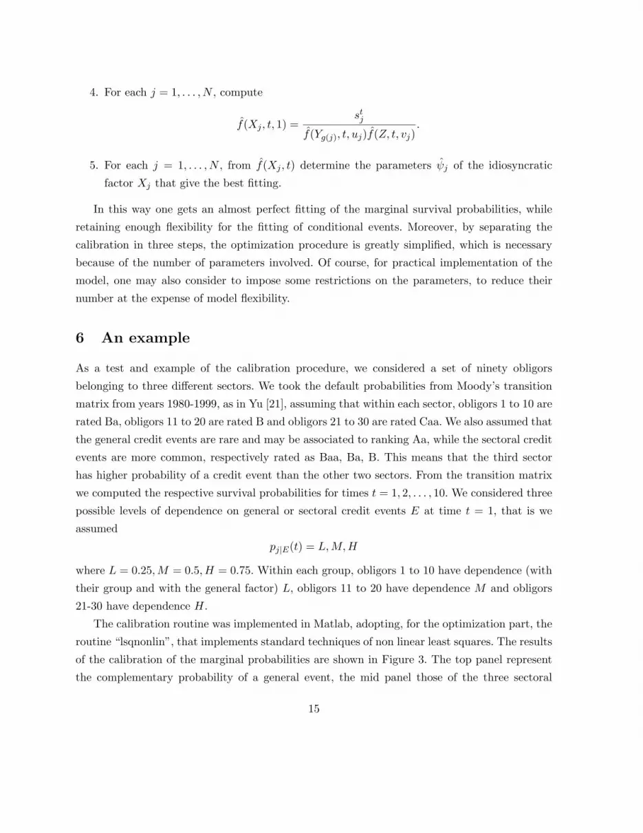
4. For each j = 1, . . . , N , compute

f(Xj , t, 1) =stj

f(Yg(j), t, uj)f(Z, t, vj).

5. For each j = 1, . . . , N , from f(Xj , t) determine the parameters ψj of the idiosyncratic

factor Xj that give the best fitting.

In this way one gets an almost perfect fitting of the marginal survival probabilities, while

retaining enough flexibility for the fitting of conditional events. Moreover, by separating the

calibration in three steps, the optimization procedure is greatly simplified, which is necessary

because of the number of parameters involved. Of course, for practical implementation of the

model, one may also consider to impose some restrictions on the parameters, to reduce their

number at the expense of model flexibility.

6 An example

As a test and example of the calibration procedure, we considered a set of ninety obligors

belonging to three different sectors. We took the default probabilities from Moody’s transition

matrix from years 1980-1999, as in Yu [21], assuming that within each sector, obligors 1 to 10 are

rated Ba, obligors 11 to 20 are rated B and obligors 21 to 30 are rated Caa. We also assumed that

the general credit events are rare and may be associated to ranking Aa, while the sectoral credit

events are more common, respectively rated as Baa, Ba, B. This means that the third sector

has higher probability of a credit event than the other two sectors. From the transition matrix

we computed the respective survival probabilities for times t = 1, 2, . . . , 10. We considered three

possible levels of dependence on general or sectoral credit events E at time t = 1, that is we

assumed

pj|E(t) = L,M,H

where L = 0.25,M = 0.5,H = 0.75. Within each group, obligors 1 to 10 have dependence (with

their group and with the general factor) L, obligors 11 to 20 have dependence M and obligors

21-30 have dependence H.

The calibration routine was implemented in Matlab, adopting, for the optimization part, the

routine “lsqnonlin”, that implements standard techniques of non linear least squares. The results

of the calibration of the marginal probabilities are shown in Figure 3. The top panel represent

the complementary probability of a general event, the mid panel those of the three sectoral

15

events and the bottom panel those of the ninety obligors. The input data are represented by

circles, the output of the calibration procedure by crosses.


From the plots it is rather evident that the fitting capabilities to the marginal probabilities

are very satisfactory. The calibration error to the conditional one year probabilities are of the

order of 10−9, that is, they are perfectly fitted by the procedure.

Once the model is calibrated, we can use it to check the effectiveness of our exact simulation

algorithm. To this purpose we computed by simulation the expectations of easily computable

stopping times, so that we can compare the values obtained through simulations to the exact

ones. More precisely, we considered the time of default τj of each obligor j and computed the

expectation of τj ∧ T , with time horizon T = 5. We computed the exact values of such expec-

tations by numerical integration of the appropriate densities that can be easily recovered from

the survival probabilities. The approximated values were computed with the exact simulation

algorithm and with the standard discretization algorithm. Figure 4 presents the result of such

computations on the ninety obligors. Both methodologies produced 1000 simulations. The dis-

crete method used a time step of 1/500. The average cpu time to produce one simulation was

1.93 seconds for the discrete method and 1.76 seconds for the exact one. It is apparent that the

exact simulation algorithm produces more precise results.


According to our experience, a finer discretization grid does not improve the results produced

by the standard algorithm, while considerably increasing the simulation time. For instance, for

N = 2000 time steps per year the standard algorithm produces a mean squared error of the

order of 2 · 10−2, that is almost ten times greater than that of the exact algorithm, which is also

more than four times faster.

16

7 Conclusions

We presented a model for the default processes of a large set of obligors. The model is based

on the double stochastic hypothesis and assumes the the intensity of default of any obligor is

a linear combination of three basic affine processes. The theory of affine processes makes many

important quantities, like survival probabilities or default correlations, available in closed form.

We developed a toolbox for such computations and used it for calibration and for simulation

of default scenarios. An important feature of any model for large credit portfolio is the ability

to produce sensible default correlations. We showed by numerical examples that the jump com-

ponent of the common factors is necessary for a high enough correlation. We believe that the

model has many interesting and promising features that make it a good candidate for further

applications.

A Appendix: Some Useful Results

In the first part of the Appendix we collect few known results frequently used through the paper.

A.1 Intensity of the First Default Event

The following lemma characterizes the intensity of the first-to-default among a group of agents

having given default intensities.

Lemma A.1 (Duffie [5], Lemma 1). Let λj , j = 1, ..., n be intensities processes associated to

the event times τj , j = 1, ..., n, and suppose P(τi = τj) = 0 for any i 6= j. Then∑n

j=1 λj is an

intensity process for τ := minτ1, ..., τn.

For the sake of completeness we provide a proof.

Proof. Let use the notations introduced in Section 2 and define the indicator of ‘at least one

default occurred before t’:

Dt = 1τ≤t.

We claim that the process A defined as

At =∫ t

0

n∑j=1

λj(s)1τ>sds

17

is the compensator process of D, that is, (Dt −At)t is a martingale. Indeed, we have

Dt −At = 0−∫ t

0

n∑j=1

λj(s)ds =n∑j=1

(Djt −Ajt ), ∀ t ≤ τ,

and

Dt −At = 1−∫ τ

0

n∑j=1

λj(s)ds = Dτ −Aτ , ∀ t ≥ τ,

from which the claimed result follows.

A.2 Basic Affine Processes

For the affine process in (4) we have the following useful results (see Duffie et al. [9]):

E[e−R t+s

t mX(u)du+rX(t+s)|Ft] = exp(C(X, t, t+ s;m, r)), (12)

E[X(t+ s)e−R t+s

t mX(u)du+rX(t+s)|Ft] = D(X, t, t+ s;m, r) exp(C(X, t, t+ s;m, r)), (13)

where

C(X, t, t+ s;m, r) = αmψ,r(s) + βmψ,r(s)X(t),

D(X, t, t+ s;m, r) = Amψ,r(s) +Bmψ,r(s)X(t)

and the coefficients αmψ,r(s), βmψ,r(s), A

mψ,r(s) and Bm

ψ,r(s) are solutions of the following Riccati

ODEs (with ξmψ,r(s) = ξ(t, t+ s, r,m) for any t ≥ 0, and for ξ = α, β,A,B):

∂β(t, T, r,m)∂t

= kβ(t, T, r,m)− 12β(t, T, r,m)2σ2 +m, β(T, T, r,m) = r

∂α(t, T, r,m)∂t

= −kθβ(t, T, r,m)− l

∫Reβ(t,T,r,m)zdν(z) + l

= −kθβ(t, T, r,m)− l

µ

∫ ∞

0ez(β(t,T,r,m)−1/µ)dz + l, α(T, T, r,m) = 0

∂B(t, T, r,m)∂t

= kB(t, T, r,m)− β(t, T, r,m)B(t, T, r,m)σ2, B(T, T, r,m) = 1

∂A(t, T, r,m)∂t

= −kθB(t, T, r,m)− lB(t, T, r,m)∫

Rzeβ(t,T,r,m)zdν(z)

= −kθB(t, T, r,m) + lµB(t, T, r,m)

(µβ(t, T, r,m)− 1)2, A(T, T, r,m) = 0.

18

For example, for m > 0, if we define

c1 =k +

√k2 + 2mσ2

−2m, d1 = (1− c1r)

−k + rσ2 +√k2 + 2mσ2

−2kr + σ2r2 − 2m,

a1 = (d1 + c1)r − 1, b1 =−d1(+k + 2mc1) + a1(−kc1 + σ2)

a1c1 − d1,

a2 =d1

c1, b2 = b1, c2 = 1− µ

c1, d2 =

d1 − µa1

c1,

then from [7] we have

βmψ,r(t) =1 + a1e

b1t

c1 + d1eb1t, (14)

αmψ,r(t) =kθ(a1c1 − d1)

b1c1d1lnc1 + d1e

b1t

c1 + d1+kθt

c1+l(a2c2 − d2)b2c2d2

lnc2 + d2e

b2t

c2 + d2+ (15)

+tl( 1c2

− 1).

B Appendix: Conditional Moment Generating Functions

In this section we provide the closed formulas required in step (IV) of our simulation algorithm

(in Section 4) in order to evaluate the value at which to re-start the default intensities after the

occurrence of a default.

B.1 The Idiosyncratic Part

By using the independence of X1, . . . , XN , Y1, . . . , YS , Z, the numerator in (11) can be rewrit-

ten as follows

E[e−R t0 Xj(s)ds+rXj(t)]

E[e−V

R t0 Z(s)ds]E[Xk(t)e−

R t0 Xk(s)ds]

∏p=1,..,N

p 6=j,k

E[e−R t0 Xp(s)ds]

∏i=1,..,S

E[e−Ui

R t0 Yi(s)ds]

+E[vkZ(t)e−VR t0 Z(s)ds]

∏p=1,..,N

p 6=j

E[e−R t0 Xp(s)ds]

∏i=1,..,S

E[e−Ui

R t0 Yi(s)ds]

+E[e−VR t0 Z(s)ds]

∏p=1,..,N

p 6=j

E[e−R t0 Xp(s)ds]

∏i=1,..,Si6=g(k)

E[e−Ui

R t0 Yi(s)ds]E[ukYg(k)(t)e

−Ug(k)

R t0 Yg(k)(s)ds]

,

19

where we set

V =N∑j=1

vj and Ui =∑

j:g(j)=i

uj .

On the same way, the denominator of (11) is given by

E[e−VR t0 Z(s)ds]E[Xk(t)e−

R t0 Xk(s)ds]

∏p=1,..,N

p 6=k

E[e−R t0 Xp(s)ds]

∏i=1,..,S

E[e−Ui

R t0 Yi(s)ds]


∏p=1,..,N

E[e−R t0 Xp(s)ds]

∏i=1,..,S

E[e−Ui

R t0 Yi(s)ds]


∏p=1,..,N

E[e−R t0 Xp(s)ds]

∏i=1,..,Si6=g(k)

E[e−Ui


−Ug(k)

R t0 Yg(k)(s)ds].

After some obvious simplifications, we get

Hj(r; t, k) =E[e−

R t0 Xj(s)ds+rXj(t)]

E[e−R t0 Xj(s)ds]

= exp(C(Xj , 0, t; 1, r)− C(Xj , 0, t; 1, 0)),

where the parameter α’s and β’s are solution of some Riccati ODEs (see Appendix A.2).

B.2 The Common Factor

The conditional moment generating function of the common factor Z is

N(r; t, k) := E[erZ(τ (1))|τ (1) = t, I(1) = k] =E[e−

R t0 Λ(s)dsλk(t)erZ(t)]


.

In this case, the numerator can be obtained as

E[e−VR t0 Z(s)ds+rZ(t)]E[Xk(t)e−

R t0 Xk(s)ds]

∏p=1,..,N

p 6=k

E[e−R t0 Xp(s)ds]

∏i=1,..,S

E[e−Ui

R t0 Yi(s)ds]

+E[vkZ(t)e−VR t0 Z(s)ds+rZ(t)]

∏p=1,..,N

E[e−R t0 Xp(s)ds]

∏i=1,..,S

E[e−Ui

R t0 Yi(s)ds]

+E[e−VR t0 Z(s)ds+rZ(t)]

∏p=1,..,N

E[e−R t0 Xp(s)ds]

∏i=1,..,Si6=g(k)

E[e−Ui


−Ug(k)

R t0 Yg(k)(s)ds],

20

and the denominator as

E[e−VR t0 Z(s)ds]E[Xk(t)e−

R t0 Xk(s)ds]

∏p=1,..,N

p 6=k

E[e−R t0 Xp(s)ds]

∏i=1,..,S

E[e−Ui

R t0 Yi(s)ds]


∏p=1,..,N

E[e−R t0 Xp(s)ds]

∏i=1,..,S

E[e−Ui

R t0 Yi(s)ds]


∏p=1,..,N

E[e−R t0 Xp(s)ds]

∏i=1,..,Si6=g(k)

E[e−Ui


−Ug(k)

R t0 Yg(k)(s)ds].

In this way, by (13) we obtain

N(r; t, k) =eC(Z,0,t;V,r)[D(Xk, 0, t; 1, 0) + vkD(Z, 0, t;V, r) + ukD(Yg(k), 0, t;Ug(k), 0)]eC(Z,0,t;V,0)[D(Xk, 0, t; 1, 0) + vkD(Z, 0, t;V, 0) + ukD(Yg(k), 0, t;Ug(k), 0)]

where again the C’s and D’s are specified in Appendix A.2.

Therefore, the conditional expectation is equal to

E[Z(τ (1))|τ (1) = t, I(1) = k] =∂

∂r

∣∣∣r=0

N(r; t, k) =∂

∂r

∣∣∣r=0

C(Z, 0, t;V, r) +

vk∂∂r

∣∣∣r=0

D(Z, 0, t;V, r)

D(Xk, 0, t; 1, 0) + vkD(Z, 0, t;V, 0) + ukD(Yg(k), 0, t;Ug(k), 0).

B.3 The Sectoral Factor

The conditional moment generating function of the sectoral factors Yi is

M i(r; t, k) := E[erYi(τ(1))|τ (1) = t, I(1) = k] =

E[e−R t0 Λ(s)dsλk(t)erYi(t)]


,

and to compute them we proceed as before by using the independence of the affine processes. So

we skip the details and just emphasize the fact that here a distinction must be made whether

the defaulter agent k does or does not belong to group i.

In the case i ∈ 1, .., S \ g(k) we have

M i(r; t, k) =E[e−Ui

R t0 Yi(s)ds+rYi(t)]

E[e−Ui

R t0 Yi(s)ds]

= exp(C(Yi, 0, t;Ui, r)− C(Yi, 0, t;Ui, 0)),

and then

E[Yi(τ (1))|τ (1) = t, I(1) = k] =∂

∂r

∣∣∣r=0

M i(r; t, k) =∂

∂r

∣∣∣r=0

C(Yi, 0, t;Ui, r).

21

On the other hand, for i = g(k) we obtain

M i(r; t, k) =eC(Yg(k),0,t;Ug(k),r)[D(Xk, 0, t; 1, 0) + vkD(Z, 0, t;V, 0) + ukD(Yg(k), 0, t;Ug(k), r)]

eC(Yg(k),0,t;Ug(k),0)[D(Xk, 0, t; 1, 0) + vkD(Z, 0, t;V, 0) + ukD(Yg(k), 0, t;Ug(k), 0)],

and then

E[Yi(τ (1))|τ (1) = t, I(1) = k] =∂

∂r

∣∣∣r=0

M i(r; t, k) =∂

∂r

∣∣∣r=0

C(Yg(k), 0, t;Ug(k), r) +

uk∂∂r

∣∣∣r=0

D(Yg(k), 0, t;Ug(k), r)

D(Xk, 0, t; 1, 0) + vkD(Z, 0, t;V, 0) + ukD(Yg(k), 0, t;Ug(k), 0).

References

[1] Brigo D. and Mercurio F. (2006). Interest Rate Models - Theory and Practice: With Smile,

Inflation and Credit. 2nd Edition, Springer Finance.

[2] Chapovsky A., Rennie A. and Tavares P. A. C. (2007). “Stochastic intensity modelling for

structured credit exotics”, International Journal of Theoretical and Applied Finance 10 (4),

633-652.

[3] Cox J., Ingersoll J. and Ross S. (1985). “A theory of the term structure of interest rates”,

Econometrica 53, 385-408.

[4] Das R. Duffie D., Kapadia N. and Saita L. (2007). “Common Failings: How Corporate

Defaults Are Correlated”, Journal of Finance 62, 93-117.

[5] Duffie D. (1998). “First to Default Valuation”, Working Paper, Graduate School of Business,

Stanford University.

[6] Duffie D., Filipovic D. and Schachermayer W. (2003). “Affine processes and applications in

finance”, Annals of Applied Probability 13, 984-1053.

[7] Duffie D. and Garleanu N. (2001). “Risk and Valuation of Collateralized Debt Obligation”,

Financial Analysts Journal 57, (1) January-February, 41-62.

[8] Duffie D. and Kan R. (1996). “A yield-factor model of interest rates”, Mathematical Finance

6, 379-406.

22

[9] Duffie D., Pan J. and Singleton K. (2000). “Transform Analysis and Asset Pricing for Affine

Jump Diffusions”, Econometrica 68, 1343-1376.

[10] Duffie D. and Singleton K. (1998). “Simulating Correlated Defaults”, Working Paper, GSB,

Stanford University.

[11] Duffie D. and Singleton K. (1999). “Modeling term structures of defaultable bonds”, Review

of Financial Studies 12, 687-720.

[12] Eckner A. (2007). “Computational Techniques for basic Affine Models of Portfolio Credit

Risk”, Working Paper, Stanford University.

[13] Feller W. (1951). “Two singular diffusion problems”, Annals of Mathematics 54 , 173-182.

[14] Higham D.J. and Mao X. (2005). “Convergence of Monte Carlo simulations involving the

mean- reverting square root process”, Journal of Computational Finance 8 , 35-62.

[15] Hull J. and White A. (2001). “Valuing credit default swaps II: Modeling default correla-

tions”, Journal of Derivatives 8, 12-22.

[16] Jarrow R. and Turnbull S. (1995). “Pricing derivatives on financial securities subject to

credit risk”, Journal of Finance 50(1), 53-86.

[17] Lando D. (1998). “On Cox processes and Credit Risk Securities”, Review of Derivatives

Research 2(2-3), 99-120.

[18] Mortensen A. (2006). “Semi-Analytical Valuation of Basket Credit Derivatives in Intensity-

Based Models”, Journal of Derivatives 13, 8-26.

[19] Schonbucher P. (2003). Credit Derivatives Pricing Models: Models, Pricing and Implemen-

tation. John Wiley and Sons Ltd.

[20] Schonbucher P. and Schubert D. (2001). “Copula-dependent default risk in intensity mod-

els”, Working paper, Bonn University

[21] Yu F. (2005). “Default correlation in reduced-form models”, Journal of Investment Man-

agement 3(4), 33-42.

23

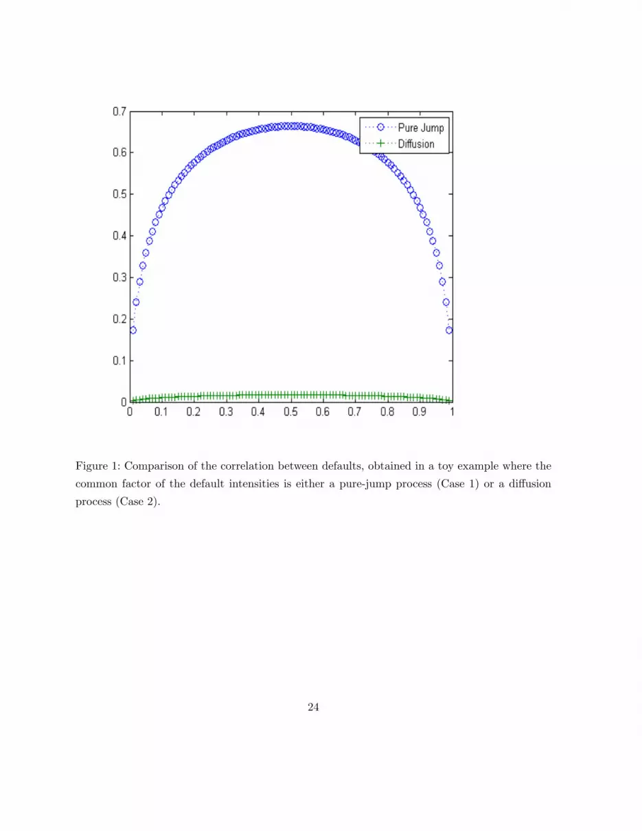
Figure 1: Comparison of the correlation between defaults, obtained in a toy example where the

common factor of the default intensities is either a pure-jump process (Case 1) or a diffusion

process (Case 2).

24

Figure 2: Comparison of the correlation between defaults, obtained in a toy example where the

common factor of the default intensities is either a pure-jump process (Case 1) or a diffusion

process (Case 2).

25

Figure 3: Comparison of the calibrated data to the input data. The three figures report the

marginal survival probabilities for the general (top), sectoral (middle) and individual (bottom)

credit events. The input data are represented with circles, the output from the calibration

procedure are crosses. Note that scales on the three plots are different.26

Figure 4: A comparison of the simulation methods. The figure shows the expected values of the

minimum between the time of defaults and T = 5 for each obligor. The exact values (circles)

are computed by numerical quadrature. The approximation were obtained by 1000 simulated

scenarios with the exact and the discrete method. The discrete method adopted a time step

equal to 1/500. The exact algorithm was 9% faster than the discrete algorithm.

27

Documents

An affine intensity model for large credit portfolios