An analysis of the accuracy of magnetic resonance flip angle measurement methods

This article has been downloaded from IOPscience. Please scroll down to see the full text article.

2010 Phys. Med. Biol. 55 6157

(http://iopscience.iop.org/0031-9155/55/20/008)

Download details:

IP Address: 137.53.249.129

The article was downloaded on 15/11/2010 at 21:19

Please note that terms and conditions apply.

View the table of contents for this issue, or go to the journal homepage for more

Home Search Collections Journals About Contact us My IOPscience

IOP PUBLISHING PHYSICS IN MEDICINE AND BIOLOGY

Phys. Med. Biol. 55 (2010) 6157–6174 doi:10.1088/0031-9155/55/20/008

An analysis of the accuracy of magnetic resonance flipangle measurement methods

Glen R Morrell1 and Matthias C Schabel

Utah Center for Advanced Imaging Research, Radiology Department, University of Utah,Salt Lake City, UT, USA

E-mail: glen.morrell@hsc.utah.edu

Received 3 May 2010, in final form 20 August 2010Published 29 September 2010Online at stacks.iop.org/PMB/55/6157

AbstractSeveral methods of flip angle mapping for magnetic resonance imaging havebeen proposed. We evaluated the accuracy of five methods of flip anglemeasurement in the presence of measurement noise. Our analysis wasperformed in a closed form by propagation of probability density functions(PDFs). The flip angle mapping methods compared were (1) the phase-sensitive method, (2) the dual-angle method using gradient recalled echoes(GRE), (3) an extended version of the GRE dual-angle method incorporatingphase information, (4) the AFI method and (5) an extended version of theAFI method incorporating phase information. Our analysis took into accountdifferences in required imaging time for these methods in the comparison ofnoise efficiency. PDFs of the flip angle estimate for each method for eachvalue of true flip angle were calculated. These PDFs completely characterizethe performance of each method. Mean bias and standard deviation werecomputed from these PDFs to more simply quantify the relative accuracy ofeach method over its range of measurable flip angles. We demonstrate that thephase-sensitive method provides the lowest mean bias and standard deviationof flip angle estimate of the five methods evaluated over a wide range of flipangles.

(Some figures in this article are in colour only in the electronic version)

Introduction

The excitation flip angle in MRI varies across the imaging volume because of inhomogeneityof the transmit radio-frequency (RF) field (B1). Precise measurement of flip angle allowscorrection of spatial variations in image intensity (Axel et al 1987, McVeigh et al 1986,Moyher et al 1995, Roemer et al 1990), has important applications in T1 mapping and

1 Author to whom any correspondence should be addressed.

0031-9155/10/206157+18$30.00 © 2010 Institute of Physics and Engineering in Medicine Printed in the UK 6157

6158 G R Morrell and M C Schabel

quantitation of absolute contrast concentration in dynamic contrast-enhanced MRI (Deoniet al 2003, Schabel and Morrell 2009, Schabel and Parker 2008) and is necessary for paralleltransmission (Katscher et al 2003, Zhu 2004), where individual RF coil field maps are neededfor RF waveform calculation.

Several methods of flip angle mapping have been proposed, which differ in their sensitivityto noise in the image data on which flip angle estimates are based. The accuracy of each methodvaries with the actual flip angle. The most complete characterization of the performance of aflip angle mapping method is the probability density function (PDF) of the flip angle estimate itproduces for a given true flip angle and given system SNR. We have evaluated the performanceof flip angle mapping methods by deriving the PDF of the flip angle estimate produced by eachmethod for each of a range of values of true flip angle, for a few different values of systemSNR. From these PDFs we have also calculated the mean bias and standard deviation of theflip angle estimates, as a simpler but less complete way of portraying their accuracy.

We evaluate the accuracy of five methods of flip angle measurement:

(1) The phase-sensitive method, which uses the phase difference between two acquisitions asa measure of actual flip angle (Morrell 2008).

(2) The gradient recalled echo (GRE) dual-angle method in which two acquisitions areperformed with different nominal flip angles (Cunningham et al 2006, Insko and Bolinger1993, Kerr et al 2007, Stollberger and Wach 1996).

(3) A modified dual-angle GRE method which takes the phase of the acquisitions into account(Insko and Bolinger 1993), which we refer to as the ‘extended dual-angle method.’

(4) The ‘actual flip angle imaging’ (AFI) method (Yarnykh 2007), which utilizes twoacquisitions interleaved in a GRE sequence with equal flip angle but different TR.

(5) A modified AFI method which takes the phase of the acquisitions into account, which werefer to as the ‘extended AFI method.’

Each of these methods is evaluated by calculating the PDF of the flip angle estimate obtainedby the method for a range of values of the actual flip angle, based on corruption of the sourceMR image with Gaussian white noise. The mean bias and standard deviation of error for thefive methods are compared.

One previous study has been performed (Wade and Rutt 2007) comparing B1 mappingmethods with Monte Carlo simulation. That study showed an advantage to the phase-sensitivemethod, but details of implementation of the phase-sensitive method were different than thatproposed in Morrell (2008), which appeared in print later. No analysis by propagation of PDFswas performed in Wade and Rutt (2007). We have previously presented a subset of the currentwork (Morrell and Schabel 2009). This paper develops the concepts suggested in Morrell andSchabel (2009) and adds comparison to the extended GRE and extended AFI methods.

Theory

Each of the five methods of flip angle mapping uses an excitation scheme that encodesinformation about the actual flip angle in image data. In the case of the dual-angle GREmethods and the AFI methods, the information about the actual flip angle is encoded in theratio of the magnitudes of two image acquisitions. In the case of the phase-sensitive method,the flip angle information is encoded in the phase of the image acquisitions. The corruptionof acquired image data by measurement noise limits the accuracy with which flip angle maybe determined. We evaluate the impact of this noise on the various methods by calculatingthe PDF of the flip angle estimate obtained by each method for each of a range of actual flipangles. Our starting point is the assumption that image data are corrupted with Gaussian white

Analysis of flip angle mapping methods 6159

noise, with variance determined by the system SNR, as defined in appendix A.1. From thiswe derive the PDF of the magnitude of each acquisition for the dual-angle and AFI methodsor the phase of each acquisition for the phase-sensitive method. The derivation of magnitudeand phase PDFs is given in appendix A.2. The PDF is then propagated through the functionused by each method to estimate the flip angle from the measured quantity. The result is thePDF of the flip angle estimate.

Phase-sensitive B1 mapping method

The phase-sensitive method of flip angle measurement (Morrell (2008)) forms an image aftera 2α flip about the x-axis followed immediately by an α flip about the y-axis, and the phaseof this image is measured. A second image is formed from an acquisition with the 2α initialexcitation reversed in sign. The phase of this image is also measured. The difference in phasebetween the two is a monotonic function of the flip angle α from which α can be calculated.Details of the derivation of the PDF of the flip angle estimate for the phase-sensitive methodare given in appendix A.3.

Dual-angle method with GRE

In the dual-angle method with GRE, two images are formed. The first image is acquired afterexcitation with a flip angle α and has magnitude proportional to sin(α). The second image isacquired after excitation with a flip angle 2α and has magnitude proportional to sin(2α). Theratio of the two acquisitions is formed giving

r = sin α

sin 2α= 1

2 cos α, (1)

from which the flip angle α can be calculated. The details of the derivation of the PDF of theflip angle estimate for the dual-angle GRE method are given in appendix A.4.

Extended dual-angle GRE method

In the dual-angle GRE method, flip angles from 180◦ to 90◦ give magnitude ratios equal tothose obtained for flip angles between 0◦ and 90◦, symmetric about 90◦. For instance, thesignal magnitude ratio for α = 70◦, 2α = 140◦ is the same as that for α = 110◦, 2α = 220◦.For this reason, the dual-angle GRE method is only valid over a range of flip angles α from0◦ to 90◦. However, the dual-angle GRE method can be extended to a range of flip angles α

from 0◦ to 180◦ by examining the phase of the two acquisitions. For flip angles α from 0◦

to 90◦, the two acquisitions have the same phase, while for flip angles from 90◦ to 180◦ thephase of the two acquisitions differs by 180◦. Thus by examining the relative phase of the twoacquisitions, a range of flip angles from 0◦ to 180◦ can be mapped. We have designated thisapproach the ‘extended dual-angle GRE’ method. The derivation of the PDF of the flip angleestimate for the extended dual-angle GRE method is detailed in appendix A.5.

AFI method

In this method two images are formed during a single sequence in which spoiled GREacquisition is performed from alternating α excitations following two different repetitiontimes TR1 and TR2, with TR2 > TR1. The ratio r of the magnitudes of the two images isformed and the flip angle α is estimated as

α ≈ cos−1

(rn − 1

n − r

), (2)

6160 G R Morrell and M C Schabel

where n = TR2/TR1. Appendix A.6 contains the details of the derivation of the PDF of theflip angle estimate for the AFI method.

Extended AFI method

The AFI method gives flip angle estimates in a range of 0◦ to about 104◦. The exact value ofthe maximum measurable flip angle depends on T1 and on the choice of TR1 and TR2. Abovethis range, the method gives erroneous estimates in a manner similar to the dual-angle GREmethod, in this case being roughly symmetric about the maximum angle of about 104◦ ratherthan 90◦. Flip angles from about 105◦ to 180◦ will give estimates ranging roughly from about104◦ to 0◦. However, similar to the dual-angle GRE method, the AFI method gives signalacquisitions which are in phase for flip angles from 0◦ to about 104◦, and opposite in phasefor flip angles from about 104◦ to 180◦. If this phase is taken into account, a range of 0◦ to180◦ can be measured. The derivation of the PDF of the flip angle estimate for the extendedAFI method is given in appendix A.7.

SNR efficiency

The dual-angle and phase-sensitive methods of B1 mapping require a somewhat long TR toallow signal regeneration after presaturation. In the case of the phase-sensitive method, thispresaturation is required because the excitation used in the phase-sensitive B1 mapping methodleaves some residual longitudinal magnetization Mz which varies as a function of true flipangle α. Variation of Mz is not usually a problem since the flip angle estimate depends onthe phase of the transverse magnetization, not its amplitude. However, for some flip anglesthe residual Mz may be negative, which could alter the sign of the phase of the subsequentexcitation. For this reason, a presaturation pulse is used to reset Mz to zero at the end ofeach acquisition. The dual-angle GRE method is also implemented with a presaturationpulse (Cunningham et al 2006) or very long TR to eliminate T1 dependence of the flip angleestimate. In contrast, the AFI method can operate with short TR. Therefore, comparison ofthese methods requires that their TR requirements be taken into account. This is done bysimulating multiple signal averages for the AFI techniques, or equivalently, decreasing thestandard deviation of the image noise for the AFI techniques compared to the phase-sensitiveand dual-angle methods. This is discussed in more detail below for the specific choice ofparameters used in our analysis.

Methods

For each of the five methods of flip angle measurement, the PDF of the flip angle estimatewas calculated for a range of actual flip angles. The PDFs were calculated according to theequations given in appendixes A.3 through A.7 with custom scripts in MATLAB (Mathworks,Natick, MA). The mean bias and standard deviation of the flip angle estimates were alsocalculated for comparison.

Choice of parameters for comparison

The accuracy of the dual-angle methods and the phase-sensitive method depends in part on thechoice of TR and the T1 of the sample, as these will affect the longitudinal magnetization M−

z

available for each excitation. Assuming a sequence repetition time TR and a minimum amount

Analysis of flip angle mapping methods 6161

of time TRmin required to complete the excitation, readout and presaturation pulse, a time TR–TRmin is available before each excitation for regeneration of the longitudinal magnetizationMz. Given an equilibrium longitudinal magnetization M0, the longitudinal magnetization M−

z

available at the beginning of excitation is

M−z = M0(1 − e−(TR−TRmin)/T1). (3)

Thus, the magnitude of the image depends on the T1 of the sample being imaged. The imagemagnitude will affect the variance of the flip angle estimate. For the AFI method, TR andT1 have more complex effects on the flip angle estimate, with increasing systemic error inestimation for shorter T1. For purposes of direct comparison of flip angle mapping methods,concrete choices of sequence parameters and sample properties must be made. We havechosen to implement the AFI method with TR1 = 30 ms and TR2 = 150 ms, as suggested inYarnykh (2007). This gives a total sequence TR of 180 ms. The dual-angle techniques andthe phase-sensitive technique have TR requirements similar to each other, as both incorporatepresaturation to reset Mz prior to each excitation. We have chosen a TR of 540 ms for both ofthese methods, which is in line with implementations described in Cunningham et al (2006)and Morrell (2008). A minimum repetition time TRmin is required for excitation, readout(typically echo-planar or spiral) and presaturation. We have set TRmin to 40 ms, giving aregeneration interval of TR–TRmin = 500 ms for presaturation recovery. Since the dual-angleand phase-sensitive techniques require two complete acquisitions, each of which takes threetimes the duration of the AFI technique (180 ms ∗ 3 = 540 ms), the signal acquired in the AFImethod is averaged six times, giving a decrease in the standard deviation of the measurementnoise for the AFI method by a factor of

√6. The performance of the phase-sensitive method

varies somewhat with off-resonance frequency. For this analysis, we assume no off-resonance.

Out-of-bounds measurements

Each of the flip angle estimation methods measures a quantity on which flip angle estimatesare based. For the phase-sensitive method, this quantity is the difference in phase betweentwo images. For the dual-angle and AFI methods, this quantity is the ratio of the magnitudeof two images. In all of the methods, the measured quantity has an allowed range. Forinstance, there is no flip angle for which the ratio of acquisitions in the AFI methods ordual-angle methods can theoretically exceed 1. Since the actual measurements are corruptedby noise, some measurements will fall into a range that is not theoretically possible and whichdoes not generate a valid flip angle measurement. We denote these measurements as ‘out ofbounds.’ We have dealt with out-of-bounds measurements in our analysis by discarding thesemeasurements and renormalizing the PDF to have area 1 over the range of valid flip angles.Another approach would be to accept out-of-bounds measurements but assign them to the flipangle which would be most likely to give this measurement, i.e. a ratio greater than 1 wouldmap to a flip angle estimate of 0◦ for the AFI method and 90◦ for the non-extended dual-anglemethod.

Range of the flip angle estimation method

The dual-angle GRE technique is valid over a range of flip angles from 0◦ to 90◦. The AFItechnique is valid over flip angles from 0◦ to approximately 100◦. The extended dual-angle,extended AFI and phase-sensitive methods are valid from 0◦ to 180◦. To allow fair comparison,each method is evaluated over a range of 0 to 2αnom, where αnom represents the middle of thevalid range for that method. For the double angle method αnom = 45◦, for the AFI method

6162 G R Morrell and M C Schabel

Figure 1. Probability density functions (PDFs) for flip angle estimates obtained by five flip anglemeasurement techniques over a range of actual flip angles for two values of the system SNR. Eachimage represents a set of PDFs for multiple actual flip angles for a given measurement method. Asingle vertical line from each image represents the PDF for the flip angle estimate at a particularactual flip angle. A perfect flip angle measurement technique would appear as a line along thediagonal. The top row shows the flip angle estimate PDFs for a system SNR of 50, while thebottom row shows the PDFs for a system SNR of 10. Difference in required imaging time forthe AFI methods has been taken into account in these results, i.e. the PDFs shown for the AFImethod and the extended AFI method represent flip angle estimates formed from the average of sixsignal acquisitions. Results are expressed in terms of a nominal flip angle α0 at the middle of themeasurable range for each method. For the phase-sensitive method and the extended dual-angleand extended AFI methods, α0 = 90◦. For the standard (non-extended) dual-angle method, α0 =45◦, and for the standard AFI method α0 = 50◦.

αnom = 50◦, and for the extended dual-angle, extended AFI and phase-sensitive methodsαnom = 90◦.

Effect of T1 on flip angle measurement accuracy

To investigate the effect of variations in T1 on the accuracy of the five methods, each methodwas simulated with T1 values of 200 ms, 500 ms and 800 ms.

Accuracy criteria

The PDF of the flip angle estimate a gives complete information on the accuracy of eachmethod. Some insight into the specific features of the performance of each method is gainedby examining the PDFs of the flip angle estimates for a range of actual flip angles, as infigure 1. For ease of depiction, the mean and standard deviation of the flip angle estimate arealso calculated from the PDF. The likelihood of an out-of-bounds measurement for a givenactual flip angle is also depicted.

Verification with Monte Carlo simulation

The PDF formulas presented above were verified by Monte Carlo simulation of flip angleestimation with each method for two values of system SNR. Histograms of the flip angleestimate under Monte Carlo simulation were compared to plots of the equations and found toagree.

Analysis of flip angle mapping methods 6163

Results

The performance of each method of flip angle measurement is most easily visualized byinspection of the PDF of the flip angle estimate for each of a range of actual flip angles. Thisis depicted in figure 1 for all five methods at two different values of system SNR for T1 of500 ms. In this figure, the PDFs are portrayed as an image, with each vertical column ofimage pixels representing the PDF of the flip angle estimate for a given actual flip angle sothat a perfect flip angle estimation method would be represented by a line along the diagonal.Figure 1 shows that the phase-sensitive method most closely approaches this ideal, followedby the extended dual-angle method and the extended AFI method, with the non-extendeddual-angle and AFI methods giving the worst results.

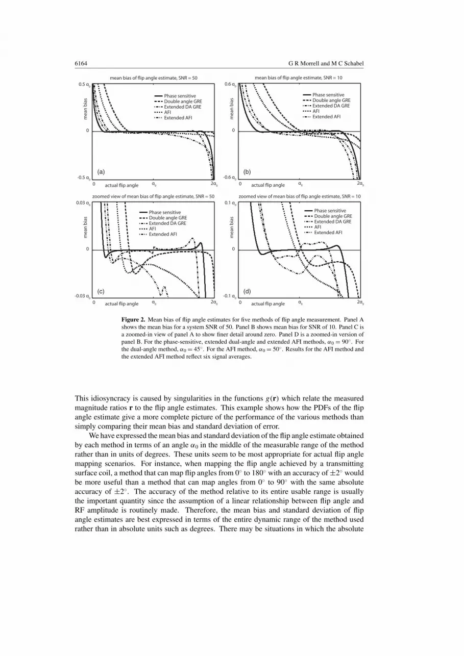
For ease of comparison, the mean bias and standard deviation of the flip angle estimatesfor all five methods at two different values of system SNR are plotted in figures 2 and 3.These plots show that both the mean bias and standard deviation of the flip angle estimateare lowest for the phase-sensitive method over most of the range of flip angles. The standarddual-angle and AFI methods both give large mean bias at low flip angles and become moreaccurate with increasing flip angle. The PDFs illustrated in figure 1 show that at low flipangles these two methods may give little useful information about the actual flip angle. Incontrast, the phase-sensitive and extended dual-angle and AFI methods show performancewhich is relatively symmetric about α0. None of the methods performs well for flip anglesnear zero.

Figure 4 shows a plot of the probability of an ‘out-of-bounds’ measurement for eachof the five methods over a range of actual flip angles. The probability of an out-of-boundsmeasurement becomes significant for all of the methods at very low flip angles, but is generallylower for the phase-sensitive method than the other methods over a wide range of flip angles.Out-of-bounds measurements are also possible at the upper limit of the range of flip anglesfor the phase-sensitive and extended dual-angle and AFI methods.

Figure 5 shows the effect of variation in T1 on the accuracy of each method, with meanbias and standard deviation of the flip angle estimates plotted for T1 values of 200 ms, 500 msand 800 ms.

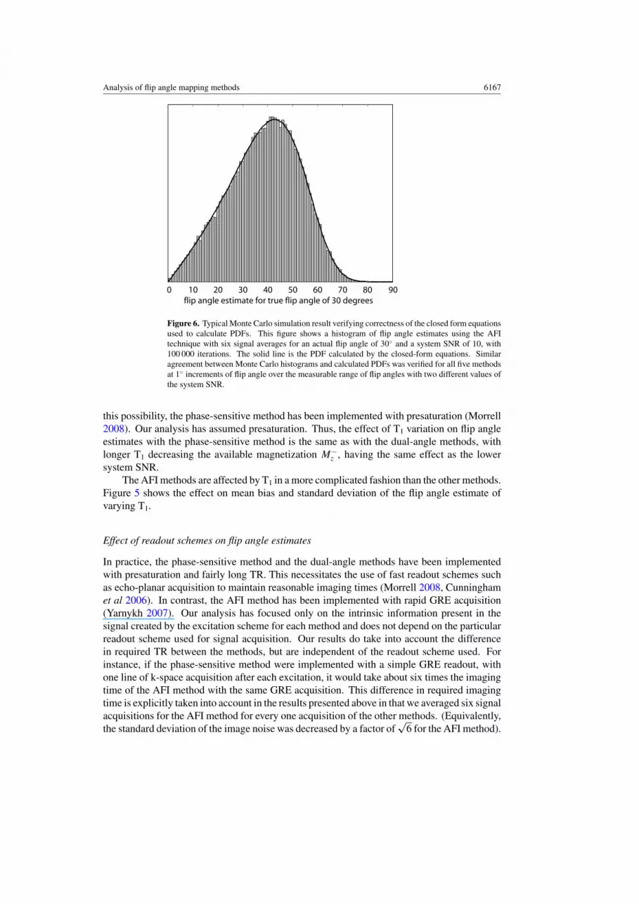
Figure 6 demonstrates a typical Monte Carlo simulation result for one flip anglemeasurement method at one SNR for one actual flip angle compared to the closed formequations. Similar comparison was made for the entire range of actual flip angles with all fivemethods at two different values of system SNR, verifying the correctness of the equations.

Discussion

Accuracy of flip angle mapping methods

The phase-sensitive method of flip angle measurement gives lower mean bias and lowerstandard deviation of flip angle estimates over a wide range of flip angles when comparedwith the other four methods considered here. After the phase-sensitive method, the extendeddual-angle and extended AFI methods have the next best performance. Both the dual-angleand AFI methods are substantially improved by incorporating phase information from thetwo signal acquisitions. Extending these methods to include phase information increases therange of flip angles they can measure, and thus decreases the relative mean bias and standarddeviation of their flip angle estimates. Inspection of the PDFs shown in figure 1 reveals that theextended dual-angle method never returns a flip angle estimate of 90◦, and that the extendedAFI method never returns an estimate of 104◦ (for the given choice of sequence parameters).

6164 G R Morrell and M C Schabel

Figure 2. Mean bias of flip angle estimates for five methods of flip angle measurement. Panel Ashows the mean bias for a system SNR of 50. Panel B shows mean bias for SNR of 10. Panel C isa zoomed-in view of panel A to show finer detail around zero. Panel D is a zoomed-in version ofpanel B. For the phase-sensitive, extended dual-angle and extended AFI methods, α0 = 90◦. Forthe dual-angle method, α0 = 45◦. For the AFI method, α0 = 50◦. Results for the AFI method andthe extended AFI method reflect six signal averages.

This idiosyncracy is caused by singularities in the functions g(r) which relate the measuredmagnitude ratios r to the flip angle estimates. This example shows how the PDFs of the flipangle estimate give a more complete picture of the performance of the various methods thansimply comparing their mean bias and standard deviation of error.

We have expressed the mean bias and standard deviation of the flip angle estimate obtainedby each method in terms of an angle α0 in the middle of the measurable range of the methodrather than in units of degrees. These units seem to be most appropriate for actual flip anglemapping scenarios. For instance, when mapping the flip angle achieved by a transmittingsurface coil, a method that can map flip angles from 0◦ to 180◦ with an accuracy of ±2◦ wouldbe more useful than a method that can map angles from 0◦ to 90◦ with the same absoluteaccuracy of ±2◦. The accuracy of the method relative to its entire usable range is usuallythe important quantity since the assumption of a linear relationship between flip angle andRF amplitude is routinely made. Therefore, the mean bias and standard deviation of flipangle estimates are best expressed in terms of the entire dynamic range of the method usedrather than in absolute units such as degrees. There may be situations in which the absolute

Analysis of flip angle mapping methods 6165

Figure 3. Standard deviation of the flip angle estimate for five methods of flip angle measurement.Panel A shows results for a system SNR of 50. Panel B shows results for a system SNR of 10. Forthe phase-sensitive, extended dual-angle and extended AFI methods, α0 = 90◦. For the dual-anglemethod, α0 = 45◦. For the AFI method, α0 = 50◦. Results for the AFI method and the extendedAFI method reflect six signal averages.

Figure 4. Probability of out-of-bounds measurement for various values of actual flip angle for thefive flip angle measurement methods. Panel A shows probability of out-of-bounds measurementfor SNR of 50. Panel B shows probability of out-of-bounds measurement for SNR of 10. Forthe phase-sensitive, extended dual-angle and extended AFI methods, α0 = 90◦. For the dual-angle method, α0 = 45◦. For the AFI method, α0 = 50◦. Results for the AFI method and theextended AFI method reflect averaging of six signal acquisitions before determining whether themeasurement is out-of-bounds.

flip angle is important. In these situations, a method with larger dynamic range such as thephase-sensitive method may have additional advantages beyond relative accuracy.

Effect of T1 on accuracy of flip angle estimates

The flip angle methods investigated vary in their sensitivity to T1. If used with short sequencerepetition time, the dual-angle methods are sensitive to T1 variations. For this reason, the dual-angle methods are typically used with long TR or with presaturation before each excitation,to make the T1 weighting of the images obtained with α and 2α flip angle excitations equalso that they cancel out when the ratio of the two acquisitions is formed (Cunningham et al

6166 G R Morrell and M C Schabel

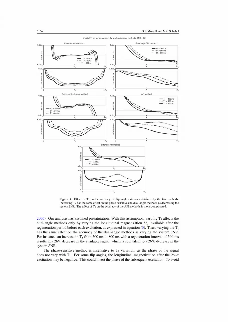
Figure 5. Effect of T1 on the accuracy of flip angle estimates obtained by the five methods.Increasing T1 has the same effect on the phase-sensitive and dual-angle methods as decreasing thesystem SNR. The effect of T1 on the accuracy of the AFI methods is more complicated.

2006). Our analysis has assumed presaturation. With this assumption, varying T1 affects thedual-angle methods only by varying the longitudinal magnetization M−

z available after theregeneration period before each excitation, as expressed in equation (3). Thus, varying the T1

has the same effect on the accuracy of the dual-angle methods as varying the system SNR.For instance, an increase in T1 from 500 ms to 800 ms with a regeneration interval of 500 msresults in a 26% decrease in the available signal, which is equivalent to a 26% decrease in thesystem SNR.

The phase-sensitive method is insensitive to T1 variation, as the phase of the signaldoes not vary with T1. For some flip angles, the longitudinal magnetization after the 2α-αexcitation may be negative. This could invert the phase of the subsequent excitation. To avoid

Analysis of flip angle mapping methods 6167

Figure 6. Typical Monte Carlo simulation result verifying correctness of the closed form equationsused to calculate PDFs. This figure shows a histogram of flip angle estimates using the AFItechnique with six signal averages for an actual flip angle of 30◦ and a system SNR of 10, with100 000 iterations. The solid line is the PDF calculated by the closed-form equations. Similaragreement between Monte Carlo histograms and calculated PDFs was verified for all five methodsat 1◦ increments of flip angle over the measurable range of flip angles with two different values ofthe system SNR.

this possibility, the phase-sensitive method has been implemented with presaturation (Morrell2008). Our analysis has assumed presaturation. Thus, the effect of T1 variation on flip angleestimates with the phase-sensitive method is the same as with the dual-angle methods, withlonger T1 decreasing the available magnetization M−

z , having the same effect as the lowersystem SNR.

The AFI methods are affected by T1 in a more complicated fashion than the other methods.Figure 5 shows the effect on mean bias and standard deviation of the flip angle estimate ofvarying T1.

Effect of readout schemes on flip angle estimates

In practice, the phase-sensitive method and the dual-angle methods have been implementedwith presaturation and fairly long TR. This necessitates the use of fast readout schemes suchas echo-planar acquisition to maintain reasonable imaging times (Morrell 2008, Cunninghamet al 2006). In contrast, the AFI method has been implemented with rapid GRE acquisition(Yarnykh 2007). Our analysis has focused only on the intrinsic information present in thesignal created by the excitation scheme for each method and does not depend on the particularreadout scheme used for signal acquisition. Our results do take into account the differencein required TR between the methods, but are independent of the readout scheme used. Forinstance, if the phase-sensitive method were implemented with a simple GRE readout, withone line of k-space acquisition after each excitation, it would take about six times the imagingtime of the AFI method with the same GRE acquisition. This difference in required imagingtime is explicitly taken into account in the results presented above in that we averaged six signalacquisitions for the AFI method for every one acquisition of the other methods. (Equivalently,the standard deviation of the image noise was decreased by a factor of

√6 for the AFI method).

6168 G R Morrell and M C Schabel

The difference in required imaging time between the AFI method and the other methods wouldbe about the same if all methods were implemented with a rapid echo-planar readout or someother readout scheme. Details of readout implementation have little effect on the accuracy ofthe methods.

Other factors influencing the choice of flip angle methods

Practical implementation issues may favor the use of one method over another. For instance,the phase-sensitive method has been implemented with rapid non-selective RF pulses whichrequire 3D imaging over the entire sensitive volume of the receive coil, which may lead to longimaging times (Morrell 2008). This method is less suitable for single-slice flip angle mapping.The dual-angle and AFI techniques have been implemented as single-slice excitations forimproved imaging speed, but this approach introduces errors in flip angle estimation due toaveraging of flip angle over slice profiles (Cunningham et al 2006). The AFI method can beimplemented in a rapid GRE configuration but has been shown to be very sensitive to RF andgradient spoiling issues (Nehrke 2009). Our analysis focuses only on the intrinsic accuracypossible with each technique, independent of other practical considerations.

Conclusion

We have analyzed five methods of flip angle mapping by calculating the PDF of the flip angleestimate over a range of actual flip angles. We compared the phase-sensitive method, the dual-angle method with GRE acquisition, an extended dual-angle GRE method which takes thephase of the acquisitions into account, the AFI method and an extended AFI method includingphase information. Our analysis shows that performance of the dual-angle and AFI methodsis greatly improved by extending their range of measurable flip angles by incorporating phaseinformation. This increased range results in smaller relative errors in B1 estimation. However,the phase-sensitive method was found to give estimates of flip angle with lower mean bias andstandard deviation than the other methods, including the extended versions of the dual-angleand AFI methods, over a wide range of actual flip angles for equivalent imaging times.

Acknowledgment

Grant support: NCI 5K08CA112449-04, NIBIB K25EB005077-05.

Appendix

A.1. Definition of image noise and system signal to noise ratio (SNR)

The complex value of a given voxel of an MR image at spatial location (x, y, z) can be expressedas

S(x, y, z) = A(x, y, z) + n(x, y, z), (A.1)

where A(x, y, z) is the noise-free image and n(x, y, z) is the noise contribution. For thepurpose of our analysis of the accuracy of flip angle mapping methods, we will assume auniform signal level and a uniform noise standard deviation over the entire imaging volumeand we will drop the explicit dependence on spatial location from subsequent notation. Thenoise sample n can be expressed as the sum of two noise components (Henkelman 1985):

n = n⊥ + in‖, (A.2)

Analysis of flip angle mapping methods 6169

with n⊥ and n‖ independent Gaussian white noise samples with zero mean and the samestandard deviation σ . The orientation of n‖ can be defined as parallel to the signal vector A,and n⊥ as orthogonal to A. We define SNR as

SNR = |A0|σ

, (A.3)

where |A0| represents the maximum signal amplitude that can be achieved with a perfect 90◦

excitation and infinite TR with no signal loss from T1 or T2 effects.

A.2. Magnitude and phase noise

The signal A can be expressed as a vector A = Axx +Ayy in the x–y imaging plane. The noise-corrupted signal in a given pixel can then be expressed as S = (Ax + nx)x + (Ay + ny)y wherenx and ny are independent Gaussian white noise samples with standard deviation σ . We candefine random variables x and y representing the x- and y-components of the noise-corruptedsignal, and their joint PDF is

fx,y(x, y) = 1

2πσ 2exp

(− (x − Ax)

2 + (y − Ay)2

2σ 2

), (A.4)

i.e. the PDF of the noise-corrupted signal is a two-dimensional Gaussian distribution withmean (Ax,Ay).

If we express the complex signal A in terms of magnitude ρ and phase φ as A = ρ eiφ , wecan define the random variable m = |A + n| as the magnitude of the noise-corrupted signal,and the random variable Φ = arg(A + n) as the phase of the noise-corrupted signal. Then, thejoint PDF of m and Φ can be found by converting equation (A.4) to polar coordinates:

fm,Φ(m,�) = m

2πσ 2exp

(−m2 − 2mρ(cos � cos φ + sin � sin φ) + ρ2

2σ 2

). (A.5)

The PDF of the random variable m has the Rician density (Papoulis 1984):

fm(m) = m

σ 2I0

(mρ

σ 2

)exp(−(m2 + ρ2)/2σ 2), (A.6)

which is obtained by integrating equation (A.5) with respect to �, with

I0(x) = 1

2π

∫ 2π

0ex cos θ dθ (A.7)

the modified Bessel function. For σ � ρ, m has approximately a Gaussian distribution(Haykin 2001) with m ∼ N(ρ, σ ).

A.3. Phase noise

The PDF of the phase Φ is found by integrating equation (A.5) with respect to m, and is givenby (Blachman (1981))

fΦ(�) = 1

2exp

(− ρ2

2σ 2

)+

ρ cos (� − φ)

2√

2πσ

× exp

(− ρ2

2σ 2sin2 (� − φ)

)erfc

(− ρ√

2σcos (� − φ)

), (A.8)

where the complementary error function is defined as

erfc(u) = 2√π

∫ ∞

u

exp(−z2) dz. (A.9)

6170 G R Morrell and M C Schabel

For σ � ρ, the phase noise Φ − φ can be approximated as

Φ − φ ≈ tan−1(n⊥/ρ)

≈ sin−1(n⊥/ρ)

≈ n⊥/ρ (A.10)

and fΦ(�) is approximated by the Gaussian distribution N(φ, σ/ρ). This is in contrast tothe distribution of magnitude noise, which for σ � ρ is approximately N(φ, σ ). Thus, thestandard deviation of phase noise is less than that of magnitude noise by a factor of the signalamplitude.

A.4. Derivation of the PDF of the flip angle estimate for the phase-sensitive method

The signal for a given voxel measured in the first acquisitions in the phase-sensitive techniqueis denoted as ρ1 eiφ1 + n1 and that from the second acquisition is denoted as ρ2 eiφ2 + n2, wheren1 and n2 are two different noise samples. The measured phases from these two acquisitionsare denoted as random variables Φ1 and Φ2 with

Φ1,2 = arg(ρ1,2eiφ1,2 + n1,2). (A.11)

The random variable Θ is formed as the difference between the phases of the two excitations,

Θ = Φ1 − Φ2. (A.12)

Φ1 and Φ2 have PDFs given by equation (A.8) (appendix A.2). The PDF of Θ is given by theconvolution of the PDFs of Φ1 and Φ2 (Papoulis 1984):

fΘ() = fΦ1() ∗ fΦ2(), (A.13)

which can be evaluated numerically. For the case of σ � ρ, both Φ1 and Φ2 have nearlyGaussian distributions and the PDF of Θ is approximately N

(φ1 − φ2,

σ√1/ρ2

1 +1/ρ22

).

Calculation of the PDF of Θ requires calculation of the nominal (noise-free) magnitude ρ

and phase angle φ of each of the two acquisitions for a given true flip angle α. From (Morrell2008) we have the following expression for the transverse magnetization measured in the twoacquisitions:

Mx = ±M−z 4αωτ

β2sin2 β cos β − M−

z α sin β

β3(α2 cos 2β + ω2τ 2)

My = ±M−z 2α sin β

β3(ω2τ 2 cos 2β + α2 cos β)

+M−

z αωτ

β4(1 − cos β)(α2 cos 2β + ω2τ 2), (A.14)

where ω is the resonance frequency offset due to the chemical shift or B0 inhomogeneity, τ

is a measure of the RF pulse length and β =√

α2 + ω2τ 2. M−z represents the longitudinal

magnetization available at the beginning of the excitation. The ± in equation (A.14) is + forthe first acquisition with the positive 2α initial tip, and − for the second acquisition with thenegative 2α initial tip. The magnitude of the resulting image is given by

ρ =√

M2x + M2

y (A.15)

and the phase is given by

φ = tan−1(My/Mx). (A.16)

Analysis of flip angle mapping methods 6171

We define a random variable a as the flip angle estimate. Once the PDF of Θ has beencalculated for given values of the flip angle α, off-resonance phase accrual ωτ (dependingon off-resonance frequency ω and RF pulse length τ ), sequence timing parameters TR andTRmin, and the T1 of the sample, the PDF of a can be calculated using the function

a = g(Θ), (A.17)

which relates the measured phase angle difference Θ to the flip angle a. Specifically, the PDFof a is given by (A.17)

fa(a) = fΘ(g−1(a))

|g′(g−1(a))| (A.18)

where g−1 is the inverse of g and g′ is the derivative of g with respect to its argument.For the phase-sensitive B1 mapping technique, the closed form of g, g−1 and g′ is not

straightforward, so we have evaluated them numerically.

A.5. Derivation of the PDF of the flip angle estimate for the dual-angle GRE method

We define the random variable m1 = |ρ1 eiφ1 + n1| as the magnitude of the first acquisition,and m2 = |ρ2 eiφ2 + n2| as the magnitude of the second acquisition. Both m1 and m2 havethe Rician distribution given in equation (A.6) (appendix A.2). Forming the ratio of the twoacquisitions gives the random variable

r = m1/m2. (A.19)

Since the noise in the two acquisitions is independent, the two magnitudes have a joint PDFequal to the product of their individual PDFs, i.e.

fm1,m2(m1,m2) = fm1(m1)fm2 (m2) . (A.20)

The PDF of r is calculated from this joint density according to (Papoulis 1984)

fr(r) =∫ ∞

−∞|ξ |fm1,m2 (rξ, ξ) dξ. (A.21)

If ρ1 � σ and ρ2 � σ , then both fm1(m)and fm2(m) are nearly Gaussian with means ρ1 andρ2, respectively, and the PDF of r can be approximated by (Papoulis 1984)

fr(r) = 1

π(r2 + 1)exp

(−ρ2

1 + ρ22

2σ 2

)+

rρ1 + ρ2√2πσ(r2 + 1)3/2

× exp

(− (rρ2 − ρ1)

2

2σ 2(r2 + 1)

)erf

(rρ1 + ρ2

σ√

2(r2 + 1)

)(A.22)

with the error function defined as

erf (u) = 2√π

∫ u

0e−y2

dy. (A.23)

However, the assumption that ρ1 � σ and ρ2 � σ does not hold for α near 0◦ oras α approaches 90◦ and the PDF of r must be calculated by numerical integration ofequation (A.21).

The noise-free signal magnitudes ρ1 and ρ2 of the two acquisitions can be calculated as

ρ1 = M−z sin α (A.24)

and

ρ2 = M−z sin 2α (A.25)

6172 G R Morrell and M C Schabel

where M−z is given by equation (3).

Having calculated the PDF of r, we calculate the PDF of the flip angle estimate a accordingto

fa(a) = fr(g−1(a))

|g′(g−1(a))| , (A.26)

where the function g relates the measured ratio r to the flip angle estimate a:

a = g(r). (A.27)

For the dual-angle GRE method,

g(r) = cos−1

(1

2r

),

g−1(a) = 1

2 cos a, (A.28)

g′(r) = 1

r√

4r2 − 1.

A.6. Derivation of the PDF of flip angle estimate for the extended dual-angle method

For this analysis, we have designated the two acquisitions in the extended dual-angle method as‘in phase’ if the phase of the second acquisition differs from the phase of the first acquisitionsby less than ±90◦. These measurements are interpreted as representing flip angles between0◦ and 90◦. The two acquisitions are considered to be ‘out of phase’ if the phase of thesecond acquisition varies from that of the first acquisition by more than ±90◦. Thesemeasurements are interpreted to represent flip angles from 90◦ to 180◦. As for the non-extended dual-angle method, the noise-corrupted image magnitude of the two acquisitions isrepresented by the random variables m1 = |ρ1 eiφ1 + n1| and m2 = |ρ2 eiφ2 + n2|. The noise-corrupted image phase is represented by the random variables Φ1 = arg(ρ1 eiφ1 + n1) andΦ2 = arg(ρ2 eiφ2 + n2). The noise-free image magnitudes ρ1 and ρ2 are given by equations(A.24) and (A.25), respectively, the same as for the non-extended dual-angle method.

To calculate the PDF of the flip angle estimate for this extended dual-angle GRE method,we need the PDF of the ratio of the two acquisition magnitudes m1 and m2, which can becalculated from the joint PDF of m1 and m2 as shown in equation (A.21). To incorporatethe phase of the two acquisitions into this analysis, we will designate the ratio r = m1/m2 aspositive if the two acquisitions are in-phase and negative if they are out of phase.

Because the noise in the two acquisitions is independent, the joint PDF of the magnitudeand phase of both acquisitions is given by

fm1,m2,�1,�2(m1,m2,�1,�2) = fm1,Φ1(m1,�1)fm2,Φ2(m2,�2) (A.29)

with the joint PDF of the magnitude and phase of each acquisition fm1,2 �1,2(m1,2,�1,2) givenby equation (A.5) (appendix A.2). Then for positive r, corresponding to in-phase signalacquisitions, the joint PDF of m1 and m2 is

f +m1,m2

(m1,m2) =∫ 2π

0

∫ �2+π/2

�2−π/2fm1,m2,�1,�2(m1,m2,�1,�2) d�1 d�2, (A.30)

while for negative r, corresponding to out-of-phase signal acquisitions, the joint PDF of m1

and m2 is

f −m1,m2

(m1,m2) =∫ 2π

0

∫ �2+3π/2

�2+π/2fm1,m2,�1,�2(m1,m2,�1,�2) d�1 d�2. (A.31)

Analysis of flip angle mapping methods 6173

The PDF of the signal ratio r is then calculated as

fr(r) =

∫ ∞

−∞|ξ |f +

m1,m2(rξ, ξ) dξ for positive r∫ ∞

−∞|ξ |f −

m1,m2(|r|ξ, ξ) dξ for negative r.

(A.32)

The relationships between the measured magnitude ratio r and flip angle estimate a are givenby

g(r) = cos−1

(1

2r

)

g−1(a) = 1

2 cos a(A.33)

g′(r) = 1

|r|√4r2 − 1,

which are nearly the same as for the limited dual-angle GRE method.

A.7. Derivation of the PDF of the flip angle estimate for the AFI method

We will denote the magnitude of the noise-free image formed with the shorter TR1 as ρ1 andthe image formed with the longer TR2 as ρ2. (This notation is reversed from Yarnykh (2007)for consistency with the above discussion of the other methods.) We again form the randomvariables m1 = |ρ1 eiφ1 + n1|, m2 = |ρ2 eiφ2 + n2| and r = m1/m2. Again, the PDFs of m1

and m2 are Rician, given by equation (A.6) (appendix A.2), and the PDF of r is given byequations (A.21) and (A.22).

Expressions for ρ1 and ρ2 are obtained from Yarnykh (2007), neglecting T2 relaxation, as

ρ1 = M0 sin α1 − E1 + (1 − E2) E1 cos α

1 − E1E2 cos2 α(A.34)

and

ρ2 = M0 sin α1 − E2 + (1 − E1) E2 cos α

1 − E1E2 cos2 α(A.35)

with E1 = exp (−TR1/T1) and E2 = exp (−TR2/T1). Having the PDF of r, we calculate thePDF of the flip angle estimate a according to equation (A.26) with

g(r) = cos−1

(rn − 1

n − r

)

g−1(a) = 1 + n cos a

n + cos a(A.36)

g′(r) = −√n2 − 1

(n − r)√

1 − r2.

A.8. Derivation of the PDF of the flip angle estimate for the extended AFI method

As for the AFI method, we form the random variables m1 = |ρ1 eiφ1 + n1| and m2 =|ρ2 eiφ2 + n2| representing the magnitude of the two acquisitions. We define the randomvariables Φ1 = arg(ρ1 eiφ1 + n1) and Φ2 = arg(ρ2 eiφ2 + n2) as the phase of the twoacquisitions. We define the ratio r = m1/m2 as positive if the phase of the two acquisitionsdiffers by less than ±90◦, and negative if the phase of the second acquisition differs from the

6174 G R Morrell and M C Schabel

phase of the first acquisition by more than ±90◦. The noise-free image magnitudes ρ1 and ρ2

are given by equations (A.34) and (A.35). The PDF of r is then found using the same methodoutlined for the extended dual-angle method, expressed in equations (A.29)–(A.32). Fromthe PDF of r, the flip angle estimate is formed according to equation (A.26) with the functiong (r) having the same form as for the non-extended AFI method, given by equation (A.36).

References

Axel L, Costantini J and Listerud J 1987 Intensity correction in surface-coil MR imaging Am. J. Roentgenol.148 418–20

Blachman N 1981 The effect of phase error on DPSK error probability IEEE Trans. Commun. 29 364–5Cunningham C H, Pauly J M and Nayak K S 2006 Saturated double-angle method for rapid B1+ mapping Magn.

Reson. Med. 55 1326–33Deoni S C, Rutt B K and Peters T M 2003 Rapid combined T1 and T2 mapping using gradient recalled acquisition

in the steady state Magn. Reson. Med. 49 515–26Haykin S 2001 Communication Systems (New York: Wiley)Henkelman R M 1985 Measurement of signal intensities in the presence of noise in MR images Med. Phys. 12 232–3Insko E and Bolinger L 1993 Mapping of the radiofrequency field J. Magn. Reson. 103 82–5Katscher U, Bornert P, Leussler C and Van Den Brink J S 2003 Transmit SENSE Magn. Reson. Med. 49 144–50Kerr A B, Cunningham C H, Pauly J M, Piel J E, Giaquinto R O, Watkins R D and Zhu Y 2007 Accelerated B1

mapping for parallel excitation Proc. 15th Annual Meeting of ISMRM (Berlin, 2007) p 352McVeigh E, Bronskill M and Henkelman R 1986 Phase and sensitivity of receiver coils in magnetic resonance imaging

Med. Phys. 13 806–14Morrell G R 2008 A phase-sensitive method of flip angle mapping Magn. Reson. Med. 60 889–94Morrell G and Schabel M C 2009 A noise analysis of flip angle mapping methods 17th Meeting ISMRM (Hawaii,

2009) p 376Moyher S E, Vigneron D B and Nelson S J 1995 Surface coil MRI of the human brain with analytic reception profile

correction J. Magn. Reson. Imaging 5 139–44Nehrke K 2009 On the steady-state properties of actual flip angle imaging (AFI) Magn. Reson. Med. 61 84–92Papoulis A 1984 Probability, Random Variables, and Stochastic Processes (New York: McGraw-Hill)Roemer P B, Edelstein W A, Hayes C E, Souza S P and Mueller O M 1990 The NMR phased array Magn. Reson.

Med. 16 192–225Schabel M C and Morrell G R 2009 Uncertainty in T(1) mapping using the variable flip angle method with two flip

angles Phys. Med. Biol. 54 N1–8Schabel M C and Parker D L 2008 Uncertainty and bias in contrast concentration measurements using spoiled gradient

echo pulse sequences Phys. Med. Biol. 53 2345–73Stollberger R and Wach P 1996 Imaging of the active B1 field in vivo Magn. Reson. Med. 35 246–51Wade T and Rutt B 2007 Comparison of current B1 mapping techniques 15th Meeting ISMRM (Berlin, 2007) p 354Yarnykh V L 2007 Actual flip-angle imaging in the pulsed steady state: a method for rapid three-dimensional mapping

of the transmitted radiofrequency field Magn. Reson. Med. 57 192–200Zhu Y 2004 Parallel excitation with an array of transmit coils Magn. Reson. Med. 51 775–84