Comput Geosci (2007) 11:183–198DOI 10.1007/s10596-007-9047-9

ORIGINAL PAPER

An immersed boundary method for compressiblemultiphase flows: application to the dynamicsof pyroclastic density currents

Mattia de’ Michieli Vitturi · Tomaso Esposti Ongaro ·Augusto Neri · Maria Vittoria Salvetti · François Beux

Received: 4 October 2005 / Accepted: 10 November 2006 / Published online: 6 June 2007© Springer Science + Business Media B.V. 2007

Abstract An immersed boundary technique suitablefor the solution of multiphase compressible equationsof gas–particle flows of volcanic origin over complex2D and 3D topographies has been developed and ap-plied. This procedure combines and extends differentexisting methods designed for incompressible flows.Furthermore, the extension to compressible multiphaseflows is achieved through a flux correction term in themass continuity equations of the immersed cells that ac-counts for density variations in the partial volumes. Thetechnique is computationally accurate and inexpensive,if compared to the use and implementation of the finite-volume technique on unstructured meshes. The firstapplications that we consider are the simulations ofpyroclastic density currents generated by the collapseof a volcanic column in 2D axisymmetric geometry andby a dome explosion in 3D. Results show that the im-mersed boundary technique can significantly improvethe description of the no-slip flow condition on an ir-regular topography even with relatively coarse meshes.

M. de’ Michieli Vitturi (B) · T. Esposti Ongaro ·A. Neri · M. V. SalvettiSezione di Pisa,Istituto Nazionale di Geofisica e Vulcanologia,Via della Faggiola, 32, 56126 Pisa, Italye-mail: demichie@pi.ingv.it

M. V. SalvettiDipartimento di Ingegneria Aerospaziale,Università di Pisa, Pisa, Italy

F. BeuxScuola Normale Superiore di Pisa, Pisa, Italy

Although the net effect of the present technique onthe results is difficult to quantify in general terms,its adoption is recommended any time that cartesiangrids are used to describe the large-scale dynamics ofpyroclastic density currents over volcano topographies.

Keywords Pyroclastic density currents ·Compressible flows · Cartesian grids ·Finite-volume method ·Immersed boundary method

1 Introduction

Pyroclastic density currents (PDCs) are high-velocity,high-temperature, particle-driven gravity currentspropagating over a volcanic topography [1, 2]. Inmore detail, PDCs can be described as a mixture ofvolcanic gases, atmospheric air, and pyroclasts withdifferent physical and transport properties, and theyare typically generated by the gravitational collapseof a volcanic column or by lateral blast/collapse ofvolcanic domes. These density currents propagatealong the volcanic slopes under the effect of the densitycontrast between the flow core and the surroundingatmosphere. Entrainment and heating of atmosphericair during the flow emplacement and sedimentationand loss of pyroclasts on the ground strongly influencethe nature and dynamics of the flow. In particular,recent volcanological models describe the gravitycurrents as a basal avalanche of a concentrateddispersion of coarse particles underlying a more dilutefine–rich ash cloud [2–5].

184 Comput Geosci (2007) 11:183–198

Because these flows move along the surface, theyare directly affected by the volcano’s topography. Thiseffect is particularly important due to the specific na-ture of PDCs. Rates of air entrainment and pyroclastsedimentation are indeed a function of the flow density,velocity, and temperature, which, in turn, are all signif-icantly influenced by the topography. In addition, theflow stratification in terms of density and velocity gradi-ents adds further complexity to the flow emplacement.For instance, it is commonly observed that the concen-trated basal portion of the flow is largely affected by thepresence of valleys and reliefs, whereas the diluted ashcloud can move more easily and overcome significanttopographic highs.

Due to their hazardous nature, an accurate assess-ment of the areas invaded by the flows and a quan-titative estimate of their destructive actions (in termsof dynamic pressure, temperature, etc.) is also of greatimportance for civil protection purposes. As a conse-quence of these assumptions, the accurate descriptionof the flow interaction with the volcano’s topography isof primary importance for a correct simulation of thisphenomenon.

In the last 15 years a major effort to model thetransient and multidimensional dynamics of PDCs hasbeen carried out. Multiphase flow models involving thesolution of the generalized compressible Navier–Stokesequations for a number of interacting phases, repre-senting the continuous gas phase and N particulatephases treated as a continuum, have been developed byseveral research groups [6–9]. In spite of the complexityof the boundary condition at the ground, which shouldalso include a description of the sedimentation andresuspension processes, as well as of soil erosion, allthe models developed so far have adopted a simple no-slip condition for the gas and solid phases considered.This condition has also been adopted by finite-volumecodes using cartesian meshes when a topographic pro-file of the volcano is considered in the simulation [10–12]. In these applications, the volcanic topography isapproximated on the grid by the nearest cell faces, thusresulting in a “stepwise” profile with a typical verticalresolution of 5–10 m. Although the accuracy required inthe simulation of PDCs is not as high as in engineeringflows (due to the large number of uncertainties in theinitial conditions), the “step” discretization becomestoo rough when the mesh size is increased, as in the caseof the large-scale 3D simulations.

Due to the extreme importance of correctly describ-ing the flow–ground interaction of PDCs, in the presentstudy we treat the problem of accurately satisfyingthe no-slip boundary condition at the flow bottom ona complex terrain morphology by using finite-volume

methods together with cartesian meshes. Typically, anaccurate description of flows over complex geometriescan be obtained by using boundary-fitted meshes. How-ever, for structured meshes and 3D flows, this approachentails a huge number of discretization points and, con-sequently, causes a prohibitive computational cost, es-pecially when, as in the present study, a multiphase flowmodelling is adopted. Alternatively, one can adopt gov-erning equations transformed into a general curvilin-ear coordinate system or unstructured meshes. In bothcases, however, a major increase in the code complexityand in computational requirements is obtained.

An alternative approach, which is the one followedin this paper, is to consider a simple structured cartesianmesh associated with a so-called immersed boundarymethod. This technique allows us to effectively mimicthe presence of a solid boundary with a generic geom-etry by introducing a body force in specific boundarycells of the cartesian mesh used [13–15]. This methodhas already been successfully applied to a number ofcases obtaining remarkable results [16–18]. A novelimplementation of this kind of technique able to dealwith multiphase compressible flows, for which the prob-lem of mass conservation is more critical, is proposedhere. The present formulation has been implemented inthe multiphase flow code Pyroclastic Dispersal AnalysisCode (PDAC) [19] (Esposti Ongaro et al. [38]) and hasbeen used to simulate the dynamics of PDCs over both2D and 3D volcanic topographies.

In the following section, the physical model andthe governing equations are presented (Sect. 2). Sec-tion 3 describes the numerical code PDAC and givesan overview of the flow solver. Section 4 describesin detail the different steps of the present immersedboundary method with, in particular, the description ofthe interpolations required to impose both the internaland external forcing on the velocity field. Section 4.3is dedicated to the flux correction procedure neededto deal with compressible flows. In Sect. 5, the nu-merical applications are shown and compared with theresults obtained without the new method. Finally, a fewconclusive remarks are drawn.

2 The physical model

In the multiphase flow formulation adopted in ourmodel, the pyroclasts emitted during an eruption aresubdivided into a discrete number of particles, char-acterized by their own size and shape, density, andthermal properties and are described as fluid phaseswith their own velocity and temperature. The gasand particulate phases are treated as interpenetrating

Comput Geosci (2007) 11:183–198 185

continua, so that a given volumetric fraction in a volumeunit is occupied by each phase. A generalized set ofNavier–Stokes equations is described for each phase,by substituting the density with its bulk density, i.e., thevolumetric fraction times the microscopic density. Fur-thermore, interphase exchange terms are introducedin the momentum and energy equations to accountfor the drag between the gas and the particles andamong different particles and the heat exchange fromthe ventilation of the gas around the particles. In ourmodel, the pressure terms in the momentum equationsare weighted with the phase volumetric fractions, butonly the gas thermodynamic pressure is considered. Inthe following, the model equations formulated for thegas phase and N solid phases are briefly recalled. Amore comprehensive description of the model can befound in Neri et al. [8].

For the gas phase and for each species, the mass,momentum, and energy transport equations are:

∂

∂tεgρg + ∇ · (εgρgug) = 0 (1)

∂

∂tεgρg yj + ∇ · (εgρg yjug) = 0 j = 1, . . . , M − 1 (2)

∂

∂t(εgρgug) = − ∇ · (εgρgugug) + ∇Tg

− εg∇P + εgρgg +N∑

l=1

Lgl (3)

∂

∂t(εgρghg)=−∇ · (εgρghgug)+∇ · qg+εg

dPdt

+N∑

l=1

Igl

(4)

whereas for each particulate phase (s = 1, 2, ..., N)

∂

∂tεsρs + ∇ · (εsρsus) = 0 (5)

∂

∂t(εsρsus) = − ∇ · (εsρsusus) + ∇Ts

− εs∇P + εsρsg − Lgs +N∑

l=1

Lsl (6)

∂

∂t(εsρshs) = −∇ · (εsρshsus) + ∇ · qs − Igs (7)

where ε is the volumetric fraction, ρ the density, ythe mass fraction of each gas component, u the ve-locity, T the viscous stress tensor, h the enthalpy, gthe gravity acceleration, L the interphase drag, P thepressure, q the heat flux, and I the interphase heattransfer term. Subscripts g and s denote the gas and

solid phases, respectively, subscript j is related to the Mspecies present in the gas phase, whereas the maximumnumber of gas species is M = 7 (corresponding to themore common gases present in volcanic emissions).Note that the mass equation for the M − th species isnot needed because the mass fractions are subject tothe constraint

∑j=1 Myj = 1. Usually, H2O, CO2, and

the atmospheric air are considered as species in thesimulations.

Equations 1–7 constitute a set of 5(N+1)+(M−1)

coupled partial differential equations. The set of trans-port equations above is closed by opportune consti-tutive equations that describe the rheology of themultiphase mixture, the interphase exchange terms,and the equations of state. The constitutive equationsare briefly reported in Appendix A1 and extensivelydiscussed in Neri et al. [8].

3 Numerical method

The numerical code PDAC [19] (Esposti Ongaro et al.[38]) represents the most recent 3D parallel versionof the PDAC2D code [8], which was used in previousstudies to simulate the 2D generation and propagationof PDCs along the slopes of Vesuvius (Italy) [12, 20].It solves the multiphase transport equations describedabove to simulate the dispersal of the multiphase mix-ture into the atmosphere by discretizing the continuousflow equations onto a discrete spatial mesh and with afinite time step.

3.1 Discretization scheme

The spatial discretization is carried out by adopt-ing a finite-volume discretization on a nonuniformcartesian or axisymmetric mesh. This discretizationis based on staggered grids, i.e., the components ofthe velocities are defined at the cell faces while theother physical quantities are evaluated at the cell cen-ters. A second-order accurate, upwind scheme withmonotone upstream-centered schemes for conserva-tion laws (MUSCL) reconstruction [21, 22] is adoptedfor convective fluxes, whereas a centered scheme isused for diffusive terms. The representation of the fluxterms on the discrete mesh is not crucial for the purposeof the discussion that follows; for more details on thespatial discretization, refer to Esposti Ongaro et al. [38].

The transport Eqs. 1–7 are discretized in time byadopting a semi-implicit Euler scheme. More precisely,the gas and particle continuity equations are solved ina fully implicit way. In the gas and solid momentumequations, only the pressure terms and the interphase

186 Comput Geosci (2007) 11:183–198

terms are implicit. The force terms (gravity and the“artificial forcing” described below) and convective anddiffusive fluxes are treated explicitly. This introduces aquite restrictive Courant–Friedrichs–Levy (CFL) con-straint CF L = �tUmax

�x < 0.2, where �t is the (constant)time step, Umax is the maximum flow velocity in timeand �x is the size of the computational mesh. In theenthalpy transport equations, only the interphase cou-pling is implicit to improve the convergence of themethod [23]. After the time discretization, the mass,momentum, and enthalpy equations can be written intwo dimensions in the following form:

Gas phase:

(εgρg)n+1ij − (εgρg)

nij

�t= − (

Sg)n+1

ij (8)

(εgρgug)n+1ij − (εgρgug)

nij

�t

= − (Fg,x

)nij +

(Gg,x

)nij −

(εg

∂ P∂x

)n+1

ij+

N∑

l=1

(Llg,x

)n+1ij

(9)

(εgρgvg)n+1ij − (εgρgvg)

nij

�t

= − (Fg,y

)nij +

(Gg,y

)nij −

(εg

∂ P∂y

)n+1

ij+

N∑

l=1

(Llg,y

)n+1ij

(10)

(εgρghg)n+1ij − (εgρghg)

nij

�t

= − (Hg

)nij +

(Qg

)nij − εn

g

(dPdt

)n

ij+

N∑

l=1

(Igl

)n+1ij (11)

Solid phases:

(εsρs)n+1ij − (εsρs)

nij

�t= − (Ss)

n+1ij (12)

(εsρsus)n+1ij − (εsρsus)

nij

�t

= − (Fs,x

)nij +

(Gs,x

)nij −

(εs

∂ P∂x

)n+1

ij(13)

− (Lsg,x

)n+1ij +

N∑

l=1

(Lls,x

)n+1ij

(εsρsvs)n+1ij − (εsρsvs)

nij

�t

= − (Fs,y

)nij +

(Gs,y

)nij −

(εs

∂ P∂y

)n+1

ij

− (Lsg,y

)n+1ij +

N∑

l=1

(Lls,y

)n+1ij (14)

(εsρshs)n+1ij − (εsρshs)

nij

�t

= − (Hs)n+1ij + (Qs)

n+1ij − (

Igk)n+1

ij (15)

where, for each phase:

S = ∂ερu∂x

+ ∂ερv

∂y(16)

Fx = ∂ερuu∂x

+ ∂ερuv

∂y; Fy = ∂ερvu

∂x+ ∂ερvv

∂y(17)

Gx = ∂Txx

∂x+ ∂Txy

∂y; Gy = ∂Txy

∂x+ ∂Tyy

∂y(18)

H = ∂ερhu∂x

+ ∂ερhv

∂y; Q = ∂qx

∂x+ ∂qy

∂y. (19)

The subscript g indicates the gas phase, whereas thesubscript s runs over all the N solid phases. The pres-sure advective derivative involved in Eq. 11 is evaluatedexplicitly after the pressure has been updated:

(dPdt

)n

ij= Pn+1

ij − Pnij

�t+ uij

(∂ P∂x

)n+1

ij

+ vnij

(∂ P∂y

)n+1

ij(20)

A low-storage Runge–Kutta method [24] has also beenimplemented to improve the stability properties withsecond-order MUSCL schemes. The extension of themethod presented below to the Runge–Kutta schemeis straightforward.

3.2 Numerical solution procedure

The system of the coupled equations is solved“cell-by-cell,” adopting a pressure-based iterativepredictor-corrector algorithm nested within asuccessive over-relaxation (SOR) iterative method toachieve global convergence. At t = (n + 1)�t, the firstcycle of the SOR loop starts by updating the velocitycomponents in each cell and for each phase by solvingdirectly the matrix of the interphase coupling (predictor

Comput Geosci (2007) 11:183–198 187

stage) by using the pressure at t = n�t. The (implicit)gas mass fluxes are then updated and the residual ofthe gas continuity equation is evaluated in each cellby using the new fluxes. If the residual is above agiven threshold, the pressure is corrected (by adoptinga descent method) to minimize the gas residual andthe velocities are computed with the new value ofthe pressure, eventually applying an over-relaxationcoefficient (corrector stage). The solid fractions and thegas equation of state are then updated before startinga new SOR cycle. The predictor-corrector sequence isiterated a number of times (of the order of 10), withoutnecessarily converging to the prescribed residual,because the convergence of the method usually needssome tens of SOR iterations through the mesh. Theadopted SOR solver has the advantage of being suitedto both compressible and incompressible flows and ofbeing easily parallelizable and well scalable by a mesh-decomposition strategy. The reader interested in thedetails of the solution procedure and on the paralleliza-tion strategy should refer to Esposti Ongaro et al. [38].

4 Immersed boundary method

4.1 An introduction to the immersedboundary technique

The immersed boundary method allows the use of sim-ple cartesian grids that do not conform to the physicalboundaries by introducing in the governing equationsan extra term (the forcing function) to simulate thepresence of the boundary without altering the com-putational grid [25]. By using the immersed boundaryapproach, the complexity and computational cost of thegrid generation are greatly reduced with respect to un-structured grids. Furthermore, the method retains therelative simplicity of the discretization of the governingequations obtained with cartesian grids.

Two different classes of immersed boundary meth-ods can be distinguished: the first, introduced in 1972by Peskin [13, 26–28] to study blood patterns aroundheart valves, deals with moving immersed boundary;the second, developed in the mid-eighties, focuseson complex static boundaries. In the case of movingboundaries, such as deforming boundaries occurring influid–structure interaction, the discretization is basedon a fixed cartesian mesh for the flow equations anda moving curvilinear grid for the elastic boundaries.The variables on the different grids are related byinteraction equations. On the other hand, when the im-mersed boundary is static, Peskin’s technique has somelimitations and gives rise to stiff systems of equations.

Goldstein et al. [14] adapted the method to the simula-tion of flows over stationary solid bodies, employing afeedback forcing coupled with a spectral method. How-ever, especially with highly unsteady flows, stabilityproblems arise due to the considerable stiffness.

More recently, Mohd-Yusof [15] and Fadlun et al.[29] proposed a direct-forcing method. This class ofmethods, instead of including a forcing function in thecontinuous equations, incorporates directly the bound-ary conditions in the discretized equations, introducinga body-force such that the desired velocity is obtainedat the boundary.

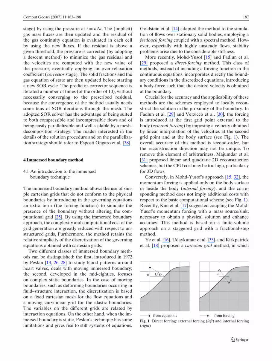
Crucial for the accuracy and the applicability of thesemethods are the schemes employed to locally recon-struct the solution in the proximity of the boundary. InFadlun et al. [29] and Verzicco et al. [30], the forcingis introduced at the first grid point external to thebody (external forcing) by imposing a velocity obtainedby linear interpolation of the velocities at the secondgrid point and at the body surface (see Fig. 1). Theoverall accuracy of this method is second-order, butthe reconstruction direction may not be unique. Toremove this element of arbitrariness, Majumdar et al.[31] proposed linear and quadratic 2D reconstructionschemes, but the CPU cost may be too high, particularlyfor 3D flows.

Conversely, in Mohd-Yusof’s approach [15, 32], themomentum forcing is applied only on the body surfaceor inside the body (internal forcing), and the corre-sponding method does not imply additional costs withrespect to the basic computational scheme (see Fig. 1).Recently, Kim et al. [17] suggested coupling the Mohd-Yusof’s momentum forcing with a mass source/sink,necessary to obtain a physical solution and enhanceaccuracy. This method is based on a finite-volumeapproach on a staggered grid with a fractional-stepmethod.

Ye et al. [16], Udaykumar et al. [33], and Kirkpatricket al. [18] proposed a cartesian grid method, in which

u U u

U

from equations from forcingFig. 1 Direct forcing: external forcing (left) and internal forcing(right)

188 Comput Geosci (2007) 11:183–198

the boundary conditions on the immersed boundariesare not imposed by a direct forcing, but by reshapingthe control volumes into trapezoidal boundary cellsto fit the local geometry and introducing a quadraticinterpolation to evaluate the fluxes through the centerof the faces of the reshaped cells. Nevertheless, theimplementation of this approach is more complicatedthan direct forcing methods, and an iterative techniquemay be required due to the different stencil of thetrapezoidal cells and the regular ones.

Very few applications of the immersed boundarytechnique to compressible flows can be found in theliterature. De Palma et al. [34] applied a method basedon the external forcing to supersonic flow conditions,and de Tullio et al. [35] combined this techniquewith local grid refinements. However, the pressure anddensity in the interface cells is imposed through afirst-order homogeneous Neumann condition becausethe Navier–Stokes equations are not solved in theimmersed cells.

The objective of the present work is to describean improved immersed boundary method for a com-plex 2D/3D static terrain morphology based on thedirect forcing methods introduced by Fadlun et al. [29]and Kim et al. [17], which combines both the exter-nal and internal momentum forcing coupled with aflux-correction procedure. This coupling allows us tocompute the flow variables also in the immersed cellsand to deal with the simulation of compressible andmultiphase flows, thus increasing the accuracy of thesolution on the boundaries. The external forcing andthe homogeneous Neumann condition on the pressure,density, and temperature are applied only in the fewcases where the internal forcing is not possible.

This method has been successfully applied to thenumerical code PDAC briefly described in the previoussection.

4.2 Forcing procedure

In this section, the procedure to derive the forcingterms on the momentum equations on the staggeredgrid is illustrated. We present the methodology for thehorizontal velocity component u on a 2D grid, but it canbe extended without difficulty to the other componentsand to 3D problems.

Referring to the gas phase, the direct forcing can beobtained by adding a force term Fij in the discretizedmomentum Eq. 9. To derive the expression of the

pseudo-force Fij, in a first step, all terms in the right-hand side (RHS) of Eq. 9 are discretized explicitly:

(εgρgug)n+1ij − (εgρgug)

nij

�t= RHSn

ij + Fnij, (21)

where RHS includes the convective, diffusive, pressuregradient, and body force terms.

By imposing un+1ij = U , the following approximation

for the pseudo-force is obtained:

Fnij ≈ (εgρg)

nU − (εgρgug)nij

�t− RHSn

ij (22)

the velocity is directly imposed and, thus, the forcingis direct. U corresponds to the velocity of the movingboundary (if the forcing point lies on the immersedboundary) while it equals zero in the case of a rigid no-slip wall (as in our case). Nevertheless, for nontrivialgeometries, the boundary does not lie on coordinatelines: an interpolation procedure is needed to computeU so that the velocity on the wall is actually nil. Fur-thermore, because in the present work a staggered gridis used, a different interpolation for each component ofthe velocity is required.

In the following, we will refer to the velocities ob-tained from the solution of the flow equations as phys-ical velocities and to the velocities obtained from theforcing as forced velocities.

The simplest possibility is to select the solid grid-points closest to the immersed boundary and to applythe forcing as if the boundary were going through theselected points. In the case of no-slip boundary condi-tions, this means fixing the velocity equal to zero at thefirst point inside the solid boundary (internal forcing),and the geometry is described in a stepwise way (seeFig. 2). We will refer to this technique as the blockingcells method.

Fluid

Solid

Fig. 2 Stepwise geometry obtained with a direct forcing withoutinterpolation procedure

Comput Geosci (2007) 11:183–198 189

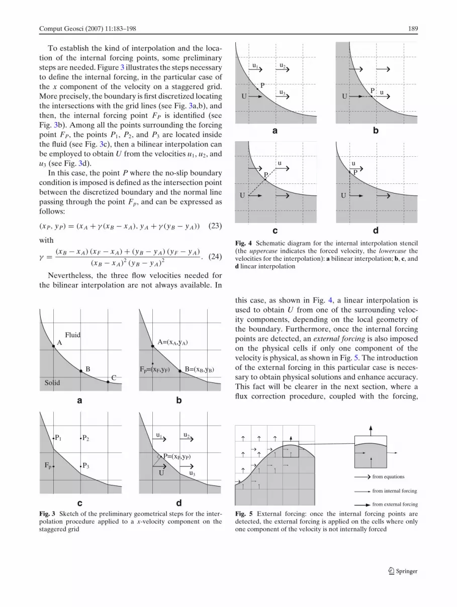
To establish the kind of interpolation and the loca-tion of the internal forcing points, some preliminarysteps are needed. Figure 3 illustrates the steps necessaryto define the internal forcing, in the particular case ofthe x component of the velocity on a staggered grid.More precisely, the boundary is first discretized locatingthe intersections with the grid lines (see Fig. 3a,b), andthen, the internal forcing point FP is identified (seeFig. 3b). Among all the points surrounding the forcingpoint FP, the points P1, P2, and P3 are located insidethe fluid (see Fig. 3c), then a bilinear interpolation canbe employed to obtain U from the velocities u1, u2, andu3 (see Fig. 3d).

In this case, the point P where the no-slip boundarycondition is imposed is defined as the intersection pointbetween the discretized boundary and the normal linepassing through the point Fp, and can be expressed asfollows:

(xP, yP) = (xA + γ (xB − xA), yA + γ (yB − yA)) (23)

with

γ = (xB − xA) (xF − xA) + (yB − yA) (yF − yA)

(xB − xA)2 (yB − yA)2 . (24)

Nevertheless, the three flow velocities needed forthe bilinear interpolation are not always available. In

Fluid

Solid

A

BC

A=(xA,yA)

B=(xB,yB)Fp=(xF,yF)

a b

Fp

P1 P2

P3U u3

u2u1

P=(xP,yP)

c dFig. 3 Sketch of the preliminary geometrical steps for the inter-polation procedure applied to a x-velocity component on thestaggered grid

Uu3

u2u1

P

UuP

a b

U

u

P

U

uP

c dFig. 4 Schematic diagram for the internal interpolation stencil(the uppercase indicates the forced velocity, the lowercase thevelocities for the interpolation): a bilinear interpolation; b, c, andd linear interpolation

this case, as shown in Fig. 4, a linear interpolation isused to obtain U from one of the surrounding veloc-ity components, depending on the local geometry ofthe boundary. Furthermore, once the internal forcingpoints are detected, an external forcing is also imposedon the physical cells if only one component of thevelocity is physical, as shown in Fig. 5. The introductionof the external forcing in this particular case is neces-sary to obtain physical solutions and enhance accuracy.This fact will be clearer in the next section, where aflux correction procedure, coupled with the forcing,

from equations

from internal forcing

from external forcing

Fig. 5 External forcing: once the internal forcing points aredetected, the external forcing is applied on the cells where onlyone component of the velocity is not internally forced

190 Comput Geosci (2007) 11:183–198

is introduced to satisfy the continuity equation in thevolume cells containing the immersed boundary.

We now describe in further detail the interpolationprocedures for the particular case of the x componentof the velocity in case of a no-slip boundary condition.As regards the internal linear interpolation, followingKim et al. [17], two cases are distinguished: when thedistance h between the forcing point FP and the no-slippoint P is smaller than the distance h1 between the firstexternal point P1 and the no-slip point (see Fig. 6a) andwhen h is greater than h1 (see Fig. 6b).

In the first case, a velocity U is imposed at the pointFP such that the linear interpolation between U and u1

vanishes at the boundary. Nevertheless, this simple in-terpolation seems not to be suitable in the second case,because a linear interpolation between U and u1 cannotguarantee a limited value of U when h1 approacheszero. In this case, as shown in Fig. 6b, a second flowvelocity value is also used; indeed, the velocity U at themirror point FP is obtained with a linear interpolationbetween the velocity at the points P1 and P2 (thisgives the desired value of U). Summarizing, the internalforcing velocity U can be expressed as:

U =

⎧⎪⎪⎪⎨

⎪⎪⎪⎩

− hh1

u1, for 0 < h ≤ h1

− (h2 − h)u1 + (h − h1)u2

h2 − h1, for h1 <h<h2

(25)

On the other hand, as previously pointed out, whenthe x components of the velocity located at the pointsP1, P2, and P3 are physical velocities (see Fig. 6c), a bi-linear interpolation can be defined giving the followingno-slip condition at the point P:

αβU +α(1−β)u3+(1−α)βu1+(1−α)(1−β)u2 =0 (26)

where

α = xP − x1

x2 − x1β = yP − y1

y2 − y1, (27)

x1, x2, xP, y1, y2, yP being defined in Fig. 6c.

Thus, the following value of the forced velocity U isobtained:

U = −α(1−β)u3+(1−α)βu1+(1−α)(1−β)u2

αβ. (28)

Finally, for the external linear forcing, a linear inter-polation scheme is applied (see Fig. 6d). In the firstnode, FP external to the boundary, the velocity U isobtained with a linear interpolation between the no-slipcondition at the point P and the value u1 at the secondexternal point u1.

Fluid

Solid

Fp

P1

Ph

h1

u1

U

Fluid

SolidFp

P1

P

h

h1

u1

UP2

u2

h2h

Fp

U

a b

Fluid

Solid

P1

P

u1

P2

u2

P3u3U Fp

y=y2

y=yP

y=y1

x=x 1

x=x P

x=x 2

Fluid

Solid

Fp

P1

Ph

h1

u1

U

c dFig. 6 Interpolation schemes: a linear interpolation scheme forthe internal forcing when 0 < h < h1; b linear interpolationscheme for the internal forcing when h > h1; c bilinear interpola-tion scheme for the internal forcing; d linear interpolation schemefor the external forcing

The external forcing is applied to avoid over-pressure or under-pressure problems in the cells withonly one physical velocity. Both the external and theinternal forcing procedures can be easily extended to3D grids, as we have done for the PDAC code.

4.3 Flux correction procedure

To deal with compressible flows, when a direct forcingto the momentum equation is applied, the continuityequation also has to be modified. The approach in-troduced by Kim et al. [17] for incompressible flowswith staggered grids, where the fluxes associated withthe internally forced velocities are neglected, cannotbe applied in a straightforward manner to compressibleflows and needs to be extended by taking into accountthe external forcing. The forcing procedure adopted inPDAC is here illustrated for the mass continuity equa-tions without specifying the phase subscript because theprocedure holds for each phase. We will therefore usethe notation ρ instead of ρkεk. The flux correction pro-cedure for the enthalpy equations and the gas speciestransport equations is identical and can be retrievedby substituting the density ρ in the following equationswith the specific enthalpy ρh or the mass fraction of thejth gas species ρy j.

Comput Geosci (2007) 11:183–198 191

To solve this problem, first of all, we distinguish fourdifferent kinds of volume cells where the forcing isapplied, depending on the presence of forced velocities(see Fig. 7):

1. Fluid cells, containing only physical velocities orphysical and externally forced velocities

2. Boundary cells of type 1, containing both physicaland internally forced velocities

3. Boundary cells of type 2, characterized by internallyand externally forced velocities only

4. Solid cells, with no physical velocities.

Let us first consider the fluid cells. For each phase,the integral form of the continuity Eq. 1 is written inthe following way:

VC∂ρ

∂t= ρLuLSL + ρTvT ST + ρRuR SR + ρBvB SB (29)

where VC is the area of the cell C; S is the length of acell edge; and the subscripts L, T, R, and B refer to theleft, top, right, and bottom edges, respectively. In thiscase, no flux correction is applied.

For the boundary cells of type 1 (see Fig. 8), the inte-gral form of the continuity equation is written exactly asEq. 29 but, for the cell C containing only fluid, the fluxesthrough the solid boundaries are null and the continuityequation reads

αVC∂ρ

∂t= ρR uR SR + ρTvT ST (30)

where α is the volume fraction of C occupied by theflow. From Eqs. 29 and 30, we obtain the followingmodified continuity equation:

αVC∂ρ

∂t=ωLρLvLSL +ωTρTvT ST +ωRρRvRSR +ωBρBvBSB (31)

fluid cell

boundary cell (type 1)

solid cell

boundary cell (type 2)

Fig. 7 Cell classification for the flux correction procedure: withrespect to other works, in our method, we distinguish two typesof boundary cells

Fluid

Solid

vT

vB

uR

uL

vT

uRC C

Fig. 8 Mass conservation for a type 1 boundary cell

where ωL , ωT , ωR , and ωB equal 0 if the correspondingvelocity is forced and 1 otherwise. In this way, we donot take into account the fluxes through the cell faceswith nonzero forcing, both external and internal.

Let us consider now the case of boundary cells C3

and C4 of type 2 illustrated in Fig. 9, where all thevelocities but one are internally forced and the remain-ing one is forced externally. In these cells, all the facefluxes are neglected, and the density cannot be updatedby means of the continuity equation. In this case, thedensity, the pressure, and the temperature are assignedequal to the value of the cell sharing the common facewhere the velocity is forced externally. For example, re-ferring to Fig. 9, in the cell C3 will be assigned the sameρ, P, and T of C2, and in the cell C4 the values of C1.

Note that, as the velocity in the common face of thecells C1 and C4 is forced, the flux through this faceis neglected also when solving the continuity equationin the fluid cell C1. This means that the continuityequation has to be modified also for the fluid cellscontaining forced velocity, accordingly with Eq. 31 andthe coefficients ω.

In practice, similar to the cartesian grid methodproposed by Ye et al. [16] and Udaykumar [33], thistechnique can be seen as a discretization of the mass

Fluid

Solid

C1 C2 C3

C4

C1

Fig. 9 Cell boundaries and forced velocity cells of type 2 and forfluid cells containing a forced velocity

192 Comput Geosci (2007) 11:183–198

conservation equation on the volume cell C1 (seeFig. 9), with the no-slip condition on the bottom face.Thus, for these particular fluid cells, the coefficient α inEq. 31 can be greater than 1.

Referring to Fig. 9, we observe that, without theintroduction of the external forcing, we should solvethe continuity equation also in the cells C3 and C4. Fora steady flow, neglecting the fluxes from the velocitiesforced internally would lead to a constant increase ordecrease of the density, in accordance with the sign ofthe unique physical velocity of the cell.

This technique can also be successfully applied toincompressible flows, where the condition of null di-vergence, coupled with the flux correction procedure,would give a null physical velocity when applied with-out the external forcing to the cells of type 2.

Finally, we observe that, neglecting all the volumefluxes due to internally and externally forced velocities,the global mass conservation is satisfied.

5 Application to the 2D/3D dynamics of PDCs

5.1 2D axisymmetric flow: column collapseand PDCs propagation

The 2D simulations presented here adopt a topographicprofile representative of the Northern sector of Vesu-vius, which is characterized by the presence of MountSomma, a topographic relief formed during a caldera

collapse episode. In particular, we will refer to thesimulation B180_w2_t950 of Todesco et al. [12]. In thissimulation, flow conditions adopted at the vent refer toa sub-Plinian eruption with a water content of 2 wt.%and a magma temperature of 950◦C. The simulationalso assumes a propagation of the PDCs over a sectorof 180 degrees.

The volcanic topography adopted was obtained froma digital elevation model with 10-m resolution [36]. Thevertical mesh resolution was constant and equal to 10 mon the topography, increasing up to 100 m at an altitudeof 3,500 m. Similarly, the radial resolution was constantand equal to 10 m for the first 500 m from the axis, thenincreased with distance reaching a cell aspect ratio of10:1 at a distance of 2,400 m.

The spatial and temporal evolution of the collapseof the volcanic column and the propagation of PDCsare fully described in Todesco et al. [12] and EspostiOngaro et al. [20]. Two simulations comparing theblocking cell and the immersed boundary techniquesare presented. Figure 10 shows the snapshots of the spa-tial dispersal of particles along the volcano slope after100 and 500 seconds. The no-slip boundary condition isapplied to the gas–particle flow both inside the crater,i.e., during the decompression of the volcanic jet, andalong the volcanic slope, i.e., after the column collapseand the formation of PDCs.

From the analysis of simulation outputs, it resultsthat the effect of the boundary condition adopted onthe jet dynamics in the crater is minor (not shown).

Fig. 10 PDC propagationalong the northern sector ofVesuvius. Vent conditionsrefer to simulationB180_w2_t950 of Todescoet al. [12]. Isolines from 10−8

to 10−1 of the total particlevolume fraction, defined as∑n

s=1 εs, are shown: a 100 safter the generation of thePDC (blocking cells); b 100 safter the generation of thePDC (immersed boundary);c 500 s after the generationof the PDC (blocking cells);d 500 s after the generationof the PDC (immersedboundary)

Comput Geosci (2007) 11:183–198 193

This can be explained by the specific flow regime char-acterizing the transition to a supersonic jet. In such aregime, the influence of the viscous term in the model isof little importance with respect to inertia and pressureterms. Moreover, the mesh resolution is maximum inthe vent region, so that the topography can be describedaccurately even with the blocking cells method. Forall these reasons, the radial velocity profile and thejet behavior are little influenced by the wall boundarycondition.

However, the dynamics of PDC propagation aremore directly affected by the ground boundary con-dition influencing the radial velocity profile and themobility of the flow. Even though this effect produces amoderate increase of the flow run-out of about 0.8 km(corresponding to about a 13% of it) when we adopt theimmersed boundary technique, the increased accuracyof the new method is evident from closer inspection ofthe results.

For instance, Fig. 11 shows a detail of the gas flowfield for the two simulations described above. In thiscase, the shaded profile represents a portion of the2D domain presented in Fig. 10 centered on the Mt.Somma relief. In detail, Fig. 11 represents the flow fieldcomputed by using the blocking cells (a, c) and theimmersed boundary methods (b, d) after 100 and 500

s from the beginning of the simulation. In these figures,the solid lines represent the isolines u = 0 of the radialcomponent of the gas velocity and indicate the virtualsurfaces where the no-slip condition is applied. Thearrows represent the gas velocity vector field computedon the radially staggered mesh.

From these figures, it is evident that the blockingcells method can adequately represent the real topog-raphy only where the mesh is sufficiently refined (i.e.,sufficiently close to the vent). On the contrary, wherethe mesh is coarse, as along the profile of Mt. Somma,the advantage of the immersed boundary technique isnotable. In fact, with this approach, the profile can beaccurately resolved even using a coarse and anisotropicmesh. As a consequence, not only is the vertical flowprofile of the PDC significantly modified by the newboundary condition, but this also affects the complexvortex dynamics overlying it. As already discussed inTodesco et al. [12], the dynamics of PDCs appears to bestrongly influenced by the complex interaction betweenthe collapsing column, the recirculating stream of thefountain and also by the formation of coignimbrite orphoenix columns generating from the upper layers ofthe flow. Even small changes in the flow pattern cantherefore produce rather large variations in the globaldynamics.

Fig. 11 PDC propagationalong the northern sector ofVesuvius. Gas velocity flowfield and isoline zero of theradial component of the gasvelocity: a 100 s after thegeneration of the PDC(blocking cells); b 100 s afterthe generation of the PDC(immersed boundary); c 500 safter the generation of thePDC (blocking cells); d 500 safter the generation of thePDC (immersed boundary)

750 1250 1750 2250 2750

500

1000

1500

2000

R(m)

Z(m)

750 1250 1750 2250 2750

500

1000

1500

2000

R(m)

Z(m)

a b

750 1250 1750 2250 2750

500

1000

1500

2000

R(m)

Z(m)

750 1250 1750 2250 2750

500

1000

1500

2000

R(m)

Z(m)

c d

194 Comput Geosci (2007) 11:183–198

5.2 3D flow: dome explosion

We tested our immersed boundary technique also for3D flows, still using the PDAC code. In this case, thesimulation describes the explosive collapse of a dome,represented as a semispherical volume filled with gasand particles of uniform size and density, and the asso-ciated propagation of a density current on a 3D irreg-ular topography. This example was specifically chosento test the influence of the flow compressibility onthe immersed boundary method. The initial conditionsand parameters assumed for the dome are reported inTable 1.

The computational domain extends 1 km in bothhorizontal directions and 500 m vertically, with anonuniform resolution of 10–40 m in the horizon-tal axes and 10–20 m in the vertical direction. Thetopographic surface used was extracted from the geo-referenced, 10-m-resolution topography of Vesuvius[36] with the dome center located at the universaltransverse mercator coordinates (453700, 4518800).

Figure 12 shows the isosurface of particle fraction of10−3 at 1 and 20 s after the beginning of the explosionobtained with the immersed boundary technique. Att = 0, the dome volume filled with gas and pyroclastsis released to expand in the atmosphere. A spheri-cal pressure wave suddenly forms and propagates inthe atmosphere from the source, initially dragging thesolid particles. Then, after a few seconds, the entiredome mass collapses to the ground and forms a densitycurrent that propagates along the valley. During thedownflow motion, the flow entrains atmospheric air andexpands, occupying the entire valley. Lateral and diluteportions of the flow also move uphill and appear ableto overcome the valley rims.

As for the 2D simulations, the use of the immersedboundary technique significantly improves the accuracyof the results. We show results for two simulations dif-fering only by the imposed ground boundary condition.

Figure 13a,b shows a planar view of the topographyand the isolines of the base 10 logarithm of the particlevolumetric fraction at 10 m above the ground and 20 s

Table 1 Initial conditions and parameters of the dome explosion

Vol. P εg ds ρs Tg, Ts

5 × 105 m3 Hydrostatic 0.3 100 μm 2, 000 Kg/m3 1, 133 K

The initial pressure profile is hydrostatic, εg is the initial void frac-tion, ds and ρs are the particle diameter and density, respectively.The gas and particle phases are assumed in thermal equilibriumwith temperature Tg and Ts

800

700

600

500

400453500

453700

453900

454100

454300

45181604518345

45185304518715

45189004519085

800

700

600

500

400453500

453700

453900

454100

454300

45181604518345

45185304518715

45189004519085

a

bFig. 12 Isosurface 10−3 of the particle volume fraction: a 1 s andb 20 s after the explosion

from the beginning of the explosion. The comparisonbetween the two approaches clearly shows that theflow calculated with the immersed boundary method isbetter confined to the valley. In turn, this produces aflow that is more mobile and able to travel uphill moreeffectively.

Figure 13c–f shows the velocity field on a slice-planealong and perpendicular to the main valley direction.The shaded profile represents a vertical section of thetopography, whereas the solid line represents the iso-line |u| = 0 for the gas phase and indicates the virtualsurface where the no-slip condition is applied. The ar-rows represent the gas velocity vector field interpolatedon the slice-plane mesh (particle velocity shows a verysimilar behavior).

The immersed boundary implementation improvesthe accuracy of the ground boundary condition. Suchan improvement is even more evident for the sectionperpendicular to the main flow direction (Fig. 13e,f).In particular, the blocking cells method (Fig. 13e) isunable to properly represent the local maxima of thetopography, thus allowing an easier overflow of thevalley rims. Vice versa, the immersed boundary method(Fig. 13f) can properly describe the valley edges so thatthe flow results in being better constrained laterally.

Comput Geosci (2007) 11:183–198 195

Fig. 13 3D dome explosionat 20 s. Left plots blockingcells, right plots immersedboundaries. a, b view fromthe top of the isolines[-4:-2:0.22] of the Log10 ofthe volumetric particlefraction at 20 m above theground level (the backgroundgrey shading is obtained by a3D rendering of thetopography). c, d plots of thegas velocity vector field andisoline of null velocity alongthe channel longitudinalsection (L in the top views). e,f plots of the same quantitiesalong the transversal section(T in the top views)

Note that, even if the differences after 20 s are yetrather small, these discrepancies in flow propagationshould sensibly increase at longer times after severalminutes of simulation.

Finally, it should be mentioned that, for this particu-lar 3D test case, for which the boundary cells are about7% of the total cells, the use of the immersed boundarymethod increases the CPU time by about 10% with anegligible increment of memory usage.

6 Conclusions

The simulation of the dynamics of PDCs over volcanictopographies is a very complex problem involving thesolution of 3D transient multiphase flow equations fora continuum compressible gas phase and a number of

interacting dispersed particulate phases. In particular,the interaction of the dense stratified PDC with the vol-cano topography is crucial due to the major influenceof topography on the transport processes governingthe nature of the flow. The accurate description of theground boundary condition along the real topographicprofile is therefore a prerequisite of any numerical codeaimed at this goal.

In this paper we have shown how the immersedboundary technique can be effectively implementedon existing 2D/3D finite-volume codes using cartesianmeshes to accurately impose a no-slip condition. Thistechnique, here presented in a novel formulation, hasbecome popular thanks to its ability to accurately de-scribe the flow around complex geometries using simplecartesian meshes with a relatively low computationalcost. In particular, the numerical simulations of 2D

196 Comput Geosci (2007) 11:183–198

and 3D PDCs here described have proved that theimmersed boundary method describes more accuratelythe no-slip boundary condition on the topography thanthe traditional blocking cells method. On a single flowunit, this is proved by the instantaneous matching ofthe isoline zero of the flow velocity and the 2D/3Dtopographic profiles.

Although it is difficult to quantify the net effectof the new ground boundary condition on the globalPDCs dynamics, due to the complex nonlinear effectsbetween the flows and the overlying atmosphere, the2D simulations performed at Vesuvius suggest an in-crease of the flow runout with respect to the use of theclassical blocking cells method. Moreover, the prelim-inary 3D simulations performed indicate that such aneffect could be even greater if we consider topogra-phies characterized by valleys, ridges, and sudden slopechanges. From this point of view, the present techniqueis recommended when applied to the simulation oflarge-scale 3D eruptive scenarios over realistic volcanotopographies for which the use of fine meshes is com-putationally unaffordable.

Acknowledgements This work was supported by the Europeanproject EXPLORIS, contract no. EVR1-CT2002-40026, by theMIUR (Ministero dell’Istruzione, dell’Università e della Ricerca)through the Project Firb RBAPO4EF3A_005 and with the con-tribution of the Istituto Nazionale di Geofisica e Vulcanologiaand the Italian Department of Civil Protection.

Appendix A1: Constitutive equations and rheologicalproperties of gas and pyroclasts

The constitutive equations express the gas density as afunction of the thermodynamic pressure and tempera-ture (gas equation of state) and the stress tensors as afunction of the strain tensors providing the closure tothe system of the transport equations. They also specifythe rheology of the flow and the interphase transportproperties. The classic Smagorinsky turbulence clo-sure model [37] expresses the turbulent diffusion interms of an effective turbulent viscosity. For particles,a correction (Coulombic repulsion) to the Newtonianapproximation accounts for the finite size of particles.Volumetric and mass fraction closures express the factthat phases are treated as interpenetrating continua.

A1.1 Closure equations

A1.1.1 Volumetric and mass fraction closures

εg +N∑

s=1

εs = 1;M∑

i=1

yi = 1 (32)

A1.1.2 Thermal equations of state

ρg = Pg

RTg; ρs = constant(s), s = 1, 2, ..., N (33)

A1.1.3 Caloric equations of state

Tg = hg

Cpg

, Ts = hs

Cps

, s = 1, 2, ..., N (34)

Cpg =M∑

i=1

yiCpg,i . (35)

where C are averaged values of the (temperature-dependent) specific heats.

A1.1.4 Gas-phase stress tensor

Tg = εg

(μgτg + μgtτg

)(36)

τg =[∇ug + (∇ug)

T]

(37)

τg = τg − 2

3(∇ · ug)I (38)

μgt = l2ρg|τg| (39)

l = lS = cS�; � = √�x�y�z (40)

l = lB = κ(z + z0); (41)

Eqs. 40 and 41 express the turbulent length scale andare used, respectively, away from and close to solidboundaries. cS is the Smagorinsky coefficient, whichis taken equal to 0.1 in the simulations presented inSect. 5.

A1.1.5 Solid stress tensor

Ts = εsμsτ v,s − τc,sI, s = 1, 2, ..., N (42)

τ v,s =[∇us + (∇us)

T]

− 2

3(∇ · us)I (43)

∇τc,s = G(εs)∇εs, G(εs) = 10−aεs+b (44)

Comput Geosci (2007) 11:183–198 197

where μs is constant and equals 0.5 Pa s for the 30μmparticles and 1.0 Pa s for the 500μm particles.

A1.1.6 Heat fluxes

qg = kgeεg∇Tg; (45)

qs = ksεs∇Ts; s = 1, ..., N (46)

where kg, ks are the coefficients of thermal conduct-ivity.

For the gas phase, the effective thermal conductivityis given by:

kge = kg + kgt

kgt = Cpgμgt

Prt

with Prt = 0.5.

A1.2 Interphase exchange terms

The general form of the interphase momentum andenthalpy exchange terms is linearized as follows:

Lgs = Dgs(ug − us); s = 1, ..., N (47)

Lsl = Dsl(us − ul); s, l = 1, ..., N (48)

Igs = Qs(Tg − Ts); s = 1, ..., N (49)

The interphase exchange coefficients are derived fromsemiempirical correlations. Their validity can dependon the flow regime, thus also including correction forturbulence and different particle concentrations.

A1.2.1 Gas–particle drag coefficient

for εg ≥ 0.8:

Dg,s = 3

4Cd,s

εgεsρg | ug − us |ds

ε−2.7g , s = 1, 2, ..., N

(50)

Cd,s = 24

Res[1 + 0.15 Re0.687

s ], Res < 1000 (51)

= 0.44, Res ≥ 1000, (52)

for εg < 0.8:

Dg,s = 150ε2

s μg

εgd2s

+ 1.75εsρg | ug − us |

ds,

s = 1, 2, ..., N (53)

Res = εgρgds | ug − us |μg

(54)

Dg,s = Ds,g so that Lg,s = −Ls,g in the equations.

A1.2.2 Particle–particle drag coefficient

Ds,p = Fspα(1 + e)ρsεsρpεp(ds + dp)

2

(ρsd3s + ρpd3

p)| us − up |,

s, p = 1, 2, ..., N; p �= s (55)

Fsp = 3ε1/3sp + (εs + εp)

1/3

2(ε1/3sp − (εs + εp)1/3)

(56)

for Xs ≤ �s

�s + (1 − �s)�p:

εsp = [(�s − �p) + (1 − a)(1 − �s)�p

]

×[�s + (1 − �p)�s

]

�sXs + �p (57)

for Xs >�s

�s + (1 − �s)�p:

εsp = (1 − a)[�s + (1 − �s)�p

](1 − Xs) + �s (58)

a =√

dp

ds, (ds ≥ dp), Xs = εs

εs + εp(59)

Dp,s = Ds,p so that Lp,s = −Ls,p in the equations.

A1.2.3 Gas–particle heat transfer coefficient

Qs = Nus6kgεs

d2s

, s = 1, 2, ..., N (60)

Nus = (2 + 5ε2s )(1 + 0.7Re0.2

s Pr1/3)

+(0.13 + 1.2ε2s )Re0.7

s Pr1/3, Res ≤ 105 (61)

Res = ρgds | ug − us |μg

, Pr = Cpgμg

kg(62)

References

1. Sparks, R.S.J., Bursik, M.I., Carey, S.N., Gilbert, J.S., Glaze,L.S., Sigurdson, H., Woods, A.W.: Volcanic Plumes. JohnWiley, Hoboken (1997)

2. Druitt, T.: Pyroclastic density current. The physics of explo-sive volcanic eruptions (Gilbert J.S., Spartks, R.S.J. eds.).Geol. Soc. Lond. Spec. Publ. 145, 145–182 (1998)

3. Sparks, R.S.J., Wilson, L., Hulme, G.: Theoretical modelingof the generation, movement, and emplacement of pyroclas-

198 Comput Geosci (2007) 11:183–198

tic flows by column collapse. J. Geophys. Res. 83(B4),1727–1739 (1978)

4. Valentine, G.A.: Stratified flow in pyroclastic surges. Bull.Volcanol. 49, 616–630 (1987)

5. Burgisser, A., Bergantz, G.W.: Reconciling pyroclastic flowand surge: the multiphase physics of pyroclastic density cur-rents. Earth Planet. Sci. Lett. 202, 405–418 (2002)

6. Valentine, G.A., Wohletz, K.H.: Numerical models of Plinianeruption columns and pyroclastic flows. J. Geophys. Res.94(B2), 1867–1887 (1989)

7. Dobran, F., Neri, A., Macedonio, G.: Numerical simulation ofcollapsing volcanic columns. J. Geophys. Res. 98(B3), 4231–4259 (1993)

8. Neri, A., Esposti Ongaro, T., Macedonio, G., Gidaspow, D.:Multiparticle simulation of collapsing volcanic columns andpyroclastic flows. J. Geophys. Res. 108, 2202 (2003)

9. Dartevelle, S., Rose, W.I., Stix, J., Kelfoun, K., Vallance,J.W.: Numerical modeling of geophysical granular flows: 2.Computer simulations of plinian clouds and pyroclastic flowsand surges. Geochemistry, Geophysics, Geosystems, 5(8),Q08004 (2004)

10. Giordano, G., Dobran, F.: Computer simulations of theTuscolano Artemisio’s second pyroclastic flow unit (albanHills, Latium, Italy). J. Volcanol. Geotherm. Res. 61, 69–94(1994)

11. Dobran, F., Neri, A., Todesco, M.: Assessing pyroclastic flowhazard at Vesuvius. Nature 367, 551–554 (1994)

12. Todesco, M., Neri, A., Esposti Ongaro, T., Papale, P.,Macedonio, G., Santacroce, R., Longo, A.: Pyroclastic flowhazard at Vesuvius from numerical modeling - 1. Large-scaledynamics. Bull. Volcanol. 64, 155–177 (2002)

13. Peskin C.S.: Flow patterns around heart valves: a numericalmethod. J. Comput. Phys. 10, 252–271 (1972)

14. Goldstein, D., Handler, R., Sirovich, L.: Modelling a no-slipflow boundary with an external force field. J. Comput. Phys.105, 354–366 (1993)

15. Mohd-Yusof, J.: Combined Immersed-Boundary/B-SplineMethods for Simulations of Flow in Complex Geome-tries. Annual Research Briefs. NASA Ames Research Cen-ter/Stanford University Center for Turbulence Research,Stanford (1997)

16. Ye, T., Mittal, R., Udaykumar, H.S., Shyy, W.: An accuratecartesian grid method for viscous incompressible flows withcomplex immersed boundaries. J. Comput. Phys. 156, 209–240 (1999)

17. Kim, J., Kim, D., Choi, H.: An immersed-boundary finite-volume method for simulations of flow in complex geome-tries. J. Comput. Phys. 171, 132–150 (2001)

18. Kirkpatrick, M.P., Armfield, S.W., Kent, J.H.: A represen-tation of curved boundaries for the solution of the Navier–Stokes equations on a staggered three-dimensional Cartesiangrid. J. Comput. Phys. 184, 1–36 (2003)

19. Neri, A., Esposti Ongaro, T., Cavazzoni, C., Erbacci, G.,Macedonio, G.: European Project Exploris (EVRI-CT-2002-40026) Deliverable 3.3B: PDAC Reference Manual. Techni-cal Report. INGV, Pisa (2005)

20. Esposti Ongaro, T., Neri, A., Todesco, M., Macedonio, G.:Pyroclastic flow hazard at Vesuvius from numerical modeling- 2. Analysis of flow variables. Bull. Volcanol. 64, 1178–1191(2002)

21. Sweby, P.K.: High resolution schemes using flux-limiters forhyperbolic conservation laws. SIAM J. Numer. Anal. 21(5),995–1011 (1984)

22. Leonard, B.P., Mokhtari, S.: Beyond first-order upwinding:the ultra-sharp alternative for non-oscillatory steady-statesimulation of convection. Int. J. Numer. Methods Eng. 30,729–766 (1990)

23. Harlow, F.H., Amsden, A.A.: Numerical calculation of mul-tiphase fluid flow. J. Comput. Phys. 17, 19–52 (1975)

24. Williamson, J.H.: Low-storage Runge–Kutta schemes. J.Comput. Phys. 35, 48–56 (1980)

25. Mittal, R., Iaccarino, G.: Immersed boundary methods.Annu. Rev. Fluid Mech. 37, 239–261 (2005)

26. Peskin C.S.: Numerical analysis of blood flow in the heart. J.Comput. Phys. 25, 220–252 (1977)

27. Peskin C.S.: The fluid dynamics of heart valves: Experi-mental, theoretical, and computational methods. Annu. Rev.Fluid Mech. 14, 235 (1982)

28. Peskin C.S.: The immersed boundary method. Acta Numer.479–517 (2002)

29. Fadlun, E.A., Verzicco, R., Orlandi, P., Mohd-Yusof, J.:Combined immersed-boundary finite-difference methods forthree-dimensional complex flow simulations. J. Comput.Phys. 161, 35–60 (2000)

30. Verzicco, R., Mohd-Yusof, J., Orlandi, P., Haworth,D.: Large eddy simulation in complex geometric config-urations using boundary body forces. AIAA J. 38(3), 427–433(2000)

31. Majumdar, S., Iaccarino, G., Durbin, P.: RANS Solverswith Adaptive Structured Boundary Non-conforming Grids.Annual Research Briefs. NASA Ames Research Center/Stanford University Center for Turbulence Research,Stanford, pp. 353–366 (2001)

32. Tseng, Y.H., Ferziger, J. H.: A ghost cell immersed boundarymethod for flow in complex geometry. J. Comput. Phys. 192,593–623 (2003)

33. Udaykumar, H.S., Mittal, R., Rampungoon, P., Khanna, A.:A sharp interface Cartesian Grid method for simulation flowswith complex moving boundaries. J. Comput. Phys. 174, 345–380 (2001)

34. De Palma, P., de Tullio, M.D., Pascazio, G., Napolitano,M.: An immersed-boundary method for compressible viscousflows. Comput. Fluids 35, 693–702 (2006)

35. de Tullio, M., Iaccarino, G.: Immersed Boundary Tech-nique for Compressible Flow Simulations on Semi-structuredMeshes. Annual Research Briefs. NASA Ames ResearchCenter/Stanford University Center for Turbulence Research,Stanford, pp. 71–83 (2005)

36. Pareschi, M.T., Santacroce, R., Favalli, M., Giannini, F.,Bisson, M., Meriggi, A., Cavarra, L.: Un GIS per il Vesuvio.Protezione Civile, GNV, OV, Commissione incaricata perl’aggiornamento dei piani di emergenza per le aree Vesu-viana E Flegrea. Felici Editore, Pisa (2000)

37. Smagorinsky, J.: General circulation experiments with theprimitive equations, part I: the basic experiment. Mon.Weather Rev. 91, 99–164 (1963)

38. Esposti Ongaro, T., Neri, A., Cavazzoni, C., Erbacci, G.,Salvetti, M.V.: A parallel multiphase flow code for the 3Dsimulation of explosive volcanic eruptions. Parallel Comput.(2007)