Annales Geophysicae (2002) 20: 1921–1934c© European Geosciences Union 2002Annales

Geophysicae

An inter-hemispheric, statistical study of nightside spectral widthdistributions from coherent HF scatter radars

E. E. Woodfield1, K. Hosokawa2, S. E. Milan1, N. Sato3, and M. Lester1

1Department of Physics and Astronomy, University of Leicester, UK2Department of Geophysics, Graduate School of Science, Kyoto University, Japan3National Institute of Polar Research, Tokyo, Japan

Received: 22 February 2002 – Revised: 27 June 2002 – Accepted: 5 July 2002

Abstract. A statistical investigation of the Doppler spec-tral width parameter routinely observed by HF coherentradars has been conducted between the Northern and South-ern Hemispheres for the nightside ionosphere. Data fromthe SuperDARN radars at Thykkvibær, Iceland and SyowaEast, Antarctica have been employed for this purpose. Bothradars frequently observe regions of high (> 200 ms−1) spec-tral width polewards of low (< 200 ms−1) spectral width.Three years of data from both radars have been analysedboth for the spectral width and line of sight velocity. Thepointing direction of these two radars is such that the flowreversal boundary may be estimated from the velocity data,and therefore, we have an estimate of the open/closed fieldline boundary location for comparison with the high spectralwidths. Five key observations regarding the behaviour of thespectral width on the nightside have been made. These are(i) the two radars observe similar characteristics on a statis-tical basis; (ii) a latitudinal dependence related to magneticlocal time is found in both hemispheres; (iii) a seasonal de-pendence of the spectral width is observed by both radars,which shows a marked absence of latitudinal dependenceduring the summer months; (iv) in general, the Syowa Eastspectral width tends to be larger than that from Iceland East,and (v) the highest spectral widths seem to appear on bothopen and closed field lines. Points (i) and (ii) indicate thatthe cause of high spectral width is magnetospheric in origin.Point (iii) suggests that either the propagation of the HF ra-dio waves to regions of high spectral width or the generatingmechanism(s) for high spectral width is affected by solar il-lumination or other seasonal effects. Point (iv) suggests thatthe radar beams from each of the radars are subject eitherto different instrumental or propagation effects, or differentgeophysical conditions due to their locations, although wesuggest that this result is more likely to be due to geophysi-cal effects. Point (v) leads us to conclude that, in general, theboundary between low and high spectral width will not be a

Correspondence to:E. E. Woodfield(Emma.Woodfield@ion.le.ac.uk)

good proxy for the open/closed field line boundary.

Key words. Ionosphere (auroral ionosphere; ionosphericirregularities)

1 Introduction

The Doppler spectral width parameter observed by the Su-per Dual Auroral Radar Network (SuperDARN) of coher-ent HF radars has been subject to increasing scrutiny. Inparticular, there are variations in spectral width as a func-tion of latitude and time which may relate to the ionosphericfootprint of magnetospheric regions. For example, regionsof high and variable spectral width observed on the daysideare generally accepted as being associated with the low al-titude cusp (Baker et al., 1990, 1995; Rodger et al., 1995;Pinnock et al., 1995; Andre et al., 1999, 2000a; Milan etal., 1999; Moen et al., 2001; Rodger, 2000). Similar re-gions of high and variable spectral width frequently occuron the nightside (Lewis et al., 1997; Dudeney et al., 1998;Lester et al., 2001; Woodfield et al., 2002a, b) and the de-bate over which magnetospheric regions these may repre-sent is ongoing. There are two hypotheses regarding themagnetospheric origin of nightside regions of high spectralwidth, more specifically, regarding the sharp gradient be-tween low spectral width (< 200 ms−1), at lower latitudes,and high spectral width (> 200 ms−1), at higher latitudes.The first proposal suggests a link between this spectral widthgradient and the boundary between the Central Plasma Sheet(CPS) and Boundary Plasma Sheet (BPS) (Dudeney et al.,1998), while the second proposes that the spectral width gra-dient could represent the Open/Closed Field Line Boundary(OCFLB) (Lester et al., 2001).

There have been several suggestions for the physical ex-planation for the generation of regions of high and variablespectral width. Andre et al. (1999; 2000a, b) simulated theeffect of a time-varying electric field, with frequencies of theorder of 0.1 to 5 Hz, on the complex autocorrelation func-

1922 E. E. Woodfield et al.: A statistical study of nightside spectral width distributions

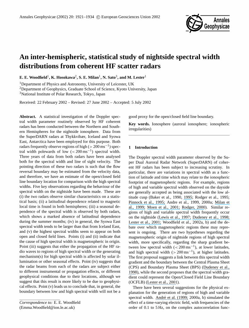
Fig. 1. A map in AACGM of the locations of the field-of-view ofthe Iceland East radar (blue) and the CUTLASS statistics summaryrange gates, C0 to C15. In yellow are the conjugately mapped field-of-view of the Syowa East radar and its statistical summary rangegates, S0 to S15.

tions (ACFs) derived from the HF coherent radars’ pulse se-quence and found that large spectral widths can be caused bysuch an electric field. The changing electric field causes thephase of the ACF to become nonlinear, which, in turn, gen-erates several large peaks in the power spectrum of the signal(the Fourier transform of the ACF). The standard softwareused to process the radar measurements (FITACF), whichfits the power spectrum parameters directly using the ACF,tends to overestimate the spectral width when there are manypeaks of comparable power in the power spectrum. The es-timated errors in the spectral width and line of sight velocityare also seen to rise where there are many peaks in the spec-trum. Andre et al. (1999; 2000a, b) then linked the largespectral widths observed in the cusp (e.g. Baker et al., 1995)to electromagnetic wave activity (0.2 to 2.2 Hz) observed bysatellites passing through the cusp (e.g. Maynard et al., 1991;Matsuoka et al., 1993) and ground magnetometer data show-ing Pc1/Pc2 wave activity underneath the cusp (Menk et al.,1992; Dyrud et al., 1997). They conclude that Alfven wavesare likely to be the major energy source that causes the mea-surement of high spectral width in the cusp. Similar Alfvenwaves may also, therefore, be responsible for the regions ofhigh and variable spectral width observed on the nightside,and such wave activity has been observed throughout the au-roral oval (Gurnett, 1991). No experimental study has yetdemonstrated conclusively the relationship between wave ac-tivity and large spectral width on the nightside.

Other possible mechanisms for generating large HF spec-tral widths have been described by Schiffler et al. (1997) andHuber and Sofko (2000). Observations of the power spec-tra obtained from the low-latitude boundary layer using themaximum entropy method indicated the presence of manyspectra with two main peaks. Therefore, they propose the

presence of vortices in the plasma flow, smaller than the radarrange cell and with a shorter lifespan than the integrationtime of the radar beam. Modelling of these vortices (Huberand Sofko, 2000) suggests that they would be capable of gen-erating double-peak spectra. It is likely that FITACF overes-timates the spectral width of the double-peak spectra. How-ever, the simulations of the autocorrelation function gener-ated by a small vortex (∼ 5 km) by Andre et al. (2000b) sug-gest that several vortices would be required within a radarrange cell for more than one large peak in the power spec-trum to be produced.

This paper investigates the statistical behaviour of thespectral width parameter measured by the Iceland East andSyowa East radars on the nightside, complementing work byHosokawa et al. (2002) regarding the dayside. These radarsare part of, and form a conjugate pair within, the Super-DARN HF radar network. The approximately meridionalarrangement of the summary range gates employed in thestatistics database, and described below, is used with the aimof determining the statistical location of the spectral widthgradient, i.e. the transition from high to low spectral width,over time. This, in turn, may reveal something of the natureand origin of the spectral width gradient.

2 SuperDARN

The Super Dual Auroral Radar Network (SuperDARN) is acollection of high-frequency coherent scatter radars in boththe Northern and Southern Hemispheres run cooperativelyby many nations (Greenwald et al., 1995). Each radar usesa multi-pulse scheme to transmit radio waves along 16 beamdirections, one at a time, with each beam returning informa-tion from a number of range gates (75 for Iceland East and 70for Syowa East). In standard common mode the signal fromeach beam is integrated for 7 s, with a gate length of 45 km.The whole scan is synchronized to start at 2-min intervals,with each beam being 3.24◦ wide. At nearer ranges the prop-agation is supported by the12-hop mode, and at further rangesby 1 1

2-hop (Milan et al., 1997). Although the exact rela-tionship between radar range and ground range is somewhatcomplex, the error in the range estimates for the radar beamsis dependent upon the propagation mode; for1

2-hop the erroris ∼ 15 km, and for 11

2-hop the error is∼ 60 km (Yeomanet al., 2001). The data are routinely processed in real timeby software (FITACF) used uniformly throughout the net-work to produce a set of parameters which include backscat-ter power, Doppler line of sight velocity and Doppler spectralwidth. The parameters are derived from the ACF of the re-turned signals for each range gate (Villain et al., 1987). Aset of criteria are used to identify scatter from the ground(ground scatter is assumed to have a velocity< 50 m s−1 andspectral width< 20 m s−1). The fit is generally successful,although certain conditions giving rise to multi-peaked spec-tra may give rise to anomalies in the spectral width (Baker etal., 1995; Andre et al., 1999).

E. E. Woodfield et al.: A statistical study of nightside spectral width distributions 1923

0

3

6

9

12

15

18

21

24

27+

Occ

urr

ence

, % p

oss

ible

ob

serv

atio

ns

Winter Spring

Summer Autumn

80o Lat 70o Lat

24 MLT 02 MLT22 MLT

20 MLT

24 MLT 02 MLT22 MLT

24 MLT 02 MLT22 MLT 24 MLT 02 MLT22 MLT

20 MLT

80o Lat 70o Lat

80o Lat 70o Lat 80o Lat 70o Lat

Figure 2

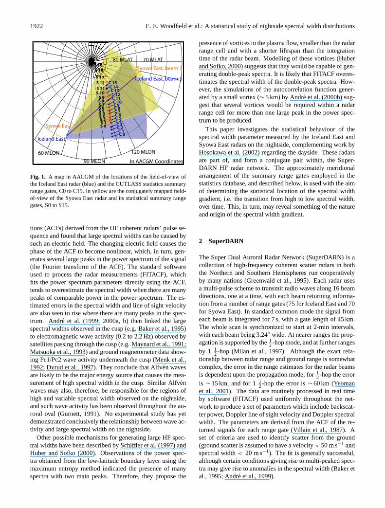
Fig. 2. Colour-coded plots of the data occurrence observed by the Iceland East radar as a function of Northern Hemisphere season, MLT andlatitude for the three years of data. Each square of colour represents an interval of 15 min of MLT and one statistical summary point. Thecolour scale indicates the number of observations of ionospheric scatter above 3 dB as a percentage of the total possible observations in thatseason from the database used. A statistical auroral oval for aKp of 2 is overlaid for comparison.

The SuperDARN radars used in this investigation are Ice-land East and Finland, situated in the Northern Hemisphereat Thykkvibær, Iceland (64.49◦ N, 68.48◦ E) and Hankasalmi(58.6◦ N, 104.9◦ E), respectively, and Syowa East situatedin the Southern Hemisphere at Syowa Station, Antarctica(66.09◦ S, 71.65◦ E). Altitude Adjusted Corrected Geomag-netic coordinates, AACGM, are used throughout this paperand are adapted from Baker and Wing (1989). The IcelandEast and Syowa East radars form a conjugate pair, as shownin Fig. 1 (the Syowa East field-of-view has been mapped intothe Northern Hemisphere using the IGRF95 model; Barton,1997).

Each SuperDARN radar produces a large amount of data,making study of long-term variations in the observationsproblematic in terms of data storage requirements and pro-cessing time. To overcome this a representative subset ofthe observations from the Co-operative U. K. Twin LocatedAuroral Sounding System (CUTLASS) Finland and IcelandEast radars are routinely stored in a “statistics database”,which is kept on hard disk, allowing for easy analysis of the6 years of radar measurements made to date (January 2002)in the common mode operations of the radars. The databaseresulting from this extra processing contains all the normalradar parameters but for only 16 summary radar cells. Sucha database was originally introduced by Milan et al. (1997).In that study the 16 summary radar cells were taken frombeam 7 of Iceland East, whereas in the present study weuse the summary points originally identified in the Finlandradar field-of-view. Thus, the summary points for IcelandEast in this study are located approximately along a geomag-netic meridian, and the gates used are chosen for the largerange of magnetic latitudes they encompass, 65◦ N to 81◦ N.

The location of the summary points are given as C0 to C15in Fig. 1. A similar set of summary range gates, spanningthe latitude range 70◦ S to 86◦ S has been determined forthe Syowa East radar data using the IGRF95 model (Barton,1997) to find magnetically conjugate positions. In order toproduce a more accurate comparison between the radar datasets, only mutual common time data (where the radars are runin the same mode) have been used for the interval 1 January1998 to 31 December 2000. For the majority of the data thefrequencies used in the common mode were consistent withIceland East running in the frequency band from 10.2 MHzto 10.7 MHz twenty-four hours a day from January 1998 un-til October 2000. During November and December 2000,the daytime frequency (08:00 to 18:00 UT) for Iceland Eastwas changed to the band from 12.1 MHz to 12.2 MHz. Com-parisons of the results using just 1998 and 1999 with thosepresented here show that this change in the frequency has nonoticeable effect on the results. The Syowa East radar wasrun in the band 10.2 MHz to 10.5 MHz twenty-four hours aday for all the days, except the period from 6–10 February1998, where the daytime frequency (06:00 to 18:00 UT) wasfrom the 11.1 MHz band. This also has very little apprecia-ble effect on the results and the conclusions reached. Datawith a received power below 3 dB are not used (to eliminate∼ 75% of the noise), and data identified as ground scatter bythe FITACF software have also been removed. The analysispresented here takes the form of occurrence distributions ofspectral width. The data have been sorted into 15-min in-tervals of MLT and spectral width bins which are 20 m s−1

wide. The spectral width data have been restricted to therange 0 to 500 m s−1; this removes a further∼ 20% of theobservations. Since the fields of view of the radars do not

1924 E. E. Woodfield et al.: A statistical study of nightside spectral width distributions

0

2

4

6

8

10

12

14

16

18+

Occ

urr

ence

, % p

oss

ible

ob

serv

atio

ns

Winter Spring

Summer Autumn

-80o Lat -70o Lat

24 MLT 02 MLT22 MLT

20 MLT

24 MLT 02 MLT22 MLT

24 MLT 02 MLT22 MLT 24 MLT 02 MLT22 MLT

20 MLT

-80o Lat -70o Lat

-80o Lat -70o Lat -80o Lat -70o Lat

Figure 3

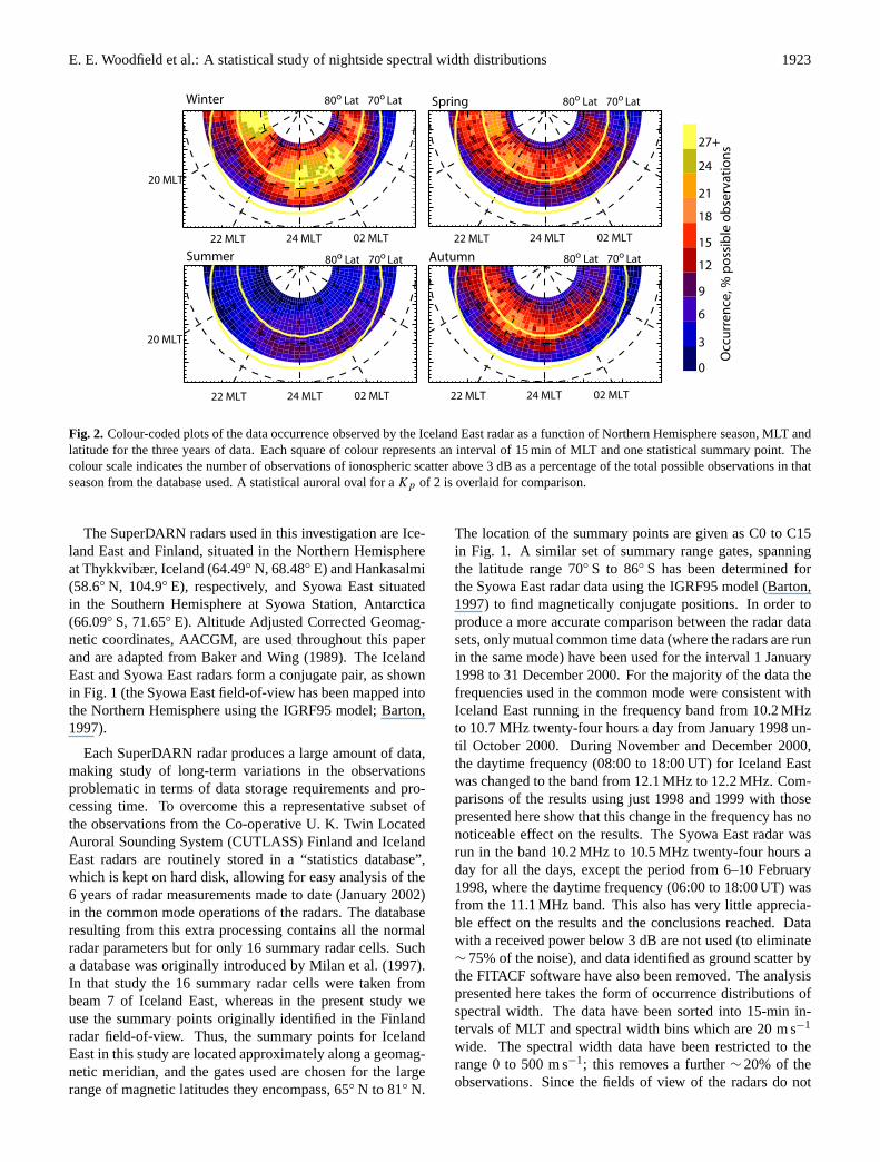
Fig. 3. Colour-coded plots of the data occurrence observed by the Syowa East radar as a function of Southern Hemisphere season, MLT andlatitude for the three years of data. Each square of colour represents an interval of 15 min of MLT and one statistical summary point. Thecolour scale indicates the number of observations of ionospheric scatter above 3 dB as a percentage of the total possible observations in thatseason from the database used. A statistical auroral oval for aKp of 2 is overlaid for comparison.

overlap completely, there are some summary range gates thatdo not have a close conjugate partner. For Iceland East pointsC0 to C3 fall into this category, while for Syowa East pointsS12 to S15 have no conjugate partner. The summary pointsare located along beam 9 of the CUTLASS Finland radar,which is almost meridional to the magnetic pole. The aimof having the points aligned with a large variation in invari-ant latitude and a small variation in longitude (∼ 15◦ for thepoints with conjugate partners) is that a long-term analysis ofthe latitudinal location of the spectral width gradient can beachieved.

3 Statistical observations

3.1 Data occurrence

Figure 2 shows the occurrence of ionospheric backscatterechoes over the three years of data used, split into sea-sons (winter consisting of November, December and Jan-uary, spring taken as February, March and April, etc., for theNorthern Hemisphere). Each colour-coded square representsa 15-min interval of MLT for each statistical point for IcelandEast. The colour scale indicates the number of observationsas a percentage of possible observations in that region andseason over the three years of data presented. The IcelandEast range gates coincident with the summary points varybetween 39 and 48, equivalent to the 1935 km to 2340 kmrange for normal mode operations. Thus, one expects mainlyF-region scatter, with a mixture of12 and 1 1

2 hop propaga-tion to have originated from these locations. However, theremay be some E-region contamination at these ranges result-ing from 1 1

2 hop propagation. An analysis of Iceland East

backscatter similar to that conducted by Milan et al. (1997)shows a small population of Type 1 E-region scatter, iden-tified by a low spectral width and a velocity which is closeto the local ion acoustic speed, observed in all of the Ice-land East summary points. An investigation of this Type 1scatter for the data used indicates that the contamination ofthe F-region scatter is negligible. A similar analysis of theSyowa East data indicates no discernable Type 1 E-regionscatter on the nightside. The largest number of observationstends to occur in winter, and the least in summer, agreeingwith work by Milan et al. (1997). Milan et al. (1997) foundthat in summer most of the observations by the Iceland Eastradar involve1

2 hop propagation and as such, are in the rangegates close to the radar. The summary points employed in thecurrent study are all in the 112 hop distance range and, there-fore, the amount of data observed in the summer is less. Thepeak occurrence in winter is over 27% of the possible obser-vations in the 15-min interval and occurs between 75◦ N and80◦ N from 18:00 MLT to 20:00 MLT, followed by a brief lullbetween 20:00 and 22:00 MLT. The number of observationsthen rises again, but at a lower latitude, with the maximumbetween 70◦ N and 75◦ N, until the occurrence begins to falloff again from 04:00 MLT. The situation in spring is simi-lar, although the maximum is smaller (approximately 24% ofthe possible observations) and the change in latitude is moregradual. Autumn is very similar to spring in the distributionof data observations. The maximum number of observationsin the summer months is only 9% to 12%, and this occursmainly below 70◦ N and between 22:00 and 04:00 MLT.

The same analysis (except with Southern Hemisphere sea-sons) for the data from the Syowa East radar is presentedin Fig. 3. The data distribution in the Southern Hemisphere

E. E. Woodfield et al.: A statistical study of nightside spectral width distributions 1925

Figure 4

Point 4, mean=145ms-1,number of points=962

Point 12, mean=182ms-1,number of points=2139

0

5

10

15

% O

ccu

rren

ce

0 100 200 300 400 500

Spectral Width, ms-1

Point 0, mean=160ms-1,number of points=481

Point 9, mean=221ms-1,number of points=1001

0

5

10

15

% O

ccu

rren

ce

0 100 200 300 400 500

Spectral Width, ms-1

(a) Iceland East (b) Syowa East

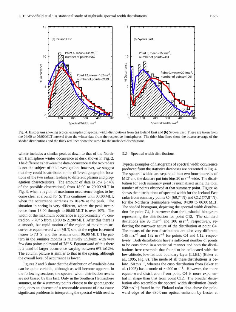
Fig. 4. Histograms showing typical examples of spectral width distributions from(a) Iceland East and(b) Syowa East. These are taken fromthe 04:00 to 06:00 MLT interval from the winter data from the respective hemispheres. The thick blue lines show the boxcar average of theshaded distributions and the thick red lines show the same for the unshaded distributions.

winter includes a similar peak at dawn to that of the North-ern Hemisphere winter occurrence at dusk shown in Fig. 2.The differences between the data occurrence at the two radarsis not the subject of this investigation; however, we suggestthat they could be attributed to the different geographic loca-tions of the two radars, leading to different plasma and prop-agation characteristics. The amount of data is low (< 4%of the possible observations) from 18:00 to 20:00 MLT inFig. 3, when a region of maximum occurrence begins to be-come clear at around 75◦ S. This continues until 03:00 MLT,when the occurrence increases to 10+% at the peak. Thesituation in spring is very different, where the peak occur-rence from 18:00 through to 06:00 MLT is over 10%. Thewidth of the maximum occurrence is approximately 7◦, cen-tred on∼ 76◦ S from 18:00 to 21:00 MLT. After this there isa smooth, but rapid motion of the region of maximum oc-currence equatorward with MLT, so that the region is centrednearer to 73◦ S, and this remains until 06:00 MLT. The pat-tern in the summer months is relatively uniform, with veryfew data points poleward of 78◦ S. Equatorward of this thereis a band of larger occurrence varying between 6% to12%.The autumn picture is similar to that in the spring, althoughthe overall level of occurrence is lower.

Figures 2 and 3 show that the distribution of available datacan be quite variable, although as will become apparent inthe following sections, the spectral width distribution resultsare not biased by this fact. Only in the Southern Hemispheresummer, at the 4 summary points closest to the geomagneticpole, does an absence of a reasonable amount of data causesignificant problems in interpreting the spectral width results.

3.2 Spectral width distributions

Typical examples of histograms of spectral width occurrenceproduced from the statistics databases are presented in Fig. 4.The spectral widths are separated into two-hour intervals ofMLT and the data are put into bins 20 m s−1 wide. The distri-bution for each summary point is normalised using the totalnumber of points observed at that summary point. Figure 4ashows the distributions of spectral width for the Iceland Eastradar from summary points C4 (69.7◦ N) and C12 (77.8◦ N),for the Northern Hemisphere winter, 04:00 to 06:00 MLT.The shaded histogram, depicting the spectral width distribu-tion for point C4, is narrower than the unshaded histogramrepresenting the distribution for point C12. The standarddeviations are 95 m s−1 and 106 m s−1, respectively, re-flecting the narrower nature of the distribution at point C4.The means of the two distributions are also very different,145 m s−1 and 182 m s−1 for points C4 and C12, respec-tively. Both distributions have a sufficient number of pointsto be considered in a statistical manner and both the distri-butions here resemble that found to be collocated with thelow-altitude, low-latitude boundary layer (LLBL) (Baker etal., 1995, Fig. 8). The mode of all these distributions is be-low 150 m s−1, whereas the cusp distribution from Baker etal. (1995) has a mode of∼ 200 m s−1. However, the moreequatorward distribution from point C4 is more exponen-tial in shape than that from point C12. The broader distri-bution also resembles the spectral width distribution (mode230 m s−1) found in the Finland radar data above the pole-ward edge of the 630.0 nm optical emission by Lester et

1926 E. E. Woodfield et al.: A statistical study of nightside spectral width distributions

12 M L T

06 M L T

00 M L T

18 M L T

18-20 MLT

20-22 MLT

22-24 MLT 00-02 MLT

02-04 MLT

04-06 MLT

% Occurrence

Sta

tist

ics

Poi

nt

Spectral Width (ms-1)

0 100 200 300 400

0 100 200 300 400 500

0 100 200 300 400 500 0 100 200 300 400 500

0 100 200 300 400 500

C0

C5

C10

C15

100 200 300 400 500

Spectral Width (ms-1) Spectral Width (ms-1)

Spectral Width (ms-1)

Sta

tist

ics

Poi

nt

15.0+ 13.5 12.0 10.5 9.0 7.5 6.0 4.5 3.0 1.5

0

mean width

C0

C5

C10

C15

C0

C5

C10

C15

C0

C5

C10C0

C5

C10

C15

C0

C5

C10

C15

70oN

80oN

70oN

80oN

70oN

80oN

70oN

80oN

70oN

80oN

Figure 5

70oN

80oN

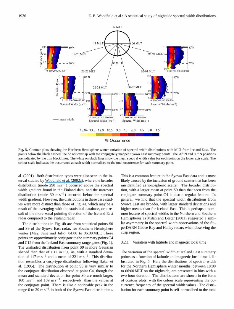
Fig. 5. Contour plots showing the Northern Hemisphere winter variation of spectral width distributions with MLT from Iceland East. Thepoints below the black dashed line do not overlap with the conjugately mapped Syowa East summary points. The 70◦ N and 80◦ N positionsare indicated by the thin black lines. The white on black lines show the mean spectral width value for each point on the lower axis scale. Thecolour scale indicates the occurrence at each width normalised to the total occurrence for each summary point.

al. (2001). Both distribution types were also seen in the in-terval studied by Woodfield et al. (2002a), where the broaderdistribution (mode 290 m s−1) occurred above the spectralwidth gradient found in the Finland data, and the narrowerdistribution (mode 30 m s−1) occurred below the spectralwidth gradient. However, the distributions in these case stud-ies were more distinct than those of Fig. 4a, which may be aresult of the averaging with the statistical database, or a re-sult of the more zonal pointing direction of the Iceland Eastradar compared to the Finland radar.

The distributions in Fig. 4b are from statistical points S0and S9 of the Syowa East radar, for Southern Hemispherewinter (May, June and July), 04:00 to 06:00 MLT. Thesepoints are approximately conjugate to the summary points C4and C12 from the Iceland East summary range gates (Fig. 1).The unshaded distribution from point S9 is more Gaussianshaped than that of C12 in Fig. 4a, with a standard devia-tion of 117 m s−1 and a mean of 221 m s−1. This distribu-tion resembles a cusp-type distribution following Baker etal. (1995). The distribution at point S0 is very similar tothe conjugate distribution observed at point C4, though themean and standard deviation for point S0 are much larger,160 m s−1 and 109 m s−1, respectively, than the values atthe conjugate point. There is also a noticeable peak in therange 0 to 20 m s−1 in both of the Syowa East distributions.

This is a common feature in the Syowa East data and is mostlikely caused by the inclusion of ground scatter that has beenmisidentified as ionospheric scatter. The broader distribu-tion, with a larger mean at point S0 than that seen from theconjugate summary point C4 is also a regular feature. Ingeneral, we find that the spectral width distributions fromSyowa East are broader, with larger standard deviations andhigher means than for Iceland East. This is perhaps a com-mon feature of spectral widths in the Northern and SouthernHemispheres as Milan and Lester (2001) suggested a simi-lar asymmetry in the spectral width observations of the Su-perDARN Goose Bay and Halley radars when observing thecusp region.

3.2.1 Variation with latitude and magnetic local time

The variation of the spectral width at Iceland East summarypoints as a function of latitude and magnetic local time is il-lustrated in Fig. 5. Here the distributions of spectral widthfor the Northern Hemisphere winter months, between 18:00to 06:00 MLT on the nightside, are presented in bins with atwo hour duration. The distributions are shown in the formof contour plots, with the colour scale representing the oc-currence frequency of the spectral width values. The distri-bution for each summary point is self-normalised to the total

E. E. Woodfield et al.: A statistical study of nightside spectral width distributions 1927

12 M L T

06 M L T

00 M L T

18 M L T

18-20 MLT

20-22 MLT

22-00 MLT 00-02 MLT

02-04 MLT

04-06 MLT

% Occurrence

Sta

tist

ics

Poi

nt

0 100 200 300 400 500

0 100 200 300 400 500

0 100 200 300 400 500 0 100 200 300 400 500

0 100 200 300 400 500

S0

S5

S10

S15

100 200 300 400 500

Spectral Width (ms-1) Spectral Width (ms-1)

Spectral Width (ms-1)

Sta

tist

ics

Poi

nt

15.0+ 13.5 12.0 10.5 9.0 7.5 6.0 4.5 3.0 1.5

0

mean width

70oS

80oS

70oS

80oS

70oS

80oS

70oSS

80oS70oS

80oS

70oS

80oS

S0

S5

S10

S15

S0

S5

S10

S15

S0

S5

S10

S15

S0

S5

S10

S15

S0

S5

S10

S15

Figure 6

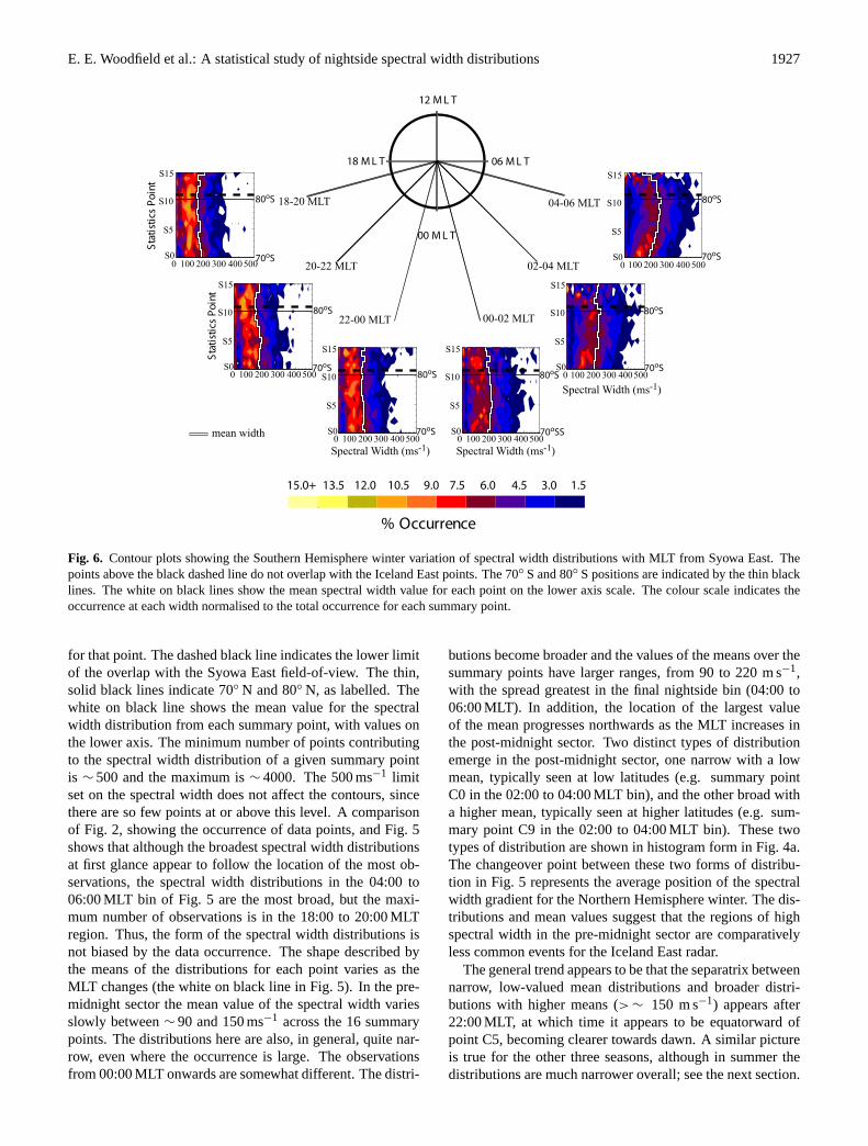
Fig. 6. Contour plots showing the Southern Hemisphere winter variation of spectral width distributions with MLT from Syowa East. Thepoints above the black dashed line do not overlap with the Iceland East points. The 70◦ S and 80◦ S positions are indicated by the thin blacklines. The white on black lines show the mean spectral width value for each point on the lower axis scale. The colour scale indicates theoccurrence at each width normalised to the total occurrence for each summary point.

for that point. The dashed black line indicates the lower limitof the overlap with the Syowa East field-of-view. The thin,solid black lines indicate 70◦ N and 80◦ N, as labelled. Thewhite on black line shows the mean value for the spectralwidth distribution from each summary point, with values onthe lower axis. The minimum number of points contributingto the spectral width distribution of a given summary pointis ∼ 500 and the maximum is∼ 4000. The 500 ms−1 limitset on the spectral width does not affect the contours, sincethere are so few points at or above this level. A comparisonof Fig. 2, showing the occurrence of data points, and Fig. 5shows that although the broadest spectral width distributionsat first glance appear to follow the location of the most ob-servations, the spectral width distributions in the 04:00 to06:00 MLT bin of Fig. 5 are the most broad, but the maxi-mum number of observations is in the 18:00 to 20:00 MLTregion. Thus, the form of the spectral width distributions isnot biased by the data occurrence. The shape described bythe means of the distributions for each point varies as theMLT changes (the white on black line in Fig. 5). In the pre-midnight sector the mean value of the spectral width variesslowly between∼ 90 and 150 ms−1 across the 16 summarypoints. The distributions here are also, in general, quite nar-row, even where the occurrence is large. The observationsfrom 00:00 MLT onwards are somewhat different. The distri-

butions become broader and the values of the means over thesummary points have larger ranges, from 90 to 220 m s−1,with the spread greatest in the final nightside bin (04:00 to06:00 MLT). In addition, the location of the largest valueof the mean progresses northwards as the MLT increases inthe post-midnight sector. Two distinct types of distributionemerge in the post-midnight sector, one narrow with a lowmean, typically seen at low latitudes (e.g. summary pointC0 in the 02:00 to 04:00 MLT bin), and the other broad witha higher mean, typically seen at higher latitudes (e.g. sum-mary point C9 in the 02:00 to 04:00 MLT bin). These twotypes of distribution are shown in histogram form in Fig. 4a.The changeover point between these two forms of distribu-tion in Fig. 5 represents the average position of the spectralwidth gradient for the Northern Hemisphere winter. The dis-tributions and mean values suggest that the regions of highspectral width in the pre-midnight sector are comparativelyless common events for the Iceland East radar.

The general trend appears to be that the separatrix betweennarrow, low-valued mean distributions and broader distri-butions with higher means (> ∼ 150 m s−1) appears after22:00 MLT, at which time it appears to be equatorward ofpoint C5, becoming clearer towards dawn. A similar pictureis true for the other three seasons, although in summer thedistributions are much narrower overall; see the next section.

1928 E. E. Woodfield et al.: A statistical study of nightside spectral width distributions

0 100 200 300 4000

100

200

300

400

Syowa East mean spectral width, ms-1

Icel

and

Eas

t m

ean

sp

ectr

al w

idth

, ms-1

Figure 7

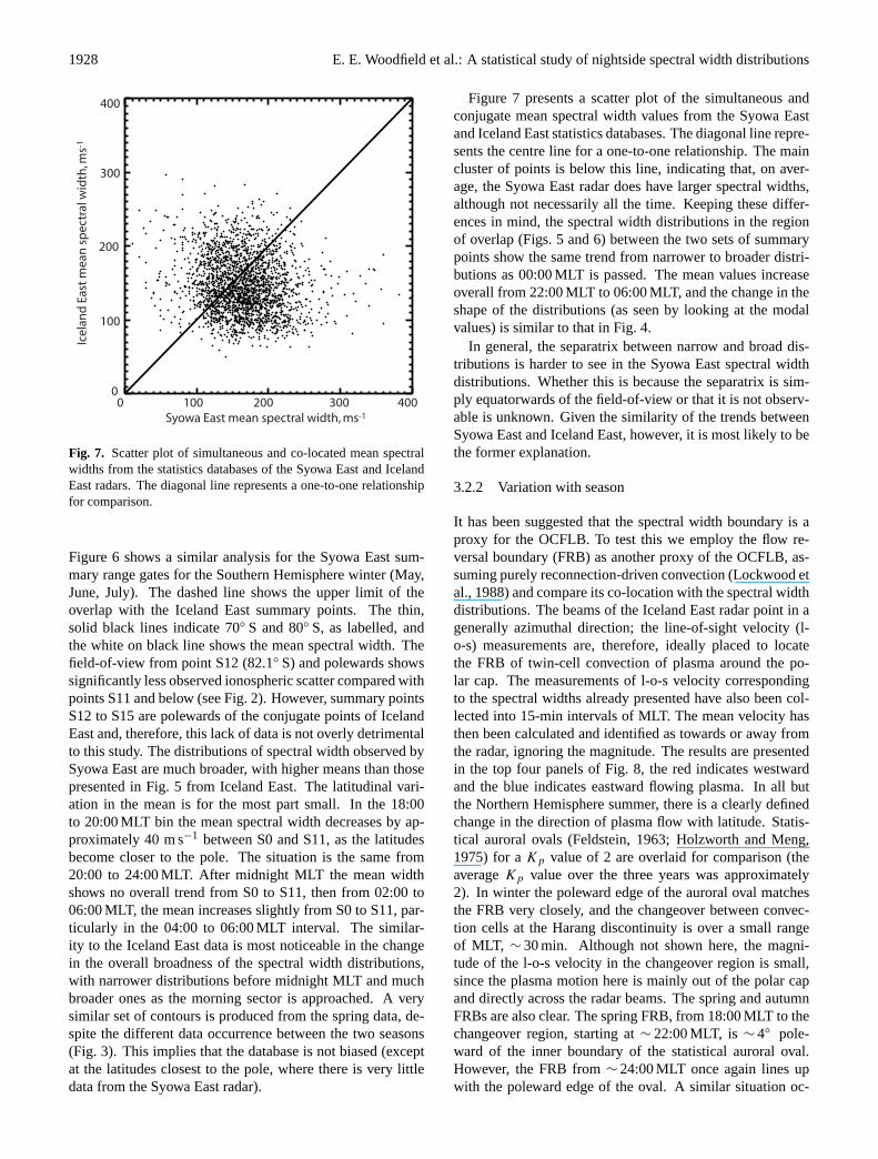
Fig. 7. Scatter plot of simultaneous and co-located mean spectralwidths from the statistics databases of the Syowa East and IcelandEast radars. The diagonal line represents a one-to-one relationshipfor comparison.

Figure 6 shows a similar analysis for the Syowa East sum-mary range gates for the Southern Hemisphere winter (May,June, July). The dashed line shows the upper limit of theoverlap with the Iceland East summary points. The thin,solid black lines indicate 70◦ S and 80◦ S, as labelled, andthe white on black line shows the mean spectral width. Thefield-of-view from point S12 (82.1◦ S) and polewards showssignificantly less observed ionospheric scatter compared withpoints S11 and below (see Fig. 2). However, summary pointsS12 to S15 are polewards of the conjugate points of IcelandEast and, therefore, this lack of data is not overly detrimentalto this study. The distributions of spectral width observed bySyowa East are much broader, with higher means than thosepresented in Fig. 5 from Iceland East. The latitudinal vari-ation in the mean is for the most part small. In the 18:00to 20:00 MLT bin the mean spectral width decreases by ap-proximately 40 m s−1 between S0 and S11, as the latitudesbecome closer to the pole. The situation is the same from20:00 to 24:00 MLT. After midnight MLT the mean widthshows no overall trend from S0 to S11, then from 02:00 to06:00 MLT, the mean increases slightly from S0 to S11, par-ticularly in the 04:00 to 06:00 MLT interval. The similar-ity to the Iceland East data is most noticeable in the changein the overall broadness of the spectral width distributions,with narrower distributions before midnight MLT and muchbroader ones as the morning sector is approached. A verysimilar set of contours is produced from the spring data, de-spite the different data occurrence between the two seasons(Fig. 3). This implies that the database is not biased (exceptat the latitudes closest to the pole, where there is very littledata from the Syowa East radar).

Figure 7 presents a scatter plot of the simultaneous andconjugate mean spectral width values from the Syowa Eastand Iceland East statistics databases. The diagonal line repre-sents the centre line for a one-to-one relationship. The maincluster of points is below this line, indicating that, on aver-age, the Syowa East radar does have larger spectral widths,although not necessarily all the time. Keeping these differ-ences in mind, the spectral width distributions in the regionof overlap (Figs. 5 and 6) between the two sets of summarypoints show the same trend from narrower to broader distri-butions as 00:00 MLT is passed. The mean values increaseoverall from 22:00 MLT to 06:00 MLT, and the change in theshape of the distributions (as seen by looking at the modalvalues) is similar to that in Fig. 4.

In general, the separatrix between narrow and broad dis-tributions is harder to see in the Syowa East spectral widthdistributions. Whether this is because the separatrix is sim-ply equatorwards of the field-of-view or that it is not observ-able is unknown. Given the similarity of the trends betweenSyowa East and Iceland East, however, it is most likely to bethe former explanation.

3.2.2 Variation with season

It has been suggested that the spectral width boundary is aproxy for the OCFLB. To test this we employ the flow re-versal boundary (FRB) as another proxy of the OCFLB, as-suming purely reconnection-driven convection (Lockwood etal., 1988) and compare its co-location with the spectral widthdistributions. The beams of the Iceland East radar point in agenerally azimuthal direction; the line-of-sight velocity (l-o-s) measurements are, therefore, ideally placed to locatethe FRB of twin-cell convection of plasma around the po-lar cap. The measurements of l-o-s velocity correspondingto the spectral widths already presented have also been col-lected into 15-min intervals of MLT. The mean velocity hasthen been calculated and identified as towards or away fromthe radar, ignoring the magnitude. The results are presentedin the top four panels of Fig. 8, the red indicates westwardand the blue indicates eastward flowing plasma. In all butthe Northern Hemisphere summer, there is a clearly definedchange in the direction of plasma flow with latitude. Statis-tical auroral ovals (Feldstein, 1963; Holzworth and Meng,1975) for aKp value of 2 are overlaid for comparison (theaverageKp value over the three years was approximately2). In winter the poleward edge of the auroral oval matchesthe FRB very closely, and the changeover between convec-tion cells at the Harang discontinuity is over a small rangeof MLT, ∼ 30 min. Although not shown here, the magni-tude of the l-o-s velocity in the changeover region is small,since the plasma motion here is mainly out of the polar capand directly across the radar beams. The spring and autumnFRBs are also clear. The spring FRB, from 18:00 MLT to thechangeover region, starting at∼ 22:00 MLT, is ∼ 4◦ pole-ward of the inner boundary of the statistical auroral oval.However, the FRB from∼ 24:00 MLT once again lines upwith the poleward edge of the oval. A similar situation oc-

E. E. Woodfield et al.: A statistical study of nightside spectral width distributions 1929

0

20

40

60

80

100

120

140

160

180+

Mea

n W

idth

, ms-1

Winter Spring

Summer Autumn

80o Lat 70o Lat

24 MLT 02 MLT22 MLT

20 MLT

24 MLT 02 MLT22 MLT

24 MLT 02 MLT22 MLT 24 MLT 02 MLT22 MLT

20 MLT

80o Lat 70o Lat

80o Lat 70o Lat 80o Lat 70o Lat

Winter Spring

Summer Autumn

80o Lat 70o Lat

24 MLT 02 MLT22 MLT

20 MLT

24 MLT 02 MLT22 MLT

24 MLT 02 MLT22 MLT 24 MLT 02 MLT22 MLT

20 MLT

80o Lat 70o Lat

80o Lat 70o Lat 80o Lat 70o Lat

Westwards

Eastwards

Velocity direction

Figure 8

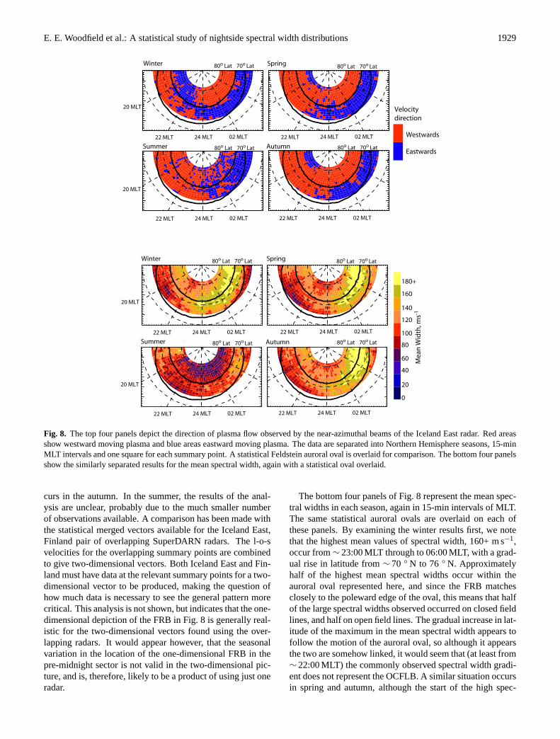
Fig. 8. The top four panels depict the direction of plasma flow observed by the near-azimuthal beams of the Iceland East radar. Red areasshow westward moving plasma and blue areas eastward moving plasma. The data are separated into Northern Hemisphere seasons, 15-minMLT intervals and one square for each summary point. A statistical Feldstein auroral oval is overlaid for comparison. The bottom four panelsshow the similarly separated results for the mean spectral width, again with a statistical oval overlaid.

curs in the autumn. In the summer, the results of the anal-ysis are unclear, probably due to the much smaller numberof observations available. A comparison has been made withthe statistical merged vectors available for the Iceland East,Finland pair of overlapping SuperDARN radars. The l-o-svelocities for the overlapping summary points are combinedto give two-dimensional vectors. Both Iceland East and Fin-land must have data at the relevant summary points for a two-dimensional vector to be produced, making the question ofhow much data is necessary to see the general pattern morecritical. This analysis is not shown, but indicates that the one-dimensional depiction of the FRB in Fig. 8 is generally real-istic for the two-dimensional vectors found using the over-lapping radars. It would appear however, that the seasonalvariation in the location of the one-dimensional FRB in thepre-midnight sector is not valid in the two-dimensional pic-ture, and is, therefore, likely to be a product of using just oneradar.

The bottom four panels of Fig. 8 represent the mean spec-tral widths in each season, again in 15-min intervals of MLT.The same statistical auroral ovals are overlaid on each ofthese panels. By examining the winter results first, we notethat the highest mean values of spectral width, 160+ m s−1,occur from∼ 23:00 MLT through to 06:00 MLT, with a grad-ual rise in latitude from∼ 70 ◦ N to 76 ◦ N. Approximatelyhalf of the highest mean spectral widths occur within theauroral oval represented here, and since the FRB matchesclosely to the poleward edge of the oval, this means that halfof the large spectral widths observed occurred on closed fieldlines, and half on open field lines. The gradual increase in lat-itude of the maximum in the mean spectral width appears tofollow the motion of the auroral oval, so although it appearsthe two are somehow linked, it would seem that (at least from∼ 22:00 MLT) the commonly observed spectral width gradi-ent does not represent the OCFLB. A similar situation occursin spring and autumn, although the start of the high spec-

1930 E. E. Woodfield et al.: A statistical study of nightside spectral width distributions

Winter Spring

Summer Autumn

-80o Lat -70o Lat

24 MLT 02 MLT22 MLT

20 MLT

24 MLT 02 MLT22 MLT

24 MLT 02 MLT22 MLT 24 MLT 02 MLT22 MLT

20 MLT

-80o Lat -70o Lat

-80o Lat -70o Lat -80o Lat -70o Lat

Westwards

Eastwards

Velocity direction

0

20

40

60

80

100

120

140

160

180+

Mea

n W

idth

, ms-1

Winter Spring

Summer Autumn

-80o Lat -70o Lat

24 MLT 02 MLT22 MLT

20 MLT

24 MLT 02 MLT22 MLT

24 MLT 02 MLT22 MLT 24 MLT 02 MLT22 MLT

20 MLT

-80o Lat -70o Lat

-80o Lat -70o Lat -80o Lat -70o Lat

Figure 9

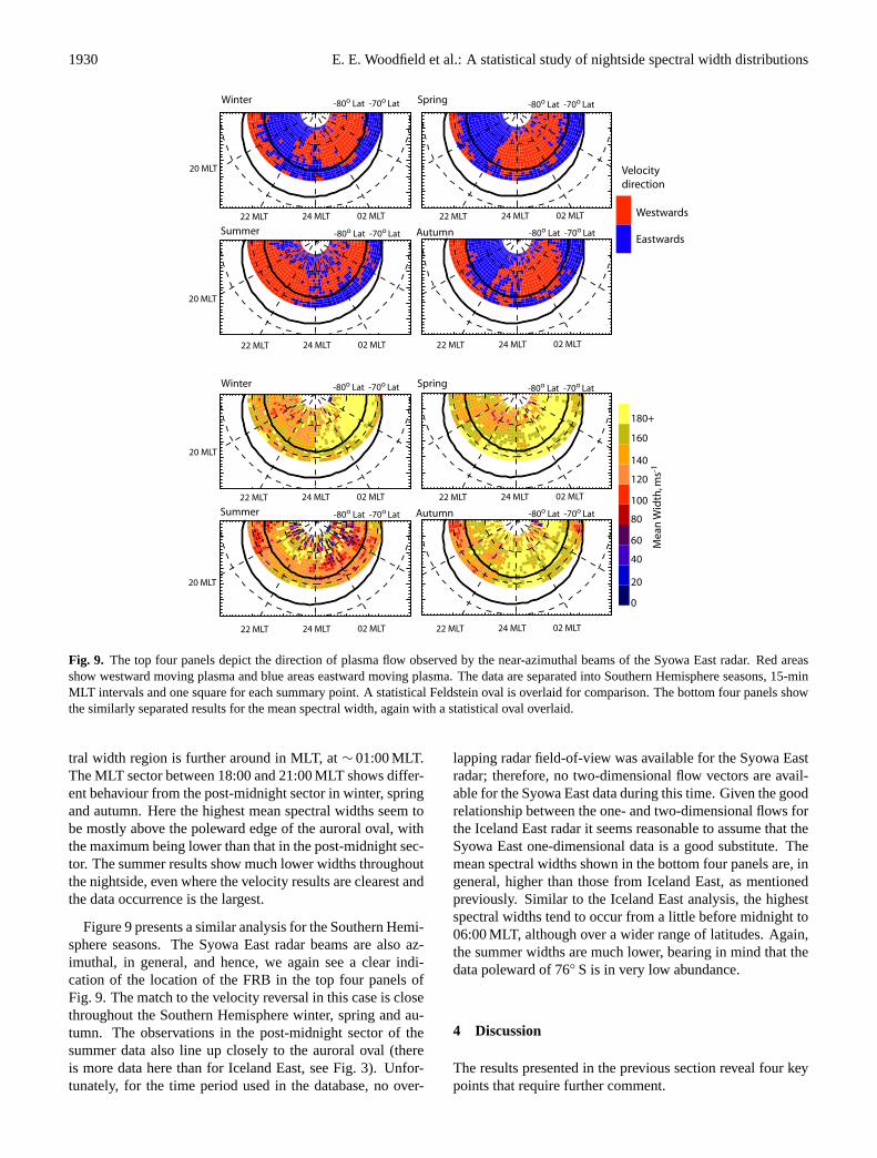
Fig. 9. The top four panels depict the direction of plasma flow observed by the near-azimuthal beams of the Syowa East radar. Red areasshow westward moving plasma and blue areas eastward moving plasma. The data are separated into Southern Hemisphere seasons, 15-minMLT intervals and one square for each summary point. A statistical Feldstein oval is overlaid for comparison. The bottom four panels showthe similarly separated results for the mean spectral width, again with a statistical oval overlaid.

tral width region is further around in MLT, at∼ 01:00 MLT.The MLT sector between 18:00 and 21:00 MLT shows differ-ent behaviour from the post-midnight sector in winter, springand autumn. Here the highest mean spectral widths seem tobe mostly above the poleward edge of the auroral oval, withthe maximum being lower than that in the post-midnight sec-tor. The summer results show much lower widths throughoutthe nightside, even where the velocity results are clearest andthe data occurrence is the largest.

Figure 9 presents a similar analysis for the Southern Hemi-sphere seasons. The Syowa East radar beams are also az-imuthal, in general, and hence, we again see a clear indi-cation of the location of the FRB in the top four panels ofFig. 9. The match to the velocity reversal in this case is closethroughout the Southern Hemisphere winter, spring and au-tumn. The observations in the post-midnight sector of thesummer data also line up closely to the auroral oval (thereis more data here than for Iceland East, see Fig. 3). Unfor-tunately, for the time period used in the database, no over-

lapping radar field-of-view was available for the Syowa Eastradar; therefore, no two-dimensional flow vectors are avail-able for the Syowa East data during this time. Given the goodrelationship between the one- and two-dimensional flows forthe Iceland East radar it seems reasonable to assume that theSyowa East one-dimensional data is a good substitute. Themean spectral widths shown in the bottom four panels are, ingeneral, higher than those from Iceland East, as mentionedpreviously. Similar to the Iceland East analysis, the highestspectral widths tend to occur from a little before midnight to06:00 MLT, although over a wider range of latitudes. Again,the summer widths are much lower, bearing in mind that thedata poleward of 76◦ S is in very low abundance.

4 Discussion

The results presented in the previous section reveal four keypoints that require further comment.

E. E. Woodfield et al.: A statistical study of nightside spectral width distributions 1931

1. The spectral width gradient observed previously in casestudies (e.g. Woodfield et al., 2002a) is seen to persistin statistical studies of the spectral width.

2. There is a variation in the latitude of the statistical gradi-ent in the spectral width as MLT changes on the night-side. The highest widths seem to occur on both openand closed field lines, using the FRB obtained from theazimuthal velocity measurements as a guide.

3. There is a seasonal effect seen in the data, where thebroader spectral width distributions do not appear to bepresent in the summer months.

4. The Southern Hemisphere spectral width values are typ-ically larger than those from the Northern Hemisphere.

The change from low (< 200 ms−1) to high (> 200 ms−1)spectral width is a feature that occurs both on a case bycase and a statistical basis in the nightside ionosphere. TheFITACF software produces two distinct forms of spectralwidth: high and variable, and low, which can be identi-fied using the distribution of spectral width over time. Thelow spectral width regions are characterised by narrow dis-tributions dominated by a large peak close to 0 ms−1. Thehigh and variable spectral width regions are characterisedby a broader distribution, with a less prominent peak dis-tinctly removed from 0 ms−1, and a larger mean (well above100 ms−1). This is demonstrated in Fig. 4 of Woodfield etal. (2002a), which shows how the spectral width distribu-tion over just 5 hours shows a trend from one to the other ofthese types of distribution described above. There is nearlyalways a distinct latitudinal gradient in the value of spectralwidth between the two regions in individual cases, and thisoften moves with time, thus, averaging over time (as in Fig. 4of Woodfield et al., 2002a), the sharp gradient becomes asmoother change between the two types of distribution. Thiseffect is prominent in the statistical distributions presented inthis paper, which are greatly averaged; hence, the distinctionbetween the idealised distributions for low and high spectralwidth becomes less obvious. Nevertheless, the trend fromone type of distribution to the other is still apparent. Thesharp gradient in the width seen in individual cases is not, ingeneral, collocated with a sharp change in either backscatterpower, l-o-s velocity or elevation angle. The broader spec-tral width distributions resemble those observed in the cusp,whereas the narrower distributions are more like those ob-served in the low-latitude boundary layer (Baker et al., 1995).This implies that a similar mechanism that causes high andvariable spectral width in the cusp may also be manifest onthe nightside.

Intense electric and magnetic field fluctuations of the or-der of 1 Hz have been observed over the auroral zone bylow-altitude, polar-orbiting satellites (Gurnett et al., 1984;Gurnett, 1991; Dudeney et al., 1998). Two models for thegeneration of these 0.1 to 5 Hz fluctuations measured by low-altitude satellites have been put forward. The first model as-sumes that the fluctuations are observed due to the motion

of the satellite through a system of static field-aligned cur-rent structures (FACs) embedded in the ionosphere (Smiddyet al., 1980). This is a space/time ambiguity problem inthe spacecraft data, not a wave in the ionosphere, and thescale size of these features would be small, approximately200 m, which is well below the size of a radar range cell.These FACs are capable of producing vortex patterns in theplasma flow around them (Lanzerotti et al., 1990 and refer-ences therein). Previous work with HF coherent radar spec-tra has attributed double-peaked spectra to vortices less thanthe scale size of the radar range cells (∼ 45 km), such asthese static FACs could produce (Schiffler et al., 1997; Hu-ber and Sofko, 2000). It is possible that double-peaked spec-tra may be observed with overestimated spectral widths, al-though simulations by Andre et al. (2000b) suggest that therewould need to be several vortices smaller than the size of theradar range cell in order to cause high spectral widths.

The second model suggests that disturbances in the distantmagnetosphere are transmitted to the ionosphere as Alfvenwaves, and it is these waves that are the Pc1 and Pc2 fre-quency range fluctuations observed by the low-altitude satel-lites (e.g. Goertz and Boswell, 1979; Lysak and Dum, 1983).This would produce the kind of temporal electric field varia-tion required for the proposed cusp mechanism of Andre andco-workers (1999; 2000a; 2000b).

The variation of the spectral width distributions observedwith MLT indicates that the root cause of the high spectralwidth does not map to a constant magnetic latitude as MLTvaries. This encourages the idea of using the spectral widthboundary as an ionospheric proxy, since both the OCFLBand CPS/BPS boundaries move in latitude with MLT. TheFRB identified using the azimuthal pointing directions of thetwo radars in Figures 8 and 9 shows that approximately halfthe highest spectral widths are likely to be on closed fieldlines in the MLT sector from 23:00 to 06:00 MLT. This im-plies that, in this sector at least, the spectral width gradientis unlikely to represent the OCFLB, since this would requireall the highest values to be above the poleward edge of theauroral oval and the FRB. This agrees with case study resultsin this region of MLT (Woodfield et al., 2002a, b). The spec-tral widths prior to 23:00 MLT are lower in magnitude, andthe distribution is such that the spectral width boundary ob-served between 18:00 and 23:00 MLT could reasonably rep-resent the OCFLB, agreeing with Lester et al. (2001). Thisasymmetry of the spectral width magnitudes in the pre- andpost-midnight sectors of the MLT indicates that the sourceregion for generating high and variable spectral widths onthe nightside is more prominent in the post-midnight sector.

A seasonal variation is observed in the magnitude of themean spectral widths; in an attempt to explain this we tryto identify here what seasonal influences might control thisvariation. One obvious seasonal factor to consider is the levelof solar illumination. During the summer in the respectivehemispheres, all the summary points are fully illuminated bythe Sun at 300 km altitude on the nightside. The plasma den-sity and, therefore, the plasma frequency is different in thesummer. It is unlikely that changes in the propagation of the

1932 E. E. Woodfield et al.: A statistical study of nightside spectral width distributions

HF radar signals in summer are the cause of the decrease inthe mean spectral widths. The decrease in the number of ob-servations available during the summer is due to this reason,but the propagation itself would be unlikely to decrease themean width unless the spectral width is height dependent.Woodfield et al. (2002a) examined the elevation angle datafor the spectral width gradient case that they were investigat-ing, and found that there was no change in elevation angleassociated with the sudden change in spectral width values.This implies that the altitude of the observations is not a fac-tor in the spectral width observations. Over the three yearsof data studied here there are enough data points availableto assume that we see an accurate description of the summerspectral widths. It seems most likely that there is a seasonalvariation in either the source of the high spectral widths, orhow the different plasma conditions affect the propagationfrom the source. For example, if the high spectral widthsare a result of a time-varying electric field (Andre et al.,1999; 2000a; 2000b), which originates from a down-tail dis-turbance in the magnetosphere and travels by Alfven wavesalong magnetic field lines to the F-region ionosphere, thenchanges in the plasma properties along the path will changefrom season to season. If vortices are the mechanism, thenthe seasonal variation in the strength of FACs (e.g. Shue etal., 2001) is important. It is also possible, however, that thesource region for this mechanism does not exist, or does notmap to the same place in the summer months.

On a statistical basis the nightside spectral widths ob-served by the Syowa East radar are larger and more var-ied than those observed by its conjugate counterpart IcelandEast. A similar situation exists on the dayside (Hosokawa etal., 2002). There are several possible explanations for this:(a) the difference in ionospheric conditions in the two hemi-spheres, both in terms of the propagation of the radar beamsand the local conditions affecting any generating mecha-nisms, (b) an inter-hemispheric/seasonal difference in waveactivity, (c) a variation in field-aligned current activity, (d)the difference in the dip-angle of the magnetic field linesfor the two sets of summary range gates, or (e) instrumentalnoise levels. The fields-of-view of the two radars, althoughin conjugate geomagnetic positions, are not geographic mir-ror images of each other. The geographic latitude ranges forSyowa East and Iceland East are 63◦ S to 72◦ S and 73◦ N to84◦ N, respectively. As such, the level of solar illuminationthe summary points from each radar receive will be differ-ent in their respective seasons. This will likely cause a smalldifference in the propagation of the respective radar beamsto the summary point locations, leading to a small differencein the height of the observations. However, even in the re-spective summers of each hemisphere, the Syowa East spec-tral width distributions are still broader, despite there beingfull (all be it at a slightly different zenith angle) illumina-tion. Also, as mentioned previously, the spectral width ap-pears to be independent of height. Points (b) and (c) amountto the same problem, where the mechanism for creating thehigh spectral width may itself vary between the hemispheresand also with season. Point d) relates to the difference in

magnetic field line dip-angle, which is∼ 10◦, where the Ice-land East summary points are subject to more vertical fieldlines. The dip-angle is important since this determines whereand at what height the radar beam will be orthogonal to themagnetic field lines and hence, able to be backscattered byfield-aligned irregularities. However, 10◦ is a relatively smalldifference, outweighed by the typical error in the range es-timation of a radar range cell at 112 hops, which is 60 km(Yeoman et al., 2001). Instrumental effects, point (e), are animportant consideration. Although the processing softwareused by both radars is identical throughout the data set, thenoise level in the readings could affect the overall output. Apower level of 3 dB and spectral width limit of 500 ms−1 wasset in the analysis of the data we conducted, to eliminate ap-proximately 95% of the data affected by low signal-to-noiseratios. We also performed a check on the comparative noiselevels of the two radars and found that the amount of noiseobserved by the Syowa East radar was significantly lowerthan at Iceland East, likely due to the lack of local radio in-terference on Antarctica. If extra noise in the signals werethe cause of the broader widths (by the introduction of pow-erful multiple peaks into the spectra), then we would expectto see higher values in the Iceland East data and not, as wehave found, in the Syowa East data. It would, therefore, ap-pear that the broader spectral widths in the Syowa East dataare caused by a geophysical effect, but not one of radar prop-agation or processing of instrumental origin.

5 Summary and conclusions

A statistical study of SuperDARN radar spectral width datafrom the nightside in both hemispheres has been carried outusing data from the Syowa East and Iceland East radars.These two radars often observe similar features in their spec-tral width data. This implies that the generating mecha-nism of high spectral width values is capable of travellinginto both the Southern and Northern Hemispheres from somemagnetospheric source region either on closed or open mag-netic field lines. There is a definite latitudinal dependenceof the spectral width distribution seen in both hemispheresthat shows a statistical location of the spectral width gradi-ent. The magnetic local time affects the spectral width dis-tributions, notably in the location of the spectral width gradi-ent, which reaches minimum latitude around magnetic mid-night. Season also plays a part in the magnitude of the spec-tral width; in summer the spectral widths are decreased. Themost marked difference between the Syowa East and IcelandEast data is that the Syowa East spectral width distributionsare, in general, broader and peaked at values greater thanthose of Iceland East. This is thought to be due to a geophys-ical rather than instrumental difference.

Acknowledgements.The authors wish to thank those involved inthe deployment and operation of the CUTLASS HF radars run bythe University of Leicester with joint funding from the UK ParticlePhysics and Astronomy Research Council (PPARC) grant numberPPA/R/R/1997/00256, the Swedish Institute for Space Physics, Up-

E. E. Woodfield et al.: A statistical study of nightside spectral width distributions 1933

psala and the Finnish Meteorological Institute, Helsinki. The au-thors also wish to thank the Ministry of Education, Culture, Sports,Science and Techonology for supporting the Syowa HF radar sys-tems and the 39th and 40th Japanese Antarctic Research Expedi-tions (JAREs) for carrying out the HF radar operations at Syowa.EEW is indebted to PPARC for a research studentship. This studyis funded by a part of ’Ground Research for Space Utilization’ pro-moted by NASDA and Japan Space Forum. KH is supported by theGrant in Aid for Scientific Research (A:11304029) from Japan So-ciety for the Promotion of Science (JSPS).

The Editor in Chief thanks C. Hanuise and I. McCrea for theirhelp in evaluating this paper.

References

Andre, R., Pinnock, M., and Rodger, A. S.: On the SuperDARNautocorrelation function observed in the ionospheric cusp, Geo-phys. Res. Lett., 26, 22, 3353–3356, 1999.

Andre, R., Pinnock, M., and Rodger, A. S.: Identification of thelow-altitude cusp by Super Dual Auroral Radar Network radars:A physical explanation for the empirically derived signature, J.Geophys. Res., 105, A12, 27 081–27 093, 2000a.

Andre, R., Pinnock, M., Villain, J.-P., and Hanuise, C.: On thefactors conditioning the Doppler spectral width determined fromSuperDARN HF radars, Int. J. Geomag. Aeronomy, 2, 1, 77–86,2000b.

Baker, K. B. and Wing, S.: A new magnetic coordinate system forconjugate studies at high latitudes, J. Geophys. Res., 94, 9139–9143, 1989.

Baker, K. B., Dudeney, J. R., Greenwald, R. A., Pinnock, M.,Newell, P. T., Rodger, A. S., Mattin, N., and Meng, C.-I.: HFradar signatures of the cusp and low-latitude boundary layer, J.Geophys. Res., 100, A5, 7671–7695, 1995.

Baker, K. B., Greenwald, R. A., Ruohoniemi, J. M., Dudeney, J.R., Pinnock, M., Newell, P. T., Greenspan, M. E., and Meng, C.-I.: Simultaneous HF-radar and DMSP observations of the cusp,Geophys. Res. Lett., 17, 11, 1869–1872, 1990.

Barton, C. E.: International Geomagnetic Reference Field: TheSeventh Generation, J. Geomag. Geoelectr., 49, 123–148, 1997.

Dudeney, J. R., Rodger, A. S., Freeman, M. P., Pickett, J., Scudder,J., Sofko, G., and Lester, M.: The nightside ionospheric responseto IMF By changes, Geophys. Res. Lett., 25, 14, 2601–2604,1998.

Dyrud, L. P., Engebretson, M. J., Posh, J. L., Hughes, W. J., Fukun-ishi, H., Arnoldy, R. L., Newell, P. T., and Horne, R. B.: Groundobservations and possible source regions of two types of PC1-2 micropulsation at very high latitudes, J. Geophys. Res., 102,27 011–27 027, 1997.

Feldstein, Y. I.: On morphology of auroral and magnetic distur-bances at high latitudes, Geomag. Aeron., 3 , 183–192, 1963.

Goertz, C. K. and Boswell, R. W.: Magnetosphere-Ionosphere Cou-pling, J. Geophys. Res., 84, 7239–7246, 1979.

Greenwald, R. A., Baker, K. B., Dudeney, J. R., Pinnock, M., Jones,T. B., Thomas, E. C., Villain, J.P., Cerisier, J.C., Senior, C.,Hanuise, C., Hunsucker, R. D., Sofko, G., Koehler, J., Nielsen,E., Pallinen, R., Walker, A. D. M., Sato, N., and Yamagishi, H.:DARN/SuperDARN: A global view of the dynamics of the high-latitude convection, Space Sci. Rev., 71, 761–796, 1995.

Gurnett, D. A.: Auroral Plasma Waves, in Auroral Physics, (Eds)Meng, C.-I., Rycroft, M. J., and Franck, L. A., Cambridge Univ.Press, New York, Ch. IV-6, pp. 241–254, 1991.

Gurnett, D. A., Huff, R. L., Menietti, J. D., Burch, J. L., Winning-ham, J. D., and Shawan, S. D.: Correlated Low-Frequency Elec-tric and Magnetic Noise Along the Auroral Field Lines, J. Geo-phys. Res., 89, 8971–8985, 1984.

Holzworth, R. H. and Meng, C.-I.: Mathematical representation ofthe auroral oval, Geophys. Res. Lett., 2, 377–380, 1975.

Hosokawa, K., Woodfield, E. E., Lester, M., Milan, S. E., Yuki-matu, A. S., and Sato, N.: Statistical Characteristics of SpectralWidth as Observed by the Conjugate SuperDARN Radars, Ann.Geophysicae, in press, 2002.

Huber, M. and Sofko, G. J.: Small-scale vortices in the high-latitudeF-region, J. Geophys. Res., 105, 20 885–20 897, 2000.

Lanzerotti, L. J., Wolfe, A., Trivedi, N., Maclennan, C. G., andMedford, L. V.: Magnetic Impulse Events at high Latitudes:Magnetopause and Boundary Layer Plasma Processes, J. Geo-phys. Res., 95, 97–107, 1990.

Lester, M., Milan, S. E., Besser, V., and Smith, R.: A Case Studyof HF Radar Spectra and 630.0 nm Auroral Emission in the PreMidnight Sector, Ann. Geophysicae, 19, 327–339, 2001.

Lewis, R. V., Freeman, M. P., Rodger, A. S., Reeves, G. D., andMilling, D. K.: The electric field response to the growth phaseand expansion phase onset of a small isolated substorm, Ann.Geophysicae, 15, 289–299, 1997.

Lockwood, M., Cowley, S. W. H., Todd, H., Willis, D. M., andClauer, C. R.: Ion flows and heating at a contracting polar-capboundary, Planet. Space Sci., 36, 11, 1229–1253, 1988.

Lysak, R. L. and Dum, C. T.: Dynamics of Magnetosphere-Ionosphere Coupling Including Turbulent Transport, J. Geophys.Res., 88, 365–380, 1983.

Matsuoka, A., Tsuruda, K., Hayakawa, H., Mukai, T., Nishida, A.,Okada, T., Kaya, N., and Fukunishi, H.: Electric field fluctua-tions and charged particle precipitation in the cusp, J. Geophys.Res., 98, 11 225–11 234, 1993.

Maynard, N. C., Aggson, T. L., Basinka, E. M., Burke, W. J.,Craven, P., Peterson, W. K., Suguira, M., and Weimer, D. R.:Magnetospheric boundary dynamics: DE-1 and DE-2 observa-tions near the magnetopause and cusp, J. Geophys. Res., 96,3505–3522, 1991.

Menk, F. W., Fraser, B. J., Hansen, H. J., Newell, P. T., Meng, C.-I., and Morris, R. J.: Identification of the magnetospheric cuspand cleft using PC1-2 ULF pulsations, J. Atmos. Terr. Phys., 54,1021–1042, 1992.

Milan, S. E. and Lester, M.: Interhemispheric differences in the HFradar signature of the cusp region A review through the studyof a case example, Adv. Polar Upper Atmos. Res., 15, 159–177,2001.

Milan, S. E., Lester, M., Cowley, S. W. H., Moen, J., Sandholt, P.E., and Owen, C. J.: Meridian-scanning photometer, coherent HFradar, and magnetometer observations of the cusp: a case study,Ann. Geophysicae, 17, 159–172, 1999.

Milan, S. E., Yeoman, T. K., Lester, M., Thomas, E. C., Jones, T.B.: Initial backscatter occurrence statistics from the CUTLASSHF radars, Ann. Geophysicae, 15, 703–718, 1997.

Moen, J., Carlson, H. C., Milan, S. E., Shumilov, N., Lybekk, B.,Sandholt, P. E., and Lester, M.: On the collocation between day-side auroral activity and coherent HF radar backscatter, Ann.Geophysicae 18, 1531–1549, 2001.

Pinnock, M., Rodger, A. S., Dudeney, J. R., Rich, F., and Baker,K. B.: High spatial and temporal resolution observations of theionospheric cusp, Ann. Geophysicae, 13, 919–925, 1995.

Rodger, A. S., Mende, S. B., Rosenberg, T. J., and Baker, K. B.: Si-multaneous optical and HF radar observations of the ionospheric

1934 E. E. Woodfield et al.: A statistical study of nightside spectral width distributions

cusp, Geophys. Res. Lett., 22, 2045–2048, 1995.Rodger, A. S.: Ground-based imaging of Magnetospheric bound-

aries, Adv. Space Res., 25, 7/8, 1461–1470, 2000.Schiffler, A., Sofko, G., Newell, P. T., and Greenwald, R.: Map-

ping the outer LLBL with SuperDARN double-peaked spectra,Geophy. Res. Lett., 24, 3149–3152, 1997.

Shue, J.-H., Newell, P. T., Liou, K., and Meng, C.-I.: The quan-titative relationship between auroral brightness and solar EUVPedersen conductance, J. Geophys. Res., 106, 5883–5894, 2001.

Smiddy, M., Burke, W. J., Kelley, M. C., Saflekos, N. A., Gussen-hoven, M. S., Hardy, D. A., and Rich, F. J.: Effects of High-Altitude Conductivity on Observed Convection Electric Fieldsand Birkeland Currents, J.Geophys. Res., 85, 6811–6818, 1980.

Villain, J.-P., Greenwald, R. A., Baker, K. B., and Ruohoniemi,

J. M.: HF radar observations of E-region plasma irregularitiesproduced by oblique electron streaming, J. Geophys. Res., 92,12 327–12 342, 1987.

Woodfield, E. E., Davies, J. A., Eglitis, P., and Lester, M.: Highand variable spectral width in the pre-dawn sector: A case studyinvolving CUTLASS, EISCAT, ESR and optical data, Ann. Geo-physicae, 20, 501–509, 2002a.

Woodfield, E. E., Davies, J. A., Lester, M., Yeoman, T. K., Eglitis,P., and Lockwood, M.: Nightside studies of coherent HF radarspectral width behaviour, Ann. Geophysicae, in press, 2002b.

Yeoman, T. K., Wright, D. M., Stocker, A. J., and Jones, T. B.: Anevaluation of range accuracy in the Super Dual Auroral RadarNetwork over-the-horizon HF radar systems, Radio Science, 36,4, 801–813, 2001.