Scatter correction in scintigraphy: the state of the art

European Journal of

Nuclear Medicine Review article

Scatter correction in scintigraphy: the state of the art

I. Buvat ''2, H. Benali 1, A. Todd-Pokropek 2, R. Di Paola 1

1 U66 INSERM, Institut Gustave-Roussy, 39 rue Camille Desmoulins, F-94805 Villejuif Cedex, France 2 Department of Medical Physics, University College London, Gower Street, London WC1E 6BT, UK

Abstract. In scintigraphy, the detection of scattered photons degrades both visual image analysis and quantitative accuracy. Many methods have been proposed and are still under investigation to cope with scattered photons. The main features of the problem of scattering in radionuclide imaging are presented first, to provide a sound foundation for a critical review of the existing scatter correction techniques. These are described using a classification relating to their aims and principles. Their theoretical potentials are analysed, as well as the difficulties of their practical implementation. Finally, the problems of their evaluation and comparison are dis- cussed.

Key words: Scatter correction - Single-photon emission tomography - Quantification - Evaluation

Eur J Nucl Med (1994) 21:675-694

Introduction

In scintigraphic imaging, the major problems affecting quantification are attenuation, camera non-uniformity, geometric collimator response and detection of scattered photons. Although the problem of Compton scattering at first received less attention than attenuation and camera non-uniformity, because of its less dramatic effects, it is now recognised as an important problem to address in single-photon emission tomography (SPET) when quantification is at issue. The publication of an increasing number of methods tackling this problem requires an up- to-date critical review of the different approaches which have been proposed. This paper presents the main features of Compton scattering in scintigraphy, the properties and the theoretical potential of the different methods, and the awkward problem of their evaluation and comparison.

Correspondence to: I. Buvat

Compton scattering in scintigraphic imaging

In scintigraphy, the history of a photon between its emission in the patient's body and its detection in the crystal of the camera results from a variable number of interactions with the different materials through which it pass- es. There are two possible types of interaction: Compton (or incoherent) scattering and Rayleigh (or coherent) scattering. During a Compton scatter, the incident photon transfers part of its energy to a recoil electron and deflects from its initial direction. Rayleigh scattering only induces a change of direction of the incident photon without any loss of energy. In both cases, scattered photons carry poor information regarding the emission location. The scattering cross-sections associated with these two phenomena indicate their relative importance in different materials. Compton scattering is the dominant interaction in water for the 40 keV-10 MeV energy range and the Compton scattering cross-sections increase as energy decreases. Above 100 keV, small deflections (i.e. small scattering angles) are much more probable than large deflections, and the higher the energy of the incident photon, the greater the forward deflection. Conse- quently, Compton scattering is the dominant interaction for tissues and becomes greater as the emission energy of the radioisotope decreases. As deflection is essentially forward, Compton scattered photons have a non-negligible probability of passing through the collimator. For a low-energy general-purpose (LEGP) collimator, the total scatter (Compton and Rayleigh) only contributes - 2% to the total point spread function (including geometric, scatter and penetration components). However, this proportion can be much greater (- 30%) when imaging low- or medium-energy isotopes which also emit high energy photons (e.g. iodine-123, indium-Ill , gallium-67) [1]. Coherent scattering is greater than Compton scattering below 150 keV, whereas the opposite is true at higher energies. In the NaI crystal, the higher the energy of the incident photon, the more Compton scattering competes with photoelectric absorption. Compton scattering becomes preponderant at energies above 260 keV. Comp- ton scattering is also the major interaction within the gamma camera light guide, when present. However, the low probability of one photon reaching the light guide without being absorbed makes Compton scattering with-

European Journal of Nuclear Medicine Vol. 21, No. 7, July 1994 - © Springer-Verlag 1994

676

in the light guide minor in comparison to Compton scattering in tissues. The contribution of coherent scatter in water, and thus in soft tissues, is negligible, and this is also the case in the light guide. It must, however, be taken into account in the crystal for low energies (below 100 keV), since the probability of coherent scattering is then close to that of Compton scattering.

The history of a photon is characterised by the number and the nature of the interactions it has undergone with the different materials before its detection. Due to the finite energy resolution of the camera, Compton scattered photons cannot necessarily be differentiated from unscattered events only on the basis of their energy when detected. A further analysis is necessary. An analytical study of the relative proportion of detected photons with different histories is not feasible since these histories depend on too many parameters. Two kinds of parameters must be distinguished:

1. Parameters related to the object, defined as the radioactivity distribution within its container, i.e. the body or a phantom. These parameters are: the emission energy of the radioisotope, the spatial distribution of the radiotracer, the geometry and the composition of the container.

2. Parameters related to the acquisition geometry, i.e. the characteristics of the camera and its location with respect to the object. These parameters are: the collimator features, the thickness of the crystal, the density and geometry of the light guide and of the photomultiplier tubes, and the distance between the collimator and the object.

The most straightforward way of obtaining an understanding of the histories of photons from their emission to their detection is by use of Monte Carlo modelling. Such studies have previously been reported [1-6] and confirm the necessity of taking scattered photons into consideration to improve both qualitative and quantitative interpretation of scintigraphic scans. They also un- derline the important features of Compton scattering:

1. Compton scattering is object-dependent: the point spread function associated with only Compton scattered photons (i.e. the scatter response function h) depends on the object o.

2. Compton scattering is a three-dimensional phenomenon since the photons are emitted isotropically within the object. If o(a,fl,),) is a three-dimensional object and g(x,y) is the spatial distribution of the detected scattered photons, the scatter response function h connecting g to o describes a three-dimensional response.

3. Compton scattering is non-stationary: the scatter response function h varies spatially, h depends on (a,fl,T,x,y) rather than on (a-x, fl-y,)'). In fact, non-stationarity is a consequence of the dependence of h on the object, as demonstrated by the following experiment. A radioactive point source is located at the centre of a cyl- inder full of water and then displaced off centre. The corresponding scatter response functions h differ, the first being symmetrical, the second asymmetrical. This

can be interpreted either as a result of a change in the object (since the position of the source within the scattering medium has changed) or as a consequence of the non-stationarity (since the position of the source in the field of view of the camera has changed).

These first three properties can be mathematically formulated in an equation:

g(x, y) = f h[x, y, a, fl, 7, o(a, fl, y)] o(a, fl, Ddadf ldy . (1)

4. Compton scattering is a structured phenomenon: the image obtained using only scattered photons displays a structure related to the object [7]. Indeed, the spatial distribution of the scattered photons results from the interactions occurring within the object and the detection system. It is then intimately related to the spatial distribution of the radiotracer, even if this relation is a complicated one. Consequently, scatter must not be considered as uncorrelated noise, but as an actual component of the imaging system response.

The experimental consequences of these specific features combined with the finite energy resolution of the camera have been extensively studied [1, 2, 8-13] and indicate the importance of taking them into account when performing a scatter correction.

Scatter correction methods

The final aim of scatter correction is to obtain the best quantitative estimate of the activity distribution within an object. Several methods have been developed to achieve this. These methods can be classified into four categories, according to their approach to the problem: limitation of the detection of scattered photons, compensation for the effects of scattered radiation, weighting of the detected events according to their energy, and elimination of the scattered photons.

Limitation of the detection of scattered photons

Due to the finite energy resolution of the camera, it is impossible to prevent the detection of some scattered photons. However, this can be limited using spectral window acquisition: the inclusion of the detected photons in the image depends on whether their energy falls inside a predefined spectral window. Such a procedure discards those photons whose energy indicates a high probability of having undergone at least one Compton interaction. Two kinds of spectral windows have been suggested.

Symmetrical window. The conventional spectral window, also called the photopeak window, is centred on the emission energy of the isotope with its width defined as a percentage of this energy, usually 20% (e.g. 126-154 keV for technetium-99m). This simple method removes

European Journal of Nuclear Medicine Vol. 21, No. 7, July 1994

677

part of the scattered photons. However, due to the finite energy resolution of the camera, photons which have been Compton scattered once or even twice may still be detected within this window [8, 14]. The proportion of scattered events detected within the photopeak window depends on the radiotracer, on the patient's size and on the geometry of the acquisition. For a 99mTc planar acquisition of a normal-sized patient, the commonly quot- ed value is that 30% of the photons detected within the 20% window have been scattered at least once. This proportion can be higher when imaging with isotopes that emit high-energy photons in addition to the main photopeak (e.g. 123I, 67Ga). Moreover, a loss of detection efficiency results from not taking into account the unscattered photons falling outside the acquisition window.

Asymmetrical window. Rejection of scattered photons can be improved by slightly shifting the spectral window towards higher energies. This technique was initially proposed for rectilinear scanners [15-18] and was then assessed for gamma cameras in planar imaging [19-23] and in tomography [24, 25]. These studies demonstrated that the use of an asymmetrical window made the interpretation of the images easier, and also improved contrast, spatial resolution and quantification for various radioisotopes [16, 19, 21-23, 25]. However, this method presents several drawbacks:

1. There is no optimal shift. The recommended shift for every acquisition depends on: the radioisotope, the energy resolution of the detector, the object and the criterion which is used to determine the optimal asymmetry [16, 17, 20, 22, 23, 26]. An adaptive technique determining a specific shift for each pixel as a function of the shape of the spectrum recorded in the pixel has also been proposed [17, 18].

2. The shift of the spectral window not only excludes more scattered photons but also some unscattered photons. Detection efficiency then decreases.

3. This procedure is particularly sensitive to the electronic stability of the detector and especially to the gain of the photomultiplier tubes [15, 19]. A slight shift may induce a large change in detection efficiency.

4. Non-uniformity artefacts resulting from the shift of the spectral window may appear [19, 21-23].

For both windowing techniques, the proportion of removed scattered and unscattered photons is not estimated: precise quantification is impossible. Nevertheless, despite such drawbacks, the windowing methods are the only ones which are universally applied to address the problem of scattering in clinical practice.

Compensation for the effects resulting from the detection of scattered photons

Methods belonging to this class process the data acquired in the photopeak window. Different procedures can be used to compensate for the effects of the detec-

tion of scattered photons without precisely estimating their contribution.

Multiplicative correction. The image is multiplied by a factor calculated from an estimate of the mean scatter fraction, which is defined as the ratio of the number of scattered photons to the number of unscattered photons. However, as this fraction is a mean value, the individual pixels are incorrectly handled. In tomography, this expe- dient may locally improve the activity quantification by scaling either the projections before the reconstruction [27] or the reconstructed slices [28]. However, the problem of the incorrect location of the scattered events remains unsolved.

Filtering. Some filters (Metz filter, Wiener filter, etc.) used in image restoration implicitly compensate for Compton scattering when they include parameters related to the response function of the imaging system measured with a scattering medium (e.g. [29]). Such methods do not offer a specific solution to the scattering problem but rather to all the degrading effects involved in the imaging process without distinguishing their origin. What- ever the filter may be, quantification from filtered images must be carefully interpreted and will depend on the filter and on the values given to its parameters.

Effective attenuation correction. The attenuation of photons through a thickness z of an attenuating medium theoretically decreases the number of detected photons n compared to the number of emitted photons n o by an ex- ponential factor. This factor depends on the density of the attenuating medium, p, and on the mass attenuation coefficient g/p (tabulated as a function of the photon energy and of the atomic number of the medium). In math- ematical terms:

Z

n(x, y, z) = n0(x, y, 0) exp(-~o(~t(r)/p)p(r)d'c ). (2)

In fact, scattering increases n, due to the contribution of photons not emitted from (x, y, 0) (Fig. 1). This effect can be described by introducing a so-called buildup function b(x, y, 0) in the previous expression (2):

f[~n(x,Y,z)>nO(x,y,O)exp(-loZ(g(z)/P)P(x)dx)

x/'/ n 0 (x,y,O)

photons contributing to the buildup effect

Fig. 1. Buildup effect: the number n(x,y,z) of photons detected in (x,y,z) is increased due to the detection in (x,y,z) of scattered photons emitted from points other than (x,y,O)


678

Z

n(x, y, z) = no(X, y, O) b(x, y, O) exp(-~o(l.t(T)lp)p('r)d'c ). (3)

The buildup function b(x,y,0) cannot be analytically determined since it depends on the same numerous parameters as scatter. Two methods have been proposed to take scatter into account when performing the attenuation correction. The first approach consists in using an effective attenuation coefficient ~teX, measured for a broad beam geometry (i.e. including the detection of scattered events) rather than the theoretical value of g corresponding to a narrow beam geometry measurement (i.e. where scattered photons are excluded using a double collima- tion) [30]. Typically, in water and for an energy equal to 140 keV, gel = 0.12 cm -1 and g = 0.15 c m 1. This procedure may locally improve the uniformity of the images [28, 31] but is not appropriate for precise quantification and may lead to significant errors [32, 33]. Indeed, it is equivalent to replacing absorbed photons by scattered photons detected in their place, but usually located in a position which does not correspond to their emission site. Furthermore, the choice of the effective attenuation coefficient must depend on the spectral window, on the object and on the acquisition geometry [34-36]. The use of a single attenuation coefficient is also incorrect, especially when imaging parts of the body like the thorax, where tissue density varies markedly. However, this method is frequently the only scatter compensation used in SPET.

To overcome the above problems, a second approach estimates the buildup function either experimentally [35, 37] or using Monte Carlo simulations [38], and includes it in the attenuation correction. This procedure has been used both for planar [35, 37] and for SPET acquisitions [38]. If a proper buildup function is introduced, quantification can be improved [35-40]. However, the knowledge of this function is difficult, indeed unrealistic, to obtain for patients. It has also been shown that some artefacts may arise from this simultaneous attenuation and scatter correction [40]. Finally, as the buildup function is much more difficult to determine when using several spectral windows simultaneously, the method can only be applied for data acquired within one single window. This will induce an important loss of efficiency for multipeak radioisotopes (e.g. 111In, 67Ga).

Simultaneous scatter correction and tomographic reconstruction. In SPET, scatter correction can be integrated into the reconstruction process. Three such approaches have been proposed. The first [41] is based on the introduction of an operator describing the contribution of single scattered photons. An iterative estimation of the activity distribution is performed, given this operator and the result of Chang's attenuation correction [42]. The determination of the operator, depending on the object, re- stricts the applicability of this method, which has not been experimentally evaluated. The hypothesis of single

scattering only also limits its potential; for 99mTC, the multiple scatter component is of the order of 20% of the total scatter in the photopeak window.

The second approach [43, 44] consists in including the effect of scattering, attenuation and collimator diver- gence in the probability matrix T connecting the matrix of the radioactive source distribution S with the matrix of the projected photon flux P. Algebraically, the relationship between the number Pj of photons detected in projection pixel j and the number S i of photons originat- ing in source voxel i can be written:

Pj = Zi Tij Si, (4)

where Tij is the probability that a photon emitted from voxel i is detected at projection pixel j. If there are M projections of N pixels and V source voxels, this model yields a system of MxN equations with V unknown values S t. The iterative solution of this system theoretically leads to an estimate of the source distribution considering all the phenomena incorporated into the determination of T and compatible with the measured projections. It is a priori a promising approach since it does not restrict the number or the nature of the phenomena which can be taken into account. Furthermore, it can be handled as a three-dimensional approach to the scattering problem, which is a three-dimensional process. Howev- er, implementing this method raises some difficulties. T is estimated using Monte Carlo techniques. The Monte Carlo model includes the physical characteristics of the detection system, which can reasonably be assumed to be well known, but it must also include the outline and the density of the object, which are much more difficult to estimate for patients. Furthermore, the probability matrix T is not sparse when scattering is included. Conse- quently, to avoid practical problems of storage and computation which would result from a fully realistic treatment of scattering, approximations are needed which damage the potential of the method [45].

Considering the practical difficulties resulting from the need to perform Monte Carlo calculations for each object, it has been suggested that scattering be taken into account by introducing a scatter response function model in the projector/backprojector involved in an iterative reconstruction [46, 47]. The scatter response function model is based on the parameterization of the scatter response functions for point sources embedded in a large slab phantom at various depths. For a uniform attenuating object, geometrical considerations are used in order to determine the connection between the relevant scatter response functions for this object and the parameterized slab phantom scatter response functions. By analysing these geometrical arguments, the asymmetric and spatially variant scatter response functions adapted to the object are derived. The inclusion of the scatter response function model in the projector/backprojector used for the iterative reconstruction is an attempt to return pro- gressively scattered photons to their original emission sites. This recent approach is particularly appealing


since it aims at relocating the scattered photons. Monte Carlo simulations are only necessary for the determination of the slab phantom scatter response functions for a particular camera and energy considered. Consequently, the technique does not require extensive Monte Carlo calculations for each object. The fitting function used to parameterize the slab phantom scatter response functions may have to be modified according to the detector and collimator features [48]. A comparison of the predicted response functions with the measured response functions will be necessary to decide whether the parameterization used is relevant for real acquisitions. The main limitations of the technique are the assumption of a uniform attenuating object and the need for knowledge of the object outlines. The qualitative and quantitative consequences of the inaccuracy of the uniform attenuation hypothesis in clinical situations (for instance when imaging the thorax) and of an erroneous object contour estimation have still to be investigated. Other limitations of the methods including scatter correction within an iterative reconstruction are those of all the iterative procedures of reconstruction. The dependence of the accuracy of the results on the number of iterations and the dependence of the advised number of iterations on the object are especially awkward when aiming at quantification.

As a post-processing operation following the photopeak window acquisition, none of the compensation methods uses the energy information associated with detected events. Yet this is probably the most relevant information for distinguishing scattered from unscattered photons, and taking it into consideration should help in discriminating scattered from unscattered events. This is the fundamental idea underlying the methods presented below.

Weighting of the detected events

All detected events (except cosmic and background radi- ations) are emitted from the distribution of the radiotracer which has to be estimated. All of them carry some information which it is desirable to exploit and properly integrate when forming the image. Unlike window acquisition, which rejects a large number of photons without using them, weighting methods are intended to take account of all events detected within a wide energy window. This basic idea was first suggested in 1972 [26, 49] when Beck proposed that a positive, negative or zero weight be attributed to each detected event according to its energy, to the absolute or relative number of photons at each energy, to the position, etc., or to a combination of such parameters. The optimum weights must depend on the criterion adopted to assess the quality of the image and must be calculated a posteriori from each un- weighted image to optimise one particular criterion. This idea of variable weights did not result in any practical applications until 1988. The energy-weighted acquisition was then proposed [50] and commercialised (Weighted

679

15 mm

W4 W4

I W4 W3 W2

W4 W2 Wl

W4 W3 W2

W4 W4!

W4

W3 W4

W2 W4

W3 W4

W4

Fig. 2. Design of the matrix used to distribute photons spatially in the weighted acquisition module. Each matrix is selected as a function of the energy of the detected event

Acquisition Module, Siemens). The notion of relocation is added to the notion of weighted acquisition which was suggested by Beck. During the acquisition, the processing acts as a black box replacing the energy analyser. Each event detected at a position (x,y) with an energy e is distributed over a 21-pixel matrix centred on (x,y) and selected as a function of e (Fig. 2). Each matrix is defined by four positive, negative or zero values, w~, w a, w 3 and w 4, symmetrically arranged (Fig. 2). An image buffer receives and accumulates the fractional weights for every input event. If the accumulated count per pixel at the location of the event exceeds 1, a unit count is sent to the corresponding (x,y) pixel on the console image. Any residual count fraction remains in the image buffer. Two weighted acquisition modules act in parallel, providing the opportunity to simultaneously acquire images corresponding to two different sets of weighting matrices. As the photopeak window acquisition corresponds to a particular set of weighting matrices defined by:

W 1 = 1, W 2 = W 3 • W 4 = 0 i f e~<e<e 2

and

w t = w 2=w 3=w 4=0 if e<e~ore>e 2, (5)

the conventional photopeak image can always be obtained for direct comparison with the energy-weighted image.

Each set of weighting matrices is specific for one radioisotope and collimator combination and for one imaging goal (e.g. the relative importance of scatter reduction compared to the signal-to-noise ratio). The procedure used for the determination of the weights has been fully described [51].

This approach addresses the problem of the poor location of Compton scattered photons. Indeed, it uses the energy information of the photons in order to weight their contribution and statistically relocate them by spreading the weights around their detection location. It significantly alters both qualitative and quantitative contents of the images [50, 52-54] although it is not clear whether the quantitative changes are beneficial [54]. However, as initially stated by Beck, the optimum


680

1st case:

1st event

signal in (x,y) resulting from the

weighting +1.1

content of the image content of the buffer in (x,y) console image

content of the update image buffer

+1.1 +1 +0.1 2rid event +1.1 +1.2 +2 +0.2 3 rd event -0.4 -0.2 +2 -0.2

The final content of the pixel (x,y) is +2.

2rid case :

1 st event

signal in (x,y) resulting from the

weighting +1.1

2 nd event -0.4 3 rd event + 1.1

The final content of the pixel (x,y) is +1.

content of the image buffer in (x,y)

content of the console image

content of the update image buffer

+1.1 +1 +0.1 -0.3 +1 -0.3 +0.8 +1 +0.8

Fig. 3. Illustration of the dependence of the results generated by the weighting acquisition module on the order of arrival of the events

weights depend on many parameters, especially related to the object, and should be calculated for each image. The predetermined weighting matrices used in the weighted acquisition module do not depend on the acquired data. Consequently, this correction does not adapt itself to the patient and to the area of the body, although the scattering depends on both. Furthermore, the weighting matrices are stationary since they do not depend on (x,y) and provide a stationary correction, whereas scat- /ering is not stationary. The size of the weighting matrix is also smaller in spatial extent than the scatter tail of the scatter response function. In tomography, it has been shown [55] that energy-weighted acquisition introduces correlated noise in the slices reconstructed from weighted projections. The workings of the module make the final image dependent on the order of arrival of the events (Fig. 3). The clinical consequences of these facts are still to be investigated. All these observations suggest a care- ful quantitative interpretation of the energy-weighted images. Although the concepts underlying this approach are particularly relevant, their practical implementation is not yet satisfactory.

~ Iuw / R(i) = Ilw (i)

Iuw (i)

Y e 20% energy window

Fig. 4. Split of the 20% energy window into two subwindows for the estimation of the contribution of scattered photons in the dual photopeak window method and in the channel ratio method

1. The spectral window used to acquire the image I, which can be the photopeak window or a wider window including energy ranges corresponding essentially to the energies of scattered photons.

2. The estimation of S. The different methods are presented according to this

classification.

Elimination of the scattered events

This last class of methods developed for scatter correction is less ambitious. Rather than relocating scattered events, the common goal of these methods is to estimate the spatial distribution of the scattered photons in order to remove them from the acquired data. A single formu- lation can be introduced to describe these methods: the contents of the pixel i of the acquired image I are com- posed of U(i) unscattered photons, S(i) scattered photons and E(i) photons corresponding to noise, often omitted, i.e.

I(i) = U(i) + S(i) + E(i). (6)

The methods described for eliminating the scattered photons differ from each other in two respects:

Methods using data acquired in the photopeak window

Dual photopeak window method. The hypothesis underlying the dual photopeak window method [56] is the following: if the 20% energy window is divided into two equal non-overlapping energy windows (Fig. 4), a regression relationship can be found between the ratio of the number of counts within these subwindows R(i) and the scatter fraction SF(i)= S(i)/U(i) within the photopeak window, for the pixel i. This hypothesis is ex- pressed by:

SF(i) = A R(i) B + C, (7)

with R(i )= Ilw(i)/Iuw(i). Ilw and Iuw represent the images acquired in the lower and upper energy windows respec-


tively and A, B, C are parameters which are experimentally determined. SF(i) can thus be deduced from the measurement of R(i). As the scatter fraction SF(i) is related to the scatter-to-total ratio ST(i) = S(i)/I(i) by:

ST(i) = SF(i)/(I+SF(i)), (8)

the number of scattered events detected within the pixel i can be calculated from:

S(i)=I(i)SF(i) / (I+SF(i)). (9)

The number of events detected within each pixel and each subwindow is usually low, and R(i) and SF(i) are consequently noisy. Therefore, S(i) is low-pass filtered first, before being subtracted from I, to get a scatter-corrected image U:

O ( i ) = I(i)-Sf(i) = I(i) / [1 + A(I,w(i) / Iuw(i)) B + C], (10)

where Sf(i) is the low-pass filtered scatter estimate. When applied in SPET, the projections are corrected

before reconstruction. For this method to be appropriate, the variations of R(i) must be exclusively a function of scatter. Therefore, in the absence of scattering medium, R(i) should be constant over the whole field of view of the camera. In fact, R(i) does vary across the field of the camera in conjunction with the location of the photomul- fiplier tubes due to uniformity artefacts [56]. R(i) has then to be replaced by R(i)/Ra(i ) where Ra(i ) is the ratio of the number of counts within the two subwindows measured in air [56]. The very principle of the method makes it sensitive to any camera electronic drift, which must be carefully controlled. The influence of the variation of Ra(i) during the camera rotation on the accuracy of the method must also be studied. Although the first reported results obtained with Monte Carlo simulations (i.e. without uniformity artefacts) [57] and with phantoms (i.e. including the problem of uniformity artefacts) [56] are encouraging, further studies are needed, especially to investigate the relevance of the regression relationship for different objects, the susceptibility of the method to uniformity artefacts and the effect of the design of the low-pass filter on quantification.

Channel ratio method. Like the dual photopeak window method, the channel ratio method [58] examines the number of photons detected in the two adjacent symmetrical windows splitting the photopeak window (Fig. 4) to deduce the contribution of scattered photons in this photopeak window. However, the method does not rely on a regression relationship but on the assumption that the ratio of the number of unscattered photons detected in the two subwindows is constant, as well as the ratio of the number of scattered photons, i.e.

U,w(i ) / U~w(i ) = k~ and Slw(i) / S,w(i ) = k 2, (11)

where U and S stand for unscattered and scattered respectively, and lw and uw stand for lower window and

681

upper window. The image acquired in the lower energy window is:

Ilw(i ) = Ulw(i ) + Slw(i), (12)

and the image acquired in the upper energy window is:

Iuw(i ) = Vuw(i ) + Suw(i ). (13)

Consequently, four equations are obtained with four unknown values U,w(i), Slw(i), Uuw(i), S~w(i) provided k 1 and k 2 a re calibrated.

The combination of the four equations leads to the determination of the number of unscattered photons in the 20% energy window [58]:

U(i) = U~w(i) + Uuw(i) = (1 + kl)(k 2 Iuw(i)-I~w(i)) / (k2-k,). (14)

Theoretically, k t equals 1 since the two subwindows split the photopeak window into two equal parts. In practice, due to the possible spatial non-uniformities of the energy response across the face of the camera and during the rotation of the head of the camera in SPET, k l may not be a constant and its average value must be calibrated [58]. The assumption that k 2 does not depend on the pixel i means that the relative shape of the scatter spectrum in the 20% energy window varies neither from one pixel to another nor from one acquisition geometry to another. The validity of this hypothesis may be investigated using Monte Carlo simulations. Furthermore, if the energy response of the camera is not spatially uniform, this assumption does not hold.

The experimental determination of k~ and k 2 for a particular camera is not easy, since U~w(i), Slw(i), Uuw(i) and Suw(i) are not directly measurable. Other hypotheses must then be used to estimate these values [58]. More- over, the method fails for pixels containing only scattered radiation and yields negative values in this instance [58] due to the low number of photons detected in the upper window. This failure shows in particular the sensitivity of the method to the statistical reliability of the content of the upper energy window.

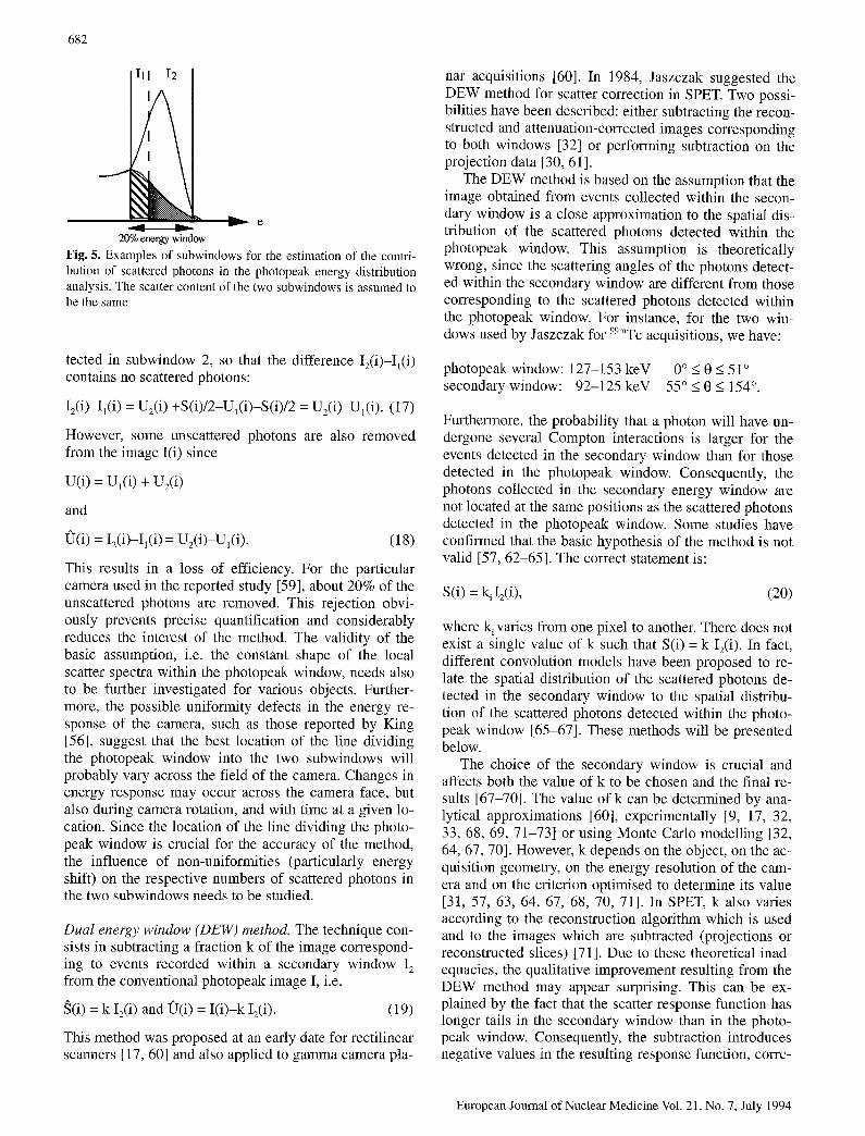
Photopeak energy distribution analysis. The measurements of point source energy spectra in air and water led Logan [59] to state that the shape of the scatter spectra is essentially constant in the spectral range of the photopeak. Consequently, he proposed that the photopeak window be divided into two adjacent subwindows 1 and 2 such that the numbers of scattered photons detected in the two subwindows are the same (Fig. 5), i.e.

I( i) = U ( i ) + S ( i ) = I1(i ) + I2(i) (15)

with

Ii(i ) = Ul(i ) + S(i)/2 and I2(i ) = U2(i ) + S(i)/2. (16)

For each pixel i, the number of events recorded in subwindow 1 is subtracted from the number of events de-


682

111 I2

L

~ e

20% energy window

Fig. 5. Examples of subwindows for the estimation of the contribution of scattered photons in the photopeak energy distribution analysis. The scatter content of the two subwindows is assumed to be the same

tected in subwindow 2, so that the difference I2(i)-Ii(i ) contains no scattered photons:

I2(i)-Ii(i ) = U2(i) +S(i)/2-Ul(i)-S(i)/2 = U2(i)-Ul(i). (17)

However, some unscattered photons are also removed from the image I(i) since

U(i) = U,(i) + U2(i )

and

O(i) = I2(i)-I1(i ) = U2(i)-U,(i ). (18)

This results in a loss of efficiency. For the particular camera used in the reported study [59], about 20% of the unscattered photons are removed. This rejection obviously prevents precise quantification and considerably reduces the interest of the method. The validity of the basic assumption, i.e. the constant shape of the local scatter spectra within the photopeak window, needs also to be further investigated for various objects. Further- more, the possible uniformity defects in the energy response of the camera, such as those reported by King [56], suggest that the best location of the line dividing the photopeak window into the two subwindows will probably vary across the field of the camera. Changes in energy response may occur across the camera face, but also during camera rotation, and with time at a given location. Since the location of the line dividing the photopeak window is crucial for the accuracy of the method, the influence of non-uniformities (particularly energy shift) on the respective numbers of scattered photons in the two subwindows needs to be studied.

Dual energy window (DEW) method. The technique consists in subtracting a fraction k of the image corresponding to events recorded within a secondary window I 2

from the conventional photopeak image I, i.e.

S(i) = k I2(i) and 00 ) = I(i)-k I2(i ). (19)

This method was proposed at an early date for rectilinear scanners [17, 60] and also applied to gamma camera pla-

nar acquisitions [60]. In 1984, Jaszczak suggested the DEW method for scatter correction in SPET. Two possibilities have been described: either subtracting the reconstructed and attenuation-corrected images corresponding to both windows [32] or performing subtraction on the projection data [30, 61].

The DEW method is based on the assumption that the image obtained from events collected within the secondary window is a close approximation to the spatial distribution of the scattered photons detected within the photopeak window. This assumption is theoretically wrong, since the scattering angles of the photons detected within the secondary window are different from those corresponding to the scattered photons detected within the photopeak window. For instance, for the two windows used by Jaszczak for 99mTC acquisitions, we have:

photopeak window: 127-153 keV 0 ° < 0 < 51 ° secondary window: 92-125 keV 55 ° < 0 < 154 °.

Furthermore, the probability that a photon will have undergone several Compton interactions is larger for the events detected in the secondary window than for those detected in the photopeak window. Consequently, the photons collected in the secondary energy window are not located at the same positions as the scattered photons detected in the photopeak window. Some studies have confirmed that the basic hypothesis of the method is not valid [57, 62-65]. The correct statement is:

S(i) = ki I2(i), (20)

where k i varies from one pixel to another. There does not exist a single value of k such that S(i) = k I2(i ). In fact, different convolution models have been proposed to relate the spatial distribution of the scattered photons detected in the secondary window to the spatial distribution of the scattered photons detected within the photopeak window [65-67]. These methods will be presented below.

The choice of the secondary window is crucial and affects both the value of k to be chosen and the final results [67-70]. The value of k can be determined by analytical approximations [60], experimentally [9, 17, 32, 33, 68, 69, 71-73] or using Monte Carlo modelling [32, 64, 67, 70]. However, k depends on the object, on the acquisition geometry, on the energy resolution of the camera and on the criterion optimised to determine its value [31, 57, 63, 64, 67, 68, 70, 71]. In SPET, k also varies according to the reconstruction algorithm which is used and to the images which are subtracted (projections or reconstructed slices) [71]. Due to these theoretical inad- equacies, the qualitative improvement resulting from the DEW method may appear surprising. This can be ex- plained by the fact that the scatter response function has longer tails in the secondary window than in the photopeak window. Consequently, the subtraction introduces negative values in the resulting response function, corre-


I21 I2r I-4 I 1--4

[ I

~-4 wl H w 2 w2

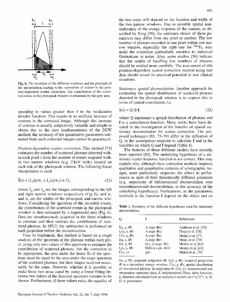
Fig. 6. The locations of the different windows and the principle of the interpolation leading to the estimation of scatter in the position-dependent scatter correction. The contribution of the scattered events to the photopeak window is estimated by the grey area

sponding to values greater than 1 in the modulation transfer function. This results in an artificial increase of contrast in the corrected image. Although this increase of contrast is usually subjectively valuable and simple to obtain due to the easy implementation of the DEW method, the accuracy of the quantitative parameters estimated from such corrected images cannot be guaranteed.

Position-dependent scatter correction. This method [74] estimates the number of scattered photons detected within each pixel i from the number of events acquired within two narrow windows (e.g. 2 keV wide) located on each side of the photopeak window. The following linear interpolation is used:

S(i) = (I21(i)/w 2 + I 2 r ( i ) / w 2 ) w J2, (21)

where I2l and I2r are the images corresponding to the left and right narrow windows respectively (Fig. 6), and w~ and w 2 are the widths of the photopeak and narrow windows. Considering the spectrum of the recorded events, the contribution of the scattered events in the photopeak window is thus estimated by a trapezoidal area (Fig. 6). Data are simultaneously acquired in the three windows to estimate and then subtract the contribution of scattered photons. In SPET, the subtraction is performed on each projection before the reconstruction.

Easy to implement, this method is based on a rough analysis of the spectrum of the photons within each pixel, using only two values of this spectrum to estimate the contribution of scattered photons. For the correction to be appropriate, the area under the linear fit of the spectrum must be equal to the area under the exact spectrum of the scattered photons, but their shapes need not necessarily be the same. However, whether it is possible to make these two areas equal by using a linear fitting between two values of the detected spectrum remains to be shown. Furthermore, if these values exist, the equality of

683

the two areas will depend on the location and width of the two narrow windows. Due to possible spatial non- uniformity of the energy response of the camera, as described by King [56], the optimum choice of these parameters may differ from one pixel to another. The low number of photons recorded in one pixel within one narrow window, especially the right one for 99mTc, may make the correction particularly sensitive to statistical fluctuations or noise. Also, some studies [56] indicate that the results of handling low numbers of photons should be studied more carefully. The assessment of this position-dependent scatter correction method using real data should reveal its practical potential in real clinical situations.

Stationary spatial deconvolution. Another approach for estimating the spatial distribution of scattered photons detected in the photopeak window is to express this in terms of spatial convolution, i.e.

S(i) = Q ® f, (22)

where Q represents a spatial distribution of photons and f is a convolution function. Many works have been de- voted to the investigation of the benefits of spatial stationary deconvolution for scatter correction. The proposed techniques [65, 75-79] differ in the definition of Q, in the assumptions required to calculate f and in the variables on which Q and f depend (Table 1).

The features of these different models have recently been reported [80]. The underlying hypothesis of a stationary scatter response function is not correct. This may explain why, although these correction methods improve qualitative and quantitative contents of scintigraphic images, none particularly surpasses the others in performance in spite of their theoretically different potentials (e.g. superiority of bidimensional deconvolution over monodimensional deconvolution, or the accuracy of the underlying hypotheses). Furthermore, as the parameters involved in the function f depend on the object and on

Table 1. Summary of the different hypotheses used for stationary deconvolution.

Q f References

I(x, y, qs) A exp(-Bx) Axelsson et al. [75] U(x, y, qJ) A exp(-Bx) Floyd et al. [76] U(x, y, qs) A exp(-Br) Msaki et al. [77] I(x, y, q~) A exp(-Br) Msaki et al. [78] I(x, y, q~) k(x, y) exp(-Br) Meikle et al. [65] I;(x, y, q~) D[~+A exp(-Br)] Meikle et al. [65] C(x, y) g(r) Mukai et al. [79]

I(x, y, qJ), acquired projection ~; I2(X , y, ~), acquired projection in a secondary energy window; U(x, y, 4~), spatial distribution

of unscattered photons in projection 4~; C(x, y), reconstructed and attenuation corrected slice; & bidimensional Dirac delta function; g, function calculated from an analytical model; r=(xZ+y2)l/2; A, B, D, k: parameters


684

the acquisition geometry, they cannot be optimal for various configurations of acquisition [67, 75, 77, 78, 81]. This can lead to significant quantitative errors, especially in SPET, where the acquisition geometry changes from one projection to another. The correction is then often poorly adapted to the particular contents of the processed images [64].

Non-stationary deconvolution. To overcome the problem of the stationarity hypothesis, different methods of non- stationary deconvolution have been suggested.

The multi-energy window acquisition technique [66, 67] assumes that the scatter component within the photopeak energy window can be derived from a weighted mean of contributions from data recorded within different energy windows. As the imaging system has different transfer functions for different energy windows, the relationship between the spatial distribution Iq of the photons detected within the qth energy window and the spatial distribution of the scattered photons detected in the photopeak window depends on the given qth energy window. For each energy window q, the recorded data are then convolved with an appropriate filter function hq, such that S(i) is finally calculated by:

S(i) = Zq Iq(i) ® hq(i). (23)

This method is not a stationary deconvolution procedure; as several energy windows are considered for estimating S, the method takes the spatial variations of scatter into account. However, it is not a genuine non-stationary deconvolution technique, since the filter hq is stationary for a given energy window q. As for the stationary deconvolution methods, their major problem is in determining the appropriate parameters of the functions hq, which strictly depend on the object and on the acquisition geometry. Moreover, in practice, monodimensional filters are used. In SPET, the scatter component is estimated and subtracted for each projection before reconstruction. Consequently, this technique leads to a bidimensional scatter correction rather than a three-dimensional one. However, the method could readily be extended to a bidimensional filtering of the projections.

Another method has been proposed [82] to make the deconvolution function dependent on the distance from the source to the detector, perpendicular to the acquisition plane. The deconvolution function is circularly symmetrical and remains stationary in the detector plane, which is not a valid assumption, especially near the edge of the object.

An approach specific to SPET takes advantage of the possibilities offered by Monte Carlo modelling [83]. Scatter line spread functions depending on the angle ~b and on the source location are calculated using Monte Carlo code and tabulated for various symmetrical positions within a particular object. A reconstructed uncorrected image C(x,y) is used as an estimate of the original activity distribution. The scatter component S(x,y,q~) in

every projection I(x,y, qb is estimated from this slice C(x,y) and from the scatter line spread functions using a monodimensional deconvolution. A correction factor accounting for attenuation is applied to obtain finally projections corrected for both attenuation and scattering.

Taking into consideration the non-stationary nature of scattering is definitely necessary to attempt quantification in SPET. However, spatial deconvolution procedures seem not to be an adequate tool to achieve this goal, even though Ljungberg's attempt [83] shows that the Monte Carlo method can be helpful and valuable. The estimation of the distribution of scattered photons in the projections results from a source distribution, estimated from an uncorrected reconstructed image, convolved with scatter line spread functions. Incorrectly located events in this reconstructed image are therefore involved, as well as properly located ones, in the estimation of the distribution of the scattered photons, necessarily preju- dicing this estimation. Moreover, scatter is considered as a bidimensional phenomenon, although inaccuracies in the reported results show that a full quantitative compensation for scattering requires three-dimensional processing [40]. However, data storage and computation time currently prevent such three-dimensional processing. Ljungberg's method also requires a precise description of the object to compute the scatter line spread functions, although no hypothesis about the source location is needed. Obtaining this description in clinical routine is a major problem which has yet to be resolved.

Use of an artificial neural network. The use of an artificial neural network has been suggested for the differenti- ation of unscattered photons from scattered ones [84]. For 99mTC, an approximately 20% energy window (125-154 keV) is divided into five energy subwindows with equal widths. For each pixel i, the input values to the five input nodes of the network are the proportions of events detected in each subwindow, i.e.

input of node q = Iq(i)/I(i), (24)

where I represents the photopeak image and Iq the qth subwindow image. The network includes one hidden layer with five nodes. The output layer consists of two nodes, namely U(i)/I(i) and S(i)/I(i), and thus provides an estimate of the scatter and unscatter contents for the pixel i. The network is trained with a back-propagation algorithm and by using Monte Carlo simulated data. Though a first assessment of the method seems to be promising, further investigations are necessary in order to study whether a neural network can cope with the va- riety of spectra corresponding to different imaging configurations. In other words, if a network is trained using data corresponding to a particular object or set of objects, will it be able to properly process data corresponding to clinical acquisitions? As there are a large number of possible combinations for the parameters involved in the design of a neural network, it may appear that, as for


all methods relying on some parameters, the optimal values of the parameters depend on the processed data. Fur- ther research should provide more information about the potential of artificial neural networks for scattered photon discrimination.

Methods using data acquired in a wide energy window

The common approach for all methods described in this section is to record the spectrum of the photons detected within each pixel and to deduce the contribution of the scattered photons S(i) from an analysis of these spectra. The analysis of the set of spectra can be performed in two different manners:

1. On a pixel-by-pixel basis: the spectra are individually analysed and no information is derived from their similarities or dissimilarities.

2. By a global analysis: the set of spectra is globally analysed using techniques of multidimensionaI data analysis to exploit their similarities and dissimilarities in order to determine the scatter contribution in each spectrum.

Pixel-by-pixel spectral analysis

Spectral analysis with a rectilinear scanner. The first work using a pixel-by-pixel spectral analysis was reported as early as 1978 for 99myc studies with rectilinear scanners [85]. In this method, the data are simultaneously acquired in a wide energy window (120-175 keV) and three other windows are used to determine the scatter component Sl(i) within the main window. Preliminary experimental measurements are performed to define two functions f and g depending on the source depth d in the scattering medium:

f(d) = Sl(d)/I2(d ) and g(d) = I3(d)/I4(d), (25)

where the subscript 1 denotes the main acquisition window and 2, 3 and 4 denote the three other spectral windows. As g is a monotone decreasing function, the estimate of S~ in every pixel is obtained as follows: I3/I 4 is calculated and d is deduced from g(d); d is used in turn to determine the value of the function f(d); the scatter component Sj can then be calculated using the relationship S~(d)= f(d)Iz(d ). This procedure is electronically coded and applied to each pixel.

Although it was not followed by further investigations and not applied to gamma camera acquisitions, this approach was noteworthy because of its original features, which were ahead of their time: the main spectral acquisition window is wide to ensure a high sensitivity; information collected in a broad spectral range (from 35 to 175 keV for 99mTC) is taken into account to estimate the scatter component; and the variations of the contribution of scattering as a function of source depth are considered.

685

Spectral fitting method. Ten years passed before another method with similar properties appeared, referred to as the spectral fitting method [86]. Each individual energy spectrum is decomposed into one scatter-free spectrum and one scatter spectrum. Two techniques for this decomposition were initially suggested. The first, using iterative peak erosion [87], was later abandoned, probably due to the variability of results with the number of iterations. The second technique requires the knowledge of a scatter-free spectrum u and assumes that the scatter spectrum can be represented by a third-order polynomial. For each pixel i, the local spectrum n(i) is modelled as the sum of a scatter-free spectrum u multiplied by a constant, and a third-order polynomial corresponding to the scatter component, i.e.

fij(i) = a0(i) + a~(i) j + a2(i ) j2 + a3(i ) j3 + b(i) uj, (26)

where j denotes an energy channel, and a 0, a~, a2, a 3 and b are parameters to be determined. Each measured spectrum is fitted to this model using a least squares method, in order to get both the value b(i) and the polynomial coefficients. The scatter component S(i) is estimated by summing the polynomial from a channel n~ (below the photopeak, typically at 117 keV for 99mTC) tO a channel n 2 (above the photopeak, typically at 162 keV for 99myc). In addition to the fact that the experimental determination of a proper scatter-free spectrum is not easy [13] and thus appears as a constraint, it seems difficult to optimise two fitting parameters, namely the order of the fitting polynomial and the energy range to consider [88]. Indeed, the best choice for these parameters depends on the analysed spectrum. This dependency occurs because the shape of the scatter spectrum changes with the change of spatial location. Furthermore, in low-count (high-noise) situations, the quantitative errors rise rapid- ly [88]. These observations led the authors to propose another Compton scatter correction technique: the regularized deconvolution-fitting method.

Regularized deconvolution-fitting method. The regularized deconvolution-fitting method [89] is also based on an individual spectral analysis, but the problem is ex- pressed in terms of spectral convolution and solved as an inverse problem. The local spectrum n(i) corresponding to a pixel i is modelled by:

riO) = R s(i) + b(i) u, (27)

where s is the spectrum of scattered events before its convolution with the camera energy response function, R is the matrix describing the energy response function of the camera for s, u is a separately measured scatter- free spectrum and b is a coefficient to be determined. The term b(i)u is thus the scatter-free part of the spectrum n(i) and its integration over the energy range considered is an estimate of the number of unscattered photons in the pixel i. Equation 27 can be rewritten as a sin-


686

gle matrix equation:

fi = T c ( 2 8 )

by adding u as the last column of R to obtain T and de- fining e as the concatenation of the vector s with b. As- suming that R and u are known, T is then known and the problem is: given n and T, solve for e. Since this inverse problem is ill-posed, a regularization technique involv- ing a regularization parameter is used to stabilise the system.

The main limitations of this approach are the necessary assumption that the energy response of the camera as a function of the energy is known, and the necessity of measuring the scatter-free spectrum. These characteristics vary from one imaging system to another, and may also change with time for one particular camera. Regular calibration procedures are therefore necessary to ensure an appropriate scatter correction. Variations of the energy response function over the field of view of the camera may occur in practice [56] and cannot be included using this method. The sensitivity of the accuracy of the spectral decomposition to these possible energy response non-uniformities still needs to be investigated. The method seems to be not too sensitive to the regularization parameter, whose optimum value depends on the signal-to-noise ratio in the spectrum; consequently, this parameter is object and location dependent. Further studies for other source geometries and acquisition configurations will probably better reveal the potential of this approach.

Scatter-free imaging. Rather than assuming s(i) to be unknown, another spectral analysis technique called scatter-free imaging [90] is based on the decomposition of the local spectrum into its unscatter and scatter components using functions derived from a physical model. Each individual spectrum is assumed to be described by:

fi(i) = Z k ak(i) S k + b(i) u. (29)

u is the scatter-free spectrum for the considered radioisotope with a contribution b(i). The first term corresponds to the physical modelling of the scatter contribution: each term s k is the probability distribution that a photon has undergone k interactions. It is derived from the Compton scattering cross-sections convolved with the system energy response function. The coefficients ak(i ) representing the unknown contributions of the different order scattered photons are estimated by a least squares fit, as is b(i). The number of scattered photons in the spectrum i then corresponds to:

~(i) = Zk ak(i). (30)

AS in the previous method, this technique requires prior knowledge of the energy response of the system for each energy and estimation of the scatter-free spectrum. The same restrictions concerning its use therefore apply. Fur- thermore, in the method as has been presented, the rele-

vance of the physical modelling of the spectra s k is ques- tionable, given the gap between what is physically expected and what is actually detected. Indeed, the information associated with each photon, including the energy information, is locally affected by various correction procedures aiming at a uniform camera response. A model using only the system energy response function, assumed to be spatially invariant, to relate the Compton scattering cross-sections to s k may therefore be an over- simplification, disregarding more subtle information dis- tortion.

As the prior knowledge required by methods of pixel- by-pixel analysis appears to limit their robustness, other spectral analysis approaches which do not necessitate such a priori knowledge have also been suggested.

Global spectral analysis

The additional idea underlying the methods of global spectral analysis, in comparison with those of pixel-by- pixel spectral analysis, is the exploitation of the correla- tions existing between the spectra corresponding to the different pixels of the image. The spectra are no longer individually considered; rather the whole set of spectra is arranged in an array N which is then processed using techniques of multidimensional data analysis. Each row i of N corresponds to the sampled spectrum recorded within one pixel. Consequently, each column corresponds to a spectral range and can also be regarded as the vectorized image of the photons whose energy is included in this spectral range (Fig. 7). The use of multidimensional data analysis to process this array for scatter correction was first suggested in 1987 [91] and two methodologies have since been described: holospectral imaging and factor analysis of spectral image sequences.

Holospectral imaging. In holospectral imaging [92, 93], the variance of the set of spectra is analysed in order to separate unscattered from scattered photons, without explicitly modelling the scatter-free and the scatter spectra. A principal component analysis of the set of spectra is

column j

r o w i

-

Ib e

spectrum of photons detected in the pixel i

image of photons detected with an energy corresponding to the speclral range j

Fig. 7. Organization of the data in an array N for performing scatter correction using a global spectral analysis


687

used to define a basis of the multidimensional energy space, so that this basis permits a classification of the photons. Each basis vector of this space accounts for a proportion of the variance of the spectra. It is assumed that the information (measured in terms of variance) associated with the unscattered photons is greater than that associated with the scattered photons and the noise, and that the information associated with scattering is greater than that attributable to noise. A change of the basis of the space is performed to remove a proportion of variance accounting for scattering. The image of the unscattered photons results from this transformation. The validity of the underlying hypotheses and the effectiveness of the method remain to be proved.

Factor analysis of medical image sequences. The other methodology of global spectral analysis is based on the application of factor analysis of medical image sequences (FAMIS) to spectral image sequences. As the set of spectra (rows of the array N) can be considered as a set of images (columns of N), the global analysis of the set of spectra can be viewed as the analysis of a spectral image sequence (Fig. 7) and FAMIS can be used to perform this analysis. FAMIS includes two fundamental steps [94, 95]. The first consists in representing the spectra within a low dimensional space S (typically a two-to four-dimensional space) obtained from the orthogonal decomposition of the covariance matrix of the data, such that:

f'l(i) = Zk Vk(i ) Wk, (31)

where {Wk}k=l. K are the orthogonal eigenvectors associated with the K highest eigenvalues resulting from the orthogonal decomposition. This step aims at explicitly removing the noise tainting the data, that is that fi is a noise-free estimate of the original data n. As the vectors w k are orthogonal, this decomposition is only a mathe- matical one, without any physical interpretation. The second step of FAMIS is the determination of an oblique basis of the space S such that the oblique basis vectors, called factors, have a physical meaning. For scatter correction, the factors searched for are the scatter-free spectrum u on the one hand, and one or several scatter spectra on the other hand, such that:

] l( i ) = Z k ak(i ) S k -t- b(i) u. (32)

The coefficients ak(i ) and b(i) correspond to the contribution of scattered and unscattered photons respectively in the spectrum fi(i). Conventional FAMIS does not per- mit proper estimation of u, since no scatter-free spectra are present among the set of analysed spectra. Two mod- ifications of the conventional FAMIS have thus been proposed to obtain a factor decomposition adapted to scatter correction. The constrained factor analysis [96-98] first conventionally estimates two factors (i.e. K = 2). Then, it replaces the factor whose shape is closest

to the expected scatter-free spectrum by a theoretical scatter-free spectrum, before calculating the coefficients b(i) and al(i ) by a least mean squares regression. Due to a coarse spectral sampling, this theoretical spectrum is in fact a Dirac delta function, i.e. it is equal to 1 in the spectral range including the photopeak and to zero everywhere else.

Estimating only two factors (one scatter-free spectrum and one scatter spectrum) makes the scatter correction stationary. Indeed, the scatter spectrum sl is assumed to be the same [weighted by the coefficient a~(i)] in every pixel i. The coarse modelling of u using a Dirac delta function results from technical considerations. It must not be considered as a significant limitation of the procedure since a more precise modelling could be performed by using another acquisition device. However, this method requires knowledge of a theoretical scatter- free spectrum and does not offer any means of control- ling the consistency of the theoretical spectrum used with respect to the processed data. In particular, the inclusion of the theoretical spectrum in S, corresponding to its consistency with the noise-free data fi(i), is not en- sured. The resulting spectral decomposition may then be inconsistent with the noise-free data.

An alternative method has been described as "target apex seeking" [99, 100]. An estimate of the scatter-free spectrum is searched for in S by minimising a criterion expressing prior knowledge related to u, namely an approximate estimate of the spectral range in which u theoretically becomes zero. This procedure leads to a scatter-free spectrum belonging to S and which is the most similar spectrum to the expected one. Using experimental or clinical data, the estimated scatter-free spectrum shows a low energy tail [99]. This is consistent with some experimental measurements previously reported [13, 86]. The scatter spectra s k are derived from the determination of the scatter-free spectrum.

As the number of scatter spectra is not restricted to one, the correction is not stationary. Indeed, the scatter component within each pixel is obtained from a linear combination of the spectra s k weighted by different coefficients a k. It can then vary from one location to another. The number of scatter spectra s k to be estimated, equal to the total number of factors involved in the analysis mi- nus one, may depend on the radioisotope but seems to be constant for one radioisotope (e.g. two scatter spectra for 99mTc acquisitions) [99]. The main advantage of this approach is that the spectra u and s k do not need to be known a priori. They are automatically determined for each set of data. Consequently, the basis of spectra automatically adapts itself to the features of the camera, to the acquisition geometry and to the object parameters. The necessity to estimate the spectral range in which u theoretically becomes zero is not constraining, since it must be specified only approximately. An error of about 4 keV does not affect the results [99].

As for many scatter correction methods, the results of FAMIS using the target apex seeking are only reliable if


688

the energy response of the camera is spatially uniform [99]. Otherwise, the method clearly displays spatial defects. It is then possible to provide a warning to the user to avoid misinterpretation of the results. The dependence of the accuracy of the quantitative results on the spectral range which is considered for the analysis and on the spectral sampling (currently equal to 4 keV) still needs to be investigated.

For all methods of spectral analysis, the number of counts detected within one pixel may be too low to provide a reliable spectrum to analyse. Consequently, most of these methods (spectral fitting method, scatter-free imaging, FAMIS) first group the spectra corresponding to neighbouring pixels and perform the spectral decomposition of the resulting spectra. The decomposition of the spectra corresponding to the initial spatial sampling is deduced using either an interpolation or a regression scheme. The spectra are usually grouped according to a regular pattern (rectangular or square grouping), without taking the shapes of the spectra into account. Mixing spectra which have different shapes may lead to some inaccuracies when coming back to the initial spatial sampling. To limit this source of inaccuracies, a three-dimensional clustering procedure which groups neighbouring spectra according to their similarities [99] may be a useful alternative.

One common feature of all the methods aiming at subtracting the scattered photons from the acquired data is that they tend to amplify noise. As photons are removed, the number of counts in the corrected image decreases, and statistical fluctuations and noise increase. Moreover, the scatter response function has wider tails than the geometric response function. Consequently, the inclusion of scattered photons produces smooth images, while their removal results in images with sharper edges but increased noise.

Evaluation

Faced with all these scatter correction methods, the user (physician or physicist) may feel confused. Which should one use and how reliable will it be? The evaluation is the step which should provide such information. However, as this stage is usually incomplete, the present situation concerning the performance of the different techniques remains unclear.

A comprehensive assessment scheme should include four steps: the theoretical analysis of the method, and investigations using simulated data, physical phantoms and clinical data.

Theoretical analysis

The theoretical analysis o f a method provides an over- view of its potential, given the physical accuracy of the underlying hypotheses. For instance, as has been

stressed when presenting the methods, the very principle of some of them excludes a precise quantification (e.g. windowing methods, photopeak energy distribution analysis). Others rely on hypotheses which are known to be inaccurate (e.g. stationarity of the scatter response function). Considering the theoretical aspects of the correction is also important in understanding how easy it will be to apply the method in different imaging situations, and how well the method should perform in those situations.

The ease with which a scatter correction could be applied is primarily of concern for the methods requiring prior knowledge regarding the object (e.g. body outlines, buildup functions, density map). It is easier to obtain this information or get a proper estimate of it in certain types of acquisition. For example, it is more difficult to obtain the density map in non-homogeneous media like the thorax.

The reliability of a method to be used in different imaging situations depends on the number of situations in which its assumptions can be considered as valid, and on whether the method performs an adaptive correction. The methods which rely on restrictive hypotheses cannot be optimal for correcting certain types of acquisition. For instance, methods assuming a uniform attenuating medium for modelling the scatter response functions [e.g. 47] are a priori not well adapted for processing tho- racic acquisitions. The methods using the hypothesis of a stationary scatter response function are inappropriate for processing brain images in which the presence of the skull results in scatter response functions which are strongly non-stationary. Most scatter correction methods do not perform an adaptive scatter correction, since they would need to define the value of parameters which should depend on the object (as in energy-weighted acquisition). Unless these parameters are well adapted to the different types of acquisition - which is difficult to achieve in clinical practice - these methods will not perform well consistently. This can make the comparison of quantitative parameters between patients unreliable. The methods which are theoretically adaptive (e.g. scatter- free imaging, holospectral imaging, factor analysis of medical image sequences) are potentially more appealing as far as quantification is concerned. A theoretical analysis of the methods is essential in order to obtain an understanding of their capabilities.

Use of simulated data

The step which should follow is an assessment using simulated data, particularly Monte Carlo simulated data. Indeed, for such data, the history of each detected photon (emission location, number and type of interaction undergone before detection) is fully known. Monte Carlo modelling can be used to evaluate the scatter correction methods in two ways. First, the assumptions of the methods can be tested; secondly, the corrected images


689

can be compared with the images formed from only unscattered events. Such a comparison may be performed qualitatively and quantitatively, as quantitative original information is available. Due to the relative ease of obtaining Monte Carlo simulation packages, this evaluation stage is conducted and reported with increasing frequen- cy in presenting the performance of the scatter correction methods [5, 13, 36, 40, 45, 57, 63, 74, 76, 83, 88, 89, 97, 101]. However, although this evaluation stage is certainly a sine qua non, it is obviously not sufficient. Indeed, even if an increasing number of phenomena tend to be included in the simulation of the gamma camera [e.g. 1, 2, 4, 102, 103], the entire complexity of the detector cannot yet be simulated. In particular, the uniformity defects resulting from the spatial variation of the camera energy response have not yet been taken into account, probably because they strongly depend on the particular camera. As these uniformity defects affect the accuracy of the energy information related to each detected photon, which is used in every scatter correction method, they should not be ignored in any complete assessment. Some methods - particularly those based on analysis of the local spectra - can be reliable when processing simulated data, but lead to unacceptable artefacts when processing real data due to the non-uniformity of the energy response across the field of the camera (especially the energy shift of the spectra). Moreover, the simulated object cannot attain the complexity of a patient, and the simulated configurations are simpler than those encountered in clinical practice. For instance, they cannot include the intricate distribution of the radionuclide in human tissues, nor a full description of the variations of tissue density. Consequently, encouraging results obtained from simulated data, though necessary, do not ensure the reliability of the method in more realistic situations.

Evaluation using physical phantoms

In order to better approximate real imaging conditions, evaluation is usually performed using physical phantoms. This kind of assessment allows the defects of the detector to be included while maintaining precise knowledge about the scanned object. On the other hand, the history of the detected photons is no longer known. Con- sequently, the problem of the gold standard to be used for assessing the processed images arises. This reference standard can be the original object, the image acquired in a similar geometrical configuration but without scattering media (i.e. in air), the image provided by a device leading to a better separation between scattered and unscattered photons as a result of a better energy resolution [9, 13, 68], or the unprocessed image itself. For a quantitative assessment, the parameters to be measured to test whether a method is of value are also of concern. The most common parameters cited are: contrast, signal-to- noise ratio, spatial resolution and correlation of detected

counts against real activity (also called linearity). How- ever, most of these parameters (e.g. contrast) can be defined in different ways, using different phantoms. There is no consensus about a comprehensive scheme of evaluation using physical phantoms. Absolute quantification is more difficult to assess since it requires the other dam- aging effects involved in the imaging process to be corrected as well (e.g. attenuation, detector response sensitivity). If many quantitative parameters can be used to characterise the performanc e of a method, a major difficulty is in combining those parameters into a single index in order to quantify the quality of an image as a function of those parameters rather than considering the parameters independently. Consequently, in spite of the numerous publications reporting phantom assessment of scatter correction techniques, the present lack of such a general index and of a precise scheme for such an evaluation prevents a ready comparison between these techniques, given the different ways the studies have been designed.

Clinical evaluation

If physical phantoms are a useful means of assessing the real potential of a scatter correction method, and most methods go through this stage, clinical assessment is clearly required for a final evaluation. Indeed, the phantoms may not be realistic models of the images encountered in clinical diagnosis. Proper clinical assessment based, for instance, on the use of receiver operating characteristic (ROC) curves (measuring the detectability of structures) could provide objective and quantitative evaluation of the performance of scatter correction methods. Such a study relies on a large number of observations and takes much time to complete. Furthermore, it requires prior knowledge of the "true" information con- tained in the images, which is difficult to obtain. These are probably the two main reasons why ROC studies have not yet been conducted for the assessment of scatter correction methods. Less extensive clinical evalua- tions have been reported for certain methods [21, 39, 54, 69, 104-106], but these are rare; assessment of scatter correction methods using clinical data is awkward and conclusions are difficult to draw (e.g. [54, 105]). Quanti- tative parameters are difficult to evaluate since accurate reference is not available. Other imaging modalities (e.g. CT, ultrasonography, nuclear magnetic resonance) could be used [39, 104, 107, 108] since they are able to provide high spatial resolution information. However, they are not suitable for use as a gold standard for SPET images which contain specific physiological information. Qualitative assessment is easier to perform using observer tests [21, 105, 106] but the overall preference of an observer does not necessarily provide information about the most accurate quantitative contents of an image.

A common problem of these evaluation steps, what- ever the data (simulated data, physical phantoms or clin-


690

ical data), is related to the error analysis. As the imaging process is complicated, the errors between expected and measured values can usually be ascribed to a number of different factors and are not necessarily the result of scatter correction. These factors include the presence of defects in the camera when processing real data (especially the non-uniformity of the camera response) and the partial volume and sampling effects encountered when imaging small objects. In SPET, the interaction between scatter correction, tomographic reconstruction and attenuation correction must also be carefully considered, if one is to be able to perform an appropriate error analysis and use it for the possible improvement or optimisa- tion of the scatter correction method.

Even if each various scatter correction method has been submitted to the kind of four-step evaluation procedure suggested here, the only means of choosing between all these techniques would be to carry out a comparative study of their performances. Such comparative studies exist [33, 40, 57, 64, 65, 67, 70, 77, 89, 97, 101, 104, 109-111] but they are very limited, looking at only two, three or four scatter correction methods in addition to the photopeak window acquisition. Consequently, for specific operating conditions and specific assessment parameters, these comparative studies have allowed classification of the tested methods by performance [33, 57, 65, 70, 77, 89, 97, 104, 109, 110], although this is not always the case [40, 64, 67, 101, 111]. As these comparative studies are designed differently from one another, a more general classification of the methods cannot be derived. To achieve more general results, it would be necessary to compare a large number of methods using identical data sets. Such a project is a far-ranging one, given the number of existing methods and the problem of synthesising the performance of each method using one single index or a small number of parameters. Fur- thermore, the data sets would have to be collected in such a way that they could be processed using any method. The only acquisition type meeting this requirement is list mode acquisition, recording the position, energy and time of each detected event. The advantage of list mode acquisition is that the data acquired in this way can be processed as many times as necessary, using any scatter correction method and without losing the original data. List mode thus represents a helpful tool for optim- ising and comparing methods. Unfortunately, only a very small number of cameras currently include this acquisition facility and hence, the exchange of data between research sites for comparative purposes is severely restricted. However, in spite of the obvious difficulty in con- ducting such a study, a wide-ranging project aimed at comparing the quantitative performances of scatter correction methods in clinical situations is probably the only means of clarifying the situation for the many concerned users and researchers.

Conclusion

In concluding this critical review, it is important to state current clinical practice with respect to scatter correction and to discuss future prospects. It must be recognised that, in spite of the numerous scatter correction methods which have been proposed during the past 20 years or more, the oldest one, i.e. the photopeak window acquisition, has not so far been superseded in clinical use. It is still the only method used as a standard in planar imaging. In SPET, the second most frequently performed scatter correction after photopeak window acquisition is the effective attenuation correction, using a decreased value for the attenuation coefficient. As these two methods are definitely not sufficient for achieving precise quantification, one can rightly wonder why they have not been replaced by more ambitious methods, which seem to have been shown to improve both qualitative and quantitative interpretation. Several reasons can be suggested for this. Although most methods have been assessed using simulated and physical data, none has yet faced an extensive procedure of clinical assessment. Consequently, none has been proved to have a beneficial diagnostic impact in clinical practice. Some methods are in fact too recent and must still be optimised and tested using simulated or physical data before being available for clinical evaluation. In particular, the sensitivity of the accuracy of the results to the parameters that they include and to the unavoidable defects of the camera (especially to the non-uniformity of the energy response) must be fully investigated. However, an extensive clinical evaluation will probably be indispensable for any technique to have a chance of modifying conventional practice. As far as commercial implementation is concerned, only a few methods have been made available on clinical systems, namely the weighted acquisition module (Siemens) and scatter-free imaging (Elscint). Other techniques which do not require particular hardware or software can also be used (e.g. the dual energy window method) but the fact that the operator has to perform additional processing limits their use. These considerations also contribute to the difficulty in assessing and comparing the methods using phantom or patient data- bases.

Another hindrance to the clinical use of scatter correction relates to the fact that observers have acquired the habit of interpreting images smoothed by the inclusion of scattered photons. Scatter-corrected images, especially those resulting from a removal of scattered events rather than a relocation of them, usually appear noisy and unpleasant to interpret, even if their contents are more reliable. A first step towards the clinical use of scatter correction is certainly to provide the users with both the conventional photopeak image and the corrected image, in order to allow them to become familiar with the appearance of scatter-free images. Relocating scattered events to make them contribute to the estimate of the original radioisotope distribution is also appealing,


691

since it could help to avoid noise amplification and increase the sensitivity of the imaging system.

Examination of the currently investigated methods shows two trends. On the one hand, some relatively simple methods essentially process the data acquired in the photopeak window and estimate the scatter component using a few parameters characterising these data (e.g. the channel ratio method, the position-dependent scatter correction, the photopeak energy distribution analysis). On the other hand, more sophisticated methods use a more comprehensive analysis of the data, based either on additional information provided by Monte Carlo simulations (as for the computation of the buildup functions, the cal- culation of the scatter line spread functions in non-stationary deconvolution, the estimation of the probability matrix for simultaneous scatter correction and tomographic reconstruction, and the modelling of the scatter response functions for their inclusion in the projector/backprojector in iterative reconstruction) or on a more specific spectral analysis of locally detected photons (e.g. the regularized deconvolution-fitting method, the neural network approach, scatter-free imaging, holospectral imaging and FAMIS). In our opinion, these more sophisticated methods probably offer more potential in terms of quantification since they rely on a more precise analysis of the data. Nevertheless, the requirements of some of them in terms of prior knowledge may make them unsuitable for clinical use. The more promising methods are probably the sophisticated ones which need prior knowledge that is available and reliable in clinical situations. Most of the scatter correction methods could be implemented in such a way that the corrected image is displayed at the same time as the photopeak image, or within a few minutes of the end of the acquisition. Pro- cessing times are currently a problem only for a few approaches, namely the methods requiring Monte Carlo simulations and/or dealing with scatter during iterative reconstruction in SPET. The superiority of these methods over those which are less demanding will have to be proved to justify the additional storage and computa- tional investment that they require. The demonstration of the reliability of a method, its clinical value and the ease of carrying it out are probably key factors in determining whether that method will become widely accept- ed.

Acknowledgements: I. Buvat thanks the IFSBM (Institut de For- mation Supdrieure Biomrdicale, Villejuif, France), Sopha Mrdical (Buc, France) and the Association pour la Recherche sur le Can- cer (Villejuif, France) for supporting this work.

References

1. De Vries DJ, Moore SC, Zimmerman RE, Mueller SP, Fried- land B, Lanza RC. Development and validation of a Monte Carlo simulation of photon transport in an Anger camera. IE- EE Trans Med Imaging 1990;9: 430~438.

2. Ljungberg M, Strand SE. A Monte Carlo program for the simulation of scintillation camera characteristics. Comput Meth- ods Prog Biomed 1989;29: 257-272.

3. Rosenthal MS, Henry LJ. Evaluation and comparison of two scatter correction techniques. J Nucl Med 1990;31: 878.

4. Gagnon D, Pouliot N, Laperri~re L. Statistical and physical content of low-energy photons in holospectral imaging. IEEE Trans IVied hnaging 1991; 10: 284-289.

5. Munley MT, Floyd CE, Tourassi GD, Bowsher JE, Coleman RE. Out-of-plane photons in SPECT. IEEE Trans Nucl Sci 1991 ;38: 776-779.

6. Gagnon D, Laperri~re L, Pouliot N, de Vries D J, Moore SC. Monte Carlo analysis of camera-induced spectral contamina- tion for different primary energies. Phys Med Biol 1992;37: 1725-1739.

7. Beck JW, Jaszczak RJ, Coleman RE, Starmer CF, Nolte LW. Analysis of SPECT including scatter and attenuation using sophisticated Monte-Carlo modeling methods. IEEE Trans Nucl Sci 1982;29: 506-511.

8. Floyd CE, Jaszczak RJ, Harris CC, Coleman RE. Energy and spatial distribution of multiple order Compton scatter in SPECT: a Monte Carlo investigation. Phys Med Biol 1984;29: 1217-1230.

9. Lowry CA, Cooper MJ. The problem of Compton scattering in emission tomography: a measurement of its spatial distribution. Phys Med Biol 1987;32:1187-1191. Coleman M, King MA, Glick S J, Knesaurek K, Penney BC. Investigation of the stationarity of the modulation transfer function and the scatter fraction in conjugate view SPECT restoration filtering. IEEE Trans Nucl Sci 1989;36: 969- 972. Frey EC, Tsui BMW. Parameterization of the scatter response function in SPECT imaging using Monte Carlo simulation. 1EEE Trans Nucl Sci 1990;37: 1308-1315. Zasadny KR, Koral KF, Floyd CE Jr, Jaszczak RJ. Measure- ment of Compton scattering in phantoms by germanium detector. IEEE Trans Nucl Sci 1990;37: 642-646. Koral KF, Wang X, Zasadny KR, Clinthorne NH, Rogers WL, Floyd CE, Jaszczak RJ. Testing of local gamma-ray scatter fractions determined by spectral fitting. Phys Med Biol 1991;36: 177-190. Floyd CE, Jaszczak RJ, Coleman RE. Scatter detection in SPECT imaging: dependence on source depth, energy, and energy window. Phys Med Biol 1988;33: 1075-1081. Beck RN, Schuh MW, Cohen TD, Lembares N. Effects of scattered radiation on scintillation detector response. In: IAE- A, ed. Medical radioisotope scintigraphy. Vienna: IAE- A;1969: 595-616. Rollo FD, Schulz AG. Effect of pulse-height selection on le- sion detection performance. J Nucl Med 1971; 12: 690-696. Ehrhardt JC, Oberley LW. Effects of spectral changes on scan- ning. Radiology 1972;104: 207-208. Oberley LW, Ehrhardt JC, Lensink SC. The variable baseline scanner. Phys Med Biol 1972; 17: 630-637. Sanders TP, Sanders TD, Kuhl DE. Optimizing the window of an Anger camera for 99mTc. J Nucl Med 1972; 12: 703-706. Atkins FB, Beck RN. Dependence of optimum baseline set- ting on scatter fraction and detector response function. In: IAEA, ed. Medical radionuclide imaging. Vienna: IAE- A;1977: 101-118. Collier BD, Palmer DW, Knobel J, Isitman AT, Hellman RS, Zielonka JS. Gamma camera energy for TC 99m bone scintigraphy: effect of asymmetry on contrast resolution. Radiology 1984;151: 495-497.

10.

11.

12.

13.

14.

15.

16.

17.

18.

19.

20.

21.


692

22. Graham LS, La Fontaine RL, Stein MA. Effects of asymmetric photopeak windows on flood field uniformity and spatial resolution of scintillation cameras. J Nucl Med 1986;27: 706-713.

23. La Fontaine R, Stein MA, Graham LS, Winter J. Cold lesions: enhanced contrast using asymmetric photopeak windows. Ra- diology 1986;160: 255-260.

24. Rogers WL, Clinthorne NH, Stamos J, Koral KF, Mayans R, Knoll GF, Juni J, Keyes JW, Harkness BA. Performance evaluation of SPRINT, a single photon ring tomograph for brain imaging. J Nucl Med 1984;25: 1013-1018.

25. Koral KF, Clinthorne NH, Rogers WL. Improving emission computed tomography quantification by Compton-scatter rejection through offset windows. Nucl Instrum Methods Phys Res 1986;A242: 610-614.

26. Beck RN, Zimmer LT, Charleston DB, Hoffer PB. Aspects of imaging and counting in nuclear medicine using scintillation and semi conductor detectors. IEEE Trans Nucl Sci 1972;19: 173-178.

27. King MA, Coleman M, Penney BC, Glick SJ. Activity quantitation in SPECT: a study of prereconstruction Metz filtering and use of the scatter degradation factor. Med Phys 1991;18: 184-189.

28. Jaszczak RJ, Coleman RE, Whitehead FR. Physical factors affecting quantitative measurements using camera-based single photon emission computed tomography. IEEE Trans NucI Sci 1981;28: 69-80.

29. King MA, Penney BC, Glick SJ. An image-dependent Metz filter for nuclear medicine images. J Nucl Med 1988;29: 1980-1989.

30. Jaszczak RJ, Floyd CE, Coleman RE. Scatter compensation techniques for SPECT. IEEE Trans Nucl Sci 1985;32: 786-793.

31. Szabo Z, Links JM, Seki C, Rhine J, Wagner HN. Scatter, spatial resolution, and quantitative recovery in high resolution SPECT. J Comput Assist Tomogr 1992;16: 461~467.

32. Jaszczak RJ, Greer KL, Floyd CE, Harris CC, Coleman RE. Improved SPECT quantification using compensation for scattered photons. J Nucl Med 1984;25: 893-900.

33. Gilland DR, Jaszczak RJ, Greer KL, Coleman RE. Quantita- tive SPECT reconstruction of iodine-123 data. J Nucl Med 1991;32: 527-533.

34. Harris CC, Greer KL, Jaszczak RJ, Floyd CE, Fearnow EC, Coleman RE. Tc-99m attenuation coefficients in water-filled phantoms determined with gamma cameras. Med Phys 1984;11: 681-685.

35. Wu RK, Siegel JA. Absolute quantification of radioactivity using the buildup factor. Med Phys 1984;11: 189-192.

36. Almquist H, Palmer J, Ljungberg M, Wollmer R Strand SE, Jonson B. Quantitative SPECT by attenuation correction of the projection set using transmission data: evaluation of a method. Eur J Nucl Ivied 1990;16: 587-594.

37. Siegel JA, Wu RK, Maurer AH. The buildup factor: effect of scatter on absolute volume determination. J NucI Med 1985;26: 390-394.

38. Ljungberg M, Strand SE. Attenuation correction in SPECT based on transmission studies and Monte Carlo simulations of buildup functions. J Nucl Med 1990;31: 493-500.

39. Siegel JA, Manrer AH, Wu RK, Denenberg BS, Gash AK, Carabello BA, Spann JF, Malmud LS. Absolute left ventricu- lar volume by an iterative build-up factor analysis of gated radionuclide study. Radiology 1984; 151:477481.

40. Ljungberg M, Strand SE. Attenuation and scatter correction in SPECT for sources in a nonhomogeneous object: a Monte Carlo study. J Nucl Med 1991;32: 1278-1284.

41. Egbert SD, May RS. An integral-transport method for Compton-scatter correction in emission computed tomography. IEEE Trans Nucl Sci 1980;27: 543-548.

42. Chang LT. A method for attenuation correction in radionuclide computed tomography. IEEE Trans Nucl Sci 1978;25: 638-643.

43. Floyd CE, Jaszczak RJ, Coleman RE. Inverse Monte Carlo: a unified reconstruction algorithm for SPECT. IEEE Trans Nucl Sci 1985;32: 779-785.

44. Floyd CE, Jaszczak RJ, Greer KL, Coleman RE. Inverse Monte Carlo as a unified reconstruction algorithm for ECT. J Nucl Med 1986;27: 1577-1585.

45. Bowsher JE, Floyd CE. Treatment of Compton scattering in maximum-likelihood, expectation-maximization reconstruc- tions of SPECT images. JNucl Med 1991;32: 1285-1291.

46. Frey EC, Ju ZW, Tsui BMW. A fast projector-backprojector pair modeling the asymmetric, spatially varying scatter response function for scatter compensation in SPECT imaging. IEEE Trans Nucl Sci 1993;40:1192-1197.

47. Frey EC, Tsui BMW. A practical method for incorporating scatter in a projector-backprojector for accurate scatter compensation in SPECT. IEEE Trans Nucl Sci 1993;40: 1107-1116.

48. Frey EC, Tsui BMW. Spatial properties of the scatter response function in SPECT. IEEE Trans Nucl Sci 1991 ;38: 789-794.

49. Beck RN, Zimmer LT, Charleston DB, Harper PV, Hoffer PB. Advances in fundamental aspects of imaging systems and techniques. In: IAEA, ed. Medical radioisotope scintigraphy. Vienna: IAEA;1972: 29-30.

50. Halama JR, Henkin RE, Friend LE. Gamma camera radionuclide images: improved contrast with energy-weighted acquisition. Radiology 1988;169: 533-538.

51. DeVito RP, Hamill JJ. Determination of weighting functions for energy-weighted acquisition. J Nucl Med 1991;32: 343-349.

52. DeVito RR Hamill JJ, Treffert JD, Stoub EW. Energy-weighted acquisition of scintigraphic images using finite spatial filters. JNucl Med 1989;30: 2029-2035.

53. Hamill JJ, DeVito RR Scatter reduction with energy-weighted acquisition. IEEE Trans NucI Sci 1989;36: 1334-1339.

54. Floyd JL, Mann RB, Shaw A. Changes in quantitative SPECT thallium-201 results associated with the use of energy-weighted acquisition. JNucl Med 1991;32: 805-807.

55. Jaszczak RJ, Hoffman DC, DeVito RE Variance propagation for SPECT with energy-weighted acquisition. IEEE Trans NucI Sci 1991;38: 739-747.

56. King MA, Hademenos GJ, Glick SJ. A dual-photopeak window method for scatter correction. J Nucl Med 1992;33: 605-612.

57. Hademenos GJ, Ljungberg M, King MA, Glick SJ. A Mon- te Carlo investigation of the dual photopeak window scatter correction method. IEEE Trans Nucl Sci 1993;40:179- 185.

58. Pretorius PH, van Rensburg AJ, van Aswegen A, Ltitter MG, Serfontein DE, Herbst CR The channel ratio method of scatter correction for radionuclide image quantitation. J Nucl Meal 1993;34: 330-335.

59. Logan KW, McFarland WD. Single photon scatter compensation by photopeak energy distribution analysis. IEEE Trans Med Imaging 1992; 11: 161-164.

60. Bloch P, Sanders T. Reduction of the effects of scattered radiation on a sodium iodide imaging system. JNucl Med 1973;14: 67-72.

61. Liang Z, Turkington TG, Gilland DR, Jaszczak RJ, Coleman RE. Simultaneous compensation for attenuation, scatter and


693

detector response for SPECT reconstruction in three dimen- sions. Phys Med Biol 1992;37: 587-603.

62. Atkins FB, Beck RN. Effect of scatter subtraction on image contrast. J Nucl Med 1975;16: 102-104.

63. Floyd CE, Jaszczak RJ, Harris CC, Greer KL, Coleman RE. Monte Carlo evaluation of Compton scatter subtraction in single photon emission computed tomography. Med Phys 1985;12: 776-778.

64. Ljungberg M, Msaki P, Strand SE. Comparison of dual-window and convolution scatter correction techniques using the Monte Carlo method. Phys Med Biol 1990;35: 1099- 1110.

65. Meikle SR, Hutton BF, Bailey DL, Fulton RR, Schindhelm K. SPECT scatter correction in non-homogeneous media. In: Colchester ACF, Hawkes D J, eds. Information processing in medical imaging. Berlin Heidelberg New York: Spring- er;1991: 34-44.

66. Todd-Pokropek AE, Clarke G, Marsh R. Preprocessing of SPECT data as a precursor for attenuation correction. In: De- coninck F, ed. Information processing in medical imaging. Brussels: Martinus Nijhoff;1983: 130-150.

67. Gilardi MC, Bettinardi V, Todd-Pokropek A, Milanesi L, Fazi- o F. Assessment and comparison of three scatter correction techniques in single photon emission computed tomography. J Nucl Med 1988;29: 1971-1979.

68. Singh M, Horne C. Use of germanium detector to optimize scatter correction in SPECT. J Nucl Med 1987;28:1853-1860.

69. Green AJ, Dewhurst SE, Begent RHJ, Bagshawe KD, Riggs SJ. Accurate quantification of 131I distribution by gamma camera imaging. Eur J Nucl Med 1990; 16:361-365.

70. Yanch JC, Flower MA, Webb S. Improved quantification of radionuclide uptake using deconvolution and windowed subtraction techniques for scatter compensation in single photon emission computed tomography. Med Phys 1990;17: 1011- 1022.

71. Koral KF, Swailem FM, Buchbinder S, Clinthorne NH, Rog- ers WL, Tsui BMW. SPECT dual-energy-window Compton correction: scatter multiplier required for quantification. J Nucl Med 1990;31: 90-98.

72. Gilland DR, Jaszczak RJ, Turkington TG, Greet KL, Coleman RE. Quantitative SPECT imaging with indium 111. IEEE Trans Nucl Sci 1991 ;38: 761-766.

73. Koral KF, Buchbinder S, Clinthorne NH, Rogers WL, Swai- lem FM, Tsui BMW. Influence of region of interest selection on the scatter multiplier required for quantification in dual-window Compton correction. J Nucl Med 1991;32: 186.

74. Ogawa K, Harata Y, Ichihara T, Kubo A, Hashimoto S. A practical method for position-dependent Compton-scattered correction in single photon emission CT. IEEE Trans Med Im- aging 1991;10: 408-412.

75. Axelsson B, Msaki R Israelsson A. Subtraction of Compton- scattered photons in single-photon emission computerized tomography. J Nucl Med 1984;25: 490-494.

76. Floyd CE, Jaszczak RJ, Greet KL, Coleman RE. Deconvolu- tion of Compton scatter in SPECT. J Nucl Med 1985;26: 403- 408.

77. Msaki P, Axelsson B, Dahl CM, Larsson SA. Generalized scatter correction method in SPECT using point scatter distribution functions. JNucl Med 1987;28: 1861-1869.

78. Msaki R Axelsson B, Larsson SA. Some physical factors in- fluencing the accuracy of convolution scatter correction in SPECT. Phys Med Biol 1989;34: 283-298.

79. Mukai T, Links JM, Douglass KH, Wagner HN. Scatter correction in SPECT using non-uniform attenuation data. Phys Med Biol 1988;33:1129-1140.

80. Msaki R Erlandsson K, Svensson L, Nolstedt L. The convolution scatter subtraction hypothesis and its validity domain in radioisotope imaging. Phys MedBiol 1993;38: 1359-1370.

81. Fleming JS. A technique for using CT images in attenuation correction and quantification in SPECT. Nucl Med Commun 1989;10: 83-97.

82. Todd-Pokropek A. Non-stationary deconvolution using a multi-resolution stack. In: de Graaf CN, Viergever MA, eds. Infor- mation processing in medical imaging. New York: Ple- num;1988: 277-290.

83. Ljungberg M, Strand SE. Scatter and attenuation correction in SPECT using density maps and Monte Carlo simulated scatter functions. J Nucl Med 1990;31: 1560-1567.

84. Ogawa K, Nishizaki N. Accurate scatter compensation using neural networks in radionuclide imaging. 1EEE Trans Nucl Sci 1993;40: 1020-1025.

85. Waggett DJ, Wilson BC. Improvement of scanner performance by subtraction of Compton scattering using multiple energy windows. Br J Radiol 1978;51: 1004-1010.

86. Koral KF, Wang X, Rogers WL, Clinthorne NH, Wang X. SPECT Compton-scattering correction by analysis of energy spectra. JNucl Med 1988;29: 195-202.

87. East LV, Phillips RL, Strong AR. A fresh approach to NaI scintillation detector spectrum analysis. Nucl Instrum Methods 1982;193: 147-155.

88. Wang X, Koral KF, Clinthorne NH, Rogers WL, Floyd CE Jr, Jaszczak RJ. Effect of noise, order and range in fitting the photopeak region of local, Anger-camera energy spectra. Nucl Instrum Methods Phys Res 1990;A299: 548-553.

89. Wang X, Koral KF. A regularized deconvolution-fitting method for Compton-scatter correction in SPECT. IEEE Trans Med hnaging 1992; 11:351-360.

90. Maor D, Berlad G, Chrem Y, Voil A, Todd-Pokropek A. Klein-Nishina based energy factors for Compton free imaging (CFI) [abstract]. J Nucl Med 1991;32: 1000.

91. Cavailloles F, Morvan D, Boudet F, Bazin JR Di Paola R. Fac- tor analysis of dynamic structures as an aid for vesicoureteral reflux diagnosis. Contrib Nephrol 1987;56: 238-242.

92. Todd-Pokropek A, Gagnon D. Scatter correction in tomography. In: MacCuaig N, Holt R, eds. Tomography and scatter imaging. London: IOP Short meetings;1988: 41-52.

93. Gagnon D, Todd-Pokropek A, Arsenault A, Dupras G. Intro- duction to holospectral imaging in nuclear medicine for scatter subtraction. IEEE Trans Med Imaging 1989;8: 245-250.

94. Barber DC. The use of principal components in the quantitative analysis of gamma camera dynamic studies. Phys Med Bi- ol 1980;25: 283-292.

95. Di Paola R, Bazin JR Aubry F, Aurengo A, Cavailloles F, Her- ry JY, Kahn E. Handling of dynamic sequences in nuclear medicine. IEEE Trans Nucl Sci 1982;29: 1310-1321.

96. Hannequin R Liehn JC, Valeyre J. Correction de la diffusion Compton par analyse factorielle des structures dynamiques. J Med Nucl Biophys 1988;12: 460.

97. Mas J, Hannequin R Ben Younes R, Bellaton B, Bidet R. Scatter correction in planar imaging and SPECT by constrained factor analysis of dynamic structures (FADS). Phys Med Biol 1990;35:1451-1465.

98. Mas J, Hannequin R Ben Younes R, Bellaton B, Bidet R. Cor- rection de la diffusion Compton en imagerie isotopique par analyse factorielle sous contraintes. Innov Tech Biol Med 1990;1 I: 641-655.


694

99. Buvat I. Correction de Ia diffusion en imagerie scintigra- phique. Th~se de doctorat en Physique. Universit6 de Paris XI, 1992.

100. Buvat I, Benali H, Frouin F, Bazin JP, Di Paola R. Target apex-seeking in factor analysis of medical image sequences. Phys Med Biol 1993;38: 123-138.

101. Ljungberg M, King MA, Hademenos GJ, Strand SE. Com- parison of four scatter correction methods using Monte Car- lo simulated source distributions. J Nucl Med 1994;35: 143-151.

102. Rosenthal MS, Henry LJ. Scattering in uniform media. Phys Med BioI 1990;35: 265-274.

103. Yanch JC, Dobrzeniecki AB, Ramanathan C, Behrman R. Physically realistic Monte Carlo simulation of source, collimator and tomographic data acquisition for emission computed tomography. Phys Med Biol 1992;37: 853-870.

104. Yanch JC, Irvine AT, Webb S, Flower MA. Deconvolution of emission tomographic data: a clinical evaluation. Br J Radiol 1988;61: 221-225.

105. Rao MG. Bone imaging with energy-weighted acquisition. J Nucl Med 1993;34: 997-999.

106. Bonnin F, Buvat I, Benali H, Di Paola R. A comparative clinical study of scatter correction methods for scintigraphic images. Eur J Nucl Med 1994;21: 388-393.

107. Mas J, Ben Younes R, Bidet R. Improvement of quantification in SPECT studies by scatter and attenuation compensation. Eur J Nucl Med 1989;15:351-356.

108. Ben Younes R, Mas J, Pousse A, Hannequin P, Bidet R. In- troducing simultaneous spatial resolution and attenuation correction after scatter removal in SPECT imaging. Nucl Med Commun 1991;12: 1031-1043.

109. Yanch JC, Webb S, Flower MA, Irvine AT. Constrained deconvolution to remove resolution degradation caused by scatter in SPECT. In: de Graaf CN, Viergever MA, eds. In- formation processing in medical imaging. New York: Ple- num;1988: 263-276.

110. Yanch JC, Flower MA, Webb S. A comparison of deconvolution and windowed subtraction techniques for scatter compensation in SPECT. IEEE Trans Med Imaging 1988;7: 13-20.

111. Tsui BMW, Zhao XD, Cao ZJ, Frey EC. Reconstruction methods for quantitative brain SPECT. IEEE Trans Nucl Sci 1993;40: 214-220.


Documents

Scatter correction in scintigraphy: the state of the art