ANALYSIS OF CHOICE MODELING DATA WITH VARIOUS CHOICE SETS

Yuki TakatsukaCommence Division, Lincoln University

Ross CullenCommerce Division, Lincoln University

Matthew WilsonSchool of Business Administration,

University of Vermont

Steve WrattenBio-Protection and Ecology Division,

Lincoln University

Introduction

Non-market valuation1. Contingent Valuation Model (CVM)

2. Discrete Choice Modelingcontains choice sets (questions)

Neoclassical economic theory…

WTP estimated delivered by CVM and choice modeling should be the same.

However…..

Several studies have observed differences in the estimated WTP between the two models.

Causations of WTP differences between the two models:

- Psychological perspective of decision making (Irwin et at., 1993; Stevens et al., 2000)

- Uncertainty about decisions(Ready et al., 1995; Champ et al, 1997)

- Substitutes for a cost associated with alternative state(Boxall et al., 1997)

- Provision rule (Boyle et al., 2004)

More….

- Experimental aspectCVM - a one shot question format

Choice Modeling – multiple question format

Objectives:

-To explore individual’s behavior on WTP decision making in the multiple question format in choice modeling.

1. Use nationwide mail surveysTwo strata: CVM and choice modeling

Choice modeling contains three sub sets, each with different number of multiple questions

2. Analysis of respondents’ sensitivity depending on the number of choice sets

CVM and Choice ModelingRandom Utility Model (RUM):

• Both the CVM and the Choice Model utilize RUM.

U=utility function V=indirect utility function=stochastic error

( )U V v

1 2 2 3 3 ...i k ki i i k ki i iv X y x x x y

Xki = {x1, x2, …, xk}= coefficient vectory=income =coefficient vector of income

(1)

(2)

Assuming ε is logistically distributed.the probability of choosing alternative i is given by:

exp( )Pr( )exp( )

iJj C i

viv

( , ) ( , )i i i j j jv X y v X y CV

( )k i j k j j jX y X y CV

To estimate the welfare impacts for a change from the status quo

vi, vj = utility before and after the changeCV = compensating variation

Using conditional logit model (i=j), welfare change is :

1k i k j jCV X X

a

(3)

(4)

(5)

(6)

Case Study

Estimation of values of Ecosystem Services (water quality, air quality, soil quality, scenic views) associated with NZ arable farming

-3012 households were randomly selected from the electoral roll960 CVM surveys2052 choice modeling surveys

Choice modeling contained three groups:

CHOICE SET 4 – Four choice questions were contained (972 surveys)

CHOICE SET 6 – Six choice questions were contained (648 surveys)

CHOICE SET 9 – Nine choice questions were contained (432 surveys)

ES Attributes on Arable Land

Attributes Levels Definitions Greenhouse Gas Emissions Big Reduction 50% reduction from the current emission level Small Reduction 20% reduction from the current emission level No Change maintain current emission level Nitrate Leaching Big Reduction 50% reduction in nitrate leaching to streams Small Reduction 20% reduction in nitrate leaching to streams No Change maintain current nitrate leaching to streams Soil Quality Small Change soil organic matter and structure are retained over 25

years No Change maintain current slow rate of soil degradation Scenic Views More Variety more trees, hedgerows and birds and a greater variety

of crops on cropping farms No change maintain the current cropping farm landscape Cost to Household 10; 30; 60; 100 annual payment to a regional council for the next 5

years (NZ$)

CVM Survey QuestionPlease tick the option that you prefer:

Option A Option B

Greenhouse Gas Emission Big Reduction No Change

Nitrate Leaching No Change No Change

Soil No Change No Change

Scenic Views No Change No Change

Cost to Household ($ per year for next 5

years)

$60 $0

Option A Option B

Choice Modeling Question

Please tick the option that you most prefer:

Option A Option B Option C

Greenhouse Gas Emission Big reduction No change No change

Nitrate Leaching Big reduction Small reduction No change

Soil No change No change No change

Scenic Views More variety No change No change

Cost to Household ($ per year for next 5 years)

$100 $10 $0

Option A Option B Option C

Choice Modeling Questions

• Multiple Questions• 144 (=22x32x4) factorial designs• D-efficient design, excluding unrealistic case• 72 designs were selected from the 144 designs,

which made up 36 choice sets. • The same choice sets were ordered in the same

technique across the 3 different groups.• All choice sets were ordered and numbered from 1 to

36.

Order of Choice Sets/QuestionsCHOICE SET 4 CHOICE SET 6 CHOICE SET 9

1 4-1-1 6-1-1 9-1-12 4-1-2 6-1-2 9-1-23 4-1-3 6-1-3 9-1-34 4-1-4 6-1-4 9-1-45 4-1-5 6-1-5 9-2-16 4-1-6 6-1-6 9-2-27 4-1-7 6-2-1 9-2-38 4-1-8 6-2-2 9-2-49 4-1-9 6-2-3 9-3-110 4-2-1 6-2-4 9-3-211 4-2-2 6-2-5 9-3-312 4-2-3 6-2-6 9-3-413 4-2-4 6-3-1 9-4-114 4-2-5 6-3-2 9-4-215 4-2-6 6-3-3 9-4-316 4-2-7 6-3-4 9-4-417 4-2-8 6-3-5 9-5-118 4-2-9 6-3-6 9-5-219 4-3-1 6-4-1 9-5-320 4-3-2 6-4-2 9-5-421 4-3-3 6-4-3 9-6-122 4-3-4 6-4-4 9-6-223 4-3-5 6-4-5 9-6-324 4-3-6 6-4-6 9-6-425 4-3-7 6-5-1 9-7-126 4-3-8 6-5-2 9-7-227 4-3-9 6-5-3 9-7-328 4-4-1 6-5-4 9-7-429 4-4-2 6-5-5 9-8-130 4-4-3 6-5-6 9-8-231 4-4-4 6-6-1 9-8-332 4-4-5 6-6-2 9-8-433 4-4-6 6-6-3 9-9-134 4-4-7 6-6-4 9-9-235 4-4-8 6-6-5 9-9-336 4-4-9 6-6-6 9-9-4* (CHOICE SET) - (Version) - (Number of choice set/question)For example, 4-3-2 is the 2nd question of the version 3 in CHOICE SET 4.

Results

Number of mailed survey

Number of undelivered

survey

Number of answered survey Response rate

CVM 960 32 333 35.9CHOICE SET 4 972 23 341 35.9CHOICE SET 6 648 8 231 36.1CHOICE SET 9 432 19 153 37.1

Response rates

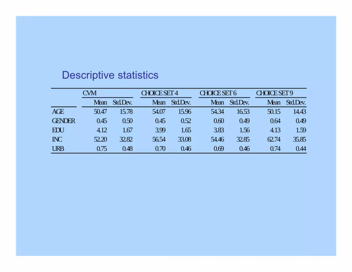
CVM CHOICE SET 4 CHOICE SET 6 CHOICE SET 9Mean Std.Dev. Mean Std.Dev. Mean Std.Dev. Mean Std.Dev.

AGE 50.47 15.78 54.07 15.96 54.34 16.53 50.15 14.43GENDER 0.45 0.50 0.45 0.52 0.60 0.49 0.64 0.49EDU 4.12 1.67 3.99 1.65 3.83 1.56 4.13 1.59INC 52.20 32.82 56.54 33.08 54.46 32.85 62.74 35.85URB 0.75 0.48 0.70 0.46 0.69 0.46 0.74 0.44

Descriptive statistics

Coeff. Std.Err. t-ratioCOST -0.009 ** 0.004 -2.550CONSTANT 0.969 ** 0.213 4.550Number of observation 305Chi-squared 6.559Log-likelihood -197.782R-squared adj. 0.021Akaike I.C. 1.310** Significant at the 0.05 level

Binomial logit: CVM

Effects codes: Choice modeling

Attributes VariablesGreen House Gas Emissions GGS 1 if small reduction ; 0 if big reduction ; -1 if no change

GGB 1 if big reduction; 0 if small reduction; -1 if no changeNitrate Leaching NLS 1 if small reduction ; 0 if big reduction ; -1 if no change

NLB 1 if big reduction; 0 if small reduction; -1 if no changeSoil Quality SOIL 1 if small change; -1 if no changeScenic Views SV 1 if more variety; -1 if no changeCost to Household COST NZ$10; $30; $60; $100

Conditional logit: Choice modeling

CHOICE SET 4 CHOICE SET 6 CHOICE SET 9Coeff. Std.Err. t-ratio Coeff. Std.Err. t-ratio Coeff. Std.Err. t-ratio

COST -0.012 ** 0.002 -4.852 -0.013 ** 0.002 -5.379 -0.011 ** 0.002 -4.903GGS 0.092 0.059 1.573 0.069 0.059 1.153 0.224 ** 0.058 3.867GGL 0.513 ** 0.073 7.016 0.440 ** 0.070 6.291 0.263 ** 0.067 3.906NLS 0.158 ** 0.067 2.362 0.167 ** 0.067 2.470 0.196 ** 0.065 2.992NLL 0.484 ** 0.066 7.302 0.399 ** 0.066 6.011 0.346 ** 0.064 5.412SOILC 0.222 ** 0.052 4.278 0.216 ** 0.052 4.158 0.212 ** 0.050 4.277SVV 0.117 ** 0.043 2.703 0.077 * 0.043 1.779 0.053 0.043 1.230A_01 0.376 0.273 1.379 0.446 * 0.260 1.712 0.212 0.261 0.813A_02 0.354 ** 0.174 2.037 0.435 ** 0.165 2.630 0.112 0.164 0.683Number of observation 1292 1264 1328Chi-squared 137.271 113.950 107.105Log-likelihood -1261.726 -1200.645 -1318.958R-squared Adj. 0.051 0.042 0.036* Significant at the 0.10 level** Significant at the 0.05 level

WTP

GGS GGL NLS NLB SQ SV ALL IMVCVM 105.27CHOICE SET 4 59.92 96.05 68.69 96.69 38.13 20.11 250.98

SET 6 45.69 75.09 58.02 76.45 34.23 12.18 197.96SET 9 65.45 68.11 66.92 85.59 38.53 9.58 196.81

Response Rate Analysis

Option A

0.010.020.030.040.050.060.070.080.090.0

1 5 9 13 17 21 25 29 33

Order Number of Choice Sets

Resp

onse

Rat

e (%

)

Choice Set 4Choice Set 6Choice Set 9

Response Rate Analysis

Option B

0.010.020.030.040.050.060.070.080.090.0

1 5 9 13 17 21 25 29 33

Order Number of Choice Sets

Resp

onse

Rat

e (%

)

Choice Set 4Choice Set 6Choice Set 9

Response Rate Analysis

Option C (Status Quo)

0.05.0

10.015.020.025.030.035.040.0

1 5 9 13 17 21 25 29 33

Order Number of Choice Sets

Res

pons

e Ra

te (%

)

Choice Set 4Choice Set 6Choice Set 9

OLS

[RATE] = f [ SET, ORDER, COST]

RATE – Response rates of choosing an optionORDER – Order of choice set (question)COST – Assigned cost for an option

OLS: Response rates (Dependent Variable)

Option A Option B Option C (Status Quo)Coeff. Std.Err. t-ratio Coeff. Std.Err. t-ratio Coeff. Std.Err. t-ratio

ONE 41.151 10.586 3.887 64.684 11.064 5.846 -5.835 3.751 -1.556SET -1.168 1.369 -0.854 -1.155 1.430 -0.807 2.323 ** 0.485 4.791ORDER 2.316 ** 0.834 2.778 -2.781 ** 0.871 -3.192 0.465 0.295 1.574COST 0.029 0.074 0.394 -0.128 0.078 -1.651 0.099 ** 0.026 3.758Observation number 108 108 108Adj R-squared 0.046 0.088 0.222Log-likelihood -4583.669 -458.435 -341.611Akaike info. 8.475 8.564 6.400Durbin-Watson 1.715 1.732 1.519* Siginificant at the 0.10 level** Siginificant at the 0.05 level

Conclusion1. CVM > Choice modeling

-Dichotomous choice format in CVM might control the process of respondent’s decisions in a similar way to the one in choice modeling

2. WTP are smaller for large choice sets in choice modeling

3. Respondents tend to choose an option with no monetary cost when they face more questions in a survey questionnaire.