Sets, Logic, Computation

Sets, Logic, ComputationAn Open Logic Text

Sets, Logic, Computation

The Open Logic Project

Instigator

Richard Zach, University of Calgary

Editorial Board

Aldo Antonelli,† University of California, DavisAndrew Arana, Université Paris I Panthénon–SorbonneJeremy Avigad, Carnegie Mellon UniversityWalter Dean, University of WarwickGillian Russell, University of North CarolinaNicole Wyatt, University of CalgaryAudrey Yap, University of Vicotoria

Contributors

Samara Burns, University of CalgaryDana Hägg, University of Calgary

Sets, Logic, ComputationAn Open Logic Text

Edited by Richard Zach

winter 2016

The Open Logic Project would like to acknowledge the generoussupport of the Faculty of Arts of the University of Calgary andthe Alberta OER Initiative.

Illustrations by Matthew Leadbeater, used under a Creative Com-mons Attribution-NonCommercial 4.0 International License.

Typeset in Baskervald X and Universalis ADF Standard by LATEX.

Sets, Logic, Computation by RichardZach is licensed under a CreativeCommons Attribution 4.0 Interna-tional License. It is based on The OpenLogic Text by the Open Logic Project,used under a Creative Commons At-tribution 4.0 International License.

http://mattleadbeater.com

http://creativecommons.org/licenses/by-nc/4.0/

http://creativecommons.org/licenses/by-nc/4.0/

https://github.com/rzach/phil379

http://richardzach.org/

http://richardzach.org/

http://creativecommons.org/licenses/by/4.0/



https://github.com/OpenLogicProject/OpenLogic

https://github.com/OpenLogicProject/OpenLogic

http://openlogicproject.org/




ContentsPreface xi

I Sets, Relations, Functions 1

1 Sets 21.1 Basics . . . . . . . . . . . . . . . . . . . . . . . . . 21.2 Some Important Sets . . . . . . . . . . . . . . . . 41.3 Subsets . . . . . . . . . . . . . . . . . . . . . . . . 51.4 Unions and Intersections . . . . . . . . . . . . . . 61.5 Proofs about Sets . . . . . . . . . . . . . . . . . . 71.6 Pairs, Tuples, Cartesian Products . . . . . . . . . 9

2 Relations 112.1 Relations as Sets . . . . . . . . . . . . . . . . . . . 112.2 Special Properties of Relations . . . . . . . . . . . 132.3 Orders . . . . . . . . . . . . . . . . . . . . . . . . 142.4 Graphs . . . . . . . . . . . . . . . . . . . . . . . . 162.5 Operations on Relations . . . . . . . . . . . . . . 17

3 Functions 193.1 Basics . . . . . . . . . . . . . . . . . . . . . . . . . 193.2 Kinds of Functions . . . . . . . . . . . . . . . . . 213.3 Inverses of Functions . . . . . . . . . . . . . . . . 22

v

vi CONTENTS

3.4 Composition of Functions . . . . . . . . . . . . . 233.5 Isomorphism . . . . . . . . . . . . . . . . . . . . . 233.6 Partial Functions . . . . . . . . . . . . . . . . . . . 243.7 Functions and Relations . . . . . . . . . . . . . . 24

4 The Size of Sets 264.1 Introduction . . . . . . . . . . . . . . . . . . . . . 264.2 Countable Sets . . . . . . . . . . . . . . . . . . . . 264.3 Uncountable Sets . . . . . . . . . . . . . . . . . . 304.4 Reduction . . . . . . . . . . . . . . . . . . . . . . 324.5 Equinumerous Sets . . . . . . . . . . . . . . . . . 334.6 Comparing Sizes of Sets . . . . . . . . . . . . . . 35

II First-order Logic 39

5 Syntax and Semantics 405.1 First-Order Languages . . . . . . . . . . . . . . . 405.2 Terms and Formulas . . . . . . . . . . . . . . . . 435.3 Unique Readability . . . . . . . . . . . . . . . . . 455.4 Main operator of a Formula . . . . . . . . . . . . 495.5 Subformulas . . . . . . . . . . . . . . . . . . . . . 505.6 Free Variables and Sentences . . . . . . . . . . . . 525.7 Substitution . . . . . . . . . . . . . . . . . . . . . 535.8 Structures for First-order Languages . . . . . . . . 545.9 Satisfaction of a Formula in a Structure . . . . . . 585.10 Extensionality . . . . . . . . . . . . . . . . . . . . 625.11 Semantic Notions . . . . . . . . . . . . . . . . . . 64

6 Theories and Their Models 666.1 Introduction . . . . . . . . . . . . . . . . . . . . . 666.2 Expressing Properties of Structures . . . . . . . . 686.3 Examples of First-Order Theories . . . . . . . . . 706.4 Expressing Relations in a Structure . . . . . . . . 736.5 The Theory of Sets . . . . . . . . . . . . . . . . . 746.6 Expressing the Size of Structures . . . . . . . . . 77

CONTENTS vii

7 Natural Deduction 797.1 Rules and Derivations . . . . . . . . . . . . . . . . 797.2 Examples of Derivations . . . . . . . . . . . . . . 827.3 Proof-Theoretic Notions . . . . . . . . . . . . . . . 877.4 Properties of Derivability . . . . . . . . . . . . . . 887.5 Soundness . . . . . . . . . . . . . . . . . . . . . . 917.6 Derivations with Identity predicate . . . . . . . . 95

8 The Completeness Theorem 978.1 Introduction . . . . . . . . . . . . . . . . . . . . . 978.2 Outline of the Proof . . . . . . . . . . . . . . . . . 988.3 Maximally Consistent Sets of Sentences . . . . . . 1008.4 Henkin Expansion . . . . . . . . . . . . . . . . . . 1028.5 Lindenbaum’s Lemma . . . . . . . . . . . . . . . 1048.6 Construction of a Model . . . . . . . . . . . . . . 1058.7 Identity . . . . . . . . . . . . . . . . . . . . . . . . 1078.8 The Completeness Theorem . . . . . . . . . . . . 1108.9 The Compactness Theorem . . . . . . . . . . . . 1118.10 The Löwenheim-Skolem Theorem . . . . . . . . . 111

9 Beyond First-order Logic 1139.1 Overview . . . . . . . . . . . . . . . . . . . . . . . 1139.2 Many-Sorted Logic . . . . . . . . . . . . . . . . . 1149.3 Second-Order logic . . . . . . . . . . . . . . . . . 1169.4 Higher-Order logic . . . . . . . . . . . . . . . . . 1219.5 Intuitionistic logic . . . . . . . . . . . . . . . . . . 1249.6 Modal Logics . . . . . . . . . . . . . . . . . . . . 1309.7 Other Logics . . . . . . . . . . . . . . . . . . . . . 132

III Turing Machines 135

10 Turing Machine Computations 13610.1 Introduction . . . . . . . . . . . . . . . . . . . . . 13610.2 Representing Turing Machines . . . . . . . . . . . 13910.3 Turing Machines . . . . . . . . . . . . . . . . . . . 144

viii CONTENTS

10.4 Configurations and Computations . . . . . . . . . 14510.5 Unary Representation of Numbers . . . . . . . . . 14710.6 Halting States . . . . . . . . . . . . . . . . . . . . 14810.7 Combining Turing Machines . . . . . . . . . . . . 14910.8 Variants of Turing Machines . . . . . . . . . . . . 15110.9 The Church-Turing Thesis . . . . . . . . . . . . . 152

11 Undecidability 15411.1 Introduction . . . . . . . . . . . . . . . . . . . . . 15411.2 Enumerating Turing Machines . . . . . . . . . . . 15611.3 The Halting Problem . . . . . . . . . . . . . . . . 15811.4 The Decision Problem . . . . . . . . . . . . . . . 16011.5 Representing Turing Machines . . . . . . . . . . . 16111.6 Verifying the Representation . . . . . . . . . . . . 16411.7 The Decision Problem is Unsolvable . . . . . . . . 168

A Induction 171A.1 Induction on N . . . . . . . . . . . . . . . . . . . 171A.2 Strong Induction . . . . . . . . . . . . . . . . . . 175A.3 Inductive Definitions . . . . . . . . . . . . . . . . 176A.4 Structural Induction . . . . . . . . . . . . . . . . . 178

B Biographies 180B.1 Georg Cantor . . . . . . . . . . . . . . . . . . . . 180B.2 Alonzo Church . . . . . . . . . . . . . . . . . . . 181B.3 Gerhard Gentzen . . . . . . . . . . . . . . . . . . 182B.4 Kurt Gödel . . . . . . . . . . . . . . . . . . . . . . 184B.5 Emmy Noether . . . . . . . . . . . . . . . . . . . 186B.6 Bertrand Russell . . . . . . . . . . . . . . . . . . . 187B.7 Alfred Tarski . . . . . . . . . . . . . . . . . . . . . 189B.8 Alan Turing . . . . . . . . . . . . . . . . . . . . . 190B.9 Ernst Zermelo . . . . . . . . . . . . . . . . . . . . 192

C Problems 194

Photo Credits 205

CONTENTS ix

Bibliography 207

PrefaceThis book is an introduction to meta-logic, aimed especially atstudents of computer science and philosophy. “Meta-logic” is so-called because it is the discipline that studies logic itself. Logicproper is concerned with canons of valid inference, and its sym-bolic or formal version presents these canons using formal lan-guages, such as those of propositional and predicate, a.k.a., first-order logic. Meta-logic investigates the properties of these lan-guage, and of the canons of correct inference that use them. Itstudies topics such as how to give precise meaning to the ex-pressions of these formal languages, how to justify the canonsof valid inference, what the properties of various proof systemsare, including their computational properties. These questionsare important and interesting in their own right, because the lan-guages and proof systems investigated are applied in many dier-ent areas—in mathematics, philosophy, computer science, andlinguistics, especially—but they also serve as examples of howto study formal systems in general. The logical languages westudy here are not the only ones people are interested in. Forinstance, linguists and philosophers are interested in languagesthat are much more complicated than those of propositional andfirst-order logic, and computer scientists are interested in otherkinds of languages altogether, such as programming languages.And the methods we discuss here—how to give semantics for for-mal languages, how to prove results about formal languages, how

xi

xii PREFACE

to investigate the properties of formal languages—are applicablein those cases as well.

Like any discipline, meta-logic both has a set of results orfacts, and a store of methods and techniques, and this text cov-ers both. Some students won’t need to know some of the resultswe discuss outside of this course, but they will need and use themethods we use to establish them. The Löwenheim-Skolem the-orem, say, does not often make an appearance in computer sci-ence, but the methods we use to prove it do. On the other hand,many of the results we discuss do have relevance for certain de-bates, say, in the philosophy of science and in metaphysics. Phi-losophy students may not need to be able to prove these resultsoutside this course, but they do need to understand what theresults are—and you really only understand these results if youhave thought through the definitions and proofs needed to es-tablish them. These are, in part, the reasons for why the resultsand the methods covered in this text are recommended study—insome cases even required—for students of computer science andphilosophy.

The material is divided into three parts. Part 1 concerns it-self with the theory of sets. Logic and meta-logic is historicallyconnected very closely to what’s called the “foundations of math-ematics.” Mathematical foundations deal with how ultimatelymathematical objects such as integers, rational, and real num-bers, functions, spaces, etc., should be understood. Set theoryprovides one answer (there are others), and so set theory andlogic have long been studied side-by-side. Sets, relations, andfunctions are also ubiquitous in any sort of formal investigation,not just in mathematics but also in computer science and in someof the more technical corners of philosophy. Certainly for thepurposes of formulating and proving results about the semanticsand proof theory of logic and the foundation of computability itis essential to have a language in which to do this. For instance,we will talk about sets of expressions, relations of consequenceand provability, interpretations of predicate symbols (which turnout to be relations), computable functions, and various relations

xiii

between and constructions using these. It will be good to haveshorthand symbols for these, and think through the general prop-erties of sets, relations, and functions in order to do that. If youare not used to thinking mathematically and to formulating math-ematical proofs, then think of the first part on set theory as atraining ground: all the basic definitions will be given, and we’llgive increasingly complicated proofs using them. Note that un-derstanding these proofs—and being able to find and formulatethem yourself—is perhaps more important than understandingthe results, and especially in the first part, and especially if youare new to mathematical thinking, it is important that you thinkthrough the examples and do the problems in appendix C.

In the first part we will establish one important result, how-ever. This result—Cantor’s theorem—relies on one of the moststriking examples of conceptual analysis to be found anywherein the sciences, namely, Cantor’s analysis of infinity. Infinity haspuzzled mathematicians and philosophers alike for centuries. No-one knew how to properly think about it. Many people eventhought it was a mistake to think about it at all, that the notionof an infinite object or infinite collection itself was incoherent.Cantor made infinity into a subject we can coherently work with,and developed an entire theory of infinite collections—and in-finite numbers with which we can measure the sizes of infinitecollections—and showed that there are dierent levels of infinity.This theory of “transfinite” numbers is beautiful and intricate,and we won’t get very far into it; but we will be able to showthat there are dierent levels of infinity, specifically, that thereare “countable” and “uncountable” levels of infinity. This resulthas important applications, but it is also really the kind of re-sult that any self-respecting mathematician, computer scientist,or philosopher should know.

In the second part we turn to first-order logic. We will definethe language of first-order logic and its semantics, i.e., what first-order structures are and when a sentence of first-order logic istrue in a structure. This will enable us to do two important things:(1) We can define, with mathematical precision, when a sentence

xiv PREFACE

is a logical consequence of another. (2) We can also consider howthe relations that make up a first-order structure are described—characterized—by the sentences that are true in them. This inparticular leads us to a discussion of the axiomatic method, inwhich sentences of first-order languages are used to characterizecertain kinds of structures. Proof theory will occupy us next,and we will consider the original version of natural deduction asdefined in the 1930s by Gerhard Gentzen. The semantic notion ofconsequence and the syntactic notion of provability give us twocompletely dierent ways to make precise the idea that a sentencemay follow from some others. The soundness and completenesstheorems link these two characterization. In particular, we willprove Gödel’s completeness theorem, which states that whenevera sentence is a semantic consequence of some others, there is alsoa deduction of said sentence from these others. An equivalentformulation is: if a collection of sentences is consistent—in thesense that nothing contradictory can be proved from them—thenthere is a structure that makes all of them true.

The second formulation of the completeness theorem is per-haps the more surprising. Around the time Gödel proved thisresult (in 1929), the German mathematician David Hilbert fa-mously held the view that consistency (i.e., freedom from con-tradiction) is all that mathematical existence requires. In otherwords, whenever a mathematician can coherently describe a struc-ture or class of structures, then they should be be entitled to be-lieve in the existence of such structures. At the time, many foundthis idea preposterous: just because you can describe a structurewithout contradicting yourself, it surely does not follow that sucha structure actually exists. But that is exactly what Gödel’s com-pleteness theorem says. In addition to this paradoxical—and cer-tainly philosophically intriguing aspect—the completeness theo-rem also has two important applications which allow us to provefurther results about the existence of structures which make givensentences true. These are the compactness and the Löwenheim-Skolem theorem.

In the third part, we connect logic with computability. Again,

xv

there is a historical connection: David Hilbert had posed as afundamental problem of logic to find a mechanical method whichwould decide, of a given sentence of logic, whether it has a proof.Such a method exists, of course, for propositional logic: one justhas to check all truth tables, and since there are only finitely manyof them, the method eventually yields a correct answer. Such astraightforward method is not possible for first-order logic, sincethe number of possible structures is infinite (and structures them-selves may be infinite). Logicians were working on finding a moreingenious methods for years. Two logicians—Alonzo Churchand Alan Turing—eventually established that there is no suchmethod. In order to do this, it was necessary to first providea precise definition of what a mechanical method is in general.If an eective method had been proposed, anyone would haverecognized it as an eective method. To prove that no eectivemethod exists, you have to define “eective method” first andgive an impossibility proof on the basis of that definition. Thisis what Turing did: he proposed the idea of a Turing machine1

as a mathematical model of what a mechanical procedure can,in principle, do. This is another example of a conceptual analysisof an informal concept using mathematical machinery; and it isperhaps of the same order of importance for computer science asCantor’s analysis of infinity is for mathematics. Our last majorundertaking will be the proof of two impossibility theorems: wewill show that the so-called “halting problem” cannot be solvedby Turing machines, and finally that Hilbert’s “decision problem”(for logic) also cannot.

This text is mathematical, in the sense that we discuss math-ematical definitions and prove our results mathematically. But itis not mathematical in the sense that you need extensive math-ematical background knowledge. Nothing in this text requiresadvanced knowledge of algebra, trigonometry, or calculus. Wehave made a special eort to also not require any familiarity withthe way mathematics works: in fact, part of the point is to develop

1Turing of course did not call it that himself.

xvi PREFACE

the kinds of reasoning and proof skills required to understandand prove our results. The organization of the text follows math-ematical convention, for one reason: these conventions have beendeveloped because clarity and precision are especially important,and so, e.g., it is critical to know when something is asserted asthe conclusion of an argument, is oered as a reason for some-thing else, or is intended to introduce new vocabulary. So we fol-low mathematical convention and label passages as “definitions”if they are used to introduce new terminology or symbols; and as“theorems,” “propositions,” “lemmas,” or “corollaries” when werecord a result or finding.2 Other than these conventions, we willonly use the methods of logical proof as they should be familiarfrom a first logic course, with one exception: we will make exten-sive use of the method of induction to prove results. Appendix Ais devoted to this principle.

2The dierence between the latter four is not terribly important, butroughly: A theorem is an important result. A proposition is a result worthrecording, but perhaps not as important as a theorem. A lemma is a result wemainly record only because we want to break up a proof into smaller, easier tomanage chunks. A corollary is a result that follows easily from a theorem orproposition, such as an interesting special case.

PART I

Sets,Relations,Functions

1

CHAPTER 1

Sets1.1 Basics

Sets are the most fundamental building blocks of mathematicalobjects. In fact, almost every mathematical object can be seen asa set of some kind. In logic, as in other parts of mathematics,sets and set theoretical talk is ubiquitous. So it will be importantto discuss what sets are, and introduce the notations necessaryto talk about sets and operations on sets in a standard way.

Denition 1.1. A set is a collection of objects, considered inde-pendently of the way it is specified, of the order of the objects inthe set, or of their multiplicity. The objects making up the setare called elements or members of the set. If a is an element of aset X , we write a ∈ X (otherwise, a < X ). The set which has noelements is called the empty set and denoted by the symbol ∅.

Example 1.2. Whenever you have a bunch of objects, you cancollect them together in a set. The set of Richard’s siblings, forinstance, is a set that contains one person, and we could writeit as S = Ruth. In general, when we have some objects a1,. . . , an , then the set consisting of exactly those objects is writtena1, . . . , an. Frequently we’ll specify a set by some property thatits elements share—as we just did, for instance, by specifying Sas the set of Richard’s siblings. We’ll use the following shorthand

2

1.1. BASICS 3

notation for that: x : . . . x . . ., where the . . . x . . . stands for theproperty that x has to have in order to be counted among theelements of the set. In our example, we could have specified Salso as

S = x : x is a sibling of Richard.When we say that sets are independent of the way they are

specified, we mean that the elements of a set are all that matters.For instance, it so happens that

Nicole, Jacob,x : x is a niece or nephew of Richard, andx : x is a child of Ruth

are three ways of specifying one and the same set.Saying that sets are considered independently of the order of

their elements and their multiplicity is a fancy way of saying that

Nicole, Jacob and

Jacob,Nicoleare two ways of specifying the same set; and that

Nicole, Jacob and

Jacob,Nicole,Nicoleare also two ways of specifying the same set. In other words, allthat matters is which elements a set has. The elements of a setare not ordered and each element occurs only once. When wespecify or describe a set, elements may occur multiple times and indierent orders, but any descriptions that only dier in the orderof elements or in how many times elements are listed describesthe same set.

Denition 1.3 (Extensionality). If X andY are sets, then X andY are identical, X =Y , i every element of X is also an elementofY , and vice versa.

4 CHAPTER 1. SETS

Extensionality gives us a way for showing that sets are iden-tical: to show that X = Y , show that whenever x ∈ X then alsox ∈Y , and whenever y ∈Y then also y ∈ X .

1.2 Some Important Sets

Example 1.4. Mostly we’ll be dealing with sets that have mathe-matical objects as members. You will remember the various setsof numbers: N is the set of natural numbers 0, 1, 2, 3, . . . ; Z theset of integers,

. . . ,−3,−2,−1, 0, 1, 2, 3, . . . ;Q the set of rationals (Q = z/n : z ∈ Z, n ∈ N, n , 0); and R theset of real numbers. These are all innite sets, that is, they eachhave infinitely many elements. As it turns out, N, Z, Q have thesame number of elements, while R has a whole bunch more—N,Z, Q are “countable and infinite” whereas R is “uncountable”.

We’ll sometimes also use the set of positive integers Z+ =1, 2, 3, . . . and the set containing just the first two natural num-bers B = 0, 1.Example 1.5 (Strings). Another interesting example is the setA∗ of nite strings over an alphabet A: any finite sequence ofelements of A is a string over A. We include the empty string Λamong the strings over A, for every alphabet A. For instance,

B∗ = Λ, 0, 1, 00, 01, 10, 11,000, 001, 010, 011, 100, 101, 110, 111, 0000, . . ..

If x = x1 . . . xn ∈ A∗is a string consisting of n “letters” from A,then we say length of the string is n and write len(x) = n.Example 1.6 (Infinite sequences). For any set A we may alsoconsider the set Aω of infinite sequences of elements of A. Aninfinite sequence a1a2a3a4 . . . consists of a one-way infinite list ofobjects, each one of which is an element of A.

1.3. SUBSETS 5

1.3 Subsets

Sets are made up of their elements, and every element of a set is apart of that set. But there is also a sense that some of the elementsof a set taken together are a “part of” that set. For instance, thenumber 2 is part of the set of integers, but the set of even numbersis also a part of the set of integers. It’s important to keep thosetwo senses of being part of a set separate.

Denition 1.7. If every element of a set X is also an element ofY , then we say that X is a subset ofY , and write X ⊆ Y .

Example 1.8. First of all, every set is a subset of itself, and ∅ isa subset of every set. The set of even numbers is a subset of theset of natural numbers. Also, a, b ⊆ a, b, c.

But a, b, e is not a subset of a, b, c.Note that a set may contain other sets, not just as subsets but

as elements! In particular, a set may happen to both be an elementand a subset of another, e.g., 0 ∈ 0, 0 and also 0 ⊆0, 0.

Extensionality gives a criterion of identity for sets: X =Y ievery element of X is also an element of Y and vice versa. Thedefinition of “subset” defines X ⊆ Y precisely as the first half ofthis criterion: every element of X is also an element of Y . Ofcourse the definition also applies if we switch X and Y : Y ⊆ Xi every element ofY is also an element of X . And that, in turn,is exactly the “vice versa” part of extensionality. In other words,extensionality amounts to: X =Y i X ⊆ Y anY ⊆ X .

Denition 1.9. The set consisting of all subsets of a set X iscalled the power set of X , written ℘(X ).

℘(X ) = x : x ⊆ X Example 1.10. What are all the possible subsets of a, b, c?They are: ∅, a, b, c, a, b, a, c, b, c, a, b, c. Theset of all these subsets is ℘(a, b, c):

℘(a, b, c) = ∅, a, b, c, a, b, b, c, a, c, a, b, c

6 CHAPTER 1. SETS

1.4 Unions and Intersections

Denition 1.11. The union of two sets X andY , written X ∪Y ,is the set of all things which are elements of X ,Y , or both.

X ∪Y = x : x ∈ X ∨ x ∈Y Example 1.12. Since the multiplicity of elements doesn’t matter,the union of two sets which have an element in common containsthat element only once, e.g., a, b, c ∪ a, 0, 1 = a, b, c, 0, 1.

The union of a set and one of its subsets is just the bigger set:a, b, c ∪ a = a, b, c.

The union of a set with the empty set is identical to the set:a, b, c ∪ ∅ = a, b, c.Denition 1.13. The intersection of two sets X and Y , writtenX ∩ Y , is the set of all things which are elements of both XandY .

X ∩Y = x : x ∈ X ∧ x ∈Y Two sets are called disjoint if their intersection is empty. Thismeans they have no elements in common.

Example 1.14. If two sets have no elements in common, theirintersection is empty: a, b, c ∩ 0, 1 = ∅.

If two sets do have elements in common, their intersection isthe set of all those: a, b, c ∩ a, b,d = a, b.

The intersection of a set with one of its subsets is just thesmaller set: a, b, c ∩ a, b = a, b.

The intersection of any set with the empty set is empty: a, b, c∩∅ = ∅.

We can also form the union or intersection of more than twosets. An elegant way of dealing with this in general is the follow-ing: suppose you collect all the sets you want to form the union(or intersection) of into a single set. Then we can define the unionof all our original sets as the set of all objects which belong to atleast one element of the set, and the intersection as the set of allobjects which belong to every element of the set.

1.5. PROOFS ABOUT SETS 7

Denition 1.15. If C is a set of sets, then⋃C is the set of

elements of elements of C :⋃C = x : x belongs to an element of C , i.e.,⋃C = x : there is a y ∈ C so that x ∈ y

Denition 1.16. IfC is a set of sets, then⋂C is the set of objects

which all elements of C have in common:⋂C = x : x belongs to every element of C , i.e.,⋂C = x : for all y ∈ C, x ∈ y

Example 1.17. SupposeC = a, b, a,d, e , a,d . Then⋃C =a, b,d, e and

⋂C = a.

We could also do the same for a sequence of sets A1, A2, . . .⋃i

Ai = x : x belongs to one of the Ai ⋂i

Ai = x : x belongs to every Ai .

Denition 1.18. The dierence X \Y is the set of all elements ofX which are not also elements ofY , i.e.,

X \Y = x : x ∈ X and x <Y .

1.5 Proofs about Sets

Sets and the notations we’ve introduced so far provide us withconvenient shorthands for specifying sets and expressing rela-tionships between them. Often it will also be necessary to proveclaims about such relationships. If you’re not familiar with math-ematical proofs, this may be new to you. So we’ll walk througha simple example. We’ll prove that for any sets X and Y , it’salways the case that X ∩ (X ∪Y ) = X . How do you prove anidentity between sets like this? Recall that sets are determined

8 CHAPTER 1. SETS

solely by their elements, i.e., sets are identical i they have thesame elements. So in this case we have to prove that (a) everyelement of X ∩ (X ∪Y ) is also an element of X and, conversely,that (b) every element of X is also an element of X ∩ (X ∪Y ).In other words, we show that both (a) X ∩ (X ∪Y ) ⊆ X and (b)X ⊆ X ∩ (X ∪Y ).

A proof of a general claim like “every element z of X ∩(X ∪Y )is also an element of X ” is proved by first assuming that an arbi-trary z ∈ X ∩ (X ∪Y ) is given, and proving from this assumtionthat z ∈ X . You may know this pattern as “general conditionalproof.” In this proof we’ll also have to make use of the definitionsinvolved in the assumption and conclusion, e.g., in this case of“∩” and “∪.” So case (a) would be argued as follows:

(a) We first want to show that X ∩ (X ∪Y ) ⊆ X , i.e.,by definition of ⊆, that if z ∈ X ∩ (X ∪Y ) then z ∈ X ,for any z . So assume that z ∈ X ∩ (X ∪Y ). Sincez is an element of the intersection of two sets i it isan element of both sets, we can conclude that z ∈ Xand also z ∈ X ∪Y . In particular, z ∈ X . But this iswhat we wanted to show.

This completes the first half of the proof. Note that in thelast step we used the fact that if a conjunction (z ∈ X and z ∈X ∪Y ) follows from an assumption, each conjunct follows fromthat same assumption. You may know this rule as “conjunctionelimination,” or ∧Elim. Now let’s prove (b):

(b) We now prove that X ⊆ X ∩ (X ∪ Y ), i.e., bydefinition of ⊆, that if z ∈ X then also z ∈ X ∩(X ∪Y ),for any z . Assume z ∈ X . To show that z ∈ X ∩ (X ∪Y ), we have to show (by definition of “∩”) that (i)z ∈ X and also (ii) z ∈ X ∪Y . Here (i) is just ourassumption, so there is nothing further to prove. For(ii), recall that z is an element of a union of sets iit is an element of at least one of those sets. Since

1.6. PAIRS, TUPLES, CARTESIAN PRODUCTS 9

z ∈ X , and X ∪Y is the union of X and Y , this isthe case here. So z ∈ X ∪Y . We’ve shown both (i)z ∈ X and (ii) z ∈ X ∪Y , hence, by definition of “∩,”z ∈ X ∩ (X ∪Y ).

This was somewhat long-winded, but it illustrates how we rea-son about sets and their relationships. We usually aren’t this ex-plicit; in particular, we might not repeat all the definitions. A“textbook” proof of our result would look something like this.

Proposition 1.19 (Absorption). For all sets X ,Y ,

X ∩ (X ∪Y ) = X

Proof. (a) Suppose z ∈ X ∩(X ∪Y ). Then z ∈ X , so X ∩(X ∪Y ) ⊆X .

(b) Now suppose z ∈ X . Then also z ∈ X ∪Y , and thereforealso z ∈ X ∩ (X ∪Y ). Thus, X ⊆ X ∩ (X ∪Y ).

1.6 Pairs, Tuples, Cartesian Products

Sets have no order to their elements. We just think of them as anunordered collection. So if we want to represent order, we useordered pairs 〈x, y〉, or more generally, ordered n-tuples 〈x1, . . . , xn〉.Denition 1.20. Given sets X andY , their Cartesian product X ×Y is 〈x, y〉 : x ∈ X and y ∈Y .Example 1.21. If X = 0, 1, andY = 1, a, b, then their prod-uct is

X ×Y = 〈0, 1〉, 〈0, a〉, 〈0, b〉, 〈1, 1〉, 〈1, a〉, 〈1, b〉.Example 1.22. If X is a set, the product of X with itself, X ×X ,is also written X 2. It is the set of all pairs 〈x, y〉 with x, y ∈ X .The set of all triples 〈x, y, z 〉 is X 3, and so on.

10 CHAPTER 1. SETS

Example 1.23. If X is a set, a word over X is any sequence ofelements of X . A sequence can be thought of as an n-tuple of ele-ments of X . For instance, if X = a, b, c, then the sequence “bac”can be though of as the triple 〈b, a, c〉. Words, i.e., sequencesof symbols, are of crucial importance in computer science, ofcourse. By convention, we count elements of X as sequences oflength 1, and ∅ as the sequence of length 0. The set of all wordsover X then is

X ∗ = ∅ ∪ X ∪ X 2 ∪ X 3 ∪ . . .

CHAPTER 2

Relations2.1 Relations as Sets

You will no doubt remember some interesting relations betweenobjects of some of the sets we’ve mentioned. For instance, num-bers come with an order relation < and from the theory of wholenumbers the relation of divisibility without remainder (usually writ-ten n | m) may be familar. There is also the relation is identicalwith that every object bears to itself and to no other thing. Butthere are many more interesting relations that we’ll encounter,and even more possible relations. Before we review them, we’lljust point out that we can look at relations as a special sort ofset. For this, first recall what a pair is: if a and b are two objects,we can combine them into the ordered pair 〈a, b〉. Note that forordered pairs the order does matter, e.g, 〈a, b〉 , 〈b, a〉, in contrastto unordered pairs, i.e., 2-element sets, where a, b = b, a.

If X andY are sets, then the Cartesian product X ×Y of X andY is the set of all pairs 〈a, b〉 with a ∈ X and b ∈Y . In particular,X 2 = X × X is the set of all pairs from X .

Now consider a relation on a set, e.g., the <-relation on theset N of natural numbers, and consider the set of all pairs ofnumbers 〈n,m〉 where n < m, i.e.,

R = 〈n,m〉 : n,m ∈ N and n < m.Then there is a close connection between the number n being

11

12 CHAPTER 2. RELATIONS

less than a number m and the corresponding pair 〈n,m〉 being amember of R, namely, n < m if and only if 〈n,m〉 ∈ R. In a sensewe can consider the set R to be the <-relation on the set N. In thesame way we can construct a subset ofN2 for any relation betweennumbers. Conversely, given any set of pairs of numbers S ⊆ N2,there is a corresponding relation between numbers, namely, therelationship n bears to m if and only if 〈n,m〉 ∈ S . This justifiesthe following definition:

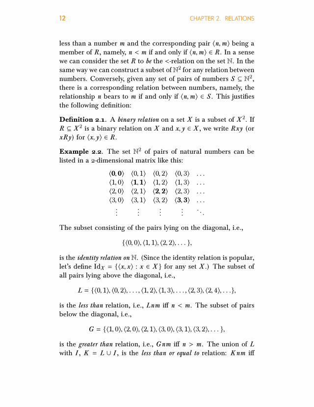
Denition 2.1. A binary relation on a set X is a subset of X 2. IfR ⊆ X 2 is a binary relation on X and x, y ∈ X , we write Rxy (orxRy) for 〈x, y〉 ∈ R.Example 2.2. The set N2 of pairs of natural numbers can belisted in a 2-dimensional matrix like this:

〈0, 0〉〈0, 1〉〈0, 2〉〈0, 3〉 . . .

〈1, 0〉〈1, 1〉〈1, 2〉〈1, 3〉 . . .

〈2, 0〉〈2, 1〉〈2, 2〉〈2, 3〉 . . .

〈3, 0〉〈3, 1〉〈3, 2〉〈3, 3〉 . . ....

......

.... . .

The subset consisting of the pairs lying on the diagonal, i.e.,

〈0, 0〉, 〈1, 1〉, 〈2, 2〉, . . . ,is the identity relation on N. (Since the identity relation is popular,let’s define IdX = 〈x, x〉 : x ∈ X for any set X .) The subset ofall pairs lying above the diagonal, i.e.,

L = 〈0, 1〉, 〈0, 2〉, . . . , 〈1, 2〉, 〈1, 3〉, . . . , 〈2, 3〉, 〈2, 4〉, . . .,is the less than relation, i.e., Lnm i n < m. The subset of pairsbelow the diagonal, i.e.,

G = 〈1, 0〉, 〈2, 0〉, 〈2, 1〉, 〈3, 0〉, 〈3, 1〉, 〈3, 2〉, . . . ,is the greater than relation, i.e., Gnm i n > m. The union of Lwith I , K = L ∪ I , is the less than or equal to relation: Knm i

2.2. SPECIAL PROPERTIES OF RELATIONS 13

n ≤ m. Similarly, H = G ∪ I is the greater than or equal to relation.L, G , K , and H are special kinds of relations called orders. L andG have the property that no number bears L or G to itself (i.e.,for all n, neither Lnn nor Gnn). Relations with this property arecalled antireexive, and, if they also happen to be orders, they arecalled strict orders.

Although orders and identity are important and natural rela-tions, it should be emphasized that according to our definitionany subset of X 2 is a relation on X , regardless of how unnaturalor contrived it seems. In particular, ∅ is a relation on any set (theempty relation, which no pair of elements bears), and X 2 itselfis a relation on X as well (one which every pair bears), calledthe universal relation. But also something like E = 〈n,m〉 : n >

5 or m × n ≥ 34 counts as a relation.

2.2 Special Properties of Relations

Some kinds of relations turn out to be so common that they havebeen given special names. For instance, ≤ and ⊆ both relate theirrespective domains (say, N in the case of ≤ and ℘(X ) in the caseof ⊆) in similar ways. To get at exactly how these relations aresimilar, and how they dier, we categorize them according tosome special properties that relations can have. It turns out that(combinations of) some of these special properties are especiallyimportant: orders and equivalence relations.

Denition 2.3. A relation R ⊆ X 2 is reexive i, for every x ∈ X ,Rxx .

Denition 2.4. A relation R ⊆ X 2 is transitive i, whenever Rxyand Ryz , then also Rxz .

Denition 2.5. A relationR ⊆ X 2 is symmetric i, wheneverRxy ,then also Ryx .


Denition 2.6. A relation R ⊆ X 2 is anti-symmetric i, wheneverboth Rxy and Ryx , then x = y (or, in other words: if x , y theneither ¬Rxy or ¬Ryx).

In a symmetric relation, Rxy and Ryx always hold together,or neither holds. In an anti-symmetric relation, the only way forRxy and Ryx to hold together is if x = y . Note that this does notrequire that Rxy and Ryx holds when x = y , only that it isn’t ruledout. So an anti-symmetric relation can be reflexive, but it is notthe case that every anti-symmetric relation is reflexive. Also notethat being anti-symmetric and merely not being symmetric aredierent conditions. In fact, a relation can be both symmetricand anti-symmetric at the same time (e.g., the identity relationis).

Denition 2.7. A relation R ⊆ X 2 is connected if for all x, y ∈ X ,if x , y , then either Rxy or Ryx .

Denition 2.8. A relation R ⊆ X 2 that is reflexive, transitive,and anti-symmetric is called a partial order. A partial order thatis also connected is called a linear order.

Denition 2.9. A relation R ⊆ X 2 that is reflexive, symmetric,and transitive is called an equivalence relation.

2.3 Orders

Denition 2.10. A relation which is both reflexive and transitiveis called a preorder. A preorder which is also anti-symmetric iscalled a partial order. A partial order which is also connected iscalled a total order or linear order. (If we want to emphasize thatthe order is reflexive, we add the adjective “weak”—see below).

Example 2.11. Every linear order is also a partial order, and ev-ery partial order is also a preorder, but the converses don’t hold.For instance, the identity relation and the full relation on X arepreorders, but they are not partial orders, because they are not

2.3. ORDERS 15

anti-symmetric (if X has more than one element). For a some-what less silly example, consider the no longer than relation 4on B∗: x 4 y i len(x) ≤ len(y). This is a preorder, even a linearpreorder, but not a partial order.

The relation of divisibility without remainder gives us an ex-ample of a partial order which isn’t a linear order: for integersn, m, we say n (evenly) divides m, in symbols: n | m, if there issome k so that m = kn. On N, this is a partial order, but not alinear order: for instance, 2 - 3 and also 3 - 2. Considered as arelation on Z, divisibility is only a preorder since anti-symmetryfails: 1 | −1 and −1 | 1 but 1 , −1. Another important partialorder is the relation ⊆ on a set of sets.

Notice that the examples L andG from Example 2.2, althoughwe said there that they were called “strict orders” are not linearorders even though they are connected (they are not reflexive).But there is a close connection, as we will see momentarily.

Denition 2.12. A relation R on X is called irreexive if, forall x ∈ X , ¬Rxx . R is called asymmetric if for no pair x, y ∈ Xwe have Rxy and Ryx . A strict partial order is a relation whichis irreflexive, asymmetric, and transitive. A strict partial orderwhich is also connected is called a strict linear order.

A strict partial orderR on X can be turned into a weak partialorder R ′by adding the identity relation on X : R ′ = R ∪ IdX .Conversely, starting from a weak partial order, one can get astrict partial order by removing IdX , i.e., R ′ = R \ IdX .

Proposition 2.13. R is a strict partial (linear) order on X i R ′ isa weak partial (linear) order. Moreover, Rxy i R ′xy for all x , y .

Example 2.14. ≤ is the weak linear order corresponding to thestrict linear order <. ⊆ is the weak partial order correspondingto the strict partial order (.


2.4 Graphs

A graph is a diagram in which points—called “nodes” or “ver-tices” (plural of “vertex”)—are connected by edges. Graphs area ubiquitous tool in descrete mathematics and in computer sci-ence. They are incredibly useful for representing, and visualizing,relationships and structures, from concrete things like networksof various kinds to abstract structures such as the possible out-comes of decisions. There are many dierent kinds of graphs inthe literature which dier, e.g., according to whether the edgesare directed or not, have labels or not, whether there can be edgesfrom a node to the same node, multiple edges between the samenodes, etc. Directed graphs have a special connection to relations.

Denition 2.15. A directed graph G = 〈V,E〉 is a set of vertices Vand a set of edges E ⊆ V 2.

According to our definition, a graph just is a set together witha relation on that set. Of course, when talking about graphs, it’sonly natural to expect that they are graphically represented: wecan draw a graph by connecting two vertices v1 and v2 by anarrow i 〈v1,v2〉 ∈ E . The only dierence between a relation byitself and a graph is that a graph specifies the set of vertices, i.e., agraph may have isolated vertices. The important point, however,is that every relation R on a set X can be seen as a directed graph〈X ,R〉, and conversely, a directed graph 〈V,E〉 can be seen as arelation E ⊆ V 2 with the set V explicitly specified.

Example 2.16. The graph 〈V,E〉 with V = 1, 2, 3, 4 and E =〈1, 1〉, 〈1, 2〉, 〈1, 3〉, 〈2, 3〉 looks like this:

1 2

3

4

2.5. OPERATIONS ON RELATIONS 17

This is a dierent graph than 〈V ′,E〉 with V ′ = 1, 2, 3, whichlooks like this:

1 2

3

2.5 Operations on Relations

It is often useful to modify or combine relations. We’ve alreadyused the union of relations above (which is just the union of tworelations considered as sets of pairs). Here are some other ways:

Denition 2.17. Let R, S ⊆ X 2 be relations andY a set.

1. The inverse R−1 of R is R−1 = 〈y, x〉 : 〈x, y〉 ∈ R.2. The relative product R | S of R and S is

(R | S ) = 〈x, z 〉 : for some y,Rxy and S yz

3. The restriction R Y of R toY is R ∩Y 2

4. The application R[Y ] of R toY is

R[Y ] = y : for some x ∈ X ,Rxy

Example 2.18. Let S ⊆ Z2 be the successor relation on Z, i.e.,the set of pairs 〈x, y〉 where x + 1 = y , for x, y ∈ Z. Sxy holds i yis the successor of x .

1. The inverse S −1 of S is the predecessor relation, i.e., S −1xyi x − 1 = y .


2. The relative product S | S is the relation x bears to y ifx + 2 = y .

3. The restriction of S to N is the successor relation on N.

4. The application of S to a set, e.g., S [1, 2, 3] is 2, 3, 4.Denition 2.19. The transitive closure R+ of a relation R ⊆ X 2

is R+ =⋃∞i=1R

i where R1 = R and Ri+1 = Ri | R.The reexive transitive closure of R is R∗ = R+ ∪ IX .

Example 2.20. Take the successor relation S ⊆ Z2. S 2xy ix + 2 = y , S 3xy i x + 3 = y , etc. So R∗xy i for some i ≥ 1,x + i = y . In other words, S +xy i x < y (and R∗xy i x ≤ y).

CHAPTER 3

Functions3.1 Basics

A function is a mapping of which pairs each object of a given setwith a unique partner. For instance, the operation of adding 1defines a function: each number n is paired with a unique num-ber n + 1. More generally, functions may take pairs, triples, etc.,of inputs and returns some kind of output. Many functions arefamiliar to us from basic arithmetic. For instance, addition andmultiplication are functions. They take in two numbers and re-turn a third. In this mathematical, abstract sense, a function isa black box: what matters is only what output is paired with whatinput, not the method for calculating the output.

Denition 3.1. A function f : X →Y is a mapping of each ele-ment of X to an element of Y . We call X the domain of f andY the codomain of f . The range ran(f ) of f is the subset of thecodomain that is actually output by f for some input.

Example 3.2. Multiplication takes pairs of natural numbers asinputs and maps them to natural numbers as outputs, so goesfrom N × N (the domain) to N (the codomain). As it turns out,the range is also N, since every n ∈ N is n × 1.

Multiplication is a function because it pairs each input—eachpair of natural numbers—with a single output: × : N2 → N. By

19

20 CHAPTER 3. FUNCTIONS

contrast, the square root operation applied to the domain N isnot functional, since each positive integer n has two square roots:√n and −

√n. We can make it functional by only returning the

positive square root:√

: N → R. The relation that pairs eachstudent in a class with their final grade is a function—no studentcan get two dierent final grades in the same class. The rela-tion that pairs each student in a class with their parents is not afunction—generally each student will have at least two parents.

Example 3.3. Let f : N → N be defined such that f (x) = x + 1.This is a definition that specifies f as a function which takes innatural numbers and outputs natural numbers. It tells us that,given a natural number x , f will output its successor x + 1. Inthis case, the codomain N is not the range of f , since the naturalnumber 0 is not the successor of any natural number. The rangeof f is the set of all positive integers, Z+.

Example 3.4. Let g : N→ N be defined such that g (x) = x+2−1.This tells us that g is a function which takes in natural numbersand outputs natural numbers. Given a natural number n, g willoutput the predecessor of the successor of the successor of x , i.e.,x + 1. Despite their dierent definitions, g and f are the samefunction.

Functions f and g defined above are the same because forany natural number x , x + 2 − 1 = x + 1. f and g pair eachnatural number with the same output. The definitions for f andg specify the same mapping by means of dierent equations, andso count as the same function.

Example 3.5. We can also define functions by cases. For in-stance, we could define h : N→ N by

h(x) =

x2 if x is evenx+12 if x is odd.

Since every natural number is either even or odd, the output ofthis function will always be a natural number. Just remember that

3.2. KINDS OF FUNCTIONS 21

if you define a function by cases, every possible input must fallinto exactly one case.

3.2 Kinds of Functions

Denition 3.6. A function f : X → Y is surjective i Y is alsothe range of f , i.e., for every y ∈ Y there is at least one x ∈ Xsuch that f (x) = y .

If you want to show that a function is surjective, then youneed to show that every object in the codomain is the output ofthe function given some input or other.

Denition 3.7. A function f : X → Y is injective i for eachy ∈Y there is at most one x ∈ X such that f (x) = y .

Any function pairs each possible input with a unique output.An injective function has a unique input for each possible output.If you want to show that a function f is injective, you need toshow that for any element y of the codomain, if f (x) = y andf (w) = y , then x = w .

A function which is neither injective, nor surjective, is theconstant function f : N→ N where f (x) = 1.

A function which is both injective and surjective is the identityfunction f : N→ N where f (x) = x .

The successor function f : N → N where f (x) = x + 1 isinjective, but not surjective.

The function

f (x) =

x2 if x is evenx+12 if x is odd.

is surjective, but not injective.

Denition 3.8. A function f : X → Y is bijective i it is bothsurjective and injective. We call such a function a bijection fromX toY (or between X andY ).


3.3 Inverses of Functions

One obvious question about functions is whether a given map-ping can be “reversed.” For instance, the successor functionf (x) = x + 1 can be reversed in the sense that the functiong (y) = y − 1 “undos” what f does. But we must be careful: Whilethe definition of g defines a function Z → Z, it does not definea function N → N (g (0) < N). So even in simple cases, it is notquite obvious if functions can be reversed, and that it may dependon the domain and codomain. Let’s give a precise definition.

Denition 3.9. A function g : Y → X is an inverse of a functionf : X →Y if f (g (y)) = y and g (f (x)) = x for all x ∈ X and y ∈Y .

When do functions have inverses? A good candidate for aninverse of f : X →Y is g : Y → X “defined by”

g (y) = “the” x such that f (x) = y .

The scare quotes around “defined by” suggest that this is nota definition. At least, it is not in general. For in order for thisdefinition to specify a function, there has to be one and only one xsuch that f (x) = y—the output of g has to be uniquely specified.Moreover, it has to be specified for every y ∈ Y . If there are x1and x2 ∈ X with x1 , x2 but f (x1) = f (x2), then g (y) would notbe uniquely specified for y = f (x1) = f (x2). And if there is no xat all such that f (x) = y , then g (y) is not specified at all. In otherwords, for g to be defined, f has to be injective and surjective.

Proposition 3.10. If f : X → Y is bijective, f has a unique in-verse f −1 : Y → X .

Proof. Exercise.

3.4. COMPOSITION OF FUNCTIONS 23

3.4 Composition of Functions

We have already seen that the inverse f −1 of a bijective function fis itself a function. It is also possible to compose functions f andg to define a new function by first applying f and then g . Ofcourse, this is only possible if the domains and codomains match,i.e., the codomain of f must be a subset of the domain of g .

Denition 3.11. Let f : X →Y and g : Y → Z . The compositionof f with g is the function (g f ) : X → Z , where (g f )(x) =g (f (x)).

The function (g f ) : X → Z pairs each member of X witha member of Z . We specify which member of Z a member of Xis paired with as follows—given an input x ∈ X , first apply thefunction f to x , which will output some y ∈ Y . Then apply thefunction g to y , which will output some z ∈ Z .

Example 3.12. Consider the functions f (x) = x + 1, and g (x) =2x . What function do you get when you compose these two?(g f )(x) = g (f (x)). So that means for every natural number yougive this function, you first add one, and then you multiply theresult by two. So their composition is (g f )(x) = 2(x + 1).

3.5 Isomorphism

An isomorphism is a bijection that preserves the structure of thesets it relates, where structure is a matter of the relationships thatobtain between the elements of the sets. Consider the followingtwo sets X = 1, 2, 3 andY = 4, 5, 6. These sets are both struc-tured by the relations successor, less than, and greater than. Anisomorphism between the two sets is a bijection that preservesthose structures. So a bijective function f : X →Y is an isomor-phism if, i < j i f (i ) < f ( j ), i > j i f (i ) > f ( j ), and j is thesuccessor of i i f ( j ) is the successor of f (i ).


Denition 3.13. Let U be the pair 〈X ,R〉 and V be the pair〈Y,S 〉 such that X andY are sets and R and S are relations on Xand Y respectively. A bijection f from X to Y is an isomorphismfrom U to V i it preserves the relational structure, that is, forany x1 and x2 in X , 〈x1, x2〉 ∈ R i 〈f (x1), f (x2)〉 ∈ S .Example 3.14. Consider the following two sets X = 1, 2, 3and Y = 4, 5, 6, and the relations less than and greater than.The function f : X → Y where f (x) = 7 − x is an isomorphismbetween 〈X , <〉 and 〈Y, >〉.

3.6 Partial Functions

It is sometimes useful to relax the definition of function so thatit is not required that the output of the function is defined for allpossible inputs. Such mappings are called partial functions.

Denition 3.15. A partial function f : X 7→ Y is a mappingwhich assigns to every element of X at most one element of Y .If f assigns an element ofY to x ∈ X , we say f (x) is dened, andotherwise undened. If f (x) is defined, we write f (x) ↓, otherwisef (x) ↑. The domain of a partial function f is the subset of Xwhere it is defined, i.e., dom(f ) = x : f (x) ↓.Example 3.16. Every function f : X →Y is also a partial func-tion. Partial functions that are defined everywhere on X—i.e.,what we so far have simply called a function—are also calledtotal functions.

Example 3.17. The partial function f : R 7→ R given by f (x) =1/x is undefined for x = 0, and defined everywhere else.

3.7 Functions and Relations

A function which maps elements of X to elements ofY obviouslydefines a relation between X and Y , namely the relation which

3.7. FUNCTIONS AND RELATIONS 25

holds between x and y i f (x) = y . In fact, we might even—if weare interested in reducing the building blocks of mathematics forinstance—identify the function f with this relation, i.e., with aset of pairs. This then raises the question: which relations definefunctions in this way?

Denition 3.18. Let f : X 7→Y be a partial function. The graphof f is the relation R f ⊆ X ×Y defined by

R f = 〈x, y〉 : f (x) = y.

Proposition 3.19. SupposeR ⊆ X ×Y has the property that wheneverRxy and Rxy ′ then y = y ′. Then R is the graph of the partial functionf : X 7→ Y dened by: if there is a y such that Rxy , then f (x) = y ,otherwise f (x) ↑. If R is also serial, i.e., for each x ∈ X there is ay ∈Y such that Rxy , then f is total.

Proof. Suppose there is a y such that Rxy . If there were anothery ′ , y such that Rxy ′, the condition on R would be violated.Hence, if there is a y such that Rxy , that y is unique, and so f iswell-defined. Obviously, R f = R and f is total if R is serial.

CHAPTER 4

The Size ofSets4.1 Introduction

When Georg Cantor developed set theory in the 1870s, his inter-est was in part to make palatable the idea of an infinite collection—an actual infinity, as the medievals would say. Key to this reha-bilitation of the notion of the infinite was a way to assign sizes—“cardinalities”—to sets. The cardinality of a finite set is just anatural number, e.g., ∅ has cardinality 0, and a set containingfive things has cardinality 5. But what about infinite sets? Dothey all have the same cardinality, ∞? It turns out, they do not.

The first important idea here is that of an enumeration. Wecan list every finite set by listing all its elements. For some infinitesets, we can also list all their elements if we allow the list itselfto be infinite. Such sets are called countable. Cantor’s surprisingresult was that some infinite sets are not countable.

4.2 Countable Sets

Denition 4.1. Informally, an enumeration of a set X is a list(possibly infinite) such that every element of X appears some

26

4.2. COUNTABLE SETS 27

finite number of places into the list. If X has an enumeration,then X is said to be countable. If X is countable and infinite, wesay X is countably infinite.

A couple of points about enumerations:

1. The order of elements of X in the enumeration does notmatter, as long as every element appears: 4, 1, 25, 16, 9enumerates the (set of the) first five square numbers just aswell as 1, 4, 9, 16, 25 does.

2. Redundant enumerations are still enumerations: 1, 1, 2, 2,3, 3, . . . enumerates the same set as 1, 2, 3, . . . does.

3. Order and redundancy do matter when we specify an enu-meration: we can enumerate the natural numbers begin-ning with 1, 2, 3, 1, . . . , but the pattern is easier to seewhen enumerated in the standard way as 1, 2, 3, 4, . . .

4. Enumerations must have a beginning: . . . , 3, 2, 1 is notan enumeration of the natural numbers because it has nofirst element. To see how this follows from the informaldefinition, ask yourself, “at what place in the list does thenumber 76 appear?”

5. The following is not an enumeration of the natural num-bers: 1, 3, 5, . . . , 2, 4, 6, . . . The problem is that the evennumbers occur at places ∞ + 1, ∞ + 2, ∞ + 3, rather thanat finite positions.

6. Lists may be gappy: 2, −, 4, −, 6, −, . . . enumerates theeven natural numbers.

7. The empty set is enumerable: it is enumerated by the emptylist!

The following provides a more formal definition of an enu-meration:

28 CHAPTER 4. THE SIZE OF SETS

Denition 4.2. An enumeration of a set X is any surjective func-tion f : N→ X .

Let’s convince ourselves that the formal definition and theinformal definition using a possibly gappy, possibly infinite list areequivalent. A surjective function (partial or total) from N to a setX enumerates X . Such a function determines an enumeration asdefined informally above. Then an enumeration for X is the listf (0), f (1), f (2), . . . . Since f is surjective, every element of X isguaranteed to be the value of f (n) for some n ∈ N. Hence, everyelement of X appears at some finite place in the list. Since thefunction may be partial or not injective, the list may be gappyor redundant, but that is acceptable (as noted above). On theother hand, given a list that enumerates all elements of X , wecan define a a surjective function f : N → X by letting f (n) bethe (n + 1)st member of the list, or undefined if the list has a gapin the (n + 1)st spot.

Example 4.3. A function enumerating the natural numbers (N)is simply the identity function given by f (n) = n.

Example 4.4. The functions f : N→ N and g : N→ N given by

f (n) = 2n and (4.1)

g (n) = 2n + 1 (4.2)

enumerate the even natural numbers and the odd natural num-bers, respectively. However, neither function is an enumerationof N, since neither is surjective.

Example 4.5. The function f (n) = d (−1)nn2 e (where dxe denotesthe ceiling function, which rounds x up to the nearest integer)enumerates the set of integers Z. Notice how f generates thevalues of Z by “hopping” back and forth between positive and

4.2. COUNTABLE SETS 29

negative integers:

f (1) f (2) f (3) f (4) f (5) f (6) . . .

d− 12e d 22e d− 3

2e d 42e d− 52e d 62e . . .

0 1 −1 2 −2 3 . . .

That is fine for “easy” sets. What about the set of, say, pairsof natural numbers?

N2 = N × N = 〈n,m〉 : n,m ∈ NAnother method we can use to enumerate sets is to organize themin an array, such as the following:

1 2 3 4 . . .

1 〈1, 1〉〈1, 2〉〈1, 3〉〈1, 4〉 . . .

2 〈2, 1〉〈2, 2〉〈2, 3〉〈2, 4〉 . . .

3 〈3, 1〉〈3, 2〉〈3, 3〉〈3, 4〉 . . .

4 〈4, 1〉〈4, 2〉〈4, 3〉〈4, 4〉 . . ....

......

......

. . .

Clearly, every ordered pair in N2 will appear at least once inthe array. In particular, 〈n,m〉 will appear in the nth column andmth row. But how do we organize the elements of an array into alist? The pattern in the array below demonstrates one way to dothis:

1 2 4 7 . . .

3 5 8 . . . . . .

6 9 . . . . . . . . .

10 . . . . . . . . . . . ....

......

.... . .

This pattern is called Cantor’s zig-zag method. Other patterns areperfectly permissible, as long as they “zig-zag” through every cell


of the array. By Cantor’s zig-zag method, the enumeration for N2

according to this scheme would be:

〈1, 1〉, 〈1, 2〉, 〈2, 1〉, 〈1, 3〉, 〈2, 2〉, 〈3, 1〉, 〈1, 4〉, 〈2, 3〉, 〈3, 2〉, 〈4, 1〉, . . .What ought we do about enumerating, say, the set of ordered

triples of natural numbers?

N3 = N × N × N = 〈n,m, k〉 : n,m, k ∈ NWe can think of N3 as the Cartesian product of N2 and N, that is,

N3 = N2 × N = 〈〈n,m〉, k〉 : 〈n,m〉 ∈ N2, k ∈ Nand thus we can enumerate N3 with an array by labelling one axiswith the enumeration of N, and the other axis with the enumer-ation of N2:

1 2 3 4 . . .

〈1, 1〉〈1, 1, 1〉〈1, 1, 2〉〈1, 1, 3〉〈1, 1, 4〉 . . .

〈1, 2〉〈1, 2, 1〉〈1, 2, 2〉〈1, 2, 3〉〈1, 2, 4〉 . . .

〈2, 1〉〈2, 1, 1〉〈2, 1, 2〉〈2, 1, 3〉〈2, 1, 4〉 . . .

〈1, 3〉〈1, 3, 1〉〈1, 3, 2〉〈1, 3, 3〉〈1, 3, 4〉 . . ....

......

......

. . .

Thus, by using a method like Cantor’s zig-zag method, we maysimilarly obtain an enumeration of N3.

4.3 Uncountable Sets

Some sets, such as the set N of natural numbers, are infinite. Sofar we’ve seen examples of infinite sets which were all countable.However, there are also infinite sets which do not have this prop-erty. Such sets are called uncountable.

Cantor’s method of diagonalization shows a set to be uncount-able via a reductio proof. We start with the assumption that theset is countable, and show that a contradiction results from thisassumption. Our first example is the set Bω of all infinite, non-gappy sequences of 0’s and 1’s.

4.3. UNCOUNTABLE SETS 31

Theorem 4.6. Bω is uncountable.

Proof. Suppose, for reductio, that Bω is countable, so that thereis a list s1, s2, s3, s4, . . . of all the elements of Bω. We may arrangethis list, and the elements of each sequence si in it, in an arraywith the positive integers on the horizontal axis, as so:

1 2 3 4 . . .

1 s1(1) s1(2) s1(3) s1(4) . . .

2 s2(1) s2(2) s2(3) s2(4) . . .

3 s3(1) s3(2) s3(3) s3(4) . . .

4 s4(1) s4(2) s4(3) s4(4) . . ....

......

......

. . .

Here s1(1) is a name for whatever number, a 0 or a 1, is the firstmember in the sequence s1, and so on.

Now define s as follows: The nth member s (n) of the sequences is set to

s (n) =

1 if sn(n) = 0

0 if sn(n) = 1.

In other words, s (n) has the opposite value to sn(n). To get s (n),take the 0’s and 1’s in the diagonal of the array, and swicth every0 to a 1 and every 1 to a 0.

Clearly s is a non-gappy infinite sequence of 0s and 1s, sinceit is just the mirror sequence to the sequence of 0s and 1s thatappear on the diagonal of our array. So s is an element of Bω.Since it is an element of Bω, it must appear somewhere in theenumeration of Bω, that is, s = sk for some k .

If s = sk , then for any m, s (m) = sk (m). (This is just thecriterion of identity for sequences—sequences are identical whenthey agree at every place.)

So in particular, s (k ) = sk (k ). s (k ) must be either an 0 or a 1.If it is a 0 then (given the definition of s ) sk (k ) must be a 1. Butif it is a 1 then sk (k ) must be a 0. In either case s (k ) , sk (k ).


This proof method is called “diagonalization” because it usesthe diagonal of the array to define s . Diagonalization need notinvolve the presence of an array: we can show that sets are notcountable by using a similar idea even when no array and noactual diagonal is involved.

Theorem 4.7. ℘(Z+) is not enumerable.

Proof. Suppose, for reductio, that ℘(Z+) is countable, and so ithas an enumeration, i.e., a list of all subsets of Z+:

Z1,Z2,Z3, . . .

We now define a set Z such that for any positive integer i , i ∈ Zi i < Zi :

Z = i ∈ Z+ : i < Zi Z is clearly a set of positive integers, and thus Z ∈ ℘(Z+). SoZ must be = Zk for some k ∈ Z+. And if that is the case, i.e.,Z = Zk , then i ∈ Z i i ∈ Zk for all i ∈ Z+.

In particular, k ∈ Z i k ∈ Zk .Now either k ∈ Zk or k < Zk . In the first case, by the previous

line, k ∈ Z . But we’ve defined Z so that it contains exactlythose i ∈ Z+ which are not elements of Zi . So by that definition,we would have to also have k < Zk . In the second case, k < Zk .But now k satisfies the condition by which we have defined Z ,and that means that k ∈ Z . And as Z = Zk , we get that k ∈ Zkafter all. Either case leads to a contradiction.

4.4 Reduction

We showed ℘(Z+) to be uncountable by a diagonalization argu-ment. However, with the proof that Bω, the set of all infinitesequences of 0s and 1s, is uncountable in place, we could haveinstead showed ℘(Z+) to be uncountable by showing that if ℘(Z+)is countable then Bω is also countable. This called reducing one prob-lem to another.

4.5. EQUINUMEROUS SETS 33

Proof of Theorem 4.7 by reduction. Suppose, for reductio, that ℘(Z+)is countable, and thus that there is an enumeration of it Z1, Z2,Z3, . . .

Define the function f : ℘(Z+) → Bω by letting f (Z ) be thesequence sk such that sk ( j ) = 1 i j ∈ Z .

Every sequence of 0s and 1s corresponds to some set of pos-itive integers, namely the one which has as its members thoseintegers corresponding to the places where the sequence has 1s.In other words, this is a surjective function.

Now consider the list

f (Z1), f (Z2), f (Z3), . . .Since f is surjective, every member of Bω must appear as a valueof f for some argument, and so must appear on the list. So thislist must enumerate Bω.

So if ℘(Z+) were countable, Bω would be countable. But Bω

is uncountable (Theorem 4.6).

4.5 Equinumerous Sets

We have an intuitive notion of “size” of sets, which works fine forfinite sets. But what about infinite sets? If we want to come upwith a formal way of comparing the sizes of two sets of any size,it is a good idea to start with defining when sets are the samesize. Let’s say sets of the same size are equinumerous. We want theformal notion of equinumerosity to correspond with our intuitivenotion of “same size,” hence the formal notion ought to satisfythe following properties:

Reexivity: Every set is equinumerous with itself.

Symmetry: For any sets X andY , if X is equinumerous withY ,thenY is equinumerous with X .

Transitivity: For any sets X ,Y , and Z , if X is equinumerouswith Y and Y is equinumerous with Z , then X is equinu-merous with Z .


In other words, we want equinumerosity to be an equivalencerelation.

Denition 4.8. A set X is equinumerous with a setY if and onlyif there is a total bijection f from X toY (that is, f : X →Y ).

Proposition 4.9. Equinumerosity denes an equivalence relation.

Proof. Let X ,Y , and Z be sets.

Reexivity: Using the identity map 1X : X → X , where 1X (x) =x for all x ∈ X , we see that X is equinumerous with itself(clearly, 1X is bijective).

Symmetry: Suppose thatX is equinumerous withY . Then thereis a bijection f : X →Y . Since f is bijective, its inverse f −1

is also a bijection. Since f is surjective, f −1 is total. Hence,f −1 : Y → X is a total bijection from Y to X , so Y is alsoequinumerous with X .

Transitivity: Suppose that X is equinumerous with Y via thetotal bijection f and thatY is equinumerous with Z via thetotal bijection g . Then the composition of g f : X → Z isa total bijection, and X is thus equinumerous with Z .

Therefore, equinumerosity is an equivalence relation by the givendefinition.

Theorem 4.10. Suppose X and Y are equinumerous. Then X iscountable if and only ifY is.

Proof. Let X and Y be equinumerous. Suppose that X is count-able. Then there is a possibly partial, surjective function f : N→X . Since X and Y are equinumerous, there is a total bijectiong : X → Y . Claim: g f : N → Y is surjective. Clearly, g fis a function (since functions are closed under composition). To

4.6. COMPARING SIZES OF SETS 35

see g f is surjective, let y ∈Y . Since g is surjective, there is anx ∈ X such that g (x) = y . Since f is surjective, there is an n ∈ Nsuch that f (n) = x . Hence,

(g f )(n) = g (f (n)) = g (x) = yand thus g f is surjective. Since g f : N → Y is surjective, itis an enumeration ofY , and soY is countable.

4.6 Comparing Sizes of Sets

Just like we were able to make precise when two sets have the samesize in a way that also accounts for the size of infinite sets, we canalso compare the sizes of sets in a precise way. Our definitionof “is smaller than (or equinumerous)” will require, instead ofa bijection between the sets, a total injective function from thefirst set to the second. If such a function exists, the size of thefirst set is less than or equal to the size of the second. Intuitively,an injective function from one set to another guarantees that therange of the function has at least as many elements as the domain,since no two elements of the domain map to the same elementof the range.

Denition 4.11. |X | ≤ |Y | if and only if there is an injectivefunction f : X →Y .

Theorem 4.12 (Schröder-Bernstein). Let X andY be sets. If |X | ≤|Y | and |Y | ≤ |X |, then |X | = |Y |.

In other words, if there is a total injective function from Xto Y , and if there is a total injective function from Y back to X ,then there is a total bijection from X toY . Sometimes, it can bedicult to think of a bijection between two equinumerous sets, sothe Schröder-Bernstein theorem allows us to break the compari-son down into cases so we only have to think of an injection fromthe first to the second, and vice-versa. The Schröder-Bernstein


theorem, apart from being convenient, justifies the act of dis-cussing the “sizes” of sets, for it tells us that set cardinalities havethe familiar anti-symmetric property that numbers have.

Denition 4.13. |X | < |Y | if and only if there is an injectivefunction f : X →Y but no bijective g : X →Y .

Theorem 4.14 (Cantor). For all X , |X | < |℘(X )|.

Proof. The function f : X → ℘(X ) that maps any x ∈ X to itssingleton x is injective, since if x , y then also f (x) = x ,y = f (y).

There cannot be a surjective function g : X → ℘(X ), let alonea bijective one. For assume that a surjective g : X → ℘(X ) exists.Then let Y = x ∈ X : x < g (x). If g (x) is defined for all x ∈ X ,then Y is clearly a well-defined subset of X . If g is surjective, Ymust be the value of g for some x0 ∈ X , i.e., Y = g (x0). Nowconsider x0: it cannot be an element of Y , since if x0 ∈ Y thenx0 ∈ g (x0), and the definition of Y then would have x0 < Y . Onthe other hand, it must be an element of Y , since if it were not,then x0 < Y = g (x0). But then x0 satisfies the defining conditionofY , and so x0 ∈Y . In either case, we have a contradiction.

PART II

First-orderLogic

39

CHAPTER 5

Syntax andSemantics5.1 First-Order Languages

Expressions of first-order logic are built up from a basic vocab-ulary containing variables, constant symbols, predicate symbols andsometimes function symbols. From them, together with logical con-nectives, quantifiers, and punctuation symbols such as parenthe-ses and commas, terms and formulas are formed.

Informally, predicate symbols are names for properties andrelations, constant symbols are names for individual objects, andfunction symbols are names for mappings. These, except forthe identity predicate =, are the non-logical symbols and togethermake up a language. Any first-order language L is determinedby its non-logical symbols. In the most general case, L containsinfinitely many symbols of each kind.

In the general case, we make use of the following symbols infirst-order logic:

1. Logical symbols

a) Logical connectives: ¬ (negation), ∧ (conjunction),

40

5.1. FIRST-ORDER LANGUAGES 41

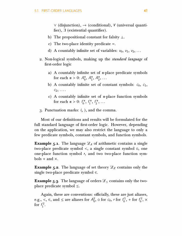
∨ (disjunction), → (conditional), ∀ (universal quanti-fier), ∃ (existential quantifier).

b) The propositional constant for falsity ⊥.

c) The two-place identity predicate =.

d) A countably infinite set of variables: v0, v1, v2, . . .

2. Non-logical symbols, making up the standard language offirst-order logic

a) A countably infinite set of n-place predicate symbolsfor each n > 0: An0 , A

n1 , A

n2 , . . .

b) A countably infinite set of constant symbols: c0, c1,c2, . . . .

c) A countably infinite set of n-place function symbolsfor each n > 0: f n0 , f

n1 , f

n2 , . . .

3. Punctuation marks: (, ), and the comma.

Most of our definitions and results will be formulated for thefull standard language of first-order logic. However, dependingon the application, we may also restrict the language to only afew predicate symbols, constant symbols, and function symbols.

Example 5.1. The language LA of arithmetic contains a singletwo-place predicate symbol <, a single constant symbol , oneone-place function symbol ′, and two two-place function sym-bols + and ×.

Example 5.2. The language of set theory LZ contains only thesingle two-place predicate symbol ∈.

Example 5.3. The language of orders L≤ contains only the two-place predicate symbol ≤.

Again, these are conventions: ocially, these are just aliases,e.g., <, ∈, and ≤ are aliases for A20, for c0, ′ for f

10 , + for f 20 , ×

for f 21 .

42 CHAPTER 5. SYNTAX AND SEMANTICS

In addition to the primitive connectives and quantifiers in-troduced above, we also use the following dened symbols: ↔(biconditional), truth >

A defined symbol is not ocially part of the language, butis introduced as an informal abbreviation: it allows us to abbre-viate formulas which would, if we only used primitive symbols,get quite long. This is obviously an advantage. The bigger ad-vantage, however, is that proofs become shorter. If a symbol isprimitive, it has to be treated separately in proofs. The moreprimitive symbols, therefore, the longer our proofs.

You may be familiar with dierent terminology and symbolsthan the ones we use above. Logic texts (and teachers) commonlyuse either ∼, ¬, and ! for “negation”, ∧, ·, and& for “conjunction”.Commonly used symbols for the “conditional” or “implication”are →, ⇒, and ⊃. Symbols for “biconditional,” “bi-implication,”or “(material) equivalence” are ↔, ⇔, and ≡. The ⊥ symbolis variously called “falsity,” “falsum,”, “absurdity,”, or “bottom.”The > symbol is variously called “truth,” “verum,”, or “top.”

It is conventional to use lower case letters (e.g., a, b , c) fromthe beginning of the Latin alphabet for constant symbols (some-times called names), and lower case letters from the end (e.g., x ,y , z) for variables. Quantifiers combine with variables, e.g., x ;notational variations include ∀x , (∀x), (x), Π x , ∧x for the uni-versal quantifier and ∃x , (∃x), (Ex), Σx , ∨x for the existentialquantifier.

We might treat all the propositional operators and both quan-tifiers as primitive symbols of the language. We might insteadchoose a smaller stock of primitive symbols and treat the otherlogical operators as defined. “Truth functionally complete” setsof Boolean operators include ¬,∨, ¬,∧, and ¬,→—thesecan be combined with either quantifier for an expressively com-plete first-order language.

You may be familiar with two other logical operators: theSheer stroke | (named after Henry Sheer), and Peirce’s ar-row ↓, also known as Quine’s dagger. When given their usualreadings of “nand” and “nor” (respectively), these operators are

5.2. TERMS AND FORMULAS 43

truth functionally complete by themselves.

5.2 Terms and Formulas

Once a first-order language L is given, we can define expressionsbuilt up from the basic vocabulary of L. These include in partic-ular terms and formulas.

Denition 5.4 (Terms). The set of terms Trm(L) of L is definedinductively by:

1. Every variable is a term.

2. Every constant symbol of L is a term.

3. If f is an n-place function symbol and t1, . . . , tn are terms,then f (t1, . . . , tn) is a term.

4. Nothing else is a term.

A term containing no variables is a closed term.

The constant symbols appear in our specification of the lan-guage and the terms as a separate category of symbols, but theycould instead have been included as zero-place function symbols.We could then do without the second clause in the definition ofterms. We just have to understand f (t1, . . . , tn) as just f by itselfif n = 0.

Denition 5.5 (Formula). The set of formulas Frm(L) of thelanguage L is defined inductively as follows:

1. ⊥ is an atomic formula.

2. If R is an n-place predicate symbol of L and t1, . . . , tn areterms of L, then R(t1, . . . , tn) is an atomic formula.

3. If t1 and t2 are terms of L, then =(t1, t2) is an atomic for-mula.


4. If A is a formula, then ¬A is formula.

5. If A and B are formulas, then (A ∧ B) is a formula.

6. If A and B are formulas, then (A ∨ B) is a formula.

7. If A and B are formulas, then (A → B) is a formula.

8. If A is a formula and x is a variable, then ∀x A is a formula.

9. If A is a formula and x is a variable, then ∃x A is a formula.

10. Nothing else is a formula.

The definitions of the set of terms and that of formulas areinductive denitions. Essentially, we construct the set of formu-las in infinitely many stages. In the initial stage, we pronounceall atomic formulas to be formulas; this corresponds to the firstfew cases of the definition, i.e., the cases for ⊥, R(t1, . . . , tn) and=(t1, t2). “Atomic formula” thus means any formula of this form.

The other cases of the definition give rules for constructingnew formulas out of formulas already constructed. At the secondstage, we can use them to construct formulas out of atomic for-mulas. At the third stage, we construct new formulas from theatomic formulas and those obtained in the second stage, and soon. A formula is anything that is eventually constructed at sucha stage, and nothing else.

By convention, we write = between its arguments and leaveout the parentheses: t1 = t2 is an abbreviation for =(t1, t2). More-over, ¬=(t1, t2) is abbreviated as t1 , t2. When writing a formula(B ∗C ) constructed from B , C using a two-place connective ∗, wewill often leave out the outermost pair of parentheses and writesimply B ∗C .

Some logic texts require that the variable x must occur in Ain order for ∃x A and ∀x A to count as formulas. Nothing badhappens if you don’t require this, and it makes things easier.

Denition 5.6. Formulas constructed using the defined opera-tors are to be understood as follows:

5.3. UNIQUE READABILITY 45

1. > abbreviates ¬⊥.

2. A ↔ B abbreviates (A → B) ∧ (B → A).If we work in a language for a specific application, we will

often write two-place predicate symbols and function symbolsbetween the respective terms, e.g., t1 < t2 and (t1 + t2) in thelanguage of arithmetic and t1 ∈ t2 in the language of set the-ory. The successor function in the language of arithmetic is evenwritten conventionally after its argument: t ′. Ocially, however,these are just conventional abbreviations for A20(t1, t2), f 20 (t1, t2),A20(t1, t2) and f 10 (t ), respectively.Denition 5.7. The symbol ≡ expresses syntactic identity be-tween strings of symbols, i.e., A ≡ B i A and B are strings ofsymbols of the same length and which contain the same symbolin each place.

The ≡ symbol may be flanked by strings obtained by con-catenation, e.g., A ≡ (B ∨ C ) means: the string of symbols A isthe same string as the one obtained by concatenating an openingparenthesis, the string B , the ∨ symbol, the string C , and a clos-ing parenthesis, in this order. If this is the case, then we knowthat the first symbol of A is an opening parenthesis, A containsB as a substring (starting at the second symbol), that substringis followed by ∨, etc.

5.3 Unique Readability

The way we defined formulas guarantees that every formula hasa unique reading, i.e., there is essentially only one way of con-structing it according to our formation rules for formulas andonly one way of “interpreting” it. If this were not so, we wouldhave ambiguous formulas, i.e., formulas that have more than onereading or intepretation—and that is clearly something we wantto avoid. But more importantly, without this property, most of thedefinitions and proofs we are going to give will not go through.


Perhaps the best way to make this clear is to see what wouldhappen if we had given bad rules for forming formulas that wouldnot guarantee unique readability. For instance, we could haveforgotten the parentheses in the formation rules for connectives,e.g., we might have allowed this:

If A and B are formulas, then so is A → B .

Starting from an atomic formula D , this would allow us to formD → D , and from this, together with D , we would get D → D →D . But there are two ways to do this: one where we take D tobe A and D → D to be B , and the other where A is D → Dand B is D . Correspondingly, there are two ways to “read” theformula D → D → D . It is of the form B → C where B is Dand C is D → D , but it is also of the form B → C with B beingD → D and C being D .

If this happens, our definitions will not always work. For in-stance, when we define the main operator of a formula, we say: ina formula of the form B → C , the main operator is the indicatedoccurrence of →. But if we can match the formula D → D → Dwith B → C in the two dierent ways mentioned above, then inone case we get the first occurrence of → as the main operator,and in the second case the second occurrence. But we intend themain operator to be a function of the formula, i.e., every formulamust have exactly one main operator occurrence.

Lemma 5.8. The number of left and right parentheses in a formula Aare equal.

Proof. We prove this by induction on the way A is constructed.This requires two things: (a) We have to prove first that all atomicformulas have the property in question (the induction basis). (b)Then we have to prove that when we construct new formulas outof given formulas, the new formulas have the property providedthe old ones do.

5.3. UNIQUE READABILITY 47

Let l (A) be the number of left parentheses, and r (A) the num-ber of right parentheses in A, and l (t ) and r (t ) similarly the num-ber of left and right parentheses in a term t . We leave the proofthat for any term t , l (t ) = r (t ) as an exercise.

1. A ≡ ⊥: A has 0 left and 0 right parentheses.

2. A ≡ R(t1, . . . , tn): l (A) = 1 + l (t1) + · · · + l (tn) = 1 + r (t1) +· · · + r (tn) = r (A). Here we make use of the fact, left as anexercise, that l (t ) = r (t ) for any term t .

3. A ≡ t1 = t2: l (A) = l (t1) + l (t2) = r (t1) + r (t2) = r (A).

4. A ≡ ¬B : By induction hypothesis, l (B) = r (B). Thusl (A) = l (B) = r (B) = r (A).

5. A ≡ (B ∗ C ): By induction hypothesis, l (B) = r (B) andl (C ) = r (C ). Thus l (A) = 1+ l (B)+ l (C ) = 1+ r (B)+ r (C ) =r (A).

6. A ≡ ∀x B : By induction hypothesis, l (B) = r (B). Thus,l (A) = l (B) = r (B) = r (A).

7. A ≡ ∃x B : Similarly.

Denition 5.9. A string of symbols B is a proper prefix of astring of symbols A if concatenating B and a non-empty string ofsymbols yields A.

Lemma 5.10. If A is a formula, and B is a proper prex of A, thenB is not a formula.

Proof. Exercise.


Proposition 5.11. If A is an atomic formula, then it satisfes one, andonly one of the following conditions.

1. A ≡ ⊥.

2. A ≡ R(t1, . . . , tn) where R is an n-place predicate symbol, t1, . . . ,tn are terms, and each of R, t1, . . . , tn is uniquely determined.

3. A ≡ t1 = t2 where t1 and t2 are uniquely determined terms.

Proof. Exercise.

Proposition 5.12 (Unique Readability). Every formula satisesone, and only one of the following conditions.

1. A is atomic.

2. A is of the form ¬B .

3. A is of the form (B ∧C ).4. A is of the form (B ∨C ).5. A is of the form (B → C ).6. A is of the form ∀x B .

7. A is of the form ∃x B .

Moreover, in each case B , or B and C , are uniquely determined. Thismeans that, e.g., there are no dierent pairs B , C and B ′, C ′ so that Ais both of the form (B → C ) and (B ′ → C ′).

Proof. The formation rules require that if a formula is not atomic,it must start with an opening parenthesis (, ¬, or with a quanti-fier. On the other hand, every formula that start with one of thefollowing symbols must be atomic: a predicate symbol, a functionsymbol, a constant symbol, ⊥.

5.4. MAIN OPERATOR OF A FORMULA 49

So we really only have to show that if A is of the form (B ∗C )and also of the form (B ′ ∗′ C ′), then B ≡ B ′, C ≡ C ′, and ∗ = ∗′.

So suppose both A ≡ (B ∗C ) and A ≡ (B ′ ∗′ C ′). Then eitherB ≡ B ′ or not. If it is, clearly ∗ = ∗′ and C ≡ C ′, since they thenare substrings of A that begin in the same place and are of thesame length. The other case is C 6≡ C ′. Since C and C ′ are bothsubstrings of A that begin at the same place, one must be a prefixof the other. But this is impossible by Lemma 5.10.

5.4 Main operator of a Formula

It is often useful to talk about the last operator used in construct-ing a formula A. This operator is called the main operator of A.Intuitively, it is the “outermost” operator of A. For example, themain operator of ¬A is ¬, the main operator of (A∨B) is ∨, etc.Denition 5.13 (Main operator). The main operator of a for-mula A is defined as follows:

1. A is atomic: A has no main operator.

2. A ≡ ¬B : the main operator of A is ¬.

3. A ≡ (B ∧C ): the main operator of A is ∧.

4. A ≡ (B ∨C ): the main operator of A is ∨.

5. A ≡ (B → C ): the main operator of A is →.

6. A ≡ ∀x B : the main operator of A is ∀.

7. A ≡ ∃x B : the main operator of A is ∃.

In each case, we intend the specific indicated occurrence of themain operator in the formula. For instance, since the formula((D → E) → (E → D)) is of the form (B → C ) where B is(D → E) and C is (E → D), the second occurrence of → is themain operator.


This is a recursive definition of a function which maps all non-atomic formulas to their main operator occurrence. Because ofthe way formulas are defined inductively, every formula A satis-fies one of the cases in Definition 5.13. This guarantees that foreach non-atomic formula A a main operator exists. Because eachformula satisfies only one of these conditions, and because thesmaller formulas from which A is constructed are uniquely deter-mined in each case, the main operator occurrence of A is unique,and so we have defined a function.

We call formulas by the following names depending on whichsymbol their main operator is:Main operator Type of formula Example

none atomic (formula) ⊥, R(t1, . . . , tn), t1 = t2¬ negation ¬A∧ conjunction (A ∧ B)∨ disjunction (A ∨ B)→ conditional (A → B)∀ universal (formula) ∀x A∃ existential (formula) ∃x A

5.5 Subformulas

It is often useful to talk about the formulas that “make up” agiven formula. We call these its subformulas. Any formula countsas a subformula of itself; a subformula of A other than A itself isa proper subformula.

Denition 5.14 (Immediate Subformula). If A is a formula, theimmediate subformulas of A are defined inductively as follows:

1. Atomic formulas have no immediate subformulas.

2. A ≡ ¬B : The only immediate subformula of A is B .

3. A ≡ (B ∗ C ): The immediate subformulas of A are B andC (∗ is any one of the two-place connectives).

5.5. SUBFORMULAS 51

4. A ≡ ∀x B : The only immediate subformula of A is B .

5. A ≡ ∃x B : The only immediate subformula of A is B .

Denition 5.15 (Proper Subformula). If A is a formula, theproper subformulas of A are recursively as follows:

1. Atomic formulas have no proper subformulas.

2. A ≡ ¬B : The proper subformulas of A are B together withall proper subformulas of B .

3. A ≡ (B ∗ C ): The proper subformulas of A are B , C ,together with all proper subformulas of B and those of C .

4. A ≡ ∀x B : The proper subformulas of A are B togetherwith all proper subformulas of B .

5. A ≡ ∃x B : The proper subformulas of A are B togetherwith all proper subformulas of B .

Denition 5.16 (Subformula). The subformulas of A are A itselftogether with all its proper subformulas.

Note the subtle dierence in how we have defined immediatesubformulas and proper subformulas. In the first case, we havedirectly defined the immediate subformulas of a formula A foreach possible form of A. It is an explicit definition by cases, andthe cases mirror the inductive definition of the set of formulas.In the second case, we have also mirrored the way the set of allformulas is defined, but in each case we have also included theproper subformulas of the smaller formulas B , C in addition tothese formulas themselves. This makes the definition recursive. Ingeneral, a definition of a function on an inductively defined set(in our case, formulas) is recursive if the cases in the definition ofthe function make use of the function itself. To be well defined,we must make sure, however, that we only ever use the valuesof the function for arguments that come “before” the one we aredefining—in our case, when defining “proper subformula” for (B∗


C ) we only use the proper subformulas of the “earlier” formulasB and C .

5.6 Free Variables and Sentences

Denition 5.17 (Free occurrences of a variable). The free oc-currences of a variable in a formula are defined inductively asfollows:

1. A is atomic: all variable occurrences in A are free.

2. A ≡ ¬B : the free variable occurrences of A are exactlythose of B .

3. A ≡ (B ∗ C ): the free variable occurrences of A are thosein B together with those in C .

4. A ≡ ∀x B : the free variable occurrences in A are all ofthose in B except for occurrences of x .

5. A ≡ ∃x B : the free variable occurrences in A are all ofthose in B except for occurrences of x .

Denition 5.18 (Bound Variables). An occurrence of a variablein a formula A is bound if it is not free.

Denition 5.19 (Scope). If ∀x B is an occurrence of a subfor-mula in a formula A, then the corresponding occurrence of Bin A is called the scope of the corresponding occurrence of ∀x .Similarly for ∃x .

If B is the scope of a quantifier occurrence ∀x or ∃x in A,then all occurrences of x which are free in B are said to be boundby the mentioned quantifier occurrence.

Example 5.20. Here is a somewhat complicated formula A:

∀x0 (A10(x0)→ A20(x0, x1))︸︷︷︸B

→ ∃x1 (A21(x0, x1) ∨ ∀x0D︷︸︸︷

¬A11(x0))︸︷︷︸C

5.7. SUBSTITUTION 53

B is the scope of the first ∀x0, C is the scope of ∃x1, and D is thescope of the second ∀x0. The first ∀x0 binds the occurrences of x0in B , ∃x1 the occurrence of x1 in C , and the second ∀x0 binds theoccurrence of x0 in D . The first occurrence of x1 and the fourthoccurrence of x0 are free in A. The last occurrence of x0 is freein D , but bound in C and A.

Denition 5.21 (Sentence). A formula A is a sentence i it con-tains no free occurrences of variables.

5.7 Substitution

Denition 5.22 (Substitution in a term). We define s [t/x], theresult of substituting t for every occurrence of x in s , recursively:

1. s ≡ c : s [t/x] is just s .2. s ≡ y : s [t/x] is also just s , provided y is a variable other

than x .

3. s ≡ x : s [t/x] is t .4. s ≡ f (t1, . . . , tn): s [t/x] is f (t1[t/x], . . . , tn[t/x]).

Denition 5.23. A term t is free for x in A if none of the freeoccurrences of x in A occur in the scope of a quantifier that bindsa variable in t .

Denition 5.24 (Substitution in a formula). If A is a formula, xis a variable, and t is a term free for x in A, then A[t/x] is theresult of substituting t for all free occurrences of x in A.

1. A ≡ P (t1, . . . , tn): A[t/x] is P (t1[t/x], . . . , tn[t/x]).2. A ≡ t1 = t2: A[t/x] is t1[t/x] = t2[t/x].3. A ≡ ¬B : A[t/x] is ¬B[t/x].4. A ≡ (B ∧C ): A[t/x] is (B[t/x] ∧C [t/x]).


5. A ≡ (B ∨C ): A[t/x] is (B[t/x] ∨C [t/x]).6. A ≡ (B → C ): A[t/x] is (B[t/x]→ C [t/x]).7. A ≡ ∀y B : A[t/x] is ∀y B[t/x], provided y is a variable

other than x ; otherwise A[t/x] is just A.8. A ≡ ∃y B : A[t/x] is ∃y B[t/x], provided y is a variable

other than x ; otherwise A[t/x] is just A.Note that substitution may be vacuous: If x does not occur in

A at all, then A[t/x] is just A.The restriction that t must be free for x in A is necessary

to exclude cases like the following. If A ≡ ∃y x < y and t ≡ y ,then A[t/y] would be ∃y y < y . In this case the free variable yis “captured” by the quantifier ∃y upon substitution, and that isundesirable. For instance, we would like it to be the case thatwhenever ∀x B holds, so does B[t/x]. But consider ∀x ∃y x < y(here B is ∃y x < y). It is sentence that is true about, e.g., thenatural numbers: for every number x there is a number y greaterthan it. If we allowed y as a possible substitution for x , we wouldend up with B[y/x] ≡ ∃y y < y , which is false. We prevent this byrequiring that none of the free variables in t would end up beingbound by a quantifier in A.

We often use the following convention to avoid cumbersumenotation: If A is a formula with a free variable x , we write A(x)to indicate this. When it is clear which A and x we have in mind,and t is a term (assumed to be free for x in A(x)), then we writeA(t ) as short for A(x)[t/x].

5.8 Structures for First-order Languages

First-order languages are, by themselves, uninterpreted: the con-stant symbols, function symbols, and predicate symbols have nospecific meaning attached to them. Meanings are given by spec-ifying a structure. It specifies the domain, i.e., the objects whichthe constant symbols pick out, the function symbols operate on,

5.8. STRUCTURES FOR FIRST-ORDER LANGUAGES 55

and the quantifiers range over. In addition, it specifies whichconstant symbols pick out which objects, how a function symbolmaps objects to objects, and which objects the predicate symbolsapply to. Structures are the basis for semantic notions in logic,e.g., the notion of consequence, validity, satisfiablity. They arevariously called “structures,” “interpretations,” or “models” inthe literature.

Denition 5.25 (Structures). A structure M, for a language L offirst-order logic consists of the following elements:

1. Domain: a non-empty set, |M |2. Interpretation of constant symbols: for each constant symbol c

of L, an element cM ∈ |M |3. Interpretation of predicate symbols: for each n-place predicate

symbol R ofL (other than =), an n-ary relation RM ⊆ |M |n

4. Interpretation of function symbols: for each n-place functionsymbol f of L, an n-ary function f M : |M |n → |M |

Example 5.26. A structure M for the language of arithmeticconsists of a set, an element of |M |, M, as interpretation of theconstant symbol , a one-place function ′M : |M | → |M |, two two-place functions +M and ×M, both |M |2 → |M |, and a two-placerelation <M ⊆ |M |2.

An obvious example of such a structure is the following:

1. |N | = N2. N = 0

3. ′N(n) = n + 1 for all n ∈ N

4. +N(n,m) = n +m for all n,m ∈ N

5. ×N(n,m) = n · m for all n,m ∈ N

6. <N = 〈n,m〉 : n ∈ N,m ∈ N, n < m


The structure N for LA so defined is called the standard model ofarithmetic, because it interprets the non-logical constants of LAexactly how you would expect.

However, there are many other possible structures forLA. Forinstance, we might take as the domain the set Z of integers insteadof N, and define the interpretations of , ′, +, ×, < accordingly.But we can also define structures for LA which have nothing evenremotely to do with numbers.

Example 5.27. A structure M for the language LZ of set theoryrequires just a set and a single-two place relation. So technically,e.g., the set of people plus the relation “x is older than y” couldbe used as a structure for LZ , as well as N together with n ≥ mfor n,m ∈ N.

A particularly interesting structure for LZ in which the ele-ments of the domain are actually sets, and the interpretation of∈ actually is the relation “x is an element of y” is the structureHF of hereditarily nite sets:

1. |HF | = ∅ ∪ ℘(∅) ∪ ℘(℘(∅)) ∪ ℘(℘(℘(∅))) ∪ . . . ;2. ∈HF = 〈x, y〉 : x, y ∈ |HF | , x ∈ y.Recall that a term is closed if it contains no variables.

Denition 5.28 (Value of closed terms). If t is a closed term ofthe langage L and M is a structure for L, the value ValM(t ) isdefined as follows:

1. If t is just the constant symbol c , then ValM(c ) = cM.

2. If t is of the form f (t1, . . . , tn), then

ValM(t ) = f M(ValM(t1), . . . ,ValM(tn)).

Denition 5.29 (Covered structure). A structure is covered if ev-ery element of the domain is the value of some closed term.

5.8. STRUCTURES FOR FIRST-ORDER LANGUAGES 57

Example 5.30. Let L be the language with constant symbolszero, one, two, . . ., the binary predicate symbols = and <, andthe binary function symbols + and ×. Then a structure M for Lis the one with domain |M | = 0, 1, 2, . . . and name assignmentzeroM = 0, oneM = 1, twoM = 2, and so forth. For the binaryrelation symbol <, the set <M is the set of all pairs 〈c1, c2〉 ∈ |M |2such that the integer c1 is less than the integer c2: for example,〈1, 3〉 ∈<M but 〈2, 2〉 <<M. For the binary function symbol +,define +M in the usual way—for example, +M(2, 3) maps to 5,and similarly for the binary function symbol ×. Hence, the valueof f our is just 4, and the value of ×(two,+(three, zero)) (or ininfix notation, two × (three + zero) ) is

ValM(×(two,+(three, zero)) == ×M(ValM(two),ValM(two,+(three, zero)))= ×M(ValM(two),+M(ValM(three),ValM(zero)))= ×M(twoM,+M(threeM, zeroM))= ×M(2,+M(3, 0))= ×M(2, 3)= 6

The stipulations we make as to what counts as a structureimpact our logic. For example, the choice to prevent empty do-mains ensures, given the usual account of satisfaction (or truth)for quantified sentences, that ∃x (A(x)∨¬A(x)) is valid—that is, alogical truth. And the stipulation that all constant symbols mustrefer to an object in the domain ensures that the existential gener-alization is a sound pattern of inference: A(a), therefore ∃x A(x).If we allowed names to refer outside the domain, or to not refer,then we would be on our way to a free logic, in which existentialgeneralization requires an additional premise: A(a) and ∃x x = a,therefore ∃x A(x).


5.9 Satisfaction of a Formula in a Structure

The basic notion that relates expressions such as terms and for-mulas, on the one hand, and structures on the other, are thoseof value of a term and satisfaction of a formula. Informally, thevalue of a term is an element of a structure—if the term is just aconstant, its value is the object assigned to the constant by thestructure, and if it is built up using function symbols, the value iscomputed from the values of constants and the functions assignedto the functions in the term. A formula is satised in a structureif the interpretation given to the predicates makes the formulatrue in the domain of the structure. This notion of satisfactionis specified inductively: the specification of the structure directlystates when atomic formulas are satisfied, and we define when acomplex formula is satisfied depending on the main connectiveor quantifier and whether or not the immediate subformulas aresatisfied. The case of the quantifiers here is a bit tricky, as theimmediate subformula of a quantified formula has a free variable,and structures don’t specify the values of variables. In order todeal with this diculty, we also introduce variable assignments anddefine satisfaction not with respect to a structure alone, but withrespect to a structure plus a variable assignment.

Denition 5.31 (Variable Assignment). A variable assignment sfor a structure M is a function which maps each variable to anelement of |M |, i.e., s : Var→ |M |.

A structure assigns a value to each constant symbol, and avariable assignment to each variable. But we want to use termsbuilt up from them to also name elements of the domain. Forthis we define the value of terms inductively. For constant sym-bols and variables the value is just as the structure or the variableassignment specifies it; for more complex terms it is computed re-cursively using the functions the structure assigns to the functionsymbols.

5.9. SATISFACTION OF A FORMULA IN A STRUCTURE 59

Denition 5.32 (Value of Terms). If t is a term of the lan-guage L, M is a structure for L, and s is a variable assignmentfor M, the value ValMs (t ) is defined as follows:

1. t ≡ c : ValMs (t ) = cM.

2. t ≡ x : ValMs (t ) = s (x).3. t ≡ f (t1, . . . , tn):

ValMs (t ) = f M(ValMs (t1), . . . ,ValMs (tn)).

Denition 5.33 (x -Variant). If s is a variable assignment for astructure M, then any variable assignment s ′ for M which diersfrom s at most in what it assigns to x is called an x -variant of s .If s ′ is an x -variant of s we write s ∼x s ′.

Note that an x -variant of an assignment s does not have toassign something dierent to x . In fact, every assignment countsas an x -variant of itself.

Denition 5.34 (Satisfaction). Satisfaction of a formula A ina structure M relative to a variable assignment s , in symbols:M, s |= A, is defined recursively as follows. (We write M, s 6|= A tomean “not M, s |= A.”)

1. A ≡ ⊥: not M, s |= A.2. A ≡ R(t1, . . . , tn): M, s |= A i 〈ValMs (t1), . . . ,ValMs (tn)〉 ∈RM.

3. A ≡ t1 = t2: M, s |= A i ValMs (t1) = ValMs (t2).4. A ≡ ¬B : M, s |= A i M, s 6|= B .5. A ≡ (B ∧C ): M, s |= A i M, s |= B and M, s |= C .6. A ≡ (B ∨C ): M, s |= A i M, s |= A or M, s |= B (or both).

7. A ≡ (B → C ): M, s |= A i M, s 6|= B or M, s |= C (or both).


8. A ≡ ∀x B : M, s |= A i for every x -variant s ′ of s , M, s ′ |= B .9. A ≡ ∃x B : M, s |= A i there is an x -variant s ′ of s so that

M, s ′ |= B .The variable assignments are important in the last two clauses.

We cannot define satisfaction of ∀x B(x) by “for all a ∈ |M |,M |= B(a).” We cannot define satisfaction of ∃x B(x) by “forat least one a ∈ |M |, M |= B(a).” The reason is that a is notsymbol of the language, and so B(a) is not a formula (that is,B[a/x] is undefined). We also cannot assume that we have con-stant symbols or terms available that name every element of M,since there is nothing in the definition of structures that requiresit. Even in the standard language the set of constant symbolsis countably infinite, so if |M | is not countable there aren’t evenenough constant symbols to name every object.

A variable assignment s provides a value for every variablein the language. This is of course not necessary: whether ornot a formula A is satisfied in a structure with respect to s onlydepends on the assignments s makes to the free variables thatactually occur in A. This is the content of the next theorem.We require variable assignments to assign values to all variablessimply because it makes things a lot easier.

Proposition 5.35. If x1, . . . , xn are the only free variables in A ands (xi ) = s ′(xi ) for i = 1, . . . , n, then M, s |= A i M, s ′ |= A.

Proof. We use induction on the complexity of A. For the basecase, where A is atomic, A can be: ⊥, R(t1, . . . , tk ) for a k -placepredicate R and terms t1, . . . , tk , or t1 = t2 for terms t1 and t2.

1. A ≡ ⊥: both M, s 6|= A and M, s ′ 6|= A.2. A ≡ R(t1, . . . , tk ): let M, s |= A. Then

〈ValMs (t1), . . . ,ValMs (tk )〉 ∈ RM .

5.9. SATISFACTION OF A FORMULA IN A STRUCTURE 61

For i = 1, . . . , k , if ti is a constant, thenValMs (ti ) = ValM(ti ) =ValMs ′ (ti ). If ti is a free variable, then since the mappingss and s ′ agree on all free variables, ValMs (ti ) = s (ti ) =s ′(ti ) = ValMs ′ (ti ). Similarly, if ti is of the form f (t ′1, . . . , t ′j ),we will also get ValMs (ti ) = ValMs ′ (ti ). Hence, ValMs (ti ) =ValMs ′ (ti ) for any term ti for i = 1, . . . , k , so we also have〈ValMs ′ (ti ), . . . ,ValMs ′ (tk )〉 ∈ RM.

3. A ≡ t1 = t2: if M, s |= A, ValMs ′ (t1) = ValMs (t1) = ValMs (t2) =ValMs ′ (t2), so M, s ′ |= t1 = t2.

Now assume M, s |= B i M, s ′ |= B for all formulas B lesscomplex than A. The induction step proceeds by cases deter-mined by the main operator of A. In each case, we only demon-strate the forward direction of the biconditional; the proof of thereverse direction is symmetrical.

1. A ≡ ¬B : if M, s |= A, then M, s 6|= B , so by the inductionhypothesis, M, s ′ 6|= B , hence M, s ′ |= A.

2. A ≡ B ∧C : exercise.

3. A ≡ B ∨ C : if M, s |= A, then M, s |= B or M, s |= C . Byinduction hypothesis, M, s ′ |= B or M, s ′ |= C , so M, s ′ |= A.

4. A ≡ B → C : exercise.

5. A ≡ ∃x B : if M, s |= A, there is an x -variant s of s so thatM, s |= B . Let s ′ denote the x -variant of s ′ that assigns thesame thing to x as does s : then by the induction hypothesis,M, s ′ |= B . Hence, there is an x -variant of s ′ that satisfiesB , so M, s ′ |= A.

6. A ≡ ∀x B : exercise.

By induction, we get that M, s |= A i M, s ′ |= A whenever x1, . . . ,xn are the only free variables in A and s (xi ) = s ′(xi ) for i = 1,. . . , n.


Denition 5.36. If A is a sentence, we say that a structure Msatises A, M |= A, i M, s |= A for all variable assignments s .

If M |= A, we also say that A is true in M.

Proposition 5.37. Suppose A(x) only contains x free, and M is astructure. Then:

1. M |= ∃x A(x) i M, s |= A(x) for at least one variable assign-ment s .

2. M |= ∀x A(x) i M, s |= A(x) for all variable assignments s .

Proof. Exercise.

5.10 Extensionality

Extensionality, sometimes called relevance, can be expressed in-formally as follows: the only thing that bears upon the satisfactionof formula A in a structure M relative to a variable assignment s ,are the assignments made by M and s to the elements of thelanguage that actually appear in A.

One immediate consequence of extensionality is that wheretwo structures M and M′ agree on all the elements of the lan-guage appearing in a sentence A and have the same domain, Mand M′ must also agree on A itself.

Proposition 5.38 (Extensionality). Let A be a sentence, andM andM′ be structures. If cM = cM′ , RM = RM′ , and f M = f M′ for everyconstant symbol c , relation symbol R, and function symbol f occurringin A, then M |= A i M′ |= A.

Moreover, the value of a term, and whether or not a structuresatisfies a formula, only depends on the values of its subterms.

5.10. EXTENSIONALITY 63

Proposition 5.39. Let M be a structure, t and t ′ terms, and s avariable assignment. Let s ′ ∼x s be the x -variant of s given by s ′(x) =ValMs (t ′). Then ValMs (t [t ′/x]) = ValMs ′ (t ).

Proof. By induction on t .

1. If t is a constant, say, t ≡ c , then t [t ′/x] = c , and ValMs (c ) =cM = ValMs ′ (c ).

2. If t is a variable other than x , say, t ≡ y , then t [t ′/x] = y ,and ValMs (y) = ValMs ′ (y) since s ′ ∼x s .

3. If t ≡ x , then t [t ′/x] = t ′. But ValMs ′ (x) = ValMs (t ′) bydefinition of s ′.

4. If t ≡ f (t1, . . . , tn) then we have:

ValMs (t [t ′/x]) == ValMs (f (t1[t ′/x], . . . , tn[t ′/x]))

by definition of t [t ′/x]= f M(ValMs (t1[t ′/x]), . . . ,ValMs (tn[t ′/x]))

by definition of ValMs (f (. . . ))= f M(ValMs ′ (t1), . . . ,ValMs ′ (tn))

by induction hypothesis

= ValMs ′ (t ) by definition of ValMs ′ (f (. . . ))

Proposition 5.40. Let M be a structure, A a formula, t a term,and s a variable assignment. Let s ′ ∼x s be the x -variant of s givenby s ′(x) = ValMs (t ). Then M, s |= A[t/x] i M, s ′ |= A.

Proof. Exercise.


5.11 Semantic Notions

Give the definition of structures for first-order languages, we candefine some basic semantic properties of and relationships be-tween sentences. The simplest of these is the notion of validityof a sentence. A sentence is valid if it is satisfied in every struc-ture. Valid sentences are those that are satisfied regardless of howthe non-logical symbols in it are interpreted. Valid sentences aretherefore also called logical truths—they are true, i.e., satisfied, inany structure and hence their truth depends only on the logicalsymbols occurring in them and their syntactic structure, but noton the non-logical symbols or their interpretation.

Denition 5.41 (Validity). A sentence A is valid, A, i M |= Afor every structure M.

Denition 5.42 (Entailment). A set of sentences Γ entails a sen-tence A, Γ A, i for every structure M with M |= Γ, M |= A.Denition 5.43 (Satisfiability). A set of sentences Γ is satisableif M |= Γ for some structure M. If Γ is not satisfiable it is calledunsatisable.

Proposition 5.44. A sentence A is valid i Γ A for every set ofsentences Γ.

Proof. For the forward direction, let A be valid, and let Γ be aset of sentences. Let M be a structure so that M |= Γ. Since A isvalid, M |= A, hence Γ A.

For the contrapositive of the reverse direction, let A be in-valid, so there is a structure M with M 6|= A. When Γ = >,since > is valid, M |= Γ. Hence, there is a structure M so thatM |= Γ but M 6|= A, hence Γ does not entail A.

Proposition 5.45. Γ A i Γ ∪ ¬A is unsatisable.

5.11. SEMANTIC NOTIONS 65

Proof. For the forward direction, suppose Γ A and suppose tothe contrary that there is a structure M so that M |= Γ ∪ ¬A.Since M |= Γ and Γ A, M |= A. Also, since M |= Γ∪¬A, M |=¬A, so we have both M |= A and M 6|= A, a contradiction. Hence,there can be no such structure M, so Γ ∪ A is unsatisfiable.

For the reverse direction, suppose Γ ∪ ¬A is unsatisfiable.So for every structure M, either M 6|= Γ or M |= A. Hence, forevery structure M with M |= Γ, M |= A, so Γ A.

Proposition 5.46. If Γ ⊆ Γ ′ and Γ A, then Γ ′ A.

Proof. Suppose that Γ ⊆ Γ ′ and Γ A. Let M be such thatM |= Γ ′; then M |= Γ, and since Γ A, we get that M |= A.Hence, whenever M |= Γ ′, M |= A, so Γ ′ A.

Theorem 5.47 (Semantic Deduction Theorem). Γ ∪ A B iΓ A → B .

Proof. For the forward direction, let Γ ∪ A B and let M be astructure so that M |= Γ. If M |= A, then M |= Γ ∪ A, so sinceΓ ∪ A entails B , we get M |= B . Therefore, M |= A → B , soΓ A → B .

For the reverse direction, let Γ A → B and M be a structureso that M |= Γ ∪ A. Then M |= Γ, so M |= A → B , and sinceM |= A, M |= B . Hence, whenever M |= Γ ∪ A, M |= B , soΓ ∪ A B .

CHAPTER 6

Theories andTheir Models6.1 Introduction

The development of the axiomatic method is a significant achieve-ment in the history of science, and is of special importnace in thehistory of mathematics. An axiomatic development of a field in-volves the clarification of many questions: What is the field about?What are the most fundamental concepts? How are they related?Can all the concepts of the field be defined in terms of thesefundamental concepts? What laws do, and must, these conceptsobey?

The axiomatic method and logic were made for each other.Formal logic provides the tools for formulating axiomatic theo-ries, for proving theorems from the axioms of the theory in aprecisely specified way, for studying the properties of all systemssatisfying the axioms in a systematic way.

Denition 6.1. A set of sentences Γ is closed i, whenever Γ Athen A ∈ Γ. The closure of a set of sentences Γ is A : Γ A.

We say that Γ is axiomatized by a set of sentences ∆ if Γ is theclosure of ∆

66

6.1. INTRODUCTION 67

We can think of an axiomatic theory as the set of sentencesthat is axiomatized by its set of axioms ∆. In other words, whenwe have a first-order language which contains non-logical sym-bols for the primitives of the axiomatically developed science wewish to study, together with a set of sentences that express thefundamental laws of the science, we can think of the theory asrepresented by all the sentences in this language that are entailedby the axioms. This ranges from simple examples with only asingle primitive and simple axioms, such as the theory of partialorders, to complex theories such as Newtonian mechanics.

The important logical facts that make this formal approachto the axiomatic method so important are the following. SupposeΓ is an axiom system for a theory, i.e., a set of sentences.

1. We can state precisely when an axiom system captures anintended class of structures. That is, if we are interestedin a certain class of structures, we will successfully capturethat class by an axiom system Γ i the structures are exactlythose M such that M |= Γ.

2. We may fail in this respect because there are M such thatM |= Γ, but M is not one of the structures we intend. Thismay lead us to add axioms which are not true in M.

3. If we are successful at least in the respect that Γ is truein all the intended structures, then a sentence A is true inall intended structures whenever Γ A. Thus we can uselogical tools (such as proof methods) to show that sentencesare true in all intended structures simply by showing thatthey are entailed by the axioms.

4. Sometimes we don’t have intended structures in mind, butinstead start from the axioms themselves: we begin withsome primitives that we want to satisfy certain laws whichwe codify in an axiom system. One thing that we wouldlike to verify right away is that the axioms do not contradicteach other: if they do, there can be no concepts that obey

68 CHAPTER 6. THEORIES AND THEIR MODELS

these laws, and we have tried to set up an incoherent theory.We can verify that this doesn’t happen by finding a modelof Γ. And if there are models of our theory, we can uselogical methods to investigate them, and we can also uselogical methods to construct models.

5. The independence of the axioms is likewise an importantquestion. It may happen that one of the axioms is actu-ally a consequence of the others, and so is redundant. Wecan prove that an axiom A in Γ is redundant by provingΓ \ A A. We can also prove that an axiom is not redun-dant by showing that (Γ \ A) ∪ ¬A is satisfiable. Forinstance, this is how it was shown that the parallel postulateis independent of the other axioms of geometry.

6. Another important question is that of definability of con-cepts in a theory: The choice of the language determineswhat the models of a theory consists of. But not everyaspect of a theory must be represented separately in itsmodels. For instance, every ordering ≤ determines a corre-sponding strict ordering <—given one, we can define theother. So it is not necessary that a model of a theory in-volving such an order must also contain the correspondingstrict ordering. When is it the case, in general, that onerelation can be defined in terms of others? When is it im-possible to define a relation in terms of other (and hencemust add it to the primitives of the language)?

6.2 Expressing Properties of Structures

It is often useful and important to express conditions on func-tions and relations, or more generally, that the functions and re-lations in a structure satisfy these conditions. For instance, wewould like to have ways of distinguishing those structures for alanguage which “capture” what we want the predicate symbolsto “mean” from those that do not. Of course we’re completely

6.2. EXPRESSING PROPERTIES OF STRUCTURES 69

free to specify which structures we “intend,” e.g., we can specifythat the interpretation of the predicate symbol ≤ must be an or-dering, or that we are only interested in interpretations of L inwhich the domain consists of sets and ∈ is interpreted by the “isan element of” relation. But can we do this with sentences of thelanguage? In other words, which conditions on a structure M canwe express by a sentence (or perhaps a set of sentences) in thelanguage of M? There are some conditions that we will not beable to express. For instance, there is no sentence of LA which isonly true in a structure M if |M | = N. We cannot express “the do-main contains only natural numbers.” But there are “structuralproperties” of structures that we perhaps can express. Whichproperties of structures can we express by sentences? Or, to putit another way, which collections of structures can we describe asthose making a sentence (or set of sentences) true?

Denition 6.2. Let Γ be a set of sentences in a language L. Wesay that a structure M is a model of Γ if M |= A for all A ∈ Γ.

Example 6.3. The sentence ∀x x ≤ x is true in M i ≤M is areflexive relation. The sentence ∀x ∀y ((x ≤ y ∧ y ≤ x)→ x = y) istrue in M i ≤M is anti-symmetric. The sentence ∀x ∀y ∀z ((x ≤y ∧ y ≤ z ) → x ≤ z ) is true in M i ≤M is transitive. Thus, themodels of

∀x x ≤ x,

∀x ∀y ((x ≤ y ∧ y ≤ x)→ x = y),∀x ∀y ∀z ((x ≤ y ∧ y ≤ z )→ x ≤ z )

are exactly those structures in which ≤M is reflexive, anti-symmetric,and transitive, i.e., a partial order. Hence, we can take them asaxioms for the rst-order theory of partial orders.


6.3 Examples of First-Order Theories

Example 6.4. The theory of strict linear orders in the languageL<

is axiomatized by the set

∀x ¬x < x,

∀x ∀y ((x < y ∨ y < x) ∨ x = y),∀x ∀y ∀z ((x < y ∧ y < z )→ x < z )

It completely captures the intended structures: every strict linearorder is a model of this axiom system, and vice versa, if R is alinear order on a set X , then the structure M with |M | = X and<M= R is a model of this theory.

Example 6.5. The theory of groups in the language (constantsymbol), · (two-place function symbol) is axiomatized by

∀x (x · ) = x∀x ∀y ∀z (x · (y · z )) = ((x · y) · z )∀x ∃y (x · y) =

Example 6.6. The theory of Peano arithmetic is axiomatized bythe following sentences in the language of arithmetic LA.

¬∃x x ′ =

∀x ∀y (x ′ = y ′ → x = y)∀x ∀y (x < y ↔ ∃z (x + z ′ = y))∀x (x + ) = x∀x ∀y (x + y ′) = (x + y)′∀x (x × ) = ∀x ∀y (x × y ′) = ((x × y) + x)

plus all sentences of the form

(A() ∧ ∀x (A(x)→ A(x ′)))→ ∀x A(x)

6.3. EXAMPLES OF FIRST-ORDER THEORIES 71

Since there are infinitely many sentences of the latter form, thisaxiom system is infinite. The latter form is called the inductionschema. (Actually, the induction schema is a bit more complicatedthan we let on here.)

The third axiom is an explicit denition of <.

Example 6.7. The theory of pure sets plays an important role inthe foundations (and in the philosophy) of mathematics. A set ispure if all its elements are also pure sets. The empty set countstherefore as pure, but a set that has something as an element thatis not a set would not be pure. So the pure sets are those that areformed just from the empty set and no “urelements,” i.e., objectsthat are not themselves sets.

The following might be considered as an axiom system for atheory of pure sets:

∃x ¬∃y y ∈ x

∀x ∀y (∀z (z ∈ x ↔ z ∈ y)→ x = y)∀x ∀y ∃z ∀u (u ∈ z ↔ (u = x ∨ u = y))∀x ∃y ∀z (z ∈ y ↔ ∃u (z ∈ u ∨ u ∈ x))

plus all sentences of the form

∃x ∀y (y ∈ x ↔ A(y))The first axiom says that there is a set with no elements (i.e., ∅exists); the second says that sets are extensional; the third thatfor any sets X and Y , the set X ,Y exists; the fourth that forany sets X andY , the set X ∪Y exists.

The sentences mentioned last are collectively called the naivecomprehension scheme. It essentially says that for every A(x), the setx : A(x) exists—so at first glance a true, useful, and perhapseven necessary axiom. It is called “naive” because, as it turns out,it makes this theory unsatisfiable: if you take A(y) to be ¬y ∈ y ,you get the sentence

∃x ∀y (y ∈ x ↔ ¬y ∈ y)


and this sentence is not satisfied in any structure.

Example 6.8. In the area of mereology, the relation of parthood isa fundamental relation. Just like theories of sets, there are theo-ries of parthood that axiomatize various conceptions (sometimesconflicting) of this relation.

The language of mereology contains a single two-place pred-icate symbol P , and P (x, y) “means” that x is a part of y . Whenwe have this interpretation in mind, a structure for this languageis called a parthood structure. Of course, not every structure for asingle two-place predicate will really deserve this name. To havea chance of capturing “parthood,” PM must satisfy some condi-tions, which we can lay down as axioms for a theory of parthood.For instance, parthood is a partial order on objects: every objectis a part (albeit an improper part) of itself; no two dierent objectscan be parts of each other; a part of a part of an object is itselfpart of that object. Note that in this sense “is a part of” resembles“is a subset of,” but does not resemble “is an element of” whichis neither reflexive nor transitive.

∀x P (x, x),∀x ∀y ((P (x, y) ∧ P (y, x))→ x = y),∀x ∀y ∀z ((P (x, y) ∧ P (y, z ))→ P (x, z )),

Moreover, any two objects have a fusion (an object that has onlythese two objects and all their parts as parts).

∀x ∀y ∃z ∀u (P (u, z )↔ (P (u, x) ∧ P (u, y)))These are only some of the basic principles of parthood consid-ered by metaphysicians. Further principles, however, quickly be-come hard to formulate or write down without first introductingsome defined relations. For instance, most metaphysicians inter-ested in mereology also view the following as a valid principle:whenever an object x has a proper part y , it also has a part z thathas no parts in common with y , and so that the fusion of y andz is x .

6.4. EXPRESSING RELATIONS IN A STRUCTURE 73

6.4 Expressing Relations in a Structure

One main use formulas can be put to is to express properties andrelations in a structure M in terms of the primitives of the lan-guage L of M. By this we mean the following: the domain of Mis a set of objects. The constant symbols, function symbols, andpredicate symbols are interpreted in M by some objects in|M |,functions on |M |, and relations on |M |. For instance, if A20 is in

L, then M assigns to it a relation R = A20M. Then the formula

A20(x1, x2) expresses that very relation, in the following sense: if avariable assignment s maps x1 to a ∈ |M | and x2 to b ∈ |M |, then

Rab i M, s |= A20(x1, x2).Note that we have to involve variable assignments here: we can’tjust say “Rab i M |= A20(a, b)” because a and b are not symbolsof our language: they are elements of |M |.

Since we don’t just have atomic formulas, but can combinethem using the logical connectives and the quantifiers, more com-plex formulas can define other relations which aren’t directly builtinto M. We’re interested in how to do that, and specifically, whichrelations we can define in a structure.

Denition 6.9. Let A(x1, . . . , xn) be a formula ofL in which onlyx1,. . . , xn occur free, and let M be a structure for L. A(x1, . . . , xn)expresses the relation R ⊆ |M |n i

Ra1 . . . an i M, s |= A(x1, . . . , xn)for any variable assignment s with s (xi ) = ai (i = 1, . . . ,n).

Example 6.10. In the standard model of arithmetic N, the for-mula x1 < x2 ∨ x1 = x2 expresses the ≤ relation on N. Theformula x2 = x ′1 expresses the successor relation, i.e., the relationR ⊆ N2 where Rnm holds if m is the successor of n. The for-mula x1 = x ′2 expresses the predecessor relation. The formulas∃x3 (x3 , ∧x2 = (x1+x3)) and ∃x3 (x1+x3′) = x2 both express the< relation. This means that the predicate symbol < is actuallysuperfluous in the language of arithmetic; it can be defined.


This idea is not just interesting in specific structures, but gen-erally whenever we use a language to describe an intended modelor models, i.e., when we consider theories. These theories oftenonly contain a few predicate symbols as basic symbols, but in thedomain they are used to describe often many other relations playan important role. If these other relations can be systematicallyexpressed by the relations that interpret the basic predicate sym-bols of the language, we say we can dene them in the language.

6.5 The Theory of Sets

Almost all of mathematics can be developed in the theory ofsets. Developing mathematics in this theory involves a numberof things. First, it requires a set of axioms for the relation ∈. Anumber of dierent axiom systems have been developed, some-times with conflicting properties of ∈. The axiom system knownas ZFC, Zermelo-Fraenkel set theory with the axiom of choicestands out: it is by far the most widely used and studied, becauseit turns out that its axioms suce to prove almost all the thingsmathematicians expect to be able to prove. But before that canbe established, it first is necessary to make clear how we can evenexpress all the things mathematicians would like to express. Forstarters, the language contains no constant symbols or functionsymbols, so it seems at first glance unclear that we can talk aboutparticular sets (such as ∅ or N), can talk about operations on sets(such as X ∪Y and ℘(X )), let alone other constructions whichinvolve things other than sets, such as relations and functions.

To begin with, “is an element of” is not the only relation weare interested in: “is a subset of” seems almost as important. Butwe can dene “is a subset of” in terms of “is an element of.” Todo this, we have to find a formula A(x, y) in the language of settheory which is satisfied by a pair of sets 〈X ,Y 〉 i X ⊆ Y . But Xis a subset of Y just in case all elements of X are also elementsofY . So we can define ⊆ by the formula

∀z (z ∈ x → z ∈ y)

6.5. THE THEORY OF SETS 75

Now, whenever we want to use the relation ⊆ in a formula, wecould instead use that formula (with x and y suitably replaced,and the bound variable z renamed if necessary). For instance,extensionality of sets means that if any sets x and y are containedin each other, then x and y must be the same set. This can beexpressed by ∀x ∀y ((x ⊆ y ∧ y ⊆ x) → x = y), or, if we replace ⊆by the above definition, by

∀x ∀y ((∀z (z ∈ x → z ∈ y) ∧ ∀z (z ∈ y → z ∈ x))→ x = y).This is in fact one of the axioms of ZFC, the “axiom of exten-sionality.”

There is no constant symbol for ∅, but we can express “x isempty” by ¬∃y y ∈ x . Then “∅ exists” becomes the sentence ∃x ¬∃y y ∈x . This is another axiom of ZFC. (Note that the axiom of ex-tensionality implies that there is only one empty set.) Wheneverwe want to talk about ∅ in the language of set theory, we wouldwrite this as “there is a set that’s empty and . . . ” As an example,to express the fact that ∅ is a subset of every set, we could write

∃x (¬∃y y ∈ x ∧ ∀z x ⊆ z )where, of course, x ⊆ z would in turn have to be replaced by itsdefinition.

To talk about operations on sets, such has X ∪Y and ℘(X ),we have to use a similar trick. There are no function symbolsin the language of set theory, but we can express the functionalrelations X ∪Y = Z and ℘(X ) =Y by

∀u ((u ∈ x ∨ u ∈ y)↔ u ∈ z )∀u (u ⊆ x ↔ u ∈ y)

since the elements of X ∪Y are exactly the sets that are eitherelements of X or elements of Y , and the elements of ℘(X ) areexactly the subsets of X . However, this doesn’t allow us to usex ∪ y or ℘(x) as if they were terms: we can only use the entireformulas that define the relations X ∪Y = Z and ℘(X ) = Y . In


fact, we do not know that these relations are ever satisfied, i.e.,we do not know that unions and power sets always exist. Forinstance, the sentence ∀x ∃y ℘(x) = y is another axiom of ZFC(the power set axiom).

Now what about talk of ordered pairs or functions? Here wehave to explain how we can think of ordered pairs and functionsas special kinds of sets. One way to define the ordered pair 〈x, y〉is as the set x, x, y. But like before, we cannot introducea function symbol that names this set; we can only define therelation 〈x, y〉 = z , i.e., x, x, y = z :

∀u (u ∈ z ↔ (∀v (v ∈ u ↔ v = x) ∨ ∀v (v ∈ u ↔ (v = x ∨ v = y))))

This says that the elements u of z are exactly those sets whicheither have x as its only element or have x and y as its onlyelements (in other words, those sets that are either identical tox or identical to x, y). Once we have this, we can say furtherthings, e.g., that X ×Y = Z :

∀z (z ∈ Z ↔ ∃x ∃y (x ∈ X ∧ y ∈Y ∧ 〈x, y〉 = z ))

A function f : X →Y can be thought of as the relation f (x) =y , i.e., as the set of pairs 〈x, y〉 : f (x) = y. We can then say thata set f is a function from X to Y if (a) it is a relation ⊆ X ×Y ,(b) it is total, i.e., for all x ∈ X there is some y ∈ Y such that〈x, y〉 ∈ f and (c) it is functional, i.e., whenever 〈x, y〉, 〈x, y ′〉 ∈ f ,y = y ′ (because values of functions must be unique). So “f is afunction from X toY ” can be written as:

∀u (u ∈ f → ∃x ∃y (x ∈ X ∧ y ∈Y ∧ 〈x, y〉 = u)) ∧∀x (x ∈ X → (∃y (y ∈Y ∧maps(f , x, y)) ∧

(∀y ∀y ′ ((maps(f , x, y) ∧maps(f , x, y ′))→ y = y ′)))

where maps(f , x, y) abbreviates ∃v (v ∈ f ∧ 〈x, y〉 = v ) (this for-mula expresses “f (x) = y”).

6.6. EXPRESSING THE SIZE OF STRUCTURES 77

It is now also not hard to express that f : X →Y is injective,for instance:

f : X →Y ∧ ∀x ∀x ′ ((x ∈ X ∧ x ′ ∈ X ∧∃y (maps(f , x, y) ∧maps(f , x ′, y)))→ x = x ′)

A function f : X →Y is injective i, whenever f maps x, x ′ ∈ Xto a single y , x = x ′. If we abbreviate this formula as inj(f ,X ,Y ),we’re already in a position to state in the language of set theorysomething as non-trivial as Cantor’s theorem: there is no injectivefunction from ℘(X ) to X :

∀X ∀Y (℘(X ) =Y → ¬∃f inj(f ,Y,X ))

6.6 Expressing the Size of Structures

There are some properties of structures we can express even with-out using the non-logical symbols of a language. For instance,there are sentences which are true in a structure i the domain ofthe structure has at least, at most, or exactly a certain number nof elements.

Proposition 6.11. The sentence

A≥n ≡ ∃x1 ∃x2 . . . ∃xn (x1 , x2 ∧ x1 , x3 ∧ x1 , x4 ∧ · · · ∧ x1 , xn ∧x2 , x3 ∧ x2 , x4 ∧ · · · ∧ x2 , xn ∧

...

xn−1 , xn)is true in a structure M i |M | contains at least n elements. Conse-quently, M |= ¬A≥n+1 i |M | contains at most n elements.


Proposition 6.12. The sentence

A=n ≡ ∃x1 ∃x2 . . . ∃xn (x1 , x2 ∧ x1 , x3 ∧ x1 , x4 ∧ · · · ∧ x1 , xn ∧x2 , x3 ∧ x2 , x4 ∧ · · · ∧ x2 , xn ∧

...

xn−1 , xn ∧

∀y (y = x1 ∨ . . . y = xn) . . . ))is true in a structure M i |M | contains exactly n elements.

Proposition 6.13. A structure is innite i it is a model of

A≥1,A≥2,A≥3, . . .

There is no single purely logical sentence which is true in M i|M | is infinite. However, one can give sentences with non-logicalpredicate symbols which only have infinite models (although notevery infinite structure is a model of them). The property of beinga finite structure, and the property of being a uncountable struc-ture cannot even be expressed with an infinite set of sentences.These facts follow from the compactness and Löwenheim-Skolemtheorems.

CHAPTER 7

NaturalDeduction7.1 Rules and Derivations

Let L be a first-order language with the usual constants, vari-ables, logical symbols, and auxiliary symbols (parentheses andthe comma).

Denition 7.1 (Inference). An inference is an expression of theform

AC

or A BC

where A,B , and C are formulas. A and B are called the upperformulas or premises and C the lower formulas or conclusion of theinference.

The rules for natural deduction are divided into two maintypes: propositional rules (quantifier-free) and quantier rules. Therules come in pairs, an introduction and an elimination rule foreach logical operator. They introduced an logical operator inthe conclusion or remove and logical operator from a premiseof the rule. Some of the rules allow an assumption of a certaintype to be discharged. To indicate which assumption is discharged

79

80 CHAPTER 7. NATURAL DEDUCTION

by which inference, we also assign labels to both the assumptionand the inference. This is indicated by writing the assumptionformula as “[A]n”.

It is customary to consider rules for all logical operators, evenfor those (if any) that we consider as defined.

Propositional Rules

Rules for ⊥

A ¬A⊥Intro

⊥

⊥⊥ElimA

Rules for ∧

A B∧IntroA ∧ B

A ∧ B∧ElimA

A ∧ B∧ElimB

Rules for ∨

A∨IntroA ∨ B

B∨IntroA ∨ B

A ∨ B

[A]n

C

[B]n

Cn ∨ElimC

Rules for ¬ [A]n

⊥n ¬Intro¬A

¬¬A¬ElimA

Rules for →

[A]n

Bn → IntroA → B

A A → B→ ElimB

7.1. RULES AND DERIVATIONS 81

Quantier Rules

Rules for ∀

A(a)∀Intro

∀x A(x)∀x A(x)

∀ElimA(t )

where t is a ground term, and a is a constant which does notoccur in A, or in any assumption which is undischarged in thederivation ending with the premise A. We call a the eigenvariableof the ∀Intro inference.

Rules for ∃

A(a)∃Intro

∃x A(x)∃x A(x)

[A(a)]n

C∃ElimnC

where t is a ground term, and a is a constant which does notoccur in the premise ∃x A(x), in C , or any assumption which isundischarged in the derivations ending with the two premises C(other than the assumptions A(a)). We call a the eigenvariable ofthe ∃Elim inference.

The condition that an eigenvariable not occur in the uppersequent of the ∀ intro or ∃ elim inference is called the eigenvariablecondition.

We use the term “eigenvariable” even though a in the aboverules is a constant. This has historical reasons.

In ∃Intro and ∀Elim there are no restrictions, and the term tcan be anything, so we do not have to worry about any conditions.However, because the t may appear elsewhere in the derivation,the values of t for which the formula is satisfied are constrained.On the other hand, in the ∃Elim and ∀ intro rules, the eigenvari-able condition requires that a does not occur anywhere else inthe formula. Thus, if the upper formula is valid, the truth valuesof the formulas other than A(a) are independent of a.


Natural deduction systems are meant to closely parallel theinformal reasoning used in mathematical proof (hence it is some-what “natural”). Natural deduction proofs begin with assump-tions. Inference rules are then applied. Assumptions are “dis-charged” by the ¬Intro, → Intro, ∨Elim and ∃Elim inferencerules, and the label of the discharged assumption is placed be-side the inference for clarity.

Denition 7.2 (Initial Formula). An initial formula or assumptionis any formula in the topmost position of any branch.

Denition 7.3 (Derivation). A derivation of a formula A fromassumptions Γ is a tree of formulas satisfying the following con-ditions:

1. The topmost formulas of the tree are either in Γ or aredischarged by an inference in the tree.

2. Every formula in the tree is an upper formula of an infer-ence whose lower formula stands directly below that for-mula in the tree.

We then say that A is the end-formula of the derivation and thatA is derivable from Γ.

Denition 7.4 (Theorem). A sentence A is a theorem if it is deriv-able from the empty set.

7.2 Examples of Derivations

Example 7.5. Let’s give a derivation of the formula (A∧B)→ A.We begin by writing the desired end-formula at the bottom of

the derivation.

(A ∧ B)→ A

Next, we need to figure out what kind of inference could resultin a formula of this form. The main operator of the end-formulais →, so we’ll try to arrive at the end-formula using the → Intro

7.2. EXAMPLES OF DERIVATIONS 83

rule. It is best to write down the assumptions involved and labelthe inference rules as you progress, so it is easy to see whetherall assumptions have been discharged at the end of the proof.

[A ∧ B]1

A1 → Intro(A ∧ B)→ A

We now need to fill in the steps from the assumption A ∧ Bto A. Since we only have one connective to deal with, ∧, we mustuse the ∧ elim rule. This gives us the following proof:

[A ∧ B]1∧ElimA1 → Intro(A ∧ B)→ A

We now have a correct derivation of the formula (A∧B)→ A.

Example 7.6. Now let’s give a derivation of the formula (¬A ∨B)→ (A → B).

We begin by writing the desired end-formula at the bottom ofthe derivation.

(¬A ∨ B)→ (A → B)To find a logical rule that could give us this end-formula, we lookat the logical connectives in the end-formula: ¬, ∨, and →. Weonly care at the moment about the first occurence of→ because itis the main operator of the sentence in the end-sequent, while ¬,∨ and the second occurence of→ are inside the scope of anotherconnective, so we will take care of those later. We therefore startwith the→ Intro rule. A correct application must look as follows:

[¬A ∨ B]1

A → B1 → Intro(¬A ∨ B)→ (A → B)


This leaves us with two possibilities to continue. Either wecan keep working from the bottom up and look for another ap-plication of the → Intro rule, or we can work from the top downand apply a ∨Elim rule. Let us apply the latter. We will use theassumption ¬A ∨B as the leftmost premise of ∨Elim. For a validapplication of ∨Elim, the other two premises must be identicalto the conclusion A → B , but each may be derived in turn fromanother assumption, namely the two disjuncts of ¬A ∨B . So ourderivation will look like this:

[¬A ∨ B]1

[¬A]2

A → B

[B]2

A → B2 ∨ElimA → B1 → Intro(¬A ∨ B)→ (A → B)

In each of the two branches on the right, we want to deriveA → B , which is best done using → Intro.

[¬A ∨ B]1

[¬A]2, [A]3

B3 → IntroA → B

[B]2, [A]4

B4 → IntroA → B2 ∨ElimA → B1 → Intro(¬A ∨ B)→ (A → B)For the two missing parts of the derivation, we need deriva-

tions of B from ¬A and A in the middle, and from A and B on theleft. Let’s take the former first. ¬A and A are the two premises of⊥Intro:

[¬A]2 [A]3⊥Intro

⊥

B

7.2. EXAMPLES OF DERIVATIONS 85

By using ⊥Elim, we can obtain B as a conclusion and completethe branch.

[¬A ∨ B]1

[¬A]2 [A]3⊥Intro

⊥⊥ElimB3 → IntroA → B

[B]2, [A]4

B4 → IntroA → B2 ∨ElimA → B1 → Intro(¬A ∨ B)→ (A → B)Let’s now look at the rightmost branch. Here it’s important

to realize that the definition of derivation allows assumptions to bedischarged but does not require them to be. In other words, if wecan derive B from one of the assumptions A and B without usingthe other, that’s ok. And to derive B from B is trivial: B by itselfis such a derivation, and no inferences are needed. So we cansimply delete the assumtion A.

[¬A ∨ B]1

[¬A]2 [A]3⊥Intro

⊥⊥ElimB3 → IntroA → B

[B]2→ IntroA → B

2 ∨ElimA → B1 → Intro(¬A ∨ B)→ (A → B)Note that in the finished derivation, the rightmost → Intro infer-ence does not actually discharge any assumptions.

Example 7.7. When dealing with quantifiers, we have to makesure not to violate the eigenvariable condition, and sometimesthis requires us to play around with the order of carrying outcertain inferences. In general, it helps to try and take care of rulessubject to the eigenvariable condition first (they will be lowerdown in the finished proof).

Let’s see how we’d give a derivation of the formula ∃x ¬A(x)→¬∀x A(x). Starting as usual, we write

∃x ¬A(x)→ ¬∀x A(x)


We start by writing down what it would take to justify that laststep using the → Intro rule.

[∃x ¬A(x)]1

¬∀x A(x)→ Intro

∃x ¬A(x)→ ¬∀x A(x)Since there is no obvious rule to apply to ¬∀x A(x), we will pro-ceed by setting up the derivation so we can use the ∃Elim rule.Here we must pay attention to the eigenvariable condition, andchoose a constant that does not appear in ∃x A(x) or any assump-tions that it depends on. (Since no constant symbols appear,however, any choice will do fine.)

[∃x ¬A(x)]1

[¬A(a)]2

¬∀x A(x)2 ∃Elim

¬∀x A(x)→ Intro

∃x ¬A(x)→ ¬∀x A(x)In order to derive ¬∀x A(x), we will attempt to use the ¬Introrule: this requires that we derive a contradiction, possibly using∀x A(x) as an additional assumption. Of coursem, this contradic-tion may involve the assumption ¬A(a) which will be dischargedby the → Intro inference. We can set it up as follows:

[∃x ¬A(x)]1

[¬A(a)]2, [∀x A(x)]3

⊥3 ¬Intro¬∀x A(x)

2 ∃Elim¬∀x A(x)

→ Intro∃x ¬A(x)→ ¬∀x A(x)

It looks like we are close to getting a contradiction. The easiestrule to apply is the ∀Elim, which has no eigenvariable conditions.

7.3. PROOF-THEORETIC NOTIONS 87

Since we can use any term we want to replace the universallyquantified x , it makes the most sense to continue using a so wecan reach a contradiction.

[∃x ¬A(x)]1[¬A(a)]2

[∀x A(x)]3∀Elim

A(a)⊥Intro

⊥3 ¬Intro¬∀x A(x)

2 ∃Elim¬∀x A(x)

→ Intro∃x ¬A(x)→ ¬∀x A(x)

It is important, especially when dealing with quantifiers, todouble check at this point that the eigenvariable condition hasnot been violated. Since the only rule we applied that is subjectto the eigenvariable condition was ∃Elim, and the eigenvariable adoes not occur in any assumptions it depends on, this is a correctderivation.

7.3 Proof-Theoretic Notions

Just as we’ve defined a number of important semantic notions(validity, entailment, satisfiabilty), we now define correspondingproof-theoretic notions. These are not defined by appeal to satisfac-tion of sentences in structures, but by appeal to the derivabilityor non-derivability of certain formulas. It was an important dis-covery, due to Gödel, that these notions coincide. That they dois the content of the completeness theorem.

Denition 7.8 (Derivability). A formula A is derivable from a setof formulas Γ, Γ ` A, if there is a derivation with end-formula Aand in which every assumption is either discharged or is in Γ. IfA is not derivable from Γ we write Γ 0 A.

Denition 7.9 (Theorems). A formula A is a theorem if there is aderivation of A from the empty set. We write ` A if A is a theoremand 0 A if it is not.


Denition 7.10 (Consistency). A set of sentences Γ is consistenti Γ 0 ⊥. If Γ is not consistent, i.e., if Γ ` ⊥, we say it isinconsistent.

Proposition 7.11. Γ ` A i Γ ∪ ¬A is inconsistent.

Proof. Exercise.

Proposition 7.12. Γ is inconsistent i Γ ` A for every sentence A.

Proof. Exercise.

Proposition 7.13. If Γ ` A i for some nite Γ0 ⊆ Γ, Γ0 ` A.

Proof. Any derivation of A from Γ can only contain finitely manyundischarged assumtions. If all these undischarged assumptionsare in Γ, then the set of them is a finite subset of Γ. The otherdirection is trivial, since a derivation from a subset of Γ is also aderivation from Γ.

7.4 Properties of Derivability

We will now establish a number of properties of the derivabilityrelation. They are independently interesting, but each will playa role in the proof of the completeness theorem.

Proposition 7.14 (Monotony). If Γ ⊆ ∆ and Γ ` A, then ∆ ` A.

Proof. Any derivation ofA from Γ is also a derivation ofA from ∆.

Proposition 7.15. If Γ ` A and Γ∪A ` ⊥, then Γ is inconsistent.

7.4. PROPERTIES OF DERIVABILITY 89

Proof. Let the derivation of A from Γ be δ1 and the derivation of⊥ from Γ ∪ A be δ2. We can then derive:

δ1

A

[A]1

δ2

⊥1 ¬Intro¬A

¬Elim⊥

In the new derivation, the assumption A is discharged, so it isa derivation from Γ.

Proposition 7.16. If Γ ∪ A ` ⊥, then Γ ` ¬A.

Proof. Suppose that Γ ∪ A ` ⊥. Then there is a derivation of ⊥from Γ ∪ A. Let δ be the derivation of ⊥, and consider

[A]1

δ

⊥1 ¬Intro¬A

Proposition 7.17. If Γ ∪ A ` ⊥ and Γ ∪ ¬A ` ⊥, then Γ ` ⊥.

Proof. There are derivations δ1 and δ2 of ⊥ from Γ∪, A and ⊥from Γ ∪ ¬A, respectively. We can then derive

[A]1

δ1

⊥1 ¬Intro¬A

[¬A]2

δ2

⊥2 ¬Intro¬¬A

¬Elim⊥

Since the assumptions A and ¬A are discharged, this is a deriva-tion from Γ alone. Hence Γ ` ⊥.


Proposition 7.18. If Γ ∪ A ` ⊥ and Γ ∪ B ` ⊥, then Γ ∪ A∨B ` ⊥.

Proof. Exercise.

Proposition 7.19. If Γ ` A or Γ ` B , then Γ ` A ∨ B .

Proof. Suppose Γ ` A. There is a derivation δ of A from Γ. Wecan derive

δ

A∨IntroA ∨ B

Therefore Γ ` A ∨ B . The proof for when Γ ` B is similar.

Proposition 7.20. If Γ ` A ∧ B then Γ ` A and Γ ` B .

Proof. Exercise

Proposition 7.21. If Γ ` A and Γ ` B , then Γ ` A ∧ B .

Proof. Exercise.

Proposition 7.22. If Γ ` A and Γ ` A → B , then Γ ` B .

Proof. Exercise.

Proposition 7.23. If Γ ` ¬A or Γ ` B , then Γ ` A → B .

Proof. Exercise.

7.5. SOUNDNESS 91

Theorem 7.24. If c is a constant not occurring in Γ or A(x) andΓ ` A(c ), then Γ ` ∀x A(c ).

Proof. Let δ be an derivation of A(c ) from Γ. By adding a ∀Introinference, we obtain a proof of ∀x A(x). Since c does not occurin Γ or A(x), the eigenvariable condition is satisfied.

Theorem 7.25. 1. If Γ ` A(t ) then Γ ` ∃x A(x).2. If Γ ` ∀x A(x) then Γ ` A(t ).

Proof. 1. Suppose Γ ` A(t ). Then there is a derivation δ ofA(t ) from Γ. The derivation

δ

A(t )∃Intro

∃x A(x)shows that Γ ` ∃x A(x).

2. Suppose Γ ` ∀x A(x). Then there is a derivation δ of∀x A(x) from Γ. The derivation

δ

∀x A(x)∀Elim

A(t )shows that Γ ` A(t ).

7.5 Soundness

A derivation system, such as natural deduction, is sound if itcannot derive things that do not actually follow. Soundness is


thus a kind of guaranteed safety property for derivation systems.Depending on which proof theoretic property is in question, wewould like to know for instance, that

1. every derivable sentence is valid;

2. if a sentence is derivable from some others, it is also aconsequence of them;

3. if a set of sentences is inconsistent, it is unsatisfiable.

These are important properties of a derivation system. If any ofthem do not hold, the derivation system is deficient—it wouldderive too much. Consequently, establishing the soundness of aderivation system is of the utmost importance.

Theorem 7.26 (Soundness). If A is derivable from the undischargedassumptions Γ, then Γ A.

Proof. Inductive Hypothesis: The premises of an inference rule fol-low from the undischarged assumptions of the subproofs endingin those premises.

Inductive Step: Show that A follows from the undischargedassumptions of the entire proof.

Let δ be a derivation of A. We proceed by induction on thenumber of inferences in δ.

If the number of inferences is 0, then δ consists only of aninitial formula. Every initial formula A is an undischarged as-sumption, and as such, any structure M that satisfies all of theundischarged assumptions of the proof also satisfies A.

If the number of inferences is greater than 0, we distinguishcases according to the type of the lowermost inference. By induc-tion hypothesis, we can assume that the premises of that inferencefollow from the undischarged assumptions of the sub-derivationsending in those premises, respectively.

First, we consider the possible inferences with only one premise.

7.5. SOUNDNESS 93

1. Suppose that the last inference is ¬Intro: By inductive hy-pothesis, ⊥ follows from the undischarged assumptions Γ∪A. Consider a structure M. We need to show that, if M |=Γ, then M |= ¬A. Suppose for reductio that M |= Γ, butM 6|= ¬A, i.e., M |= A. This would mean that M |= Γ ∪ A.This is contrary to our inductive hypothesis. So, M |= ¬A.

2. The last inference is ¬Elim: Exercise.

3. The last inference is ∧Elim: There are two variants: A orB may be inferred from the premise A ∧ B . Consider thefirst case. By inductive hypothesis, A ∧ B follows from theundischarged assumptions Γ. Consider a structure M. Weneed to show that, if M |= Γ, then M |= A. By our inductivehypothesis, we know that M |= A∧B . So, M |= A. The casewhere B is inferred from A ∧ B is handled similarly.

4. The last inference is ∨Intro: There are two variants: A ∨Bmay be inferred from the premise A or the premise B . Con-sider the first case. By inductive hypothesis, A follows fromthe undischarged assumptions Γ. Consider a structure M.We need to show that, if M |= Γ, then M |= A ∨ B . SinceM |= Γ, it must be the case that M |= A, by inductive hy-pothesis. So it must also be the case that M |= A ∨ B . Thecase where A ∨ B is inferred from B is handled similarly.

5. The last inference is→ Intro: A → B is inferred from a sub-proof with assumption A and conclusion B . By inductivehypothesis, B follows from the undischarged assumptionsΓ and A. Consider a structure M. We need to show that,if Γ A → B . For reductio, suppose that for some struc-ture M, M |= Γ but M 6|= A → B . So, M |= A and M 6|= B .But by hypothesis, B is a consequence of Γ ∪ A. So,M |= A → B .

6. The last inference is ∀Intro: The premise A(a) is a con-sequence of the undischarged assumptions Γ by induction


hypothesis. Consider some structure, M, such that M |= Γ.Let M′ be exactly like M except that aM , aM′. We musthave M′ |= A(a).We now show that M |= ∀x A(x). Since ∀x A(x) is a sen-tence, this means we have to show that for every variableassignment s , M, s |= A(x). Since Γ consists entirely of sen-tences, M, s |= B for all B ∈ Γ. Let M′ be like M except thataM′ = s (x). Then M, s |= A(x) i M′ |= A(a) (as A(x) doesnot contain a). Since a also does not occur in Γ, M′ |= Γ.Since Γ A(a), M′ |= A(a). This means that M, s |= A(x).Since s is an arbitrary variable assignment, M |= ∀x A(x).

7. The last inference is ∃Intro: Exercise.

8. The last inference is ∀Elim: Exercise.

Now let’s consider the possible inferences with several premises:∨Elim, ∧Intro, → Elim, and ∃Elim.

1. The last inference is ∧Intro. A ∧ B is inferred from thepremises A and B . By induction hypothesis, A follows fromthe undischarged assumptions Γ and B follows from theundischarged assumptions ∆. We have to show that Γ∪ ∆ A ∧ B . Consider a structure M with M |= Γ ∪ ∆. SinceM |= Γ, it must be the case that M |= A, and ince M |= ∆,M |= B , by inductive hypothesis. Together, M |= A ∧ B .

2. The last inference is ∨Elim: Exercise.

3. The last inference is→ Elim. B is inferred from the premisesA → B and A. By induction hypothesis, A → B followsfrom the undischarged assumptions Γ and A follows fromthe undischarged assumptions ∆. Consider a structure M.We need to show that, if M |= Γ ∪ ∆, then M |= B . It mustbe the case that M |= A → B , and M |= A, by inductivehypothesis. Thus it must be the case that M |= B .

4. The last inference is ∃Elim: Exercise.

7.6. DERIVATIONS WITH IDENTITY PREDICATE 95

Corollary 7.27. If ` A, then A is valid.

Corollary 7.28. If Γ is satisable, then it is consistent.

Proof. We prove the contrapositive. Suppose that Γ is not con-sistent. Then Γ ` ⊥, i.e., there is a derivation of ⊥ from undis-charged assumptions in Γ. By Theorem 7.26, any structure Mthat satisfies Γ must satisfy ⊥. Since M 6|= ⊥ for every struc-ture M, no M can satisfy Γ, i.e., Γ is not satisfiable.

7.6 Derivations with Identity predicate

Derivations with the identity predicate require additional infer-ence rules.

Rules for =:

= Introt = tt1 = t2 A(t1)

= ElimA(t2) and t1 = t2 A(t2)= ElimA(t1)

where t1 and t2 are closed terms. The = Intro rule allows us toderive any identity statement of teh form t = t outright.

Example 7.29. If s and t are closed terms, thenA(s ), s = t ` A(t ):A(s ) s = t

= ElimA(t )This may be familiar as the “principle of substitutability of iden-ticals,” or Leibniz’ Law.

Proposition 7.30. Natural deduction with rules for identity is sound.


Proof. Any formula of the form t = t is valid, since for everystructure M, M |= t = t . (Note that we assume the term t to beground, i.e., it contains no variables, so variable assignments areirrelevant).

Suppose the last inference in a derivation is = Elim. Thenthe premises are t1 = t2 and A(t1); they are derived from undis-charged assumptions Γ and ∆, respectively. We want to show thatA(s ) follows from Γ∪ ∆. Consider a structure M with M |= Γ∪ ∆.By induction hypothesis, M satisfies the two premises by induc-tion hypothesis. So, M |= t1 = t2. Therefore, ValM(t1) = ValM(t2).Let s be any variable assignment, and s ′ be the x -variant givenby s ′(x) = ValM(t1) = ValM(t2). By Proposition 5.40, M, s |= A(t2)i M, s ′ |= A(x) i M, s |= A(t1). Since M |= A(t1) thereforeM |= A(t2).

CHAPTER 8

TheCompletenessTheorem8.1 Introduction

The completeness theorem is one of the most fundamental re-sults about logic. It comes in two formulations, the equivalenceof which we’ll prove. In its first formulation it says something fun-damental about the relationship between semantic consequenceand our proof system: if a sentence A follows from some sen-tences Γ, then there is also a derivation that establishes Γ ` A.Thus, the proof system is as strong as it can possibly be withoutproving things that don’t actually follow. In its second formula-tion, it can be stated as a model existence result: every consistentset of sentences is satisfiable.

These aren’t the only reasons the completeness theorem—orrather, its proof—is important. It has a number of important con-sequences, some of which we’ll discuss separately. For instance,since any derivation that shows Γ ` A is finite and so can only

97

98 CHAPTER 8. THE COMPLETENESS THEOREM

use finitely many of the sentences in Γ, it follows by the com-pleteness theorem that if A is a consequence of Γ, it is alreadya consequence of a finite subset of Γ. This is called compactness.Equivalently, if every finite subset of Γ is consistent, then Γ itselfmust be consistent. It also follows from the proof of the complete-ness theorem that any satisfiable set of sentences has a finite orcountably infinite model. This result is called the Löwenheim-Skolem theorem.

8.2 Outline of the Proof

The proof of the completeness theorem is a bit complex, andupon first reading it, it is easy to get lost. So let us outline theproof. The first step is a shift of perspective, that allows us to seea route to a proof. When completeness is thought of as “wheneverΓ A then Γ ` A,” it may be hard to even come up with an idea:for to show that Γ ` A we have to find a derivation, and it doesnot look like the hypothesis that Γ A helps us for this in anyway. For some proof systems it is possible to directly construct aderivation, but we will take a slightly dierent tack. The shift inperspective required is this: completeness can also be formulatedas: “if Γ is consistent, it has a model.” Perhaps we can use theinformation in Γ together with the hypothesis that it is consistentto construct a model. After all, we know what kind of model weare looking for: one that is as Γ describes it!

If Γ contains only atomic sentences, it is easy to construct amodel for it: for atomic sentences are all of the form P (a1, . . . , an)where the ai are constant symbols. So all we have to do is comeup with a domain |M | and an interpretation for P so that M |=P (a1, . . . , an). But nothing’s easier than that: put |M | = N, cM

i = i ,and for every P (a1, . . . , an) ∈ Γ, put the tuple 〈k1, . . . , kn〉 into PM,where ki is the index of the constant symbol ai (i.e., ai ≡ cki ).

Now suppose Γ contains some sentence ¬B , with B atomic.We might worry that the construction of M interferes with thepossibility of making ¬B true. But here’s where the consistency

8.2. OUTLINE OF THE PROOF 99

of Γ comes in: if ¬B ∈ Γ, then B < Γ, or else Γ would beinconsistent. And if B < Γ, then according to our constructionof M, M 6|= B , so M |= ¬B . So far so good.

Now what if Γ contains complex, non-atomic formulas? Say,it contains A ∧ B . Then we should proceed as if both A and Bwere in Γ. And if A ∨ B ∈ Γ, then we will have to make at leastone of them true, i.e., proceed as if one of them was in‘Γ.

This suggests the following idea: we add additional sentencesto Γ so as to (a) keep the resulting set consistent and (b) makesure that for every possible atomic sentence A, either A is in theresulting set, or ¬A, and (c) such that, whenever A ∧ B is in theset, so are both A and B , if A∨B is in the set, at least one of A orB is also, etc. We keep doing this (potentially forever). Call theset of all sentences so added Γ∗. Then our construction abovewould provide us with a structure for which we could prove, byinduction, that all sentences in Γ∗ are true in M, and hence alsoall sentence in Γ since Γ ⊆ Γ∗.

There is one wrinkle in this plan: if ∃x A(x) ∈ Γ we wouldhope to be able to pick some constant symbol c and add A(c )in this process. But how do we know we can always do that?Perhaps we only have a few constant symbols in our language,and for each one of them we have ¬B(c ) ∈ Γ. We can’t also addB(c ), since this would make the set inconsistent, and we wouldn’tknow whether M has to make B(c ) or ¬B(c ) true. Moreover, itmight happen that Γ contains only sentences in a language thathas no constant symbols at all (e.g., the language of set theory).

The solution to this problem is to simply add infinitely manyconstants at the beginning, plus sentences that connect them withthe quantifiers in the right way. (Of course, we have to verify thatthis cannot introduce an inconsistency.)

Our original construction works well if we only have constantsymbols in the atomic sentences. But the language might alsocontain function symbols. In that case, it might be tricky to findthe right functions on N to assign to these function symbols tomake everything work. So here’s another trick: instead of usingi to interpret ci , just take the set of constant symbols itself as


the domain. Then M can assign every constant symbol to itself:cMi = ci . But why not go all the way: let |M | be all terms ofthe language! If we do this, there is an obvious assignment offunctions (that take terms as arguments and have terms as values)to function symbols: we assign to the function symbol f ni thefunction which, given n terms t1, . . . , tn as input, produces theterm f ni (t1, . . . , tn) as value.

The last piece of the puzzle is what to do with =. The predi-cate symbol = has a fixed interpretation: M |= t = t ′ i ValM(t ) =ValM(t ′). Now if we set things up so that the value of a term t is titself, then this structure will make no sentence of the form t = t ′

true unless t and t ′ are one and the same term. And of coursethis is a problem, since basically every interesting theory in alanguage with function symbols will have as theorems sentencest = t ′ where t and t ′ are not the same term (e.g., in theories ofarithmetic: ( + ) = ). To solve this problem, we change thedomain of M: instead of using terms as the objects in |M |, we usesets of terms, and each set is so that it contains all those termswhich the sentences in Γ require to be equal. So, e.g., if Γ is atheory of arithmetic, one of these sets will contain: , ( + ),( × ), etc. This will be the set we assign to , and it will turnout that this set is also the value of all the terms in it, e.g., alsoof ( + ). Therefore, the sentence ( + ) = will be true in thisrevised structure.

8.3 Maximally Consistent Sets of Sentences

Denition 8.1. A set Γ of sentences is maximally consistent i

1. Γ is consistent, and

2. if Γ ( Γ ′, then Γ ′ is inconsistent.

An alternate definition equivalent to the above is: a set Γ ofsentences is maximally consistent i

1. Γ is consistent, and

8.3. MAXIMALLY CONSISTENT SETS OF SENTENCES 101

2. If Γ ∪ A is consistent, then A ∈ Γ.

In other words, one cannot add sentences not already in Γ to amaximally consistent set Γ without making the resulting largerset inconsistent.

Maximally consistent sets are important in the completenessproof since we can guarantee that every consistent set of sen-tences Γ is contained in a maximally consistent set Γ∗, and amaximally consistent set contains, for each sentence A, either Aor its negation ¬A. This is true in particular for atomic sentences,so from a maximally consistent set in a language suitably ex-panded by constant symbols, we can construct a structure wherethe interpretation of predicate symbols is defined according towhich atomic sentences are in Γ∗. This structure can then beshown to make all sentences in Γ∗ (and hence also in Γ) true.The proof of this latter fact requires that ¬A ∈ Γ∗ i A < Γ∗,(A ∨ B) ∈ Γ∗ i A ∈ Γ∗ or B ∈ Γ∗, etc.

Proposition 8.2. Suppose Γ is maximally consistent. Then:

1. If Γ ` A, then A ∈ Γ.

2. For any A, either A ∈ Γ or ¬A ∈ Γ.

3. (A ∧ B) ∈ Γ i both A ∈ Γ and B ∈ Γ.4. (A ∨ B) ∈ Γ i either A ∈ Γ or B ∈ Γ.5. (A → B) ∈ Γ i either A < Γ or B ∈ Γ.

Proof. Let us suppose for all of the following that Γ is maximallyconsistent.

1. If Γ ` A, then A ∈ Γ.

Suppose that Γ ` A. Suppose to the contrary that A < Γ:then since Γ is maximally consistent, Γ ∪ A is inconsis-tent, hence Γ ∪ A ` ⊥. By Proposition 7.15, Γ is inconsis-


tent. This contradicts the assumption that Γ is consistent.Hence, it cannot be the case that A < Γ, so A ∈ Γ.

2. For any A, either A ∈ Γ or ¬A ∈ Γ.

Suppose to the contrary that for some A both A < Γ and¬A < Γ. Since Γ is maximally consistent, Γ ∪ A and Γ ∪¬A are both inconsistent, so Γ∪ A ` ⊥ and Γ∪ ¬A `⊥. By Proposition 7.17, Γ is inconsistent, a contradiction.Hence there cannot be such a sentence A and, for every A,A ∈ Γ or ¬A ∈ Γ.

3. Exercise.

4. (A ∨ B) ∈ Γ i either A ∈ Γ or B ∈ Γ.

For the contrapositive of the forward direction, supposethat A < Γ and B < Γ. We want to show that (A ∨ B) < Γ.Since Γ is maximally consistent, Γ∪A ` ⊥ and Γ∪B `⊥. By Proposition 7.18, Γ∪(A∨B) is inconsistent. Hence,(A ∨ B) < Γ, as required.For the reverse direction, suppose that A ∈ Γ or B ∈ Γ.Then Γ ` A or Γ ` B . By Proposition 7.19, Γ ` A ∨ B . By(1), (A ∨ B) ∈ Γ, as required.

5. Exercise.

8.4 Henkin Expansion

Part of the challenge in proving the completeness theorem is thatthe model we construct from a maximally consistent set Γ mustmake all the quantified formulas in Γ true. In order to guaranteethis, we use a trick due to Leon Henkin. In essence, the trickconsists in expanding the language by infinitely many constantsand adding, for each formula with one free variable A(x) a for-mula of the form ∃x A → A(c ), where c is one of the new constant

8.4. HENKIN EXPANSION 103

symbols. When we construct the structure satisfying Γ, this willguarantee that each true existential sentence has a witness amongthe new constants.

Lemma 8.3. If Γ is consistent in L and L′ is obtained from L byadding a countably innite set of new constant symbols d1, d2, . . . , thenΓ is consistent in L′.

Denition 8.4. A set Γ of formulas of a language L is saturatedif and only if for each formula A ∈ Frm(L) and variable x thereis a constant symbol c such that ∃x A → A(c ) ∈ Γ.

The following definition will be used in the proof of the nexttheorem.

Denition 8.5. Let L′ be as in Lemma 8.3. Fix an enumeration〈A1, x1〉, 〈A2, x2〉, . . . of all formula-variable pairs of L′. We definethe sentences Dn by recursion on n. Assuming that D1, . . . , Dnhave already been defined, let cn+1 be the first new constant sym-bol among the di that does not occur in D1, . . . , Dn , and let Dn+1be the formula ∃xn+1An+1(xn+1) → An+1(cn+1). This includes thecase where n = 0 and the list of previous Di ’s is empty, i.e., D1 is∃x1A1 → A1(c1).

Theorem 8.6. Every consistent set Γ can be extended to a saturatedconsistent set Γ ′.

Proof. Given a consistent set of sentences Γ in a language L,expand the language by adding a countably infinite set of newconstant symbols to form L′. By the previous Lemma, Γ is stillconsistent in the richer language. Further, let Di be as in theprevious definition: then Γ ∪ D1,D2, . . . is saturated by con-struction. Let

Γ0 = Γ

Γn+1 = Γn ∪ Dn+1


i.e., Γn = Γ ∪ D1, . . . ,Dn, and let Γ ′ =⋃n Γn . To show that

Γ ′ is consistent it suces to show, by induction on n, that eachset Γn is consistent.

The induction basis is simply the claim that Γ0 = Γ is consis-tent, which is the hypothesis of the theorem. For the inductionstep, suppose that Γn−1 is consistent but Γn = Γn−1 ∪ Dn is in-consistent. Recall that Dn is ∃xn An(xn) → An(cn). where A(x) isa formula of L′ with only the variable xn free and not containingany constant symbols ci where i ≥ n.

If Γn−1 ∪ Dn is inconsistent, then Γn−1 ` ¬Dn , and henceboth of the following hold:

Γn−1 ` ∃xn An(xn) Γn−1 ` ¬An(cn)

Here cn does not occur in Γn−1 or An(xn) (remember, it was addedonly withDn). By Theorem 7.24, from Γ ` ¬An(cn), we obtain Γ `∀xn ¬An(xn). Thus we have that both Γn−1 ` ∃xn An and Γn−1 `

∀xn ¬An(xn), so Γ itself is inconsistent. (Note that ∀xn ¬An(xn) `¬∃xn An(xn).) Contradiction: Γn−1 was supposed to be consistent.Hence Γn ∪ Dn is consistent.

8.5 Lindenbaum’s Lemma

Lemma 8.7 (Lindenbaum’s Lemma). Every consistent set Γ can beextended to a maximally consistent saturated set Γ∗.

Proof. Let Γ be consistent, and let Γ ′ be as in the proof of Theo-rem 8.6: we proved there that Γ ∪ Γ ′ is a consistent saturated setin the richer language L′ (with the countably infinite set of newconstants). Let A0, A1, . . . be an enumeration of all the formulasof L′. Define Γ0 = Γ ∪ Γ ′, and

Γn+1 =

Γn ∪ An if Γn ∪ An is consistent;

Γn ∪ ¬An otherwise.

8.6. CONSTRUCTION OF A MODEL 105

Let Γ∗ =⋃n≥0 Γn . Since Γ ′ ⊆ Γ∗, for each formula A, Γ∗

contains a formula of the form ∃x A → A(c ) and thus is saturated.Each Γn is consistent: Γ0 is consistent by definition. If Γn+1 =

Γn ∪ A, this is because the latter is consistent. If it isn’t, Γn+1 =Γn ∪ ¬A, which must be consistent. If it weren’t, i.e., bothΓn∪A and Γn∪¬A are inconsistent, then Γn ` ¬A and Γn ` A,so Γn would be inconsistent contrary to induction hypothesis.

Every formula of Frm(L′) appears on the list used to de-fine Γ∗. If An < Γ∗, then that is because Γn ∪ An was inconsis-tent. But that means that Γ∗ is maximally consistent.

8.6 Construction of a Model

We will begin by showing how to construct a structure whichsatisfies a maximally consistent, saturated set of sentences in alanguage L without =.

Denition 8.8. Let Γ∗ be a maximally consistent, saturated setof sentences in a language L. The term model M(Γ∗) of Γ∗ is thestructure defined as follows:

1. The domain |M(Γ∗)| is the set of all closed terms of L.

2. The interpretation of a constant symbol c is c itself: cM(Γ∗) =c .

3. The function symbol f is assigned the function

f M(Γ∗)(t1, . . . , tn) = f (ValM(Γ∗)(t1), . . . ,ValM(Γ∗)(t1))

4. IfR is an n-place predicate symbol, then 〈t1, . . . , tn〉 ∈ RM(Γ∗)i R(t1, . . . , tn) ∈ Γ∗.

Lemma 8.9 (Truth Lemma). Suppose A does not contain =. ThenM(Γ∗) |= A i A ∈ Γ∗.


Proof. We prove both directions simultaneously, and by inductionon A.

1. A ≡ R(t1, . . . , tn): M(Γ∗) |= R(t1, . . . , tn) i 〈t1, . . . , tn〉 ∈RM(Γ∗) (by the definition of satisfaction) i R(t1, . . . , tn) ∈Γ∗ (the construction of M(Γ∗).

2. A ≡ ¬B : M(Γ∗) |= A i M(Γ∗) 6|= B (by definition ofsatisfaction). By induction hypothesis, M(Γ∗) 6|= B i B <Γ∗. By Proposition 8.2(2), ¬B ∈ Γ∗ if B < Γ∗; and ¬B < Γ∗

if B ∈ Γ∗ since Γ∗ is consistent.

3. A ≡ B ∧C : exercise.

4. A ≡ B ∨ C : M(Γ∗) |= A i at M(Γ∗) |= B or M(Γ∗) |= C(by definition of satisfaction) i B ∈ Γ∗ or C ∈ Γ∗ (byinduction hypothesis). This is the case i (B ∨C ) ∈ Γ∗ (byProposition 8.2(4)).

5. A ≡ B → C : exercise.

6. A ≡ ∀x B(x): exercise.

7. A ≡ ∃x B(x): First suppose that M(Γ∗) |= A. By thedefinition of satisfaction, for some variable assignment s ,M(Γ∗), s |= B(x). The value s (x) is some term t ∈ |M(Γ∗)|.Thus, M(Γ∗) |= B(t ), and by our induction hypothesis,B(t ) ∈ Γ∗. By Theorem 7.25 we have Γ∗ ` ∃x B(x). Then,by Proposition 8.2(1), we can conclude that A ∈ Γ∗.

Conversely, suppose that ∃x B(x) ∈ Γ∗. Because Γ∗ is satu-rated, (∃x B(x)→ B(c )) ∈ Γ∗. By Proposition 7.22 togetherwith Proposition 8.2(1), B(c ) ∈ Γ∗. By inductive hypothe-sis, M(Γ∗) |= B(c ). Now consider the variable assignmentwith s (x) = cM(Γ∗). Then M(Γ∗), s |= B(x). By definition ofsatisfaction, M(Γ∗) |= ∃x B(x).

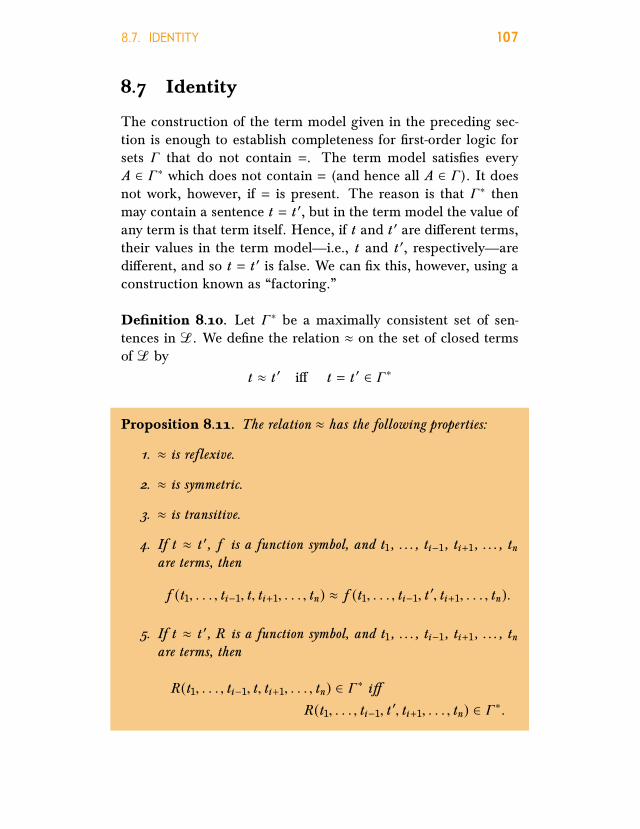
8.7. IDENTITY 107

8.7 Identity

The construction of the term model given in the preceding sec-tion is enough to establish completeness for first-order logic forsets Γ that do not contain =. The term model satisfies everyA ∈ Γ∗ which does not contain = (and hence all A ∈ Γ). It doesnot work, however, if = is present. The reason is that Γ∗ thenmay contain a sentence t = t ′, but in the term model the value ofany term is that term itself. Hence, if t and t ′ are dierent terms,their values in the term model—i.e., t and t ′, respectively—aredierent, and so t = t ′ is false. We can fix this, however, using aconstruction known as “factoring.”

Denition 8.10. Let Γ∗ be a maximally consistent set of sen-tences in L. We define the relation ≈ on the set of closed termsof L by

t ≈ t ′ i t = t ′ ∈ Γ∗

Proposition 8.11. The relation ≈ has the following properties:

1. ≈ is reexive.

2. ≈ is symmetric.

3. ≈ is transitive.

4. If t ≈ t ′, f is a function symbol, and t1, . . . , ti−1, ti+1, . . . , tnare terms, then

f (t1, . . . , ti−1, t, ti+1, . . . , tn) ≈ f (t1, . . . , ti−1, t ′, ti+1, . . . , tn).

5. If t ≈ t ′, R is a function symbol, and t1, . . . , ti−1, ti+1, . . . , tnare terms, then

R(t1, . . . , ti−1, t, ti+1, . . . , tn) ∈ Γ∗ iR(t1, . . . , ti−1, t ′, ti+1, . . . , tn) ∈ Γ∗.


Proof. Since Γ∗ is maximally consistent, t = t ′ ∈ Γ∗ i Γ∗ ` t = t ′.Thus it is enough to show the following:

1. Γ∗ ` t = t for all terms t .

2. If Γ∗ ` t = t ′ then Γ∗ ` t ′ = t .

3. If Γ∗ ` t = t ′ and Γ∗ ` t ′ = t ′′, then Γ∗ ` t = t ′′.

4. If Γ∗ ` t = t ′, then

Γ∗ ` f (t1, . . . , ti−1, t, ti+1, , . . . , tn) = f (t1, . . . , ti−1, t ′, ti+1, . . . , tn)

for every n-place function symbol f and terms t1, . . . , ti−1,ti+1, . . . , tn .

5. If Γ∗ ` t = t ′ and Γ∗ ` R(t1, . . . , ti−1, t, ti+1, . . . , tn), thenΓ∗ ` R(t1, . . . , ti−1, t ′, ti+1, . . . , tn) for every n-place predicatesymbol R and terms t1, . . . , ti−1, ti+1, . . . , tn .

Denition 8.12. Suppose Γ∗ is a maximally consistent set in alanguageL, t is a term, and ≈ as in the previous definition. Then:

[t ]≈ = t ′ : t ′ ∈ Trm(L), t ≈ t ′

and Trm(L)/≈ = [t ]≈ : t ∈ Trm(L).Denition 8.13. Let M =M(Γ∗) be the termmodel for Γ∗. ThenM/≈ is the following structure:

1. |M/≈ | = Trm(L)/≈.2. cM/≈ = [c ]≈3. f M/≈([t1]≈, . . . , [tn]≈) = [f (t1, . . . , tn)]≈4. 〈[t1]≈, . . . , [tn]≈〉 ∈ RM/≈ i M |= R(t1, . . . , tn).

8.7. IDENTITY 109

Note that we have defined f M/≈ and RM/≈ for elements ofTrm(L)/≈ by referring to them as [t ]≈, i.e., via representatives t ∈[t ]≈. We have to make sure that these definitions do not dependon the choice of these representatives, i.e., that for some otherchoices t ′ which determine the same equivalence classes ([t ]≈ =[t ′]≈), the definitions yield the same result. For instance, if R is aone-place predicate symbol, the last clause of the definition saysthat [t ]≈ ∈ RM/≈ i M |= R(t ). If for some other term t ′ witht ≈ t ′, M 6|= R(t ), then the definition would require [t ′]≈ < RM/≈ .If t ≈ t ′, then [t ]≈ = [t ′]≈, but we can’t have both [t ]≈ ∈ RM/≈

and [t ]≈ < RM/≈ . However, Proposition 8.11 guarantees that thiscannot happen.

Proposition 8.14. M/≈ is well dened, i.e., if t1, . . . , tn , t ′1, . . . , t′n

are terms, and ti ≈ t ′i then

1. [f (t1, . . . , tn)]≈ = [f (t ′1, . . . , t ′n)]≈, i.e., f (t1, . . . , tn) ≈

f (t ′1, . . . , t ′n) and2. M |= R(t1, . . . , tn) i M |= R(t ′1, . . . , t ′n), i.e., R(t1, . . . , tn) ∈

Γ∗ i R(t ′1, . . . , t ′n) ∈ Γ∗.

Proof. Follows from Proposition 8.11.

Lemma 8.15. M/≈ |= A i A ∈ Γ∗ for all sentences A.

Proof. By induction on A, just as in the proof of Lemma 8.9. Theonly case that needs additional attention is when A ≡ t = t ′.

M/≈ |= t = t ′ i [t ]≈ = [t ′]≈ (by definition of M/≈)

i t ≈ t ′ (by definition of [t ]≈)i t = t ′ ∈ Γ∗ (by definition of ≈).


Note that while M(Γ∗) is always countable and infinite, M/≈may be finite, since it may turn out that there are only finitelymany classes [t ]≈. This is to be expected, since Γ may containsentences which require any structure in which they are true tobe finite. For instance, ∀x ∀y x = y is a consistent sentence, butis satisfied only in structures with a domain that contains exactlyone element.

8.8 The Completeness Theorem

Theorem 8.16 (Completeness Theorem). Let Γ be a set of sen-tences. If Γ is consistent, it is satisable.

Proof. Suppose Γ is consistent. By Lemma 8.7, there is a Γ∗ ⊇Γ which is maximally consistent and saturated. If Γ does notcontain =, then by Lemma 8.9, M(Γ∗) |= A i A ∈ Γ∗. From thisit follows in particular that for all A ∈ Γ, M(Γ∗) |= A, so Γ issatisfiable. If Γ does contain =, then by Lemma 8.15, M/≈ |= Ai A ∈ Γ∗ for all sentences A. In particular, M/≈ |= A for allA ∈ Γ, so Γ is satisfiable.

Corollary 8.17 (Completeness Theorem, Second Version). Forall Γ and A sentences: if Γ A then Γ ` A.

Proof. Note that the Γ’s in Corollary 8.17 and Theorem 8.16 areuniversally quantified. To make sure we do not confuse ourselves,let us restate Theorem 8.16 using a dierent variable: for any setof sentences ∆, if ∆ is consistent, it is satisfiable. By contraposi-tion, if ∆ is not satisfiable, then ∆ is inconsistent. We will use thisto prove the corollary.

Suppose that Γ A. Then Γ∪¬A is unsatisfiable by Propo-sition 5.45. Taking Γ ∪ ¬A as our ∆, the previous version ofTheorem 8.16 gives us that Γ ∪ ¬A is inconsistent. By Propo-sition 7.11, Γ ` A.

8.9. THE COMPACTNESS THEOREM 111

8.9 The Compactness Theorem

Denition 8.18. A set Γ of formulas is nitely satisable if andonly if every finite Γ0 ⊆ Γ is satisfiable.

Theorem 8.19 (Compactness Theorem). The following hold forany sentences Γ and A:

1. Γ A i there is a nite Γ0 ⊆ Γ such that Γ0 A.

2. Γ is satisable if and only if it is nitely satisable.

Proof. We prove (2). If Γ is satisfiable, then there is a structure Msuch that M |= A for all A ∈ Γ. Of course, this M also satisfiesevery finite subset of Γ, so Γ is finitely satisfiable.

Now suppose that Γ is finitely satisfiable. Then every finitesubset Γ0 ⊆ Γ is satisfiable. By soundness, every finite subset isconsistent. Then Γ itself must be consistent. For assume it is not,i.e., Γ ` ⊥. But derivations are finite, and so already some finitesubset Γ0 ⊆ Γ must be inconsistent (cf. Proposition 7.13). Butwe just showed they are all consistent, a contradiction. Now bycompleteness, since Γ is consistent, it is satisfiable.

8.10 The Löwenheim-Skolem Theorem

Theorem 8.20. If Γ is consistent then it has a countably innitemodel, i.e., it is satisable in a structure whose domain is either niteor innite but countable.

Proof. If Γ is consistent, the structure M delivered by the proofof the completeness theorem has a domain |M | whose cardinalityis bounded by that of the set of the terms of the language L. SoM is at most countably infinite.


Theorem 8.21. If Γ is consistent set of sentences in the languageof rst-order logic without identity, then it has a countably innitemodel, i.e., it is satisable in a structure whose domain is innite andcountable.

Proof. If Γ is consistent and contains no sentences in which iden-tity appears, then the structure M delivered by the proof of thecompletness theorem has a domain |M | whose cardinality is iden-tical to that of the set of the terms of the language L. So M isdenumerably infinite.

CHAPTER 9

BeyondFirst-orderLogic9.1 Overview

First-order logic is not the only system of logic of interest: thereare many extensions and variations of first-order logic. A logictypically consists of the formal specification of a language, usu-ally, but not always, a deductive system, and usually, but notalways, an intended semantics. But the technical use of the termraises an obvious question: what do logics that are not first-orderlogic have to do with the word “logic,” used in the intuitive orphilosophical sense? All of the systems described below are de-signed to model reasoning of some form or another; can we saywhat makes them logical?

No easy answers are forthcoming. The word “logic” is usedin dierent ways and in dierent contexts, and the notion, likethat of “truth,” has been analyzed from numerous philosophicalstances. For example, one might take the goal of logical reason-

113

114 CHAPTER 9. BEYOND FIRST-ORDER LOGIC

ing to be the determination of which statements are necessarilytrue, true a priori, true independent of the interpretation of thenonlogical terms, true by virtue of their form, or true by linguis-tic convention; and each of these conceptions requires a gooddeal of clarification. Even if one restricts one’s attention to thekind of logic used in mathematical, there is little agreement as toits scope. For example, in the Principia Mathematica, Russell andWhitehead tried to develop mathematics on the basis of logic, inthe logicist tradition begun by Frege. Their system of logic wasa form of higher-type logic similar to the one described below.In the end they were forced to introduce axioms which, by moststandards, do not seem purely logical (notably, the axiom of in-finity, and the axiom of reducibility), but one might nonethelesshold that some forms of higher-order reasoning should be ac-cepted as logical. In contrast, Quine, whose ontology does notadmit “propositions” as legitimate objects of discourse, arguesthat second-order and higher-order logic are really manifestationsof set theory in sheep’s clothing; in other words, systems involv-ing quantification over predicates are not purely logical.

For now, it is best to leave such philosophical issues for a rainyday, and simply think of the systems below as formal idealizationsof various kinds of reasoning, logical or otherwise.

9.2 Many-Sorted Logic

In first-order logic, variables and quantifiers range over a singledomain. But it is often useful to have multiple (disjoint) domains:for example, you might want to have a domain of numbers, a do-main of geometric objects, a domain of functions from numbersto numbers, a domain of abelian groups, and so on.

Many-sorted logic provides this kind of framework. One startswith a list of “sorts”—the “sort” of an object indicates the “do-main” it is supposed to inhabit. One then has variables and quan-tifiers for each sort, and (usually) an identity predicate for eachsort. Functions and relations are also “typed” by the sorts of ob-

9.2. MANY-SORTED LOGIC 115

jects they can take as arguments. Otherwise, one keeps the usualrules of first-order logic, with versions of the quantifier-rules re-peated for each sort.

For example, to study international relations we might choosea language with two sorts of objects, French citizens and Germancitizens. We might have a unary relation, “drinks wine,” for ob-jects of the first sort; another unary relation, “eats wurst,” forobjects of the second sort; and a binary relation, “forms a multi-national married couple,” which takes two arguments, where thefirst argument is of the first sort and the second argument is ofthe second sort. If we use variables a, b , c to range over Frenchcitizens and x , y , z to range over German citizens, then

∀a ∀x[(Marr iedTo(a, x)→ (DrinksW ine(a)∨¬EatsWurst(x))]]asserts that if any French person is married to a German, eitherthe French person drinks wine or the German doesn’t eat wurst.

Many-sorted logic can be embedded in first-order logic in anatural way, by lumping all the objects of the many-sorted do-mains together into one first-order domain, using unary predicatesymbols to keep track of the sorts, and relativizing quantifiers.For example, the first-order language corresponding to the exam-ple above would have unary predicate symbolss “German” and“F rench,” in addition to the other relations described, with thesort requirements erased. A sorted quantifier ∀x A, where x is avariable of the German sort, translates to

∀x (German(x)→ A).We need to add axioms that insure that the sorts are separate—e.g., ∀x ¬(German(x)∧F rench(x))—as well as axioms that guar-antee that “drinks wine” only holds of objects satisfying the pred-icate F rench(x), etc. With these conventions and axioms, it isnot dicult to show that many-sorted sentences translate to first-order sentences, and many-sorted derivations translate to first-order derivations. Also, many-sorted structures “translate” to cor-responding first-order structures and vice-versa, so we also havea completeness theorem for many-sorted logic.


9.3 Second-Order logic

The language of second-order logic allows one to quantify notjust over a domain of individuals, but over relations on that do-main as well. Given a first-order language L, for each k one addsvariables R which range over k -ary relations, and allows quantifi-cation over those variables. If R is a variable for a k -ary rela-tion, and t1, . . . , tk are ordinary (first-order) terms, R(t1, . . . , tk )is an atomic formula. Otherwise, the set of formulas is definedjust as in the case of first-order logic, with additional clauses forsecond-order quantification. Note that we only have the identitypredicate for first-order terms: if R and S are relation variablesof the same arity k , we can define R = S to be an abbreviationfor

∀x1 . . . ∀xk (R(x1, . . . , xk )↔ S (x1, . . . , xk )).The rules for second-order logic simply extend the quanti-

fier rules to the new second order variables. Here, however, onehas to be a little bit careful to explain how these variables in-teract with the predicate symbols of L, and with formulas of Lmore generally. At the bare minimum, relation variables countas terms, so one has inferences of the form

A(R) ` ∃R A(R)But if L is the language of arithmetic with a constant relationsymbol <, one would also expect the following inference to bevalid:

x < y ` ∃R R(x, y)or for a given formula A,

A(x1, . . . , xk ) ` ∃R R(x1, . . . , xk )More generally, we might want to allow inferences of the form

A[λ~x .B(~x)/R]∃R Awhere A[λ~x .B(~x)/R] denotes the result of replacing every atomicformula of the form Rt1, . . . , tk in A by B(t1, . . . , tk ). This last rule

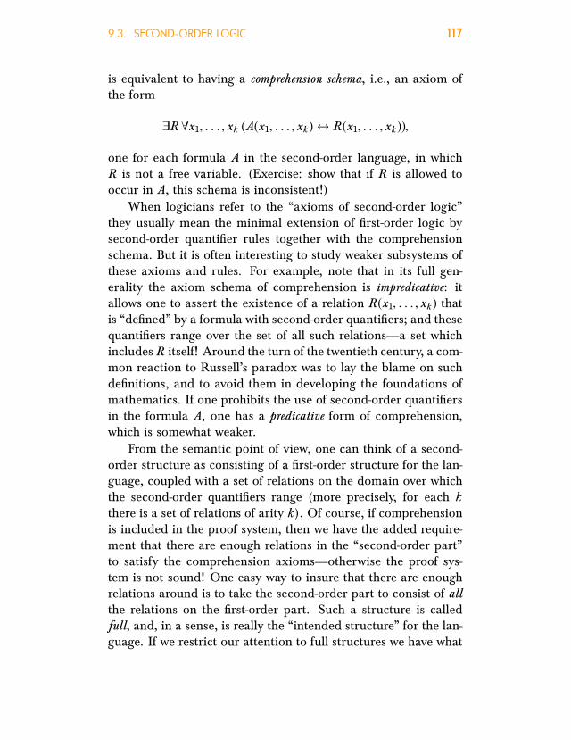
9.3. SECOND-ORDER LOGIC 117

is equivalent to having a comprehension schema, i.e., an axiom ofthe form

∃R ∀x1, . . . , xk (A(x1, . . . , xk )↔ R(x1, . . . , xk )),

one for each formula A in the second-order language, in whichR is not a free variable. (Exercise: show that if R is allowed tooccur in A, this schema is inconsistent!)

When logicians refer to the “axioms of second-order logic”they usually mean the minimal extension of first-order logic bysecond-order quantifier rules together with the comprehensionschema. But it is often interesting to study weaker subsystems ofthese axioms and rules. For example, note that in its full gen-erality the axiom schema of comprehension is impredicative: itallows one to assert the existence of a relation R(x1, . . . , xk ) thatis “defined” by a formula with second-order quantifiers; and thesequantifiers range over the set of all such relations—a set whichincludesR itself! Around the turn of the twentieth century, a com-mon reaction to Russell’s paradox was to lay the blame on suchdefinitions, and to avoid them in developing the foundations ofmathematics. If one prohibits the use of second-order quantifiersin the formula A, one has a predicative form of comprehension,which is somewhat weaker.

From the semantic point of view, one can think of a second-order structure as consisting of a first-order structure for the lan-guage, coupled with a set of relations on the domain over whichthe second-order quantifiers range (more precisely, for each kthere is a set of relations of arity k). Of course, if comprehensionis included in the proof system, then we have the added require-ment that there are enough relations in the “second-order part”to satisfy the comprehension axioms—otherwise the proof sys-tem is not sound! One easy way to insure that there are enoughrelations around is to take the second-order part to consist of allthe relations on the first-order part. Such a structure is calledfull, and, in a sense, is really the “intended structure” for the lan-guage. If we restrict our attention to full structures we have what


is known as the full second-order semantics. In that case, specify-ing a structure boils down to specifying the first-order part, sincethe contents of the second-order part follow from that implicitly.

To summarize, there is some ambiguity when talking aboutsecond-order logic. In terms of the proof system, one might havein mind either

1. A “minimal” second-order proof system, together with somecomprehension axioms.

2. The “standard” second-order proof system, with full com-prehension.

In terms of the semantics, one might be interested in either

1. The “weak” semantics, where a structure consists of a first-order part, together with a second-order part big enoughto satisfy the comprehension axioms.

2. The “standard” second-order semantics, in which one con-siders full structures only.

When logicians do not specify the proof system or the semanticsthey have in mind, they are usually refering to the second itemon each list. The advantage to using this semantics is that, aswe will see, it gives us categorical descriptions of many naturalmathematical structures; at the same time, the proof system isquite strong, and sound for this semantics. The drawback is thatthe proof system is not complete for the semantics; in fact, no ef-fectively given proof system is complete for the full second-ordersemantics. On the other hand, we will see that the proof systemis complete for the weakened semantics; this implies that if a sen-tence is not provable, then there is some structure, not necessarilythe full one, in which it is false.

The language of second-order logic is quite rich. One canidentify unary relations with subsets of the domain, and so in

9.3. SECOND-ORDER LOGIC 119

particular you can quantify over these sets; for example, one canexpress induction for the natural numbers with a single axiom

∀R ((R() ∧ ∀x (R(x)→ R(x ′)))→ ∀x R(x)).If one takes the language of arithmetic to have symbols , ′,+,×and <, one can add the following axioms to describe their behav-ior:

1. ∀x ¬x ′ =

2. ∀x ∀y (s (x) = s (y)→ x = y)3. ∀x (x + 0) = x4. ∀x ∀y (x + y ′) = (x + y)′

5. ∀x (x × 0) = 0

6. ∀x ∀y (x × y ′) = ((x × y) + x)7. ∀x ∀y (x < y ↔ ∃z y = (x + z ′))

It is not dicult to show that these axioms, together with theaxiom of induction above, provide a categorical description ofthe structure N, the standard model of arithmetic, provided weare using the full second-order semantics. Given any structure Ain which these axioms are true, define a function f from N to thedomain of A using ordinary recursion on N, so that f (0) = A

and f (x + 1) = ′A(f (x)). Using ordinary induction on N and thefact that axioms (1) and (2) hold in A, we see that f is injective.To see that f is surjective, let P be the set of elements of |A|that are in the range of f . Since A is full, P is in the second-order domain. By the construction of f , we know that A is in P ,and that P is closed under ′A. The fact that the induction axiomholds in A (in particular, for P ) guarantees that P is equal to theentire first-order domain of A. This shows that f is a bijection.Showing that f is a homomorphism is no more dicult, usingordinary induction on N repeatedly.


In set-theoretic terms, a function is just a special kind of re-lation; for example, a unary function f can be identified witha binary relation R satisfying ∀x ∃y R(x, y). As a result, one canquantify over functions too. Using the full semantics, one canthen define the class of infinite structures to be the class of struc-tures A for which there is an injective function from the domainof A to a proper subset of itself:

∃f (∀x ∀y (f (x) = f (y)→ x = y) ∧ ∃y ∀x f (x) , y).The negation of this sentence then defines the class of finite struc-tures.

In addition, one can define the class of well-orderings, byadding the following to the definition of a linear ordering:

∀P (∃x P (x)→ ∃x (P (x) ∧ ∀y (y < x → ¬P (y)))).This asserts that every nonempty set has a least element, modulothe identification of “set” with “one-place relation”. For anotherexample, one can express the notion of connectedness for graphs,by saying that there is no nontrivial separation of the vertices intodisconnected parts:

¬∃A (∃x A(x)∧∃y ¬A(y)∧∀[w][∀z ((A(w)∧¬A(z ))→ ¬R(w, z ))]).For yet another example, you might try as an exercise to definethe class of finite structures whose domain has even size. Morestrikingly, one can provide a categorical description of the realnumbers as a complete ordered field containing the rationals.

In short, second-order logic is much more expressive thanfirst-order logic. That’s the good news; now for the bad. We havealready mentioned that there is no eective proof system thatis complete for the full second-order semantics. For better orfor worse, many of the properties of first-order logic are absent,including compactness and the Löwenheim-Skolem theorems.

On the other hand, if one is willing to give up the full second-order semantics in terms of the weaker one, then the minimal

9.4. HIGHER-ORDER LOGIC 121

second-order proof system is complete for this semantics. In otherwords, if we read ` as “proves in the minimal system” and as“logically implies in the weaker semantics”, we can show thatwhenever Γ A then Γ ` A. If one wants to include specific com-prehension axioms in the proof system, one has to restrict thesemantics to second-order structures that satisfy these axioms:for example, if ∆ consists of a set of comprehension axioms (pos-sibly all of them), we have that if Γ ∪ ∆ A, then Γ ∪ ∆ ` A. Inparticular, if A is not provable using the comprehension axiomswe are considering, then there is a model of ¬A in which thesecomprehension axioms nonetheless hold.

The easiest way to see that the completeness theorem holdsfor the weaker semantics is to think of second-order logic as amany-sorted logic, as follows. One sort is interpreted as the ordi-nary “first-order” domain, and then for each k we have a domainof “relations of arity k .” We take the language to have built-inrelation symbols “truek (R, x1, . . . , xk )” which is meant to assertthat R holds of x1, . . . , xk , where R is a variable of the sort “k -aryrelation” and x1, . . . , xk are objects of the first-order sort.

With this identification, the weak second-order semantics isessentially the usual semantics for many-sorted logic; and we havealready observed that many-sorted logic can be embedded in first-order logic. Modulo the translations back and forth, then, theweaker conception of second-order logic is really a form of first-order logic in disguise, where the domain contains both “objects”and “relations” governed by the appropriate axioms.

9.4 Higher-Order logic

Passing from first-order logic to second-order logic enabled usto talk about sets of objects in the first-order domain, within theformal language. Why stop there? For example, third-order logicshould enable us to deal with sets of sets of objects, or perhapseven sets which contain both objects and sets of objects. Andfourth-order logic will let us talk about sets of objects of that kind.


As you may have guessed, one can iterate this idea arbitrarily.In practice, higher-order logic is often formulated in terms

of functions instead of relations. (Modulo the natural identifica-tions, this dierence is inessential.) Given some basic “sorts” A,B , C , . . . (which we will now call “types”), we can create newones by stipulating

If σ and τ are finite types then so is σ → τ.

Think of types as syntactic “labels,” which classify the objectswe want in our domain; σ → τ describes those objects that arefunctions which take objects of type σ to objects of type τ. Forexample, we might want to have a type Ω of truth values, “true”and “false,” and a type N of natural numbers. In that case, youcan think of objects of type N→ Ω as unary relations, or subsetsof N; objects of type N→ N are functions from natural numers tonatural numbers; and objects of type (N→ N)→ N are “function-als,” that is, higher-type functions that take functions to numbers.

As in the case of second-order logic, one can think of higher-order logic as a kind of many-sorted logic, where there is a sort foreach type of object we want to consider. But it is usually clearerjust to define the syntax of higher-type logic from the ground up.For example, we can define a set of finite types inductively, asfollows:

1. N is a finite type.

2. If σ and τ are finite types, then so is σ → τ.

3. If σ and τ are finite types, so is σ × τ.

Intuitively, N denotes the type of the natural numbers, σ → τ

denotes the type of functions from σ to τ, and σ × τ denotes thetype of pairs of objects, one from σ and one from τ. We can thendefine a set of terms inductively, as follows:

1. For each type σ, there is a stock of variables x , y , z , . . . oftype σ

9.4. HIGHER-ORDER LOGIC 123

2. is a term of type N

3. S (successor) is a term of type N→ N

4. If s is a term of type σ, and t is a term of typeN→ (σ → σ),then Rs t is a term of type N→ σ

5. If s is a term of type τ → σ and t is a term of type τ, thens (t ) is a term of type σ

6. If s is a term of type σ and x is a variable of type τ, thenλx . s is a term of type τ → σ.

7. If s is a term of type σ and t is a term of type τ, then 〈s, t〉is a term of type σ × τ.

8. If s is a term of type σ × τ then p1(s ) is a term of type σand p2(s ) is a term of type τ.

Intuitively, Rs t denotes the function defined recursively by

Rs t (0) = sRs t (x + 1) = t (x,Rs t (x)),

〈s, t〉 denotes the pair whose first component is s and whose sec-ond component is t , and p1(s ) and p2(s ) denote the first andsecond elements (“projections”) of s . Finally, λx . s denotes thefunction f defined by

f (x) = sfor any x of type σ; so item (6) gives us a form of comprehension,enabling us to define functions using terms. Formulas are builtup from identity predicate statements s = t between terms of thesame type, the usual propositional connectives, and higher-typequantification. One can then take the axioms of the system to bethe basic equations governing the terms defined above, togetherwith the usual rules of logic with quantifiers and identity predi-cate.


If one augments the finite type system with a type Ω of truthvalues, one has to include axioms which govern its use as well. Infact, if one is clever, one can get rid of complex formulas entirely,replacing them with terms of type Ω! The proof system can thenbe modified accordingly. The result is essentially the simple theoryof types set forth by Alonzo Church in the 1930s.

As in the case of second-order logic, there are dierent ver-sions of higher-type semantics that one might want to use. In thefull version, variables of type σ → τ range over the set of allfunctions from the objects of type σ to objects of type τ. As youmight expect, this semantics is too strong to admit a complete,eective proof system. But one can consider a weaker semantics,in which a structure consists of sets of elements Tτ for each typeτ, together with appropriate operations for application, projec-tion, etc. If the details are carried out correctly, one can obtaincompleteness theorems for the kinds of proof systems describedabove.

Higher-type logic is attractive because it provides a frame-work in which we can embed a good deal of mathematics in anatural way: starting with N, one can define real numbers, con-tinuous functions, and so on. It is also particularly attractive inthe context of intuitionistic logic, since the types have clear “con-structive” intepretations. In fact, one can develop constructiveversions of higher-type semantics (based on intuitionistic, ratherthan classical logic) that clarify these constructive interpretationsquite nicely, and are, in many ways, more interesting than theclassical counterparts.

9.5 Intuitionistic logic

In constrast to second-order and higher-order logic, intuitionisticfirst-order logic represents a restriction of the classical version,intended to model a more “constructive” kind of reasoning. Thefollowing examples may serve to illustrate some of the underlyingmotivations.

9.5. INTUITIONISTIC LOGIC 125

Suppose someone came up to you one day and announcedthat they had determined a natural number x , with the propertythat if x is prime, the Riemann hypothesis is true, and if x is com-posite, the Riemann hypothesis is false. Great news! Whether theRiemann hypothesis is true or not is one of the big open ques-tions of mathematics, and here they seem to have reduced theproblem to one of calculation, that is, to the determination ofwhether a specific number is prime or not.

What is the magic value of x? They describe it as follows: x isthe natural number that is equal to 7 if the Riemann hypothesisis true, and 9 otherwise.

Angrily, you demand your money back. From a classical pointof view, the description above does in fact determine a uniquevalue of x ; but what you really want is a value of x that is givenexplicitly.

To take another, perhaps less contrived example, considerthe following question. We know that it is possible to raise anirrational number to a rational power, and get a rational result.

For example,√22= 2. What is less clear is whether or not it is

possible to raise an irrational number to an irrational power, andget a rational result. The following theorem answers this in thearmative:

Theorem 9.1. There are irrational numbers a and b such that ab isrational.

Proof. Consider√2√2. If this is rational, we are done: we can let

a = b =√2. Otherwise, it is irrational. Then we have

(√2√2)√2 =√2√2·√2=√22= 2,

which is certainly rational. So, in this case, let a be√2√2, and let

b be√2.


Does this constitute a valid proof? Most mathematicians feelthat it does. But again, there is something a little bit unsatisfyinghere: we have proved the existence of a pair of real numberswith a certain property, without being able to say which pair ofnumbers it is. It is possible to prove the same result, but in sucha way that the pair a, b is given in the proof: take a =

√3 and

b = log3 4. Then

ab =√3log3 4

= 31/2·log3 4 = (3log3 4)1/2 = 41/2 = 2,

since 3log3 x = x .Intuitionistic logic is designed to model a kind of reasoning

where moves like the one in the first proof are disallowed. Provingthe existence of an x satisfying A(x)means that you have to give aspecific x , and a proof that it satisfies A, like in the second proof.Proving that A or B holds requires that you can prove one or theother.

Formally speaking, intuitionistic first-order logic is what youget if you omit restrict a proof system for first-order logic in acertain way. Similarly, there are intuitionistic versions of second-order or higher-order logic. From the mathematical point of view,these are just formal deductive systems, but, as already noted,they are intended to model a kind of mathematical reasoning.One can take this to be the kind of reasoning that is justified ona certain philosophical view of mathematics (such as Brouwer’sintuitionism); one can take it to be a kind of mathematical rea-soning which is more “concrete” and satisfying (along the linesof Bishop’s constructivism); and one can argue about whether ornot the formal description captures the informal motivation. Butwhatever philosophical positions we may hold, we can study in-tuitionistic logic as a formally presented logic; and for whateverreasons, many mathematical logicians find it interesting to do so.

There is an informal constructive interpretation of the intu-itionist connectives, usually known as the Brouwer-Heyting-Kolmogorovinterpretation. It runs as follows: a proof of A ∧ B consists of aproof of A paired with a proof of B ; a proof of A ∨ B consists


of either a proof of A, or a proof of B , where we have explicitinformation as to which is the case; a proof of A → B consistsof a procedure, which transforms a proof of A to a proof of B ;a proof of ∀x A(x) consists of a procedure which returns a proofof A(x) for any value of x ; and a proof of ∃x A(x) consists of avalue of x , together with a proof that this value satisfies A. Onecan describe the interpretation in computational terms knownas the “Curry-Howard isomorphism” or the “formulas-as-typesparadigm”: think of a formula as specifying a certain kind of datatype, and proofs as computational objects of these data types thatenable us to see that the corresponding formula is true.

Intuitionistic logic is often thought of as being classical logic“minus” the law of the excluded middle. This following theoremmakes this more precise.

Theorem 9.2. Intuitionistically, the following axiom schemata areequivalent:

1. (A → ⊥)→ ¬A.2. A ∨ ¬A

3. ¬¬A → A

Obtaining instances of one schema from either of the others is agood exercise in intuitionistic logic.

The first deductive systems for intuitionistic propositional logic,put forth as formalizations of Brouwer’s intuitionism, are due, in-dependently, to Kolmogorov, Glivenko, and Heyting. The firstformalization of intuitionistic first-order logic (and parts of intu-itionist mathematics) is due to Heyting. Though a number ofclassically valid schemata are not intuitionistically valid, manyare.

The double-negation translation describes an important rela-tionship between classical and intuitionist logic. It is defined in-ductively follows (think of AN as the “intuitionist” translation of


the classical formula A):

AN ≡ ¬¬A for atomic formulas A

(A ∧ B)N ≡ (AN ∧ BN )(A ∨ B)N ≡ ¬¬(AN ∨ BN )(A → B)N ≡ (AN → BN )(∀x A)N ≡ ∀x AN(∃x A)N ≡ ¬¬∃x AN

Kolmogorov and Glivenko had versions of this translation forpropositional logic; for predicate logic, it is due to Gödel andGentzen, independently. We have

Theorem 9.3. 1. A ↔ AN is provable classically

2. IfA is provable classically, thenAN is provable intuitionistically.

We can now envision the following dialogue. Classical math-ematician: “I’ve proved A!” Intuitionist mathematician: “Yourproof isn’t valid. What you’ve really proved is AN .” Classicalmathematician: “Fine by me!” As far as the classical mathemati-cian is concerned, the intuitionist is just splitting hairs, since thetwo are equivalent. But the intuitionist insists there is a dier-ence.

Note that the above translation concerns pure logic only; itdoes not address the question as to what the appropriate nonlog-ical axioms are for classical and intuitionistic mathematics, orwhat the relationship is between them. But the following slightextension of the theorem above provides some useful informa-tion:

Theorem 9.4. If Γ proves A classically, ΓN proves AN intuitionisti-cally.


In other words, if A is provable from some hypotheses classi-cally, thenAN is provable from their double-negation translations.

To show that a sentence or propositional formula is intuition-istically valid, all you have to do is provide a proof. But how canyou show that it is not valid? For that purpose, we need a seman-tics that is sound, and preferrably complete. A semantics due toKripke nicely fits the bill.

We can play the same game we did for classical logic: de-fine the semantics, and prove soundness and completeness. Itis worthwhile, however, to note the following distinction. In thecase of classical logic, the semantics was the “obvious” one, ina sense implicit in the meaning of the connectives. Though onecan provide some intuitive motivation for Kripke semantics, thelatter does not oer the same feeling of inevitability. In addi-tion, the notion of a classical structure is a natural mathematicalone, so we can either take the notion of a structure to be a toolfor studying classical first-order logic, or take classical first-orderlogic to be a tool for studying mathematical structures. In con-trast, Kripke structures can only be viewed as a logical construct;they don’t seem to have independent mathematical interest.

A Kripke structure for a propositional langauge consists of apartial order Mod(P ) with a least element, and an “monotone”assignment of propositional variables to the elements ofMod(P ).The intuition is that the elements of Mod(P ) represent “worlds,”or “states of knowledge”; an element p ≥ q represents a “possiblefuture state” of q ; and the propositional variables assigned to pare the propositions that are known to be true in state p . Theforcing relation P, p A then extends this relationship to arbi-trary formulas in the language; read P, p A as “A is true instate p .” The relationship is defined inductively, as follows:

1. P, p pi i pi is one of the propositional variables assignedto p .

2. P, p 1 ⊥.

3. P, p (A ∧ B) i P, p A and P, p B .


4. P, p (A ∨ B) i P, p A or P, p B .

5. P, p (A → B) i, whenever q ≥ p and P, q A, thenP, q B .

It is a good exercise to try to show that ¬(p ∧ q ) → (¬p ∨ ¬q ) isnot intuitionistically valid, by cooking up a Kripke structure thatprovides a counterexample.

9.6 Modal Logics

Consider the following example of a conditional sentence:

If Jeremy is alone in that room, then he is drunk andnaked and dancing on the chairs.

This is an example of a conditional assertion that may be mate-rially true but nonetheless misleading, since it seems to suggestthat there is a stronger link between the antecedent and conclu-sion other than simply that either the antecedent is false or theconsequent true. That is, the wording suggests that the claim isnot only true in this particular world (where it may be triviallytrue, because Jeremy is not alone in the room), but that, more-over, the conclusion would have been true had the antecedentbeen true. In other words, one can take the assertion to meanthat the claim is true not just in this world, but in any “possible”world; or that it is necessarily true, as opposed to just true in thisparticular world.

Modal logic was designed to make sense of this kind of ne-cessity. One obtains modal propositional logic from ordinarypropositional logic by adding a box operator; which is to say, ifA is a formula, so is A. Intuitively, A asserts that A is neces-sarily true, or true in any possible world. ♦A is usually taken tobe an abbreviation for ¬¬A, and can be read as asserting thatA is possibly true. Of course, modality can be added to predicatelogic as well.

9.6. MODAL LOGICS 131

Kripke structures can be used to provide a semantics formodal logic; in fact, Kripke first designed this semantics withmodal logic in mind. Rather than restricting to partial orders,more generally one has a set of “possible worlds,” P , and a bi-nary “accessibility” relation R(x, y) between worlds. Intuitively,R(p, q ) asserts that the world q is compatible with p; i.e., if weare “in” world p, we have to entertain the possibility that theworld could have been like q .

Modal logic is sometimes called an “intensional” logic, as op-posed to an “extensional” one. The intended semantics for anextensional logic, like classical logic, will only refer to a singleworld, the “actual” one; while the semantics for an “intensional”logic relies on a more elaborate ontology. In addition to structure-ing necessity, one can use modality to structure other linguisticconstructions, reinterpreting and ♦ according to the applica-tion. For example:

1. In provability logic, A is read “A is provable” and ♦A isread “A is consistent.”

2. In epistemic logic, one might read A as “I know A” or “Ibelieve A.”

3. In temporal logic, one can read A as “A is always true”and ♦A as “A is sometimes true.”

One would like to augment logic with rules and axioms deal-ing with modality. For example, the system S4 consists of theordinary axioms and rules of propositional logic, together withthe following axioms:

(A → B)→ (A → B)A → A

A → A


as well as a rule, “from A conclude A.” S5 adds the followingaxiom:

♦A → ♦A

Variations of these axioms may be suitable for dierent applica-tions; for example, S5 is usually taken to characterize the notionof logical necessity. And the nice thing is that one can usuallyfind a semantics for which the proof system is sound and completeby restricting the accessibility relation in the Kripke structures innatural ways. For example, S4 corresponds to the class of Kripkestructures in which the accessibility relation is reflexive and tran-sitive. S5 corresponds to the class of Kripke structures in whichthe accessibility relation is universal, which is to say that everyworld is accessible from every other; so A holds if and only ifA holds in every world.

9.7 Other Logics

As you may have gathered by now, it is not hard to design a newlogic. You too can create your own a syntax, make up a deductivesystem, and fashion a semantics to go with it. You might haveto be a bit clever if you want the proof system to be completefor the semantics, and it might take some eort to convince theworld at large that your logic is truly interesting. But, in return,you can enjoy hours of good, clean fun, exploring your logic’smathematical and computational properties.

Recent decades have witnessed a veritable explosion of for-mal logics. Fuzzy logic is designed to model reasoning aboutvague properties. Probabilistic logic is designed to model reason-ing about uncertainty. Default logics and nonmonotonic logicsare designed to model defeasible forms of reasoning, which is tosay, “reasonable” inferences that can later be overturned in theface of new information. There are epistemic logics, designedto model reasoning about knowledge; causal logics, designed tomodel reasoning about causal relationships; and even “deontic”

9.7. OTHER LOGICS 133

logics, which are designed to model reasoning about moral andethical obligations. Depending on whether the primary motiva-tion for introducing these systems is philosophical, mathematical,or computational, you may find such creatures studies under therubric of mathematical logic, philosophical logic, artificial intel-ligence, cognitive science, or elsewhere.

The list goes on and on, and the possibilities seem endless.We may never attain Leibniz’ dream of reducing all of humanreason to calculation—but that can’t stop us from trying.

PART III

TuringMachines

135

CHAPTER 10

TuringMachineComputations10.1 Introduction

What does it mean for a function, say, from N to N to be com-putable? Among the first answers, and the most well known one,is that a function is computable if it can be computed by a Tur-ing machine. This notion was set out by Alan Turing in 1936.Turing machines are an example of a model of computation—theyare a mathematically precise way of defining the idea of a “com-putational procedure.” What exactly that means is debated, butit is widely agreed that Turing machines are one way of speci-fying computational procedures. Even though the term “Turingmachine” evokes the image of a physical machine with movingparts, strictly speaking a Turing machine is a purely mathemat-ical construct, and as such it idealizes the idea of a computa-tional procedure. For instance, we place no restriction on eitherthe time or memory requirements of a Turing machine: Turing

136


machines can compute something even if the computation wouldrequire more storage space or more steps than there are atoms inthe universe.

It is perhaps best to think of a Turing machine as a programfor a special kind of imaginary mechanism. This mechanism con-sists of a tape and a read-write head. In our version of Turing ma-chines, the tape is infinite in one direction (to the right), and itis divided into squares, each of which may contain a symbol froma finite alphabet. Such alphabets can contain any number of dif-ferent symbols, but we will mainly make do with three: ., t, andI . When the mechanism is started, the tape is empty (i.e., eachsquare contains the symbol t) except for the leftmost square,which contains ., and a finite number of squares which containthe input. At any time, the mechanism is in one of a finite numberof states. At the outset, the head scans the leftmost square and ina specified initial state. At each step of the mechanism’s run, thecontent of the square currently scanned together with the statethe mechanism is in and the Turing machine program determinewhat happens next. The Turing machine program is given by apartial function which takes as input a state q and a symbol σand outputs a triple 〈q ′, σ′,D〉. Whenever the mechanism is instate q and reads symbol σ, it replaces the symbol on the currentsquare with σ′, the head moves left, right, or stays put accordingto whether D is L, R, or N , and the mechanism goes into state q ′.

For instance, consider the situation below:

. I I I t I I I I t t tq1

The tape of the Turing machine contains the end-of-tape sym-bol . on the leftmost square, followed by three I ’s, a t, four moreI ’s, and the rest of the tape is filled with t’s. The head is read-ing the third square from the left, which contains a I , and isin state q1—we say “the machine is reading a I in state q1.” Ifthe program of the Turing machine returns, for input 〈q1, I 〉, thetriple 〈q5,t,R〉, we would now replace the I on the third square

138 CHAPTER 10. TURING MACHINE COMPUTATIONS

with a t, move right to the fourth square, and change the stateof the machine to q5.

We say that the machine halts when it encounters some state,qn , and symbol, σ such that there is no instruction for 〈qn, σ〉,i.e., the transition function for input 〈qn, σ〉 is undefined. In otherwords, the machine has no instruction to carry out, and at thatpoint, it ceases operation. Halting is sometimes represented bya specific halt state h. This will be demonstrated in more detaillater on.

The beauty of Turing’s paper, “On computable numbers,”is that he presents not only a formal definition, but also an ar-gument that the definition captures the intuitive notion of com-putability. From the definition, it should be clear that any func-tion computable by a Turing machine is computable in the intu-itive sense. Turing oers three types of argument that the con-verse is true, i.e., that any function that we would naturally regardas computable is computable by such a machine. They are (inTuring’s words):

1. A direct appeal to intuition.

2. A proof of the equivalence of two definitions (in case thenew definition has a greater intuitive appeal).

3. Giving examples of large classes of numbers which are com-putable.

Our goal is to try to define the notion of computability “in prin-ciple,” i.e., without taking into account practical limitations oftime and space. Of course, with the broadest definition of com-putability in place, one can then go on to consider computationwith bounded resources; this forms the heart of the subject knownas “computational complexity.”

Historical Remarks Alan Turing invented Turing machines in1936. While his interest at the time was the decidability of first-order logic, the paper has been described as a definitive paper

10.2. REPRESENTING TURING MACHINES 139

on the foundations of computer design. In the paper, Turingfocuses on computable real numbers, i.e., real numbers whosedecimal expansions are computable; but he notes that it is nothard to adapt his notions to computable functions on the naturalnumbers, and so on. Notice that this was a full five years be-fore the first working general purpose computer was built in 1941(by the German Konrad Zuse in his parents living room), sevenyears before Turing and his colleagues at Bletchley Park built thecode-breaking Colossus (1943), nine years before the AmericanENIAC (1945), twelve years before the first British general pur-pose computer the Manchester Mark I was built in Manchester(1948) and thirteen years before the Americans first tested theBINAC (1949). The Manchester Mark I has the distinction of be-ing the first stored-program computer—previous machines hadto be rewired by hand for each new task.

10.2 Representing Turing Machines

Turing machines can be represented visually by state diagrams.The diagrams are composed of state cells connected by arrows.Unsurprisingly, each state cell represents a state of the machine.Each arrow represents an instruction that can be carried out fromthat state, with the specifics of the instruction written above orbelow the appropriate arrow. Consider the following machine,which has only two internal states, q0 and q1, and one instruction:

q0start q1t, I ,R

Recall that the Turing machine has a read/write head and a tapewith the input written on it. The instruction can be read as ifreading a blank in state q0, write a stroke, move right, and move tostate q1. This is equivalent to the transition function mapping〈q0,t〉 to 〈q1, I ,R〉.


Example 10.1. Even Machine: The following Turing machinehalts if, and only if, there are an even number of strokes on thetape.

q0start q1

I , I ,Rt,t,R

I , I ,R

The state diagram corresponds to the following transitionfunction:

δ(q0, I ) = 〈q1, I ,R〉,δ(q1, I ) = 〈q0, I ,R〉,δ(q0,t) = 〈q0,t,R〉

The above machine halts only when the input is an even num-ber of strokes. Otherwise, the machine (theoretically) continuesto operate indefinitely. For any machine and input, it is possi-ble to trace through the congurations of the machine in order todetermine the output. We will give a formal definition of config-urations later. For now, we can intuitively think of configurationsas a series of diagrams showing the state of the machine at anypoint in time during operation. Configurations show the con-tent of the tape, the state of the machine and the location of theread/write head.

Let us trace through the configurations of the even machineif it is started with an input of 4 I s. In this case, we expect thatthe machine will halt. We will then run the machine on an inputof 3 I s, where the machine will run forever.

The machine starts in state q0, scanning the leftmost I . Wecan represent the initial state of the machine as follows:

.I0I I I t . . .

The above configuration is straightforward. As can be seen, themachine starts in state one, scanning the leftmost I . This is rep-


resented by a subscript of the state name on the first I . Theapplicable instruction at this point is δ(q0, I ) = 〈q1, I ,R〉, and sothe machine moves right on the tape and changes to state q1.

.I I1I I t . . .

Since the machine is now in state q1 scanning a stroke, we haveto “follow” the instruction δ(q1, I ) = 〈q0, I ,R〉. This results in theconfiguration

.I I I0I t . . .

As the machine continues, the rules are applied again in the sameorder, resulting in the following two configurations:

.I I I I1 t . . .

.I I I I t0 . . .

The machine is now in state q0 scanning a blank. Based on thetransition diagram, we can easily see that there is no instructionto be carried out, and thus the machine has halted. This meansthat the input has been accepted.

Suppose next we start the machine with an input of threestrokes. The first few configurations are similar, as the same in-structions are carried out, with only a small dierence of the tapeinput:

.I0I I t . . .

.I I1I t . . .

.I I I0 t . . .

.I I I t1 . . .

The machine has now traversed past all the strokes, and is read-ing a blank in state q1. As shown in the diagram, there is aninstruction of the form δ(q1,t) = 〈q1,t,R〉. Since the tape is in-finitely blank to the right, the machine will continue to executethis instruction forever, staying in state q1 and moving ever further


to the right. The machine will never halt, and does not acceptthe input.

It is important to note that not all machines will halt. If halt-ing means that the machine runs out of instructions to execute,then we can create a machine that never halts simply by ensuringthat there is an outgoing arrow for each symbol at each state.The even machine can be modified to run infinitely by adding aninstruction for scanning a blank at q0.

Example 10.2.

q0start q1

I , I ,Rt,t,R t,t,R

I , I ,R

Machine tables are another way of representing Turing ma-chines. Machine tables have the tape alphabet displayed on thex -axis, and the set of machine states across the y -axis. Inside thetable, at the intersection of each state and symbol, is written therest of the instruction—the new state, new symbol, and direc-tion of movement. Machine tables make it easy to determine inwhat state, and for what symbol, the machine halts. Wheneverthere is a gap in the table is a possible point for the machine tohalt. Unlike state diagrams and instruction sets, where the pointsat which the machine halts are not always immediately obvious,any halting points are quickly identified by finding the gaps inthe machine table.

Example 10.3. The machine table for the even machine is:

t Iq0 I , q1,Rq1 t, q1,t I , q0,R

As we can see, the machine halts when scanning a blank in stateq0.


So far we have only considered machines that read and acceptinput. However, Turing machines have the capacity to both readand write. An example of such a machine (although there aremany, many examples) is a doubler. A doubler, when started witha block of n strokes on the tape, outputs a block of 2n strokes.

Example 10.4. Before building a doubler machine, it is impor-tant to come up with a strategy for solving the problem. Since themachine (as we have formulated it) cannot remember how manystrokes it has read, we need to come up with a way to keep trackof all the strokes on the tape. One such way is to separate theoutput from the input with a blank. The machine can then erasethe first stroke from the input, traverse over the rest of the input,leave a blank, and write two new strokes. The machine will thengo back and find the second stroke in the input, and double thatone as well. For each one stroke of input, it will write two strokesof output. By erasing the input as the machine goes, we can guar-antee that no stroke is missed or doubled twice. When the entireinput is erased, there will be 2n strokes left on the tape.

q0start q1 q2

q3q4q5

I ,t,R

I , I ,R

t,t,L

I , I ,R

t, I ,R

t, I ,L

I , I ,L

I , I ,L

t,t,L

I , I ,L

t,t,R


10.3 Turing Machines

The formal definition of what constitutes a Turing machine looksabstract, but is actually simple: it merely packs into one mathe-matical structure all the information needed to specify the work-ings of a Turing machine. This includes (1) which states themachine can be in, (2) which symbols are allowed to be on thetape, (3) which state the machine should start in, and (4) whatthe instruction set of the machine is.

Denition 10.5. A Turing machine T = 〈Q , Σ, q0, δ〉 consists of

1. a finite set of states Q ,

2. a finite alphabet Σ which includes . and t,

3. an initial state q0 ∈ Q ,

4. a finite instruction set δ : Q × Σ 7→ Q × Σ × L,R,N .

The function δ is also called the transition function of T .

We assume that the tape is infinite in one direction only. Forthis reason it is useful to designate a special symbol . as a markerfor the left end of the tape. This makes it easier for Turing ma-chine programs to tell when they’re “in danger” of running othe tape.

Example 10.6. Even Machine: The even machine is formally thequadruple 〈Q , Σ, q0, δ〉 where

Q = q0, q1Σ = .,t, I ,

δ(q0, I ) = 〈q1, I ,R〉,δ(q1, I ) = 〈q0, I ,R〉,δ(q0,t) = 〈q0,t,R〉.

10.4. CONFIGURATIONS AND COMPUTATIONS 145

10.4 Congurations and Computations

Recall tracing through the configurations of the even machineearlier. The imaginary mechanism consisting of tape, read/writehead, and Turing machine program is really just in intuitive wayof visualizing what a Turing machine computation is. Formally,we can define the computation of a Turing machine on a giveninput as a sequence of congurations—and a configuration in turnis a sequence of symbols (corresponding to the contents of thetape at a given point in the computation), a number indicatingthe position of the read/write head, and a state. Using these,we can define what the Turing machine M computes on a giveninput.

Denition 10.7. A conguration of Turing machineM = 〈Q , Σ, q0, δ〉is a triple 〈C, n, q 〉 where

1. C ∈ Σ ∗ is a finite sequence of symbols from Σ ,

2. n ∈ N is a number < len(C ), and3. q ∈ Q

Intuitively, the sequence C is the content of the tape (symbols ofall squares from the leftmost square to the last non-blank or previ-ously visited square), n is the number of the square the read/writehead is scanning (beginning with 0 being the number of the left-most square), and q is the current state of the machine.

The potential input for a Turing machine is a sequence ofsymbols, usually a sequence that encodes a number in some form.The initial configuration of the Turing machine is that configura-tion in which we start the Turing machine to work on that input:the tape contains the tape end marker immediately followed bythe input written on the squares to the right, the read/write headis scanning the leftmost square of the input (i.e., the square tothe right of the left end marker), and the mechanism is in thedesignated start state q0.


Denition 10.8. The initial conguration of M for input I ∈ Σ ∗

is〈. _ I , 1, q0〉

The _ symbol is for concatenation—we want to ensure thatthere are no blanks between the left end marker and the begin-ning of the input.

Denition 10.9. We say that a configuration 〈C, n, q 〉 yields 〈C ′, n ′, q ′〉in one step (according to M ), i

1. the n-th symbol of C is σ,

2. the instruction set of M specifies δ(q, σ) = 〈q ′, σ′,D〉,3. the n-th symbol of C ′ is σ′, and

4. a) D = L and n ′ = n − 1, or

b) D = R and n ′ = n + 1, or

c) D = N and n ′ = n,

5. if n ′ > len(C ), then len(C ′) = len(C ) + 1 and the n ′-thsymbol of C ′ is t.

6. for all i such that i < len(C ′) and i , n, C ′(i ) = C (i ),Denition 10.10. A run of M on input I is a sequence Ci ofconfigurations of M , where C0 is the initial configuration of Mfor input I , and each Ci yields Ci+1 in one step.

We say that M halts on input I after k steps if Ck = 〈C, n, q 〉,the nth symbol of C is σ, and δ(q, σ) is undefined. In that case,the output of M for input I is O , where O is a string of symbolsnot beginning or ending in t such that C = . _ ti _ O _ t j

for some i, j ∈ N.

According to this definition, the outputO ofM always beginsand ends in a symbol other than t, or, if at time k the entire tapeis filled with t (except for the leftmost .), O is the empty string.

10.5. UNARY REPRESENTATION OF NUMBERS 147

10.5 Unary Representation of Numbers

Turing machines work on sequences of symbols written on theirtape. Depending on the alphabet a Turing machine uses, thesesequences of symbols can represent various inputs and outputs.Of particular interest, of course, are Turing machines which com-pute arithmetical functions, i.e., functions of natural numbers. Asimple way to represent positive integers is by coding them assequences of a single symbol I . If n ∈ N, let I n be the empty se-quence if n = 0, and otherwise the sequence consisting of exactlyn I ’s.

Denition 10.11. A Turing machine M computes the functionf : Nn → N i M halts on input

I k1 t I k2 t . . . t I kn

with output I f (k1,...,kn ).

Example 10.12. Addition: Build a machine that, when given aninput of two non-empty strings of I ’s of length n and m, computesthe function f (n,m) = n +m.

We want to come up with a machine that starts with twoblocks of strokes on the tape and halts with one block of strokes.We first need a method to carry out. The input strokes are sepa-rated by a blank, so one method would be to write a stroke on thesquare containing the blank, and erase the first (or last) stroke.This would result in a block of n +m I ’s. Alternatively, we couldproceed in a similar way to the doubler machine, by erasing astroke from the first block, and adding one to the second blockof strokes until the first block has been removed completely. Wewill proceed with the former example.

q0start q1 q2t, I ,R

I , I ,R I , I ,R

t,t,L

I ,t,N


10.6 Halting States

Although we have defined our machines to halt only when thereis no instruction to carry out, common representations of Turingmachines have a dedicated halting state, h, such that h ∈ Q .

The idea behind a halting state is simple: when the machinehas finished operation (it is ready to accept input, or has finishedwriting the output), it goes into a state h where it halts. Somemachines have two halting states, one that accepts input and onethat rejects input.

Example 10.13. Halting States. To elucidate this concept, let usbegin with an alteration of the even machine. Instead of havingthe machine halt in state q0 if the input is even, we can add aninstruction to send the machine into a halt state.

q0start q1

h

I , I ,R

t,t,N

t,t,R

I , I ,R

Let us further expand the example. When the machine de-termines that the input is odd, it never halts. We can alter themachine to include a reject state by replacing the looping instruc-

10.7. COMBINING TURING MACHINES 149

tion with an instruction to go to a reject state r .

q0start q1

h r

I , I ,R

t,t,N t,t,N

I , I ,R

Adding a dedicated halting state can be advantageous in caseslike this, where it makes explicit when the machine accepts/rejectscertain inputs. However, it is important to note that no comput-ing power is gained by adding a dedicated halting state. Similarly,a less formal notion of halting has its own advantages. The def-inition of halting used so far in this chapter makes the proof ofthe Halting Problem intuitive and easy to demonstrate. For thisreason, we continue with our original definition.

10.7 Combining Turing Machines

The examples of Turing machines we have seen so far have beenfairly simple in nature. But in fact, any problem that can be solvedwith any modern programming language can als o be solved withTuring machines. To build more complex Turing machines, itis important to convince ourselves that we can combine them,so we can build machines to solve more complex problems bybreaking the procedure into simpler parts. If we can find a natu-ral way to break a complex problem down into constituent parts,we can tackle the problem in several stages, creating several sim-ple Turing machines and combining then into one machine thatcan solve the problem. This point is especially important whentackling the Halting Problem in the next section.


Example 10.14. Combining Machines: Design a machine thatcomputes the function f (m, n) = 2(m + n).

In order to build this machine, we can combine two machineswe are already familiar with: the addition machine, and the dou-bler. We begin by drawing a state diagram for the addition ma-chine.

q0start q1 q2t, I ,R

I , I ,R I , I ,R

t,t,L

I ,t,N

Instead of halting at state q2, we want to continue operation in or-der to double the output. Recall that the doubler machine erasesthe first stroke in the input and writes two strokes in a separateoutput. Let’s add an instruction to make sure the tape head isreading the first stroke of the output of the addition machine.

q0start q1 q2

q3

q4

t, I ,R

I , I ,R I , I ,R

t,t,L

I ,t,L

I , I ,L

I , I ,L

t,t,R

It is now easy to double the input—all we have to do is connectthe doubler machine onto state q4. This requires renaming the

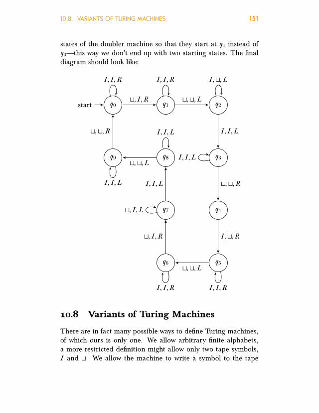
10.8. VARIANTS OF TURING MACHINES 151

states of the doubler machine so that they start at q4 instead ofq0—this way we don’t end up with two starting states. The finaldiagram should look like:

q0start q1 q2

q3

q4

q5q6

q7

q8q9

t, I ,R

I , I ,R I , I ,R

t,t,L

I ,t,L

I , I ,L

I , I ,L

t,t,R

I ,t,R

I , I ,R

t,t,L

I , I ,R

t, I ,R

t, I ,L

I , I ,L

I , I ,L

t,t,L

I , I ,L

t,t,R

10.8 Variants of Turing Machines

There are in fact many possible ways to define Turing machines,of which ours is only one. We allow arbitrary finite alphabets,a more restricted definition might allow only two tape symbols,I and t. We allow the machine to write a symbol to the tape


and move at the same time, other definitions allow either writingor moving. We allow the possibility of writing without movingthe tape head, other definitions leave out the N “instruction.”Our definition assumes that the tape is infinite in one directiononly, other definitions allow the tape to be infinite both to theleft and the right. In fact, we might even allow any number ofseparate tapes, or even an infinite grid of squares. We representthe instruction set of the Turing machine by a transition function;other definitions use a transition relation.

This last relaxation of the definition is particularly interest-ing. In our definition, when the machine is in state q readingsymbol σ, δ(q, σ) determines what the new symbol, state, andtape head position is. But if we allow the instruction set to be arelation between current state-symbol pairs 〈q, σ〉 and new state-symbol-direction triples 〈q ′, σ′,D〉, the action of the Turing ma-chine may not be uniquely determined—the instruction relationmay contain both 〈q, σ, q ′, σ′,D〉 and 〈q, σ, q ′′, σ′′,D ′〉. In thiscase we have a non-deterministic Turing machine. These play animportant role in computational complexity theory.

There are also dierent conventions for when a Turing ma-chine halts: we say it halts when the transition function is un-defined, other definitions require the machine to be in a specialdesignated halting state. And there are diernt ways of repre-senting numbers: we use unary representation, but you can alsouse binary representation (this requires two symbols in additionto t).

Now here is an interesting fact: none of these variations mat-ters as to which functions are Turing computable. If a functionis Turing computable according to one definition, it is Turingcomputable according to all of them.

10.9 The Church-Turing Thesis

Turing machines are supposed to be a precise replacement forthe concept of an eective procedure. Turing took it that anyone

10.9. THE CHURCH-TURING THESIS 153

who grasped the concept of an eective procedure and the con-cept of a Turing machine would have the intuition that anythingthat could be done via an eective procedure could be done byTuring machine. This claim is given support by the fact that allthe other proposed precise replacements for the concept of aneective procedure turn out to be extensionally equivalent to theconcept of a Turing machine—that is, they can compute exactlythe same set of functions. This claim is called the Church-Turingthesis.

Denition 10.15. The Church-Turing Thesis: Anything computablevia an eective procedure is Turing computable.

The Church-Turing thesis is appealed to in two ways. The firstkind of use of the Church-Turing thesis is an excuse for laziness.Suppose we have a description of an eective procedure to com-pute something, say, in “pseudo-code.” Then we can invoke theChurch-Turing thesis to justify the claim that the same functionis computed by some Turing machine, eve if we have not in factconstructed it.

The other use of the Church-Turing thesis is more philosoph-ically interesting. It can be shown that there are functions whchcannot be computed by a Turing machines. From this, using theChurch-Turing thesis, one can conclude that it cannot be eec-tively computed, using any procedure whatsoever. For if therewere such a procedure, by the Church-Turing thesis, it would fol-low that there would be a Turing machine. So if we can prove thatthere is no Turing machine that computes it, there also can’t bean eective procedure. In particular, the Church-Turing thesis isinvoked to claim that the so-called halting problem not only can-not be solved by Turing machines, it cannot be eectively solvedat all.

CHAPTER 11

Undecidability11.1 Introduction

It might seem obvious that not every function, even every arith-metical function, can be computable. There are just too many,whose behavior is too complicated. Functions defined from thedecay of radioactive particles, for instance, or other chaotic orrandom behavior. Suppose we start counting 1-second intervalsfrom a given time, and define the function f (n) as the numberof particles in the universe that decay in the n-th 1-second inter-val after that initial moment. This seems like a candidate for afunction we cannot ever hope to compute.

But it is one thing to not be able to imagine how one wouldcompute such functions, and quite another to actually prove thatthey are uncomputable. In fact, even functions that seem hope-lessly complicated may, in an abstract sense, be computable. Forinstance, suppose the universe is finite in time—some day, in thevery distant future the universe will contract into a single point,as some cosmological theories predict. Then there is only a fi-nite (but incredibly large) number of seconds from that initialmoment for which f (n) is defined. And any function which isdefined for only finitely many inputs is computable: we could listthe outputs in one big table, or code it in one very big Turingmachine state transition diagram.

154


We are often interested in special cases of functions whosevalues give the answers to yes/no questions. For instance, thequestion “is n a prime number?” is associated with the function

isprime(n) =

1 if n is prime

0 otherwise.

We say that a yes/no question can be eectively decided, if the as-sociated 1/0-valued function is eectively computable.

To prove mathematically that there are functions which can-not be eectively computed, or problems that cannot eectivelydecided, it is essential to fix a specific model of computation,and show about it that there are functions it cannot compute orproblems it cannot decide. We can show, for instance, that notevery function can be computed by Turing machines, and notevery problem can be decided by Turing machines. We can thenappeal to the Church-Turing thesis to conclude that not only areTuring machines not powerful enough to compute every function,but no eective procedure can.

The key to proving such negative results is the fact that we canassign numbers to Turing machines themselves. The easiest wayto do this is to enumerate them, perhaps by fixing a specific way towrite down Turing machines and their programs, and then listingthem in a systematic fashion. Once we see that this can be done,then the existence of Turing-uncomputable functions follows bysimple cardinality considerations: there functions from N to N(in fact, even just from N to 0, 1) are uncountable, but since wecan enumerate all the Turing machines, the Turing-computablefunctions are only countably infinite.

We can also define specic functions and problems which wecan prove to be uncomputable and undecidable, respectively.One such problem is the so-called Halting Problem. Turing ma-chines can be finitely described by listing their instructions. Sucha description of a Turing machine, i.e., a Turing machine pro-gram, can of course be used as input to another Turing machine.So we can consider Turing machines that decide questions about

156 CHAPTER 11. UNDECIDABILITY

other Turing machines. One particularly interesting question isthis: “Does the given Turing machine eventually halt when startedon input n?” It would be nice if there were a Turing machine thatcould decide this question: think of it as a quality-control Turingmachine which ensures that Turing machines don’t get caughtin infinite loops and such. The interestign fact, which Turingproved, is that there cannot be such a Turing machine. Therecannot be a single Turing machine which, when started on in-put consisting of a description of a Turing machine M and somenumber n, will always halt with either output 1 or 0 according towhether M machine would have halted when started on input nor not.

Once we have examples of specific undecidable problems wecan use them to show that other problems are undecidable, too.For instance, one celebrated undecidable problem is the question,“Is the first-order formula A valid?”. There is no Turing machinewhich, given as input a first-order formula A, is guaranteed to haltwith output 1 or 0 according to whether A is valid or not. His-torically, the question of finding a procedure to eectively solvethis problem was called simply “the” decision problem; and so wesay that the decision problem is unsolvable. Turing and Churchproved this result independently at around the same time, so itis also called the Church-Turing Theorem.

11.2 Enumerating Turing Machines

We can show that the set of all Turing-machines is countable. Thisfollows from the fact that each Turing machine can be finitelydescribed. The set of states and the tape vocabulary are finitesets. The transition function is a partial function from Q × Σ

to Q × Σ × L,R,N , and so likewise can be specified by listingits values for the finitely many argument pairs for which it is de-fined. Of course, strictly speaking, the states and vocabulary canbe anything; but the behavior of the Turing machine is indepen-dent of which objects serve as states and vocabulary. So we may

11.2. ENUMERATING TURING MACHINES 157

assume, for instance, that the states and vocabulary symbols arenatural numbers, or that the states and vocabulary are all stringsof letters and digits.

Suppose we fix a countably infinite vocabulary for specifyingTuring machines: σ0 = ., σ1 = t, σ2 = I , σ3, . . . , R, L, N ,q0, q1, . . . . Then any Turing machine can be specified by somefinite string of symbols from this alphabet (though not every fi-nite string of symbols specifies a Turing machine). For instance,suppose we have a Turing machine M = 〈Q , Σ, q, δ〉 where

Q = q ′0, . . . , q ′n ⊆ q0, q1, . . . and

Σ = ., σ′1, σ′2, . . . , σ′m ⊆ σ0, σ1, . . . .We could specify it by the string

q ′0q′1 . . . q

′n . σ

′1 . . . σ

′m . q . S (σ′0, q ′0) . . . . . S (σ′m, q ′n)

where S (σ′i, q ′j ) is the string σ′iq′j δ(σ′i, q ′j ) if δ(σ′i, q ′j ) is defined,

and σ′iq′j otherwise.

Theorem 11.1. There are functions fromN toNwhich are not Turingcomputable.

Proof. We know that the set of finite strings of symbols froma countably infinite alphabet is countable. This gives us that theset of descriptions of Turing machines, as a subset of the finitestrings from the countable vocabulary q0, q1, . . . , ., σ1, σ2, . . . ,is itself enumerable. Since every Turing computable function iscomputed by some (in fact, many) Turing machines, this meansthat the set of all Turing computable functions from N to N isalso enumerable.

On the other hand, the set of all functions from N to N is notcountable. This follows immediately from the fact that not eventhe set of all functions of one argument from N to the set 0, 1is countable. If all functions were computable by some Turingmachine we could enumerate the set of all functions. So thereare some functions that are not Turing-computable.


11.3 The Halting Problem

Assume we have fixed some finite descriptions of Turing ma-chines. Using these, we can enumerate Turing machines via theirdescriptions, say, ordered by the lexicographic ordering. EachTuring machine thus receives an index: its place in the enumera-tion M1, M2, M3, . . . of Turing machine descriptions.

We know that there must be non-Turing-computable func-tions: the set of Turing machine descriptions—and hence the setof Turing machines—is enumerable, but the set of all functionsfrom N to N is not. But we can find specific examples of non-computable function as well. One such function is the haltingfunction.

Denition 11.2. The halting function h is defined as

h(e, n) =

0 if machine Me does not halt for input n

1 if machine Me halts for input n

Denition 11.3. The Halting Problem is the problem of deter-mining (for any m, w) whether the Turing machine Me halts foran input of n strokes.

We show that h is not Turing-computable by showing that arelated function, s , is not Turing-computable. This proof relies onthe fact that anything that can be computed by a Turing machinecan be computed using just two symbols: t and I , and the factthat two Turing machines can be hooked together to create asingle machine.

Denition 11.4. The function s is defined as

s (e ) =

0 if machine Me does not halt for input e

1 if machine Me halts for input e

Lemma 11.5. The function s is not Turing computable.

11.3. THE HALTING PROBLEM 159

Proof. We suppose, for contradiction, that the function s is Turing-computable. Then there would be a Turing machine S that com-putes s . We may assume, without loss of generality, that whenS halts, it does so while scanning the first square. This machinecan be “hooked up” to another machine J , which halts if it isstarted on a blank tape (i.e., if it reads t in the initial state whilescanning the square to the right of the end-of-tape symbol), andotherwise wanders o to the right, never halting. S _ J , themachine created by hooking S to J , is a Turing machine, so it isMe for some e (i.e., it appears somewhere in the enumeration).Start Me on an input of e I s. There are two possibilities: eitherMe halts or it does not halt.

1. Suppose Me halts for an input of e I s. Then s (e ) = 1. SoS , when started on e , halts with a single I as output on thetape. Then J starts with a I on the tape. In that case Jdoes not halt. But Me is the machine S _ J , so it shoulddo exactly what S followed by J would do. So Me cannothalt for an input of e I ’s.

2. Now suppose Me does not halt for an input of e I s. Thens (e ) = 0, and S , when started on input e , halts with a blanktape. J , when started on a blank tape, immediately halts.Again,Me does what S followed by J would do, soMe musthalt for an input of e I ’s.

This shows there cannot be a Turing machine S : s is not Turingcomputable.

Theorem 11.6 (Unsolvability of the Halting Problem). The halt-ing problem is unsolvable, i.e., the function h is not Turing computable.

Proof. Suppose h were Turing computable, say, by a Turing ma-chine H . We could use H to build a Turing machine that com-putes s : First, make a copy of the input (separated by a blank).Then move back to the beginning, and run H . We can clearly


make a machine that does the former, and if H existed, we wouldbe able to “hook it up” to such a modified doubling machine toget a new machine which would determine if Me halts on input e ,i.e., computes s . But we’ve already shown that no such machinecan exist. Hence, h is also not Turing computable.

11.4 The Decision Problem

We say that first-order logic is decidable i there is an eectivemethod for determining whether or not a given sentence is valid.AS it turns out, there is no such method: the problem of decidingvalidity of first-order sentences is unsolvable.

In order to establish this important negative result, we provethat the decision problem cannot be solved by a Turing machine.That is, we show that there is no Turing machine which, when-ever it is started on a tape that contains a first-order sentence,eventually halts and outputs either 1 or 0 depending on whetherthe sentence is valid or not. By the Church-Turing thesis, everyfunction which is computable is Turing computable. So if if this“validity function” were eectively computable at all, it would beTuring computable. If it isn’t Turing computable, then, it alsocannot be eectively computable.

Our strategy for proving that the decision problem is unsolv-able is to reduce the halting problem to it. This means the follow-ing: We have proved that the function h(e,w) that halts with out-put 1 if the Turing-machine described by e halts on input w andoutputs 0 otherwise, is not Turing-computable. We will show thatif there were a Turing machine that decides validity of first-ordersentences, then there is also Turing machine that computes h.Since h cannot be computed by a Turing machine, there cannotbe a Turing machine that decides validity either.

The first step in this strategy is to show that for every input wand a Turing machineM , we can eectively describe a sentenceTrepresentingM andw and a sentence E expressing “M eventuallyhalts” such that:


T → E i M halts for input w .

The bulk of our proof will consist in describing these sentencesT (M,w) and E(M,w) and verifying that T (M,w) → E(M,w) isvalid i M halts on input w .

11.5 Representing Turing Machines

In order to represent Turing machines and their behavior by asentence of first-order logic, we have to define a suitable language.The language consists of two parts: predicate symbols for describ-ing configurations of the machine, and expressions for countingexecution steps (“moments”) and positions on the tape. The lat-ter require an initial moment, , a “successor” function whichis traditionally written as a postfix ′, and an ordering x < y of“before.”

Denition 11.7. Given a Turing machine M = 〈Q , Σ, q0, δ〉, thelanguage LM consists of:

1. A two-place predicate symbolQq (x, y) for every state q ∈ Q .Intuitively, Qq (n,m) expresses “after m steps,M is in state qscanning the nth square.”

2. A two-place predicate symbol Sσ(x, y) for every symbol σ ∈Σ . Intuitively, Sσ(n,m) expresses “after m steps, the nthsquare contains symbol σ.”

3. A constant

4. A one-place function ′

5. A two-place predicate <

For each number n there is a canonical term n, the numeralfor n, which represents it in LM . 0 is , 1 is ′, 2 is ′′, and so


on. More formally:

0 =

n + 1 = n ′

The sentences describing the operation of the Turing ma-chine M on input w = σi1 . . . σin are the following:

1. Axioms describing numbers:

a) A sentence that says that the successor function is in-jective:

∀x ∀y (x ′ = y ′ → x = y)b) A sentence that says that every number is less than its

successor:∀x (x < x ′)

c) A sentence that ensures that < is transitive:

∀x ∀y ∀z ((x < y ∧ y < z )→ x < z )

2. Axioms describing the input configuration:

a) M is in the inital state q0 at time 0, scanning square 1:

Qq0(1, 0)

b) The first n + 1 squares contain the symbols ., σ1, . . . ,σn :

S.(0, 0) ∧ Sσ1(1, 0) ∧ · · · ∧ Sσn (n, 0)c) Otherwise, the tape is empty:

∀x (n < x → St(x, 0))

3. Axioms describing the transition from one configuration tothe next:


For the following, let A(x, y) be the conjunction of all sen-tences of the form

∀z (((z < x ∨ x < z ) ∧ Sσ(z, y))→ Sσ(z, y ′))where σ ∈ Σ . We use A(n,m) to express “other than atsquare n, the tape after m + 1 steps is the same as after msteps.”

a) For every instruction δ(qi, σ) = 〈q j , σ′,R〉, the sen-tence:

∀x ∀y ((Qqi (x, y) ∧ Sσ(x, y))→(Qq j (x ′, y ′) ∧ Sσ′(x, y ′) ∧ A(x, y)))

b) For every instruction δ(qi, σ) = 〈q j , σ′,L〉, the sen-tence:

∀x ∀y ((Qqi (x ′, y) ∧ Sσ(x ′, y))→(Qq j (x, y ′) ∧ Sσ′(x ′, y ′) ∧ A(x, y)))

Take a moment to think about how this works: nowwe don’t start with “if scanning square x . . . ” but: “ifscanning square x + 1 . . . ” A move to the left meansthat in the next step the machine is scanning square x .But the square that is written on is x +1. We do it thisway since we don’t have subtraction or a predecessorfunction.

c) For every instruction δ(qi, σ) = 〈q j , σ′,N 〉, the sen-tence:

∀x ∀y ((Qqi (x, y) ∧ Sσ(x, y))→(Qq j (x, y ′) ∧ Sσ′(x, y ′) ∧ A(x, y)))

Let T (M,w) be the conjunction of all the above sentences forTuring machine M and input w


In order to express that M eventualy halts, we have to finda sentence that says “after some number of steps, the transitionfunction will be undefined.” Let X be the set of all pairs 〈q, σ〉such that δ(q, σ) is undefined. Let E(M,w) then be the sentence

∃x ∃y (∨

〈q,σ〉∈X(Qq (x, y) ∧ Sσ(x, y)))

If we use a Turing machine with a designated halting state h,it is even easier: then the sentence E(M,w)

∃x ∃y Qh(x, y)expresses that the machine eventually halts.

11.6 Verifying the Representation

In order to verify that our representation works, we first have tomake sure that if M halts on input w , then T (M,w)→ E(M,w) isvalid. We can do this simply by proving thatT (M,w) implies a de-scription of the configuration of M for each step of the executionofM on inputw . IfM halts on inputw , then for some n,M will bein a halting configuration at step n (and be scanning squarem, forsome m). Hence, T (M,w) implies Qq (m, n)∧Sσ(m, n) for some qand σ such that δ(q, σ) is undefined.Denition 11.8. Let C (M,w, n) be the sentenceQq (m, n) ∧ Sσ0(0, n) ∧ · · · ∧ Sσk (k, n) ∧ ∀x (k < x → St(x, n))

where q is the state of M at time n, M is scanning square m attime n, square i contains symbol σi at time n for 0 ≤ i ≤ k andk is the right-most non-blank square of the tape at time m.

Suppose that M does halt for input w . Then there is sometime n, state q , square m, and symbol σ such that:

1. At time n the machine is in state q scanning square m onwhich σ appears.

11.6. VERIFYING THE REPRESENTATION 165

2. There transition function δ(q, σ) is undefined.C (M,w, n) will be the description of this time and will include

the clauses Qq (m, n) and Sσ(m, n). These clauses together implyE(M,w):

∃x ∃y (∨

〈q,σ〉∈X(Qq (x, y) ∧ Sσ(x, y)))

since Qq ′(m, n) ∧ Sσ′(m, n) ∨〈q,σ〉∈X (Qq (m, n) ∧ Sσ(m, n), as〈q ′, σ′〉 ∈ X .

So if M halts for input w , then there is some time n such thatC (M,w, n) E(M,w)

Since consequence is transitive, it is sucient to show that forany time n, T (M,w) C (M,w, n).

Lemma 11.9. For each n, T (M,w) C (M,w, n).

Proof. If n = 0, then the conjuncts ofC (M,w, 0) are also conjunctsof T (M,w), so entailed by it.

Inductive hypothesis: If M has not halted before time n, thenT (M,w) C (M,w, n).

Suppose n > 0 and at time n, M started on w is in state qscanning square m, and the content of the tape is σ0, . . . , σk .

Suppose that M has not halted before time n + 1. If T (M, n)is true in a structure M, the inductive hypothesis tells us thatC (M,w, n) is true in M also. In particular, Qq (m, n) and Sσ(m, n)are true in M.

Since M does not halt at n, there must be an instruction ofone of the following three forms in the program of M :

1. δ(q, σ) = 〈q ′, σ′,R〉2. δ(q, σ) = 〈q ′, σ′,L〉3. δ(q, σ) = 〈q ′, σ′,N 〉We will consider each of these three cases in turn. First, as-

sume that m ≤ k .


1. Suppose there is an instruction of the form (1). By Defini-tion 11.7, (3a), this means that

∀x ∀y ((Qq (x, y) ∧ Sσ(x, y))→(Qq ′(x ′, y ′) ∧ Sσ′(x, y ′) ∧ A(x, y)))

is a conjunct of T (M,w). This entails the following sen-tence, through universal instantiation:

(Qq (m, n)∧Sσ(m, n))→ (Qq ′(m ′, n ′)∧Sσ′(m, n ′)∧A(m, n)).

This in turn entails,

Qq ′(m ′, n ′) ∧ Sσ′(m, n ′) ∧Sσ0(0, n ′) ∧ · · · ∧ Sσk (k, n ′) ∧

∀x (k < x → St(x, n ′))

The first line comes directly from the consequent of the pre-ceding conditional. The each conjunct in the middle line—which excludes Sσm (m, n ′)—follows from the correspondingconjunct in C (M,w, n) together with A(m, n). The last linefollows from the corresponding conjunct in C (M,w, n), m <

x → k < x , and A(m, n). Together, this just is C (M,w, n ′).

2. Suppose there is an instruction of the form (2). Then, byDefinition 11.7, (3b),

∀x ∀y ((Qq (x ′, y) ∧ Sσ(x ′, y))→(Qq ′(x, y ′) ∧ Sσ′(x ′, y ′) ∧ A(x, y)))

is a conjunct of T (M,w), which entails the following sen-tence:

(Qq (m ′, n) ∧ Sσ(m ′, n)→ (Qq ′(m, n ′) ∧ Sσ′(m ′, n ′) ∧A(x, y)),

11.6. VERIFYING THE REPRESENTATION 167

which in turn implies

Qq ′(m, n ′) ∧ Sσ′m (m, n ′) ∧Sσ0(0, n ′) · · · ∧ Sσk (k, n ′) ∧

∀x (k < x → St(x, n ′))as before. But this just is C (M,w, n ′).

3. Case (3) is left as an exercise.

If m > k and σ′ , t, the last instruction has written a non-blanksymbol to the right of the right-most non-blank square k at time n.In this case, C (M,w, n ′) has the form

Qq ′(m ′, n ′) ∧Sσ0(0, n ′) ∧ · · · ∧ Sσk (k, n ′) ∧

St(k + 1, n ′) ∧ · · · ∧ St(m − 1, n ′) ∧Sσ′(m, n ′) ∧

∀x (m < x → St(x, n ′))

For k < i < m, St(i, n) follows from the conjunct ∀x (k < x →St(x, n)) of C (M,w, n) and the fact that T (M,w) k < i if k < i .St(i, n ′) then follows from A(m, n) and i < m. From ∀x (k < x →St(x, n)) we get ∀x (m < x → St(x, n)) since k < m and < istransitive. From that plus A(m, n) we get ∀x (m < x → St(x, n ′)).Similarly for cases (2) and (3).

We have shown that for any n, T (M,w) C (M,w, n).

Lemma 11.10. If M halts on input w , then T (M,w)→ E(M,w) isvalid.

Proof. By Lemma 11.9, we know that, for any time n, the de-scription C (M,w, n) of the configuration of M at time n is a con-sequence of T (M,w). Suppose M halts after k steps. It will


be scanning square m, say. Then C (M,w, k ) contains as con-juncts both Qq (m, k ) and Sσ(m, k ) with δ(q, σ) undefined. Thus,C (M,w, k ) E(M,w). But then T (M,w) E(M,w) and thereforeT (M,w)→ E(M,w) is valid.

To complete the verification of our claim, we also have toestablish the reverse direction: if T (M,w) → E(M,w) is valid,then M does in fact halt when started on input m.

Lemma 11.11. If T (M,w)→ E(M,w), thenM halts on inputw .

Proof. Consider the LM -structure M with domain N which inter-prets as 0, ′ as the successor function, and < as the less-thanrelation, and the predicates Qq and Sσ as follows:

QMq = 〈m, n〉 : started on w , after n steps,

M is in state q scanning square m

SMσ = 〈m, n〉 : started on w , after n steps,

square m of M contains symbol σ

In other words, we construct the structure M so that it describeswhat M started on input w actually does, step by step. Clearly,M |= T (M,w). If T (M,w)→ E(M,w), then also M |= E(M,w),i.e.,

M |= ∃x ∃y (∨

〈q,σ〉∈X(Qq (x, y) ∧ Sσ(x, y))).

As |M | = N, there must be m, n ∈ N so that M |= Qq (m, n) ∧Sσ(m, n) for some q and σ such that δ(q, σ) is undefined. By thedefinition of M, this means thatM started on inputw after n stepsis in state q and reading symbol σ, and the transition function isundefined, i.e., M has halted.

11.7 The Decision Problem is Unsolvable

Theorem 11.12. The decision problem is unsolvable.

11.7. THE DECISION PROBLEM IS UNSOLVABLE 169

Proof. Suppose the decision problem were solvable, i.e., supposethere were a Turing machineD of the following sort. WheneverDis started on a tape that contains a sentence B of first-order logicas input, D eventually halts, and outputs 1 i B is valid and 0 oth-erwise. Then we could solve the halting problem as follows. Weconstruct a Turing machine E that, given as input the number eof Turing machine Me and input w , computes the correspondingsentence T (Me,w) → E(Me,w) and halts, scanning the leftmostsquare on the tape. The machine E _ D would then, given inpute and w , first compute T (Me,w)→ E(Me,w) and then run the de-cision problem machine D on that input. D halts with output 1i T (Me,w) → E(Me,w) is valid and outputs 0 otherwise. ByLemma 11.11 and Lemma 11.10, T (Me,w) → E(Me,w) is validi Me halts on input w . Thus, E _ D , given input e and w haltswith output 1 i Me halts on input w and halts with output 0 oth-erwise. In other words, E _ D would solve the halting problem.But we know, by Theorem 11.6, that no such Turing machine canexist.

APPENDIX A

InductionInduction is an important proof technique which is used, in dif-ferent forms, in almost all areas of logic, theoretical computerscience, and mathematics. It is needed to prove many of the re-sults in this book.

A.1 Induction on N

In its simplest form, induction is a technique used to prove resultsfor all natural numbers. It uses the fact that by starting from 0 andrepeatedly adding 1 we eventually reach every natural number.So to prove that something is true for every number, we can (1)establish that it is true for 0 and (2) show that whenever a numberhas it, the next number has it too. If we abbreviate “number nhas property P ” by P (n), then a proof by induction that P (n) forall n ∈ N consists of:

1. a proof of P (0), and2. a proof that, for any n, if P (n) then P (n + 1).

To make this crystal clear, suppose we have both (1) and (2).Then (1) tells us that P (0) is true. If we also have (2), we knowin particular that if P (0) then P (0 + 1), i.e., P (1). (This followsfrom the general statement “for any n, if P (n) then P (n + 1)” by

171

172 APPENDIX A. INDUCTION

putting 0 for n. So by modus ponens, we have that P (1). From(2) again, now taking 1 for n, we have: if P (1) then P (2). Sincewe’ve just established P (1), by modus ponens, we have P (2). Andso on. For any number k , after doing this k steps, we eventuallyarrive at P (k ). So (1) and (2) together established P (k ) for anyk ∈ N.

Let’s look at an example. Suppose we want to find out howmany dierent sums we can throw with n dice. Although it mightseem silly, let’s start with 0 dice. If you have no dice there’s onlyone possible sum you can “throw”: no dots at all, which sumsto 0. So the number of dierent possible throws is 1. If you haveonly one die, i.e., n = 1, there are six possible values, 1 through 6.With two dice, we can throw any sum from 2 through 12, that’s 11possibilities. With three dice, we can throw any number from 3 to18, i.e., 16 dierent possibilities. 1, 6, 11, 16: looks like a pattern:maybe the answer is 5n + 1? Of course, 5n + 1 is the maximumpossible, because there are only 5n + 1 numbers between n, thelowest value you can throw with n dice (all 1’s) and 6n, the highestyou can throw (all 6’s).

Theorem A.1. With n dice one can throw all 5n + 1 possible valuesbetween n and 6n.

Proof. To prove that this holds for any number of dice, we useinduction: we prove, (1) that the number of dierent throws with0 dice is 5 ·0+1 = 1, and (2) that if we can throw all 5n+1 valuesbetween n and 6n with n dice, then with n + 1 dice we can throwall 5(n+1)+1 = 5n+6 possible values between n+1 and 6(n+1).We’ve already established (1): If you have no dice, there’s onlyone possible outcome: you throw all 0 dice, and the number ofdots visible is 0.

Now let’s see how many possible total values you can throwwith n + 1 dice: we’re going to show that it’s all 5n + 6 dierentsums between n + 1 and 6n + 6, assuming that you can throwall 5n + 1 dierent sums between n and 6n with n dice. This

A.1. INDUCTION ON N 173

assumption is called the induction hypothesis. So: assume thatyou can throw all 5n + 1 dierent sums between n and 6n withn dice

Suppose you have n dice. Each possible throw sums to somenumber between n (all n dice show 1’s) and 6n (all 6’s). Nowthrow another die. You get another number between 1 and 6. Ifyour total is less than 6n you could have thrown the same totalwith your original n dice, by induction hypothesis. Only the possi-ble totals 6n+1 through 6n+6 are totals you couldn’t have thrownwith just n dice—and these are new possible totals, which you’dget, e.g., by throwing n 6’s plus whatever your new die shows. Sothere are 6 new possible totals. You can still throw any of theold totals, except one. With n + 1 dice you can’t roll just n. Butany other value you can throw with n dice you can also throwwith n + 1 dice: just imagine one of your n dice showed one eyefewer (and at least one of them must show at least a 2) and your(n + 1)st die shows a 1. With an additional die we lose only onepossible total (n) and gain 6 new possible totals (6n + 1 through6n +6). So the number of possible totals with n +1 dice is 5n +1,minus 1, plus 6, i.e., 5n+6. So we have proved that, assuming thenumber of totals we can throw with n dice is 5n + 1, the numberof totals we can throw with n + 1 dice is 5n + 6 = 5(n + 1)+ 1.

Very often we use induction when we want to prove somethingabout a series of objects (numbers, sets, etc.) that is itself defined“inductively,” i.e., by defining the (n+1)-st object in terms of the n-th. For instance, we can define the sum sn of the natural numbersup to n by

s0 = 0

sn+1 = sn + (n + 1)


This definition gives:

s0 = 0,

s1 = s0 + 1 = 1,

s2 = s1 + 2 = 1 + 2 = 3

s3 = ss + 3 = 1 + 2 + 3 = 6, etc.

Now we can prove, b=y induction, that sn = n(n + 1)/2.

Proposition A.2. sn = n(n + 1)/2.

Proof. We have to prove (1) that s0 = 0 · (0 + 1)/2 and (2) ifsn = n(n + 1)/2 then sn+1 = (n + 1)(n + 2)/2. (1) is obvious. Toprove (2), we assume the inductive hypothesis: sn = n(n + 1)/2.Using it, we have to show that sn+1 = (n + 1)(n + 2)/2.

What is sn+1? By the definition, sn+1 = sn + (n + 1). By in-ductive hypothesis, sn = n(n + 1)/2. We can substitute this intothe previous equation, and then just need a bit of arithmetic offractions:

sn+1 =n(n + 1)

2+ (n + 1) =

=n(n + 1)

2+2(n + 1)

2=

=n(n + 1) + 2(n + 1)

2=

=(n + 2)(n + 1)

2.

The important lesson here is that if you’re proving somethingabout some inductively defined sequence an , induction is the ob-vious way to go. And even if it isn’t (as in the case of the possibil-ities of dice throws), you can use induction if you can somehowrelate the case for n + 1 to the case for n.

A.2. STRONG INDUCTION 175

A.2 Strong Induction

In the principle of induction discussed above, we prove P (0) andalso if P (n), then P (n+1). In the second part, we assume that P (n)is true and use this assumption to prove P (n + 1). Equivalently,of course, we could assume P (n − 1) and use it to prove P (n)—the important part is that we be able to carry out the inferencefrom any number to its successor; that we can prove the claimin question for any number under the assumption it holds for itspredecessor.

There is a variant of the principle of induction in which wedon’t just assume that the claim holds for the predecessor n − 1of n, but for all numbers smaller than n, and use this assumptionto establish the claim for n. This also gives us the claim P (k ) forall k ∈ N. For once we have established P (0), we have therebyestablished that P holds for all numbers less than 1. And if weknow that if P (l ) for all l < n then P (n), we know this in particularfor n = 1. So we can conclude P (2). With this we have provedP (0), P (1), P (2), i.e., P (l ) for all l < 3, and since we have also theconditional, if P (l ) for all l < 3, then P (3), we can conclude P (3),and so on.

In fact, if we can establish the general conditional “for all n,if P (l ) for all l < n, then P (n),” we do not have to establish P (0)anymore, since it follows from it. For remember that a generalclaim like “for all l < n, P (l )” is true if there are no l < n. Thisis a case of vacuous quantification: “all As are Bs” is true if thereare no As, ∀x (A(x) → B(x)) is true if no x satisfies A(x). In thiscase, the formalized version would be “∀l (l < n → P (l ))”—andthat is true if there are no l < n. And if n = 0 that’s exactly thecase: no l < 0, hence “for all l < 0, P (0)” is true, whatever P is.A proof of “if P (l ) for all l < n, then P (n)” thus automaticallyestablishes P (0).

This variant is useful if establishing the claim for n can’t bemade to just rely on the claim for n − 1 but may require theassumption that it is true for one or more l < n.


A.3 Inductive Denitions

In logic we very often define kinds of objects inductively, i.e., byspecifying rules for what counts as an object of the kind to be de-fined which explain how to get new objects of that kind from oldobjects of that kind. For instance, we often define special kindsof sequences of symbols, such as the terms and formulas of a lan-guage, by induction. For a simpler example, consider strings ofparentheses, such as “(()(” or “()(())”. In the second string, theparentheses “balance,” in the first one, they don’t. The shortestsuch expression is “()”. Actually, the very shortest string of paren-theses in which every opening parenthesis has a matching closingparenthesis is “”, i.e., the empty sequence ∅. If we already havea parenthesis expression p, then putting matching parenthesesaround it makes another balanced parenthesis expression. Andif p and p ′ are two balanced parentheses expressions, writing oneafter the other, “pp ′” is also a balanced parenthesis expression.In fact, any sequence of balanced parentheses can be generatedin this way, and we might use these operations to dene the set ofsuch expressions. This is an inductive denition.

Denition A.3. The set of parexpressions is inductively definedas follows:

1. ∅ is a parexpression.

2. If p is a parexpression, then so is (p).3. If p and p ′ are parexpressions , ∅, then so is pp ′.

4. Nothing else is a parexpression.

(Note that we have not yet proved that every balanced paren-thesis expression is a parexpression, although it is quite clear thatevery parexpression is a balanced parenthesis expression.)

The key feature of inductive definitions is that if you want toprove something about all parexpressions, the definition tells youwhich cases you must consider. For instance, if you are told that

A.3. INDUCTIVE DEFINITIONS 177

q is a parexpression, the inductive definition tells you what q canlook like: q can be ∅, it can be (p) for some other parexpression p,or it can be pp ′ for two parexpressions p and p ′ , ∅. Because ofclause (4), those are all the possibilities.

When proving claims about all of an inductively defined set,the strong form of induction becomes particularly important. Forinstance, suppose we want to prove that for every parexpressionof length n, the number of ( in it is n/2. This can be seen as aclaim about all n: for every n, the number of ( in any parexpres-sion of length n is n/2.

Proposition A.4. For any n, the number of ( in a parexpression oflength n is n/2.

Proof. To prove this result by (strong) induction, we have to showthat the following conditional claim is true:

If for every k < n, any parexpression of length k hask/2 (’s, then any parexpression of length n has n/2(’s.

To show this conditional, assume that its antecedent is true, i.e.,assume that for any k < n, parexpressions of length k contain k(’s. We call this assumption the inductive hypothesis. We want toshow the same is true for parexpressions of length n.

So suppose q is a parexpression of length n. Because parex-pressions are inductively defined, we have three cases: (1) q is∅, (2) q is (p) for some parexpression p, or (3) q is pp ′ for someparexpressions p and p ′ , ∅.

1. q is ∅. Then n = 0, and the number of ( in q is also 0. Since0 = 0/2, the claim holds.

2. q is (p) for some parexpression p . Since q contains twomore symbols than p, len(p) = n − 2, in particular, len(p) <n, so the inductive hypothesis applies: the number of ( inp is len(p)/2. The number of ( in q is 1 + the number of (


in p, so = 1 + len(p)/2, and since len(p) = n − 2, this gives1 + (n − 2)/2 = n/2.

3. q is pp ′ for some parexpression p and p ′ , ∅. Since neitherp nor p ′ = ∅, both len(p) and len(p ′) < n. Thus the induc-tive hypothesis applies in each case: The number of ( in pis len(p)/2, and the number of ( in p ′ is len(p ′)/2. On theother hand, the number of ( in q is obviously the sum of thenumbers of ( in p and p ′, since q = pp ′. Hence, the num-ber of ( in q is len(p)/2 + len(p ′)/2 = (len(p) + len(p ′))/2 =len(pp ′)/2 = n/2.

In each case, we’ve shown that teh number of ( in q is n/2 (onthe basis of the inductive hypothesis). By strong induction, theproposition follows.

A.4 Structural Induction

So far we have used induction to establish results about all naturalnumbers. But a corresponding principle can be used directly toprove results about all elements of an inductively defined set.This often called structural induction, because it depends on thestructure of the inductively defined objects.

Generally, an inductive definition is given by (a) a list of “ini-tial” elements of the set and (b) a list of operations which producenew elements of the set from old ones. In the case of parexpres-sions, for instance, the initial object is ∅ and the operations are

o1(p) =(p)o2(q, q ′) =qq ′

You can even think of the natural numbers N themselves as beinggiven be an inductive definition: the initial object is 0, and theoperation is the successor function x + 1.

In order to prove something about all elements of an induc-tively defined set, i.e., that every element of the set has a prop-erty P , we must:

A.4. STRUCTURAL INDUCTION 179

1. Prove that the initial objects have P

2. Prove that for each operation o, if the arguments have P ,so does the result.

For instance, in order to prove something about all parexpres-sions, we would prove that it is true about ∅, that it is true of (p)provided it is true of p, and that it is true about qq ′ provided itis true of q and q ′ individually.

Proposition A.5. The number of ( equals the number of ) in anyparexpression p .

Proof. We use structural induction. Parexpressions are induc-tively defined, with initial object ∅ and the operations o1 ando2.

1. The claim is true for ∅, since the number of ( in ∅ = 0 andthe number of ) in ∅ also = 0.

2. Suppose the number of ( in p equals the number of ) in p .We have to show that this is also true for (p), i.e., o1(p). Butthe number of ( in (p) is 1+ the number of ( in p . And thenumber of ) in (p) is 1+ the number of ) in p, so the claimalso holds for (p).

3. Suppose the number of ( in q equals the number of ), andthe same is true for q ′. The number of ( in o2(p, p ′), i.e., inpp ′, is the sum of the number ( in p and p ′. The number of) in o2(p, p ′), i.e., in pp ′, is the sum of the number of ) in pand p ′. The number of ( in o2(p, p ′) equals the number of )in o2(p, p ′).

The result follows by structural induction.

APPENDIX B

BiographiesB.1 Georg Cantor

Fig. B.1: Georg Cantor

An early biography of Georg Can-tor (gay-org kahn-tor) claimed thathe was born and found on a shipthat was sailing for Saint Peters-burg, Russia, and that his parentswere unknown. This, however, isnot true; although he was born inSaint Petersburg in 1845.

Cantor recieved his doctoratein mathematics at the University ofBerlin in 1867. He is known for hiswork in set theory, and is creditedwith founding set theory as a dis-tinctive research discipline. He wasthe first to prove that there are infi-nite sets of dierent sizes. His theories, and especially his theoryof infinities, caused much debate among mathematicians at thetime, and his work was controversial.

Cantor’s religious beliefs and his mathematical work were in-extricably tied; he even claimed that the theory of transfinite num-bers had been communicated to him directly by God. In later

180

B.2. ALONZO CHURCH 181

life, Cantor suered from mental illness. Beginning in 1984, andmore frequently towards his later years, Cantor was hospitalized.The heavy criticism of his work, including a falling out with themathematician Leopold Kronecker, led to depression and a lackof interest in mathematics. During depressive episodes, Cantorwould turn to philosophy and literature, and even published atheory that Francis Bacon was the author of Shakespeare’s plays.

Cantor died on January 6, 1918, in a sanitorium in Halle.

Further Reading For full biographies of Cantor, see Dauben(1990) and Grattan-Guinness (1971). Cantor’s radical views arealso described in the BBC Radio 4 program A Brief History ofMathematics (Sautoy, 2014). If you’d like to hear about Cantor’stheories in rap form, see Rose (2012).

B.2 Alonzo Church

Fig. B.2: Alonzo Church

Alonzo Church was born in Wash-ington, DC on June 14, 1903. Inearly childhood, an air gun incidentleft Church blind in one eye. Hefinished prepratory school in Con-necticut in 1920 and began his uni-versity education at Princeton thatsame year. He completed his doc-toral studies in 1927. After a cou-ple years abroad, Church returnedto Princeton. Church was knownexceedingly polite and careful. Hisblackboard writing was immaculate, and he would preserve im-portant papers by carefully covering them in Duco cement. Out-side of his academic pursuits, he enjoyed reading science fictionmagazines and was not afraid to write to the editors if he spottedany inaccuracies in the writing.

182 APPENDIX B. BIOGRAPHIES

Church’s academic achievments were great. Together with hisstudents Stephen Kleene and Barkley Rosser, he developed a the-ory of eective calculability, the lambda calculus, independentlyof Alan Turing’s development of the Turing machine. The twodefinitions of computability are equivalent, and give rise to whatis now known as the Church-Turing Thesis, that a function of thenatural numbers is eectively computable if and only if it is com-putable via Turing machine (or lambda calculus). He also provedwhat is now known as Church’s Theorem: The decision problem forthe validity of first-order formulas is unsolvable.

Church continued his work into old age. In 1967 he leftPrinceton for UCLA, where he was professor until his retirementin 1990. Church passed away on August 1, 1995 at the age of 92.

Further Reading For a brief biography of Church, see En-derton (N.D.). Church’s original writings on the lambda calcu-lus and the Entscheidungsproblem (Church’s Thesis) are Church(1936a,b). Aspray (1984) records an interview with Church aboutthe Princeton mathematics community in the 1930s. Church wrotea series of book reviews of the Journal of Symbolic Logic from 1936until 1979. They are all archived on John MacFarlane’s website(MacFarlane, 2015).

B.3 Gerhard Gentzen

Fig. B.3: Gerhard Gentzen

Gerhard Gentzen is known primar-ily as the creator of structural prooftheory, and specifically the creationof the natural deduction and se-quent calclus proof systems. Hewas born on November 24, 1909in Greifswald, Germany. Gerhardwas homeschooled for three yearsbefore attending prepratory school,where he was behind most of his classmates in terms of educa-

B.3. GERHARD GENTZEN 183

tion. Despite this, he was a brilliant student and showed a strongaptitude for mathematics. His interests were varied, and he, forinstance, also write poems for his mother and plays for the schooltheatre.

Gentzen began his university studies at the University of Greif-swald, but moved around to Göttingen, Munich, and Berlin. Herecieved his doctorate in 1933 from the University of Göttingenunder Hermann Weyl. (Paul Bernays supervised most of hiswork, but was dismissed from the university by the Nazis.) In1934, Gentzen began work as an assistant to David Hilbert. Thatsame year he developed the sequent calculus and natural deduc-tion proof systems, in his papers Untersuchungen über das logischeSchließen I–II [Investigations Into Logical Deduction I–II]. He provedthe consistency of the Peano axioms in 1936.

Gentzen’s relationship with the Nazis is complicated. At thesame time his mentor Bernays was forced to leave Germany, Gentzenjoined the university branch of the SA, the Nazi paramilitary or-ganization. Like many Germans, he was a member of the Naziparty. During the war, he served as a telecommunications ocerfor the air intelligence unit. However, in 1942 he was releasedfrom duty due to a nervous breakdown. It is unclear whetheror not Gentzen’s loyalties lay with the Nazi party, or whether hejoined the party in order to ensure academic success.

In 1943, Gentzen was oered an academic position at theMathematical Institute of the German University of Prague, whichhe accepted. However, in 1945 the citizens of Prague revoltedagainst German occupation. Soviet forces arrived in the city andarrested all the professors at the univeristy. Because of his mem-bership in Nazi organizations, Gentzen was taken to a forcedlabour camp. He died of malnutrition while in his cell on August4, 1945 at the age of 35.

Further Reading For a full biography of Gentzen, see Menzler-Trott (2007). An interesting read about mathematicians underNazi rule, which gives a brief note about Gentzen’s life, is given by


Segal (2014). Gentzen’s papers on logical deduction are availablein the original german (Gentzen, 1935a,b). English translationsof Gentzen’s papers have been collected in a single volume bySzabo (1969), which also includes a biographical sketch.

B.4 Kurt Gödel

Fig. B.4: Kurt Gödel

Kurt Gödel (ger-dle) was bornon April 28, 1906 in Brünn inthe Austro-Hungarian empire (nowBrno in the Czech Republic). Dueto his inquisitive and bright na-ture, young Kurtele was often called“Der kleine Herr Warum” (LittleMr. Why) by his family. He excelledin academics from primary schoolonward, where he got less than thehighest grade only in mathematics.Gödel was often absent from schooldue to poor health and was exemptfrom physical education. Gödel wasdiagnosed with rheumatic fever during his childhood. Through-out his life, he believed this permanently aected his heart despitemedical assessment saying otherwise.

Gödel began studying at the University of Vienna in 1920 andcompleted his doctoral studies in 1929. He first intended to studyphysics, but his interests soon moved to mathematics and espe-cially logic, in part due to the influence of the philosopher RudolfCarnap. His dissertation, written under the supervision of HansHahn, proved the completeness theorem of first-order predicatelogic with identity. Only a couple years later, his most famousresults were published—the first and second incompleteness the-orems (Gödel, 1931). During his time in Vienna, Gödel was alsoinvolved with the Vienna Circle, a group of scientifically-mindedphilosophers.

B.4. KURT GÖDEL 185

In 1938, Gödel married Adele Nimbursky. His parents werenot pleased: not only was she six years older than him and al-ready divorced, but she worked as a dancer in a nightclub. Socialpressures did not aect Gödel, however, and they remained hap-pily married until his death.

After Nazi Germany annexed Austria in 1938, Gödel andAdele emmigrated to the United States, where he took up a po-sition at the Institute for Advanced Study in Princeton, New Jer-sey. Despite his introversion and eccentric nature, Gödel’s timeat Princeton was collaborative and fruitful. He published essaysin set theory, philosophy and physics. Notably, he struck up a par-ticularly strong friendship with his colleague at the IAS, AlbertEinstein.

In his later years, Gödel’s mental health deteriorated. Hiswife’s hospitalization in 1977 meant she was no longer able tocook his meals for him. Succumbing to both paranoia and anorexia,and deathly afraid of being poisoned, Gödel refused to eat. Hedied of starvation on January 14, 1978 in Princeton.

Further Reading For a complete biography of Gödel’s life isavailable, see Dawson Jr (1997). For further biographical pieces,as well as essays about Gödel’s contributions to logic and philos-ophy, see Wang (1990), Baaz et al. (2011), Takeuti et al. (2003),and Sigmund et al. (2007).

Gödel’s PhD thesis is available in the original German (Gödel,1929). The original text of the incompleteness theorems is (Gödel,1931). All of Gödel’s published and unpublished writings, as wellas a selection of correspondence, are available in English in hisCollected Papers Feferman et al. (1986, 1990).

For a detailed treatment of Gödel’s incompleteness theorems,see Smith (2013). For an informal, philosophical discussion ofGödel’s theorems, seeMark Linsenmayer’s podcast (Linsenmayer,2014).

The Kurt Gödel society keeps Gödel’s memory alive by pro-moting research in logic and other areas influenced by his works


Beckmann and Preining (2004).

B.5 Emmy Noether

Fig. B.5: Emmy Noether

Emmy Noether was born in Erlan-gen, Germany, on March 23, 1882,to an upper-middle class scholarlyfamily. Hailed as the “mother ofmodern algebra,” Noether madegroundbreaking contributions toboth mathematics and physics, de-spite significant barriers to women’seducation. In Germany at the time,young girls were meant to be ed-ucated in arts and were not al-lowed to attend college preparatoryschools. However, after auditingclasses at the Universities of Göttin-gen and Erlangen (where her father was professor of mathemat-ics), Noether was eventually able to enrol as a student at Erlangenin 1904, when their policy was updated to allow female students.She received her doctorate in mathematics in 1907.

Despite her qualifications, Noether experienced much resis-tance during her career. From 1908–1915, she taught at Erlangenwithout pay. During this time, she caught the attention of DavidHilbert, one of the world’s foremost mathematicians of the time,who invited her to Göttingen. However, women were prohibitedfrom obtaining professorships, and she was only able to lectureunder Hilbert’s name, again without pay. During this time sheproved what is now known as Noether’s theorem, which is stillused in theoretical physics today. Noether was finally grantedthe right to teach in 1919. Hilbert’s response to continued resis-tance of his university colleagues reportedly was: “Gentlemen,the faculty senate is not a bathhouse.”

Noether was Jewish, and when the Nazis came to power in

B.6. BERTRAND RUSSELL 187

1933, she was dismissed from her position. Luckily, Noether wasable to emigrate to the United States for a temporary position atBrynMawr, Pennsylvania. During her time there she also lecturedat Princeton, although she found the university to be unwelcom-ing to women (Dick, 1981, 81). In 1935, Noether underwent anoperation to remove a uterine tumour. She died from an infectionas a result of the surgery, and was buried at Bryn Mawr.

Further Reading For a biography of Noether, see Dick (1981).The Perimeter Institute for Theoretical Physics has their lectureson Noether’s life and influence available online (Institute, 2015).If you’re tired of reading, Stu You Missed in History Class has apodcast on Noether’s life and influence (Frey and Wilson, 2015).The collected works of Noether are available in the original Ger-man Jacobson (1983).

B.6 Bertrand Russell

Fig. B.6: Bertrand Russell

Bertrand Russell is hailed as oneof the founders of modern analyticphilosophy. Born May 18, 1872,Russell was not only known for hiswork in philsoophy and logic, butwrote many popular books in vari-ous subject areas. He was also anardent political activist throughouthis life.

Russell was born in Trellech,Monmouthshire, Wales. His par-ents were members of the Britishnobility. They were free-thinkers,and even made friends with the rad-icals in Boston at the time. Unfortunately, Russell’s parents diedwhen he was young, and Russell was sent to live with his grand-parents. There, he was given a religious upbringing (something


his parents had wanted to avoid at all costs). His grandmotherwas very strict in all matters of morality. During adolesence hewas mostly homeschooled by private tutors.

Russell’s influence in analytic philosophy, and especially logic,is tremendous. He studied mathematics and philosophy at Trin-ity College, Cambridge, where he was influenced by the math-ematician and philosopher Alfred North Whitehead. In 1910,Russell and Whitehead published the first volume of PrincipiaMathematica, where they championed the view that mathematicsis reducible to logic. He went on to publish hundreds of books,essays and political pamphlets. In 1950, he won the Nobel Prizefor literature.

Russell’s was deeply entrenched in politics and social activism.During World War I he was arrested and sent to prison for sixmonths due to pacifist activities and protest. While in prison,he was able to write and read, and claims to have found the ex-perience “quite agreeable.”. He remained a pacifist throughouthis life, and was again incarcerated for attending a nuclear disar-marment rally in 1961. He also survived a plane crash in 1948,where the only survivors were those sitting in the smoking sec-tion. As such, Russell claimed that he owed his life to smoking.Russell was married four times, but had a reputation for carryingon extra-marital aairs. He died on February 2, 1970 at the ageof 97 in Penrhyndeudraeth, Wales.

Further Reading Russell wrote an autobiography in three parts,spanning his life from 1872–1967 (Russell, 1967, 1968, 1969).The Bertrand Russell Research Centre at McMaster Universityis home of the Bertrand Russell archives. See their website atDuncan (2015), for information on the volumes of his collectedworks (including searchable indexes), and archival projects. Rus-sell’s paper On Denoting (Russell, 1905) is a classic of 20th centuryanalytic philosophy.

The Stanford Encyclopedia of Philosophy entry on Russell(Irvine, 2015) has sound clips of Russell speaking on Desire and

B.7. ALFRED TARSKI 189

Political theory. Many video interviews with Russell are availableonline. To see him talk about smoking and being involved in aplane crash, e.g., see Russell (N.D.). Some of Russell’s works,including his Introduction to Mathematical Philosophy are availableas free audiobooks on LibriVox (n.d.).

B.7 Alfred Tarski

Fig. B.7: Alfred Tarski

Alfred Tarski was born on January14, 1901 in Warsaw, Poland (thenpart of the Russian Empire). Oftendescribed as “Napoleonic,” Tarskiwas boistrous, talkative, and in-tense. His energy was often re-flected in his lectures—he once setfire to a wastebasket while disposingof a cigarette during a lecture, andwas forbidden from lecturing in thatbuilding again.

Tarski had a thirst for knowl-edge from a young age. Althoughlater in life he would tell studentsthat he studied logic because it was the only class in which hegot a B, his high school records show that he got A’s across theboard—even in logic. He studied at the University of Warsawfrom 1918 to 1924. Although he first intended to study biology,he became interested in mathematics, philosophy, and logic, asthe university was the center of the Warsaw School of Logic andPhilosophy. Tarski earned his doctorate in 1924 under the super-vision of Stanisław Leśniewski.

Before emigrating to the United States in 1939, Tarski com-pleted some of his most important work while working as a sec-ondary school teacher in Warsaw. His work on logical conse-quence and logical truth were written during this time. In 1939,Tarski was visiting the United States for a lecture tour. During


his visit, Germany invaded Poland, and because of his Jewish her-itage, Tarski could not return. His wife and children remained inPoland until the end of the war, but were then able to emigrate tothe United States as well. Tarski taught at Harvard, the Collegeof the City of New York, and the Institute for Advanced Studyat Princeton, and finally the University of California, Berkeley.There he founded the multidisciplinary program in Logic andthe Methodology of Science. Tarski died on October 26, 1983 atthe age of 82.

Further Reading For more on Tarski’s life, see the biogra-phy Alfred Tarski: Life and Logic (Feferman and Feferman, 2004).Tarski’s seminal works on logical consequence and truth are avail-able in English in Corcoran (1983). All of Tarski’s original workshave been collected into a four volume series, Tarski (1981).

B.8 Alan Turing

Fig. B.8: Alan Turing

Alan Turing was born in MaildaVale, London, on June 23, 1912. Heis considered the father of theoret-ical computer science. Turing’s in-terest in the physical sciences andmathematics started at a young age.However, as a boy his interests werenot represented well in his schools,where emphasis was placed on lit-erature and classics. Consequently,he did poorly in school and was rep-rimanded by many of his teachers.

Turing attended King’s College,Cambridge as an undergraduate, where he studied mathematics.In 1936 Turing developed (what is now called) the Turing ma-chine as an attempt to precisely define the notion of a computablefunction and to prove the undecidability of the decision problem.

B.8. ALAN TURING 191

He was beaten to the result by Alonzo Church, who proved theresult via his own lambda calculus. Turing’s paper was still pub-lished with reference to Church’s result. Church invited Turing toPrinceton, where he spent 1936–1938, and obtained a doctorateunder Church.

Despite his interest in logic, Turing’s earlier interests in phys-ical sciences remained prevalent. His practical skills were put towork during his service with the British cryptanalytic departmentat Bletchley Park during World War II. Turing was a central figurein cracking the cypher used by German Naval communications—the Enigma code. Turing’s expertise in statistics and cryptogra-phy, together with the introduction of electronic machinery, gavethe team the ability to crack the code by creating a de-cryptingmachine called a “bombe.” His ideas also helped in the creationof the world’s first programmable electronic computer, the Colos-sus, also used at Bletchley park to break the German Lorenzcypher.

Turing was gay. Nevertheless, in 1942 he proposed to JoanClarke, one of his teammates at Bletchley Park, but broke o theengagement and confessed to her that he was homosexual. Hehad several lovers throughout his lifetime, although homosexualacts were then criminal oences in the UK. In 1952, Turing’shouse was burgled by a friend of his lover at the time, and whenfiling a police report, Turing admitted to having a homosexualrelationship, under the impression that the government was ontheir way to legalizing homosexual acts. This was not true, andhe was charged with gross indecency. Instead of going to prison,Turing opted for a hormone treatment that reduced libido. Turingwas found dead on June 8, 1954, of a cyanide overdose—mostlikely suicide. He was given a royal pardon by Queen Elizabeth IIin 2013.

Further Reading For a comprehensive biography of Alan Tur-ing, see Hodges (2014). Turing’s life and work inspired a play,Breaking the Code, which was produced in 1996 for TV starring


Derek Jacobi as Turing. The Imitation Game, an Academy Awardnominated film starring Bendict Cumberbatch and Kiera Knight-ley, is also loosely based on Alan TuringâĂŹs life and time atBletchley Park Tyldum (2014).

Radiolab (2012) has several podcasts on Turings life and work.BBC Horizon’s documentary The Strange Life and Death of Dr. Tur-ing is available to watch online (Sykes, 1992). Theelen (2012) is ashort video of a working LEGO Turing Machine—made to hon-our Turing’s centenary in 2012.

Turing’s original paper on Turing machines and the decisionproblem is Turing (1937).

B.9 Ernst Zermelo

Fig. B.9: Ernst Zermelo

Ernst Zermelo was born on July 27,1871 in Berlin, Germany. He hadfive sisters, though his family suf-fered from poor health and onlythree made it to adulthood. His par-ents also passed away when he wasyoung, leaving him and his sibil-ings orphans when he was seven-teen. Zermelo had a deep interestin the arts, and especially in po-etry. He was known for being sharp,witty, and critical. His most cele-brated mathematical achievementsinclude the intruduction of the ax-iom of choice (in 1904), and his axiomatization of set theory (in1908).

Zermelo’s interests at university were varied. He took coursesin physics, mathematics, and philosophy. Under the supervisionof Hermann Schwarz, Zermelo completed his dissertation Inves-tigations in the Calculus of Variations in 1894 at the University ofBerlin. In 1897, he decided to pursue more studies at the Univer-

B.9. ERNST ZERMELO 193

sity of Göttigen, where he was heavily influenced by the founda-tional work of David Hilbert. In 1899 he became eligible for pro-fessorship, but did not get one until eleven years later—possiblydue to his strange demeanour and “nervous haste.”

Zermelo finally received a paid professorship at the Univer-sity of Zurich in 1910, but was forced to retire in 1916 due totuberculosis. After his recovery, he was given an honourary pro-fessorship at the University of Freiburg in 1921. During this timehe worked on foundational mathematics. He became irritatedwith the works of Thoralf Skolem and Kurt Gödel, and publi-cally criticized their approaches in his papers. He was dismissedfrom his position at Freiburg in 1935, due to his unpopularity andhis opposition to Hitler’s rise to power in Germany.

The later years of Zermelo’s life were marked by isolation. Af-ter his dismissal in 1935, he abandoned mathematics. He movedto the country where he lived modestly. He married in 1944, andbecame completely dependent on his wife as he was going blind.Zermelo lost his sight completely by 1951. He passed away inGünterstal, Germany, on May 21, 1953.

Further Reading For a full biography of Zermelo, see Ebbing-haus (2015). Zermelo’s seminal 1904 and 1908 papers are avail-able to read in the original German (Zermelo, 1904, 1908). Zer-melo’s collected works, including his writing on physics, are avail-able in English translation in Ebbinghaus et al. (2010); Ebbing-haus and Kanamori (2013).

APPENDIX C

ProblemsProblems for Chapter 0

Problems for Chapter 1

Problem 1.1. Show that there is only one empty set, i.e., showthat if X andY are sets without members, then X =Y .

Problem 1.2. List all subsets of a, b, c,d .

Problem 1.3. Show that if X has n elements, then ℘(X ) has 2nelements.

Problem 1.4. Prove rigorously that if X ⊆ Y , then X ∪Y =Y .

Problem 1.5. Prove rigorously that if X ⊆ Y , then X ∩Y = X .

Problem 1.6. Prove in detail that X ∪ (X ∩Y ) = X . Then com-press it into a “textbook proof.” (Hint: for the X ∪ (X ∩Y ) ⊆ Xdirection you will need proof by cases, aka ∨Elim.)

Problem 1.7. List all elements of 1, 2, 33.

Problem 1.8. Show that if X has n elements, then X k has nk

elements.

194

195


Problem 2.1. List the elements of the relation ⊆ on the set℘(a, b, c).Problem 2.2. Give examples of relations that are (a) reflexiveand symmetric but not transitive, (b) reflexive and anti-symmetric,(c) anti-symmetric, transitive, but not reflexive, and (d) reflexive,symmetric, and transitive. Do not use relations on numbers orsets.

Problem 2.3. Show that if R is a weak partial order on X , thenR− = R \ IdX is a strict partial order and Rxy i R−xy for allx , y .

Problem 2.4. Consider the less-than-or-equal-to relation ≤ on theset 1, 2, 3, 4 as a graph and draw the corresponding diagram.

Problem 2.5. Show that the transitive closure of R is in facttransitive.


Problem 3.1. Show that if f is bijective, an inverse g of f exists,i.e., define such a g , show that it is a function, and show that itis an inverse of f , i.e., f (g (y)) = y and g (f (x)) = x for all x ∈ Xand y ∈Y .

Problem 3.2. Show that if f : X → Y has an inverse g , then fis bijective.

Problem 3.3. Show that if g : Y → X and g ′ : Y → X are in-verses of f : X →Y , then g = g ′, i.e., for all y ∈Y , g (y) = g ′(y).Problem 3.4. Show that if f : X → Y and g : Y → Z are bothinjective, then g f : X → Z is injective.

Problem 3.5. Show that if f : X → Y and g : Y → Z are bothsurjective, then g f : X → Z is surjective.

196 APPENDIX C. PROBLEMS

Problem 3.6. Given f : X 7→ Y , define the partial functiong : Y 7→ X by: for any y ∈ Y , if there is a unique x ∈ X suchthat f (x) = y , then g (y) = x ; otherwise g (y) ↑. Show that if f isinjective, then g (f (x)) = x for all x ∈ dom(f ), and f (g (y)) = yfor all y ∈ ran(f ).Problem 3.7. Suppose f : X →Y and g : Y → Z . Show that thegraph of (g f ) is R f | Rg .


Problem 4.1. Give an enumeration of the set of all ordered pairsof positive rational numbers.

Problem 4.2. Recall from your introductory logic course thateach possible truth table expresses a truth function. In otherwords, the truth functions are all functions from Bk → B forsome k . Prove that the set of all truth functions is enumerable.

Problem 4.3. Show that the set of all finite subsets of an arbitraryinfinite enumerable set is enumerable.

Problem 4.4. Show that if X andY are countable, so is X ∪Y .

Problem 4.5. A set of positive integers is said to be conite i itis the complement of a finite set of positive integers. Let I be theset that contains all the finite and cofinite sets of positive integers.Show that I is enumerable.

Problem 4.6. Show that the countable union of countable sets iscountable. That is, whenever X1, X2, . . . are sets, and each Xi iscountable, then the union

⋃∞i=1 Xi of all of them is also countable.

Problem 4.7. Show that ℘(N) is uncountable.Problem 4.8. Show that the set of functions f : Z+ → Z+ is un-countable by a direct diagonal argument.

197

Problem 4.9. Show that the set of all sets of pairs of positiveintegers is uncountable.

Problem 4.10. Show that Nω, the set of infinite sequences ofnatural numbers, is uncountable.

Problem 4.11. Let P be the set of total functions from the setof positive integers to the set 0, and let Q be the set of partialfunctions from the set of positive integers to the set 0. Showthat P is countable and Q is not.

Problem 4.12. Let S be the set of all total surjective functionsfrom the set of positive integers to the set 0,1. Show that S isuncountable.

Problem 4.13. Show that the set R of all real numbers is un-countable.

Problem 4.14. Show that if X is equinumerous with U and andY is equinumerous withV , and the intersections X ∩Y andU ∩Vare empty, then the unions X ∪Y and U ∪V are equinumerous.

Problem 4.15. Given an enumeration of a set X , show that if Xis not finite then it is equinumerous with the positive integers Z+.


Problem 5.1. Prove Lemma 5.10.

Problem 5.2. Prove Proposition 5.11 (Hint: Formulate and provea version of Lemma 5.10 for terms.)

Problem 5.3. Give an inductive definition of the bound variableoccurrences along the lines of Definition 5.17.

Problem 5.4. Is N, the standard model of arithmetic, covered?Explain.


Problem 5.5. Let L = c, f ,A with one constant symbol, oneone-place function symbol and one two-place predicate symbol,and let the structure M be given by

1. |M | = 1, 2, 32. cM = 3

3. f M(1) = 2, f M(2) = 3, f M(3) = 2

4. AM = 〈1, 2〉, 〈2, 3〉, 〈3, 3〉(a) Let s (v ) = 1 for all variables v . Find out whether

M, s |= ∃x (A(f (z ), c )→ ∀y (A(y, x) ∨ A(f (y), x)))Explain why or why not.

(b) Give a dierent structure and variable assignment in whichthe formula is not satisfied.

Problem 5.6. Complete the proof of Proposition 5.35.

Problem 5.7. Show that if A is a sentence, M |= A i there is avariable assignment s so that M, s |= A.Problem 5.8. Prove Proposition 5.37.

Problem 5.9. Suppose L is a language without function sym-bols. Given a structure M and a ∈ |M |, define M[a/c ] to bethe structure that is just like M, except that cM[a/c ] = a. DefineM ||= A for sentences A by:

1. A ≡ ⊥: not M ||= A.2. A ≡ R(d1, . . . ,dn): M ||= A i 〈dM

1 , . . . ,dMn 〉 ∈ RM.

3. A ≡ d1 = d2: M ||= A i dM1 = d

M2 .

4. A ≡ ¬B : M ||= A i not M ||= B .5. A ≡ (B ∧C ): M ||= A i M ||= B and M ||= C .

199

6. A ≡ (B ∨C ): M ||= A i M ||= A or M ||= B (or both).

7. A ≡ (B → C ): M ||= A i not M ||= B or M ||= C (or both).

8. A ≡ ∀x B : M ||= A i for all a ∈ |M |, M[a/c ] ||= B[c/x], ifc does not occur in B .

9. A ≡ ∃x B : M ||= A i there is an a ∈ |M | such thatM[a/c ] ||= B[c/x], if c does not occur in B .

Let x1, . . . , xn be all free variables in A, c1, . . . , cn constant sym-bols not in A, a1, . . . , an ∈ |M |, and s (xi ) = ai .

Show that M, s |= A i M[a1/c1, . . . , an/cn] ||= A[c1/x1] . . . [cn/xn].Problem 5.10. Suppose that f is a function symbol not inA(x, y).Show that there is a M such that M |= ∀x ∃y A(x, y) i there is a M′

such that M′ |= ∀x A(x, f (x)).Problem 5.11. Prove Proposition 5.40

Problem 5.12. 1. Show that Γ ⊥ i Γ is unsatisfiable.

2. Show that Γ,A ⊥ i Γ ¬A.

3. Suppose c does not occur in A or Γ. Show that Γ ∀x Ai Γ A[c/x].


Problem 6.1. Find formulas in LA which define the followingrelations:

1. n is between i and j ;

2. n evenly divides m (i.e., m is a multiple of n);

3. n is a prime number (i.e., no number other than 1 and nevenly divides n).


Problem 6.2. Suppose the formula A(x1, x2) expresses the rela-tion R ⊆ |M |2 in a structure M. Find formulas that express thefollowing relations:

1. the inverse R−1 of R;

2. the relative product R | R;Can you find a way to express R+, the transitive closure of R?

Problem 6.3. Let L be the language containing a 2-place predi-cate symbol < only (no other constant symbols, function symbolsor predicate symbols— except of course =). Let N be the struc-ture such that |N | = N, and <N= 〈n,m〉 : n < m. Prove thefollowing:

1. 0 is definable in N;



4. for each n ∈ N, the set n is definable in N;

5. every finite subset of |N | is definable in N;

6. every co-finite subset of |N | is definable in N (where X ⊆ Nis co-finite i N \ X is finite).


Problem 7.1. Give derivations of the following formulas:

1. ¬(A → B)→ (A ∧ ¬B)2. ∀x (A(x)→ B)→ (∃y A(y)→ B)

Problem 7.2. Prove Proposition 7.11


201


Problem 7.5. Prove Proposition 7.19.





Problem 7.10. Complete the proof of Theorem 7.26.

Problem 7.11. Prove that = is both symmetric and transitive,i.e., give derivations of ∀x ∀y (x = y → y = x) and ∀x ∀y ∀z ((x =y ∧ y = z )→ x = z )

Problem 7.12. Give derivations of the following formulas:

1. ∀x ∀y ((x = y ∧ A(x))→ A(y))

2. ∃x A(x) ∧ ∀y ∀z ((A(y) ∧ A(z )) → y = z ) → ∃x (A(x) ∧∀y (A(y)→ y = x))



Problem 8.2. Complete the proof of Lemma 8.9.


Problem 8.4. Use Corollary 8.17 to prove Theorem 8.16, thusshowing that the two formulations of the completeness theoremare equivalent.


Problem 8.5. In order for a derivation system to be complete,its rules must be strong enough to prove every unsatisfiable setinconsistent. Which of the rules of LK were necessary to provecompleteness? Are any of these rules not used anywhere in theproof? In order to answer these questions, make a list or diagramthat shows which of the rules of LK were used in which resultsthat lead up to the proof of Theorem 8.16. Be sure to note anytacit uses of rules in these proofs.

Problem 8.6. Prove (1) of Theorem 8.19.



Problem 10.1. Choose an arbitary input and trace through theconfigurations of the doubler machine in Example 10.4.

Problem 10.2. The double machine in Example 10.4 writes itsoutput to the right of the input. Come up with a new methodfor solving the doubler problem which generates its output im-mediately to the right of the end-of-tape marker. Build a machinethat executes your method. Check that your machine works bytracing through the configurations.

Problem 10.3. Design a Turing-machine with alphabet t,A,Bthat accepts any string of As and Bs where the number of Asis the same as the number of Bs and all the As precede all theBs, and rejects any string where the number of As is not equalto the number of Bs or the As do not precede all the Bs. (E.g.,the machine should accept AABB , and AAABBB , but reject bothAAB and AABBAABB .)

Problem 10.4. Design a Turing-machine with alphabet t,A,Bthat takes as input any string α of As and Bs and duplicates themto produce an output of the form αα. (E.g. input ABBA shouldresult in output ABBAABBA).

203

Problem 10.5. Alphabetical?: Design a Turing-machine with al-phabet t,A,B that when given as input a finite sequence of Asand Bs checks to see if all the As appear left of all the Bs or not.The machine should leave the input string on the tape, and out-put either halt if the string is “alphabetical”, or loop forever ifthe string is not.

Problem 10.6. Alphabetizer: Design a Turing-machine with al-phabet t,A,B that takes as input a finite sequence of As and Bsrearranges them so that all theAs are to the left of all the Bs. (e.g.,the sequence BABAA should become the sequence AAABB , andthe sequence ABBABB should become the sequence AABBBB).

Problem 10.7. Trace through the configurations of the machinefor input 〈3, 5〉.

Problem 10.8. Subtraction: Design a Turing machine that whengiven an input of two non-empty strings of strokes of length nand m, where n > m, computes the function f (n,m) = n −m.

Problem 10.9. Equality: Design a Turing machine to computethe following function:

equality(x, y) =

1 if x = y

0 if x , y

where x and y are integers greater than 0.

Problem 10.10. Design a Turing machine to compute the func-tion min(x, y) where x and y are positive integers represented onthe tape by strings of I ’s separated by a t. You may use addi-tional symbols in the alphabet of the machine.

The function min selects the smallest value from its argu-ments, so min(3, 5) = 3, min(20, 16) = 16, and min(4, 4) = 4, andso on.



Problem 11.1. The Three Halting (3-Halt) problem is the prob-lem of giving a decision procedure to determine whether or notan arbitrarily chosen Turing Machine halts for an input of threestrokes on an otherwise blank tape. Prove that the 3-Halt problemis unsolvable.

Problem 11.2. Show that if the halting problem is solvable forTuring machine and input pairs Me and n where e , n, then it isalso solvable for the cases where e = n.

Problem 11.3. We proved that the halting problem is unsolvableif the input is a number e , which identifies a Turing machine Me

via an enumaration of all Turing machines. What if we allowthe description of Turing machines from section 11.2 directly asinput? (This would require a larger alphabet of course.) Canthere be a Turing machine which decides the halting problembut takes as input descriptions of Turing machines rather thanindices? Explain why or why not.

Problem 11.4. Complete case (3) of the proof of Lemma 11.9.

Photo CreditsGeorg Cantor, p. 180: Portrait of Georg Cantor by Otto Zethcourtesy of the Universitätsarchiv, Martin-Luther Universität Halle–Wittenberg. UAHW Rep. 40-VI, Nr. 3 Bild 102.

Alonzo Church, p. 181: Portrait of Alonzo Church courtesy ofthe Department of Rare Books and Special Collections, Prince-ton University Library. Alonzo Church Papers (C0948), Box 60,Folder 3. cO Princeton University.

Gerhard Gentzen, p. 182: Portrait of Gerhard Gentzen play-ing ping-pong courtesy of Ekhart Mentzler-Trott.

Kurt Gödel, p. 184: Portrait of Kurt Gödel from the ShelbyWhite and Leon Levy Archives Center, Institute for AdvancedStudy, Princeton, NJ, USA, on deposit at Princeton University Li-brary, Department of Rare Books and Special Collections, KurtGödel Papers (C0282), Box 14b, #110,000. The Open LogicProject has obtained permission from the Institute’s Archives Cen-ter to use this image. Permission from the Archives Center isrequired for any other use.

Emmy Noether, p. 186: Portrait of Emmy Noether, ca. 1922,courtesy of the Abteilung für Handschriften und Seltene Drucke,Niedersächsische Staats- und Universitätsbibliothek Göttingen,Cod. Ms. D. Hilbert 754, Bl. 14 Nr. 73.

Bertrand Russell, p. 187: Portrait of Bertrand Russell, ca. 1907,courtesy of the William Ready Division of Archives and ResearchCollections, McMaster University Library. Bertrand Russell Archives,

205

206 Photo Credits

Box 2, f. 4.Alfred Tarski, p. 189: Passport photo of Alfred Tarski, 1939,

courtesy of the Bancroft Library, University of California, Berke-ley. Alfred Tarski Papers, Banc MSS 84/49.

Alan Turing, p. 190: AlanMathison Turing by Elliott & Fry, 29March 1951, NPG x82217, cO National Portrait Gallery, London.Used under a Creative Commons BY-NC-ND 3.0 license.

Ernst Zermelo, p. 192: Portrait of Ernst Zermelo, ca. 1922,courtesy of the Abteilung für Handschriften und Seltene Drucke,Niedersächsische Staats- und Universitätsbibliothek Göttingen,Cod. Ms. D. Hilbert 754, Bl. 6 Nr. 25.

http://www.npg.org.uk/collections/search/portrait/mw63680/Alan-Mathison-Turing?

BibliographyAspray, William. 1984. The Princeton mathematics communityin the 1930s: Alonzo Church. URL http://www.princeton.edu/mudd/finding_aids/mathoral/pmc05.htm. Interview.

Baaz, Matthias, Christos H. Papadimitriou, Hilary W. Putnam,Dana S. Scott, and Charles L. Harper Jr. 2011. Kurt Gödel andthe Foundations of Mathematics: Horizons of Truth. Cambridge:Cambridge University Press.

Beckmann, Arnold and Norbert Preining. 2004. Kurt Gödel So-ciety. URL http://kgs.logic.at/index.php?id=2.

Church, Alonzo. 1936a. A note on the Entscheidungsproblem.Journal of Symbolic Logic 1: 40–41.

Church, Alonzo. 1936b. An unsolvable problem of elementarynumber theory. American Journal of Mathematics 58: 345–363.

Corcoran, John. 1983. Logic, Semantics, Metamathematics. Indi-anapolis: Hackett, 2nd ed.

Dauben, Joseph. 1990. Georg Cantor: His Mathematics and Philoso-phy of the Innite. Princeton: Princeton University Press.

Dawson Jr, John. 1997. Logical Dilemmas: The Life and Work ofKurt Gödel. Boca Raton: CRC Press.

207

http://www.princeton.edu/mudd/finding_aids/mathoral/pmc05.htm

http://www.princeton.edu/mudd/finding_aids/mathoral/pmc05.htm

http://kgs.logic.at/index.php?id=2

208 BIBLIOGRAPHY

Dick, Auguste. 1981. Emmy Noether 1882–1935. Boston:Birkhäuser.

Duncan, Arlene. 2015. The Bertrand Russell Research Centre.URL http://russell.mcmaster.ca/.

Ebbinghaus, Heinz-Dieter. 2015. Ernst Zermelo: An Approach to hisLife and Work. Berlin: Springer-Verlag.

Ebbinghaus, Heinz-Dieter, Craig G. Fraser, and AkihiroKanamori. 2010. Ernst Zermelo. Collected Works, vol. 1. Berlin:Springer-Verlag.

Ebbinghaus, Heinz-Dieter and Akihiro Kanamori. 2013. ErnstZermelo: Collected Works, vol. 2. Berlin: Springer-Verlag.

Enderton, Herbert B. N.D. Alonzo Church: Life and Work. Cam-bridge: MIT Press.

Feferman, Anita and Solomon Feferman. 2004. Alfred Tarski: Lifeand Logic. Cambridge: Cambridge University Press.

Feferman, Solomon, JohnW. Dawson Jr., Stephen C. Kleene, Gre-gory H. Moore, Robert M. Solovay, and Jean van Heijenoort.1986. Kurt Gödel: Collected Works. Vol. 1: Publications 1929-1936.Oxford: Oxford University Press.

Feferman, Solomon, JohnW. Dawson Jr., Stephen C. Kleene, Gre-gory H. Moore, Robert M. Solovay, and Jean van Heijenoort.1990. Kurt Gödel: Collected Works. Vol. 2: Publications 1938–1974.Oxford: Oxford University Press.

Frey, Holly and Tracy V. Wilson. 2015. Stu you Missedin History Class: Emmy Noether, Mathematics Trail-blazer. URL http://www.missedinhistory.com/podcasts/emmy-noether-mathematics-trailblazer/. Podcast audio.

Gentzen, Gerhard. 1935a. Untersuchungen über das logischeSchließen I. Mathematische Zeitschrift 39: 176–210. Englishtranslation in Szabo (1969), pp. 68–131.

http://russell.mcmaster.ca/

http://www.missedinhistory.com/podcasts/emmy-noether-mathematics-trailblazer/

http://www.missedinhistory.com/podcasts/emmy-noether-mathematics-trailblazer/

BIBLIOGRAPHY 209

Gentzen, Gerhard. 1935b. Untersuchungen über das logischeSchließen II. Mathematische Zeitschrift 39: 176–210, 405–431.English translation in Szabo (1969), pp. 68–131.

Gödel, Kurt. 1929. Über die Vollständigkeit des Logikkalküls[on the completeness of the calculus of logic]. Dissertation,Universität Wien. Reprinted and translated in Feferman et al.(1986), pp. 60–101.

Gödel, Kurt. 1931. Über formal unentscheidbare Sätze der Prin-cipia Mathematica und verwandter Systeme I [On Formally Un-decidable Propositions of Principia Mathematica and RelatedSystems I]. Monatshefte für Mathematik und Physik 38: 173–198.Reprinted and translated in Feferman et al. (1986), pp. 144–195.

Grattan-Guinness, Ivor. 1971. Towards a biography of GeorgCantor. Annals of Science 27(4): 345–391.

Hodges, Andrew. 2014. Alan Turing: The Enigma. London: Vin-tage.

Institute, Perimeter. 2015. Emmy Noether: Her Life, Work,and Influence. URL https://www.youtube.com/watch?v=tNNyAyMRsgE. Video Lecture.

Irvine, Andrew David. 2015. Stanford Encyclopedia ofPhilosophy: Sound Clips of Bertrand Russell Speak-ing. URL http://plato.stanford.edu/entries/russell/russell-soundclips.html.

Jacobson, Nathan. 1983. Emmy Noether: GesammelteAbhandlungen—Collected Papers. Berlin: Springer-Verlag.

LibriVox. n.d. LibriVox - Bertrand Russell. URLhttps://librivox.org/author/1508?primary_key=1508&search_category=author&search_page=1&search_form=get_results. Collection of public domain audiobooks.

https://www.youtube.com/watch?v=tNNyAyMRsgE

https://www.youtube.com/watch?v=tNNyAyMRsgE

http://plato.stanford.edu/entries/russell/russell-soundclips.html

http://plato.stanford.edu/entries/russell/russell-soundclips.html

https://librivox.org/author/1508?primary_key=1508&search_category=author&search_page=1&search_form=get_results



210 BIBLIOGRAPHY

Linsenmayer, Mark. 2014. The Partially Examined Life: Gödelon Math. URL http://www.partiallyexaminedlife.com/2014/06/16/ep95-godel/. Podcast audio.

MacFarlane, John. 2015. Alonzo Church’s JSL Reviews. URLhttp://johnmacfarlane.net/church.html.

Menzler-Trott, Eckart. 2007. Logic’s Lost Genius: The Life of GerhardGentzen. Providence: American Mathematical Society.

Radiolab. 2012. The Turing Problem. URL http://www.radiolab.org/story/193037-turing-problem/. Podcastaudio.

Rose, Daniel. 2012. A Song About Georg Cantor. URL https://www.youtube.com/watch?v=QUP5Z4Fb5k4. Audio Recording.

Russell, Bertrand. 1905. On denoting. Mind 14: 479–493.

Russell, Bertrand. 1967. The Autobiography of Bertrand Russell,vol. 1. London: Allen and Unwin.



Russell, Bertrand. N.D. Bertrand Russell on Smoking. URLhttps://www.youtube.com/watch?v=80oLTiVW_lc. VideoInterview.

Sautoy, du Marcus. 2014. A Brief History of Mathematics:Georg Cantor. URL http://www.bbc.co.uk/programmes/b00ss1j0. Audio Recording.

Segal, Sanford L. 2014. Mathematicians under the Nazis. Princeton:Princeton University Press.

http://www.partiallyexaminedlife.com/2014/06/16/ep95-godel/

http://www.partiallyexaminedlife.com/2014/06/16/ep95-godel/

http://johnmacfarlane.net/church.html

http://www.radiolab.org/story/193037-turing-problem/

http://www.radiolab.org/story/193037-turing-problem/

https://www.youtube.com/watch?v=QUP5Z4Fb5k4

https://www.youtube.com/watch?v=QUP5Z4Fb5k4

https://www.youtube.com/watch?v=80oLTiVW_lc

http://www.bbc.co.uk/programmes/b00ss1j0

http://www.bbc.co.uk/programmes/b00ss1j0

BIBLIOGRAPHY 211

Sigmund, Karl, John Dawson, Kurt Mühlberger, Hans MagnusEnzensberger, and Juliette Kennedy. 2007. Kurt Gödel: DasAlbum–The Album. The Mathematical Intelligencer 29(3): 73–76.

Smith, Peter. 2013. An Introduction to Gödel’s Theorems. Cambridge:Cambridge University Press.

Sykes, Christopher. 1992. BBC Horizon: The strange life anddeath of Dr. Turing. URL https://www.youtube.com/watch?v=gyusnGbBSHE.

Szabo, M. E. 1969. The Collected Papers of Gerhard Gentzen. Ams-terdam: North-Holland.

Takeuti, Gaisi, Nicholas Passell, and Mariko Yasugi. 2003. Mem-oirs of a Proof Theorist: Gödel and Other Logicians. Singapore:World Scientific.

Tarski, Alfred. 1981. The Collected Works of Alfred Tarski, vol. I–IV.Basel: Birkhäuser.

Theelen, Andre. 2012. Lego turing machine. URL https://www.youtube.com/watch?v=FTSAiF9AHN4.

Turing, Alan M. 1937. On computable numbers, with an applica-tion to the “Entscheidungsproblem”. Proceedings of the LondonMathematical Society, 2nd Series 42: 230–265.

Tyldum, Morten. 2014. The Imitation Game. Motion picture.

Wang, Hao. 1990. Reections on Kurt Gödel. Cambridge: MITPress.

Zermelo, Ernst. 1904. Beweis, daß jede Menge wohlgeordnetwerden kann. Mathematische Annalen 59: 514–516. Englishtranslation in (Ebbinghaus et al., 2010, pp. 115-119).

https://www.youtube.com/watch?v=gyusnGbBSHE

https://www.youtube.com/watch?v=gyusnGbBSHE

https://www.youtube.com/watch?v=FTSAiF9AHN4

https://www.youtube.com/watch?v=FTSAiF9AHN4

212 BIBLIOGRAPHY

Zermelo, Ernst. 1908. Untersuchungen über die Grundlagen derMengenlehre I. Mathematische Annalen 65(2): 261–281. Englishtranslation in (Ebbinghaus et al., 2010, pp. 189-229).

About theOpen LogicProjectThe Open Logic Text is an open-source, collaborative textbook offormal meta-logic and formal methods, starting at an intermedi-ate level (i.e., after an introductory formal logic course). Thoughaimed at a non-mathematical audience (in particular, students ofphilosophy and computer science), it is rigorous.

The Open Logic Text is a collaborative project and is underactive development. Coverage of some topics currently includedmay not yet be complete, and many sections still require substan-tial revision. We plan to expand the text to cover more topics inthe future. We also plan to add features to the text, such as aglossary, a list of further reading, historical notes, pictures, bet-ter explanations, sections explaining the relevance of results tophilosophy, computer science, and mathematics, and more prob-lems and examples. If you find an error, or have a suggestion,please let the project team know.

The project operates in the spirit of open source. Not onlyis the text freely available, we provide the LaTeX source under

213

https://github.com/OpenLogicProject/OpenLogic/wiki/Contributing

214 BIBLIOGRAPHY

the Creative Commons Attribution license, which gives anyonethe right to download, use, modify, re-arrange, convert, and re-distribute our work, as long as they give appropriate credit.

Please see the Open Logic Project website at openlogicpro-ject.org for additional information.



Documents

Sets, Logic, Computation