ANALYSIS OF POLYGONAL FINS USING THE BOUNDARY ELEMENT

METHOD

L. Marin1,∗, L. Elliott2, P.J. Heggs3, D.B. Ingham2, D. Lesnic2 & X. Wen1

1School of the Environment, University of Leeds, Leeds LS2 9JT, UK2Department of Applied Mathematics, University of Leeds, Leeds LS2 9JT, UK

3Department of Chemical Engineering, UMIST, P.O. Box 88, Manchester M60 1QD, UK∗Communicating author. E-mail: liviu@env.leeds.ac.uk Telephone: +44-(0)113-343 6744

Fax: +44-(0)113-343 6716

Abstract

In this paper, polygonal fins on square and hexagonal (equilateral-triangular) pitches areanalysed and compared with the equivalent radial rectangular fin based on the same surfacearea of the fins. Semi-analytical solutions for the aforementioned fins are obtained usingthe boundary element method and, in addition, the convergence, stability and consistencyof the numerical method employed are checked. The heat flows corresponding to the polyg-onal fins analysed in this study are compared in the normal energy procedure taking theradial fin with an adiabatic boundary condition on the extreme radius. The isothermsfor the geometries investigated in this paper are also presented. The numerical analysisdeveloped for the polygonal fins is based on typical geometries and operating conditionsused in evaporators and condensers in an industrial 5 kW refrigeration system employingvapour-recompression cycles.

Keywords: Polygonal fins; Heat transfer; Fin performance indicators; Refrigeration;Boundary element method.

1. INTRODUCTION

Heat exchangers (evaporators and condensers) are integral parts of vapour-recompression refrig-eration systems. Many of these exchangers employ extended surfaces on the air side and therefrigerant flows through tubes arranged in either square or hexagonal arrangements. The heatexchangers configurations are cross flow with the air unmixed and the refrigerant stream is splitinto paths which are multi-pass. The overall flow is countercurrent for both the evaporators andthe condensers.The extended surfaces are equally spaced thin metal sheets (normally either 0.2 mm or 0.4 mmthick in the industrial refrigeration system under investigation) which have been punched toprovide the passages for the tubes on the appropriate geometrical arrangement, see Figure 1for polygonal fins on a square pitch. The tubes are expanded into the holes in the sheets toobtain intimate contact between the base of the fins and the outer surface of the tubes. Theresulting extended surfaces are referred to as polygonal fins. Each tube is assumed to have eithersquare or hexagonal fins attached to its outer surface and by assuming symmetry and no tubeto tube heat transfer then the outer boundary of the fins is adiabatic. Hence the temperaturedistribution throughout the fin surface is two-dimensional (radial and angular directions) caused

1

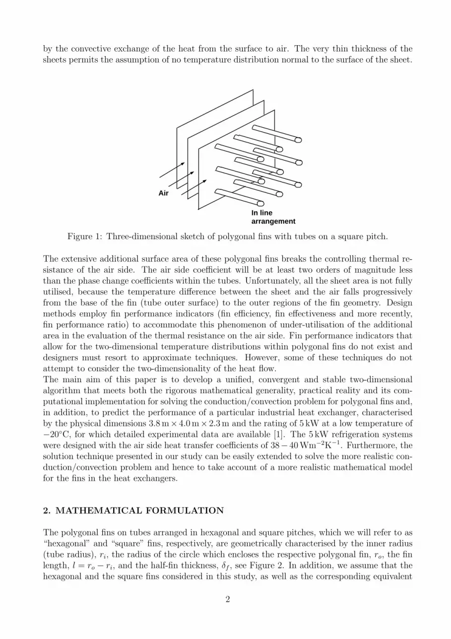
by the convective exchange of the heat from the surface to air. The very thin thickness of thesheets permits the assumption of no temperature distribution normal to the surface of the sheet.

Air

In linearrangement

Figure 1: Three-dimensional sketch of polygonal fins with tubes on a square pitch.

The extensive additional surface area of these polygonal fins breaks the controlling thermal re-sistance of the air side. The air side coefficient will be at least two orders of magnitude lessthan the phase change coefficients within the tubes. Unfortunately, all the sheet area is not fullyutilised, because the temperature difference between the sheet and the air falls progressivelyfrom the base of the fin (tube outer surface) to the outer regions of the fin geometry. Designmethods employ fin performance indicators (fin efficiency, fin effectiveness and more recently,fin performance ratio) to accommodate this phenomenon of under-utilisation of the additionalarea in the evaluation of the thermal resistance on the air side. Fin performance indicators thatallow for the two-dimensional temperature distributions within polygonal fins do not exist anddesigners must resort to approximate techniques. However, some of these techniques do notattempt to consider the two-dimensionality of the heat flow.The main aim of this paper is to develop a unified, convergent and stable two-dimensionalalgorithm that meets both the rigorous mathematical generality, practical reality and its com-putational implementation for solving the conduction/convection problem for polygonal fins and,in addition, to predict the performance of a particular industrial heat exchanger, characterisedby the physical dimensions 3.8m× 4.0m× 2.3m and the rating of 5 kW at a low temperature of−20C, for which detailed experimental data are available [1]. The 5 kW refrigeration systemswere designed with the air side heat transfer coefficients of 38− 40Wm−2K−1. Furthermore, thesolution technique presented in our study can be easily extended to solve the more realistic con-duction/convection problem and hence to take account of a more realistic mathematical modelfor the fins in the heat exchangers.

2. MATHEMATICAL FORMULATION

The polygonal fins on tubes arranged in hexagonal and square pitches, which we will refer to as“hexagonal” and “square” fins, respectively, are geometrically characterised by the inner radius(tube radius), ri, the radius of the circle which encloses the respective polygonal fin, ro, the finlength, l = ro − ri, and the half-fin thickness, δf , see Figure 2. In addition, we assume that thehexagonal and the square fins considered in this study, as well as the corresponding equivalent

2

radial rectangular fin, have the same surface area and the same inner radius. More specifically,

if we denote by r(r)o , r

(h)o and r

(s)o the outer radius of the equivalent radial rectangular fin and

the radius of the circle which encloses the hexagonal and the square fins, respectively, then these

are related by r(r)o = r

(h)o

√(3√3)/(2π) = r(s)o

√2/π.

The theoretical model is based on the following assumptions which are commonly made for theanalysis of fin heat transfer regardless of the fin geometry, see [2− 6],

(i) The heat transfer through the fin is at steady state and, in addition, there is no heatgeneration in the fin material.

(ii) The fin transfers heat to the ambient medium solely due to convection and the coefficientof convective heat transfer, α, is uniform over the entire fin surface.

(iii) The temperature of the ambient medium, T∞, is uniform and constant over the fin surface.

(iv) The material is of constant thermal conductivity, λf .

(v) The surface temperature of the tube, Tb, is constant.

(vi) Based on the thin fin assumption, the temperature variation in the fin normal to the finsurface is neglected.

ro

ri ro

ri

(a) (b)

Figure 2: Polygonal fins: (a) Hexagonal fin; (b) Square fin.

Consequently, the two-dimensional polygonal fin occupies an open bounded domain Ω ⊂ R2,Ω ⊂

x = (x1, x2)

∣∣ x21 + x2

2 < r2o, with the boundary ∂Ω = Γi ∪ Γo, Γi ∩ Γo = ∅, Γi =

x = (x1, x2)∣∣ x2

1 + x22 = r2i

, with the mention that in the limiting case the polygonal fin be-

comes a radial fin, i.e. Γo =x = (x1, x2)

∣∣ x21 + x2

2 = r2o. The governing partial differential

equation for the two-dimensional temperature distribution Tf (x) can be derived as follows:

∂2Tf (x)

∂x21

+∂2Tf (x)

∂x22

− α

λfδf(Tf (x)− T∞) = 0, x ∈ Ω. (1)

The boundary conditions for the two-dimensional thin fin temperature are given by an isothermalcondition at the base of the polygonal fin, Γi,

Tf (x) = Tb, x ∈ Γi, (2)

3

and at the fin tip, Γo, by assuming the heat and mass transfer from the fin tip to the surroundingambient medium to be negligible (adiabatic condition) due to its very small thickness

∂Tf (x)

∂ν= 0, x ∈ Γo, (3)

where ν(x) is the outward normal vector at the boundary Γo.The governing partial differential equation (1) and the boundary conditions (2) and (3) can berecast in non-dimensional and homogeneous form as

∂2θf (X)

∂X21

+∂2θf (X)

∂X22

− θf (X) = 0, X ∈ Ω, (4)

θf (X) = 1, X ∈ Γi, (5)

∂θf (X)

∂ν= 0, X ∈ Γo, (6)

on introducing the following dimensionless variables and parameters, see [2, 7]:

Xj =1

ζmax

(xj

δf

), j = 1, 2, ζmax =

√λf

αδf, θf (X) =

Tf (x)− T∞Tb − T∞

. (7)

Here Ω, Γi, Γo and ν are the transformed domain Ω, inner boundary Γi, outer boundary Γo

and outward normal ν at the boundary Γo, respectively, obtained using the change of variablesgiven by equation (7). More precisely, we have Ω ⊂

X = (X1, X2)

∣∣ X21 +X2

2 < R2o

, Ro =

ro/ (δfζmax), ∂Ω = Γi ∪ Γo, Γi ∩ Γo = ∅, Γi =X = (X1, X2)

∣∣ X21 +X2

2 = R2i

and Ri =

ri/ (δfζmax). It should be mentioned that the non-dimensional variables Xj and θf , as well asthe dimensionless parameters ζmax and xj/δf , given by relation (7) occur in a natural mannerin the non-dimensionalisation process of the governing equation (1), in the sense that the heattransfer/conduction dimensional group α/ (λfδf ) in equation (1) has the dimension m−2. Hencethe dimensionless length variables, Xj, are obtained by multiplying the length variables xj by√

α/ (λfδf ). In order to obtain dimensionless variables for the problem, the aspect ratios for

the fin geometry, xj/δf , are used which then results in the dimensionless parameter√λf

/(αδf ),

the so called maximum fin effectiveness, [2]. Furthermore, it should be noted that the governingnon-dimensionalised equation (4) is a Helmholtz-type equation, namely the modified Helmholtzequation. Although the boundary value problem given by equations (4)− (5) is a direct, mixed,well-posed problem, its closed form analytical solution is not available even if the outer boundaryis a circle, i.e Γo =

X = (X1, X2)

∣∣ X21 +X2

2 = R2o

. Hence a numerical method to solve the

boundary value problem (4)− (5) must be employed.

3. FIN PERFORMANCE INDICATORS

In this section, the performance indicators of the fins are briefly reviewed in the framework ofthe two-dimensional analysis. In the steady state, the heat flow through the fin, Qf , is obtainedfrom the temperature profile either by considering the heat flow through the base of the fin orby integrating the heat flow from the domain occupied by the fin, see e.g. [2− 6], namely

Qf = −λf (2δf )

∫Γi

∂Tf (x)

∂νdS(x) = −λf (2δf ) (Tb − T∞)

∫Γi

∂θf (X)

∂νdS(X), (8)

4

or

Qf = 2α

∫∫Ω(Tf (x)− T∞) dx = λf (2δf ) (Tb − T∞)

∫∫Ωθf (X) dX. (9)

The heat flow through a fin of infinite length is obtained by either substituting the (dimensionless)temperature gradient into equation (8), or substituting the (dimensionless) temperature intoequation (9), and taking the limit of the corresponding integrals as the (dimensionless) finlength lf = ro − ri (Lf = Ro −Ri) tends to infinity. The result is the maximum possible heatflow through the fin and is denoted by Qf, max.The fin effectiveness, ζf , is defined as the ratio of the heat flowing through the fin, Qf , to thatwhich would flow if the fin was not attached to the primary heat transfer surface, Q, see [2− 7],

ζf =Qf

Q, (10)

whereQ = 4πriδfα (Tb − T∞) . (11)

As a consequence of the previous definitions, the maximum fin effectiveness, ζmax, is given bythe ratio of the maximum possible heat flowing through the fin, Qf, max, and the heat whichwould flow if the fin was not attached to the primary heat transfer surface, Q, i.e.

ζmax =Qf, max

Q. (12)

The performance of the fin can be described by the ratio of the heat flow through the fin, Qf ,and the heat flow through a fin of infinite length (the maximum possible heat flow through thefin), Qf, max, and the resulting expression is called the fin performance ratio, PR, namely

PR =Qf

Qf, max. (13)

It should be noted from expressions (10) − (13) that the fin performance ratio, the heat flowthrough the fin, the maximum heat flow through the fin, the fin effectiveness and the maximumfin effectiveness are related by

PR =Qf

Qf, max=

ζfζmax

. (14)

Hence the introduction of the fin performance ratio provides an indicator which has an upperbound of unity, whilst the lower bound of the fin performance ratio is dependent upon the valueof the maximum fin effectiveness.The commonly used fin efficiency, ηf , is the ratio of the heat flow through the fin, Qf , to theheat flow if all the fin was at the base temperature, QfTb

, namely

ηf =Qf

QfTb

. (15)

whereQfTb

= 2α (Tb − T∞) π(r(r)o

2 − r2i

), (16)

and

QfTb= 2α (Tb − T∞)

∫∫Ω

dx = λf (2δf ) (Tb − T∞)

∫∫Ω

dX, (17)

5

for radial rectangular and polygonal fins, respectively. The physics of the fin problem dictatesthat there must be a diminishing temperature difference between the fin and the surroundingfluid as distances increase away from the fin base. Hence QfTb

is a hypothetical value, and ifthe fin dimensions are very large then the denominator in equation (15) tends to infinity andthe fin efficiency tends to zero. Whereas if the dimensions are very small so that ro −→ ri, thenQf −→ QfTb

and so the fin efficiency tends to unity. This does not seem to be a good indicatorwith respect to the flow of heat: when it is unity, there is no heat flow and when it is zero, theheat flow is maximum.It is worth mentioning that in the context of the one-dimensional theory in planar coordinates,

the maximum fin effectiveness is given by ζmax =√

λf

/(αδf ) and this justifies the notation

used in the two-dimensional non-dimensionalisation procedure (7). Furthermore, the heat flowthrough the fin, Qf , the maximum possible heat flow through the fin, Qf, max, and the finperformance ratio, PR, corresponding to a radial fin with isothermal and adiabatic conditionsat its base and tip, respectively, are given by the following expressions:

Qf = 4πriδfαζmax (Tb − T∞)

K1

(ri

δfζmax

)I1

(ro

δfζmax

)− I1

(ri

δfζmax

)K1

(ro

δfζmax

)K0

(ri

δfζmax

)I1

(ro

δfζmax

)+ I0

(ri

δfζmax

)K1

(ri

δfζmax

)= 4πRiδfλf (Tb − T∞)

K1 (Ri) I1 (Ro)− I1 (Ri)K1 (Ro)K0 (Ri) I1 (Ro) + I0 (Ri)K1 (Ro)

,

(18)

Qf, max = 4πriδfαζmax (Tb − T∞)

K1

(ri

δfζmax

)K0

(ri

δfζmax

) = 4πRiδfλf (Tb − T∞)K1 (Ri)

K0 (Ri), (19)

PR =Qf

Qf, max=

1− K1 (Ro)

K1 (Ri)

/ I1 (Ri)

I1 (Ro)

/1 +

K1 (Ro)

K0 (Ri)

/ I1 (Ri)

I0 (Ro)

. (20)

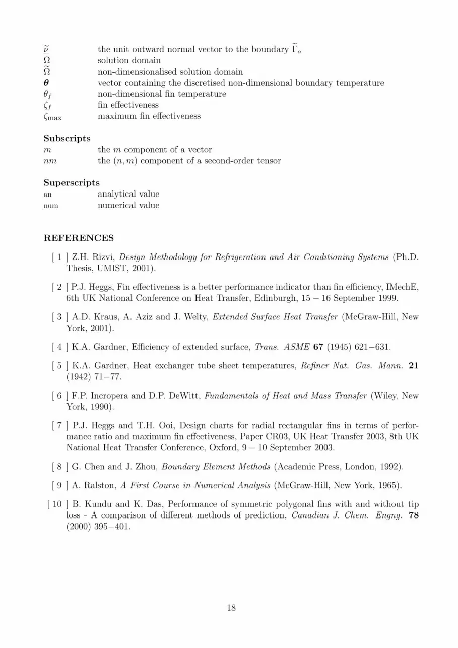
Here I0 and I1 are the modified Bessel functions of the first kind of orders zero and one, re-spectively, whilst K0 and K1 are the modified Bessel functions of the second kind of orders zeroand one, respectively. Note for the radial rectangular fin, the maximum effectiveness is multi-plied by the ratio K1/K0. By an appropriate regrouping of the problem parameters involved inthe expression (20) for the fin performance ratio in the one-dimensional theory, it can be seenthat this performance indicator is a function of the ratio, ri/δf , of the inner radius and thehalf-thickness of the fin, the reduced fin length, l/δf , and the maximum fin effectiveness, ζmax,i.e. PR = PR (ri/δf , l/δf , ζmax). Since the first two parameters of the problem (ri/δf , l/δf ) con-tain information on the geometry of the fin and the last one (ζmax) directly reflects the physicsof the heat flow through the fin, the fin performance ratio is expected to be a comprehensivepeformance indicator of the fin under consideration in both one- and two-dimensional theories.Moreover, from equations (18)−(20) we obtain the following expression for the heat flow throughthe fin

Qf = 4πriδfαPR (ri/δf , l/δf , ζmax)K1 (ri/ (δfζmax))

K0 (ri/ (δfζmax))(Tb − T∞) . (21)

The above expression is of practical importance for determining the value of the heat flow,Qf , through a fin characterised by the coefficient of convective heat transfer, α, the thermalconductivity, λf , the half-thickness, δf , the inner radius, ri, and the fin length, l = ro − ri, byusing the design charts for the prediction of the performance ratio, PR, of radial rectangular fins,

6

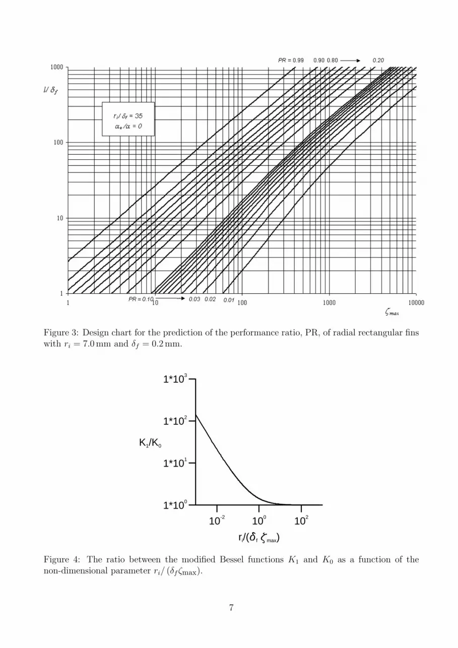
Figure 3: Design chart for the prediction of the performance ratio, PR, of radial rectangular finswith ri = 7.0mm and δf = 0.2mm.

10-2 100 102

ri/( f max)

1*100

1*101

1*102

1*103

K1/K0

Figure 4: The ratio between the modified Bessel functions K1 and K0 as a function of thenon-dimensional parameter ri/ (δfζmax).

7

see Figure 3, and the graph of the function K1/K0, see Figure 4. Furthermore, the charts forthe prediction of the fin performance ratio give very good information on the fin performance,the geometry (dimensions) of the fin and the fin material. More specifically, from Figure 3 it canbe seen that such a design chart consists of three specific regions. The first one which is locatedabove the graph of the function PR = 0.99, say, corresponds to very long fins, i.e. too muchmaterial has been used for the fin. The region below the graph of the function PR = 0.01, say,characterises fins made of materials having properties unsuitable for design purposes. Finally, theregion between the graphs of the functions PR = 0.01 and PR = 0.99 is of practical importanceand gives the designers comprehensive information on both the geometry of the fin and thephysics of the heat flow through the fin. It should be mentioned that the normal practice is touse a fin efficiency with a value greater than 0.80 and this will correspond to a fin performanceratio with a value of around 0.40 or less. Consequently, the fin performance ratio, PR, is a betterfin performance indicator than the fin efficiency, ηf .

4. THE BOUNDARY ELEMENT METHOD

The governing non-dimensionalised partial differential equation (4) can also be formulated inintegral form, see e.g. Chen and Zhou [8], as

c(X) θf (X) +

∫∂Ω

∂E(X,Y )

∂νθf (Y ) dS(Y ) =

∫∂Ω

E(X,Y )∂θf (Y )

∂νdS(Y ) , (22)

for X ∈ Ω∪ ∂Ω, where c(X) = 1 for X ∈ Ω and c(X) = 1/2 for X ∈ ∂Ω (smooth), and E is thefundamental solution for the modified Helmholtz equation (4), which is given by

E(X,Y ) =1

2πK0 (r(X,Y )) . (23)

Here r(X,Y ) represents the distance between the load point X and the field point Y . Alterna-tively, one can also use the real part of the complex fundamental solution E for the modifiedHelmholtz equation in the boundary integral equation (22), namely

E(X,Y ) = Re

i

4H

(1)0 (i r(X,Y ))

, (24)

where i =√−1 and H

(1)0 is the Hankel function of order zero of the first kind.

It should be noted that in practice the boundary integral equation (22) can rarely be solvedanalytically and thus a numerical approximation is required. A Boundary Element Method(BEM) with piecewise constant boundary elements is used in order to solve the direct, mixed,

well-posed boundary value problem (4) − (6). Consequently, the outer boundary Γo is approx-

imated by No straight line segments in a counterclockwise sense and the inner boundary Γi isapproximated by Ni straight line segments in a clockwise sense, such that the boundary ∂Ω isdiscretised into N = No + Ni boundary elements, whilst the non-dimensional temperature andthe non-dimensional flux are considered to be constant and take their values at the midpoint,i.e. the collocation point, also known as the node, of each element. More specifically, we have

Γo ≈No∪n=1

Γn, Γ(n)o =

[Yo

n−1, Yon], n = 1, . . . , No, Yo

No = Yo0,

Γi ≈Ni∪n=1

Γ(n)i , Γ

(n)i =

[Yi

n−1, Yin], n = 1, . . . , Ni, Yi

Ni = Yi0,

Xn =Yo

n−1 + Yon

2 , n = 1, . . . , No, XNo+n =Yi

n−1 + Yin

2 , n = 1, . . . , Ni,

(25)

8

and

θf (Y ) = θf (Xn),

∂θf (Y )∂ν

=∂θf (X

n)∂ν

, Y ∈ Γn, n = 1, . . . , N, (26)

where Γn = Γ(n)o for n = 1, . . . , No and ΓNo+n = Γ

(n)i for n = 1, . . . , Ni.

By applying the boundary integral equation (22) at each collocation point Xm, m = 1, . . . , N ,and taking into account the fact that the boundary is always smooth at these points, we arriveat the following system of linear algebraic equations

Aθ = Bφ, (27)

where the matrices A,B ∈ RN×N depend solely on the geometry of the boundary ∂Ω and thevectors θ,φ ∈ RN consist of the discretised values of the non-dimensional temperature and fluxon the boundary ∂Ω, namely

θm = θf (Xm), φm =

∂θf (Xm)

∂ν, m = 1, . . . , N, (28)

Anm = 12 δnm + An (X

m) = 12 δnm +

∫Γn

∂E(Xm, Y )

∂νdS(Y ), m, n = 1, . . . , N, (29)

Bnm = Bn (Xm) =

∫Γn

E(Xm, Y ) dS(Y ), m, n = 1, . . . , N, (30)

where δnm is the Kronecker tensor. It should be noted that equation (27) represents a system ofN linear algebraic equations with 2N unknowns. The discretisation of the boundary conditions(5) and (6) provides the values of N of the unknowns and the problem reduces to solving asystem of N equations with N unknowns which can be generically written as

C x = f , (31)

where the right-hand side vector f ∈ RN is computed using the boundary conditions (5) and

(6), the system matrix C ∈ RN×N depends solely on the geometry of the boundary ∂Ω and thevector x ∈ RN contains the unknown values of the non-dimensional temperature on the outerboundary Γo and the non-dimensional flux on the inner boundary Γi.Once the unknown values of the non-dimensional temperature and flux on the outer and in-ner boundaries, respectively, have been computed then by employing the discretisation of theboundary integral equation (22) for internal points X ∈ Ω, the BEM approximation of thenon-dimensional temperature θf can be obtained at any internal point in the form

θf (X) =N∑

n=1

Bn (X) φn − An (X) θn , (32)

where An (X) and Bn (X) are given by relations (29) and (30), respectively, with Xm = X.

5. NUMERICAL RESULTS

In this section, we illustrate the numerical results obtained using the BEM described in theprevious section and, in addition, we investigate the convergence, stability and consistency ofthe numerical method proposed. It should be mentioned that the numerical analysis developed

9

for the polygonal fins is based on typical geometries and operating conditions used in practi-cal evaporators and condensers in 5 kW refrigeration systems, see e.g. Rizvi [1]. We considerpolygonal fins on a hexagonal pitch which are characterised by the inner radius (tube outer

radius) ri = 7.0mm, the radius of the circle which encloses the fin r(h)o = 25.0mm, the half-fin

thickness δf = 0.1mm and δf = 0.2mm and the thermal conductivity λf = 204.4Wm−1K−1

(aluminium), as well as polygonal fins on an equivalent square pitch(r(s)o = 28.49mm

)and the

equivalent radial fin(r(r)o = 22.74mm

). For all the fins considered in this study, the fin length

is given by l = ro − ri, where ro ∈r(h)o , r

(s)o , r

(r)o

, the convective heat transfer coefficient is

given by α = 20.0Wm−2K−1 and Tb − T∞ = 1K.The solution to the boundary value problem described by equations (4)− (6) by any techniquewhich involves approximations in the solution procedure invariably includes an error. Morespecifically, the errors in the solutions predicted by the BEM are related to the associated meshsize. These errors diminish as the mesh size discretisation is refined and, consequently, the ap-proximate solutions approach the exact solution. In order to check for this convergence, we usethree levels of discretisation which are given by the number of boundary elements used, namelyN ∈ 80, 160, 320, Ni = No/3 = N/4, in the case of the hexagonal fin and N ∈ 60, 120, 240,Ni = No/2 = N/3, in the case of both the square and the equivalent radial fins. Although aclosed form analytical solution is not available for the polygonal fins analysed in this study, itis reported that the BEM solutions for the non-dimensional temperature display a convergentbehaviour as the corresponding discretisation is refined.Figures 5(a), (b) and (c) show the numerical results obtained for the non-dimensional tempera-ture θf in the hexagonal, the square and the equivalent radial fins, respectively, with δf = 0.1mm.Although not presented here, it should be mentioned that the BEM solution for the dimension-less temperature in the equivalent radial fin obtained using the two-dimensional approach hasbeen found to be consistent with its analytical value given by the one-dimensional theory. Itcan be seen from Figure 5 that in the case of the hexagonal and the square fins, the isothermskeep the shape of the inner boundary Γi until θf reaches a specifc value after which they takea different shape, whilst in the case of the equivalent radial fin the isotherms remain circles re-gardless of the value of θf . Therefore, from this figure we can conclude that the two-dimensionaltreatment of the polygonal fins is fully justified. Moreover, since the boundary conditions (5)and (6) contain the analytical values of the non-dimensional temperature on the inner boundary

Γi and flux on the outer boundary Γo, respectively, then these boundary data are polluted withnumerical noise and therefore the numerical method proposed is also stable. Similar results havebeen obtained for δf = 0.2mm and hence they are not presented here.In the context of numerical methods, such as finite-difference, finite element and boundary el-ement methods, the integrations from relations (8) and (9) can be performed employing anappropriate quadrature formula. However, as these numerical techniques only provide approxi-mate solutions, the corresponding values for the integrations in equations (8) and (9) need not beexactly the same, although, these should agree to within an acceptable tolerance in order for thenumerical solutions to be satisfactory. Therefore, in the subsequent calculations Q

(1)f and Q

(2)f

denote the values of the heat flow through the fin corresponding to the expressions (8) and (9),respectively. It is important to mention that a further requirement for the numerical solutions tobe satisfactory is that the corresponding heat flows through the fin show a convergent behaviouras the order of the approximation is improved.The values of the heat flows Q

(1)f and Q

(2)f , as well as the performance ratio PR, obtained for the

hexagonal, the square and the equivalent radial fins with δf = 0.1mm and δf = 0.2mm usingthe two-dimensional BEM procedure proposed in this study and their analytical values for the

10

(a) (b)

(c)

Figure 5: The non-dimensional temperature distribution, θf , in (a) the hexagonal, (b) the square,and (c) the equivalent radial fins, obtained for δf = 0.1mm and using (a) N = 320, (b) N = 240,and (c) N = 240 boundary elements, respectively.

11

equivalent radial fin given by the one-dimensional theory are presented in Table 1. From thistable it can be seen that all the aforementioned fin performance indicators exhibit convergencewith respect to the mesh refinement and the numerical results obtained for the heat flow throughthe fin and the fin performance ratio are very good approximations for their analytical values.In addition, we can conclude that the numerical technique proposed is also consistent, in thesense that the difference between the computed heat flows Q

(1)f and Q

(2)f is O (10−4) for all

the fins, thicknesses and discretisations considered. It should be noted that in the expression(13) for the fin performance ratio in the two-dimensional approach, the value of the maximumpossible heat flow through the fin, Qf, max, has been approximated by its value (19) given bythe one-dimensional theory. Moreover, as further refinement of the boundary discretisationis impractical, the limiting values of Q

(1)f , Q

(2)f and PR are computed by the extrapolation

of their BEM solutions, obtained for N ∈ 80, 160, 320 in the case of the hexagonal fin andN ∈ 60, 120, 240 in the case of both the square and the equivalent radial fins, and by employingRichardson’s formula, see e.g. Ralston [9]. These values are excellent approximations for theheat flow, as well as for the fin performance ratio, in all the cases analysed in this paper.

Table 1: The 1D analytical, the 2D BEM and the corresponding Richardson’s extrapolationvalues for the heat flows Q

(1)f and Q

(2)f and the performance ratio PR for the hexagonal, the

square and the equivalent radial fins, obtained with δf = 0.1mm and δf = 0.2mm.

δf Fin type Solution type Q(1)f Q

(2)f PR

0.1mm Radial (1D) Analytical 0.05136 0.05136 0.35394Radial (2D) N = 60 0.05116 0.05128 0.35260

N = 120 0.05131 0.05133 0.35361N = 240 0.05134 0.05135 0.35386Richardson’s extrapolation 0.05135 0.05136 0.35394

Hexagonal (2D) N = 80 0.05133 0.05151 0.35380N = 160 0.05134 0.05158 0.35383N = 320 0.05134 0.05160 0.35384Richardson’s extrapolation 0.05134 0.05161 0.35384

Square (2D) N = 60 0.05121 0.05130 0.35295N = 120 0.05122 0.05137 0.35299N = 240 0.05122 0.05139 0.35300Richardson’s extrapolation 0.05122 0.05140 0.35300

0.2mm Radial (1D) Analytical 0.05480 0.05480 0.22152Radial (2D) N = 60 0.05461 0.05476 0.22078

N = 120 0.05475 0.05479 0.22134N = 240 0.05479 0.05479 0.22148Richardson’s extrapolation 0.05481 0.05479 0.22153

Hexagonal (2D) N = 80 0.05483 0.05488 0.22165N = 160 0.05480 0.05492 0.22153N = 320 0.05479 0.05493 0.22150Richardson’s extrapolation 0.05479 0.05493 0.22149

Square (2D) N = 60 0.05475 0.05476 0.22134N = 120 0.05473 0.05481 0.22123N = 240 0.05472 0.05482 0.22120Richardson’s extrapolation 0.05471 0.05482 0.22119

It should be mentioned that the value for the heat flow if all the radial rectangular fin was at the

12

base temperature calculated according to the formula (16) is QfTb= 0.058. On using this value

for QfTb, equation (15) and Table 1, the values for the fin efficiency, ηf , and fin performance

ratio, PR, corresponding to the radial fins presented in Table 1 are ηf = 0.87 and PR = 0.35when δf = 0.1mm, and ηf = 0.93 and PR = 0.22 when δf = 0.2mm. Since the thicker the fin,the lower the heat flow, we can conclude that the fin performance ratio characterises better theflow of the heat than the fin efficiency.In order to get more insight into the features of the numerical method proposed, we investigatethe behaviour of the fin performance ratio PR = PR (ri/δf , l/δf , ζmax) for the polygonal finsconsidered in this study with respect to the parameters of the problem, namely the ratio ofthe inner radius and the half-thickness of the fin, ri/δf , the reduced fin length, l/δf , and themaximum fin effectiveness, ζmax. More precisely, in the following, the convective heat transfercoefficient is given by α = 20.0Wm−2 K−1, we set the ratio ri/δf to a fixed value by assigningri = 7.0mm and δf = 0.2mm, and we keep fixed one of the remaining two problem parameters,l/δf or ζmax, while at the same time varying the other (we actually vary either the outer radiusof the fin, ro, or the thermal conductivity of the fin, λf ).Figure 6(a) illustrates the analytical value based on the one-dimensional theory and the numericalvalues for the performance ratio, PR, as a function of l/δf , obtained for the hexagonal fin withλf = 204.4Wm−1K−1, ζmax constant and using N ∈ 80, 160, 320 boundary elements. Itcan be seen from this figure that the BEM results are excellent approximations for the one-dimensional based analytical value of the fin performance ratio over a wide range of values ofthe reduced fin length, l/δf . In order to get a better understanding of the qualitative behaviourof the above dependence, we define the relative percentage error

err (PR) =

∣∣∣PR(num) − PR(an)∣∣∣

PR(an) × 100, (33)

where PR(an) and PR(num) are the analytical and the numerical values for the performance ratio,respectively. In Figure 6(b) we present the evolution of the error err (PR) given by expression(33) with respect to the reduced fin length, l/δf , obtained for the hexagonal fin using variousBEM discretisations. It should be noted from this figure that the highest values of the error inthe numerical results occur for very small values of the reduced fin length, i.e. for very shorthexagonal fins. This error decreases up to a specific (optimal) value of l/δf after which it in-creases slowly until it reaches a stable value of less than 0.5%. However, even for very smallvalues of the reduced fin length, the numerical results can be significantly improved by refiningthe BEM discretisation and very good numerical approximations for the hexagonal fin perfor-mance ratio can be obtained; for example, err (PR) < 1% for all l/δf ∈ (0, 5000) and N = 160.From Figures 6(a) and (b) it can also be seen that the highest values of the error err (PR) actu-ally correspond to very small values of the fin performance ratio PR and hence the informationabout the fin performance is still accurate. Therefore, we can conclude that the two-dimensionalBEM proposed in this study provides very good numerical approximations for the performanceratio in the case of the hexagonal fin for a wide range of the fin length.Figures 7(a) and (b) show the numerical values for the performance ratio, PR, in comparison withits analytical value given by the one-dimensional theory and the error err (PR), respectively, asfunctions of ζmax, obtained for the hexagonal fin with l/δf constant and using N ∈ 80, 160, 320boundary elements. It can be seen from Figure 7(a) that the two-dimensional BEM providesexcellent approximations for the one-dimensional based analytical value of the fin performanceratio over a long range of the values of the maximum fin effectiveness ζmax ∈ (0, 1000), i.e.for hexagonal fins made of various materials. The behaviour of the error err (PR) when themaximum fin effectiveness, ζmax, varies is different from that of err (PR) when the reduced fin

13

0 1000 2000 3000 4000 5000 6000

l/ f

0.0

0.2

0.4

0.6

0.8

1.0

PR

Analytical (1D)

N = 80

N = 160

N = 320

(a)

0 1000 2000 3000 4000 5000 6000

l/ l

0

1

2

3

4

5

err(

PR

) [%

]

N = 60

N = 160

N = 320

(b)

Figure 6: (a) The analytical and the numerical values for the performance ratio PR, and (b) theerror err (PR), as functions of l/δf , obtained for the hexagonal fin with λf = 204.4Wm−1K−1,ζmax constant and N ∈ 80, 160, 320 boundary elements.

14

0 200 400 600 800 1000

max

0.0

0.2

0.4

0.6

0.8

1.0

PR

Analytical (1D)

N = 60

N = 120

N = 240

(a)

0 200 400 600 800 1000

max

0

1

2

3

4

5

err(

PR

) [%

]

N = 80

N = 160

N = 320

(b)

Figure 7: (a) The analytical and the numerical values for the performance ratio PR, and (b)the error err (PR), as functions of ζmax, obtained for the hexagonal fin with δf = 0.2mm, l/δfconstant and N ∈ 80, 160, 320 boundary elements.

15

length, l/δf , varies, as can be noticed from Figures 6(b) and 7(b). From Figure 7(b) it canbe seen that for all the mesh sizes used, err (PR) decreases up to a specific (optimal) value ofζmax after which it starts increasing, with sharp increases followed by flat portions. However,by comparing Figures 7(a) and (b), we notice that value of the maximum fin effectiveness, ζmax,at which the error in the numerical results for the fin performance ratio, PR, starts increasing,corresponds to a very small value of PR and the accuracy in the numerical results is still verygood. Hence the two-dimensional BEM estimates for the fin performance ratio are in very goodagreement with their analytical values for a wide range of materials used for the hexagonal finunder investigation. Similar results have been obtained for the hexagonal fin with δf = 0.1mm,as well as for the square fin with both δf = 0.1mm and δf = 0.2mm, however, these are notpresented here.Overall, from the numerical results presented and discussed in this section we can conclude thatthe BEM, in conjunction with the two-dimensional approach, provides excellent estimates forpolygonal fins on both hexagonal and square pitches and which are in a very good agreementwith the results given by considering the design charts for the equivalent rectangular radial finin the framework of the one-dimensional theory of heat flow along fins, see Figure 3. Moreover,this two-dimensional BEM technique emphasizes very well the two-dimensional character of thetemperature profile in polygonal fins.

6. CONCLUSIONS

In this paper, polygonal fins on hexagonal and square pitches were analysed in the context ofthe two-dimensional theory and compared with the equivalent radial rectangular fin based onthe same surface area of the fins. A semi-analytical solution for the aforementioned fins wasobtained using the BEM and, in addition, the convergence, stability and consistency of the nu-merical method employed were checked. The main advantages of this numerical method overthe domain discretisation methods, such as the finite-difference and the finite element methods,are its increased accuracy from the use of Green’s integral identities, the simultaneous predictionof the solution function and its normal derivatives at the boundary without the need of furtherfinite differencing, and the fact that only the boundary of the solution domain has to be discre-tised. The heat flows corresponding to the polygonal fins analysed in this study were comparedin the normal energy procedure taking the radial fin with an adiabatic boundary condition on theextreme radius. The numerical results obtained for the fin performance indicators, namely theheat flow through the fin and the fin performance ratio, were found to be in very good agreementwith their corresponding analytical values obtained for the equivalent radial fin in the frameworkof the one-dimensional theory. In addition, the two-dimensional character of the temperaturedistribution in polygonal fins has been emphasized by employing the two-dimensional BEM pro-posed. In conclusion, the numerical technique investigated in this paper has been found to be asuitable numerical method to analyse polygonal fins since it provides very accurate, convergent,stable and consistent numerical results for both the temperature profile and the fin performanceindicators. Furthermore, the two-dimensional BEM proposed in this paper does not take intoaccount the symmetry of the fin, see [10], and hence can be easily extended to more realisticmathematical models for fins in heat exchangers but this is deferred to future work.

Acknowledgement. L. Marin would like to acknowledge the financial support received fromthe EPSRC.

16

NOMENCLATURE

A,B,C matrices corresponding to the boundary element discretisationerr (PR) relative percentage error in evaluating the fin peformance ratioE the fundamental solution for the modified Helmholtz equationf the right-hand side vector of the discretised systemH

(1)0 the Hankel function of the first kind of order zero

I0 the modified Bessel function of the first kind of order zeroI1 the modified Bessel function of the first kind of order oneK0 the modified Bessel function of the second kind of order zeroK1 the modified Bessel function of the second kind of order onel length of the finN,Ni, No numbers of boundary elementsPR fin performance ratioQ heat flow if the fin was not attached to the primary surfaceQf heat flow through the fin

Q(1)f , Q

(2)f calculated heat flows through the fin

Qf,max maximum possible heat flow through the finQfTb

heat flow if all the fin was at the base temperaturer (X,Y ) distance between the load point X and the field point Yri inner radius of the finro radius of the circle which encloses the polygonal finRi inner radius of the non-dimensionalised finRo radius of the circle which encloses the non-dimensionalised polygonal finR the real number setTb fin base (tube) temperatureTf fin temperatureT∞ ambient medium temperaturex vector containing the unknown boundary values of the non-dimensional

temperature and flux at the collocation pointsx, y,X, Y space variablesXm collocation point/node

Yin−1, Yi

n endpoints of the boundary element Γ(n)i

Yon−1, Yo

n endpoints of the boundary element Γ(n)o

Greek Symbolsα convective heat transfer coefficientδf half-fin thicknessδmn the Kronecker delta symbolφ vector containing the discretised non-dimensional boundary flux∅ the empty set∂Ω the boundary of the solution domain Ω∂Ω the boundary of the non-dimensionalised solution domain ΩΓi,Γo parts of the boundary of the solution domain ΩΓi, Γo parts of the boundary of the non-dimensionalised solution domain ΩΓ(n)i , Γ

(n)o , Γn boundary elements

λf thermal conductivity of the finν the unit outward normal vector to the boundary Γo

17

ν the unit outward normal vector to the boundary Γo

Ω solution domainΩ non-dimensionalised solution domainθ vector containing the discretised non-dimensional boundary temperatureθf non-dimensional fin temperatureζf fin effectivenessζmax maximum fin effectiveness

Subscriptsm the m component of a vectornm the (n,m) component of a second-order tensor

Superscriptsan analytical valuenum numerical value

REFERENCES

[ 1 ] Z.H. Rizvi, Design Methodology for Refrigeration and Air Conditioning Systems (Ph.D.Thesis, UMIST, 2001).

[ 2 ] P.J. Heggs, Fin effectiveness is a better performance indicator than fin efficiency, IMechE,6th UK National Conference on Heat Transfer, Edinburgh, 15− 16 September 1999.

[ 3 ] A.D. Kraus, A. Aziz and J. Welty, Extended Surface Heat Transfer (McGraw-Hill, NewYork, 2001).

[ 4 ] K.A. Gardner, Efficiency of extended surface, Trans. ASME 67 (1945) 621−631.

[ 5 ] K.A. Gardner, Heat exchanger tube sheet temperatures, Refiner Nat. Gas. Mann. 21(1942) 71−77.

[ 6 ] F.P. Incropera and D.P. DeWitt, Fundamentals of Heat and Mass Transfer (Wiley, NewYork, 1990).

[ 7 ] P.J. Heggs and T.H. Ooi, Design charts for radial rectangular fins in terms of perfor-mance ratio and maximum fin effectiveness, Paper CR03, UK Heat Transfer 2003, 8th UKNational Heat Transfer Conference, Oxford, 9− 10 September 2003.

[ 8 ] G. Chen and J. Zhou, Boundary Element Methods (Academic Press, London, 1992).

[ 9 ] A. Ralston, A First Course in Numerical Analysis (McGraw-Hill, New York, 1965).

[ 10 ] B. Kundu and K. Das, Performance of symmetric polygonal fins with and without tiploss - A comparison of different methods of prediction, Canadian J. Chem. Engng. 78(2000) 395−401.

18