Embed Size (px)
Citation preview

METRON - International Journal of Statistics2009, vol. LXVII, n. 1, pp. 57-74
M. T. ALODAT – M. Y. AL-RAWWASHI. M. NAWAJAH
Analysis of simple linear regressionvia median ranked set sampling
Summary - The purpose of this article is to study the simple linear regression model un-der the median ranked set sampling (MRSS) scheme. In fact, if the response variablecan be easily ranked than quantified or measuring the response variable is expensivebut can be ranked easily, then it is recommended to use the MRSS to collect data on theresponse variable. We obtain estimators of the regression parameters using the col-lected data under the assumption that the errors are symmetrically distributed also weelaborate on some of the mathematical properties of these estimators. We also showthat the new estimators are more efficient than those obtained via simple random sam-ple (SRS) and extreme ranked set sample (ERSS). An application to real data is alsopresented.
Key Words - Extreme ranked set sample; Median ranked set sample; Ranked setsample; Simple linear regression.
1. Introduction
McIntyre (1952) was the first to introduce the so called Ranked Set Sam-pling (RSS) which is considered to be a relatively new method of samplingcompared to other sampling methods. The RSS can be summarized as follows.Randomly select m2 sample units from the population of interest by visualinspection and allocate these selected units as randomly as possible into m setseach of size m. Accordingly, select the RSS of size m for actual analysisthat consists of the smallest ranked unit from the first set, the second smallestranked unit from second set, continuing in this fashion until the largest rankedunit is selected from the last set. The cycle may be repeated r times until adesired sample of size n = rm is obtained. The RSS scheme can be comparedto the SRS scheme via the following two criteria:
Received June 2008 and revised April 2009.

58 M. T. ALODAT – M. Y. AL-RAWWASH – I. M. NAWAJAH
1. Relative efficiency. The relative efficiency of RSS with respect to SRS inthe estimation of the population mean is defined as
RE(XRSS, XSRS) = Var(XSRS)
Var(XRSS)
where XSRS and XRSS are unbiased estimators for the population mean µ
based on equal size samples obtained from the SRS and the RSS samplingschemes, respectively. If, RE(XRSS, XSRS) > 1, then
Var(XRSS) < Var(XSRS).
2. Relative saving.
RS = 1 − 1
RE(XRSS, XSRS),
which equals the number of saved sampling units due to using the RSSmethod.
Ranked set sampling has been considered and modified by many authors overthe last few decades. To summarize the main and important activities in thisfield, we introduce this review based on the bibliography by Kaur et al. (1995).Among the early work on RSS, McIntyre (1952) illustrated the RSS techniqueand proposed the estimate XRSS = ∑n
i=1 Xi(i)/n as a trial estimator of µ versusthe traditional estimate XSRS. McIntyre (1952) claimed without proof that XRSS
is unbiased estimator of the population mean regardless of any error in rankingjudgment. Numerous authors have tried to evaluate the performance of RSS,(for more details see Halls and Dell, 1966; Martin et al. 1980; and Alodat andAl-Sagheer, 2007). On the other hand, some authors have studied RSS undercertain distributional assumptions and we will briefly introduce some of them.
Takahashi and Wakimoto (1968) gave the mathematical framework for theRSS. They showed that the sample mean XRSS is the minimum variance un-biased estimator for the population mean. Moreover, when ranking is perfect,they established the following inequality on RE(XRSS, XSRS)
1 ≤ RE(XRSS, XSRS) ≤ m + 1
2,
where m is the set size. Muttlak (1995) used the RSS to estimate the parametersof the simple linear regression model assuming that the explanatory variable Xis known constants. Muttlak (1997) proposed the median ranked set sampling(MRSS) scheme. This scheme is similar the RSS scheme, but we quantifythe median of each set instead of quantifying other order statistics. Muttlak(1997) showed that the MRSS is more efficient than the RSS for estimating

Analysis of simple linear regression via median ranked set sampling 59
the population mean when the population is symmetric. Yu and Lam (1997)proposed a regression-type estimator based on RSS. They demonstrated thatthis estimator is always more efficient than the regression estimator using SRSand it is more efficient than the estimator proposed by Patil et al. (1993),unless the correlation coefficient is low (|ρ| < 0.4).
In order to decide which sampling method is more appropriate to use forregression analysis, Patil et al. (1993) conducted an experiment to obtain theparameters estimates of a linear regression model. They showed that the esti-mator of the population mean using RSS is more efficient than the usual SRSregression estimator unless the correlation coefficient between the response Yand the concomitant variable X is high (say, ρ > 0.85). Under the assumptionthat the interest variable and the concomitant variable follow a joint bivariatenormal distribution, Yu and Lam (1997) found that the RSS regression estima-tor is more efficient than the SRS regression estimator unless the correlationbetween the interest variable and the concomitant variable is low (say ρ < 0.4).
Later, Chen and Wang (2004) proposed a general unbalanced RSS schemein order to study the polynomial regression model by ranking on the concomitantvariable X . They considered the regression model
Y = β0 + β1 X + β2 X2 + · · · + βp X p + ε,
where Y is response variable, X is predictor variable, β’s are the regressionparameters and ε is a random error independent of X .
The extreme ranked set sampling (ERSS) procedure, as proposed by Sama-wi et al. (1996), can be described as follows:
1. Select m random sets each of size m from the population of interest.2. Rank the units within each set with respect to a variable of interest by
visual inspection.3. If m is even, we select the smallest unit from each of the first m/2 sets,
while we choose the largest unit from each of the last m/2 s sets for actualmeasurement. However, if m is odd, we select the smallest unit from eachof the first (m −1)/2 sets for actual measurement and we select the largestunit from each of the next (m − 1)/2 sets, while we select the median ofthe last set for actual measurement.
The cycle may be repeated r times to get n = mr units. These n units representan ERSS sample.
In this paper, we introduce a new method to analyze the simple linearregression model. The measurements are collected using the median ranked setsampling scheme where the response variable is assumed to be easily rankedthan quantified or the quantification of the response happens to be expensive.In Section 2, we introduce the MRSS to the regression framework in orderto build the estimation strategy accordingly. Later, we introduce the least

60 M. T. ALODAT – M. Y. AL-RAWWASH – I. M. NAWAJAH
squares estimators of the regression parameters using the MRSS scheme anddiscuss its properties. In Section 3, we present the ERSS to simple linearregression setup and outline the estimation strategy as well as the propertiesof the estimators obtained accordingly. In Section 4, we conduct a comparisonstudy via simulation among the three sampling schemes namely SRS, ERSSand MRSS. In Section 5, a real example illustrates our procedure and theoryregarding the advantages of the MRSS compared to SRS. Finally, we presentour findings, discuss our ideas and state the final conclusions.
2. Median ranked set sample for regression
Consider the following simple linear regression model
Yj = β0 + β1xj + εj , j = 1, . . . , r,
where
1. β0 and β1 are unknown parameters.2. E(Yj |X j = xj ) = β0 + β1xj .3. εj ’s are iid random errors with mean zero and unknown variance σ 2. The
distribution of the errors should be symmetric and we may assume thenormality for more convenience in this article.
To this end, we assume x1, x2, . . . , xr to be different values of the predictorX which are chosen by the experimenter. We assume that for each xj , theexperimenter has repeated the experiment n = 2m − 1 times, consequently welet Yj j1, Yj j2, . . . , Yj jn , j = 1, 2, . . . , r , be the corresponding values of Y atxj , i.e.,
Yj ji = β0 + β1xj + εj j i , j = 1, . . . , r, i = 1, . . . , n,
where εj j i are the corresponding errors. If the variable Y seems to be moreeasily ranked than quantified or if measuring the variable Y is expensive whileit can be ranked easily, then the median ranked set sampling could be a properscheme to collect our data on the variable Y . To accomplish this missionand using visual inspection, let Yj(m) denote the quantified median of Yj j1,Yj j2, . . . , Yj jn . Using the collected data, Yj(m) can be related to xj using thefollowing simple linear regression model
Yj(m) = β0 + β1xj + εj(m), j = 1, . . . , r, (1)
where εj(m) is the median of εj j1, εj j2, . . . , εj jn .

Analysis of simple linear regression via median ranked set sampling 61
Many authors in a wide range of research reported that data collectionis expensive and time-consuming task. For example, environmental mangershighlighted this obstacle in several occasions and explain how hard and ex-pensive the process of obtaining estimates of species abundance especially ifthe species are rare or occur in remote locations. Patts and Elith (2006) foundthat the Australian threatened plant species, Leinomea ralstonni, is protectedunder both state and federal legislation due to its small geographic range andpopulation size. Prediction of species abundance is supposed to guide manage-ment of the species and as an input for population viability. Model structureincludes the choice of environmental characteristics (explanatory variables) thatare expected to affect pj , the species abundance (the response variable). Themodel of interest is
log ρj = β0 + β1xj + εj ,
where xj is an environmental cutting factor which could be controlled by theexperimenter.
Other examples could be found in animal growth literature such as studyingthe age of animals. The age of animals needs to be determined in this field ofresearch, but aging an animal is usually time-consuming and costly. However,variables on the physical size of an animal, which is closely related to age,can be collected easily and cheaply.
2.1. Distribution of errors
Based on the setup so far mentioned in this article, we carry out ourestimation strategy of the regression parameters in (1) and we assume thatthe errors εj j i ’s are normally distributed N (0, σ 2), thus the probability densityfunction (pdf) of εj(m) is given by
fεj(m)(ε; σ 2) = Cm
σ
[�
(ε
σ
)]m−1 [1 − �
(ε
σ
)]m−1
φ
(ε
σ
)= Cm
σ
[�
(ε
σ
)�
(−ε
σ
)]m−1
φ
(ε
σ
), for ε ∈ R,
where Cm = (2m−1)!(m−1)!2
.
It can be seen that
a. fεj(m)(ε; σ 2) is symmetric around zero.
b. E(εj(m)) = 0.

62 M. T. ALODAT – M. Y. AL-RAWWASH – I. M. NAWAJAH
c. The ordered errors εj(m)’s have a constant variance, since
Var(εj(m) = Eε2j(m) − (Eεj(m))
2.
Eε2j(m) = Cm
σ
∫ ∞
−∞ε2�
(ε
σ
)m−1
�
(−ε
σ
)m−1
φ
(ε
σ
)dε
= σCm
∫ ∞
−∞
(ε
σ
)2 [�
(ε
σ
)�
(−ε
σ
)]m−1
φ
(ε
σ
)dε.
Using the transformtaion w = εσ
, we get
Eε2j(m) = σ 2Cm
∫ ∞
−∞w2�(w)m−1�(−w)m−1φ(w)dw
= σ 2 Dm,
where Dm = Cm∫∞−∞ w2�(w)m−1�(−w)m−1φ(w)dw.
Note that Dm is a constant depending only on m.The following theorem is given in Arnold et al. (1992) and will be used
in the sequel.
Theorem 1. Let X1:n, X2:n, . . . Xn:n be the order statistics of a random sample ofsize n taken from a standard normal distribution. Let σi j = cov(Xi :n, X j :n), thenσi j ≥ 0 and
∑nj=1 σi j = 1, for all i = 1, 2, . . . , n.
Using the above theorem with i = m, j = m and X j :m = εj(m), we concludethat
σmm = cov(Xm:n, Xm:n) = Var(Xm:n) = Dm ≤ 1.
Table 1 reveals that Dm is a decreasing function of m.
Table 1: Values of Dm for different values of m.
m 1 2 3 4 5 6Dm 1 0.449 0.287 0.210 0.167 0.137
Moreover Yj(m), j = 1, 2, . . . , r are independent random variables such thatfor each j , Yj has the following probability density function
fYj(m)(yj , β0, β1, σ
2) = Cm
σ�(uj )
m−1[1 − �(uj )]m−1φ(uj ),
where uj = uj −β0−β1xjσ
. The mean and the variance of Yj(m) are
E(Yj(m)|xj ) = β0 + β1xj ,

Analysis of simple linear regression via median ranked set sampling 63
and
Var(Yj(m)|xj ) = Var(β0 + β1xj + εj(m)) = σ 2 Dm .
2.2. Least squares estimation using MRSS
To find the least squares estimators of β0 and β1, it is necessary to minimizethe quantity
h1(β0, β1) =r∑
j=1
(Yj(m) − β0 − β1xj )2.
It can be easily seen that the least squares estimates of β0 and β1 are β0M andβ1M where
β0M = Y m − β1M x,
β1M =
r∑j=1
(Yj(m) − Y m)(xj − x)
Sxx,
and
x = 1
r
r∑j=1
xj , Y m = 1
r
r∑j=1
Yj(m) and Sxx =r∑
j=1
(xj − x)2.
Hence the best-fitting model is
Yj = β0M + β1M xj .
Theorem 2. Based upon the assumptions and results stated earlier, the least squaresestimators of the regression parameters have the following properties
1. E(β1M) = β1.
2. E(β0M) = β0.
3. Var(β1M) = σ 2 Dm/Sxx .
4. Var(β0M) = σ 2 Dm[ 1r − x2
Sxx].
5. Cov(Y m, β1M) = 0.
6. Cov(β0M , β1M = −xσ 2 Dm/Sxx .

64 M. T. ALODAT – M. Y. AL-RAWWASH – I. M. NAWAJAH
Proof. We outline the proof only for the properties 1 and 5 and leave the restto the reader
1. β1M is unbiased estimator for β1
E(β1M) = E
r∑
j=1(xj − x)Yj(m)
SX X
=
r∑j=1
(xj − x)EYj(m)
Sxx
E(β1M) +
r∑j=1
(xj − x)β0
Sxx+
β1
r∑j=1
(xj − x)xj
Sxx+
r∑j=1
(xj − x)Eεj(m)
Sxx
So
E(β1M) = β1.
5. Cov(Y m, β1M) = E(Y m β1M) − EY m E β1M .
Cov(Y m, β1M) = E
r∑
j=1(xj − x)Yj(m)
Sxx
r∑i=1
Yi(m)
r
− (β0 + β1x)β1
= 1
r SxxE
r∑i=1
r∑j=1
(xi − x)E(Yj(m)Yi(m))
− (β0 + β1x)β1
= 1
r SxxE
r∑i=1
r∑j=1
(xj − x){Cov(Yj(m), Yi(m))+EYj(m)EYi(m)}
− (β0 + β1x)β1.
Cov(Y m, β1M)= 1
r Sxx
r∑i=1
r∑j=1
(xj − x)(β0 + β1xj )(β0 + β1xi)
−(β0 + β1x)β1
= 1
r Sxx
r∑j=1
[(xj − x)(β0 + β1xj )
r∑i=1
(β0 + β1xi)]
−(β0 + β1x)β1

Analysis of simple linear regression via median ranked set sampling 65
Cov(Y m, β1M)= 1
r Sxx
(β0
r∑j=1
(xj − x) + β1
r∑j=1
(xj − x)xj )
r∑i=1
(β0 + β1xi)
−(β0 + β1x)β1 = 1
r Sxx
[β1Sxx
r∑i=1
(β0+β1xi)
]−(β0+β1x)β1,
Cov(Y m, β1M) = β1
r
r∑i=1
(β0 + β1xi) − (β0 + β1x)β1
Cov(Y m, β1M) = β1β0 + β21 x − β1β0 − β2
1 x = 0,
Cov(Y m, β1M) = 0.
Theorem 3. Under the same assumption stated in this article and using model (1),the statistic
1
Dm(r − 2)
r∑j=1
(Yj(m) − Yj )2
is an unbiased estimator for σ 2.
Proof. To show this, let
S2m = SSE/(r − 2), SSE =
r∑j=1
(Yj(m) − Yj )2
Yj = β0M + β1M xj , j = 1, . . . , r.
It is easy to rewrite the term SSE as
SSE =r∑
j=1
(Yj(m) − Y m)2 − β21M Sxx .
Taking the expectation of the first term in the last equation yields,
E
r∑j=1
(Yj(m) − Y m)2
= E
r∑j=1
Y 2j(m)
− E(rY2m).
Since
EY m = β0 + β1x and Var(Y m) = σ 2 Dm
r,
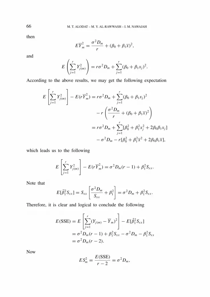
66 M. T. ALODAT – M. Y. AL-RAWWASH – I. M. NAWAJAH
then
EY2m = σ 2 Dm
r+ (β0 + β1x)2,
and
E
r∑j=1
Y 2j(m)
= rσ 2 Dm +r∑
j=1
(β0 + β1xj )2.
According to the above results, we may get the following expectation
E
r∑j=1
Y 2j(m)
− E(rY2m) = rσ 2 Dm +
r∑j=1
(β0 + β1xj )2
− r
(σ 2 Dm
r+ (β0 + β1x)2
)
= rσ 2 Dm +r∑
j=1
[β20 + β2
1 x2j + 2β0β1xj ]
− σ 2 Dm − r [β20 + β2
1 x2 + 2β0β1x],
which leads us to the following
E
r∑j=1
Y 2j(m)
− E(rY2m) = σ 2 Dm(r − 1) + β2
1 Sxx .
Note that
E[β21 Sxx ] = Sxx
[σ 2 Dm
Sxx+ β2
1
]= σ 2 Dm + β2
1 Sxx .
Therefore, it is clear and logical to conclude the following
E(SSE) = E
r∑j=1
(Yj(m) − Y m)2
− E[β21 Sxx ]
= σ 2 Dm(r − 1) + β21 Sxx − σ 2 Dm − β2
1 Sxx
= σ 2 Dm(r − 2).
Now
E S2m = E(SSE)
r − 2= σ 2 Dm,

Analysis of simple linear regression via median ranked set sampling 67
which allows us to conclude that
SSE
(r − 2)Dmis an unbiased estimator for σ 2.
On the other hand, it is easy to see that
SSE =r∑
j=1
(Yj(m) − Yj(m))2
= Syy − β21M Sxx ,
where Syy = ∑rj=1(Yj(m) −Y m)2 and SSR = β2
1M Sxx . Also, we may identify the
relation SST = SSR + SSE such that SSR = ∑rj=1(Yj(m) − Y m)2 is the sum of
squares due to the regression line and SST = Syy is the total sum of squares.Knowing that SSR = β2
1M Sxx allows us to take its expectation in thefollowing manner
E(SSR) = Sxx E(β21M) = β2
1 Sxx + σ 2 DM .
Also
E(Syy) = Er∑
j=1
Y 2j(m) − rY
2m
=r∑
j=1
EY 2j(m) − r EY
2m
=r∑
j=1
[Var(Yj(m)) + (EYj(m))2] − {r Var Y m + r(EY m)2}.
More simplification reveals the following
E(Syy) = rσ 2 Dm +r∑
j=1
(β0 + β1xj )2 − r
(σ 2 Dm
r+ (β0 + β1x)2
)
= rσ 2 Dm +r∑
j=1
(β20 + β0β1xj + β2
1 x2j ) − σ 2 Dm
− r(β20 + β0β1x + β2
1 x2).
This leads to concluding that
E(Syy) = (r − 1)σ 2 Dm + β21 Sxx .

68 M. T. ALODAT – M. Y. AL-RAWWASH – I. M. NAWAJAH
3. Extreme rank set sampling
Let x11, x12, . . . , x1r , x21, x22, . . . , x2r be different values of x which arespecified by the experimenter prior to the experiment. For each xi j i = 1, 2 andj = 1, 2, . . . , r assume that the experiment has been repeated an odd numberof times. Let Yj (1) and Yj(n), j = 1, 2, . . . , r be the measurements on theresponse variable obtained using the ERSS procedure. Then
Yj (1) = β0 + β1x1 j + εj (1)
andYj (n) = β0 + β1x2 j + εj (n),
where j = 1, 2, . . . , r and εj (1), εj (n) are the corresponding errors. We notethat the random errors ε1(1), ε2(1), . . . , εr(1) are iid with pdf
f1(ε) = n[1 − �
(ε
σ
)]n−1
φ
(ε
σ
)1
σ, for ε ∈ R,
and ε1(n), ε2(n), . . . , εr(n) are iid with pdf
f2(ε) = n[φ
(ε
σ
)]n−1
φ
(ε
σ
)1
σ, for ε ∈ R.
Since the normal density is symmetric, then εj (1) = −εj (n) and
E(εj (1)) = −E(εj (n)) = µσ, say,
where
µ = n∫ ∞
−∞w[1 − φ(w)]n−1φ(w)dw.
It is easy to see that
Var(εj (1)) = Var(εj (n))
= σ 2∫ ∞
−∞
ε2
σ 2n[�
(ε
σ
)]n−1
φ
(ε
σ
)1
σdε − µ2σ 2.
Using the transformation w = ε/σ we get
Var(εj (1) = σ 2∫ ∞
−∞nw2[�(w)]n−1φ(w)dw − µ2σ 2
= σ D∗m,

Analysis of simple linear regression via median ranked set sampling 69
where D∗m = ∫∞
−∞ nw2�n−1(w)φ(w)dw−µ2. It can be noted, using Theorem 1,that D∗
m ≤ 1. Let
Yj (i) = β0 + β1xi j + εj (i), i = 1, 2, j = 1, 2, . . . , r,
where Yj (i) denotes the j th observation in the i th group. The least squaresestimators of β0 and β1 can be obtained by minimizing the quantity h2(β0, β1) =∑
i=1,n
∑rj=1 ε2
j (i) as a function of β0 and β1. Since
h2(β0, β1) =r∑
j=1
(Yj (1) − β0 − β1x1 j )2 +
r∑j=1
(Yj (n) − β0 − β1x2 j )2,
then it easy to see that
β1E =
r∑j=1
(x1 j − x1)Yj (1) +r∑
j=1(x2 j − x2)Yj (n)
r∑j=1
(x1 j − x1)2 +r∑
j=1(x2 j − x2)2
,
and
β0E = Y − β1E X ,
where
x1 = 1
r
r∑j=1
x1 j , x2 = 1
r
r∑j=1
x2 j and Y = 1
2r
r∑j=1
(Yj (1) + Yj (n)).
Theorem 4. The estimators β0E and β1E are unbiased estimators of β0 and β1,respectively, and
1. Var(β1E) = σ2 D∗m
Sxx1+Sxx2,
2. Var(β1E) ≤ Var(β1S),
where β1S is the SRS estimator of β0 based on a sample of size 2r , Sxx1 =∑rj=1(x1 j − x1)
2 and Sxx2 = ∑rj=1(x2 j − x2)
2.
Note that it is complicated to find Var(β0E) at this stage and we intend tolook for some solutions in future work.

70 M. T. ALODAT – M. Y. AL-RAWWASH – I. M. NAWAJAH
Proof. Taking the expectation of β1E gives
E(β1E) =
r∑j=1
(x1 j − x1)E(Yj (1)) +r∑
j=1(x2 j − x2)E(Yj (n))
r∑j=1
(x1 j − x1)2 +r∑
j=1(x2 j − x2)2
=
r∑j=1
(x1 j − x1)(β0 + β1x1 j + µ) +r∑
j=1(x2 j − x2)(β0 + β1x2 j − µ)
r∑j=1
(x1 j − x1)2 +r∑
j=1(x2 j − x2)2
= β1
r∑
j=1(x1 j − x1)
2 +r∑
j=1(x2 j − x2)
2
r∑j=1
(x1 j − x1)2 +r∑
k=1(x2 j − x2)2
= β1.
This implies that β1E is an unbiased estimator of β1. The variance of β1E isgiven by
Var(β1E) =
r∑j=1
(x1 j − x1)2 Var(εj (1)) +
r∑j=1
(x2 j − x2)2 Var(εj (2))[
r∑j=1
(x1 j − x1)2 +r∑
j=1(x2 j − x2)2
]2
= σ 2 D∗m
r∑j=1
(x1 j − x1)2 +r∑
j=1(x2 j − x2)2
Since D∗m ≤ 1, then
Var(β1E) ≤ σ 2
r∑j=1
(x1 j − x1)2 +r∑
j=1(x2 j − x2)2
.
4. Comparison Among SRS, MRSS and ERSS
Let βi S , i = 0, 1 denote the least squares estimator of βi based on a SRS.In this section, we compare the estimators βi S , βi M and βi E , i = 0 or 1 viatheir efficiencies.
Analysis of simple linear regression via median ranked set sampling 71
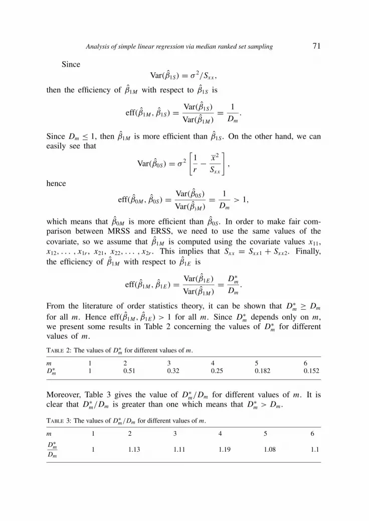
SinceVar(β1S) = σ 2/Sxx ,
then the efficiency of β1M with respect to β1S is
eff(β1M , β1S) = Var(β1S)
Var(β1M)= 1
Dm.
Since Dm ≤ 1, then β1M is more efficient than β1S . On the other hand, we caneasily see that
Var(β0S) = σ 2
[1
r− x2
Sxx
],
hence
eff(β0M , β0S) = Var(β0S)
Var(β)M)= 1
Dm> 1,
which means that β0M is more efficient than β0S . In order to make fair com-parison between MRSS and ERSS, we need to use the same values of thecovariate, so we assume that β1M is computed using the covariate values x11,x12, . . . , x1r , x21, x22, . . . , x2r . This implies that Sxx = Sxx1 + Sxx2. Finally,the efficiency of β1M with respect to β1E is
eff(β1M , β1E) = Var(β1E)
Var(β1M)= D∗
m
Dm.
From the literature of order statistics theory, it can be shown that D∗m ≥ Dm
for all m. Hence eff(β1M , β1E) > 1 for all m. Since D∗m depends only on m,
we present some results in Table 2 concerning the values of D∗m for different
values of m.
Table 2: The values of D∗m for different values of m.
m 1 2 3 4 5 6D∗
m 1 0.51 0.32 0.25 0.182 0.152
Moreover, Table 3 gives the value of D∗m/Dm for different values of m. It is
clear that D∗m/Dm is greater than one which means that D∗
m > Dm .
Table 3: The values of D∗m/Dm for different values of m.
m 1 2 3 4 5 6
D∗m
Dm1 1.13 1.11 1.19 1.08 1.1

72 M. T. ALODAT – M. Y. AL-RAWWASH – I. M. NAWAJAH
This is an indication that β1M is more efficient than β1E . As a conclusion, wesay that the MRSS estimators of β0 and β1 are more efficient and better thanERSS estimators.
5. Application
The MRSS technique is illustrated here in the shape of a real examplestudied by Platt, et al. (1988). The data set comprises 399 conifer (pinuspalustris) trees sorted according to two principal variables: X , the diameter incentimeters at breast height and Y , the entire height in feet. To compare theestimators obtained via MRSS to those obtained via SRS setup, we consider asimple random sample of size n = 29 and a MRSS of size n = 29. However,for MRSS we take m = 3 and take the median of the three observationscorresponding to its value Y and finally we obtain the MRSS based on Yvalues which eventually leads to MRSS X -values. Preliminary analysis showsthat the data could be fitted by a simple linear regression model. Applyingthe theory developed in this paper to this real data, we obtain β0M = 12.54and β1M = 0.38 with standard errors of 0.67 and 0.02, respectively. Using thesample random sampling scheme, the data produced the estimates β0S = 10.36and β1S = 0.43 with standard errors of 1.26 and 0.05, respectively. Accordinglyand based on the above analysis, we may conclude that the MRSS is moreefficient than the SRS for the simple linear regression analysis.
6. Discussion and Conclusion
In this paper, we introduced a new method to estimate the parameters ofthe simple linear regression model. We show that the new method producesestimators that are more efficient than those obtained via both SRS and ERSS.The distribution of the random errors in this article is assumed to be symmetric.Despite the fact that we directed our work to the case of normal distribution,yet we may consider other examples of symmetric distributions where we applyour findings. The list of such kind of distributions includes many options butwe limit our investigation to the logistic, student t and laplace distributions.The variance of the errors in this article is σ 2 Dm which differs according tothe distributional assumption. In order to show that the parameters estimatesusing MRSS are more efficient than those obtained under the SRS setup, weneed to check for the value of Dm for the previously mentioned distributionswhich are illustrated in Table 4. Arnold, et al. (1992) reported part of theresults related to the logistic distribution. The results indicate that Dm < 1for all m > 2 which agrees with the literature of ranked set sampling thatrecommends 3 ≤ m ≤ 7.

Analysis of simple linear regression via median ranked set sampling 73
Table 4: The values of Dm for different values of m.
m Laplace(0,1) Student t (5) Logistic(0,1)
2 0.6389 0.5830 1.28993 0.3512 0.3502 0.78994 0.3256 0.2498 0.56765 0.1751 0.1941 0.44266 0.1383 0.1587 0.36267 0.1138 0.1341 0.3071
Finally, this method may be easily extended to multiple regression setup, es-pecially the polynomial regression model proposed by Chen and Wang (2004).
Acknowledgments
The authors would like to thank the editor and the referees for the valuable comments that helpedus to bring this work in a good shape.
REFERENCES
Alodat, M. T. and Al-Sagheer, O. A. (2007) Estimation the location and scale parameters usingranked set sampling, J. Appl. Statis. Sci, 15, 245-252.
Arnold, B. C., Balakrishnan, N. and Nagaraja, H. N. (1992) A first Course in Order Statistic.,John Wiley and Sons, Inc, New York.
Chen, Z. and Wang, Y. (2004) Efficient regression analysis with ranked-set sampling, Biometrics,60, 997-1004.
Halls, L. S. and Dell, T. R. (1966) Trial of ranked set sampling for forage yields, Forest Science,12 (1), 22-226.
Kaur, A., Patil, G. P., Sinha, A. K. and Taillie, C. (1995) Ranked set sampling: an annotatedbibliography, Environ. and Ecol. Stat, 2, 25-54.
Martin, W. L., Shank, T., Oderwald, G. and Smith, D. W. (1980) Evaluation of ranked setsampling for estimating shrub phytomass in Application Oak forest, School of Forestry andWildlife Recourses VPI and SU Blackburg, VA.
McIntyre, G. A. (1952) A method of unbiased selective sampling, using ranked sets, Australian J.Agricultural Research, 3, 385-390.
Muttlak, H. (1995) Parameters estimation in a simple linear regression using rank set sampling,Biometrical J., 37 , 799-810.
Muttlak, H. (1997) Median ranked set sampling, J. Appl. Statist. Sci., 6, 245-255.
Patil, G. P., Sinha, A. K. and Taillie, C. (1993) Relative precision of ranked set sampling:comparison with regression estimator, Environmetrics., 4, 399-412.
Patts, J. M. and Elith, J. (2006) Comparing Species abundance model, Ecological Modelling,199, 153-163.
Platt, W. J., Evans, G. W. and Rathbun, S. L. (1988) The population dynamics of a long-livedconifer (Pinus palustris), Am. Nat., 131 (4), 491-525.

74 M. T. ALODAT – M. Y. AL-RAWWASH – I. M. NAWAJAH
Samawi, H. M., Ahmed, M. S. and Abu-Dayyeh, W. (1996). Estimating the population meanusing extreme ranked set sampling, Biometrical J., 38, 5, 577-586.
Takahasi, K. and Wakimoto, K. (1968) On unbiased estimates of the population mean based onthe sample stratified by means of ordering, Annals of Institute of Statistical Mathematics, 20,1-31.
Yu, P. L. and Lam, K. (1997) Regression estimator in ranked set sampling, Biometrics, 53, 1070-1080.
M. T. ALODATDepartment of StatisticsYarmouk University, [email protected]
M. Y. AL-RAWWASHDepartment of StatisticsYarmouk University, [email protected]
I. M. NAWAJAHDepartment of StatisticsYarmouk University, [email protected]


