Elsevier Editorial System(tm) for Chemical Engineering Science Manuscript Draft Manuscript Number: CES-D-14-01366R1 Title: Analysis of the Velocity and Displacement of a Condensing Bubble in a Liquid Solution Article Type: Regular Article Keywords: Bubble; Absorption; Lithium Bromide; Displacement; Mass Transfer; Absorber Corresponding Author: Mr. Philip Donnellan, B.E. Corresponding Author's Institution: University College Cork First Author: Philip Donnellan, B.E. Order of Authors: Philip Donnellan, B.E.; Edmond Byrne, PhD; Kevin Cronin, PhD Abstract: The absorption of steam bubbles in a hot aqueous solution of Lithium Bromide is a key process that occurs in the absorber vessel of a heat transformer system. During the condensation process, their size and shape changes dynamically with time as they rise up through the column of liquid. An understanding of the factors that control the vertical upwards motion of the bubbles is necessary to enable proper design of such units. However the exact vertical displacement of a bubble moving through a liquid is difficult to predict and becomes much more complex if the bubble is simultaneously collapsing. In this paper, the displacement of steam bubbles collapsing in a concentrated aqueous lithium bromide solution (LiBr-H2O) has been quantified experimentally. A simple kinetic model predicting the vertical displacement as a function of time was then developed from elementary force-balance considerations. A key feature of the system is the large variability in the motion of the bubbles arising from extreme fluctuations in their size and shape. Bubble dynamic morphology was modelled with stochastic techniques and the output from this was used in the kinetic model to predict dispersion in bubble displacement with time. While the uncertainty predicted by the stochastic model is shown to be less than that observed experimentally, it nonetheless highlights the importance of this random behaviour during the design of such an absorption column.

Department of Process and Chemical Engineering,

University College Cork,

Ireland.

07/01/2015

Dear Sir/Madame,

I wish to re-submit this paper for your review and potential publication in your journal. All

observations and corrections outlined by the editor and reviewers have been addressed carefully by

the authors to the best of our ability.

I hope that you find this application to be worthy of a place in your journal.

Sincerely,

Philip Donnellan.

Cover Letter

In this document, the reviewer’s corrections have been copied and

pasted directly from the e-mail received by the authors and

addressed individually in turn.

Line numbers may refer to the original manuscript, the revised

manuscript showing the changes made or the revised manuscript

which doesn’t show the changes which have been made. It shall be

made clear in each case which is meant by the use of

abbreviations.

Original manuscript – OM

Revised manuscript clean version – RMCV

Revised manuscript showing changes – RMSC

The line numbers refer the line numbers on the far left hand side of

the page.

The comments are addressed in the following order:

1. Reviewer #1’s comments

2. Reviewer #2’s comments

Within each of these sections, the individual points are numbered

according to the order in which they appear.

*Response to ReviewsClick here to download Response to Reviews: Response to reviewers comments.pdf

Reviewer #1’s comments:

1. Figs. 2 and 3 should be discarded because these figures are same

your previous paper (reference 4, CES).

Response:

Figure 3 has been removed.

Figure 2 has been retained, as the authors believe that it is of

pivotal importance that the reader is able to visualise the

experimental set up and procedure. It is now called Figure 3 in the

revised manuscripts.

2. Please explain the history force in Fig. 8.

Response:

The explanation of the history force in section 2.2 has been

extended (RMCV page 9, line 201-210 and page 9, line 201-210).

The Basset history force is a force which accounts for the vorticity

diffusion in the surrounding liquid and disturbances caused by

acceleration or deceleration of the particle [18]. It is sometimes called

the “Basset History Integral” and is a term which quantifies the effect of

previous bubble acceleration upon its current motion. This force is

defined for spherical particles at finite Reynolds numbers by equations 12

and 13, where R is the radius of the particle [19].

t

L

LHLH d

u

t

RCRF

2

6 (12)

3

2

12

32.048.0

dtduR

u

CH

(13)

3. In Fig. 5, please discuss the reason of fluctuation of bubble aspect

ratio with time.

Response:

The paragraph in section 4.1 which addresses the reason for bubble

shape fluctuations/variations has been extended (RMCV page 16,

line 393-411 and page 16, line 394-412).

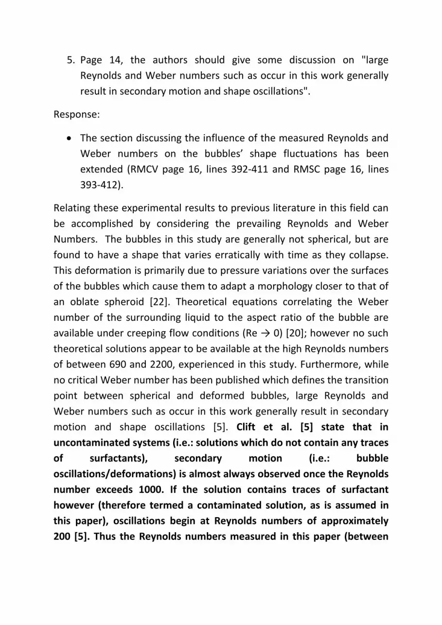
The bubbles in this study are generally not spherical, but are found to

have a shape that varies erratically with time as they collapse. This

deformation is primarily due to pressure variations over the surfaces of

the bubbles which cause them to adapt a morphology closer to that of an

oblate spheroid [22]. Theoretical equations correlating the Weber

number of the surrounding liquid to the aspect ratio of the bubble are

available under creeping flow conditions (Re → 0) [20]; however no such

theoretical solutions appear to be available at the high Reynolds numbers

of between 690 and 2200, experienced in this study. Furthermore, while

no critical Weber number has been published which defines the transition

point between spherical and deformed bubbles, large Reynolds and

Weber numbers such as occur in this work generally result in secondary

motion and shape oscillations [5]. Clift et al. [5] state that in

uncontaminated systems (i.e.: solutions which do not contain any traces

of surfactants), secondary motion (i.e.: bubble

oscillations/deformations) is almost always observed once the Reynolds

number exceeds 1000. If the solution contains traces of surfactant

however (therefore termed a contaminated solution, as is assumed in

this paper), oscillations begin at Reynolds numbers of approximately

200 [5]. Thus the Reynolds numbers measured in this paper (between

690 and 2200) justify the treatment of these bubbles as behaving in an

oscillatory (or random) manner.

4. Please show the real bubble images in the text.

Response:

A figure has been included showing the images of an experimental

bubble at different time-steps as rendered by the ProAnalyst

software from the high speed camera data (Figure 4).

Figure 4 - Images rendered by the ProAnalyst software (using

experimental high speed camera data) of a single experimental bubble at

different time steps as it travels vertically upwards.

Reviewer #2’s comments:

1. Page 6, line 103, how to make sure the experimental data used

were only up the point at which this air fraction becomes dominant.

Response:

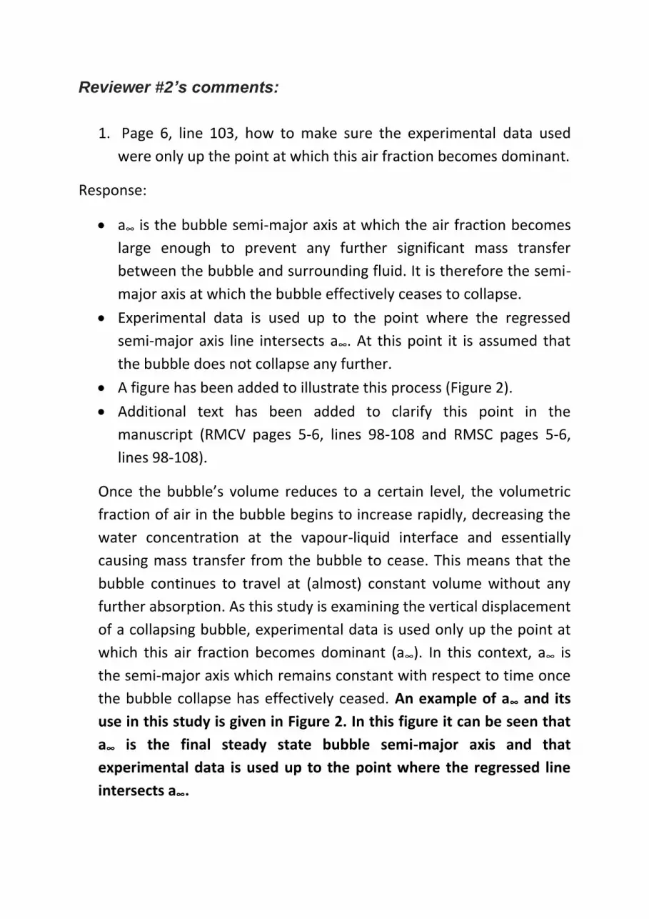
a∞ is the bubble semi-major axis at which the air fraction becomes

large enough to prevent any further significant mass transfer

between the bubble and surrounding fluid. It is therefore the semi-

major axis at which the bubble effectively ceases to collapse.

Experimental data is used up to the point where the regressed

semi-major axis line intersects a∞. At this point it is assumed that

the bubble does not collapse any further.

A figure has been added to illustrate this process (Figure 2).

Additional text has been added to clarify this point in the

manuscript (RMCV pages 5-6, lines 98-108 and RMSC pages 5-6,

lines 98-108).

Once the bubble’s volume reduces to a certain level, the volumetric

fraction of air in the bubble begins to increase rapidly, decreasing the

water concentration at the vapour-liquid interface and essentially

causing mass transfer from the bubble to cease. This means that the

bubble continues to travel at (almost) constant volume without any

further absorption. As this study is examining the vertical displacement

of a collapsing bubble, experimental data is used only up the point at

which this air fraction becomes dominant (a∞). In this context, a∞ is

the semi-major axis which remains constant with respect to time once

the bubble collapse has effectively ceased. An example of a∞ and its

use in this study is given in Figure 2. In this figure it can be seen that

a∞ is the final steady state bubble semi-major axis and that

experimental data is used up to the point where the regressed line

intersects a∞.

Figure 2 - Experimental bubble semi-major axis versus time for a bubble,

highlighting the transition point at which the volumetric fraction of air in

the bubble effectively causes mass transfer from the bubble to cease.

2. Page 6, line 116, besides the experimental observation, the authors

should also discuss the theoretical basis of the assumption that the

average rate of bubble collapse with time is linear.

Response:

The rate of bubble collapse is dependent upon many different

factors such as the liquid concentration and temperature, the

bubble volume, temperature and air fraction etc. Conducting mass

and energy balanced across the bubble is very tedious as the

equations are non-linear and highly coupled. This analysis has been

conducted previously by the authors (reference number 4, P.

Donnellan, et al., "Absorption of steam bubbles in Lithium Bromide

solution," Chemical Engineering Science, vol. 119, pp. 10-21, 2014.).

Therefore in order to avoid repetition, the theoretical analysis is not

repeated in this paper.

A sentence has been added to the text referencing the theoretical

analysis carried out in the authors’ previous paper (RMCV page 6,

lines 117-121 and RMSC page 6, lines 117-121).

For the purpose of this analysis (and as indicated by measured

experimental data), it is assumed that the average rate of bubble collapse

with time is approximately linear and therefore, a regression line can be

drawn through the experimental data with slope, βa. This linear rate of

bubble collapse has previously been demonstrated using a

comprehensive theoretical approach by Donnellan et al. [4].

3. Page 10, the drag coefficient correlation for solid non-spherical

particles presented by Hölzer and Sommerfeld should be proven to

be suitable for the solution in this paper since different kind of

contamination has different effects on the drag force.

Response:

According to Clift et al. [5], bubbles moving through solutions which

may be said to be contaminated with some levels of surfactants

experience a drag coefficient similar to that of an equivalent solid

undergoing the same translation. Even very small levels of

contamination can increase the drag coefficient to levels

experienced by solids. In this study, no emphasis has been placed

upon ensuring that the solution does not contain surfactants, and

thus it is inevitable that it should be considered “contaminated”.

Clift et al. [5] state that in this case, the drag coefficient of an

equivalent solid should be used for the bubble. Thus this is the

approach which has been taken in this study. The drag coefficient

which has been used is the drag coefficient which would be

experienced by a solid of equivalent shape and size, moving at the

same relative velocity.

The drag coefficient referenced from Hölzer and Sommerfeld has

been correlated based upon experimental data for many different

arbitrary solid shapes and sizes, and is primarily based upon the

sphericity of the object. Thus the authors believe it to be suitable

for use in this study, as it enables the drag coefficient to vary with

fluctuations in the bubble semi-major axis and aspect ratio.

The authors did not have the required equipment to be able to

experimentally separate and validate the correlation developed by

Hölzer and Sommerfeld in this situation (due to the large amount of

other degrees of freedom present). However it is believed that its

use is justified based upon the theory presented by Clift et al [5].

4. Page 12, photos taken by high speed camera should be given and

the data analysis process is also necessary for better understanding

the data collection and processing and to show the reliability of

data.

Response:

A figure has been included showing the images of an experimental

bubble at different time-steps as rendered by the ProAnalyst

software from the high speed camera data (Figure 4).

Figure 4 - Images rendered by the ProAnalyst software (using

experimental high speed camera data) of a single experimental bubble

at different time steps as it travels vertically upwards.

The text outlining the process of analysing the data has also been

adjusted in order to clarify the procedure (RMCV pages 12-13, lines

293-303 and RMSC pages 12-13, lines 294-304).

The bubble is produced by the gas sparger, and thus these are (at least

initially) located in the same plane relative to the camera. Therefore the

width of the sparger is measured using a micrometer and compared to its

width in pixels as recorded by the high speed camera. This allows for a

conversion between pixels and length to be established which takes into

consideration all refractive obstacles encountered by the light. This

conversion ratio is measured for every single experimental recording, as

small movements of the camera or its refocusing may otherwise cause

discrepancies. Thus the ProAnalyst software records both the bubble

perimeter and area (in pixels) at every time-step, which are then

converted into units of length and area respectively using the

conversion factor (between pixel width and meter) obtained from the

measured sparger width.

5. Page 14, the authors should give some discussion on "large

Reynolds and Weber numbers such as occur in this work generally

result in secondary motion and shape oscillations".

Response:

The section discussing the influence of the measured Reynolds and

Weber numbers on the bubbles’ shape fluctuations has been

extended (RMCV page 16, lines 392-411 and RMSC page 16, lines

393-412).

Relating these experimental results to previous literature in this field can

be accomplished by considering the prevailing Reynolds and Weber

Numbers. The bubbles in this study are generally not spherical, but are

found to have a shape that varies erratically with time as they collapse.

This deformation is primarily due to pressure variations over the surfaces

of the bubbles which cause them to adapt a morphology closer to that of

an oblate spheroid [22]. Theoretical equations correlating the Weber

number of the surrounding liquid to the aspect ratio of the bubble are

available under creeping flow conditions (Re → 0) [20]; however no such

theoretical solutions appear to be available at the high Reynolds numbers

of between 690 and 2200, experienced in this study. Furthermore, while

no critical Weber number has been published which defines the transition

point between spherical and deformed bubbles, large Reynolds and

Weber numbers such as occur in this work generally result in secondary

motion and shape oscillations [5]. Clift et al. [5] state that in

uncontaminated systems (i.e.: solutions which do not contain any traces

of surfactants), secondary motion (i.e.: bubble

oscillations/deformations) is almost always observed once the Reynolds

number exceeds 1000. If the solution contains traces of surfactant

however (therefore termed a contaminated solution, as is assumed in

this paper), oscillations begin at Reynolds numbers of approximately

200 [5]. Thus the Reynolds numbers measured in this paper (between

690 and 2200) justify the treatment of these bubbles as behaving in an

oscillatory (or random) manner.

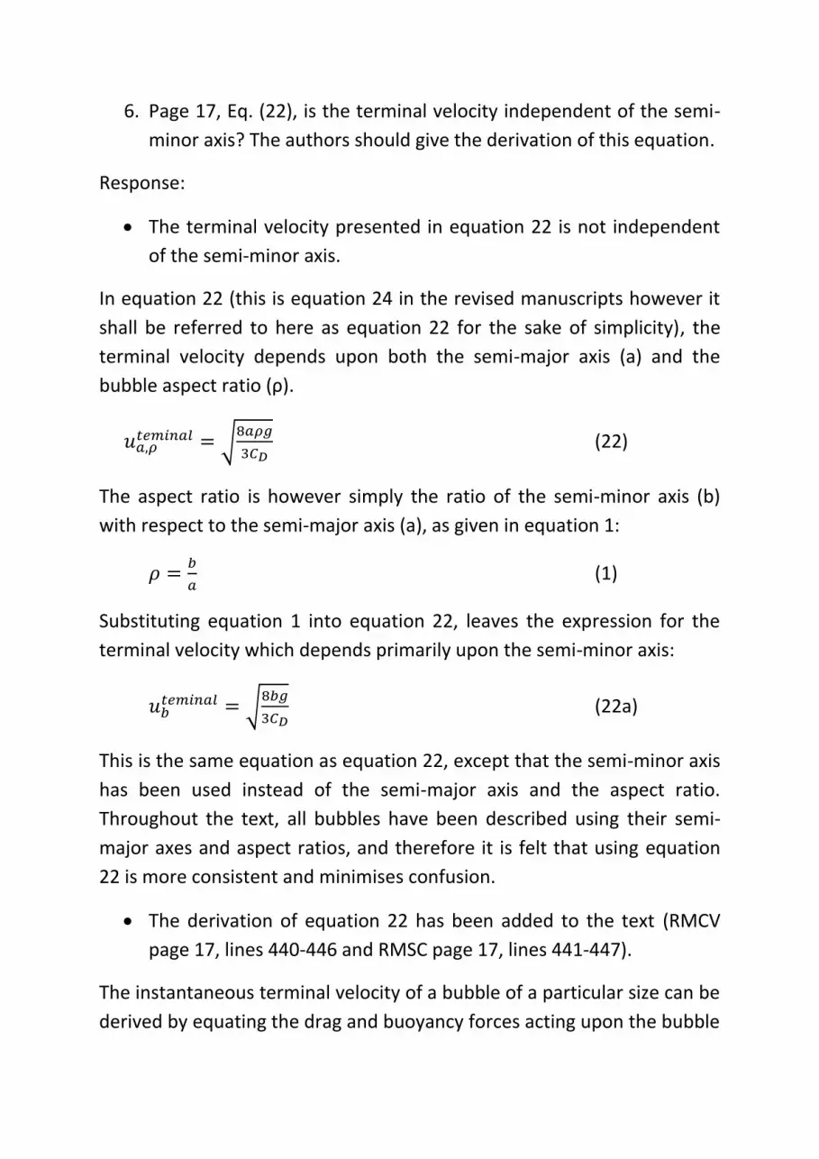
6. Page 17, Eq. (22), is the terminal velocity independent of the semi-

minor axis? The authors should give the derivation of this equation.

Response:

The terminal velocity presented in equation 22 is not independent

of the semi-minor axis.

In equation 22 (this is equation 24 in the revised manuscripts however it

shall be referred to here as equation 22 for the sake of simplicity), the

terminal velocity depends upon both the semi-major axis (a) and the

bubble aspect ratio (ρ).

𝑢𝑎,𝜌𝑡𝑒𝑚𝑖𝑛𝑎𝑙 = √

8𝑎𝜌𝑔

3𝐶𝐷 (22)

The aspect ratio is however simply the ratio of the semi-minor axis (b)

with respect to the semi-major axis (a), as given in equation 1:

𝜌 =𝑏

𝑎 (1)

Substituting equation 1 into equation 22, leaves the expression for the

terminal velocity which depends primarily upon the semi-minor axis:

𝑢𝑏𝑡𝑒𝑚𝑖𝑛𝑎𝑙 = √

8𝑏𝑔

3𝐶𝐷 (22a)

This is the same equation as equation 22, except that the semi-minor axis

has been used instead of the semi-major axis and the aspect ratio.

Throughout the text, all bubbles have been described using their semi-

major axes and aspect ratios, and therefore it is felt that using equation

22 is more consistent and minimises confusion.

The derivation of equation 22 has been added to the text (RMCV

page 17, lines 440-446 and RMSC page 17, lines 441-447).

The instantaneous terminal velocity of a bubble of a particular size can be

derived by equating the drag and buoyancy forces acting upon the bubble

(there is no acceleration once terminal velocity is reached, and thus the

added mass and history forces may be ignored).

VgACu LpDL 2

2

1 (22)

ga

aCu LDL3

4

2

1 322

(23)

D

alter

aC

gau

3

8min

,

(24)

7. The predicted confidence interval in 3~4 s is very big.

Experimentally it is noted that there is a large degree of variability

in the motion of the bubbles as they move up the column.

However, the agreement between the experimental data and

predictions are very close. How these sets of experimental data

were chosen?

Response:

No special data selection procedures were used.

The data sets presented for each experimental settings are

averages of all the bubbles tracked at the respective setting as

outlined in section 3.2:

Averaged profiles are generated for each experimental setting by

combining the data from that setting’s 18 individual bubbles at each time

step. All of the experimental data presented in this paper refers to these

setting-averaged results.

The significant variability which exists (i.e.: large confidence

intervals), is due to this combining of a large number of individual

bubbles at each setting (with each bubble having its own random

oscillatory motion as outlined in the paper).

The good agreement which is observed in Figures 12, 13 and 14

stems from the fact in these figures represent average values.

Simulated displacements in these figures are the combination of

2000 simulated random bubbles (section 3.4), while experimental

trends represent average experimental displacements at each

setting (once more with each individual bubble having its own

random component).

While each bubble contains a random component which will

contribute to the large confidence interval of the model, the

bubbles fundamentally behave according to the classic Newtonian

displacement equations derived in section 2.2. Thus by taking the

average of a large number of random bubbles, one would expect to

achieve results very consistent with these deterministic equations.

Highlights

The absorption of steam bubbles in a hotter lithium bromide solution is tracked

A model is developed to describe the vertical translation of the collapsing bubbles

The developed model incorporates both deterministic and random bubble behaviour

The added mass force is the dominant force causing upward vertical motion

The model adequately describes the observed displacement randomness

*Highlights

1

1 Analysis of the Velocity and Displacement of a Condensing Bubble in a 2

Liquid Solution 3

4

Philip Donnellan∗, Edmond Byrne, Kevin Cronin 5

Department of Process and Chemical Engineering, University College Cork, Ireland 6

7

ABSTRACT 8

The absorption of steam bubbles in a hot aqueous solution of Lithium Bromide is a key 9

process that occurs in the absorber vessel of a heat transformer system. During the 10

condensation process, their size and shape changes dynamically with time as they rise up 11

through the column of liquid. An understanding of the factors that control the vertical 12

upwards motion of the bubbles is necessary to enable proper design of such units. 13

However the exact vertical displacement of a bubble moving through a liquid is difficult 14

to predict and becomes much more complex if the bubble is simultaneously collapsing. 15

In this paper, the displacement of steam bubbles collapsing in a concentrated aqueous 16

lithium bromide solution (LiBr-H2O) has been quantified experimentally. A simple 17

kinetic model predicting the vertical displacement as a function of time was then 18

developed from elementary force-balance considerations. A key feature of the system is 19

the large variability in the motion of the bubbles arising from extreme fluctuations in 20

their size and shape. Bubble dynamic morphology was modelled with stochastic 21

techniques and the output from this was used in the kinetic model to predict dispersion in 22

bubble displacement with time. While the uncertainty predicted by the stochastic model 23

is shown to be less than that observed experimentally, it nonetheless highlights the 24

importance of this random behaviour during the design of such an absorption column. 25

26

*Corresponding author Tel: 00353 214903096 27 Email address: p.donnellan@umail.ucc.ie (Philip Donnellan ) 28

*Marked RevisionClick here to download Marked Revision: ReviewedManuscript_Marked.docx Click here to view linked References

2

Nomenclature a Bubble semi-major axis (m)

ao Initial bubble semi-major axis (m)

a∞ Semi major axis at which the experiment is considered to be finished for any bubble (m)

b Bubble semi-minor axis (m)

Ap Vertically projected bubble surface Area (m2)

CD Drag force coefficient

CH History force coefficient

Cam Added mass force coefficient F Force (N)

g Acceleration due to gravity (m/s2) m Mass (kg) N Number of probability distribution samples in a random realisation p Probability density function R Radius (m)

Rζ Bubble aspect ratio random component correlation function

Rη Bubble semi-major axis random component correlation function S Random component spectral density t Time (s) u Bubble vertical velocity (m/s)

uL Liquid velocity (m/s)

uterminala,p Terminal velocity of a bubble at constant semi-major axis and aspect ratio (m/s)

V Bubble Volume (m3)

29

1. INTRODUCTION 30

Absorption heat transformers and absorption chillers are devices primarily based upon 31

the interaction between saturated water vapour (the dispersed phase) and a concentrated 32

liquid salt solution such as aqueous lithium bromide (LiBr-H2O) [1-3]. This interaction is 33

can potentially be achieved using bubble columns. In a previous study conducted by 34

Donnellan et al [4], the heat and mass transfer rates of such steam bubbles being absorbed 35

in a LiBr-H2O solution were examined experimentally. The paper developed a model 36

describing the heat and mass transfer process, and demonstrated that these bubbles are 37

3

Nomenclature Continued Dimensionless Numbers

Re Reynold Number = ρLvbD / μL

We Weber Number = ρLvb2D / σL

Greek Symbols

βa Semi-major axis linear collapse rate (m/s)

βρ Aspect ratio linear collapse rate (1/s)

μ Viscosity (Ns/m2) ζ Bubble aspect ratio zero-mean component η Bubble semi-major axis zero-mean component (m) ρ Bubble aspect ratio

ρo Initial bubble Aspect Ratio

ρL Solution density (kg/m3)

ρv Bubble density (kg/m3) σ Standard Deviation

σL Solution surface tension (N/m)

τc Random component characteristic time (s) φ Bubble sphericity

φ Bubble lengthwise sphericity

φ Bubble crosswise sphericity

ωU Auto-correlation parameter Subscripts am Added Mass B Buoyancy D Drag H History L Bulk Liquid LiBr Lithium Bromide term Terminal v vapour w weight ζ Bubble aspect ratio zero-mean component η Bubble semi-major axis zero-mean component

38

4

prone to shape oscillations and deformations, leading to significant amounts of random 39

behaviour. This unpredictability implies that significant variability exists within the 40

system. In a design scenario, it is very important to be able to quantify this 41

unpredictability, especially that associated with the vertical displacement of the bubbles 42

as it impacts directly upon the required height of the bubble column. 43

44

The two phase flow of vapour bubbles moving through a liquid is a complex 45

phenomenon that is encountered in many different areas of chemical engineering such as 46

in biological reactors or in absorption columns. Often other phenomena may be 47

connected to the bubble rise, such as a simultaneous chemical reaction or heat and mass 48

transfer. Two conventional approaches to examine bubble motion are either theoretical 49

analysis or numerical CFD techniques. Developing analytical solutions of such flow 50

scenarios is extremely difficult however and generally relies upon assumptions such as 51

negligible liquid viscosity or creeping flow conditions (Re→0) [5]. While detailed 52

analytical formulae developed under such assumptions are extremely useful from the 53

perspective of gaining a better understanding of underlying principles, they do not 54

generally apply to real world situations in which liquid viscosities or Reynolds numbers 55

may be significant. More recently much work has been conducted examining such 56

situations using detailed CFD simulation techniques [6-8]. CFD enables parameters such 57

as the mass transfer rate, bubble size, velocity fields and gas hold-up to be investigated in 58

addition to pure flow phenomena [9-11]. CFD also has the advantage of permitting 59

detailed analysis of the influence of turbulence on bubble motion [12, 13]. Such detailed 60

CFD approaches are extremely beneficial as they allow an insight into the complex 61

processes which are taking place at the vapour-liquid interface and in the bubble wake. 62

63

The objective of this paper is to develop a model of the motion (velocity and 64

displacement) of condensing steam bubbles in an aqueous LiBr solution. A large focus is 65

on the randomness associated with this motion so that the mean and variance in 66

displacement versus time can be predicted. As the system is very complex, a standard 67

deterministic model of bubble motion is selected by making simplifying assumptions 68

which allow basic but adequate descriptions of the process. Correct identification and 69

5

quantification of the forces acting on a bubble is a prerequisite. Drag [14] and lift [15] 70

force equations have been examined using DNS (Direct Numerical Simulation) 71

techniques, while the importance of including the added mass, wake and history forces 72

was demonstrated by Zhang and Fan [16]. To the authors’ best knowledge no previous 73

studies exist which examine the random behaviour of collapsing bubbles and therefore 74

this paper investigates the unpredictability associated with the vertical displacement of 75

steam bubbles being absorbed into a concentrated LiBr-H2O solution. The model 76

developed in this paper utilises probabilistic methods to predict the vertical displacement 77

of the bubble as it collapses under the action of heat and mass transfer. 78

79

80

2. THEORY 81

2.1 Bubble Shape Model 82

Solution of the differential equation of motion for bubbles requires prior knowledge of 83

their size and shape (as both these parameters affect bubble inertia and bubble interaction 84

with the continuous phase) and their dynamic evolution with time. The real bubbles of 85

this study have a very complex morphology that does not conform to any standard 86

geometry and moreover changes very significantly with time. They emanate from a 87

sparger pipe, at the base of the column of liquid, with an approximately spherical shape, 88

then, they become pronouncedly non-spherical before returning to an approximately 89

spherical shape just before extinction. One approach to model the dynamic change in size 90

and shape is to treat the bubble as being an oblate spheroid [5] which is an ellipsoid 91

where two of the axes are the same length with semi-major axis, a, while the third is 92

shorter than the other two with semi-minor axis length, b (Figure 1). For a bubble, the 93

shortened axis is parallel to the motion direction. This approach permits shape variation 94

to be explored without an excessive number of unknown degrees of freedom. A small 95

residual amount of air is contained in these bubbles however which causes the collapse 96

rate to decrease towards the end of the bubble’s lifetime as discussed by Donnellan et al. 97

[4]. Once the bubble’s volume reduces to a certain level, the volumetric fraction of air in 98

the bubble begins to increase rapidly, decreasing the water concentration at the vapour-99

liquid interface and essentially causing mass transfer from the bubble to cease. This 100

6

means that the bubble continues to travel at (almost) constant volume without any further 101

absorption. As this study is examining the vertical displacement of a collapsing bubble, 102

experimental data is used only up the point at which this air fraction becomes dominant 103

(a∞). In this context, a∞ is the semi-major axis which remains constant with respect to 104

time once the bubble collapse has effectively ceased. An example of a∞ and its use in this 105

study is given in Figure 2. In this figure it can be seen that a∞ is the final steady state 106

bubble semi-major axis and that experimental data is used up to the point where the 107

regressed line intersects a∞. 108

109

The aspect ratio, ρ, volume and vertically projected cross sectional area of the ellipsoid 110

are 111

Ap = πa2 (1) 112

The steam bubbles are being absorbed into the lithium bromide solution as they flow 113

vertically upwards, and therefore the magnitude of the bubble’s semi-major axis is 114

dependent upon the rate of heat and mass transfer from the bubble. Initially the bubbles 115

have a characteristic dimension of between 4 and 5 mm and this falls down to 1 mm 116

within ~0.1 s. For the purpose of this analysis (and as indicated by measured 117

experimental data), it is assumed that the average rate of bubble collapse with time is 118

approximately linear and therefore, a regression line can be drawn through the 119

experimental data with slope, βa. This linear rate of bubble collapse has previously been 120

demonstrated using a comprehensive theoretical approach by Donnellan et al. [4]. The 121

residual can be treated as a zero-mean random signal versus time, η(t), and is discussed in 122

the next section. Regarding aspect ratio, initially the bubbles tend to have a high aspect 123

ratio close to 1 reflecting their approximate sphericity, but on average this aspect ratio 124

decreases with time. Once more the actual experimental profile is decomposed into a 125

deterministic linear component quantified by a linear regression line with a slope βρ and a 126

zero-mean random residual component, ζ(t). 127

128

a

b=ρ3

4 2 baV

π=

7

Bubble size (represented by the semi-major axis) and bubble shape (represented by aspect 129

ratio) have both deterministic and random components. The deterministic component 130

reflects the fact that bubble volume reduces consistently with time due to absorption. The 131

random component exists as this size reduction may be erratic and also due to 132

unpredictability in how the shape changes with time. Hence semi-major axis and aspect 133

ratio are described by 134

135

( ) ( ) 00 aaaforttata a <<++= ∞ηβ (2) 136

137

( ) ( )ttt ζβρρ ρ ++= 0 (3) 138

139

where η (t) and ζ (t) are zero-mean random processes. Examination of the experimental 140

data gave no indication of any cross correlation between the random processes and they 141

are assumed to be independent. 142

143

Any random process is defined by its auto-correlation function and probability density 144

function. Regarding the former, for η(t) and ζ (t), the key task is to identify the nature of 145

the correlation function for each and to obtain the magnitudes of the parameters that will 146

define them. Correlation function identification must primarily come from analysis of the 147

temporal structure of the measured data and also is informed by physical reasoning. The 148

measured correlation coefficient falls monotonically from unity and crosses the lag time 149

axis to give negative values at long lag times. The fact that no periodicity is present in the 150

data and that statistically significant negative values are found for both signals indicate 151

that the correlation function corresponding to band-limited white noise may be 152

appropriate for both η(t) and ζ (t) [17]. 153

154

( )τ

τωωσ

τ ηηη

U

U

Rsin2

=

( )τ

τωωσ

τ ζζζ

U

U

Rsin2

=

(4) 155

156

8

where τ is the lag time and ωUη and ωUζ are the auto-correlation parameters for each 157

signal. To provide an indicative measure of de-correlation, a de-correlation time scale, 158

can be defined as the time of the first crossing of the lag time axis by the auto-correlation 159

function, τC. Also at this point, where the correlation coefficient equals zero, the function 160

given by equation 4 must be satisfied, and hence the magnitudes of the parameters ωU for 161

each random signal can be found using equation 5. 162

CU τ

πω = (5) 163

164

The statistical structure of the random component of the semi-major axis and aspect ratio 165

can also be quantified in the frequency domain using the relationship that mean square 166

spectral density of η(t) and ζ (t) will be given by the Fourier transform of the associated 167

auto-correlation function. As Eq. 4 is an even real function, the normalised (continuous) 168

spectral density is given by equation 6. 169

170

( ) ( )U

U

U

dSω

σττω

ττω

ωσ

πω ηη

η 2cos

sin12

0

2

== ∫∞

( )ζ

ζζ ω

σω

U

S2

2

= (6) 171

172

Equation 6 can be interpreted as giving the contribution to the total variance in the 173

random component of each signal attributable at each frequency level. Given Sη(ω) is 174

constant at a value up to ωU and then is zero at frequencies beyond that, it implies that 175

only frequencies below ωU contribute to the variance in the signal. 176

177

In addition to a description of the correlation structure of the random processes in time, 178

information is also needed on the amplitudes of both signals. Analyses of the distribution 179

in the magnitudes of both signals indicated that they follow the Gaussian probability 180

density function, and are defined by equation 7. 181

182

( )

−

=2

2

2

22

1 ηση

ησπη ep ( )

−

=2

2

2

22

1 ζσζ

ζσπζ ep (7) 183

9

184

2.2 Bubble Kinematic Model 185

In order to predict its displacement, the forces acting on the bubble must be quantified. 186

The bubble is being treated as a single bubble in an infinite body of quiescent liquid and 187

thus the lift force is excluded. The active forces include weight, buoyancy, drag, added 188

mass and Basset history forces. Weight, buoyancy and drag are defined in equations 8 to 189

10. 190

VgF vw ρ−= (8) 191

VgF LB ρ= (9) 192

pDLD ACuF 2

2

1 ρ−= (10) 193

194

As the surrounding fluid is assumed to be in a steady, isotropic state, the standard term 195

D(uL)/Dt = 0, and thus the added mass force expression used in this model may be 196

simplified to equation 11. 197

198

( )

∂∂+

∂∂−=−=

t

Vu

t

uVCuVC

dt

dF amLLamam ρρ (11) 199

200

The Basset history force is a force which accounts for the vorticity diffusion in the 201

surrounding liquid and disturbances caused by acceleration or deceleration of the particle 202

[18]. It is sometimes called the “Basset History Integral” and is a term which quantifies 203

the effect of previous bubble acceleration upon its current motion. This force is defined 204

for spherical particles at finite Reynolds numbers by equations 12 and 13, where R is the 205

radius of the particle [19]. 206

207

[ ]∫∞−

∂∂

−−=

t

L

LHLH d

u

t

RCRF τ

ττπµρπµ

2

6 (12) 208

3

2

12

32.048.0

+

−=

dtduR

u

CH

(13) 209

210

10

The overall hydrodynamic model is found by applying Newton’s Law of motion to the 211

bubble and treating the bubble as a particle subject to rectilinear motion along a line. 212

213

HvmBwDv FFFFFdt

dum ++++= (14) 214

215

This formulation assumes the liquid is stationary and portions of it are gradually 216

accelerated (decelerated) with the bubble. It ignores the small steady flow that exists in 217

the experimental LiBr-H2O solution. It also ignores the slight disturbances which may be 218

present in the liquid due to the motion of previous bubbles. Inserting equations 8 to 13 219

into equation 14 and noting that the mass of the bubble is given by mv = ρvV and that 220

vapour density is negligible compared to liquid density gives the equation of motion 221

(equation 15). 222

∫∞− −

−−

−=

t

L

Lham

pDvm d

d

du

t

R

V

RCu

dt

dV

VCu

V

ACg

dt

duC τ

ττρπµ 2

2 121222 (15) 223

224

The equation of motion can be seen to be a non-linear, first-order integro-differential 225

equation with non-constant coefficients. These coefficients primarily depend on 226

geometrical information of the bubble, principally its volume and its area cross sectional 227

to the flow direction and how these parameters change dynamically with time. The 228

situation is made more complex because as the bubble moves upwards through the 229

solution, its volume and cross sectional area vary in both an erratic and systematic 230

fashion with time. Treating the bubble as an oblate spheroid, the differential equation 231

becomes: 232

233

( ) ( ) ( ) ( ) ( ) ( ) ( )( )

( )( )

∫∞− −

−

+−

−=

t

L

LhamDam d

d

du

t

a

tta

tCu

dt

d

tdt

da

tatCu

ttatCg

dt

dutC τ

τττ

πρρµρ

ρρ

2

22

)(

9132

75.022234

(16) 235

236

11

Due to the changing bubble size and velocity, the drag, added mass and history force 237

coefficients will also vary with respect to time. The drag force acting upon a bubble is 238

highly dependent upon the choice of drag coefficient (CD). Vapour bubbles in a pure 239

liquid which does not contain any trace of surfactants experience a drag force which is 240

much less than that acting upon an equivalent liquid drop or solid particle [5]. However 241

in the presence of contamination, surfactants accumulate at the vapour-liquid interface 242

reducing internal circulation within the bubble and causing it to experience a drag force 243

similar to that of a solid particle [20]. As no special emphasis has been placed upon 244

ensuring that there are no surfactants present, the drag coefficient correlation for solid 245

non-spherical particles presented by Hölzer and Sommerfeld [21] is utilised in this study 246

(equation 14), which is primarily a function of the bubble’s sphericity (ϕ). 247

248

( )( )

⊥

−×+++=φφφφ

φ 11042.0

1

Re

31

Re

161

Re

8 2..0log4.0

43

||

DC (17) 249

250

The added mass coefficient (Cam) is a function of the aspect ratio of the bubble. For an 251

oblate spheroid in unbounded fluid, this coefficient is given by equation 18 [5]. 252

253

( )( )ρρρρ

ρρρ122

21

cos1

1cos−

−

−−

−−=amC (18) 254

255

where ρ is the aspect ratio of the bubble. As no expression for the history force of an 256

oblate spheroid at finite Reynolds numbers could be obtained by the authors, the 257

expression for a spherical particle shall be used using the bubble semi-major axis in place 258

of the radius. While this is a slight oversimplification of this force, it has previously been 259

demonstrated that it only has a very small effect upon a particle translating through a 260

quiescent liquid at high Reynolds numbers [18]. 261

262

263

264

265

12

3. MATERIALS & METHODS 266

3.1 Experimental Equipment 267

The experimental bubble column consists of a 1m high, 10cm wide glass cylinder, bolted 268

on to a stainless steel base plate (Figure 23). The cylinder is filled with approximately 269

32cm of aqueous lithium bromide, and the solution is maintained at a constant 270

temperature by circulating it through a temperature controlled oil bath at a flowrate of 271

29mL/s. The oil bath is operated in on-off mode, controlled by a Honeywell UDC 3000 272

PID controller, and the solution is pumped from the oil bath back into the cylinder by 273

means of a Watson Marlow 505S peristaltic pump. Saturated steam for the experiment 274

was produced in a 53x25cm stainless steel cylindrical steam generator. The steam enters 275

the bubble column at the base through a sparger. Condensed steam is prevented from 276

entering the bubble column by passing all steam through a steam trap, and the flowrate of 277

steam entering the cylinder is controlled by means of a needle valve following this steam 278

trap. Upon start-up, a certain mass of air is contained within the steam generator. While 279

much effort was given to removing as much of this air as possible, a small fraction 280

remained entrained in the steam (~0.001 m3/m3). The temperature of the steam produced 281

is approximately 100˚C, and bubbles with nominal semi-major axes of between 4 and 282

5mm are produced. 283

284

Bubble motion was recorded using an AOS X-Motion high speed camera operating with 285

a shutter speed of 500 frames per second (Figure 3). In order to ensure high visibility of 286

the bubbles for the recordings, the bubble point of entry was illuminated using two 287

Dedolight 150W Tungsten Aspherics spotlights and a Luxform 500W Halogen spotlight. 288

The reflection of light off the bubble caused by these three spotlights ensures that there 289

was sufficient contrast between the bubble and its surrounding fluid. Each recording was 290

then analysed using the ProAnalyst Contour Tracking software package (Xcitex Inc.) 291

(Figure 4). This software was used to determine both the perimeter and projected area of 292

each analysed bubble (in pixels). All perimeter and projected area readings are recorded 293

in pixels. The bubble is produced by the gas sparger, and thus these are (at least initially) 294

located in the same plane relative to the camera. Therefore the width of the sparger is 295

measured using a micrometer and compared to its width in pixels as recorded by the high 296

13

speed camera. This allows for a conversion between pixels and length to be established 297

which takes into consideration all refractive obstacles encountered by the light. This 298

conversion ratio is measured for every single experimental recording, as small 299

movements of the camera or its refocusing may otherwise cause discrepancies. Thus the 300

ProAnalyst software records both the bubble perimeter and area (in pixels) at every time-301

step, which are then converted into units of length and area respectively using the 302

conversion factor (between pixel width and meter) obtained from the measured sparger 303

width. 304

3.2 Experimental Test Programme 305

The kinematic behaviour of the bubbles was investigated at three different temperatures 306

and concentrations of the liquid solution. Three mass fractions (of lithium bromide salt) 307

were selected. At each concentration, three different temperatures were then analysed. As 308

the pressure of the system is to remain atmospheric, the temperatures selected for each 309

concentration are limited by the saturation temperature of the solution. Thus for each 310

concentration, temperatures were selected so that one is about 3.5˚C, one is 10˚C, and one 311

is 15˚C below the saturation temperature for the solution. The resulting temperatures and 312

concentrations used in the experiment are outlined Table 1. Different settings in this table 313

shall be referred to throughout this paper using a subscript system where for example 314

C46T119 refers to the experimental setting operating with a 46% LiBr-H2O concentration 315

and a temperature of 119˚C. 316

317

Two experimental runs were conducted for each concentration and temperature setting at 318

different flowrates, with each experimental run lasting ten minutes. Three recordings 319

were taken during each experimental run at evenly spaced intervals. From each recording, 320

three bubbles were selected at random (one from the beginning, one from the middle and 321

one from the end of the recording) for analysis in order to ensure that representative 322

results were obtained. Thus 18 bubbles were analysed for each experimental setting given 323

in the table. Averaged profiles are generated for each experimental setting by combining 324

the data from that setting’s 18 individual bubbles at each time step. All of the 325

experimental data presented in this paper refers to these setting-averaged results. Table 2 326

14

summarises the physical properties of the solution at each setting and gives the average 327

Reynolds and Weber Numbers for the bubbles for each setting. 328

329 3.3 Numerical Simulation 330 For the deterministic model of motion, the governing differential equation for bubble 331

velocity was solved in MATLAB using a time step of 0.02ms (the experimental time step 332

is 2ms) and the Euler method. The trapezoidal rule numerical integration scheme was 333

used to obtain displacement. For the probabilistic approach, the following method is 334

employed to generate realisations of the random component of semi-major axis (an 335

identical scheme is used for aspect ratio). 336

337

( ) ( ) ( )tqtpN

t jj

N

jjj ωω

ση η sincos

1

+= ∑=

(19) 338

339

For each value of j, the magnitudes of the coefficients p and q are drawn from the unit 340

Normal distribution. 341

342

[ ]1,0Np ← [ ]1,0Nq ← (20) 343

344

Similarly for each value of j, the magnitudes of ω are drawn or randomly sampled from 345

the distribution whose probability density function is defined as the mean square spectral 346

density of η(t) (which is the continuous uniform distribution as given by Eq. 6). 347

348

[ ]UU ωω ,0← (21) 349

350

The Central Limit Theorem will ensure that the summation of Eq. 19 (for sufficiently 351

large values of N) will give a Gaussian distribution for η(t) with zero mean and unit 352

variance. Scaling the returned values by ση means the particular Gaussian distribution for 353

the magnitude of random deviation bubble semi-major axis is obtained. The sampling 354

routine employed for p and q ensures that the realisations of η(t) have the correct 355

distribution in magnitude while the routine used to sample ω, ensures η(t) realisations 356

15

have the correct frequency components. The Monte Carlo method was employed to 357

generate the random process. For equation 19, N was set at 50. 358

359

360

4. RESULTS 361

4.1 Evolution of Bubble Shape with Time 362

Figure 4 5 shows a representative experimental bubble semi-major axis versus time curve 363

that was found for the system (up to a∞) while figure 56 depicts aspect ratio versus time. 364

The parameters for the linear regression line for each parameter are presented in Table 3. 365

It is clear that, in accordance with the results previously presented by Donnellan et al. [4], 366

lower temperature levels lead to more rapid rates of collapse as shown by the values of βa 367

while the solution’s concentration does not appear to have as strong an impact. The 368

aspect ratio appears to consistently reduce with respect to time (i.e.: negative values for 369

βρ), however there does not appear to be a clear correlation between this rate of change 370

and the concentration and temperature settings. The highest rates of aspect ratio reduction 371

are recorded at temperature level one, indicating that an increased rate of collapse of the 372

bubbles leads to a greater level of shape deformation. 373

374

Table 4 summarises the output of the probabilistic analysis of bubble motion giving the 375

magnitudes of the standard deviation, the de-correlation time and the corresponding cut-376

off frequency level for the random components of semi-major axis and aspect ratio. From 377

the data presented in this table for both the bubble semi-major axis and its aspect ratio, it 378

may be seen that the standard deviation of both random signals seems quite insensitive to 379

the condition of the liquid solution. By contrast the characteristic time increases as both 380

solution temperature and concentration increase showing that as temperature and 381

concentration increase the frequency of fluctuations in the random components becomes 382

lower. 383

384

Figure 67 compares the experimentally measured correlogram to the theoretical auto-385

correlation function for a concentration of 56 % and temperature 136˚C, demonstrating 386

the appropriateness of the selected auto-correlation function. Figure 8 illustrates the 387

16

experimentally measured distribution in the random components of semi-major axis, η(t) 388

and aspect ratio, ζ(t) in frequency histogram form. The Normal distribution is 389

superimposed for each and while the experimental data has a slight positive skewness, it 390

can be seen that the fit is good. 391

392

Relating these experimental results to previous literature in this field can be accomplished 393

by considering the prevailing Reynolds and Weber Numbers. The bubbles in this study 394

are generally not spherical, but are found to have a shape that varies erratically with time 395

as they collapse. This deformation is primarily due to pressure variations over the 396

surfaces of the bubbles which cause them to adapt a morphology closer to that of an 397

oblate spheroid [22]. Theoretical equations correlating the Weber number of the 398

surrounding liquid to the aspect ratio of the bubble are available under creeping flow 399

conditions (Re → 0) [20]; however no such theoretical solutions appear to be available at 400

the high Reynolds numbers of between 690 and 2200, experienced in this study. 401

Furthermore, while no critical Weber number has been published which defines the 402

transition point between spherical and deformed bubbles, large Reynolds and Weber 403

numbers such as occur in this work generally result in secondary motion and shape 404

oscillations [5]. Clift et al. [5] state that in uncontaminated systems (i.e.: solutions which 405

do not contain any traces of surfactants), secondary motion (i.e.: bubble 406

oscillations/deformations) is almost always observed once the Reynolds number exceeds 407

1000. If the solution contains traces of surfactant however (therefore termed a 408

contaminated solution, as is assumed in this paper), oscillations begin at Reynolds 409

numbers of approximately 200 [5]. Thus the Reynolds numbers measured in this paper 410

(between 690 and 2200) justify the treatment of these bubbles as behaving in an 411

oscillatory (or random) manner. 412

413 414 4.2 Deterministic Analysis of Bubble Motion 415

The motion of the bubble can be understood in terms of its inertia and the forces acting 416

on it. The primary external forces acting upon the bubble are the drag, added mass, 417

history and buoyancy forces. Note as the mass of steam vapour in the bubble is 418

negligible, the effective mass of the bubble arises from one of the terms of the added 419

17

mass force i.e. the term ρLCvmV. The second term of the added mass force (i.e.: 420

ρLCvmudV/dt) is henceforth considered to constitute the added mass force for the 421

purposes of this analysis. Figure 8 9 shows a comparison between the magnitudes of the 422

different forces acting upon the bubble at the setting C56T126. It is evident that the added 423

mass force (as defined above) has a significant effect upon the motion of the bubble. This 424

force acts vertically upwards due to the shedding of entrained liquid from the bubble’s 425

surface as its size decreases. While the buoyancy force initiates the motion, this added 426

mass force rapidly exceeds it in magnitude and becomes the dominant force causing 427

vertical translation. In direct contrast, the history force is demonstrated to have negligible 428

effect upon the displacement of the bubble. As expected, the magnitudes of the buoyancy, 429

drag and added mass forces decay with time as bubble volume decreases. 430

431

432

Figure 9 10 displays the resulting deterministic velocity and displacement model 433

predictions at the concentration setting of 56%. Note for these plots, the random 434

fluctuation in bubble size and shape is neglected and only the deterministic component of 435

morphology change is included. Also note the bubbles have a non-zero initial velocity as 436

they exit the sparger pipe. In Figure 9 10 it may be observed that the bubbles’ velocity 437

initially increases under the action of the buoyancy and added mass forces in an attempt 438

to reach a terminal or steady-state velocity. Velocity then reaches a maximum value 439

before falling backreducing once more; hence the bubble experiences an acceleration 440

phase followed by a deceleration phase. The instantaneous terminal velocity of a bubble 441

of a particular size can be shown to be approximately given asderived by equating the 442

drag and buoyancy forces acting upon the bubble (there is no acceleration once terminal 443

velocity is reached, and thus the added mass and history forces may be ignored). 444

VgACu LpDL ρρ =2

2

1 (22) 445

ga

aCu LDL 3

4

2

1 322 ρπρπρ = (23) 446

D

altera C

gau

3

8min,

ρρ =

(224) 447

Field Code Changed

Field Code Changed

18

and is determined by the balance between buoyancy and drag. Because both the bubble’s 448

semi-major axis and its aspect ratio decrease with time, the bubble is constantly trying to 449

reach its terminal velocity, however this terminal velocity is itself decreasing with time. 450

This results in the steadily decreasing bubble velocities illustrated in Figure 910. In 451

general a maximum velocity of between 0.21 m/s and 0.24 m/s is achieved by the bubbles 452

prior to entering this deceleration phase. The nature of this constantly changing velocity 453

does not impact significantly upon the displacement pattern, which remains almost 454

perfectly linear. As expected, bubbles with slower collapse rates (i.e.: at higher 455

temperature levels) have longer residence times, and hence also significantly larger 456

vertical displacements. In Figure 9 10 it is evident that the difference between selecting a 457

temperature level of one (Figure 9a10a) and a temperature level of three (Figure 9c10c) 458

can result in a fourfold difference in vertical displacement and hence a fourfold 459

difference in the required absorber height. 460

461

Finally the behaviour of these steam bubbles shall be compared with the behaviour of 462

idealised, identical bubbles which retain both their initial aspect ratios and semi-major 463

axes throughout their life-span (i.e.: they do not collapse). In Figure 10 11 it may be seen 464

that the vertical velocity of the absorbing bubble is essentially the same as that of the 465

non-absorbing bubble up to this point of maxima. After this the velocity of the constant-466

volume bubble continues to increase asymptotically to its terminal velocity while the 467

velocity of the absorbing bubble decreases rapidly. 468

469

4.3 Probabilistic Analysis of Bubble Motion 470

The Monte Carlo model is used to generate random realizations of the evolution of 471

bubble shape and size with time and these are inputted to the deterministic model of 472

bubble motion. The model is firstly used to predict the mean displacement observed in 473

the experimental data for each concentration and temperature setting and then dispersion 474

in displacement is examined. The results of the probabilistic displacement model are 475

plotted in Figures 11 12 to 1314. These graphs figures have been generated by combining 476

the results of the 2000 random simulations described in section 3.4. It is evident that the 477

agreement between the modelled and experimental data is quite good. The mean 478

19

displacements predicted in Figures 1112, 12 13 and 13a 14a almost perfectly match the 479

averaged experimental data for those respective settings. The model slightly under-480

predicts the vertical displacement in Figures 13b 14b and 13c14c. 481

482

Experimentally it is noted that there is a large degree of variability in the motion of the 483

bubbles as they move up the column. Figure 14 15 demonstrates the use of the 484

probabilistic model to indicate potential dispersion in vertical displacement. This figure 485

shows the data from individually tracked bubbles at a concentration of 46% and 486

temperature of 119˚C, as well as the confidence interval predicted by the stochastic 487

model corresponding to three standard deviations. From these results it is clear that the 488

model does in general predict an appropriate degree of uncertainty. Dispersion in the final 489

experimental vertical displacement of up to 100% may be seen in Figure 14 15 (between 490

7mm and 14mm) highlighting the inherent uncertainty associated with this variable. 491

492

493 5. DISCUSSION & CONCLUSIONS 494

The results presented in this paper indicate the ability of a standard ordinary differential 495

equation model to predict the vertical displacement of a bubble which is collapsing under 496

the action of both heat and mass transfer. The phenomenon is complex due to the 497

extremely short time-scales involved and the erratic and unpredictable dynamic bubble 498

morphology. The problem was compounded by the limited information that was available 499

concerning the dynamic change in bubble shape and size due to the two dimensional 500

nature of the recorded data. Nonetheless agreement between theory and experiment was 501

satisfactory. The added mass force acting upon the bubble has been demonstrated to be of 502

pivotal importance in such a model, as it is the dominant force causing vertical 503

translation. Selecting the correct solution temperature level has been demonstrated to 504

have the potential to cause up to fourfold reductions in the final mean bubble vertical 505

displacement (and hence absorber height), hence reiterating the importance of this 506

variable as identified in the previously paper. The vertical displacement dispersion 507

observed in the experimental data, and predicted by the model, indicates that the accurate 508

prediction of bubble residence time is however extremely difficult however. Variability 509

20

of up to 100% has been highlighted at a particular experimental setting, which would 510

have a significant impact upon the design and operation of such a unit. It should also be 511

noted that this unpredictable behaviour has been demonstrated in this paper using single 512

steam bubbles collapsing in a concentrated LiBr-H20 solution. In reality however, this 513

collapse would generally occur in a fully functioning bubble column in which interactive 514

effects may begin to dominate, further amplifying this uncertainty. 515

516

Acknowledgements 517

Philip Donnellan would like to acknowledge the receipt of funding from the Embark 518

Initiative issued by the Irish Research Council. 519

520

REFERENCES 521

[1] P. Donnellan, et al., "Internal energy and exergy recovery in high temperature 522 application absorption heat transformers," Applied Thermal Engineering, vol. 56, 523 pp. 1-10, 2013. 524

[2] P. Donnellan, et al., "First and second law multidimensional analysis of a triple 525 absorption heat transformer (TAHT)," Applied Energy, vol. 113, pp. 141-151, 526 2014. 527

[3] P. Donnellan, et al., "Economic evaluation of an industrial high temperature lift 528 heat transformer," Energy, vol. 73, pp. 581-591, 2014. 529

[4] P. Donnellan, et al., "Absorption of steam bubbles in Lithium Bromide solution," 530 Chemical Engineering Science. 531

[5] R. Clift, et al., Bubbles, Drops, and Particles. New York: Academic Press Inc, 532 1978. 533

[6] R. Krishna and J. M. Van Baten, "Mass transfer in bubble columns," Catalysis 534 Today, vol. 79-80, pp. 67-75, 2003. 535

[7] F. B. Campos and P. L. C. Lage, "Simultaneous heat and mass transfer during the 536 ascension of superheated bubbles," International Journal of Heat and Mass 537 Transfer, vol. 43, pp. 179-189, 2000. 538

[8] F. B. Campos and P. L. C. Lage, "Heat and mass transfer modeling during the 539 formation and ascension of superheated bubbles," International Journal of Heat 540 and Mass Transfer, vol. 43, pp. 2883-2894, 2000. 541

[9] D. Darmana, et al., "Detailed modelling of hydrodynamics, mass transfer and 542 chemical reactions in a bubble column using a discrete bubble model: 543 Chemisorption of into NaOH solution, numerical and experimental study," 544 Chemical Engineering Science, vol. 62, pp. 2556-2575, 2007. 545

[10] T. Wang and J. Wang, "Numerical simulations of gas–liquid mass transfer in 546 bubble columns with a CFD–PBM coupled model," Chemical Engineering 547 Science, vol. 62, pp. 7107-7118, 2007. 548

21

[11] R. Lau, et al., "Mass transfer studies in shallow bubble column reactors," 549 Chemical Engineering and Processing: Process Intensification, vol. 62, pp. 18-550 25, 2012. 551

[12] K. Ekambara and M. T. Dhotre, "CFD simulation of bubble column," Nuclear 552 Engineering and Design, vol. 240, pp. 963-969, 2010. 553

[13] M. K. Silva, et al., "Study of the interfacial forces and turbulence models in a 554 bubble column," Computers & Chemical Engineering, vol. 44, pp. 34-44, 2012. 555

[14] I. Roghair, et al., "On the drag force of bubbles in bubble swarms at intermediate 556 and high Reynolds numbers," Chemical Engineering Science, vol. 66, pp. 3204-557 3211, 2011. 558

[15] W. Dijkhuizen, et al., "Numerical and experimental investigation of the lift force 559 on single bubbles," Chemical Engineering Science, vol. 65, pp. 1274-1287, 2010. 560

[16] J. Zhang and L.-S. Fan, "On the rise velocity of an interactive bubble in liquids," 561 Chemical Engineering Journal, vol. 92, pp. 169-176, 2003. 562

[17] D. E. Newland, An Introduction to Random Vibrations, Spectral & Wavelet 563 Analysis: Third Edition: Dover Publications, 2012. 564

[18] A. A. Mohammad Rostami, Goodarz Ahmadi, Peter Joerg Thomas, "Can the 565 history force be neglected for the motion of particles at high subcritical Reynolds 566 Number range?," International Journal of Engineering, vol. 19, pp. 23-34, 2006. 567

[19] F. Odar and W. S. Hamilton, "Forces on a sphere accelerating in a viscous fluid," 568 Journal of Fluid Mechanics, vol. 18, pp. 302-314, 1964. 569

[20] D. W. Moore, "The velocity of rise of distorted gas bubbles in a liquid of small 570 viscosity," Journal of Fluid Mechanics, vol. 23, pp. 749-766, 1965. 571

[21] A. Hölzer and M. Sommerfeld, "New simple correlation formula for the drag 572 coefficient of non-spherical particles," Powder Technology, vol. 184, pp. 361-365, 573 2008. 574

[22] J. Magnaudet and I. Eames, "The Motion of High-Reynolds-Number Bubbles in 575 Inhomogeneous Flows," Annual Review of Fluid Mechanics, vol. 32, pp. 659-708, 576 2000. 577

578 579

1

1 Analysis of the Velocity and Displacement of a Condensing Bubble in a 2

Liquid Solution 3

4

Philip Donnellan∗, Edmond Byrne, Kevin Cronin 5

Department of Process and Chemical Engineering, University College Cork, Ireland 6

7

ABSTRACT 8

The absorption of steam bubbles in a hot aqueous solution of Lithium Bromide is a key 9

process that occurs in the absorber vessel of a heat transformer system. During the 10

condensation process, their size and shape changes dynamically with time as they rise up 11

through the column of liquid. An understanding of the factors that control the vertical 12

upwards motion of the bubbles is necessary to enable proper design of such units. 13

However the exact vertical displacement of a bubble moving through a liquid is difficult 14

to predict and becomes much more complex if the bubble is simultaneously collapsing. 15

In this paper, the displacement of steam bubbles collapsing in a concentrated aqueous 16

lithium bromide solution (LiBr-H2O) has been quantified experimentally. A simple 17

kinetic model predicting the vertical displacement as a function of time was then 18

developed from elementary force-balance considerations. A key feature of the system is 19

the large variability in the motion of the bubbles arising from extreme fluctuations in 20

their size and shape. Bubble dynamic morphology was modelled with stochastic 21

techniques and the output from this was used in the kinetic model to predict dispersion in 22

bubble displacement with time. While the uncertainty predicted by the stochastic model 23

is shown to be less than that observed experimentally, it nonetheless highlights the 24

importance of this random behaviour during the design of such an absorption column. 25

26

*Corresponding author Tel: 00353 214903096 27 Email address: p.donnellan@umail.ucc.ie (Philip Donnellan ) 28

*Revised ManuscriptClick here to download Revised Manuscript: ReviewedManuscript.docx Click here to view linked References

2

Nomenclature a Bubble semi-major axis (m)

ao Initial bubble semi-major axis (m)

a∞ Semi major axis at which the experiment is considered to be finished for any bubble (m)

b Bubble semi-minor axis (m)

Ap Vertically projected bubble surface Area (m2)

CD Drag force coefficient

CH History force coefficient

Cam Added mass force coefficient F Force (N)

g Acceleration due to gravity (m/s2) m Mass (kg) N Number of probability distribution samples in a random realisation p Probability density function R Radius (m)

Rζ Bubble aspect ratio random component correlation function

Rη Bubble semi-major axis random component correlation function S Random component spectral density t Time (s) u Bubble vertical velocity (m/s)

uL Liquid velocity (m/s)

uterminala,p Terminal velocity of a bubble at constant semi-major axis and aspect ratio (m/s)

V Bubble Volume (m3)

29

1. INTRODUCTION 30

Absorption heat transformers and absorption chillers are devices primarily based upon 31

the interaction between saturated water vapour (the dispersed phase) and a concentrated 32

liquid salt solution such as aqueous lithium bromide (LiBr-H2O) [1-3]. This interaction is 33

can potentially be achieved using bubble columns. In a previous study conducted by 34

Donnellan et al [4], the heat and mass transfer rates of such steam bubbles being absorbed 35

in a LiBr-H2O solution were examined experimentally. The paper developed a model 36

describing the heat and mass transfer process, and demonstrated that these bubbles are 37

3

Nomenclature Continued Dimensionless Numbers

Re Reynold Number = ρLvbD / μL

We Weber Number = ρLvb2D / σL

Greek Symbols

βa Semi-major axis linear collapse rate (m/s)

βρ Aspect ratio linear collapse rate (1/s)

μ Viscosity (Ns/m2) ζ Bubble aspect ratio zero-mean component η Bubble semi-major axis zero-mean component (m) ρ Bubble aspect ratio

ρo Initial bubble Aspect Ratio

ρL Solution density (kg/m3)

ρv Bubble density (kg/m3) σ Standard Deviation

σL Solution surface tension (N/m)

τc Random component characteristic time (s) φ Bubble sphericity

φ Bubble lengthwise sphericity

φ Bubble crosswise sphericity

ωU Auto-correlation parameter Subscripts am Added Mass B Buoyancy D Drag H History L Bulk Liquid LiBr Lithium Bromide term Terminal v vapour w weight ζ Bubble aspect ratio zero-mean component η Bubble semi-major axis zero-mean component

38

4

prone to shape oscillations and deformations, leading to significant amounts of random 39

behaviour. This unpredictability implies that significant variability exists within the 40

system. In a design scenario, it is very important to be able to quantify this 41

unpredictability, especially that associated with the vertical displacement of the bubbles 42

as it impacts directly upon the required height of the bubble column. 43

44

The two phase flow of vapour bubbles moving through a liquid is a complex 45

phenomenon that is encountered in many different areas of chemical engineering such as 46

in biological reactors or in absorption columns. Often other phenomena may be 47

connected to the bubble rise, such as a simultaneous chemical reaction or heat and mass 48

transfer. Two conventional approaches to examine bubble motion are either theoretical 49

analysis or numerical CFD techniques. Developing analytical solutions of such flow 50

scenarios is extremely difficult however and generally relies upon assumptions such as 51

negligible liquid viscosity or creeping flow conditions (Re→0) [5]. While detailed 52

analytical formulae developed under such assumptions are extremely useful from the 53

perspective of gaining a better understanding of underlying principles, they do not 54

generally apply to real world situations in which liquid viscosities or Reynolds numbers 55

may be significant. More recently much work has been conducted examining such 56

situations using detailed CFD simulation techniques [6-8]. CFD enables parameters such 57

as the mass transfer rate, bubble size, velocity fields and gas hold-up to be investigated in 58

addition to pure flow phenomena [9-11]. CFD also has the advantage of permitting 59

detailed analysis of the influence of turbulence on bubble motion [12, 13]. Such detailed 60

CFD approaches are extremely beneficial as they allow an insight into the complex 61

processes which are taking place at the vapour-liquid interface and in the bubble wake. 62

63

The objective of this paper is to develop a model of the motion (velocity and 64

displacement) of condensing steam bubbles in an aqueous LiBr solution. A large focus is 65

on the randomness associated with this motion so that the mean and variance in 66

displacement versus time can be predicted. As the system is very complex, a standard 67

deterministic model of bubble motion is selected by making simplifying assumptions 68

which allow basic but adequate descriptions of the process. Correct identification and 69

5

quantification of the forces acting on a bubble is a prerequisite. Drag [14] and lift [15] 70

force equations have been examined using DNS (Direct Numerical Simulation) 71

techniques, while the importance of including the added mass, wake and history forces 72

was demonstrated by Zhang and Fan [16]. To the authors’ best knowledge no previous 73

studies exist which examine the random behaviour of collapsing bubbles and therefore 74

this paper investigates the unpredictability associated with the vertical displacement of 75

steam bubbles being absorbed into a concentrated LiBr-H2O solution. The model 76

developed in this paper utilises probabilistic methods to predict the vertical displacement 77

of the bubble as it collapses under the action of heat and mass transfer. 78

79

80

2. THEORY 81

2.1 Bubble Shape Model 82

Solution of the differential equation of motion for bubbles requires prior knowledge of 83

their size and shape (as both these parameters affect bubble inertia and bubble interaction 84

with the continuous phase) and their dynamic evolution with time. The real bubbles of 85

this study have a very complex morphology that does not conform to any standard 86

geometry and moreover changes very significantly with time. They emanate from a 87

sparger pipe, at the base of the column of liquid, with an approximately spherical shape, 88

then, they become pronouncedly non-spherical before returning to an approximately 89

spherical shape just before extinction. One approach to model the dynamic change in size 90

and shape is to treat the bubble as being an oblate spheroid [5] which is an ellipsoid 91

where two of the axes are the same length with semi-major axis, a, while the third is 92

shorter than the other two with semi-minor axis length, b (Figure 1). For a bubble, the 93

shortened axis is parallel to the motion direction. This approach permits shape variation 94

to be explored without an excessive number of unknown degrees of freedom. A small 95

residual amount of air is contained in these bubbles however which causes the collapse 96

rate to decrease towards the end of the bubble’s lifetime as discussed by Donnellan et al. 97

[4]. Once the bubble’s volume reduces to a certain level, the volumetric fraction of air in 98

the bubble begins to increase rapidly, decreasing the water concentration at the vapour-99

liquid interface and essentially causing mass transfer from the bubble to cease. This 100

6

means that the bubble continues to travel at (almost) constant volume without any further 101

absorption. As this study is examining the vertical displacement of a collapsing bubble, 102

experimental data is used only up the point at which this air fraction becomes dominant 103

(a∞). In this context, a∞ is the semi-major axis which remains constant with respect to 104

time once the bubble collapse has effectively ceased. An example of a∞ and its use in this 105

study is given in Figure 2. In this figure it can be seen that a∞ is the final steady state 106

bubble semi-major axis and that experimental data is used up to the point where the 107

regressed line intersects a∞. 108

109

The aspect ratio, ρ, volume and vertically projected cross sectional area of the ellipsoid 110

are 111

Ap = πa2 (1) 112

The steam bubbles are being absorbed into the lithium bromide solution as they flow 113

vertically upwards, and therefore the magnitude of the bubble’s semi-major axis is 114

dependent upon the rate of heat and mass transfer from the bubble. Initially the bubbles 115

have a characteristic dimension of between 4 and 5 mm and this falls down to 1 mm 116

within ~0.1 s. For the purpose of this analysis (and as indicated by measured 117

experimental data), it is assumed that the average rate of bubble collapse with time is 118

approximately linear and therefore, a regression line can be drawn through the 119

experimental data with slope, βa. This linear rate of bubble collapse has previously been 120

demonstrated using a comprehensive theoretical approach by Donnellan et al. [4]. The 121

residual can be treated as a zero-mean random signal versus time, η(t), and is discussed in 122

the next section. Regarding aspect ratio, initially the bubbles tend to have a high aspect 123

ratio close to 1 reflecting their approximate sphericity, but on average this aspect ratio 124

decreases with time. Once more the actual experimental profile is decomposed into a 125

deterministic linear component quantified by a linear regression line with a slope βρ and a 126

zero-mean random residual component, ζ(t). 127

128

a

b=ρ3

4 2 baV

π=

7

Bubble size (represented by the semi-major axis) and bubble shape (represented by aspect 129

ratio) have both deterministic and random components. The deterministic component 130

reflects the fact that bubble volume reduces consistently with time due to absorption. The 131

random component exists as this size reduction may be erratic and also due to 132

unpredictability in how the shape changes with time. Hence semi-major axis and aspect 133

ratio are described by 134

135

( ) ( ) 00 aaaforttata a <<++= ∞ηβ (2) 136

137

( ) ( )ttt ζβρρ ρ ++= 0 (3) 138

139

where η (t) and ζ (t) are zero-mean random processes. Examination of the experimental 140

data gave no indication of any cross correlation between the random processes and they 141

are assumed to be independent. 142

143

Any random process is defined by its auto-correlation function and probability density 144

function. Regarding the former, for η(t) and ζ (t), the key task is to identify the nature of 145

the correlation function for each and to obtain the magnitudes of the parameters that will 146

define them. Correlation function identification must primarily come from analysis of the 147

temporal structure of the measured data and also is informed by physical reasoning. The 148

measured correlation coefficient falls monotonically from unity and crosses the lag time 149

axis to give negative values at long lag times. The fact that no periodicity is present in the 150

data and that statistically significant negative values are found for both signals indicate 151

that the correlation function corresponding to band-limited white noise may be 152

appropriate for both η(t) and ζ (t) [17]. 153

154

( )τ

τωωσ

τ ηηη

U

U

Rsin2

=

( )τ

τωωσ

τ ζζζ

U

U

Rsin2

=

(4) 155

156

8

where τ is the lag time and ωUη and ωUζ are the auto-correlation parameters for each 157

signal. To provide an indicative measure of de-correlation, a de-correlation time scale, 158

can be defined as the time of the first crossing of the lag time axis by the auto-correlation 159

function, τC. Also at this point, where the correlation coefficient equals zero, the function 160

given by equation 4 must be satisfied, and hence the magnitudes of the parameters ωU for 161

each random signal can be found using equation 5. 162

CU τ

πω = (5) 163

164

The statistical structure of the random component of the semi-major axis and aspect ratio 165

can also be quantified in the frequency domain using the relationship that mean square 166

spectral density of η(t) and ζ (t) will be given by the Fourier transform of the associated 167

auto-correlation function. As Eq. 4 is an even real function, the normalised (continuous) 168

spectral density is given by equation 6. 169

170

( ) ( )U

U

U

dSω

σττω

ττω

ωσ

πω ηη

η 2cos

sin12

0

2

== ∫∞

( )ζ

ζζ ω

σω

U

S2

2

= (6) 171

172

Equation 6 can be interpreted as giving the contribution to the total variance in the 173

random component of each signal attributable at each frequency level. Given Sη(ω) is 174

constant at a value up to ωU and then is zero at frequencies beyond that, it implies that 175

only frequencies below ωU contribute to the variance in the signal. 176

177

In addition to a description of the correlation structure of the random processes in time, 178

information is also needed on the amplitudes of both signals. Analyses of the distribution 179

in the magnitudes of both signals indicated that they follow the Gaussian probability 180

density function, and are defined by equation 7. 181

182

( )

−

=2

2

2

22

1 ηση

ησπη ep ( )

−

=2

2

2

22

1 ζσζ

ζσπζ ep (7) 183

9

184

2.2 Bubble Kinematic Model 185

In order to predict its displacement, the forces acting on the bubble must be quantified. 186

The bubble is being treated as a single bubble in an infinite body of quiescent liquid and 187

thus the lift force is excluded. The active forces include weight, buoyancy, drag, added 188

mass and Basset history forces. Weight, buoyancy and drag are defined in equations 8 to 189

10. 190

VgF vw ρ−= (8) 191

VgF LB ρ= (9) 192

pDLD ACuF 2

2

1 ρ−= (10) 193

194

As the surrounding fluid is assumed to be in a steady, isotropic state, the standard term 195

D(uL)/Dt = 0, and thus the added mass force expression used in this model may be 196

simplified to equation 11. 197

198

( )

∂∂+

∂∂−=−=

t

Vu

t

uVCuVC

dt

dF amLLamam ρρ (11) 199

200

The Basset history force is a force which accounts for the vorticity diffusion in the 201

surrounding liquid and disturbances caused by acceleration or deceleration of the particle 202

[18]. It is sometimes called the “Basset History Integral” and is a term which quantifies 203

the effect of previous bubble acceleration upon its current motion. This force is defined 204

for spherical particles at finite Reynolds numbers by equations 12 and 13, where R is the 205

radius of the particle [19]. 206

207

[ ]∫∞−

∂∂

−−=

t

L

LHLH d

u

t

RCRF τ

ττπµρπµ

2

6 (12) 208

3

2

12

32.048.0

+

−=

dtduR

u

CH

(13) 209

210

10

The overall hydrodynamic model is found by applying Newton’s Law of motion to the 211

bubble and treating the bubble as a particle subject to rectilinear motion along a line. 212

213

HvmBwDv FFFFFdt

dum ++++= (14) 214

215

This formulation assumes the liquid is stationary and portions of it are gradually 216

accelerated (decelerated) with the bubble. It ignores the small steady flow that exists in 217

the experimental LiBr-H2O solution. It also ignores the slight disturbances which may be 218

present in the liquid due to the motion of previous bubbles. Inserting equations 8 to 13 219

into equation 14 and noting that the mass of the bubble is given by mv = ρvV and that 220

vapour density is negligible compared to liquid density gives the equation of motion 221

(equation 15). 222

∫∞− −

−−

−=

t

L

Lham

pDvm d

d

du

t

R

V

RCu

dt

dV

VCu

V

ACg

dt

duC τ

ττρπµ 2

2 121222 (15) 223

224

The equation of motion can be seen to be a non-linear, first-order integro-differential 225

equation with non-constant coefficients. These coefficients primarily depend on 226

geometrical information of the bubble, principally its volume and its area cross sectional 227

to the flow direction and how these parameters change dynamically with time. The 228

situation is made more complex because as the bubble moves upwards through the 229

solution, its volume and cross sectional area vary in both an erratic and systematic 230

fashion with time. Treating the bubble as an oblate spheroid, the differential equation 231

becomes: 232

233

( ) ( ) ( ) ( ) ( ) ( ) ( )( )

( )( )

∫∞− −

−

+−

−=

t

L

LhamDam d

d

du

t

a

tta

tCu

dt

d

tdt

da

tatCu

ttatCg

dt

dutC τ

τττ

πρρµρ

ρρ

2

22

)(

9132

75.022234

(16) 235

236

11

Due to the changing bubble size and velocity, the drag, added mass and history force 237

coefficients will also vary with respect to time. The drag force acting upon a bubble is 238

highly dependent upon the choice of drag coefficient (CD). Vapour bubbles in a pure 239

liquid which does not contain any trace of surfactants experience a drag force which is 240

much less than that acting upon an equivalent liquid drop or solid particle [5]. However 241

in the presence of contamination, surfactants accumulate at the vapour-liquid interface 242

reducing internal circulation within the bubble and causing it to experience a drag force 243

similar to that of a solid particle [20]. As no special emphasis has been placed upon 244

ensuring that there are no surfactants present, the drag coefficient correlation for solid 245

non-spherical particles presented by Hölzer and Sommerfeld [21] is utilised in this study 246

(equation 14), which is primarily a function of the bubble’s sphericity (ϕ). 247

248

( )( )

⊥

−×+++=φφφφ

φ 11042.0

1

Re

31

Re

161

Re

8 2..0log4.0

43

||

DC (17) 249

250

The added mass coefficient (Cam) is a function of the aspect ratio of the bubble. For an 251

oblate spheroid in unbounded fluid, this coefficient is given by equation 18 [5]. 252

253

( )( )ρρρρ

ρρρ122

21

cos1

1cos−

−

−−

−−=amC (18) 254

255

where ρ is the aspect ratio of the bubble. As no expression for the history force of an 256

oblate spheroid at finite Reynolds numbers could be obtained by the authors, the 257

expression for a spherical particle shall be used using the bubble semi-major axis in place 258

of the radius. While this is a slight oversimplification of this force, it has previously been 259

demonstrated that it only has a very small effect upon a particle translating through a 260

quiescent liquid at high Reynolds numbers [18]. 261

262

263

264

265

12

3. MATERIALS & METHODS 266

3.1 Experimental Equipment 267

The experimental bubble column consists of a 1m high, 10cm wide glass cylinder, bolted 268

on to a stainless steel base plate (Figure 3). The cylinder is filled with approximately 269

32cm of aqueous lithium bromide, and the solution is maintained at a constant 270

temperature by circulating it through a temperature controlled oil bath at a flowrate of 271

29mL/s. The oil bath is operated in on-off mode, controlled by a Honeywell UDC 3000 272

PID controller, and the solution is pumped from the oil bath back into the cylinder by 273

means of a Watson Marlow 505S peristaltic pump. Saturated steam for the experiment 274

was produced in a 53x25cm stainless steel cylindrical steam generator. The steam enters 275

the bubble column at the base through a sparger. Condensed steam is prevented from 276

entering the bubble column by passing all steam through a steam trap, and the flowrate of 277

steam entering the cylinder is controlled by means of a needle valve following this steam 278

trap. Upon start-up, a certain mass of air is contained within the steam generator. While 279

much effort was given to removing as much of this air as possible, a small fraction 280

remained entrained in the steam (~0.001 m3/m3). The temperature of the steam produced 281

is approximately 100˚C, and bubbles with nominal semi-major axes of between 4 and 282

5mm are produced. 283

284

Bubble motion was recorded using an AOS X-Motion high speed camera operating with 285

a shutter speed of 500 frames per second. In order to ensure high visibility of the bubbles 286

for the recordings, the bubble point of entry was illuminated using two Dedolight 150W 287

Tungsten Aspherics spotlights and a Luxform 500W Halogen spotlight. The reflection of 288

light off the bubble caused by these three spotlights ensures that there was sufficient 289

contrast between the bubble and its surrounding fluid. Each recording was then analysed 290

using the ProAnalyst Contour Tracking software package (Xcitex Inc.) (Figure 4). This 291

software was used to determine both the perimeter and projected area of each analysed 292

bubble in pixels. The bubble is produced by the gas sparger, and thus these are (at least 293

initially) located in the same plane relative to the camera. Therefore the width of the 294

sparger is measured using a micrometer and compared to its width in pixels as recorded 295

by the high speed camera. This allows for a conversion between pixels and length to be 296

13

established which takes into consideration all refractive obstacles encountered by the 297

light. This conversion ratio is measured for every single experimental recording, as small 298

movements of the camera or its refocusing may otherwise cause discrepancies. Thus the 299

ProAnalyst software records both the bubble perimeter and area (in pixels) at every time-300

step, which are then converted into units of length and area respectively using the 301

conversion factor (between pixel width and meter) obtained from the measured sparger 302

width. 303

3.2 Experimental Test Programme 304

The kinematic behaviour of the bubbles was investigated at three different temperatures 305

and concentrations of the liquid solution. Three mass fractions (of lithium bromide salt) 306

were selected. At each concentration, three different temperatures were then analysed. As 307

the pressure of the system is to remain atmospheric, the temperatures selected for each 308

concentration are limited by the saturation temperature of the solution. Thus for each 309

concentration, temperatures were selected so that one is about 3.5˚C, one is 10˚C, and one 310

is 15˚C below the saturation temperature for the solution. The resulting temperatures and 311

concentrations used in the experiment are outlined Table 1. Different settings in this table 312

shall be referred to throughout this paper using a subscript system where for example 313

C46T119 refers to the experimental setting operating with a 46% LiBr-H2O concentration 314

and a temperature of 119˚C. 315

316

Two experimental runs were conducted for each concentration and temperature setting at 317

different flowrates, with each experimental run lasting ten minutes. Three recordings 318

were taken during each experimental run at evenly spaced intervals. From each recording, 319

three bubbles were selected at random (one from the beginning, one from the middle and 320

one from the end of the recording) for analysis in order to ensure that representative 321

results were obtained. Thus 18 bubbles were analysed for each experimental setting given 322

in the table. Averaged profiles are generated for each experimental setting by combining 323

the data from that setting’s 18 individual bubbles at each time step. All of the 324

experimental data presented in this paper refers to these setting-averaged results. Table 2 325

summarises the physical properties of the solution at each setting and gives the average 326

Reynolds and Weber Numbers for the bubbles for each setting. 327

14

328 3.3 Numerical Simulation 329 For the deterministic model of motion, the governing differential equation for bubble 330

velocity was solved in MATLAB using a time step of 0.02ms (the experimental time step 331

is 2ms) and the Euler method. The trapezoidal rule numerical integration scheme was 332

used to obtain displacement. For the probabilistic approach, the following method is 333

employed to generate realisations of the random component of semi-major axis (an 334

identical scheme is used for aspect ratio). 335

336

( ) ( ) ( )tqtpN

t jj

N

jjj ωω

ση η sincos

1

+= ∑=

(19) 337

338

For each value of j, the magnitudes of the coefficients p and q are drawn from the unit 339

Normal distribution. 340

341

[ ]1,0Np ← [ ]1,0Nq ← (20) 342

343

Similarly for each value of j, the magnitudes of ω are drawn or randomly sampled from 344

the distribution whose probability density function is defined as the mean square spectral 345

density of η(t) (which is the continuous uniform distribution as given by Eq. 6). 346

347

[ ]UU ωω ,0← (21) 348

349

The Central Limit Theorem will ensure that the summation of Eq. 19 (for sufficiently 350

large values of N) will give a Gaussian distribution for η(t) with zero mean and unit 351

variance. Scaling the returned values by ση means the particular Gaussian distribution for 352

the magnitude of random deviation bubble semi-major axis is obtained. The sampling 353

routine employed for p and q ensures that the realisations of η(t) have the correct 354

distribution in magnitude while the routine used to sample ω, ensures η(t) realisations 355

have the correct frequency components. The Monte Carlo method was employed to 356

generate the random process. For equation 19, N was set at 50. 357

15

358

359

4. RESULTS 360

4.1 Evolution of Bubble Shape with Time 361

Figure 5 shows a representative experimental bubble semi-major axis versus time curve 362

that was found for the system (up to a∞) while figure 6 depicts aspect ratio versus time. 363

The parameters for the linear regression line for each parameter are presented in Table 3. 364

It is clear that, in accordance with the results previously presented by Donnellan et al. [4], 365

lower temperature levels lead to more rapid rates of collapse as shown by the values of βa 366

while the solution’s concentration does not appear to have as strong an impact. The 367

aspect ratio appears to consistently reduce with respect to time (i.e.: negative values for 368

βρ), however there does not appear to be a clear correlation between this rate of change 369

and the concentration and temperature settings. The highest rates of aspect ratio reduction 370

are recorded at temperature level one, indicating that an increased rate of collapse of the 371

bubbles leads to a greater level of shape deformation. 372

373

Table 4 summarises the output of the probabilistic analysis of bubble motion giving the 374

magnitudes of the standard deviation, the de-correlation time and the corresponding cut-375

off frequency level for the random components of semi-major axis and aspect ratio. From 376

the data presented in this table for both the bubble semi-major axis and its aspect ratio, it 377

may be seen that the standard deviation of both random signals seems quite insensitive to 378

the condition of the liquid solution. By contrast the characteristic time increases as both 379

solution temperature and concentration increase showing that as temperature and 380

concentration increase the frequency of fluctuations in the random components becomes 381

lower. 382

383

Figure 7 compares the experimentally measured correlogram to the theoretical auto-384

correlation function for a concentration of 56 % and temperature 136˚C, demonstrating 385

the appropriateness of the selected auto-correlation function. Figure 8 illustrates the 386

experimentally measured distribution in the random components of semi-major axis, η(t) 387

and aspect ratio, ζ(t) in frequency histogram form. The Normal distribution is 388

16

superimposed for each and while the experimental data has a slight positive skewness, it 389

can be seen that the fit is good. 390

391

Relating these experimental results to previous literature in this field can be accomplished 392

by considering the prevailing Reynolds and Weber Numbers. The bubbles in this study 393

are generally not spherical, but are found to have a shape that varies erratically with time 394

as they collapse. This deformation is primarily due to pressure variations over the 395

surfaces of the bubbles which cause them to adapt a morphology closer to that of an 396

oblate spheroid [22]. Theoretical equations correlating the Weber number of the 397

surrounding liquid to the aspect ratio of the bubble are available under creeping flow 398

conditions (Re → 0) [20]; however no such theoretical solutions appear to be available at 399

the high Reynolds numbers of between 690 and 2200, experienced in this study. 400

Furthermore, while no critical Weber number has been published which defines the 401

transition point between spherical and deformed bubbles, large Reynolds and Weber 402

numbers such as occur in this work generally result in secondary motion and shape 403

oscillations [5]. Clift et al. [5] state that in uncontaminated systems (i.e.: solutions which 404

do not contain any traces of surfactants), secondary motion (i.e.: bubble 405

oscillations/deformations) is almost always observed once the Reynolds number exceeds 406

1000. If the solution contains traces of surfactant however (therefore termed a 407

contaminated solution, as is assumed in this paper), oscillations begin at Reynolds 408

numbers of approximately 200 [5]. Thus the Reynolds numbers measured in this paper 409

(between 690 and 2200) justify the treatment of these bubbles as behaving in an 410

oscillatory (or random) manner. 411

412 413 4.2 Deterministic Analysis of Bubble Motion 414

The motion of the bubble can be understood in terms of its inertia and the forces acting 415

on it. The primary external forces acting upon the bubble are the drag, added mass, 416

history and buoyancy forces. Note as the mass of steam vapour in the bubble is 417

negligible, the effective mass of the bubble arises from one of the terms of the added 418

mass force i.e. the term ρLCvmV. The second term of the added mass force (i.e.: 419

ρLCvmudV/dt) is henceforth considered to constitute the added mass force for the 420

17

purposes of this analysis. Figure 9 shows a comparison between the magnitudes of the 421

different forces acting upon the bubble at the setting C56T126. It is evident that the added 422

mass force (as defined above) has a significant effect upon the motion of the bubble. This 423

force acts vertically upwards due to the shedding of entrained liquid from the bubble’s 424

surface as its size decreases. While the buoyancy force initiates the motion, this added 425

mass force rapidly exceeds it in magnitude and becomes the dominant force causing 426

vertical translation. In direct contrast, the history force is demonstrated to have negligible 427

effect upon the displacement of the bubble. As expected, the magnitudes of the buoyancy, 428

drag and added mass forces decay with time as bubble volume decreases. 429

430

431

Figure 10 displays the resulting deterministic velocity and displacement model 432

predictions at the concentration setting of 56%. Note for these plots, the random 433

fluctuation in bubble size and shape is neglected and only the deterministic component of 434

morphology change is included. Also note the bubbles have a non-zero initial velocity as 435

they exit the sparger pipe. In Figure 10 it may be observed that the bubbles’ velocity 436

initially increases under the action of the buoyancy and added mass forces in an attempt 437

to reach a terminal or steady-state velocity. Velocity then reaches a maximum value 438

before reducing once more; hence the bubble experiences an acceleration phase followed 439

by a deceleration phase. The instantaneous terminal velocity of a bubble of a particular 440

size can be derived by equating the drag and buoyancy forces acting upon the bubble 441

(there is no acceleration once terminal velocity is reached, and thus the added mass and 442

history forces may be ignored). 443

VgACu LpDL ρρ =2

2

1 (22) 444

ga

aCu LDL 3

4

2

1 322 ρπρπρ = (23) 445

D

altera C

gau

3

8min,

ρρ =

(24) 446

Because both the bubble’s semi-major axis and its aspect ratio decrease with time, the 447

bubble is constantly trying to reach its terminal velocity, however this terminal velocity is 448

18

itself decreasing with time. This results in the steadily decreasing bubble velocities 449

illustrated in Figure 10. In general a maximum velocity of between 0.21 m/s and 0.24 m/s 450

is achieved by the bubbles prior to entering this deceleration phase. The nature of this 451

constantly changing velocity does not impact significantly upon the displacement pattern, 452

which remains almost perfectly linear. As expected, bubbles with slower collapse rates 453

(i.e.: at higher temperature levels) have longer residence times, and hence also 454

significantly larger vertical displacements. In Figure 10 it is evident that the difference 455

between selecting a temperature level of one (Figure 10a) and a temperature level of three 456

(Figure 10c) can result in a fourfold difference in vertical displacement and hence a 457

fourfold difference in the required absorber height. 458

459

Finally the behaviour of these steam bubbles shall be compared with the behaviour of 460

idealised, identical bubbles which retain both their initial aspect ratios and semi-major 461

axes throughout their life-span (i.e.: they do not collapse). In Figure 11 it may be seen 462

that the vertical velocity of the absorbing bubble is essentially the same as that of the 463

non-absorbing bubble up to this point of maxima. After this the velocity of the constant-464

volume bubble continues to increase asymptotically to its terminal velocity while the 465

velocity of the absorbing bubble decreases rapidly. 466

467

4.3 Probabilistic Analysis of Bubble Motion 468

The Monte Carlo model is used to generate random realizations of the evolution of 469

bubble shape and size with time and these are inputted to the deterministic model of 470

bubble motion. The model is firstly used to predict the mean displacement observed in 471

the experimental data for each concentration and temperature setting and then dispersion 472

in displacement is examined. The results of the probabilistic displacement model are 473

plotted in Figures 12 to 14. These figures have been generated by combining the results 474

of the 2000 random simulations described in section 3.4. It is evident that the agreement 475

between the modelled and experimental data is quite good. The mean displacements 476

predicted in Figures 12, 13 and 14a almost perfectly match the averaged experimental 477

data for those respective settings. The model slightly under-predicts the vertical 478

displacement in Figures 14b and 14c. 479

19

480

Experimentally it is noted that there is a large degree of variability in the motion of the 481

bubbles as they move up the column. Figure 15 demonstrates the use of the probabilistic 482

model to indicate potential dispersion in vertical displacement. This figure shows the data 483

from individually tracked bubbles at a concentration of 46% and temperature of 119˚C, as 484

well as the confidence interval predicted by the stochastic model corresponding to three 485

standard deviations. From these results it is clear that the model does in general predict an 486

appropriate degree of uncertainty. Dispersion in the final experimental vertical 487

displacement of up to 100% may be seen in Figure 15 (between 7mm and 14mm) 488

highlighting the inherent uncertainty associated with this variable. 489

490

491 5. DISCUSSION & CONCLUSIONS 492

The results presented in this paper indicate the ability of a standard ordinary differential 493

equation model to predict the vertical displacement of a bubble which is collapsing under 494

the action of both heat and mass transfer. The phenomenon is complex due to the 495

extremely short time-scales involved and the erratic and unpredictable dynamic bubble 496

morphology. The problem was compounded by the limited information that was available 497

concerning the dynamic change in bubble shape and size due to the two dimensional 498

nature of the recorded data. Nonetheless agreement between theory and experiment was 499

satisfactory. The added mass force acting upon the bubble has been demonstrated to be of 500

pivotal importance in such a model, as it is the dominant force causing vertical 501

translation. Selecting the correct solution temperature level has been demonstrated to 502

have the potential to cause up to fourfold reductions in the final mean bubble vertical 503

displacement (and hence absorber height), hence reiterating the importance of this 504

variable as identified previously. The vertical displacement dispersion observed in the 505

experimental data, and predicted by the model, indicates that the accurate prediction of 506

bubble residence time is however extremely difficult. Variability of up to 100% has been 507

highlighted at a particular experimental setting, which would have a significant impact 508

upon the design and operation of such a unit. It should also be noted that this 509

unpredictable behaviour has been demonstrated in this paper using single steam bubbles 510

20

collapsing in a concentrated LiBr-H20 solution. In reality however, this collapse would 511

generally occur in a fully functioning bubble column in which interactive effects may 512

begin to dominate, further amplifying this uncertainty. 513

514

Acknowledgements 515

Philip Donnellan would like to acknowledge the receipt of funding from the Embark 516

Initiative issued by the Irish Research Council. 517

518

REFERENCES 519

[1] P. Donnellan, et al., "Internal energy and exergy recovery in high temperature 520 application absorption heat transformers," Applied Thermal Engineering, vol. 56, 521 pp. 1-10, 2013. 522

[2] P. Donnellan, et al., "First and second law multidimensional analysis of a triple 523 absorption heat transformer (TAHT)," Applied Energy, vol. 113, pp. 141-151, 524 2014. 525

[3] P. Donnellan, et al., "Economic evaluation of an industrial high temperature lift 526 heat transformer," Energy, vol. 73, pp. 581-591, 2014. 527

[4] P. Donnellan, et al., "Absorption of steam bubbles in Lithium Bromide solution," 528 Chemical Engineering Science. 529

[5] R. Clift, et al., Bubbles, Drops, and Particles. New York: Academic Press Inc, 530 1978. 531

[6] R. Krishna and J. M. Van Baten, "Mass transfer in bubble columns," Catalysis 532 Today, vol. 79-80, pp. 67-75, 2003. 533

[7] F. B. Campos and P. L. C. Lage, "Simultaneous heat and mass transfer during the 534 ascension of superheated bubbles," International Journal of Heat and Mass 535 Transfer, vol. 43, pp. 179-189, 2000. 536

[8] F. B. Campos and P. L. C. Lage, "Heat and mass transfer modeling during the 537 formation and ascension of superheated bubbles," International Journal of Heat 538 and Mass Transfer, vol. 43, pp. 2883-2894, 2000. 539

[9] D. Darmana, et al., "Detailed modelling of hydrodynamics, mass transfer and 540 chemical reactions in a bubble column using a discrete bubble model: 541 Chemisorption of into NaOH solution, numerical and experimental study," 542 Chemical Engineering Science, vol. 62, pp. 2556-2575, 2007. 543

[10] T. Wang and J. Wang, "Numerical simulations of gas–liquid mass transfer in 544 bubble columns with a CFD–PBM coupled model," Chemical Engineering 545 Science, vol. 62, pp. 7107-7118, 2007. 546

[11] R. Lau, et al., "Mass transfer studies in shallow bubble column reactors," 547 Chemical Engineering and Processing: Process Intensification, vol. 62, pp. 18-548 25, 2012. 549

[12] K. Ekambara and M. T. Dhotre, "CFD simulation of bubble column," Nuclear 550 Engineering and Design, vol. 240, pp. 963-969, 2010. 551

21

[13] M. K. Silva, et al., "Study of the interfacial forces and turbulence models in a 552 bubble column," Computers & Chemical Engineering, vol. 44, pp. 34-44, 2012. 553

[14] I. Roghair, et al., "On the drag force of bubbles in bubble swarms at intermediate 554 and high Reynolds numbers," Chemical Engineering Science, vol. 66, pp. 3204-555 3211, 2011. 556

[15] W. Dijkhuizen, et al., "Numerical and experimental investigation of the lift force 557 on single bubbles," Chemical Engineering Science, vol. 65, pp. 1274-1287, 2010. 558

[16] J. Zhang and L.-S. Fan, "On the rise velocity of an interactive bubble in liquids," 559 Chemical Engineering Journal, vol. 92, pp. 169-176, 2003. 560

[17] D. E. Newland, An Introduction to Random Vibrations, Spectral & Wavelet 561 Analysis: Third Edition: Dover Publications, 2012. 562

[18] A. A. Mohammad Rostami, Goodarz Ahmadi, Peter Joerg Thomas, "Can the 563 history force be neglected for the motion of particles at high subcritical Reynolds 564 Number range?," International Journal of Engineering, vol. 19, pp. 23-34, 2006. 565

[19] F. Odar and W. S. Hamilton, "Forces on a sphere accelerating in a viscous fluid," 566 Journal of Fluid Mechanics, vol. 18, pp. 302-314, 1964. 567

[20] D. W. Moore, "The velocity of rise of distorted gas bubbles in a liquid of small 568 viscosity," Journal of Fluid Mechanics, vol. 23, pp. 749-766, 1965. 569

[21] A. Hölzer and M. Sommerfeld, "New simple correlation formula for the drag 570 coefficient of non-spherical particles," Powder Technology, vol. 184, pp. 361-365, 571 2008. 572

[22] J. Magnaudet and I. Eames, "The Motion of High-Reynolds-Number Bubbles in 573 Inhomogeneous Flows," Annual Review of Fluid Mechanics, vol. 32, pp. 659-708, 574 2000. 575

576 577

Figure 1Click here to download Figure: fig1.eps

Figure 2Click here to download Figure: fig2.eps

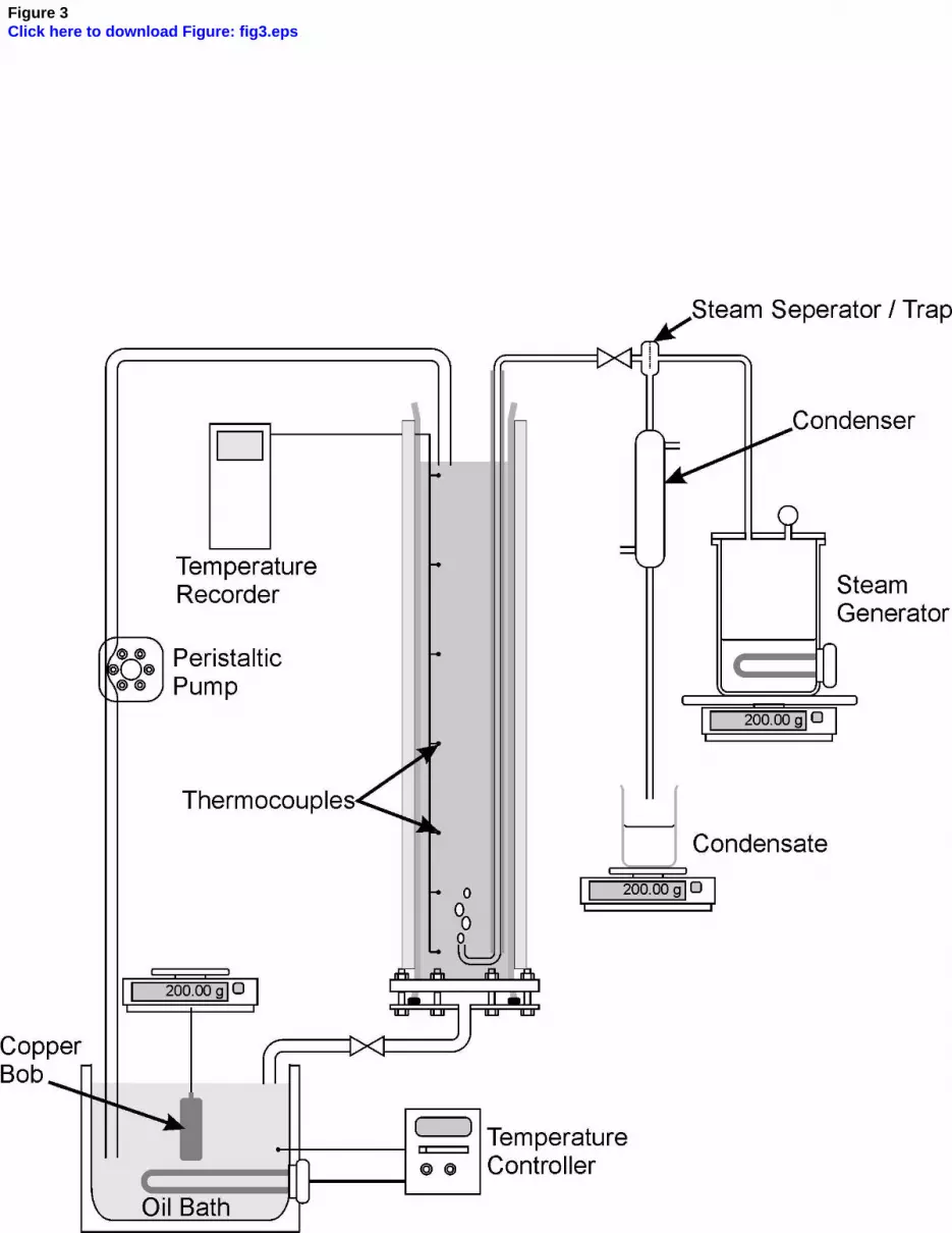
Figure 3Click here to download Figure: fig3.eps

Figure 4Click here to download Figure: fig4.eps

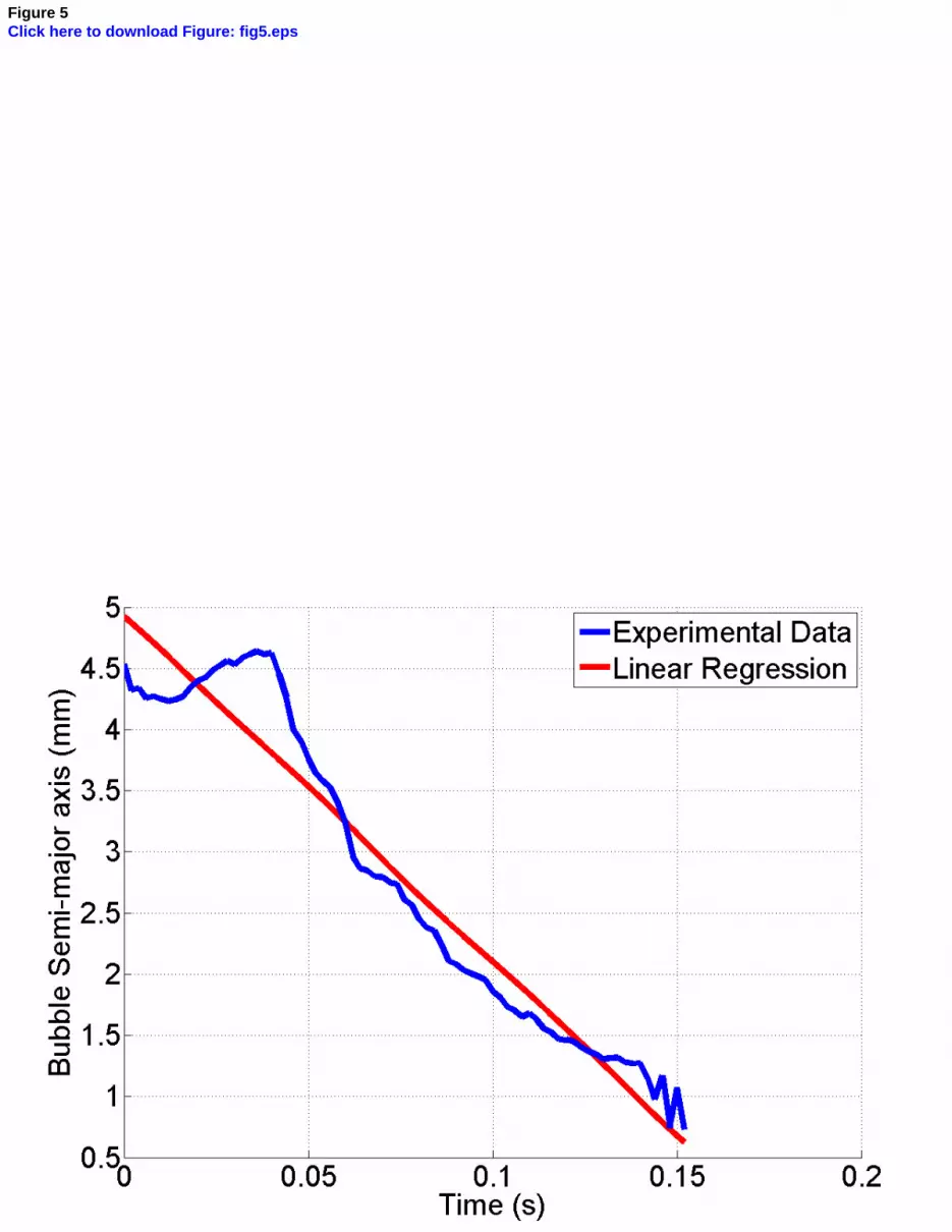
Figure 5Click here to download Figure: fig5.eps

Figure 6Click here to download Figure: fig6.eps

Figure 7AClick here to download Figure: fig7a.eps

Figure 7BClick here to download Figure: fig7b.eps

Figure 8AClick here to download Figure: fig8a.eps

Figure 8BClick here to download Figure: fig8b.eps

Figure 9Click here to download Figure: fig9.eps

Figure 10AClick here to download Figure: fig10a.eps

Figure 10BClick here to download Figure: fig10b.eps

Figure 10CClick here to download Figure: fig10c.eps

Figure 11AClick here to download Figure: fig11a.eps

Figure 11BClick here to download Figure: fig11b.eps

Figure 12AClick here to download Figure: fig12a.eps

Figure 12BClick here to download Figure: fig12b.eps

Figure 13AClick here to download Figure: fig13a.eps

Figure 13BClick here to download Figure: fig13b.eps

Figure 14AClick here to download Figure: fig14a.eps

Figure 14BClick here to download Figure: fig14b.eps

Figure 14CClick here to download Figure: fig14c.eps

Figure 15Click here to download Figure: fig15.eps

Table 1 – Lithium-Bromide solution concentrations and temperatures used in the experiment

Concentration (%w/w)

46 111 119 122

51 121 126 132

56 131 136 141

Temperature (˚C)

Table 1Click here to download Table: Table 1.docx

Table 2 - Solution properties at each experimental setting

Property Units C46T111 C46T119 C51T121 C51T126 C56T131 C56T136 C56T141

μL Ns/m

2 x

10-4

8.11 7.77 9.68 9.54 11.74 11.1 10.79

ρL kg/m3 1414 1413 1489 1493 1567 1560 1560

ρv kg/m3 0.64 0.57 0.62 0.59 0.58 0.57 0.55

σL N/m 0.073 0.072 0.073 0.072 0.073 0.072 0.071

ReL 694 2143 873 1042 776 1126 1785

WeL 1.75 7.32 2.93 3.72 3.25 5.1 9.18

ReL 694 2143 873 1042 776 1126 1785

Table 2Click here to download Table: Table 2.docx

Table 3 – Semi-major axis and Aspect ratio: initial values and linear regression line data

Setting ao (mm) βa (mm/s) ρo βρ

C46T111 4.4 -91.3 0.65 -8.77

C46T119 4.9 -77.1 0.53 -0.95 C51T121 4.7 -72.1 0.63 -7.59 C51T126 4.8 -71.9 0.64 -4.48 C56T131 4.7 -84.5 0.65 -5.54 C56T136 4.8 -48.8 0.55 0.86

C56T141 4.9 -28.1 0.57 -0.05

Table 3Click here to download Table: Table 3.docx

Table 4 – Probabilistic model input data

Setting ση (mm) ωη τcη (ms) σζ (x10-2) ωζ τcζ (ms)

C46T111 0.52 473.6 6.6 10.9 636.7 4.9

C46T119 0.40 395.7 7.9 9.2 610.4 5.1 C51T121 0.71 422.7 7.4 12.2 542.9 5.8 C51T126 0.55 278.7 11.3 10.4 298.4 10.5 C56T131 0.59 348.8 9.0 11.2 456.8 6.9 C56T136 0.43 236.1 13.3 9.4 188.3 16.7

C56T141 0.41 170.5 18.4 8.8 153.0 20.5

Table 4Click here to download Table: Table 4.docx

Figure CaptionsClick here to download Supplementary Material: Figure Captions.docx