Chemical Engineering Science, 61, 3610-3622, 2006

Effect of antifoam agents on bubble characteristics in bubble

columns based on acoustic sound measurements

Waheed A. Al-Masry*, Emad M. Ali and Yehya M. Aqeel

Department of Chemical Engineering, King Saud University, Riyadh, Saudi Arabia

Abstract

In this paper, the effect of antifoam agents on bubble characteristics in bubble columns is

studied. Specifically, the bubble characteristics of air in tap water are compared to those

of air in 5% and 10% antifoam solutions. Bubble characteristics such as gas holdup,

bubble diameter, bubble-size distribution, and damping ratio were investigated at various

superficial gas velocities. These properties were deduced from the acoustic sound

measurement. The study revealed that the addition of antifoam chemicals reduces the

overall gas holdup and increases the average bubble diameter. The bubble-size

distribution in tap water is found to be homogeneous while in antifoam solutions to be

heterogeneous. It is also found that at low gas velocities the damping ratio for antifoam

solutions is higher than that for tap water, while at high gas velocities the damping ratio

is not affected. The results affirm that acoustic probes are excellent measuring tools over

classical tools at moderate gas velocities.

Keywords: acoustic, bubble column, bubble size, damping ratio, gas holdup.

* Corresponding author: walmasry@ksu.edu.sa

Page 1 of 37

Chemical Engineering Science, 61, 3610-3622, 2006

1. Introduction

Bubble column reactors are widely used in chemical and biochemical processes such as

oxidation, chlorination, polymerization, hydrogenation, synthetic fuels by gas conversion

processes, fermentation and wastewater treatment. Bubble columns are preferred two-

phase contactors for their ease of operation, maintenance and absence of moving parts,

yet they have complex hydrodynamics characteristics. Bubble columns can be operated in

different flow regimes depending on the gas flow rate, column dimensions, the

physicochemical properties of the two-phase mixture, and the operating conditions.

Foam is a persistence phenomenon in different technologies involving multiphase

operations; such as pulp and paper, food processing, textile dyeing, fermentation,

wastewater treatment, detergents, paints, froth flotation of ores, and oil industry. There

are two factors necessary for foam to form: a process that disperses a gas into a liquid to

form bubbles, and stabilization of bubbles through adsorption of a surface-active material

at the liquid surface. For example, in biotechnology, surfactants are almost always

present, as both raw materials such as peptides, and substances such as proteins released

by the growing microorganisms. Foam formed during fermentation is stabilized by

components present in the growth medium and by fermentation products, such as

extracellular proteins or other biological molecules. The amount and nature of the foam is

likely to change during the course of the fermentation. Foam in bioreactors can carry

away fermentation broth, leading to product losses and blocked filters downstream. Foam

production can lead to microbial containment issues and loss of process sterility.

Foaming can also lead to fouling of probes which can result in poor process control.

Foam can be controlled by adding chemicals or broken by mechanical devices, with the

later being the most efficient.

Several studies dealing with the effect of antifoam chemicals on the

hydrodynamics and mass transfer properties in bubble columns have been reported in the

literature. Antifoam addition leads to increase in bubble sizes and therefore reduction in

the interfacial area. Consequently the gas holdup and volumetric mass transfer coefficient

are reduced. The decrease in gas holdup was related to higher slip velocity of larger

bubbles formed by coalescence and the decrease in volumetric mass transfer coefficient is

mainly due to the decrease in interfacial area caused by formation of large bubbles

Page 2 of 37

Chemical Engineering Science, 61, 3610-3622, 2006

(Koide et al., 1985, Kawase and Moo-Young, 1987, Al-Masry, 1999, Pelton, 2002,

Denkov, 2004).

The aim of this work is to study the effect of antifoam chemicals addition on

bubble characteristics in bubble columns inferred from acoustic probes. The acoustic

sound measurements for bubbles characterization in gas-liquid systems are attractive

technology over other methods, particularly for systems with foaming characteristics

which fouls classical sensors.

2. Theory of acoustic waves

Sound waves are acoustic waves audible to the human ear and these occur at frequencies

between 20 and 20,000 Hz. Acoustic sounds are characterized by their frequency, speed

at which they travel and its amplitude. The amplitude changes with time and depends on

the distance from the sound source at which it is measured. As an acoustic wave travels

through a medium its amplitude will decrease due to attenuation. Attenuation of the wave

is caused by adsorption (conversion of acoustic energy to other forms of energy) and

scattering.

The production of an acoustic signal by bubbles was first proposed by Minnaert

(1933). Bubbles produce an acoustic sound due to gas compression in the bubble. Under

adiabatic conditions, the natural frequency of a single, millimeter size, linearly oscillating

bubble is given (Minnaert 1933) by:

23

o

oo R

Pργ

=ω

(1)

where ωo is the radian frequency, γ is the ratio of specific heats, Po is the absolute liquid

pressure, ρ is the liquid density and Ro is the equivalent spherical radius of the bubble.

The above equation indicates a unique relationship exists between the frequency of

volume pulsations and the radius of the bubble at a particular static pressure. This

principle is utilized to determine the bubble size distribution in a gas-sparged bubble

column.

Page 3 of 37

Chemical Engineering Science, 61, 3610-3622, 2006

As the newly formed bubble detaches from the sprager, it emits a pulse of sound.

Such pulse lasts less than 20 ms. The bubble then oscillates producing an acoustic

pressure pulse, eventually returning to its equilibrium bubble size. For small amplitude

oscillations the resulting sound pressure pulse is an exponentially damped sine wave:

teftpp β−π= )2sin(0 (2)

where p is pressure at the hydrophone at time t; po is the initial pressure magnitude of the

bubble oscillation; and β is the exponential decay constant.

Hydrodynamic forces usually distort the bubbles while they are rising up in the

column. These shape distortion alter the oscillation frequency. The shape distortion

themselves induce acoustic oscillation by nonlinear resonance. It is common that the

bubbling rate increase with the gas flowrate. The bubbling rate could be considered high

once bubbles begin to collide. As the bubble rate increases, bubbles also become larger

and more distorted and begin to affect each other. At these conditions, the correlation

given in Equation (1) becomes invalid (Mannaseh et al., 2001). Moreover, the

aforementioned factors affect the bubble pulsation and as results modulated or short

length oscillation may occur.

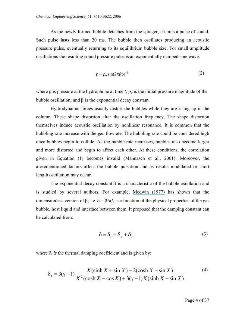
The exponential decay constant β is a characteristic of the bubble oscillation and

is studied by several authors. For example, Medwin (1977) has shown that the

dimensionless version of β, i.e. δ = β/πf, is a function of the physical properties of the gas

bubble, host liquid and interface between them. It proposed that the damping constant can

be calculated from:

rvt δ+δ+δ=δ (3)

where δt is the thermal damping coefficient and is given by:

)sin(sinh)1(3)cos(cosh)sin(cosh2)sin(sinh)1(3 2 XXXXXX

XXXXXt −−γ+−

−−+−γ=δ

(4)

Page 4 of 37

Chemical Engineering Science, 61, 3610-3622, 2006

2/1

00 )/2( ggg KCpRX ρω= (5)

and δv is the viscous damping coefficient and is given by:

)/(4 200Rv ρωμ=δ (6)

and δr is the radiation damping coefficient and is given by:

0kRr =δ (7)

Assuming bubbles of a uniform size are oscillating simultaneously, the actual number of

bubble presented in a bubble column can be estimated directly from the following ratio

(Pandit et. al., 1992):

2

⎟⎠⎞

⎜⎝⎛=

PPn r

a (8)

where Pr the resultant measured pressure and P is the instantaneous sound pressure

which can be found from solving a given bubble volume-pulsation equation under certain

conditions. Pandit et. al., 1992 have shown that the number of bubbles of certain size can

be related to their sound pressure and frequency as follows:

2

02 fCPn ra = (9)

Boyd and Varely, 1998 used Equation (8) to estimate the number of bubbles but they

computed the sound pressure from the following equation:

Page 5 of 37

Chemical Engineering Science, 61, 3610-3622, 2006

dteftpT

PT

ft∫ πδ−π=0

20

2 ])2sin([1

(10)

Application of Boyed and Varely method requires the prior knowledge of the damping

constant and more important P0, which is the initial peak of the bubble oscillation.

Nevertheless, both aforementioned methods did not provide any procedure to validate the

estimated bubble number (density).

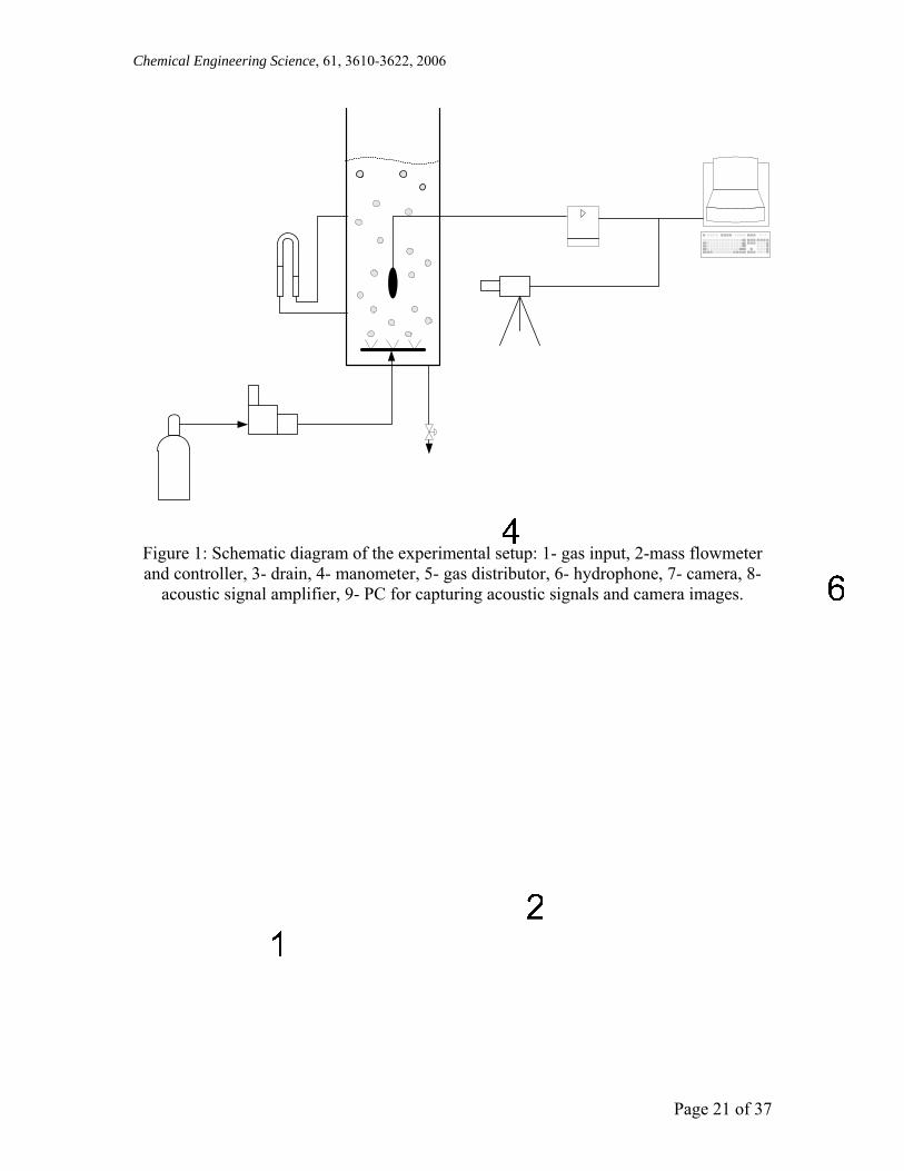
3. Experimental methods

Schematic diagram of the experimental setup is shown in Figure 1. The bubble column

was made from transparent acrylic resin with 0.15 m diameter and 0.66 m clear liquid

height. The gas distributor was a ring sparger with six legs in a star like cross, with 85

holes and 1 mm diameter equally distributed. Clean air from cylinder was supplied to tap

water medium at controllable flow rates using thermal mass flowmeter and controller

(FMA2613, Omega, USA). All experiments were carried out at room temperature and

atmospheric pressure. A miniature hydrophone (Type8103, Bruel & Kjær, Denmark) was

used to record the pressure fluctuation. The hydrophone was located in the center of the

column at a depth of 40 cm from the bottom. The location is selected such that the

hydrophone resides in the heart of the bubble region and away from the sparger to avoid

the latter effect. The hydrophone signals were pre-amplified by charge amplifier

(Type2635, Bruel & Kjær, Denmark) set to the given calibration. Acoustic pressures

were digitized as voltage signals using data acquisition system (DT9806, Data

Translation, USA). The signal generated by a sensor has to be amplified to provide a

higher more usable voltage. The pre-amplification stage can also include filters that

remove unwanted frequencies (noise) in the signal. Gas holdup is determined by

measuring the difference in pressure between two levels within the column. In each

experimental run, the gas flow was set, the voidage and acoustic signal were recorded

after certain time (several minutes) to reach steady state, and then the gas flowrate was

increased. High speed CCD camera (KP-F120CL, Hitachi, Japan) was sued to take

images of the bubble generated in the column. The images were digitized by camera link

board (PIXCI CL1, Epix, USA) and analyzed by interactive image processing software

Page 6 of 37

Chemical Engineering Science, 61, 3610-3622, 2006

(XCAP, Epix, USA). The estimated bubble radiuses from the photography method were

used only to verify those from the acoustic measurements. The experiment were

conducted on three types of water solutions: air injected into tap water system, air into a

water with 5% and 10% volume silicone based antifoam solutions (Antifoam B, Sigma,

USA). For all experiments, the hydrophone location is fixed for fair comparison.

The sound measurements are collected at different gas flow rates using a specific

sampling rate of 20 kHz and a capture time of 10 seconds. Since the bubble oscillation

may last at the most 20 ms, the 10-second long data signal may contain several bubble

pulsations. In this paper, the collected data signals are differenced to remove offset and

slow drifts. Moreover, data differencing will act as high-pass filtering that remove static

components in the signals. The filtered data is then analyzed using Fourier Transform and

bubble counting methods [Al-Masry, et. al. 2005]. Fourier Transform is applied to the

filtered data to produce power spectra from which the sound pressure distribution and

dominant frequency of the bubble pulsation can be obtained. With the bubble count

method, the bubble pulsations within a specific captured signal are detected using the

statistical zero crossing. In this method, the data signal is screened and whenever, the

signal exceeds a threshold value of 186 Pa, a data segment of duration 7 ms is captured.

The number of captured segments is counted to produce the bubble pulsation count and

consequently the bubbling rate. For each captured segment, the autocorrelation of the

signal is computed from which the bubble oscillation frequency is estimated using the

zero crossing approach. The ratio of two consecutive oscillation peaks for each bubble

pulsation is calculated to produce the decay ratio and consequently the damping

coefficient. Based on the two above numerical techniques, we will study the effect of the

antifoam on the bubble characteristics.

4. Results and analysis

4.1 Void fraction and bubble-size distribution

Gas holdup can be calculated directly form the pressure difference between two points or

from the bed expansion method. Figure 2 illustrates how the gas holdup measured from

the pressure difference varies with superficial gas velocity averaged over several runs. In

general, the gas holdup varies as a monotone function over the given range of superficial

Page 7 of 37

Chemical Engineering Science, 61, 3610-3622, 2006

velocity. There is no doubt that the air-water system has larger gas holdup than those for

surfactant solutions (5% and 10% antifoam). It can also be seen that there is negligible

difference in the holdup of 5% antifoam and 10% antifoam solutions. The higher void

fraction for the tap water system can be attributed to many factors such as the size of the

bubbles, the bubbling rate and the density of the produced bubbles. The results that

follow are a maneuver to understand the observed discrepancy between the gas holdup in

tap water and that in presence of antifoam solutions. Figure 3 shows photographs of the

three systems investigated at UG = 0.037 m/s near the hydrophone zone. It can be seen

clearly the difference between the three systems with the antifoam solutions are more

turbid and less transparent.

Figures 4-6 show the distribution of pulsating bubble count for the same three

water solutions discussed above at different superficial gas velocities. The bubble

distribution is obtained using the bubble count method [Al-Masry et al., 2005] where a

signal sample is scanned for possible bubble pulsation. Whenever, a pulsation satisfies

predefined criteria, a bubble oscillation is detected and its frequency and number of

recurrence are recorded leading to the so-called bubble-size distribution. It should be

mentioned that the results shown in Figures 4-6 do not provide the exact number of

bubbles presented in the column. The results provide qualitative information about the

relative density of the different bubble sizes presented locally in the column. The true

bubble counts will be discussed in section 4.4. Based on Figures 4-6, the first observation

is that the detected bubble pulsation ranges from 600 to 3000 Hz (according to Equation

1, this corresponds to bubble size of 0.9 to 5.3 mm). For tap water system the frequency

range is narrower (1200 < f < 2500 corresponding to smaller bubbles) with dominant

frequency of 2000 Hz. With the addition of antifoam larger bubbles are detected. At low

superficial velocities, antifoam solutions have a mix of small and large bubbles with the

smaller bubbles being dominant. As superficial velocity increases, the large bubbles

disappear and the small bubbles prevail. Over all cases, bubbles with radius 1.6 mm (f =

2000 Hz) are dominating. Exception is found for 5% antifoam solution at UG = 0.0994

m/s where bubble frequency of 1400 Hz is dominating. However, the accuracy of this

result can not be verified. The existence of larger bubbles in the surfactant solutions may

explain the smaller gas voidage. However, the large bubbles are only observed at low

Page 8 of 37

Chemical Engineering Science, 61, 3610-3622, 2006

superficial gas velocities. Bubble sizes estimated from photography supported this

observation, with bubble sizes are in the same range as those estimated here (see Table 1).

4.2 Damping constant

The advantage of the bubble count method is that it allows for computing the damping

constant of the bubble oscillation. For each detected bubble pulsation, the oscillating

sound wave can be easily constructed using the Auto correlation function from which the

decay ratio (DR) can be easily estimated from the ratio of the second peak to the first

peak. According to classical harmonic response, the calculated decay ratio can be

converted to damping constant according to:

π−=δ /)ln(DR (11)

Note that for each detected bubble pulsation, the damping coefficient of the oscillation is

calculated according to Equation 11. Afterward, the calculated damping coefficients for a

specific oscillation frequency are grouped and averaged.

Figure 7 depicts the experimental mean δ for each detected bubble oscillation for

three water solutions at different superficial velocities. The result emphasizes that tap

water has narrower range of oscillation frequencies. Moreover, the damping factor

increases slightly with superficial velocity for the three solutions. Alternatively, Figure 8

compares the damping constant of the three solutions to each other and to that computed

theoretically using Equation 3. Clearly, the results in Figure 8 indicate that the antifoam

agents do not affect the damping constant as the mismatch in δ among the three solutions

is minor. However the superficial gas velocity shows some effect on the magnitude of δ.

As the superficial velocity increases, the damping constant for all solutions increases

departing away from the theoretical value. The larger δ could be the result of elevated

bubble collision due to higher velocity. It is clear, that the damping correlations

(Equations 3-6) do not account for variation in gas velocity since all physical properties

and the wave number are considered constant.

Interestingly, the results in Figure 8 question the validity of the theoretical

correlation for δ. At low superficial velocity, apparent mismatch between the theoretical

Page 9 of 37

Chemical Engineering Science, 61, 3610-3622, 2006

damping constant and the experimental results exists. It can be argued that the theoretical

correlation may not apply to water mixed with antifoam traces noting that the physical

properties are that for tap water system. The slight increase of the experimentally

measured δ is also observed and discussed by other authors (Boyd and Varely, 1998). It

was suggested that other factors may affect the damping mechanism other than what the

correlations (Equations 3-7) account for. For example, there may be an energy transfer

between the bubble volume-oscillation and its shape-oscillation causing increased

damping. Moreover, turbulence may continuously change the bubble shape leading to

increased damping.

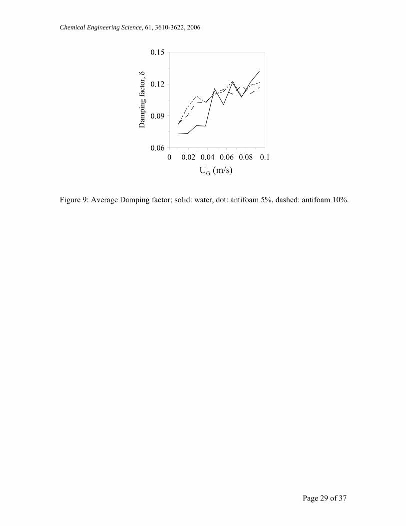
Figure 9 illustrates the variation of the damping constant with superficial gas

velocity. The damping constant at each superficial velocity is the average value over the

detected oscillation frequencies. The damping constant for all water solutions propagate

with gas velocity due to bubble to bubble collision and bubble to wall collision. Despite

the mismatch in δ for tap water and water-antifoam systems at low gas velocity, the

magnitude of δ for dissimilar solutions converges at high gas velocity. Consequently,

the damping constant can not provide further information about the bubble behavior in

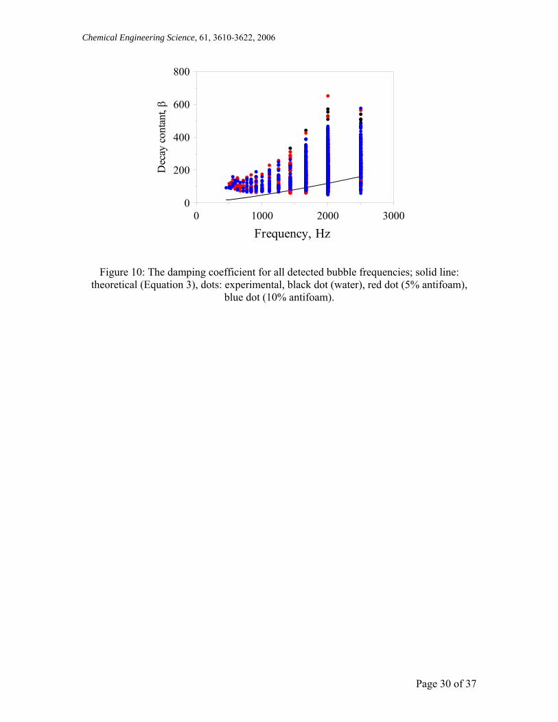
the presence of antifoam solutions. More interesting results can be observed from Figure

10 where the entire damping coefficients (in terms of exponential decay constant, β = πfδ)

calculated for all three types of water-antifoam solutions at several gas superficial

velocities are plotted collectively as a function of their corresponding oscillation

frequency. The discrete dots represent the experimental β while the line is theoretical one.

Clearly, at low frequency the experimental β cluster around small value. This means that

large bubbles of the same size have almost the same damping behavior. On the other

hand, the high frequency region shows that smaller bubbles have a wide range of

damping coefficient.

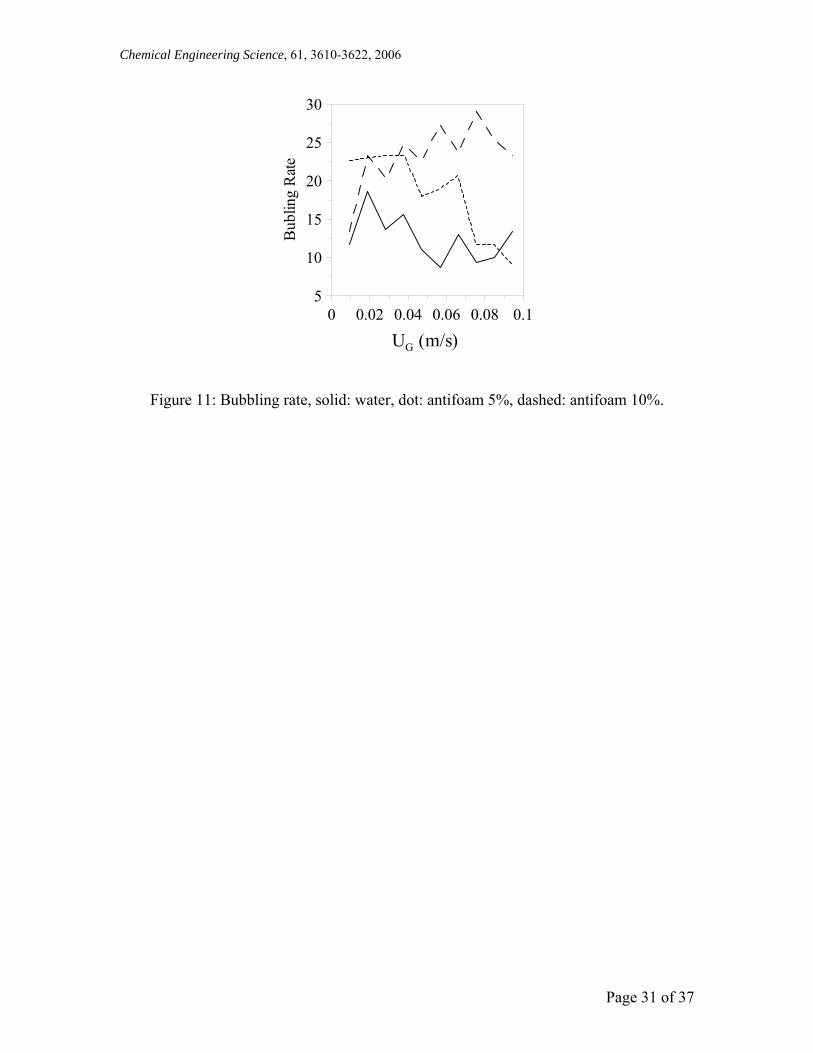
4.3 Bubbling rate and root mean square of sound pressure

Figure 11 demonstrate the alteration of bubbling rate with superficial gas velocity. The

bubbling rate is computed using the bubble count method. Although it does not represent

the true bubbling rate but it can provide relative comparison. Obviously, for tap water

system, the bubbling rate decreases marginally, while for 10% antifoam solution, the

Page 10 of 37

Chemical Engineering Science, 61, 3610-3622, 2006

bubbling rate increases. Interestingly, the bubbling rate for 5% antifoam solution declines

sharply in contrast to what is observed for 10% antifoam solution. The information

gained from the bubbling rate makes it difficult to explain the mismatch between the gas

holdup of the tap water and that of the antifoam solutions.

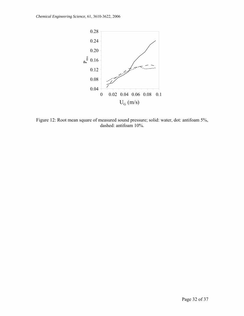
Figure 12 on the other hand, compares the root mean square of the measured

sound pressure for the three solutions. This figure shows how the bubble characteristic

for tap water differs form that of antifoam solutions. The increased Prms for tap water can

not be attributed to the bubbling rate because the result in Figure 9 indicated that tap

water has less relative bubbling rate. It is known that a larger bubble emits higher sound.

However, tap water posses the same bubble size (if not smaller than) that antifoam

solutions have. This is obvious from the previous results and later in Figure 14. By

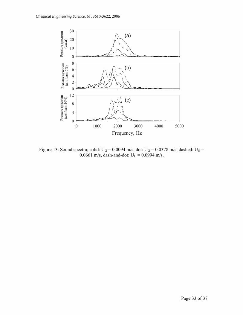
inspecting Figure 13 which demonstrates the power spectrum of the bubble-sound

pressure at different superficial velocities, one can make some observations. For tap

water system, the intensity of sound pressure visibly increases with increased gas velocity.

Furthermore, the pressure spectrum has a unique peak that is shifting to the right (towards

smaller bubble size) as gas velocity propagates. On the other hand, the spectra for the

antifoam solutions do not show a uniform trend. In fact, the spectrum of the antifoam

solutions possesses multiple peaks. One can conclude that the tap water operates closer to

a homogeneous regime while the antifoam solution seems to depart away from the

homogeneous regime. The intensity of the power spectra and the homogeneity of the

bubble size may explain the amplified Prms of the tap water.

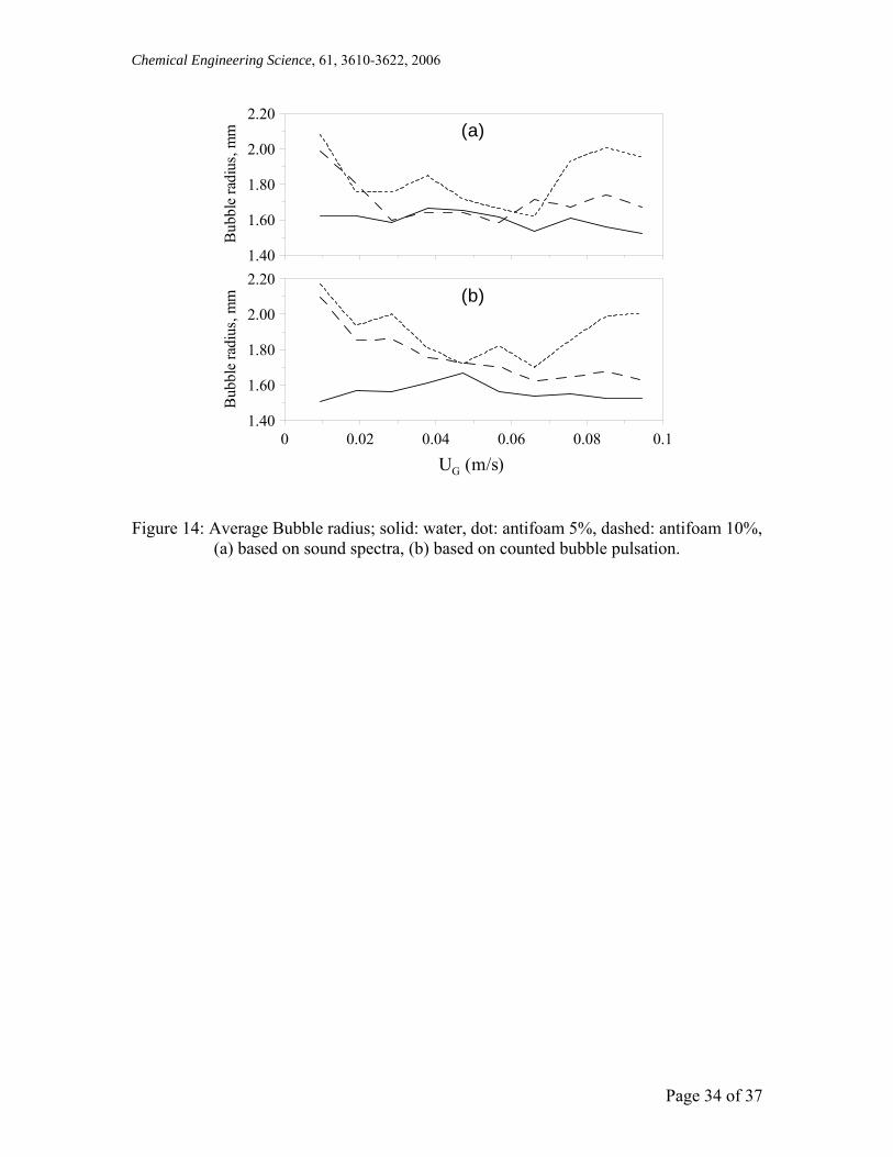
To emphasize the effect of the antifoaming agent on bubble size, the average

bubble radius is computed by two means. One way is to compute the weighted bubble-

radius based on the power spectra as follows:

∑

∑

=

== n

iir

n

iiir

ave

fP

fRfPR

1

1

)(

)()(

(12)

In Equation (12) and considering the power spectra shown in Figure 13, it is assumed that

each point in the frequency domain (x-axis) of the spectra plot corresponds to a bubble

Page 11 of 37

Chemical Engineering Science, 61, 3610-3622, 2006

oscillating at that specific value of frequency. Since the plot in Figure 13 is continuous

we must carry out the summation over a finite number of steps. Therefore, n is the

number of data points which depends on the step size. The step size can be chosen

arbitrary. In the same way, the value of the pressure power (Pr) is the weight for that

specific oscillation and R is the corresponding bubble radius computed via Equation (1).

Alternatively, the average bubble radius can be computed from:

∑

∑=

=

=

== 3000

500

3000

500

i

i

i

if

fia

f

fiia

ave

fn

fRfnR

)(

)()(

(13)

Accordingly, na is the relative bubble density at a given frequency. Considering Figure 4

as an example, na is obtained directly from the y-axis in the bubble-size distribution plots.

Equation (13) provides more realistic estimates of the average bubble size because it is

based on authentic detected bubble oscillation. Moreover, Equation (13) is evaluated only

at specific values for f at which bubble pulsation is discovered, i.e. the summation is

carried out over finite discrete points comprising the detected bubble pulsations. Figure

14 shows the results of using Equations 12 and 13. It is evident that for the case of tap

water the bubble radius is almost constant (around 1.5 mm) over the entire gas velocities.

For the case of 10% antifoam solution, the bubble radius starts from 2.1 mm and reduces

with gas superficial velocity till reaches a value of 1.6 mm. For the case of 5% antifoam

solution, the bubble radius distribution is similar to that for 10% antifoam solution except

at high gas velocity where the bubble radius increases again. This observation was also

noticed in Figure 5. One can also conclude that the addition of antifoam produces larger

bubble sizes over the operating range of gas velocities.

4.4 Bubble-size distribution

Several authors have tried to estimate the actual number of bubbles existing in sparged

systems using Equation 8. However, these estimated bubble counts are not validated

against measured values. It is not easy to measure the true bubble counts directly.

Page 12 of 37

Chemical Engineering Science, 61, 3610-3622, 2006

Therefore, we will infer the bubble counts indirectly from the measured gas holdup. We

assume that the total gas volume trapped in the liquid phase is the sum of the volume of

all entrained bubbles. In this case, one can estimate the bubble count using Equation 9

from which estimation of the gas holdup can be obtained. A good confidence on the

calculated bubble count can be achieved when the discrepancy between the calculated gas

holdup and the measured one approaches zero. To estimate the bubble density using

Equation 9, the parameter C needs to be specified. According to Pandit et. al., C is a

lumped parameter of the bubble radius ratio, physical properties and the distance between

the bubble and the hydrophone. To determine a suitable value for C and hence the bubble

quantity, we solve the following optimization problem:

( )2expmin G GcalC

e ε ε= − (14)

subject to

gGcal

g l

VV V

ε =+

(15)

)(),,( ibria

n

ig RVPfCnV

i∑=

=1

(16)

where Vl is the liquid phase volume, and na is the bubble quantity for a specific volume

Vb that can be computed using Equation 9. Note that Equation 14 is solved repeatedly at

each superficial gas velocity using MATLAB software. For each gas velocity, C is

allowed to have a different value.

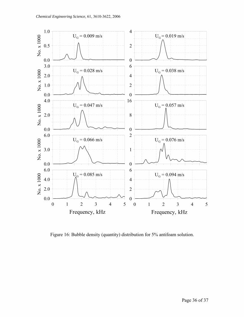
The result of applying the above optimization to a typical experimental run for

5% antifoam solution is shown in Figure 15 and 16. The solution of the optimization

problem will result in an optimum value for C denoted as C*. The solid line in Figure 15

represents the experimental value of the hold up while the ‘+’ sign indicates the

calculated hold up obtained from solving the optimization problem (Eq. 12). The

Page 13 of 37

Chemical Engineering Science, 61, 3610-3622, 2006

excellent agreement between the calculated and measured holdup is obvious. The

corresponding bubble density (quantity) is shown in Figure 16 for each gas velocity. The

figure shows presumably the true number of bubbles that exist at each frequency which

indicates that exiting bubble quantity may range from 500 to 5000. For each gas velocity,

the sum of all bubble quantities multiplied by their corresponding volume comprises the

gas voidage in the system. The other plots shown in Figure 15 that were indicated by

different symbols are the calculated gas holdup for different experimental runs. Some of

the runs are for 5% antifoam solution and some are for 10% antifoam solution. These

calculated holdups are obtained using Equations 15 and 16 for a fixed optimum value of

C, i.e. C* obtained previously. A set of bubble-size distributions similar to those in

Figure 15 is produced. These bubble-size distributions are not shown for brevity. There is

an obvious mismatch between the calculated and the measured holdup especially at high

gas velocity where heterogeneity is expected. The mismatch is due to the measured sound

spectra, i.e. Pr, which may vary slightly from run to run. However, the idea is not to

calculate the gas holdup but to use it as a benchmark. This means that the resulted bubble

count is considered acceptable if the gas holdup computed from the bubble count is close

enough to its benchmark value.

5. Conclusions

It is well known that the addition of surfactant species affects the surface tension of air

bubbles in water. This work aimed at examining the impact of 5% and 10 % antifoam

solutions on bubble characteristics. The results indicated that gas holdup in tap water

decreases upon addition of antifoam agents. It is also found that tap water possesses a

uniform bubble diameter over wide range of, and unique bubble distribution for each,

superficial velocity. On the other hand, the addition of antifoam created a heterogeneous

bubbling environment. In fact, larger bubble sizes were observed in the case of antifoam

solutions especially at low gas velocities. Large bubble sizes disappear at high velocities

maybe because of bubble break up due to turbulence. The damping coefficient of bubble

pulsation was also found to increase with gas velocity for both tap water and tap water in

presence of antifoaming agents. This is common because at high velocities, bubble start

colliding and coalescing which results in rapid decaying of the bubble oscillation.

Page 14 of 37

Chemical Engineering Science, 61, 3610-3622, 2006

However, at low gas velocities, the damping coefficient for antifoam solutions is greater

than that for tap water. Moreover, a rigorous method for estimating the bubble-size

distribution is proposed. The method is based on numerical optimization and is validated

with experimental data for gas holdup.

Page 15 of 37

Chemical Engineering Science, 61, 3610-3622, 2006

6. Notation

C constant in Equation 9.

C* optimum value of C

Cpg specific heat of gas, for air ~ 0.24 cal/gm

D column diameter, m

DR decay ratio

f frequency, Hz

f0 pulsation frequency, Hz

k wave number

Kg thermal conductivity of gas, for air ~ 5.6x10-5 cal/cm s oC

na number of bubbles

p pressure at the hydrophone, Pa

P instantaneous sound pressure, Pa

P0 absolute pressure of the liquid, Pa

p0 initial pressure of the bubble oscillation, Pa

Pr resultant measured pressure, Pa

Prms the root means square of the pressure measurement, Pa

r distant between the hydrophone and detected bubble sound, mm

R0 bubble radius, mm

Rave average bubble radius, mm

t time, s

T sampling time, s

UG superficial gas velocity, m/s

Vb bubble specific volume

Vg gas phase volume, m3

Vl liquid phase volume, m3

X constant defined by Equation (5)

ω0 radian frequency, Hz

εGcal calculated gas holdup

εGexp experimental gas holdup

β exponential decay constant

Page 16 of 37

Chemical Engineering Science, 61, 3610-3622, 2006

δ damping constant

δr radiation damping constant

δt thermal damping constant

δv viscous damping constant

γ ratio of specific heat = 1.4 for air

μ liquid shear viscosity, for water ~ 0.01 gm/cm s

ρ liquid density, for water ∼ 0.998 gm/cm3

ρg air density, for air ~1.29x10-3 gm/cm3

Page 17 of 37

Chemical Engineering Science, 61, 3610-3622, 2006

7. References

Al-Masry W. A., Ali, E. M., Aqeel, Y. M. 2005. Determination of bubble characteristics

in bubble columns using statistical analysis of acoustic sound measurements.

Chemical Engineering Research and Design, 83: 1196-1207.

Al-Masry, W. A., 1999. Effect of antifoam and scale-up on operation of bioreactors.

Chemical Engineering and Processing, 38: 197-201.

Boyd, J., and Varley, J., 1998. Sound Measurement as a Means of Gas-Bubble Sizing in

Aerated Agitated Tanks. American Institute of Chemical Engineers Journal, 44:

1731-1739.

Denkov, N. D., 2004. Mechanisms of foam destruction by oil based antifoams. Langmuir,

20: 9463-9505.

Kawase, Y., Moo-Young, M., 1987. Influence of antifoam agents on gas holdup and mass

transfer in bubble columns with non-Newtonian fluids. Applied Microbiology and

Biotechnology, 27: 159-167.

Koide, K., Yamazoe, S., Harada, S., 1985. Effects of surface active substances on gas

holdup and gas liquid mass transfer in bubble column. Journal of Chemical

Engineering of Japan, 18: 287-292.

Mannasseh, R., LaFontain, R. F., Davy, J., Shepherd, I. C., Zhu, Y., 2001. Passive

acoustic bubble sizing in sparged systems. Experiments in Fluids, 30: 672-682.

Medwin H., 1977. Acoustical determination of bubble-size spectra. The Journal of

Acoustical Society of. America, 62: 1041–1044.

Minnaert M. 1933, On musical air-bubble and the sound of tuning water. Philosophical

Magazine, 16, 235-248.

Pandit, A. B., Varely, J., Thorpe, R. B., Davidson, J. F., 1992. Measurement of bubble

size distribution: an acoustic technique. Chemical Engineering Science, 47: 1079-

1089.

Pelton, R, 2002. A review of antifoam mechanisms in fermentation. Journal of Industrial

Microbiology and Biotechnology, 29: 149-154.

Page 18 of 37

Chemical Engineering Science, 61, 3610-3622, 2006

Figures Captions Figure 1: Schematic diagram of the experimental setup: 1- gas input, 2-mass flowmeter and controller, 3- drain, 4- manometer, 5- gas distributor, 6- hydrophone, 7- camera, 8- acoustic signal amplifier, 9- PC for capturing acoustic signals and camera images. Figure 2: Gas Hold up versus superficial gas velocity; solid: water, dot: antifoam 5%, dashed: antifoam 10%. Figure 3: Photographs near the hydrophone zone at UG = 0.037 m/s: (A): air-water, air-5% antifoam solution, (C): air-10% antifoam solution. Figure 4: Bubble count (size) distribution for tap water; (a): UG = 0.0094 m/s, (b): UG = 0.0378 m/s, (c): UG = 0.0661 m/s; (d): UG = 0.0994 m/s. Figure 5: Bubble count (size) distribution for water with 5% antifoam; (a): UG = 0.0094 m/s, (b): UG = 0.0378 m/s, (c): UG = 0.0661 m/s; (d): UG = 0.0994 m/s. Figure 6: Bubble count (size) distribution for water with 10% antifoam; (a): Ug = 0.0094 m/s, (b): UG = 0.0378 m/s, (c): UG = 0.0661 m/s; (d): UG = 0.0994 m/s. Figure 7: Damping factor; solid: UG = 0.0094 m/s, dot: UG = 0.0378 m/s, dashed: UG = 0.0661 m/s; dot-dash: UG = 0.0994 m/s. Figure 8: Damping factor; solid: water, dot: antifoam 5%, dashed: antifoam 10%, dots: theoretical (Equation 3). Figure 9: Average Damping factor; solid: water, dot: antifoam 5%, dashed: antifoam 10%. Figure 10: The damping coefficient for all detected bubble frequencies; solid line: theoretical (Equation 3), dots: experimental, black dot (water), red dot (5% antifoam), blue dot (10% antifoam). Figure 11: Bubbling rate, solid: water, dot: antifoam 5%, dashed: antifoam 10%. Figure 12: Root mean Square of measured sound pressure; solid: water, dot: antifoam 5%, dashed: antifoam 10%. Figure 13: Sound spectra; solid: UG = 0.0094 m/s, dot: UG = 0.0378 m/s, dashed: UG = 0.0661 m/s, dash-and-dot: UG = 0.0994 m/s. Figure 14: Average Bubble radius; solid: water, dot: antifoam 5%, dashed: antifoam 10%, (a) based on sound spectra, (b) based on counted bubble pulsation. Figure 15: Gas holdup as a validation measure for bubble quantity; ‘+’, ‘x’ symbols denote two independent experiments for 5% antifoam solution; ‘◊’ , ‘∇ ’ symbols denote

Page 19 of 37

Chemical Engineering Science, 61, 3610-3622, 2006

two independent experiments for 10% antifoam solution; ‘*’, ‘○’ symbols denote two independent experiments for tap water. Figure 16: Bubble density (quantity) distribution for 5% antifoam solution.

Page 20 of 37

Chemical Engineering Science, 61, 3610-3622, 2006

Figure 1: Schematic diagram of the experimental setup: 1- gas input, 2-mass flowmeter and controller, 3- drain, 4- manometer, 5- gas distributor, 6- hydrophone, 7- camera, 8-

acoustic signal amplifier, 9- PC for capturing acoustic signals and camera images.

Page 21 of 37

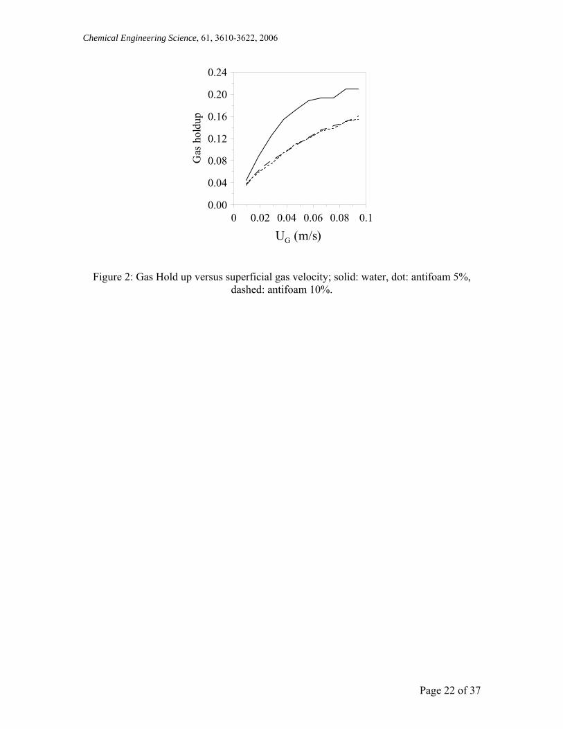
Chemical Engineering Science, 61, 3610-3622, 2006

0 0.02 0.04 0.06 0.08 0.1

UG (m/s)

0.00

0.04

0.08

0.12

0.16

0.20

0.24

Gas

hol

dup

Figure 2: Gas Hold up versus superficial gas velocity; solid: water, dot: antifoam 5%, dashed: antifoam 10%.

Page 22 of 37

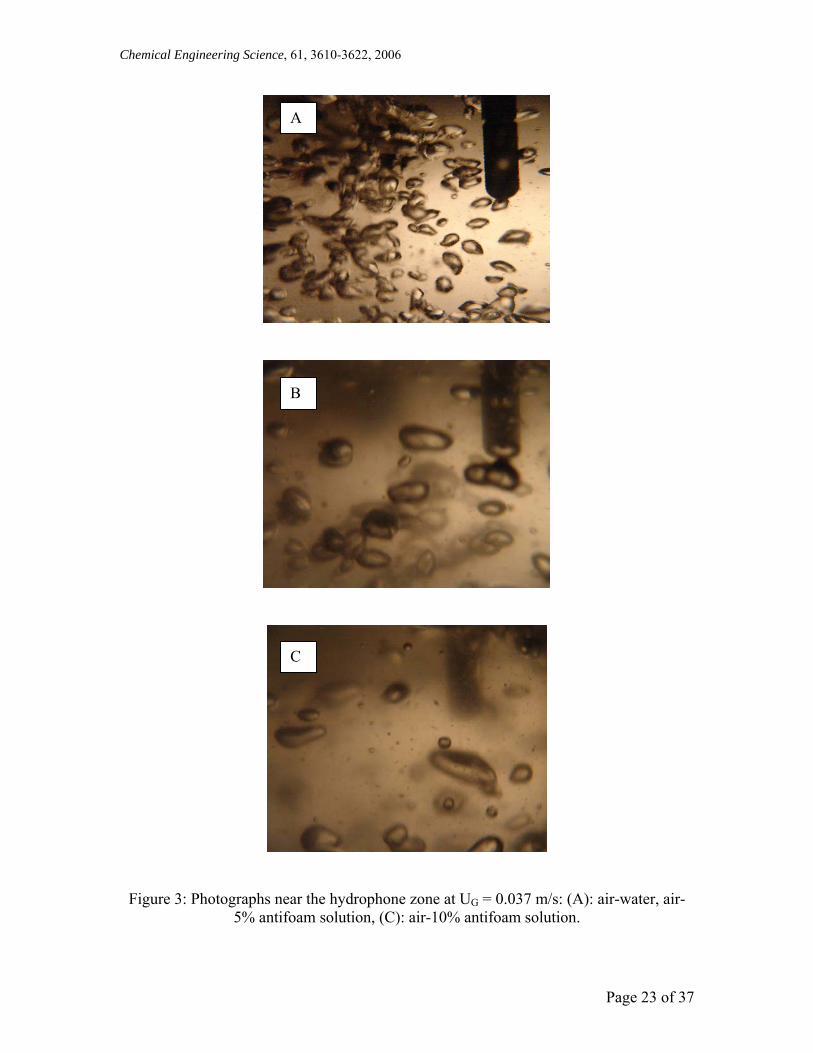
Chemical Engineering Science, 61, 3610-3622, 2006

A

B

C

Figure 3: Photographs near the hydrophone zone at UG = 0.037 m/s: (A): air-water, air-5% antifoam solution, (C): air-10% antifoam solution.

Page 23 of 37

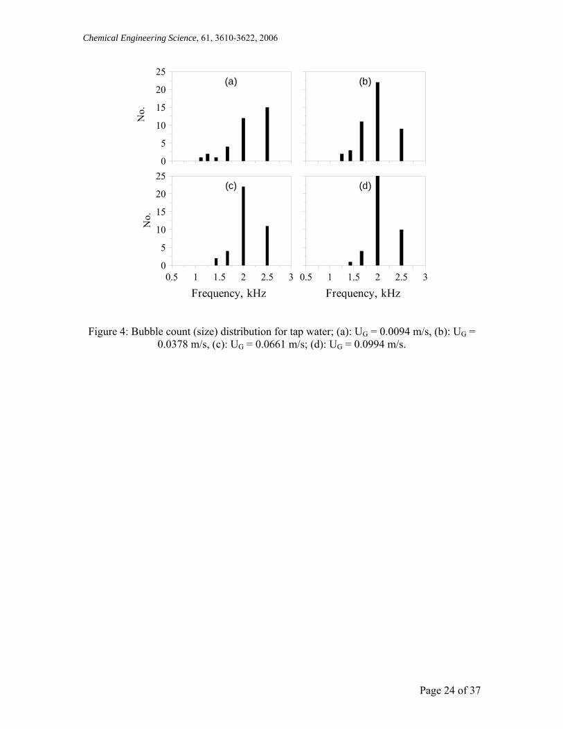
Chemical Engineering Science, 61, 3610-3622, 2006

0.5 1 1.5 2 2.5 3

Frequency, kHz

0

5

10

15

20

25

No.

(c)

0

5

10

15

20

25

No.

(a) (b)

0.5 1 1.5 2 2.5 3

Frequency, kHz

(d)

Figure 4: Bubble count (size) distribution for tap water; (a): UG = 0.0094 m/s, (b): UG = 0.0378 m/s, (c): UG = 0.0661 m/s; (d): UG = 0.0994 m/s.

Page 24 of 37

Chemical Engineering Science, 61, 3610-3622, 2006

0.5 1 1.5 2 2.5 3

Frequency, kHz

0

10

20

30

40

No.

(c)

0

10

20

30

40

No.

(a) (b)

0.5 1 1.5 2 2.5 3

Frequency, kHz

(d)

Figure 5: Bubble count (size) distribution for water with 5% antifoam; (a): UG = 0.0094 m/s, (b): UG = 0.0378 m/s, (c): UG = 0.0661 m/s; (d): UG = 0.0994 m/s.

Page 25 of 37

Chemical Engineering Science, 61, 3610-3622, 2006

0.5 1 1.5 2 2.5 3

Frequency, kHz

0

11

22

33

44

55

No.

(c)

0

11

22

33

44

55

No.

(a) (b)

0.5 1 1.5 2 2.5 3

Frequency, kHz

(d)

Figure 6: Bubble count (size) distribution for water with 10% antifoam; (a): UG = 0.0094 m/s, (b): UG = 0.0378 m/s, (c): UG = 0.0661 m/s; (d): UG = 0.0994 m/s.

Page 26 of 37

Chemical Engineering Science, 61, 3610-3622, 2006

500 900 1300 1700 2100 2500

Frequency, Hz

0.0

0.1

0.2

0.3

Dam

ping

fact

or(a

ntifo

am 1

0%)

0.0

0.1

0.2

0.3D

ampi

ng fa

ctor

(ant

ifoam

5%

)

0.0

0.1

0.2

0.3

Dam

ping

fact

or

(wat

er)

Figure 7: Damping factor; solid: UG = 0.0094 m/s, dot: UG = 0.0378 m/s, dashed: UG = 0.0661 m/s; dot-dash: UG = 0.0994 m/s.

Page 27 of 37

Chemical Engineering Science, 61, 3610-3622, 2006

500 900 1300 1700 2100 2500

Frequency, Hz

0.0

0.1

0.2

0.3

Dam

ping

fact

or UG = 0.094 m/s

0.0

0.1

0.2

0.3D

ampi

ng fa

ctor UG = 0.047 m/s

0.0

0.1

0.2

0.3

Dam

ping

fact

or

UG = 0.009 m/s

Figure 8: Damping factor; solid: water, dot: antifoam 5%, dashed: antifoam 10%, dots: theoretical (Equation 3).

Page 28 of 37

Chemical Engineering Science, 61, 3610-3622, 2006

0 0.02 0.04 0.06 0.08 0.1

UG (m/s)

0.06

0.09

0.12

0.15

Dam

ping

fact

or, δ

Figure 9: Average Damping factor; solid: water, dot: antifoam 5%, dashed: antifoam 10%.

Page 29 of 37

Chemical Engineering Science, 61, 3610-3622, 2006

0 1000 2000 3000

Frequency, Hz

0

200

400

600

800

Dec

ay c

onta

nt, β

Figure 10: The damping coefficient for all detected bubble frequencies; solid line: theoretical (Equation 3), dots: experimental, black dot (water), red dot (5% antifoam),

blue dot (10% antifoam).

Page 30 of 37

Chemical Engineering Science, 61, 3610-3622, 2006

0 0.02 0.04 0.06 0.08 0.1

UG (m/s)

5

10

15

20

25

30

Bub

ling

Rat

e

Figure 11: Bubbling rate, solid: water, dot: antifoam 5%, dashed: antifoam 10%.

Page 31 of 37

Chemical Engineering Science, 61, 3610-3622, 2006

0 0.02 0.04 0.06 0.08 0.1

UG (m/s)

0.04

0.08

0.12

0.16

0.20

0.24

0.28

P rm

s

Figure 12: Root mean square of measured sound pressure; solid: water, dot: antifoam 5%, dashed: antifoam 10%.

Page 32 of 37

Chemical Engineering Science, 61, 3610-3622, 2006

0 1000 2000 3000 4000 5000

Frequency, Hz

0

4

8

12

Pres

sure

spe

ctru

m(a

ntifo

am 1

0%)

(c)

02468

Pres

sure

spe

ctru

m(a

ntifo

am 5

%) (b)

0

10

20

30

Pres

sure

spe

ctru

m

(wat

er)

(a)

Figure 13: Sound spectra; solid: UG = 0.0094 m/s, dot: UG = 0.0378 m/s, dashed: UG = 0.0661 m/s, dash-and-dot: UG = 0.0994 m/s.

Page 33 of 37

Chemical Engineering Science, 61, 3610-3622, 2006

0 0.02 0.04 0.06 0.08 0.1

UG (m/s)

1.40

1.60

1.80

2.00

2.20

Bub

ble

radi

us, m

m (b)

1.40

1.60

1.80

2.00

2.20

Bub

ble

radi

us, m

m (a)

Figure 14: Average Bubble radius; solid: water, dot: antifoam 5%, dashed: antifoam 10%, (a) based on sound spectra, (b) based on counted bubble pulsation.

Page 34 of 37

Chemical Engineering Science, 61, 3610-3622, 2006

0 0.02 0.04 0.06 0.08 0.1

UG (m/s)

0.00

0.05

0.10

0.15

0.20

0.25

Gas

hol

dup

Figure 15: Gas holdup as a validation measure for bubble quantity; ‘+’, ‘x’ symbols denote two independent experiments for 5% antifoam solution; ‘◊’ , ‘∇ ’ symbols denote

two independent experiments for 10% antifoam solution; ‘*’, ‘○’ symbols denote two independent experiments for tap water.

Page 35 of 37

Chemical Engineering Science, 61, 3610-3622, 2006

0 1 2 3 4 5

Frequency, kHz

0.0

2.0

4.0

6.0

No.

x 1

000 UG = 0.085 m/s

0 1 2 3 4 5

Frequency, kHz

0

2

4

6UG = 0.094 m/s

0.0

3.0

6.0

No.

x 1

000 UG = 0.066 m/s

0

1

2UG = 0.076 m/s

0.0

2.0

4.0

No.

x 1

000 UG = 0.047 m/s

0

8

16UG = 0.057 m/s

0.0

1.0

2.0

3.0

No.

x 1

000 UG = 0.028 m/s

0

2

4

6UG = 0.038 m/s

0.0

0.5

1.0N

o. x

100

0 UG = 0.009 m/s

0

2

4UG = 0.019 m/s

Figure 16: Bubble density (quantity) distribution for 5% antifoam solution.

Page 36 of 37

Chemical Engineering Science, 61, 3610-3622, 2006

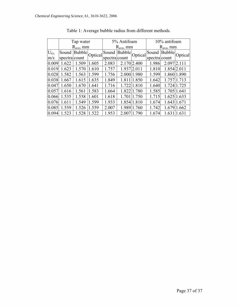
Table 1: Average bubble radius from different methods.

Tap water Rave, mm

5% Antifoam Rave, mm

10% antifoam Rave, mm

UG, m/s

Sound spectra

Bubble count Optical Sound

spectraBubble count Optical Sound

spectraBubble count Optical

0.009 1.622 1.509 1.605 2.083 2.170 2.400 1.986 2.097 2.111 0.019 1.623 1.570 1.610 1.757 1.937 2.011 1.810 1.854 2.011 0.028 1.582 1.563 1.599 1.756 2.000 1.980 1.599 1.860 1.890 0.038 1.667 1.615 1.635 1.849 1.811 1.850 1.642 1.757 1.713 0.047 1.650 1.670 1.641 1.716 1.722 1.810 1.640 1.724 1.725 0.057 1.616 1.561 1.583 1.664 1.822 1.780 1.585 1.705 1.641 0.066 1.535 1.538 1.601 1.618 1.701 1.750 1.715 1.625 1.633 0.076 1.611 1.549 1.599 1.933 1.854 1.810 1.674 1.643 1.671 0.085 1.559 1.526 1.559 2.007 1.989 1.760 1.742 1.679 1.662 0.094 1.523 1.528 1.522 1.953 2.007 1.790 1.674 1.631 1.631

Page 37 of 37