Analysis of Urea Electrolysis for Generation of Hydrogen

A thesis presented to

the faculty of

the Russ College of Engineering and Technology of Ohio University

In partial fulfillment

of the requirements for the degree

Master of Science

Deepika Singh

November 2009

2

This thesis titled

Analysis of Urea Electrolysis for Generation of Hydrogen

by

DEEPIKA SINGH

has been approved for

the Department of Chemical and Biomolecular Engineering

and the Russ College of Engineering and Technology by

Gerardine G. Botte

Associate Professor of Chemical and Biomolecular Engineering

Dennis Irwin

Dean, Russ College of Engineering and Technology

3

ABSTRACT

SINGH, DEEPIKA, M.S., November 2009, Chemical Engineering

Analysis of Urea Electrolysis for Generation of Hydrogen (100 pp.)

Director of Thesis: Gerardine G. Botte

The oxidation of urea was studied as a means of remediating urine-rich waste

water to produce hydrogen and simultaneously denitrificating the waste water. The

proposed reaction mechanisms, preferred pathway and rate determining steps have been

predicted using Density Functional Theory calculations. Both the electro-oxidation

reaction as well as the chemical oxidation reaction mechanisms have been postulated on

the surface of the active catalyst NiOOH. The preferred pathway for electro-oxidation

was found to be: *CO(NH2)2→ *CO(NH.NH2)→ *CO(NH.NH)→

*CO(NH.N)→*CO(N2) → *CO(OH) →*CO(OH.OH) →*CO2 with desorption of CO2

as the rate limiting step. From the thermodynamic calculations of the chemical oxidation

reactions, it was evident that the presence of OH- catalyzes the reaction. Experimentally,

the effects of varying concentrations of KOH and urea were investigated. The

experimental results supported the argument that a higher concentration of OH- is more

favorable for the reaction.

Approved: _____________________________________________________________

Gerardine G. Botte

Associate Professor of Chemical and Biomolecular Engineering

4

ACKNOWLEDGMENTS

Firstly I would like to acknowledge the guidance, motivation and tremendous

support of my advisor, Dr. Gerardine Botte. She will continue to be a source of

inspiration for me throughout my career. I would also like to thank my colleagues at the

Electrochemical Engineering Research Laboratory for their guidance and patience in

helping me learn the basic laboratory techniques. In particular, I want to acknowledge the

tremendous contribution of Damilola Daramola who has helped me from the initial stages

of teaching computational techniques right untill the end for editing and formatting of the

submitted publications, apart from mentoring me at all stages in my research. Without his

support none of this would have possible. I would also like to extend my heartiest

gratitude to the Ohio Super Computing Center for providing valuable resources and

computing time for the computational calculations.

I would also like to thank all friends, especially Saurin Shah and Santosh Vijapur

for being there for me all the time. For all the emotional and moral support and for

believing in me, for giving me the strength to persevere, I can never thank both of you

enough. Finally I’d like to thank my immediate family who has always been there with

me mentally, if not physically. For their undying belief, the kind words and unfailing

support. For being with me through thick and thin, at all times of the day. Thank you so

much. I could not have done this without you all.

5

TABLE OF CONTENTS

Page

Abstract ............................................................................................................................... 3 

Acknowledgments............................................................................................................... 4 

List of Tables ...................................................................................................................... 7 

List of Figures ..................................................................................................................... 8 

Chapter 1 : Introduction .................................................................................................... 10 

1.1  Project Overview .............................................................................................. 10 

1.2  Statement of Objectives .................................................................................... 13 

1.3  Significance of Research ................................................................................... 14 

Chapter 2 : Literature Review ........................................................................................... 15 

2.1  Theoretical ........................................................................................................ 15 

2.2  Experimental ..................................................................................................... 18 

Chapter 3 : Computational Methods ................................................................................. 19 

Chapter 4 : Electro-Oxidation Mechanisms ...................................................................... 23 

4.1  Reaction Mechanism Path 1.............................................................................. 25 

4.2  Reaction Mechanism: Path 2 ............................................................................ 36 

4.3  Reaction Mechanisms: Path 3 ........................................................................... 41 

4.5  Conclusion ........................................................................................................ 49 

Chapter 5 : Chemical Oxidation Mechanisms .................................................................. 51 

5.1  Different Orientations of Urea towards NiOOH ............................................... 51 

5.2  Urea decomposition with NiOOH ................................................................... 53 

5.3  Urea and NiOOH in the presence of OH- ion: .................................................. 55 

5.4  Conclusion ........................................................................................................ 58 

6 Chapter 6 : Experimental .................................................................................................. 59 

6.1  Experimental Methods: Electroplating and Preliminary Results ...................... 59 

6.2  Potentio-dynamic Tests ..................................................................................... 60 

6.3  Results and Discussion ..................................................................................... 61 

6.4  Conclusion ........................................................................................................ 64 

Chapter 7 : Conclusions and Recommendations .............................................................. 65 

References ......................................................................................................................... 67 

Appendix A: Supporting Information for Urea Electro-Oxidation Reaction ....................72

Appendix B: Supporting Information for Urea Chemical Oxidation Reaction .................93

7

LIST OF TABLES

Page

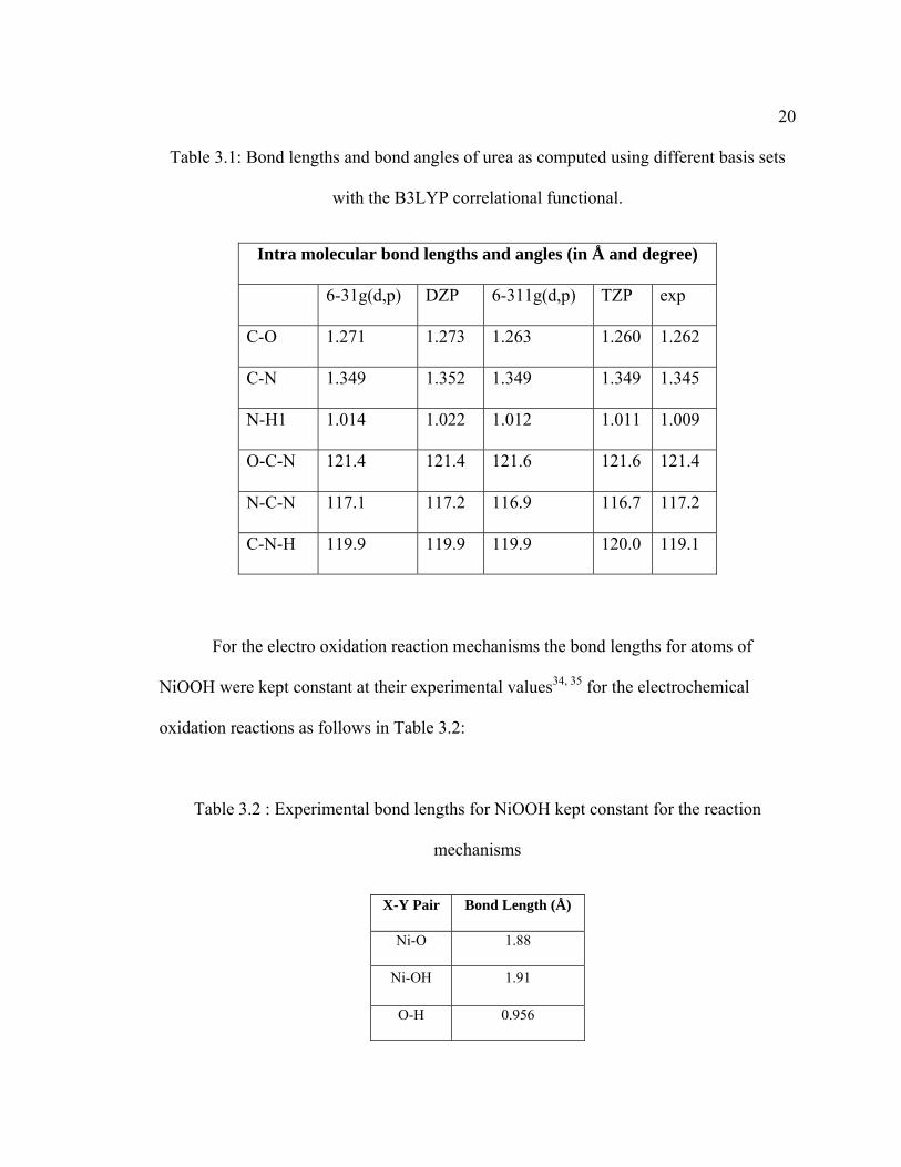
Table 3.1: Bond lengths and bond angles of urea as computed using different basis sets with the B3LYP correlational functional ...........................................................................20

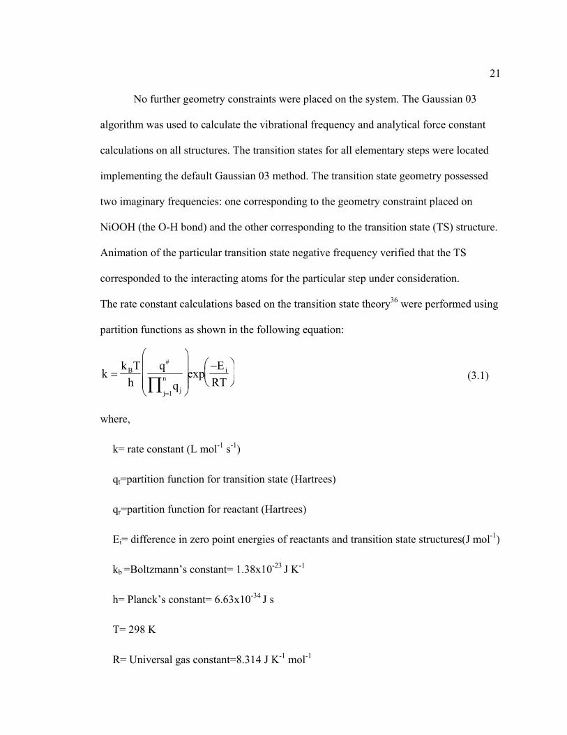
Table 3.2 : Experimental bond lengths for NiOOH kept constant for the reaction mechanisms ........................................................................................................................20

Table 4.1: Proposed reaction mechanisms for urea electro oxidation reaction .................25

Table 4.2: Sum of free energies for all the intermediate steps ...........................................48

Table 4.3: Kinetics of the reaction pathways and rate constants for intermediate steps ...49

Table 5.1: Binding Energies of different orientations of urea towards NiOOH ................53

Table 5.2: Free Energies differences for Equations 5.1 and 5.2 ........................................55

Table 5.3: Free Energies differences for Equations 5.3 and 5.4 ........................................58

8

LIST OF FIGURES

Page

Figure 1.1:Global Energy Systems Transition1 ................................................................ 10 

Figure 2.1: Mechanism of urease catalyzed urea hydrolysis14 ......................................... 16 

Figure 4.1: Initial state (a) Transition state (b) and Final structure (c) for Equation 4.5 ...................................................................................................................... 26 

Figure 4.2: Initial state (a), transition state (b) and final structure (c) for Equation 4.6 ...................................................................................................................... 27 

Figure 4.3: Initial state (a), transition state (b) and final structure (c) for Equation 4.7 ...................................................................................................................... 29 

Figure 4.4: Initial state (a), transition state (b) and final structure (c) for Equation 4.8 ...................................................................................................................... 30 

Figure 4.5: Initial state (a), transition state (b) and final structure (c) for Equation 4.9 ...................................................................................................................... 31 

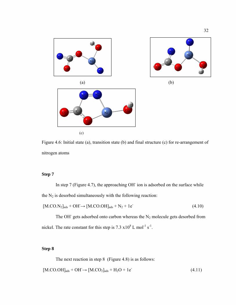
Figure 4.6: Initial state (a), transition state (b) and final structure (c) for re-arrangement of nitrogen atoms .............................................................................................................. 32 

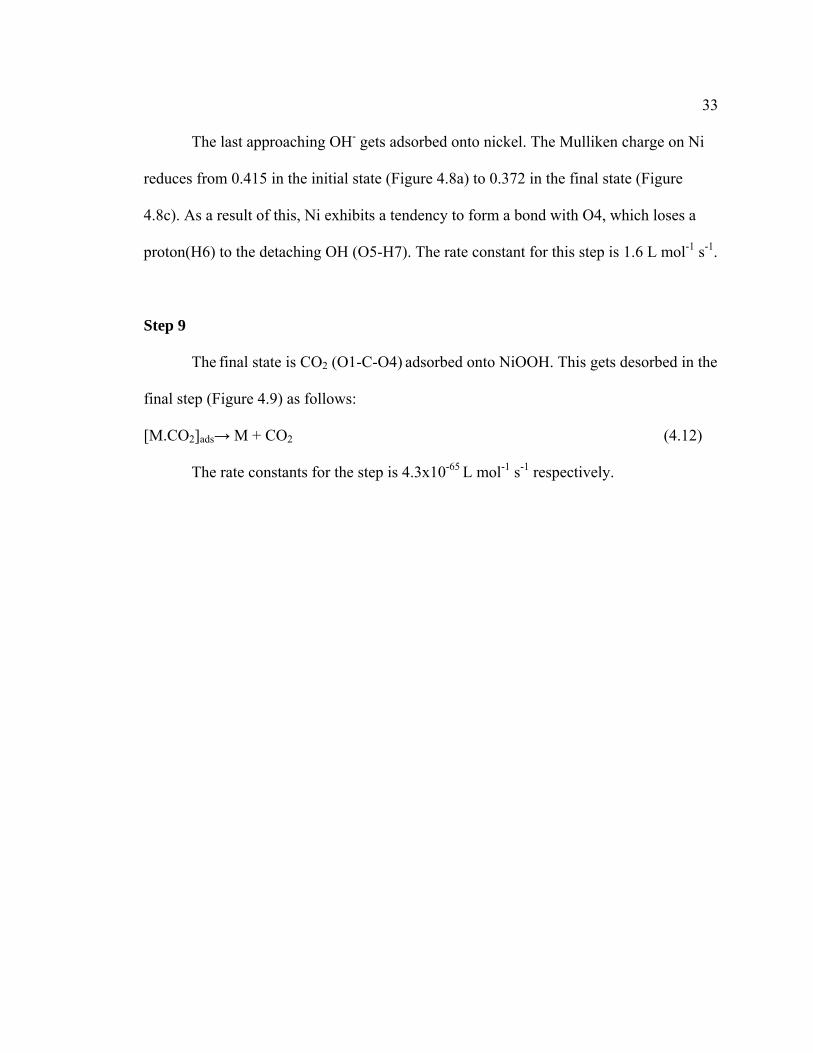
Figure 4.7: Initial state (a), transition state (b) and final structure (c) for Equation 4.10............................................................................................................................................ .34 

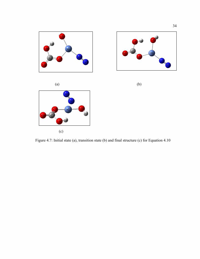
Figure 4.8: Initial state (a), transition state (b) and final structure (c) for Equation 4.11 .................................................................................................................... 35 

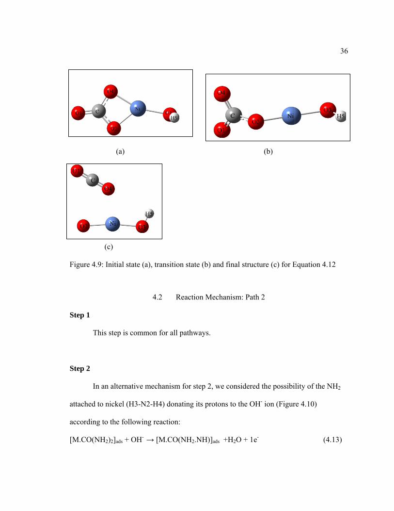
Figure 4.9: Initial state (a), transition state (b) and final structure (c) for Equation 4.12 .................................................................................................................... 36 

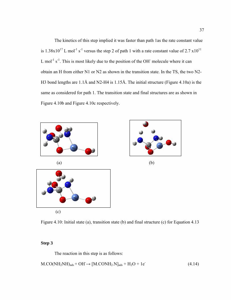
Figure 4.10: Initial state (a), transition state (b) and final structure (c) for Equation 4.13 .................................................................................................................... 37 

Figure 4.11: Initial state (a), transition state (b) and final structure (c) for Equation 4.14 .................................................................................................................... 38 

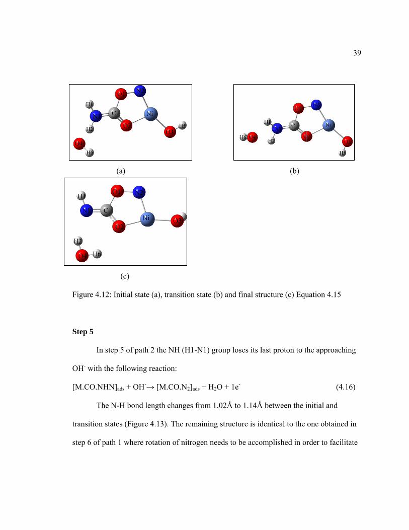
9 Figure 4.12: Initial state (a), transition state (b) and final structure (c) for Equation 4.15 .................................................................................................................... 39 

Figure 4.13: Initial state (a), transition state (b) and final structure (c) for Equation 4.16 .................................................................................................................... 40 

Figure 4.14: Initial state (a), transition state (b) and final structure (c) for rearrangement of amine groups................................................................................................................. 42 

Figure 4.15: Initial state (a), transition state (b) and final structure (c) for Equation 4.17……………………………………………………………………………………….42 

Figure 4.16: Initial state (a), transition state (b) and final structure (c) for Equation 4.18 .................................................................................................................... 44 

Figure 4.17: Initial state (a), transition state (b) and final structure (c) for Equation 4.17............................................................................................................................................ 45 

Figure 5.1: Optimized structures for different orientations of urea towards NiOOH ....... 52 

Figure 5.2: Optimized structures for Equations 5.1 and 5.2 ............................................. 54 

Figure 5.3: Optimized Transition States for Reactions 2 and 3 ........................................ 55 

Figure 5.4: Adsorption of OH- onto NiOOH .................................................................... 56 

Figure 5.5: Optimized structures for Equations 5.3 and 5.4. ............................................ 56 

Figure 5.6: Transition State Structures for Equations 5.3 and 5.4 .................................... 57 

Figure 6.1: Preliminary experiment. Different concentrations of KOH at 20g L-1 urea to determine lower setpoint. .................................................................................................. 62 

Figure 6.2: Urea concentration of 5 g L-1 varying KOH concentrations. Scan rate: 20mV s-1. Speed of rotation: 1000rpm. ............................................................................. 63 

Figure 6.3: Urea Concentration of 10 g L-1 with varying KOH concentrations. Scan Rate: 20mV s-1. Speed of rotation 1000rpm. .............................................................................. 63 

Figure 6.4: Urea concentration of 20 g L-1 with varying KOH concentrations. Scan rate 20mV s-1. Speed of rotation 1000 rpm. ............................................................................. 64 

10

Chapter 1 : INTRODUCTION

1.1 Project Overview

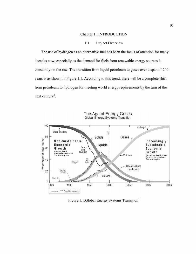
The use of hydrogen as an alternative fuel has been the focus of attention for many

decades now, especially as the demand for fuels from renewable energy sources is

constantly on the rise. The transition from liquid petroleum to gases over a span of 200

years is as shown in Figure 1.1. According to this trend, there will be a complete shift

from petroleum to hydrogen for meeting world energy requirements by the turn of the

next century1.

Figure 1.1:Global Energy Systems Transition1

11

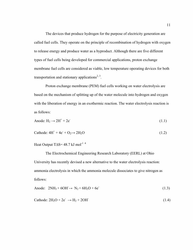
The devices that produce hydrogen for the purpose of electricity generation are

called fuel cells. They operate on the principle of recombination of hydrogen with oxygen

to release energy and produce water as a byproduct. Although there are five different

types of fuel cells being developed for commercial applications, proton exchange

membrane fuel cells are considered as viable, low temperature operating devices for both

transportation and stationary applications2, 3.

Proton exchange membrane (PEM) fuel cells working on water electrolysis are

based on the mechanism of splitting up of the water molecule into hydrogen and oxygen

with the liberation of energy in an exothermic reaction. The water electrolysis reaction is

as follows:

Anode: H2 → 2H+ + 2e- (1.1)

Cathode: 4H+ + 4e- + O2→ 2H2O (1.2)

Heat Output T∆S= 48.7 kJ mol-1 4

The Electrochemical Engineering Research Laboratory (EERL) at Ohio

University has recently devised a new alternative to the water electrolysis reaction:

ammonia electrolysis in which the ammonia molecule dissociates to give nitrogen as

follows:

Anode: 2NH3 + 6OH-→ N2 + 6H2O + 6e- (1.3)

Cathode: 2H2O + 2e- → H2 + 2OH- (1.4)

12

This process produces hydrogen to power PEM fuel cells and is a self sustainable

source of energy. It eliminates the problems associated with storing hydrogen as it

produces hydrogen on demand5-7.

An alternative to the above mentioned ammonia electrolysis process is urea

electrolysis, by means of which urine from animal farms and waste water lagoons can be

directly utilized to produce hydrogen to power fuel cells8. Urea is known to naturally

decompose to ammonia, hence is a major issue among farmers regarding taxes on

ammonia emissions9. This process once commercialized will not only help farmers

receive tax cuts for reduced ammonia emissions, but it will also decrease their

dependence on fossil fuels for power generation.

Urea electrolysis in alkaline medium is being investigated at the Electrochemical

Engineering Research Laboratory (EERL) at Ohio University as a novel technique for

hydrogen production. This project is of importance as it addresses the need to remediate

waste water from poultry farms as well as residential and commercial areas and using it

as a tool to solve one of the world’s impending energy crises. This following project was

undertaken to understand urea electrolysis for the purpose of generation of hydrogen for

fuel cells using theoretical and experimental methods.

Experimental methods will be combined with molecular modeling to gain a better

understanding of the electrolysis process. The reaction mechanisms are being studied

both chemically and electrochemically using the Gaussian 03 software. Experimental

techniques involve studying the effect of reaction parameters using a rotating disk

electrode.

13

1.2 Statement of Objectives

The purpose of this thesis is to gain a better understanding of the urea electrolysis

process in order to aid further development of the technology to make it commercially

viable for fuel cells. The following objectives are proposed to be accomplished with the

completion of the thesis.

1) Postulating reaction mechanisms for urea electrolysis using molecular modeling

techniques along with activation energies and rate constant calculations both in terms

of chemical oxidation and electrochemical oxidation. Under this objective, two

possible scenarios were considered:

i) Chemical Decomposition: Urea is known to dissociate naturally to ammonia

and carbamates. This reaction has been studied in the presence of the catalyst

nickel oxyhydroxide.

ii) Electrochemical Oxidation: Urea has also been found to undergo

electrochemical oxidation as found by the Electrochemical Engineering

Research Laboratory according to the following reactions:

Anode: CO(NH2)2(aq) + 6OH-→ N2(g) + 5H2O(l) + CO2 (aq) + 6e- (1.5)

Cathode: 6H2O (l) + 6e-→ 3H2(g) + 6OH- (1.6)

Overall: CO(NH2)2(aq) + H2O(l) → N2(g) + 3H2(g) + CO2 (aq) (1.7)

The elementary steps involved in the anodic reaction have been studied.

2) Determining the effect of reaction parameters such as concentration of potassium

hydroxide (KOH) and urea on process.

14

With the help of these reaction mechanisms and by determining the preferred

pathway as well as the rate determining step, measures can be taken to improve

efficiency of the process experimentally.

1.3 Significance of Research

The most important technological impact of this project arises from the utilization

of the most abundant waste on earth, urine, to produce cheap electricity. Apart from

being a significant source of hydrogen production, this technology can also be used to de-

nitrificate waste water, thus saving a huge amount of expenditure on waste water

remediation. At present, the permissible nitrate concentration in water is 10 mg L-1

however, most denitrification processes are expensive and ineffective10. Natural

hydrolysis of urea to ammonia leads to the formation of ammonium sulfate and

ammonium nitrate in the atmosphere which pose significant health hazards11. Hence, by

electrolyzing urea to useful products, we are able to bypass the formation of the hazard-

causing products.

Another important aspect is that the electrolytic cell potential required for the

overall reaction to occur is only 0.37 V at standard conditions. When this is compared to

the cell potential required to produce hydrogen (1.23 V), it amounts to generation of 70%

cheaper hydrogen theoretically12.

These factors emphasize the need for a better understanding of the ongoing

process, which has been achieved in this project by means of the invaluable tool of

molecular modeling.

15

Chapter 2 : LITERATURE REVIEW

2.1 Theoretical

Urea electrolysis is a modification of the ammonia electrolysis technology for the

purpose of generating hydrogen for fuel cells. Urea hydrolysis and decomposition

mechanisms have generated interest in the past in varied fields including removal of urea

from the blood using dialyzers and also formulation of urease inhibitors for better soil

fertility. When urea dissociates in the presence of the bio enzyme urea amidohydrolase 13-

15(urease), it leads to a sudden increase in pH of the soil due to the liberation of ammonia,

leading to its decreased fertility thus rendering it ineffective for agricultural purposes16, 17.

For this reason, biocatalytic decomposition of urea by urease which catalyzes the

reaction has been given considerable attention in the literature18-20. Urease decomposes

urea to ammonia and carbon dioxide under specific reaction conditions according to the

following reactions21:

( ) HNCONHNHCO 3urease

22 +⎯⎯ →⎯ (2.1)

NH3 + HNCO +H2O → 2NH3 + CO2 (2.2)

The enzyme urease comprises of two pseudo-octahedral Ni(II) ions as its active

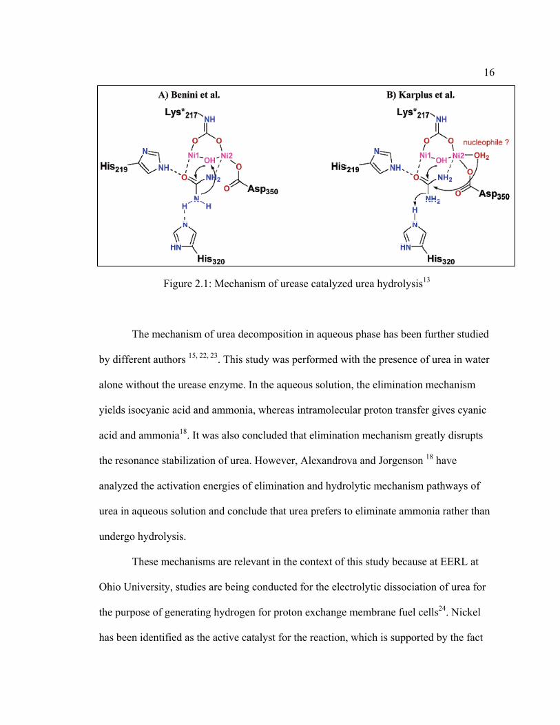
sites. Suarez et al.13 have proposed the reaction mechanisms for urea hydrolysis.

According to their work, urea binds to the two active nickel sites in urea in a bidentate

manner. The more electrophilic nickel attaches itself to the carbonyl group of urea, while

the other nickel atom attacks one of the amino groups. They have considered a bridging

hydroxide group between the two nickel atoms, which donates a proton to the amino

group that is attached to the second nickel atom as shown in Figure 2.1.

16

Figure 2.1: Mechanism of urease catalyzed urea hydrolysis13

The mechanism of urea decomposition in aqueous phase has been further studied

by different authors 15, 22, 23. This study was performed with the presence of urea in water

alone without the urease enzyme. In the aqueous solution, the elimination mechanism

yields isocyanic acid and ammonia, whereas intramolecular proton transfer gives cyanic

acid and ammonia18. It was also concluded that elimination mechanism greatly disrupts

the resonance stabilization of urea. However, Alexandrova and Jorgenson 18 have

analyzed the activation energies of elimination and hydrolytic mechanism pathways of

urea in aqueous solution and conclude that urea prefers to eliminate ammonia rather than

undergo hydrolysis.

These mechanisms are relevant in the context of this study because at EERL at

Ohio University, studies are being conducted for the electrolytic dissociation of urea for

the purpose of generating hydrogen for proton exchange membrane fuel cells24. Nickel

has been identified as the active catalyst for the reaction, which is supported by the fact

17 that urea undergoes natural hydrolysis in the presence of the urease enzyme which has

nickel as its active site.

An alkaline medium is used to carry out the electrolysis, and nickel undergoes

oxidation to its active state: nickel oxyhydroxide (NiOOH) in this medium by the

following reaction:

Ni(OH)2(s) + OH- → NiOOH(s) + H2O (l) + e- (2.3)

Nickel oxyhydroxide plays the role of an active catalyst in many alkaline

batteries, and has thus received considerable attention in electrochemical research.

This reaction is hypothesized to occur on the surface of the nickel electrode in the

presence of urea as well. As a result, it is important to study the interaction of the nickel

oxyhydroxide molecule with urea to come up with feasible reaction mechanisms for the

nature of interactions on the electrode surface.

The above mentioned modeling calculations have been performed using Gaussian

03 softwares. In an analogy to experimental operating conditions, theoretical calculations

comprise of basis sets which are the pre-defined parameters within the confines of which

the calculations are performed.

In the past, quantum chemical calculations have been performed using Linear

Combination of Atomic Orbitals Molecular Orbitals (LCAO MO). These molecular

orbitals exist as a linear combination of atomic orbitals as follows:

18

Where ψi is the ith molecular orbital, cμi are the coefficients of linear combination

andΦμis the μth atomic orbital and n is the number of atomic orbitals.25 These atomic

orbitals (AO) are solutions of the wave functions for a single electron in an atom. A basis

set is a set of these wave functions within the framework of which quantum chemical

calculations are performed. Basis sets play a crucial role in the binding energies obtained

from the molecular modeling calculations.

2.2 Experimental

Experimentally, urea electrolysis has been traditionally applied in techniques such

as dialysis and synthesis of carbon nitride thin films. These applications have been

studied in acidic medium with noble metals like platinum, iridium, ruthenium. Simka et

al.26 have investigated different compositions of Ti/(Pt-Ir), Ti/RuO2, Ti/(Ta2O5-IrO2) to

produce non toxic products with this reaction. But it is for the first time that alkaline

electrolysis of urea is being considered for the purpose of hydrogen production. Here we

have considered nickel as the catalyst for this reaction as it is cheap, economically

feasible and shows high activity for urea electrolysis. Currently, high concentrations of

alkali potassium hydroxide (KOH) are being used in the reaction. Typical concentration

used is 5 M (280 g L-1). It is important to examine the effect of KOH concentration to

investigate if lower concentrations can be used under the given operating conditions.

19

Chapter 3 : COMPUTATIONAL METHODS

With the primary purpose of elucidating the reaction mechanism, single molecule

interactions of NiOOH with urea have been considered. DFT calculations were carried

out using the Gaussian 03 program27 with the B3LYP correlation functional28. A mixed

basis set was used comprising of Los Alamos National Laboratory of double zeta quality

(LANL2DZ)29-31 and 6-31g*32 for carbon, nitrogen hydrogen and oxygen atoms, also

referred to as the LACVP* basis set. The comparison of the relevant geometrical

features of the urea molecule was reported on the B3LYP level in literature33 (Table 3.1).

These values of bond angles and bond lengths reported using the 6-31g* basis set were

found to be reasonably accurate in comparison with the experimental values. Considering

its requirement of less processing time, 6-31g* was chosen as a building block for these

calculations.

20

Table 3.1: Bond lengths and bond angles of urea as computed using different basis sets

with the B3LYP correlational functional.

Intra molecular bond lengths and angles (in Å and degree)

6-31g(d,p) DZP 6-311g(d,p) TZP exp

C-O 1.271 1.273 1.263 1.260 1.262

C-N 1.349 1.352 1.349 1.349 1.345

N-H1 1.014 1.022 1.012 1.011 1.009

O-C-N 121.4 121.4 121.6 121.6 121.4

N-C-N 117.1 117.2 116.9 116.7 117.2

C-N-H 119.9 119.9 119.9 120.0 119.1

For the electro oxidation reaction mechanisms the bond lengths for atoms of

NiOOH were kept constant at their experimental values34, 35 for the electrochemical

oxidation reactions as follows in Table 3.2:

Table 3.2 : Experimental bond lengths for NiOOH kept constant for the reaction

mechanisms

X-Y Pair Bond Length (Å)

Ni-O 1.88

Ni-OH 1.91

O-H 0.956

21

No further geometry constraints were placed on the system. The Gaussian 03

algorithm was used to calculate the vibrational frequency and analytical force constant

calculations on all structures. The transition states for all elementary steps were located

implementing the default Gaussian 03 method. The transition state geometry possessed

two imaginary frequencies: one corresponding to the geometry constraint placed on

NiOOH (the O-H bond) and the other corresponding to the transition state (TS) structure.

Animation of the particular transition state negative frequency verified that the TS

corresponded to the interacting atoms for the particular step under consideration.

The rate constant calculations based on the transition state theory36 were performed using

partition functions as shown in the following equation:

k =kBT

hq#

qjj=1

n∏

⎛

⎝

⎜ ⎜ ⎜

⎞

⎠

⎟ ⎟ ⎟ exp

−Ei

RT⎛ ⎝ ⎜

⎞ ⎠ ⎟ (3.1)

where,

k= rate constant (L mol-1 s-1)

qt=partition function for transition state (Hartrees)

qr=partition function for reactant (Hartrees)

Ei= difference in zero point energies of reactants and transition state structures(J mol-1)

kb =Boltzmann’s constant= 1.38x10-23 J K-1

h= Planck’s constant= 6.63x10-34 J s

T= 298 K

R= Universal gas constant=8.314 J K-1 mol-1

22

On solving the above equation for a second order reaction, the rate constant value

is obtained in L mol-1 s-1 upon multiplying by a unit concentration term.

The free energies in Gaussian 03 are evaluated from the vibrational frequency analysis,

which is in turn used to determing the partition function based on the harmonic oscillator

model. Therefore, the underlying assumption in this analysis is that the second derivative

matrix is evaluated at a point on the potential energy surface where the gradient is zero.

As such, since the gradient is zero, the coupling between the nuclear degrees of freedom

and the molecular orbital coefficients can be ignored.

When using geometry constraints, the non-zero forces are ignored while

evaluating the optimization criteria. As a result, the energy values change and these

changes cannot be measured legitimately with the implementation of geometry

constraints during optimization. Hence for the thermodynamic calculations, individual

intermediate structures were considered with the entering OH- and leaving H2O

molecules with no geometry constraints on the NiOOH molecule. . For the chemical

oxidation mechanisms no geometry constraints were placed on the system.

23

Chapter 4 : ELECTRO OXIDATION MECHANISMS

The urea electro-oxidation reactions are as follows12:

Anode: CO(NH2)2(aq) + 6OH-→ N2(g) + 5H2O(l) + CO2 (aq) + 6e- (4.1)

Cathode: 6H2O (l) + 6e-→ 3H2(g) + 6OH- (4.2)

Overall: CO(NH2)2(aq) + H2O(l) → N2(g) + 3H2(g) + CO2 (aq) (4.3)

The anodic reaction is proposed to be taking place on nickel which undergoes

oxidation according to the following reaction in an alkaline medium:

Ni(OH)2(s) + OH- → NiOOH(s) + H2O (l) + e- (4.4)

Within this context the objective in this study is to use Density Functional Theory

(DFT) methods to predict the mechanism and rate determining step of the anodic urea

oxidation reaction on the NiOOH surface. This study is significant in order to understand

and improve overall efficiency of the experimental process of urea electro oxidation. In

order to predict the reaction mechanisms, the electronic energy barriers for the

elementary steps were estimated. Based on these steps, three reaction mechanisms have

been predicted. The proposed reaction mechanisms are as shown in Table 2. To

summarize the pathways, the first step involved the adsorption of urea onto the NiOOH

catalyst, and was common for all three mechanisms. From here onwards, path 1

demonstrated the initial loss of protons from the amino group H1-N1-H2, while path 2

involved the initial loss of protons from the second amino group H3-N2-H4. In path 3,

the amino groups bonded together by the rotation of the group H1-N1-H2 towards N2-

H3, whereas in paths 1 and 2 this rotation takes place only after the elimination of all

protons from the adsorbed species.

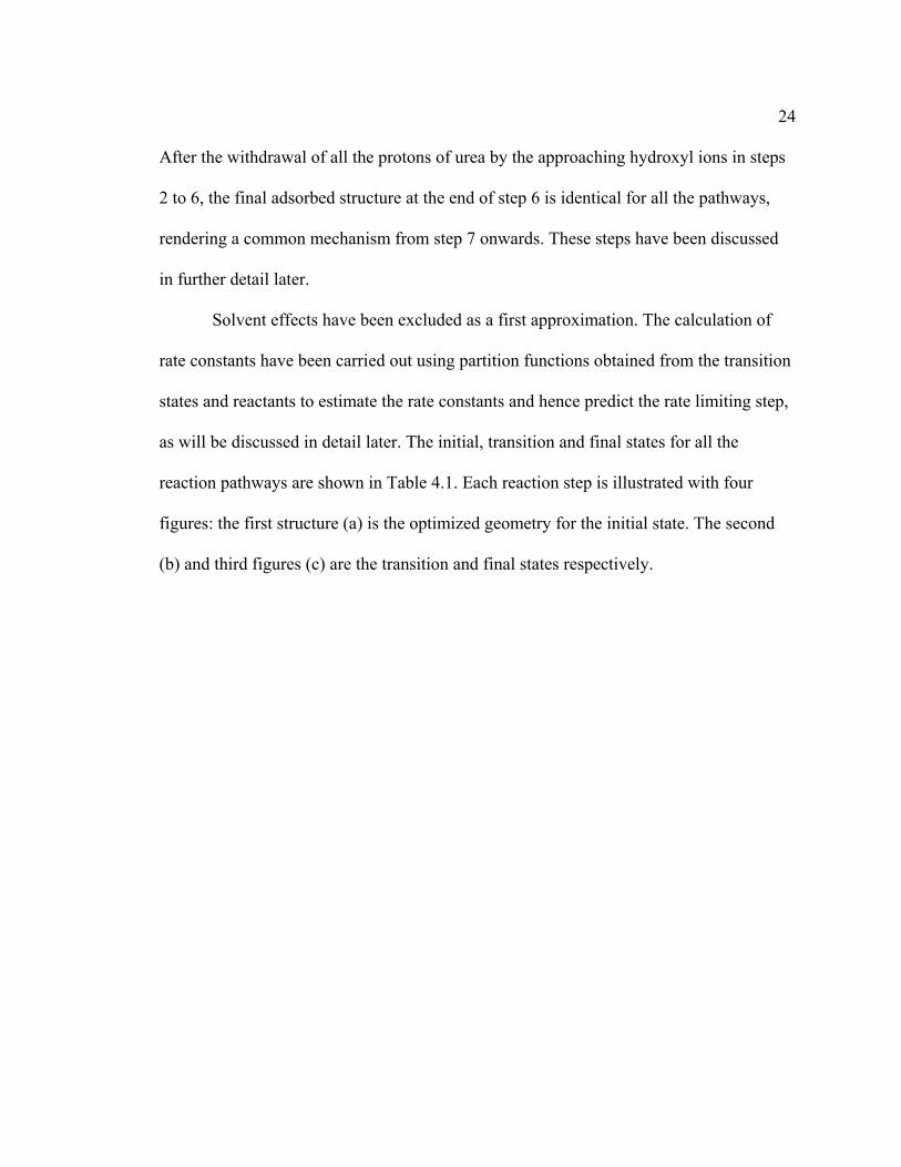
24 After the withdrawal of all the protons of urea by the approaching hydroxyl ions in steps

2 to 6, the final adsorbed structure at the end of step 6 is identical for all the pathways,

rendering a common mechanism from step 7 onwards. These steps have been discussed

in further detail later.

Solvent effects have been excluded as a first approximation. The calculation of

rate constants have been carried out using partition functions obtained from the transition

states and reactants to estimate the rate constants and hence predict the rate limiting step,

as will be discussed in detail later. The initial, transition and final states for all the

reaction pathways are shown in Table 4.1. Each reaction step is illustrated with four

figures: the first structure (a) is the optimized geometry for the initial state. The second

(b) and third figures (c) are the transition and final states respectively.

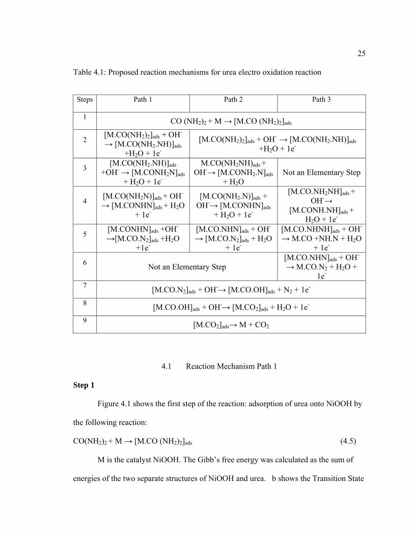
25 Table 4.1: Proposed reaction mechanisms for urea electro oxidation reaction

4.1 Reaction Mechanism Path 1

Step 1

Figure 4.1 shows the first step of the reaction: adsorption of urea onto NiOOH by

the following reaction:

CO(NH2)2 + M → [M.CO (NH2)2]ads (4.5)

M is the catalyst NiOOH. The Gibb’s free energy was calculated as the sum of

energies of the two separate structures of NiOOH and urea. b shows the Transition State

Steps Path 1 Path 2 Path 3

1 CO (NH2)2 + M → [M.CO (NH2)2]ads

2 [M.CO(NH2)2]ads + OH-

→ [M.CO(NH2.NH)]ads +H2O + 1e-

[M.CO(NH2)2]ads + OH- → [M.CO(NH2.NH)]ads +H2O + 1e-

3 [M.CO(NH2.NH)]ads +OH- → [M.CONH2N]ads

+ H2O + 1e-

M.CO(NH2NH)ads + OH-→ [M.CONH2.N]ads

+ H2O Not an Elementary Step

4 [M.CO(NH2N)]ads + OH-

→ [M.CONHN]ads + H2O + 1e-

[M.CO(NH2.N)]ads + OH-→ [M.CONHN]ads

+ H2O + 1e-

[M.CO.NH2NH]ads + OH-→

[M.CONH.NH]ads + H2O + 1e-

5 [M.CONHN]ads +OH-

→[M.CO.N2]ads +H2O +1e-

[M.CO.NHN]ads + OH-

→ [M.CO.N2]ads + H2O + 1e-

[M.CO.NHNH]ads + OH-

→ M.CO +NH.N + H2O + 1e-

6 Not an Elementary Step [M.CO.NHN]ads + OH- → M.CO.N2 + H2O +

1e- 7 [M.CO.N2]ads + OH-→ [M.CO.OH]ads + N2 + 1e- 8 [M.CO.OH]ads + OH-→ [M.CO2]ads + H2O + 1e- 9 [M.CO2]ads→ M + CO2

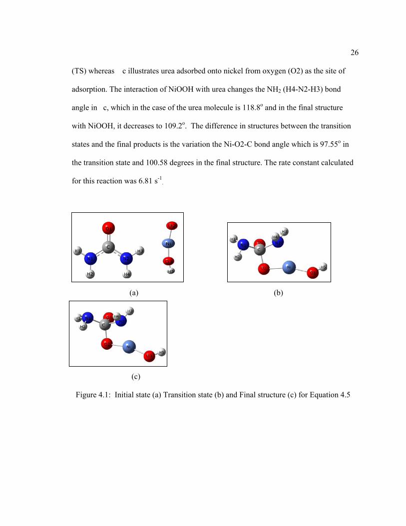
(T

ad

an

w

st

th

fo

F

TS) whereas

dsorption. T

ngle in c, w

with NiOOH,

tates and the

he transition

or this reacti

Figure 4.1:

s c illustrat

The interactio

which in the

, it decreases

e final produ

state and 10

ion was 6.81

(a)

(c)

Initial state

tes urea adso

on of NiOOH

case of the u

s to 109.2o.

cts is the var

00.58 degree

s-1.

(a) Transitio

orbed onto ni

H with urea c

urea molecul

The differen

riation the N

es in the fina

on state (b) a

ickel from o

changes the

le is 118.8o a

nce in structu

Ni-O2-C bon

al structure. T

and Final stru

oxygen (O2)

NH2 (H4-N

and in the fin

ures between

nd angle whic

The rate con

(b)

ucture (c) fo

as the site o

2-H3) bond

nal structure

n the transiti

ch is 97.55o

nstant calcula

or Equation 4

26

of

e

ion

in

ated

4.5

F

S

th

[M

w

N

2

(c)

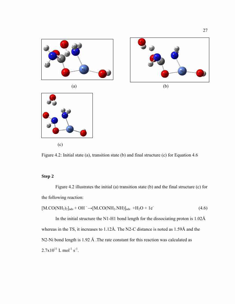
igure 4.2: In

tep 2

Figure

he following

M.CO(NH2)

In the

whereas in th

N2-Ni bond l

.7x1011 L m

(a)

nitial state (a

e 4.2 illustra

g reaction:

2]ads + OH - →

initial struc

he TS, it incr

length is 1.92

mol-1 s-1.

a), transition

ates the initia

→[M.CO(N

ture the N1-

eases to 1.12

2 Å .The rat

state (b) and

al (a) transiti

NH2.NH)]ads

-H1 bond len

2Å. The N2-

e constant fo

d final struct

ion state (b)

+H2O + 1e-

ngth for the d

-C distance i

or this reacti

(b)

ture (c) for E

and the fina

dissociating

is noted as 1

ion was calcu

Equation 4.6

al structure (c

proton is 1.0

.59Å and th

ulated as

27

c) for

(4.6)

02Å

e

28 Step 3

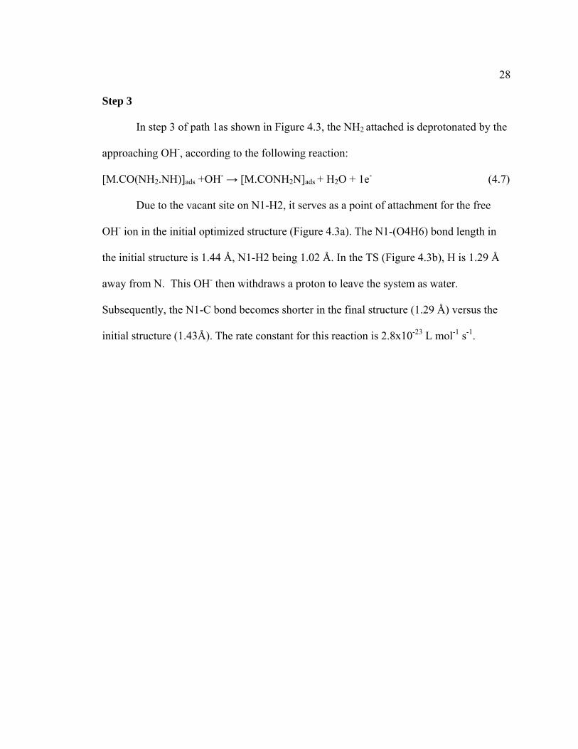
In step 3 of path 1as shown in Figure 4.3, the NH2 attached is deprotonated by the

approaching OH-, according to the following reaction:

[M.CO(NH2.NH)]ads +OH- → [M.CONH2N]ads + H2O + 1e- (4.7)

Due to the vacant site on N1-H2, it serves as a point of attachment for the free

OH- ion in the initial optimized structure (Figure 4.3a). The N1-(O4H6) bond length in

the initial structure is 1.44 Å, N1-H2 being 1.02 Å. In the TS (Figure 4.3b), H is 1.29 Å

away from N. This OH- then withdraws a proton to leave the system as water.

Subsequently, the N1-C bond becomes shorter in the final structure (1.29 Å) versus the

initial structure (1.43Å). The rate constant for this reaction is 2.8x10-23 L mol-1 s-1.

F

S

[M

W

aw

st

as

Å

L

igure 4.3: In

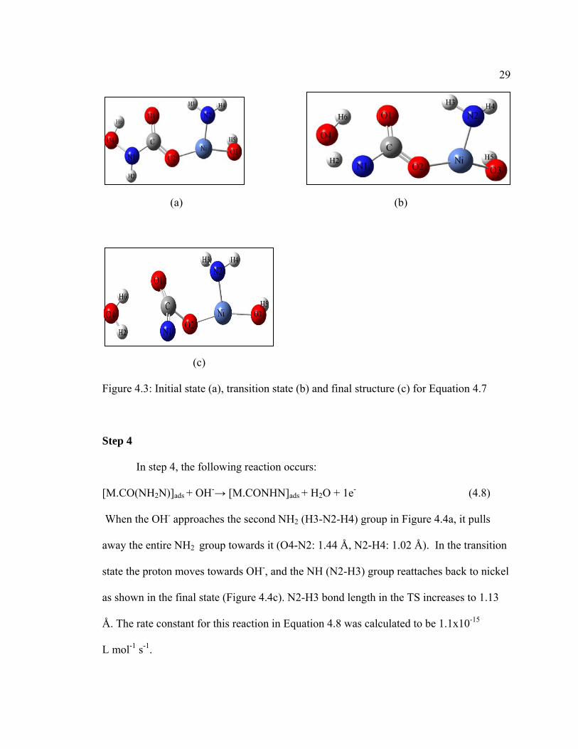
tep 4

In step

M.CO(NH2N

When the OH

way the enti

tate the proto

s shown in th

Å. The rate co

L mol-1 s-1.

(a)

(c)

nitial state (a

p 4, the follo

N)]ads + OH-→

H- approache

ire NH2 grou

on moves tow

he final state

onstant for t

a), transition

owing reactio

→ [M.CONH

es the second

up towards i

wards OH-,

e (Figure 4.4

his reaction

state (b) and

on occurs:

HN]ads + H2O

d NH2 (H3-N

t (O4-N2: 1.

and the NH

4c). N2-H3 b

in Equation

d final struct

O + 1e-

N2-H4) grou

.44 Å, N2-H

(N2-H3) gro

bond length

4.8 was calc

(b)

ture (c) for E

up in Figure

H4: 1.02 Å).

oup reattach

in the TS inc

culated to be

Equation 4.7

(4.8

4.4a, it pulls

In the transi

hes back to n

creases to 1.

e 1.1x10-15

29

)

s

ition

nickel

.13

F

S

(O

th

[M

an

In

T

igure 4.4: In

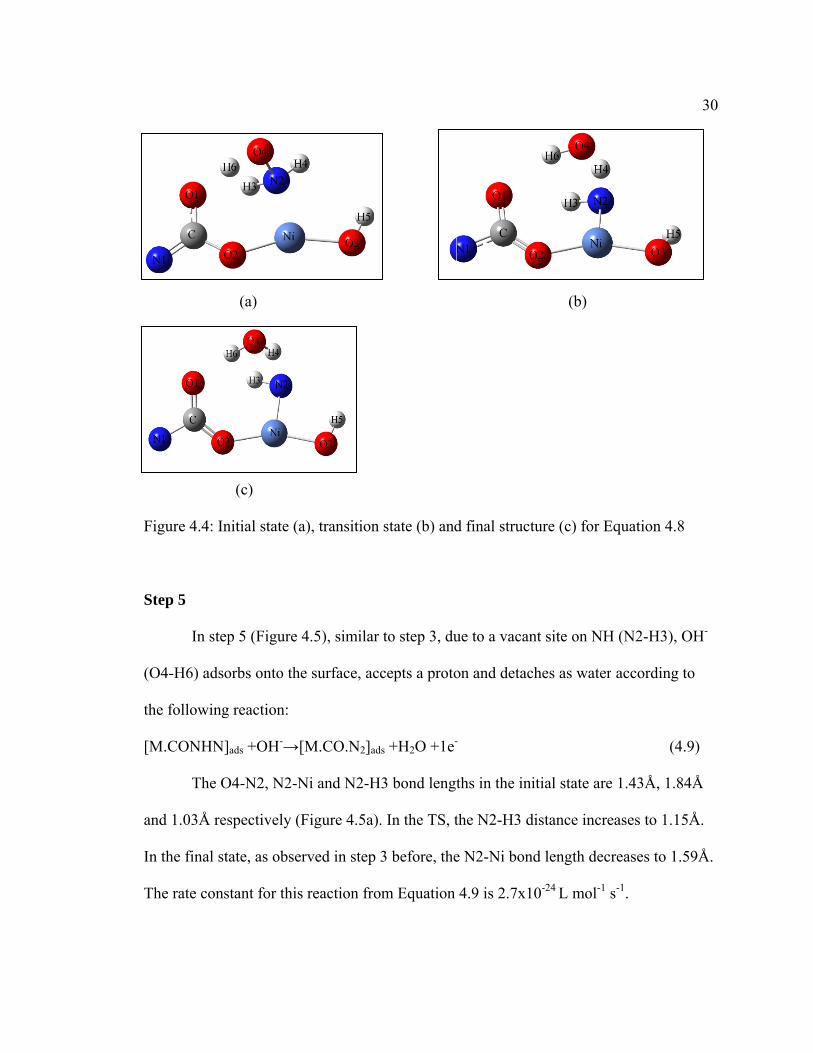
tep 5

In step

O4-H6) adso

he following

M.CONHN]

The O

nd 1.03Å res

n the final st

The rate cons

(a)

(c)

nitial state (a

p 5 (Figure 4

orbs onto the

g reaction:

ads +OH-→[

O4-N2, N2-N

spectively (F

tate, as obser

stant for this

a), transition

4.5), similar

e surface, acc

M.CO.N2]ad

Ni and N2-H

Figure 4.5a).

rved in step

reaction fro

state (b) and

to step 3, du

cepts a proto

ds +H2O +1e-

H3 bond lengt

. In the TS, t

3 before, the

om Equation

d final struct

ue to a vacan

on and detac

-

ths in the ini

the N2-H3 d

e N2-Ni bon

4.9 is 2.7x1

(b)

ture (c) for E

nt site on NH

ches as water

itial state are

distance incre

nd length dec

0-24 L mol-1

Equation 4.8

H (N2-H3), O

r according t

(4.

e 1.43Å, 1.84

eases to 1.15

creases to 1.5

s-1.

30

OH-

to

.9)

4Å

5Å.

59Å.

F

S

si

su

fo

b

st

N

O

igure 4.5: In

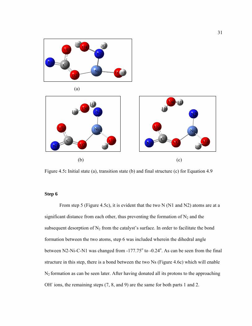
tep 6

From

ignificant di

ubsequent de

ormation bet

etween N2-N

tructure in th

N2 formation

OH- ions, the

(a)

(b)

nitial state (a

step 5 (Figu

stance from

esorption of

tween the tw

Ni-C-N1 wa

his step, ther

as can be se

remaining s

a), transition

ure 4.5c), it i

each other,

f N2 from the

wo atoms, ste

as changed fr

re is a bond b

een later. Aft

steps (7, 8, a

state (b) and

s evident tha

thus prevent

e catalyst’s s

ep 6 was incl

rom -177.75

between the

ter having do

and 9) are the

d final struct

at the two N

ting the form

surface. In or

luded where

o to -0.24o. A

two Ns (Fig

onated all its

e same for b

(c)

ture (c) for E

(N1 and N2

mation of N2

rder to facili

ein the dihed

As can be se

gure 4.6c) wh

s protons to t

oth parts 1 a

Equation 4.9

2) atoms are

and the

itate the bond

dral angle

een from the

hich will ena

the approach

and 2.

31

9

at a

d

final

able

hing

F

n

S

th

[

n

S

[

igure 4.6: In

itrogen atom

tep 7

In step

he N2 is deso

[M.CO.N2]ad

The O

ickel. The ra

tep 8

The n

[M.CO.OH]a

(a)

(c)

nitial state (a

ms

p 7 (Figure 4

orbed simult

ds + OH-→ [M

OH- gets adso

ate constant

next reaction

ads + OH-→

a), transition

4.7), the app

aneously wi

M.CO.OH]ad

orbed onto c

for this step

in step 8 (F

[M.CO2]ads +

state (b) and

proaching OH

ith the follow

ds + N2 + 1e-

carbon where

is 7.3 x108 L

Figure 4.8) is

+ H2O + 1e-

d final struct

H- ion is ads

wing reaction

-

eas the N2 m

L mol-1 s-1.

s as follows:

(b)

ture (c) for r

orbed on the

n:

molecule gets

re-arrangeme

e surface wh

(4.1

s desorbed fr

(4.11

32

ent of

hile

10)

rom

1)

33

The last approaching OH- gets adsorbed onto nickel. The Mulliken charge on Ni

reduces from 0.415 in the initial state (Figure 4.8a) to 0.372 in the final state (Figure

4.8c). As a result of this, Ni exhibits a tendency to form a bond with O4, which loses a

proton(H6) to the detaching OH (O5-H7). The rate constant for this step is 1.6 L mol-1 s-1.

Step 9

The final state is CO2 (O1-C-O4) adsorbed onto NiOOH. This gets desorbed in the

final step (Figure 4.9) as follows:

[M.CO2]ads→ M + CO2 (4.12)

The rate constants for the step is 4.3x10-65 L mol-1 s-1 respectively.

F

(

igure 4.7: In

(a)

(c)

nitial state (a

a), transition

state (b) and

d final struct

(b)

ture (c) for EEquation 4.1

34

0

F

(a

igure 4.8: In

)

(c)

nitial state (a

a), transition

state (b) and

(b)

d final structture (c) for E

Equation 4.1

35

1

F

S

S

at

ac

[M

(c

igure 4.9: In

tep 1

This s

tep 2

In an

ttached to ni

ccording to t

M.CO(NH2)

(a)

)

nitial state (a

step is comm

alternative m

ickel (H3-N2

the followin

2]ads + OH- →

a), transition

4.2 Re

mon for all pa

mechanism f

2-H4) donati

ng reaction:

→ [M.CO(N

state (b) and

action Mech

athways.

for step 2, we

ing its proto

NH2.NH)]ads

d final struct

hanism: Path

e considered

ns to the OH

+H2O + 1e-

(b)

ture (c) for E

h 2

d the possibi

H- ion (Figur

-

Equation 4.1

lity of the N

re 4.10)

(4.

36

2

NH2

13)

is

L

ob

H

sa

F

F

S

M

The k

s 1.38x1017 L

L mol-1 s-1. Th

btain an H fr

H3 bond leng

ame as consi

igure 4.10b

(a)

(c)

igure 4.10: I

tep 3

The re

M.CO(NH2N

kinetics of thi

L mol-1 s-1 ve

his is most l

from either N

gths are 1.1Å

idered for pa

and Figure 4

Initial state (

eaction in th

NH)ads + OH-→

is step impli

ersus the ste

likely due to

N1 or N2 as s

Å and N2-H4

ath 1. The tra

4.10c respec

(a), transition

his step is as

→ [M.CONH

ied it was fas

ep 2 of path 1

the position

shown in the

4 is 1.15Å. T

ansition stat

ctively.

n state (b) an

follows:

H2.N]ads + H

ster than pat

1 with a rate

n of the OH-

e transition s

The initial str

e and final s

(b

nd final struc

H2O + 1e-

th 1as the rat

e constant va

molecule wh

state. In the T

ructure (Figu

structures are

b)

cture (c) for

te constant v

alue of 2.7 x1

here it can

TS, the two

ure 4.10a) is

e as shown i

Equation 4.

(4.1

37

value

1011

N2-

s the

n

13

14)

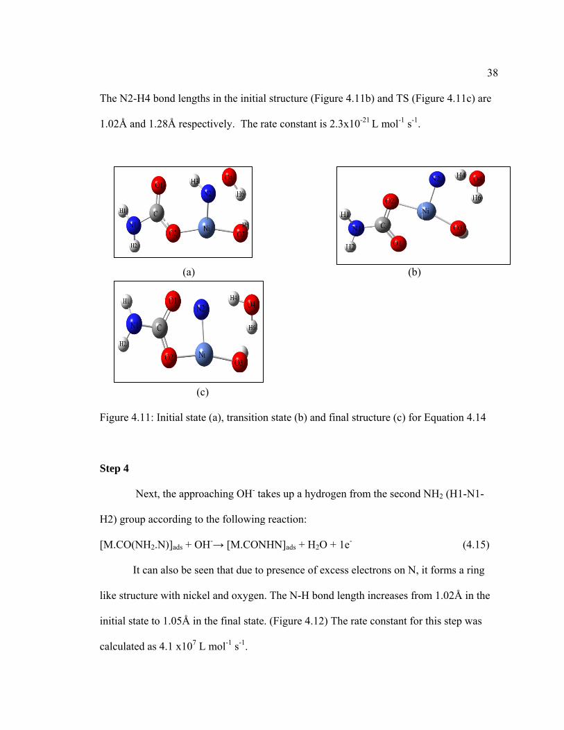
T

1

F

S

H

[M

li

in

ca

The N2-H4 b

.02Å and 1.2

igure 4.11: I

tep 4

Next,

H2) group ac

M.CO(NH2.N

It can

ike structure

nitial state to

alculated as

ond lengths

28Å respecti

(a)

(c)

Initial state (

, the approac

cording to th

N)]ads + OH-

also be seen

with nickel

o 1.05Å in th

4.1 x107 L m

in the initial

ively. The r

(a), transition

ching OH- ta

he following

-→ [M.CON

n that due to

and oxygen

he final state

mol-1 s-1.

l structure (F

rate constant

n state (b) an

akes up a hyd

g reaction:

NHN]ads + H2

presence of

n. The N-H b

. (Figure 4.1

Figure 4.11b

t is 2.3x10-21

nd final struc

drogen from

2O + 1e-

f excess elec

bond length i

12) The rate

b) and TS (Fi

L mol-1 s-1.

(b)

cture (c) for

m the second

trons on N, i

increases fro

constant for

igure 4.11c)

Equation 4.

NH2 (H1-N

(4.

it forms a rin

om 1.02Å in

r this step wa

38

are

14

1-

15)

ng

the

as

F

S

O

[M

tr

st

igure 4.12: I

tep 5

In step

OH- with the

M.CO.NHN

The N

ransition stat

tep 6 of path

(a)

(c)

Initial state (

p 5 of path 2

following re

]ads + OH-→

N-H bond len

tes (Figure 4

h 1 where rot

(a), transition

2 the NH (H

eaction:

→ [M.CO.N2]

ngth changes

4.13). The re

tation of nitr

n state (b) an

1-N1) group

]ads + H2O +

s from 1.02Å

emaining stru

rogen needs

nd final struc

p loses its las

1e-

Å to 1.14Å b

ucture is iden

to be accom

(b)

cture (c) Equ

st proton to t

between the i

ntical to the

mplished in o

uation 4.15

the approach

(4.

initial and

one obtaine

order to facili

39

hing

16)

d in

itate

d

F

F

esorption of

rom here on

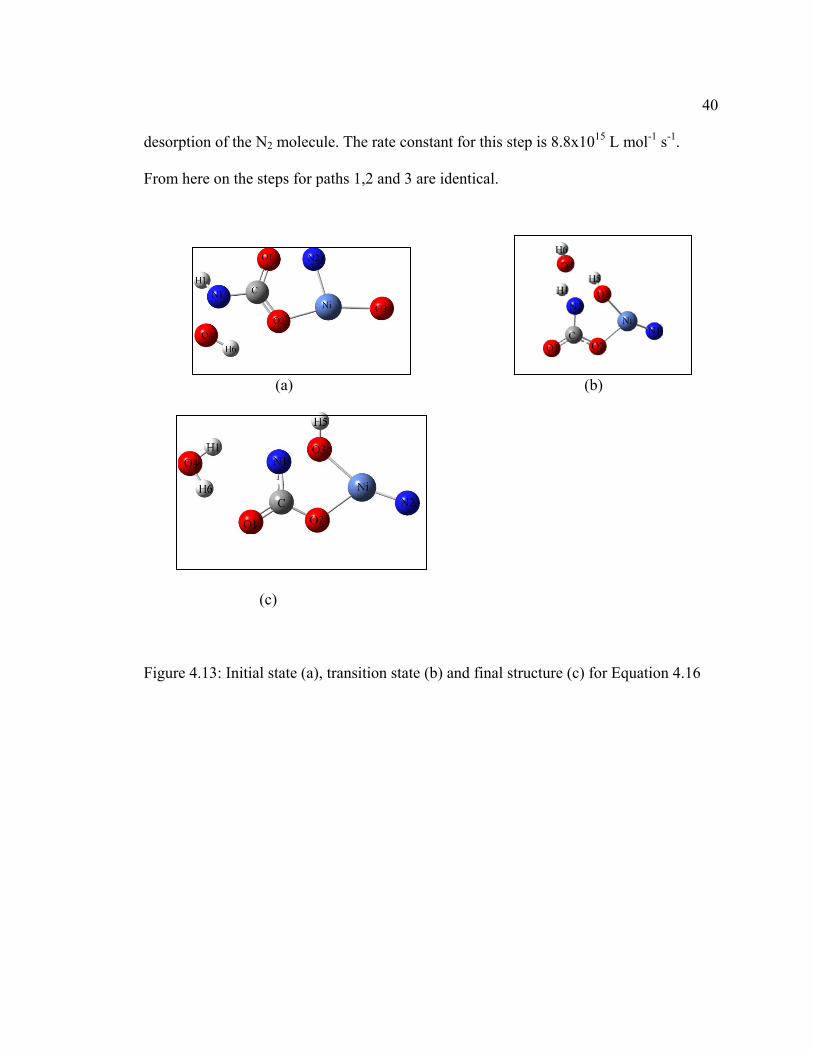
igure 4.13: I

f the N2 mole

n the steps fo

(a)

(c)

Initial state (

ecule. The ra

or paths 1,2 a

(a), transition

ate constant

and 3 are ide

n state (b) an

for this step

entical.

nd final struc

is 8.8x1015

(b)

cture (c) for

L mol-1 s-1.

Equation 4.

40

16

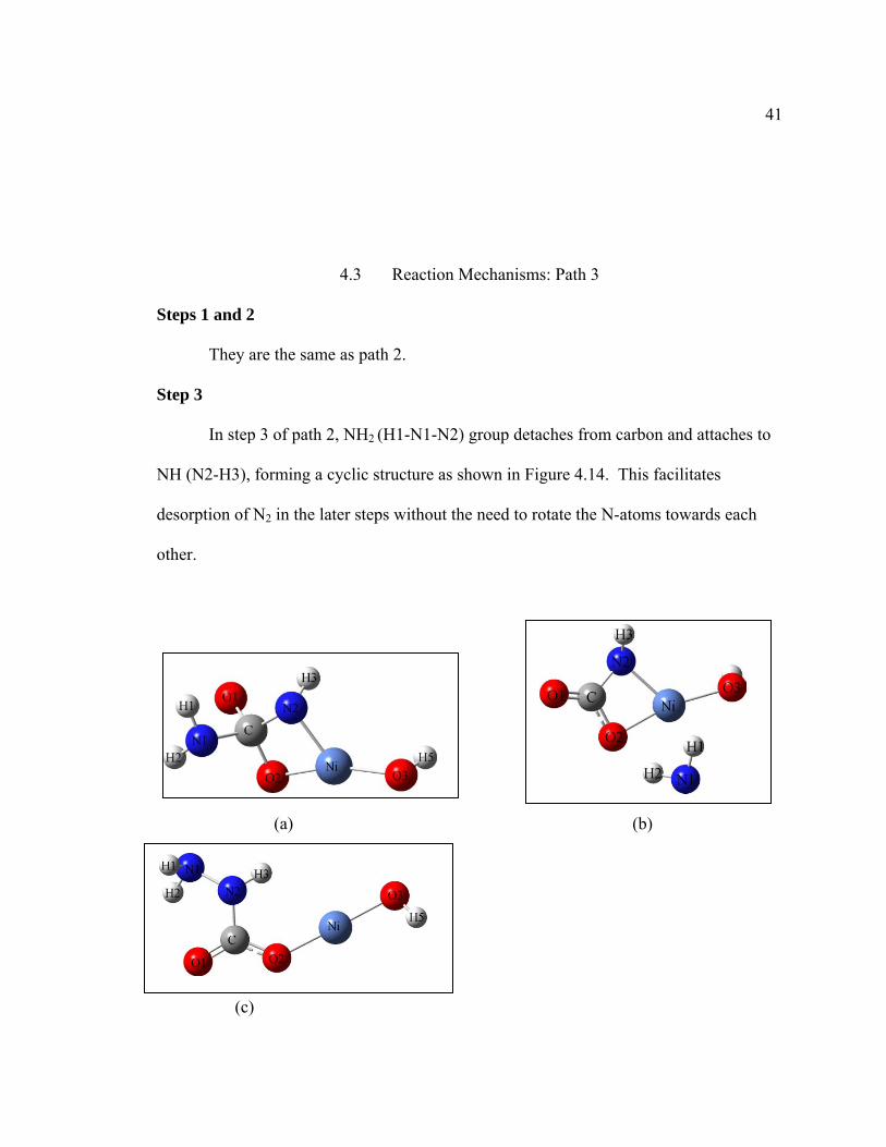
S

S

N

d

ot

teps 1 and 2

They

tep 3

In step

NH (N2-H3),

esorption of

ther.

(c

2

are the same

p 3 of path 2

, forming a c

f N2 in the la

(a)

)

4.3 Rea

e as path 2.

2, NH2 (H1-N

cyclic structu

ater steps wit

action Mech

N1-N2) grou

ure as shown

thout the nee

hanisms: Path

up detaches f

n in Figure 4

ed to rotate t

h 3

from carbon

4.14. This fa

the N-atoms

(b)

and attache

acilitates

towards eac

41

s to

ch

F

o

S

O

[M

pr

th

pr

4

1

F

igure 4.14: I

f amine grou

tep 4

In the

OH- ion, form

M.CO.NH2N

As sho

roton from e

he rate const

roton are 1.0

.15b) respec

.43Å to 1.39

(a)

igure 4.15: I

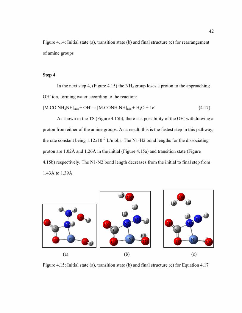
Initial state (

ups

next step 4,

ming water a

NH]ads + OH-

own in the T

either of the

tant being 1.

02Å and 1.26

ctively. The N

9Å.

)

Initial state (

(a), transition

, (Figure 4.1

according to

-→ [M.CON

TS (Figure 4

amine group

12x1017 L/m

6Å in the ini

N1-N2 bond

(a), transition

n state (b) an

5) the NH2 g

the reaction

NH.NH]ads +

.15b), there

ps. As a resu

mol.s. The N

itial (Figure

d length decr

(b)

n state (b) an

nd final struc

group loses a

:

H2O + 1e-

is a possibil

ult, this is the

1-H2 bond l

4.15a) and t

reases from t

nd final struc

cture (c) for

a proton to th

lity of the OH

e fastest step

lengths for th

transition sta

the initial to

cture (c) for

rearrangeme

he approach

(4.

H- withdraw

p in this path

he dissociati

ate (Figure

final step fr

(c)

Equation 4.

42

ent

ing

17)

wing a

hway,

ing

rom

17

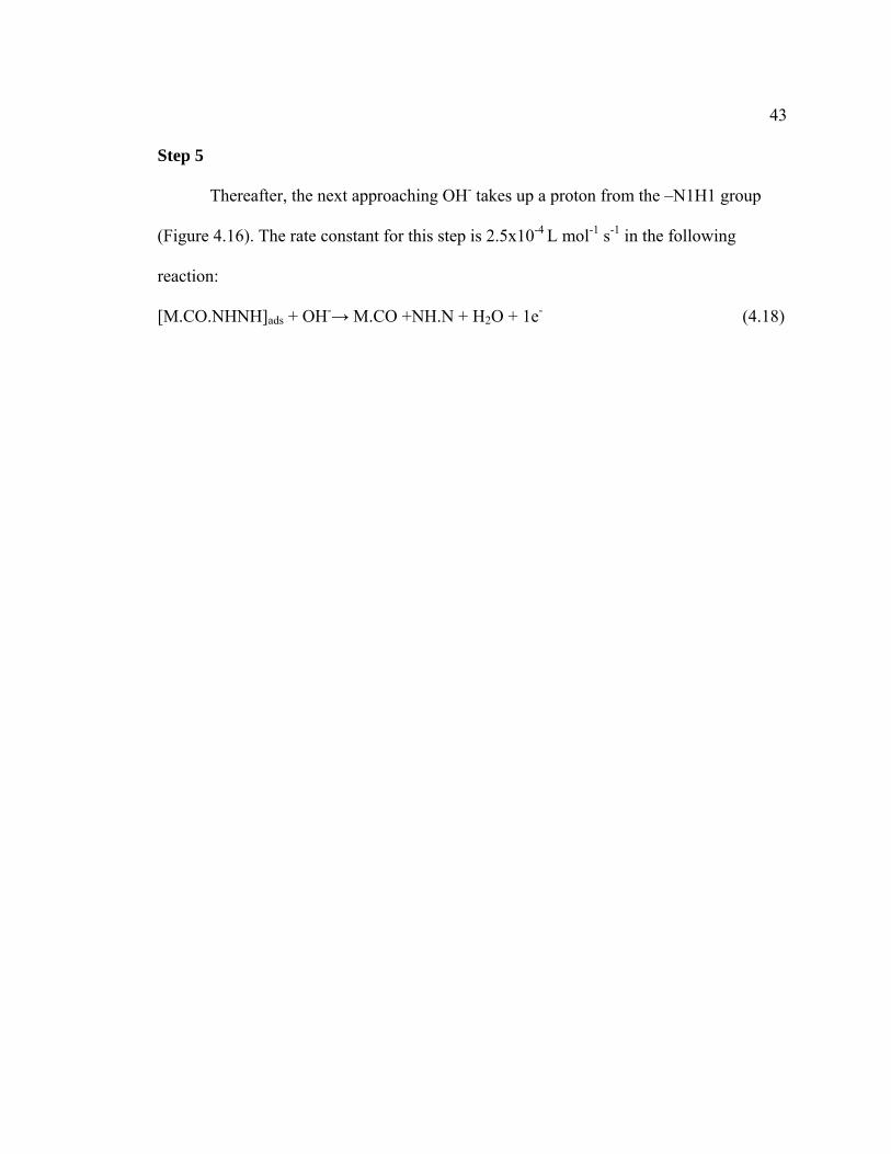
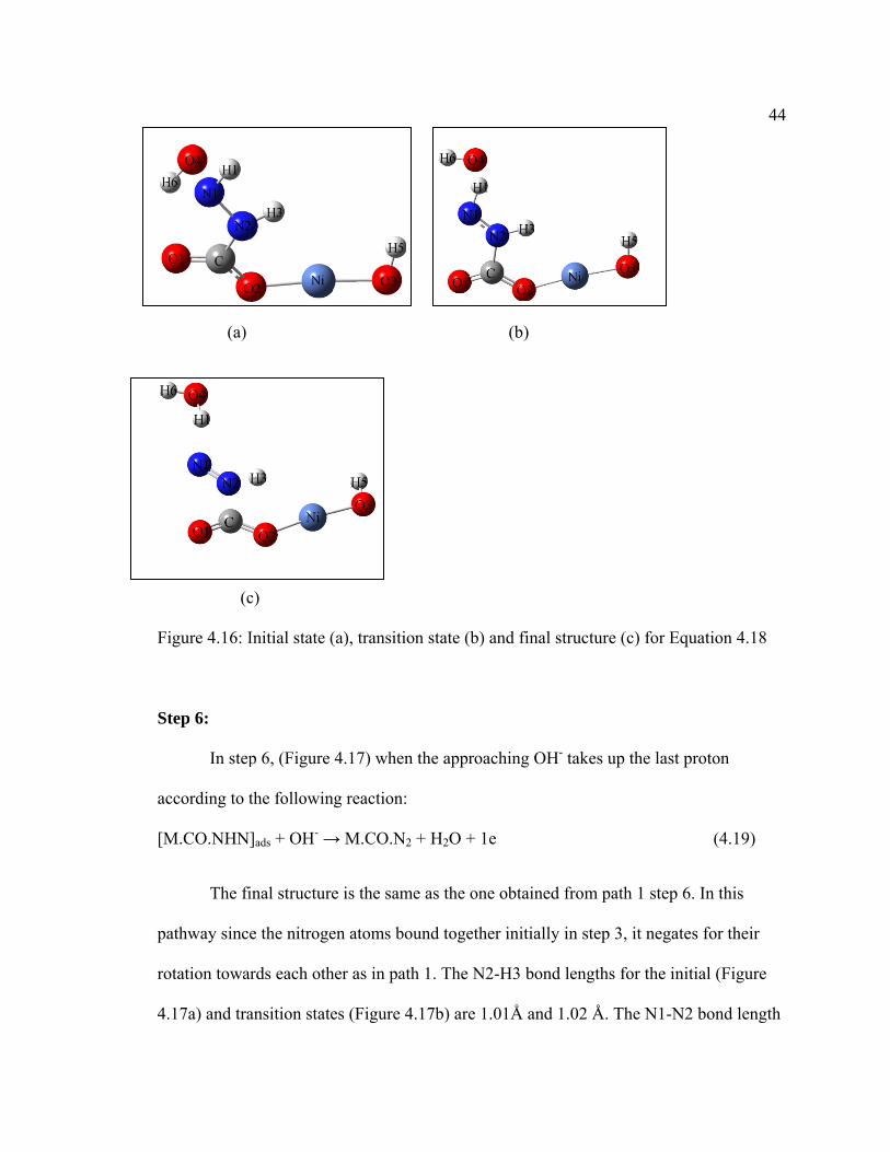
43 Step 5

Thereafter, the next approaching OH- takes up a proton from the –N1H1 group

(Figure 4.16). The rate constant for this step is 2.5x10-4 L mol-1 s-1 in the following

reaction:

[M.CO.NHNH]ads + OH-→ M.CO +NH.N + H2O + 1e- (4.18)

F

S

ac

[M

p

ro

4

(a)

(c

igure 4.16: I

tep 6:

In step

ccording to t

M.CO.NHN

The fi

athway since

otation towa

.17a) and tra

c)

Initial state (

p 6, (Figure

the followin

]ads + OH- →

inal structure

e the nitroge

ards each oth

ansition state

(a), transition

4.17) when

ng reaction:

→ M.CO.N2

e is the same

en atoms bou

her as in path

es (Figure 4.

n state (b) an

the approach

+ H2O + 1e

e as the one

und together

h 1. The N2-

.17b) are 1.0

(b)

nd final struc

hing OH- tak

obtained fro

r initially in s

H3 bond len

01Å and 1.02

cture (c) for

kes up the la

om path 1 ste

step 3, it neg

ngths for the

2 Å. The N1

Equation 4.

ast proton

(4.19

ep 6. In this

gates for thei

initial (Figu

-N2 bond le

44

18

)

ir

ure

ngth

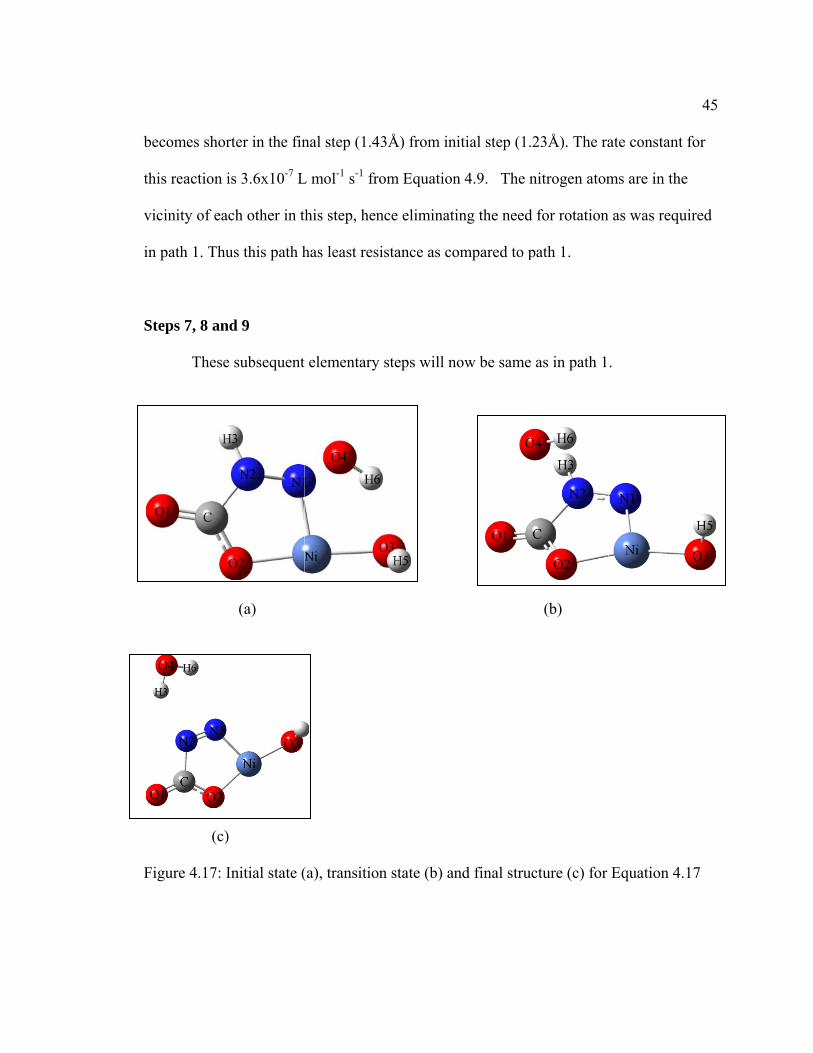
b

th

v

in

S

F

ecomes shor

his reaction i

icinity of ea

n path 1. Thu

teps 7, 8 an

These

(c)

igure 4.17: I

rter in the fin

is 3.6x10-7 L

ch other in t

us this path h

nd 9

e subsequent

(a)

)

Initial state (

nal step (1.4

L mol-1 s-1 fro

this step, hen

has least resi

t elementary

(a), transition

3Å) from in

om Equation

nce eliminati

istance as co

steps will n

n state (b) an

itial step (1.2

n 4.9. The n

ing the need

ompared to p

ow be same

nd final struc

23Å). The ra

nitrogen atom

d for rotation

path 1.

as in path 1

(b)

cture (c) for

ate constant

ms are in the

n as was requ

.

Equation 4.

45

for

e

uired

17

46

The free energies values as well as the rate constants for the steps for the different

pathways are summarized in Tables 4.2 and 4.3.

As can be seen from the rate constant values, the desorption of CO2 from NiOOH

is the rate limiting step with a value of the order of magnitude of -65. This conclusion is

supported by the fact that the urea electrolysis reaction rate decreases with time which

can be attributed to a surface blockage of the catalyst when a build up of CO2 takes place

over a period of time8. Thermodynamic calculations also suggest the largest contribution

to the free energy change of the reaction is from the last step. The total free energy

change (ΔG) required is 1227.7 kJ mol-1, whereas the requirement for CO2 desorption

alone is 1242.2 kJ mol-1. Using this value of ΔG, the theoretical value of of the cell

potential was calculated using the Nernst Equation

ΔG=-nFEocell (4.20)

where,

ΔG= Change in Gibbs Free Energy (kJ mol-1)

n= Number of electrons transferred per mole of reactant

F= Faraday’s Constant (96485 coulombs mol-1)

Eocell= Standard Potential (V)

The calculated Standard Potential was calculated as -2.12V at 298 K and 1

atmosphere pressure. The difference between this calculated potential and the theoretical

potential versus SHE8 of -0.46V can be attributed to two main factors. Firstly, in this

system one NiOOH site per molecule of urea has been considered. This system of single

molecule interactions limits the available active catalyst sites per molecule of urea. As a

47 result the overall energy required to desorb the final product CO2 is expected to be higher

in such a system, as compared to systems with larger NiOOH cluster sizes where a

greater number of catalytic sites are available per molecule of reactant. This in turn

explains the higher value of calculated standard potential. Secondly, gas phase

calculations have been performed without using solvent effects in order to simplify the

system. This has also possibly accounted for deviation in calculation of cell potential.

However, since the objective of this study was to gain a relativistic view of the kinetics of

the elementary steps, this has been well accomplished using a considerably simple model

of single molecule gas phase interactions.

Furthermore, we considered the possibility of other causes of surface blockage,

mainly from the preferential adsorption of OH- onto the surface of NiOOH. The binding

energies of CO2 and OH- calculated to be 9.2 kJ mol-1 and 18.0 kJ mol-1 respectively. This

suggested that in excess of OH- ions, the hydroxyl group is more preferentially adsorbed

onto the catalyst’s surface than CO2. This competition between adsorbed OH- and CO2 on

the catalyst’s surface leads to an increased tendency of surface blockage which could

further explain the decreased rate of reaction with time.

48

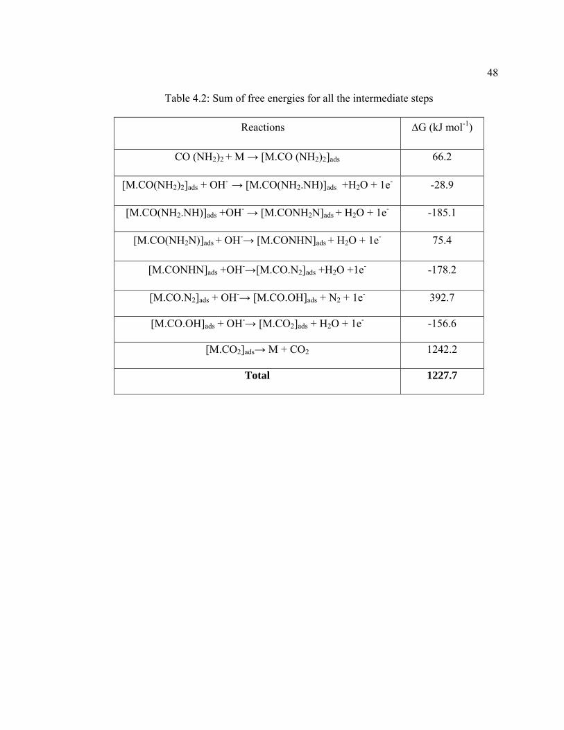
Table 4.2: Sum of free energies for all the intermediate steps

Reactions ∆G (kJ mol-1)

CO (NH2)2 + M → [M.CO (NH2)2]ads 66.2

[M.CO(NH2)2]ads + OH- → [M.CO(NH2.NH)]ads +H2O + 1e- -28.9

[M.CO(NH2.NH)]ads +OH- → [M.CONH2N]ads + H2O + 1e- -185.1

[M.CO(NH2N)]ads + OH-→ [M.CONHN]ads + H2O + 1e- 75.4

[M.CONHN]ads +OH-→[M.CO.N2]ads +H2O +1e- -178.2

[M.CO.N2]ads + OH-→ [M.CO.OH]ads + N2 + 1e- 392.7

[M.CO.OH]ads + OH-→ [M.CO2]ads + H2O + 1e- -156.6

[M.CO2]ads→ M + CO2 1242.2

Total 1227.7

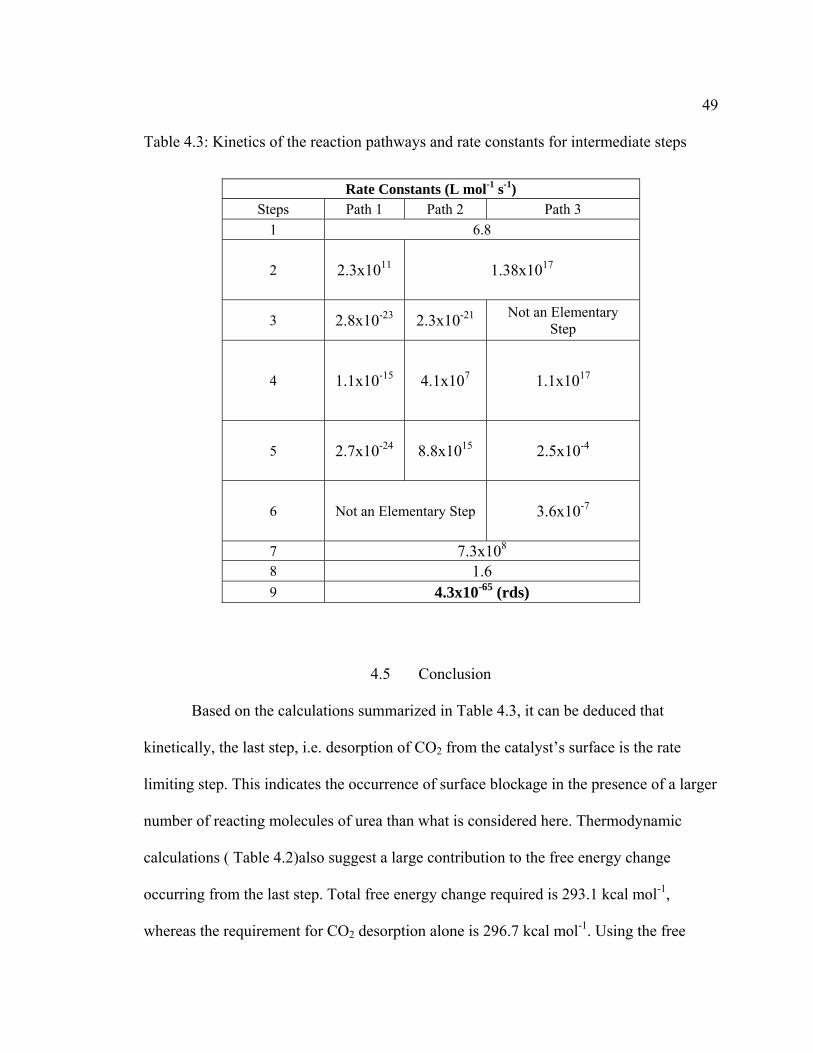
49 Table 4.3: Kinetics of the reaction pathways and rate constants for intermediate steps

4.5 Conclusion

Based on the calculations summarized in Table 4.3, it can be deduced that

kinetically, the last step, i.e. desorption of CO2 from the catalyst’s surface is the rate

limiting step. This indicates the occurrence of surface blockage in the presence of a larger

number of reacting molecules of urea than what is considered here. Thermodynamic

calculations ( Table 4.2)also suggest a large contribution to the free energy change

occurring from the last step. Total free energy change required is 293.1 kcal mol-1,

whereas the requirement for CO2 desorption alone is 296.7 kcal mol-1. Using the free

Rate Constants (L mol-1 s-1) Steps Path 1 Path 2 Path 3

1 6.8

2 2.3x1011 1.38x1017

3 2.8x10-23 2.3x10-21 Not an Elementary Step

4 1.1x10-15 4.1x107 1.1x1017

5 2.7x10-24 8.8x1015 2.5x10-4

6 Not an Elementary Step 3.6x10-7

7 7.3x108 8 1.6 9 4.3x10-65 (rds)

50 energy, the theoretical value of the cell potential was calculated to be -2.12V. The

difference between this theoretical and experimental value8 of -0.46V obtained can be

attributed to the limitation of using gas phase calculations as well as single molecule

interactions in the system.

Also, the path of least resistance is path 2, wherein the NH2 migrates to bond with

the NH group initially in step 3, before the remaining proton transfer could take place. As

a result of this migration, it involves no further need to rotate the N molecules towards

each other to bring about N2 desorption, as the atoms are already in the vicinity of each

other. This makes path 2 the preferred pathway. However, even if the reaction progresses

via any given mechanism, the rate limiting step, i.e, desorption of CO2 is common to all

the mechanisms.

51

Chapter 5 : CHEMICAL OXIDATION MECHANISMS

The objective of this study was to investigate the thermodynamics and kinetics of

the urea decomposition reactions occurring on NiOOH. The first consideration was urea

adsorbed onto the surface of NiOOH, and secondly the inclusion of a hydroxide ion in the

system was considered, to investigate the catalytic effects of OH- in the reaction.

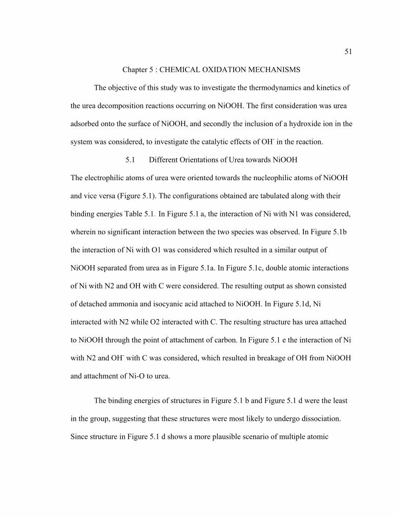
5.1 Different Orientations of Urea towards NiOOH

The electrophilic atoms of urea were oriented towards the nucleophilic atoms of NiOOH

and vice versa (Figure 5.1). The configurations obtained are tabulated along with their

binding energies Table 5.1. In Figure 5.1 a, the interaction of Ni with N1 was considered,

wherein no significant interaction between the two species was observed. In Figure 5.1b

the interaction of Ni with O1 was considered which resulted in a similar output of

NiOOH separated from urea as in Figure 5.1a. In Figure 5.1c, double atomic interactions

of Ni with N2 and OH with C were considered. The resulting output as shown consisted

of detached ammonia and isocyanic acid attached to NiOOH. In Figure 5.1d, Ni

interacted with N2 while O2 interacted with C. The resulting structure has urea attached

to NiOOH through the point of attachment of carbon. In Figure 5.1 e the interaction of Ni

with N2 and OH- with C was considered, which resulted in breakage of OH from NiOOH

and attachment of Ni-O to urea.

The binding energies of structures in Figure 5.1 b and Figure 5.1 d were the least

in the group, suggesting that these structures were most likely to undergo dissociation.

Since structure in Figure 5.1 d shows a more plausible scenario of multiple atomic

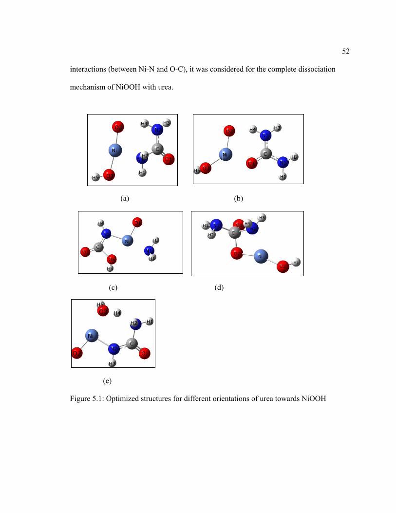
in

m

F

nteractions (b

mechanism o

(

(e)

igure 5.1: O

between Ni-

f NiOOH wi

(a)

(c)

)

Optimized str

-N and O-C)

ith urea.

ructures for d

), it was cons

(d)

different orie

sidered for th

(b)

)

entations of

he complete

urea toward

dissociation

ds NiOOH

52

n

53

Table 5.1:Binding Energies of different orientations of urea towards NiOOH

Binding Energies (kJ mol-1)

a. 11.7

b. 5.9

c. 11.3

d. 8.3

e. 12.6

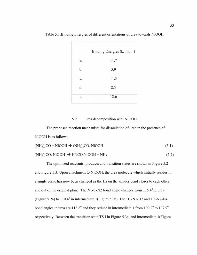
5.2 Urea decomposition with NiOOH

The proposed reaction mechanism for dissociation of urea in the presence of

NiOOH is as follows:

(NH2)2CO + NiOOH (NH2)2CO. NiOOH (5.1)

(NH2)2CO. NiOOH HNCO.NiOOH + NH3 (5.2)

The optimized reactants, products and transition states are shown in Figure 5.2

and Figure 5.3. Upon attachment to NiOOH, the urea molecule which initially resides in

a single plane has now been changed as the Hs on the amides bend closer to each other

and out of the original plane. The N1-C-N2 bond angle changes from 115.4o in urea

(Figure 5.2a) to 110.4o in intermediate 1(Figure 5.2b). The H1-N1-H2 and H3-N2-H4

bond angles in urea are 118.8o and they reduce in intermediate 1 from 109.2o to 107.9o

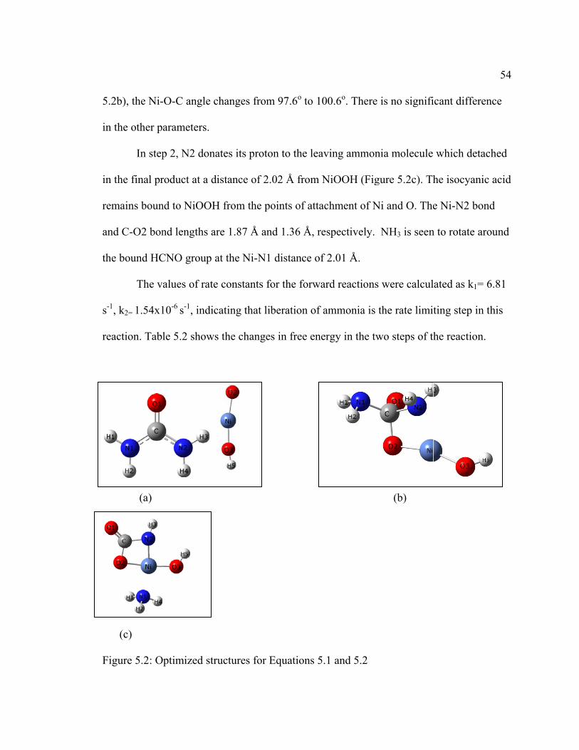
respectively. Between the transition state TS I in Figure 5.3a, and intermediate 1(Figure

5

in

in

re

an

th

s-

re

F

.2b), the Ni-

n the other p

In step

n the final pr

emains boun

nd C-O2 bon

he bound HC

The v

-1, k2= 1.54x1

eaction. Tab

(a)

(c)

igure 5.2: O

-O-C angle c

arameters.

p 2, N2 dona

roduct at a d

nd to NiOOH

nd lengths ar

CNO group a

alues of rate

10-6 s-1, indic

le 5.2 shows

Optimized str

changes from

ates its proto

istance of 2.

H from the po

re 1.87 Å an

at the Ni-N1

e constants fo

cating that lib

s the change

ructures for E

m 97.6o to 10

on to the leav

.02 Å from N

oints of attac

nd 1.36 Å, re

distance of

for the forwa

beration of a

s in free ene

Equations 5.

00.6o. There

ving ammon

NiOOH (Fig

chment of N

espectively.

f 2.01 Å.

ard reactions

ammonia is t

ergy in the tw

.1 and 5.2

is no signifi

nia molecule

gure 5.2c). Th

Ni and O. The

NH3 is seen

were calcul

the rate limi

wo steps of th

(b)

icant differen

which detac

he isocyanic

e Ni-N2 bon

n to rotate aro

lated as k1= 6

ting step in t

he reaction.

54

nce

ched

c acid

nd

ound

6.81

this

F

hy

op

T

(N

(N

igure 5.3: O

When

ydroxide ion

ptimized wit

The proposed

NiO.OHOH)

Ni(OH)3CON

(a)

Optimized Tr

Table 5.2:

St

Equ

Equ

O

5.3

n OH- was op

n onto Ni as

th urea.

d reaction me

)ads + CO(NH

NH.NH2)ads →

ansition Stat

Free Energy

tructures

uation 5.1

uation 5.2

Overall

Urea and N

ptimized wit

shown in Fi

echanism is

H2)2→ (Ni(O

→(Ni(OH)3.C

tes for React

y differences

Fre

NiOOH in th

th NiOOH, it

igure 5.4. Th

as follows:

OH)3.CONH

CNO)ads + N

tions 2 and 3

s for equatio

ee energies ch

-6

-20

-27

e presence o

t resulted in

he output stru

.NH2)ads

NH3

(b)

3

ons 5.1 and 5

hanges (kJ mo

66.9

09.3

76.3

of OH- ion:

the adsorpti

ucture was t

5.2

ol-1)

ion of the

then further

(

55

(5.3)

(5.4)

F

F

N

un

pr

sa

igure 5.4: A

(a)

(

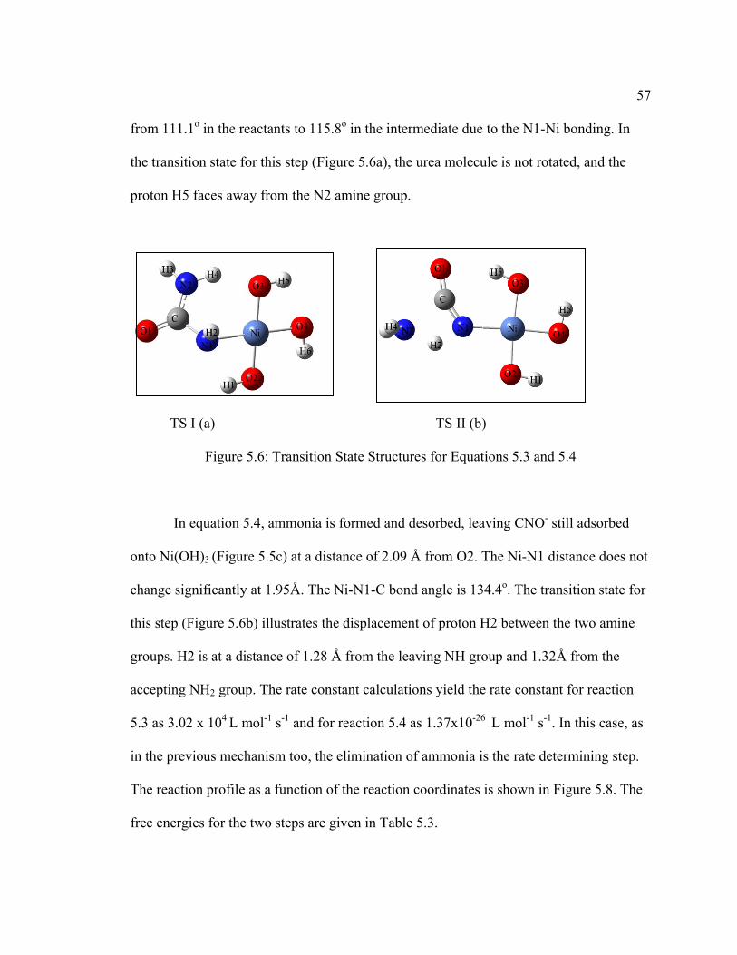
igure 5.5: O

Figure

Ni distance is

ndergoes rot

roximity of N

ame time. Th

Adsorption of

(c)

Optimized str

e 5.5a illustr

s 2.06Å. In th

tation to suc

N1-H1 to O

he N1-Ni bo

f OH- onto N

ructures for E

rates the opti

he intermedi

h that both N

2, O2 withdr

ond length re

NiOOH

Equations 5.

imized react

iate structure

NH2 groups

raws the pro

educes to 1.9

(b)

.3 and 5.4.

tants for Equ

e (Figure 5.5

face downw

oton from N1

96Å. The N1

uation 5.3 an

5b), the urea

wards. Due to

1 while N1 b

1-C-N2 bond

nd 5.4. The N

a molecule

o the close

bonds to Ni a

d angle incre

56

N1-

at the

eases

fr

th

pr

on

ch

th

gr

ac

5

in

T

fr

rom 111.1o i

he transition

roton H5 fac

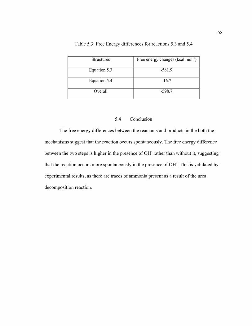
TS I (a

F

In equ

nto Ni(OH)3

hange signif

his step (Figu

roups. H2 is

ccepting NH

.3 as 3.02 x

n the previou

The reaction p

ree energies

n the reactan

state for thi

ces away fro

a)

Figure 5.6: T

uation 5.4, am

3 (Figure 5.5

ficantly at 1.

ure 5.6b) illu

s at a distanc

H2 group. Th

104 L mol-1

us mechanism

profile as a f

for the two

nts to 115.8o

s step (Figur

om the N2 am

Transition St

mmonia is fo

c) at a distan

95Å. The Ni

ustrates the d

ce of 1.28 Å

e rate consta

s-1 and for re

m too, the el

function of t

steps are giv

o in the interm

re 5.6a), the

mine group.

tate Structur

formed and d

nce of 2.09 Å

i-N1-C bond

displacemen

from the lea

ant calculatio

eaction 5.4 a

limination o

the reaction

ven in Table

mediate due

urea molecu

TS II (b)

res for Equat

desorbed, lea

Å from O2. T

d angle is 13

nt of proton H

aving NH gro

ons yield the

as 1.37x10-26

f ammonia i

coordinates

5.3.

to the N1-N

ule is not rot

)

tions 5.3 and

aving CNO-

The Ni-N1 d

34.4o. The tra

H2 between

oup and 1.32

e rate consta

6 L mol-1 s-1

is the rate de

is shown in

Ni bonding. I

tated, and the

d 5.4

still adsorbe

distance doe

ansition state

the two ami

2Å from the

ant for reactio

. In this case

etermining st

Figure 5.8.

57

In

e

ed

s not

e for

ine

on

e, as

tep.

The

58

Table 5.3: Free Energy differences for reactions 5.3 and 5.4

Structures Free energy changes (kcal mol-1)

Equation 5.3 -581.9

Equation 5.4 -16.7

Overall -598.7

5.4 Conclusion

The free energy differences between the reactants and products in the both the

mechanisms suggest that the reaction occurs spontaneously. The free energy difference

between the two steps is higher in the presence of OH- rather than without it, suggesting

that the reaction occurs more spontaneously in the presence of OH-. This is validated by

experimental results, as there are traces of ammonia present as a result of the urea

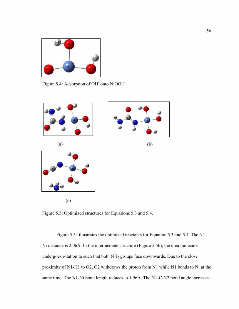
decomposition reaction.

59

Chapter 6 : EXPERIMENTAL

The experimental section is a brief study carried out in order to study the effect of

varying concentrations of KOH and urea on the current density obtained. The urea electro

oxidation reaction has been analyzed by conducting potentiodynamic tests with a rotating

disk electrode. The rotating disk electrode offers several advantages over stationery

electrode experiments. With the disk in constant motion, reaction rates are not diffusion

limited. Hence it throws light on the nature of the reaction taking place37. With

conventional experiments conducted using a rotating disk electrode, a steady state current

profile is obtained with changing potentials. However this is not the case with the urea

electro oxidation reaction, where reactions of a more complex nature seem to be going on

at the surface of the electrode, as will be discussed later.

The different operational parameters studied are the concentration of KOH, urea

and temperature effects on the current density of the reaction. Preliminary tests were

conducted to identify the lowest possible concentrations of KOH at which a response is

obtained. Once the lowest concentration was established, the current density at 5 levels of

concentration of KOH tested for 3 levels of concentration of urea were carried out at

room temperature.

6.1 Experimental Methods: Electroplating and Preliminary Results

Catalyst preparation was performed in two stages: one for the preliminary tests

and another for the main set of experiments. The chemicals were obtained from Alfa

Aesar or Fisher Scientific. Electroplating was carried out in a 200 mL beaker at 45° C

60

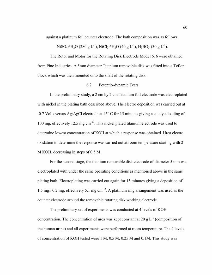
against a platinum foil counter electrode. The bath composition was as follows:

NiSO4.6H2O (280 g L-1), NiCl2.6H2O (40 g L-1), H3BO3 (30 g L-1).

The Rotor and Motor for the Rotating Disk Electrode Model 616 were obtained

from Pine Industries. A 5mm diameter Titanium removable disk was fitted into a Teflon

block which was then mounted onto the shaft of the rotating disk.

6.2 Potentio-dynamic Tests

In the preliminary study, a 2 cm by 2 cm Titanium foil electrode was electroplated

with nickel in the plating bath described above. The electro deposition was carried out at

-0.7 Volts versus Ag/AgCl electrode at 45o C for 15 minutes giving a catalyst loading of

100 mg, effectively 12.5 mg cm-2.. This nickel plated titanium electrode was used to

determine lowest concentration of KOH at which a response was obtained. Urea electro

oxidation to determine the response was carried out at room temperature starting with 2

M KOH, decreasing in steps of 0.5 M.

For the second stage, the titanium removable disk electrode of diameter 5 mm was

electroplated with under the same operating conditions as mentioned above in the same

plating bath. Electroplating was carried out again for 15 minutes giving a deposition of

1.5 mg± 0.2 mg, effectively 5.1 mg cm -2. A platinum ring arrangement was used as the

counter electrode around the removable rotating disk working electrode.

The preliminary set of experiments was conducted at 4 levels of KOH

concentration. The concentration of urea was kept constant at 20 g L-1 (composition of

the human urine) and all experiments were performed at room temperature. The 4 levels

of concentration of KOH tested were 1 M, 0.5 M, 0.25 M and 0.1M. This study was

61 conducted to purely select the lowest concentration at which a response is obtained. The

upper limit of the experiment matrix is set at 5 M KOH.

The second stage of experiments was carried out at five levels of concentration of

KOH and three levels of concentration of urea namely 0.5 M, 1 M, 2 M, 3 M, 5 M KOH.

The speed of rotation of the rotating disk electrode was set at 1000 rpm, with the Hg-

HgO reference With 0.5 M KOH solution, the three levels of concentration of urea were

tested by performing cyclic voltammetry on the Solartron potentiostat. Then the

concentration of KOH was changed and the three concentrations of urea were again

tested. All experiments were performed at room temperature. The scan rate used was

20mV s-1.

6.3 Results and Discussion

Figure 6.1 represents the set of experiments performed initially to determine the

lower set point of KOH concentrations. 4 concentrations of KOH were tested starting

with 0.1 M. There was no response peak at 0.1 M. The lowest concentration of KOH that

gave a response was 0.25 M. There was not a significant difference between the

maximum current obtained with 0.25 M and 0.5 M. Hence 0.5 M was chosen as the lower

set point.

62

Figure 6.1: Preliminary experiment. Different concentrations of KOH at 20g L-1 urea to

determine lower setpoint.

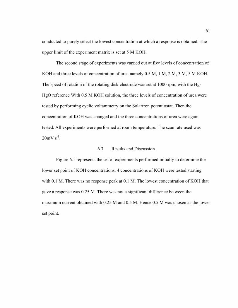
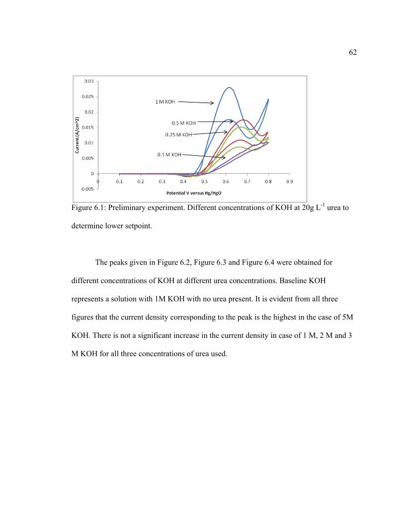
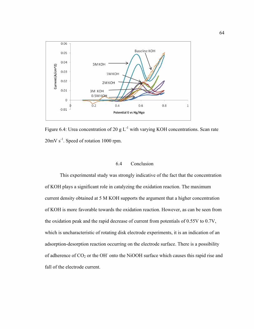
The peaks given in Figure 6.2, Figure 6.3 and Figure 6.4 were obtained for

different concentrations of KOH at different urea concentrations. Baseline KOH

represents a solution with 1M KOH with no urea present. It is evident from all three

figures that the current density corresponding to the peak is the highest in the case of 5M

KOH. There is not a significant increase in the current density in case of 1 M, 2 M and 3

M KOH for all three concentrations of urea used.

63

Figure 6.2: Urea concentration of 5 g L-1 varying KOH concentrations. Scan rate: 20mV

s-1. Speed of rotation: 1000rpm.

Figure 6.3: Urea Concentration of 10 g L-1 with varying KOH concentrations. Scan Rate:

20mV s-1. Speed of rotation 1000rpm.

64

Figure 6.4: Urea concentration of 20 g L-1 with varying KOH concentrations. Scan rate

20mV s-1. Speed of rotation 1000 rpm.

6.4 Conclusion

This experimental study was strongly indicative of the fact that the concentration

of KOH plays a significant role in catalyzing the oxidation reaction. The maximum

current density obtained at 5 M KOH supports the argument that a higher concentration

of KOH is more favorable towards the oxidation reaction. However, as can be seen from

the oxidation peak and the rapid decrease of current from potentials of 0.55V to 0.7V,

which is uncharacteristic of rotating disk electrode experiments, it is an indication of an

adsorption-desorption reaction occurring on the electrode surface. There is a possibility

of adherence of CO2 or the OH- onto the NiOOH surface which causes this rapid rise and

fall of the electrode current.

65

Chapter 7 : CONCLUSIONS AND RECOMMENDATIONS

In summary, the electro oxidation reaction mechanisms studied indicate the

desorption of CO2 as the rate limiting step with the calculated rate constant value of

4.32x10-65 L mol-1s-1 . The desorption step also contributes to the maximum energy

requirement of the path (1242.2 kJ mol-1). Also based on the kinetics of the reaction,

*CO(NH2)2→ *CO(NH.NH2)→ *CO(NH.NH)→ *CO(NH.N)→*CO(N2) → *CO(OH)

→*CO(OH.OH) →*CO2 has been identified as the preferred pathway among the three

mechanisms. This has been discussed in Chapter 4 as Path 2. In this pathway, the bonding

between the NH2-NH group occurs initially versus the rotation of the nitrogen atoms

towards each other in the later stages as in Path 1. This facilitates easy desorption of the

nitrogen molecule.

Another important finding of this study is the investigation of causes of surface

blockage, mainly from the preferential adsorption of OH- onto the surface of NiOOH.

The binding energies of CO2 and OH- calculated to be 9.2 kJ mol-1 and 18.0 kJ mol-1

respectively. This suggested that in excess of OH- ions, the hydroxyl group is more

preferentially adsorbed onto the catalyst’s surface than CO2. This competition between

the molecules leading to adsorption onto the NiOOH surface leads to an increased

tendency of surface blockage which explains the decreased rate of reaction as time

progresses.

In the chemical oxidation mechanisms, the thermodynamic feasibility of the

reaction mechanisms both without and in the presence of OH- has been discussed.

Change in free energy for the oxidation mechanism without OH- is -276.3 kJ mol-1

66 whereas with OH- it is -598.7 kJ mol-1. This indicates a greater spontaneity of the

reaction in the presence of hydroxide ions, which is known to catalyze the reaction. In

both the reaction mechanisms, the desorption of ammonia is the rate limiting step. In

mechanism 1 it was calculated as 1.54x10-6 s-1 and in mechanism 2 it is 1.37x10-26

L/mol.s.

The experimental potentio-dynamic tests carried out with 3 levels of

concentration of KOH (0.5 M, 1 M, 2 M, 3 M, 5 M) indicate a significant increase in

current density of the anodic reaction with the highest KOH concentration in the matrix

of 5M in case of all three levels of concentration of urea of 5, 10 and 15 g L-1. There is no

significant difference in current densities for the lower concentrations of KOH. This is in

agreement with the modeling results which also indicate a greater favorability of the

reaction in presence of OH-.

After the role of OH- and the rate limiting step in the oxidation mechanism has

been established with this study, it is now recommended to look into improvements in the

rate constant approximations with inclusion of solvent effects in the system. Greater basis

sets can also be used to carry out similar calculations. At the same time, an experimental

model should be developed to calculate experimentally the kinetic parameters of the

model which can then be compared to the theoretical values.

67

REFERENCES

1. Dunn, S., Hydrogen futures: toward a sustainable energy system. International

Journal of Hydrogen Energy 2002, 27, (3), 235-264.

2. Penner, S. S.; Appleby, A. J.; Baker, B. S.; Bates, J. L.; Buss, L. B.; Dollard, W.

J.; Farris, P. J.; Gillis, E. A.; Gunsher, J. A.; Khandkar, A.; Krumpelt, M.; Osullivan, J.

B.; Runte, G.; Savinell, R. F.; Selman, J. R.; Shores, D. A.; Tarman, P.,

Commercialization of Fuel-Cells. Progress in Energy and Combustion Science 1995, 21,

(2), 145-151.

3. Mehta, V.; Cooper, J. S., Review and analysis of PEM fuel cell design and

manufacturing. Journal of Power Sources 2003, 114, (1), 32-53.

4. Georgia State University. Hyperphysics Homepage. . http://hyperphysics.phy-

astr.gsu.edu/Hbase/thermo/electrol.html (23rd March 2009)

5. Vitse, F.; Cooper, M.; Botte, G. G., On the use of ammonia electrolysis for

hydrogen production (vol 142, pg 18, 2005). Journal of Power Sources 2005, 152, (1),

311-312.

6. Boggs, B. K.; Botte, G. G., On-board hydrogen storage and production: An

application of ammonia electrolysis. Journal of Power Sources 2009, 192, (2), 573-581.

7. Bonnin, E. P.; Biddinger, E. J.; Botte, G. G., Effect of catalyst on electrolysis of

ammonia effluents. Journal of Power Sources 2008, 182, (1), 284-290.

8. Boggs, B. K.; King, R. L.; Botte, G. G., Urea electrolysis: direct hydrogen

production from urine. Chemical Communications 2009, (32), 4859-4861.

68 9. Maryland Department of Agriculture Homepage.

http://www.mda.state.us/publications/poultry_action_team_report.php (20th May 2009)

10. Pfenning, K. S.; McMahon, P. B., Effect of nitrate, organic carbon, and

temperature on potential denitrification rates in nitrate-rich riverbed sediments. Journal

of Hydrology 1997, 187, (3-4), 283-295.

11. US Environmental Protection Agency Homepage.

http://www.epa.gov/etv/pubs/600s07009.pdf (15th March 2009)

12. Bryan Boggs, R. L. K., Gerardine G, Botte, Urea Electrolysis: Direct hydrogen

production from urine. Chem. Commun. 2009.

13. Suarez, D.; Diaz, N.; Merz, K. M., Ureases: Quantum chemical calculations on

cluster models. Journal of the American Chemical Society 2003, 125, (50), 15324-15337.

14. Estiu, G.; Merz, K. M., Enzymatic catalysis of urea decomposition: Elimination

or hydrolysis? Journal of the American Chemical Society 2004, 126, (38), 11832-11842.

15. Estiu, G.; Metz, K. M., The hydrolysis of urea and the proficiency of urease.

Journal of the American Chemical Society 2004, 126, (22), 6932-6944.

16. Yeomans, J. C.; Bremner, J. M., Effects of Urease Inhibitors on Denitrification in

Soil. Communications in Soil Science and Plant Analysis 1986, 17, (1), 63-73.

17. Bremner, J. M.; Krogmeier, M. J., Effects of Urease Inhibitors on Germination of

Seeds in Soil. Communications in Soil Science and Plant Analysis 1990, 21, (3-4), 311-

321.

18. Alexandrova, A. N.; Jorgensen, W. L., Why urea eliminates ammonia rather than

hydrolyzes in aqueous solution. Journal of Physical Chemistry B 2007, 111, (4), 720-730.

69 19. Estiu, G.; Suarez, D.; Merz, K. M., Quantum mechanical and molecular dynamics

simulations of ureases and Zn beta-lactamases. Journal of Computational Chemistry

2006, 27, (12), 1240-1262.

20. Maaref, A.; Barhoumi, H.; Rammah, M.; Martelet, C.; Jaffrezic-Renault, N.;

Mousty, C.; Cosnier, S.; Perez, E.; Rico-Lattes, I., Comparative study between organic

and inorganic entrapment matrices for urease biosensor development (vol 123, pg 671,

2007). Sensors and Actuators B-Chemical 2007, 126, (2), 710-710.

21. Fearon, W. R., The Biochemistry of Urea. Physiological Reviews 1926, 6, (3),

399-439.

22. Barrios, A. M.; Lippard, S. J., Interaction of urea with a hydroxide-bridged

dinuclear nickel center: An alternative model for the mechanism of urease. Journal of the

American Chemical Society 2000, 122, (38), 9172-9177.

23. Benini, S.; Rypniewski, W. R.; Wilson, K. S.; Miletti, S.; Ciurli, S.; Mangani, S.,

A new proposal for urease mechanism based on the crystal structures of the native and

inhibited enzyme from Bacillus pasteurii: why urea hydrolysis casts two nickels.

Structure 1999, 7, (2), 205-216.

24. Botte, G. G. Electrolysis of urea/urine to produce ammonia and hydrogen, and

methods and uses , and fuel cells related there to. 2007.

25. Computational Chemistry Ltd, Homepage.

http://www.ccl.net/cca/documents/basis-sets/basis.html (14th November 2008)

26. Simka, W.; Piotrowski, J.; Nawrat, G., Influence of anode material on

electrochemical decomposition of urea. Electrochimica Acta 2007, 52, (18), 5696-5703.

70 27. Frisch, M. J. T., G.W; Schlegel H.B; Scuseria G.E; Robb, M.A.; Cheeseman, J.R.;

Montgomery, J.A.,Jr; Vreven, T; Kudin K.N.; Burant, J.C; Millam,J.M.; Iyengar S.S;

Tomasi, J; Barone, V.; Menucci, B.; Cossi,M.; Scalmani, G.; Rega, N.;Petersson G.A.;

Nakatsuji, H.; Hada, M.; Ehara, M.; Toyota, K.; Fukuda, R.; Hasegawa, J.; Ishida, M.;

Nakajima,T.;Honda,Y.; Kitao,O.; Nakai,H.; Klene,M.;Li,X.; Knox,J.E; Hratchian, H.P;

Cross, J.B; Bakken, V.; Adamo,C.; Jaramillo,J.; Gomperts,R.; Stratmann,R.E.;

Yazyev,O.; Austin,A.J.; Cammi,R.; Pomelli, C.; Ochterski, J.W.; Ayala, P.Y.;

Morokuma,K.; Voth,G.a; Salvador,P.; Dannenburg, J.J.; Zakrzewski,V.G.; Dapprich,S.;

Daniels,A.D.; Strain,M.C.; Farkas,O.; Malick,D.K.; Rabuck,A.D.; Raghavachari,K.;

Foresman,J.B.; Ortitz,J.V.; Cui,Q.; Baboul,A.G.; Clifford, S.; Cioslowski,J.;

Stefanov,B.B.; Liu,G.; Liashenko,A.; Piskorz,P.; Komaromi,I.; Martin,R.L.; Fox,D.J.;

Keith,T.; Al-Laham,M.A.; Peng,C.Y.; Nanayakkara,A.; Challacombe,M.; Gill,P.M.W;

Johnson,B.; Chen,W; Wong,M.w.; Gonzalez,C.; Pople ,J.A, Gaussian 03

2003, Revison C.02; Gaussian Inc.;.

28. Becke, A. D., Density-Functional Thermochemistry .3. the Role of Exact

Exchange. Journal of Chemical Physics 1993, 98, (7), 5648-5652.

29. Wadt, W. R.; Hay, P. J., Abinitio Effective Core Potentials for Molecular

Calculations - Potentials for Main Group Elements Na to Bi. Journal of Chemical Physics

1985, 82, (1), 284-298.

30. Hay, P. J.; Wadt, W. R., Abinitio Effective Core Potentials for Molecular

Calculations - Potentials for the Transition-Metal Atoms Sc to Hg. Journal of Chemical

Physics 1985, 82, (1), 270-283.

71 31. Hay, P. J.; Wadt, W. R., Abinitio Effective Core Potentials for Molecular

Calculations - Potentials for K to Au Including the Outermost Core Orbitals. Journal of

Chemical Physics 1985, 82, (1), 299-310.

32. Hehre, W. J. R., L.; Schlayer, P.v R.; Pople J.A.;, Ab Initio Molecular Orbital

Theory. John Wiley & Sons: New York, 1986.

33. Civalleri, B.; Doll, K.; Zicovich-Wilson, C. M., Ab initio investigation of

structure and cohesive energy of crystalline urea. Journal of Physical Chemistry B 2007,

111, (1), 26-33.

34. Szalay, V.; Kovacs, L.; Wohlecke, M.; Libowitzky, E., Stretching potential and

equilibrium length of the OH bond in solids. Chemical Physics Letters 2002, 354, (1-2),

56-61.

35. Mansour, A. N.; Melendres, C. A., Analysis of X-ray absorption spectra of some

nickel oxycompounds using theoretical standards. Journal of Physical Chemistry A 1998,

102, (1), 65-81.

36. R.A van Santen, J. W. N., Chemical Kinetics and Catalysis. Plenum Press: New

York, 1995.

37. Bruckenstein S., M. B., Unraveling reactions with rotating electrodes. Accounts of

Chemical Research 1977, 10, (2), 54-61.

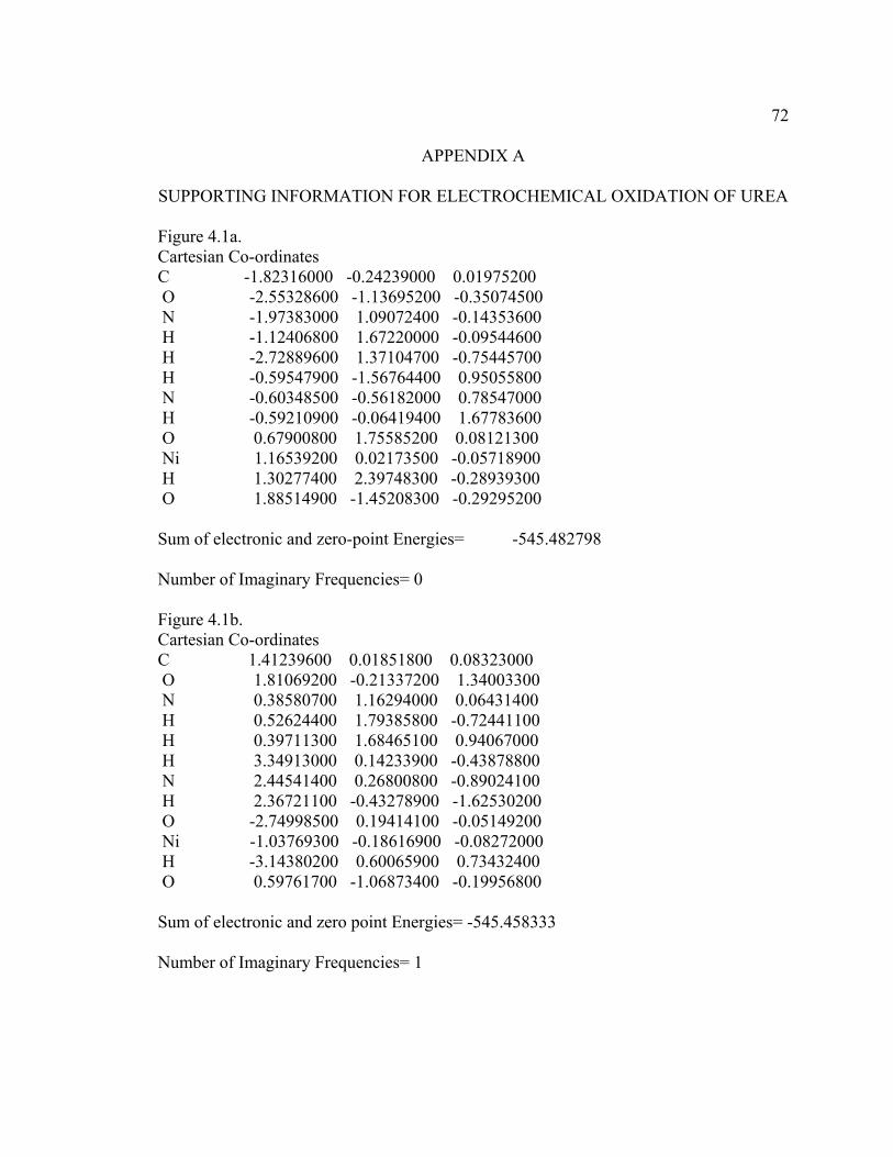
72

APPENDIX A

SUPPORTING INFORMATION FOR ELECTROCHEMICAL OXIDATION OF UREA Figure 4.1a. Cartesian Co-ordinates C -1.82316000 -0.24239000 0.01975200 O -2.55328600 -1.13695200 -0.35074500 N -1.97383000 1.09072400 -0.14353600 H -1.12406800 1.67220000 -0.09544600 H -2.72889600 1.37104700 -0.75445700 H -0.59547900 -1.56764400 0.95055800 N -0.60348500 -0.56182000 0.78547000 H -0.59210900 -0.06419400 1.67783600 O 0.67900800 1.75585200 0.08121300 Ni 1.16539200 0.02173500 -0.05718900 H 1.30277400 2.39748300 -0.28939300 O 1.88514900 -1.45208300 -0.29295200 Sum of electronic and zero-point Energies= -545.482798 Number of Imaginary Frequencies= 0 Figure 4.1b. Cartesian Co-ordinates C 1.41239600 0.01851800 0.08323000 O 1.81069200 -0.21337200 1.34003300 N 0.38580700 1.16294000 0.06431400 H 0.52624400 1.79385800 -0.72441100 H 0.39711300 1.68465100 0.94067000 H 3.34913000 0.14233900 -0.43878800 N 2.44541400 0.26800800 -0.89024100 H 2.36721100 -0.43278900 -1.62530200 O -2.74998500 0.19414100 -0.05149200 Ni -1.03769300 -0.18616900 -0.08272000 H -3.14380200 0.60065900 0.73432400 O 0.59761700 -1.06873400 -0.19956800 Sum of electronic and zero point Energies= -545.458333 Number of Imaginary Frequencies= 1

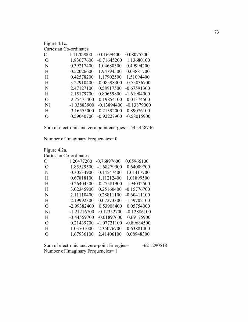
73 Figure 4.1c. Cartesian Co-ordinates C 1.41709000 -0.01699400 0.08075200 O 1.83677600 -0.71645200 1.13680100 N 0.39217400 1.04688300 0.49994200 H 0.52026600 1.94794500 0.03881700 H 0.42578200 1.17902500 1.51094400 H 3.22910400 -0.08598300 -0.75036700 N 2.47127100 0.58917500 -0.67591300 H 2.15179700 0.80659800 -1.61984000 O -2.75475400 0.19854100 0.01374500 Ni -1.03883900 -0.13894400 -0.13879000 H -3.16555000 0.21392000 0.89076100 O 0.59040700 -0.92227900 -0.58015900 Sum of electronic and zero point energies= -545.458736 Number of Imaginary Frequencies= 0 Figure 4.2a. Cartesian Co-ordinates C 1.20477200 -0.76897600 0.05966100 O 1.85529500 -1.68279900 0.64009700 N 0.30534900 0.14547400 1.01417700 H 0.67818100 1.11212400 1.01899500 H 0.26404500 -0.27581900 1.94032500 H 3.02345900 0.25160400 -0.15776700 N 2.11110400 0.28811100 -0.60411100 H 2.19992300 0.07273300 -1.59702100 O -2.99382400 0.53908400 0.05754000 Ni -1.21216700 -0.12352700 -0.12886100 H -3.44559700 -0.01897600 0.69175900 O 0.21439700 -1.07721100 -0.89684500 H 1.03501000 2.35076700 -0.63881400 O 1.67936100 2.41406100 0.08948300 Sum of electronic and zero-point Energies= -621.290518 Number of Imaginary Frequencies= 1

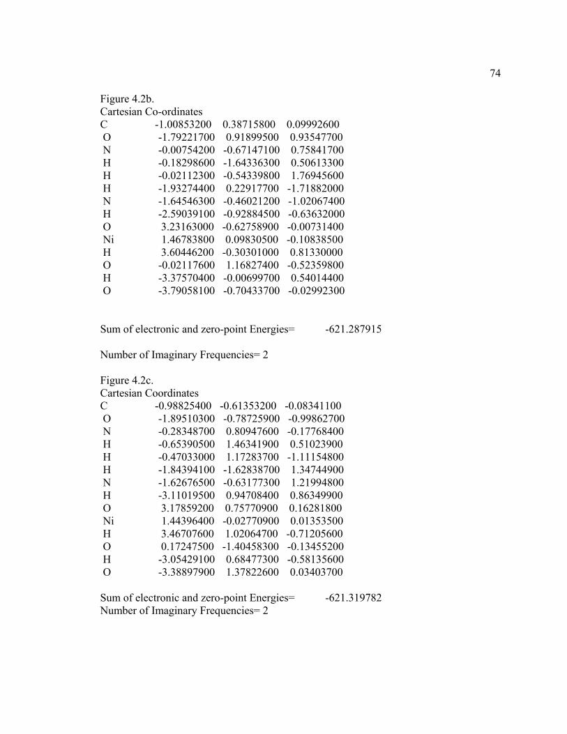
74 Figure 4.2b. Cartesian Co-ordinates C -1.00853200 0.38715800 0.09992600 O -1.79221700 0.91899500 0.93547700 N -0.00754200 -0.67147100 0.75841700 H -0.18298600 -1.64336300 0.50613300 H -0.02112300 -0.54339800 1.76945600 H -1.93274400 0.22917700 -1.71882000 N -1.64546300 -0.46021200 -1.02067400 H -2.59039100 -0.92884500 -0.63632000 O 3.23163000 -0.62758900 -0.00731400 Ni 1.46783800 0.09830500 -0.10838500 H 3.60446200 -0.30301000 0.81330000 O -0.02117600 1.16827400 -0.52359800 H -3.37570400 -0.00699700 0.54014400 O -3.79058100 -0.70433700 -0.02992300 Sum of electronic and zero-point Energies= -621.287915 Number of Imaginary Frequencies= 2 Figure 4.2c. Cartesian Coordinates C -0.98825400 -0.61353200 -0.08341100 O -1.89510300 -0.78725900 -0.99862700 N -0.28348700 0.80947600 -0.17768400 H -0.65390500 1.46341900 0.51023900 H -0.47033000 1.17283700 -1.11154800 H -1.84394100 -1.62838700 1.34744900 N -1.62676500 -0.63177300 1.21994800 H -3.11019500 0.94708400 0.86349900 O 3.17859200 0.75770900 0.16281800 Ni 1.44396400 -0.02770900 0.01353500 H 3.46707600 1.02064700 -0.71205600 O 0.17247500 -1.40458300 -0.13455200 H -3.05429100 0.68477300 -0.58135600 O -3.38897900 1.37822600 0.03403700 Sum of electronic and zero-point Energies= -621.319782 Number of Imaginary Frequencies= 2

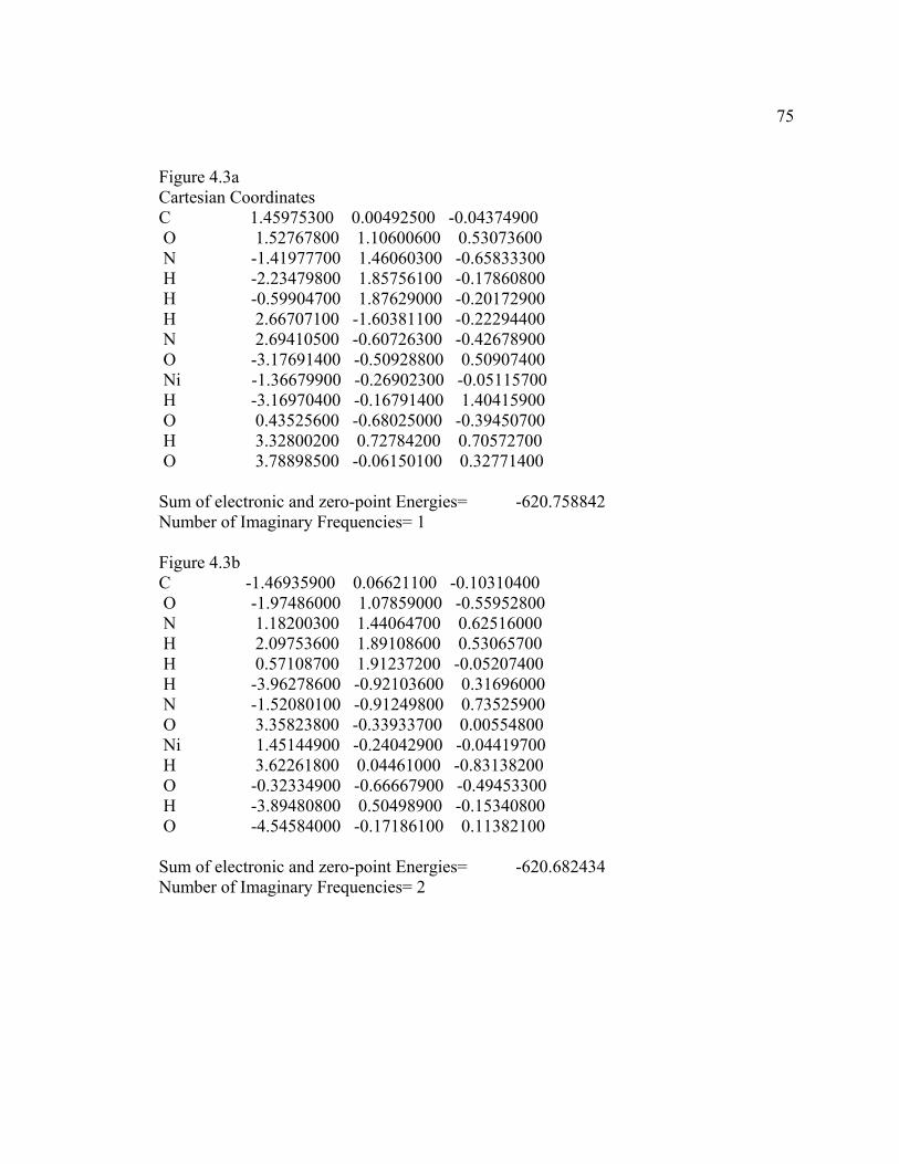
75 Figure 4.3a Cartesian Coordinates C 1.45975300 0.00492500 -0.04374900 O 1.52767800 1.10600600 0.53073600 N -1.41977700 1.46060300 -0.65833300 H -2.23479800 1.85756100 -0.17860800 H -0.59904700 1.87629000 -0.20172900 H 2.66707100 -1.60381100 -0.22294400 N 2.69410500 -0.60726300 -0.42678900 O -3.17691400 -0.50928800 0.50907400 Ni -1.36679900 -0.26902300 -0.05115700 H -3.16970400 -0.16791400 1.40415900 O 0.43525600 -0.68025000 -0.39450700 H 3.32800200 0.72784200 0.70572700 O 3.78898500 -0.06150100 0.32771400 Sum of electronic and zero-point Energies= -620.758842 Number of Imaginary Frequencies= 1 Figure 4.3b C -1.46935900 0.06621100 -0.10310400 O -1.97486000 1.07859000 -0.55952800 N 1.18200300 1.44064700 0.62516000 H 2.09753600 1.89108600 0.53065700 H 0.57108700 1.91237200 -0.05207400 H -3.96278600 -0.92103600 0.31696000 N -1.52080100 -0.91249800 0.73525900 O 3.35823800 -0.33933700 0.00554800 Ni 1.45144900 -0.24042900 -0.04419700 H 3.62261800 0.04461000 -0.83138200 O -0.32334900 -0.66667900 -0.49453300 H -3.89480800 0.50498900 -0.15340800 O -4.54584000 -0.17186100 0.11382100 Sum of electronic and zero-point Energies= -620.682434 Number of Imaginary Frequencies= 2

76 Figure 4.3c. C -1.46935900 0.06621100 -0.10310400 O -1.97486000 1.07859000 -0.55952800 N 1.18200300 1.44064700 0.62516000 H 2.09753600 1.89108600 0.53065700 H 0.57108700 1.91237200 -0.05207400 H -3.96278600 -0.92103600 0.31696000 N -1.52080100 -0.91249800 0.73525900 O 3.35823800 -0.33933700 0.00554800 Ni 1.45144900 -0.24042900 -0.04419700 H 3.62261800 0.04461000 -0.83138200 O -0.32334900 -0.66667900 -0.49453300 H -3.89480800 0.50498900 -0.15340800 O -4.54584000 -0.17186100 0.11382100 Sum of electronic and zero-point Energies= -620.698557 Number of Imaginary Frequencies= 1 Figure 4.4a. C 2.02492500 -0.38489000 -0.00241700 O 1.99230200 0.91605100 0.08180300 N -0.61064000 1.43887000 0.56088100 H -1.36543800 2.04508800 0.88167600 H 0.16339300 1.45952600 1.23586300 N 3.10461800 -1.09422100 0.09749400 O -2.81349600 -0.74968000 -0.07955800 Ni -0.91949600 -0.52005600 0.01063900 H -3.23848300 0.10260600 0.02417000 O 0.86501000 -1.07525700 -0.19354400 H 0.87111100 1.60390300 -0.56236200 O -0.08032800 2.06478900 -0.61762000 Sum of electronic and zero-point Energies= -620.105700 Number of Imaginary Frequencies= 1

77 Figure 4.4b. C 2.01170900 -0.35367700 0.00509000 O 2.18295300 0.86382800 0.29183800 N -0.97253500 1.00690500 1.05888200 H -0.90336700 1.85766900 0.31385400 H -0.07156000 1.03695000 1.55617200 N 3.21320000 -0.94561200 -0.18820800 O -2.76489000 -0.75587600 -0.29843000 Ni -0.89091900 -0.51640500 -0.01738600 H -3.16585000 -0.08689400 0.25785900 O 0.92016600 -1.01324400 -0.10412700 H 0.66233400 2.05342800 -0.57228000 O -0.25457200 2.31669100 -0.78853600 Sum of electronic and zero-point Energies= -620.043488 Number of Imaginary Frequencies= 2 Figure 4.4c. C 1.96280600 -0.43774300 0.00690100 O 2.15911500 0.75955800 0.29045100 N -1.01634500 0.81115600 1.12483600 H -0.52846700 2.35796200 -0.09843000 H -0.07393700 0.78283100 1.55640600 N 3.10837800 -1.22417600 -0.20758200 O -2.82974900 -0.56562900 -0.38717700 Ni -0.95133400 -0.54084800 -0.04215000 H -3.13908700 0.18970600 0.11436400 O 0.85033100 -1.07380200 -0.10819300 H 0.94280400 2.18654700 -0.37593500 O 0.19717400 2.77291100 -0.60488200 Sum of electronic and zero-point Energies= -620.073313 Number of Imaginary frequencies= 1 Figure 4.5a. C 1.85531900 -0.51445200 -0.04685200 O 2.02630300 0.33721900 0.96322400 N -1.00502600 1.39784300 -0.11606600 H -1.15329900 1.59437300 0.88437800 N 3.14067500 -0.54648500 -0.09955600 O -2.72238400 -0.61415200 0.49622800 Ni -0.91312400 -0.44327300 -0.09154700 H -3.18626000 -0.03964600 -0.11412000 O 0.81996400 -0.96466100 -0.60042600 H 0.91654400 1.69123500 0.19153900

78 O 0.23974600 2.02820400 -0.43503000 Sum of electronic and zero-point Energies= -619.463527 Number of Imaginary Frequencies= 1 Figure 4.5b. C -1.80307200 -0.43587900 -0.03111000 O -2.06590800 0.82757900 -0.32615400 N 1.40802000 1.26871100 -0.77548000 H 1.18727100 2.05879800 0.03327100 N -3.05916200 -0.53880500 0.22860600 O 1.84845500 -1.49960600 0.69189800 Ni 0.88835200 -0.20613000 -0.33436800 H 1.15059400 -1.81839300 1.26559500 O -0.73322100 -1.10888000 -0.03446300 H -0.49570300 1.86977900 0.71847700 O 0.40822500 1.92683000 1.08868700 Sum of electronic and zero-point Energies= -619.383245 Number of Imaginary Frequencies= 2 Figure 4.5c. C -1.55801100 -0.86827500 -0.01634100 O -2.12518300 0.17772100 -0.59183200 N 1.10723600 1.45677200 -0.74826800 H -0.14275900 2.44646300 0.36703300 N -2.75314600 -1.28669700 0.20188800 O 2.26529900 -0.99142700 0.85525700 Ni 1.07705900 -0.08490500 -0.33403100 H 1.64146200 -1.41536100 1.44591000 O -0.35094200 -1.19375100 0.18140300 H -1.52060900 1.80655600 0.47647100 O -0.94746300 2.45230400 0.92844100 Sum of electronic and zero-point Energies= -619.398179 Number of Imaginary Frequencies= 1 Figure 4.6a. C -1.82804700 0.19467100 -0.00024900 O -2.23271100 -1.05845200 0.00616400 N 1.97273000 -1.44818500 -0.00202400 N -3.07606300 0.50789200 -0.00490500 O 1.81955400 1.48553400 0.00312700 Ni 0.94313600 -0.21151400 -0.00089600 H 1.04159700 2.04459100 0.00486400 O -0.68156600 0.73439600 -0.00051200

79 Sum of electronic and zero-point Energies= -542.992980 Number of Imaginary Frequencies= 1 Figure 4.6b. C -1.63484600 -0.09523300 -0.00410300 O -2.83955600 -0.37128000 0.01681500 N 1.11450600 1.52061700 0.62042600 N -1.06448400 0.94766600 -0.61927200 O 2.02456000 -1.19952400 -0.27830400 Ni 0.70852500 0.17304800 -0.09887300 H 1.65641400 -1.86311300 0.30640300 O -0.68952800 -0.89029800 0.57131000 Sum of electronic and zero-point Energies= -543.003947 Number of Imaginary Frequencies=2 Figure 4.6c. C -1.77365400 -0.14105900 0.00890900 O -2.97989100 -0.30110800 0.03424500 N -0.00409200 1.34012200 -0.02902100 N -1.22717800 1.28134900 -0.01027800 O 2.76664500 0.03632900 -0.05209600 Ni 0.88179200 -0.27035900 -0.01508000 H 2.96961400 0.44625400 0.78964600 O -0.83662600 -1.03273900 -0.00037100 Sum of electronic and zero-point Energies= -543.202457 Number of Imaginary Frequencies= 1 Figure 4.7a. C 1.20477200 -0.76897600 0.05966100 O 1.85529500 -1.68279900 0.64009700 N 0.30534900 0.14547400 1.01417700 H 0.67818100 1.11212400 1.01899500 H 0.26404500 -0.27581900 1.94032500 H 3.02345900 0.25160400 -0.15776700 N 2.11110400 0.28811100 -0.60411100 H 2.19992300 0.07273300 -1.59702100 O -2.99382400 0.53908400 0.05754000 Ni -1.21216700 -0.12352700 -0.12886100 H -3.44559700 -0.01897600 0.69175900 O 0.21439700 -1.07721100 -0.89684500

80 H 1.03501000 2.35076700 -0.63881400 O 1.67936100 2.41406100 0.08948300 Sum of electronic and zero-point Energies= -621.290518 Number of Imaginary Frequencies= 1 Figure 4.7b. C 1.11893100 -0.73269800 0.05283800 O 1.92178300 -1.43583100 0.82940900 N 0.31997700 0.37140100 0.75932000 H 0.79280000 1.35376400 0.57014000 H 0.29309100 0.14710300 1.75441800 H 2.20324600 1.06996200 -0.52331000 N 2.03676700 -0.02633800 -0.82170100 H 2.72240500 -0.64937200 -1.23704700 O -2.91919800 0.74401700 0.00072800 Ni -1.24860500 -0.17519500 -0.11003000 H -3.32197200 0.46847600 0.82511500 O 0.08690300 -1.41727000 -0.56617600 H 1.38512900 2.75363600 -0.67991600 O 1.86994300 2.32691200 0.04742200 Sum of electronic and zero-point Energies= -621.301259 Number of Imaginary Frequencies=2 Figure 4.7c. C 0.99746100 -0.78442200 0.08853800 O 1.81397600 -1.49510900 0.90042200 N 0.38280100 0.42593500 0.66379300 H 1.45038100 1.81702300 0.39054500 H 0.30536100 0.23990700 1.66850400 H 2.56283500 0.41764900 -0.60344900 N 1.98359200 -0.35347000 -0.94270900 H 2.53471600 -1.14934600 -1.25722700 O -2.92928800 0.86073800 -0.05867100 Ni -1.28226400 -0.10614900 -0.08192800 H -3.35673400 0.65211500 0.77291200 O -0.05528100 -1.48195200 -0.45081800 H 1.82922200 2.65544200 -0.82412500 O 2.17410300 2.43365500 0.05506900 Sum of electronic and zero-point Energies= -621.317789 Number of Imaginary Frequencies= 1

81 Figure 4.8a. C 2.07533200 0.15923400 0.05206000 O 1.91428500 1.35279200 0.33248100 N -0.98069100 1.13176900 -0.60469600 H -0.19066600 1.64968800 -0.19527700 H 4.03864900 0.18640400 0.54568700 N 3.39767200 -0.35319800 -0.02314400 H 3.44676700 -1.34977100 0.15291500 O -2.52425600 -1.00716700 0.24593200 Ni -0.68445500 -0.59698500 -0.06226100 H -2.59765000 -0.95643800 1.19976900 O 1.18239400 -0.73350200 -0.23729300 O -2.09995500 1.63084400 0.16401700 H -2.68296300 0.83655000 0.08163100 Sum of electronic and zero-point Energies= -620.767669 Number of Imaginary Frequencies= 1 Figure 4.8b. C -2.01971700 -0.04641800 0.03517700 O -1.63251600 1.14885200 0.05996500 N 1.44529700 -1.24220100 0.00133000 H 2.54472200 -0.97774800 0.60593200 H -3.96335600 0.38467800 -0.29700100 N -3.38071700 -0.36026500 0.06348300 H -3.58822800 -1.27189000 -0.32512200 O 1.52765100 1.48282000 -0.11058600 Ni 0.33632700 0.08971000 -0.03435800 H 1.48228400 1.85457200 0.78646500 O -1.18267700 -1.01696300 0.01359700 O 3.38207700 -0.53705400 -0.00544700 H 3.01739700 0.37303700 -0.13324000 Sum of electronic and zero-point Energies= -620.710005 Number of Imaginary Frequencies= 2

82 Figure 4.8c. C 1.92185800 0.18612900 -0.06240300 O 1.31353900 1.18693000 0.44695700 N -0.21271600 0.89510200 0.67233400 H -2.82797000 0.76435300 -0.40241700 H 3.73100600 1.00943800 0.30147100 N 3.28794200 0.33039700 -0.30551700 H 3.76579300 -0.56249900 -0.32411500 O -2.38315200 -0.94589000 0.14991600 Ni -0.49067200 -0.73092200 0.00705700 H -2.54290500 -0.87886600 1.09212100 O 1.34181800 -0.89563300 -0.37927400 O -2.72928200 1.73246700 -0.56262400 H -1.78824100 1.81513400 -0.29776600 Sum of electronic and zero-point Energies= -620.710005 Number of Imaginary Frequencies=1 Figure 4.9a. C -1.10122000 0.39373100 -0.18453500 O -0.55989300 1.65287000 0.10855100 N 0.80418900 1.66410000 0.23462000 H -2.83943900 1.29120000 -0.18867400 N -2.40089700 0.38732100 -0.36498100 H -3.02709300 -0.40148200 -0.20352100 O 2.73944200 -1.48309000 -0.03380100 Ni 1.47603800 -0.05218100 0.03261500 H 3.62369500 -1.14916200 0.12225100 O -0.30589800 -0.58011800 -0.25090900 O -4.08180100 -1.23072900 0.24513900 H -3.63676600 -1.87328000 0.82461900 Sum of electronic and zero-point Energies= -620.078074 Number of Imaginary Frequencies=1 Figure 4.9b. C 1.03551900 0.06890400 0.27798200 O 0.72848200 1.41223800 0.05818700 N -0.60113600 1.66506400 -0.15052500 H 3.09045600 0.40864900 0.15097200 N 2.29896700 -0.15961800 0.55800600 H 2.79023400 -1.05148900 0.28024500 O -2.99256100 -1.18496100 -0.07399000

83 Ni -1.56030900 0.07859600 -0.08735300 H -2.61596100 -2.05287100 0.07657200 O 0.08957200 -0.76574800 0.22788900 O 4.34828800 -0.67666300 -0.56188500 H 4.93573800 -0.73543900 0.21621400 Sum of electronic and zero-point Energies= -620.068123 Number of Imaginary Frequencies=2 Figure 4.9c. C 1.22622900 0.73729100 -0.00670100 O 0.32081600 1.80642100 0.01919000 N -1.02153600 1.44997900 0.00145100 H 2.63257000 1.99918400 0.03851600 N 2.49045500 0.98969800 0.00967500 H 3.42709400 -0.79707400 0.03125800 O -3.03500200 -0.86549300 -0.03561600 Ni -1.19376300 -0.35769400 -0.02680700 H -3.36695000 -0.65886100 0.83895700 O 0.68449700 -0.43699000 -0.04275500 O 3.36652200 -1.77574000 0.03426500 H 2.39816700 -1.85489400 0.00353100 Sum of electronic and zero-point Energies= -620.134964 Number of Imaginary Frequencies=1 Figure 4.10a. C 1.28372000 0.36211600 -0.05855400 O 0.77513400 1.51590400 0.06553200 N -0.83279900 1.44016300 0.03944000 H 3.14490000 0.93437400 0.41503000 N 2.68242300 0.26792300 -0.19951600 O -3.12296400 -0.43741700 0.02286800 Ni -1.22047900 -0.28288700 -0.04619700 H -3.30299800 -0.25129400 0.94520700 O 0.60760900 -0.71283000 -0.13363700 O 3.15887000 -1.03249500 0.20545400 H 2.33261900 -1.55683400 0.12340100 Sum of electronic and zero-point Energies= -619.445090 Number of Imaginary Frequencies=1

84 Figure 4.10b. C 1.07048800 1.22872700 0.01385300 O 1.87619200 2.11851100 -0.23583100 N -2.82397300 -0.22638400 -0.41218900 H 2.15024300 -0.70207600 -0.07420300 N 1.50094800 0.00940000 0.53803600 O 0.37911500 -0.93155500 0.61282500 Ni -1.28692600 -0.17631400 0.06326300 H 0.81515100 -1.65751900 0.16492600 O -0.24553100 1.37622300 -0.13554800 O 2.14338100 -2.06472300 -0.60101200 H 2.68153000 -2.54474400 0.05039800 Sum of electronic and zero-point Energies= -619.418264 Number of Imaginary Frequencies=2 Figure 4.10c. C -1.03104100 -0.61339600 0.02962100 O -2.01134700 -1.38501600 0.06616600 N 3.16613400 -0.32873800 0.14334800 H -3.62230600 -0.35434900 0.00499100 N -1.20226600 0.73400000 0.12515900 O 0.14225200 1.31385500 -0.06078000 Ni 1.63771900 0.12580200 -0.04638300 H 0.07969200 2.19215700 0.31662700 O 0.21561600 -1.10288000 -0.09498200 O -4.15372800 0.47130500 -0.03992200 H -3.41670700 1.10516200 -0.04402100 Sum of electronic and zero-point Energies= -619.431958 Number of Imaginary Frequencies= 1 Figure 4.11a. C -1.43331000 -0.57440100 0.05632800 O -2.46176500 -1.22281500 -0.17251000 N -1.54662400 0.82412800 0.27775200 H -0.73200100 1.34066500 -0.04021800 H -3.22462500 0.72246100 -0.71904600 N -2.76397700 1.44029300 -0.14895600 H -3.35303500 1.49551600 0.68451700 O 3.06344400 0.79265900 -0.13256200 Ni 1.40847700 -0.15263700 -0.00766600 H 3.69522900 0.19496600 0.26915300

85 O -0.23278600 -1.05538400 0.15266100 Sum of electronic and zero-point Energies= -544.993594 Number of Imaginary Frequencies= 1 Figure 4.11b. C 1.67138600 -0.23508800 -0.01004800 O 2.85490100 -0.05748600 0.25548100 N 0.81855100 -1.23915400 0.45123400 H 0.95356300 -1.46292600 1.43577200 H -0.82075600 2.18524000 1.23917600 N -0.74859600 2.70981400 0.35181500 H 0.06312900 2.25077100 -0.09945700 O -2.45950900 -0.75164800 0.25640100 Ni -0.66286500 -0.28575000 -0.19427500 H -2.64313900 -1.55311300 -0.23522800 O 0.91578500 0.52125300 -0.81958300 Sum of electronic and zero-point Energies= -544.942875 Number of Imaginary Frequencies=2 Figure 4.11c. C -1.32900000 0.05968900 -0.08359900 O -2.27563200 0.50500300 -0.95108900 N -0.33787300 1.04021700 0.35109000 H -0.28957900 1.73150100 -0.40713600 H -2.71759000 0.52720100 1.38973300 N -2.21435400 -0.30173600 1.07425000 H -2.88588400 -1.00297700 0.75874600 O 2.86966300 0.20088300 0.25633600 Ni 1.02069900 -0.17470700 -0.04092500 H 3.15880300 0.63677800 -0.54625900 O -0.59474800 -1.02191300 -0.49586800 Sum of electronic and zero-point Energies= -544.904115 Number of Imaginary Frequencies=1 Figure 4.12a. C 1.20228000 -1.00064900 -0.14041600 O 2.34234600 -1.34082300 0.10842900 N 0.66153000 0.33815300 0.12692400 H 0.81933100 1.07303700 -0.56260100

86 H 2.00659000 0.51053300 1.54305200 N 1.12199600 0.96965600 1.32602600 H 1.33025200 1.88828700 0.93468600 O -2.67560200 0.55203300 0.38811800 Ni -1.06992100 -0.38037800 -0.05965500 H -2.82520500 1.17051000 -0.32803000 O 0.18564800 -1.66911600 -0.60472400 O 1.21941500 2.45273900 -0.93044000 H 0.35400700 2.89877200 -0.93598600 Sum of electronic and zero-point Energies= -620.736065 Number of imaginary frequencies=1 Figure 4.12b. C 0.88637500 1.22595500 -0.01745800 O 1.99165100 1.71551000 -0.00849800 N 0.59656000 -0.23096000 0.03473600 H 1.05761700 -0.74606800 -0.76922600 H 0.45076000 -1.62838200 1.39209800 N 1.14750600 -0.89842700 1.20609900 H 1.97771500 -1.51529200 0.48205000 O -2.54868000 -1.23192000 -0.00602000 Ni -1.23352100 0.15195500 -0.06386700 H -2.57693400 -1.61157200 -0.88512800 O -0.29129900 1.77796500 -0.11590400 O 2.46372800 -1.88274000 -0.65093700 H 3.17952500 -1.23396800 -0.76173300 Sum of electronic and zero-point Energies= -620.733923 Number of imaginary frequencies= 2 Figure 4.12c. C 0.88245100 1.03228600 0.04788700 O 2.03898900 1.40571300 -0.02163800 N 0.47536800 -0.41708700 -0.00890200 H 0.75418100 -0.81002300 -0.91980100 H 0.51667900 -2.09565200 0.89504600 N 0.90114300 -1.16285800 1.09303700 H 2.61812300 -1.41212200 0.20598900 O -2.75976600 -1.09439300 -0.20277400 Ni -1.33230600 0.16404200 -0.03906800 H -2.92282100 -1.16293500 -1.14430400 O -0.22666400 1.67589400 0.12298000 O 3.22228400 -1.23539000 -0.55894600

87 H 3.20939900 -0.26113200 -0.53627800 Sum of electronic and zero-point Energies= -620.745255 Number of Imaginary Frequencies= 1 Figure 4.13a. C -1.05145600 0.82665700 -0.15465900 O -2.03201400 1.53156600 0.10256500 N -1.25927300 -0.51796800 -0.62364400 H -0.59857500 -1.14814600 -0.16008800 H -2.59701900 -1.90944500 -0.82555400 N -2.60321200 -0.92134600 -0.57442200 O 3.38847000 -0.84863400 0.09637700 Ni 1.73762200 0.11055000 0.04379800 H 3.13720800 -1.74107200 0.33759300 O 0.18726700 1.16947800 -0.05353100 O -3.05519400 -0.99596900 0.82535900 H -3.15712200 -0.03301700 0.96996400 Sum of electronic and zero-point Energies= -620.159263 Number of Imaginary Frequencies= 1 Figure 4.13b. C 0.90139800 1.23664100 -0.02634000 O 1.75293600 2.09188700 -0.15191200 N 1.31962600 -0.11823100 0.43495000 H 0.56100200 -0.81719800 0.41730300 H 2.67775400 -1.46271800 0.74953700 N 2.52076000 -0.41539300 0.71600300 O -3.19803000 -1.19682900 0.09359400 Ni -1.71774300 -0.00042700 -0.06600200 H -2.80602100 -2.06904500 0.15131600 O -0.36915000 1.30236700 -0.20174300 O 3.22145900 -1.92062400 -0.58611700 H 4.11525200 -1.53795900 -0.59929400 Sum of electronic and zero-point Energies= -620.122504 Number of Imaginary Frequencies=2

88 Figure 4.13c. C 0.45338500 1.62193200 0.00034500 O 1.06372000 2.66592200 0.00334700 N 1.30628900 0.29921100 -0.00983600 H 0.64645600 -0.53745400 -0.01105300 H 3.43696500 -1.44664900 -0.01457500 N 2.51444900 0.23624500 -0.01471100 O -2.84091100 -1.81938300 -0.00510000 Ni -1.72880600 -0.26656300 0.00337600 H -2.23087000 -2.55803800 -0.00675700 O -0.79682800 1.36617000 0.00380000 O 4.09381200 -2.18429600 0.00245500 H 4.93020100 -1.70119900 0.07159100 Sum of electronic and zero-point Energies= -620.167276 Number of Imaginary Frequencies=1 Figure 4.14a. C 1.87237300 -0.12034900 -0.06347700 O 3.10232700 -0.11537100 -0.06692000 N 1.15502300 1.10443100 -0.07318500 H 1.68057300 1.86216600 0.35722700 N -0.15046500 0.98959200 0.50297200 O -2.59182200 -0.31285700 0.01764400 Ni -0.71911900 -0.68791800 0.03788800 H -2.81104200 -0.31614500 -0.91493100 O 1.09370600 -1.17198500 -0.07935100 O -0.99680800 1.89219600 -0.25532200 H -1.85957300 1.44374200 -0.05923000 Sum of electronic and zero-point Energies= -619.562461 Number of Imaginary Frequencies=1 Figure 4.14b. C 1.47486200 -0.66919400 0.06258000 O 2.58927600 -1.11176000 0.23345300 N 1.07900000 0.61611900 0.72037600 H 1.82346400 1.17489400 1.13909100 N -0.13958400 0.87589900 0.94022500 O -2.98581800 0.26133800 -0.00660300 Ni -1.14870600 -0.25355200 -0.09609000 H -3.04988400 1.07419400 -0.50951900 O 0.43474400 -1.18296600 -0.50016200

89 O 2.05541500 1.58250900 -0.83761800 H 1.21617500 2.02845200 -1.05129600 Sum of electronic and zero-point Energies= -619.519978 Number of Imaginary Frequencies=2 Figure 4.14c. C -0.97219500 -1.46887400 0.01016600 O -1.86348000 -2.29451100 0.04041400 N -1.34638900 0.00638600 -0.01146900 H -2.89407200 1.46493500 0.01137300 N -0.38306600 0.76807900 -0.03326900 O 2.62666500 1.30733700 -0.04417700 Ni 1.26491900 -0.03170300 -0.01733200 H 2.57281700 1.74824200 0.80462600 O 0.30860600 -1.65025500 -0.00497000 O -2.96390500 2.43822500 0.00474700 H -2.02021400 2.66010900 -0.04664700 Sum of electronic and zero-point Energies= -619.603755 Number of Imaginary Frequencies=1 Figure 4.15a. C 1.85361000 -0.69527000 0.00091400 O 2.69658600 -1.58546300 0.05749100 N -2.19381500 -0.69743100 -0.01696000 N -3.03606200 -1.43428000 0.02505900 O 0.06399500 2.18771100 -0.03204300 Ni -0.74856200 0.45923400 -0.01727400 H 0.13435100 2.48004500 0.87754700 O 0.55852900 -0.89189500 0.00180700 O 2.28225800 0.60559500 -0.07008500 H 1.50191500 1.22742000 -0.11339900 Sum of electronic and zero-point Energies= -619.102835 Number of Imaginary Frequencies= 1 Figure 4.15b. C 2.07737000 -0.45788100 0.01378600 O 3.08608700 -1.14307300 0.13593200 N -2.37830500 -0.55203600 0.09565100 N -3.43377200 -0.92670700 0.19530400 O -0.33935300 1.97861600 -0.12792400 Ni -0.68252400 0.10037600 -0.07744500

90 H -0.53759300 2.38683300 0.71577200 O 0.88501100 -0.91719300 -0.28187000 O 2.18771100 0.90001700 0.18733400 H 1.31294000 1.35420300 0.02549500 Sum of electronic and zero-point Energies= -619.096785 Number of Imaginary Frequencies=2 Figure 4.15c. C -1.51305700 -0.99905100 0.02089600 O -2.61158000 -1.40528200 -0.32088400 N -1.01175700 2.42502400 0.37036200 N -1.48718000 2.67041300 -0.59690900 O 3.02054600 0.28074300 0.22431900 Ni 1.25514200 -0.32156200 -0.18638400 H 2.99958700 0.47718500 1.16172800 O -0.44890900 -0.90362500 -0.72657900 O -1.35425600 -0.57776200 1.33634100 H -0.41907400 -0.29979600 1.41190700 Sum of electronic and zero-point Energies= -619.094919 Number of Imaginary Frequencies= 1 Figure 4.16a. C 1.95169500 -0.14060800 0.04005900 O 3.05976200 -0.64582300 0.15361100 O -2.76653900 -0.39470300 0.34836600 Ni -0.90896200 -0.30726900 -0.08737100 H -2.77721800 -0.26993600 1.29814700 O 0.88502900 -0.78408700 -0.38509100 O 1.77194400 1.17261900 0.35679900 H 0.83480500 1.43149500 0.15065600 O -0.78521400 1.46528700 -0.37543900 H -1.63667100 1.77926800 -0.02875300 Sum of electronic and zero-point Energies= -585.380718 Number of Imaginary Frequencies=1 Figure 4.16b. C 1.79641700 -0.00963800 0.13052900 O 3.01358100 -0.19572800 0.16389200 O -2.54966500 -0.23536600 0.55097800 Ni -0.76634400 -0.42748000 -0.10549700

91 H -2.45825200 -0.21433500 1.50437500 O 1.00250900 -0.83668200 -0.59346600 O 1.14975300 0.94479900 0.76174000 H 0.06349600 1.51776400 -0.14201400 O -0.78610100 1.45640600 -0.75672100 H -1.56673800 1.65641300 -0.20300100 Sum of electronic and zero-point Energies= -585.354161 Number of Imaginary Frequencies=2 Figure 4.16c. C 1.74801200 0.34345300 0.03470600 O 2.80315800 0.94982800 0.08126800 O -2.19391200 -0.81692000 0.14615900 Ni -0.29431100 -0.72541800 -0.03060100 H -2.38395800 -0.87326100 1.08342800 O 1.54657900 -0.90880200 -0.36510600 O 0.54518500 0.83864600 0.39620700 H -1.26952200 1.99212100 -0.10830200 O -2.22596700 1.95512400 -0.27659400 H -2.39422600 0.98911600 -0.18200300 Sum of electronic and zero-point Energies= -585.389147 Number of Imaginary Frequencies= 1 Figure 4.17a. C -1.57006600 -0.05627200 0.00681100 O -2.78384100 -0.18973200 0.02369600 O 2.60967800 -0.20197200 -0.07037200 Ni 0.72906000 0.12738300 -0.01651300 H 2.87080600 -0.37518500 0.83493100 O -0.88717500 1.08717500 0.01487600 O -0.67167200 -1.05221100 -0.01987800 Sum of electronic and zero-point Energies= -508.978193 Number of Imaginary Frequencies=1

92 Figure 4.17b. C -1.83991200 0.00009500 0.02852300 O -2.40824700 -1.06644000 -0.32254400 O 2.84993300 0.00044600 -0.50413500 Ni 1.03944500 -0.00029500 0.10433300 H 3.50864600 0.00181000 0.19146500 O -0.73053400 -0.00034400 0.73803200 O -2.40785800 1.06707400 -0.32184500 Sum of electronic and zero-point Energies= -508.809218 Number of Imaginary Frequencies=2 Figure 4.17c. C -2.08348900 -0.53288100 0.00291700 O -3.18104700 -0.15537300 -0.01856600 O 2.30042100 -1.06685600 -0.01230200 Ni 0.95452600 0.28833100 -0.00066100 H 1.93702600 -1.95309600 0.00460900 O -0.16030000 1.80210800 0.00571400 O -0.97942600 -0.94523900 0.02470100 Sum of electronic and zero-point Energies= -508.806195 Number of Imaginary Frequencies=1

93

APPENDIX B:

SUPPORTING INFORMATION FOR CHEMICAL OXIDATION OF UREA

Figure 5.1a. Cartesian Co-ordinates C 1.79999000 -0.27177200 0.01907400 O 2.47628600 -1.24210400 -0.24614600 N 1.99579300 1.02149400 -0.29783000 H 1.17481100 1.64682200 -0.26584000 H 2.76085800 1.22065900 -0.92750300 H 0.51542400 -1.43418000 1.09125100 N 0.57107600 -0.44743500 0.83845100 H 0.62807100 0.11146100 1.69279800 O -2.00042900 -1.32354100 -0.34514300 Ni -1.10904300 0.16156700 -0.01248300 H -1.53119700 -2.12569400 -0.61949500 O -0.63370500 1.77430300 0.02623100 Sum of electronic and zero-point Energies= -545.478109 Number of Imaginary Frequencies= 0 Figure 5.1b. C -1.79914400 -0.20186200 -0.00811300 O -0.69068500 -0.79472300 0.08449100 N -2.94461500 -0.93478100 0.13396200 H -3.80994000 -0.58804200 -0.25565400 H -2.81538600 -1.93683600 0.10789800 H -1.01264300 1.64306800 -0.16896100 N -1.90334600 1.12072100 -0.23359600 H -2.77604700 1.60150300 -0.07094700 O 2.59110700 -0.93860000 -0.17292700 Ni 1.11318100 0.02580200 -0.02517600 H 3.02872500 -1.16549900 0.66263400 O 0.71793200 1.68744200 0.23544500 Sum of electronic and zero point Energies= -545.482146 Number of Imaginary Frequencies= 0

94

Figure 5.1c. C 1.87733800 0.03577100 -0.01829500 O 3.05747600 -0.11991500 0.17401700 N -2.18224100 -1.08778200 0.05514600 H -2.27774300 -1.68407000 0.87698900 H -2.33964100 -1.65468600 -0.77825000 H 1.30893300 1.98016200 -0.02933900 N 1.00353700 1.02227400 -0.13759700 H -2.87274100 -0.33059300 0.09564000 O 0.98987200 -1.15452300 -0.17801600 Ni -0.60526100 0.09471300 -0.01894200 H 1.33476600 -1.86541000 0.38892400 O -1.69976800 1.41775900 0.08691800 Sum of electronic and zero-point Energies= -545.492283 Number of Imaginary Frequencies= 0 Figure 5.1d. C 1.41709000 -0.01699400 0.08075200 O 1.83677600 -0.71645200 1.13680100 N 0.39217400 1.04688300 0.49994200 H 0.52026600 1.94794500 0.03881700 H 0.42578200 1.17902500 1.51094400 H 3.22910400 -0.08598300 -0.75036700 N 2.47127100 0.58917500 -0.67591300 H 2.15179700 0.80659800 -1.61984000 O -2.75475400 0.19854100 0.01374500 Ni -1.03883900 -0.13894400 -0.13879000 H -3.16555000 0.21392000 0.89076100 O 0.59040700 -0.92227900 -0.58015900 Sum of electronic and zero-point energies= Number of Imaginary Frequencies= 0

95 Figure 5.1e. C 1.71291800 -0.44840700 0.01029800 O 2.62526100 -1.11562200 -0.45310900 N 1.94385400 0.94163000 0.38932100 H 0.60634200 1.72396200 -0.12224000 H 1.81155000 1.05630900 1.39489600 H 0.33158300 -1.84568400 0.04647300 N 0.44408500 -0.85921000 0.26100300 H 2.90604400 1.17816700 0.15586200 O -0.40794400 1.85223100 -0.22389400 Ni -1.15224800 0.05584300 -0.00267500 H -0.58575300 2.25804500 -1.08795400 O -2.19230600 -1.21422200 0.06122900 Sum of electronic and zero-point Energies= -545.473262 Number of Imaginary Frequencies= 0 Figure 5.2a. C -1.82316000 -0.24239000 0.01975200 O -2.55328600 -1.13695200 -0.35074500 N -1.97383000 1.09072400 -0.14353600 H -1.12406800 1.67220000 -0.09544600 H -2.72889600 1.37104700 -0.75445700 H -0.59547900 -1.56764400 0.95055800 N -0.60348500 -0.56182000 0.78547000 H -0.59210900 -0.06419400 1.67783600 O 0.67900800 1.75585200 0.08121300 Ni 1.16539200 0.02173500 -0.05718900 H 1.30277400 2.39748300 -0.28939300 O 1.88514900 -1.45208300 -0.29295200 Sum of electronic and zero-point Energies= -545.482798 Number of Imaginary Frequencies= 0

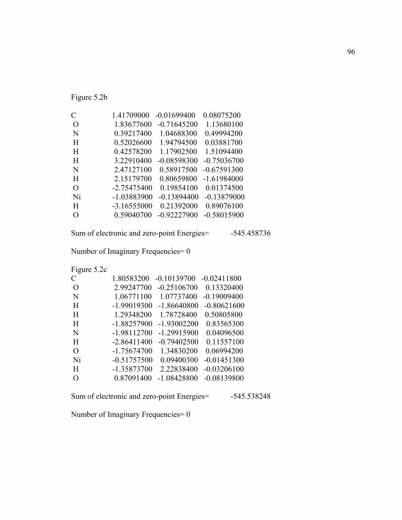
96 Figure 5.2b C 1.41709000 -0.01699400 0.08075200 O 1.83677600 -0.71645200 1.13680100 N 0.39217400 1.04688300 0.49994200 H 0.52026600 1.94794500 0.03881700 H 0.42578200 1.17902500 1.51094400 H 3.22910400 -0.08598300 -0.75036700 N 2.47127100 0.58917500 -0.67591300 H 2.15179700 0.80659800 -1.61984000 O -2.75475400 0.19854100 0.01374500 Ni -1.03883900 -0.13894400 -0.13879000 H -3.16555000 0.21392000 0.89076100 O 0.59040700 -0.92227900 -0.58015900 Sum of electronic and zero-point Energies= -545.458736 Number of Imaginary Frequencies= 0 Figure 5.2c C 1.80583200 -0.10139700 -0.02411800 O 2.99247700 -0.25106700 0.13320400 N 1.06771100 1.07737400 -0.19009400 H -1.99019300 -1.86640800 -0.80621600 H 1.29348200 1.78728400 0.50805800 H -1.88257900 -1.93002200 0.83565300 N -1.98112700 -1.29915900 0.04096500 H -2.86411400 -0.79402500 0.11557100 O -1.75674700 1.34830200 0.06994200 Ni -0.51757500 0.09400300 -0.01451300 H -1.35873700 2.22838400 -0.03206100 O 0.87091400 -1.08428800 -0.08139800 Sum of electronic and zero-point Energies= -545.538248 Number of Imaginary Frequencies= 0

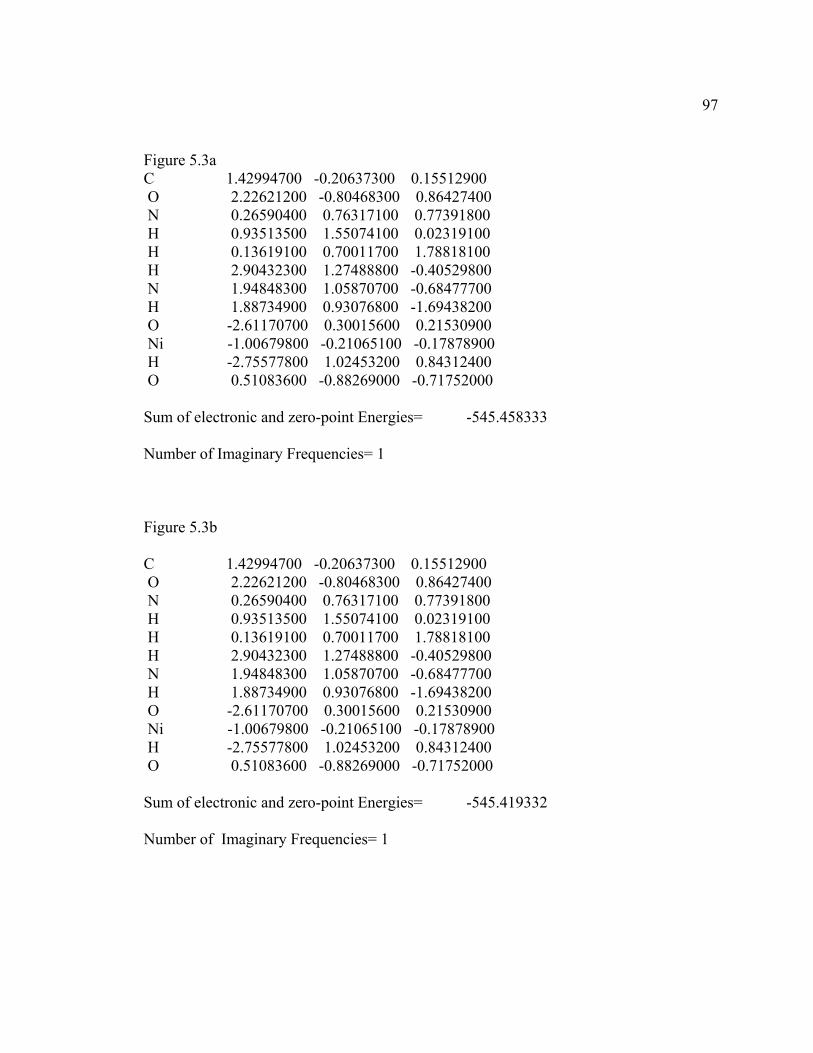
97 Figure 5.3a C 1.42994700 -0.20637300 0.15512900 O 2.22621200 -0.80468300 0.86427400 N 0.26590400 0.76317100 0.77391800 H 0.93513500 1.55074100 0.02319100 H 0.13619100 0.70011700 1.78818100 H 2.90432300 1.27488800 -0.40529800 N 1.94848300 1.05870700 -0.68477700 H 1.88734900 0.93076800 -1.69438200 O -2.61170700 0.30015600 0.21530900 Ni -1.00679800 -0.21065100 -0.17878900 H -2.75577800 1.02453200 0.84312400 O 0.51083600 -0.88269000 -0.71752000 Sum of electronic and zero-point Energies= -545.458333 Number of Imaginary Frequencies= 1 Figure 5.3b C 1.42994700 -0.20637300 0.15512900 O 2.22621200 -0.80468300 0.86427400 N 0.26590400 0.76317100 0.77391800 H 0.93513500 1.55074100 0.02319100 H 0.13619100 0.70011700 1.78818100 H 2.90432300 1.27488800 -0.40529800 N 1.94848300 1.05870700 -0.68477700 H 1.88734900 0.93076800 -1.69438200 O -2.61170700 0.30015600 0.21530900 Ni -1.00679800 -0.21065100 -0.17878900 H -2.75577800 1.02453200 0.84312400 O 0.51083600 -0.88269000 -0.71752000 Sum of electronic and zero-point Energies= -545.419332 Number of Imaginary Frequencies= 1

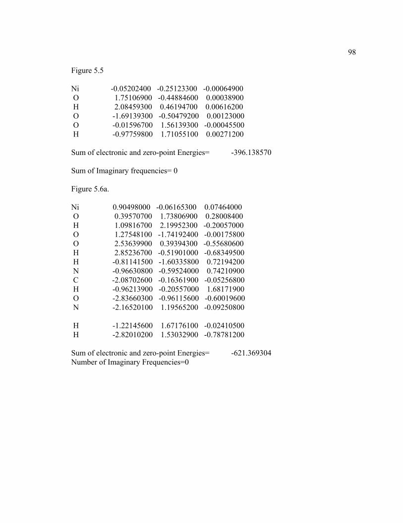
98 Figure 5.5 Ni -0.05202400 -0.25123300 -0.00064900 O 1.75106900 -0.44884600 0.00038900 H 2.08459300 0.46194700 0.00616200 O -1.69139300 -0.50479200 0.00123000 O -0.01596700 1.56139300 -0.00045500 H -0.97759800 1.71055100 0.00271200 Sum of electronic and zero-point Energies= -396.138570 Sum of Imaginary frequencies= 0 Figure 5.6a. Ni 0.90498000 -0.06165300 0.07464000 O 0.39570700 1.73806900 0.28008400 H 1.09816700 2.19952300 -0.20057000 O 1.27548100 -1.74192400 -0.00175800 O 2.53639900 0.39394300 -0.55680600 H 2.85236700 -0.51901000 -0.68349500 H -0.81141500 -1.60335800 0.72194200 N -0.96630800 -0.59524000 0.74210900 C -2.08702600 -0.16361900 -0.05256800 H -0.96213900 -0.20557000 1.68171900 O -2.83660300 -0.96115600 -0.60019600 N -2.16520100 1.19565200 -0.09250800 H -1.22145600 1.67176100 -0.02410500 H -2.82010200 1.53032900 -0.78781200 Sum of electronic and zero-point Energies= -621.369304 Number of Imaginary Frequencies=0

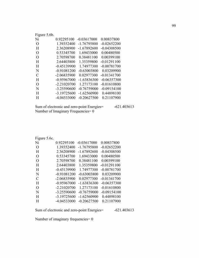
99 Figure 5.6b. Ni 0.92295100 -0.03617000 0.00837800 O 1.39352400 -1.76795800 -0.02652200 H 2.36208900 -1.67892600 -0.04308500 O 0.53345700 1.69433000 0.00480500 O 2.70598700 0.38481100 0.00399100 H 2.64403800 1.35359800 -0.01291100 H -0.45139900 1.74977300 -0.00781700 N -0.91081200 -0.63003800 0.03209900 C -2.06835900 0.02977300 -0.01341700 H -0.95967000 -1.63836300 -0.06357300 O -2.21020700 1.27173100 -0.01610800 N -3.25590600 -0.76759000 -0.09154100 H -3.19725600 -1.62560900 0.44898100 H -4.04533000 -0.20627500 0.21107900 Sum of electronic and zero-point Energies= -621.403613 Number of Imaginary Frequencies= 0 Figure 5.6c. Ni 0.92295100 -0.03617000 0.00837800 O 1.39352400 -1.76795800 -0.02652200 H 2.36208900 -1.67892600 -0.04308500 O 0.53345700 1.69433000 0.00480500 O 2.70598700 0.38481100 0.00399100 H 2.64403800 1.35359800 -0.01291100 H -0.45139900 1.74977300 -0.00781700 N -0.91081200 -0.63003800 0.03209900 C -2.06835900 0.02977300 -0.01341700 H -0.95967000 -1.63836300 -0.06357300 O -2.21020700 1.27173100 -0.01610800 N -3.25590600 -0.76759000 -0.09154100 H -3.19725600 -1.62560900 0.44898100 H -4.04533000 -0.20627500 0.21107900 Sum of electronic and zero-point Energies= -621.403613 Number of imaginary frequencies= 0

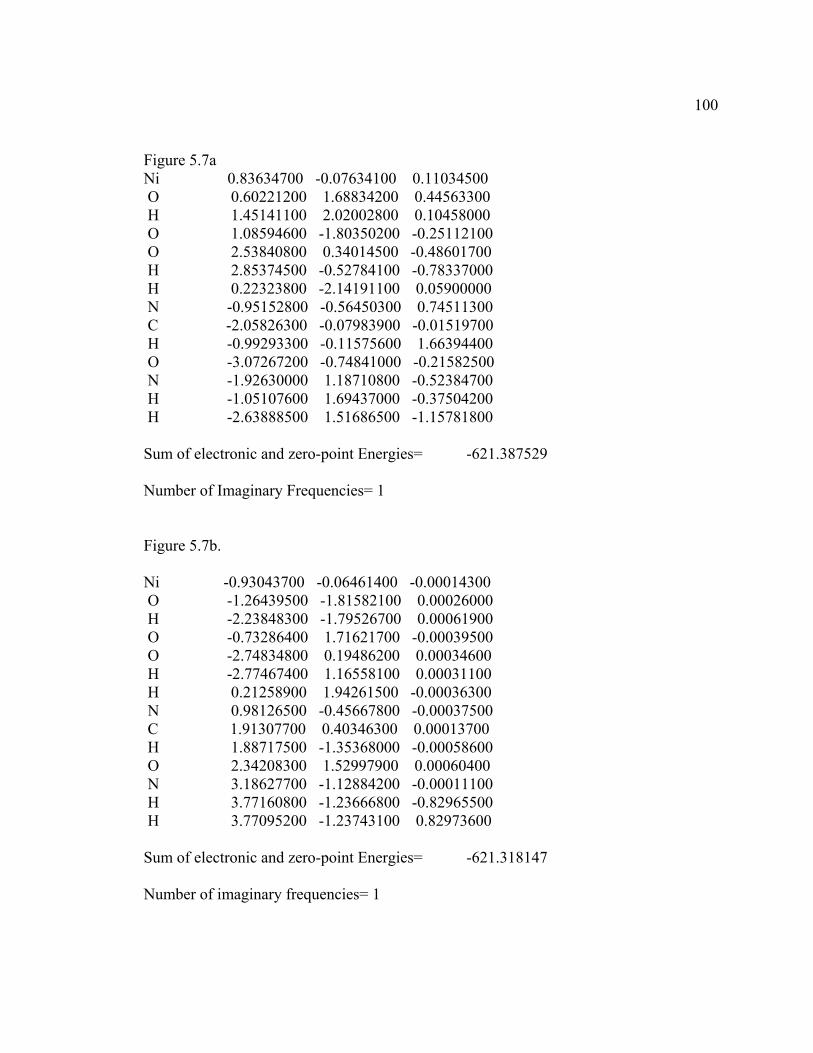
100 Figure 5.7a Ni 0.83634700 -0.07634100 0.11034500 O 0.60221200 1.68834200 0.44563300 H 1.45141100 2.02002800 0.10458000 O 1.08594600 -1.80350200 -0.25112100 O 2.53840800 0.34014500 -0.48601700 H 2.85374500 -0.52784100 -0.78337000 H 0.22323800 -2.14191100 0.05900000 N -0.95152800 -0.56450300 0.74511300 C -2.05826300 -0.07983900 -0.01519700 H -0.99293300 -0.11575600 1.66394400 O -3.07267200 -0.74841000 -0.21582500 N -1.92630000 1.18710800 -0.52384700 H -1.05107600 1.69437000 -0.37504200 H -2.63888500 1.51686500 -1.15781800 Sum of electronic and zero-point Energies= -621.387529 Number of Imaginary Frequencies= 1 Figure 5.7b. Ni -0.93043700 -0.06461400 -0.00014300 O -1.26439500 -1.81582100 0.00026000 H -2.23848300 -1.79526700 0.00061900 O -0.73286400 1.71621700 -0.00039500 O -2.74834800 0.19486200 0.00034600 H -2.77467400 1.16558100 0.00031100 H 0.21258900 1.94261500 -0.00036300 N 0.98126500 -0.45667800 -0.00037500 C 1.91307700 0.40346300 0.00013700 H 1.88717500 -1.35368000 -0.00058600 O 2.34208300 1.52997900 0.00060400 N 3.18627700 -1.12884200 -0.00011100 H 3.77160800 -1.23666800 -0.82965500 H 3.77095200 -1.23743100 0.82973600 Sum of electronic and zero-point Energies= -621.318147 Number of imaginary frequencies= 1