Analytical Hysteretic Behavior of Square Concrete-Filled Steel

Citation: Zhang, T.; Wen, Q.; Gao, L.;

Xu, Q.; Tang, J. Analytical Hysteretic

Behavior of Square Concrete-Filled

Steel Tube Pier Columns under

Alternate Sulfate Corrosion and

Freeze-Thaw Cycles. Materials 2022,

15, 3099. https://doi.org/10.3390/

ma15093099

Academic Editors: Shao-Bo Kang and

Shan Gao

Received: 25 March 2022

Accepted: 21 April 2022

Published: 25 April 2022

Publisher’s Note: MDPI stays neutral

with regard to jurisdictional claims in

published maps and institutional affil-

iations.

Copyright: © 2022 by the authors.

Licensee MDPI, Basel, Switzerland.

This article is an open access article

distributed under the terms and

conditions of the Creative Commons

Attribution (CC BY) license (https://

creativecommons.org/licenses/by/

4.0/).

materials

Article

Analytical Hysteretic Behavior of Square Concrete-Filled SteelTube Pier Columns under Alternate Sulfate Corrosion andFreeze-Thaw CyclesTong Zhang 1,2, Qianxin Wen 1, Lei Gao 3, Qian Xu 1,* and Jupeng Tang 2

1 School of Civil Engineering, Liaoning Technical University, Fuxin 123000, China; [email protected] (T.Z.);[email protected] (Q.W.)

2 School of Mechanics and Engineering, Liaoning Technical University, Fuxin 123000, China; [email protected] Liaoning Hanshi Technology Group Co., Ltd., Fuxin 123099, China; [email protected]* Correspondence: [email protected]; Tel./Fax: +86-0418-2162036

Abstract: The hysteretic behavior of square concrete-filled steel tube (CFST) stub columns subjectedto sulfate corrosion and freeze-thaw cycle is examined by numerical investigation. The constitutivemodel of steel considered the Bauschinger effect, and compression (tension) damage coefficientwas also adopted for the constitutive model of core concrete. The experimental results are usedto verify the finite element (FE) model, which could accurately predict the hysteretic behaviors ofthe CFST piers. Then, the effects of the yield strength of steel, compressive strength of concrete,steel ratio, axial compression ratio, and alternation time on ultimate horizontal load are evaluatedby a parametric study. The results showed that the yield strength of steel and the steel ratio havea positive effect of hysteretic behavior. The compressive strength of concrete and alternation timesignificantly decreased the unloading stiffness which causes the pinching phenomenon. The yieldstrength of steel, compressive strength of concrete, and alternation time of environmental factors(corrosion-freeze-thaw cycles) has no obvious effect on the initial stiffness, while the steel ratio hasa remarkable effect. The ultimate horizontal load increases with the increasing steel ratio, yieldstrength of steel and compressive strength of concrete. Meanwhile, the decrement of alternation timeled to the increase of ultimate horizontal load. This suggests that the confinement coefficient andalternation time are the two main factors that impact the ultimate horizontal load. A formula whichconsiders the reduction coefficient for the ultimate horizontal load of the CFST columns subjectedto sulfate corrosion and freeze-thaw cycles is proposed. The formulae can accurately predict theultimate horizontal load with mean value of 1.022 and standard deviation of 0.003.

Keywords: sulfate corrosion; freeze-thaw cycle; alternation effect; CFST pier column; hystereticbehavior

1. Introduction

Concrete-filled steel tubes (CFST) are composite structural members with an outersteel tube and an inner core of concrete [1,2]. The utilization of CFST columns has beencommonplace in recent decades due to the infilling concrete supporting the steel tube,which prevents its inward buckling and postpones its outward buckling [3]. Moreover, thesteel tube restricts the core concrete in transverse, and thus, due to the confinement effect,the concrete is under three-dimensional compression, which leads to the improvement ofload-bearing capacity and ductility [4,5]. Considerable research of CFST columns has beenconducted on buildings and bridges’ rib arches [6–9]. In addition, the feasibility of usingCFST columns as bridge piers has been reported [10–13].

Tomii et al. [14] firstly studied the seismic behavior of square CFST through a quasi-staticmethod and illustrated that CFSTs were excellent in energy dissipation. K. Nakanishi et al. [15]investigated the peak horizontal load and ductility of bridge pier columns with different

Materials 2022, 15, 3099. https://doi.org/10.3390/ma15093099 https://www.mdpi.com/journal/materials

https://doi.org/10.3390/ma15093099

https://doi.org/10.3390/ma15093099

https://creativecommons.org/

https://creativecommons.org/licenses/by/4.0/

https://creativecommons.org/licenses/by/4.0/

https://www.mdpi.com/journal/materials

https://www.mdpi.com

https://orcid.org/0000-0002-3800-714X

https://doi.org/10.3390/ma15093099

https://www.mdpi.com/journal/materials

https://www.mdpi.com/article/10.3390/ma15093099?type=check_update&version=1

Materials 2022, 15, 3099 2 of 27

composite forms experimentally. The study theoretically verified the analogous rule betweenfull-scale models and scaled-down specimens and found that the CFST pier columns werebetter in resistant cyclic loading. Aval et al. [16] adopted an inelastic fiber element modelconsidering the axial elongation and curvature of steel tubes and concrete to analyze CFSTcolumns under cyclic load. The results showed that the CFST with studs or reinforcementribs has a higher dissipation of energy. M. Bruneau et al. [17] evaluated the limitation ofexisting design codes for circular CFST bridge piers by establishing an experimental database.Then, based on the simple plastic model, a new equation was proposed and the specifications“Guide for Load and Resistance Factor Desing (LRFD) Criteria for Offshore Structures” wererecommended for the seismic design of bridge piers. Li [18] carried out a dynamic time historyanalysis of CFST piers according to practical engineering at a 7-degree (M = 0.58I + 1.5, whereM is Richter scale, I denotes seismic fortification intensity, I = 7 here) protected earthquakeintensity. It illustrated that the vertex displacement of pier columns was below the ultimatedisplacement for all 18 earthquake excitations, which verified that the CFST pier columnhas good seismic resistant. Wang [19] studied the effect of concrete fill percentage on theseismic behavior of CFST pier columns with filling ratios of 0%, 23%, 27%, 30%, and 31%. Thestudy also considered the slenderness ratio and width-to-thickness ratio. It showed that thesupporting role of concrete has the advantage of seismic resistance but the optional filling raterequires further investigation.

The bridge pier is generally used as a pressure-bearing member and works undercomplex conditions including load action, vehicle impact, harsh environment, and seismiceffect, which takes disadvantage of the lifelong service of the bridge [20]. Chen et al. [21] in-vestigated the effect of corrosion ratio and recycled aggregate replacement ratio on the axialcompressive behavior of circular CFST columns by experimental and numerical research. Itdemonstrated that the type of recycled aggregate has a slight effect on loadbearing capacityof specimens under sulfate corrosion. Chen et al. [22–24] consider the effect of corrosionratio and recycled aggregate replacement ratio to investigate the axial compressive behav-ior of 16 square CFST columns under sulfate corrosion experimentally and numerically.They demonstrated that the recycled aggregate type has negligible effect on specimensunder sulfate corrosion. However, the corrosion time resulted in the decrement of ultimatebearing capacity, ductility, and composite elastic modulus of the specimen. FE modelsconsidering the reduction of thickness of the steel tubes could effectively simulate the effectof sulfate corrosion on steel tubes. Zhang [25] carried out a durability test on 20 thin-walledsteel tube columns under SO4

2− corrosion. The study found that ultimate bearing capacity,ductility, and stiffness decreased with the corrosion ratio, especially for the specimens withthinner walls. The finial failure mode of the CFST stub columns under sulfate corrosionwas due to shear failure. After corrosion by SO4

2−, local bucking of the slender steel tubewould occur to a large extent.

Yang et al. [26] experimentally dealt with the effect of freeze-thaw cycles, section type,and compressive strength of axially loaded CFST columns under freeze-thaw conditions.The test results demonstrated that the freeze-thaw cycle significantly influenced the load-bearing capacity, composite elastic modulus, and ductility index but slightly impacted thefailure mode. They mentioned that the circular specimens performed better with regards toductility. Wang [27] carried out an experimental test of axially loaded square CFST columnswith an end plate to enlarge the effect of freeze-thaw cycles on compressive behavior.Wang [27] found that the cyclic time has a negative linear relationship on loadbearingcapacity and initial stiffness of the specimens. Yan [28–30] investigated the axially loadedCFST stub columns under the freezing temperatures of −30 ◦C, −60 ◦C, and −80 ◦C. Thetest results presented that square specimens were destroyed in crushing failure, and fewspecimens appeared tensile fracture. Freezing temperature improved the ultimate compres-sive load and initial stiffness of CFST columns but decreased the ductility. Gao et al. [31]focused on the mechanical behaviors of circular CFST stub columns under freeze-thawcycles in experimental tests. The effect of cyclic time and compressive strength of concretefor the axially loaded specimens was analyzed. Gao et al. [31] found that axial compressive

Materials 2022, 15, 3099 3 of 27

strength decreased linearly with cyclic time while it increased with a higher compressivestrength of concrete.

The durability of CFST pier columns is significantly influenced by a harsh environment,such as corrosion [32] and freeze-thaw [33]. However, few studies have investigatedthe compound influence of multiple environmental factors, which is in accordance withpractical structure. Studies on dynamic properties were concentrated on CFST columns inambient conditions. The steel tube suffering alternating sulfate corrosion and freeze-thawcycles will result in higher brittleness and the concrete will crack at the interfacial transitionzone due to the mechanical deterioration of the specimen. In addition, the seismic effectcoupling with the alternation of sulfate corrosion and freeze-thaw cycles will rapidly causematerial deterioration, and thus will cause corrosion fatigue cracks to occur more easily.This study thus carries out a simulation study of hysteretic behavior on 126 square CFSTpier columns. Based on the reasonable constitutive model, nonlinear finite element (FE)models are set to analyze the CFST pier columns with a failure mode of shear failure byABAQUS software. Then, the effect of strength of materials, steel ratio, axial compressionratio, and alternate time on the horizontal load-deformation hysteretic curve and skeletoncurve. Ultimately, the reduction coefficient corresponding to the ultimate horizontal loadwas analyzed and a design formula to predict the ultimate horizontal load of square CFSTpier columns after alternate of sulfate corrosion and freeze-thaw cycles was proposed.

2. Empirical Experimental Research

The square CFST pier columns were corroded through electrochemical corrosion.The electrolyte was a mixed solution of Ca(NO3)2, Na2SO4, and NH4Cl and adoptedHNO3 to adjust pH value, which was set as 4.5. The specimens were fully immersedinto the electrolyte. The corrosion rate was defined as the loss of mass of the steel andcorrosion rate γ = 10%, 20%, and 30% corresponded to the terms of service of 5, 10, and15 years. Hemispherical pitting was formed on the surface of the steel tubes. The testresults reported in previous studies [34–43] were selected to verify the CFST pier columnsmodeled in ABAQUS software [44]. Table 1 summarizes their experimental test results. Theparameters of each specimen were listed in Table 1, and it can be found that the specimenlabels dividing different groups were the same as those tested in [34–43]. As shown inTable 1, the length of the specimens ranged from 530 to 1250 mm, corresponding to a length-to-width (L/B) ratio of 2.12–5.00. Thus, the influence of the slenderness effect could beavoided [45]. The compressive strength of the concrete cores ranges from 33.0 to 75.1 MPa,which includes normal-strength concrete and high-strength concrete [45] (f ck ≤ 50 MPa isdefined as normal strength concrete). Specimens with reinforcement bars consist of 8Φ16and 4Φ11, and the ties used are Φ8@100 mm and Φ8@200 mm, which meet the specificationrequirements [46]. Then, the yield strength of the steel tubes varies from 242.2 to 389.0 MPa,and the axial compression ratio ranges from 0.2 to 0.60. The material properties of steeland infilled concrete can be obtained from tests or specifications such as GB50010 [46],ACI-318-08 [47], EN-1992-1-1 [48], GB50017 [49], AS4100 [50], etc. Figure 1 presents detailsof the typical testing device with which the hysteretic behavior of the specimens couldbe tested.

The method of quasi-static tests was generally adopted to investigate the effect ofreciprocating cyclic loading on structural members. This method took advantage of easyoperation and observation, controlled loading process, and convenience of checking data,and thus the quasi-static test method was selected to investigate the hysteretic behaviors ofspecimens. According to JGJ/T101-2015 [51], the loading history of cyclic loading includeda force control phase and a displacement control phase, as showed in Figure 2. In theforce control phase, one cycle was imposed at the load levels of 0.5Nvy, 0.5Nvy, and Nvy,respectively, where Nvy is the estimated value of specimen yield strength. Afterward,displacement-controlled loading was performed at the incremental levels of 1δy, 2δy, 3δy,etc, where δy represents the estimated displacement corresponding to the yield strength,and the cyclic loading was reported twice for each displacement level. The cyclic load-

Materials 2022, 15, 3099 4 of 27

ing was repeated twice for each displacement level. The yield strength Nvy and yielddisplacement δy were tested with the GYM (general yield moment) method. Horizontaldeformation was measured by linear variable differential transformers (LVDTs) and strainwas measured by strain gauges. Final failure was defined as horizontal load decreasing to85% of its peak value [51]. The test results of the specimens in Refs. [34–43] were listed inTable 1.

Table 1. Specifications of the tested CFST columns in Refs. [34–43].

No. Reference Labels B × L × t (mm) f cu, test (MPa) f y (MPa) f by (MPa) d (mm) n

1[34,35]

STRC-60-1.5-4200 × 600 × 1.89 60.0 309.2 357.0 16.4

0.402 STRC-60-1.5-6 0.603

[36,37]STRC-70-4-1.5

200 × 600 × 3.00 75.1 254.0 449.4 11.00.35

4 STRC-70-5-1.5 0.455 STRC-70-6-1.5 0.556 [38] FGZ4 250 × 1250 × 5.00 33.0 389.0

NA NA

0.247

[39–41]A1

200 × 600 × 6.00 50.1 330.00.20

8 A2 0.409 A3 0.60

10[42,43]

RS-4L 250 × 530 × 4.0041.0

265.0 0.2011 RS-6M 250 × 530 × 6.00 317.6 0.4012 RS-10H 250 × 530 × 10.00 242.2 0.54

Note: NA denotes the abbreviation of not available.

Materials 2022, 15, x FOR PEER REVIEW 4 of 27

Figure 1. Experimental device and layout of the specimen.

Table 1. Specifications of the tested CFST columns in Refs. [34–43].

No. Reference Labels B × L × t

(mm)

fcu, test

(MPa) fy (MPa)

fby

(MPa) d (mm) n

1 [34,35]

STRC-60-1.5-4 200 × 600 ×

1.89 60.0 309.2 357.0 16.4

0.40

2 STRC-60-1.5-6 0.60

3

[36,37]

STRC-70-4-1.5 200 × 600 ×

3.00 75.1 254.0 449.4 11.0

0.35

4 STRC-70-5-1.5 0.45

5 STRC-70-6-1.5 0.55

6 [38] FGZ4 250 × 1250 ×

5.00 33.0 389.0

NA NA

0.24

7

[39–41]

A1 200 × 600 ×

6.00 50.1 330.0

0.20

8 A2 0.40

9 A3 0.60

10

[42,43]

RS-4L 250 × 530 ×

4.00

41.0

265.0 0.20

11 RS-6M 250 × 530 ×

6.00 317.6 0.40

12 RS-10H 250 × 530 ×

10.00 242.2 0.54

Note: NA denotes the abbreviation of not available.

The method of quasi-static tests was generally adopted to investigate the effect of

reciprocating cyclic loading on structural members. This method took advantage of easy

operation and observation, controlled loading process, and convenience of checking data,

and thus the quasi-static test method was selected to investigate the hysteretic behaviors

of specimens. According to JGJ/T101-2015 [51], the loading history of cyclic loading in-

cluded a force control phase and a displacement control phase, as showed in Figure 2. In

the force control phase, one cycle was imposed at the load levels of 0.5Nvy, 0.5Nvy, and Nvy,

respectively, where Nvy is the estimated value of specimen yield strength. Afterward, dis-

placement-controlled loading was performed at the incremental levels of 1δy, 2δy, 3δy, etc,

where δy represents the estimated displacement corresponding to the yield strength, and

the cyclic loading was reported twice for each displacement level. The cyclic loading was

repeated twice for each displacement level. The yield strength Nvy and yield displacement

δy were tested with the GYM (general yield moment) method. Horizontal deformation

was measured by linear variable differential transformers (LVDTs) and strain was meas-

ured by strain gauges. Final failure was defined as horizontal load decreasing to 85% of

its peak value [51]. The test results of the specimens in Refs. [34–43] were listed in Table

1.

Figure 1. Experimental device and layout of the specimen.


0 T0 T

1δh

2δh

3δh

Nhy

Nh Δh

(a) (b)

Figure 2. Loading system of specimens. (a) Vertical loading system; (b) Horizontal loading system.

The test results obtained for the square CFST columns under reciprocating cyclic

loading in terms of different main parameters were sketched and compared with the FE

results in Section 3.5 in the forms of failure mode, skeleton curve, and horizontal ultimate

compressive load in detail.

3. Finite Element Modeling

The phenomenological modeling of square CFSTs is typically performed by using

differential [52,53] or non-differential models [54,55] and is determined by three main

parts, including core concrete, steel tube, and interaction between these two raw materials.

In addition, in FE analysis of the specimens, selection of element type and mesh size

should balance the accuracy of the simulation results and simulation time. Since square

CFST pier columns under cyclic load are not symmetrical, the whole specimen is modelled

to investigate the hysteretic behaviors.

3.1. Material Properties

3.1.1. Steel Tube

A secondary plastic flow stress-strain curve [45] was modified according to the effect

of corrosion-freeze-thaw cycles on the relationship of stress–strain and then adopted to

define the material behavior under sulfate corrosion and freeze-thaw cycles of steel tubes,

which include five stages: elastic, elastic-plastic stage, plastic, yield strength, and strength-

ening and secondary plastic flow stages. The main parameters for defining the stress–

strain curve of a steel tube include the limit of proportionality (fp), yield strength of the

steel tube (fy), ultimate compressive strength (fu), and the corresponding strain (εe, εe1, εe2

and εe3). The five-stage stress–strain model of a steel tube can be defined as Equation (1)

shows. Young’s modulus and Poisson’s ratio in the model adopted were 206 GPa and

0.283 [47,49] respectively.

Figure 2. Loading system of specimens. (a) Vertical loading system; (b) Horizontal loading system.

Materials 2022, 15, 3099 5 of 27

The test results obtained for the square CFST columns under reciprocating cyclicloading in terms of different main parameters were sketched and compared with the FEresults in Section 3.5 in the forms of failure mode, skeleton curve, and horizontal ultimatecompressive load in detail.

3. Finite Element Modeling

The phenomenological modeling of square CFSTs is typically performed by usingdifferential [52,53] or non-differential models [54,55] and is determined by three main parts,including core concrete, steel tube, and interaction between these two raw materials. Inaddition, in FE analysis of the specimens, selection of element type and mesh size shouldbalance the accuracy of the simulation results and simulation time. Since square CFSTpier columns under cyclic load are not symmetrical, the whole specimen is modelled toinvestigate the hysteretic behaviors.

3.1. Material Properties3.1.1. Steel Tube

A secondary plastic flow stress-strain curve [45] was modified according to the effect ofcorrosion-freeze-thaw cycles on the relationship of stress–strain and then adopted to definethe material behavior under sulfate corrosion and freeze-thaw cycles of steel tubes, whichinclude five stages: elastic, elastic-plastic stage, plastic, yield strength, and strengtheningand secondary plastic flow stages. The main parameters for defining the stress–straincurve of a steel tube include the limit of proportionality (f p), yield strength of the steeltube (f y), ultimate compressive strength (f u), and the corresponding strain (εe, εe1, εe2 andεe3). The five-stage stress–strain model of a steel tube can be defined as Equation (1) shows.Young’s modulus and Poisson’s ratio in the model adopted were 206 GPa and 0.283 [47,49]respectively.

σs =

Eseεs εs ≤ εe−Aε2

s + Bεs + C εe < εs ≤ εe1fye εe1 < εs ≤ εe2

fye

[1 + 0.6 εs−εe2

εs3−εe2

]εe2 < εs ≤ εe3

1.6 fye εs > εe3

(1)

where εe = 0.8f ye/Ese, εe1 = 1.5εe, εe2 = 10εe1, εe3 = 100εe1, A = 0.2f y(εe1 − εe)2, B = 2Aεe1,C = 0.8f ye + Aεe2 − Bεe, Ese = (1 − 0.525γ)Es, f ye = (1 − 0.908γ)f y, and β = ∆t/t, ∆t = t − te.

When the CFST columns were subjected to the alternation effect of sulfate corrosionand freeze-thaw cycles, not only the thickness, but also the mechanical properties of thesteel tube changed. A series of typical stress–strain curves of steel tubes of 345 MPa withcorrosion rates of 0%, 10%, 30%, and 50% was presented in Figure 3. The von Mises criterionis adopted to estimate steel yield stress.


se s s e

2

s s e s e1

ye e1 s e2

s e2ye e2 s e3

s3 e2

ye

1 0.6

1.6

s

E

A B C

f

f

f

s e3

(1)

where εe = 0.8fye/Ese, εe1 = 1.5εe, εe2 = 10εe1, εe3 = 100εe1, A = 0.2fy(εe1 − εe)2, B = 2Aεe1, C = 0.8fye

+ Aεe2 − Bεe, Ese = (1 − 0.525γ)Es, fye = (1 − 0.908γ)fy, and β = Δt/t, Δt = t − te.

When the CFST columns were subjected to the alternation effect of sulfate corrosion

and freeze-thaw cycles, not only the thickness, but also the mechanical properties of the

steel tube changed. A series of typical stress–strain curves of steel tubes of 345 MPa with

corrosion rates of 0%, 10%, 30%, and 50% was presented in Figure 3. The von Mises crite-

rion is adopted to estimate steel yield stress.

Figure 3. Stress–strain curve of steel tube under alternation of sulfate corrosion and freeze-thaw

cycles.

The Bouc–Wen modified model [56] is not particularly sensitive to the selection of its

parameters. Vaiana et al. [57] proposed a hysteretic mechanical system by combining a

novel rate-independent model and an explicit time integration method which avoid the

convergence problem for its small time step. Since the hysteretic behaviors of steel tubes

under cyclic loading are complex and the effects of corrosion-freeze-thaw cycles have

strong randomness, using a bilinear model is more easily describes the complex environ-

ment effects. The stress–strain skeleton curve of a steel tube corresponding to its hysteretic

behavior is composed of two parts, which are the elastic stage and the strain hardening

stage, as shown in Figure 4. It can be seen that unloading occurred in the strain hardening

stage, which caused non-negligible residual strain. The residual stress would decrease

when reverse loading, which caused dimensional stability issues. Due to the effect of re-

sidual strain on the loading and unloading process, the Bausinger effect should be taken

into account. The stress–strain model of the steel tube was presented in Equation (2),

where the elastic modulus in the strain hardening stage was defined as 0.01Ese.

se y

ye se y y

0

0.01

E

f E

(2)

Figure 3. Stress–strain curve of steel tube under alternation of sulfate corrosion and freeze-thaw cycles.

Materials 2022, 15, 3099 6 of 27

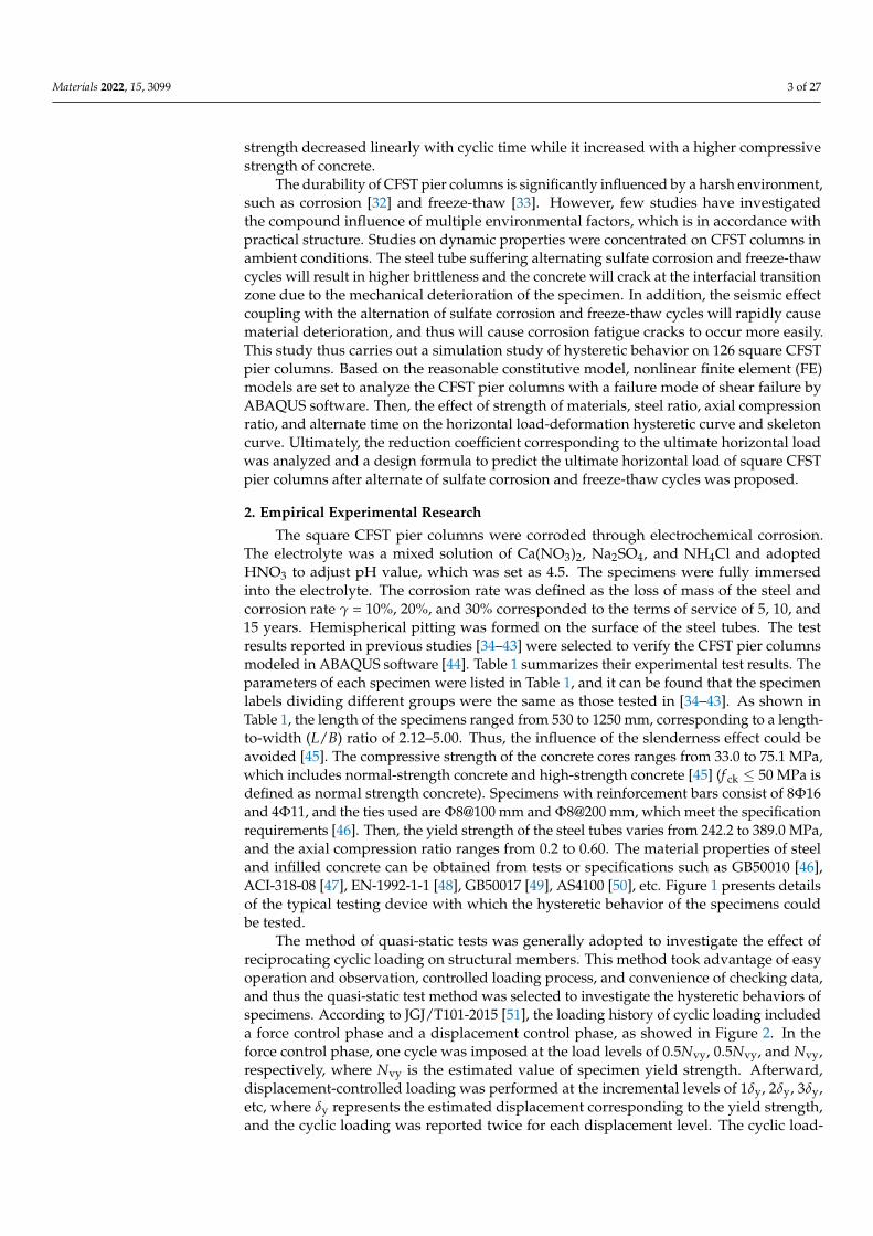
The Bouc–Wen modified model [56] is not particularly sensitive to the selection ofits parameters. Vaiana et al. [57] proposed a hysteretic mechanical system by combininga novel rate-independent model and an explicit time integration method which avoidthe convergence problem for its small time step. Since the hysteretic behaviors of steeltubes under cyclic loading are complex and the effects of corrosion-freeze-thaw cycleshave strong randomness, using a bilinear model is more easily describes the complexenvironment effects. The stress–strain skeleton curve of a steel tube corresponding to itshysteretic behavior is composed of two parts, which are the elastic stage and the strainhardening stage, as shown in Figure 4. It can be seen that unloading occurred in the strainhardening stage, which caused non-negligible residual strain. The residual stress woulddecrease when reverse loading, which caused dimensional stability issues. Due to the effectof residual strain on the loading and unloading process, the Bausinger effect should betaken into account. The stress–strain model of the steel tube was presented in Equation (2),where the elastic modulus in the strain hardening stage was defined as 0.01Ese.

σ =

{Ese ε

(0 ≤ ε ≤ εy

)fye + 0.01Ese

(ε− εy

) (ε ≥ εy

) (2)

where σ is the stress of the steel tube, Ese is the elastic modulus of steel, ε is the strain of thesteel tube below yield strain, εy is the yield strain corresponding to the yield strength of thesteel tube.


where σ is the stress of the steel tube, Ese is the elastic modulus of steel, ε is the strain of

the steel tube below yield strain, εy is the yield strain corresponding to the yield strength

of the steel tube.

Figure 4. Bilinear kinematic hardening model of steel tube.

3.1.2. Confined Core Concrete

The stress–strain model proposed by Han et al. [45] was adopted to simulate the

properties of core concrete. The material law for the core concrete under the alternation

effect of sulfate corrosion and freeze-thaw cycles was illustrated in Figure 5.

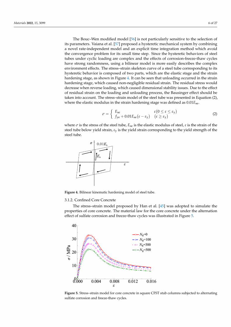
Figure 5. Stress–strain model for core concrete in square CFST stub columns subjected to alternating

sulfate corrosion and freeze-thaw cycles.

The core concrete is modelled through the concrete damage plasticity (CDP) model.

A stress–strain model considering the confinement effect in improving the behavior of

core concrete by Han et al. [45] was applied to define the concrete material in the FE

model.

22 1

11

x x x

y xx

x x

(3)

where x = ε/ε0, ε is the strain of the concrete and ε0 is the peak strain corresponding to

peak load, ε0 = (1300 + 12.5'

cf + 800ξe2) × 10−6, y = σ/σ0, σ is the stress of concrete and σ0 is

the stress corresponding to the peak load, σ0 = fc’(1 − 0.035Nft/100), '

cf = [0.76 +

0.2log10(fcu/19.6)]fcu, '

cf is the cylinder strength of concrete, fcu is the cube compressive

strength of concrete, η = 1.6 + 1.5/x, η is defined as shape coefficient to reflect the properties

of shape cross section, β = ('

cf )0.1/[1.2(1 + ξe)0.5], ξe =αe × fye/fck, ξe is the effective confine-

ment factor, fye and fck are the effective yield strength of steel tube and characteristic com-

pressive strength of concrete, respectively; fck = 0.88 × 0.76 × fcu, αe = Ase/Ac; αe is the steel



The stress–strain model proposed by Han et al. [45] was adopted to simulate theproperties of core concrete. The material law for the core concrete under the alternationeffect of sulfate corrosion and freeze-thaw cycles was illustrated in Figure 5.


where σ is the stress of the steel tube, Ese is the elastic modulus of steel, ε is the strain of

the steel tube below yield strain, εy is the yield strain corresponding to the yield strength

of the steel tube.



The stress–strain model proposed by Han et al. [45] was adopted to simulate the

properties of core concrete. The material law for the core concrete under the alternation

effect of sulfate corrosion and freeze-thaw cycles was illustrated in Figure 5.

Figure 5. Stress–strain model for core concrete in square CFST stub columns subjected to alternating

sulfate corrosion and freeze-thaw cycles.

The core concrete is modelled through the concrete damage plasticity (CDP) model.

A stress–strain model considering the confinement effect in improving the behavior of

core concrete by Han et al. [45] was applied to define the concrete material in the FE

model.

22 1

11

x x x

y xx

x x

(3)

where x = ε/ε0, ε is the strain of the concrete and ε0 is the peak strain corresponding to

peak load, ε0 = (1300 + 12.5'

cf + 800ξe2) × 10−6, y = σ/σ0, σ is the stress of concrete and σ0 is

the stress corresponding to the peak load, σ0 = fc’(1 − 0.035Nft/100), '

cf = [0.76 +

0.2log10(fcu/19.6)]fcu, '

cf is the cylinder strength of concrete, fcu is the cube compressive

strength of concrete, η = 1.6 + 1.5/x, η is defined as shape coefficient to reflect the properties

of shape cross section, β = ('

cf )0.1/[1.2(1 + ξe)0.5], ξe =αe × fye/fck, ξe is the effective confine-

ment factor, fye and fck are the effective yield strength of steel tube and characteristic com-

pressive strength of concrete, respectively; fck = 0.88 × 0.76 × fcu, αe = Ase/Ac; αe is the steel

Figure 5. Stress–strain model for core concrete in square CFST stub columns subjected to alternatingsulfate corrosion and freeze-thaw cycles.

Materials 2022, 15, 3099 7 of 27

The core concrete is modelled through the concrete damage plasticity (CDP) model. Astress–strain model considering the confinement effect in improving the behavior of coreconcrete by Han et al. [45] was applied to define the concrete material in the FE model.

y =

{2x− x2 (x ≤ 1)

xβ(x−1)η+x (x > 1) (3)

where x = ε/ε0, ε is the strain of the concrete and ε0 is the peak strain correspondingto peak load, ε0 = (1300 + 12.5 f ′c + 800ξe

2) × 10−6, y = σ/σ0, σ is the stress of con-crete and σ0 is the stress corresponding to the peak load, σ0 = f c

’(1 − 0.035Nft/100),f ′c = [0.76 + 0.2log10(f cu/19.6)]f cu, f ′c is the cylinder strength of concrete, f cu is the cubecompressive strength of concrete, η = 1.6 + 1.5/x, η is defined as shape coefficient to reflectthe properties of shape cross section, β = ( f ′c)0.1/[1.2(1 + ξe)0.5], ξe =αe × f ye/f ck, ξe isthe effective confinement factor, f ye and f ck are the effective yield strength of steel tubeand characteristic compressive strength of concrete, respectively; f ck = 0.88 × 0.76 × f cu,αe = Ase/Ac; αe is the steel ratio, and Ase and Ac are the effective cross-sectional areas ofthe steel tube and core concrete, respectively.

The elastic modulus of core concrete was calculated by Equation (4), which wasproposed by ACI 318 [47] as follows:

Ec = 4700√

f ′c (4)

where Ec is the elastic modulus of core concrete and f ′c denotes the cylinder strengthof concrete.

The parameters of the CDP model were defined in the numerical model using theformula provided by Tao et al. [58]. The value of the dilation angle (ψ), Kc, f b0/f c0 wasdetermined by Equations (5)–(7). The eccentricity value was selected as 0.1 and the viscosityparameter was chosen as 0.0001 to improve the convergency of the model.

ψ =

{56.3(1− ξe) ξe ≤ 0.5

6.672e7.4

4.64+ξe ξe > 0.5(5)

Kc =5.5

5 + 2( f ′c)0.075 (6)

fb0/ fc0 = 1.5(

f ′c)0.075 (7)

where ξe is the effective confinement factor, f ′c is the cylinder strength of concrete, f b0 is theinitial biaxial strength of concrete, and f c0 is the initial axial strength of concrete.

Since the stress–strain relationship of concrete under hysteretic load could be replacedby that under uniaxial load [45], the stress–strain model of uniaxial load was adoptedherein to be the skeleton curve of the hysteretic relationship. However, the concrete of theCFSTs under hysteretic load experienced the phenomenon of strain softening and stiffnessdegradation, which were caused by the development of cracks. Based on the characteristicsof energy absorption and energy dissipation in the process of plastic deformation, theconcrete damage model proposed by Britel and Mark [59] was introduced to the constitutivemodel of core concrete

D =W0 −Wε

W0=

W0 −∑aj=1 Wεj

W0(8)

where D is the damage variable of core concrete, W0 presents the strain energy in non-destructive state, Wε presents the strain energy under damage state, and a denotes thenumber of calculation steps.

dc(t) = 1−σc(t)E−1

c

εplc(t)

(1/bc(t) − 1

)+ σc(t)E

−1c

(9)

Materials 2022, 15, 3099 8 of 27

where σc(t) is the compression (tensile) stress under a damaged state and Ec denotes the elas-tic modulus of concrete. In order to ensure the convergence and rationality, coefficient bc(t) isselected as 0.5 and 0.25 corresponding to compression and tension condition, respectively.

The tension recovery of core concrete should be considered in the CDP model underlow cyclic load. This characteristic was determined by compression stiffness recoveryparameter wc and tension stiffness recovery parameter wt. According to a former study,micro cracks in concrete could convey compression under compressive load, while concretewith micro cracks could not convey tensile strength [60]. In this model, wc = 1.0 and wt = 0were employed.

3.2. Element Type and Mesh

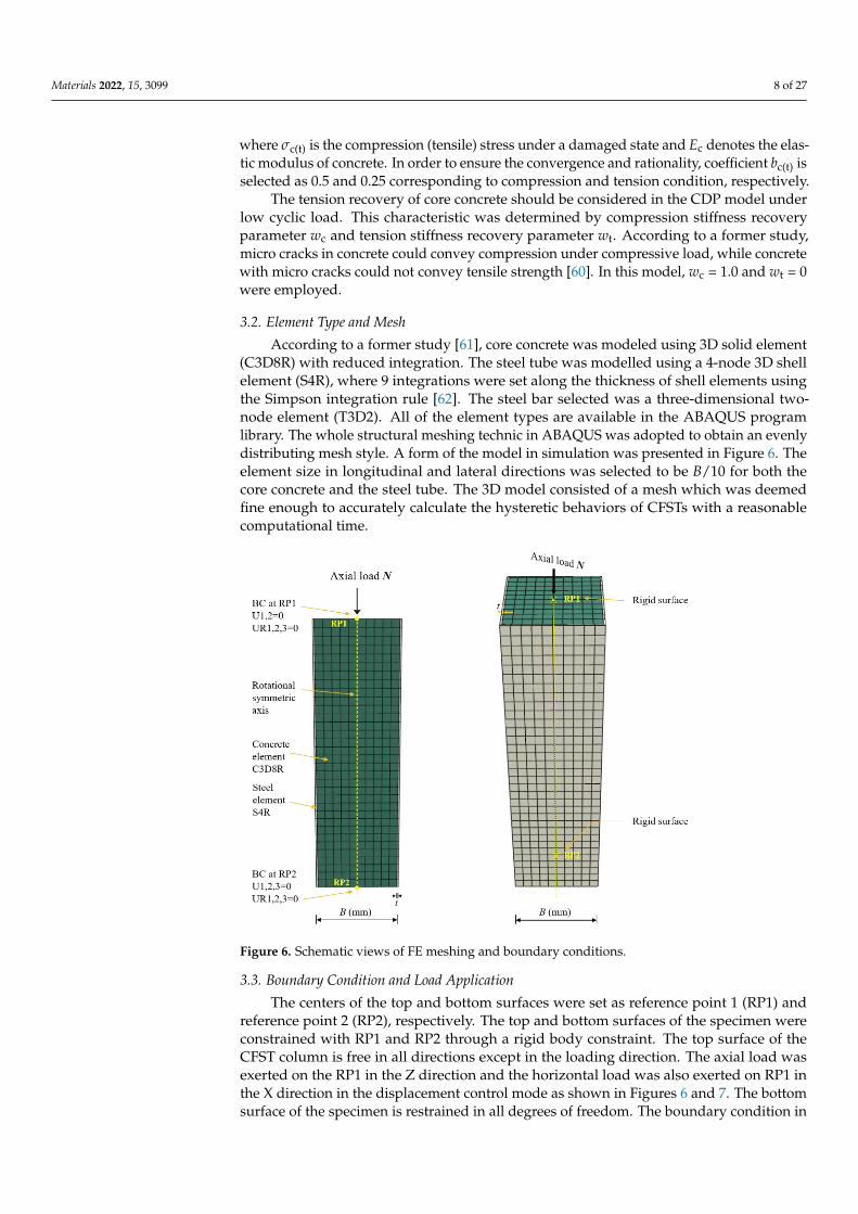
According to a former study [61], core concrete was modeled using 3D solid element(C3D8R) with reduced integration. The steel tube was modelled using a 4-node 3D shellelement (S4R), where 9 integrations were set along the thickness of shell elements usingthe Simpson integration rule [62]. The steel bar selected was a three-dimensional two-node element (T3D2). All of the element types are available in the ABAQUS programlibrary. The whole structural meshing technic in ABAQUS was adopted to obtain an evenlydistributing mesh style. A form of the model in simulation was presented in Figure 6. Theelement size in longitudinal and lateral directions was selected to be B/10 for both thecore concrete and the steel tube. The 3D model consisted of a mesh which was deemedfine enough to accurately calculate the hysteretic behaviors of CFSTs with a reasonablecomputational time.


rameter wc and tension stiffness recovery parameter wt. According to a former study, mi-

cro cracks in concrete could convey compression under compressive load, while concrete

with micro cracks could not convey tensile strength [60]. In this model, wc = 1.0 and wt = 0

were employed.

3.2. Element Type and Mesh

According to a former study [61], core concrete was modeled using 3D solid element

(C3D8R) with reduced integration. The steel tube was modelled using a 4-node 3D shell

element (S4R), where 9 integrations were set along the thickness of shell elements using

the Simpson integration rule [62]. The steel bar selected was a three-dimensional two-

node element (T3D2). All of the element types are available in the ABAQUS program li-

brary. The whole structural meshing technic in ABAQUS was adopted to obtain an evenly

distributing mesh style. A form of the model in simulation was presented in Figure 6. The

element size in longitudinal and lateral directions was selected to be B/10 for both the core

concrete and the steel tube. The 3D model consisted of a mesh which was deemed fine

enough to accurately calculate the hysteretic behaviors of CFSTs with a reasonable com-

putational time.

Figure 6. Schematic views of FE meshing and boundary conditions.

3.3. Boundary Condition and Load Application

The centers of the top and bottom surfaces were set as reference point 1 (RP1) and

reference point 2 (RP2), respectively. The top and bottom surfaces of the specimen were

constrained with RP1 and RP2 through a rigid body constraint. The top surface of the

CFST column is free in all directions except in the loading direction. The axial load was

exerted on the RP1 in the Z direction and the horizontal load was also exerted on RP1 in

the X direction in the displacement control mode as shown in Figure 6 and Figure 7. The

bottom surface of the specimen is restrained in all degrees of freedom. The boundary con-

dition in the model can simulate the CFST column effectively, which corresponds to one

end hinged and one end fixed in reality as shown in Figure 8, where P presents the lateral

load, Δm denotes lateral displacement, and L0 defined as calculation length.

Figure 6. Schematic views of FE meshing and boundary conditions.

3.3. Boundary Condition and Load Application

The centers of the top and bottom surfaces were set as reference point 1 (RP1) andreference point 2 (RP2), respectively. The top and bottom surfaces of the specimen wereconstrained with RP1 and RP2 through a rigid body constraint. The top surface of theCFST column is free in all directions except in the loading direction. The axial load wasexerted on the RP1 in the Z direction and the horizontal load was also exerted on RP1 inthe X direction in the displacement control mode as shown in Figures 6 and 7. The bottomsurface of the specimen is restrained in all degrees of freedom. The boundary condition in

Materials 2022, 15, 3099 9 of 27

the model can simulate the CFST column effectively, which corresponds to one end hingedand one end fixed in reality as shown in Figure 8, where P presents the lateral load, ∆mdenotes lateral displacement, and L0 defined as calculation length.


Figure 7. Schematic views of CFST stub columns under cyclic load.

Figure 8. Schematic views of FE model under cyclic load.

The model includes three steps: (1) an initial analysis step, where boundary condi-

tions were set up; (2) step 2, where axial load is applied in the load-control mode; (3) step

3, where horizontal load exerted to RP1 with desired displacement in the displacement-

control mode. The time of each analysis step was separated according to the displacement

loading amplitude curve. The calculated result was obtained by Gauss integral iteration

and output at the end of each analysis step.

3.4. Concrete-Steel Tube Interface Modeling

The concrete core and steel tube employed surface-to-surface contact to ensure the

concrete core and the steel tube maintained an adequate bond, which created the CFST

column as a whole. Since the stiffness of the concrete core was higher than that of the steel

tube, the concrete core was selected as the master surface, while the steel tube was set as

the slave surface. Moreover, the formula of small sliding was adopted in this section since

the relative slip of the concrete core and the steel tube was small. Mechanical properties

of tangential behavior were simulated by a penalty and friction coefficient, which is 0.6

[62]. The value of the shear stress limit was selected as 0.15 MPa [63]. Normal behavior

adopted hard contact, which resulted in surface contact with no limitation.

3.5. Verification of Finite Element Model

3.5.1. Failure Mode

The typical failure mode of specimens under cyclic loading at ambient temperature

(20 ± 2 °C) was depicted in Figure 9. As shown in the figure, the FE model presents a shear

failure mode with outward buckling at the end of the steel tube. The results of the FE

models and test specimens were consistent, which suggests that the FE model was effec-

tive.





The model includes three steps: (1) an initial analysis step, where boundary condi-

tions were set up; (2) step 2, where axial load is applied in the load-control mode; (3) step

3, where horizontal load exerted to RP1 with desired displacement in the displacement-

control mode. The time of each analysis step was separated according to the displacement

loading amplitude curve. The calculated result was obtained by Gauss integral iteration

and output at the end of each analysis step.


The concrete core and steel tube employed surface-to-surface contact to ensure the

concrete core and the steel tube maintained an adequate bond, which created the CFST

column as a whole. Since the stiffness of the concrete core was higher than that of the steel

tube, the concrete core was selected as the master surface, while the steel tube was set as

the slave surface. Moreover, the formula of small sliding was adopted in this section since

the relative slip of the concrete core and the steel tube was small. Mechanical properties

of tangential behavior were simulated by a penalty and friction coefficient, which is 0.6

[62]. The value of the shear stress limit was selected as 0.15 MPa [63]. Normal behavior

adopted hard contact, which resulted in surface contact with no limitation.

3.5. Verification of Finite Element Model

3.5.1. Failure Mode

The typical failure mode of specimens under cyclic loading at ambient temperature

(20 ± 2 °C) was depicted in Figure 9. As shown in the figure, the FE model presents a shear

failure mode with outward buckling at the end of the steel tube. The results of the FE

models and test specimens were consistent, which suggests that the FE model was effec-

tive.


The model includes three steps: (1) an initial analysis step, where boundary conditionswere set up; (2) step 2, where axial load is applied in the load-control mode; (3) step 3,where horizontal load exerted to RP1 with desired displacement in the displacement-controlmode. The time of each analysis step was separated according to the displacement loadingamplitude curve. The calculated result was obtained by Gauss integral iteration and outputat the end of each analysis step.


The concrete core and steel tube employed surface-to-surface contact to ensure theconcrete core and the steel tube maintained an adequate bond, which created the CFSTcolumn as a whole. Since the stiffness of the concrete core was higher than that of the steeltube, the concrete core was selected as the master surface, while the steel tube was set asthe slave surface. Moreover, the formula of small sliding was adopted in this section sincethe relative slip of the concrete core and the steel tube was small. Mechanical properties oftangential behavior were simulated by a penalty and friction coefficient, which is 0.6 [62].

Materials 2022, 15, 3099 10 of 27

The value of the shear stress limit was selected as 0.15 MPa [63]. Normal behavior adoptedhard contact, which resulted in surface contact with no limitation.

3.5. Verification of Finite Element Model3.5.1. Failure Mode

The typical failure mode of specimens under cyclic loading at ambient temperature(20 ± 2 ◦C) was depicted in Figure 9. As shown in the figure, the FE model presents ashear failure mode with outward buckling at the end of the steel tube. The results of the FEmodels and test specimens were consistent, which suggests that the FE model was effective.


(a) (b)

(c) (d)

Figure 9. Comparison of failure modes between test specimens and FE models under cyclic loading

under ambient temperature. (a) STRC-60-1.5-4; (b) STRC-70-1.5-4; (c) FGZ4; (d) A1.

3.5.2. Skeleton Curve

The experimental results were compared with those obtained via FE modelling in

terms of skeleton curve, as depicted in Figure 10. It can be seen in the figure that in the

elastic stage, the skeleton curves of specimens in accordance with the FE models.

50 25 0 25 50400

200

0

200

400

ref [34-35]

FE model

P/k

N

Δm/mm 50 25 0 25 50

400

200

0

200

400

ref [34-35]

FE model

P/k

N

Δm/mm 30 20 10 0 10 20 30

400

200

0

200

400

ref [36-37]

FE model

P/k

N

Δm/mm

(a) (b) (c)

30 20 10 0 10 20 30400

200

0

200

400

ref [36-37]

FE model

P/k

N

Δm/mm

30 20 10 0 10 20 30500

250

0

250

500

ref [36-37]

FE model

P/k

N

Δm/mm 60 40 20 0 20 40 60

300

150

0

150

300

ref [38]

FE model

P/k

N

Δm/mm

(d) (e) (f)

Figure 9. Comparison of failure modes between test specimens and FE models under cyclic loadingunder ambient temperature. (a) STRC-60-1.5-4; (b) STRC-70-1.5-4; (c) FGZ4; (d) A1.


The experimental results were compared with those obtained via FE modelling interms of skeleton curve, as depicted in Figure 10. It can be seen in the figure that in theelastic stage, the skeleton curves of specimens in accordance with the FE models.

However, in the elastic plastic stage, the slope of FE results was higher than test results.For the twelve verified specimens, the skeleton curves match the FE curves with a subtledifference in slope, which is likely to be associated with a geometric and loading defectgenerated through the experiment. These results were then employed in investigatinghysteretic behavior.

3.5.3. Horizontal Ultimate Compressive Strength

The horizontal ultimate compressive strength was obtained from the FE model andcompared with the test specimens. Table 2 compares the peak load of the specimens with

Materials 2022, 15, 3099 11 of 27

the capacity derived from the FE modelling. The mean and standard deviation valueshighlight a favorable efficiency of the FE model in predicting the desired measures.


(a) (b)

(c) (d)

Figure 9. Comparison of failure modes between test specimens and FE models under cyclic loading

under ambient temperature. (a) STRC-60-1.5-4; (b) STRC-70-1.5-4; (c) FGZ4; (d) A1.


The experimental results were compared with those obtained via FE modelling in

terms of skeleton curve, as depicted in Figure 10. It can be seen in the figure that in the

elastic stage, the skeleton curves of specimens in accordance with the FE models.

50 25 0 25 50400

200

0

200

400

ref [34-35]

FE model

P/k

N

Δm/mm 50 25 0 25 50

400

200

0

200

400

ref [34-35]

FE model

P/k

NΔm/mm

30 20 10 0 10 20 30400

200

0

200

400

ref [36-37]

FE model

P/k

N

Δm/mm

(a) (b) (c)

30 20 10 0 10 20 30400

200

0

200

400

ref [36-37]

FE model

P/k

N

Δm/mm

30 20 10 0 10 20 30500

250

0

250

500

ref [36-37]

FE model

P/k

N

Δm/mm 60 40 20 0 20 40 60

300

150

0

150

300

ref [38]

FE model

P/k

N

Δm/mm

(d) (e) (f)


30 20 10 0 10 20 30500

250

0

250

500

ref [39-41]

FE model

P/k

N

Δm/mm 30 20 10 0 10 20 30

500

250

0

250

500

ref [39-41]

FE model

P/k

N

Δm/mm 30 20 10 0 10 20 30

500

250

0

250

500

ref [39-41]

FE model

P/k

N

Δm/mm (g) (h) (i)

30 20 10 0 10 20 30500

250

0

250

500

ref [42-43]

FE model

P/k

N

Δm/mm 30 20 10 0 10 20 30

600

300

0

300

600

ref [42-43]

FE model

P/k

N

Δm/mm 30 20 10 0 10 20 30

800

400

0

400

800

ref [42-43]

FE model

P/k

N

Δm/mm (j) (k) (l)

Figure 10. Comparison of skeleton curve between test specimen and FE model under cyclic loading

at ambient temperature. (a) STRC-60-1.5-4; (b) STRC-60-1.5-6; (c) STRC-70-1.5-4; (d) STRC-70-1.5-5;

(e) STRC-70-1.5-6; (f) FGZ4; (g) A1; (h) A2; (i) A3; (j) RS-4L; (k) RS-6M; (l) RS-10H.

However, in the elastic plastic stage, the slope of FE results was higher than test re-

sults. For the twelve verified specimens, the skeleton curves match the FE curves with a

subtle difference in slope, which is likely to be associated with a geometric and loading

defect generated through the experiment. These results were then employed in investi-

gating hysteretic behavior.

3.5.3. Horizontal Ultimate Compressive Strength

The horizontal ultimate compressive strength was obtained from the FE model and

compared with the test specimens. Table 2 compares the peak load of the specimens with

the capacity derived from the FE modelling. The mean and standard deviation values

highlight a favorable efficiency of the FE model in predicting the desired measures.

Table 2. Comparison of ultimate horizontal load between specimens and FE model.

No. Ref. Specimen Labels Pue1 (kN) Pue2 (kN) Pfe1 (kN) Pfe2 (kN) Pue1/Pfe1 Pue2/Pfe2

1

[34,35]

STRC-60-1.5-4 304 296 335 335 0.907 0.884

2 STRC-60-1.5-6 337 348 307 307 1.098 1.134

3 STRC-70-4-1.5 262 267 260 260 1.008 1.027

4 [36,37]

STRC-70-5-1.5 285 290 258 258 1.105 1.124

5 STRC-70-6-1.5 324 329 426 426 0.761 0.772

6 [38]

FGZ4 216 240 195 195 1.108 1.231

7 A1 397 275 433 433 0.917 0.635

8

[39–41]

A2 454 424 412 412 1.102 1.029

9 A3 445 449 436 436 1.021 1.030

10 RS-4L 434 361 458 458 0.948 0.788

11 [42,43]

RS-6M 556 572 544 544 1.022 1.051

12 RS-10H 773 771 614 614 1.259 1.256

Mean 1.064 1.022

SD 0.046 0.032

Note: Specimen labels in the table are the same as the test specimen in Refs. [34–43].

Figure 10. Comparison of skeleton curve between test specimen and FE model under cyclic loadingat ambient temperature. (a) STRC-60-1.5-4; (b) STRC-60-1.5-6; (c) STRC-70-1.5-4; (d) STRC-70-1.5-5;(e) STRC-70-1.5-6; (f) FGZ4; (g) A1; (h) A2; (i) A3; (j) RS-4L; (k) RS-6M; (l) RS-10H.

3.5.4. Hysteretic Behavior of CFSTs after Sulfate Corrosion

The experimental results were compared with the results of the FE model in terms ofhysteretic behavior, as depicted in Figure 11. The rationality of the FE model on calculatingultimate horizontal load was verified by the existing test results [64–66], as shown inFigure 12.

Materials 2022, 15, 3099 12 of 27

Table 2. Comparison of ultimate horizontal load between specimens and FE model.

No. Ref. Specimen Labels Pue1 (kN) Pue2 (kN) Pfe1 (kN) Pfe2 (kN) Pue1/Pfe1 Pue2/Pfe2

1[34,35]

STRC-60-1.5-4 304 296 335 335 0.907 0.8842 STRC-60-1.5-6 337 348 307 307 1.098 1.1343 STRC-70-4-1.5 262 267 260 260 1.008 1.0274

[36,37]STRC-70-5-1.5 285 290 258 258 1.105 1.124

5 STRC-70-6-1.5 324 329 426 426 0.761 0.7726

[38]FGZ4 216 240 195 195 1.108 1.231

7 A1 397 275 433 433 0.917 0.6358

[39–41]A2 454 424 412 412 1.102 1.029

9 A3 445 449 436 436 1.021 1.03010 RS-4L 434 361 458 458 0.948 0.78811

[42,43]RS-6M 556 572 544 544 1.022 1.051

12 RS-10H 773 771 614 614 1.259 1.256

Mean 1.064 1.022SD 0.046 0.032

Note: Specimen labels in the table are the same as the test specimen in Refs. [34–43].



The experimental results were compared with the results of the FE model in terms of

hysteretic behavior, as depicted in Figure 11. The rationality of the FE model on calculat-

ing ultimate horizontal load was verified by the existing test results [64–66], as shown in

Figure 12.

40 30 20 10 0 10 20 30 40150

100

50

0

50

100

150

ref [64-66]

FE model

P/k

N

Δm / mm 40 30 20 10 0 10 20 30 40

150

100

50

0

50

100

150

ref [64-66]

FE model

P/k

N

Δm/mm 40 30 20 10 0 10 20 30 40

150

100

50

0

50

100

150

ref [64-66]

FE model

P/k

N

Δm/mm (a) (b) (c)

40 30 20 10 0 10 20 30 40150

100

50

0

50

100

150

ref [64-66]

FE model

P/k

N

Δm/mm 40 30 20 10 0 10 20 30 40

150

100

50

0

50

100

150

ref [64-66]

FE model

P/k

N

Δm/mm 40 30 20 10 0 10 20 30 40

150

100

50

0

50

100

150

ref [64-66]

FE model

P/k

N

Δm / mm (d) (e) (f)

40 30 20 10 0 10 20 30 40150

100

50

0

50

100

150

ref [64-66]

FE model

P/k

N

Δm/mm 40 30 20 10 0 10 20 30 40

150

100

50

0

50

100

150

ref [64-66]

FE model

P/k

N

Δm/mm

40 30 20 10 0 10 20 30 40150

100

50

0

50

100

150

ref [64-66]

FE model

P/k

N

Δm/mm (g) (h) (i)

Figure 11. Comparison between FE model and test results of specimens after sulfate corrosion. (a)

RC-0A; (b) RC-10A; (c) RC-20A; (d) RC-0B; (e) RC-10B; (f) RC-20B; (g) RC-0C; (h) RC-10C; (i) RC-

20C.

(a) (b)

0 50 100 1500

50

100

150

Pfe (

kN

)

Pue1

(kN)

mean value: 0.892

standard deviation: 0.004

0 50 100 1500

50

100

150

Pfe (

kN

)

Pue2

(kN)

mean value: 0.884


Figure 11. Comparison between FE model and test results of specimens after sulfate corrosion.(a) RC-0A; (b) RC-10A; (c) RC-20A; (d) RC-0B; (e) RC-10B; (f) RC-20B; (g) RC-0C; (h) RC-10C;(i) RC-20C.

Materials 2022, 15, 3099 13 of 27



The experimental results were compared with the results of the FE model in terms of

hysteretic behavior, as depicted in Figure 11. The rationality of the FE model on calculat-

ing ultimate horizontal load was verified by the existing test results [64–66], as shown in

Figure 12.

40 30 20 10 0 10 20 30 40150

100

50

0

50

100

150

ref [64-66]

FE model

P/k

N

Δm / mm 40 30 20 10 0 10 20 30 40

150

100

50

0

50

100

150

ref [64-66]

FE model

P/k

N

Δm/mm 40 30 20 10 0 10 20 30 40

150

100

50

0

50

100

150

ref [64-66]

FE model

P/k

N

Δm/mm (a) (b) (c)

40 30 20 10 0 10 20 30 40150

100

50

0

50

100

150

ref [64-66]

FE model

P/k

N

Δm/mm 40 30 20 10 0 10 20 30 40

150

100

50

0

50

100

150

ref [64-66]

FE model

P/k

N

Δm/mm 40 30 20 10 0 10 20 30 40

150

100

50

0

50

100

150

ref [64-66]

FE model

P/k

N

Δm / mm (d) (e) (f)

40 30 20 10 0 10 20 30 40150

100

50

0

50

100

150

ref [64-66]

FE model

P/k

N

Δm/mm 40 30 20 10 0 10 20 30 40

150

100

50

0

50

100

150

ref [64-66]

FE model

P/k

N

Δm/mm

40 30 20 10 0 10 20 30 40150

100

50

0

50

100

150

ref [64-66]

FE model

P/k

N

Δm/mm (g) (h) (i)

Figure 11. Comparison between FE model and test results of specimens after sulfate corrosion. (a)

RC-0A; (b) RC-10A; (c) RC-20A; (d) RC-0B; (e) RC-10B; (f) RC-20B; (g) RC-0C; (h) RC-10C; (i) RC-

20C.

(a) (b)

0 50 100 1500

50

100

150

Pfe (

kN

)

Pue1

(kN)

mean value: 0.892


0 50 100 1500

50

100

150

Pfe (

kN

)

Pue2

(kN)

mean value: 0.884


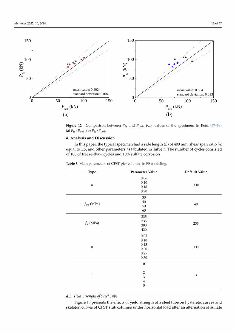
Figure 12. Comparison between Pfe and Pue1, Pue2 values of the specimens in Refs. [57–59].(a) Pfe/Pue1; (b) Pfe/Pue2.

4. Analysis and Discussion

In this paper, the typical specimen had a side length (B) of 400 mm, shear span ratio (λ)equal to 1.5, and other parameters as tabulated in Table 3. The number of cycles consistedof 100 of freeze-thaw cycles and 10% sulfate corrosion.

Table 3. Main parameters of CFST pier columns in FE modeling.

Type Parameter Value Default Value

α

0.06

0.100.100.180.20

f cu (MPa)

30

40405060

f y (MPa)

235

235335390420

n

0.05

0.15

0.100.150.200.250.30

i

0

3

12345

4.1. Yield Strength of Steel Tube

Figure 13 presents the effects of yield strength of a steel tube on hysteretic curves andskeleton curves of CFST stub columns under horizontal load after an alternation of sulfate

Materials 2022, 15, 3099 14 of 27

corrosion and freeze-thaw cycles. It can be seen that the effect of yield strength of the steeltube was significant on the shape of the curves and cyclic displacement corresponding toultimate bearing capacity. Regarding the hysteretic curves, with the increase of the yieldstrength of the steel tube, they became fuller, which resulted in a larger surrounded area.When the hysteretic curve enters the second half, the cyclic displacement declined fasterwith the larger yield strength of the steel tube due to the damage accumulation of the steeltube under cyclic reciprocating load after sulfate corrosion.


20 10 0 10 20600

300

0

300

600

fy=235MPa

P /

kN

Δm / mm

20 10 0 10 20600

300

0

300

600

fy=335MPa

P /

kN

Δm / mm

(a) (b)

20 10 0 10 20600

300

0

300

600

fy=390MPa

P /

kN

Δm / mm

20 10 0 10 20600

300

0

300

600

fy=420MPa

P /

kN

Δm / mm

(c) (d)

Figure 13. Effect of yield strength of steel tube on hysteretic curve. (a) fy = 235 MPa; (b) fy = 335

MPa; (c) fy = 390 MPa; (d) fy = 420 MPa.

Skeleton curves presented in Figure 14 kept a similar trend in the elastic stage, which

illustrated the effect of yield strength of the steel tube on initial stiffness. However, the

effect of yield strength of the steel tube on horizontal load at peak point was significant,

especially when the yield strength of the steel tube increased from 235 to 335 MPa. The

ultimate horizontal load increased by 26.3%, 35.0%, and 39.2%, respectively as the yield

strength of the steel tube increased from 235 to 335, 390, and 420 MPa. Meanwhile, the

effect of yield strength of the steel tube on the slope of the curves in the descending stage

and ductility was negligible.

20 10 0 10 20600

300

0

300

600

fy=235Mpa

fy=355Mpa

fy=390Mpa

fy=420Mpa

P /

kN

Δm / mm

Figure 14. Effect of yield strength of steel tube on skeleton curve.

Figure 13. Effect of yield strength of steel tube on hysteretic curve. (a) f y = 235 MPa; (b) f y = 335 MPa;(c) f y = 390 MPa; (d) f y = 420 MPa.

Skeleton curves presented in Figure 14 kept a similar trend in the elastic stage, whichillustrated the effect of yield strength of the steel tube on initial stiffness. However, theeffect of yield strength of the steel tube on horizontal load at peak point was significant,especially when the yield strength of the steel tube increased from 235 to 335 MPa. Theultimate horizontal load increased by 26.3%, 35.0%, and 39.2%, respectively as the yieldstrength of the steel tube increased from 235 to 335, 390, and 420 MPa. Meanwhile, theeffect of yield strength of the steel tube on the slope of the curves in the descending stageand ductility was negligible.

Materials 2022, 15, 3099 15 of 27


20 10 0 10 20600

300

0

300

600

fy=235MPa

P /

kN

Δm / mm

20 10 0 10 20600

300

0

300

600

fy=335MPa

P /

kN

Δm / mm

(a) (b)

20 10 0 10 20600

300

0

300

600

fy=390MPa

P /

kN

Δm / mm

20 10 0 10 20600

300

0

300

600

fy=420MPa

P /

kN

Δm / mm

(c) (d)

Figure 13. Effect of yield strength of steel tube on hysteretic curve. (a) fy = 235 MPa; (b) fy = 335

MPa; (c) fy = 390 MPa; (d) fy = 420 MPa.

Skeleton curves presented in Figure 14 kept a similar trend in the elastic stage, which

illustrated the effect of yield strength of the steel tube on initial stiffness. However, the

effect of yield strength of the steel tube on horizontal load at peak point was significant,

especially when the yield strength of the steel tube increased from 235 to 335 MPa. The

ultimate horizontal load increased by 26.3%, 35.0%, and 39.2%, respectively as the yield

strength of the steel tube increased from 235 to 335, 390, and 420 MPa. Meanwhile, the

effect of yield strength of the steel tube on the slope of the curves in the descending stage

and ductility was negligible.

20 10 0 10 20600

300

0

300

600

fy=235Mpa

fy=355Mpa

fy=390Mpa

fy=420Mpa

P /

kN

Δm / mm



4.2. Compressive Strength of Core Concrete

Figures 15 and 16 depict the effects of the compressive strength of concrete on hystereticcurves and skeleton curves of CFST stub columns under horizontal load after an alternationof sulfate corrosion and freeze-thaw cycles. It can be seen that the effect of the compressivestrength of concrete was significant on the shape of the curves and cyclic displacementcorresponding to ultimate bearing capacity. For the hysteretic curves, when the compressivestrength of the concrete increased, the stiffness of the specimen was weaker, which resultedin the “S” shape of the P-∆m curve. For skeleton curves, all four curves showed a similartrend in the elastic stage which illustrated that the effect of the compressive strength ofthe concrete on initial stiffness was slight. However, the effect of the compressive strengthof the concrete on horizontal load at peak point was significant. The ultimate horizontalload increased by 16.0%, 27.7%, and 33.7%, respectively as the compressive strength ofconcrete increased from 30 to 40, 50, and 60 MPa. The compressive strength of concretehad some effect on the slope of the curves in the descending stage. With the increaseof the compressive strength of the concrete, the descending stage of the skeleton curvedecreased faster, which demonstrated that the ductility of the specimens was weaker dueto the brittleness of the high strength of the concrete core. Although high compressivestrength of concrete could improve the horizontal ultimate bearing capacity to some degree,the ductility would decrease, which should be focused on.

4.3. Steel Ratio

Figures 17 and 18 depicted the variations of hysteretic curves and skeleton curves withdifferent steel ratios under alternating sulfate corrosion and freeze-thaw cycles. The effectsof steel ratio on hysteretic curve, skeleton curve, and bearing capacity corresponding toeach cycle were significant. With the increase of steel ratio, the hysteretic curves changedfrom flat to full and the area within the curves became larger, which illustrated that thespecimens were sufficient in the plastic deformation capacity.

Materials 2022, 15, 3099 16 of 27


4.2. Compressive Strength of Core Concrete

Figures 15 and 16 depict the effects of the compressive strength of concrete on hys-

teretic curves and skeleton curves of CFST stub columns under horizontal load after an

alternation of sulfate corrosion and freeze-thaw cycles. It can be seen that the effect of the

compressive strength of concrete was significant on the shape of the curves and cyclic

displacement corresponding to ultimate bearing capacity. For the hysteretic curves, when

the compressive strength of the concrete increased, the stiffness of the specimen was

weaker, which resulted in the “S” shape of the P-Δm curve. For skeleton curves, all four

curves showed a similar trend in the elastic stage which illustrated that the effect of the

compressive strength of the concrete on initial stiffness was slight. However, the effect of

the compressive strength of the concrete on horizontal load at peak point was significant.

The ultimate horizontal load increased by 16.0%, 27.7%, and 33.7%, respectively as the

compressive strength of concrete increased from 30 to 40, 50, and 60 MPa. The compres-

sive strength of concrete had some effect on the slope of the curves in the descending

stage. With the increase of the compressive strength of the concrete, the descending stage

of the skeleton curve decreased faster, which demonstrated that the ductility of the spec-

imens was weaker due to the brittleness of the high strength of the concrete core. Although

high compressive strength of concrete could improve the horizontal ultimate bearing ca-

pacity to some degree, the ductility would decrease, which should be focused on.

20 10 0 10 20500

250

0

250

500

fcu=30MPa

P /

kN

Δm / mm

20 10 0 10 20500

250

0

250

500

fcu=40MPa

P /

kN

Δm / mm

(a) (b)

20 10 0 10 20500

250

0

250

500

fcu=50MPa

P /

kN

Δm / mm

20 10 0 10 20500

250

0

250

500

fcu=60MPa

P /

kN

Δm / mm

(c) (d)

Figure 15. Effect of compressive strength of core concrete on hysteretic curve. (a) fcu = 30 MPa; (b)

fcu = 40 MPa; (c) fcu = 50 MPa; (d) fcu = 60 MPa. Figure 15. Effect of compressive strength of core concrete on hysteretic curve. (a) f cu = 30 MPa;(b) f cu = 40 MPa; (c) f cu = 50 MPa; (d) f cu = 60 MPa.


20 10 0 10 20500

250

0

250

500

fcu=30Mpa

fcu=40Mpa

fcu=50Mpa

fcu=60Mpa

P /

kN

Δm / mm

Figure 16. Effect of compressive strength of core concrete on skeleton curve.

4.3. Steel Ratio

Figures 17 and 18 depicted the variations of hysteretic curves and skeleton curves

with different steel ratios under alternating sulfate corrosion and freeze-thaw cycles. The

effects of steel ratio on hysteretic curve, skeleton curve, and bearing capacity correspond-

ing to each cycle were significant. With the increase of steel ratio, the hysteretic curves

changed from flat to full and the area within the curves became larger, which illustrated

that the specimens were sufficient in the plastic deformation capacity.

20 10 0 10 20800

400

0

400

800

α=0.06

P /

kN

Δm / mm

20 10 0 10 20800

400

0

400

800

α=0.10

P /

kN

Δm / mm

(a) (b)

20 10 0 10 20800

400

0

400

800

α=0.18

P /

kN

Δm / mm

20 10 0 10 20800

400

0

400

800

α=0.20

P /

kN

Δm / mm

(c) (d)

Figure 17. Effect of steel ratio on hysteretic curve. (a) α = 0.06; (b) α = 0.10; (c) α = 0.18; (d) α = 0.20.


Materials 2022, 15, 3099 17 of 27


20 10 0 10 20500

250

0

250

500

fcu=30Mpa

fcu=40Mpa

fcu=50Mpa

fcu=60Mpa

P /

kN

Δm / mm


4.3. Steel Ratio

Figures 17 and 18 depicted the variations of hysteretic curves and skeleton curves

with different steel ratios under alternating sulfate corrosion and freeze-thaw cycles. The

effects of steel ratio on hysteretic curve, skeleton curve, and bearing capacity correspond-

ing to each cycle were significant. With the increase of steel ratio, the hysteretic curves

changed from flat to full and the area within the curves became larger, which illustrated

that the specimens were sufficient in the plastic deformation capacity.

20 10 0 10 20800

400

0

400

800

α=0.06

P /

kN

Δm / mm

20 10 0 10 20800

400

0

400

800

α=0.10

P /

kN

Δm / mm

(a) (b)

20 10 0 10 20800

400

0

400

800

α=0.18

P /

kN

Δm / mm

20 10 0 10 20800

400

0

400

800

α=0.20

P /

kN

Δm / mm

(c) (d)

Figure 17. Effect of steel ratio on hysteretic curve. (a) α = 0.06; (b) α = 0.10; (c) α = 0.18; (d) α = 0.20. Figure 17. Effect of steel ratio on hysteretic curve. (a) α = 0.06; (b) α = 0.10; (c) α = 0.18; (d) α = 0.20.


20 10 0 10 20800

400

0

400

800

α=0.06

α=0.10

α=0.18

α=0.20

P /

kN

Δm / mm

Figure 18. Effect of steel ratio on skeleton curve.

It can be seen in Figure 18 that the slope of the four skeleton curves in the elastic stage

was obviously different. The higher steel ratio resulted in higher elastic stiffness and ulti-

mate horizontal load. The ultimate horizontal load increased by 21.4%, 61.0%, and 126.4%

when the steel ratio increased from 0.06 to 0.10, 0.18, and 0.20, respectively. Moreover, the

skeleton curves decreased slowly and even presented strain hardening phenomenon due

to the confinement effect of the steel tube, which presented ductile behavior.

4.4. Axial Compression Ratio

Figures 19 and 20 presented the effects of the axial compression ratio on the hysteretic

curves and skeleton curves of CFST stub columns under horizontal load after an alterna-

tion of sulfate corrosion and freeze-thaw cycles. All the shapes of hysteretic curves demon-

strated that the effect of the axial compression ratio was slight. The ultimate horizontal

load slightly increased by 4.2%,6.6%, 8.1%, 9.0%, and 9.3%, respectively as the axial com-

pression ratio increased from 0.05 to 0.1, 0.15, 0.20, 0.25, and 0.30 when the alternation

time was three. The descending stage of the skeleton curves decreased more with the in-

crease of the axial compression ratio, which demonstrated that the ductility of the speci-

mens was weaker. This was for the reason that the material damage became more serious

with the increasing axial compressive load due to the increasing axial compression ratio.

20 10 0 10 20500

250

0

250

500

n=0.05

P /

kN

Δm / mm

20 10 0 10 20500

250

0

250

500

n=0.1

P /

kN

Δm / mm

(a) (b)

Figure 18. Effect of steel ratio on skeleton curve.

Materials 2022, 15, 3099 18 of 27

It can be seen in Figure 18 that the slope of the four skeleton curves in the elastic stagewas obviously different. The higher steel ratio resulted in higher elastic stiffness and ulti-mate horizontal load. The ultimate horizontal load increased by 21.4%, 61.0%, and 126.4%when the steel ratio increased from 0.06 to 0.10, 0.18, and 0.20, respectively. Moreover, theskeleton curves decreased slowly and even presented strain hardening phenomenon dueto the confinement effect of the steel tube, which presented ductile behavior.

4.4. Axial Compression Ratio

Figures 19 and 20 presented the effects of the axial compression ratio on the hystereticcurves and skeleton curves of CFST stub columns under horizontal load after an alternationof sulfate corrosion and freeze-thaw cycles. All the shapes of hysteretic curves demonstratedthat the effect of the axial compression ratio was slight. The ultimate horizontal load slightlyincreased by 4.2%,6.6%, 8.1%, 9.0%, and 9.3%, respectively as the axial compression ratioincreased from 0.05 to 0.1, 0.15, 0.20, 0.25, and 0.30 when the alternation time was three.The descending stage of the skeleton curves decreased more with the increase of the axialcompression ratio, which demonstrated that the ductility of the specimens was weaker.This was for the reason that the material damage became more serious with the increasingaxial compressive load due to the increasing axial compression ratio.

1

−20 −10 0 10 20−500

−250

0

250

500

n=0.05

P / k

N

Δm / mm −20 −10 0 10 20

−500

−250

0

250

500

n=0.1

P / k

N

Δm / mm (a) (b)

−20 −10 0 10 20−500

−250

0

250

500

n=0.15

P / k

N

Δm / mm −20 −10 0 10 20

−500

−250

0

250

500

n=0.2

P / k

N

Δm / mm (c) (d)

−20 −10 0 10 20−500

−250

0

250

500

n=0.25

P / k

N

Δm / mm −20 −10 0 10 20

−500

−250

0

250

500

n=0.3

P / k

N

Δm / mm (e) (f)

Figure 19. Cont.

Materials 2022, 15, 3099 19 of 27

1

−20 −10 0 10 20−500

−250

0

250

500

n=0.05

P / k

N

Δm / mm −20 −10 0 10 20

−500

−250

0

250

500

n=0.1

P / k

N

Δm / mm (a) (b)

−20 −10 0 10 20−500

−250

0

250

500

n=0.15

P / k

NΔm / mm

−20 −10 0 10 20−500

−250

0

250

500

n=0.2

P / k

N

Δm / mm (c) (d)

−20 −10 0 10 20−500

−250

0

250

500

n=0.25

P / k

N

Δm / mm −20 −10 0 10 20

−500

−250

0

250

500

n=0.3

P / k

N

Δm / mm (e) (f)

Figure 19. Effect of axial load ratio on hysteretic curve. (a) n = 0.05; (b) n = 0.10; (c) n = 0.15;(d) n = 0.20; (e) n = 0.25; (f) n = 0.30.


20 10 0 10 20500

250

0

250

500

n=0.15

P /

kN

Δm / mm

20 10 0 10 20500

250

0

250

500

n=0.2

P /

kN

Δm / mm

(c) (d)

20 10 0 10 20500

250

0

250

500

n=0.25

P /

kN

Δm / mm

20 10 0 10 20500

250

0

250

500

n=0.3

P /

kN

Δm / mm

(e) (f)

Figure 19. Effect of axial load ratio on hysteretic curve. (a) n = 0.05; (b) n = 0.10; (c) n = 0.15; (d) n =

0.20; (e) n = 0.25; (f) n = 0.30.

20 10 0 10 20500

250

0

250

500

n=0.05

n=0.10

n=0.15

n=0.20

n=0.25

n=0.30

P /

kN

Δm / mm

Figure 20. Effect of axial load ratio on skeleton curve.

4.5. Sulfate Corrosion and Freeze-Thaw Cycles

Figure 21 depicted the effects of alternation time on hysteretic curves of CFST piers

under horizontal load after an alternation of sulfate corrosion and freeze-thaw cycles. It

can be seen that the effect of alternation time was significant on the shape of the curves

and cyclic displacement corresponding to ultimate bearing capacity. For hysteretic curves,

with the increase of alternation time, the phenomenon of pinch occurred, which resulted

in the smaller area.

Figure 20. Effect of axial load ratio on skeleton curve.

4.5. Sulfate Corrosion and Freeze-Thaw Cycles

Figure 21 depicted the effects of alternation time on hysteretic curves of CFST piersunder horizontal load after an alternation of sulfate corrosion and freeze-thaw cycles. Itcan be seen that the effect of alternation time was significant on the shape of the curves andcyclic displacement corresponding to ultimate bearing capacity. For hysteretic curves, withthe increase of alternation time, the phenomenon of pinch occurred, which resulted in thesmaller area.

For skeleton curves as showed in Figure 22, five curves kept a similar trend in theelastic stage, which illustrated that the effect of alternate time on initial stiffness couldbe ignored. However, the effect of alternation time on the horizontal load at peak pointwas significant. The ultimate horizontal load decreased by 16.2%, 29.8%, 40.5% and 50.2%,respectively as the alternation time increased from 1 to 2, 3, 4, and 5. Meanwhile, alternationtime has effects on the slope of the curves in the descending stage. The skeleton curve hasa lower ductility, as the skeleton curves decreased faster in the descending stage due to theserious material damage caused by the alternate time on load resistance.

Materials 2022, 15, 3099 20 of 27Materials 2022, 15, x FOR PEER REVIEW 20 of 27

20 10 0 10 20600

300

0

300

600

i=1

P /

kN

Δm / mm

20 10 0 10 20600

300

0

300

600

i=2

P /

kN

Δm / mm

(a) (b)

20 10 0 10 20600

300

0

300

600

i=3

P /

kN

Δm / mm

20 10 0 10 20600

300

0

300

600

i=4

P /

kN

Δm / mm

(c) (d)

20 10 0 10 20600

300

0

300

600

i=5

P /

kN

Δm / mm

(e)

Figure 21. Effect of alternation time on hysteretic curve. (a) i = 1; (b) i = 2; (c) i = 3; (d) i = 4; (e) i = 5.

For skeleton curves as showed in Figure 22, five curves kept a similar trend in the

elastic stage, which illustrated that the effect of alternate time on initial stiffness could be

ignored. However, the effect of alternation time on the horizontal load at peak point was

significant. The ultimate horizontal load decreased by 16.2%, 29.8%, 40.5% and 50.2%, re-

spectively as the alternation time increased from 1 to 2, 3, 4, and 5. Meanwhile, alternation

time has effects on the slope of the curves in the descending stage. The skeleton curve has

a lower ductility, as the skeleton curves decreased faster in the descending stage due to

the serious material damage caused by the alternate time on load resistance.

Figure 21. Effect of alternation time on hysteretic curve. (a) i = 1; (b) i = 2; (c) i = 3; (d) i = 4; (e) i = 5.


20 10 0 10 20700

350

0

350

700

i=1

i=2

i=3

i=4

i=5

P /

kN

Δm / mm

Figure 22. Effect of alternate times on skeleton curve.

5. Simplified Formula for Horizontal Ultimate Compressive Strength

According to the parameter analysis in Section 4, the reduction factor of the horizon-

tal ultimate compressive load of CFST under alternation between sulfate corrosion and

freeze-thaw cycles is mainly determined by confinement coefficient (ξ) and alternation

time (i). In this study, according to practical engineering, the range of parameters was

selected as ξ = 0.6–2.1 and i = 0–5.

5.1. Design Method

According to Figure 7, the bending moment of CFST stub columns under low cycle

reciprocating load was expressed in Equation (10) as follows:

u u0M P L N

(10)

where Mu represents the flexure capacity; Pu0 denotes the horizontal ultimate axial load; L

is the length of the CFST column; N stands for the axial compressive load; and Δ corre-

sponds to lateral deformation.

Based on CJJ166-2011 [67], the axial compression ratio of CFST pier columns with

regular section in earthquake fortification zone should be less than 0.3, i.e., n ≤ 0.3. Mean-

while, lateral deformation was far less than the calculated length of CFST pier column, so

the bending moment caused by the axial compressive load could be ignored. Thus, the

ultimate horizontal load was expressed in Equation (11) as follows:

u0 u 0P M L

(11)

The design formula to calculate the flexure capacity in GB50936-2014 was described

in Equations (12)–(14) as follows:

u m sc scM W f

(12)

3

sc 0 4W r

(13)

m 0.483 1.962

(14)

where γm represents the plastic adaption coefficient of cross section; Wsc denotes the mod-

ulus of section of CFST pier columns (mm3); r0 corresponding to the equivalent circle ra-

dius (mm); and Mu is the flexure capacity (N·mm).

5.2. Modified Reduction Coefficient

To evaluate reduction of loading bearing capacity of the square CFST pier columns

after alternate sulfate corrosion and freeze-thaw cycles, the reduction coefficient ksq was

defined in Equation (15) as follows:

Figure 22. Effect of alternate times on skeleton curve.

Materials 2022, 15, 3099 21 of 27

5. Simplified Formula for Horizontal Ultimate Compressive Strength

According to the parameter analysis in Section 4, the reduction factor of the horizontalultimate compressive load of CFST under alternation between sulfate corrosion and freeze-thaw cycles is mainly determined by confinement coefficient (ξ) and alternation time (i).In this study, according to practical engineering, the range of parameters was selected asξ = 0.6–2.1 and i = 0–5.

5.1. Design Method

According to Figure 7, the bending moment of CFST stub columns under low cyclereciprocating load was expressed in Equation (10) as follows:

Mu = Pu0L + N∆ (10)

where Mu represents the flexure capacity; Pu0 denotes the horizontal ultimate axial load; L isthe length of the CFST column; N stands for the axial compressive load; and ∆ correspondsto lateral deformation.

Based on CJJ166-2011 [67], the axial compression ratio of CFST pier columns withregular section in earthquake fortification zone should be less than 0.3, i.e., n ≤ 0.3. Mean-while, lateral deformation was far less than the calculated length of CFST pier column, sothe bending moment caused by the axial compressive load could be ignored. Thus, theultimate horizontal load was expressed in Equation (11) as follows:

Pu0 = Mu/L0 (11)

The design formula to calculate the flexure capacity in GB50936-2014 was described inEquations (12)–(14) as follows:

Mu = γmWsc fsc (12)

Wsc = r30/4 (13)

γm = −0.483ξ + 1.962√

ξ (14)

where γm represents the plastic adaption coefficient of cross section; Wsc denotes themodulus of section of CFST pier columns (mm3); r0 corresponding to the equivalent circleradius (mm); and Mu is the flexure capacity (N·mm).

5.2. Modified Reduction Coefficient

To evaluate reduction of loading bearing capacity of the square CFST pier columnsafter alternate sulfate corrosion and freeze-thaw cycles, the reduction coefficient ksq wasdefined in Equation (15) as follows:

ksq =Pue

Pu0(15)

where, Pue is the ultimate horizontal load under sulfate corrosion and freeze-thaw cycles;Pu0 is the ultimate horizontal load under ambient condition. The major effect was presentedin Figure 23.

The reduction coefficient varied with alternation time (i) linearly. With the increaseof alternation time, the reduction coefficient decreased rapidly and decreased up to 75.0%compared to the specimens under ambient conditions, which illustrated that i was themajor factor that affects the ultimate horizontal load. In Figure 23a, the reduction coefficientdecreased with the steel ratio significantly. The reduction coefficient decreased up to 64.0%,61.0%, 59.1%, 59.0%, 53.1%, and 50.7%, respectively as the steel ratio increased from 0.06to 0.08, 0.10, 0.15, 0.18, and 0.20, with the alternation time of 3. Thus, the steel ratio wasselected to be a major factor of the reduction coefficient.

Materials 2022, 15, 3099 22 of 27


uesq

u0

Pk

P

(15)

where, Pue is the ultimate horizontal load under sulfate corrosion and freeze-thaw cycles;

Pu0 is the ultimate horizontal load under ambient condition. The major effect was pre-

sented in Figure 23.

(a) (b)

(c) (d)

(e)

Figure 23. Effects of main parameters on reduction factor of horizontal bearing capacity. (a) Steel

ratio; (b) Compressive strength of concrete; (c) Yield strength of steel tube; (d) Confinement coeffi-

cient; (e) Axial compression ratio.

The reduction coefficient varied with alternation time (i) linearly. With the increase

of alternation time, the reduction coefficient decreased rapidly and decreased up to 75.0%

compared to the specimens under ambient conditions, which illustrated that i was the

major factor that affects the ultimate horizontal load. In Figure 23a, the reduction coeffi-

cient decreased with the steel ratio significantly. The reduction coefficient decreased up

0 1 2 3 4 50.0

0.3

0.6

0.9

1.2

α=0.06

α=0.08

α=0.10

α=0.15

α=0.18

α=0.20ksq

i0 1 2 3 4 5

0.0

0.3

0.6

0.9

1.2 f

cu=30MPa

fcu

=40MPa

fcu

=50MPa

fcu

=60MPa

ksq

i

0 1 2 3 4 50.0

0.3

0.6

0.9

1.2 f

y=235MPa

fy=335MPa

fy=390MPa

fy=420MPa

ksq

i0 1 2 3 4 5

0.0

0.3

0.6

0.9

1.2

ksq

i

ξ=2.06

ξ=1.70

ξ=1.57

ξ=1.48

ξ=1.27

ξ=0.76

ξ=0.63

0 1 2 3 4 50.0

0.3

0.6

0.9

1.2 n=0.05

n=0.10

n=0.15

n=0.20

n=0.25

n=0.30

ksq

i

Figure 23. Effects of main parameters on reduction factor of horizontal bearing capacity. (a) Steel ratio;(b) Compressive strength of concrete; (c) Yield strength of steel tube; (d) Confinement coefficient;(e) Axial compression ratio.

It can be seen in Figure 23b,c the reduction coefficient decreased greatly with differentcompressive strengths of core concrete and yield strengths of steel tube with increasingalternation time. The specimens with lower compressive strength of core concrete or higheryield strength of steel tube corresponded to smaller reduction coefficients. The reductioncoefficient decreased up to 61.6%, 59.1%, 59.0% and 56.4%, respectively corresponding tocompressive strengths of core concrete of 50, 40, and 30 MPa, compared to the specimenswith a compressive strength of core concrete of 60 MPa. Meanwhile, ksq decreased up to

Materials 2022, 15, 3099 23 of 27

59.1%, 56.0%, and 52.3%, respectively as the yield strength of steel tube increased from 235to 335, 390, and 420 MPa.

Then, the reduction coefficient decreased obviously with the increasing confinementcoefficient, as shown in Figure 23d. Since the confinement coefficient (ξ = αf y/f c) wasdetermined by the steel ratio and the relative ratio of yield strength of the steel tube tocompressive strength of the core concrete, the reduction coefficient considering ξ couldreflect three above parameters. As shown in Figure 23e, the curves almost overlappedwith the axial compression ratio (n) when it ranged from 0.05 to 0.30. This illustratedthat the effect of axial compression ratio was negligible. Therefore, alternation time andconfinement coefficient were adopted to be the major factors for evaluating the reductioncoefficient of square CFST pier columns after alternate sulfate corrosion and freeze-thawcycles. The reduction coefficient was described in Equation (16) as follows:

ksq = 1−(

0.008ξ2 + 0.004ξ + 0.119)

i (16)

where ξ is the confinement coefficient; i presents the alternate time.

5.3. Verified Design Model

The reduction coefficient of the horizontal ultimate compressive load of square CFSTpier columns after sulfate corrosion and freeze-thaw cycles was calculated based onEquations (15) and (16). All the reduction coefficients corresponding to FE models werecompared with the calculated results, as shown in Figure 24. It can be seen that the formulafor predicting reduction coefficient has high accuracy with a mean value of 1.028 and astandard deviation of 0.001.


to 64.0%, 61.0%, 59.1%, 59.0%, 53.1%, and 50.7%, respectively as the steel ratio increased

from 0.06 to 0.08, 0.10, 0.15, 0.18, and 0.20, with the alternation time of 3. Thus, the steel

ratio was selected to be a major factor of the reduction coefficient.

It can be seen in Figure 23b,c the reduction coefficient decreased greatly with differ-

ent compressive strengths of core concrete and yield strengths of steel tube with increas-

ing alternation time. The specimens with lower compressive strength of core concrete or

higher yield strength of steel tube corresponded to smaller reduction coefficients. The re-

duction coefficient decreased up to 61.6%, 59.1%, 59.0% and 56.4%, respectively corre-

sponding to compressive strengths of core concrete of 50, 40, and 30 MPa, compared to

the specimens with a compressive strength of core concrete of 60 MPa. Meanwhile, ksq

decreased up to 59.1%, 56.0%, and 52.3%, respectively as the yield strength of steel tube

increased from 235 to 335, 390, and 420 MPa.

Then, the reduction coefficient decreased obviously with the increasing confinement

coefficient, as shown in Figure 23d. Since the confinement coefficient (ξ = αfy/fc) was de-

termined by the steel ratio and the relative ratio of yield strength of the steel tube to com-

pressive strength of the core concrete, the reduction coefficient considering ξ could reflect

three above parameters. As shown in Figure 23e, the curves almost overlapped with the

axial compression ratio (n) when it ranged from 0.05 to 0.30. This illustrated that the effect

of axial compression ratio was negligible. Therefore, alternation time and confinement

coefficient were adopted to be the major factors for evaluating the reduction coefficient of

square CFST pier columns after alternate sulfate corrosion and freeze-thaw cycles. The

reduction coefficient was described in Equation (16) as follows:

2

sq 1 0.008 0.004 0.119k i

(16)

where ξ is the confinement coefficient; i presents the alternate time.

5.3. Verified Design Model

The reduction coefficient of the horizontal ultimate compressive load of square CFST

pier columns after sulfate corrosion and freeze-thaw cycles was calculated based on Equa-

tions (15) and (16). All the reduction coefficients corresponding to FE models were com-

pared with the calculated results, as shown in Figure 24. It can be seen that the formula

for predicting reduction coefficient has high accuracy with a mean value of 1.028 and a

standard deviation of 0.001.

0.0 0.3 0.6 0.9 1.20.0

0.3

0.6

0.9

1.2

+10%

mean value:1.028


ksq

,be

ksq,fe

10%

Figure 24. Comparison between calculated and simulated values of horizontal reduction coefficient.

For the square CFST pier column after alternate of sulfate corrosion and freeze-thaw

cycles, ultimate horizontal load can be calculated by modifying the formula under ambi-

ent condition, which is expressed as follows:

2

be sq u0 f u01 0.008 0.004 0.119 0.00375 6.25tP k P N P

(17)

Figure 24. Comparison between calculated and simulated values of horizontal reduction coefficient.

For the square CFST pier column after alternate of sulfate corrosion and freeze-thawcycles, ultimate horizontal load can be calculated by modifying the formula under ambientcondition, which is expressed as follows:

Pbe = ksqPu0 =[1−

(0.008ξ2 + 0.004ξ + 0.119

)(0.00375Nft + 6.25γ)

]Pu0 (17)

where ksq is the reduction coefficient; Pu0 presents the ultimate horizontal load underambient conditions; the relationship between Nft and γ was defined as i in Ref. [68].

The comparison between the calculated values and numberical values of the ultimatehorizontal load of square CFST pier columns after alternate sulfate corrosion and freeze-thaw cycles was presented in Figure 25. The error of the modified simplified formula inGB50936-2014 [62] was within 15%, with a mean value of 1.022 and standard deviation of0.003, which illustrated that the proposed model was accurate in predicting the ultimatehorizontal load. Therefore, the modified formula for GB50936-2014 [69] could be adopted

Materials 2022, 15, 3099 24 of 27

to evaluate the ultimate horizontal load of square CFST pier columns after alternate sulfatecorrosion and freeze-thaw cycles.


where ksq is the reduction coefficient; Pu0 presents the ultimate horizontal load under am-

bient conditions; the relationship between Nft and γ was defined as i in Ref. [68].

The comparison between the calculated values and numberical values of the ultimate

horizontal load of square CFST pier columns after alternate sulfate corrosion and freeze-

thaw cycles was presented in Figure 25. The error of the modified simplified formula in

GB50936-2014 [62] was within 15%, with a mean value of 1.022 and standard deviation of

0.003, which illustrated that the proposed model was accurate in predicting the ultimate

horizontal load. Therefore, the modified formula for GB50936-2014 [69] could be adopted

to evaluate the ultimate horizontal load of square CFST pier columns after alternate sul-

fate corrosion and freeze-thaw cycles.

0 400 800 1200 16000

400

800

1200

1600

Mean:1.022

SD:0.003

15%

Pbe /

kN

Pfe

/ kN

+15%

Figure 25. Comparison of ultimate horizontal load between calculated values and numerical values.

It should be mentioned that the modified simplified formula could be adopted to

calculate the ultimate horizontal load of square CFST pier columns after alternate sulfate

corrosion and freeze-thaw cycles with the limited parameters: (1) the section side length

ranges from 200–1200 mm; (2) compressive strength ranges from 30–60 MPa; (3) yield

strength of steel tubes ranges from 235–420 MPa, (4) alternation time ranges from 0–500;

and (5) corrosion ratio ranges from 0%–50%.

6. Conclusions

The study presented a nonlinear finite element (FE) model to analyze the hysteretic

behavior of concrete-filled steel tube (CFST) pier columns subjected to alternate of sulfate

corrosion and freeze-thaw cyclic. Quantitative and qualitative verifications performed in

this paper indicate that the FE model can accurately predict the hysteretic behavior of

CFST pier columns. According to the numerical analysis, the following conclusions can

be drawn:

(1) The nonlinear finite element (FE) model considering the dual environmental impact

of sulfate corrosion and freeze-thaw cycles was accurate in simulating the degrada-

tion of loading stiffness and unloading stiffness, bearing load, and ductility on the

basis of reasonable damage factors.

(2) The steel ratio, yield strength of steel tube, compressive strength of core concrete and

alternation time have a significant effect on hysteretic behaviors of square concrete-

filled steel tube (CFST) pier columns after alternate sulfate corrosion and freeze-thaw

cycles. The cyclic curves of hysteresis loops increased with increasing steel ratio and

yield strength of steel tube caused the increasing initial stiffness of the specimens.

The skeleton curves corresponding to the hysteresis loops presented ductile behavior

with increasing steel ratio and yield strength of steel tube. The effect of yield strength

of the steel tube, compressive strength of core concrete, and alternation time on initial

stiffness was negligible. The ultimate horizontal load increased by 21.4–126.4%, 26.3–

39.2%, and 16.0–33.7% as the steel ratio increased from 0.06 to 0.20, the yield strength

Figure 25. Comparison of ultimate horizontal load between calculated values and numerical values.

It should be mentioned that the modified simplified formula could be adopted tocalculate the ultimate horizontal load of square CFST pier columns after alternate sulfatecorrosion and freeze-thaw cycles with the limited parameters: (1) the section side lengthranges from 200–1200 mm; (2) compressive strength ranges from 30–60 MPa; (3) yieldstrength of steel tubes ranges from 235–420 MPa, (4) alternation time ranges from 0–500;and (5) corrosion ratio ranges from 0%–50%.

6. Conclusions

The study presented a nonlinear finite element (FE) model to analyze the hystereticbehavior of concrete-filled steel tube (CFST) pier columns subjected to alternate of sulfatecorrosion and freeze-thaw cyclic. Quantitative and qualitative verifications performedin this paper indicate that the FE model can accurately predict the hysteretic behavior ofCFST pier columns. According to the numerical analysis, the following conclusions canbe drawn:

(1) The nonlinear finite element (FE) model considering the dual environmental impact ofsulfate corrosion and freeze-thaw cycles was accurate in simulating the degradationof loading stiffness and unloading stiffness, bearing load, and ductility on the basis ofreasonable damage factors.

(2) The steel ratio, yield strength of steel tube, compressive strength of core concrete andalternation time have a significant effect on hysteretic behaviors of square concrete-filled steel tube (CFST) pier columns after alternate sulfate corrosion and freeze-thawcycles. The cyclic curves of hysteresis loops increased with increasing steel ratio andyield strength of steel tube caused the increasing initial stiffness of the specimens.The skeleton curves corresponding to the hysteresis loops presented ductile behaviorwith increasing steel ratio and yield strength of steel tube. The effect of yield strengthof the steel tube, compressive strength of core concrete, and alternation time oninitial stiffness was negligible. The ultimate horizontal load increased by 21.4–126.4%,26.3–39.2%, and 16.0–33.7% as the steel ratio increased from 0.06 to 0.20, the yieldstrength of steel tube increased from 235 MPa to 420 MPa, and compressive strengthof core concrete increased from 30 MPa to 60 MPa, respectively while the ultimatehorizontal load decreased by 16.2–50.2% as alternation time increased from 1 time to5 times.

(3) The steel ratio, compressive strength of core concrete, axial compression ratio, andalternation time have a significant effect on ductility behavior. The ductility of thespecimens increased with the increasing steel ratio since the post stage of the skeleton

Materials 2022, 15, 3099 25 of 27

curve varied from the descending stage to the ascending stage, while the ductility ofthe specimens decreased with the increasing compressive strength, axial compressionratio, and alternation time for the increasing brittleness caused by the damage ofraw materials.

(4) The confinement coefficient and alternation time were the two major factors thataffect the reduction coefficient of the ultimate horizontal load of square CFST piercolumns after alternate sulfate corrosion and freeze-thaw cycles. The horizontalbearing capacity decreased by 16.2–50.2% with the alternation time increasing from1 time to 5 times. The horizontal bearing capacity decreased up to 17.7% as theconfinement coefficient increased from 0.63 to 2.06.

(5) A simplified formula for predicting the reduction coefficient of the horizontal bearingload with high accuracy with a mean value of 1.028 and standard deviation of 0.001was developed.

(6) A modified equation for predicting the ultimate horizontal load of square CFST piercolumns after alternate sulfate corrosion and freeze-thaw cycles was proposed withinthe error of 15%.

Author Contributions: Conceptualization, Q.X.; methodology, Q.X. and T.Z.; software, T.Z. and Q.W.;investigation, Q.X., T.Z. and L.G.; writing—original draft preparation Q.X. and T.Z.; writing—reviewand editing, Q.X. and J.T. All authors have read and agreed to the published version of the manuscript.

Funding: This research received no external funding.

Institutional Review Board Statement: Not applicable.

Informed Consent Statement: Not applicable.

Data Availability Statement: The study did not report any data.

Conflicts of Interest: The authors declare no conflict of interest.

References1. Han, L.H.; Li, W.; Bjorhovde, R. Developements and advanced applications of concrete-filled steel tubular (CFST) structures:

Members. J. Constr. Steel Res. 2014, 100, 211–228. [CrossRef]2. Sakino, K.; Nakahara, H.; Morino, S.; Nishiyama, I. Behavior of centrally loaded concrete-filled steel tube short columns. J. Struct.

Eng. 2004, 130, 180–188. [CrossRef]3. Li, W.; Wang, T.; Han, L.H. Seismic performance of concrete-filled double skin steel tubes after exposure to fire: Experiments. J.

Constr. Steel Res. 2019, 154, 209–223. [CrossRef]4. Tao, Z.; Han, L.H.; Wang, D.Y. Strength and ductility of stiffened thin-walled hollow steel structural stub columns filled with

concrete. Thin-Walled Struct. 2008, 45, 1113–1128. [CrossRef]5. Uy, B. Local and post-local buckling of concrete filled steel welded box columns. J. Constr. Steel Res. 1998, 47, 47–72. [CrossRef]6. Zheng, Y.Q.; Zeng, S.X. Design of L-shaped and T-shaped concrete-filled steel tubular stub columns under axial compression.

Eng. Struct. 2020, 207, 110262. [CrossRef]7. Zhang, Y.B.; Han, L.H.; Zhou, K.; Yang, S.T. Mechanical performance of hexagonal multi-cell concrete-filled steel tubular (CFST)

stub columns under axial compression. Thin-Walled Struct. 2019, 134, 71–83. [CrossRef]8. Zheng, J.L.; Wang, J.J. Concrete-filled steel tube arch bridges in China. Engineering 2018, 4, 143–155. [CrossRef]9. Gao, Q.F.; Ma, Q.L.; Cui, K.M.; Li, J.; Xu, C. Numerical investigation of the characteristics of the dynamic load allowance in a

concrete-filled steel tube arch bridge subjected to moving vehicles. Shock. Vib. 2020, 2020, 8819137. [CrossRef]10. Yue, C.; Xiong, G.; Li, L.A.; Wang, S.B.; Li, H.Q.; Tong, J.W.; Mu, X.X. Reset monitoring for the cross—bridge of much across

continuous beam. J. Exp. Mech. 2004, 19, 29–33.11. Fan, X.J. The application of concrete filled steel tube in columns piers. Shanxi Archit. 2007, 33, 321–322.12. Huang, Y.F.; Wu, Q.X.; Yuan, H.H. Vehicle vibration analysis of lightweight bridge with CFST composite truss girder and lattice

pier. J. Guangxi Univ. (Nat. Sci. Ed.) 2018, 43, 1640–1650.13. Ou, Z.J. The practice of concrete filled steel tube piers to bridges: A review. Appl. Mech. Mater. 2013, 2685, 1602–1605. [CrossRef]14. Tomii, M.; Sakino, K. Experimental studies on the ultimate moment of concrete filled square steel tubular beam-columns. Trans.

Archit. Inst. Jpn. 1979, 275, 55–65. [CrossRef]15. Nakanishi, K.; Kitada, T.; Nakai, H. Experimental study on ultimate strength and ductility of concrete-filled steel columns under

strong earthquake. J. Constr. Steel Res. 1999, 51, 297–319. [CrossRef]16. Aval SB, B.; Saadeghvaziri, M.A.; Golafshani, A.A. Comprehensive composite inelastic fiber element for cyclic analysis of

concrete-filled steel tube columns. J. Eng. Mech. 2002, 128, 428–437. [CrossRef]

http://doi.org/10.1016/j.jcsr.2014.04.016

http://doi.org/10.1061/(ASCE)0733-9445(2004)130:2(180)


http://doi.org/10.1016/j.tws.2008.01.007

http://doi.org/10.1016/S0143-974X(98)80102-8

http://doi.org/10.1016/j.engstruct.2020.110262

http://doi.org/10.1016/j.tws.2018.09.027

http://doi.org/10.1016/j.eng.2017.12.003

http://doi.org/10.1155/2020/8819137

http://doi.org/10.4028/www.scientific.net/AMM.405-408.1602

http://doi.org/10.3130/aijsaxx.275.0_55

http://doi.org/10.1016/S0143-974X(99)00006-1

http://doi.org/10.1061/(ASCE)0733-9399(2002)128:4(428)

Materials 2022, 15, 3099 26 of 27

17. Bruneau, M.; Marson, J. Seismic design of concrete-filled circular steel bridge piers. J. Bridge Eng. 2004, 9, 24–34. [CrossRef]18. Li, J. Dynamic Time-History Analysis and Cumulative Damage Assessment of Concrete-Filled Steel Tube Columns; Hunan University:

Changsha, China, 2016.19. Wang, Z.F.; Zhang, H.; Zhang, M.J.; Sui, W.N.; Toshitaka, Y. Analytical study on seismic performance partially concrete-filled steel

bridge piers. J. Shenyang Jianzhu Univ. (Nat. Sci.) 2008, 24, 949–953.20. Chen, Z.Y.; Fang, H.; Zhu, L.; Mao, Y.F.; Liu, W.Q. Experimental tests and numerical simulations of circular reinforced concrete

piers under ship impact. Adv. Bridge Eng. 2020, 1, 9–16. [CrossRef]21. Chen, M.C.; Fang, W.; Huang, H.; Wang, C.; Liu, J.J. Axial compressive behavior of recycled concrete filled corroded circular steel

tubular columns. J. Build. Struct. 2019, 40, 138–146.22. Chen, M.C.; Wang, C.; Huang, H.; Liu, J.J. Study on mechanical properties of recycled concrete filled steel square tube under acid

rain environment. Concrete 2016, 12, 1–12.23. Chen, M.C.; Lin, B.Y.; Huang, H. Research on the bearing capacity of corroded square concrete filled steel tubular short column.

Steel Constr. 2017, 32, 110–116.24. Chen, M.C.; Wang, C.; Huang, H.; Liu, J.J. Experimental study on mechanical properties of the recycled concrete filled steel square

tube short column under acid rain environment. Build Struct. 2017, 47, 35–40.25. Zhang, F.J.; Xia, J.W.; Guo, L.; Guo, Z.; Chang, H.F.; Wang, K.J. Degradation of axial ultimate loading-bearing capacity of circular

thin-walled concrete filled steel tubular stub columns after corrosion. Materials 2020, 13, 795. [CrossRef] [PubMed]26. Yang, Y.F.; Cao, K.; Wang, T.Z. Experimental behavior of CFST stub columns after being exposed to freezing and thaw. Cold Reg.

Technol. 2013, 89, 7–21. [CrossRef]27. Wang, K.; Liu, W.H.; Chen, Y.; Wang, J.; Xie, Y.; Fang, Y.; Liu, C. Investigation on mechanical behavior of square CFST stub

columns after being exposed to freezing and thawing. J. Guangxi Univ. (Nat. Sci. Ed.) 2017, 42, 1250–1255.28. Yan, J.B.; Dong, X.; Wang, T. Axial compressive behaviours of square CFST stub columns at low temperatures. J. Constr. Steel Res.

2020, 164, 105812. [CrossRef]29. Yan, J.B.; Dong, X.; Zhu, J.S. Behaviurs of stub steel tubular columns subjected to axial compression at low temperatures. Constr.

Build. Mater. 2019, 228, 116788. [CrossRef]30. Yan, J.B.; Dong, X.; Zhu, J.S. Compressive behaviours of CFST stub columns at low temperatures relevant to the Arctic environment.

Constr. Build. Mater. 2019, 223, 503–519. [CrossRef]31. Gao, S.; Peng, Z.; Guo, L.H.; Fu, F.; Wang, Y.G. Compressive behavior of circular concrete-filled steel tubular columns under

freeze-thaw cycles. J. Constr. Steel Res. 2020, 166, 1–9. [CrossRef]32. Li, G.; Hou, C.; Shen, L.M.; Yao, G.H. Performance and strength calculation of CFST columns with localized pitting corrosion

damage. J. Constr. Steel Res. 2022, 188, 107011. [CrossRef]33. Zhang, T.; Lyu, X.T.; Liu, H.Q.; Zhang, L.Q.; Wang, J.F.; Gao, S. Axial performance degradation of squared CFST stubs in severe

cold and acid rain area. Constr. Build. Mater. 2020, 282, 120612. [CrossRef]34. Gan, D. Static and Seismic Behavior of Steel Tube Confined Concrete Short Columns; Lanzhou University: Lanzhou, China, 2012.35. Wu, B. Experimental Research on Seismic Behavior of Tubed RC Short Columns with High Longitudinal Reinforcement Ratio; Harbin

Institute of Technology: Harbin, China, 2008.36. Ye, J.X. Experimental Research on Seismic Behavior of Steel Tube Confined Reinforced High-Strength Concrete Short Columns; Harbin

Institute of Technology: Harbin, China, 2010.37. Zhou, X.H.; Liu, J.P. Seismic behavior and strength of tubed steel reinforced concrete (SRC) short columns. J. Constr. Steel Res.

2010, 66, 885–896. [CrossRef]38. Wu, C.; Xu, S.C.; Zhao, Q.S.; Yang, Y.K. Experimental research on seismic behavior of ultrahigh-performance concrete filled

square steel tubular short columns. Ind. Constr. 2019, 49, 188–194.39. Wang, Y.T.; Cai, J.; Long, Y.L.; Yang, C.; Chen, Q.J.; Zuo, Z.L. Experimental study on seismic behavior of square concrete-filled

steel tubular stub columns with binding bars. J. Build. Struct. 2015, 36, 18–25.40. Wang, Y.T. Seismic Behavior of Rectangular Concrete-Filled Steel Tubular Stub Columns with Binding Bars; South China University of

Technology: Guangzhou, China, 2015.41. Liao, X.S. Research on Seismic Behavior of Square CFST Columns with Binding Bars; South China University of Technology: Guangzhou,

China, 2014.42. Wang, T.C.; Zhang, L.; Zhao, H.L.; Du, C. Analysis of parameter influence on seismic behavior of concrete filled square steel

tubular columns. J. Build. Struct. 2013, 34, 339–344.43. Li, L.M.; Li, N.; Chen, Z.H.; Jiang, X.L. Anti-seismic test on concrete-filled square steel tube column. J. Jilin Univ. (Eng. Technol.

Ed.) 2008, 38, 817–822.44. ABAQUS. ABAQUS Standard User’s Manual; Version 6.13; Dassault Systemems Crop.: Providence, RI, USA, 2013.45. Han, L.H. Concrete Filled Steel Tubular Structures: Theory and Practice, 3rd ed.; Science Press: Beijing, China, 2016.46. Ministry of Housing and Urban-Rural Development of the People’s Republic of China (MOHURD). GB50010-2010: Code for

Design of Concrete Structures; China Architecture & Building Press: Beijing, China, 2011. (In Chinese)47. American Concrete Institute (ACI). ACI318-08: Building Code Requirements for Structural Concrete and Commentary; ACI: Farmington

Hills, MI, USA, 2008.

http://doi.org/10.1061/(ASCE)1084-0702(2004)9:1(24)

http://doi.org/10.1186/s43251-020-00002-x

http://doi.org/10.3390/ma13030795

http://www.ncbi.nlm.nih.gov/pubmed/32050526

http://doi.org/10.1016/j.coldregions.2013.01.005

http://doi.org/10.1016/j.jcsr.2019.105812

http://doi.org/10.1016/j.conbuildmat.2019.116788

http://doi.org/10.1016/j.conbuildmat.2019.07.026



http://doi.org/10.1016/j.conbuildmat.2020.120612


Materials 2022, 15, 3099 27 of 27

48. EN-1992-1-1; Eurocode 2-Design of Concrete Structures, Part 1-1: General Rules and Rules for Buildings. European Committeefor Standardization: Brussels, Belgium, 2004.

49. Ministry of Housing and Urban-Rural Development of the People’s Republic of China (MOHURD). GB50017-2017: Standard forDesign of Steel Structures; China Architecture & Building Press: Beijing, China, 2018. (In Chinese)

50. Australian Standard (AS). AS4100-2020: Steel Structures; Australian Standard: Sydney, Australia, 2020.51. Ministry of Housing and Urban-Rural Development of the People’s Republic of China (MOHURD). JGJ/T 101-2015: Specification

for Seismic Test of Buildings; China Architecture & Building Press: Beijing, China, 2015. (In Chinese)52. Wen, Y.K. Method for random vibration of hysteretic systems. J. Eng. Mech. Div. 1976, 102, 249–263. [CrossRef]53. Wen, Y.K. Equivalent linearization for hysteretic systems under random excitation. J. Appl. Mech. 1980, 47, 150–154. [CrossRef]54. Nicolo, V.; Salvatore, S.; Francesco, M.; Luciano, R. A class of uniaxial phenomenological models for simulating hysteretic

phenomena in rate-independent mechanical systems and materials. Nonlinear Dyn. 2018, 93, 1647–1669.55. Nicolo, V.; Salvatore, S.; Luciano, R. A generalized class of uniaxial rate-independent models for simulating asymmetric

mechanical hysteresis phenomena. Mech. Syst. Signal Processing 2021, 146, 106984.56. Charalampakis, A.E.; Koumousis, V.K. Identification of Bouc-Wen hysteretic systems by a hybrid evolutionary algorithm. J. Sound

Vib. 2008, 314, 571–585. [CrossRef]57. Nicolo, V.; Salvotore, S.; Francesco, M.; Luciano, R. Nonlinear dynamic analysis of hysteretic mechanical systems by combining a

novel rate-independent model and an explicit time integration method. Nonlinear Dyn. 2019, 98, 2879–2901.58. Tao, Z.; Wang, Z.B.; Yu, Q. Finite element modeling of concrete-filled steel tube columns under axial compression. J. Constr. Steel

Res. 2013, 89, 121–131. [CrossRef]59. Wilfried, B.; Krazig, R.P. An elasto-plastic damage model for reinforced concrete with minimum number of material paramters.

Comput. Struct. 2004, 82, 1201–1215.60. Wang, Z.Q.; Yu, Z.W. Concrete damage model based on energy loss. J. Build. Mater. 2004, 7, 365–369.61. Lyu, W.Q.; Han, L.H.; Hou, C. Axial compressive behaviour and design calculations on recycled aggregate concrete-filled steel

tubular (RAC-FST) stub columns. Eng. Struct. 2021, 241, 112452. [CrossRef]62. Han, L.H.; Yao, G.H.; Tao, Z. Performance of concrete-filled thin-walled steel tubes under pure torsion. Thin-Walled Struct. 2007,

45, 24–36. [CrossRef]63. Yan, R. Post-Fire Behaviors of Axially Loaded Reinforced Concrete Stub Columns Confined by Square Steel Tubes; Harbin Institute of

Technology: Harbin, China, 2017.64. Zhang, F.M. An Seismic Performance Research on Components of Square Concrete Filled Steel Tubes after the Simulated Acid Rain Corrosion;

East China Jiaotong University: Nanchang, China, 2016.65. Chen, M.C.; Zhang, M.F.; Huang, H.; Wang, C. Study on seismic performance of concrete filled square steel tubes subjected to

simulated acid rain attack. J. China Railw. Soc. 2018, 44, 106–114.66. Yuan, F.; Chen, M.C.; Huang, H. Square CFST columns under cyclic load and acid rain attack: Experiments. Steel Compos. Struct.

2019, 30, 171–183.67. Ministry of Housing and Urban-Rural Development of the People’s Republic of China (MOHURD). CJJ166-2011: Code for Seismic

Design of Urban Bridges; China Architecture & Building Press: Beijing, China, 2011. (In Chinese)68. Zhang, T.; Lyu, X.T.; Yang, Y. Prediction and analysis of the residual capacity of concrete-filled steel tube stub columns under

axial compression subjected to combined freeze-thaw cycles and acid rain corrosion. Materials 2019, 12, 3070. [CrossRef]69. Ministry of Housing and Urban-Rural Development of the People’s Republic of China (MOHURD). GB50936-2014: Code for

Design of Concrete Filled Steel Tubular Structures; China Architecture & Building Press: Beijing, China, 2014. (In Chinese)

http://doi.org/10.1061/JMCEA3.0002106

http://doi.org/10.1115/1.3153594

http://doi.org/10.1016/j.jsv.2008.01.018


http://doi.org/10.1016/j.engstruct.2021.112452

http://doi.org/10.1016/j.tws.2007.01.008

http://doi.org/10.3390/ma12193070

Documents

Analytical Hysteretic Behavior of Square Concrete-Filled Steel