Appendix L

Linear Algebra Linear algebra is a language and a collection of results used throughout mathematics and in a great many applications. Elementary linea,r algebra is not very difficult; in fact, mathematicians tend to consider a problem solved when they can say: "and now it's just linear algebra." For all that, the field involves a number of ideas that are typical of modern mathematics and rather foreign to students whose background is strictly calculus.

Furthermore, although basic linear algebra is rather simple, the problem for the beginner is that it takes so many words to describe the simple procedures and results that the subject may seem tedious and deadly. So let us try to put it in a lighter perspective to keep you going while we lay out the essential tools.

Linear algebra is a bit like a classical symphony, with three main move­ments and a minuet thrown in for diversion. The main movements are:

I. the theory of linear equations (Iento ponderoso);

II. the geometry of inner product spaces (andante grazioso);

III. the theory of eigenvalues and eigenvectors (allegro).

The minuet is the theory of determinants (allegretto) and is played between the second and third movements.

Only the third part is really a branch of the theory of dynamical systems, which includes differential equations, but the others are necessary there as well as in practically every other aspect of mathematics.

Each of the parts above has its key words and themes: for the first,

vector space, linear independence, span, dimension, basis;

for the second,

orthonormal basis, quadratic form;

finally, for the third,

eigenvalue, eigenvector, diagonalizability, invariant subspace.

The key words above all relate to the theoretical aspect of linear alge­bra, but there is a different way of looking at the field. Especially in these days of computers, linear algebra is an essential computational tool, and one can also organize linear algebra around the algorithms used in compu­tations. The main algorithm of the first part (and perhaps of all of linear mathematics) is

370

row reduction.

The key algorithm for the second part is the

Gram-Schmidt orthogonalization process.

Appendix L

Finally, the third part depends on a variety of more recent algorithms. The decision as to which ones are key is perhaps not yet final; however, the

QR algorithm

is emerging as central for arbitrary matrices, and

Jacobi's method

appears to be an excellent way to approach symmetric matrices. The remainder of this appendix on linear algebra is arranged in the

following eight sections:

Ll The theory of linear equations: in practice first movement L2 The theory of linear equations: in theory

L3 Vector spaces with inner product spaces second movement L4 Linear transformations and inner products

L5 The theory of determinants minuet

L6 The theory of eigenvalues and eigenvectors third movement L 7 Finding eigenvalues: the QR method L8 Finding eigenvalues: Jacobi's method

The first movement is so "ponderous" as to require splitting into two sections. Nevertheless, they share the common theme of "existence and uniqueness of solutions to systems of linear equations." The second move­ment and the algorithms of the third movement are also lengthy enough that they are better as separate sections.

After L8 we return to the overall Appendix L to give a very brief summary of all eight subsections and some exercises. You can use the summaries for a quick reference or review, then refer to the specified sections for details.

L 1 Theory of Linear Equations: In Practice

All readers of this book will have solved systems of simultaneous linear (nondifferential) equations. Such problems keep arising allover mathemat­ics and its applications, so a thorough understanding of the problem is essential. What most people encounter in high school is systems of n equa­tions in n unknowns, where n might be general or restricted to n $ 3. Such a system usually has a unique solution, but sometimes something goes

Appendix Ll 371

wrong and some equations are "consequences of others" or "incompatible with others," and in these cases there will be infinitely many solutions or no solutions, respectively. This section is largely concerned with making these notions systematic.

A language has evolved to deal with these concepts, using the words "linear transformation," "linear combination," "linear independence," "ker­nel," "span," "basis," and "dimension." These words may sound unfriendly, but they correspond to notions that are unavoidable and actually quite transparent if thought of in terms of linear equations. They are needed to answer questions like: "How many equations are consequences of the others?"

The relationship of all these words with linear equations goes further. Throughout this section and the next, there is just one method of proof:

Reduce the statement to a statement about linear equations, row-reduce the resulting matrix, and see whether the statement becomes obvious.

If so, the statement is true, and otherwise it is likely false. This is not the only way to do these proofs; some people might prefer

abstract induction proofs. But we use this method in order to hook into what most students more readily understand.

L1.1. INTRODUCING THE ACTORS: VECTORS AND

MATRICES

Much of linear algebra takes place within JRn or en. These are the spaces of ordered n-tuples of numbers, real for IRn and complex for en.

Such ordered n-tuples, or vectors, occur everywhere, from grades on a transcript to prices on the stock exchange. But the most important exam­ples of vector spaces are also the most familiar, namely IR2 and IR3, which everyone has encountered when studying analytic geometry.

These spaces are important because they have a geometric interpretation, as the plane and space, for which almost everyone has some intuitive feel. Much of linear algebra consists of trying to extend this geometric feel to higher-dimensional spaces; the results and the language of linear algebra are largely extrapolated from these cases. We will often speak of things like "three-dimensional subspaces of IR5." In case these words sound scary, you should realize that even the experts understand such objects only by "educated analogy" to objects in JR2 or JR3; the authors cannot actually "visualize IR4" and they believe that no one really can.

We will write our n-tuples, the vectors, as columns. Some people (espe­cially typists) are bothered by writing vectors as columns rather than rows. But there really are reasons for doing it as columns, such as in expressing systems of linear equations (this section) and in interpreting determinants

372 Appendix L

(Section L4). So if you stick to columns religiously you will avoid endless confusion later.

As you know from basic calculus, an important operation unique to vec­tors is the scalar or dot product, formally defined as follows:

The dot product is a special case of the inner product, to be studied in Section L3.

The other concrete objects that occur in linear algebra are matrices. An m X n matrix is simply a rectangular array, m high and n wide. A vector v E am is also an m x 1 matrix. Usually our matrices will be arrays of numbers, real or complex, but sometimes one might wish to consider matrices of polynomials or of more general functions. Clearly, the space of m x n real or complex matrices is just amn (or cmn). Putting the entries into a rectangular array allows another operation to be performed with matrices: matrix multiplication.

You cannot multiply just any two matrices A and Bj for the product AB to be defined, the length of A must be equal to the height of B, and then the resulting matrix has height A and length B.

The formal definition is as follows: if A = (ai,j) is an m x n matrix, and B = (bi,i) is an n X p matrix, then C = AB is the m x p matrix with entries

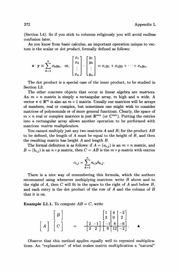
There is a nice way of remembering this formula, which the authors recommend using whenever multiplying matrices: write B above and to the right of A, then C will fit in the space to the right of A and below B, and each entry is the dot product of the row of A and the column of B that it is on.

Example L!.!. To compute AB = C, write

[! 4 o

Observe that this method applies equally well to repeated multiplica­tions. An "explanation" of what makes matrix multiplication a "natural"

Appendix L1 373

operation to perform appears in Theorem L2.20. Exercise L1#1 provides practice on matrix multiplication if you need it.

Once you have matrix multiplication, you can write a system of linear equations much more succinctly, as follows:

is the same as

[I I] [J] [I] , ,

which can be written far more simply as

Ax=b.

The m x n matrix A is comprised of the coefficients on the left of the equa­tions; the vector x in lRn represents the unknowns, the operation between A and x is matrix multiplication, and the vector b in lRm represents the constants on the right of the equations.

L1.2. THE MAIN ALGORITHMS: Row REDUCTION

Given a matrix A, a row opemtion on A is one of the following three operations:

(1) multiplying a row by a nonzero number;

(2) adding a multiple of a row onto another row;

(3) exchanging two rows.

There are two good reasons why these operations are so important. The first is that they only involve arithmetic, i.e., addition, subtraction, multi­plication, and division. That is just what computers do well; in some sense, it is all they can do. And they spend a lot of their time doing it: row operations are fundamental to most other mathematical algorithms.

The other reason is that row operations are closely connected to linear equations. Suppose Ax = b represents a system of m linear equations in n

374 Appendix L

unknowns. Then the m x (n + 1) matrix [A, b] composed of the coefficients on the left and the constants on the right,

al,n bl] : : = [A, b],

am,n bm

sums up all the crucial numerical information in each equation. Now the key property is the following:

Theorem Ll.2. If the matrix [A', b'] is obtained from [A, b] by a sequence of row operations, then the set of solutions of Ax = b and of A'x = b' coincide.

Proof. This fact is not hard to see: the row operations correspond to multiplying one equation through by a nonzero number, adding a multiple of one equation onto another, and exchanging two equations. Thus, any solution of Ax = b is also a solution of A'x = b'. On the other hand, any row operation can be undone by another row operation (Exercise L1#2), so any solution A'x = b' is also a solution of Ax = b. 0

Theorem L1.2 suggests trying to solve Ax = b by using row operations on [A, b] to bring it to the most convenient form. The following example shows this idea in action.

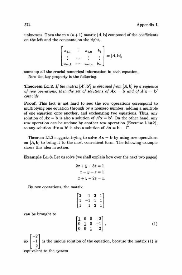
Example L1.3. Let us solve (we shall explain how over the next two pages)

2x+y+3z = 1

x-y+z=l

x+y+2z = 1.

By row operations, the matrix

[2 1 3 1] 1 -1 1 1 1 1 2 1

can be brought to

[* ~ ~ =~], 001 2

(1)

so [:: n .. the unique solution of the equation, boca .... the matrix (1) ..

equivalent to the system

Appendix L1

X= -2

y= -1

z=2 .•

375

Most people agree that the "echelon" form (1) at the center of Example L1.3 is best for solving systems of linear equations (though there are many variants, and the echelon form is not actually best for all purposes).

A matrix is in echelon form if

( a) for every row, the first nonzero entry is 1, called a leading 1;

(b) the leading 1 of a lower row is always further to the right then the leading 1 of a higher row;

(c) for every column containing a leading 1, all other entries are O.

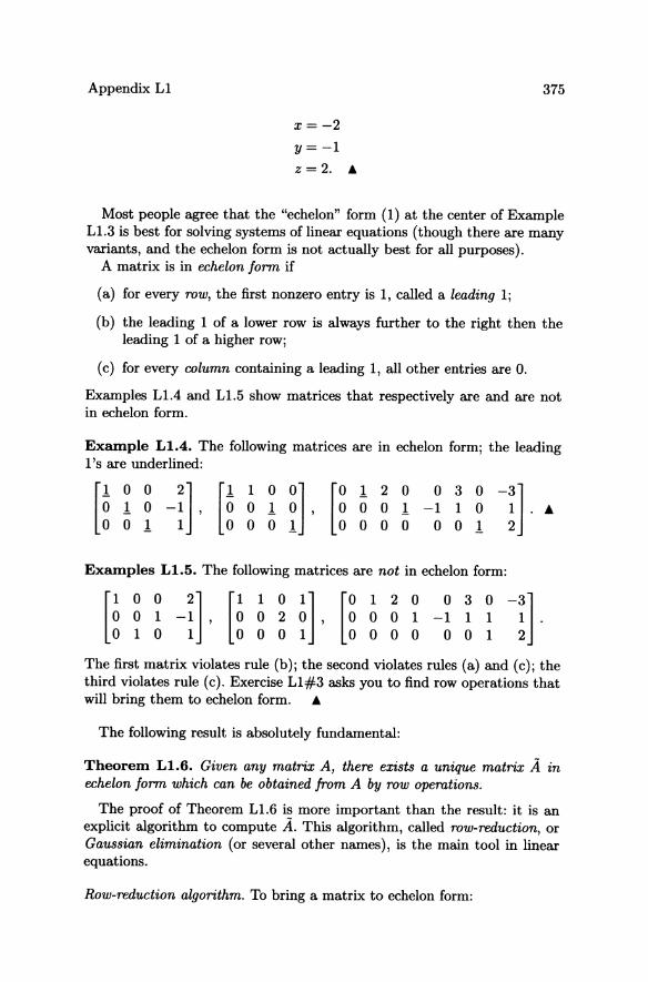
Examples L1.4 and L1.5 show matrices that respectively are and are not in echelon form.

Example L1.4. The following matrices are in echelon form; the leading l's are underlined:

[1 0 0 2] o 1 0 -1 , o 0 1 1

[1 1 0 0] o 010 , o 0 0 1

[0 1 2 0 0 3 0 -3] o 0 0 1 -1 1 0 1 o 0 0 0 001 2

••

Examples L1.5. The following matrices are not in echelon form:

[1 0 0 2] o 0 1 -1 , o 1 0 1

[1 1 0 1] o 0 2 0 , 000 1

[0 1 2 0 0 3 0 -3] o 0 0 1 -1 1 1 1 o 0 0 0 001 2

The first matrix violates rule (b); the second violates rules (a) and (c); the third violates rule (c). Exercise L1#3 asks you to find row operations that will bring them to echelon form. •

The following result is absolutely fundamental:

Theorem L1.6. Given any matrix A, there exists a unique matrix A in echelon form which can be obtained from A by row opemtions.

The proof of Theorem L1.6 is more important than the result: it is an explicit algorithm to compute A. This algorithm, called row-reduction, or Gaussian elimination (or several other names), is the main tool in linear equations.

Row-reduction algorithm. To bring a matrix to echelon form:

376 Appendix L

(1) Look down the first column until you find a nonzero entry (called a pivot). If you do not find one, then look in the second column, etc.

(2) Move the row containing the pivot to the first row position, and then divide that row by the pivot to make that entry a leading 1, as defined above.

(3) Add appropriate mUltiples of this row onto the other rows to cancel the entries in the first column of each of the other rows.

Now look down the next column over (and then the next column if neces­sary, etc.), starting beneath the row you just worked with, and look for a nonzero entry (the next pivot). As above, exchange its row with the second row, divide through, etc.

This proves existence of a matrix in echelon form which can be obtained from a given matrix. Uniqueness is more subtle (and less important) and will have to wait. D

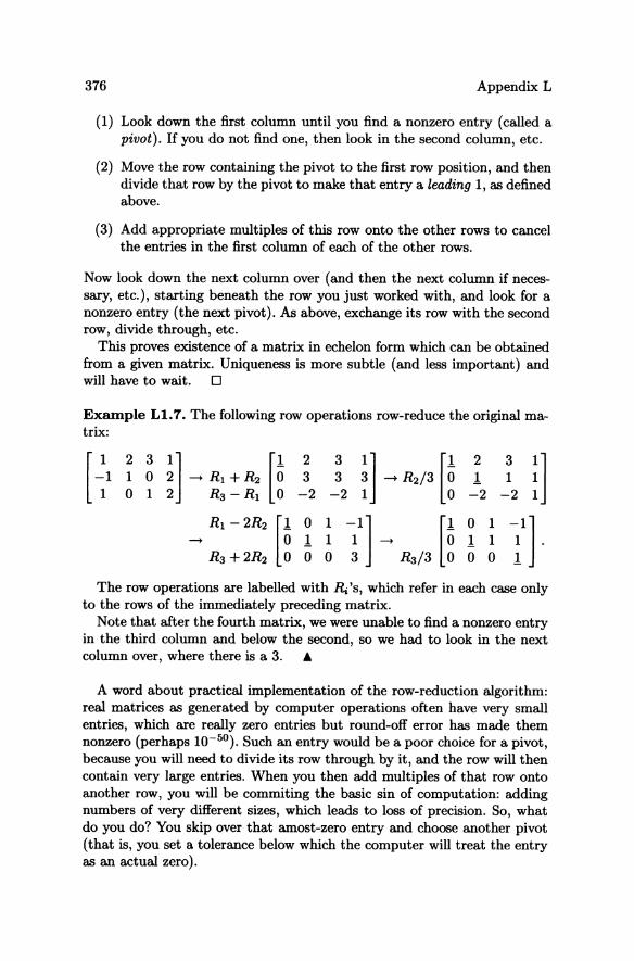
Example L1.7. The following row operations row-reduce the original ma-trix:

[ ~I 2 3 I] [1 2 3 1] [1 2 3

:] 1 0 2 --+ Rl + R2 0 3 3 3 --+ R 2/3 0 1 1 0 1 2 R3 - Rl 0 -2 -2 1 0 -2 -2

RI - 2R, [1 0 1 Tl [~

0 1 -I] --+ 011 --+ 1 1 1 . R3 +2R2 0 0 0 R 3/3 0 0 1

The row operations are labelled with R; 's, which refer in each case only to the rows of the immediately preceding matrix.

Note that after the fourth matrix, we were unable to find a nonzero entry in the third column and below the second, so we had to look in the next column over, where there is a 3. A

A word about practical implementation of the row-reduction algorithm: real matrices as generated by computer operations often have very small entries, which are really zero entries but round-off error has made them nonzero (perhaps 10-5°). Such an entry would be a poor choice for a pivot, because you will need to divide its row through by it, and the row will then contain very large entries. When you then add multiples of that row onto another row, you will be commiting the basic sin of computation: adding numbers of very different sizes, which leads to loss of precision. So, what do you do? You skip over that amost-zero entry and choose another pivot (that is, you set a tolerance below which the computer will treat the entry as an actual zero).

Appendix L1 377

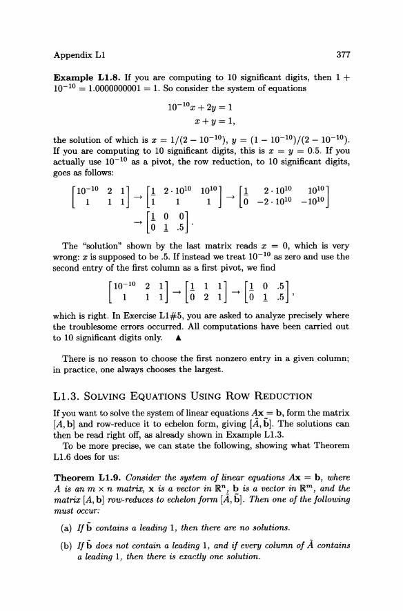
Example L1.8. If you are computing to 10 significant digits, then 1 + 10-10 = 1.0000000001 = 1. So consider the system of equations

lO- lOx + 2y = 1

x+ Y = 1,

the solution of which is x = 1/(2 - 10-10 ), y = (1 - 10-10)/(2 - 10-1°). If you are computing to 10 significant digits, this is x = Y = 0.5. If you actually use 10-10 as a pivot, the row reduction, to 10 significant digits, goes as follows:

[10-10 2

1 1 2.1010

1

f .~]. The "solution" shown by the last matrix reads x = 0, which is very

wrong: x is supposed to be .5. If instead we treat 10-10 as zero and use the second entry of the first column as a first pivot, we find

2 1

1] [1 1 1 ~ 0 2

1] [1 0 .5] 1 ~ 0 1 .5 '

which is right. In Exercise Ll#5, you are asked to analyze precisely where the troublesome errors occurred. All computations have been carried out to 10 significant digits only. A

There is no reason to choose the first nonzero entry in a given column; in practice, one always chooses the largest.

L1.3. SOLVING EQUATIONS USING Row REDUCTION

If you want to solve the system of linear equations Ax = b, form the matrix [A, bj and row-reduce it to echelon form, giving [A, bj. The solutions can then be read right off, as already shown in Example L1.3.

To be more precise, we can state the following, showing what Theorem L1.6 does for us:

Theorem L1.9. Consider the system of linear equations Ax = b, where A is an m x n matrix, x is a vector in IRn , b is a vector in IRm , and the matrix [A, bj row-reduces to echelon form [A, bj. Then one of the following must occur:

(a) If b contains a leading 1, then there are no solutions.

(b) If b does not contain a leading 1, and if every column of A contains a leading 1, then there is exactly one solution.

378 Appendix L

(c) If b does not contain a leading 1, and if some column of A contains no leading 1, then there are infinitely many solutions. They form a family that depends on as many parameters as the number of columns of A not containing leading 1 'so

Before discussing details of this theorem, let us consider the instance where the results are most intuitive, where n = m. Case (b) of Theorem L1.9 has been illustrated by Example L1.3; Examples L1.lO and L1.11 illustrate cases (a) and (c), respectively.

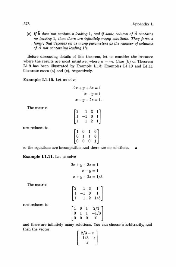
Example L1.10. Let us solve

The matrix

row-reduces to

2x+y+3z = 1

x-y=1

x + y + 2z = 1.

[: ' 3 '] -1 0 1 121

[~ 0 1

1] 1 1 0 0

so the equations are incompatible and there are no solutions. &

Example L1.11. Let us solve

The matrix

row-reduces to

2x + y +3z = 1

x-y=1

x + y + 2z = 1/3.

[: 1 3

'~3] -1 0 1 2

[~ 0 , 2/3] 1 1 -1/3 0 o 0

and there are infinitely many solutions. You can choose z arbitrarily, and then the vector

[ 2/3 - z ] -1/~ - z

Appendix Ll 379

is a solution, the only one with that value of z. A

For instances where n i= m, examples for Theorem Ll.9 are provided in Exercises Ll#4 and Ll#6e.

These examples have a geometric interpretation. As the reader surely knows, and can verify in Exercise Ll#7, two equations in two unknowns

a1X + b1y = C1

a2X + b2y = C2

are incompatible if and only if the lines £1 and £2 in 1R2 with equations a1x+b1Y = C1 and a2x+b2Y = C2 are parallel. The equations have infinitely many equations if and only if (1 = (2'

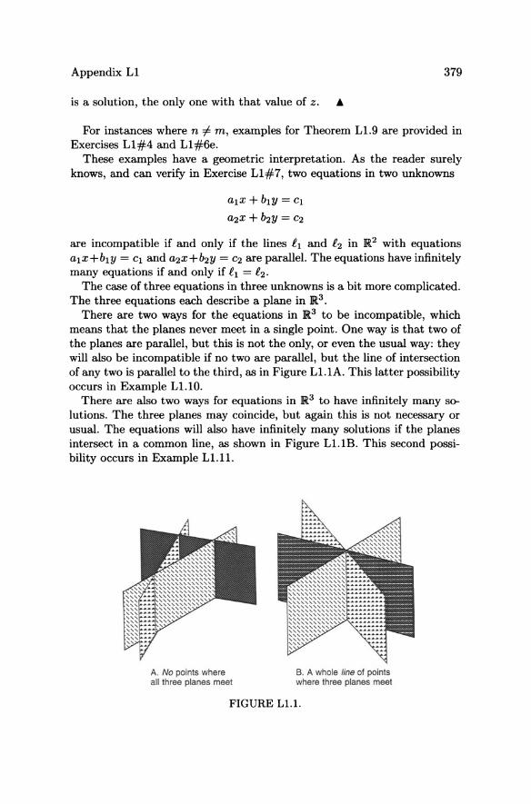
The case of three equations in three unknowns is a bit more complicated. The three equations each describe a plane in 1R3 .

There are two ways for the equations in 1R3 to be incompatible, which means that the planes never meet in a single point. One way is that two of the planes are parallel, but this is not the only, or even the usual way: they will also be incompatible if no two are parallel, but the line of intersection of any two is parallel to the third, as in Figure Ll.IA. This latter possibility occurs in Example Ll.lO.

There are also two ways for equations in 1R3 to have infinitely many so­lutions. The three planes may coincide, but again this is not necessary or usual. The equations will also have infinitely many solutions if the planes intersect in a common line, as shown in Figure Ll.IB. This second possi­bility occurs in Example Ll.ll.

A. No points where all three planes meet

B. A whole line of points where three planes meet

FIGURE L1.l.

380 Appendix L

The phrase in part (c) of Theorem L1.9 concerning the number of param­eters is actually a statement about the "dimension of the solution space," a concept that will be explained in Subsections L2.1 and L2.2.

Theorem L1.9 has additional spin-offs, such as the following:

Remark: If you want to solve several systems of n linear equations in n unknowns with the same matrix, e.g., AXl = bI. ... , AXk = bk, you can deal with them all at once using row reduction. Form the matrix

and row-reduce it to get

Various cases can occur:

(a) If A is the identity, then hi is the solution to the ith system Axi = bi'

(b) If hi has a nonzero entry in a row and all the entries of A in that row are zero, then the ith equation has no solutions.

(c) If hi has only zeroes in the rows in which A has only zeroes, then the ith equation has infinitely many solutions, depending on as many parameters as the number of columns of A not containing leading 1 'so

This remark will be very useful when we come to computing inverses of matrices, in the next subsection.

L1.4. INVERSE AND TRANSPOSE OF A MATRIX

The identity matrix In is the n x n-matrix with 1's along the diagonal and O's elsewhere:

I, = [~ ~ 1 and 13 = [~ ! ~]. It is called an identity matrix because multiplication by it does not change the matrix being multiplied: If A is an n x m matrix, then

The columns el, ... , en of In, i.e., the vectors with just one 1 and all other entries 0, will play an important role, particularly in Appendix L2.

For any matrix A, its matrix inverse is another matrix A-I such that

AA-I = A-I A = I, the identity matrix.

The existence of a matrix inverse gives another possible tock to solving equations. That is because A-I Ax = x, so the solution of Ax = b is then

Appendix Ll 381

x = A-lb. In practice, computing matrix inverses is not often a good way of solving linear equations, but it is nevertheless a very important construction.

Only square matrices can have inverses: Exercise Ll#8 asks you

(a) to derive this from Theorem L1.9, and

(b) to show an example where AB = I, but BA :F I. Such a B would be only a "one-sided inverse" for A; a "one-sided inverse" can give uniqueness or existence of solutions to Ax = b, but not both.

Example L1.12. The inverse of a 2 x 2 matrix

as Exercise Ll#9 asks you to confirm by matrix multiplication of AA-I and A-IA. ~

Notice that this 2 x 2 matrix A has an inverse if and only if ad - be :F 0; we will see much more about this sort of thing in the section about determinants. There are analogous formulas for larger matrices, but they rapidly get out of hand.

The effective way of computing matrix inverses for larger matrices is by row reduction:

Theorem L1.13. If A is a square n x n matrix, and if you construct the n x 2n matrix [A I I] and row-reduce it, then there are two possibilities:

(1) the first n columns row-reduce to the identity; in that case the last n columns are the inverse of A;

(2) the first n columns do not row-reduce to the identity, in which case A does not have an inverse.

Proof. (1) Suppose [A I I] row-reduces to [I I B]. Then, since the columns (n + 1, ... , 2n) behave independently, the ith column of B is the solution Xi to the equation AXi = ei. Putting the columns together, this shows A[XI,X2,""Xn ] =AB=I.

In order to show BA = I, start with the matrix [B I I]. Undoing the row operations that led from [A I I] to [I I B] will lead from [B I I] to [I I AJ, so BA= I.

(2) If row-reducing [A I I] does not reduce to [I I B] but to [A' I A"], with the bottom row of A' all zeroes, then there are two possibilities. If the bottom row of A" is also all zeroes, there are infinitely many solutions; if there is a nonzero element in the bottom row of A", then there is no solution. In either case, A is noninvertible. 0

382 Appendix L

Remark. The careful reader will observe that we have shown that if [A I f] row-reduces to [f I BJ, then AB = f. We have not shown that BA = f, although this also is true.

Example L1.14.

A ~ [: -: [] has inverse A- 1 = [ ~ =~ =i] -2 1 3

because

[: 1 3·1 0

~] -1 1·0 1 1 2·0 0

row-reduces to [1 0 O· 3 -1 -4] o 1 o· 1 -1 -1 .

o 0 1· -2 1 3

You can confirm in Exercise LI#9 that AA-l = A-l A = f and that you can use this inverse matrix to solve the system of Example L1.3. •

Example L1.15.

[: 1

~] A= -1 1

has no inverse A -1 because

[ 2~ 1 3· 1 0 0] -1 0·0 1 0

1 2·0 0 1

row-reduces to

[1 0 1· 1 0 -1] o 1 1· -1 0 2. o 0 O· -2 1 3

This is the matrix of Examples L1.lO and L1.l1, for two systems of linear equations, neither of which has a unique solution. •

Note: Examples L1.14 and L1.15 are unusually "simple" in the sense that the row reduction involved no fractions; this is the exception rather than the rule (as you might guess from Example L1.12). So do not be alarmed when your calculations look a lot messier.

Finally, to complete our list of matrix definitions, we note that one more matrix related to a matrix A is its transpose AT, the matrix that inter­changes all the rows and columns of A.

Appendix L2 383

[ 1 4 -2] T [1 3] Example L1.16. If B = 3 0 2' then B = _~ ~. A

A frequently used result involving the transpose is the following:

Theorem L1.17. The tmnspose of a product is the product of the tmns­poses in reverse order:

The proof of Theorem L 1.1 7 is straightforward and is left as Exercise L1#11.

The importance of the transpose will be discussed in Section L3.3.

L2 Theory of Linear Equations: Vocabulary

We now come to the most unpleasant chore of linear algebra: defining a fairly large number of essential concepts. These concepts have been isolated by generations of mathematicians as the right way to speak about the phenomena involved in linear equations. For all that, their usefulness, or for that matter meaningfulness, may not be apparent at first.

The most unpleasant of all is the notion of vector space. This is the arena in which "linear phenomena" occur; that is, the structure imposed by a vector space is the bare minimum needed for such phenomena to occur.

L2.1. VECTOR SPACES

A vector space is a set V, the elements of which can be added and multi­plied by numbers, and satisfying all the rules which you probably consider "obvious." Being specific about what this means will probably seem both pedantic and mysterious, and it is. In practice, one rapidly gets an intuitive feeling for what a vector space is, and never verifies the axioms explicitly.

A vector space is a set endowed with two operations, addition and mul­tiplication by scalars. A scalar is a number, and in this book the scalars will always be either the real numbers or the complex numbers.

For a vector space V, these two operations must satisfy the following ten rules:

(1) Closure under addition. For all v, w E V, we have v + w E V.

(2) Closure under multiplication by scalars. For any v E V and any scalar a, we have av E V.

(3) Additive identity. There exists a vector 0 E V such that for any v E V, 0 + v = v.

384 Appendix L

(4) Additive inverse. For any v E V, there exists a vector -v E V such that v + (-v) = O.

(5) Commutative law for addition. For all v, W E V, we have v + W = W + v.

(6) Associative law for addition. For all Vb V2, v3 E V, we have VI + (V2 + V3) = (VI + V2) + V3'

(7) Multiplicative identity. For all v E V, we have Iv = v.

(8) Associative law for multiplication. For all scalars a, f3 and all v E V, we have o.(f3v) = (o.f3)v.

(9) Distributive law for scalar addition. For all scalars a, f3 and all v E V, we have (a + f3)v = o.v + f3v.

(10) Distributive law for vector addition. For all scalars a and v, WE V, we have o.(v + w) = o.v + o.w.

We shall now give four examples of vector spaces, which with their vari­ants will be the main examples used in this book.

Example L2.1. The basic example of a vector space is IRn, with the obvious componentwise addition and multiplication by scalars. Actually, you should think of the ten rules as some sort of "essence of IRn ," abstracting from IRn

all its most important properties. &

Example L2.2. The more restricted set of vectors

[ ~ 1 E R3 ,uch that 2x - 3. + z ~ 0

(or any similar homogeneous linear relation on the variables of IRn) forms another vector space, because all ten rules are satisfied by such x, y, z triples (Exercise L2#1). These are important examples also, since they are sub-spaces of the vector space IRn. &

A subspace of a vector space is a subset that is also a vector space under the same operations as the original vector space. Exercise L2#2 asks you to show that all requirements for a vector space are automatically satisfied if just the following two statements are true for any elements Wi, Wj of a subset W of V and any scalar a:

i) Wi +Wj E W; ii) o.Wi E W;

The "vectors" in our third example will probably seem more exotic.

Appendix L2 385

Example L2.3. Consider the space C([O, 1]), which denotes the space of continuous real-valued functions f(x) defined for 0 :5 x :5 1, with addition and multiplication by scalars the usual operations. That is, the "vectors" are now functions f(x), so addition means f(x) + g(x) and multiplication means 0: f(x). Although these functions are not geometric vectors in the sense of our previous example, this space also satisfies all ten requirements for a vector space. •

Example L2.4. Consider the space of twice-differentiable functions f(x) defined for all x E IR such that rP f / dx2 = O. This is a subspace of the vector space of the preceding example and is a vector space itself. But since a function has a vanishing second derivative if and only if it is a polynomial of degree 1, we see that this space is the set of functions

fa.b(X) = a + bx.

In some sense, this space "is" 1R2 , by identifying fa.b with [:] E 1R2 j this

was not obvious from the definition. •

L2.2. LINEAR COMBINATIONS, LINEAR INDEPENDENCE AND

SPAN

If Vb •.• , Vk is a collection of vectors in some vector space V, then a linear combination of the viis a vector v of the form

k

v = Laivi. i=i

The span of Vi, ••• , Vk is the set of linear combinations of the Vi.

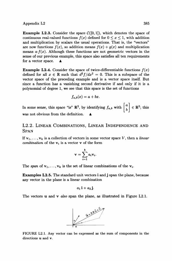
Examples L2.5. The standard unit vectors i and j span the plane, because any vector in the plane is a linear combination

The vectors u and V also span the plane, as illustrated in Figure L2.1.

FIGURE L2.1. Any vector can be expressed as the sum of components in the directions u and v.

386 Appendix L

A set of vectors VI,"" Vk spans a vector space V if every element of V is in the span. For instance, i and j span ]R2 but not ]R3.

The vectors V}, ... , Vk are linearly independent if there is only one way of writing a given linear combination, i.e., if

k k

L aiVi = L biVi implies al = b}, a2 = ~, ... , ak = bk'

i=1 i=1

Many books use the following as the definition of linear independence, then prove the equivalence of our definition: A set of vectors VI, ... ,Vk is linearly independent if and only if the only solution to

Another equivalent statement is to say that none of the viis a linear combination of the others (Exercise L2#3). If one of the Vi is a linear combination of the others, they are called linearly dependent.

Remark. Geometrically, linear independence means the following:

(1) One vector is linearly independent if it is not the zero vector.

(2) Two vectors are linearly independent if they do not lie on a line, i.e., if they are not collinear.

(3) Three vectors are linearly independent if they do not lie in a plane, i.e., if they are not coplanar.

The following theorem is basic to the entire theory.

Theorem L2.6. In ]Rn, n + 1 vectors are never linearly independent, and n - 1 vectors never span.

Proof. The idea is to reduce both statements in the theorem to linear equations.

For the first part, let the n + 1 vectors in ]Rn be

[VII] [VI 2] [VI n+l] VI = :' , V2 = :' , ... ,Vn+l = ':

Vn,1 Vn ,2 Vn,n+l

Linear independence for n + 1 vectors can be written as the vector equa­tion alVI + a2V2 + ... + an+lvn+l = 0 or as a system of linear equations

Appendix L2 387

which is n equations in n + 1 unknowns al, ... , an+! , with Vl,l, ... - Vn,n+l

as coefficients (exactly the reverse of the usual interpretation of such a system). These equations are certainly compatible, since al = ... = an+! = o is a solution, but this solution cannot be the only solution: that would mean that fewer equations than unknowns determined the values of the unknowns.

To see this rigorously, row reduce the matrix [Vl, ... ,vn +1. 01. At least one of the n + 1 columns must not contain a leading 1, since there is at most one per row and there are fewer rows than columns. By Theorem L1.9, there cannot be a unique solution to the system of equations.

For the second part, let Vt. ... , Vn-l be vectors in ]Rn. To say they do not span is to say that there exists a vector b such that the equation

has no solutions. Again write this out in full, to get

= :'

i.e., n equations in the n-l unknowns al, ... , an-t. with Vl,l, ... , Vn,n-l as coefficients. We must see that the bi's can be chosen so that the equations are incompatible. Write the matrix

[Vt. ... , Vn-t. I,

temporarily leaving the last column blank. Row-reduce it, at least the first n - 1 columns. There must then be a row starting with n - 1 zeroes, since any row must either begin with a leading one or be all zeroes; furthermore, there is at most one leading 1 per column. Now put a 1 in the nth, or last, position of that row and fill up the nth column by making all the other entries O. By Theorem L1.9, case (b), such an echelon form of the matrix represents a system with no solution. Since any row operation can be undone, we can bring the echelon matrix back to where it started, with the matrix A on the left; the last column will then be a vector b, making the system incompatible. 0

In a vector space, an ordered set of vectors Vl, ... ,Vn is called a basis if it satisfies one of the three following equivalent conditions (We will see below that they are indeed equivalent):

(1) The set is a maximal linearly independent set.

(2) The set is a minimal spanning set.

(3) The set is a linearly independent spanning set.

388 Appendix L

Example L2.7. The most fundamental example of basis is the standard basis of ]Rn:

Clearly, every vector is in the span of el, ... , en:

it is equally clear that el, ... ,en are linearly independent (Exercise L2#4) .

• Example L2.S. The standard basis is not in any sense the only one. Quite the contrary: in general, any old n vectors in ]Rn form a basis. For instance,

We need to show that the three conditions for a basis are indeed equiv­alent:

If a set Vl,"" Vn is a maximal linearly independent set, then for any other vector w, the set {Vl, ... , Vn, w} is linearly dependent, and there exists a nontrivial relation

al Vl + ... + an Vn + bw = O.

The coeffcient b is not zero, because the relation would then involve only the v's, which are linearly independent by hypothesis; so w can be expressed as a linear combination of the v's and we see that the v's do span.

But {Vl,"" vn} is a minimal spanning set: if one of the Vi'S is omitted, the set no longer spans, since the omitted Vi is linearly independent of the others and hence cannot be in the span of the others. This shows that (1) and (2) are equivalent; the other equivalences are similar and left as Exercise L2#6.

Now Theorem L2.6 above can be restated:

Theorem L2.9. Every basis of]Rn has exactly n elements.

Indeed, a set of vectors never spans if it has fewer than n elements, and is never linearly independent when it has more than n elements.

Appendix L2 389

A vector space is finite-dimensional if it is spanned by finitely many elements. It then has a basis (in fact, many bases): find any finite spanning set and discard elements of it until what is left still spans, but if another vector is discarded, it no longer does.

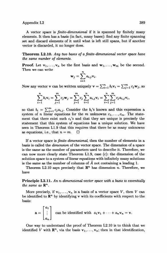
Theorem L2.10. Any two bases of a finite-dimensional vector space have the same number of elements.

Proof. Let Vb ... , vn be the first basis and W1, .•• , Wm be the second. Then we can write

n

Wj = L ai,jVi· i=1

Now any vector V can be written uniquely v = E~1 biVi = Ej:1 CjWj, so

n m m n n m

LbiVi = LCjWj = LCj Lai,jVi = LLCjai,jVi, i=1 j=1 j=1 i=1 i=1 j=1

so that bi = Ej:1 Cjai,j. Consider the bi's known and this expression a system of n linear equations for the m unknowns C1, •.. , em. The state­ment that there exist such Ci'S and that they are unique is precisely the statement that this system of equations has a unique solution. We have seen in Theorem Ll.9 that this requires that there be as many unknowns as equations, i.e., that n = m. 0

If a vector space is finite-dimensional, then the number of elements in a basis is called the dimension of the vector space. The dimension of a space is the same as the number of parameters used to describe it. Therefore, we can now more clearly state Theorem Ll.9, case (c): the dimension of the solution space to a system of linear equations with infinitely many solutions is the same as the number of columns of A not containing a leading l.

Theorem L2.10 says precisely that an has dimension n. Therefore, we have

Principle L2.11. An n-dimensional vector space with a basis is essentially the same as an.

More precisely, if Vb .•. , vn is a basis of a vector space V, then V can be identified to an by identifying v with its coefficients with respect to the basis:

a ~ [] can be identilied with a,v,+··· + .. v. ~ v.

One way to understand the proof of Theorem L2.10 is to think that we identified V with an, via the basis Vb ... , vn; then in that identification,

390 Appendix L

Wl, ... , Wm became m vectors of ]Rn, namely the columns of the matrix (ai,j)' (Think about this, as Exercises L2#1O, 11.) The identification pre­serves all "linear features"; in particular, these m vectors are a basis of]Rn, hence there are n of them. We shall use this fact in Section L2.4.

Remark. Not every vector space comes with an outstanding basis like ]Rn does.

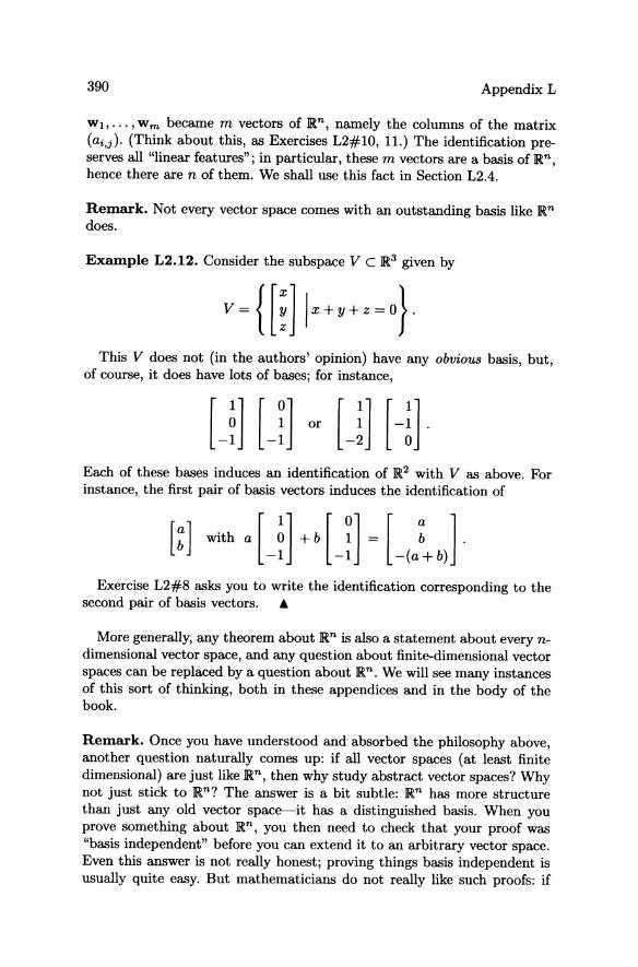
Example L2.12. Consider the subspace V c ]R3 given by

This V does not (in the authors' opinion) have any obvious basis, but, of course, it does have lots of bases; for instance,

U] U] m U] [-1] Each of these bases induces an identification of ]R2 with V as above. For instance, the first pair of basis vectors induces the identification of

Exercise L2#8 asks you to write the identification corresponding to the second pair of basis vectors. •

More generally, any theorem about ]Rn is also a statement about every n­dimensional vector space, and any question about finite-dimensional vector spaces can be replaced by a question about ]Rn. We will see many instances of this sort of thinking, both in these appendices and in the body of the book.

Remark. Once you have understood and absorbed the philosophy above, another question naturally comes up: if all vector spaces (at least finite dimensional) are just like]Rn, then why study abstract vector spaces? Why not just stick to ]Rn? The answer is a bit subtle: ]Rn has more structure than just any old vector space-it has a distinguished basis. When you prove something about ]Rn, you then need to check that your proof was "basis independent" before you can extend it to an arbitrary vector space. Even this answer is not really honest; proving things basis independent is usually quite easy. But mathematicians do not really like such proofs: if

Appendix L2 391

you can prove something by adding some structure and then showing you did not need it, it should be possible to prove the same thing without ever mentioning the extra structure. This aesthetic-philosophical consideration is also part of why abstract vector spaces are studied.

Let us turn briefly to the idea of a vector space that is infinite-dimensional.

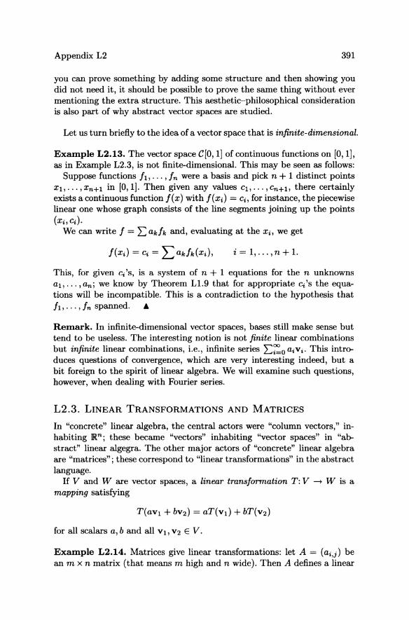
Example L2.13. The vector space e[O, 1] of continuous functions on [0,1], as in Example L2.3, is not finite-dimensional. This may be seen as follows:

Suppose functions It, ... , / n were a basis and pick n + 1 distinct points xb ... ,Xn+I in [0,1]. Then given any values CI, ... ,Cn+b there certainly exists a continuous function /(x) with /(Xi) = Ci, for instance, the piecewise linear one whose graph consists of the line segments joining up the points (Xi, Ci).

We can write / = E ak/k and, evaluating at the Xi, we get

i = 1, ... ,n + 1.

This, for given Ci'S, is a system of n + 1 equations for the n unknowns ab ... , an; we know by Theorem L1.9 that for appropriate c/s the equa­tions will be incompatible. This is a contradiction to the hypothesis that /b ... , /n spanned. •

Remark. In infinite-dimensional vector spaces, bases still make sense but tend to be useless. The interesting notion is not finite linear combinations but infinite linear combinations, i.e., infinite series E:'o aiVi. This intro­duces questions of convergence, which are very interesting indeed, but a bit foreign to the spirit of linear algebra. We will examine such questions, however, when dealing with Fourier series.

L2.3. LINEAR TRANSFORMATIONS AND MATRICES

In "concrete" linear algebra, the central actors were "column vectors," in­habiting ]Rn; these became ''vectors'' inhabiting ''vector spaces" in "ab­stract" linear algegra. The other major actors of "concrete" linear algebra are "matrices"; these correspond to "linear transformations" in the abstract language.

If V and W are vector spaces, a linear trans/ormation T: V -+ W is a mapping satisfying

for all scalars a, b and all VI, V2 E V.

Example L2.14. Matrices give linear transformations: let A = (ai,i) be an m x n matrix (that means m high and n wide). Then A defines a linear

392

transformation T: IRn _ IRm by matrix multiplication:

T(v) = Av.

Such mappings are indeed linear, because A(v + w) A(cv) = cAY. A

Appendix L

Av + Aw and

Remark. In practice, a matrix and its associated linear transformation are usually identified, and the linear transformation T : IRn _ IRm is denoted simply by its matrix A.

For an infinite-dimensional V, a linear transformation T is often given as a differential opemtor on the functions that comprise V:

Example L2.15. Let V be the vector space P2 of polynomials p(x) of degree at most 2; then an example of a linear transformation T is given by the formula

T(p)(x) = (x2 + l)p"(x) - xp'(x) + 2p(x).

The notation T(p)(x) emphasizes that T acts on the polynomials p that comprise the vector space P2 , never on a number p(x) that might describe p for a particular x.

We leave it to the reader as Exercise L2# 13 to verify linearity. A

Example L2.16. A differential operator like that in Example L2.15 can be used on a more general function f ( x) to define a linear transformation such as

T(f)(x) = (x2 + 1)!"(x) - xJ'(x) + 2f(x), T: C2 [0, 1] - C[O, 1]

from the space of twice continuously differentiable functions on [0,1] to the space of continuous functions on [0,1]. A

Alternatively, for an infinite-dimensional V, a linear transformation T is sometimes given by an integml involving the functions of V, corresponding to the matrix A of the finite-dimensional case.

Example L2.17. There are analogs of matrices in C[O, 1]. Let K(x,y) be a continuous function of x and y defined for 0 ::; x, y ::; 1, and consider the mapping

T:C[O, 1]- C[O, 1]

given by

T(f)(x) = fa1 K(x,y)f(y)dy.

Appendix L2

This is analogous to Example L2.14, which could be written

n

T(V)i = Lai,jVj, j=l

393

but here the discrete indices i, j have become "continuous indices" x, y. A

For finite-dimensional matrices, the following result is crucial:

Theorem L2.1S. Every linear transformation T:]Rn -+ ]Rm is given by an m x n matrix MT , the ith column of which is T(ei).

This means that Example L2.14 is "the general" linear transformation in finite-dimensional vector spaces.

Proof. Start with the linear transformation T of Example L2.14 and man­ufacture the matrix A according to the given rule. Then given any v E ]Rn,

we may write

then, by linearity,

which is precisely the column vector Av. 0

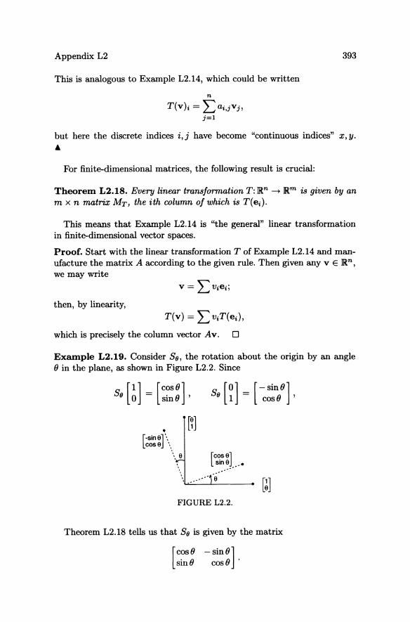
Example L2.19. Consider Sf}, the rotation about the origin by an angle () in the plane, as shown in Figure L2.2. Since

Sf} [~] = [:~::] , S [0] _ [-sin(}] f} 1 - cos(} ,

• [ -sin 9] '.. COsS ...

... 9

[~]

[ COS 9] sin9 __ •

.' .•.•.. 9 ---

FIGURE L2.2.

Theorem L2.18 tells us that Sf} is given by the matrix

[ COS(} -Sin(}] sin () cos () .

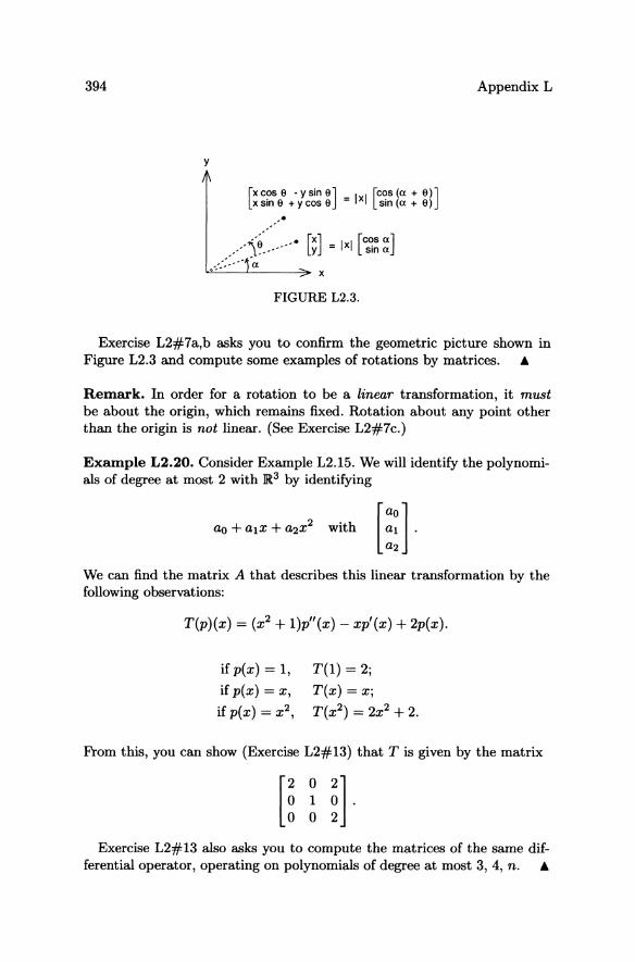
394 Appendix L

y

[ XCOSO-YSinO]_ rCOs(a+o)] xsinO+ycosO -lxILsin(a+O)

FIGURE L2.3.

Exercise L2#7a,b asks you to confirm the geometric picture shown in Figure L2.3 and compute some examples of rotations by matrices. A

Remark. In order for a rotation to be a linear transformation, it must be about the origin, which remains fixed. Rotation about any point other than the origin is not linear. (See Exercise L2#7c.)

Example L2.20. Consider Example L2.15. We will identify the polynomi­als of degree at most 2 with ]R3 by identifying

We can find the matrix A that describes this linear transformation by the following observations:

T{p){x) = (x2 + l)p"{x) - xp'{x) + 2p{x).

if p{x) = 1,

if p{x) = x, if p{x) = x2,

T(l) = 2;

T(x) = x; T(x2) = 2x2 + 2.

From this, you can show (Exercise L2#13) that T is given by the matrix

Exercise L2#13 also asks you to compute the matrices of the same dif­ferential operator, operating on polynomials of degree at most 3, 4, n. A

Appendix L2 395

If Vi! V2, and V3 are vector spaces and if S: Vl - V2 and T: V2 - V3 are linear transformations, then the composition To S: Vl - V3 is again a linear transformation. In particular, if Vl = anI, V2 = an2 , and Va = an3 ,

then the matrix MTos should be computable in terms of Ms and MT.

Theorem L2.21. Composition corresponds to matrix multiplication:

MTos =MTMS.

Proof. Take ei E anI, then S(ei) E an2 is the ith column of Ms, and T(S(ei» = MTS(ei) E an3 is the ith column of MTMS. 0

Remark. Many mathematicians would claim that this proposition "ex­plains and justifies" the definition of matrix multiplication. This may seem odd to the novice, who probably feels that composition of linear mappings is far more baroque than matrix multiplication.

One immediate consequence of Theorem L2.21 is:

Corollary L2.22. Matrix multiplication is associative: if A, B, and C are matrices such that the matrix multiplication (AB)C is allowed, then so is A(BC), and they are equal.

Proof. Composition of mappings is associative. 0

L2.4. MATRICES OF LINEAR TRANSFORMATIONS WITH

RESPECT TO A BASIS

So far, matrices have corresponded to linear transformations an _ an or en _ en. What about linear transformations defined on more general vector spaces?

In accordance with Principle L2.11 that a vector space with a basis is an, we will not be surprised to hear that if vector spaces V and W have bases {Vl, ... , vn } and {Wi! ... , w m }, respectively, then any linear transforma­tion T: V - W has a matrix (ti,j) with respect to the bases. One way to see this is to say that the bases allow us to identify V and W to an and am, respectively, via the coefficients of the basis vectors. Then the coefficients ofT(v) with respect to the Wi must depend linearly on the coefficients ofv with respect to the Vi. What this boils down to, in practice, is the following formula:

T(Vi) = Ltj,iWj,

which can be taken as the definition of the matrix. Note the order of the indices: the ith column of ti,j is the vector of coefficients of T(Vi) with respect to {Wi! ... , wm }. A look at Theorem L2.18 will show that this is indeed the correct definition.

396 Appendix L

In practical applications, the vector spaces V and W are often !R.n and !R.m themselves, but the bases {Vl,"" v n } and {Wl,"" w m } are not the standard bases. Is it possible to find the matrix of a linear transformation in terms of the new bases in terms of the old matrix? Of course, it is possible, and the important change of basis theorem is the answer:

Theorem L2.23. If {Vb ... , v n } and {Wb"" wm } are bases of!R.n and !R.m respectively, and if we form the matrices

P = [Vb' .. ,vnJ and Q = [Wb' .. ,wmJ,

then the linear transformation T:!R.n -+ !R.m having matrix A with respect to the standard basis has matrix Q-l AP with respect to the new bases.

The matrices P and Q are called the change of basis matrices, and Q-l AP is the change of basis formula.

Before proving Theorem L2.23 formally, let us see exactly what the change of basis matrices actually do.

If a E !R.n , then Pa = alVl + ... + anvn , so that P takes a column of numbers and uses them as coefficients of the Vi:

[z]

Thus, p- l must do the opposite; it takes vectors in !R.n and gives you their coordinates with respect to the Vi. You might think of P as synthesis and p- l as analysis.

Proof of Theorem L2.23. The ith column of a matrix is the result of applying the matrix to ei' So let us compute Q-l AP(ei). Well, P(ei) = Vi,

so AP(ei) = A(Vi)' Finally, Q-l takes a vector and gives its coordinates with respect to the basis {Wb ... , w m }. So the ith column of Q-l AP is formed of the coordinates of Vi with respect to {Wl, ... , w m }; this is precisely what was to be proved. 0

Of particular importance will be the case where n = m, and the bases in the domain and the range coincide. In that case, there is only one change of basis matrix P, and the matrix of the linear transformation with respect to the new basis is p- 1 AP. The matrices A and p- l AP are said to be conjugate: they are different descriptions of the same linear transformation.

Appendix L2 397

They will share many properties: determinants, characteristic polynomials, eigenvalues, dimensions of eigenspaces, etc. Over and over, we will say that some property of linear transformations is "basis independenf'; this means that if a matrix has the property, then all its conjugates do too. (See Appendix L5, Theorems L5.6, L5.8, and L5.1O.)

Note: Any invertible matrix is a change of basis matrix if you use its columns for the basis.

L2.5. KERNELS AND IMAGES

The kernel and the image of a linear transformation are the "abstract" no­tions that allow a precise treatment of uniqueness and existence of solutions to linear equations.

If V and W are vector spaces and T: V -+ W is a linear transformation, then the kernel of T is the subspace ker(T) C V given by

ker(T) = {v E V I T(v) = o}.

For more or less obvious reasons, this space is also often called the null space of T.

The image of T is the set of vectors w such that there is a vector v with T(v) = w. That is,

Im(T) = {w E W I there exists v E V such that T(v) = w}.

(Sometimes the image is also called the "range": this usage is a source of confusion since most authors, including ourselves, call the whole vector space W the range of T; consequently, we shall not use the word "range" to refer to the image.)

If V and W are finite-dimensional, we may choose bases for V and W; i.e., we may assume that V = IRn, W = IRm and that T has an m x n matrix A. If we row-reduce A to echelon form A, we can read off a basis for the kernel and the image by the following two neat tricks:

(i) The image is a subspace of W = IRm. Hence any basis will consist of m-vectors. Such a basis is provided by those columns of the original matrix A that after row-reduction will contain a leading 1; the row-reduced matrix A shows that these columns of A are linearly independent.

(ii) The kernel is a subspace of V = IRn. Hence, any basis will consist of n-vectors. We will find one such basis vector for each column of A that does not contain a leading 1, as follows:

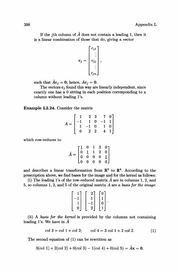
398 Appendix L

If the jth column of..4 does not contain a leading 1, then it is a linear combination of those that do, giving a vector

Cj = Cjj ,

such that ..4Cj = OJ hence, ACj = o. The vectors Cj found this way are linearly independent, since

exactly one has a 0 sitting in each position corresponding to a column without leading 1 'so

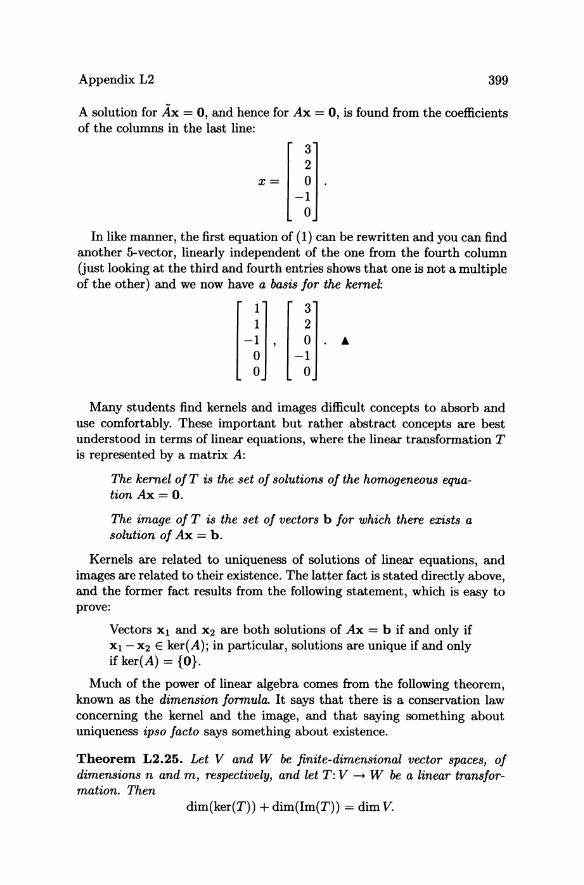
Example L2.24. Consider the matrix

[-: 2 3 7

~l 1 0 -1 A= 1 -1 0 1 0 2 2 4

which row-reduces to

[1 0 1 3 0] ..4= 0 1 1 2 0

o 0 0 0 1 o 0 000

and describes a linear transformation from ]R5 to ]R4. According to the prescription above, we find bases for the image and for the kernel as follows:

(i) The leading l's of the row-reduced matrix..4 are in columns 1, 2, and 5, so columns 1, 2, and 5 of the original matrix A are a basis for the image:

(ii) A basis for the kernel is provided by the columns not containing leading 1 'so We have in ..4

col 3 = col 1 + col 2j col 4 = 3 colI + 2 col 2. (1)

The second equation of (1) can be rewritten as

3(coll) + 2(col 2) + O(col 3) - l(col 4) + O(col 5) = Ax = O.

Appendix L2 399

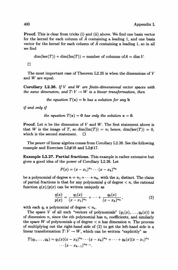
A solution for Ax = 0, and hence for Ax = 0, is found from the coefficients of the columns in the last line:

In like manner, the first equation of (1) can be rewritten and you can find another 5-vector, linearly independent of the one from the fourth column (just looking at the third and fourth entries shows that one is not a multiple of the other) and we now have a basis for the kernel:

Hl' [-rl· · Many students find kernels and images difficult concepts to absorb and

use comfortably. These important but rather abstract concepts are best understood in terms of linear equations, where the linear transformation T is represented by a matrix A:

The kernel of T is the set of solutions of the homogeneous equa­tion Ax = O.

The image of T is the set of vectors b for which there exists a solution of Ax = b.

Kernels are related to uniqueness of solutions of linear equations, and images are related to their existence. The latter fact is stated directly above, and the former fact results from the following statement, which is easy to prove:

Vectors Xl and X2 are both solutions of Ax = b if and only if Xl -x2 E ker(A)j in particular, solutions are unique if and only if ker(A) = {O}.

Much of the power of linear algebra comes from the following theorem, known as the dimension formula. It says that there is a conservation law concerning the kernel and the image, and that saying something about uniqueness ipso facto says something about existence.

Theorem L2.2S. Let V and W be finite-dimensional vector spaces, of dimensions nand m, respectively, and let T: V -+ W be a linear transfor­mation. Then

dim(ker(T)) + dim(Im(T)) = dim V.

400 Appendix L

Proof. This is clear from tricks (i) and (ii) above. We find one basis vector for the kernel for each column of A containing a leading 1, and one basis vector for the kernel for each column of A containing a leading 1, so in all we find

dim(ker(T)) + dim(Im(T)) = number of columns of A = dim V.

o

The most important case of Theorem L2.25 is when the dimensions of V and W are equal.

Corollary L2.26. If V and W are finite-dimensional vector spaces with the same dimension, and T: V -+ W is a linear transformation, then

the equation T(x) = b has a solution for any b

if and only if

the equation T(x) = 0 has only the solution x = O.

Proof. Let n be the dimension of V and W. The first statement above is that W is the image of T, so dim(Im(T)) = nj hence, dim(ker(T)) = 0, which is the second statement. 0

The power oflinear algebra comes from Corollary L2.26. See the following example and Exercises L2#16 and L2#17.

Example L2.27. Partial fractions. This example is rather extensive but gives a good idea of the power of Corollary L2.26. Let

P(x) = (x - xt}nl ... (x - Xk)nk

be a polynomial of degree n = nl + ... +nk, with the Xi distinct. The claim of partial fractions is that for any polynomial q of degree < n, the rational function q(x)/p(x) can be written uniquely as

q(x) ql(X) + ... + qk(X) (2) p(x) (x - Xl)n1 (x - Xk)nk '

with each qi a polynomial of degree < ni. The space V of all such ''vectors of polynomials" (ql (x), ... , qk (x)) is

of dimension n, since the ith polynomial has ni coefficients, and similarly the space W of polynomials q of degree < n has dimension n. The process of multiplying out the right-hand side of (2) to get the left-hand side is a linear transformation T: V -+ W, which can be written "explicitly" as

T(ql, . .. , qk) = ql (x)(x - X2)n2 ••• (x - Xk)n k + ... + qk(X)(X - xt}nl ... (x - Xk_l)n k - 1 •

Appendix L2 401

Except in the simplest cases, however, computing the matrix of T would be a big job.

Saying that q/p can be decomposed into partial fractions is precisely saying that W is the image of T, i.e., the first condition of Corollary L2.26. Since it is equivalent to the second alternative, we see that "partial fractions 'Vork" if and only if

the only solution of T( qb ... ,qk) = 0 is ql = ... = qk = O.

Lemma L2.2S. If qi =1= 0 is a polynomial of degree < ni, then

Proof. By making the change of variables u = x - Xi, we can suppose Xi = O. Since qi =1= 0, qi(X) = amxm+ higher terms, with am =1= 0 and m < ni' By Taylor's theorem, for any c there exists 6 such that

if Ixi < 6. So

which tends to 00 as X tends to O. It follows from this that T(qt, . .. , qk) =1= 0 if some qi =1= 0, since for all

j =1= i, the rational functions

have the finite limits qj(Xi)/(X, - Xj)n; as X -+ Xi, and therefore the sum

has infinite limit as X -+ Xi and therefore q cannot vanish identically. 0

Examine Example L2.27 carefully. It really put linear algebra to work. Even after translating the problem into linear algebra, via the linear trans­formation T, the answer was not clear, and only after using dimensions and the dimension formula is the result apparent. Still, all of this is noth­ing more than the intuitively obvious statement that either n equations in n unknowns are independent, the good case, or everything goes wrong at once.

402 Appendix L

L3 Vector Spaces and Inner Products

An inner product on a vector space is that extra structure that makes met­ric statements meaningful: such notions as angles, orthogonality, and length are only meaningful in inner product spaces. The archetypal examples are the dot product on JRn and en. Just as in the case of vector spaces, we will see that these examples are not just the most obvious ones, but that all others are just like them.

However, also just as for vector spaces, there are frequent occasions where stripping away the extra structure of JRn and en is helpful, and we will begin with the general definition.

In this appendix, we will describe spaces with inner products; then in Appendix L4 we will deal with the relations between linear transformations and inner products.

L3.1. REAL INNER PRODUCTS

An inner product on a real vector space V is a rule that takes two vectors a and b and gives a number (a, b) E JR, satisfying the following three rules:

(i) (a, b) = (b, a)

(ii) (aal + f3a2, b) = a(at, b) + f3(a2, b)

(iii) (a, a) > 0 if a =F 0

symmetric

linear

positive definite.

The norm of a vector a with respect to an inner product is

lIall = ../(a,a).

Example L3.!. The standard inner product or dot product on JRn,

n

a·b= Laibi =aTb, i=l

satisfies all these properties. Furthermore,

lIall = va:a: = Ja~ +a~ + ... +a~

gives the standard, or Euclidean norm. &

Example L3.2. On JR2, consider the function

Appendix L3 403

This function easily satisfies properties (i) and (ii). For property (iii), ob­serve that

(a, a) = 2a~ + 2a~ + 2ala2 = (al + a2)2 + a~ + a~ is a sum of squares and is certainly strictly positive unless a = O. Hence, (a, b) is also an inner product. &

The next example will probably be less familiar; it is, however, of great importance, particularly in trying to understand what Fourier series are all about.

Example L3.3. Consider V the vector space of continuous functions on an interval [a, b], and p(x) a positive continuous function on [a, b]. Then the integml

(/,g) = lb p(x)f(x)g(x)dx

defines an inner product on V. The case p = 1 is the continuous analog of the standard inner product. &

L3.2. COMPLEX INNER PRODUCTS

A complex inner product (also called a Hermitian inner product) on a com­plex vector space V is a complex-valued function on two vectors a and b giving a number (a, b) E e, satisfying the following three rules:

(i) (a, b) = (b, a)

(ii)

(iii) (a, a) > 0 if a ;of 0

conjugate-symmetric

linear with respect to first argument

positive definite.

where the bar denotes the complex conjugate. Note that property (ii) is unchanged from the real case, but, in combination with (i), it says that the complex inner product is linear with respect to the first variable but not the second. Note also that property (iii) makes sense because, from (i), (a, a) is real.

Example L3.4. In en, the standard inner product is (a, b) = Li aibi, and the norm is lIall = V(a,a). &

Example L3.5. Let V be the vector space of complex-valued continuous functions on [-11", 11"]. Then the formula

(/,9) = i: f(x)g(x)dx

404 Appendix L

defines an inner product on V [where g(x) is the complex conjugate of g(x)]. •

L3.3. BASIC THEOREMS AND DEFINITIONS USING INNER

PRODUCTS

The following rather surprising theorem concerning the transpose of a ma­trix (defined at the end of Section L1.4) is very useful in manipulating and proving other theorems throughout the rest of linear algebra.

Theorem L3.6. For any two vectors v and w in a real or complex inner product space and any real or complex-valued matrix A,

T -(A v, w) = (v, Aw).

The proof of Theorem L3.6 is straightforward and is left as Exercise L3#1.

Remark. Theorem L3.6 says that the transpose depends on the inner product, not the basis; this is why it is important.

Suppose V and W are vector spaces with inner products (but without chosen bases). If T: V - W is a linear transformation, then there is an abstract transposed linear transformation TT: W - V, often called the adjoint, defined by the formula

(TT w, v) = (w,Tv).

If V = an and W = am, with inner products the standard dot product, the matrix for TT is (MT ) T.

Another fact we shall want to have handy is the following:

Theorem L3. 7. The derivative of an inner product follows the ordinary product rule for derivatives: (v(t) , w(t)}' = (v/(t), w(t) + (v(t), w/(t).

The proof of Theorem L3.7 is straightforward and is left as Exercise L3#2.

In the case of a complex vector space, Theorem L3.7, in conjunction with the definition of inner product, leads to interesting results like the following:

Example L3.S. If a vector v E en,

! IIvll2 = (v', v) + (v, v') = (v', v) + (VI, v) = 2Re (v', v),

Appendix L3 405

where Re refers to the "real part" of the complex inner product (Vi, v) .

• Another result, absolutely fundamental, about inner products is the fol­

lowing:

Theorem L3.9 (Schwarz's Inequality). For any two vectors a and b in a real or complex inner product space, the inequality

I(a, b)1 :::; IIail IIbil (1)

holds, and equality holds if and only if one of a and b is a multiple of the other by a scalar.

Proof. This proof is not simply crank-turning and really requires some thought. The inequality is no easier to prove for the standard dot product than it is in the general case. We will prove the real case only; the complex case is in Exercise L3#3.

For the first part, consider the function IIa + kbll 2 as a function of k. It is a second degree polynomial, in fact

and it also only takes on values ~ O. But if the discriminant

of the polynomial were positive, the polynomial would have two distinct roots and certainly would change sign. So the discriminant is nonpositive, as we wanted to show.

For the second part, assume b = ca with c > 0; equality now drops out of inequality (1) when the discriminant is zero. Moreover, if a and b are linearly independent, the polynomial Iia + kbll 2 never vanishes; so the discriminant is strictly negative, and equality cannot occur. 0

Having Schwarz's inequality, we can make the following definition: The angle between two vectors v and w of an inner product space V is

that angle 0 satisfying 0 :::; 0 :::; 7r such that

(v,w) coso = IIvil IIwil'

Schwarz's inequality was needed to make sure that there is such an angle, since cosines always have absolute value at most 1.

406 Appendix L

L3.4. ORTHOGONAL SETS AND BASES

Two vectors are called orthogonal (with respect to an inner product) if their inner product is zero; this means that the angle between them (just defined) is a right angle, as it should be. A set of vectors is orthogonal if each pair is orthogonal. A set of vectors is further said to be orthonormal if all the vectors are of unit length.

In general, you cannot say whether a set of vectors is independent just by looking at pairs, but if they are orthogonal, you can.

Theorem L3.10. If a set of nonzero vectors is orthogonal, then the vectors are linearly independent.

Proof. Let al, ... ,lin be an orthogonal set of nonzero vectors and suppose L ki 8.i = O. Then

0= lIL:ki8.i1l2 = L:kikj (8.i,aj) = L:k;I!8.i1!2,

i,j

and the only way this can occur is for all the ki to be zero. D

Orthogonal bases have a remarkable property. In general, if you wish to express a vector with respect to a basis, you must write it as a linear com­bination of the basis vectors, using unknowns as coefficients, and expand. You then obtain a system of linear equations, with as many equations and unknowns as the dimension of the space. Solving such a system is cumber­some when there are many equations. But if the basis is orthogonal, each coefficient can be computed with one inner product; this result is essential to motivating the definition of Fourier coefficients.

Theorem L3.11. If Ut, U2,··., Un is an orthogonal basis of V, then for any a E V, we have

a = t (a, Ui) Ui'

i=l (Ui' Ui)

Proof. Certainly, we can write a = LajUj, since the Uj form a basis. Take the inner product of both sides with Ui, to get (a, Ui) = ai(ui, Ui), which can be solved for ai' D

Remark. The formula of Theorem L3.11 will find its main use in calculat­ing the coefficients of Fourier series. In that case, the basis in use is often orthogonal but not orthonormal.

Theorem L3.12. If Wt, ... , Wn is an orthonormal basis of a real vector space V, and if

Appendix L3 407

then (a, b) = I: aibi'

Proof. Just plug in: (a, b) = L:i,j aibj(wi, Wj) = L:i aibi' 0

Simple though the proof might be, this result is important; it says that if you identify an inner product space V with IRn using an orthonormal basis of V, then the inner product becomes the ordinary dot product on the coordinates. This says that vector spaces with inner products have no individuality; they all look just like IRn with the ordinary dot product, at least if they have orthonormal bases, which they do, as we will see below.

L3.5. THE GRAM-SCHMIDT ALGORITHM

The Gram-Schmidt algorithm is one of the fundamental tools of linear algebra, used in innumerable settings.

Theorem L3.13 (Gram-Schmidt Orthogonalization). Let V be a vec­tor space with an inner product and Ul, U2, ... , Urn be m linearly indepen­dent vectors of V. Then the algorithm below constructs an orthonormal set of vectors WI,"" Wrn having the same span.

Proof. Define new vectors a; and Wi inductively as follows:

al = Ul, a2 = U2 - (U2' Wl)Wb a3 = U3 - (U3, Wl)Wl - (U3, W2)W2,

WI = a1/lIall1, W2 = a2/lla211, W3 = a3/lIa311,

Wm = 3m/1I3m1l·

The WI, ... , Wk are clearly unit vectors, so the normal aspect is covered; showing algebraically that they are orthogonal is left as Exercise L3-4#6a.

To finish proving the theorem, assume by induction that the span of Wb ... , Wk-l is the same as the span of Ul,"" Uk-I. Writing ak = 0 is precisely writing Uk as a linear combination of Wb"" Wk-b which is impossible, so ak i- 0 and the division by Ilak II is possible. Then in the kth line above, Uk is a linear combination of WI,"" Wk, and that Wk is a linear combination of Uk, Wk-l, ... , Wb verifying the inductive hypothesis for k. 0

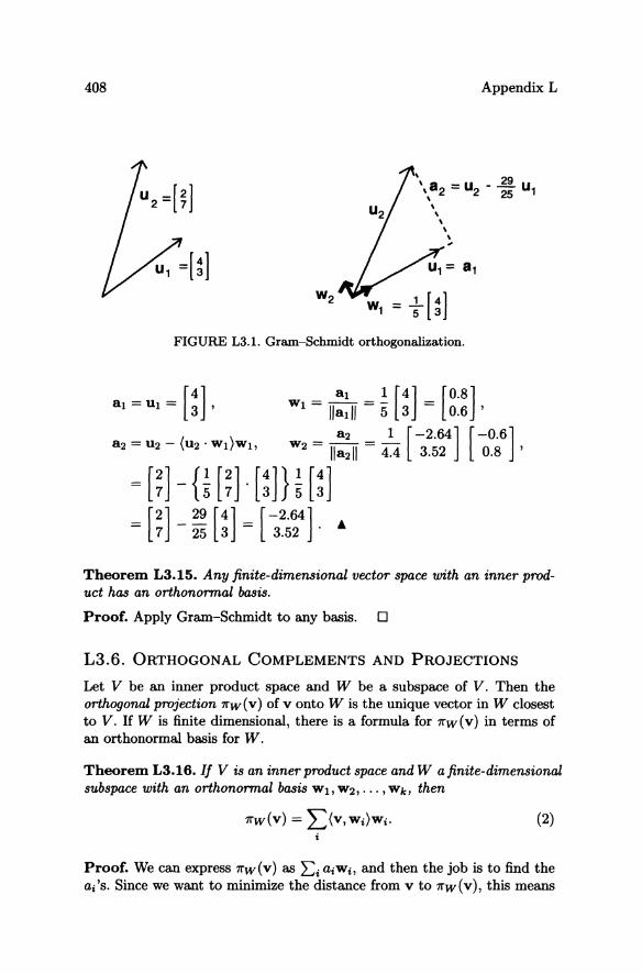
Example L3.14. Figure L3.1 shows the Gram-Schmidt algorithm in action in 1R2 .

408 Appendix L

'a-u 29 U '2- 2-25 1 , , , , ,

W1 = t[~]

, ,

FIGURE L3.1. Gram-Schmidt orthogonalization.

al 1 [4] [0.8] WI = IIal II = 5 3 = 0.6 '

a2 1 [-2.64] [-0.6] W2 = lIa211 = 4.4 3.52 0.8'

= [~] - {~[~]. [~]} ~ [~] [2] 29 [4] [-2.64]

= 7 - 25 3 = 3.52 . A

Theorem L3.15. Any finite-dimensional vector space with an inner prod­uct has an orthonormal basis.

Proof. Apply Gram-Schmidt to any basis. 0

L3.6. ORTHOGONAL COMPLEMENTS AND PROJECTIONS

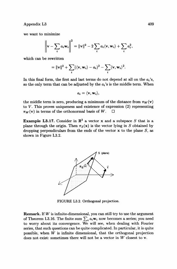
Let V be an inner product space and W be a subspace of V. Then the orthogonal projection 1i"w(v) ofv onto W is the unique vector in W closest to V. If W is finite dimensional, there is a formula for 1i"w (v) in terms of an orthonormal basis for W.

Theorem L3.16. If V is an inner product space and W a finite-dimensional subspace with an orthonormal basis W17 W2, ••. , Wk, then

(2)

Proof. We can express 1i"w(v) as Ei aiwi, and then the job is to find the ai's. Since we want to minimize the distance from v to 1i"w(v), this means

Appendix L3 409

we want to minimize

which can be rewritten

= IIvll2 + ~) (v, Wi) - ai)2 - L (v, Wi)2.

i i

In this final form, the first and last terms do not depend at all on the ai's, so the only term that can be adjusted by the ai's is the middle term. When

the middle term is zero, producing a minimum of the distance from 7rw{v) to V. This proves uniqueness and existence of expression (2) representing 7rw (v) in terms of the orthonormal basis of W. 0

Example L3.I7. Consider in 1R3 a vector x and a subspace S that is a plane through the origin. Then 7rs{x) is the vector lying in S obtained by dropping perpendiculars from the ends of the vector x to the plane S, as shown in Figure L3.2.

FIGURE L3.2. Orthogonal projection.

Remark. If W is infinite-dimensional, you can still try to use the argument of Theorem L3.16. The finite sum Li aiWi now becomes a series; you need to worry about its convergence. We will see, when dealing with Fourier series, that such questions can be quite complicated. In particular, it is quite possible, when W is infinite dimensional, that the orthogonal projection does not exist: sometimes there will not be a vector in W closest to v.

410 Appendix L

There is now one more term to define: The orthogonal complement of W is the subspace

W.L = {v E V I (v, w) = 0 for all w E W}.

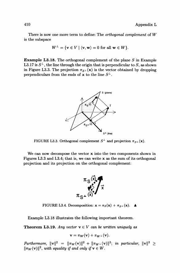
Example L3.18. The orthogonal complement of the plane S in Example L3.17 is S.l., the line through the origin that is perpendicular to S, as shown in Figure L3.3. The projection 7rs.!. (x) is the vector obtained by dropping perpendiculars from the ends of x to the line S.L.

FIGURE L3.3. Orthogonal complement S.!. and projection 7rs.!. (x).

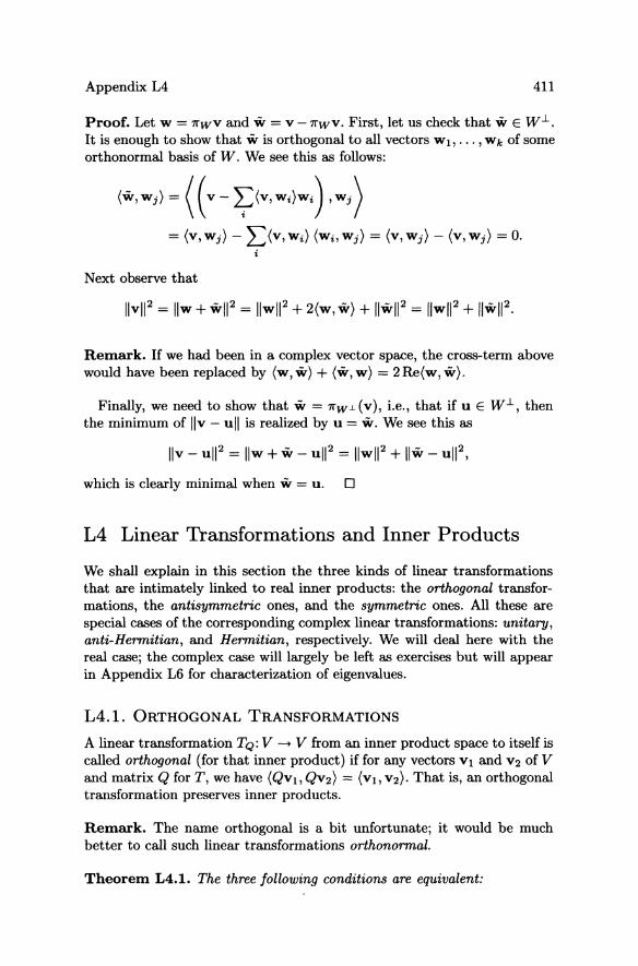
We can now decompose the vector x into the two components shown in Figures L3.3 and L3.4j that is, we can write x as the sum of its orthogonal projection and its projection on the orthogonal complement:

FIGURE L3.4. Decomposition: x = 7rs(x) + 7rs.!.(x). ..

Example L3.18 illustrates the following important theorem.

Theorem L3.19. Any vector v E V can be written uniquely as

v = 7rw{v) + 7rw.!.{v).

Furthermore, IIvll2 = l17rw(v)1I2 + l17rw.!.(v)1I2j in particular, IIvll2 > l17rw{v)1I2, with equality if and only if v E W.

Appendix L4 411

Proof. Let W = ll'WV and w = V-ll'WV. First, let us check that wE W.L. It is enough to show that w is orthogonal to all vectors WI, ••• , Wk of some orthonormal basis of W. We see this as follows:

= (v, wi) - I)v, Wi) (Wi, Wi) = (v, wi) - (v, wi) = O. i

Next observe that

Remark. If we had been in a complex vector space, the cross-term above would have been replaced by (w, w) + (w, w) = 2 Re{w, w).

Finally, we need to show that w = ll'w.L(v), i.e., that if u E W.L, then the minimum of IIv - ull is realized by u = w. We see this as

which is clearly minimal when w = u. 0

L4 Linear Transformations and Inner Products

We shall explain in this section the three kinds of linear transformations that are intimately linked to real inner products: the orthogonal transfor­mations, the antisymmetric ones, and the symmetric ones. All these are special cases of the corresponding complex linear transformations: unitary, anti-Hermitian, and Hermitian, respectively. We will deal here with the real case; the complex case will largely be left as exercises but will appear in Appendix L6 for characterization of eigenvalues.

L4.1. ORTHOGONAL TRANSFORMATIONS

A linear transformation TQ: V - V from an inner product space to itself is called orthogonal (for that inner product) iffor any vectors VI and V2 of V and matrix Q for T, we have (QVI, QV2) = (VI, V2). That is, an orthogonal transformation preserves inner products.

Remark. The name orthogonal is a bit unfortunate; it would be much better to call such linear transformations orthonormal.

Theorem L4.1. The three following conditions are equivalent:

412 Appendix L

(1) A trons/ormation TQ: Rn --+ Rn is orthogonal/or the dot product.

(2) The column vectors 0/ the matrix Q 0/ an orthogonal linear trons/or­mation form an orthonormal basis.

(3) The inverse 0/ the matrix Q 0/ a linear trons/ormation is its trons-pose; i.e., QT = Q-l.

Proof. (1) implies (2) follows from the fact that the columns of WI, ... , Wn

of Q are the vectors TQ(ei); from the definition of an orthogonal transfor­mation, we see that

Wi' Wj = TQ(ei)' TQ(ej) = ei' ej.

The equivalence of (2) and (3) follows from the following computations: To see the equivalence, suppose that the columns of Q are WI..'" W n • Then writing QT Q = I, i.e.,

we see that the dot product of each column with itself is 1 (the normal part) and with another is 0 (the orthogonal part) because the Wi form an orthonormal basis.

Finally, (3) implies (1) is seen as follows: pick any vectors v, W ERn. Then, by the definition of dot product and Theorem Ll.17 about trans-poses,

TQ(v), TQ(w) = (Qv)T(Qw) = V T QT Qw = V· w,

because we are now back to the definition of orthogonal transformation. o

It follows immediately from the definition and Theorem L4.1 that the orthogonal trons/ormations form a group, denoted O(n). This means that the orthogonal transformations that compose the group must and do satisfy the following properties:

(i) the product of two orthogonal transformations is orthogonal (this was clear right from the definition);

(ii) an orthogonal transformation is invertible;

(iii) its inverse is orthogonal.

Appendix L4 413

Example L4.2. As we saw in Example L2.19, the orthogonal matrix giving rotation in JR.2 by angle 0 is

Q( 0) = [ cc:s 0 sin 0] . - smO cosO

You can confirm that the columns of Q(O) form an orthonormal basis. The inverse of Q(O) is rotation by -0, and since sin( -0) = - sin 0, we see that

(1)

the transpose, as it should. These are not the only elements of 0(2); the matrix

is also orthogonal; geometrically, it represents reflection with respect to the x-axis. More generally, the product

[COS 0 - sin 0] [1 0] [cos 0 sin 0] sinO cosO 0 -1 = sinO - cosO

is an element of 0(2), and in Exercise L3-4#16 you are asked to show that these and the matrices Q(O) are all elements of 0(2). A

There is a way of expressing the Gram-Schmidt orthogonalization pro­cess in terms of orthogonal matrices; this formulation will be used twice in the remainder of these notes, once in the section on determinants and once in the section on the QR method.

Theorem L4.3. Any matrix M can be written as the product M = QR, where Q is orthogonal and R is upper-triangular.

Proof. This is just a way of condensing the Gram-Schmidt process. Let the columns of M be UI,"" Un. First, we will assume that the Ui are linearly independent. Then we can apply Gram-Schmidt to them, and using the notation of Theorem L3.13 we see that all the Gram-Schmidt formulas can be condensed into the following matrix multiplication:

[IT U2 'WI U3 'WI

lIa211 U3 'W2

0

Un' WI] Un 'W2

II~II [WI ... W n ] [ UI U2

which is precisely what we need, since the matrix [WI,"" wnl is orthogonal (Theorem L4.1, part 2). 0

414 Appendix L

L4.2. ANTISYMMETRIC TRANSFORMATIONS

A linear transformation T from a vector space V to itself is called antisym­metric with respect to an inner product if for any vectors VI and V2 we have

(antisymmetric T).

The appropriate definition for the complex case is an anti-Hermitian transformation, which takes the complex conjugate of the right-hand side:

(anti-Hermitian T).

The reason why antisymmetry is an important property is that

A ntisymmetric linear transformations are infinitesimal orthog­onal transformations.

More precisely,

Theorem L4.4. Let Q(t) be a family of orthogonal matrices depending on the parameter t. Then Q-l(t)Q'(t) is antisymmetric.

Proof. Start with the definition of orthogonal matrices

and differentiate with respect to t to get

Since Q is orthogonal, we can apply Q-l to both terms in each inner product, so the equation can be rewritten

Theorem L4.4 will have the consequence that if T is antisymmetric with matrix A, then a solution x( t) of x' = Ax will have constant length; i.e., the vector x(t) will move on a sphere of constant radius. Such examples will occur and be of central importance in classical mechanics.

The reason for the word "antisymmetric" is the following.

Theorem L4.5. If V = IRn with the standard inner product, then a linear transformation is antisymmetric if and only if its matrix A is antisymmet­ric, that is, if AT = -A.

The proof is easy and left to the reader.

Appendix L4 415

L4.3. SYMMETRIC LINEAR TRANSFORMATIONS

A linear transformation T: V -+ V is symmetric with respect to an inner product if for any vectors Vl, v2 E V we have

(symmetric T).

The appropriate definition for the complex case is a Hermitian transfor­mation, which takes the complex conjugate of the right-hand side:

(Hermitian T).

Remark. Linear transformations symmetric with respect to an inner prod­uct are often called self-adjoint (and antisymmetric ones are called anti­self-adjoint) .

The matrix interpretation is as follows, and the easy proof is left to the reader:

Theorem L4.6. If V = lRn with the standard inner product, then a linear tmnsformation T: V -+ V is symmetric if and only if its matrix A is sym­metric, that is, if AT = A. Similarly, if V = en and T is Hermitian, then the matrix A ofT is Hermitian; i.e., it satisfies A = AT.

Orthogonal linear transformations are more or less obviously important. Antisymmetric and anti-Hermitian transformations are important because of their intimate relation with orthogonal and unitary transformations. Symmetric and Hermitian transformations are rather harder to motivate, even though they are studied far more frequently than the anti-Hermitian ones.

Remark. One might look for motivation in quantum mechanics, where Hermitian matrices show up constantly. For instance, finding the energy levels of atoms or molecules boils down to computing the eigenvalues of a Hermitian matrix. Actually, anti-Hermitian matrices are the ones impor­tant to quantum mechanics, and the presence of Hermitian matrices is due to the following trick: If H is a Hermitian matrix, then iH is anti-Hermitian.

Indeed, the basic equation of quantum mechanics is the Schrodinger equation

o'l/J h h dt = 27ri(~'l/J+ V'l/J) = 27ri H ('l/J),

where h is Planck's constant. As we will see in Example L4.7 for a one­dimensional case, the Laplace operator ~ (in that case, just the second derivative) is a symmetric operator, if appropriate boundary conditions are imposed, and so is the multiplication operator V. Thus, H is sym­metric, and it is usually H, the Hamiltonian opemtor, which is studied.

416 Appendix L

But a glance at the equation shows that the really fundamental operator is (h/27ri)H, which is anti-Hermitian. One consequence of the principle "anti-Hermitian operators are infinitesimal unitary operators" is that 111P112 is constant in time; physically, this just says that the probability of finding the system in some state is always 1.

Symmetric matrices show up in their own right when studying quadratic forms; in fact, they correspond precisely to quadratic forms. Our treatment will emphasize this relationship, which will be elaborated in Subsection L4.5 of this appendix and in Appendix L8.

There is not really much point in writing down finite-dimensional exam­ples of Theorem L4.6; they are simply given by symmetric matrices.

The next example is the real reason for Fourier series. It is a bit less straightforward but well worth poring over a bit.

Example L4. 7. Let V be the space of twice continuously differentiable functions on [0,7r] which vanish at ° and 7r, and W the space of continuous functions on [0,7r]. Both spaces are endowed with the inner product

(f, g) = 101< f(x)g(x)dx.

Consider the second derivative operator D2: V -+ W. We claim that D2 is symmetric.

Remark. The attentive reader may well complain: since V and W are different vector spaces, how can such an operator be symmetric? But V is a subspace of W, so the equation (D2 f, g) = (f, D2g) makes perfectly good sense.

The proof that this is so is an exercise in integration by parts:

(D2 f, g) = 101< J"(x)g(x)dx = [f'(x)g(x)]o -101< f'(x)g'(x)dx = (f, D2g).

The second equality is integration by parts; the third comes from the fact that the boundary term drops out since g(O) = g(7r) = 0, and only the integral, which is obviously symmetric in f and 9 (in the ordinary sense of the word), is left. A

Several more examples of a similar style are given in Exercise L3-4#17.

L4.4. THE INNER PRODUCTS ON Rn

We can finally come full circle and describe all inner products on IRn.

Theorem L4.8. Let ( , ) be an inner product on IRn, and let G be the symmetric matrix with entries

Appendix L4 417

Then the given inner product can be written in terms of the standard dot product as

(a, b) = a· Gb. (2)

Conversely, if G is a symmetric matrix and a· Ga =I- 0 for all a =I- 0, then (2) defines an inner product on ]Rn.

Remark. We shall see in Section L4.5 that the property a· Ga =I- 0 for all a =I- 0 makes G a "positive definite" or "negative definite" matrix.

Example L4.9. G = the identity matrix gives the standard inner product .

• But Theorem L4.8 holds true for an arbitrary inner product, not just the

standard one, as we show in the following:

Example L4.1O. In Example L3.1, (a, b) == 2a1b1 + 2a2b2 + a1b2 + a2b1 is

given by the matrix [i ~] because

(a, b) = [:~] . [i ~] [~~]. • Proof of Proposition L4.S. The first part follows from the fact that if you know an inner product on all pairs of basis vectors, then you know it on any pair of vectors by writing the vectors in terms of the basis and multiplying them out.

The second part, the converse, is easy to prove by referring to the sym­metric, linear, and positive definite properties listed for an inner product in Section L3.1j this is left to the reader. 0

L4.5. QUADRATIC FORMS

After linear functions, the next simplest to study are the quadratics, and they are important in any mathematician's vocabulary. We often want to know the character of a surface at a critical point, for instance.

Consider the function f(x) that describes the surface in ]Rn+1 for a vector x in ]Rn. Expanding about a critical point a by Taylor series gives

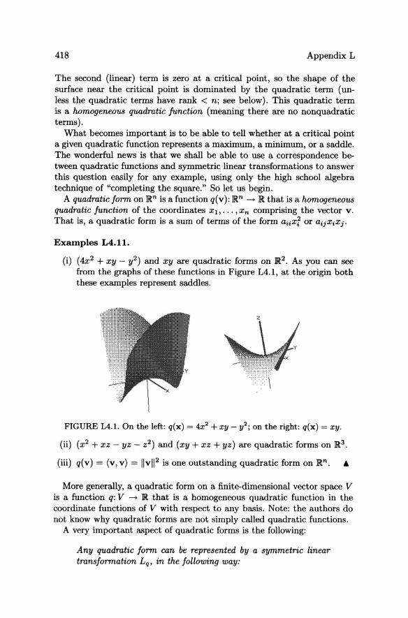
418 Appendix L

The second (linear) term is zero at a critical point, so the shape of the surface near the critical point is dominated by the quadratic term (un­less the quadratic terms have rank < n; see below). This quadratic term is a homogeneous quadratic function (meaning there are no nonquadratic terms).

What becomes important is to be able to tell whether at a critical point a given quadratic function represents a maximum, a minimum, or a saddle. The wonderful news is that we shall be able to use a correspondence be­tween quadratic functions and symmetric linear transformations to answer this question easily for any example, using only the high school algebra technique of "completing the square." So let us begin.

A quadratic form on]Rn is a function q(v):]Rn ---+ ]R that is a homogeneous quadratic function of the coordinates Xl,' .. ,Xn comprising the vector v. That is, a quadratic form is a sum of terms of the form aiix~ or aijXiXj'

Examples L4.11.

(i) (4X2 + xy - y2) and xy are quadratic forms on ]R2. As you can see from the graphs of these functions in Figure L4.1, at the origin both these examples represent saddles.

z

FIGURE L4.1. On the left: q(x) = 4x2 + xy - y2j on the right: q(x) = xy.

(ii) (X2 + xz - yz - Z2) and (xy + xz + yz) are quadratic forms on ]R3.

(iii) q(v) = (v, v) = IIvll 2 is one outstanding quadratic form on ]Rn. ~

More generally, a quadratic form on a finite-dimensional vector space V is a function q: V ---+ ]R that is a homogeneous quadratic function in the coordinate functions of V with respect to any basis. Note: the authors do not know why quadratic forms are not simply called quadratic functions.

A very important aspect of quadratic forms is the following:

Any quadratic form can be represented by a symmetric linear transformation Lq , in the following way:

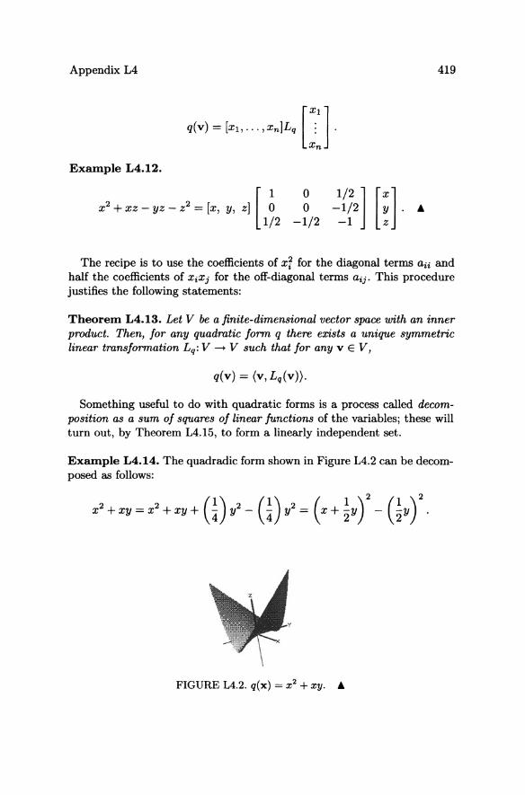
Appendix L4

.(v) ~ Ix" ,xnlL, [] .

Example L4.12.

X2 + xz - yz - z2 = [x, y, z] [ ~ 1/2

o o

-1/2

419

The recipe is to use the coefficients of x~ for the diagonal terms aii and half the coefficients of XiXj for the off-diagonal terms aij. This procedure justifies the following statements:

Theorem L4.13. Let V be a finite-dimensional vector space with an inner product. Then, for any quadratic form q there exists a unique symmetric linear transformation Lq : V -> V such that for any v E V,

q(v) = (v, Lq(v)).

Something useful to do with quadratic forms is a process called decom­position as a sum of squares of linear functions of the variables; these will turn out, by Theorem L4.15, to form a linearly independent set.

Example L4.14. The quadradic form shown in Figure L4.2 can be decom­posed as follows:

FIGURE L4.2. q(x) = x 2 + xy. •

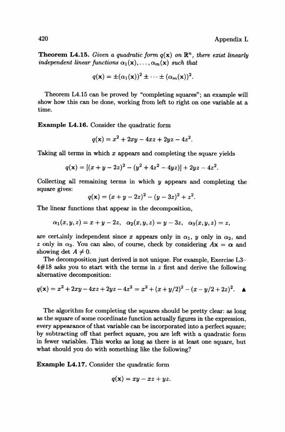
420 Appendix L

Theorem L4.15. Given a quadratic form q(x) on]Rn, there exist linearly independent linear functions 01 (x), ... , Om (x) such that

Theorem L4.15 can be proved by "completing squares"; an eXaIllple will show how this can be done, working from left to right on one variable at a time.

Example L4.16. Consider the quadratic form

q(x) = x 2 + 2xy - 4xz + 2yz - 4z2.

Taking all terms in which x appears and completing the square yields

q(x) = [(x + y - 2z)2 - (y2 + 4z2 - 4yz)] + 2yz - 4z2.

Collecting all remaining terms in which y appears and completing the square gives:

q(x) = (x + y - 2z)2 - (y - 3z)2 + z2.

The linear functions that appear in the decomposition,

01 (x, y, z) = x + y - 2z, 02(X, y, z) = y - 3z, 03(X, y, z) = z,

are cert.linly independent since x appears only in Ot, y only in 02, and z only in 03' You can also, of course, check by considering Ax = 0: and showing det A ¥- O.

The decomposition just derived is not unique. For eXaIllple, Exercise L3-4#18 asks you to start with the terms in z first and derive the following alternative decomposition:

q(x) = x 2 + 2xy - 4xz + 2yz - 4Z2 = x 2 + (x + y/2)2 - (x - y/2 + 2Z)2. A

The algorithm for completing the squares should be pretty clear: as long as the square of some coordinate function actually figures in the expression, every appearance of that variable can be incorporated into a perfect square; by subtracting off that perfect square, you are left with a quadratic form in fewer variables. This works as long as there is at least one square, but what should you do with something like the following?

Example L4.17. Consider the quadratic form

q(x) = xy - xz + yz.

Appendix L4 421

One possibility is to trade x for the new variable u = x - y, Le., x = u + y, to give

(u + y)y - uz = y2 + uy - uz

= (y + U/2)2 - u2 /4 - uz - z2 + Z2

= (y + U/2)2 - (u/2 + Z)2 + z2

= (x/2 + y/2)2 - (x/2 - y/2 + z)2 + z2.

There was not anything magical about the choice of Uj almost anything would have done.

We leave it as Exercise L3-4#20 to verify that the linear functions found in this way are indeed linearly independent. A

One more example elaborates on the crucial hypothesis of Theorem L4.15:

EXaIIlple L4.1S. Consider the quadratic form from Example L3.2:

q(x) = (x, x) = 2x~ + 2x~ + 2XIX2.

We can write

q(x) = 2x~ + 2x~ + 2XIX2 = (2x~ + 2XIX2 + xV2) + 2x~ - x~/2

= (V2Xl +x2/V2)2 + (y'372x2)2.

So the quadratic form shown in Figure L4.3 has been decomposed into the sum of two squared linear functions.

FIGURE L4.3. q(x) = 2x~ + 2x~ + 2XIX2.

But, how about writing q(x) = x~ +x~ + (Xl +X2)2, as we did in Example L3.2, with three squared linear functions? This alternative "decomposition"

422 Appendix L

does not reflect Theorem L4.15 because the three linear functions Xl, X2,

and Xl + X2 are not linearly independent. &

There are many ways of decomposing a quadratic form as a sum of lin­early independent squares. We will see in Theorem L4.19 that the number m of squares which appear does not depend on the decomposition.

In order to use decomposition of a quadratic form to identify the char­acter of a quadric surface, we must introduce a few more terms.

The number m of linearly independent squares in a representation as above is called the rank of the quadratic form; if m = n, then the form is called nondegenerate. The examples in this section are all nondegenerate; some degenerate cases are illustrated in Exercise L3-4#21.

If there are k plus signs appearing and f minus signs, then the form has signature (k, f); a form of signature (n, 0) is called positive definite, and one of signature (0, n) is called negative definite; the others are called indefinite. The symmetric matrices corresponding to the forms are also called positive or negative definite. Note: Without loss of generality we may assume that the first k have plus signs and the last f have minus signs.

According to these definitions, the form of Example L4.14 has signature (1,1) and rank 2; Examples L4.16 and L4.17 both have signature (2,1) and rank 3; Example L4.18 is positive definite with rank 2; all four examples are nondegenerate.

Now we are ready for the following:

Theorem L4.19. In any two representations of a quadratic form as the sums of squares of linearly independent linear functions

q(x) = 0::1 (x)2 + ... + O::k(x)2 - O::k+1 (x)2 - ... - O::k+l(x)2,

the number (k) of plus and the number (f) of minus signs appearing will be the same; i.e., the signature (k, f) is the same in every representation of a given quadratic form.

There will usually be many ways of representing a quadratic form as a sum of squares of linearly independent linear functions; why should the signs be independent of the representation? In the case of definite matrices, this is clear, as follows:

A quadratic form is positive (resp. negative) definite if and only if it takes positive (resp. negative) values on all nonzero vectors.

This second characterization of positive definiteness says nothing about any decomposition. Similarly, the following statement describes the signa­ture in a third way, also independently of any decomposition:

The numbers (k,f) of the signature are respectively the largest dimensions of the subspaces on which a quadratic form is posi­tive and negative definite.

Appendix L4 423

Proof of Theorem L4.19. Let us make vectors 0i from the coefficients of the variables in the Qi; e.g., for

Q1 = x+2y - z, Q2 = -x + z,

then 01 = (1,2, -I); 02 = (-1,0,1).

Next add to the k + i vectors formed this way 0i independent vectors Ok+l+ 1, ... ,an to make a basis for IRn.

If we now define the positive definite subspace

P = {x I Qk+1(X) = ... = Qn(X) = O},

then P is a k-dimensional subspace of vectors in IRn, by the dimension formula of Theorem L2.9. Likewise, we can define the negative definite subspace which has dimension i

omitting the i terms from k + 1 to k + i + 1. If We IRn is a subspace with dim(W) = k+ 1, then there must be x =I- 0

in W such that Q1(X) = ... = Qk(X) = 0,

again by the dimension formula. On such a vector the quadratic form must take a nonpositive value, so the form is not positive definite on W. This proves that the number k of positive Qi cannot change; likewise, we can show that the number i of negative Qi cannot change. A

Remark. The number n - m is not the dimension of a maximal subspace on which q vanishes. For instance, the form xy = ((x+y)/2)2 - ((x-y)/2)2 has signature (1,1) and is nondegenerate, but it vanishes on the x-axis and on the y-axis.

The following example shows the use of the quadratic form representation in terms of the Xi'S to determine whether a function has a maximum, minimum, or neither.

Example L4.20. Consider the function

f(x, y, z) = 3 + (x2 + 2xy - 4yz + 5z2) + terms of order three or higher.

This function has a critical point at (x, y, z) = (0,0,0) since af lax, af lay, and af laz are all zero there. We want to see whether it is a maximum, a minimum, or neither.

424 Appendix L

For small x, y, and z the quadratic terms are larger than the higher order terms, so we look at

x2 + 2xy - 4yz + 5z2 = (x + y? - (y + 2Z)2 + (3Z)2. ~ ____ '-v-'

Since the signature is (k, £) = (2, 1), I( x, y, z) has neither a maximum nor a minimum.

If you move away from (0,0,0) in a direction where y = -2z (Le., where a2 = 0), then the function will increase.

Try 1(0, -2, 1) > 3 = 1(0,0,0).

If you move away from (0,0,0) in a direction where x = -y and z = ° (Le., al = a3 = 0), then the function will decrease.

Try 1(1, -1,0) < 3 = 1(0,0,0).

This illustrates how the ai give you planar directions along which the func­tion increases (if the a is preceded by a +) or decreases (if the a is pre­ceded by a -). Different planes can be chosen (by the ai), but in every case, the number of linearly independent planes along which the function increases/decreases stays the same. A

L5 Determinants and Volumes

The determinant is a function of square matrices. It is given by various for­mulas, all of which are far too messy for hand computation once the matrix gets larger than 3 x 3. It can also be computed (much more reasonably) by row reduction. The determinant has a geometric interpretation as a signed volume, and this really makes it important.

In order not to favor anyone of the formulas and to obtain the volume interpretation most easily, we shall define the determinant by three prop­erties that characterize it. We will think of the determinant as a function of n vectors rather than as a function of a matrix; this is a minor point, since whenever you have n vectors in IRn , you can always place them side by side to make an n x n matrix.

L5.1. DEFINITION, EXISTENCE, AND UNIQUENESS OF

DETERMINANT FUNCTION

The determinant

detA = det [+ + ... , +] = det(a"8,, ... , .... )

Appendix L5 425

is the unique real-valued function of n vectors in R.n such that

(1) det A is linear with respect to each of its arguments, Le., (multilinearity)

det(aI, ... , Iii-I, (au + /3w), 8i+l, ... , an)

= a det( a1, ... , Iii-1, u, 1ii+1, ... , an)

+/3 det(a1, ... , Iii-l, w, Iii+I,· .. , an).

(2) det A is antisymmetric, Le., ( antisymmetry )

(3) det I of the identity is 1, Le., (scaling, or normalization)

det(el, e2,"" en) = 1, where ei is the ith standard unit basis vector.

In order to see that this definition of determinant is reasonable, we will want the following theorem:

Theorem L5.1. There indeed exists a function satisfying the three prop­erties of determinant, det A, and it is unique.

The proofs of these two parts are quite different, with a somewhat lengthy but necessary construction for each. The outline for the next several pages is as follows:

First, we shall use a computer program to construct a func­tion D(A) by a process called "development according to the first row." Of course, this could be developed differently, e.g., according to the first column, but you can show in Exercise L5#4 that the result is equivalent to this definition.

Then, we shall prove that D(A) satisfies the properties of det A, thus establishing existence of a function appropriate to the definition of determinant.

Finally, we shall proceed by "column operations" to evaluate this function D(A) and show that it is unique, which will prove uniqueness of the determinant function.

Development according to the first row. Consider the function

n

D(A) = L( -l)1+ial,idet Al,i, i=l

(1)

where Al,i is the (n - 1) x (n - 1) matrix obtained from A by erasing the first line and the ith column.

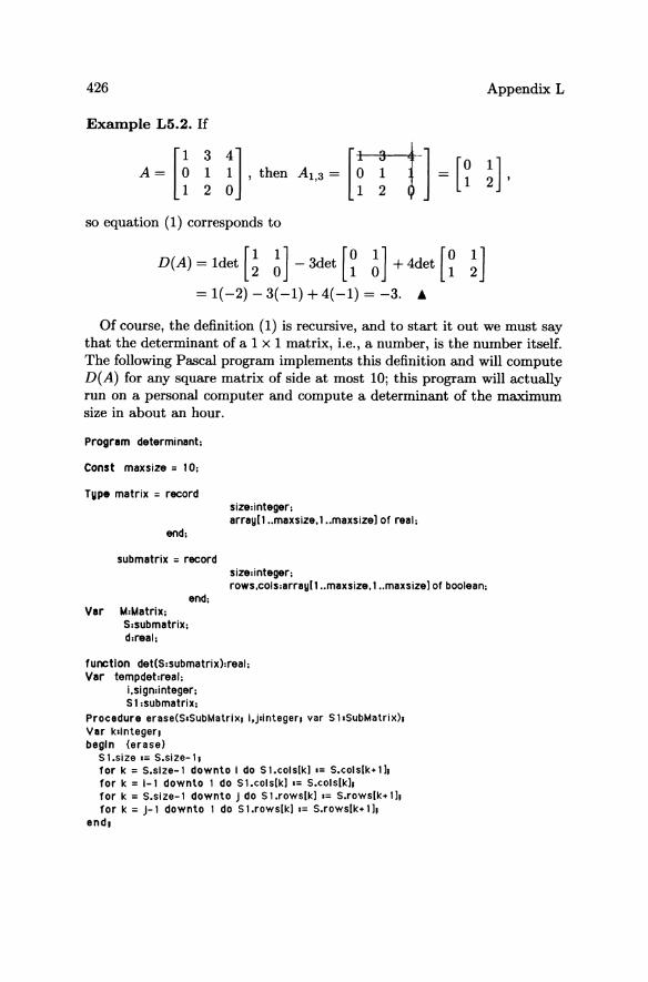
426 Appendix L

Example L5.2. If

[011 3~ 4~1 A = , then A 1,3 = [rTil so equation (1) corresponds to

D(A) = 1det [~ ~] - 3det [~ ~] + 4det [~ ~] =1(-2)-3(-1)+4(-1)=-3. ~

Of course, the definition (1) is recursive, and to start it out we must say that the determinant of a 1 x 1 matrix, Le., a number, is the number itself. The following Pascal program implements this definition and will compute D(A) for any square matrix of side at most 10; this program will actually run on a personal computer and compute a determinant of the maximum size in about an hour.

Program determinant;

Canst maxsize = 10;

Tupe matrix = record

end;

submatrix = record

Var M:Matrix; S:submatrix; d:real;

end;

size:integer; array[l .. maxsize.l .. maxsizel of real;

size:integer; rows.cols:array[l .. maxsize.l .. maxsizel of boolean;

function det(S:submatrix):real; Var tempdet:real;

i.sign:integer; 51 :submatrix;

Procedure erase(S,SubMatrix, I,jdnteger, liar SIISubMatrix), Var kllnteger, begin {erase)

5 l.slze 1= S.size-l, for k = S.slze-l downto I do S1.cols(k) 1= S.cols[k+ 1 h for k = 1-1 downto 1 do Sl.cols(k) 1= S.cols(k), for k = S.slze-l downto J do 5 1.rows(k) 1= S.rows[k+ 1 h for k = J-l downto 1 do Sl.rows[k) 1= S.rows(k+ 1 h

end,

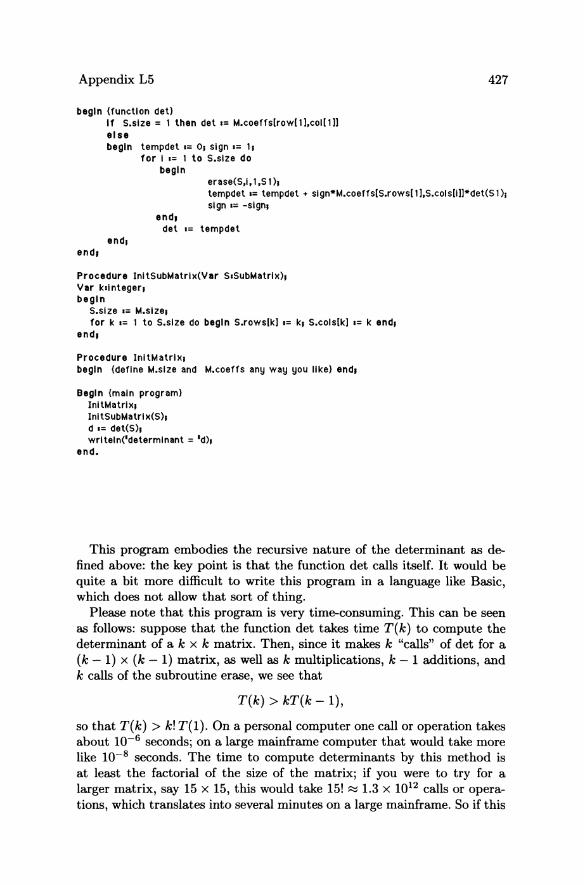
Appendix L5

begin (function deU If S.slze = 1 then det .= M.coeffs[row[ 11,coll1]] else begin tempdet.= 0, sign .= I,

for I .= 1 to S.slze do begin

erase(S,I, I,S 0,

427

tempdet .= tempdet .. slgn*M.coeffs[S.rows[ 1),S.colsllll*det(S I), sl gn .= -sl gn,

end, det .= tempdet

end,

Procedure InltSubMatrlx(Var S.SubMatrlx}, Var kll nteger, begin

S.slze .= M.slze, for k .= 1 to S.slze do begin S.rows[k) .= k, S.cols[k) .= k end,

end,

Procedure InltMatrlx, begin {define M.slze and M.coeffs any way you like} end,

eegln {main program} Inl tMatrl x, InltSubMatrl x(S}, d .= det(S}, wrlteln('determlnant = 'd},

end.

This program embodies the recursive nature of the determinant as de­fined above: the key point is that the function det calls itself. It would be quite a bit more difficult to write this program in a language like Basic, which does not allow that sort of thing.

Please note that this program is very time-consuming. This can be seen as follows: suppose that the function det takes time T(k) to compute the determinant of a k x k matrix. Then, since it makes k "calls" of det for a (k - 1) x (k - 1) matrix, as well as k multiplications, k - 1 additions, and k calls of the subroutine erase, we see that

T(k) > kT(k - 1),

so that T(k) > k!T(I). On a personal computer one call or operation takes about 10-6 seconds; on a large mainframe computer that would take more like 10-8 seconds. The time to compute determinants by this method is at least the factorial of the size of the matrix; if you were to try for a larger matrix, say 15 x 15, this would take 15! ~ 1.3 x 1012 calls or opera­tions, which translates into several minutes on a large mainframe. So if this

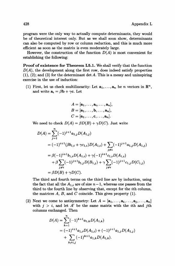
428 Appendix L

program were the only way to actually compute determinants, they would be of theoretical interest only. But as we shall soon show, determinants can also be computed by row or column reduction, and this is much more efficient as soon as the matrix is even moderately large.

However, the construction of the function D(A) is most convenient for establishing the following:

Proof of existence for Theorem LS.l. We shall verify that the function D(A), the development along the first row, does indeed satisfy properties (1), (2); and (3) for the determinant det A. This is a messy and uninspiring exercise in the use of induction:

(1) First, let us check multilinearity: Let a1, .. ' ,a.. be n vectors in lRn ,

and write Si = (3b + 'Yc. Let

A = [ab'" ,Si,··· ,a..j, B = [ab"" b, ... ,a..j, C = [a1,'" ,c, ... ,a..j.

We need to check D(A) = (3D(B) + 'YD(C). Just write n

D(A) = ~)-I)j+1a1,jD(A1,j) j=l

0+1 '"' 0+1 = (-1)' ((3b1,i + 'YC1,i)D(A1,i) + L) -I}' a1,jD(A1,j) #i

°+1 °+1 = (3( -I}' b1,iD(A1,i) + 'Y( -I)' C1,iD(A1,i)

+ (3 L( -1)j+1b1,jD(B1,j) + 'Y L( -1)j+1C1 ,jD(C1,j) #i #i

= (3D(B) + 'YD(C).

The third and fourth terms on the third line are by induction, using the fact that all the A 1 ,i are of size n -1, whereas one passes from the third to the fourth line by observing that, except for the ith column, the matrices A, B, and C coincide. This gives property (1).

(2) Next we come to antisymmetry: Let A = [ab"" Si, ... , aj," ., a..l with j > i, and let A' be the same matrix with the ith and jth columns exchanged. Then

n

D(A) = L(-I)k+1a1,kD(A1,k) k=l

°+1 °+1 = (-I)' a1,iD(A1,i) + (-I)' a1,jD(A1,j)

+ L (-I)k+1 a1 ,kD(A1,k). k#i,j

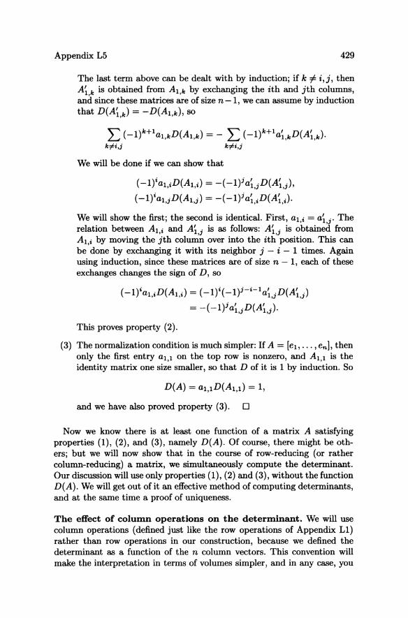
Appendix L5 429

The last term above can be dealt with by induction; if k 1= i,j, then ALk is obtained from Al,k by exchanging the ith and jth columns, and since these matrices are of size n-I, we can assume by induction that D{ALk) = -D{Al,k), so

L (-I)k+1 al,kD {Al ,k) = - L (-I)k+1a~,kD{A~,k)· ki-i,j ki-i,j

We will be done if we can show that

(-I)ial,iD{Al,i) = -(-l)ja~,jD{A~,j)'

(-I)ial,jD{Al,j) = -(-I)ja~,iD{A~,i)·

We will show the first; the second is identical. First, al,i = a~,j. The relation between Al,i and A~,j is as follows: A~,j is obtained from Al,i by moving the jth column over into the ith position. This can be done by exchanging it with its neighbor j - i-I times. Again using induction, since these matrices are of size n - 1, each of these exchanges changes the sign of D, so

(-l)ial ,iD {Al ,i) = (_I)i{ -l)j-i-la~,jD{A~,j)

= -(-l)ja~,jD{A~,j).

This proves property (2).

(3) The normalization condition is much simpler: If A = [eb ... ,en], then only the first entry al,l on the top row is nonzero, and Al,l is the identity matrix one size smaller, so that D of it is 1 by induction. So

D{A) = al,lD{Al,l) = 1,

and we have also proved property (3). 0

Now we know there is at least one function of a matrix A satisfying properties (I), (2), and (3), namely D{A). Of course, there might be oth­ers; but we will now show that in the course of row-reducing (or rather column-reducing) a matrix, we simultaneously compute the determinant. Our discussion will use only properties (I), (2) and (3), without the function D{A). We will get out of it an effective method of computing determinants, and at the same time a proof of uniqueness.

The effect of column operations on the determinant. We will use column operations (defined just like the row operations of Appendix L1) rather than row operations in our construction, because we defined the determinant as a function of the n column vectors. This convention will make the interpretation in terms of volumes simpler, and in any case, you

430 Appendix L

will be able to show in Exercise L5#4 that row operations could have been used just as well.

Let us check how each of the three column operations affects the determi­nant. It turns out that each multiplies the determinant by an appropriate factor fJ-:

(a) Multiply a column through by a number m. Clearly, by property (1), this will have the effect of multiplying the determinant by the same number, so

fJ-=m.

(b) Exchange two columns. By property (2), this changes the sign of the determinant, so

fJ- =-1.

(c) Add a multiple of one column onto another. By property (1), this does not change the determinant, because

det(al,.··, aj, ... , aj + /3a;, ... , a..) = det(al, ... ,a;, ... ,aj, ... ,a..)

+ /3det(at, ... , a;, ... , a;, ... , s.n)

and the last term is zero (since two columns are equal, so exchanging them both changes the sign of the determinant and leaves it un­changed). Therefore,

fJ-=1.

Now any square matrix can be column-reduced until, at the end, you either get the identity or you get a matrix with a column of zeroes (by a corollary of Theorem L1.13). A sequence of matrices resulting from column operations can be denoted as follows, with the multipliers fJ-i atop arrows for each operation:

1-'2 ~ A 1-'3 I-'n-l A

2 ~ ••. ~ n-l

Then, working backward by property (1),

detAn _ 1 = (:n) detAn, det A n- 2 = ( 1 ) det An,

/-Ln-lfJ-n

!

I-'n ~

det A = det An. ( 1) fJ-lfJ-2 ... fJ-n-lfJ-n

(2a)

(2b)

(2c)

Appendix L5

Therefore, from equation (2c),

if An = I, det An = 1 by property (3)

1 detA = ;

J1.1J1.2 ... J1.n-lJ1.n

if An =I- I, det An = 0 by property (1)

detA = O.

431

(3)

(4)

Proof of uniqueness of determinant. Suppose that the function Dl (A) obeys properties (1), (2), and (3). Then for any matrix A,

Dl (A) = ( 1 ) det(An) = D(A); J1.1J1.2··· J1.n

i.e., Dl = D. You may object that a different sequence of row operations might lead to a different sequence of J1.i'S. If that were the case, it would show that the axioms for the determinant were inconsistent; we know they are consistent because of Theorem L5.1.

We have finally finished proving Theorem L5.1. 0

L5.2. THEOREMS RELATING MATRICES AND

DETERMINANTS

There are some matrices whose determinant is easy to compute: the trian­gular matrices, both upper and lower.

Theorem L5.3. If a matrix is triangular, then its determinant is the prod­uct of the entries along the diagonal.

Proof. Suppose the matrix is upper-triangular. If the entries along the diagonal are nonzero, then by adding multiples of the first columns to the others, the first row can be cleared beyond the diagonal, then adding multiples of the second to the third and later columns, the second row can be cleared, etc. We are left (Exercise L5#2) with a diagonal matrix with the same diagonal entries as the original matrix; such a matrix can be turned into the identity by dividing each column through by its entry on the diagonal.

If any of the diagonal entries are zero, then the same clearing operation as above, carried out until you come to such a column, leaves a matrix with a column of zeroes and, hence, has determinant 0 (like the product of the diagonal entries).

If the original matrix had been lower-triangular, the same argument would work, only starting with the last column, and first clearing the bot­tom row. 0

432 Appendix L

Remark. It is fairly easy to prove Theorem L5.3 from the recursive defi­nition of D, at least if the matrix is lower-triangular. Exercise L5#3 asks you to do so and to adapt the proof to the upper-triangular case.

Appendix L2.5 gives several characterizations of invertible matrices; here are some more:

Theorem L5.4. A matrix A is invertible if and only if its determinant is not zero.

Proof. This follows immediately from the column-reduction algorithm and the uniqueness proof, since along the way we showed, in equations (3) and (4), that a matrix has a nonzero determinant if and only if it can be column­reduced to the identity. (See Section L1.4.) 0

A key property of the determinant, for which we will see a geometric interpretation later, is

Theorem L5.5. If A and B are n x n matrices, then

det(A) det(B) = det(AB).

Proof. If A is invertible, consider the function det(AB)/det(A), as a func­tion of the matrix B. As the reader will easily check, it has properties (1), (2), and (3), which characterize the determinant function. If A is not in­vertible, the left-hand side of the theorem is zero; the right-hand side must be zero also, because

Image(AB) C Image(A).

Therefore, dimImage(AB) ~ dimImage(A) < n, so AB is not invertible either. 0

Theorem L5.6. If a matrix A is invertible, then detA- 1 = l/detA.

Proof. This is a simple consequence of Theorem L5.5. 0

Theorem L5. 7. The determinant function is basis independent, that is,

det A = det(p- 1 AP).

Again this follows immediately from Theorem L5.5. 0

These facts will be very important in Appendix L6 on eigenvalues and eigenvectors, as will be the next theorem and the next section.

Theorem L5.8. If A is an n x n matrix and B is an m x m matrix, then for the (n + m) x (n + m) matrix formed with these as diagonal elements,

Appendix L5

det [ :I~] = det A det B.

The proof of Theorem L5.8 is left to the reader.

L5.3. THE CHARACTERISTIC POLYNOMIAL OF A MATRIX

AND ITS COEFFICIENTS

433

The characteristic polynomial of a square n x n matrix A is the polynomial det(AI - A). Such A's will playa crucial role in the next Appendix, L6.

Example L5.9. Computing characteristic polynomials is usually just a grind:

is

The characteristic polynomial of

[A+ 1

det ~ o

A-I 1

[-1 0 -2 1 o -1 -~l -1

-;1 1 = (A + 1)2(A - 1) - 2 - 2(A + 1) A+l

= A3 + A2 - 3A - 5. &

Remark. You may encounter elsewhere the definition of the characteristic polynomial as det(A-AI), but you will still get essentially the same results. These expressions match exactly if n is even, and are of opposite sign if n is odd.

The characteristic polynomial is an important application of the deter­minant, which will really come into its own when we deal with eigenvectors and eigenvalues. However, in this section, we want to define and prove some of the properties of the trace, another important function of a matrix, and finding the characteristic polynomial is an easy way of going about it.

Until now, we have behaved as if all the matrices we had were matrices of numbers. But AI - A is a matrix of polynomials; does our theory of determinants still apply? Certainly, the development according to the first row defined in Section L5.1 makes perfectly good sense even for a matrix of polynomials. Actually, the entire development works for matrices whose entries are any rational function. The only thing we use in row-reduction is the ability to do arithmetic, i.e., to add, subtract, multiply, and divide by everything except 0, and these operations do hold for rational functions.

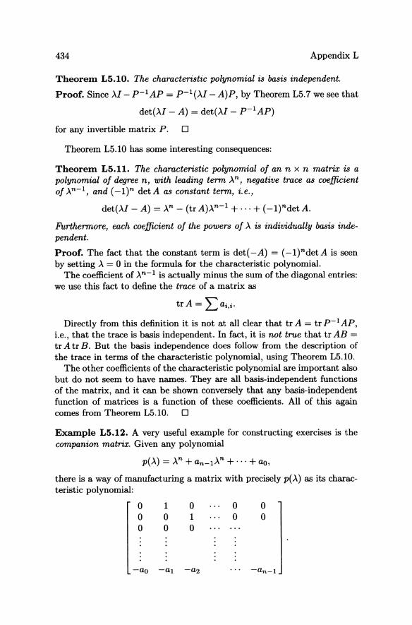
434 Appendix L

Theorem L5.10. The characteristic polynomial is basis independent.

Proof. Since M - p- l AP = P-l(M - A)P, by Theorem L5.7 we see that

det(M - A) = det(M - p- l AP)

for any invertible matrix P. 0

Theorem L5.1O has some interesting consequences:

Theorem L5.11. The characteristic polynomial of an n x n matrix is a polynomial of degree n, with leading term >.n, negative trace as coefficient of >.n-l, and (-l)n detA as constant term, i.e.,

det(M - A) = >.n - (tr A)>.n-l + ... + (-ltdet A.

FUrthermore, each coefficient of the powers of >. is individually basis inde­pendent.

Proof. The fact that the constant term is det ( - A) = (-1) ndet A is seen by setting>. = 0 in the formula for the characteristic polynomial.

The coefficient of >. n-l is actually minus the sum of the diagonal entries: we use this fact to define the trace of a matrix as

tr A = Lai,i.

Directly from this definition it is not at all clear that tr A = tr p- l AP, i.e., that the trace is basis independent. In fact, it is not true that tr AB = tr A tr B. But the basis independence does follow from the description of the trace in terms of the characteristic polynomial, using Theorem L5.1O.

The other coefficients of the characteristic polynomial are important also but do not seem to have names. They are all basis-independent functions of the matrix, and it can be shown conversely that any basis-independent function of matrices is a function of these coefficients. All of this again comes from Theorem L5.1O. 0

Example L5.12. A very useful example for constructing exercises is the companion matrix. Given any polynomial

p(>.) = >.n + an_l>.n + ... + ao,

there is a way of manufacturing a matrix with precisely p(>.) as its charac­teristic polynomial:

o o o

1 o o

o 1 o

o o

o o

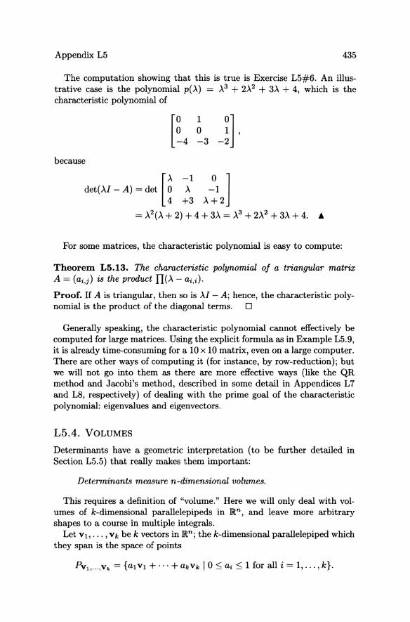
Appendix L5 435

The computation showing that this is true is Exercise L5#6. An illus­trative case is the polynomial p( A) = A 3 + 2A 2 + 3A + 4, which is the characteristic polynomial of

[0 1 0] o 0 1, -4 -3 -2

because

det(M - A) = det [~~1 ~1] 4 +3 A+2

= A2(A + 2) + 4 + 3A = A3 + 2A2 + 3A + 4. •

For some matrices, the characteristic polynomial is easy to compute:

Theorem L5.13. The characteristic polynomial of a triangular matrix A = (ai,j) is the product n(A - ai,i)'

Proof. If A is triangular, then so is AI - A; hence, the characteristic poly­nomial is the product of the diagonal terms. 0

Generally speaking, the characteristic polynomial cannot effectively be computed for large matrices. Using the explicit formula as in Example L5.9, it is already time-consuming for a 10 x 10 matrix, even on a large computer. There are other ways of computing it (for instance, by row-reduction); but we will not go into them as there are more effective ways (like the QR method and Jacobi's method, described in some detail in Appendices L7 and LB, respectively) of dealing with the prime goal of the characteristic polynomial: eigenvalues and eigenvectors.

L5.4. VOLUMES

Determinants have a geometric interpretation (to be further detailed in Section L5.5) that really makes them important:

Determinants measure n-dimensional volumes.

This requires a definition of "volume." Here we will only deal with vol­umes of k-dimensional parallelepipeds in JRn, and leave more arbitrary shapes to a course in multiple integrals.

Let Vb"" vk be k vectors in JRn; the k-dimensional parallelepiped which they span is the space of points

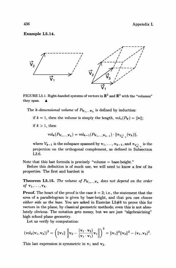
436 Appendix L

Example L5.14.

------------7

I I

I

I

I I

I

FIGURE L5.1. Right-handed systems of vectors in lR? and lR.3 with the "volumes" they span. •

The k-dimensional volume of PV1 ""Vk is defined by induction:

if k = 1, then the volume is simply the length, voh (Pv ) = IIvll;

if k > 1, then

where Vk-I is the subspace spanned by VI,"" vk-I, and 7rv:-L is the k-l

projection on the orthogonal complement, as defined in Subsection L3.6.

Note that this last formula is precisely "volume = base· height." Before this definition is of much use, we will need to know a few of its

properties. The first and hardest is

Theorem L5.15. The volume of pv" ... ,Vk does not depend on the order ofvl, ... ,vk.

Proof. The heart of the proof is the case k = 2; i.e., the statement that the area of a parallelogram is given by base·height, and that you can choose either side as the base. You are asked in Exercise L5#8 to prove this for vectors in the plane, by classical geometric methods; even this is not abso­lutely obvious. The notation gets messy, but we are just "algebraicizing" high school plane geometry.

Let us verify by computation:

This last expression is symmetric in VI and V2.

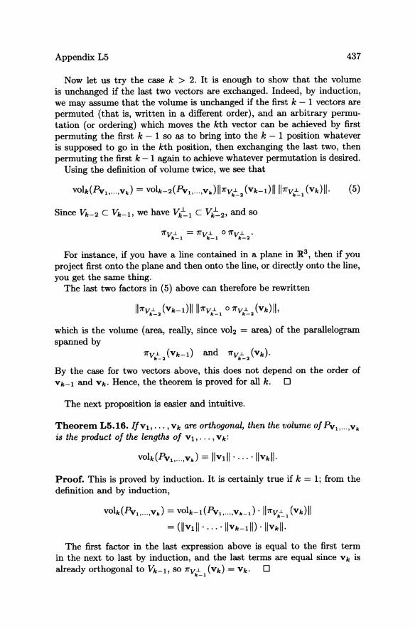
Appendix L5 437

Now let us try the case k > 2. It is enough to show that the volume is unchanged if the last two vectors are exchanged. Indeed, by induction, we may assume that the volume is unchanged if the first k - 1 vectors are permuted (that is, written in a different order), and an arbitrary permu­tation (or ordering) which moves the kth vector can be achieved by first permuting the first k - 1 so as to bring into the k - 1 position whatever is supposed to go in the kth position, then exchanging the last two, then permuting the first k - 1 again to achieve whatever permutation is desired.

Using the definition of volume twice, we see that

For instance, if you have a line contained in a plane in ]R3, then if you project first onto the plane and then onto the line, or directly onto the line, you get the same thing.

The last two factors in (5) above can therefore be rewritten

which is the volume (area, really, since voh = area) of the parallelogram spanned by

By the case for two vectors above, this does not depend on the order of Vk-l and Vk. Hence, the theorem is proved for all k. 0

The next proposition is easier and intuitive.

Theorem L5.16. [fvb ... ,Vk are orthogonal, then the volume of PV"""Vk is the product of the lengths of Vb ... ,Vk:

Proof. This is proved by induction. It is certainly true if k = 1; from the definition and by induction,

VOlk(PV" ... ,Vk) = VOlk-l(PV" ... ,vk_J ·llll'y.L (vk)11 k-l

= (1Ivlll···· ·llvk-I!D ·llvkll·

The first factor in the last expression above is equal to the first term in the next to last by induction, and the last terms are equal since Vk is already orthogonal to Vk-l, so ll'y.L (Vk) = Vk. 0

k-l

438 Appendix L

One more intuitively desirable property of volumes:

Theorem L5.17. If Q is an orthogonal matrix, then the image under Q of a parallelepiped has the same volume as the original parallelepiped:

Proof. Again, this is proved by induction on k. For k = 1, it is immedi­ate since orthogonal transformations preserve length. By the definition of volume,

and we may assume by induction that

VOlk-l (PV1 , ... ,Vk-l) = VOlk_l (PQ(Vl), ... ,Q(Vk-d)j

the proposition will follow if we know Q(1rVk-:'l (Vk)) = '7rQ(Vk_d.L(Q(Vk)).

This formula should be clear. 0

L5.5. THE RELATION BETWEEN DETERMINANTS AND

VOLUMES

Theorem L5.18. The determinant measures volume, in the sense that its absolute value

Idet[al, ... , an] 1 = vol(Palo ... ,a,,).

Proof. Let us see how Idetl is affected by column operations.

(i) Multiplying a column through by I-' multiplies Idetl by 11-'1.

(ii) Exchanging two columns leaves Idetl unchanged.

(iii) Adding a multiple of one column onto another leaves Idetl unchanged.

Moreover,

(iv) Idet(I)/ = 1, Idet(A)/ = 0 if a column of A is 0,

and exactly as in Section L5.1, these four properties characterize Idetl, since any matrix can be column-reduced.

However, these four properties are also true of the function that takes a matrix and gives the volume of the parallelepiped spanned by the column vectors.

Appendix L5 439

Property (i) is clear, from the definition of volume, if the vector chosen is the last and is therefore true for any column by Theorem L5.15. Property (ii) is Theorem L5.15. Finally, Property (iii) is clear if the column being added to is the last, since if w is obtained by adding an arbitrary linear combination of VI, ... ,Vk-l to Vk, then 7rv.L w = 7rv.L (Vk). That is, (iii)

k-l k-l

is true of any column by (ii). As for (iv), the first part follows from the definition of volume, and the second part is obvious if the column is the last, hence once more is true for any column by (ii). 0

Corollary L5.19. The determinant of an orthogonal matrix is ±1.

Proof. The columns of an orthogonal matrix form an orthnormal basis, so the parallelepiped which they span has volume 1, by either Theorem L5.15 or Theorem L5.17. 0

We are finally in a position to prove the following result. It is surprising how hard it is to prove; we will be using just about everything developed up to now.

Theorem L5.20. For any n x n matrix A, we have det(A) = det(AT ).

Proof. By Theorem L4.3, any matrix can be written A = QR with Q orthogonal and R upper-triangular. Thus, AT = RTQT and det(AT ) = det(RT)det(QT). By Theorem L5.3, det(RT ) = det(R), since both are the product of their diagonal entries. Moreover, det(QT) = det(Q), since they are both of absolute value 1 and their product is 1. 0

One important consequence of Theorem L5.20 is that throughout this text, whenever we were speaking of column operations, we could just as well have spoken of row operations.

Now for the promised geometric explanation of Theorem L5.5,that

det(AB) = det(A)det(B).

As we have just seen, det(A) is the volume of the image under A of the unit cube, i.e., the image of the parallelepiped spanned by el, ... , en, which, of course, has volume 1. Actually, for any "body" X in IRn , det(A) measures the ratio of the volume of the image A(X) to the volume of X; that is, det(A) measures the expansion factor on volumes.

This fact can be heuristically seen as follows: Fill X up with little disjoint cubes whose faces are aligned with the coordinate axes; it seems reasonable to define the volume of X to be the maximum of the sum of the volumes of such little cubes. Then the images of these little cubes under A will fill up A(X), but the volume of each of the image cubes is precisely the volume of the original little cube multiplied by Idet(A)I.

440 Appendix L

Now it should be clear that Idet(AB)1 = Idet(A)det(B)I, since under AB the unit cube is first taken to B(unit cube) with volume Idet(B)I, and then to A(B(unit cube», with volume Idet(A)1 Idet(B)I.

In particular, if A is not invertible, then the column vectors are linearly dependent, and hence A squashes the unit cube down onto a space of lower dimension, by making one or more sides the zero vector. Of course, the volume of the image of the unit cube is then zero.

Signed volumes. As anybody who has integrated functions knows, the area under the curve has to be taken negative when the curve is beneath the x-axis. In integration theory, it is usually much easier to deal with signed areas, volumes, etc., than with unsigned ones. The first step in doing this in n dimensions is the following definition:

The signed volume of the parallelepiped P A spanned by the column vec­tors of A is given by det A.

Of course, the signed volume does depend on the order of the spanning vectors. The meaning of signed volume is best explained by the following two examples.

Example LS.21. In 1R2, two vectors 81 and 82 in that order span a par­allelogram of positive area if and only if the smallest angle from 81 to 82

is counterclockwise, as shown in Example L5.14. A

Example LS.22. In 1R3 , three vectors 8}, 82, and Sa in that order span a parallelepiped of positive signed volume if and only if they form a right­handed coordinate system, as shown in Example L5.14. A

L6 Eigenvalues and Eigenvectors

L6.1. EIGENVALUES AND EIGENVECTORS

Let V be a complex vector space and T: V -+ V be a linear transformation with matrix A. IT for some number A E C and some vector v E V, v =f 0,

AV=AV,

then the number A is called an eigenvalue of A, and every nonzero vector v for which Av = AV is called a corresponding eigenvector of A.

Note that eigenvectors corresponding to a given eigenvalue are never unique: nonzero multiples of an eigenvector are eigenvectors. Note also that the zero vector is never, by definition, an eigenvector. However, nothing prevents zero from being an eigenvalue; in fact, the eigenvectors for the eigenvalue 0 form the kernel of A, and 0 is an eigenvalue if and only if ker A =f {O}.

Appendix L6 441

Example L6.1. If A = [~ -~], the number -i is an eigenvalue and

v = [~] is a corresponding eigenvector of A, since

The next example is the real reason for Fourier series. It is a bit less straightforward but well worth poring over a bit.

Example L6.2. Recalling Example L4.7, let V be the space of infinitely differentiable functions on [0,71"] which vanish at 0 and at 71". Consider the second derivative operator D2: V -+ V. We will describe the eigenvectors (often called eigenfunctions, since they live in a function space) of D2.

The functions !k (x) = sin kx are eigenvectors of D2, with eigen­value -k2 •

This is nothing more or less than the fact that d2 / dx2 (sin kx) = - k2 sin kx, which everyone learned in elementary calculus. &

L6.2. EIGENVALUES AND THE CHARACTERISTIC

POLYNOMIAL

From a theoretical point of view, the characteristic polynomial is the main actor in the theory of eigenvectors and eigenvalues, at least in finite-dimen­sional vector spaces.

Theorem L6.3. The eigenvalues of a square matrix A are the roots of its characteristic polynomial.

Proof. From Appendix L2.5 and Theorem L5.4, we can state (Exercise L6#1) that the following four conditions are equivalent:

(a) A has no inverse.

(b) There exists a vector x =I- 0 such that Ax = o.

(c) There exists a vector y that cannot be written as Ax.

(d) detA = o.

By part (b) of these conditions for noninvertibility, det(>.I - A) = 0 if and only if there exists v =I- 0 with (>.1 - A)v = 0, i.e., Av = >.v. D

Theorem L6.3 has many corollaries:

442 Appendix L

Corollary L6.4. An n x n matrix has at most n eigenvalues, and at least one.

Proof. The first part is immediate from Theorem L6.3; the second part is the fundamental theorem of algebra (see below). D

The fundamental theorem of algebra is the following statement:

Every polynomial of degree > 0 with complex coefficients has at least one complex root.

This theorem is what guarantees that an nth degree polynomial equation Pn(x) = 0 has n roots, although some of them may coincide. Naming the root promised as rI, you divide the polynomial Pn by (x - rl) and reapply the theorem to the resulting new polynomial of degree n - 1. As you might guess from the name, the fundamental theorem of algebra is an important theorem. It is also hard to prove, and, more seriously, the proofs tend not to be constructive: they do not give an algorithm for finding the root. We need the statement now in this section and not before, because the subject of eigenvectors and eigenvalues is the first time we must solve polynomial equations, which are not linear; nonlinear equations cannot be treated us­ing row reduction or anything else which uses only arithmetic (addition, subtraction, multiplication, division).

Corollary L6.5. The trace of a matrix is the sum of the eigenvalues and the determinant is their product, each one being taken with its multiplicity.

Proof. This follows directly from Theorem L5.11. D

Remark. It is perfectly common for real polynomials to have complex roots, so there is no reason to expect that real matrices will have real eigenvalues. If the eigenvalues of a real matrix are complex, then so are the corresponding eigenvectors, and the vector space we are dealing with is en rather than ]Rn. Furthermore, we see that an n x n matrix has at most n distinct eigenvalues, and "in general" will have exactly that many, since a polynomial will "in general" have distinct roots.

[0 -1] Example L6.6. If A = 1 0' then the eigenvalues are the roots of

det [_~ ~], or >,2 + 1, so the eigenvalues are ±i. Since

we can write the following system of linear equations:

>'x + y = 0,

-x + >,y = 0,

Appendix L6 443

which is linearly dependent. The eigenvectors are the solutions to this sys­tem, but they are determined only up to a multiplicative constant. Solving the system for each value of A, we find that

[x] [1].. . h· val . VI = Y = -i IS an eIgenvector WIt elgen ue Zj

V2 = [:] = [:] is an eigenvector with eigenvalue -i. •

We need one more theorem to complete the general theory:

Theorem L6.7. If A is a square matrix and VI, ... , vm are eigenvectors with distinct eigenvalues, then Vb ... , Vm are linearly independent.

Proof. This result is a good deal harder to prove than the earlier results. We shall do it by contradiction. If Vb ... , Vm are not linearly independent, then there is a first vector Vj which is a linear combination of the earlier linearly independent ones. Thus, we can write

where at least one of the ai is different from zero. Apply AjI - A to both sides to get

Since the A'S are all different, the coefficients ai (Ai - Aj) cannot all be zero. Move the ith such term to the other side of the equality and divide out by the (nonzero) coefficient. This expresses an even earlier Vi with i < j as a linear combination of the Vb ... , Vj-I, which is a contradiction of the assumption that v j is the earliest. 0

Putting TheorelllS L6.3 and L6.7 together yields the following result:

Theorem L6.8. If A is a square n x n matrix whose characteristic poly­nomial has n distinct roots, then en has a basis Vb ... , vn made of eigen­vectors of A.

If all the roots of the characteristic polynomial are real, then the basis vectors in Theorem L6.8 can also be chosen to be real, providing a basis of ]Rn, but if any eigenvalues are not real, then there definitely will not be a basis of]Rn made up of eigenvectors of A.

Theorem L6.8 describes the nicest linear transformations, which are also the most common ones (except in textbooks). Bases of eigenvectors are very important, so we invent a new word to describe them.

444 Appendix L

Definition L6.9. Let T: V -t V be a linear transformation. A basis VI, ... , Vn will be called an eigenbasis for T if each vector Vi is an eigen­vector ofT.

Note that Theorem L6.8 does not say that if the characteristic polyno­mial of a matrix A has multiple roots, then there is no eigenbasis for A. For instance, the identity has only 1 as an eigenvalue, but every basis is an eigenbasis. The correct statement, of which Theorem L6.8 is a special case, is the following:

Theorem L6.10. If A is a square n x n-matrix whose characteristic poly­nomial has m ~ n distinct roots, then en has an eigenbasis for A if and only if, for each root A of the characteristic polynomial, the dimension of the eigenspace E),. for A,

E),. = {v E en I Av = AV},

is equal to the multiplicity of A as a root of the characteristic polynomial.

Proof: The proof is very similar to that of Theorem L6.8 and is left to the reader. 0

L6.3. DIAGONALIZATION

There is another way of saying that a vector space has an eigenbasis for a matrix:

Theorem L6.1I. Suppose that VI, ... ,Vn is an eigenbasis of en for a linear transformation with matrix Ai let Ai be the eigenvalue of Vi· Let P be the matrix whose ith column is Vi, i.e., the change of basis matrix. Then

The result of Theorem L6.11 is the reason for which the theory of eigen­values and eigenvectors is frequently called diagonalization of matrices. A matrix A is diagonalizable if and only if there is an eigenbasis for A.

Proof of Theorem L6.11. Let us see what p-I AP does to a standard basis vector ei. Well, P(ei) = Vi; so AP(ei) = AiVi, by definition of eigen­vector and eigenvalue. Finally, p-IAP(ei) = Aiei, by undoing the first step. However, the diagonal matrix with Ai in the ith place on the diagonal is precisely the matrix that sends ei to Aiei. 0

Appendix L6 445

Definition L6.l2 A matrix P such that p-1 AP is diagonal will be said to diagonalize A.

Most square matrices can be diagonalized; the one place where this is not true is in the exercise sections of textbooks. More precisely, among all n x n matrices, those that cannot be diagonalized form a subset of a locus defined by a polynomial equation in the entries.

The 2 x 2 case can be worked out explicitly. A matrix A = [~ :] is

definitely diagonalizable if its characteristic polynomial has distinct roots, which happens except when its discriminant vanishes, Le., except if

tr2 A = 4det A or (a + d)2 = 4(ad - be).

It may happen that tr2 A = 4 det A and A is diagonalizable anyway; this occurs precisely if A is a multiple of the identity. If A satisfies tr2 A = 4 det A and if A is not already diagonal, then A is not diagonalizable, as you can prove in Exercise L6#2 So the set of nondiagonalizable 2 x 2 matrices is precisely those whose entries satisfy (a + d)2 = 4(ad - be) but for which b and c do not both vanish.

Example L6.l3. The matrix A = [~ ~] is not diagonalizable. •

The 3 x 3 case has a similar but messier analysis, which you are invited to provide in Exercise L6#3.

PSEUDO-DIAGONAL MATRICES

All the above applies to complex matrices, and even if A is real, it can usually not be diagonalized over the reals. There are bases WI, ... , wn of an such that if P = [WI."" wnl is the change of basis matrix, then p- l AP has many of the pleasant features of diagonal matrices.

Theorem L6.l4. Let A be the matrix of a real linear transformation with eigenvalues

with the first 2k eigenvalues not real and the last n - 2k real. Let

be a corresponding eigenbasis of en, and we may assume that the vectors W2k+l, ... , Wn are real. For j = 1, ... , k set

W2j-l = ReV2j-l and W2j = 1m V2j-l.

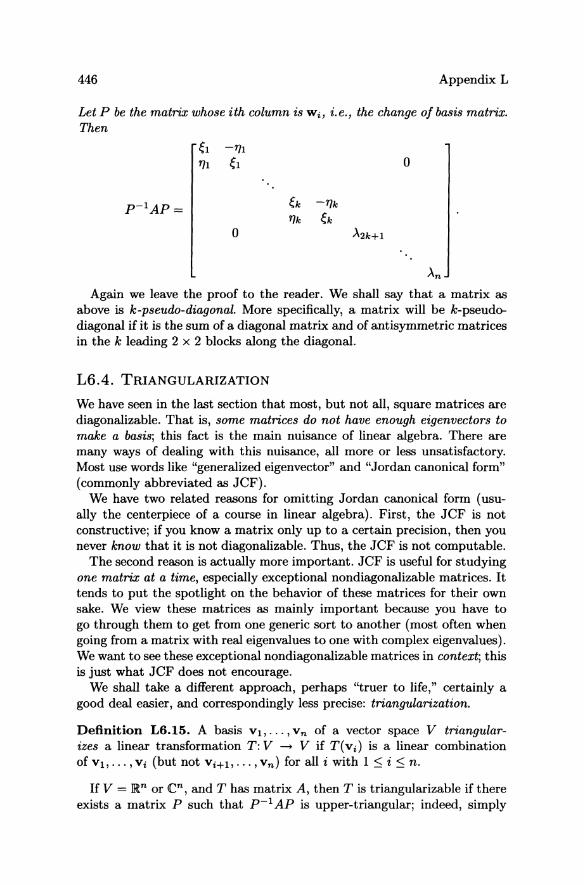
446 Appendix L

Let P be the matrix whose ith column is Wi, i.e., the change of basis matrix. Then

el -"'1 "'1 6 0

P-1AP= ele -"'Ie "'Ie ele

0 A21e+l

An Again we leave the proof to the reader. We shall say that a matrix as

above is k-pseudo-diagonal. More specifically, a matrix will be k-pseudo­diagonal if it is the sum of a diagonal matrix and of antisymmetric matrices in the k leading 2 x 2 blocks along the diagonal.

L6.4. TRIANGULARIZATION

We have seen in the last section that most, but not all, square matrices are diagonalizable. That is, some matrices do not have enough eigenvectors to make a basis; this fact is the main nuisance of linear algebra. There are many ways of dealing with this nuisance, all more or less unsatisfactory. Most use words like "generalized eigenvector" and "Jordan canonical form" (commonly abbreviated as JCF).

We have two related reasons for omitting Jordan canonical form (usu­ally the centerpiece of a course in linear algebra). First, the JCF is not constructive; if you know a matrix only up to a certain precision, then you never know that it is not diagonalizable. Thus, the JCF is not computable.

The second reason is actually more important. JCF is useful for studying one matrix at a time, especially exceptional nondiagonalizable matrices. It tends to put the spotlight on the behavior of these matrices for their own sake. We view these matrices as mainly important because you have to go through them to get from one generic sort to another (most often when going from a matrix with real eigenvalues to one with complex eigenvalues). We want to see these exceptional nondiagonalizable matrices in context; this is just what JCF does not encourage.

We shall take a different approach, perhaps "truer to life," certainly a good deal easier, and correspondingly less precise: triangularization.

Definition L6.15. A basis VI, ... , vn of a vector space V triangular­izes a linear transformation T: V -+ V if T(Vi) is a linear combination of Vb ... ,Vi (but not Vi+b ... ,vn ) for all i with 1 ::; i ::; n.

If V = lRn or en, and T has matrix A, then T is triangularizable if there exists a matrix P such that p-1 AP is upper-triangular; indeed, simply

Appendix L6 447

take the vectors Vi as the columns of P, i.e., take P as the appropriate change of basis matrix. We will say that P triangularizes A.

Triangularization is similar to diagonalization. In particular, recall from Theorem L5.13 and Exercise L6#4 or L6#5 that the diagonal terms of a triangular matrix are the eigenvalues. Therefore, triangularizing a matrix is at least as hard as finding the eigenvalues.

The following theorem is our main tool:

Theorem L6.16. Given any complex matrix A, there exists a unitary ma­trix M such that M-I AM is upper-triangular.

Equivalently, given any complex n-dimensional vector space V with an inner product and any linear transformation T: V ---t V, there exists an orthonormal basis VI, V2, ... , Vn of V such that for any i, 1 ::; i ::; n, the vector T(Vi) is a linear combination of Vb' .. , Vi and not the further vectors.

The proof we will give is fairly simple but not very constructive: it de­pends on the fact that any linear transformation from a vector space to itself has at least one (perhaps complex) eigenvector (Theorem L6.4). Re­call that this requires the fundamental theorem of algebra, as applied to the characteristic polynomial; both are rather hard to compute. Moreover, the fundamental theorem of algebra is a result about complex numbers, which explains why unitary matrices, the complex analog of orthogonal matrices, as defined in Section L4.1, make their way into the statement. The corresponding statement to Theorem L6.16 with "complex" replaced by "real" and "unitary" replaced by "orthogonal" is simply false; we will see in Theorem L6.17 what replaces it.

The QR method (Appendix L7) gives precisely the orthonormal basis promised by Theorem L6.16, when it converges; so, in fact, exhibiting such a basis is usually possible in practice.

Proof. The equivalence of the two statements is simply the matrix char­acterization of trianguiarizabilityj we will prove the second statement. The proof is by induction on n; so assume that the theorem is true for all vector spaces of dimension n - 1.

Choose VI a unit eigenvector of T, let VI be the space orthogonal to VI,

and let 11": V ---t VI be the orthogonal projection. Now let TI : VI ---t VI be given by TI(V) = 1I"(T(v)). Since VI has dimension n -1, we can apply the inductive hypothesis and find an orthonormal basis V2,"" Vn of VI such that TI (Vi) is a linear combination of V2, ... ,Vi for all i = 2, ... , n.

We claim that the vectors VI,"" vn do the trick. It is an orthonormal set, with n elements, hence a basis. For 2 ::; i ::; n, the vector T(Vi) differs from TI (Vi) only by some multiple of VI. so it is a linear combination of Vb"" Vi. Finally, VI is an eigenvector. 0

448 Appendix L

When we must work with real matrices, Theorem L6.17 is often an ade­quate substitute. Let us call a matrix k-pseudo-upper-triangular if it is the sum of a pseudo-diagonal matrix and a matrix with nonzero entries only above the k-pseudo-diagonal. In Exercise L6#6, you are asked to show that the characteristic polynomial of a real k-pseudo-upper-triangular matrix has at most k conjugate pairs of nonreal eigenvalues.

Theorem L6.17 If A is a real n x n matrix with k conjugate pairs of non­real eigenvalues, there exists a real invertible matrix M such that M-1 AM is k-pseudo-upper-triangular.

Equivalently, given a real vector space V with an inner product and a linear transformation T: V -t V with k conjugate pairs of nonreal eigen­values, there exists a basis Wl, W2, .•. ,Wn of V such that in that basis the matrix of T is k-pseudo-upper-triangular.

Proof. The proof is similar to that of Theorem L6.16. Suppose the state­ment is true for all vector spaces of dimension less than nj we may also suppose k > 0: if all the eigenvalues are real the proof of Theorem L6.16 actually shows that there is a real orthonormal basis in which the matrix of T is upper-triangular.

So let A = e +i1J be a nonreal eigenvalue, and v a corresponding eigenvec­tor (necessarily complex). Let Wl and W2 be the real and imaginary parts of Vj note that Wl and W2 are linearly independent, since their complex span is the space spanned by v and v, which are linearly independent since they are eigenvectors for the distinct eigenvalues A and X. This is where we use that A is not real.

Let W be the orthogonal of the plane spanned of Wl and W2, and con­sider, as above, Tl = 7rw 0 Tlw. By induction, we can assume that there exists a basis W3," . , Wn of W such that the matrix of Tl in that basis is l­pseudo-upper-triangular for some l. The proof that in the basis Wl,"" Wn

the matrix of T is (l + 1 )-pseudo-upper-triangular is the same as in Theorem L6.16

Since the determinant of a pseudo-upper-triangular matrix is the same as the determinant of the pseudo-diagonal part, we see that the eigenvalues of T are exactly those of Tl and A, with multiplicity. Thus, l = k - 1. 0

As we have seen, the eigenvalues of A are precisely the diagonal entries of the triangular matrix. One consequence of this result is that, as we have been claiming all along, any matrix can be perturbed arbitrarily little so that its eigenvalues become distinct. Indeed, write any matrix A as MDM-l with D triangular, and let Dl be a slight perturbation of D, where only the diagonal entries have been modified to make the entries distinct. Then M D1M-1 is close to A and has distinct eigenvalues.

Unfortunately, triangular matrices are not diagonal. But, as we shall see in Chapter 8, if we go beyond Theorem L6.16 and add a little trick

Appendix L6 449

of allowing bases that are not orthonormal, the triangular matrix can be further modified to make the off-diagonal terms as small (but not zero) as one wishes.

It is easy to see how to do this. Let us look at the 2 x 2 case: suppose that with respect to some basis VI, V2, a linear transformation T has an upper-triangular matrix. This means that

so that the matrix for T is

T(vt} = ).IVI + aVI, T(V2) = ).2V2

(1)

Note that V2 is an eigenvector and a is the off-diagonal term of the matrix.

Now replace VI by WI = CVI. Equations (1) can now be written

so that

T(vt} = ).IWI + caV2 (we haven't touched V2) and

T(V2) = ).2V2·

T [ :: ] [~l~;] [::] . In the basis WI, V2, the matrix of T has as its only off-diagonal term ca,

which by taking c small can be made as small as you like. (Yes, that also makes WI very small, but we care only about its direction, not its size.)

Theorem L6.18. Given any n x n complex matrix A and any c > 0, there exists an orthogonal basis WI, W2, ... , Wn of en such that if P = [WI, W2, ... , Wn], then p- I AP is upper-triangular, with off-diagonal terms of absolute value smaller than c.

Proof. First find an orthonormal basis Vb ... , vn such that if P = [VI, ... , vnl then p- I AP is upper-triangular, as above. Next let Wk = ckVk. Since

we find

AWk = ck(al,kvI + ... + ak,kvk)

= al,kck-lwl + a2,kck- 2w2 + ... + ak,kwk·

We see that in the basis WI, ... , Wn all the off-diagonal terms are multiplied by a positive power of c and hence can be made as small as one wishes by taking c sufficiently small. D

450 Appendix L

There is a real variant of this result.

Theorem L6.19. Given any n x n real matrix A with k pairs of nonreal eigenvalues and any IE> 0, there exists a basis WI, W2,"" Wn ofRn such that if P = [WI, W2, ... ,Wn ], then p- l AP is k-pseudo-upper-triangular, with off-pseudo-diagonal terms of absolute value smaller than IE.

The proof is analogous to the proof of L6.18 and is left to the reader (Exercise L6#7).

L6.5. EIGENVALUES AND INNER PRODUCTS

The three classes (symmetric, antisymmetric, and orthogonal) of linear transformations that are closely related to inner products (Sections L4.1, L4.2, and L4.3) have rather special eigenvalues and eigenvectors.

We have strived so far to treat the real and the complex cases separately; at this point it becomes misleading to do so; so please remember that real antisymmetric is a special case of complex anti-Hermitian and that orthogonal is the real case of unitary.

Theorem L6.20.

( a) If A is a real symmetric or Hermitian linear transformation, then the eigenvalues of A are real.

(b) If A is a real antisymmetric or anti-Hermitian linear transformation, then the eigenvalues of A are purely imaginary.

(c) If A is an orthogonal or unitary linear transformation, then the eigen­values of A are of absolute value 1.

In all three cases, any two eigenvectors of A with distinct eigenvalues are orthogonal.

Note that (c) says in particular that the only real eigenvalues an orthog­onal matrix can have are ± 1.

Proof. Theorem L6.20 is an easy computation, outlined in the exercises. The proof of Theorem L6.22 in any case will also prove Theorem L6.20 in the finite-dimensional case. 0

Example L6.21. One consequence of Examples L4.7, and L6.2 and Exer­cise L3-4#17 is that if n =f. m, then i: sin nx sin mx dx = i: cos nx sin mx dx

= i: cosnxcosmxdx = O.

Appendix L6 451

Indeed, the functions sin nx, sin mx, cos nx, and cos mx are eigenvectors of the second derivative operator with distinct eigenvalues _n2 and _m2

as appropriate, so they are hereby shown to be orthogonal. You will meet these integrals when Fourier series are introduced in partial

differential equations. We do not want to claim that the proof given here of their being zero is especially simple, but it is more revealing than just computing the integrals using trigonometric formulas. A

The next result is really of very great importance. It is central to classi­cal mechanics and to quantum mechanics; it is surely the most important mathematical contribution to chemistry, and probably to the engineering of structures as well. The proof we will give here, essentially a corollary of Theorem L6.16, is short but suffers from being nonconstructive, since it relies on the characteristic polynomial and the fundamental theorem of algebra. In application, one needs not only to know that an eigenvector ex­ists but also how to compute it. Jacobi's method (Appendix L8) provides such a method, as well as a constructive proof of the theorem.

Theorem L6.22 (Spectral Theorem).

(a) If A is a Hermitian, anti-Hermitian, or unitary matrix, then en has an orthonormal eigenbasis Vb V2, ... , Vn for A.

(b) If A is real symmetric, then the eigenvalues are real and the basis vectors can be chosen real so that IRn has an orthonormal eigenbasis for A.

Proof. By Theorem L6.16, there exists a unitary matrix P such that p-1 AP is upper-triangular. However, since P is unitary, p-1 AP is still Hermitian, anti-Hermitian, or unitary. Clearly, for a Hermitian matrix to be upper-triangular, it must be diagonal with real entries on the diagonal; for an anti-Hermitian matrix to be upper-triangular, it must be diagonal with purely imaginary entries on the diagonal. Furthermore, since the in­verse of an upper-triangular matrix is also upper-triangular, if p- 1 AP is unitary, then it must be diagonal, this time with entries of absolute value 1 on the diagonal (Exercise L6#8).

Since in all three cases p-1 AP turned out to be diagonal, the column vectors of P form an eigenbasis for A, which is orthonormal since P is unitary. The italicized statements, together with the fact that P is unitary, prove Theorem L6.22, part (a).

Part (b) follows from the fact, just proved, that the eigenvalues of a Hermitian matrix, hence of a real symmetric matrix, are real; hence, the eigenvectors can be chosen real. 0

In Exercise L6#9 we will define and prove appropriate properties of nor­mal linear transformations. These include all three of the classes above-

452 Appendix L

unitary, Hermitian, and anti-Hermitian-and allow a unified proof of The­orem L6.22.

L6.6. FACTORING THE CHARACTERISTIC POLYNOMIAL

The characteristic polynomial has already had many uses in this section. The next ones are rather deeper, and techniques along these lines are the most powerful that linear algebra has at its disposal. On the other hand, the characteristic polynomial is more or less uncomputable, and so the results are mainly of theoretical interest.

A first statement is the following:

Theorem L6.23. Any matrix A satisfies its characteristic polynomial PA, i.e., PA(A) = O.

Example L6.24. The characteristic polynomial of the matrix

[ 1 0 2] A = -1 0 1

010

is PA(.~) = A3 - A2 - A + 3. If we compute PA(A) = A3 - A2 - A + 31, we find

[!1 ~ ~] + [~ ~ ~] o 1 0 0 0 3

A + 31

=0. &

Proof of Theorem L6.23. The method of proof is typical of a large class of proofs in this part of linear algebra. First, do it for the diagonal matrices, then the diagonalizable matrices, then the others by approximation.

(i) Suppose A is diagonal, with the eigenvalues Ai along the diagonal. Then all Ak are also diagonal, with powers of the eigenvalues on the diag­onal, so PA(A) is diagonal, with PA(Ai) in the ith spot on the diagonal. Since the eigenvalues are the roots of the characteristic polynomial, the result is true.

(ii) Now suppose A is diagonalizable; say, p- I AP = Al is diagonal. Since by Theorem L5.1O PAl = PA, we have

Appendix L6 453

(iii) Now suppose A is anything. In any case, there exists a sequence of matrices Ai converging to A with all the Ai diagonalizable. Since A ....... PA(A) is a continuous function, PA(A) = limi-+OO PA; (Ai) = O. 0

Now we come to the main idea of this section: factorizations of the char­acteristic polynomial. We will be mainly concerned with factorizations into relatively prime factors, i.e., factors that have no common roots. Such a factorization corresponds to a grouping of the roots of the characteristic polynomial. This will allow the astute reader to isolate the part of the behavior coming from various kinds of eigenvalues.

Theorem L6.25. Let A be an n x n matrix, with characteristic polynomial PA, and suppose that PA is factored: PA = PI112, with PI and 112 relatively prime with leading coefficient 1. Let VI = kerpl(A) and V2 = ker112(A). Then

(i) Any vector x E R." can be written uniquely as x = Xl + X2, with Xl E VI and X2 E Vi.

(ii) For any vector X E Vi we have A(x) E Vi.

(iii) The eigenvectors of A with corresponding eigenvalues roots of Pi are in Vi.

(iv) The characteristic polynomial of A: Vi - Vi is Pi.

Before proceeding to the proof of this result, we make a few comments, insert an example, and prove a lemma.

What does (iv) mean? After all, A: Vi - Vi is not a matrix, at least not until a basis has been chosen for Vi. But recall that characteristic polyno­mials do not depend on the basis, all they require is a linear transformation mapping a vector space to itself; (ii) says that A: Vi - Vi is such a thing.

Let's move to the example:

Example L6.26. The characteristic polynomial of the matrix

is PA(.~) = >.3 - 2>.2 + >. - 2 = (>.2 + 1)(>' - 2).

So we want to examine VI = ker( A - 2/) and V2 = ker( A 2 + I). The space VI: ker(A - 21) contains all vectors X E R.3 such that (A - 2I)x = 0;

454

i.e.,

Appendix L

-2XI +X2 = 0 =:} -2X2 + X3 = 0

2XI - X2 = 0

The result for the vector x shows that with eigenvalue 2, we have but one parameter, a one-dimensional space of eigenvectors of A. We have shown that VI is a line.

V2: ker(A2 + f) contains all vectors u E IR3 such that (A2 + f)u = 0; i.e.,

the only condition, so vectors in V2 are of the form

The fact that we have two arbitrary constants a, b for the vector u shows that with eigenvalue ±i we have a two-dimensional space of eigenvectors of A. We have shown that V2 is a plane, described, for example, by vectors

Of course, there are other ways to derive these results; the above method was chosen to most clearly show what is happening; a more efficient purely matrix method uses row reduction and the dimension Theorem L2.25 (see Exercise L6#lOa).

Now we are ready to illustrate the conclusions of Theorem L6.25:

(i) Any vecto, [~] in JR' can be wdtten uniquely as

Appendix L6 455

with a correct choice of a, b, and c (from three equations in these three unknowns).

(ii)

A [2~] [~ ~~] [2~] [!~] = [2~:] , 4c 2 -1 2 4c 8c 4c*

where c* = 2c; hence, the resulting vector belongs to ker(A - 21), i.e., A maps Vl --t Vl.

A [ !] = [~ ~~] [!] [-:] = [ !:], -b 2 -1 2 -b -a -b*

where b* = a, and a* = -b; hence, the resulting vector belongs to ker(A2 + I), i.e., A maps lt2 --t V2 •

Exercise L6#lOb asks you to verify properties (iii), and (iv) in similar fashion. &

The lemma we need is the following, which appears to have nothing to do with linear algebra at all. It is known as Bezout's theorem and is an important result in its own right. Another proof appears as Exercise L2#17.

Lemma L6.27 (Bezout's Theorem). Two polynomials Pl and P2 are relatively prime if and only if there exist polynomials ql and q2 such that Plql + P2q2 = 1.

Proof. In one direction, this is clear: if q divides both Pl and P2, then it will also divide Plql + P2q2 for any ql and q2; so q must divide 1, which implies that q must be a constant. This exactly means that Pl and P2 are relatively prime.

The converse is more interesting and involves an algorithm that is impor­tant in itself: the Euclidean Algorithm. Let deg(pl) ~ deg(P2), and define a finite sequence of polynomials P3, P4,'" ,Pk by division with remainder as follows:

Pl = q2P2 + P3 with deg(p3) < deg(P2),

P2 = qaPa + P4 with deg(p4) < deg(Pa),

Since the degrees of the Pi are strictly decreasing, this process must end, in fact, in at most deg(PI) steps. The only way in which it can end is with Pk+1 = 0 for some k, since 0 is the only polynomial by which you cannot divide.

456 Appendix L

Consider Pkj it divides Pk-l! and hence Pk-2, etc., and finally both PI and P2. As such, it must be a constant. On the other hand, all the Pi can be written in the form 8lPl + 82P2 for appropriate 81 and 82:

P3 = PI - q2P2,

P4 = P2 - q3P3 = P2 - q3(Pl - q2P2) = -q3Pl + (1 + q2q3)P2,

This ends the proof: Pk is a constant c which can be written c = 8lPl + 82P2j set q2 = 82/C, q2 = 82/C to find 1 = qlPl + Q2P2. 0

Remark. Note that the proof of Lemma L6.27 actually gave a recipe for computing Ql and Q2 (as well as the greatest common divisor of two polyno­mials). It can also be used to compute greatest common divisors of integers in precisely the same way.

Proof of Theorem L6.25. (i) Suppose Ql('x) and Q2('x) are two polyno­mials such that PlQl + P2Q2 = 1. Then since PI (A)Ql (A) + P2{A)Q2{A) = I, we have for any vector x that

x = P2{A)Q2{A)x + PI (A)Ql{A)x.

Now P2(A)Q2{A)x E VI since PI (A)P2(A)Q2(A) = PA(A)Q2(A) = 0 by The­orem L6.23 and, similarly, Pl{A)Ql{A)x E V2. This shows that there is a decomposition as in x = Xl + X2 with Xl E VI and X2 E Viz.

For uniqueness of the decomposition, it is enough to show VI n Viz = {O}j indeed, if

X = Xl + X2 = Yl + Y2

with Xl,Yl E VI and X2,Y2 E V2 , then Xl-Yl = Y2 -X2 is in both VI and in V2 • Therefore, if the intersection is 0, we have Xl = Yl and X2 = Y2. If X E VI n Viz, then

so X = O. This proves (i). (ii) If X E VI, then PI (A)x = 0 and PI (A) Ax = ApI (A)x = o. (iii) Suppose Pl{'x) = 0, and Av = 'xv. Then Pl(A)v = Pl('x)V = 0, so

vE VI. (iv) This part is a bit more unpleasant. If you choose a basis of VI and a

basis of Viz, then together these form a basis of V, and since A sends each of these spaces into itself, in this basis A has a matrix of the form

Appendix L7 457

By Theorem L5.8, the characteristic polynomial PA can be written qlq2, where ql and q2 are the characteristic polynomials of Al and A 2, respec­tively, which in turn are simply the matrices of A: Vi - Vi with respect to the chosen bases of these subspaces. So we have PA = qlq2 = PlP2, and we need to show Pl = ql, P2 = q2. If we show that no root of ql is also a root of P2 and no root of q2 is also a root of Pl, we will be done. But any root A of ql is an eigenvalue of A: Vl - Vi. On the other hand, any eigenvalue of A with corresponding eigenvector in Vi is a root of Pl, hence not a root ofP2. 0

L 7 Finding Eigenvalues: The QR Method

As indicated in Chapter 7 and subsequent chapters, the main task in solving linear differential equations with constant coefficients,

x' = Ax,

is to find the eigenvectors and eigenvalues of A. At the end of Section 7.3, we remarked that computing the characteristic

polynomial of A, finding the eigenvalues as its roots, and solving for the eigenvectors by solving linear equations turns out to be impractical as soon as the matrix A is at all large. The QR method (and its variants) is a differ­ent algorithm, and it is probably the one most often used in applications, at least for nonsymmetric matrices. Although it is much more practical than the characteristic polynomial approach, it still has its problems. For one thing, the explanation and proof are especially lengthy and complicated. Finding eigenvectors and eigenvalues really is hard, and nothing will make it quite simple. Our presentation was inspired by a lecture by Michael Shub.

We will begin by a description of the power method, which is a simpler cousin of the QR method.

L 7 .1. THE "POWER" METHOD

Suppose an n x n real matrix A has eigenvalues Al, ... ,An with distinct absolute values, and suppose IAll > IAil, i = 2, ... ,no We then call Al the dominant eigenvalue.

Take from an any vector x "I 0, and consider the sequence of unit vectors

x Axo Axk Xo = /lxII' Xl = IIAxoll'··· ,Xk+1 = IIAxk ll·

It is trivial (for a computer) to compute the sequence Xk. The main point of the "power" method is the following result.

Theorem L7.1. In general, the sequence of vectors X2k converges to a unit eigenvector of A with dominant eigenvalue Al.

458 Appendix L

Proof. We might as well work in a basis Vb"" Vn of unit eigenvectors of A. Suppose that x = ClVl + ... + CnVn , with Cl =1= 0. (This last condition is what "in general" means.) Then

and the various terms have very different magnitudes. In fact, if we divide through by ClA~, we get

AkX CnA~ --k = VI + ... + --k V n , ClAl ClAl

and all the coefficients except the first tend to zero as k -t 00.

Now Xk is a multiple of AkX, so for k large, Xk is close to one of the vectors +Vl or -VI' If Al > 0, then Xk+l is close to the same vector and the sequence Xk converges. If Al < 0, then Xk or Xk+1 is close to the opposite vector; in any case, the even terms X2k converge. 0

You may wonder why we normalized Xi at each step rather than com­puting Akx directly. The proof of Theorem L7.1 shows that the entries of Akx grow like A~ and will rapidly get out of hand.

The QR method is essentially a way of teasing the other eigenvectors away from the voracious attraction of VI.

Remark. It may seem strange to find the eigenvectors first and then the eigenvalues, but we shall see in Theorem L7.4 how it works.

L7.2. A DESCRIPTION OF THE QR METHOD

Begin with an invertible matrix A.

(i) Find Ql and Rl so that A = QlRb where Ql is orthogonal; Rl is upper-triangular; this is done by the Gram-Schmidt algorithm, The­orem L3.13.

(ii) Now, reverse the orner of the factors and write Al repeat step (i) using Al instead of A.

Note: A = QlRl implies QJ A = Rb which implies Al = QJ AQI = Q1l AQb so Al and A have the same eigenvalues, by Theorem L5.7. We continue, with

Ak- l = QkRk, Ak == RkQk'

As we will see in Section L7.7, the matrices Ak miraculously converge under appropriate circumstances to an upper-triangular matrix with the eigenvalues on the diagonal.

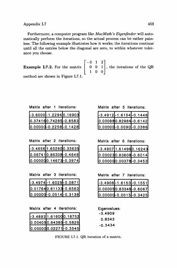
Appendix L7 459

Furthermore, a computer program like MacMath's Eigenfinder will auto­matically perform the iterations, so the actual process can be rather pain­less. The following example illustrates how it works; the iterations continue until all the entries below the diagonal are zero, to within whatever toler­ance you choose.

Example L7.2. Fb, the matrix [-~ ~ ~], the itemtions of the QR

method are shown in Figure L 7.1.

Matrix after 1 iterations: Matrix after 5 iterations:

-3.6000 -1.2294 0.16903 -3.4912 -1.6154 -0.1448

0.37416 0.74285 -0.8583 0.00098 0.82984 -0.6142

O.OOOOC -0.2258 -0.1428 0.00000 -0.0090 -0.3386

Matrix after 2 iterations: Matrix after 6 iterations:

-3.4656 1.6526C 0.3363Ji -3.4907 1.6149§ 0.1624:3

0.06741 0.8630e -0.4648 0.00023 0.83608 -0.6014

O.OOOOC 0.146n -0.3974 0.00000 0.00378 -0.3453

Matrix after 3 iterations: Matrix after 7 iterations:

-3.4974 -1.6029 -0.0871 -3.4908 -1.6153

0.01764 0.81133 -0.6563 0.00005 0.83346

0.00000 -0.0514 -0.3138 O.OOOOC -0.0015

Matrix after 4 iterations: Eigenvalues:

-3.4893

0.00405

0.0000_0

1.61600 0.1875:1

0.84385 -0.5826

0.02271 -0.3545

-3.4909

0.8343

-0.3434

FIGURE L7.1. QR iteration of a matrix.

-0.1551

-0.6067

-0.3425

460 Appendix L

The program stops after eight iterations because the subdiagonal ele­ments are all less than the chosen tolerance of 0.000l.

The eigenvalues have been boxed on the main diagonal and have rounded values (using more decimal places than shown on the diagonal) of -3.4909, 0.8343, and -0.3434. ~

L7.3. THE MAIN CONVERGENCE RESULT

Theorem L7.3. Suppose A has n real eigenvalues, with distinct absolute values. Then the matrices Ak converge as k --+ 00 to an upper-triangular matrix with the eigenvalues of A on the diagonal.

The proof of Theorem L 7.3 requires laying quite a bit of groundwork, to which we shall shortly proceed. We will be able to explain why this result is true in Section L7.7. Meanwhile, we shall first make some observations.

There is more to be said than Theorem L7.3 gives. First, the requirement that the eigenvalues, or for that matter the matrix A, be real is unnecessary. If A is complex, then Q should be chosen unitary, and Gram-Schmidt works exactly the same way; the reference is Appendix L3.

Unfortunately, if A is real and has complex eigenvalues, then they never have distinct absolute values since they come in conjugate pairs. It turns out that all is still not lost: a pair of complex conjugate eigenvectors leads to matrices Ak with a 2 x 2 submatrix M along the diagonal. The entries in M do not converge as the algorithm proceeds; however, the pair of complex eigenvalues are then the roots of the characteristic polynomial of M. It turns out that this characteristic polynomial does converge even though the entries of the submatrix do not, and characteristic polynomials for 2 x 2 matrices are easy to compute: they always have the form

)..2 _ (tr M» .. + (det M), (1)

as discussed in Chapter 7, Section 5. We do not here prove these results for the complex case, but for completeness we state the theorem that explains how the QR algorithm extends to complex eigenvalues.

Theorem L7.4. Suppose A has n complex (including real) eigenvalues, with distinct absolute values, except for complex conjugate pairs. Then the matrices Ak tend as k --+ 00 to almost upper-triangular matrices. The ex­ceptions are 2 x 2 submatrices along the diagonal, which yield the nonreal complex eigenvalues of A in conjugate pairs, as solutions to the character­istic polynomials of these 2 x 2 submatrices. The real eigenvalues of A lie on the diagonal.

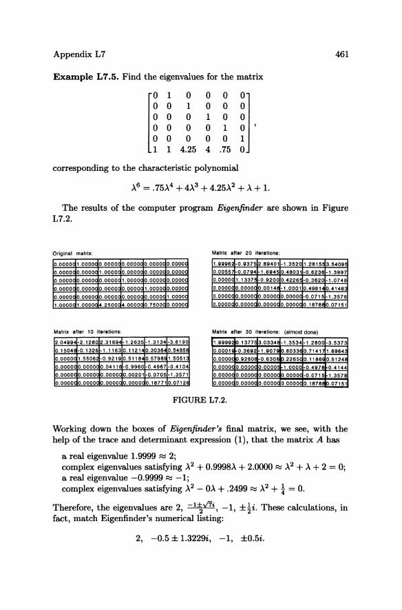
Appendix L7

Example L7.5. Find the eigenvalues for the matrix

o 1 o 0 o 0 o 0 o 0 1 1

o 1 o o o

4.25

o o 1 o o 4

o o o 1 o

.75

corresponding to the characteristic polynomial

o o o o 1 o

461

The results of the computer program Eigenfinder are shown in Figure L7.2.

Original matrix: Matrix alter 20 iteralions:

0.0000 1.00000 0.00000 0.0000 o.ooooc o.ooooc 1.9996 -0.9375 2.89401 -1.352C 1.2815 3.5409

0.0000 0.0000 1.0000C 0.0000 O.ooooc 0.0000 0.0055 -0.0794 -1.6945 0.48031 -0.6236 -1.3997

0.0000 o.ooooc o.OOOOC 1.0000 O.OOO~C O.ooo~ 0.0000 1.133n -0.9200 0.4226 -0.3620 -1.0748

0.0000 o.ooooc O.OOOOC 0.0000 1.0000C 0.0000 0.0000 O.OOOOC 0.0014 -1.0001 0.4981 0.4148

0.0000 O.OOOOC O.OOO~c 0.0000 0.0000 1.0000 O.OOOOC O.OOOOC O.OOOOC 0.0000 -0.0715 -1.3578

1.0000 1.0000 .2500 4.0000 0.7500 0.0000 O.OOOOC O.OOOOC O.OOOOC 0.0000 O. t878 0.07151

Matrix alter 10 Iterations: Matrix alter 30 Ilerations: (almost done)

2.0499 -2.1280 2.3169 -1.2635 -1.3134 -3.6190 1.9999 1o.1377! 3.0334 -1.3534 -1.2800 -3.5373 O. t504E -0.1326 1. t t63 0.t121 0.3036 0.5465E 0.0001 0.3892 1.9079 b.6033E 0.7141 1.6964 0.00000 1.5506! -0.9219 0.5118 0.5798 1.5051 0.0000 10.92801 0.630E b.22650 0.1186 0.5124'1 O.OOOOC 0.0000 ~.0411 -0.9960 -0.4967 -0.4104 0.0000 0.0000 0.0000 1.0000 -0.4978 0.4144 O.OOOOC 0.0000 ~.OOOOC 0.00201 0.0705 -1.3571 0.0000 0.0000 0.0000 10.0000 -0.0715 1.357E 0.0000 0.0000 ~.OOOO 0.0000 0.18771 0.0712E 0.0000 0.0000 0.0000 0.00000 0.1878 10.07151

FIGURE L7.2.

Working down the boxes of Eigenfinder's final matrix, we see, with the help of the trace and determinant expression (1), that the matrix A has

a real eigenvalue 1.9999 ~ 2; complex eigenvalues satisfying >.2 + 0.9998>' + 2.0000 ~ >.2 + >. + 2 = 0; a real eigenvalue -0.9999 ~ -1; complex eigenvalues satisfying >.2 - 0>' + .2499 ~ >.2 + 1 = O.

Therefore, the eigenvalues are 2, -l~v7i, -1, ±!i. These calculations, in fact, match Eigenfinder's numerical listing:

2, -0.5 ± 1.3229i, -1, ±0.5i.

462 Appendix L

L7.4. FLAGS

Unfortunately, although the QR method is quite easy to implement, it is fairly complicated to understand why it works. The key notion is the following:

A flag of R.n is an ascending sequence of subspaces

with each subspace Ui of dimension i, and therefore Un = R.n. A flag may appear to be a nebulous notion, but it is quite easy to work

with in practice. For instance, if the columns a1 ••• ,an of a matrix A are linearly independent, they form a basis of R.nj we may consider the flag FA defined as above with the subspaces defined as follows: each Ui is spanned by a1. ... ,8ij this flag is called the flag associated to the basis.

Of course, many bases have the same associated flag.

Examp~ L7.6. Conmd& A ~ 0 ~ n and B ~ 0 : can write

31) 73 . We

115

The first and last entries in each flag are the samej if we can show that the middle entries each span the same plane, we will have shown that the flags are the same. That is, can we find numbers a and b such that

Yes: a = 2, b = 4. Therefore, FA = FB . •

In fact, if A is the matrix with ith column 8i, then B has the same flag associated to its columns as A if and only if B = AR, with R an invertible upper-triangular matrix. The proof of this fact involves a straightforward calculation in Exercise L7#2, which you should consider compulsory and central to getting a feel for the heart of the QR method. An essential

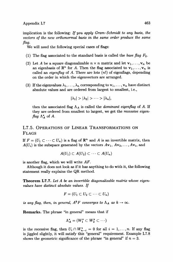
Appendix L7 463

implication is the following: If you apply Gram-Schmidt to any basis, the vectors of the new orthonormal basis in the same order produce the same flag.

We will need the following special cases of flags:

(1) The flag associated to the standard basis is called the base flag FQ •

(2) Let A be a square diagonalizable n x n matrix and let VI,"" vn be an eigenbasis of IRn for A. Then the flag associated to Vb' .. , Vn is called an eigenflag of A. There are lots (n!) of eigenflags, depending on the order in which the eigenvectors are arranged.

(3) If the eigenvalues Ab"" An corresponding to VI,"" vn have distinct absolute values and are ordered from largest to smallest, i.e.,

then the associated flag AA is called the dominant eigenflag of A. If they are ordered from smallest to largest, we get the recessive eigen­flag A:4. of A.

L7.5. OPERATIONS OF LINEAR TRANSFORMATIONS ON

FLAGS

If F = (UI C ... C Un) is a flag of IRn and A is an invertible matrix, then A(Ui ) is the subspace generated by the vectors AVl, AV2,"" AVi, and

is another flag, which we will write AF. Although it does not look as if it has anything to do with it, the following

statement really explains the QR method.

Theorem L7.7. Let A be an invertible diagonalizable matrix whose eigen­values have distinct absolute values. If

is any flag, then, in general, Ak F converges to AA as k ---- 00.

Remarks. The phrase "in general" means that if

A:4. = (W; C W; C ... )

is the recessive flag, then Ui n W.'::_i = 0 for all i = 1, ... , n. If any flag is jiggled slightly, it will satisfy this "general" requirement. Example L 7.8 shows the geometric significance of the phrase "in general" if n = 3.

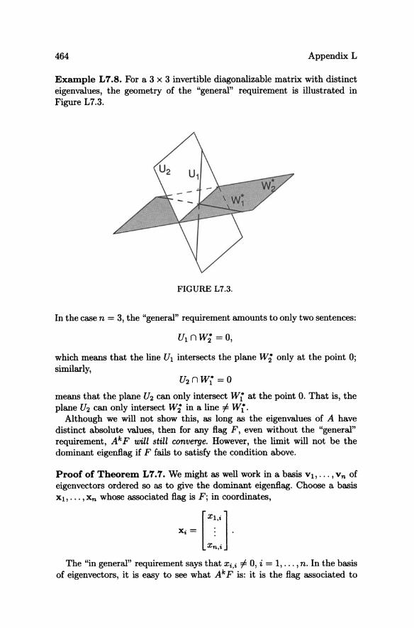
464 Appendix L

Example L7.8. For a 3 x 3 invertible diagonalizable matrix with distinct eigenvalues, the geometry of the "general" requirement is illustrated in Figure L7.3.

FIGURE L7.3.

In the case n = 3, the "general" requirement amounts to only two sentences:

u1nw; =0,

which means that the line U1 intersects the plane Wi only at the point 0; similarly,

u2 nw; =0

means that the plane U2 can only intersect Wi at the point O. That is, the plane U2 can only intersect Wi in a line =f. Wi.

Although we will not show this, as long as the eigenvalues of A have distinct absolute values, then for any flag F, even without the "general" requirement, A k F will still converge. However, the limit will not be the dominant eigenflag if F fails to satisfy the condition above.

Proof of Theorem L7.7. We might as well work in a basis Vii ... , Vn of eigenvectors ordered so as to give the dominant eigenflag. Choose a basis Xii ... ,Xn whose associated flag is F; in coordinates,

[Xl 'J

X< ~ x~:: . The "in general" requirement says that Xi,i =f. 0, i = 1, ... ,n. In the basis

of eigenvectors, it is easy to see what Ak F is: it is the flag associated to

Appendix L7 465

the basis

[ ~i::::l ' [~::::l , ... , [~i::::l' >'~Xn,1 >'~Xn,2 >'~xn,n

The coordinates of the vectors above have very different magnitudes; in order to see this more clearly, divide the ith vector by >.fXi,i' These new vectors give the same flag, but this time they look like

where * represents an entry that becomes arbitrarily small as k - 00,

and # represents an entry that is probably very large but its magnitude is irrelevant.

The flag associated to these vectors is very nearly the dominant eigenflag of A. The first vector nearly points in the direction of VI' The second vector is a large multiple of VI plus a vector which nearly points in the direction of V2, so the first and second vectors nearly span the subspace spanned by VI and V2, and so forth. 0

We shall see in Section L 7.7 that while Theorem L 7.7 is true theoretically, numerically it does not lead to a productive algorithm unless the vectors are orthogonal. Without orthogonality, the vectors can get too wild; e.g., if the first # above the diagonal is huge, you could divide the second vector by that number and it would be very close to the first vector.

L7.6. THE RELATION BETWEEN EIGENFLAGS AND

EIGENVALUES

There is a good reason for wanting to find an eigenflag for a matrix A.

Theorem L7.9. If WI, ... , Wn is a basis ofJRn with the associated flag an eigenflag of A, then the matrix of A in that basis is upper-triangular with the eigenvalues on the diagonal.

Proof. Let VI, ... , Vn be eigenvectors such that Wi is a linear combination of VI,"" Vi, say

(2)

Then

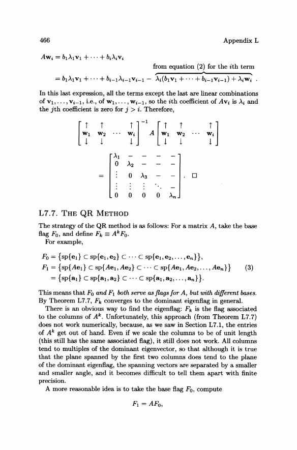
466 Appendix L

from equation (2) for the ith term ..

In this last expression, all the terms except the last are linear combinations of V1, ... , Vi-l, Le., of wl, ... , Wi-1, so the ith coefficient of AVi is Ai and the jth coefficient is zero for j > i. Therefore,

i i ]-1 [i ~i A ~1

i ... +]

. 0

OOOOAn

L7.7. THE QR METHOD

The strategy of the QR method is as follows: For a matrix A, take the base flag Fo, and define Fk == Ak Fo.

For example,

Fo = {sp{et} C sp{e1,e2} c··· c sp{el,e2, ... ,en}},

F1 = {sp{Aet} c SP{Ae1, Ae2} c ... c Sp{Ael, Ae2, ... , Aen }} (3)

= {sp{at} C sp{al,a2} c··· c sp{al,a2, . .. ,an}}.

This means that Fo and F1 both serve as flags for A, but with different bases. By Theorem L7.7, Fk converges to the dominant eigenflag in general.

There is an obvious way to find the eigenflag: Fk is the flag associated to the columns of Ak. Unfortunately, this approach (from Theorem L7.7) does not work numerically, because, as we saw in Section L7.1, the entries of Ak get out of hand. Even if we scale the columns to be of unit length (this still has the same associated flag), it still does not work. All columns tend to multiples of the dominant eigenvector, so that although it is true that the plane spanned by the first two columns does tend to the plane of the dominant eigenflag, the spanning vectors are separated by a smaller and smaller angle, and it becomes difficult to tell them apart with finite precision.

A more reasonable idea is to take the base flag Fo, compute

Appendix L7 467

and then describe F1 by an orthogonal basis (from Gram-Schmidt). Con­tinue this way, each time computing Fk by applying A to an orthonormal basis whose associated flag is Fk- 1 and reencoding Fk by an orthonormal basis. This is exactly what the QR method does, but we have to prove it:

Theorem L1.1O. Let A = QIRI, Al = R IQ1, Al = Q2R2, .... The flag associated to the orthogonal matrix

is Fk = Ak Fo, and Ak = Pk- I APk is the linear transformation A written in the basis formed by the columns of Pk . In particular, this means that Ak has the same eigenvalues as A.

Proof. The proof is by induction on k. The base step is for k = 1 with PI = Ql' By Gram-Schmidt, we can write A = Q1R1, and then we see that

Al = RlQl = Q1l AQI

is actually A in a new orthonormal basis. We showed in (3) that the flags Fo and AFo = FI both serve as flags (by different bases) for A. The matrices A and Q1 have the same flag, by Exercise L7#2d. Therefore, AFo indeed is a flag in the orthonormal basis of Q1.

Next suppose that the theorem is true for k - 1, that the flag for Qk-l is Ak-l Fo, and A k- l = Pk.!l APk-I' Writing, by the definition of Qk and Rk ,

A k- 1 = QkRk

means that Qk has the same associated flag as A k- 1 ; by expressions similar to (3), we can show that the flags Fk and A(Fk-1) both serve (by different bases) for Ak • On the other hand,

Ak = RkQk = Qkl Ak-1Qk

shows that Ak is Ak-l written in the orthonormal basis of columns of Qk, so for k we indeed have that the flag Fk = Ak Fo. So when we get done, by Theorem L7.9,

o

OOOOAn

The combination of Theorems L7.1O and L7.9 proves Theorem L7.3 at least if Fo satisfies the "general" condition about the recessive eigenflag of A, the general case.

468 Appendix L

L7.8. ACTUAL COMPUTATIONS WITH QR

We have proved in Section L7.7 that the QR method will find the eigen­values of A, at least for the usual case of distinct eigenvalues. The flags, which are essential for the proofs, are not used in the actual calculations. The computational algorithm simply is as follows:

(i) Find Qk by Gram-Schmidt on Ak- b so that Ak- 1 = QkRk.

(ii) Find Ak = QJ Ak-lQk, because Ak = RkQk = Qkl Ak-lQk = QJAk-lQk.

(iii) Repeat steps (i) and (ii) until Ak is sufficiently upper-triangular.

The phrase "sufficiently upper-triangular" means the following: First, "zero" in practice means below a preset tolerance (like 0.001), and we are aiming at that for all elements below the diagonal. But we must also allow for the possibility of complex eigenvalues, which leave 2 x 2 submatrices on the diagonal rather than in strictly upper-triangular form. In those cases, as we have already noted in Section L7.3 and Example L7.5, it is simple to compute the eigenvalues of a submatrix from its characteristic polynomial; we note here the same truth even if the eigenvalues are real. So, in practice, we simply continue QR until the subdiagonal of Ak has no two consecutive nonzero elements. Then for each 2 x 2 submatrix, we form the characteristic polynomial from the trace and the determinant and find its eigenvalues; any remaining eigenvalues will be real and already lying on the diagonal of the overall matrix.

There are matrices for which QR does not work. Some examples are given in Exercise L7#8. One is the case of repeated eigenvalues (which need more eigenvectors than the method can find). Another possibility is a matrix with distinct eigenvalues that nevertheless have the same absolute value (which has the effect that none can dominate).

Nevertheless, "in general," the QR method does its job well. Moreover, there is yet an extra twist that enormously improves the computational efficiency of the QR algorithm-the use of Hessenberg matrices. This is what the program Eigenfinder actually does, and the remaining sections of this appendix will explain it.

L7.9. HESSENBERG MATRICES IN QR

Each iteration of the QR method involves doing Gram-Schmidt to the columns of a square n x n matrix, and multiplying two n x n matrices. A bit of checking will show that each of these computations takes Cn3 oper­ations, where C is a constant not depending on n (and actually only well defined after a unit has been chosen). In this section, we will describe a trick to reduce each of these operations to be of order n2 • The underlying

Appendix L7 469

mathematics is not actually very different, but the efficiency of the calcu­lation is so much greater that many numerical analysts would say this is the heart of the QR method.

As we described the QR method, we started with an invertible matrix A and the standard flag Fo, and considered the images FI = A(Fo), F2 = A(Fd, ... , claiming that it converged in general to the dominant eigenflag. The idea behind the Hessenberg calculation is to start with a flag HA better adapted to the situation.

A Hessenberg matrix is a matrix that has nonzero entries only on or above the subdiagonal, the diagonal line beneath the main diagonal.

The neat thing is that a Hessenberg matrix can be reduced to an upper­triangular matrix R efficiently. You can remove the sub diagonal elements one at a time by carefully chosen rotations; the product of these rotations gives the Q in Q R.

Furthermore, everything we do with a Hessenberg matrix will remain Hessenberg: QR and RQ, so if we can just get HA to start, we can continue to find all Qk by the simple product-of-rotations process just mentioned.

Product-Rotation Algorithm

Given a Hessenberg matrix H on which to perform the QR method, we can focus on R = Q-I H = QT H and find QT by a product of rotations that gradually lead to the required upper-triangular form for R. We shall find that

where

Q T H = 8(n - 1, On-I) ..... 8(1, OdH,

1 0 o 1

o 0 o 0

o 0

i i + 1

0 0 0 0

cosO -sinO sinO cosO

0 0

0 0

1

0

0 0 0 0 i 0 i+1 0

1

That is 8(i,Oi) represents the rotation by Oi in the (i,i + 1) plane. In particular, 8(i,Oi) is orthogonal, and (8(i,Oi))-1 = (8(i,Oi))T = 8(i, -Oi).

The product-rotation algorithm begins with i = 1 and proceeds through i = n - 1, at which point all the sub diagonal elements will have been cleared.

The idea is to use 8( i, Oi) to cancel the ith term on the subdiagonal, after the first i-I terms on the sub diagonal of H have vanished. You can accomplish this by solving for Oi whatever equation results from the

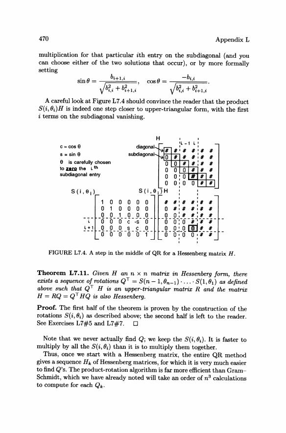
470 Appendix L

multiplication for that particular ith entry on the subdiagonal (and you can choose either of the two solutions that occur), or by more formally setting

-b· . cos () = ---r=="=' ==

A careful look at Figure L7.4 should convince the reader that the product 8(i, (}i)H is indeed one step closer to upper-triangular form, with the first i terms on the subdiagonal vanishing.

c=cose

s = sin e

H , 'l -,

diagonal # /I: /I subdiagonal 0 # #

#

e is carefully chosen to ZUQ the l th subdiagonal entry

o ,-,0;.+-#,:-+..."...; o 0 0

o 0: 0 ~+::+...::~

l l +,

o 0, 0 , S (i. 9,) H : , ,

1 0 0 0 0 0 # #:# #:# # o 1 0 0 0 0 0 #'# #'# # o 0 1 0 0 0 0 0:# #:# #

-6-0--0--6"--8--0- -5-o-'-0-#-'·:f-i--

-Ot! - -00- _00- _SO- - 50- -1Q. - _Q - _O_:_Q. li::L#_ -~-o 0'0 0,# # , , , ,

FIGURE L7.4. A step in the middle of QR for a Hessenberg matrix H.

Theorem L 7 .11. Given H an n x n matrix in H essenberg form, there exists a sequence of rotations QT = 8(n - 1, (}n-I) .... ·8(1, (}I) as defined above such that QT H is an upper-triangular matrix R and the matrix H = RQ = QT HQ is also Hessenberg.

Proof. The first half of the theorem is proven by the construction of the rotations 8(i, (}i) as described above; the second half is left to the reader. See Exercises L7#5 and L7#7. 0

Note that we never actually find Q; we keep the 8(i, (}i). It is faster to multiply by all the 8( i, (}i) than it is to multiply them together.

Thus, once we start with a Hessenberg matrix, the entire QR method gives a sequence H k of Hessenberg matrices, for which it is very much easier to find Q's. The product-rotation algorithm is far more efficient than Gram­Schmidt, which we have already noted will take an order of n3 calculations to compute for each Qk.

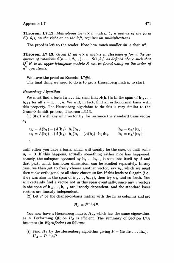
Appendix L7 471

Theorem L7.12. Multiplying an n x n matrix by a matrix of the form 8(i,Oi), on the right or on the left, requires 4n multiplications.

The proof is left to the reader. Note how much smaller 4n is than n 3 •

Theorem L7.13. Given H an n x n matrix in Hessenberg form, the se­quence of rotations 8(n - 1, On-l) .... ·8(1, OI) as defined above such that QT H is an upper-triangular matrix R can be found using on the order of n2 operations.

We leave the proof as Exercise L7#6. The final thing we need to do is to get a Hessenberg matrix to start.

Hessenberg Algorithm

We must find a basis hl, ... ,hn such that A(hi ) is in the span of hl, ... , hi+l for all i = 1, ... , n. We will, in fact, find an orthonormal basis with this property. The Hessenberg algorithm to do this is very similar to the Gram-Schmidt process, Theorem L3.13.

(1) Start with any unit vector hl, for instance the standard basis vector

U2 = A(hd - (A(hd . hl)hl, U3 = A(h2) - (A(h2) . hl)hl - (A(h2) . h2)h2'

h2 = u2/llu21i, h3 = U3/li u31i,

until either you have a basis, which will usually be the case, or until some Ui = O. If this happens, actually something rather nice has happened, namely, the subspace spanned by hl, ... , h i - l is sent into itself by A and that part, which has lower dimension, can be studied separately. In any case, we then get to freely choose another vector, say e2, which we must then make orthogonal to all those chosen so far. If this leads to 0 again (Le., if e2 was also in the span of h l , .. . , hi-d, then try e3, and so forth. You will certainly find a vector not in this span eventually, since any i vectors in the span of hl, ... ,hi - l are linearly dependent, and the standard basis vectors are linearly independent.

(2) Let P be the change-of-basis matrix with the hi as columns and set

HA = P-lAP.

You now have a Hessenberg matrix H A , which has the same eigenvalues as A. Performing QR on HA is efficient. The summary of Section L7.8 becomes (in Eigenfinder) as follows:

(i) Find HA by the Hessenberg algorithm giving P = (hl' h 2, ... ,hn ),

HA = P-lAP.

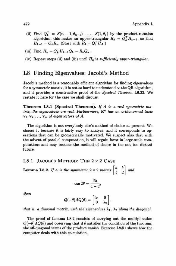
472 Appendix L

(ii) Find Ql = Sen - 1,6n - 1 ) ••••• S(I, ( 1) by the product-rotation algorithm; this makes an upper-triangular Rk = Ql Hk- b so that Hk-l = QkRk. (Start with Rl = Qi HA.)

(iii) Find Hk = Ql Hk-lQk = RkQk,

(iv) Repeat steps (ii) and (iii) until Hk is sufficiently upper-triangular.

L8 Finding Eigenvalues: Jacobi's Method

Jacobi's method is a reasonably efficient algorithm for finding eigenvalues for a symmetric matrix, it is not as hard to understand as the QR algorithm, and it provides a constructive proof of the Spectral Theorem L6.22. We restate it here for the case we shall discuss.

Theorem LS.1 (Spectral Theorem). If A is a real symmetric ma­trix, the eigenvalues are real. Furthermore, R.n has an orthonormal basis Vb V2, ••• , Vn of eigenvectors of A.

The algorithm is not everybody else's method of choice at present. We choose it because it is fairly easy to analyze, and it corresponds to op­erations that can be geometrically motivated. We suspect also that with the advent of parallel computation, it will regain favor in large-scale com­putations and may become the method of choice in the not too distant future.

LB.l. JACOBI'S METHOD: THE 2 X 2 CASE

Lemma LS.2. If A is the symmetric 2 x 2 matrix [: :] and

then

2b tan 26 = --d'

a-

Q(-6)AQ(6) = [~1 ~2]' that is, a diagonal matrix, with the eigenvalues >'1, >'2 along the diagonal.

The proof of Lemma LB.2 consists of carrying out the multiplication Q( -6)AQ( 6) and observing that if 6 satisfies the condition of the theorem, the off-diagonal terms of the product vanish. Exercise LB#1 shows how the computer deals with this calculation.

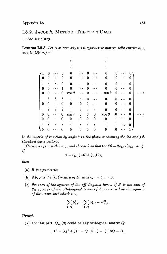
Appendix L8 473

L8.2. JACOBI'S METHOD: THE n X n CASE

1. l'he basic step.

Lemma L8.3. Let A be now any n x n symmetric matrix, with entries ai,j, and let Q( i, Bi ) =

i j

1 0 0 0 0 0 0 0 0 1 0 0 0 0 0 0

0 0 0 0 0 0 0 0 1 0 0 0 0 0 0 0 0 cos B 0 - sinB 0 0 ... i

0 0 0 0 0 0 0 0 0 1 0 0 0

0 0 0 0 0 0 sin B 0 0 0 cosB 0 0 ... j

0 0 0 0 0 0 0 0 1 0

0 0 0 0 0 0 0 0 0 0 1

be the matrix of rotation by angle B in the plane containing the ith and jth standard basis vectors.

Choose any i, j with i < j, and choose B so that tan 2B = 2ai,j / (ai,i -aj,j). If

B = Q. ·(-B)AQ· ·(B) 'I.,J t,J'

then

( a) B is symmetric;

(b) if bk,l is the (k, f) -entry of B, then bi,j = bj,i = 0;

(c) the sum of the squares of the off-diagonal terms of B is the sum of the squares of the off-diagonal terms of A, decreased by the squares of the terms just killed; i. e.,

L b%,l = L a%,l - 2a~,j' k# k-f-l

Proof.

(a) For this part, Qi,j(B) could be any orthogonal matrix Q:

BT = (QT AQ)T = QT AT Q = QT AQ = B.

474 Appendix L

(b) This is exactly the computation in the 2 x 2 case of Lemma LS.2. You can show as Exercise LS#2 that for n > 2 the resulting relevant computations involve just the ith and jth rows and columns, which is just like the 2 x 2 case.

(c) This is where the real content of Jacobi's method is. Let ek be the standard basis vectors and Wk be the orthonormal basis vectors form­ing the columns of Qi,j((J)j in particular, ek = Wk if k =f i,j. Note that

and

Aet ~

lth column of A , '" kth component of lth column of A

bk,t = ek . Bet = ek . Q-l AQel = Wk . AWL.

This restates that B is the matrix of A in the basis of the Wi'S.

Now we will look at 2:k;ll b~,l and 2:k;ll a~,l' considering the three dif­ferent possibilities for k and l:

(i) If neither index is an i or a j, then bk,l = ak,l, so the corresponding squares are certainly equal (k =f i,jj l =f i,jj k =f l).

ii) On the other hand, if exactly one index is an i or a j, we will handle the entries in pairs (k =f i,j): The quantity

a~,i + a~,j = (Aek . ei)2 + (Aek . ej)2

is the squared length of the projection of Aek onto the plane spanned by ei and ej. Since the same plane is spanned by Wi and Wj, we see that

bk2 • + b2k • ,'l ,3

is also the squared length of the projection of AWk = Aek onto that plane, so that

a~,i + aL = b~,i + bL·

The same argument applies to indices (i, k) and (j, k) with k =f i, j.

(iii) Lastly, if both indices are from the off-diagonal term i, j or j, i, then

b~ . + b~ . = 2b~ . = 0 '&,3 3,1. '&,3 '

though a~ . + a2 . = 2a~ . ...J. O. '&,3 3," 'I.,) -;-

Summing up the contributions from (i), (ii), and (iii), we have

L: btl = L: b~,l + 2 L: (bL + b~,j) + 0 k# k;li,j;l;li,j;k# k;li,j

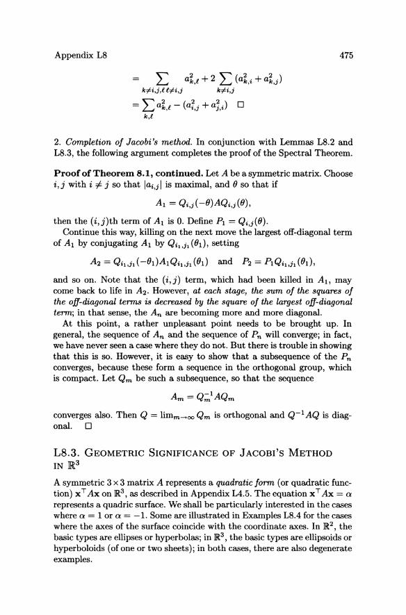
Appendix LS 475

= L atl + 2 L (a%,i + a%,j) kt-i,j,Ut-i,j kt-i,j

= ~ ak2 • - (a~ . + a~.) 0 L.-J ,-t. ',3 J,'t

k,l

2. Completion of Jacobi's method. In conjunction with Lemmas LS.2 and LS.3, the following argument completes the proof of the Spectral Theorem.

Proof of Theorem 8.1, continued. Let A be a symmetric matrix. Choose i, j with i =F j so that lai,j I is maximal, and () so that if

Al = Qi,j( -(})AQi,j«(}),

then the (i,j)th term of Al is O. Define PI = Qi,j«(})' Continue this way, killing on the next move the largest off-diagonal term

of Al by conjugating Al by Qil,jl «(}l), setting

A2 = Qit.i1 (-(}1)A1Qil,i1 «(}l) and P2 = PI Qit.i1 «(}t},

and so on. Note that the (i,j) term, which had been killed in AI. may come back to life in A 2 • However, at each stage, the sum of the squares of the off-diagonal terms is decreased by the square of the largest off-diagonal term; in that sense, the An are becoming more and more diagonal.

At this point, a rather unpleasant point needs to be brought up. In general, the sequence of An and the sequence of Pn will converge; in fact, we have never seen a case where they do not. But there is trouble in showing that this is so. However, it is easy to show that a subsequence of the Pn

converges, because these form a sequence in the orthogonal group, which is compact. Let Qm be such a subsequence, so that the sequence

Am = Q;;'; AQm

converges also. Then Q = limm ..... oo Qm is orthogonal and Q-l AQ is diag­onal. 0

L8.3. GEOMETRIC SIGNIFICANCE OF JACOBI'S METHOD IN ]R3

A symmetric 3 x 3 matrix A represents a quadratic form (or quadratic func­tion) x TAx on IR3, as described in Appendix L4.5. The equation x TAx = O!

represents a quadric surface. We shall be particularly interested in the cases where O! = 1 or O! = -1. Some are illustrated in Examples LS.4 for the cases where the axes of the surface coincide with the coordinate axes. In IR2, the basic types are ellipses or hyperbolas; in IR3 , the basic types are ellipsoids or hyperboloids (of one or two sheets); in both cases, there are also degenerate examples.

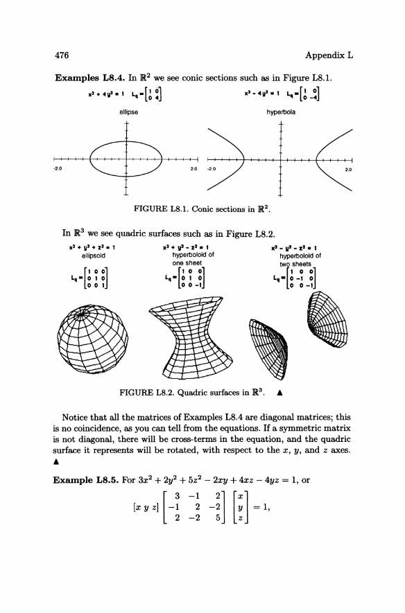
476 Appendix L

Examples LS.4. In ]R2 we see conic sections such as in Figure L8.1.

-2.0

1I'.4v'·1 ~-[!~ ellipse

2.0

1I'-4V'·1 ~-[!..:] hyperbola

FIGURE LB.1. Conic sections in ]R2.

In ]R3 we see quadric surfaces such as in Figure L8.2.

1I'.y'.z'.1 ellipsoid

[ 1 00] L.- 0 1 0 001

1I'.y'-Z'.1 hyperboloid of

on[~ s~ee~] L.- 0 1 0

00-1

1I'-II'-z'.1 hyperboloid of

two[r:et~] L.- 0 -1 0

o 0-1

FIGURE LB.2. Quadric surfaces in ]R3. A

Notice that all the matrices of Examples LS.4 are diagonal matrices; this is no coincidence, as you can tell from the equations. If a symmetric matrix is not diagonal, there will be cross-terms in the equation, and the quadric surface it represents will be rotated, with respect to the x, y, and z axes. A

Example LS.5. For 3x2 + 2y2 + 5z2 - 2xy + 4xz - 4yz = 1, or

-1 2] [X] 2 -2 Y -2 5 z

= 1,

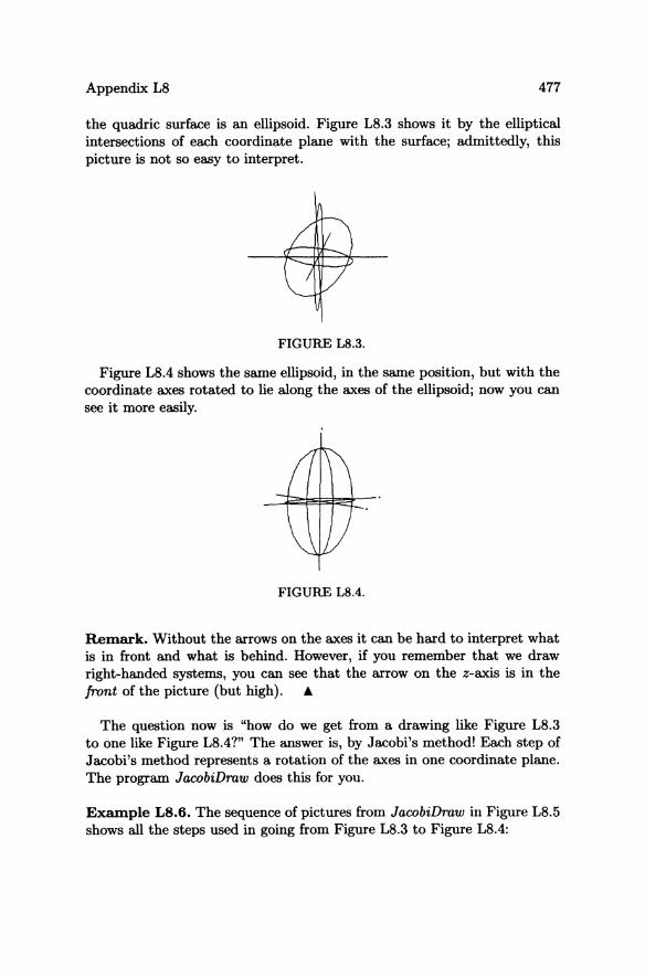
Appendix L8 477

the quadric surface is an ellipsoid. Figure L8.3 shows it by the elliptical intersections of each coordinate plane with the surface; admittedly, this picture is not so easy to interpret.

FIGURE LS.3.

Figure L8.4 shows the same ellipsoid, in the same position, but with the coordinate axes rotated to lie along the axes of the ellipsoid; now you can see it more easily.

FIGURE LS.4.

Remark. Without the arrows on the axes it can be hard to interpret what is in front and what is behind. However, if you remember that we draw right-handed systems, you can see that the arrow on the z-axis is in the front of the picture (but high). &

The question now is "how do we get from a drawing like Figure L8.3 to one like Figure L8.4?" The answer is, by Jacobi's method! Each step of Jacobi's method represents a rotation of the axes in one coordinate plane. The program JacobiDraw does this for you.

Example L8.6. The sequence of pictures from JacobiDraw in Figure L8.5 shows all the steps used in going from Figure L8.3 to Figure L8.4:

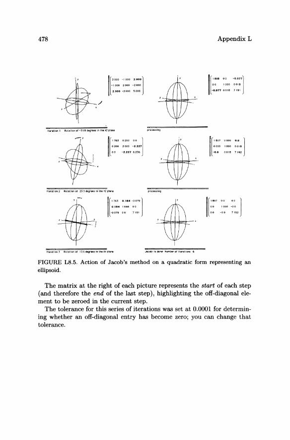
478

1[·" 70: .~:: .::::] 2.000 -2000 5.000

Itenllon I Rotation of -31" dlgrees In the Xl plane

1['- 0'00 00 ] 0200 2000 -2.227

00 -2.221 6.236

n.ratlon2 Rot,tlonol 2JJ dlgra.s In the VZ plen,

1[ '7.' 0.' •• -0079]

0.1114 1044 00

-0079 00 7191

. !

ItlAtlon J RotatIonal Il6d1grl" In lhe XV pI.",

pnlClss'ng

Jacobi 's dOn.I Hwnblr of HtrlUons 6

Appendix L

1['000 00

00 1000

-0.077 0018

1['·' 0000

0000 1000

-0.0 0016

-.. 077] 00'8

7191

00 ] 0.016

7192

1[ ~:07 '000 -:: ]

00 -00 7192

FIGURE L8.5. Action of Jacob's method on a quadratic form representing an ellipsoid.

The matrix at the right of each picture represents the start of each step (and therefore the end of the last step), highlighting the off-diagonal ele­ment to be zeroed in the current step.

The tolerance for this series of iterations was set at 0.0001 for determin­ing whether an off-diagonal entry has become zero; you can change that tolerance.

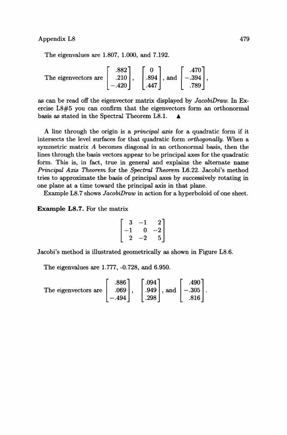
Appendix L8 479

The eigenvalues are 1.807, 1.000, and 7.192.

[ .882]

The eigenvectors are .210, -.420

[ 0 ] [.470] .894 ,and - .394 , .447 .789

as can be read off the eigenvector matrix displayed by JacobiDmw. In Ex­ercise L8#5 you can confirm that the eigenvectors form an orthonormal basis as stated in the Spectral Theorem L8.1. ~

A line through the origin is a principal axis for a quadratic form if it intersects the level surfaces for that quadratic form orthogonally. When a symmetric matrix A becomes diagonal in an orthonormal basis, then the lines through the basis vectors appear to be principal axes for the quadratic form. This is, in fact, true in general and explains the alternate name Principal Axis Theorem for the Spectrol Theorem L6.22. Jacobi's method tries to approximate the basis of principal axes by successively rotating in one plane at a time toward the principal axis in that plane.

Example L8.7 shows JacobiDmw in action for a hyperboloid of one sheet.

Example L8.7. For the matrix

H -1 2] o -2 -2 5

Jacobi's method is illustrated geometrically as shown in Figure L8.6.

The eigenvalues are 1.777, -0.728, and 6.950.

[ .886]

The eigenvectors are .069, -.494

[.094] [.490] .949 ,and -.305 . .298 .816

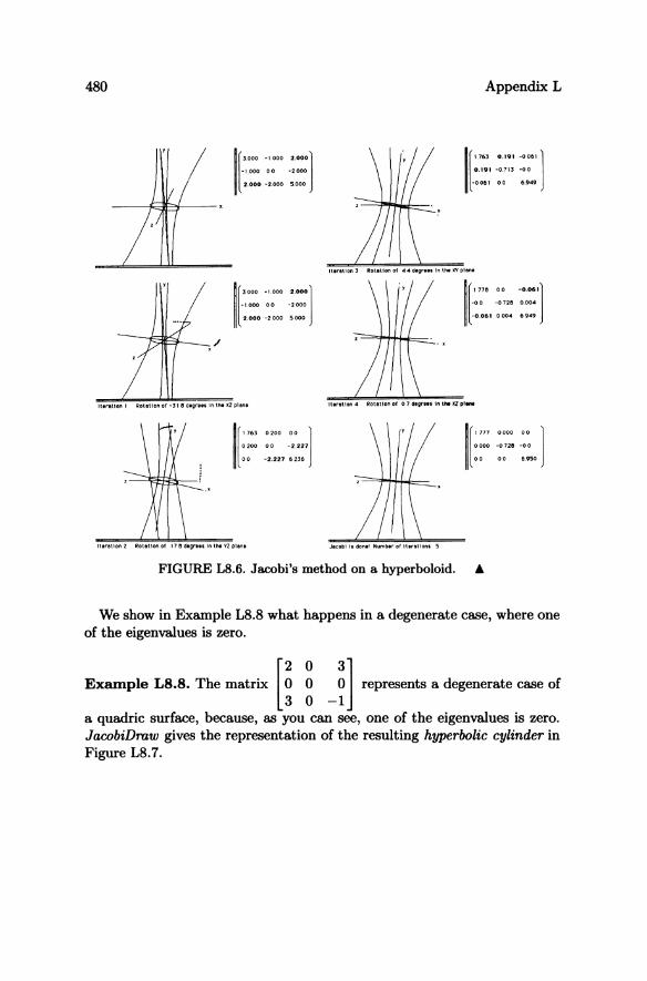
480

[

3.000 ., 000 2 .••• )

-1.000 00 -2000

2.000 -2.000 5.000

[

"63

0200

00

0200 00 ) 00 -2.221

-2.227 6236

Appendix L

1[ 1.763 •. , ••• 006')

0.19l -0.713 -00

-0061 00 6.949

I[ ~:: .:: .:: ) 00 00 6950

FIGURE L8.6. Jacobi's method on a hyperboloid. A

We show in Example LS.S what happens in a degenerate case, where one of the eigenvalues is zero.

Example L8.8. The matrix [~~ ~l represents a degenerate case of 3 0 -1

a quadric surface, because, as you can see, one of the eigenvalues is zero. JacobiDraw gives the representation of the resulting hyperbolic cylinder in Figure LS.7.

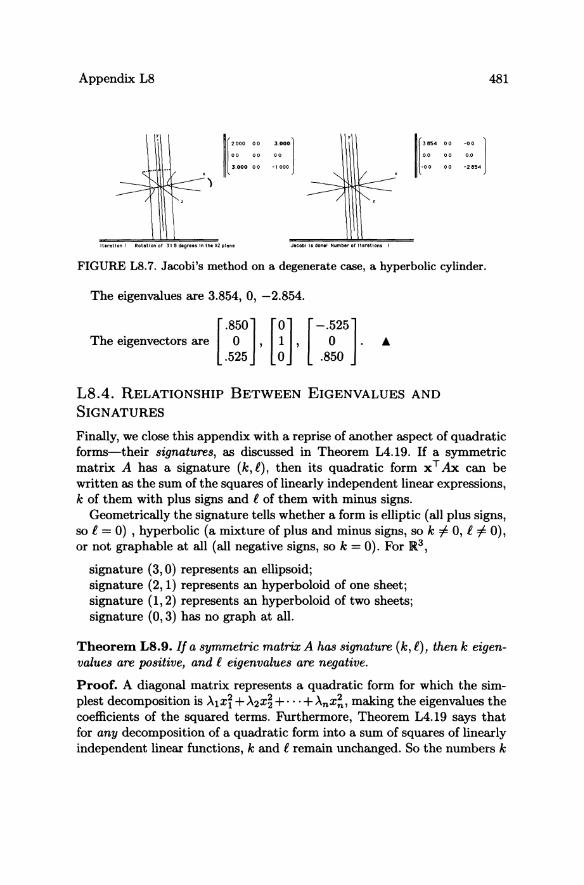
Appendix L8

1[::00:: ::00) 3.000 00 -,000

)

1[30.4 00 -00 ) 0,0 00 0.0

-00 00 -2854

It .... tlan I Rotatlonof 318dlgre ... nlh,lIlplenl Jacobi II don,1 Number of tteratlon, I

FIGURE L8.7. Jacobi's method on a degenerate case, a hyperbolic cylinder.

The eigenvalues are 3.854,0, -2.854.

[ .850] [0] [-.525] The eigenvectors are ° , 1, ° . . 525 0 .850

L8.4. RELATIONSHIP BETWEEN EIGENVALUES AND

SIGNATURES

481

Finally, we close this appendix with a reprise of another aspect of quadratic forms-their signatures, as discussed in Theorem L4.19. If a symmetric matrix A has a signature (k, i), then its quadratic form x TAx can be written as the sum of the squares of linearly independent linear expressions, k of them with plus signs and i of them with minus signs.

Geometrically the signature tells whether a form is elliptic (all plus signs, so i = 0) , hyperbolic (a mixture of plus and minus signs, so k "# 0, i "# 0), or not graphable at all (all negative signs, so k = 0). For 1R3 ,

signature (3,0) represents an ellipsoid; signature (2,1) represents an hyperboloid of one sheet; signature (1,2) represents an hyperboloid of two sheets; signature (0,3) has no graph at all.

Theorem L8.9. If a symmetric matrix A has signature (k, i), then k eigen­values are positive, and i eigenvalues are negative.

Proof. A diagonal matrix represents a quadratic form for which the sim­plest decomposition is Al x~ + A2X~ + ... + AnX~, making the eigenvalues the coefficients of the squared terms. Furthermore, Theorem L4.19 says that for any decomposition of a quadratic form into a sum of squares of linearly independent linear functions, k and i remain unchanged. So the numbers k

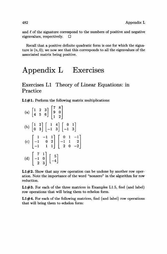
482 Appendix L

and i of the signature correspond to the numbers of positive and negative eigenvalues, respectively. 0

Recall that a positive definite quadratic form is one for which the signa­ture is (n, 0); we now see that this corresponds to all the eigenvalues of the associated matrix being positive.

Appendix L Exercises

Exercises Ll Theory of Linear Equations: In Practice

Ll#l. Perform the following matrix multiplications:

(a) [1 2 3J [7 8] 4 5 6 9 0 I 2

(b) [~ ~] [-! :] [-~ !] [~: -1

~] H 1 ~~] (c) 0 1 -1 1 0 -2

(d) H i] [~:J Ll#2. Show that any row operation can be undone by another row oper­ation. Note the importance of the word "nonzero" in the algorithm for row reduction.

Ll#3. For each of the three matrices in Examples L1.5, find (and label) row operations that will bring them to echelon form.

Ll#4. For each of the following matrices, find (and label) row operations that will bring them to echelon form:

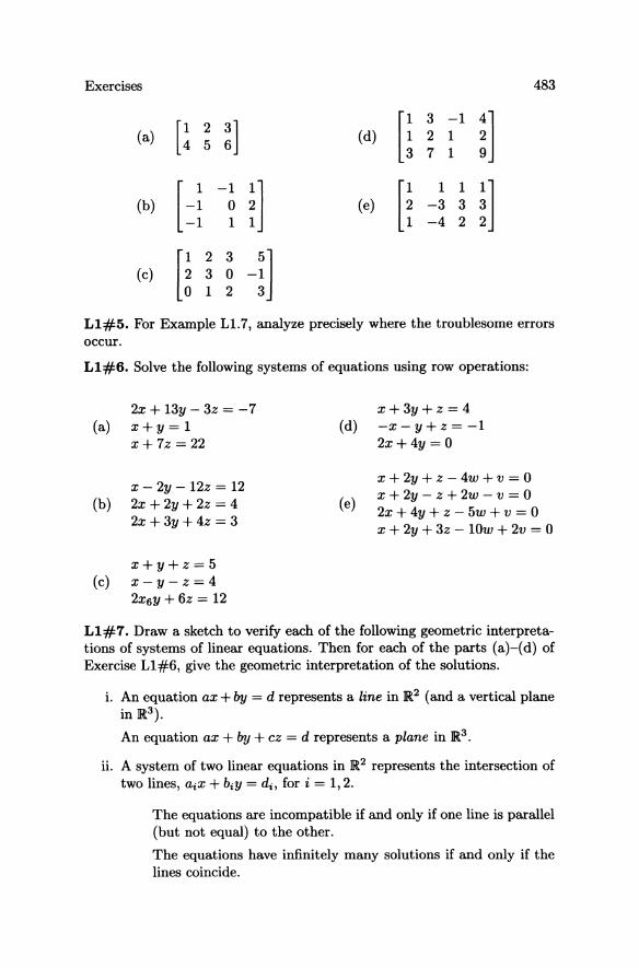
Exercises 483

[1 2 3] [!

3 -1

~l (a) 456 (d) 2 1 7 1

[-: -1

~l [~ 1 1

~l (b) 0 (e) -3 3 -1 1 -4 2

[1 2 3 -!l (c) 2 3 0 o 1 2

Ll#5. For Example L1.7, analyze precisely where the troublesome errors occur.

Ll#6. Solve the following systems of equations using row operations:

2x + 13y - 3z = -7 (a) x + y = 1

x+ 7z = 22

x - 2y - 12z = 12 (b) 2x + 2y + 2z = 4

2x+3y+4z = 3

x+y+z=5 (c) x-y-z=4

2X6Y + 6z = 12

(d)

(e)

x+3y+z=4 -x-y+z =-1 2x+4y = 0

x + 2y + z - 4w + v = 0 x + 2y - z + 2w - v = 0 2x + 4y + z - 5w + v = 0 x + 2y + 3z - lOw + 2v = 0

Ll#7. Draw a sketch to verify each of the following geometric interpreta­tions of systems of linear equations. Then for each of the parts (a)-(d) of Exercise Ll#6, give the geometric interpretation of the solutions.

i. An equation ax + by = d represents a line in ]R2 (and a vertical plane in ]R3).

An equation ax + InJ + cz = d represents a plane in ]R3.

11. A system of two linear equations in ]R2 represents the intersection of two lines, aix + biy = di , for i = 1,2.

The equations are incompatible if and only if one line is parallel (but not equal) to the other.

The equations have infinitely many solutions if and only if the lines coincide.

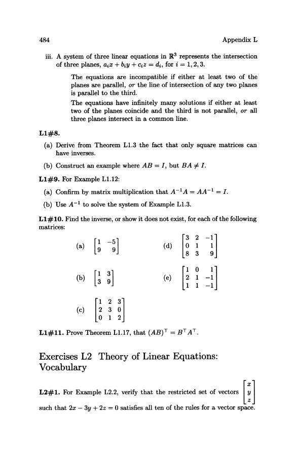
484 Appendix L

iii. A system of three linear equations in 1R3 represents the intersection of three planes, aiX + biy + CiZ = d i , for i = 1,2,3.

Ll#8.

The equations are incompatible if either at least two of the planes are parallel, or the line of intersection of any two planes is parallel to the third.

The equations have infinitely many solutions if either at least two of the planes coincide and the third is not parallel, or all three planes intersect in a common line.

(a) Derive from Theorem L1.3 the fact that only square matrices can have inverses.

(b) Construct an example where AB = I, but BA:f:. I.

Ll#9. For Example L1.12:

(a) Confirm by matrix multiplication that A-I A = AA-I = I. (b) Use A-I to solve the system of Example L1.3.

Ll#10. Find the inverse, or show it does not exist, for each of the following matrices:

[~ -~] [~ 2

-i] (a) (d) 1 3

[! ~] [1 0 -:] (b) (e) 1 1 -1

(e) U H] Ll#l1. Prove Theorem L1.17, that (AB)T = BT AT.

Exercises L2 Theory of Linear Equations: Vocabulary

L2#1. Fo, Example L2.2, ""'iCy that the 'estrieted set of veeto", [~] such that 2x - 3y + 2z = 0 satisfies all ten of the rules for a vector space.

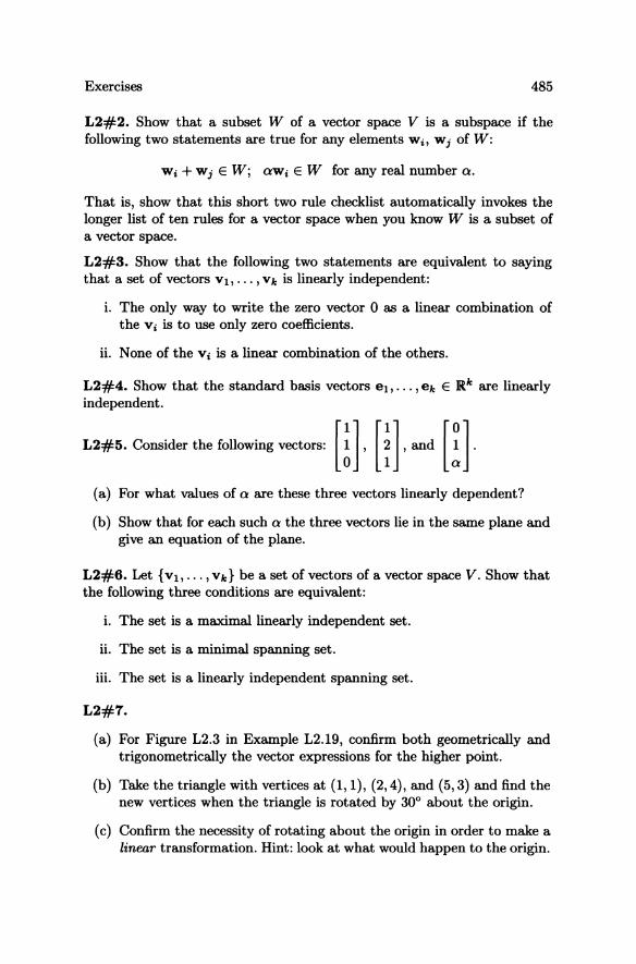
Exercises 485

L2#2. Show that a subset W of a vector space V is a subspace if the following two statements are true for any elements Wi, Wi of W:

Wi + Wi E Wj aWi E W for any real number a.

That is, show that this short two rule checklist automatically invokes the longer list of ten rules for a vector space when you know W is a subset of a vector space.

L2#3. Show that the following two statements are equivalent to saying that a set of vectors Vl, ... ,Vk is linearly independent:

i. The only way to write the zero vector 0 as a linear combination of the viis to use only zero coefficients.

ii. None of the Vi is a linear combination of the others.

L2#4. Show that the standard basis vectors el, ... ,ek E IRk are linearly independent.

L2#5. ~nmder the fullowffig vreOOrn' m. [~]. and [!]. (a) For what values of a are these three vectors linearly dependent?

(b) Show that for each such a the three vectors lie in the same plane and give an equation of the plane.

L2#6. Let {Vb ... , Vk} be a set of vectors of a vector space V. Show that the following three conditions are equivalent:

i. The set is a maximal linearly independent set.

ii. The set is a minimal spanning set.

iii. The set is a linearly independent spanning set.

L2#7.

(a) For Figure L2.3 in Example L2.19, confirm both geometrically and trigonometrically the vector expressions for the higher point.

(b) Take the triangle with vertices at (1,1), (2,4), and (5,3) and find the new vertices when the triangle is rotated by 30° about the origin.

(c) Confirm the necessity of rotating about the origin in order to make a linear transformation. Hint: look at what would happen to the origin.

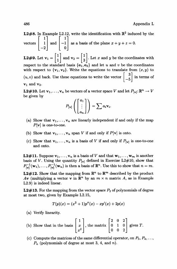
486 Appendix L

L2#8. In Example L2.12, write the identification with JR2 induced by the -= Ul and Hl as a baffis oflhe plane x+y+z ~ o.

L2#9. Let VI = [~] and V2 = [!]. Let x and y be the coordinates with

respect to the standard basis {ell e2} and let u and v be the coordinates with respect to {Vb V2}. Write the equations to translate from (x, y) to

(u, v) and back. Use these equations to write the vector [ _:] in terms of

VI and V2.

L2#10. Let Vb ... , V n be vectors of a vector space V and let p[vJ: JRn ~ V be given by

(a) Show that VI, ... , Vn are linearly independent if and only if the map P[v] is one-to-one.

(b) Show that Vb ... , Vn span V if and only if P[v] is onto.

(c) Show that Vb ... , vn is a basis of V if and only if p[vJ is one-to-one and onto.

L2#11. Suppose Vb ... ,Vn is a basis of V and that Wb ... , Wm is another basis of V. Using the quantity p[vJ defined in Exercise L2#1D, show that p[~JI(WI)' ... ' P[~{(Wn) is then a basis of JRn. Use this to show that n = m.

L2#12. Show that the mapping from JRn to JRm described by the product Av (multiplying a vector V in JRn by an m x n matrix A, as in Example L2.9) is indeed linear.

L2# 13. For the mapping from the vector space P2 of polynomials of degree at most two, given by Example L2.15,

T(p)(x) = (x2 + l)p"(x) - xp'(x) + 2p(x)

(a) Verify linearity.

(b) Show that in the basis [! 1 ' the matrix [~ ~ ~l gives T. x 2 0 0 2

(c) Compute the matrices of the same differential operator, on P3 , P4 , ••• ,

Pn (polynomials of degree at most 3, 4, and n).

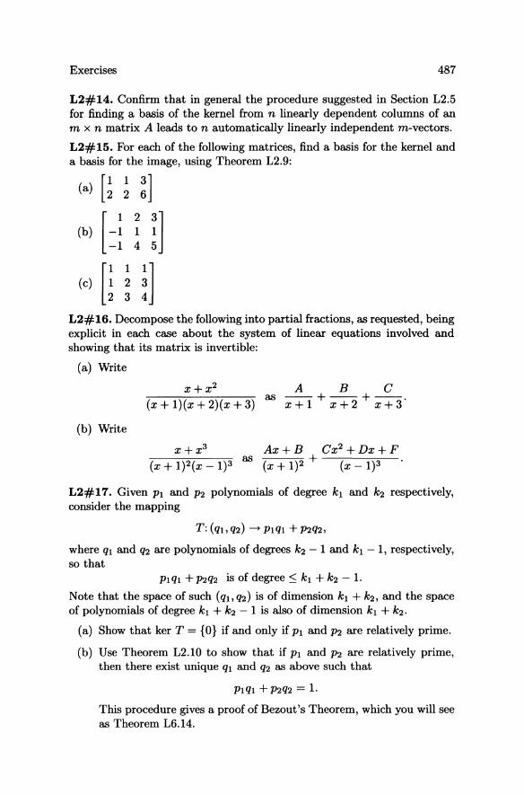
Exercises 487

L2#14. Confirm that in general the procedure suggested in Section L2.5 for finding a basis of the kernel from n linearly dependent columns of an m x n matrix A leads to n automatically linearly independent m-vectors.

L2#15. For each of the following matrices, find a basis for the kernel and a basis for the image, using Theorem L2.9:

(a) [~ ~ !] (b) [-~ ~ ~]

-1 4 5

(c) [~ ~ !] 234

L2#16. Decompose the following into partial fractions, as requested, being explicit in each case about the system of linear equations involved and showing that its matrix is invertible:

(a) Write

(b) Write

x+x2

(x + 1)(x + 2)(x + 3) as

ABC --+--+--. x+l x+2 x+3

(x + 1)2(x - 1)3 Ax + B Cx2 + Dx + F

as (x + 1)2 + (x _ 1)3

L2#17. Given PI and P2 polynomials of degree kl and k2 respectively, consider the mapping

T: (qt, q2) -+ Plql + P2q2,

where ql and q2 are polynomials of degrees k2 - 1 and kl - 1, respectively, so that

PI ql + P2q2 is of degree ~ kl + k2 - 1.

Note that the space of such (ql, q2) is of dimension kl + k2' and the space of polynomials of degree kl + k2 - 1 is also of dimension kl + k 2.

(a) Show that ker T = {O} if and only if PI and P2 are relatively prime.

(b) Use Theorem L2.1O to show that if PI and P2 are relatively prime, then there exist unique ql and q2 as above such that

Plql + P2q2 = 1.

This procedure gives a proof of Bezout's Theorem, which you will see as Theorem L6.14.

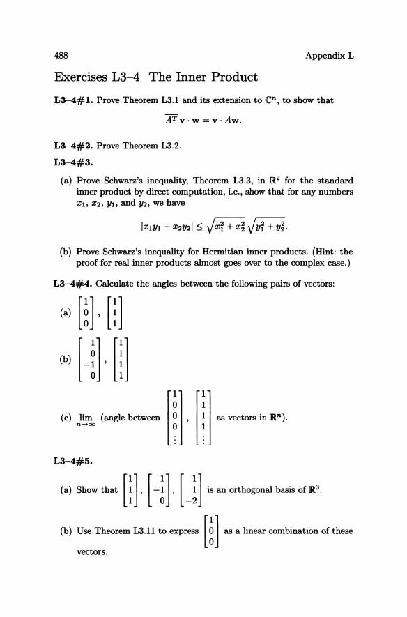
488 Appendix L

Exercises L3-4 The Inner Product

L3-4#1. Prove Theorem L3.1 and its extension to en, to show that

ATy·w=y·Aw.

L3-4#2. Prove Theorem L3.2.

L3-4#3.

(a) Prove Schwarz's inequality, Theorem L3.3, in ]R2 for the standard inner product by direct computation, i.e., show that for any numbers Xl, X2, Ylo and Y2, we have

(b) Prove Schwarz's inequality for Hermitian inner products. (Hint: the proof for real inner products almost goes over to the complex case.)

L3-4#4. Calculate the angles between the following pairs of vectors:

L3-4#5.

(a) Show that [ll Hl U 1 m an orthogonal - of R'.

(h) Use Themem L3.11 to express [i las a linear comhinat;on of theoe

vectors.

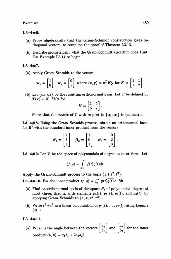
Exercises 489

L3-4#6.

(a) Prove algebraically that the Gram-Schmidt construction gives or­thogonal vectors, to complete the proof of Theorem L3.13.

(b) Describe geometrically what the Gram-Schmidt algorithm does. Hint: Use Example L3.14 to begin.

L3-4#7.

(a) Apply Gram-Schmidt to the vectors

Wl= [~], W2= [~] where (x,y) =xTKy for K= U ~]. (b) Let {u!, U2} be the resulting orthonormal basis. Let T be defined by

T(x) = K-l Hx for

H=[!~]. Show that the matrix of T with respect to {u!, U2} is symmetric.

L3-4#8. Using the Gram-Schmidt process, obtain an orthonormal basis for 1R3 with the standard inner product from the vectors

L3-4#9. Let V be the space of polynomials of degree at most three. Let

(f,g) = 11 f(t)g(t)dt.

Apply the Gram-Schmidt process to the basis {I, t, t2 , t3}.

L3-4#1O. For the inner product (p, q) = Jooo p(t)q(t) ctdt

(a) Find an orthonormal basis of the space P3 of polynomials degree at most three, that is, with elements Po(t), Pl(t), P2(t), and P3(t), by applying Gram-Schmidt to {I, X, x 2 , x3 }.

(b) Write t2 + t3 as a linear combination of Po ( t), ... , P3 ( t ), using Lemma L3.11.

L3-4#1l.

( a) What is the angle between the vectors [:~] and [:~] for the inner

product (a, b) = albl + 2a2b2?

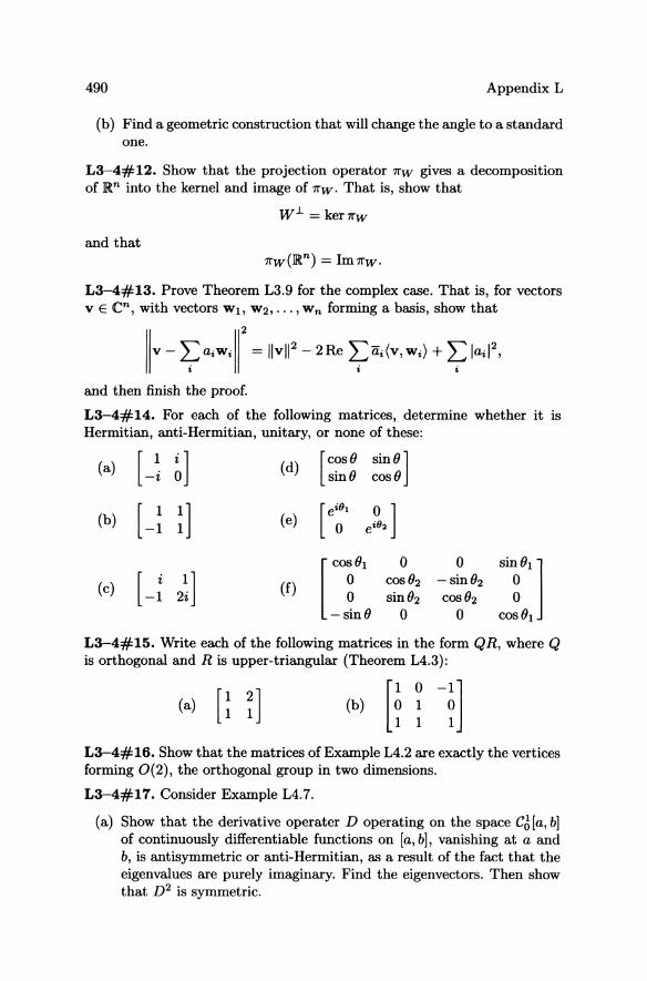
490 Appendix L

(b) Find a geometric construction that will change the angle to a standard one.

L3-4#12. Show that the projection operator 1Tw gives a decomposition of]Rn into the kernel and image of 1Tw. That is, show that

Wl. = ker1Tw

and that

L3-4#13. Prove Theorem L3.9 for the complex case. That is, for vectors v E en, with vectors WI, W2, ... , Wn forming a basis, show that

and then finish the proof.

L3-4#14. For each of the following matrices, determine whether it is Hermitian, anti-Hermitian, unitary, or none of these:

(a) [ Ii] -i 0 (d) [ cosO

sinO sin 0] cosO

(b) (e) [ e~l e~2 ]

[~61 0 0

161 ] -sto

cos O2 - sin O2

sin O2 cos O2

0 0 COS Ol

(c) [ i 1] -1 2i (f)

L3-4#15. Write each of the following matrices in the form QR, where Q is orthogonal and R is upper-triangular (Theorem L4.3):

(a) [~ i] L3-4#16. Show that the matrices of Example L4.2 are exactly the vertices forming 0(2), the orthogonal group in two dimensions.

L3-4#17. Consider Example L4.7.

(a) Show that the derivative operater D operating on the space CJ [a, bj of continuously differentiable functions on [a, bj, vanishing at a and b, is antisymmetric or anti-Hermitian, as a result of the fact that the eigenvalues are purely imaginary. Find the eigenvectors. Then show that D2 is symmetric.

Exercises 491

(b) Do the same for the space of functions satisfying I (a) = I (b), I' (a) = /,(b).

(c) Show that D2 is symmetric, operating on the space of functions which vanish at a and whose derivatives vanish at b.

(d) Do the same as in part (c) for the space of functions such that I(a) = I'(a) and I(b) = /,(b).

(e) For any numbers 0: and (3 not both zero, and any numbers 'Y and 6 not both zero, do the same as in part (c) for the space of functions I such that

0:/(0) + (3/'(0) = 0

'YI(7r) + 6/,(7r) = o.

L3-4#18. For the quadratic form of Example L4.16,

x 2 + 2xy - 4xz + 2yz - 4Z2

(a) Show that completing the square starting with the z terms, then the y term, and finally the x terms leads to x 2+(x+y/2)2 - (x-y/2+2z)2, as stated in the example.

(b) Find the decomposition by completing the square if you start with the y terms, then do the x terms, and finally the z terms.

L3-4#19. Decompose each of the following quadratic forms by completing squares, and determine its signature.

(a) x 2 + xy _ y2

(b) x 2 + 2xy _ y2

(c) x 2 +xy+yz

(d) xy+yz

L3-L4#20. Consider Example L4.17

q(x) = xy - xz + yz.

(a) Verify that the decomposition

(x/2 + y/2)2 - (x/2 - y/2 + Z)2 + Z2

is indeed composed of linearly independent functions.

(b) Decompose q(x) with a different choice of u, to support the statement that u = x - y was not a magical choice.

492 Appendix L

L3-4#21. Check that the following quadratic forms are degenerate.

(a) x2 + 4xy + 4y2 on ]R2.

(b) x2 + 2xy + 2y2 + 2yz + z2 on ]R3.

(c) 2x2 + 2y2 + z2 + w2 + 4xy + 2xz - 2xw - 2yw on ]R4.

L3-4#22. On R4 88 described by M = [: ~ ], consider the quadratic

form q(M) = det M. What is its signature?

L3-4#23. On W 88 described by H = [b ~ ic b ~ ic ], the space of

Hermitian 2 x 2 matrices, consider the quadratic form q(H) = det H. What is its signature?

L3-4#24. For any real n x n matrix M

(a) Show that M can be written uniquely 88 a sum of a symmetric matrix and an antisymmetric matrix. (Hint: M + MT is symmetric.)

(b) Consider the quadratic form on the vector space of symmetric matri­ces Ms given by qs(Ms) = tr(M~). Show that qs is positive definite.

(c) Consider the quadratic form on the vector space of antisymmetric matrices MA given by qA(MA) = tr(Ml). Show that qA is negative definite.

(d) Find the signature of q, defined by q(M) = tr(M2).

L3-4#25. For any complex n x n matrix M, find the signature of q, the Hermitian quadratic form defined by q(M) = tr(M M).

L3-4#26. Consider again q( M) = tr{ M2), operating on the space of upper

triangular matrices described by M = [~ : ] .

(a) What kind of surface in ]R3 do you get by setting q(M2) = 1?

(b) What kind of surface in]R3 do you get by setting q(MMT) = 1?

L3-4#27.

(a) Show that the function

([:~], [:~]) = 11(a1 +a2x)(b1 +b2x)dx

defines an inner product on ]R2, and compute its matrix.

Exercises 493

(b) There is an obvious generalization of part a to IR3 , using second degree polynomials. Do the corresponding problem.

L3-4#28. Show that a 2 x 2 matrix G = [: ~] represents an inner

product on IR2 if and only if G is symmetric, det G > 0, and tr G > O.

Exercises L5 Determinants and Volumes

L5#1. Compute the determinants of the following matrices according to development by the first row:

[1 23] (a) 4 01 5 -12

[1 -12]

(b) 0 34 2 10

[1 2 3 4] o 1-1 2

(c) 3 0 1-1 1-1 2 0

L5#2. In the proof of Theorem L5.3, show that the specified row opera­tions give a diagonal matrix with the same diagonal entries as the original matrix.

L5#3. For Theorem L5.3,

(a) Give an alternate proof direct from the recursive definition of D for the case where the matrix is lower triangular.

(b) Adapt the proof in part (a) to the case where the matrix is upper­triangular .

L5#4. For a matrix A, we defined the determinant D(A) recursively by development according to the first row. Show that it could have equally well been defined, with the same result, as development according to the first column.

L5#5. For the matrix A = [! ~ ] (a) Compute the characteristic polynomial and find its roots.

(b) With the change of basis matrix P = [~ ! ] , compute the charac­

teristic polynomial of p-1 AP and find its roots, thus confirming the basis independence of the characteristic polynomial.

L5#6. As stated in Example L5.12, prove that given a polynomial p(A), you can easily construct a matrix that has p(A) as its characteristic polyno­mial. You simply need to show that the stated general "companion" matrix M (or its transpose) indeed has the stated p(A) as detlAI - MI.

494 Appendix L

L5#7. Referring to change-of-basis as introduced in Section L2.4, prove the part of Theorem L5.15 that states the trace is also basis independent.

L5#8. Using classical geometry, show that for a parallelogram you can use either side as a base and still get the same area, confirming Theorem L5.15 for k = 2.

L5#9. To get a better feeling for the relation between volumes and de­terminants, make a drawing in the plane illustrating that property (iii) of Theorem L5.18 is true for areas of parallelograms. That is, show that the "before" and "after" parallelograms have the same area = base x height. (Hint: use a dissection argument.)

Remark: The general case is analogous, using volume = base x height.

L5#10. Find and identify geometrically the volumes of the solids spanned by the following sets of vectors:

(a) [~], [=~]

(b) [~], [~]

(c) [j], [=:] , [~] (d) m, [~~], m

Exercises L6 Eigenvalues and Eigenvectors

L6#1. Show that for a square matrix A the following four statements are equivalent, thus confirming the proof of Theorem L6.1:

i. A has no inverse.

ii. There exists a vector x =I 0 such that Ax = O.

iii. There exists a vector y that cannot be written as Ax.

IV. detA = O.

L6#2. Prove that if a 2 x 2 matrix A has only one eigenvalue and is not already diagonal, then A is not diagonalizable.

L6#3. For a 3 x 3 matrix A, derive the more complicated conditions and results for diagonalizability. You might refer to Exercise 9.6#14.

L6#4. Prove that if A is a triangular matrix, the eigenvalues of A are the diagonal entries, by applying Theorem L5.3 to >"1 - A.

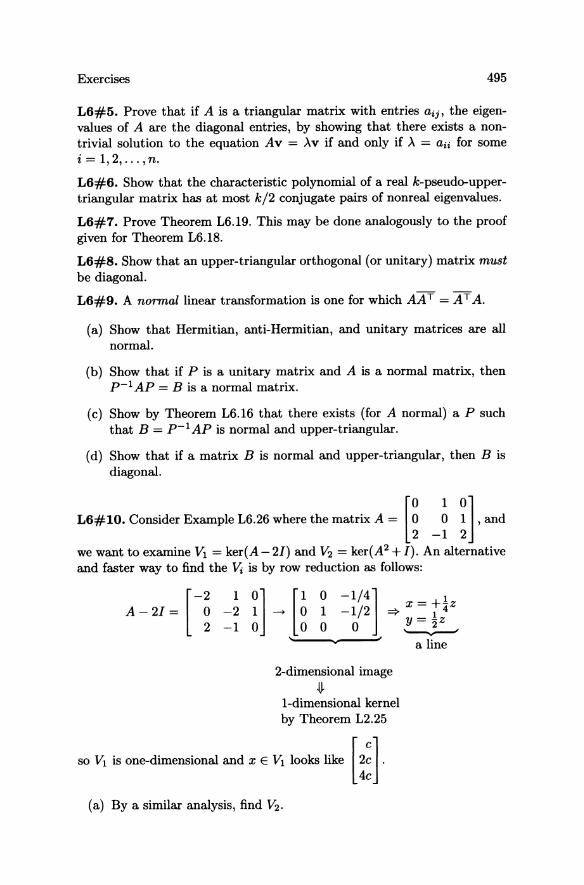
Exercises 495

L6#5. Prove that if A is a triangular matrix with entries aij, the eigen­values of A are the diagonal entries, by showing that there exists a non­trivial solution to the equation Av = .xv if and only if .x = aii for some i = 1,2, ... ,no

L6#6. Show that the characteristic polynomial of a real k-pseudo-upper­triangular matrix has at most k/2 conjugate pairs of nonreal eigenvalues.

L6#7. Prove Theorem L6.19. This may be done analogously to the proof given for Theorem L6.18.

L6#8. Show that an upper-triangular orthogonal (or unitary) matrix must be diagonal.

L6#9. A normal linear transformation is one for which AA T = AT A.

(a) Show that Hermitian, anti-Hermitian, and unitary matrices are all normal.

(b) Show that if P is a unitary matrix and A is a normal matrix, then p-l AP = B is a normal matrix.

(c) Show by Theorem L6.16 that there exists (for A normal) a P such that B = p- l AP is normal and upper-triangular.

(d) Show that if a matrix B is normal and upper-triangular, then B is diagonal.

L6#10. Consider Example L6.26 where the matrix A = 0 0 1 ,and [0 1 0] 2 -1 2

we want to examine VI = ker(A - 2J) and V2 = ker(A2 + I). An alternative and faster way to find the Vi is by row reduction as follows:

A-2I=

2-dimensional image .u.

I-dimensional kernel by Theorem L2.25

'" V, i, one-dimensional and x E V, 100,", Illre [~]. (a) By a similar analysis, find V2 •

496 Appendix L

(b) Verify properties (iii) and (iv) of Theorem L6.25 to finish Example L6.26.

L6#11. Apply the Euclidean algorithm to the following pairs of relatively prime numbers PI and 1'2 to verify Bezout's Theorem L6.27. That is, find a pair of numbers a and b such that PIa + P2b = 1:

(a) 21,16. (b) 537,791.

Exercises L 7 Finding Eigenvalues, Eigenvectors: QR Method

:f7t:l~~~:: [1genfinl(O'T::::~ha7nh::~n~:h:h:=~: 6 -11 6

polynomial, its roots are indeed the eigenvalues found by QR.

L1#2. For the heart of the QR method, you should provide the following proofs and examples:

(a) Verify the following lemma: For any n x n matrix

A = [~I ~2 . .. ~ 1 ' !! !

where we label the ith column as a vector a;, and any n x n upper­triangular matrix R, the product AR is given by

[

iii

Tl,la1 (Tl,2al + T2,2a2) (Tl,3al + T2,3a2 + T3,383) ...

111

(t t ,<,j.,) ]. 3=1 ,=1

1

(b) Use the lemma in part (a) to prove the following theorem:

Invertible matrices B and A have the same flag if and only if there exists an R such that B = AR.

(c) Use the theorem in part (b) to show the core statement:

If you apply Gmm-Schmidt to any basis, the vectors of the new orthonormal basis in the same order produce the same flag.

Exercises

(d) As an example, consider

[1 1

A= 0 0 o 1

497

-1] [1 2 3] 2 and R = 0 4 5 . o 006

For B = AR, show that the flag FA associated with the column vectors of A as a basis is the same flag FE associated with the column vectors of B as a basis.

L7#3. Confirm the second step of the induction proof for Theorem L7.1O by showing explicitly that A 2 Fo is a flag associated with Ql Q2'

L7#4. Explain the reasons for each step in the proof of Theorem L7.12.

L7#5. For Figure L7.4 in the Product-Rotation Algorithm (Section L7.4)

(a) Verify that each zero is indeed zero.

(b) Show that this procedure works if you begin with [~ -g] in the

upper left corner and end with [~ -g] in the lower right corner,

but not if you try to cancel nonzero entries by working up the matrix starting at the lower right. In other words, the order is important.

L7#6. Show that the count of operations in Theorem L7.13 is indeed of order n2 .

L7#7. Prove Theorem L7.11 using a manner similar to Figure L7.4. That is, show that RQ; = R8(1, 01 ) T 8(2,02 ) T ... 8(n - 1, On-I) T works to fill the sub diagonal with nonzero terms, from the top down but leaves all zeroes below the subdiagonal.

L7#8. Confirm that for the following matrices, QR gets hung up. The reason is that the eigenvalues do not have distinct absolute values (for different reasons, which you should explain).

(b) [~ j !] Exercises L8 Finding Eigenvalues, Eigenvectors: Jacobi's Method

L8#1. Let A be the symmetric 2 x 2 matrix [~ ~ ] . Then Jacobi's method

will multiply by a rotation matrix Q(O), where tan20 = 2b/(a - d), in

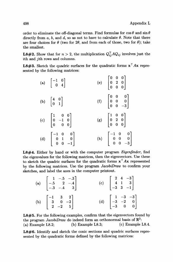
498 Appendix L

order to eliminate the off-diagonal terms. Find formulas for cos () and sin () directly from a, b, and d, so as not to have to calculate (). Note that there are four choices for () (two for 2(), and from each of those, two for ()); take the smallest.

L8#2. Show that for n > 2, the multiplication Q~AQij involves just the ith and jth rows and columns.

L8#3. Sketch the quadric surfaces for the quadratic forms x T Ax repre-sented by the following matrices:

[-~ ~] [~ 0

~] (a) (e) 2 0

[~ ~] [~ 0 J] (b) (f) 0 0

[~ 0

~] [~ 0

~] (c) -1 (g) 2 0 0

[-~ 0 J] [-I 0 J] (d) 1 (h) o 0 0 o 0

L8#4. Either by hand or with the computer program Eigenfinder, find the eigenvalues for the following matrices, then the eigenvectors. Use these to sketch the quadric surfaces for the quadratic forms x T Ax represented by the following matrices. Use the program JacobiDraw to confirm your sketches, and label the axes in the computer printout.

(a) [-.! -.~ =:!] -.3 -.4 3 (c) U! =~]

(b) [-~ j -~] (d) [-~ =~ -~] -3 0 0

L8#5. For the following examples, confirm that the eigenvectors found by the program JacobiDraw do indeed form an orthonormal basis of JR3: (a) Example L8.2j (b) Example L8.3j (c) Example L8.4.

L8#6. Identify and sketch the conic sections and quadric surfaces repre­sented by the quadratic forms defined by the following matrices:

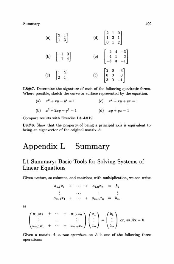
Summary 499

[i ;] [! 1 !l (a) (d) 2 1

[-~ ~] [ 2 4 -~] (b) (e) 4 1 -3 3 -1

[~ !] [~ 0 j] (c) (f) 0 0

L8#7. Determine the signature of each of the following quadratic forms. Where possible, sketch the curve or surface represented by the equation.

(a) x 2 + xy - y2 = 1 (c) x2 + xy + yz = 1

(d) xy+yz=1

Compare results with Exercise L3-4#19.

L8#8. Show that the property of being a principal axis is equivalent to being an eigenvector of the original matrix A.

Appendix L Summary

Ll Summary: Basic Tools for Solving Systems of Linear Equations

Given vectors, as columns, and matrices, with multiplication, we can write

as

Given a matrix A, a row operation on A is one of the following three operations:

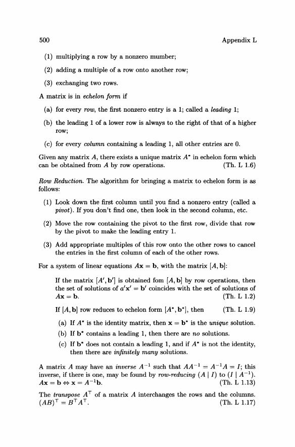
500 Appendix L

(I) multiplying a row by a nonzero mumber;

(2) adding a multiple of a row onto another row;

(3) exchanging two rows.

A matrix is in echelon form if

(a) for every row, the first nonzero entry is a 1; called a leading 1;

(b) the leading 1 of a lower row is always to the right of that of a higher row;

(c) for every column containing a leading 1, all other entries are O.

Given any matrix A, there exists a unique matrix A * in echelon form which can be obtained from A by row operations. (Th. L 1.6)

Row Reduction. The algorithm for bringing a matrix to echelon form is as follows:

(I) Look down the first column until you find a nonzero entry (called a pivot). If you don't find one, then look in the second column, etc.

(2) Move the row containing the pivot to the first row, divide that row by the pivot to make the leading entry 1.

(3) Add appropriate multiples of this row onto the other rows to cancel the entries in the first column of each of the other rows.

For a system of linear equations Ax = b, with the matrix [A, b]:

If the matrix [A', b'] is obtained fom [A, b] by row operations, then the set of solutions of a'x' = b' coincides with the set of solutions of Ax = b. (Th. L 1.2)

If [A, b] row reduces to echelon form [A*, b*], then (Th. L 1.9)

(a) If A* is the identity matrix, then x = b* is the unique solution.

(b) If b* contains a leading 1, then there are no solutions.

(c) If b* does not contain a leading 1, and if A* is not the identity, then there are infinitely many solutions.

A matrix A may have an inverse A-l such that AA-l = A-l A = I; this inverse, if there is one, may be found by row-reducing (A I I) to (I I A -1). Ax = b # x = A-lb. (Th. L 1.13)

The transpose AT of a matrix A interchanges the rows and the columns. {AB)T = BT AT. (Th. L 1.17)

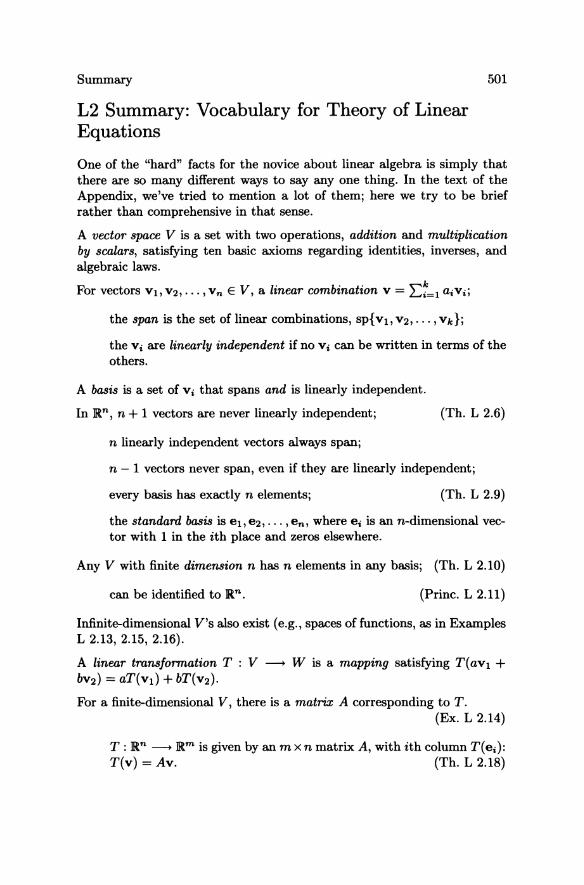
Summary

L2 Summary: Vocabulary for Theory of Linear Equations

501

One of the "hard" facts for the novice about linear algebra is simply that there are so many different ways to say anyone thing. In the text of the Appendix, we've tried to mention a lot of them; here we try to be brief rather than comprehensive in that sense.

A vector space V is a set with two operations, addition and multiplication by scalars, satisfying ten basic axioms regarding identities, inverses, and algebraic laws.

For vectors VI, V2, ••• , Vn E V, a linear combination V = E:=l aiVi;

the span is the set of linear combinations, SP{Vb V2, •.. , Vk};

the Vi are linearly independent if no Vi can be written in terms of the others.

A basis is a set of Vi that spans and is linearly independent.

In an, n + 1 vectors are never linearly independent;

n linearly independent vectors always span;

(Th. L 2.6)

n - 1 vectors never span, even if they are linearly independent;

every basis has exactly n elements; (Th. L 2.9)

the standard basis is el, e2, ... , en, where ei is an n-dimensional vec­tor with 1 in the ith place and zeros elsewhere.

Any V with finite dimension n has n elements in any basis; (Th. L 2.10)

can be identified to an. (Princ. L 2.11)

Infinite-dimensional V's also exist (e.g., spaces of functions, as in Examples L 2.13, 2.15, 2.16).

A linear transformation T : V - W is a mapping satisfying T(avI + bv2 } = aT(vI} + bT(v2}.

For a finite-dimensional V, there is a matrix A corresponding to T. (Ex. L 2.14)

T : an _ am is given by an m x n matrix A, with ith column T( ei}: T(v} = Av. (Th. L 2.18)

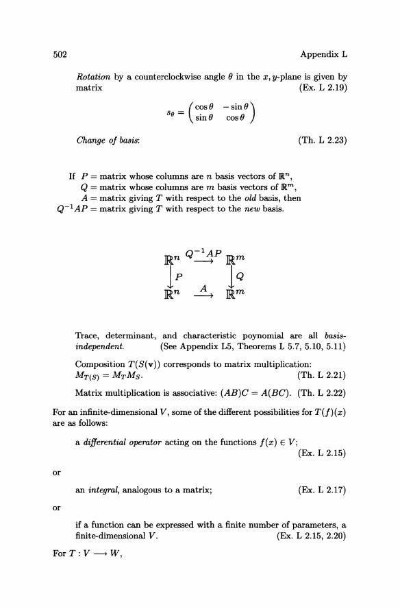
502 Appendix L

Rotation by a counterclockwise angle 0 in the x, y-plane is given by matrix (Ex. L 2.19)

8 = (COSO -SinO) 9 sin 0 cos 0

Change of basis: (Th. L 2.23)

If P = matrix whose columns are n basis vectors of an, Q = matrix whose columns are m basis vectors of am, A = matrix giving T with respect to the old basis, then

Q-l AP = matrix giving T with respect to the new basis.

Trace, determinant, and characteristic poynomial are all basis­independent. (See Appendix L5, Theorems L 5.7, 5.10, 5.11)

Composition T(S(v» corresponds to matrix multiplication: MT(s) = MTMS' (Th. L 2.21)

Matrix multiplication is associative: (AB)C = A(BC). (Th. L 2.22)

For an infinite-dimensional V, some of the different possibilities for T(f)(x) are as follows:

or

or

a differential operator acting on the functions f (x) E V; (Ex. L 2.15)

an integral, analogous to a matrix; (Ex. L 2.17)

if a function can be expressed with a finite number of parameters, a finite-dimensional V. (Ex. L 2.15, 2.20)

For T: V --+ W,

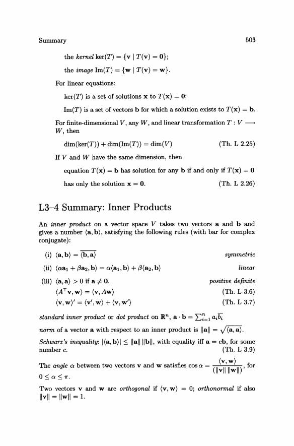
Summary

the kernel ker(T) = {v I T(v) = O}j

the image Im(T) = {w I T(v) = w}.

For linear equations:

ker(T) is a set of solutions x to T(x) = OJ

503

Im(T) is a set of vectors b for which a solution exists to T(x) = b.

For finite-dimensional V, any W, and linear transformation T : V ~ W, then

dim(ker(T)) + dim(Im(T)) = dim(V) (Th. L 2.25)

If V and W have the same dimension, then

equation T(x) = b has solution for any b if and only if T(x) = 0

has only the solution x = o. (Th. L 2.26)

L3-4 Summary: Inner Products

An inner product on a vector space V takes two vectors a and b and gives a number (a, b), satisfying the following rules (with bar for complex conjugate):

(i) (a, b) = (b, a)

(ii) (aal + f3a2, b) = a(aI, b) + f3(a2, b)

(iii) (a, a) > 0 if a =I- o. (ATv,w) = (v,Aw)

(v, W)' = (v', w) + (v, w')

symmetric

linear

positive definite

(Th. L 3.6)

(Th. L 3.7)

standard inner product or dot product on ]Rn, a· b = L~=l aibi

norm of a vector a with respect to an inner product is lIall = v(a, a).

Schwarz's inequality: I (a, b) I ~ lIalillbll, with equality iff a = cb, for some number c. (Th. L 3.9)

The angle a between two vectors v and w satisfies cos a = (II~~I'I~II)' for

0~a~1r.

Two vectors v and w are orthogonal if (v, w) = OJ orthonormal if also IIvll = IIwll = 1.

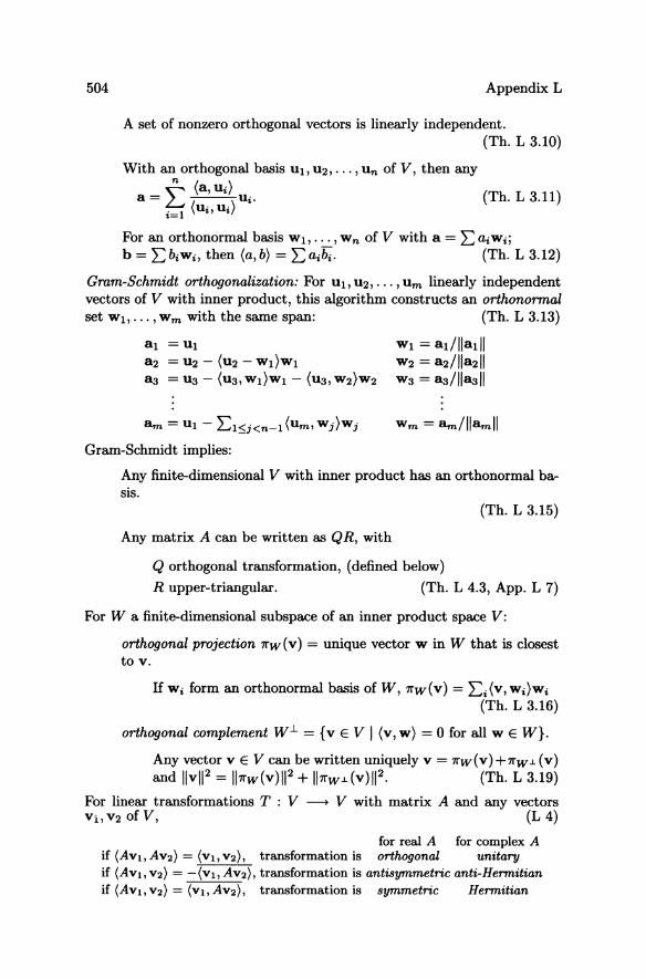
504 Appendix L

A set of nonzero orthogonal vectors is linearly independent. (Th. L 3.10)

With an orthogonal basis Ul. U2, ... , Un of V, then any

a = t (a, Ui) Ui. (Th. L 3.11) i=1 (lli, lli)

For an orthonormal basis W1,"" Wn of V with a = E aiwi; b = E biWi, then (a, b) = E aibi' (Th. L 3.12)

Gram-Schmidt orthogonalization: For Ul. U2,"" Um linearly independent vectors of V with inner product, this algorithm constructs an orthonormal set Wl. ... ,Wm with the same span: (Th. L 3.13)

a1 =U1 a2 = U2 - (U2 - W1}W1 83 = U3 - (U3, W1}W1 - (U3, W2}W2

W1 = a1//la1/1 W2 = a2//la2/1 W3 = 83//183/1

8m = U1 - E 1:S;j<n-1 (Urn, Wj}Wj

Gram-Schmidt implies:

Any finite-dimensional V with inner product has an orthonormal ba-sis.

(Th. L 3.15)

Any matrix A can be written as Q R, with

Q orthogonal transformation, (defined below)

R upper-triangular. (Th. L 4.3, App. L 7)

For W a finite-dimensional subspace of an inner product space V:

orthogonal projection 71'w (v) = unique vector W in W that is closest to v.

If Wi form an orthonormal basis of W, 71'w(v) = Ei(V, Wi}Wi (Th. L 3.16)

orthogonal complement Wl. = {v E V I (v, w) = 0 for all W E W}.

Any vector v E V can be written uniquely v = 71'w(v) +7I'w.l. (v) and /lv/l2 = /l7I'W(v)/l2 + /l7I'w.l.(v)/l 2 • (Th. L 3.19)

For linear transformations T : V --+ V with matrix A and any vectors Vi, V2 of V, (L 4)

for real A for complex A if (AVI, AV2) = (VI, V2), transformation is orthogonal unitary if (AVI, V2) = -(VI, AV2)' transformation is antisymmetric anti-Hermitian if (AVI, V2) = (v!, AV2), transformation is symmetric Hermitian

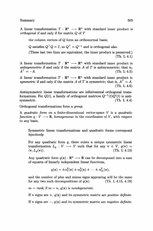
Summary 505

A linear transformation T : JR.n --+ JR.n with standard inner product is orthogonal if and only if for matrix Q of T

the column vectors of Q form an orthonormal basis;

Q satisfies QT Q = I, so QT = Q-l and is orthogonal also.

(These last two lines are equivalent; the inner product is preserved.) (Th. L 4.1)

A linear transformation T : JR.n --+ JR.n with standard inner product is antisymmetric if and only if the matrix A of T is antisymmetric; that is, AT = -A. (Th. L 4.5)

A linear transformation T : JR.n --+ JR.n with standard inner product is symmetric if and only if the matrix A of T is symmetric; that is, AT = A.

(Th. L 4.6)

Antisymmetric linear transformations are infinitesimal orthogonal trans­formations. For Q(t), a family of orthogonal matrices Q-l(t)Q'(t) is anti­symmetric. (Th. L 4.4)

Orthogonal transformations form a group.

A quadratic form on a finite-dimensional vector-space V is a quadratic function q : V --+ JR., homogeneous in the coordinates of V, with respect to any basis.

Symmetric linear transformations and quadratic forms correspond bijectively:

For any quadratic form q, there exists a unique symmetric linear transformation Lq : V --+ V such that for any v E V, q( v} = (v, Lq(v}). (Th. L 4.13)

Any quadratic form q(x} : JR.n --+ JR. can be decomposed into a sum of squares of linearly independent linear functions,

q(x} = ±a~(x} ± a~(x} ± ... ± a~(x},

and the number of plus and minus signs appearing will be the same for any two such decompositions of q(x). (Th. L 4.15, 4.19)

m = rank; if m = n, q(x} is nondegenerate.

If n signs are +, q(x) and its symmetric matrix are positive definite.

If n signs are -, q(x} and its symmetric matrix are negative definite.

506 Appendix L

If k signs are + and £ signs are -, q(x) has signature (k, f).

An often quicker way to determine the signature of a symmetric ma­trix is by the signs of its eigenvalues (Appendix L 6). In Appendix L 8.3 we discuss that, for a positive definite matrix, all the eigenvalues are positive, and, more generally, that a matrix of signature (k, £) will have k positive eigenvalues and i negative eigenvalues.

For ( , ) an inner product on ]Rn, and G, the symmetric matrix with entries

Gi,j = (ei,ej),

the given inner product can be written in terms of the standard dot product:

(a, b) = a· Gb.

Conversely, if G is a positive definite symmetric matrix, then (*) defines an inner product on ]Rn. (Th. L 4.8)

L5 Summary: Determinants

The determinant function det A satisfies three properties, exists, and is unique: (Th. L 5.1)

(1) det(ab ... , 8i-b (au + ,Bw), 8i+l, ... , 8n) = adet(al, ... ,8i-l,U,8i+l, ... ,8n)

+ ,Bdet(al, ... ,8i-l, W,8i+l, ... ,8n). (multilinearity)

(2) det(al, ... , 8i, ... , aj, ... , 8n) = -det(al, ... ,aj, ... ,8i, ... ,8n) ( antisymmetry)

(3) detI = det(el,e2, ... ,en) = 1, where ei is the ith standard unit basis vector. ( normalization)

Construction of the determinant function can be done either by

(i) development according to the first row: D(A) given by computer pro­gram;

(ii) column operations: Each of the three column operations multiplies the determinant by an appropriate factor /-l:

(a) Multiply a column through by a number m. (b) Exchange two columns.

(c) Add a multiple of one column onto another.

Any square matrix can be column-reduced until

/-l=m. /-l =-l.

/-l=l.

Summary

where either An = I, and det A = 1-'11-'2 .. . l-'n-1I-'n; or An = 0, and detA = O.

Theorems:

507

If A is triangular, det A = product of diagonal entries; (Th. L 5.3)

characteristic polynomial: det(AI - A) = n('x - au). (Th. L 5.13)

For A,B both n x n, detAdetB = detAB. (Th. L 5.5)

For A, B both square matrices, det [ :I~] = det A det B.

(Th. L 5.8)

A is invertible {=::} det A -:f:. 0, and then det A -1 = (1/ det A). (Th. L 5.6)

The following are all basis independent:

determinant, det A because det A = det p-1 AP (Th. L 5.7)

trace, tr A == sum of diagonal entries, but tr A tr B -:f:. tr AB (Th. L 5.11)

characteristic polynomial, det(AI - A) (Th. L 5.10)

The k-dimensional volume of PV1 , ... ,v/c is defined by induction:

if k = 1, then the volume is simply the length: voh(Pv = IIvlI;

if k > 1, then volk{Pvt, ... ,v/e) = VOlk-I{Pvt, ... ,v/e_J . 117rv:.L (Vk) II, /c-1 where Vk-I is the subspace spanned by Vb"" Vk-1.

The volume of PV1 , ... ,v/c does not depend on the order of Vb"" Vk. (Th. L 5.15)

IfVb···,Vk are orthogonal, then volk{Pvt, ... ,v,,) = IIVIII· ... ·IIVkll. (Th. L 5.16)

If Q is an orthogonal matrix, then the image under Q of a parallelepiped has the same volume as the original parallelepiped: (Th. L 5.17)

VOlk(PQ(v1), ... ,Q(v,,») = VOlk{Pv1 , ... ,v/c).

The volume of PV1 , ... ,v/c is measured by det{vb"" Vk).

The determinant of an orthogonal matrix is ± 1.

For any n x n matrix A, detA = detAT.

(Th. L 5.18)

(Cor. L 5.19)

(Th. L 5.20)

508 Appendix L

L6 Summary: Eigenvalues and Eigenvectors

For an n x n matrix A, if there exist A E e and nonzero v E en such that AV = Av, then A is an eigenvalue of A and v is its associated eigenvector.

A is an eigenvalue if and only if it is a root of the chamcteristic polynomial:

or,

det(.>.I - A) = 0, (Th. L 6.3)

(Th. L 5.11)

The characteristic polynomial, and hence the set of eigenvalues, is independent of change of basis. Thus A and p-1 AP have the same eigenvalues. (Th. L 6.10)

The matrix A has at least one and at most n eigenvalues. (Th. L 6.4)

( dtr tAA= sum d t} of eigenvalues, each taken with its multiplicity. e = pro uc

(Th. L 6.5)

Eigenvectors with distinct eigenvalues are linearly independent. (Th. L 6.7)

If n Ns are distinct, then en has an eigenbasis (basis of eigenvectors). (Th. L 6.8)

If m A'S are distinct, for m ::; n, then en has an eigenbasis for A if and only if dim (eigenspace E>. of eigenvectors) = multiplicity of A in the characteristic polynomial. (Th. L 6.10)

If P is an invertible matrix whose columns are eigenvectors, then we can diagonalize:

(AI

P-1AP = 0 ... 0), An

with all eigenvalues of A along the diagonal. (Th. L 6.11)

Most matrices can be diagonalizedj all can be triangularizedj the eigenvalues of a triangular matrix will be along the diagonal.

There exists unitary matrix M such that M- 1 AM is upper-triangular. (Th. L 6.16)

For any A and any c > 0, there exists a matrix M with orthogonal columns (but not normalized) such that M- 1 AM is upper-triangular with off-diagonal terms of absolute value < c.

(Th. L 6.17,6.18,6.19)

Summary 509

For a linear transformation with n x n matrix A: (Th. L 6.20)

(a) if A is real symmetric or Hermitian, then the eigenvalues of A are real;

(b) if A is real antisymmetric or anti-Hermitian, then the eigennvalues of A are purely imaginary;

(c) if A is real orthogonal or unitary, then the eigenvalues of A are of absolute value 1;

In all three cases, any two eigenvectors of A with distinct eigenvalues are orthogonal.

Spectral Theorem: (Th. L 6.22)

For A Hermitian, anti-Hermitian, or unitary, en has an orthonormal eigenbasis for A;

If A is real symmetric, the eigenvalues are real, and the basis vectors can be chosen real (meaning that p-l AP is diagonal and the entries are the eigenvalues.)

Appendix L 8, Jacobi's method, gives a constructive proof and dis­cusses for quadratic forms (Appendix L 4.4) the fact that the signa­ture (k, i) is given by the signs of the eigenvalues of the symmetric matrix associated with the quadratic form: the matrix will have k positive eigenvalues and i negative eigenvalues; a positive definite matrix has all positive eigenvalues.

Factoring the characteristic polynomial PA for an n x n matrix A:

PA(A) = o. (Th. L 6.23)

If PA = PIP2, where PI and P2 are relatively prime with leading coef­ficient 1, and Vi = ker Pi(A), then (Th. L 6.25)

(i) any vector x E lRn can be written uniquely as Xl + X2, where Xi E Vi;

(ii) for any vector Xi E Vi, AXi E Vi; (iii) if an eigenvalue Ai is a root of Pi, its corresponding eigenvectors

E Vi; (iv) the characteristic polynomial of A: Vi --+ Vi is Pi'

This is proved using Bezout's Theorem: (Th. L 6.27)

Two polynomials PI and P2 are relatively prime if and only if there exist polynomials ql and q2 such that PI ql + P2q2 = 1.

Appendices L 7 and L8 each elaborate on a single result, and so are not summarized here.

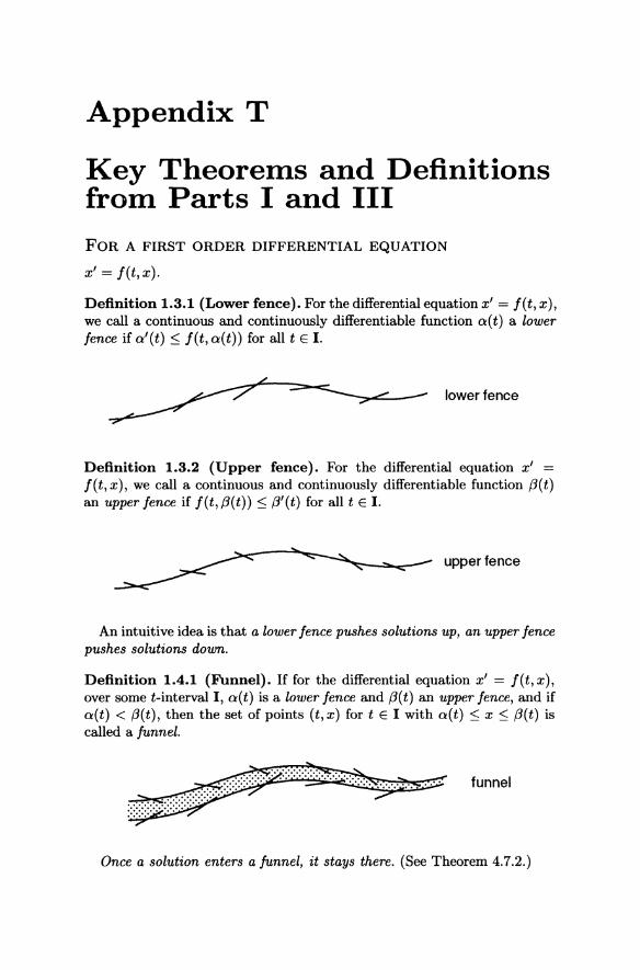
Appendix T

Key Theorems and Definitions from Parts I and III FOR A FIRST ORDER DIFFERENTIAL EQUATION

x' = f(t,x).

Definition 1.3.1 (Lower fence). For the differential equation x' = f (t, x), we call a continuous and continuously differentiable function a(t) a lower fence if a/(t) :5 f(t, a(t» for all tEl.

lower fence

Definition 1.3.2 (Upper fence). For the differential equation x' = f(t, x), we call a continuous and continuously differentiable function f3(t) an upper fence if f(t,f3(t» :5 f3'(t) for all tEl.

upper fence

An intuitive idea is that a lower fence pushes solutions up, an upper fence pushes solutions down.

Definition 1.4.1 (Funnel). If for the differential equation x' = f(t, x), over some t-interval I, a(t) is a lower fence and f3(t) an upper fence, and if a(t) < f3(t), then the set of points (t,x) for tEl with a(t) :5 x :5 f3(t) is called a funnel.

funnel

Once a solution enters a funnel, it stays there. (See Theorem 4.7.2.)

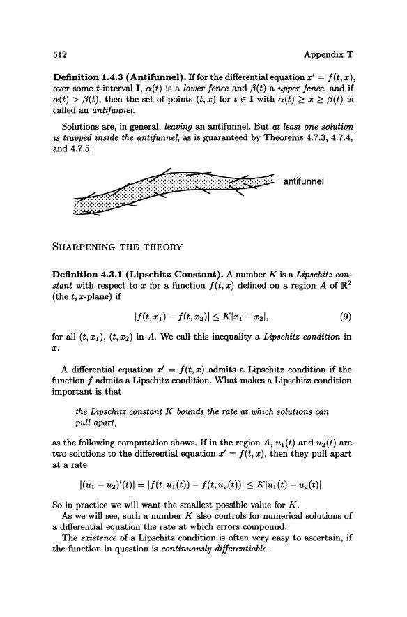
512 Appendix T

Definition 1.4.3 (Antifunnel). Iffor the differential equation x, = I(t, x), over some t-interval I, aCt) is a lower lence and f3(t) a upper lence, and if aCt) > f3(t), then the set of points (t, x) for tEl with aCt) ~ x ~ f3(t) is called an anti funnel.

Solutions are, in general, leaving an antifunnel. But at least one solution is trapped inside the anti funnel, as is guaranteed by Theorems 4.7.3, 4.7.4, and 4.7.5.

antifunnel

SHARPENING THE THEORY

Definition 4.3.1 (Lipschitz Constant). A number K is a Lipschitz con­stant with respect to x for a function I(t,x) defined on a region A of R.2

(the t, x-plane) if

(9)

for all (t, xt), (t, X2) in A. We call this inequality a Lipschitz condition in x.

A differential equation x' = I(t, x) admits a Lipschitz condition if the function I admits a Lipschitz condition. What makes a Lipschitz condition important is that

the Lipschitz constant K bounds the rate at which solutions can pull apart,

as the following computation shows. If in the region A, Ul(t) and U2(t) are two solutions to the differential equation x' = I(t, x), then they pull apart at a rate

So in practice we will want the smallest possible value for K. As we will see, such a number K also controls for numerical solutions of

a differential equation the rate at which errors compound. The existence of a Lipschitz condition is often very easy to ascertain, if

the function in question is continuously differentiable.

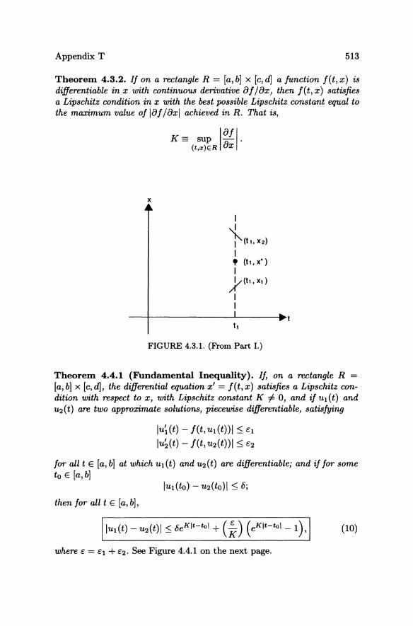
Appendix T 513

Theorem 4.3.2. If on a rectangle R = [a, b] x [e, dJ a function f(t, x) is differentiable in x with continuous derivative of lax, then f(t, x) satisfies a Lipschitz condition in x with the best possible Lipschitz constant equal to the maximum value of laf laxl achieved in R. That is,

x

K == sup 1 of I. (t,z)ER ax

I

{ I (tl. X2)

I • (tl. X·) I

y(h.XI)

I I

FIGURE 4.3.1. (From Part I.)

Theorem 4.4.1 (Fundamental Inequality). If, on a rectangle R = [a, b] x [c, dJ, the differential equation x' = f(t, x) satisfies a Lipschitz con­dition with respect to x, with Lipschitz constant K =F 0, and if Ul (t) and U2 ( t) are two approximate solutions, piecewise differentiable, satisfying

lu~(t) - f(t,ul(t))1 ~ Cl

lu~(t) - f(t, U2(t)) I ~ C2

for all t E [a, b] at which Ul (t) and U2 (t) are differentiable; and if for some to E [a,b]

then for all t E [a, b],

where g = Cl + C2. See Figure 4.4.1 on the next page.

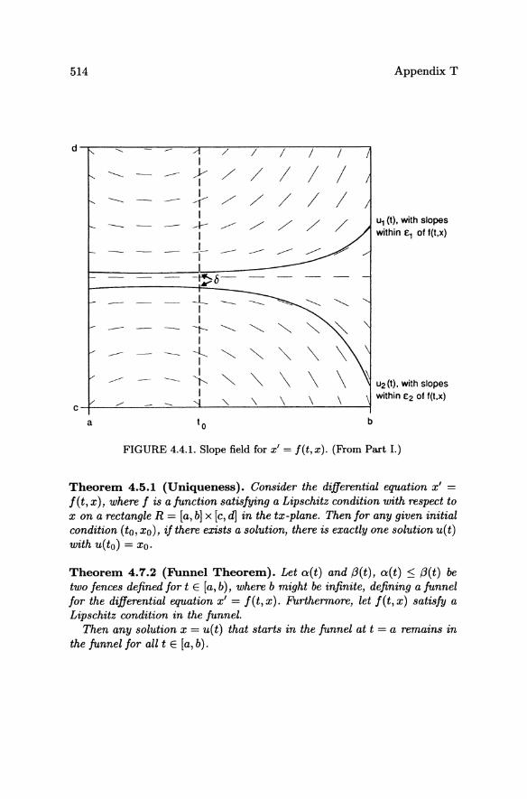
514 Appendix T

d '- / I

/ / / /

------ ---- t / / / / / --- ~ / / / / /

I U1 (I). with slopes -- --+- ~ / /' / I wilhin £1 of f(l.x)

J- -- --- ~ ~ I I

-,!>{;-

-L I -- --- """"- "- ~ I

r-- "- "- ~ "" I

--- --l--.. ~ "" '" '\ I I

"" '" \ \ --- ------- 1---- U2(1). with slopes I wilhin £2 of f(l.x)

/' "- \ \ \ c a 10 b

FIGURE 4.4.1. Slope field for x' = f(t,x). (From Part I.)

Theorem 4.5.1 (Uniqueness). Consider the differential equation x' = f(t, x), where f is a function satisfying a Lipschitz condition with respect to x on a rectangle R = [a, bj x [c, d] in the tx-plane. Then for any given initial condition (to, xo), if there exists a solution, there is exactly one solution u( t) with u(to) = Xo.

Theorem 4.7.2 (Funnel Theorem). Let a(t) and (3(t), a(t) :::; (3(t) be two fences defined for t E [a, b), where b might be infinite, defining a funnel for the differential equation x' = f(t,x). Jilurthermore, let f(t, x) satisfy a Lipschitz condition in the funnel.

Then any solution x = u(t) that starts in the funnel at t = a remains in the funnel for all t E [a, b).

Appendix T

___ __"",_"-<: _-- 13 (t) = upper fence ~ -.:...,. --'-.--,,"-"'--..... - -"<. --......... -""

J_-r-~ ,/_-r

~--/--__ r

--r-~--- a (t) = lower fence _-/ __ /--r

FIGURE 4.7.2. Funnel. (From Part I.)

515

Theorem 4.7.3 (Antifunnel Theorem; Existence). Let a(t) and f3(t) , f3(t) ~ a(t), be two fences defined for t E [a, b), where b might be infi­nite, that bound an antifunnel for the differential equation x' = f( t, x). FUrthermore, let f (t, x) satisfy a Lipschitz condition in the anti funnel.

Then there exists a solution x = u(t) that remains in the antifunnel for all t E [a, b) where u(t) is defined.

---;;.0<' -~--.r--/--r--7"'--~--/--/--r-~--- a (t) = lower fence

FIGURE 4.7.3. Antifunnel. (From Part I).

The really interesting results about antifunnels are the ones which give properties which ensure that the solutions which stay in them are unique. We will give two such properties; the first is a special case of the second, but is so much easier to prove that it seems worthwhile to isolate it.

Theorem 4.7.4 (First uniqueness criterion for antifunnels). Let a(t) and f3(t), f3(t) ~ a(t), be two fences defined for t E [a, b) that bound an antifunnel for the differential equation x' = f(t,x). Let f(t,x) satisfy a Lipschitz condition in the antifunnel. FUrthermore, let the antifunnel be narrowing, with

lim(a(t) - f3(t» = o. t-+b

If of / ax 2: 0 in the antifunnel, then there is a unique solution that stays in the antifunnel.

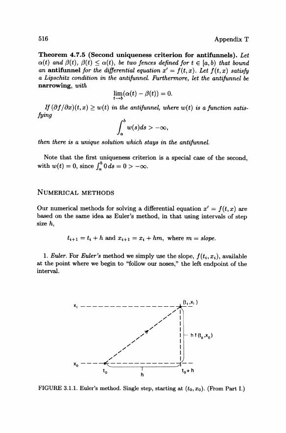
516 Appendix T

Theorem 4.7.5 (Second uniqueness criterion for antifunnels). Let aCt) and (J(t), (J(t) ~ aCt), be two fences defined for t E [a, b) that bound an antifunnel for the differential equation x' = f(t,x). Let f(t,x) satisfy a Lipschitz condition in the antifunnel. FUrthermore, let the antifunnel be narrowing, with

lim(a(t) - (J(t» = O. t-+b

If (8f/8x)(t, x) ~ wet) in the antifunnel, where wet) is a function satis­fying

lb w(s)ds > -00,

then there is a unique solution which stays in the antifunnel.

Note that the first uniqueness criterion is a special case of the second,

with wet) = 0, since J: Ods = 0> -00.

NUMERICAL METHODS

Our numerical methods for solving a differential equation x' = f(t,x) are based on the same idea as Euler's method, in that using intervals of step size h,

ti+l = ti + h and Xi+! = Xi + hm, where m = slope.

1. Euler. For Euler's method we simply use the slope, f(ti, Xi), available at the point where we begin to "follow our noses," the left endpoint of the interval.

(I, ,X, ) X, ________________ *_ /1

// 1

// 1 / 1

/7If' 1 h f (to ,xo ) // 1

// 1 / 1

// 1 Xo ----~-----------::;I--

to I 10+ h h

FIGURE 3.1.1. Euler's method. Single step, starting at (to, xo). (From Part I.)

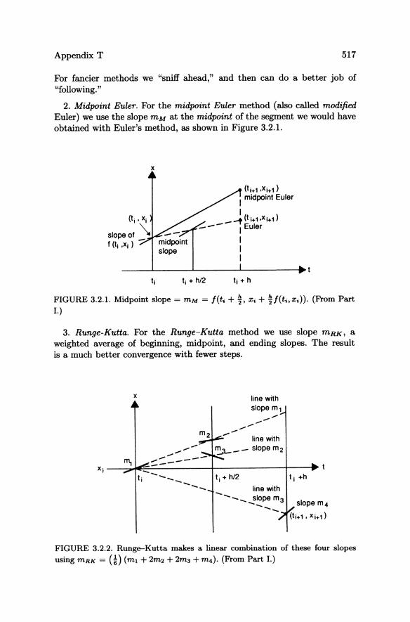
Appendix T 517

For fancier methods we "sniff ahead," and then can do a better job of "following."

2. Midpoint Euler. For the midpoint Euler method (also called modified Euler) we use the slope mM at the midpoint of the segment we would have obtained with Euler's method, as shown in Figure 3.2.1.

x

(li+1 .xi+1) I midpoinl Euler

I _ -t (I 1+1.x l+1)

--- I Euler

I I I

FIGURE 3.2.1. Midpoint slope = mM = f(ti +~, Xi + ~f(ti'Xi»' (From Part I.)

3. Runge-Kutta. For the Runge-Kutta method we use slope mRK, a weighted average of beginning, midpoint, and ending slopes. The result is a much better convergence with fewer steps.

x line wilh slope m,

-------Xi----~~_~_=-----------+--------------+----~

1 i - - _ 1 i + h/2 1 i +h ........................ line with ---_...,:;Iope m3 --- slope m4

(li+1. Xi+1)

FIGURE 3.2.2. Runge--Kutta makes a linear combination of these four slopes

using mRK = U) (ml + 2m2 + 2m3 + m4)' (From Part I.)

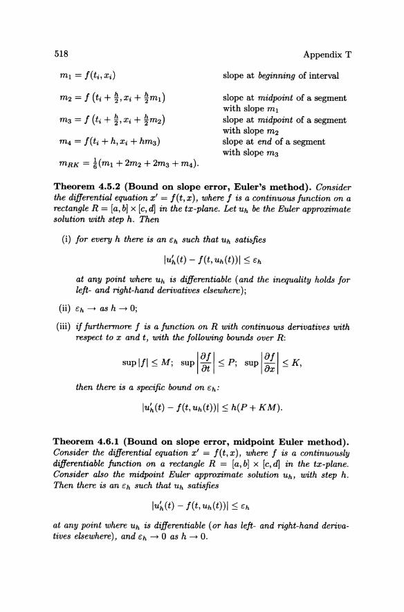
518 Appendix T

slope at beginning of interval

slope at midpoint of a segment with slope ml

slope at midpoint of a segment with slope m2

slope at end of a segment with slope m3

Theorem 4.5.2 (Bound on slope error, Euler's method). Consider the differential equation x' = I(t,x), where I is a continuous function on a rectangle R = [a, bJ x [c, d] in the tx-plane. Let Uh be the Euler approximate solution with step h. Then

(i) lor every h there is an Ch such that Uh satisfies

at any point where Uh is differentiable (and the inequality holds for lejt- and right-hand derivatives elsewhere);

(ii) Ch --+ as h --+ 0;

(iii) if furthermore I is a function on R with continuous derivatives with respect to x and t, with the following bounds over R:

then there is a specific bound on Ch:

lu~(t) - f(t, uh(t»1 ~ h(P + KM).

Theorem 4.6.1 (Bound on slope error, midpoint Euler method). Consider the differential equation x' = f(t,x), where I is a continuously differentiable function on a rectangle R = [a, bJ x [c, d] in the tx-plane. Consider also the midpoint Euler approximate solution Uh, with step h. Then there is an Ch such that Uh satisfies

at any point where Uh is differentiable (or has lejt- and right-hand deriva­tives elsewhere), and Ch --+ 0 as h --+ o.

Appendix T 519

Furthermore, if f is a function on R with continuous derivatives up to order two with respect to x and t, then there is a constant BM such that

lu;'(t) - f(t, uh(t»1 ::; BMh2 .

This computation is not too difficult if you don't insist on knowing B M, which is a fairly elaborate combination of sup's of the second order partial derivatives.

FROM MULTIVARIABLE CALCULUS

Theorem 13.6.4 (Implicit Function Theorem). Let U = V x W be an open set in IRn x 1R7n , f: U ---- 1R7n a differentiable mapping, and (xo, Yo) a point in U such that f(xo, Yo) = o. If the square m x m matrix of partial derivatives 8f/8y(xo,yo) is invertible, and if 8f/8y satisfies the Lipschitz condition

118f/8y(x,yt} - 8f/8y(X,Y2)11 ::; KYI - Y211

on U for some K, then the equation f(x, y) = 0 expresses Y locally as an implicit function of x near Xo.

More precisely, there exists a neighborhood VI of Xo in IRn and a dif­ferentiable function g: VI ---- 1R7n with g(xo) = Yo and f(x,g(x» = o. This function can be computed as follows: Choose x and solve the equation f(x, y) = 0 for Y by Newton's method, starting at Yo, i.e., set

Yn+1 = Yn - [Of/8y(x,Yn)-ljf(x,Yn).

Then if x is chosen sufficiently close to xo, this sequence will converge to a limit which depends of course on x; if you set g(x) equal to this limit, then g will be the required implicit function.

Moreover, the function g computed this way is differentiable at Xo, with derivative

Corollary 13.6.5 (Inverse Function Theorem). Let U C 1R7n be an open neighborhood of 0, and f: U ---- 1R7n a continuously differentiable func­tion, with dxf satisfying a Lipschitz condition

Idx1 f - dX1 fl ::; Klxl - x21

for some constant K. If dof is invertible, there exist neighborhoods U1 C U and VI of 0 in 1R7n and a continuously differentiable mapping g: VI ---- U1

such that g 0 f is the identity of U1 and fog is the identity of VI. The derivative of g at the origin is given by

dog = (dof)-l.

References

Arnold, V.I., Ordinary Differential Equations, M.LT. Press, 1973 (Russian orig­inal, Moscow, 1971).

Artigue, Michele and Gautheron, Veronique, Systemes Differentiels: Etude Graph­ique, CEDIC, Paris, 1983.

Birkhoff, G. and Rota, G. C., Ordinary Differential Equations, Ginn, 1962.

Borrelli, R., Boyce, W. E., and Coleman, c., Differential Equations Laboratory Workbook, John Wiley, 1992.

Borrelli, R. and Coleman, C., Differential Equations: A Modeling Approach, Pren­tice-Hall 1987.

Boyce, W. E. and DiPrima, R. C., Elementary Differential Equations, John Wiley, 1969, 1994.

Dieudonne, Jean, Calcul Infinitesimal, Hermann, Paris, 1968.

Guckenheimer, J. and Holmes, P., Nonlinear Oscillations, Dynamical Systems, and Bifurcations of Vector Fields, Springer-Verlag, Applied Mathematical Sci­ences 42, 1983.

Hale, Jack, Ordinary Differential Equations, Wiley-Interscience, 1969.

Hale, Jack and Ko<;ak, Huseyn, Dynamics and Bifurcations, Springer-Verlag, 1991.

Hirsch, M.W. and Smale, S., Differential Equations, Dynamical Systems, and Linear Algebra, Academic Press, 1974.

Kaplansky, I., Differential Algebra.

LaSalle, J.P. and Lefschetz, S., Stability by Liapunov's Direct Method with Ap­plications, Academic Press, 1961.

Lorenz, E.N., "Deterministic Nonperiodic Flow," J. Atmos. Sci. 20, 130, 1963.

Marsden, Jerrold, and McCracken, M., The Hopf Bifurcation and Its Applications, Springer-Verlag, New York 1976.

Peixoto, M.M., Dynamical Systems, Proceedings of 1971 Bahia conference, Aca­demic Press, 1973.

Peixoto, M.M., "Structural Stability on Two Dimensional Manifolds," Topology 1, 101, 1962.

Roessler, O.E., "Continuous Chaos - Four Prototype Equations," Bifurcation Theory and Applications in Scientific Disciplines, edited by O. Gurel and O.E. Rossler, Ann. N. Y. Acad. Sci. 316, 376, 1979.

Sanchez, David A., Allen, Richard C., Jr., and Kyner, Walter T., Differential Equations, An Introduction, Addison-Wesley, 1983.

Simmons, George F., Differential Equations, with Applications and Historical Notes, McGraw-Hill, 1972.

522 References

Smale, Stephen, "Structurally Stable Systems Are Not Dense," American Journal of Mathematics 88, 491, 1966.

Sparrow, C., The Lorenz Equations: Bifurcations, Chaos, and Strange Attractors, Springer-Verlag, Applied Mathematical Sciences 41, 1982.

Strogatz, Steven H., Nonlinear Dynamics and Chaos, with Applictions to Physics, Biology, Chemistry, and Engineering, Addison-Wesley, 1994.

Williams, R.F., "The Structure of Lorenz Attractors," Publ. Math. IHES 50, 101, 1979.

Ye Yan-Qian, The Theory of Limit Cycles, American Mathematical Society, 1984.

Software

Hubbard, J.H. and West, B.H., MacMath 9.2, A Dynamical Systems Software Package, Springer-Verlag, 1994.

Hubbard, J.H., Hinkle, B. and West, B.H., Extensions of MacMath, Springer­Verlag (to appear).

Gollwitzer, Herman, Differential Systems, U'Betcha Publications, 1991.

Khibnik, Alexander and Levitin, V.V., TraX: Analysis of Dynamical Systems, Exeter Software, 1992.

Ko<;ak, Huseyn, Phaser, Springer-Verlag, 1989.

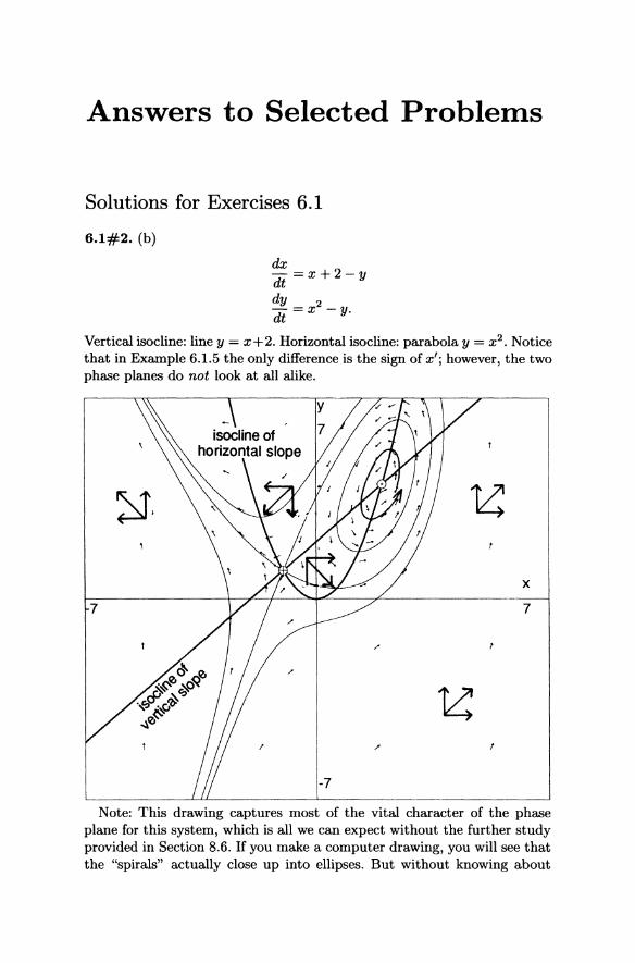
Answers to Selected Problems

Solutions for Exercises 6.1

6.1#2. (b)

dx -=x+2-y dt dy 2 - =X -yo dt

Vertical isocline: line y = x+2. Horizontal isocline: parabola y = x 2 • Notice that in Example 6.1.5 the only difference is the sign of x'; however, the two phase planes do not look at all alike.

x

7

Note: This drawing captures most of the vital character of the phase plane for this system, which is all we can expect without the further study provided in Section 8.6. If you make a computer drawing, you will see that the "spirals" actually close up into ellipses. But without knowing about

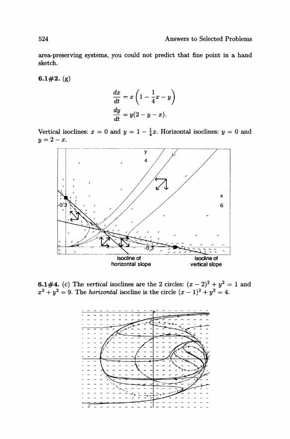
524 Answers to Selected Problems

area-preserving systems, you could not predict that fine point in a hand sketch.

6.1#2. (g)

Vertical isoclines: x = 0 and y = 1 - ~x. Horizontal isoclines: y = 0 and y = 2 - x.

y

4

isocline of horizontal slope

x

6

isocline of vertical slope

6.1#4. (c) The vertical isoclines are the 2 circles: (x - 2)2 + y2 = 1 and x2 + y2 = 9. The horizontal isocline is the circle (x - 1)2 + y2 = 4.

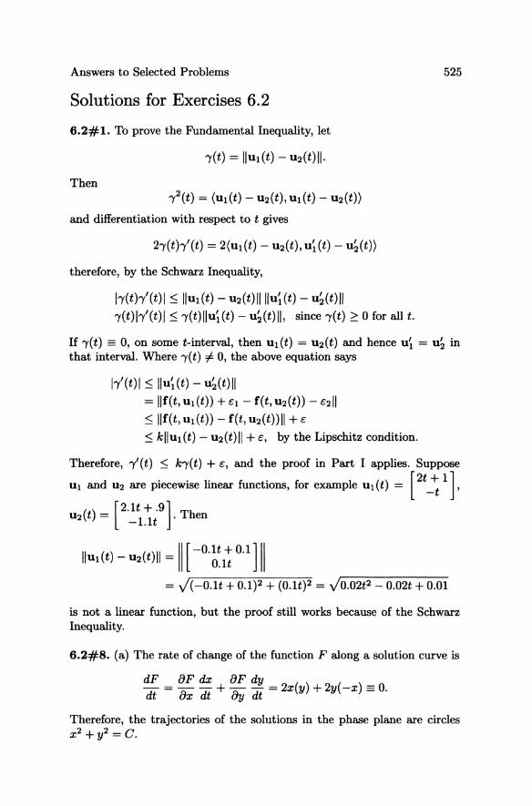
Answers to Selected Problems 525

Solutions for Exercises 6.2

6.2#1. To prove the Fundamental Inequality, let

Then

and differentiation with respect to t gives

2-y(th'(t) = 2(UI(t) - U2(t), u~(t) - u~(t»)

therefore, by the Schwarz Inequality,

l-y(th'(t)I $IIUI(t) - u2(t)lIlIu~(t) - u~(t)1I

-y(t)I-y'(t)1 $ -y(t)lIu~(t) - u~(t)lI, since -y(t) ~ 0 for all t.

If -y(t) = 0, on some t-interval, then UI(t) = U2(t) and hence ui = ua in that interval. Where -y(t) i 0, the above equation says

l-y'(t)I $lIu~(t) - u~(t)1I = IIf(t, UI(t» + el - f(t, U2(t» - e211

$lIf(t, UI(t» - f(t, U2(t» II + e

$ kllul(t) - U2(t) II + e, by the Lipschitz condition.

Therefore, -y'(t) $ k-y(t) + e, and the proof in Part I applies. Suppose

[2t_+t 1], UI and U2 are piecewise linear functions, for example UI(t) =

IIUI (t) - u2(t)1I = II [ -0·~~1~ 0.1] II = J(-O.lt + 0.1)2 + (O.lt)2 = JO.02t2 - 0.02t + 0.01

is not a linear function, but the proof still works because of the Schwarz Inequality.

6.2#8. (a) The rate of change of the function F along a solution curve is

dF aF dx aF dy - = - - + - - =2x(y)+2y(-x) =0. dt ax dt 8y dt

Therefore, the trajectories of the solutions in the phase plane are circles x2 +y2 =c.

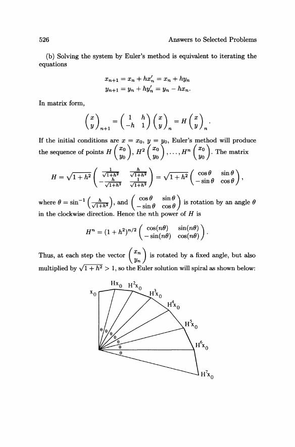
526 Answers to Selected Problems

(b) Solving the system by Euler's method is equivalent to iterating the equations

In matrix form,

X n+l =xn+hx~ =xn+hYn

Yn+1 = Yn + hy~ = Yn - hxn·

If the initial conditions are x = Xo, Y = Yo, Euler's method will produce

the sequence of points H ( :~ ), H2 (:~) , ... ,Hn (:~ ). The matrix

v'1~h2) =v'I+h2 ( c~O SinO) _1_ -smO cosO ' ~

where () = sin-1 (v'I~h2)' and (~~::O ~::) is rotation by an angle ()

in the clockwise direction. Hence the nth power of H is

Hn = (I + h2)n/2 (c~{n()) sin{n()) ) . - sm{ n()) cos{ n())

Thus, at each step the vector (::) is rotated by a fixed angle, but also

multiplied by VI + h2 > 1, so the Euler solution will spiral as shown below:

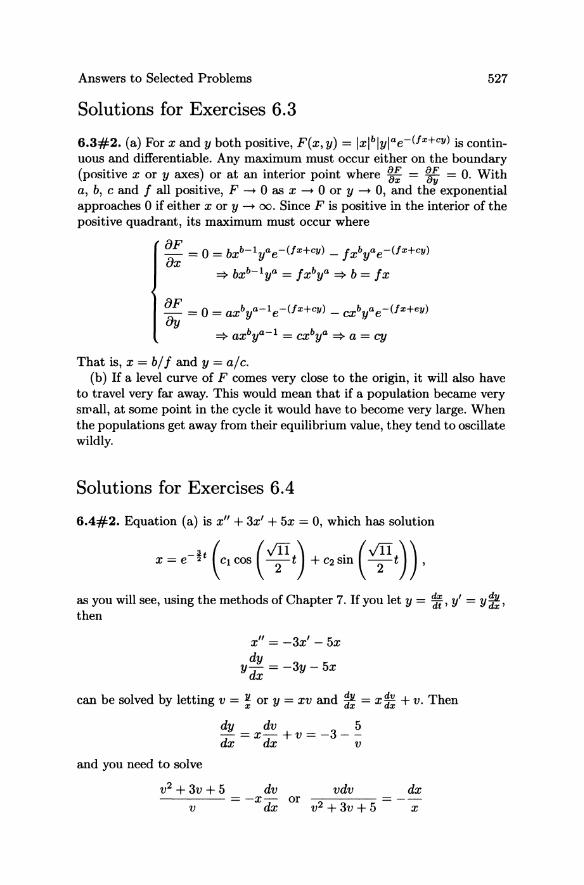
Answers to Selected Problems 527

Solutions for Exercises 6.3

6.3#2. (a) For x and y both positive, F(x, y) = Ixlblylae-(fo:+cy) is contin­uous and differentiable. Any maximum must occur either on the boundary (positive x or y axes) or at an interior point where ~; = ~~ = O. With a, b, c and f all positive, F -+ 0 as x -+ 0 or y -+ 0, and the exponential approaches 0 if either x or y -+ 00. Since F is positive in the interior of the positive quadrant, its maximum must occur where

That is, x = b/ f and y = a/c. (b) If a level curve of F comes very close to the origin, it will also have

to travel very far away. This would mean that if a population became very swall, at some point in the cycle it would have to become very large. When the populations get away from their equilibrium value, they tend to oscillate wildly.

Solutions for Exercises 6.4

6.4#2. Equation (a) is x" + 3x' + 5x = 0, which has solution

as you will see, using the methods of Chapter 7. If you let y = :' y' = y~, then

x" = -3x' - 5x dy

y dx = -3y - 5x

can be solved by letting v = ~ or y = xv and ~ = x: + v. Then

dy = x dv + v = -3 _ ~ dx dx v

and you need to solve

v2 + 3v + 5 dv vdv dx v = -x dx or v2 + 3v + 5 = x

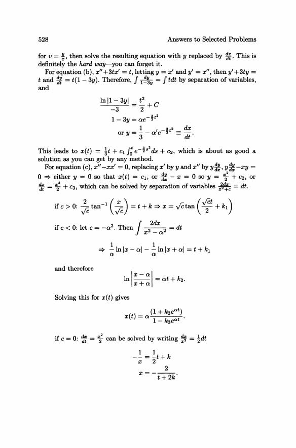
528 Answers to Selected Problems

for v = ~, then solve the resulting equation with y replaced by ~. This is definitely the hard way-you can forget it.

For equation (b), x" +3tx' = t, letting y = x' and y' = x", then y' +3ty = t and ¥t = t(1 - 3y). Therefore, J l~~Y = J tdt by separation of variables, and

In 11 - 3YI _ t 2 C -3 - 2 +

lIt2 1- 3y = ae- 2

1 ,_lIt2 dx or y = - - a e 2" ==-.

3 dt

This leads to x(t) = ~t + Cl J; e-!s2 ds + C2, which is about as good a solution as you can get by any method.

For equation (c), x"-xx' = 0, replacing x' by y and x" by y*, y*-xy =

o => either y = 0 so that x(t) = Ct, or * -x = 0 so y = ;2 + C2, or

~~ = "'; + C3, which can be solved by separation of variables ",1~c = dt.

ifc>O: ~tan-l(Jc) =t+k=>x=yCtan(~ +k1)

if c < 0: let c = _a2 • Then J 22dx 2 = dt x -a

1 1 => - In Ix - al - -In Ix + al = t + kl

a a

and therefore

In -- =at+k2 • Ix-al x+a

Solving this for x{t) gives

if c = 0: ~ = "'22 can be solved by writing ~ = ~dt

1 1 --=-t+k

x 2 2

X=---. t+2k

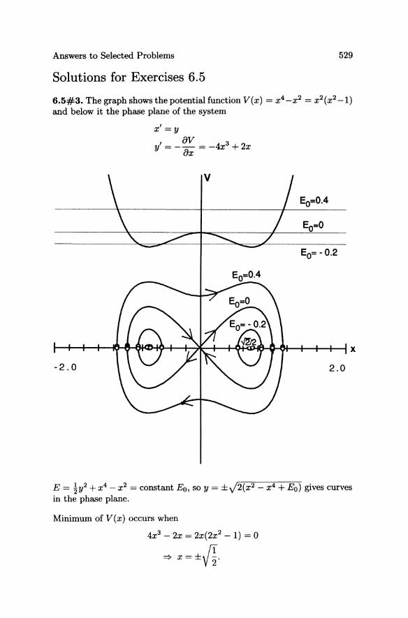
Answers to Selected Problems 529

Solutions for Exercises 6.5

6.5#3. The graph shows the potential function V(x) = x4_X2 = x 2(x2-1) and below it the phase plane of the system

x' = y

I aV 3 y = -- = -4x + 2x ax

EO= - 0.2

E = ~y2 + x4 - x2 = constant Eo, so y = ±J2(x2 - x4 + Eo) gives curves in the phase plane.

Minimum of V (x) occurs when

4x3 - 2x = 2x(2x2 - 1) = 0

~ x=±/I.

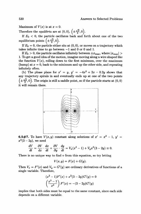
530 Answers to Selected Problems

Maximum of V(x) is at x = 0.

Therefore the equilibria are at (0,0), (±4,0). If Eo < 0, the particle oscillates back and forth about one of the two

equilibrium points (±4, 0). If Eo = 0, the particle either sits at (0,0), or moves on a trajectory which

takes infinite time to go between -1 and ° or ° and 1. If Eo > 0, the particle oscillates infinitely between ±xmax, where Ixmaxl >

1. To get a good idea of the motion, imagine moving along a wire shaped like the function V(x), rolling down to the first minimum, over the maximum (hump) at x = 0, back to the minimum and up the other side, and repeating infinitely often.

(b) The phase plane for x' = y, y' = -4x3 + 2x - 0.2y shows that any trajectory spirals in and eventually ends up at one of the two points

( ±4, 0). The origin is still a saddle point, so if the particle starts at (0,0) it will remain there.

-------- -5

--- -------'

6.5#7. To have V(x, y) constant along solutions of x' = x 2 - 1, y' = x 2 (3 - 2y), we need

dV BV dx BV dy 2 2 dt = dx . dt + By . dt = Vx(x - 1) + VyX (3 - 2y) == o.

There is no unique way to find v from this equation, so try letting

V(x, y) = F(x) + G(y).

Then Vx = F' (x) and Vy = G' (y) are ordinary derivatives of functions of a single variable. Therefore,

(x2 - I)F'(x) + x2(3 - 2y)G'(y) = ° (x2X: 1) F'(x) = -(3 - 2y)G'(y)

implies that both sides must be equal to the same constant, since each side depends on a different variable.

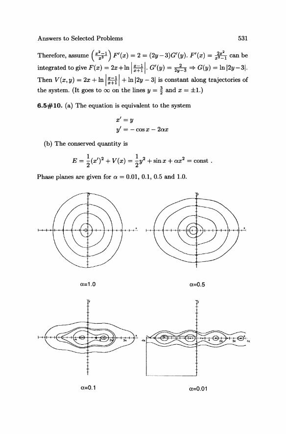
Answers to Selected Problems 531

Therefore, assume ( x:; 1 ) F'(x) = 2 = (2y - 3)G'(y). F'(x) = X~~1 can be

integrated to give F(x) = 2x+ln 1 :+~ I· G'(y) = 2Y~3 ~ G(y) = In 12y-31·

Then V(x, y) = 2x + In 1 :+~ 1 + In 12y - 31 is constant along trajectories of

the system. (It goes to 00 on the lines y = ~ and x = ±1.)

6.5#10. (a) The equation is equivalent to the system

x'=y

y' = -cosx - 2ax

(b) The conserved quantity is

E = ~(X')2 + V(x) = ~y2 + sin x + ax2 = const .

Phase planes are given for a = 0.01,0.1,0.5 and 1.0.

a=1.0 a=O.5

••

a=O.1 a=O.01

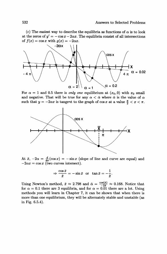
532 Answers to Selected Problems

(c) The easiest way to describe the equilibria as functions of 0 is to look at the zeros of y' = - cos x - 20x. The equilibria consist of all intersections of f(x) = cos x with g(x) = -20x.

-2ax

~~~~1=~~~b±~~~x 41t a = 0.02

For 0 = 1 and 0.5 there is only one equilibrium at (xo,O) with Xo small and negative. That will be true for any 0 < it where it is the value of 0

such that y = - 20x is tangeTlt to the graph of cos x at a value ~ < x < 11".

cos X

At x, - 20 = d~ (cos x) = - sin x (slope of line and curve are equal) and - 20x = cos x (two curves intersect).

cos X . _ 1 =} -- = -SIllX or tan x = --. x x

Using Newton's method, x ~ 2.798 and it = c~J:) ~ 0.168. Notice that for 0 = 0.1 there are 3 equilibria, and for 0 = 0.01 there are a lot. Using methods you will learn in Chapter 7, it can be shown that when there is more than one equilibrium, they will be alternately stable and unstable (as in Fig. 6.5.4).

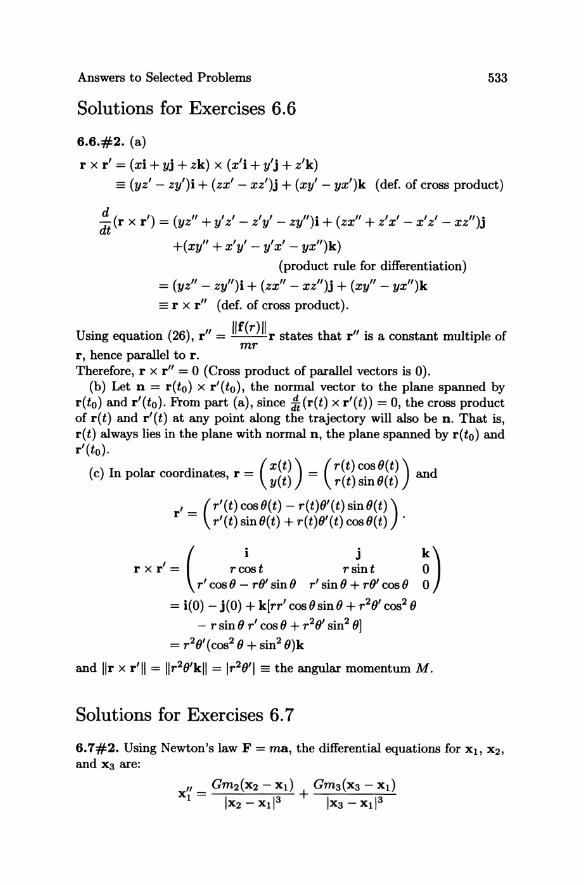
Answers to Selected Problems 533

Solutions for Exercises 6.6

6.6.#2. (a)

r x r' = (xi + yj + zk) x (x'i + y'j + z'k)

== (yz' - zy')i + (zx' - xz')j + (xy' - yx')k (def. of cross product)

!!..(r x r') = (yz" + y'z' - z'y' - zy")i + (zx" + z'x' - x'z' - xz")j dt

+(xy" + x' y' - y' x' - yx")k)

(product rule for differentiation)

= (yz" - zy")i + (zx" - xz")j + (xy" - yx")k

== r x r" (def. of cross product).

Using equation (26), r" = IIr(r)II r states that r" is a constant multiple of mr

r, hence parallel to r. Therefore, r x r" = 0 (Cross product of parallel vectors is 0).

(b) Let n = r(to) x r'(to), the normal vector to the plane spanned by r(to) and r'(to). From part (a), since !t(r(t) x r'(t)) = 0, the cross product of ret) and r'(t) at any point along the trajectory will also be n. That is, ret) always lies in the plane with normal n, the plane spanned by r(to) and r'(to).

. (X(t)) (r(t)COSO(t)) (c) In polar coordmates, r = yet) = r(t)sinO(t) and

r' = (r'(t) cos OCt) - r(t)O'(t) sin O(t)) . r'(t) sinO(t) + r(t)O'(t) cosO(t)

r x r' = (rc~t rs1nt ~O) r' cos 0 - rO' sin 0 r' sin 0 + rO' cos 0

= i(O) - j(O) + k[rr' cos 0 sin 0 + r20' cos2 0

- r sin 0 r' cos 0 + r 20' sin2 OJ

= r 20' (cos2 0 + sin2 O)k

and IIr x r'lI = IIr20'kll = Ir20'1 == the angular momentum M.

Solutions for Exercises 6.7

6.7#2. Using Newton's law F = rna, the differential equations for Xl, X2,

and X3 are:

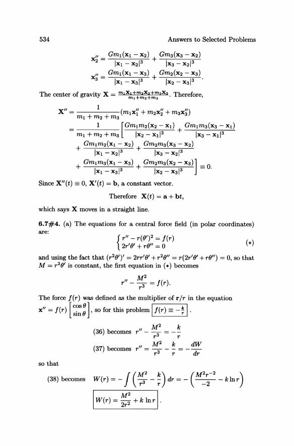
534 Answers to Selected Problems

The center of gravity X = m 1Xl±m2X2±maXa. Therefore ml±m2±ma '

1 X" = (m x" + m x" + m x") + + I I 2 2 3 3 ml m2 m3

= 1 [Gmlm2(X2 - Xl) + Gmlm3(x3 - xt) ml + m2 + m3 IX2 - xl13 IX3 - xl13

Gmlm2(xl - X2) Gm2m3(x3 - X2) + +_--c'-----'-':........:...-=-----'-IXI - x213 IX3 - x213

Gmlm3(xl - X3) Gm2m3(x2 - X3)] - 0 + IXI-X313 + IX2 -x313 =.

Since X"(t) == 0, X'(t) = b, a constant vector.

Therefore X(t) = a + bt,

which says X moves in a straight line.

6.7#4. (a) The equations for a central force field (in polar coordinates) are:

{ r" - r(O')2 = f(r) 2r' 0' + rO" = 0

and using the fact that (r20')' = 2rr'O' +r20" = r(2r'O' +rO") = 0, so that M = r20' is constant, the first equation in (*) becomes

"M2 ( ) r --=fr. r3

The force f(r) was defined as the multiplier of r/r in the equation

x" = f(r) [~~::], so for this problem 1 f(r) == -~ I·

(36) becomes " M2 k r --

r3 r

(37) becomes " M2 k dW

r =---r3 r dr

so that

(38) becomes W(r) = - ! (~-~) dr = _ (M~~-2 - klnr)

M2 W(r) = 2r2 + k lnr

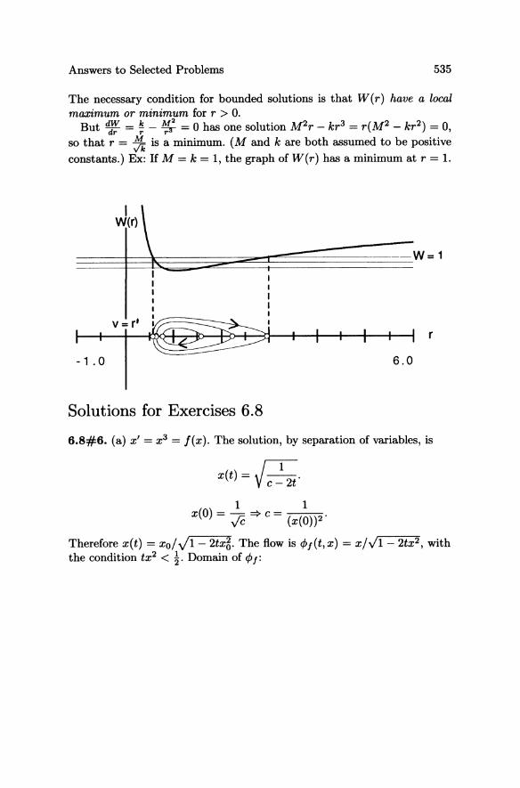
Answers to Selected Problems 535

The necessary condition for bounded solutions is that W(r) have a local maximum or minimum for r > O.

But dd~ = ~ - ~ = 0 has one solution M2r - kr3 = r(M2 - kr2) = 0, so that r = 0c is a minimum. (M and k are both assumed to be positive constants.) Ex: If M = k = 1, the graph of W(r) has a minimum at r = 1.

-1 .0

I W(r)

v = r'

Solutions for Exercises 6.8

r

6.8#6. (a) x' = x3 = I(x). The solution, by separation of variables, is

x(t) = V 1 2 , c- t

1 1 x(O) = y'C ::::} c = (x(O) )2'

Therefore x(t) = xo/../1- 2tx~. The flow is cPf(t,x) = x/'J1- 2tx2 , with the condition tx2 < ~. Domain of 4> f:

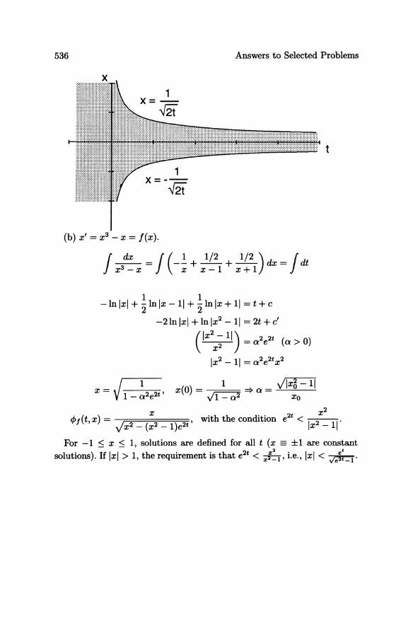
536 Answers to Selected Problems

t

1 x=---

{2t

(b) x' = x3 - X = f(x).

J ~=J(-.!.+ 1/2 + 1/2 )dX=Jdt x3 - x X x-I x + 1

1 1 -In Ixl + "2 In Ix - 11 + "2 In Ix + 11 = t + c

-21n Ixl + In Ix2 - 11 = 2t + c'

CX2x~ 11) = a 2e2t (a> 0)

Ix2 - 11 = a 2e2t x 2

x(O) = 1 => a = Jlx5 - 11 VI - a 2 Xo

x u ~ </>f(t,x) = , with the condition e < Ix2 -11·

Jx2 - (x2 - l)e2t

For -1 ~ x ~ 1, solutions are defined for all t (x == ±1 are constant

solutions). If Ixl > 1, the requirement is that e2t < X:~l' Le., Ixl < v'e~:-l·

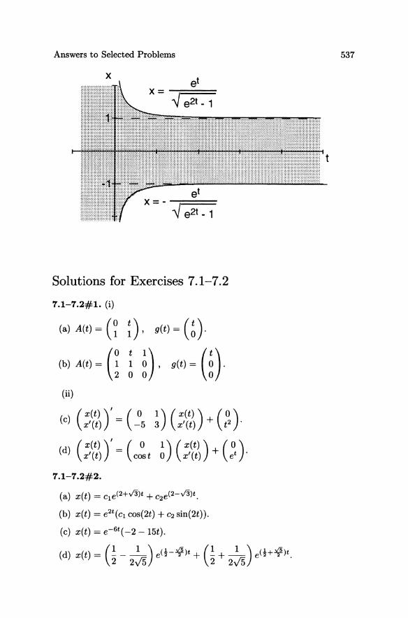
Answers to Selected Problems

Solutions for Exercises 7.1-7.2

7.1-7.2#1. (i)

(a) A(t) = (~ ~), g(t) = (~).

(b) A(t) ~ Gin, g(t) ~ m (ii)

(c) (:,~t2»)' = (~5 !) (:,w») + (t~ ). (d) (;W»)' = (c!t ~) (;W») + (~).

7.1-7.2#2.

(a) x(t) = cle(2+v'3)t + C2e(2-v'3)t.

(b) x(t) = e 2t (cl cos(2t) + C2 sin(2t».

(c) x(t) = e-6t ( -2 - 15t).

(d) x(t) = (~ __ 1_) e(!-~)t + (~+ _1_) e(!+~)t. 2 2J5 2 2J5

537

t

538 Answers to Selected Problems

7.1-7.2#3.

(a) x{t)=J3etsin(~).

7.1-7.2#4.

(a) x{ t) = CI/t + C2/t2.

(b) Solutions are defined for t > 0 or for t < 0, depending on where the initial conditions are given.

• 1+2V5 1-V5 (c) The cookbook method produces the solutlOn x{t) = CIt +C2t---r-.

(d) The solution in (c) is defined for t > O. For t < 0, x{t) = CI (-t) 1+2V5 + C2{-t)¥ is a solution of the differential equation. Therefore, the

most general solution is x{t) = cIltI 1\V5 + c2ItI 1- 2V5 , which holds for t ¥= o.

7.1-7.2#7. Schwarz's Inequality says: Given vectors x and y, l(x,y)1 ~ IIxlillyll·

A ~)(~)' ::~ V(l:::r)':: 0: ~:~::: :~:t ~, a,. (a,., x)

IIAxll2 = (al,x)2 + (a2,x)2 + ... + (a,.,x)2

= ~)a;,x)2 ~ L 1Ia;1I211x1l2 (by Schwarz Inequality)

= IIxl1 2 L IlBill2 = IIxll211AI12 i

(if IIAII is defined by Vr..i,; lai;12).

Therefore II Ax II ~ IIxliliAIl by taking the square root. (b) x' = Ax satisfies a Lipschitz condition on a x an if there exists a

real number k such that IIA(x - y)11 ~ kllx - yll for all X,y E an. (c) From part (a), IIA{x-y)1I ~ IIAllllx-yll, where IIAII = Jr-r..-i,-;(-a'-"j)-2 ~

k, since the elements of A are bounded. Therefore, the linear system always satisfies a Lipschitz condition.

Answers to Selected Problems

(d) For x = [~ ;] x, the constant k could be taken to be

v'02 + 12 + 12 + 22 = v'6.

539

Note: other norms for A can be defined. The one used here does not give the "best" Lipschitz constant k.

Solutions for Exercises 7.3

7.3#1. (i)

(a) Al = -1, U1 = C (~) A2 = 2, U2 = C (~).

(b) A = 2, U = C ( ~ ).

(c) A1,2 = -2 ± i, eigenvectors (!), (2i).

(d) A, ~ 1, u, ~ UJ A, ~ 2 with 2 line.dy mdependent eigenvecto'" G) and G)-

(e) A, ~ -1, u, ~ c ( ~1 ); A, ~ 1, u, ~ c UJ Aa ~ 5, Ua ~ em·

(f) Al = 3, U1 = C ( ~ ) j A2 = 1 - 2V2j U2 = C ( -~ ) j -5 -2 + V2

A3 = 1 + 2V2, U3 = C ( ~ ) •

-2 - V2

(g) A, ~ -3, u, ~ c ( ~1 }

A2,3 = 4 ± v7 i, U2,3 = ( ~ ) ± i ( J.r ) . -13 5v7

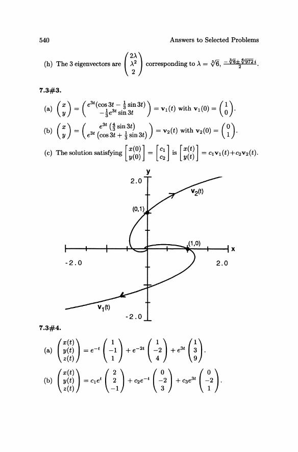
540 Answers to Selected Problems

(b) The 3 eigenveclo," Me (~) corresponding 10 ~ ~ ?'ii, - W±,='.

7.3#3.

y

-2.0

7.3#4.

(a) G1:D ~ e-' ( ~1 ) +e-" ( ~2 ) + e" m (b) G1lD ~ c,e' UJ He-' ( ~2 ) he" ( ~2 )

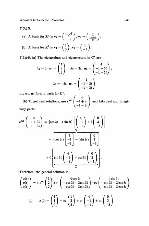
Answers to Selected Problems

7.3#5.

(a) A basis for ]R2 is VI = ( 1~; ), V2 = ( H~y'5 ).

(b) A basis for ]R2 is Vl = (~), V2 = ( ! 1 ) .

7.3#6. (a) The eigenvalues and eigenvectors in C3 are

'>'1 = 0, Ul = (~) j '>'2 = 3i, U2 = (-1 ~ 3~) j

2 -1- 3~

'>'3 = -3i, U3 = (-1 ~ 3i) -1 +3i

Ul! U2, U3 form a basis for C3 •

541

(b) To get real solutions, use e 3it (-1 ~ 3i) and take real and imagi­-1-3i

nary parts.

e3" (=:~=) ~ [amat+i&n~l [( ;:) +i (!a)]

U ..

~ .(=~) [ ;:]- (~n~) [ ~J

+i!~at (;:) :cm~ Ua}). Therefore, the general solution is

(X(t») (1) ( 4cos3t ) ( 4sin3t ) y(t) =CleOt 2 +C2 -cos3t-3sin3t +C3 -sin3t+ 3cos3t . z(t) 2 -cos3t + 3sin3t -sin3t-3cos3t

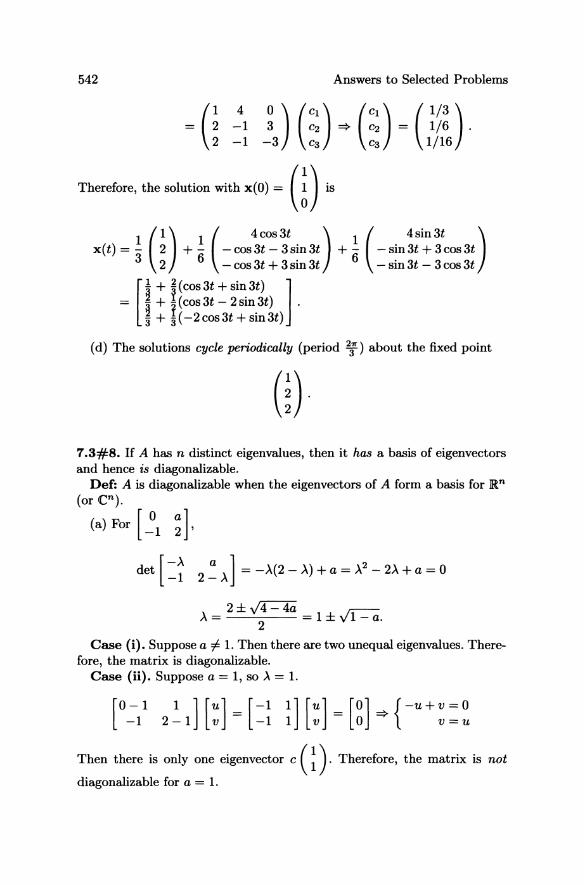
542 Answers to Selected Problems

Therefore, the solution with x(O) ~ 0) is

x(t) = ~ (~) + ~ (-cos~~~~tsin3t) + ~ (_sin!:i~;tCOS3t) 3 2 6 _ cos 3t + 3 sin 3t - sin 3t - 3 cos 3t

= t + t(coS3t - 2sin3t) . [! + ~ (cos 3t + sin 3t) ]

3 + 3( -2 cos 3t + sin3t)

(d) The solutions cycle periodically (period 2;) about the fixed point

7.3#8. If A has n distinct eigenvalues, then it has a basis of eigenvectors and hence is diagonalizable.

DeC: A is diagonalizable when the eigenvectors of A form a basis for IRn

(or en).

(a) For [~1 ;],

det [=~ 2 ~ >.] = ->'(2 - >.) + a = >.2 - 2>' + a = °

>. = 2 ± v'4=4li = 1 ± vT=a 2 .

Case (i). Suppose a :f:. 1. Then there are two unequal eigenvalues. There­fore, the matrix is diagonalizable.

Case (ii). Suppose a = 1, so >. = 1.

[0-1 1 ][U]=[-l l][U]=[O]=>{-U+v:o -1 2 -1 v -1 1 v ° v - U

Then there is only one eigenvector c ( ! ). Therefore, the matrix is not

diagonalizable for a = 1.

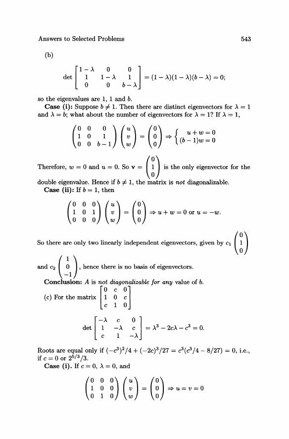
Answers to Selected Problems

(b)

[1- A

det ~ o

I-A o

~ 1 = (1 - A)(1 - A)(b - A) = OJ b-A

so the eigenvalues are 1, 1 and b.

543

Case (i): Suppose b 1: 1. Then there are distinct eigenvectors for A = 1 and A = bj what about the number of eigenvectors for A = I? If A = 1,

(0 0 0) (U) (0) { u+w=O ~ ~ b ~ 1 : = ~ =? (b - l)w = 0

The<efo"', w ~ 0 and • ~ O. So v ~ G) ;" the only eigenvector £0, the

double eigenvalue. Hence if b 1: 1, the matrix is not diagonalizable. Case (ii): If b = 1, then

So the", Me only two line.dy "'dependent e;genvee_, given by c, (!) and c, ( i 1) , hence th"", ;" no bas .. of e;gen"",torn.

Conclusion: A is n[o~ d~ago;lalizable for any value of b.

(c) For the matrix 1 0 c c 1 0

[-A COl

det 1 -A C

C 1 -A

Roots are equal only if (-2)2/4 + (-2c)3 /27 = c3(c3/4 - 8/27) = 0, i.e., if C = 0 or 25/ 3 /3.

Case (i). If C = 0, A = 0, and

544 Answers to Selected Problems

"" there ;" only one e\genvecto, (~), Case (ii). If c = 25/ 3 /3, then ,\ = 2c/~, -c/~, -c/~. For the

double root, ,\ = -c/ ~ = _24/ 3 /3.

(2r 25 / 3 -3-

2 5 / 3 -3-24 / 3 -3-

1

"" ( ~F) ;" the only eigenvect",,

::~::~: m(ar ; dt)g~naHZahle except when c ~ ° 0' 25

/3/3,

c02

det (1 ~,\ 2 ~ ,\ ~) = (2 _ ,\)[,\2 - 3'\ + 2 - ac] = O. c 0 2-,\

Therefore, the eigenvalues are ,\ = 2, 3±~. If either a or c is 0, ,\ = 2 is a double eigenvalue. If 4ac = -1, ,\ = ~ is a double eigenvalue. Case (i): a = 0, ,\ = 2.

01 ~ ~)(n ~ (~) If bolO, the'e ;" only one eigenvecto, (!), If b ~ 0, m and m are both ~genvecto~, Similarly, for c = 0, ,\ = 2. Case (ii): If 4ac = -1, so ,\ = 3/2 is a double eigenvalue:

C{a i i)(~)~Cf:.:~:)~m=>{::~a2~ and ( ~b) is the only eigenvectm, Therefore, the matdx ;" not diago­

nalizable.

Answers to Selected Problems 545

Conclusion: This matrix is diagonalizable unless a = 0 (with b =I- 0), c = 0 (with b =I- 0) or 4ac = -1 (arbitrary b).

Solutions for Exercises 7.4

7.4#6. Write x" + 3x' + 2x = 0 as a system

{X' =y y' = -2x - 3y.

Then (~)' = (~2 !3) (~) and we need to find eAt where A =

(~2 !3). The eigenvalues and eigenvectors of A are Al = -1, Ul =

( !1) and A2 = -2, U2 = ( !2)· Therefore,

At (1 1) (e- t 0) (1 1)-1 e = -1 -2 0 e-2t -1-2

( 2e-t _ e-2t e-t _ e-2t )

= -2e-t + 2e-2t _e-t + 2e-2t .

The solution of the differential equation with initial condition (~g~?) =

Xo is given by u(t) = eA(t-to)xo. If you let t = to and (~) = x(O), then

( -t) (-2t) can be put in the form Cl ~e-t + C2 ;:-2t by letting Cl = 20 + {3

and C2 = 0 + {3.

7.4#11. (a) Any 2 x 2 matrix with trace = 0 can be written as

A = (a b), det A = _(a2 + bc) C -a

A2 = (a b) (a b) e -a c-a

( a2 + be 0) 2 = 0 a2+be =(a + be) I = (-detA)I.

546 Answers to Selected Problems

(b)

tA t2 2 t3 3 t 4 4 e = 1+ tA + - A + -A + -A + ... 2! 3! 4!

= I + tA - C; det A ) I - (~~ det A ) A + ~ (det A)2 I + ...

= 1[1- ~~ detA + ~~ (detA)2 - ~~ (detA)3 + ... J

+ A [t - t~ det A + t~ (detA)2 - ... J = a(t)I + ,B(t)A. 3. 5.

(c) If detA > 0, then

If det A < 0, then

{ a(t) = cos(JdetA· t)

,B(t) = ~sin(v'detA.t) detA

{ a(t) = cosh( vi det AI t)

,B(t) = 1 sinh( vi det AI . t). vldetAI

Solutions for Exercises 7.5

7.5#3. Given x' = Ax with trace A = 0, let

x' = (a b) x. c -a

Then ~~ = ax + by and !fit = ex - ay. To see that the equation

dy ex - ay

dx ax+by

is exact, write it in the form P(x, y)dx + Q(x, y)dy = 0 and check that oP/oy = oQ/ox. From (*), (ex - ay)dx - (ax + by)dy = ° = Pdx + Qdy

OP oQ -=-a=-oy ax'

Integrating P and Q partially with respect to x and y gives

ex2 by2 V(x, y) = 2 - axy - 2 = const.

Answers to Selected Problems 547

(To check: ~~ = ex - ay = P and t = -ax - by = Q.) The level curves of V are trajectories in the phase plane.

7.5#7. If A is real and A is a complex eigenvalue, then X is also an eigen­value. Furthermore, if

Aw = AW (w is the complex eigenvector corresponding to A),

then taking complex conjugates:

Aw = AW.

Since A is real (A = ..4), this says Aw = Xw. That is, w is the eigenvector corresponding to X.

Since A and X are distinct eigenvalues, W and w are linearly independent. Now suppose W = W1 + iW2 and W1 and W2 are not linearly independent. Then W1 = c· W2 for some scalar c. But this implies that

W1+iW2=CW2+iW2=(C+i)W2} . (C+i) . ~ W1 + ZW2 = --. (W1 - ZW2)

WI - iW2 = CW2 - iW2 = (c - i)W2 C - Z

which contradicts the linear independence of W and w. Therefore, W1 and W2 must be linearly independent.

7.5.#8. If x' = (: :) x, and the trajectories spiral, then detA = ad­

be> 0 and trace A = a + d satisfies (trace A)2 < 4(detA), i.e.,

(a + d)2 < 4(ad - bc).

The polar angle O( t) = tan -1 (~), and the direction of the trajectories

will be clockwise if dO / dt < 0 and counterclockwise if dO / dt > O.

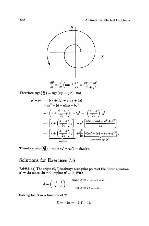
548 Answers to Selected Problems

y

x

dJ} d ( -1 Y) xy' - yx' dt = dt tan ;; = X2 + y2 •

Therefore sign(~n = sign(xy' - yx'). But

xy' - yx' = x(cx + dy) - y(ax + by) = cx2 + (d - a)xy _ by2

Therefore, sign(~n = sign(xy' - yx') = sign(c).

Solutions for Exercises 7.6

7.6#5. (a) The origin (0, 0) is always a singular point of the linear equation x' = Ax since AO = 0 implies x' = O. With

A= (-1 1) o 0 '

traceA=:T= -1+0

detA =: D = -20.

Solving for D as a function of T:

D = -20 = -2(T + 1).

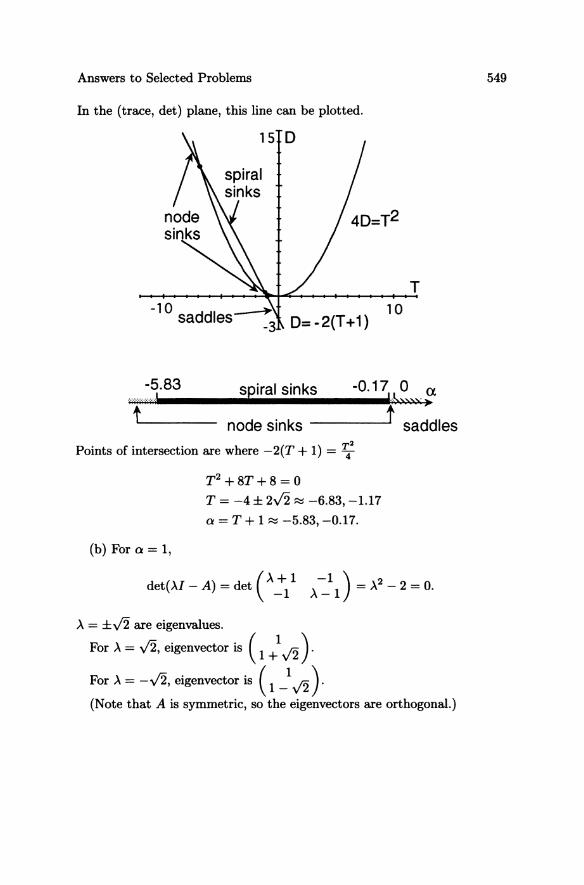
Answers to Selected Problems

In the (trace, det) plane, this line can be plotted.

T

-5.83 .................... 1

t node sinks ___ ---'t saddles

Points of intersection are where -2(T + 1) = ~2

(b) For a = 1,

T 2 +8T+8=0 T = -4 ± 2V2 ~ -6.83, -1.17

a = T + 1 ~ -5.83, -0.17.

det(,\l- A) = det (A + 1 -1) = A2 - 2 = O. -1 A-I

A = ±J2 are eigenvalues.

For A = J2, eigenvector is (1 +1 V2 ) .

For A = -v'2, eigenvector is (1 _1 J2). (Note that A is symmetric, so the eigenvectors are orthogonal.)

549

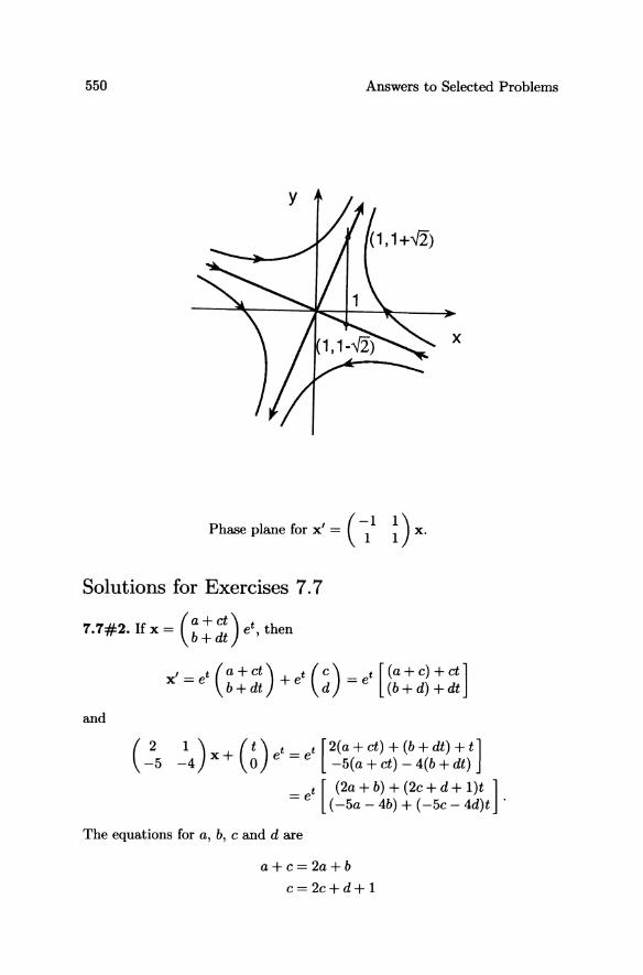
550 Answers to Selected Problems

x

Phase plane for x' = ( ~ 1 ~ ) x.

Solutions for Exercises 7.7

and

,= t(a+ct)+ t(c)= t[(a+c)+ct] x e b + dt e d e (b + d) + dt

x+ e =e 1 ) (t) t t [2(a+ct)+(b+dt)+t] -4 0 -5(a + ct) - 4(b + dt)

t [ (2a+b)+(2c+d+l)t ] = e ( -5a - 4b) + ( -5c - 4d)t .

The equations for a, b, c and d are

a+c=2a+b

c= 2c+d+ 1

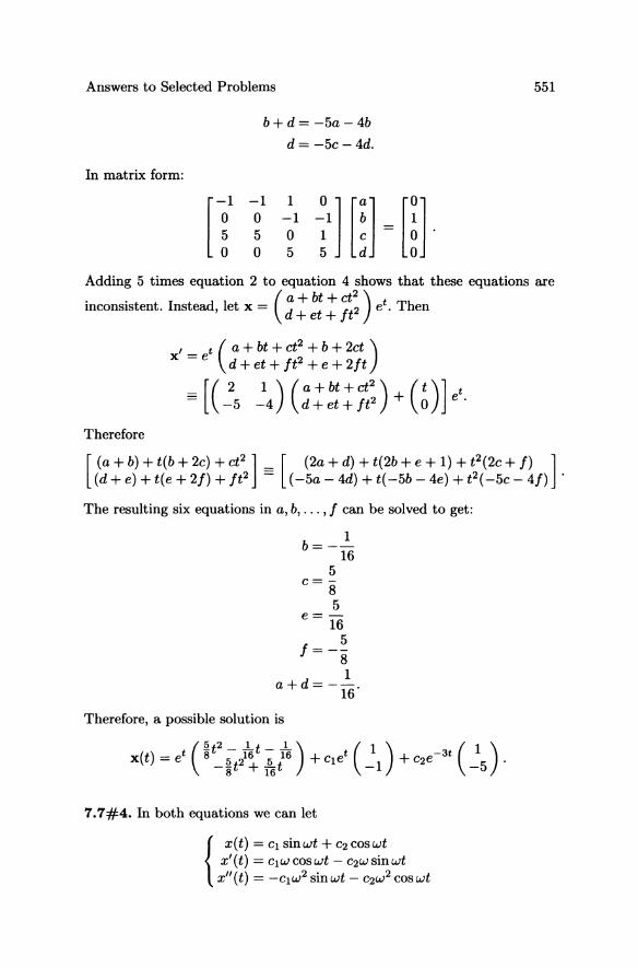
Answers to Selected Problems

In matrix form:

b+d= -5a- 4b d= -5c- 4d.

551

Adding 5 times equation 2 to equation 4 shows that these equations are

inconsistent. Instead, let x = (;::: ~ 1t: ) et • Then

, t(a+bt+ct2+b+2ct) x = e d + et + ft2 + e + 2ft

== [( _~ !4) (;:::: 1t: ) + ( ~ ) ] et .

Therefore

[ (a+b)+t(b+2C)+ct2 ] _ [ (2a+d)+t(2b+e+1)+t2(2c+J) ] (d+e)+t(e+2J)+ft2 = (-5a-4d)+t(-5b-4e)+t2(-5c-4J) .

The resulting six equations in a, b, ... , f can be solved to get:

1 b=--

16 5

c= -8 5

e = 16 5

f=--8 1

a+d= -16'

Therefore, a possible solution is

7.7#4. In both equations we can let

{ x(t) = Cl sinwt + C2 coswt

x'(t) = ClwcosWt - c2wsinwt x"(t) = -CIW2 sinwt - C2W2 coswt

552 Answers to Selected Problems

For x" + x' + x = sin(wt):

(Cl sinwt + C2 coswt) + (CIW coswt - C2W sinwt)

+ (-Cl w2 sin wt - C2W2 cos wt)

= sinwt(cl - C2W - Clw2) + coswt(C2 + CIW - C2w2)

1· sinwt + O· coswt

which says

This gives

( 1-W2 ) ( w ) x(t) = (1 _ w2)2 + w2 sinwt - (1 _ W2)2 + w2 coswt

= sinwt 1 [1 -w2

J(l - w2)2 + w2 J(l- w2)2 + w2

- coswt W ] J(l- w2)2 + w2

= R(w)[coscpsinwt - sin cp coswt]

where

(b) Adding the homogeneous solution,

R(w) sin(wt - cp) , ' ...

x(t) = e-!t (ACOS ~t + Bsin ~t) +

steady state solution with amplitude R(w) = 1jJ(1-w2)2 +w2

(Note: R(w) is called the gain.)

, ~

'" transient solution --+ 0 as t --+ 00

(c) For x" + 2x = sinwt

(-CIW2 sinwt - C2w2 coswt) + 2(Cl sinwt + C2 coswt)

= 1 - sin wt + 0 . cos wt

Therefore, (2 - W2)Cl = 1, (2 - W2)C2 = 0 =? C2

(w =I- v'2). o and Cl 1

2-w2

Answers to Selected Problems 553

The full solution is x(t) = A cos J2t + Bsin J2t+ 2!w2 sinwt if w =F J2. For w = J2, write the equation in the form

{X' =y y'=-2x+sinJ2t j

that is, (:)' = (~2 ~) (:) + (sin~t) = Ax+ g(t).

A2 = (~2 ~) (~2 ~) = (~2 ~2) = -21

At t2 2 t3 3 e = 1 + tA + -A + -A + ... 2! 3! t2 t3 t4 t5

= 1 + tA + -(-21) + -(-2A) + -(41) + -(4A) + ... 2! 3! 4! 5!

= 1 (1- (J2t)2 + (J2t)4 _ ... ) 2! 4!

+ ~ (J2t _ (J2t)3 + (J2t)5 _ ... ) J2 3! 5!

= cos(v2t)1 + sin(J2t) A = ( cosJ2t J2 -J2 sin J2t

The variation of parameters formula gives:

u(t) = etAx(O) + lot e<t-s)Ag(s)ds

= ----v"2. x(O) ( cosJ2t ~) - J2 sin J2t cos J2t

~). cosJ2t

ft ( cos(J2(t - s» Sin(~-S») ( 0 ) + 10 -J2sin(J2(t-s» cos(J2(~-s» sinJ2s ds

= v'2 x(O) (COS J2t sin VZt )

-J2 sin J2t cos J2t

+ ft ( ~ sin( J2s) sin( J2(t - S») ds. 10 sin( J2s) cos( J2(t - s»

Finally, we get (noting that the integration is very messy)

u(t) = x(O) ( -~st::nt ) + x'(O) ( c:~t ) + (! sin(J2t) _ tco;~t») .

tsin(v'2t) 2

554 Answers to Selected Problems

7.7#9. To solve x" + w2x = g(t) = 1. ",,00_ sin«2n-l)t) let 11" wn-l 2n-l '

00

x(t) = 2: an sin(nt) n=l

00

x'(t) = 2: nan cos(nt) n=l

00

x"(t) = - 2: n 2an sin(nt) n=l

then - Z=:=l n 2a n sin(nt) + w2 Z=:=l an sin(nt) 1 sin(3t) + ... ). Therefore,

~(sint + 0 . sin(2t) +

n positive odd integer n positive even integer

Therefore an = n11"(wLn2) if n is odd, and 0 if n is even. This works if, and only if, w is not an odd integer. It gives the solution

1 2:00 sin((2n - l)t) x t --( ) - 7r n=l (2n - 1)[w2 - (2n - 1)2]

which obviously converges as n -+ 00.

If w is an odd integer, there is a zero in the denominator, and the solution above is not well defined. Suppose w = 2m - 1 for some integer m > O. Then we need to solve separately the equation

and the equations

"( )2 1 sin(2m - l)t x + 2m -1 x = ---'----'-7r 2m-l

" ( _)2 _.!. sin(2n - l)t x + 2m 1 x - 2 1 ' 7r n-

for n -I- m.

The second set of equations are solved as above, but the first is the resonant case, and to solve it by undetermined coefficients, one must try a solution of the form

x(t) = Atsin(2m -1)t+ Btcos(2m-l)t+C sin(2m -1)t+ Dcos(2m -1)t.

Differentiating twice and substituting in the equation leads to

A=O, 1

B = ---, C,D arbitrary. 2m7r

Thus in that case the general solution of the equation is

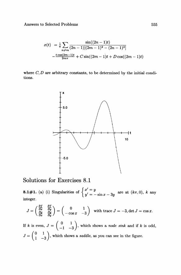
Answers to Selected Problems 555

1 "" sin((2n - l)t) x(t) =:;r ~ (2n _ 1)[(2m - 1)2 - (2n - 1)2]

n#m

- tCOS~;":-l)t + Csin((2m - l)t + Dcos((2m - l)t)

where C, D are arbitrary constants, to be determined by the initial condi­tions.

x

10

Solutions for Exercises 8.1

8.1#1. (a) (i) Singularities of {x; = y. 3 are at (k7r,O), k any y = -smx - y

integer.

~

J=(t 8x

~) (0 1 ) ~~ = 3 with trace J = -3, det J = cos x. =- -cosx-8y

If k is even, J = (~1 !3)' which shows a node sink and if k is odd,

J = (~ !3)' which shows a saddle, as you can see in the figure.

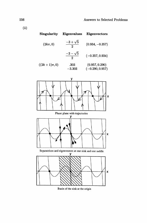
556 Answers to Selected Problems

(ii)

Singularity Eigenvalues Eigenvectors

(2k1r,0) -3 + v'5 (0.934, -0.357)

2

-3 - v'5 (-0.357,0.934)

2

((2k + 1)11",0) .303 (0.957,0.290) -3.303 (-0.290,0.957)

Phase plane with trajectories y

Separatrices and eigenvectors at one sink and one saddle y

Basin of the sink at the origin

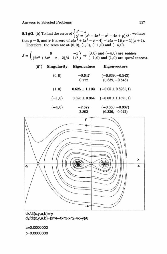
Answers to Selected Problems 557

{Xi =y

8.1#3. (b) To find the zeros of I (4 + 4 3 2 4 + )/8' we have y = X X -x - x y that y = 0, and x is a zero of x{x3 + 4x2 - X - 4) = x{x -l){x + l){x + 4).

Therefore, the zeros are at (O,O), (1,0), (-I, 0) and (-4, 0).

J-( ° - {2x3 + 6x2 - X - 2)/4 -1 ) (O,O) and (-4,0) are saddles 1/8 =? (-1,0) and (1,0) are spiral sources.

(ii") Singularity Eigenvalues

(O,O) -0.647 0.772

(1,0) 0.625 ± 1.116i

(-1,0) 0.625 ± 0.864

(-4,0) -2.677 2.802

dxlctt(x,y,a,b)=-y dy/dt(x,y ,a,b )=(x"4+4xA3-xA2-4x+y)/8

a=O.OOOOOOO

b=O.OOOOOOO

Eigenvectors

( -0.839, -0.543) (0.839, -0.648)

(-0.05 ± 0.893i, 1)

(-0.08 ± 1.152i, 1)

( -0.350, -0.937) (0.336, -0.942)

x

4

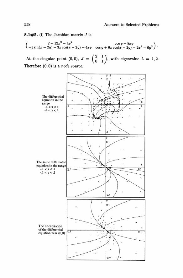
558 Answers to Selected Problems

8.1#5. (i) The Jacobian matrix J is

( 2 - 12x2 - 4y2 -3sin(x - 2y) - 3xcos(x - 2y) - 4xy

cosy - 8xy ) cosy + 6xcos(x - 2y) - 2X2 - 6y2 .

At the singular point (0,0), J = (~ ~), with eigenvalue .A = 1,2.

Therefore (0,0) is a node source.

The differential equation in the range

-4 < x < 4 2

-4 < Y <4

The same differential equation in the range

-.1 < x < .1 0.1

-.I < Y <.I

The linearization of the differential equation near (0,0)

y

2

·0.1'

0.1

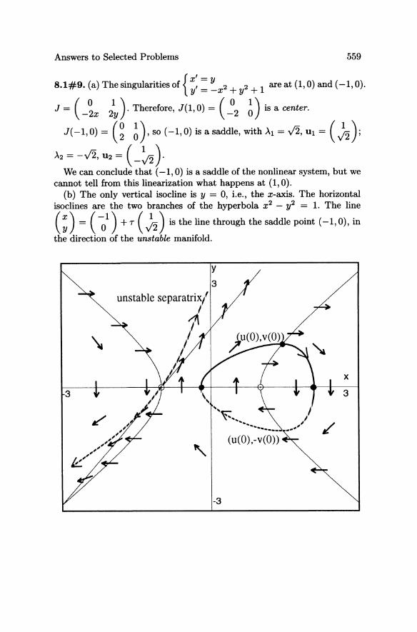
Answers to Selected Problems 559

8.1#9. (a) The singularities of {x; = Y 2 2 1 are at (1,0) and (-1,0). y = -x +y +

( 0 1) (0 1). J = -2x 2y . Therefore, J(l,O) = -2 0 IS a center.

J( -1,0) = (~ ~), so (-1,0) is a saddle, with Al = y'2, Ul = ( ~);

A2 = -y'2, U2 = (_~). We can conclude that (-1,0) is a saddle of the nonlinear system, but we

cannot tell from this linearization what happens at (1,0). (b) The only vertical isocline is y = 0, i.e., the x-axis. The horizontal

isoclines are the two branches of the hyperbola x 2 - y2 = 1. The line

(:) = ( ~1 ) + T ( ~) is the line through the saddle point (-1,0), in

the direction of the unstable manifold.

3

y

3

-3

.. -(u(O),-v(O))

x

3

~" /

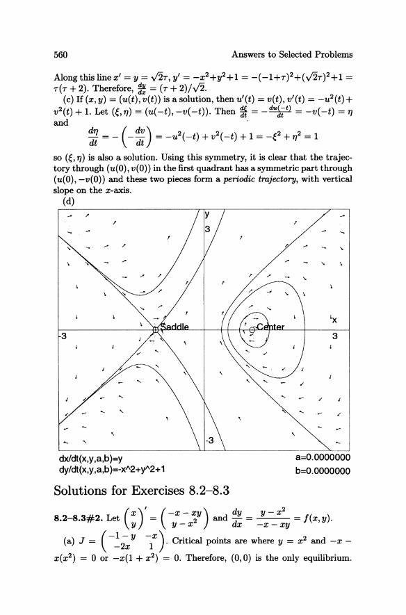
560 Answers to Selected Problems

Along this line x' =y = Y2r,y' = _X2+y2+1 = -(-1+r)2+{Y2r)2+1 = r{r + 2). Therefore, ~ = {r + 2)/Y2.

(c) If (x, y) = (u(t), v(t)) is a solution, then u'{t) = v{t), v'{t) = -u2(t)+ v2{t) + 1. Let (e,.,,) = (u{ -t), -v{ -t)). Then ~ = - du~~t) = -v{ -t) = ." ~d .

d." = _ (_ dV) = -u2{-t) +v2(-t) + 1 = -e +.,,2 = 1 dt dt

so (e,.,,) is also a solution. Using this symmetry, it is clear that the trajec­tory through (u{O), v{O» in the first quadr~t has a symmetric part through (u{O), -v{O)) ~d these two pieces form a periodic tmjectory, with vertical slope on the x-axis.

(d)

, ,

3 3

, , ,

~----------------------~--~------------.----~-

dxldt(x,y ,a,b )=y a=O.OOOOOOO dy/dt(x,y ,a,b )=-x"2+Y"2+ 1 b=O.OOOOOOO

Solutions for Exercises 8.2-8.3

( x)' (-x-Xy) dy y-x2 8.2-8.3#2. Let = 2 ~d dx = = f{x, y). y y-x -x-xy

( -1- y -x) 2 (a) J = -2x 1 . Critical points are where y = x ~d -x -

x(x2) = 0 or -x{1 + x2) = O. Therefore, (0,0) is the only equilibrium.

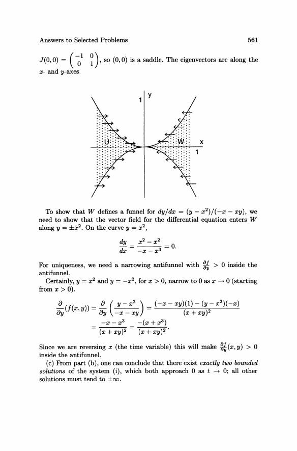
Answers to Selected Problems 561

J(O,O) = (~1 ~), so (0,0) is a saddle. The eigenvectors are along the

x- and y-axes.

1 Y

x 1

To show that W defines a funnel for dy/dx = (y - x2)/( -x - xy), we need to show that the vector field for the differential equation enters W along y = ±x2 • On the curve y = x 2 ,

dy x 2 - x 2 = == o.

dx -x - x 3

For uniqueness, we need a narrowing antifunnel with ~ > 0 inside the antifunnel.

Certainly, y = x2 and y = _x2, for x > 0, narrow to 0 as x -t 0 (starting from x > 0).

~(f(x, y» = ~ ( y - x2 ) = (-x - xy)(I) - (y - x 2)( -x) 8y 8y -x - xy (x + xy)2

-x - x 3 -(x + x 3 ) = -;------;:-:;-

(x + xy)2 (x + xy)2 .

Since we are reversing x (the time variable) this will make ~ (x, y) > 0 inside the antifunnel.

(c) From part (b), one can conclude that there exist exactly two bounded solutions of the system (i), which both approach 0 as t -t OJ all other solutions must tend to ±oo.

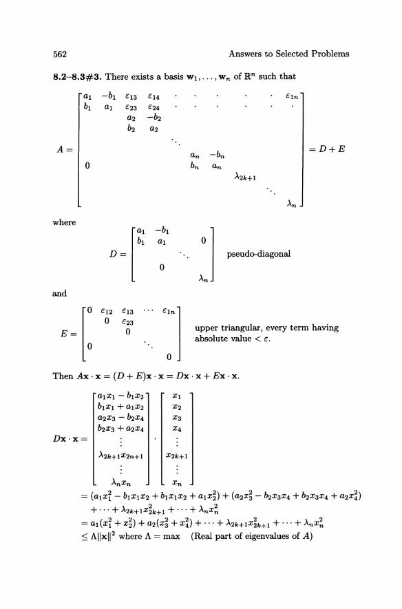
562 Answers to Selected Problems

8.2-8.3#3. There exists a basis WI,"" wn of IRn such that

al -bl 1::13

b l al 1::23

a2

b 2

A=

0

where

[a, bl

D=

and

1::14

1::24 -b2

a2

-bl

al

0

I:: In

-bn =D+E

an

bn an

>'2k+1

An

:1 pseudo-diagonal

upper triangular, every term having absolute value < 1::.

Then Ax·x = (D+ E)x· x = Dx· x+ Ex ·x.

alXI - b l X 2 Xl

blXl + alx2 X2

a2x3 - b2X 4 X3

b2X3 + a2 X 4 X4

Dx·x=

A2k+I X 2n+1 X2k+l

AnXn Xn

= (alX~ - blXIX2 + blXlX2 + aIX~) + (a2X~ - b2X3X4 + b2X3X4 + a2X~) + ... + A2k+1X~k+1 + ... + AnX~

= al(X~ + X~) + a2(X~ + X~) + ... + >'2k+1X~k+1 + ... + AnX~ ::; Allxl1 2 where A = max (Real part of eigenvalues of A)

Answers to Selected Problems

II Ell = ~ e~. < v'n2e2 = ne. ~ ']-

Therefore, Ax· x:5 (A + ne)lIxIl2.

8.2-8.3#9. If

{X' = -ax + P(x,y) y' = -ay + Q(x, y)

563

with a > 0 then (0,0) is a node sink and we know that for IIxli < p, IIx(t)1I2 :5 IIx(0)1I 2e-c1t for some constant Cl > O.

In polar coordinates, x = rcos8, y = rsin8, 8 = tan-1(y/x) and

d8 xy'-x'y x(-ay + Q(x,y» -y(-ax+P(x,y)) = =

dt x2 +y2 x2 +y2 r cos 8Q(r cos 8, r sin 8) - r sin 8(P(r cos 8, r sin 8»

= r2 cos 8Q(r cos 8, r sin 8) - sin 8P(r cos 8, r sin 8)

=--~~--~----~----~--~~--~ r

Since P and Q start with quadratic terms, for r small enough

P(rcos 8, r sin 8) < r2(Mt + el(r» } Q(r cos 8, r sin 8) < r2(M2 +e2(r))

where ei(r) --t 0 as r --t 0 if i = 1,2.

Therefore, I ~~ I :5 k;2 = kr :5 kllxolle-c1t/ 2 for small enough r, where k is a constant.

Thus the solutions do not spiral infinitely as (x, y) --t (0,0).

8.2-8.3#11. Let JLX = P(x,y), where P is a quadratic or higher-order form. Then the Implicit Function Theorem shows that this defines a curve x = x(y) passing through x = 0 at y = O. The derivative ~ can be obtained by implicit differentiation with respect to y:

dx d fJp dx fJP JL dy = dy (P(x, y» = fJx dy + fJy

dx fJP/fJy dy = JL - (fJP/fJx)'

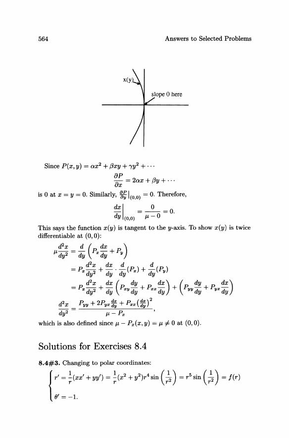
564 Answers to Selected Problems

Since P(x, y) = ax2 + f3xy + 'Yy2 + ... oP ox = 2ax + f3y + ...

is 0 at x = y = O. Similarly, ~~ 1(0,0) = O. Therefore,

dxl = _0_ =0. dy (0,0) J1- - 0

This says the function x(y) is tangent to the y-axis. To show x(y) is twice differentiable at (0,0):

d2x d (dX ) J1- dy2 = dy Px dy + Py

d2x dx d d = Px dy2 + dy . dy (Px) + dy (Py)

d2x dx (dY dX) (dY dX) = Px dy2 + dy Pxy dy + Pxx dy + Pyy dy + Pyx dy

d2x Pyy + 2Pyx~ + Pxx(~)2 dy2 '" - Px

which is also defined since J1- - Px(x, y) = J1- =1= 0 at (0,0).

Solutions for Exercises 8.4

8.4#3. Changing to polar coordinates:

{ r:: ~(xx' +yy') ~ ~(x' +y')r',;" (:,) ~ hin (:,) ~ i(r)

() --1.

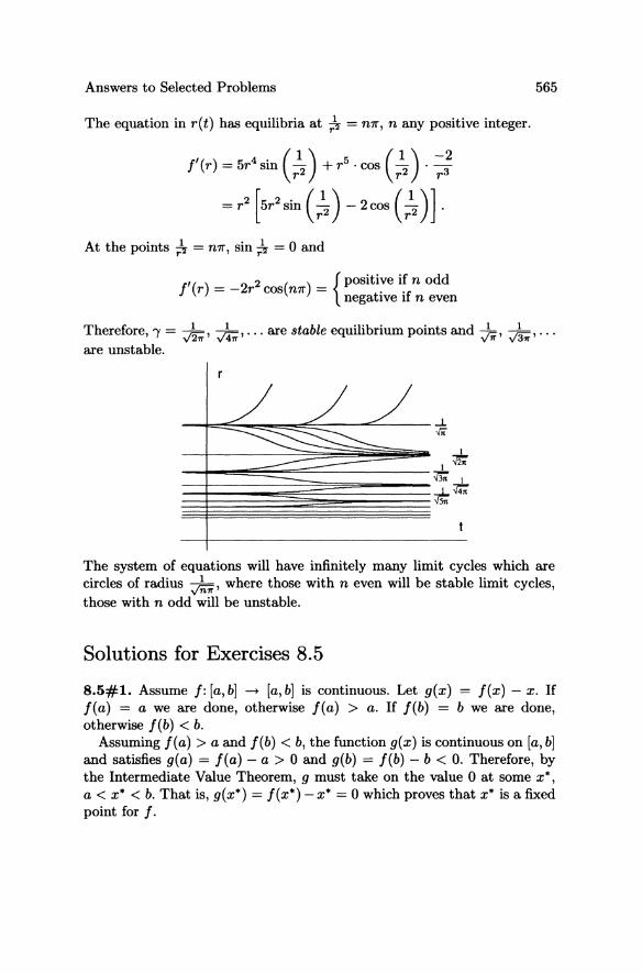
Answers to Selected Problems

The equation in r(t) has equilibria at ~ = mr, n any positive integer.

J'(r) = 5r4 sin (:2) + r5 . cos (r12 ) . ~;

= r2 [5r2 sin (r12 ) - 2 cos (r12 ) ] .

At the points ~ = mr, sin ~ = 0 and

J'( ) 2 2 ( ) {Positive if n odd r = - r cos n7!" = .. negative If n even

565

Therefore, 'Y = vk:, vh-, ... are stable equilibrium points and J:;r, .An:, ... are unstable.

The system of equations will have infinitely many limit cycles which are circles of radius h, where those with n even will be stable limit cycles,

v n ". those with n odd will be unstable.

Solutions for Exercises 8.5

8.5#1. Assume J: [a, b] --+ [a, b] is continuous. Let g(x) = J(x) - x. If J(a) = a we are done, otherwise J(a) > a. If J(b) = b we are done, otherwise J(b) < b.

Assuming J(a) > a and J(b) < b, the function g(x) is continuous on [a, b] and satisfies g(a) = J(a) - a > 0 and g(b) = J(b) - b < O. Therefore, by the Intermediate Value Theorem, 9 must take on the value 0 at some x*, a < x* < b. That is, g(x*) = J(x*) - x* = 0 which proves that x* is a fixed point for J.

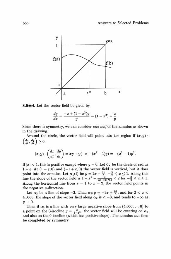
566

y

b

f(a)

a

a

Answers to Selected Problems

x* b x

8.5#4. Let the vector field be given by

dy = -x + (1 - x 2 )y = (1 _ x 2 ) _ ::.

dx y y

Since there is symmetry, we can consider one half of the annulus as shown in the drawing.

Around the circle, the vector field will point into the region if (x, y) .

(~~, ~) ~ 0.

( ) ( dx dy ) ( 2 2 2 x,Y· dt'dt =xy+y(-x- x -l)y)=-(x -l)y.

If Ixl < 1, this is positive except where y = 0. Let Cc be the circle of radius 1- c. At (1 - 10,0) and (-1 + 10,0) the vector field is vertical, but it does point into the annulus. Let a1 (t) be y = 2x + 2i, - ~ S; x S; 1. Along this line the slope of the vector field is 1 - x 2 - 2x+(~1/5) < 2 for - ~ S; x S; l. Along the horizontal line from x = 1 to x = 2, the vector field points in the negative y-direction.

Let a2 be a line of slope -3. Then a2: Y = -3x + 651, and for 2 < x < 4.0666, the slope of the vector field along a2 is < -3, and tends to -00 as y --+ 0.

Then if a3 is a line with very large negative slope from (4.066 ... ,0) to a point on the O-isocline y = 1~x2' the vector field will be entering on 0:3

and also on the O-isocline (which has positive slope). The annulus can then be completed by symmetry.

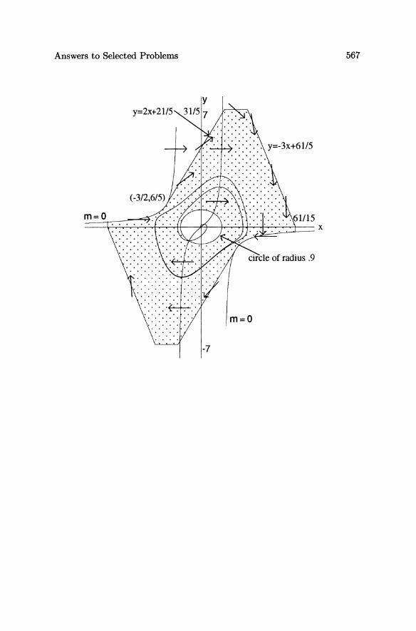
Answers to Selected Problems 567

y=2Xf-21/5

y=-3x+61/5

m=O

-7

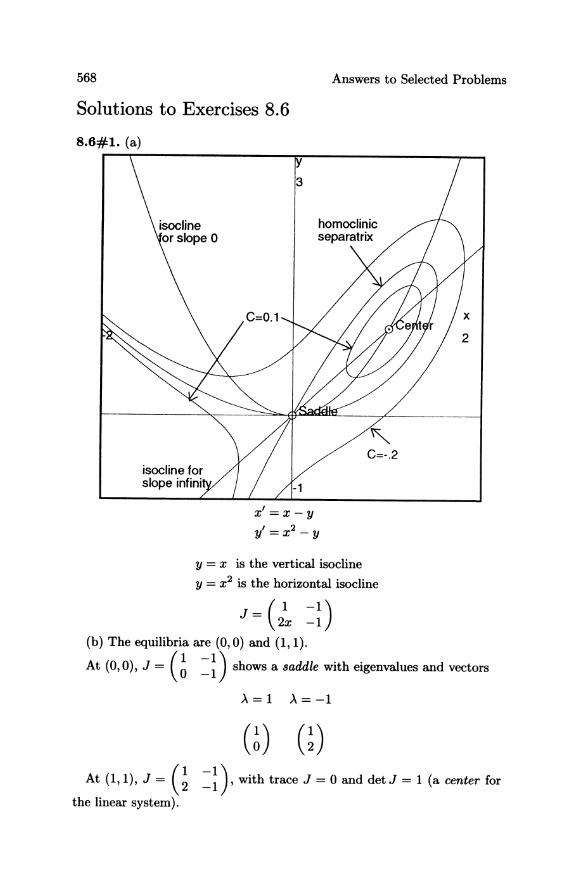
568 Answers to Selected Problems

Solutions to Exercises 8.6

8.6#1. (a)

x' = x - y

y' = X 2 _ Y

y = x is the vertical isocline

y = x 2 is the horizontal isocline

J = (2~ =~) (b) The equilibria are (0,0) and (1,1).

At (0,0), J = (~ =~) shows a saddle with eigenvalues and vectors

A=l A=-l

At (1,1), J = (; =~). with trace J = 0 and detJ = 1 (a center for

the linear system).

Answers to Selected Problems 569

The equation is exact:

V'" VII dy x2 -y

= dx x-y ~ ------so _(X2 - y) dx + (x - y) dy = 0,

which integrates to V(x,y) = xy-f-"'; = C. This can be solved explicitly

by writing as a quadratic in y: f - xy + (C + "';) = 0

y = x ± J x 2 - 2(c + ~)

y~x (l± x' - !~'-2C ~ x (l± V1 - ~X-2:,) (*)

For C = 0, y = x (1 ± Jl - ~x) describes both the stable and unstable

manifolds for the saddle point (0,0). (c) Level curves of (*) with 0 < c < 1 define the cycles about (1,1),

within the homoclinic separatrix.

8.6#3. Let u' = Au be the linearization of x' = f(x) at a zero Xo. Then the matrix

~ ... ~) !lh. 8"'2

!!b. 8"'n (X=Xo)

is the Jacobian evaluated at the singularity Xo. Therefore, trace(A) = L:~=l ~ IXo = div f(Xo).

Suppose a vector field x' = f(x) has a source or sink at Xo. Then it has been shown that the eigenvalues of A must have all positive real parts (or all negative real parts). Trace(A) = L:~=l Ai = L:~=l R(Ad (since complex Ai come in conjugate pairs). Therefore, trace(A) will be strictly positive (or strictly negative) at Xo. But this would say div f(Xo) =1= 0, and therefore the differential equation is not area preserving. If the field is area preserving, div f(x) = 0 at every point x. Thus any singularities cannot be sinks or sources.

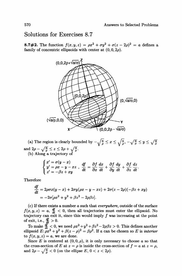
570 Answers to Selected Problems

Solutions for Exercises 8.7

8.7#2. The function f(x,y,z) = px2 + ay2 + a(z - 2p)2 = a defines a family of concentric ellipsoids with center at (0,0, 2p).

(O,..JaiG,O)

(a) The region is clearly bounded by -If, ~ x ~ If" -~ ~ y ~ ~ and 2p - ~ ~ z ~ 2p + ~.

(b) Along a trajectory of

Therefore

{X' = a(y - x) df of dx of dy of dz y' = px - y - xz , dt = ox dt + {)y dt + oz dt· z' = -(3z+xy

df dt = 2pax(y - x) + 2ay(px - y - xz) + 2a(z - 2p)( -(3z + xy)

= -2a[px2 + y2 + (3z2 - 2p{3z].

(c) If there exists a number a such that everywhere, outside of the surface f(x, y, z) = a, i < 0, then all trajectories must enter the ellipsoid. No trajectory can exit it, since this would imply f was increasing at the point of exit, i.e., * > o.

To make * < 0, we need px2+y2+{3z2_2p{3z > O. This defines another ellipsoid E: px2 + y2 + {3(z - p)2 = (3p2. If a can be chosen so E is interior to f(x, y, z) = a, we are done.

Since E is centered at (0,0, p), it is only necessary to choose a so that the cross-section of E at z = p is inside the cross-section of f = a at z = p, and 2p - ~ < 0 (on the ellipse E, 0 < z < 2p).

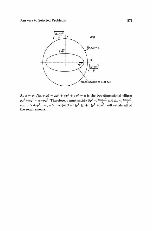
Answers to Selected Problems 571

!(X.Y." = a

x

At z = p, f(x, y, p) = px2 + uy2 + up2 = a is the two-dimensional ellipse px2 +uy2 = a-up2. Therefore, a must satisfy {3p2 < a_;p2 and {3p < a_;p2 and a > 4up2, i.e., a> max(u({3 + 1)p2, ({3 + u)p2, 4up2) will satisfy all of the requirements.

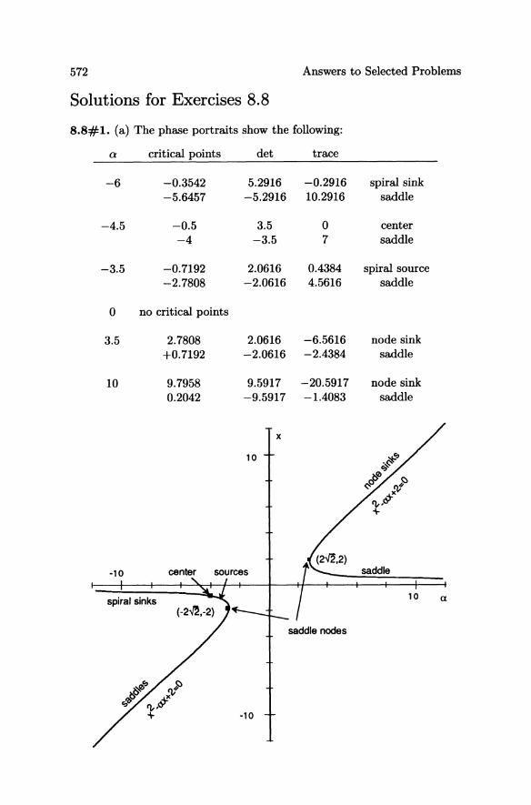
572 Answers to Selected Problems

Solutions for Exercises 8.8

8.8#1. (a) The phase portraits show the following:

a critical points det trace

-6 -0.3542 5.2916 -0.2916 spiral sink -5.6457 -5.2916 10.2916 saddle

-4.5 -0.5 3.5 0 center -4 -3.5 7 saddle

-3.5 -0.7192 2.0616 0.4384 spiral source -2.7808 -2.0616 4.5616 saddle

0 no critical points

3.5 2.7808 2.0616 -6.5616 node sink +0.7192 -2.0616 -2.4384 saddle

10 9.7958 9.5917 -20.5917 node sink 0.2042 -9.5917 -1.4083 saddle

x

10

·10 saddle

spiral sinks 10 a

·10

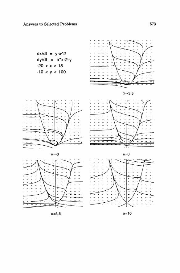
Answers to Selected Problems 573

dx/dt = y-xA2 - - - -

dy/dt = a*x-2-y -20 < X < 15 -10 < Y < 100

a=-3.5

a=-6

a=3.5 a=10

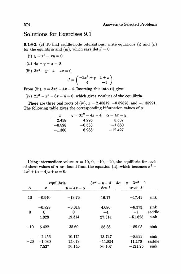
574 Answers to Selected Problems

Solutions for Exercises 9.1

9.1#2. (c) To find saddle-node bifurcations, write equations (i) and (ii) for the equilibria and (iii), which says det J = O.

(i) y - x 3 + xy = 0

(ii) 4x - y - a = 0

(iii) 3x2 - y - 4 - 4x = 0

J _ (-3x2 + y 1 + x) - 4 -1

From (iii), y = 3x2 - 4x - 4. Inserting this into (i) gives

(iv) 2x3 - x 2 - 8x - 4 = 0, which gives x-values of the equilibria.

There are three real roots of (iv), x = 2.45819, -0.59828, and -1.35991. The following table gives the corresponding bifurcation values of a.

x y = 3x2 - 4x - 4 a = 4x - y 2.458 4.295 5.537

-0.598 -0.533 -1.860 -1.360 6.988 -12.427

Using intermediate values a = 10, 0, -10, -20, the equilibria for each of these values of a are found from the equation (ii), which becomes x3 -

4x2 + (a - 4)x + a = O.

equilibria 3x2 - y - 4 - 4a y - 3x2 -1 a x y=4x-a detJ trace J

10 -0.940 -13.76 16.17 -17.41 sink

-0.828 -3.314 4.686 -6.373 sink 0 0 0 -4 -1 saddle

4.828 19.314 27.314 -51.628 sink

-10 6.422 35.69 58.36 -89.05 sink

-2.456 10.175 13.747 -8.922 sink -20 -1.080 15.678 -11.854 11.176 saddle

7.537 50.146 86.107 -121.25 sink

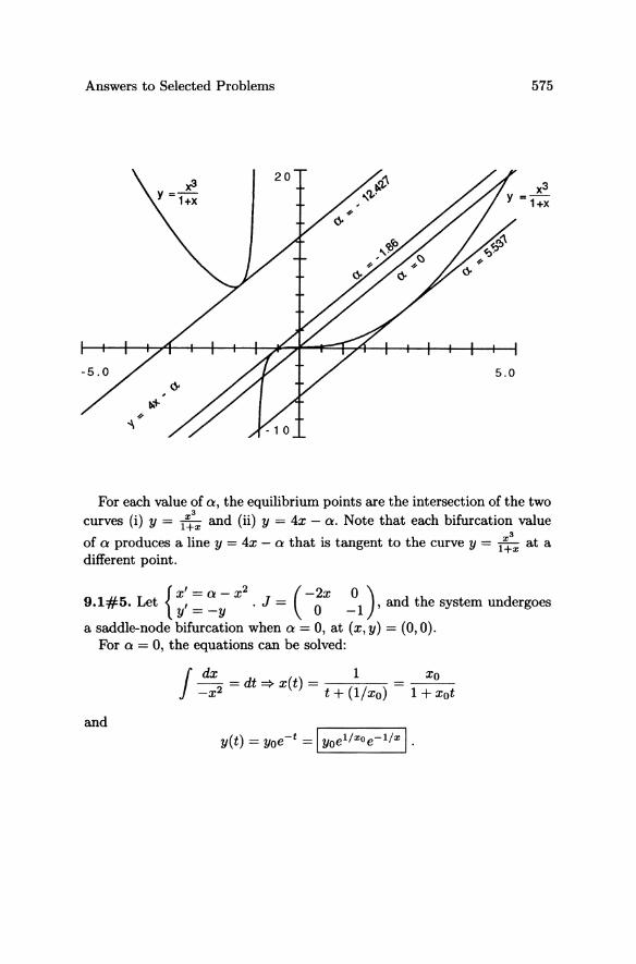
Answers to Selected Problems 575

For each value of a, the equilibrium points are the intersection of the two curves (i) y = lx:.z and (ii) y = 4x - a. Note that each bifurcation value

of a produces a line y = 4x - a that is tangent to the curve y = lx:.z at a different point.

{X' = a - x2 (-2X 0) 9.1#5. Let y' = _y . J = ° -1' and the system undergoes

a saddle-node bifurcation when a = 0, at (x,y) = (0,0). For a = 0, the equations can be solved:

J dx 1 Xo _X2 = dt => x(t) = t + (l/xo) = 1 + xot

and

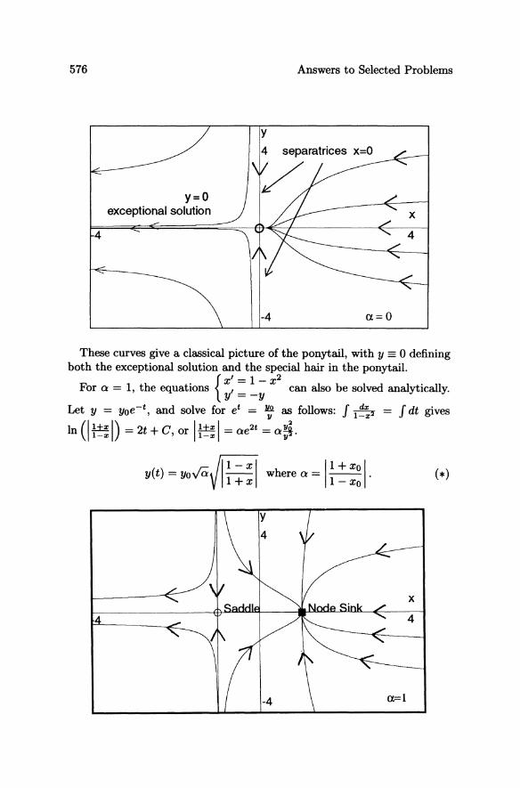
576 Answers to Selected Problems

4

y=o exceptional solution

y

-4

x

4

a=O

These curves give a classical picture of the ponytail, with y == 0 defining both the exceptional solution and the special hair in the ponytail.

{X' = 1- x2

For a = 1, the equations I can also be solved analytically. y =-y

Let y = yoe-t , and solve for et = ~ as follows: f 1~~2 = f dt gives

In (I !tl. I) = 2t + C or 1!tl.1 = ae2t = a~. 1-", , 1-", tr

Co FI-xi 11+xol y(t) = yoyay I~I where a = 1- Xo .

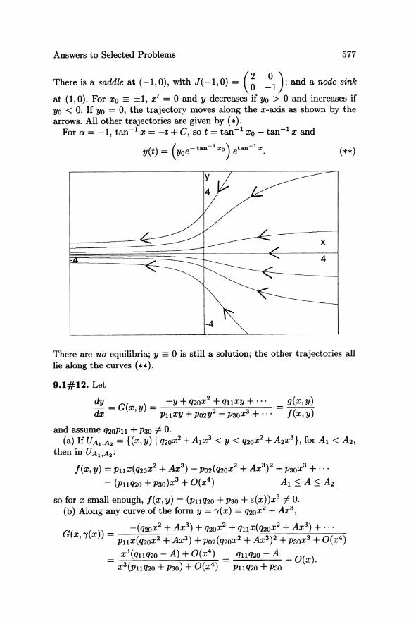
Answers to Selected Problems 577

There is a saddle at (-1,0), with J(-I,O) = (~ ~1) and a node sink

at (1,0). For Xo == ±1, x' = 0 and y decreases if Yo > 0 and increases if Yo < O. If Yo = 0, the trajectory moves along the x-axis as shown by the arrows. All other trajectories are given by (*).

For 0: = -1, tan- 1 x = -t + C, so t = tan-1 Xo - tan-1 x and

(**)

x

4

There are no equilibria; y == 0 is still a solution; the other trajectories all lie along the curves (**).

9.1#12. Let

dy -y + q20x2 + ql1XY + ... - = G(x, y) = -----:::--~­dx Pl1XY + P02y2 + P30X3 + ...

and assume q20Pl1 + P30 =J O.

g(x,y)

I(x,y)

(a) If UAt.A2 = {(x,y) I q20x2 +AIX3 < y < q20x2 +A2x3}, for Al < A2, then in U Ai ,A2 :

I(x, y) = Pl1X(q20x2 + Ax3) + P02(Q2ox2 + AX3)2 + P30x3 + ... = (PllQ20 + P30)X3 + O(X4) Al :s; A :s; A2

so for x small enough, I(x, y) = (Pl1Q20 + P30 + c(x))x3 =J O. (b) Along any curve of the form y = ,(x) = Q20x2 + Ax3,

G(x ,(x)) _ -(Q20x2 + Ax3) + Q20x2 + Ql1 X(Q2ox2 + Ax3) + ... , - Pl1X(Q2ox2 + Ax3) + P02(Q2ox2 + Ax3)2 + P30x3 + O(x4)

= X3(Ql1Q20 - A) + O(x4) = Q1lQ20 - A + O(x) X3(pUQ20 + P30) + O(X4) PllQ20 + P30 .

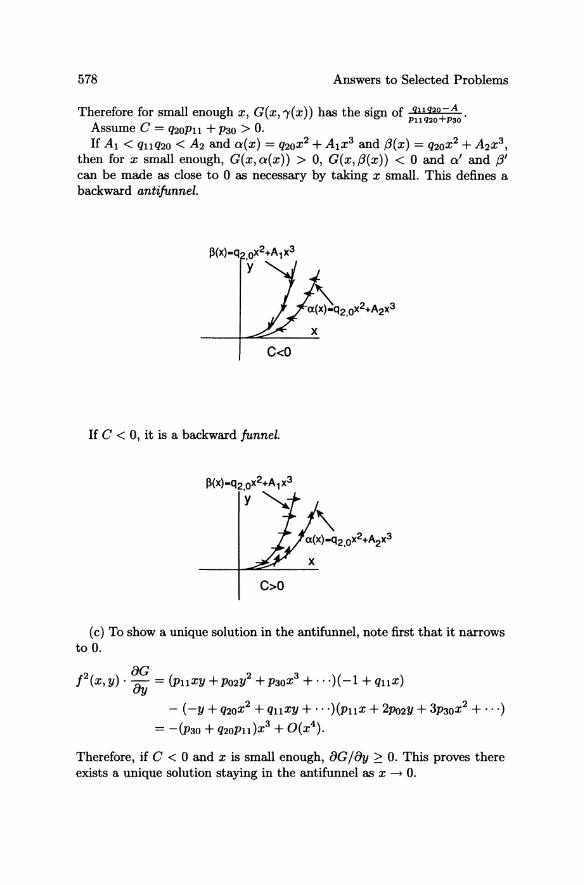
578 Answers to Selected Problems

Therefore for small enough x, G{x,'Y{x» has the sign of Ql1920;A • Pl1Q20 P30

Assume C = q20Pll + P30 > o. If Al < Qllq20 < A2 and a{x) = Q20x2 + AlX3 and {3{x) = Q20x2 + A2x3,

then for x small enough, G{x, a{x)) > 0, G{x, {3{x)) < 0 and a' and {3' can be made as close to 0 as necessary by taking x small. This defines a backward anti funnel.

If C < 0, it is a backward funnel.

(c) To show a unique solution in the antifunnel, note first that it narrows to o.

f2{X, y) . : = (puxy + P02y2 + P30x3 + ... )( -1 + Qux)

- {-y + Q20x2 + QllXY + .. ·)(pux + 2po2y + 3P30x2 + ... ) = -(p30 + Q20PU)X3 + O{x4).

Therefore, if C < 0 and x is small enough, 8G / 8y ~ O. This proves there exists a unique solution staying in the antifunnel as x -+ o.

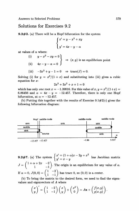
Answers to Selected Problems 579

Solutions for Exercises 9.2

9.2#2. (a) There will be a Hopf bifurcation for the system

{X,=y-x3 +xy

y'=4x-y-a

at values of a where:

(i) y - x3 - xy = 0 } ==> (x, y) is an equilibrium point

(ii) 4x - y - a = 0

(iii) -3x2 + y - 1 = 0 ==> trace(J) = O.

Solving (i) for y = x 3 /(1 + x) and substituting into (iii) gives a cubic equation for x:

2x3 +3x2 +x+ 1 = 0

which has only one root x = -1.39816. For this value of x, y = x3 / (1 +x) = 6.86456 and a = 4x - Y = -12.457. Therefore, there is only one Hopf bifurcation, at a = -12.457.

(b) Putting this together with the results of Exercise 9.1#2(c) gives the following bifurcation diagram:

Hopi saddle-node saddle-node saddle-node

sink sink sink

saddle saddle ~ sink t

..... source sink (l

-12.457 -12.427 -1.86 5.537

{ X' = (1 + a)x - 2y + x2 9.2#1. (a) The system , has Jacobian matrix y =x-y

J ( 1 + a + 2x - 2 ) Th ... ·l·b . J: I f = 1 -1· e OrIgm IS an eqUl 1 rlUm lor any va ue 0 a.

(1 -2) If a = 0, J(O, 0) = 1 -1 has trace 0, so (0,0) is a center.

(b) To bring the matrix to the desired form, we need to find the eigen­values and eigenvectors of A where

( x)' = (1 -2) (x) + (X2) = Ax+ (f(X,y)). y 1 -1 Y 0 g(x,y)

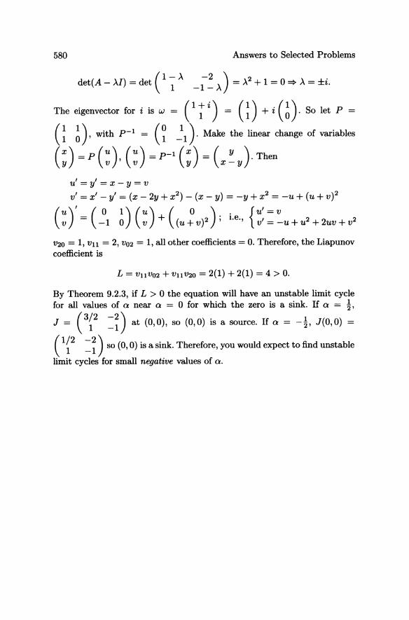
580 Answers to Selected Problems

( 1- A det(A - AI) = det 1 -2) 2 . -I-A =A +1=O~A=±z.

The eigenvector for i is w = (1 ~ i) = (~) + i (~). So let P

(~ ~), with p-l = (~ !1)' Make the linear change of variables

( :) = p ( ~ ), (~) = p-l (:) = (x ~ y). Then

u' = y' = X - Y = v

Vi = x' - y' = (x - 2y + x 2) - (x - y) = -y + x 2 = -u + (u + V)2

( U ) I (0 1) (u) + ( 0 ) . { u' = V V = -1 0 v (u + v)2 j l.e., Vi = -u + u 2 + 2uv + v 2

V20 = 1, Vll = 2, V02 = 1, all other coefficients = O. Therefore, the Liapunov coefficient is

L = VllV02 + VllV20 = 2(1) + 2(1) = 4> O.

By Theorem 9.2.3, if L > 0 the equation will have an unstable limit cycle for all values of Q near Q = 0 for which the zero is a sink. If Q = ~,

_ (3/2 -2) ( ) ( ). f _ 1 ( )_ J - 1 -1 at 0, 0 ,so 0, 0 IS a source. I Q - - 2' J 0, 0 -

(1{2 =~) so (0,0) is a sink. Therefore, you would expect to find unstable

limit cycles for small negative values of Q.

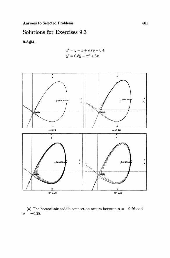
Answers to Selected Problems 581

Solutions for Exercises 9.3

9.3#4.

=-0.24

=-0.28

x' = y - x + axy - 0.4

y' = 0.8y - X 3 + 3x

4.

a=-0.26

a=-O.30

(a) The homoclinic saddle connection occurs between a =- 0.26 and a = -0.28.

4.

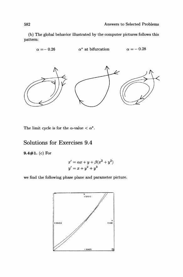
582 Answers to Selected Problems

(b) The global behavior illustrated by the computer pictures follows this pattern:

a =- 0.26 a* at bifurcation

The limit cycle is for the a-value < a*.

Solutions for Exercises 9.4

9.4#1. (c) For

x' = ax + y + (3(x2 + y2)

y'=X+y2+ y3

a = - 0.28

we find the following phase plane and parameter picture.

0448

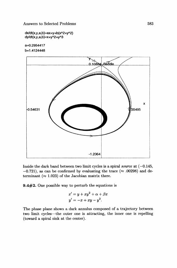
Answers to Selected Problems

dxIdt(x,y,a,b)=ax+y+b(xI\2+yI\2) dy/dt(x,y ,a,b )=x+yI\2+Y"3

a=0.2954417

b=1.4124448

.54631

583

x

-1.2064

Inside the dark band between two limit cycles is a spiral source at (-0.145, -0.721), as can be confirmed by evaluating the trace (::::i .00298) and de­terminant (::::i 1.023) of the Jacobian matrix there.

9.4#2. One possible way to perturb the equations is

x' = y + xy2 + a + fix y' = -x + xy _ y2.

The phase plane shows a dark annulus composed of a trajectory between two limit cycles-the outer one is attracting, the inner one is repelling (toward a spiral sink at the center).

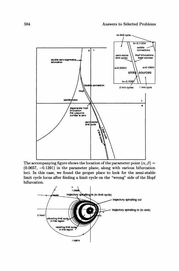
584 Answers to Selected Problems

b 1

2 limit cycles 1 limit cycle

•

The accompanying figure shows the location of the parameter point (a, {3) = (0.0657, -0.1391) in the parameter plane, along with various bifurcation loci. In this case, we found the proper place to look for the semi-stable limit cycle locus after finding a limit cycle on the ''wrong'' side of the Hopf bifurcation.

trajectory spiralling out

trajectory spiraling In (to sink)

-2.7_7

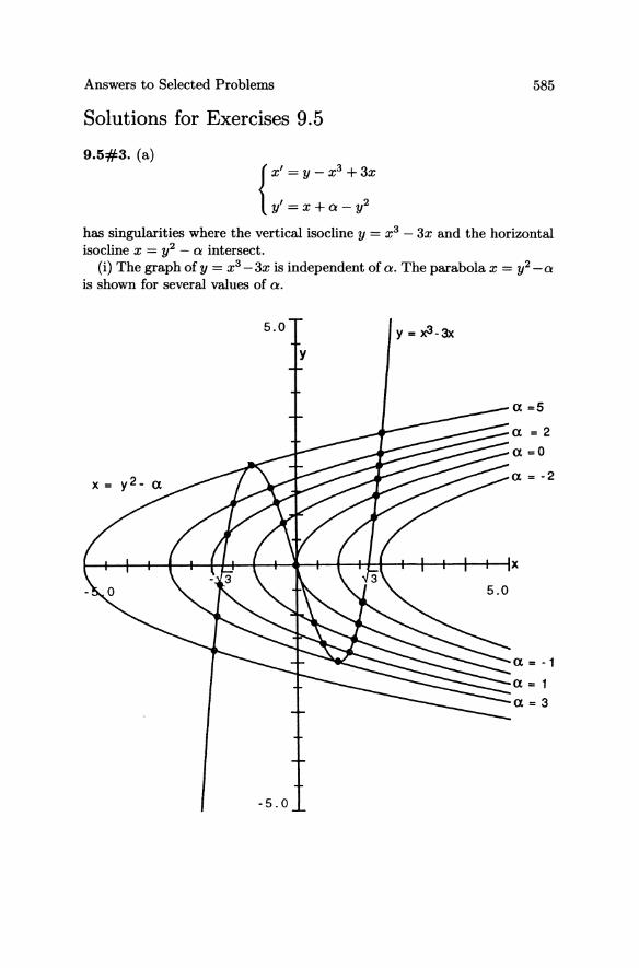
Answers to Selected Problems

Solutions for Exercises 9.5

9.5#3. (a)

{X1 =Y-X3 +3X

y' =x+o _ y2

585

has singularities where the vertical isocline y = x3 - 3x and the horizontal isocline x = y2 - 0 intersect.

(i) The graph of y = x3 - 3x is independent of o. The parabola x = y2 - 0

is shown for several values of o.

5.0

y

-5.0

y = x3-3x

a =5

a = 2

a =0

a = -2

a = -1

a = 1

a=3

586 Answers to Selected Problems

a number of zeros -2 0

-J3 1 -1 2 0 3 1 4

J3 5 2 6 3 5 4 4 5 3 6 2

(ii) Saddle node bifurcations occur where the two isoclines have a point of tangency, i.e., at a = -J3, 0, J3, 3 and 5.

(iii) No saddle connections occur.

(iv) For a Hopf bifurcation to occur, the trace (-3X2 + 3 1) = 1 -2y

3(1 - x2) - 2y must be 0, and det J = 2y(3x2 - 3) - 1 > 0 at a critical point (xo, Yo). Using the above equations for Xo and Yo, Xo would have to be a root of x 3 + ~X2 - 3x - ~ = o. At each of the three roots, det J < O. Therefore, no Hopf bifurcations occur.

(b) If the formulas for x' and y' are interchanged, so that

{X' =x+a _ y2 y'=y-x3 +3x

(i), (ii) the intersection of the horizontal and vertical isoclines are exactly the same as in #3(a), so number of zeros and saddle node bifurcations do not change. However, the phase portrait does change. The trace and

determinant of J = (3 _13x2 -;y) are entirely different. Det J = 1 + 2y(3 - 3x2) and trace J = 2.

(iii) Saddle connections occur at a = 2.37765,3.02866,0.4527. (iv) Because the tr J == 2, there can be no Hopf bifurcations.

Solutions for Exercises 9.6

9.6#8. (a) The Euler equation x" + TX' + .g.x = 0, t > 0, can be solved analytically by making the change of independent variable eU = t. Letting y(u) = x(t), the equation becomes

y"(u) + (a - l)y'(u) + (3y(u) = O.

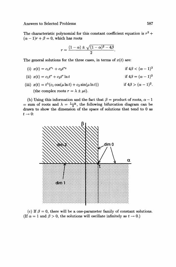
Answers to Selected Problems 587

The characteristic polynomial for this constant coefficient equation is r2 + (0: - 1)r + (3 = 0, which has roots

(1 - 0:) ± V(1 - 0:)2 - 4(3 r= 2 .

The general solutions for the three cases, in terms of x(t) are:

(i) x(t) = cltr1 + C2tr2

(ii) x(t) = Cltr + C2tr In t

(iii) x(t) = tA(Cl cos (J.dn t) + C2 sin(JL In t))

(the complex roots r = A ± JLi).

if 4(3 < (0: - 1)2

if 4(3 = (0: - 1)2

if 4(3 > (0: - 1)2.

(b) Using this information and the fact that (3 = product of roots, 0: - 1 = sum of roots and A = 12"", the following bifurcation diagram can be drawn to show the dimension of the space of solutions that tend to 0 as t --+ 0:

(c) If (3 = 0, there will be a one-parameter family of constant solutions. (If 0: = 1 and (3 > 0, the solutions will oscillate infinitely as t --+ 0.)

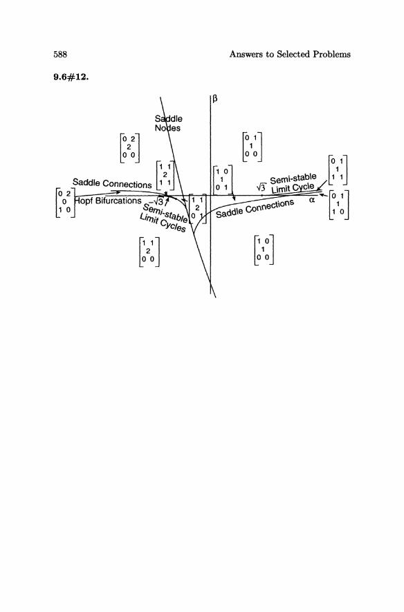
588 Answers to Selected Problems

9.6#12.

~2:J ~':J ~';J r ' ~ .. ~I. Connections ,',

1 0

~2:J ~':J

Index

A Abato, Michael ix acceleration 23 addition

of matrix exponentials 87 of vectors 501

adjoint linear transformation 404 affine space 78 algorithm 369

Gram-Schmidt 407 Hessenberg 471 Jacobi's 473 product rotation 469 QR 471-472

Allen, Richard C., Jr. 521 Andronov, A.A. 203, 245, 247, 288 Andronov-Hopfbifurcation 266,270,

288-298, 315, 319 angular momentum 38-40, 43, 44,

46,47,63 annihilation of equilibria 271, 324 annulus form ofPoincare-Bendixson

Theorem 162-167, 197 use of 309

Anosov's theorem 181 antifunnel theorem 515 antifunnels 151-155,157-159,192-

194, 198, 284, 285, 347, 355, 363, 512

anti-Hermitian matrices 90 anti-Hermitian operator 416 anti-Hermitian transformation 414,

415,450,451,504,509 antisymmetric matrices 90-91 antisymmetric transformation 414,

450, 504, 505, 509 antisymmetry for determinant 425,

428, 506 approximation 12-14, 54-55 arclength 181

area dilation and contraction 165, 170-172

area-preserving 168, 170-174, 197-199

Arnold, V.I. 521 Artigue, Michele ix, 521 associated homogeneous equations

74,76 associativity

for vector space 384 of matrix multiplication 395

astronomy 41 asymptotic development 222 attracting cycles 177 attracting fixed point 177 attracting limit cycle 160-161 attracting saddle connection 303,

304 Australia 22 autonomous 2, 7, 15, 49, 131, 142

B Back, Allen ix, 328-329 Bailey, Graeme x Baranova, Yelena ix Barber, Frederick ix basin 139, 141, 187, 190, 195

boundary 203 basis 80, 104, 117, 369, 387, 388,

406, 486, 501 for image 398-400 for kernel 399-400 for linear transformations 395 independence 397,433-434,502,

507 bead on wire 34-35, 62-63 behavior vii Bekele, Fassil ix Bendixson, I. 162

590 Index

Bernoulli equation 207 Bezout's theorem 455-456,487,496,

509 bifurcation vii, 125-126, 265

summary 270 bifurcation diagram 267-269, 327 bijective correspondence 505 Birkhoff, Garrett 91 Birkhoff, George 91, 245, 521 Blanchard, Paul ix Borrelli, Robert 521 Bott, Raoul 245, 246 boundary conditions 15-17 bounds, on slope error 518 Boyce, William E. 521 Brahe, Tycho 41 Branner, Bodil ix Brown, Daniel ix

C calculus of variations 245 Campbell, Douglas ix Cantor set 181,236, 262 capacitance 71-72 capsule 317-319,327,339,343,358-

359 cardboard model of Lorenz equa-

tion 176-177 cat flow 48 center of mass 42, 47 centers 94-95, 106, 142, 144, 191,

193, 199 central force 38-40, 65 change of basis 80-83, 396, 502

in matrix exponentials 89 matrix for 446

change of variables 138 chaos 132, 199-200, 203, 236-237

in higher dimensions 174-181 characteristic equation 73, 100 characteristic polynomial 84-85, 118,

121, 433-435, 443, 452-457, 493, 495

in summary 502, 507, 508, 509

chemistry 451 Christensen, Marc ix circuit, electrical 71-72 classical mechanics 451 coalescence

of three limit cycles 322, 334 of two limit cycles 309-314

cobasin 139, 141, 187, 190 codimension 183-184, 320, 365 Coleman, Courtney 521 column operations 425-427, 429-

431,506 combat model 57-58 commutativity for vector space 384 companion matrix 434-435,493 competition 56-57 complement, orthogonal 409-411,

504 complex basis 142 complex eigenvalues 93-95, 200

and eigenvectors 83-84, 442 complex inner product 403 composition of linear transforma­

tions 395, 502 computation 369 computer program for determinant

425-427 configuration space 23 conic sections 476 conjugacy of flows 206, 229, 259 conjugate-symmetric property for

inner products 403 conservation laws 37-40, 42, 43,

47, 63-65, 529-531 constant coefficients 69-129 continuous functions for vector space

385, 391, 403, 416 continuously differentiable function

512 contraction 165, 170-172 control parameter 292, 301 convergence of matrix exponen-

tials 87 cookbook method 73, 114, 119 Copernicus 41

creation of equilibria 324 curvature 181 cusp in parameter plane 332-334 cycle 22-23, 159, 177-180, 200

at infinity 342 cylinder

D

for labyrinth 262-263 for mapping differential equa­

tion 314

d'Ancona, Umberto 17-23 damped harmonic oscillator 147 damped oscillator 161 damped pendulum 134-135 damping 70-71 DDT 22 decomposition

of]Rn 490 of quadratic forms 419-422,

505 decoupling 79-83, 115-118, 361 definitions, from Parts I and III

511-519 degenerate bifurcation 320-334 degenerate cases 98, 106, 138, 183-

184 of Jacobi's method 480-481

degenerate limit cycle 266, 267 degenerate saddle connections 341 degenerate saddle-node 288,367 degrees of freedom 29, 109 density theorem 252-258 determinant 369, 424-440, 493, 502,

506-508 as product of eigenvalues 442 development according to first

row 425-427 diagonal matrix 86 diagonal section 219 diagonalizability 369, 453 diagonalizable matrices 102, 104,

542-545 diagonalization 444, 508

Index 591

Dieudonne, Jean 521 differentiability of flow 210-213 differentiable conjugacy 206-207,

259-260 differentiable functions for vector

space 385, 416, 441 differential operator 79, 392, 441,

486 for vector space 502

differentiation of matrix exponen­tials 88-89

dilation 165, 170-172 dimension 25-26,369,503

formula 399-400 of vector space 389, 391

DiPrima, R.C. 521 discriminant 332, 365

for inner product 405 dissipative 199 distributivity for vector space 384 divergence 165, 171, 198 dot product 372 Douady, Adrien ix, 218, 221 Douady, proof of theorem 220-223 double eigenvalue 96-98 double pony tail 321, 333 double saddle connection 322 driven oscillator 161 driving force 161 driving functions 106-110 dynamical plane 6 dynamical systems 369

section mapping 228-229

E Earle, Clifford ix echelon form 375-376, 482, 500 eigenbasis 80-81, 117, 156, 444 eigendirections 150 Eigenfinder program 459, 461, 468 eigenflag 465-466 eigenfunctions 441 eigenvalue

double 96-98

592 Index

zero 98, 106, 320, 321 eigenvalues vii, 79, 187-189, 369,

370, 440-482 and eigenvectors 494-499,508-

509 and global behavior 101-106,

124-126 and signatures 481-482, 505 by Jacobi's method 472-482 by QR 457-472 complex 83-84, 93-95, 200 finding 84-85 imaginary 106, 137-138 real 92

eigenvector, generalized 446 eigenvectors vii, 79-83, 187-189,

369, 370, 440-481 and decoupling 79-83,115-118 computing matrix exponen-

tials 90 electrical circuit 71-72 ellipsoid 476-480 elliptical orbits 45-47 energy 46,47, 529-531 engineering 451 entomology 22 equations of motion 1 equilibrium 8, 19-21,31, 133, 137,

141 error 13

slope 518 essential size 36-40, 63 Euclidean norm 402 Euler equation 586 Euler's method 12-13, 54-55, 516,

518,526 evolution 80 exact differential equation 172 exceptional cases 95-98, 106 exceptional equations 183-185 exceptional solution 139, 154 exceptional trajectories 347 existence vii, 2, 14, 131 exponentials of matrices 85-91, 118-

120

F families of differential equations

183-186, 267 one-parameter 314-318 two-parameter 318-343

Felsager, BjlZlrn ix fence 144, 155, 511 fence argument 308 Fields medal 246 finite-dimensional vector space 389,

399-400, 501-504 first nondegeneracy condition 279-

280,320 first order, one-dimensional differ­

ential equation 511-519 fishing 21-22 fixed point, attracting or repelling

177 flag 462-466, 496 flow times 219-223 flow

differentiability 210-213 geodesic 181 scattering theory 215-216

flows 47-51, 67-68, 165, 170, 210 conjugate 206 continuity 51

force 26 central 38-40, 65 gravitational 27 restoring 147

Fourier coefficients 406 Fourier series 106, 110, 128, 406,

416,451 Fourier transform 106, 110-111 fractal attractor 203 friction 31, 147, 191 fundamental inequality 2, 14, 75,

212-213, 513, 525 fundamental theorem of algebra

442 funnel 151-155, 163-165, 192,284,

285, 347, 363, 511 funnel theorem 514

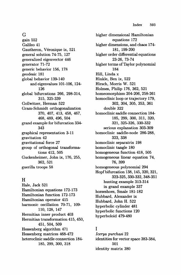
G gain 552 Galileo 41 Gautheron, Veronique ix, 521 general solution 74-75, 127 generalized eigenvector 446 generator 71-72 generic behavior 156, 178 geodesic 181 global behavior 139-140

and eigenvalues 101-106, 124-126

global bifurcations 266, 298-314, 315, 325-339

Gollwitzer, Herman 522 Gram-Schmidt orthogonalization

370, 407, 413, 458, 467, 468, 489, 496, 504

grand example for bifurcation 334-343

graphical representation 3-11 gravitation 42 gravitational force 27 group of orthogonal transforma­

tions 412, 505 Guckenheimer, John ix, 176, 255,

362,521 guerilla troops 58

H Hale, Jack 521 Hamiltonian equations 172-173 Hamiltonian function 172-173 Hamiltonian operator 415 harmonic oscillation 70-71, 109-

110, 128, 147 Hermitian inner product 403 Hermitian transformation 415, 450,

451, 504, 509 Hessenberg algorithm 471 Hessenberg matrices 468-472 heteroclinic saddle connection 184-

185, 299, 300, 318

Index 593

higher dimensional Hamiltonian equations 172

higher dimensions, and chaos 174-181, 199-200

higher order differential equations 23-26, 73-74

higher terms of Taylor polynomial 184

Hill, Linda x Hinkle, Ben ix, 522 Hirsch, Morris W. 521 Holmes, Philip 176, 362, 521 homeomorphism 204-206, 258-261 homoclinic loop or trajectory 179,

302, 304, 305, 353, 361 double 322

homoclinic saddle connection 184-185, 299, 300, 311, 320, 321, 325-326, 330-332

serious explanation 303-309 homoclinic saddle-node 286-288,

323, 338 homoclinic separatrix 198 homoclinic tangle 180 homogeneous function 418,505 homogeneous linear equation 74,

76,399 homogeneous polynomial 294 Hopfbifurcation 138,145,320,321,

323-325,330-332,348-351 hunting example 313-314 in grand example 337

horseshoes, Smale 181-182 Hubbard, Alexander ix Hubbard, John H. 522 hyperbolic cylinder 481 hyperbolic functions 120 hyperboloid 479-480

I Icerya purchasi 22 identities for vector space 383-384,

501 identity matrix 380

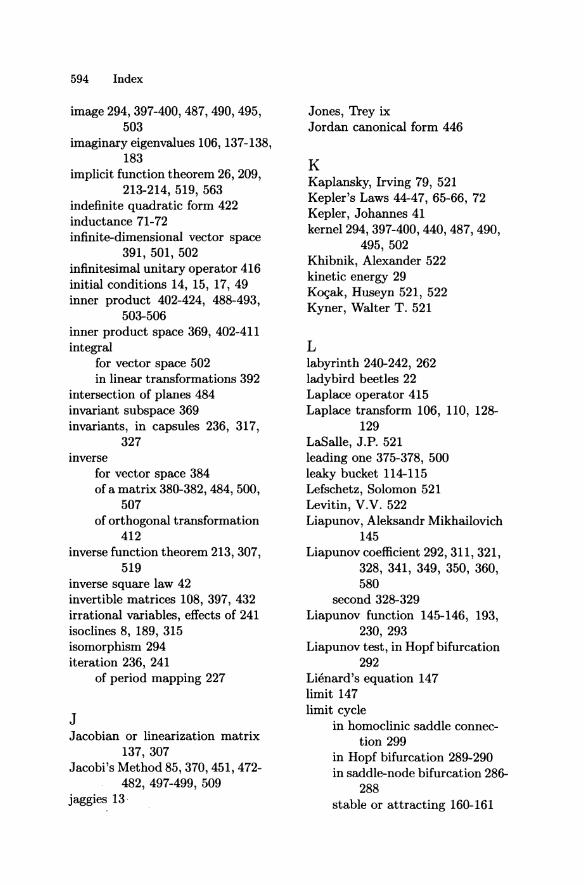
594 Index

image 294,397-400,487,490,495, 503

imaginary eigenvalues 106,137-138, 183

implicit function theorem 26, 209, 213-214, 519, 563

indefinite quadratic form 422 inductance 71-72 infinite-dimensional vector space

391, 501, 502 infinitesimal unitary operator 416 initial conditions 14, 15, 17, 49 inner product 402-424, 488-493,

503-506 inner product space 369,402-411 integral

for vector space 502 in linear transformations 392

intersection of planes 484 invariant subspace 369 invariants, in capsules 236, 317,

327 inverse

for vector space 384 of a matrix 380-382, 484, 500,

507 of orthogonal transformation

412 inverse function theorem 213,307,

519 inverse square law 42 invertible matrices 108, 397, 432 irrational variables, effects of 241 isoclines 8, 189, 315 isomorphism 294 iteration 236, 241

of period mapping 227

J Jacobian or linearization matrix

137, 307 Jacobi's Method 85, 370, 451, 472-

482, 497-499, 509 jaggies 13-

Jones, Trey ix Jordan canonical form 446

K Kaplansky, Irving 79, 521 Kepler's Laws 44-47, 65-66, 72 Kepler, Johannes 41 kernel 294, 397-400, 440, 487,490,

495,502 Khibnik, Alexander 522 kinetic energy 29 K~ak, Huseyn 521, 522 Kyner, Walter T. 521

L labyrinth 240-242, 262 ladybird beetles 22 Laplace operator 415 Laplace transform 106, 110, 128-

129 LaSalle, J.P. 521 leading one 375-378, 500 leaky bucket 114-115 Lefschetz, Solomon 521 Levitin, V.V. 522 Liapunov, Aleksandr Mikhailovich

145 Liapunov coefficient 292, 311, 321,

328, 341, 349, 350, 360, 580

second 328-329 Liapunov function 145-146, 193,

230,293 Liapunov test, in Hopf bifurcation

292 Lienard's equation 147 limit 147 limit cycle

in homoclinic saddle connec­tion 299

in Hopf bifurcation 289-290 in saddle-node bifurcation 286-

288 stable or attracting 160-161

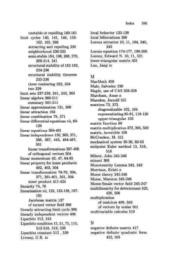
unstable or repelling 160-161 limit cycles 140, 141, 146, 159-

162, 165, 266 attracting and repelling 230 neighborhood 230-233 semi-stable 184 196 266 270 , , , ,

309-314, 341 structural stability of 182-183,

224-236 structural stability theorem

233-236 three coalescing 322, 334 two 329

limit sets 237-239, 241, 243, 262 linear algebra 369-511

summary 501-511 linear approximation 131, 306 linear attraction 183 linear combination 78, 371 linear differential equations vii, 69-

129 linear equations 369-401 linear independence 150, 369, 371,

386, 387, 443, 484-487, 501

linear transformations 397-400 of orthogonal vectors 504

linear momentum 42,47,64-65 linear property for inner products

402, 403, 504 linear transformation 78-79 294 , ,

371, 391-401, 501, 504 inner product 411-424

linearity 74, 78 linearization vii, 132, 133-138, 187-

191 Jacobean matrix 137 of turned vector field 366

linearly attracting limit cycle 366 linearly independent vectors 406 Lipschitz 213, 243 Lipschitz condition 15 51 75 115 , , , ,

512-516, 519, 538 Lipschitz constant 512 , 539 Livesay, G.R. ix

Index 595

local behavior 133-138 local bifurcations 266 Lorenz attractor 10, 11, 194, 240,

242 Lorenz equation 174-177, 199-200 Lorenz, Edward N. 10, 11, 521 lower-triangular matrix 431 Luo, Jaiqi ix

M MacMath 459 Malo, Salvador 230 Maple, use of CAS 328-329 Marcham, Anne x Marsden, Jerrold 521 matrices 73, 372

diagonalizable 102, 104 exponentiating 85-91, 118-120 upper-triangular 103

matrix function 69 matrix multiplication 372, 395, 502 matrix, invertible 108 McCracken, M. 521 mechanical system 26-36, 60-63 midpoint Euler method 13 516

518 " Milnor, John 245-246 minuet 369 Monotonicity Lemma 242, 243 Morrison, Kristi x Morse theory 245-246 Morse, Marston 245-246 Morse-Smale vector field 245-247 multilinearity for determinant 425

428,506 multiplication

of matrices 499, 502 of vectors by scalar 501

multivariable calculus 519

N negative definite matrix 417 negative definite quadratic form

422, 505

,

596 Index

negative real parts 102-106, 124-126, 142

neighborhood of limit cycle 230-233 of sink 171

Newton, Isaac 41, 42, 46 node sinks and sources 92-93, 150-

155 nonautonomous 2,7 nondegeneracy 191 nondegeneracy conditions 347 nondegeneracy hypothesis 320 nondegenerate quadratic forms 505 nonhomogeneous linear differen-

tial equations 74-78, 106-113, 126-129

nonlinear differential equations vii, 72, 131-201

Noonburg, Anne ix, x Noonburg, Derek ix norm of vector 402, 504 normal linear transformation 495 normalization for determinant 425,

429, 506 null space 397-400 nullcline 8, 189 numerical approximation 2,12-14,

54-55 numerical methods 516-518

o Oberste-Vorth, Ralph ix one-parameter families 314-319 operator, differential 79 orbit 22-23, 181 orbits, planetary 45 order 1, 2, 23, 73-74 order (as opposed to chaos) 180-

181 orthogonal basis 406 orthogonal complement 409-411,

504 orthogonal matrices 90-91, 495, 507

determinant 439

in QR method 458 orthogonal projection 408-411,504 orthogonal transformation 411-413,

414, 450, 504, 505, 509 orthogonal vectors 406, 504

volume 437 orthogonalization, Gram-Schmidt

370 orthonormal basis 369, 406 orthonormal matrices 91,472 orthonormal transformations 411 orthonormal vectors 406,407,504 oscillation 31, 180

harmonic 109-110, 128 oscillator

p

damped harmonic 70-71,147 Van der Pol 161

Palmer, Thomas ix Papadopol, Peter ix parallelepiped 507 parameter 265 parameter line 316, 317, 319 parameter plane 327 parameter: one-parameter families

314-319 parameter: two-parameter families

318-335 Park, Heather x Parmet, Marc ix partial fractions 400-401, 487 particular solution 75-76 Peixoto, M.M. vii, 203, 521 Peixoto, M.M., density theorem

252-258 pendulum 26-32, 72, 128, 191,357

nonlinear damped 134-135 rotating 346

period mapping 164, 224, 227 periodic cycle 542 periodic differential equations 313-

314 periodic orbit 22-23, 236

periodic points 180-181 perturbation 31, 138,208,303-305,

321,329 in exercises 349, 351, 353 of limit cycles 224-236, 298,

311 of matrix 448-449 of saddles 247-252 of sinks and sources 215-218

phase plane 6-9, 131, 132, 141 phase space 10-11, 23 pitchfork bifurcation 288, 346 pivot 376, 500 planar system 6-9 planar systems program 338, 342,

362 Planck's constant 415 planets 41, 66-67 Poincare, Henri 162, 245 Poincare...Bendixson theorem vii,

140, 162-167, 196-197, 203, 236-237, 288, 289, 296, 309, 329, 366

corollary 247 statements 163, 239 why it rules out chaos in the

plane 236-245, 262 Poincare section 224, see also sec­

tion mapping polar coordinates 361 polynomial, characteristic 452-457,

493, 495, 502, 507, 508, 509

polynomial equations 442 polynomials 294, 295, 401, 509

relatively prime 455-456 vector space 486,487,489

Pontryagin, L. vii, 203, 245, 247 pony tail 272, 273, 275, 281, 286,

345,576 double 321, 333

population interacting 17-23, 56-58, 72 single 313-314

Porter, Dawn x

Index 597

positive definite matrix 417 positive definite property for in­

ner products 402, 403, 504 positive definite quadratic forms

422, 505 positive real parts 102-106, 124-

126,200 potential, electrical 71-72 potential energy 27-29, 301 potential function 27, 191, 346,

357, 529-530 power method 457-458 power series 120 predator-prey 17-23, 56, 72 principal axis 479, 499 principal axis theorem 479 product-rotation algorithm 469, 497 product rule for inner products

404 projection 6

orthogonal 408-411, 504 projection operator 490 proof 371 properties of matrix exponentials

87-89 pseudo-diagonal 143, 192,445-446,

562 pseudo-upper-triangular matrix 143,

192,448

Q QR method vii, 85, 370, 457-472,

496-497, 504 quadratic forms 369, 417-424, 475,

492, 498-499, 505 quadric surface 476, 498 quantum mechanics 415, 451

R rank, for quadratic forms 422, 505 real eigenvalues 92 repelling cycles 177 repelling fixed point 177 repelling limit cycle 160-161

598 Index

repelling saddle connection 303, 304

resistance 71-72 resonance 108-110 restoring force 147 resultant 8 RLC circuit 71-72 Rodolia cardinalis 22 Roessler, O.E. 53, 521 Rota, G.C. 521 rotated vector field 230-232, 336,

365-366, 367 rotation

in Jacobi's method 473 in QR method 13

rotation matrix 497,502 rotation transformations 393-394,

413 row operations 482-483, 499-500 row reduction 370, 371, 373-380,

500 algorithm 375-376 and linear independence 387 for inverse 381

Runge-Kutta 13, 517

S saddle connection 173,184-185,266,

270,298-309,315-319,338, 340-341, 351-353

heteroclinic 184-185, 299, 300, 315, 318

homoclinic 184-185, 299, 300, 311, 315, 320, 321, 325-326, 330-332

serious explanation of homo­clinic 303-309

saddle-node 138, 266, 270, 271-288, 314, 320, 323-324, 333, 336-337, 344-347

degenerate 367 homoclinic 286-288, 323, 338

saddles 31, 93, 155-159, 192-195, 199

and eigenvalues 104-106,124-126

structural stability of 182-183 Sanchez, David A. 521 sardines 17-23, 56 scalar product 374 scale insects 22 scaling for determinant 425 scattering theory 215-216, 229, 234-

236 Schleicher, Dierk ix Schrodinger equation 415 Schwarz's inequality 115, 405, 504,

525,538 second nondegeneracy condition

321 section mapping 177-180, 200, 224-

230 derivative 229-230

semi-stable limit cycle 184, 196, 266, 270, 309-314, 320, 330-332, 334, 339, 343, 353-355

sensitive dependence on initial con­dition 203

separatrices 31, 139, 141, 156, 178-181, 189, 195, 200, 347, 348, 355, 365

series 120 Fourier 106, 110, 128,406, 416,

451 sharks 17-23, 56 Siegel, Carl Ludwig 245 signature

and eigenvalues 481-482 for quadratic forms 422-424,

491, 492, 499, 505 signed volume 440 Simmons, George F. 521 singular point 8, 133 singularities 133 sink 142, 146, 148-155, 192-195,

199 structural stability of 182-183,

215-218, 259-260

weak, in Hopf bifurcation 292-297

sinks and sources and eigenvalues 102-106, 124-

126 node 92-93 spiral 94-95

Sisson, Peter ix slope 516 slope error 518 Smale horseshoes 181-182 Smale, Stephen ix, 181-182, 245,

247, 521, 522 solving linear equations 294, 377-

380 source 142, 148-155, 192-195, 199

structural stability of 182-183, 215-280, 259-260

weak, in Hopf bifurcation 292-297

span 369, 386, 387, 486, 501 of vectors forming parallelepiped

435-436,438,440 Sparrow, C. 176, 522 spectral theorem 451, 509

proof 472-482 spiral 122 spiral sinks and sources 94-95,148-

150 spring 70-71 spurious solution 13 square matrices 507 square wave 128 stability vii, see also structural sta-

bility stable equilibrium 31 stable limit cycle 141, 160-161 stable separatrix 178-181 standard basis 388, 501 standard dot product 417 standard inner product 402, 403,

504 standard norm 402 state space 6, 23 steady state solution 127, 552

Index 599

stepsize 13, 516 Strogatz, Steven H. 522 structural stability 180-186, 200-

202, 203-263 definition 210 of limit cycles 224-236, 262 of saddles 247-252 of sinks and sources 215-218,

259-260 structural stability theorem 247-

252,317 subcritical bifurcation 292 subdiagonal469 subspace 384 supercritical bifurcation 292 superposition 74, 77, 78, 107, 110 symmetric linear transformation

418,419 symmetric matrix 472, 475

signature 481-482 symmetric property for inner prod­

ucts 402, 504 symmetric saddle node 288 symmetric transformation 415,450,

451,504,505, 509 symmetries 39, 168-169, 173, 193,

197-199 symphony 369 system 1, 2

T tadpoles 241, 262 tangent bifurcation loci 327, 330-

331 tangent isoclines 315 tangential approach 151-155, 156-

159 Taylor polynomial 133-134, 137 Terrell, Robert ix theorems, from Parts I and III 511-

519 Thorn, Rene ix Thomas, Katrina x three limit cycles coalesce 322,334

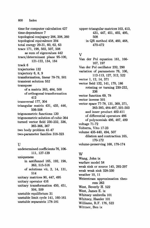
600 Index

time for computer calculation 427 time-dependence 7 topological conjugacy 206, 208, 260 topological equivalence 204 total energy 29-31, 60, 62, 63 trace 171, 198, 502, 507, 508

as sum of eigenvalues 442 trace/determinant plane 95-100,

121-122, 134, 184 track 6 trajectories 132 trajectory 6, 8, 9 transformation, linear 78-79, 501 transient solution 552 transpose

of a matrix 383, 484, 500 of orthogonal transformation

412 transversal 177, 304 triangular matrix 431, 435, 446,

506-508 trigonometric functions 120 trigonometric solution of cubic 364 turned vector field 230-232, 336,

365-366, 367 two body problem 41-47 two-parameter families 318-323

U undetermined coefficients 76, 106-

111, 127-129 uniqueness

in antifunnel 165, 192, 198, 363, 515-516

of solutions vii, 2, 14, 131, 514

unitary matrices 90,447,495 unitary operator 416 unitary transformation 450, 451,

504, 509 unstable equilibrium 31 unstable limit cycle 141, 160-161 unstable separatrix 178-181

upper-triangular matrices 103, 413, 431, 447, 451, 492, 495, 508

V

in QR method 458, 460, 468, 470-472

Van der Pol equation 161, 166-167, 197

Van der Pol oscillator 232, 290 variation of parameters 76, 106,

112-113, 127, 312, 522 vector 1, 12, 14, 371 vector field 132, 141, 170, 186

rotating or turning 230-232, 336

vector function 69, 78 vector inverse 501 vector space 77-78, 131,369,371,

383-385,484-487,501-503 and inner product 402-411 of differential operators 486 of polynomials 486,487,489

voltage 71-72 Volterra, Vito 17-23 volume 435-440,494,507

dilation and contraction 165, 170-172

volume-preserving 168, 170-174

W Wang, John ix warfare model 58 weak sink or source 145, 292-297 weak weak sink 328-330 weather 10, 11 Weierstrass approximation theo-

rem 263 West, Beverly H. 522 West, James E. ix Whitney umbrella 101 Whitney, Hassler 101 Williams, R.F. 176, 522 Wittner, Ben ix

World War I 17-23 World War II 22

y Van, Anthony ix Yan, Thomas ix Ye, Yan-Qian 312, 522

Z zero eigenvalue 98, 106, 183, 320,

321 double 183-184

zeroes 8, 131, 132, 137, 140, 146, 187-191, 199

structural stability of 182-183 Zhang, Zhi-fen 312-313

Index 601

Texts in Applied Mathematics

(continued from page ii)

33. Thomas: Numerical Partial Differential Equations: Conservation Laws and Elliptic Equations.

34. Chicone: Ordinary Differential Equations with Applications.

35. Kevorkian: Partial Differential Equations: Analytical Solution Techniques, 2nd ed. 36. DullerudlPaganini: A Course in Robust Control Theory: A Convex Approach. 37. QuarteronilSaccolSaleri: Numerical Mathematics.