Application of fracture mechanics in analyzing delamination of

$Page 1: Application of fracture mechanics in analyzing delamination of$
APPLICATION OF FRACTURE MECHANICS IN ANALYZING DELAMINATION OF CYCLICALLY LOADED PAPERBOARD CORE

MARKOILOMÄKI

Department of Mechanical Engineering,University of Oulu

OULU 2004


MARKO ILOMÄKI

APPLICATION OF FRACTURE MECHANICS IN ANALYZING DELAMINATION OF CYCLICALLY LOADED PAPERBOARD CORE

Academic Dissertation to be presented with the assent ofthe Faculty of Technology, University of Oulu, for publicdiscussion in Raahensali (Auditorium L10), Linnanmaa, onAugust 27th, 2004, at 12 noon.

OULUN YLIOPISTO, OULU 2004

Copyright © 2004University of Oulu, 2004

Reviewed byProfessor Mauri MäättänenLicentiate in Philosophy Pekka Pakarinen

ISBN 951-42-7399-0 (nid.)ISBN 951-42-7400-8 (PDF) http://herkules.oulu.fi/isbn9514274008/

ISSN 0355-3213 http://herkules.oulu.fi/issn03553213/

OULU UNIVERSITY PRESSOULU 2004

Ilomäki, Marko, Application of fracture mechanics in analyzing delamination ofcyclically loaded paperboard core Department of Mechanical Engineering, University of Oulu, P.O.Box 4200, FIN-90014 Universityof Oulu, Finland 2004Oulu, Finland

AbstractThe primary objective of this work is to study and model the fracture process and durability ofpaperboard cores in cyclic loading. The results are utilized in creating analytic model to estimate thelife time of cores in printing industry. The life time means here the maximum number of winding-unwinding cycles before the core delaminates. This study serves also as an example of use of boardas a constructional engineering material.

Board is an example of complicated, fibrous, porous, hydroscopic, time dependent and statisticmaterial. Different core board grades are typically made of recycled fibers. The material model inthis work is linear-elastic, homogeneous and orthotropic.

The material characteristics, elastic and strength properties are studied first. Then the material isstudied from the points of view of fracture and fatigue mechanics. Some of the analysis and testmethods are originally developed for fiber composites but have been applied successfully here alsofor laminated board specimen. An interesting finding is that Scott Bond correlates well with the sumof mode I and mode II critical strain energy release rates. It was also possible to apply Paris' law andMiner's cumulative damage theory in the studied example situations.

The creation of the life time model starts by FEM-analysis of cracked and non cracked cores in atypical loading situation. The elastic-linear material model is used here. The calculated stresses areutilized in analytic J-integral model. The agreement between analytic and numerical J-integralestimations is good.

The analytic life time model utilizes the analytic J-integral model, Miner's cumulative damagetheory and analytically formulated Wöhler-curves which were constructed by applying the Paris' law.The Wöhler-curves were constructed also by testing cores to validate the theoretical results. Thetesting conditions are validated by FEM-analysis.

The cores heat up when tested or used with non expanding chucks and a temperature correctionwas needed in the life time model to consider this. Also, single or multi crack model was useddepending on the studied case. The calculated and tested durability prediction curves show goodcorrespondence. The results are finally reduced to correspond to certain confidence level.

Keywords: core, fracture, life time, paperboard, statistical


Preface

This study has been compiled during recent years by the author at his work at the Ahlstrom Core Competence Center (CCC) in Karhula, Finland. The presented findings were born as a result of efforts to be able to design better cores and to better understand board as a constructional material. There was also a need to be able to predict life time of cores in winding processes with certain failure probability. In the early phase of the studies, the winding simulator was built for the practical tests. The simulator offered a close presence of practice for further studies. Designing and building of the simulator was a considerable effort. The whole study is relatively large and this is largely because it was found in the beginning that there was not much published information available concerning the subject. This kind of study would have been a very difficult project without a close contact to the paper, board, core and printing industries. This study has been fully financed by Ahlstrom Cores Oy while the author has been working for the company as research scientist.

The author owes a debt of gratitude to many people for making this study possible. I would like to thank Mr. Markku Järvinen, Mr. Risto Anttonen, Mr. Leif Frilund and Mr. Michael Fejer for providing the financial resources and supporting atmosphere. I also would like to point gratitude to Mr. Markku Järvinen for his contribution in starting this project and giving constructive comments. He also presented the requirements for this work from the company side. I would like to thank Mr. Ismo Kervinen for his assistance with winding simulations and core durability tests, Mr. Taisto Auvinen for preparing the test structures and board specimen and Ms. Heli Kuosmanen for her assistance with material analysis. Finally, I owe my sincere gratitude to my supervisor, Professor Stig-Göran Sjölind for his excellent guidance, encouragement and professional comments.

Karhula, June 2004 Marko Ilomäki


List of symbols

γ1, γ2, γ3 shear strains σ1, σ2, σ3 normal stresses σij stress component ij σboard stress in board layer σglue stress in glue layer σr radial stress σraverage average of radial stress σref maximum of positive radial stress at certain reference chuck load σθ tangential stress σθaverage average of tangential stress εboard strain in board εglue strain in glue layer ε1, ε2, ε3 normal strains εlin the maximum linear elastic material response strain εzaverage average longitudinal strain in a core cross section νij Poisson´s ratio ij α winding angle Γ(n) gamma function δ displacement of the center span of the ENF-specimen δ displacement of the split DCB specimen beam end δA increase in crack area ∆ the total bending of split DCB specimen free end ∆a the change of crack length ∆AB ,∆BC ,∆CD displacements ∆G the change of strain energy release rate ∆Gth threshold value of strain energy release rate ∆K the change of stress intensity factor during a loading cycle ∆Laverage average lengthening of core cross section θ tangential coordinate λ the independent variable in the standard normal distribution ρA basis weight of paper τ1, τ2, τ3 shear stresses

τref maximum of shear stress at certain reference chuck load 1, 2 and 3 principal material directions a crack length a inner radius of a core a0 the initial crack length a1 the crack length after n loading cycles ac critical crack length Aboard the board area in cross section Aglue the glue area in cross section Alaminate lamina cross section b outer radius of a core b reel width B the web gap width b0 and b1 coefficients bt belt tester (the winding simulator) c radial ratio C the given confidence level C compliance C and n Paris´ equation material constants Cij stiffness matrix cd the cross-machine direction clc chuck load capacity dA change in crack surface da incremental crack length dN the number of loading cycles Dm layer inside diameter Dw layer outside diameter E1, E2, E3 Young´s modulus (E-modulus) in direction 1, 2 and 3 Eboard E-modulus of board in machine or cross direction Eglue E-modulus of glue Er E modulus of core wall in the radial direction Eθ E modulus of core material in the tangential direction f fraction of deflection F certain fraction of shear deformation F chuck load Fref reference chuck load g gravity constant 9.81 m/s2 g(µ) non dimensional energy release rate coefficient G strain energy release rate G shear modulus Gc work required to create a unit crack area GIc mode I fracture toughness GIIc mode II fracture toughness G(µ)II strain energy release rate considering friction effect h glue layer thickness h half thickness of ENF specimen

h thickness of a DCB specimen H complementary potential energy H board-glue laminate thickness I the second moment of inertia I, II and III crack loading modes k the slope factor K anisotropy ratio L initial core length Ls web edge length of one board web revolution Lwi web edge length of ply i in 1 meter long core md machine direction meanC the population mean with confidence level C meansample mean of the measured samples mR reel weight mRmax maximum reel weight n the number of data samples n1, n2,…,nk the number of revolutions N1,N2,…,Nk chuck load levels NR number of loading revolutions NRmax maximum number of loading revolutions num number of cracks P load P the probability of failure Pc critical load pt pneumatic roller tester r radial coordinate Ri residuals Slog standard deviation of residuals (using log-points) SB Scott Bond SC the population standard deviation with confidence level SCrelative the relative population standard deviation with confidence level SF safety factor Sij compliance ij t board web thickness t2 the upper integration limit for probability density function of t-distrib. td thickness direction (called also z-direction in some context) U displacement U elastic strain energy stored in the body vw web speed w width of a fracture specimen W the width of a paperboard web W potential energy of external forces xi and yi random samples ZS z-strength (thickness direction strength of board)


Contents

Abstract Preface List of symbols Contents 1 Introduction ...................................................................................................................15 2 Cores in the paper industry............................................................................................16

2.1 General ...................................................................................................................16 2.2 Requirements for paper industry cores ...................................................................19 2.3 Failure mechanism..................................................................................................20

3 Elastic properties of paperboard ....................................................................................21 3.1 Assumptions concerning the material model ..........................................................21

3.1.1 Orthotropy .......................................................................................................21 3.1.2 Linearity and homogeneity ..............................................................................22

3.2 The stress-strain relations in the principal material coordinates .............................22 3.3 Restrictions on the elastic constants .......................................................................24 3.4 Stress-strain behavior of boards..............................................................................25 3.5 Thickness direction E-modulus of laminated board ...............................................28 3.6 Poisson’s ratio of board ..........................................................................................29

3.6.1 Literature study................................................................................................29 3.6.2 Studies of Poisson ratio values ........................................................................30

3.7 Shear modulus ........................................................................................................30 3.8 Homogenized elastic modulus of glued board........................................................31

3.8.1 Voight´s upper bound.......................................................................................34 3.8.2 Reuss´ lower bound .........................................................................................34 3.8.3 Comparison between calculated and measured results ....................................35

3.9 Elastic constants of the example board web ...........................................................36 3.10 The effect of winding angle on the elastic constants ............................................37

4 Strength properties of paperboard .................................................................................39 4.1 Machine and cross direction breaking stress of board ............................................39 4.2 Thickness (z-) direction tensile strength of boards .................................................40

4.3 Scott Bond ..............................................................................................................41

4.3.1 The effect of testing direction on the test results .............................................42 4.4 Out of plane shear strength .....................................................................................43 4.5 Relationships between Scott Bond, z-strength and shear strength..........................44

5 Geometry of cores .........................................................................................................45 6 Delamination strength of cores......................................................................................48

6.1 Chuck load capacity................................................................................................48 6.1.1 The testing principle ........................................................................................49 6.1.2 Tests with expanding and non expanding chuck..............................................49 6.1.3 Scott Bond versus chuck load capacity............................................................51 6.1.4 Statistical variation in the test results ..............................................................52

6.2 The winding simulator............................................................................................52 6.3 Flat crush resistance................................................................................................53 6.4 Flat crush versus chuck load capacity.....................................................................54

7 Fracture mechanics studies of board specimen..............................................................57 7.1 Strain energy release rate........................................................................................57 7.2 Mode I fracture .......................................................................................................60

7.2.1 Mode I DCB specimen design considerations .................................................61 7.3 Mode II fracture......................................................................................................62

7.3.1 Mode II ENF specimen design considerations ................................................64 7.4 Static mode I and II tests ........................................................................................65

7.4.1 Determination of GIc and GIIc ..........................................................................66 7.5 Cyclic mode I and II tests .......................................................................................67

8 Stress distributions in non cracked cores.......................................................................76 8.1 Analyzed structures.................................................................................................77 8.2 FEM-models ...........................................................................................................78

8.2.1 Assumption of plane strain condition ..............................................................79 8.2.2 Elements and contact modelling......................................................................79 8.2.3 Material properties...........................................................................................79 8.2.4 About the calculated results .............................................................................80 8.2.5 The calculated stress distributions ...................................................................81 8.2.6 Some additional observations from stress distributions...................................85 8.2.7 FEM-analysis of cracked cores in belt tester ...................................................87

8.3 Numerical and analytic J-integral estimations........................................................90 9 Crack propagation in cores ............................................................................................93

9.1 About the practical tests..........................................................................................93 9.2 Studies of the effect of number and size of cracks on delamination of test cores .......................................................................................94 9.3 Comparison of durability between different test cores .........................................101

10 Modeling cyclic durability of cores...........................................................................105 10.1 Theory of estimating Wöhler-curves of cores in testing situation ....................105 10.2 Representative material constants of Paris´ equation .........................................108 10.3 Measured and calculated Wöhler-curves ............................................................ 110

10.3.1 76x15 mm cores .......................................................................................... 110 10.3.2 150x13 mm cores ........................................................................................ 112

10.4 Calculated chuck load capacity in the example cases......................................... 112 10.5 Estimations of the limit load............................................................................... 113 10.6 The effect of crack length on durability.............................................................. 115 10.7 The effect of number of cracks (four crack model) ............................................ 117

11 Winding simulations ..................................................................................................120 11.1 Practical tests ......................................................................................................120 11.2 Temperature and revolution speed versus dynamic durability ............................122 11.3 Theoretical model and results .............................................................................126

12 Durability of cores with different failure probabilities ..............................................129 12.1 Confidence of the mean ......................................................................................131 12.2 Confidence of the standard deviation .................................................................133 12.3 Failure probability and safety factor...................................................................134 12.4 The confidence and prediction limits for the curve fit........................................136 12.5 Failure probability and safety factor...................................................................138 12.6 Example of reduced results.................................................................................139

13 Summary ...................................................................................................................141 References Appendix 1 Stresses and dimensional changes of cores under external pressure Appendix 2 Stress distributions in cross section of non cracked cores Appendix 3 Results of dynamic mode I and II crack propagation tests Appendix 4 Crack propagation in 76x15 mm cores


1 Introduction

Board is an example of a fibrous engineering material. Core boards are typically made of recycled fibers. The closest like material is paper but board is thicker and is generally better suited for constructional purposes. One user of board is the core industry.

The number of published articles, studies and conference presentations concerning mechanical or constructional properties of boards and cores is relatively limited. Publications are made by Tappi Journal, The Finnish Pulp and Paper Research Institute (KCL), the American society of mechanical engineering, ERA (the European Rotogravure association) and IWEB (the International Conference on Web Handling). Also, engineering thesis has been written concerning cores and boards including the authors MSc. [1] and Licentiate thesis [2]. Lack of material data is usually one of the first problems in the start of analysis of board structures. That was the case in this work too. It was necessary to study the representative constructional characteristics and material properties of example boards.

There is not either many publications concerning fracture mechanics or fatigue related topics of board materials. On the other hand, it is easier to find such publications concerning orthotropic materials and composites. In certain conditions, it is possible to consider laminated boards as fibrous, orthotropic, homogeneous and linear-elastic composites and utilize the testing and analysis methods developed for fiber composites.

The primary interest in this work is to study and model the fracture process and durability of board cores in cyclic loading. The practical application is an analytic model which could estimate the life time of cores in printing industry.

The term “life time” refers here to the maximum number of winding-unwinding cycles before the core delaminates by the dynamic crack growth process. One winding- unwinding cycle is a process when all paper is first wound on core in paper mill slitter-rewinder and then unwound in printing press during the printing process.

The loading conditions vary in different winders and unwinders. Also, every core is unique, since the material and construction of cores vary statistically. The modeling will be based on certain assumptions concerning board material, core structure and winding conditions. We will also utilize statistical methods in reducing the estimated or measured results to correspond to certain confidence level. This process requires practical simulations and studies of statistical characteristics of boards and cores.

2 Cores in the paper industry

2.1 General

We will start with a review of board cores in paper industry. This topic has also been discussed in reference [3]. Core is an integral part of paper reel. Cores work as winding shafts in paper mill slitter-rewinders and as unwinding shafts in printing press unwinders. Considering our study, it is important to understand the loading conditions, requirements and failure mechanisms of cores. Cores and chucks must function in such a way that vibrations, web breaks, core breaks and other winding and unwinding problems are minimal.

Examples of typical paper industry cores are shown in figure 1 a) and b). The highest requirements for cores are in rotogravure industry. Rotogravure printing presses run typically at 11-14 m/s while the reel widths are today up to 3.68 m. There has been discussion concerning higher combinations of printing speeds and reel widths. Speeds are today limited by the folding process to about 16 m/s. If this limitation is overcome, even higher speeds will be possible. Regarding the width, a 4.3 m wide machine is already coming on the market [4]. Figure 1 c) shows a 4.4 m wide, 10 ton test reel which was wound on 150x13 mm board core.

a) b) c) Fig. 1. 150x13 mm cores a) , 76x15 mm cores b) and 4.4 m wide, 10 ton reel c). Figures 2-4 show examples of ways of supporting paper reels in different paper mill slitter-rewinders [5]. In a two-drum surface winder in figure 2, the whole reel weight is supported by the reel surface nip. Figure 3 shows a center-surface winder in which the reel weight is supported by a combination of large drum and chucks. 70–80 % of the reel

17weight is supported by the chucks [3]. The maximum center torque in the start of winding process is typically 100–250 Nm. 76x15 mm high strength paper industry cores can withstand even 1500–2000 Nm torque loads. The torque strength of cores has been discussed in reference [6]. In some older constructions, the whole reel mass and nip force is transmitted by the chucks as in figure 4.

Fig. 2. Two drum winder [5].

Fig. 3. Combination core and roll support winder [5].

Fig. 4. Core support winder [5]. Some examples of typical slitter-rewinder chucks are shown in figure 5. Representative cylindrical supporting chuck length is typically 150 mm and chucks can be non-expanding or equipped with expanding elements to improve torque transmissibility.

18

a) b) c) Fig. 5. Examples of paper mill winder chucks. 76 mm expanding chuck a), 150 mm expanding chuck adapter b) and 150 mm non expanding chuck c). In printing presses the reels are supported from core ends by the chucks as in figure 6. In the beginning of unwinding process, the reel is accelerated to paper web speed from the reel surface by using acceleration belts. Depending on the construction, the acceleration belts bring some 10 kN extra load or support during the acceleration process. In modern constructions, the acceleration belts are located below the reel and they also support the reel during the acceleration process.

The printing machine chucks are usually equipped with expanding elements to minimize the possibility of slip between chuck and core. Examples of rotogravure printing machine chucks are shown in figure 7. Representative typical cylindrical supporting length of these chucks is 200 mm. The chucks may be longer but the chuck tip is conical and does not support the core. Printing machine chucks are also discussed in reference [7].

a) b) Fig. 6. Cross section image a) of a paper reel in printing press unwinder b).

a) b) c) Fig. 7. Examples of rotogravure printing machine unwinder chucks: a) and b) 76 mm chucks, c) 150 mm chuck.

19

2.2 Requirements for paper industry cores

Majority of the paper industry cores are made of paperboard. Paperboard cores are light, strong, stiff and easy to recycle. Some of the most important requirements for paper industry cores are listed below to help understanding how demanding engineering application the core actually is [4]:

- Good dimensional tolerances. - Good straightness (less vibration problems and fewer paper web breaks). - High enough chuck load capacity (minimum risk of core break). - High bending stiffness (high resonance frequency to avoid rest reel explosions, less paper burst problems with stiffer cores, minimum bending in the start of winding). - Tolerate high cyclic bending deformations (safety, if a rest reel is driven too close to the resonance rotation speed). - Right size and hardness (good core-chuck contact to avoid core chew-out problems). - Smooth surface (less paper ridges in reel center which could cause web breaks). - Small moisture exchange with paper (keep dimensions and minimize changes in winding tightness during storage. - Low weight (handling, transportation & resonance frequency). - Minimal space utilization (transportation and storage). - Minimal lengthening during winding (avoid bending and vibration problems). - Easy and cheap to dispose of the cores after usage. - Rigidity against dimensional changes under paper pressure and external loads. Considering the objectives in this study, we will later discuss about chuck load capacity and flat crush resistance. The flat crush resistance test is a standardized method but, there is no worldwide generally accepted standard method to measure the chuck load capacity. There are some chuck load capacity testing devices but they differ in working principle and the results are not directly comparable.

DIN (Deutsches Institut fur Normung), DIS (Deutche Industrie Norm), CCTI (Composite Can and Tube Institute) and ISO (International Organization for Standardization) have published several core related standards. Examples of (ISO/DIS) core standards are listed below:

- Inside and outside diameter [mm] (ISO/DIS 11093-4) - Moisture content [%] (ISO/DIS 11093-3) - flat crush resistance [N/100 mm] (ISO/DIS 11093-9) - E-modulus [MPa] (ISO/DIS 11093-8) - Out of straightness [mm/m] (ISO/DIS 11093-5) - Out of roundness [mm] (ISO/DIS 11093-5)

20

2.3 Failure mechanism

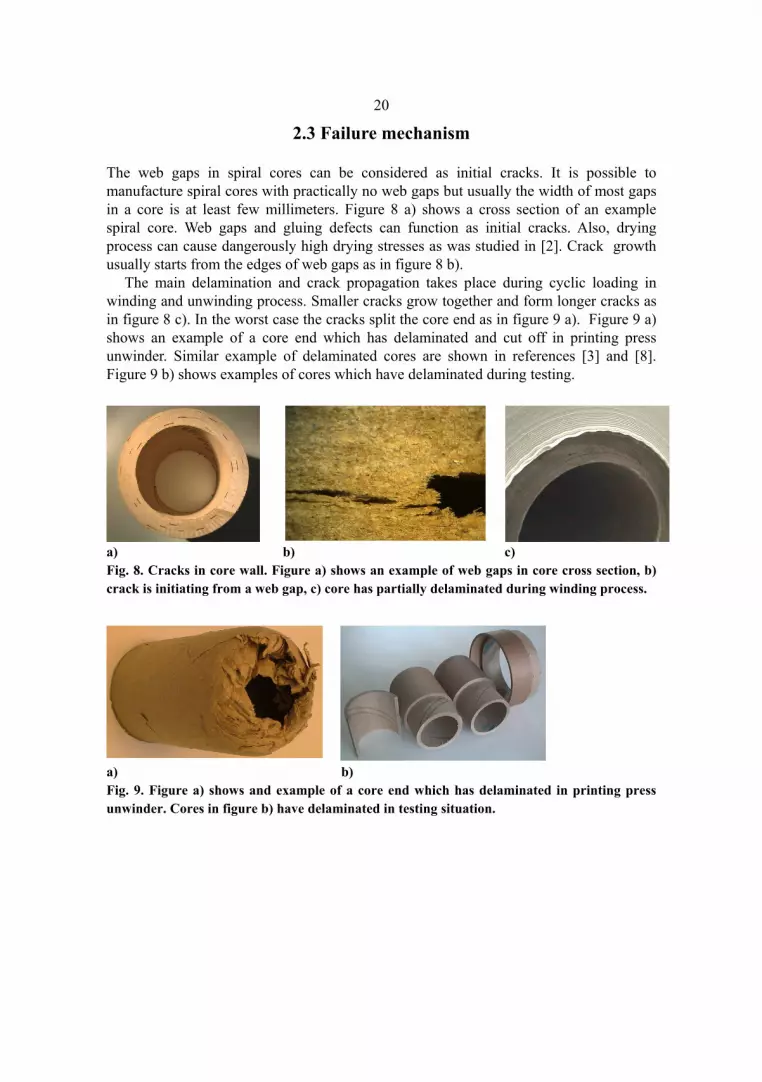
The web gaps in spiral cores can be considered as initial cracks. It is possible to manufacture spiral cores with practically no web gaps but usually the width of most gaps in a core is at least few millimeters. Figure 8 a) shows a cross section of an example spiral core. Web gaps and gluing defects can function as initial cracks. Also, drying process can cause dangerously high drying stresses as was studied in [2]. Crack growth usually starts from the edges of web gaps as in figure 8 b).

The main delamination and crack propagation takes place during cyclic loading in winding and unwinding process. Smaller cracks grow together and form longer cracks as in figure 8 c). In the worst case the cracks split the core end as in figure 9 a). Figure 9 a) shows an example of a core end which has delaminated and cut off in printing press unwinder. Similar example of delaminated cores are shown in references [3] and [8]. Figure 9 b) shows examples of cores which have delaminated during testing.

a) b) c) Fig. 8. Cracks in core wall. Figure a) shows an example of web gaps in core cross section, b) crack is initiating from a web gap, c) core has partially delaminated during winding process.

a) b) Fig. 9. Figure a) shows and example of a core end which has delaminated in printing press unwinder. Cores in figure b) have delaminated in testing situation.

3 Elastic properties of paperboard

Board is a good example of complicated, fibrous engineering material which possesses hydroscopic, time depending and statistical characteristics. The close alike material is paper but board is thicker and suits generally better for constructional purposes. Different core board grades are typically made of recycled fibers. Before going into further studies, we will study the elastic characteristics of example boards and glue laminated boards. Later we will study the strength properties. The moisture of the studied samples is between 7-8 % which is also typical delivery moisture range of rotogravure cores. The results will help making assumptions concerning the material model and estimating the validity of the analysis results. We will later study also relationships between mechanical behavior of board and cores which help understanding the material better. Finally, we will study board and cores from the fatigue and fracture mechanics points of view.

3.1 Assumptions concerning the material model

3.1.1 Orthotropy

Board has three principal material directions and is considered in this study as an orthotropic material in the principal material coordinates. The three principal material directions are the machine direction (md), the cross-machine direction (cd) and the thickness direction (td). In board and paper related articles, the thickness direction is typically called the z-direction.

We will use Abaqus FEM-program in structural analysis. Considering the coordinate numbering in Abaqus, the principal board web coordinates in this work are numbered in such a way that the principal board web coordinate 1 refers to the board web thickness direction, coordinate 2 refers to the board web machine direction and coordinate 3 refers to the board web cross-machine direction.

22

3.1.2 Linearity and homogeneity

We will assume board as a linear-elastic, homogeneous material. The assumption of homogeneity disregards the fibrous and porous nature of the material with its local and statistical variations but is applicable in our macro mechanical studies. It is still important to understand the micro mechanical characteristics of the material.

The question of validity of linear stress-strain behavior is interesting question in the cyclic loading situation where the loading level, loading speed and sample temperature is changing. Examples of considerations of plasticity of boards has been discussed in references [9] and [10]. In clearly long term loadings, it is important to consider the plasticity effects. Biaxial tensile behavior of paper has been discussed in reference [11]. The results are discussed in terms of the linear elasticity as a first approximation.

We will study in this work mainly dynamic loading conditions where the loading frequency can vary from few Hertz to tens of Hertz. The cycle load can vary in winding applications from small values to high values but in most cases in this study the maximum stresses are below 50 % of the breaking stress.

If we study the representative load-strain curves later in figure 11, we will find that the tangent slope is the greatest in the beginning of the curves. From figure 20 we can see that the load-strain curves of glued boards show slightly more linear behavior.

In this work, the representative linear material modulus, the tangent modulus [12], is determined using the greatest slope. We can estimate the linearization error at different load levels from the example stress-strain curves. Considering this work, the error is still relatively small if the load is less than 50 % of the breaking stress.

In this work, the humidity changes are minimal during the tests and the samples are conditioned to standard conditions. From this reason, the effect of humidity changes can be ignored. The cores may heat up in some tests from 20 °C to 60 °C.

We are not going to study more deeply the question of linearity here. This topic would be comprehensive enough for a separate study.

3.2 The stress-strain relations in the principal material coordinates

Orthotropic materials have two orthogonal symmetry planes for the elastic properties. Symmetry will exist also relative to a third mutually orthogonal plane. There is no interaction between normal stresses σ1, σ2, σ3 and shearing strains γ1, γ2, γ3 in the principal material coordinates. Similarly, there is no interaction between shearing stresses τ1, τ2, τ3 and normal strains ε1, ε2, ε3 as well as none between the shearing stresses and shearing strains in different planes. The generalized Hooke´s law for orthotropic material, relating stresses to strains can be written as [13], [14]

23

(1)

where the σij are the stress components, Cij is the stiffness matrix, εij and γij are the strain components [8]. The shear terms are in different order in the stress-strain relations in references [13] and [14]. Both relations are correct but we will utilize the relations in Abaqus User’s manual [14]. It is important to notify such differences when using FEM-programs. Considering the differences in [13] and [14] the stress-strain relation in terms of engineering constants like generalized Young´s moduli, Poisson´s ratios and shear moduli can be presented in the form (2) Where [14]

(3) The strain-stress relations are (4)

σ11

σ22

σ33

τ12

τ13

τ23

C11

C12

C13

0

0

0

C12

C22

C23

0

0

0

C13

C23

C33

0

0

0

0

0

0

C44

0

0

0

0

0

0

C55

0

0

0

0

0

0

C66

ε 11

ε 22

ε 33

γ12

γ13

γ23

⋅

∆1 ν 12 ν 21⋅− ν 23 ν 32⋅− ν 31 ν 13⋅− 2 ν 21⋅ ν 32⋅ ν 13⋅−

E1 E2⋅ E3⋅

σ11

σ22

σ33

τ12

τ13

τ23

1 ν 23 ν 32⋅−E2 E3⋅ ∆⋅

ν 12 ν 32 ν 13⋅+E1 E3⋅ ∆⋅

ν 13 ν 12 ν 23⋅+E1 E2⋅ ∆⋅

0

0

0

ν 12 ν 32 ν 13⋅+E1 E3⋅ ∆⋅

1 ν 13 ν 31⋅−E1 E3⋅ ∆⋅

ν 23 ν 21 ν 13⋅+E1 E2⋅ ∆⋅

0

0

0

ν 13 ν 12 ν 23⋅+E1 E2⋅ ∆⋅

ν 23 ν 21 ν 13⋅+E1 E2⋅ ∆⋅

1 ν 12 ν 21⋅−E1 E2⋅ ∆⋅

0

0

0

0

0

0

G12

0

0

0

0

0

0

G13

0

0

0

0

0

0

G23

ε 11

ε 22

ε 33

γ12

γ13

γ23

⋅

ε 11

ε 22

ε 33

γ12

γ13

γ23

S11

S12

S13

0

0

0

S12

S22

S23

0

0

0

S13

S23

S33

0

0

0

0

0

0

S44

0

0

0

0

0

0

S55

0

0

0

0

0

0

S66

σ1

σ2

σ3

τ12

τ13

τ23

⋅

24The compliance [Sij] matrix is the inverse of the stiffness [Cij] matrix and the strain-stress relations in terms of engineering constants in the principal board web directions 1, 2 and 3 are

(5) where E1, E2, E3=Young´s (E) modulus values, νij=Poisson´s ratios and G12, G13, G23 the shear modulus in the 1-2, 1-3 and 2-3 planes. Because of symmetry Sij=Sji.

3.3 Restrictions on the elastic constants

The product of a stress component and the corresponding strain component represents work done by the stress. The sum of the work done by all stress components must be positive in order to avoid the creation of energy when loading a structure [13]. Mathematically this means that the stiffness and compliance matrices must be positive definite [13]. This condition provides a thermodynamic constraint on the values of the elastic constants.

If only one normal stress is applied at a time, the corresponding strain is determined by the diagonal elements of the compliance matrix. Those elements must be positive, that is in terms of the engineering constants, [13] (6) Similarly, under suitable conditions, deformation is possible in which only one extensional strain arises. Again, work is produced by the corresponding stress alone. Thus, since the work is determined by the diagonal elements of the stiffness (inverse of compliance) matrix, those elements must be positive, that is [13] (7)

ε 11

ε 22

ε 33

γ12

γ13

γ23

1

E1

ν 12

E1−

ν 13

E1−

0

0

0

ν 21

E2−

1

E2

ν 23

E2−

0

0

0

ν 31

E3−

ν 32

E3−

1

E3

0

0

0

0

0

0

1

G12

0

0

0

0

0

0

1

G13

0

0

0

0

0

0

1

G23

σ1

σ2

σ3

τ12

τ13

τ23

⋅

E1 E2, E3, G12, G13, G23 0>,

1 ν 23 ν 32⋅−( ) 1 ν 13 ν 31⋅−( ), 1 ν 12 ν 21⋅−( ) 0>,

25The following inequality must also be satisfied [13]

(8) This is because the determinant of a matrix must be positive for positive definiteness [13]. When the left hand side of the inequalities approaches zero, the material exhibits incompressible behavior [14]. By using the symmetry of the compliances, the conditions (7) can be written as [13] (9) Similarly, equation (8) can be expressed as [13]

(10) The last two restricting equations can be used to test if the material behaves as an orthotropic material within the framework of the mathematical elasticity model.

3.4 Stress-strain behavior of boards

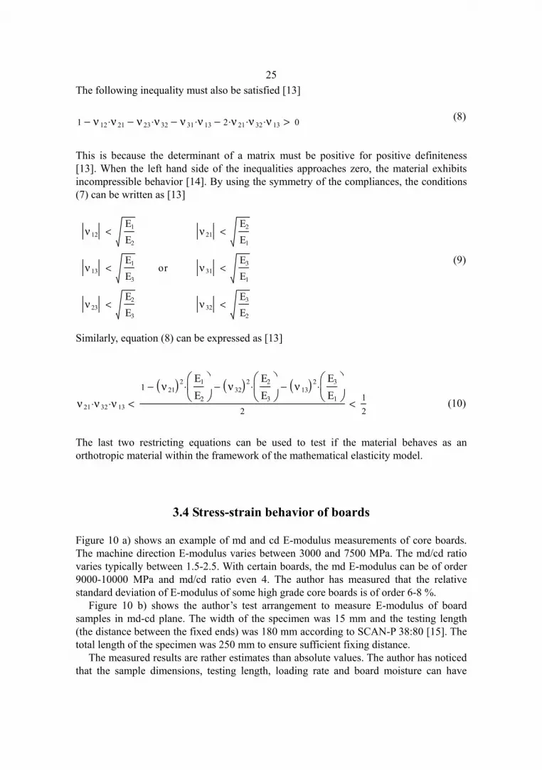
Figure 10 a) shows an example of md and cd E-modulus measurements of core boards. The machine direction E-modulus varies between 3000 and 7500 MPa. The md/cd ratio varies typically between 1.5-2.5. With certain boards, the md E-modulus can be of order 9000-10000 MPa and md/cd ratio even 4. The author has measured that the relative standard deviation of E-modulus of some high grade core boards is of order 6-8 %.

Figure 10 b) shows the author’s test arrangement to measure E-modulus of board samples in md-cd plane. The width of the specimen was 15 mm and the testing length (the distance between the fixed ends) was 180 mm according to SCAN-P 38:80 [15]. The total length of the specimen was 250 mm to ensure sufficient fixing distance.

The measured results are rather estimates than absolute values. The author has noticed that the sample dimensions, testing length, loading rate and board moisture can have

1 ν 12 ν 21⋅− ν 23 ν 32⋅− ν 31 ν 13⋅− 2 ν 21⋅ ν 32⋅ ν 13⋅− 0>

ν 12E1

E2< ν 21

E2

E1<

ν 13E1

E3< or ν 31

E3

E1<

ν 23E2

E3< ν 32

E3

E2<

ν 21 ν 32⋅ ν 13⋅1 ν 21( )2 E1

E2

⋅− ν 32( )2 E2

E3

⋅− ν 13( )2 E3

E1

⋅−

2< 1

2<

26effect on the test results. Some error in the results is also caused by the assumption that the specimen is homogenous and the cross section dimensions remain unchanged through the test.

a) b) Fig. 10. Md and cd E-modulus measurement results a) and tensile testing device b).

Figure 11 shows examples of the measured load-strain curves at tensile loading rates 25 mm/min and 500 mm/min. The samples were tensioned to rupture and there is not a big difference in the shape of the curves. It was also found that there is not a big difference in the shape of the curves if the loading rate is decreased from 25 mm/min to 5 mm/min. Anyway, if we study the long term constant load tensile test curves in figure 12, we can find clear time dependent creeping which is the faster, the higher is the load. Creeping is faster in the beginning of the tests than in the end.

The specified tensile loading rate in SCAN-P 38:80 [15] is 21.6 mm/min for 180 mm testing length and 12.0 mm/min for 100 mm testing length. The shape of the md and cd curves is different. Deviation between the curves and the greatest slope tangent in figure 11 is relatively small up to some 50 % of the breaking load. The testing machine searches the greatest tangent slope from the load-strain curve and calculates the E-modulus from that part of the curve. The greatest slope is not necessarily located in the very beginning of the curves, since the board samples may straighten up in the beginning of the tensile loading. This straightening depends on the testing dimensions and preload.

Machine and cross direction E-modulus of different core boards

0

1000

2000

3000

4000

5000

6000

7000

8000

0 1000 2000 3000 4000 5000

Cross direction E-modulus [MPa]

Mac

hine

dire

ctio

n E

-mod

ulus

[MP

a]

27

Fig. 11. The effect of tensile loading rate on load-strain behavior of board samples.

Fig. 12. Long term constant load strain curves.

28

3.5 Thickness direction E-modulus of laminated board

The thickness direction compression E-modulus was measured using laminated board and cut core samples as in figure 13. Figure 14 shows the linear correlation between sample density and compression direction E. The measured E increased if the compression test was repeated several times using the same test sample.

The tensile test results of non cracked specimen suggest that the tensile E is approximately 0.6-0.7 times the compression direction E. On the other hand, J. Aliranta [16] measured compression and tension E-modulus of samples cut from core walls. The web gaps were considered by reducing the effective cross section area. In some tests, the the compression E was even 4 times the tensile E. a) b) c) d) Fig. 13. Figures a) and b) show compression tests and figures c) and d) tensile tests. In figures b) and c) the sample size is 50x100 mm and in figure d) it is 25x100. Fig. 14. Board density versus compression E-modulus.

Relation betw een core density and compression E-modulus

0

100

200

300

0.7 0.75 0.8 0.85 0.9 0.95 1Board density [g/cm3]

Com

pres

sion

E-m

odul

us [M

Pa]

glued board pieces76x15 mm core wall150x13 mm core wall

29

3.6 Poisson’s ratio of board

νij=Poisson´s ratio for transverse strain in the j-direction when stressed in the i-direction [14], that is,

(11) A value of νij greater than one means that a stress applied in the i direction results in a greater strain in the j direction than in the i direction. Tensile deformation is considered positive and compressive deformation negative. The definition of Poisson's ratio contains a minus sign so that normal materials have a positive ratio. From the symmetry requirement of the compliance matrix (Sij = Sji) it follows that [13]

(12) Using this relation, only ν12 , ν13 and ν23 need to be measured, since ν21 , ν31 and ν32 can be calculated.

3.6.1 Literature study

Determination of Poisson´s ratios of paper and board by the direct measurements of stresses and strains is difficult [17]. Uncertainty arises from non-uniformity of stress and strain within the region of measurement, the specimen dimensions, error in the strain measurement, the possibility of specimen “tension buckling” (wrinkles) under uniaxial tensile stress and inelastic contributions to the measured strain [18]. It is also possible to measure the Poisson ratios of board or paper by ultrasonic [19] or image analysis method [20]. We will next review two examples from literature.

J. Aliranta [16] measured the in-plane νmachine cross values of some core boards using direct measurements. For the board with average E-modulus values of order Emachine 6700 MPa, Ecross 2400 MPa and Ethickness 100 MPa, the average of measured νmachine cross results was 0.2. The out of plane Poisson´s ratios he used in his studies were: νmachine thickness 3.35, νcross thickness 2.4, νthickness machine 0.05 and νthickness cross 0.1.

R.W. Mann et al [19] determined the elastic constants of liquid packaging board using ultrasonic methods. The Poisson ratio in the machine-thickness direction was located in the range from 0.59 to 2.45. The value of νmachine thickness was located in the range from 1.32 to 2.36. Some other measured values were: νmachine cross 0.32, Emachine 7440 MPa, Ecross 3470 MPa and Ethickness 39 MPa.

ν ijε j

ε i− for σ i σ and σ j 0

ν ij

Ei

ν ji

Eji j 1, 2, 3,

30

3.6.2 Studies of Poisson ratio values

We will determine in chapter 3.9 the elastic constants of a Silicate glued example board in its principal material directions which will be used later in stress analysis of cores. In our case the machine direction modulus E2=6500 MPa and thickness direction modulus E1=130 MPa which is almost the same as in [16]. Anyway, in our case the cross-machine direction modulus E3 is 4000 MPa and in reference [16] it is only 2400 MPa.

The author has measured and calculated estimations of elongation of cores in winding in reference [21] and in appendix 1. The E-modulus of cores in this work and those in the elongation studies are closely the same. It was found that out of plane Poisson ratios ν21=2.4 and ν31=3.0 give closer correlation with calculated and measured results than the corresponding ratios in [16]. The in plane Poisson’s ratio ν23 was 0.3 as in [16] and [19].

3.7 Shear modulus

The shear modulus for the linear portion of the stress strain curve is [13] (13) where γij is the shearing strain under shear stress τij. The torsion-tube, cross-beam and rail shear tests have been mentioned in reference [13] to determine the shear modulus. It is also possible to test laminated board samples as shown in figure 15 a) and determine shear modulus from the stress strain curves.

Figures 15 b) and c) show the pendulum test device discussed in reference [22]. It provides a relatively simple and effective method to measure the shear modulus values of pure paperboard and thin board laminates. It is important to measure the test sample dimensions carefully.

G.A. Baum et al [23] tested the empirical equation (14) for different papers and found an excellent agreement between the calculated and measured results. It was noted that this equation should only be used for papers with anisotropy ratio Emd / Ecd less than 3.

Equation (14) has been applied in reference [16] to estimate the shear modulus for similar boards as in this study. The author tested board specimen by pendulum and shear methods (figure 15) and found also that equation (14) gives good estimates of the measured Gij values.

(14)

GijEi Ej⋅

2 1 ν ij ν ji⋅+( )⋅

Gijτij

γij

31

a) b) c) Fig. 15. Shear test samples a) and torsion pendulum test device b) and c).

3.8 Homogenized elastic modulus of glued board

Spiral cores are manufactured as in figure 16 by winding glued paperboard plies tightly around a shaft so that each ply forms a radial layer. The glued plies are adhered to each other. Sodium Silicate is one example of many adhesives that are used in core industry. We will estimate its effect on the elastic modulus of board.

Fig. 16. Winding spiral cores. Figure 17 shows a sample of surface roughness profile of an example board. Figure 18 a) shows microscope image of example board surface. Figures 18 b) and 19 show images of Sodium Silicate laminated board. The Silicate fills the surface roughness cavities and the

32effective layer thickness is in the example case 20 µm. In reference [16], the homogenization approach was utilized to examine the E-modulus of glued board. It was estimated that the E-modulus of dry Silicate layer is 20 GPa. The authors measurements support this result.

Fig. 17. Surface roughness profile of example board.

a) b) Fig. 18. Board surface a) and Silicate glued board surface b).

a) b) Fig. 19. Board cross section a). Figure b) shows magnified part of figure a). Figure 20 shows load-strain curves of board samples. Part of the samples have Silicate layer on one side. The load-strain curves of the glued samples is more linear than that of not glued samples. We can also see that the glued samples rupture with smaller strain than the not glued board samples.

33

Fig. 20. The effect of Silicate layer on core surface on load-strain behavior.

J. Aliranta [16] used Voight´s upper bound and Reuss´ lower bound methods to estimate the upper and lower limits of elastic modulus of glued board. Figure 21 shows the studied situation. Assuming the same strain in glue and board gives the upper estimate and assuming the same stress in adhesive and board gives the lower estimate of homogenized elastic modulus. An average of these two estimates (the Hill’s average values) are used as the representative homogenized material modulus.

Fig. 21. Board and adhesive layers under the same strain or stress.

34

3.8.1 Voight´s upper bound

Assuming that board and adhesive layers follow Hooke´s law and have the same strain ε, the stresses in board and adhesive layers are:

(15) (16) where σboard is stress in board layer, σglue is stress in adhesive layer, Eboard is E-modulus of board in machine or cross direction, Eglue is E-modulus of adhesive and ε is constant strain. If we denote the average stress in the laminate by σ, there is stress σboard in the board cross section Aboard and stress σglue in the cross section of both adhesive layers which is denoted by Aglue. The total force in the lamina cross section Alaminate is (17) If we solve equation (17) for σ we get

(18) The upper limit of E-modulus of the glued board is

(19) where h is the adhesive layer thickness and H is the laminate thickness as in figure 21.

3.8.2 Reuss´ lower bound

Assuming that board and adhesive layers follow Hooke´s law and have the same strain ε, the strains in board and adhesive layers are:

(20)

(21) where εboard is strain in board layer, εglue is strain in adhesive layer, σ is stress in laminate, Eboard is E modulus of board in studied direction and Eglue is E modulus of adhesive. The average of strain in laminate is

σboard Eboard ε⋅

σglue Eglue ε⋅

F σ Alaminate⋅ σboard Aboard⋅ σglue Aglue⋅+

σσboard Aboard⋅ σglue Aglue⋅+

Alaminate

Eupperσε

Eboard Aboard⋅ Eglue Aglue⋅+Alaminate

Eboard H 2 h⋅−( ) 2 h⋅ Eglue⋅+H

ε boardσ

Eboard

ε glueσ

Eglue

35 (22) where Aboard is the area of board cross section, Aglue is the total area of adhesive in cross section and A is the area of laminate cross section. The E modulus of laminate can be calculated as

(23) Considering the relation between cross section area and thickness the equation for E can be written as

(24)

3.8.3 Comparison between calculated and measured results

Using equations (19) and (24) we can calculate the upper and lower limits for the glued laminate in machine and cross directions. The averages of the upper and lover limits are compared against the measured result. The calculation parameters are: Eglue = 20000 MPa estimated E-modulus of dry Silicate adhesive layer E2 = 5852 MPa measured E-modulus of reference board in machine direction E3 = 2666 MPa measured E-modulus of reference board in cross direction h = 0.02 mm estimated Silicate layer thickness on both side of board H = 0.53 mm measured board thickness The calculated results are: E2 upper = 6845 MPa, E2 lower = 6158 MPa, E2 average = 6501 MPa E3 upper = 3882 MPa, E3 lower = 2839 MPa, E3 average = 3361 MPa The measured results of laminated boards are: E2 average = 6704 MPa and E3 average = 3346 MPa. Comparing now the calculated and measured results, we find that the estimated E-modulus and effective thickness of the adhesive layer are of right magnitude for the practical studies.

εAboard ε board⋅ Aglue ε glue⋅+

A

Elowerσε

σ A⋅Aboard ε board⋅ Aglue ε glue⋅+

σ A⋅

Aboardσ

Eboard⋅ Aglue

σEglue

⋅+

AAboard

Eboard

Aglue

Eglue+

ElowerH

H 2 h⋅−Eboard

2 h⋅Eglue

+

36

3.9 Elastic constants of the example board web

We will determine in this chapter the representative elastic constants for the material model which will be used later in FEM analysis of cores. Based on certain measured results, we will first choose the following in-plane E-modulus values:

E2 board = 5850 MPa E-modulus of board in machine direction E3 board = 3310 MPa E-modulus of board in cross-machine direction Assuming that the effective adhesive layer thickness is 0.02 mm, we can estimate (as in the previous chapter) that two face Silicate gluing increases E2 and E3 as E2glued = 6500 MPa E-modulus of glued board in machine direction E3glued = 4000 MPa E-modulus of glued board in cross-machine direction We will use the measured compression E-modulus of laminated structure as the first approximation of the thickness direction E-modulus.

E1board = 130 MPa E-modulus of glued board in thickness direction In chapter 3.6.2 we discussed the following Poisson ratios

ν23 = 0.3 Poisson ratio of glued board in machine-cross direction ν21 = 2.4 Poisson ratio of glued board in machine-thickness direction ν31 = 3.0 Poisson ratio of glued board in cross-thickness direction We can estimate the rest of the Poisson ratios by equation (12).

ν32 = 0.185 Poisson ratio of glued board in cross-machine direction ν12 = 0.048 Poisson ratio of glued board in thickness-machine direction ν13 = 0.098 Poisson ratio of glued board in thickness-cross direction Shear modulus values were measured and estimated by equation (14). We will use the following results:

G23 = 2200 MPa shear modulus of glued board in machine-cross direction G12 = 343 MPa shear modulus of glued board in thickness-machine direction G13 = 234 MPa shear modulus of glued board in thickness-cross direction Substituting the above material parameters into equations (6), (9) and (10) shows that all the restriction equations on elastic constant of orthotropic materials are satisfied.

37

3.10 The effect of winding angle on the elastic constants

From figure 22 we can see that spiral cores are constructed in such a manner that the principal board web directions do not coincide with the natural core coordinates. The principal core coordinates are the thickness direction (r), the tangential direction (θ) and the longitudinal direction (z). The principal board web directions are the thickness direction (1), the machine direction (2) and the cross-machine direction (3). Material directions 2 and 3 are rotated around the radial direction by the winding angle α.

Fig. 22. Principal board and core coordinates.

We need to calculate stresses and strains of cores in the principal core coordinates but we know the elastic constants only in the principal board web coordinates. Applying the theory in reference [13], we can write the material stiffness matrix in the principal core coordinates as a function of winding angle as (25) where, (26) and c = cos(α), s = sin(α) and α is the winding angle in degrees as in figure 22. The components of matrix C are shown in equations (1) and (2) in page 23. We will apply next equation (27) and study the correlation between calculated and measured E-modulus in machine-cross plane. Equation (27) the is the same equation as Jones used in reference [13] but instead of winding angle α, we use (90-α). This is because of differences in measuring α. Equation (27) is evaluated from equation (25).

T

1

0

0

0

0

0

0

c2

s2

0

0

c− s⋅

0

s2

c2

0

0

c s⋅

0

0

0

c

s−

0

0

0

0

s

c

0

0

2 c⋅ s⋅

2− c⋅ s⋅

0

0

c2 s2−

C

T 1− C⋅ T T−⋅

38In our example, E-modulus was measured in different machine-cross plane directions. The comparison results were also calculated by equation (27). From figure 23 we can see that the measured and calculated results are well in accordance. The elastic constants of the tested board were E2=7174 MPa, E3=3693 MPa, G23=2100 MPa and ν23=0.3. It is to be noted here that incorrect shear modulus would cause incorrect shape of the calculated curve in figure 23. (27)

Fig. 23. E-modulus of board as a function of α. Rotation of the elastic stiffness matrix corresponding to certain winding angle is needed in FEM-analysis. The used two-dimensional solid elements can redefine only the in-pane directions and the third dimension must remain unchanged. In our case, the elements are modeled in the (r, θ)-plane but we need to rotate the (θ, z)-plane as in figure 22. From this reason, the elastic stiffness matrix was first rotated by equation (25) and the terms of the resulting anisotropic matrix (in the principal core coordinates) were inputted into the analysis program in the requested order. After this procedure, there was no more need to rotate the material coordinates in the analysis program (Abaqus).

Ez1

1E2

cos 90 α−( )( )4⋅1

G23

2 ν23⋅

E2−

sin 90 α−( )( )2⋅ cos 90 α−( )( )2⋅+1E3

sin 90 α−( )( )4⋅+

4 Strength properties of paperboard

4.1 Machine and cross direction breaking stress of board

The relation between tensile E-modulus and breaking stress of several different core boards is shown in figure 24. The machine and cross-machine direction measurements are on the same linear fit. Figure 25 shows an example of the effect of tensile loading rate on the tensile machine direction strength. The result suggests that the higher the loading rate the more load is needed to achieve the same strain. The average of the test results increase with increasing loading rate but the correlation is non linear. The result could be explained by viscoelastic material behavior. The stress caused by internal damping in the material is related to its straining rate. Some error in the shape of the curve in figure 25 is caused by the assumption that the cross section dimensions of the test specimen remain unchanged through the test.

Fig. 24. Tensile E-modulus versus stress at break.

0 2000 4000 6000 8000E-modulus [Mpa]

0

20

40

60

80

Stre

ss a

t bre

ak [M

pa]

Relation between tensile E-modulus and breaking stressSeveral different types of boards (testing length 180 mm. sample width 15 mm)

machine direction testscross direction tests

40

Fig. 25. The effect of tensile loading rate on machine direction breaking stress.

4.2 Thickness (z-) direction tensile strength of boards

One of the methods for classifying different boards is the thickness direction tensile strength. The method is explained in references [24] and [25]. The thickness direction of paper and board is often called the z-direction. Figure 26 shows the testing principle. Samples are attached by two sided adhesive tape on platens and pulled to rupture. The samples must rupture inside the board. When testing high strength boards, it was found that the adhesive tapes easily lost the contact at low loading rates. From this reason, the loading rate was increased to 500 mm/min and the tests succeeded better. It was also found that the test results can increase if glues are used instead of adhesive tapes to attach the board samples. The in plane deformation of thin samples is practically restricted and the diameter / thickness relation can have effect on the test results.

a) b) Fig. 26. Thickness (z-direction) tensile test a) and broken specimen b).

0 100 200 300 400 500

Tensile loading rate [mm/min]

28

30

32

34

36Br

eaki

ng s

tress

[MP

a]

The effect of tensile loading rate on board machine direction breaking stress Specimen length 180 mm, width 15 mm, thickness 0.55 mm

Tested with Lloyd LR10K testing machine

41

4.3 Scott Bond

Scott Bond test is a method to measure the delamination energy of boards. The testing method is explained in [26]. Scott Bond is also discussed more generally in references [27] and [28].

The test device is shown in figure 27 a) and the board sample area is one square inch (25.4 mm x 25.4 mm). The test principle is shown in figures 27 b), c) and d). The pendulum hammer hits the aluminum platen, which is attached by two sided adhesive tape to the board sample. The required delamination energy [J/m2] is shown in the calibrated pointer scale. The more energy needed to break the sample, the sooner the hammer stops. Stronger boards may need extra weights on the swinging arm and different scales than weaker boards.

a) b) c) d) Fig. 27. Scott Bond testing. The test device is shown in figure a). Figures b), c) and d) show a picture series of the tester hammer hitting the aluminum platen.

Figure 28 shows the histogram of 33991 Scott Bond measurements of an example board. The shape of the distribution suggests that the results are normally distributed.

Fig. 28. Histogram of 33991 Scott Bond measurements.

42

4.3.1 The effect of testing direction on the test results

Figure 29 shows Scott Bond test results of different boards. The idea has been to study the effect of testing direction on the results. The pendulum hammer has hit half of the samples in machine direction and the other half in cross-machine direction. The averages of the test results in both test directions are closely the same which suggests that Scott Bond test result is practically independent of the testing direction.

Fig. 29. The effect of testing direction on Scott Bond result.

md1 cd1 md2 cd2 md3 cd3 md4 cd4 Machine (md ) and cross (cd) direction of boards 1 - 4

400

600

800

1000

1200

Sco

tt-bo

nd [J

/m^2

]

board 1, machine direction, 18 measurements, average 867 J/m 2, std 109 J/m 2, relative std 12.5 % board 1, cross direction, 18 measurements, average 834 J/m 2, std 92 J/m 2, relative std 11.1 % board 2, machine direction, 24 measurements, average 785 J/m 2, std 88 J/m 2, relative std 11.3 % board 2, cross direction, 24 measurements, average 814 J/m 2, std 112 J/m 2, relative std 13.8 % board 3, machine direction, 20 measurements, average 473 J/m 2, std 27 J/m 2, relative std 5.7 % board 3, cross direction, 24 measurements, average 483 J/m 2, std 31 J/m 2, relative std 6.5 % board 4, machine direction, 99 measurements, average 773 J/m 2, std 187 J/m 2, relative std 24.2 % board 4, cross direction, 99 measurements, average 684 J/m 2, std 122 J/m 2, relative std 17.8 %

The effect of board orientation on Scott-Bond test resultBoard machine and cross direction parallel to hammer direction

43

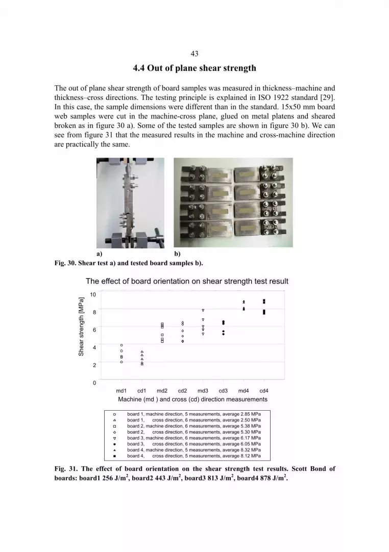
4.4 Out of plane shear strength

The out of plane shear strength of board samples was measured in thickness–machine and thickness–cross directions. The testing principle is explained in ISO 1922 standard [29]. In this case, the sample dimensions were different than in the standard. 15x50 mm board web samples were cut in the machine-cross plane, glued on metal platens and sheared broken as in figure 30 a). Some of the tested samples are shown in figure 30 b). We can see from figure 31 that the measured results in the machine and cross-machine direction are practically the same.

a) b) Fig. 30. Shear test a) and tested board samples b).

Fig. 31. The effect of board orientation on the shear strength test results. Scott Bond of boards: board1 256 J/m2, board2 443 J/m2, board3 813 J/m2, board4 878 J/m2.

md1 cd1 md2 cd2 md3 cd3 md4 cd4Machine (md ) and cross (cd) direction measurements

0

2

4

6

8

10

She

ar s

treng

th [M

Pa]

board 1, machine direction, 5 measurements, average 2.85 MPaboard 1, cross direction, 6 measurements, average 2.50 MPaboard 2, machine direction, 6 measurements, average 5.38 MPaboard 2, cross direction, 6 measurements, average 5.30 MPaboard 3, machine direction, 6 measurements, average 6.17 MPaboard 3, cross direction, 6 measurements, average 6.05 MPaboard 4, machine direction, 5 measurements, average 8.32 MPaboard 4, cross direction, 5 measurements, average 8.12 MPa

The effect of board orientation on shear strength test result

44

4.5 Relationships between Scott Bond, z-strength and shear strength

We will see in chapter 7.4.1 that the Scott Bond results correlate with the sum of mode I and II critical strain energy release rates. This result suggests that the samples split in Scott Bond test mainly by the shearing and z-direction tensile stresses.

From figure 32 we can see that the average of the out of plane shear strength is approximately 5 times the thickness direction breaking strength. Figure 33 shows the relationship between Scott Bond and z-strength. The 99 % confidence and prediction limits give an idea of the variation in the results. The correlation is not as linear as in reference [27]. These relationships help understanding better the material characteristics and estimating the missing values if all strength data is not available. The authors experiments suggest that the percentage variation in the measured results in the z-strength and Scott Bond tests is of the same order if the measured area is the same.

Fig. 32. Z-strength versus out of plane shear strength of boards 1-4.

Fig. 33. Scott Bond versus z-strength of boards 1-9.

Relation between td tensile breaking stress and td - (md, cd) shear breaking stress

0

2

4

6

8

10

0 0.5 1 1.5 2Thickness direction (td) breaking stress [MPa]

Td -

(md

and

cd) s

hear

br

eaki

ng s

tress

[MP

a]

Relation between board scott-bond and thickness direction tensile breaking stress

99 % confidence and prediction limits

0 200 400 600 800 1000Board scott-bond [J/m2]

0

0.2

0.4

0.6

0.8

1

1.2

1.4

1.6

1.8

2

Thic

knes

s di

rect

ion

brea

king

stre

ss [M

Pa]

5 Geometry of cores

To understand better, how cores are constructed, we will review shortly some important geometrical relationships of cores. There is a certain relationship between winding diameter, web width and winding angle [30]. Figure 34 shows the geometry in spiral winding.

Fig. 34. Geometry in spiral core winding.

The width of web and gap in axial direction can be calculated by

(28) where W is the width of a paperboard web [mm], B is the web gap width [mm] and α is orientation angle of a paperboard web [mm]. The orientation angle is calculated as

XW B+cosα

46

(29) where Dw is the outside diameter of a board layer (figure 34). If the thickness of a web is t, then the outside diameter Dw of a layer is Dw=Dm+2t (30) where Dm is the layer inside diameter. The web edge length of one web revolution is (31) From equation (29) we can see that the orientation angle of ply i is less than 90° as long as (W + B)i is less than Dwi⋅π. If the orientation angle is 0° or 90° degrees as in figure 35 a), then the length of the parallel core depends on the width of the web. Figure 35 b) shows a spiral wound core (web angle is 0°< α < 90°). a) b) Fig. 35. Parallel core, α = 0° or 90° a) and spiral core, 0°< α < 90°.

The web edge length (figure 36) is also interesting parameter since the web gaps function as initial cracks [31]. The web edge length of ply i of 1000 mm long core can be calculated as

(32) where X is the distance, every web travels during one rotation (equation 28). We can see from figure 37 that the web edge length of different example cores depend practically only on the winding angle. The higher the winding angle, the shorter the web edge length.

Fig. 36. The Geometry of a web edge in a core.

sinαW B+Dw π⋅

Lwi1000

XLsi⋅

Ls π Dw⋅ cosα⋅ W B+( ) tanα⋅+

47

Fig. 37. The effect of core dimensions and winding angle α on web edge length. The web gaps function as initial cracks.

10 20 30 40 50 60Average orientation angle of plies [degrees]

1000

1500

2000

2500

3000

3500M

iddl

e w

eb e

dge

leng

th [m

m]

76x15 mm core150x13 mm core300x13 mm core

Middle web edge length. Axial distance=1000 mm

6 Delamination strength of cores

Cores must withstand the alternating, cyclic reel supporting stresses during winding and unwinding. The risk of core failure can be minimized by choosing cores which have a sufficiently high delamination strength.

There are different methods to measure the delamination strength of cores. The simplest test is the static flat crush test, in which the core sample is compressed to rupture between two flat levels. The test is discussed in this context, since the flat crush strength is sometimes the only available strength information of cores.

The cyclic chuck load capacity test is an example of more advanced production test. The term chuck load capacity is also called the dynamic load resistance, the roll weight capacity [3] and the dynamic strength [8]. The term, chuck load capacity, refers to the maximum cyclic chuck load, the core can carry in test conditions before delamination.

More accurate information of durability of cores in winding-unwinding processes can be achieved by studying the strength of cores in practice and/or simulating the real conditions. The possibility to arrange full scale winding-unwinding tests with paper reels is limited. From this reason, the author designed a winding simulator which is used in this work to test the durability of cores in certain simulated winding-unwinding processes.

Testing the chuck load capacity of the simulated cores helps relating the chuck load capacity result to certain maximum tolerated reel weight. We will also study the correlation between flat crush strength and chuck load capacity.

6.1 Chuck load capacity

The chuck load capacity test serves as a simple, short term cyclic production test. It simulates the loading conditions in core supported winding but not as accurately as the winding simulator. Without additional reference information, the test result does not tell directly how heavy reels could be handled safely. The test results can be compared to the reference results tested with the same device and make conclusions about the strength level. The device also reveals certain production defects and faults in the raw materials.

49

6.1.1 The testing principle

There is no international standard for chuck load capacity testing. Some tester constructions are shown in figure 38. In figure 38 a) the core is surrounded by an aluminum sleeve and loaded by a belt. The testing principle is explained in [32]. Figure 38 b) shows a construction where the belt is in a direct contact with the core. The principle of this tester is explained in [8]. Similar testing principle with a sleeve around the core is shown in [3]. Figure 38 c) shows the pneumatic roller tester. The core is surrounded by a Nylon sleeve and the loading is handled by a roll. The test method is explained in [33]. The results with different testers are not directly comparable as the loading conditions and chucks are different.

In this work, the cores are tested with the pneumatic roller tester or with the winding simulator (chapter 6.2). In pneumatic roller tester the test core is fitted inside a Nylon sleeve. The sleeve outside diameter is 160 mm and the diameter difference between the sleeve and core is 0.2-0.3 mm. The core and sleeve are locked axially on non expanding, 100 mm long chuck which rotates 500 rev/min. The freely rotating roll is pressed by a pneumatic piston against the sleeve with linearly increasing load. The tester is stopped as the core delaminates. The unit of the chuck load capacity result is [ton] if a core is tested with the roller tester and [kN] if the test is done with the winding simulator.

a) b) c) Fig. 38. Chuck load capacity tester constructions. Figure c) shows the pneumatic roller tester.

6.1.2 Tests with expanding and non expanding chuck

The effect of chuck expansion on the test result is interesting, since in this work we test cores with non expanding chucks. Contact between an expanding chuck and the core depends upon the system geometry and expansion forces. Depending on the situation, it is possible that only the expanding elements touch the core, or that the chuck body is in contact with the core surface. We can sometimes see polished places on core surface between the expanding elements. This suggest that the chuck body could be in contact with the core. If there is no expansion elements, the core and chuck rotate in relation to

50each other. Core deformation increase the clearance between core and chuck and relative rotation. If the chuck is well anchored to the core by the expansion elements, there is no such relative rotation. On the other hand, poor expansion can easily cause core chew out.

Figure 39 shows the effect of chuck expansion on dynamic durability of lower and higher strength level cores (dash and solid lines). The cores were tested with the chuck in figure 40 a). The expansion force of expanding elements was controlled by oil pressure in hydraulic cylinder inside the chuck. The contact pressure between element and chuck is less than the oil pressure. Figure 40 b) shows examples of cores tested with 250, 500 and 700 bar oil pressure. Figure 41 shows expansion element tracks on surface of cores made by printing press unwinder chucks. We should be on the safe side if we test cores with non expanding chuck since expansion elements seem to have rather increasing effect than decreasing effect on the chuck load capacity test results. It is more difficult for the cracks to grow at the point where the expansion elements compress core wall.

Fig. 39. The chuck load capacity test results tested with different expansion forces. The effect is almost the same for the higher and lower strength cores (dash and solid line). a) b) Fig. 40. 76 mm expanding chuck a) and cores tested with different expansion forces b).

0 100 200 300 400 500 600 700oil pressure [bar]

10

15

20

25

30

35

chuc

k lo

ad c

apac

ity (l

inea

rly in

crea

sing

load

) [kN

]

The effect of chuck expansion on core durability100 mm testing length. 3 expanding elements. 76 x15 mm cores700 bar oil pressure in the chuck gives the highest expansion force

51

a) b) Fig. 41. 150x13 mm cores a) and 76x15 mm core cores b) after unwinding process.

6.1.3 Scott Bond versus chuck load capacity

Figure 42 shows the effect of board Scott Bond on chuck load capacity. Geometry of the test cores is identical. The data points are fitted with second order least squares fit. The Scott Bond measurements over 1000 J/m2 are not very reliable since they are out of the measuring scale. There is also considerable variation in the test results over 800 J/m2.

Fig. 42. The effect of board Scott Bond on chuck load capacity. The results over 1000 J/m2 are out of measuring scale and not very reliable.

0 200 400 600 800 1000 1200

Board Scott Bond [J/m2]

0

1

2

3

Chu

ck lo

ad c

apac

ity [t

on]

Relation between chuck load capacity and board Scott Bond76x15 mm test cores.

52

6.1.4 Statistical variation in the test results

Form figure 43 we can see that the histogram of 5063 chuck load capacity tests is normally distributed. This result is expected considering that the histogram of Scott Bond tests in figure 28 was also normally distributed.

The author has found that long term percentage standard deviation in the chuck load capacity results is of the same order than that of the raw material Scott Bond test results.

Fig. 43. Histogram of 5063 chuck load capacity measurements.

6.2 The winding simulator

The winding simulator was built to simulate winding & unwind processes and to study how the reel dimensions, weight and paper properties affect the dynamic durability of cores. The simulator offer also interesting possibilities to test constant load Wöhler-curves of cores and to verify theoretical life time models.

The simulator construction was optimized by FEM-analysis to match the core stresses in testing and application. It is possible to simulate real winding curves and test with constant or linearly increasing loads. Both, the load and rotation speed can be controlled simultaneously. The features of this equipment include a possibility to use different chuck designs, diameters, lengths (40-250 mm) and even pressure from surrounding paper. The maximum reel weight can be as high as 20 tons, which means that the heaviest reels today can be simulated easily.

Figure 44 a) shows the overall construction of the simulator. The test core is loaded by a belt as in figure 44 b). Figure 44 c) shows the sleeve used in testing of cores. The sleeve structure has been optimized to simulate the surrounding paper in an actual reel. The sleeve outside diameter is 300 mm.

53Figure 44 d) shows testing of 150x13 mm core. The testing length of 76 mm cores is 100 mm and that of 150 mm cores is only 50 mm to avoid excessive heat generation when testing strong 150 mm cores. The results tested with 50 mm samples are very accurately half of the results tested with 100 mm samples. Cores bend somewhat inside reels and there is some stress concentration at chuck end (see the example 3D-FEM results in appendix 2). The chuck end do not usually leave visible marking on the core surface.

a) b) c) d) Fig. 44. The winding simulator. Figures a)-d) show testing of 76 and 150 mm cores.

6.3 Flat crush resistance

We will discuss here briefly about the flat crush test, since it is sometimes used as the principal measure of strength of cores. The test method is explained in [34]. The tested core is compressed between two plates. Figure 45 a) and b) show the testing situation and figure 46 shows examples of load-compression curves. The compressive load is increased until the core ruptures. The test result is the first maximum of compressive force or leveling off of the load deformation curve [34]. The core delaminates only partially as in figure 45 b). In dynamic load test, the core delaminates completely under cyclic loads. Figure 45 c) shows a core inside a dropped reel.

a) b) c) Fig. 45. Flat crush testing a), delaminating core b) and an example of a dropped reel c).

54

Fig. 46. Flat crush test curves of 76x15 mm and 150x13 mm cores.

6.4 Flat crush versus chuck load capacity

Figure 47 shows correlation between flat crush and chuck load capacity of cores with identical dimensions, moisture content, winding angle and crack structure. Figure 48 shows an example of correlation between chuck load capacity and flat crush of 76 mm cores which are otherwise identical but have different wall thickness. The smaller the wall thickness the higher the chuck load capacity and the lower the flat crush.

If we test cores with different crack structures, it is clear that the flat crush test result depends on the location of the cracks in relation to the loading points. We will see later that initial cracks can have a considerable effect on the chuck load capacity. Also, if we test cores with different winding angles, the results are no more as in figure 47.

The effect of moisture on flat crush strength is discussed in [35] and [36]. The authors measurements in figures 49 and 50 suggest that the moisture content do not have the same effect on flat crush and chuck load capacity. From this and the previous reasons, flat crush cannot be considered as an estimator of chuck load capacity unless we compare structurally identical cores.

55

Fig. 47. Chuck load capacity versus flat crush of test cores with identical construction.

Fig. 48. Chuck load capacity versus flat crush of cores with different wall thickness.

2000 3000 4000 5000 6000 7000 8000Flat crush [N/100 mm]

0.5

1.0

1.5

2.0

2.5

3.0

3.5C

huck

load

cap

acity

[ton

]

Relation between chuck load capacity and flat crush76x15 mm test cores.

3000 4000 5000 6000 7000 8000 9000 10000Flat crush [N]

2.5

3.0

3.5

4.0

Chu

ck lo

ad c

apac

ity [t

on]

The effect of wall thickness on relation between chuck load capacity and flat crush 76 mm test cores made of 1080 J/m^2 board.

7x76 mm cores

10x76 mm cores

13x76 mm cores

15 -16x76 mm cores

19x76 mm cores

56

Fig. 49. The effect of moisture content on chuck load capacity of test cores 1-6.

Fig. 50. The effect of moisture content of flat crush of test cores 1-6.

6 7 8 9 10 11 12Core moisture [%]

0.0

0.5

1.0

1.5

2.0

2.5C

huck

load

cap

acity

[ton

]

The effect of moisture on chuck load capacity

core 1 core 2 core 3 core 4 core 5 core 6

76x15 mm cores

6 7 8 9 10 11 12

Core moisture [%]

0

1000

2000

3000

4000

5000

6000

flat c

rush

[N]

core 1 core 2 core 3 core 4 core 5 core 6

The effect of moisture on flat crush 76x15 mm cores

7 Fracture mechanics studies of board specimen

We will study first static and dynamic fracture of the board specimen. The results will be utilized later when estimating crack propagation rate and life time of board cores. The studies are based on linear fracture mechanics which assume small strains in an elastic analysis of stress field. With the occurrence of plasticity we would enter into nonlinear fracture mechanics.

7.1 Strain energy release rate

Figure 51 shows an example of a cracked body which has constant thickness w. The crack length is a and the body is loaded by force P which causes the displacement u.

Fig. 51. Example of a cracked structure of constant thickness w and crack length a. We assume linear load displacement relationship. If there is no crack extension the displacement u is

58

(33) where C [m/N] is the compliance of the cracked body. A complementary potential energy H may be defined for a cracked body as [37] H=W-U (34) where W [J] is the potential energy of external forces [37] (35) and U [J] is the elastic strain energy stored in the body [37] (36) The strain energy release rate G [J/m2], which is also called crack driving force [38], is defined as [37] (37) G is a thermodynamic variable associated to the crack area [39]. Usually the fracture specimen have a constant width w and the change in the crack surface dA is (38) where da is incremental crack length. Considering equations (37) and (38), the strain energy release rate can be written as (39) If Gc is the work required to create a unit crack area then the criterion for crack growth is

(40) where dA is increase in crack area.

dA w da⋅

u C P⋅

W0

u

uP⌠⌡

d

U12

P⋅ u⋅12

C⋅ P2⋅

GdHdA

GdH

w da⋅

dH Gc dA⋅≥

59If dH=Gc dA, then the fracture is controlled and the kinetic energy is not increasing. If dH>Gc dA, then the crack grows suddenly. Figure 52 shows the same structure as in figure 51 but with increased crack length from a to a + da. Using equations (33)-(36) and (39) the strain energy release rate can be written as [37]

(41)

Fig. 52. Cracked structure with increased crack length from a to a+da. The three basic crack loading modes are shown in figure 53 [37]. The total strain energy release rate is an energy parameter which consists of the sum of the G values of crack loading modes I, II and III [37] as G=GI+GII+GIII (42)

Fig. 53. Crack loading modes: (a) opening mode, (b) shearing mode, (c) tearing mode.

GP2

2 w⋅dCda

⋅

60

7.2 Mode I fracture

Considering the symmetry of the Double Cantilever beam (DCB) in figure 54 we can study the structure in figure 55. In our case, the modulus of elasticity E in figure 55 refers to E2. The beam analysis here assumes that the loaded beams are rigidly built into the remainder of the uncracked specimen and that classical small deflection beam theory is valid [37]. Also, the analysis does not incorporate interlaminar shear deformation. The DCB specimen should be dimensioned so that the influences of interlaminar shear deformation and large deflections are minimized.

Fig. 54. Mode I DCB specimen.

Fig. 55. Split DCB specimen. Displacement δ of the split DCB specimen beam end in figure 55 is [40] (43) where P [N] is the applied load, a [mm] is the crack length and E [MPa] is the longitudinal E-modulus of the specimen. The result is only approximate since the effect of shear deformation has not been considered. The error decreases the smaller the beam thickness h/2 is in relation to its length. It has been also assumed that the crack tip end of the beam in figure 55 is fixed. This is not completely true in reality which may have a slight effect on the results. The second moment of inertia I of the beam in figure 55 is calculated as

(44) I

wh2

3⋅

12

δP a3⋅

3 E2⋅ I⋅

61where w is the specimen width and h is the total thickness of the specimen. Compliance of the DCB specimen can now be calculated as (45) The strain energy release rate GI can be calculated by equation (41) (46)

7.2.1 Mode I DCB specimen design considerations

Considering shear deformation, the total bending of split DCB specimen free end ∆ can be calculated by equation [37] (47) where ∆B = 2δ and δ is deflection of the split specimen beam end as calculated in equation 43 (shear deformation not considered). G12 is the DCB specimen interlaminar shear modulus. The coordinate directions are shown in figure 54. Let f denote a certain fraction of deflection as [37] (48) Solving this equation for a/h equals

(49) If the shear deformation is for example 5 % of the total bending (f = 0.05) then equation (49) can be written as

(50)

CI2δP

2 a3⋅3 E2⋅ I⋅

GIP2

2 w⋅

dCI

da⋅

P2 a2⋅w E2⋅ I⋅

f3 h2⋅ E2⋅

40 a2⋅ G12⋅

∆ ∆B 13 h2⋅ E2⋅

40 a2⋅ G12⋅+

⋅

ah

32

E2

G12⋅≥

ah

340

E2

f G12⋅⋅

62Equation 50 can be further solved for minimum crack length to keep the deformation below 5 % (which is just an example value.), as (51)

The upper limit for crack length is based on a requirement of small deflection and linear elastic loading response, given in [37] as

(52) For example, if E2=6500 MPa, G21=343 MPa, GIc=300 N/m and h=10 mm we can calculate from equations (51) and (52) that amin=53.3 mm and amax=4.3 m. The amax is beyond of the practical testing lengths.

7.3 Mode II fracture

Figure 56 shows the mode II fracture ENF specimen geometry. This is essentially a cracked 3-point flexure specimen loaded by a point force in the mid span. The crack length a is the distance from the crack tip to the center of the support pin.

Fig. 56. End notch flexure (ENF) specimen. Span length is 2L, total thickness is 2h and width is w [37]. The ENF specimen is subjected to transverse shear and flexural loadings. The crack driving force depends on specimen geometry, material properties and load P. The shear stresses which distort the beam cross section are strongly dependent on the specimen thickness to length ratio and interlaminar shear modulus of the material [37]. The flexural mechanism is related to crack length, flexural E-modulus and specimen thickness. With typical sample dimensions, the dominant crack driving mechanism corresponds to the relative sliding deformation between the delaminated sublaminates [37]. This

amax 0.92E2 h3⋅

GIc⋅

amin32

E2

G12⋅ h⋅

63discontinuity in flexural stresses of the upper and lower beam of the cracked interface cause shear mode stress singularity in the crack tip [37]. The beam theory analysis of the ENF specimen in figure 56 is summarized in reference [37]. Linear stress strain behavior has been assumed and small strain and deflection theory has been applied.

Fig. 57. Symbols of ENF-specimen analysis [37]. Displacement δ of the center span of the specimen is defined as [37]

(53) where the displacements ∆AB , ∆BC ∆CD are as shown in figure 57. An analytical expression for the mode II compliance CII considering shear deformation is [37] (54) Considering equations (41) and (54), the mode II strain energy release rate can be calculated as

(55) For small values of (E/G12)(h/a)2

(56)

δ∆AB ∆BC+ ∆CD+( )

2

CIIδP

2 L3⋅ 3 a3⋅+

8 E2⋅ w⋅ h3⋅1

2 1.2 L⋅ 0.9 a⋅+( )⋅ h2⋅ E2⋅

2 L3⋅ 3 a3⋅+( ) G12⋅+

⋅

GIIP2

2 w⋅

dCII

da⋅

9 a2⋅ P2⋅

16 E2⋅ w2⋅ h3⋅1 0.2

E2

G12⋅

ha

2⋅+

⋅

GIIBT9 a2⋅ P2⋅

16 E2⋅ w2⋅ h3⋅

64

7.3.1 Mode II ENF specimen design considerations

In the previous analysis the friction forces between the crack surfaces were not considered. Friction is an energy absorbing mechanism that tends to increase the fracture toughness [37]. Frictional effects should be minimized by appropriate specimen design to avoid reducing the energy release rate more than just a small fraction [37]. ENF specimen design considerations have been discussed more in reference [37]. There, the non dimensional energy release rate coefficient g(µ) is defined as (57) where G(µ)II is the strain energy release rate considering friction effect. Parameter g(µ) considers the effect of friction between crack surfaces on reduction in strain energy release rate. Figure 58 shows g(µ) for different values of h/a. As an example, ENF specimen with h/a equal to 0.15 introduces theoretically 5 % error in the GII if the friction coefficient between the crack surfaces is 0.25 [37].

Fig. 58. The effect of friction between crack surfaces on reduction coefficient in strain energy release rate [37]. Solving equation (57) for a, it is possible to formulate a limit for the minimum crack length. Let f denote the maximum allowed fraction of the strain energy release rate. The minimum crack length is (58)

g µ( ) GII G µ( )II−( )GIIBT

4 µ⋅ h⋅3 a⋅

amin

4 µ⋅ h⋅3 f⋅

65The crack is arrested at mid-span due to the compressive load [37]. Since the contact pressure distribution is symmetrical around the loading point, the maximum crack length is [37] (59) Equations 58 and 59 identify the admissible range of crack lengths. The other point to be considered is the specimen thickness. The specimen thickness must be chosen to minimize geometric non-linearity and to maintain linear material response. Minimum semi thickness of ENF specimen can be calculated using a requirement that the maximum bending strain must be less than the proportional limit of the material as

(60) where εlin is the maximum linear elastic material response strain and GIIc is mode II toughness. Equations (58)-(60) can be used for specimen design.

As an example, if h=5 mm, L=75 mm, µ=0.25 and f=0.05 then we can calculate from equations (59) and (60) that amin=33 mm and amax=65 mm. In this study, initial crack length amin of mode II ENF specimen is 40-50 mm. If specimen E2=6500 MPa, GIIc=900 J/m2 and εlin=0.01 (1 %) then we can calculate from equation (60) that the minimum half thickness of the specimen hmin=4.9 mm.

7.4 Static mode I and II tests

Figure 59 a) and b) show the principles of mode I DCB and mode II ENF tests. The tests can be done statically or dynamically. The static tests can be done to evaluate critical strain energy release rates GIC and GIIC. The specimens are fabricated by gluing several board layers together. The initial crack is created by separating the crack surfaces by thin plastic film which is removed before testing. The crack tip position is marked before testing as accurately as possible. The method to determine the crack tip was subjective. Magnifier and type writer correction fluid was used to improve the accuracy of visual examining of the crack tip. The crack front may not be straight and fiber and board layer bridging as shown in figure 65 cause difficulties in determining where the crack tip is.

The specimens were 25 mm wide and depending on the board grade, 9-12 mm thick. The specimens were conditioned before testing to 8 % moisture content. The initial crack length in static tests was of order 50 mm and the specimens were loaded until the crack tip had propagated 25 mm.

amax L 2 h⋅−

h minL2 GIIc⋅

a2 εlin( )2⋅ E2⋅

66

a) b) Fig. 59. Mode I DCB testing principle a) and mode II ENF testing principle b).

7.4.1 Determination of GIc and GIIc

GIc and GIIc can be determined from equations (46) and (55) respectively or using the area method [37]. Critical conditions occur when the crack starts to propagate at the critical load Pc. Figure 60 shows an example of the area inside the load-displacement curve in mode I test but the method applies for mode II as well. In the example case, the crack propagation was 25 mm and the specimen width was also 25 mm. The crack driving force can be calculated from equation (61) where Gc can be GIc or GIIc depending on the test, ∆A is the yellow area in figure 60, w is the specimen width as in figure 54 and ∆a is the change in crack length.

Fig. 60. Example of area inside the load-displacement curve in mode I test. Figure 61 a) and b) show examples of static mode I and mode II test results. The GIc and GIIc values have been determined by the area method and they represent averages of the tested results. There are 5 mode I and mode II measurements of each board grade and the

Gc∆A

w ∆a⋅

67loading rate was 5 mm/min. The GIc results increased some 15 % when the loading rate was increased from 5 mm/min to 500 mm/min. The GIIc results increased also some 15 % when the loading rate was increased from 5 mm/min to 250-300 mm/min. a) b) Fig. 61. Examples of a ) GIc and b) GIIc test curves. Loading rate is 5 mm/min. The sums of the measured GIc and GIIc results in table 1 (loading rate 5 mm/min) are closely equal to the measured board Scott Bond results. Since G is an energy parameter, GIc and GIIc can be summed to evaluate the combined Gc. The result suggest that Scott Bond test measure the combined fracture toughness of modes I and II. This result offers a link between fracture toughness and Scott Bond testing. Scott Bond test is considerably easier and faster to do than the fracture toughness tests. The average of the GIIc/GIc ratio of different boards in table 1 is 1.34. If we know the board Scott Bond, we can estimate the magnitude of the mode I and II fracture toughness values by using this ratio.

Table 1. GIc,GIIc and Scott Bond results of board specimens and boards from figure 61.

GIc [J/m2]

GIIc [J/m2]

GIIc /GIc [J/m2]

GIc + GIIc

[J/m2] Scott Bond [J/m2]

140 200 1.43 340 340 350 480 1.37 830 870 450 550 1.22 1000 1019

7.5 Cyclic mode I and II tests

Figures 62 and 63 are from the cyclic mode I and II fracture tests of the glued board specimens. The same tests are commonly used to test fiber composites. Part of the tests

Mode I static fracture testsblue lines, board Scott bond 340 J/m2, GIc 140 J/m2

green lines, board Scott bond 870 J/m2, GIc 350 J/m2

red lines, board Scott bond 1019 J/m2, GIc 450 J/m2

01020304050607080

0 2 4 6 8 10 12 14Displacement [mm]

Load

[N]

Mode II static fracture testsblue lines, board Scott bond 340 J/m2, GIIc 200 J/m2

green lines, board Scott bond 870 J/m2, GIIc 480 J/m2

red lines, board Scott bond 1019 J/m2, GIIc 550 J/m2

050

100150200250300350400

0 1 2 3 4 5 6

Displacement [mm]

Load

[N]

68were done with approximately 12 Hz cyclic load with self built testing device shown in figures 62 a) and 63 a). In this device, an electric saw works as an actuator and a special mechanism is used to adjust the up and down movement amplitude. A force sensor in figure 62 b) measures the dynamic force during loading cycles. Load P changes sinusoidally during each loading cycle from 0 to Pmax. Pmax can be kept at constant level using the mechanism which regulates the displacement amplitude. Adjustments are needed as crack length changes. The samples were loaded at different load levels and the number of loading cycles dN was counted by the testing device. The testing device was stopped after certain number of cycles and the operator determined the change in crack length da visually. Magnifier and type writer correction fluid can help finding the crack tip but the results are still subjective and approximate.

Part of the tests were done also using a Lloyd LRX testing machine in figure 63 c) fitted with 5 kN load cell. This machine is computer controlled and accurately keeps the loading cycles at a certain level, but the maximum applicable cycle frequency is only of the order 0.5 Hz.

Very high loads caused problems with the manual force control. There is more delay in the manual control which causes error, especially if a crack propagates very fast. This delay is considerably smaller if the loading machine has fast automatic force control. Manual control suits better for tests where only minor adjustments are needed and the number of cycles is big. The number of cycles ranged from approximately 10 to 600502 cycles. The time consuming tests were done with the manually controlled tester. The maximum number of cycles in testing with Lloyd ranged usually from few tens to few hundreds of cycles. a) b) c) Fig. 62. Mode I dynamic testing a), closer view b), test specimens c).

a) b) c) Fig. 63. Mode II dynamic testing a), closer view b), Lloyd LRX 5 kN c).

Figure 64 gives an idea of the theoretical shape of crack propagation speed versus strain energy release rate curve in log-log coordinates. The example figure could present mode I

69or mode II situation. If ∆G is below the threshold value ∆Gth then the crack does not propagate. If ∆G reach the critical value ∆Gcr then the crack propagation becomes unstable. Between ∆Gth and ∆Gcr the curve is quite linear for many composite materials.

Fig. 64. Crack propagation speed versus strain energy release rate in log-log coordinates.

The test results in the linear part of the curve in figure 64 can be fitted for many fiber composites using the Paris law written as [41] (62) where ∆G is the change of strain energy release rate in each cycle and C and n are material constants. If the load changes from 0 to Pmax in each cycle, ∆P is equal to Pmax. ∆GI and ∆GII can be calculated from equation (46) and (55) respectively by substituting P by ∆P. After a number of cycles at constant loading amplitude the crack length has changed from the initial length a0 to a new length a1. The ∆G values are calculated using average crack length in each loading period as (63) where a0 is the initial crack length and a1 the crack length after n loading cycles. This procedure is practical but introduces some error depending on da, since we could expect that ∆G does not change linearly from crack length a0 to a1. Keeping da relatively small, we can calculate estimations of ∆GI and ∆GII as in [37] (64)

dadN

C ∆Gn⋅

aaverage a0da2

+12

a0 a1+( )⋅

∆GI∆P2 aaverage( )2⋅

w E2⋅ I⋅

70 (65) Equation (62) can be written in log-log coordinates as

(66) from which the material constants C and n can be estimated by using the least squares estimates. The Paris equation (62) is often written also as (67)

where ∆K is the change of stress intensity factor during loading cycles. Some alternative equations are shown in reference [38]. Considering further analysis of cracked core structures, equation (62) is more usable than equation (67) since energy parameters can be easily summed as ∆G=∆GI+∆GII (68) Examples of cyclic mode I and II test results are shown in figures 66-71 and in appendix 3. The Silicate glued specimens were fabricated of 340 J/m2-1019 J/m2 boards.

Considering the big variation in the results, we could say that equation (62) fits the data points acceptably well. The statistical nature of the material is one reason for the variation but part of the variation comes also from inaccuracies in testing and sample preparation. It is difficult to determine the crack tip position accurately and sometimes there are smaller cracks propagating together with the major crack. It is also possible to make crack growth observations only from the specimen sides. The crack front shape may not be straight inside the specimen and there can be fiber and board layer bridging in crack tip. Figures 65 a) and b) show some examples of mode I loaded crack tips. a) b) c) Fig. 65. Example crack tips of mode I specimens a), b) and fractured specimen c). Cores and board samples fracture usually inside board as in figure 65 c). If a glue seam can be seen on a fracture surface then there has been a gluing defect. Anyway, crack can initiate between board and a glue seam. The 50 mm long initial crack has been made by

∆GII9 aaverage( )2⋅ ∆P2⋅

16 E2⋅ w2⋅ h3⋅1 0.2

E2

G12⋅

haaverage

2⋅+

⋅

logdadN

log C( ) n log ∆G( )⋅+

dadN

C ∆Kn⋅

71separating the crack surfaces by a thin plastic membrane. Some glue may spread on the surface between board and membrane which can be seen in figure 65 c).

The mode I and II test results in figures 66-71 are relatively near to each other but the low frequency Lloyd testing results are clearly at a different level than those tested with a higher loading frequency. The applied load was usually rather high in the low frequency tests and the crack propagated fast. We can see that ∆GI of some data points are even at a higher level than the measured Gcr. One possible explanation for this could be found from the loading rate. The Gcr tests were done at 5 mm/min loading rate to make it easier for the operator to follow the crack growth. As mentioned in chapter 7.4.1, the Gcr test results showed some increase with increasing loading rate.

There are also small differences in the results depending on the board Scott Bond. The Paris equation constants n and C are collected in tables 2 and 3. The results give estimates of the magnitude of the material constants. In some low loading rate cases there has been too much scattering in data points to find these constants. In such cases the position of the data points can be compared with other data points to estimate the magnitude of those results.

Some mode I cylinder machine board results from reference [2] are compared in figure 70 against mode I results in figure 66. The comparison samples in figure 70 and 71 were fabricated of 800–900 J/m2 board using different commercial adhesives. Variation in the comparison results is so big that it is difficult to say reliably whether adhesives really have effect on the results or not. Specimen moisture become different with different adhesives if the samples are not conditioned carefully before testing. Fig. 66. Mode I and II cyclic loading 12 Hz.

102 1032 3 4 5 6 7 8 2 3 4 5 6 7 8 2

Energy release rate range dG [J/m^2]

10-8

10-7

10-6

10-5

10-4

10-3

10-2

Cra

ck p

ropa

gatio

n ra

te d

a/dN

[m /

cycl

e]

Delamination growth in fatigue.

870 J/m2 machine direction (mode I)870 J/m2 machine direction (mode II)340 J/m2 machine direction (mode II)340 J/m2 machine direction (mode I)1019 J/m2 machine direction (mode II)1019 J/m2 machine direction (mode I)

Board Scott-bond values: 340 J/m2, 870 J/m2, 1019 J/m2

2.207E-011 * x(1.743)

1.004E-010 * x(1.765)

2.102E-010 * x(1.675)

4.21E-012 * x(2.274)

5.678E-012 * x(2.197)

1.814E-012 * x(2.137)

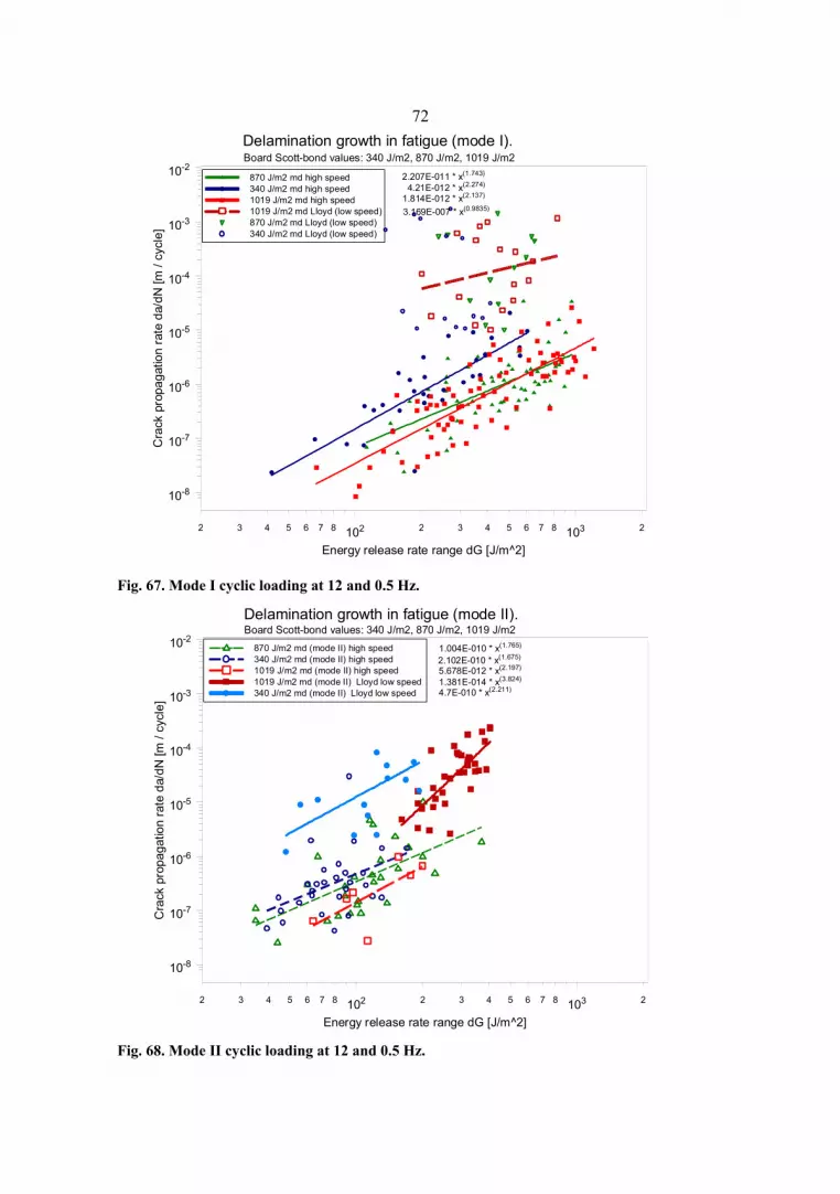
72

Fig. 67. Mode I cyclic loading at 12 and 0.5 Hz.

Fig. 68. Mode II cyclic loading at 12 and 0.5 Hz.

102 1032 3 4 5 6 7 8 2 3 4 5 6 7 8 2


10-8

10-7

10-6

10-5

10-4

10-3

10-2C

rack

pro

paga

tion

rate

da/

dN [m

/ cy

cle]

Delamination growth in fatigue (mode I). Board Scott-bond values: 340 J/m2, 870 J/m2, 1019 J/m2

870 J/m2 md high speed 340 J/m2 md high speed 1019 J/m2 md high speed 1019 J/m2 md Lloyd (low speed)870 J/m2 md Lloyd (low speed)340 J/m2 md Lloyd (low speed)

2.207E-011 * x(1.743)

4.21E-012 * x(2.274)

1.814E-012 * x(2.137)

3.169E-007 * x(0.9835)

102 1032 3 4 5 6 7 8 2 3 4 5 6 7 8 2


10-8

10-7

10-6

10-5

10-4

10-3

10-2

Cra

ck p

ropa

gatio

n ra

te d

a/dN

[m /

cycl

e]

Delamination growth in fatigue (mode II).Board Scott-bond values: 340 J/m2, 870 J/m2, 1019 J/m2

870 J/m2 md (mode II) high speed 340 J/m2 md (mode II) high speed1019 J/m2 md (mode II) high speed1019 J/m2 md (mode II) Lloyd low speed340 J/m2 md (mode II) Lloyd low speed

1.004E-010 * x(1.765)

2.102E-010 * x(1.675)

5.678E-012 * x(2.197)

1.381E-014 * x(3.824)

4.7E-010 * x(2.211)

73 Fig. 69. Mode I and II cyclic loading at 0.5 Hz.

Fig. 70. Mode I cyclic loading at 12 Hz. Comparison results from reference[2] and new tests.

102 1032 3 4 5 6 7 8 2 3 4 5 6 7 8 2


10-8

10-7

10-6

10-5

10-4

10-3

10-2C

rack

pro

paga

tion

rate

da/

dN [m

/ cy

cle]

Delamination growth in fatigue (mode I and II). Board Scott-bond values: 340 J/m2, 870 J/m2, 1019 J/m2

1019 J/m2 md (mode II) 340 J/m2 md (mode II) 1019 J/m2 md (mode I) 870 J/m2 md (mode I) 340 J/m2 md (mode I)

1.381E-014 * x(3.824)

4.7E-010 * x(2.211)

3.169E-007 * x(0.9835)

102 1032 3 4 5 6 7 8 2 3 4 5 6 7 8 2


10-8

10-7

10-6

10-5

10-4

10-3

10-2

Cra

ck p

ropa

gatio

n ra

te d

a/dN

[m /

cycl

e]

Delamination growth in fatigue (mode I)mode I, delamination in board machine direction.

board Scott-bond 340 J/m2board Scott-bond 1019 J/m2board Scott-bond 870 J/m2comparison board, Scott-bond 800 - 900 J/m2

4.21E-012 * x(2.274)

1.814E-012 * x(2.137)

2.207E-011 * x(1.743)

7.724E-009 * x(0.9938)

74

Fig. 71. Mode I comparison results [2] (the black points from figure 70). Table 2. High speed mode I and II tests.

Scott Bond [J/m2]

C mode I

n mode I

C mode II

n mode II

340 4.210E-12 2.274 2.102E-10 1.675 870 2.207E-11 1.743 1.004E-11 1.785 1019 1.814E-12 2.137 5.678E-12 2.197 800-900 7.724E-009 0.9938 - -

Table 3. Low speed mode I and II tests.

Scott Bond [J/m2]

C mode I

n mode I

C mode II

n mode II

340 - - 4.700E-10 2.211 1019 3.169E-007 0.9835 1.381E-14 3.824

Some examples of searching the threshold values are shown in tables 4 and 5. From table 4 we can see that the mode I ∆GIth value of 340 J/m2 board is of the order of 40 J/m2.

102 1032 3 4 5 6 7 8 2 3 4 5 6 7 8 2

Energy release rate range dGI [J/m^2]

10-8

10-7

10-6

10-5

10-4

10-3

10-2C

rack

pro

paga

tion

rate

da/

dN [m

/ cy

cle]

Delamination growth in fatigue Comparison DCB specimen glued with different glues, mode I, machine direction

Silicate 1Silicate 2Silicate 3Silicate 4Dekstrin White plasticSilicate 5

7.415E-011 * x(2.094)

4.877E-010 * x(1.635)

2.527E-010 * x(1.687)

8.115E-014 * x(3.09)

7.252E-011 * x(1.643)

5.796E-012 * x(2.732)

6.32E-013 * x(2.69)

75From table 5 we can see that the mode I ∆GIth value of 1019 J/m2 board is of the order of somewhere between 63 and 101 J/m2. We could estimate that it is approximately 80 J/m2. ∆GIth of 870 J/m2 board is somewhere between the previous values. We could estimate that it is 60 J/m2. The mode II ∆GIIth values are somewhat lower than the mode I values.

Table 4. 340 J/m2 specimens, mode I.

a [mm]

da [mm]

a+(da/2) [mm]

dP [N]

dN cycles]

w mm]

h [mm]

da / dN [m/cycle]

dGI [J/m^2]

46.17 0 46.17 25 - 28 130764 25.0 10.7 0 37 46.17 5.46 48.90 25 - 28 234990 25.0 10.7 2.32E-08 42

Table 5. 1019 J/m2 specimens, mode I.

a [mm]

da [mm]

a+(da/2) [mm]

dP [N]

dN cycles]

w mm]

h [mm]

da / dN [m/cycle]

dGI [J/m^2]

45.00 0 45.00 25 - 28 451295 25.0 9.0 0 63 54.33 4.94 56.80 30 600502 25.0 9.0 8.23E-09 101

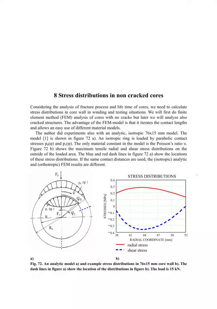
8 Stress distributions in non cracked cores

Considering the analysis of fracture process and life time of cores, we need to calculate stress distributions in core wall in winding and testing situations. We will first do finite element method (FEM) analysis of cores with no cracks but later we will analyze also cracked structures. The advantage of the FEM-model is that it iterates the contact lengths and allows an easy use of different material models.

The author did experiments also with an analytic, isotropic 76x15 mm model. The model [1] is shown in figure 72 a). An isotropic ring is loaded by parabolic contact stresses p0(φ) and p1(φ). The only material constant in the model is the Poisson’s ratio υ. Figure 72 b) shows the maximum tensile radial and shear stress distributions on the outside of the loaded area. The blue and red dash lines in figure 72 a) show the locations of these stress distributions. If the same contact distances are used, the (isotropic) analytic and (orthotropic) FEM results are different.

a) b) Fig. 72. An analytic model a) and example stress distributions in 76x15 mm core wall b). The dash lines in figure a) show the location of the distributions in figure b). The load is 15 kN.

38 41 44 47 50 530.4

0.3

0.2

0.1

0

0.1

0.2

0.3

0.4

radial stressshear stress

STRESS DISTRIBUTIONS

RADIAL COORDINATE [mm]

STR

ESSE

S [M

Pa]

.

77

8.1 Analyzed structures

Figures 73 a) and b) show the belt tester testing situation of a 100 mm long core sample with 76 mm inside diameter. The 50 mm long, 150 mm core samples are tested as shown in figure 73 c).

a) b) c) Fig. 73. The belt tester a) and its cross section with b) 100 mm and c) 50 mm long sample.

Figures 74 a) and b) show the principle of testing a 100 mm long, 76 mm inside diameter core sample with the pneumatic roller tester. Figures 75 a) and b) show reels in a center winder and in a printing machine unwinder respectively. In most center winders, part of the reel mass is supported by the winding drum as in figure 75 a). In printing presses, the reels are supported as shown in figures 75 b) and 76 a). Figure 76 b) shows a core end after the unwinding process. The polished parts between the expanding element tracks reveal that the chuck body has been in contact with the core

a) b) Fig. 74. The roller tester a) and its cross section b).

78

a) b) Fig. 75. Reel in a paper mill winder a) and in a printing press unwinder b).

a) b) Fig. 76. Reel supported by the chucks a) and core end after unwinding process b).

8.2 FEM-models

In this study, paper reels have been modeled by 2D-contact models, but additionally some previously calculated 3D-results will be reviewed. The 2D-approach applies well for the analysis of testing situations in figures 73 and 74 since the core sample is supported from the whole length by the chuck. In practical tests, the loading capacity of the 50 mm core samples is very closely half of that of the 100 mm long core samples.

Considering the analysis of paper reels supported by chucks, the 2D-models cannot consider the stress concentration at the end of the chucks. Anyway, we could expect the 2D-models to give generally a good estimation of the stress distribution in the core wall, since chuck ends do not usually impart visible markings on the inner surface of cores.

79

8.2.1 Assumption of plane strain condition

The plane strain condition assumes that the strains in the r, θ plane are functions of r and θ alone, and also that strains in the z-direction (figure 22) are equal to zero. In the testing situation the core is locked axially (in z-direction) by the stoppers shown in figures 73 and 74. The stopper prevents the core from moving axially. The stopper cannot cover the whole core end since the operator must be able to see when the core splits. In a printing machine unwinder, the core ends are against the chucks as in figure 76 a) and the longitudinal strain is essentially restricted. In some paper mill winders, the chucks may give up somewhat axially to compensate the forces caused by core lengthening. Considering the axial constraints, plane strain elements are used in the 2D-models.

8.2.2 Elements and contact modelling

Biquadratic 8-node plane strain Abaqus CPE8-elements [42] were used in the 2D-models to model chuck, core, sleeve and paper. The contact was modeled using contact pair approach (explained in [42]). Friction between the contact surfaces was not considered in the model. The solver did usually 60–80 iterations during analysis. The uniform clearance and the master & slave elements of contact surfaces were specified for the contact surfaces. The clearance is specified in this work as in figure 77 d).

Examples of contact surfaces (free edge plots) are shown in figure 77. The contact was modeled between chuck and core but also between core and Nylon sleeve or between core and paper. It was necessary to connect the contact surfaces within few elements to prevent convergence problems.

Paper was considered as a homogenous cylinder possessing orthotropy in its principal material coordinates. It was not practical to model the layered reel structure due to huge size of such a model. The contact between core and paper was modeled with a zero initial clearance. The contact modeling prevents the radial tensile stresses between paper and core since paper layers can transmit only compressive radial stresses.

8.2.3 Material properties

Core and paper are assumed as homogenous in this analysis. The E-modulus of the Nylon sleeve is 4000 MPa and the chuck is made of steel. The representative board properties are shown in chapter 3.9. The effect of winding angle is considered according to the theory in chapter 3.10. Paper has been modeled softer in the compression direction. Also, paper properties are the same in the whole reel. In reality, the paper E-modulus in compression direction is a function of compression pressure and it is also different in reel bottom than in reel surface.

80

a) b) c) d) Fig. 77. Contact surfaces in belt tester model a), paper reel model b) and rollel tester model c). Figure d) determines the clearance between the contact surfaces.

8.2.4 About the calculated results

As said, it was necessary to connect the contact surfaces from a few elements in order to help the solver. This causes local stress concentrations in the vicinity of the connected nodes and can be seen in the stress distributions. We are mostly interested in the positive (tensile) stresses and negative shear stresses located approximately 90 degrees out of phase of the middle of the compression area, and the stress concentrations do not affect these stresses. In most figures in chapter 8.2.5, only the interesting stresses have been plotted so that they could be examined better. Examples of maximums of these stresses are collected in figure 78. The maximum stresses do not tell everything since the distributions are somewhat different in calculated situations (belt tester model, paper reel model and roller tester model).

Fig. 78. Tensile radial stress and absolute of shear stress maximums in 76x15 mm core wall .

Tensile radial stress and absolute shear stress Chuck load 1500 kg, chuck clearance 0.3 mm

00.20.40.60.8

11.21.41.6

paper reel belt tester reel tester belt on core

Stre

ss [M

Pa]

Tensile stress

Shear stress

81

8.2.5 The calculated stress distributions

All calculated stress distributions [MPa] of non-cracked core cross sections are shown in appendix 2. Some comparable stress distributions are shown in figures 79–87. The reader should note that the color scales are not the same in parallel pictures. The results cover the cases in figures 73–76. The chuck clearance (figure 77 d) is 0.3 mm in figures 79–87, chuck load is 1500 kg and chuck length in all 2D-models is 100 mm.

The simulator was used for an extensive series of winding simulations and tests. Figure 80 shows that the stress distributions are much the same in situations where the core is loaded in the belt tester, and as in the reference situation where the core is surrounded by paper reel and loaded by the reel weight.

a) b) c) d) Fig. 79. Comparison between tensile (positive) radial stress and negative shear stress distributions [MPa] in belt tester and in paper reel model. Figure a) belt tester model (tensile radial stresses), b) paper reel model (tensile radial stresses), c) belt tester model (shear stresses), d) paper reel model (shear stresses).

Figure 80 shows the stress distributions in the belt tester analysis with a 76x15 mm core. The results from the belt tester analysis with a 150x13 mm core are shown in figure 81. The z-direction tensile stress and shear stress maximums are approximately 5 times higher in 76x15 mm core wall than in 150x13 mm core wall. Figure 85 shows the stresses in belt tester analysis with expanding chuck. The test results in figure 39 showed that cores lasted longer with an expanding chuck than with a non-expanding chuck. The expanding elements cause very high compressive stresses which may work as blocks to slow down crack propagation.

Figure 82 shows the stresses in a core surrounded by paper, and figure 83 shows the stresses in the reel bottom. These stresses are related with some winding problems like paper burst in the reel bottom.

Figure 84 shows the stresses in pneumatic roller tester analysis. The belt tester stresses were closer to the reference stresses than these here. On the other hand, the stresses become higher if the belt is placed directly on the core as in figure 86.

Figure 87 shows an example of stress distribution in 3D-analysis of core surrounded by paper reel. These results were calculated by the author in reference [1]. These stresses are of the same magnitude as 2D-stresses. The element mesh is rather coarse but small stress intensity can be seen at chuck end.

82

a) b)

c) d) e) f) Fig. 80. Belt tester FEM-model and core stresses (compare the roller tester analysis results in figure 84). 76x15 mm core. Initial clearance between chuck and core=0.3 mm. Initial clearance between core and Nylon sleeve=0. Figure a) modeled situation (180 degrees out of phase in relation to the FEM-model), b) FEM-model, c) radial core stresses, d) positive radial core stresses, e) shear stresses, f) negative shear stresses.

a) b) c) Fig. 81. Belt tester FEM-model and core stresses. 150x13 mm core. Initial clearance between chuck and core=0.3 mm. Initial clearance between core and Nylon sleeve=0.1 mm. Figure a) modeled situation (180 degrees out of phase in relation to the FEM-model), b) positive radial core stresses, c) shear stresses.

83

a) b) c) d)

e) f) Fig. 82. Paper reel model (non expanding chucks). 76x15 mm core. Initial clearance between chuck and core=0.3 mm. Initial clearance between core and paper=0. Modeled situation a), FEM-model b), radial core stresses c), positive radial core stresses d), shear stresses e), negative shear stresses f).

a b) c) Fig. 83. Stresses in paper reel bottom in figure 82 b). The core is not shown in these images. Radial stresses a), shear stresses b) and tangential stresses c).

84

a) b) c) d)

e) f) Fig. 84. Pneumatic roller tester model. 76x15 mm core. Initial clearance between chuck and core=0.3 mm. Initial clearance between sleeve and core=0.1 mm. Figure a) modeled situation (180 degrees out of phase in relation to the FEM-model), b) FEM-model, c) radial core stresses, d) only positive radial core stresses, e) shear stresses, f) only negative shear stresses.

a) b) c) d) Fig. 85. Belt tester model with expanding chuck. 76x15 mm core. Figure a) image of the modeled chuck, b) FEM-model c) positive radial core stresses, d) shear stresses.

85

a) b) c) d) Fig. 86. Belt directly on core, no sleeve. 76x15 mm core. Figures a) image of the modeled situation (180 degrees out of phase in relation to the FEM-model), b) FEM-model, c) positive radial core stresses, d) shear stresses.

a) b) c) Fig. 87. 3D model. 76x15 mm core is surrounded by paper reel and supported by 100 mm non-expanding chuck. Figures a) and b) FEM-model, c) radial stresses.

8.2.6 Some additional observations from stress distributions

Figures 88-91 show example results collected from figures in appendix 2. Figure 88 shows the effect of initial chuck clearance (core inside diameter-chuck outside diameter) on stress maximums. In practical tests, the chuck load capacity results with bigger chuck clearance are lower than those with a better fit. From figure 89 we can see how core stresses change with reel weight. The relationship is not exactly linear but close. This deviation from linearity is caused by changes in contact. From figure 90 we can see the effect of winding angle on core stresses. The winding angle affects core elasticity in the tangential direction and in this way also has an effect on stresses. The higher the winding angle the lower are the stresses. Practical measurements show that cores with a higher winding angle have greater strength. Figure 91 shows that the thicker the core wall the higher are the stresses. From figure 48 we can see that the thin wall cores have higher chuck load capacity than the thick wall cores.

86 Fig. 88. Analysis of core inside a paper reel. Reel weight 3 ton. Fig. 89. Analysis of belt tester situation.

Fig. 90. Analysis of belt tester situation. Reel weight 3 ton.

The effect of chuck clearance on stress maximum in 76x15 mm core wall. Reel weight 3 ton.

00.10.20.30.40.50.60.70.80.9

0 0.1 0.2 0.3 0.4 0.5 0.6Chuck clearance [mm]

Stre

ss [M

Pa]

tensile radial stressesshear stress (absolute value)

The effect of reel weight on stress maximums in 76x15 mm core wall

00.10.20.30.40.50.60.70.80.9

0 1 2 3 4 5 6 7Reel weight [ton]

Stre

ss [M

Pa]


The effect of winding angle on stress maximums in 76x15 mm core wall

0.2

0.25

0.3

0.35

0.4

0.45

0 10 20 30 40 50 60 70 80 90Winding angle [degrees]

Stre

ss [M

Pa]


87 Fig. 91. Analysis of belt tester situation. Reel weight 3 ton.

8.2.7 FEM-analysis of cracked cores in belt tester

Figures 92-98 show stress distributions [MPa] in cracked 76x15 mm cores. The chuck load is 14.7 kN in all cases. Figures a) show the crack length and location, figures b) show the tensile (positive) radial stresses and figures c) show the shear stresses. The cracked core is in the belt tester contact model shown in figure 80. The reference stresses of a non-cracked core are shown in figure 92. The belt tester model was used in these studies since the practical crack propagation studies were done with a belt tester. The stresses in the belt tester model and in the paper reel model are closely similar. This allows application of the belt tester results for practical estimations.

The crack surfaces are modeled as master and slave surfaces using the contact pair approach [42]. Figure 98 a) and b) show examples of tensile radial and shear stresses in vicinity of crack tips. The mesh density can be seen better in these figures. Non-linear geometry (the NLGEOM parameter in the *STEP option [43]) has been considered in the analysis and all elements are non-singular. To study the error in J-integral estimation caused by non-singular crack tip modeling, the author modeled the crack in figure 95 with singular tips (1/4 singularity). The averages of the J-integral estimates in singular crack tips 1 and 2 were 0.24 % and 2.09 % higher, respectively, than in the corresponding non-singular case.

Figure 96 shows a modeled situation with a 8.5 mm long crack (2a=8.5 mm in figure 99). Figure 97 shows a situation with two similar 8.5 mm cracks (crack 1 and crack 2). One of these cracks (crack 2) is the same as in figure 96. Even if the cracks are relatively close to each other, the stress distribution in the vicinity of crack 2 is much the same as without crack 1.

The effect of core wall thickness on stress maximums in 76 mm core wall

0

0.1

0.2

0.3

0.4

0.5

10 12 14 16 18 20 22Wall thickness [mm]

Stre

ss [M

Pa]


88

a) b) c) Fig. 92. FEM-model with no crack a), tensile radial stresses b), shear stresses c).

a) b) c) Fig. 93. FEM-model with a 5.1 mm long crack a), tensile radial b), shear stresses c).

a) b) c) Fig. 94. FEM-model with a 12.7 mm long crack a), tensile radial stresses b) and shear stresses c). Figure 98 shows more detailed stresses in vicinity of this crack.

89



a) b) c) Fig. 97. FEM-model with 2 8.5 mm long cracks a), tensile radial b), shear stresses c).

90

a) b) Fig. 98. Stresses in vicinity of 12.7 mm long crack in 76x15 mm core wall (figure 94). Tensile radial stresses a), shear stresses b).

8.3 Numerical and analytic J-integral estimations

J-integral is defined in terms of the energy release rate associated with virtual crack growth. For elastic material, the J-integral represents the energy available for crack growth [44]. We are interested here in the analytic and numerical J-integral results. The numerical results are calculated using Abaqus FEM-program. There is a detailed explanation of numerical J-integration evaluation with Abaqus in reference [14]. Some main principles are summarized here.

The contour integral is calculated numerically by using a ring of elements completely surrounding the crack tip or crack front from one crack face to the opposite crack face. Abaqus finds automatically the elements surrounding the crack tip. The J-integral should be independent of the domain used, but J-integral estimates may vary from ring to ring because of the approximate nature of the finite element solution [14]. J-integral estimation is typically calculated for several element rings. Strong variation in these estimates indicates usually a need for mesh refinement [14]. Also, numerical tests suggest that the estimate from the first element ring abutting the crack front does not provide a high accuracy result and at least two contours are recommended [14]. Crack tip causes a stress concentration in the vicinity of the crack tip and focused meshes are normally used in small-strain fracture mechanics evaluations [14].

Singularity at the crack tip should be considered in small-strain analysis [14]. Singularity improves the accuracy of both the J-integral and the stress strain calculations. Singularity can be modeled by quarter-point technique by moving the mid-side nodes to the quarter points. In large strain analysis (when the NLGEOM parameter is included on the *STEP option) singular elements should not normally be used [14]. The mesh must be sufficiently refined to model the strain gradients in the region of the crack tip [14].

The reference J-integral values are evaluated analytically using equation (69). The model is shown in figure 99 and can be used if there is a single crack in the core wall. The original model in reference [45] is named as “a crack along the interface of two bonded dissimilar half-planes subjected to tension and shear”. If both half planes are of the same material and the plane strain condition is assumed, then the J-integral equation in [45] simplifies to

(69) J

π2 G⋅

1 ν−( )⋅ σ2 τ2+( )⋅ a⋅

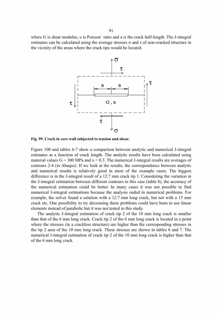
91where G is shear modulus, υ is Poisson´ ratio and a is the crack half-length. The J-integral estimates can be calculated using the average stresses σ and τ of non-cracked structure in the vicinity of the areas where the crack tips would be located.

Fig. 99. Crack in core wall subjected to tension and shear. Figure 100 and tables 6-7 show a comparison between analytic and numerical J-integral estimates as a function of crack length. The analytic results have been calculated using material values G = 300 MPa and υ = 0.3. The numerical J-integral results are averages of contours 2-4 (in Abaqus). If we look at the results, the correspondence between analytic and numerical results is relatively good in most of the example cases. The biggest difference is in the J-integral result of a 12.7 mm crack tip 1. Considering the variation in the J-integral estimation between different contours in this case (table 8), the accuracy of the numerical estimation could be better. In many cases it was not possible to find numerical J-integral estimations because the analysis ended in numerical problems. For example, the solver found a solution with a 12.7 mm long crack, but not with a 15 mm crack etc. One possibility to try decreasing these problems could have been to use linear elements instead of parabolic but it was not tested in this study.

The analytic J-integral estimation of crack tip 2 of the 10 mm long crack is smaller than that of the 6 mm long crack. Crack tip 2 of the 6 mm long crack is located in a point where the stresses (in a crackless structure) are higher than the corresponding stresses in the tip 2 area of the 10 mm long crack. These stresses are shown in tables 6 and 7. The numerical J-integral estimation of crack tip 2 of the 10 mm long crack is higher than that of the 6 mm long crack.

92

a) b) Fig. 100. Comparison between analytic and numeric J-integral estimations. Crack tip 1 a), crack tip 2 b). Table 6. Crack tip 1.

Crack length elem.

Crack length 2a [mm]

σmax [MPa]

τmax [MPa]

analytic J-integral [N/m]

Abaqus J-integral estimation [N/m] Average of contours J-integral contour number 2-4 1 2 3 4

6 5.1 0.28 -0.33 1.744 1.867 0 2.355 1.813 1.434 10 8.47 0.22 -0.32 2.341 3.376 0 3.739 3.358 3.031 15 12.7 0.28 -0.36 3.437 6.200 1.79 4.189 8.146 6.265 54 45.7 0.14 -0.26 7.309 7.151 0 3.239 7.848 10.366

Table 7. Crack tip 2.

Crack length elem.

Crack length 2a [mm]

σmax [MPa]

τ max [MPa]

analytic J-integral [N/m]

Abaqus J-integral estimation [N/m] Average of contours J-integral contour number 2-4 1 2 3 4

6 5.1 0.26 -0.36 1.841 1.910 0 2.160 1.827 1.743 10 8.47 0.16 -0.29 1.703 2.464 0 2.705 2.445 2.243 15 12.7 0.28 -0.36 3.767 4.709 2.02 3.337 5.719 5.071 54 45.7 0.05 -0.25 5.448 5.719 0 5.583 5.791 5.782

Comparison betw een analytic and numerical J-integral estimations of crack tip 1

0

2

4

6

8

0 10 20 30 40 50crack length [mm]

J-in

tegr

al [N

/m]

AbaqusAnalytic

Comparison betw een analytic and numerical J-integral estimations of crack tip 2

0

2

4

6

8

0 10 20 30 40 50crack length [mm]

J-in

tegr

al [N

/m]

AbaqusAnalytic

9 Crack propagation in cores

9.1 About the practical tests

We will study next crack growth in cross section of different test cores tested in the winding simulator. The studied cases give a good overview of how the cracks behave in different situations. The detailed results are shown in appendix 4 as Test series 1. 6 crack propagation tests of cores with no initial cracks ……………..... 181 Test series 2. 9 crack propagation tests of spiral cores ……..…………...…...……..… 187 Test series 3. 10 crack propagation tests of cores with 11 initial cracks ……………... 196 Test series 4. 8 crack propagation tests of cores with a single initial crack ………….. 206 Test series 5. 2 crack propagation tests of cores constructed of two materials ………. 214 The studied 100 mm long 76x15 mm core samples were loaded in the winding simulator. Since it is not possible to see inside the cores, observations were made from both core ends. Most of the tests were done with a 15 kN constant load, but in some tests the load was 10 kN. The revolution speed was 500 rpm in all tests. The tester was stopped and started several times during the test to make observations on cracks on both sides of the test cores. New cracks were marked with a pen to make the observations easier. The test was continued until the core was completely delaminated. The crack propagation images are shown in appendix 4. Figures 101-105 show representative set of images from each test series.

Figures 101 a)-105 a) show the total length of cracks in the vicinity of the core wall cross section center line as a function of revolutions. The small cracks outside of the main crack line which are not “active” and do not grow are not considered in the total crack length. The lines with “o” and triangle symbols show the total crack length in the front and back side of a test core respectively. The thin dash line represents the least squares estimate of data points on both sides of the core and approximates the average crack length inside the core. The curve fit equation is shown in the figures.

94

9.2 Studies of the effect of number and size of cracks on delamination of test cores

If we study the test cores with no initial cracks in appendix 4 (test series 1) and in figure 101, we can see that at first several small cracks appear on both sides of cores. Some of the cracks continue growing and join together forming longer cracks. Just before the split up there are usually several cracks in the vicinity of the “splitting path”.

In spiral cores in appendix 4 (test series 2) and in figure 102, the web gaps work as initial cracks. Spacing of these gaps depends on the position of the webs in relation to each other as they enter the core machine shaft. Initial cracks are also caused by gluing defects and drying stresses. In test cores, the length of the initial cracks is typically 1.5-6 mm and there is one web gap in each ply. If we compare the total crack length versus number of revolutions, we can see that spiral cores can sometimes split suddenly without long visible cracks. The final splitting path goes usually through some of the web gaps. The final splitting path is often circular but sometimes cores split also spirally.

Crack propagation tests of cores with multiple initial cracks and with only a single initial crack are shown in test series 3 and 4 (respectively) in appendix 4. These tests help understanding the effect of crack length and the number of cracks on crack propagation. The average of the initial crack length in cores with several cracks varied between 2-6 mm. The crack length in cores with only a single crack varied between 7-55 mm.

The multiple initial crack cores were constructed in such a way that there was a crack in the middle ply and also in 5 layers on both sides of the middle ply (11 cracks). The cracks were spaced on the whole circumference of the test cores. In the manufacturing process, a tape strip prevented the crack surfaces from becoming glued together.

From the results we can see that cores which had the shortest cracks, behaved much like cores with no initial cracks. The multiple initial cracks were located spirally but the main line often took a “short cut” so that the final splitting path was circular. The longer the initial cracks the more easily one or more of these cracks start to grow and join together with other cracks. Examples of cores with multiple and single initial cracks are shown in figures 103 and 104 respectively.

It was also found that if a core is constructed of two boards which have even a relatively small difference in Scott Bond, then there is a high risk that the final delamination takes place along the border line of the two boards. Example of such test is shown in figure 105.

95

b) c)

a) d) e) Fig. 101. Example images of appendix 4, test series 1, test 2/6. Crack propagation on front side of a core with no initial cracks. a) Crack propagation versus time, b) 4500 rev. 17.4 %, c) 14500 rev. 56.0 %, d) 21500 rev. 83.0 %, e) 25000 rev. 96.6 %.

b) c)

a) d) e) Fig. 102. Example images of appendix 4, test series 2, test 6/9. Crack propagation on front side of spiral core with 1.5–5 mm initial cracks. a) Crack propagation versus time, b) 1000 rev. 4.6 %, c) 7000 rev. 32.1 %, d) 21000 rev. 96.4 %, e) 21779 rev. 100 %.

0 5000 10000 15000 20000 25000 30000

Number of revolutions

0

50

100

150

200

250

Cra

ck le

ngth

[mm

]

Crack length growth in core wall as a function of revolutions 76x15 mm core with no initial cracks. Load 15 kN. Crack propagation on front side.

front sidecurve fit 5.416 + 0.004713*x + 1.927E-007*x2

0 2500 5000 7500 10000 12500 15000 17500 20000 22500


0

100

200

300

400

Cra

ck le

ngth

[mm

]

Crack length growth in core wall as a function of revolutions 76x15 mm production core. Load 15 KN. Initial cracks 1.5 - 5 mm.

front sideBack sideCurve fit 4.549 * e(0.0001775*x)

96

b) c) a) d) e) Fig. 103. Example images of appendix 4, test series 3, test 5/10. Crack propagation on front side of a core with 11 6-8 mm initial cracks. a) Crack propagation versus time, b) Start situation, c) 1200 rev. 10.4 %, d) 8000 rev. 69.4 %, e) 11520 rev. 100 %.

b) c)

a) d) e) Fig. 104. Example images of appendix 4, test series 4, test 4/8. Crack propagation on front side of a core with single 15-20 mm initial crack. a) Crack propagation versus time, b) Start situation, c) 6100 rev., 20.1 %, d) 28100 rev. 92.7 %, e) 30230 rev. 100 %.

0 2000 4000 6000 8000 10000 12000


0

100

200

300

400

500

600

Cra

ck le

ngth

[mm

]

Crack length growth in core wall as a function of revolutions 76x15 mm core with 11 6 - 8 mm initial cracks. Most of the cracks 6 mm long. Load 10 kN.

front sideBack sideCurve fit 32.77 * x(0.1937)

0 5000 10000 15000 20000 25000 30000


0

50

100

150

200

250

300

350

Cra

ck le

ngth

[mm

]

Crack length growth in core wall as a function of revolutions 76x15 mm core with single 15 mm initial crack onfront side and 20 mm crack on back side. Load 15 kN.

front sideBack sideCurve fit

14.97 * e(0.0002177*x - 1.039E-008*x2 + 2.178E-013*x3)

97 b) c)

a) d) e) Fig. 105. Example images of appendix 4, test series 5, test 1/2. Crack propagation on front side of a core with no initial cracks. The core is made of 740 J/m^2 and 878 J/m^2 boards. The 6 mm layer of 740 J/m^2 board (yellow) on the top. a) crack propagation vs. time, b) start situation, c) 13000 rev. 22.4 %, d) 39000 rev. 67.2 %, e) 58000 rev. 100 %. The curves in figures 106-111 have been collected from the data in appendix 4. The figures give an idea of how fast the total crack length reach the final length. The scales are the same in each picture but the load is not the same in all tests. The cores in figures 106, 109 and 110 are made of the same board. The cores with no initial cracks and those with up to 15 mm single initial crack have a relatively evenly increasing curve. The spiral production cores with approximately 4 mm crack in each layer delaminate slowly in the start but split up rapidly in the end. The trend is similar with many cores with 11 initial cracks. It seems as though if the initial cracks are located evenly around the core circumference, then the final splitting path usually finds its way through these cracks. The longer the cracks are, the easier this happens. If there are no such cracks already, it is more difficult for the main crack line to find a path to split up the core using the available crack driving force.

0 10000 20000 30000 40000 50000 60000Number of revolutions

0

100

200

300

400

Cra

ck le

ngth

[mm

]

Crack length growth in core wall as a function of revolutions. Test 1.Core made of 740 J/m^2 and 878 J/m^2 boards. 76x15 mm core with no initial cracks. Load 10 kN. The 6 mm layer of 740 J/m^2 board on the top of the core.


1.673 * e(0.0003672*x - 9.03E-009*x2 + 7.417E-014*x3)

98

Fig. 106. Tests 1-6 from appendix 4, test series 1, no initial cracks. Fig. 107. Tests 1-9 from appendix 4, test series 2, spiral cores.


0

50

100

150

200

250

300

Crit

ical

cra

ck le

ngth

[mm

]

76x15 mm cores with no initial cracks. Load 15 kN. Average of board Scott-bond level 1019 J/m^2).

test 1test 2test 3test 4test 5test 6

3.903E+004 * x(-3.403 + 0.2963*ln x)

6.055 + 0.01087*x - 3.297E-007*x2 + 1.304E-011*x35.416 + 0.004713*x + 1.927E-007*x2

7.908 * e(7.377E-005*x)

6.353 * e(0.0004962*x - 3.156E-008*x2 + 6.982E-013*x3)

-23.46 + 0.01197*x

0 5000 10000 15000 20000 25000 30000


0

50

100

150

200

250

300

Cra

ck le

ngth

[mm

]

76x15 mm production cores. Chuck load capacity 1.1 - 2.9 ton. Initial cracks of cores with 2.1 - 2.9 ton chuck load capacity 1.5 - 6 mm. Initial cracks of cores with 1.1 ton chuck load capacity 3 - 10 mm.

2.90 ton, 15 kN2.90 ton, 15 kN2.78 ton, 10 kN2.78 ton, 10 kN2.24 ton, 10 kN2.24 ton, 10 kN2.11 ton, 15 kN2.11 ton, 15 kN1.10 ton, 10 kN 10.09 * e(0.0005161*x + 2.467E-005*x2)

4.451 * e(0.001065*x - 7.205E-007*x2 + 1.708E-010*x3)4.274 * e(0.0008582*x - 4.877E-007*x2 + 8.02E-011*x3)5.454 * e(-0.0001279*x + 1.314E-008*x2)

4.549 * e(0.0001775*x)4.691 * e(8.957E-005*x + 9.772E-009*x2)4.817 * e(0.0005223*x - 1.479E-008*x2)

4.707 * e(0.0001296*x - 3.13E-008*x2 + 1.786E-012*x3)4.5 * e(0.0003472*x - 5.157E-008*x2 + 2.564E-012*x3)

99 Fig. 108. Tests 1-6 from appendix 4, test series 3, cores with 11 initial cracks.

Fig. 109. Tests 7-10 from appendix 4, test series 3, cores with 11 initial cracks.


0

50

100

150

200

250

300C

rack

leng

th [m

m]

76x15 mm cores with 11 initial cracks (crack in middle layer and in 5 layers on both sides). Initial cracks scattered around core circumference. Load 10 kN. Length of main crack line on boths sides of cores was measured. Curve fit of crack propagation on both sides is presented in figure. Average of board Scott-bond level 760 J/m 2̂).

1 - 4 mm initial cracks. Most cracks 2 mm long. 2.5 - 4 mm initial cracks. Most cracks 2.5 mm. 2.5 - 4 mm initial cracks. Most cracks 2.5 mm. 6 - 8 mm initial cracks. Most of the cracks 6 mm. 6 - 8 mm initial cracks. Most of the cracks 6 mm. 1 - 4 mm initial cracks. Most cracks 2 mm long. 15.06 + 0.002263*x + 3.675E-007*x2

70.07 * e(0.0001995*x)32.77 * x(0.1937)33.07 * e(0.0002635*x - 2.356E-008*x2 + 1.088E-012*x3)33.19 * e(0.0001281*x - 1.296E-009*x2)

17.24 + 0.03229*x - 9.808E-006*x2 + 1.284E-009*x3 - 2.029E-015*x4

- 1.164E-017*x5 + 8.088E-022*x6 - 1.615E-026*x7


0

50

100

150

200

250

300

Cra

ck le

ngth

[mm

]

Crack length growth in core wall as a function of revolutions 76x15 mm cores with 11 5 -15 mm initial cracks. Average of board Scott-bond level 1019 J/m^2).

Load 15 kNLoad 15 kNLoad 10 kNLoad 10 kN 108.2 + 0.08352*x - 2.229E-005*x2 + 2.049E-009*x3

2472 * x(-1.484 + 0.2232*ln x - 0.008975*ln x2)

96.19 * e(1.852E-005*x + 1.705E-007*x2)

86.28 * e(0.001699*x)

100

Fig. 110. Tests 1-8 from appendix 4, test series 4, cores with a single initial crack.

Fig. 111. Tests 1-2 from appendix 4, test series 5, cores constructed of two boards.


0

50

100

150

200

250

300

Cra

ck le

ngth

[mm

]76x15 mm cores with single initial crack. Load 15 kN.Average of board Scott-bond level 1019 J/m^2).

7 mm initial crack on front side and 8 mm crack on back side10 mm initial crack on front side and 14 mm crack on back side15 mm initial crack on front side and 13 mm crack on back side15 mm initial crack on front side and 20 mm crack on back side30 mm initial crack on both sides35 mm initial crack in both sides55 mm initial crack on front side and 55 mm crack on back side58 mm initial crack on front side and 55 mm crack on back side

7.501 * e(0.000114*x)

13.62 * e(8.057E-005*x)

13.12 * e(0.0003021*x - 1.238E-008*x2 + 1.945E-013*x3)

14.97 * e(0.0002177*x - 1.039E-008*x2 + 2.178E-013*x3)

21.24 + 0.1301*x - 4.775E-005*x2 + 6.734E-009*x3

32.61 + 0.09313*x + 1.698E-005*x2

56.17 + 0.4784*x - 0.0005785*x2 + 2.69E-007*x3

70.84 + 0.9112*x - 0.002442*x2 + 2.29E-006*x3

0 6000 12000 18000 24000 30000Number of revolutions

0

50

100

150

200

250

Cra

ck le

ngth

[mm

]

Core made of 740 J/m^2 and 878 J/m^2 boards. 76x15 mm core with no initial cracks. Load 10 kN. 6 mm 740 J/m2 board layer on the top of the core.

test 1test 2

1.556E-243 * x(280.2 - 51.74*ln x + 4.167*ln x2 - 0.1231*ln x3)

1.673 * e(0.0003672*x - 9.03E-009*x2 + 7.417E-014*x3)

101

9.3 Comparison of durability between different test cores

Figures 106-111 showed total “effective” crack length versus the number of revolutions of different cores under constant load. Figures 112-117 show the durability of cores in revolutions at different constant chuck load levels. All the tests have been done with the winding simulator (the belt tester). The 76x15 mm cores have been tested using a 100 mm long non expanding chuck and the 150x13 mm cores have been tested using a 50 mm long chuck. The 150 mm test results have been multiplied by 2 to estimate the test results with a 100 mm long chuck. Core durability in a number of revolutions is presented in a logarithmic x-scale and the chuck load level is presented in a linear y-scale. The figures are presented in the same form as Wöhler-curves in mechanics of materials. In some cases it is possible to roughly estimate the limit load level where the curves would become horizontal. Below this limit load the material could in theory take an infinite number of loading cycles. The chuck load capacity of the test cores is shown in the legend of each picture. If we know the chuck load capacity test result of a core, we can estimate its Wöhler-curve using results in figures 112-117. The Wöhler-curves of cores with the same chuck load capacity are closely the same.

Figure 112 shows the results of 76x15 mm and 150x13 mm spiral cores with different durability levels. The 150x13 mm cores can take considerably more load than the 76x15 mm cores made of the same material. All the test results of 76x15 mm cores are collected in figures 113 and 114. Figure 113 has a different scale to make it easier to study small details. In these figures are shown the 76x15 mm spiral cores, cores with no initial crack, cores with single initial crack in 90 or 45 degree angle and cores with 11 initial cracks. In these figures it is possible to form a general idea of the position of the curves in relation to each other. In general, the higher the chuck load capacity test result, the higher the durability.

The cores in figure 115 are made of the same material. We have results of cores with no initial cracks, cores with a single 5 mm initial crack, and cores with multiple cracks. Cores with a 5 mm long initial crack in 90 and 45 degrees angle have practically the same strength. This result suggests that studies with parallel cracks could also be used to estimate the durability of cores with spirally oriented short cracks. Both cores were made of the same material and the only difference was the crack direction.

If we study the cores with 11 single initial cracks in figure 116, we can see that the shorter the initial cracks, the higher the durability. The cores with the shortest 11 initial cracks (avg. 2 mm) have closely the same curve as the cores with a single 5 mm initial crack. The cores with no initial crack have the highest durability but the cores with a 5 mm initial crack have almost identical curve as cores with no initial cracks. This result suggests that even if there is no visible macro cracks in a (crackless) core, there is still small initial cracks in porous board material which contribute to initiation of macro cracks. Examples of delamination of different test cores are shown in appendix 4.

Figure 117 shows results of cores made of 740 J/m2 and 878 J/m2 boards. The lower strength 740 J/m2 board layer was placed on the surface of the core. This layer thickness varied between 2–4 mm. The results show clearly that the thicker the lower strength board layer on core surface side, the lower the strength of the core. The test cores often split up from the border of these two materials.

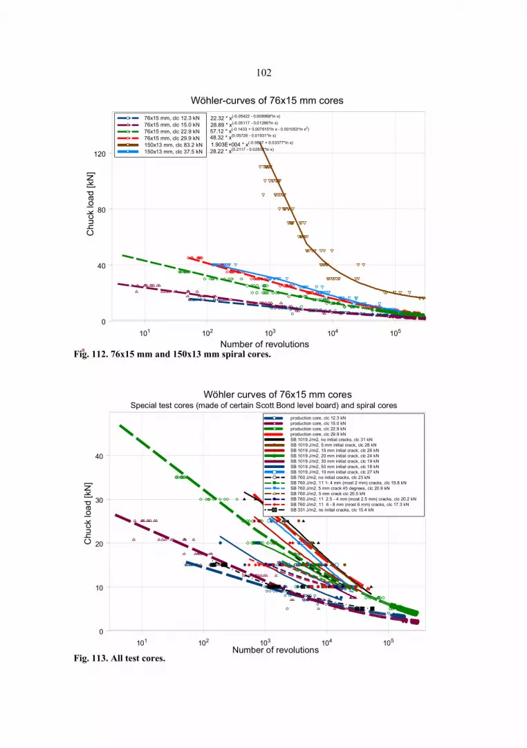
102

Fig. 112. 76x15 mm and 150x13 mm spiral cores.

Fig. 113. All test cores.

101 102 103 104 105


0

40

80

120

Chu

ck lo

ad [k

N]

76x15 mm, clc 12.3 kN76x15 mm, clc 15.0 kN76x15 mm, clc 22.9 kN76x15 mm, clc 29.9 kN150x13 mm, clc 83.2 kN150x13 mm, clc 37.5 kN

Wöhler-curves of 76x15 mm cores

1.903E+004 * x(-0.9867 + 0.03377*ln x)

28.22 * x(0.2117 - 0.02833*ln x)

48.32 * x(0.05726 - 0.01931*ln x)57.12 * x(-0.1433 + 0.007615*ln x - 0.001053*ln x2)28.89 * x(-0.05117 - 0.01286*ln x)22.32 * x(-0.05422 - 0.008968*ln x)

101 102 103 104 105


0

10

20

30

40

Chu

ck lo

ad [k

N]

Wöhler curves of 76x15 mm cores

production core, clc 12.3 kNproduction core, clc 15.0 kNproduction core, clc 22.9 kNproduction core, clc 29.9 kNSB 1019 J/m2, no initial cracks, clc 31 kNSB 1019 J/m2, 5 mm initial crack, clc 28 kNSB 1019 J/m2, 15 mm initial crack, clc 26 kNSB 1019 J/m2, 20 mm initial crack, clc 24 kNSB 1019 J/m2, 30 mm initial crack, clc 19 kNSB 1019 J/m2, 50 mm initial crack, clc 18 kNSB 1019 J/m2, 10 mm initial crack, clc 27 kNSB 760 J/m2, no initial cracks, clc 23 kNSB 760 J/m2, 11 1- 4 mm (most 2 mm) cracks, clc 19.8 kNSB 760 J/m2, 5 mm crack 45 degrees, clc 20.9 kNSB 760 J/m2, 5 mm crack clc 20.5 kNSB 760 J/m2, 11 2.5 - 4 mm (most 2.5 mm) cracks, clc 20.2 kN SB 760 J/m2, 11 6 - 8 mm (most 6 mm) cracks, clc 17.3 kNSB 331 J/m2, no initial cracks, clc 15.4 kN

Special test cores (made of certain Scott Bond level board) and spiral cores

103

Fig. 114. Same as figure 113 but with different scales.

Fig. 115. Test cores made of 760 J/m2 board.

103 1044 5 6 7 8 9 2 3 4 5 6 7 8 9 2 3 4


5

10

15

20

25

30C

huck

load

[kN

]

Wöhler curves of 76x15 mm cores

production core, clc 12.3 kNproduction core, clc 15.0 kNproduction core, clc 22.9 kNproduction core, clc 29.9 kNSB 1019 J/m2, no initial cracks, clc 31 kNSB 1019 J/m2, 5 mm initial crack, clc 28 kNSB 1019 J/m2, 15 mm initial crack, clc 26 kNSB 1019 J/m2, 20 mm initial crack, clc 24 kNSB 1019 J/m2, 30 mm initial crack, clc 19 kNSB 1019 J/m2, 50 mm initial crack, clc 18 kNSB 1019 J/m2, 10 mm initial crack, clc 27 kNSB 760 J/m2, no initial cracks, clc 23 kNSB 760 J/m2, 11 1- 4 mm (most 2 mm) cracks, clc 19.8 kNSB 760 J/m2, 5 mm crack 45 degrees, clc 20.9 kNSB 760 J/m2, 5 mm crack clc 20.5 kNSB 760 J/m2, 11 2.5 - 4 mm (most 2.5 mm) cracks, clc 20.2 kN SB 760 J/m2, 11 6 - 8 mm (most 6 mm) cracks, clc 17.3 kNSB 331 J/m2, no initial cracks, clc 15.4 kN

Special test cores (made of certain Scott Bond level board) and spiral cores

103 1044 5 6 7 8 2 3 4 5 6 7 8 2 3Number of revolutions

10

12

14

16

Chu

ck lo

ad [k

N]

Wöhler curves of 76x15 mm cores with variable initial crack length

no initial cracks, clc 23 kNsingle 5 mm initial crack clc 20.5 kNsingle 5 mm initial crack 45 degrees, clc 20.9 kN11 6 - 8 mm (most 6 mm) initial cracks, clc 17.3 kN11 1- 4 mm (most 2 mm) initial cracks, clc 19.8 kN11 2.5 - 4 mm (most 2.5 mm) initial cracks, clc 20.2 kN

Special test cores made of 760 J/m^2 board

139.2 * x(-0.2637)

45.95 * x(-0.1639)76.02 * x(-0.2111)63.41 * x(-0.1892)

73.08 * x(-0.2021)

51.01 * x(-0.1732)

104 Fig. 116. Test cores made of 1019 J/m2 board.

Fig. 117. Test cores made of two materials.

102 103 1042 3 4 5 6 7 8 2 3 4 5 6 7 8 2 3 4 5 6 7 8


10

15

20

25

30

Chu

ck lo

ad [k

N]

Wöhler curves of 76x15 mm cores with variable initial crack length

50 mm initial crack, clc 18 kN30 mm initial crack, clc 19 kN20 mm initial crack, clc 24 kN15 mm initial crack, clc 26 kN10 mm initial crack, clc 27 kN 5 mm initial crack, clc 28 kN no initial crack, clc 31 kN

Special test cores made of 1019 J/m^2 board

4.53 * x(0.6078 - 0.05094*ln x)8.61 * x(0.4812 - 0.04619*ln x)

45.85 * x(0.02473 - 0.01719*ln x)9.97 * x(0.3242 - 0.03306*ln x)3.72 * x(0.5257 - 0.04453*ln x)

40.96 * x(-0.05688 - 0.01272*ln x)

10.6 * x(0.4359 - 0.0421*ln x)

1042 3 4 5 6 7 8 9 2 3 4 5 6 7 8 9


10

11

12

13

14

15

16

17

Chu

ck lo

ad [k

N]

Wöhler curves of 76x15 mm cores made of 740 J/m^2 and 878 J/m^2 boards

710 J/m2 layer thickness 8 mm on the surface710 J/m2 layer thickness 2 mm on the surface710 J/m2 layer thickness 6 mm on the surface710 J/m2 layer thickness 4 mm on the surface

104.8 * x(-0.238)

92.12 * x(-0.2032)

133.7 * x(-0.2532)

143.8 * x(-0.2531)

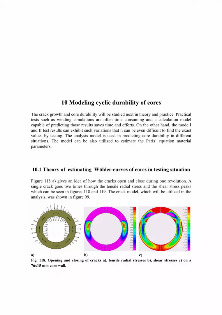
10 Modeling cyclic durability of cores

The crack growth and core durability will be studied next in theory and practice. Practical tests such as winding simulations are often time consuming and a calculation model capable of predicting those results saves time and efforts. On the other hand, the mode I and II test results can exhibit such variations that it can be even difficult to find the exact values by testing. The analysis model is used in predicting core durability in different situations. The model can be also utilized to estimate the Paris´ equation material parameters.

10.1 Theory of estimating Wöhler-curves of cores in testing situation

Figure 118 a) gives an idea of how the cracks open and close during one revolution. A single crack goes two times through the tensile radial stress and the shear stress peaks which can be seen in figures 118 and 119. The crack model, which will be utilized in the analysis, was shown in figure 99.

a) b) c) Fig. 118. Opening and closing of cracks a), tensile radial stresses b), shear stresses c) on a 76x15 mm core wall.

106

a) b) Fig. 119. Tensile radial stresses a) and shear stresses b) on 150x13 mm core wall. The analytic and numerical J-integral estimations were compared in chapter 8.3. The analytic J-integrals were calculated by equation (69) which will be used also in further analysis. If we solve the Paris´ equation (62) for the number of loading cycles, the durability of the test specimen can be written as

(70) If the revolutions are counted, we must consider that a single crack goes through the opening cycle 2 times during one revolution. Equation (70) can be rewritten in case of single crack for the number of revolutions as

(71) We need to consider the mode I and mode II strain energy release rates. Since, G is energy parameter its components can be summed and equation (71) becomes

(72) Considering equation (69), equation (72) can be written as (73)

NC

a0

ac

a1

C dGn⋅

⌠⌡

d

NR12

a0

ac

a1

CI dGI( ) nI⋅ CII dGII( ) nII⋅+

⌠⌡

d⋅

NR12

a0

ac

a1

C dGn⋅

⌠⌡

d⋅

NR12

a0

ac

a1

CIπ 1 ν−( )⋅

2 G⋅σ

2⋅ a⋅

nI

⋅ CIIπ 1 ν−( )⋅

2 G⋅τ2

⋅ a⋅

nII

⋅+

⌠⌡

d⋅

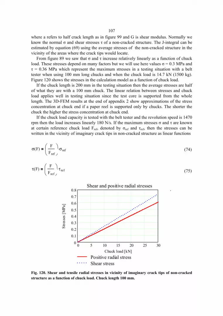
107where a refers to half crack length as in figure 99 and G is shear modulus. Normally we know the normal σ and shear stresses τ of a non-cracked structure. The J-integral can be estimated by equation (69) using the average stresses of the non-cracked structure in the vicinity of the areas where the crack tips would locate.

From figure 89 we saw that σ and τ increase relatively linearly as a function of chuck load. These stresses depend on many factors but we will use here values σ = 0.3 MPa and τ = 0.36 MPa which represent the maximum stresses in a testing situation with a belt tester when using 100 mm long chucks and when the chuck load is 14.7 kN (1500 kg). Figure 120 shows the stresses in the calculation model as a function of chuck load.

If the chuck length is 200 mm in the testing situation then the average stresses are half of what they are with a 100 mm chuck. The linear relation between stresses and chuck load applies well in testing situation since the test core is supported from the whole length. The 3D-FEM results at the end of appendix 2 show approximations of the stress concentration at chuck end if a paper reel is supported only by chucks. The shorter the chuck the higher the stress concentration at chuck end.

If the chuck load capacity is tested with the belt tester and the revolution speed is 1470 rpm then the load increases linearly 180 N/s. If the maximum stresses σ and τ are known at certain reference chuck load Fref, denoted by σref and τref, then the stresses can be written in the vicinity of imaginary crack tips in non-cracked structure as linear functions

(74) (75)

Fig. 120. Shear and tensile radial stresses in vicinity of imaginary crack tips of non-cracked structure as a function of chuck load. Chuck length 100 mm.

σ F( )F

Fref

σ ref⋅

τ F( )F

Fref

τ ref⋅

0 5 10 15 20 25 300

0.10.20.30.40.5

0.60.70.8

Positive radial stressShear stress

Shear and positive radial stresses

Chuck load [kN]

Stre

sses

[MPa

]

.

108Considering equations (74) and (75) it is now possible to write equation (73) as a function of chuck load F

(76) If there is more than one crack in the same diameter in the core wall, we can use equation

(77) where num refers is the number of cracks. Figure 121 shows an example of model with one and four cracks. We will see later that the four crack model can be used with typical spiral cores.

a) b) Fig. 121. Core with one crack a) and four cracks b). The arrows give an idea of the crack opening and closing stresses.

10.2 Representative material constants of Paris´ equation

The mode I and II Paris´ equation material constants n and C are needed in equations (76) and (77). There was a lot of variation in the test results of cyclic mode I and mode II cracked specimens in figures 66-71. The difference between the high and low speed test results was also considerable. Considering the differences in the durability results of

NR F( )12

a0

ac

a1

CIπ 1 ν−( )⋅

2 G⋅σ F( )

2⋅ a⋅

nI

⋅ CIIπ 1 ν−( )⋅

2 G⋅τ F( )

2⋅ a⋅

nII

⋅+

⌠⌡

d⋅

NR F( )1

num12

⋅

a0

ac

a1

CIπ 1 ν−( )⋅

2 G⋅σ F( )

2⋅ a⋅

nI

⋅ CIIπ 1 ν−( )⋅

2 G⋅τ F( )

2⋅ a⋅

nII

⋅+

⌠⌡

d⋅

109cores made of different boards, we could also have expected clearer differences in the n and C results of different board specimens. It could be said that these results cannot give more precise information than an idea of the magnitude of what the material constants should be in the model. If these constants are used in equation (76) the results are not in accordance with the tested reference results in figure 113. Some test cores in figure 113 were made of the same board and some very closely of the same board as the tested mode I and mode II cracked specimens. The test results showed that the test cores which had no initial macro cracks or the test cores with a single 5 mm crack had closely the same durability. The calculation model is more sensitive to the initial crack length and the initial crack length must start from minimum 5 mm to get realistic results. On the other hand, it does not make a big difference if the final crack length is 50 mm or 100 mm in the model if the initial crack length is short (chapter 10.6).

It was finally searched by trial and error which n and C values would give the measured Wöhler-curves in four different cases. The chuck load capacity is a useful classification tool since it was found earlier that the Wöhler-curves of cores with the same chuck load capacity are very closely the same. The results in table 8 are divided into four cases representing material constants of cores with different chuck load capacity. The initial crack length a0 is 5 mm and the final crack length ac is 100 mm in all cases. Table 8. Reference cores and corresponding Paris´ equation material constants.

Case number

Chuck load capacity

[kN]

Scott Bond [J/m2]

C mode I

n mode I

C mode II

n mode II

1 28 - 31 1019 4.0E-8 1.8 8.0E-8 1.8 2 20.5 - 23 760 8.0E-8 2.2 1.6E-7 2.2 3 15 - 15.4 331 1.0E-6 2.3 2.0E-6 2.3 4 12.3 300< 2.5E-6 2.5 5.0E-6 2.5

The reference cores in figures 113 and 114 were tested with 500 rpm rotation speed at different constant load levels and the durability was registered. The chuck load capacity was also tested but not from each core. There was a limited number of test cores available and in some cases it was possible to test the chuck load capacity from only a couple of test specimens. Six samples are normally tested to find out the representative chuck load capacity result.

The linear part of the da/dN versus dG curves are shown in figure 122. The curves are drawn using the n and C values in table 8. The curves do not show the lower and upper threshold values. If we compare the results in figure 122 with the measured results in figures 66-71, we find that they are between the tested slow and fast speed results. If we study the representative iterated n and C-values in table 8, we find that the n-values of mode I and II are the same but the mode II C-values are 2 times the mode I values. This is relatively well in accordance with the measured results of 1019 J/m2 board in table 2.

110

Fig. 122. Linear part of the da/dN versus dG curves with material properties which gives a good correlation with practical core test results.

10.3 Measured and calculated Wöhler-curves

10.3.1 76x15 mm cores

Figure 123 shows the results if the Paris´ equation constants in table 8 are used. It has been assumed that the cores have only one 5 mm long initial crack. The results correspond well with the measured results. The solid lines represent the calculated results. The dash and dash-dot lines represent the results of the measured cores. The test cores in cases 1-3 are made of the same or similar board as the corresponding mode I and II crack specimens in figures 66-71. In each case, there are also example production cores which have almost the same chuck load capacity and Wöhler-curve as the reference test cores.

1 10 100 1 .1031 .10 7

1 .10 6

1 .10 5

1 .10 4

1 .10 3

0.01

case1, mode Icase1, mode IIcase2, modeIcase2, modeIIcase3, modeIcase3, modeIIcase4, modeIcase4, modeII

Delamination growth in fatique

Energy release rate dG [J/m2]

Cra

ck p

ropa

gatio

n ra

te d

a/dN

[m/c

ycle

]

.

111

Fig. 123. Measured and calculated Wöhler-curves of 76x15 mm cores in cases 1-4. The final crack length in the calculated results is 100 mm. In the first case, the reference test cores are made of the same 1019 J/m2 board as the corresponding mode I and II test specimens in figures 66-71. The reference test cores with no initial cracks had a chuck load capacity 31 kN, and cores made of the same board with a single 5 mm initial crack had a 28 kN chuck load capacity. The example production cores in the first case have a 29.9 kN chuck load capacity.

In case 2, the reference test cores with no initial cracks have a chuck load capacity 23 kN and cores with a 5 mm initial crack have a 20.5-20.9 kN chuck load capacity. The test cores are made of 760 J/m2 board. The corresponding mode I and II test specimens in figures 66-71 were made of 840 J/m2 board. The example production cores in this case had a chuck load capacity 22.9 kN.

In case 3 the reference test cores are made of 331 J/m2 board. The test cores with no initial cracks have 15.4 kN chuck load capacity. The example production cores, made of different board, have a 15 kN chuck load capacity.

In the fourth case there are only production cores with 12.3 kN chuck load capacity. The cores were made of board which had approximately 350 J/m2 Scott Bond.

1 10 100 1 .103 1 .104 1 .105 1 .106 1 .107 1 .108 1 .1090

5

10

15

20

25

30

35

40

Case 1, measured spiral cores, clc 29.9 kNCase 1, measured parallel cores, no initial cracks, clc 31 kNCase 1, calculated 5 mm initial crack, clc 29.3 kNCase 2, measured spiral cores, clc 22.9 kNCase 2, measured parallel cores, no initial cracks, clc 23 kNCase 2. calculated curve 2, clc 22.4 kNCase 3, measured spiral production cores, clc 15 kNCase 3, measured parallel cores, no initial cracks, clc 15.4 kNCase 3, calculated curve 3, clc 13.9 kNCase 4, measured spiral cores, clc 12.3 kNCase 4. calculated curve 4, clc 11.8 kN

WÖHLER CURVES OF 76x15 mm CORES

NUMBER OF REVOLUTIONS

CH

UC

K L

OA

D [k

N]

.

112

10.3.2 150x13 mm cores

The tested and calculated results of 150x13 mm cores are shown in figure 124. The two studied cases are denoted as cases 5 and 6. The material properties in case 5 are of the same order as in case 2 and the material properties in case 6 are of the same order as in case 4. The initial cracks in case 6 are longer than in case 5. This was considered in calculations. The final crack length was 100 mm as in the analysis of 76x15 mm cores.

Fig. 124. Measured and calculated Wöhler-curves of 150x13 mm cores in cases 5 and 6. The final crack length in the calculated results is 100 mm.

10.4 Calculated chuck load capacity in the example cases

We will apply next the Miner´s cumulative damage theory and calculate the chuck load capacity using the previously calculated Wöhler-curves. The Miners´s theory [46] simply assumes that

(78) where the n1, n2,…,nk are now the number of revolutions at different chuck load capacity levels N1,N2,…,Nk.

n1

N1

n2

N2+ ..+

nk

Nk+ 1

1 10 100 1 .103 1 .104 1 .105 1 .106 1 .107 1 .108 1 .109 1 .10100

102030405060708090

100110

Case 5, measured spiral cores, clc 86,0 kNCase 5, calculated curve, 5 mm initial crack, clc 80.7 kNCase 6, measured spiral cores, clc 37,0 kNCase 6, calculated curve, 10 mm initial crack, clc 36.8 kN



CHU

CK L

OA

D [k

N]

.

113The weak side in this theory is that it does not consider the order of occurrence of loading levels. Considering that boards do not harden like many metals, we will try this theory in our case with an evenly increasing load.

The constant revolution speed is in the studied case 1470 rpm and loading speed is 180 N/s. The load increases during each revolution theoretically 180/24.5=7.347 N/rev= 0.007347 kN/rev. Using equations (76) or (77) and (78) we can now write equation

(79)

which can be used to find the number of revolutions before the test core delaminates. The root-function is used to search the biggest rev which makes the equation in the parenthesis equal to zero. The chuck load capacity [kN] can now be calculated by multiplying the iterated maximum number of revolutions by the amount of load increase by each revolution [kN/rev] as

(80) The results in table 9 shows the difference between calculated and measured results. The biggest deviation is in case 3 but the correspondence is generally good from low to high strength cores. Table 9. Measured and calculated chuck load capacity results.

Case

number Chuck load capacity [kN]

Measured Calculated 1 28 - 31 28.8 2 20.5 - 23 22.2 3 15 - 15.4 13.8 4 12.3 11.8

10.5 Estimations of the limit load

Figures 123 and 124 show the calculated Wöhler-curves with x-scale up to 1010 revolutions. From these figures it can be estimated that the limit load with a 100 mm long non expanding chuck is approximately 1 kN (1 kN/100 mm). This result is purely academic, since cores never need to take such a high number of loading cycles and they would wear out far before delaminating at 1 kN load. It could be said more practically that if the chuck load is less than 2 kN/100mm, then the risk of damage among the studied cores is minimal.

NRmax root

1

rev

rev1

NR 0.007347 rev⋅( )⌠⌡

d

1−

clc NRmax 0.007347⋅

114To test the calculated estimations, some practical tests were done with 76x15 mm cores using 1 kN and 2 kN constant load. The cores were tested with a 100 mm long non-expanding chuck and the revolution speed was constant at 1450 rpm. The test cores were parallel test cores (case 1, figure 123) with no initial macro cracks. The chuck load capacity of the test cores was 31 kN. Figure 125 a) shows a picture of part of the test core wall before the test. It could be estimated that the initial local “micro” cracks are shorter than 0.5 mm. Figure 125 b) shows the situation after 41447 revolutions. The first 6 mm long crack appeared on one side of the core wall. Figures 125 a) and b) are taken closely from the same part of the core. Figure 125 c) shows the situation after 95047 revolutions. The crack length is now 15 mm. Figure 125 d) shows the situation after 133203 revolutions. Figure 125 e) shows the situation after 133203 revolutions on side 2. Several 3 mm cracks have appeared since the start situation. a) b) c) d) e) Fig. 125. Constant load test 1 with 1 kN load. Core wall (side 1) in the start of the test a), side 1 after 41447 revolutions b), side 1 after 95047 revolutions c), side 1 after 133203 revolutions d), side 2 after 133203 revolutions e).

Figures 126 a) and b) are from a crack propagation test 2 with 2 a kN load, 1500 rpm. The test core was the same as in test 1. Figure 126 a) shows part of the cross section of the core before the test. Figure 126 b) shows the situation after 40813 revolutions. A small 2 mm long crack appeared on the core wall. Figure 126 a) is taken almost on the same position as figure 126 b). a) b) Fig. 126. Constant load test 2 with 2 kN load. Start situation a) and after 40813 revolutions b).

115

The results of tests 1 and 2 suggest that the estimated limit load 1 kN/100 mm could be of the correct level. We saw some new cracks appearing even with 1 kN and 2 kN loads but those are still just barely visible cracks. Again, board material is not one of the easiest kind of materials when it comes to this kind of testing. Considering the tests 1 and 2, we could say here that the calculated results give accurate enough estimations for practical purposes.

10.6 The effect of crack length on durability

Figures 127 and 128 show calculated and measured results. The measured results are the same as in figure 116. The initial crack length varies from 5 to 50 mm. The idea was to study the effect of single initial crack length on the durability of cores. All test cores were made of the same 1019 J/m2 board to eliminate the material effects. The calculated results have been calculated using the case 1 material constants. The difference between calculated results in figures 127 and 128 is that the Paris´ equation final crack length ac is 50 mm in the calculated results in figure 127 and 100 mm in figure 128. The measured and calculated chuck load capacity test results are shown in the legends of both figures.

The differences in the results in figures 127 and 128 are relatively small with small initial crack lengths. Naturally, if the initial and final crack lengths are 50 mm then the crack cannot grow at all. With a 100 mm long final crack, the calculated and measured results are close to each other. If there is only one initial crack in the analysis model, we use the final crack length 100 mm in 76 mm and 150 mm core models. Using an even longer final crack would not practically change the results with 5-50 mm initial crack lengths.

116

Fig. 127. Calculated and measured results. Initial crack length 5-50 mm, final 50 mm.

Fig. 128. Calculated and measured results. Initial crack length 5-50 mm, final 100 mm.

100 1 .103 1 .104 1 .1055

10

15

20

25

30

35

Measured parallel cores, no initial cracks, clc 31 kNMeasured parallel cores, 5 mm initial crack, clc 28 kNCalculated curve, 5 mm initial crack, clc 28.8 kNMeasured parallel cores, 10 mm initial crack, clc 27 kNCalculated curve, 10 mm initial crack, clc 24.7 kNMeasured parallel cores, 15 mm initial crack, clc 26 kNCalculated curve, 15 mm initial crack, clc 22.3 kNMeasured parallel cores, 20 mm initial crack, clc 24 kNCalculated curve, 20 mm initial crack, clc 20.4 kNMeasured parallel cores, 30 mm initial crack, clc 19 kNCalculated curve, 30 mm initial crack, clc 19 kNMeasured parallel cores, 50 mm initial crack, clc 18 kNCalculated curve, 50 mm initial crack, clc 0 kN



CH

UC

K L

OA

D [k

N]

.

100 1 .103 1 .104 1 .1055

10

15

20

25

30

35

Measured parallel cores, no initial cracks, clc 31 kNMeasured parallel cores, 5 mm initial crack, clc 28 kNCalculated curve, 5 mm initial crack, clc 28.8 kNMeasured parallel cores, 10 mm initial crack, clc 27 kNCalculated curve, 10 mm initial crack, clc 24.7 kNMeasured parallel cores, 15 mm initial crack, clc 26 kNCalculated curve, 15 mm initial crack, clc 22.3 kNMeasured parallel cores, 20 mm initial crack, clc 24 kNCalculated curve, 20 mm initial crack, clc 20.4 kNMeasured parallel cores, 30 mm initial crack, clc 19 kNCalculated curve, 30 mm initial crack, clc 19 kNMeasured parallel cores, 50 mm initial crack, clc 18 kNCalculated curve, 50 mm initial crack, clc 0 kN



CH

UC

K L

OA

D [k

N]

.

.

117

10.7 The effect of number of cracks (the four crack model)

Figure 129 shows calculated and measured results of the effect of a number of cracks in 76x15 mm cores. The measured reference cores are the multi-crack test cores from figure 115. There is one initial crack in five layers on both sides of the middle ply. The crack propagation of these and the production spiral cores can be a very complicated process. If we study the figures in appendix 4 it is very difficult to find any systematic crack propagation rule for multi-crack cores. If we want to study numerically the multi-crack cores using correct crack lengths and material properties, we need to use a multi-crack model.

The four crack model, shown in figure 121 b), is utilized here (the num parameter in equation (77) is set to four). The model assumes that the cracks are located symmetrically in the same diameter and not spirally. The final crack length of each crack is 50 mm. The distance between the middle points of the cracks is 71.5 mm if the cracks are located in the middle ply of a 76x15 mm core. The middle sphere length is 286 mm.

It can be seen from the results in figure 129 that the calculation model with four cracks gives closely the same results as the tests with multi crack cores. The measured and calculated chuck load capacity results are shown in the legend.

Fig. 129. Calculated and measured results. One or several initial cracks. Figures 130-132 show calculated examples of the effect of size of initial cracks on multi-crack cores. The board properties are from cases 1-3 respectively. The four crack model has been utilized to estimate the results of spiral cores. The calculated chuck load capacity values are shown in the legend of each figure. The first reference curve represents the situation with a single 5 mm crack and the rest of the results are with multi

100 1 .103 1 .104 1 .105

6

8

10

12

14

16

Measured parallel cores, no initial cracks, clc 23 kNMeasured parallel cores, 5 mm crack (90 degrees), clc 20.5 kNMeasured parallel cores, 5 mm crack (45 degrees), clc 20.5 kNCalculated curve, single 5 mm initial crack, clc 22.2 kNMeasured parallel cores, 1-4 mm cracks (most 2 mm), clc 19.8 kNCalculated curve, four 2 mm initial cracks, clc 21.2 kNMeasured parallel, 2-4 mm cracks (most 2.5 mm), clc 20.2 kNCalculated curve, four 2.5 mm initial cracks, clc 20.2 kNMeasured parallel, 6-8 mm cracks (most 6 mm), clc 17.3 kNCalculated curve, four 6 mm initial cracks, clc 17.2 kN



CH

UC

K L

OA

D [k

N]

.

.

1182.5-15 mm long cracks. The 2.5 mm or shorter initial multi-cracks are not very dangerous but 5 mm initial cracks clearly diminish the strength. Naturally, the longer the initial cracks, the lower the strength. Fig. 130. The board properties are from case 1. The blue lines represent calculated results of cores with 4 initial crack simulating spiral cores with the same crack length.

Fig. 131. The board properties are from the case 2.

1 10 100 1 .103 1 .104 1 .105 1 .1060

10

20

30

40

Single 5 mm initial crack, clc 28.8 kNFour 2.5 mm initial cracks, clc 24.5 kNFour 5 mm initial cracks, clc 21.3 kNFour 10 mm initial cracks, clc 18.3 kNFour 15 mm initial cracks, clc 16.5 kN



CHUC

K L

OAD

[kN

]

.

1 10 100 1 .103 1 .104 1 .105 1 .1060

5

10

15

20

25

30

35

40




CHUC

K L

OAD

[kN

]

.

119 Fig. 132. The board properties are from the case 3.

1 10 100 1 .103 1 .104 1 .105 1 .1060

5

10

15

20

25

30

35

40




CHUC

K L

OAD

[kN

]

.

11 Winding simulations

11.1 Practical tests

We will next compare the measured and calculated winding simulation results. Figures 133 a) and b) show examples of winding simulation curves. The idea is to load the core in a same way as in a selected winding situation and to find how many winding-unwinding cycles the core can take before delaminating. Figure 133 a) shows one winding cycle. One winding cycle is half of the winding-unwinding cycle in figure 133 b).

a) b) Fig. 133. Winding simulation curve a) and winding-unwinding simulation cycles b). Test results of both 76x15 mm and 150x13 mm cores are shown in figure 134. It is easy to make comparisons in this figure. Figure 135 shows only the test results of 76x15 mm cores and the scale is different than in figure 134. The x-scale starts from 0.5. The durability is 0.5 cycles if the core breaks before the unwinding part as in figure 133.

0 1000 2000 3000 4000 5000 6000 70000

5

10

15

20

25

30

theoretical curvesimulation curve (belt tester)belt tester loading curve

WINDING SIMULATION CURVE

REVOLUTIONS

CH

UC

K L

OA

D [k

N]

s 0.00005= paper thickness [m]r1 0.053= outside radius of a core [m]neliöm 65= paper weight [g/m^2]leveys 2.5= reel width [m]

121There is relatively high variation in the results. The test chuck and cores heat up during long test periods, which affects the durability of test cores. The effect of temperature is studied in the next chapter. The tested results with initially cold chuck are higher than those tested with a hot chuck. The winders are often equipped with expanding chucks which prevent slip between core and chuck. If the chuck bearings are working properly, the chuck temperature is typically in the range 35-55 °C. With poor bearings, the temperature may rise up to 75 °C or even higher. The printing press unwinders are always equipped with expanding chucks and do not typically get hot.

Fig. 134. Winding simulation test results of 76x15 mm and 150x13 mm cores.

0.0 0.5 1.0 1.5 2.0 2.5 3.0 3.5 4.0 4.5 5.0Durability [winding-unwinding cycles]

0

2

4

6

8

10

12

14

16

Max

imum

reel

wei

ght [

ton]

Winding simulation results of 76x15 mm and 150x13 mm cores100 mm non expaning chuck, reel width 2.5 m, paper (65 g/m^2, 50 um).

76x15 mm, clc 12.3 kN76x15 mm, clc 15.0 kN76x15 mm, clc 23.0 kN76x15 mm, clc 30.0 kN150x13 mm, clc 37.5 kN150x13 mm, clc 86 kN

5.387 * x(-0.2374)3.729 * x(-0.2)

1.963 * x(-0.1842)

2.692 * x(-0.2176)

13.9 * x(-0.1475)4.973 * x(-0.2019)

122

Fig. 135. Winding simulation test results of 76x15 mm cores.

11.2 Temperature and revolution speed versus dynamic durability

The strength of board and cores is affected by temperature in testing situation. Figures 136 and 137 show that the thickness direction tensile strength of board, and dynamic chuck load capacity decrease as the sample temperature increases. The tested cores were not made of the tested board, but the purpose of the test results is to give an idea of the magnitude of the temperature effect.

Testing moisture of board samples in figure 136 was 6.5-6.7 % and 8 measurements were taken at temperatures 23°C and 100 °C. At the temperature of 23°C the average of test results was 1.77 MPa. At the temperature of 100 C the average was only 1.22 MPa. Figure 137 shows the effect of temperature on chuck load capacity. Moisture of the cores was 7-7.5 %. At the temperature of 25 °C the average of the test results was 1.03 ton. At the temperature of 75 °C the average of the results was only 0.58 ton.

0.5 1.0 1.5 2.0 2.5 3.0 3.5 4.0 4.5Durability [winding-unwinding cycles]

1

2

3

4

5

6

Max

imum

reel

wei

ght [

ton]

Belt tester winding simulation results of 76x15 mm cores 100 mm non expanding chuck, reel width 2.5 m, paper (65 g/m^2, 50 um)

pneumatic 1.2 ton, belt tester 12.3 kNpneumatic 1.5 ton, belt tester 15.0 kNpneumatic 2.1 ton, belt tester 23.0 kNpneumatic 2.8 ton, belt tester 31.0 kN

2.383 * x(-0.2035)

5.387 * x(-0.2374)

1.963 * x(-0.1842)

3.729 * x(-0.2)

123

Fig. 136. Temperature versus thickness direction tensile strength of board.

Fig. 137. Temperature versus chuck load capacity.

The chuck warms up usually relatively fast in core testing. The temperature camera images, 138 a) and b), show an example of core and chuck heating during a chuck load capacity test. The chuck and core were initially at room temperature. Figure 138 a) has been taken in the beginning of the chuck load capacity test. Figure 138 b) has been taken at the end of the test and core temperature is approximately 50 °C.

Figure 139 shows an example of the temperature on winding simulation results. We can see that simulations with cold chuck (blue points) give usually the highest results. After a few tests the chuck warms up and the test results tend to decrease.

20 40 60 80 100Testing temperature of board [C]

0.0

0.1

0.2

0.3

0.4

0.5

0.6

0.7

0.8

0.9

1.0

1.1Th

ickn

ess

dire

ctio

n te

nsile

stre

ngth

[Mpa

]testing temperature 23 C, moisture 6.7 %testing temperature 100 C, moisture 6.5 %

The effect of temperature on thickness direction tensile strength of board

20 40 60 80 100Testing temperature of cores [C]

0.0

0.1

0.2

0.3

0.4

0.5

0.6

0.7

0.8

0.9

1.0

1.1

Chu

ck lo

ad c

apac

ity [t

on]

testing temperature 25 C, moisture 7 %testing temperature 75 C, moisture 7.5 %

The effect of temperature on chuck load capacity of cores

124

a) b) Fig. 138. Temperature in the start a) and end b) of an example chuck load capacity test.

Fig. 139. Example of the effect on temperature in winding simulations.

0.0 0.5 1.0 1.5 2.0 2.5 3.0 3.5 4.0 4.5 5.0Durability of winding-unwinding cycles

0

2

4

6

8

10

12

14

16

18

Max

imum

reel

wei

ght [

ton]

150x13 mm cores, testing length 50 mm. Simulation parameters: reel width 2.5 m, paper (65 g/m^2, 50 um).

The effect of temperature in winding simulations

warm chukCold chuck (the first testing)

125 Figure 140 gives an example of the winding curve of 2.5 m wide paper reel with 76x15 mm core. Most of the time the revolution speed in winding is less than 750 rpm. Using a higher revolution speed 1500 rev/min in winding simulations and special tests, gives rise to a question of the effect of the speed on the test results.

Fig. 140. Revolution speed versus reel weight at different web speeds. Reel width 2.5 m, paper thickness 50 µm.

Figures 141 and 142 show that testing with a revolution speed 1500 rpm gives slightly higher test results than testing with 500 rpm. The average of the number of revolutions at 500 rpm is 7.7 % smaller than that with 1500 rpm. We can also see that there can be some 40 % difference in the test results tested with warm and hot cores. Chuck and core temperatures has been measured after every test in the middle of the chuck in the longitudinal direction. Core temperature has been measured from the inside surface.

A paper mill winder chuck temperature is, under normal conditions, approximately 40-50 °C if there are no expanding chucks. If there is for example a bearing fault in the winding arm, the temperature can be considerable higher. The chucks with expanding elements are cooler as there is no such slippage and rolling between chuck and core as with non expanding chucks. Testing and simulating cores with non expanding chucks consider also the variation from temperature, and we remain on the safe side when applying the results for normal winding conditions.

126

Fig. 141. Chuck temperature has been measured.

Fig. 142. Core temperature has been measured.

11.3 Theoretical model and results

If we know the web speed vw [m/s], reel width b [m], basis weight of paper ρA [kg/m2] and winding time t [s], then the reel weight mR [kg] can be written as (81)

The effect of revolution speed and core temperature on dynamic durability w ith 20 kN constant load

0

2000

4000

6000

8000

10000

12000

14000

16000

20 30 40 50 60 70 80Chuck temperature [ºC]

Cor

e du

rabi

lity

[revo

lutio

ns] 1500 rpm/20kN

500rpm/20kN

The effect of revolution speed and core temperature on dynamic durability w ith 20 kN constant load

0

2000

4000

6000

8000

10000

12000

14000

16000

20 30 40 50 60 70 80Core temperature [ºC]

Cor

e du

rabi

lity

[revo

lutio

ns] 1500 rpm/20kN

500rpm/20kN

mR v w b⋅ ρ A⋅ t⋅

127The chuck load [kN] is calculated by equation

(82) where g is 9.81 m/s2. In equation (79), the Miner´s cumulative theory was applied and the maximum number of revolutions with linearly increasing load was iterated. In equation (83) we will utilize the same principle but we iterate the winding time for maximum chuck load levels as (83) where the winding-unwinding cycles go from 0.5 to necessary number of cycles. Considering equations (81) and (82), equation (83) can also be written as

(84) Before we can compare the calculated and simulated winding simulation curves we need to calculate the reel weight [ton] as a function of winding-unwinding cycles.

Considering the effect of temperature on the results, when testing with a non-expanding chuck, we need to introduce a temperature correction factor. This factor is different for 76 and 150 mm cores. 150 mm cores heat up more than 76 mm cores since the chuck loads are higher. The heat correction factor introduced here is empirical. We will use a factor 0.7 for 76 mm cores and a factor of 2.7 for 150 mm cores.

The maximum reel weight [ton] as a function of winding-unwinding cycles with temperature correction TC is

(85)

Figures 143 and 144 show the comparison between the calculated and measured results. Paper basis weight is 65 g/m2, reel width 2.5 m and chuck length is 100 mm. The curves represent the average results and do not tell anything about variations in the results. In the next chapter we will consider also the variation in the results and formulate model with confidence & prediction limits and reduced curves with different failure probability levels.

t cycles( ) root cycles

1

t

t1

NR F( )

⌠⌡

d

⋅ 1−

FmR g⋅

2000

mRmax cycles( )⋅v w b⋅ ρA⋅ t cycles( )⋅

1000TC−

.

t cycles( ) root cycles

1

t

t1

NRvw b⋅ ρ A⋅ t⋅ g⋅( )

2000

⌠⌡

d

1−

128

Fig. 143. Calculated and measured results.

Fig. 144. Calculated and measured results.

0 0.5 1 1.5 2 2.5 3 3.5 41

2

3

4

5

6

7

Case 1, measured spiral cores, clc 29.9 kNCase 1, calculated curve, 5 mm initial crack, clc 28.8 kNCase 2, measured spiral cores, clc 23.0 kNCase 2, calculated curve, 5 mm initial crack. clc 22.9 kNCase 3, measured cores, clc 15.0 kNCase 3, calculated curve, 5 mm initial crack, clc 13.8 kNCase 4, measured spiral cores, clc 12.3 kNCase 4, calculated curve, clc 11.8 kN

WINDING SIMULATIONS OF 76x15 mm CORES

WINDING - UNWINDING CYCLES

MA

XIM

UM R

EEL

WEI

GHT

[ton

]

.

0 0.5 1 1.5 2 2.5 3 3.5 40

2

4

6

8

10

12

14

16

18

Case 5, measured spiral cores, clc 86.0 kNCase 5, calculated curve, 5 mm initial crack, clc 80.1 kNCase 6, measured 150x13 core, clc 37.0 kNCase 6, calculated curve, 10 mm initial crack, clc 36.4 kN

WINDING SIMULATIONS OF 150x13 mm CORES


MA

XIM

UM

REE

L W

EIG

HT

[ton]

.

12 Durability of cores with different failure probabilities

The measured results in figures 134 and 135 represent mathematically random samples of unknown population. We could do an infinite number of measurements with different cores and the population is in our case basically infinite. The more measured result there are the better we can predict the statistical values of the unknown population. Let xi and yi be these measured random samples. The measured results in winding simulation curves follow the power law (86) where x represents the number of winding-unwinding cycles starting from 0.5 and y(x) represents the predicted maximum reel weight results. The curve in equation (86) can be returned to linear equation by taking the logarithms on both sides as (87) We will study next the linearly fitted data points log(xi) and log(yi). The coefficients b0 and b1 can be solved by using the least squares estimates. Equations (88) and (89) minimize the vertical distance from points to curve. Considering the lower limit load, this is physically better choice than horizontal minimization. The equations of the unknown coefficients are [47]

(88)

(89)

log y x( )( ) log b0( ) b1 log x( )⋅+

y x( ) b0 xb1⋅

b1

n

1

n

i

log xi( ) log yi( )⋅∑=

⋅

1

n

i

log xi( )∑= 1

n

i

log yi( )∑=

⋅−

n

1

n

i

log xi( )( )2∑=

⋅

1

n

i

log xi( )∑=

2

−

log b0( )1

n

i

log yi( )n∑

=

b1

1

n

i

log xi( )n∑

=

⋅−

130

(90) where the xi and yi are the measured data points and n is the number of the measured (xi, yi) data pairs. Figure 145 shows 58 measured (xi, yi) data points with least squares curve fit. The measured core samples are 76x15 mm cores with a 30 kN chuck load capacity. Figure 146 shows the (log(xi), log(yi)) data points.

Fig. 145. Linear data points in linear scales.

Fig. 146. Logarithmic data points in linear scales.

Figures 145 and 146 show how the random sample variables vary about the sample population curve fit. The residuals Ri represent the deviation of the observed yi from the fitted data points y(xi). The residuals are written as (91)

0 1 2 3 43

4

5

6

7

Durability of winding-unwinding cycles

Max

imum

reel

wei

ght [

ton] .

0.4 0.2 0 0.2 0.4 0.60.5

0.6

0.7

0.8

Durability of winding -unwinding cycles

Max

imum

reel

wei

ght [

ton] .

b0 10log b0( )

Ri yi y xi( )−

131Figure 147 a, b and c show residuals histograms of winding simulation curves of 76x15 mm cores with chuck load capacities 30 kN, 22 kN and 15 kN respectively from figure 134. Figure 147 a) shows the residuals histogram of the data points in figure 145. It will be assumed in the further studies that the residuals are normally distributed. a) b) c) Fig. 147 Histograms of winding simulation curves. Chuck load capacity of the test cores is a) 30 kN, b) 22 kN and c) 15 kN.

12.1 Confidence of the mean

Since, we are able to study only a small sample of a huge population, the sample mean and variance are also random variables. The curve fits represent the local sample averages. The true values are inside the confidence limits. The more confidence is needed the further the limits are from each other.

The sample mean of a normally distributed random variable is characterized by t-distribution. Figure 148 shows the shape of t-distribution as a function of degrees of freedom (n). With degrees of freedom 30, the t-distribution is almost identical with normal distribution.

Residuals histogram

-3 -1 1 3SD

0

2.5

5

7.5

10

12.5

15

17.5

20

Cou

nt

Residuals histogram

-3 -1 1 3SD

0

2.5

5

7.5

10

12.5

15

17.5

20

Cou

nt

Residuals plot

-3 -1 1 3SD

0

5

10

15

20

25

Cou

nt

132

Fig. 148. The t-distribution for different degrees of freedom. In durability studies, we are interested in the probability that the local sample average could fall below a certain limit. We can reduce the local population mean with confidence level by equation [48] (92) where meanC is the population mean with confidence level C, t2 is the upper integration limit for probability density function of t-distribution, S is the sample standard deviation of residuals of the curve fit and n is the number of data samples. The probability density function of t-distribution is [48] (93) where the Euler´s gamma function is given by [48]

(94)

4 2 0 2 40

0.1

0.2

0.3

0.4

dof = 1dof = 3dof = 30dof = 300

The effect of d.o.f:s on t distribution

Random variable (t)

Prob

abili

ty d

ensi

ty fu

nctio

n

.

meanC meansample t2S

n 1−⋅−

f n t,( )1n π⋅

Γn 1+

2

Γn

2

⋅ 1 t2

n+

n 1+

2

−

⋅

Γ n( )0

∞

xe x− xn 1−⋅⌠⌡

d

133If the given confidence level is denoted by C (for example 99 %), then the upper integration limit t2 can be found by iterating equation [48] (95) The standard deviation of residuals of log(yi) data points is [47]

(96)

It is to be noted here that Slog is not equal to log(S) which would denote the logarithm of standard deviation of residuals of yi data points. The subscript log in Slog denotes that we analyze linearly fitted data points log(xi), log(yi) using equation for linear data points instead of studying data points (xi, yi) which follow the power fit.

12.2 Confidence of the standard deviation

If the population mean is replaced by the sample mean, the resulting random variable follows a chi-square distribution with n-1 degrees of freedom [47]. The probability density for the chi-square distribution is given with the following expression [48] (97) where Γ(n) is the gamma function (100), h = χ2 is the independent variable in the chi-square distribution, n is the degree of freedom and e is the base of natural logarithms (2.71828…). Figure 149 shows chi-square distribution for 57 degrees of freedom

f n h,( )1

2n Γn2

⋅h

n 2−2

⋅ e

h−2

⋅

C∞−

t2

t2f n 1− t2,( )⌠⌡

d

Slog1

n

i

log yi( ) log b0( )− b1 log xi( )⋅−( )2∑=

n 2−

134

Fig. 149. Probability density function for the chi-square distribution for 57 degrees of freedom. The higher limit of the population standard deviation with confidence level is [48] (98) where h1 is iterated from equation (99) C is the confidence level (for example 99 %).

12.3 Failure probability and safety factor

This chapter follows also the principles in reference [48]. The core durability can be assumed to be normally distributed with estimated population mean and standard deviation. We can ask how many standard deviations the mean value or core durability curve fit should be reduced to reach certain failure probability. The failure probability is equal to the integral of the density function of standard normal distribution from –infinity to this number. The density function for the standard normal distribution is [48] (100)

0 20 40 60 80 1000

0.01

0.02

0.03

0.04

Chi-square variable h

prob

abili

ty d

ensit

y fu

nctio

n

0.038

0

f n h,( )

1000 h

Ch1

∞

hf n 1− h,( )⌠⌡

d

SCnh1

S⋅

f x( )1

2 π⋅e

x2−2

⋅

135The value of λ is iterated from equation [48] (101) where P is the probability of failure and λ is the independent variable in the standard normal distribution at failure probability P (figure 150). Figure 151 shows the relation between the integral function and λ.

Fig. 150. Density function of normal distribution.

Fig. 151. The relation between the integral function (101) and λ. When the value of λ has been iterated, we can reduce the population mean to the failure probability P by equation [48]

(102)

P x λ≤( )∞−

λ

x1

2 π⋅e

x2−2

⋅

⌠⌡

d

4 3 2 1 0 1 2 3 40

0.13

0.25

0.38

0.5Density function of normal distribution

Normalized variable

Prob

abili

ty d

ensi

ty

.

meanreduced meanC λ SC⋅+

4 3 2 1 00

0.1

0.2

0.3

0.4

0.5

∞−

λ

xf x( )⌠⌡

d

λ

.

136where meanC is the population mean with needed confidence level (92) and SC is the population standard deviation with confidence level (98). It is often more convenient to use the relative standard deviation defined as (103) Using the relative standard deviation, the safety factor with regard to population mean can be calculated by equation [48] (104) Table 10 shows the relationship between failure probability, reduction factor and safety factor for relative standard deviations 5 %, 10 % and 15 %. Table 10. Relation between failure probability, reduction factor and safety factor.

Failure probability P 0.5 0.01 0.001 0.0001 0.00001 0.000001 Reduction factor λ 0.0 -2.326 -3.090 -3.719 -4.265 -4.753 Safety factor Sf Screlative 5 %

1.0 1.132 1.183 1.228 1.271 1.312

Safety factor Sf Screlative 10 %

1.0 1.303 1.447 1.592 1.774 1.906

Safety factor Sf Screlative 15 %

1.0 1.536 1.864 2.262 2.776 3.484

12.4 The confidence and prediction limits for the curve fit

The next step is to calculate the prediction and confidence limits for the example curve in figure 146. The population curve fit is with chosen probability C inside the confidence limits. The population samples are within probability C inside the prediction limits. We assumed earlier that the residuals are normally distributed in y-direction. We assume here that also the logarithmic residuals of the measured data points yi are normally distributed. The detailed procedures of constructing the limits are explained in reference [47] and only the most important equations without derivation are shown here. Using the same notations as in reference [47] we determine term Sxxlog which is

(105)

SCrelativeSC

meanC

SFmeanC

meanreduced

11 λ SCrelative⋅+

Sxxlog

1

n

i

log xi( )1

n

j

log xj( )n∑

=−

2

∑=

137The confidence limit on the mean is now [47] (using log(xi) points)

(106) The confidence (prediction) limit on the y-values is [26]

(107) where t2 is the upper integration limit in t-distribution. Finally, the confidence limit CL(xi) and prediction limit PL(xi) data points are:

(108) (109) (110) (111) To get a continuous line, a curve must be fitted through the calculated data points. Figure 152 shows the example results from figure 146 with 99 % prediction and confidence limits. Figure 153 shows how the results are returned back to linear coordinates by plotting the log(xi) and log(yi) data points as 10log(xi) , 10log(yi)

.

LC xi( )log

t2 Slog⋅1n

log xi( )1

n

j

log xj( )n∑

=−

2

Sxxlog+⋅

LP xi( )log

t2 Slog⋅ 11n

+

log xi( )1

n

j

log xj( )n∑

=−

2

Sxxlog+⋅

CL xi( )log

log y xi( )( ) LC xi( )log

−

CU xi( )log

log y xi( )( ) LC xi( )log

+

PL xi( )log

log y xi( )( ) LP xi( )log

−

PU xi( )log

log y xi( )( ) LP xi( )log

+

138

Fig. 152. Logarithmic data points in linear scales with linear least squares curve fit and 99% prediction and confidence limits.

Fig. 153. Linear data points in linear scales with power least squares curve fit and 99% prediction and confidence limits.

12.5 Failure probability and safety factor

In our case, it is not enough if we know the curve fit of the durability curve and its prediction and confidence limits. We also need to know the reduced curve fit corresponding to certain failure probability. Figure 154 shows the situation where we want to reduce the curve fit of the measured results by one standard deviation. We can

0.4 0.2 0 0.2 0.4 0.60.5

0.6

0.7

0.8

WINDING SIMULATION CURVE


REE

L W

EIG

HT

[ton]

.

0.5 1 1.5 2 2.5 3 3.53

4

5

6

7

8WINDING SIMULATION CURVE


REE

L W

EIG

HT

[ton]

.

139construct the reduced log(x) and log(y) data points log(x)R and log(y)R by using the slope of the fitted curve and Slog as

(112) (113) where k is the slope factor, λ determines how many standard deviations the durability curve fit should be reduced to reach certain failure probability. λ is iterated from equation (101) and standard deviation Slog is calculated from equation (96). The logarithmic results can be returned to linear coordinates by plotting the log(x) and log(y) data points as 10log(x) , 10log(y)

. Fig. 154. Reduction of the curve fit.

12.6 Example of reduced results

Figure 155 shows an example of application of the theory to the results in figure 154. The curves show the confidence and prediction limits. The curve fit has also been reduced for different failure probabilities. It can be estimated how many winding-unwinding cycles the 100 mm long test core samples can take with certain failure probability in a winding simulator equipped a with 100 mm long non expanding test chuck.

log x( )R log x( ) λSlog

k−⋅+

log y( )R log y x( )( ) λ Slog⋅+

140

Fig. 155. Durability of cores in winding simulations. Data points, least squares curve fit, 99 % confidence and prediction limits and reduced results.

Durability of 76x15 mm cores in winding simulations Chuck load capacity of cores 31 kN

99 % confidence and prediction limits. Curve fits for different failure propabilities.Least squares regression, fitstd = 0.34 ton. Results for 100 mm chuck length.

0.5 1 1.5 2 2.5 3 3.51

2

3

4

5

6

7

8

Measured data pointsFailure probability = 0.5 Failure probability = 0.01Failure probability = 0.001Failure probability = 0.0001Failure probability = 0.00001Failure probability = 0.000001upper 99 % confidence limitlower 99 % confidence limitupper 99 % prediction limitlower 99 % prediction limit

DURABILITY OF WINDING-UNWINDING CYCLES

MA

XIM

UM

REE

L W

EIG

HT

[ton]

13 Summary

Paperboard has certain weaknesses and strengths as a construction material. Board products are usually recyclable and can be light, stiff and strong. Board is also a continuous sheet product which makes it suitable for continuous manufacturing processes. The weak sides of boards are generally the poor moisture resistance without special treatments and relatively weak resistance against wear. Boards have also highly statistical nature and strong variation in many physical properties. One of the weak sides is also that the thickness direction tensile strength of boards is relatively low in comparison to the machine and cross machine direction properties. It is often possible to compensate the material weaknesses to some extent by proper design of constructions and use of materials.

In some applications the boards can be very optimal engineering materials. For example, the core industry has used different boards for decades as the main raw material. Different board grades have their own strengths. There are differences in the thickness direction strength, density, machine and cross machine direction stiffness, etc.

The measuring methods in the board and core industry are partly standardized. It is very important to know the mechanical properties and proper ways of measuring them. It is also important to know how different board properties correlate with mechanical properties of the final product. When measuring the correlations, it is important to try eliminating the unwanted variables.

We have studied the most important mechanical properties of some example boards. In many cases, the measuring and analysis methods designed for fiber composites can be applied for boards or laminated board samples. One interesting discovery was that the Scott Bond test result correlates well with the sum of mode I and mode II critical strain energy release rates. The Scott Bond test has been used traditionally to measure the “strength” of boards.

Interesting parts of this study are also studies of laminated board specimens, studies of crack propagation in cores and analysis of durability of cores in winding simulations. There was again considerable variation in mode I and mode II dynamic fracture test results and it was difficult to find universal representative results for example boards. The results depended also on the loading rate. Anyway, it was possible to estimate the magnitude of the overall results and the relation between mode I and mode II test results. It was found that the Paris´ law could be applied to fit the measured data points.

142The next step was to formulate analytic model to estimate life time of cores in simulated winding conditions. The creation of the model started by FEM analysis of supporting stresses at the ends of example cores. Cracked cores were also analyzed and the correlation between the analytic and numeric J-integration estimations was generally good. The crack propagation and life time of different core constructions was studied in practice. Part of the tests were done with constant load so that it was possible to construct Wöhler-curves of different cores. Part of the tests simulated winding and unwinding curves and it was tested how many winding-unwinding cycles different cores can take.

The Wöhler-curves were constructed also analytically by applying the Paris´ law and analytic J-integral model. The measured Paris´ equation constants were corrected by comparing the calculated and measured results. After this, the Miner´s cumulative law was applied to create a model which could be used to predict life time and chuck load capacity of cores. Temperature correction was needed in the models to consider the effect of temperature in the results. Single and multi crack models were used depending on the case. The analytical models are relatively simple but can give closely the same results with practical tests. The results showed that the length and number of initial cracks can have a considerable effect on durability of cores.

Finally the winding-unwinding durability results were reduced to correspond to certain confidence levels. This was done by reducing the curve fit by certain number of standard deviations.

References

1. Ilomäki M (1993) Kartonkihylsyn mekaanisen käyttäytymisen analysointi. Diplomityö, Oulun yliopisto, Teknillisen mekaniikan laboratorio.

2. Ilomäki M (1994) Hylsyn istukkakestävyyteen vaikuttavien tekijöiden analysointi. Lisensiaatintyö, Oulun Yliopisto, Teknillisen mekaniikan laboratorio.

3. Staples J (1994) Roll Weight Capacity of Paper Mill Cores. Tappi Journal, Vol. 77, No. 5, pp. 190-194.

4. Ilomäki M & Fejer M (2003) New Challenges in Unwinding and Their Impact on Core Requirements. Ipw (international paperworld) magazine 5.2003, pp. 33-38.

5. Gronewold J (1998) Winders The Complete Guide for Paper Mills and Converters. Tappi, Atlanta.

6. Herranen P (1978) Paperiteollisuushylsyjen hyvyyskriteerit ja niihin vaikuttavat tekijät. Diplomityö, Teknillinen Korkeakoulu, Puunjalostusosasto, Paperitekniikan laboratorio, Diplomityö 3/78.

7. IFRA (1984) IFRA Rotary Press Guide, Book3, Edition 2, Darmstadt, pp. 1-10. 8. Staples J & Stephens J (1998) Next generation of dynamic testing devices. Tappi

Journal, Vol. 81, No. 7, pp. 69-73. 9. Liliana B (2001) Mechanics of paperboard packages. Performance at short term

static loading. Licentiate Dissertation, Lund University, Department of Structural Mechanics, Sweden.

10. Stenberg N (1999) Mechanical properties in the thickness direction of paper and paperboard. Licentiate Thesis no. 69, Royal Institute of Technology, Stockholm.

11. Uesaka T, Murakami K & Imamura R (1979) Biaxial tensile behaviour of paper, Tappi Journal, Vol. 62, No. 8, pp. 111-114.

12. Niskanen K (1998) Paper Physics, Papermaking Science and Technology Book 16. Gummerus Printing, Jyväskylä, Finland.

13. Jones RM (1975) Mechanics of Composite Materials. Scripta Book Company, Washington D.C.

14. Hibbit, Karlsson & Sorensen Inc. (1996) Abaqus 5.6 User´s Manual Volume I. 15. SCAN-P 38:30 (1980) Vetolujuus, venymä ja murtotyö, paperi ja kartonki.

Standard of Scandinavian Pulp, paper and Board.

14416. Aliranta J (1988) Rakenneparametrien vaikutus kartonkihylsyn ominaisuuksiin.

Diplomityö, Oulun Yliopisto, Teknillisen mekaniikan laboratorio. 17. Brezinski JP & Hardacker KW (1982) Poisson ratio values. Tappi Journal, Vol.

65, No. 8, pp. 114-115. 18. Uesaka T, Murakami K & Imamura R (1982) On the Poisson ratio of paper and

its experimental determination, Tappi Journal, Vol. 65, No. 8, pp. 115-116. 19. Mann RW, Baum GA & Habeger CC (1980) Determination of all nine

orthotropic elastic constants for machine-made paper. Tappi Journal, Vol. 63, No. 2, pp. 163-166.

20. Kujala M & Kajanto I (1995) Paperin poissonin vakioitten määrittäminen kuva-analyysillä. KCL paper science center publication no. 84.

21. Ilomäki M & Jorkama M (2003) A study of CD elongation of core in winding. Proceedings of the Seventh International Conference on Web Handling, June 1 – 4, 2003, Oklahoma State University, Stillwater, USA.

22. Mark RE (1983) Handbook of Physical and Mechanical Testing of Paper and Paperboard, Vol. 1. Marcel Dekker Inc, New York.

23. Baum GA, Brennan DC & Habeger CC (1981) Orthotropic elastic constants of paper. Tappi Journal, Vol 64, No. 8, pp. 97-101.

24. SCAN-P 80:98 (1998) Z-suuntainen vetolujuus, paperi ja kartonki. Standard of Scandinavian Pulp, Paper and Board Committee.

25. T 541 om-89 (1989) Internal Bond Strength of Paperboard (z-direction tensile). Official test method of TAPPI.

26. T 569 pm-00 (2000) Internal bond strength (Scott type). Provisional method of TAPPI.

27. Koubaa A & Koran Z (1995) Measure of the internal bond strength of paper/board, Tappi Journal, Vol. 78, No. 3, pp. 103-111.

28. Multanen E (1983) Nestepakkauskartongin jäykkyyden ja palstautumislujuuden hallinta. Diplomityö, Teknillinen Korkeakoulu, Puunjalostusosasto, Paperitekniikan laboratorio, Diplomityö nro. 2453.

29. ISO 1922 (1981) Cellular plastics - Determination of shear strength of rigid materials, second edition.

30. Harvey DM (1970) Operating Variables in Spiral Winding: Theoretical Interrelationships and Significance. Tappi Journal, Vol. 53, No. 8, pp. 1521-1524.

31. Järvinen M (2003), Paperboard core with an improved chuck strength, for the paper industry, and a method of fabricating such, US patent 6,540,174 B1.

32. Morel J (1987) Resistance des mandrins – gache de bobineaux: Simulateur de contraintes de derouleurs pour rotatives. Seminaire de L´IFRA, techniques de presse janvier 1987.

33. Järvinen M, Novaky M & Rommi H (1989) Method of testing cores, EP patent 0 309 123 A2.

34. ISO 11093-9 (1994) Paper and board - Testing of cores – Part 9: Determination of flat crush resistance.

35. TCR-2 (1989) The Effect of Moisture Content on Dimensional Stability and Strength Properties of a Typical Paperboard Tube or Core. CCTI Technical Committee Report, June 1989.

14536. Gerhardt T, Qiu Y et al (1999) Engineering paper tubes to improve winding

performance. Mechanics of cellulosic materials, AMD-Vol. 231/MD-Vol. 85, The American Society of Mechanical Engineering.

37. Carlsson LA & Gillespie JW (1991) Delaware Composites Design Encyclopedia, Vol. 6., Technomic Publishing Company, Lancaster.

38. Ikonen K & Kantola K (1991) Murtumismekaniikka. Otatieto, toinen uudistettu painos, Helsinki.

39. Lemaitre J & Chaboche JL (1990) Mechanics of Solid Materials. Cambridge University Press, New York.

40. Pennala E (1993) Lujuusopin perusteet, kuudes uudistettu painos. Otatieto, Hämeenlinna.

41. Kelly A, Zweben C et al (2000) Comprehensive Composite Materials Vol. 2, Cambridge University Press, England.

42. Hibbit, Karlsson & Sorensen Inc (1996) Abaqus 5.6 User´s manual, Vol. II. 43. Hibbit, Karlsson & Sorensen Inc (1996) Abaqus 5.6 User´s manual, Vol. III. 44. Yuhara T, Kortschot M (1992) Fracture toughness of paper evaluated by the J-

integral, Proceedings of the 1992 Paper Physics Seminar, KCL Paper Science Centre, PSC Communications 32, Oy Keskuslaboratorio.

45. Murakami Y (1987) Stress Intensity Handbook, Vol. 1. Pergamon Press, New York.

46. Outinen H, Koski J & Salmi T (1997) Lujuusopin perusteet. Pressus Oy, Tampere.

47. Milton JS & Arnold JC (1987) Probability and Statistics in the Engineering and Computing Sciences. McGRAW-Hill Book Co., Singapore.

48. Rabb BR (1999) Fatique Testing and Its Statistical Evaluation into Design Rules. Dissertation, Tampere University of technology, Publications 253.

49. Wadood H (1998) Winding Mechanics of Anisotropic Materials. Pira technology series. Pira International, Surrey, UK.

50. Lekhnitskii S (1981) Theory of Elasticity of an Anisotropic Body. MIR Publishers, Moscow.

51. Dally JW & Riley WF (1991) Experimental Stress Analysis, Third edition. McGRAW-HILL International Editions, Engineering mechanics series, Singapore.

52. Gerhardt TD & Kearns RW (1994) Radial crush takes the measure of a core. Converting magazine, February, pp. 50-52.

53. Saliklis EP & Rowlands RE (1997) A novel radial compression testing device for tubes. Tappi Journal, Vol. 80, pp. 234-237.

Appendix 1 Stresses and dimensional changes of cores under external pressure

We will study here the stresses and dimensional changes of cores under external pressure in theory and practice. We will first study the change of in-plane dimensions and then the change of length (elongation). The elongation studies help to estimate the goodness of the used out of plane Poisson’s ratios.

1.1 Calculation of changes of inside and outside diameter

Hamad has studied in reference [49] the behaviour of a core with cylindrical anisotropy. Lekhnitskii [50] has also studied the same problem. It has been assumed that the material follows the linear Hooke´s law. The faces of the core are free from load. The core has constant thickness h and the state of (generalized) plane stress has been assumed, as said in the original text. In the plane-stress approach it is generally assumed that out of plane stresses are zero. The principal material directions of the plate are the radial (r) and tangential (θ) directions. Figure a1.1 shows such a core cross section under external pressure.

Fig. a1.1. Core cross section with cylindrical anisotropy. The polar angle is θ and r represents the radius to any point inside the core cross section.

147 (1) where a and b denote the inner and outer radius of core as in figure a1.1. The tangential displacements uθ=0. The radial ratio c=a/b. The uniform pressure at the exterior core surface is denoted by q [MPa]. The radius to any point in the core cross section is denoted by r [mm] and νθr is the Poisson´ ratio of core material in the tangential thickness direction. Eθ is the E modulus of core material in the tangential direction [MPa]. Er is the E modulus of core wall in the radial direction [MPa]. The most important material parameter is Eθ and the two others have only a small effect. The anisotropy ratio, k, is defined as (2) It is possible to calculate the change of the inside and outside diameters of the core by equation (1). Substituting r by a or b and multiplying equation (1) by 2, the equations for the change of inside and outside diameter become

(3) (4) In paper mill winders, the lengthening of cores is usually not free and the axial stresses are not zero. From this reason, we are more interested in the plane strain solution. In plane strain situation the out of plane strains are zero. The change of outside diameter is the same in plane stress and plane strain situations. Change of the inside diameter is slightly smaller in the plane strain case but the difference is negligible for winding angles less than 30 degrees. Correlation between FEM and analytic results is excellent.

Figure a1.2 a) and b) show examples of displacement distributions in 150x13 mm core wall. The FEM results have been calculated by Abaqus, using CPS8 plane stress and CPE8 plane strain elements.

∆inside 2b

Eθ 1 c2 k⋅−( )⋅

q− k νθr−( )⋅ab

k⋅ q− c k 1−( )⋅ c k 1+( )⋅ k νθr+( )⋅

ba

k⋅+

⋅

⋅

∆outside 2 qbEθ

⋅k 1 c2 k⋅+( )⋅

1 c2 k⋅−νθr−

⋅

⋅

kEθ

Er

u rb

Eθ 1 c2 k⋅−( )⋅q− k νθr−( )⋅

rb

k⋅ q− c k 1−( )⋅ c k 1+( )⋅ k νθr+( )⋅

br

k⋅+

⋅

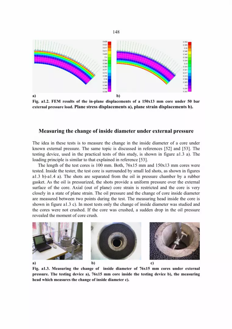
148

a) b) Fig. a1.2. FEM results of the in-plane displacements of a 150x13 mm core under 50 bar external pressure load. Plane stress displacements a), plane strain displacements b).

Measuring the change of inside diameter under external pressure

The idea in these tests is to measure the change in the inside diameter of a core under known external pressure. The same topic is discussed in references [52] and [53]. The testing device, used in the practical tests of this study, is shown in figure a1.3 a). The loading principle is similar to that explained in reference [53].

The length of the test cores is 100 mm. Both, 76x15 mm and 150x13 mm cores were tested. Inside the tester, the test core is surrounded by small led shots, as shown in figures a1.3 b)-a1.4 a). The shots are separated from the oil in pressure chamber by a rubber gasket. As the oil is pressurized, the shots provide a uniform pressure over the external surface of the core. Axial (out of plane) core strain is restricted and the core is very closely in a state of plane strain. The oil pressure and the change of core inside diameter are measured between two points during the test. The measuring head inside the core is shown in figure a1.3 c). In most tests only the change of inside diameter was studied and the cores were not crushed. If the core was crushed, a sudden drop in the oil pressure revealed the moment of core crush.

a) b) c) Fig. a1.3. Measuring the change of inside diameter of 76x15 mm cores under external pressure. The testing device a), 76x15 mm core inside the testing device b), the measuring head which measures the change of inside diameter c).

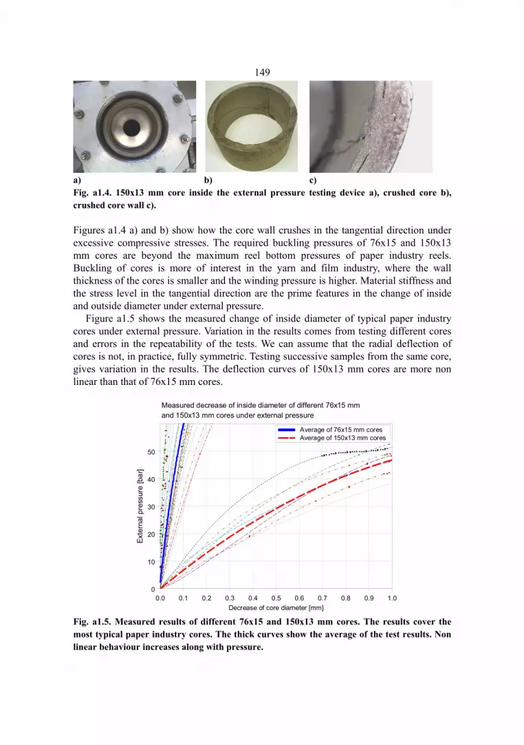
149

a) b) c) Fig. a1.4. 150x13 mm core inside the external pressure testing device a), crushed core b), crushed core wall c). Figures a1.4 a) and b) show how the core wall crushes in the tangential direction under excessive compressive stresses. The required buckling pressures of 76x15 and 150x13 mm cores are beyond the maximum reel bottom pressures of paper industry reels. Buckling of cores is more of interest in the yarn and film industry, where the wall thickness of the cores is smaller and the winding pressure is higher. Material stiffness and the stress level in the tangential direction are the prime features in the change of inside and outside diameter under external pressure.

Figure a1.5 shows the measured change of inside diameter of typical paper industry cores under external pressure. Variation in the results comes from testing different cores and errors in the repeatability of the tests. We can assume that the radial deflection of cores is not, in practice, fully symmetric. Testing successive samples from the same core, gives variation in the results. The deflection curves of 150x13 mm cores are more non linear than that of 76x15 mm cores.

Fig. a1.5. Measured results of different 76x15 and 150x13 mm cores. The results cover the most typical paper industry cores. The thick curves show the average of the test results. Non linear behaviour increases along with pressure.

0.0 0.1 0.2 0.3 0.4 0.5 0.6 0.7 0.8 0.9 1.0Decrease of core diameter [mm]

0

10

20

30

40

50

Exte

rnal

pre

ssur

e [b

ar]

Measured decrease of inside diameter of different 76x15 mm and 150x13 mm cores under external pressure

Average of 76x15 mm coresAverage of 150x13 mm cores

150

Comparison between calculated and measured results

Figure a1.6 shows the correlation between the measured and calculated results. The radial tests were done with the testing apparatus in figure a1.3. The elastic material constants in the principal core coordinates were Eθ=6000 MPa, Er=130 MPa and νθr=2.4. The measured and calculated results are well in accordance for 13-15 mm wall thickness. The smaller the wall thickness, the bigger the difference between the measured and calculated results. This can be explained by the assumption of linear material behaviour in the calculated results. The smaller the wall thickness, the higher the compressive tangential stress and the more non linear is the behaviour.

Figure a1.7 shows some calculated results of 150x13 mm and 76x15 mm cores using the same material constants. The external pressure is 20 bar and the wall thickness is 13-18 mm. With these parameters the core behaviour is still relatively linear. The calculated radial decrease of 150x13 mm core under 20 bar external pressure is 6 times bigger than that of 76x15 mm core.

Fig. a1.6. Measured and calculated results of the effect of wall thickness on decrease of inside diameter of 76x15 mm cores under external pressure.

7 8 9 10 11 12 13 14 15 16Wall thickness [mm]

0.0

0.1

0.2

0.3

0.4

0.5

0.6

Dec

reas

e of

insi

de d

iam

eter

[mm

]

The effect of wall thickness on decrease of inside diameterof 76x15 mm cores under 50 bar external pressure

measured resultscalculated curve (Ehoop 6000 MPa, Eradial 130 MPa, nu(hoop radial) 2.4)

151

Fig. a1.7. Calculated results of the effect of wall thickness on decrease of inside diameter of 76x15 mm and 150x13 mm cores under external pressure.

Distribution of radial and tangential stresses in core wall

Hamad [49] has studied the core under external pressure possessing cylindrical anisotropy. It has been assumed that the material follows the linear Hooke´s law. The faces of the core are free from load. The core has constant thickness and the state of plane stress has been assumed. The principal material directions of the 2D-model are the radial (r) and tangential (θ) directions as in figure a1.1.

The distribution of tangential σθ and radial σr stresses in the core wall under only external or both external and internal pressure will be studied next. In reference [49] it was shown that the equations of tangential and radial stresses of anisotropic cylinder under external and internal pressure load can be written as

(5)

(6)

13 14 15 16 17 18Wall thickness [mm]

0.00

0.05

0.10

0.15

0.20

0.25

0.30

0.35

0.40D

ecre

ase

of in

side

dia

met

er [m

m]

150 mm inside diameter 76 mm inside diameter

Calculated effect of wall thickness on decrease of inside diameter of 76 mm and 150 mm cores under 20 bar external pressure.Core properties: Ehoop 6000 MPa, Eradial 130 MPa, nu(hoop radial) 2.4

σθp ck 1+⋅ q−( )

1 c2 k⋅−( ) k⋅rb

k 1−( )⋅

p q c k 1−( )⋅−

1 c2 k⋅−

k⋅ c k 1+( )⋅br

k 1+( )⋅+

σ rp ck 1+⋅ q−( )

1 c2 k⋅−( )rb

k 1−( )⋅

p q c k 1−( )⋅−

1 c2 k⋅−

c k 1+( )⋅br

k 1+( )⋅−

152Shear stress τrθ=0. The equations for isotropic materials are evaluated by setting k=1. Figure a1.8 shows a comparison of tangential stresses, calculated analytically from equation (5) and by 2D-FEM model (Abaqus). The material constants are Eθ=6100 MPa and Er = 130 MPa. The analytic and FEM plane stress results are identical. The plane strain stress distribution is slightly different than the plane stress distribution. The averages of the plane strain and plane stress distributions are the same. The distribution of radial stresses is linear and compressive (figure a1.9). This distribution is the same for plane stress and plane strain solutions.

Fig. a1.8. Tangential stresses σθ in a core wall under 50 bar external pressure.

0 2 4 6 8 10 12 14Core wall position [mm]

-45

-42

-39

-36

-33

-30

-27

Tangential stress [MPa

Analytic result (plane stress)FEM plane stressFEM plane strain

Tangential stress distribution in 150x13 mm core wall under 50 bar pressure load.

153

Fig. a1.9. Radial stresses σr in a core wall under 50 bar external pressure.

Longitudinal strain and lengthening of cores under external pressure

The equation, which is used to estimate the longitudinal strain of a core is evaluated from the stress strain relations. The average of longitudinal lengthening of a core is calculated by multiplying the average of axial strain in the core cross section by the initial core length. The averages of radial and circumferential stresses are needed in this calculation process. The calculated result is not exact but estimates the magnitude of lengthening.

It has been assumed that the paper and core are allowed to lengthen and rotate freely. This means that longitudinal and shear stresses are equal to zero. Applying the stress-strain relations of orthotropic material, the strain in the z-direction is written as

(7) where the lower indexes refer to principal core coordinates r (radial), θ (tangential) and z (longitudinal). σθ and σr as are calculated as in equations (5) and (6). The averages of radial and tangential stresses distributions are (8)

(9) where h is the core wall thickness. Using the average stresses, the average strain in the core cross section is

σ raverage1

h a

b

rσ r⌠⌡

d⋅

σθaverage1

h a

b

θσθ⌠⌡

d⋅

ε zν rz−Er

σ r⋅νθz

Eθσθ⋅−

0 2 4 6 8 10 12 14Core wall position [mm]

-5

-4

-3

-2

-1

0

Rad

ial s

tress

[MP

a]

Radial stress distribution in 150x13 mm core wall under 50 bar pressure load

154 (10) The average lengthening of the core cross section is now

(11) where L is the initial core length. Examples of calculated results of the lengthening of 76 mm and 150 mm cores are shown in figures a1.10-a1.13. The results have been calculated using the constants of material elasticity of glued board material in its principal material coordinates. The core properties have been calculated in the principal core coordinates as a function of the winding angle.

Cores are under external pressure and paper layers under external and internal pressure. The results show that 76x15 mm cores lengthen less than 150x13 mm cores.

Figures a1.10 a) and b) show estimations of the effect of the winding angle. The more oriented the example board md direction is to the core longitudinal direction, the less the cores lengthen. The measured results support this result as we will see later. Figures a1.11 a) and b) give an idea of the effect of the thickness (radial) direction E-modulus of the core wall on core lengthening. The smaller the E-modulus, the greater is the effect. The less compressible the material, the less it should lengthen.

Figures a1.12 a) and b) show that the stiffer the core material is in the circumferential core coordinates, the less the core should lengthen. This effect is not as clear as that of the thickness direction E-modulus.

The calculated results in figures a1.11-a1.12 are only indicative, since the effect of changing one material property on others has not been considered. For example, changing the thickness E-modulus could affect also the out of plane Poisson´s ratios. In any case, the variation has been done on a relatively narrow band.

a) b) Fig. a1.10. The effect of winding angle on lengthening of a) 76x15 mm and b) 150x13 mm cores.

ε zaverageν rz−Er

σ raverage⋅νθz

Eθσθaverage⋅−

∆Laverage ε zaverage L⋅

0 20 40 60 800

0.2

0.4

0.6

0.8

1

1.2

1.4

external pressure 5 barexternal pressure 10 barexternal pressure 15 barexternal pressure 20 bar

76x15 mm core

WINDING ANGLE

CHA

NG

E O

F CO

RE

LEN

GTH

[mm

/m]

.

0 20 40 60 800

0.2

0.4

0.6

0.8

1

1.2

1.4

external pressure 5 barexternal pressure 10 barexternal pressure 15 barexternal pressure 20 bar

150x13 mm core

WINDING ANGLE

CH

AN

GE

OF

CO

RE L

ENG

TH [m

m/m

]

.

155

a) b) Fig. a1.11. The effect of thickness (radial) direction E-modulus on lengthening of a) 76 mm and b) 150 mm cores.

a) b) Fig. a1.12. The effect of E-modulus in circumferential (hoop) direction on lengthening of a) 76 mm and b) 150 mm cores. Figure a1.13 shows the effect of E-modulus on the lengthening of isotropic cores. The stiffer the material the smaller the lengthening.

100 200 300 400 5000

0.2

0.4

0.6

0.8

1

1.2

76x13 mm core, external pressure76x15 mm core, external pressure76x18 mm core, external pressure76x20 mm core, external pressure76x15 mm core, int. and ext. pressure

Lengthening of cores. Pressure 10 bar.

E-MODULUS IN THICKNESS DIRECTION [MPa]

CHA

NGE

OF

CORE

LEN

GTH

[mm]

.

100 200 300 400 5000

0.2

0.4

0.6

0.8

1

1.2



E-MODULUS IN THICKNESS DIRECTION [MPa]

CHA

NGE

OF

CORE

LEN

GTH

[mm]

.

4000 5000 6000 7000 80000

0.2

0.4

0.6

0.8

1

1.2



E-MODULUS IN CIRCUMFERENTIAL DIR. [MPa]

CHAN

GE O

F CO

RE LE

NGTH

[mm]

.

t l l d [b ]

4000 5000 6000 7000 80000

0.2

0.4

0.6

0.8

1

1.2



E-MODULUS IN CIRCUMFERENTIAL DIR. [MPa]

CHAN

GE O

F CO

RE LE

NGTH

[mm]

.

t l l d [b ]

156

a) b) Fig. a1.13. Lengthening of a) 76 mm and b) 150 mm isotropic cores.

Measured results

One important difference should be noted when comparing the measured and calculated results. The calculation equations consider only the pressure effect but not the friction interaction between the core and the paper layers. It is possible that in practice, the core and the paper layers have different lengthening tendencies but friction forces constrain their lengthening. This could explain some differences between the calculated and measured results of core lengthening.

Core lengthening has been measured in practice in paper mills and during test winder runs. The lengths of the cores have been measured before and after the winding process. Core length has been measured by using a tape measure as well as by a more accurate device as shown in figure a1.14 a). It is important to do the measurements from the same position before and after winding. Paper lengthening is, in general, more difficult to measure reliably.

Paper pressure on the core has been measured by using FlexiForce sensors or by measuring the change of the core’s inside diameter during winding. Figure a1.14 b) shows the FlexiForce sensor on the core surface. If several sensors are attached on the same core there is usually some 20 % variation in the results as even small bumps on the core’s surface could cause local variation in pressure distribution. The other methods to estimate the paper pressure are the pull-tabs and by measuring the change of the core’s inside diameter.

Figure a1.15 shows an example of winding test results with a Winbelt test winder. The compression E-modulus of the test V5 and V5M cores was in the order of 130-150 MPa. Static friction between different papers and cores was 0.3-0.36. Static friction between paper layers was 0.4 -0.5.

0 2000 4000 6000 8000 1 .1040

1

2

150x13 mm isotropic core 150x15 mm isotropic core 150x18 mm isotropic core 150x20 mm isotropic core

Lengthening of cores. Pressure 10 bar

E-MODULUS [MPa]

CH

AN

GE

OF

LEN

GH

T [m

m]

.

.

0 2000 4000 6000 8000 1 .1040

1

2

76x13 mm isotropic core 76x15 mm isotropic core 76x18 mm isotropic core 76x20 mm isotropic core

Lengthening of cores. Pressure 10 bar

E-MODULUS [MPa]

CH

AN

GE

OF

LEN

GH

T [m

m]

.

157Figures a1.16 and a1.17 show the results of measurements of the lengthening of cores in paper mills. There is a relatively good correlation between the calculated and measured results. The results in figure a1.17 have been measured using a tape measure.

a) b) Fig. a1.14. Lengthening measurement a) and FlexiForce sensors b). Fig. a1.15. Winding tests with 76x15 mm cores.

Fig. a1.16. Paper mill winder measurements of 76x15 mm cores.

Lengthening of 76x15 mm cores inside paper reels.Measured results. Reels w ound w ith Winroll test w inder.

0

0.5

1

1.5

2

0 10 20 30 40Pressure betw een core and paper [bar]

Core

leng

then

ing

[mm

/m]

V5 76x15 core, LWC 60 g/m2 paper

V6M 76x15 core, News 40 g/m2 paper

V4 76x15 core, News 40 g/m2 paper

calculated line (no friction between core and paper)

Lengthening of 76x15 cores inside paper reels.Test run w ith Winbelt w inder

0

0.5

1

1.5

2


Core

leng

then

ing

[mm

/m]

V5 76x15 core, SC 51 g/m2 paper

V5M 76x15 core, SC 51 g/m2 paper

V5 76x15 core, DIP news 45 g/m2 paper

V5M 76x15 core, DIP news 45 g/m2 paper

V5 76x15 core, WFC 85 g/m2 paper

V5M 76x15 core, WFC 85 g/m2 paper


158 Fig. a1.17. Paper mill measurements of 150x13 mm cores. Some results from figure a1.17 have been collected in table 1. We can see that 150x13 mm cores with higher winding angle lengthen less than cores with smaller winding angle. The results are in accordance with the calculated results in figures a1.11 a) and b). The greater the winding angle of board plies, the more the board machine direction is oriented to the longitudinal core direction. This increases the core’s stiffness in the longitudinal core coordinate, and affects also the Poisson´ ratios in the principal core coordinates. Table 1. Measured effect of winding angle on lengthening of 150x13 mm cores.

Winding pressure Winding angle 20 bar 30 bar

18˚ 0.85 1.7 51˚ 0.8 1.3

Considerations of compressibility and friction

Depending on the properties of the paper and the core, it is possible that paper and cores might tend to lengthen differently. In problem cases the paper is typically more compressible than the core wall. A good example of this was seen in the results in figure a1.17. Lengthening of cores with soft DIP news was more than what would have been expected from a pure pressure effect. Figures a1.18 and a1.19 show results of compressibility of paper and core wall.

Figure a1.18 shows the compressibility of example paper layers as a function of compressive pressure. The compression E-modulus of glued board stacks and core wall samples are shown in figure a1.19. The compression behaviour of core wall samples and glued board stacks are more linear than that of paper stacks. This is because the board

Lengthening of 150x13 mm cores inside paper reels.Measured results after reel w inding.

0

0.5

1

1.5

2


Core

leng

then

ing

[mm

/m]

V7M 150x13 core, SC 39 g/m2 paper, Vari-plus winder

V6 150x13 core, SC 39 g/m2 paper, Vari-plus winder

V7M 150x13 core, SC 39 g/m2 paper, Vari-plus winder

V6 150x13 paper, SC 39 g/m2 paper, Vari-plus winder

V6 150x13 core, SC 57 g/m2 paper, JR1000 winder




159layers have already been heavily compressed together during the gluing process. We can say that in practice, the core wall compresses linearly as a function of pressure. After several compression cycles over the limit of elasticity, the density and compression E of board and paper could increase somewhat further. Figures a1.18 and a1.19 show that depending on the winding tightness and the paper & core grade, there can be differences between compressibility of paper at reel bottom and the core wall.

Fig. a1.18. Compression E-modulus of example papers as a function of compression pressure. Density of papers SC (1.11 g/m3), DIP news (0.74 kg/m3), WFC (1.32 g/m3).

Fig. a1.19. Compression E-modulus of core walls and of glued core board samples. We could expect that friction forces between paper and core could affect core lengthening. If we use Coulomb’s friction law, we can find that friction forces between core and paper are in many cases high enough to affect core lengthening. Even a relatively small coefficient of friction, such as 0.1 with some 15 bar winding pressure, is enough to transmit the necessary forces to stretch most cores.

Relation betw een core density and compression E-modulus

0

100

200

300

0.7 0.75 0.8 0.85 0.9 0.95 1Board density [cm3/g]

Com

pres

sion

E

-mod

ulus

[MP

a

glued board pieces76x15 mm core wall150x13 mm core wall

Compression E-modulus of paper stack as a function of pressure

0.050.0

100.0150.0200.0250.0300.0350.0

0.00 1.00 2.00 3.00Pressure [MPa]

Com

pres

sion

E-m

odul

us [M

Pa] SC

DIP newsWFC

Appendix 2 Stress distributions in cross section of non cracked cores

FEM analysis of non cracked cores

In all 2D-models, the reel weight is supported from the core ends by 100 mm long non-expanding chucks. Because of symmetry, only half of the structure has been modelled.

The effect of chuck-core clearance on stresses in 76x15 mm core cross section

A 76x15 mm core is surrounded by a 1250 mm diameter, 3 ton paper reel. There is no pressure load from paper to core. The first picture in each picture pair for different clearances in figure a2.1 shows the (positive) tensile stress distribution in thickness (radial) direction, and the second picture shows the shear stress distribution. The term, chuck-core clearance, is used here to denote the difference between core inside diameter and chuck outside diameter. The bigger the clearance, the looser the fit between core and chuck.

Clearance = 0 mm. Clearance = 0.1 mm.

161

Clearance = 0.2 mm. Clearance = 0.3 mm.

Clearance = 0.4 mm. Clearance = 0.5 mm. Fig. a2.1. The effect of chuck-core clearance on positive radial stresses and shear stresses.

The effect of paper pressure on stresses in 76x15 mm core cross section

A 76x15 mm core is surrounded by a 1250 mm diameter, 3 ton paper reel. Chuck clearance is 0.3 mm. Figure a2.2 shows the distribution of tensile stresses in thickness (radial) direction at 0 bar, 5 bar, 10 bar, 15 bar and 20 bar paper pressure. Shear stress distribution is independent of paper pressure.

162

0 bar 5 bar 10 bar 15 bar

20 bar Shear stress distribution. Fig. a2.2. The effect of paper pressure on positive radial stresses.

The effect of chuck-core and core-mandrel clearance on stresses in 76x15 mm core cross section

A reel tester situation. A 76x15 mm core is surrounded by a 160 mm Nylon mandrel. The chuck load is 1.5 ton. The first picture in each picture pair for different clearances in figure a2.3 shows the (positive) tensile stress distribution in thickness or radial direction, and the second picture shows the shear stress distribution. The clearances are core inside-chuck outside diameter and mandrel inside-core outside diameter respectively.

163

Clearances 0 mm and 0 mm. Clearances 0.3 mm and 0.1 mm.

Clearances 0.3 mm and 0.2 mm. Clearances 0.4 mm and 0.2 mm.

Clearances 0.5 mm and 0.3 mm. Clearances 0.5 mm and 0.5 mm. Fig. a2.3. The effect of chuck-core and core-mandrel clearance on positive radial stresses and shear stresses.

The effect of winding angle α on stresses on a 76x15 mm core

A belt tester situation. The first picture in each picture pair for different winding angles in figure a2.4 shows the (positive) tensile stress distribution in thickness (radial) direction, and the second picture shows the shear stress distribution. Core inside diameter-chuck

164outside diameter (chuck clearance)=0.3 mm and chuck load is 1.5 ton. Because of symmetry, only half of the reel has been modelled using a 2D-contact model.

α = 0° α = 10°

α = 20° α = 30°

α = 40° α = 50°

165

α = 60° α = 70°

α = 80° α = 90° Fig. a2.4. The effect of winding angle on positive radial stresses and shear stresses.

The effect of core wall thickness on stresses on 76 mm cores

A belt tester situation with a 300 mm Nylon mandrel. The first picture in each picture pair for different wall thickness in figure a2.5 shows the (positive) tensile stress distribution in thickness (radial) direction, and the second picture shows the shear stress distribution. Initial core inside diameter-chuck outside diameter (chuck clearance)=0 mm. Chuck load is 1.5 ton.

76x10 mm core 76x15 mm core

166

76x20 mm core Fig. a2.5. The effect of wall thickness on positive radial stresses and shear stresses.

The effect of chuck clearance on stresses when the belt is straight on a 76x15 mm core

Clearance=core inside diameter-chuck outside diameter. Because of symmetry, only half of the reel has been modelled using a 2D-contact model.

a) clearance = 0 mm b) clearance = 0.3 mm Fig. a2.6. The effect of chuck clearance on positive radial stresses and shear stresses when the belt is straight on a core.

The effect of chuck load on stresses on a 76x15 mm core

Belt tester situation. The first picture in each picture pair for different reel weight in figure a2.7 shows the (positive) tensile stress distribution in thickness (radial) direction, and the second picture shows the shear stress distribution. Core inside diameter-chuck outside diameter (chuck clearance)=0.3 mm. Because of symmetry, only half of the reel has been modelled using a 2D-contact model.

167

Reel weight 2.0 tons. Reel weight 3.0 tons.

Reel weight 4.5 tons. Reel weight 6.0 tons. Fig. a2.7. The effect of reel weight on positive radial stresses and shear stresses.

The effect of clearance between chuck-core and core-mandrel on a 150x13 mm core stresses

A belt tester case. The 150x13 core is surrounded by a 160 mm Nylon mandrel. The first picture in each picture pair for different clearances in figure a2.8 shows the (positive) tensile stress distribution in thickness (radial) direction, and the second picture shows the shear stress distribution. 2D-contact model (symmetry considered). The clearances are core inside-chuck outside diameter and mandrel inside-chuck outside diameter respectively.

168

Clearances 0 mm and 0 mm. Clearances 0.3 mm and 0.1 mm.

Clearances 0.3 mm and 0.2 mm. Clearances 0.4 mm and 0.2 mm. Fig. a2.8. The effect of clearance between chuck-core and mandrel core on positive radial stresses and shear stresses on 150x13 mm core.

3D-Fem contact analysis results of core stresses

Fig. a2.9. 3D-Fem model of 1250 mm diameter paper reel with 76mm core.

169

Fig. a2.10. 3D-Fem model of 1250 mm diameter paper reel with 150 mm core.

Fig. a2.11. 76x15 mm core, chuck length 60 mm, reel weight 3 ton, chuck clearance 0.3 mm.


170




171




172


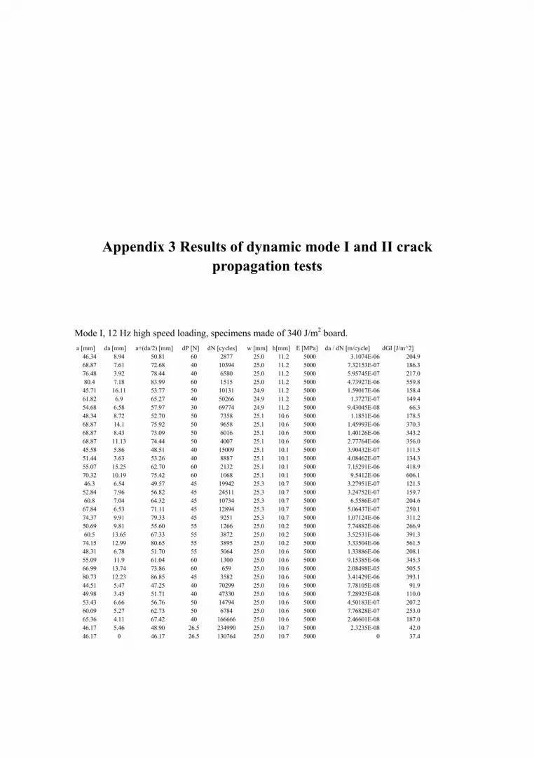
Appendix 3 Results of dynamic mode I and II crack propagation tests

Mode I, 12 Hz high speed loading, specimens made of 340 J/m2 board.

a [mm] da [mm] a+(da/2) [mm] dP [N] dN [cycles] w [mm] h[mm] E [MPa] da / dN [m/cycle] dGI [J/m^2]46.34 8.94 50.81 60 2877 25.0 11.2 5000 3.1074E-06 204.968.87 7.61 72.68 40 10394 25.0 11.2 5000 7.32153E-07 186.376.48 3.92 78.44 40 6580 25.0 11.2 5000 5.95745E-07 217.080.4 7.18 83.99 60 1515 25.0 11.2 5000 4.73927E-06 559.845.71 16.11 53.77 50 10131 24.9 11.2 5000 1.59017E-06 158.461.82 6.9 65.27 40 50266 24.9 11.2 5000 1.3727E-07 149.454.68 6.58 57.97 30 69774 24.9 11.2 5000 9.43045E-08 66.348.34 8.72 52.70 50 7358 25.1 10.6 5000 1.1851E-06 178.568.87 14.1 75.92 50 9658 25.1 10.6 5000 1.45993E-06 370.368.87 8.43 73.09 50 6016 25.1 10.6 5000 1.40126E-06 343.268.87 11.13 74.44 50 4007 25.1 10.6 5000 2.77764E-06 356.045.58 5.86 48.51 40 15009 25.1 10.1 5000 3.90432E-07 111.551.44 3.63 53.26 40 8887 25.1 10.1 5000 4.08462E-07 134.355.07 15.25 62.70 60 2132 25.1 10.1 5000 7.15291E-06 418.970.32 10.19 75.42 60 1068 25.1 10.1 5000 9.5412E-06 606.146.3 6.54 49.57 45 19942 25.3 10.7 5000 3.27951E-07 121.552.84 7.96 56.82 45 24511 25.3 10.7 5000 3.24752E-07 159.760.8 7.04 64.32 45 10734 25.3 10.7 5000 6.5586E-07 204.667.84 6.53 71.11 45 12894 25.3 10.7 5000 5.06437E-07 250.174.37 9.91 79.33 45 9251 25.3 10.7 5000 1.07124E-06 311.250.69 9.81 55.60 55 1266 25.0 10.2 5000 7.74882E-06 266.960.5 13.65 67.33 55 3872 25.0 10.2 5000 3.52531E-06 391.374.15 12.99 80.65 55 3895 25.0 10.2 5000 3.33504E-06 561.548.31 6.78 51.70 55 5064 25.0 10.6 5000 1.33886E-06 208.155.09 11.9 61.04 60 1300 25.0 10.6 5000 9.15385E-06 345.366.99 13.74 73.86 60 659 25.0 10.6 5000 2.08498E-05 505.580.73 12.23 86.85 45 3582 25.0 10.6 5000 3.41429E-06 393.144.51 5.47 47.25 40 70299 25.0 10.6 5000 7.78105E-08 91.949.98 3.45 51.71 40 47330 25.0 10.6 5000 7.28925E-08 110.053.43 6.66 56.76 50 14794 25.0 10.6 5000 4.50183E-07 207.260.09 5.27 62.73 50 6784 25.0 10.6 5000 7.76828E-07 253.065.36 4.11 67.42 40 166666 25.0 10.6 5000 2.46601E-08 187.046.17 5.46 48.90 26.5 234990 25.0 10.7 5000 2.3235E-08 42.046.17 0 46.17 26.5 130764 25.0 10.7 5000 0 37.4

174 Mode I, 0.5 Hz low speed loading (tested with Lloyd), specimens made of 340 J/m2 board.

Mode II, 0.5 Hz low speed loading (tested with Lloyd), specimens made of 340 J/m2 board.

Mode II, 12 Hz high speed loading, specimens made of 340 J/m2 board.

a [mm] da [mm] a+(da/2) [mm] dP [N] dN [cycles] w [mm] h[mm] E [MPa] da / dN [m/cycle] dGI [J/m^2]44.75 11.59 50.55 55 10 25.1 10.6 5000 0.001159 198.456.34 2.45 57.57 55 150 25.1 10.6 5000 1.63333E-05 257.358.79 3.98 60.78 55 350 25.1 10.6 5000 1.13714E-05 286.962.77 2.11 63.83 55 200 25.1 10.6 5000 0.00001055 316.364.88 3.58 66.67 55 200 25.1 10.6 5000 0.0000179 345.145.5 17.33 54.17 60 10 25.1 10.6 5000 0.001733 271.362.83 2.36 64.01 60 140 25.1 10.6 5000 1.68571E-05 378.965.19 3.1 66.74 60 100 25.1 10.6 5000 0.000031 411.944.79 13.8 51.69 52 10 25.1 10.6 5000 0.00138 185.658.59 5.4 61.29 52 10 25.1 10.6 5000 0.00054 260.963.99 4.98 66.48 52 10 25.1 10.6 5000 0.000498 307.045.46 7.01 48.97 50 10 24.9 11.1 5000 0.000701 137.652.47 2.2 53.57 50 100 24.9 11.1 5000 0.000022 164.754.67 6.33 57.84 50 600 24.9 11.1 5000 0.00001055 191.9

a [mm] da [mm] a+(da/2) [mdP [N] dN [cycle w [mm] h[mm] E [MPa] G [MPa] L [mm] da / dN [m/cycle] dGI 2 [J/m^2]45.6 23.02 57.11 210 424 24.96 5.2 5000 1400 75 5.42925E-05 183.245.57 10.76 50.95 210 10 25.01 5.3 5000 1400 75 0.001076 143.445.72 9.49 50.465 195 200 25.03 5.0 5000 1400 75 0.00004745 137.643.51 6.38 46.7 195 720 25.09 5.2 5000 1400 75 8.86111E-06 109.449.89 5.44 52.61 195 200 25.09 5.2 5000 1400 75 0.0000272 138.655.33 5.14 57.9 195 200 25.09 5.2 5000 1400 75 0.0000257 167.760.47 3.22 62.08 195 200 25.09 5.2 5000 1400 75 0.0000161 192.745.45 3.1 47 185 2600 25.01 6.6 5000 1400 75 1.19231E-06 48.048.55 4.44 50.77 185 500 25.01 6.6 5000 1400 75 0.00000888 55.952.99 5.47 55.725 185 500 25.01 6.6 5000 1400 75 0.00001094 67.245.49 15.79 53.385 190 192 25.05 5.3 5000 1400 75 8.22396E-05 123.749.54 4.87 51.975 175 2000 25 5.4 5000 1400 75 0.000002435 98.054.41 2.8 55.81 175 500 25 5.4 5000 1400 75 0.0000056 112.957.21 2.46 58.44 175 1000 25 5.4 5000 1400 75 0.00000246 123.7

a [mm] da [mm] a+(da/2) [mdP [N] dN [cycle w [mm] h[mm] E [MPa] G [MPa] L [mm] da / dN [m/cycle] dG [J/m^2]46.89 2.44 48.11 120 52000 25.03 5.4 5000 1400 75 4.69231E-08 39.349.33 3.99 51.325 150 47582 25.03 5.4 5000 1400 75 8.38552E-08 69.853.32 4.01 55.325 160 50447 25.03 5.4 5000 1400 75 7.94894E-08 92.257.33 2.487 58.5735 180 14387 25.03 5.4 5000 1400 75 1.72864E-07 130.844.93 12.93 51.395 170 433 25.01 5.3 5000 1400 75 2.98614E-05 92.957.86 4.5 60.11 120 24015 25.01 5.3 5000 1400 75 1.87383E-07 63.246.24 3.33 47.905 150 10240 25.04 5.1 5000 1400 75 3.25195E-07 71.749.57 1.86 50.5 150 44294 25.04 5.1 5000 1400 75 4.19921E-08 79.645.03 14.35 52.205 175 7636 24.98 5.4 5000 1400 75 1.87926E-06 97.945.15 5.1 47.7 150 22260 25.01 5.3 5000 1400 75 2.29111E-07 63.350.25 2.44 51.47 160 13713 25.01 5.3 5000 1400 75 1.77933E-07 83.752.69 3.76 54.57 160 11561 25.01 5.3 5000 1400 75 3.25231E-07 94.054.46 12.01 60.465 160 8636 25.05 5.1 5000 1400 75 1.39069E-06 130.966.47 4.83 68.885 160 3453 25.05 5.1 5000 1400 75 1.39878E-06 169.845.8 6.19 48.895 140 20478 25.03 5.2 5000 1400 75 3.02276E-07 60.344.41 2.96 45.89 130 50000 25.07 5.2 5000 1400 75 5.92E-08 46.547.37 5.3 50.02 130 38227 25.07 5.2 5000 1400 75 1.38645E-07 55.243.63 5.67 46.465 160 10029 25.02 5.2 5000 1400 75 5.6536E-07 71.549.3 5.27 51.935 160 10773 25.02 5.2 5000 1400 75 4.89186E-07 89.154.57 4.99 57.065 160 10177 25.02 5.2 5000 1400 75 4.90321E-07 107.545.92 2.62 47.23 170 3663 25.01 5.2 5000 1400 75 7.15261E-07 83.448.54 2.98 50.03 185 10136 25.01 5.2 5000 1400 75 2.94002E-07 110.744.06 19.07 53.595 130 9879 24.96 5.2 5000 1400 75 1.93036E-06 62.448.55 2.69 49.895 120 27412 25.04 5.2 5000 1400 75 9.81322E-08 45.645.64 9.1 50.19 120 53200 25.1 5.3 5000 1400 75 1.71053E-07 44.554.74 7.06 58.27 140 17800 25.1 5.3 5000 1400 75 3.96629E-07 81.4

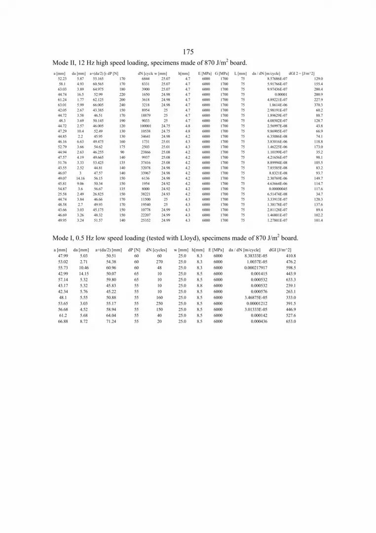
175Mode II, 12 Hz high speed loading, specimens made of 870 J/m2 board.

Mode I, 0.5 Hz low speed loading (tested with Lloyd), specimens made of 870 J/m2 board.

a [mm] da [mm] a+(da/2) [mdP [N] dN [cycle w [mm] h[mm] E [MPa] G [MPa] L [mm] da / dN [m/cycle] dGI 2 = [J/m^2]52.23 5.87 55.165 170 6844 25.07 4.7 6000 1700 75 8.57686E-07 129.058.1 4.93 60.565 170 8331 25.07 4.7 6000 1700 75 5.91766E-07 155.463.03 3.89 64.975 180 3900 25.07 4.7 6000 1700 75 9.97436E-07 200.444.74 16.5 52.99 220 1650 24.98 4.7 6000 1700 75 0.00001 200.961.24 1.77 62.125 200 3618 24.98 4.7 6000 1700 75 4.89221E-07 227.963.01 5.99 66.005 240 3218 24.98 4.7 6000 1700 75 1.8614E-06 370.342.05 2.67 43.385 150 8954 25 4.7 6000 1700 75 2.98191E-07 60.244.72 3.58 46.51 170 18879 25 4.7 6000 1700 75 1.89629E-07 88.748.3 3.69 50.145 190 9033 25 4.7 6000 1700 75 4.08502E-07 128.744.72 2.57 46.005 120 100001 24.75 4.8 6000 1700 75 2.56997E-08 43.847.29 10.4 52.49 130 10538 24.75 4.8 6000 1700 75 9.86905E-07 66.944.85 2.2 45.95 130 34641 24.98 4.2 6000 1700 75 6.35086E-08 74.146.16 6.63 49.475 160 1731 25.01 4.3 6000 1700 75 3.83016E-06 118.852.79 3.66 54.62 175 2503 25.01 4.3 6000 1700 75 1.46225E-06 173.044.94 2.63 46.255 90 23866 25.08 4.2 6000 1700 75 1.10199E-07 35.247.57 4.19 49.665 140 9937 25.08 4.2 6000 1700 75 4.21656E-07 98.151.76 3.33 53.425 135 37416 25.08 4.2 6000 1700 75 8.89994E-08 105.543.55 2.52 44.81 140 32078 24.98 4.2 6000 1700 75 7.85585E-08 83.246.07 3 47.57 140 33967 24.98 4.2 6000 1700 75 8.8321E-08 93.749.07 14.16 56.15 150 6136 24.98 4.2 6000 1700 75 2.30769E-06 149.745.81 9.06 50.34 150 1954 24.92 4.2 6000 1700 75 4.63664E-06 114.754.87 3.6 56.67 135 8000 24.92 4.2 6000 1700 75 0.00000045 117.625.58 2.49 26.825 150 38221 24.93 4.2 6000 1700 75 6.51474E-08 34.744.74 3.84 46.66 170 11500 25 4.3 6000 1700 75 3.33913E-07 120.348.58 2.7 49.93 170 19540 25 4.3 6000 1700 75 1.38178E-07 137.643.66 3.03 45.175 150 10778 24.99 4.3 6000 1700 75 2.81128E-07 89.446.69 3.26 48.32 150 22207 24.99 4.3 6000 1700 75 1.46801E-07 102.249.95 3.24 51.57 140 25352 24.99 4.3 6000 1700 75 1.27801E-07 101.4

a [mm] da [mm] a+(da/2) [mm] dP [N] dN [cycles] w [mm] h[mm] E [MPa] da / dN [m/cycle] dGI [J/m^2]47.99 5.03 50.51 60 60 25.0 8.3 6000 8.38333E-05 410.853.02 2.71 54.38 60 270 25.0 8.3 6000 1.0037E-05 476.255.73 10.46 60.96 60 48 25.0 8.3 6000 0.000217917 598.542.99 14.15 50.07 65 10 25.0 8.5 6000 0.001415 443.957.14 5.32 59.80 65 10 25.0 8.5 6000 0.000532 633.343.17 5.32 45.83 55 10 25.0 8.8 6000 0.000532 239.142.34 5.76 45.22 55 10 25.0 8.5 6000 0.000576 263.148.1 5.55 50.88 55 160 25.0 8.5 6000 3.46875E-05 333.053.65 3.03 55.17 55 250 25.0 8.5 6000 0.00001212 391.556.68 4.52 58.94 55 150 25.0 8.5 6000 3.01333E-05 446.961.2 5.68 64.04 55 40 25.0 8.5 6000 0.000142 527.666.88 8.72 71.24 55 20 25.0 8.5 6000 0.000436 653.0

176Mode I, 12 Hz high speed loading, specimens made of 870 J/m2 board.

a [mm] da [mm] a+(da/2) [mm] dP [N] dN [cycles] w [mm] h[mm] E [MPa] da / dN [m/cycle] dGI [J/m^2]43.37 6.13 46.44 50 12801 25.0 9.2 6000 4.78869E-07 177.249.5 9.83 54.42 40 183231 25.0 9.2 6000 5.36481E-08 155.859.33 8.75 63.71 40 62220 25.0 9.2 6000 1.4063E-07 213.568.08 4.1 70.13 40 3798 25.0 9.2 6000 1.07952E-06 258.772.18 4.42 74.39 40 9097 25.0 9.2 6000 4.85874E-07 291.176.6 4.1 78.65 40 9733 25.0 9.2 6000 4.21247E-07 325.443.3 12.55 49.58 55 6124 25.0 8.4 6000 2.04931E-06 326.155.85 2.7 57.20 45 12953 25.0 8.4 6000 2.08446E-07 290.658.55 8.73 62.92 45 29869 25.0 8.4 6000 2.92276E-07 351.667.28 7.72 71.14 35 76987 25.0 8.4 6000 1.00277E-07 272.0

75 4.45 77.23 40 10756 25.0 8.4 6000 4.13723E-07 418.679.45 3.63 81.27 30 61284 25.0 8.4 6000 5.92324E-08 260.742.05 13.63 48.87 75 400 25.1 8.4 6000 0.000034075 581.555.68 13.31 62.34 45 27500 25.1 8.4 6000 0.000000484 340.768.99 17.26 77.62 40 12896 25.1 8.4 6000 1.3384E-06 417.346.75 9.88 51.69 60 8726 25.0 8.4 6000 1.13225E-06 421.656.63 14.85 64.06 50 46249 25.0 8.4 6000 3.21088E-07 449.671.48 3.93 73.45 50 5053 25.0 8.4 6000 7.77756E-07 591.175.41 5.23 78.03 45 15592 25.0 8.4 6000 3.35428E-07 540.480.64 6.97 84.13 45 3640 25.0 8.4 6000 1.91484E-06 628.246.67 6.37 49.86 35 93732 25.0 8.8 6000 6.79597E-08 112.853.04 6.78 56.43 35 36062 25.0 8.8 6000 1.8801E-07 144.659.82 1.81 60.73 35 75654 25.0 8.8 6000 2.39247E-08 167.445.32 4.32 47.48 50 5414 26.0 8.5 6000 7.97931E-07 215.149.64 12.21 55.75 90 363 26.0 8.5 6000 3.36364E-05 960.661.85 13.02 68.36 70 3783 26.0 8.5 6000 3.44171E-06 873.974.87 6.86 78.30 60 3035 26.0 8.5 6000 2.2603E-06 842.381.73 5.23 84.35 50 5381 26.0 8.5 6000 9.71938E-07 678.844.24 6.39 47.44 60 2000 25.0 8.3 6000 0.000003195 361.450.63 5.73 53.50 60 3508 25.0 8.3 6000 1.63341E-06 459.656.36 4.73 58.73 60 9542 25.0 8.3 6000 4.95703E-07 553.861.09 4.93 63.56 60 7062 25.0 8.3 6000 6.98103E-07 648.726.9 7.76 30.78 80 5646 25.0 8.4 6000 1.37442E-06 261.334.66 5.32 37.32 80 5224 25.0 8.4 6000 1.01838E-06 384.139.98 6.6 43.28 80 3536 25.0 8.4 6000 1.86652E-06 516.646.58 17.26 55.21 80 1112 25.0 8.4 6000 1.55216E-05 840.663.84 11.85 69.77 60 1985 25.0 8.4 6000 5.96977E-06 755.046.05 8.29 50.20 60 7031 25.0 8.5 6000 1.17906E-06 374.554.34 10.43 59.56 60 11737 25.0 8.5 6000 8.88643E-07 527.364.77 3.36 66.45 60 3048 25.0 8.5 6000 1.10236E-06 656.468.13 7.57 71.92 60 6564 25.0 8.5 6000 1.15326E-06 768.875.7 11.15 81.28 50 11225 25.0 8.5 6000 9.93318E-07 681.942.4 11.16 47.98 70 5015 25.0 8.3 6000 2.22532E-06 498.053.56 8.05 57.59 70 5716 25.0 8.3 6000 1.40833E-06 717.461.61 5.31 64.27 70 5907 25.0 8.3 6000 8.98933E-07 893.466.92 4.85 69.35 60 12200 25.0 8.3 6000 3.97541E-07 764.324.94 10.61 30.25 80 3546 25.0 8.3 6000 2.9921E-06 264.035.55 9.99 40.55 80 8444 25.0 8.3 6000 1.18309E-06 474.545.54 13.19 52.14 70 7651 25.0 8.3 6000 1.72396E-06 600.658.73 10.19 63.83 50 22310 25.0 8.3 6000 4.56746E-07 459.368.92 8.77 73.31 55 3481 25.0 8.3 6000 2.51939E-06 733.145.84 11.1 51.39 70 2739 25.0 8.4 6000 4.05257E-06 554.356.94 6.12 60.00 70 4168 25.0 8.4 6000 1.46833E-06 755.663.06 6.67 66.40 50 14004 25.0 8.4 6000 4.76292E-07 472.169.73 5.77 72.62 60 2733 25.0 8.4 6000 2.11123E-06 813.175.5 7.56 79.28 50 4430 25.0 8.4 6000 1.70655E-06 673.145.6 7.55 49.38 50 10119 25.0 8.5 6000 7.46121E-07 258.453.15 9.05 57.68 80 1000 25.0 8.5 6000 0.00000905 902.662.2 8.78 66.59 55 10669 25.0 8.5 6000 8.22945E-07 568.770.98 8.22 75.09 50 15790 25.0 8.5 6000 5.20583E-07 597.679.2 7.09 82.75 50 6348 25.0 8.5 6000 1.11689E-06 725.7

177Mode I, 12 Hz high speed loading, specimens made of 1019 J/m2 board. a [m m ] da [m m ] a+(da/2) [m m ] dP [N] dN [cycles] w [m m ] h[m m ] E [MPa] da / dN [m /cycle] dGI [J/m ^2]

45.5 10.75 50.88 50 30611 25.2 9.2 6000 3.51181E-07 211.656.25 3.28 57.89 50 14187 25.2 9.2 6000 2.31198E-07 273.959.53 9.32 64.19 55 2657 25.2 9.2 6000 3.50772E-06 407.568.85 4.41 71.06 40 24805 25.2 9.2 6000 1.77787E-07 264.144.7 6.89 48.15 65 9268 25.2 9.0 6000 7.43418E-07 335.9

51.59 8.13 55.66 60 13258 25.2 9.0 6000 6.13215E-07 382.559.72 2.81 61.13 50 34830 25.2 9.0 6000 8.06776E-08 320.462.53 7.14 66.10 55 5034 25.2 9.0 6000 1.41836E-06 453.369.67 3.65 71.50 45 22569 25.2 9.0 6000 1.61726E-07 355.073.32 4.43 75.54 35 25183 25.2 9.0 6000 1.75912E-07 239.777.75 7.2 81.35 35 32574 25.2 9.0 6000 2.21035E-07 278.144.2 4.93 46.67 30 171631 25.1 9.1 6000 2.87244E-08 66.5

49.13 2.25 50.26 35 174079 25.1 9.1 6000 1.29252E-08 105.151.38 3.1 52.93 45 104272 25.1 9.1 6000 2.97299E-08 192.654.48 4.77 56.87 45 46319 25.1 9.1 6000 1.02981E-07 222.359.25 3.05 60.78 45 21172 25.1 9.1 6000 1.44058E-07 254.062.3 6.98 65.79 50 8350 25.1 9.1 6000 8.35928E-07 367.4

69.28 4.77 71.67 35 104094 25.1 9.1 6000 4.5824E-08 213.674.05 3.05 75.58 35 59891 25.1 9.1 6000 5.09258E-08 237.644.49 3.62 46.30 40 125832 25.1 9.1 6000 2.87685E-08 116.648.11 3.55 49.89 40 62245 25.1 9.1 6000 5.70327E-08 135.451.66 6.38 54.85 40 179382 25.1 9.1 6000 3.55666E-08 163.758.04 3.15 59.62 40 6576 25.1 9.1 6000 4.79015E-07 193.461.19 5.05 63.72 40 8592 25.1 9.1 6000 5.87756E-07 220.966.24 4.44 68.46 40 10303 25.1 9.1 6000 4.30942E-07 255.070.68 2.19 71.78 40 3585 25.1 9.1 6000 6.10879E-07 280.372.87 4.9 75.32 35 12144 25.1 9.1 6000 4.03491E-07 236.377.77 5.38 80.46 26 40903 25.1 9.1 6000 1.31531E-07 148.883.15 3.31 84.81 28 10314 25.1 9.1 6000 3.20923E-07 191.746.13 5.5 48.88 60 2402 25.1 8.7 6000 2.28976E-06 333.151.63 7.35 55.31 50 19808 25.1 8.7 6000 3.71062E-07 296.158.98 6.36 62.16 45 32029 25.1 8.7 6000 1.9857E-07 303.065.34 3.59 67.14 40 48811 25.1 8.7 6000 7.3549E-08 279.268.93 8.26 73.06 45 38941 25.1 8.7 6000 2.12116E-07 418.577.19 3.64 79.01 45 23321 25.1 8.7 6000 1.56083E-07 489.545.02 6.47 48.26 70 1212 25.1 8.8 6000 5.33828E-06 425.951.49 3.84 53.41 50 4800 25.1 8.8 6000 0.0000008 266.255.33 3.9 57.28 50 9986 25.1 8.8 6000 3.90547E-07 306.259.23 1.96 60.21 60 1212 25.1 8.8 6000 1.61716E-06 487.161.19 2.8 62.59 50 7380 25.1 8.8 6000 3.79404E-07 365.663.99 7.45 67.72 40 31324 25.1 8.8 6000 2.37837E-07 273.852.66 14.72 60.02 90 1013 25.1 8.9 6000 1.45311E-05 1041.567.38 4.87 69.82 80 3550 25.1 8.9 6000 1.37183E-06 1113.446.87 14.17 53.96 100 549 25.1 9.2 6000 2.58106E-05 962.861.04 13.37 67.73 80 7152 25.1 9.2 6000 1.86941E-06 970.874.41 5.94 77.38 60 2403 25.1 9.2 6000 2.47191E-06 712.980.35 6.5 83.60 60 1784 25.1 9.2 6000 3.6435E-06 832.186.85 9.06 91.38 45 2105 25.1 9.2 6000 4.30404E-06 559.245.03 6.09 48.08 75 2180 25.1 9.0 6000 2.79358E-06 456.751.12 9.49 55.87 75 3412 25.1 9.0 6000 2.78136E-06 616.760.61 5.95 63.59 70 1580 25.1 9.0 6000 3.76582E-06 696.066.56 4.2 68.66 70 1756 25.1 9.0 6000 2.3918E-06 811.570.76 5.83 73.68 65 3525 25.1 9.0 6000 1.6539E-06 805.776.59 2.48 77.83 60 7023 25.1 9.0 6000 3.53125E-07 766.143.72 3.9 45.67 70 3087 25.2 8.9 6000 1.26336E-06 370.547.62 3.29 49.27 70 4591 25.2 8.9 6000 7.16619E-07 431.250.91 2.93 52.38 70 5565 25.2 8.9 6000 5.26505E-07 487.353.84 2.59 55.14 70 7026 25.2 8.9 6000 3.68631E-07 540.056.43 4.28 58.57 80 1263 25.2 8.9 6000 3.38876E-06 796.060.71 9.1 65.26 80 2936 25.2 8.9 6000 3.09946E-06 988.269.81 5.04 72.33 70 3031 25.2 8.9 6000 1.66282E-06 929.474.85 4.47 77.09 75 1002 25.2 8.9 6000 4.46108E-06 1211.879.32 3.27 80.96 65 1218 25.2 8.9 6000 2.68473E-06 1003.949.35 4.58 51.64 45 7331 25.0 9.6 6000 6.24744E-07 154.853.93 2.9 55.38 50 7019 25.0 9.6 6000 4.13164E-07 219.856.83 7.45 60.56 80 1209 25.0 9.6 6000 6.16212E-06 672.764.28 5.55 67.06 70 3563 25.0 9.6 6000 1.55768E-06 631.569.83 5.57 72.62 70 4009 25.0 9.6 6000 1.38937E-06 740.675.4 6.38 78.59 70 2500 25.0 9.6 6000 0.000002552 867.5

46.32 8.37 50.51 80 904 25.1 9.0 6000 9.25885E-06 570.554.69 3.54 56.46 80 2524 25.1 9.0 6000 1.40254E-06 713.058.23 7.29 61.88 80 2566 25.1 9.0 6000 2.841E-06 856.365.52 12.03 71.54 65 920 25.1 9.0 6000 1.30761E-05 755.6

45 0 45.00 30 451295 25.0 9.0 6000 0 63.254.33 4.94 56.80 30 600502 25.0 9.0 6000 8.22645E-09 100.6

178Mode I, 0.5 Hz low speed loading (tested with Lloyd), specimens made of 1019 J/m2 board.

Mode II, 0.5 Hz high speed loading, specimens made of 1019 J/m2 board.

Mode II, 12 Hz Low speed loading (tested with Lloyd), specimens made of 1019 J/m2 board.

a [mm] da [mm] a+(da/2) [mm] dP [N] dN [cycles] w [mm] h[mm] E [MPa] da / dN [m/cycle] dGI [J/m^2]44.22 6.07 47.26 60 10 25.0 8.9 6000 0.000607 291.050.29 9.09 54.84 60 20 25.2 9.2 6000 0.0004545 353.944.48 9.95 49.46 60 10 25.0 8.3 6000 0.000995 398.754.43 5.54 57.20 60 20 25.0 8.3 6000 0.000277 533.359.97 5.58 62.76 60 30 25.0 8.3 6000 0.000186 642.165.55 11.51 71.31 60 10 25.0 8.3 6000 0.001151 828.848.89 3.25 50.52 50 30 25.1 9.3 6000 0.000108333 201.452.14 1.8 53.04 50 100 25.1 9.3 6000 0.000018 222.153.94 3.71 55.80 55 90 25.1 9.3 6000 4.12222E-05 297.357.65 6.02 60.66 55 500 25.1 9.3 6000 0.00001204 351.463.67 4.02 65.68 55 400 25.1 9.3 6000 0.00001005 412.067.69 4.64 70.01 55 200 25.1 9.3 6000 0.0000232 468.172.33 3.52 74.09 55 100 25.1 9.3 6000 0.0000352 524.346.42 8.13 50.49 65 10 25.1 9.1 6000 0.000813 369.054.55 3.07 56.09 65 10 25.1 9.1 6000 0.000307 455.457.62 5.51 60.38 65 80 25.1 9.1 6000 0.000068875 527.763.13 4.08 65.17 65 50 25.1 9.1 6000 0.0000816 614.8

a [mm] da [mm] a+(da/2) [mdP [N] dN [cycle w [mm] h[mm] E [MPa] G [MPa] L [mm] da / dN [m/cycle] dGI 2 = [J/m^2]45.8 5.57 48.585 150 26012 25.05 4.4 6000 1800 75 2.14132E-07 96.6

51.37 2.25 52.495 150 82538 25.05 4.4 6000 1800 75 2.72602E-08 112.751.36 4.87 53.795 180 5089 25.1 4.5 6000 1800 75 9.56966E-07 155.956.23 2.2 57.33 180 4946 25.1 4.5 6000 1800 75 4.44804E-07 177.058.43 4.9 60.88 180 7504 25.1 4.5 6000 1800 75 6.52985E-07 199.547.91 3.75 49.785 150 22914 24.88 4.5 6000 1800 75 1.63655E-07 90.544.31 2.89 45.755 130 45458 25.04 4.4 6000 1800 75 6.35752E-08 63.8

a [mm] da [mm] a+(da/2) [mdP [N] dN [cycle w [mm] h[mm] E [MPa] G [MPa] L [mm] da / dN [m/cycle] dGI 2 = [J/m^2]51.13 4.45 53.355 220 50 25.04 4.6 6000 1800 75 0.000089 219.055.58 3.79 57.475 220 50 25.04 4.4 6000 1800 75 0.0000758 290.543.44 2.35 44.615 210 500 25.03 4.4 6000 1800 75 0.0000047 160.645.79 5.75 48.665 210 1750 25.03 4.4 6000 1800 75 3.28571E-06 190.951.54 2.41 52.745 210 300 25.03 4.4 6000 1800 75 8.03333E-06 224.153.95 2.56 55.23 210 170 25.03 4.4 6000 1800 75 1.50588E-05 245.656.51 2.08 57.55 210 800 25.03 4.4 6000 1800 75 0.0000026 266.544.87 4.49 47.115 230 1500 25.03 4.4 6000 1800 75 2.99333E-06 214.749.36 3.69 51.205 230 400 25.03 4.4 6000 1800 75 0.000009225 253.453.05 9.08 57.59 230 173 25.03 4.4 6000 1800 75 5.24855E-05 320.243.23 6.56 46.51 220 700 25.03 4.4 6000 1800 75 9.37143E-06 191.449.79 7.26 53.42 220 250 25.03 4.4 6000 1800 75 0.00002904 252.257.05 8.28 61.19 220 480 25.03 4.4 6000 1800 75 0.00001725 330.643.79 5.65 46.615 240 500 25.03 4.4 6000 1800 75 0.0000113 228.949.44 16.06 57.47 240 440 25.03 4.4 6000 1800 75 0.0000365 347.242.93 4.09 44.975 240 260 25.03 4.5 6000 1800 75 1.57308E-05 191.347.02 17.33 55.685 240 500 25.03 4.5 6000 1800 75 0.00003466 292.645.84 5.41 48.545 240 50 24.04 4.3 6000 1800 75 0.0001082 279.451.25 12.34 57.42 238 94 24.04 4.3 6000 1800 75 0.000131277 383.843.43 2.8 44.83 240 370 25 4.4 6000 1800 75 7.56757E-06 199.046.23 2.72 47.59 240 150 25 4.4 6000 1800 75 1.81333E-05 224.148.95 5.96 51.93 240 220 25 4.4 6000 1800 75 2.70909E-05 266.654.91 4.64 57.23 240 70 25 4.4 6000 1800 75 6.62857E-05 323.549.52 5.18 52.11 250 64 25.17 4.4 6000 1800 75 8.09375E-05 287.454.7 5.07 57.235 250 100 25.17 4.4 6000 1800 75 0.0000507 346.4

45.77 4.09 47.815 250 116 25.07 4.1 6000 1800 75 3.52586E-05 308.549.86 7.89 53.805 250 200 25.07 4.1 6000 1800 75 0.00003945 390.343.97 7.25 47.595 260 100 25.12 4.2 6000 1800 75 0.0000725 300.151.22 8.37 55.405 260 35 25.12 4.2 6000 1800 75 0.000239143 406.046.21 7.81 50.115 260 45 25.11 4.3 6000 1800 75 0.000173556 321.354.02 4.51 56.275 260 20 25.11 4.3 6000 1800 75 0.0002255 404.749.4 5.34 52.07 260 85 25.07 4.4 6000 1800 75 6.28235E-05 328.0

54.74 4.19 56.835 250 110 25.07 4.4 6000 1800 75 3.80909E-05 361.047.73 9.81 52.635 260 50 25.12 4.2 6000 1800 75 0.0001962 371.844.94 4.54 47.21 260 75 25.03 4.1 6000 1800 75 6.05333E-05 321.749.48 3.2 51.08 240 67 25.03 4.1 6000 1800 75 4.77612E-05 320.6

Appendix 4 Crack propagation in 76x15 mm cores

Contents

Test series 1. 6 crack propagation tests of cores with no initial cracks ……………..... 181 Test series 2. 9 crack propagation tests of spiral cores ………………...…….……..… 187 Test series 3. 10 crack propagation tests of cores with 11 initial cracks ……………... 196 Test series 4. 8 crack propagation tests of cores with a single initial crack ………….. 206 Test series 5. 2 crack propagation tests of cores constructed of two materials ………. 214

General

The idea here is to study crack growth in 100 mm long 76x15 mm core samples which are loaded in a winding simulator. Since it is not possible to see inside the cores, the only possibility is to make observations from both core ends. Images in this appendix show examples of these tests. Most of the tests have been done with the belt tester with a 10 kN constant load but in some tests the load has been 15 kN. The revolution speed is 500 rpm in all tests. The tester has been stopped after a certain number of revolutions and a picture has been taken from both sides of a test core. The test has been continued until the core has completely delaminated.

Figure a4.1 and a4.2 are examples of the figures in this appendix. The curves in figure a4.1 represent the total length of smaller and longer cracks in the vicinity of core wall cross section center line as a function of revolutions. The small cracks which were not at the main crack line and which did not keep growing, were not considered. The lines with “o” and triangle symbols show the total crack length on the front and back sides of a core. The thin dash line represents the least squares estimate of data points on both sides of the core and shows the average crack length inside the core. The curve fit equation of this curve is shown under the legend in figure a4.1.

180Figure a4.2 shows the front and back side of the same core. The core has rotated 6100 revolutions and 20.1 % of the ”life time” is used. The front side is on the left and the back side on the right picture. The back side image is a mirror image by vertical axis so that it is easier to compare the position of cracks on both sides.

Fig. a4.1. Crack propagation during the test. Fig. a4.2. 6100 revolutions, 20.1 % of the life time used.

0 5000 10000 15000 20000 25000 30000


0

50

100

150

200

250

300

350

Cra

ck le

ngth

[mm

]



14.97 * e(0.0002177*x - 1.039E-008*x2 + 2.178E-013*x3)

181 Crack propagation. 1000 rev., 4.2 % of life time used. 3 and 7 mm cracks.

3500 rev., 15.0 %. 5200 rev., 22.0 %. 6700 rev., 28.0 %. 8200 rev., 35.0 %. 12700 rev., 54.0 %. 14200 rev., 60.0 %. 15700 rev., 66 %. 17200 rev., 72.0 %.

18700 rev., 79.0 %. 20500 rev., 86.0 %. 22000 rev., 93.0 %. 23730 rev., 100 %. Fig. a4.3. Test series 1, test 1/6. Crack propagation test of a 76x15 mm core with no initial cracks. Constant load 15 kN, revolution speed 500 rpm. Chuck load capacity of the test core is 3 tons. Crack propagation on the front side of the core.

0 5000 10000 15000 20000 25000 30000


0

50

100

150

200

250

Cra

ck le

ngth

[mm

]


front sidecurve fit -23.46 + 0.01197*x

182

Crack propagation during the test. 500 rev., 1.9%. 2000 rev, 7.7 %.

7500 rev., 29.0%. 9900 rev., 38.2%. 12500 rev., 48.3%. 14500 rev., 56.0%.

16500 rev., 63.7 %. 18500 r., 71.5%. 20500 r., 79.2%. 21500 r., 83.0 %.

23000 rev., 88.8 %. 25000 rev., 96.6 %. 25892 rev., 100 % (split core). Fig. a4.4. Test series 1, test 2/6. Crack propagation test of a 76x15 mm core with no initial cracks. Constant load 15 kN, revolution speed 500 rpm. Chuck load capacity of the test core is 3 tons. Crack propagation on the front side of the core.

0 5000 10000 15000 20000 25000 30000


0

50

100

150

200

250

Cra

ck le

ngth

[mm

]


front sidecurve fit 5.416 + 0.004713*x + 1.927E-007*x2

183 Crack propagation during the test. 500 revolutions, 2.1 %. 1000 revolutions, 4.1 %. 4000 revolutions, 16.5 %. 5500 revolutions, 22.7 %. 7000 revolutions, 28.9 %. 24000 revolutions, 98.9 %. 24245 revolutions, 100 %. Fig. a4.5. Test series 1, test 3/6. Crack propagation test of a 76x15 mm core with no initial cracks. Constant load 15 kN, revolution speed 500 rpm. Chuck load capacity of the test core is 3 tons. Crack propagation on the front and back sides of the core.

0 5000 10000 15000 20000 25000 30000


0

50

100

150

200

250

Cra

ck le

ngth

[mm

]

Crack length growth in core wall as a function of revolutions 76x15 mm parallel core with no initial cracks. Load 15 kN. Crack propagation on front side.

front sidecurve fit

6.055 + 0.01087*x - 3.297E-007*x2 + 1.304E-011*x3

184 Crack propagation during the test. 250 rev., 1.0 %. 500 rev., 1.9 %. 1000 rev., 3.9 %. 3000 rev., 11.7 %. 5000 rev., 19.5 %. 6500 rev., 25.3 %. 9500 rev., 37.0 %. 12500 rev., 48.6 %. 15500 rev., 60.3 %. 18500 rev., 72.0 %.

21500 r., 83.7 %. 24500 r., 95.3 %. 25700 r., 100 %. Crack surfaces. Fig. a4.6. Test series 1, test 4/6. Crack propagation test of a 76x15 mm core with no initial cracks. Constant load 15 kN, revolution speed 500 rpm. Chuck load capacity of the test core is 3 tons. Crack propagation on the front side of the core.

0 5000 10000 15000 20000 25000 30000


0

50

100

150

200

250

Cra

ck le

ngth

[mm

]

Crack length growth in core wall as a function of revolutions 76x15 mm parallel core with no initial cracks. Load 15 kN. Crack propagation on back side.

back sidecurve fit 6.353 * e(0.0004962*x - 3.156E-008*x2 + 6.982E-013*x3)

185

Crack propagation during the test. 1500 rev., 7.9 %. 5500 rev., 29.1 %. 8500 rev., 44.9 %.

12500 rev. 66.1 %. 14500 rev., 76.6 %. 17500 rev., 92.5 %. 18919 rev., 100 %. Fig. a4.7. Test series 1, test 5/6. Crack propagation test of a 76x15 mm core with no initial cracks. Constant load 15 kN, revolution speed 500 rpm. Chuck load capacity of the test core is 3 tons. Crack propagation on the front and back sides of the core.

0 5000 10000 15000 20000 25000 30000


0

50

100

150

200

250

Cra

ck le

ngth

[mm

]

Crack length growth in core wall as a function of revolutions 76x15 mm core with no initial cracks. Load 15 kN.

front sideback sidefity 3.903E+004 * x(-3.403 + 0.2963*ln x)

186

Crack propagation during the test. 250 revolutions, 0.45 %. 11000 revolutions, 19.8 %. 25500 revolutions, 45.9 %. 42000 revolutions, 75.6 %. 55000 revolutions, 99.0 %. 55530 revolutions, 100 %. Crack surfaces. Fig. a4.8. Test series 1, test 6/6. Crack propagation test of a 76x15 mm core with no initial cracks. Constant load 15 kN, revolution speed 500 rpm. Chuck load capacity of the test core is 3 tons. Crack propagation on the front and back sides of the core.

0 10000 20000 30000 40000 50000


0

50

100

150

200

250

Cra

ck le

ngth

[mm

]

Crack length growth in core wall as a function of revolutions 76x15 mm core with no initial cracks. Load 15 kN.

front sideback sidefity 7.908 * e(7.377E-005*x)

187

Crack propagation during the test. Start situation. Front and back side.

200 revolutions, 50 %. 200 revolutions, 50 %.

400 revolutions, 100 %. Crack surfaces. Fig. a4.9. Test series 2, test 1/9. Crack propagation test of a 76x15 mm spiral core. Constant load 15 kN, revolution speed 500 rpm. Chuck load capacity of the test core is 1.1 ton. The initial cracks are 4-10 mm long. Crack propagation on the front and back sides of the core.

0 50 100 150 200 250 300 350 400


0

100

200

300

400

500

600

700

Cra

ck le

ngth

[mm

]

Crack length growth in core wall as a function of revolutions 76x15 mm production core. Load 10 kN. Chuck load capacity 1.1 ton. Initial cracks 4 - 10 mm.

front sideBack sideCurve fit 10.09 * e(0.0005161*x + 2.467E-005*x2)

188

Crack propagation during the test. 200 rev., 3.5 %. 1300 rev., 22.9 %. 2300 rev., 40.6 %. 4700 rev., 82.9 %. 5200 rev., 91.7 %. 5670 rev., 100 %. Crack surfaces. Fig. a4.10. Test series 2, test 2/9. Crack propagation test of a 76x15 mm spiral core. Constant load 15 kN, revolution speed 500 rpm. Chuck load capacity of the test core is 2.11 tons. The initial cracks are 2-6 mm long. Crack propagation on the front side of the core.

0 1000 2000 3000 4000 5000 6000


0

50

100

150

200

250

300

Cra

ck le

ngth

[mm

]



4.274 * e(0.0008582*x - 4.877E-007*x2 + 8.02E-011*x3)

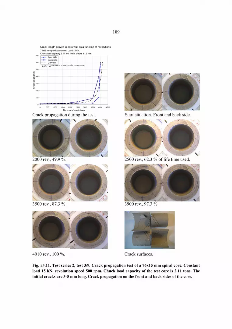
189

Crack propagation during the test. Start situation. Front and back side. 2000 rev., 49.9 %. 2500 rev., 62.3 % of life time used. 3500 rev., 87.3 % . 3900 rev., 97.3 %. 4010 rev., 100 %. Crack surfaces. Fig. a4.11. Test series 2, test 3/9. Crack propagation test of a 76x15 mm spiral core. Constant load 15 kN, revolution speed 500 rpm. Chuck load capacity of the test core is 2.11 tons. The initial cracks are 3-5 mm long. Crack propagation on the front and back sides of the core.

0 500 1000 1500 2000 2500 3000 3500 4000 4500


0

50

100

150

200

250

300

350

Cra

ck le

ngth

[mm

]



4.451 * e(0.001065*x - 7.205E-007*x2 + 1.708E-010*x3)

190

Crack propagation during the test. Start situation. 3200 revolutions, 16.2 %. 8700 revolutions, 44.2 %. 11700 revolutions, 59.4 %. 17700 revolutions, 89.8 %. 19700 revolutions, 100 %. Crack surfaces. Fig. a4.12. Test series 2, test 4/9. Crack propagation test of a 76x15 mm spiral core. Constant load 10 kN, revolution speed 500 rpm. Chuck load capacity of the test core is 2.24 tons. The initial cracks are 2-6 mm long. Crack propagation on the front and back sides of the core.

0 2500 5000 7500 10000 12500 15000 17500 20000


0

50

100

150

200

250

300

Cra

ck le

ngth

[mm

]



4.707 * e(0.0001296*x - 3.13E-008*x2 + 1.786E-012*x3)

191

Crack propagation during the test. Start situation. 10000 rev., 43.5 %. 16000 rev., 69.6 %. 18000 rev., 78.3 %. 20000 rev., 87.0 %. 23000 rev., 100 %. Crack surfaces. Fig. a4.13. Test series 2, test 5/9. Crack propagation test of a 76x15 mm spiral core. Constant load 10 kN, revolution speed 500 rpm. Chuck load capacity of the test core is 2.24 tons. The initial cracks are 2-6 mm long. Crack propagation on the front and back sides of the core.

0 2500 5000 7500 10000 12500 15000 17500 20000 22500 25000


0

50

100

150

200

250

300

350

Cra

ck le

ngth

[mm

]



5.454 * e(-0.0001279*x + 1.314E-008*x2)

192

Crack propagation during the test. 300 rev., 1.4 %. 13000 rev., 59.7 %. 7000 rev., 78.1 %. 19000 rev., 87.2 %. 21000 rev., 96.4 %. 21779 rev., 100 %. Crack surfaces. Fig. a4.14. Test series 2, test 6/9. Crack propagation test of 76x15 mm spiral core. Constant load 15 kN, revolution speed 500 rpm. Chuck load capacity of the test core is 2.78 tons. The initial cracks are 1.5-5 mm long. Crack propagation on the front and back sides of the core.

0 2500 5000 7500 10000 12500 15000 17500 20000 22500


0

100

200

300

400

Cra

ck le

ngth

[mm

]

Crack length growth in core wall as a function of revolutions 76x15 mm production core. Load 15 kN. Chuck load capacity 2.78 ton. Initial cracks 1.5 - 5 mm.


193

Crack propagation during the test. Start situation. 9800 rev., 56.5 %. 13800 rev., 79.5 %. 14800 rev., 85.3 %. 16800 rev., 96.8 %. 8500 rev., 39.0 %. Crack surfaces. Fig. a4.15. Test series 2, test 7/9. Crack propagation test of a 76x15 mm spiral core. Constant load 15 kN, revolution speed 500 rpm. Chuck load capacity of the test core is 2.78 tons. The initial cracks are 1.5-5 mm long. Crack propagation on the front and back sides of the core

0 2500 5000 7500 10000 12500 15000 17500 20000 22500


0

100

200

300

Cra

ck le

ngth

[mm

]


front sideBack sideCurve fit 4.5 * e(0.0003472*x - 5.157E-008*x2 + 2.564E-012*x3)

194

Crack propagation during the test. Start situation.

4050 rev., 33.0 %. 6050 rev., 49.2 %. 8500 rev., 65.5 %. 12050 rev., 98.0 %.

12290 rev., 100 %. Crack surfaces. Fig. a4.16. Test series 2, test 8/9. Crack propagation test of a 76x15 mm spiral core. Constant load 15 kN, revolution speed 500 rpm. Chuck load capacity of the test core is 2.9 ton. The initial cracks are 1.5-6 mm long. Crack propagation on the front and back sides of the core.

0 2500 5000 7500 10000 12500 15000 17500


0

100

200

300

400

500

600

700

800

900

Cra

ck le

ngth

[mm

]



4.817 * e(0.0005223*x - 1.479E-008*x2)

195

Crack propagation during the test. Start situation. 7600 rev., 41.1 %. 10600 revolutions, 57.3 %. 13600 rev., 73.5 %. 16300 rev., 88.1 %. 18506 rev., 100 %. Crack surfaces. Fig. a4.17. Test series 2, test 9/9. Crack propagation test of a 76x15 mm spiral core. Constant load 15 kN, revolution speed 500 rpm. Chuck load capacity of the test core is 2.9 ton. The initial cracks are 1-5 mm long. Crack propagation on the front and back sides of the core.

0 2500 5000 7500 10000 12500 15000 17500


0

200

400

600

Cra

ck le

ngth

[mm

]


front sideBack sideCurve fit 4.691 * e(8.957E-005*x + 9.772E-009*x2)

196

Crack propagation during the test. Start situation. 5200 rev., 25.1 %. 9200 rev., 44.4 %. 14200 rev., 68.6 %. 18200 rev., 87.9 %. 20700 rev., 100 %. Fracture surfaces. Fig. a4.18. Test series 3, test 1/10. Crack propagation test of a 76x15 mm core with 11 1-3 mm initial cracks, most cracks are 2 mm long. Constant load 10 kN, revolution speed 500 rpm. Crack propagation on the front and back sides of the core.

0 5000 10000 15000 20000


0

200

400

600

Cra

ck le

ngth

[mm

]

Crack length growth in core wall as a function of revolutions 76x15 mm core with 11 1 - 3 mm initial cracks. Most of the cracks 2 mm long. Load 1


17.24 + 0.03229*x - 9.808E-006*x2 + 1.284E-009*x3

- 2.029E-015*x4 - 1.164E-017*x5 + 8.088E-022*x6 - 1.615E-026*x7

197

Crack propagation during the test. Start situation. 5800 rev., 22.5 %. 10800 rev., 41.9 %. 18800 rev., 72.9 %. 22800 rev., 88.4 %. 25800 rev., 100 %. Fracture surfaces. Fig. a4.19. Test series 3, test 2/10. Crack propagation test of a 76x15 mm cores with 11 1-4 mm initial cracks, most cracks are 2 mm long. Constant load 10 kN, revolution speed 500 rpm. Crack propagation on the front and back sides of the core.

0 5000 10000 15000 20000 25000


0

200

400

600

Cra

ck le

ngth

[mm

]

Crack length growth in core wall as a function of revolutions 76x15 mm core with 11 1 - 4 mm initial cracks. Most of the cracks 2 mm long. Load 1

front sideBack sideCurve fit 15.06 + 0.002263*x + 3.675E-007*x2

198

Crack propagation during the test. Start situation. 6000 rev., 29.3 %. 12000 rev., 58.5 %. 18000 rev., 87.8 %. 20000 rev., 97.6 %. 20500 rev., 100 %. Fracture surfaces. Fig. a4.20. Test series 3, test 3/10. Crack propagation test of a 76x15 mm core with 11 2.5-4 mm initial cracks, most cracks 2.5 mm long. Constant load 10 kN, revolution speed 500 rpm. Crack propagation on the front and back sides of the core.

0 5000 10000 15000 20000


0

50

100

150

200

250

Cra

ck le

ngth

[mm

]

Crack length growth in core wall as a function of revolutions 76x15 mm core with 11 2.5 - 4 mm initial cracks. Most of the cracks 2.5 mm long. Lo

front sideBack sideCurve fit 33.19 * e(0.0001281*x - 1.296E-009*x2)

199

Crack propagation during the test. Start situation. 3000 rev., 21.1 %. 5000 rev., 35.1 %. 7000 rev., 49.1 %. 11000 rev., 77.2 %. 14250 rev., 100 %. Fracture surfaces. Fig. a4.21. Test series 3, test 4/10. Crack propagation test of a 76x15 mm core with 11 2.5-4 mm initial cracks, most cracks are 2.5 mm long. Constant load 10 kN, revolution speed 500 rpm. Crack propagation on the front and back sides of the core.

0 5000 10000 15000 20000


0

50

100

150

200

250

Cra

ck le

ngth

[mm

]

Crack length growth in core wall as a function of revolutions 76x15 mm core with 11 2.5 - 4 mm initial cracks. Most of the cracks 2.5 mm long. Load 10 kN.

front sideBack sideCurve fit 33.07 * e(0.0002635*x - 2.356E-008*x2 + 1.088E-012*x3)

200

Crack propagation during the test. Start situation. 2000 rev., 17.4 %. 4000 rev., 34.7 %. 6000 rev., 52.1 %. 8000 rev., 69.4 %. 11520 rev., 100 %. Fracture surfaces. Fig. a4.22. Test series 3, test 5/10. Crack propagation test of a 76x15 mm core with 11 initial cracks. 6-8 mm initial cracks, most cracks are 6 mm long. Constant load 10 kN, revolution speed 500 rpm. Crack propagation on the front and back sides of the core.

0 2000 4000 6000 8000 10000 12000


0

100

200

300

400

500

600

Cra

ck le

ngth

[mm

]


front sideBack sideCurve fit 32.77 * x(0.1937)

201

Crack propagation during the test. 500 rev., 6.6 %. 2500 rev., 32.9 %. 3500 rev., 46.1 %. 4500 rev., 59.2 %. 6500 rev., 85.5 %. 7600 rev., 100 %. Fracture surfaces. Fig. a4.23. Test series 3, test 6/10. Crack propagation test of 76x15 mm core with 11 6-8 mm initial cracks, most cracks are 6 mm long. Constant load 10 kN, revolution speed 500 rpm. Crack propagation on the front and back sides of the core.

0 2000 4000 6000 8000 10000 12000


0

100

200

300

400

500

600

Cra

ck le

ngth

[mm

]



202

Crack propagation during the test. Start situation. 1000 rev., 49.0 %. 2000 rev., 97.9 %. 2042 rev., 100 %. Fracture surfaces. Fig. a4.24. Test series 3, test 7/10. Crack propagation test of a 76x15 mm core with 11 5-8 mm initial cracks. Constant load is 15 kN, revolution speed 500 rpm. Crack propagation on the front and back sides of the core.

0 500 1000 1500 2000


0

100

200

300

400

Cra

ck le

ngth

[mm

]

Crack length growth in core wall as a function of revolutions 76x15 mm core with 11 5 - 8 mm initial cracks. Load 15 kN.

front sideBack sideCurve fit 96.19 * e(1.852E-005*x + 1.705E-007*x2)

203

Crack propagation during the test. Start situation. 700 revolutions, 87.5 %. 800 rev., 100 %. Fracture surfaces. Fig. a4.25. Test series 3, test 8/10. Crack propagation test of a 76x15 mm core with 11 5-8 mm initial cracks. Constant load is 15 kN, revolution speed 500 rpm. Crack propagation on the front and back sides of the core.

0 200 400 600 800


0

100

200

300

Cra

ck le

ngth

[mm

]

Crack length growth in core wall as a function of revolutions 76x15 mm parallel core with 11 5 - 8 mm initial cracks. Load 15 kN.


204

Crack propagation during the test. Start situation. 750 rev., 3.9 %. 2350 rev., 12.1 %. 4350 rev., 22.5 %. 9350 rev., 48.3 %. 19350 rev., 100 %. Fracture surfaces. Fig. a4.26. Test series 3, test 9/10. Crack propagation test of a 76x15 mm core with 11 5-16 mm initial cracks. Constant load is 15 kN, revolution speed 500 rpm. Crack propagation on the front and back sides of the core.

0 1000 2000 3000 4000 5000 6000 7000 8000 9000 10000


0

100

200

300

400

Cra

ck le

ngth

[mm

]


front sideBack sideCurve fit 2472 * x(-1.484 + 0.2232*ln x - 0.008975*ln x2)

205

Crack propagation during the test. Start situation. 600 rev., 6.4 %. 2900 rev. 30.9 %. 5400 rev., 57.4 %. 6900 rev., 74.3 %. 9400 rev., 100 %. Fracture surfaces. Fig. a4.27. Test series 3, test 10/10. Crack propagation test of a 76x15 mm core with 11 initial 5-15 mm initial cracks. Constant load is 15 kN, revolution speed 500 rpm. Crack propagation on the front and back sides of the core.

0 1000 2000 3000 4000 5000 6000 7000 8000 9000 10000


0

100

200

300

400

500

600

700

Cra

ck le

ngth

[mm

]



108.2 + 0.08352*x - 2.229E-005*x2 + 2.049E-009*x3

206

Crack propagation during the test. Start situation. 6750 rev., 21.9 %. 12750 rev., 41.3 %. 19250 rev., 62.3 %. 25250 rev., 81.8 %. 30875 rev., 100 %. Fracture surfaces. Fig. a4.28. Test series 4, test 1/8. Crack propagation tests of a 76x15 mm core with a single 7 mm initial crack on the front side and 8 mm crack on the back side. Constant load is 15 kN, revolution speed 500 rpm. Crack propagation on the front and back sides of the core.

0 5000 10000 15000 20000 25000 30000 35000


0

50

100

150

200

250

Cra

ck le

ngth

[mm

]

Crack length growth in core wall as a function of revolutions 76x15 mm core with single 7 mm initial crack on front side and 8 mm crack on back side. Load 15 kN.


207


12700 rev., 29.1 %. 19700 rev., 45.2 %.

28700 rev., 65.8 %. 38700 rev., 88.7 %.

43610 rev., 100 %. Fracture surfaces.

Fig. a4.29. Test series 4, test 2/8. Crack propagation test of a 76x15 mm core with a single 10 mm initial crack on the front side and 14 mm crack on the back side. Constant load 15 kN, revolution speed 500 rpm. Crack propagation on the front and back sides of the core.

0 10000 20000 30000 40000 50000


0

50

100

150

200

250

300

350

Cra

ck le

ngth

[mm

]

Crack length growth in core wall as a function of revolutions76x15 mm core with single 10 mm initial crack on front side and 14 mm crack on back side. Load 15 kN.

Front sideBack sideCurve fit 13.62 * e(8.057E-005*x)

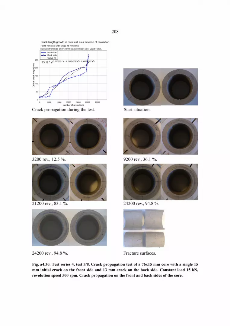
208


3200 rev., 12.5 %. 9200 rev., 36.1 %.

21200 rev., 83.1 %. 24200 rev., 94.8 %.

24200 rev., 94.8 %. Fracture surfaces. Fig. a4.30. Test series 4, test 3/8. Crack propagation test of a 76x15 mm core with a single 15 mm initial crack on the front side and 13 mm crack on the back side. Constant load 15 kN, revolution speed 500 rpm. Crack propagation on the front and back sides of the core.

0 5000 10000 15000 20000 25000 30000


0

50

100

150

200

250

Crit

ical

cra

ck le

ngth

[mm

]

Crack length growth in core wall as a function of revolution76x15 mm core with single 15 mm initialcrack on front side and 13 mm crack on back side. Load 15 kN.


13.12 * e(0.0003021*x - 1.238E-008*x2 + 1.945E-013*x3)

209


6100 rev., 20.1 %. 24100 rev., 79.5 %.

28100 rev., 92.7 %. 30100 rev., 99.2 %.

30230 rev., 100 %. Fracture surfaces. Fig. a4.31. Test series 4, test 4/8. Crack propagation tests of a 76x15 mm core with a single 15 mm initial crack on the front side and 20 mm crack on the back side. Constant load 15 kN, revolution speed 500 rpm. Crack propagation on the front and back sides of the core.

0 5000 10000 15000 20000 25000 30000


0

50

100

150

200

250

300

350

Cra

ck le

ngth

[mm

]



14.97 * e(0.0002177*x - 1.039E-008*x2 + 2.178E-013*x3)

210

Crack propagation during the test. Start situation. 500 rev., 9.2 %. 1500 rev., 27.6 %. 3000 rev., 55.2 %. 4500 rev., 82.7 %. 5440 rev., 100 %. Fracture surfaces. Fig. a4.33. Test series 4, test 5/8. Crack propagation test of a 76x15 mm core with a single 30 mm initial crack on both sides. Constant load 15 kN, revolution speed 500 rpm. Crack propagation on the front and back sides of the core.

0 1000 2000 3000 4000 5000


0

50

100

150

200

250

300

350

400

Cra

ck le

ngth

[mm

]

Crack length growth in core wall as a function of revolutions 76x15 mm core. Load 15 kN. Single 30 mm initial crack on both sides.


21.24 + 0.1301*x - 4.775E-005*x2 + 6.734E-009*x3

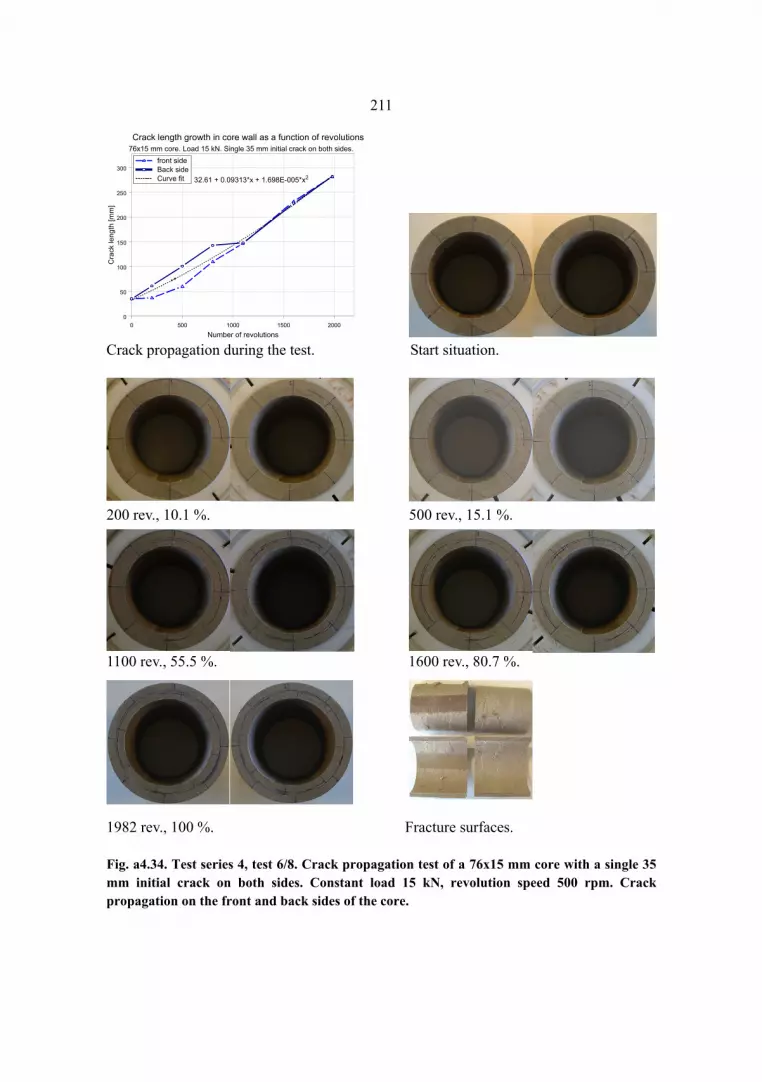
211

Crack propagation during the test. Start situation. 200 rev., 10.1 %. 500 rev., 15.1 %. 1100 rev., 55.5 %. 1600 rev., 80.7 %.

1982 rev., 100 %. Fracture surfaces. Fig. a4.34. Test series 4, test 6/8. Crack propagation test of a 76x15 mm core with a single 35 mm initial crack on both sides. Constant load 15 kN, revolution speed 500 rpm. Crack propagation on the front and back sides of the core.

0 500 1000 1500 2000


0

50

100

150

200

250

300

Cra

ck le

ngth

[mm

]

Crack length growth in core wall as a function of revolutions 76x15 mm core. Load 15 kN. Single 35 mm initial crack on both sides.

front sideBack sideCurve fit 32.61 + 0.09313*x + 1.698E-005*x2

212

Crack propagation during the test. Start situation. 300 rev., 22.7 %. 500 rev., 27.9 %. 750 rev., 56.8 %. 1050 rev., 79.5 %. 1320 rev., 100 %. Fracture surfaces. Fig. a4.35. Test series 4, test 7/8. Crack propagation test of a 76x15 mm core with a single 55 mm initial crack on both sides. Constant load 15 kN, revolution speed 500 rpm. Crack propagation on the front and back sides of the core.

0 200 400 600 800 1000 1200 1400


0

50

100

150

200

250

300

Crit

ical

cra

ck le

ngth

[mm

]


Front sideBack sideCurve fit

56.17 + 0.4784*x - 0.0005785*x2 + 2.69E-007*x3

213

Crack propagation during the test. Start situation. 100 rev., 18.8 %. 300 rev., 35.3 %. 500 rev., 58.5 %. 700 rev., 82.4 %. 850 rev., 100 %. Fracture surfaces. Fig. a4.36. Test series 4, test 8/8. Crack propagation test of a 76x15 mm core with a single 58 mm initial crack on the front side and 55 mm crack on the back side. Constant load 15 kN, revolution speed 500 rpm. Crack propagation on the front and back sides of the core.

0 100 200 300 400 500 600 700 800 900


0

50

100

150

200

250

300

350

400

450

Cra

ck le

ngth

[mm

]


Front sideBack sideCurve fit

70.84 + 0.9112*x - 0.002442*x2 + 2.29E-006*x3

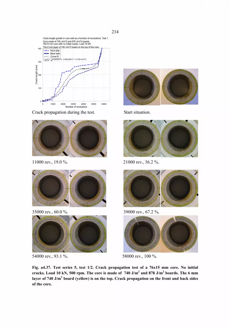
214

Crack propagation during the test. Start situation. 11000 rev., 19.0 %. 21000 rev., 36.2 %. 35000 rev., 60.0 %. 39000 rev., 67.2 %. 54000 rev., 93.1 %. 58000 rev., 100 %. Fig. a4.37. Test series 5, test 1/2. Crack propagation test of a 76x15 mm core. No initial cracks. Load 10 kN, 500 rpm. The core is made of 740 J/m2 and 878 J/m2 boards. The 6 mm layer of 740 J/m2 board (yellow) is on the top. Crack propagation on the front and back sides of the core.


0

100

200

300

400

Cra

ck le

ngth

[mm

]Crack length growth in core wall as a function of revolutions. Test 1.Core made of 740 J/m^2 and 878 J/m^2 boards. 76x15 mm core with no initial cracks. Load 10 kN. The 6 mm layer of 740 J/m^2 board on the top of the core.


1.673 * e(0.0003672*x - 9.03E-009*x2 + 7.417E-014*x3)

215

Crack propagation during the test. Start situation. 17500 rev., 54.4 %. 21500 rev., 66.9 %. 25500 rev., 79.3 %. 29500 rev., 91.8 %. 32150 rev., 100 %. Fracture surfaces. Fig. a4.38. Test series 5, test 2/2. Crack propagation test of a 76x15 mm core. No initial cracks. Load 10 kN, 500 rpm. The core is made of 740 J/m2 and 878 J/m2 boards. The 6 mm layer of 740 J/m2 board (yellow) is on the top. Crack propagation on the front and back sides of the core.

0 10000 20000 30000 40000 50000 60000


0

100

200

300

400

Cra

ck le

ngth

[mm

]Crack length growth in core wall as a function of revolutions. Test 2.Core made of 740 J/m^2 and 878 J/m^2 boards. 76x15 mm core with no initial cracks. Load 10 kN. The 6 mm layer of 740 J/m^2 board on the top of the core.


Documents

Application of fracture mechanics in analyzing delamination of