Application of the Proper Orthogonal Decomposition Techniques to AN Annular Cascade Flowfield

Energy Conversion and Management xxx (2014) xxx–xxx

Contents lists available at ScienceDirect

Energy Conversion and Management

journal homepage: www.elsevier .com/ locate /enconman

An application of the Proper Orthogonal Decomposition methodto the thermo-economic optimization of a dual pressure, combined cyclepowerplant

http://dx.doi.org/10.1016/j.enconman.2014.04.0050196-8904/� 2014 Elsevier Ltd. All rights reserved.

⇑ Corresponding author. Address: Via Eudossiana 18, 00184 Rome, Italy. Tel.: +390644585272.

E-mail addresses: [email protected] (R. Melli), [email protected] (E. Sciubba), [email protected] (C. Toro).

Please cite this article in press as: Melli R et al. An application of the Proper Orthogonal Decomposition method to the thermo-economic optimizatdual pressure, combined cycle powerplant. Energy Convers Manage (2014), http://dx.doi.org/10.1016/j.enconman.2014.04.005

Roberto Melli, Enrico Sciubba, Claudia Toro ⇑Università di Roma ‘‘Sapienza’’, Department of Mechanical and Aerospace Engineering, Via Eudossiana 18, Rome, Italy

a r t i c l e i n f o

Article history:Available online xxxx

Keywords:Proper Orthogonal DecompositionProcess simulationCCGTOptimization

a b s t r a c t

This paper presents a thermo-economic optimization of a combined cycle power plant obtained via theProper Orthogonal Decomposition–Radial Basis Functions (POD–RBF) procedure. POD, also known as‘‘Karhunen–Loewe decomposition’’ or as ‘‘Method of Snapshots’’ is a powerful mathematical methodfor the low-order approximation of highly dimensional processes for which a set of initial data is knownin the form of a discrete and finite set of experimental (or simulated) data: the procedure consists in con-structing an approximated representation of a matricial operator that optimally ‘‘represents’’ the originaldata set on the basis of the eigenvalues and eigenvectors of the properly re-assembled data set. By com-bining POD and RBF it is possible to construct, by interpolation, a functional (parametric) approximationof such a representation.

In this paper the set of starting data for the POD–RBF procedure has been obtained by the CAMEL-Pro™process simulator. The proposed procedure does not require the generation of a complete simulated set ofresults at each iteration step of the optimization, because POD constructs a very accurate approximationto the function described by a relatively small number of initial simulations, and thus ‘‘new’’ points indesign space can be extrapolated without recurring to additional and expensive process simulations.Thus, the often taxing computational effort needed to iteratively generate numerical process simulationsof incrementally different configurations is substantially reduced by replacing much of it by easy-to-per-form matrix operations.

The object of the study was a fossil-fuelled, combined cycle powerplant of nameplate power Pel = 160 -MW, for which a set of operational and costing data was available: different combinations of the relevantprocess parameters were considered and the corresponding process variables calculated for each simu-lation were collected. In our case the aim of the application of the procedure was to find the combinationof process parameters which corresponds to the minimum the thermo-economic cost of the products.

The results obtained by the application of this model have been validated by comparison with litera-ture data obtained by the application of genetic algorithm optimization.

� 2014 Elsevier Ltd. All rights reserved.

1. Introduction

The thermo-economic optimization of combined cycle powerplants is an important but difficult problem due to the intrinsicnonlinear characteristics of the systems and to thermodynamicrestrictions. As pointed out by several researchers [1], it is moreimportant to identify and focus on the main variables of the opti-mization problem rather than manipulate them all at once.

The result of a thermo-economic plant optimization, combiningsecond-law and cost analyses, is the (possibly non unique) combi-nation of the process/plant parameters which lead to the attain-ment of the most convenient compromise between plantefficiency and generation costs.

Several thermoeconomic optimization methods can be found inthe literature, run at different levels of disaggregation, all aimed tothe calculation of the ‘‘minimal’’ unit cost of the products. Most ofthem use algebraic methods applying a modified productive struc-ture analysis [10] or specific exergy costing [12] to reduce theinfluence of fuel and product definitions and of cost partitioning(cost allocation). These authors use iterative exergoeconomic

ion of a

http://dx.doi.org/10.1016/j.enconman.2014.04.005

mailto:[email protected]





http://www.sciencedirect.com/science/journal/01968904

http://www.elsevier.com/locate/enconman


Nomenclature

Symbol Quantitycf cost of fuel per energy unit, $/MJ_C cost flow rate, $/s_ED exergy destruction rate, kWLHV lower heating value, kJ/kg_m mass flow rate, kg/s

p pressure, kPaPOD Proper Orthogonal DecompositionRBF Radial Basis FunctionT temperature, KTIT turbine inlet temperature, K_Z capital cost rate, $/s

Greek symbolsp pressure ratiok eigenvalues

Subscripts and superscriptsapp approachDB duct burnerF fuelHP high pressureHRSG heat recovery steam generatorLP low pressure

2 R. Melli et al. / Energy Conversion and Management xxx (2014) xxx–xxx

performance procedures based on exergoeconomic variables asintroduced by Tsatsaronis [20].

Other studies of thermoeconomic optimization of CCGT plantsuse calculus methods [9,21] based on Lagrange multipliers andThermoeconomical Functional Analysis (TFA) [11]. There are alsoseveral works [18] proposing second law-based decompositionmethods to reduce the complexity of the system optimization.

A detailed literature review of combined cycle thermoeconomicoptimization can be found in [1].

The main goal of the present study is to perform the thermo-economic optimization of a combined cycle, dual pressure powerplant by means of the Proper Orthogonal Decomposition–RadialBasis Function (POD–RBF) method. A correct implementation ofthe POD–RBF procedure enables the designer to quickly inspectthe range of the feasible solutions and to find, with a substantiallyreduced use of computational resources, the optimal configurationfor a pre-assigned set of constraints.

As stated above, the procedure proposed in this paper differsfrom the previous ones because of the lower number of plant/pro-cess simulations required to reach the same objective.

The POD–RBF procedure has been previously tested by the pres-ent authors on an optimization of a simple MSF desalination plant[15] and of a single pressure CCGT [14] and the very satisfactoryresults obtained for these plants suggested extending the applica-tion of the procedure to more complex configurations and to differ-ent processes.

More details about POD as well as an introductory mathemati-cal explanation of its conceptual basis are provided in the followingof the paper. In Section 3 the layout and operative parameters ofthe specific case-study are presented and in the last part the resultsobtained by the POD procedure are compared with suitable litera-ture data.

2. The POD–RBF method

The Proper Orthogonal Decomposition method is a method ofdata analysis aimed at obtaining low dimensional approximatedescriptions of highly dimensional processes. This method pro-vides the most efficient way of capturing the dominant compo-nents of the behaviour of these processes with a small number of‘‘modes’’. In essence, POD is a procedure that provides an optimallinear basis for the reconstruction of multidimensional data: itsmain advantage is that it allows for a substantial reduction in theorder of the system under consideration. Another very useful fea-ture is that it filters out data noise very efficiently.

This method was originally developed over 100 years ago byPearson [16] as a tool for graphical analysis and processing of sta-tistical data. The theory was then re-developed several times under

Please cite this article in press as: Melli R et al. An application of the Proper Ortdual pressure, combined cycle powerplant. Energy Convers Manage (2014), ht

different names, such as Principal Component Analysis (PCA),Karhunen–Loève Decomposition (KLD), or Singular Value Decom-position (SVD) and applied in different fields including signal pro-cessing and control theory [13], fluid dynamics and turbulence [6],adaptive control, image processing, neural activity, structuralmechanics [7] and many others.

We shall follow here Sirovich’ description [19]: he nicknamedPOD ‘‘the method of snapshots’’, and recommended it as an effi-cient way for determining the coefficients of a ‘‘proper’’ (in a sensediscussed here below) eigenfunctions expansion for large problemsfor which a set of initial data is known not functionally but as a setof ‘‘experimental’’ data points. The method, like other fitting proce-dures, provides a parametric fit of a set of given multidimensionaldata by constructing an appropriate expansion series and its coef-ficients. The intrinsic properties of POD suggest that it is a prefer-able basis in the sense that it is constructed to maximize theaccuracy of the approximation. For a given data set and for a givennumber of modes used to approximate the data there is no otherbasis which can give a better approximation in a least squaresense. POD extracts both the interpolating functions and the coef-ficients from the information contained in the data set.

The fundamental notion of the POD method is the snapshotwhich is a vector of N relevant variables of the system under con-sideration obtained by experiment or simulation for a certain com-bination of S known process parameters collected in the vector p.The collection of snapshots generated by changing the values ofsome of the process parameters within a predefined range is storedin a rectangular matrix UNxM called the snapshot matrix. Aim of thePOD is to construct the set of orthonormal vectors Uj, j = 1. . .Mresembling the original snapshots matrix in an optimal way. Tothis scope, the covariance of U, its eigenvalues ki and correspondingeigenvectors are calculated.

The eigenvalues are first ranked and then pruned by discardingthose that are negligible by some norm with respect to the others:this is achieved by applying an ‘‘energy’’ method based on a linearalgebra theorem which states that the energy of the kth modescales with the corresponding eigenvalue kk. The truncation ofthe POD basis is accomplished by deciding which fraction b ofthe global energy we wish to include in further calculations, andthis leads to the search for the mode number K that fulfils:

Xk

1

kk 6 bXM

1

kk ð1Þ

the resulting truncated POD �U basis consists of K < M vectors oflength N and it can be demonstrated that there is no other orthog-onal basis that transfers more energy within the same number of

hogonal Decomposition method to the thermo-economic optimization of atp://dx.doi.org/10.1016/j.enconman.2014.04.005


R. Melli et al. / Energy Conversion and Management xxx (2014) xxx–xxx 3

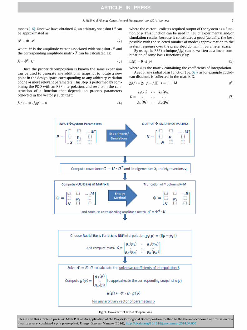
modes [16]. Once we have obtained �U, an arbitrary snapshot Ua canbe approximated as:

Ua ¼ �U � �aa ð2Þ

where �aa is the amplitude vector associated with snapshot Ua andthe corresponding amplitude matrix A can be calculated as:

A ¼ �UT � U ð3Þ

Once the proper decomposition is known the same expansioncan be used to generate any additional snapshot to locate a newpoint in the design space corresponding to any arbitrary variationof one or more relevant parameters. This step is performed by com-bining the POD with an RBF interpolation, and results in the con-struction of a function that depends on process parameterscollected in the vector p such that:

f ðpÞ ¼ �U � faðpÞ ¼ u ð4Þ

Fig. 1. Flow-chart of PO


where the vector u collects required output of the system as a func-tion of p. This function can be used in lieu of experimental and/orsimulation results, because it constitutes a good (actually, the bestpossible with the selected number of modes) approximation to thesystem response over the prescribed domain in parameter space.

By using the RBF technique fa(p) can be written as a linear com-bination of some basis functions g(p):

faðpÞ ¼ B � gðpÞ ð5Þ

where B is the matrix containing the coefficients of interpolation.A set of any radial basis function (Eq. (6)), as for example Euclid-

ean distance, is collected in the matrix G.

giðpÞ ¼ gðjjp� pijjÞ; i ¼ 1 . . . M ð6Þ

G ¼g1ðp1Þ . . . gMðpMÞ

. . . . . . . . .

gMðp1Þ . . . gMðpMÞð7Þ

D–RBF operations.



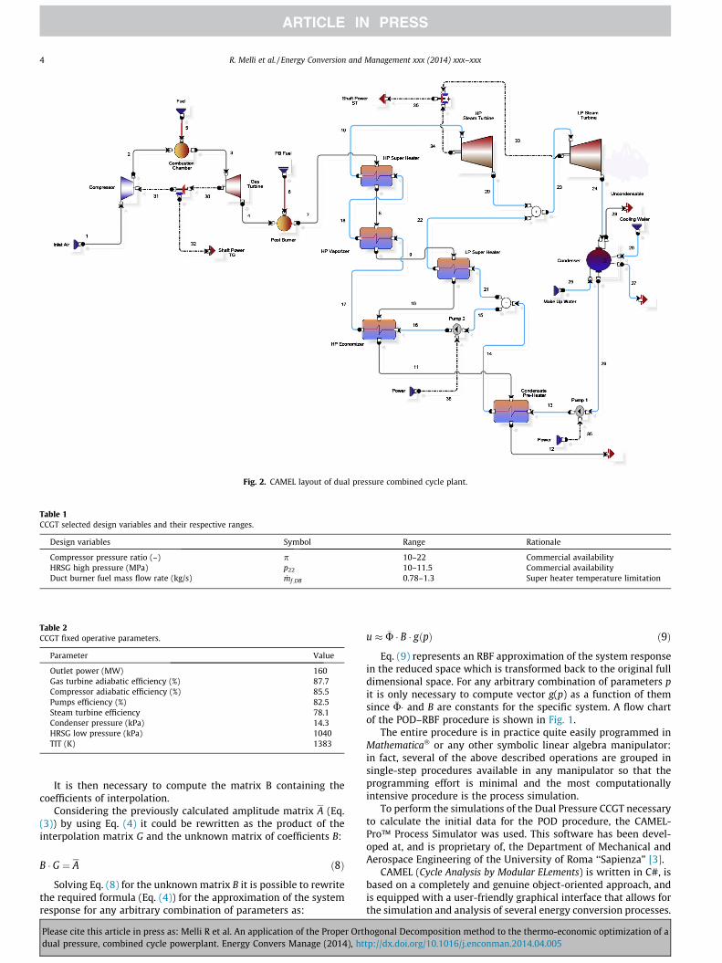
Fig. 2. CAMEL layout of dual pressure combined cycle plant.

Table 1CCGT selected design variables and their respective ranges.

Design variables Symbol Range Rationale

Compressor pressure ratio (–) p 10–22 Commercial availabilityHRSG high pressure (MPa) p22 10–11.5 Commercial availabilityDuct burner fuel mass flow rate (kg/s) _mf ;DB 0.78–1.3 Super heater temperature limitation

Table 2CCGT fixed operative parameters.

Parameter Value

Outlet power (MW) 160Gas turbine adiabatic efficiency (%) 87.7Compressor adiabatic efficiency (%) 85.5Pumps efficiency (%) 82.5Steam turbine efficiency 78.1Condenser pressure (kPa) 14.3HRSG low pressure (kPa) 1040TIT (K) 1383


It is then necessary to compute the matrix B containing thecoefficients of interpolation.

Considering the previously calculated amplitude matrix A (Eq.(3)) by using Eq. (4) it could be rewritten as the product of theinterpolation matrix G and the unknown matrix of coefficients B:

B � G ¼ A ð8Þ

Solving Eq. (8) for the unknown matrix B it is possible to rewritethe required formula (Eq. (4)) for the approximation of the systemresponse for any arbitrary combination of parameters as:


u � �U � B � gðpÞ ð9Þ

Eq. (9) represents an RBF approximation of the system responsein the reduced space which is transformed back to the original fulldimensional space. For any arbitrary combination of parameters pit is only necessary to compute vector g(p) as a function of themsince �U� and B are constants for the specific system. A flow chartof the POD–RBF procedure is shown in Fig. 1.

The entire procedure is in practice quite easily programmed inMathematica� or any other symbolic linear algebra manipulator:in fact, several of the above described operations are grouped insingle-step procedures available in any manipulator so that theprogramming effort is minimal and the most computationallyintensive procedure is the process simulation.

To perform the simulations of the Dual Pressure CCGT necessaryto calculate the initial data for the POD procedure, the CAMEL-Pro™ Process Simulator was used. This software has been devel-oped at, and is proprietary of, the Department of Mechanical andAerospace Engineering of the University of Roma ‘‘Sapienza" [3].

CAMEL (Cycle Analysis by Modular ELements) is written in C#, isbased on a completely and genuine object-oriented approach, andis equipped with a user-friendly graphical interface that allows forthe simulation and analysis of several energy conversion processes.



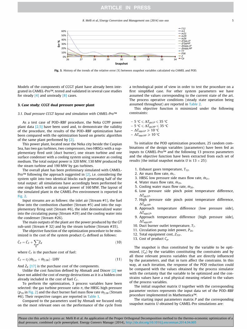
Fig. 3. History of the trends of the relative error (%) between snapshot variables calculated via CAMEL and POD.


Models of the components of CCGT plant have already been inte-grated in CAMEL-Pro™, tested and validated in several case studiesfor steady [4] and unsteady [8] cases.

3. Case study: CCGT dual pressure power plant

3.1. Dual pressure CCGT layout and simulation with CAMEL-Pro™

As a test case of POD–RBF procedure, the Neka CCPP powerplant data [2,5] have been used and, to demonstrate the validityof the procedure, the results of the POD–RBF optimization havebeen compared with the optimization based on genetic algorithmof the same plant performed by [2].

This power plant, located near the Neka city beside the CaspianSea, has two gas turbines, two compressors, two HRSGs with a sup-plementary fired unit (duct burner), one steam turbine and onesurface condenser with a cooling system using seawater as coolingmedium. The total output power is 320 MW, 130 MW produced bythe steam turbine and 190 MW by gas turbines.

The overall plant has been preliminary simulated with CAMEL-Pro™ following the approach suggested in [2], i.e. considering thesystem split into two identical blocks each generating half of thetotal output: all simulations have accordingly been performed forone single block with an output power of 160 MW. The layout ofthe simulated plant in the CAMEL-Pro environment is reported inFig. 2.

Input streams are as follows: the inlet air (Stream #1), the fuelflow into the combustion chamber (Stream #5) and into the sup-plementary firing unit (Stream #6), the inlet demineralized waterinto the circulating pump (Stream #29) and the cooling water intothe condenser (Stream #26).

The main outputs of the plant are the power produced by the GTsub-unit (Stream # 32) and by the steam turbine (Stream #35).

The objective function of the optimization procedure to be min-imized is the cost of the system product CP defined as follows:

_CP ¼ _CF þX

K

_ZK ð10Þ

where _CF is the purchase cost of fuel:

_CF ¼ cf ð _mf ;cc þ _mf ;DBÞ � LHV ð11Þ

And _ZK [17] is the purchase cost of the components.Unlike the cost function defined by Ahmadi and Dincer [2] we

have not added the cost of exergy destructions as it is a hidden costalready included in the cost of fuel _CF .

To perform the optimization, 3 process variables have beenselected: the gas turbine pressure ratio p, the HRSG high pressure(p16 in Fig. 2) and the duct burner fuel mass flow rate _mf ;DB (Stream#6). Their respective ranges are reported in Table 1.

Compared to the parameters used by Ahmadi we focused onlyon the most relevant ones on the performance of the cycle from


a technological point of view in order to test the procedure on afirst simplified case. For other system parameters we haveassumed the values corresponding to the current state of the art.The process operative conditions (steady state operation beingassumed throughout) are reported in Table 2.

This objective function is minimized under the followingconstraints:

– 5 �C 6 DTpp,LP 6 35 �C– 5 �C 6 DTpp,HP 6 35 �C– DTapp,LP P 10 �C– DTapp,HP P 10 �C

To initialize the POD optimization procedure, 25 random com-binations of the design variables (parameters) have been fed asinputs to CAMEL-Pro™ and the following 13 process parametersand the objective function have been extracted from each set ofresults (the initial snapshot matrix U is 13 � 25):

1. Exhaust gases temperature, T12.2. Air mass flow rate, _m1.3. HRSG low pressure side mass flow rate, _m21.4. Water mass flow rate, _m29.5. Cooling water mass flow rate, _m26.6. Low pressure side pinch point temperature difference,

DTpp,LP.7. High pressure side pinch point temperature difference,

DTpp,HP.8. Approach temperature difference (low pressure side),

DTapp,LP.9. Approach temperature difference (high pressure side),

DTapp,HP.10. Duct burner outlet temperature, T7.11. Circulation pump inlet power, P35.12. Total equipment cost, _ZTOT .13. Cost of product Cp.

The snapshot is thus constituted by the variable to be opti-mized, (Cp) by the variables constituting the constraints and byall those relevant process variables that are directly influencedby the parameters, and that in turn affect the constrains. In thisway, at each iteration, the response of the POD reduction couldbe compared with the values obtained by the process simulatorwith the certainty that the variable to be optimized and the con-strains values have a real physical meaning related to the valuesof the process variables.

The initial snapshot matrix U together with the correspondingparameter vectors represents the input data set of the POD–RBFprocedure implemented in Mathematica™.

The starting input parameters matrix P and the correspondingsnapshot matrix U obtained by CAMEL-Pro simulations are:



P¼

p½—�p16 ½MPa�_mf ;DB

kgs

h i

2664

3775

3�25

¼11:4 12:1 11 11 10:5 11:2 12 12 15 18 22 13:3 14 12 10:9 10:8 12:1 10:1 11:4 12:6 13:7 12:7 12:5 11:2 11:410 10:4 11:5 11:5 11:5 11 10 10:2 11:5 12 11:5 11 10:9 11:3 11 11:5 10 11 11 11 10:8 11:2 11 11 11:30:85 1:3 1 0:9 0:85 0:8 1:3 0:96 0:8 0:8 0:85 1:1 1:13 0:96 0:8 0:82 0:82 0:85 0:85 1 1:14 1:04 0:96 0:78 0:8

264

375

U¼

T12 ½�C�

_m1kgs

h i

_m21kgs

h i

_m29kgs

h i

_m26kgs

h i

Tpp;LP ½�C�

Tpp;HP ½�C�

Tapp;LP ½�C�

Tapp;HP ½�C�

T7 ½�C�

P35 ½kW�_ZTOT s

� �

Cp s

� �

266666666666666666666666666666664

377777777777777777777777777777775

13x25

¼

134 146 124 112 116 97 149 106 43 19 9 95 96 101 103 106 105 127 95 99 103 100 96 95 95328 311 312 312 313 312 311 311 313 319 329 309 312 311 312 312 299 313 312 311 312 311 311 312 3125 2:3 5 5 5 3:9 1:2 1:8 5 6:04 5 3:85 3:8 4:8 3:9 5 1:2 3:9 5 3:9 3:4 4:4 3:9 3:9 3:965 64 65 65 65 65 64 64 65 65 65 64 65 65 65 65 64 65 65 65 64 65 65 65 657103 7054 7103 7103 7103 7082 7033 7044 7103 7121 7103 7082 7081 7100 7082 7103 7033 7082 7103 7082 7075 7092 7084 7082 708254:0 69:5 49:8 37:8 41:5 23:1 72:0 30:6 �29:7 �55:0 �68:2 22 21:9 26:8 28:5 31:9 33:3 51:0 21:2 24:8 28:3 26:3 21:7 20:6 20:654:9 62:8 57:4 45:8 49:2 25:9 59:3 22:3 �19:6 �40:9 �63:5 25 24:1 34:6 31:0 40:1 25:9 52:1 30:0 27:6 28:5 31:8 25:2 23:5 23:544 43 41 29 33 7 39 1 �38 �57 �78 15 6 17 13 23 0 35 13 9 10 14 7 5 5149 182 166 156 158 143 183 148 96 67 40 145 141 147 147 151 167 165 142 145 146 146 142 141 141691 724 708 698 700 685 725 690 638 609 582 687 683 689 689 693 709 707 684 687 688 688 684 683 683776 714 776 776 776 747 691 703 776 804 776 769 746 771 747 776 691 747 776 747 738 760 750 747 7470:302 0:298 0:299 0:298 0:297 0:295 0:295 0:292 0:301 0:309 0:320 0:298 0:302 0:299 0:295 0:297 0:291 0:295 0:297 0:299 0:300 0:300 0:298 0:295 0:2951:388 1:396 1:374 1:358 1:360 1:336 1:396 1:342 1:288 1:272 1:272 1:338 1:348 1:348 1:342 1:349 1:340 1:368 1:337 1:345 1:352 1:349 1:341 1:333 1:333

��

��


The following eigenvalues were obtained:

Pd

k1

lease cite this article in press as:ual pressure, combined cycle pow

1.29 � 109

k2
1.436 � 105
k3
1.437 � 104
k4
1901 k5 74 k6 1.023 k7 0.073 k8 0.0155 k9 0.0018 k10 3.5 � 10�4
k11
5.137 � 10�5
k12
1.355 � 10�6
k13
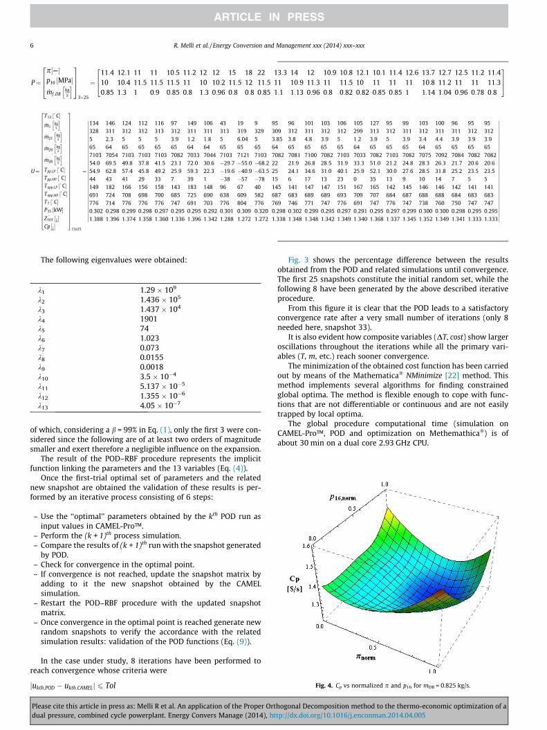
4.05 � 10�7
Fig. 4. Cp vs normalized p and p16 for mDB = 0.825 kg/s.

of which, considering a b = 99% in Eq. (1), only the first 3 were con-sidered since the following are of at least two orders of magnitudesmaller and exert therefore a negligible influence on the expansion.

The result of the POD–RBF procedure represents the implicitfunction linking the parameters and the 13 variables (Eq. (4)).

Once the first-trial optimal set of parameters and the relatednew snapshot are obtained the validation of these results is per-formed by an iterative process consisting of 6 steps:

– Use the ‘‘optimal’’ parameters obtained by the kth POD run asinput values in CAMEL-Pro™.

– Perform the (k + 1)th process simulation.– Compare the results of (k + 1)th run with the snapshot generated

by POD.– Check for convergence in the optimal point.– If convergence is not reached, update the snapshot matrix by

adding to it the new snapshot obtained by the CAMELsimulation.

– Restart the POD–RBF procedure with the updated snapshotmatrix.

– Once convergence in the optimal point is reached generate newrandom snapshots to verify the accordance with the relatedsimulation results: validation of the POD functions (Eq. (9)).

In the case under study, 8 iterations have been performed toreach convergence whose criteria were

jukth;POD � ukth;CAMELj 6 Tol

Melli R et al. An application of the Proper Orterplant. Energy Convers Manage (2014), ht

Fig. 3 shows the percentage difference between the resultsobtained from the POD and related simulations until convergence.The first 25 snapshots constitute the initial random set, while thefollowing 8 have been generated by the above described iterativeprocedure.

From this figure it is clear that the POD leads to a satisfactoryconvergence rate after a very small number of iterations (only 8needed here, snapshot 33).

It is also evident how composite variables (DT, cost) show largeroscillations throughout the iterations while all the primary vari-ables (T, m, etc.) reach sooner convergence.

The minimization of the obtained cost function has been carriedout by means of the Mathematica� NMinimize [22] method. Thismethod implements several algorithms for finding constrainedglobal optima. The method is flexible enough to cope with func-tions that are not differentiable or continuous and are not easilytrapped by local optima.

The global procedure computational time (simulation onCAMEL-Pro™, POD and optimization on Methemathica�) is ofabout 30 min on a dual core 2.93 GHz CPU.




4. Results

The POD–RBF locate the optimum configuration of the CCGTdual pressure power plant at the following design point:

– p = 11.3,– p16 = 11200 kPa,– _mf ;DB ¼ 0:825,

which correspond to a value of the Cp = 1.338 [$/s] and to the fol-lowing values of the other snapshots variables:

� T12 = 101 �C� _m1 = 305 kg/s� _m21 = 4.32 kg/s� _m29 = 64 kg/s� _m26 = 7090 kg/s� DTpp,LP = 23 �C� DTpp,HP = 28 �C� DTapp,LP = 11 �C� DTapp,HP = 144 �C� T7 = 685�C� P35 = 758 kW� _ZTOT=0.29 $/s

The results obtained in this study are in excellent agreementwith the ones presented in [2]: Ahmadi and Dincer, using a geneticalgorithm procedure, identified as minimising values for the objec-tive function values that differ less than 3% from ours, as shown inTable 3.

The added value of the method described in this paper is thepossibility to extract not only the combination of ‘‘optimal’’ param-eters but also the (implicit) functional relation linking the variablesto be optimized to the process parameters. This allows to study the‘‘marginal variation’’ of the objective function, an especially

Table 3Comparison of POD results with genetic algorithm optimization of [2].

Variables POD Genetic algorithm D%

Compressor pressure ratio (–) 11.3 11.4 0.8Steam turbine inlet pressure (kPa) 9770 9800 0.3Duct burner fuel mass flow rate (kg/s) 0.825 0.8 3

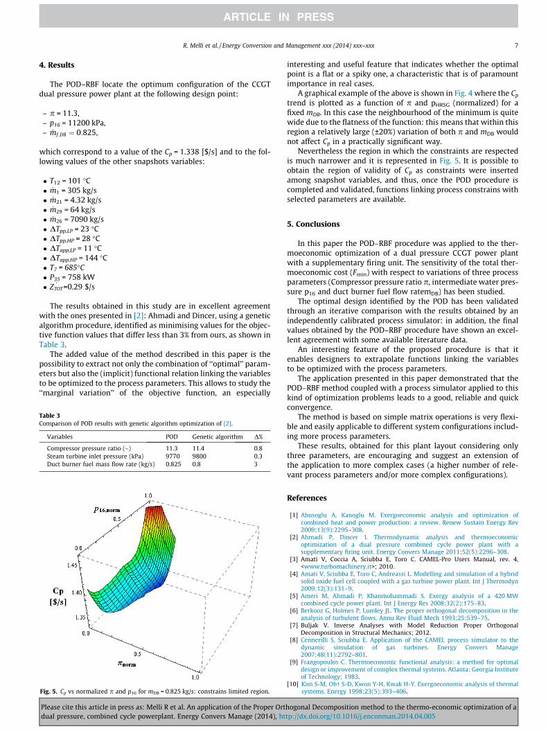
Fig. 5. Cp vs normalized p and p16 for mDB = 0.825 kg/s: constrains limited region.


interesting and useful feature that indicates whether the optimalpoint is a flat or a spiky one, a characteristic that is of paramountimportance in real cases.

A graphical example of the above is shown in Fig. 4 where the Cp

trend is plotted as a function of p and pHRSG (normalized) for afixed mDB. In this case the neighbourhood of the minimum is quitewide due to the flatness of the function: this means that within thisregion a relatively large (±20%) variation of both p and mDB wouldnot affect Cp in a practically significant way.

Nevertheless the region in which the constraints are respectedis much narrower and it is represented in Fig. 5. It is possible toobtain the region of validity of Cp as constraints were insertedamong snapshot variables, and thus, once the POD procedure iscompleted and validated, functions linking process constrains withselected parameters are available.

5. Conclusions

In this paper the POD–RBF procedure was applied to the ther-moeconomic optimization of a dual pressure CCGT power plantwith a supplementary firing unit. The sensitivity of the total ther-moeconomic cost (Fmin) with respect to variations of three processparameters (Compressor pressure ratio p, intermediate water pres-sure p16 and duct burner fuel flow ratemDB) has been studied.

The optimal design identified by the POD has been validatedthrough an iterative comparison with the results obtained by anindependently calibrated process simulator: in addition, the finalvalues obtained by the POD–RBF procedure have shown an excel-lent agreement with some available literature data.

An interesting feature of the proposed procedure is that itenables designers to extrapolate functions linking the variablesto be optimized with the process parameters.

The application presented in this paper demonstrated that thePOD–RBF method coupled with a process simulator applied to thiskind of optimization problems leads to a good, reliable and quickconvergence.

The method is based on simple matrix operations is very flexi-ble and easily applicable to different system configurations includ-ing more process parameters.

These results, obtained for this plant layout considering onlythree parameters, are encouraging and suggest an extension ofthe application to more complex cases (a higher number of rele-vant process parameters and/or more complex configurations).

References

[1] Abusoglu A, Kanoglu M. Exergoeconomic analysis and optimization ofcombined heat and power production: a review. Renew Sustain Energy Rev2009;13(9):2295–308.

[2] Ahmadi P, Dincer I. Thermodynamic analysis and thermoeconomicoptimization of a dual pressure combined cycle power plant with asupplementary firing unit. Energy Convers Manage 2011;52(5):2296–308.

[3] Amati V, Coccia A, Sciubba E, Toro C. CAMEL-Pro Users Manual, rev. 4,<www.turbomachinery.it>; 2010.

[4] Amati V, Sciubba E, Toro C, Andreassi L. Modelling and simulation of a hybridsolid oxide fuel cell coupled with a gas turbine power plant. Int J Thermodyn2009;12(3):131–9.

[5] Ameri M, Ahmadi P, Khanmohammadi S. Exergy analysis of a 420 MWcombined cycle power plant. Int J Energy Res 2008;32(2):175–83.

[6] Berkooz G, Holmes P, Lumley JL. The proper orthogonal decomposition in theanalysis of turbulent flows. Annu Rev Fluid Mech 1993;25:539–75.

[7] Buljak V. Inverse Analyses with Model Reduction Proper OrthogonalDecomposition in Structural Mechanics; 2012.

[8] Cennerilli S, Sciubba E. Application of the CAMEL process simulator to thedynamic simulation of gas turbines. Energy Convers Manage2007;48(11):2792–801.

[9] Frangopoulos C. Thermoeconomic functional analysis: a method for optimaldesign or improvement of complex thermal systems. Atlanta: Georgia Instituteof Technology; 1983.

[10] Kim S-M, Oh� S-D, Kwon Y-H, Kwak H-Y. Exergoeconomic analysis of thermalsystems. Energy 1998;23(5):393–406.


http://refhub.elsevier.com/S0196-8904(14)00301-X/h0005






http://www.turbomachinery.it



















[11] Kwak H-Y, Byun G-T, Kwon Y-H, Yang H. Cost structure of CGAM cogenerationsystem. Int J Energy Res 2004;28(13):1145–58.

[12] Lazzaretto A, Tsatsaronis G. SPECO: a systematic and general methodology forcalculating efficiencies and costs in thermal systems. Energy 2006;31(8–9):1257–89.

[13] Ly HV, Tran HT. Modeling and control of physical processes usingproper orthogonal decomposition. Math Comput Modell 2001;33(1–3):223–36.

[14] Melli R, Sciubba E, Toro C, Zoli-Porroni A. An example of thermo-economicoptimization of a CCGT by means of the proper orthogonal decompositionmethod, IMECE 2012, Houston, TX; 2012.

[15] Melli R, Sciubba E, Toro C, Zoli-Porroni A. An improved POD technique for theoptimization of MSF processes. Int J Thermodyn 2012;15(4):231–8.

[16] Pearson K. On lines and planes of closest fit to systems of points in space. PhilMag 1901;2:559–72.


[17] Roosen P, Uhlenbruck S, Lucas K. Pareto optimization of a combined cyclepower system as a decision support tool for trading off investment vs.operating costs. Int J Therm Sci 2003;42(6):553–60.

[18] Silveira JL, Tuna CE. Thermoeconomic analysis method for optimization ofcombined heat and power systems. Part I, Prog Energy Combust Sci2003;29(6):479–85.

[19] Sirovich L. Turbulence and the dynamics of coherent structures. Parts I, II andIII, Quart Appl Math 1987;45(561–571):573–90.

[20] Tsatsaronis G, Winhold M. Exergoeconomic analysis and evaluation of energy-conversion plants—I. A new general methodology. Energy 1985;10(1):69–80.

[21] von Spakovsky MR, Batato M, Curti V. The performance optimization of a gasturbine cogeneration/heat pump facility with thermal storage. J Eng GasTurbines Power 1995;117(1):2–9.

[22] Wolfram, Mathematica 9, <http://reference.wolfram.com/mathematica/guide/Mathematica.html>; 2014, pp. Documentation Center.



























http://reference.wolfram.com/mathematica/guide/Mathematica.html

http://reference.wolfram.com/mathematica/guide/Mathematica.html


Documents

Application of the Proper Orthogonal Decomposition Techniques to AN Annular Cascade Flowfield