Embed Size (px)
Citation preview

System Identification via the Proper Orthogonal Decomposition
Timothy Charles Allison
Dissertation submitted to the faculty of the Virginia Polytechnic Institute and State University in partial fulfillment of the requirements for the degree of
Doctor of Philosophy In
Mechanical Engineering
Daniel J. Inman, Chairman Christopher A. Beattie
Nakhiah C. Goulbourne Andrew J. Kurdila
A. Keith Miller
October 26, 2007 Blacksburg, Virginia
Keywords: System Identification, Linear Time-Varying Systems, Nonlinear Dynamics, Proper Orthogonal Decomposition, Deconvolution
Copyright © 2007 by Timothy C. Allison

System Identification via the Proper Orthogonal Decomposition
Timothy C. Allison
ABSTRACT Although the finite element method is often applied to analyze the dynamics of structures, its application to large, complex structures can be time-consuming and errors in the modeling process may negatively affect the accuracy of analyses based on the model. System identification techniques attempt to circumvent these problems by using experimental response data to characterize or identify a system. However, identification of structures that are time-varying or nonlinear is problematic because the available methods generally require prior understanding about the equations of motion for the system. Nonlinear system identification techniques are generally only applicable to nonlinearities where the functional form of the nonlinearity is known and a general nonlinear system identification theory is not available as is the case with linear theory. Linear time-varying identification methods have been proposed for application to nonlinear systems, but methods for general time-varying systems where the form of the time variance is unknown have only been available for single-input single-output models. This dissertation presents several general linear time-varying methods for multiple-input multiple-output systems where the form of the time variance is entirely unknown. The methods use the proper orthogonal decomposition of measured response data combined with linear system theory to construct a model for predicting the response of an arbitrary linear or nonlinear system without any knowledge of the equations of motion. Separate methods are derived for predicting responses to initial displacements, initial velocities, and forcing functions. Some methods require only one data set but only promise accurate solutions for linear, time-invariant systems that are lightly damped and have a mass matrix proportional to the identity matrix. Other methods use multiple data sets and are valid for general time-varying systems. The proposed methods are applied to linear time-invariant, time-varying, and nonlinear systems via numerical examples and experiments and the factors affecting the accuracy of the methods are discussed.

iv
Acknowledgements My first thanks go to my wife, Alexa, for her dedicated support during my doctorate
research and coursework. She motivated me to work hard and encouraged me through the
whole learning process.
I am extremely grateful to Dan Inman for his support and guidance as my advisor. He
allowed me an enormous amount of flexibility in my research, generously sent me to
several conferences, and provided advice and support whenever I asked. I firmly believe
there is no better place to be a graduate student than at CIMSS. Thanks also to all of my
CIMSS colleagues for their everyday help and in studying for qualifying exams, working
on homework, setting up experiments, and so on.
I’m also indebted to Keith Miller of Sandia National Laboratories for providing endless
enthusiasm for my research and for developing funding to support me on a fellowship. It
was a great privilege to work with him both at Sandia and as he served on my committee.
Finally, I’d like to express appreciation to the administrators of the National Physical
Science Consortium and the Virginia Space Grant Consortium for their efforts in
managing and providing my fellowship funds.

v
This page intentionally left blank.

vi
Table of Contents Acknowledgements .......................................................................................................... iv
List of Tables .................................................................................................................. viii
List of Figures................................................................................................................... ix
1. Introduction................................................................................................................... 1
2. Literature Review ......................................................................................................... 5
2.1 Nonlinear System Identification ............................................................................ 6
2.2 Linear Time-Varying System Identification ...................................................... 10
2.3 The Proper Orthogonal Decomposition (POD).................................................. 12
2.4 Use of the POD in Structural Dynamics System Identification........................ 16
3. Development of POD-based System Identification Methods .................................. 18
3.1 Proper Orthogonal Coordinate Histories ........................................................... 18
3.2 Free Response........................................................................................................ 24
3.2.1 Method of POV Recalculation ......................................................................... 25
3.2.2 POV Recalculation from a State-Space Perspective ....................................... 29
3.2.3 Multiple Data Set Method ................................................................................ 31
3.3 Forced Response ................................................................................................... 35
3.3.1 The Single-Load Method.................................................................................. 37
3.3.2 The Multiple-Load Method .............................................................................. 39
3.4 Mixed Response..................................................................................................... 41
3.5 Deconvolution and Least Squares Methods ....................................................... 46
3.6 Sources of Error.................................................................................................... 52
3.7 Summary................................................................................................................ 55
4. Numerical Examples ................................................................................................... 57
4.1 Beam Models ......................................................................................................... 57
4.1.1 Free Response .................................................................................................. 59
4.1.2 Forced Response .............................................................................................. 73
4.1.3 Mixed Response ............................................................................................... 79
4.2 Satellite Truss Model ............................................................................................ 93
4.2.1 Free Response .................................................................................................. 95
4.2.2 Forced Response .............................................................................................. 99

vii
4.3 Concluding Remarks .......................................................................................... 102
5. Experimental Verification........................................................................................ 104
5.1 Linear Beam ........................................................................................................ 104
5.2 Nonlinear Beam................................................................................................... 110
5.2 Concluding Remarks .......................................................................................... 117
6. Conclusions and Recommendations ........................................................................ 119
References ...................................................................................................................... 124
Appendix 1: Matlab Codes........................................................................................... 130
Vita ................................................................................................................................. 144

viii
List of Tables 3.1 Summary of Proposed System Identification Methods .............................................56 4.1 Truss Member Geometry and Material Properties.....................................................93 4.2 Static Loads Applied to Generate Initial Displacements for Truss............................95 4.3 Impulsive Loads Applied to Generate Initial Velocities for Truss ............................97
ix
List of Figures 2.1 Nonlinear System Identification Process ...................................................................7 3.1 Example Mass-Spring System with Equal Masses....................................................21 3.2 Flowchart for POVR Method.....................................................................................29 3.3 Flowchart for MDS Method.......................................................................................34 3.4 Flowchart for SL Method...........................................................................................39 3.5 Flowchart for ML Method .........................................................................................41 3.6 Flowchart for MR Method.........................................................................................46 4.1 LTI, LTV, and NL Beam Models ..............................................................................58 4.2 Cubic Spring Force for Nonlinear Beam Model........................................................58 4.3 Time Variation of Tip Mass for LTI Beam Model ....................................................59 4.4 Applied Initial Displacement Profiles........................................................................60 4.5 Original and Recalculated POVs for Linear Beam Model ........................................61 4.6 Displacement Norms for LTI Beam Model in Response to 3w ...............................63 4.7 Percent Error of Displacement Norms for LTI Beam Model in Response to 3w .....64 4.8 Displacement Norms for LTV Beam Model in Response to 3w ..............................64 4.9 Percent Error of Displacement Norms for LTV Beam Model in Response to 3w ...65 4.10 Displacement Norms for NL Beam Model in Response to 3w ..............................66 4.11 Percent Error of Displacement Norms for NL Beam Model in Response to 3w ....67 4.12 Applied Initial Velocity Profiles..............................................................................68 4.13 Displacement Norms for LTI Beam Model in Response to 4w .............................69 4.14 Percent Error of Displacement Norms for LTI Beam Model in Response to 4w ...69

x
4.15 Displacement Norms for LTV Beam Model in Response to 4w ............................70 4.16 Percent Error of Displacement Norms for LTV Beam Model in Response to 4w .71 4.17 Displacement Norms for NL Beam Model in Response to 4w ..............................72 4.18 Percent Error of Displacement Norms for NL Beam Model in Response to 4w ....72 4.19 Pulse Load Applied to Beam Models ......................................................................73 4.20 Five Locations of Pulse Load Application...............................................................74 4.21 Displacement Norms for LTI Beam Response to Load 5........................................75 4.22 Percent Error of Displacement Norms for LTI Beam Response to Load 5 .............75 4.23 Displacement Norms for LTV Beam Response to Load 5 ......................................76 4.24 Percent Error of Displacement Norms for LTV Beam Response to Load 5 ...........77 4.25 Displacement Norms for NL Beam Response to Load 5.........................................78 4.26 Percent Error of Displacement Norms for NL Beam Response to Load 5..............78 4.27 Initial Displacements in Excitation Sets a, b, and c.................................................79 4.28 Initial Velocities in Excitation Sets a, b, and c ........................................................80 4.29 New Initial Displacement Profile 0
~w .....................................................................81 4.30 New Initial Velocity Profile 0
~w ..............................................................................81 4.31 New Load Applied Vertically at Beam Tip .............................................................82 4.32 Displacement Norms for LTI Beam in Response to 0
~w .........................................83 4.33 Percent Error of Displacement Norms for LTI Beam in Response to 0
~w ..............83 4.34 Displacement Norms for LTI Beam in Response to 0
~w .........................................84 4.35 Percent Error of Displacement Norms for LTI Beam in Response to 0
~w ..............84 4.36 Displacement Norms for LTI Beam in Response to ( )tF~ ........................................85
xi
4.37 Percent Error of Displacement Norms for LTI Beam in Response to ( )tF~ .............85 4.38 Displacement Norms for LTV Beam in Response to 0
~w .......................................86 4.39 Percent Error of Displacement Norms for LTV Beam in Response to 0
~w .............87 4.40 Displacement Norms for LTV Beam in Response to 0
~w ........................................87 4.41 Percent Error of Displacement Norms for LTV Beam in Response to 0
~w .............88 4.42 Displacement Norms for LTV Beam in Response to ( )tF~ ......................................88 4.43 Percent Error of Displacement Norms for LTV Beam in Response to ( )tF~ ............89 4.44 Displacement Norms for NL Beam in Response to 0
~w ..........................................90 4.45 Percent Error of Displacement Norms for NL Beam in Response to 0
~w ...............90 4.46 Displacement Norms for NL Beam in Response to 0
~w ..........................................91 4.47 Percent Error of Displacement Norms for NL Beam in Response to 0
~w ...............91 4.48 Displacement Norms for NL Beam in Response to ( )tF~ .........................................92 4.49 Percent Error of Displacement Norms for NL Beam in Response to ( )tF~ ..............92 4.50 Cross Section and Schematic View of a Single Truss Element...............................93 4.51 Coordinates for Truss Element ................................................................................94 4.52 Displacement Norms for Truss Model in Response to 6w .....................................96 4.53 Percent Error of Displacement Norms for Truss Model in Response to 6w ..........96 4.54 Displacement Norms for Truss Model in Response to 8w .....................................98 4.55 Percent Error of Displacement Norms for Truss Model in Response to 8w ..........98 4.56 Pulse Load Applied to Satellite Truss Model ..........................................................99

xii
4.57 Displacement Norms for Truss Model in Response to Load...................................100 4.58 Percent Error of Displacement Norms for Truss Model in Response to Load ........101 5.1 Experimental Setup....................................................................................................105 5.2 Application of Impulsive Load via Shaker Strike......................................................105 5.3 Load Cell Output With and Without Beam Impact ...................................................107 5.4 Forces Applied to Various Beam Locations ..............................................................107 5.5 Two Most Dominant POMs for Linear Beam ...........................................................108 5.6 POVs for Experimental Linear Beam........................................................................109 5.7 Displacement Norms for Linear Experimental Beam Response to Load at 4” ........109 5.8 Percent Error of Displacement Norms for Linear Experimental Beam Response.....110 5.9 Rubber Band Acting as Linear Spring .......................................................................111 5.10 Rubber Band Providing no Stiffness........................................................................112 5.11 Impulsive Loads Applied to Nonlinear Beam to Assess Nonlinear Activity ..........113 5.12 Scaled Tip Displacements for Various Impulse Magnitudes...................................113 5.13 Phase Lag for Various Impulse Magnitudes............................................................114 5.14 Forced Applied to Locations on Nonlinear Beam ...................................................115 5.15 Displacement Norms for NL Experimental Beam Response ..................................116 5.16 Percent Error of Displacement Norms for NL Experimental Beam Response........117

1
1. Introduction
The Finite Element (FE) method is commonly used to analyze the dynamics of complex
structures [1]. Although the method is very powerful and its extensive use in analyses is
therefore justified, some of its limitations become apparent when it is applied for analysis
of very large, possibly nonlinear structures with millions of degrees of freedom. Months
may be required to develop the geometry and form the element mesh for such models.
After the model is completed the analysis may require days or weeks of processing time
[2]. Finally, there is no guarantee that the analysis will accurately predict behavior of an
actual structure. The analysis may be incorrect due to modeling errors (e.g., incorrect
assumptions about damping or linearity), parameter errors (e.g., inaccuracy of Young’s
modulus), or other factors [3]. For this reason, model updating and validation procedures
are often employed to ensure that the model accurately produces results that are
consistent with experimental measurements.
Many system identification methods have been developed that use experimental response
data to improve or create numerical modes for structures. For example, modal analysis is
commonly used to compare resonant frequencies and/or mode shapes of linear FE models
with experimental results [4]. Model updating is also considered a type of system
identification because it applies experimental data to improve the numerical model [5].
Other system identification methods have been developed for linear and nonlinear
systems that attempt to develop a numerical model from the data when no finite element
model is available. However, current nonlinear identification techniques are only

2
developed for systems where the functional form of the nonlinearity is known ahead of
time.
Linear time-varying systems may be well-suited to model the behavior of nonlinear
systems and time-varying system identification has been proposed as an alternative to
nonlinear system identification [6], but most linear time-varying identification methods
require a prior understanding of the functional form of the time variance. A general
method for time-varying system identification was proposed for biological systems in [7],
but its application is limited to single-input single-output systems and a large number of
data sets are required. Perhaps due to these limitations, linear time-varying methods have
not yet been applied for nonlinear system identification.
This dissertation proposes new methods for time-varying system identification of
multiple-input multiple-output systems where understanding of the form of the time
variance is not required. The methods are based on the Proper Orthogonal Decomposition
(POD), a statistical tool for extracting dominant information from experimental data. The
POD has been applied in a variety of fields such as fluid mechanics, economics, heat
transfer, and, recently, structural dynamics.
The POD is attractive because it can be applied to any linear or nonlinear system to
express a measured response as a summation of modes [3]. These modes are generally
different from the familiar eigenmodes of a (linear time-invariant) system and can
represent the measured response (even for a nonlinear system) to any desired degree of
3
accuracy by using enough dominant modes. The POD is a linear procedure but it does
“not do the physical violence of linearization methods” and has been referred to as a
“safe haven in the intimidating world of nonlinearity” [8]. The system identification
methods proposed in this dissertation use the POD to cast a measured response into the
framework of a modal sum. Ideas from linear system theory and mode summation theory
are then applied to develop methods for using the data in the POD to express the response
of the system to new excitations.
The research in this dissertation contributes to the existing literature in several ways.
First, new methods for identifying time-varying systems from experimental data are
defined. These methods do not require any knowledge regarding the form of the time
variance in the structure. Next, the methods are applied to nonlinear systems and the
strengths and weaknesses of time-varying identification for nonlinear systems are
discussed. Finally, new insight into the POD for structural systems is gained as the POD
is applied in new ways to system identification.
This dissertation is comprised of six chapters and an appendix. The following chapter is a
literature review that discusses the current state-of-the-art in linear time-varying and
nonlinear system identification and summarizes many of the limitations of existing
theory. The background and calculation of the POD is also summarized and previous
applications of the POD to system identification are reviewed. Chapter 3 derives time-
varying system identification methods for systems responding to initial displacements,
initial velocities, forcing functions, or a combination of all three. Since methods

4
involving applied loads require the deconvolution of noisy data, a discussion on the
difficulties of deconvolution when noise is present is also presented and a solution
method is proposed. An overview of various sources of error in the methods is also given.
Chapters 4 and 5 apply the methods to numerical models and experimental data for linear
and nonlinear systems and present remarks regarding the accuracy of the methods for
various types of systems. Finally, conclusions and recommendations for future research
are contained in Chapter 6. The appendix at the end contains Matlab codes that were
used to implement the proposed identification methods.

5
2. Literature Review
This section offers a brief review of system identification theory for both nonlinear and
linear systems and also discusses the proper orthogonal decomposition and its previous
applications to structural dynamics and system identification.
System identification can be most generally described as “the process of developing or
improving a mathematical representation of a physical system using experimental data”
[9]. Keeping this broad definition in mind, a variety of research topics such as modal
testing, system realization, and model updating can all be classified as different
approaches to system identification.
In this dissertation, two distinct classes of system identification methods are defined. The
first class is composed of methods that must be used in conjunction with an existing
numerical model (e.g. a finite element model). As described in Chapter 1, the finite
element method is used very extensively in structural dynamics analysis and a wide
variety of methods exist for improving these existing models. The second class of
methods is those that may be used to develop a model without any prior representation of
the system. These methods seek to find input/output models of a given system based
solely on experimental measurements. Due to the difficulties that may be associated with
finite element modeling, this research is involved with extending this latter class of
methods.

6
2.1 Nonlinear System Identification
The current state of the art in nonlinear system identification techniques is thoroughly
reviewed in [3], but a summary of the relevant information is presented here.
Although there are many nonlinear system identification methods, generally all follow
the same essential pattern illustrated in Fig. 2.1. First, the experimental data are examined
to verify that the system in question is, in fact, responding nonlinearly to the specific
input. Next, the location, type, and functional form of the nonlinearity must be
determined. Finally, once the nonlinear forms present in the structural equations of
motion have been established, the nonlinear parameters (e.g. cubic spring constant, joint
parameters, Coulomb friction constant, etc.) can be estimated.
Several methods exist for evaluating the presence of nonlinearity in a signal, but the most
popular methods use measured frequency response function (FRF) data from different
excitation levels. Nonlinear systems generally do not follow the principle of
superposition and their frequency of response typically changes with varying excitation
amplitude [3, 10, 11]. Therefore, the FRFs obtained from inputs of varying amplitudes
will show amplitude and frequency discrepancies. More recent methods use the Hilbert
transform and can detect the presence of nonlinearity from a single FRF [12, 13].

7
Fig. 2.1 Nonlinear System Identification Process (from [3], used with author’s permission)
Once the presence of nonlinearity is established, the next step in the system identification
process is characterizing the nonlinearity, i.e. determining its location, mechanism, and
functional form. “Characterization is a very challenging step” [3] in the nonlinear system
identification process because there exists a wide variety of mechanisms for nonlinearity.
The location of a nonlinearity is typically determined by engineering judgment and
knowledge about the system (e.g., a joint is a likely source of nonlinearity), which is
generally acceptable for simple structures. For complex structures, several methods have
been developed to locate nonlinearities [14-16].

8
Once the nonlinearity has been located, it must be classified, i.e. the mechanism of the
nonlinearity must be identified. Questions that must be answered at this stage are “(i)
does the nonlinearity come from stiffness or damping (or both)? (ii) does the system have
hardening or softening characteristics? (iii) is the restoring force symmetric or
asymmetric? (iv) is the nonlinearity weak or strong? (v) is the restoring force smooth or
non-smooth?” [3] and (vi) does the system have multiple equilibrium positions? Analysis
of the FRFs of the system combined with engineering experience will typically yield
insight into the classification process [12, 17].
Next, the functional form of the nonlinearity must be identified, i.e. the nonlinear
equation(s) relating the system’s dynamics must be defined. If the functional form is not
recognizable from the classification of the nonlinearity or from the body of literature, one
typically assumes that the functional form of the nonlinearity can be accurately
represented by a polynomial series. This assumption may be inaccurate (e.g. for non-
smooth nonlinearities [3]) and the method may also suffer from poor numerical
conditioning [18].
If all of the nonlinearities in the system have been successfully characterized, then one
reaches the final step in the nonlinear system identification procedure, namely, parameter
estimation. Several established methods for parameter estimation are reviewed in [3], but
the author concludes that although progress is being made, parameter estimation is still

9
only tractable for simple structures and further research must be completed to estimate a
large number of parameters for complex systems.
In some cases, methods may be available for creating a nonlinear model without
determining the type or functional form of the nonlinearity. The Volterra kernel method
[3, 19] is a popular method for this type of “black box” identification of nonlinear
systems. The Volterra method assumes that the functional mapping input to output can be
represented as a generalization of the convolution operator, namely the Volterra series.
As long as the series converges for a system, identification may be accomplished by
identifying the Volterra kernels in each term of the series. The Volterra kernels are
typically correlated and can be calculated directly by solving a set of integral-equations.
However, this calculation can be difficult and Volterra kernels are often expressed in
terms of orthogonalized functions (e.g. a Wiener series) that are much simpler to
determine. Unfortunately, systems with discontinuous or non-smooth nonlinearities (e.g.
joints or vibroimpacts) do not have a Volterra series representation [3] and the method
cannot be used for such systems.
Some key points may now be made about the current state of the art in nonlinear system
identification based upon this review. First, although progress is being made, nonlinear
system identification is still an active field of research and must continue to progress in
order to accommodate complex structures or structures whose nonlinear functional forms
are not well understood. Second, due to the wide variety of nonlinearities that may exist,
nonlinear system identification “will have to retain its current ‘toolbox’ philosophy” [3]

10
for the foreseeable future. Thus, identification of nonlinear structures for which the
nonlinearities cannot be adequately characterized remains out of reach.
What may be the key difficulty encountered with nonlinear system identification is
explained in [3]:
“[O]ne is forced to admit that there is no general analysis method that can be applied to all systems in all instances, as it is the case for modal analysis in linear structural dynamics…Two reasons for this failure, namely the inapplicability of various concepts of linear theory and the highly ‘individualistic’ nature of nonlinear systems. A third reason is that the functional which maps the input to the output is not known beforehand…this represents a major difficulty compared with linear system identification for which the structure of the functional is well defined.”
Due to the inherent limitation of nonlinear theory described above, the research described
in this dissertation develops several linear methods for system identification that, while
suffering from limitations of linear theory, can be applied to any nonlinear system and are
more accurate than other linear system identification techniques in the sense that the
methods can reconstruct the original nonlinear response accurately regardless of the type
of nonlinearity.
2.2 Linear Time-Varying System Identification
As explained in Section 2.1, the limitations and complexities of nonlinear theory motivate
the application of linear system identification methods to nonlinear systems. Linear
theory, of course, is unable to capture many of the behaviors exhibited by nonlinear
systems, but linearization is nevertheless performed quite often because powerful tools
and intuition have been developed for linear systems. Linearization is often justified

11
because many nonlinear systems are locally linear, i.e. their behavior is approximately
linear over a limited range of motion.
Almost all linear system identification techniques that are presently used (e.g. the
Eigensystem Realization Algorithm) assume that, in addition to being linear, the system
is time-invariant [9]. Although this restriction simplifies the mathematics considerably,
linear time-varying systems are better suited to model the dynamic behavior of nonlinear
systems and linear time-varying system identification has been proposed (but never
actually applied) as an attractive alternative to nonlinear system identification [6].
Unfortunately, as is the case with nonlinear system identification methods, most linear
time-varying system identification methods require an a priori knowledge of the nature of
the time variation. If there is even a slight error in the assumed form of the time variation,
these methods have been shown to completely fail [20].
A general method for modeling arbitrary linear time-varying systems was proposed for
biological applications in [7]. Unfortunately, the method requires a very large number of
data sets (equal to the number of time samples required to capture the system’s impulse
response function, i.e. until the impulse response dies out) and is only developed for
single-input single-output systems. However, this method is, to this author’s knowledge,
the only method available for arbitrary linear time-varying system identification.
The methods proposed in this research extend the capabilities of current linear time-
varying system identification methods. The new methods require fewer data sets than the
12
method presented in [7] and may be applied to multiple-input multiple-output systems. In
addition, the new methods are derived and based on the familiar concepts of mode
summation theory in structural dynamics. Finally, the methods are also applied to
nonlinear systems as proposed in [6] and their performance is evaluated.
2.3 The Proper Orthogonal Decomposition (POD)
The POD is a statistical method for extracting significant shapes and their corresponding
amplitude modulations that are present in a displacement field time history. The POD is
an attractive tool because it is a linear procedure and its governing mathematics is
therefore relatively straightforward. However, it is often applied to both linear and
nonlinear problems to extract dominant information from a response. In fact, the POD
has been referred to as a “safe haven in the intimidating world of nonlinearity” because it
is a linear procedure but does “not do the physical violence of linearization methods” [8].
The POD, also known as the Karhunen-Loève decomposition or principle component
analysis, has been applied in many fields, including fluid mechanics, statistics,
oceanography, meteorology, psychology, and economics. The method has been used in
fluid mechanics to extract coherent structures from a turbulent flow [8] or to generate a
basis for model reduction of unsteady viscous flows [21]. The POD has also recently
been applied in structural dynamics for model order reduction [22-27], vibration control
[28, 29], structural health monitoring [30-32], modal analysis [33, 34], sensor validation
[35, 36], nonlinear vibration analysis [37, 38], and system identification [39-42]. A more

13
detailed overview of the applications of the POD in structural dynamics may be found in
[43].
The POD can be computed by several methods [43]. This section explains how the POD
is computed with the singular value decomposition of a snapshot matrix. First, a system
response is generated by exciting the system by applying a load or imposing an initial
condition, or both simultaneously. Next, the displacement at m degrees of freedom is
sampled n times and the data are arranged in a “snapshot” matrixW :
( ) ( ) ( )( ) ( )
( ) ( )⎥⎥⎥⎥
⎦
⎤
⎢⎢⎢⎢
⎣
⎡
=
nmm
n
twtw
twtwtwtwtw
W
1
2212
12111
(2.1)
Next, the singular value decomposition of W is computed:
TVUW Σ= (2.2)
In Eq. (2.2), the columns iu of U are the Proper Orthogonal Modes (POMs), the
columns iv of V are the proper orthogonal coordinate (POC) histories that correspond to
each POM, and Σ is a diagonal matrix whose diagonal elements iσ are the proper
orthogonal values (POVs) corresponding to each POM. The POC histories describe the
amplitude modulation of each POM and the POVs describe the relative significance of
each POM in the response W [43, 44]. If the system is a linear and lightly damped with a
mass matrix proportional to the identity matrix then the POMs will be equal to the linear
normal modes [44]. For nonlinear systems if a single nonlinear normal mode is excited

14
then the first POM is a linear approximation to the excited nonlinear normal mode [44,
45]. The percentage of signal energy captured by a single POM iu is given by
.
1∑=
= m
jj
ii
σ
σε (2.3)
Typically, only POMs that constitute a certain percentage of signal energy (e.g. 99% or
99.9%) are considered [8, 33, 43]. If k dominant POMs are considered then we may
approximate W as a summation of POMs and corresponding POC histories, shown below
(noting that Σ is diagonal):
∑=
≈k
i
TiiiW
1
vuσ (2.4)
We note that even signals generated by nonlinear systems may be represented by a
summation of POMs. The POMs are “appealing for nonlinear system identification”, in
part because they “obey a ‘sort of principle of superposition’ due to the fact that the
original signal is retrieved when all of the modal contributions are added up” [3]. In
addition, the POMs are the optimal basis for reconstructing the original displacement
efficiently. In other words, W may be approximated using fewer POMs than any other
modes while maintaining the same level of accuracy. Finally, it should be noted that the
POMs and POC histories are orthonormal:
IVVUU TT == (2.5)

15
Although this section has focused on calculation of the POMs, POVs, and POC histories
by performing a singular value decomposition, these quantities may also be determined
when calculating the POD by other methods [43]. The singular value decomposition is
used in this instance for its simplicity and convenient expression as a summation of
modes.
Most applications of the POD use only the POMs, meaning that only the spatial
information about the system is obtained. The only documented use for the POC histories
is to examine their frequency content to determine which linear normal modes are
represented in each POM [33, 43]. This research describes a new application for the POC
histories by using them with the other components of the POD to predict the response of
the system to new excitations.
Finally, there are features of the POD that affect its usefulness for modeling applications.
First, the POMs are excitation dependent, i.e. although a few dominant POMs may
accurately describe the original response, there is no guarantee of their accuracy when
they are used to predict the response to a new excitation. Although research is being
performed to develop an a priori estimate of this error [45], a satisfactory estimate is still
beyond reach. Another limitation presents itself when the POD is applied for model
reduction of a large system. In order to construct an original data set and determine
dominant POMs, one must first simulate a response using the full-order model.
Therefore, the POD is most useful for model reduction applications where multiple
16
responses must be simulated. Despite these limitations, the POD is considered a useful
tool for structural dynamics analyses, particularly for nonlinear systems.
2.4 Use of the POD in Structural Dynamics System Identification
The POD has been used for structural dynamics system identification purposes in several
recent publications. This section reviews the literature and discusses how the research
presented in this dissertation differs from existing methods.
First, two publications describe research that combines the POD with other established
system identification methods. References [39] and [40] use a limited number of
dominant POMs to significantly reduce the number of coordinates in a measured data set.
Then, the Eigensystem Realization Algorithm (ERA) is applied to the reduced coordinate
data to construct a reduced-order state space model for the system. The research
described in this dissertation formulates a new linear time-varying system identification
method and can be applied to nonlinear systems without requiring characterization of the
nonlinearities.
Another strategy for system identification is model updating, where experimental data are
compared with simulation data from a finite element model and adjustments are made to
the finite element model so that its prediction matches the experiment. The POD has been
applied in a model updating strategy in [41]. Specifically, the POMs are compared for
both experimental and simulated data and an optimization procedure is employed to
estimate nonlinear parameters. Unfortunately, a model updating approach requires that a

17
finite element model be constructed and a simulation be generated for comparison with
the experimental data. The methods presented in Chapter 3 construct a predictive model
from experimental data without requiring prior construction of a finite element model.
Finally, a method was presented in [42] for detecting nonlinearity in a system. As the
degree of nonlinearity was increased a transfer of energy from low to high order POMs
was observed as measured by the corresponding POV. Although this method is useful for
the first step of the nonlinear system identification process, it does not yield a model and
the remaining steps of the process must be completed before a model is obtained. The
method proposed in this research differs in that it yields a predictive model for a system.
To summarize, the methods proposed in this research improve upon previous applications
of the POD to system identification in two ways. First, the proposed methods construct a
predictive model for time-varying or nonlinear systems. Second, the proposed methods
are able to construct the model without requiring any prior knowledge regarding the
equations of motion for the structure.

18
3. Development of POD-based System Identification Methods
In this section, new POD-based system identification methods are presented for three
classes of system responses. The first methods apply to systems that are excited only by
initial conditions and whose response is accordingly labeled a free response. Next,
methods are developed for systems that are subjected to an applied forcing function and
start at rest. Because the responses of these types of systems are entirely due to the
applied forces, their response is termed a forced response. Systems responding to both
initial conditions and applied forces are considered in the “mixed response” section.
Since both the forced- and mixed-response methods involve deconvolution operations, a
section on the challenges of deconvolution is also included with a description of a
proposed solution method. Finally, a section is included that discusses the various sources
of error that are present in the predicted responses for various methods.
3.1 Proper Orthogonal Coordinate Histories
Because all of the methods involve modifying the proper orthogonal coordinate (POC)
histories in order to predict responses to new excitations, an analytical expression for the
POC histories is developed in this section. The displacement ( )txw , of a vibratory system
is governed by the (generally time-varying) equation
{ } { } { } ( )txftwtwtw ,,,, =++ LDM (3.1)
Where M , D , and L are mass, damping, and stiffness operators, respectively, and
( )txf , is a distributed forcing function. At this point we do not make any assumptions

19
about the form of M , D , and L other than that they are linear. The solution to Eq. (3.1)
may be computed by approximating the displacement variable with a modal sum:
( ) ( ) ( )∑=
≈k
iii tTxutxw
1, (3.2)
In this paper we assume that the POMs are used as the modes ( )xui . If this is the case
then the modal coordinates ( )tTi are equivalent to the POCs scaled by the POVs. In other
words, the scaled POC histories iii vv σ=ˆ are time-sampled forms of the modal
coordinates. We may then combine Eqs. (3.1) and (3.2) to obtain a matrix ordinary
differential equation for the POCs:
( ) ( ) ( ) ( ) ( ) ( ) ( )tttKttDttM qTTT =++ (3.3)
In Eq. (3.3), the quantities ( )tM , ( )tD , and ( )tK are the mass, damping, and stiffness
matrices formed by taking inner products of the POMs with the respective operators [47].
The quantity ( )tq is a vector of modal forces obtained by forming the inner product of
the POMs with the applied load ( )txf , . In general, the matrices in Eq. (3.3) are full and
an expression for the POCs is found by converting Eq. (3.3) to state form:
( )( )
( ) ( )( ) ( ) ( )ttBtt
tAtt
qTT
TT
+⎭⎬⎫
⎩⎨⎧
=⎭⎬⎫
⎩⎨⎧
(3.4)
In Eq. (3.4), ( )tA and ( )tB are state matrices formed from ( )tM , ( )tD , and ( )tK :

20
( ) ( ) ( ) ( ) ( )⎥⎦⎤
⎢⎣
⎡−−
= −− tDtMtKtMI
tA 11
0 (3.5)
( ) ( ) ⎥⎦
⎤⎢⎣
⎡= −1
0tM
tB (3.6)
The solution to Eq. (3.4) is given by [47]:
( )( ) ( ) ( )
( ) ( ) ( ) ( )∫ −−Φ+⎭⎬⎫
⎩⎨⎧
Φ=⎭⎬⎫
⎩⎨⎧ t
dtBtttt
000
ττττ qTT
TT
(3.7)
where ( )tΦ is the state transition matrix, which for time-varying systems can be
computed from the Peano-Baker series [48]:
( ) ( ) ( ) ( ) …+++=Φ ∫ ∫∫tt
ddAAdAIt0
120
210
11
1
σσσσσσσ
(3.8)
The scaled POC histories are obtained from the upper-half partition of Eq. (3.7), i.e.
( ) ( ) ( )[ ] ( )
( ) ( ) ( ) ( )∫ −−Φ+⎭⎬⎫
⎩⎨⎧
ΦΦ= −tdtMtttt
01
121211 00
ττττ qTT
T (3.9)
where ( )tΦ is partitioned into four equal submatrices:
( ) ( ) ( )( ) ( )⎥⎦
⎤⎢⎣
⎡ΦΦΦΦ
=Φtttt
t2221
1211
(3.10)
If a system is linear, lightly damped, has a mass matrix proportional to the identity
matrix, and is responding to initial conditions only, then the POMs are equivalent to the
eigenmodes of the system [44, 45] and the mass and stiffness matrices in Eq. (3.3) are

21
diagonal. If proportional damping exists, then the damping matrix is also diagonal and
the state matrix ( )tA is a block matrix composed of four equally sized submatrices that
are diagonal. If ( )tA is composed of diagonal submatrices, then so are all of the integrals
of ( )tA and matrix products of ( )tA with its integrals in Eq. (3.8). Because every term in
Eq. (3.8) is composed of diagonal submatrices, then the submatrices of ( )tΦ in Eq. (3.10)
are all diagonal.
An example is now presented of a system that meets the requirements for the POMs to be
equal to the eigenmodes. Consider the nondimensional mass-spring system shown in Fig.
3.1.
Fig. 3.1 Example Mass-Spring System with Equal Masses
The mass matrix for the system is
⎥⎥⎥
⎦
⎤
⎢⎢⎢
⎣
⎡=
100010001
M
and the stiffness matrix is
1=m 1=m 1=m
1=k 1=k 1=k

22
.
110121
012
⎥⎥⎥
⎦
⎤
⎢⎢⎢
⎣
⎡
−−−
−=K
This system is undamped and the mass matrix is proportional to (in fact, it is equal to) the
identity matrix. The eigenmodes (scaled so that they are orthonormal) for the system are:
[ ]
⎥⎥⎥
⎦
⎤
⎢⎢⎢
⎣
⎡
−−
−=
328.0591.0737.0737.0328.0591.0591.0737.0328.0
321 ψψψ
The system is given an initial displacement of [ ]T1000 =w and the response is
sampled every 0.1 s for 120 seconds. The proper orthogonal modes for the system may be
computed from the measured response and are equal to:
[ ]
⎥⎥⎥
⎦
⎤
⎢⎢⎢
⎣
⎡
−−
−=
3235.05843.07443.07403.03337.05836.05893.07398.03246.0
213 uuu
We note that the order of the POMs is not the same as that of the eigenmodes. This is
because the third eigenmode is most active in the measured response and is therefore
approximated by the POM that corresponds to the highest POV, i.e. the first POM. The
POMs and eigenmodes, although very similar, are not exactly equal. However, the study
in [45] demonstrated empirically that the difference in POMs and eigenmodes disappears
as number of samples and the total measurement time increase. In this case, we will show
that the POMs and eigenmodes are similar enough that the assumption of diagonal

23
submatrices of ( )tΦ holds. The PO-modal mass and stiffness matrices are calculated to
be:
⎥⎥⎥
⎦
⎤
⎢⎢⎢
⎣
⎡=′
100010001
M
⎥⎥⎥
⎦
⎤
⎢⎢⎢
⎣
⎡=′
1983.00178.00126.00178.02469.30004.00126.00004.05546.1
K
We note that although the modal stiffness matrix is not diagonal, it is diagonally
dominant. The modal matrices may now be used to form the state matrix A :
⎥⎦
⎤⎢⎣
⎡′−
=×
××
33
33330
0K
IA
Finally, the state transition matrix ( )tΦ may be formed at every time step from the series
in Eq. (3.8). Although it is impractical here to show all of the data at multiple time steps,
we can illustrate the diagonal dominance of the various submatrices of ( )tΦ by
examining the 2-norm of each matrix element over a time range. The values of each
element of ( )tΦ were calculated at every 0.1 s for 10 seconds and a vector was formed
containing the time-series data for each element, i.e.:
( )( )
( )⎥⎥⎥⎥⎥
⎦
⎤
⎢⎢⎢⎢⎢
⎣
⎡
Φ
ΦΦ
=Φ
100
2
1
t
tt
ij
ij
ij
ij

24
The 2-norm of each vector ijΦ was then calculated. The 2-norms for each element of
( )tΦ are shown below:
⎥⎥⎥⎥⎥⎥⎥⎥
⎦
⎤
⎢⎢⎢⎢⎢⎢⎢⎢
⎣
⎡
=
⎥⎥⎥⎥⎥
⎦
⎤
⎢⎢⎢⎢⎢
⎣
⎡
ΦΦ
ΦΦ
ΦΦΦ
33.5300.001.044.901.001.000.036.4900.001.066.16700.001.000.060.5001.000.034.7857.24001.002.033.5300.001.0
01.090.1500.000.036.4900.002.000.040.3201.000.060.50
266261
222221
216212211
Clearly, the diagonal terms in each of the four submatrices of ( )tΦ contain much larger
values than the off-diagonal terms. Thus, we will describe methods for systems that are
lightly damped with a mass matrix proportional to the identity matrix where these terms
are neglected. Even in cases where the POMs are not exactly equal to the eigenmodes,
the modal matrices may be diagonally dominant and the approximation may still be
accurate, as was demonstrated by this example.
3.2 Free Response
This section provides several methods for using the POMs and POC histories obtained
from a system’s response to an original set of initial conditions to predict the system’s
response to other initial conditions. Specifically, if an initial displacement is used to
generate the original response, a method is presented for predicting the response to a new
initial displacement, and likewise for velocities. An original method termed ‘POV
Recalculation’ is described first that was developed without using the state-space
concepts described in Section 3.1 (see [49] and [50]). The method of POV recalculation
is then explored in the state-space framework to show that it is equivalent to assuming

25
that the modal matrices are diagonal. Finally, a new method is proposed using multiple
data sets for systems that may have full modal matrices.
3.2.1 Method of POV Recalculation
This section describes the original proposed method for performing free response
predictions. As shown in Eq. (2.2), the matricesU ,V and Σ describe completely a
system’s response to an excitation without requiring information about the system’s
governing equations of motion. Suppose that an initial displacement profile 0w or
velocity profile 0w was imposed to form W . We now wish to modify the matrices to
describe the system’s response to a different initial displacement profile 0~w . Since the
matrices U ,V and Σ represent a given response (linear or nonlinear) as a modal sum,
we draw upon ideas from mode summation theory to develop a method for modifying
them to predict a response to a new set of initial conditions.
When solving vibration problems (e.g., the wave equation) analytically using separation
of variables, a typical approach is to express the response as a summation of spatial
eigenfunctions, temporal functions, and coefficients that indicate the relative significance
of each mode in the response. While the eigenfunctions and temporal functions do not
depend on the initial conditions, the significance coefficients do depend on them and are
calculated using inner products of the eigenfunctions with the initial displacement or
velocity profile [51].

26
Our original approach mimics this pattern and assumes that U and V do not change for
a given system, but that the participation of each POM, measured by iσ , changes to
represent the response to new initial conditions. If these assumptions are made then the
response W~ to 0~w may be written as
∑=
≈k
i
TiiiW
1
~~ vuσ (3.11)
where the tilde notation indicates that the values in the diagonal matrix Σ have changed,
although Σ~ is still diagonal. Methods for calculating the new POVs are now presented
separately for responses to initial displacements and initial velocities.
We now explain how to calculate the new POVs for a system excited by initial
displacements. We begin by writing the first column of Eq. (3.11), which corresponds to
the initial time 0tt = :
∑=
≈k
iiii v
10,0
~~ uw σ (3.12)
In Eq. (3.12), the scalar 0,iv is the first element in each POC history iv . The new POVs
iσ~ are the only unknowns in Eq. (3.12). We recall that the POMs are orthonormal and
multiply both sides of Eq. (3.12) on the left by Tju to eliminate all but the jth term in the
summation. The resulting equation may be solved for jσ~ :
.,,2,1,~
~0,
0 kjv j
Tj
j …==wu
σ (3.13)

27
We note that Eq. (3.13) is valid for any POV-initial displacement pair. Inserting the
original POVs and original initial displacement profile into Eq. (3.13) yields:
.,,2,1,0,
0 kjv j
Tj
j …==wu
σ (3.14)
Because the original POVs are finite we may conclude that the initial value of each POC
history 0,jv is nonzero and that new POVs calculated from Eq. (3.13) will always be
finite. After the new POVs jσ~ have been calculated, the response to 0~w may be
approximated using Eq. (3.11), replacing the dummy index variable j with i.
If an initial velocity profile 0w is applied to form W , the response to a different velocity
profile 0~w may be calculated using the same reasoning given for initial displacements.
However, we first take the time derivative of Eq. (3.11) in order to deal with velocities
instead of displacements:
∑=
≈k
i
TiiiW
1
~~ vuσ (3.15)
We consider the first column of Eq. (3.15), corresponding to 0tt = :
∑=
≈k
iiii v
10,0 uw σ (3.16)
Again, we may use the orthogonality of the POMs to solve for the POVs. For initial
velocities, the new POVs are calculated from

28
.,,2,1,~
~0,
0 kjv j
Tj
j …==wu
σ (3.17)
In Eq. (3.17), the time derivative of the POC histories at 0tt = may be calculated from
the original velocity profile 0w if it is known. Eq. (3.17) is valid for any set of initial
velocity and corresponding POVs, so we may replace jσ~ and 0~w with the original values
and solve for 0,jv
.,,2,1,00, kjv
j
Tj
j …==σ
wu (3.18)
By using the new POVs calculated from Eqs. (3.13) (for initial displacements) or (3.17)
(for initial velocities) in Eq. (3.11), we are able to predict the free response of a system to
a variety of initial conditions using only data obtained from the original POD. A
flowchart describing the POVR method for initial displacements is shown in Fig. 3.2
below. The method for initial velocities is very similar and a separate flowchart is not
provided.

29
Fig. 3.2 Flowchart for POVR Method
3.2.2 POV Recalculation from a State-Space Perspective
This section interprets the method given in 3.2.1 from the perspective introduced in
Section 3.1 and exposes a hidden assumption in the first method. If we assume that the
original response was formed by imposing an initial displacement on the structure then
the expression for the scaled POC histories is quite simple:
( ) ( ) ( )011 TT tt Φ= (3.19)
If we assume that ( )t11Φ is diagonal (a true assumption if the conditions outlined in
Section 3.1 are met) then the expression is simplified even more and a single scaled POC
history can be written as
( ) ( ) ( )0,11 jjj TttT Φ= (3.20)
Measure original response W
Calculate POD (Eq. 2.2)
Calculate new POVs for response to 0
~w (Eq. 3.13)
Use new POVs to predict new response (Eq. 3.11)

30
or in time-sampled form at all time steps as
0,,11ˆˆ jjjjj vφσ == vv (3.21)
where j,11φ is a vector containing the values of the thj diagonal element of ( )t11Φ at
every time step. The POC history may be modified to represent the response to a new
initial condition:
0,
0,0,,11 ˆ
~ˆ~
ˆ~ˆ
j
jjjjjj v
vv
vv
σφ == (3.22)
The initial values for the scaled POC histories are related to the initial displacement
profiles through a POM:
[ ] [ ]000,0,~~̂ˆ wwuT
jjj vv = (3.23)
Finally, we may insert Eq. (3.23) into Eq. (3.22) to rewrite the modified POC history as
jjj
jjjT
j
Tj
jjj vvwuwu
vv σσσ
σσ ~~~~̂
0
0 === (3.24)
where jσ~ is the new POV obtained from Eq. (3.13). Eqs. (3.20) – (3.24) show that the
method of POV recalculation explained in Section 3.2.1 assumes that the modal matrices
in Eq. (3.3) are diagonal, although this assumption was not obvious from the formulation
of the method. It is trivial to show that the same assumption is made for initial velocity
profiles. The method of POV recalculation is therefore invalid for structures with
arbitrary damping or with a mass matrix not proportional to the identity matrix.

31
3.2.3 Multiple Data Set Method
The previous section demonstrated that the method of POV recalculation is only valid for
structures with light or no damping and mass matrices proportional to the identity matrix.
This section proposes a method for using multiple data sets to identify relevant matrices
( )t11Φ (for initial displacements) and ( )t12Φ (for initial velocities) without assuming
anything about their form. Examination of Eq. (3.19) suggests that data sets resulting
from k linearly independent initial velocity profiles may be used to solve for ( )t11Φ . First
the data sets must all be approximated in terms of the original POMs because the state-
space formulation in Section 3.1 used only one set of POMs (see Eq. (3.2)). This
approximation is peformed as:
( ) ( ) kjVUWUUW TjjTj ,,2,1,ˆ …==≈ (3.25)
In Eq. (3.25), the columns of Vj ˆ now describe the time modulations of the original POMs
in the new response. The new POC histories for all k data sets at a particular time step
it can now be written in terms of ( )it11Φ :
( ) ( ) ( )( ) ( ) ( )
( ) ( ) ( )
( )[ ] ( ) 011002
011
22
222
2
112
1
ˆˆˆˆ
ˆˆˆ
ˆˆˆˆˆˆ
Vtt
tvtvtv
tvtvtvtvtvtv
ik
i
ikk
iik
ik
ii
ik
ii
Φ=Φ=
⎥⎥⎥⎥⎥
⎦
⎤
⎢⎢⎢⎢⎢
⎣
⎡
vvv (3.26)
If the initial displacement profiles are linearly independent then we may solve for ( )it11Φ :

32
( )
( ) ( ) ( )( ) ( ) ( )
( ) ( ) ( )
10
22
222
2
112
1
11ˆ
ˆˆˆ
ˆˆˆˆˆˆ
−
⎥⎥⎥⎥⎥
⎦
⎤
⎢⎢⎢⎢⎢
⎣
⎡
=Φ V
tvtvtv
tvtvtvtvtvtv
t
ikk
iik
ik
ii
ik
ii
(3.27)
After ( )it11Φ has been obtained from Eq. (3.27) at every time step, the POC histories
representing a response to a new initial displacement profile may be calculated at each
time step from
( )( )
( )
( ) 0112
1~ˆ
~ˆ
~ˆ
~ˆ
vi
ik
i
i
t
tv
tvtv
Φ=
⎥⎥⎥⎥⎥
⎦
⎤
⎢⎢⎢⎢⎢
⎣
⎡
(3.28)
and the new response in physical coordinates may be calculated:
∑=
≈k
j
TjjW
1
~ˆ~ vu (3.29)
The procedure is very similar for initial velocity profiles. The POC histories for k data
sets may be expressed as
( ) ( ) ( )( ) ( ) ( )
( ) ( ) ( )
( )[ ] ( ) 011002
012
22
222
2
112
1
ˆˆˆˆ
ˆˆˆ
ˆˆˆˆˆˆ
Vtt
tvtvtv
tvtvtvtvtvtv
ik
i
ikk
iik
ik
ii
ik
ii
Φ=Φ=
⎥⎥⎥⎥⎥
⎦
⎤
⎢⎢⎢⎢⎢
⎣
⎡
vvv (3.30)
where the initial time derivatives of the POC histories may be calculated using the
original initial velocity profiles and the original POMs, i.e.

33
[ ] [ ]002
0002
0 ˆˆˆ wwwvvv kTk U= (3.31)
If the initial velocity profiles are chosen so that they are linearly independent then we
may solve for ( )it12Φ :
( )
( ) ( ) ( )( ) ( ) ( )
( ) ( ) ( )
10
22
222
2
112
1
12ˆ
ˆˆˆ
ˆˆˆˆˆˆ
−
⎥⎥⎥⎥⎥
⎦
⎤
⎢⎢⎢⎢⎢
⎣
⎡
=Φ V
tvtvtv
tvtvtvtvtvtv
t
ikk
iik
ik
ii
ik
ii
i (3.32)
Finally, the POC histories corresponding to a new initial velocity profile are calculated
from
( )( )
( )
( ) 0122
1~ˆ
~ˆ
~ˆ
~ˆ
vi
ik
i
i
t
tv
tvtv
Φ=
⎥⎥⎥⎥⎥
⎦
⎤
⎢⎢⎢⎢⎢
⎣
⎡
(3.33)
and the new response in physical coordinates may be obtained from Eq. (3.29).
Both of the free response methods obtained in this section are very similar to the method
proposed in [52] for solving for the full state transition matrix ( )tΦ . The method
proposed here requires far fewer data sets, however, because (1) only the submatrices of
( )tΦ that are necessary for predicting the response of the displacement states are
calculated and (2) the size of ( )tΦ is reduced considerably because the optimality of the
POD allows the original response to be approximated by only using a few dominant
POMs.

34
A flowchart describing the MDS method for initial displacements is given in Fig. 3.3.
The method for initial velocities is trivially similar and a separate flowchart is
unnecessary.
Fig. 3.3 Flowchart for MDS Method
Measure original data set W and 0w
Calculate POD (Eq. 2.2). Determine k for a desired signal energy percentage
Calculate ( )it11Φ at every time step from Eq. (3.27)
Calculate new scaled POC histories from Eq. (3.28)
Measure k-1 supplemental data sets
Express all data sets in terms of original POMs (Eqs. (3.25) and (3.31))
Predict new response from Eq. (3.29)

35
3.3 Forced Response
This section builds upon this concepts introduced in Section 3.1 to develop two methods
(see [53]) for modifying the POC histories obtained from a system’s forced response to
create a system model for predicting system responses to new loads. If the system starts
at rest, the POCs are found from the upper half of the second term in Eq. (3.7):
( ) ( ) ( ) ( ) ( )ttCdtCt
tqqT ∗=−= ∫
0
τττ (3.34)
In Eq. (3.34), the square matrix ( )tC is of dimension k and is defined as the upper-half
partition of the matrix product ( ) ( )tBtΦ , i.e.
( ) ( ) ( )[ ] ( ) 11211211
0 −− Φ=⎥⎦
⎤⎢⎣
⎡ΦΦ= Mt
MtttC (3.35)
Eq. (3.34) shows that the POC histories are the result of a matrix-vector convolution. Our
strategy for system identification, then, is to calculate the matrix ( )tC through
deconvolution methods. Once ( )tC has been calculated, the response of the system to
new loads may be predicted by convolving ( )tC with a new modal force vector.
We will now set up the deconvolution problem that must be solved to compute the
matrix ( )tC at each time from the POC histories. First, we write the thi row of Eq. (3.34)
in time-sampled form to express a scaled POC history as a sum of convolutions
kikiii qcqcqcv ∗++∗+∗= 2211ˆ (3.36)

36
where the n-vectors ijc and jq are the time-sampled forms of ( )tCij and ( )tq j ,
respectively. Next, we sample the applied load ( )txf , at the same locations and time
steps used to form W in Eq. (3.1) and store the data in a force matrix F :
( ) ( ) ( )( ) ( )
( ) ( )⎥⎥⎥⎥
⎦
⎤
⎢⎢⎢⎢
⎣
⎡
=
nmm
n
tftf
tftftftftf
F
1
2212
12111
(3.37)
The modal forces are computed by taking the inner product of the POMs with the force
matrix:
( ) kiFTii ,,2,1, …== uq (3.38)
The convolution of ijc and jq in the time domain may be written as a summation [58]:
( )[ ] [ ] [ ] ns
ptttt
s
psjpijsjij ,,2,1,1
1 …==
Δ=∗ ∑ +−qcqc (3.39)
When the summation in Eq. (3.39) is performed for all times ns ,,2,1 …= , the convolution
may be written as a matrix-vector product:
[ ][ ] [ ]
[ ] [ ] [ ]
[ ][ ]
[ ]ijj
nij
ij
ij
jnjnj
jj
j
jij Q
t
tt
ttt
ttt
t c
c
cc
qqq
qqq
qc =
⎥⎥⎥⎥⎥
⎦
⎤
⎢⎢⎢⎢⎢
⎣
⎡
⎥⎥⎥⎥⎥
⎦
⎤
⎢⎢⎢⎢⎢
⎣
⎡
Δ=∗
−
2
1
11
12
1
0
00
(3.40)

37
We will refer to the Toeplitz matrix jQ in Eq. (3.40) as a convolution matrix for jq . We
now use convolution matrices to write each convolution in Eq. (3.36) as a matrix-vector
product:
ikkiii QQQ cccv +++= 2211ˆ (3.41)
Now we may write the convolution for all k POC histories in matrix form:
[ ] [ ]CQQQQQQV k
kkkk
k
k
k 21
21
22212
12111
21ˆ =
⎥⎥⎥⎥
⎦
⎤
⎢⎢⎢⎢
⎣
⎡
=
ccc
cccccc
(3.42)
In Eq. (3.42), the matrix C contains the information in ( )tC at all n time steps. The
dimensions of C are knk × . We are unable to solve for C by solving Eq. (3.42) because
it is a system of only nk equations and C is composed of 2nk unknown terms. The next
two sections present two methods for computing C . First, as explained in Section 3.1,
systems that meet special conditions will have a diagonal ( )tC matrix, and the
deconvolution may be performed separately for each POM using only a single load-
response data set (see [54]). If the system does not meet the necessary conditions then we
propose a second method that incorporates load and response data from multiple load
cases in order to add rows to Eq. (3.42) and solve for the full C matrix (see [55]).
3.3.1 The Single-Load Method
If a system is lightly damped and has a mass matrix proportional to the identity matrix,
then the POMs are equivalent to the eigenmodes of the system and we can conclude that

38
the matrix ( )tC in Eq. (3.35) is diagonal because ( )t12Φ and ( )tM are both diagonal. In
this case, the terms in Eq. (3.42) due to off-diagonal elements of ( )tC vanish and the
diagonal elements of ( )tC can be calculated by solving the linear system
kiQ iiii ,,2,1,ˆ …== cv (3.43)
Once the diagonal elements of ( )tC have been calculated, we can use them to form
modified POC histories to represent the response to a new load ( )txf ,~. First, ( )txf ,~
is
written in matrix form as F~ and new modal forces iq~ are formed as in Eq. (3.38). Next,
the modal forces are convolved with the diagonal elements of ( )tC to form new POC
histories:
kiQ iiii ,,2,1,~~̂
…== cv (3.44)
In Eq. (3.44), the matrices iQ~
are convolution matrices formed from the new modal
forces. Finally, the new POC histories are used with the original POMs to predict the
response of the system to F~ :
∑=
=k
i
TiiW
1
~̂~ vu (3.45)
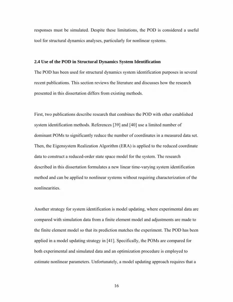
A flowchart describing the SL method is shown in Fig. 3.4.
39
Fig. 3.4 Flowchart for SL Method
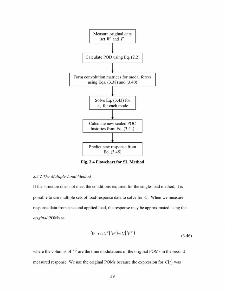
3.3.2 The Multiple-Load Method
If the structure does not meet the conditions required for the single-load method, it is
possible to use multiple sets of load-response data to solve for C . When we measure
response data from a second applied load, the response may be approximated using the
original POMs as
( ) ( )TT VUWUUW ˆ222 =≈ (3.46)
where the columns of V̂2 are the time modulations of the original POMs in the second
measured response. We use the original POMs because the expression for ( )tC was
Measure original data set W and F
Calculate POD using Eq. (2.2)
Solve Eq. (3.43) for iic for each mode
Calculate new scaled POC histories from Eq. (3.44)
Form convolution matrices for modal forces using Eqs. (3.38) and (3.40)
Predict new response from Eq. (3.45)

40
developed using only one set of POMs in Eq. (3.2). The modal forces may also be
computed for the second load case using the original POMs:
( )FTii
22 uq = (3.47)
In Eq. (3.47), F2 is a matrix similar to F in Eq. (3.37), but it contains force data for the
second load case. We may repeat this procedure for k sets of load and response data and
add a sufficient number of rows to Eq. (3.42) to solve for C :
C
QQQ
QQQQQQ
V
VV
kkkk
k
k
k ⎥⎥⎥⎥⎥
⎦
⎤
⎢⎢⎢⎢⎢
⎣
⎡
=
⎥⎥⎥⎥⎥
⎦
⎤
⎢⎢⎢⎢⎢
⎣
⎡
21
22
21
221
2
ˆ
ˆˆ
(3.48)
In Eq. (3.48), ijQ is defined as the convolution matrix for the thi modal force and the thj
load case. Once C has been identified by solving Eq. (3.48), we may compute POC
histories for the response to a new force F~ . New modal forces are calculated as in Eq.
(3.38) and formed into convolution matrices as shown in Eq. (3.40). The new POC
histories are then calculated by convolving the new modal forces with C :
CQQQV k ⎥⎦⎤
⎢⎣⎡=
~~~~̂21 (3.49)
Once the new POC histories have been calculated, Eq. (3.45) may be used to calculate the
predicted response of the system to the new load. A flowchart for the ML method is
provided in Fig. 3.5.

41
Fig. 3.5 Flowchart for ML Method
3.4 Mixed Response
The previous sections introduced methods for using strictly free or forced responses of a
system to predict new free or forced responses, respectively, but the methods could not be
combined, i.e. a measured free response could not be used to predict a forced response or
Measure original data set W and F
Calculate POD (Eq. 2.2). Determine k for a desired signal energy percentage
Measure k-1 supplemental data sets
Express all data sets in terms of original POMs (Eqs. (3.25) and (3.31))
Calculate new scaled POC histories from Eq. (3.49)
Solve Eq. (3.48) for C
Form convolution matrices for modal forces using Eqs. (3.38) and (3.40)
Predict new response from Eq. (3.45)

42
vice versa. This section describes a method from [56] and [57] for using measured mixed
responses of a system to form a predictive model for both free and forced responses. The
method assumes that the structure is lightly damped and that the mass matrix is
proportional to the identity matrix and that the POMs are therefore equal to the
eigenmodes.
We begin by measuring three distinct sets of response data that all result from separate
combinations of both applied loads and initial conditions. The data are arranged in
snapshot matrices Wa , Wb and Wc . We now calculate the POD of the first snapshot
matrix:
( )( )( ) ( )( )TaaTaaaa VUVUW ˆ=Σ≈ (3.50)
In Equation (3.50) we have combined the POVs with the POC histories. Equation (3.50)
is an approximation because we have kept only the k dominant POMs. We may
approximate the snapshot matrix Wb using the first set of POMs as
( )( )( )WUUW bTaab ≈ (3.51)
where the approximation is now transformed into the subspace spanned by the POMs
Ua . We may rewrite Equation (3.51) as
( )( )Tbab VUW ˆ≈ (3.52)

43
where TbV̂ contains the time modulations of the POMs Ua in the response Wb . Similarly,
Wc can be approximated by
( )( )Tcac VUW ˆ≈ (3.53)
where
( )( )WUV cTaTc =ˆ (3.54)
Using the POV recalculation and single-load identification methods outlined in the
previous sections, we now write each POC history as a superposition of free and forced
responses:
iiia
velivelia
dispidispia
ia Q cvvv ~ˆ ,,,, ++= σσ (3.55)
iiib
velivelib
dispidispib
ib Q cvvv ~ˆ ,,,, ++= σσ (3.56)
iiic
velivelic
dispidispic
ic Q cvvv ~ˆ ,,,, ++= σσ (3.57)
The modal forces used to form the matrices iaQ~ , i
bQ~ and icQ~ are all computed using the
POMs Ua . The terms dispi,v and veli,v are POC histories for calculating the response to
initial displacements and velocities, respectively. The term iic may be considered a
discretized modal impulse response function. We wish to solve for dispi,v , veli ,v , and iic as
they will allow us to predict system responses to new initial displacements, initial

44
velocities, and loads, respectively. However, Eqs. (3.55) - (3.57) represent only three
matrix equations and there are nine matrix unknowns.
Additional equations may be found by considering the initial displacement and velocity
profiles used to generate Wa , Wb and Wc . We can compute the ratio of two displacement
related POVs as
( )( )( )( )
( )( )( )( )0
0
,0,0
,0,0
,
,
//
wuwu
wuwu
bTi
a
aTi
a
dispibT
ia
dispiaT
ia
dispib
dispia
vv
==σσ
(3.58)
Similarly, the remaining displacement POV ratio and the velocity POV ratios can be
computed as
( )( )( )( )0
0
,
,
wuwu
cTi
a
aTi
a
dispic
dispia
=σσ
(3.59)
( )( )( )( )0
0
,
,
wuwu
bTi
a
aTi
a
velib
velia
=σσ
(3.60)
( )( )( )( )0
0
,
,
wuwu
cTi
a
aTi
a
velic
velia
=σσ
(3.61)
The final two equations are obtained by recalling the orthonormality of POC histories:
1,dispi, =dispiT vv (3.62)
1,veli, =veliT vv (3.63)

45
Eqs. (3.55) - (3.63) represent a system of linear equations that may be solved to obtain
dispi,v , veli ,v , and iic for i = 1, 2, …, k. Once these quantities are obtained they may be
used as explained in the previous sections to predict the response of the system to any
combination of initial displacements or applied loads.
If mixed response data are used to predict the response to initial velocities then the
method given in Section 3.2.1 must be modified slightly. In Section 3.2.1 the initial time
derivative of each POC history was calculated from Equation (3.18). If mixed response
data are used to identify veli ,v then the initial time derivative veliv ,0, can not be calculated
in the same way because there are no POVs directly corresponding to veli ,v . In this case,
however, we can approximate veliv ,0, a
( ) ( )
ttvtv
v veliveliveli Δ
−≈ 1,2,
,0, (3.64)
The MR method is described in a flowchart in Fig. 3.6 below.
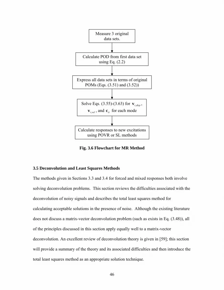
46
Fig. 3.6 Flowchart for MR Method
3.5 Deconvolution and Least Squares Methods
The methods given in Sections 3.3 and 3.4 for forced and mixed responses both involve
solving deconvolution problems. This section reviews the difficulties associated with the
deconvolution of noisy signals and describes the total least squares method for
calculating acceptable solutions in the presence of noise. Although the existing literature
does not discuss a matrix-vector deconvolution problem (such as exists in Eq. (3.48)), all
of the principles discussed in this section apply equally well to a matrix-vector
deconvolution. An excellent review of deconvolution theory is given in [59]; this section
will provide a summary of the theory and its associated difficulties and then introduce the
total least squares method as an appropriate solution technique.
Measure 3 original data sets.
Calculate POD from first data set using Eq. (2.2)
Express all data sets in terms of original POMs (Eqs. (3.51) and (3.52))
Calculate responses to new excitations using POVR or SL methods
Solve Eqs. (3.55)-(3.63) for dispi,v ,
veli ,v , and iic for each mode

47
The convolution of two signals ( )th and ( )tx in the time domain is given by
( ) ( ) ( ) ( ) ( )∫∫ −=−=tt
dhtxdxthty00
ττττττ (3.65)
and is usually symbolized by the ‘*’ operator:
( ) ( ) ( ) ( ) ( )thtxtxthty ∗=∗= (3.66)
Deconvolution is the procedure of determining ( )th from knowledge of ( )tx and ( )ty .
Deconvolution has no direct mathematical definition in the time domain other than being
the inverse of Eq. (3.65). In the frequency domain, however, convolution is expressed as
multiplication
( ) ( ) ( )ωωω jXjHjY = (3.67)
and deconvolution is performed by division of frequency spectra:
( ) ( )( )ωωω
jjjH
XY
= (3.68)
With exact knowledge of ( )tx and ( )ty , deconvolution is possible and ( )th can be
determined exactly in the frequency domain from Eq.. (3.52) or in the time domain by
solving a system of linear equations as in Eq. (3.43). In practice, however, ( )tx and ( )ty
are not known exactly, but are obtained from noisy measurements. The measured signals,
denoted ( )txw and ( )tyw , can be expressed as
48
( ) ( ) ( )txtxtx ew += (3.69)
( ) ( ) ( )tytyty ew += (3.70)
where ( )txe and ( )tye are unknown error components. Expressing the true signals in
terms of measured and error components into Eq. (3.67) yields
( ) ( ) ( ) ( ) ( )[ ]ωωωωω jXjXjHjYjY ewew −=− (3.71)
Eq. (3.71) cannot be solved for ( )ωjH because the error components are unknown.
Instead, we solve for
( ) ( )( )ωω
ωjj
jH ww
w
XY
= (3.72)
which may or may not be a good approximation to ( )ωjH . In fact, we can examine the
approximation by rewriting Eq. (3.71) and comparing it with Eq. (3.72). The
approximation is
( ) ( )( )
( ) ( )( ) ( )
( )( ) ( )ωωω
ωωωω
ωωω jH
jj
jjjj
jjjH w=≈
−−
==w
w
ew
ew
XY
XXYY
XY
(3.73)
Unfortunately, there are several situations where this approximation fails, resulting in a
very poor estimate of ( )ωjH . First, there are regions where ( )ωjX may be very small
(and, from Eq. (3.67), ( )ωjY is small as well). The resulting approximations that
( ) ( )ωω jXjX w≈ and ( ) ( )ωω jYjY w≈ are then likely to be inaccurate and the ratio
( ) ( )ωω jXjY ww / may be orders of magnitude off [59]. Another special case is where

49
( ) ( )ωω jXjX e−= , resulting in infinite values for ( )ωjH w . These errors in ( )ωjH w
may dominate the entire behavior of the time-domain signal, obscuring all meaningful
details of ( )thw [59].
Although this description has utilized the frequency-domain form of deconvolution in Eq.
(3.68) for explanation, the same errors exist when deconvolution is performed entirely in
the time domain [59]. Due to these errors, the deconvolution problem cannot be solved
uniquely and is therefore often referred to as “ill-conditioned” or “ill-posed” [60]. It is
possible, however, to calculate an acceptable estimate for ( )thw using least squares
methods [58].
We recall that the deconvolution problem for single- and multiple-load methods can be
solved by solving the linear systems in Eqs. (3.27) and (3.32), respectively. A general
system of linear equations may be written as
bxA = (3.74)
where nnA ×ℜ∈ is called the data matrix 1×ℜ∈ nb is typically known as a vector of
observations. If the system represents the structural deconvolution problems in Eqs.
(3.43) and (3.48), then A corresponds to a modal force and b corresponds to a POC
history, which is calculated from measured displacements. Therefore, uncertainty in
force and displacement measurements result in errors in A and b , respectively.
50
The least squares approach to deconvolution considers only errors in b and may be cast
in terms of calculating LSx [58] such that
rbxA LS += (3.75)
where we minimize 2
r subject to the constraint that ( )ARangerb ∈+ . In other words,
we allow b to vary the minimum amount required so that it falls in the column space of
A . The solution may be computed as
( ) bAbAAAx TTLS
+−==
1
(3.76)
where +A is the Moore-Penrose pseudoinverse of A . If measurement errors are present
in the displacements only and the applied is known exactly then a least-squares estimate
will yield an accurate response prediction [58].
The total least squares method is designed for application when errors in both A and b
are significant and can be posed as solving for TLSx such that
( ) rbxEA TLS +=+ (3.77)
and for which we minimize [ ]F
rE subject to ( )EARangerb +∈+ , whereF
⋅
signifies the Frobenius norm. The total least squares problem is “equivalent to the
problem of solving a nearest least squares problem of minimizing ( ) ( )2
rbxEA +−+
51
where nearness is measured by the…Frobenius norm” [58]. We may calculate TLSx by
first forming an augmented matrix C :
[ ]bAC = (3.78)
Reference [58] shows that if the singular value decomposition of C is computed as
T
CCC VUC Σ= (3.79)
then a total least squares solution may be calculated from the r most dominant right
singular vectors of C :
[ ]
⎟⎠
⎞⎜⎝
⎛−
⎟⎟⎠
⎞⎜⎜⎝
⎛
=
∑
∑
=+
=+
r
iinC
Tr
iinCiCiCinC
TLS
V
VVVV
x
1
2,1,
1,,,2,,1,,1,
1 (3.80)
Reference [58] gives a method for choosing a value for r based on the signal-to-noise
ratio of the measured data.
Finally, we note that the proposed algorithm for total least squares from [58] assumes that
weighting matrices for the problem are equal to the identity matrix. A more general total
least squares method is formulated by solving Eqn. (3.77) while minimizing
FD E r T⎡ ⎤⎣ ⎦ , where D and T are diagonal weighting matrices with positive diagonal
terms. It is possible, perhaps even probable, that non-identity weighting matrices will
yield a more accurate solution, but this topic is left for future research.

52
3.6 Sources of Error
Several types of error will be present in predictions made with the POD-based methods
presented in this section. This section discusses four probably sources of error, namely
projection error, diagonalization error, linearization error, and deconvolution error.
The first type of error is called “projection” error because the original problem is
projected onto a reduced subspace spanned by a limited set of dominant POMs. Because
of this projection, the model can only accurately predict a response matrix that may be
spanned by the original set of POMs. If a new excitation is introduced that generates a
response that cannot be expressed by the original POMs then the prediction will be
inaccurate. An extreme example arises when a model constructed from a response that is
restricted to one plane is used to predict the response an excitation that excites motion
that is restricted to a perpendicular plane. In this case, the measured POMs are entirely
unable to represent the responses to these new initial conditions and the method predicts
no response at all. Therefore, when constructing the model it is desirable to use a
response to that exhibits a wide variety of motion in order to generate POMs that can
represent responses to a large selection of new excitations.
Projection error is also encountered when a limited set of POMs is used as a basis for
model reduction (linear or nonlinear). Despite the presence of this error, POMs are often
used for model reduction and it is assumed that the error will be low. Currently there is
no satisfactory method for estimating this error ahead of time, although an attempt has
been made in [46]. Their method estimates an upper bound for the projection error, but

53
they assume that the new excitation is similar to the original one and admit that the
method is invalid for excitations that are substantially different. Because there is no
indication of how similar is similar enough, the method has no guarantee of accuracy.
Another source of error for several of the methods lies in the assumption that the matrices
( )t11Φ , ( )t12Φ , and ( )tC are diagonal. In reality, structures will not generally meet the
conditions required for these matrices to be diagonal and the resulting error is called
“diagonalization” error. The mass matrix of almost any real structure will not be
proportional to the identity matrix (e.g. even the mass matrix for a beam element is not
diagonal). The damping of a system may also be heavy and the damping matrix is
generally not proportional to a linear combination of the mass and stiffness matrices.
When the conditions are not met exactly then the accuracy of the method will suffer.
However, the damping may be light and the mass matrix may be diagonally dominant
with diagonal terms that are similar even if they are not identical. In these cases the
solution may be accurate enough that it may be appropriate to use methods that assume
diagonal ( )t11Φ , ( )t12Φ , and ( )tC matrices.
When the methods are applied to nonlinear systems, a linear time-varying model is
obtained that will match the measured nonlinear response exactly. For nonlinear systems,
a new excitation can result in a significant change in the natural frequencies of the system
and/or cause the system exhibit new behaviors [10, 11]. The model constructed from
these linear methods will be unable to predict these new effects and we call the resulting
error “linearization” error. However, the model may be used to accurately predict the

54
structure’s response to an excitation that is “nearby” the original one. This error is
inherent in using linear methods to identify nonlinear systems, but may be acceptable
when nonlinear methods cannot be applied due to difficulties described in Chapter 2.
Another manifestation of linearization error occurs when multiple data sets are used to
construct the model. When these methods are applied to identify a linear time-varying
system, each data set results from a system that varies with time in the same way over
time, i.e. the time variance repeats itself in each data set. Nonlinear systems will exhibit
different time-varying behaviors in each data set and therefore all of the data sets cannot
be represented by the same linear time-varying system. The methods, then, will identify
an “average” linear time-varying system in the sense that it contains characteristics from
each measured response and can reconstruct all of the original responses accurately (as
long as they can be accurately expressed by the chosen POMs). When the methods are
applied to predict the response to a new excitation, amplitude errors may present that
result from a combination of periodic signals of varying frequencies. Due to the
differences in frequencies, each signal will move in and out of phase with the others and
the combined signal will exhibit amplitude distortions as a result (this is analogous to
averaging two sine waves of slightly different frequencies). This error will grow with the
strength of the nonlinearities in the system because the frequency content in each data set
will differ more in the presence of strong nonlinearities than weak ones.
Finally, as explained in the previous section, the deconvolution operations in the forced
and mixed response methods cannot be performed exactly when noise is present in the

55
data. The magnitude of this error will depend on the quality of the data and is likely to be
very high if the data are very noise. As with linearization error for multiple data sets, an
interesting compromise arises because of the deconvolution and projection error. In order
to minimize projection error, one may desire to use a large number of POMs in the
identification methods. Unfortunately, this will generally lead to higher deconvolution
error because the noise level is higher in the lower POMs and POC histories.
3.7 Summary
This chapter has explained the theory behind five methods for identification of linear
time-varying systems. The methods extend the capabilities beyond other existing
methods in that they may be applied to multiple-input multiple-output systems, they
require only a small number of data sets, and no knowledge regarding the form of the
time variance in the structure is necessary to obtain a predictive model.
The methods are summarized in Table 3.1 below. The methods are referred to as POVR,
MDS, SL, ML, and MR for the Proper Orthogonal Value Recalculation”, “Multiple Data
Set”, “Single-Load”, “Multiple-Load”, and “Mixed Response” methods, respectively.
The table shows the excitation type each method is valid for, and types of error that are
expected to be present in the methods’ predictions for linear systems (other than errors
related to noise in the data). These error types are abbreviated as “Proj” for projection
error and “Diag” for diagonalization error. The table also shows the number of data sets
(NDS) required be each method, as well as any assumptions made by the method other
than that the system is linear.

56
Table 3.1 Summary of Proposed System Identification Methods
Method Excitation Type Error NDS Assumptions POVR Initial Conditions Proj, Diag 1 Diagonal ( )t11Φ or ( )t12Φ MDS Initial Conditions Proj k None SL Loads Proj, Diag 1 Diagonal ( )tC ML Loads Proj, k None MR Both Proj, Diag 3 Diagonal ( )tC , ( )t11Φ and ( )t12Φ

57
4. Numerical Examples
This chapter applies the methods described in Chapter 3 to three beam models and a
satellite truss model. The strengths and weakness of each method when applied to various
types of systems are then discussed at the end of the chapter.
4.1 Beam Models
The three beam models are shown in Fig. 4.1. The first model is a linear time-invariant
(LTI) undamped cantilever beam. Next, a time-varying tip mass is attached to the tip of
the beam to convert it to a linear time-varying (LTV) system. The LTI beam is also
converted to a nonlinear (NL) system by attaching a cubic spring to the tip. A dashpot is
also attached to the nonlinear beam to simulate damping. All of the beam models were
made of steel (E = 61029× psi, ρ = 500 lbm/ft3) and had dimensions of 24 x 1 x 0.75
inches. Finite element (FE) models were created for each beam using 24 beam elements.
The spring force (over the tip displacement range seen in simulations) for the nonlinear
beam is shown in Fig. 4.2 and the time variance in the tip mass for the second beam is
shown in Fig. 4.3 along with their respective governing equations. The value of the
dashpot was 0.2 lbf-s/in.

58
Fig. 4.1 LTI (top), LTV (middle), and NL (bottom) Beam Models
Fig. 4.2 Cubic Spring Force for Nonlinear Beam Model
( ) 360010 tiptiptip wwwF +=
( )tm

59
Fig. 4.3 Time Variation of Tip Mass for LTI Beam Model
The Newmark method [61] was applied to simulate the exact response of each beam
model to various excitations and the appropriate methods were applied to predict the
response of the beam to new free, forced, or mixed responses as shown in the respective
following sections.
4.1.1 Free Response
The FE models were used to simulate the exact response of each model beam model to
four initial displacement profiles, shown in Fig. 4.4. Each displacement profile was
generated by applying static loads to the LTI beam. The displacement profile 0w was
generated by applying static loads of 300, 200, and -260 lbf at locations 17, 18, and 24
inches from the root of the beam. Profiles 1w and 2w were formed by applying static
loads of 100 and -300 lbf at locations 24 and 8 inches from the root of the beam,
( ) tetm 30005.0 −=

60
respectively. Finally, the initial displacement profile 3w was formed by applying loads
of 2000 and -1300 lbf at locations 14 and 18 inches from the beam root. The free
responses of each model to each initial displacement were simulated for 0.05 seconds
(approximately twice the fundamental period of 0.0238 seconds for the linear beam) and
the vertical displacements at 25 points were captured at every time step (0.1 milliseconds)
to form W . Thus the dimensions of W were (25 x 500) for both models.
Fig. 4.4 Applied Initial Displacement Profiles
Next, the POD was computed from each beam’s response to 0w and the method of POV
recalculation (POVR) was applied to simulate the responses of each of the beams to
initial displacement profile 3w . The free response method using multiple data sets (MDS)
was also applied to predict the response to 3w using the responses to initial displacement
profiles 1w and 2w as supplementary data sets. The responses were simulated using the
first three POMs, which corresponded to 99% of the signal energy in the LTI beam’s

61
response to 0w . The three most dominant original POVs (calculated from the measured
response to 0w ) and recalculated POVs (for the response to 3w ) are shown in Fig. 4.5
for the LTI beam. The “index” on the horizontal axis simply denotes the order of each
POV in dominance (i.e. the largest POV is first, the second-largest POV is second and so
on). The original POVs drop off very quickly, showing that only a few POMs are
necessary to represent the measured response accurately. This figure also illustrates how
the significance of each mode changes in response to the different initial displacement
profiles. For example, the first POV for both beams is larger in response to 0w than to
3w , indicating that the first POM is more active in the response to 0w than to 3w . The
original and recalculated POVs for the LTV and NL beams show similar behaviors and
are not shown.
Fig. 4.5 Original and Recalculated POVs for Linear Beam Model

62
In order to represent the displacement of every point at each time step, a displacement
norm is defined as:
[ ] [ ] [ ]iT
ii ttt www =2 (4.1)
Direct comparison of time-series data is generally considered a very strict validation
metric for a model, but is useful in this case because it can be used to express all of the
prediction data in a single plot for easy comparison with ‘exact’ results from a finite
element model. The displacement norms at each time step calculated by the FE models
and the POVR and MDS methods for the linear beam responses to 3w are shown in Figs.
4.6 and 4.8 for the LTI and LTV beams, respectively. The percent errors in each
prediction were calculated at each time step from the equation
[ ]
[ ] [ ][ ] 2
22%100
iFE
ipredictediFEi t
tttPE
w
ww −×=
(4.2)
and are shown in Figs. 4.7 and 4.9 for the LTI and LTV beams. These figures show that
the MDS method predicts the displacements very accurately (nearly always < 5% error)
for the linear beams in response to the new initial displacement profiles. Small
inaccuracies exist in the MDS prediction are attributed to projection error, i.e. the POMs
from the response to 0w are not optimal for predicting the response to 3w . The percent
error is relatively high at locations where the displacement norm of the FE model is close
to zero, resulting in a very small number in the denominator of Eq. (4.2). The POVR
method works very well for the LTI beam, although it is not as accurate as the MDS
method due to the diagonalization error described in Section 3.6. For the LTV beam,

63
however, the POVR method does not provide an accurate prediction. The diagonalization
error for the LTV beam is expected to be much greater because the large value of the tip
mass results in a mass matrix with diagonal terms that are not close in value.
Fig 4.6 Displacement Norms for LTI Beam Model in Response to 3w
64
Fig. 4.7 Percent Error of Displacement Norms for LTI Beam Model in Response to
3w
Fig. 4.8 Displacement Norms for LTV Beam Model in Response to 3w

65
Fig. 4.9 Percent Error of Displacement Norms for LTV Beam Model in Response to
3w
The displacement norms and corresponding percent errors for the nonlinear beam’s
response to 3w are shown in Figs. 4.10 and 4.11. It is very apparent that, in this case,
significant errors exist in the predictions generated by both the POVR and MDS methods.
Frequency errors exist in both predicted responses, and significant amplitude errors are
present in the MDS method’s response. The frequency errors result in phase shifts that
increase with time and are visible in the percent error plots as the error increases in
magnitude over time. Both the frequency and amplitude discrepancies are most likely
manifestations of linearization error, i.e., they can be attributed to the fact that the natural
frequencies of the nonlinear beam change with each new initial condition and the POD-
based methods are unable to reproduce (POVR and MDS methods) or interpret (MDS
method) the changing frequencies appropriately. The significant amplitude errors in the
response predicted by the MDS method result from the method attempting to create an

66
“average” time-varying model from periodic signals of different frequencies. The various
responses are out of phase with each other and their combination results in the amplitude
distortions that are present. For this model and the corresponding excitation sets, the
POVR method is actually more accurate than the MDS method. Projection error (for both
methods) and diagonalization error (for the POVR method) are both present as well, but
they are dwarfed by the linearization error.
Fig. 4.10 Displacement Norms for NL Beam Model in Response to 3w
67
Fig. 4.11 Percent Error of Displacement Norms for NL Beam Model in Response to
3w
Next, we applied the methods described in Section 3.2 to the three beam models (Fig.
4.1) to predict the initial velocity response of each beam. As with the initial displacement
example, FE models for each beam were used to simulate the exact response of each
beam to multiple initial velocity profiles, shown in Fig. 4.12. The initial velocity profiles
were constructed by applying 1000-lbf impulses to locations 19, 15, 11, 7, and 3 inches
from the root of the LTI beam and measuring the resulting velocity changes. Four POMs
and POC histories (capturing 99% of the original signal energy) were obtained from the
response of each model to the initial velocity profile 0w and used to predict responses to
4w for each beam using both the POVR and MDS methods. The maximum tip
displacements of the nonlinear beam in response to 0w , 1w , 2w , 3w , and 4w were
0.30, 0.26, 0.18, 0.10, and 0.03 inches, respectively, so that the nonlinear spring was
excited at various levels of its nonlinear range.
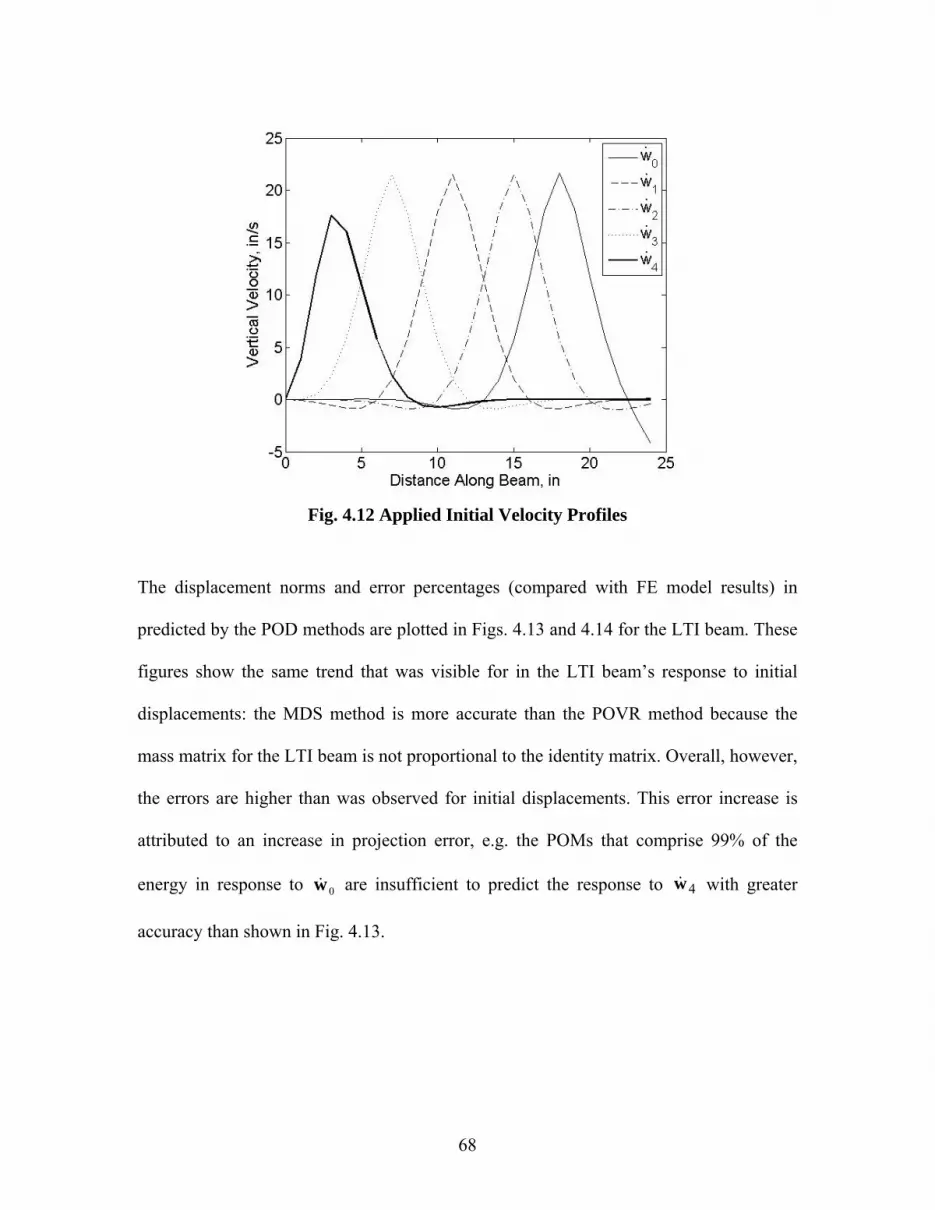
68
Fig. 4.12 Applied Initial Velocity Profiles
The displacement norms and error percentages (compared with FE model results) in
predicted by the POD methods are plotted in Figs. 4.13 and 4.14 for the LTI beam. These
figures show the same trend that was visible for in the LTI beam’s response to initial
displacements: the MDS method is more accurate than the POVR method because the
mass matrix for the LTI beam is not proportional to the identity matrix. Overall, however,
the errors are higher than was observed for initial displacements. This error increase is
attributed to an increase in projection error, e.g. the POMs that comprise 99% of the
energy in response to 0w are insufficient to predict the response to 4w with greater
accuracy than shown in Fig. 4.13.

69
Fig. 4.13 Displacement Norm for LTI Beam Model in Response to 4w
Fig. 4.14 Percent Error of Displacement Norms for LTI Beam Model in Response to
4w
Figs. 4.15 and 4.16 show the response predictions and percent errors for the LTV beam.
Again, the error is higher using the POVR method than the MDS method, likely because

70
the large mass at the tip of the beam increases the diagonalization error. The level of error
for the MDS method in this response is approximately the same as for the LTI beam, and
is attributed to projection error.
Fig. 4.15 Displacement Norm for LTV Beam Model in Response to 4w

71
Fig. 4.16 Percent Error of Displacement Norms for LTV Beam Model in Response
to 4w
The response predictions generated by the POVR and MDS methods for the nonlinear
beam are compared with finite element model predictions in Figs. 4.17 and 4.18 below.
Both response predictions exhibit a slight frequency error (the increasing phase
difference between signals is visible in the percent error plot for the MDS method as the
error increases over time) and is assumed to be a result of linearization effects. The
linearization error is also present for the POVR method but it is difficult to see in the
percent error plot because errors associated with diagonalization are also present.

72
Fig. 4.17 Displacement Norm for NL Beam Model in Response to 4w
Fig. 4.18 Percent Error of Displacement Norms for NL Beam Model in Response to
4w
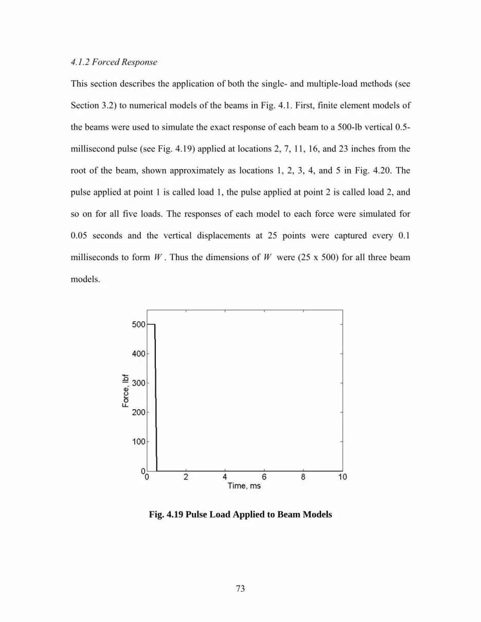
73
4.1.2 Forced Response
This section describes the application of both the single- and multiple-load methods (see
Section 3.2) to numerical models of the beams in Fig. 4.1. First, finite element models of
the beams were used to simulate the exact response of each beam to a 500-lb vertical 0.5-
millisecond pulse (see Fig. 4.19) applied at locations 2, 7, 11, 16, and 23 inches from the
root of the beam, shown approximately as locations 1, 2, 3, 4, and 5 in Fig. 4.20. The
pulse applied at point 1 is called load 1, the pulse applied at point 2 is called load 2, and
so on for all five loads. The responses of each model to each force were simulated for
0.05 seconds and the vertical displacements at 25 points were captured every 0.1
milliseconds to form W . Thus the dimensions of W were (25 x 500) for all three beam
models.
Fig. 4.19 Pulse Load Applied to Beam Models

74
Fig. 4.20 Five Locations of Pulse Load Application
Next, the POD was computed for each beam from the response to load 1 and both the
single-load (SL) and multiple-load (ML) methods were applied to simulate the responses
of each beam to load 5. The first four POMs were considered, corresponding to 99% of
the original signal energy. For the ML method, responses to loads 2, 3, and 4 were used
as supplementary loads to solve for off-diagonal elements of ( )tC .
The displacement norm at each time step was calculated for the FE results and the
predictions obtained using the single-load (SL) and multiple-load (ML) methods. Fig.
4.21 shows the displacement norms for the LTI beam’s response to load 5, and Fig. 4.22
shows the percent errors for displacement norms of the SL and ML methods. The figures
show that while both methods are able to predict the displacement of the LTI beam
accurately when compared with the FE model, the ML method is more accurate than the
SL method. This accuracy difference is attributed to the fact that the beam does not have
a mass matrix proportional to the identity matrix as the SL method assumes.
1 2 3 4 5
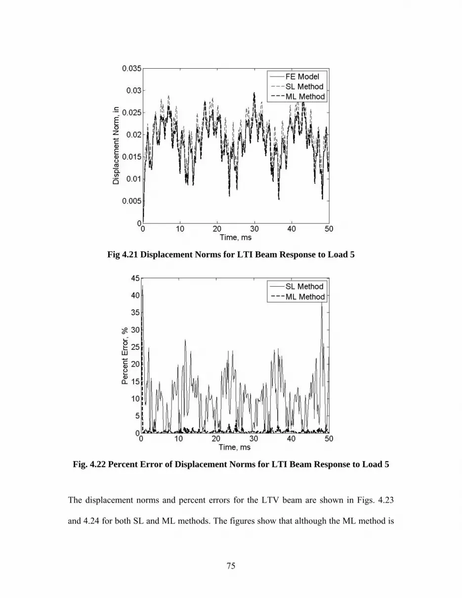
75
Fig 4.21 Displacement Norms for LTI Beam Response to Load 5
Fig. 4.22 Percent Error of Displacement Norms for LTI Beam Response to Load 5
The displacement norms and percent errors for the LTV beam are shown in Figs. 4.23
and 4.24 for both SL and ML methods. The figures show that although the ML method is

76
able to predict the displacement of the LTV beam very accurately when compared with
the FE model, the SL method is terribly inaccurate. The large tip mass that is present in
the LTV beam likely leads to very high diagonalization error when the SL method is
applied.
Fig 4.23 Displacement Norms for LTV Beam Response to Load 5

77
Fig. 4.24 Percent Error of Displacement Norms for LTV Beam Response to Load 5
The displacement norms for response of the NL beam are shown in Fig. 4.25, and the
percent errors for both the SL and ML methods are shown in Fig. 4.26. The amplitude of
the displacement norm decreases over time due to the damping effect of the dashpot.
Again, the ML method provides a better prediction than the SL method because it does
not assume a diagonal ( )tC matrix. The percent error for the ML method increases over
time due to linearization error. Linearization error is, of course, also present for the SL
method, but it is combined with diagonalization error and is more difficult to visualize in
Fig. 4.26.

78
Fig 4.25 Displacement Norms for NL Beam Response to Load 5
Fig. 4.26 Percent Error of Displacement Norms for NL Beam Response to Load 5

79
4.1.3 Mixed Response
This section applies the mixed response (MR) method described in Section 3.4 to the
beam models in Fig. 4.1. The Newmark method was used to simulate the exact response
of each model to three excitation sets consisting of initial displacements and velocities
and an applied force. The initial displacement and velocity profiles for the beams are
shown in Figures 4.27 and 4.28, respectively, and a 500-lb vertical pulse was applied for
0.5 millisecond (see Fig. 4.19) at locations 21, 12, and 3 inches from the beam root for
respective excitation sets a, b, and c. The responses of each beam model to each
excitation set were simulated for 50 milliseconds and the vertical displacements at 25
points along each beam were captured every 0.1 milliseconds to form W . Thus the
dimensions of Wa , Wb and Wc were (25 x 500) for all beam models.
Fig. 4.27 Initial Displacements in Excitation Sets a, b, and c

80
Fig. 4.28 Initial Velocities in Excitation Sets a, b, and c
Next, the POD was computed for each beam’s response to the first excitation set and the
MR method described in Section 3.4 was applied to identify dispi,v , veli ,v , and iic for each
beam. These quantities were used to simulate the response of both systems to a new
initial displacement 0~w , a new initial velocity 0
~w , and a new applied load ( )tF~ , shown
in Figures 4.29, 4.30, and 4.31, respectively. The responses were simulated using the first
four POMs, which corresponded to 99% of the signal energy.

81
Fig. 4.29 New Initial Displacement Profile 0~w
Fig. 4.30 New Initial Velocity Profile 0~w
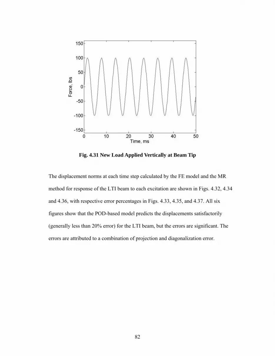
82
Fig. 4.31 New Load Applied Vertically at Beam Tip
The displacement norms at each time step calculated by the FE model and the MR
method for response of the LTI beam to each excitation are shown in Figs. 4.32, 4.34
and 4.36, with respective error percentages in Figs. 4.33, 4.35, and 4.37. All six
figures show that the POD-based model predicts the displacements satisfactorily
(generally less than 20% error) for the LTI beam, but the errors are significant. The
errors are attributed to a combination of projection and diagonalization error.

83
Fig. 4.32 Displacement Norms for LTI Beam in Response to 0~w
Fig. 4.33 Percent Error of Displacement Norms for LTI Beam in Response to 0~w

84
Fig. 4.34 Displacement Norms for LTI Beam in Response to 0~w
Fig. 4.35 Percent Error of Displacement Norms for LTI Beam in Response to 0~w

85
Fig. 4.36 Displacement Norms for LTI Beam in Response to ( )tF~
Fig. 4.37 Percent Error of Displacement Norms for LTI Beam in Response to ( )tF~

86
The displacement norms at each time step calculated by the FE model and the MR
method for the LTV beam are shown in Figs. 4.38, 4.40, and 4.42 for the responses to the
initial displacement, initial velocity, and load, respectively. The corresponding error
percentages are shown in Figs. 4.39, 4.41, and 4.43. The figures show that MR method
does not provide good predictions for the LTV beam model for any of the excitations,
particularly the response to the initial velocity and applied load. These high errors are
attributed to the fact that the tip mass causes high diagonalization error.
Fig. 4.38 Displacement Norms for LTV Beam in Response to 0~w

87
Fig. 4.39 Percent Error of Displacement Norms for LTV Beam in Response to 0~w
Fig. 4.40 Displacement Norms for LTV Beam in Response to 0~w

88
Fig. 4.41 Percent Error of Displacement Norms for LTV Beam in Response to 0~w
Fig. 4.42 Displacement Norms for LTV Beam in Response to ( )tF~

89
Fig. 4.43 Percent Error of Displacement Norms for LTV Beam in Response to ( )tF~
The displacement norms for the NL beam are shown in Figs. 4.44, 4.46, and 4.48 for the
three new excitations, with corresponding error percentages in Figs. 4.45, 4.47, and 4.49.
In each figure the results obtained using the MR method are plotted with the exact results
obtained by the FE models. The figures show that the MR method is capable of
generating a reasonably accurate response prediction, although several sources of error
are present. Projection errors and diagonalization errors are probably present, although
diagonalization error is significantly lower than for the LTV beam because the model
approximately meets the conditions for ( )tC to be diagonal. The response predictions for
the NL beam contain additional linearization errors that show up as frequency and
magnitude discrepancies in Figs. 4.44 and 4.46.

90
Fig. 4.44 Displacement Norms for NL Beam in Response to 0~w
Fig. 4.45 Percent Error of Displacement Norms for NL Beam in Response to 0~w

91
Fig. 4.46 Displacement Norms for NL Beam in Response to 0~w
Fig. 4.47 Percent Error of Displacement Norms for NL Beam in Response to 0~w

92
Fig. 4.48 Displacement Norms for NL Beam in Response to ( )tF~
Fig. 4.49 Percent Error of Displacement Norms for NL Beam in Response to ( )tF~

93
4.2 Satellite Truss Model
In this section, the POVR, MDS, SL, and ML methods from Sections 3.2 and 3.3 are
applied to a satellite truss structure, one element of which is shown in Fig. 4.50. The MR
method is not applied because the diagonalization error is anticipated to be very high
based on the results from the POVR and SL methods.
The cross section of a truss element is an equilateral triangle as shown in Fig. 4.50, and
the length of each side is 3 meters. Each element is constructed of 21 truss members,
many of which share the same geometry and material properties (see Table 4.1). The
members all have hollow circular cross sections and are joined by idealized pin joints.
Fig. 4.50 Cross Section and Schematic View of a Single Truss Element [Courtesy Armaghan Salehian]
Table 4.1 Truss Member Geometry and Material Properties
Members Length (ft)
Diameter (in)
Thickness (in)
Young’s Modulus (psi)
Density (lbm/ft3)
1,1’,2,2’,3,3’ 9.8 3 0.04 1.00E+07 112.3 4,5,6,7,7’,8,8’,9,9’ 9.8 1 0.02 1.00E+07 112.3
10,10’,11,11’,12,12’ 13.9 1 0.02 1.00E+07 112.3
X3
X2 X2
X3
X1
4
600
11’11
12’12
10’ 10 7’
8’
9’ 65
1’1
3 3’
2’2
7 8
9
O

94
The motion of each truss element was described by nine coordinates that are defined in
Fig. 4.51. Only motion in the X1-X2 plane is considered and the displacement of the three
top joints is described by Δ1, Δ3, and Δ5. The displacements of the two bottom joints at
each cross-sectional face are assumed to be equal due to the symmetry of the truss
structure and are described by Δ2, Δ4, and Δ6. Rotation of the three cross-sectional faces
about the X3 axis is described by the coordinates Θ1, Θ2, and Θ3. Fifty truss elements
were assembled together lengthwise (the three boundary degrees of freedom at each truss
segment boundary overlapped with the boundary degrees of freedom of the elements on
either side) and pinned boundary conditions were applied to each end of the assembled
truss structure. The dimension of the global mass and stiffness matrices with boundary
conditions applied was therefore 299. After 3 seconds, the stiffness matrix for the 10th
truss element from the left boundary was removed from the global stiffness matrix to
simulate a fracture (i.e. the 10th truss element breaks off and disappears). As a result, the
remaining truss sections on the right and left of the break are free to exhibit rigid-body
rotation around each pinned end. The structure is therefore a linear time-varying system.
Fig. 4.51 Coordinates for Truss Element [Courtesy Armaghan Salehian]
Δ1
Δ2 Δ2 Δ4 Δ6
Δ3
Θ2 Θ1
Δ5
Δ6
Δ4
Θ3
7
9
4
6
58
1
2
3

95
4.2.1 Free Response
The POVR and MDS methods that were discussed in Section 3.2 for predicting responses
to initial displacements and velocities are applied to the satellite truss structure in this
section. First, six initial displacement profiles were formed by applying static loads as
shown in Table 4.2. The responses to each initial displacement were simulated for 10
seconds using the FE model for the truss using the Newmark method with a time step of
0.05 s, so the dimensions of W were (299 x 200) for each response.
Table 4.2 Static Loads Applied to Generate Initial Displacements for Truss
Force (lbf) DOF DOF Description 1w 11.3 140 Δ2 on 23rd truss element from left boundary
2w -16.9 22.5
50 80
Δ2 on 8th truss element from left boundary Δ2 on 13th truss element from left boundary
3w -6.7 200 Δ2 on 33rd truss element from left boundary
4w 67.4 290 Δ2 on 48th truss element from left boundary
5w 18.0 -13.5
56 170
Δ2 on 9th truss element from left boundary Δ2 on 28th truss element from left boundary
6w -89.9 20 Δ2 on 3rd truss element from left boundary
Next, the POD was computed from the response to 1w and the POVR method was
applied to predict the response to 6w with 5 POMs (99% of the original signal energy).
The MDS method was also applied to predict the response to 6w and the responses to
2w - 5w were used as supplementary data sets. The displacement norms and percent
errors for the response predictions are shown in Figs. 4.52 and 4.53, respectively. The
relatively large displacements due to the rigid body rotation of the two truss segments
after the break at 3 seconds are clearly visible in all of the displacement norms. The
POVR method generated a less accurate prediction than the MDS method, probably due
to diagonalization error, but the predicted responses for both methods are reasonably

96
accurate. Projection error is likely present in the predictions from both methods, but is
quite small in this case (the MDS method has very low error).
Fig. 4.52 Displacement Norms for Truss Model in Response to 6w
Fig. 4.53 Percent Error of Displacement Norms for Truss Model in Response to 6w

97
Next, eight initial velocity profiles were generated by applying 1125-lbf impulses to
various points along the truss and measuring the change in velocity. The locations of the
impulsive loads are given in Table 4.3 below.
Table 4.3 Impulsive Loads Applied to Generate Initial Velocities for Truss
Force (lbf) DOF DOF Description 1w 1125 80 Δ2 on 13th truss element from left boundary
2w 1125 140 Δ2 on 23rd truss element from left boundary
3w 1125 170 Δ2 on 28th truss element from left boundary
4w 1125 50 Δ2 on 8th truss element from left boundary
5w 1125 20 Δ2 on 3rd truss element from left boundary
6w 1125 200 Δ2 on 33rd truss element from left boundary
7w 1125 230 Δ2 on 38th truss element from left boundary
8w 1125 110 Δ2 on 18th truss element from left boundary
The POD was computed from the response to 1w and the POVR method for initial
velocities was applied to predict the response to 8w with 7 POMs (99% of the original
signal energy). The MDS method was also applied to predict the response to 8w and the
responses to 2w - 7w were used as supplementary data sets. The displacement norms
and percent errors for the response predictions are shown in Figs. 4.54 and 4.55,
respectively. Again, the relatively large displacements due to the rigid body rotation of
the two truss segments are clearly visible in the plots of the displacement norms. The
error is higher than for the initial displacement case for both methods due to an assumed
increase in projection error. In this case, the MDS method produced a satisfactory
response prediction, but the accuracy of the POVR method is unacceptable due to what is
assumed to be high diagonalization error. Although the same system was used for initial

98
displacements and velocities, the diagonalization error may change because it depends on
the POMs, which are excitation-dependent.
Fig. 4.54 Displacement Norms for Truss Model in Response to 8w
Fig. 4.55 Percent Error of Displacement Norms for Truss Model in Response to 8w

99
4.2.2 Forced Response
This section applies the SL and ML methods from Section 3.3 to predict the forced
response of the satellite truss structure. A 225-lbf pulse load (lasting 0.4 s) was applied to
six points along the structure (see Fig. 4.56) and the Newmark method was applied to
simulate the transient response of the system to each load for 10 seconds. The loads were
applied at the Δ2 DOF at truss elements numbers 23, 18, 33, 13, 8, and 38 (counting from
the left boundary).
Fig. 4.56 Pulse Load Applied to Satellite Truss Model
The POD was computed from the response to the load applied at truss element 23, and
the SL method was applied to predict the response of the structure to the load applied to
element 38 with 5 POMs (99% of the original signal energy). The ML method was also
applied and the responses to loads applied to truss elements 18, 33, 13, and 8 were used
as supplementary loads. The displacement norms for both methods and the FE method

100
and the percent errors for the SL and ML methods when compared to the FE method are
shown in Figs. 4.57 and 4.58, respectively.
The plots show that the ML method produces a very accurate prediction, but that there
are significant errors in the prediction generated by the SL method. Again, the large
errors in the SL method’s prediction are attributed to diagonalization error. Projection
error likely affects the accuracy of both methods slightly and can be visualized in the ML
method’s response prediction.
Fig. 4.57 Displacement Norms for Truss Model in Response to Load

101
Fig. 4.58 Percent Error of Displacement Norms for Truss Model in Response to
Load

102
4.3 Concluding Remarks
This chapter has applied the system identification methods described in Chapter 3 to four
systems: linear time-invariant (LTI) and linear time-varying (LTV) beams, a nonlinear
(NL) beam, and a linear time-varying satellite truss model. The errors that were visible in
the response predictions for the various models are attributed to the sources described in
Section 3.6. For linear (both LTI and LTV) beam examples, the MDS and ML methods
produced accurate predictions with percent error generally less than 10% for initial
displacements and loads and 20% for initial velocities (the projection error was higher for
initial velocity responses). The POVR, SL, and MR methods also produced satisfactory
predictions for the beams with a reasonably uniform and diagonally dominant mass
matrix, e.g. the LTI beam. For other models (such as the LTV beam) that did not meet
these requirements, the error was extremely high in many cases.
The methods’ application to the NL beam highlighted the strengths and weaknesses of a
linear time-varying approach to nonlinear system identification. The methods were able
to construct a predictive model for a nonlinear system without requiring any knowledge
about the form of the nonlinearity. In addition, the methods are formulated so that they
are able to accurately reconstruct the nonlinear responses in the original data. The
methods must be used with caution, however, as several of the drawbacks of using a
linear time-varying method for identification of nonlinear systems were highlighted in the
predictions for the NL beam. In several cases, linearization error manifested itself as
frequency and/or amplitude discrepancies between the response predicted by the methods
and a finite element model prediction. These errors are a result of imposing a linear

103
framework onto a nonlinear system. However, the methods will predict the response of a
nonlinear system to a new excitation accurately if it is ‘nearby’ the response(s) in the
original data set(s).
Finally, the POVR, MDS, ML and SL methods were applied to a satellite truss model to
assess the effectiveness of the methods when they are applied to models that are more
complex than simple beam models. The predictions generated for the truss model indicate
that the methods may be applied to complex structures and achieve results with the same
accuracy as for the simple beam models, i.e. the results indicate that the complexity of the
satellite model did not present any additional problems at all for the methods.

104
5. Experimental Verification
The forced and mixed response methods described in Chapter 3 all involve performing
the deconvolution of two or more signals. As explained in Ssection 3.5, the
deconvolution problem can be difficult to solve when noise is present in the data. The
total least squares method was introduced in Section 3.5 in order to calculate an
acceptable estimate of the deconvolved signal. In this section, the single-load (SL) and
multiple-load (ML) methods are applied two experimental data from a linear beam and a
nonlinear beam and the total least squares method is applied to perform the
deconvolution of the data. Sections 5.1 and 5.2 describe the experiments and results for
the linear and nonlinear beams, respectively, and Section 5.3 presents some concluding
remarks about the effectiveness of the total least squares method.
5.1 Linear Beam
This section applies the system identification methods from Section 3.3 to experimental
data obtained from the linear cantilever beam shown in Fig. 5.1. Although the beam is a
simple system, it is sufficient for verifying that the methods presented in this paper can be
used with experimental data. The beam is constructed from aluminum and is 20 inches
long with a 1” x 0.125” cross-section. A Ling Dynamical Systems permanent magnet
shaker was set up next the beam as shown in Fig. 5.2 and excited with a single
rectangular pulse so that the sting struck the beam impulsively and a PCB 208C02 load
cell measured the force applied to the beam at the striking location. Loads were applied in
this manner at locations 4, 8, and 12 inches from the root of the beam. Although double

105
or triple impacts occurred for all of the load cases, the system identification methods are
valid for any applied load and the extra hits do not interfere as long as they are measured.
Fig. 5.1 Experimental Setup
Fig. 5.2 Application of Impulsive Load via Shaker Strike
For each load case, a Polytec OFV-303 laser vibrometer was set up to measure the
transverse displacement of the beam at different locations 0, 4, 8, 12, 16, and 20 inches
106
from the root of the beam. The shaker was used in order to apply the same load six times
while the laser vibrometer measured the displacement of one point each time. The force
and displacement response data were sampled every 0.1 milliseconds for 10.24 seconds (
equal to the fundamental period of 0.1024 s), so the dimensions of W were (6 x 1024).
The force data obtained from the load cell were composed of the actual force applied to
the beam and the inertial force experienced by the load cell due to the rapid pulse. In
order to identify the actual force applied to the beam, the shaker was pulsed without
impacting the beam and the resulting inertial load was measured. The shaker was then
pulsed so that it impacted the beam and the two signals were compared to identify the
impulsive loads that are applied to the beam (see Fig. 5.3 for example). This procedure
was repeated for all three load cases to extract the applied force data and the resulting
forces are shown in Fig. 5.4. No other methods of noise removal were employed to filter
the force or displacement data.

107
Fig. 5.3 Load Cell Output With and Without Beam Impact
Fig. 5.4 Forces Applied to Various Beam Locations
Next, the POD was computed from the beam’s response to the load applied 8” from the
root. The first two POMs (shown in Fig. 5.5) were considered, corresponding to 90% of

108
the original signal energy. The first four POVs are shown in Fig. 5.6. Next, both the
single-load (SL) and multiple-load (ML) methods were applied to simulate the response
of the beam to the load 4” from the root. For the multiple-load method, the response to
the load 12” from the root was used as a supplementary load to solve for off-diagonal
elements of ( )tC . Fig. 5.7 shows the displacement norms (see Eq. (4.1)) for the linear
beam response to the load 4” from the root that were calculated by the SL and ML
methods. Fig. 5.8 shows the percent errors (see Eq. (4.2)) for the displacement norms of
the SL and ML methods compared with the measured data.
Fig. 5.5 Two Most Dominant POMs for Linear Beam

109
Fig. 5.6 POVs for Experimental Linear Beam
Fig. 5.7 Displacement Norms for Linear Experimental Beam Response to Load at 4”

110
Fig. 5.8 Percent Error of Displacement Norms for Linear Experimental Beam
Response
These figures show that while both the SL and ML methods are able to predict the
displacement of the linear beam satisfactorily when compared with the measured
response, the ML method is the more accurate of the two. The error is higher in the SL
method’s prediction because the method assumes that the mass matrix of the beam is
proportional to the identity matrix, which is not true. The sharp increases in percent error
near 0, 5, and 10 ms are due to the fact that the magnitude of the displacement norm is
very low at those times and the percent error is calculated by dividing by a very small
number.
5.2 Nonlinear Beam
This section describes the application of the forced response methods from Section 3.3 to
a nonlinear experiment. A rubber band with stiffness of 0.12 lb/in was attached to the tip

111
of the linear beam from Section 5.1 (Fig. 5.1). The rubber band provides a nonlinearity
for the system because it provides linear stiffness when the beam tip deflects away from
where the rubber band is attached (see Fig. 5.9) but then provides zero stiffness when the
beam tip deflects toward the rubber band attachment point (the rubber band buckles as
shown in Fig. 5.10).
Fig. 5.9 Rubber Band Acting as Linear Spring

112
Fig. 5.10 Rubber Band Providing no Stiffness
In order to determine if the nonlinearity affected the response over the excitation range
seen in the experiment, five impulses of increasing strength were applied to the point 4
inches from the root of the beam using the same shaker setup shown in Figs. 5.1 and 5.2.
The five loads are shown in Fig. 5.11. The tip displacement of the beam in response to
each impulse was measured and then scaled by the corresponding impulse magnitude.
For a linear system, the principle of superposition dictates that the scaled tip
displacements should be equal. Instead, the scaled tip displacements for this system,
shown in Fig. 5.12, decrease as the impulse magnitude is increased, showing that the
system does not satisfy superposition.

113
Fig. 5.11 Impulsive Loads Applied to Nonlinear Beam to Assess Nonlinear Activity
Fig. 5.12 Scaled Tip Displacements for Various Impulse Magnitudes

114
In addition to not satisfying superposition, the response of the nonlinear beam contains
slightly different frequency content in the responses to various impulse magnitudes. The
frequency discrepancies manifest themselves as phase differences in the signals that grow
with time. The response to the 1.8-lb impulse was defined as a baseline and the phase lag
of the other responses behind the baseline was measured at 500, 1000, 1500, and 2000 ms
after impact. The phase lags are shown as percentages of the fundamental period of the
reference linear beam (10.24 ms) for each of the impulse magnitudes in Fig. 5.13. From
Fig. 5.13 we conclude that the lowest frequency of the system increases with the
excitation magnitude, indicating that the nonlinearity is active in the beam response.
Fig. 5.13 Phase Lag for Various Impulse Magnitudes
Once the presence of the nonlinearity was verified, the beam was excited by three loads
applied at points 4, 12, and 16 inches from the root of the beam. The loads applied to the
beam were extracted from the load cell output by measuring and subtracting out the

115
inertial loads as was done for the linear beam. The loads are shown in Fig. 5.14. The
tension in the rubber band drew the beam back into contact with the shaker more often,
leading to multiple impacts for each load case, sometime for as long as 6 ms after the
initial impact.
Fig. 5.14 Forced Applied to Locations on Nonlinear Beam
The response of each beam was measured for a fundamental period (10.24 ms) and
sampled every 0.01 ms. The POD was calculated from the response to the load applied 12
inches from the root and the SL and ML methods were used to predict the response to the
load applied 4” from the root, with the ML method using the response to the load applied
16” from the root as a supplementary data set.
The displacement norms for the SL and ML methods and the actual response are all
shown in Fig. 5.15 and the percent errors for the SL and ML methods are shown in Fig.

116
5.16. The ML method is does not suffer from diagonalization error and is therefore
generally more accurate than the SL method, although there is a sharp increase in the
percent error for the ML method near 9 milliseconds. This error increase may be caused
by errors in the deconvolution procedure or linearization error (the signals are slightly out
of phase at 9 ms). The linearization error is smaller than was visible for the nonlinear
example in Chapter 4 because the nonlinearity in the experimental beam is not as strong
as in the numerical example.
Fig. 5.15 Displacement Norms for NL Experimental Beam Response to Load at 4”
Location

117
Fig. 5.16 Percent Error of Displacement Norms for NL Experimental Beam
Response
5.2 Concluding Remarks
This section applied the SL and ML forced response methods from Section 3.3 to
experimental data from a linear beam and a nonlinear beam. The total least squares
method was applied to solve the deconvolution problem because the data were corrupted
by measurement noise.
Both the SL and ML method produced accurate predictions for both beams without
requiring any information about the equations of motion governing the beam, including
the geometry, material properties, damping, boundary conditions, form of nonlinearity,
etc. The ML method produced more accurate results than the SL method because
diagonalization error was not present. The linearization error was much lower for the
nonlinear beam presented in this section that for the numerical example in Chapter 4

118
because the nonlinearity was not as strong as in the example. The results show that the
methods may be applied to experimental data to generate accurate predictions
The experimental results show that the SL and ML methods may be successfully applied
to actual experimental data, but they also highlight some of the difficulties associated
with noisy data. First, a smaller number of POMs were used for the experimental models
in order to keep the deconvolution error low. As was explained in Section 3.6, the POD
serves as a type of filter and most measurement noise is contained in the POMs and POC
histories with low POVs as long as the noise is not the dominant part of the signal. Thus,
as more POMs are used for the model, the noise in the POC histories increases and it is
more difficult to perform the deconvolution accurately for the less-dominant POC
histories. Second, the overall error for the predictions in this section is higher than was
visible for the beams in Chapter 4 because the noisy data makes the deconvolution
operation less accurate. However, the error increase is relatively small (approximately 5-
10%) and we conclude that the total least squares method provided an accurate solution
to the deconvolution problems in the SL and ML methods.

119
6. Conclusions and Recommendations
This chapter summarizes the research presented in the previous chapters and presents
conclusions about the strengths and weaknesses of the identification methods that were
explained in Chapter 3 and applied to systems in Chapters 4 and 5. The contributions of
the research are explained, and several recommendations for future research are also
presented.
This dissertation has presented five methods (see Chapter 3) for linear time-varying
system identification based on the proper orthogonal decomposition. The methods
identify input/output models (i.e. a physical model is not obtained) to predict the dynamic
response of a structure to initial conditions and applied loads and do not require any
knowledge regarding the equations of motion for the structure such as the form of the
time variance, damping, boundary conditions, etc. The method of proper orthogonal
value recalculation (POVR) and the multiple data set (MDS) method may be applied
when a structure is excited only by initial displacements or velocities, and the single-load
(SL) and multiple-load (ML) methods were proposed for systems that start at rest and are
subjected to a load. Finally, the mixed response (MR) method is proposed for the case
where a structure is excited by a combination of initial conditions and loads.
Chapters 4 and 5 have described the application of the methods to various numerical and
experimental systems. The MDS and ML methods were able to provide accurate
predictions consistently for linear time-invariant and linear time-varying systems. The
POVR, SL, and MR methods provide satisfactory predictions for linear systems in cases

120
where the proper orthogonal modes are equal (or approximately equal) to the system’s
eigenmodes, but these methods must be used with caution as their predictions were
shown to be inaccurate for systems that do not meet this requirement.
All of the methods were also applied to nonlinear systems to explore the advantages and
disadvantages of using time-varying methods for nonlinear system identification. The
clear advantage of using the proposed methods is that they may be applied to any
nonlinear system, even if the form of the nonlinearity is unknown. The methods, although
based on linear system theory, are able to accurately reproduce the original data sets
generated by the nonlinear system. However, when they are applied to predict the
response of the system to new excitations, errors may be present because the methods
rely on linear theory. The methods will not be able to accurately predict responses with
new frequency content or other nonlinear phenomena that were not measured in the
original response.
The strength of the MDS and ML methods is their ability to construct models without
requiring any knowledge of the equations of motion of the structure, unlike most other
time-varying identification methods. Although they require measurement of multiple
input/output data sets, the number required is minimized by the optimality of the proper
orthogonal modes. The advantage of the POVR and SL methods is that they require only
a single data set. However, they are only valid for systems with mass, damping, and
stiffness matrices that are diagonalized by the proper orthogonal modes and can yield
inaccurate results for systems and/or excitations that do not meet these criteria. The MR

121
method may be applied to systems that are excited by a combination of initial conditions
and loads and requires only three data sets to form a model, but it relies on the same
assumptions as the POVR and SL methods. All of the methods are also based on familiar
ideas of mode summation and linear system theory and are therefore quite intuitive. A
weakness of all of the methods is that a method for predicting the error in predicted
response is not yet available. In addition, experimental testing of large, complex
structures may present difficulties that have not been addressed here.
This work contributes to the existing body of knowledge in several ways. First, the
proposed methods extend the capabilities of current linear time-varying identification
methods by enabling the identification of multiple-input multiple-output systems without
requiring the functional form of the time variance to be known. The research also
presents a new application of the proper orthogonal decomposition to system
identification and gives insight into the meaning of the proper orthogonal coordinate
histories. Finally, the methods have been applied to nonlinear systems and the merits and
drawbacks of such an approach have been assessed.
There are several opportunities for continuing research with the proposed methods.
Although sources of error present in the various methods have been described in Chapter
3, methods for quantifying and predicting the error were not explored. The ability to
generate error bounds for predictions generated by the various methods would enhance
the methods considerably.

122
Another area of potential research lies in adapting the identification methods for
substructuring applications. As mentioned previously, the cost and difficulty associated
with testing a large and complex structure may be great, and in many cases a finite
element model is available before a structure is ever built. In these cases, it may be
profitable to define certain components experimentally and incorporate them into the
finite element model. An experimental test of a component may be considerably simpler
than for a whole structure. If the component is time-varying or nonlinear, it may be
simpler to construct an experimental model using these methods than to build a finite
element model of the component. Traditionally, substructuring is accomplished by
assembling experimentally defined mass, damping, and stiffness matrices for a
component into the finite element matrices for a model.
Since the methods proposed in this research do not yield mass, damping, and stiffness
matrices explicitly, a nontraditional approach to substructuring may be required. It may
be possible to incorporate the effects of a substructure by performing a two-step analysis,
i.e. by simulating the response of the finite element portion of the model, translating it
into inputs for the experimental component, and using the predicted outputs as inputs for
the finite element model at the following time step. The computational costs associated
with such an approach may be high and should be included in any study of this concept.
Finally, the methods described in this dissertation have been developed for situations
where displacements are measured and forces are applied. However, in many cases,
vibration tests are performed by applying base excitations instead of loads. Acceleration,

123
strain or stress output may be of more interest than displacements. It may be possible to
adapt the methods for different types of inputs and outputs that will be useful for other
applications.

124
References
[1] Huebner, K.H., Byrom, T.G., Dewhirst, D.L. and Smith, D.E., The Finite Element Method for Engineers, Wiley, New York, 2001, Chap. 1.
[2] Bennighof, J.K., Muller, M.B., and Kaplan, M.F., “Computational Costs for Large
Structure Frequency Response Methods,” AIAA Structures, Structural Dynamics, and Materials Conference, AIAA Paper 1977-1274, AIAA, Kissimmee, FL, April 1997.
[3] Kerschen, G., Worden, K., Vakakis, A.F., and Golinval, J.C., “Past, present and
future of nonlinear system identification in structural dynamics,” Mechanical Systems and Signal Processing, Vol. 20, No. 3, 2006, pp. 505-592.
[4] Ewins, D.J., Modal Testing: Theory and Practice, Research Studies Press Ltd.,
Hertfordshire, 1984. [5] Friswell, M. and Mottershead, J.E., Finite Element Model Updating in Structural
Dynamics (Solid Mechanics and Its Applications). Dordrecht: Kluwer, 1995. [6] Verhaegen, M. and Yu, X., “A class of subspace model identification algorithms
to identify periodically and arbitrarily linear time-varying systems,” Automatica, Vol. 31, No. 2, 1995, pp. 201-216.
[7] MacNeil, J.B., Kearney, R.E., and Hunter, I.W., “Identification of time-varying
biological systems from ensemble data,” IEEE Transactions on Biomedical Engineering, Vol. 39, No. 12, 1992, pp. 1213-1225.
[8] Berkooz, G., Homes, P., and Lumley, J.L., “The Proper Orthogonal
Decomposition in the Analysis of Turbulent Flows,” Annual Review of Fluid Mechanics, Vol. 25, No. 1, 1993, pp. 539-575.
[9] Juang, J.-N. Applied System Identification, Prentice-Hall, Upper Saddle River, NJ,
1994. [10] Virgin, L.N., Introduction to Experimental Nonlinear Dynamics: A Case Study in
Mechanical Vibration, Cambridge University Press, New York, 2000. [11] Worden, K. and Tomlinson, G.R., Nonlinearity in Structural Dynamics:
Detection, Identification, and Modeling, Institute of Physics Publishing, Pennsylvania, 2001.
[12] Simon, M. and Tomlinson, G.R., “Use of the Hilbert transform in modal analysis
of linear and non-linear structures,” Journal of Sound and Vibration, Vol. 96, No. 4, 1984, pp. 421–436.

125
[13] Rauch, A., “Coherence: a powerful estimator of nonlinearity, theory and application,” Proceedings of 10th International Modal Analysis Conference, San Diego, 1992, pp. 784–795.
[14] Al-Hadid, M.A. and Wright, J.R., “Developments in the force-state mapping
technique for non-linear systems and the extension to the location of non-linear elements in a lumped-parameter system,” Mechanical Systems and Signal Processing, Vol. 3, No. 3, 1989, pp. 269–290.
[15] Lin, R. and Ewins, D.J., “Location of localised stiffness non-linearity using
measured modal data,” Mechanical Systems and Signal Processing, Vol. 9, No.3, 1995, pp. 329–339.
[16] Trendafilova, I., Lenaerts, V., Kerschen, G., Golinval, J.C., and Van Brussel, H.,
“Detection, localization and identification of nonlinearities in structural dynamics,” Proceedings of the International Seminar on Modal Analysis (ISMA), Leuven, 2000.
[17] Nayfeh, A.H. and Mook, D.T., Nonlinear Oscillations, Wiley-Interscience, New
York, 1979. [18] Adams, D.E. and Allemang, R.J., “Polynomia,l non-polynomial, and orthogonal
polynomial generating functions for nonlinear system identification,” Proceedings of the International Seminar on Modal Analysis (ISMA), Leuven, 2000.
[19] Schetzen, M., The Volterra and Wiener Theories of Nonlinear Systems, Wiley,
New York, 1980. [20] Niedzwiecki, M., “Recursive functional series modeling estimators for
identification of time-varying plants-more bad news than good?” IEEE Transactions on Automatic Control, Vol. 35, No. 5, 1990, pp. 610-616.
[21] Epureanu, B.I., Hall, K.C., and Dowell, E.H., “Reduced-Order Models of
Unsteady Viscous Flows in Turbomachinery Using Viscous-Inviscid Coupling,” Journal of Fluids and Structures, Vol. 15, No. 2, 2001, pp. 255-273.
[22] Azeez, M.F.A. and Vakakis, A.F., “Numerical and Experimental Analysis of a
Continuous Overhang Rotor Undergoing Vibro-Impacts,” International Journal of Non-Linear Mechanics, Vol. 34, No. 3, 1998, pp. 415-435.
[23] Kappagantu, R., and Feeny, B.F., “An Optimal Modal Reduction of a System
with Frictional Excitation,” Journal of Sound and Vibration, Vol. 224, No. 5, 1999, pp. 863-877.
[24] Liang, Y.C., Lin, W.Z., Lee, H.P., Lim, S.P., Lee, K.H., and Sun, H., “Proper
Orthogonal Decomposition and its Applications, Part II: Model Reduction for

126
MEMS Dynamical Analysis,” Journal of Sound and Vibration, Vol. 256, No. 3, 2002, pp. 515-532.
[25] Ma, X., Vakakis, A.F., and Bergman, L.A., “Karhunen-Loève Modes of a Truss:
Transient Response Reconstruction and Experimental Verification,” AIAA Journal, Vol. 39, No. 4, 2001, pp. 687-696.
[26] Ma, X., Vakakis, A.F., and Bergman, L.A., “Karhunen-Loève Decomposition of
the Transient Dynamics of a Multibay Truss,” AIAA Journal, Vol. 37, No. 8, 1999, pp. 939-946.
[27] Steindl, A. and Troger, H., “Methods for Dimension Reduction and their
Application in Nonlinear Dynamics,” International Journal of Solids and Structures, Vol. 38, March 2001, pp. 2131-2147.
[28] Kreuzer, E. and Kust, O., “Analysis of Long Torsional Strings by Proper
Orthogonal Decomposition,” Archive of Applied Mechanics, Vol. 67, December 1996, pp. 68-80.
[29] Al-Dmour, A.S. and Mohammed, K.S., “Active Control of Flexible Structures
Using Principal Component Analysis in the Time Domain,” Journal of Sound and Vibration, Vol. 253, No. 3, 2002, pp. 545-569.
[30] De Boe, P. and Golinval, J.C., “Principal Component Analysis of a Piezosensor
Array for Damage Localization,” Structural Health Monitoring, Vol. 2, No. 2, 2003, pp. 137-144.
[31] Feldmann, U., Kreuzer, E., and Pinto, F., “Dynamic Diagnosis of Railway Tracks
by means of the Karhunen-Loève Transformation,” Nonlinear Dynamics, Vol. 22, No. 2, 2000, pp. 183-193.
[32] Tumer, I.Y., Wood, K.L., and Busch-Vishniac, I.J., “Monitoring of Signals from
Manufacturing Processes Using K-L Transform,” Mechanical Systems and Signal Processing, Vol. 14, No. 6, 2000, pp. 1011-1026.
[33] Feeny, B.F., “On Proper Orthogonal Co-ordinates as Indicators of Modal
Activity,” Journal of Sound and Vibration, Vol. 255, No. 5, 2002, pp. 805-817. [34] Han, S. and Feeny, B.F., “Application of Proper Orthogonal Decomposition to
Structural Vibration Analysis,” Mechanical Systems and Signal Processing, Vol. 17, No. 5, 2003, pp. 989-1001.
[35] Friswell, M. and Inman, D.J., “Sensor Validation for Smart Structures,” Journal
of Intelligent Material Systems and Structures, Vol. 10, No. 12, 1999, pp. 973-982.

127
[36] Kerschen, G., De Boe, P., Golinval, J.C., and Worden, K., “Sensor Validation Using Principal Component Analysis,” Smart Materials and Structures, Vol. 14, No. 1, 2005, pp. 36-42.
[37] Trindade, M.A., Wolter, C., and Sampaio, R., “Karhunen-Loève Decomposition
of Coupled Axial/Bending Vibrations of Beams Subject to Impacts,” Journal of Sound and Vibration, Vol. 279, No. 3-5, 2005, pp. 1015-1036.
[38] Bellizzi, S. and Sampaio, R., “POMs Analysis of Randomly Vibrating Systems
Obtained from Karhunen-Loève Expansion,” Journal of Sound and Vibration, Vol. 297, No. 3-5, 2006, pp. 774-793.
[39] Lucia, D.J., Beran, P.S., and Silva, W.A., “Aeroelastic System Development
Using Proper Orthogonal Decomposition and Volterra Theory,” AIAA Structures, Structural Dynamics, and Materials Conference, AIAA Paper 2003-1922, AIAA, Norfolk, VA, April 2003.
[40] Masarati, P., Quaranta, G., Lanz, M., and Mantegazza, P., “Dynamic
Characterization and Stability of a Large Size Multibody Tiltrotor Model by POD Analysis,” ASME 19th Biennial Conference on Mechanical Vibration and Noise, ASME Paper DETC/VIB-48440, ASME, Chicago, IL, September 2003.
[41] Lenaerts, V., Kerschen, G., and Golinval, J.C., “Proper Orthogonal
Decomposition for Model Updating of Non-linear Mechanical Systems,” Mechanical Systems and Signal Processing, Vol. 15, No. 1, 2001, pp. 31-43.
[42] Azeez, M.F.A. and Vakakis, A.F., “Proper Orthogonal Decomposition (POD) of a
Class of Vibroimpact Oscillations,” Journal of Sound and Vibration, Vol. 240, No. 5, 2001, pp. 859–889.
[43] Kerschen, G., Golinval, J.C., Vakakis, A.F., and Bergman, L.A., “The Method of
Proper Orthogonal Decomposition for Dynamical Characterization and Order Reduction of Mechanical Systems: An Overview,” Nonlinear Dynamics, Vol. 41 (1-3), 2005, pp. 147-169.
[44] Feeny, B.F., “On the Proper Orthogonal Modes and Normal Modes of Continuous
Vibration Systems,” Journal of Vibration and Acoustics, Vol. 124, No. 1, 2002, pp. 157-160.
[45] Feeny, B.F., “On the Physical Interpretation of Proper Orthogonal Modes in
Vibrations,” Journal of Sound and Vibration, Vol. 211, No. 4, 1998, pp. 607–616. [46] Homescu, C., Petzold, L.R., and Serban, R., “Error Estimation for Reduced-Order
Models of Dynamical Systems,” Journal of Numerical Analysis, Vol. 43, No. 4, 2005, pp. 1693-1714.

128
[47] Meirovitch, L., Principles and Techniques of Vibrations, Prentice Hall, New Jersey, 1997, Chaps. 1, 7.
[48] Dacunha, J.J., “Transition Matrix and Generalized Matrix Exponential via the
Peano-Baker Series,” Journal of Difference Equations and Applications, Vol. 11, No. 15, 2005, pp. 1245-1264.
[49] Allison, T.C., Miller, A.K., and Inman, D.J., “Unforced Response Simulation by
Proper Orthogonal Value Recalculation,” AIAA Structures, Structural Dynamics, and Materials Conference, AIAA, Honolulu, HI, April 2007.
[50] Allison, T.C., Miller, A.K., and Inman, D.J., “Free-Response Simulation via the
Proper Orthogonal Decomposition,” AIAA Journal, Vol. 45, No. 10, 2007, pp. 2548-2543.
[51] Pinchover, Y and Rubenstein, J., Introduction to Partial Differential Equations,
New York Cambridge University Press, 2005. [52] Woolsey, C., “Linear Differential Systems,” AOE 5224 Lecture 4, Virginia
Polytechnic Institute and University, Unpublished, 2006. [53] Allison, T.C., Miller, A.K., and Inman, D.J., “ A Deconvolution-Based Approach
to Structural Dynamics System Identification and Response Prediction,” ASME Journal of Vibration and Acoustics, in press.
[54] Allison, T.C., Miller, A.K., and Inman, D.J., “Modification of Proper Orthogonal
Coordinate Histories for Forced Response Simulation,” Proceedings of the International Conference on Engineering Dynamics, Paper #1001, Carvoeiro, Portugal, April 2007.
[55] Allison, T.C., Miller, A.K., and Inman, D.J., “System Identification Using the
Proper Orthogonal Decomposition with Multiple Loads,” Proceedings of the SEM Annual Conference & Exposition, SEM, Springfield, MA, June 2007.
[56] Allison, T.C., Miller, A.K., and Inman, D.J., “System Identification Techniques
for Mixed Responses Using the Proper Orthogonal Decomposition,” ASME IDETC/CIE 2007, Paper VIB-35407, ASME, Las Vegas, NV, September 2007.
[57] Allison, T.C., Miller, A.K., and Inman, D.J., “ A Time-Varying Identification
Method for Mixed Response Measurements,” Journal of Sound and Vibration, under review.
[58] Rahman, J. and Sarkar, T.K., “Deconvolution and Total Least Squares in Finding
the Impulse Response of an Electromagnetic System from Measured Data,” IEEE Transactions on Antennas and Propagation, Vol. 43, No. 4, April 1995, pp. 416-421.

129
[59] Riad, S.M., “The Deconvolution Problem: An Overview,” Proceedings of the
IEEE, Vol. 74, No. 1, January 1986, pp.82-85. [60] Lavrent’ev, M.M. and Savel’ev, L.Y., Linear Operators and Ill-Posed Problems,
Springer, 1995. [61] Subbaraj, K. and Dokainish, M.A., “A Survey of Direct Time-Integration
Methods in Computational Structural Dynamics – II. Implicit Methods,” Journal of Computers & Structures, Vol. 32, No. 6, 1989, pp. 1387-1401.

130
Appendix 1: Matlab Codes
This appendix contains the Matlab codes used for applying the system identification methods described in Chapter 3 and generating the figures in Chapter 4. Separate m-files are provided for (1) initial displacements, (2) initial velocities, (3) forced responses (both single- and multiple-load methods), and (4) mixed responses. 1. Response to initial displacements %Application of POD-based identification method %Free response to initial displacements %Tim Allison %August 2007 clear all close all clc %define the vector of sample times T = [0:1e-4:499e-4]; %load files that contain responses to various initial displacement profiles load disp0 D0 = d; D00 = d(:,1); load disp1 D1 = d; D10 = d(:,1); load disp2 D2 = d; D20 = d(:,1); load disp3 D3 = d; D30 = d(:,1); %define a 'true' response, i.e. the response you want to predict Dtrue = D3; %use function 'icresp_disp' to predict response using POD method %the function is defined at the bottom of this m-file Dnew_povr = icresp_disp(D0,Dtrue(:,1),3); %use function 'icresp_disp_multi' to predict response using MDS method %the function is defined at the bottom of this m-file Dnew_mds = icresp_disp_multi([D0 D1 D2],Dtrue(:,1),T); %calculate displacement norms and percent errors for i=1:1:length(T) dtnorm(i) = norm(Dtrue(:,i));

131
dnnorm_povr(i) = norm(Dnew_povr(:,i)); dnnorm_mds(i) = norm(Dnew_mds(:,i)); perr_povr(i) = 100*abs(dtnorm(i)-dnnorm_povr(i))/dtnorm(i); perr_mds(i) = 100*abs(dtnorm(i)-dnnorm_mds(i))/dtnorm(i); end %plot displacement norms plot(100*T,dtnorm,'k') hold on plot(100*T,dnnorm_povr,'k--') plot(100*T,dnnorm_mds,'k--','LineWidth',2) xlabel('Time, ms') ylabel('Displacement Norm, in') legend('FE Model','POVR Method','MDS Method') %plot percent error figure(2) plot(100*T,perr_povr,'k') hold on plot(100*T,perr_mds,'k','LineWidth',2) xlabel('Time, ms') ylabel('Percent Error, %') legend('POVR Method','MDS Method') %----------define function icresp_disp--------------------- function Dnew = icresp_disp(old_disp,new_idisp,nmodes) % %definition of inputs and outputs % % inputs: old_disp = old displacement response matrix % new_idisp = new initial displacement profile % nmodes = number of POMs to use % % outputs: Dnew = new displacement prediction matrix % %calculate the POD from the old displacement [U,S,V]=svd(Dold); %solve for new POVs Snew = (U(:,1:nmodes)'*D0new)./V(1,1:nmodes)'; %form new response matrix with new POVs Dnew = U(:,1:nmodes)*diag(Snew)*V(:,1:nmodes)'; end %end of function definition for 'icresp_disp' %----------define function icresp_disp_multi--------------- function Dnew = icresp_disp_multi(Dold,D0new,T) %determine number of cases (=nmodes) ntimes = length(T); [nrow,ncol] = size(Dold); nmodes = ncol/ntimes;

132
%calculate POD and convert displacements to scaled POC histories [U,S,V1]=svd(Dold(:,1:ntimes),'econ'); U=U(:,1:nmodes); Vold = U'*Dold; V0new = U'*D0new; %arrange matrix of initial displacements in modal space for i=1:1:nmodes V(:,:,i) = Vold(:,1+ntimes*(i-1):ntimes*i); V0(:,i) = Vold(:,1+ntimes*(i-1)); end %arrange V for all modes at each time step for j=1:1:ntimes for i=1:1:nmodes for k=1:1:nmodes %ncases, really Vj(k,i) = V(k,j,i); end end phi11j(:,:,j) = Vj*inv(V0); Vnew_transp(:,j) = phi11j(:,:,j)*V0new; end Dnew = U*Vnew_transp; end %end of function definition for 'icresp_disp_multi' 2. Response to initial velocities %Application of POD-based identification method %Free response to initial velocities %Tim Allison %August 2007 clear all close all clc %define the vector of sample times T = [0:1e-4:499e-4]; %load files that contain responses to various initial velocity profiles load vel0 D0 = d; v00 = v(:,1); load vel1 D1 = d; v10 = v(:,1); load vel2 D2 = d;

133
v20 = v(:,1); load vel3 D3 = d; v30 = v(:,1); load vel4 D4 = d; v40 = v(:,1); %define a 'true' response, i.e. the response you want to predict Dtrue = D4; %use function 'icresp_velo' to predict response using POVR method %the function is defined at the bottom of this m-file Dnew_povr = icresp_velo(D0,v00,v40,4); %use function 'icresp_velo_multi' to predict response using MDS method %the function is defined at the bottom of this m-file Dnew_mds = icresp_velo_multi([D0 D1 D2 D3],[v00 v10 v20 v30],v40,T); %calculate displacement norms and percent errors for i=1:1:length(T) dtnorm(i) = norm(Dtrue(:,i)); dnnorm_povr(i) = norm(Dnew_povr(:,i)); dnnorm_mds(i) = norm(Dnew_mds(:,i)); perr_povr(i) = 100*abs(dtnorm(i)-dnnorm_povr(i))/dtnorm(i); perr_mds(i) = 100*abs(dtnorm(i)-dnnorm_mds(i))/dtnorm(i); end %plot displacement norms plot(100*T,dtnorm,'k') hold on plot(100*T,dnnorm_povr,'k--') plot(100*T,dnnorm_mds,'k--','LineWidth',2) xlabel('Time, ms') ylabel('Displacement Norm, in') legend('FE Model','POVR Method','MDS Method') %plot percent error figure(2) plot(100*T,perr_povr,'k') hold on plot(100*T,perr_mds,'k','LineWidth',2) xlabel('Time, ms') ylabel('Percent Error, %') legend('POVR Method','MDS Method') %----------define function icresp_velo--------------------- function Dnew = icresp_velo(old_disp,v0old,v0new,nmodes) % %definition of inputs and outputs %

134
% inputs: old_disp = old displacement response matrix % v0old = old initial velocity profile % v0new = new initial velocity profile % nmodes = number of POMs to use % % outputs: Dnew = new displacement prediction matrix % %calculate the POD from the old displacement [U,S,V]=svd(Dold); %solve for original POC time derivatives Vdot0(1,1:nmodes) = (U(:,1:nmodes)'*v0old)./diag(S(1:nmodes,1:nmodes)); %solve for new POVs Snew = (U(:,1:nmodes)'*v0new)./Vdot0(1,1:nmodes)'; %form new response matrix with new POVs Dnew = U(:,1:nmodes)*diag(Snew)*V(:,1:nmodes)'; end %end of function definition for 'icresp_velo’ %----------define function icresp_velo--------------------- function Dnew = icresp_velo_multi(Dold,V0old,V0new,times) %determine number of cases (=nmodes) ntimes = length(times); [nrow,ncol] = size(Dold); nmodes = ncol/ntimes; %calculate POD and scaled POC histories [U,S,T1]=svd(Dold(:,1:ntimes),'econ'); U=U(:,1:nmodes); Told = U'*Dold; Td0new = U'*V0new; Td0old = U'*V0old; for i=1:1:nmodes T(:,:,i) = Told(:,1+ntimes*(i-1):ntimes*i); end %arrange V for all modes at each time step for j=1:1:ntimes for i=1:1:nmodes for k=1:1:nmodes %ncases, really Tj(k,i) = T(k,j,i); end end phi12j(:,:,j) = Tj*inv(Td0old); Vnew_transp(:,j) = phi12j(:,:,j)*Td0new; end Dnew = U*Vnew_transp;
135
end %end of function definition for 'icresp_velo_multi’ 3. Response to Applied Forces %Application of POD-based identification method %Forced response, single- and multiple-load methods %Tim Allison %August 2007 clear all close all clc %define the vector of sample times T = [0:1e-4:499e-4]; %load files that contain responses to various loads load force1.mat F1 = F; D1 = d; load force2.mat F2 = F; D2 = d; load force3.mat F3 = F; D3 = d; load force4.mat F4 = F; D4 = d; load force5.mat F5 = F; D5= d; %set the exact answer Dtrue = D5; %use both multi-load and single-load methods to predict response %the functions 'podforce' and 'podforce_mloads' are defined at %the bottom of this m-file %single load method Dnew_sl = podforce(D1,F1,F5,T,4); %multiple load method Dnew_ml = podforce_mloads([D1 D2 D3 D4],[F1 F2 F3 F4],F5,T); %calculate displacement norms and percent error for i=1:1:length(T) dtnorm(i) = norm(Dtrue(:,i)); dnnorm_sl(i) = norm(Dnew_sl(:,i));

136
dnnorm_ml(i) = norm(Dnew_ml(:,i)); p_err_sl(i) = 100*abs(dtnorm(i)-dnnorm_sl(i))/dtnorm(i); p_err_ml(i) = 100*abs(dtnorm(i)-dnnorm_ml(i))/dtnorm(i); end %plot displacement norms plot(100*T,dtnorm,'k') hold on plot(100*T,dnnorm_sl,'k--') plot(100*T,dnnorm_ml,'k--','LineWidth',2) xlabel('Time, ms') ylabel('Displacement Norm, in') legend('FE Model','SL POD Model','ML POD Model') %plot percent errors figure(2) plot(100*T,p_err_sl,'k') hold on plot(100*T,p_err_ml,'k--','LineWidth',2) xlabel('Time, ms') ylabel('Percent Error, %') legend('SL POD Model','ML POD Model') %----------define function podforce--------------------- function Dnew = podforce(Dold,Fold,Fnew,T,nmodes) % %definition of inputs and outputs % % inputs: Dold = old displacement response matrix % Fold = old force matrix % Fnew = new forcing function % T = vector of time steps % nmodes = number of POMs to use % % outputs: Dnew = new displacement prediction matrix % %calculate delta t (time step size) dt = T(length(T))/(length(T)-1); [ndof,ntimes] = size(Dold); %calculate the POD using the "old" data set [U,S,V] = svd(Dold,'econ'); %use only the specified number of POMs %note that we include POVs in the POC histories U = U(:,1:nmodes); S = S(1:nmodes,1:nmodes); V = (S*V(:,1:nmodes)')'; %Calculate the modal forces (old and new) Qold = U'*Fold; Qnew = U'*Fnew; %for each POC history we form convolution matrices from the old and new

137
%modal forces and deconvolve the old one out and convolve the new one in % %If noise is present then the deconvolution step is performed by a %function called 'tlsdeconv' instead of 'deconvolve' % %function definitions for 'form_conv_mat', 'deconvolve', and 'tlsdeconv' %are given below for i=1:1:nmodes Q_unhat_oldi = form_conv_mat(Qold(i,:)); %form convolution matrix for the old modal force Q_unhat_newi = form_conv_mat(Qnew(i,:)); %form convolution matrix for the new modal force Cii(:,i) = deconvolve(V(:,i),Q_unhat_oldi); %Cii(:,i) = tlsdeconv(V(:,i),Q_unhat_oldi); %noisy case Vnew(:,i) = Q_unhat_newi*Cii(:,i); %doing the deconvolution and convolution as matrix multiplications end %Finally, calculate Dnew with modified POC histories Dnew = U*Vnew'; end %end of function definition for 'podforce' %----------define function podforce_mloads---------------- function Dnew = podforce_mloads(Dold,Fold,Fnew,T) % %definition of inputs and outputs % % inputs: Dold = old displacement response matrices % Fold = old force matrices % Fnew = new forcing function % T = vector of time steps % % % outputs: Dnew = new displacement prediction matrix % %calculate some dimensions and the time step size ntimes = length(T); dt = T(ntimes)/(ntimes-1); [ndof,ncols] = size(Dold); %count the number of old load sets. this is equal to the number of POMs nloads = ncols/ntimes; nmodes = nloads; %separate out the old displacement and force data sets from the input for i=1:1:nmodes D(:,:,i) = Dold(:,1+ntimes*(i-1):ntimes*i); F(:,:,i) = Fold(:,1+ntimes*(i-1):ntimes*i); end clear Dold Fold
138
%do the POD of the first load and keep only required number of POMS [U1,S1,V1] = svd(D(:,:,1),'econ'); U1 = U1(:,1:nmodes); S1 = S1(1:nmodes,1:nmodes); V1 = (S1*V1(:,1:nmodes)')'; %scaled POC histories %form the modal forces for all load cases using the first POMs only for i=1:1:nmodes q(:,:,i) = U1'*F(:,:,i); end %form scaled POC histories for other load cases % %note that POC histories for supplemental cases are not formed with an SVD; %they are formed using the original POMs! for i=1:1:nmodes Vscal(:,:,i) = (U1'*D(:,:,i))'; end clear D S1 F %calculate Qbar. this is a giant matrix of convolution matrices with all %forces % %the function 'form_conv_mat' is defined below for i=1:1:nmodes for j=1:1:nmodes qi = q(:,:,i); Qbar((i-1)*ntimes+1:i*ntimes,(j-1)*ntimes+1:j*ntimes) = form_conv_mat(qi(j,:)); end end %assemble POC histories for load cases into large matrix V = Vscal(:,:,1); if nmodes > 1 for i=2:1:nmodes V = [V; Vscal(:,:,i)]; end end %do the coupled deconvolution % %if the data are noisy, need to use the 'tlsdeconv' function % %function definitions for 'deconvolve' and 'tlsdeconv' are given below C = deconvolve(V,Qbar); clear V Qbar %Calculate new Q_bar matrix. This is not a square matrix...it is just a row %of convolution matrices for the new modal forces Qnew = U(:,1:nmodes)'*Fnew; for i=1:1:nmodes Qbarnew(:,(i-1)*ntimes+1:i*ntimes) = form_conv_mat(Qnew(i,:));

139
end %Now calculate Vnew by convolution Vnew = Qbarnew*C; %Finally, calculate Dnew Dnew = U1*Vnew'; end %end of function definition for 'podforce_mloads' %----------define function form_conv_mat---------------- function A = form_conv_mat(a) % %this function forms a convolution matrix for a vector ntimes = length(a); for i=1:1:ntimes A(i,1:i) = fliplr(a(1:i)); end end %end of function definition for 'form_conv_mat' %----------define function deconvolve------------------- function h = deconvolve(y,X) % %this function deconvolves an input x from an output y for cases when the %load measurement has little or no noise % %x must be in convolution matrix form h = pinv(X)*y; end %end of function definition for 'form_conv_mat' %----------define function tlsdeconv-------------------- function h = tlsdeconv(y,X) % %this function deconvolves an input x from an output y for cases when the %load measurement is noisy % %x must be in convolution matrix form %form augmented matrix and calculate its SVD C = [X y]; [U,S,V] = svd(C); [nrow,ncol]=size(S); %choose number of singular vectors to use based on condition number of %augmented matrix r=0; tol = 1000; %based on SNR of data

140
for i=1:1:nrow cn(i) = S(1,1)/S(i,i); if cn(i) <= tol r = r+1; end end %TLS technique using r singular values. calculation of r needs to be %automated, not specified like it is now n = length(V) - 1; num = zeros(n,1); sum1 = 0; for i=1:1:r num = num + V(n+1,i)*V(1:n,i); sum1 = sum1 + V(n+1,i)^2; end den = 1 - sum1; h= num/den; end %end of function definition for 'tlsdeconv' 3. Mixed Response Method %Application of POD-based identification method %Mixed Response Method %Tim Allison %August 2007 clear all close all clc %define the vector of sample times T = [0:1e-4:499e-4]; %load files that contain responses to various initial displacement profiles load comb_a Da = d; Velo_a = v; Fa = F; load comb_b Db = d; Velo_b = v; Fb = F; load comb_c Dc = d; Velo_c = v; Fc = F; %load new_velo %initial velocity %load new_disp %initial displacement load new_load Dtrue = d;

141
Vtrue = v; Fnew = F; %calculate POD for case a [Ua,Sa,Va] = svd(Da,'econ'); Ua = Ua(:,1:nmodes); Sa = Sa(1:nmodes,1:nmodes); Va = Va(:,1:nmodes); %calculate scaled POC histories. Note that for cases b and c, POC histories %are not calculated from the SVD. Va_hat = (Sa*Va')'; Vb_hat = (Ua'*Db)'; Vc_hat = (Ua'*Dc)'; %initial displacement profiles, initial velocity profiles, and modal forces %for 3 cases d0a = Da(:,1); d0b = Db(:,1); d0c = Dc(:,1); v0a = Velo_a(:,1); v0b = Velo_b(:,1); v0c = Velo_c(:,1); qa = Ua'*Fti; qb = Ua'*Fmi; qc = Ua'*Fbi; %loop over modes and calculate POC histories for displacements and %velocities as well as diagonals of the C matrix for i=1:1:nmodes %POV ratios rbad =(Ua(:,i)'*d0b)/(Ua(:,i)'*d0a); rbav =(Ua(:,i)'*v0b)/(Ua(:,i)'*v0a); rcad =(Ua(:,i)'*d0c)/(Ua(:,i)'*d0a); rcav =(Ua(:,i)'*v0c)/(Ua(:,i)'*v0a); Rcb = (rcav-rcad)/(rbav-rbad); %form convolution matrices for modal forces % %the function 'form_conv_mat' is defined below Qa = form_conv_mat(qa(i,:)); Qb = form_conv_mat(qb(i,:)); Qc = form_conv_mat(qc(i,:)); %now start solving the system Q = Qc-rcad*Qa-Rcb*(Qb-rbad*Qa); dtCbar((i-1)*500+1:i*500,i) = inv(Q)*(Vc_hat(:,i)-rcad*Va_hat(:,i)-Rcb*(Vb_hat(:,i)-rbad*Va_hat(:,i))); V_iv(:,i) = (1/(rbav-rbad))*(Vb_hat(:,i)-rbad*Va_hat(:,i)- (Qb-rbad*Qa)*dtCbar((i-1)*500+1:i*500,i)); V_id(:,i) = Va_hat(:,i)-V_iv(:,i)-Qa*dtCbar((i-1)*500+1:i*500,i);

142
end V_id_t = V_id'; %Calculate new free resp to initial displacement A = (Ua'*Dtrue(:,1))./V_id_t(1:nmodes,1); D_new_id = Ua*diag(A)*V_id_t; %Calculate new free resp to initial velocity delta_t = tspan(2)-tspan(1); %estimate initial time derivatives of V_iv for i=1:1:nmodes V_iv_dot0(i,1) = (V_iv(2,i) - V_iv(1,i))/delta_t; end A = (Ua'*Vts(:,1))./V_iv_dot0; D_new_iv = Ua*diag(A)*V_iv'; %Calculate new forced resp (assumes 4 POMs are used) qnew = Ua'*Fnew; Qnew(:,1:500) = form_conv_mat(qnew(1,:)); Qnew(:,501:1000) = form_conv_mat(qnew(2,:)); Qnew(:,1001:1500) = form_conv_mat(qnew(3,:)); Qnew(:,1501:2000) = form_conv_mat(qnew(4,:)); D_new_f = Ua*(Qnew*dtCbar)'; %add up contributions from initial conditions and loads Dnew = D_new_id + D_new_iv + D_new_f; %calculate displacement norms and percent error for i=1:1:length(T) dtnorm(i) = norm(Dtrue(:,i)); dnnorm(i) = norm(Dnew(:,i)); p_err(i) = 100*abs(dtnorm(i)-dnnorm(i))/dtnorm(i); end %plot displacement norms plot(100*T,dtnorm,'k') hold on plot(100*T,dnnorm,'k--','LineWidth',2) xlabel('Time, ms') ylabel('Displacement Norm, in') legend('FE Model','POD Model') %plot percent error figure(2) plot(100*T,p_err,'k') xlabel('Time, ms') ylabel('Percent Error, %') %----------define function form_conv_mat---------------- function A = form_conv_mat(a) % %this function forms a convolution matrix for a vector ntimes = length(a);

143
for i=1:1:ntimes A(i,1:i) = fliplr(a(1:i)); end end %end of function definition for 'form_conv_mat'

144
Vita
Tim Allison was born on April 4, 1980 in San Antonio, Texas. He was home schooled
and received a diploma from American High School in Lansing, IL in 1996, after which
he studied Aerospace Engineering at San Antonio College and the University of Texas at
Austin for several years. Once he completed 3 years of undergraduate study, he moved to
Fukuoka, Japan for two years to serve as a volunteer missionary for the Church of Jesus
Christ of Latter-Day Saints. After returning, he completed his B.S Aerospace Engineering
with High Honors at the University of Texas at Austin in May 2004. He was employed
from 2001-2004 at the Applied Research Laboratories for the University of Texas and
peformed GPS data quality analyses for the Space and Geophysics Department.
He remained at the University of Texas at Austin for his M.S. Aerospace Engineering,
which he earned in December 2005. His M.S. research was supervised by Dr. Jeffrey K.
Bennighof and dealt with adapting algorithms for efficiently solving the modal frequency
response problem for large structures to multiprocessor computing applications. He also
completed an internship at Sandia National Laboratories in the Structural Dynamics
Engineering Department in the summer of 2005.
Tim transferred to Virginia Polytechnic Institute & State University in January 2006 in
order to pursue his doctoral studies. He was awarded fellowships from the National
Physical Science Consortium (sponsored by Sandia National Laboratories) and the
Virginia Space Grant Consortium. He has since completed another internship with Sandia
National Laboratories and will complete his Ph.D. in December 2007.


