Aeronautics Research Center – US Air Force Academy

State estimation of State estimation of transient flow fields using transient flow fields using DDouble ouble PProper roper OOrthogonal rthogonal

DDecomposition (ecomposition (DPODDPOD))11stst Active Flow Control Conference 2006Active Flow Control Conference 2006

Berlin, GermanyBerlin, Germany

Stefan SiegelStefan SiegelKelly CohenKelly Cohen

JJüürgen Seidelrgen SeidelThomas McLaughlinThomas McLaughlin

OutlineOutline�� Introduction and BackgroundIntroduction and Background

–– Estimation ProblemEstimation Problem–– D shaped Cylinder Wake FlowD shaped Cylinder Wake Flow–– Simulation and Experimental VerificationSimulation and Experimental Verification

�� Development of Limit CycleDevelopment of Limit Cycle�� DPOD MethodDPOD Method

–– SegmentationSegmentation–– Short Time POD (SPOD)Short Time POD (SPOD)–– Double POD Double POD AnsatzAnsatz–– Discussion of Spatial Modes Discussion of Spatial Modes –– Time CoefficientsTime Coefficients

�� Sensor based Estimation using Neural Network MappingSensor based Estimation using Neural Network Mapping–– Neural Network TopologyNeural Network Topology–– Estimation ResultsEstimation Results

�� ConclusionsConclusions�� Future WorkFuture Work

Transient Estimation ProblemTransient Estimation Problem�� POD based models are (strictly speaking) only POD based models are (strictly speaking) only

valid for the data set from which they are derivedvalid for the data set from which they are derived�� When applying POD to a transient flow field, When applying POD to a transient flow field,

modes that span states from the beginning of the modes that span states from the beginning of the transient to the end of the transient are derivedtransient to the end of the transient are derived

�� This poses a problem when a controller uses This poses a problem when a controller uses individual modes for feedback controlindividual modes for feedback control

ÖÖHow can one derive POD modes whose physical How can one derive POD modes whose physical meaning is maintained throughout transient flow meaning is maintained throughout transient flow behavior?behavior?

Cylinder Wake Feedback ControlCylinder Wake Feedback Control

Actuation

Controller

Sensors

steady

unsteady

Sketch adapted from: Munson, Young, Okiishi. Fundamentals of Fluid Mechanics. p 601.

Develop a closedDevelop a closed--loop loop control strategy to control strategy to suppress the Karman suppress the Karman vortex street of a D vortex street of a D shaped Cylinder at shaped Cylinder at Reynolds numbers of 300Reynolds numbers of 300

Control StrategyControl Strategy

Mode Estimator

(LSE)

Sensor Information(Velocity, Pressure)

Flow Modes(POD Amplitudes)

PD Controller(acts on

POD Mode 1)

Actuator Command(Displacement, Velocity)

Low PassFilter

Fc = 4*Fn

Actuation

Controller

Sensors

Experimental GeometryExperimental Geometry�� DD--shaped Body Modelshaped Body Model

–– SemiSemi--Ellipse AR 140:8Ellipse AR 140:8–– Base height H Base height H –– 7 mm7 mm–– Span Span –– 380 mm380 mm–– Length Length –– 61.25 mm61.25 mm

�� Use a DUse a D--shaped shaped geometry because:geometry because:–– It provides a fixed It provides a fixed

separation pointseparation point–– More internal room to More internal room to

implement actuatorsimplement actuators–– Blowing and suction Blowing and suction

actuators instead of actuators instead of translationtranslation

Computational GridComputational Grid

Strouhal # CFD vs. ExperimentStrouhal # CFD vs. Experiment

POD DomainPOD DomainPOD Domain

2D Simulation, ~200k Grid points, structured

250 time steps per shedding cycle

Transient Startup Data SetTransient Startup Data Set

0.5 1 1.5 2 2.5 3

−0.2

0

0.2

0.4

0.6

0.8

1

1.2

Drag/DragssLift/Dragss

Re = 300

U Velocity Startup Flow StatesU Velocity Startup Flow States

0.5 1 1.5 2 2.5 3

−0.2

0

0.2

0.4

0.6

0.8

1

1.2

Drag/DragssLift/Dragss

PODPOD

POD(Proper

OrthogonalDecomposition)

K Spatial ModesM1_U(x,y)M1_V(x,y)

M2_U(x,y)....

MK_V(x,y)

K Temporal ModeAmplitudes

A1(t)A2(t)…

AK(t)

N Snapshots of Flow Field

U(x,y,t)V(x,y,t)

SPOD SegmentationSPOD Segmentation

0 0.5 1

1 2 3 4 56

78

910

11121314

1516

1718

1920

21

1.5 2 2.5 36

4

2

0

0.02

0.04

0.06

Simulation Time [s]

Lift

Forc

e [N

]

Lift ForceSegmentation

Bin 4

Bin 18

Comparison SPOD ModesComparison SPOD Modes

DPOD Basis Construction DPOD Basis Construction ((AnimAnim))

1

( , , ) ( ) ( , )J

j jj

u x y t a t x yM

¦

( ) ( ) ( )

1

( , , ) ( ) ( , ).J

i i ij j

j

u x y t a t x yM

¦

m x n DPOD Modes f(x,y)

Orthonormalization

n snapshots

k bins

f(x,y,t)

POD(Sirovich)

Truncationto m

Phys. Modesk b

ins

m spatial SPOD modes

�� POD:POD:

�� SPOD:SPOD:

�� DPOD:DPOD: ( ) ( )

1 1

( , , ) ( ) ( , ).J K

i ijk jk

j k

u x y t t x yD

)¦¦

POD(Sirovich)

Truncation ton Shift Modes

n sh

ift

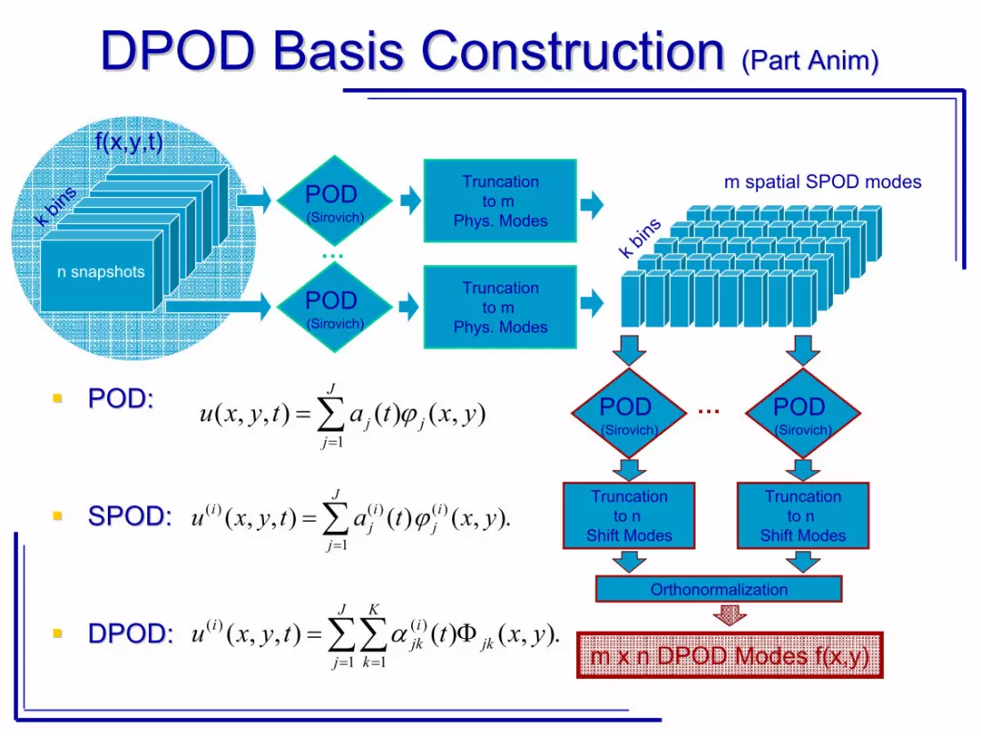
DPOD Basis Construction DPOD Basis Construction (Part (Part AnimAnim))

1

( , , ) ( ) ( , )J

j jj

u x y t a t x yM

¦

( ) ( ) ( )

1

( , , ) ( ) ( , ).J

i i ij j

j

u x y t a t x yM

¦

m x n DPOD Modes f(x,y)

Truncationto m

Phys. Modes

…

Orthonormalization

POD(Sirovich)

Truncationto n

Shift Modes

n snapshots

k bins

f(x,y,t)

POD(Sirovich)

POD(Sirovich)

Truncationto m

Phys. Modes

k bins

m spatial SPOD modes

�� POD:POD:

�� SPOD:SPOD:

�� DPOD:DPOD: ( ) ( )

1 1

( , , ) ( ) ( , ).J K

i ijk jk

j k

u x y t t x yD

)¦¦

POD(Sirovich)

Truncationto n

Shift Modes

…

DPOD Mean Flow ModesDPOD Mean Flow Modes

DPOD DPOD AnsatzAnsatz�� POD:POD:

�� SPOD:SPOD:

�� DPOD:DPOD:

1

( , , ) ( ) ( , )J

j jj

u x y t a t x yM

¦

( ) ( )

1 1

( , , ) ( ) ( , ).J K

i ijk jk

j k

u x y t t x yD

)¦¦

( ) ( ) ( )

1

( , , ) ( ) ( , ).J

i i ij j

j

u x y t a t x yM

¦

DPOD Energy ContentDPOD Energy Content

DPOD Karman ModesDPOD Karman Modes

DPOD Higher Order ModesDPOD Higher Order Modes

DPOD Time CoefficientsDPOD Time Coefficients

Shift TC Phase Shift TC Phase

ANNE Topology ExampleANNE Topology Example

-1S1

Time Coeff 1S2

S3

-1

-1

Time Coeff 2

Time Delays

-1

-1

-1

-1

-1

-1

Hidden Layertanh

Neurons

Output Layerlinear

Neurons

Ntd = 3

Nhl = 3

Nlin = 2Ns = 3Ntc = 2

W1 = (Nhl *Ns +1) x Ntd = 10 x 3

W2 = Nhl x Nlin = 3 x 2 Matrix

Example Parameters: • 3 Sensors

• 3 Time Delays

• 2 Outputs

Bias

ANNE ParametersANNE Parameters�� Number of Sensors NNumber of Sensors Nss = 8= 8�� Number of Time Delays Number of Time Delays NNtdtd = 15= 15�� Number of Hidden Layer Neurons Number of Hidden Layer Neurons NNhlhl = 15= 15�� Number of Output Layer Neurons Number of Output Layer Neurons NNlinlin = 15= 15�� Number of Time Coefficients Number of Time Coefficients NNtctc = 15= 15

ANN Training DataANN Training Data

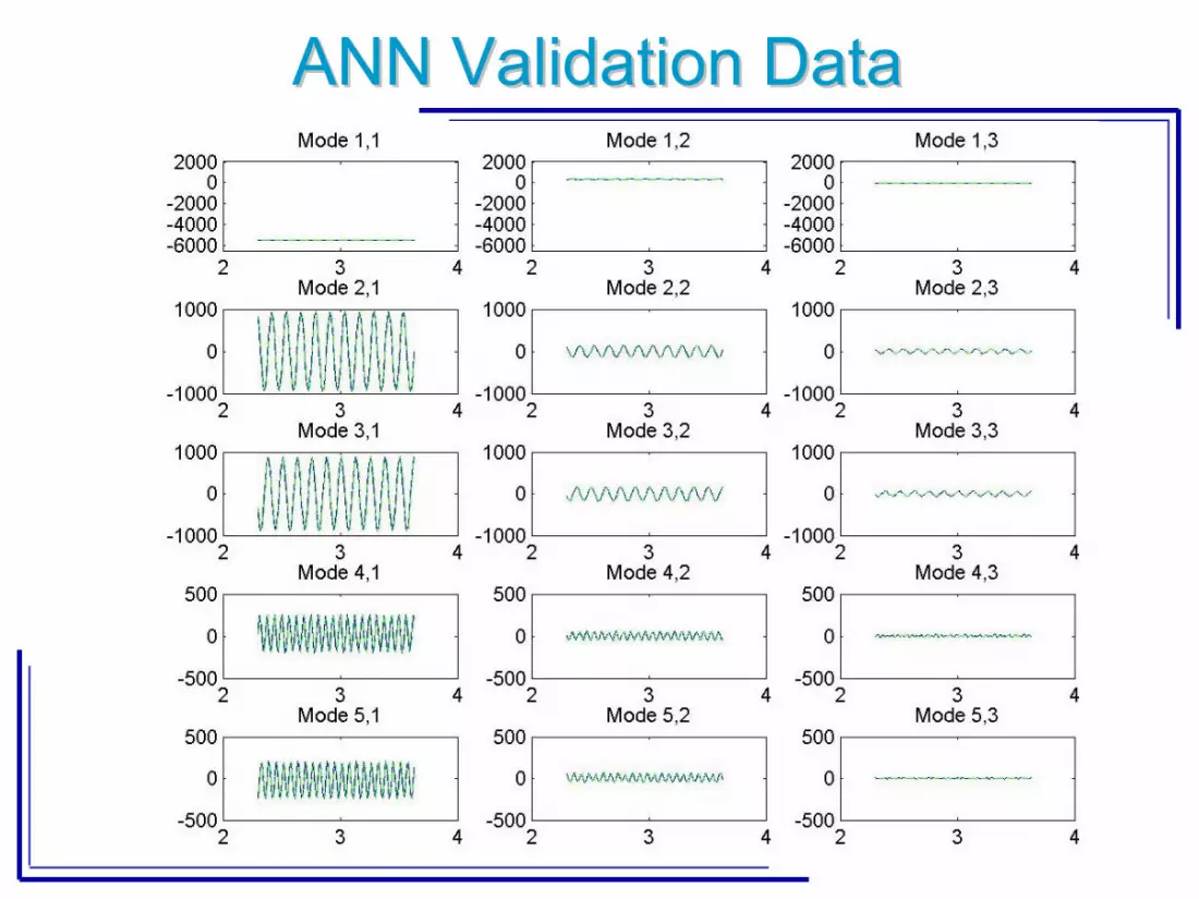
ANN Validation DataANN Validation Data

Estimation Errors GraphEstimation Errors Graph

ANN Estimation ErrorsANN Estimation Errors

23.711.35,3

10.05.04,3

3.72.63,3

3.82.82,3

5.83.21,3

6.32.45,2

4.02.04,2

4.22.53,2

5.32.42,2

2.01.61,2

3.61.65,1

2.81.54,1

2.41.43,1

1.51.32,1

0.060.04 1,1

RMS of Validation Error [%]

RMS of Training Error [%]

Mode

ConclusionsConclusions�� DPOD, an extension to POD particularly suited for transient DPOD, an extension to POD particularly suited for transient

data sets, is introduceddata sets, is introduced�� We demonstrate its application to analyze the transient We demonstrate its application to analyze the transient

development of the limit cycle oscillation downstream of a D development of the limit cycle oscillation downstream of a D shaped cylindershaped cylinder

�� The DPOD method yields shift modes for every physical mode The DPOD method yields shift modes for every physical mode of the flow, capturing the spatial changes to the modes due to of the flow, capturing the spatial changes to the modes due to the transient flow changesthe transient flow changes

�� The corresponding time coefficients contain all of the fluid The corresponding time coefficients contain all of the fluid dynamic energy exchange, enabling low dimensional model dynamic energy exchange, enabling low dimensional model development using system identification methodsdevelopment using system identification methods

�� Sensor based estimation of the DPOD time coefficients is Sensor based estimation of the DPOD time coefficients is demonstrated using an artificial neural network (ANNE)demonstrated using an artificial neural network (ANNE)

�� While demonstrated for modeling the transient limit cycle While demonstrated for modeling the transient limit cycle development, the DPOD method can also be applied to model development, the DPOD method can also be applied to model mode changes due to open or closed loop forcing, changes in mode changes due to open or closed loop forcing, changes in Re or other parameters that lead to similar but slightly distortRe or other parameters that lead to similar but slightly distorted ed spatial modes.spatial modes.

AcknowledgementsAcknowledgements�� Financial Support from AFRL / AFOSR Financial Support from AFRL / AFOSR ––

LtColLtCol Sharon Sharon HeiseHeise, , LtColLtCol Scott Wells, Dr. Scott Wells, Dr. James James MyattMyatt�� CFD Support from Cobalt Solutions CFD Support from Cobalt Solutions –– Mr. Mr.

Bill Bill StrangStrang, Dr. James Forsythe, Dr. James Forsythe�� Neural Network Support by Dr. YoungNeural Network Support by Dr. Young--SugSug

Shin, Visiting Researcher from KoreaShin, Visiting Researcher from Korea

Next StepsNext Steps�� Dynamic Model developmentDynamic Model development�� Controller development (linear and Controller development (linear and

nonlinear) nonlinear) �� Testing of controllers against modelsTesting of controllers against models

–– Nonlinear Neural Network System ID for Nonlinear Neural Network System ID for controller analysiscontroller analysis

–– CFD as truth modelCFD as truth model–– Performance comparison to black box PID Performance comparison to black box PID

controllercontroller�� Testing of controllers in experimentTesting of controllers in experiment