Embed Size (px)
Citation preview
The Infrared & 1 I Electro-Optical
K£CTIö3™ Systems Handbook
VOLUME 2
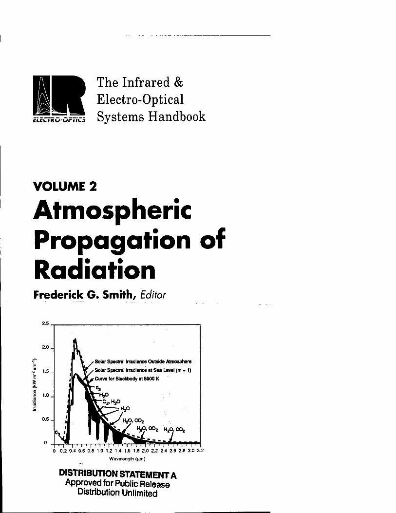
Atmospheric Propagation of Radiation Frederick G. Smith, Editor
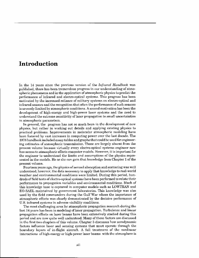
t Solar Spectral Irradiance Outside Atmosphere
' Solar Spectra] Irradiance at Sea Level (m ■ 1)
r Curve for Blackbody at 5900 K
t-HjO
5f"02,H20 |aV"~~PH20
•■^^/HJO.COJ
I Jw»/ Hß'*10* HjO.COj
I 0 0.2 0.4 0.6 0.8 1.0 1.2 1.4 1.6 1.8 2.0 2.2 2.4 2.6 2.8 3.0 3.2
Wavelength (urn)
DISTRIBUTION STATEMENT A Approved for Public Release
Distribution Unlimited
Atmospheric Propagation of Radiation
v OHHM E
The Infrared and Electro-Optical Systems Handbook
DTIC QUALITY INSPECTED 4
L
The Infrared and Electro-Optical Systems Handbook
Joseph S. Accetta, David L. Shumaker, Executive Editors
■ VOLUME 1. Sources of Radiation, George J. Zissis, Editor
Chapter 1. Radiation Theory, William L. Wolfe
Chapter 2. Artificial Sources, Anthony J. LaRocca
Chapter 3. Natural Sources, David Kryskowski, Gwynn H. Suits
Chapter 4. Radiometry, George J. Zissis
■ VOLUME 2. Atmospheric Propagation of Radiation, Fred G. Smith, Editor
Chapter 1. Atmospheric Transmission, Michael E. Thomas, Donald D. Duncan
Chapter 2. Propagation through Atmospheric Optical Turbulence, Robert R. Beland
Chapter 3. Aerodynamic Effects, Keith G. Gilbert, L. John Otten III, William C. Rose
Chapter 4. Nonlinear Propagation: Thermal Blooming, Frederick G. Gebhardt
VOLUME 3. Electro
Chapter
Chapter
Chapter
Chapter
Chapter
Chapter
Chapter
Chapter
Chapter
Chapter
VOLUME 4. Electro
-Optical Components, William D. Rogatto, Editor
1. Optical Materials, William L. Wolfe
2. Optical Design, Warren J. Smith
3. Optomechanical Scanning Applications, Techniques, and Devices, Jean Montagu, Herman DeWeerd
4. Detectors, Devon G. Crowe, Paul R. Norton, Thomas Limperis, Joseph Mudar
5. Readout Electronics for Infrared Sensors, John L. Vampola
6. Thermal and Mechanical Design of Cryogenic Cooling Systems, P.Thomas Blotter, J. Clair Batty
7. Image Display Technology and Problems with Emphasis on Airborne Systems, Lucien M. Biberman, Brian H. Tsou
8. Photographic Film, H. Lou Gibson
9. Reticles, Richard Legault
10. Lasers, Hugo Weichel
Electro-Optical Systems Design, Analysis, and Testing, Michael C. Dudzik, Editor
Chapter 1. Fundamentals of Electro-Optical Imaging Systems Analysis, J. M. Lloyd
Chapter 2. Electro-Optical Imaging System Performance Prediction, James D. Howe
Chapter 3. Optomechanical System Design, Daniel Vukobratovich
Chapter 4. Infrared Imaging System Testing, Gerald C. Hoist
Chapter 5. Tracking and Control Systems, Robert E. Nasburg
Chapter 6. Signature Prediction and Modeling, John A. Conant, Malcolm A. LeCompte
■ VOLUME 5. Passive Electro-Optical Systems, Stephen B. Campana, Editor
Chapter 1. Infrared Line Scanning Systems, William L. McCracken
Chapter 2. Forward-Looking Infrared Systems, George S. Hopper
Chapter 3. Staring-Sensor Systems, Michael J. Cantella
Chapter 4. Infrared Search and Track Systems, Joseph S. Accetta
■ VOLUME 6. Active Electro-Optical Systems, Clifton S. Fox, Editor
Chapter 1. Laser Radar, Gary W. Kamerman
Chapter 2. Laser Rangefinders, Robert W. Byren
Chapter 3. Millimeter-Wave Radar, Elmer L. Johansen
Chapter 4. Fiber Optic Systems, Norris E. Lewis, Michael B. Miller
■ VOLUME 7. Countermeasure Systems, David Pollock, Editor
Chapter 1. Warning Systems, Donald W. Wilmot, William R. Owens, Robert J. Shelton
Chapter 2. Camouflage, Suppression, and Screening Systems, David E. Schmieaer, Grayson W. Walker
Chapter 3. Active Infrared Countermeasures, Charles J. Tranchita, Kazimierasjakstas, Robert G. Palazzo, Joseph C. O'Connell
Chapter 4. Expendable Decoys, Neal Brune
Chapter 5. Optical and Sensor Protection, Michael C. Dudzik
Chapter 6. Obscuration Countermeasures, Donald W. Hoock, Jr., Robert A. Sutherland
■ VOLUME 8. Emerging Systems and Technologies, Stanley R. Robinson, Editor
Chapter 1. Unconventional Imaging Systems, Carl C. Aleksoff, J. Christopher Dainty, James R. Fienup, Robert Q. Fugate, Jean-Marie Mariotti, Peter Nisenson, Francois Roddier
Chapter 2. Adaptive Optics, Robert K. Tyson, Peter B. Ulrich
Chapter 3. Sensor and Data Fusion, Alan N. Steinberg
Chapter 4. Automatic Target Recognition Systems, James W. Sherman, David N. Spector, C. W. "Ron" Swonger, Lloyd G. Clark, Edmund G. Zelnio, Terry L. Jones, Martin J. Lahart
Chapter 5. Directed Energy Systems, Gary Golnik
Chapter 6. Holography, Emmett N. Leith
Chapter 7. System Design Considerations for a Visually-Coupled System, Brian H. Tsou
Copublished by
®7ERIM
Infrared Information Analysis Center Environmental Research Institute of Michigan
Ann Arbor, Michigan USA
and
SPIE OPTICAL ENGINEERING PRESS Bellingham, Washington USA
Sponsored by
Defense Technical Information Center, DTIC-DF Cameron Station, Alexandria, Virginia 22304-6145
Atmospheric Propagation of Radiation
Frederick G. Smith, Editor OptiMetrics Incorporated
v of TIM E
The Infrared and Electro-Optical Systems Handbook
Joseph S. Accetta, David L. Shumaker, Executive Editors Environmental Research Institute of Michigan
Library of Congress Cataloging-in-Publication Data
The Infrared and electro-optical systems handbook / Joseph S. Accetta, David L. Shumaker, executive editors,
p. cm. Spine title: IR/EO systems handbook. Cover title: The Infrared & electro-optical systems handbook. Completely rev. ed. of: Infrared handbook. 1978 Includes bibliographical references and indexes. Contents: v. 1. Sources of radiation / George J. Zissis, editor —
v. 2. Atmospheric propagation of radiation / Fred G. Smith, editor — v. 3. Electro-optical components / William D. Rogatto, editor — v. 4. Electro-optical systems design, analysis, and testing / Michael C. Dudzik, editor — v. 5. Passive electro-optical systems / Stephen B. Campana, editor — v. 6. Active electro-optical systems / Clifton S. Fox, editor — v. 7. Countermeasure systems / David Pollock, editor — v. 8. Emerging systems and technologies / Stanley R. Robinson, editor.
ISBN 0-8194-1072-1 1. Infrared technology—Handbooks, manuals, etc.
2. Electrooptical devices—Handbooks, manuals, etc. I. Accetta, J. S. II. Shumaker, David L. III. Infrared handbook. IV. Title: IR/EO systems handbook. V. Title: Infrared & electro-optical systems handbook. TA1570.I5 1993 621.36'2—dc20 92-38055
CIP
Copublished by
Infrared Information Analysis Center Environmental Research Institute of Michigan P.O. Box 134001 Ann Arbor, Michigan 48113-4001
and
SPIE Optical Engineering Press P.O. Box 10 Bellingham, Washington 98227-0010
Copyright © 1993 The Society of Photo-Optical Instrumentation Engineers
All rights reserved. No part of this publication may be reproduced or distributed in any form or by any means without written permission of one of the publishers. However, the U.S. Government retains an irrevocable, royalty-free license to reproduce, for U.S. Government purposes, any portion of this publication not otherwise subject to third-party copyright protection.
PRINTED IN THE UNITED STATES OF AMERICA
Preface
The Infrared and Electro-Optical Systems Handbook is a joint product of the Infrared Information Analysis Center (IRIA) and the International Society for Optical Engineering (SPIE). Sponsored by the Defense Technical Information Center (DTIC), this work is an outgrowth of its predecessor, The Infrared Handbook, published in 1978. The circulation of nearly 20,000 copies is adequate testimony to its wide acceptance in the electro-optics and infrared communities. The Infrared Handbook was itself preceded by The Handbook of Military Infrared Technology. Since its original inception, new topics and technologies have emerged for which little or no reference material exists. This work is intended to update and complement the current Infrared Handbook by revision, addition of new materials, and reformatting to increase its utility. Of necessity, some material from the current book was reproduced as is, havingbeen adjudged as being current and adequate. The 45 chapters represent most subject areas of current activity in the military, aerospace, and civilian communities and contain material that has rarely appeared so extensively in the open literature.
Because the contents are in part derivatives of advanced military technology, it seemed reasonable to categorize those chapters dealing with systems in analogy to the specialty groups comprising the annual Infrared Information Symposia (IRIS), a Department of Defense (DoD) sponsored forum administered by the Infrared Information Analysis Center of the Environmental Research Institute of Michigan (ERIM); thus, the presence of chapters on active, passive, and countermeasure systems.
There appears to be no general agreement on what format constitutes a "handbook." The term has been applied to a number of reference works with markedly different presentation styles ranging from data compendiums to tutorials. In the process of organizing this book, we were obliged to embrace a style of our choosing that best seemed to satisfy the objectives of the book: to provide derivational material data, descriptions, equations, procedures, and examples that will enable an investigator with a basic engineering and science education, but not necessarily an extensive background in the specific technol- ogy, to solve the types of problems he or she will encounter in design and analysis of electro-optical systems. Usability was the prime consideration. In addition, we wanted each chapter to be largely self-contained to avoid time-consuming and tedious referrals to other chapters. Although best addressed by example, the essence of our handbook style embodies four essential ingredients: a brief but well-referenced tutorial, a practical formulary, pertinent data, and, finally, example problems illustrating the use of the formulary and data.
viii PREFACE
The final product represents varying degrees of success in achieving this structure, with some chapters being quite successful in meeting our objectives and others following a somewhat different organization. Suffice it to say that the practical exigencies of organizing and producing a compendium of this magni- tude necessitated some compromises and latitude. Its ultimate success will be judged by the community that it serves. Although largely oriented toward system applications, a good measure of this book concentrates on topics endemic and fundamental to systems performance. It is organized into eight volumes:
Volume 1, edited by George Zissis of ERIM, treats sources of radiation, including both artificial and natural sources, the latter of which in most military applications is generally regarded as background radiation.
Volume 2, edited by Fred Smith of OptiMetrics, Inc., treats the propagation of radiation. It features significant amounts of new material and data on absorption, scattering, and turbulence, including nonlinear propagation relevant to high-energy laser systems and propagation through aerody- namically induced flow relevant to systems mounted on high-performance aircraft.
Volume 3, edited by William Rogatto of Santa Barbara Research Center, treats traditional system components and devices and includes recent material on focal plane array read-out electronics.
Volume 4, edited by Michael Dudzik of ERIM, treats system design, analysis, and testing, including adjunct technology and methods such as trackers, mechanical design considerations, and signature modeling.
Volume 5, edited by Stephen Campana of the Naval Air Warfare Center, treats contemporary infrared passive systems such as FLIRs, IRSTs, IR line scanners, and staring array configurations.
Volume 6, edited by Clifton Fox of the Night Vision and Electronic Sensors Directorate, treats active systems and includes mostly new material on laser radar, laser rangefinders, millimeter-wave systems, and fiber optic systems.
Volume 7, edited by David Pollock, consultant, treats a number of coun- termeasure topics rarely appearing in the open literature.
Volume 8, edited by Stanley Robinson of ERIM, treats emerging technolo- gies such as unconventional imaging, synthetic arrays, sensor and data fusion, adaptive optics, and automatic target recognition.
Acknowledgments
It is extremely difficult to give credit to all the people and organizations that contributed to this project in diverse ways. A significant amount of material in this book was generated by the sheer dedication and professionalism of many esteemed members of the IR and EO community who unselfishly contributed extensive amounts of precious personal time to this effort and to whom the modest honorarium extended was scarcely an inducement. Their contributions speak elegantly of their skills.
PREFACE ix
Directly involved were some 85 authors and editors from numerous organiza- tions, as well as scores of technical reviewers, copyeditors, graphic artists, and photographers whose skill contributed immeasurably to the final product.
We acknowledge the extensive material and moral support given to this project by various members of the managements of all the sponsoring and supporting organizations. In many cases, organizations donated staff time and internal resources to the preparation of this book. Specifically, we would like to acknowledge J. MacCallum of DoD, W. Brown and J. Walker of ERIM, and J. Yaver of SPIE, who had the foresight and confidence to invest significant resources in the preparation of this book. We also extend our appreciation to P. Klinefelter, B. McCabe, and F. Frank of DTIC for their administrative support during the course of this program.
Supporting ERIM staff included Ivan demons, Jenni Cook, Tim Kellman, Lisa Lyons, Judy Steeh, Barbara Wood, and the members of their respective organizations that contributed to this project.
We acknowledge Lorretta Palagi and the publications staff at SPIE for a professional approach to the truly monumental task of transforming the manu- scripts into presentable copy and the patience required to interact effectively with the authors.
We would like to pay special tribute to Nancy Hall of the IRIA Center at ERIM who administrated this at times chaotic project with considerable interpersonal skill, marshaling the numerous manuscripts and coordinating the myriad details characteristic of a work of this magnitude.
We properly dedicate this book to the people who created it and trust it will stand as a monument to their skills, experience, and dedication. It is, in the final analysis, a product of the community it is intended to serve.
Joseph S. Accetta David L. Shumaker
January 1993 Ann Arbor, Michigan
Notices and Disclaimer
This handbook was prepared by the Infrared Information Analysis Center (IRIA) in cooperation with the International Society for Optical Engineering (SPIE). The IRIA Center, Environmental Research Institute of Michigan, is a Defense Technical Information Center-sponsored activity under contract DLA-800-C- 393 and administrated by the Defense Electronics Supply Center, Defense Logistics Agency.
This work relates to the aforementioned ERIM contract and is in part sponsored by the Department of Defense; however, the contents do not necessar- ily reflect the position or the policy of the Department of Defense or the United States government and no official endorsement should be inferred.
The use of product names does not in any way constitute an endorsement of the product by the authors, editors, Department of Defense or any of its agencies, the Environmental Research Institute of Michigan, or the Interna- tional Society for Optical Engineering.
The information in this handbook is judged to be from the best available sources; however, the authors, editors, Department of Defense or any of its agencies, the Environmental Research Institute of Michigan, or the Interna- tional Society for Optical Engineering do not assume any liability for the validity of the information contained herein or for any consequence of its use.
Contents
CHAPTER 1
CHAPTER 2
CHAPTER 3
CHAPTER 4
Introduction
Atmospheric Transmission, Michael E. Thomas, Donald D. Duncan 1.1 Introduction
1.2 The Atmosphere of the Earth
1.3 Atmospheric Absorption and Refraction
1.4 Atmospheric Scattering
1.5 Computer Codes on Atmospheric Propagation
XIII
3
7
13
92
127
Propagation through Atmospheric Optical Turbulence, Robert R. Beland 2.1 Introduction 159
2.2 Theory of Optical Turbulence in the Atmosphere 161
2.3 Optical/IR Propagation through Turbulence 176
2.4 Measurements of Optical Turbulence in the Atmosphere 201
2.5 Models of Optical Turbulence 211
2.6 Sample Problems 224
Aerodynamic Effects, Keith G. Gilbert, L. John Often III, William C. Rose 3.1 Introduction 235
3.2 Aerodynamic Considerations 237
3.3 Optical Considerations 246
3.4 Aero-Optical Design and Analysis Examples 264
3.5 Aero-Optics: Visions and Opportunities 278
Nonlinear Propagation: Thermal Blooming, Frederick G. Gebhardt 4.1 Introduction 289
4.2 Historical Overview 289
4.3 Blooming Basics 291
4.4 Steady-State Blooming with Wind/Beam Motion 294
4.5 Conclusions 311
Index 314
Introduction
In the 14 years since the previous version of the Infrared Handbook was published, there has been tremendous progress in our understanding of atmo- spheric phenomena and in the application of atmospheric physics to predict the performance of infrared and electro-optical systems. This progress has been motivated by the increased reliance of military systems on electro-optical and infrared sensors and the recognition that often the performance of such sensors is severely limited by atmospheric conditions. A second motivation has been the development of high-energy and high-power laser systems and the need to understand the extreme sensitivity of laser propagation to small uncertainties in atmospheric parameters.
In general, the progress has not so much been in the development of new physics, but rather in working out details and applying existing physics to practical problems. Improvements in molecular atmospheric modeling have been fostered by vast increases in computing power over the last decade. The 1978 handbook included many tables and graphs that could be used for engineer- ing estimates of atmospheric transmission. Those are largely absent from the present volume because virtually every electro-optical systems engineer now has access to atmospheric effects computer models. However, it is important for the engineer to understand the limits and assumptions of the physics repre- sented in the models. He or she can gain that knowledge from Chapter 1 of the present volume.
Fourteen years ago, the physics of aerosol absorption and scattering was well understood; however, the data necessary to apply that knowledge to real-world weather and environmental conditions were limited. During this period, hun- dreds of field tests of electro-optical systems have been performed to relate their performance to propagation variables and environmental conditions. Much of this knowledge base is captured in computer models such as LOWTRAN and EO-SAEL maintained by government laboratories. This knowledge was also used by the field commanders during the Gulf War where the importance of atmospheric effects was clearly demonstrated by the decisive performance of U.S. infrared systems in adverse visibility conditions.
The most challenging area for atmospheric propagation research during the last 14 years has been in modeling of laser propagation. Turbulence and linear propagation effects on laser beams have been extensively studied during this period and are now quite well understood. Many of these factors are discussed in the first two chapters of this volume. Chapter 3 discusses how aerodynamic factors influence laser and sensing systems that must operate through the boundary layers of in-flight aircraft. A full treatment of the nonlinear interactions of high-energy or high-power laser beams with the atmosphere is
xiv INTRODUCTION
beyond the scope of this handbook. However, Chapter 4 provides a good introduction to the subject and provides references for further study.
Acknowledgments
I would like to thank the authors of this volume, in particular the authors of the original material in the first three chapters. They put in much more effort on their sections than their modest compensation could justify. The support of the IRIA staff in development of this volume is also greatly appreciated.
Frederick G. Smith January 1993 Ann Arbor, Michigan
CHAPTER 1
Atmospheric Transmission
Michael E. Thomas Donald D. Duncan
The Johns Hopkins University Applied Physics Laboratory
Laurel, Maryland
CONTENTS
1.1 Introduction 3 1.1.1 Symbols and Units 3 1.1.2 Radiative Transfer in the Atmosphere 3
1.2 The Atmosphere of the Earth 7 1.2.1 Atmospheric Structure 7 1.2.2 Gas Composition 9 1.2.3 Particle Composition 11 1.2.4 Density Variation 12
1.3 Atmospheric Absorption and Refraction 13 1.3.1 Background 13 1.3.2 Absorption by Atmospheric Gases 39 1.3.3 HITRAN Database 65 1.3.4 Band Models 69 1.3.5 Refractive Effects of the Atmosphere 86
1.4 Atmospheric Scattering 92 1.4.1 Aerosol Scatter 92 1.4.2 Molecular (Rayleigh) Scatter 109 1.4.3 Example Applications 110 1.4.4 Propagation through a Highly Scattering Medium 115 1.4.5 Imaging through a Scattering Medium 123
1.5 Computer Codes on Atmospheric Propagation 127 1.5.1 LOWTRAN 127 1.5.2 MODTRAN 128 1.5.3 FASCODE 128 1.5.4 Algorithms for Calculation of Scatter Parameters 133
References 147 Bibliography 155
1
ATMOSPHERIC TRANSMISSION 3
1.1 INTRODUCTION
The atmosphere is always an important consideration in the performance of many electro-optical systems. An electro-optical system can be described as containing three basic components: source, detector, and propagation medium. Because of the quality of source and detection systems today, the limiting factor in overall system performance often is the propagation medium. Thus, a thorough discussion of the atmosphere and various mechanisms of atten- uation is required. Absorption, scattering, and turbulence are the dominant mechanisms of loss. This chapter addresses absorption and scattering. Tur- bulence is covered in Chap. 2 of this volume.
1.1.1 Symbols and Units
Table 1.1 lists symbols with the corresponding meaning and units used in this chapter. An attempt is made to consistently use mks units, but convention does not always allow this. Also, the defined symbols are used consistently throughout the chapter. However, absorption and scattering theory were de- veloped separately and different symbols are often used for the same quantity. An attempt is made to use the most common symbols with both sets of literature and to otherwise select symbols in the most unambiguous way. When the usage should clearly indicate the meaning, the same symbol is sometimes used for two different quantities.
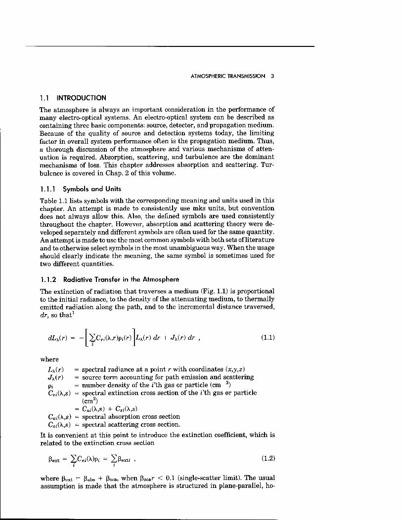
1.1.2 Radiative Transfer in the Atmosphere
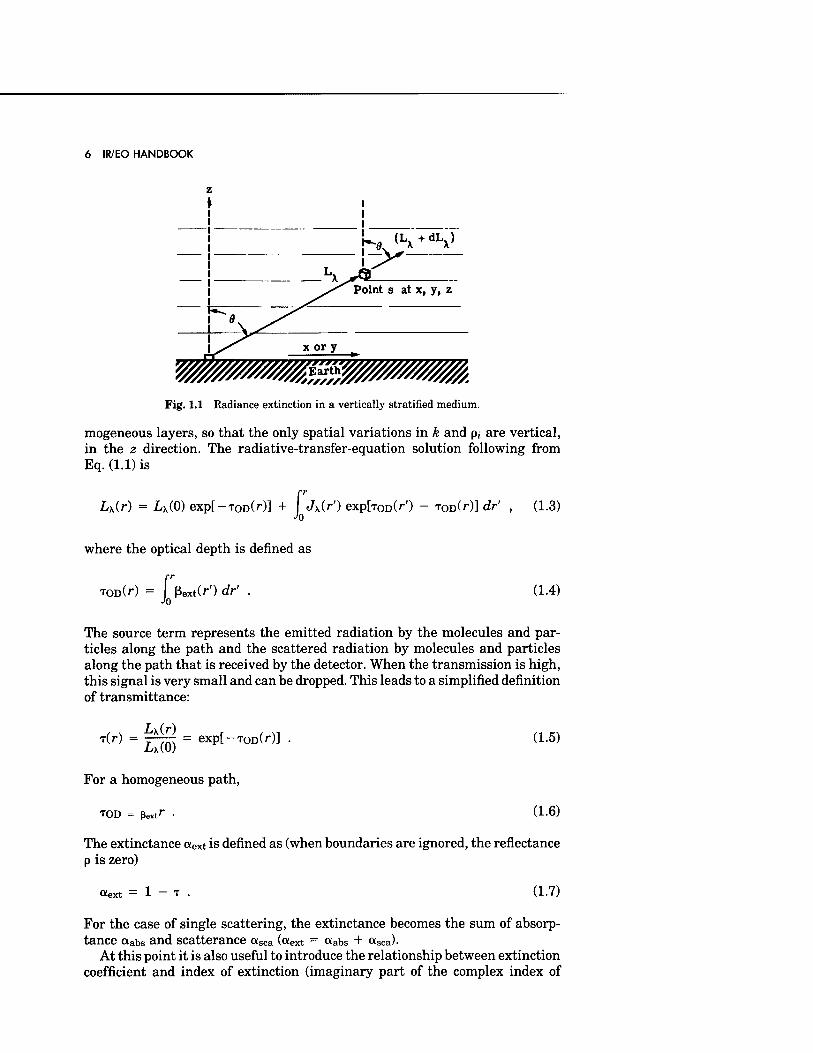
The extinction of radiation that traverses a medium (Fig. 1.1) is proportional to the initial radiance, to the density of the attenuating medium, to thermally emitted radiation along the path, and to the incremental distance traversed, dr, so that1
dLx(r) = - 2Cei(k,r)pi(r) LK(r) dr + Jx(r) dr , (1.1)
where L\(r) = spectral radiance at a point r with coordinates (x,y,z) J\(r) = source term accounting for path emission and scattering pi = number density of the i'th gas or particle (cm-3) Cej(X.,s) = spectral extinction cross section of the i'th gas or particle
(cm2) = CaiiKs) + Csi(X,s)
CaiiKs) = spectral absorption cross section CSj(X,s) = spectral scattering cross section.
It is convenient at this point to introduce the extinction coefficient, which is related to the extinction cross section
ßext = 2Cei(Vpi = Eßext, , (1.2) i i
where ßext = ßabs + ßsca, when ßscar < 0.1 (single-scatter limit). The usual assumption is made that the atmosphere is structured in plane-parallel, ho-
4 IR/EO HANDBOOK
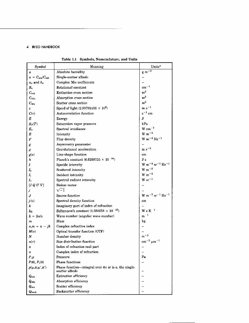
Table 1.1 Symbols, Nomenclature, and Units
Symbol Meaning Units*
a Absolute humidity gm"3
O- = ksca'^ext Single-scatter albedo - an and bn Complex Mie coefficients - Be Rotational constant cm-1
t-'ext Extinction cross section m2
^abs Absorption cross section m2
^sca Scatter cross section m2
C
C(T)
Speed of light (2.99792458 x 10⁸)
Autocorrelation function
m s""1
s""1 cm
£ Energy J
B.(T) Ev
Saturation vapor pressure Spectral irradiance
kPa Wem"2
E
F
Intensity Flux density
Wm-2
Wm-2Hz"1
e g
Asymmetry parameter Gravitational acceleration m s~2
giv) h
Line-shape function Planck's constant (6.6260755 x 10 _34)
cm Js
I Specific intensity Wm^sr'Hz" l
Is Scattered intensity Wm"2
h Incident intensity Wm-2
/» Spectral radiant intensity Wsr-1
UQUV] Stokes vector - j V^l - J Source function Wm-2sr-1Hz" l
j(v) Spectral density function cm
k Imaginary part of index of refraction - kB Boltzmann's constant (1.380658 x 10""23) WsK"1
k = 2ir/\ Wave number (angular wave number) m"1
TO Mass kg ra,m = n - jk Complex refractive index - M(v) AT
n(r)
Optical transfer function (OTF) Number density Size distribution function
m~3
cm-3 (im-1
re re
Index of refraction real part Complex index of refraction
-
P.P Pressure Pa
P(9), Pi(6) Phase functions - p(M-»<t>;M-'»4>') Phase function—integral over 4ir sr is a, the single-
scatter albedo _
Qext
Qabs
Extinction efficiency Absorption efficiency
—
«csca
Qback
Scatter efficiency Backscatter efficiency -
ATMOSPHERIC TRANSMISSION 5
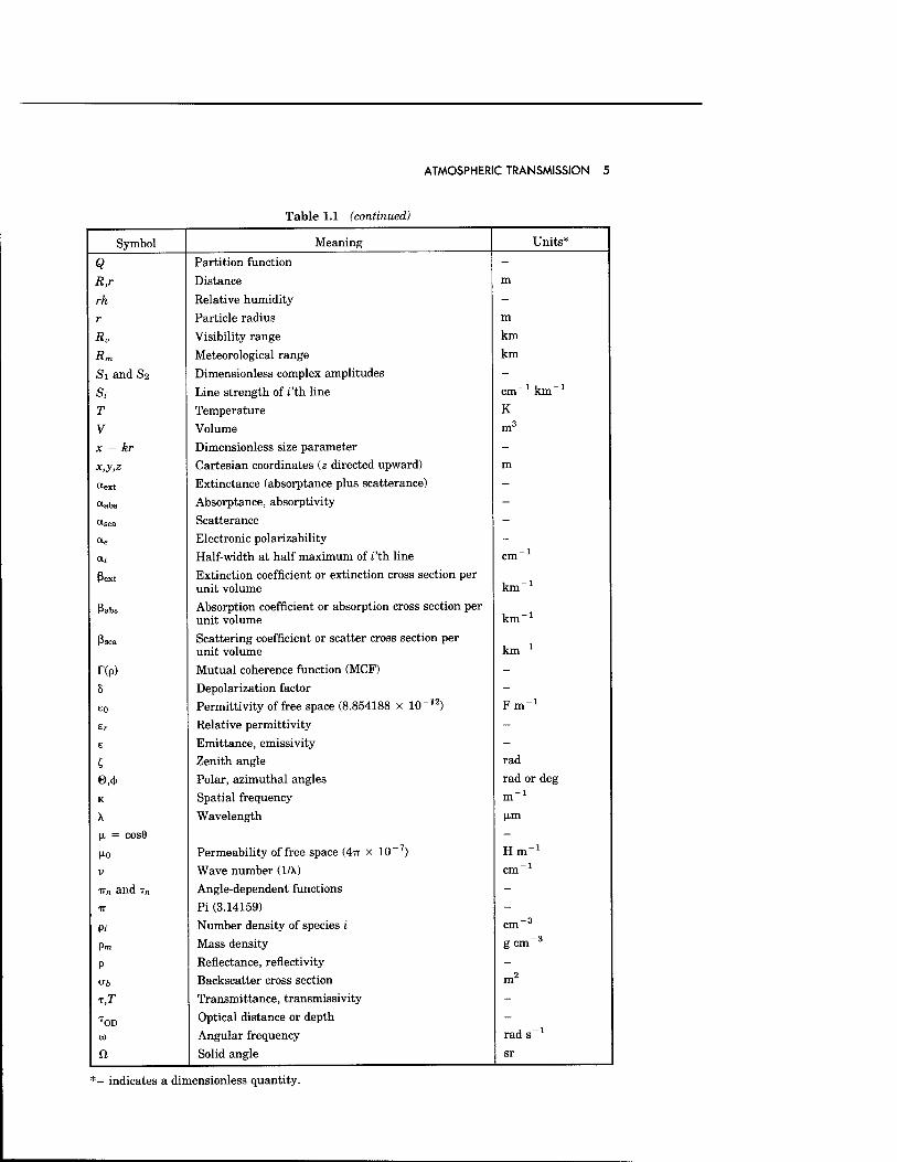
Table 1.1 (continued)
Symbol Meaning Units*
Q Partition function -
R,r Distance m
rh Relative humidity -
r Particle radius m
Rv Visibility range km
Rm Meteorological range km
Si and S2 Dimensionless complex amplitudes -
Si Line strength of i'th line cm'1 km-1
T Temperature K
V Volume m3
x = kr Dimensionless size parameter -
x,y,z Cartesian coordinates (z directed upward) m
«ext Extinctance (absorptance plus scatterance) -
<*abs Absorptance, absorptivity - asca Scatterance -
<*e Electronic polarizability -
at Half-width at half maximum of fth line cm-1
ßext Extinction coefficient or extinction cross section per unit volume km"1
ßabs Absorption coefficient or absorption cross section per unit volume km"1
Psca Scattering coefficient or scatter cross section per unit volume km"1
r(p) Mutual coherence function (MCF) -
8 Depolarization factor -
EO Permittivity of free space (8.854188 x 10 _12) Fm"1
£r Relative permittivity -
e Emittance, emissivity -
I Zenith angle rad
0,<j) Polar, azimuthal angles rad or deg
K Spatial frequency m"1
X Wavelength (xm
\x. = cos8 -
M-o Permeability of free space (4TT X 10 ~7) Hm"1
V Wave number (l/\) cm-1
Trn and T„ Angle-dependent functions -
Tt Pi (3.14159) -
Pi Number density of species i cm"3
Pm Mass density gem"3
P Reflectance, reflectivity -
CT6 Backscatter cross section ™2 m
T,T Transmittance, transmissivity -
T0D Optical distance or depth -
CÜ Angular frequency rad s"1
fi Solid angle sr
*- indicates a dimensionless quantity.
6 IR/EO HANDBOOK
K ^ + dL^
Fig. 1.1 Radiance extinction in a vertically stratified medium.
mogeneous layers, so that the only spatial variations in k and p; are vertical, in the z direction. The radiative-transfer-equation solution following from Eq. (1.1) is
LK(r) = Lx(0) exp[-T0D(r)] + J Jx(r') exptWr') - TODM] dr'
where the optical depth is defined as
TOD(r) = ßext(r') dr' . Jo
(1.3)
(1.4)
The source term represents the emitted radiation by the molecules and par- ticles along the path and the scattered radiation by molecules and particles along the path that is received by the detector. When the transmission is high, this signal is very small and can be dropped. This leads to a simplified definition of transmittance:
T(r) = 7^ = exp[-TOD(r)] -IA(,U)
For a homogeneous path,
TOD = ßextf •
(1.5)
(1.6)
The extinctance aext is defined as (when boundaries are ignored, the reflectance p is zero)
Otext = 1 - T (1.7)
For the case of single scattering, the extinctance becomes the sum of absorp- tance aabs and scatterance asca (aext = aabs + asca).
At this point it is also useful to introduce the relationship between extinction coefficient and index of extinction (imaginary part of the complex index of
ATMOSPHERIC TRANSMISSION 7
refraction, m = n - jk), when the single-scatter approximation is valid Oscar < 0.1):
k = ^ . (1.8) 4irv
This equation is obtained by comparing the radiation-transfer solution to the plane-wave solution of Maxwell's equations in an unbounded homogeneous medium. These definitions, parameters, and formulas are fundamental to the description of optical propagation in the atmosphere.
1.2 THE ATMOSPHERE OF THE EARTH
The atmosphere surrounds and protects the earth in the form of a gaseous blanket forming the transition between the solid surface of the earth and the near vacuum of the outer solar atmosphere. It acts as a shield against harmful radiation and meteors. The dynamics of the atmosphere drive the weather on the surface. It provides for life itself as part of the earth's biosphere. Optical propagation in this medium has many important characteristics and conse- quences. These include meteorological remote sensing, infrared and visible astronomy, remote sensing in general, and electro-optical systems perfor- mance. Therefore, it is appropriate to include in this chapter an introduction to the nature of the atmosphere.
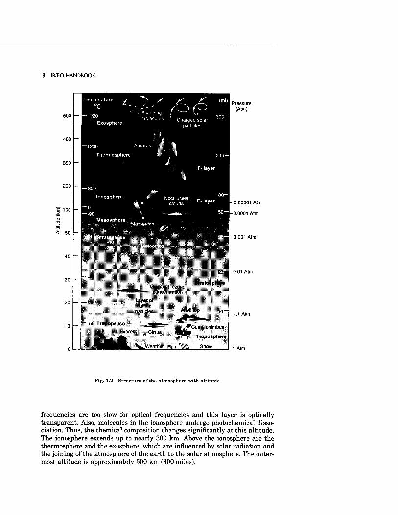
1.2.1 Atmospheric Structure
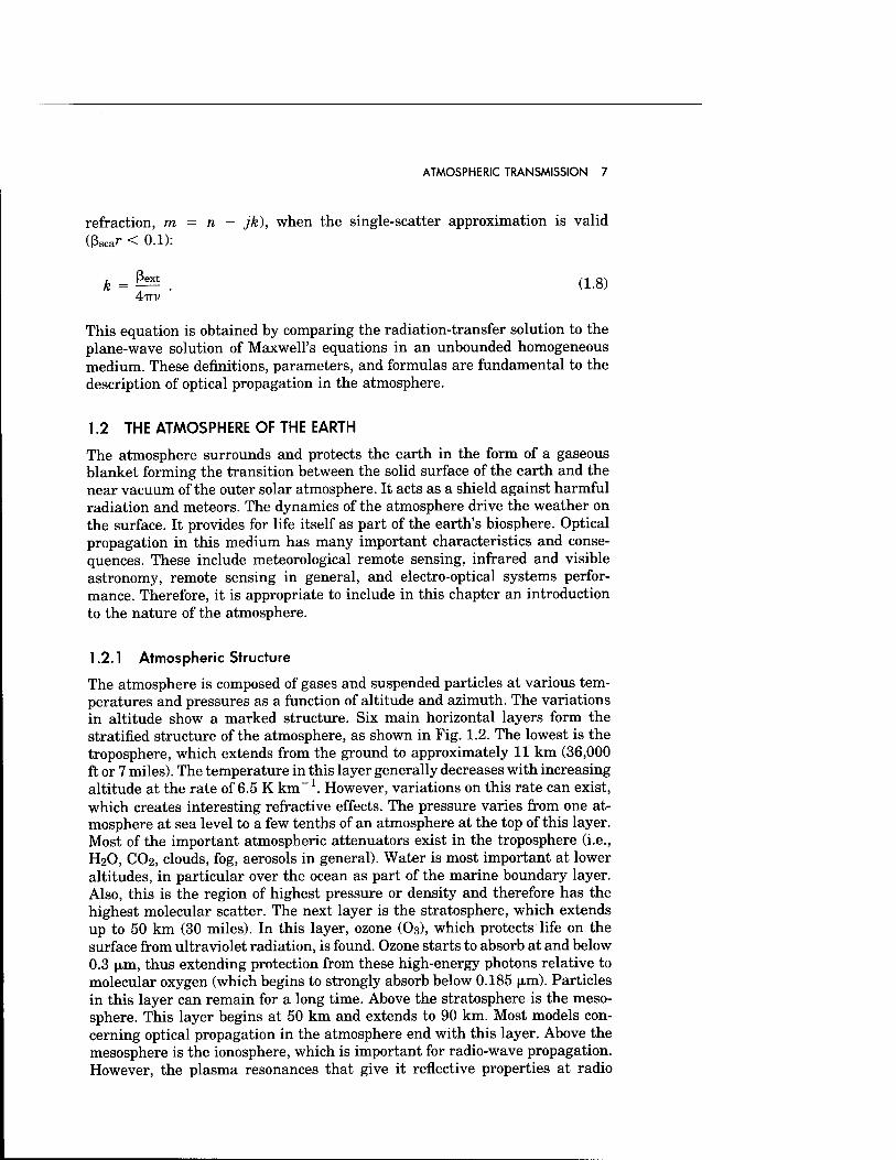
The atmosphere is composed of gases and suspended particles at various tem- peratures and pressures as a function of altitude and azimuth. The variations in altitude show a marked structure. Six main horizontal layers form the stratified structure of the atmosphere, as shown in Fig. 1.2. The lowest is the troposphere, which extends from the ground to approximately 11 km (36,000 ft or 7 miles). The temperature in this layer generally decreases with increasing altitude at the rate of 6.5 K km""1. However, variations on this rate can exist, which creates interesting refractive effects. The pressure varies from one at- mosphere at sea level to a few tenths of an atmosphere at the top of this layer. Most of the important atmospheric attenuators exist in the troposphere (i.e., H2O, CO2, clouds, fog, aerosols in general). Water is most important at lower altitudes, in particular over the ocean as part of the marine boundary layer. Also, this is the region of highest pressure or density and therefore has the highest molecular scatter. The next layer is the stratosphere, which extends up to 50 km (30 miles). In this layer, ozone (O3), which protects life on the surface from ultraviolet radiation, is found. Ozone starts to absorb at and below 0.3 |xm, thus extending protection from these high-energy photons relative to molecular oxygen (which begins to strongly absorb below 0.185 jjim). Particles in this layer can remain for a long time. Above the stratosphere is the meso- sphere. This layer begins at 50 km and extends to 90 km. Most models con- cerning optical propagation in the atmosphere end with this layer. Above the mesosphere is the ionosphere, which is important for radio-wave propagation. However, the plasma resonances that give it reflective properties at radio
8 IR/EO HANDBOOK
500
400
300
200
E 100
< 50
40
30
20
10
Temperature °C
Exosphere
/ Escaping molecules
Pressure (Atm)
Charged solar particles
Thermosphere
Ionosphere
Mesosphere
F- layer
Noctilucent r , clouds E-|ayer
'Meteorites
Si« ^m^^*m
--44
56
Greatest ozone concentration
slip
Stratosphere
Layer of suffate
Anvil top
0.00001 Atm
-0.0001 Atm
0.001 Atm
0.01 Atm
-.1 Atm
1 Atm
Fig. 1.2 Structure of the atmosphere with altitude.
frequencies are too slow for optical frequencies and this layer is optically transparent. Also, molecules in the ionosphere undergo photochemical disso- ciation. Thus, the chemical composition changes significantly at this altitude. The ionosphere extends up to nearly 300 km. Above the ionosphere are the thermosphere and the exosphere, which are influenced by solar radiation and the joining of the atmosphere of the earth to the solar atmosphere. The outer- most altitude is approximately 500 km (300 miles).
ATMOSPHERIC TRANSMISSION 9
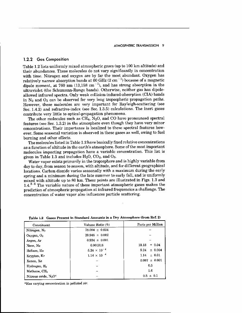
1.2.2 Gas Composition
Table 1.2 lists uniformly mixed atmospheric gases (up to 100 km altitude) and their abundances. These molecules do not vary significantly in concentration with time. Nitrogen and oxygen are by far the most abundant. Oxygen has relatively narrow absorption bands at 60 GHz (2 cm-1) because of a magnetic dipole moment, at 760 nm (13,158 cm"1), and has strong absorption in the ultraviolet (the Schumann-Runge bands). Otherwise, neither gas has dipole- allowed infrared spectra. Only weak collision-induced-absorption (CIA) bands in N2 and O2 can be observed for very long tropospheric propagation paths. However, these molecules are very important for Rayleigh-scattering (see Sec. 1.4.2) and refractive-index (see Sec. 1.3.5) calculations. The inert gases contribute very little to optical-propagation phenomena.
The other molecules such as CH4, N20, and CO have pronounced spectral features (see Sec. 1.3.2) in the atmosphere even though they have very minor concentrations. Their importance is localized to these spectral features how- ever. Some seasonal variation is observed in these gases as well, owing to fuel burning and other effects.
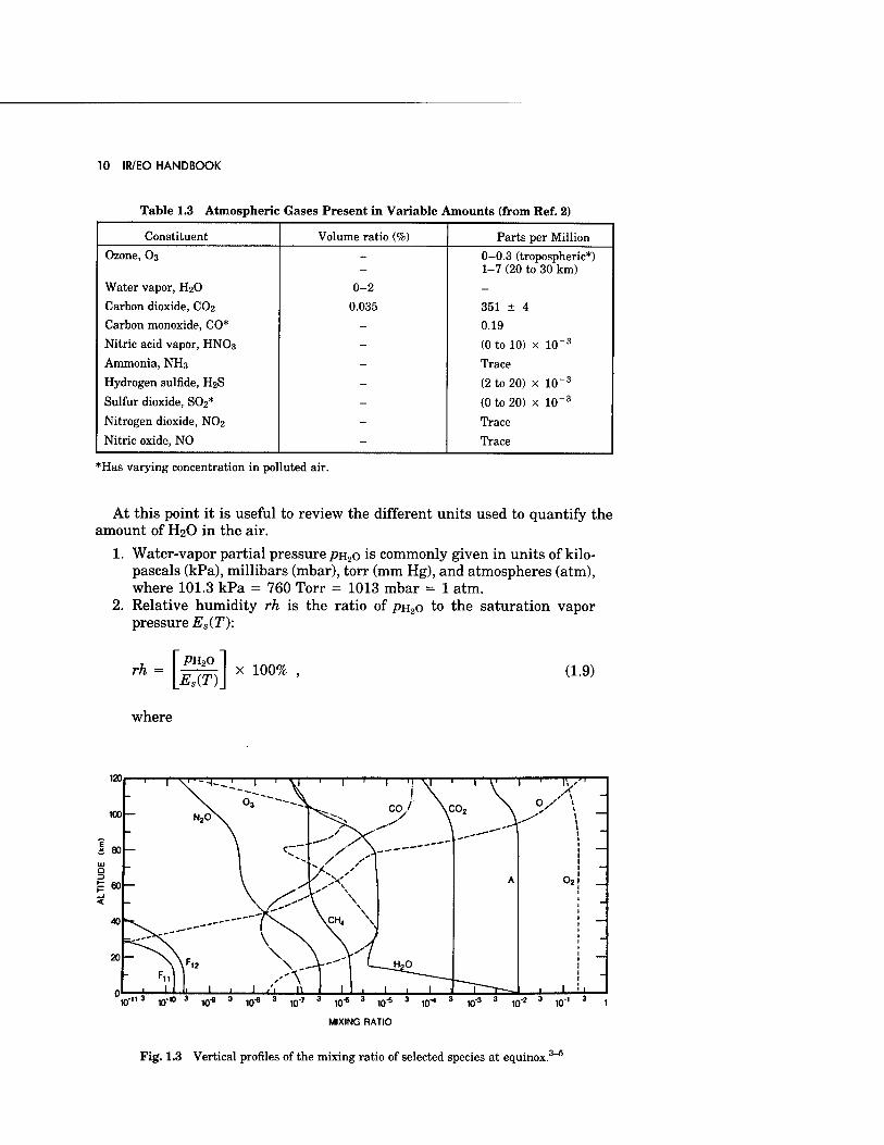
The molecules listed in Table 1.2 have basically fixed relative concentrations as a function of altitude in the earth's atmosphere. Some of the most important molecules impacting propagation have a variable concentration. This list is given in Table 1.3 and includes H2O, CO2, and O3.
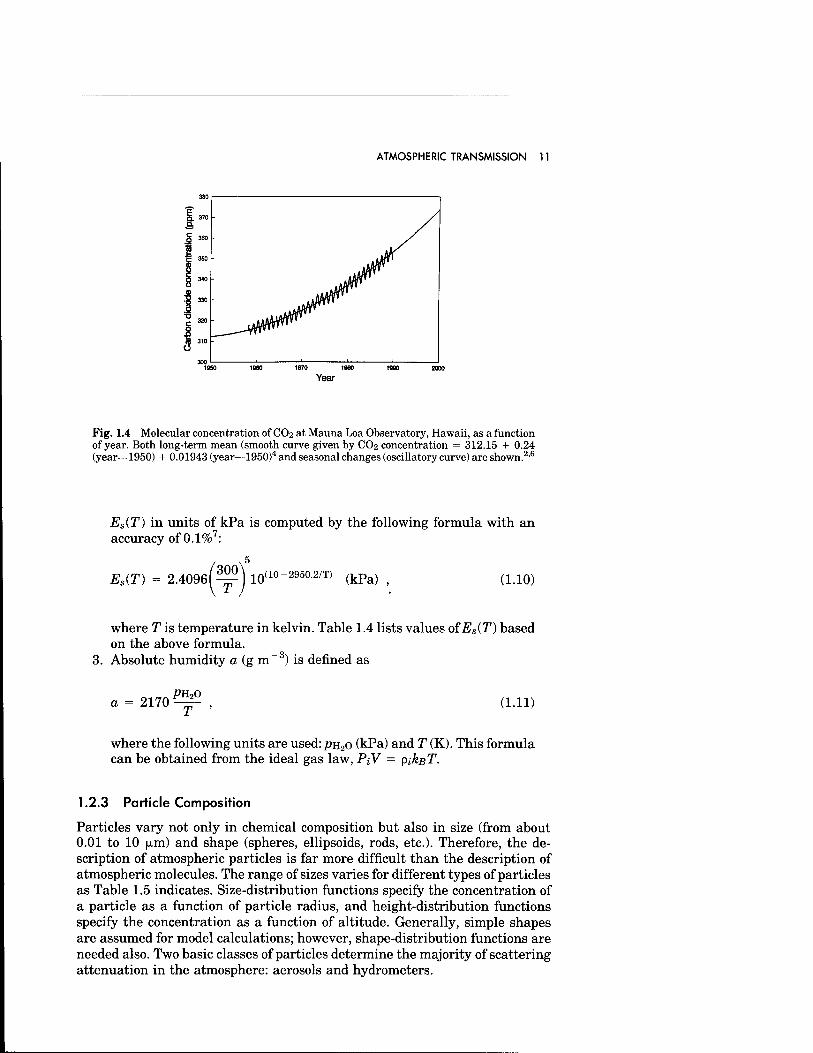
Water vapor exists primarily in the troposphere and is highly variable from day to day, from season to season, with altitude, and for different geographical locations. Carbon dioxide varies seasonally with a maximum during the early spring and a minimum during the late summer to early fall, and is uniformly mixed with altitude up to 80 km. These points are illustrated in Figs. 1.3 and I.4.3-6 The variable nature of these important atmospheric gases makes the prediction of atmospheric propagation at infrared frequencies a challenge. The concentration of water vapor also influences particle scattering.
Table 1.2 Gases Present in Standard Amounts in a Dry Atmosphere (from Ref. 2)
Constituent Volume Ratio (%) Parts per Million
Nitrogen, N2 78.084 ± 0.004 - Oxygen, O2 20.946 ± 0.002 - Argon, Ar 0.934 ± 0.001 - Neon, Ne 0.001818 18.18 ± 0.04
Helium, He 5.24 x 10~4 5.24 ± 0.004
Krypton, Kr 1.14 x 10"4 1.14 ± 0.01
Xenon, Xe - 0.087 ± 0.001
Hydrogen, H2 - 0.5
Methane, CH4 - 1.6
Nitrous oxide, N2O* - 0.5 ± 0.1
*Has varying concentration in polluted air.
10 IR/EO HANDBOOK
Table 1.3 Atmospheric Gases Present in Variable Amounts (from Ref. 2)
Constituent Volume ratio (%) Parts per Million
Ozone, O3 - 0-0.3 (tropospheric*) 1-7 (20 to 30 km)
Water vapor, H2O 0-2 - Carbon dioxide, CO2 0.035 351 ± 4 Carbon monoxide, CO* - 0.19
Nitric acid vapor, HNO3 - (0 to 10) x 10~3
Ammonia, NH3 - Trace
Hydrogen sulfide, H2S - (2 to 20) x 10~3
Sulfur dioxide, S02* - (0 to 20) x 10~3
Nitrogen dioxide, NO2 - Trace
Nitric oxide, NO - Trace
*Has varying concentration in polluted air.
At this point it is useful to review the different units used to quantify the amount of H2O in the air.
1. Water-vapor partial pressure pn2o is commonly given in units of kilo- pascals (kPa), millibars (mbar), torr (mm Hg), and atmospheres (atm), where 101.3 kPa = 760 Torr = 1013 mbar = 1 atm.
2. Relative humidity rh is the ratio of pn2o to the saturation vapor pressure ES(T):
rh Pn2o Es(T)
x 100% (1.9)
where
,-tl3 .-10 3 „.-9 3 1fVe 3 .--7 3 ,„-6 3 ..-s 3 10"' 10' 1-3 3 10-2 3 m-l 3
MIXING RATIO
Fig. 1.3 Vertical profiles of the mixing ratio of selected species at equinox.3
ATMOSPHERIC TRANSMISSION 11
1970 1980
Year
Fig. 1.4 Molecular concentration of CO2 at Mauna Loa Observatory, Hawaii, as a function of year. Both long-term mean (smooth curve given by CO2 concentration = 312.15 + 0.24 (year—1950) + 0.01943 (year—1950)4 and seasonal changes (oscillatory curve) are shown.2,6
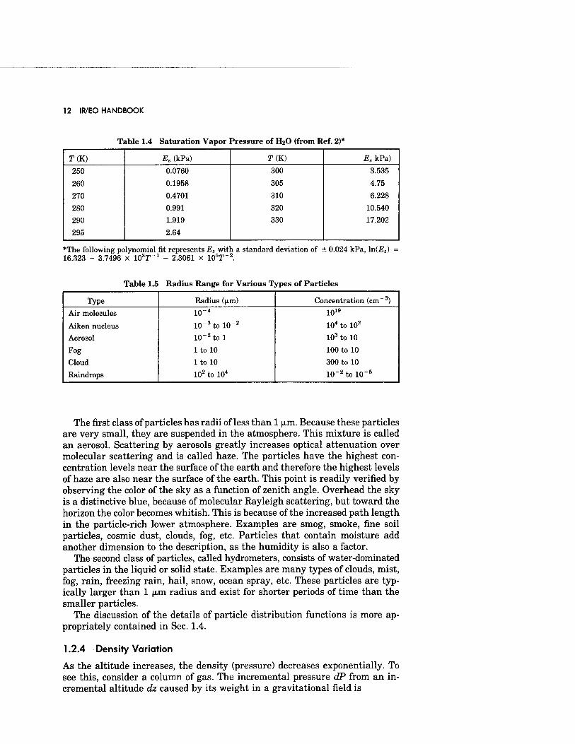
ES(T) in units of kPa is computed by the following formula with an accuracy of 0.1%7:
ES(T) = 2.4096(^) 10(1°-29502/T) (kPa) , (1.10)
where T is temperature in kelvin. Table 1.4 lists values of ES(T) based on the above formula.
3. Absolute humidity a (g m~3) is defined as
a = 2170 Pn2o
(1.11)
where the following units are used: pn2o (kPa) and T (K). This formula can be obtained from the ideal gas law, PiV = pj&sT.
1.2.3 Particle Composition
Particles vary not only in chemical composition but also in size (from about 0.01 to 10 |i.m) and shape (spheres, ellipsoids, rods, etc.). Therefore, the de- scription of atmospheric particles is far more difficult than the description of atmospheric molecules. The range of sizes varies for different types of particles as Table 1.5 indicates. Size-distribution functions specify the concentration of a particle as a function of particle radius, and height-distribution functions specify the concentration as a function of altitude. Generally, simple shapes are assumed for model calculations; however, shape-distribution functions are needed also. Two basic classes of particles determine the majority of scattering attenuation in the atmosphere: aerosols and hydrometers.
12 IR/EO HANDBOOK
Table 1.4 Saturation Vapor Pressure of H2O (from Ref. 2)*
T(K) Es (kPa) T(K) Es kPa)
250 0.0760 300 3.535
260 0.1958 305 4.75
270 0.4701 310 6.228
280 0.991 320 10.540
290 1.919 330 17.202
295 2.64
*The following polynomial fit represents Es with a standard deviation of ± 0.024 kPa, ln(Es) 16.323 - 3.7496 x 10³T-1 - 2.3061 x 10⁵r-2.
Table 1.5 Radius Range for Various Types of Particles
Type Radius (|im) Concentration (cm 3)
Air molecules 10~4 1019
Aiken nucleus 10"3tol0"2 104 to 102
Aerosol 10~2tol 103 to 10
Fog ltolO 100 to 10
Cloud ltolO 300 to 10
Raindrops 102 to 104 10_2tol0-6
The first class of particles has radii of less than 1 (xm. Because these particles are very small, they are suspended in the atmosphere. This mixture is called an aerosol. Scattering by aerosols greatly increases optical attenuation over molecular scattering and is called haze. The particles have the highest con- centration levels near the surface of the earth and therefore the highest levels of haze are also near the surface of the earth. This point is readily verified by observing the color of the sky as a function of zenith angle. Overhead the sky is a distinctive blue, because of molecular Rayleigh scattering, but toward the horizon the color becomes whitish. This is because of the increased path length in the particle-rich lower atmosphere. Examples are smog, smoke, fine soil particles, cosmic dust, clouds, fog, etc. Particles that contain moisture add another dimension to the description, as the humidity is also a factor.
The second class of particles, called hydrometers, consists of water-dominated particles in the liquid or solid state. Examples are many types of clouds, mist, fog, rain, freezing rain, hail, snow, ocean spray, etc. These particles are typ- ically larger than 1 u.m radius and exist for shorter periods of time than the smaller particles.
The discussion of the details of particle distribution functions is more ap- propriately contained in Sec. 1.4.
1.2.4 Density Variation
As the altitude increases, the density (pressure) decreases exponentially. To see this, consider a column of gas. The incremental pressure dP from an in- cremental altitude dz caused by its weight in a gravitational field is
ATMOSPHERIC TRANSMISSION 13
dP = -pmgdz , (1.12)
where pm is the mass density and g is the gravitational acceleration. However, pm must vary with altitude z [i.e., pm = pm(z)]. Now let us use the ideal gas law,
Pm = mp = iSixij' (L13)
where p is the number density and m is the average mass per molecule. Thus,
dP mg P(z) kBT(z)
dz . (1.14)
Now let us assume T(z) = To + az. (Note: a = -6.5 K/km, which is valid for the lower 10 km of the 1976 U.S. standard atmosphere.) Then it follows that
/T(^Vmg/akB
P(z) = P(0)( ^J . (1.15)
[Note: For the value of a given above, the numerical value of the exponent, -mglakB, in Eq. (1.15) is 5.256.] In the isothermal limit [i.e., T(z) = T0] Eq. (1.14) becomes
P(z) = P(0) exJ-^-J . (1.16)
These formulas can be used to form a piecewise continuous representation of the pressure variation of the real atmosphere with altitude given the temper- ature profile.
1.3 ATMOSPHERIC ABSORPTION AND REFRACTION
Absorption and refraction by atmospheric molecules are the topics of this section. The atmospheric window regions are defined by molecular absorption (primarily water vapor and carbon dioxide). Local-line and continuum ab- sorption are of concern within the window regions. A basic understanding of the spectroscopy of these molecules is necessary for the understanding of the location and nature of the window regions. Also, dispersion and temperature dependence of the index of refraction are based on the spectroscopy of the atmospheric molecules. Thus, the discussion of absorption and refraction will begin with a background section on atmospheric spectroscopy.
1.3.1 Background
This section will lay the foundation concerning the description of atmospheric absorption and refraction. The formal development will be briefly outlined, resulting in formulas that are used in atmospheric modeling.
14 IR/EO HANDBOOK
1.3.1.1 Basic Concepts
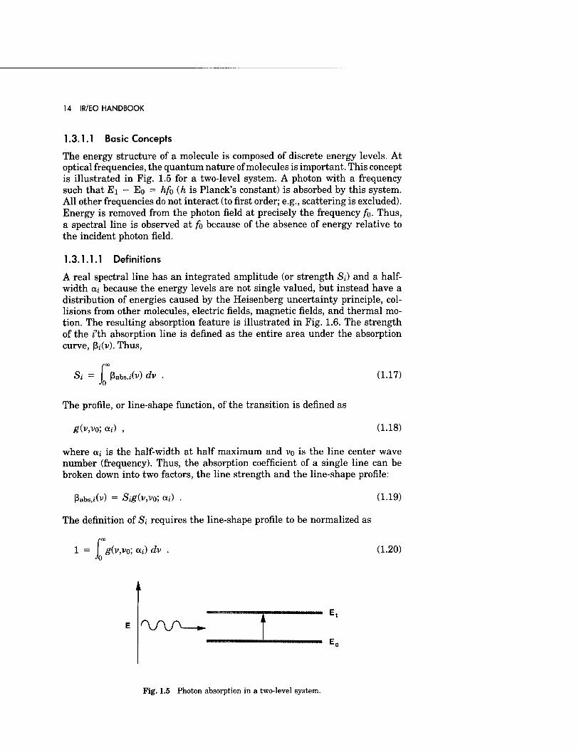
The energy structure of a molecule is composed of discrete energy levels. At optical frequencies, the quantum nature of molecules is important. This concept is illustrated in Fig. 1.5 for a two-level system. A photon with a frequency such that Ei - Eo = hfo (h is Planck's constant) is absorbed by this system. All other frequencies do not interact (to first order; e.g., scattering is excluded). Energy is removed from the photon field at precisely the frequency /b. Thus, a spectral line is observed at /b because of the absence of energy relative to the incident photon field.
1.3.1.1.1 Definitions
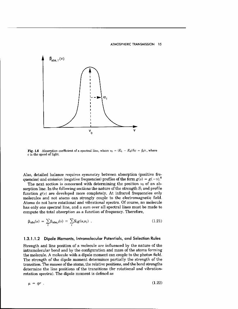
A real spectral line has an integrated amplitude (or strength Si) and a half- width at because the energy levels are not single valued, but instead have a distribution of energies caused by the Heisenberg uncertainty principle, col- lisions from other molecules, electric fields, magnetic fields, and thermal mo- tion. The resulting absorption feature is illustrated in Fig. 1.6. The strength of the i'th absorption line is defined as the entire area under the absorption curve, ßj(v). Thus,
Si Jroo
ßabs,i(v) dv 0
(1.17)
The profile, or line-shape function, of the transition is defined as
g(v,vo; ad , (1.18)
where at is the half-width at half maximum and vo is the line center wave number (frequency). Thus, the absorption coefficient of a single line can be broken down into two factors, the line strength and the line-shape profile:
ßabs,i(v) = Sig(v,v0; at) . (1.19)
The definition of Si requires the line-shape profile to be normalized as
1 Jroo
g(v,v0; a, o
)dv (1.20)
'XAA-
Fig. 1.5 Photon absorption in a two-level system.
ATMOSPHERIC TRANSMISSION 15
Fig. 1.6 Absorption coefficient of a spectral line, where vo c is the speed of light.
(Ei - Eo)/hc = fo/c, where
Also, detailed balance requires symmetry between absorption (positive fre- quencies) and emission (negative frequencies) profiles of the formg(v) = g(-v).s
The next section is concerned with determining the position vo of an ab- sorption line. In the following sections the nature of the strength S; and profile function g{v) are developed more completely. At infrared frequencies only molecules and not atoms can strongly couple to the electromagnetic field. Atoms do not have rotational and vibrational spectra. Of course, no molecule has only one spectral line, and a sum over all spectral lines must be made to compute the total absorption as a function of frequency. Therefore,
ßabs(v) = Eßabs,i(v) = ^ZSig(v,Vi) (1.21)
1.3.1.1.2 Dipole Moments, Intramolecular Potentials, and Selection Rules
Strength and line position of a molecule are influenced by the nature of the intramolecular bond and by the configuration and mass of the atoms forming the molecule. A molecule with a dipole moment can couple to the photon field. The strength of the dipole moment determines partially the strength of the transition. The masses of the atoms, the relative positions, and the bond strengths determine the line positions of the transitions (for rotational and vibration- rotation spectra). The dipole moment is defined as
^ = qr ■ (1.22)
16 IR/EO HANDBOOK
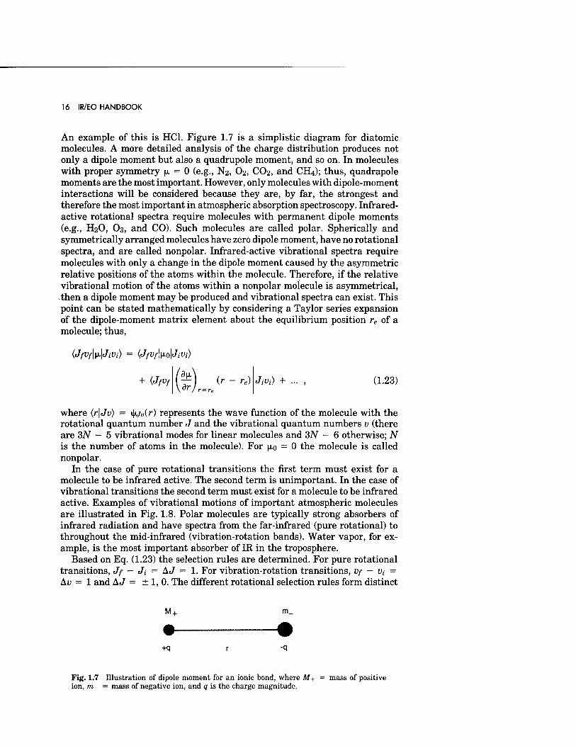
An example of this is HC1. Figure 1.7 is a simplistic diagram for diatomic molecules. A more detailed analysis of the charge distribution produces not only a dipole moment but also a quadrupole moment, and so on. In molecules with proper symmetry |x = 0 (e.g., N2, O2, CO2, and CH4); thus, quadrapole moments are the most important. However, only molecules with dipole-moment interactions will be considered because they are, by far, the strongest and therefore the most important in atmospheric absorption spectroscopy. Infrared- active rotational spectra require molecules with permanent dipole moments (e.g., H2O, O3, and CO). Such molecules are called polar. Spherically and symmetrically arranged molecules have zero dipole moment, have no rotational spectra, and are called nonpolar. Infrared-active vibrational spectra require molecules with only a change in the dipole moment caused by the asymmetric relative positions of the atoms within the molecule. Therefore, if the relative vibrational motion of the atoms within a nonpolar molecule is asymmetrical, then a dipole moment may be produced and vibrational spectra can exist. This point can be stated mathematically by considering a Taylor series expansion of the dipole-moment matrix element about the equilibrium position re of a molecule; thus,
{JfVf\\l\JiVi) = {JfVf\\Lo\JiVi)
(r - re) r=re
Jm) + ... , (1.23)
where (r\Jv) = \\ijv(r) represents the wave function of the molecule with the rotational quantum number J and the vibrational quantum numbers v (there are 3iV - 5 vibrational modes for linear molecules and 3N - 6 otherwise; N is the number of atoms in the molecule). For |xo = 0 the molecule is called nonpolar.
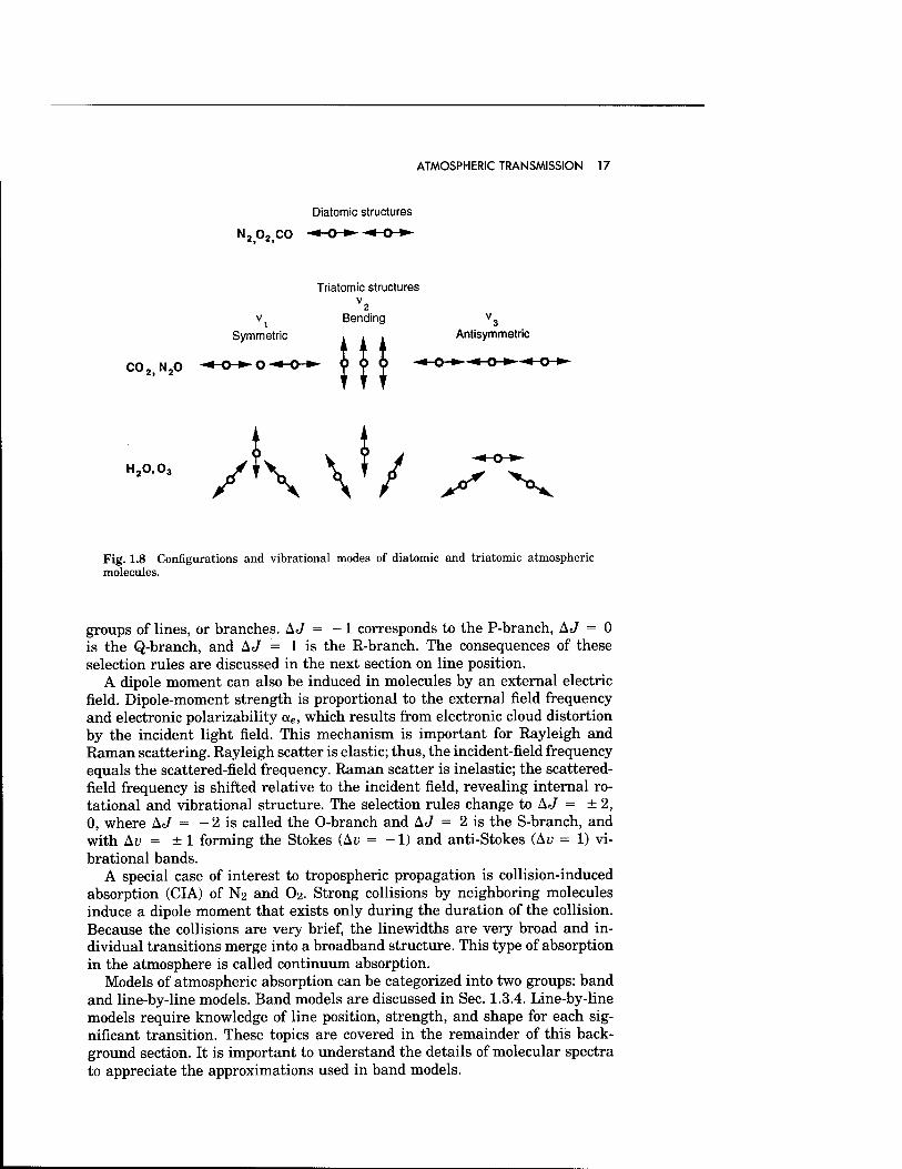
In the case of pure rotational transitions the first term must exist for a molecule to be infrared active. The second term is unimportant. In the case of vibrational transitions the second term must exist for a molecule to be infrared active. Examples of vibrational motions of important atmospheric molecules are illustrated in Fig. 1.8. Polar molecules are typically strong absorbers of infrared radiation and have spectra from the far-infrared (pure rotational) to throughout the mid-infrared (vibration-rotation bands). Water vapor, for ex- ample, is the most important absorber of IR in the troposphere.
Based on Eq. (1.23) the selection rules are determined. For pure rotational transitions, <//• - Ji = At/ = 1. For vibration-rotation transitions, Vf - vi = Au = 1 and At/ = ±1,0. The different rotational selection rules form distinct
M+ m_
+q r -Q
Fig. 1.7 Illustration of dipole moment for an ionic bond, where M+ = mass of positive ion, m- = mass of negative ion, and q is the charge magnitude.
ATMOSPHERIC TRANSMISSION 17
N202iCO
Diatomic structures
Triatomic structures
C02iN20
H20,03
v Bending v3
Symmetric A A A Antisymmetric
Fig. 1.8 Configurations and vibrational modes of diatomic and triatomic atmospheric molecules.
groups of lines, or branches. AJ = -1 corresponds to the P-branch, A J = 0 is the Q-branch, and AJ = 1 is the R-branch. The consequences of these selection rules are discussed in the next section on line position.
A dipole moment can also be induced in molecules by an external electric field. Dipole-moment strength is proportional to the external field frequency and electronic polarizability ae, which results from electronic cloud distortion by the incident light field. This mechanism is important for Rayleigh and Raman scattering. Rayleigh scatter is elastic; thus, the incident-field frequency equals the scattered-field frequency. Raman scatter is inelastic; the scattered- field frequency is shifted relative to the incident field, revealing internal ro- tational and vibrational structure. The selection rules change to A J = ± 2, 0, where AJ = - 2 is called the O-branch and A J = 2 is the S-branch, and with Av = ± 1 forming the Stokes (Av = -1) and anti-Stokes (Av = 1) vi- brational bands.
A special case of interest to tropospheric propagation is collision-induced absorption (CIA) of N2 and O2. Strong collisions by neighboring molecules induce a dipole moment that exists only during the duration of the collision. Because the collisions are very brief, the linewidths are very broad and in- dividual transitions merge into a broadband structure. This type of absorption in the atmosphere is called continuum absorption.
Models of atmospheric absorption can be categorized into two groups: band and line-by-line models. Band models are discussed in Sec. 1.3.4. Line-by-line models require knowledge of line position, strength, and shape for each sig- nificant transition. These topics are covered in the remainder of this back- ground section. It is important to understand the details of molecular spectra to appreciate the approximations used in band models.
18 IR/EO HANDBOOK
1.3.1.2 Line Position
Fortunately, nature has greatly simplified the study of spectroscopy by suffi- ciently separating the fundamental energies of rotational, vibrational, and electronic transitions: EEI > EVib > Erot. The energy structure of each dy- namics problem can be solved separately and then treated as a perturbation to the higher-energy term. Rotational spectra typically occur in the far-infrared (0.1 to 100 cm-1). Vibrational spectra typically occur in the mid-infrared and near-infrared (100 to 10,000 cm-1). Electronic spectra typically occur in the visible (weak bands) and ultraviolet (strong absorption bands, which determine the end of atmospheric transparency). Since the topics in this handbook are concerned with infrared and visible phenomena, electronic structure will not be covered in detail.
The development begins with rotation spectra, then vibration-rotation spec- tra. We close with a brief description of electronic spectra.
1.3.1.2.1 Rotational Spectra
Pure rotational bands typically exist from millimeter waves to the far-infrared. The formulas for rotational spectral line positions vary for different types of molecules. Molecules are classified as linear (e.g., N2, O2, H2, CO, OH, CO2, N2O, OCS, HCN, etc.), spherical top (e.g., CH4), symmetric top (e.g., NH3, CH3D, CH3CI, C2H6, etc.), and asymmetric top (e.g., H20,03, S02, N02, H202, H2S, etc.). Energy-level structure is specified by the rotational term value F( J) (=E/hc) and the rotational constants (A, B, and C), both in units of cm-1. In general, there are three rotational degrees of freedom and three corresponding quantum numbers; however, symmetry reduces the degrees of freedom. The following lists the term-value functions with the degeneracy factor gj for the various types of molecules.
Linear molecules
F(J) = BJ(J + 1) and gj = 2J+ 1 . (1.24)
Spherical-top molecules (A = B = C)
F(J) = BJ(J + 1) and gj = (2J + l)2 . (1.25)
Symmetric-top molecules
Prolate (A > B = C) F(J,K) = BJ( J + 1) + (A -B)K2 and (1 26)
_ J2J + 1, K = 0 gJ [2(2 J + 1), K + 0 .
Oblate (A = B > C) F( J,K) = BJ{ J + 1) + (C - B)K2 and (1 27)
f 2J + 1, K = 0 gJ \2{2J + 1), K + 0 .
ATMOSPHERIC TRANSMISSION 19
Asymmetric-top molecules (A > B > C)
F( J,Ka,Kc) is treated as an intermediate state between oblate and prolate symmetric tops. Thus, a precise statement depends on the molecule and the degree of asymmetry. For more information on this class of molecules see Herzberg.9
The rotational constants are defined as
h
8-n2cIa
B 8TT
2C/& 8ir2c/c
(1.28)
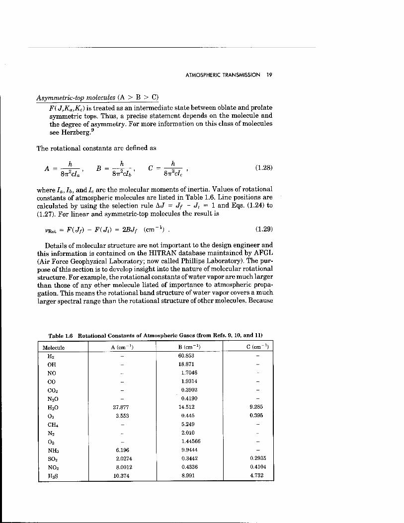
where Ia,h, and Ic are the molecular moments of inertia. Values of rotational constants of atmospheric molecules are listed in Table 1.6. Line positions are calculated by using the selection rule AJ = Jf - Ji = 1 and Eqs. (1.24) to (1.27). For linear and symmetric-top molecules the result is
vRot = F{Jf) - F(Ji) = 2BJf (cm"1) (1.29)
Details of molecular structure are not important to the design engineer and this information is contained on the HITRAN database maintained by AFGL (Air Force Geophysical Laboratory; now called Phillips Laboratory). The pur- pose of this section is to develop insight into the nature of molecular rotational structure. For example, the rotational constants of water vapor are much larger than those of any other molecule listed of importance to atmospheric propa- gation. This means the rotational band structure of water vapor covers a much larger spectral range than the rotational structure of other molecules. Because
Table 1.6 Rotational Constants of Atmospheric Gases (from Refs. 9, 10, and 11)
Molecule A (cm-1) B (cm-1) CCcm"1)
H2 - 60.853 -
OH - 18.871 -
NO - 1.7046 -
CO - 1.9314 -
C02 - 0.3902 -
N20 - 0.4190 -
H20 27.877 14.512 9.285
o3 3.553 0.445 0.395
CH.4 - 5.249 -
N2 - 2.010 -
o2 - 1.44566 -
NH3 6.196 9.9444 -
S02 2.0274 0.3442 0.2935
N02 8.0012 0.4336 0.4104
H2S 10.374 8.991 4.732
20 IR/EO HANDBOOK
of this (and other properties), water vapor plays an important role in every infrared spectral region.
1.3.1.2.2 Vibration-Rotation Bands
Vibration bands of atmospheric gases typically exist in the mid-infrared. Atmo- spheric infrared windows are denned by the locations of these vibrational frequencies.
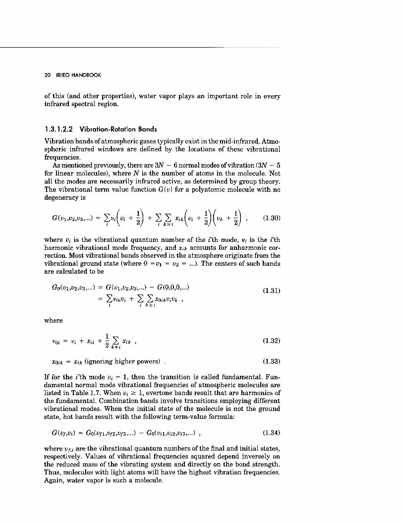
As mentioned previously, there are 3N - 6 normal modes of vibration (3N - 5 for linear molecules), where N is the number of atoms in the molecule. Not all the modes are necessarily infrared active, as determined by group theory. The vibrational term value function G(v) for a polyatomic molecule with no degeneracy is
G(Vl,v2,v3,...) = XVi(Vi + |) + 2 X.XikUi + Wvk + |j , (1.30)
where vt is the vibrational quantum number of the i'th mode, v, is the i'th harmonic vibrational mode frequency, and xik accounts for anharmonic cor- rection. Most vibrational bands observed in the atmosphere originate from the vibrational ground state (where 0 =v\ = v<i = ...)• The centers of such bands are calculated to be
Go(Vl,V2,V3,-) = G(vi,v2,v3,-) ~ 0(0,0,0,...) (131)
i i ksii
where
v0i = vt + xu + - X xik , (1.32)
xoik = Xik (ignoring higher powers) . (1.33)
If for the i'th mode vi = 1, then the transition is called fundamental. Fun- damental normal mode vibrational frequencies of atmospheric molecules are listed in Table 1.7. When vt > 1, overtone bands result that are harmonics of the fundamental. Combination bands involve transitions employing different vibrational modes. When the initial state of the molecule is not the ground state, hot bands result with the following term-value formula:
G(Vf,Vi) = Go(Vfl,Vf2,Vf3,-) - Go(Vil,Vi2,Vi3,...) , (1.34)
where Vf,i are the vibrational quantum numbers of the final and initial states, respectively. Values of vibrational frequencies squared depend inversely on the reduced mass of the vibrating system and directly on the bond strength. Thus, molecules with light atoms will have the highest vibration frequencies. Again, water vapor is such a molecule.
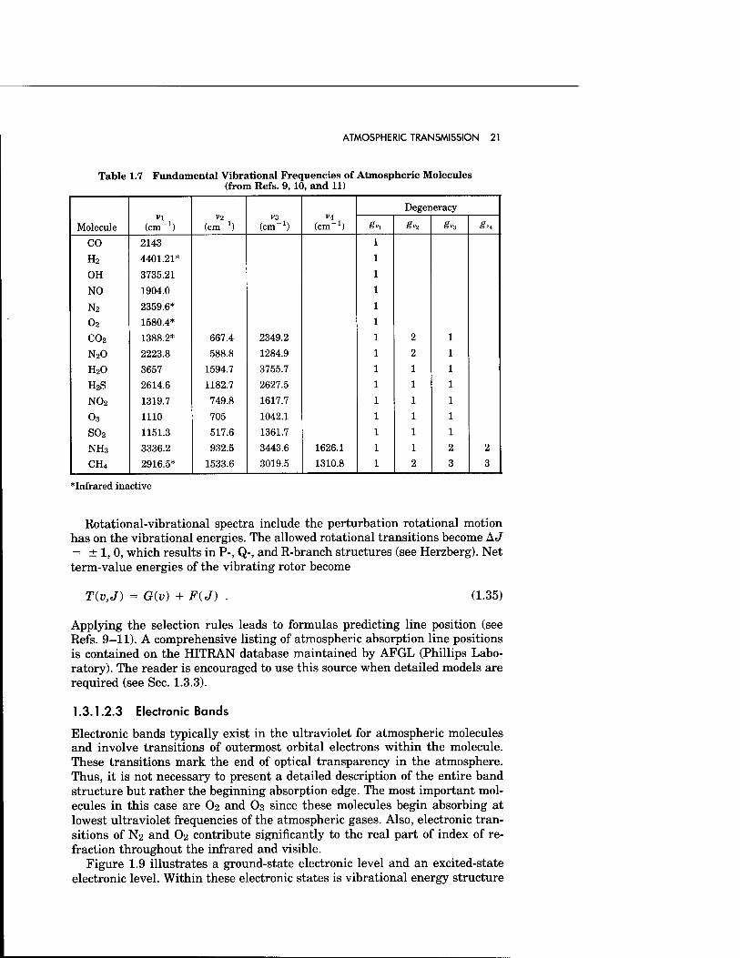
ATMOSPHERIC TRANSMISSION 21
Table 1.7 Fundamental Vibrational Frequencies of Atmospheric Molecules (from Refs. 9, 10, and 11)
Molecule (cm"1) V2
(cm'1) V3
(cm'1) V4
(cm"1)
Degeneracy
§n Sv2 £v3 gvi
CO 2143
H2 4401.21*
OH 3735.21
NO 1904.0
N2 2359.6*
o2 1580.4*
co2 1388.2* 667.4 2349.2 2
N20 2223.8 588.8 1284.9 2
H20 3657 1594.7 3755.7 1
H2S 2614.6 1182.7 2627.5 1
N02 1319.7 749.8 1617.7 1
o3 1110 705 1042.1 1
S02 1151.3 517.6 1361.7 1
NH3 3336.2 932.5 3443.6 1626.1 1 2 2
CH4 2916.5* 1533.6 3019.5 1310.8 2 3 3
* Infrared inactive
Rotational-vibrational spectra include the perturbation rotational motion has on the vibrational energies. The allowed rotational transitions become AJ = ± 1, 0, which results in P-, Q-, and R-branch structures (see Herzberg). Net term-value energies of the vibrating rotor become
T{v,J) = G(v) + F(J) . (1.35)
Applying the selection rules leads to formulas predicting line position (see Refs. 9-11). A comprehensive listing of atmospheric absorption line positions is contained on the HITRAN database maintained by AFGL (Phillips Labo- ratory). The reader is encouraged to use this source when detailed models are required (see Sec. 1.3.3).
1.3.1.2.3 Electronic Bands
Electronic bands typically exist in the ultraviolet for atmospheric molecules and involve transitions of outermost orbital electrons within the molecule. These transitions mark the end of optical transparency in the atmosphere. Thus, it is not necessary to present a detailed description of the entire band structure but rather the beginning absorption edge. The most important mol- ecules in this case are O2 and O3 since these molecules begin absorbing at lowest ultraviolet frequencies of the atmospheric gases. Also, electronic tran- sitions of N2 and O2 contribute significantly to the real part of index of re- fraction throughout the infrared and visible.
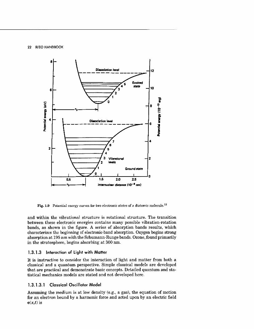
Figure 1.9 illustrates a ground-state electronic level and an excited-state electronic level. Within these electronic states is vibrational energy structure
22 IR/EO HANDBOOK
C i o
i
as I < 'o >|
1.5 20 2.5
Internudear distance (10~* cm)
Fig. 1.9 Potential energy curves for two electronic states of a diatomic molecule.12
and within the vibrational structure is rotational structure. The transition between these electronic energies contains many possible vibration-rotation bands, as shown in the figure. A series of absorption bands results, which characterizes the beginning of electronic-band absorption. Oxygen begins strong absorption at 195 nm with the Schumann-Runge bands. Ozone, found primarily in the stratosphere, begins absorbing at 300 nm.
1.3.1.3 Interaction of Light with Matter
It is instructive to consider the interaction of light and matter from both a classical and a quantum perspective. Simple classical models are developed that are practical and demonstrate basic concepts. Detailed quantum and sta- tistical mechanics models are stated and not developed here.
1.3.1.3.1 Classical Oscillator Model
Assuming the medium is at low density (e.g., a gas), the equation of motion for an electron bound by a harmonic force and acted upon by an electric field e(x,t) is
ATMOSPHERIC TRANSMISSION 23
mx + m-yx + mtoox = qe(x,t) , (1.36)
where m = mass, 7 = phenomenological damping force, q = charge of the mass, and wo = oscillation frequency. Magnetic-field effects will be ignored and the strength of the electric field will not distort the molecule to reveal anharmonic effects in the potential. Then, assume a time harmonic behavior as x(t) = X(w)ej<at. The above equation becomes
-mto2X + jmyuX + mw%X = qE(u,t) . (1.37)
This is an algebraic equation with the following solution for X(w):
X(to) = -(cog - to2 + >7)_1E(ü>) . (1.38) m
Now, the dipole-moment vector p (|x is scalar dipole moment) contributed by one bound electron becomes
a2
p = qXx = —(co| - co2 + >7)_1E . (1.39) m
If there are Na absorbing molecules per unit volume V with a number density pa = N/V, then summing over the different rotational, vibrational, and elec- tronic transitions gives
P = xeoE , (140)
|P| e(co) = 6r(co)eo = eo + T^; = [1 + x(w)]£o ,
where P is the polarization vector, eo is the free-space permittivity, er is the relative permittivity, and x is the electric susceptibility. Further, recall from electromagnetic theory that
pa(q2/m)iE P = Pa ZPi = Z ~2 2~T^ • {1A1)
i j to; - to + j(a~ii
Using Eqs. (1.40) and (1.41), the relative permittivity becomes
e» = 1 + S 29a{q2':°m).1 • d-42)
i u>i - w + joi-yt
Again, the sum on i is over all allowed rotational, vibrational, and electronic transitions. Let
Ae, = Pa^r- (1-43) mjtoj EO
24 IR/EO HANDBOOK
be the oscillator strength; then
er(co) - jer(a) = 1 + 2/ ~1 2 :— ■ i Wj - co + ./ab-
solving for the real and imaginary parts of the permittivity gives
„,,„, _ •, , y to2Ae;(co2 - co2) Er(co) - 1 + 2,—ä 2x2 , , ^2 '
i (co,- - co ) + (co7,-r
.2/ e»((0) = V o>iAe,-Q>7« EA10J t (cof - co2)2 + (CO7J)
2 •
Further, the absorption coefficient is defined as
Near line center (co ~ co;) the expression reduces to
co^y 2CO2AE;(7;/2)
nc i (co,- + coj)2(coi - co)2 + 4[co,(7;/2)]
(1.44)
(1.45)
ßabs(w) = 4TTVÄ(CO) = 2-Ha) = ~e"r(a) . (1.46) c nc
Substituting Eq. (1.45) for e" leads to (assuming n is constant)
/ ^ w v w,Aej7j ßabs(w) = —2 7^ 2,2 , ^ • (1.47)
„ / v w2v 2cofAe,(7j/2)
ßabS(ü>) = —y-—■— * ';n ; . (i.48)
Then,
ßabs(w)=?^-y^(w)' (i-49)
where the dimension of ßabs is reciprocal length and
JL^^Z-, "^ , 2, (1-50) TT (Cüj -CO) + O-j)
is the Lorentz line shape with a; = 7,72 representing the half-width at half maximum. Let
2
*<») = (-)jL(a) and ft = ^^ ; (1.51) \coj/ 2nc
then,
ßabs(to) = ^Sig(a,ai) near line center . (1.52)
ATMOSPHERIC TRANSMISSION 25
This equation agrees with the form stipulated in the introduction of this section [Eq. (1.21)]. Notice that gtco.wi) is the Van Vleck-Weisskopf line-shape func- tion,13 is valid only near line center, and cannot satisfy the normalization condition as given by Eq. (1.20). A complete line-profile description is presented in the next section.
The real part of the permittivity z'r is related to the complex index of re- fraction by the expression
e'r = n2 - kl . (1-53)
In the region of transparency (i.e., n » ka) a simple expression for the real part of the index of refraction is obtained:
i*«o) = l + 2-J^V (1-54) i COj - Ü)
This formula is known as Sellmeier's equation and is a convenient way of representing the index of refraction of gases, liquids, and solids in spectral regions of transparency.
1.3.1.3.2 Quantum-Mechanical Model
The following expressions for line-profile function and line strength are based on statistical and quantum mechanics14-17 as applied to the interaction of light and matter. They can be applied quite generally to a wide class of problems: atmospheric propagation and molecular absorption (the AFGL codes FASCODE, MODTRAN, and LOWTRAN are based on these equations); small-signal laser gain calculations; and remote sensing.
The line-profile function is
. . v tanh(/icv/2^ßT) n „s S{V) = ^tanh(W2^T)Ü(v) + ji~v)] ' (L55)
where kß is Boltzmann's constant andj'(v) is the power spectral density func- tion. The first factor states that the ability of the electromagnetic field to couple to a molecule increases with frequency. The second factor requires that Maxwell- Boltzmann statistics be satisfied across the entire line shape and fulfills de- tailed balance conditions.17'18 Here, j(v) is the power spectral density func- tion or the Fourier transform of the time-dependent autocorrelation function C(T), which describes the time evolution of the state of the absorbing molecule, and is expressed by
i r j(v) = — di exp( -j2ircPT) exp(J'2TTCVOT)C(T) , (1.56)
2TT J-CO
26 IR/EO HANDBOOK
where
CM = C„(T)C6(T)...Cm(T) ,
g(v) = g{-v) , (1.57)
dvjtv) = lforC(O) = 1 , Jroo
0
where the subscripts designate the different types of molecules in the medium and different broadening mechanisms and C(T) = C*(-T). Note that,/(v) is a real and even function. More details on the autocorrelation function will be given in the section on line shapes (Sec. 1.3.1.5).
The line strength is expressed as
8ir3v0exp(-gf/feBr) / hcv0\ V|,,|2 „ _
where pa is the absorbing gas density (molecules per volume), n is the index of refraction (real part), Ei is the lower energy level of the transition, kß is Boltzmann's constant, Q is the partition function (denned below), and |M|2 is the dipole matrix element.
1.3.1.4 Line Strength
To complete the line-strength expression requires specifying the partition func- tion Q, the lower energy level Ei, and the matrix elements S|M|2. The matrix elements and the lower energy level are provided by the HITRAN database (see Sec. 1.3.3). The index of refraction of the atmosphere is approximately one. The partition functions must be determined for each class of molecule and this is discussed in the following.
1.3.1.4.1 Partition Functions
The partition function is a normalization factor in the Maxwell-Boltzmann distribution function. It is the sum over all energy levels (quantum numbers) of the molecule, as given by
Q = ?* eXP(^) ' (L59)
where gi is the degeneracy factor for the i'th energy level. However, because of the large differences between the different types of energies in molecules, the partition function can be approximately expressed by the following product:
Q ~ QEiQvibQRot Q 6Q)
= -2ft. exP|^j 2ft exP(^rJ 2ft/ exp ER, ;ot
kBT
ATMOSPHERIC TRANSMISSION 27
Over the range of atmospheric temperatures, QEI = 1 and Qvib ~ 1 are good approximations. Knowledge of the rotational partition function is important and a listing is given, according to the class of molecule, in the following.
Diatomic molecules
Because the rotational energy levels are closely spaced, the sum is converted to an integral. The rotational partition function becomes
Qßot = 8TT%kBT vB - H • (1.61)
ah2 o- 1.4388B,
where o- is a symmetry number with
a = 2 for A=B (i.e., N2, 02...) ,
o- = lforA^ß (i.e., CO, NO...) ,
and Be can be found in Table 1.6. The vibrational partition function for a purely harmonic potential becomes
l
Q Vib / /icvo\l v ( hcvvo\ (1.62)
Polyatomic molecules
a. Linear molecules
Since the same energy eigenvalues are obtained for linear polyatomic mole- cules as for diatomic molecules, the partition functions are also the same.
b. Symmetric top molecules
For symmetric top molecules,
K = ™ r I../ * T>\TS2
QRot - _ Zi hc(A-BW
k T J=\K\ (2J+1) exp
hcBJ(J+l) k T
(1.63)
As before, the sums can be replaced by integrals; thus, for prolate symmetric top,
Q Rot v^/8A^r^/8Afer\ a \
VTT
hz
T W T \ a V1.4388A/ Vl-4388S7
(1.64)

28 IR/EO HANDBOOK
Spherical-top molecules are a special case of the prolate symmetric top where A = B or Ia = h- This substitution into the above formulas produces the ro- tational partition function for the spherical top.
Similarly, for the oblate case (CT is a symmetry number),
Q Rot _ VW T \ VS
a \l.4388Cy \1.4388B
c. Asymmetric top molecules
(1.65)
For asymmetric top molecules,
VTT .^ Vi;
_^ \i
\ Vi
^Rot CT \1.4388Ay \I.4388B) \lA388C)
The vibrational partition function for polyatomic molecules becomes
(1.66)
Qvib = 2 exP Vl,V2,...Vn
exp
hc{v\V\ + V2V2 + ... + vnvn) kBT
exp
hcv\
hcv2
-,-1
exp Acv„
T -1
(1.67)
where n is the number of normal modes.
1.3.1.5 Line-Shape Profiles
Homogeneous and inhomogeneous broadening are the most general classifi- cation of line shapes. Homogeneous broadening means that all molecules have the same basic line-shape characteristics. That is, if a line shape is observed for a collection of molecules, the same line shape will be observed for each molecule. Examples are natural broadening (radiation damping) and collision broadening. Inhomogeneously broadened lines represent a collection of shifted homogeneously broadened lines. Thus, each molecule's line shape may be com- pletely different from the total line shape of a collection of molecules. Examples are Doppler broadening, nonuniform electric and magnetic fields in Stark and Zeeman effects, and inhomogeneities in a medium (such as crystalline strains and defects in solids). These concepts should become more clear when Doppler broadening is thoroughly treated.
1.3.1.5.1 Homogeneous Line Shapes
Two related cases will be considered, radiation damping (natural broadening) and collision broadening. Consider a perturbation to a quantum system, whether it be a photon or a neighboring molecule that will change the energy-level
ATMOSPHERIC TRANSMISSION 29
structure with a certain probability. Owing to this probabilistic nature, an uncertainty results in observing the effects of the perturbation. This is man- ifested by the Heisenberg uncertainty principle:
AxAp = AtAE = h .
Using AE = hAf, where Af is the change in frequency,
(1.68)
AtAf~- Af = At2lT 2TT
(1.69)
where 7 is the reciprocal lifetime. A transition between two energy levels of a quantum system that results in the emission or absorption of a photon will have an uncertainty in the separation of the levels and therefore an uncertainty in the emitted photon frequency. Therefore,
Afui = Afiu = ^(AEU + AEi) -^(lu + yi) (1.70)
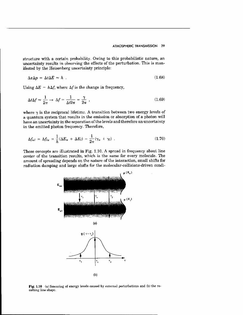
These concepts are illustrated in Fig. 1.10. A spread in frequency about line center of the transition results, which is the same for every molecule. The amount of spreading depends on the nature of the interaction, small shifts for radiation damping and large shifts for the molecular-collisions-driven condi-
<EU)
p(E,)
(b)
Fig. 1.10 (a) Smearing of energy levels caused by external perturbations and (b) the re- sulting line shape.
30 IR/EO HANDBOOK
tions of the lower troposphere. A brief discussion of these different mechanisms follows.
Natural line shape
The natural line shape gN(v - vo) is caused by the perturbations an incident photon has on a molecule. The effect is small but is important in determining lifetimes of energy levels and astrophysical problems.
The line-shape function JN(V) is based on an exponential autocorrelation function [i.e., CAKT) = exp(-owT)] and is a Lorentzian function:
JAKV-VO) = - CW
(v - vo) + aN (1.71)
where ew is the half-width at half-intensity and is related to the Einstein spontaneous emission coefficient by18
_ Aul _ 1 ,.. „_.
ZltC ^TCtspontaneous
with Spontaneous being the lifetime of the upper level and Aui being the Einstein A-coefficient. Further, the line-profile function becomes
v tanh(/icv/2&sT) r . , . . . gN(v, Vo) = - —-T7T—^=r [JN(V) + Jn( - v)] . (1.73)
vo tanh(ncvo/2«ßT)
For near line center (v = vo) and vo » OAT,
gN(v, v0) = JN(V ^ v0) . (1.74)
Natural linewidths are very narrow, making this an excellent approximation. Further, the line-profile function #(v) is normalized as required by Eq. (1.20) within this approximation.
Collision-broadened line shape
The collision-broadened line shape is essential for accurate atmospheric prop- agation models. Long-path propagation simulations require characterization of the line profiles far from line center, and the commonly used Lorentz line- profile function is not adequate. This point is readily made by observing that the normalization condition of Eq. (1.20) cannot be satisfied by the simple Lorentz formula. Thus, a more complete theory must be applied and the work of Birnbaum19'20 will be followed because it leads to a simple, practical, and versatile line-shape function. Other formalisms are also possible21-23 but lead to complicated numerical techniques for a complete line-profile representation. The autocorrelation function for a binary mixture is empirically chosen to be
ATMOSPHERIC TRANSMISSION 31
C(T) = Ca(x)C6(T)
f[Ta2-(Tg2 + T2 + i2T0)1/2]) f [T62 ~ (if 2 + T2 + i2TQT)1/2] = exp-^ f exp^
(1.75)
where C0(T) is the autocorrelation function for absorber-absorber interactions and C&(T) is the autocorrelation function for absorber-broadener interactions. The relaxation times n and T2 represent the long-time and short-time behavior of the autocorrelation function. The term TO is a thermal time denned by
TO = —— • (1-76)
(Note: for T = 298 K, TO = 1.29 x l(T14s.) The long-time behavior of the autocorrelation function becomes
C(T-X») = exp(-^j , (1.77)
where
Tf1 = Tal1 + Tfti1 = 0-c = aca + Ucb (1.78)
for a binary mixture and ac is the usual collision-broadened half-width at half- intensity. Based on the kinetic theory of gases,
o-c&o
= crc60"
i i °"eoo\ P6 + Pa
O-c60/
(pb + Bpa) (1.79)
jf/2
where p = plkßT and the ratio o-Cao/o-c&o is the dimensionless-self-broadening coefficient B. Table 1.8 lists B values for various atmospheric absorbing gases relative to nitrogen. The exponent of the temperature can vary between 0.5 and 1.0, based on experimental results and more complete theories.
The long-time autocorrelation function results in the near-line-center line- shape function. Substituting Eq. (1.77) into Eqs. (1.56) and (1.55) results in the following near-line-center profile:
. . v tanh(-Acv/2feßT) .,..,., y, ri am *NLC(V;V;) = -tanh(-W2*ßr)ÜNLc(v) ^^ '
JNLCW = -: ,ac ^2 . 2 > (L81)
Tf (v - Vj + OLc,i) + <*c

32 IR/EO HANDBOOK
Table 1.8 Dimensionless-Self-Broadening Coefficient Relative to Nitrogen and Near Line Center
Molecule B H20 5
CH4 1.3 N20 1.24
CO 1.02
C02 1.3
03 1.0
where CTC = 2iTcac. This result is consistent with the FASCODE model (see Sec. 1.5.3) and, for hcvlksT small, the millimeter-wave propagation model (MPM) (Sec. 1.3.2, Refs. 55 and 58). Equation (1.81) includes a pressure-shift term aC;;, which occurs in more general theories producing a complex ac {ac,i = Im[ac]). Pressure-shift contributions are roughly one hundred times smaller than Re[ac] and for this reason are usually ignored. It can be important for laser or narrow-band system propagation (e.g., lidar) when operating near a spectral absorption line. Many of the other popular line shapes can be obtained from these formulas by using various approximations. It should be noted that most of these approximations are not always appropriate for the rf-millimeter region.
One important shortcoming of this near-line-center model is that it does not include line-mixing effects. This is important for O2 absorption of the 60 GHz band24,25 and for CO2,26'27 but greatly complicates absorption-line modeling. A relatively simple modified Lorentz line shape, as given by Rosenkranz and applied to O2,24 is
JNLCM = ~ + (v - Vj)yj
IT (v VJ + ac,i)2 + a2 (1.82)
where yj is the coupling constant, representing the effects of neighboring en- ergy levels on the levels involved in the transition. Birnbaum has recently improved this line-shape formalism and now includes line-mixing effects28; however, this complicates the model.
The leading factor in the line-shape profile,
v tanh(hcv/2kBT) vo taiihihcvofäkßT)
= H(v,T;v0) (1.83)
is an important part of this model and makes g(v) more general. The term g(v) reduces to other models in appropriate limits. The following illustrates this point.
Classical limit (h —» 0)
,2
gNLC&yo) -> I — I ÜNLcfr) + JNLC(-V)] A->0 \ Vo/
(1.84)
ATMOSPHERIC TRANSMISSION 33
This result is consistent with the classical oscillator model of Eq. (1.52).
v^O
bv2/T £NLC(
V;V
O) v^o vo tanh(6vo/T) [JNLCW + JNLC(-V
)1 > (1.85)
where b = hc/2kß. The frequency-squared dependence is commonly observed at microwave and millimeter-wave frequencies.
v = vo
£NLC(V
;V
O) =JNLC(T) +JNLC(-V) .
Thus, at line center the profile is Lorentzian.
bv » T and bvo » T (infrared approximation)
(1.86)
£NLC (V;V
O) -> — [ JNLC (v) + JNLC (- v)] bv»T vo 6v0»r
(1.87)
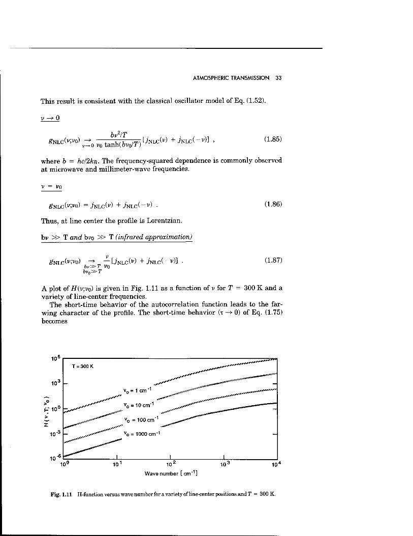
A plot of iJ(v;vo) is given in Fig. 1.11 as a function of v for T = 300 K and a variety of line-center frequencies.
The short-time behavior of the autocorrelation function leads to the far- wing character of the profile. The short-time behavior (T —» 0) of Eq. (1.75) becomes
106
T = 300 K ■,*""■ „**"'
■IMM«""'
10" Wave number [ cm"1]
Fig. 1.11 H-function versus wave number for a variety of line-center positions and T = 300 K.
34 IR/EO HANDBOOK
C(T) -* expf--1-1 . (1.88)
The Gaussian form is consistent with theoretical models of the autocorrelation function.29 Thus, a complete line shape is specified from line center to the far wing. The far-wing result has been obtained for the case of a single absorbing molecule [i.e., C(T) = C0(T)] and is given by20
. v tanh(hcv/2kßT) . g™iv;Vj) = Vj tanUhcvj/2kBT)J™iv) ' (L89)
. , , /Ta2\^ 1 eXP(-2TTc|v - Vj\Ta2) Jvyfiv) = -z- —ö; rp= exp[2TTc(v - V,)T0] . (1.90)
\4TT/ Tal 4lT |V - Vj\ '
The exponential wing is consistent with experimental observation.20'30 The general far-wing result for a binary mixture can be obtained by solving a convolution integral of the individual line-shape functions (ja and jb) in the far-wing limit. Thus, given
1 r ja(v) = —\ dr exp(-i2TTCv)Ca(T) ,
1 r Jb(v) = 7T rfTexp(-i2TTCv)C6(T) , (1.91)
2TT J-00
j(v) = ja(x)jb(v ~ Vj - X)dx , J — 00
then using contour integration and in the far-wing limit,
. , . (ta2\V2 1 eXp(-2TTc|v - Vj\ja2) r_ . . , ./FWW
= U~ 7~2i Ü5 exp[2irc(v - V/)T0]
eXp(-2TTc|v - Vj\jb2) „ 2| n= exp[2irc(v - V,)T0] . (1.92)
4TT V - V; '
The formula for the autocorrelation function given by Eq. (1.75) agrees with theoretical and experimental results concerning near-line-center and far-wing phenomena. Because the function is continuous in time, a complete line-shape function is specified. The closed-form expression for the line shape has been obtained for a pure gas; the result is
/T2\ exp(2i Ti /T2\ exp(2TTCv_T0)Z_.K"i(Z_) exp(2TTCv+T0)Z+Ä'i(Z+) j(v) = - exp( - ) , , /rt . ^ + —— 72
IT \T!/ 1 + (2-nCV-Tl) 1 + (2TTCV + Tir
(1.93)
ATMOSPHERIC TRANSMISSION 35
where
v± = v ± vo , (1#94)
Z± = (Tf2 + vi^Oli + # ,
and K\(Z±) is the modified Bessel function of the second kind. This line shape is consistent with the near-line-center results obtained earlier and in addition provides insight into the nature of the far wing as previously shown. Most important, a complete line shape allows proper normalization according to Eq. (1.20). The following result is obtained:
I dvg(v,v0) = (1 + ^] cotUhcv0/kBT) . (1.95) 'o \ aovo/
For practical values of the parameters this line-profile function is normalized to one.
A line-shape formula for homogeneous collision-broadened lines has been developed that is compatible with the AFGL HITRAN database. The line shape has validity from line center to the far wing. Local line absorption and far- wing continuum absorption can now be modeled in greater detail. The present formalism, however, lacks line overlap or coupling effects.
1.3.1.5.2 Inhomogeneous Line Shapes
Doppler line shape
The random kinetic motion of the atoms causes a Doppler shift of the narrow homogeneously broadened atoms. Atoms with different velocities will be shifted by different amounts so that a new line shape results in the inhomogeneous Doppler profile.
Derivation of this effect begins with Doppler's equation
v = (c - V)VQ , v = U.yb; vo
and Maxwell-Boltzmann's distribution
^ - «»(si)' (1'97)
Using the kinetic energy E = V2mv2 and the previous equations, it follows that
f(v) = JD(V - vo) = exp c(v - vo)
vo 'ägrl • a98)
36 IR/EO HANDBOOK
which represents the probability distribution of the shifted frequencies due to the velocity components of the atoms parallel to the incident photon field. Since Doppler lines are very narrow, it is valid to enforce normalization on the spectral density function, accounting for absorption as well as emission; thus,
1" Jo [JD(V - vo) + JD(V + vo)]dv = 1 (1.99)
The Doppler spectral density function is commonly expressed as
(v - vo)2 ln2~ , (ha)*» JD{v - vo) = — exp
Ct£)VTT <*D
where
(1.100)
aD = kBT ln2
mc v = 3.578 x 10~7(- vo
ml (1.101)
is the half-width at half-intensity, T is the temperature in kelvin, m is the reduced mass in amu, and vo is the line-center frequency in cm-1. Because Doppler lines are narrow, a good approximation is
go(v ~ vo) ~JD(V - v0) (1.102)
Voigt line shape
The Doppler line shape assumes the shifted homogeneous line shapes are delta functions, which is usually a good approximation at very low pressures. How- ever, the natural line shape is always present in any experiment and, in problems of atmospheric importance, collision broadening is present.
Figure 1.12 illustrates the shifted homogeneous line shape weighted by a Gaussian (Doppler) distribution. This process can be thought of as a convolution of a homogeneous shape, g#(v), through a Doppler profile. Thus,
Jroo
^H(V,VO)[JD(V - v' - vo) + JD(V - v' + vo)]dv' . 0
(1.103)
The resulting line shape is called the Voigt line shape gv(v). From the definition of the above equation, the normalization condition can be seen to be satisfied; i.e.,
f Jo
gv(v,vo)dv = 1 . (1.104)
The homogeneous line shape most often used is the Lorentz profile (but it may not always apply). Substituting in the Lorentz and Doppler line shapes and ignoring the emission term,
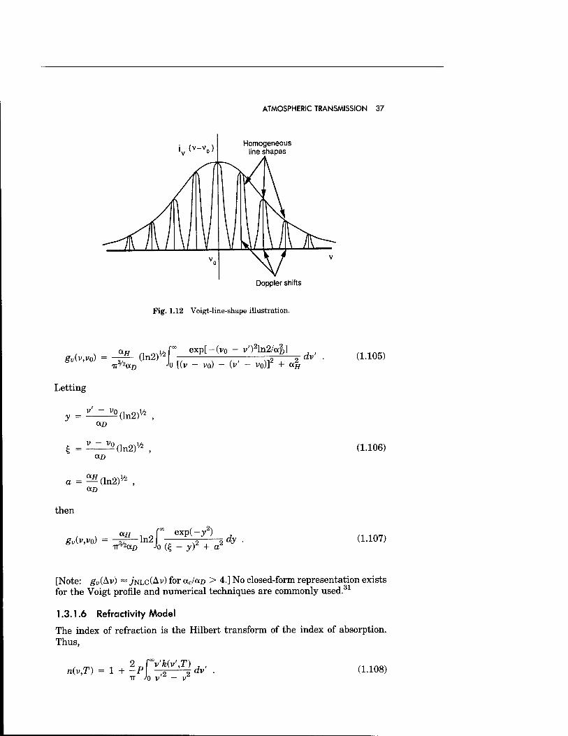
ATMOSPHERIC TRANSMISSION 37
iv(v-vo>
Homogeneous line shapes
Doppler shifts
Fig. 1.12 Voigt-line-shape illustration.
gv(v,v0) = TT3/2aD
(ln2)^f Jo
exp[-(vo - v')2ln2/af)]
[(v - vo) - (v' - vo)] + aH
dv' (1.105)
Letting
y = ^^(ln2)* , OLD
g = LZJ!o(ln2)V4 OLD
(1.106)
aß
then
gu(v,v0) = -jrr—ln2 n/2an Jo
exp(-y ) —2~,—2dy TTd/2a0 Jo (£ - yr + a
(1.107)
[Note: gv(hv) = J'NLC(AV) for ac/ao > 4.] No closed-form representation exists for the Voigt profile and numerical techniques are commonly used.31
1.3.1.6 Refractivity Model
The index of refraction is the Hilbert transform of the index of absorption. Thus,
n(v,T) = 1 + 2 rvw,r IT Jo v'2 - V:
T) i dv' (1.108)
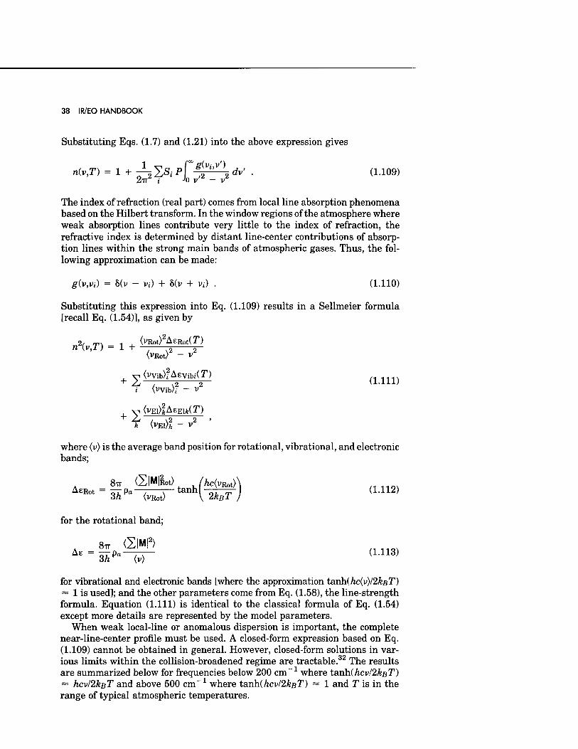
38 IR/EO HANDBOOK
Substituting Eqs. (1.7) and (1.21) into the above expression gives
n{v,T) = 1 + -K^Si P\ 8i2i,V \ dv' ■ d-109)
2ir2 i h v'2 - v2
The index of refraction (real part) comes from local line absorption phenomena based on the Hubert transform. In the window regions of the atmosphere where weak absorption lines contribute very little to the index of refraction, the refractive index is determined by distant line-center contributions of absorp- tion lines within the strong main bands of atmospheric gases. Thus, the fol- lowing approximation can be made:
g{v,vi) = 8(v - vi) + 8(v + vi) . (1.110)
Substituting this expression into Eq. (1.109) results in a Sellmeier formula [recall Eq. (1.54)], as given by
2, m-. -. , (vRot)2AERot(r) n\v,T) = 1 + — -2 2~
<VRot>* - V2
(vvib)fAevibi(r) (vvib)f - v2
<VEI)*AEEI*(T)
+ SW;'- 2 2 J (LIU)
+ 2 k {vn)k - v
where (v) is the average band position for rotational, vibrational, and electronic bands;
8TT <2Ät> /Ac(vRQt)\ ni1„ AeRot = Sä pa -^r tanh[^^r) (L112)
for the rotational band;
8„ S|M|2> 48 " 3Ä""— (1'113)
for vibrational and electronic bands [where the approximation tanh(/ic(v)/2&ßT) = 1 is used]; and the other parameters come from Eq. (1.58), the line-strength formula. Equation (1.111) is identical to the classical formula of Eq. (1.54) except more details are represented by the model parameters.
When weak local-line or anomalous dispersion is important, the complete near-line-center profile must be used. A closed-form expression based on Eq. (1.109) cannot be obtained in general. However, closed-form solutions in var- ious limits within the collision-broadened regime are tractable.32 The results are summarized below for frequencies below 200 cm-1 where tanh(/icv/2^ßT) =» hcv/2kßT and above 500 cm-1 where tanh(/icv/2&ßT) = 1 and T is in the range of typical atmospheric temperatures.
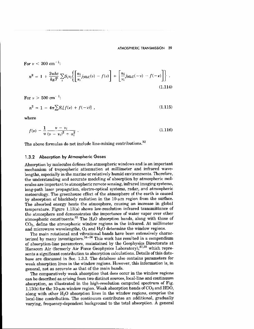
ATMOSPHERIC TRANSMISSION 39
For v < 200 cm"1:
2TTAC v-, _ I a;.
"2 = 1+fer?s" —JNLC(V) - fiy) Vi
a JNLC(-V) - f(-v)
Vi
(1.114)
For v > 500 cm-1:
n2 = 1 - 4Tr2Si[/"(v) + /-(-v)] , (1.115)
where
fM = l( V"/l 2- (1-116) IT (V - Vi) + dj
The above formulas do not include line-mixing contributions.32
1.3.2 Absorption by Atmospheric Gases
Absorption by molecules defines the atmospheric windows and is an important mechanism of tropospheric attenuation at millimeter and infrared wave- lengths, especially in the marine or relatively humid environments. Therefore, the understanding and accurate modeling of absorption by atmospheric mol- ecules are important to atmospheric remote sensing, infrared imaging systems, long-path laser propagation, electro-optical systems, radar, and atmospheric meteorology. The greenhouse effect of the atmosphere of the earth is caused by absorption of blackbody radiation in the 10-|xm region from the surface. The absorbed energy heats the atmosphere, causing an increase in global temperature. Figure 1.13(a) shows low-resolution infrared transmittance of the atmosphere and demonstrates the importance of water vapor over other atmospheric constituents.33 The H2O absorption bands, along with those of CO2, define the atmospheric window regions in the infrared. At millimeter and microwave wavelengths, O2 and H2O determine the window regions.
The main rotational and vibrational bands have been extensively charac- terized by many investigators.34-36 This work has resulted in a compendium of absorption-line parameters, maintained by the Geophysics Directorate at Hanscom Air (formerly Air Force Geophysics Laboratory),37'38 which repre- sents a significant contribution to absorption calculations. Details of this data- base are discussed in Sec. 1.3.3. The database also contains parameters for weak absorption lines in the window regions. However, this information is, in general, not as accurate as that of the main bands.
The comparatively weak absorption that does occur in the window regions can be described as arising from two distinct sources, local-line and continuum absorption, as illustrated in the high-resolution computed spectrum of Fig. 1.13(b) for the 10-|xm window region. Weak absorption bands of CO2 and HDO, along with other H2O absorption lines in the window regions, comprise the local-line contribution. The continuum contributes an additional, gradually varying, frequency-dependent background to the total absorption. A general
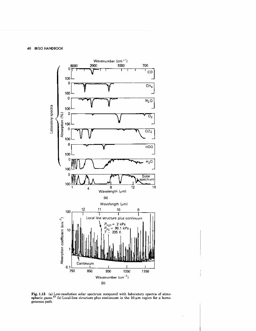
40 IR/EO HANDBOOK
/ 8000 Wavenumber (cm ')
2000 1000 700
CL Vt
o
o
100
n—r "\r i r i i r CO
100>- 1 IT CH,
100
-^y—y~ NoO
<! •2 100
Y 100 TT 100 L-
-y- HDO
0
100
100
~l"*NyKW. H20
Solar spectrum
100 12
8 Wavelength (^m)
(a)
Wavelength (^m)
10
12 16
11
E
*-* c gj o it 0) o o c o
.Q < 0.1
Local line structure plus continuum
PH2O = 2 kPa PN,= 99.1 kPa T = 295 K
Continuum _L _L
750 850 950 1050
Wavenumber (cm )
(b)
1150
Fig. 1.13 (a) Low-resolution solar spectrum compared with laboratory spectra of atmo- spheric gases.33 (b) Local-line structure plus continuum in the lO-jim region for a homo- geneous path.
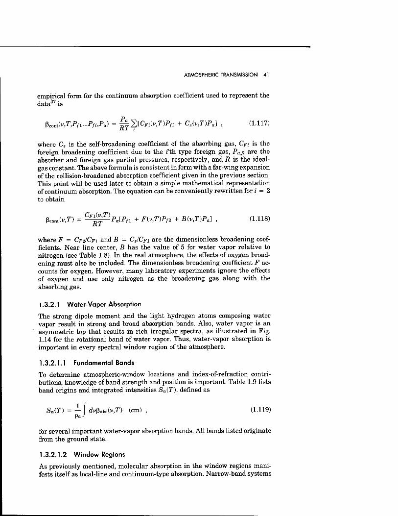
ATMOSPHERIC TRANSMISSION 41
empirical form for the continuum absorption coefficient used to represent the data37 is
ßcont(v,r,PA...P^,Pa) = ^^[CFi{v,T)Pfi + Cs(v,T)Pa] , (1.117)
where Cs is the self-broadening coefficient of the absorbing gas, CFI is the foreign broadening coefficient due to the i'th type foreign gas, Pafi are the absorber and foreign gas partial pressures, respectively, and R is the ideal- gas constant. The above formula is consistent in form with a far-wing expansion of the collision-broadened absorption coefficient given in the previous section. This point will be used later to obtain a simple mathematical representation of continuum absorption. The equation can be conveniently rewritten for i = 2 to obtain
ßcont(v,T) = CF1^T)Pa[Pfl + F(v,T)Pf2 + B{v,T)Pa] , (1.118)
where F = CF2/CFI and B = CSICF\ are the dimensionless broadening coef- ficients. Near line center, B has the value of 5 for water vapor relative to nitrogen (see Table 1.8). In the real atmosphere, the effects of oxygen broad- ening must also be included. The dimensionless broadening coefficient F ac- counts for oxygen. However, many laboratory experiments ignore the effects of oxygen and use only nitrogen as the broadening gas along with the absorbing gas.
1.3.2.1 Water-Vapor Absorption
The strong dipole moment and the light hydrogen atoms composing water vapor result in strong and broad absorption bands. Also, water vapor is an asymmetric top that results in rich irregular spectra, as illustrated in Fig. 1.14 for the rotational band of water vapor. Thus, water-vapor absorption is important in every spectral window region of the atmosphere.
1.3.2.1.1 Fundamental Bands
To determine atmospheric-window locations and index-of-refraction contri- butions, knowledge of band strength and position is important. Table 1.9 lists band origins and integrated intensities Sn(T), defined as
Sn(T) = — f dvßabs(v,T) (cm) , (1.119)
for several important water-vapor absorption bands. All bands listed originate from the ground state.
1.3.2.1.2 Window Regions
As previously mentioned, molecular absorption in the window regions mani- fests itself as local-line and continuum-type absorption. Narrow-band systems
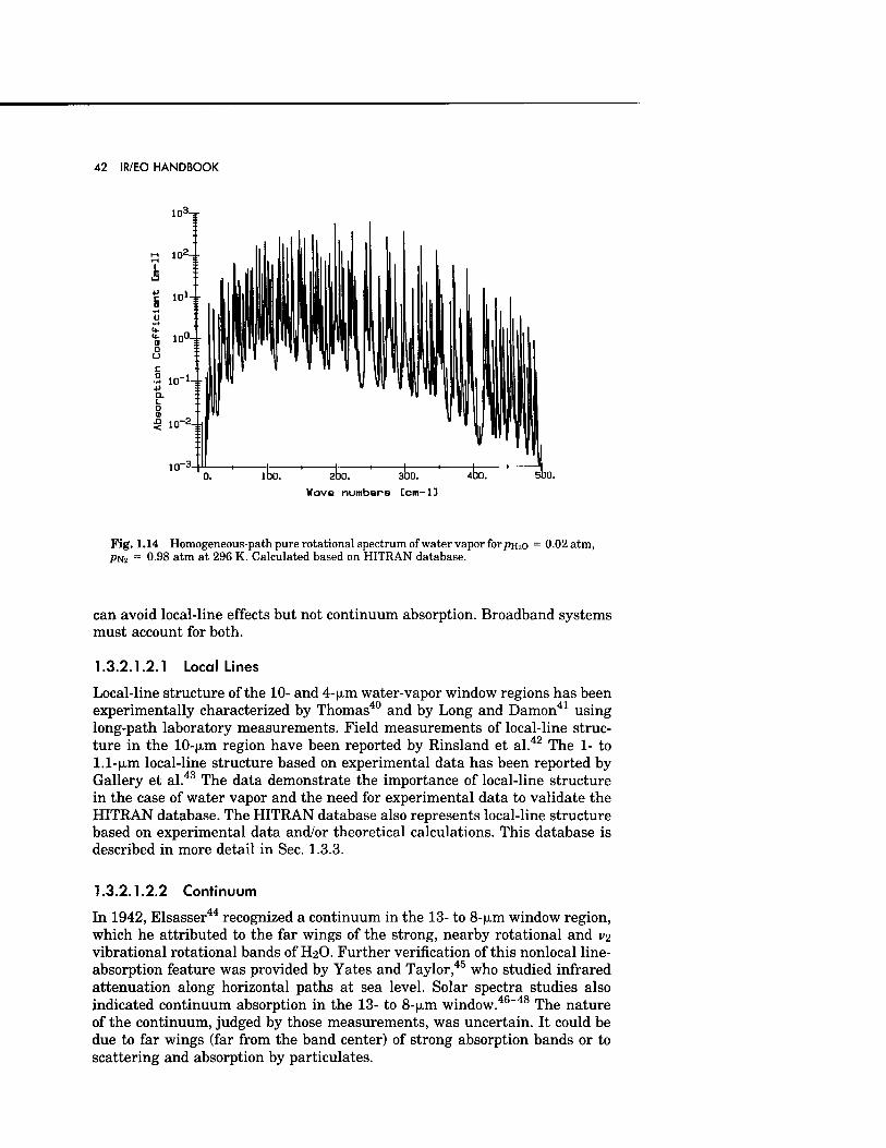
42 IR/EO HANDBOOK
■p Q- L O U
100. 2DCÜ 300.
Wavo numboro Ccm-13
Fig. 1.14 Homogeneous-path pure rotational spectrum of water vapor forpH20 = 0.02 atm, PN2 = 0.98 atm at 296 K. Calculated based on HITRAN database.
can avoid local-line effects but not continuum absorption. Broadband systems must account for both.
1.3.2.1.2.1 Local Lines
Local-line structure of the 10- and 4-|o.m water-vapor window regions has been experimentally characterized by Thomas40 and by Long and Damon41 using long-path laboratory measurements. Field measurements of local-line struc- ture in the 10-jj.m region have been reported by Rinsland et al.42 The 1- to 1.1-jjim local-line structure based on experimental data has been reported by Gallery et al.43 The data demonstrate the importance of local-line structure in the case of water vapor and the need for experimental data to validate the HITRAN database. The HITRAN database also represents local-line structure based on experimental data and/or theoretical calculations. This database is described in more detail in Sec. 1.3.3.
1.3.2.1.2.2 Continuum
In 1942, Elsasser44 recognized a continuum in the 13- to 8-|xm window region, which he attributed to the far wings of the strong, nearby rotational and V2 vibrational rotational bands of H2O. Further verification of this nonlocal line- absorption feature was provided by Yates and Taylor,45 who studied infrared attenuation along horizontal paths at sea level. Solar spectra studies also indicated continuum absorption in the 13- to 8-^m window.46-48 The nature of the continuum, judged by those measurements, was uncertain. It could be due to far wings (far from the band center) of strong absorption bands or to scattering and absorption by particulates.
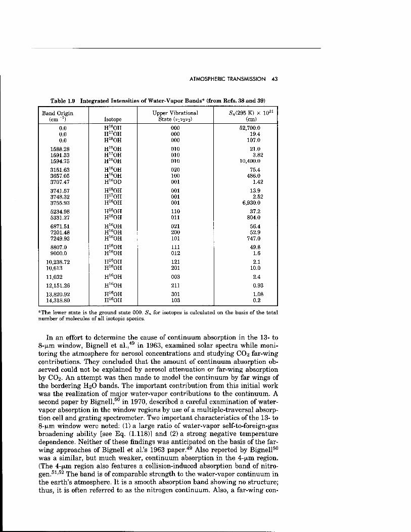
ATMOSPHERIC TRANSMISSION 43
Table 1.9 Integrated Intensities of Water-Vapor Bands* (from Refs. 38 and 39)
Band Origin (cm-1) Isotope
Upper Vibrational State (V1V2V3)
S„(295 K) x 1021
(cm)
0.0 0.0 0.0
H16OH H17OH H18OH
000 000 000
52,700.0 19.4
107.0
1588.28 1591.33 1594.75
H18OH H17OH H16OH
010 010 010
21.0 3.82
10,400.0
3151.63 3657.05 3707.47
H16OH H16OH H16OD
020 100 001
75.4 486.0
1.42
3741.57 3748.32 3755.93
H18OH H17OH H16OH
001 001 001
13.9 2.52
6,930.0
5234.98 5331.27
H16OH H16OH
110 011
37.2 804.0
6871.51 7201.48 7249.93
H16OH H16OH H16OH
021 200 101
56.4 52.9
747.0
8807.0 9000.0
H16OH H16OH
111 012
49.8 1.6
10,238.72 10,613
H16OH H16OH
121 201
2.1 10.0
11,032 H16OH 003 2.4
12,151.26 H16OH 211 0.93
13,820.92 14,318.80
H16OH H16OH
301 103
1.08 0.2
*The lower state is the ground state 000. S„ for isotopes is calculated on the basis of the total number of molecules of all isotopic species.
In an effort to determine the cause of continuum absorption in the 13- to 8-|xm window, Bignell et al.,49 in 1963, examined solar spectra while moni- toring the atmosphere for aerosol concentrations and studying CO2 far-wing contributions. They concluded that the amount of continuum absorption ob- served could not be explained by aerosol attenuation or far-wing absorption by CO2. An attempt was then made to model the continuum by far wings of the bordering H2O bands. The important contribution from this initial work was the realization of major water-vapor contributions to the continuum. A second paper by Bignell,50 in 1970, described a careful examination of water- vapor absorption in the window regions by use of a multiple-traversal absorp- tion cell and grating spectrometer. Two important characteristics of the 13- to 8-|xm window were noted: (1) a large ratio of water-vapor self-to-foreign-gas broadening ability [see Eq. (1.118)] and (2) a strong negative temperature dependence. Neither of these findings was anticipated on the basis of the far- wing approaches of Bignell et al.'s 1963 paper.49 Also reported by Bignell50
was a similar, but much weaker, continuum absorption in the 4-fjim region. (The 4-(xm region also features a collision-induced absorption band of nitro- gen.51'52 The band is of comparable strength to the water-vapor continuum in the earth's atmosphere. It is a smooth absorption band showing no structure; thus, it is often referred to as the nitrogen continuum. Also, a far-wing con-
44 IR/EO HANDBOOK
tinuum of CO2 beyond the V3 bandhead is observed between 4.1 and 4.0 (xm.53
These other continua are discussed later (see Sees. 1.3.2.4 and 1.3.2.2). Since those initial experimental efforts to characterize water-vapor contin-
uum absorption, many measurements have been made. They fall into three categories: (1) measurements within the earth's atmosphere or field measure- ments, (2) laboratory measurements using a long-path cell and a spectrometer, and (3) laboratory measurements using a long-path cell or a photoacoustic cell and a laser. Although continuum absorption was first observed through long- path field measurements, its precise characterization requires control and knowledge of the propagation path. The effects of turbulence, particulate scat- tering, temperature variations, and partial-pressure variations are difficult to determine in a field measurement. Thus, laboratory measurements are needed to characterize the pressure and temperature dependence of each atmospheric constituent. Spectrometer measurements determine the frequency dependence of the window regions, i.e., local lines and continuum absorption. Laser mea- surements are limited to discrete frequencies, but because of the laser's higher power and stability, greater accuracy can be obtained; this is particularly true for photoacoustic techniques. Laboratory transmission measurements require very long path lengths (~ 1 km or longer) and thus are difficult to obtain. The photoacoustic cell, on the other hand, is compact (about 30 cm) but still main- tains considerable sensitivity. Of course, field measurements will have the final say in the validation of atmospheric propagation computer codes.
As a result of these experiments, a good characterization of the commonly used window regions exists today. An excellent review of the field is given in the recent work of Hinderung et al.54 and Grant.55 They emphasize the 8- to 14-p.m window region, which, along with the millimeter-wave window, is the most extensively measured. A review of the current experimental data for all the window regions is given in the next section, followed by a brief review of the theoretical and empirical models used to explain the experimental data.
Millimeter-wave window
Figure 1.1556"60 shows continuum absorption from 10 to 1000 GHz (total ab- sorption minus local lines). The solid line represents an empirical formula given by Gaut and Reifenstein57:
ßcont = (1.08 x 10"6)Pa(^)^(^)/-2 (km"1) , (1.120)
where pa is the water-vapor density (g/m3), PT is the total pressure (kPa), and f is the frequency (GHz). The plotted points indicate experimental data. The formula correctly demonstrates the frequency dependence of the continuum but not the temperature and pressure dependence. More recent work by Liebe61
uses a continuum formula, fitted to experimental data at 138 GHz, of the form 3 r / \75 1
(km-1) ßcont = (4.73 x 10-V(^)P.[JV + 31-6(^r) P«
(1.121)
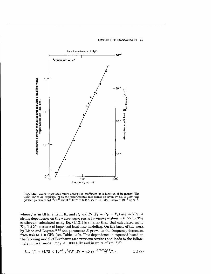
ATMOSPHERIC TRANSMISSION 45
Far-IR continuum of H20
10 100 Frequency (GHz)
1000
Fig. 1.15 Water-vapor-continuum absorption coefficient as a function of frequency. The solid line is an empirical fit to the experimental data points as given by Eq. (1.120). The plotted points are (A),
58 M,59 and t")60 for T = 300 K, PT = 101 kPa, and pa = 10 " 3 kg m ~ 3.
where f is in GHz, T is in K, and Pa and Pf {Pf = PT - Pa) are in kPa. A strong dependence on the water-vapor partial pressure is shown (B » 5). The continuum calculated using Eq. (1.121) is smaller than that calculated using Eq. (1.120) because of improved local-line modeling. On the basis of the work by Liebe and Layton,62,63 the parameter B grows as the frequency decreases from 833 to 110 GHz (see Table 1.10). This dependence is expected based on the far-wing model of Birnbaum (see previous section) and leads to the follow- ing empirical model (for f < 1000 GHz and in units of km-1)64:
ßconttf) = (4.73 x 10⁻⁸)f2Q4Pa(Pf + 40.9e-°0025/e6-5P„) (1.122)
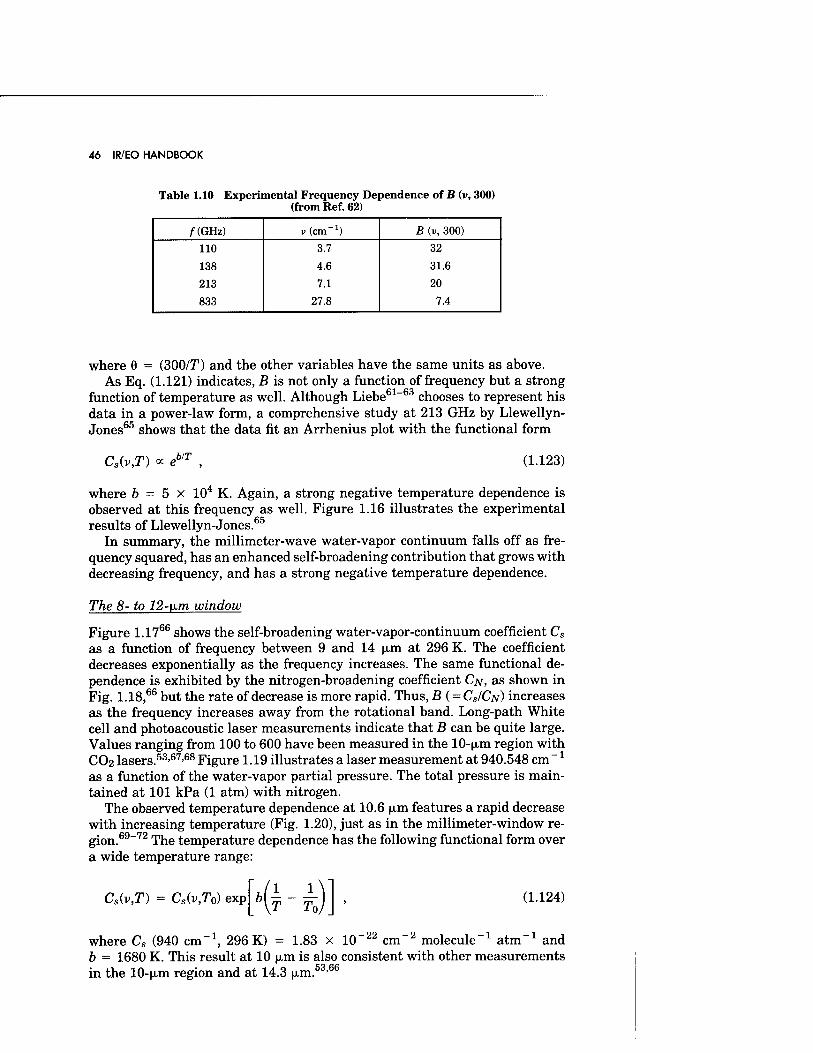
46 IR/EO HANDBOOK
Table 1.10 Experimental Frequency De (from Ref. 62)
pendence of B (v, 300)
/•(GHz) v (cm J) B (v, 300)
110 3.7 32
138 4.6 31.6
213 7.1 20
833 27.8 7.4
where 6 = (300/T) and the other variables have the same units as above. As Eq. (1.121) indicates, B is not only a function of frequency but a strong
function of temperature as well. Although Liebe61-63 chooses to represent his data in a power-law form, a comprehensive study at 213 GHz by Llewellyn- Jones65 shows that the data fit an Arrhenius plot with the functional form
C,{v,T) « e' b/T (1.123)
where b = 5 x 10⁴ K. Again, a strong negative temperature dependence is observed at this frequency as well. Figure 1.16 illustrates the experimental results of Llewellyn-Jones.65
In summary, the millimeter-wave water-vapor continuum falls off as fre- quency squared, has an enhanced self-broadening contribution that grows with decreasing frequency, and has a strong negative temperature dependence.
The 8- to 12-\im window
Figure 1.1766 shows the self-broadening water-vapor-continuum coefficient Cs
as a function of frequency between 9 and 14 \im at 296 K. The coefficient decreases exponentially as the frequency increases. The same functional de- pendence is exhibited by the nitrogen-broadening coefficient CN, as shown in Fig. 1.18,66 but the rate of decrease is more rapid. Thus, B { = CS/CN) increases as the frequency increases away from the rotational band. Long-path White cell and photoacoustic laser measurements indicate that B can be quite large. Values ranging from 100 to 600 have been measured in the 10-|i,m region with CO2 lasers.53,67,68 Figure 1.19 illustrates a laser measurement at 940.548 cm"1
as a function of the water-vapor partial pressure. The total pressure is main- tained at 101 kPa (1 atm) with nitrogen.
The observed temperature dependence at 10.6 (x.m features a rapid decrease with increasing temperature (Fig. 1.20), just as in the millimeter-window re gion a wide temperature range:
69 72 rpkg temperature dependence has the following functional form over
Cs(v,T) = Cs(v,T0) exp J. To
(1.124)
-22 where Cs (940 cm-1, 296 K) = 1.83 x 10~zz cm_/ molecule l atm-1 and b = 1680 K. This result at 10 (xm is also consistent with other measurements in the 10-|xm region and at 14.3 jjim.53'66
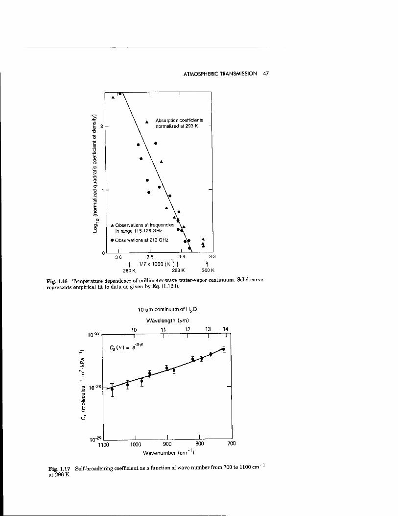
ATMOSPHERIC TRANSMISSION 47
c 2 •D
O c CD
O
3= <D O o ü
Absorption coefficients normalized at 293 K
o c
o A Observations at frequencies
in range 115-126 GHz •«
• Observations at 213 GHz A
1 36 3-5 34 3-3
| 1/Tx1000(K1)t f 280 K 293 K 300 K
Fig. 1.16 Temperature dependence of millimeter-wave water-vapor continuum. Solid curve represents empirical fit to data as given by Eq. (1.123).
10-M.m continuum of H20
Wavelength (fim)
10 11 12 13 14
1100 1000 900 800 -1> Wavenumber (cm" )
700
Fig. 1.17 Self-broadening coefficient as a function of wave number from 700 to 1100 cm at 296 K.
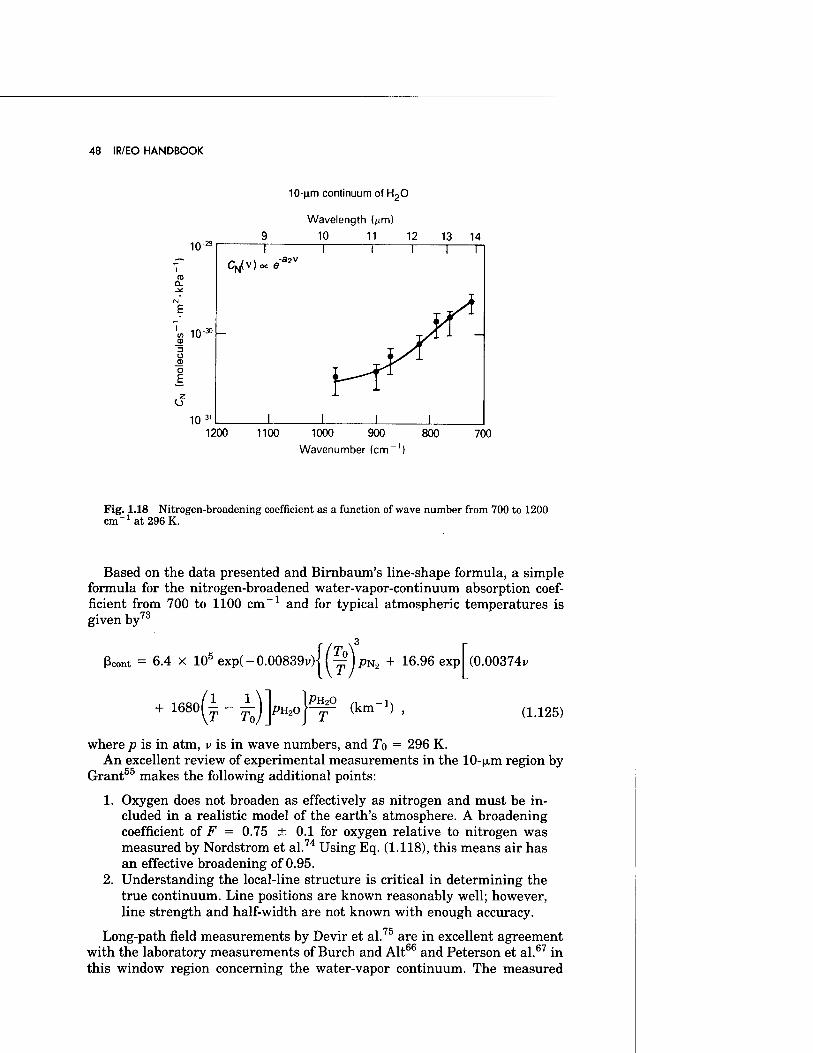
48 IR/EO HANDBOOK
10-um continuum of H20
Wavelength (^m)
10 11 12
700
Wavenumber (cm
Fig. 1.18 Nitrogen-broadening coefficient as a function of wave number from 700 to 1200 cm"1 at 296 K.
Based on the data presented and Birnbaum's line-shape formula, a simple formula for the nitrogen-broadened water-vapor-continuum absorption coef- ficient from 700 to 1100 cm-1 and for typical atmospheric temperatures is given by73
Jcont 6.4 x 10öexp(-0.00839v)^Y)PN2 + 16.96 exp (0.00374v
+ 168011 - i W2O ,, _K m^oY-jr (km 1 (1.125)
where p is in atm, v is in wave numbers, and To = 296 K. An excellent review of experimental measurements in the 10-(i,m region by
Grant55 makes the following additional points:
1. Oxygen does not broaden as effectively as nitrogen and must be in- cluded in a realistic model of the earth's atmosphere. A broadening coefficient of F = 0.75 ± 0.1 for oxygen relative to nitrogen was measured by Nordstrom et al.74 Using Eq. (1.118), this means air has an effective broadening of 0.95.
2. Understanding the local-line structure is critical in determining the true continuum. Line positions are known reasonably well; however, line strength and half-width are not known with enough accuracy.
Long-path field measurements by Devir et al.75 are in excellent agreement with the laboratory measurements of Burch and Alt66 and Peterson et al.67 in this window region concerning the water-vapor continuum. The measured
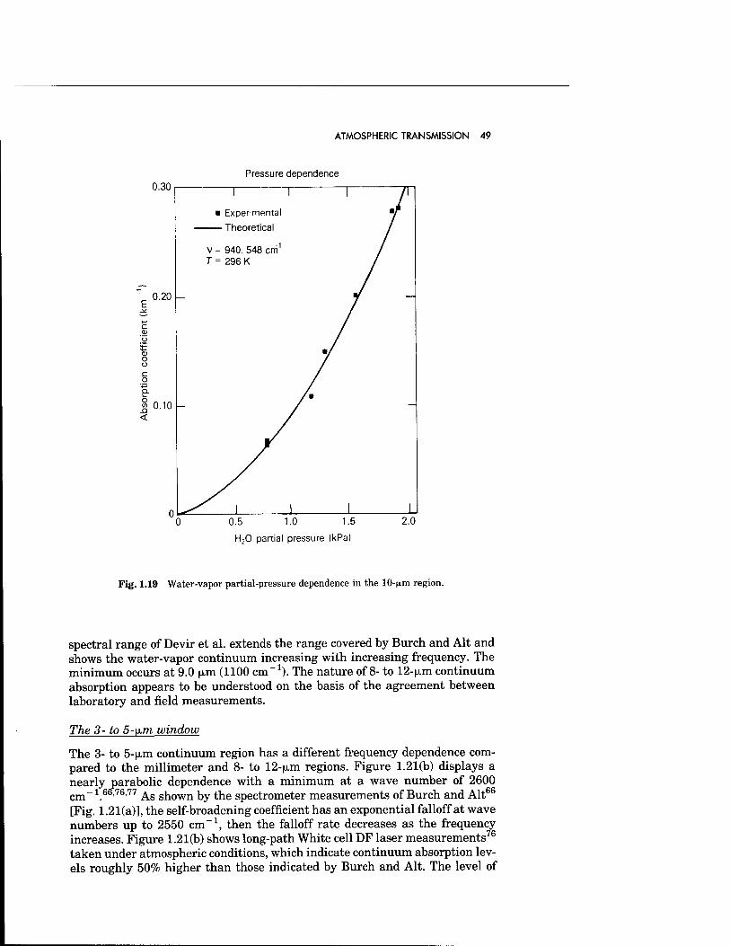
ATMOSPHERIC TRANSMISSION 49
Pressure dependence 0.30
0.5 1.0 1.5
H20 partial pressure (kPa)
Fig. 1.19 Water-vapor partial-pressure dependence in the lO-p-m region.
spectral range of Devir et al. extends the range covered by Burch and Alt and shows the water-vapor continuum increasing with increasing frequency. The minimum occurs at 9.0 |xm (1100 cm-1). The nature of 8- to 12-(jim continuum absorption appears to be understood on the basis of the agreement between laboratory and field measurements.
The 3- to 5-ixm window
The 3- to 5-n.m continuum region has a different frequency dependence com- pared to the millimeter and 8- to 12-|xm regions. Figure 1.21(b) displays a nearly parabolic dependence with a minimum at a wave number of 2600 cm-1.66'76'77 As shown by the spectrometer measurements of Burch and Alt66
[Fig. 1.21(a)], the self-broadening coefficient has an exponential falloff at wave numbers up to 2550 cm-1, then the falloff rate decreases as the frequency increases. Figure 1.21(b) shows long-path White cell DF laser measurements76
taken under atmospheric conditions, which indicate continuum absorption lev- els roughly 50% higher than those indicated by Burch and Alt. The level of
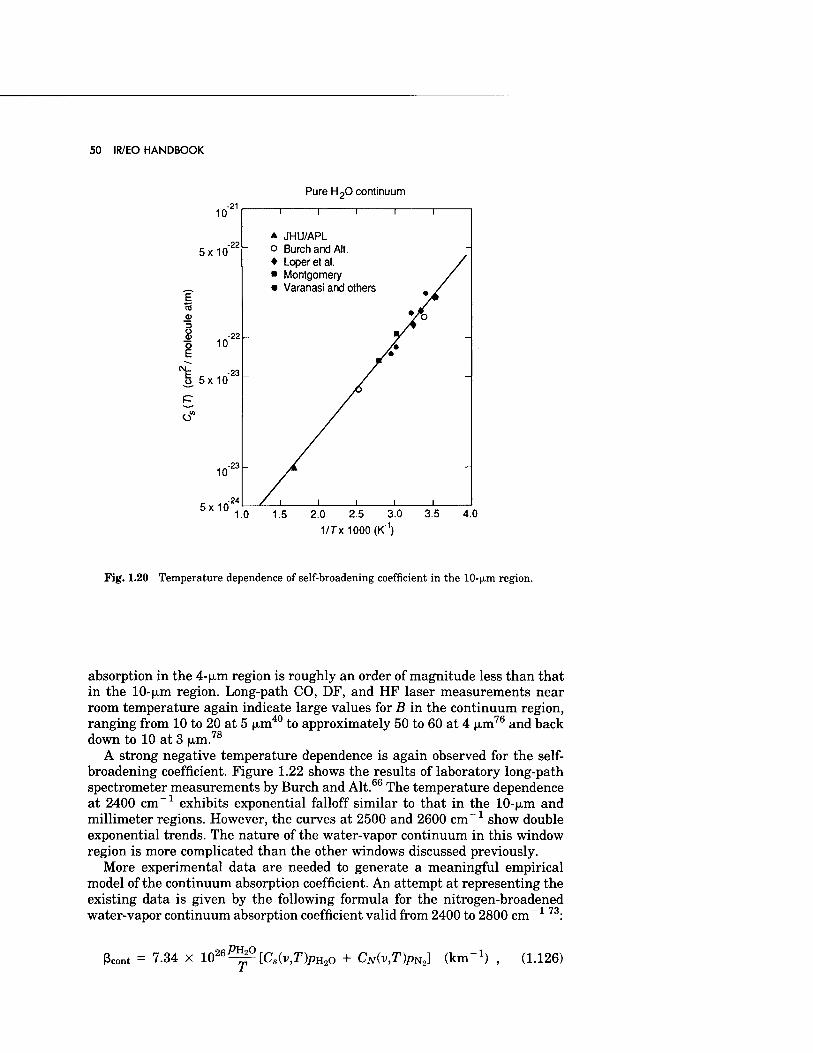
50 IR/EO HANDBOOK
10 -21
5x10 -22
E T3
o E
10 •22
o. 5x 10 -23
10 23
5x10 24
1.0
Pure H20 continuum
A JHU/APL o BurchandAlt. ♦ Loperetal. ■ Montgomery • Varanasi and others
1.5 2.0 2.5 3.0 3.5 4.0
1/7x1000(K'1)
Fig. 1.20 Temperature dependence of self-broadening coefficient in the 10-p.m region.
absorption in the 4-(j,m region is roughly an order of magnitude less than that in the 10-u.m region. Long-path CO, DF, and HF laser measurements near room temperature again indicate large values for B in the continuum region, ranging from 10 to 20 at 5 |xm40 to approximately 50 to 60 at 4 (xm76 and back down to 10 at 3 |xm.78
A strong negative temperature dependence is again observed for the self- broadening coefficient. Figure 1.22 shows the results of laboratory long-path spectrometer measurements by Burch and Alt.66 The temperature dependence at 2400 cm-1 exhibits exponential falloff similar to that in the 10-|xm and millimeter regions. However, the curves at 2500 and 2600 cm-1 show double exponential trends. The nature of the water-vapor continuum in this window region is more complicated than the other windows discussed previously.
More experimental data are needed to generate a meaningful empirical model of the continuum absorption coefficient. An attempt at representing the existing data is given by the following formula for the nitrogen-broadened water-vapor continuum absorption coefficient valid from 2400 to 2800 cm-1 73:
ßcont = 7.34 x 1026^[CS(V,7>H2O + CN(v,T)pN2] (km"1) (1.126)
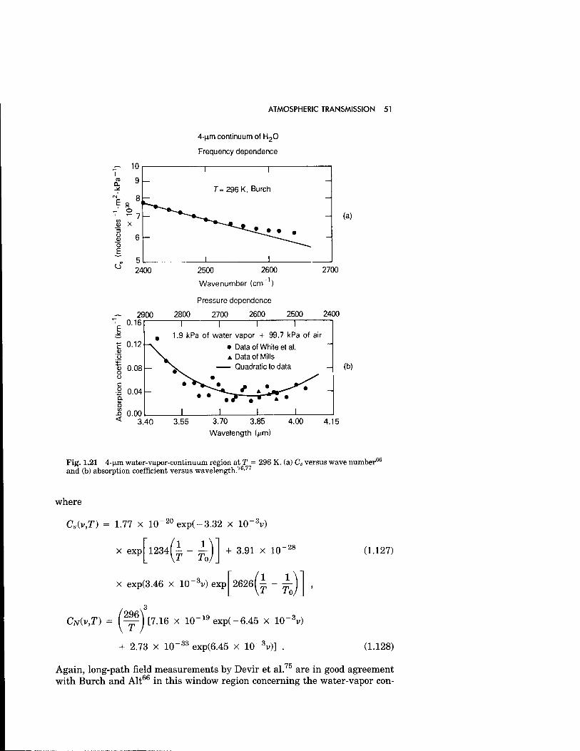
ATMOSPHERIC TRANSMISSION 51
2400
— 2900 ^ 0.16
4-u.m continuum of H20
Frequency dependence
2500
Wavenumber (cm
2600 1.
Pressure dependence
2800 2700 2600 2500
a) 'u
§ 0.08 o
B 0.04 a.
I 0.00
- 0)
2700
2400 —\ 1 1 1
1.9 kPa of water vapor + 99.7 kPa of air
• Data of White et al. A Data of Mills Quadratic to data
• •
(b)
3.40 3.55 3.70 3.85
Wavelength |/im)
4.00 4.15
Fig. 1.21 4-|xm water-vapor-continuum region at T = 296 K. (a) Cs versus wave number6
and (b) absorption coefficient versus wavelength.76,77
where
C,(v,T) = 1.77 x 10⁻²⁰exp(-3.32 x 10_3v)
x exp 123<-£ + 3.91 x 10 -28
x exp(3.46 x 10~av) exp
3
26261 i-A
CN(v,T) = | ^p) [7.16 x KT19exp(-6.45 x 10"3v)
-3,. + 2.73 x 10-dd exp(6.45 x 10~dv)] .
(1.127)
(1.128)
Again, long-path field measurements by Devir et al.75 are in good agreement with Burch and Alt66 in this window region concerning the water-vapor con-
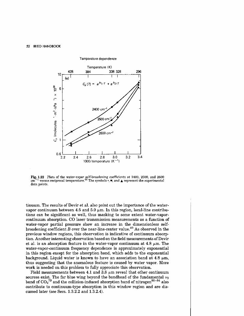
52 IR/EO HANDBOOK
10
o 6
o" 1
428
Temperature dependence
Temperature (K) 384 338 328 296
0.6
.(a)' I I I I
- CS(T) <* e"i"" +eb2""
Z^-
- 2400 cm-\S // -
- S^ISMI crnV/ -
^^X^2600 cm-1
I I I I
-
2.2 2.4 2.6 2.8 3.0 3.2 1000/temperature (K_1)
3.4
Fig. 1.22 Plots of the water-vapor self-broadening coefficients at 2400, 2500, and 2600 cm-1 versus reciprocal temperature.66 The symbols •, ■, and A represent the experimental data points.
tinuum. The results of Devir et al. also point out the importance of the water- vapor continuum between 4.5 and 5.0 jjim. In this region, local-line contribu- tions can be significant as well, thus masking to some extent water-vapor- continuum absorption. CO laser transmission measurements as a function of water-vapor partial pressure show an increase in the dimensionless self- broadening coefficient B over the near-line-center value.40 As observed in the previous window regions, this observation is indicative of continuum absorp- tion. Another interesting observation based on the field measurements of Devir et al. is an absorption feature in the water-vapor continuum at 4.8 |xm. The water-vapor-continuum frequency dependence is approximately exponential in this region except for the absorption band, which adds to the exponential background. Liquid water is known to have an association band at 4.8 (xm, thus suggesting that the anomalous feature is caused by water vapor. More work is needed on this problem to fully appreciate this observation.
Field measurements between 4.1 and 3.8 u.m reveal that other continuum sources exist. The far blue wing beyond the bandhead of the fundamental V3 band of CO279 and the collision-induced absorption band of nitrogen80-84 also contribute to continuum-type absorption in this window region and are dis- cussed later (see Sees. 1.3.2.2 and 1.3.2.4).
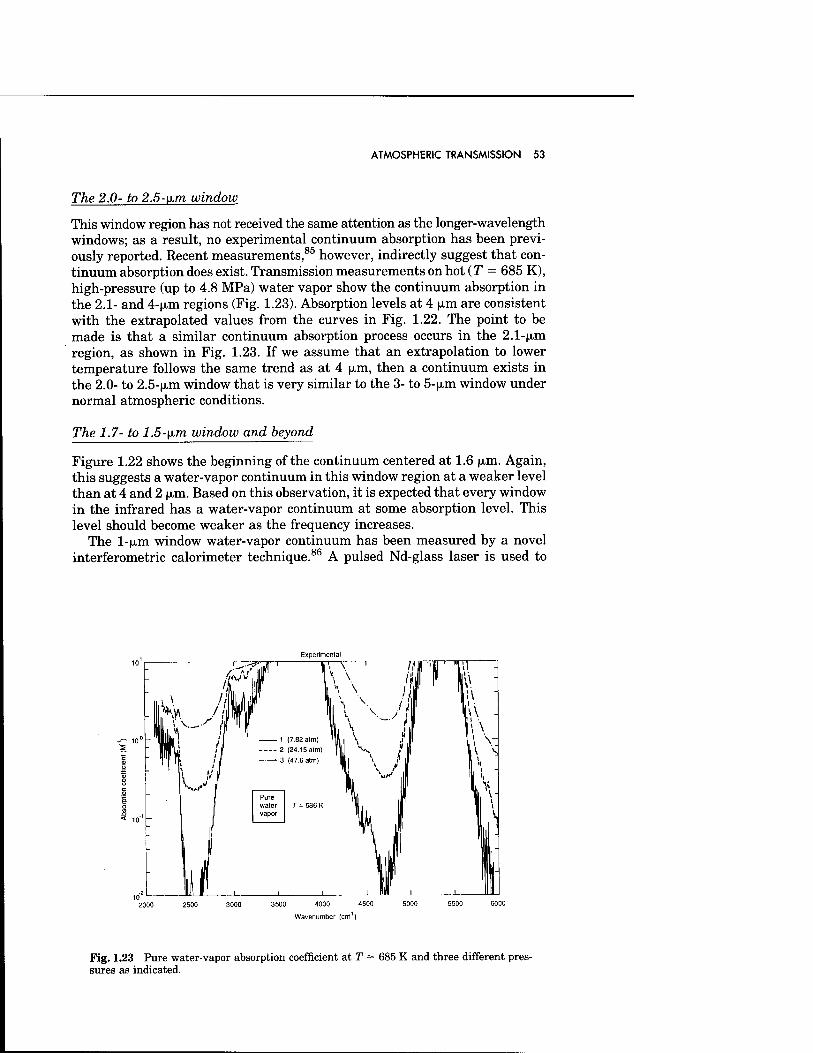
ATMOSPHERIC TRANSMISSION 53
The 2.0- to 2.5-\x.m window
This window region has not received the same attention as the longer-wavelength windows; as a result, no experimental continuum absorption has been previ- ously reported. Recent measurements,85 however, indirectly suggest that con- tinuum absorption does exist. Transmission measurements on hot (T = 685 K), high-pressure (up to 4.8 MPa) water vapor show the continuum absorption in the 2.1- and 4-jjim regions (Fig. 1.23). Absorption levels at 4 jxm are consistent with the extrapolated values from the curves in Fig. 1.22. The point to be made is that a similar continuum absorption process occurs in the 2.1-|xm region, as shown in Fig. 1.23. If we assume that an extrapolation to lower temperature follows the same trend as at 4 |xm, then a continuum exists in the 2.0- to 2.5-jJim window that is very similar to the 3- to 5-|xm window under normal atmospheric conditions.
The 1.7- to 1.5-|xm window and beyond
Figure 1.22 shows the beginning of the continuum centered at 1.6 |xm. Again, this suggests a water-vapor continuum in this window region at a weaker level than at 4 and 2 |xm. Based on this observation, it is expected that every window in the infrared has a water-vapor continuum at some absorption level. This level should become weaker as the frequency increases.
The l-|xm window water-vapor continuum has been measured by a novel interferometric calorimeter technique.86 A pulsed Nd-glass laser is used to
< 10"'
3500 4000 4500
Wavenumber (cm1)
Fig. 1.23 Pure water-vapor absorption coefficient at T = 685 K and three different pres- sures as indicated.
54 IR/EO HANDBOOK
heat a nitrogen-buffered water-vapor sample placed in the arm of a He-Ne Mach-Zehnder interferometer. Variations in the index of refraction due to the heating cause measurable fringe shifts proportional to the absorption coeffi- cient. The resulting continuum absorption coefficient measured at 9466 cm ~~1
is 6 x 10~10 cm-1 for a water-vapor partial pressure of 16.5 Torr buffered by nitrogen to a total pressure of 1 atm at 30°C. Thus, the water-vapor continuum is roughly two orders of magnitude weaker near 1 jim than at 4 or 2 |xm. Further measurements to determine the water-vapor partial pressure depen- dence and temperature dependence are needed.
The tragedy of experimental water-vapor-continuum characterization is that unlike nitrogen and CO2 experiments, it presently cannot be done at high pressure. High-pressure water-vapor measurements also require high tem- perature and thus a theoretical understanding of the continuum-absorption temperature dependence to extrapolate back to atmospheric temperatures.
Concepts and models
No universal interpretation of continuum absorption by water vapor presently exists. Clearly, far wings must play a role in continuum absorption because of the observed frequency dependence observed in every window, and work is continuing to find a line-shape theory valid in the far wing.19"23'87"90 The major shortcoming of most current line-shape theories is in their failure to predict the observed strong negative temperature dependence characteristic of all the window regions, except for the work of Ma and Tipping in the mil- limeter wave and infrared windows. But this weakness is the very strength of an alternative hypothesis to explain the water-vapor continuum: the water dimer. The formation of water-vapor dimers has a strong negative temperature dependence that closely matches the temperature dependence of the continuum absorption in the 10-fjim region.72'91 However, this near match does not occur in the microwave window or in the 4-^m window. This approach also requires dimer absorption bands to account for the continuum. However, the hypothesis would require a dimer absorption band in every water-vapor window, a con- dition that has not been experimentally found or theoretically shown.54,92
Furthermore, measurements on supersaturated water vapor indicate that di- mer absorption is an order of magnitude too small to account for the water- vapor continuum at 10 |xm.54 In spite of these shortcomings, the dimer hy- pothesis demonstrates the importance of understanding water-vapor/water- vapor interactions to explain the continuum absorption temperature dependence.54
Because of the lack of closed-form line-shape models or fast numerical tech- niques for water-vapor-continuum absorption calculations, it is commonly characterized by empirical models. One such model, developed at Johns Hop- kins University/Applied Physics Laboratory (JHU/APL) and Ohio State Uni- versity, uses a far-wing model with a semiempirical line shape and the Air Force Geophysics Laboratory's absorption-line data.93-95 The model has been applied to the 10- and 4-|xm window regions and reproduces the experimental data quite well as a function of frequency, pressure, and temperature. An example is the curve in Fig. 1.19. The water-vapor-broadened far wing falls off less rapidly than the nitrogen-broadened far wing; thus, the self-broadening
ATMOSPHERIC TRANSMISSION 55
coefficient grows as the line shape extends from line center. This is the trend observed in the data. The line shape is normalized, and the line-center function has been experimentally verified.96 The far wings (> 100 cm-1 from line cen- ter) of a line shape represent a very small percentage of the total area under an absorption line contour. Nonetheless, it is interesting to note that the magnitude of the continuum absorption can be correctly calculated from the far-wing contributions by this model. Contributions to the 10-|xm region are dominated by far wings of the very strong rotational band of water vapor on the long-wavelength side of that window, whereas the 4-|xm continuum ab- sorption arises from the bordering strong vibrational bands of almost equal strength. That difference between sources explains the difference between the frequency dependence of the 10-|xm continuum region and that of the 4-fJim continuum region (see Figs. 1.17, 1.18, and 1.21). Unfortunately, the model is not valid in the millimeter region and does not fully represent the recent progress in line-shape theories as discussed in the background section (1.3.1). The success of this model, therefore, is by no means a statement of the validity of a far-wing interpretation of continuum absorption, but rather a statement of its feasibility.
The continuum models for the popular Air Force Geophysics Laboratory codes FASCODE and LOWTRAN are based on the efforts of Clough et al.,87'88
who used far-wing concepts to represent the water-vapor continuum through- out the entire infrared region. The experimental data previously described are reasonably represented by these codes. The strength of this approach and the previously mentioned approach over the APL model is accounting for the fluc- tuation dissipation theorem in enforcing detailed balance across the entire line shape. This results in a more physically meaningful far wing and a more versatile line shape overall.
On the basis of these far-wing models, the water-vapor continuum is ex- trapolated to higher frequencies beyond 4 |xm in LOWTRAN-7 and FASCODE-2. As the previous section indicates, except for the limited data in the l-|xm region, no direct experimental evidence exists beyond 4 |xm. Thus, the extrapolated continuum values must be applied with great care. Figure 1.24 illustrates this point by comparing the water-vapor-continuum models of LOWTRAN-6 and the APL model from 500 to 5000 cm'1. The figure also shows another contin- uum loss mechanism, molecular Rayleigh scattering, based on the LOWTRAN-7 model. The conditions used in the calculation are for a horizontal path with PH2o = 2.0 kPa, PN2 = 99.0 kPa, and T = 295 K. The APL model has been extended beyond 4 \x.m by using the same empirical far-wing parameters of the vi and V3 vibrational bands for all vibrational bands to higher frequencies. The fundamental vibrational band far-wing parameters do not vary greatly; thus, this is a reasonable approximation. Surprisingly, this extrapolation pre- dicts closely the l-|xm laser measurements of the water-vapor continuum. Fair agreement between the two models exists in the region of the 10-(xm window. Good agreement is obtained in the 4- and 2-(xm windows as well. The water- vapor-continuum model in LOWTRAN-6 and -7 is also extrapolated beyond 5000 cm-1. The LOWTRAN-6 model extrapolation is incorrect and is 100 times too large at 1 |xm. The latest version of LOWTRAN-7 has corrected this error and now agrees reasonably well with the APL model.
Figure 1.24 illustrates another interesting point. Continuum absorption decreases with increasing frequency, and scattering loss increases with in-
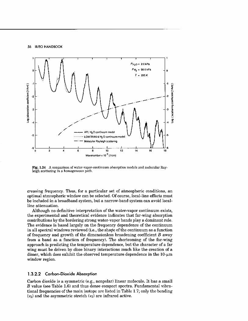
56 IR/EO HANDBOOK
E
E -2
S APLH20 continuum model
LOWTRAN-6 H2 O continuum model
Molecular Raylekjh scattering
I I I
.3 Wavenumberx 10 (1'cm)
Fig. 1.24 A comparison of water-vapor-continuum absorption models and molecular Ray- leigh scattering in a homogeneous path.
creasing frequency. Thus, for a particular set of atmospheric conditions, an optimal atmospheric window can be selected. Of course, local-line effects must be included in a broadband system, but a narrow-band system can avoid local- line attenuation.
Although no definitive interpretation of the water-vapor continuum exists, the experimental and theoretical evidence indicates that far-wing absorption contributions by the bordering strong water-vapor bands play a dominant role. The evidence is based largely on the frequency dependence of the continuum in all spectral windows reviewed (i.e., the shape of the continuum as a function of frequency and growth of the dimensionless broadening coefficient B away from a band as a function of frequency). The shortcoming of the far-wing approach is predicting the temperature dependence, but the character of a far wing must be driven by close binary interactions much like the creation of a dimer, which does exhibit the observed temperature dependence in the 10-|xm window region.
1.3.2.2 Carbon-Dioxide Absorption
Carbon dioxide is a symmetric (e.g., nonpolar) linear molecule. It has a small B value (see Table 1.6) and thus dense compact spectra. Fundamental vibra- tional frequencies of the main isotope are listed in Table 1.7; only the bending (v2) and the asymmetric stretch (V2) are infrared active.
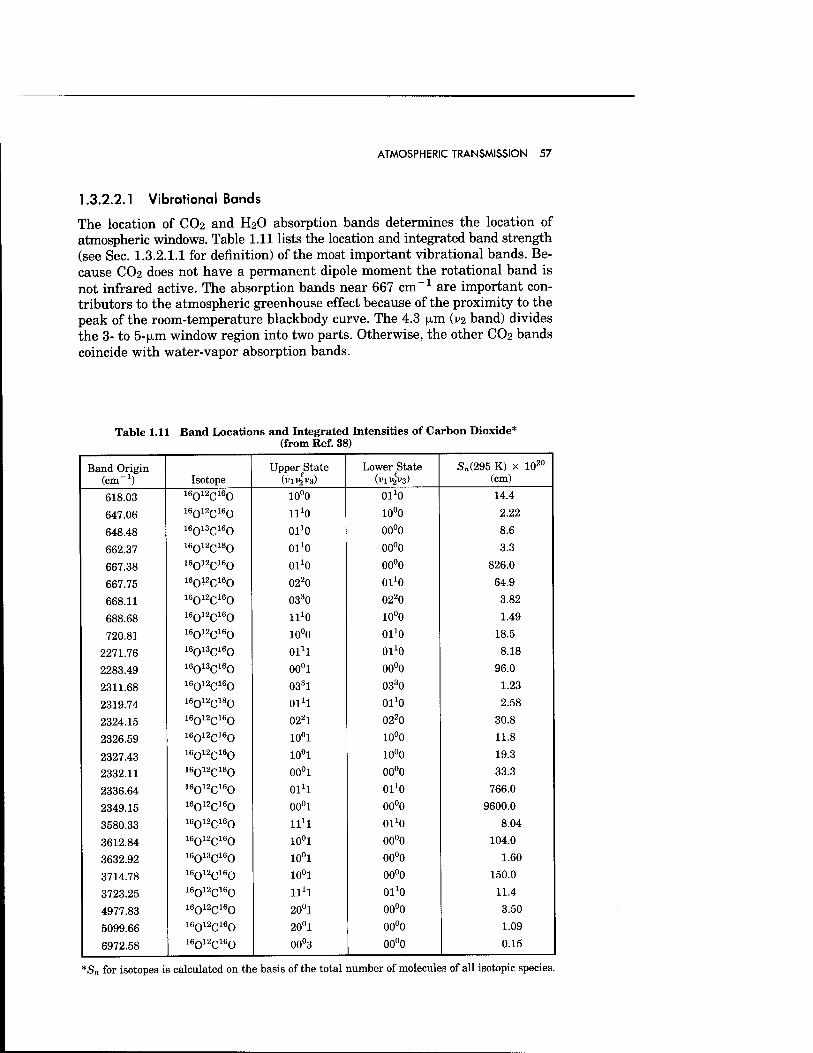
ATMOSPHERIC TRANSMISSION 57
1.3.2.2.1 Vibrational Bands
The location of CO2 and H2O absorption bands determines the location of atmospheric windows. Table 1.11 lists the location and integrated band strength (see Sec. 1.3.2.1.1 for definition) of the most important vibrational bands. Be- cause CO2 does not have a permanent dipole moment the rotational band is not infrared active. The absorption bands near 667 cm-1 are important con- tributors to the atmospheric greenhouse effect because of the proximity to the peak of the room-temperature blackbody curve. The 4.3 (xm (v2 band) divides the 3- to 5-(jim window region into two parts. Otherwise, the other CO2 bands coincide with water-vapor absorption bands.
Table 1.11 Band Locations and Integrated Intensities of Carbon Dioxide* (from Ref. 38)
Band Origin (cm-1) Isotope
Upper State (vn^v3)
Lower State (vii^v3)
S„(295 K) x 1020
(cm)
618.03 16012C160 10°0 Ol'O 14.4
647.06 16Q12C160 11*0 10°0 2.22
648.48 16013C16Q 01*0 00°0 8.6
662.37 16012C18Q 0^0 00°0 3.3
667.38 16Q12C160 01*0 00°0 826.0
667.75 16Q12C160 0220 01*0 64.9
668.11 16Q12C160 0330 0220 3.82
688.68 16012C16Q 11X0 10°0 1.49
720.81 16012C160 10°0 01x0 18.5
2271.76 16Q13C160 Ol1! 01*0 8.18
2283.49 16013C160 00°1 00°0 96.0
2311.68 16012C160 0331 0330 1.23
2319.74 16012C180 014 Ol'O 2.58
2324.15 16012C160 0221 0220 30.8
2326.59 16012C160 10°1 10°0 11.8
2327.43 16012C16Q 10°1 10°0 19.3
2332.11 16012C18Q 00°1 00°0 33.3
2336.64 16012C16Q 01J1 Ol'O 766.0
2349.15 16012C160 00°1 00°0 9600.0
3580.33 16012C160 11*1 01*0 8.04
3612.84 16Q12C160 10°1 00°0 104.0
3632.92 16013C160 10°1 00°0 1.60
3714.78 16012C160 10°1 00°0 150.0
3723.25 16012C160 ll1! 01x0 11.4
4977.83 16Q12C160 20°1 00°0 3.50
5099.66 16012C160 20°1 00°0 1.09
6972.58 16012C160 00°3 00°0 0.15
*Sn for isotopes is calculated on the basis of the total number of molecules of all isotopic species.
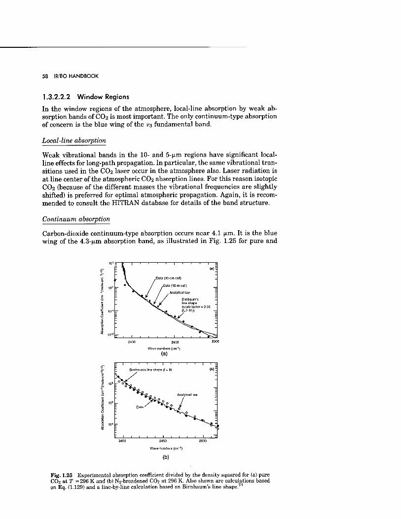
58 IR/EO HANDBOOK
1.3.2.2.2 Window Regions
In the window regions of the atmosphere, local-line absorption by weak ab- sorption bands of CO2 is most important. The only continuum-type absorption of concern is the blue wing of the V3 fundamental band.
Local-line absorption
Weak vibrational bands in the 10- and 5-(xm regions have significant local- line effects for long-path propagation. In particular, the same vibrational tran- sitions used in the CO2 laser occur in the atmosphere also. Laser radiation is at line center of the atmospheric CO2 absorption lines. For this reason isotopic CO2 (because of the different masses the vibrational frequencies are slightly shifted) is preferred for optimal atmospheric propagation. Again, it is recom- mended to consult the HITRAN database for details of the band structure.
Continuum absorption
Carbon-dioxide continuum-type absorption occurs near 4.1 (xm. It is the blue wing of the 4.3-(xm absorption band, as illustrated in Fig. 1.25 for pure and
2450
Wave numbers (cm'1)
(a)
Bimbaum's line shape (f = 8) (b):
106 _° 0^
- Analytical law -
T^£n / ~ 10* / J
^VN^O __ -
104
r I 1 1 1
~:
2450 2500
Wave numbers (cm-1)
(b)
Fig. 1.25 Experimental absorption coefficient divided by the density squared for (a) pure CO2 at T = 296 K and (b) N2-broadened CO2 at 296 K. Also shown are calculations based on Eq. (1.129) and a line-by-line calculation based on Bimbaum's line shape.73
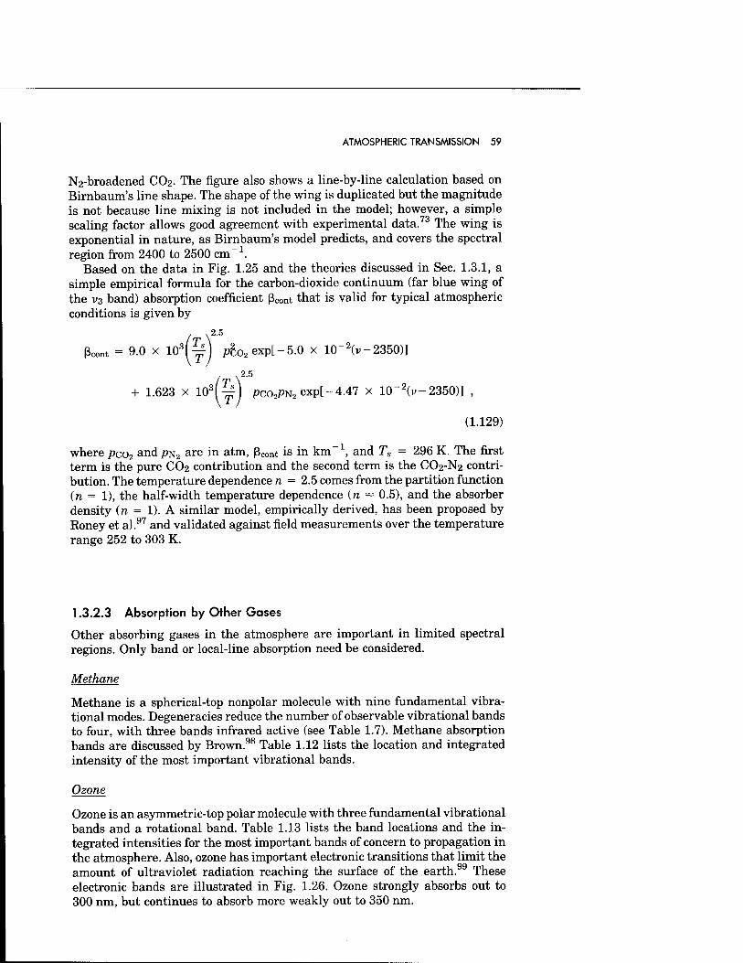
ATMOSPHERIC TRANSMISSION 59
N2-broadened CO2. The figure also shows a line-by-line calculation based on Birnbaum's line shape. The shape of the wing is duplicated but the magnitude is not because line mixing is not included in the model; however, a simple scaling factor allows good agreement with experimental data.73 The wing is exponential in nature, as Birnbaum's model predicts, and covers the spectral region from 2400 to 2500 cm"1.
Based on the data in Fig. 1.25 and the theories discussed in Sec. 1.3.1, a simple empirical formula for the carbon-dioxide continuum (far blue wing of the V3 band) absorption coefficient ßCOnt that is valid for typical atmospheric conditions is given by
/ \2'5
ßcont = 9.0 x lO^YJ ^co2exp[-5.0 x 10"2(v-2350)]
+ 1.623 x 10³(Y) pco2PN2exp[-4.47 x 10^2(v-2350)] ,
(1.129)
where pco2 and/?N2 are in atm, ßcont is in km"1, and Ts = 296 K. The first term is the pure CO2 contribution and the second term is the CO2-N2 contri- bution. The temperature dependence n = 2.5 comes from the partition function (n = 1), the half-width temperature dependence (n ~ 0.5), and the absorber density (n = 1). A similar model, empirically derived, has been proposed by Roney et al.97 and validated against field measurements over the temperature range 252 to 303 K.
1.3.2.3 Absorption by Other Gases
Other absorbing gases in the atmosphere are important in limited spectral regions. Only band or local-line absorption need be considered.
Methane
Methane is a spherical-top nonpolar molecule with nine fundamental vibra- tional modes. Degeneracies reduce the number of observable vibrational bands to four, with three bands infrared active (see Table 1.7). Methane absorption bands are discussed by Brown.98 Table 1.12 lists the location and integrated intensity of the most important vibrational bands.
Ozone
Ozone is an asymmetric-top polar molecule with three fundamental vibrational bands and a rotational band. Table 1.13 lists the band locations and the in- tegrated intensities for the most important bands of concern to propagation in the atmosphere. Also, ozone has important electronic transitions that limit the amount of ultraviolet radiation reaching the surface of the earth.99 These electronic bands are illustrated in Fig. 1.26. Ozone strongly absorbs out to 300 nm, but continues to absorb more weakly out to 350 nm.
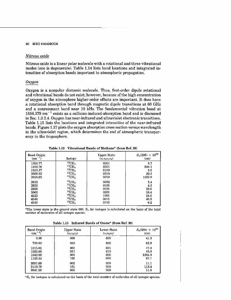
60 IR/EO HANDBOOK
Nitrous oxide
Nitrous oxide is a linear polar molecule with a rotational and three vibrational modes (one is degenerate). Table 1.14 lists band locations and integrated in- tensities of absorption bands important to atmospheric propagation.
Oxygen
Oxygen is a nonpolar diatomic molecule. Thus, first-order dipole rotational and vibrational bands do not exist; however, because of the high concentration of oxygen in the atmosphere higher-order effects are important. It does have a rotational absorption band through magnetic dipole transitions at 60 GHz and a nonresonant band near 10 kHz. The fundamental vibration band at 1556.379 cm-1 exists as a collision-induced-absorption band and is discussed in Sec. 1.3.2.4. Oxygen has near-infrared and ultraviolet electronic transitions. Table 1.15 lists the locations and integrated intensities of the near-infrared bands. Figure 1.27 plots the oxygen absorption cross section versus wavelength in the ultraviolet region, which determines the end of atmospheric transpar- ency in the troposphere.
Table 1.12 Vibrational Bands of Methane* (from Ref. 38)
Band Origin Upper State S„(295) x 1020
(cm-1) Isotope (V1V2V3V4) (cm)
1302.77 13CH4 0001 5.7 1310.76 12CH4 0001 504.1 1533.37 12CH4 0100 5.5 3009.53 13CH4 0010 29.3 3018.92 12CH4 0010 1022.0
2612 12CH4 0002 5.4 2822 13CH4 0101 4.3 2830 12CH4 0101 38.0 3062 12CH4 0201 16.4 4223 12CH4 1001 24.0 4340 12CH4 0011 40.8 4540 12CH4 0110 6.2
*The lower state is the ground state 000. S„ for isotopes is calculated on the basis of the total number of molecules of all isotopic species.
Table 1.13 Infrared Bands of Ozone* (from Ref. 38)
Band Origin (cm"1)
Upper State (V1V2V3)
Lower State (V1V2V3)
S„(295) x 1020
(cm)
0.00 000 000 41.3
700.93 010 000 62.8
1015.81 1025.60 1042.08 1103.14
002 011 001 100
001 010 000 000
17.4 45.0
1394.0 67.1
2057.89 2110.79 3041.20
002 101 003
000 000 000
11.1 113.4
11.0
*Sn for isotopes is calculated on the basis of the total number of molecules of all isotopic species.
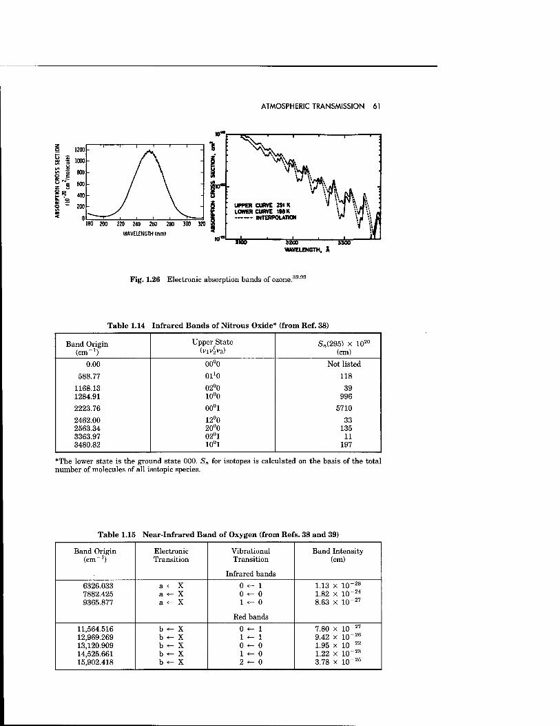
ATMOSPHERIC TRANSMISSION 61
180 200 220 240 260 280 300 320
WAVELENGTH (nm) 10*
UPPER CURVE 291 K LOWER CURVE 1MK INTERPOLATION
TISB" ""525 WAVELENGTH, A
Fig. 1.26 Electronic absorption bands of ozone.3
Table 1.14 Infrared Bands of Nitrous Oxide* (from Ref. 38)
Band Origin (cm-1)
Upper State (viv|v3)
S„(295) x 1020
(cm)
0.00
588.77
1168.13 1284.91
2223.76
2462.00 2563.34 3363.97 3480.82
00°0
Ol'O
02°0 10°0
00°1
12°0 20°0 02°1 10°1
Not listed
118
39 996
5710
33 135
11 197
*The lower state is the ground state 000. Sn for isotopes is calculated on the basis of the total number of molecules of all isotopic species.
Table 1.15 Near-Infrared Band of Oxygen (from Refs. 38 and 39)
Band Origin (cm"1)
Electronic Transition
Vibrational Transition
Infrared bands
Band Intensity (cm)
6326.033 7882.425 9365.877
a ^ X a <- X a ^ X
0 «- 1 0^0 1^0
Red bands
1.13 x 10"28
1.82 x 10⁻²⁴
8.63 x 10 "27
11,564.516 12,969.269 13,120.909 14,525.661 15,902.418
b ^ X b «- X b «- X b <- X b <- X
0 <- 1 1 <- 1 0^0 1 <- 0 2 *- 0
7.80 x 10 "27
9.42 x 10⁻²⁶
1.95 x IQ"22
1.22 x 10" 23
3.78 x 10"2B
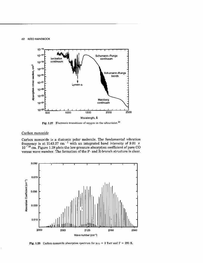
62 IR/EO HANDBOOK
8 o c .& H- o
10-16
io-17
10-18
IO-I9
10-20
IO"21
10-22
10-23
IO"2*
n-25 10-
I I I I I I I i—r
lonization continuum
500
Lyman a
Herzberg continuum
i ■ ■ i
1000 2000 1500
Wavelength, A
Fig. 1.27 Electronic transitions of oxygen in the ultraviolet.39
2500
Carbon monoxide
Carbon monoxide is a diatomic polar molecule. The fundamental vibration frequency is at 2143.27 cm-1 with an integrated band intensity of 9.81 x 10 ~18 cm. Figure 1.28 plots the low-pressure absorption coefficient of pure CO versus wave number. The formation of the P- and R-branch structure is clear.
0.090
2000 2060 2120
Wave number (cm"i)
2180 2240
Fig. 1.28 Carbon-monoxide absorption spectrum for pco = 3 Torr and T = 295 K.
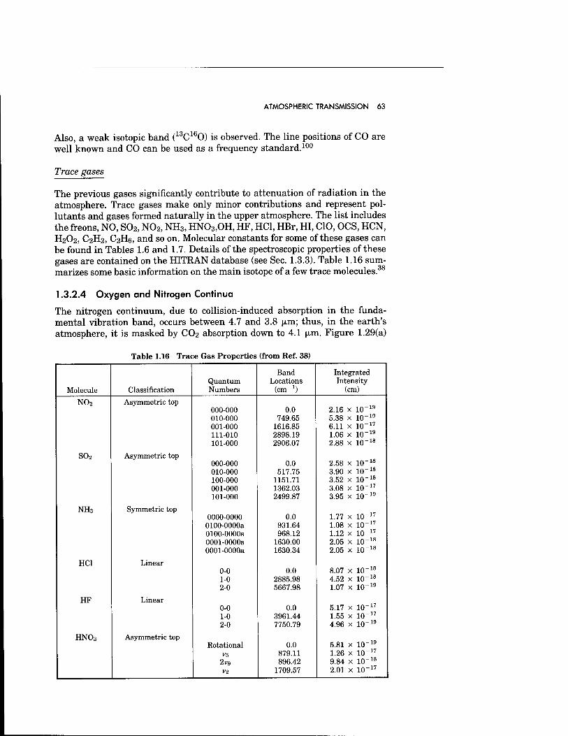
ATMOSPHERIC TRANSMISSION 63
Also, a weak isotopic band (13C160) is observed. The line positions of CO are well known and CO can be used as a frequency standard.100
Trace gases
The previous gases significantly contribute to attenuation of radiation in the atmosphere. Trace gases make only minor contributions and represent pol- lutants and gases formed naturally in the upper atmosphere. The list includes the freons, NO, S02, N02, NH3, HN03,OH, HF, HC1, HBr, HI, CIO, OCS, HCN, H2O2, C2H2, C2H6, and so on. Molecular constants for some of these gases can be found in Tables 1.6 and 1.7. Details of the spectroscopic properties of these gases are contained on the HITRAN database (see Sec. 1.3.3). Table 1.16 sum- marizes some basic information on the main isotope of a few trace molecules.38
1.3.2.4 Oxygen and Nitrogen Continua
The nitrogen continuum, due to collision-induced absorption in the funda- mental vibration band, occurs between 4.7 and 3.8 |xm; thus, in the earth's atmosphere, it is masked by CO2 absorption down to 4.1 |xm. Figure 1.29(a)
Table 1.16 Trace Gas Properties (from Ref. 38)
Molecule Classification Quantum Numbers
Band Locations
(cm^1)
Integrated Intensity
(cm)
N02 Asymmetric top 000-000 0.0 2.16 x 10⁻¹⁹
010-000 749.65 5.38 x 10~19
001-000 1616.85 6.11 x 10⁻¹⁷
111-010 2898.19 1.06 x 10⁻¹⁹
101-000 2906.07 2.88 x 10 ~18
S02 Asymmetric top 000-000 0.0 2.58 x 10⁻¹⁸
010-000 517.75 3.90 x 10~18
100-000 1151.71 3.52 x 10 "18
001-000 1362.03 3.08 x 10_17
101-000 2499.87 3.95 x 10~19
NH3 Symmetric top 0000-0000 0.0 1.77 x 10~17
0100-OOOOa 931.64 1.08 x 10⁻¹⁷
0100-OOOOs 968.12 1.12 x 10~17
0001-OOOOs 1630.00 2.05 x 10"18
0001-OOOOa 1630.34 2.05 x 10_18
HC1 Linear 0-0 0.0 8.07 x 10"18
1-0 2885.98 4.52 x 10 "18
2-0 5667.98 1.07 x 10~19
HF Linear 0-0 0.0 5.17 x 10⁻¹⁷
1-0 3961.44 1.55 x 10⁻¹⁷
2-0 7750.79 4.96 x 10 "19
HNO3 Asymmetric top Rotational 0.0 5.81 x 10⁻¹⁹
V5 879.11 1.26 x 10"17
2v9 896.42 9.84 x 10⁻¹⁸
V2 1709.57 2.01 x 10"17
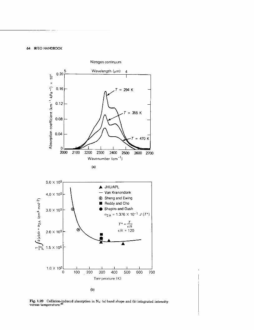
64 IR/EO HANDBOOK
o
x
TO 0-
I
E
c <u
'G
O U c ,g v» Q. 6 <n XI <
Nitrogen continuum
0.20
0.16
5 Wavelength (^m) 4
I
.T = 294 K
0.12 — / \ —
/ \^T = 355 K
0.08 — J j \r \ —
0.04
f y "\\-7" = 470 K
0 J^"l I I l^*fc~_ 2000 2100 2200 2300 2400 2500 2600 2700
Wavenumber (cm-1)
(a)
5.0 X 10⁵
4.0 X 10⁵
3.0 X 105
* 2.0 X105
-l^ 1.5 X 10⁵
1.0 X 10⁵
▲ JHU/APL
— Van Kranendonk
© Sheng and Ewing
■ ReddyandCho
• Shapiro and Gush
a2A = 1-376 X 10~1 J (D
T elk
elk = 120
0 100 200 300 400 500 600 700
Temperature (K)
(b)
Fig. 1.29 Collision-induced absorption in N2: (a) band shape and (b) integrated intensity versus temperature.85
ATMOSPHERIC TRANSMISSION 65
illustrates pure nitrogen spectra at a variety of temperatures based on FTS measurements at JHU/APL.85 In this case, the entire optical path was under vacuum to avoid CO2 contamination. The temperature dependence of the in- tegrated intensity divided by the density squared is shown in Fig. 1.29(b). A minor temperature dependence is observed over the range of atmospheric tem- peratures, and this dependence is modeled by the theory of Van Kranendonk.80
Following the work of Sheng and Ewing,81 we obtain
Pa
where
\jk(v)dv = 1.376 x 10-V(T*) (cm4mor2) , (1.130)
£-'{■ J(T*) = 12-TT jT^exp
T T* = ——
100
^)(*-12-*-°) x2 dx, (1.131)
The solid curve in Fig. 1.29(b) is Eq. (1.130). The coefficient in front of J(T*) is obtained by scaling to the experimental data.
In the earth's atmosphere, the effects of oxygen collisions on nitrogen con- tinuum absorption must also be considered. A dimensionless broadening coef- ficient B of 1.28 was measured by Moskalenko et al.84 relative to oxygen (B is 0.78 when relative to nitrogen). Another gas that may be important to nitrogen continuum models is water vapor. Because of the strong dipole mo- ment of water vapor over the quadrupole moment of nitrogen, collisions be- tween water vapor and nitrogen could be very effective in inducing a dipole moment in nitrogen. Thus, the much smaller concentration of water vapor over nitrogen could be neutralized by a large broadening coefficient. To the best of our knowledge, the value of B relative to water vapor has not been determined. Field measurements suggest this may be important and capable of explaining observed discrepancies between atmospheric measurements and laboratory measurements on pure nitrogen.75 An analysis of the nitrogen con- tinuum is given by Roney et al.97
The collision-induced rotation band of nitrogen also exists and is important for microwave propagation modeling in the atmosphere.
The oxygen collision-induced-absorption vibration band or continuum occurs at 1556 cm-1 and is masked by the V2 vibration band of water vapor in the troposphere. The oxygen continuum is important for long-path attenuation in the upper troposphere and stratosphere. Figure 1.30 illustrates this collision- induced-absorption band as a function of frequency.83
1.3.3 HITRAN Database
High-resolution calculations require a detailed database of spectral-line pa- rameters needed to complete the formulas given in Sec. 1.3.1. With projected computer capabilities of the future, computationally intensive atmospheric transmission codes will become more standard. Thus, the endeavor to create
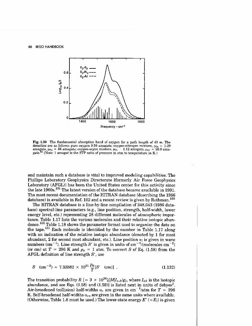
66 IR/EO HANDBOOK
1 1
°2-°2
1 , 1
0.6 02-N2 02-Ar i
1 « \ "
0.4 /» * \ - / i / a ■%*-■. \
/ t v\ \ / A ■» \
0.2 / f / / \\ \
v» \ yy 1 1, , s\\
V> 1 1 1 \\\ 0 ^rö^T l M 1 . \i II 1 Ii 'so>-—
1400 1600
Frequency - cm-1
1800
Fig. 1.30 The fundamental absorption band of oxygen for a path length of 40 m. The densities are as follows: pure oxygen 9.59 amagats; oxygen-nitrogen mixture, po2 = 109
1.12 amagats, pAr = 56.9 ama- amagats, PN2 = 56 amagats; oxygen-argon mixture, po2 gats. (Note: 1 amagat is the STP ratio of pressure in ; pressure in atm to temperature in K.)
and maintain such a database is vital to improved modeling capabilities. The Phillips Laboratory Geophysics Directorate [formerly Air Force Geophysics Laboratory (AFGL)] has been the United States center for this activity since the late 1960s.101 The latest version of the database became available in 1991. The most recent documentation of the HITRAN database (describing the 1986 database) is available in Ref. 102 and a recent review is given by Rothman.103
The HITRAN database is a line-by-line compilation of 348,043 (1986 data- base) spectral-line parameters (e.g., line position, strength, half-width, lower energy level, etc.) representing 28 different molecules of atmospheric impor- tance. Table 1.17 lists the various molecules and their relative isotopic abun- dance.101 Table 1.18 shows the parameter format used to organize the data on the tape.101 Each molecule is identified by the number in Table 1.17 along with an indication of the relative isotopic abundance (denoted by 1 for most abundant, 2 for second most abundant, etc.). Line position v; is given in wave numbers (cm-1). Line strength S' is given in units of cm ^/(molecules cm-2) (or cm) at T = 296 K and pa = 1 atm. To convert S of Eq. (1.58) from the AFGL definition of line strength S', use
S (cm"2) = 7.33882 x 10²¹^[S' (cm)] (1.132)
The transition probability R [= 3 x 10362|M|/a,&/g/, where Iab is the isotopic abundance, and see Eqs. (1.58) and (1.59)] is listed next in units of debyes2. Air-broadened (collision) half-widths ac are given in cm^Vatm for T = 296 K. Self-broadened half-widths aea are given in the same units where available. (Otherwise, Table 1.8 must be used.) The lower-state energy E" (=Ei) is given
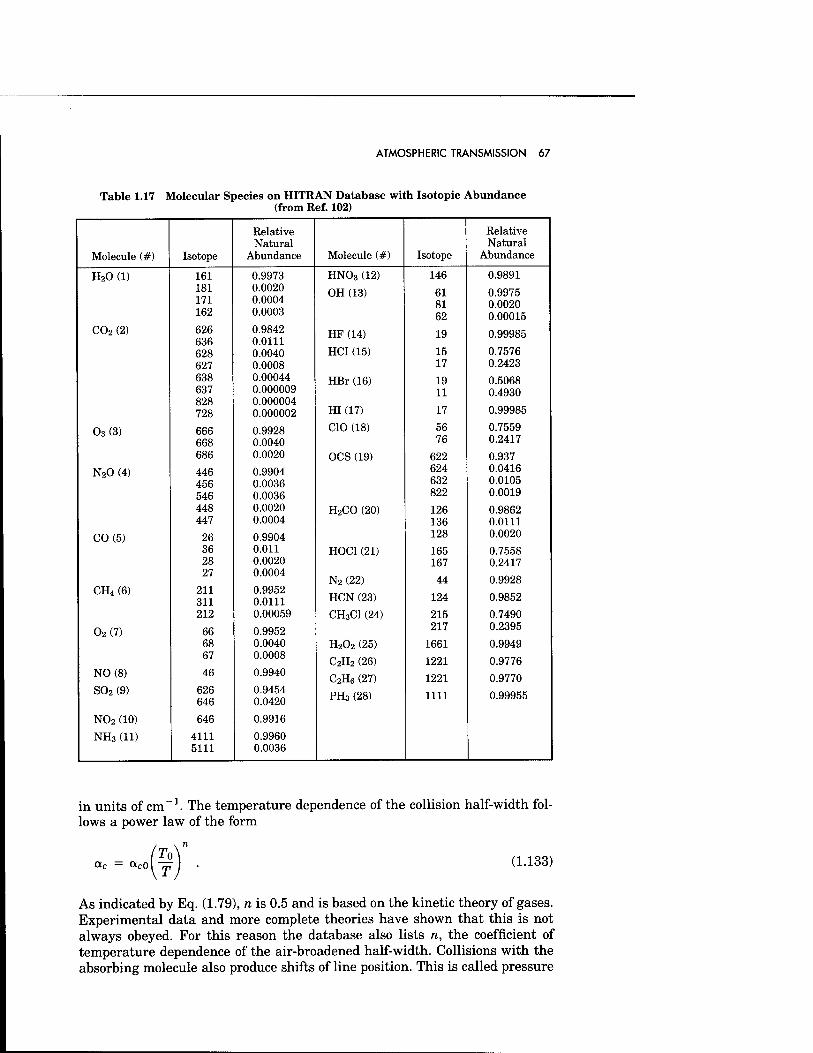
ATMOSPHERIC TRANSMISSION 67
Table 1.17 Molecular Species on HITRAN Database with Isotopic Abundance (from Ref. 102)
Relative Relative Natural Natural
Molecule (#) Isotope Abundance Molecule (#) Isotope Abundance
H20 (1) 161 0.9973 HNO3 (12) 146 0.9891 181 171
0.0020 0.0004
OH (13) 61 81
0.9975 0.0020
162 0.0003 62 0.00015 C02 (2) 626
636 0.9842 0.0111
HF (14) 19 0.99985
628 0.0040 HCI (15) 15 0.7576 627 0.0008 17 0.2423 638 0.00044 HBr (16) 19 0.5068 637 0.000009 11 0.4930 828 0.000004 728 0.000002 HI (17) 17 0.99985
03(3) 666 0.9928 CIO (18) 56 0.7559
668 0.0040 76 0.2417
686 0.0020 OCS (19) 622 0.937
N20 (4) 446 0.9904 624 0.0416
456 0.0036 632 0.0105
546 0.0036 822 0.0019
448 0.0020 H2CO (20) 126 0.9862 447 0.0004 136 0.0111
CO (5) 26 0.9904 128 0.0020
36 0.011 HOC1 (21) 165 0.7558 28 0.0020 167 0.2417 27 0.0004
N2 (22) 44 0.9928 CH4 (6) 211 0.9952
311 0.0111 HCN (23) 124 0.9852
212 0.00059 CH3CI (24) 215 0.7490
02(7) 66 0.9952 217 0.2395
68 0.0040 H2O2 (25) 1661 0.9949 67 0.0008
C2H2 (26) 1221 0.9776 NO (8) 46 0.9940
C2H6 (27) 1221 0.9770 S02 (9) 626
646 0.9454 0.0420 PH3 (28) 1111 0.99955
N02 (10) 646 0.9916
NH3 (11) 4111 5111
0.9960 0.0036
in units of cm 1. The temperature dependence of the collision half-width fol- lows a power law of the form
«cO To (1.133)
As indicated by Eq. (1.79), n is 0.5 and is based on the kinetic theory of gases. Experimental data and more complete theories have shown that this is not always obeyed. For this reason the database also lists n, the coefficient of temperature dependence of the air-broadened half-width. Collisions with the absorbing molecule also produce shifts of line position. This is called pressure
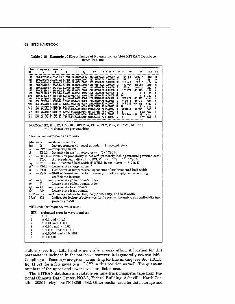
68 IR/EO HANDBOOK
Table 1.18 Example of Direct Image of Parameters on 1986 HITRAN Database (from Ref. 102)
iso Frequency Intensity Mo v S' R 7 7, E" n * or y v' v« 0' 0," IER IREF
31 800.276500 4.316E-25 3.777E-07.0599.0000 1162.00600.76 0.00000 2 12418 6 2517 9 382 0 281 800.287000 2.270E-23 4.717E-05.0750.0000 1483.94700.50 0.00000 2 117 7 18 7 381 0 101 800.301900 4.680E-23 2.421E-07.0630.0000 105.93600.50 0.00000 2 1844-937 -84 0 31 800.304700 1.286E-24 1.131E.05.0618.0000 1636.93510.76 0.00000 2 159 951 58 850 382 0 31 800.322500 1.243E-23 1.274E-06.0610.0000 720.65800.76 0.00000 2 11615 1 1614 2 382 0 101 800.322700 1.840E-22 2.195E-06.0630.0000 277.86000.50 0.00000 2 126 224 -25 125 -84 0 23 800.326900 5.380E-26 2.668E-05.0793.1103 1326.41920.75 0.00000 8 3 R 13 186 0
271 800.332030 1.100E-22 3.212E-02.1000.0000 2354.24000.50 0.00000 19 14 4 8 382 0 101 800.361600 1.910E-22 2.278E-06.0630.0000 277.80700.50 0.00000 2 126 224 +25 125 +84 0 31 800.379600 6.380E-24 6.554E-07.0602.0000 707.21200.76 0.00000 2 11515 1 1514 2 382 0
101 800.416400 5.300E-23 1.025E-05.0630.0000 851.01800.50 0.00000 2 145 244 +44 143 +84 0 271 800.416750 1.330E-22 2.035E-02.1000.0000 2221.36110.50 0.00000 19 14 3 8 382 0 31 800.434100 4.273E-25 2.225E-05.0618.0000 1982.04700.76 0.00000 3 2501040 49 941 382 0 22 800.444000 6.390E-26 1.396E-04.0653.0846 1844.81880.75 0.00000 8 3 R 38 186 0
101 800.447000 5.180E-23 1.002E-05.0630.0000 851.04100.50 0.00000 2 145 244 -44 143 - 84 0 21 800.451200 3.210E-26 1.731E-05.0661.0872 2481.56150.75 0.00000 14 6 P 37 186 0
FORMAT (12, II, F12, 1P2E10.3, 0P2F5.4, F10.4, F4.2, F8.5, 213, 2A9, 311, 312) = 100 characters per transition
This format corresponds as follows:
Mo —12 — Molecule number iso —II —Isotope number (1—most abundant, 2—second, etc.) v —F12.6—Frequency in cm-1
S' —E10.3 —Intensity in cm'Vdnolecules cm"2) @ 296 K R —E10.3 —Transition probability in debyes2 (presently lacking internal partition sum) -y —F5.4 —Air-broadened half-width (HWHM) in cm^Vatm^1 @ 296 K 7s —F5.4 —Self-broadened half-width (HWHM) in cm-'/atm-1 @ 296 K E" —F10.4 —Lower-state energy in cm-1
n —F4.2 —Coefficient of temperature dependence of air-broadened half-width y —F8.5 —Shift of transition due to pressure (presently empty; some coupling
coefficients inserted) v' —13 —Upper-state global quanta index v" —13 — Lower-state global quanta index Q' —A9 —Upper-state local quanta Q" —A9 —Lower-state local quanta IER —311 —Accuracy indices for frequency,* intensity, and half-width IRef—312 —Indices for lookup of references for frequency, intensity, and half-width (not
presently used)
*IER code for frequency when used:
IER estimated error in wave numbers 0 > 1. 1 a 0.1 and < 1.0 2 > 0.01 and < 0.1 3 > 0.001 and < 0.01 4 > 0.0001 and < 0.001 5 a 0.00001 and < 0.0001 6 < 0.00001
shift aCfi [see Eq. (1.81)] and is generally a weak effect. A location for this parameter is included in the database; however, it is generally not available. Coupling coefficients v; are given, accounting for line mixing [see Sec. 1.3.1.5, Eq. (1.82)] for a few gases (e.g., O2)102 in this position as well. The quantum numbers of the upper and lower levels are listed next.
The HITRAN database is available on nine-track magnetic tape from Na- tional Climatic Data Center, NOAA, Federal Building, Asheville, North Car- olina 28801, telephone (704)259-0682. Other media, used for data storage and
ATMOSPHERIC TRANSMISSION 69
retrieval, containing the HITRAN database will most likely be available in the future.
Other databases exist and one is worth mentioning briefly. The GEISA database is maintained by a French group and is very similar to the HITRAN database.104 It includes molecules of importance to other planetary atmo- spheres and therefore may be a useful source for molecules not included on HITRAN.
1.3.4 Band Models
The most practical approach to computing atmospheric broadband absorption (transmittance) is to use an approximate, mathematically workable model of the band structure. This assumes that line positions and strengths are dis- tributed in a way that can be represented by a simple mathematical formula. Band models compute transmittance averaged over a spectral band as de- fined by
T(V) = -H lr(v)dv . (1.134) 2
i r' AvJ v-
The most commonly used band models are listed below:
1. The Elsasser, or regular model,105'106 assumes spectral lines of equal strength, equal spacing, and identical half-widths. The transmission function is averaged over an interval equal to the spacing between the line centers.
2. The statistical, or random model, originally developed for water vapor, assumes that the positions and strengths of the lines are given by a probability function. The statistical model was worked out by Mayer107
and (independently) Goody.108
3. The random-Elsasser model109 is a generalization of the Elsasser and the statistical models. It assumes a random superposition of any num- ber of Elsasser bands of different strengths, spacings, and half-widths.
4. The most accurate, presently available model is the quasi-random model,110 provided the averaging interval can be made sufficiently small. It requires the greatest amount of computation of all the models.
Assuming that the shape of a single spectral line for a homogeneous path in a single absorbing gas is represented by the Lorentz formula, the absorbance is given by
f If S'apa (1 - T)AV = aabsAv = < 1 - exp -Ö
JAv IT •'pathlv — vn) + a dv .
(1.135)
For a homogeneous path, S', a, and pa are constant; Eq. (1.135) then further reduces to
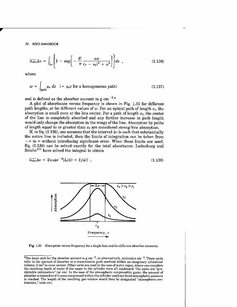
70 IR/EO HANDBOOK
«absAv -/ JAv
exp S' 77 (v
aw
v0)2 + a2. dv (1.136)
where
w •»path
pa dz (= paz for a homogeneous path) (1.137)
and is defined as the absorber amount in g cm-2.3
A plot of absorbance versus frequency is shown in Fig. 1.31 for different path lengths, or for different values of w. For an optical path of length z\, the absorption is small even at the line center. For a path of length 23, the center of the line is completely absorbed and any further increase in path length would only change the absorption in the wings of the line. Absorption by paths of length equal to or greater than z<i are considered strong-line absorption.
If, in Eq. (1.136), one assumes that the interval Av is such that substantially the entire line is included, then the limits of integration can be taken from -00 to <x> without introducing significant error. When these limits are used, Eq. (1.136) can be solved exactly for the total absorbance. Ladenburg and Reiche111 have solved the integral to obtain
Ö^Av = 2TTOLtye-\loW + /l(t|l)] (1.138)
"0
Frequency, v
Fig. 1.31 Absorption versus frequency for a single line and for different absorber amounts.
The basic unit for the absorber amount is g cm-2, or alternatively, molecules cm"2. These units refer to the amount of absorber in a transmission path confined within an imaginary cylindrical volume, 1 cm2 in cross section. Other units are used in the case of water vapor, where one considers the resulting depth of water if the vapor in the cylinder were all condensed. The units are "pre- cipitable centimeters" (pr cm). In the case of the atmospheric compressible gases, the amount of absorber is treated as if it were compressed within the cylinder until sea-level atmospheric pressure is reached. The length of the resulting gas volume would then be designated "atmospheric cen- timeters," (atm cm).
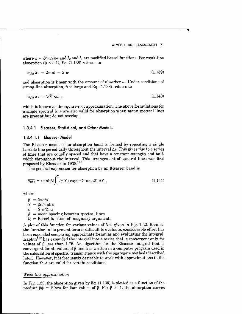
ATMOSPHERIC TRANSMISSION 71
where i|/ = S'w/2Tia and Jo and h are modified Bessel functions. For weak-line absorption (i|; « 1), Eq. (1.138) reduces to
^Av = 2ITCH|I = S'w (1.139)
and absorption is linear with the amount of absorber it;. Under conditions of strong-line absorption, \\i is large and Eq. (1.138) reduces to
«absAv = VS'aw , (1.140)
which is known as the square-root approximation. The above formulations for a single spectral line are also valid for absorption when many spectral lines are present but do not overlap.
1.3.4.1 Elsasser, Statistical, and Other Models
1.3.4.1.1 Elsasser Model
The Elsasser model of an absorption band is formed by repeating a single Lorentz line periodically throughout the interval Av. This gives rise to a series of lines that are equally spaced and that have a constant strength and half- width throughout the interval. This arrangement of spectral lines was first proposed by Elsasser in 1938.106
The general expression for absorption by an Elsasser band is
^ = (sinhß)f I0(Y) exp(-Y coshß) dY , (1.141)
where
ß = 2-na/d Y = ßiji/sinhß i|i = SW2TT(X d = mean spacing between spectral lines 7o = Bessel function of imaginary argument.
A plot of this function for various values of ß is given in Fig. 1.32. Because the function in its present form is difficult to evaluate, considerable effort has been expended comparing approximate formulas and evaluating the integral. Kaplan112 has expanded the integral into a series that is convergent only for values of ß less than 1.76. An algorithm for the Elsasser integral that is convergent for all values of ß and i|> is written in a computer program used in the calculation of spectral transmittance with the aggregate method (described later). However, it is frequently desirable to work with approximations to the function that are valid for certain conditions.
Weak-line approximation
In Fig. 1.33, the absorption given by Eq. (1.135) is plotted as a function of the product ßi|j = S'w/d for four values of ß. For ß 3= 1, the absorption curves
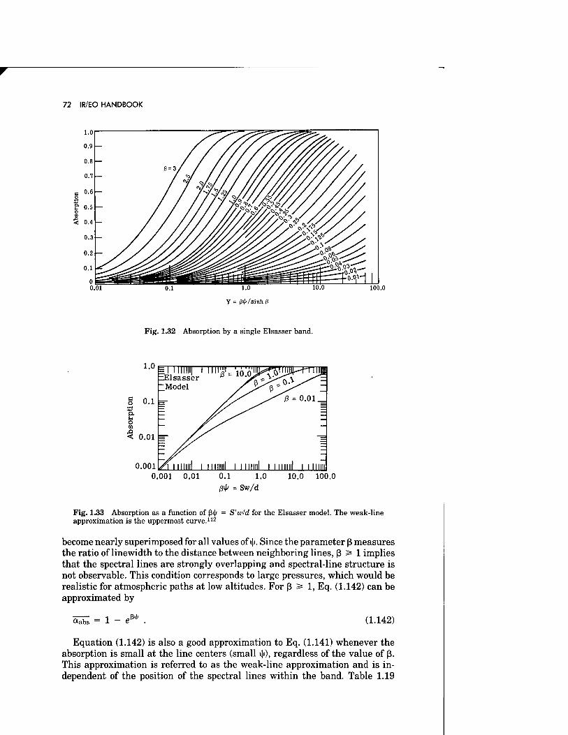
72 IR/EO HANDBOOK
100.0
Fig. 1.32 Absorption by a single Elsasser band.
1.0 I Illllll I II ^Elsasser
Model c o
X) o. u o CO
0.1 =-
0.01 =-
0.001 0.001 0.01 0.1 1.0
ß4> = Sw/d
10.0 100.0
Fig. 1.33 Absorption as a function of ßi|* = S'w/d for the Elsasser model. The weak-line approximation is the uppermost curve.112
become nearly superimposed for all values of i|/. Since the parameter ß measures the ratio of linewidth to the distance between neighboring lines, ß s= 1 implies that the spectral lines are strongly overlapping and spectral-line structure is not observable. This condition corresponds to large pressures, which would be realistic for atmospheric paths at low altitudes. For ß 2s 1, Eq. (1.142) can be approximated by
<*abs = 1 ,ß>l> (1.142)
Equation (1.142) is also a good approximation to Eq. (1.141) whenever the absorption is small at the line centers (small \\i), regardless of the value of ß. This approximation is referred to as the weak-line approximation and is in- dependent of the position of the spectral lines within the band. Table 1.19
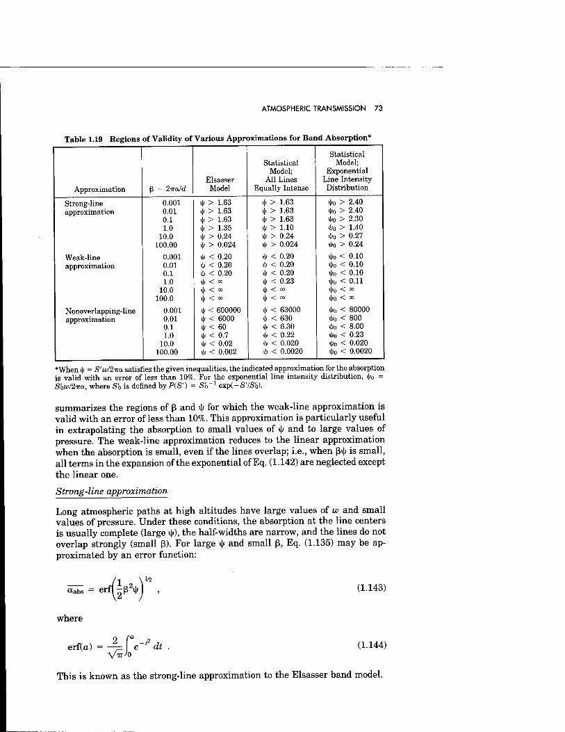
ATMOSPHERIC TRANSMISSION 73
Table 1.19 Regions of Validity of Various Approximations for Band Absorption*
Statistical Statistical Model;
Model; Exponential Elsasser All Lines Line Intensity
Approximation ß = 2ira/d Model Equally Intense Distribution
Strong-line 0.001 i|) > 1.63 4. > 1.63 4.0 > 2.40 approximation 0.01 i|) > 1.63 4< > 1.63 4.0 > 2.40
0.1 4> > 1.63 4. > 1.63 4<o > 2.30 1.0 41 > 1.35 4> > 1.10 4<o > 1.40
10.0 4< > 0.24 41 > 0.24 4.0 > 0.27 100.00 4. > 0.024 4< > 0.024 4<o > 0.24
Weak-line 0.001 4. < 0.20 4/ < 0.20 410 < 0.10 approximation 0.01 <\i < 0.20 4/ < 0.20 4.0 < 0.10
0.1 4< < 0.20 41 < 0.20 4J0 < 0.10 1.0 4l < °o 41 < 0.23 4<o < 0.11
10.0 4< < 00 4/ < 00 4<o < °° 100.0 i\l < 00 4< < 00 4<o < °°
Nonoverlapping-line 0.001 4. < 600000 4. < 63000 4<o < 80000 approximation 0.01 4» < 6000 4. < 630 4>o < 800
0.1 <\i < 60 41 < 6.30 4>o < 8.00 1.0 41 < 0.7 4« < 0.22 4<o < 0.23
10.0 4< < 0.02 <\i < 0.020 4/0 < 0.020 100.00 4> < 0.002 ijj < 0.0020 4.0 < 0.0020
*When 41 = S'wl2Tta satisfies the given inequalities, the indicated approximation for the absorption is valid with an error of less than 10%. For the exponential line intensity distribution, 4>o = S'o">/2Tra, where Sfa is defined by P(S') = Sir1 exp(-SVSb).
summarizes the regions of ß and \\i for which the weak-line approximation is valid with an error of less than 10%. This approximation is particularly useful in extrapolating the absorption to small values of v|> and to large values of pressure. The weak-line approximation reduces to the linear approximation when the absorption is small, even if the lines overlap; i.e., when ßi|i is small, all terms in the expansion of the exponential of Eq. (1.142) are neglected except the linear one.
Strong-line approximation
Long atmospheric paths at high altitudes have large values of w and small values of pressure. Under these conditions, the absorption at the line centers is usually complete (large i|>), the half-widths are narrow, and the lines do not overlap strongly (small ß). For large 4* and small ß, Eq. (1.135) may be ap- proximated by an error function:
otabs = erf(-ß2i|> V2
(1.143)
where
erf(a) 'ur«-'* TTJ0 VTT (1.144)
This is known as the strong-line approximation to the Elsasser band model.
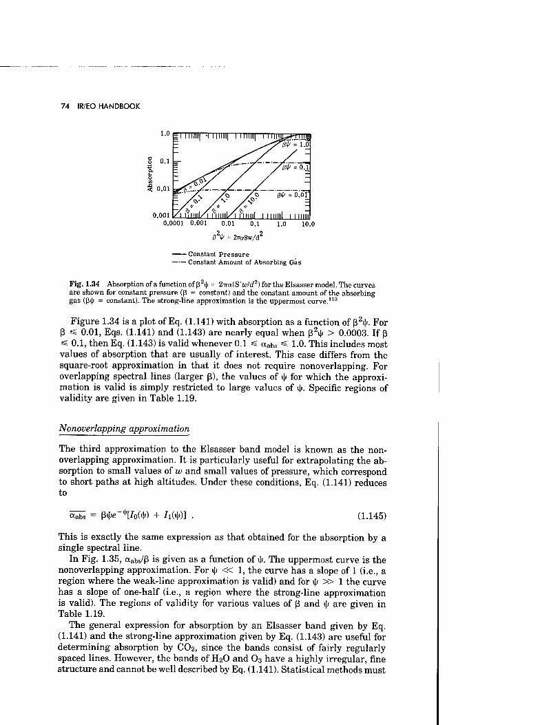
74 IR/EO HANDBOOK
1.0
a
<! 0.01
0.001
IIIHII| • llllllll 1 llllllll l llim^+rmH ^^sA> = 'fa
s- S..--/- "'"/'ßi^Voa
A ffllllll/l llllllll/ A-
\ h mill
0^ = o.o r
l llllllll iii 0.0001 0.001 0.01 0.1 1.0 10.0
ßV = 27roSw/d2
Constant Pressure Constant Amount of Absorbing Gas
Fig. 1.34 Absorption ofa function of ß2i|i = 2-na(S'wld2) for the Elsasser model. The curves are shown for constant pressure (ß = constant) and the constant amount of the absorbing gas (ßi(j = constant). The strong-line approximation is the uppermost curve.113
Figure 1.34 is a plot of Eq. (1.141) with absorption as a function of ß2i[». For ß =£ 0.01, Eqs. (1.141) and (1.143) are nearly equal when ß2vp > 0.0003. If ß =£ 0.1, then Eq. (1.143) is valid whenever 0.1 =£ «abs ^ 1.0. This includes most values of absorption that are usually of interest. This case differs from the square-root approximation in that it does not require nonoverlapping. For overlapping spectral lines (larger ß), the values of \\i for which the approxi- mation is valid is simply restricted to large values of 4». Specific regions of validity are given in Table 1.19.
Nonoverlapping approximation
The third approximation to the Elsasser band model is known as the non- overlapping approximation. It is particularly useful for extrapolating the ab- sorption to small values of w and small values of pressure, which correspond to short paths at high altitudes. Under these conditions, Eq. (1.141) reduces to
«abs = ßllKT^/oW + hm (1.145)
This is exactly the same expression as that obtained for the absorption by a single spectral line.
In Fig. 1.35, aabs/ß is given as a function of ij>. The uppermost curve is the nonoverlapping approximation. For i|; « 1, the curve has a slope of 1 (i.e., a region where the weak-line approximation is valid) and for i|i » 1 the curve has a slope of one-half (i.e., a region where the strong-line approximation is valid). The regions of validity for various values of ß and 4» are given in Table 1.19.
The general expression for absorption by an Elsasser band given by Eq. (1.141) and the strong-line approximation given by Eq. (1.143) are useful for determining absorption by CO2, since the bands consist of fairly regularly spaced lines. However, the bands of H2O and O3 have a highly irregular, fine structure and cannot be well described by Eq. (1.141). Statistical methods must
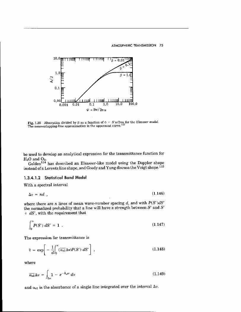
ATMOSPHERIC TRANSMISSION 75
10.0
i.o=-
0.1 =-
0.01
si iiIIIIIJ
~i II mill'
i II HIHI i iiiiiii|
A\ mini IIIIIIIII
'-^ ß = l.OJ
i I mini i niiiii 0.001 0.01 0.1 1.0 10.0 100.0
4> = SW/27TO
Fig. 1.35 Absorption divided by ß as a function of i|< = S'WI2TIOL for the Elsasser model. The nonoverlapping-line approximation is the uppermost curve.113
be used to develop an analytical expression for the transmittance function for H20 and 03.
Golden114 has described an Elsasser-like model using the Doppler shape instead of a Lorentz line shape, and Goody and Yung discuss the Voigt shape.115
1.3.4.1.2 Statistical Band Model
With a spectral interval
Av = nd , d-146)
where there are n lines of mean wave-number spacing d, and with P(S')dS' the normalized probability that a line will have a strength between S' and S' + dS', with the requirement that
Jo P(S') dS' = 1 . (1.147)
The expression for transmittance is
T = exp
where
ctiiAv = h
if dh
(^Av)P(S') dS' (1.148)
1 - e~kjo dv (1.149)
and asi is the absorbance of a single line integrated over the interval Av.
76 IR/EO HANDBOOK
Equal-intensity lines
Equation (1.148) can be evaluated for two special cases. When all the lines have equal intensities, P(S) = 8(S - So), in which b(x) is the Dirac delta function, and Eq. (1.148) reduces to
expi—— = expf-ßilie-'T/oOlO + 7i(i|i)]} .
In terms of absorption,
o^ = 1 - expi-ßilie-^/oW + 7i(»|»)]}
(1.150)
(1.151)
If each of the lines absorbs weakly, so that \\i is small, then Eq. (1.142) reduces to
ö££ = 1 - e-M .
If the lines absorb strongly, then Eq. (1.151) reduces to
(1.152)
otabs = 1 - exp
In terms of ß and \\i,
-»--¥) (1.153)
«abs = 1 - exp -l> W
(1.154)
The nonoverlapping approximation to Eq. (1.151) is obtained from the first term in the expansion of the exponential, so that
«abs = ßilie-VoM») + hm ■ (1.155)
This is the same expression as that obtained for the nonoverlapping approx- imation to the Elsasser model [Eq. (1.145)].
Line strength with an exponential probability distribution
When lines are of different strength and the distribution for the probability of their strength is an exponential distribution, namely,
P(S,) = iHif (1.156)
where S& is a mean line strength, then
exp WS'OOL
d U2 + wS'ooX 1/2
ATMOSPHERIC TRANSMISSION 77
(1.157)
In terms of absorption, and ß and i|/,
-ß«|»o aabs = 1 - exp
(1 + 2i|i0) Ml (1.158)
where tyo = Sow^a. This is the formula developed by Goody108 and is there- fore referred to as the Goody band model.
The weak-line approximation to Eq. (1.158) is obtained when i|/0 « 1. Under these conditions,
dabs = 1 - e -ßvl-0 (1.159)
The strong-line approximation to the statistical model with an exponential distribution of line strengths is obtained when i|i0 » 1. Under these conditions, Eq. (1.158) becomes
CXabs 1 - exp |ß2*o VS
(1.160)
The nonoverlapping approximation is obtained from Eq. (1.158) when the exponent is small and is therefore given by the first two terms of the expansion, or
Ctabs = ß^O
(1 + 2i|;o) M (1.161)
Strong-line, weak-line, and nonoverlapping approximations
These three approximations to the statistical models are discussed concurrently because they are so closely related. For the weak-line approximation, absorp- tion is given by aabs = 1 - exp( - ßi|/), similar to that for the Elsasser model. When an exponential distribution of line strengths is assumed, \\i is replaced by i|>o. This confirms that weak-line absorption is independent of the arrange- ment of the spectral lines within the band. Absorption versus ßvTj is plotted for Eq. (1.151) in Fig. 1.36. The solid curves give the absorption for the statistical model for the case in which all lines are equally strong. The dashed curves give the absorption for the statistical model with an exponential distribution of line strengths. The uppermost solid and dashed curves represent the weak- line approximations for those strength distributions. The regions of validity are given in Table 1.19. When all lines are equally strong, the weak-line approximation is always valid within 10% when i|; < 0.2. It is valid for the exponential strength distribution when i|i < 0.1.
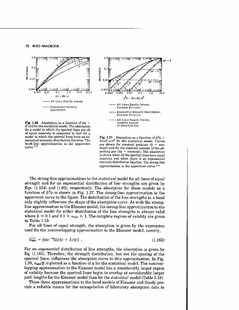
78 IR/EO HANDBOOK
1'°NI I Mil I
0.001 0.001 0.01 0.1 1.0 10.0 100.0
0>P = Sw/d
All Lines Equally Intense
Exponential Intensity Distribution
Fig. 1.36 Absorption as a function of ßi|/ = S'w/d for the statistical model. The absorption for a model in which the spectral lines are all of equal intensity is compared to that for a model in which the spectral lines have an ex- ponential intensity-distribution function. The weak-line approximation is the uppermost curve.113
0.001 0.0001 0.001 0.01 0.1 1.0 10.0
ß2<l> = 2i7aSw/d2
All Lines Equally Intense, Constant Pressure
Exponential Intensity Distribution, Constant Pressure
All Lines Equally Intense, Constant Amount of Absorbing Gas
Fig. 1.37 Absorption as a function of ß2i|i = 2TxaS'wld2 for the statistical model. Curves are shown for constant pressure (ß = con- stant) and for the constant amount of the ab- sorbing gas (ß<Jj = constant). The absorption is shown when all the spectral lines have equal intensity and when there is an exponential intensity-distribution function. The strong-line approximation is the uppermost curve.113
The strong-line approximations to the statistical model for all lines of equal strength and for an exponential distribution of line strengths are given by Eqs. (1.154) and (1.60), respectively. The absorption for these models as a function of ß2v|i is shown in Fig. 1.37. The strong-line approximation is the uppermost curve in the figure. The distribution of the line strengths in a band only slightly influences the shape of the absorption curve. As with the strong- line approximation to the Elsasser model, the strong-line approximation to the statistical model for either distribution of the line strengths is always valid where ß ^ 0.1 and 0.1 ^ aabs ** 1. The complete regions of validity are given in Table 1.19.
For all lines of equal strength, the absorption is given by the expression used for the nonoverlapping approximation to the Elsasser model; namely,
Ctabs = ß«|KT*[/oG|l) + /l(«I>)] (1.162)
For an exponential distribution of line strengths, the absorption is given by Eq. (1.161). Therefore, the strength distribution, but not the spacing of the spectral lines, influences the absorption curve in this approximation. In Fig. 1.38, ctabs/ß is plotted as a function of ij/ for the statistical model. The nonover- lapping approximation to the Elsasser model has a considerably larger region of validity because the spectral lines begin to overlap at considerably larger path lengths for the Elsasser model than for the statistical model (Table 1.19).
These three approximations to the band models of Elsasser and Goody pro- vide a reliable means for the extrapolation of laboratory absorption data to
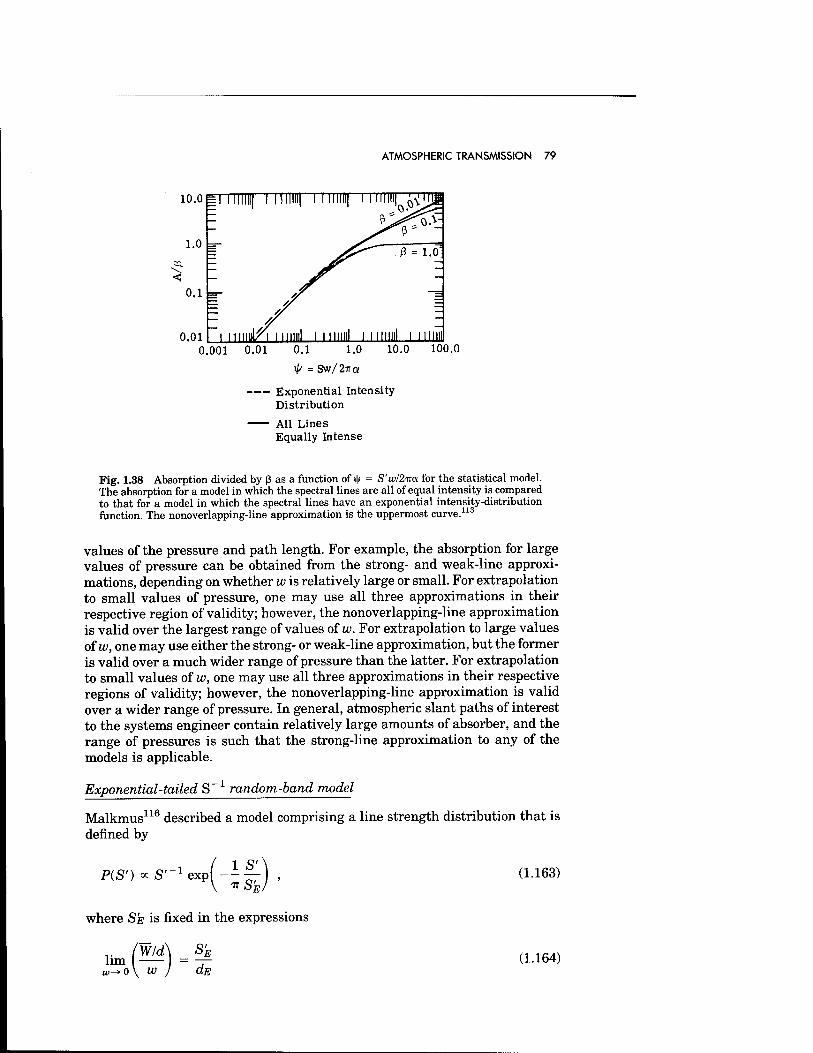
ATMOSPHERIC TRANSMISSION 79
lo.o m
1.0 =r
0.1 =-
0.01
|iiiii!ii[ tmiiui
— y
- y i iniiul^i imnii
1 Mlllfl|
i 1
i iiiimi $m
'— . 0 = 1.0"
i IIIMIII i iini 0.001 0.01 0.1 1.0 10.0 100.0
i> = Sw/27ra
Exponential Intensity Distribution
All Lines Equally Intense
Fig. 1.38 Absorption divided by ß as a function of i|< = S'w/2-na for the statistical model. The absorption for a model in which the spectral lines are all of equal intensity is compared to that for a model in which the spectral lines have an exponential intensity-distribution function. The nonoverlapping-line approximation is the uppermost curve.113
values of the pressure and path length. For example, the absorption for large values of pressure can be obtained from the strong- and weak-line approxi- mations, depending on whether w is relatively large or small. For extrapolation to small values of pressure, one may use all three approximations in their respective region of validity; however, the nonoverlapping-line approximation is valid over the largest range of values of w. For extrapolation to large values of w, one may use either the strong- or weak-line approximation, but the former is valid over a much wider range of pressure than the latter. For extrapolation to small values of w, one may use all three approximations in their respective regions of validity; however, the nonoverlapping-line approximation is valid over a wider range of pressure. In general, atmospheric slant paths of interest to the systems engineer contain relatively large amounts of absorber, and the range of pressures is such that the strong-line approximation to any of the models is applicable.
Exponential-tailed S'1 random-band model
Malkmus116 described a model comprising a line strength distribution that is denned by
P(S') * S'^exp - is; KS'E
(1.163)
where Sk is fixed in the expressions
(W/d\ _ SE lim K w dß
(1.164)
80 IR/EO HANDBOOK
and
.. (W/d\ 2{S'Ea)v> liml^j=^^' (L165) w-* °° \ W
with W/d = -Zn(TAv), an experimentally determined value. The resultant calculated transmittance is given by
TAV = exp 2a dß
i + -M - l (1.166)
= expi -%(1 + 2^E)^ - 1]\ . (1.167)
1.3.4.1.3 Random Elsasser Band Model
For some gases and spectral regions, absorption can be represented more ac- curately by the random Elsasser band model than by either the statistical or Elsasser model alone. This is a natural generalization of the original models that assumes that the absorption can be represented by the random super- position of Elsasser bands. The individual bands may have different line spac- ings, half-widths, and strengths. As the number of superposed Elsasser bands becomes large, the predicted absorption approaches that of the usual statistical model.
The absorption for N randomly superposed Elsasser bands with arbitrary strengths, half-widths, and line spacings is given by
N
ol^ = 1 - f] [1 - aEM$i)] , (1.168) i = 1
where
i|; = S'iw/2-nai ßi = 2'nai/di Si and a; = the line strength and half-width of the i'th Elsasser band di = the line spacing of the i'th band.
The derivation of this general equation for different strengths, half-widths, and line spacings is discussed in detail by Plass.109
1.3.4.1.4 Quasi-Random Model
The quasi-random model is the most accurate and, necessarily, the most com- plicated of the band models. It is especially useful when the absorbance is required over a wide range of path lengths and pressures.
The spectral lines in an actual band are arranged neither as regularly as required by the Elsasser band model nor in as random a fashion as in the
ATMOSPHERIC TRANSMISSION 81
statistical model, but there is some order in their arrangement. In the quasi- random model, the absorptance is calculated first for a frequency interval that is much smaller than the interval size of interest. This localizes the stronger lines to a narrow interval around their actual positions and prevents the introduction of spurious overlapping effects. The absorptance of this narrow interval is calculated from the equation for the single-line absorptance over a finite interval. The absorptance for each of the N spectral lines in the interval is calculated separately and the results combined by assuming a random plac- ing of the spectral lines within the small interval. The absorption from the wings of lines in neighboring intervals is included in the calculation. The results are averaged for at least two different arrangements of the mesh that divides the spectrum into frequency intervals. Finally, the absorbance values for all of the small intervals that fill the larger interval of interest are averaged to obtain the final value for the absorbance. A computer is commonly used to calculate results for this model when many spectral lines are involved. The many weak spectral lines and their relative spacing are accurately taken into account by this model.
The absorbance for the quasi-random model is given by
I n
«abs = - E «abs, , (1.169) nj = 1
where aabs is the absorbance of each of the n smaller wave-number intervals of width D into which the original interval Av is subdivided. The absorptance is calculated from
M
aabs - = 1 - FF [1 - aatoij-fiij)] , (1-170) 1 i = 1
where asi is the single-line absorbance of the i'th line over the/th finite interval D and M is the number of lines in the j'th. frequency interval D.no
References 117 and 118 give absorptance tables for H2O and CO2 based on the quasi-random-model calculations. In these calculations, the lines in the small frequency interval were grouped by line-strength decades. The average strength and number of lines in each of these decades were calculated and used in Eq. (1.170). All lines (from all isotopic species) having strengths greater than 10 ~8 of the strongest line in an absorption region were included in the calculation.
1.3.4.1.5 Temperature and Frequency Dependence of Band-Model Parameters
Table 1.20 is a summary of the band models that yield closed-form expressions for spectral-band absorption. All of these expressions are functions of two parameters, ß and I|J, which in turn are functions of temperature, pressure, absorber concentration, and wave number of wavelength (or frequency).
Since the variation of line strength with temperature is different for each spectral line, it would be impossible to include the effect of temperature on line strength and still retain the band-model expressions in closed form. For
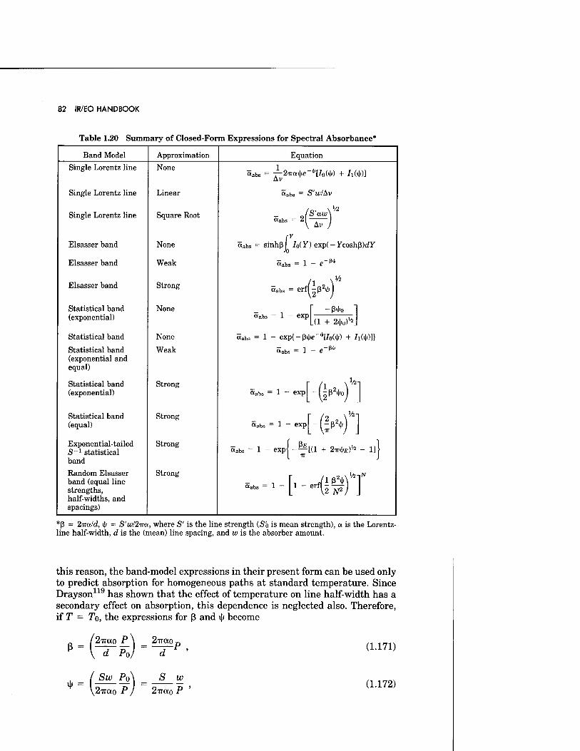
82 IR/EO HANDBOOK
Table 1.20 Summary of Closed-Form Expressions for Spectral Absorbance*
Band Model Approximation Equation
Single Lorentz line None «ab., = —2tratye-*[IoW + hW]
Av
Single Lorentz line Linear <*abs = S'ui/Av
Single Lorentz line Square Root «abs = \^)
Elsasser band None öabs = sinhß 7o(y)exp(-Fcoshß)dY Jo
Elsasser band Weak äBbs = l - e-W
Elsasser band Strong /l \V2
aabs = erfl-ß2t|< 1
Statistical band (exponential)
None dabs = 1 - exp
-ß>l>o
.(1 + 2<\i0)\
Statistical band None aabs = 1 - expi-ßilie-nW) + /i(«|i)]}
Statistical band (exponential and equal)
Weak äabs = 1 - <re*
Statistical band (exponential)
Strong <*abs = 1 - exp -{i»'4\
Statistical band (equal)
Strong «abs = 1 - exp H>T\
Exponential-tailed S^1 statistical band
Strong 5abs = 1 - expj -^[(1 + 2mte)^ - 1]|
Random Elsasser band (equal line strengths, half-widths, and spacings)
Strong
dabs = 1 - [--Gsr: N
*ß = 2-tra/d, i|; = S'wfäira, where S' is the line strength (So is mean strength), a is the Lorentz- line half-width, d is the (mean) line spacing, and w is the absorber amount.
this reason, the band-model expressions in their present form can be used only to predict absorption for homogeneous paths at standard temperature. Since Drayson119 has shown that the effect of temperature on line half-width has a secondary effect on absorption, this dependence is neglected also. Therefore, if T = To, the expressions for ß and vj/ become
ß = 2irao P \ 2irao,
d Po d
«I» = ( Sw ?°\ = s E ~ \ 27ra0 PJ ~ 2<i7ao P
(1.171)
(1.172)
ATMOSPHERIC TRANSMISSION 83
where ao is the half-width at standard conditions, per unit pressure. The expressions listed in Table 1.20 are of the following general form:
1. otabs = aabs(ß,^) when no approximation of the model is assumed. 2. aabs = aabs(ß2i|') for the strong-line approximation. 3. aabs = aabs(ß4<) for the weak-line approximation.
The first expression is a function of two frequency-dependent parameters, 2-n-ao, and two path parameters, w and P. The second expression gives absorp- tion as a function of one frequency-dependent parameter, 2TtaoS'/d2, and two path parameters, w and P. The last is a function of S'/d and w, being inde- pendent of pressure.
The next problem in completely specifying the absorption expressions is that of evaluating the frequency-dependent parameters by empirically fitting the respective equations to laboratory, homogeneous-absorption spectra. The empirical procedure is most involved when no approximations to the model are assumed, since in this case two parameters must be evaluated. After the frequency-dependent parameters have been specified and the values of w and P have been determined for a given slant path, it becomes a simple matter to generate absorption spectra.
There are two practical methods for calculating spectral transmittance, the aggregate and LOWTRAN methods.120 The aggregate method, so-called be- cause it uses a selected collection of the conventional two-parameter models described earlier in this chapter, is perhaps more adaptable to a wide variety of different atmospheric conditions than LOWTRAN, which is strictly empir- ical and depends essentially on a single adjustable parameter. However, for transmittances between roughly 10 and 90%, the values calculated using either method are not greatly different, and the simplicity of using LOWTRAN makes it much more attractive for routine computations. Neither method perfectly reproduces the results of field measurements. Direct line-by-line calculations are required to achieve accuracies consistent with that of the basic data.
1.3.4.1.6 Aggregate Method
Table 1.21 shows which models are used for different spectral regions for the various atmospheric molecules. Details of the aggregate method are contained in Chapter 5 of The Infrared Handbook (see Bibliography).
1.3.4.2 LOWTRAN Method
This method is empirical, yielding a form for the transmittance given by (wave- number resolution = 20 cm-1)
TQO = f[Gv,w,Pn] = f[G(\),w*] , (1.173)
where
Gv = spectral coefficients, independent of temperature and pressure, empirically derived from the HITRAN database with data points every 5 cm""1
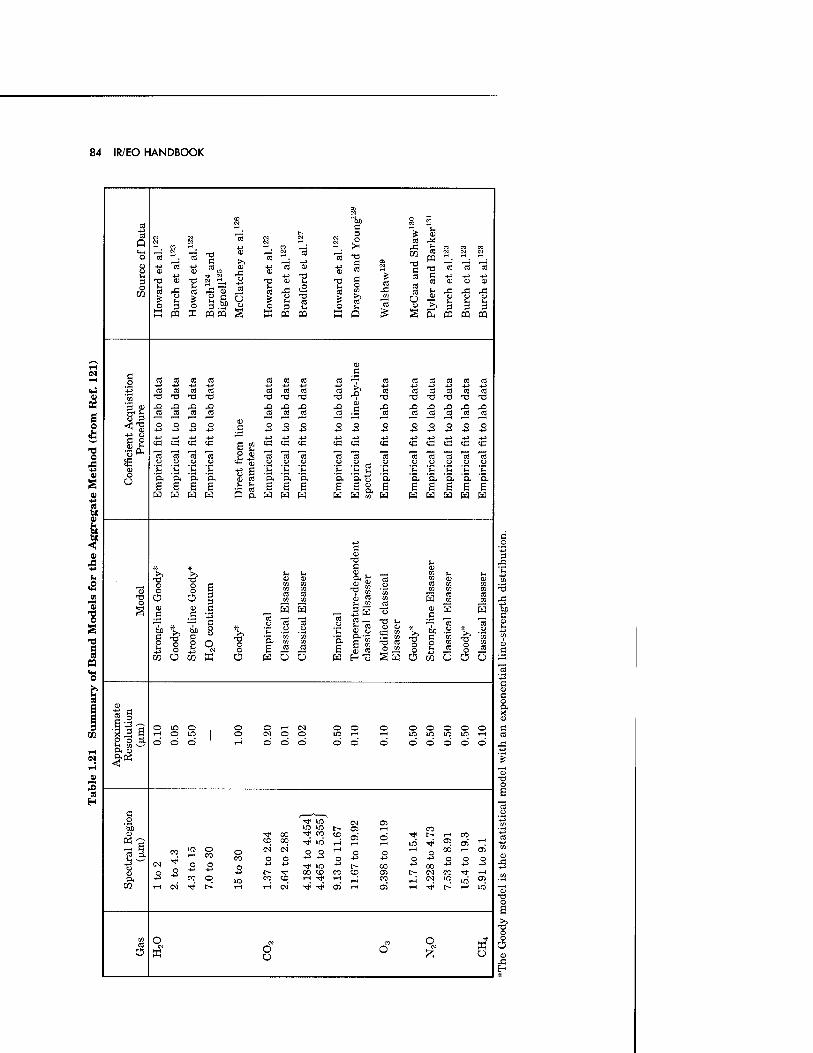
84 IR/EO HANDBOOK
3 u
I «2
CO
X
CO
P N M
m
CD
73 CN CO
r- « to ß 3 o
><
o CO
Is ra l- 0
u m m m
O "3 CM "ra XJ
c 0 "ra (N "ra 73 XI CO ra
m N N N
>> 4-J ß ra ß o CO
CJ X) c ra
0 CJ
4J 0
ra -4->
0 0
0 ra 0
X) 0
IN
's ra X
XI fi CO ra ra
3 o
CO
XJ
CO
0
X XJ
ra ra X!
ra 0 XI
ra ra ra ra u
0
X 0
43
0
J3 £ CJ S gg> 5 S XJ ra & ra to
ü 0 CJ ü CJ
1* o 3 o cj o 3 f~< o u ra CJ >% 3 3 3 w m K mm § X m m X p § E m m m
0
C o CO ra ra ra ra ra ra ra CO ra ra CO CO co
■M +j -^» +J -*J -*J +J -4J +-» +-> +-> -M -M -M +3 CO « ra ra ra ra ra ra cC ra ra ra ra CO 'Efl XI XJ TJ XI XI X! X! T3
^ X! XJ XJ XJ XI
'3 0 X X X ,0 XI J2 X X 0 c rO J2 X X X X
o" b _C8 a ra ra J$ _ra Gt J2 JS ra _ra _ra _ra jt u 3 ^ 0
O o o o 0 o o O o o O o o o o o ■4J ■+J -tj -M -u +J +J +-> +-> -M -*-> -M -M -M
-l-> CJ c g HJ 4J +J -M ^fi -tj -t^> -*^> +J -M -4-i +J -^ *J -M -1-» cß cß * *
-8 ß
cß cß tß cß cß tc cß cß cß cß cß •n OH CJ ra ra ra ra ra ra ra ra ra CO ra ra CO ra ra iß ü o cj cj cj u CJ CJ ü _ u CJ CJ CJ CJ CJ
0 'C •c 'C v •c •c *C 'C •r ra *C 'u 'u 'u 'E 'C o Ü O. "cj a a a a. 0 ra p. p. o. a. 'a a a a o, a
ß ß ß fi •^ ra ß ß ß S S ß ß ß ß ß H a W H P o. w w w H W W W W W W
-tj
ß 0
XI b .V. * c 0 ">1 >> b u
Is (» ^ ^
XI XI 0 0 CC CO 0 0
75 XJ o
O O Ü
O O Ü
S 3
w tn ra to
CO CO ra CO
ra CO
s CO CO
CO CO
CO w ra t»
s 0 0 ,g ^H S S , , ss 'o 0 ß 3 s
C ra cj "ra "ra ra
CJ ra — Ö g ß's
T3 fc- To 73 tic c o
>> XJ O O
tic ß o »H
o CJ
o CN
-X-
XI o o
'E a fi
u 'Eo
CO ra
o
'co CO ra 'a
ß
CC « rS co TJ ra O to
>> XI o o
tic fi o
CJ
'co CO ra
* >>
XI o o
CJ
'co CO ra
CO Ü CO X Ü w ü ü W HT3 Ü CO 5 Ü Ü
0
1 S '3,3 !
o lO o o o rM (N o o o o o o o o iH o lO 1 o <N O O lO rH !-H in in in in rH
o o i Ö Ö Ö 1 1-1 Ö Ö Ö ö d Ö ö ö ö ö Ö a 0
fi o
•5b •* m <N OS io m t~ ai 1-H CO
a; Tt> 00 •"# CO CO rH
Ö T-l
■* t> TH CO
*ß to 00 •* in rH in ■*'
C35 CJS T-<
CO
Mi
in o CO o
CO
CN
o CN
o o o
o O o rH
O o 00
O O cjS
o -8 <N o
4J o o -M -M rji m +J c- oo ■*^ 00 -M +-» ■*-»
0 o o -*H o Tt< 00 to CO CD C5 t> <M CO ■* rH P. 4J CO o «5 CO CO r-t TC '-f rH CO rA CM in in as
co l-i CN •* [-' 1-H l-H CN Tt Tf oS rH oS TH ■*' C-' iri
to ra O
O o o
O CM
o
XJ
X to fi 0
rH « rH ^_>
>> XJ o o Ü
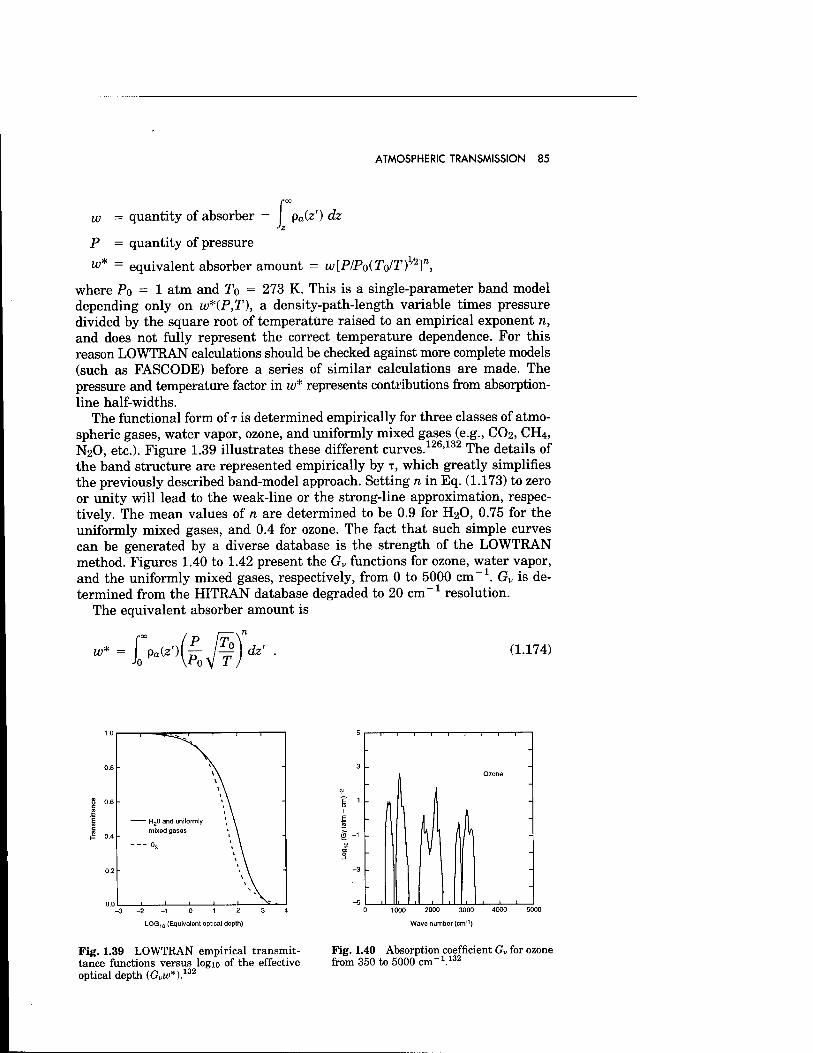
ATMOSPHERIC TRANSMISSION 85
roc
w = quantity of absorber = pa(z') dz
P = quantity of pressure
™* = equivalent absorber amount = W[PIPQ(,TQIT)1/2
Y,
where Po = 1 atm and To = 273 K. This is a single-parameter band model depending only on w*(P,T), a density-path-length variable times pressure divided by the square root of temperature raised to an empirical exponent n, and does not fully represent the correct temperature dependence. For this reason LOWTKAN calculations should be checked against more complete models (such as FASCODE) before a series of similar calculations are made. The pressure and temperature factor in w* represents contributions from absorption- line half-widths.
The functional form of T is determined empirically for three classes of atmo- spheric gases, water vapor, ozone, and uniformly mixed gases (e.g., CO2, CH4, N20, etc.). Figure 1.39 illustrates these different curves.126'132 The details of the band structure are represented empirically by T, which greatly simplifies the previously described band-model approach. Setting n in Eq. (1.173) to zero or unity will lead to the weak-line or the strong-line approximation, respec- tively. The mean values of n are determined to be 0.9 for H2O, 0.75 for the uniformly mixed gases, and 0.4 for ozone. The fact that such simple curves can be generated by a diverse database is the strength of the LOWTRAN method. Figures 1.40 to 1.42 present the Gv functions for ozone, water vapor, and the uniformly mixed gases, respectively, from 0 to 5000 cm-1. Gv is de- termined from the HITRAN database degraded to 20 cm-1 resolution.
The equivalent absorber amount is
w'-[»HkMdz'- (1.174)
1 ^-g-g^J p" 1 1
\
-
H20 and uniformly '
mixed gases 1 \ .
--- o3
\ \
■ 1 1 1
\ \
i 1 1 1— r ■" i i i
3 1 Ozone
- -
I 1 " fl
- E
$ -1 ; fl U / ~
0 M - -3
; -5 , , 1 , 1, 1 1 1 1
LOG10 (Equivalent optical depth)
1000 2000 3000 4000 5000
Wave number (cm'1)
Fig. 1.39 LOWTRAN empirical transmit- tance functions versus logio of the effective optical depth (G„w*).132
Fig. 1.40 Absorption coefficient Gv for ozone from 350 to 5000 cm"1.132
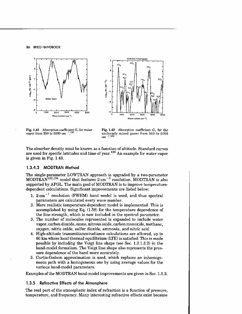
86 IR/EO HANDBOOK
Water Vapor
—5 I i i i
Uniformly mixed gases
0 1000 2000 3000 4000 5000
Wave number (cm-1) 0 1000 2000 3000 4000 5000
Wave number (cm-1)
Fig. 1.41 Absorption coefficient Gv for water Fig. 1.42 Absorption coefficient Gv for the vapor from 350 to 5000 cm-1.132 uniformly mixed gases from 350 to 5000
The absorber density must be known as a function of altitude. Standard curves are used for specific latitudes and time of year.126 An example for water vapor is given in Fig. 1.43.
1.3.4.3 MODTRAN Method
The single-parameter LOWTRAN approach is upgraded by a two-parameter MODTRAN133,134 model that features 2-cm-1 resolution. MODTRAN is also supported by AFGL. The main goal of MODTRAN is to improve temperature- dependent calculations. Significant improvements are listed below:
1. 2-cm-1 resolution (FWHM) band model is used, and thus spectral parameters are calculated every wave number.
2. More realistic temperature-dependent model is implemented. This is accomplished by using Eq. (1.58) for the temperature dependence of the line strength, which is now included in the spectral parameter.
3. The number of molecules represented is expanded to include water vapor, carbon dioxide, ozone, nitrous oxide, carbon monoxide, methane, oxygen, nitric oxide, sulfur dioxide, ammonia, and nitric acid.
4. High-altitude transmittance/radiance calculations are allowed, up to 60 km where local thermal equilibrium (LTE) is satisfied. This is made possible by including the Voigt line shape (see Sec. 1.3.1.3.2) in the band-model formalism. The Voigt line shape also represents the pres- sure dependence of the band more accurately.
5. Curtis-Godson approximation is used, which replaces an inhomoge- neous path with a homogeneous one by using average values for the various band-model parameters.
Examples of the MODTRAN band-model improvements are given in Sec. 1.5.2.
1.3.5 Refractive Effects of the Atmosphere
The real part of the atmospheric index of refraction is a function of pressure, temperature, and frequency. Many interesting refractive effects exist because
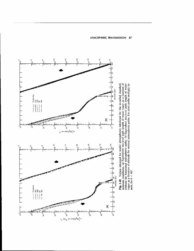
ATMOSPHERIC TRANSMISSION 87
(,-""! z_m=ui3)(oZH)|J*
88 IR/EO HANDBOOK
of tropospheric variations in density and water-vapor partial pressure as a function of position. This section begins with a discussion of atmospheric index- of-refraction models at optical frequencies and then examines different effects caused by refractive variations. Also of importance is the refractive index of particles in the atmosphere.
1.3.5.1 Index of Refraction of the Atmosphere
Because of their abundance, nitrogen and oxygen make significant contribu- tions to the refractivity of the earth's atmosphere. These molecules have no infrared bands of importance to the refractive index and thus only electronic bands need to be considered for a model valid from low frequency to the ultra- violet. Based on the work of Edlen,135 a simple Sellmeier-type model (see Sec. 1.3.1.3.1) for the dry atmospheric index can be obtained :
ry = KTl ~ L, A ±u = ( 237.2 + -g ~2 + ~2 ^2 ) ~f > iVdry = (n - 1) x 10b = ( 237.2 + 2 ' 2 + Vl - V V2
(1.175)
where N is refractivity, v is wave number in cm-1, vi = 114,000.0 cm-1, V2 = 62,400.0 cm-1, Pdry is dry-air pressure in kPa, and T is temperature in kelvin. This model is valid from 0.2 to °° (xm (near dc) and compares well with other models.137'138 Moist air requires an additional term accounting for water vapor. Based on the work of Hill and Lawrence,139 a Sellmeier-type term is obtained, representing the electronic transition contributions of pure water vapor:
651.7vg PH2O iVH2o = 3-73 -^ , (1-176)
where V3 = 111,575.0 cm 1. The net refractivity is the sum of iVdry plus NH2O-
The model becomes more complicated at infrared wavelengths because the strong infrared vibrational and rotational absorption bands of water vapor must be considered. The importance of water vapor is demonstrated by the refractivity model at radar frequencies, which is the sum of all oscillator strengths,
i_ 140 141 as given by '
776.4Pdry 717PÄ2o 3.744 x 10⁶P„2o iVrf = + + -2 . (1.177)
The rf refractivity can vary from 250 to 500 over the range of atmospheric temperatures and water-vapor partial pressures.142 Most of this variation is caused by the presence of water vapor. In particular, the last term in Eq. (1.177) represents the rotational band of water vapor. A model can be con- structed, however, based on Eqs. (1.111), (1.112), (1.113), and Table 1.9 that allows reasonable prediction of refractivity at infrared wavelengths. Table 1.22 lists parameters for a refractivity Sellmeier model that includes the effect of
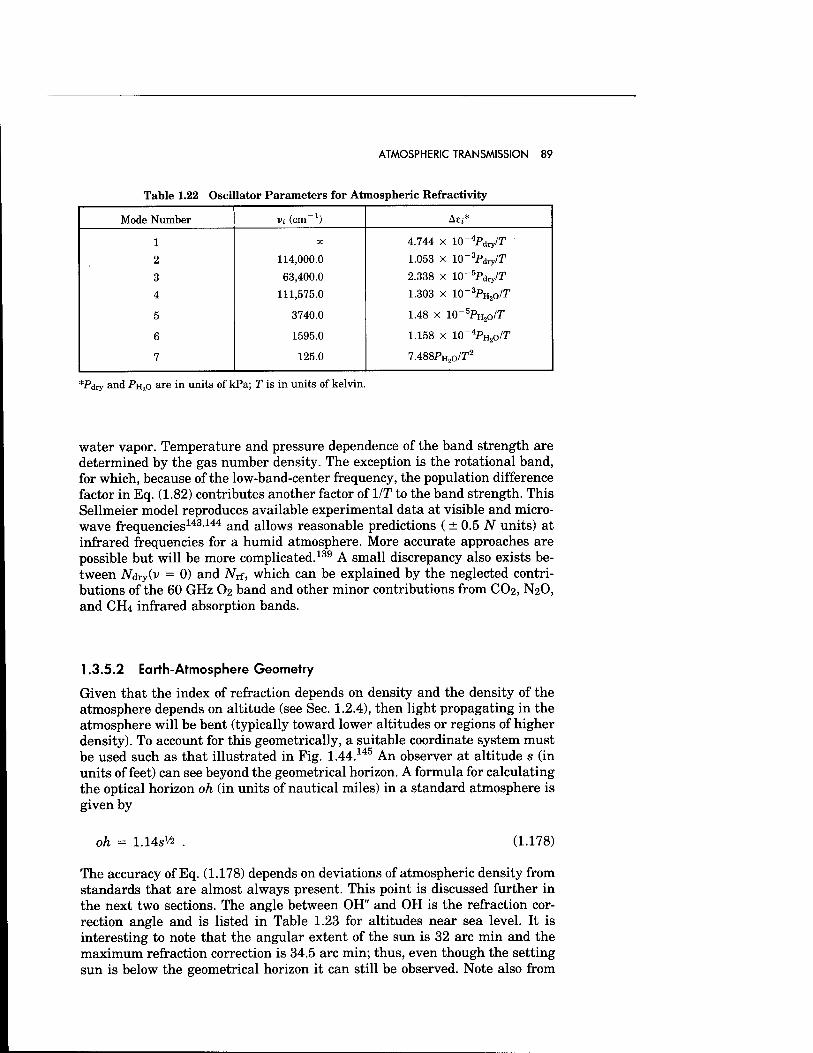
ATMOSPHERIC TRANSMISSION 89
Table 1.22 Oscillator Parameters for Atmospheric Refractivity
Mode Number vt (cm *) Ae;*
1 00 4.744 X 10"4Pdry/T
2 114,000.0 1.053 x 10~3Pdr/T
3 63,400.0 2.338 x 10~5Pdry/T
4 111,575.0 1.303 x 10~ 3PH2p/T
5 3740.0 1.48 x 10⁻⁵PH2O/T
6 1595.0 1.158 x io~4pH2o/r
7 125.0 7.488PH2O/T2
*Pdry and PH2O are in units of kPa; T is in units of kelvin.
water vapor. Temperature and pressure dependence of the band strength are determined by the gas number density. The exception is the rotational band, for which, because of the low-band-center frequency, the population difference factor in Eq. (1.82) contributes another factor of \IT to the band strength. This Sellmeier model reproduces available experimental data at visible and micro- wave frequencies143,144 and allows reasonable predictions ( ± 0.5 N units) at infrared frequencies for a humid atmosphere. More accurate approaches are possible but will be more complicated.139 A small discrepancy also exists be- tween iVdry(v = 0) and Nrf, which can be explained by the neglected contri- butions of the 60 GHz O2 band and other minor contributions from CO2, N2O, and CH4 infrared absorption bands.
1.3.5.2 Earth-Atmosphere Geometry
Given that the index of refraction depends on density and the density of the atmosphere depends on altitude (see Sec. 1.2.4), then light propagating in the atmosphere will be bent (typically toward lower altitudes or regions of higher density). To account for this geometrically, a suitable coordinate system must be used such as that illustrated in Fig. 1.44.145 An observer at altitude s (in units of feet) can see beyond the geometrical horizon. A formula for calculating the optical horizon oh (in units of nautical miles) in a standard atmosphere is given by
oh = 1.14s** (1.178)
The accuracy of Eq. (1.178) depends on deviations of atmospheric density from standards that are almost always present. This point is discussed further in the next two sections. The angle between OH" and OH is the refraction cor- rection angle and is listed in Table 1.23 for altitudes near sea level. It is interesting to note that the angular extent of the sun is 32 arc min and the maximum refraction correction is 34.5 arc min; thus, even though the setting sun is below the geometrical horizon it can still be observed. Note also from
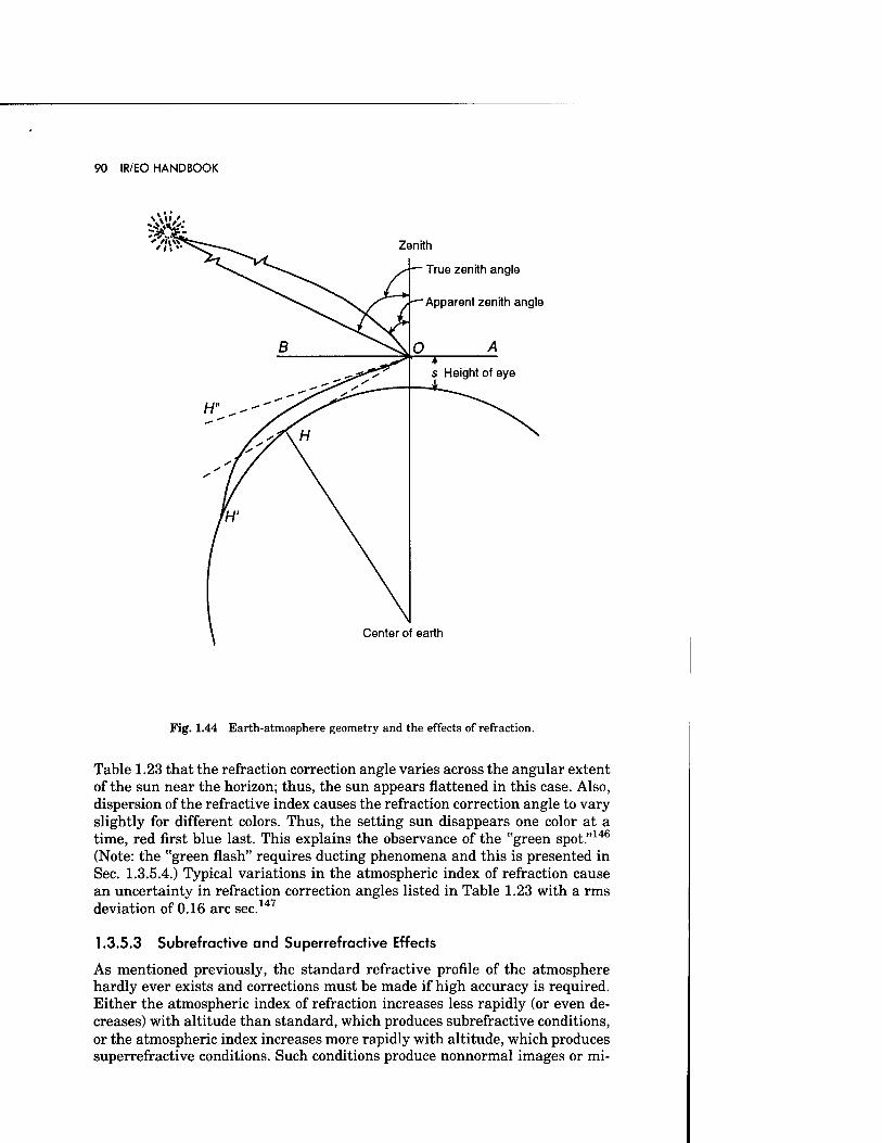
90 IR/EO HANDBOOK
Zenith
True zenith angle
Apparent zenith angle
Center of earth
Fig. 1.44 Earth-atmosphere geometry and the effects of refraction.
Table 1.23 that the refraction correction angle varies across the angular extent of the sun near the horizon; thus, the sun appears flattened in this case. Also, dispersion of the refractive index causes the refraction correction angle to vary slightly for different colors. Thus, the setting sun disappears one color at a time, red first blue last. This explains the observance of the "green spot."146
(Note: the "green flash" requires ducting phenomena and this is presented in Sec. 1.3.5.4.) Typical variations in the atmospheric index of refraction cause an uncertainty in refraction correction angles listed in Table 1.23 with a rms deviation of 0.16 arc sec.147
1.3.5.3 Subrefractive and Superrefractive Effects
As mentioned previously, the standard refractive profile of the atmosphere hardly ever exists and corrections must be made if high accuracy is required. Either the atmospheric index of refraction increases less rapidly (or even de- creases) with altitude than standard, which produces subrefractive conditions, or the atmospheric index increases more rapidly with altitude, which produces superrefractive conditions. Such conditions produce nonnormal images or mi-
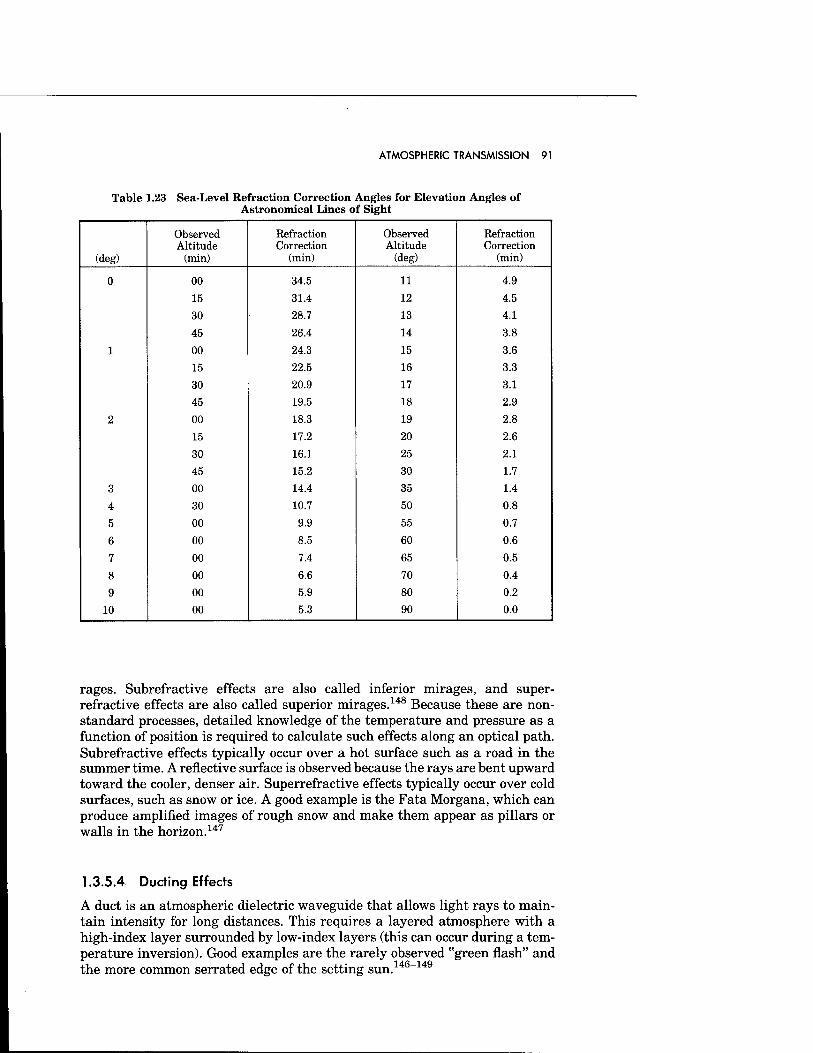
ATMOSPHERIC TRANSMISSION 91
Table 1.23 Sea-Level Refraction Correction Angles for Elevation Angles of Astronomical Lines of Sight
(deg)
Observed Altitude
(min)
Refraction Correction
(min)
Observed Altitude
(deg)
Refraction Correction
(min)
0 00 34.5 11 4.9
15 31.4 12 4.5
30 28.7 13 4.1
45 26.4 14 3.8
1 00 24.3 15 3.6
15 22.5 16 3.3
30 20.9 17 3.1
45 19.5 18 2.9
2 00 18.3 19 2.8
15 17.2 20 2.6
30 16.1 25 2.1
45 15.2 30 1.7
3 00 14.4 35 1.4
4 30 10.7 50 0.8
5 00 9.9 55 0.7
6 00 8.5 60 0.6
7 00 7.4 65 0.5
8 00 6.6 70 0.4
9 00 5.9 80 0.2
10 00 5.3 90 0.0
rages. Subrefractive effects are also called inferior mirages, and super- refractive effects are also called superior mirages.148 Because these are non- standard processes, detailed knowledge of the temperature and pressure as a function of position is required to calculate such effects along an optical path. Subrefractive effects typically occur over a hot surface such as a road in the summer time. A reflective surface is observed because the rays are bent upward toward the cooler, denser air. Superrefractive effects typically occur over cold surfaces, such as snow or ice. A good example is the Fata Morgana, which can produce amplified images of rough snow and make them appear as pillars or walls in the horizon.147
1.3.5.4 Ducting Effects
A duct is an atmospheric dielectric waveguide that allows light rays to main- tain intensity for long distances. This requires a layered atmosphere with a high-index layer surrounded by low-index layers (this can occur during a tem- perature inversion). Good examples are the rarely observed "green flash" and the more common serrated edge of the setting sun.146-149
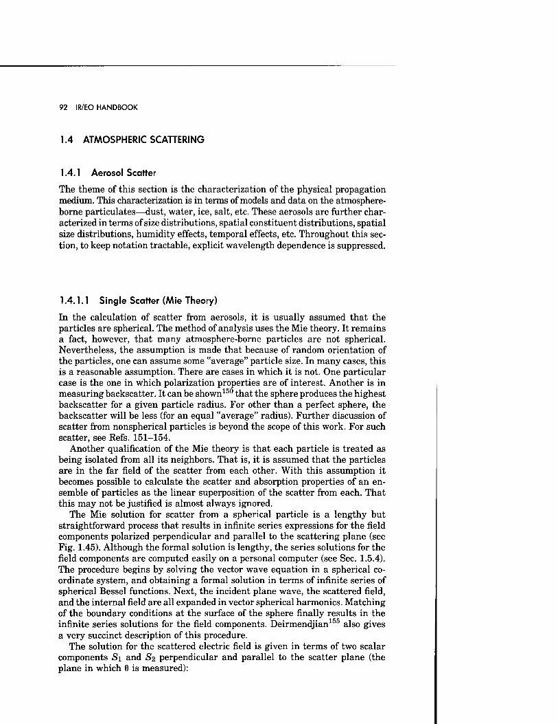
92 IR/EO HANDBOOK
1.4 ATMOSPHERIC SCATTERING
1.4.1 Aerosol Scatter
The theme of this section is the characterization of the physical propagation medium. This characterization is in terms of models and data on the atmosphere- borne particulates—dust, water, ice, salt, etc. These aerosols are further char- acterized in terms of size distributions, spatial constituent distributions, spatial size distributions, humidity effects, temporal effects, etc. Throughout this sec- tion, to keep notation tractable, explicit wavelength dependence is suppressed.
1.4.1.1 Single Scatter (Mie Theory)
In the calculation of scatter from aerosols, it is usually assumed that the particles are spherical. The method of analysis uses the Mie theory. It remains a fact, however, that many atmosphere-borne particles are not spherical. Nevertheless, the assumption is made that because of random orientation of the particles, one can assume some "average" particle size. In many cases, this is a reasonable assumption. There are cases in which it is not. One particular case is the one in which polarization properties are of interest. Another is in measuring backscatter. It can be shown150 that the sphere produces the highest backscatter for a given particle radius. For other than a perfect sphere, the backscatter will be less (for an equal "average" radius). Further discussion of scatter from nonspherical particles is beyond the scope of this work. For such scatter, see Refs. 151-154.
Another qualification of the Mie theory is that each particle is treated as being isolated from all its neighbors. That is, it is assumed that the particles are in the far field of the scatter from each other. With this assumption it becomes possible to calculate the scatter and absorption properties of an en- semble of particles as the linear superposition of the scatter from each. That this may not be justified is almost always ignored.
The Mie solution for scatter from a spherical particle is a lengthy but straightforward process that results in infinite series expressions for the field components polarized perpendicular and parallel to the scattering plane (see Fig. 1.45). Although the formal solution is lengthy, the series solutions for the field components are computed easily on a personal computer (see Sec. 1.5.4). The procedure begins by solving the vector wave equation in a spherical co- ordinate system, and obtaining a formal solution in terms of infinite series of spherical Bessel functions. Next, the incident plane wave, the scattered field, and the internal field are all expanded in vector spherical harmonics. Matching of the boundary conditions at the surface of the sphere finally results in the infinite series solutions for the field components. Deirmendjian155 also gives a very succinct description of this procedure.
The solution for the scattered electric field is given in terms of two scalar components Si and S2 perpendicular and parallel to the scatter plane (the plane in which 6 is measured):
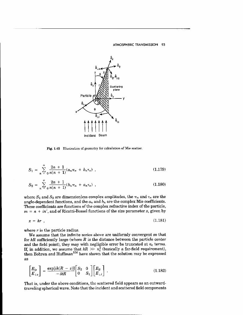
ATMOSPHERIC TRANSMISSION 93
A , i t > i > i V 1 v n
Incident Beam
Fig. 1.45 Illustration of geometry for calculation of Mie scatter.
00 _ ^
Si = 2 -; —T-Mn'nn + bnin) , n = 0n(n + 1)
(1.179)
v In + 1 n = 0n(n + 1)
(1.180)
where Si and S2 are dimensionless complex amplitudes, the Trn and T„ are the angle-dependent functions, and the an and bn are the complex Mie coefficients. These coefficients are functions of the complex refractive index of the particle, m = n + in', and of Ricatti-Bessel functions of the size parameter x, given by
x = kr , (1.181)
where r is the particle radius. We assume that the infinite series above are uniformly convergent so that
for kR sufficiently large (where R is the distance between the particle center and the field point), they may with negligible error be truncated at nc terms. If, in addition, we assume that kR » n% (basically a far-field requirement), then Bohren and Huffman150 have shown that the solution may be expressed as
E\\s exp[ik(R — z)] s2 0 E\\i
ß±s_ -ikR 0 Si \_ELI (1.182)
That is, under the above conditions, the scattered field appears as an outward- traveling spherical wave. Note that the incident and scattered field components
94 IR/EO HANDBOOK
are expressed in terms of different basis vectors (see Fig. 1.44), and that the assumption of a spherical particle results in a scatter that does not depolarize the incident radiation; i.e., the S3 element [upper right in Eq. (1.182)] and the S4 element (lower left) are zero. See the following discussion of polarization effects.
These field components are often expressed in terms of the Stokes vector [I,Q,U,V], whose components are given by
/ = <|E|||2 + \E±\2) ,
Q = (\Ef - \E±\2) ,
U = <E||Bj.* + ExEf) ,
V = (E\Ei* - ExEf) .
(1.183)
With this notation, the relationship between the Stokes vectors of the incident and scattered fields becomes
Is Qs 1 Us k2R2
Vs
Su S12 0 0 S12 S11 0 0 0 0 S33 S34 0 0 — S34 S33
Ii Qi Ui
(1.184)
where the (Mueller) matrix elements156 are defined as
Su = i(|s2|2 + N2)
S12 = „(l^l - |Si| ) ,
S33 = |(S|Si + S2Sf)
(1.185)
S34 = |*(SiS| - S2Si) .
The utility of the Stokes formulation is that the Stokes parameters of the light scattered by a collection of randomly separated particles are the sum of the Stokes parameters of the light scattered by the individual particles. The ran- dom positions of the particles ensure that (except in the exact forward direction150) the relative phases of the scattered fields are uniformly distributed over the interval (0,2TT), thus allowing addition of intensities rather than of fields.
On the basis of the above formulation, it is easily seen that for incident radiation polarized parallel to the scattering plane, the resulting scattered radiation is fully polarized parallel to the scattering plane. This same result holds for incident radiation polarized perpendicular to the scattering plane. On the other hand, if the incident radiation is unpolarized, the differential
ATMOSPHERIC TRANSMISSION 95
scatter of the two field components parallel and perpendicular to the scattering plane results in a degree of polarization P given by
= -Si2(6) (1 186)
Sn(8)
For P > 0, we have partial polarization perpendicular to the scattering plane; for P < 0, we have partial polarization parallel to the scattering plane. In general, \P\ =£ 1. If a collection of scatterers is heterogeneous by virtue of variations in either size or optical properties, or both, the polarization is strictly less than unity.
The energy removed from the incident beam by scatter on the particle is proportional to the extinction cross section Cext:
•>ext = Cabs + Csca , (1.187)
which is the sum of the absorption and scatter cross sections. The extinction cross section is expressed as
Cext(r) = ^Re{Si(0,r)} , (1.188)
where i = 1 or 2. [Note: Si(0,r) = S2(0,r).] The scatter cross section is expressed as
CSca(r) = \ f Sn(0,r) da) , (1.189) k J4ir
where the integration is over the entire solid angle. In these last two equations, the dependence on the particle radius has been explicitly denoted.
A very useful parameter, the significance of which will be discussed later, is the single-scatter albedo. This is defined as the ratio of the scatter and extinction cross sections:
a = ^ . (1.190) t>ext
This notation is used, for example, by van de Hülst.157-158 Others, Deirmendjian,155 for example, use the notation w or simply w.
By normalizing the above scatter and extinction cross sections to the geo- metrical cross sections, one may define the corresponding efficiencies:
(1.191)
(1.192)
tysca - " irr2
t^ext Qext =
^r2
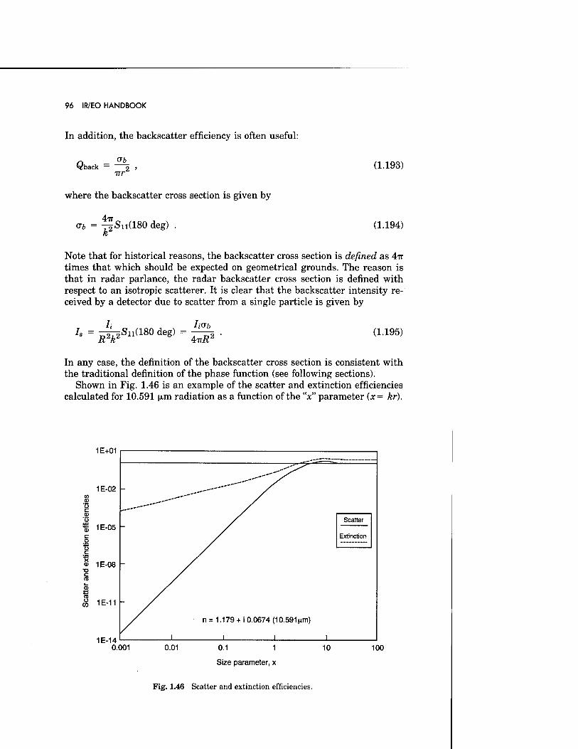
96 IR/EO HANDBOOK
In addition, the backscatter efficiency is often useful:
n _ _£1 vtfback — o > (1.193) •nr
where the backscatter cross section is given by
4IT,
T2 0-6 = 7äSn(180 deg) (1.194)
Note that for historical reasons, the backscatter cross section is defined as 4TT times that which should be expected on geometrical grounds. The reason is that in radar parlance, the radar backscatter cross section is defined with respect to an isotropic scatterer. It is clear that the backscatter intensity re- ceived by a detector due to scatter from a single particle is given by
/. = 4i2Sii(i8°de^ =Ii(Tb Rzk 4TTä'
(1.195)
In any case, the definition of the backscatter cross section is consistent with the traditional definition of the phase function (see following sections).
Shown in Fig. 1.46 is an example of the scatter and extinction efficiencies calculated for 10.591 |xm radiation as a function of the 'V parameter (x= kr).
1E+01
1E-02
1E-14 0.001 0.1 1
Size parameter, x
100
Fig. 1.46 Scatter and extinction efficiencies.
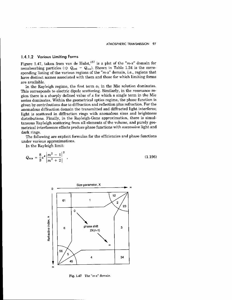
ATMOSPHERIC TRANSMISSION 97
1.4.1.2 Various Limiting Forms
Figure 1.47, taken from van de Hülst,157 is a plot of the "m-x" domain for nonabsorbing particles (=> Qext = Qsca). Shown in Table 1.24 is the corre- sponding listing of the various regions of the "m-x" domain, i.e., regions that have distinct names associated with them and those for which limiting forms are available.
In the Rayleigh regime, the first term ai in the Mie solution dominates. This corresponds to electric dipole scattering. Similarly, in the resonance re- gion there is a sharply defined value of x for which a single term in the Mie series dominates. Within the geometrical optics regime, the phase function is given by contributions due to diffraction and reflection plus refraction. For the anomalous diffraction domain the transmitted and diffracted light interferes; light is scattered in diffraction rings with anomalous sizes and brightness distributions. Finally, in the Rayleigh-Gans approximation, there is simul- taneous Rayleigh scattering from all elements of the volume, and purely geo- metrical interference effects produce phase functions with successive light and dark rings.
The following are explicit formulas for the efficiencies and phase functions under various approximations.
In the Rayleigh limit:
Qsca ~ oX m2 - 1 mz + 2
(1.196)
Size parameter, X -► oo
Fig. 1.47 The "m-x" domain.
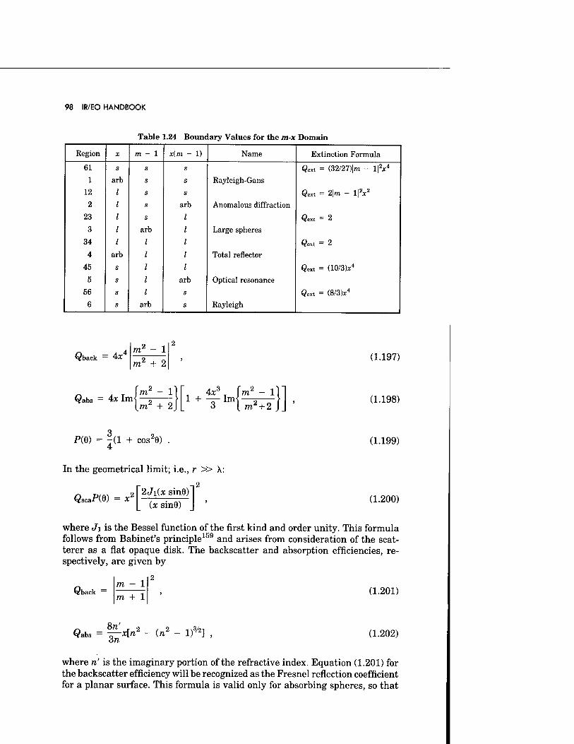
98 IR/EO HANDBOOK
Table 1.24 Boundary Values for the m-x Domain
Region X m - 1 x(m - 1) Name Extinction Formula
61 s s s Qext = (32/27)|m - 1|V 1 arb s s Rayleigh-Gans
12 s s Qext = 1\m - 1|2*2
2 s arb Anomalous diffraction
23 s Qext = 2
3 arb Large spheres
34 Qext = 2
4 arb Total reflector
45 s Qext = (10/3)*4
5 s arb Optical resonance
56 s s Qext = (8/3)x4
6 s arb s Rayleigh
Qback = 4x4
Qabs = 4x Im
m2 - 1 2
m2 + 2 )
Jm2- 11 [m2 + 2j
, 4x% \ml - 1 1 + — Im^ —5
3 m2 + 2
(1.197)
(1.198)
P(6) = -Q + cos26) 4 (1.199)
In the geometrical limit; i.e., r » \:
-,2
QscaPO) = X2 2 Ji(x sine) (x sinG) (1.200)
where J\ is the Bessel function of the first kind and order unity. This formula follows from Babinet's principle159 and arises from consideration of the scat- terer as a fiat opaque disk. The backscatter and absorption efficiencies, re- spectively, are given by
Qback m — 1 m + 1 (1.201)
^ 8"' r 2 Qabs = -T—*[«
3rc (71 1)%] , (1.202)
where n' is the imaginary portion of the refractive index. Equation (1.201) for the backscatter efficiency will be recognized as the Fresnel reflection coefficient for a planar surface. This formula is valid only for absorbing spheres, so that
ATMOSPHERIC TRANSMISSION 99
the internally reflected rays do not contribute to the backscatter. Further, Eq. (1.202) for the absorption cross section is valid only for weakly absorbing spheres, so that the total absorption is proportional to volume as it is for small particles [see Eq. (1.198)]. For strongly absorbing particles, such that 4n'x » 1, the absorption takes place only in the surface layer of the particle, and the absorption efficiency becomes equal to the geometrical cross section (as does the scatter efficiency for r » A.).
1.4.1.3 Polydispersions
We next generalize the above results to scattering on many particles of various sizes. To this end, we define a scatter cross section per unit volume ßsca, ex- pressed as
J-oo
Csca(r) n(r) dr , (1.203) o
where the function n(r) is the particle size distribution function defined as the number of particles per unit volume with radii between r and r + dr. These distribution functions are usually expressed in units of cm-3 jjim-1. For more on these distribution models, see Sec. 1.4.1.4.3. Also note that the scatter cross section per unit volume has units of inverse length. It is often called the scatter "coefficient." The extinction cross section per unit volume is defined analo- gously to that for scatter, and the corresponding single-scatter albedo is defined as a = ßsca/ßext-
The corresponding generalization of the Mueller matrix elements is the following:
Sy(e) = I Sij(Q,r) n(r) dr . (1.204)
Note that this element is now defined per unit scatter volume. The implications for the interpretation and use of this redefined variable are discussed in Sec. 1.4.3.
Before proceeding with examples of the use of these concepts in calculating the power due to scatter that is received by a sensor, we connect the above notation with that used by other authors, notably Deirmendjian.155 Let us assume that the incident radiation is unpolarized and that the receiver is insensitive to the polarization of the scattered radiation. In this case, the relevant Mueller matrix element is Su. Deirmendjian and others define a "phase function" P(8) that can be considered a three-dimensional probability density function (unnormalized) for the scatter direction. In the notation es- tablished above, this phase function is given by
4irSii(8,r) PM = ,2r - • (L205)
100 IR/EO HANDBOOK
The normalization of this phase function is such that its integral over the entire solid angle is equal to 4TT sr; the phase function P(0) is thus dimension- less. For a polydispersion, the corresponding relationship is
TO) - «£*> . a.206) A psca
The specific connection between Deirmendjian's Mueller matrix components and those discussed herein is the following:
„ _ 4TT[SII(6) - Si2(6)] (1207)
(1.208)
(1.209)
^1W k Psca
P2(0) 4ir[Sii(e) + Si2(6)]
A psca
P3(6) 4™S33(e)
"- Psca
P4(6) 4TrS34(e)
A psca (1.210)
Note that in each of the above equations, the P/(6) are dimensionless. Other authors, for example, Fenn et al.,160 define the phase function such that the integral over the entire solid angle is unity. In this case, therefore, the phase function has the formal interpretation as a (three-dimensional) probability density function with the units of inverse steradians. Shown in Fig. 1.48 are example phase functions for x « 1, a 0.55 (im wavelength, and a 0.6328 |xm wavelength, respectively. Note the shift in features between the latter two figures for this small wavelength change.
1.4.1.4 Terrestrial Aerosols
One can perform a number of categorizations of terrestrial aerosol particles. Here, we use the general classifications of dust and hygroscopic particles. Dust particles are a rather passive constituent of atmospheric haze. On the other hand, hygroscopic particles display a strong dependence on relative humidity and are thus more highly variable.
Dust particles are derived from a number of terrestrial and extraterrestrial sources. Extraterrestrial sources include planetary accretion (due to interplan- etary debris within the volume swept by the earth's passage through space) and meteoroids. Particles due to these two sources are the predominant haze components in the outermost atmosphere. Volcanos generate a huge volume of fine ash and gases. These particles are injected high into the stratosphere, where they remain for extended periods of time. In the lowest levels of the atmosphere, surface winds play an important role in sweeping up soil-based dusts. Finally, industry and construction are important sources of dust particles.
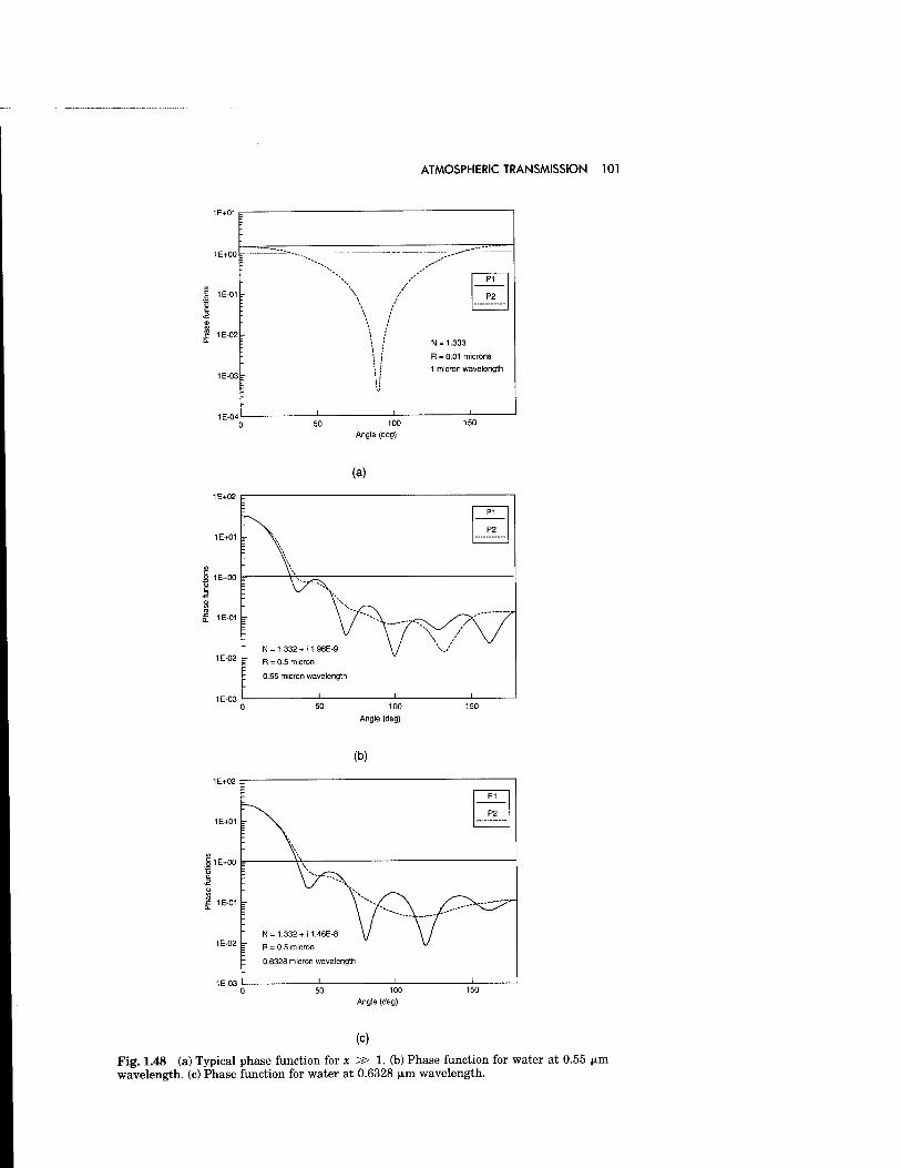
ATMOSPHERIC TRANSMISSION 101
: ,—-"
l ~-~\ ^**'~~
T
P1
P2
\ \ I N = 1.333 : \ \ R = 0.01 microns
> ; 1 micron wavelength
i i i 100
Angle (deg)
(a)
r
P1
P2
" \\ ! V/^~^
r
- N = 1.332 + i 1.96E-9 \l \J r R = 0.5 micron
: 0.55 micron wavelength
" i i 100
Angle (deg)
(b)
1E+02
P1
1E+01 P2
V)
\ = \ \
u = \ ^v^-^X » \ / "A <D i-
1 1E-01 Q. r \ ~*r- \ /^-^
^T
- N = 1.332+ M.46E-8 \J \ / 1E-02 R = 0.5 micron
0.6328 micron wavelength ■
i i 100
Angle (deg)
(c)
Fig. 1.48 (a) Typical phase function for x s> 1. (b) Phase function for water at 0.55 |xm wavelength, (c) Phase function for water at 0.6328 JAHI wavelength.
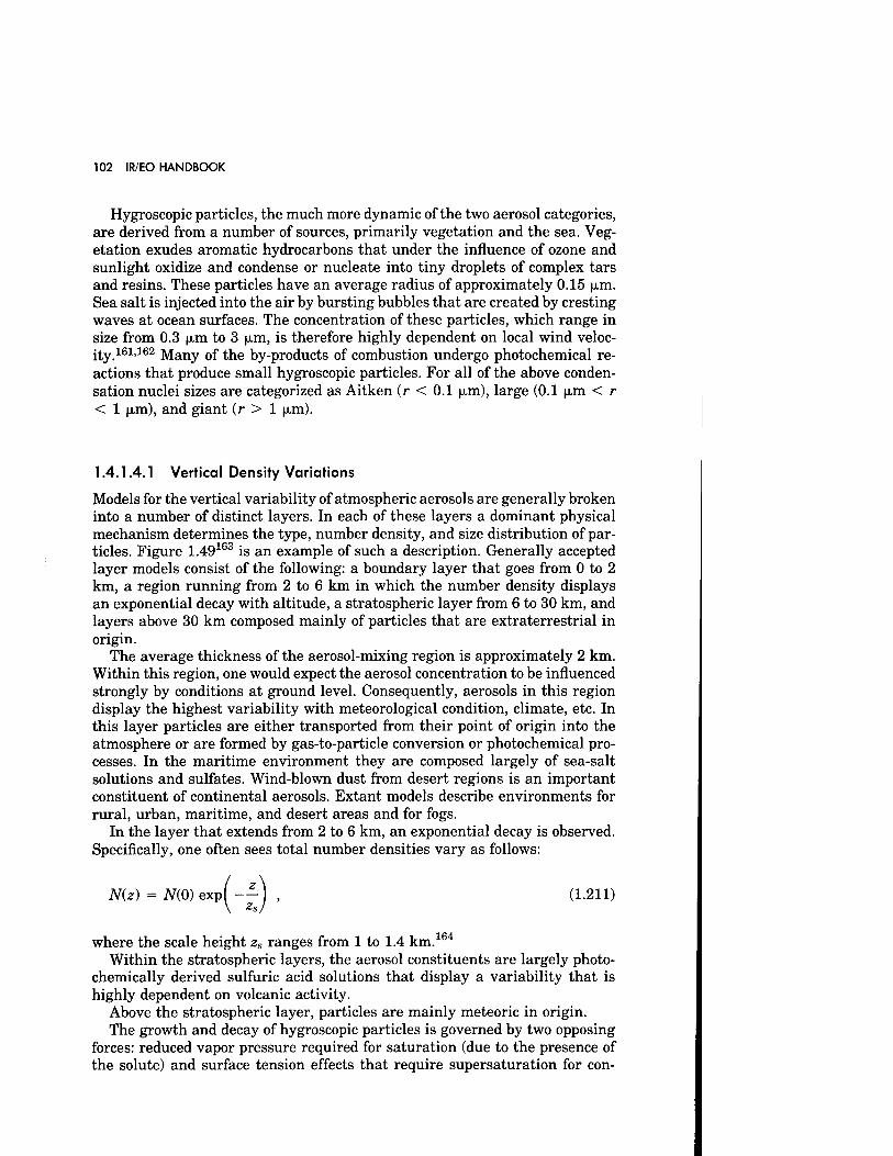
102 IR/EO HANDBOOK
Hygroscopic particles, the much more dynamic of the two aerosol categories, are derived from a number of sources, primarily vegetation and the sea. Veg- etation exudes aromatic hydrocarbons that under the influence of ozone and sunlight oxidize and condense or nucleate into tiny droplets of complex tars and resins. These particles have an average radius of approximately 0.15 jxm. Sea salt is injected into the air by bursting bubbles that are created by cresting waves at ocean surfaces. The concentration of these particles, which range in size from 0.3 jxm to 3 |xm, is therefore highly dependent on local wind veloc- ity.161,162 Many of the by-products of combustion undergo photochemical re- actions that produce small hygroscopic particles. For all of the above conden- sation nuclei sizes are categorized as Aitken (r < 0.1 |xm), large (0.1 (xm < r < 1 (xm), and giant (r > 1 (xm).
1.4.1.4.1 Vertical Density Variations
Models for the vertical variability of atmospheric aerosols are generally broken into a number of distinct layers. In each of these layers a dominant physical mechanism determines the type, number density, and size distribution of par- ticles. Figure 1.49163 is an example of such a description. Generally accepted layer models consist of the following: a boundary layer that goes from 0 to 2 km, a region running from 2 to 6 km in which the number density displays an exponential decay with altitude, a stratospheric layer from 6 to 30 km, and layers above 30 km composed mainly of particles that are extraterrestrial in origin.
The average thickness of the aerosol-mixing region is approximately 2 km. Within this region, one would expect the aerosol concentration to be influenced strongly by conditions at ground level. Consequently, aerosols in this region display the highest variability with meteorological condition, climate, etc. In this layer particles are either transported from their point of origin into the atmosphere or are formed by gas-to-particle conversion or photochemical pro- cesses. In the maritime environment they are composed largely of sea-salt solutions and sulfates. Wind-blown dust from desert regions is an important constituent of continental aerosols. Extant models describe environments for rural, urban, maritime, and desert areas and for fogs.
In the layer that extends from 2 to 6 km, an exponential decay is observed. Specifically, one often sees total number densities vary as follows:
N(z) = iV(0)exp( --j , (1.211)
where the scale height zs ranges from 1 to 1.4 km.164
Within the stratospheric layers, the aerosol constituents are largely photo- chemically derived sulfuric acid solutions that display a variability that is highly dependent on volcanic activity.
Above the stratospheric layer, particles are mainly meteoric in origin. The growth and decay of hygroscopic particles is governed by two opposing
forces: reduced vapor pressure required for saturation (due to the presence of the solute) and surface tension effects that require supersaturation for con-
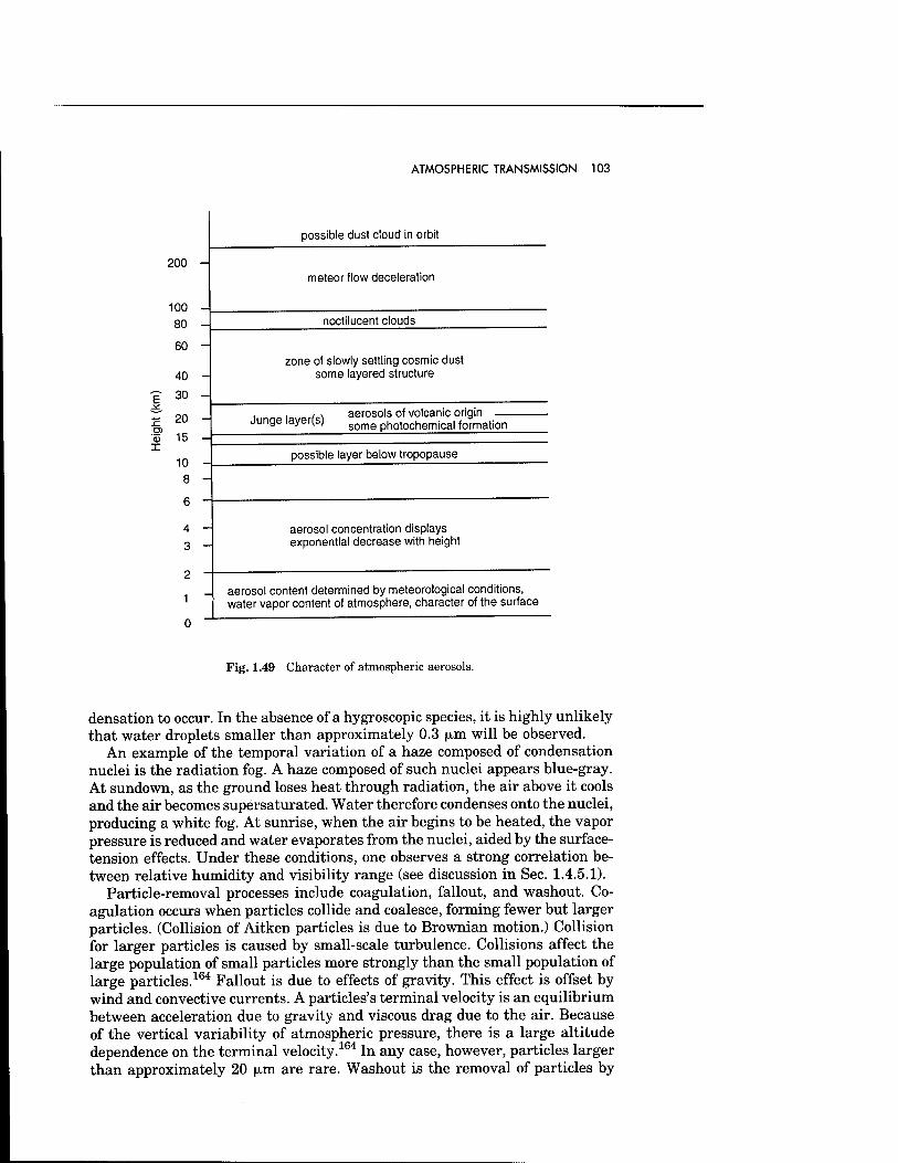
ATMOSPHERIC TRANSMISSION 103
100 80
D) 0) X
200 -
60 -
40
30
20
15
10 8
4
3
2
1
0
possible dust cloud in orbit
meteor flow deceleration
noctilucent clouds
zone of slowly settling cosmic dust some layered structure
,„n„Q |.„.r,., aerosols of volcanic origin — junge layers sQme photochemica| formation
possible layer below tropopause
aerosol concentration displays exponential decrease with height
aerosol content determined by meteorological conditions, water vapor content of atmosphere, character of the surface
Fig. 1.49 Character of atmospheric aerosols.
densation to occur. In the absence of a hygroscopic species, it is highly unlikely that water droplets smaller than approximately 0.3 u.m will be observed.
An example of the temporal variation of a haze composed of condensation nuclei is the radiation fog. A haze composed of such nuclei appears blue-gray. At sundown, as the ground loses heat through radiation, the air above it cools and the air becomes supersaturated. Water therefore condenses onto the nuclei, producing a white fog. At sunrise, when the air begins to be heated, the vapor pressure is reduced and water evaporates from the nuclei, aided by the surface- tension effects. Under these conditions, one observes a strong correlation be- tween relative humidity and visibility range (see discussion in Sec. 1.4.5.1).
Particle-removal processes include coagulation, fallout, and washout. Co- agulation occurs when particles collide and coalesce, forming fewer but larger particles. (Collision of Aitken particles is due to Brownian motion.) Collision for larger particles is caused by small-scale turbulence. Collisions affect the large population of small particles more strongly than the small population of large particles.164 Fallout is due to effects of gravity. This effect is offset by wind and convective currents. A particles's terminal velocity is an equilibrium between acceleration due to gravity and viscous drag due to the air. Because of the vertical variability of atmospheric pressure, there is a large altitude dependence on the terminal velocity.164 In any case, however, particles larger than approximately 20 (Jim are rare. Washout is the removal of particles by
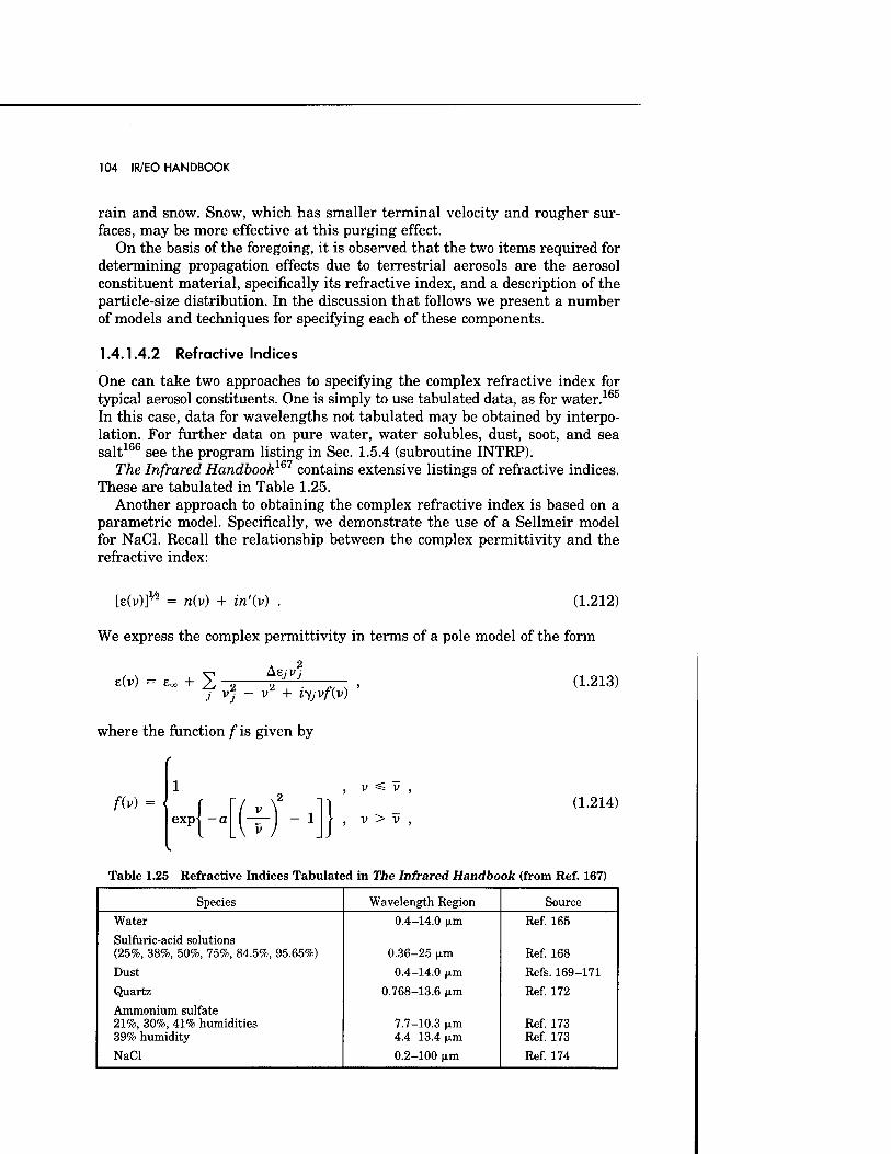
104 IR/EO HANDBOOK
rain and snow. Snow, which has smaller terminal velocity and rougher sur- faces, may be more effective at this purging effect.
On the basis of the foregoing, it is observed that the two items required for determining propagation effects due to terrestrial aerosols are the aerosol constituent material, specifically its refractive index, and a description of the particle-size distribution. In the discussion that follows we present a number of models and techniques for specifying each of these components.
1.4.1.4.2 Refractive Indices
One can take two approaches to specifying the complex refractive index for typical aerosol constituents. One is simply to use tabulated data, as for water.165
In this case, data for wavelengths not tabulated may be obtained by interpo- lation. For further data on pure water, water solubles, dust, soot, and sea salt166 see the program listing in Sec. 1.5.4 (subroutine INTRP).
The Infrared Handbook™1 contains extensive listings of refractive indices. These are tabulated in Table 1.25.
Another approach to obtaining the complex refractive index is based on a parametric model. Specifically, we demonstrate the use of a Sellmeir model for NaCl. Recall the relationship between the complex permittivity and the refractive index:
[e(v)]w = n(v) + in'(v) . (1.212)
We express the complex permittivity in terms of a pole model of the form
e(v) = Eoo + 2) A 2
j v) - v2 + iyjvfiv) '
where the function f is given by
(1.213)
f(v) = expi -a - 1
V =£ V
, V > V ,
(1.214)
Table 1.25 Refractive Indices Tabulated in The Infrared Handbook (from Ref. 167)
Species Wavelength Region Source
Water 0.4-14.0 (Jim Ref. 165
Sulfuric-acid solutions (25%, 38%, 50%, 75%, 84.5%, 95.65%) 0.36-25 (im Ref. 168
Dust 0.4-14.0 (j.m Refs. 169-171
Quartz 0.768-13.6 u.m Ref. 172
Ammonium sulfate 21%, 30%, 41% humidities 7.7-10.3 um Ref. 173 39% humidity 4.4-13.4 (im Ref. 173
NaCl 0.2-100 pj.m Ref. 174
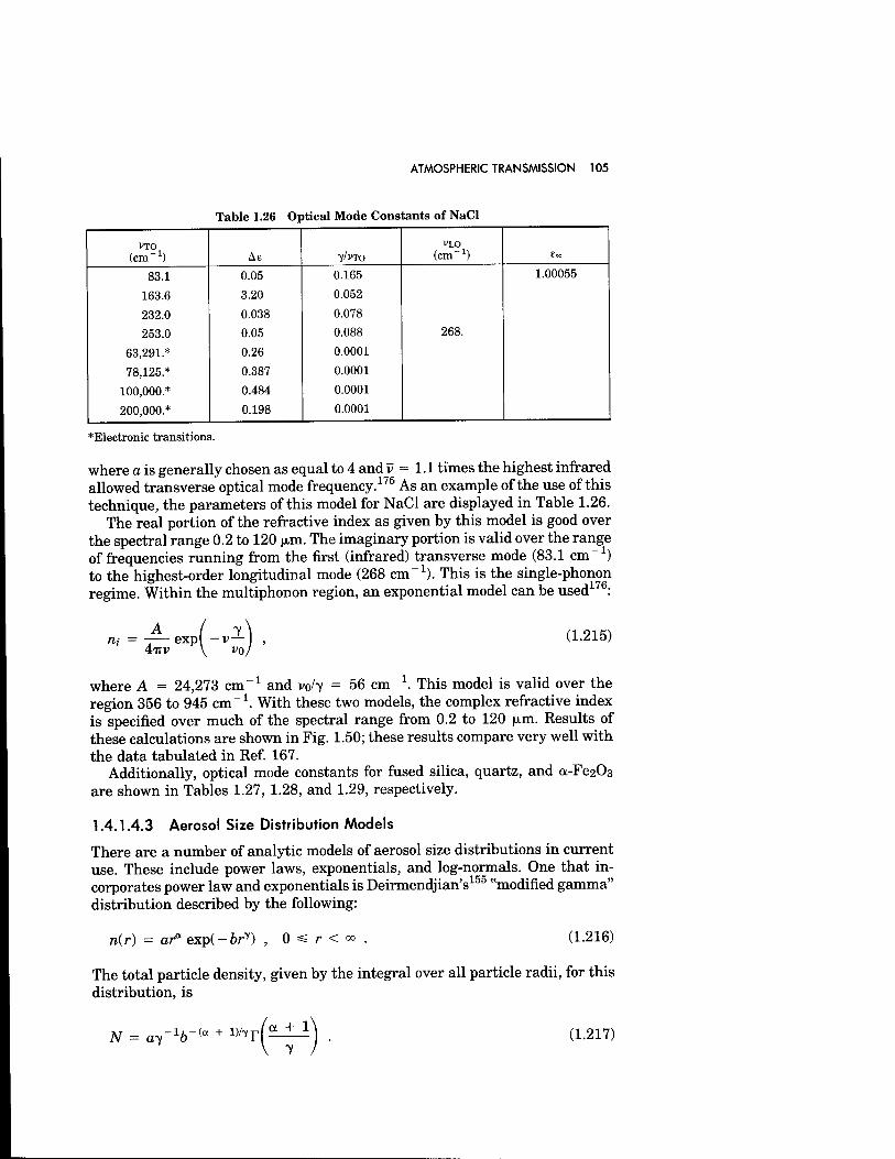
ATMOSPHERIC TRANSMISSION 105
Table 1.26 Optical Mode Constants of NaCl
VTO (cm"1) AE 7/vTo
VLO (cm^1) E«,
83.1 0.05 0.165 1.00055
163.6 3.20 0.052
232.0 0.038 0.078
253.0 0.05 0.088 268.
63,291.* 0.26 0.0001
78,125.* 0.387 0.0001
100,000.* 0.484 0.0001
200,000.* 0.198 0.0001
*Electronic transitions.
where a is generally chosen as equal to 4 and v = 1.1 times the highest infrared allowed transverse optical mode frequency.175 As an example of the use of this technique, the parameters of this model for NaCl are displayed in Table 1.26.
The real portion of the refractive index as given by this model is good over the spectral range 0.2 to 120 (im. The imaginary portion is valid over the range of frequencies running from the first (infrared) transverse mode (83.1 cm-1) to the highest-order longitudinal mode (268 cm"1). This is the single-phonon regime. Within the multiphonon region, an exponential model can be used176:
4TTV exp
vo (1.215)
where A = 24,273 cm-1 and voh = 56 cm"1. This model is valid over the region 356 to 945 cm"1. With these two models, the complex refractive index is specified over much of the spectral range from 0.2 to 120 |xm. Results of these calculations are shown in Fig. 1.50; these results compare very well with the data tabulated in Ref. 167.
Additionally, optical mode constants for fused silica, quartz, and a-Fe2C>3 are shown in Tables 1.27, 1.28, and 1.29, respectively.
1.4.1.4.3 Aerosol Size Distribution Models
There are a number of analytic models of aerosol size distributions in current use. These include power laws, exponentials, and log-normals. One that in- corporates power law and exponentials is Deirmendjian's155 "modified gamma" distribution described by the following:
Mr) = ara exp(-bry) , 0 =s r < 00 (1.216)
The total particle density, given by the integral over all particle radii, for this distribution, is
N = a-y-V« + 1)/7r(^~) (1.217)
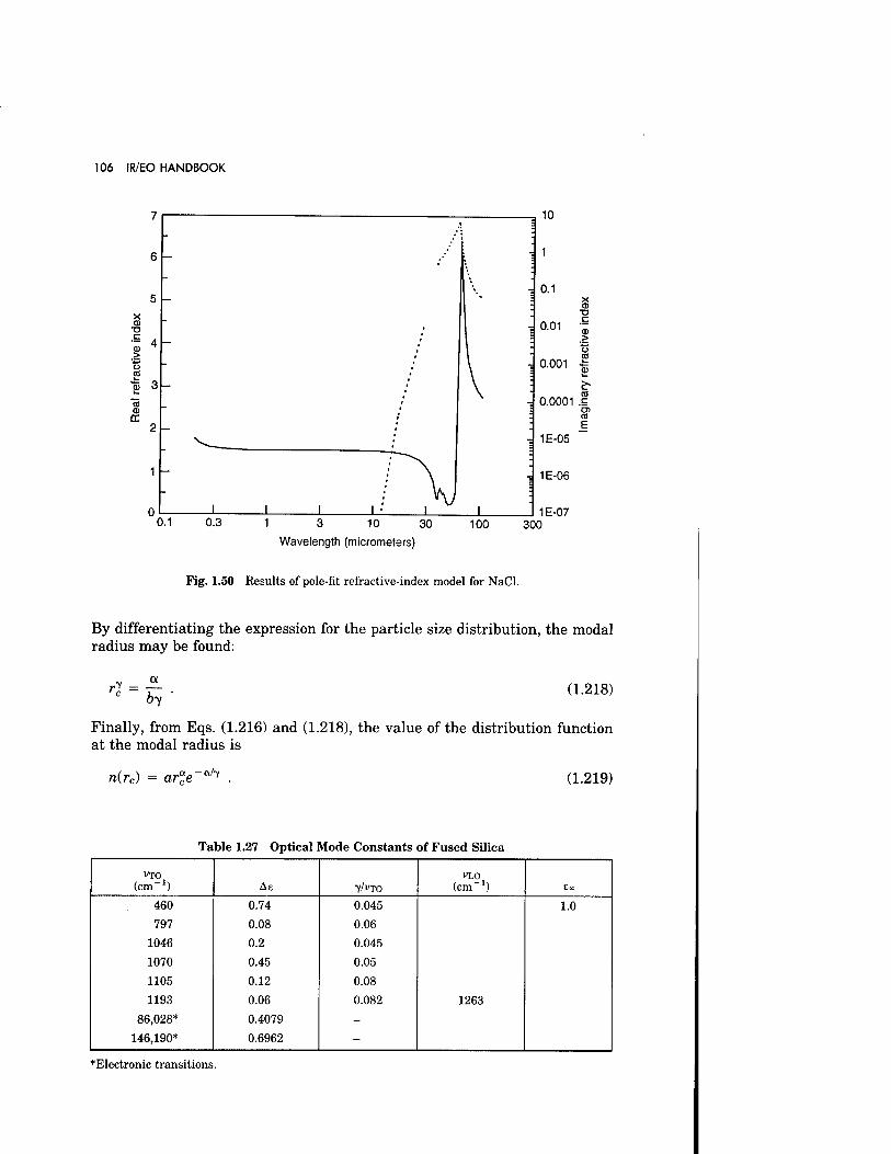
106 IR/EO HANDBOOK
x <c
c
*o 3
(0
EC
4
I J_ I 0.1 0.3 1 3 10 30
Wavelength (micrometers)
100
4 1
0.1
0.01
10
x o •D c
0.001 I
0.0001 .1 CO
£ 1E-05
1E-06
1E-07 300
Fig. 1.50 Results of pole-fit refractive-index model for NaCl.
By differentiating the expression for the particle size distribution, the modal radius may be found:
by (1.218)
Finally, from Eqs. (1.216) and (1.218), the value of the distribution function at the modal radius is
n(rc) = arace-
ah . (1.219)
Table 1.27 Optical Mode Constants of Fused Silica
VTO (cm-1) AE 7/vTO
VLO (cm"1) Eoo
460 0.74 0.045 1.0 797 0.08 0.06
1046 0.2 0.045
1070 0.45 0.05
1105 0.12 0.08
1193 0.06 0.082 1263
86,028* 0.4079 - 146,190* 0.6962 -
*Electronic transitions.
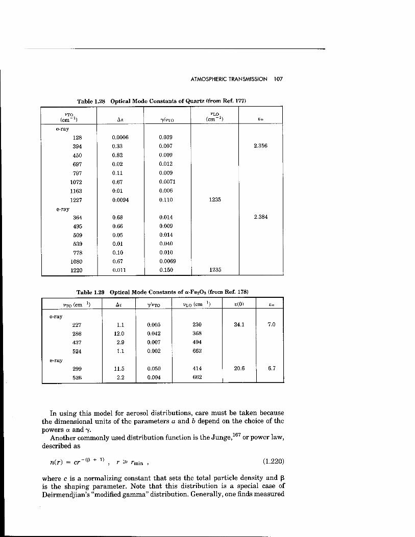
ATMOSPHERIC TRANSMISSION 107
Table 1.28 Optical Mode Constants of Quartz (from Ref. 177)
VTO (cm"1) AE 7/vTo
VLO (cm"1) £«>
o-ray
128 0.0006 0.039
394 0.33 0.007 2.356
450 0.82 0.009
697 0.02 0.012
797 0.11 0.009
1072 0.67 0.0071
1163 0.01 0.006
1227 0.0094 0.110 1235
e-ray
364 0.68 0.014 2.384
495 0.66 0.009
509 0.05 0.014
539 0.01 0.040
778 0.10 0.010
1080 0.67 0.0069
1220 0.011 0.150 1235
Table 1.29 Optical Mode Constants of a-Fe203 (from Ref. 178)
VTO (cm x) Ae -y/vxo VLO (cm *) e(0) £=o
o-ray
227 1.1 0.005 230 24.1 7.0
286 12.0 0.042 368
437 2.9 0.007 494
524 1.1 0.002 662
e-ray
299 11.5 0.050 414 20.6 6.7
526 2.2 0.004 662
In using this model for aerosol distributions, care must be taken because the dimensional units of the parameters a and b depend on the choice of the powers a and 7.
Another commonly used distribution function is the Junge,167 or power law, described as
n(r) = cr-(ß + « r 3* (1.220)
where c is a normalizing constant that sets the total particle density and ß is the shaping parameter. Note that this distribution is a special case of Deirmendjian's "modified gamma" distribution. Generally, one finds measured
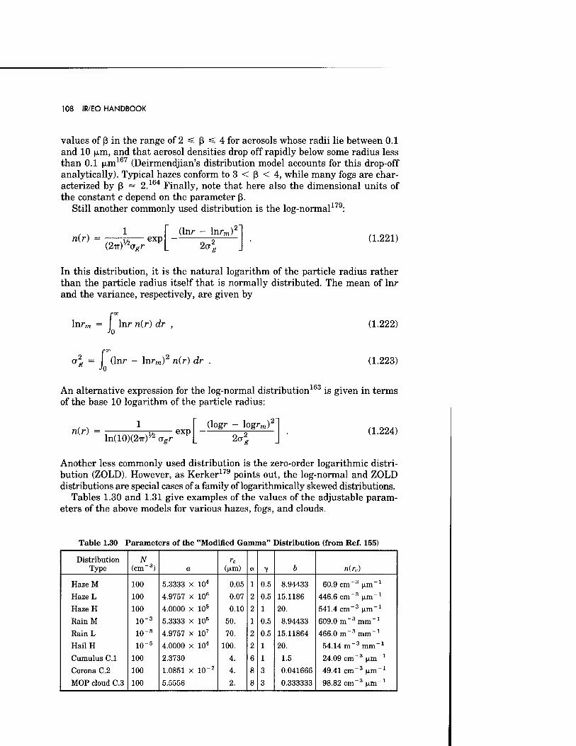
108 IR/EO HANDBOOK
values of ß in the range of 2 =£ ß =£ 4 for aerosols whose radii lie between 0.1 and 10 (xm, and that aerosol densities drop off rapidly below some radius less than 0.1 |xm167 (Deirmendjian's distribution model accounts for this drop-off analytically). Typical hazes conform to 3 < ß < 4, while many fogs are char- acterized by ß = 2.164 Finally, note that here also the dimensional units of the constant c depend on the parameter ß.
Still another commonly used distribution is the log-normal179:
n{r) = (2Tt)Kgr
exp (lnr - lnrm)'
2ul (1.221)
In this distribution, it is the natural logarithm of the particle radius rather than the particle radius itself that is normally distributed. The mean of lnr and the variance, respectively, are given by
lnr„ f Jo lnr n(r) dr
"* - ( (lnr - lnrm) n(r) dr .
(1.222)
(1.223)
An alternative expression for the log-normal distribution163 is given in terms of the base 10 logarithm of the particle radius:
n(r) = ln(10)(2ir)M! o>r
exp (logr - logrm)2
20-1 (1.224)
Another less commonly used distribution is the zero-order logarithmic distri- bution (ZOLD). However, as Kerker179 points out, the log-normal and ZOLD distributions are special cases of a family of logarithmically skewed distributions.
Tables 1.30 and 1.31 give examples of the values of the adjustable param- eters of the above models for various hazes, fogs, and clouds.
Table 1.30 Parameters of the "Modified Gamma" Distribution (from Ref. 155)
Distribution Type
N (cm"3) a (H-m) a 7 b n(rc)
Haze M 100 5.3333 x 10⁴ 0.05 1 0.5 8.94433 60.9 cm-3 (xm-1
Haze L 100 4.9757 x 10⁶ 0.07 2 0.5 15.1186 446.6 cm-3 (im-1
HazeH 100 4.0000 x 10⁵ 0.10 2 1 20. 541.4 cm-3 |xm_1
Rain M 10""3 5.3333 x 10⁵ 50. 1 0.5 8.94433 609.0 m-3 mm-1
Rain L 10"3 4.9757 x 10⁷ 70. 2 0.5 15.11864 466.0 m""3 mm-1
HailH 10-5 4.0000 x 10⁴ 100. 2 1 20. 54.14 m"3 mm"1
Cumulus C.l 100 2.3730 4. 6 1 1.5 24.09 cm"3 M-m"1
Corona C.2 100 1.0851 x 10⁻² 4. 8 3 0.041666 49.41 cm-3 (Jim-1
MOP cloud C.3 100 5.5556 2. 8 3 0.333333 98.82 cm-3 ^.m"1
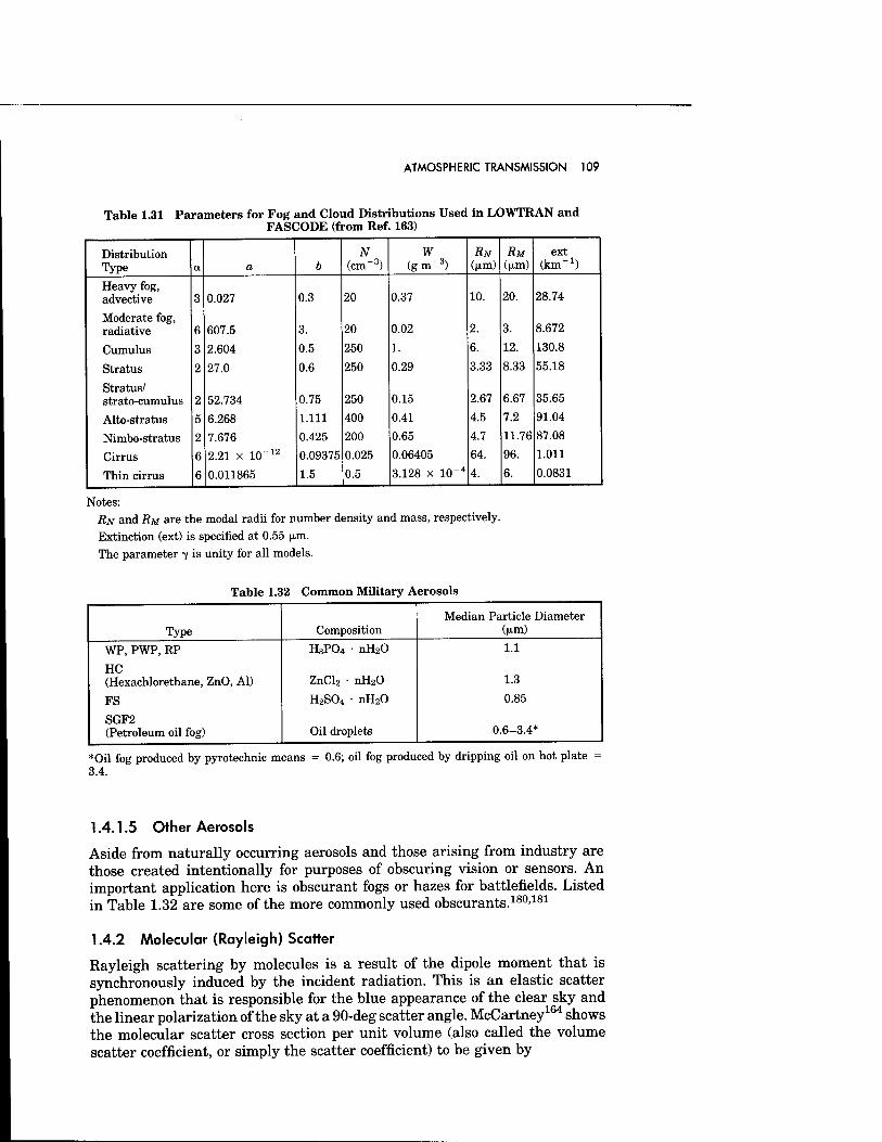
ATMOSPHERIC TRANSMISSION 109
Table 1.31 Parameters for Fog and Cloud Distributions Used FASCODE (from Ref. 163)
in LOWTRAN and
Distribution Type a a b
N (cm"3)
W (g nr3)
RN (jim)
RM (pi,m)
ext (km"1)
Heavy fog, advective 3 0.027 0.3 20 0.37 10. 20. 28.74
Moderate fog, radiative 6 607.5 3. 20 0.02 2. 3. 8.672
Cumulus 3 2.604 0.5 250 1. 6. 12. 130.8
Stratus 2 27.0 0.6 250 0.29 3.33 8.33 55.18
Stratus/ strato-cumulus 2 52.734 0.75 250 0.15 2.67 6.67 35.65
Alto-stratus 5 6.268 1.111 400 0.41 4.5 7.2 91.04
Nimbo-stratus 2 7.676 0.425 200 0.65 4.7 11.76 87.08
Cirrus 6 2.21 x 10~12 0.09375 0.025 0.06405 64. 96. 1.011
Thin cirrus 6 0.011865 1.5 0.5 3.128 x 10⁻⁴ 4. 6. 0.0831
Notes: RN and RM are the modal radii for number density and mass, respectively. Extinction (ext) is specified at 0.55 n-m. The parameter y is unity for all models.
Table 1.32 Common Military Aerosols
Type Composition Median Particle Diameter
((Jim)
WP, PWP, RP H3PO4 • nH20 1.1
HC (Hexachlorethane, ZnO, Al)
FS
ZnCl2 • nH20
H2SO4 • nH20
1.3
0.85
SGF2 (Petroleum oil fog) Oil droplets 0.6-3.4*
*Oil fog produced by pyrotechnic means = 0.6; oil fog produced by dripping oil on hot plate 3.4.
1.4.1.5 Other Aerosols
Aside from naturally occurring aerosols and those arising from industry are those created intentionally for purposes of obscuring vision or sensors. An important application here is obscurant fogs or hazes for battlefields. Listed in Table 1.32 are some of the more commonly used obscurants.180'181
1.4.2 Molecular (Rayleigh) Scatter
Rayleigh scattering by molecules is a result of the dipole moment that is synchronously induced by the incident radiation. This is an elastic scatter phenomenon that is responsible for the blue appearance of the clear sky and the linear polarization of the sky at a 90-deg scatter angle. McCartney164 shows the molecular scatter cross section per unit volume (also called the volume scatter coefficient, or simply the scatter coefficient) to be given by
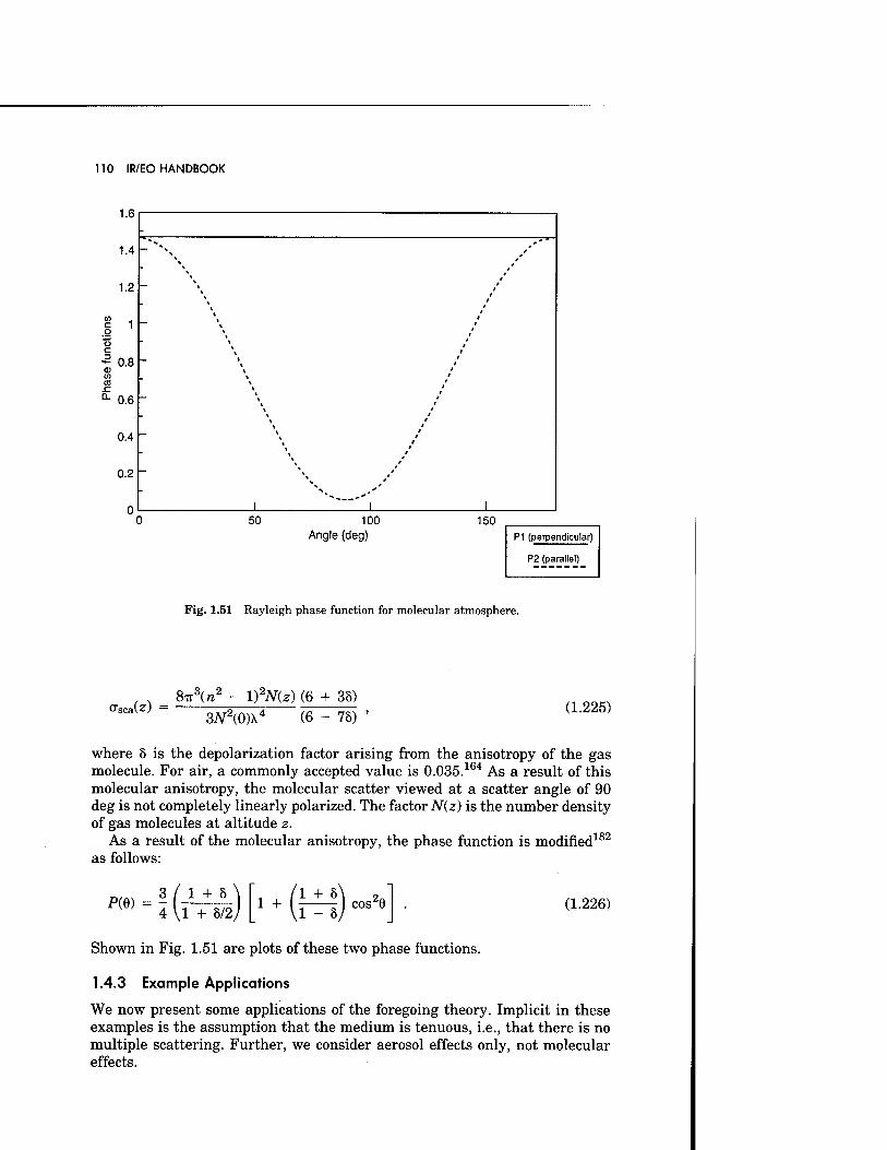
110 IR/EO HANDBOOK
I.D
1.4 • /
\ / 1.2
\ \
* %
i x t
"> * i c 1 % * g * t* o c * t
^0.8 t
Q) t (0 / CÖ .c * ' ^ 0.6 ■— *
/ t
i -
0.4 % t
0.2 \
r\ i i i 50 100
Angle (deg) 150
P1 (perpendicular)
P2 (parallel)
Fig. 1.51 Rayleigh phase function for molecular atmosphere.
Osca(z) = 8TT
3(/X
2 - l)2N(z) (6 + 38)
(6 - 75) ' W2(0)k4 (1.225)
where 8 is the depolarization factor arising from the anisotropy of the gas molecule. For air, a commonly accepted value is 0.035.164 As a result of this molecular anisotropy, the molecular scatter viewed at a scatter angle of 90 deg is not completely linearly polarized. The factor N(z) is the number density of gas molecules at altitude z.
As a result of the molecular anisotropy, the phase function is modified182
as follows:
P(6) = -A 4 1 + 8
1 + 8/2 1 +
1 + 8 1 2„ cos^e (1.226)
Shown in Fig. 1.51 are plots of these two phase functions.
1.4.3 Example Applications
We now present some applications of the foregoing theory. Implicit in these examples is the assumption that the medium is tenuous, i.e., that there is no multiple scattering. Further, we consider aerosol effects only, not molecular effects.
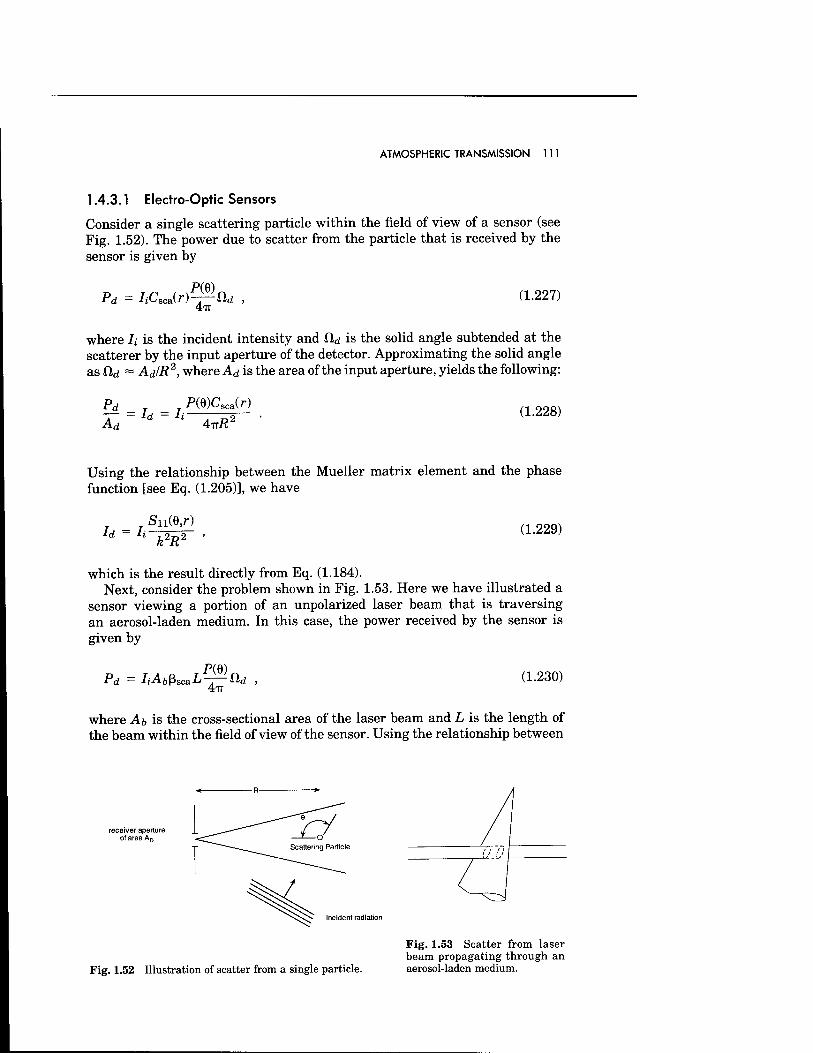
ATMOSPHERIC TRANSMISSION 111
1.4.3.1 Electro-Optic Sensors
Consider a single scattering particle within the field of view of a sensor (see Fig. 1.52). The power due to scatter from the particle that is received by the sensor is given by
Pd = /iCsca(r)^Üd (1.227)
where h is the incident intensity and Cld is the solid angle subtended at the scatterer by the input aperture of the detector. Approximating the solid angle as ttd ~ AdIR2, where Ad is the area of the input aperture, yields the following:
Ad Id = Ii
P(9)Csca(r)
4-rri?2 (1.228)
Using the relationship between the Mueller matrix element and the phase function [see Eq. (1.205)], we have
Id = 1, Sii(6,r)
2E>2 kzR (1.229)
which is the result directly from Eq. (1.184). Next, consider the problem shown in Fig. 1.53. Here we have illustrated a
sensor viewing a portion of an unpolarized laser beam that is traversing an aerosol-laden medium. In this case, the power received by the sensor is given by
P(Q) Pd = ZjAftßscaL—— fld
4lT (1.230)
where Ab is the cross-sectional area of the laser beam and L is the length of the beam within the field of view of the sensor. Using the relationship between
receiver aperture of area AD
Incident radiation
Fig. 1.52 Illustration of scatter from a single particle.
Fig. 1.53 Scatter from laser beam propagating through an aerosol-laden medium.
112 IR/EO HANDBOOK
the phase function and the Mueller matrix element, Eq. (1.205), this equation can be expressed as
Id =Ii VSn(6) k2R2 '
where V = AbL is the volume of the beam viewed by the sensor.
(1.231)
1.4.3.2 Transmission along a Slant Path
The change in the intensity for propagating a differential distance dz is pro- portional to the product of the intensity and a constant. This constant is given by the "extinction coefficient":
dJE dz
ßextE . (1.232)
This differential equation is solved easily to yield an exponential damping of the intensity known as Bouguer's law (sometimes called Beer-Lambert's law):
E(z) =E(0)exp(-ßextz) (1.233)
We define the transmission as the quotient of the observed intensity and the incident intensity;
(1.234)
This is the solution for the case of propagation through a homogeneous medium. For the case in which the scatter properties of the medium vary along the path length, the exponent is the path integral along the propagation path:
exp ■/:
ßext(s) ds (1.235)
Finally, if we consider molecular absorption, the total transmission is simply the product ofthat due to aerosol extinction and that due to molecular absorption.
On the basis of the previous development, we see that the transmission from ground level to a point R along a slant path is given by the following formula:
T(0,R) = exp (R
- ßext(r) dr Jo
(1.236)
By dividing and multiplying the exponent by the path integral along the vertical path, we can write this expression in the following form:
ATMOSPHERIC TRANSMISSION 113
7X0,Ä) = exp(-|v) , (1-237)
where we have defined the slant path and vertical line integrals, respectively, as
S = I ßext(r) dr , J° (1.238)
V = ßext(s) ds Jo
Finally, we observe that the slant path transmission is simply the vertical transmission raised to the secant of the angle of the slant path with respect to vertical:
T(0,R) = exp(-V)s/v , (1.239)
or, finally,
T(0,R) = T{0,z)secl , (1.240)
where £ is the zenith angle. Note that implicit in this development is the assumption that the earth is flat, i.e., that the medium is plane-stratified. This approximation is generally adequate if the zenith angle is less than 75 deg. Beyond this point, however, earth-curvature effects come into play.
A convenient means of accounting for earth-curvature effects is to use the Chapman function183 in place of the term sect,. This function is expressed as
Ch(v,£) = x sin£ exp(x - x sinC cscv|») csc2\\s d\\i , (1.241)
where
{Zp + Te) , (1.242) lP
where, as illustrated in Fig. 1.54, Zp is the altitude of the receiver, re is the radius of the earth, and Hp is the density scale height appropriate for the altitude Zp.
This function is based on an isothermal atmosphere, and ignores refractive bending. The sea-level density scale height is given by the expression
H0 = — , (1.243)
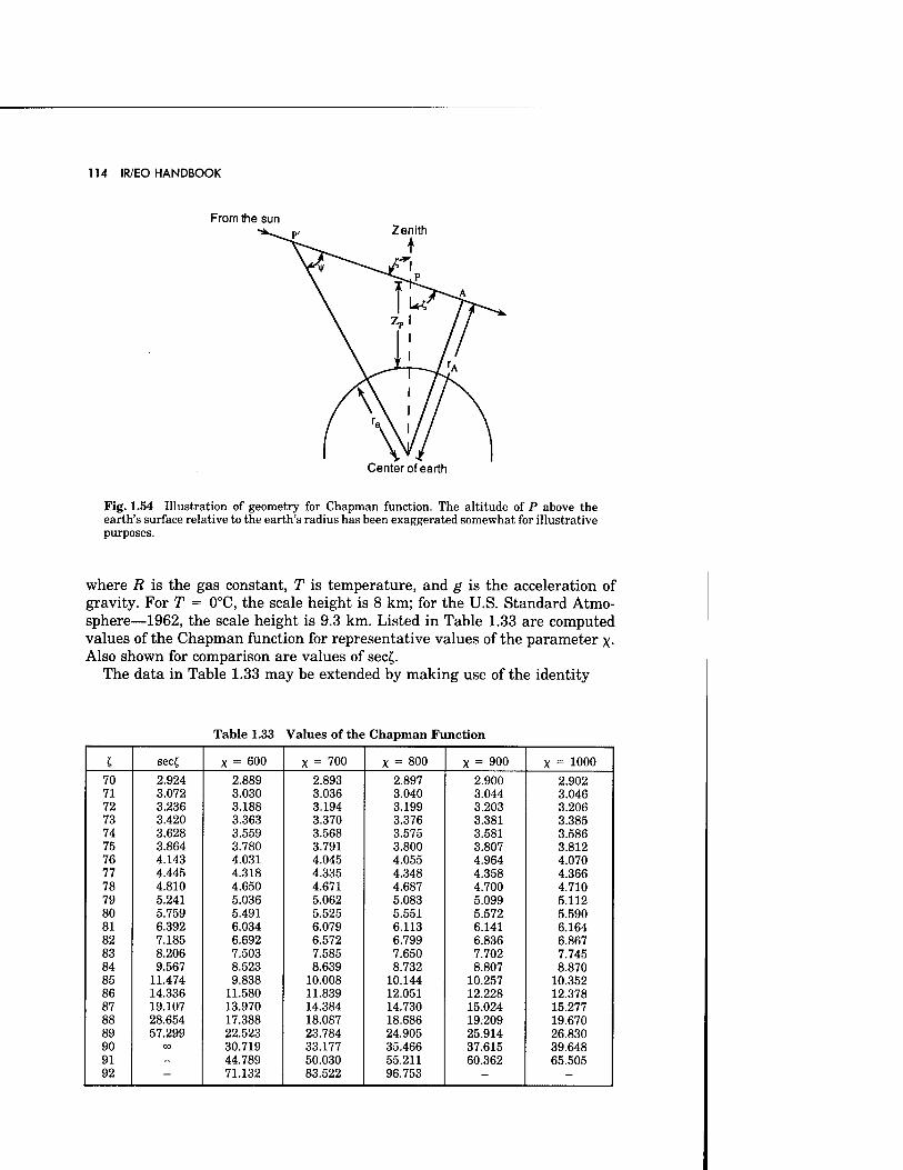
114 IR/EO HANDBOOK
From the sun
Center of earth
Fig. 1.54 Illustration of geometry for Chapman function. The altitude of P above the earth's surface relative to the earth's radius has been exaggerated somewhat for illustrative purposes.
where R is the gas constant, T is temperature, and g is the acceleration of gravity. For T = 0°C, the scale height is 8 km; for the U.S. Standard Atmo- sphere—1962, the scale height is 9.3 km. Listed in Table 1.33 are computed values of the Chapman function for representative values of the parameter x- Also shown for comparison are values of sec£.
The data in Table 1.33 may be extended by making use of the identity
Table 1.33 Values of the Chapman Function
I sec£ X = 600 X = 700 X = 800 X = 900 X = 1000
70 2.924 2.889 2.893 2.897 2.900 2.902 71 3.072 3.030 3.036 3.040 3.044 3.046 72 3.236 3.188 3.194 3.199 3.203 3.206 73 3.420 3.363 3.370 3.376 3.381 3.385 74 3.628 3.559 3.568 3.575 3.581 3.586 75 3.864 3.780 3.791 3.800 3.807 3.812 76 4.143 4.031 4.045 4.055 4.964 4.070 77 4.445 4.318 4.335 4.348 4.358 4.366 78 4.810 4.650 4.671 4.687 4.700 4.710 79 5.241 5.036 5.062 5.083 5.099 5.112 80 5.759 5.491 5.525 5.551 5.572 5.590 81 6.392 6.034 6.079 6.113 6.141 6.164 82 7.185 6.692 6.572 6.799 6.836 6.867 83 8.206 7.503 7.585 7.650 7.702 7.745 84 9.567 8.523 8.639 8.732 8.807 8.870 85 11.474 9.838 10.008 10.144 10.257 10.352 86 14.336 11.580 11.839 12.051 12.228 12.378 87 19.107 13.970 14.384 14.730 15.024 15.277 88 28.654 17.388 18.087 18.686 19:209 19.670 89 57.299 22.523 23.784 24.905 25.914 26.830 90 oo 30.719 33.177 35.466 37.615 39.648 91 - 44.789 50.030 55.211 60.362 65.505 92 - 71.132 83.522 96.753 - -
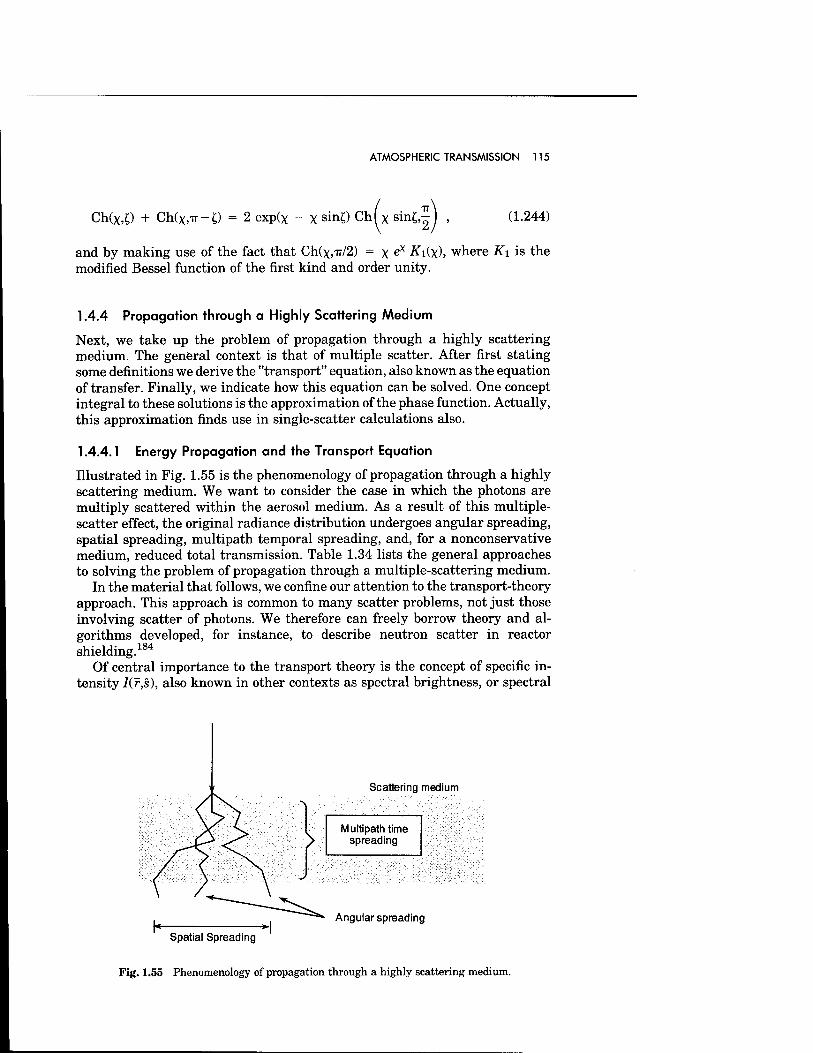
Ch(x,0 + Ch(x,ir-Ö = 2 exp(X - x sinÖ Ch( x sin£,-
ATMOSPHERIC TRANSMISSION 115
(1.244)
and by making use of the fact that Ch(x,-rr/2) = x e* Ki(\), where K\ is the modified Bessel function of the first kind and order unity.
1.4.4 Propagation through a Highly Scattering Medium
Next, we take up the problem of propagation through a highly scattering medium. The general context is that of multiple scatter. After first stating some definitions we derive the "transport" equation, also known as the equation of transfer. Finally, we indicate how this equation can be solved. One concept integral to these solutions is the approximation of the phase function. Actually, this approximation finds use in single-scatter calculations also.
1.4.4.1 Energy Propagation and the Transport Equation
Illustrated in Fig. 1.55 is the phenomenology of propagation through a highly scattering medium. We want to consider the case in which the photons are multiply scattered within the aerosol medium. As a result of this multiple- scatter effect, the original radiance distribution undergoes angular spreading, spatial spreading, multipath temporal spreading, and, for a nonconservative medium, reduced total transmission. Table 1.34 lists the general approaches to solving the problem of propagation through a multiple-scattering medium.
In the material that follows, we confine our attention to the transport-theory approach. This approach is common to many scatter problems, not just those involving scatter of photons. We therefore can freely borrow theory and al- gorithms developed, for instance, to describe neutron scatter in reactor shielding.184
Of central importance to the transport theory is the concept of specific in- tensity I(r,s), also known in other contexts as spectral brightness, or spectral
Scattering medium
Multipath time spreading
Angular spreading
Spatial Spreading
Fig. 1.55 Phenomenology of propagation through a highly scattering medium.
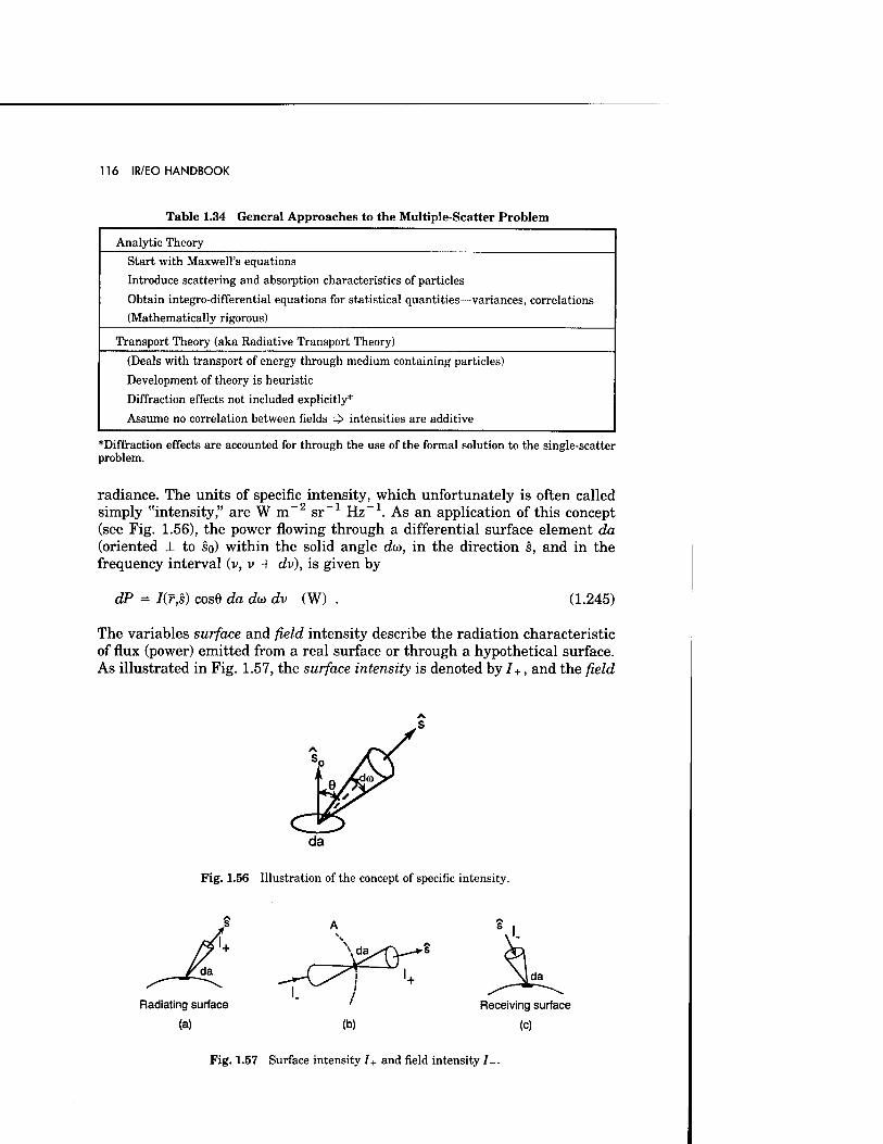
116 IR/EO HANDBOOK
Table 1.34 General Approaches to the Multiple-Scatter Problem
Analytic Theory
Start with Maxwell's equations
Introduce scattering and absorption characteristics of particles
Obtain integro-differential equations for statistical quantities—variances, correlations
(Mathematically rigorous)
Transport Theory (aka Radiative Transport Theory)
(Deals with transport of energy through medium containing particles)
Development of theory is heuristic
Diffraction effects not included explicitly*
Assume no correlation between fields => intensities are additive
*Diffraction effects are accounted for through the use of the formal solution to the single-scatter problem.
radiance. The units of specific intensity, which unfortunately is often called simply "intensity," are W m~2 sr_1 Hz-1. As an application of this concept (see Fig. 1.56), the power flowing through a differential surface element da (oriented 1 to so) within the solid angle da>, in the direction s, and in the frequency interval (v, v + dv), is given by
dP = I(r,s) cos6 da dco dv (W) . (1.245)
The variables surface and field intensity describe the radiation characteristic of flux (power) emitted from a real surface or through a hypothetical surface. As illustrated in Fig. 1.57, the surface intensity is denoted by 7+, and the field
Fig. 1.56 Illustration of the concept of specific intensity.
I. Radiating surface ' Receiving surface
(a) (b) (c)
Fig. 1.57 Surface intensity /+ and field intensity /-.
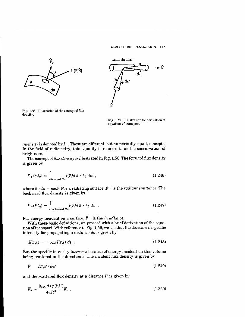
ATMOSPHERIC TRANSMISSION 117
A s„
Pig. 1.58 Illustration of the concept of flux density.
■ ds
fl-p^n- -*~s
Fig. 1.59 Illustration for derivation of equation of transport.
intensity is denoted by I-. These are different, but numerically equal, concepts. In the field of radiometry, this equality is referred to as the conservation of brightness.
The concept of flux density is illustrated in Fig. 1.58. The forward flux density is given by
\(T;SO) = [ forward 2ir
I(r,s) S • So dw , (1.246)
where s • so = cos6. For a radiating surface, F+ is the radiant emittance. The backward flux density is given by
F_(r,so) = f backward 2n
I(r,s) S • So d(x> (1.247)
For energy incident on a surface, F- is the irradiance. With these basic definitions, we proceed with a brief derivation of the equa-
tion of transport. With reference to Fig. 1.59, we see that the decrease in specific intensity for propagating a distance ds is given by
dl(r,s) = - (TexJ(r,s) ds . (1.248)
But the specific intensity increases because of energy incident on this volume being scattered in the direction s. The incident flux density is given by
Ft = Kr,s') dm'
and the scattered flux density at a distance R is given by
ßext dsp(s,s'). F„ =
4TTRZ -Ft ,
(1.249)
(1.250)
118 IR/EO HANDBOOK
where p(s,s') is the phase function such that
-^ | p(s,s) dw = a (albedo) . (1.251)
Integrating over the solid angle, the contribution to the specific intensity is
^-^ f p(s,s')I(f,s') dco' . (1.252) 4lT Uv
Including the possibility of emission within the volume, the specific intensity is increased by
e(r,s) ds , (1.253)
where e(r,s) is the power radiated per unit volume and per solid angle in the direction s. The equation of transport thus becomes
dl(f,s) , = -ßext/(r,s) + ^ [ p(s,s')/(r,s') dco' + e(f,s) . (1.254)
OS 4lT J4TT
In this equation, the left-hand side represents the change in specific intensity. Terms on the right-hand side represent the extinction, the increase due to scatter, and the increase due to sources within the scattering medium, respectively.
By defining the "optical distance" T as the path integral of the extinction cross section per unit volume,
T = I ßext ds ,
the transport equation can be written as
(1.255)
d/(r's) - I(f,s) + -^ I p(s,s')I(r,s') dw' + J(f,s) , (1.256) dr 4TT
where
Jim = ^ (1.257) Pext
is commonly called the source function. There are myriad approaches to solution of the transport equation. Chapter
4 of Ref. 167 discusses various exact (normal-mode expansion, Wiener-Hopf) and approximate (spherical harmonics, discrete ordinates, doubling, Monte Carlo, etc.) techniques. Here we show one example of each of the exact and approximate techniques. We restrict our attention to the plane-parallel ge-
ATMOSPHERIC TRANSMISSION 119
ometry. This geometry is appropriate, for example, to planetary atmospheres, clouds, ocean waters illuminated by the sun, etc. The basic assumption is that of a plane wave incident on a plane-parallel medium. For discussion of other geometries and solution approaches, see Refs. 158, 182, and 185.
1.4.4.1.1 Two- and Four-Flux Theory
The (Kubelka-Munk) two-flux theory is an approximate solution that ade- quately describes the case in which the illumination is diffused and the medium is "dull" so that light is diffusely scattered. It does not adequately describe the case of collimated incident radiation; for this case, the four-flux theory is required.
In the two-flux theory the flux is envisioned as being composed of a positive- flowing flux F+ and a negative-flowing flux F-. Conceptually, it is equivalent to approximating the phase function as a weighted sum of delta functions in the forward and backward directions.
In propagating a differential distance dz, the positive-flowing flux is de- creased due to absorption within dz and scattering into the backward direction:
dF+ = -{K + S)F+ßext dz= -{K + S)F+ dx , (1.258)
where K and S are dimensionless absorption and scatter coefficients. On the other hand, the positive-flowing flux is increased due to backward scattering fromF-:
dF+ = SF_ßeXt dz = SF- dj . (1.259)
With similar behavior for the backward-flowing flux, we arrive at a coupled set of differential equations:
^i = -(K + S)F+ + SF^- , dr
(1.260) dF ^ = (K + S)F- - SF+ . di
By assuming an exponential behavior for F+ and F-, exp(az) so that dldi = a, we obtain a pair of algebraic equations whose solution is given by
a± = [K(K + 2S)]^ = ±a0 . (1.261)
The complete solutions for F+ and F- are then given by
F+(T) = Ciea0T + C2e"a0T , (1.262)
F-M = C3ea0T + C4e-a0T ,
120 IR/EO HANDBOOK
where the C's are determined by application of the boundary conditions. As Ishimaru185 points out, the coefficients K and S are not clearly related to the physical properties of the scattering particles. However, they can be deter- mined empirically, with the following result186:
Äßext ~ ^ßabs , ,-, nnr>\
S ~ |a(l - g) ,
where a is the single-scatter albedo and g is the asymmetry parameter (see Sec. 1.4.4.2).
As noted previously, the four-flux theory is required for describing the prop- agation, for example, of a laser beam in a highly scattering medium. In this theory, the power flow is represented in terms of forward- and backward- flowing collimated fluxes and foward- and backward-flowing diffuse fluxes. The collimated fluxes, i.e., the reduced intensities, decrease due to scattering and absorption; they are continuously being converted into diffuse intensities by scattering. This approach is similar to that of the two-flux method, with the addition of parameters that represent the scatter and absorption from colli- mated beams.
1.4.4.1.2 Discrete Ordinates Method
This is an example of an exact method. We restrict our attention to a source- free region, so the transport equation becomes
^T^ = -ßext/(r,s) + ^tf p(s;s')I(f,s') dco' . (1.264) as 4TT J4TT
We decompose the intensity into the sum of the reduced incident intensity and the diffuse intensity, and use for the incident (plane-wave) flux
Iri(r,s) = Fo exp(-T)8(|x - 1)8(4>) , (1.265)
where (x = cos6. Using this decomposition of the specific intensity and Eq. (1.265) for the reduced incident intensity in the transport equation and inte- grating over the azimuthal variable ()>, we obtain the following equation for the diffuse intensity:
|X 37 + /d(T,|x) = -J /70(^,^')/d(T,(A') d\i' dr
+ -^po(|x,l)F0e-T , (1.266)
where
PO(M.,M/) = ^- [ "d* 7TI *W P(M-.4>;M.\<I>') • d-267)
ATMOSPHERIC TRANSMISSION 121
As an example, for the Rayleigh phase function,
pOi.,<|>;H',<|>') = |o(l + cos27) , (1.268)
where 7 is the angle between (\L,<\>) and (n.', ()>'), given by
COS7 = cos6 cos6' + sine sine' cos(<J> - <)>') . (1.269)
Integrating this phase function over cj> and <(>', one obtains
po(|JL,|x') = -a 1 + M.V'2 + |d - (x2)d - V.'2) (1.270)
Equation (1.266) plus the boundary conditions constitute the complete state- ment of the problem. One commonly used solution of this integro-differential equation is to approximate the integral with a quadrature technique; the integration is replaced by a summation. In effect, the integrand is sampled at a number of discrete angles (JL'J. AS a result, one obtains a matrix linear first- order differential equation. Upon assuming exponential variations for the ho- mogeneous and particular solutions, the problem reduces to a matrix eigen- value problem. See Ishimaru185 for details.
1.4.4.2 Phase Function Approximation
A very useful computational expedient, especially within the context of multiple- scatter calculations, is the approximate representation of the single-scatter phase function. The traditional expansion is the following:
N
oP(cose) = E w« P„(cose) , (1.271) n = 0
where the single-scatter albedo is denoted by a and Pn is the Legendre poly- nomial of order n. Making use of the orthogonality of these polynomials results in the expression for the expansion coefficients:
<o„ = (2n * 1)a f P(cose) p„(cose) d(cose) . (1.272) z J — 1
From this equation, one finds that wo = a and wi = 3ag, where g is the asymmetry parameter defined as
g = i I P(cose) cose d(cos6) . (1.273)
This asymmetry parameter finds use as a parameter in many other phase- function approximations, notably the Henyey-Greenstein approximation187:
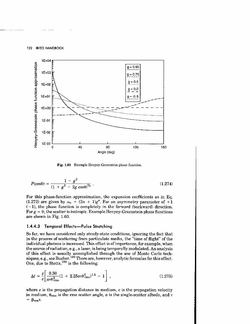
122 IR/EO HANDBOOK
1E+04
1E+03
1E+02 -
c o '■a E "x 9 Q. Q. CO
C o
c 1E+01 3
03 CO CO x: D. c
'(D t£ 1E-01
CD 1E-02 r Q>
C CD I
1E-03
I g = 0.95
r g = 0.75
**• \
g = o.5
g = 0.0
i— \v«-.-.--..
•■^"— ■-.-.-- ---•-
g=-0.5 .
--""— -
r
i i i
1E+00 | *v
45 90 Angle (deg)
135 180
Fig. 1.60 Example Henyey-Greenstein phase function.
P(cos8) = (1 + g2 - 2g cos9)% (1.274)
For this phase-function approximation, the expansion coefficients as in Eq. (1.272) are given by a>„ = (2n + l)gn. For an asymmetry parameter of +1 (-1), the phase function is completely in the forward (backward) direction. For g = 0, the scatter is isotropic. Example Henyey-Greenstein phase functions are shown in Fig. 1.60.
1.4.4.3 Temporal Effects—Pulse Stretching
So far, we have considered only steady-state conditions, ignoring the fact that in the process of scattering from particulate media, the "time of flight" of the individual photons is increased. This effect is of importance, for example, when the source of radiation, e.g., a laser, is being temporally modulated. An analysis of this effect is usually accomplished through the use of Monte Carlo tech- niques, e.g., see Bücher.188 There are, however, analytic formulas for this effect. One, due to Stotts,189 is the following:
At = 0.30
(1 + 2.25aT0?ms)1'5 - 1 (1.275)
where z is the propagation distance in medium, c is the propagation velocity in medium, 6rms is the rms scatter angle, a is the single-scatter albedo, and T = PscaZ.
ATMOSPHERIC TRANSMISSION 123
This formula for pulse stretching (At) is based purely on geometrical ar- guments. Implicit in the derivation is that we are in the geometrical optics regime; i.e., the phase function is highly peaked in the forward direction.
1.4.5 Imaging through a Scattering Medium
In this section we draw a link between the characterization of the aerosol- scattering medium and its effect on imaging. As examples we discuss "visibility range" and the mutual coherence function (MCF) for multiple-forward-scatter media.190-191
1.4.5.1 Visibility Range
Estimates of the visual range usually are made from the appearance of build- ings and special targets at differing distances against the skyline. The formula for the visual range Rv is
Rv = ^~ In- , (1.276) Psca E
where C is the inherent contrast of the target and e is the threshold contrast of the observer. The use of the scatter cross section rather than the extinction cross section in this definition implies that absorption by atmospheric particles at visual wavelengths is small enough to ignore. This view probably is justified except in cases of polluted air. Meteorological range is defined in terms of a black target (inherent contrast against sky is unity, C = 1) and for a 2% contrast threshold:
Rm = ~ • d.277)
Unfortunately, sometimes reference is made to a "visibility range" at a wavelength other than the visible. From the above discussion, however, it is obvious that at wavelengths for which absorption cannot be ignored, ßsca in Eq. (1.277) must be replaced by ßext- See the earlier discussion of the wave- length variation of scatter cross section (and extinction cross section) and also McCartney's164 discussion.
1.4.5.2 MCF for Aerosol Scatter
We here derive an expression for the point-spread function for propagation through aerosol-laden media. We do this first by deriving an expression for the (spatial) Fourier transform of the PSF, i.e., the optical transfer function (OTF).
Goodman192 has shown that the OTF for propagation through a random inhomogeneous medium can be written as
M(v) = ^ , (1.278) p = X/v
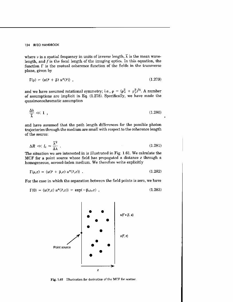
124 IR/EO HANDBOOK
where v is a spatial frequency in units of inverse length, X is the mean wave- length, and / is the focal length of the imaging optics. In this equation, the function T is the mutual coherence function of the fields in the transverse plane, given by
r(p) = (u(f + p) u*(r)) , (1.279)
and we have assumed rotational symmetry; i.e., p = (p* + p2y) . A number
of assumptions are implicit in Eq. (1.278). Specifically, we have made the quasimonochromatic assumption
T<<x' (1.280)
and have assumed that the path length differences for the possible photon trajectories through the medium are small with respect to the coherence length of the source:
AR « lc A\ (1.281)
The situation we are interested in is illustrated in Fig. 1.61. We calculate the MCF for a point source whose field has propagated a distance z through a homogeneous, aerosol-laden medium. We therefore write explicitly
r(p,z) = {u(f + p,z) u*(r,z)) . (1.282)
For the case in which the separation between the field points is zero, we have
T(0) = (u(r,z) u*(r,z)) = exp(-ßabsz) , (1-283)
Point source
• •
U(f+p, 2)
u(nz)
Fig. 1.61 Illustration for derivation of the MCF for scatter.
ATMOSPHERIC TRANSMISSION 125
where ßabs is the aerosol absorption cross section per unit volume. We now consider separations so large that no radiation scattered from any single aero- sol particle can reach both points f + p and r. In this case, any coherence that exists between the fields at the two points must be due to radiation that has not been scattered; i.e.,
IX«) = exp(-ßextz) , (1.284)
where the extinction cross section per unit volume ßext is given by the sum of the absorption and scatter cross sections per unit volume:
ßext = ßabs + ßsca . (1.285)
Between these two limits the MCF decreases more or less monotonically from a maximum at p = 0 to a minimum as p —> °°. Based on the assumption of multiple independent small-angle scatterings, Wells193 has shown that the MCF can be expressed as
Hp) = exp{-ßabs2 - ßscaZtl - ftp)]} , (1.286)
where the function f(p) is given by
AP) = T- I -P(Ö) dÜ, Mkpu sinG) du , (1.287) 4TT J4TT JO
where P(6) is the average of the two scatter polarization components perpen- dicular and parallel to the scattering plane:
P») - [Pm : P2(e)1 , (1.288)
and Jo is the Bessel function of the first kind and order zero. With the preceding, we can write the OTF as the linear superposition:
M(p) = exp(-ßScaz) + [1 - exp(-ßScaz)]Msca(p) . (1.289)
The first term on the right-hand side of Eq. (1.289) represents the contribution to the OTF that is due to light not scattered within the medium; it represents the asymptote to which the OTF falls for large separation p. The second term is due to that portion of the radiation that is scattered. From Eqs. (1.278), (1.286), and (1.289), we can write this portion as
.. , , /exp{-ßscaz[l - ftp)]}- exp(-ßscaz)\ Msca(p) = [ l-exp(-ßscaZ) j • (L290)
We formally regard this as the OTF due to scatter. These two components of the OTF [Eqs. (1.289) and (1.290)] are illustrated in Fig. 1.62.
We now derive an expression for the OTF due to scatter in the multiple- scatter regime. In this case ßSCaZ » 1, and Eq. (1.290) becomes Msca(p) =
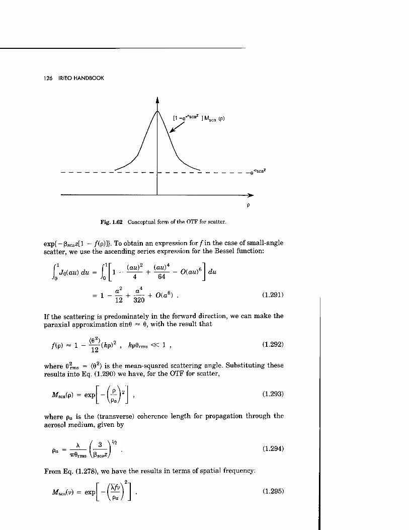
126 IR/EO HANDBOOK
[1 -e-°scaZ ] Msca (p)
,"°scaz
Fig. 1.62 Conceptual form of the OTF for scatter.
exp{ - ßsca^tl _ /Xp)]}- To obtain an expression for /"in the case of small-angle scatter, we use the ascending series expression for the Bessel function:
Jo(au) du = Jo Jo
(auf , (au) 6 1 — + — O(au) 4 64
du
«2 „4
1 - 12 + 320 + °ia) ■ (1.291)
If the scattering is predominately in the forward direction, we can make the paraxial approximation sinö ~ 9, with the result that
/o2\
/Xp) - 1 - -jj(ÄP)2 , Mrms « 1 > (1.292)
where 6 rms = (Ö2) is the mean-squared scattering angle. Substituting these results into Eq. (1.290) we have, for the OTF for scatter,
MSca(p) = exp .£.12
Pa, (1.293)
where pa is the (transverse) coherence length for propagation through the aerosol medium, given by
Pa TTÖrms VPsca^
Vi (1.294)
From Eq. (1.278), we have the results in terms of spatial frequency:
2-
MSca(v) = exp A/v
Pa (1.295)
ATMOSPHERIC TRANSMISSION 127
Recall that the point-spread function is the inverse Fourier transform of the OTF. It therefore can be shown easily that the PSF for scatter ssca(r) is given by
Tpa Ssca(r) = —2 exp
(Ay)
2 2 TT r (1.296)
(Xf/Paf
We note that the lie point of this PSF is given by
r = -^ , (1-297)
or, expressed in terms of the angle at the focal plane,
- = — . (1.298) f vPa
These results state that in the focal plane, the image of a point source will appear as a bright spot at the geometrical image position, surrounded by a diffuse halo. The bright spot is due to light that has not undergone scatter [the first term on the right-hand side of Eq. (1.289)] and a portion that has been scattered [the second term in Eq. (1.289)]. The angular half-width of the halo surrounding the geometrical point image is given by Eq. (1.298).
1.5 COMPUTER CODES ON ATMOSPHERIC PROPAGATION
Many of the models discussed previously are contained in atmospheric trans- mission codes, which provide a powerful tool for quantifying atmospheric ef- fects. The most commonly used codes are maintained by the Geophysics Di- rectorate at Hanscom Air Force Base, Massachusetts (formerly Air Force Geophysics Laboratory and Air Force Cambridge Research Laboratory). They are LOWTRAN, MODTRAN, and FASCODE and are briefly described in this section. These codes allow for complex atmospheric transmittance and radiance calculations based on absorption and scattering phenomena for a variety of path geometries. LOWTRAN is a low-resolution (20-cm_1) code, MODTRAN is a moderate resolution (2-cm-1) code, and FASCODE is a high-resolution code. FASCODE uses the HITRAN database directly and LOWTRAN and MODTRAN use the HITRAN database indirectly to determine band-model parameters. The widespread availability and use of these codes is why this chapter foregoes extensive figures and tables of limited value on transmittance and radiance.
1.5.1 LOWTRAN
LOWTRAN is the name of a series of computer codes beginning with LOWTRAN 2 (first available in 1972) and ending with the most recent version LOWTRAN 7 (first available in 1989).194"200 LOWTRAN calculates the transmittance and/or radiance for a specified path through the atmosphere based on the LOWTRAN band model discussed previously, molecular continuum absorp- tion, molecular scattering, and aerosol absorption and scattering models. Ra-
128 IR/EO HANDBOOK
diance calculations include atmospheric self-emission, solar and/or lunar ra- diance single scattered into the path, direct solar irradiance through a slant path to space, and multiple scattered solar and/or self-emission radiance into the path. The model covers the spectral range from 0 to 50,000 cm-1 at a resolution of 20 cm ~1. The band model spectral parameters exist every 5 cm ~1.
The atmosphere is represented as 32 layers from 0 to 100,000 km altitude. Layer thickness varies from 1 km up to 25 km, 5 km from 25 to 50 km (the top of the stratosphere), and the last two layers are 20 and 30 km thick, respectively. Detailed structure just above the land or sea is not represented by this model and thus model predictions can be inaccurate if nonstandard conditions exist. Attenuation and refractive effects are calculated for each layer and summed along the path. The physical characteristics of each layer are determined by inputs and predetermined standard models of various regions and seasons (see Table 1.35).194~200 The option to specify a particular atmo- sphere also exists. The atmosphere is assumed to be in thermal equilibrium; the code should not be used above 100 km or at and above the ionosphere.
Figures 1.63 to 1.67 illustrate typical LOWTRAN outputs for various types of atmospheres, spectral regions, mechanisms of attenuation, path emission, and path geometries.
LOWTRAN has been validated against field measurements75,201 and is widely used for many broadband system performance studies. However, the single- parameter band model used in LOWTRAN has limited validity with respect to temperature dependence. Calculations above and below room temperature should be checked against more physically complete codes such as FASCODE (see Sec. 1.5.3). In particular, LOWTRAN works best at low altitudes with moderate temperatures. High-altitude calculations (> 40 km) will have the least accurate results. Because of the limited resolution of LOWTRAN it should not be applied to laser propagation modeling when local line absorption is important.
1.5.2 MODTRAN
MODTRAN is identical to LOWTRAN except it contains the MODTRAN band model as described in Sec.1.3.4.3. MODTRAN offers moderate-resolution (2 cm-1) calculations with improved temperature and pressure dependence over LOWTRAN. Thus, high-altitude (< 60 km) calculations are more valid com- pared to LOWTRAN calculations. Figure 1.68 compares a MODTRAN output to a LOWTRAN output and clearly demonstrates the improved representation when resolution is an issue. Figure 1.69 compares a high-altitude radiance calculation from LOWTRAN and MODTRAN. In this case LOWTRAN 7 does not correctly model the radiance at low temperature.
1.5.3 FASCODE
For studies involving the propagation of very narrow optical bandwidth ra- diation, for example, lasers, the high resolution afforded by FASCODE is re- quired. Characterization of the aerosol and molecular medium in FASCODE is much the sme as that for LOWTRAN. In fact, FASCODE contains a version of LOWTRAN. Here, we present an example of typical results to be obtained with FASCODE. This test case was run on a 386 PC using ONTAR's version
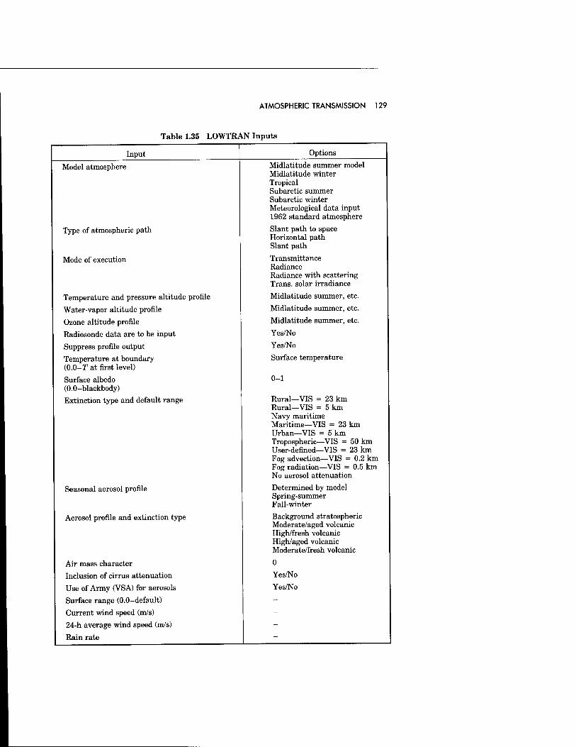
ATMOSPHERIC TRANSMISSION 129
Table 1.35 LOWTRAN Inputs
Input
Model atmosphere
Type of atmospheric path
Mode of execution
Temperature and pressure altitude profile
Water-vapor altitude profile
Ozone altitude profile
Radiosonde data are to be input
Suppress profile output
Temperature at boundary (0.0-T at first level)
Surface albedo (0.0-blackbody)
Extinction type and default range
Options
Seasonal aerosol profile
Aerosol profile and extinction type
Air mass character
Inclusion of cirrus attenuation
Use of Army (VSA) for aerosols
Surface range (0.0-default)
Current wind speed (m/s)
24-h average wind speed (m/s)
Rain rate
Midlatitude summer model Midlatitude winter Tropical Subarctic summer Subarctic winter Meteorological data input 1962 standard atmosphere
Slant path to space Horizontal path Slant path
Transmittance Radiance Radiance with scattering Trans, solar irradiance
Midlatitude summer, etc.
Midlatitude summer, etc.
Midlatitude summer, etc.
Yes/No
Yes/No
Surface temperature
0-1
Rural—VIS = 23 km Rural—VIS = 5 km Navy maritime Maritime—VIS = 23 km Urban—VIS = 5 km Tropospheric—VIS = 50 km User-defined—VIS = 23 km Fog advection—VIS = 0.2 km Fog radiation—VIS = 0.5 km No aerosol attenuation
Determined by model Spring-summer Fall-winter
Background stratospheric Moderate/aged volcanic High/fresh volcanic High/aged volcanic Moderate/fresh volcanic
0
Yes/No
Yes/No
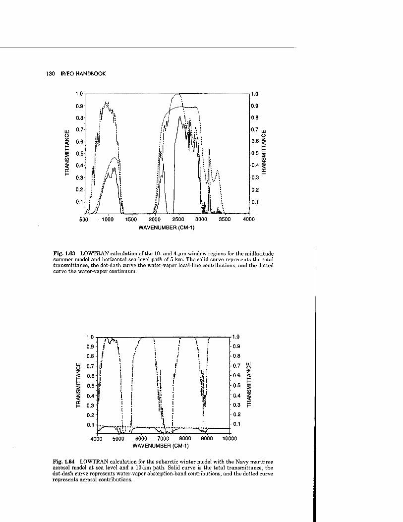
130 IR/EO HANDBOOK
w ü
5
I-
1000 1500 2000 2500 3000
WAVENUMBER(CM-I)
Fig. 1.63 LOWTRAN calculation of the 10- and 4-p.m window regions for the midlatitude summer model and horizontal sea-level path of 5 km. The solid curve represents the total transmittance, the dot-dash curve the water-vapor local-line contributions, and the dotted curve the water-vapor continuum.
4000 5000 6000 7000 8000 WAVENUMBER(CNM)
9000 10000
LU Ü z
2 CO
Fig. 1.64 LOWTRAN calculation for the subarctic winter model with the Navy maritime aerosol model at sea level and a 10-km path. Solid curve is the total transmittance, the dot-dash curve represents water-vapor absorption-band contributions, and the dotted curve represents aerosol contributions.
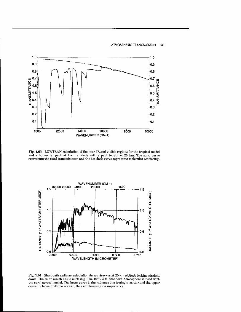
ATMOSPHERIC TRANSMISSION 131
1000 12000 14000 16000 WAVENUMBER(CM-I)
18000 20000
Fig. 1.65 LOWTRAN calculation of the near-IR and visible regions for the tropical model and a horizontal path at 1-km altitude with a path length of 25 km. The solid curve represents the total transmittance and the dot-dash curve represents molecular scattering.
. 32000 28000 WAVENUMBER(CM-I)
24000 20000 1600 cr ü
cr 111
& 2 Ü
UJ ü z < < CT
0.300 0.400 0.500 0.600 WAVELENGTH (MICROMETER)
0.0 0.700
o
cr HI h- W cvi 5 O
I UJ Ü 2 < Q < IX
Fig. 1.66 Slant-path radiance calculation for an observer at 20-km altitude looking straight down. The solar zenith angle is 60 deg. The 1976 U.S. Standard Atmosphere is used with the rural aerosol model. The lower curve is the radiance due to single scatter and the upper curve includes multiple scatter, thus emphasizing its importance.
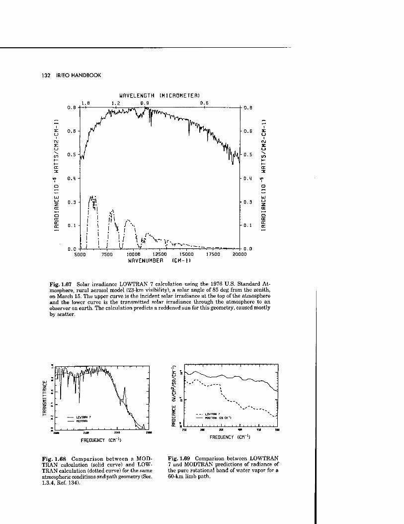
132 IR/EO HANDBOOK
en
□
cc cc
0.8
0.6
0.5 -
0.1
0.3 -
0. 1
l.B WAVELENGTH (MICROMETER)
1.2 0.9 0.6
0.0 5000 7500 10000 12500 15000
WRVENUMBER (CM-1) 17500 20000
Fig. 1.67 Solar irradiance LOWTRAN 7 calculation using the 1976 U.S. Standard At- mosphere, rural aerosol model (23-km visibility), a solar angle of 85 deg from the zenith, on March 15. The upper curve is the incident solar irradiance at the top of the atmosphere and the lower curve is the transmitted solar irradiance through the atmosphere to an observer on earth. The calculation predicts a reddened sun for this geometry, caused mostly by scatter.
^ ' ' ' ■ l ■ ' ' ■ 1 ' ' ' ■ 1 ■ ' ' ■ 1 ' ■ ' '
r T ~^s~*~. CJ •v a: V) • N-'"v^ ^-^\.—^ ^
"*"" ** \ >1
JE , ^^ <J N. * is \ _
V cc LOWTRAN 7 X- ;
o MOOTRflN <2fl CM1)
• .... 1 .... 1 .... 1 .... 1 ... .
FREQUENCY (CM"1) FREQUENCY (Cfl"1)
Fig. 1.68 Comparison between a MOD- TRAN calculation (solid curve) and LOW- TRAN calculation (dotted curve) for the same atmospheric conditions and path geometry (Sec. 1.3.4, Ref. 134).
Fig. 1.69 Comparison between LOWTRAN 7 and MODTRAN predictions of radiance of the pure rotational band of water vapor for a 60-km limb path.
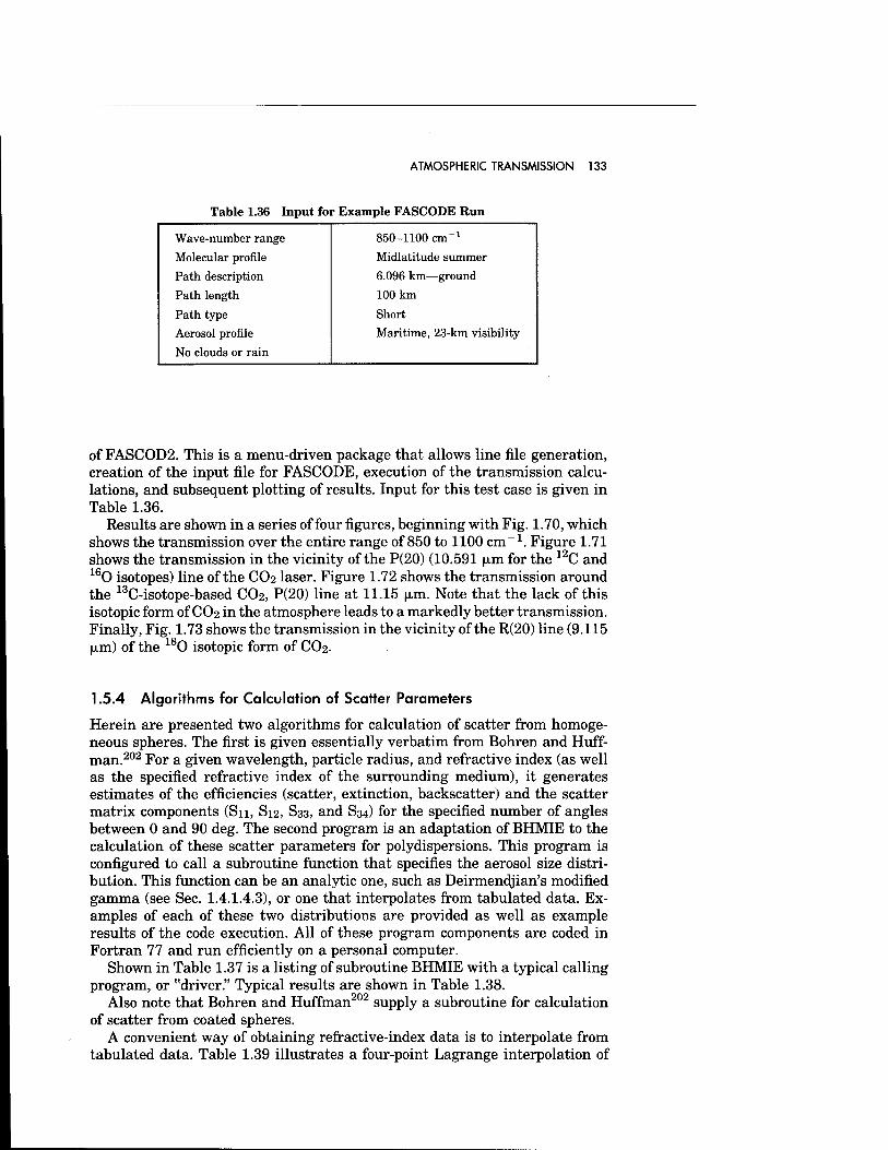
ATMOSPHERIC TRANSMISSION 133
Table 1.36 Input for Example FASCODE Run
Wave-number range 850-1100 cm"1
Molecular profile Midlatitude summer
Path description 6.096 km—ground
Path length 100 km
Path type Short
Aerosol profile Maritime, 23-km visibility
No clouds or rain
of FASCOD2. This is a menu-driven package that allows line file generation, creation of the input file for FASCODE, execution of the transmission calcu- lations, and subsequent plotting of results. Input for this test case is given in Table 1.36.
Results are shown in a series of four figures, beginning with Fig. 1.70, which shows the transmission over the entire range of 850 to 1100 cm-1. Figure 1.71 shows the transmission in the vicinity of the P(20) (10.591 |xm for the 12C and 160 isotopes) line of the CO2 laser. Figure 1.72 shows the transmission around the 13C-isotope-based C02, P(20) line at 11.15 (Am. Note that the lack of this isotopic form of CO2 in the atmosphere leads to a markedly better transmission. Finally, Fig. 1.73 shows the transmission in the vicinity of the R(20) line (9.115 |xm) of the 180 isotopic form of CO2.
1.5.4 Algorithms for Calculation of Scatter Parameters
Herein are presented two algorithms for calculation of scatter from homoge- neous spheres. The first is given essentially verbatim from Bohren and Huff- man.202 For a given wavelength, particle radius, and refractive index (as well as the specified refractive index of the surrounding medium), it generates estimates of the efficiencies (scatter, extinction, backscatter) and the scatter matrix components (Sn, S12, S33, and S34) for the specified number of angles between 0 and 90 deg. The second program is an adaptation of BHMIE to the calculation of these scatter parameters for polydispersions. This program is configured to call a subroutine function that specifies the aerosol size distri- bution. This function can be an analytic one, such as Deirmendjian's modified gamma (see Sec. 1.4.1.4.3), or one that interpolates from tabulated data. Ex- amples of each of these two distributions are provided as well as example results of the code execution. All of these program components are coded in Fortran 77 and run efficiently on a personal computer.
Shown in Table 1.37 is a listing of subroutine BHMIE with a typical calling program, or "driver." Typical results are shown in Table 1.38.
Also note that Bohren and Huffman202 supply a subroutine for calculation of scatter from coated spheres.
A convenient way of obtaining refractive-index data is to interpolate from tabulated data. Table 1.39 illustrates a four-point Lagrange interpolation of
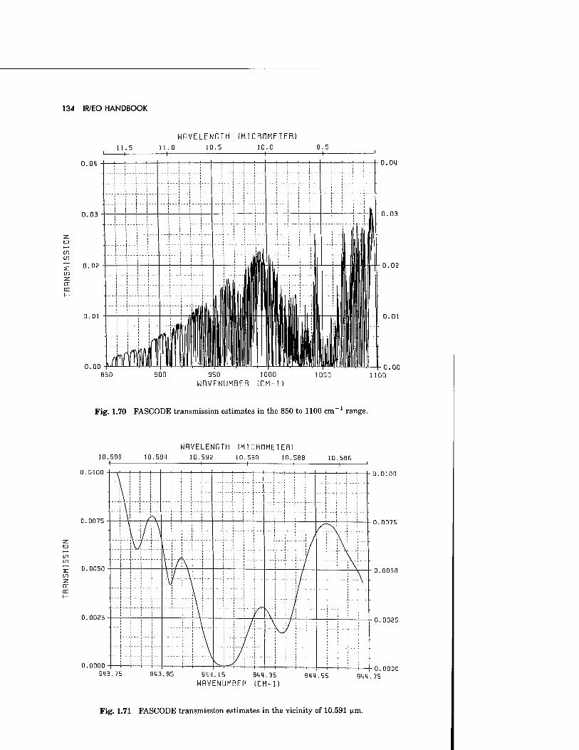
134 IR/EO HANDBOOK
WAVELENGTH (MICROMETER)
en to
11. 5 11.[ ) 10 .5 10. 0 9 .5 1
■
J\
■
0.00 Of f\ 850 900 950 1000
WRVENUMBER ICM-1) 1050
0.04
D.D3
0.02
0.01
0.00 1100
Fig. 1.70 FASCODE transmission estimates in the 850 to 1100 cm 1 range.
WRVELENGTH (MICROMETER)
10.596 10.59U 10.592 10.59D 10.588 1D.SBS J| 1 1 1 , ,
CE
0.0100
0.0075
D.0050
0.0025
0.0DDD
\' L
•
■
...| .. . .
■
^
■
1 1
| ■
0.0100
O.OD75
0.0D5D
-0.0025
913.75 943.95 914.15 94H.35
WRVENUMBER (CM-1)
0.0000 9UH.5S 9UH.7S
Fig. 1.71 FASCODE transmission estimates in the vicinity of 10.591 |xm.
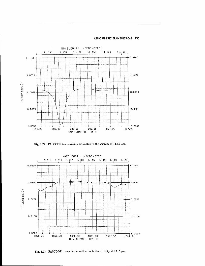
ATMOSPHERIC TRANSMISSION 135
WRVELENGTH (MICROMETER)
11.156 11.1511 11.152 11.150 11. 1MB 11.116
m in
1 1 1 1 1 1 .
\ \ \ \ \ \ , 1
0.O0DD i— — \J , , -
D.QD75
0.005D
0.0025
O.OD00 B9B.25 B96.4S B9B.B5 B9B.B5
WRVENUMBER 1CM-1) B97.D5 B97.25
Fig. 1.72 FASCODE transmission estimates in the vicinity of 11.15 p.m.
NHVELENGTH (MICROMETER)
cr
9 . 119 9 . MB 9 .117 9 . 11B 9 . 115 9 . Ill 9 . 113 9 .112
D.OODO - i , , ,
0.D4D0
D.D3DD
O.Q20D
0.D100
109B.5D 109B.70 O.ODDQ
1096.90 1097.10
WRVENUMBER 1CM-1) 1D97.30 1097.50
Fig. 1.73 FASCODE transmission estimates in the vicinity of 9.115 |xm.
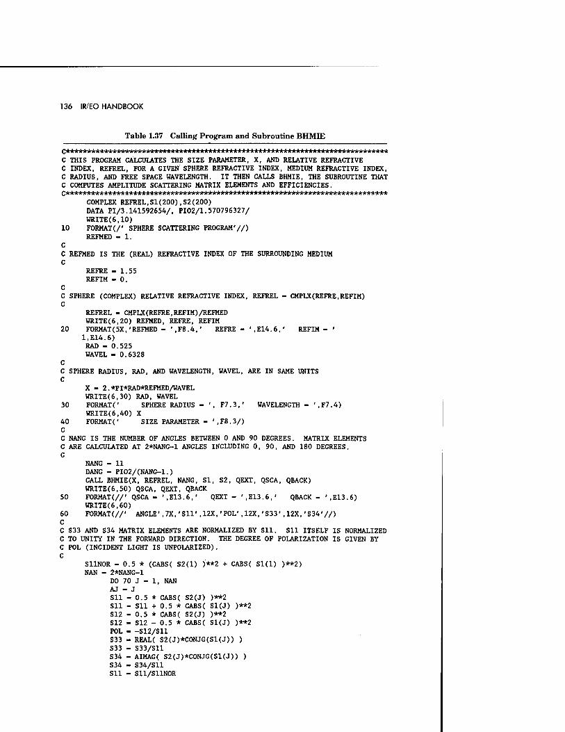
136 IR/EO HANDBOOK
Table 1.37 Calling Program and Subroutine BHMIE
C THIS PROGRAM CALCULATES THE SIZE PARAMETER, X, AND RELATIVE REFRACTIVE C INDEX, REFREL, FOR A GIVEN SPHERE REFRACTIVE INDEX, MEDIUM REFRACTIVE INDEX, C RADIUS, AND FREE SPACE WAVELENGTH. IT THEN CALLS BHMIE, THE SUBROUTINE THAT C COMPUTES AMPLITUDE SCATTERING MATRIX ELEMENTS AND EFFICIENCIES.
COMPLEX REFREL,S1(200),S2(200) DATA PI/3.141592654/, PI02/1.570796327/ WRITE(6,10)
10 FORMAT(/' SPHERE SCATTERING PROGRAM'//) REFMED - 1.
C C REFMED IS THE (REAL) REFRACTIVE INDEX OF THE SURROUNDING MEDIUM C
REFRE - 1.55 REFIM - 0.
C C SPHERE (COMPLEX) RELATIVE REFRACTIVE INDEX, REFREL - CMPLX(REFRE,REFIM) C
REFREL - CMPLX(REFRE,REFIM)/REFMED WRITE(6,20) REFMED, REFRE, REFIM
20 FORMAT(5X,'REFMED - *,F8.4,' REFRE - ',E14.6,' REFIM-' 1.E14.6) RAD - 0.525 WAVEL - 0.6328
C C SPHERE RADIUS, RAD, AND WAVELENGTH, WAVEL, ARE IN SAME UNITS C
X - 2.*PI*RAD*REFMED/WAVEL WRITE(6,30) RAD, WAVEL
30 FORMATC SPHERE RADIUS - ', F7.3,' WAVELENGTH - \F7.4) WRITE(6,40) X
40 FORMATC SIZE PARAMETER - ',F8.3/) C C NANG IS THE NUMBER OF ANGLES BETWEEN 0 AND 90 DEGREES. MATRIX ELEMENTS C ARE CALCULATED AT 2*NANG-1 ANGLES INCLUDING 0, 90, AND 180 DEGREES. C
NANG - 11 DANG - PI02/(NANG-1.) CALL BHMIE(X, REFREL, NANG, SI, S2, QEXT, QSCA, QBACK) WRITE(6,50) QSCA, QEXT, QBACK
50 FORMAT(//' QSCA- '.E13.6,' QEXT- ',E13.6,' QBACK- '.E13.6) WRITE(6,60)
60 FORMAT(//' ANGLE',7X,'Sll*,12X,'POL',12X,*S33',12X,'S34'//) C C S33 AND S34 MATRIX ELEMENTS ARE NORMALIZED BY Sll. Sll ITSELF IS NORMALIZED C TO UNITY IN THE FORWARD DIRECTION. THE DEGREE OF POLARIZATION IS GIVEN BY C POL (INCIDENT LIGHT IS UNPOLARIZED). C
S11NOR - 0.5 * (CABS( S2(l) )**2 + CABS( Sl(l) )**2) NAN - 2*NANG-1
DO 70 J - 1, NAN AJ - J Sll - 0.5 * CABS( S2(J) )**2 511 - Sll + 0.5 * CABS( S1(J) )**2 512 - 0.5 * CABS( S2(J) )**2 S12 - S12 - 0.5 * CABS( S1(J) )**2 POL S12/S11 S33 - REAL( S2(J)*C0NJG(S1(J)) ) 533 - S33/S11 534 - AIMAG( S2(J)*C0NJG(S1(J)) ) S34 - S34/S11 Sll - S11/S11NOR
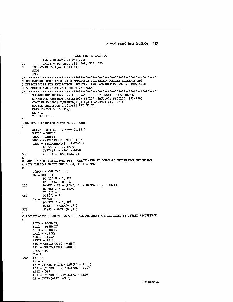
ATMOSPHERIC TRANSMISSION 137
Table 1.37 (continued) ANG - DANG*(AJ-1)*57.2958
70 WRITE(6,80) ANG, Sll, POL, S33, S34 80 F0RMAT(1X,F6.2,4(2X,E13.6))
STOP END
C SUBROUTINE BHMIE CALCULATES AMPLITUDE SCATTERING MATRIX ELEMENTS AND C EFFICIENCIES FOR EXTINCTION, SCATTER, AND BACKSCATTER FOR A GIVEN SIZE C PARAMETER AND RELATIVE REFRACTIVE INDEX.
SUBROUTINE BHMIE(X, REFREL, NANG, SI, S2, QEXT, QSCA, QBACK) DIMENSION AMU(IOO),THETA(100),PI(100),TAU(100),PI0(100),PI1(100) COMPLEX D(3000),Y,REFREL,XI,XIO,XII,AN,BN,S1(I),S2(1) DOUBLE PRECISION PSI0,PSI1,PSI,DN,DX DATA PI02/1.570796327/ DX - X Y - X*REFREL
C SERIES TERMINATED AFTER NSTOP TERMS C
XSTOP - X + 2. + 4.*X**(0.3333) NSTOP - XSTOP YMOD - CABS(Y) NMX - AMAX1(XSTOP, YMOD) + 15 DANG - PI02/AMAX1(1., NANG-1.)
DO 555 J - 1, NANG THETA(J) - (J-1.)*DANG AMU(J) - COS(THETA(J)) 555
C LOGARITHMIC DERIVATIVE, D(J), CALCULATED BY DOWNWARD RECURRENCE BEGINNING WITH INITIAL VALUE CMPLX(O.O) AT J - NMX
D(NMX) - CMPLX(0.,0.) NN - NMX - 1
DO 120 N - 1, NN RN - NMX - N + 1
120
666
777 C
D(NMX - N) DO 666 J - PIO(J) - 0. PI1(J) - 1.
NN - 2*NANG - 1 DO 777 J - 1, NN S1(J) - CMPLX(0.,0.) S2(J) - CMPLX(0.,0.)
- (RN/Y)-(1./(D(NMX-N+1) + RN/Y)) 1, NANG
C RICCATI-BESSEL FUNCTIONS WITH REAL ARGUMENT X CALCULATED BY UPWARD RECURRENCE
C PSIO ■ PSI1 ■ CHIO ■ CHI1 ■ APSIO APSI1 XIO - XII -
■ DCOS(DX) ■ DSIN(DX) ■ -SIN(X) ■ COS(X) - PSIO - PSI1 CMPLX(APSIO, CMPLX(APSI1,
-CHIO) -CHI1)
200
QSCA - 0. N - 1 DN - N RN - N FN - (2.*RN + l.)/( RN*(RN + 1.) ) PSI - (2.*DN - l.)*PSIl/DX - PSIO APSI - PSI CHI - (2.*RN - l.)*CHIl/X - CHIO XI - CMPLX(APSI, -CHI)
(continued)
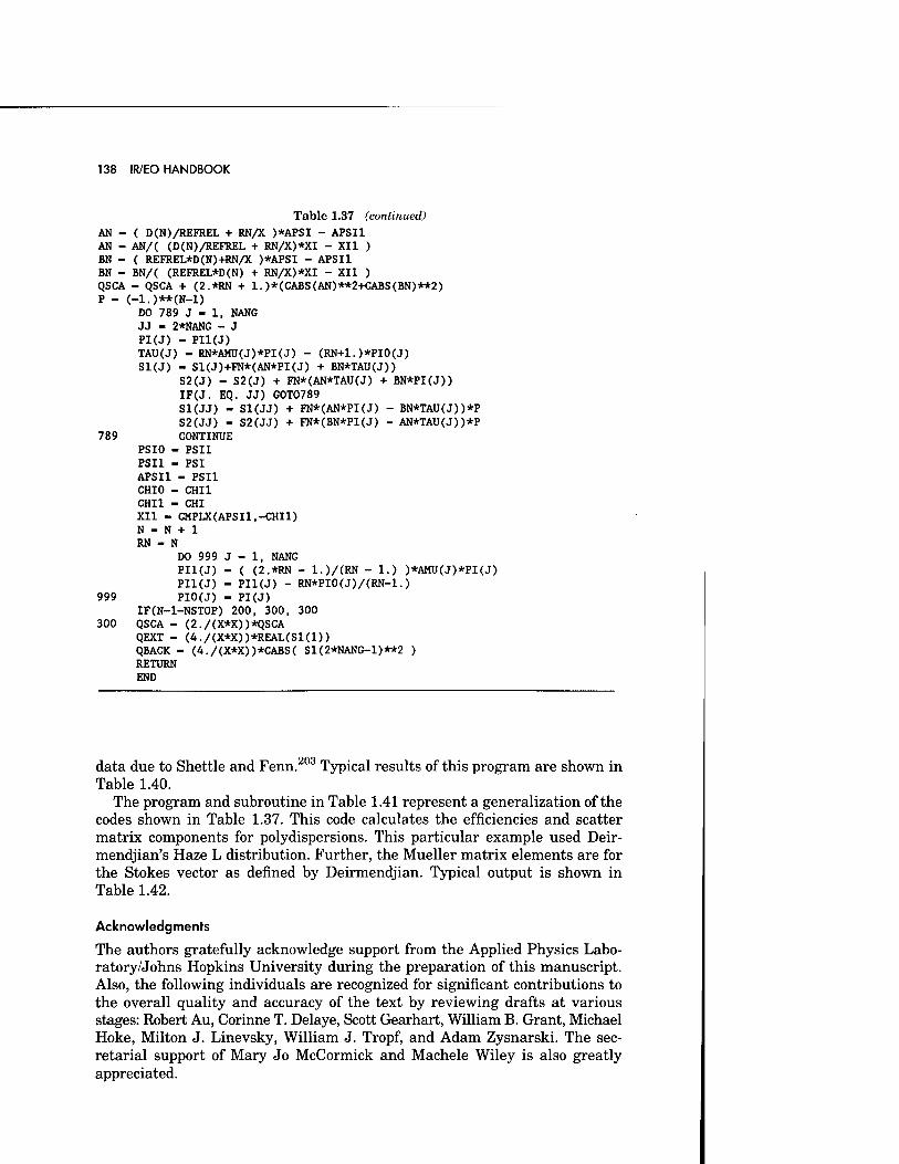
138 IR/EO HANDBOOK
Table 1.37 (continued) AN - ( D(N)/REFREL + RN/X )*APSI - APSI1 AN - AN/( (D(N)/REFREL + RN/X)*XI - XII ) BN - ( REFREL*D(N)+RN/X )*APSI - APSI1 BN - BN/( (REFREL*D(N) + RN/X)*XI - XII ) QSCA - QSCA + (2.*RN + 1.)*(CABS(AN)**2+CABS(BN)**2) P - (-l.)**(N-l)
DO 789 J - 1, NANG JJ - 2*NANG - J PI(J) - PI1(J) TAU(J) - RN*AMU(J)*PI(J) - (RN+1.)*PI0(J) S1(J) - S1(J)+FN*(AN*PI(J) + BN*TAU(J))
S2(J) - S2(J) + FN*(AN*TAU(J) + BN*PI(J)) IF(J. EQ. JJ) GOT0789 Sl(JJ) - Sl(JJ) + FN*(AN*PI(J) - BN*TAU(J))*P S2(JJ) - S2(JJ) + FN*(BN*PI(J) - AN*TAU(J))*P
789 CONTINUE PSIO - PSI1 PSI1 - PSI APSI1 - PSI1 CHIO - CHI1 CHI1 - CHI XII - CMPLX(APSI1,-CHI1) N - N + I RN - N
DO 999 J - 1, NANG PI1(J) - ( (2.*RN - l.)/(RN - 1.) )*AMU(J)*PI(J) PI1(J) - PI1(J) - RN*PI0(J)/(RN-1.)
999 PIO(J) - PI(J) IF(N-l-NSTOP) 200, 300, 300
300 QSCA - (2./(X*X))*QSCA QEXT - (A./(X*X))*REAL(S1(1)) QBACK - (4./(X*X))*CABS( S1(2*NANG-1)**2 ) RETURN END
data due to Shettle and Fenn.203 Typical results of this program are shown in Table 1.40.
The program and subroutine in Table 1.41 represent a generalization of the codes shown in Table 1.37. This code calculates the efficiencies and scatter matrix components for polydispersions. This particular example used Deir- mendjian's Haze L distribution. Further, the Mueller matrix elements are for the Stokes vector as defined by Deirmendjian. Typical output is shown in Table 1.42.
Acknowledgments
The authors gratefully acknowledge support from the Applied Physics Labo- ratory/Johns Hopkins University during the preparation of this manuscript. Also, the following individuals are recognized for significant contributions to the overall quality and accuracy of the text by reviewing drafts at various stages: Robert Au, Corinne T. Delaye, Scott Gearhart, William B. Grant, Michael Hoke, Milton J. Linevsky, William J. Tropf, and Adam Zysnarski. The sec- retarial support of Mary Jo McCormick and Machele Wiley is also greatly appreciated.
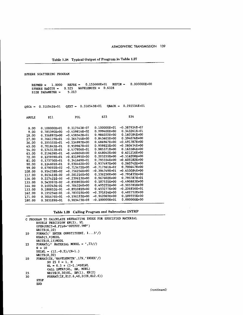
ATMOSPHERIC TRANSMISSION 139
Table 1.38 Typical Output of Program in Table 1.37
SPHERE SCATTERING PROGRAM
REFMED - 1.0000 REFRE - 0.155000E+01 REFIM SPHERE RADIUS - 0.525 WAVELENGTH - 0.6328 SIZE PARAMETER - 5.213
0.000000E+00
QSCA - 0.310543E+01 QEXT - 0.310543E+01 QBACK - 0.292534E+01
ANGLE Sll POL S33 S34
,00 ,00
18.00 27.00 36.00 45.00 54.00 63.00 72.00 81.00 90.00 99.00
108.00 117.00 126.00 135.00 144.00 153.00 162.00 171.00 180.00
0.100000E+01 0.785390E+00 0.356897E+00 0.766119E-01 0.355355E-01 0.701845E-01 0.574313E-01 0.219659E-01 0.125959E-01 0.173750E-01 0.124601E-01
.679092E-02
.954238E-02
.863418E-02
.227421E-02
.543997E-02 0.160243E-01 0.188852E-01 0.195254E-01 0.301676E-01 0.383189E-01
0.317543E-07 -0.459814E-02 -0.458542E-01 -0.364744E+00 -0.534997E+00 0.959967E-02 0.477926E-01
-0.440604E+00 -0.831995E+00 0.341669E-01 0.230462E+00
-0.713472E+00 -0.756256E+00 -0.281216E+00 -0.239613E+00 -0.850803E+00 -0.706334E+00 -0.891081E+00 -0.783319E+00 -0.196193E+00 0.903473E-08
0.100000E+01 0.999400E+00 0.986022E+00 0.843603E+00 0.686967E+00 0.959825E+00 0.985371E+00 0.648042E+00 0.203255E+00 0.795354E+00 0.937497E+00 -0.717361E-02 -0.394749E-01 0.536250E+00 0.967602E+00 0.187531E+00 0.495255E+00 0.453277E+00 -0.391614E+00 -0.962069E+00 -0.100000E+01
-0.387934E-07 0.343261E-01 0.160184E+00 0.394076E+00
-0.491787E+00 -0.280434E+00 0.163584E+00 0.621216E+00
-0.516208E+00 -0.605182E+00 0.260742E+00 0.700647E+00
-0.653084E+00 -0.795835E+00 0.795787E-01
-0.490883E+00 -0.505781E+00 -0.226816E-01 0.482752E+00 0.189555E+00 0.000000E+00
Table 1.39 Calling Program and Subroutine INTRP
C PROGRAM TO CALCULATE REFRACTIVE INDEX FOR SPECIFIED MATERIAL DOUBLE PRECISION EN(2) , VfL OPEN(UNIT-8,FILE-'OUTPUT.TMP') WRITE(6,10) FORMAT(' ENTER CONSTITUENT, 1...5'/) READ(5,*)M0DL WRITE(8,15)M0DL FORMAT(/* MATERIAL MODEL - ',13//) N - 10 DELWL - (12.-0.5)/(N-l.) WRITE(8,20) FORMAT(2X,'WAVELENGTH',17X,'INDEX'/)
DO 25 I - 1, N WL - 0.5 + (I-1.)*DELWL CALL INTRP(WL, EN, MODL) WRITE(8,30)WL, EN(1), EN(2) FORMAT(lX,E12.6,4X, 2(2X,E12.6))
STOP END
10
15
20
25 30
(continued)
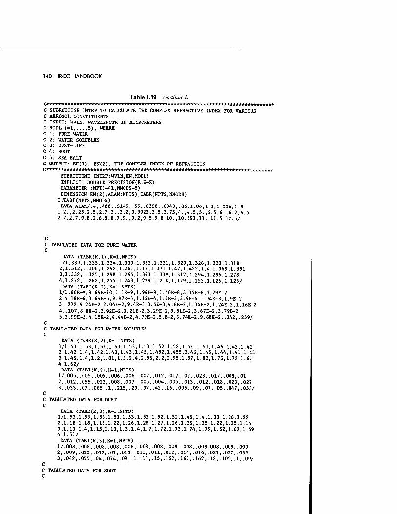
140 IR/EO HANDBOOK
Table 1.39 (continued)
C SUBROUTINE INTRP TO CALCULATE THE COMPLEX REFRACTIVE INDEX FOR VARIOUS C AEROSOL CONSTITUENTS C INPUT: WVLN, WAVELENGTH IN MICROMETERS C MODL (-1 5), WHERE C 1: PURE WATER C 2: WATER SOLUBLES C 3: DUST-LIKE C 4: SOOT C 5: SEA SALT C OUTPUT: EN(1), EN(2), THE COMPLEX INDEX OF REFRACTION C****************************>M:*^
SUBROUTINE INTRP(WVLN,EN,MODL) IMPLICIT DOUBLE PRECISIONS,W-Z) PARAMETER (NPTS-41.NMODS-5) DIMENSION EN(2).ALAM(NPTS)(TABR(NPTS,NMODS) l,TABI(NPTS,NMODS) DATA ALAM/.4,.488,.5145,.55,.6328,.6943,.86,1.06,1.3,1.536,1.8
1,2., 2.25,2.5,2.7,3.,3.2,3.3923,3.5,3.75,4.,4.5,5.,5.5,6.,6.2,6.5 2,7.2,7.9,8.2,8.5,8.7,9.,9.2,9.5,9.8,10.,10.591,11.,11.5,12.5/
C C TABULATED DATA FOR PURE WATER C
DATA (TABR(K,1),K-1,NPTS) 1/1.339,1.335,1.334,1.333,1.332,1.331,1.329,1.326,1.323,1.318 2,1.312,1.306,1.292,1.261,1.18,1.371,1.47,1.422,1.4,1.369,1.351 3,1.332,1.325,1.298,1.265,1.363,1.339,1.312,1.294,1.286,1.278 4,1.272,1.262,1.255,1.243,1.229,1.218,1.179,1.153,1.126,1.123/ DATA (TABI (K, 1) , K-l, NPTS ) l/1.86E-9,9.69E-10,l.lE-9,1.96E-9,1.46E-8,3.35E-8,3.29E-7 2,4.18E-6,3.69E-5,9.97E-5,1.15E-4,l.lE-3,3.9E-4,1.74E-3,1.9E-2 3,.272,9.24E-212.04E-2,9.4E-3,3.5E-3,4.6E-3,1.34E-2,1.24E-2,1.16E-2
4,.107,8.8E-2,3.92E-2,3.21E-2,3.29E-2,3.51E-2,3.67E-2,3.79E-2 5,3.99E-2,4.15E-2,4.44E-2,4.79E-2,5.E-2,6.74E-2,9.68E-2,.142,.259/
C C TABULATED DATA FOR WATER SOLUBLES C
DATA (TABR(K,2),K-l,NPTS) 1/1.53,1.53,1.53,1.53,1.53,1.53,1.52,1.52,1.51,1.51,1.46,1.42,1.42 2,1.42,1.4,1.42,1.43,1.43,1.45,1.452,1.455,1.46,1.45,1.44,1.41,1.43 3,1.46,1.4,1.2,1.01,1.3,2.4,2.56,2.2,1.95,1.87,1.82,1.76,1.72,1.67 4,1.62/ DATA (TABI(K,2),K-1,NPTS) 1/.005,.005,.005,.006,.006,.007,.012,.017, .02, .023,.017,.008,.01 2,.012,.055,.022,.008,.007,.005,.004,.005,.013,.012,.018,.023,.027 3,.033,.07,.065,.1,.215,.29,.37,.42,.16,.095,.09,.07,.05,.047,.053/
C C TABULATED DATA FOR DUST C
DATA (TABR(K,3),K-1,NPTS) 1/1.53,1.53,1.53,1.53,1.53,1.53,1.52,1.52,1.46,1.4,1.33,1.26,1.22 2,1.18,1.18,1.16,1.22,1.26,1.28,1.27,1.26,1.26,1.25,1.22,1.15,1.14 3,1.13,1.4,1.15,1.13,1.3,1.4,1.7,1.72,1.73,1.74,1.75,1.62,1.62,1.59 4,1.51/ DATA (TABI(K,3),K-1,NPTS) 1/.008,.008,.008,.008,.008,.008,.008,.008,.008,.008,008,.008,.009 2, .009,.013,.012,.01,.013,.011,.011,.012,.014,.016,.021,.037,.039 3,.042,.055,.04,.074,.09,.1,.14,.15,.162,.162,.162,.12,.105,.1,.09/
C C TABULATED DATA FOR SOOT C
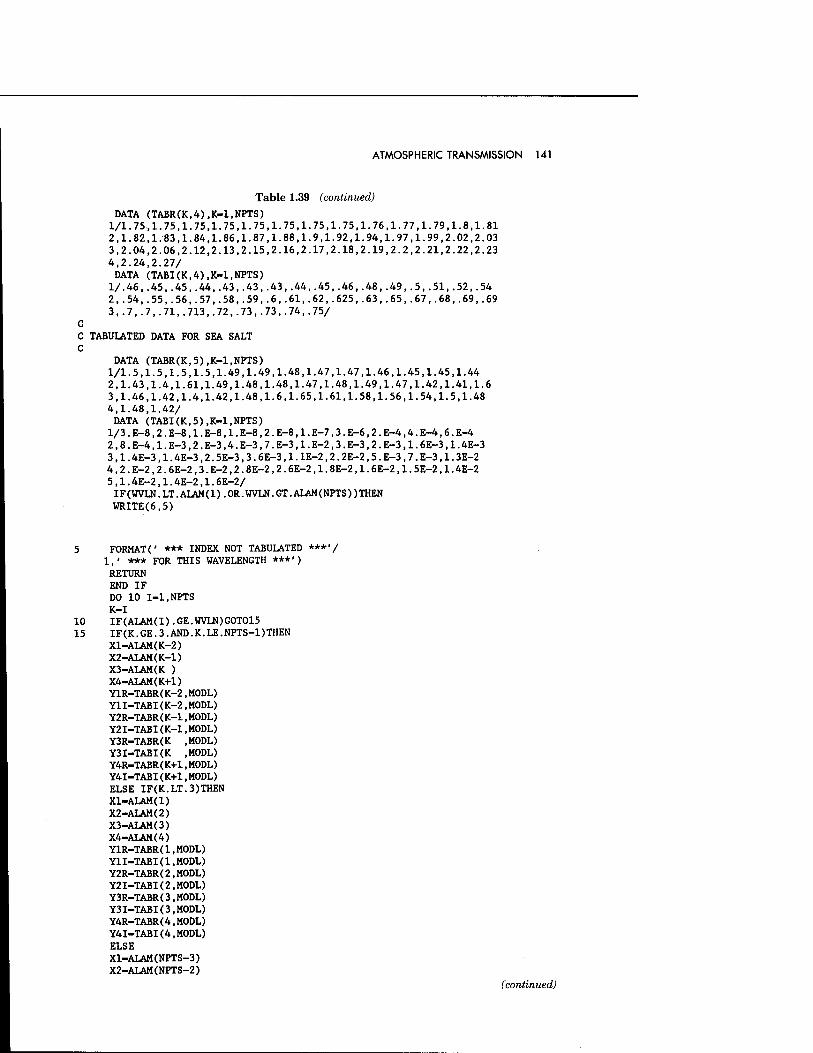
ATMOSPHERIC TRANSMISSION 141
Table 1.39 (continued)
DATA (TABR(K,4),K-1,NPTS) 1/1.75-, 1.75,1.75,1.75,1.75,1.75,1.75,1.75,1.76,1.77,1.79,1.8,1.81 2,1.82,1.-83,1.84,1.86,1.87,1.88,1.9,1.92,1.94,1.97,1.99,2.02,2.03 3,2.04,2.06,2.12,2.13,2.15,2.16,2.17,2.18,2.19,2.2,2.21,2.22,2.23 4,2.24,2.27/ DATA (TABI(K, 4),K-l,NPTS) 1/.46,.45,.45,.44,.43,.43,.43,.44,.45,.46,.48,.49,.5,.51,.52,.54 2,.54,.55,.56,.57,.58,.59,.6,.61,.62,.625,.63,.65,.67,.68,.69,.69 3, . 7, . 7, . 71,. 713,. 72,. 73, . 73,. 74,. 75/
C C TABULATED DATA FOR SEA SALT C
DATA (TABR(K,5),K-1,NPTS) 1/1.5,1.5,1.5,1.5,1.49,1.49,1.48,1.47,1.47,1.46,1.45,1.45,1.44 2,1.43,1.4,1.61,1.49,1.48,1.48,1.47,1.48,1.49,1.47,1.42,1.41,1.6 3,1.46,1.42,1.4,1.42,1.48,1.6,1.65,1.61,1.58,1.56,1.54,1.5,1.48 4,1.48,1.42/ DATA (TABI(K, 5),K-l,NPTS) l/3.E-8,2.E-8,l.E-8,l.E-8,2.E-8,l.E-7,3.E-6,2.E-4,4.E-4,6.E-4 2,8.E-4,l.E-3,2.E-3,4.E-3,7.E-3,l.E-2,3.E-3,2.E-3,1.6E-3,1.4E-3 3,1.4E-3,1.4E-3,2.5E-3,3.6E-3,l.lE-2,2.2E-2,5.E-3,7.E-3,1.3E-2 4,2.E-2,2.6E-2,3.E-2,2.8E-2,2.6E-2,1.8E-2,1.6E-2,1.5E-2,1.4E-2 5,1.4E-2,1.4E-2,1.6E-2/ IF(WVLN.LT.ALAM(1).0R.WVLN.GT.ALAM(NPTS))THEN WRITE(6,5)
5 FORMAT(' *** INDEX NOT TABULATED ***'/ 1,' *** FOR THIS WAVELENGTH ***') RETURN END IF DO 10 I-l.NPTS K-I
10 IF(ALAM(I).GE.WVLN)GOT015 15 IF(K.GE.3.AND.K.LE.NPTS-1)THEN
Xl-ALAM(K-2) X2-ALAM(K-1) X3-ALAM(K ) X4-ALAM(K+1) YlR-TABR(K-2,MODL) Y1I-TABI(K-2,M0DL) Y2R-TABR(K-l,MODL) Y2I-TABI(K-l,MODL) Y3R-TABR(K ,MODL) Y3I-TABI(K ,MODL) Y4R-TABR(K+1,MODL) Y4I-TABI(K+1,M0DL) ELSE IF(K.LT.3)THEN Xl-ALAM(l) X2-ALAM(2) X3-ALAM(3) X4-ALAM(4) Y1R-TABR(1,M0DL) YlI-TABI(l.MODL) Y2R-TABR(2,M0DL) Y2I-TABI(2,M0DL) Y3R-TABR(3,M0DL) Y3I-TABI(3,M0DL) Y4R-TABR(4,M0DL) Y4I-TABI(4,MODL) ELSE Xl-ALAM(NPTS-3) X2-ALAM(NPTS-2)
(continued)
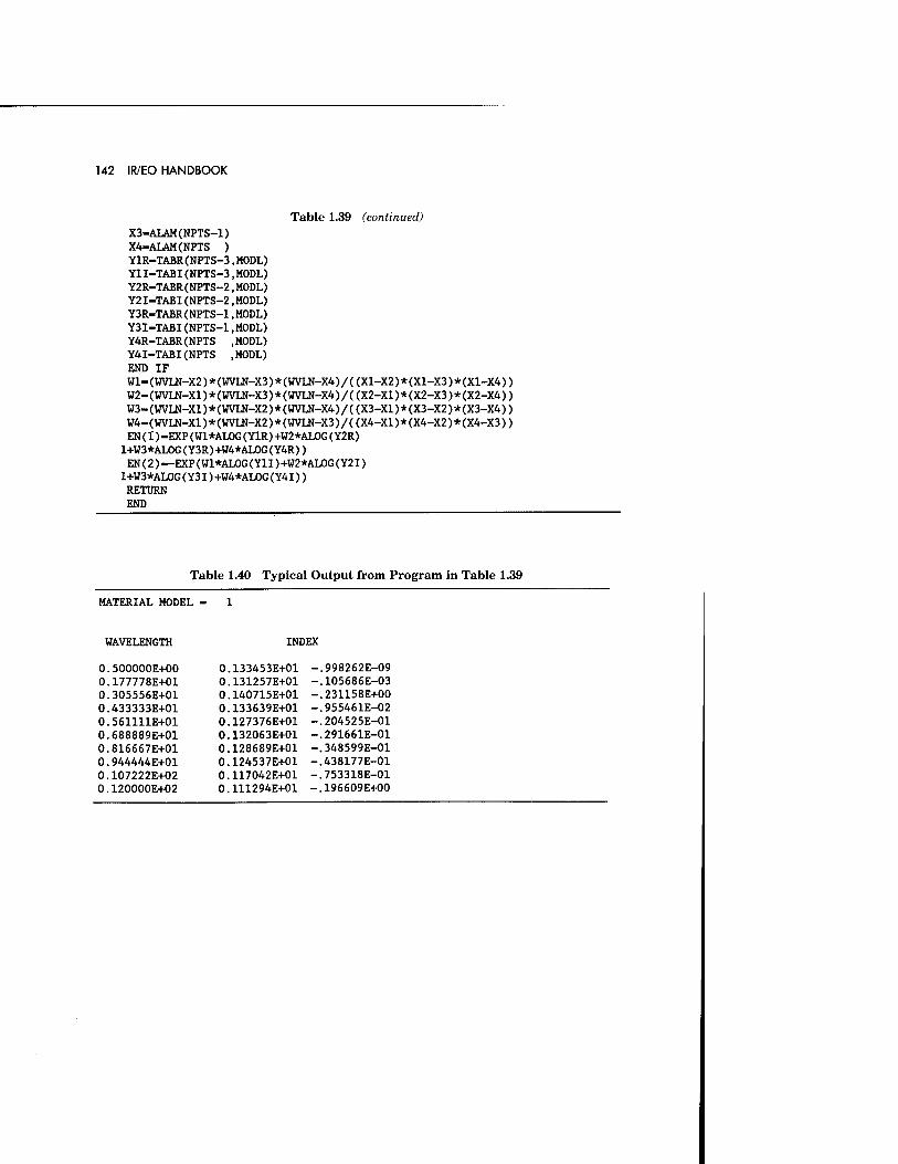
142 IR/EO HANDBOOK
Table 1.39 (continued) X3-ALAM(NPTS-1) X4-ALAM(NPTS ) YlR-TABR(NPTS-3,MODL) Y1I-TABI(NPTS-3,MODL) Y2R-TABR(NPTS-2,MODL) Y2I-TABI(NPTS-2,MODL) Y3R-TABR(NPTS-1,MODL) Y3I-TABI(NPTS-1,MODL) Y4R-TABR(NPTS ,MODL) Y4I-TABI(NPTS ,MODL) END IF Wl-(WVLN-X2)*(WVLN-X3)*(WVLN-X4)/((X1-X2)*(X1-X3)*(X1-X4)) W2-(WVLN-Xl)*(WVLN-X3)*(WVLN-X4)/((X2-X1)*(X2-X3)*(X2-X4)) W3-(WVLN-X1)*(WVLN-X2)*(WVLN-X4)/((X3-X1)*(X3-X2)*(X3-X4)) W4- (WVLN-X1)*(WVLN-X2)*(WVLN-X3)/((X4-X1)*(X4-X2)*(X4-X3)) EN(1)-EXP(W1*AL0G(Y1R)+W2*AL0G(Y2R) l+W3*ALOG (Y3R) +W4*AL0G ( Y4R) ) EN(2)—EXP(W1*AL0G(Y1I)+W2*AL0G(Y2I) l+W3*ALOG(Y3I)+W4*ALOG(Y4I)) RETURN END
Table 1.40 Typical Output from Program in Table 1.39
MATERIAL MODEL - 1
WAVELENGTH INDEX
0.500000E+00 0.177778E+01 0.305556E+01 0.433333E+01 0.561111E+01 0.688889E+01 0.816667E+01 0.944444E+01 0.107222E+02 0.120000E+02
0.133453E+01 0.131257E+01 0.140715E+01 0.133639E+01 0.127376E+01 0.132063E+01 0.128689E+01 0.124537E+01 0.117042E+01 0.111294E+01
-.998262E-09 -.105686E-03 -.231158E+00 -.955461E-02 -.204525E-01 -.291661E-01 -.348599E-01 -.438177E-01 -.753318E-01 -.196609E+00
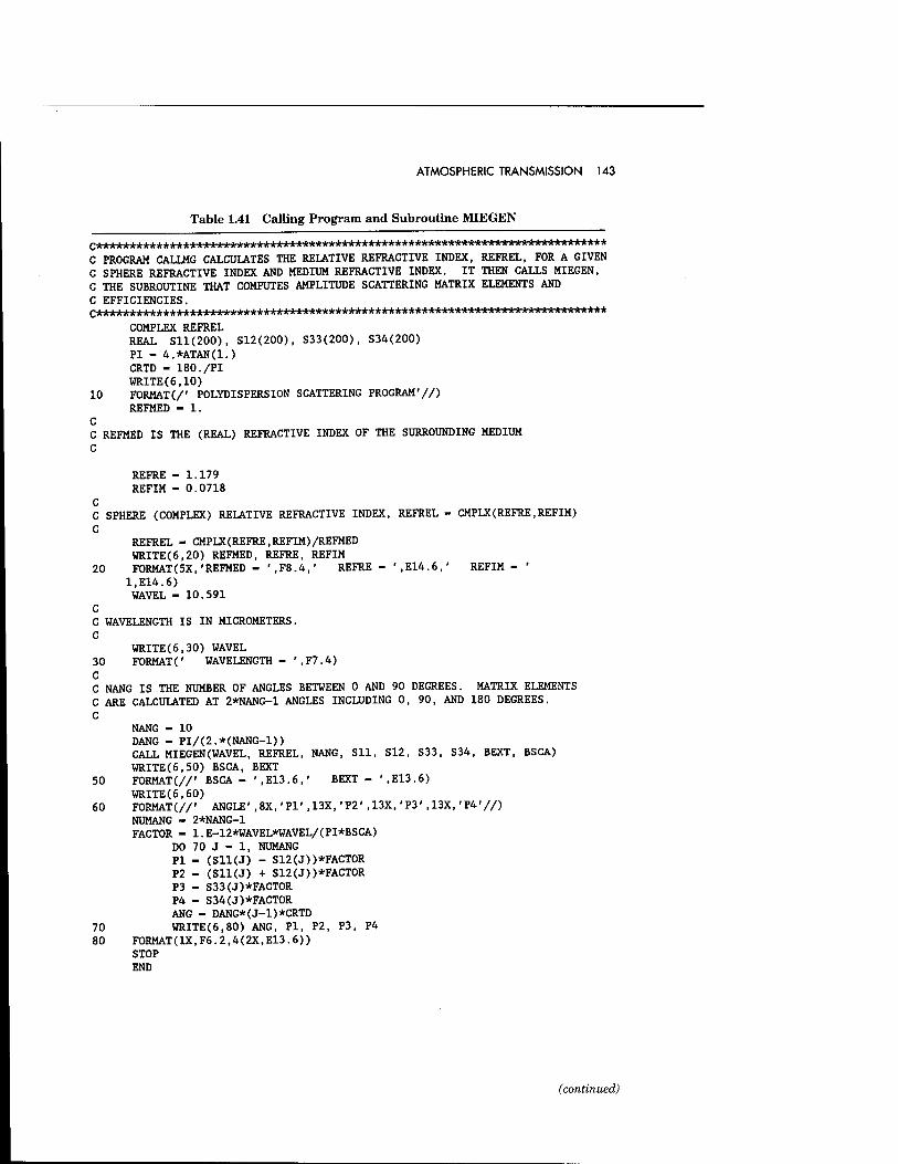
ATMOSPHERIC TRANSMISSION 143
Table 1.41 Calling Program and Subroutine MIEGEN
C PROGRAM CALLMG CALCULATES THE RELATIVE REFRACTIVE INDEX, REFREL, FOR A GIVEN C SPHERE REFRACTIVE INDEX AND MEDIUM REFRACTIVE INDEX. IT THEN CALLS MIEGEN, C THE SUBROUTINE THAT COMPUTES AMPLITUDE SCATTERING MATRIX ELEMENTS AND C EFFICIENCIES.
COMPLEX REFREL REAL Sll(200), S12(200), S33(200), S34(200) PI - 4.*ATAN(1.) CRTD - 180./PI HRITE(6,10)
10 FORMAT(/' POLYDISPERSION SCATTERING PROGRAM'//) REFMED - 1.
C C REFMED IS THE (REAL) REFRACTIVE INDEX OF THE SURROUNDING MEDIUM C
REFRE - 1.179 REFIM - 0.0718
C C SPHERE (COMPLEX) RELATIVE REFRACTIVE INDEX, REFREL - CMPLX(REFRE,REFIM)
C REFREL - CMPLX(REFRE,REFIM)/REFMED WRITE(6,20) REFMED, REFRE, REFIM
20 FORMAT(5X,'REFMED - \F8.4,' REFRE- \E14.6,' REFIM- ' 1.E14.6) WAVEL - 10.591
C C WAVELENGTH IS IN MICROMETERS. C
WRITE(6,30) WAVEL 30 FORMATC WAVELENGTH -',F7.4) C C NANG IS THE NUMBER OF ANGLES BETWEEN 0 AND 90 DEGREES. MATRIX ELEMENTS C ARE CALCULATED AT 2*NANG-1 ANGLES INCLUDING 0, 90, AND 180 DEGREES. C
NANG - 10 DANG - PI/(2.*(NANG-1)) CALL MIEGEN(WAVEL, REFREL, NANG, Sll, S12, S33, S34, BEXT, BSCA) WRITE(6,50) BSCA, BEXT
50 FORMAT(//' BSCA- \E13.6,' BEXT- \E13.6) WRITE(6,60)
60 F0RMAT(//' ANGLE',8X,'PI',13X,'P2',13X,'P3',13X,'P4'//) NUMANG - 2*NANG-1 FACTOR - l.E-12*WAVEL*WAVEL/(PI*BSCA)
DO 70 J - 1, NUMANG PI - (Sll(J) - S12(J))*FACTOR P2 - (Sll(J) + S12(J))*FACT0R P3 - S33(J)*FACT0R P4 - S34(J)*FACTOR ANG - DANG*(J-1)*CRTD
70 WRITE(6,80) ANG, PI, P2, P3, P4 80 F0RMAT(1X,F6.2,4(2X,E13.6))
STOP END
(continued)
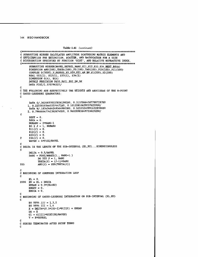
144 IR/EO HANDBOOK
Table 1.41 (continued) KWTrTCTTXTCXWX********
C SUBROUTINE MIEGEN CALCULATES AMPLITUDE SCATTERING MATRIX ELEMENTS AND C EFFICIENCIES FOR EXTINCTION, SCATTER, AND BACKSCATTER FOR A SIZE C DISTRIBUTION SPECIFIED BY FUNCTION 'DIST', AND RELATIVE REFRACTIVE INDEX.
SUBROUTINE MIEGEN(WAVEL,REFREL,NANG,S11,S12,S33,S34,BEXT,BSCA) DIMENSION AMU(IOO),THETA(100),PI(100),TAU(100),PI0(100),PI1(100) COMPLEX D(3000),Y,REFREL,XI,XI0,XI1,AN,BN,S1(200),S2(200) REAL Sll(l), S12(l), S33(l), S34(l) DIMENSION G(4), W(4) DOUBLE PRECISION PSI0,PSI1,PSI,DN,DX DATA PI02/1.570796327/
C C THE FOLLOWING ARE RESPECTIVELY THE WEIGHTS AND ABSCISSAS OF THE 8-POINT C GAUSS-LEGENDRE QUADRATURE: C
DATA G/.362683783378361983D0, 0.313706645877887287D0 1, 0.222381034453374471D0, 0.101228536290376259DO/ DATA W/.183434642495649805D0, 0.525532409916328986D0
2, 0.796666477413626740D0, 0.960289856497536232D0/
BEXT - 0. BSCA - 0. NUMANG - 2*NANG-1 DO 2 J - 1, NUMANG Sll(J) - 0. S12(J) - 0. S33(J) - 0. S34(J) - 0. WAVEN - ■ 4*PI02/WAVEL
C C DELTA IS THE LENGTH OF THE SUB-INTERVAL (XL.XU)...DIMENSIONSLESS C
DELTA - 0.5/WAVEL DANG - PI02/AMAXK1., NANG-1.)
DO 555 J - 1, NANG THETA(J) - (J-1)*DANG
555 AMU(J) - COS(THETA(J))
C C BEGINNING OF COMPOUND INTEGRATION LOOP C
XL - 0. 9990 XU - XL + DELTA
XMEAN - 0.5*(XL+XU) DBEXT - 0. DBSCA - 0.
C C BEGINNING OF GAUSS-LEGENDRE INTEGRATION ON SUB-INTERVAL (XL.XU) C
DO 9994 JJJ - 1,3,2 DO 9994 III - 1,4 X - DELTA*(0.5*JJJ-1)*W(III) + XMEAN DX - X Gl - G(III)*DIST(DX/WAVEN) Y - X*REFREL
C C SERIES TERMINATED AFTER NSTOP TERMS C
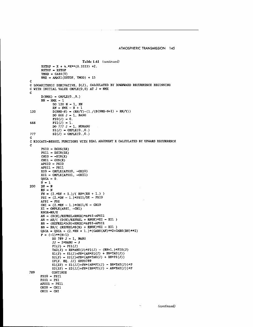
ATMOSPHERIC TRANSMISSION 145
Table 1.41 (continued)
XSTOP - X + 4.*X**(0.3333) +2. NSTOP - XSTOP YMOD - CABS(Y) NMX - AMAX1 (XSTOP, YMOD) + 15
C C LOGARITHMIC DERIVATIVE, D(J), CALCULATED BY DOWNWARD RECURRENCE BEGINNING C WITH INITIAL VALUE CMPLX(0,0) AT J - NMX C
D(NMX) - CMPLX(0.,0.) NN - NMX - 1
DO 120 N - 1, NN RN - NMX - N + 1
120 D(NMX-N) - (RN/Y)-(1./(D(NMX-N+1) + RN/Y)) DO 666 J - 1, NANG PIO(J) - 0.
666 PH(J) - 1. DO 777 J - 1, NUMANG S1(J) - CMPLX(0.,0.)
777 S2(J) - CMPLX(0.,0.) C C RICCATI-BESSEL FUNCTIONS WITH REAL ARGUMENT X CALCULATED BY UPWARD RECURRENCE C
PSIO - DCOS(DX) PSI1 - DSIN(DX) CHIO SIN(X) CHI1 - COS(X) APSIO - PSIO APSI1 - PSI1 XIO - CMPLX(APSIO, -CHIO) XII - CMPLX(APSI1, -CHI1) QSCA - 0. N - 1
200 DN - N RN - N FN - (2.*RN + l.)/( RN*(RN + 1.) ) PSI - (2.*DN - l.)*PSIl/DX - PSIO APSI - PSI CHI - (2.*RN - l.)*CHIl/X - CHIO XI - CMPLX(APSI, -CHI) RNOX-RN/X AN - (D(N)/REFREL+RN0X)*APSI-APSI1 AN - AN/( (D(N)/REFREL + RNOX)*XI - XII ) BN - (REFREL*D(N)+RN0X)*APSI-APSI1 BN - BN/( (REFREL*D(N) + RN0X)*XI - XII ) QSCA - QSCA + (2.*RN + 1.)*(CABS(AN)**2+CABS(BN)**2) P - (-1)**(N-1)
DO 789 J - 1, NANG JJ - 2*NANG - J PI(J) - PI1(J) TAU(J) - RN*AMU(J)*PI(J) - (RN+1.)*PIO(J) S1(J) - S1(J)+FN*(AN*PI(J) + BN*TAU(J)) S2(J) - S2(J)+FN*(AN*TAU(J) + BN*PI(J)) IF(J. EQ. JJ) GOT0789 Sl(JJ) - S1(JJ)+FN*(AN*PI(J) - BN*TAU(J))*P S2(JJ) - S2(JJ)+FN*(BN*PI(J) - AN*TAU(J))*P
789 CONTINUE PSIO - PSI1 PSI1 - PSI APSI1 - PSI1 CHIO - CHI1 CHI1 - CHI
(continued)
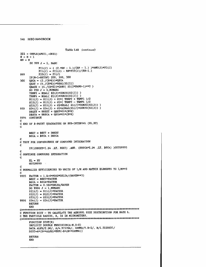
146 IR/EO HANDBOOK
Table 1.41 (continued)
XII - CMPLX(APSI1,-CHI1) N - N + 1 RN - N
DO 999 J - 1, NANG
PI1(J) - ( (2.*RN - l.)/(RN - 1.) )*AMU(J)*PI(J) PI1(J) - PI1(J) - RN*PI0(J)/(RN-1.)
999 PIO(J) - PI(J) IF(N-l-NSTOP) 200, 300, 300
300 QSCA - (2./(X*X))*QSCA QEXT - (4./(X*X))*REAL(Sl(l)) QBACK - (4./(X*X))*CABS( S1(2*NANG-1)**2 ) DO 950 J - l.NUMANG TEMP2 - REAL( S2(J)*C0NJG(S2(J)) ) TEMPI - REAL( S1(J)*C0NJG(S1(J)) ) Sll(J) - Sll(J) + Gl*( TEMP2 + TEMPI )/2 S12(J) - S12(J) + Gl*( TEMP2 - TEMPI )/2 S33(J) - S33(J) + G1*REAL( Sl(J)*CONJG(S2(J)) )
950 S34(J) - S34(J) + Gl*AIMAG(Sl(J)*CONJG(S2(J)) ) DBEXT - DBEXT + QEXT*G1*(X*X) DBSCA - DBSCA + QSCA*G1*(X*X)
9994 CONTINUE C C END OF 8-POINT QUADRATURE ON SUB-INTERVAL (XL,XU) C
BEXT - BEXT + DBEXT BSCA - BSCA + DBSCA
C C TEST FOR CONVERGENCE OF COMPOUND INTEGRATION C
IF((DBEXT*1.D4 .LT. BEXT) .AND. (DBSCA*1.D4 .LT. BSCA) )GOT09995
C C CONTINUE COMPOUND INTEGRATION C
XL - XU GOT09990
C C NORMALIZE EFFICIENCIES TO UNITS OF 1/M AND MATRIX ELEMENTS TO 1/M**3
C 9995 FACTOR - 1.E-6*PI02*DELTA/(WAVEN**3)
BEXT - BEXT*FACTOR BSCA - BSCA*FACTOR FACTOR - 0.5E6*DELTA/WAVEN DO 9996 J - l.NUMANG Sll(J) - S11(J)*FACT0R S12(J) - S12(J)*FACT0R S33(J) - S33(J)*FACT0R
9996 S34(J) - S34(J)*FACT0R RETURN END
C***********************************^*****^ C FUNCTION DIST - TO CALCULATE THE AEROSOL SIZE DISTRIBUTION FOR HAZE L. C THE PARTICLE RADIUS, R, IS IN MICROMETERS.
FUNCTION DIST(R) IMPLICIT DOUBLE PRECISION(A-H,0-Z) DATA ALPH/2.D0/, A/4.9757D6/, GAMMA/5.D-l/, B/1.51186D1/ DIST-A*(R**ALPH)*EXP(-B*(R**GAMMA) )
RETURN END
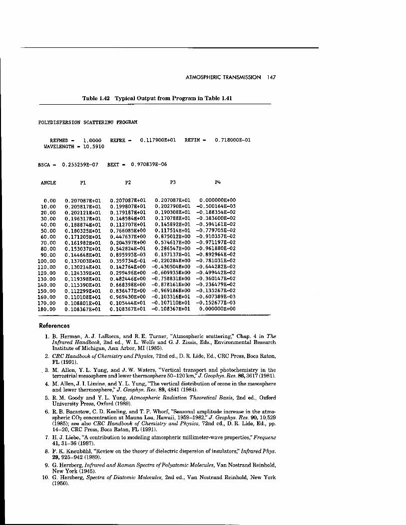
ATMOSPHERIC TRANSMISSION 147
Table 1.42 Typical Output from Program in Table 1.41
POLYDISPERSION SCATTERING PROGRAM
REFMED - 1.0000 REFRE WAVELENGTH - 10.5910
0.117900E+01 REFIM 0.718000E-01
BSCA 0.255259E-07 BEXT - 0.970839E-06
ANGLE PI P2 P3 P4
0.00 10.00 20.00 30.00 40.00 50.00 60.00 70.00 80.00 90.00
100.00 110.00 120.00 130.00 140.00 150.00 160.00 170.00 180.00
.207087E+01
.205817E+01
.202121E+01
.196317E+01
.188874E+01
.180325E+01 0.171205E+01 0.161982E+01 0.153037E+01 0.144648E+01 0.137003E+01 0.130214E+01 0.124339E+01 0.119398E+01 0.115390E+01 .112299E+01 .110108E+01 .108801E+01 .108367E+01
0.207087E+01 0.199807E+01 0.179187E+01 0.148584E+01 0.112707E+01 0.766085E+00 0.447637E+O0 0.204397E+00 0.542824E-01 0.895995E-03 0.359734E-01 0.142764E+00 0.299496E+00 0.482446E+00 0.668398E+00 0.836477E+00 0.969430E+00 0.105444E+01 0.108367E+01
0.207087E+01 0.202790E+01 0.190308E+01 0.170788E+01 0.145892E+01 0.117514E+01 0.875012E+00 0.574617E+00 0.286547E+00 0.197137E-01 -0.220284E+00 -0.430504E+00 -0.609935E+00 -0.758831E+00 -0.878161E+00 -0.969186E+00 -0.103316E+01 -0.107U0E+01 -0.108367E+01
0.000000E+00 -0.500164E-03 -0.188354E-02 -0.383600E-02 -0.594161E-02 -0.779705E-02 -0.910357E-02 -0.971197E-02 -0.961880E-02 -0.892964E-02 -0.781031E-02 -0.644282E-02 -0.499442E-02 -0.360147E-02 -0.236479E-02 -0.135267E-02 -0.607389E-03 -0.152677E-03 0.000000E+00
References
1. B. Herman, A. J. LaRocca, and R. E. Turner, "Atmospheric scattering," Chap. 4 in The Infrared Handbook, 2nd ed., W. L. Wolfe and G. J. Zissis, Eds., Environmental Research Institute of Michigan, Ann Arbor, MI (1985).
2. CRC Handbook of Chemistry and Physics, 72nd ed., D. R. Lide, Ed., CRC Press, Boca Raton, FL (1991).
3. M. Allen, Y. L. Yung, and J. W. Waters, "Vertical transport and photochemistry in the terrestrial mesosphere and lower thermosphere 50-120 km," J. Geophys. Res. 86,3617 (1981).
4. M. Allen, J. I. Limine, and Y. L. Yung, "The vertical distribution of ozone in the mesosphere and lower thermosphere," J. Geophys. Res. 89, 4841 (1984).
5. R. M. Goody and Y. L. Yung, Atmospheric Radiation Theoretical Basis, 2nd ed., Oxford University Press, Oxford (1989).
6. R. B. Bacastow, C. D. Keeling, and T. P. Whorf, "Seasonal amplitude increase in the atmo- spheric CO2 concentration at Mauna Loa, Hawaii, 1959-1982," J. Geophys. Res. 90, 10,529 (1985); see also CRC Handbook of Chemistry and Physics, 72nd ed., D. R. Lide, Ed., pp. 14-20, CRC Press, Boca Raton, FL (1991).
7. H. J. Liebe, "A contribution to modeling atmospheric millimeter-wave properties," Frequenz 41, 31-36 (1987).
8. F. K. Kneubühl, "Review on the theory of dielectric dispersion of insulators," Infrared Phys. 29, 925-942 (1989).
9. G. Herzberg, Infrared and Raman Spectra of Polyatomic Molecules, Van Nostrand Reinhold, New York (1945).
10. G. Herzberg, Spectra of Diatomic Molecules, 2nd ed., Van Nostrand Reinhold, New York (1950).
148 IR/EO HANDBOOK
11. G. Herzberg, Electronic Spectra and Electronic Structure of Polyatomic Molecules, Van Nos- trand Reinhold, New York (1966).
12. E. J. McCartney, Absorption and Emission by Atmospheric Gases, John Wiley & Sons, New York (1983).
13. J. H. Van Vleck and V. F. Weisskopf, "On the shape of collision-broadened lines," Rev. Mod. Phys. 17, 227-236 (1945).
14. A. Einstein, Phys. Z. 18, 121 (1917).
15. P. W. Anderson, "Pressure broadening in the microwave and infrared regions," Phys. Rev. 76, 647 (1949).
16. C. J. Tsao and B. Curnutte, "Line widths of pressure broadened spectral lines," J. Quant. Spectros. Radiat. Transfer 2, 41 (1962).
17. J. H. Van Vleck and D. L. Huber, "Absorption, emission and linebreadths: a semihistorical perspective," Rev. Mod. Phys. 49, 939-959 (1977).
18. P. W. Milonni and J. H. Eberly, Lasers, John Wiley & Sons, New York (1988). 19. G. Birnbaum and E. R. Cohen, "Theory of line shape in pressure-induced absorption," Can.
J. Phys. 54, 593-602 (1976). 20. G. Birnbaum, "The shape of collision broadened lines from resonance to the far wing," J.
Quant. Spectros. Radiat. Transfer 21, 597-607 (1979). 21. C. Boulet and D. Robert, "Short time behavior of the dipole autocorrelation function and
molecular gases absorption spectrum," J. Chem. Phys. 77, 4288-4299 (1982). 22. Q. Ma and R. H. Tipping, "Water vapor continuum in the millimeter spectral region," J.
Chem. Phys. 93, 6127-6139 (1990); see also Q. Ma and R. H. Tipping, "The atmospheric water continuum in the infrared: extension of the statistical theory of Rosenkranz," J. Chem. Phys. 93, 7066-7075 (1990).
23. P. W. Rosenkranz, "Pressure broadening of rotational band. II. Water vapor from 300 to 1100 cm-1," J. Chem. Phys. 83, 6139 (1985); see also P. W. Rosenkranz, J. Chem. Phys. 87, 163- 170 (1987).
24. P. W. Rosenkranz, "Shape of the 5 mm oxygen band in the atmosphere," IEEE Trans. An- tennas Propag. 23(4), 498-506 (1975).
25. P. W. Rosenkranz, "Interference coefficients for overlapping oxygen lines in air," J. Quant. Spectros. Radiat. Transfer 39(4), 287-297 (1988).
26. L. L. Strow, "Line mixing in infrared atmospheric spectra," in Modeling of the Atmosphere, L. S. Rothman, Ed., Proc. SPIE 928, 194-212 (1988).
27. J. M. Hartman, "Line mixing and finite duration of collision effects in pure CO2 infrared spectra: fitting and scaling analysis, J. Chem. Phys. 94, 6406-6419 (1991).
28. G. Birnbaum, "A kinetic approach to the shape of pressure broadened molecular bands," in Spectral Line Shapes AIP Conference Proceedings (1990).
29. R. W. Davies, R. H. Tipping, and S. A. Clough, "Dipole autocorrelation function for molecular pressure broadening: a quantum theory which satisfies the fluctuation-dissipation theorem," Phys. Rev. 26, 3378 (1982).
30. M. E. Thomas, "Infrared- and Millimeter-wavelength continuum absorption in the atmo- spheric windows: measurements and models," Infrared Phys. 30, 161-174 (1990).
31. C. Young, "Calculation of the absorption coefficient for lines with combined Doppler and Lorentz broadening," J. Quant. Spectros. Radiat. Transfer 5, 549 (1965).
32. K. Tomiyama, S. A. Clough, and F. K. Kneizys, "Unified real part of the susceptibility for collisional broadening," Report No. AFGL-TR-86-0181, Air Force Geophysics Laboratory, Hanscom AFB, MA (1986).
33. J. H. Shaw, Ohio J. Sei. 53, 258 (1953). 34. W. S. Benedict and R. F. Calfee, "Line parameters for the 1.9 and 6.3 micron water vapor
bands," ESSA Professional Paper 2, U.S. Government Printing Office, Washington, D.C. (1987).
35. D. M. Gates, R. F. Calfee, D. W. Hansen, and W. S. Benedict, "Line parameters and computed spectra for water vapor bands at 2.7 \x.m" National Bureau of Standards Monograph 71, U.S. Government Printing Office, Washington, D.C. (1964).
36. C. Camy-Peyret and J.-M. Flaud, "Line positions and intensities in the band of H2O," Mol. Phys. 32, 523 (1976).
37. R. A. McClatchey, W. S. Benedict, S. A. Clough, D. E. Burch, R. F. Calfee, K. Fox, L. S.
ATMOSPHERIC TRANSMISSION 149
Rothman, and J. S. Garing, "AFCRL atmospheric absorption line parameters compilation," AFCRL-TR-73-0096, Air Force Cambridge Research Laboratories, Bedford, MA (1973).
38. L. S. Rothman, R. R. Gamache, A. Goldman, L. R. Brown, R. A. Toth, H. M. Pickett, R. L. Poynter, J.-M. Flaud, C. Camy-Peyret, A. Barbe, N. Husson, C. P. Rinsland, and M. A. H. Smith, "The HITRAN database: 1986 edition," Appl. Opt. 26, 4058-4097 (1987).
39. R. M. Goody and Y. L. Yung, Atmospheric Radiation Theoretical Basis, 2nd ed., Oxford University Press, Oxford (1989).
40. M. E. Thomas, "Tropospheric water vapor absorption in the infrared window regions," Dis- sertation, Ohio State University (1979).
41. R. K. Long and E. K. Damon, "An atlas of pure water vapor spectra from 500 to 5000 cm-1
Vol. I and II," Ohio State University/ElectroScience Laboratory, Report No. 713774-3 (1984). 42. C. P. Rinsland, A. Goldman, M. A. H. Smith, and V. Malathy Devi, "Measurements of Lorentz
air-broadening coefficients and relative intensities in the H2160 pure rotational and V2 bands from long horizontal path atmospheric spectra," Appl. Opt. 30, 1427-1438 (1991).
43. R. E. Meredith, R. L. Spellicy, W. O. Gallery, S. G. O'Brien, and B. K. Matise, "Revised water vapor line parameters in the 1.0 to 1.1 p.m region," in Propagation Engineering: Third in a Series, L. R. Bissonnette and W. B. Miller, Eds., Proc. SPIE 1312, 364-366 (1990).
44. W. M. Elsasser, Heat Transfer by Infrared Radiation in the Atmosphere, Harvard University Press, Cambridge, MA (1942).
45. H. W. Yates and J. H. Taylor, "Infrared transmission of the atmosphere," NRL Report 5453 (1960).
46. A. Adel, Astrophys. J. 89, 1 (1939). 47. R. Anthony, "Atmospheric absorption of solar infrared radiation," Phys. Rev. 85, 674 (1952). 48. W. T. Roach and R. W. Goody, Q. J. R. Meteorol. Soc. 84, 319 (1958). 49. K. Bignell, F. Saiedy, and P. A. Sheppard, "On the atmospheric infrared continuum," J. Opt.
Soc. Am. 53, 466 (1963). 50. K. Bignell, "The water-vapour infra-red continuum," Q.J.R. Meteorol. Soc. 96, 390-403
(1970). 51. M. F. Crawford, H. L. Welsh, and J. L. Locke, "Infrared absorption of oxygen and nitrogen
induced by intermolecular forces," Phys. Rev. 75, 1607 (1949). 52. J. Susskind and J. E. Searl, "Atmospheric absorption near 2400 cm"1," J. Quant. Spectros.
Radiat. Transfer 18, 581 (1977). 53. B. H. Winters, S. Silverman, and W. S. Benedict, J. Quant. Spectros. Radiat. Transfer 4, 527
(1964). 54. J. Hinderung, M. W. Sigrist, and F. K. Kneubuhl, "Laser photoacoustic spectroscopy of water-
vapor continuum and line-absorption in the 8- to 14-^m atmospheric window," Infrared Phys. 27, 63 (1987).
55. W. B. Grant, "A critical review of measurements of water vapor absorption in the 840 to 1100 cm-1 spectral region," Appl. Opt. 29, 451-462 (1990).
56. J. W. Waters, "Methods of experimental physics," in Astrophysics Radio Telescopes, M. L. Meeks, Ed., Vol. 12, Part B, Academic Press, New York (1976).
57. N. E. Gaut and E. C. Reifenstein III, Environmental Research and Technical Report No. 13, Lexington, MA (1971).
58. G. E. Becker and S. H. Autler, "Water vapor absorption of electromagnetic radiation in the centimeter wavelength range," Phys. Rev. 70, 300 (1946).
59. L. Frenkel and D. Woods, "The microwave absorption by H2O vapor and its mixtures with other gases between 100 and 300 GHz," Proc. IEEE 54, 498 (1966).
60. D. E. Burch, "Absorption of infrared radiant energy by CO2 and H2O. III. Absorption by H2O between 0.5 and 36 cm"1 (278(1-2 cm)," J. Opt. Soc. Am. 58, 1383 (1986).
61. H. J. Liebe, "A contribution to modeling atmospheric millimeter-wave properties," Frequenz 41, 31 (1987).
62. H. J. Liebe and D. H. Layton, "Experimental and analytical aspects of atmospheric EHF refractivity," in Proc. URSI Commission F 1983 Symposium, Louvain, Belgium (1983).
63. H. J. Liebe, "An updated model for millimeter wave propagation in moist air," Radio Sei. 20, 1069 (1985).
64. M. E. Thomas, "Atmospheric absorption model from 0.01 to 10 wave numbers," in Propagation
150 IR/EO HANDBOOK
Engineering, L. R. Bissonnette and W. B. Miller, Eds., Proc. SPIE 1312, 355-363 (1990). 65. D. T. Llewellyn-Jones, "Laboratory measurements of absorption by water vapor in the fre-
quency range 100 to 1000 GHz," in Atmospheric Water Vapor, A. Deepak, T. D. Wilkerson, and L. H. Ruhnke, Eds., p. 255, Academic Press, New York (1980).
66. D. E. Burch and R. L. Alt, "Continuum absorption by H20 in the 700-1200 cm"x and 2400- 2800 cm-1 windows," AFGL-TR84-0128, Ford Aerospace and Communications Corp., Aero- nutronic Div. (1984).
67. J. C. Peterson, M. E. Thomas, R. J. Nordstrom, E. K. Damon, and R. K. Long, "Water vapor nitrogen absorption at CO2 laser frequencies," Appl. Opt. 18, 834 (1979).
68. G. L. Loper, M. A. O'Neill, and J. A. Gelbwachs, "Water-vapor continuum CO2 laser ab- sorption spectra between 27°C and 10°C," Appl. Opt. 22, 3701 (1983).
69. J. C. Peterson, "A study of water vapor absorption at CO2 laser frequencies using a differ- ential spectrophone and white cell," Dissertation, Ohio State University (1978).
70. V. N. Aref'ev and V. I. Dianov-Klokov, "Attenuation of 10.6-n.m radiation by water vapor and the role of (H20)2 dimers," Opt. Spectros. (USSR) 42, 488 (1977).
71. G. P. Montgomery, Jr., "Temperature dependence of infrared absorption by the water vapor continuum near 1200 cm"1," Appl. Opt. 17, 2299 (1979).
72. P. S. Varanasi, S. Chou, andS. S. Penner, J. Quant. Spectros. Radiat. Transfer», 1537 (1968); see also P. Varanasi and S. Chadamani, "Self- and N2-broadened spectra of water vapor between 7.5 and 14.5 p-m," J. Quant. Spectros. Radiat. Transfer 38, 407 (1987); and P. Varanasi, "Infrared absorption by water vapor in the atmosphere," in Modeling of the Atmo- sphere, L. R. Rothman, Ed., Proc. SPIE 928, 213 (1988).
73. C. T. Delaye and M. E. Thomas, "Atmospheric continuum absorption models," in Propagation Engineering: Fourth in a Series, L. R. Bissonnette and W. B. Miller, Eds., Proc. SPIE 1487, 291-298 (1991).
74. R. J. Nordstrom, M. E. Thomas, J. C. Peterson, E. K. Damon, and R. K. Long, "Effects of oxygen addition on pressure-broadened water vapor absorption in the 10-p.m region," Appl. Opt. 17, 2724 (1978).
75. A. D. Devir, A. Ben-Shalom, E. Trakhovsky, E. Raz, M. Engel, S. G. Lipson, and U. P. Oppenheim, "Experimental validation of atmospheric transmittance codes," in Optical, In- frared, and Millimeter-Wave Propagation Engineering, W. B. Miller and N. S. Kopeika, Eds., Proc. SPIE 926, 54-64 (1988).
76. K. O. White, W. R. Watkins, C. W. Bruce, R. E. Meredith, and F. G. Smith, "Water vapor continuum absorption in the 3.5 to 4.0 |im region," Appl. Opt. 17, 2711 (1978).
77. F. S. Mills, "Absorption of deuterium fluoride laser radiation by the atmosphere," Disser- tation, Ohio State University (1975).
78. W. R. Watkins, R. L. Spellicy, K. O. White, B. Z. Sojka, and L. R. Bower, "Water vapor absorption coefficients at HF laser wavelength (2.64 & 2.93 p-m)," Appl. Opt. 18,1582 (1979).
79. T. G. Kyle, D. G. Murcray, F. H. Murcray, and M. J. Williams, "Absorption of solar radiation by atmospheric carbon dioxide," J. Opt. Soc. Am. 55, 1421 (1965).
80. J. Van Kranendonk, "Induced infrared absorption in gases: calculation of the binary ab- sorption coefficients of symmetrical diatomic molecules," Physica 24, 347 (1958).
81. D. T. Sheng and G. E. Ewing, "Collision-induced infrared absorption of gaseous nitrogen at low temperatures," J. Chem. Phys. 55, 5425 (1971).
82. S. P. Reddy and C. W. Cho, "Induced infrared absorption of nitrogen and nitrogen-foreign gas mixtures," Can. J. Phys. 43, 2331 (1965).
83. M. M. Shapiro and H. P. Gush, "The collision-induced fundamental and first overtone bands of oxygen and nitrogen," Can. J. Phys. 44, 949 (1966).
84. N. I. Moskalenko, Y. A. Hin, S. N. Parzhin, and L. V. Rodionov, "Pressure-induced IR ra- diation absorption in atmospheres," Izv. Acad. Sei. USSR Atmos. Oceanic Phys. 15,632 (1979).
85. M. E. Thomas, "Infrared and millimeter-wavelength absorption in the atmospheric windows by water vapor and nitrogen: measurements and models," Infrared Phys. 30, 161 (1990).
86. S. F. Fulghum and M. M. Tilleman, "Interferometric calorimeter for the measurement of water vapor absorption," J. Opt. Soc. Am. B, 2401-2413 (1991).
87. S. A. Clough, F. X. Kneizys, R. Davies, R. Gamache, and R. H. Tipping, "Theoretical line shape for H2O vapor; application to the continuum," in Atmospheric Water Vapor, A. Deepak, T. D. Wilkerson, and L. H. Ruhnke, Eds., p. 25, Academic Press, New York (1980).
ATMOSPHERIC TRANSMISSION 151
88. S. A. Clough, F. X. Kneizys, and R. Davies, "Line shape and water vapor continuum," At- mospheric Research 23, 229-241 (1989).
89. V. E. Zuev and V. V. Fomin, "Consideration of continuum absorption in the problems of sounding from outer space," Presentation at the Sympossium on Remote Sensing of the Atmosphere from Space, Innsbruck, Austria (1978).
90. E. Hudis, Y. Ben-Aryeh, and Y. P. Oppenheim, "Third order linear absorption by pairs of molecules," Phys. Rev. A43, 3631-3639 (1991).
91. S. S. Penner, J. Quant. Spectros. Radiat. Transfer 13, 383 (1973). 92. R. A. Bohlander, R. J. Emery, D. T. Llewellyn-Jones, G. G. Gimmestad, H. A. Gebbie, 0. A.
Simpson, J. J. Gallagher, and S. Perkowitz, "Excess absorption by water vapor and com- parison with theoretical dimer absorption," in Atmospheric Water Vapor, A. Deepak, T. D. Wilkerson, and L. H. Ruhnke, Eds., p. 241, Academic Press, New York (1980).
93. M. E. Thomas and R. J. Nordstrom, "The N2-broadened water vapor absorption line shape and infrared continuum absorption I. Theoretical development," J. Quant. Spectros. Radiat. Transfer 28, 81 (1982).
94. M. E. Thomas and R. J. Nordstrom, "The N2-broadened water vapor absorption line shape and infrared continuum absorption II. Implementation of the line shape," J. Quant. Spectros. Radiat. Transfer 28, 103 (1982).
95. M. E. Thomas and R. J. Nordstrom, "Line shape model for describing infrared absorption by water vapor," Appl. Opt. 24, 3526 (1985).
96. C. B. Farmer, "Extinction coefficients and computed spectra for the rotational band of water vapor between 0.7 and 1000 cm"1" Contract No. KHG5828CB19(d)3, EMI Electronics, En- gland (1967).
97. P. L. Roney, F. Reid, and J.-M. Theriault, "Transmission window near 2400 cm-1: an ex- perimental and modeling study," Appl. Opt. 30, 1995-2004 (1991).
98. L. R. Brown, "Methane line parameters from 3700 to 4136 cm"1," Appl. Opt. 27, 3275-3279 (1988).
99. L. T. Molina and M. J. Molina, "Absolute absorption cross sections of ozone in the 185- to 350-nm wavelength range," J. Geophys. Res. 91, 14,501-14,508 (1986).
100. G. Guelachvili and K. N. Rao, Handbook of Infrared Standards: With Spectral Maps and Transition Assignments between 3 and 2600 \>.m, Academic Press, London (1986).
101. R. A. McClatchey et al., "AFCRL atmospheric absorption line parameter compilation," AFCRL Technical Report 0096 (1973); see also L. S. Rothman and R. A. McClatchey, "Updating of the AFCRL atmospheric absorption line parameters compilation," Appl. Opt. 15,2616 (1976); L. S. Rothman et al., "AFGL trace compilation," Appl. Opt. 17, 507 (1978); L. S. Rothman, "Update of the AFGL atmospheric absorption line parameters compilation," Appl. Opt. 17, 3517-3518 (1978); L. S. Rothman, "AFGL atmospheric absorption line parameters compi- lation: 1980 version," Appl. Opt. 20, 791-795 (1981); L. S. Rothman et al., "AFGL trace compilation: 1980 version," Appl. Opt. 20, 1323-1328 (1981); L. S. Rothman et al., "AFGL atmospheric absorption line parameters compilation: 1982 version," Appl. Opt. 22,2247-2256 (1983); L. S. Rothman et al., "AFGL trace compilation: 1982 version," Appl. Opt. 22,1616-1627 (1983).
102. L. S. Rothman, R. R. Gamache, A. Goldman, L. R. Brown, R. A. Toth, H. M. Pickett, R. L. Poynter, J.-M. Flaud, C. Camy-Peyret, A. Barbe, N. Husson, C. P. Rinsland, and M. A. H. Smith, "The HITRAN database: 1986 edition," Appl. Opt. 26, 4058-4097 (1987).
103. L. S. Rothman, "The spectroscopic database for high resolution atmospheric modeling," in Modeling of the Atmosphere, L. S. Rothman, Ed., Proc. SPIE 928, 79-93 (1988).
104. N. Husson, A. Chedin, N. A. Scott, D. Bailey, et al., "The GEISA spectroscopic line parameter data bank in 1984," Ann. Geophys. 4 A2, 185-190 (1986).
105. J. C. Gille and R. G. Ellingson, "Correction of random exponential band transmissions for Doppler effects," Appl. Opt. 7(3), 471-474 (1968).
106. W. M. Elsasser, "Mean absorption and equivalent absorption coefficient of a band spectrum," Phys. Rev. 54, 126 (1938).
107. H. Mayer, "Methods of opacity calculations, V. Effect of lines on opacity, methods for treating line contributions," Los Alamos Scientific Laboratory Report No. AECD-1870 (1947).
108. R. M. Goody, "A statistical model for water-vapour absorption," Q. J. R. Meteorol. Soc. 58, 165-169 (1952).
109. G. N. Plass, "Models for spectral band absorption," J. Opt. Soc. Am. 48, 690-703 (1958).
152 IR/EO HANDBOOK
110. P. J. Wyatt, V. R. Stull, and G. N. Plass, "Quasi-random model of band absorption," J. Opt. Soc. Am. 52, 1209 (1962).
111. R. Ladenburg and F. Reiche, "Über selektive absorption," Ann. Phys. (Leipzig) 42,181 (1913). 112. L. D. Kaplan, "Regions of validity of various absorption-coefficient approximations," J. Me-
teorology 10, 100-104 (1953). 113. G. N. Plass, "Useful representations for measurements of spectral band absorption," J. Opt.
Soc. Am. 50, 868-875 (1960). 114. S. A. Golden, "The Doppler analog of the Elsasser band model," J. Quant. Spectros. Radiat.
Transfer 7, 483-494 (1967). 115. R. M. Goody and Y. L. Yung, Atmospheric Radiation Theoretical Basis, 2nd ed., Oxford
University Press, Oxford (1989). 116. W. Malkmus, "Random Lorentz band model with exponential-tailed S_1 line intensity dis-
tribution function," J. Opt. Soc. Am. 57(3), 323-329 (1967). 117. P. J. Wyatt, V. R. Stull, and G. N. Plass, "The infrared transmittance of water vapor," Appl.
Opt. 3(2) (1964); see also Aeronutronic Report U-1717, Aeronutronic Systems, Newport Beach, CA (1962).
118. V. R. Stull, P. J. Wyatt, and G. N. Plass, "The infrared transmittance of water vapor," Appl. Opt. 3(2) (1964); Aeronutronic Report U-1718, Aeronutronic Systems, Newport Beach, CA (1962).
119. S. R. Drayson, "Atmospheric slant-path transmission in the 15(JL CO2 band," Report No. 05863-6T, The Institute of Science and Technology, University of Michigan, Ann Arbor, MI (1964).
120. A. J. LaRocca and R. E. Turner, "Atmospheric transmittance and radiance: methods of cal- culation," Report No. 107600-10-T, Environmental Research Institute of Michigan, Ann Arbor, MI.
121. J. N. Hamilton, J. A. Rowe, and D. Anding, "Atmospheric transmission and emission pro- gram," Report No. TOR-0073(3050-02)-3, Aerospace Corp., El Segundo, CA (1973).
122. J. N. Howard, D. Burch, and D. Williams, "Near-infrared transmission through synthetic atmospheres," Geophysics Research Paper No. 40, Report No. AFCRL-TR-55-213, Ohio State University Research Foundation, Columbus, OH (1955).
123. D. E. Burch, D. A. Gryvnak, and J. D. Pembrook, "Investigation of infrared absorption by nitrous oxide from 4000 to 6000 cm-1 (2.5 to 1.5 ^m)," Aeronutronics Report U-4393, AFCRL-71-0536, Philco-Ford Corp., Newport Beach, CA (1971); see also D. E. Burch, D. A. Gryvnak, and J. D. Pembrook, "760 to 2380 cm"1 (13.2 to 4.2 ^.m)," Aeronutronics Report U-4995, AFCRL-71-0620, Philco-Ford Corp., Newport Beach, CA (1971).
124. D. E. Burch, "Investigation of the absorption of infrared radiation by atmospheric gases," Philco Report No. U-4784, Philco-Ford Corp., Newport Beach, CA (1970).
125. K. Bignell, "The water vapor infrared continuum," Q. J. R. Meteorol. Soc. 96,390-403 (1970). 126. R. A. McClatchey et al., "Optical properties of the atmosphere," AFCRL-72-0497, 3rd ed.,
Air Force Cambridge Research Lab, Bedford, MA (1972); see also R. A. McClatchey et al., "AFCRL atmospheric absorption line parameters compilation," Report No. AFCRL-TR-73-0096, Air Force Research Labs., Hanscom Field, Bedford, MA (1973).
127. W. R. Bradford, T. M. McCormick, and J. A. Selby, "Laboratory representation of atmospheric paths for infrared absorption," Report No. DMP 1431, EMI Electronics, Hayes, Middlesex, England (1963).
128. S. R. Drayson and C. Young, "The frequencies and intensities of carbon dioxide absorption lines between 12 to 18 microns," Report No. 08183-1-T, Institute of Science and Technology, University of Michigan, Ann Arbor, MI (1967).
129. C. Walshaw, "Integrated absorption by the 9.6 y.m band of ozone," Q. J. R. Meteorol. Soc. 83, 315-321 (1957).
130. D. J. McCaa and J. H. Shaw, "The infrared spectrum of ozone," J. Mol. Spectrosc. 25(3), 374-397 (1968).
131. E. Plyler and E. Barker, "Infrared spectrum and molecular configuration on N2O," Phys. Rev. 38, 1827 (1931).
132. R. W. Fenn et al., "Optical and infrared properties of the atmosphere," Chap. 18 in Handbook of Geophysics and Space Environment, Adolph S. Jeursa, Ed., Air Force Geophysics Labo- ratory (1985).
ATMOSPHERIC TRANSMISSION 153
133. D. C. Robertson, L. S. Bernstein, R. Haimes, J. Wunderlich, and L. Vega, "5-cm x band model option to LOWTRAN 5," Appl. Opt. 20, 3218-3226 (1981).
134. A. Berk, L. S. Bernstein, and D. C. Robertson, "MODTRAN: a moderate resolution model for LOWTRAN 7," Report No. GL-TR-89-0122, Geophysics Laboratory, Air Force Systems Command, Hanscom AFB, MA (1989).
135. B. Edlen, "The refractive index of air," Metrologie 2, 12 (1966). 136. R. W. Fenn et al., "Optical and infrared properties of the atmosphere," Chap. 18 in Air Force
Handbook of Geophysics and Space Science (1985). 137. L. D. Lorah and E. Rubin, "Aerodynamic influences on infrared system design," Chap. 24 in
The Infrared Handbook, 2nd ed., W. L. Wolfe and C. J. Zissis, Eds., Environmental Research Institute of Michigan, Ann Arbor, MI (1985).
138. H. Barrell and J. E. Sears, "The refraction and dispersion of air for the visible spectrum," Philos. Trans. R. Soc. London A 238, 1-64 (1939).
139. R. J. Hill and R. S. Lawrence, "Refractive index of water vapor in infrared windows," Infrared Phys. 26, 371-376 (1986).
140. H. J. Leibe, "An updated model for millimeter wave propagation in moist air," Radio Sei. 20, 1069-1089 (1985).
141. B. R. Bean and E. J. Dutton, Radio Meteorology, Dover, New York (1968). 142. H. W. Ko, J. W. Sari, and J. P. Skura, "Anomalous microwave propagation through atmo-
spheric ducts," Johns Hopkins APL Technical Digest 4(1), 12-26 (1983). 143. D. E. Gray, American Institute of Physics Handbook, 3rd ed., pp. 6-110, McGraw-Hill, New
York (1972). 144. C. M. Crain, "The dielectric constant of several gases at a wavelength of 3.2 centimeters,"
Phys. Rev. 74, 691-693 (1948). 145. E. J. McCartney, Optics of the Atmosphere: Scattering by Molecules and Particles, Wiley,
New York (1976). 146. A. Aden and M. Meinel, "At sunset," Optics News 14(11), 6 (1988). 147. B. E. Schaefer and W. Liller, "Refraction near the horizon," Publ. Astron. Soc. Pac. 102,
796-805 (1990). 148. R. Greenler, Rainbows, Halos, and Glories, Cambridge University Press, Cambridge, En-
gland (1980). 149. D. J. K. O'Connell S. J., "The green flash and other low sun phenomena," North-Holland,
Vatican Observatory (1958). 150. C. F. Bohren and D. R. Huffman, Absorption and Scattering of Light by Small Particles,
Wiley-Interscience, New York (1983). 151. P. Barber and C. Yeh, "Scattering of electromagnetic waves by arbitrarily shaped dielectric
bodies," Appl. Opt. 14, 2864-2872 (1975). 152. P. W. Barber and S. C. Hill, Optical Effects Associated with Small Particles, World Scientific,
Singapore (1990). 153. P. W. Barber and S. C. Hill, Light Scattering by Particles: Computational Methods, World
Scientific, Singapore (1990). 154. D. W. Schuerman, Ed., Light Scattering by Irregularly Shaped Particles, Plenum Press, New
York (1979). 155. D. Deirmendjian, Electromagnetic Scattering on Spherical Polydispersions, American Elsev-
ier Publishing, New York (1969). 156. E. Hecht, Optics, 2nd ed., Addison-Wesley, Reading, MA (1987). 157. H. C. van de Hülst, Light Scattering by Small Particles, Dover, New York (1981). 158. H. C. van de Hülst, Multiple Light Scattering: Tables, Formulas, and Applications, Vols. 1
and 2, Academic Press, New York (1980). 159. M. Born and E. Wolf, Principles of Optics: Electromagnetic Theory ofPropagation, Interference
and Diffraction of Light, Pergamon Press, Elmsford, NY (1970). 160. R. W. Fenn, S. A. Clough, W. O. Gallery, R. E. Good, F. X. Kneizys, J. D. Mill, L. S. Rothman,
E. P. Shettle, and F. E. Volz, "Optical and infrared properties of the atmosphere," Chap. 18 in Handbook of Geophysics and Space Environment, Adolph S. Jeursa, Ed., Air Force Geo- physics Laboratory (1985).

154 IR/EO HANDBOOK
161. G. de Leeuw, K. L. Davidson, S. G. Gathman, and R. V. Noonkester, "Modeling of aerosols in the marine mixed layer," in Propagation Engineering, N. S. Kopeika and W. B. Miller, Eds., Proc. SPIE 1115, 287-294 (1989).
162. M. H. Smith, P. M. Park, and I. E. Consterdine, "Wind speed dependence of North Atlantic aerosol spectra," in Propagation Engineering, N. S. Kopeika and W. B. Miller, Eds., Proc. SPIE 1115, 278-286 (1989).
163. E. P. Shettle, "Models of aerosols, clouds and precipitation for atmospheric propagation stud- ies," in AGARD Conference Proceedings No. 454 on Atmospheric Propagation in the UV, Visible, IR, and MM-Wave Region and Related Systems Aspects, pp. 15-1 to 15-13 (1989).
164. E. J. McCartney, Optics of the Atmosphere: Scattering by Molecules and Particles, John Wiley & Sons, New York (1976).
165. G. M. Hale and M. R. Querry, "Optical constants of water in the 200-nm to 200-jj.m wave- length region," Appl. Opt. 12, 555-563 (1973).
166. E. P. Shettle and R. W. Fenn, "Models for the aerosols of the lower atmosphere and the effects of humidity variations on their optical properties," Air Force Geophysics Laboratory Report AFGL-TR-79-0214, Environmental Research Papers, N0676 (1979).
167. W. L. Wolfe and G. J. Zissis, Eds., The Infrared Handbook, The Infrared Information and Analysis (IRIA) Center, Environmental Research Institute of Michigan, Ann Arbor, MI (1978).
168. K. F. Palmer and D. Williams, "Optical constants of sulphuric acid: applications to the clouds of Venus," Appl. Opt. 14, 208-219 (1975).
169. L. S. Ivlev and S. I. Popova, "The complex index of refraction of the matter of the disperse phase of the atmospheric aerosol," Izv. Acad. Sei. USSR Atmos. Oceanic Phys. 9, 587-591 (1973).
170. F. E. Volz, "Infrared optical properties of ammonium sulphate, volcanic pumice, and flyash," Appl. Opt. 12, 564-568 (1973).
171. F. E. Volz, "Infrared refractive index of atmospheric aerosol substances," Appl. Opt. 11, 755-759 (1972).
172. J. T. Peterson and J. A. Weinman, "Optical properties of quartz dust particles at IR wave- lengths," J. Geophys. Res. 74, 6947-6952 (1969).
173. E. E. Remsberg, "Radiative properties of several probable constituents of atmospheric aero- sols," PhD Thesis, University of Wisconsin (1971).
174. O. B. Toon and J. P. Pollack, "A global average model of atmospheric aerosols for radiative transfer calculations," J. Appl. Meteorol. 15(3), 225-246 (1976).
175. M. E. Thomas and R. I. Joseph, "A comprehensive model for the intrinsic transmission prop- erties of optical windows," in Infrared Optical Materials VI, S. Musikant, Ed., Proc. SPIE 929, 87-92 (1988).
176. T. F. Deutsch, "Absorption coefficient of infrared laser window material," J. Phys. Chem. Solids 34, 2091-2104 (1973).
177. W. G. Spitzer and D. A. Kleinman, "Infrared lattice bonds of quartz," Phys. Rev. 121,1324-1335 (1961).
178. S. Onari, T. Arai, and K. Kudo, "Infrared lattice vibrations and dielectric dispersion in Fe203," Phys. Rev. B 16, 1717-1721 (1977).
179. M. Kerker, The Scattering of Light and Other Electromagnetic Radiation, Academic Press, New York (1969).
180. R. C. Harney, "Military applications of coherent infrared radar," in Physics and Technology of Coherent Infrared Radar, R. C. Harney, Ed., Proc. SPIE 300, 2-11 (1981).
181. M. Milham, "A catalog of optical extinction data for various aerosols/smokes," Special Pub- lication ED-SP-77002, Edgewood Arsenal (1976).
182. S. Chandrasekhar, Radiative Transfer, Dover, New York (1960). 183. M. V. Wilkes, "A table of Chapman's grazing incidence integral, Ch(x,x)," Proc. Phys. Soc.
London B67, 304-308 (1954). 184. "RSIC computer code & data collections: a capsule review of the computer code collection
(CCC), peripheral shielding routines (PSR), and data library collection (DLC)"; see also "Personal computer codes/data availability," both documents available from Oak Ridge Na- tional Laboratory (Feb. 1990).
ATMOSPHERIC TRANSMISSION 155
185. A. Ishimaru, Wave Propagation and Scattering in Random Media, Volume 1: Single Scat- tering and Transport Theory, Volume 2: Multiple Scattering, Turbulence, Rough Surfaces, and Remote Sensing, Academic Press, New York (1978).
186. P. S. Mudgett and L. W. Richards, "Multiple scattering calculations for technology," Appl. Opt. 10, 1485-1502 (1971).
187. L. Henyey and J. Greenstein, "Diffuse radiation in the galaxy," Astrophys. J. 93, 70-83 (1941).
188. E. A. Bücher, "Computer simulation of light pulse propagation for communication through thick clouds," Appl. Opt. 12, 2391-2400 (1973).
189. L. B. Stotts, "Closed form expression for optical pulse broadening in multiple-scattering media," Appl. Opt. 17, 504-505 (1978).
190. R. F. Lutomirski, "Atmospheric degradation of electro-optical system performance," Appl. Opt. 17, 3915-3921 (1978).
191. R. F. Lutomirski, "The irradiance distribution in a scattering medium," PSR Note 73, Pacific- Sierra Research Corp. (1975).
192. J. W. Goodman, Statistical Optics, John Wiley & Sons, New York (1985). 193. W. H. Wells, "Loss of resolution in water as a result of multiple small-angle scattering," J.
Opt. Soc. Am. 59, 686-691 (1969). 194. J. E. A. Selby and R. A. McClatchey, "Atmospheric transmittance from 0.25-28.5 p.m: com-
puter code LOWTRAN 2 " Report AFCRL-72-0745, Air Force Cambridge Research Labora- tory (1972).
195. J. E. A. Selby and R. A. McClatchey, "Atmospheric transmittance from 0.25-28.5 n.m: com- puter code LOWTRAN 3," Report AFCRL-75-0255, Air Force Cambridge Research Labora- tory (1975).
196. J. E. A. Selby and R. A. McClatchey, "Atmospheric transmittance from 0.25-28.5 \im: com- puter code LOWTRAN 3B," Report AFCRL-TR-76-0258, Air Force Cambridge Research Lab- oratory (1976).
197. J. E. A. Selby, F. X. Kneizys, J. H. Chetwynd, and R. A. McClatchey, "Atmospheric trans- mittance/radiance: computer code LOWTRAN 4," Report AFGL-TR-78-0053, Air Force Cam- bridge Research Laboratory (1978).
198. F. X. Kneizys, E. P. Shettle, W. O. Gallery, J. H. Chetwynd, L. W. Abreu, J. E. A. Selby, R. W. Fenn, and R. A. McClatchey, "Atmospheric transmittance/radiance: computer code LOWTRAN 5," Report AFGL-TR-80-0067, Air Force Cambridge Research Laboratory (1980).
199. F. X. Kneizys, E. P. Shettle, W. O. Gallery, J. H. Chetwynd, L. W. Abreu, J. E. A. Selby, S. A. Clough, and R. W. Fenn, "Atmospheric transmittance/radiance: computer code LOWTRAN 6," Report AFGL-TR-83-0187, Air Force Cambridge Research Laboratory (1985).
200. F. X. Kneizys, E. P. Shettle, L. W. Abreu, G. P. Anderson, J. H. Chetwynd, W. O. Gallery, J. E. A. Selby, and S. A. Clough, "Atmospheric transmittance/radiance: the LOWTRAN 7 model," (in preparation).
201. A. D. Devir, A. Ben-Shalom, S. G. Lipson, U. P. Oppenheim, and E. Ribak, "Atmospheric transmittance measurements: comparison with LOWTRAN 6," Report RAA/99-85, Technion— Israel Institute of Technology (1985).
202. C. F. Bohren and D. R. Huffman, Absorption and Scattering of Light by Small Particles, Wiley-Interscience, New York (1983).
203. E. P. Shettle and R. W. Fenn, "Models for the aerosols of the lower atmosphere and the effects of humidity variations on their optical properties," Air Force Geophysics Laboratory Report AFGL-TR-79-0214, Environmental Research Papers, N0676 (1979).
Bibliography
Section 7.7
Goody, R. M., and Y. L. Yung, Atmospheric Radiation Theoretical Basis, 2nd ed., Oxford University Press, Oxford (1989).
156 IR/EO HANDBOOK
Section 1.2
McCartney, E. J., Absorption and Emission by Atmospheric Gases: The Physical Processes, John Wiley & Sons, New York (1983).
McCartney, E. J., Optics of the Atmosphere: Scattering by Molecules and Particles, John Wiley & Sons, New York (1976).
Section 1.3.1
Breene, R. G., Jr., Theories of Spectral Line Shape, John Wiley & Sons, New York (1981). Cohen-Tannoudji, C, J. Dupont-Roc, and G. Grynberg, Photons and Atoms: Introduction to Quan-
tum Electrodynamics, John Wiley & Sons, New York (1989). Guelachvili, G., and K. N. Rao, Handbook of Infrared Standards: With Spectral Maps and Tran-
sition Assignments between 3 and 2600 |xm, Academic Press, London (1986). Haken, H., Light: Waves, Photons, Atoms, Vol. I, North-Holland, Amsterdam (1986). Herzberg, G., Atomic Spectra and Atomic Structure, Dover, Mineola, NY (1944). Herzberg, G., Electronic Spectra and Electronic Structure of Polyatomic Molecules, Van Nostrand
Reinhold, New York (1966). Herzberg, G., Infrared and Raman Spectra of Polyatomic Molecules, Van Nostrand Reinhold, New
York (1945). Herzberg, G, Spectra of Diatomic Molecules, 2nd ed., Van Nostrand Reinhold, New York (1950). Jackson, J. D., Classical Electrodynamics, 2nd ed., John Wiley & Sons, New York (1975). Rothman, L. S., Ed., Modeling of the Atmosphere, Proc. SPIE 928 (1988). Webster, C. R., R. T. Menzies, and E. D. Hinkley, "Infrared laser absorption: theory and appli-
cations," Chap. 3 in Laser Remote Chemical Analysis, R. M. Measures, Ed., pp. 163-272, John Wiley & Sons, New York (1988).
Weissbluth, M., Photon-Atom Interactions, Academic Press, Orlando, FL (1989).
Section 1.3.2
Bojkov, R. D., and P. Fabian, Eds., Ozone in the Atmosphere, A. Deepak Publishing Co., Hampton, VA (1989).
Deepak, A., T. D. Wilkerson, and L. H. Ruhnke, Eds., Atmospheric Water Vapor, Academic Press, New York (1980).
Flaud, J.-M., C. Camy-Peyret, C. P. Rinsland, M. A. H. Smith, and V. Malathy Devi, Atlas of Ozone Spectral Parameters from the Microwave to Medium Infrared, Academic Press, San Diego, CA (1990).
Goody, R. M., and Y. L. Yung, Atmospheric Radiation Theoretical Basis, 2nd ed., Oxford University Press, Oxford (1989).
Grant, W. B., Ed., Ozone Measuring Instruments for the Stratosphere, Optical Society of America (1989).
LaRocca, A. J., "Atmospheric absorption," Chap. 5 in The Infrared Handbook, 2nd ed., W. L. Wolfe and G. J. Zissis, Eds., Environmental Research Institute of Michigan, Ann Arbor, MI (1985).
McCartney, E. J., Absorption and Emission by Atmospheric Gases: The Physical Processes, John Wiley & Sons, New York (1983).
Zuev, V. E., Laser Beams in the Atmosphere, Plenum Press, New York (1982). Zuev, V. E., Propagation of Visible and Infrared Radiation in the Atmosphere, John Wiley & Sons,
New York (1974).
Section 1.4
Bohren, C. F., Ed., Selected Papers on Scattering in the Atmosphere, SPIE Milestone Series Vol. MS 7, SPIE Optical Engineering Press, Bellingham, WA (1989).
Karp, S., R. M. Gagliardi, S. E. Moran, and L. B. Stotts, Optical Channels: Fibers, Clouds, and the Atmosphere, Plenum Press, New York (1988).
CHAPTER 2
Propagation through Atmospheric Optical Turbulence
Robert R. Beland Phillips Laboratory
Geophysics Directorate Hanscom Air Force Base, Massachusetts
CONTENTS
2.1 Introduction 159 2.2 Theory of Optical Turbulence in the Atmosphere 161
2.2.1 Introduction 161 2.2.2 Statistical Concepts 161 2.2.3 Structure Functions 165 2.2.4 Kolmogorov Theory of Turbulence 167 2.2.5 Conservative Passive Scalars 169 2.2.6 Index of Refraction 171 2.2.7 Atmospheric Temporal Statistics 174
2.3 Optical/IR Propagation through Turbulence 176 2.3.1 Introduction 176 2.3.2 Formal Solutions of the Wave Equation 177 2.3.3 Amplitude and Phase Statistics 179 2.3.4 Scintillation 184 2.3.5 Imaging Effects 190 2.3.6 Beam Effects 195 2.3.7 Isoplanatism 201
2.4 Measurements of Optical Turbulence in the Atmosphere 201 2.4.1 Introduction 201 2.4.2 Atmospheric Boundary Layer 202 2.4.3 Free Atmosphere 206 2.4.4 Issues of Measurement 209 2.4.5 Measurements of Moments 210
157
158 IR/EO HANDBOOK
2.5 Models of Optical Turbulence 211 2.5.1 Introduction 211 2.5.2 Boundary-Layer Turbulence 212 2.5.3 Model Optical Turbulence Profiles 217 2.5.4 Parametric Models 221
2.6 Sample Problems 224 2.6.1 Scintillation 224 2.6.2 Image Resolution 226 2.6.3 Beam Wander and Broadening 227
References 229
PROPAGATION THROUGH ATMOSPHERIC OPTICAL TURBULENCE 159
2.1 INTRODUCTION
All systems utilizing electromagnetic waves must take into account the char- acteristics of the medium in which propagation occurs. As more sophisticated electro-optic systems are developed, details of the propagation medium that had previously been ignored become important. Optical turbulence is such an important characteristic for propagation through the atmosphere. Optical tur- bulence can be defined as the fluctuations in the index of refraction resulting from atmospheric turbulence. It is responsible for a variety of effects, such as temporal intensity fluctuations, or scintillation; the twinkling of stars is the classic example. In laser beam propagation, the effects include beam wander and broadening. In imaging applications, turbulence effects include image dancing and blurring. It is turbulence that limits the resolution of astronomical telescopes and motivates the placement of telescopes in space to avoid the atmosphere's deleterious effect. There are other more sophisticated and subtle effects that arise in modern systems, particularly those that utilize adaptive optics elements.
Atmospheric turbulence produces small fluctuations in the index of refrac- tion. Although the magnitude of the individual fluctuations is very small, the cumulative effect in propagation along an atmospheric path may be very sig- nificant. Their effect is easily described qualitatively. The turbulence-induced fluctuations in the refractive index produce a phase distortion of the wavefront as it passes through the turbulence, and it is this distorted wavefront that continues to propagate and is itself further distorted.
In this chapter, the theory of optical turbulence in the atmosphere is re- viewed. The propagation through turbulence by optical and infrared radiation also is treated. The focus is on "small"-scale atmospheric turbulence, where "small" is used in the sense of micrometeorology. No consideration is given to the "large"-scale atmospheric turbulence that is associated with large-scale flow, such as the meridional flow from the equator to the poles or synoptic meteorology. Our interest is in the characterization of optical paths. As will be seen, the index of refraction structure parameter C« along the path emerges as the critical parameter in characterizing the effects of the atmosphere.
The propagation of electromagnetic radiation through random media is a large subject area. Only the optical/IR segment of the electromagnetic spectrum is discussed here. The approach to turbulence and its effects treats the at- mosphere and the turbulence-induced refractive-index fluctuations as a con- tinuum. Effects arising out of discrete scatterers, such as aerosols, are not treated, despite the fact that they may be considered as representing fluctua- tions in the index of refraction. The effects of absorption by atmospheric par- ticulates or molecules also are excluded. This last exclusion includes the phe- nomenon of thermal blooming of high-power laser beams in the atmosphere, but the effect of optical turbulence on low-power laser beams is treated. The complex phenomena associated with high-energy laser propagation through the atmosphere, including stimulated Raman scattering, aerosol vaporization, thermal-blooming instability, and interactions with turbulence effects are an area of active research that warrants a more thorough and diverse treatment than could be given in the present chapter.
A listing of symbols and notation used in this chapter is given in Table 2.1.
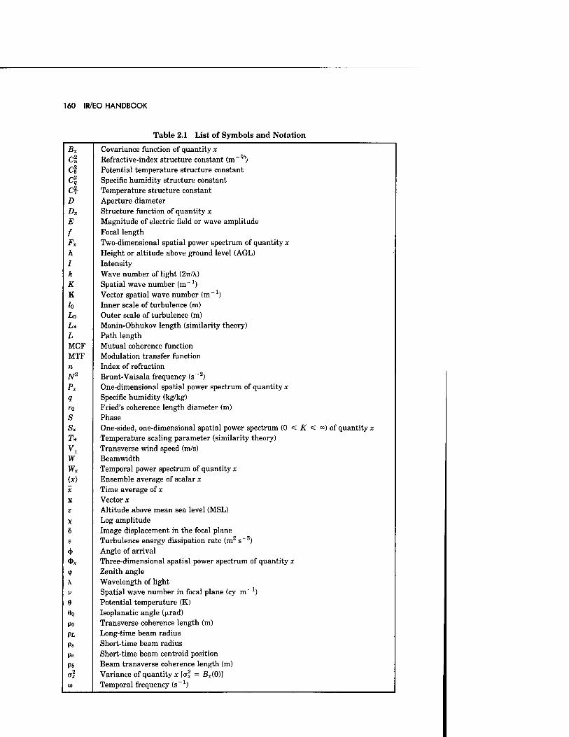
160 IR/EO HANDBOOK
Table 2.1 List of Symbols and Notation
Bx Covariance function of quantity x cl Refractive-index structure constant (m~^ c* Potential temperature structure constant
c? Specific humidity structure constant c* Temperature structure constant D Aperture diameter Dx Structure function of quantity x E Magnitude of electric field or wave amplitude
f Focal length Fx Two-dimensional spatial power spectrum of quantity x h Height or altitude above ground level (AGL) I Intensity k Wave number of light (2IT/\)
K Spatial wave number (m_1) K Vector spatial wave number (m_1)
h Inner scale of turbulence (m) Lo Outer scale of turbulence (m) L* Monin-Obhukov length (similarity theory) L Path length MCF Mutual coherence function MTF Modulation transfer function n Index of refraction N2 Brunt-Vaisala frequency (s~2) Px One-dimensional spatial power spectrum of quantity x
<? Specific humidity (kg/kg) ro Fried's coherence length diameter (m) S Phase sx One-sided, one-dimensional spatial power spectrum (0 =s K *s °°) of quantity x T* Temperature scaling parameter (similarity theory)
vx Transverse wind speed (m/s) w Beamwidth wx Temporal power spectrum of quantity * (x) Ensemble average of scalar x X Time average of x X Vector x z Altitude above mean sea level (MSL)
X Log amplitude 8 Image displacement in the focal plane e Turbulence energy dissipation rate (m2 s~3)
+ Angle of arrival *x Three-dimensional spatial power spectrum of quantity x
<p Zenith angle X. Wavelength of light V Spatial wave number in focal plane (cy m_1) 8 Potential temperature (K) e0 Isoplanatic angle (n-rad) P0 Transverse coherence length (m) PL Long-time beam radius
Ps Short-time beam radius Pc Short-time beam centroid position Pb Beam transverse coherence length (m) a? Variance of quantity x [o-2 = Bx(0)] (a Temporal frequency (s_1)
PROPAGATION THROUGH ATMOSPHERIC OPTICAL TURBULENCE 161
2.2 THEORY OF OPTICAL TURBULENCE IN THE ATMOSPHERE
2.2.1 Introduction
When the flow of a viscous fluid, characterized by the Reynold's number, ex- ceeds a critical value, the flow changes from laminar to a more chaotic regime. This regime is turbulence. It is fundamentally a state where the velocity of a parcel of the fluid fluctuates about the mean velocity of the flow and these fluctuations possess a continuous power spectrum. The fluctuations are usually conceptualized in the form of vortices or eddies. These eddies result in the transport or mixing of other characteristics of the fluid. In the case of the atmosphere, the turbulent fluctuations in wind speed result in the mixing of atmospheric quantities, such as temperature, aerosols, or water vapor. The quantity that is the focus here is the index of refraction, that is, optical tur- bulence. The theoretical framework of optical turbulence is based on the theory of the fundamental physical process, velocity turbulence.
Turbulence is fundamentally a nonlinear process. The governing equations, the Navier-Stokes equations, are nonlinear. As if this were not difficult enough, they also suffer from the closure problem; i.e., there are more variables than equations. This difficult subject matter has occupied some of the great minds of twentieth century science. Because of these difficulties, a statistical ap- proach, relying heavily on dimensional analysis, was pursued by Kolmogorov. Kolmogorov's theory provides the cornerstone for the study of optical turbu- lence and is the subject of a subsequent section. It should be emphasized that turbulence theory is not rigorously derived from first principles. Furthermore, when one is considering a fluid as complex and varied as the atmosphere, additional simplifications and approximations enter.
2.2.2 Statistical Concepts
As mentioned earlier, a statistical approach has achieved considerable success in describing both atmospheric turbulence and its effects on optical/IR systems. In this section, the necessary tools and concepts are summarized, first for scalar random processes in one dimension and then for scalar processes in three dimensions. The generalization to vector processes is cumbersome but straight- forward. Let tit) be a random variable at time t. This is a one-dimensional time series that is the subject of a vast literature.1,2 The ensemble average of an arbitrary function, say /, of £ will be denoted by the bracketed quantity < fiQ). Most of our treatment is in terms of first- and second-order statistics. The covariance function of £ is defined by
Bkih,t2) = Wti) - <£(*i)>]R(fe) - <€(fc)>]> • (2.D
In this general definition, the covariance represents the correlation between the fluctuations from the mean at t\ with those at fe- If the process is stationary, then its moments are invariant under translations in time.3 For stationary
aThe distinction between second order and strict stationarity is not important for this discussion. We shall assume strict stationarity so that all moments and all order probability distributions are invariant under translation of the time origin.
162 IR/EO HANDBOOK
random processes, the mean is independent of time (that is, (£(£)) = (£)) and the covariance depends only on the difference T = t\ - fe and can be written for any time t as
B«(T) = (W + T) - (OMit) ~ m = W + T)£(*)> - (02 ■ (2.2)
For the class of stationary processes that are known as ergodic processes, the ensemble averages such as the mean and the covariance can be determined from time averages.3 In our notation, the time average_over a time interval T of some quantity, say f, is denoted by an overbar, fr- For example, the covariance averaged over a time T is
B^ii-r) = i f W + T) - hM(t) - IT] dt . (2.3) l Jo
The ergodic property assures us that
B6(T) = lim5e,j<T) . (2.4) T—»oo
Thus, we have the equivalence between infinite time_averages and ensemble averages. This presentation shows that for finite T, B^T is a statistical esti- mator of the infinite time average, denoted by B%, or equivalently, of the ensemble average B%. The accuracy of the statistical estimator for a stationary process is a central issue in the accuracy of measurements.
There is an alternative description of the correlations of fluctuations of stationary random processes that is heavily utilized. The Wiener-Khinchine theorem1'3 established a Fourier transform relationship between the autoco- variance and the power spectrum of a stationary random process, denoted by W^(w); that is,
W4(co) = J- f B€(T) e'MT di . (2.5) ZlT J-OO
The inverse relation is
B«(T) = I W{(w) e~'WT do> . J — oo
(2.6)
Since the covariance is a real, even function, it can be shown that the spectrum is a real, even function. Therefore, these two Fourier integrals can be written as cosine transforms:
1 r W«(w) = r- ä6(T) COS(WT) rfx , (2.7)
^77 J — oo
Bgto = W?(w) COS(WT) rfw . (2.8)
PROPAGATION THROUGH ATMOSPHERIC OPTICAL TURBULENCE 163
The power spectrum is a frequency-domain representation or spectral decom- position of the temporal correlations. By ergodicity, it can also be estimated by time averages and its estimation is the domain of the subject of spectral analysis.4
Next, consider scalar random processes in three dimensions, also called random fields. The spatial covariance of the field £(r) is defined as
B«(ri,r2) = <R(ri) - <£(ri))][£(r2) - <£(r2)>]> .
The property of homogeneity is the spatial counterpart of stationarity in time. A homogeneous process is one that has moments that are invariant under a spatial translation. Thus, the mean is independent of r (that is, (£(r)) = (£)), and the covariance depends only on r = r2 - ri and can be written as
߀(n,r2) = B6(r) = <£(ri)£(ri + r)) - <£>2 . (2.10)
For homogeneous random processes, there is also an analogous property to ergodicity that allows ensemble properties to be measured by spatial aver- aging.5 Thus, the ensemble covariance for a separation r can be measured by averaging measurements that are spatially separated by r. There is still a further simplification that occurs for homogeneous processes that are also spatially isotropic, that is, have invariance properties under rotations. For such processes, the ensemble properties of the fluctuations do not depend on direction and thus the dependence is on r only, the magnitude of r: B^(r) = B%(r). For this kind of process, the ensemble properties can be readily estimated by spatial averaging.
These assumptions of stationarity, homogeneity, and isotropism of course are not likely to be strictly true in the physical world, and this is especially true in turbulence modeling. They are utilized assuming they are approxi- mately true. For example, the atmosphere could never be treated strictly as homogeneous and isotropic, but over some limited volume and time, these properties are reasonable. The key to the validity of these assumptions is in terms of local behavior.
There are spectral representations for the homogeneous and isotropic cases. For a homogeneous process, the power spectrum <fp(K) is simply a three- dimensional Fourier transform of the covariance:
*e(K) = Qy jjj Bi(r) eiKr dr . (2.11)
where K is the vector wavenumber. The inverse relation is thus
Bi(r) = \\\ ^4^ e'iK'r dK ■ (2-12)
Since both the covariance and the spectrum are real, even functions, these can be written as cosine transforms:
164 IR/EO HANDBOOK
^(K) = \h) l!L„Biir) COs(K"r) dT ' (213)
5e(r) = jjj *e(K) cos(K-r) dK . (2.14)
If the process is also isotropic, then <$>% depends only on the magnitude of K, and thus, by integrating out the angular spherical coordinates, we get
Bt(r) = (4ir/r)| K<S>dK) sin(Kr) dK , (2.15) Jo
Qf/LK) = —U t fl«(r) sin(Kr)r dr . (2.16) 2TT K J
In some instances we are interested in the covariance of a spatial random process along a single axis. This situation often arises in measurements. Thus, we are sometimes interested in the one-dimensional spectrum, denoted by P%(K), of three-dimensional fluctuations. This relation is6
As an example of this relation, a one-dimensional spectrum that has a K~ /3
dependence will behave as K~ /3 in three dimensions. It will often occur in the analysis of propagation problems that we are
interested in the spectrum of the fluctuations in a plane perpendicular to the direction of propagation. Thus, we shall consider the two-dimensional spectrum in the x-y plane with propagation in the z direction. Let F^{K\,K2,z) be the spectrum of the homogeneous fluctuations between planes separated by z. Then F% is readily obtained from <t>^ by integrating over the K3 dependence:
F^K^K^z) = I QtjLKifaKs) cos(Ksz) dK3 . (2.18) J — CO
If the fluctuations are homogeneous and isotropic in three dimensions, then they are also homogeneous and isotropic in the plane z = constant. Thus, we can convert to cylindrical spatial variables (p,0,z) and the fluctuations in the z = constant plane have a spectrum given by F^Kifaß) and a two-dimensional covariance that depends only on p, given by7
/*oo
B€(p) = 2TTJ JoöCpWffftßyX d% , (2.19)
where % = [K\ + K\Hh and Jo(0 is a Bessel function of the first kind of zero order.
PROPAGATION THROUGH ATMOSPHERIC OPTICAL TURBULENCE 165
2.2.3 Structure Functions
The treatment of spatial (or temporal) fluctuations in terms of the covariance and the spectrum depends on the assumptions of homogeneity (or stationarity). Of particular importance is the assumption that the mean is the same over all space (time). This constancy of the mean is clearly not satisfied by atmo- spheric parameters, for example, wind or temperature. Nor is it always satisfied by optical parameters, such as the phase of a beam at a telescope aperture. In the case of wind, there is a mean that varies in space. In such cases, the fluctuations about the spatially (temporally) varying means may be a homogeneous/isotropic (stationary) process. Thus, the random variable £(r) may be decomposed into a mean and a fluctuating part:
€(r) = <$(r)> + r(r) , (2.20)
where the fluctuations £' satisfy (£'(r)> = 0 for all r. Random processes that allow such a decomposition into a varying mean and stationary fluctuations are referred to as possessing stationary increments in the time domain and the analogous spatial property is referred to as local homogeneity. Of course, all homogeneous (stationary) random processes are locally homogeneous (have stationary increments). The theoretical framework of the previous section may be applied to the homogeneous fluctuations £'. However, it is not always ad- vantageous to do so. Measurements and effects of such processes almost always include the spatially varying mean, and in some cases, mean square differences are the relevant and measurable quantity, such as the phase difference be- tween two aperture points. The utilization of structure functions provides a framework for the treatment of random processes with slowly varying means. The structure function of ^ is defined as
ü?(n,r2) = <K(ri) - £(r2)]2> . (2.21)
If the decomposition into mean and fluctuations is substituted, we get
D6n,r2) = [<£(ri)> - <£(r2)>]2 + (Win) - S'fo)]2) , (2.22)
which shows the utility of the structure-function approach: the structure func- tion decomposes into a contribution from the difference in the means and a difference in the fluctuations. Since the means are by definition slowly varying, for separations between ri and r2 that are not too large, the term in £' dominates the structure function. The extension of the structure function to locally ho- mogeneous and isotropic random processes is straightforward. For any n, we have
D«(r) = <[£(ri) - «ri + r)]2) , (2.23)
where r is the magnitude of r. As with covariance functions, there is a gen- eralization of the Wiener-Khinchine theorem giving the spectral representa- tion of D^. For a locally homogeneous random field, the spectrum is related to the structure function by
166 IR/EO HANDBOOK
D{(r) = 2Jjj $(K)[1 - cos(K-r)] dK . (2.24)
If the fluctuations are also locally isotropic, this can be written as7
D«(r) = 8T7 Q(K) F ■>o
sin(Kr) Kr
K2 dK (2.25)
The value of the structure function approach is also apparent in this spectral representation. The term {1 - [sin(.K»/Ä>} acts as a high-pass filter, removing the low spatial frequencies K < r_1. In other words, the contribution from scale sizes much larger than the separation is removed in the structure func- tion. Note also that the spectrum of the structure function is allowed to have a singularity at K = 0 (of type K~a, where a < 5).6 Due to this singularity, the inverse relation is not as straightforward as for the covariance. For a locally homogeneous isotropic process, the inverse relation is7
•«""-lOT'H-fe K sin(Kr) d dr -iD<w
dr (2.26)
For locally homogeneous, isotropic fields, the relation between the spectrum in three dimensions and the one-dimensional spectrum, P^(K), along any axis is exactly the same as for homogeneous fields:
*{(#) = -(UmK)dPi(K)/dK (2.27)
Next, consider the two-dimensional spectrum in the x-y plane with propa- gation in the z direction. If F^{K\,Kz,z) is the spectrum of the homogeneous fluctuations between planes separated by z, it is given by
F£Kx,K2,z) /:
^(KuK^Ka) cos(K3z) dK3 (2.28)
This relation is again the same for homogeneous, isotropic fields as for those that also satisfy the local property. Using the local isotropy property, it can also be shown that the fluctuations in the z = constant plane have a spectrum given by F^(Ki,K2,0) and a two-dimensional structure function in the cylin- drical coordinate p that depends only on p, given by6
Z)€(p) = 4-J7 I [1 - JoO£p)]*€0C,O)9£ <BC , ■>o
(2.29)
-1V2 where % = [K\ + Ki For random fields that are homogeneous and isotropic, we can derive expres-
sions between the co variance and structure functions and their spectra. It is straightforward to show that for such a case
PROPAGATION THROUGH ATMOSPHERIC OPTICAL TURBULENCE 167
D€(r) = 2[fi€(0) - ßs(r)] . (2.30)
Substitution of the spectral expansions for B^ yields
Ds(r) = 2 JJJ &i(K)[l - cos(K-r)] dr , (2.31)
which is identical to our earlier result. Thus, the spectrum of the covariance is the same as the spectrum corresponding to the structure function. In this case, the structure function spectrum represents only the fluctuations. In the more general case of a field that is homogeneous and isotropic only locally, the spectrum contains a contribution from the spatially varying mean. The spectrum in this case is not necessarily integrable, and thus there is no co- variance that can be associated with it.
2.2.4 Kolmogorov Theory of Turbulence
It is significant that Kolmogorov's theory was presented in terms of a set of hypotheses,8 which embody considerable physical insight. His theory treated the velocity fluctuations. Kolmogorov assumed that the velocity fluctuations can be represented by a locally homogeneous and isotropic random field for scales less than the largest eddies or the energy source. The treatment in terms of structure functions follows. The central physical concept of Kolmogorov's theory is the description due to Richardson9 of a cascade of energy from large- scale sizes to the small. The source of the energy at the large-scale sizes may be convection or wind shear. The energy is dissipated by viscosity at the small- scale sizes. In between, there is a range where inertial forces dominate. Fur- thermore, in this range the fluctuations are assumed to be spatially homo- geneous and isotropic. If e is the energy dissipation rate (units of m2 s"3), Kolmogorov showed by dimensional arguments that in this inertial range, the longitudinal structure function of wind velocity satisfies the famous % power law:
DrÄr) = C2vr
2/3 , lo < r < Lo , (2.32)
where the longitudinal velocity component is that parallel to the vector r connecting the two observation points. The constant C2 is known as the velocity structure constant, which Kolmogorov defined to be given by
C2 = ae2/3 = 2e% , (2.33)
where a is a dimensionless constant whose value has been determined from measurements.10'11 The domain of validity of the % structure function law is the so-called inertial range, defined by the inner scale lo and the outer scale Lo. The inner scale lo is the small-scale size at which viscosity effects become dominant and the energy is dissipated into heat. For velocity fluctuations, the inner scale is often equated to the Kolmogorov microscale, given by12
168 IR/EO HANDBOOK
h = (V3/E)
1/4 , (2.34)
where v is the kinematic viscosity (units of m2 s_1). The inner scale ranges from a few millimeters near the surface to centimeters or more in the tropo- sphere and stratosphere. Note that lo increases with kinematic viscosity, which increases with altitude. The inverse dependence on the energy dissipation rate shows that strong turbulence has small inner scales and weak turbulence larger inner scales.
The outer scale Lo is regarded as (1) the largest scale size where local homo- geneity and isotropy are reasonable, (2) the scale size of the energy source, or (3) the dimension of the flow as a whole. In the theory presented by Tatarski,6'13
this vagueness arises partly out of the heavy use of dimensional arguments, where factors of order unity are used throughout. It has become customary to define the outer scale by the limits of the % power law. Representative values of Lo are from tens to a few hundred meters. Near the surface, Lo scales with height above ground according to6 Lo = OAh. This can produce values of the order of hundreds of meters in the atmospheric or planetary boundary layer, that is, the region (typically the first kilometer) where frictional forces and heat exchange with the surface dominate. In the free atmosphere, the outer scale is typically of the order of tens of meters14'15 but can reach values of hundreds of meters in large, strong layers. Lo can be shown to scale with zh, so the outer scale increases with the strength of turbulence. Thus, the inertial range broadens at both ends in strong turbulence; lo decreases and Lo increases.
The behavior of the structure function at small-scale sizes (i.e., r < lo) can be easily inferred. From the definition of a structure function, we can show by a Taylor series expansion applied to small r that the structure function behaves as r2 The two domains and power laws are reconciled by choosing the constant such that the two power laws agree at IQ. This gives6 the relation
Drr{r) = C*lö4/3r2 , r < lo . (2.35)
Tatarski6 uses this definition to consistently define lo so that the two power laws agree at r = lo. He gives
lo = 12.8(V3
/E)1/4 . (2.36)
In Fig. 2.1, the behavior of the structure function is shown. For values of separation r larger than Lo, no general behavior can be predicted in most cases since the structure function depends on anisotropic eddies and the theory breaks down. Tatarski6 states that the growth of the structure function in general slows down in the region r > Lo- However, if the random field were strictly homogeneous and isotropic, then for large r the structure function would asymptotically approach the value of 2a2, where a2 is the variance of the fluctuations. This latter case is schematically shown in the figure.
The % structure function can be shown to be equivalent to the power spec- trum in three dimensions:
&rr(K) = 0.033C^"n/3 , (2.37)
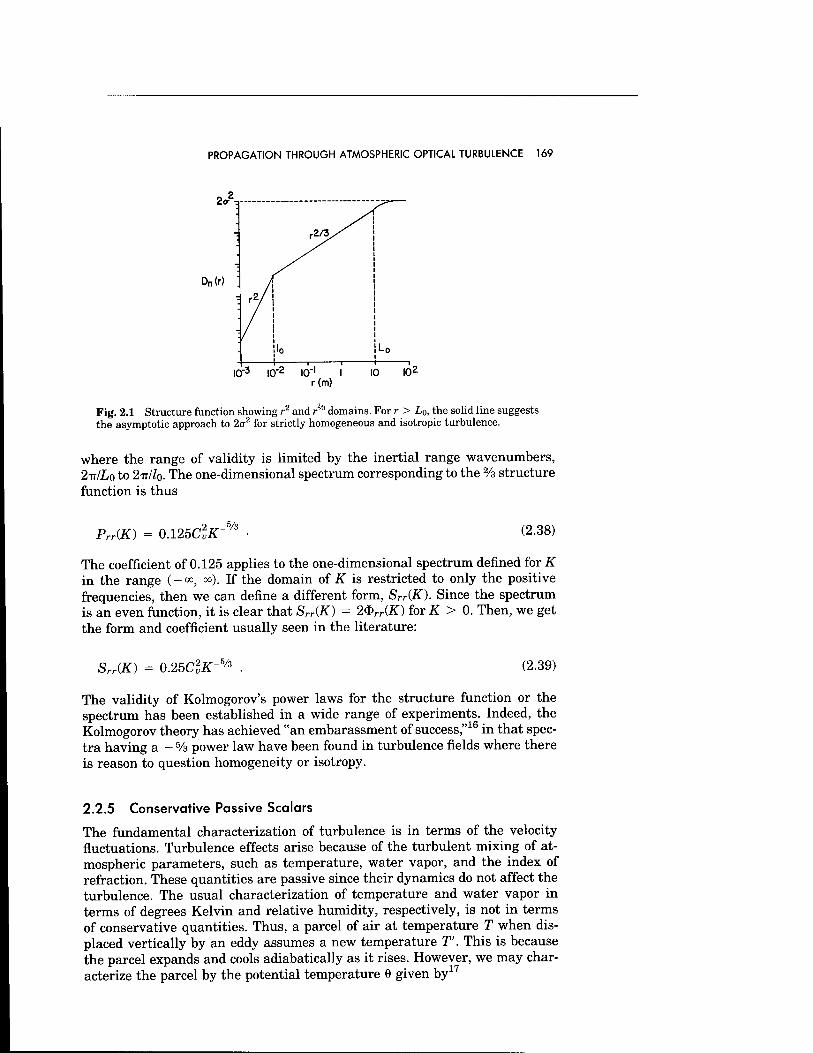
PROPAGATION THROUGH ATMOSPHERIC OPTICAL TURBULENCE 169
Dn(r)
r(m)
Fig. 2.1 Structure function showing r2 and r2/J domains. For r > L0, the solid line suggests the asymptotic approach to 2CT
2 for strictly homogeneous and isotropic turbulence.
where the range of validity is limited by the inertial range wavenumbers, 2WLo to 2TT/IO. The one-dimensional spectrum corresponding to the % structure function is thus
PrAK) = 0.125CT .5/3 (2.38)
The coefficient of 0.125 applies to the one-dimensional spectrum denned for K in the range (-<», oo). If the domain of if is restricted to only the positive frequencies, then we can define a different form, SrAK). Since the spectrum is an even function, it is clear that Srr(K) = 2<&rAK) for K > 0. Then, we get the form and coefficient usually seen in the literature:
SrAK) = 0.25CZK -5/3 (2.39)
The validity of Kolmogorov's power laws for the structure function or the spectrum has been established in a wide range of experiments. Indeed, the Kolmogorov theory has achieved "an embarassment of success,"16 in that spec- tra having a - % power law have been found in turbulence fields where there is reason to question homogeneity or isotropy.
2.2.5 Conservative Passive Scalars
The fundamental characterization of turbulence is in terms of the velocity fluctuations. Turbulence effects arise because of the turbulent mixing of at- mospheric parameters, such as temperature, water vapor, and the index of refraction. These quantities are passive since their dynamics do not affect the turbulence. The usual characterization of temperature and water vapor in terms of degrees Kelvin and relative humidity, respectively, is not in terms of conservative quantities. Thus, a parcel of air at temperature T when dis- placed vertically by an eddy assumes a new temperature T". This is because the parcel expands and cools adiabatically as it rises. However, we may char- acterize the parcel by the potential temperature 6 given by17
170 IR/EO HANDBOOK
6(2) = T(z)[P0/P(z)]a , (2.40)
where the units of T are kelvins, the pressure P is in mb, Po is the reference pressure of 1000 mbar, and the exponent a is 0.286 for air. This is the definition in widespread use in the meteorological community, which defines the potential temperature as the temperature a parcel of air at temperature T and pressure P would have if it were expanded or compressed adiabatically to a pressure of 1000 mb. The potential temperature is a property of a parcel of air that is unchanged under adiabatic displacements and is a conservative quantity. Tur- bulence mixing of air is an adiabatic process18 in that the parcel of air being swirled about by an eddy does not have time to gain or lose heat. Another definition of potential temperature, used by Tatarski,6 is in widespread use in optical propagation studies:
6'(2) = T(z) + Tz , (2.41)
where T is the adiabatic lapse rate given by 9.8 K/km. In 6, the definition is made with regard to a fixed reference defined by pressure, whereas in 0' the definition is relative. The difference in the definitions for calculating changes in potential temperature is not significant for pressures near the reference of 1000 mbar. Note that 0 is the appropriate definition for calculating profiles of potential temperature or Brunt-Vaisala frequency. In a similar manner, the specific humidity is the conservative passive representation of humidity used.
The Kolmogorov theory of structure functions was extended by Corrsin and Obhukov to conservative passive scalars. For concreteness, the potential tem- perature 0 will be developed here; however, any conservative passive scalar can be substituted in the equations. Such a scalar can be treated as a locally homogeneous and isotropic random field, and the structure function for 0 sat- isfies the relationships6
DQ(r) = i CVh , l0 =£ r < U , (2.42)
CW\2 , r < Zo • (2.43)
The three-dimensional spectrum is defined in the inertial subrange to be
<&e(/D = 0.033Ce2lT11/3 . (2.44)
The one-dimensional spectrum is defined as
Se(K) = 0.25C2iT5/3 . (2.45)
The parameter Ce is known as the potential temperature structure constant. The dissipation mechanism for potential temperature inhomogeneities is not viscosity, as in the case of velocity fluctuations. Temperature fluctuations are dissipated through molecular diffusion. Thus, the inner scale Zo is again defined by the equality of the r2 and rh forms of the structure function. The inner scale for temperature fluctuations has been shown19 to be
PROPAGATION THROUGH ATMOSPHERIC OPTICAL TURBULENCE 171
l0 = 5.8(D3/E)
1/4 , (2.46)
where D is the diffusivity of heat in air. Since the Prandtl number, v/D, is approximately 0.72 for air, the diffusion scale is larger than the viscous scale. Hill and Clifford19 have shown that this gives rise to a bump in the spectrum at small scales that can be important in optical problems. They also point out that this problem arises not just for temperature, but also in a wide range of cases where structure functions and the inertial range are defined. However, this is a subtle distinction, and in this treatment we use the inner scale for velocity.
Despite the fact that it is not a conservative quantity, the temperature structure constant is used extensively in the literature. This arises because it is the straightforward quantity to measure.20 In the usual experimental case, the structure function is measured over a horizontal distance. In such a sit- uation, the distinction between temperature and potential temperature need not be made. In a horizontal plane, the temperature can be treated as locally homogeneous and isotropic and possesses a % power-structure function and a -% power spectrum (one dimensional). In three dimensions, temperature can still be treated as locally homogeneous and isotropic, but only over a smaller vertical scale than potential temperature. This can be readily seen from the Tatarski form of potential temperature.
2.2.6 Index of Refraction
The index of refraction n for the atmosphere can be written for optical and infrared wavelengths as21
n - 1 = ad{\)PdlT + aw(k)Pw/T , (2.47)
where adOO and Pd are the wavelength-dependence function and partial pres- sure of the dry air (in mbar), aw(k) and Pw are those for the water vapor, and the temperature is in kelvins. The wavelength dependence is, for X in micrometers,
ad(\) = [2371.34 + 68393.7/(130 - X~2) (2 48)
+ 4547.3/(38.9 - X"2)] x 10 ~8 ,
a„,(X) = (6487.31 + 58.08/X2-0.71150/X4 + 0.08851/X6)xl0~8 . (2.49)
The dry-air term applies in the range 0.23 to 20 |xm, while the water-vapor term is limited to the visible, 0.36 to 0.64 |xm. These are the two dominant terms; the contributions from other atmospheric constituents, such as CO2, are negligible in comparison. The refractive index can be written in terms of the conservative passive scalars, potential temperature 9, and specific humidity q, where q is defined by6
q = PJ1.62P , (2.50)
where P = Pd + Pw Note that the form of the water-vapor contribution differs from that of Tatarski,6 who uses a form suitable for microwaves. Let Arc =
172 IR/EO HANDBOOK
n(ri) - n(ri + r). For a fixed X, the differential of n can be formally written in terms of conservative passive variables as
An = (dnm)AQ + (dn/dq)Aq . (2.51)
The term in AP has been neglected; pressure fluctuations are not important in steady-state turbulence, as they damp out quickly. In this form, it is apparent that n is a passive scalar and is locally homogeneous and isotropic, since its fluctuations are a function of scalars satisfying these properties. However, it is not a conservative quantity, since a parcel of air assumes a different value of refractive index when displaced vertically, owing to the dependence on pressure. Squaring the fluctuation An and taking the ensemble average, we get the structure function:
Dn(r) = (ön/ö9)2De(r) + (dn/dq)2Dq(r) + 2(dn/dQ)(dn/dq) (2.52)
x <[e(n) - e(n + r)][9(n) - g(n + r)]> .
Here, 9 and q have % power-structure functions. Furthermore, since the fluc- tuations in 6 and q are locally homogeneous and isotropic, so is their cross- covariance, and the term <[8(ri) - 9(ri + r)][q(ri) - q(n + r)]) can also be shown to satisfy an r% power law22 and this is used to define the structure coefficient Ce9. Thus, the fluctuations in the index of refraction are locally homogeneous and isotropic and the structure function satisfies the relationships
D»ir) = \clr^ , r*h. (2'53)
The three-dimensional spectrum is defined in the inertial subrange to be
<&„(£) = 0.033C2/T11/3 . (2.54)
The one-dimensional spectrum is defined as
Sn(K) = 0.25C2iT5/3 . (2.55)
These equations define the refractive-index structure constant C2, which is the critical parameter for describing optical turbulence. Indeed, C2 will be used synonymously with optical turbulence. In the above differential form, it is apparent that C„is a function of the structure constants of q and 9. Specifically,
C\ = {MimfCl + (dn/dqfC% + 2(dnm)(dn/dq)Ceg . (2.56)
Differentiation of the expression for n in terms of 9 and q will yield the specific functional form of the coefficients in this relation. For the vast majority of applications in the atmosphere, the dry-air term dominates. Contributions calculated using the complete expressions represent no more than a factor of two to Cn at best. The humidity effects on Cn through the index of refraction
PROPAGATION THROUGH ATMOSPHERIC OPTICAL TURBULENCE 173
can be ignored except near a marine surface or saturated soil where a maximum of 20% contribution to C2 can occur. It is interesting to note that when humidity effects are important, it is through the contribution of C9(?.
23 Although hu- midity generally has a negligible direct contribution to C% it does however have an important indirect effect on atmospheric C2 through meteorological processes. Thus, for example, the convection and thermal pluming is reduced by the presence of ground moisture since part of the solar energy is diverted from thermal pluming into evaporation.
The dry-air wavelength-dependence function adOO gives a range of values of 82.9 x 10"6 at 0.3 \xm to 77.5 x 10⁻⁶ at 10 |xm. Since C2 in the atmosphere varies by more than an order of magnitude, it is customary in the literature to ignore the wavelength dependence and to simply use the value at 0.5 |xm, which is 79 x 10 ~6. Thus, we have
n - 1 = 79 x 10'6 PIT , (2.57)
and the structure constants are related by
Cl = (dnmfCl = [79 x 10-6(P/P0)aP/e2]2Ci = [(n - 1)/Q]2C2 . (2.58)
In situations where we have locally homogeneous and isotropic temperature fluctuations, it is also easily shown that we can write the relation involv- ing C\:
C2 = (dn/dT)2Cl = (79 x 10 ~6P/T2)2C^ = [(n - 1)/T]2C| . (2.59)
There are several more useful expressions involving C2. Tatarski6 showed a useful relationship between optical turbulence and the gradients of the means. The fluctuations in the index of refraction are not independent of the gradient of the mean index, but rather are determined by it. This is due to the mixing action of mechanical turbulence. Tatarski quantifies this relationship in the equation
C2 = aZ#3(gradrc)2 , (2.60)
where a is a constant generally taken to be 2.8 24 and where n is the mean, nonfluctuating refractive index. Tatarski refers to this quantity Lo as the outer scale of turbulence, although this equivalence has been questioned.25 Since the mean gradient of n is primarily in the vertical direction, we can explicitly calculate it by
gradn - dn/dz = (dn/dWdQ/dz) = (79 x 10'6P/gT)N2 , (2.61)
where N2 = {gl%){d%ldz) is the Brunt-Vaisala frequency17 and g is the accel- eration of gravity. This expression for grad n is sometimes referred to as the potential refractivity. The reason for this name can be seen by combining the results to show
174 IR/EO HANDBOOK
Cl = ah%z (79 x 10~eP/gTfN4 . (2.62)
In this form, the refractive-index structure constant, which gives the strength of the turbulence, is related directly to the Brunt-Vaisala frequency, which gives the strength of the temperature gradients. Note that C2 is nonzero only if there is incomplete mixing; that is, N2 is nonzero. If the temperature lapse rate is zero, i.e., adiabatic, C2 is also zero. This occurs in strong mechanical turbulence near the ground, where the turbulence produces perfect mixing. Furthermore, this equation also supports the experimental observations of the occurrence of strong optical turbulence at temperature inversions, that is, where the temperature gradients are large. Note that the dependence is on iV4, so that positive and negative temperature inversions contribute equally.
There are additional forms of the spectrum for the refractive-index fluctua- tions that are very useful in calculations. The previous expressions, giving the -11/3 power law, apply only for wave numbers corresponding to the inertial range. Tatarski13 introduced a form of the spectrum that is a reasonable ap- proximation for large wave numbers:
<D„(/0 = 0.033C2nK~n/3 exp(-K*/lO , (2.63)
where the constant Km is related to the inner scale by Km = 5.92/Zo- Note that this Gaussian cutoff is not strictly a transform of the behavior for r < lo, but rather is a convenient form for computations. Since refractive-index fluctua- tions are essentially temperature fluctuations, the bump in the temperature spectrum19 also occurs in the refractive-index spectrum and this physical effect is also not modeled by this spectral form. The behavior of the fluctuations for large scales also is treated in an ad hoc manner by the addition of another form. The von Karman26 form of the spectrum is given by
<!>„(#) = 0.033C2(i^ + i^)-n/6 , (2.64)
where Ko is related to the outer scale by Ko = 2TT/LO. This von Karman form is useful in some computations since it avoids the singularity at K = 0 that occurs with the -11/3 power law. If we combine both of these extensions to the inertial range spectrum, we get the modified von Karman spectrum:
<Pn(K) = 0.033C2n(K
2 + /^r11/6 exp(-K2/K2m) . (2.65)
These different forms of the turbulence spectrum are shown in Fig. 2.2. All of the forms have the correct physical behavior in the inertial range. These forms of the spectrum, however, are used for computational reasons and are not based on physical models. They must be used with caution if the results of the calculations depend strongly on scales outside the inertial range.
2.2.7 Atmospheric Temporal Statistics
The theory presented so far has described turbulence in terms of spatial sta- tistics. In many applications, it is the temporal statistics that are measured
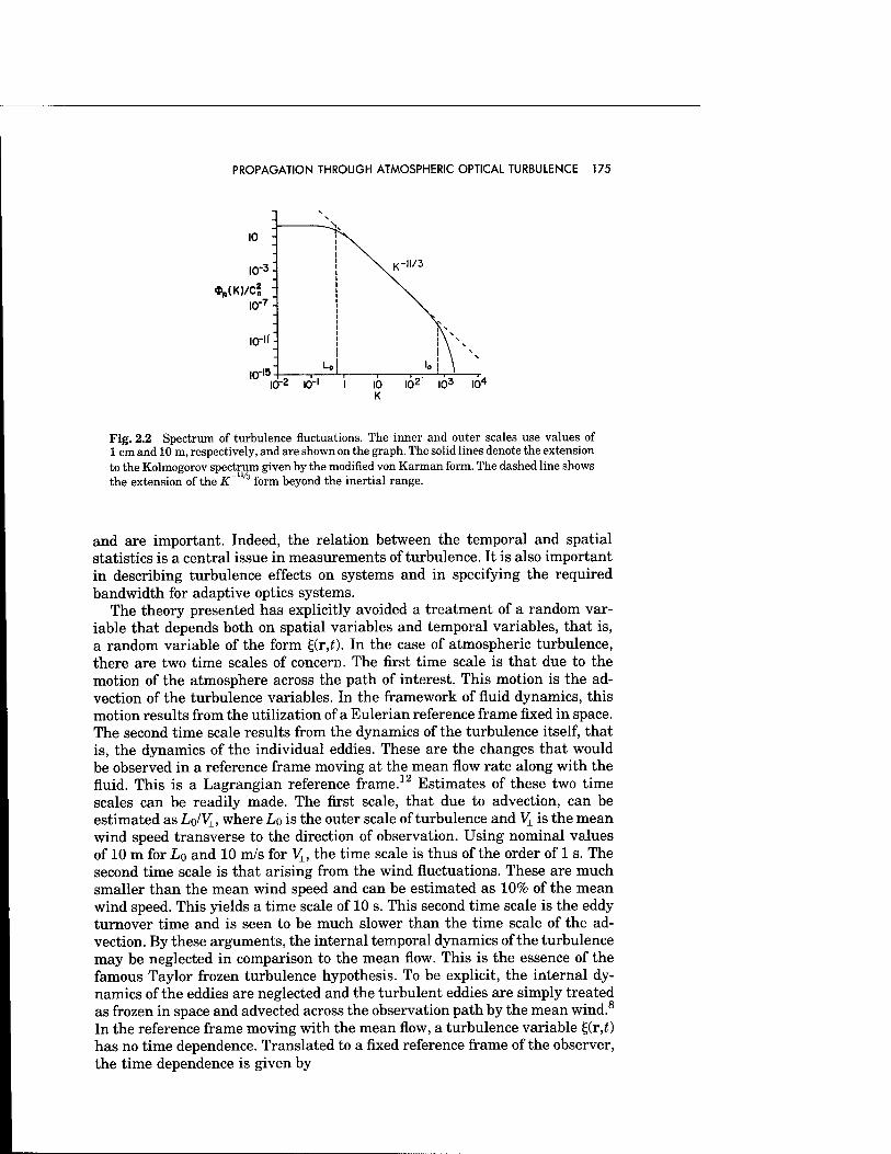
PROPAGATION THROUGH ATMOSPHERIC OPTICAL TURBULENCE 175
*„(K)/C2 "•
ICT2 I0"1 I 10 I02' I03 I04
K
Fig. 2.2 Spectrum of turbulence fluctuations. The inner and outer scales use values of 1 cm and 10 m, respectively, and are shown on the graph. The solid lines denote the extension to the Kolmogorov spectrum given by the modified von Karman form. The dashed line shows the extension of the K~ 3 form beyond the inertial range.
and are important. Indeed, the relation between the temporal and spatial statistics is a central issue in measurements of turbulence. It is also important in describing turbulence effects on systems and in specifying the required bandwidth for adaptive optics systems.
The theory presented has explicitly avoided a treatment of a random var- iable that depends both on spatial variables and temporal variables, that is, a random variable of the form %x,t). In the case of atmospheric turbulence, there are two time scales of concern. The first time scale is that due to the motion of the atmosphere across the path of interest. This motion is the ad- vection of the turbulence variables. In the framework of fluid dynamics, this motion results from the utilization of a Eulerian reference frame fixed in space. The second time scale results from the dynamics of the turbulence itself, that is, the dynamics of the individual eddies. These are the changes that would be observed in a reference frame moving at the mean flow rate along with the fluid. This is a Lagrangian reference frame.12 Estimates of these two time scales can be readily made. The first scale, that due to advection, can be estimated as LQIVL, where LQ is the outer scale of turbulence and VI is the mean wind speed transverse to the direction of observation. Using nominal values of 10 m for Lo and 10 m/s for V±, the time scale is thus of the order of 1 s. The second time scale is that arising from the wind fluctuations. These are much smaller than the mean wind speed and can be estimated as 10% of the mean wind speed. This yields a time scale of 10 s. This second time scale is the eddy turnover time and is seen to be much slower than the time scale of the ad- vection. By these arguments, the internal temporal dynamics of the turbulence may be neglected in comparison to the mean flow. This is the essence of the famous Taylor frozen turbulence hypothesis. To be explicit, the internal dy- namics of the eddies are neglected and the turbulent eddies are simply treated as frozen in space and advected across the observation path by the mean wind.8
In the reference frame moving with the mean flow, a turbulence variable %(r,t) has no time dependence. Translated to a fixed reference frame of the observer, the time dependence is given by
176 IR/EO HANDBOOK
&r,t + T) = £(r - V±j,t) (2.66)
for any time t. The reasonableness of this hypothesis has been established in a variety of measurements.6 The important limitation arises when the trans- verse wind flow is small, as occurs when the wind is parallel to the observation path. Lawrence and Strohbehn18 give as the condition for validity of the frozen turbulence assumption that
L0 » (XL)1/2 , (2.67)
where L is the path length. This condition applies even to the case of very low wind speed. This condition implicitly assumes that the propagation is along a homogeneous path, so that Lo is unambiguously defined. Substitution of nom- inal values for Lo (10 m) and optical/IR wavelengths shows that the condition is nearly always satisfied for propagation along reasonable horizontal paths. For inhomogeneous paths such as vertical, the transverse wind speed varies in the vertical direction, as does the outer scale, and the applicability of this criterion is uncertain. Nonetheless, the frozen turbulence hypothesis is in common use. Its limitations must be recognized when interpreting data under conditions with small transverse wind speeds.
Equation (2.66) allows the relationship between spatial and temporal co- variance, structure functions, and power spectra to be immediately written down. For the covariance and structure function, the important relation is that x = VJT; for the power spectrum, the temporal and spatial frequencies are related by w = KV±. In our notation, the relations for the structure functions and spectra are, for the one-dimensional spatial fluctuations of the parameter £,
BS(T) = B{(V[T) , (2.68)
LVT) = LVV» , (2.69)
where the interpretation of the covariance or structure function as being spatial or temporal is to be understood from the argument. Using the definitions of the spectra [Eq. (2.8)], it is easy to show that the relation between the temporal and spatial one-dimensional spectra is
W€(<o) = (l/VJP^/VJ . (2.70)
The different notation for the spectra makes it clear whether it is the temporal or the spatial spectrum.
2.3 OPTICAL/IR PROPAGATION THROUGH TURBULENCE
2.3.1 Introduction
There are several detailed presentations on propagation through optical tur- bulence that should be consulted. In particular, the books by Tatarski,6,13
Chernov,27 Strohbehn,28 Ishimaru,29 and Goodman30 and the reviews by Law-
PROPAGATION THROUGH ATMOSPHERIC OPTICAL TURBULENCE 177
rence and Strohbehn,18 Fante,31,32 and Coulman33 provide more detail than can be provided here. In this section, we sketch the methodology and formu- lation of the problems and their solution and focus on the presentation of formulas describing the major effects of optical turbulence on the propagation of optical/IR radiation.
2.3.2 Formal Solutions of the Wave Equation
The starting point for describing the propagation through turbulence is, of course, Maxwell's equations. For a monochromatic wave, the following wave equation for the vector electric field E results:
V2E + k2n2E + 2V[E • V log(n)] = 0 , (2.71)
where k is the wave number of the radiation (2u7\). In this equation, we have implicitly assumed that the time variations of the refractive index are slow compared to the frequency of the radiation. Since the wavelength for optical/IR radiation is much smaller than the smallest scale of turbulence (the inner scale, which ranges from the order of millimeters to centimeters), it can be shown that the third term in the wave equation can be neglected. This term represents polarization effects in the propagation, and thus the approximation implies that there is no depolarization in propagation through turbulence. The neglect of this term allows the above equation to be reduced to the wave equation for a scalar component of the electric field:
V2E + k2n2E = 0 . (2.72)
Because of the term in n2, this is a stochastic equation that cannot be exactly solved, and various approaches have been applied. The most straightforward solution is a perturbation expansion. First, we acknowledge that refractive- index fluctuations n\ are small and can be written as n = no + n\, where m « no. Second, we assume thatE = Eo + E\ + ..., where Eo is the incident field, Ei is the first-order scattered field, and so on for higher-order terms. The higher-order terms represent multiple scattering. Our approach is to treat single or weak scattering only. Since ni/no is small, we have
V2E + k2oE = -2k2o{nilno)E , (2.73)
where ko = nok. To simplify notation, we will drop the subscript on k and will simply write n\ instead of nilno- This equation, in conjunction with the ob- servation that the wavelength is smaller than any of the scale sizes of the turbulence, implies that there is negligible backscattering and that small- angle forward scattering dominates the propagation. In contrast, radar wave- lengths are of the same order as the turbulence eddies, and this enables their measurement from backscatter. The perturbation series solution is then straightforward. By grouping terms of zeroth-order and first-order perturba- tion, we arrive at the equation
V2£i + k2E! = -2k2mEo . (2.74)
178 IR/EO HANDBOOK
The solution of this is formally straightforward utilizing the Green's function for the wave equation. It is
lir)-i f exp(ik\r - r'|) Ei(r) = 2^(4TT)"1 —^—J -^ni(r')E0(r') dr' , (2.75)
J |r - r |
where the integration is over the scattering volume between the source and receiver. Since the turbulence scattering is very weak and in the forward direction, we can make the Fresnel or paraxial approximation to these equa- tions. Specifically, let p be a vector in the plane transverse to the direction of propagation. Then the term in the exponent can be approximated by
|r - r'H* - «1(1 + |p - pf/[2(2 - z')2}} , (2.76)
and in the denominator we replace |r - r'| by \z - z'\. Then the integral becomes
aw - **,>- / {Ä_ÄiiS]„,(rt (2.77)
x exp(ik\z - z'\)Eo(r') dr' .
The perturbation method presented so far is essentially the Born approxi- mation. Its applicability is determined by the neglect of terms higher than E\ in the perturbation expansion. Its domain of validity is restricted to very weak turbulence; that is, E\ « EQ. Another perturbation method, applied by Ta- tarski, is the Rytov method, or the method of smooth perturbations. Its as- sumptions are less restrictive than the Born method and therefore it has a wider range of applicability, although it is still restricted to weak turbulence. The Rytov method begins by writing
E = exp(i|i) = A exp(iS) , (2.78)
where \\i — x + iS and so x - log(A). Here, x is the so-called log amplitude and S is the phase. This approximation is closer to our objectives in determining amplitude and phase distortions due to the turbulence. In the Rytov method, the substitution exp(i[0 is made into the wave equation, which yields the Ricatti equation in \\r.
V2i|/ + Vi|rVi|/ + k2n2 = 0 . (2.79)
The essence of the Rytov approximation is to perform a perturbation expansion in i|/. Tatarski6 should be consulted for the details. The solution is
Mr) = Aktfoto]-1 f eXPf^|r ",r'^ni(r')E0(r') dr' . (2.80) J \r — r |
This solution can be shown to be equivalent to the Born method. The important result is that the Rytov method, since the perturbation is essentially multi-
PROPAGATION THROUGH ATMOSPHERIC OPTICAL TURBULENCE 179
plicative [since E = exp(i|/o) exp(i|»i)], is less restrictive than the Born method, requiring only that the changes in the perturbations be small over a scale of a wavelength, rather than simply that the perturbations themselves be small.
There is a third approach developed by Lutomirski and Yura.34 This ap- proach uses an extended Huygens-Fresnel theory. A diffraction-type integral results for the scattered field:
E(r) = -iA/(2ir) f exP^r ~ r'^E0(r') exp[v|i(r,r')] dV . (2.81) J |r - r I
Note that this expression gives the total field, which is the sum of incident and scattered fields. In contrast to the previous integrals, which were over volume, this integral is a diffraction-type integral that expresses the scattered field at r in terms of an integral over a surface. However, the factor \\i has an implied integration along the z axis. If we use the geometric optics approxi- mation, then I|J can be written as an integral along the path from z to z'\
>|;(r,r') = iKz,z') = k J rci© dl . (2.82)
The utility and appeal of the extended Huygens-Fresnel approach is that it allows a linear systems type representation:
E(p) = J h(p,p')E0{p') dp' , (2.83)
where h(p,p') is the atmospheric propagation impulse response function. The Fresnel approximation could be utilized in the Lutomirski and Yura
and the Rytov solutions as well. All these formal solutions apply to weak scattering. This case includes most of the applications involving propagation from the ground up to space. The specific limitations will be described later. However, when there is propagation through strong turbulence such as through long horizontal paths, other more sophisticated techniques must be applied. The reviews by Strohbehn35 and Fante32 should be consulted for some of these approaches.
2.3.3 Amplitude and Phase Statistics
The key questions to be answered are the effects of the turbulence on amplitude and phase. From the definition of I|J, it is straightforward to show that the perturbation 4>i is given by
»|ii = «I» - <|*> « Ei/Eo , (2.84)
where the approximation of small perturbation has been used. This equation shows the equivalence of the Rytov and Born integral solutions. Using the Fresnel approximation to the Rytov solution, we get formal solutions for the log amplitude and phase from the real and imaginary parts:
180 IR/EO HANDBOOK
2ro_E..,-vi-l f COs[feIP ~ P'|2/(21* ~ Z'\)] Xi(r) = Äz[2irEo(D]
z - 2
x m(r') exp(i£|z - z'\)E0(r') dr' ,
Si(r) = Ä^irEoW]-1 { i f sin[fe|p - pf/(2|z - z'j)]
|Z - Z |
x ni(r') exp(- ik\z - z'\)E0(r') dr'
(2.85)
(2.86)
In the following, the subscript on x and S will be dropped for simplicity. In this form, it is apparent that the statistics of log amplitude and phase are determined by those of the refractive-index fluctuations. In particular, it fol- lows from the Rytov solution that the means of x and S are zero since the mean of n\ is zero. Furthermore, both S and x are made up of the sum of a very large number of fluctuations in n along the propagation path. Since the fluctuations arising from different eddies are considered independent (as occurs in different layers), the central limit theorem can be invoked to predict that S and x should be normally distributed. Since A = exp(x) and / = exp(2x), it follows that both amplitude A and intensity / are log-normally distributed. Note that the Born solution, on the other hand, implies that the field E is normally distributed, and as a consequence, the amplitude and intensity would each have Rice-Nakagami distributions.18 For very low levels of turbulence the distinction between these distributions is small, and for higher levels of turbulence (but still weak) the evidence supports the log normal. It is standard to assume the log-normal distribution applies in weak turbulence, not only because the Rytov solution is less restrictive than the Born, but also because measurements and strong scintillation theory applied to the weak regime support the conclusion.
In determining optical effects of turbulence, it is the second-order statistics that are of most concern. From Eqs. (2.85) and (2.86), it is clear that all statistics of x and S are determined from those of n\ in the volume between the source and the receiver. The statistics of x and S are in a plane, and we are particularly interested in the receiver aperture plane. Even allowing for some variation in the statistics of the fluctuations along the propagation path, it still follows that the statistical homogeneity of the log amplitude and phase in the aperture plane is a consequence of the two-dimensional homogeneity of n\ along the path.
The covariance, spectrum, and structure function of x and S in the aperture plane are calculated from the Rytov solutions. These are dependent on the characteristics of the incident wave, for example, plane or spherical wave, or focused or collimated beam. The calculations are lengthy and involve difficult integration. In the general case, the turbulence is allowed to vary in strength along the path (e.g., layers) by parameterizing the spectrum. Thus, we write <&n(K,z) for the turbulence spectrum at position z along the path. In using the Kolmogorov spectrum, this simply allows C\ to vary along the path. To simplify the formulas, let £ be a parameter that can be either x or S. For a plane wave given by Eo(r) = Eo exp(ikz), the covariance and structure functions for prop- agation from z = 0 to L are
PROPAGATION THROUGH ATMOSPHERIC OPTICAL TURBULENCE 181
Br(p,L) = 4TT2 f d-n f dKKMKpW^L - -r],K)^n(K^) , (2.87)
Jo •'0
DAp,L) = 8TT2 [ d-n f dKK[l - J0(Kp)]HAL - y\,K)<S>n{K,T\) . (2.88) Jo Jo
Comparison of Eq. (2.88) with Eq. (2.29) yields the expression for the two- dimensional spectrum of the fluctuations in x or S in the plane z = L:
F^K,0,L) = 2ir J dr\ Ht{L - r\,K)^n(K,rO . (2.89)
The filter functions Hx and Hs depend on the characteristics of the radiation and, for a plane wave, are given by
Hx{x,K) = {k sinllPx/m)]}2 , (2.90)
Hs(x,K) = {k coslK^x/Vk)]}2 . (2.91)
It is sometimes useful in calculations of optical effects to use the wave- structure function. This is defined by
Dw(p) = Dx(p) + Ds(p) . (2.92)
From Eqs. (2.90) and (2.91) the computational advantages of Dw can be seen for a plane wave after substituting Eq. (2.88) into Eq. (2.92):
Dw(p,L) = 8v2k2 f di] f dKK[l - JoiKpWniK^) . (2.93) Jo Jo
This integral can be evaluated for a Kolmogorov spectrum given by <$>n(K,T)) = 0.03301(1]) K~u/3. The plane-wave structure function becomes
Dw(p,L) = 2.91fc2p5/3 Cli-n) dt! , for (\L)1/2< p < L0 Jo
Dw(p,L) = 3A4k2lo~1/sp2\ C2(-n) dt] , for p < l0 . Jo
(2.94)
It is instructive to express the covariance, structure function, and spectrum for constant turbulence along the propagation path; i.e., C2(z) = C2. The covariance, structure function, and spectrum for a plane wave become7
rco
Bx(p,L) = 2-n2k2Lj dKKJo(Kp){l-[k/(K2L)]sm(K2L/k)}<S>n(K) , (2.95)
Bs(p,L) = 2v2k2L [ dK KMKp){\ + [k/(K2L)] sm(K2L/k)}<Pn(K) , (2.96) Jo
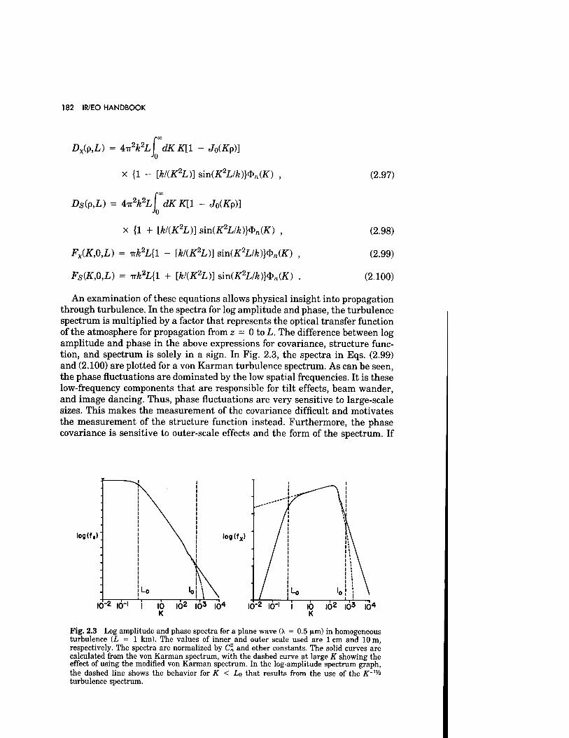
182 IR/EO HANDBOOK
Dx(p,L) = 4TT2£
2L| dKK[l - J0(Kp)]
x {1 - [k/(K2L)] sm(K2L/k)}<Pn(K) ,
Ds(p,L) = 4TT2£
2L[ dKK[l - J0(Kp)]
Jo
x {1 + [k/(K2D] sm(K2L/k)}<S>n(K) ,
Fx(K,0,L) = Trk2L{l - [k/(K2D] sin(K2L/k)}<S>n(K)
Fs(K,0,L) = T:k2L{l + [k/{K2L)] sin(K2L/k)}<t>n(K)
(2.97)
(2.98)
(2.99)
(2.100)
An examination of these equations allows physical insight into propagation through turbulence. In the spectra for log amplitude and phase, the turbulence spectrum is multiplied by a factor that represents the optical transfer function of the atmosphere for propagation from z = 0 to L. The difference between log amplitude and phase in the above expressions for covariance, structure func- tion, and spectrum is solely in a sign. In Fig. 2.3, the spectra in Eqs. (2.99) and (2.100) are plotted for a von Karman turbulence spectrum. As can be seen, the phase fluctuations are dominated by the low spatial frequencies. It is these low-frequency components that are responsible for tilt effects, beam wander, and image dancing. Thus, phase fluctuations are very sensitive to large-scale sizes. This makes the measurement of the covariance difficult and motivates the measurement of the structure function instead. Furthermore, the phase covariance is sensitive to outer-scale effects and the form of the spectrum. If
log(f.)
10-2 lO"1
log(fx)
10 I02 I03 I04
K IO"2 10"' I 10 I02 I03 I04
K
Fig. 2.3 Log amplitude and phase spectra for a plane wave (\ = 0.5 (un) in homogeneous turbulence (L = 1 km). The values of inner and outer scale used are 1 cm and 10 m, respectively. The spectra are normalized by C„ and other constants. The solid curves are calculated from the von Karman spectrum, with the dashed curve at large K showing the effect of using the modified von Karman spectrum. In the log-amplitude spectrum graph, the dashed line shows the behavior for K < Lo that results from the use of the Jf-1^3
turbulence spectrum.
PROPAGATION THROUGH ATMOSPHERIC OPTICAL TURBULENCE 183
the Kolmogorov spectrum is used with its implied infinite outer scale, the phase variance does not exist, as the integral of Eq. (2.96) is infinite. This further motivates the use of phase structure function.
The figure also shows the insensitivity of log-amplitude fluctuations to large- scale sizes. The log-amplitude spectrum goes to zero at K = 0. Further, it is seen to reach a peak, and it can be shown that this peak occurs for scale sizes approximately equal to the Fresnel zone scale, (XL)~1/2. The consequences of these log-amplitude statistics will be discussed in terms of scintillation. Fi- nally, the different spectral characteristics of x and S allow the approximation of Dw to be used instead of Ds for computational simplicity. This approximation is reasonable in those effects that arise primarily from low-frequency phase.
The light from astronomical objects can be treated by the plane-wave case. However, another important case is that of a spherical wave. This applies to point objects within the atmosphere. The spherical wave originating at z = 0, E(r) = r~x exp(ikr), gives
ZMp,L) = 2.91&2p5/3f C^i)(V£)5/3 di\ . (2.101) Jo
The spherical-wave expressions for covariance and structure function are
BAp,L) = 4TT2[ di\{ dKKMK^IDH^L - ^,K,L)<$>n(K,T\) , (2.102) Jo Jo
D1(P,L) = 8TT2\ drif dKK[l-MKfn)/L)]H{L-T\,K,LyS>n(K,T\) . (2.103) Jo Jo
The spherical-wave filter functions Hx and Hs are
HX(L - x,K,L) = (k sin{K2[x(L - x)]/(2kL)})2 , (2.104)
Hs(L - x,K,L) = (k cos{K2[x(L - x)]/(2kL)})2 . (2.105)
For a collimated beam, the plane-wave formulas may be used to sufficient approximation in many applications. For a beam wave, starting at z = 0 and focused at L, Sasiela36 states that the equations for a plane wave (2.87), (2.88), and (2.89) can be used with the filter functions defined as follows:
HX(L - x,K,L) = [(L - x)/Lf3(k sin{K2xL/[2k(L - x)]})2 , (2.106)
HS(L - x,K,L) = [(L - x)ILf\k cos{K2xL/[2k(L - x)]})2 . (2.107)
This representation, valid for a Kolmogorov spectrum, does not include the beam width. The same is true for the approximation of a collimated beam by a plane wave or a diverging beam by a spherical wave. However, the beam width is not important in many applications. The discussion of beam waves with finite widths will follow in a subsequent section.
184 IR/EO HANDBOOK
2.3.4 Scintillation
The fluctuation in received intensity resulting from propagation through tur- bulence is described as scintillation. The term scintillation is applied to various phenomena, including the temporal variation in received intensity (such as the twinkling of a star) or the spatial variation in received intensity within a receiver aperture. From the definition of log amplitude, it is seen that the statistics of intensity are determined by those of log amplitude. Since there is experimental evidence supporting the log-normal distribution of intensity, it can be shown that if x is a normal random variable, then
(/) = <exp(2x)> = exp(2(x) + 2o*) . (2.108)
Note that in our notation, o\ = Bx(0). The variance of intensity is a fourth- order moment. For log-normal variables, all statistics are specified in terms of the first- and second-order moments, and thus it can be shown that the normalized intensity variance erf is defined by and satisfies
o? = <[/ - </>]W (2 109)
= exp(4a^) - 1 .
This relation is solely a consequence of the normality of x and the relation between I and x- For weak turbulence and hence small a\, this can be approximated by
of - Aa\ . (2.110)
Since turbulence does not attenuate the light, conservation of energy re- quires that the average intensity be the same with or without turbulence. From Eq. (2.108), this is true provided the average of log amplitude satisfies
<X> = -°x • (2-llD
This is a requirement on the overall fluctuations, that is, the exact solution that includes all order perturbations. As discussed earlier, the Rytov solution implies that (x) = 0. The Rytov solution violates conservation of energy, but it is only a first-order perturbation solution. This contradiction is seldom man- ifest in weak fluctuation problems within the domain of the Rytov approximation.
The intensity variance is a readily observable quantity and is the important quantity in many applications. From the formulations for the covariance of x in the previous section, the quantities necessary for the calculation of the intensity variance are at hand. For a plane wave, Eq. (2.87) can be evaluated at p = 0 and gives, for h « (\L)V2,
v\{L) = 0.56&7/6J Cl(T))(L - TI)5/6
d-n . (2.112)
For a spherical wave, the equation becomes
a-l(L) = 0.56£7/6J C*(TI)(V£)5/6
(L - -n)5/6 dt\ . (2.113)
PROPAGATION THROUGH ATMOSPHERIC OPTICAL TURBULENCE 185
In these equations, the source is at z = 0 and the observation point is at 2 = L. It can be seen that the scintillation from a spherical wave is less than that from a plane wave, owing to the inclusion of the extra factor (r\/L)/6 in the integrand. In these forms, it is apparent that the path weighting of C2 for scintillation favors turbulence far from the receiver. Generally speaking, tur- bulence near the receiver does not contribute to scintillation. For the case of constant C2 along the path, as might approximate a horizontal path, these equations become
cx2(L) = 0.307k1/6Ln/6Cl , plane wave , 7 ,1 (2-114)
o-2(L) = 0.124k/6L/6C2n , spherical wave .
The wavelength dependence of this scintillation variance exhibits a general feature of turbulence effects: turbulence effects are greater for shorter wave- lengths.
These equations have limited applicability as they stand. The spherical- wave expressions of course assume a point source, but more important, both expressions assume a point receiver. Whether a receiver can be approximated by a point receiver depends on its lateral dimension relative to the lateral dimensions of the intensity fluctuations. The important scale size of scintil- lation is determined from the log-amplitude covariance. Unfortunately, even for a plane wave in homogeneous turbulence, the resulting expression is quite complex and will not be reproduced here. Lawrence and Strohbehn18 give a complete expression, and Ishimaru29 gives a slightly different form. The im- portance of the Fresnel scale, (X.L)/2, emerges in these expressions, as does a slight dependence on the inner scale. Clifford7 discusses the important features of the covariance for constant C2. First, the covariance is small in magnitude for p greater than the Fresnel length, (XL)/2, and second, the covariance goes to small negative values at greater lengths.
The general behavior of the log-amplitude fluctuations can be inferred from properties of the integrand in the plane-wave spectrum [Eq. (2.89)]. The sin2
term in the filter function dominates the shape of the spectrum. It is easy to see that the integrand, and hence the spectrum, has a peak approximately at the first maximum of the sine. Indeed, this peak is approximately given by the Fresnel scale. For scales smaller than the Fresnel scale, the sin2 term causes an attenuation of the turbulence spectrum, as seen in Fig. 2.3. For larger scales (or smaller wave numbers), the approach of the sin2 term to zero is according to K4, which dominates even the Kolmogorov K~ /3 singularity. If the Fresnel scale is smaller than the inner scale, the log-amplitude spectrum in the inertial range is attenuated, but now has a maximum at the inner scale; in this case, it is the inner scale and not the Fresnel scale that is the dominant scale size of the fluctuations. However, in some such cases, the existence of the bump in the spectrum19 near the inner scale may be an important feature. The other extreme situation where the Fresnel scale is larger than the outer scale is analogous; the log-amplitude fluctuations are greatly attenuated since the sin2 term filters out fluctuations with scale sizes in the inertial range.
These properties of the log-amplitude covariance and spectrum covariance allow a qualitative explanation of the characteristics of scintillation in weak turbulence where C2 varies along the path. Suppose there is only one narrow
186 IR/EO HANDBOOK
layer of turbulence along the propagation path at a distance z from the source. As can be seen from Eq. (2.112), the intensity fluctuations will increase as the strength of the turbulence, Cn, increases. Second, for constant Cn, the mag- nitude of the intensity fluctuations will increase as the distance from the layer to the detector, L - z, increases. But there is a limit to this increase. From the discussion of the spectrum, it is shown that the eddies of the Fresnel scale size are the dominant contributors to the scintillation. However, note that the Fresnel scale is determined by the distance from the turbulence layer to the detector, L - z.b At a far enough distance, the Fresnel scale is larger than the outer scale, and thus there is negligible contribution to intensity fluctuations from turbulence scales.
Observations of scintillation from stars show the fine-scale structure of the intensity distribution; that is, the intensity tends to get broken up into patches and, from the covariance function, these are also of the size of the Fresnel length. But since the covariance goes negative for separations greater than [X.(L - z)]/2, this implies that, on average, points in the observation plane separated by a Fresnel length will be alternately bright and dark. A final qualitative observation is that, from the frozen turbulence hypothesis, these patches move across the aperture according to the wind speed at the distance corresponding to the Fresnel length.
This discussion of the characteristics and scales of scintillation suggests a method for measuring path-resolved Cn- Thus, the strength of the intensity fluctuation determines Cn and the scale size of the fluctuation determines the height of the turbulence. This concept is the principle behind the stellar scintillometer37 for profiling Cn and the horizontal scintillometer38 for mea- suring path-averaged Cn- In addition, the technique also has been applied to the remote sensing of winds.39
Equations (2.112) and (2.113) predict that the variance of log amplitude is a linear function of Cn- This was derived under the Rytov approximation and is true only for weak turbulence. Figure 2.4 shows the experimental behavior of the intensity variance. In agreement with the Rytov theory, the variance increases linearly with C„ only for low levels of turbulence. For higher levels, the experimental variance approaches a constant and indeed decreases slightly for still higher levels of turbulence. This behavior has been confirmed in many measurements40 and is known as the saturation of scintillations. Physically, saturation occurs when the fluctuations in intensity become so large that the intensity fluctuates to zero much of the time.
As a result of saturation, the limits of applicability of the Rytov solution are usually stated in terms of a o^ criterion. The Rytov theory is regarded as applicable for log-amplitude fluctuations provided a* < 0.3. However, exper- imental evidence suggests that the Rytov solution for phase fluctuations is applicable to higher levels of turbulence, so that the phase solution may still be accurate even though the log-amplitude solution is not. The failure of the Rytov solution is rooted in the fact that it does not accurately account for the multiple scattering effects that occur in strong turbulence, nor does it account for the progressive loss of coherence as the wave propagates through strong
bThe turbulence layer is located at z. For a source at z = 0 and receiver at z = L, the relevant plane-wave Fresnel scale is given by [X(L - z)]1/2. For a source at z = L and receiver at z = 0, it is given by (\z)1/2.
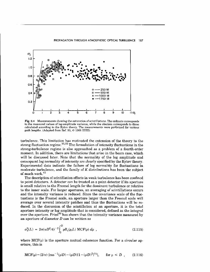
PROPAGATION THROUGH ATMOSPHERIC OPTICAL TURBULENCE 187
(w> o 250 M D 500 M A —1000 M • —1750 M
I0 HOy
Fig. 2.4 Measurements showing the saturation of scintillations. The ordinate corresponds to the measured values of log-amplitude variance, while the abscissa corresponds to those calculated according to the Rytov theory. The measurements were performed for various path lengths. (Adapted from Ref. 93, © 1968 IEEE)
turbulence. This limitation has motivated the extension of the theory to the strong fluctuation regime.35,32 The formulation of intensity fluctuations in the strong-turbulence regime is also approached as a problem of a fourth-order moment. In addition, there are limitations that arise in the beam case, which will be discussed later. Note that the normality of the log amplitude and consequent log normality of intensity are clearly specified by the Rytov theory. Experimental data indicate the failure of log normality for fluctuations in moderate turbulence, and the family of K distributions has been the subject of much work.41
The description of scintillation effects in weak turbulence has been confined to point detectors. A detector can be treated as a point detector if its aperture is small relative to the Fresnel length for the dominant turbulence or relative to the inner scale. For larger apertures, an averaging of scintillations occurs and the intensity variance is reduced. Since the covariance scale of the fluc- tuations is the Fresnel scale, an aperture larger than the Fresnel scale will average over several intensity patches and thus the fluctuations will be re- duced. In the discussion of the scintillation at an aperture, it is the total aperture intensity or log amplitude that is considered, defined as the integral over the aperture. Fried42 has shown that the intensity variance measured by an aperture of diameter D can be written as
al(L) = 2TT(TTZ)2/4)- (p,L) MCF(p) dp (2.115)
where MCF(p) is the aperture mutual coherence function. For a circular ap- erture, this is
MCF(p) = (2/TT) {cos"Hp/D) - (p/D)[l - (p/D)2f2}, forp^D, (2.116)

188 IR/EO HANDBOOK
and where the MCF is 0 for p > D. It can be shown that this MCF has a transfer or filter function
H(K) = [2Ji(XD/2)/(XD/2)]2 . (2.117)
Simply stated, the effect of an aperture is to spatially filter the log-amplitude spectrum. The effect of aperture averaging can be included in our plane-wave formalism by making the following substitution for the filter function:
HX{L - i],K) -»• HX{L - -n,üO[2Ji(XZ)/2)/(iCD/2)]2 , (2.118)
Substitution into Eq. (2.89) for a plane wave yields an expression that can be written as
o-2(L) = 16TT2f dJ dKKHx{L-r\,K)[Ji{KDI2)l{KDI2)?<bn{Kn) , (2.119) -*0 -'0
which yields the log-amplitude spectrum as
FJK,L) = 8-a[Ji(KD/2V(KD/2)f\ dt\ HX(L - i\,K)$n(K,-r\) . (2.120) Jo
These expressions show that the aperture acts as a low-pass filter. The eval- uation of this integral for the variance is difficult and has been done numer- ically for constant turbulence.42 The qualitative features of the aperture av- eraging can be understood from the scale characteristics of scintillation. This filtering in the frequency domain is equivalent to the filtering out of various small-scale sizes. Since small-scale scintillation comes from near the aperture, the aperture filters out the scintillation arising from turbulence nearer to the aperture and changes the path weighting of the variance from (L - z)M. If the aperture is larger than the outer scale of the turbulent layers at all alti- tudes, the filtering will almost eliminate all scintillation.
There is a completely analogous procedure for a spherical wave. The receiver aperture averaging filter function for a point source at z = 0 is given by
H(K,L) = {2J1[KDy]/(2L)V[KD^(2L)}2 . (2.121)
This filter function is then included in the formalism by making the analogous substitution as for the plane-wave case. The spherical-wave filter function becomes
HX(L - T\,K) -* HX(L - y],K,L){2J1[KDi]/(2LW[KDi]/(2L)}2 . (2.122)
A similar approach is used to treat the scintillation from an extended source, such as a planet. For an extended source that consists of multiple, independent radiators, it is expected that scintillation will be reduced, owing to an averaging of the scintillation from the independent sources. For a source of diameter a, located at z = 0 and observed at z = L, the appropriate filter function is
PROPAGATION THROUGH ATMOSPHERIC OPTICAL TURBULENCE 189
H(K) = {2J1[Ka(L - T])/2]/[Ka(L - T])/2]}2 . (2.123)
We again make the substitution in our formalism, only this time the filter arising from the source has a path dependence
HX(L - y\,K) -> HX(L - ^,K){2{JAKa(L - r))/2]}/[Ka(L - T])/2])2 . (2.124)
Performing this substitution into Eq. (2.87) for the plane-wave covariance results in a useful form:
o-2.(L) = 16TT2| dJ dKKHJL - T),K) Jo Jo
(2.125) x ({JdKaiL - T))/2W[Ka(L - -n)/2])2<I>„(#,'n) ,
which gives the log-amplitude spectrum including the finite-source effect:
fn HX(L - ■n.K)
(2.126)
Fx(K,0,L) = 8TT| dn\ HX(L - T\,K)
x ({JAKaiL - T,)/2]}/[ffa(L - ^^f^niK^)
Again, this form shows the filtering performed by the spatial extent of the source. Note that the low-pass filtering is altitude dependent. This treatment of extended sources applies to the case where the size of the source is such that the anisoplanatic effects can be neglected.
The spherical-wave expression for the source averaging effect is given by the filter
H(K) = {2JAKa(L - y\)l{2L)]l[Ka{L - -n)/(2L)]}2 , (2.127)
and the analogous filter substitution is made into the spherical-wave co- variance, structure function, and spectrum.
If we have both aperture averaging and an extended source, the substitution of the filter function in the covariance equation can be extended. The substi- tution uses both filter functions. The emphasis has been on presenting a formalism36 on how such problems are treated. Thus, the filter substitutions can readily be made for spherical waves or for apertures with another transfer function, such as those with central obscurations.
The equations that have been provided apply to those cases where either Cn is known along the propagation path or the zenith angle is zero. For the case where we know or model the C2 profile in the vertical direction, a cor- rection with zenith angle must be applied. This correction simply scales the optical path. If tp is the angle from zenith, it is easy to show that the correct altitude scaling is achieved by multiplying the path variables by sec(<p) in Eqs. (2.112) and (2.113), yielding a scaling of a2 according to [sec(<p)] /6 and the following expressions for a plane wave:
190 IR/EO HANDBOOK
t&L) = 0.56£7/6[sec((p)]n/6f C2("n)(L - T,)5/6
dt\ , (2.128) Jo
and for a spherical wave:
rL rl{L) = 0.56^7/6[sec(<p)]11/6 Cli-qM/Lf^L - ^f6d^ . (2.129)
Jo «#
For vertical propagation through the entire atmosphere, this scaling in zenith angle is appropriate only up to about 40 deg or less, dependent on the strength of the atmospheric turbulence. At larger angles, the variance of log amplitude becomes larger than the limit imposed by the Rytov approximation, owing to the greater turbulence in the optical path.
2.3.5 Imaging Effects
Turbulence effects on imaging arise primarily from the effects of turbulence on the phase, in contrast to scintillation, which arises from log-amplitude effects. The most common effects are those of image blurring and image danc- ing. These image-degradation effects are different manifestations of the phase distortions that result from propagation through turbulence.
The approach to image degradation involves the determination of the at- mospheric transfer function or point-spread function. This is determined by the image of a point through the atmosphere. It is most convenient to utilize the Lutomirski and Yura solution to the wave equation [Eq. (2.81)]. The in- stantaneous intensity at a position vector r in the aperture plane is
J(r) = E(r)E*(r) . (2.130)
The average of this is, using Eq. (2.81),
9 9({ exp(i&|r - r'|) exp(-i&|r - r"|) J J r — r r — r 11 ' ' (2.131)
x <exp(i[»' + i|»*")> dV d2r" .
This quantity is a form of the mutual coherence function, also known as the mutual intensity function. This function is determined by evaluating the en- semble average (exp(4»' + »J»*")). Indeed, this latter quantity is the atmospheric mutual coherence function in the aperture plane. By using the Fresnel ap- proximation, this equation is simplified and some of the integration can be performed. Since the Rytov solution has justified the normality of 4>, it can be shown43 from properties of log-normal variables that this can be evaluated to yield
<exp(i|i'-+ i|;*")> = exp[-Du,(p)/2] , (2.132)
where p is the radial position magnitude in the aperture plane and Dw is the wave-structure function, defined in Eq. (2.92). But Dw has previously been
PROPAGATION THROUGH ATMOSPHERIC OPTICAL TURBULENCE 191
evaluated in Eqs. (2.94) for a plane wave and Eq. (2.101) for a spherical wave. If this substitution is made, the result can be written as
MCF(p) = <exp(i|»' + 4<*")> = exp[-(p/po)6/3] . (2.133)
In this expression, po is called the transverse coherence length, given by
-3/5
PO 1.46k2f Cl(i\)dT\ Jo
plane wave , (2.134)
po = L.46£2 C2(TI)(TI/£)5/3 d-n Jo
-3/5
spherical wave . (2.135)
In these expressions, the form of the wave structure function applicable to most problems is used. For those problems that require a smaller scale, as for example when p < IQ, a different form of the transverse coherence length must be used based on the second equation in (2.94).
This formulation of the propagation problem in terms of the atmospheric mutual coherence function has a very important interpretation that clearly shows one of the pronounced effects of propagation through turbulence. For a wave that starts out at a transmitter or other source with some very large spatial coherence, the spatial coherence of the wave front will have been de- graded and reduced to po after propagation through turbulence. Two points on the wave front separated by a distance greater than po will be uncorrelated. This loss of coherence is important in a wide range of applications. Since a collimated laser beam can be approximated by a plane wave, a collimated beam with a spatial coherence length of D (transmitter aperture diameter) at the source will have its coherence length reduced to po in its transit through the atmosphere. Since a typical value of po is 5 cm for a vertical path at X = 0.5 pjn, it is clear that this is a very important effect. The variation in coherence length, as well as the result of measurements, is discussed in a subsequent section.
Several aspects of the expression for the coherence length should be em- phasized. First, the plane-wave form shows a dependence simply on the in- tegrated optical turbulence, with no path weighting. Since usually the largest values of C\ occur near the ground, these are very important to coherence length. This is especially true for the turbulence at the receiving or trans- mitting apertures or associated dome structures. Second, the coherence length scales with wavelength according to X6/5; po increases with wavelength, so the loss of coherence is less in the IR than at visible wavelengths.
The formulation of the mutual coherence function has been in the aperture plane. In most applications, it is more useful to translate these results into the focal plane of the imaging system. This involves the translation of the mutual coherence function in the spatial domain into the modulation transfer function in the spatial frequency domain. The modulation transfer function (MTF) is the magnitude of a system's optical transfer function.30 The customary convention will be followed for spatial frequency; namely, in the focal plane
192 IR/EO HANDBOOK
of a system with focal length f, the spatial frequency will be represented by v (in units of cycles per unit length) instead of K, as has been our custom. The relation between the two is simply K = 2TTV. Following Fried,43 the MTF in the focal plane is given by
MTF(v) = exp[-3.44(\/Wr0)5/3] (2.136)
where ro is called the atmospheric coherence length and is related to po by ro = 2.1po. As with scintillation, ro is a function of the zenith angle <p. The complete expressions for Fried's coherence length are
ro = 2.1
ro = 2.1
1.46 sec(cp)r C%{t\)di\ Jo
-3/5
L.46 sec(<p)Ai2 C2n(r\MILf3 dT\
Jo
plane wave ,
-3/5
(2.137)
, spherical wave . (2.138)
This coherence length ro is in more widespread use than po. A typical value for ro at X. = 0.5 (xm is 10 cm for a vertical path. The atmospheric coherence length ro is one of the most important parameters for characterizing the effects of turbulence on an optical system, ranging from telescopes to lasers. The interpretation of the MTF formulation is straightforward. The net MTF of an optical system looking through the atmosphere is the product of the MTF of the system and the atmospheric turbulence MTF.44 Optical turbulence behaves as a low-pass filter on an optical system by filtering out the high spatial frequencies. Thus, sharp edges are lost and even point sources become blurred objects. The lie point of the MTF can be found and gives, for a plane wave, a cutoff frequency vc due to turbulence:
vc = r0/(2.1kf)
0.0878 /-V/5sec-3/5((p) f Cl (T!) d-n Jo
-3/5
(2.139)
This cutoff frequency has a direct interpretation in terms of resolution. Note that this cutoff frequency depends on wavelength to the Vs power, a very weak dependence. Since the inverse of vc is a representation of resolution, this shows that the resolution degradation caused by atmospheric turbulence is only slightly improved at longer wavelengths.
The motivation for the use of ro can be seen from Fried's original work. The resolution R of a system can be defined as a volume associated with the transfer function:
R /•
MTF0(v) MTF(v) dv (2.140)
where MTF0(v) is the MTF associated with the system optics (i.e., the MTF without the atmosphere) and MTF(v) is that of the atmosphere. For a circular aperture with diameter D, this integral becomes
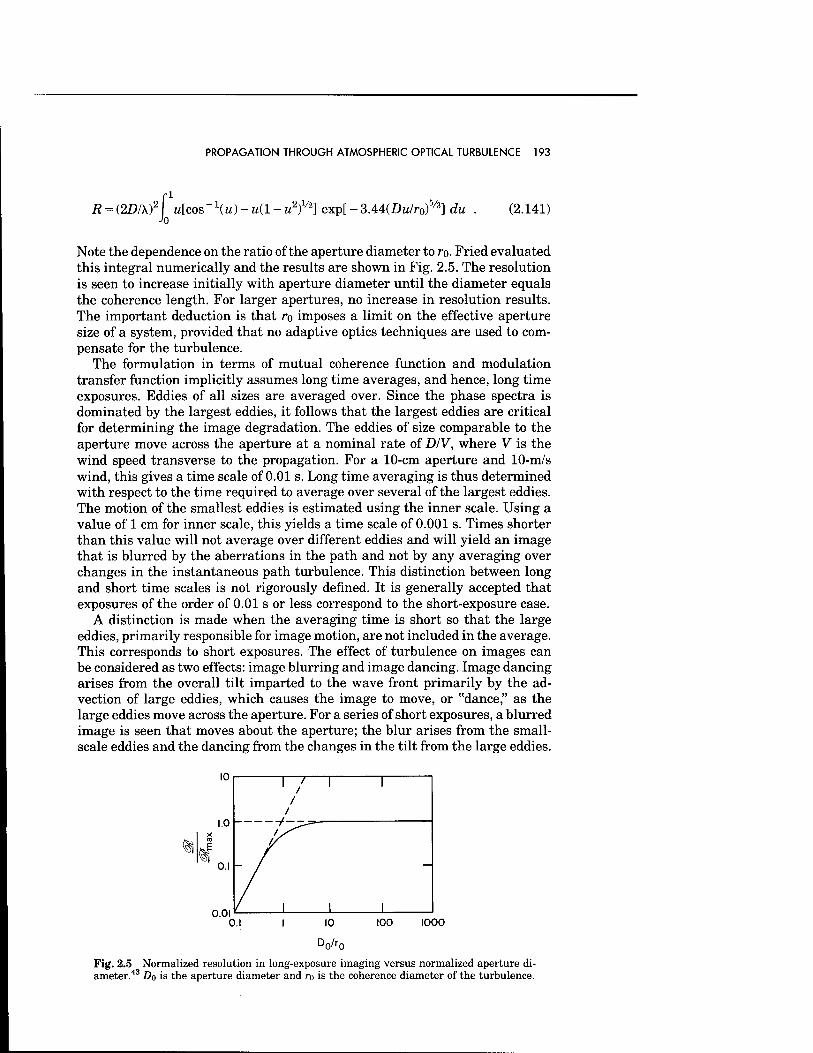
PROPAGATION THROUGH ATMOSPHERIC OPTICAL TURBULENCE 193
R = (2D/kf\ u[cos~\u) Jo
u(l-u2)1/2]exp[- ■3.U(Du/r0f/3]du (2.141)
Note the dependence on the ratio of the aperture diameter to ro. Fried evaluated this integral numerically and the results are shown in Fig. 2.5. The resolution is seen to increase initially with aperture diameter until the diameter equals the coherence length. For larger apertures, no increase in resolution results. The important deduction is that ro imposes a limit on the effective aperture size of a system, provided that no adaptive optics techniques are used to com- pensate for the turbulence.
The formulation in terms of mutual coherence function and modulation transfer function implicitly assumes long time averages, and hence, long time exposures. Eddies of all sizes are averaged over. Since the phase spectra is dominated by the largest eddies, it follows that the largest eddies are critical for determining the image degradation. The eddies of size comparable to the aperture move across the aperture at a nominal rate of D/V, where V is the wind speed transverse to the propagation. For a 10-cm aperture and 10-m/s wind, this gives a time scale of 0.01 s. Long time averaging is thus determined with respect to the time required to average over several of the largest eddies. The motion of the smallest eddies is estimated using the inner scale. Using a value of 1 cm for inner scale, this yields a time scale of 0.001 s. Times shorter than this value will not average over different eddies and will yield an image that is blurred by the aberrations in the path and not by any averaging over changes in the instantaneous path turbulence. This distinction between long and short time scales is not rigorously denned. It is generally accepted that exposures of the order of 0.01 s or less correspond to the short-exposure case.
A distinction is made when the averaging time is short so that the large eddies, primarily responsible for image motion, are not included in the average. This corresponds to short exposures. The effect of turbulence on images can be considered as two effects: image blurring and image dancing. Image dancing arises from the overall tilt imparted to the wave front primarily by the ad- vection of large eddies, which causes the image to move, or "dance," as the large eddies move across the aperture. For a series of short exposures, a blurred image is seen that moves about the aperture; the blur arises from the small- scale eddies and the dancing from the changes in the tilt from the large eddies.
Vo
IOOO
Fig. 2.5 Normalized resolution in long-exposure imaging versus normalized aperture di- ameter.43 Do is the aperture diameter and ro is the coherence diameter of the turbulence.
194 IR/EO HANDBOOK
For a long exposure, the resulting blur arises from the superposition of the dancing and the short-term blur and thus includes the effect of all scale sizes.
The approach to treatment of short exposures is to make this distinction in time scales. The formulation considers the "tilt-removed" phase of the wave front. Fried's approach43 performs a least-squares fit of a plane to an incident wave front, defining this as the tilt and performing a subtraction to determine the short exposure MTF. From his analysis, the short-term MTF is
MTFs(v) = exp{-3.44(\/Vr0)5/3[l - b(\fv/D)1/3]} , (2.142)
where ft is a constant taking the value 1 for near-field propagation and 0.5 for far-field propagation. The distinction between near-field and far-field propa- gation is that the log-amplitude fluctuations are taken into effect in the far- field case but are negligible in the near-field case. The short-term MTF is given as a correction factor applied to the long-term MTF. Especially noteworthy is the fact that the correction factor depends on the aperture diameter. In this expression, it can be seen that as v gets larger and approaches D/fX, the correction term gets smaller. If D > ro, this effect produces a higher value at large v for the short-exposure MTF than for the long-term MTF. Thus, higher spatial frequencies are present in the short term than in the long term and superior resolution results.
Closely related conceptually to the short-term MTF are the effects of image dancing and angle of arrival fluctuations. These effects are the short-term manifestations of wave front tilt and the temporal dynamics of the large-scale eddies. Consider two points on the wave front, separated by p. A plane wave passing through these two points will be tilted from the normal to the aperture by an amount <|> satisfying
(S2 - Si) = kp<$> , (2.143)
where the approximation sin(4>) ~ 4> has been used. The mean-square angle of arrival is therefore given by
<<1>2> = Ds(p)/(kp)2 • (2-144)
Using the approximation of Ds ~ Dw and using Eq. (2.94) for a plane wave, this becomes
<<f>2> = 2.91p-1/3 ClWdv . (2.145) Jo
It is primarily the larger scales responsible for these angle-of-arrival fluctua- tions, since phase variations smaller than the aperture are averaged. It is therefore customary to replace p with the aperture size D, and this equation becomes
fL 1/3 cl
Jo (4>2) = 2MD~V3\ Cl{r\)dy\ . (2.146)
PROPAGATION THROUGH ATMOSPHERIC OPTICAL TURBULENCE 195
The absence of a wavelength dependence in the angle of arrival warrants emphasis. An analogous expression can be written for the spherical-wave case by using Eq. (2.101) for Dw. This formulation of the angle of arrival is one dimensional, i.e., the angular fluctuations relative to a plane containing the axis of propagation. A more rigorous derivation can be made by including the aperture filter function, but at the expense of difficult integrations, and yields the same result. Measurements have verified this expression for angle-of-arrival fluctuations. Values of the order of tens of microradians were measured for path lengths of a few hundred meters. A noteworthy result of these measure- ments is that this formulation still holds even in the regime where the Rytov approximation breaks down. This is one example of the applicability of the Rytov phase results in a regime where the log-amplitude results are not applicable.
The calculation of image dancing is very similar, except this takes place in the focal plane of the system. Thus, the theoretical approach is the same except for the inclusion of the focal length. Hufnagel45 performs a rigorous derivation of the image displacement in the focal plane. The mean-square displacement can be written from the angle-of-arrival result at the aperture by using the simple relation 8 ~ f§. The expression for the mean-square displacement in the focal plane then follows from Eq. (2.145) for a plane wave:
<82> = 2.91/-2Z>-1/3f C2(-n) dr\ . (2.147) JO
The effect of turbulence and its decomposition into short- and long-term effects is essential to the understanding of speckle imaging techniques. A short exposure of an object yields an image that possesses a speckle texture from the turbulence; that is, it is made up of many tiny spots, or speckles, similar to the result from laser scattering from a surface that is rough on the scale of the laser wavelength. The size of the speckles arising from propagation through turbulence can be as small as the diffraction limit of the imaging system. From the discussion of short exposures, it has been shown that short exposures still contain the high spatial frequency information filtered out in long expo- sures. Speckle imaging is an image reconstruction technique that uses the statistics of short exposures to correct for the turbulence distortion and thereby achieve a resolution in excess of the limitation imposed by the long-exposure MTF. The discussion of this technique, as well as other imaging methods for turbulence compensation, is beyond the scope of this chapter. There are many works in speckle imaging and speckle interferometry that should be consulted.30'46-49
2.3.6 Beam Effects
Much of the treatment of the previous sections on scintillation and imaging can be carried over to laser beam propagation through the atmosphere. This is because a beam wave front, in general, falls somewhere between the plane- wave and spherical-wave cases. Indeed, a collimated beam can be treated as a plane wave in some problems, while a diverging beam may be treated as a spherical wave. The case of a focused beam, however, often requires special
196 IR/EO HANDBOOK
treatment. At the focus, the beam can sometimes be treated as a spherical wave originating from the focal point. However, there are exceptions to this as well, since the turbulence phase distortions in a focused beam can in some cases be sufficient to overwhelm the focusing.
The general beam case can be formulated as follows.50'31'29 At the trans- mitter aperture, the beam is assumed for mathematical simplicity to have a Gaussian amplitude profile. Let Wo be the beam width and /"be the wave front radius of curvature at the aperture. Then, the wave is given by
£o(p,0) = exp{-p2[W0-2 + ik/(2f)]} . (2.148)
Note that the wave front is radially symmetric at the aperture. The radius of curvature f is positive for a converging beam and negative for a diverging, and /"is, in fact, the focal length. A collimated beam corresponds to /"-» °°, and thus the imaginary part of Eq. (2.148) can be dropped. The beamwidth Wo is the beam radius at the Gaussian lie points. Since a Gaussian beam has long tails and is an approximation of a beam truncated by an aperture of diameter D, the Gaussian width is related to the aperture diameter by Wo = D/y/2. Following Ishimaru,50 another notation is convenient. If we define a by
a = ai + ia2 = 2l{kWl) + if , (2.149)
then we have the notationally simple form
Eo(p,0) = exp(-MP2/2) . (2.150)
At an arbitrary point for propagation along z, the wave in free space is
E0(p,z) = (1 + iazr1exp[-ikz - p2(W2)/(l + iaz)] . (2.151)
It is straightforward to show that the free-space beam size is given by
W = W°[(l - a2zf + (ahff2 . (2152)
Beam spreading and beam wander are the beam counterparts to image blurring and image dancing. As with imaging, it is customary to make the distinction between the short- and long-term effects. The discussion of the time and spatial scales in imaging carries over to beams. In particular, turbulence scales that are large with respect to the beam size cause tilt and thereby deflect the beam and result in beam wander. The turbulence scales that are small relative to the beam cause the beam broadening. A long-time exposure of a beam would show the superposition of the wander of the broadened beam. The wander is important for beam pointing and tracking considerations, while the short-time broadening is important for pulse propagation problems and high- energy laser systems. The long-term beam radius is denoted by PL. The short- term beam radius is denoted by ps, but the position of the short-term beam centroid is denoted by pc. The variation in the centroid position is the beam wander. The long-term broadening is thus represented by (pi), the short-term
PROPAGATION THROUGH ATMOSPHERIC OPTICAL TURBULENCE 197
broadening by (pi), and the wander in the centroid by (pc). The relation between these is
<Pi> = (Pt) + <Pc> ■ (2.153)
9 2 The long-term beamwidth is given by (note W = 2(pL))
(pi) = 4L2/(kD)2 + (D/2)2(l - Llff + 4L2/(kp0f , (2.154)
where po is the transverse coherence length given by
po = Jo
2 „„„/-„A r<2/„w-, ,T ^5/3 1.46F sec(<p) Ci(t\)a - VL)/3 di\ (2.155)
Although the beam propagates from z = 0 to L, this is the expression for po of a spherical wave propagated from z = L to 0. The long-term beamwidth is given as the sum of the width for the vaccum-propagation case [Eq. (2.152)] and the turbulence broadening. The first term is due to diffraction, the second is due to focusing, and the third is the long-time average beam spreading due to turbulence. For a collimated beam, the second expression is constant. This expression applies to most cases of practical interest (within the domain of weak-fluctuation theory) except very long horizontal or slant paths.
For (p2) and (p2), there are different solution regimes. For po « D < Lo, the useful expressions are
<p?> = 4L2/(kD)2 + (D/2f(l - Llff (2 156)
+ 4L2/(£Po)2[l - 0.62(po/D)1/3]6/5 ,
<p2> = 2.97L2/(k2p%3 D1/3) . (2.157)
It is seen that the beam wander, (p2), has no wavelength dependence since p<{3 behaves as k~2. For the case where po » D, which corresponds to a very- small-diameter beam as is used for lidar or communications, (p2) is negligible in comparison to (p2) or (p2). Thus, there is negligible beam wander and the short- and long-term spreading are the same and can be calculated using the above expression for (p2). These expressions apply to the weak-turbulence case. For the strong-turbulence case, the beam will be broken up into multiple patches and strong-fluctuation theory must be resorted to.
As with the discussion of dancing, angle of arrival, and tilt in their appli- cation to imaging, the concept of beam tilt is closely related to beam wander. The tilt, or angle-of-arrival fluctuations, is in fact equal to (p2)/L. Sasiela36 has derived expressions for the collimated and focused cases:
(p2) - 6.08L2D~V3 I C20n) di\ , collimated , (2.158) Jo
198 IR/EO HANDBOOK
<pf) = 6.08L2ir1/3 I C^(TI)(1 - T)/L)U/3
dx\ , focused . (2.159) Jo
The collimated expression agrees with our previous expression except for a slight disagreement with numerical coefficient and the use of a plane wave po instead of Eq. (2.155). The focused form, however, is distinctly different and, because of the altitude weighting, shows a reduction in the wander for a focused beam relative to a collimated beam.
If we neglect the finite beam diameter, the beam waves can be treated as either plane or spherical waves for the calculation of scintillation on the beam axis. For a collimated beam, if the separation p is well within the beam so the edge of the beam can be neglected, the plane-wave expressions for spectra, covariance, and structure function can be used and the earlier equations can be directly applied. For a focused wave, the approximations by a plane wave or a spherical wave can be used, depending on the circumstances. Thus, for a beam focused at a point much further than the observation point, the focusing curvature of the beam wave front can be neglected and the beam treated as a collimated beam, and the plane-wave approximations can be used. For cal- culations near the focal point, the treatment is nearly a spherical wave, pro- vided the width at the focus can also be neglected. The spherical-wave ap- proximation to a focused beam wave involves an inversion of the spatial coordinates for the spherical-wave case, as we have previously seen for po in Eq. (2.155).
With regard to scintillation effects, we can immediately write a useful ap- proximation for the fluctuations in the on-axis intensity of a beam, neglecting the beam width. The expressions are
a\(L) = 0.56£7/6 C2n(r])(L - r)f6d°c) , collimated , (2.160)
JO
cr2(L) = 0.56&% J CS0n)0n)6/*(l - Vf )5/6 di\ , focused . (2.161)
In the focused-beam case, the expression has been written in a general form where the beam is focused at a point f that may be beyond the observation point L. When f » L, the focused expression in fact reduces to a collimated expression. This approximation also applies if the focal point is much higher than the atmosphere (i.e., Cn(z) = 0 for z > L), as applies for a target in space.
In those applications where the finite beamwidth must be accounted for, the complexity increases considerably since the characteristics of the beam are not homogeneous in a plane transverse to the propagation direction. The statistics cannot be written in terms of the difference between the coordinates in the plane, but must include their position relative to the beam axis. Thus, the covariance and structure functions are in general written as functions of the two observation points in the plane. These expressions are complex integrals and can be found elsewhere.31,18,29 For the case of the variance in log amplitude, it can be written in terms of a single position relative to the beam axis,
PROPAGATION THROUGH ATMOSPHERIC OPTICAL TURBULENCE 199
o-2(p,L). This too is a complicated integral,29 and only the results on the beam axis (p = 0) will be stated. For a general beam as defined previously, the expression is
rL aid,) = 2.1755&7/6L5/6 C2
(T,)G(TI) di\ Jo
(2.162)
where
GK-n) = Re[7d - r\/L)f/e + hid - T)/L)f6
-y = (1 + iai))/(l + iaL) = yr - hi , (2.163)
where a is as defined earlier. This expression reduces to expressions similar to plane and spherical waves when the beam is collimated and diverging, respectively. Figure 2.6 shows the predictions of this theory by comparing the predictions to those of a spherical wave. For either long paths through tur- bulence or small apertures, the log-amplitude variances for both focused and collimated beams are closely approximated by the spherical-wave results. For short paths or large apertures, a collimated beam is approximated by the plane- wave results, while a focused beam is distinctly different. The focused beam is predicted to have significantly reduced scintillation. Ishimaru29 reviewed experimental evidence of the behavior of scintillation by a focused beam and states that there is no experimental confirmation of this predicted scintillation reduction. Rather, data suggest that focused beams behave very similarly to collimated beams. Ishimaru also suggests that this inadequacy of the theory may result from the limitation of the Rytov approximation applied to the scintillation of focused beams, and that a much lower limit in o-2. than 0.3 may be true for the focused case.
This theory has been reviewed for completeness. The best approach for the calculation of the on-axis log-amplitude variance for a focused beam is to use either the plane- or spherical-wave approximation. A further limitation of the approach to on-axis scintillation is that it does not apply to many actual mea-
Fig. 2.6 Log-intensity variance for beam waves in homogeneous turbulence. The ordinate is the log-intensity variance normalized by that of a spherical wave. The abscissa is the normalized aperture size given by fl = kWo/(2L). (Adapted from Ref. 94)
200 IR/EO HANDBOOK
surement scenarios. A measurement of intensity fluctuation will generally have a contribution from scintillation, but also from the beam motion since the tilt is not removed.
The coherence of a beam can be treated as an extension of the treatment of plane and spherical waves. It is expected that under certain conditions, the plane- and spherical-wave results may be used. The starting point is again the extended Huygens-Fresnel approach in Eq. (2.131). Substitution of the general Gaussian beam expression yields a modulation transfer function of the form31
MCF(p) = exp[-(p/p6)%] , (2.164)
where p& is the beam transverse coherence length given by
f g-L/f)2 + [2L/(kD2)f[l + (V3)(D/pof] } Pb ~ po{l-(m)L/f+(m)(L/ff + [4L2/m2D4)][l + (D/2po)2]} ' ( '
where po is the plane-wave coherence length given in Eq. (2.134). The beam coherence length is written as a correction to the plane-wave coherence arising from diffraction, the finite beam size, and focusing. A limitation of this for- mulation of the coherence of laser beams is that it is the long-term coherence length. In many cases, it is the coherence over short-time scales, within the wandering beam, that is important. Fante31 gives an approximation that de- rives from the approach in Eq. (2.142) and thus uses the previous equation to define the short-term beam coherence pfts by replacing the long-term plane- wave coherence po in Eq. (2.165) with the short-time plane-wave coherence pos, defined by
POs = P0[l + 0.37(po/ö)1/3] . (2.166)
The average beam intensity at a distance L can be estimated using previous results. Since there is no loss of energy due to propagation through optical turbulence, conservation of energy requires that the total energy in the beam is a constant. The total energy in the beam can be approximated using the on- axis intensity and the beamwidth [Eq. (2.154)], yielding the result
<7(0,L)> - (TTZ)2
/4)7O/(P!> . (2.167)
This is the long-term average on-axis intensity. The analogous expression for the short term is, using Eq. (2.156),
</(0,L))s - (TTD2/4)I0/(P
2) . (2.168)
Substitution of the expressions for the long- or short-term beamwidth yields the desired expressions. As pointed out by Fante,31 these expressions can be used to determine the maximum intensity possible at the beam focus without the use of adaptive optics. For an aperture that is large with respect to po, the maximum on-axis intensity can be written as
(7(0,L))MAX - P0kVo/(4L2) , (2.169)
PROPAGATION THROUGH ATMOSPHERIC OPTICAL TURBULENCE 201
where L = f and Po = (TTD2/4)/O is the power output at the aperture. This
equation shows that, for constant power and D » po, increasing the aperture size does not increase the on-axis intensity at the focal point.
2.3.7 Isoplanatism
The previous sections have shown that optical turbulence degrades and limits the performance of imaging and laser beams in the atmosphere. Adaptive techniques have arisen to overcome the turbulence effects and enhance per- formance. The principle behind one broad area of these methods is to sense the phase distortions from some known source or beacon and apply the con- jugate of this phase to the outgoing laser beam or incoming image. A class of problems known as anisoplanatism arises from the difference in turbulence along the beacon path and along the outgoing laser or incoming image. The pioneering work in this area was performed by Fried.51 The foundation of his approach lies in the isoplanatic angle 60, defined by
rL 6o = [2.91£2 sec(cp)8/3 C20n>n5/3 dTir3/5 , (2.170)
Jo
where <p is the angle from zenith. Physically, 60 defines the maximum angle between the beacon optical path and the outgoing laser beam (or incoming image wave front) for which the two paths may be regarded to possess the same turbulence distortions. In this way, we speak of an isoplanatic patch. If this angle between the beacon and outgoing beam is larger than the isoplanatic angle, the application of the wave-front correction sensed along the beacon path will not completely correct for the turbulence on the outgoing path. A typical value for 60 at X = 0.5 jxm is 10 |xrad for a near-vertical ground-to- space path. This concept of isoplanatic angle also has implications for the imaging from extended sources. Thus, if an object being imaged subtends an angle greater than 0o at the aperture, the treatment of the propagation as passing through the same optical turbulence breaks down.
The effect of isoplanatism can be formulated in terms of an optical transfer function or modulation transfer function. For a system with perfect adaptive optics and satisfying D » ro, the effect of isoplanatism is represented by
MTF9(v,0) = exp[-(9/6o)5/3] , (2.171)
where 0 is the angle between the beacon and aim points. This function provides no filtering, just simply an overall reduction in system performance. The iso- planatic angle is seen to be defined as the lie point of the MTF. This approach has been extended52 to include the case where the adaptive optics compensation is bandlimited.
2.4 MEASUREMENTS OF OPTICAL TURBULENCE IN THE ATMOSPHERE
2.4.1 Introduction
In discussing measurements of optical turbulence in the atmosphere, it is convenient to make the distinction between the atmospheric boundary layer
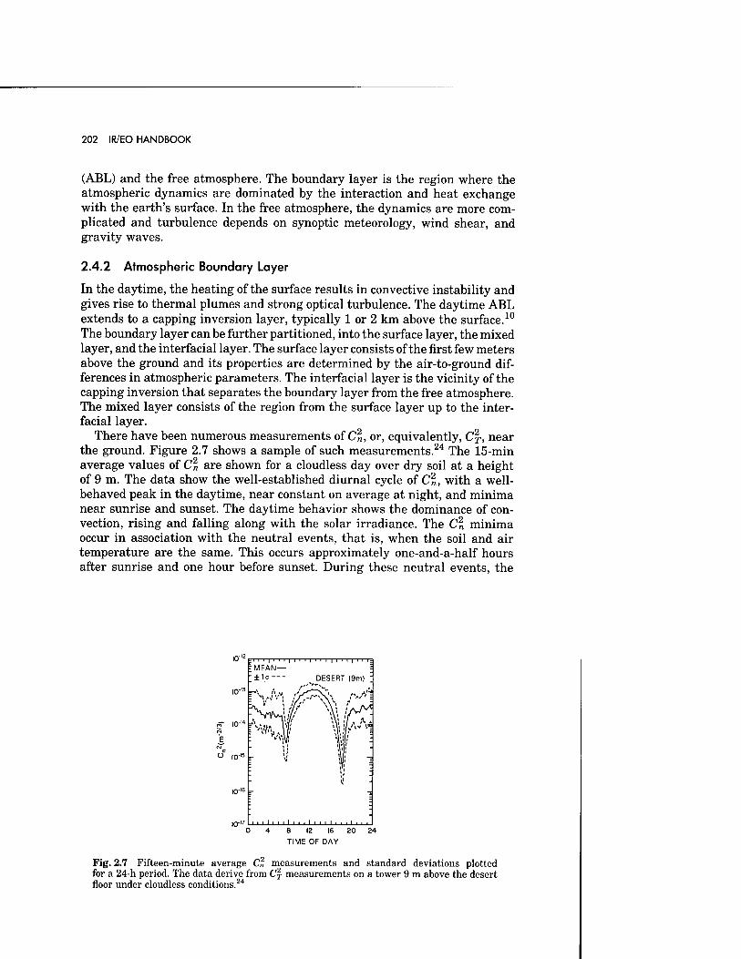
202 IR/EO HANDBOOK
(ABL) and the free atmosphere. The boundary layer is the region where the atmospheric dynamics are dominated by the interaction and heat exchange with the earth's surface. In the free atmosphere, the dynamics are more com- plicated and turbulence depends on synoptic meteorology, wind shear, and gravity waves.
2.4.2 Atmospheric Boundary Layer
In the daytime, the heating of the surface results in convective instability and gives rise to thermal plumes and strong optical turbulence. The daytime ABL extends to a capping inversion layer, typically 1 or 2 km above the surface.10
The boundary layer can be further partitioned, into the surface layer, the mixed layer, and the interfacial layer. The surface layer consists of the first few meters above the ground and its properties are determined by the air-to-ground dif- ferences in atmospheric parameters. The interfacial layer is the vicinity of the capping inversion that separates the boundary layer from the free atmosphere. The mixed layer consists of the region from the surface layer up to the inter- facial layer.
There have been numerous measurements of C„, or, equivalently, C\, near the ground. Figure 2.7 shows a sample of such measurements.24 The 15-min average values of C2 are shown for a cloudless day over dry soil at a height of 9 m. The data show the well-established diurnal cycle of C2, with a well- behaved peak in the daytime, near constant on average at night, and minima near sunrise and sunset. The daytime behavior shows the dominance of con- vection, rising and falling along with the solar irradiance. The C2 minima occur in association with the neutral events, that is, when the soil and air temperature are the same. This occurs approximately one-and-a-half hours after sunrise and one hour before sunset. During these neutral events, the
11' 11111111111111' 11'''
MEAN — ±1/i— ^ DESERT (9m)
i ■ i 0 4 8 12 16 20 24
TIME OF DAY
Fig. 2.7 Fifteen-minute average Cn measurements and standard deviations plotted for a 24-h period. The data derive from C\ measurements on a tower 9 m above the desert floor under cloudless conditions.24
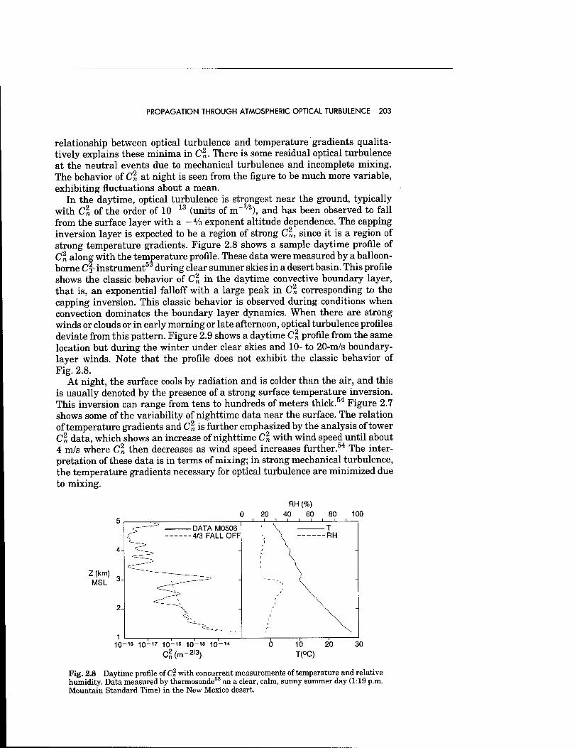
PROPAGATION THROUGH ATMOSPHERIC OPTICAL TURBULENCE 203
relationship between optical turbulence and temperature gradients qualita- tively explains these minima in C„. There is some residual optical turbulence at the neutral events due to mechanical turbulence and incomplete mixing. The behavior of Cn at night is seen from the figure to be much more variable, exhibiting fluctuations about a mean.
In the daytime, optical turbulence is strongest near the ground, typically with C\ of the order of 10~13 (units of m"2/3), and has been observed to fall from the surface layer with a - % exponent altitude dependence. The capping inversion layer is expected to be a region of strong C\, since it is a region of strong temperature gradients. Figure 2.8 shows a sample daytime profile of Cn along with the temperature profile. These data were measured by a balloon- borne CT instrument5 during clear summer skies in a desert basin. This profile shows the classic behavior of C\ in the daytime convective boundary layer, that is, an exponential falloff with a large peak in C\ corresponding to the capping inversion. This classic behavior is observed during conditions when convection dominates the boundary layer dynamics. When there are strong winds or clouds or in early morning or late afternoon, optical turbulence profiles deviate from this pattern. Figure 2.9 shows a daytime Cn profile from the same location but during the winter under clear skies and 10- to 20-m/s boundary- layer winds. Note that the profile does not exhibit the classic behavior of Fig. 2.8.
At night, the surface cools by radiation and is colder than the air, and this is usually denoted by the presence of a strong surface temperature inversion. This inversion can range from tens to hundreds of meters thick.54 Figure 2.7 shows some of the variability of nighttime data near the surface. The relation of temperature gradients and Cn is further emphasized by the analysis of tower Cn data, which shows an increase of nighttime Cn with wind speed until about 4 m/s where Cn then decreases as wind speed increases further.54 The inter- pretation of these data is in terms of mixing; in strong mechanical turbulence, the temperature gradients necessary for optical turbulence are minimized due to mixing.
Z(km) MSL
RH (%) 40 60 100
DATA M0506 4/3 FALL OFF
1 ' 1 , , , 10-18 10-17 10-16 10~15 10-14
C|(m-2/3)
Fig. 2.8 Daytime profile of Cn with concurrent measurements of temperature and relative humidity. Data measured by thermosonde53 on a clear, calm, sunny summer day (1:19 p.m. Mountain Standard Time) in the New Mexico desert.
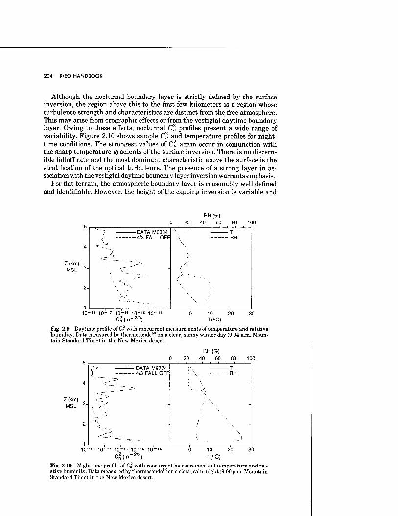
204 IR/EO HANDBOOK
Although the nocturnal boundary layer is strictly defined by the surface inversion, the region above this to the first few kilometers is a region whose turbulence strength and characteristics are distinct from the free atmosphere. This may arise from orographic effects or from the vestigial daytime boundary layer. Owing to these effects, nocturnal C\ profiles present a wide range of variability. Figure 2.10 shows sample C\ and temperature profiles for night- time conditions. The strongest values of Cn again occur in conjunction with the sharp temperature gradients of the surface inversion. There is no discern- ible falloff rate and the most dominant characteristic above the surface is the stratification of the optical turbulence. The presence of a strong layer in as- sociation with the vestigial daytime boundary layer inversion warrants emphasis.
For flat terrain, the atmospheric boundary layer is reasonably well defined and identifiable. However, the height of the capping inversion is variable and
RH (%) 0 20 40 60 80 100
j i i i i i i i i_
Z(km) MSL
DATA M6384 4/3 FALL OFF
\5T 1
10-1° 10-17 io~16 10-15 10-11
T RH
10 20 T(°C)
30
Fig. 2.9 Daytime profile of C„ with concurrent measurements of temperature and relative humidity. Data measured by thermosonde53 on a clear, sunny winter day (9:04 a.m. Moun- tain Standard Time) in the New Mexico desert.
Z(km) MSL 3-
2-
r DATA M9774 4/3 FALL OFF
1 10-1B 1Q-17 1Q-16 1Q-15 10-1"
RH (%) 20 40 60 80 100
_i i i i i i_
Cn2(m-2/3)
30 0 10 20 T(°C)
Fig. 2.10 Nighttime profile of C% with concurrent measurements of temperature and rel- ative humidity. Data measured by thermosonde53 on a clear, calm night (9:00 p.m. Mountain Standard Time) in the New Mexico desert.
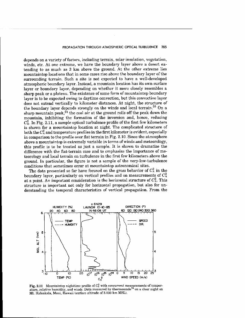
PROPAGATION THROUGH ATMOSPHERIC OPTICAL TURBULENCE 205
depends on a variety of factors, including terrain, solar insolation, vegetation, winds, etc. At one extreme, we have the boundary layer above a desert ex- tending to as much as 3 km above the ground. At the other extreme lies mountaintop locations that in some cases rise above the boundary layer of the surrounding terrain. Such a site is not expected to have a well-developed atmospheric boundary layer. Instead, a mountain location has its own surface layer or boundary layer, depending on whether it more closely resembles a sharp peak or a plateau. The existence of some form of mountaintop boundary layer is to be expected owing to daytime convection, but this convective layer does not extend vertically to kilometer distances. At night, the structure of the boundary layer depends strongly on the winds and local terrain.55 On a sharp mountain peak,24 the cool air at the ground rolls off the peak down the mountain, inhibiting the formation of the inversion and, hence, reducing C\. In Fig. 2.11, a sample optical turbulence profile of the first few kilometers is shown for a mountaintop location at night. The complicated structure of both the Cn and temperature profiles in the first kilometer is evident, especially in comparison to the profile over flat terrain in Fig. 2.10. Since the atmosphere above a mountaintop is extremely variable in terms of winds and meteorology, this profile is to be treated as just a sample. It is shown to dramatize the difference with the flat-terrain case and to emphasize the importance of me- teorology and local terrain on turbulence in the first few kilometers above the ground. In particular, the figure is not a sample of the very-low-turbulence conditions that sometimes occur at mountaintop astronomical sites.
The data presented so far have focused on the gross behavior of Cn in the boundary layer, particularly on vertical profiles and on measurements of Cn at a point. An important consideration is the horizontal structure of Cn. This structure is important not only for horizontal propagation, but also for un- derstanding the temporal characteristics of vertical propagation. From the
HUMIDITY (%) 20 40 60 80
0 6429 LAUNCH 10-10-85
1446 08 UT DIRECTION (°)
60 120 180 240 300 360
E 5
< to
TEMP HUMIDITY
SPEED DIR.
-10 0 10 TEMP PC)
20 lö17 IÖ16 IOi5 IÖ14 ° j i i i i_
5 10 15 20 25
WIND SPEED (m/s)
Fig. 2.11 Mountaintop nighttime profile of Cn with concurrent measurements of temper- ature, relative humidity, and winds. Data measured by thermosonde53 on a clear night on Mt. Haleakala, Maui, Hawaii (surface altitude of 3.030 km MSL).
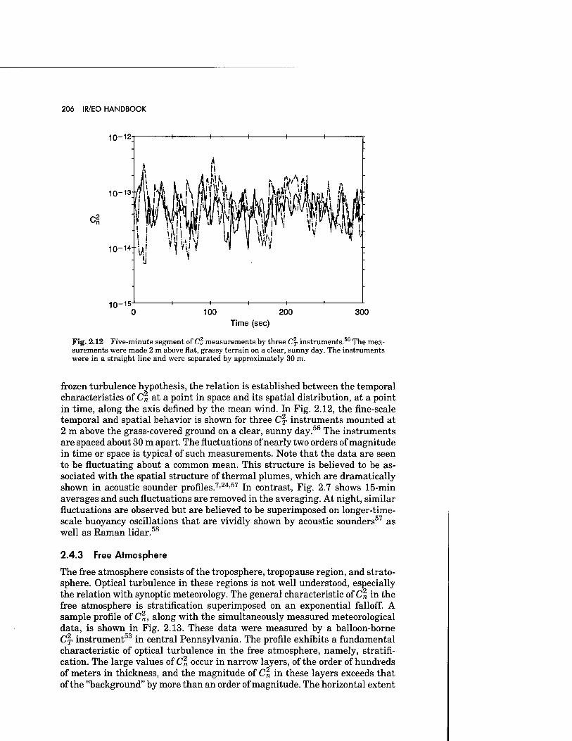
206 IR/EO HANDBOOK
10-12
10-13
r2
10-14
10-15 100 200 300
Time (sec)
Fig. 2.12 Five-minute segment of Cn measurements by three C% instruments.56 The mea- surements were made 2 m above flat, grassy terrain on a clear, sunny day. The instruments were in a straight line and were separated by approximately 30 m.
frozen turbulence hypothesis, the relation is established between the temporal characteristics of Cn at a point in space and its spatial distribution, at a point in time, along the axis defined by the mean wind. In Fig. 2.12, the fine-scale temporal and spatial behavior is shown for three C\ instruments mounted at 2 m above the grass-covered ground on a clear, sunny day.56 The instruments are spaced about 30 m apart. The fluctuations of nearly two orders of magnitude in time or space is typical of such measurements. Note that the data are seen to be fluctuating about a common mean. This structure is believed to be as- sociated with the spatial structure of thermal plumes, which are dramatically shown in acoustic sounder profiles.7'24'57 In contrast, Fig. 2.7 shows 15-min averages and such fluctuations are removed in the averaging. At night, similar fluctuations are observed but are believed to be superimposed on longer-time- scale buoyancy oscillations that are vividly shown by acoustic sounders57 as well as Raman lidar.58
2.4.3 Free Atmosphere
The free atmosphere consists of the troposphere, tropopause region, and strato- sphere. Optical turbulence in these regions is not well understood, especially the relation with synoptic meteorology. The general characteristic of C2. in the free atmosphere is stratification superimposed on an exponential falloff. A sample profile of C2., along with the simultaneously measured meteorological data, is shown in Fig. 2.13. These data were measured by a balloon-borne C\ instrument53 in central Pennsylvania. The profile exhibits a fundamental characteristic of optical turbulence in the free atmosphere, namely, stratifi- cation. The large values of Cn occur in narrow layers, of the order of hundreds of meters in thickness, and the magnitude of Cn in these layers exceeds that of the "background" by more than an order of magnitude. The horizontal extent
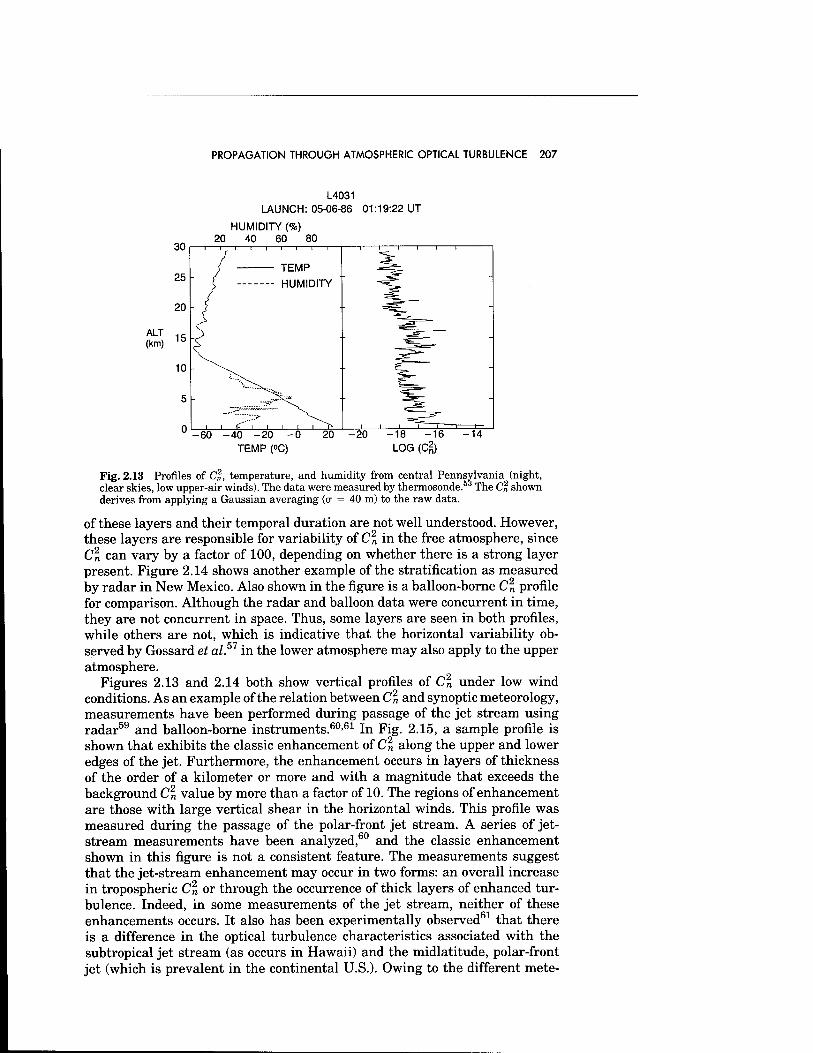
PROPAGATION THROUGH ATMOSPHERIC OPTICAL TURBULENCE 207
L4031 LAUNCH: 05-06-86 01:19:22 UT
HUMIDITY (%) 20 40 60 80
ALT (km)
-60 -40 -20 -0 20 -20 TEMP (°C)
18 -16 LOG (C2)
-14
Fig. 2.13 Profiles of Cn, temperature, and humidity from central Pennsylvania (night, clear skies, low upper-air winds). The data were measured by thermosonde. The Cf shown derives from applying a Gaussian averaging (o = 40 m) to the raw data.
of these layers and their temporal duration are not well understood. However, these layers are responsible for variability of Cn in the free atmosphere, since Cn can vary by a factor of 100, depending on whether there is a strong layer present. Figure 2.14 shows another example of the stratification as measured by radar in New Mexico. Also shown in the figure is a balloon-borne Cn profile for comparison. Although the radar and balloon data were concurrent in time, they are not concurrent in space. Thus, some layers are seen in both profiles, while others are not, which is indicative that the horizontal variability ob- served by Gossard et al.57 in the lower atmosphere may also apply to the upper atmosphere.
Figures 2.13 and 2.14 both show vertical profiles of Cn under low wind conditions. As an example of the relation between Cn and synoptic meteorology, measurements have been performed during passage of the jet stream using radar59 and balloon-borne instruments.60,61 In Fig. 2.15, a sample profile is shown that exhibits the classic enhancement of Cn along the upper and lower edges of the jet. Furthermore, the enhancement occurs in layers of thickness of the order of a kilometer or more and with a magnitude that exceeds the background Cn value by more than a factor of 10. The regions of enhancement are those with large vertical shear in the horizontal winds. This profile was measured during the passage of the polar-front jet stream. A series of jet- stream measurements have been analyzed,60 and the classic enhancement shown in this figure is not a consistent feature. The measurements suggest that the jet-stream enhancement may occur in two forms: an overall increase in tropospheric Cn or through the occurrence of thick layers of enhanced tur- bulence. Indeed, in some measurements of the jet stream, neither of these enhancements occurs. It also has been experimentally observed61 that there is a difference in the optical turbulence characteristics associated with the subtropical jet stream (as occurs in Hawaii) and the midlatitude, polar-front jet (which is prevalent in the continental U.S.). Owing to the different mete-
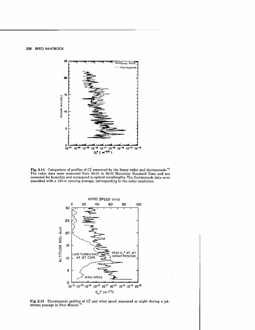
208 IR/EO HANDBOOK
25
20
15
3 10 -
5 -
niiuq iiii»i iimq IIIII^ iiui^ -Sousy Radar
■Thermosonde-
Q I titl»J .J ■ IIIMJ IIIIMJ J I .....J U ■
10" io-; 10" 10_™ 10"" 10"'* 10"1* 10"14 10-"
C.» ( m-V* )
Fig. 2.14 Comparison of profiles of C2 measured by the Sousy radar and thermosonde.72
The radar data were measured from 20:25 to 20:40 Mountain Standard Time and are corrected for humidity and correspond to optical wavelengths. The thermosonde data were smoothed with a 150-m running average, corresponding to the radar resolution.
30
25
E
CO
LU Q 3 H
20 ■)
15 -
10
5 -
WIND SPEED (m/s)
20 40 60 80 ~i 1 1 1 1—
100
_ PEAK C 2 AT JET "•;, SHEAR REGIONS
ij i i ill ■ ■ ■■' ■ ■ ■■' ■ ■ • ■' • ■ ■■' • • ••' ■ ■ ■■
io"21 io"2010"19 i0"18 i0"17 io-'6 i0"15 ia14 io"13
C 2 (m-2/3)
Fig. 2.15 Thermosonde profiles of C2 and wind speed measured at night during a jet- stream passage in New Mexico.75
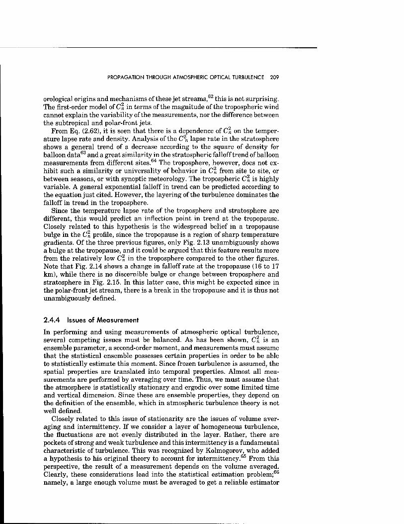
PROPAGATION THROUGH ATMOSPHERIC OPTICAL TURBULENCE 209
orological origins and mechanisms of these jet streams,62 this is not surprising. The first-order model of C2 in terms of the magnitude of the tropospheric wind cannot explain the variability of the measurements, nor the difference between the subtropical and polar-front jets.
From Eq. (2.62), it is seen that there is a dependence of C2 on the temper- ature lapse rate and density. Analysis of the C2
n lapse rate in the stratosphere shows a general trend of a decrease according to the square of density for balloon data63 and a great similarity in the stratospheric falloff trend of balloon measurements from different sites.64 The troposphere, however, does not ex- hibit such a similarity or universality of behavior in C2 from site to site, or between seasons, or with synoptic meteorology. The tropospheric C2 is highly variable. A general exponential falloff in trend can be predicted according to the equation just cited. However, the layering of the turbulence dominates the falloff in trend in the troposphere.
Since the temperature lapse rate of the troposphere and stratosphere are different, this would predict an inflection point in trend at the tropopause. Closely related to this hypothesis is the widespread belief in a tropopause bulge in the C2 profile, since the tropopause is a region of sharp temperature gradients. Of the three previous figures, only Fig. 2.13 unambiguously shows a bulge at the tropopause, and it could be argued that this feature results more from the relatively low C2 in the troposphere compared to the other figures. Note that Fig. 2.14 shows a change in falloff rate at the tropopause (16 to 17 km), while there is no discernible bulge or change between troposphere and stratosphere in Fig. 2.15. In this latter case, this might be expected since in the polar-front jet stream, there is a break in the tropopause and it is thus not unambiguously defined.
2.4.4 Issues of Measurement
In performing and using measurements of atmospheric optical turbulence, several competing issues must be balanced. As has been shown, C2 is an ensemble parameter, a second-order moment, and measurements must assume that the statistical ensemble possesses certain properties in order to be able to statistically estimate this moment. Since frozen turbulence is assumed, the spatial properties are translated into temporal properties. Almost all mea- surements are performed by averaging over time. Thus, we must assume that the atmosphere is statistically stationary and ergodic over some limited time and vertical dimension. Since these are ensemble properties, they depend on the definition of the ensemble, which in atmospheric turbulence theory is not well defined.
Closely related to this issue of stationarity are the issues of volume aver- aging and intermittency. If we consider a layer of homogeneous turbulence, the fluctuations are not evenly distributed in the layer. Rather, there are pockets of strong and weak turbulence and this intermittency is a fundamental characteristic of turbulence. This was recognized by Kolmogorov, who added a hypothesis to his original theory to account for intermittency.65 From this perspective, the result of a measurement depends on the volume averaged. Clearly, these considerations lead into the statistical estimation problem;66
namely, a large enough volume must be averaged to get a reliable estimator
210 IR/EO HANDBOOK
of the ensemble parameter. However, since turbulence is a nonlinear phenom- enon, the distribution of the pockets is not necessarily the same as a linear random process and thus the statistical estimation theory is very difficult.
These are far from solely academic issues, but have important applications in comparing measurements from different instruments or in using data or models to predict a system's performance. For example, suppose we wish to estimate the turbulence effects on the propagation of a collimated laser beam over a short time interval. A Doppler radar measurement of C« may measure the backscatter from a volume with a scale size of a kilometer and further may average over several minutes. Another instrument in routine use for Cn profiling is the stellar scintillometer,37 which typically measures along an optical path with a vertical resolution of kilometers and averages over minutes. Scintillometers and some low-resolution radars cannot resolve the narrow lay- ers of turbulence. At the other extreme are balloon-borne instruments, which possess the highest resolution but measure along a vertical path determined by the wind. Clearly, as one measures a smaller and smaller volume, the structure in the Cn profile increases. However, there is a limit to this resolution, namely, that imposed by statistical estimation requirements.
Both the tower data shown in Fig. 2.7 and the radar data in Fig. 2.14 are 15-min averages. Whether this averaging is too long depends on the appli- cation. The most prudent definition of the ensemble is not in terms of the atmosphere, with its layering and large- and small-scale dynamics, but rather in terms of the particular optical effect and the system. For example, if scin- tillation is the important effect, the important scale size has been shown to be the Fresnel scale. Furthermore, the volume of interest is determined by the source and the optical path. Similarly, if the dominant optical effect of interest arises from coherence length, the vertical volume averaging or vertical reso- lution are not important since coherence length is determined from integrated d
2.4.5 Measurements of Moments
Numerous measurements have been reported of the two most important mo- ments of Cn- the coherence length ro and the isoplanatic angle 6o- These have been reported in the open literature by direct measurements via optical means67-72 and by numerical integration of measured profiles.7374 Table 2.2 lists some of these measurements at a variety of times and locations.
For coherence length, several features emerge from these data. First, in general, daytime values are smaller than nighttime values. This is due to the greater daytime turbulence arising from convection. Depending on season and location, this diurnal variation in ro can be weak, as during the desert winter data when winds dominated the boundary layer meteorology, or strong, as during the desert summer data when surface convection dominated. Second, in general, mountain locations have larger average values of coherence length at night than desert. Again, this can be explained in terms of the boundary layers. In the day, the difference between mountain and desert is not as clear and similar values have been reported. A third observation from the data is the much larger standard deviation associated with nighttime ro at mountain- tops. This indicates the existence of very good (as well as very poor) seeing conditions on some nights, which are conditions that do not occur in deserts.
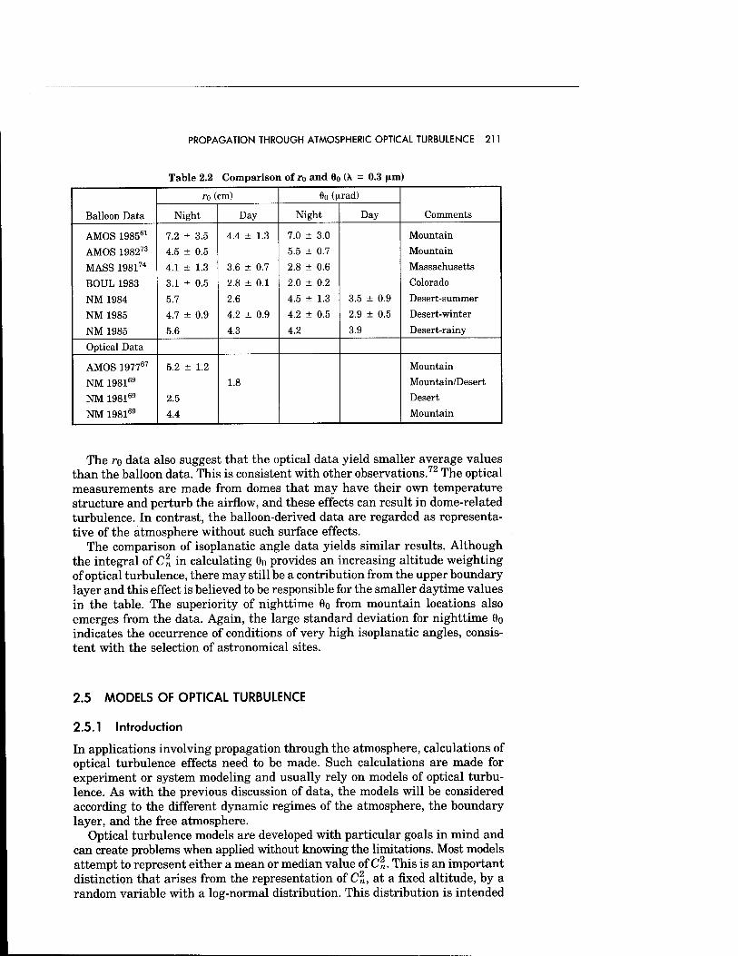
PROPAGATION THROUGH ATMOSPHERIC OPTICAL TURBULENCE 211
Table 2.2 Comparison of r0 and 8o (A. = 0.3 (Am)
Balloon Data
ro ( cm) 8o (pxad)
Comments Night Day Night Day
AMOS 198561 7.2 ± 3.5 4.4 ± 1.3 7.0 ± 3.0 Mountain
AMOS 198273 4.5 ± 0.5 5.5 ± 0.7 Mountain
MASS 198174 4.1 ± 1.3 3.6 ± 0.7 2.8 ± 0.6 Massachusetts
BOUL 1983 3.1 ± 0.5 2.8 ± 0.1 2.0 ± 0.2 Colorado
NM 1984 5.7 2.6 4.5 ± 1.3 3.5 ± 0.9 Desert-summer
NM 1985 4.7 ± 0.9 4.2 ± 0.9 4.2 ± 0.5 2.9 ± 0.5 Desert-winter
NM 1985 5.6 4.3 4.2 3.9 Desert-rainy
Optical Data
AMOS 197767 5.2 ± 1.2 Mountain
NM 198169 1.8 Mountain/Desert
NM 198169 2.5 Desert
NM 198169 4.4 Mountain
The ro data also suggest that the optical data yield smaller average values than the balloon data. This is consistent with other observations.72 The optical measurements are made from domes that may have their own temperature structure and perturb the airflow, and these effects can result in dome-related turbulence. In contrast, the balloon-derived data are regarded as representa- tive of the atmosphere without such surface effects.
The comparison of isoplanatic angle data yields similar results. Although the integral of C\ in calculating 6o provides an increasing altitude weighting of optical turbulence, there may still be a contribution from the upper boundary layer and this effect is believed to be responsible for the smaller daytime values in the table. The superiority of nighttime Go from mountain locations also emerges from the data. Again, the large standard deviation for nighttime 9o indicates the occurrence of conditions of very high isoplanatic angles, consis- tent with the selection of astronomical sites.
2.5 MODELS OF OPTICAL TURBULENCE
2.5.1 Introduction
In applications involving propagation through the atmosphere, calculations of optical turbulence effects need to be made. Such calculations are made for experiment or system modeling and usually rely on models of optical turbu- lence. As with the previous discussion of data, the models will be considered according to the different dynamic regimes of the atmosphere, the boundary layer, and the free atmosphere.
Optical turbulence models are developed with particular goals in mind and can create problems when applied without knowing the limitations. Most models attempt to represent either a mean or median value of C„. This is an important distinction that arises from the representation of Cn, at a fixed altitude, by a random variable with a log-normal distribution. This distribution is intended
212 IR/EO HANDBOOK
to model the stratification and variation on different days and meteorological conditions. Many models are therefore developed by log averaging of data. The difficulty arises because the mean of the log of Cn is of course the median for a Gaussian distribution, but this is distinct from, and smaller than, the mean of Cn. As the data have shown, a fundamental characteristic of atmospheric turbulence is stratification, which is responsible in part for the order of mag- nitude variation in Cn at a fixed altitude. With respect to a sample profile such as those in Fig. 2.13 or Fig. 2.14, the eye draws a median curve (that is, averaging the logarithm of Cn) through the fluctuations to generate a model profile. However, most applications are concerned with average or mean values of Cn, not the median value, and moments involve linear averaging of C„ with some appropriate weighting. Because of the log-normal distribution, the re- lationship between the median and mean can be estimated and is typically a factor of 2. A more thorough discussion of the assumptions and limitations of the individual models will be provided in the following.
There have come into existence a variety of models of Cn profiles.75 These arrange themselves into a hierarchy. There are no-parameter models, which are assumed to provide representative average profiles. A slight improvement on this are the site-dependent models. The parametric models have been de- veloped in an attempt to incorporate the dependency on site and meteorology. However, these still tend to provide models only for average conditions. These models will be discussed in terms of their hierarchy of increasing complexity. It is not the intent of this presentation to perform a historical and all-inclusive review of models. Rather, the most useful and representative models, as well as those in the most widespread use, are the focus.
It will become apparent that the current state of Cn modeling has several deficiencies. For example, one category of models simply represents average conditions and shows no stratification. A significant omission of this category is the absence of error bars about the averages, which could be used to deter- mine confidence levels. Such error bars would be of limited use because of the layering of Cn and the subsequent vertical correlation, that is, the multipara- metric statistical nature of an optical turbulence profile. Thus, a profile con- structed of 2a values would represent an integrated level of turbulence far in excess of any real profile and additionally, a real profile would also likely exceed the 2a value at several layers. The second broad category of models introduces stratification by incorporating a dependence on meteorological pa- rameters. A limitation of these models tends to be the restricted altitude do- main; none of these models extends to the boundary layer. In particular, the nocturnal boundary layer remains a key problem in Cn modeling. Nonetheless, these models show considerable promise, not only in terms of providing more realistic models for system designers, but also in terms of providing insight into the relation between meteorological conditions and atmospheric turbulence.
2.5.2 Boundary-Layer Turbulence
The cornerstone of models of boundary-layer turbulence is similarity the- ory.10'76 Similarity theory utilizes a dimensional analysis and physical mod- eling to determine dominant length scales. The Monin-Obhukov length is the scaling length parameter in the surface layer to describe the heat and mo-
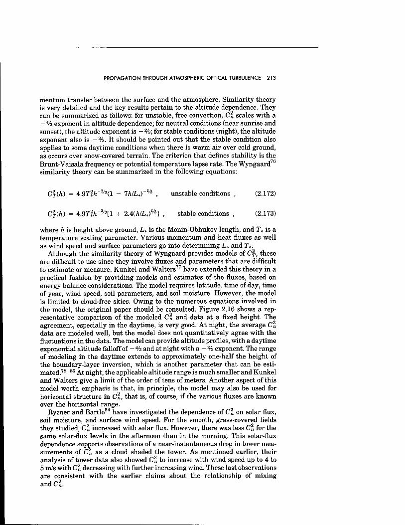
PROPAGATION THROUGH ATMOSPHERIC OPTICAL TURBULENCE 213
mentum transfer between the surface and the atmosphere. Similarity theory is very detailed and the key results pertain to the altitude dependence. They can be summarized as follows: for unstable, free convection, Cn scales with a - Va exponent in altitude dependence; for neutral conditions (near sunrise and sunset), the altitude exponent is - %; for stable conditions (night), the altitude exponent also is -%. It should be pointed out that the stable condition also applies to some daytime conditions when there is warm air over cold ground, as occurs over snow-covered terrain. The criterion that defines stability is the Brunt-Vaisala frequency or potential temperature lapse rate. The Wyngaard76
similarity theory can be summarized in the following equations:
C\{h) = 4.97l/T2/3(l - 7A/L*)~2/3 , unstable conditions , (2.172)
C%(h) = 4.97l/T2/3[l + 2.4(/i/L*)2/3] , stable conditions , (2.173)
where h is height above ground, L* is the Monin-Obhukov length, and T* is a temperature scaling parameter. Various momentum and heat fluxes as well as wind speed and surface parameters go into determining L* and T*.
Although the similarity theory of Wyngaard provides models of C%, these are difficult to use since they involve fluxes and parameters that are difficult to estimate or measure. Kunkel and Walters77 have extended this theory in a practical fashion by providing models and estimates of the fluxes, based on energy balance considerations. The model requires latitude, time of day, time of year, wind speed, soil parameters, and soil moisture. However, the model is limited to cloud-free skies. Owing to the numerous equations involved in the model, the original paper should be consulted. Figure 2.16 shows a rep- resentative comparison of the modeled Cn and data at a fixed height. The agreement, especially in the daytime, is very good. At night, the average Cn
data are modeled well, but the model does not quantitatively agree with the fluctuations in the data. The model can provide altitude profiles, with a daytime exponential altitude falloff of - 4/a and at night with a - % exponent. The range of modeling in the daytime extends to approximately one-half the height of the boundary-layer inversion, which is another parameter that can be esti- mated.78-80 At night, the applicable altitude range is much smaller and Kunkel and Walters give a limit of the order of tens of meters. Another aspect of this model worth emphasis is that, in principle, the model may also be used for horizontal structure in Cn, that is, of course, if the various fluxes are known over the horizontal range.
Ryzner and Bartlo54 have investigated the dependence of Cn on solar flux, soil moisture, and surface wind speed. For the smooth, grass-covered fields they studied, Cn increased with solar flux. However, there was less Cn for the same solar-flux levels in the afternoon than in the morning. This solar-flux dependence supports observations of a near-instantaneous drop in tower mea- surements of Cn as a cloud shaded the tower. As mentioned earlier, their analysis of tower data also showed Cn to increase with wind speed up to 4 to 5 m/s with Cn decreasing with further increasing wind. These last observations are consistent with the earlier claims about the relationship of mixing and C\.
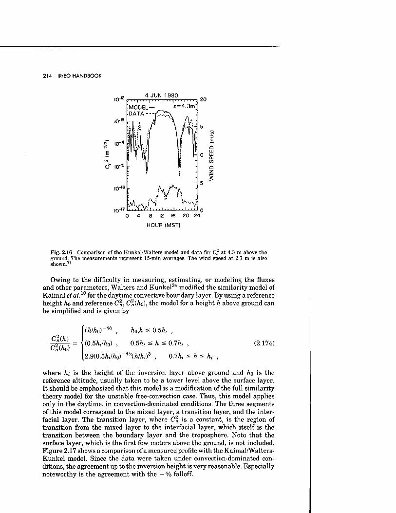
214 IR/EO HANDBOOK
IQ"1 4JUN 1980
I I I | I I T | I r I [ T T I | I I I | I I I
MODEL— z = 4.3m DATA---^
,0-i6
10"
... 'if '\ ii<i 11 ■ 111 ■ 11 ■ ■ ■ i ■ ■ i
20
0 4 8 12 16 20 24
HOUR (MST)
UJ 0- CO
Q Z
Fig. 2.16 Comparison of the Kunkel-Walters model and data for C% at 4.3 m above the ground. The measurements represent 15-min averages. The wind speed at 2.7 m is also shown.77
Owing to the difficulty in measuring, estimating, or modeling the fluxes and other parameters, Walters and Kunkel24 modified the similarity model of Kaimal et al.10 for the daytime convective boundary layer. By using a reference height ho and reference Cn, Cn(ho), the model for a height h above ground can be simplified and is given by
Clih) c'i(ho)
(h/h0)~4/3 , h0,h^0.5hi ,
(0.5Ä.7Ä0) , 0.5Ä,- < h == 0.7/i, ,
2.W.5hi/h0r4/3(h/hi)3 , 0.7hi < h < ht ,
(2.174)
where hi is the height of the inversion layer above ground and ho is the reference altitude, usually taken to be a tower level above the surface layer. It should be emphasized that this model is a modification of the full similarity theory model for the unstable free-convection case. Thus, this model applies only in the daytime, in convection-dominated conditions. The three segments of this model correspond to the mixed layer, a transition layer, and the inter- facial layer. The transition layer, where Cn is a constant, is the region of transition from the mixed layer to the interfacial layer, which itself is the transition between the boundary layer and the troposphere. Note that the surface layer, which is the first few meters above the ground, is not included. Figure 2.17 shows a comparison of a measured profile with the Kaimal/Walters- Kunkel model. Since the data were taken under convection-dominated con- ditions, the agreement up to the inversion height is very reasonable. Especially noteworthy is the agreement with the - 4/3 falloff.
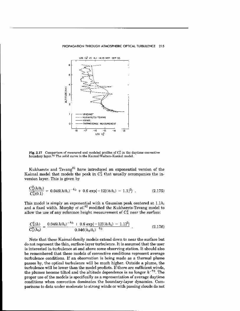
PROPAGATION THROUGH ATMOSPHERIC OPTICAL TURBULENCE 215
LOG Cn VS ALT 14:19 MDT SEP 05
5 -
E
UJ 9 3
-VANZANDT ■■KUKHARETS/TSVANG -KAI MAL -THERMOSONDE MEASUREMENT
-16 -15 LOG C„
-14
Fig. 2.17 Comparison of measured and modeled profiles of Cn in the daytime convective boundary layer.82 The solid curve is the Kaimal/Walters-Kunkel model.
Kukharets and Tsvang81 have introduced an exponential version of the Kaimal model that models the peak in Cn that usually accompanies the in- version layer. This is given by
Clihlhi) CliO.l)
-V3 = 0.046(h/hi)-/3 + 0.6exp{-12[(Mji) - l.l]z} (2.175)
This model is simply an exponential with a Gaussian peak centered at l.lhi and a fixed width. Murphy et al.82 modified the Kukharets-Tsvang model to allow the use of any reference height measurement of Cn near the surface:
Cl(h) _ 0.046(W~4/3 + 0.6exp{-12[(A/^) - l.l]2} Cl(h0) ~ 0.046(h0/hi) -4/3
(2.176)
Note that these Kaimal-family models extend down to near the surface but do not represent the thin, surface-layer turbulence. It is assumed that the user is interested in turbulence at and above some observing station. It should also be remembered that these models of convective conditions represent average turbulence conditions. If an observation is being made as a thermal plume passes by, the optical turbulence will be much higher. Outside a plume, the turbulence will be lower than the model predicts. If there are sufficient winds, the plumes become tilted and the altitude dependence is no longer h~ /3. The proper use of the models is specifically as a representation of average daytime conditions when convection dominates the boundary-layer dynamics. Com- parisons to data under moderate to strong winds or with passing clouds do not
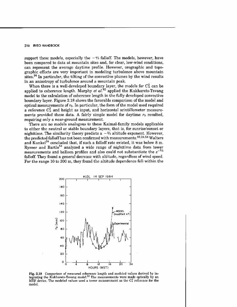
216 IR/EO HANDBOOK
support these models, especially the -Vs falloff. The models, however, have been compared to data at mountain sites and, for clear, low-wind conditions, can represent the average daytime profile. However, orographic and topo- graphic effects are very important in modeling turbulence above mountain sites.24 In particular, the tilting of the convective plumes by the wind results in an anisotropy of turbulence around a mountain peak.
When there is a well-developed boundary layer, the models for C2 can be applied to coherence length. Murphy et al.82 applied the Kukharets-Tsvang model to the calculation of coherence length in the fully developed convective boundary layer. Figure 2.18 shows the favorable comparison of the model and optical measurements of ro. In particular, the form of the model used required a reference C2 and height as input, and horizontal scintillometer measure- ments provided these data. A fairly simple model for daytime ro resulted, requiring only a near-ground measurement.
There are no models analogous to these Kaimal-family models applicable to either the neutral or stable boundary layers, that is, for sunrise/sunset or nighttime. The similarity theory predicts a - % altitude exponent. However, the predicted falloff has not been confirmed with measurements.83,24,54 Walters and Kunkel24 concluded that, if such a falloff rate existed, it was below 8 m. Ryzner and Bartlo54 analyzed a wide range of nighttime data from tower measurements and balloon profiles and also could not substantiate the z~ /3
falloff. They found a general decrease with altitude, regardless of wind speed. For the range 10 to 300 m, they found the altitude dependence fell within the
200
180 -
HIDL 14 SEP 1984 T~ "T
8 12 16 HOURS (MST)
20 24
Fig. 2.18 Comparison of measured coherence length and modeled values derived by in- tegrating the Kukharets-Tsvang model.82 The measurements were made optically by an MTF device. The modeled values used a tower measurement as the C„ reference for the model.
PROPAGATION THROUGH ATMOSPHERIC OPTICAL TURBULENCE 217
range z~os and z~2, depending on the strength of the winds. They also found the interesting result that C\ fell as 2" /3 for winds in the 4 to 6 m/s range and stated that this exponent was the most reasonable approximation. How- ever, in contrast to the daytime convective boundary layer where the -V3 exponent applies up to a kilometer or so, stable nighttime conditions allow this exponent to apply only through the surface inversion, that is, to a height of the order of a few hundred meters. Above this height, the stratification of optical turbulence is the dominant characteristic and no simple exponential behavior can be predicted. This nighttime model of Ryzner and Bartlo requires further validation. In particular, much of their analysis was based on slopes computed from averages at different heights. Thus, although the slope of the averages may be satisfactorily modeled by z~ /3, it is not clear that this slope is an effective model of an individual profile.
Ryzner and Bartlo54 also performed a similar analysis on C« data from the transition period of sunrise and sunset. Again, a - ¥3 slope was determined as the best fit. Their results should be treated cautiously, since the data sets were very limited.
The class of empirical models provides alternatives for boundary-layer mod- eling. These fall into two categories. The first corresponds to model profiles derived from averaging measured profiles. These are discussed in more detail in the following section, since such averages include the free atmosphere as well. A caveat in the use of these models is that they tend to vary from site to site, with season and meteorology. Furthermore, in averaging boundary- layer data, any variation in the height of the boundary-layer inversion in the daytime, or the nocturnal surface inversion, tends to distort the resulting average. Such average profiles do not correspond to any boundary-layer profile and correlations with meteorology and winds are lost in the averaging. The second alternative for modeling is to use an actual representative profile. Thus, the daytime desert could be represented by the profile in Fig. 2.8, the nighttime desert by Fig. 2.10, and the nighttime mountaintop by Fig. 2.11. The advantage of such profiles is that they correspond to actual measurements and have correlations with winds and meteorology. The disadvantage is that they are dependent on time of day, site, season, and meteorology.
The issue of horizontal models arises in propagation over horizontal or slant paths through the atmosphere. The customary approach for a horizontal path over flat terrain is to use the value determined for the proper height from one of the previous boundary-layer models or even data such as Fig. 2.16 and assume that C\ is a constant over the path. Although this assumption conflicts with point measurements, the variation along the path is less important for the calculation of many of the standard optical effects because of volume av- eraging. This is analogous to the issues that arise in comparing a point mea- surement of Cn with data from a path-averaging instrument.
2.5.3 Model Optical Turbulence Profiles
The first class of model profiles is empirically derived from averaged data. The most widely used of these are the so-called SLC models, from Miller and Zieske68
(the acronym derives from submarine laser communications studies). These models were derived by curve-fitting a piecewise-continuous polynomial to a
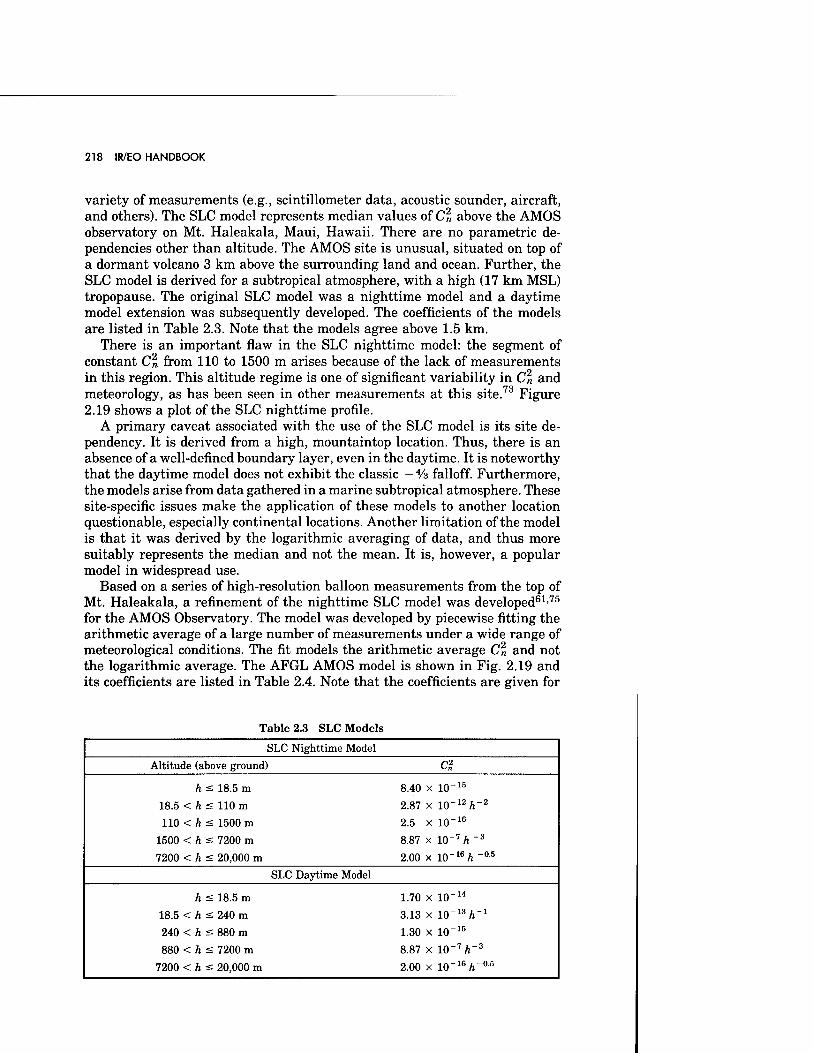
218 IR/EO HANDBOOK
variety of measurements (e.g., scintillometer data, acoustic sounder, aircraft, and others). The SLC model represents median values of Cn above the AMOS observatory on Mt. Haleakala, Maui, Hawaii. There are no parametric de- pendencies other than altitude. The AMOS site is unusual, situated on top of a dormant volcano 3 km above the surrounding land and ocean. Further, the SLC model is derived for a subtropical atmosphere, with a high (17 km MSL) tropopause. The original SLC model was a nighttime model and a daytime model extension was subsequently developed. The coefficients of the models are listed in Table 2.3. Note that the models agree above 1.5 km.
There is an important flaw in the SLC nighttime model: the segment of constant Cn from 110 to 1500 m arises because of the lack of measurements in this region. This altitude regime is one of significant variability in Cn and meteorology, as has been seen in other measurements at this site.73 Figure 2.19 shows a plot of the SLC nighttime profile.
A primary caveat associated with the use of the SLC model is its site de- pendency. It is derived from a high, mountaintop location. Thus, there is an absence of a well-defined boundary layer, even in the daytime. It is noteworthy that the daytime model does not exhibit the classic - % falloff. Furthermore, the models arise from data gathered in a marine subtropical atmosphere. These site-specific issues make the application of these models to another location questionable, especially continental locations. Another limitation of the model is that it was derived by the logarithmic averaging of data, and thus more suitably represents the median and not the mean. It is, however, a popular model in widespread use.
Based on a series of high-resolution balloon measurements from the top of Mt. Haleakala, a refinement of the nighttime SLC model was developed61'75
for the AMOS Observatory. The model was developed by piecewise fitting the arithmetic average of a large number of measurements under a wide range of meteorological conditions. The fit models the arithmetic average Cn and not the logarithmic average. The AFGL AMOS model is shown in Fig. 2.19 and its coefficients are listed in Table 2.4. Note that the coefficients are given for
Table 2.3 SLC Models
SLC Nighttime Model
Altitude (above ground cl h == 18.5 m 8.40 X io-15
18.5 < h =s 110 m 2.87 X io~12/r2
110 < h < 1500 m 2.5 X 10 -16
1500 < h < 7200 m 8.87 X 10"7A-3
7200 < h < 20,000 m 2.00 X 10⁻¹⁶Ä-0.5
SLC Daytime Model
h < 18.5 m 1.70 X 10⁻¹⁴
18.5 < h s 240 m 3.13 X IO"13/*"1
240 < h s 880 m 1.30 X 10"15
880 < h =£ 7200 m 8.87 X io-7/r3
7200 < h < 20,000 m 2.00 X 10⁻¹⁶A-0.5
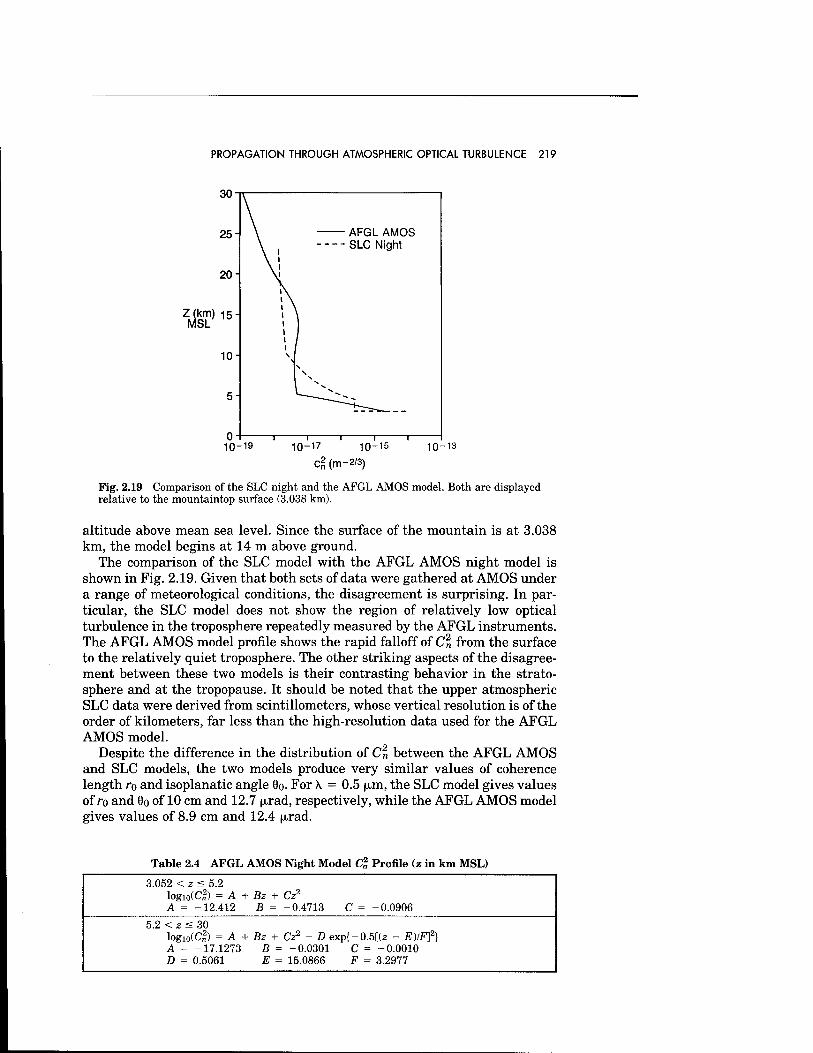
PROPAGATION THROUGH ATMOSPHERIC OPTICAL TURBULENCE 219
25- \ AFGL AMOS \ ( SLC Night
20- H Zfi)15" n
10-
5-
o-
>
i
10-19 10-17 10-15
C2(m-2/3)
10-13
Fig. 2.19 Comparison of the SLC night and the AFGL AMOS model. Both are displayed relative to the mountaintop surface (3.038 km).
altitude above mean sea level. Since the surface of the mountain is at 3.038 km, the model begins at 14 m above ground.
The comparison of the SLC model with the AFGL AMOS night model is shown in Fig. 2.19. Given that both sets of data were gathered at AMOS under a range of meteorological conditions, the disagreement is surprising. In par- ticular, the SLC model does not show the region of relatively low optical turbulence in the troposphere repeatedly measured by the AFGL instruments. The AFGL AMOS model profile shows the rapid falloff of C2
n from the surface to the relatively quiet troposphere. The other striking aspects of the disagree- ment between these two models is their contrasting behavior in the strato- sphere and at the tropopause. It should be noted that the upper atmospheric SLC data were derived from scintillometers, whose vertical resolution is of the order of kilometers, far less than the high-resolution data used for the AFGL AMOS model.
Despite the difference in the distribution of C\ between the AFGL AMOS and SLC models, the two models produce very similar values of coherence length ro and isoplanatic angle 9o- For X = 0.5 (xm, the SLC model gives values of ro and 6o of 10 cm and 12.7 (xrad, respectively, while the AFGL AMOS model gives values of 8.9 cm and 12.4 (Jirad.
Table 2.4 AFGL AMOS Night Model Cg Profile (z in km MSL)
3.052 < z < 5.2 logio(C^) = A A = -12.412
+ Bz + B =
Cz2
-0.4713 c -- = -0.0906
5.2 < z < 30 logio(C^) = A A = -17.1273 D = 0.5061
+ Bz + B = E =
Cz2 + D -0.0301 15.0866
exp{- C F
0.5[(z - E)/F]2} = -0.0010 = 3.2977
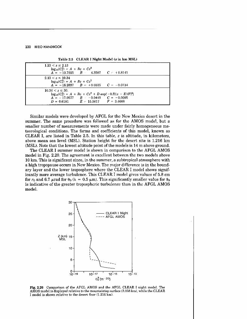
220 IR/EO HANDBOOK
Table 2.5 CLEAR I Night Model (z in km MSL)
1.23 < z < 2.13 logio(C^) = A + Bz + Cz2
A = -10.7025 B = -4.3507 C = +0.8141
2.13 < z £ 10.34 logio(C^) = A + Bz + Cz2
A = -16.2897 B = +0.0335 C = -0.0134
10.34 < z < 30. logio(Cl) = A + Bz + Cz2 + D exp{-0.5[(z - E)/F]2} A = -17.0577 B = -0.0449 C = -0.0005 D = 0.6181 E = 15.5617 F = 3.4666
Similar models were developed by AFGL for the New Mexico desert in the summer. The same procedure was followed as for the AMOS model, but a smaller number of measurements were made under fairly homogeneous me- teorological conditions. The forms and coefficients of this model, known as CLEAR I, are listed in Table 2.5. In this table, z is altitude, in kilometers, above mean sea level (MSL). Station height for the desert site is 1.216 km (MSL). Note that the lowest altitude point of the models is 14 m above ground.
The CLEAR I summer model is shown in comparison to the AFGL AMOS model in Fig. 2.20. The agreement is excellent between the two models above 10 km. This is significant since, in the summer, a subtropical atmosphere with a high tropopause occurs in New Mexico. The major difference is in the bound- ary layer and the lower troposphere where the CLEAR I model shows signif- icantly more average turbulence. This CLEAR I model gives values of 5.8 cm for ro and 6.7 (jirad for 6o (A. = 0.5 |xm). This significantly smaller value for 9o is indicative of the greater tropospheric turbulence than in the AFGL AMOS model.
30
25
20
Z(km) 15- /ISL
10
CLEAR I Night AFGL AMOS
10-19 10-17 10-15 10-13
cg(m-2/3)
Fig. 2.20 Comparison of the AFGL AMOS and the AFGL CLEAR I night model. The AMOS model is displayed relative to the mountaintop surface (3.038 km), while the CLEAR I model is shown relative to the desert floor (1.216 km).
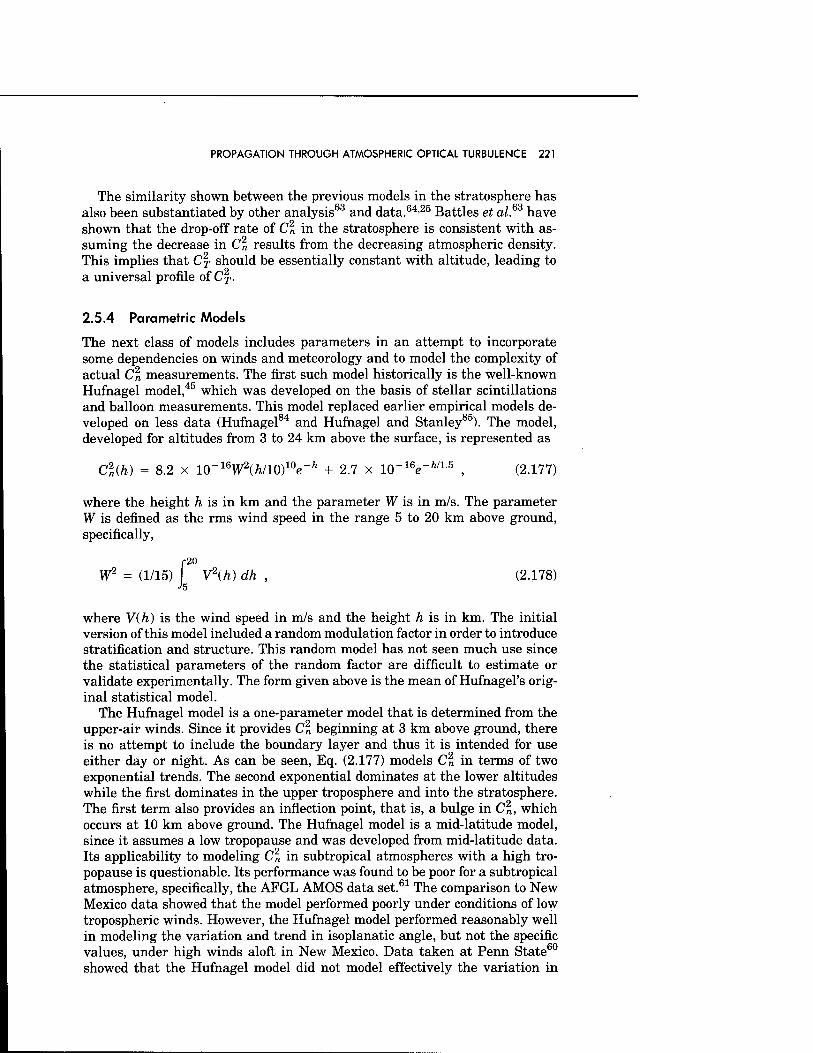
PROPAGATION THROUGH ATMOSPHERIC OPTICAL TURBULENCE 221
The similarity shown between the previous models in the stratosphere has also been substantiated by other analysis63 and data.64,25 Battles et al.6S have shown that the drop-off rate of C\ in the stratosphere is consistent with as- suming the decrease in Cn results from the decreasing atmospheric density. This implies that C\ should be essentially constant with altitude, leading to a universal profile of C\.
2.5.4 Parametric Models
The next class of models includes parameters in an attempt to incorporate some dependencies on winds and meteorology and to model the complexity of actual Cn measurements. The first such model historically is the well-known Hufnagel model,45 which was developed on the basis of stellar scintillations and balloon measurements. This model replaced earlier empirical models de- veloped on less data (Hufnagel84 and Hufnagel and Stanley85). The model, developed for altitudes from 3 to 24 km above the surface, is represented as
Clih) = 8.2 x 10~16W2(h/10)we-h + 2.7 x 10~16e""W15 , (2.177)
where the height h is in km and the parameter W is in m/s. The parameter W is defined as the rms wind speed in the range 5 to 20 km above ground, specifically,
r20
h Wz = (1/15) V\h) dh , (2.178)
where V(h) is the wind speed in m/s and the height h is in km. The initial version of this model included a random modulation factor in order to introduce stratification and structure. This random model has not seen much use since the statistical parameters of the random factor are difficult to estimate or validate experimentally. The form given above is the mean of Hufnagel's orig- inal statistical model.
The Hufnagel model is a one-parameter model that is determined from the upper-air winds. Since it provides Cn beginning at 3 km above ground, there is no attempt to include the boundary layer and thus it is intended for use either day or night. As can be seen, Eq. (2.177) models Cn in terms of two exponential trends. The second exponential dominates at the lower altitudes while the first dominates in the upper troposphere and into the stratosphere. The first term also provides an inflection point, that is, a bulge in Cn, which occurs at 10 km above ground. The Hufnagel model is a mid-latitude model, since it assumes a low tropopause and was developed from mid-latitude data. Its applicability to modeling Cn in subtropical atmospheres with a high tro- popause is questionable. Its performance was found to be poor for a subtropical atmosphere, specifically, the AFGL AMOS data set.61 The comparison to New Mexico data showed that the model performed poorly under conditions of low tropospheric winds. However, the Hufnagel model performed reasonably well in modeling the variation and trend in isoplanatic angle, but not the specific values, under high winds aloft in New Mexico. Data taken at Penn State60
showed that the Hufnagel model did not model effectively the variation in
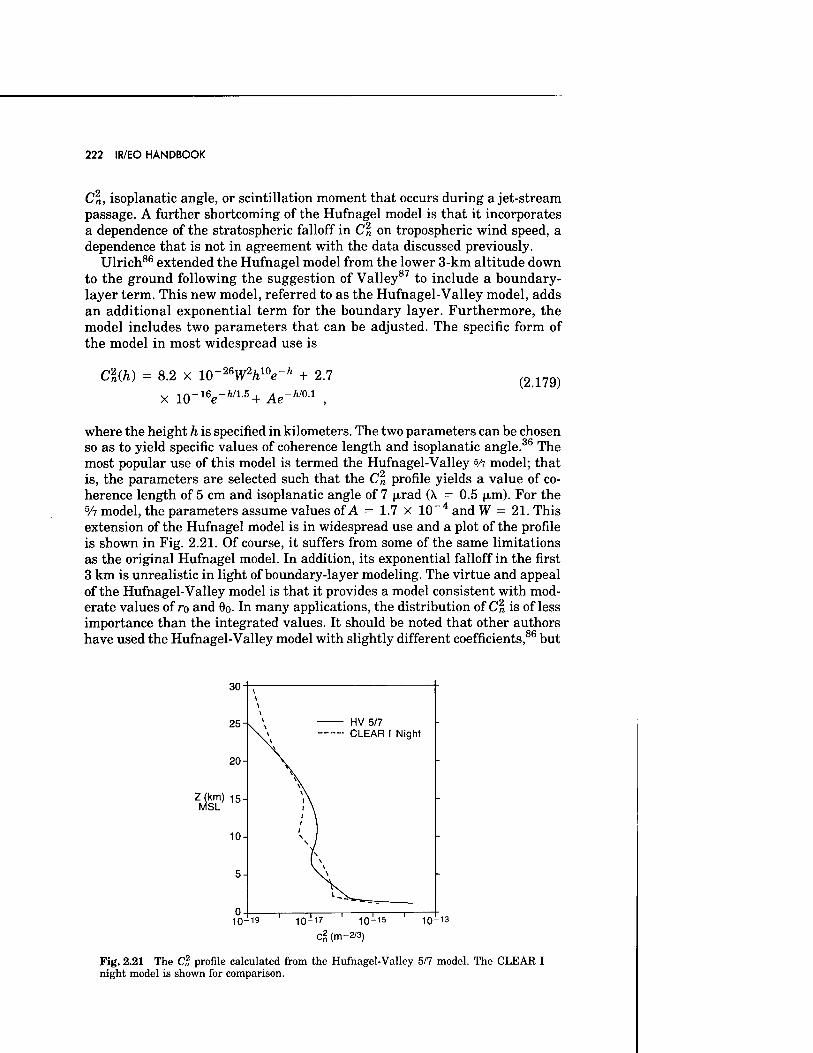
222 IR/EO HANDBOOK
Cn, isoplanatic angle, or scintillation moment that occurs during a jet-stream passage. A further shortcoming of the Hufnagel model is that it incorporates a dependence of the stratospheric falloff in C\ on tropospheric wind speed, a dependence that is not in agreement with the data discussed previously.
Ulrich86 extended the Hufnagel model from the lower 3-km altitude down to the ground following the suggestion of Valley87 to include a boundary- layer term. This new model, referred to as the Hufnagel-Valley model, adds an additional exponential term for the boundary layer. Furthermore, the model includes two parameters that can be adjusted. The specific form of the model in most widespread use is
Clih) = 8.2 x KT^W^V1 + 2.7
x 10-16e-
ft/15+ Ae-h'01 , (2.179)
where the height h is specified in kilometers. The two parameters can be chosen so as to yield specific values of coherence length and isoplanatic angle.36 The most popular use of this model is termed the Hufnagel-Valley 5/7 model; that is, the parameters are selected such that the Cn profile yields a value of co- herence length of 5 cm and isoplanatic angle of 7 |xrad (\ = 0.5 (xm). For the 5/7 model, the parameters assume values of A = 1.7 x 10~4 and W = 21. This extension of the Hufnagel model is in widespread use and a plot of the profile is shown in Fig. 2.21. Of course, it suffers from some of the same limitations as the original Hufnagel model. In addition, its exponential falloff in the first 3 km is unrealistic in light of boundary-layer modeling. The virtue and appeal of the Hufnagel-Valley model is that it provides a model consistent with mod- erate values of ro and 6o- In many applications, the distribution of Cn is of less importance than the integrated values. It should be noted that other authors have used the Hufnagel-Valley model with slightly different coefficients,86 but
30'
^ 15
o. 10
HV5/7 CLEAR I Night
10-17 10-15
C2(m-2/3)
10-13
Fig. 2.21 The Cl profile calculated from the Hufnagel-Valley 5/7 model. The CLEAR I night model is shown for comparison.
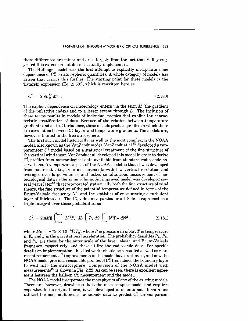
PROPAGATION THROUGH ATMOSPHERIC OPTICAL TURBULENCE 223
these differences are minor and arise largely from the fact that Valley sug- gested this extension but did not actually implement it.
The Hufnagel model was the first attempt to explicitly incorporate some dependence of C\ on atmospheric quantities. A whole category of models has arisen that carries this further. The starting point for these models is the Tatarski expression [Eq. (2.60)], which is rewritten here as
Cl = 2.8L40/3M2 . (2.180)
The explicit dependence on meteorology enters via the term M (the gradient of the refractive index) and to a lesser extent through Lo. The inclusion of these terms results in models of individual profiles that exhibit the charac- teristic stratification of data. Because of the relation between temperature gradients and optical turbulence, these models produce profiles in which there is a correlation between C2
n layers and temperature gradients. The models are, however, limited to the free atmosphere.
The first such model historically, as well as the most complex, is the NOAA model, also known as the VanZandt model. VanZandt et al.59 developed a two- parameter Cn model based on a statistical treatment of the fine structure of the vertical wind shear. VanZandt et al. developed this model in order to derive Cn profiles from meteorological data available from standard radiosonde ob- servations. An important aspect of the NOAA model is that it was developed from radar data, i.e., from measurements with low vertical resolution and averaged over large volumes, and lacked simultaneous measurement of me- teorological data in the same volume. An improved model was developed sev- eral years later88 that incorporated statistically both the fine structure of wind shears, the fine structure of the potential temperature defined in terms of the Brunt-Vaisala frequency N2, and the statistics of encountering a turbulent layer of thickness L. The C« value at a particular altitude is expressed as a triple integral over these probabilities as
fLmax f00 fx
Cl = 2.8Mg L4/3PL dL PsdS N4PN dN* , (2.181)
where Mo = - 79 x 10 ~~ eP/Tg, where P is pressure in mbar, T is temperature in K, and g is the gravitational acceleration. The probability densities PL, PS, and PN are those for the outer scale of the layer, shear, and Brunt-Vaisala frequency, respectively, and these utilize the radiosonde data. For specific details on implementation, the cited works should be consulted as well as more recent refinements.89 Improvements in the model have continued, and now the NOAA model provides reasonable profiles of C« from above the boundary layer to well into the stratosphere. Comparison of the NOAA model with measurements90 is shown in Fig. 2.22. As can be seen, there is excellent agree- ment between the balloon Cn measurement and the model.
The NOAA model incorporates the most physics of any of the existing models. There are, however, drawbacks. It is the most complex model and requires expertise. In its original form, it was developed in mountainous terrain and utilized the nonsimultaneous radiosonde data to predict Cn for comparison
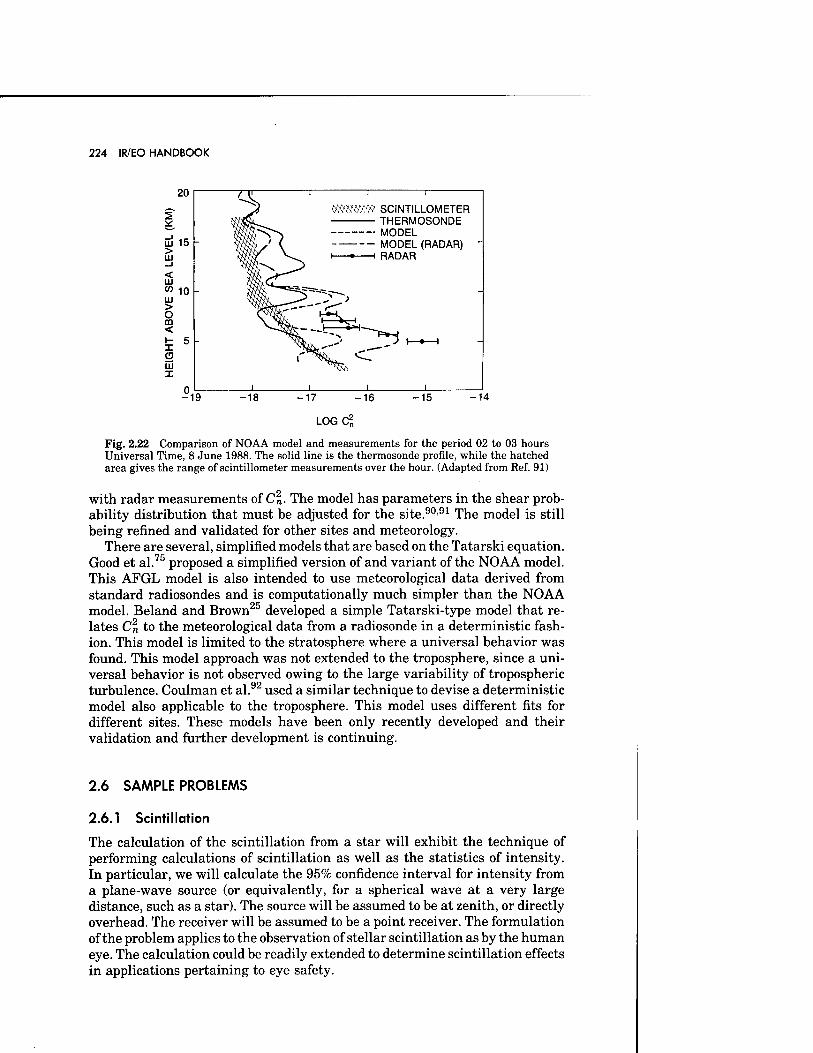
224 IR/EO HANDBOOK
20
2
Lu 15 - > LU I < LU
» 10 LU > o m < fe 5
g LU I
mW&ft SCINTILLOMETER THERMOSONDE MODEL MODEL (RADAR) i • 1 RADAR
^1— I—•—I
-°19 -18 -17 -16 -15 -14
LOGC^
Fig. 2.22 Comparison of NOAA model and measurements for the period 02 to 03 hours Universal Time, 8 June 1988. The solid line is the thermosonde profile, while the hatched area gives the range of scintillometer measurements over the hour. (Adapted from Ref. 91)
with radar measurements of C2. The model has parameters in the shear prob- ability distribution that must be adjusted for the site.90,91 The model is still being refined and validated for other sites and meteorology.
There are several, simplified models that are based on the Tatarski equation. Good et al.75 proposed a simplified version of and variant of the NOAA model. This AFGL model is also intended to use meteorological data derived from standard radiosondes and is computationally much simpler than the NOAA model. Beland and Brown25 developed a simple Tatarski-type model that re- lates C2 to the meteorological data from a radiosonde in a deterministic fash- ion. This model is limited to the stratosphere where a universal behavior was found. This model approach was not extended to the troposphere, since a uni- versal behavior is not observed owing to the large variability of tropospheric turbulence. Coulman et al.92 used a similar technique to devise a deterministic model also applicable to the troposphere. This model uses different fits for different sites. These models have been only recently developed and their validation and further development is continuing.
2.6 SAMPLE PROBLEMS
2.6.1 Scintillation
The calculation of the scintillation from a star will exhibit the technique of performing calculations of scintillation as well as the statistics of intensity. In particular, we will calculate the 95% confidence interval for intensity from a plane-wave source (or equivalently, for a spherical wave at a very large distance, such as a star). The source will be assumed to be at zenith, or directly overhead. The receiver will be assumed to be a point receiver. The formulation of the problem applies to the observation of stellar scintillation as by the human eye. The calculation could be readily extended to determine scintillation effects in applications pertaining to eye safety.
PROPAGATION THROUGH ATMOSPHERIC OPTICAL TURBULENCE 225
Equation (2.128) could be used directly to calculate the log-amplitude var- iance. This assumes that the source is located at r\ = 0 and the receiver at T) = L. However, it is more useful to translate from the path variable T\ to altitude z. The source is then at z = L and the receiver at z = 0 and Eq. (2.128) becomes
rL o-f = 0.56&7/6 J Cl(z)zS/6 dz . (2.182)
The calculation will be performed for a wavelength of 0.5 jjum. The C2n profile
will be provided by the Hufnagel-Valley 5A model [Eq. (2.179)]. The use of the Hufhagel-Valley ¥i model allows the variance to be evaluated analytically. The result is crx = 0.059. This value shows that we are well within the limits of the Rytov theory, which is generally the case for vertical propagation.
Statements about the range of variation in intensity can be immediately made. Since the fluctuations are weak, we have from Eq. (2.109) that the normalized intensity variance is
o-? = ((/ - </»2>/<J>2 - 4a2 = 0.236 . (2.183)
Thus, an estimate of the fluctuations in normalized intensity can be given by 07. This gives a value of approximately 0.5, that is, 50% fluctuations. This value is typical of stellar scintillation and quantifies the familiar observations of twinkling.
The estimate of the fluctuations must take into account the relevant sta- tistical distributions to be precise. From the Rytov theory, it has been estab- lished that log amplitude satisfies a normal distribution. Therefore, it follows that 95% of the fluctuations in x will fall in the range of ± 2a about the mean (x)- Specifically, the confidence interval is
«X> - 2ax, <x> + 2ax) . (2.184)
Since the intensity is given by I = exp(2x), this immediately yields the 95% confidence interval for intensity:
[exp(2<x> - 4ax), exp(2(X) + 4ax)] . (2.185)
Note that the normality of x and the resulting log normality of I produces a confidence interval for intensity that is determined by multiplication and di- vision by the factor exp(4crx). The intensity confidence interval is also written in terms of the median intensity Im, and not the mean (where Im = exp(2(x)). This can be translated into the mean intensity by using Eq. (2.108), which can be written as
(/) = Im exp(2a2) . (2.186)
Since conservation of energy requires that (/) = 1, the confidence interval for normalized intensity is given by
226 IR/EO HANDBOOK
[exp( - 2a2) exp( - 4CTX), exp( - 2a2.) exp( + 4ax)] . (2.187)
Substitution yields the values of [0.34,2.35]. Especially noteworthy is the upper limit, where even in this weak scintillation case, the normalized intensity fluctuates by more than a factor of 2. If we had instead used the less precise Rytov approximation of (x) = 0, the interval would have been calculated as [0.38, 2.64], which is a small correction.
An alternative approach to this problem is to formulate it in terms of the probability distribution of the intensity. Our approach followed the easier route, since normal distributions have statistically desirable properties. None- theless, in some problems the intensity distribution itself must be resorted to. For a unit intensity source and requiring that (7) = 1 (and consequently (x) = - a2), it can be shown30 that the probability distribution of the intensity is given by
P/(7) = [27ax(2Tr)1/2]_1exp{-[ln(7) + 2a2]2/(8a2.)} . (2.188)
This can be written in terms of only intensity variables without reference to log amplitude. Equation (2.110) can be solved to give
o-2 = (1/4) ln(o? + 1) . (2.189)
Substitution into Eq. (2.188) gives the form of the distribution
PAD = {[2T7 ln(a2 + l)]K1/2(l/7)
X exp{-[ln(7) + (V2) ln(af + l)]2/[2 ln(a2 + 1)]} . (2.190)
Since the normalized intensity and its variance are the directly measurable quantities, this form is useful in some applications.
2.6.2 Image Resolution
As an example of turbulence in imaging problems, the long-exposure resolution of an imaging system will be calculated. The specifications of the system are similar to those of a small telescope: aperture diameter D of 8 in. and focal length /"of 2.032 m. The object to be imaged will be assumed to be at a distance L of 300 m. The light of interest will be assumed to be monochromatic and of wavelength \ = 0.5 \um.
For comparison to the turbulence-induced limitation in resolution, the res- olution limit due to diffraction can be readily estimated from
Rd « XL/7) « 0.74 mm . (2.191)
This spatial resolution is readily given in terms of a range-independent angular resolution K/D, which yields 2.5 (xrad.
From Eq. (2.139), the minimum resolvable scale size in the system's focal plane is given by
7^ = l/vc = 2.U/7/-0 . (2.192)
PROPAGATION THROUGH ATMOSPHERIC OPTICAL TURBULENCE 227
For line-of-sight propagation a few meters above the ground, Fig. 2.7 shows that a Cn value of 1.0 x 10 ~13 is a reasonable approximation. The turbulence will be assumed to be homogeneous along the horizontal path. This assumption is not critical, since the coherence length has no path weighting and is deter- mined by the integrated C\ along the path. The illumination from the object will be assumed to be a plane wave. From Eq. (2.137), the coherence diameter for homogeneous turbulence is
r0 = 2.1(1.46k2C2nL)-3/5 = 1.04 cm . (2.193)
Comparison of this value to data in Table 2.2 or Fig. 2.18 shows that this 300-m horizontal path has smaller ro and hence more integrated turbulence than a ground-to-space path. Substitution of this value into Eq. (2.192) yields
Rf = 2.05 x 10⁻⁴m . (2.194)
This is the minimum resolvable scale in the focal plane. The resolution is sought in the object plane for comparison to the diffraction limit. These two are simply related by the magnification of the system, so that
Rt = RfLlf= 3.0 cm . (2.195)
Dividing by L, this spatial resolution can be stated as an angular resolution and yields the value of 101 |xrad. This limit is more than 40 times larger than the diffraction limit. Objects smaller than 3 cm will be blurred in long-exposure images. Since the object-plane resolution limit scales with path length as L /s, longer paths will produce significantly worse degradation.
In this calculation of the resolution degradation, the resolution has been calculated in both the focal and object planes. This same result could have been derived starting from the mutual coherence function formulation in the aperture plane and using Yura's transverse coherence length po. In particular, it is easy to show that our calculation of Rt in the object plane is equivalent to
Rt = XL/po . (2.196)
In this form, the resolution degradation in the object plane induced by tur- bulence is seen to be independent of aperture diameter D and focal length /. Greater magnification or a larger aperture will not alleviate the problem. The angular resolution, given by X/po, is range dependent owing to the dependence ofpo.
2.6.3 Beam Wander and Broadening
As an example of the calculation of the turbulence effects on a laser beam, the problem of the beam broadening and wander will be treated. The specific case is the propagation of a collimated beam from the ground to an object in space. This general problem has many applications. The object will be assumed to be at a distance of 200 km and at zenith. The laser beam will have a
228 IR/EO HANDBOOK
transmitter diameter of 1 m and will be assumed to have a Gaussian intensity profile at the aperture. The laser wavelength is assumed to be 0.5 p.m. The model for C2 will be that of the CLEAR I night model (Table 2.5).
The diffraction-limited beam radius will be calculated and compared to the case of propagation through turbulence. For the turbulence case, the long-term radius, short-term radius, and beam-wander radius will all be calculated. From Eq. (2.154), the long-term beam radius for a collimated beam is given by
<p£> = 4L2/(kD)2 + (D/2)2 + 4L2/(kp0)2 , (2.197)
where po is the transverse coherence length given by
ch po = W.m? sec(cp) ClWl - V£)% dr\V3/b . (2.198)
Jo
We can write this equation as
<p£) = p2d + 4L2/(kp0)2 , (2.199)
where
pd = [4L2/(kDf + (Z)/2)2]1/2 . (2.200)
Clearly, pd is the beam radius that results in the absence of turbulence (po —» oo), that is, the diffraction limit. Substitution of the numerical values of the parameters yields a value of p<* of 0.501 m. Thus, diffraction is negligible in this problem, as the diffraction broadens the beam by only 1 mm.
To calculate the turbulence effects, the value of the coherence length must be specified. It will be assumed that C2 is zero for altitudes greater than 30 km. This is a reasonable assumption, since as has been shown, there is evidence that C2 falls off with the square of density in the stratosphere and is therefore small compared to tropospheric turbulence. The weighting factor of (1 - T\IL)
in the integrand is negligible since r\ « L, where C2 is nonzero and the coherence length expression reduces to that of a plane wave [Eq. (2.134)]. The value of the coherence diameter po can be calculated from the CLEAR I model and yields a value of 2.76 cm at \ = 0.5 p,m. The mean-square beam radius for long exposure can then be calculated from Eq. (2.199) and gives a value of 1.58 m2. Of more importance is the rms radius, which is 1.257 m. Thus, tur- bulence more than doubles the beam radius.
This is the long-exposure value that would be seen at the target. Of more practical importance is the short-term broadening and the beam wander. Equa- tion (2.153) gives the relation between these as
<p£> = <P2) + <Pc) • (2.201)
Since po « D < Lo, the expressions for broadening and wander are given by Eqs. (2.156) and (2.157), which are written here as
(p2) = p2, + 4L2/(£po)2[l - 0.62(po/D)1/3f/5 , (2.202)
PROPAGATION THROUGH ATMOSPHERIC OPTICAL TURBULENCE 229
<p2> = 2.97L2/(k2p%3 D1/3) . (2.203)
Substitution results in the values of <p2) = 1.28 m2 and <p2} = 0.30 m2. In terms of the rms quantities, the rms short-term beam radius is 1.13 m and the rms wander is 0.55 m. Even in the short-time case, turbulence broadens the beam by more than a factor of 2 compared to the vacuum radius. The long- term beam radius comprises a broadened beam of rms radius 1.13 m that wanders about with an rms radius of 0.55 m. The beam wander is especially significant in applications where the object is smaller than or of the same order as the wander radius. In such cases, the turbulence will cause the laser illu- mination to wander on and off the object.
References
1. E. Parzen, Stochastic Processes, Holden-Day, San Francisco (1962). 2. G. E. P. Box and G. M. Jenkins, Time Series Analysis: Forecasting and Control, Holden-Day,
San Francisco (1976). 3. J. L. Doob, Stochastic Processes, Wiley, New York (1953). 4. R. B. Blackman and J. W. Tukey, The Measurement of Power Spectra, Dover, New York (1958). 5. A. S. Monin and A. M. Yaglom, Statistical Fluid Mechanics: Mechanics of Turbulence,
Vol. 1, MIT Press, Cambridge, MA (1971). 6. V. I. Tatarski, Wave Propagation in a Turbulent Medium, McGraw-Hill, New York (1961). 7. S. F. Clifford, "The classical theory of wave propagation in a turbulent medium," Chap. 2, in
Laser Beam Propagation in the Atmosphere, J. W. Strohbehn, Ed., Springer-Verlag, New York (1978).
8. A. S. Monin and A. M. Yaglom, Statistical Fluid Mechanics: Mechanics of Turbulence, Vol. 2, MIT Press, Cambridge, MA (1975).
9. L. F. Richardson, Weather Prediction by Numerical Process, Cambridge Univ. Press, Cam- bridge, U.K. (1922).
10. J. C. Kaimal, J. C. Wyngaard, D. A. Haugen, O. R. Cote, and Y. Izumi, "Turbulence structure in the convective boundary layer," J. Atmos. Sei. 33, 2152-2169 (1976).
11. F. H. Champagne, C. A. Friehe, J. C. Larue, and J. C. Wyngaard, "Flux measurements, flux estimation techniques and fine scale turbulence measurements in the unstable surface layer over land," J. Atmos. Sei. 34, 515-530 (1977).
12. H. Tennekes and J. L. Lumley, A First Course in Turbulence, MIT Press, Cambridge, MA (1972).
13. V. I. Tatarski, "The effects of the turbulent atmosphere on wave propagation," NOAA Report No. TT 68-50464, U.S. Dept. of Commerce, Springfield, VA (1971).
14. J. Barat, "Some characteristics of clear-air turbulence in the middle stratosphere," J. Atmos. Sei. 39, 2553-2564 (1982).
15. W. K. Hocking, "Measurement of turbulent energy dissipation rates in the middle atmosphere by radar techniques: A review," Radio Sei. 20, 1403-1422 (1985).
16. R. H. Kraichnan, "On Kolmogorov's inertial-range theories," J. Fluid Mech. 62, 305-330 (1974).
17. J. R. Holton, An Introduction to Dynamic Meteorology, Academic Press, New York (1972). 18. R. S. Lawrence and J. W. Strohbehn, "A survey of clear-air propagation effects relevant to
optical communications," Proc. IEEE 58, 1523-1545 (1970). 19. R. J. Hill and S. F. Clifford, "Modified spectrum of atmospheric temperature fluctuations and
its application to optical propagation," J. Opt. Soc. Am. 68, 892-899 (1978). 20. R. S. Lawrence, G. R. Ochs, and S. F. Clifford, "Measurements of atmospheric optical turbu-
lence relevant to optical propagation," J. Opt. Soc. Am. 60, 826-830 (1970). 21. J. C. Owens, "Optical refractive index of air: Dependence on pressure, temperature and com-
positions," Appl. Opt. 6, 51-59 (1967).
230 IR/EO HANDBOOK
22. J. C. Wyngaard and M. A. LeMone, "Behavior of the refractive index structure parameter in the entraining convective boundary layer," J. Atmos. Sei. 37, 1573-1585 (1980).
23. C. A. Friehe, J. C. La Rue, F. H. Champagne, C. H. Gibson, and G. F. Dreyer, "Effects of temperature and humidity fluctuations on the optical refractive index in the marine boundary layer," J. Opt. Soc. Am. 65, 1502-1511 (1975).
24. D. L. Walters and K. E. Kunkel, "Atmospheric modulation transfer function for desert and mountain locations: the atmospheric effects on ro," J. Opt. Soc. Am. 71, 397-405 (1981).
25. R. R. Beland and J. H. Brown, "A deterministic temperature model for stratospheric optical turbulence," Physica Scripta 37, 419-423 (1988).
26. V. A. Banakh and V. L. Mironov, Lidar in a Turbulent Atmosphere, Artech House, Boston (1987).
27. L. A. Chernov, Wave Propagation in a Random Medium, McGraw-Hill, New York (1960). 28. J. W. Strohbehn, Ed., Laser Beam Propagation in the Atmosphere, Springer-Verlag, New York
(1978). 29. A. Ishimaru, Wave Propagation and Scattering in Random Media, Vol. 2, Academic Press,
New York (1978). 30. J. W. Goodman, Statistical Optics, Wiley, New York (1985). 31. R. L. Fante, "Electromagnetic beam propagation in a turbulent media," Proc. IEEE 63,1669-1692
(1975). 32. R. L. Fante, "Electromagnetic beam propagation in a turbulent media: An update," Proc. IEEE
68, 1424-1443 (1980). 33. C. E. Coulman, "Fundamental and applied aspects of astronomical seeing," Ann. Rev. Astron.
Astrophys. 23, 19-57 (1985). 34. R. F. Lutomirski and H. T. Yura, "Wave structure function and mutual coherence function
of an optical wave in a turbulent atmosphere," J. Opt. Soc. Am. 61, 482-487 (1971). 35. J. W. Strohbehn, "Modern theories in the propagation of optical waves in a turbulent medium,"
in Laser Beam Propagation in the Atmosphere, J. W. Strohbehn, Ed., Springer-Verlag, New York (1978).
36. R. J. Sasiela, "A unified approach to electromagnetic wave propagation in turbulence and the evaluation of multiparameter integrals," Technical Report No. 807, MIT/Lincoln Laboratory (1988).
37. T. Wang, G. R. Ochs, and S. F. Clifford, "A saturation-resistant optical scintillometer to mea- sure Cl" J. Opt. Soc. Am. 68, 334-338 (1978).
38. G. R. Ochs, D. S. Reynolds, and R. L. Zurawski, "Folded-Path Optical C„ Instrument," NOAA Technical Memorandum ERL WPL-123, Boulder, CO (1985).
39. G. R. Ochs and T. Wang, "Finite aperture scintillometer for profiling wind and Cn" Appl. Opt. 17, 3774-3778 (1978).
40. S. F. Clifford, G. R. Ochs, and R. S. Lawrence, "Saturation of optical scintillations by strong turbulence," J. Opt. Soc. Am. 64, 148 (1974).
41. L. C. Andrews, R. L. Phillips, and B. K. Shivamoggi, "Relations of the parameters of the I-K distribution for irradiance fluctuations to physical parameters of the turbulence," Appl. Opt. 27, 2150-2156 (1988).
42. D. L. Fried, "Aperture averaging of scintillation," J. Opt. Soc. Am. 57, 169-175 (1967). 43. D. L. Fried, "Optical resolution through a randomly inhomogeneous medium," J. Opt. Soc.
Am. 56, 1372-1379 (1966). 44. R. F. Lutomirski, "Atmospheric degradation of electrooptical system performance," Appl. Opt.
17, 3915-3921 (1978). 45. R. E. Hufnagel, "Propagation through atmospheric turbulence," in The Infrared Handbook,
Chap. 6, USGPO, Washington, D.C. (1974). 46. D. Y. Gezari, A. Labeyrie, and R. V. Stachnik, "Speckle interferometry: Diffraction-limited
measurements of nine stars with the 200 inch telescope," Astrophys. J. 173, L1-L5 (1972). 47. A. Labeyrie, "Speckle interferometry observations at Mount Palomar," Nouvelle Revue
D'Optique 5, 141-151 (1974). 48. D. Korff, "Analysis of a method for obtaining near-diffraction-limited information in the
presence of atmospheric turbulence," J. Opt. Soc. Am. 63, 971-980 (1973). 49. K. T. Knox and B. J. Thompson, "Recovery of images from atmospherically degraded short-
exposure photographs," Astrophys. J. 193, L45-L48 (1973).
PROPAGATION THROUGH ATMOSPHERIC OPTICAL TURBULENCE 231
50. A. Ishimaru, "The beam wave case and remote sensing," in Laser Beam Propagation in the Atmosphere, J. W. Strohbehn, Ed., Springer-Verlag, New York (1978).
51. D. L. Fried, "Anisoplanatism in adaptive optics," J. Opt. Soc. Am. 72, 52-61 (1982). 52. G. A. Tyler, "Turbulence induced adaptive optics performance degradation: evaluation in the
time domain," in Laser Beam Propagation in the Atmosphere, Proc. SPIE 410,179-188 (1983). 53. J. H. Brown, R. E. Good, P. M. Bench, and G. Faucher, "Sonde measurements for comparative
measurements of optical turbulence," Air Force Geophysics Laboratory, AFGL-TR-82-0079, ADA118740, NTIS (1982).
54. E. Ryzner and J. A. Bartlo, "Dependence of C% (Cf.) in the atmospheric boundary layer on conventional meteorological parameters," Air Force Geophysics Laboratory, AFGL-TR-86-0013 (1986).
55. R. Lynds and J. W. Goad, "Observatory-site reconnaissance," Pub. of the Astron. Soc. of the Pacific 96, 750-766 (1984).
56. R. R. Beland, E. A. Murphy, G. G. Koenig, and P. C. Thomas, "Comparison of horizontal scintillation measurements and models," in Optical, Infrared, and Millimeter Wave Propa- gation Engineering, Proc. SPIE 926, 44-51 (1988).
57. E. E. Gossard, W. D. Neff, R. J. Zamora, and J. E. Gaynor, "The fine structure of elevated refractive layers: Implications for over-the-horizon propagation and radar sounding systems," Radio Sei. 19, 1523-1533 (1984).
58. S. H. Melfi and D. Whiteman, "Observation of lower atmospheric moisture structure and its evolution using a Raman lidar," Bull. Am. Meteor. Soc. 66, 1288-1292 (1985).
59. T. E. Van Zandt, J. L. Green, K. S. Gage, and W. L. Clark, "Vertical profiles of refractivity turbulence structure constant: Comparison of observations by the Sunset Radar with a new theoretical model," Radio Sei. 13, 819-829 (1978).
60. R. R. Beland and J. H. Brown, "Optical turbulence measurements in jet streams," Annual Review Conf. on Atmospheric Transmission Models, June 2-3, 1987, Hanscom AFB, MA (1987).
61. R. R. Beland, J. H. Brown, R. E. Good, and E. A. Murphy, "Optical turbulence characterization of AMOS, 1985," AFGL-TR-88-0153, Air Force Geophysics Laboratory (1988).
62. E. R. Reiter, Jet Stream Meteorology, Univ. of Chicago Press, Chicago (1963). 63. F. P. Battles, E. A. Murphy, and J. P. Noonan, "The contribution of atmospheric density to
the drop-off rate of Cl" Physica Scripta 37, 151-153 (1988). 64. J. H. Brown and R. R. Beland, "A site comparison of optical turbulence in the lower strato-
sphere at night using thermosonde data," Physica Scripta 37, 424-426 (1988). 65. A. N. Kolmogorov, "A refinement of previous hypotheses concerning the local structure of
turbulence in a viscous incompressible fluid at high Reynolds number," J. Fluid Mech. 13, 82-85 (1962).
66. E. L. Andreas, "Estimating averaging times for point and path-averaged measurements of turbulence spectra," J. Appl. Meteor. 27, 295-304 (1988).
67. M. G. Miller and P. L. Zieske, "Measurements of the atmospheric correlation scale," J. Opt. Soc. Am. 67, 1680-1685 (1977).
68. M. G. Miller and P. L. Zieske, "Turbulence environment characterization," RADC-79-131, ADA072379, Rome Air Development Center (1979).
69. D. L. Walters, "Atmospheric modulation transfer function for desert and mountain locations: r0 measurements," J. Opt. Soc. Am. 71, 406-409 (1981).
70. F. D. Eaton, D. M. Garvey, E. Dewan, and R. Beland, "Transverse coherence length (ro) observations," in Adaptive Optics, Proc. SPIE 551, 42-51 (1985).
71. F. D. Eaton, W. A. Peterson, J. R. Hines, and G. Fernandez, "Isoplanatic angle direct mea- surements and associated atmospheric conditions," Appl. Opt. 24, 3264-3273 (1985).
72. F. D. Eaton, W. A. Peterson, J. R. Hines, K. R. Peterman, R. E. Good, R. R. Beland, and J. H. Brown, "Comparisons of VHF radar, optical, and temperature fluctuation measurements of Cl, r0 and 60," Theor. Appl. Climatol. 39, 17-29 (1988).
73. J. H. Brown and R. E. Good, "Thermosonde Cn measurements in Hawaii—August 1982," AFGL-TR-84-0110, ADA148016, Air Force Geophysics Laboratory (1984).
74. J. H. Brown and R. E. Good, "Thermosonde and UHF radar measurements at Westford, Mas- sachusetts—July 1981," AFGL-TR-84-0109, ADA145398, Air Force Geophysics Laboratory (1984).
75. R. E. Good, R. R. Beland, E. A. Murphy, J. H. Brown, and E. M. Dewan, "Atmospheric models
232 IR/EO HANDBOOK
of optical turbulence," in Modeling of the Atmosphere, Proc. SPIE 928, 165-186 (1988). 76. J. C. Wyngaard, "On surface layer turbulence," in Workshop of Micrometeorology, Chap. 3,
pp. 101-149, American Meteorological Society, Boston (1973). 77. K. E. Kunkel and D. L. Walters, "Modeling the diurnal dependence of the optical refractive
index structure parameter," J. Geophys. Res. 88, 10,999-11,004 (1983). 78. G. C. Holzworth, "Estimates of the mean maximum mixing boundary layer," Atmos. Environ.
3, 519-536 (1969). 79. G. C. Holzworth, "Mixing depths, wind speeds and air pollution potential for selected locations
in the United States," J. Appl. Meteor. 6, 1039-1044 (1967). 80. C. L. Norton and G. B. Hoidale, "The diurnal variation of mixing height by season over White
Sands Missile Range, New Mexico," Monthly Weather Review, 104, 1317-1320 (1976). 81. V. P. Kukharets and L. R. Tsvang, "Structure parameter of the refractive index in the at-
mospheric boundary layer," Izv. Atmos. Oceanic Phys. 16, 73-77 (1980). 82. E. A. Murphy, E. M. Dewan, and S. M-. Sheldon, "Daytime comparison of C% models to mea-
surements in a desert location," in Adaptive Optics, Proc. SPIE 551, 156-162 (1985). 83. K. E. Kunkel, D. L. Walters, and G. A. Ely, "Behavior of the temperature structure parameter
in a desert basin," J. Appl. Meteor. 20, 130-136 (1981). 84. R. Hufnagel, "Restoration of atmospherically degraded images," Vol. 2 (Woods Hole Summer
Study, July 1966), National Academy of Sciences, 806879 (1966). 85. R. Hufnagel and N. R. Stanley, "Modulation transfer function associated with image trans-
mission through turbulent media," J. Opt. Soc. Am. 54, 52-61 (1964). 86. P. B. Ulrich, "Hufnagel-Valley profiles for specified values of the coherence length and iso-
planatic angle," MA-TN-88-013, W. J. Schäfer Associates (1988). 87. G. C. Valley, "Isoplanatic degradation of tilt correction and short-term imaging systems,"
Appl. Opt. 19, 574-577 (1980). 88. T. W. VanZandt, K. S. Gage, and J. M. Warnock, "An improved model for the calculation of
profiles of C„ and E in the free atmosphere from background profiles of wind, temperature and humidity," Proc. 20th Conf. on Radar Meteorology, Am. Meteor. Soc. (1981).
89. J. M. Warnock and T. E. VanZandt, "A statistical model to estimate the refractivity turbulence structure constant C„ in the free atmosphere," NOAA Tech. Memo. ERL AL-10, Boulder, CO (1985).
90. J. M. Warnock, R. R. Beland, J. H. Brown, W. L. Clark, F. D. Eaton, L. D. Favier, K. S. Gage, J. L. Green, W. H. Hatch, J. R. Hines, E. A. Murphy, G. D. Nastrom, W. A. Peterson, and T. E. VanZandt, "Comparison among clear air radar, thermosonde and optical measurements and model estimates of Cl made in very flat terrain over Illinois," MAP Handbook for Fourth MST Radar Workshop (1989).
91. J. L. Green, R. R Beland, J. H. Brown, W. L. Clark, F. D. Eaton, L. D. Favier, K. S. Gage, W. H. Hatch, J. R. Hines, E. A. Murphy, G. D. Nastrom, W. A. Peterson, T. E. VanZandt, and J. M. Warnock, "Comparisons of refractivity measurements from the flatlands VHF radar with other measurement techniques," 24th Conf. on Radar Meteorology, Tallahassee, FL, March 27-31, 1989.
92. C. E. Coulman, J. Vernin, Y. Coqueugnoit, and J. L. Caccia, "Outer scale of turbulence ap- propriate to modeling refractive-index profiles," Appl. Opt. 27, 155-160 (1988).
93. J. W. Strohbehn, "Line-of-sight wave propagation through the turbulent atmosphere," Proc. IEEE 56, 1301-1318 (1968).
94. D. L. Fried and J. B. Seidman, "Laser beam scintillation in the atmosphere," J. Opt. Soc. Am. 57, 181-185 (1967).
CHAPTER 3
Aerodynamic Effects
Keith G. Gilbert* BDM International, Inc.
Albuquerque, New Mexico
L John Often III Phillips Laboratory
Kirtland Air Force Base, New Mexico
William C. Rose Rose Engineering, Inc.
Incline Village, Nevada
CONTENTS
3.1 Introduction 235 3.2 Aerodynamic Considerations 237
3.2.1 Boundary Layers 241 3.2.2 Open Cavities and Shear Layers 243
3.3 Optical Considerations 246 3.3.1 Inviscid Flows 247 3.3.2 ShockWaves 249 3.3.3 Random Flows 253
3.4 Aero-Optical Design and Analysis Examples 264 3.4.1 Example 1—Subsonic Imaging Platform: Boundary-Layer
Aberrations 264 3.4.2 Example 2—Supersonic Imaging Platform: Boundary-Layer
Aberrations 268 3.4.3 Example 3—Optical Degradation Resulting from Open
Cavity 269 3.4.4 Example 4—Visible Imager: Selecting the Optimal
Wavelength 270 3.4.5 Example 5—Aperture Optimization 271 3.4.6 Example 6—Thermal Noise Resulting from an IR Window 272 3.4.7 Example 7—Supersonic Vehicle Optical Aberrations 274
*Presently with Logicon RDA, Albuquerque, New Mexico.
233
234 IR/EO HANDBOOK
3.4.8 Example 8—Supersonic Vehicle Flow-Field-Induced Thermal-Radiation Effects 277
3.5 Aero-Optics: Visions and Opportunities 278 References 284
AERODYNAMIC EFFECTS 235
3.1 INTRODUCTION
This chapter discusses the aberrating influences of aerodynamics on optical systems. While the focus is on airborne platforms, the discussions are relevant to all manner of moving transmitting media. Two classes of optical systems will be discussed, those that gather optical information and those that emit photons (optical energy). The physics of interaction with an airflow is the same (for a particular wavelength) whether the beam is incoming or outgoing, co- herent or incoherent (in the absence of nonlinear effects). However, the impact of the resulting degradation depends markedly on the application.
Two central issues influence the overall performance of optical systems located in aerodynamic environments. The first is aeromechanical effects. These arise from interactions of the external flow field with the airborne platform. This base motion, in concert with intrinsic platform sources of vibration (e.g., engines, pumps, fluid flow, etc.), defines the overall mechanical jitter environ- ment in which the optical system must operate. Jitter can result in spurious laser beam motion on target and image blurring as well as general misalign- ments of optical elements. The second major issue influencing airborne optical systems is aero-optical (AO) effects. These are caused by index-of-refraction variations induced by the platform moving through the flow field. This results in reduced far-field peak intensity as well as beam spread and wander for outgoing wave fronts. For imaging systems, these several effects manifest themselves as loss of contrast and resolution. In designing an airborne optical system one seeks first to mitigate mechanical effects, and then addresses aero- optical phenomena.
Optical aberrations resulting from aerodynamic flow fields can be placed in two categories: First, viscous flow phenomena include laminar and turbulent boundary layers, shear layers, and wake turbulence. The second category, inviscid or potential flow, arises from the acceleration of (compressible) fluid, generally along fuselage contours or around protuberances.
For wavelengths ranging from the visible to the mid-IR, flush-mounted material windows generally can be employed to shield the optical components from the external aerodynamic flow field. An exception may occur if a high- power laser is to be transmitted through the window; in this case, thermal- induced distortions or potential damage may preclude its use. If such instal- lations are feasible, then the aeromechanical issue is only associated with the aircraft motion. The resulting aero-optical performance is driven by the aero- dynamic flow field that exists over the external portion of the aircraft and window itself. These aerodynamic flow fields, if laminar, tend to be relatively benign and are influenced by the mean flow fields that exist over the aero- dynamic contours. However, if the surface boundary layer over the window is turbulent, as is more likely in operational settings, the resulting unsteady air density variations (resulting in unsteady index-of-refraction fields) can yield significant optical aberrations. These platform-induced aero-optical effects are discussed in this chapter.
For long-wavelength IR transmission and reception (\ 5= 10 Jim), a material window becomes much less attractive owing to optical transmission losses and window radiative effects. For such applications, cavities that are open to the surrounding aerodynamic flow field may be used. These cavities may take on
236 IR/EO HANDBOOK
various configurations; however, all are basically openings in the nominal mold line of the aircraft surrounded by bulkheads, floors, or other walls creating the cavity. The aeromechanical environment of such a cavity flow field is potentially debilitating. In addition, the AO flow field can cause a whole range of optical aberrations. The net result is degraded system performance. These aberrations can be severe enough to stifle the mission of interest; effective control of these aberrations is a prerequisite to any optical application.
Our approach offers classes of solutions via three steps:
1. What are the requirements? An optical instrument on an airborne platform either collects or projects optical information. As mentioned earlier, the physics of interaction with an airflow is generally the same (for a particular wavelength) whether the beam is incoming or out- going, coherent or incoherent. However, the impact of the degradation depends markedly on the application.
In general, the objective for an outgoing laser wave front is to max- imize peak irradiance at the target. This is often referred to as "power in the bucket." Applications include lidar, optical meteorology, and weaponry. The net effect of the AO field in all cases is a reduction of intensity at the target.
An incoming wave front is also scattered, absorbed, refracted, and reflected by the AO interface. If the optical system is an imager, an important parameter is the pixel field of view (FOV). In general, rays will be deflected from the intended (unaberrated) focus to adjacent areas on the array. The result is an image that suffers both resolution and contrast losses.
2. Once the requirements are defined, scaling relations will be developed that allow the planner to size and prioritize these several optical aberrations.
3. Finally, we offer several options for ameliorating these AO aberra- tions. These options include changing optics beam diameter or wave- length, tailoring the flow field, introducing advanced beam control techniques, or postexperiment processing. Sometimes several ap- proaches must be combined.
Random flow fields include turbulent boundary layers and shear layers, the latter being developed at a flow discontinuity (e.g., fuselage protuberance or recession). The optical aberrations impressed on a beam transiting these ran- dom flows are determined by three aerodynamic parameters: the field's fluc- tuating density p', the correlation length along the optical axis (z, and the total path length through the disturbance L. The prediced wave-front variance o-2 is given by1
-2 - <^-2f <p' Jo
o-2 = 2G2 < p'2 ) €2 dz, €z « L , (3.1)
with G being the Gladstone-Dale parameter,2 relating medium index of re- fraction to density fluctuations. Note that the above equation assumes isotropic turbulence. If the condition iz « L is not fulfilled, for example, generally in
AERODYNAMIC EFFECTS 237
the case of shear layers,1,3 then the above expression overestimates the actual optical aberrations.
Table 3.1 depicts broad AO characteristics of the several germane flow fields. The examples that follow deal with several important elements of this table. Wind tunnels are valuable simulation tools for some facets of an airborne- platform optical system. For example, high-fidelity aeromechanical simula- tions of turrets and open ports have been accomplished. Less success has been achieved simulating platform-induced optical turbulence effects. This is be- cause wind tunnels tend to have considerable intrinsic turbulence, caused by the flow-generation system, as well as wall boundary layers. This background "noise" can mask model-induced flow fields. Reference 4 details a variety of wind-tunnel experiments. Recently, tunnels have been developed to be "opti- cally quiet." In general, however, tunnels as a simulator of airborne-platform optical turbulence must be approached with considerable caution. In many cases, actual flight testing is more cost-effective.
A variety of AO instrumentation has been developed for both wind-tunnel and airborne-platform testing. Rugged thin-film sensors have been fielded that yield the above three primary aerodynamic parameters of interest. Bandwidths of order 10 to 50 kHz are achievable; however, signal to noise is frequently the dominant design dimension. Standard techniques such as interferometry or holography have been used to infer the integrated-path wave-front variance o-2. Careful AO experiments have shown good correlations between the aero- dynamic predictions of cr2 and the actual optical measurements.1
Section 3.2 discusses the range of aerodynamic phenomena that can affect airborne optical systems. Section 3.3 highlights the optical physics of inter- action with these flow fields, including germane scaling relationships. Section 3.4 is a collection of examples that serve as guidelines to the AO analyst or experimentalist. The final section looks to the future; advanced AO beam- control techniques are emerging that may offer a path to near-pristine optical platforms for both outgoing and incoming wave-front systems.
Table 3.2 gives the symbols, nomenclature, and units used in this chapter.
3.2 AERODYNAMIC CONSIDERATIONS
This section discusses the nature of aerodynamic flows that one encounters in an aero-optical situation.
The motion of a simple (Newtonian) flow is characterized by two dimen- sionless parameters, the Reynolds number Re and the Mach number M, defined by
Re VW
v ' (3.2)
M =
where
V = fluid velocity W = size of flow pattern v = kinematic viscosity a = velocity of sound.
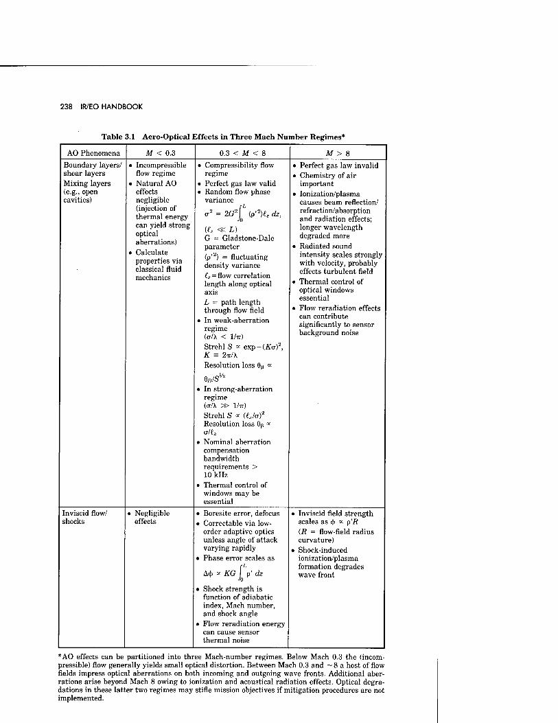
238 IR/EO HANDBOOK
Table 3.1 Aero-Optical Effects in Three Mach Number Regimes*
AO Phenomena M < 0.3 0.3 < M < 8 M > 8
Boundary layers/ • Incompressible • Compressibility flow • Perfect gas law invalid shear layers flow regime regime • Chemistry of air Mixing layers • Natural AO • Perfect gas law valid important (e.g., open effects • Random flow phase • Ionization/plasma cavities) negligible variance causes beam reflection/
(injection of o-2 = 2G2[ (p'2)ezdz, refraction/absorption
thermal energy and radiation effects; can yield strong optical aberrations)
(tz « L) G = Gladstone-Dale
longer wavelength degraded more
parameter • Radiated sound • Calculate
(p ) = fluctuating intensity scales strongly properties via
density variance with velocity, probably classical fluid mprbflnipQ 4 = flow correlation effects turbulent field lllt^Vlldlllt'O
length along optical • Thermal control of
axis optical windows
L = path length essential
through flow field • Flow reradiation effects
• In weak-aberration can contribute significantly to sensor
regime (o7X < 1/ir)
background noise
StrehlS * exp-(#o-)2, K = 2-K/K
Resolution loss 6ß «
eB/s1/2
• In strong-aberration regime (CT/X » 1/ir) Strehl S * ((Jo)2
Resolution loss 8p <* <x/4
• Nominal aberration compensation bandwidth requirements > 10 kHz
• Thermal control of windows may be essential
Inviscid flow/ • Negligible • Boresite error, defocus • Inviscid field strength shocks effects • Correctable via low- scales as <(> « p'R
order adaptive optics (Ä = flow-field radius unless angle of attack curvature) varying rapidly • Shock-induced
• Phase error scales as ionization/plasma
A<|> <* KG I p' dz Jo
formation degrades wave front
• Shock strength is function of adiabatic index, Mach number, and shock angle
• Flow reradiation energy can cause sensor thermal noise
*AO effects can be partitioned into three Mach-number regimes. Below Mach 0.3 the (incom- pressible) flow generally yields small optical distortion. Between Mach 0.3 and ~8 a host of flow fields impress optical aberrations on both incoming and outgoing wave fronts. Additional aber- rations arise beyond Mach 8 owing to ionization and acoustical radiation effects. Optical degra- dations in these latter two regimes may stifle mission objectives if mitigation procedures are not implemented.
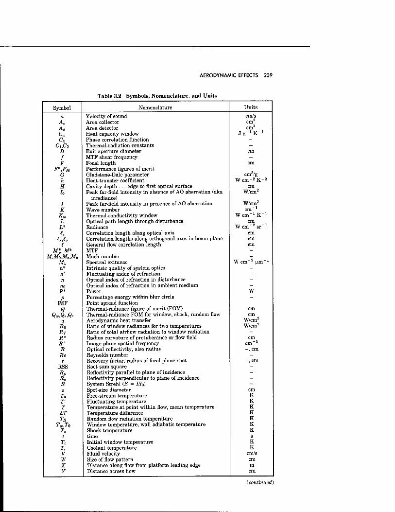
AERODYNAMIC EFFECTS 239
Table 3.2 Symbols, Nomenclature, and Units
Symbol Nomenclature Units
a Velocity of sound cm/s Ac Area collector cm2
Ad Area detector cm2
l^w Heat capacity window Jg^K"1
C<t> Phase correlation function - C\,Cz Thermal-radiation constants -
D Exit aperture diameter cm
f MTF shear frequency - F Focal length cm
F*,FM Performance figures of merit - G Gladstone-Dale parameter cm3/g h Heat-transfer coefficient Wcm-2K-2
H Cavity depth ... edge to first optical surface cm h Peak far-field intensity in absence of AO aberration (aka
irradiance) W/cm2
I Peak far-field intensity in presence of AO aberration W/cm2
K Wave number cm-1
Kw Thermal-conductivity window Wcm^K"1
L Optical path length through disturbance cm L* Radiance Wem"2 sr"1
tz Correlation length along optical axis cm txf^y Correlation lengths along orthogonal axes in beam plane cm
(. General flow correlation length cm M*,M* MTF -
MMoMaMb Mach number - Mx Spectral exitance W cm-2 ^m'1
re* Intrinsic quality of system optics - re' Fluctuating index of refraction - n Optical index of refraction in disturbance - reo Optical index of refraction in ambient medium - p* Power W
P Percentage energy within blur circle - PSF Point spread function
Q Thermal-radiance figure of merit (FOM) cm Qw,Qs,Qr Thermal-radiance FOM for window, shock, random flow cm
q Aerodynamic heat transfer W/cm2
Ä0 Ratio of window radiances for two temperatures W/cm2
RT Ratio of total airflow radiation to window radiation - R* Radius curvature of protuberance or flow field cm R + Image plane spatial frequency cm-1
R Optical reflectivity, also radius -, cm Re Reynolds number - r Recovery factor, radius of focal-plane spot -, cm
RSS Root sum square - Rp Reflectivity parallel to plane of incidence - Rs Reflectivity perpendicular to plane of incidence - S System Strehl (S = III0) - s Spot-size diameter cm
To Free-stream temperature K T Fluctuating temperature K T Temperature at point within flow, mean temperature K
AT Temperature difference K TR Random flow radiation temperature K
Tw,To Window temperature, wall adiabatic temperature K Ts Shock temperature K t time s
Ti Initial window temperature K Tc Coolant temperature K V Fluid velocity cm/s W Size of flow pattern cm X Distance along flow from platform leading edge m Y Distance across flow cm
(continued)
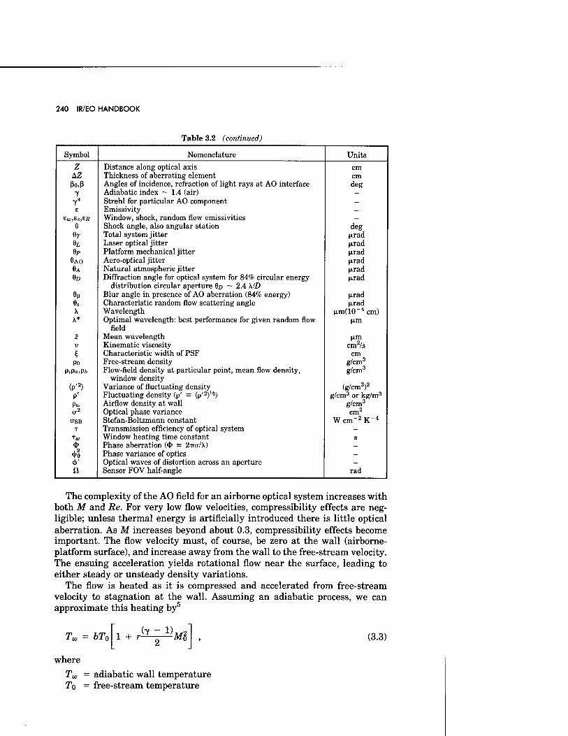
240 IR/EO HANDBOOK
Table 3.2 (continued)
Symbol Nomenclature Units
Z Distance along optical axis cm AZ Thickness of aberrating element cm ßo,ß Angles of incidence, refraction of light rays at AO interface deg
"Y Adiabatic index — 1.4 (air) - y* Strehl for particular AO component — £ Emissivity -
eu),Es,Eß Window, shock, random flow emissivities _ e Shock angle, also angular station deg 6r Total system jitter (jLrad 6L Laser optical jitter (j.rad 9P Platform mechanical jitter p.rad
6AO Aero-optical jitter M-rad QA Natural atmospheric jitter ixrad OB Diffraction angle for optical system for 84% circular energy
distribution circular aperture 6D ~ 2.4 X/D |U*ad
6ß Blur angle in presence of AO aberration (84% energy) (j.rad 8S Characteristic random flow scattering angle (jtrad \ Wavelength H.m(10~4 cm)
X* Optimal wavelength: best performance for given random flow field
|i.m
z Mean wavelength \x.m V Kinematic viscosity cm2/s « Characteristic width of PSF cm
P0 Free-stream density g/cm3
P,Pa,P6 Flow-field density at particular point, mean flow density, window density
g/cm3
<P'2> Variance of fluctuating density (g/cm3)2
P' Fluctuating density (p' = (p'2)1/S) g/cm3 or kg/m3
Pw Airflow density at wall g/cm3
a2 Optical phase variance cm2
CTSB Stefan-Boltzmann constant Wcm-2K-4
T Transmission efficiency of optical system - Tw Window heating time constant s 4> Phase aberration (<1> = 2TTCT/\) -
<t>0 Phase variance of optics - +' Optical waves of distortion across an aperture - a Sensor FOV half-angle rad
The complexity of the AO field for an airborne optical system increases with both M and Re. For very low flow velocities, compressibility effects are neg- ligible; unless thermal energy is artificially introduced there is little optical aberration. As M increases beyond about 0.3, compressibility effects become important. The flow velocity must, of course, be zero at the wall (airborne- platform surface), and increase away from the wall to the free-stream velocity. The ensuing acceleration yields rotational flow near the surface, leading to either steady or unsteady density variations.
The flow is heated as it is compressed and accelerated from free-stream velocity to stagnation at the wall. Assuming an adiabatic process, we can approximate this heating by5
Tw = bTo
where
1 + r^Ml (3.3)
Tw = adiabatic wall temperature To = free-stream temperature
AERODYNAMIC EFFECTS 241
Mo = free-stream Mach number r = recovery parameter (r = 0.85 laminar, 0.89 turbulent) ■y = adiabatic index, the ratio of the specific heat at constant
pressure to that at constant volume; for most AO conditions of interest, 7 — 1.4 (air)
b = a constant reflecting real gas effects; for Mach numbers below about 6, b =* 1.0; for M0 > 8, b - 0.5.
As Mo continues to increase, the fluid temperature and velocity changes induce increasing density changes. From Eq. (3.1) we note this yields even greater optical aberrations. Further increases to transonic flow lead to local supersonic- flow regimes in which shocks appear, causing additional reflection and re- fraction effects. In the supersonic regime (Mach 1 to 8) the high stagnation temperatures can cause thermo-optical window distortions. In some cases a window coolant is essential. Above Mach 8, dissociation and ionization result from the heating of the gas. These plasmas introduce another level of optical distortion, with particularly strong vibrational absorption bands. In this hy- personic regime, strong coupling between acoustical and turbulence fields oc- curs. Because the radiated acoustical power scales very strongly with M, it may even dominate above some critical Mach number. We next examine the several platform-induced aerodynamic flow fields of interest to airborne optical systems.
3.2.1 Boundary Layers
Boundary layer flows are described here as attached-wall viscous layers that naturally occur over aerodynamic surfaces due to the nonslip velocity condition at the wall. These boundary layers can be either laminar or turbulent.
Laminar Boundary Layers. Laminar boundary layers exhibit well-behaved, steady flow in which fluid particles in the boundary layer slide smoothly past one another. As a result of accelerating the gas from the flight velocity to zero at the surface of the aircraft, the mean temperature varies throughout the boundary layer. For most boundary-layer flows the static pressure remains constant throughout the layer, thus giving rise to a variation in density throughout the boundary layer. For laminar boundary layers, the density variation is smooth; these idealized flow fields usually cause little optical deg- radation. Exceptions exist if there is external heating or cooling of the flow; both situations can result in significant system optical aberrations.
Also, in the presence of accelerating flows (such as those occurring on plat- form external protuberances) inviscid lensing effects occur. These generally result in weak optical aberrations of low order (e.g., focus, tilt, astigmatism). Only limited subsonic experimental investigations of such effects have been described.4 Computational fluid dynamics is the best tool today for estimating the strength of these inviscid flow fields.
Turbulent Boundary Layers. Turbulent boundary layers differ from laminar boundary layers in that the orderly sliding of the fluid layers past one another exhibited in laminar flow breaks down and the process becomes chaotic, al- though the chaos is known to be statistically definite. Scaling relations have been developed for turbulent boundary-layer flow [e.g., Eq. (3.1)] that estimate
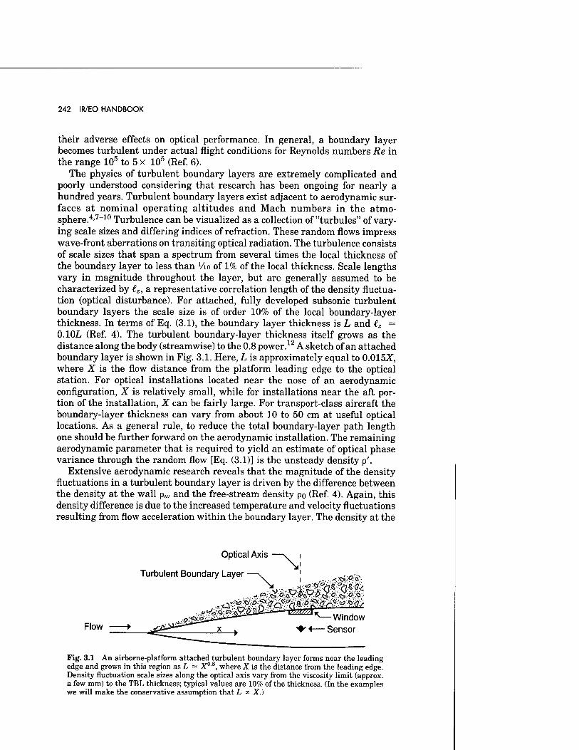
242 IR/EO HANDBOOK
their adverse effects on optical performance. In general, a boundary layer becomes turbulent under actual flight conditions for Reynolds numbers Re in the range 105 to 5 x 10⁵ (Ref. 6).
The physics of turbulent boundary layers are extremely complicated and poorly understood considering that research has been ongoing for nearly a hundred years. Turbulent boundary layers exist adjacent to aerodynamic sur- faces at nominal operating altitudes and Mach numbers in the atmo- sphere.4'7-10 Turbulence can be visualized as a collection of "turbules" of vary- ing scale sizes and differing indices of refraction. These random flows impress wave-front aberrations on transiting optical radiation. The turbulence consists of scale sizes that span a spectrum from several times the local thickness of the boundary layer to less than Vio of 1% of the local thickness. Scale lengths vary in magnitude throughout the layer, but are generally assumed to be characterized by tz, a representative correlation length of the density fluctua- tion (optical disturbance). For attached, fully developed subsonic turbulent boundary layers the scale size is of order 10% of the local boundary-layer thickness. In terms of Eq. (3.1), the boundary layer thickness is L and iz — 0.10L (Ref. 4). The turbulent boundary-layer thickness itself grows as the distance along the body (streamwise) to the 0.8 power.12 A sketch of an attached boundary layer is shown in Fig. 3.1. Here, L is approximately equal to 0.015Z, where X is the flow distance from the platform leading edge to the optical station. For optical installations located near the nose of an aerodynamic configuration, X is relatively small, while for installations near the aft por- tion of the installation, X can be fairly large. For transport-class aircraft the boundary-layer thickness can vary from about 10 to 50 cm at useful optical locations. As a general rule, to reduce the total boundary-layer path length one should be further forward on the aerodynamic installation. The remaining aerodynamic parameter that is required to yield an estimate of optical phase variance through the random flow [Eq. (3.1)] is the unsteady density p'.
Extensive aerodynamic research reveals that the magnitude of the density fluctuations in a turbulent boundary layer is driven by the difference between the density at the wall pw and the free-stream density po (Ref. 4). Again, this density difference is due to the increased temperature and velocity fluctuations resulting from flow acceleration within the boundary layer. The density at the
i i i i ....... <;s>°tf:
Optical Axis
Turbulent Boundary Layer —^
..o^güitfi"*-"*^ ^—Window Flow ► .-2£2^__x_k +><—Sensor
Fig. 3.1 An airborne-platform attached turbulent boundary layer forms near the leading edge and grows in this region as L ~ X08, where X is the distance from the leading edge. Density fluctuation scale sizes along the optical axis vary from the viscosity limit (approx. a few mm) to the TBL thickness; typical values are 10% of the thickness. (In the examples we will make the conservative assumption that L « X.)
AERODYNAMIC EFFECTS 243
wall in the regime of no shock waves and assuming zero pressure gradient across the boundary layer is
Pw = po l + r\^)M2o (3.4)
For purposes of making fluctuating density estimates, the density variation for a turbulent boundary layer may be assumed to occur in a fashion such that a peak density fluctuation occurs halfway through the turbulent boundary layer and has an average magnitude of about 10% of the difference between the wall and free-stream densities. This produces a triangular-like fluctuating density profile; generally, a weighted mean value is used to estimate the optical losses. Herein we adopt the conservative approach of selecting as this char- acteristic fluctuating density the peak value in the flow.
3.2.2 Open Cavities and Shear Layers
Shear layers develop when the wall beneath the boundary layer is removed, whether via an open cavity or a fuselage recession. Shear layers also can occur on the downstream side of a turret or cylindrical protuberance from an aircraft. Shear layers are inherently more optically degrading than attached boundary layers. Moreover, they can drive severe acoustical effects within open cavity geometries.
Material windows can serve two important functions on an optical airborne platform: First, they insulate the optical train from the relatively hostile ex- ternal aero-optical environment. Second, if the window is fuselage-flush mounted, it provides a more predictable flow over the optical aperture. However, windows can have considerable disadvantages, particularly for IR optical systems, in- cluding (1) poor transmission properties, particularly for wavelengths beyond 10 (Jim, (2) optical aberrations, either intrinsic or environmentally induced (e.g., pressure or thermally driven), and (3) strong thermal radiation (IR emis- sions) within the instrument bandpass.
An alternative to a material window is an open cavity, which interacts with external flow around the aircraft. The most profound aerodynamic phenomenon that exists over an open cavity at moderate and transonic flow speeds is known as cavity resonance. This is usually defined as the presence of ordered, single- frequency pressure variations within the confines of the cavity. If uncontrolled, these pressure fluctuations can cause unwanted vibrations of the optical com- ponents located within the cavity. Both this and the resulting cavity turbulence cause degradation of the overall optical performance. In addition, the structural implications of an uncontrolled cavity resonance are potentially harmful and must be avoided at all costs.
A sequence of events occurs in an uncontrolled cavity that produces reso- nance (Fig. 3.2). Flow is assumed to exist from left to right over a cross section of a cavity. In general, a shear layer forms at the leading edge of the cavity. This shear layer expands and interacts with the superimposed natural fuselage boundary layer as well as the cavity flow field. Wind-tunnel and airborne- platform experiments4'8 suggest the thickness L of a free shear layer is ap- proximately L = 0.25-X", with X being the distance downstream from the for-
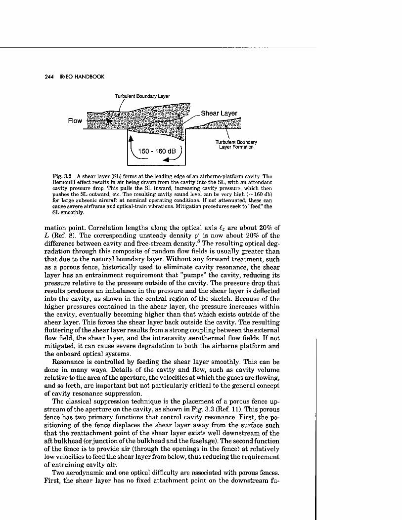
244 IR/EO HANDBOOK
Turbulent Boundary Layer
Flow n ii »i iiTfiß»!' L i' ft .
Shear Layer
Turbulent Boundary Layer Formation
Fig. 3.2 A shear layer (SL) forms at the leading edge of an airborne-platform cavity. The Bernoulli effect results in air being drawn from the cavity into the SL, with an attendant cavity pressure drop. This pulls the SL inward, increasing cavity pressure, which then pushes the SL outward, etc. The resulting cavity sound level can be very high (~ 160 db) for large subsonic aircraft at nominal operating conditions. If not attenuated, these can cause severe airframe and optical-train vibrations. Mitigation procedures seek to "feed" the SL smoothly.
mation point. Correlation lengths along the optical axis €z are about 20% of L (Ref. 8). The corresponding unsteady density p' is now about 20% of the difference between cavity and free-stream density.8 The resulting optical deg- radation through this composite of random flow fields is usually greater than that due to the natural boundary layer. Without any forward treatment, such as a porous fence, historically used to eliminate cavity resonance, the shear layer has an entrainment requirement that "pumps" the cavity, reducing its pressure relative to the pressure outside of the cavity. The pressure drop that results produces an imbalance in the pressure and the shear layer is deflected into the cavity, as shown in the central region of the sketch. Because of the higher pressures contained in the shear layer, the pressure increases within the cavity, eventually becoming higher than that which exists outside of the shear layer. This forces the shear layer back outside the cavity. The resulting fluttering of the shear layer results from a strong coupling between the external flow field, the shear layer, and the intracavity aerothermal flow fields. If not mitigated, it can cause severe degradation to both the airborne platform and the onboard optical systems.
Resonance is controlled by feeding the shear layer smoothly. This can be done in many ways. Details of the cavity and flow, such as cavity volume relative to the area of the aperture, the velocities at which the gases are flowing, and so forth, are important but not particularly critical to the general concept of cavity resonance suppression.
The classical suppression technique is the placement of a porous fence up- stream of the aperture on the cavity, as shown in Fig. 3.3 (Ref. 11). This porous fence has two primary functions that control cavity resonance. First, the po- sitioning of the fence displaces the shear layer away from the surface such that the reattachment point of the shear layer exists well downstream of the aft bulkhead (or junction of the bulkhead and the fuselage). The second function of the fence is to provide air (through the openings in the fence) at relatively low velocities to feed the shear layer from below, thus reducing the requirement of entraining cavity air.
Two aerodynamic and one optical difficulty are associated with porous fences. First, the shear layer has no fixed attachment point on the downstream fu-
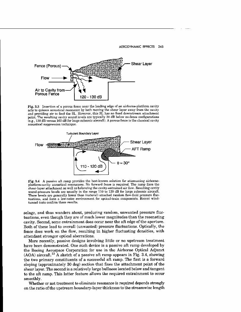
AERODYNAMIC EFFECTS 245
Fence (Porous)
Flow
Shear Layer
Air to Cavity from Porous Fence
Fig. 3.3 Insertion of a porous fence near the leading edge of an airborne-platform cavity acts to quiesce acoustical resonance by both moving the shear layer away from the cavity and providing air to feed the SL. However, this SL has no fixed downstream attachment point. The resulting cavity sound levels are typically 30 dB below no-fence configurations (e.g., 130 dB versus 160 dB for large subsonic aircraft). A porous fence is the classical cavity acoustical suppression technique.
Turbulent Boundary Layer
Flow !ffl"a«i'nfi Shear Layer
AFT Ramp
I 110 -120 dB J 9 = 30°
Fig. 3.4 A passive aft ramp provides the best-known solution for attenuating airborne- platform-cavity acoustical resonances. No forward fence is required. The ramp fixes the shear-layer attachment as well as balancing the cavity-entrained air flow. Resulting cavity sound-pressure levels are usually in the range 110 to 120 dB for large subsonic aircraft. These levels are generally lower than (natural) attached random flow-field pressure fluc- tuations, and form a low-noise environment for optical-train components. Recent wind- tunnel tests confirm these results.
selage, and thus wanders about, producing random, unwanted pressure fluc- tuations, even though they are of much lower magnitudes than the resonating cavity. Second, some entrainment does occur near the aft edge of the aperture. Both of these lead to overall (unwanted) pressure fluctuations. Optically, the fence does work on the flow, resulting in higher fluctuating densities, with attendant stronger optical aberrations.
More recently, passive designs involving little or no upstream treatment have been demonstrated. One such device is a passive aft ramp developed by the Boeing Aerospace Corporation for use in the Airborne Optical Adjunct (AOA) aircraft.13 A sketch of a passive aft ramp appears in Fig. 3.4, showing the two primary constituents of a successful aft ramp. The first is a forward sloping (approximately 30 deg) section that fixes the attachment point of the shear layer. The second is a relatively large bullnose located below and tangent to the aft ramp. This latter feature allows the required entrainment to occur smoothly.
Whether or not treatment to eliminate resonance is required depends strongly on the ratio of the upstream boundary-layer thickness to the streamwise length
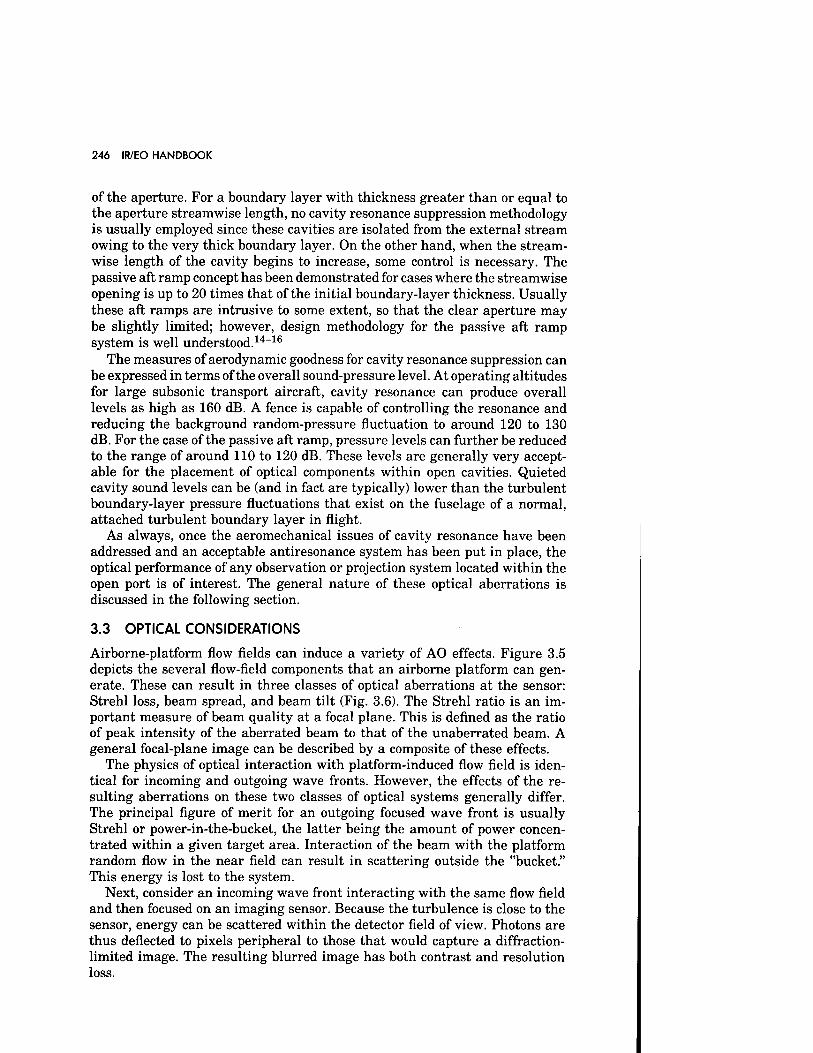
246 IR/EO HANDBOOK
of the aperture. For a boundary layer with thickness greater than or equal to the aperture streamwise length, no cavity resonance suppression methodology is usually employed since these cavities are isolated from the external stream owing to the very thick boundary layer. On the other hand, when the stream- wise length of the cavity begins to increase, some control is necessary. The passive aft ramp concept has been demonstrated for cases where the streamwise opening is up to 20 times that of the initial boundary-layer thickness. Usually these aft ramps are intrusive to some extent, so that the clear aperture may be slightly limited; however, design methodology for the passive aft ramp system is well understood.14-16
The measures of aerodynamic goodness for cavity resonance suppression can be expressed in terms of the overall sound-pressure level. At operating altitudes for large subsonic transport aircraft, cavity resonance can produce overall levels as high as 160 dB. A fence is capable of controlling the resonance and reducing the background random-pressure fluctuation to around 120 to 130 dB. For the case of the passive aft ramp, pressure levels can further be reduced to the range of around 110 to 120 dB. These levels are generally very accept- able for the placement of optical components within open cavities. Quieted cavity sound levels can be (and in fact are typically) lower than the turbulent boundary-layer pressure fluctuations that exist on the fuselage of a normal, attached turbulent boundary layer in flight.
As always, once the aeromechanical issues of cavity resonance have been addressed and an acceptable antiresonance system has been put in place, the optical performance of any observation or projection system located within the open port is of interest. The general nature of these optical aberrations is discussed in the following section.
3.3 OPTICAL CONSIDERATIONS
Airborne-platform flow fields can induce a variety of AO effects. Figure 3.5 depicts the several flow-field components that an airborne platform can gen- erate. These can result in three classes of optical aberrations at the sensor: Strehl loss, beam spread, and beam tilt (Fig. 3.6). The Strehl ratio is an im- portant measure of beam quality at a focal plane. This is defined as the ratio of peak intensity of the aberrated beam to that of the unaberrated beam. A general focal-plane image can be described by a composite of these effects.
The physics of optical interaction with platform-induced flow field is iden- tical for incoming and outgoing wave fronts. However, the effects of the re- sulting aberrations on these two classes of optical systems generally differ. The principal figure of merit for an outgoing focused wave front is usually Strehl or power-in-the-bucket, the latter being the amount of power concen- trated within a given target area. Interaction of the beam with the platform random flow in the near field can result in scattering outside the "bucket." This energy is lost to the system.
Next, consider an incoming wave front interacting with the same flow field and then focused on an imaging sensor. Because the turbulence is close to the sensor, energy can be scattered within the detector field of view. Photons are thus deflected to pixels peripheral to those that would capture a diffraction- limited image. The resulting blurred image has both contrast and resolution loss.
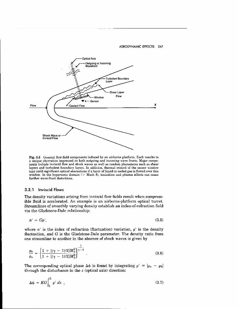
AERODYNAMIC EFFECTS 247
-Optical Axis
Shock Wave or Inviscid Flow
Fig. 3.5 General flow-field components induced by an airborne platform. Each results in a unique aberration impressed on both outgoing and incoming wave fronts. Major compo- nents include inviscid flow and shock waves as well as random phenomena such as shear layers and turbulent boundary layers. In addition, thermal control of the sensor window may yield significant optical aberrations if a layer of liquid or cooled gas is flowed over this window. In the hypersonic domain (> Mach 8), ionization and plasma effects can cause further wave-front distortions.
3.3.1 Inviscid Flows
The density variations arising from inviscid flow fields result when compress- ible fluid is accelerated. An example is an airborne-platform optical turret. Streamlines of smoothly varying density establish an index-of-refraction field via the Gladstone-Dale relationship:
n' = Gp', (3.5)
where n' is the index of refraction (fluctuation) variation, p' is the density fluctuation, and G is the Gladstone-Dale parameter. The density ratio from one streamline to another in the absence of shock waves is given by
p* = (1 + [(7 - D/2]Mgp Pa U + [(7 - D/2WI)
The corresponding optical phase Ac)) is found by integrating p' = |pa - p&| through the disturbance in the z (optical axis) direction:
Acj> = KG \ p' dz , (3.7) Jo
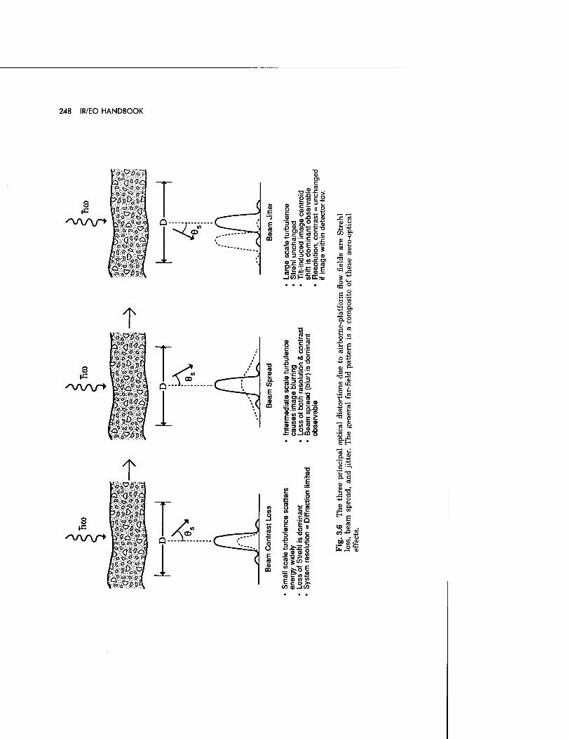
248 IR/EO HANDBOOK
3
^v\A/~> a = "9 -=-n a>
<n a)
Ptl 2 c E 2 t; «"-.£ »£13 c
„DDT! m "Ö (0 »
ra
U II O
a *
8|
Is sa O IS CO p
IT»
<p u I- m3
2 8 cd CD
m a
2 a a 8
m
3
'WV"*
T ^*<P«£S
■.*»;:<J.'0.-Q,.it > ö o<> of.
;&p0$3
t ■.»;:W;:0.;0'.<:
o CO 2 a.
CO
E « IB m
to 51
£ «I 3 «8 i ■S ™ =
sl| » <D 2 S EPS US ESO !s <" S2 a> 3 w
_2
i" CD jg
°-g to ffi
«8 ,8-° CO o
a c o
CO *t
!? ■o c C0.Q
us! Ä: ° § 2>cnS CD co to c o >• CÖ-1W
« E 9-8 E s.s
-£ e cd cu
o £ *» cd a o.
§1 eti
CO (- T3 c
1) cd M
• I-* CD
13 —>
a c
e-d- J3 cd 53 CD
L.
to g . . * o
•>" 8 fa
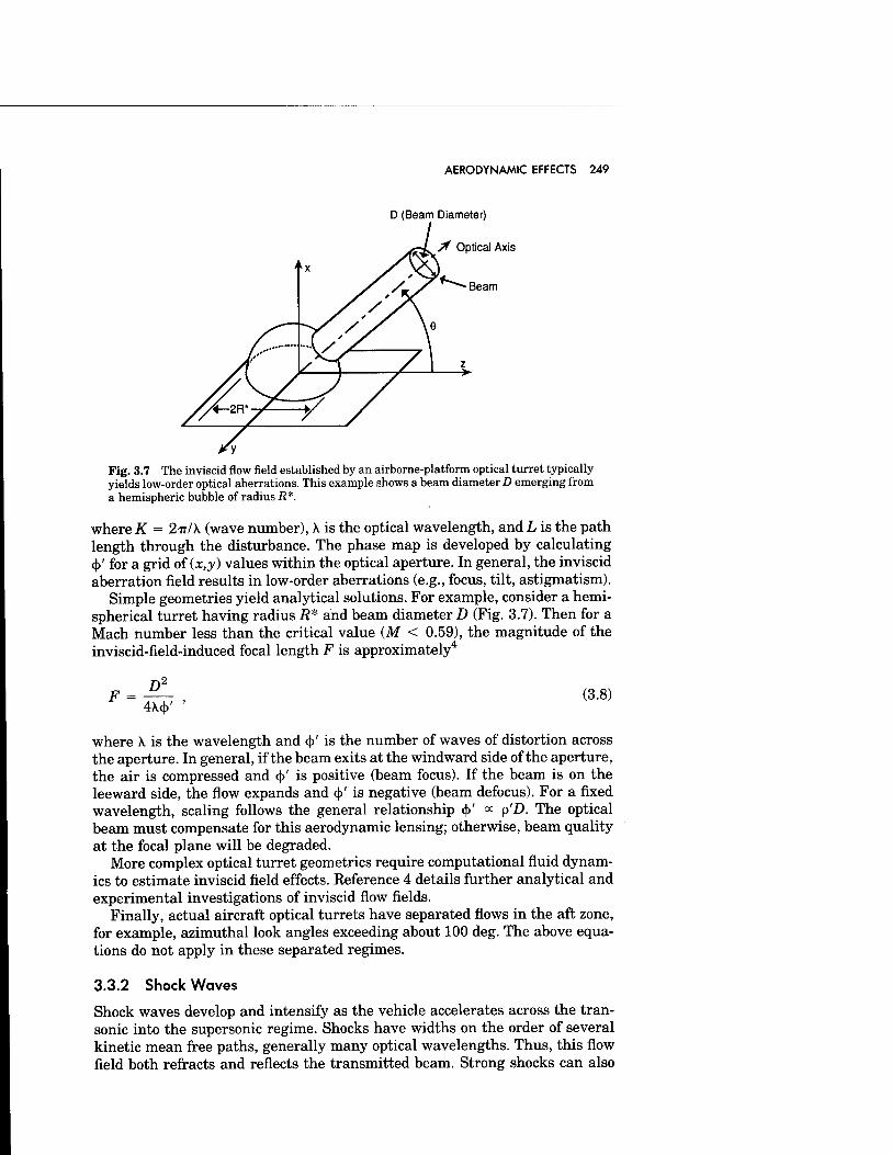
AERODYNAMIC EFFECTS 249
D (Beam Diameter)
tf Optical Axis
Beam
Fig. 3.7 The inviscid flow field established by an airborne-platform optical turret typically yields low-order optical aberrations. This example shows a beam diameter D emerging from a hemispheric bubble of radius R*.
where K = 2ir/\ (wave number), k is the optical wavelength, and L is the path length through the disturbance. The phase map is developed by calculating <J)' for a grid of (x,y) values within the optical aperture. In general, the inviscid aberration field results in low-order aberrations (e.g., focus, tilt, astigmatism).
Simple geometries yield analytical solutions. For example, consider a hemi- spherical turret having radius R* and beam diameter D (Fig. 3.7). Then for a Mach number less than the critical value (M < 0.59), the magnitude of the inviscid-field-induced focal length F is approximately4
F = D2
4\<(>' (3.8)
where A. is the wavelength and 4>' is the number of waves of distortion across the aperture. In general, if the beam exits at the windward side of the aperture, the air is compressed and ()>' is positive (beam focus). If the beam is on the leeward side, the flow expands and d>' is negative (beam defocus). For a fixed wavelength, scaling follows the general relationship 4>' « p'D. The optical beam must compensate for this aerodynamic lensing; otherwise, beam quality at the focal plane will be degraded.
More complex optical turret geometries require computational fluid dynam- ics to estimate inviscid field effects. Reference 4 details further analytical and experimental investigations of inviscid flow fields.
Finally, actual aircraft optical turrets have separated flows in the aft zone, for example, azimuthal look angles exceeding about 100 deg. The above equa- tions do not apply in these separated regimes.
3.3.2 Shock Waves
Shock waves develop and intensify as the vehicle accelerates across the tran- sonic into the supersonic regime. Shocks have widths on the order of several kinetic mean free paths, generally many optical wavelengths. Thus, this flow field both refracts and reflects the transmitted beam. Strong shocks can also
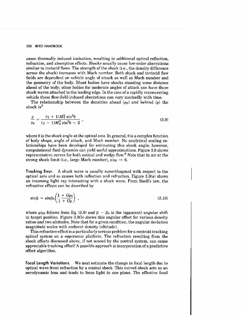
250 IR/EO HANDBOOK
cause thermally induced ionization, resulting in additional optical reflection, refraction, and absorption effects. Shocks usually cause low-order aberrations similar to inviscid flows. The strength of the shock (i.e., the density difference across the shock) increases with Mach number. Both shock and inviscid flow fields are dependent on vehicle angle of attack as well as Mach number and the geometry of the body. Blunt bodies have shocks standing some distance ahead of the body; other bodies for moderate angles of attack can have these shock waves attached to the leading edge. In the case of a rapidly maneuvering vehicle these flow-field-induced aberrations can vary markedly with time.
The relationship between the densities ahead (po) and behind (p) the shock is5
_p = (7 + DM2, sin2e Po (7 - l)Ml sin26 + 2 '
where 9 is the shock angle at the optical axis. In general, 8 is a complex function of body shape, angle of attack, and Mach number. No analytical scaling re- lationships have been developed for estimating this shock angle; however, computational fluid dynamics can yield useful approximations. Figure 3.8 shows representative curves for both conical and wedge flow.6 Note that in air at the strong shock limit (i.e., large Mach number), p/po —» 6.
Tracking Error. A shock wave is usually nonorthogonal with respect to the optical axis and so causes both reflection and refraction. Figure 3.9(a) shows an incoming light ray interacting with a shock wave. From Snell's law, the refractive effects can be described by
sinß = sinßoK^ ßPOj , (3.10)
where p/po follows from Eq. (3.9) and ß - ßo is the (apparent) angular shift in target position. Figure 3.9(b) shows this angular offset for various density ratios and two altitudes. Note that for a given condition, the angular deviation magnitude scales with ambient density (altitude).
This refractive effect is a particularly serious problem for a centroid tracking optical system on a supersonic platform. The refraction resulting from the shock effects discussed above, if not sensed by the control system, can cause appreciable tracking offset! A possible approach is incorporation of a predictive offset algorithm.
Focal Length Variations. We next estimate the change in focal length due to optical wave-front refraction by a conical shock. This curved shock acts as an aerodynamic lens and tends to focus light in one plane. The effective focal
AERODYNAMIC EFFECTS 251
CD T3
C < CD >
■ Ü o sz
10 20 30 40 50 60
Cone Semivertex Angle, % (deg)
Weak Shock Wave - Strong Shock Wave ■ l '
10 20 30 40
Deflection Angle, ev (deg)
(b)
50
Fig. 3.8 (a) Shock-wave angle for conical flow, (b) Shock-wave angle for wedge flow.
length F of this shock in the plane perpendicular to the airframe longitudinal axis is6
F _ Titane X n - no
(3.11)
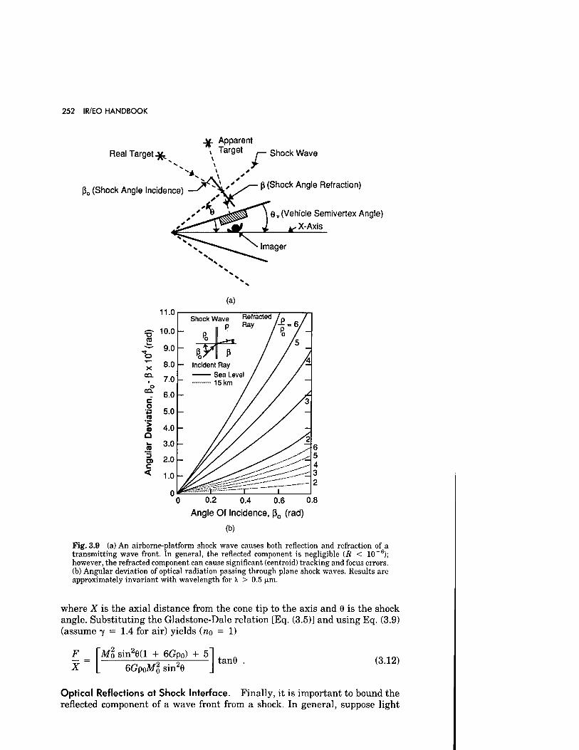
252 IR/EO HANDBOOK
Real Target ^
ß0 (Shock Angle Incidence)
jL Apparent x Target Shock Wave
ß (Shock Angle Refraction)
ev (Vehicle Semivertex Angle)
■o CO
t> x
CO.
CO.
c o a > Q
3 at c <
0.2 0.4 0.6 0.8
Angle Of Incidence, ß0 (rad)
(b)
Fig. 3.9 (a) An airborne-platform shock wave causes both reflection and refraction of a transmitting wave front. In general, the reflected component is negligible (R < 10~6); however, the refracted component can cause significant (centroid) tracking and focus errors, (b) Angular deviation of optical radiation passing through plane shock waves. Results are approximately invariant with wavelength for X > 0.5 |xm.
where X is the axial distance from the cone tip to the axis and 9 is the shock angle. Substituting the Gladstone-Dale relation [Eq. (3.5)] and using Eq. (3.9) (assume 7 = 1.4 for air) yields (no = 1)
F X
Mp sin26(l + 6GPo) + 5 6Gp0Ml sin2e
tan6 (3.12)
Optical Reflections at Shock Interface. Finally, it is important to bound the reflected component of a wave front from a shock. In general, suppose light
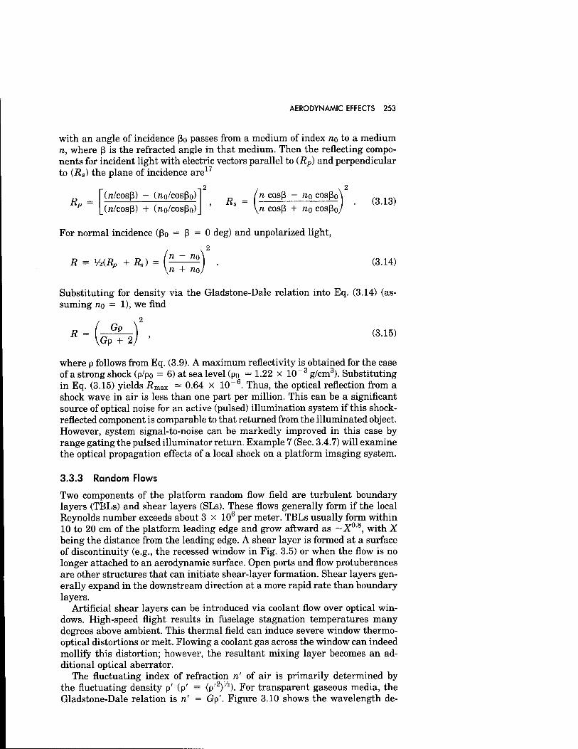
AERODYNAMIC EFFECTS 253
with an angle of incidence ßo passes from a medium of index no to a medium n, where ß is the refracted angle in that medium. Then the reflecting compo- nents for incident light with electric vectors parallel to (Rp) and perpendicular to (Rs) the plane of incidence are17
Rp — (n/cosß) - (np/cosßo) (n/cosß) + (no/cosßo)
2 , ,2 n cosß - n0 cosßo ^
Kn cosß + no cosßo/
For normal incidence (ßo = ß = 0 deg) and unpolarized light,
R = V2(RP + Rs) = (ü—JjA . (3.14) \n + no/
Substituting for density via the Gladstone-Dale relation into Eq. (3.14) (as- suming no = 1), we find
R = I ^ß2-^ I , (3.15) Gp + 2
where p follows from Eq. (3.9). A maximum reflectivity is obtained for the case of a strong shock (p/po = 6) at sea level (po — 1.22 x 10"3 g/cm3). Substituting in Eq. (3.15) yields jRmax — 0.64 x 10~6. Thus, the optical reflection from a shock wave in air is less than one part per million. This can be a significant source of optical noise for an active (pulsed) illumination system if this shock- reflected component is comparable to that returned from the illuminated object. However, system signal-to-noise can be markedly improved in this case by range gating the pulsed illuminator return. Example 7 (Sec. 3.4.7) will examine the optical propagation effects of a local shock on a platform imaging system.
3.3.3 Random Flows
Two components of the platform random flow field are turbulent boundary layers (TBLs) and shear layers (SLs). These flows generally form if the local Reynolds number exceeds about 3 x 10⁶ per meter. TBLs usually form within 10 to 20 cm of the platform leading edge and grow aftward as ~X08, with X being the distance from the leading edge. A shear layer is formed at a surface of discontinuity (e.g., the recessed window in Fig. 3.5) or when the flow is no longer attached to an aerodynamic surface. Open ports and flow protuberances are other structures that can initiate shear-layer formation. Shear layers gen- erally expand in the downstream direction at a more rapid rate than boundary layers.
Artificial shear layers can be introduced via coolant flow over optical win- dows. High-speed flight results in fuselage stagnation temperatures many degrees above ambient. This thermal field can induce severe window thermo- optical distortions or melt. Flowing a coolant gas across the window can indeed mollify this distortion; however, the resultant mixing layer becomes an ad- ditional optical aberrator.
The fluctuating index of refraction n' of air is primarily determined by the fluctuating density p' (p' = (p'2)1/2). For transparent gaseous media, the Gladstone-Dale relation is n' = Gp'. Figure 3.10 shows the wavelength de-
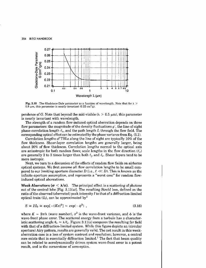
254 IR/EO HANDBOOK
3 4 5 6 7 89
Wavelength X (urn)
Fig. 3.10 The Gladstone-Dale parameter as a function of wavelength. Note that for X > 0.5 |im, this parameter is nearly invariant (0.22 cm3/g).
pendence of G. Note that beyond the mid-visible (X > 0.5 |xm), this parameter is nearly invariant with wavelength.
The strength of a random flow-induced optical aberration depends on three flow parameters: the magnitude of the density fluctuations p', the line-of-sight phase-correlation length (z, and the path length L through the flow field. The corresponding optical effect can be estimated by the phase variance from Eq. (3.1).
Correlation lengths of TBLs along the line of sight are typically 10% of the flow thickness. Shear-layer correlation lengths are generally larger, being about 20% of flow thickness. Correlation lengths normal to the optical axis are anisotropic for both random flows; scale lengths in the flow direction (tx) are generally 2 to 3 times larger than both €y and (z. Shear layers tend to be more isotropic.
Next, we turn to a discussion of the effects of random flow fields on airborne optical systems. We first assume all flow correlation lengths to be small com- pared to our limiting aperture diameter D (i.e., ( « D). This is known as the infinite-aperture assumption, and represents a "worst case" for random flow- induced optical aberrations.
Weak Aberrations (<r < A/TT). The principal effect is a scattering of photons out of the central lobe [Fig. 3.11(a)]. The resulting Strehl loss, defined as the ratio of the observed (aberrated) peak intensity I to that of a diffraction-limited optical train do), can be approximated by1
S s //Jo = exp[-(#cx)2] = exp(-c|>2) (3.16)
where K = 2TT/X (wave number), a2 is the wave-front variance, and <f> is the wave-front phase error. The scattered energy from a turbule has a character- istic scattering angle 6S = X./€2. Figure 3.11(a) compares the resulting far field with that of a diffraction-limited system. While this figure depicts an (circular aperture) Airy pattern, results are generally valid. The net result in this weak- aberration case is a loss of system contrast and resolution; however, a central core exists that is essentially diffraction limited.1 The fact that beam quality can be related to aerodynamically driven system wave-front error is a potent result, and is the cornerstone of aero-optics.
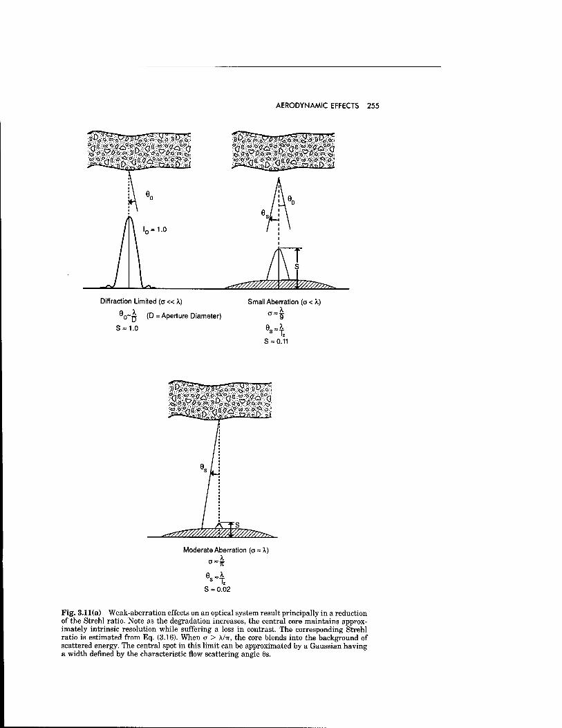
AERODYNAMIC EFFECTS 255
"^TR
Wv?^ Diffraction Limited (a « X)
9D~w (D = Aperture Diameter)
S = 1.0
Small Aberration (a < X)
es.x S = 0.11
^7^///^&^?^
Moderate Aberration (a = X)
S = 0.02
Fig. 3.11(a) Weak-aberration effects on an optical system result principally in a reduction of the Strehl ratio. Note as the degradation increases, the central core maintains approx- imately intrinsic resolution while suffering a loss in contrast. The corresponding Strehl ratio is estimated from Eq. (3.16). When o- > X/ir, the core blends into the background of scattered energy. The central spot in this limit can be approximated by a Gaussian having a width denned by the characteristic flow scattering angle 9s.
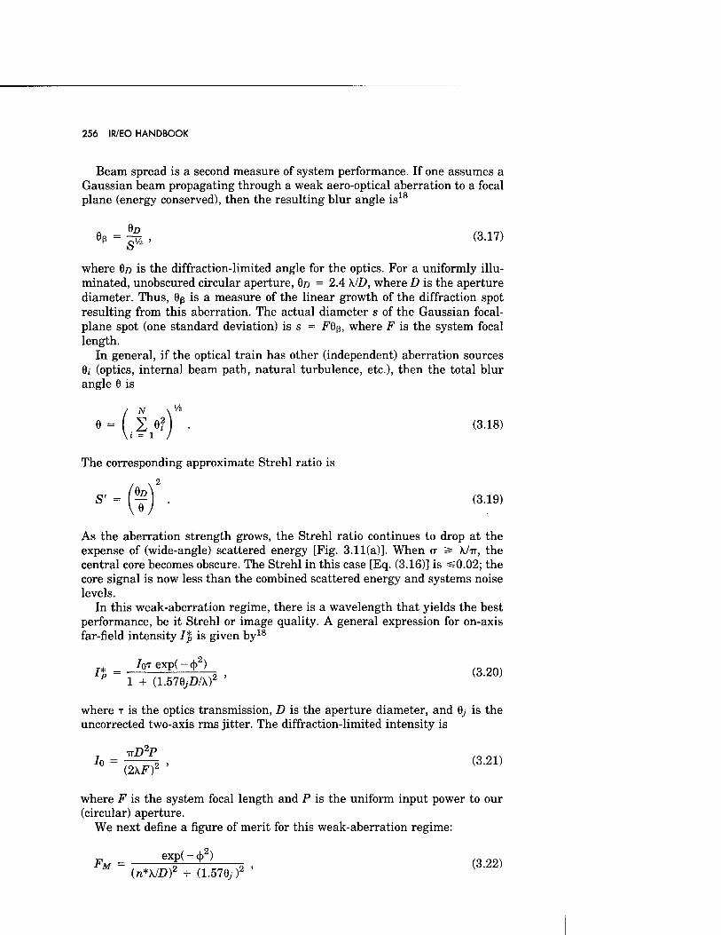
256 IR/EO HANDBOOK
Beam spread is a second measure of system performance. If one assumes a Gaussian beam propagating through a weak aero-optical aberration to a focal plane (energy conserved), then the resulting blur angle is18
S (3.17)
where 6D is the diffraction-limited angle for the optics. For a uniformly illu- minated, unobscured circular aperture, 0ß = 2.4 KID, where D is the aperture diameter. Thus, 6ß is a measure of the linear growth of the diffraction spot resulting from this aberration. The actual diameter s of the Gaussian focal- plane spot (one standard deviation) is s = F6p, where F is the system focal length.
In general, if the optical train has other (independent) aberration sources 6; (optics, internal beam path, natural turbulence, etc.), then the total blur angle 6 is
■ CM N N*4
(3.18)
The corresponding approximate Strehl ratio is
S' = (j) ■ (3.19)
As the aberration strength grows, the Strehl ratio continues to drop at the expense of (wide-angle) scattered energy [Fig. 3.11(a)]. When cr > k/ir, the central core becomes obscure. The Strehl in this case [Eq. (3.16)] is =s0.02; the core signal is now less than the combined scattered energy and systems noise levels.
In this weak-aberration regime, there is a wavelength that yields the best performance, be it Strehl or image quality. A general expression for on-axis far-field intensity 1% is given by18
= /oTexpt-d,2) P 1 + (1.578/Z)/X)2
where T is the optics transmission, D is the aperture diameter, and 0, is the uncorrected two-axis rms jitter. The diffraction-limited intensity is
'" s£ • where F is the system focal length and P is the uniform input power to our (circular) aperture.
We next define a figure of merit for this weak-aberration regime:
FM = 5 5 i (3.22)
(n*K/Df + (1.576, )2
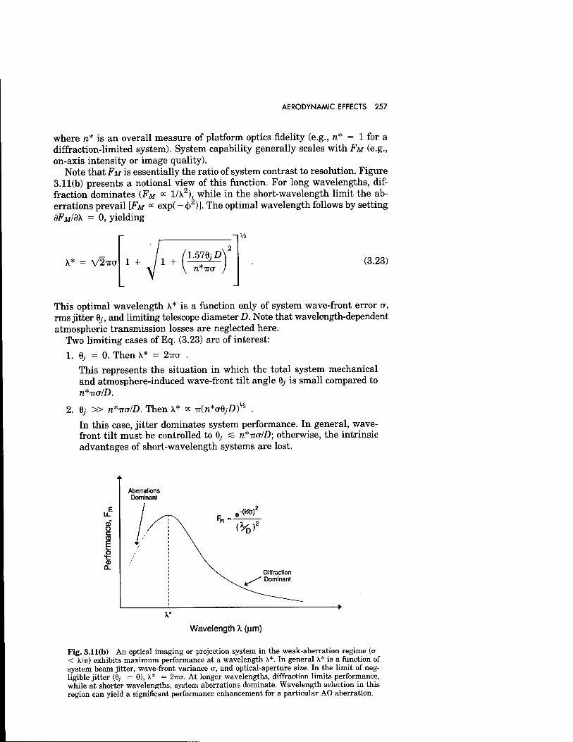
AERODYNAMIC EFFECTS 257
where n* is an overall measure of platform optics fidelity (e.g., n* = 1 for a diffraction-limited system). System capability generally scales with FM (e.g., on-axis intensity or image quality).
Note thati^M is essentially the ratio of system contrast to resolution. Figure 3.11(b) presents a notional view of this function. For long wavelengths, dif- fraction dominates (FM
a 1/A2), while in the short-wavelength limit the ab- errations prevail [FM
a exp( - <J>2)]. The optimal wavelength follows by setting OFMIöK = 0, yielding
A* = V2TUT 1 + 1 + 1.576, D
Vi
(3.23)
This optimal wavelength A* is a function only of system wave-front error CT, rms jitter 6,, and limiting telescope diameter D. Note that wavelength-dependent atmospheric transmission losses are neglected here.
Two limiting cases of Eq. (3.23) are of interest:
1. 9, = 0. Then A.* 2mr
This represents the situation in which the total system mechanical and atmosphere-induced wave-front tilt angle 6, is small compared to n*TTo7D.
\V2 2. 6/ » n*TTo7D. Then X* <* Tr(n*v%jD)'
In this case, jitter dominates system performance. In general, wave- front tilt must be controlled to 6, s re*iro7D; otherwise, the intrinsic advantages of short-wavelength systems are lost.
0} ü c CO E
•g 0) Q.
Wavelength X (\im)
Fig. 3.11(b) An optical imaging or projection system in the weak-aberration regime {a < Kl-n) exhibits maximum performance at a wavelength \*. In general \* is a function of system beam jitter, wave-front variance a, and optical-aperture size. In the limit of neg- ligible jitter (8, ~ 0), X* = 2w. At longer wavelengths, diffraction limits performance, while at shorter wavelengths, system aberrations dominate. Wavelength selection in this region can yield a significant performance enhancement for a particular AO aberration.
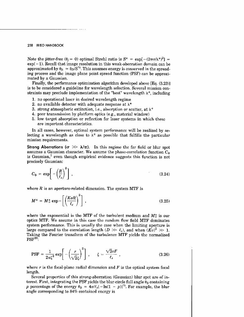
258 IR/EO HANDBOOK
Note the jitter-free (6,- = 0) optimal Strehl ratio is S* = exp[ - (2TTO7X*)2] =
exp( -1). Recall that image resolution in this weak-aberration domain can be approximated by 6p ~ QD/S
V2. This assumes energy is conserved in the spread-
ing process and the image plane point spread function (PSF) can be approxi- mated by a Gaussian.
Finally, the performance optimization algorithm developed above [Eq. (3.23)] is to be considered a guideline for wavelength selection. Several mission con- straints may preclude implementation of the "best" wavelength A*, including
1. no operational laser in desired wavelength regime 2. no available detector with adequate response at X* 3. strong atmospheric extinction, i.e., absorption or scatter, at X* 4. poor transmission by platform optics (e.g., material window) 5. low target absorption or reflection for laser systems in which these
are important characteristics.
In all cases, however, optimal system performance will be realized by se- lecting a wavelength as close to X* as possible that fulfills the particular mission requirements.
Strong Aberrations (a » A/ir). In this regime the far field or blur spot assumes a Gaussian character. We assume the phase-correlation function C<j, is Gaussian,1 even though empirical evidence suggests this function is not precisely Gaussian:
C<j, = exp 2-,
(3.24)
where R is an aperture-related dimension. The system MTF is
M* = Ml exp- V w (3.25)
where the exponential is the MTF of the turbulent medium and M% is our optics MTF. We assume in this case the random flow field MTF dominates system performance. This is usually the case when the limiting aperture is large compared to the correlation length (D » £z), and when (Ku)2 » 1. Taking the Fourier transform of the turbulence MTF yields the normalized PSF20:
PSF = 2<
exp V21
2-1
£s V20-F (3.26)
where r is the focal-plane radial dimension and F is the optical system focal length.
Several properties of this strong-aberration (Gaussian) blur spot are of in- terest. First, integrating the PSF yields the blur-circle full angle 6ß containing p percentage of the energy 6P = 4o7€2[ - ln(l - p)]v\ For example, the blur angle corresponding to 84% contained energy is
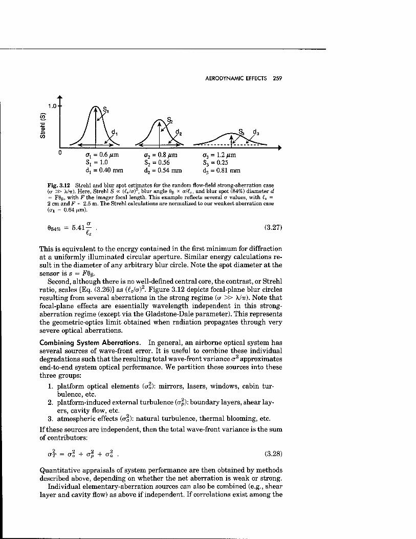
AERODYNAMIC EFFECTS 259
LO-
CO
55
ax = 0.6 um S, = 1.0 d, = 0.40 mm
a2 = 0.8 fim S2 = 0.56 d2 = 0.54 mm
ff3 = 1.2 ^m S3 = 0.25 d3 = 0.81 mm
Fig. 3.12 Strehl and blur spot estimates for the random flow-field strong-aberration case (a S> \/n). Here, Strehl S a (tzlaf, blur angle 6p « CT/4, and blur spot (84%) diameter d = F6ß, with F the imager focal length. This example reflects several a values, with tz = 2 cm and F = 2.5 m. The Strehl calculations are normalized to our weakest aberration case (o-i = 0.64 (un).
684% = 5.41- (3.27)
This is equivalent to the energy contained in the first minimum for diffraction at a uniformly illuminated circular aperture. Similar energy calculations re- sult in the diameter of any arbitrary blur circle. Note the spot diameter at the sensor is s = F6ß.
Second, although there is no well-defined central core, the contrast, or Strehl ratio, scales [Eq. (3.26)] as (€Z/CT)
2. Figure 3.12 depicts focal-plane blur circles
resulting from several aberrations in the strong regime (a » X./TT). Note that focal-plane effects are essentially wavelength independent in this strong- aberration regime (except via the Gladstone-Dale parameter). This represents the geometric-optics limit obtained when radiation propagates through very severe optical aberrations.
Combining System Aberrations. In general, an airborne optical system has several sources of wave-front error. It is useful to combine these individual degradations such that the resulting total wave-front variance CT
2 approximates
end-to-end system optical performance. We partition these sources into these three groups:
1. platform optical elements (a2,): mirrors, lasers, windows, cabin tur- bulence, etc.
2. platform-induced external turbulence (a2): boundary layers, shear lay- ers, cavity flow, etc.
3. atmospheric effects (CT2): natural turbulence, thermal blooming, etc.
If these sources are independent, then the total wave-front variance is the sum of contributors:
2 cry + CTS + al (3.28)
Quantitative appraisals of system performance are then obtained by methods described above, depending on whether the net aberration is weak or strong.
Individual elementary-aberration sources can also be combined (e.g., shear layer and cavity flow) as above if independent. If correlations exist among the
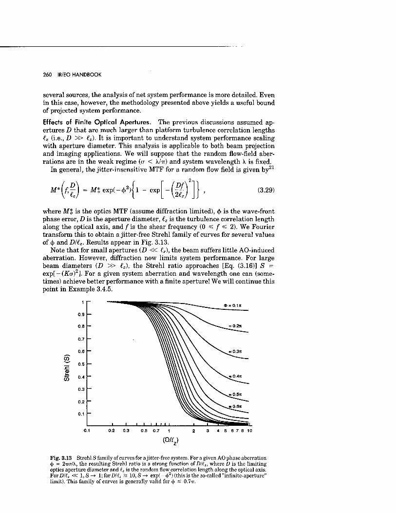
260 IR/EO HANDBOOK
several sources, the analysis of net system performance is more detailed. Even in this case, however, the methodology presented above yields a useful bound of projected system performance.
Effects of Finite Optical Apertures. The previous discussions assumed ap- ertures D that are much larger than platform turbulence correlation lengths €z (i.e., D » €2). It is important to understand system performance scaling with aperture diameter. This analysis is applicable to both beam projection and imaging applications. We will suppose that the random flow-field aber- rations are in the weak regime (a < A/IT) and system wavelength X is fixed.
In general, the jitter-insensitive MTF for a random flow field is given by21
M* f,j) =M*exp(-(}>2)il - exp Df 21
(3.29)
where M% is the optics MTF (assume diffraction limited), cj> is the wave-front phase error, D is the aperture diameter, iz is the turbulence correlation length along the optical axis, and /"is the shear frequency (0 =£ f =s 2). We Fourier transform this to obtain a jitter-free Strehl family of curves for several values of 4> and Dl(.z. Results appear in Fig. 3.13.
Note that for small apertures (D « tz), the beam suffers little AO-induced aberration. However, diffraction now limits system performance. For large beam diameters (D » €2), the Strehl ratio approaches [Eq. (3.16)] S = exp[-(Ka)2]. For a given system aberration and wavelength one can (some- times) achieve better performance with a finite aperture! We will continue this point in Example 3.4.5.
4> = 0.l!t
CO
!c 03
CO
0.5 0.7 1 2 3 45678 10
(D/g
Fig. 3.13 Strehl S family of curves for a jitter-free system. For a given AO phase aberration (|> = 2TTCT/X, the resulting Strehl ratio is a strong function of D/(z, where D is the limiting optics aperture diameter and (z is the random flow correlation length along the optical axis. ForD/4 « l,S-> l;forD/€2 a 10, S-^ exp(-4>2) (this is the so-called "infinite-aperture" limit). This family of curves is generally valid for <)> s 0.7ir.
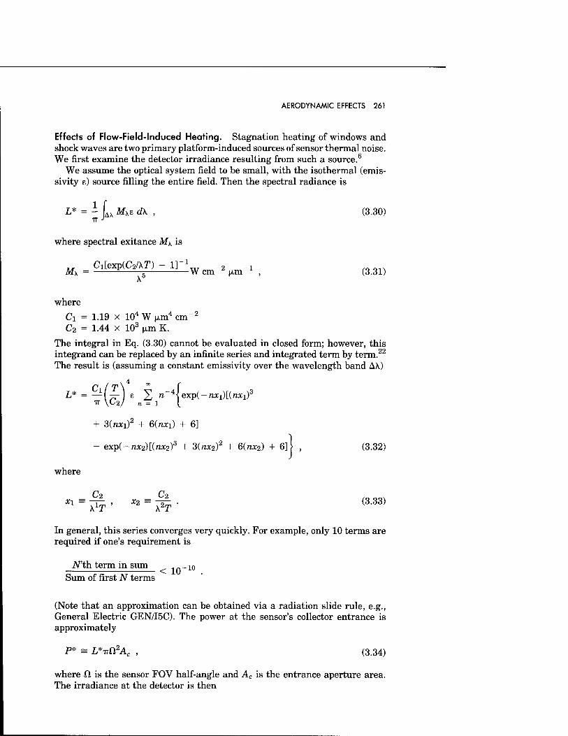
AERODYNAMIC EFFECTS 261
Effects of Flow-Field-lnduced Heating. Stagnation heating of windows and shock waves are two primary platform-induced sources of sensor thermal noise. We first examine the detector irradiance resulting from such a source.6
We assume the optical system field to be small, with the isothermal (emis- sivity e) source filling the entire field. Then the spectral radiance is
L* = - L Mxe d\ , (3.30)
where spectral exitance M\ is
.. Ci[exp(C2/XD - l]-\Tr _2 _j .QO1. M\ = 5 Wem z |xm , (3.31) A
where
Ci = 1.19 x 10⁴ W (xm4 cm-2
Ci = 1.44 x 10³ |xm K.
The integral in Eq. (3.30) cannot be evaluated in closed form; however, this integrand can be replaced by an infinite series and integrated term by term.22
The result is (assuming a constant emissivity over the wavelength band A\)
L* = — l — j e 2 n 4\exp(-nx1)[(nxif
+ 3(/H;I)2 + G(nxi) + 6]
- exp(-nx2)[{nx2)3 + 3(nx2)2 + 6(nx2) + 6] \ , (3.32)
where
Xl " Ä ' X2" Ä ' (3'33)
In general, this series converges very quickly. For example, only 10 terms are required if one's requirement is
APth term in sum 10
Sum of first N terms
(Note that an approximation can be obtained via a radiation slide rule, e.g., General Electric GEN/I5C). The power at the sensor's collector entrance is approximately
P* = L*TTü2AC , (3.34)
where il is the sensor FOV half-angle and Ac is the entrance aperture area. The irradiance at the detector is then
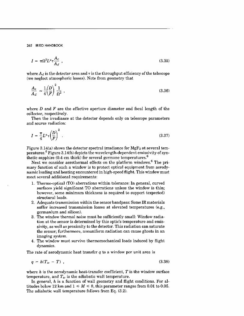
262 IR/EO HANDBOOK
/ = rrtfL*^ , (3.35) Ad
where Ad is the detector area and T is the throughput efficiency of the telescope (we neglect atmospheric losses). Note from geometry that
Ac 1(D\2 1 Ad 4\FJ a2 '
(3.36)
where D and F are the effective aperture diameter and focal length of the collector, respectively.
Then the irradiance at the detector depends only on telescope parameters and source radiation:
/ = IL*T(f) • (3-37)
Figure 3.14(a) shows the detector spectral irradiance for MgF2 at several tem- peratures.6 Figure 3.14(b) depicts the wavelength-dependent emissivity of syn- thetic sapphire (0.4 cm thick) for several germane temperatures.6
Next we consider aerothermal effects on the platform windows.6 The pri- mary function of such a window is to protect optical equipment from aerody- namic loading and heating encountered in high-speed flight. This window must meet several additional requirements:
1. Thermo-optical (TO) aberrations within tolerance: In general, curved surfaces yield significant TO aberrations unless the window is thin; however, some minimum thickness is required to support (expected) structural loads.
2. Adequate transmission within the sensor bandpass: Some IR materials suffer increased transmission losses at elevated temperatures (e.g., germanium and silicon).
3. The window thermal noise must be sufficiently small: Window radia- tion at the sensor is determined by this optic's temperature and emis- sivity, as well as proximity to the detector. This radiation can saturate the sensor; furthermore, nonuniform radiation can cause ghosts in an imaging system.
4. The window must survive thermomechanical loads induced by flight dynamics.
The rate of aerodynamic heat transfer q to a window per unit area is
q = h(Tw - T) , (3.38)
where h is the aerodynamic heat-transfer coefficient, T is the window surface temperature, and Tw is the adiabatic wall temperature.
In general, h is a function of wall geometry and flight conditions. For al- titudes below 12 km and 1 =s M =£ 8, this parameter ranges from 0.01 to 0.05. The adiabatic wall temperature follows from Eq. (3.2).
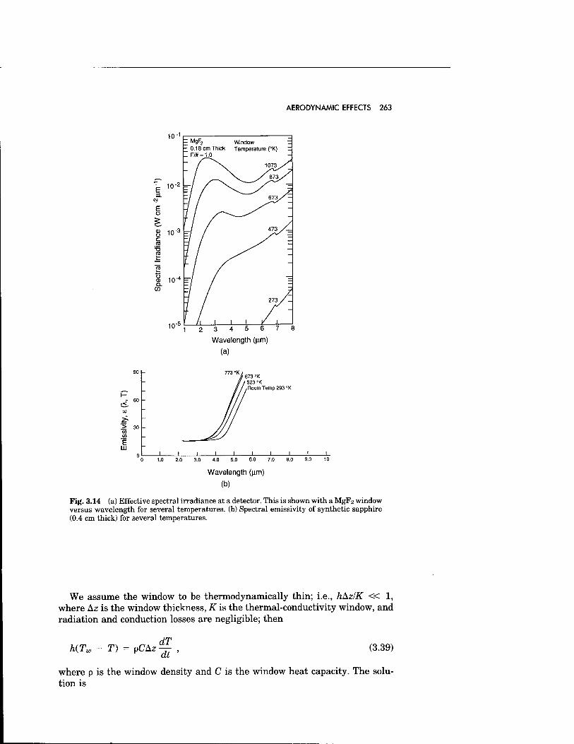
AERODYNAMIC EFFECTS 263
10-1
10 -z =■
8 10"3
o 10-4
Q.
10":
= MgF2 Window E - 0.18 cm Thick Temperature (°K) ~ - F/# = 1.0 - " 1073>
23/
^ 673/ z~
ll 473. /-=
5
/i I I I
273-
/ I
=
1 2 3 4 5 6 7 8
Wavelength (|im)
(a)
.> 30
E
673 °K 523 °K Room Temp 293 °K
0 1.0 2.0 3.0 4.0 5.0 6.0 7.0 8.0 9.0 10
Wavelength (urn)
(b)
Fig. 3.14 (a) Effective spectral irradiance at a detector. This is shown with a MgF2 window versus wavelength for several temperatures, (b) Spectral emissivity of synthetic sapphire (0.4 cm thick) for several temperatures.
We assume the window to be thermodynamically thin; i.e., hAz/K « 1, where Az is the window thickness, K is the thermal-conductivity window, and radiation and conduction losses are negligible; then
dT h(Tw -T) = pCAz — (3.39)
where p is the window density and C is the window heat capacity. The solu- tion is
264 IR/EO HANDBOOK
£f£ - -p(-j) , (3.40,
where Tj is the initial temperature and T is the window heating time constant:
T - If! . 8.41,
Consider, for example, a 0.5-cm-thick fused-quartz window at —350 K. Taking h = 0.03, p = 2.2 g/cm3, and C = 0.8 J g_1 K_1 results in a window time constant T = 29 s. This is the time required for the temperature ratio [Eq. (3.40)] of this thermodynamically thin window to achieve lie percent of its final value.
For many applications, the time of operation is short enough to neglect window-heating effects. Also, several approaches can increase the effective window time constant, including
1. Window precool: However, H2O condensation effects can be important. 2. Increasing window thickness: Here, factors such as increased absorp-
tion, optical distortion, and window weight must be considered. 3. Recessing window: This separates the flow boundary layer from the
window surface, thus reducing the heat-transfer coefficient. However, this action may also reduce the system field of view as well as induce additional optical aberrrations.
4. Window active cooling: This may also result in enhanced AO aberrations.
Recall that the above discussion neglects aerodynamic-induced radiation. At higher Mach numbers, radiation heat transfer becomes significant. In this case, the heat-balance equation becomes
h(Tw -T) = pCAz — + O-SBET4 , (3.42)
where e = equivalent total wall emissivity; CTSB - Stefan-Boltzmann constant. The above treatment of the interaction of an optical wave front with
airborne-platform-induced flow fields gives a flavor for the types of problems encountered in flight. We have not broached the hypersonic regime (M s 8), where dissociation, ionization (plasma) effects, and acoustical radiation can be important. Neither have we discussed high-power laser (nonlinear) airflow interactions such as thermal blooming and Raman or Brillouin scattering. However, we have developed the tools that allow the optical designer to quan- titatively investigate and bound optical-system performance for a broad spec- trum of germane airborne-platform scenarios. We turn now to examples of how this information can be applied to practical AO situations.
3.4 AERO-OPTICAL DESIGN AND ANALYSIS EXAMPLES
3.4.1 Example 1—Subsonic Imaging Platform: Boundary-Layer Aberrations
An optical designer has been asked to investigate the quality of images that can be expected to occur on a large transport aircraft flying at various Mach
AERODYNAMIC EFFECTS 265
numbers and altitudes. The camera operates in the mid-visible (A. ~ 0.5 |xm). There are two possible aircraft locations for this instrument. The first site is approximately 10 m aft of the nose, while the second site is located 25 m aft. Both positions are expected to have attached turbulent boundary layers since those location sites are on nominally smooth, nonexpanding or contracting sections of the fuselage. Images are to be collected by a 30-cm-diameter tele- scope primary mirror; this is taken to be the system limiting aperture. Because of the short-wavelength requirements for this imaging system, a flush material window of high quality is used. The window is conformal with the existing mold lines of the aircraft at both proposed installation sites (Fig. 3.1).
Note that large F-number imaging systems are frequently "detector limited." That is, intrinsic resolution is set by the imager pixel size and spacing rather than the limiting optics (6D). For this example we assume an unobscured circular aperture having diameter D; its full diffraction angle 0D is 0D = 2.4 k/D = 4 (Jirad at X = 0.5 |xm. If the detector limit is, say, 20 jjirad, then AO aberrations will not be important to system resolution unless they are on the order of 20 |xrad or greater.
For attached turbulent boundary layers, one may assume that the total turbulent boundary-layer thickness is between 1 and 1.5% of the distance from the origin of the boundary layer. For the purpose of example here, we take the conservative value and estimate the boundary-layer thicknesses to be 1.5% of the total boundary-layer length (flow direction). The turbulent scale sizes in an attached boundary layer are known to be approximately 10% of the total thickness of the layers. The density fluctuations, on the other hand, are driven by the difference between the wall density and the density that exists external to the boundary layer. The external density is chosen to be the ambient density. The wall density can be computed from the recovery temperature of the ve- hicle's surface, with the assumption that the static pressure at the surface has a value equal to the atmospheric pressure at the operating altitude [Eq. (3.4)]. The wave-front errors can then be estimated from the square of the fluctuating density values and the product of the scale length and total path length through the turbulent boundary layers according to Eq. (3.1).
Case I (Baseline). For this case, the aircraft's operating altitude is expected to be about 12 km, with a flight Mach number of 0.6. The surface density p is about 94% of the free-stream value, with fluctuations of about 10% of the difference, or about 0.006 times the free-stream density. For a station located 10 m downstream of the leading edge, the boundary-layer thickness is ap- proximately 15 cm, with the scale sizes being estimated at 1.5 cm; i.e.,
X = 10 m, L = 15 cm, iz = 1.5 cm ,
po = 3.1 x 10~4 g/cm3, p' = 1.9 x 10⁻⁶ g/cm3 .
From Eq. (3.1), we have the approximate wave-front error a as
CT = G(p'2)I/2(24L)1/2 , (3.43)
or o- = (0.22X1.9 x 10"6)(2 x 1.5 x 15)'/2 = 2.8 x 10~~6cm= 0.028 |xm .
266 IR/EO HANDBOOK
For visible wavelengths (X = 0.5 fim), the diffraction limit of the system is 2.4X/D = 4 |xrad. The nondimensional wave-front error is o7X = 0.056 at X = 0.5 fjim.
This case represents a weak aberration. From Eq. (3.16), we find the Strehl ratio has a value of 0.88, and the blur angle [Eq. (3.17)] 0P = QD/SV2 is ap- proximately 1.07 times the diffraction-limited value. This is an approximation for the increase in the diameter of a point source imaged through the boundary layer. For this imaging system, little loss of resolution occurs and negligible contrast loss is experienced.
This optimistic view can be changed significantly by variations in the flight parameters, location on the aircraft, and imager wavelength. The following cases discuss some of these variations.
Case II (Mach Number Excursion). For this case, conditions remain similar to that for Case I, except that the flight Mach number is increased to 0.9. Here we ignore local shock wave effects. Such aero-optical phenomena are broached in Example 7. Now the surface density is only 87% of the atmospheric density, with attendant larger density fluctuations. The TBL thickness and scale sizes are nearly invariant with this increase in Mach number, and the wave-front error is 2.1 times that of Case I. The Strehl ratio drops to 0.57, while the focal- plane spot size becomes 1.33 times the diffraction-limited value; i.e.,
p'n = 2.1p{ = 4 x 10~6g/cm3 .
The resulting wave-front error is
o-ii= 2.1 ai and — ~ 0.12 at X = 0.5 |xm . X
The point of Case II is that although this is still a relatively weak aberration (-X/10), the Mach number does have a strong effect on the contrast because the Strehl ratio has dropped by 30%. If the sensor has sufficient dynamic range, the effect of this contrast loss is minimal. However, a resolution loss will result from image blurring owing to light rays being scattered by the TBL to adjacent sensor (pixel) elements. The resulting blur spot in this case has a diameter that is 33% larger than a diffraction-limited spot diameter.
Case III (Turbulent Boundary-Layer Thickness Excursion). For this case, we examine aero-optical effects 25 m downstream of the origin of the turbulent boundary layer, and assume Case I flight conditions. The boundary-layer thick- ness is now increased by a factor of 2.5 over the Case I value, while the scale sizes are also 2.5 times that for Case I. (Note our conservative assumption that the TBL thickness L and scale size €2 scale linearly with distance X down- stream, rather than the more traditional L = X° 8 scaling.) Thus, the wave- front error becomes 2.5 times as large as that for Case I; i.e.,
X = 25 m, Lin « 2.5Li, and €ra * 2.5ft ,
am = 2.5CTI and o7X = 0.14 at X = 0.5 (xm .
The image contrast loss (Strehl) is now 0.46, with a corresponding blur angle 9ß~1.478ß, or about 6 (xrad.
AERODYNAMIC EFFECTS 267
The message from Case III is that the wave-front errors scale linearly with distance downstream of the origin of the turbulent boundary layer; thus, it is highly advantageous to move imaging equipment as far forward on the vehicle as possible. It should be noted that even though the wave-front error scales linearly, the focal-plane effect has a highly nonlinear scaling in this domain according to Eqs. (3.16) and (3.17).
Case IV (Effect of Boundary-Layer Thickness and Increased Mach Num- ber). This is similar to Case II (Mach 0.9), except our optical system is located at the 25 m station. Again, the ratio of surface to atmospheric density is 0.87. The wave-front error is o7\ ~ 0.3 at A. = 0.5 pjn. This aberration level is between the weak and strong regimes; the far-field Strehl ratio has been reduced such that it is comparable to the (scattered) background. The estimated Strehl is 0.03, with a (weak-aberration) image blur angle 6ß ~ 5.9 0D, or approximately 24 |xrad. Note that approaching this as a strong aberration yields a predicted blur circle (84% energy) of 6P = 5.41 a/€z = 22 p-rad.
A substantial loss of both contrast and resolution exists for this visible imaging system. For example, effective resolution is between five and six times the optics-limited resolution. This condition is similar to those measured on operational platforms.
Case V (Effect of Wavelength). We assume the same flight conditions and position on the vehicle as that in Case IV, but now the imaging-system wave- length is taken to be 2 p,m. We suppose an IR window exists that is conformal with the fuselage. Now, the relative wave-front error is reduced fourfold from the higher Mach number case at the aft installation location, so that o7\ = 0.075 at A. = 2p,m. This yields a corresponding Strehl ratio and blur angle of S= 0.8, 6P ~ 1.10D, respectively. Note, however, in this case, that the (optics- limited) diffraction angle is four times that of the visible case. Assuming diffraction-limited optics, this X = 2 p,m system (6p = 18 pxad, S = 0.8) may outperform its visible-wavelength counterpart (9p = 24 p,rad, S = 0.03). This example demonstrates the highly nonlinear nature of system Strehl (contrast) with o- and X. [Eq. (3.16)]. Whether or not selecting a longer wavelength is a useful approach to ameliorate airborne-platform random flow effects obviously depends on the designer's application.
One means of reducing aero-optical platform aberrations is to fly higher or slower. To demonstrate the effects of altitude on system performance, the following case is given.
Case VI (Altitude Effects). Consider the example of Case III with the flight Mach number maintained at 0.6 but the altitude reduced to 1 km. Again, the ratio of surface density to that of the atmosphere remains at 0.94; however, the atmospheric density has increased considerably. This causes a 3.5-fold increase in the wave-front error over that for Case III; i.e., po = 1.1 x 10~3
g/cm3, p' = 6.6 x 10"6 g/cm3, and avi = 3.5 x am = 0.24 p,m. Thus, o7\ = 0.48. This example represents a situation that is well into the strong-aberration regime. An upper bound for the resulting full blur angle (84% energy) follows from Eq. (3.27):
8P = 5.41-^ = 35 |xrad .
268 IR/EO HANDBOOK
Note that the aberration strength in this strong domain has a weak wavelength dependence (via the Gladstone-Dale parameter). The blur angle 6ß is essen- tially determined solely by flow aerodynamic parameters. This situation rep- resents the geometric-optics limit.
This case demonstrates that the magnitude of the ambient density has a strong effect on the strength of the aberrations caused by an attached turbulent boundary layer. In general, flying as high and as slowly as possible, while having the optical axis as far forward as feasible, minimizes AO aberrations.
3.4.2 Example 2—Supersonic Imaging Platform: Boundary-Layer Aberrations
Our optical designer had no sooner completed the calculations for the subsonic aircraft when a second mission required the placement of a similar visible imager on a high-speed, high-altitude supersonic aircraft.
Case I (Baseline). Here we consider only optical aberrations due to the super- sonic turbulent boundary layer. Associated shock-wave refractive and reflec- tive optical effects will be examined in Example 7. The expected flight Mach number is about 3.0, with an operating altitude of about 20 km. We now assume a 15-cm imaging-aperture diameter. For this situation, the outside atmospheric density is about po ~ 0.9 x 10 ~4 g/cm3; however, because of the aircraft's high Mach number, the surface density is now about 38% of the atmospheric value. If the camera location were limited to a single position approximately 10 m downstream, one estimates a 15-cm-thick boundary layer with 1.5-cm scale sizes. The fluctuating density magnitudes are now substantially larger than those from Example 1 because of the increased difference in the densities at the surface and in the natural atmosphere. Now the fluctuating density is about 6 x 10 ~6 g/cm3. For this case, the wave-front error is a ~ 8.9 x 10 ~~6
cm, or about 0.18 waves (\ = 0.5 pjm). The Strehl ratio for this weak aberration is approximately 0.28, and the blur angle is 1.9 times that of a diffraction- limited system. The diffraction angle 0z> is about 8 (xrad for a system with a 15-cm effective aperture diameter, so that 6ß - 15 p.rad. This example shows that good optical fidelity can be achieved from a supersonic airborne platform.
Case II (Altitude Excursion). This is like Case I except the platform altitude is reduced to 10 km. The outside atmospheric density is now 4.1 x 10 ~4 g/cm3, with p' ~ 4.6 times that of Case I. Hence, o7\ ~ 0.83 at X. = 0.5 |xm, which is a strong aberration. Our corresponding 84% blur angle 0P ~ 5.41 o7€* ~ 148 ixrad!
The system Strehl ratio at this altitude relative to Case I can be estimated [Eq. (3.19)] by
8 - (M) - io-2 .
Again, we note that selection of a longer wavelength could markedly improve system performance. For example, a X = 3 p,m system returns the system to the weak-aberration domain (b7\ — 0.14), with S = 0.46. The system dif- fraction angle 0# is now 48 p,rad, with a corresponding blur angle 0ß — 0£>/S1/2
AERODYNAMIC EFFECTS 269
~ 71 |xrad. This longer-wavelength system offers our designer a potential factor of two resolution improvement. Note, however, that other radiometric factors must be considered, for example, reduced detector signal-to-noise ratio at the longer wavelength.
3.4.3 Example 3—Optical Degradation Resulting from Open Cavity
Other people in the optical designer's group interested in longer wavelengths now ask what the effect might be in a subsonic installation if open-cavity flows were present and the same 15-cm aperture-receiving optics were used for a 2- |xm wavelength sensor. A windowless configuration may be selected to afford low-loss transmission for multiple or long wavelengths or to minimize IR ther- mal noise due to material windows. For these cases, the field between the sensor and the atmosphere consists of a turbulent shear layer and cavity flow (see, for example, Fig. 3.3), rather than the attached turbulent boundary layers of Examples 1 and 2. The thickness and scale sizes characterizing this shear layer depend principally on the cavity length (in the flow direction) and, to a lesser extent, on properties of the upstream fuselage boundary layer. We sup- pose the 15-cm aperture requires a full one-meter square opening to achieve the desired field of regard. The cavity depth H is taken to be 15 cm. The porous fence located upstream (Fig.3.3) is assumed to extend beyond the edge of the attached turbulent boundary layer. In this example, we consider optional ab- errations resulting from both shear layer and cavity flow fields.
Recall that the thickness L of the shear layer can be estimated by L — 0.25X, where X is the downstream distance. We suppose the average thickness across this open cavity to be 15 cm. Moreover, we assume for a conservative optical design that the scale sizes (with respect to Case I, baseline) have increased by approximately a factor of two (i.e., €2 — 0.2L), and the rms density fluctuation p' has also increased by a factor of two. Thus, the values of the wave-front variance will increase by a factor of 8 [Eq. (3.1)]. Note that the difference between the outside and inside densities has not changed from those in Ex- ample 1 (baseline case), since the cavity gas temperature is at the aerodynamic recovery temperature. With these considerations in mind, we see that o- has increased by V8, but the wavelength has increased by a factor of 4. This results in a value of oVA. that has decreased to about 71% of the Example 1 baseline example. The corresponding Strehl ratio and blur angles are 0.94 and 1.03 6z>, respectively. For this 2-|xm imaging system, AO effects of this shear flow are negligible.
Next, suppose the 2-|xm imager is replaced by a visible sensor (\ ~ 0.5 (im). Now o7A is V8 times larger than the Example 1 baseline case (o7\ — 0.16). The corresponding Strehl ratio S and blur angle 0p are 0.36 and 1.66 QD,
respectively. A second source of aberration is flow within the cavity itself. Although cavity
scale sizes are large compared to the shear layer, the low-velocity flow results in small values of fluctuating density. Thus, the resulting optical aberrations are usually negligible with respect to the external flow fields unless a marked thermal mismatch exists between the cavity gas temperature and the recovery temperature. We now treat this case.
Let AT be the temperature differential between the air in the upper and lower parts of the cavity and suppose the fluctuating component T" is 10% of this difference; i.e., T' = 0.1A71. Neglecting cavity velocity fluctuations,
270 IR/EO HANDBOOK
/ rpt
— = — , where p and T are the cavity mean values . (3.44) P T
Substitution yields
p' = O.IP(Y) • (3-45)
We choose as our parameters the Example 1 baseline case: aircraft Mach number = 0.6, aircraft altitude = 12 km, mean cavity density p = 2.9 x 10~4 g/cm3, and mean cavity temperature T = 230 K. Here, the mean cavity density and temperature are taken to be the recovery parameters [Eqs. (3.3) and (3.4)].
In addition, the cavity correlation length is taken to be (z — 0.2H, with H — 15 cm (cavity depth). Finally, a temperature differential AT — 30 K yields
a cavity wave-front error of o7\ = 0.16 at X = 0.5 (xm. In general, the cavity and external random flows are independent. Thus, the
net wave-front variance o"r follows from ay = o-^hearlayer+ o-j?avity. Substituting the above values yields a total wave-front error or/A. — 0.23 at X. = 0.5 p,m. This is a weak aberration, with Strehl ratio S and blur angle 8ß of 0.13 and 2.70D, respectively.
An interesting limiting case is that of a shallow cavity. This may occur, for example, if a material window is recessed into the fuselage to optimize the field of regard of a platform optical instrument. Such a cavity is defined to be shallow if the expanding shear layer formed at the leading edge intersects the cavity bottom (e.g., window).
Recall that the thickness of a freely expanding shear layer is L — 0.25Z, where X is the downstream distance. This corresponds to a divergence half- angle of about 7 deg. At the window reattachment point, the incipient flow adopts characteristics more akin to a boundary layer. Thus, in the general situation, one can have the remnants of the original shear layer sandwiched between the nascent window boundary layer and the fuselage boundary layer. Though the precise magnitude of the composite wave-front variance is difficult to calculate in this situation, the net optical aberration will probably be some- what less than that of a deeper cavity. The most desirable aero-optical approach with a window is to mount it conformally with the fuselage, thus avoiding shear-layer formation.
The message here is that open-cavity AO mixing-layer aberration levels can be comparable to shear-layer or boundary-layer effects, particularly if significant thermal differences exist. If the cavity is shallow, shear layer im- pingement can occur on the bottom surface (e.g., window). The designer is now in a good position to assess the impact of an open cavity on system optical performance.
3.4.4 Example 4—Visible Imager: Selecting the Optimal Wavelength
Imaging tests are being planned using a 30-cm-diameter high-resolution cam- era system on board a wide-body aircraft. The camera has a rotatable filter wheel that provides selectable imaging band widths in steps of 0.1 |xm from
AERODYNAMIC EFFECTS 271
0.35 to 1.15 fim (filter bandpass full width at half maximum is -0.04 |xm). The lead experimenter selects the shortest available wavelength (0.35 |xm) wheel position because good resolution is important. The mission is flown at 5-km altitude and Mach 0.8. Postmission analysis reveals unexpectedly poor target resolution. The aircraft boundary layer is suspected to be the culprit. Effective in-flight image resolutions of order 35 to 45 ixrad are inferred. Ground calibrations show a system resolution of about 20 (Jirad limited by the detector. The intrinsic optics resolution limit 6D at this wavelength is approximately 10 |xrad. The test director decides to probe the aircraft boundary layer via a series of aerodynamic measurements. Results reveal a boundary-layer thick- ness of 20 cm and correlation length €2 of 2 cm at the mission Mach number. The inferred fluctuating density for this random flow is 0.8 x 10 ~5 g/cm3. Using Eq. (3.1), he estimates an rms phase error o- = 0.16 (Jim. The resulting aberration o7\ ~ 0.46 borders on the strong regime. The approximate 84% blur angle 0ß is [Eq. (3.27)] 43 |xrad, with a corresponding Strehl ratio of S = (6D%)
2 — 5.3 x 10 ~ 2, in good agreement with observations. This loss of image
contrast can be a constraint unless the detector has adequate sensitivity. Recall [Fig. 3.11(b)] that there is a wavelength that offers optimal perfor-
mance for an airborne (infinite aperture) optical system. This wavelength yields the best focal-plane quality for a given array of optics diffraction, plat- form jitter, and system (weak) aberrations arising from optical elements, aero- optics, and natural turbulence. Here we assume the platform optics are dif- fraction limited and neglect atmospheric turbulence effects. For this situation, a= 0.16 |xm, and D = 30 cm; the two-axis rms jitter is taken to be 1.0 (xrad. Substituting in Eq. (3.23) reveals an optimal wavelength A* = 1.1 |xm. The resulting optical aberration is now weak (o7A* = 0.15), with a corresponding estimated Strehl ratio S and blur angle 6ß of 0.43 and 15 |xrad, respectively.
Note we have not considered wave-front aberrations due to natural atmo- spheric turbulence. Since these are independent aero-optical aberrations, the residual atmospheric phase error 4>a can be RSS'D with platform error to yield <j) = (<j}2 + <$)v\ If this composite aberration § is weak (<|> = 2TTO7A S 2), then a new "best" performance wavelength A* follows from Eq. (3.23).
The message here is that for a given AO aberration strength, there is a wavelength that yields best system performance. If our optical designer is able to select this optimal wavelength, or one close to it, significant enhancements can result.
3.4.5 Example 5—Aperture Optimization
The experimental team in Example 4 has garnered a considerable imaging database with its 30-cm-diameter high-resolution camera system. Excellent performance has indeed been confirmed at the optimal wavelength (A.* — 1.1 (xm). Now a crucial mission looms that requires propagating a laser beam (wavelength A ~ 0.53 |xm) from the platform to the far field. (Flight parameters are unchanged: Mach 0.8, altitude 5 km.) The leader challenges the optical designer: can better overall performance be obtained via a smaller aperture?
Recall that the estimated boundary-layer phase error is o- = 0.16 |xm, with a corresponding correlation length iz - 2 cm. From Fig. 3.13, we note that the proper Strehl curve is 4> = 0.60ir. As the aperture diameter D is reduced,
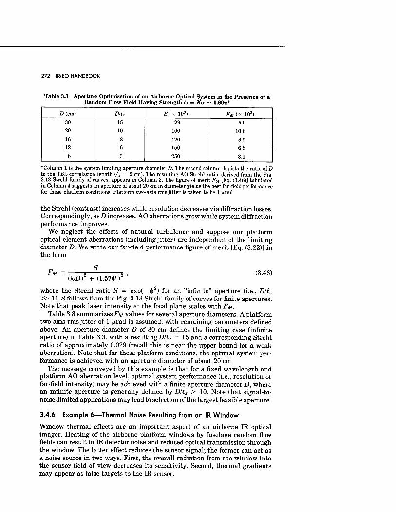
272 IR/EO HANDBOOK
Table 3.3 Aperture Optimization of an Airborne Optical System in the Presence of a Random Flow Field Having Strength <)> = Ka ~ 0.60-n*
D(cm) D/ez S(x 103) FM(,x 103)
30 15 29 5.0 20 10 100 10.6
16 8 120 8.9 12 6 150 6.8 6 3 250 3.1
*Column 1 is the system limiting aperture diameter D. The second column depicts the ratio of D to the TBL correlation length (tz = 2 cm). The resulting AO Strehl ratio, derived from the Fig. 3.13 Strehl family of curves, appears in Column 3. The figure of merit FM [Eq. (3.46)] tabulated in Column 4 suggests an aperture of about 20 cm in diameter yields the best far-field performance for these platform conditions. Platform two-axis rms jitter is taken to be 1 urad.
the Strehl (contrast) increases while resolution decreases via diffraction losses. Correspondingly, as D increases, AO aberrations grow while system diffraction performance improves.
We neglect the effects of natural turbulence and suppose our platform optical-element aberrations (including jitter) are independent of the limiting diameter D. We write our far-field performance figure of merit [Eq. (3.22)] in the form
FM = S
(\/D)2 + (1.57602 ' (3.46)
where the Strehl ratio S = exp(-<j>2) for an "infinite" aperture (i.e., D/(z
» 1). S follows from the Fig. 3.13 Strehl family of curves for finite apertures. Note that peak laser intensity at the focal plane scales with FM-
Table 3.3 summarizes FM values for several aperture diameters. A platform two-axis rms jitter of 1 |xrad is assumed, with remaining parameters defined above. An aperture diameter D of 30 cm defines the limiting case (infinite aperture) in Table 3.3, with a resulting Dltz = 15 and a corresponding Strehl ratio of approximately 0.029 (recall this is near the upper bound for a weak aberration). Note that for these platform conditions, the optimal system per- formance is achieved with an aperture diameter of about 20 cm.
The message conveyed by this example is that for a fixed wavelength and platform AO aberration level, optimal system performance (i.e., resolution or far-field intensity) may be achieved with a finite-aperture diameter D, where an infinite aperture is generally defined by D/(z > 10. Note that signal-to- noise-limited applications may lead to selection of the largest feasible aperture.
3.4.6 Example 6—Thermal Noise Resulting from an IR Window
Window thermal effects are an important aspect of an airborne IR optical imager. Heating of the airborne platform windows by fuselage random flow fields can result in IR detector noise and reduced optical transmission through the window. The latter effect reduces the sensor signal; the former can act as a noise source in two ways. First, the overall radiation from the window into the sensor field of view decreases its sensitivity. Second, thermal gradients may appear as false targets to the IR sensor.
AERODYNAMIC EFFECTS 273
A dual-wavelength IR imager has traditionally been flown at an altitude and Mach number of 8 km and 0.45, respectively. Sensor bandwidths are AXi = 3 to 5 fjum and AX.2 = 8 to 11.5 \xm. The nominal signal-to-noise ratio (S/N) has been estimated to be about 10 for each wavelength band, with the dominant "thermal-noise" source being the germanium (Ge) IR window. (We assume a minimum acceptable S/N of 5 has been established for both wavelength bands.) This inner window surface is convectively heated by cabin air only when its temperature approaches the dew point.
A candidate mission is proposed against a fast, highly dynamic target. The test director concludes that getting an acceptable IR imaging data collection window will require an aircraft Mach number of 0.9 at 8-km altitude. What S/N is expected for the experiment, and what can one do to enhance this?
Assuming a standard atmospheric temperature of 236 K, we find the wall (window) temperature for these two conditions to be [Eq. (3.3)]
Ti = T(M = 0.45) = 244 K ,
T2 = T(M = 0.90) = 270 K .
We assume the following characteristics for our IR imaging system:
1. The imager field of view (FOV) is small. 2. The IR window is the dominant source of thermal noise. 3. The IR window fills the entire sensor FOV. 4. The emissivities of germanium are constant across each of the two
wavelength bands, with EAXX = 0.45, EA\2 = 0.30. 5. The IR window is thermodynamically thin; e.g., see Eq. (3.39).
We next examine the ratio Ro of the window-induced intensities at the detec- tors. We use Eq. (3.32) to estimate the spectral radiances of the IR window at the two temperatures T\ and T2- We find
Ltxi (244 K) = 0.72 x 10"5 W cnT2 (l-1
Ltxi (270 K) = 0.25 x HT4 W cm"2 Ü'1
L%x2 (244 K) = 0.33 x 10⁻³ W cm-2 Ü-1
LAx2 (270 K) = 0.57 x 10"3 W cm-2 CL'1
with the thermal noise ratio at the detector being
_ L*AXI (270 K) KAXI
~ LU (244 K) ~ d-5 '
" = LAX2 (270 K) _ R*k2 - LAH (244 K) - L? •
Assuming a window-dominated detector S/N at the lower temperature (T\ = 244 K) of 10 for each wavelength band, the effective S/N at the candidate mission (Mach 0.9) will be (S/N)AXI = 2.9, (S/N)A\2 = 5.9. Note that the 3 to
274 IR/EO HANDBOOK
5 |xm band S/N is substantially below the minimum acceptable threshold, while the longer-wavelength S/N value is marginal.
One can perhaps improve this by cooling the inner surface of our IR window (e.g., with a convective flow of gaseous nitrogen). However, the cabin dew point must be monitored to preclude window condensation or frost formation. Either can dramatically alter effective window transmission properties in the IR. An alternative is to fly this mission at higher altitude or lower Mach number. Either approach will lower the effective window temperature, thus reducing detector thermal noise.
A second concern associated with IR windows is thermal-optical aberrations. In general, these depend on several complex factors, including the external and internal surface temperatures, window material properties, and window- mounting techniques. However, the causes of such thermally induced optical distortions are local strains e due to temperature gradients AT, which have the relationship e = a AT, where a is the coefficient of linear thermal expansion in the optical element. These AO-induced optical distortions are of concern for both outgoing wave-front and imaging systems. Although such effects are generally ameliorated at the longer IR wavelengths, the optical designer must be aware of these aberration sources and include estimates as part of the overall system error budget.
3.4.7 Example 7—Supersonic Vehicle Optical Aberrations
Case I (Nose-Mounted System). Our next challenge is to estimate the AO effects for a nose-mounted optical system on a Mach 6 endoatmospheric vehicle. Figure 3.15 shows a conceptual configuration. When the leading edge of the body is blunt, the shock, or bow, wave does not touch the body. Rather, a subsonic flow field exists behind the shock; the velocity field normal to the surface must be zero at the leading edge. This region in which our optical window is located is known as the flow stagnation zone.
There are three principal sources of optical aberrations: (1) bow shock cur- vature; (2) stagnation pressure, steady and unsteady at the optical window; and (3) thermo-optical effects.
First consider the strength of the (normal) shock at the optical axis. For a Mach 6.0 vehicle at 8-km altitude, Eq. (3.9) yields p/po = 5.3, with po = 5.3 x 10~4 g/cm3. This is close to the strong shock limit (p/po —> 6). The corre- sponding shock reflectivity [Eq. (3.15)] is R -9x 10 ~8. Although radiation transmission losses are negligible, the shock-reflected component for an out- going wave front could be a noise source for the detector unless gated out of the return signal.
The pressure at the nose for incident supersonic flow is given by5
s [(7 + l)/(7-l)l 7 + M w2
V—] M° P = Po
(7 - 1) 2M% .
I7PFTT ■ (3-47)
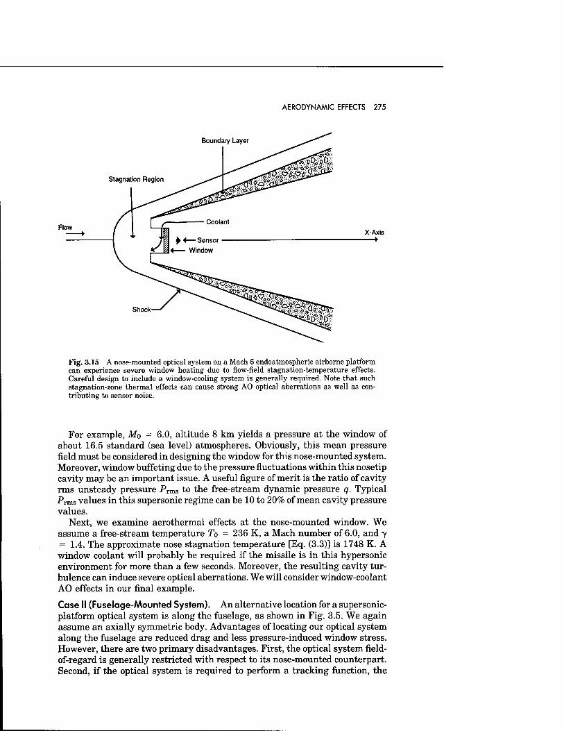
AERODYNAMIC EFFECTS 275
Boundary Layer
Stagnation Region
Flow
Shock-
Fig. 3.15 A nose-mounted optical system on a Mach 6 endoatmospheric airborne platform can experience severe window heating due to flow-field stagnation-temperature effects. Careful design to include a window-cooling system is generally required. Note that such stagnation-zone thermal effects can cause strong AO optical aberrations as well as con- tributing to sensor noise.
For example, Mo = 6.0, altitude 8 km yields a pressure at the window of about 16.5 standard (sea level) atmospheres. Obviously, this mean pressure field must be considered in designing the window for this nose-mounted system. Moreover, window buffeting due to the pressure fluctuations within this nosetip cavity may be an important issue. A useful figure of merit is the ratio of cavity rms unsteady pressure Prms to the free-stream dynamic pressure q. Typical Prms values in this supersonic regime can be 10 to 20% of mean cavity pressure values.
Next, we examine aerothermal effects at the nose-mounted window. We assume a free-stream temperature To = 236 K, a Mach number of 6.0, and 7 = 1.4. The approximate nose stagnation temperature [Eq. (3.3)] is 1748 K. A window coolant will probably be required if the missile is in this hypersonic environment for more than a few seconds. Moreover, the resulting cavity tur- bulence can induce severe optical aberrations. We will consider window-coolant AO effects in our final example.
Case II (Fuselage-Mounted System). An alternative location for a supersonic- platform optical system is along the fuselage, as shown in Fig. 3.5. We again assume an axially symmetric body. Advantages of locating our optical system along the fuselage are reduced drag and less pressure-induced window stress. However, there are two primary disadvantages. First, the optical system field- of-regard is generally restricted with respect to its nose-mounted counterpart. Second, if the optical system is required to perform a tracking function, the
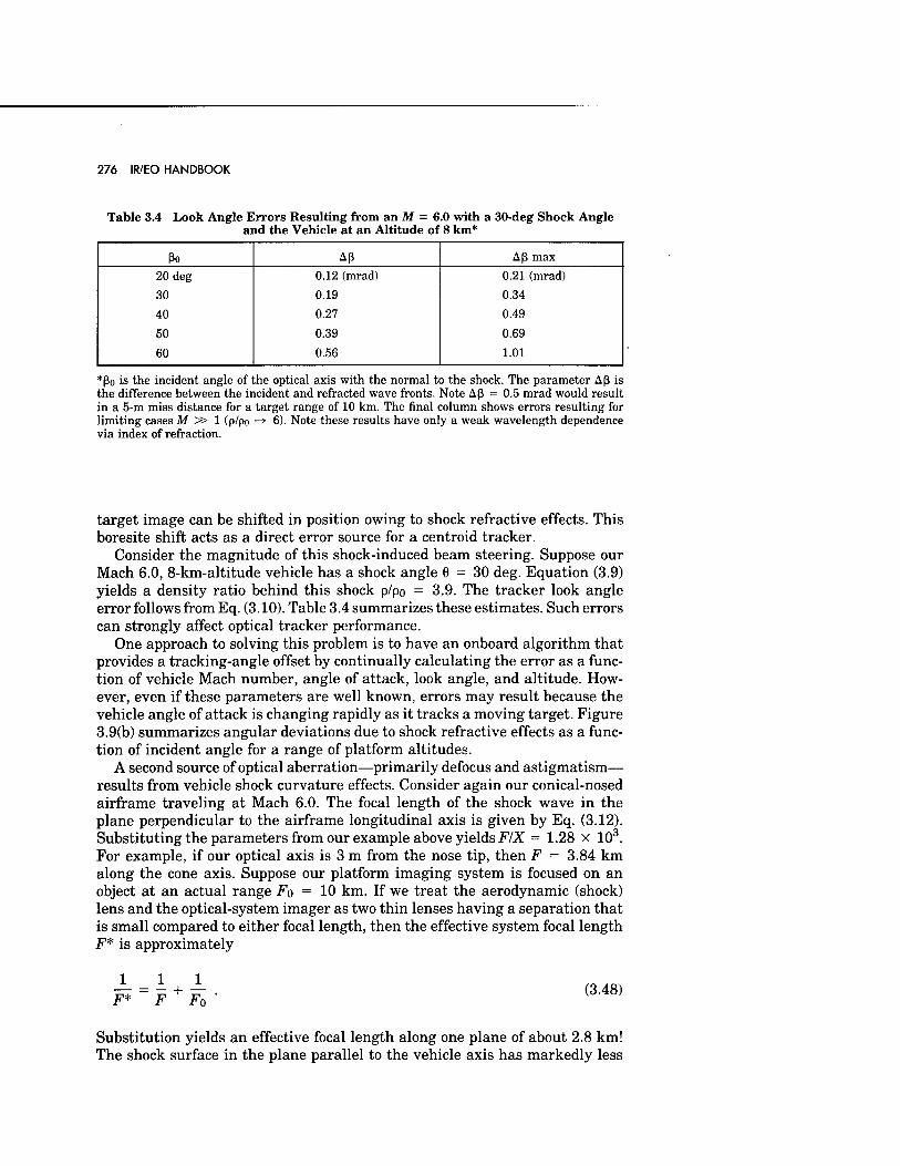
276 IR/EO HANDBOOK
Table 3.4 Look Angle Errors Resulting from an M = 6.0 with a 30-deg Shock Angle and the Vehicle at an Altitude of 8 km*
ßo Aß Aß max
20deg 0.12 (mrad) 0.21 (mrad)
30 0.19 0.34
40 0.27 0.49
50 0.39 0.69
60 0.56 1.01
*ßo is the incident angle of the optical axis with the normal to the shock. The parameter Aß is the difference between the incident and refracted wave fronts. Note Aß = 0.5 mrad would result in a 5-m miss distance for a target range of 10 km. The final column shows errors resulting for limiting cases M :» 1 (p/po —> 6). Note these results have only a weak wavelength dependence via index of refraction.
target image can be shifted in position owing to shock refractive effects. This boresite shift acts as a direct error source for a centroid tracker.
Consider the magnitude of this shock-induced beam steering. Suppose our Mach 6.0, 8-km-altitude vehicle has a shock angle 6 = 30 deg. Equation (3.9) yields a density ratio behind this shock p/po = 3.9. The tracker look angle error follows from Eq. (3.10). Table 3.4 summarizes these estimates. Such errors can strongly affect optical tracker performance.
One approach to solving this problem is to have an onboard algorithm that provides a tracking-angle offset by continually calculating the error as a func- tion of vehicle Mach number, angle of attack, look angle, and altitude. How- ever, even if these parameters are well known, errors may result because the vehicle angle of attack is changing rapidly as it tracks a moving target. Figure 3.9(b) summarizes angular deviations due to shock refractive effects as a func- tion of incident angle for a range of platform altitudes.
A second source of optical aberration—primarily defocus and astigmatism— results from vehicle shock curvature effects. Consider again our conical-nosed airframe traveling at Mach 6.0. The focal length of the shock wave in the plane perpendicular to the airframe longitudinal axis is given by Eq. (3.12). Substituting the parameters from our example above yields FIX = 1.28 x 10³. For example, if our optical axis is 3 m from the nose tip, then F = 3.84 km along the cone axis. Suppose our platform imaging system is focused on an object at an actual range Fo = 10 km. If we treat the aerodynamic (shock) lens and the optical-system imager as two thin lenses having a separation that is small compared to either focal length, then the effective system focal length F* is approximately
-1 = - — F* ~~ F + Fo
(3.48)
Substitution yields an effective focal length along one plane of about 2.8 km! The shock surface in the plane parallel to the vehicle axis has markedly less
AERODYNAMIC EFFECTS 277
curvature; thus, this supersonic flow field also causes astigmatic optical effects. If the platform beam-control system does not sense and correct for this shock aero-optical aberration, the transmitted beam will suffer significant loss of far-field performance. Note also that the above results are only weakly wave- length dependent via the Gladstone-Dale parameter.
This example conveys two important messages. First, supersonic vehicle windows will be exposed to extremely hostile environments. Second, fuselage- mounted optical imagers/trackers can experience mission-threatening aber- rations from platform shocks and inviscid effects even before random flow effects are considered. All factors must be carefully weighed by an optical designer.
3.4.8 Example 8—Supersonic Vehicle Flow-Field-Induced Thermal- Radiation Effects
Shock waves, random flows, and windows can introduce thermal noise into the platform sensors. We next examine the radiation strengths of these several sources. Consider a Mach 8 vehicle at altitude 10 km (To = 223 K) having a wedge-shaped nose with deflection angle Qv = 30 deg. From Fig. 8(b), the corresponding shock angle 6 is approximately 40 deg. The platform near-IR imaging system (sensor bandpass 1 to 2 (im) is located 1 m aft of the vehicle nosetip. We suppose the window coolant system maintains an average window temperature of 300 K. Radiation from flow ionization and plasmas can be important above this Mach number regime; however, these effects are ne- glected here.
There are, in general, three major vehicle flow-field contributors to sensor thermal noise: the shock layer, the fuselage boundary layer, and the window (adiabatic) temperature.
First, the ratio of static temperatures across a shock wave follows from the perfect gas law and Eq. (3.9):
JT _ [2yMl sin26 - (7 - 1)] [(7 - \)M% sin26 + 2] T0 (7 + If Ml sin20 • ( '
Substitution of the above values into Eq. (3.49) reveals a temperature T within the shock layer of approximately 1356 K.
Next, the boundary-layer temperature is estimated by taking the temper- ature behind the shock T as our effective static temperature, with a Mach number in this region following from4
fo sin26
2-yilfg sinz8 - (7 - 1) (sinzA9) 9 2 + (7 - l)Mo sinz9
M = ~ .,2 . 2 71 , • 2,-. • <3-5°)
Here, A6 is the difference between our shock angle 6 and the wedge angle Qv
(A6 — 10 deg). From Eq. (3.50), the Mach number behind the vehicle shock is M= 2.38, with a corresponding adiabatic wall temperature [Eq. (3.3)] Tw
= 2723 K. Note that Eq. (3.50), with A8 defined as above, is valid for all two-
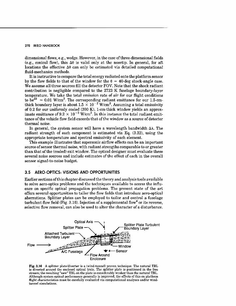
278 IR/EO HANDBOOK
dimensional flows, e.g., wedge. However, in the case of three-dimensional fields (e.g., conical flow), this A6 is valid only at the nosetip. In general, for aft locations the effective A6 can only be estimated via detailed computational fluid-mechanics methods.
It is instructive to compare the total energy radiated onto the platform sensor by the flow fields to that of the window for the 6 = 40-deg shock-angle case. We assume all three sources fill the detector FOV. Note that the shock radiant contribution is negligible compared to the 2723 K fuselage boundary-layer temperature. We take the total emission rate of air for our flight conditions to be23 — 0.01 W/cm3. The corresponding radiant emittance for our 1.5-cm- thick boundary layer is about 1.5 x 10 _2 W/cm2. Assuming a total emissivity of 0.2 for our uniformly cooled (300 K), 1-cm-thick window yields an approx- imate emittance of 9.2 x 10 ~3 W/cm2. In this instance the total radiant emit- tance of the vehicle flow field exceeds that of the window as a source of detector thermal noise.
In general, the system sensor will have a wavelength bandwidth A\. The radiant strength of each component is estimated via Eq. (3.32), using the appropriate temperature and spectral emissivity of each element.
This example illustrates that supersonic airflow effects can be an important source of sensor thermal noise, with radiant strengths comparable to or greater than that of the (cooled) exit window. The optical designer must evaluate these several noise sources and include estimates of the effect of each in the overall sensor signal-to-noise budget.
3.5 AERO-OPTICS: VISIONS AND OPPORTUNITIES
Earlier sections of this chapter discussed the theory and analysis tools available to solve aero-optics problems and the techniques available to access the influ- ence on specific optical propagation problems. The present state of the art offers several opportunities to tailor the flow fields that introduce aero-optical aberrations. Splitter plates can be employed to tailor and control a fuselage turbulent flow field (Fig. 3.16). Injection of a supplemental flow4 or its reverse, selective flow removal, can also be used to alter the character of a disturbance.
Optical Axis
Splitter Plate ■
Flow
Attached Turbulent Boundary Layer
Splitter Plate Turbulent Boundary Layer
Window Sensor
Flow Around Enclosure
Fig. 3.16 A splitter plate/diverter is a (wind-tunnel) proven technique. The natural TBL is diverted around the enclosed optical train. The splitter plate is positioned in the free stream; the resulting "new" TBL on the plate is considerably weaker than the natural TBL. Although system optical performance generally is improved, the effects of this on platform flight characteristics must be carefully evaluated via computational analyses and/or wind- tunnel simulations.
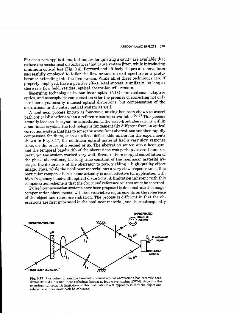
AERODYNAMIC EFFECTS 279
For open-port applications, techniques for quieting a cavity are available that reduce the mechanical disturbances that cause system jitter, while introducing minimum optical loss (Fig. 3.4). Forward and aft body shapes also have been successfully employed to tailor the flow around an exit aperture or a protu- berance extending into the free stream. While all of these techniques can, if properly employed, have a positive effect, total success is unlikely. As long as there is a flow field, residual optical aberration will remain.
Emerging technologies in nonlinear optics (NLO), conventional adaptive optics, and atmospheric compensation offer the promise of correcting not only local aerodynamically induced optical distortions, but compensation of the aberrations in the entire optical system as well.
A nonlinear process known as four-wave mixing has been shown to cancel path optical distortions when a reference source is available.24-27 This process actually leads to the dynamic cancellation of the wave-front aberrations within a nonlinear crystal. The technology is fundamentally different from an optical correction system that has to sense the wave-front aberrations and then rapidly compensate for them, such as with a deformable mirror. In the experiments shown in Fig. 3.17, the nonlinear optical material had a very slow response time, on the order of a second or so. The aberration source was a heat gun, and the temporal bandwidth of the aberrations was perhaps several hundred hertz, yet the system worked very well. Because there is rapid cancellation of the phase aberrations, the long time constant of the nonlinear material av- erages the distortions of the aberrator to zero, yielding a high-quality object image. Thus, while the nonlinear material has a very slow response time, this particular compensation scheme actually is most effective for application with high-frequency bandwidth optical distortions. A limitation inherent with this compensation scheme is that the object and reference sources must be coherent.
Pulsed compensation systems have been proposed to demonstrate the image- compensation phenomenon with less restrictive requirements on the coherence of the object and reference radiation. The process is different in that the ab- errations are first imprinted in the nonlinear material, and then subsequently
FROM POINT SOURCE
UNABERRATED IMAGE OF OUECT
E, PLANE-WAVE ' PUMP
Fig. 3.17 Correction of random flow-field-induced optical aberrations has recently been demonstrated via a nonlinear technique known as four-wave mixing (FWM). Shown is the experimental setup. A limitation of this particular FWM approach is that the object and reference sources must both be coherent.
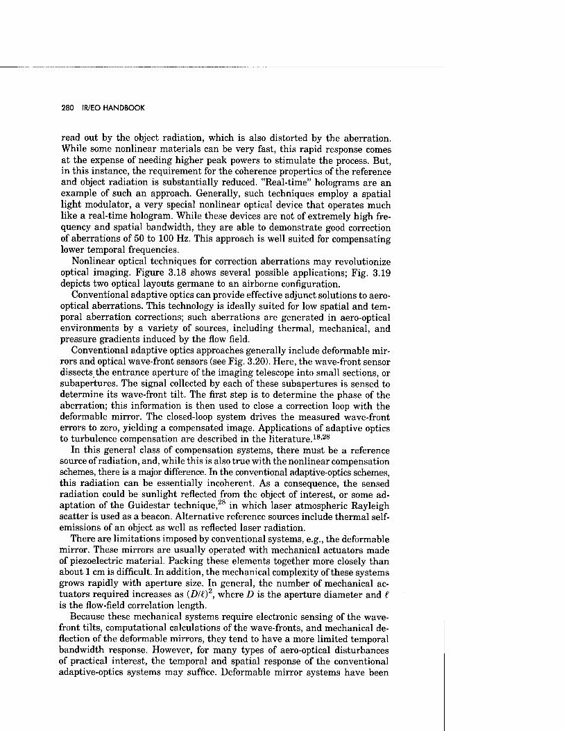
280 IR/EO HANDBOOK
read out by the object radiation, which is also distorted by the aberration. While some nonlinear materials can be very fast, this rapid response comes at the expense of needing higher peak powers to stimulate the process. But, in this instance, the requirement for the coherence properties of the reference and object radiation is substantially reduced. "Real-time" holograms are an example of such an approach. Generally, such techniques employ a spatial light modulator, a very special nonlinear optical device that operates much like a real-time hologram. While these devices are not of extremely high fre- quency and spatial bandwidth, they are able to demonstrate good correction of aberrations of 50 to 100 Hz. This approach is well suited for compensating lower temporal frequencies.
Nonlinear optical techniques for correction aberrations may revolutionize optical imaging. Figure 3.18 shows several possible applications; Fig. 3.19 depicts two optical layouts germane to an airborne configuration.
Conventional adaptive optics can provide effective adjunct solutions to aero- optical aberrations. This technology is ideally suited for low spatial and tem- poral aberration corrections; such aberrations are generated in aero-optical environments by a variety of sources, including thermal, mechanical, and pressure gradients induced by the flow field.
Conventional adaptive optics approaches generally include deformable mir- rors and optical wave-front sensors (see Fig. 3.20). Here, the wave-front sensor dissects the entrance aperture of the imaging telescope into small sections, or subapertures. The signal collected by each of these subapertures is sensed to determine its wave-front tilt. The first step is to determine the phase of the aberration; this information is then used to close a correction loop with the deformable mirror. The closed-loop system drives the measured wave-front errors to zero, yielding a compensated image. Applications of adaptive optics to turbulence compensation are described in the literature.18'28
In this general class of compensation systems, there must be a reference source of radiation, and, while this is also true with the nonlinear compensation schemes, there is a major difference. In the conventional adaptive-optics schemes, this radiation can be essentially incoherent. As a consequence, the sensed radiation could be sunlight reflected from the object of interest, or some ad- aptation of the Guidestar technique,28 in which laser atmospheric Rayleigh scatter is used as a beacon. Alternative reference sources include thermal self- emissions of an object as well as reflected laser radiation.
There are limitations imposed by conventional systems, e.g., the deformable mirror. These mirrors are usually operated with mechanical actuators made of piezoelectric material. Packing these elements together more closely than about 1 cm is difficult. In addition, the mechanical complexity of these systems grows rapidly with aperture size. In general, the number of mechanical ac- tuators required increases as (D/t)2, where D is the aperture diameter and € is the flow-field correlation length.
Because these mechanical systems require electronic sensing of the wave- front tilts, computational calculations of the wave-fronts, and mechanical de- flection of the deformable mirrors, they tend to have a more limited temporal bandwidth response. However, for many types of aero-optical disturbances of practical interest, the temporal and spatial response of the conventional adaptive-optics systems may suffice. Deformable mirror systems have been
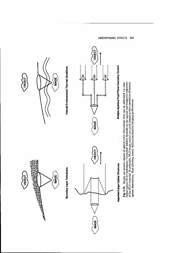
AERODYNAMIC EFFECTS 281
<n c
i 3 a E a
a E c s > e
UJ
c
8
E s a a c
JS a. Q. 3 Q. O ̂ 3 •c
.2 a
s c .£ 3
■fi
1 a
3 <8
3 XS 3 5
a O o s> 2
I S. E
- ä> a>
L « Ö Ö 0) Ö o w a)
I "I" £8*8 w CO o
11 g g »jj g It
■"Cob a <*c2<3
eg cö -t^> be
+3 03 O.S 03 0) S Sf)
§« « s
ftuJ
c2 2^ >> o-Sr *■
8 IS S
2 111 lf'&l
, H Ä u
K" .9 <*» o> fe 3 o o
■in:
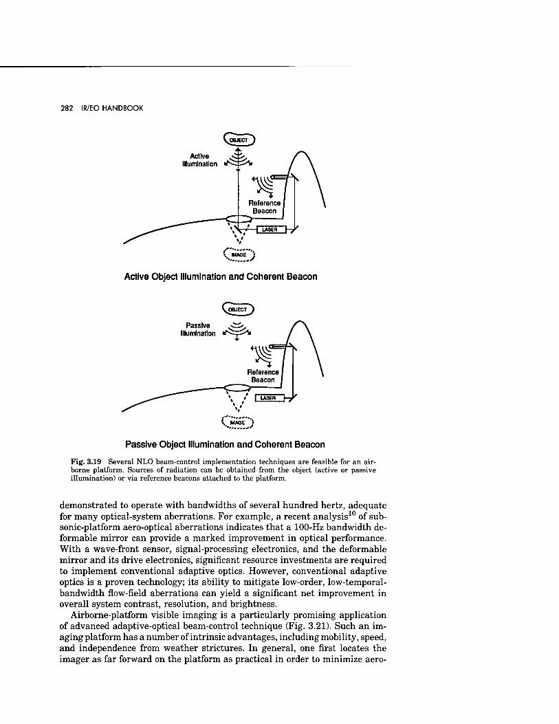
282 IR/EO HANDBOOK
Active Illumination
/ .. \MM3£ J
Active Object Illumination and Coherent Beacon
^OBJECT
Passive ji^. Illumination I^W-^SI
Passive Object Illumination and Coherent Beacon
Fig. 3.19 Several NLO beam-control implementation techniques are feasible for an air- borne platform. Sources of radiation can be obtained from the object (active or passive illumination) or via reference beacons attached to the platform.
demonstrated to operate with bandwidths of several hundred hertz, adequate for many optical-system aberrations. For example, a recent analysis10 of sub- sonic-platform aero-optical aberrations indicates that a 100-Hz bandwidth de- formable mirror can provide a marked improvement in optical performance. With a wave-front sensor, signal-processing electronics, and the deformable mirror and its drive electronics, significant resource investments are required to implement conventional adaptive optics. However, conventional adaptive optics is a proven technology; its ability to mitigate low-order, low-temporal- bandwidth flow-field aberrations can yield a significant net improvement in overall system contrast, resolution, and brightness.
Airborne-platform visible imaging is a particularly promising application of advanced adaptive-optical beam-control technique (Fig. 3.21). Such an im- aging platform has a number of intrinsic advantages, including mobility, speed, and independence from weather strictures. In general, one first locates the imager as far forward on the platform as practical in order to minimize aero-
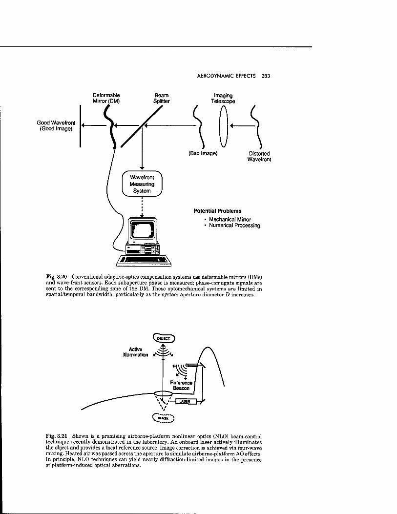
AERODYNAMIC EFFECTS 283
Deformable Mirror (DM)
Beam Splitter
Good Wavefront (Good Image)
Imaging Telescope
A
\J (Bad Image)
Wavefront Measuring
System
Distorted Wavefront
Potential Problems
• Mechanical Mirror • Numerical Processing
Fig. 3.20 Conventional adaptive-optics compensation systems use deformable mirrors (DMs) and wave-front sensors. Each subaperture phase is measured; phase-conjugate signals are sent to the corresponding zone of the DM. These optomechanical systems are limited in spatial/temporal bandwidth, particularly as the system aperture diameter D increases.
Active Illumination
Fig. 3.21 Shown is a promising airborne-platform nonlinear optics (NLO) beam-control technique recently demonstrated in the laboratory. An onboard laser actively illuminates the object and provides a local reference source. Image correction is achieved via four-wave mixing. Heated air was passed across the aperture to simulate airborne-platform AO effects. In principle, NLO techniques can yield nearly diffraction-limited images in the presence of platform-induced optical aberrations.
284 IR/EO HANDBOOK
optical effects. Even so, aircraft-fuselage boundary layers can sometimes se- verely constrain the performance of large-aperture, visible imaging systems. Nonlinear optical beam-control methods, perhaps in concert with conventional techniques, hold the potential of effecting almost total correction of both ac- induced and natural atmospheric optical aberrations. The exciting result could be image quality from airborne platforms limited only by intrinsic optical- system performance. Such is indeed a noble goal!
References
1. G. W. Sutton, "Effect of turbulent fluctuations in an optically active fluid medium," AIAA Journal 7(9), 1737-1743 (Sep. 1969).
2. J. H. Gladstone and J. Dale, "On the influence of temperature on the refraction of \ight"Phil. Trans. 148, 887 (1858).
3. G. Havener, "Optical wave front variance: a study of analytical models in use today," AIAA Paper 92-0654 (January 1992).
4. K. G. Gilbert and L. J. Otten, Aero-Optical Phenomena, Program in Astronautics and Aero- nautics (Volume 80), American Institute of Aeronautics and Astronautics, New York (1982).
5. L. D. Landau and E. M. Lifshitz, Fluid Mechanics, 2nd ed., p. 319, Pergamon Press, Elmsford, NY (1987).
6. L. D. Lorah and E. Rubin, "Aerodynamic influences on infrared system design," in The Infrared Handbook, W. L. Wolfe and G. J. Zissis, Eds., The Environmental Research Institute of Mich- igan, Ann Arbor, MI (Revised 1985).
7. J. E. Craig and W. C. Rose, "Wavelength effects on images formed through turbulence," AIAA Paper 87-1398 (June 1987).
8. J. E. Craig and W. C. Rose, "The optics of aircraft shear flows," AIAA Paper 85-0557 (March 1985).
9. W. C. Rose and J. M. Cooley, "Aerodynamics of the Kuiper Airborne Observatory cavity flow- field," REAR-TR-84-1, Rose Engineering and Research, Inc. (October 1984).
10. J. E. Craig and C. Allen, "Aero-optical turbulent boundary layer/shear layer experiment on the KC-135 aircraft revisited," Opt. Eng. 24(3), 446-454 (1985).
11. J. L. Elliot, E. W. Dunham, R. L. Baron, A. W. Watts, S. E. Kruse, W. C. Rose, and C. M. Gillespie, Jr., "Image quality on the Kuiper Airborne Observatory. I. Results of the first flight series," Astronomical Soc. Pacific 101, 737-764 (1989).
12. H. Schlichting, Boundary Layer Theory, 4th ed., McGraw-Hill Book Company, New York (1968).
13. W. C. Rose and J. M. Cooley, "Analysis of the aerodynamic data from the AOA wind tunnel test and implications for the AOA platform," Final Report Contract DAAH01-85-C-0312 (October 1985).
14. W. C. Rose and J. M. Cooley, "Feasibility of the contoured-aft-ramp concept for the KAO. Results from the Phase A and B studies," prepared for Northrop Services, Inc., NASA/Ames Research Center under Prime Contract NAS2-12235 (1987).
15. D. A. Buell, "Airloads near the open port of a one-meter airborne telescope," AIAA Paper 75-71, presented at the 13th Aerospace Sciences Meeting (January 1975).
16. W. C. Rose, "Aerodynamics of seeing on large transport aircraft—Progress report 1 December 1985-31 May 1986," prepared for NASA/Ames Research Center under Contract NCC2-382.
17. W. T. Welford, Optics, 3rd ed., p. 61, Oxford University Press, Oxford, UK (1988). 18. R. K. Tyson, Principles of Adaptive Optics, p. 15, Academic Press, Orlando, FL (1991). 19. J. B. Shellan, "Phased-array performance degradation due to mirror misfigures, piston error,
jitter, and polarization errors," Journal of the Optical Society of America A 2, 4 (1985). 20. M. R. Banish, R. L. Clark, and A. D. Kathman, "Wavelength dependence of blur circle size
through turbulent flow," Teledyne Brown Engineering Report No. 1326-25 (1990). 21. D. L. Fried, "Optical resolution through a randomly inhomogeneous medium for very long
and very short exposures," J. Opt. Soc. Am. 56, 1372 (1966).
AERODYNAMIC EFFECTS 285
22. M. S. Scholl, "Simulation of spectral radiance of a dynamic infrared source," dissertation, University of Arizona (1980).
23. S. S. Penner, Quantitative Molecular Spectroscopy and Gas Emissivities, Addison-Wesley Pub- lishing Company, Reading, MA (1959).
24. K. R. MacDonald, W. R. Tompkin, and R. W. Boyd, "Passive one way aberration correction using four wave mixing," Opt. Lett. 13, 485 (1988).
25. T. G. Alley, M. A. Kramer, D. R. Martinez, and L. P. Schelonka, "Single-pass imaging through a thick dynamic distorter using four wave mixing," Opt. Lett. 15, 81 (1990).
26. M. A. Kramer, T. G. Alley, D. R. Martinez, and L. P. Schelonka, "Effects of thick aberrations on a polarization dependent one-way imaging scheme," Appl. Opt. 29, 2576 (1990).
27. M. A. Kramer, C. J. Wetterer, and T. Martinez, "One way imaging through an aberrator with spatially incoherent light using an optically addressed spatial light modulator," Appl. Opt. 30, 3319 (1991).
28. R. Q. Fugate, D. L. Fried, G. A. Ameer, B. R. Boeke, S. L. Browne, P. H. Roberts, R. E. Ruane, G. A. Tyler, and L. M. Wopat, "Measurement of atmospheric wavefront distortion using scat- tered light from a laser guide-star," Nature 353, 144-146 (1991).
CHAPTER 4
Nonlinear Propagation: Thermal Blooming
Frederick G. Gebhardt Science Applications International Corporation
Lexington, Massachusetts
CONTENTS
4.1 Introduction 289 4.2 Historical Overview 289
4.2.1 The Early Years: 1964-1969 290 4.2.2 The Middle Years: 1969-1979 290 4.2.3 The Later Years: 1979-Present 290
4.3 Blooming Basics 291 4.3.1 Governing Equations 291 4.3.2 Isobaric Heating 292 4.3.3 Nonisobaric Heating 293
4.4 Steady-State Blooming with Wind/Beam Motion 294 4.4.1 Collimated Beam—Homogeneous Path 294 4.4.2 Focused Beams—Inhomogeneous Paths 299 4.4.3 Up-link Thermal Blooming 304
4.5 Conclusions 311 References 311
287
NONLINEAR PROPAGATION: THERAAAL BLOOMING 289
4.1 INTRODUCTION
When a high-energy laser (HEL) beam propagates through the atmosphere, a small portion of the energy is absorbed by certain molecules and particulate matter in the air. The absorbed energy heats the air, causing it to expand and form a distributed thermal lens along the atmospheric path that, in turn, spreads, bends, and distorts the laser beam. This self-induced effect is called thermal blooming and, since it can limit the maximum power that can be efficiently transmitted through the atmosphere, is one of the most serious nonlinear problems encountered in the propagation of high-energy laser ra- diation in the atmosphere. A variety of thermal blooming effects are relevant for high-energy laser beams in the atmosphere. Many of these effects have been studied extensively and a number of detailed review articles have been written that describe most of the work prior to about 1980.1_6
Because of the recent intense interest in small-scale thermal-blooming in- stabilities,7 it has become customary to refer to the large-scale thermal-blooming effects that spread, bend, and distort the entire beam as "whole-beam" thermal blooming. We restrict our attention here primarily to the problem of whole- beam thermal-blooming effects, which represents the bulk of the work prior to 1985. It is interesting to note, however, that the initial interest in and studies of thermal-blooming amplification of small-scale intensity perturba- tions, or stimulated thermal Rayleigh scattering (STRS),8,9 occurred prior to most of the work on whole-beam blooming effects in the atmosphere.
In this chapter we begin with an overview of the work that has been done on thermal blooming during the past twenty-five years. The emphasis here is to try to connect the extensive earlier results for whole-beam blooming effects with the more recent work on up-link thermal-blooming compensation and related small-scale instabilities. Section 2 gives a brief historical overview outlining the particular types of blooming problems that have been studied during each of the major periods of work on blooming since the first obser- vations of "thermal-lens" effects in liquids were reported.10'11 The fundamental thermal-blooming equations for continuous-wave (cw) and single-pulse laser beams are presented in Sec. 3. In Sec. 4 some of the basic results and scaling parameters for steady-state whole-beam thermal-blooming effects in the at- mosphere are reviewed. Here the blooming is characterized by isobaric heating with convection-dominated heat transfer, due to the combined effects of wind and beam motion. The cases considered include both collimated and focused beams propagating within the absorbing atmosphere as well as that of a ground- based laser beam propagating through the atmosphere to a target in space. Conclusions are presented in Sec. 5.
4.2 HISTORICAL OVERVIEW
If one looks at the work on thermal blooming over the past twenty-five years, one finds that it can be roughly divided into the following three periods based on the types and applications of the blooming problems being studied: (1) the early years (1964-1969), (2) the middle years (1969-1979), and (3) the late years (1979 to the present). The nature and emphasis of the thermal blooming work in these three periods is summarized below.
290 IR/EO HANDBOOK
4.2.1 The Early Years: 1964-1969
Work on whole-beam thermal blooming began with the first reported obser- vation of a new "thermal-lens effect" when transparent absorbing liquids (and some solids) were placed in a laser cavity.10,11 The major emphasis initially was on the thermal blooming of stationary cw laser beams in liquids. With thermal conduction as the dominant heat-transfer mechanism, the dominant effect on the laser beam was the spreading produced by the negative-lens-like refractive-index gradient, which naturally led to the use of terms like "thermal defocusing," "self-defocusing," "nonlinear defocusing," "self-induced diver- gence," etc.12-16 Early interest in the thermal-lens effect was in its practical application for low-absorption measurements.17-19 Another early application reported for the thermal-lens effect was for its use as a power-limiting device.20
Interest in high-energy laser-beam propagation in the atmosphere led to the earliest studies of both small-scale89 and whole-beam21-24 convection-dominated thermal-blooming effects in gases.15-18
4.2.2 The Middle Years: 1969-1979
For the next five years or so extensive experimental and theoretical efforts were devoted to developing a basic understanding of atmospheric thermal- blooming effects and their limits for cw, pulsed, and repetitively pulsed high- energy laser-beam propagation.1-5 The emphasis in these earlier studies was to develop a basic understanding of the physics of thermal-blooming process using simple and, more-or-less, idealized conditions to represent the charac- teristics of the laser beam and the atmosphere. A number of detailed wave- optics propagation codes were also developed to treat a variety of atmospheric thermal-blooming problems.1'2'4'5,25 Good agreement was obtained from com- parisons of the results from the codes and laboratory simulation experiments.4
Some of the special blooming problems studied, in addition to the important case of convection-dominated blooming with wind and beam slewing, included the effects of beam jitter, optical turbulence, turbulent mixing, kinetic cooling, stagnation zones, noncoplanar wind and beam slewing, transonic slewing, aero- sol blooming, and imaging through blooming. The use of focusing/defocusing, different beam profiles and aperture shapes, and phase compensation were all considered as possible ways for correcting or reducing thermal-blooming ef- fects.4 During the later years of this period the emphasis shifted toward (1) the development of both detailed wave-optics codes and systems-level scaling laws for treating the combined effects of thermal blooming together with all relevant linear effects (e.g., nonideal beam quality, beam jitter, turbulence-induced beam spreading and wander) and (2) the consideration of more realistic con- ditions for the laser beam, scenario, and electro-optical and meteorological (EO-MET) properties of the atmosphere.
4.2.3 The Later Years: 1979-Present
During this most recent period the major emphasis has been on the problems of blooming and its compensation for ground-to-space HEL beam propagation. Interest also shifted from the longer infrared wavelengths of the 10.6-fjim CO2 and 3.8-|xm DF lasers of greatest interest in the 1970s to the much shorter
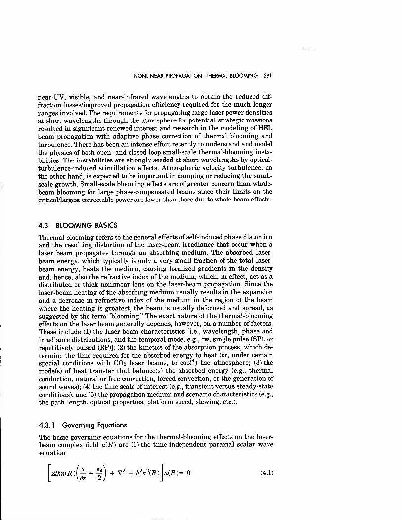
NONLINEAR PROPAGATION: THERMAL BLOOMING 291
near-UV, visible, and near-infrared wavelengths to obtain the reduced dif- fraction losses/improved propagation efficiency required for the much longer ranges involved. The requirements for propagating large laser power densities at short wavelengths through the atmosphere for potential strategic missions resulted in significant renewed interest and research in the modeling of HEL beam propagation with adaptive phase correction of thermal blooming and turbulence. There has been an intense effort recently to understand and model the physics of both open- and closed-loop small-scale thermal-blooming insta- bilities. The instabilities are strongly seeded at short wavelengths by optical- turbulence-induced scintillation effects. Atmospheric velocity turbulence, on the other hand, is expected to be important in damping or reducing the small- scale growth. Small-scale blooming effects are of greater concern than whole- beam blooming for large phase-compensated beams since their limits on the critical/largest correctable power are lower than those due to whole-beam effects.
4.3 BLOOMING BASICS
Thermal blooming refers to the general effects of self-induced phase distortion and the resulting distortion of the laser-beam irradiance that occur when a laser beam propagates through an absorbing medium. The absorbed laser- beam energy, which typically is only a very small fraction of the total laser- beam energy, heats the medium, causing localized gradients in the density and, hence, also the refractive index of the medium, which, in effect, act as a distributed or thick nonlinear lens on the laser-beam propagation. Since the laser-beam heating of the absorbing medium usually results in the expansion and a decrease in refractive index of the medium in the region of the beam where the heating is greatest, the beam is usually defocused and spread, as suggested by the term "blooming." The exact nature of the thermal-blooming effects on the laser beam generally depends, however, on a number of factors. These include (1) the laser beam characteristics [i.e., wavelength, phase and irradiance distributions, and the temporal mode, e.g., cw, single pulse (SP), or repetitively pulsed (RP)]; (2) the kinetics of the absorption process, which de- termine the time required for the absorbed energy to heat (or, under certain special conditions with CO2 laser beams, to cool4) the atmosphere; (3) the mode(s) of heat transfer that balance(s) the absorbed energy (e.g., thermal conduction, natural or free convection, forced convection, or the generation of sound waves); (4) the time scale of interest (e.g., transient versus steady-state conditions); and (5) the propagation medium and scenario characteristics (e.g., the path length, optical properties, platform speed, slewing, etc.).
4.3.1 Governing Equations
The basic governing equations for the thermal-blooming effects on the laser- beam complex field u(R) are (1) the time-independent paraxial scalar wave equation
If 2ikn(R)\^ + % \dz 2
+ V^ + *V(Ä) u(R)= 0 (4.1)
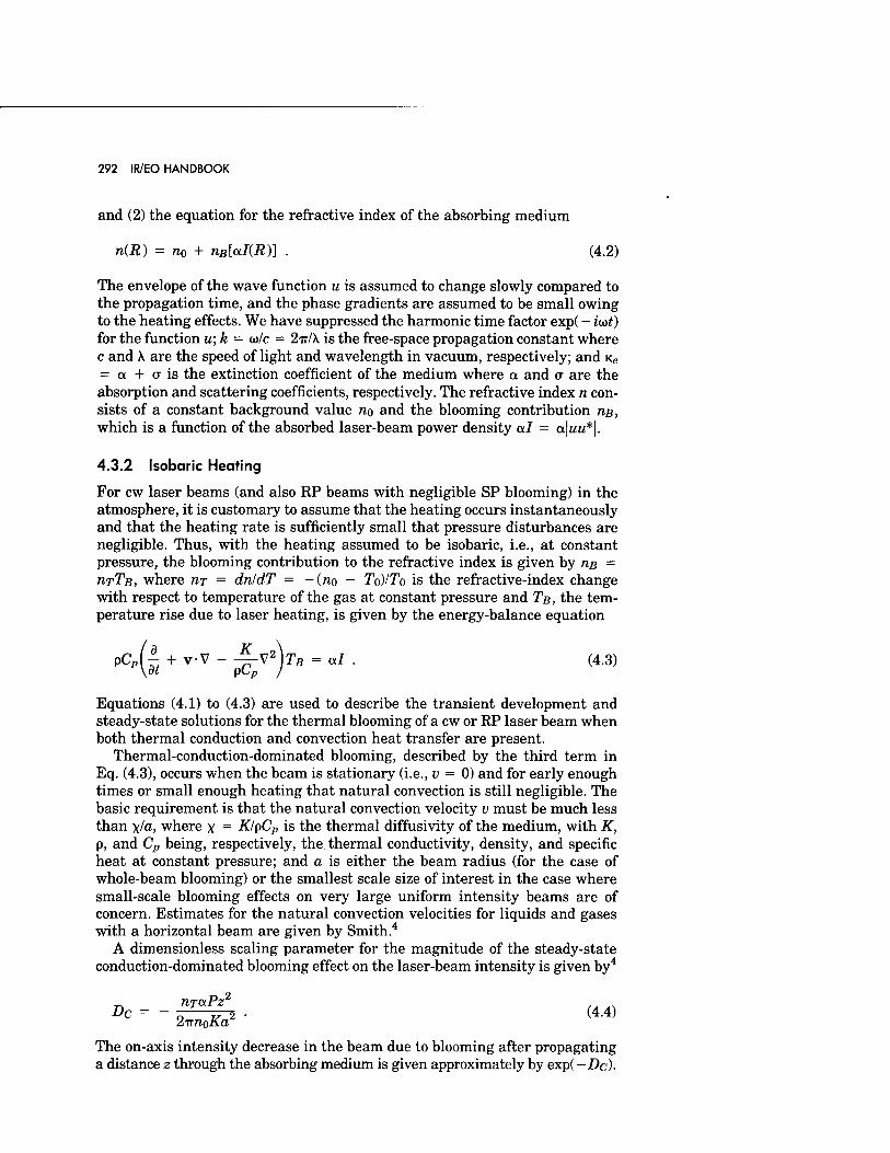
292 IR/EO HANDBOOK
and (2) the equation for the refractive index of the absorbing medium
MR) = n0 + nB[aI(R)] . (4.2)
The envelope of the wave function u is assumed to change slowly compared to the propagation time, and the phase gradients are assumed to be small owing to the heating effects. We have suppressed the harmonic time factor exp( - mt) for the function u;k = w/c = 2TT/X. is the free-space propagation constant where c and X are the speed of light and wavelength in vacuum, respectively; and Ke
= a + o- is the extinction coefficient of the medium where a and a are the absorption and scattering coefficients, respectively. The refractive index n con- sists of a constant background value no and the blooming contribution TIB, which is a function of the absorbed laser-beam power density al = a.\uu*\.
4.3.2 Isobaric Heating
For cw laser beams (and also RP beams with negligible SP blooming) in the atmosphere, it is customary to assume that the heating occurs instantaneously and that the heating rate is sufficiently small that pressure disturbances are negligible. Thus, with the heating assumed to be isobaric, i.e., at constant pressure, the blooming contribution to the refractive index is given by riß = UTTB, where TIT = dnldT = -(no - To)ITo is the refractive-index change with respect to temperature of the gas at constant pressure and TB, the tem- perature rise due to laser heating, is given by the energy-balance equation
t + v-V -4rv2 dt pCp
pCp\ T + vV - — Vz )TB = al . (4.3)
Equations (4.1) to (4.3) are used to describe the transient development and steady-state solutions for the thermal blooming of a cw or RP laser beam when both thermal conduction and convection heat transfer are present.
Thermal-conduction-dominated blooming, described by the third term in Eq. (4.3), occurs when the beam is stationary (i.e., v = 0) and for early enough times or small enough heating that natural convection is still negligible. The basic requirement is that the natural convection velocity v must be much less than x/o, where x = K/pCp is the thermal diffusivity of the medium, with K, p, and Cp being, respectively, the thermal conductivity, density, and specific heat at constant pressure; and a is either the beam radius (for the case of whole-beam blooming) or the smallest scale size of interest in the case where small-scale blooming effects on very large uniform intensity beams are of concern. Estimates for the natural convection velocities for liquids and gases with a horizontal beam are given by Smith.4
A dimensionless scaling parameter for the magnitude of the steady-state conduction-dominated blooming effect on the laser-beam intensity is given by4
D UTCLPZ2
2-nnoKa2
The on-axis intensity decrease in the beam due to blooming after propagating a distance z through the absorbing medium is given approximately by exp( -De).
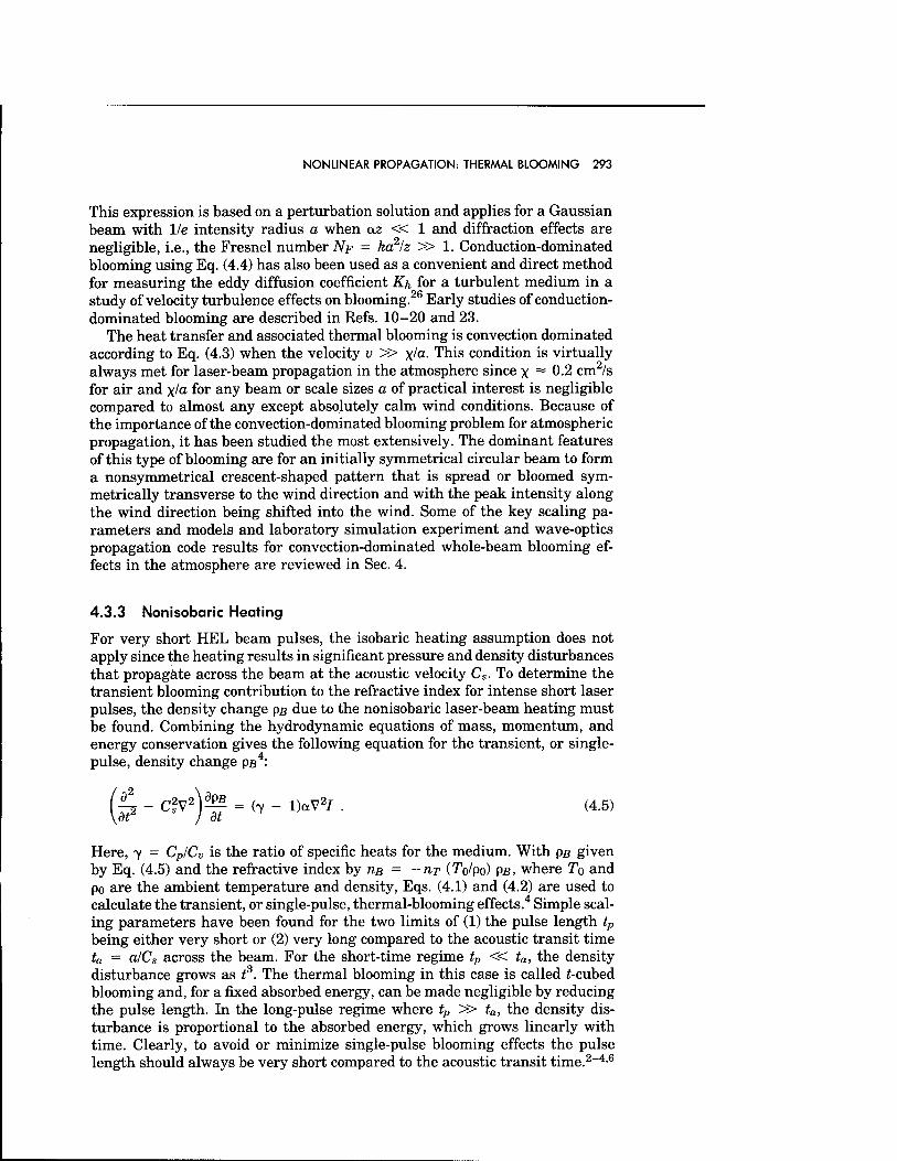
NONLINEAR PROPAGATION: THERMAL BLOOMING 293
This expression is based on a perturbation solution and applies for a Gaussian beam with lie intensity radius a when az « 1 and diffraction effects are negligible, i.e., the Fresnel number NF = ka2/z » 1. Conduction-dominated blooming using Eq. (4.4) has also been used as a convenient and direct method for measuring the eddy diffusion coefficient Kh for a turbulent medium in a study of velocity turbulence effects on blooming.26 Early studies of conduction- dominated blooming are described in Refs. 10-20 and 23.
The heat transfer and associated thermal blooming is convection dominated according to Eq. (4.3) when the velocity v » x/°- This condition is virtually always met for laser-beam propagation in the atmosphere since x "" 0.2 cm2/s for air and \la for any beam or scale sizes a of practical interest is negligible compared to almost any except absolutely calm wind conditions. Because of the importance of the convection-dominated blooming problem for atmospheric propagation, it has been studied the most extensively. The dominant features of this type of blooming are for an initially symmetrical circular beam to form a nonsymmetrical crescent-shaped pattern that is spread or bloomed sym- metrically transverse to the wind direction and with the peak intensity along the wind direction being shifted into the wind. Some of the key scaling pa- rameters and models and laboratory simulation experiment and wave-optics propagation code results for convection-dominated whole-beam blooming ef- fects in the atmosphere are reviewed in Sec. 4.
4.3.3 Nonisobaric Heating
For very short HEL beam pulses, the isobaric heating assumption does not apply since the heating results in significant pressure and density disturbances that propagate across the beam at the acoustic velocity Cs. To determine the transient blooming contribution to the refractive index for intense short laser pulses, the density change ps due to the nonisobaric laser-beam heating must be found. Combining the hydrodynamic equations of mass, momentum, and energy conservation gives the following equation for the transient, or single- pulse, density change pß4:
S - C2V2)^ = (7 - l)aV2/ . (4.5) at / at
Here, 7 = Cp/Cv is the ratio of specific heats for the medium. With ps given by Eq. (4.5) and the refractive index by res = -TIT (To/po) ps, where To and po are the ambient temperature and density, Eqs. (4.1) and (4.2) are used to calculate the transient, or single-pulse, thermal-blooming effects.4 Simple scal- ing parameters have been found for the two limits of (1) the pulse length tp
being either very short or (2) very long compared to the acoustic transit time ta = alCs across the beam. For the short-time regime tp « ta, the density disturbance grows as t3. The thermal blooming in this case is called f-cubed blooming and, for a fixed absorbed energy, can be made negligible by reducing the pulse length. In the long-pulse regime where tp » ta, the density dis- turbance is proportional to the absorbed energy, which grows linearly with time. Clearly, to avoid or minimize single-pulse blooming effects the pulse length should always be very short compared to the acoustic transit time.2-4,6
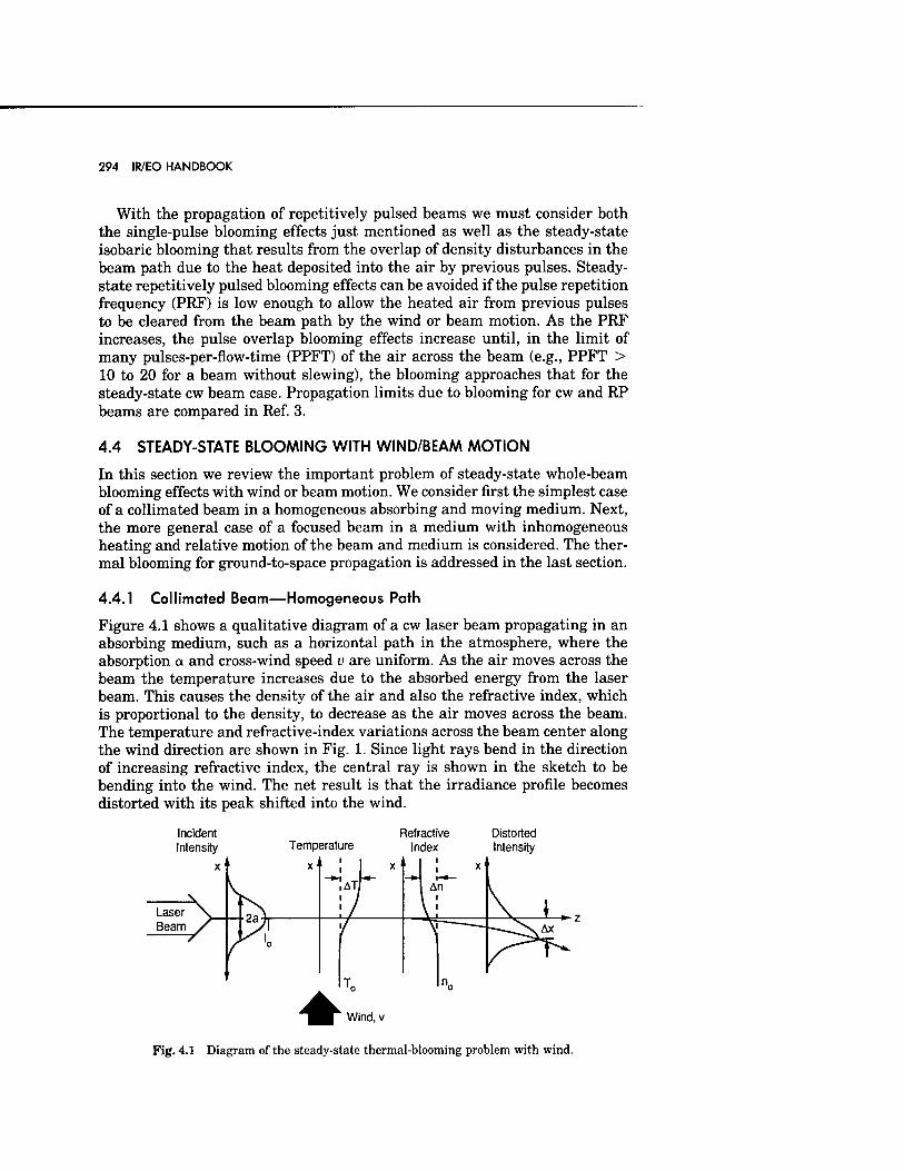
294 IR/EO HANDBOOK
With the propagation of repetitively pulsed beams we must consider both the single-pulse blooming effects just mentioned as well as the steady-state isobaric blooming that results from the overlap of density disturbances in the beam path due to the heat deposited into the air by previous pulses. Steady- state repetitively pulsed blooming effects can be avoided if the pulse repetition frequency (PRF) is low enough to allow the heated air from previous pulses to be cleared from the beam path by the wind or beam motion. As the PRF increases, the pulse overlap blooming effects increase until, in the limit of many pulses-per-flow-time (PPFT) of the air across the beam (e.g., PPFT > 10 to 20 for a beam without slewing), the blooming approaches that for the steady-state cw beam case. Propagation limits due to blooming for cw and RP beams are compared in Ref. 3.
4.4 STEADY-STATE BLOOMING WITH WIND/BEAM MOTION
In this section we review the important problem of steady-state whole-beam blooming effects with wind or beam motion. We consider first the simplest case of a collimated beam in a homogeneous absorbing and moving medium. Next, the more general case of a focused beam in a medium with inhomogeneous heating and relative motion of the beam and medium is considered. The ther- mal blooming for ground-to-space propagation is addressed in the last section.
4.4.1 Collimated Beam—Homogeneous Path
Figure 4.1 shows a qualitative diagram of a cw laser beam propagating in an absorbing medium, such as a horizontal path in the atmosphere, where the absorption a and cross-wind speed v are uniform. As the air moves across the beam the temperature increases due to the absorbed energy from the laser beam. This causes the density of the air and also the refractive index, which is proportional to the density, to decrease as the air moves across the beam. The temperature and refractive-index variations across the beam center along the wind direction are shown in Fig. 1. Since light rays bend in the direction of increasing refractive index, the central ray is shown in the sketch to be bending into the wind. The net result is that the irradiance profile becomes distorted with its peak shifted into the wind.
Incident Intensity Temperature
Refractive Index
Distorted Intensity
T0
Wind, v
Fig. 4.1 Diagram of the steady-state thermal-blooming problem with wind.
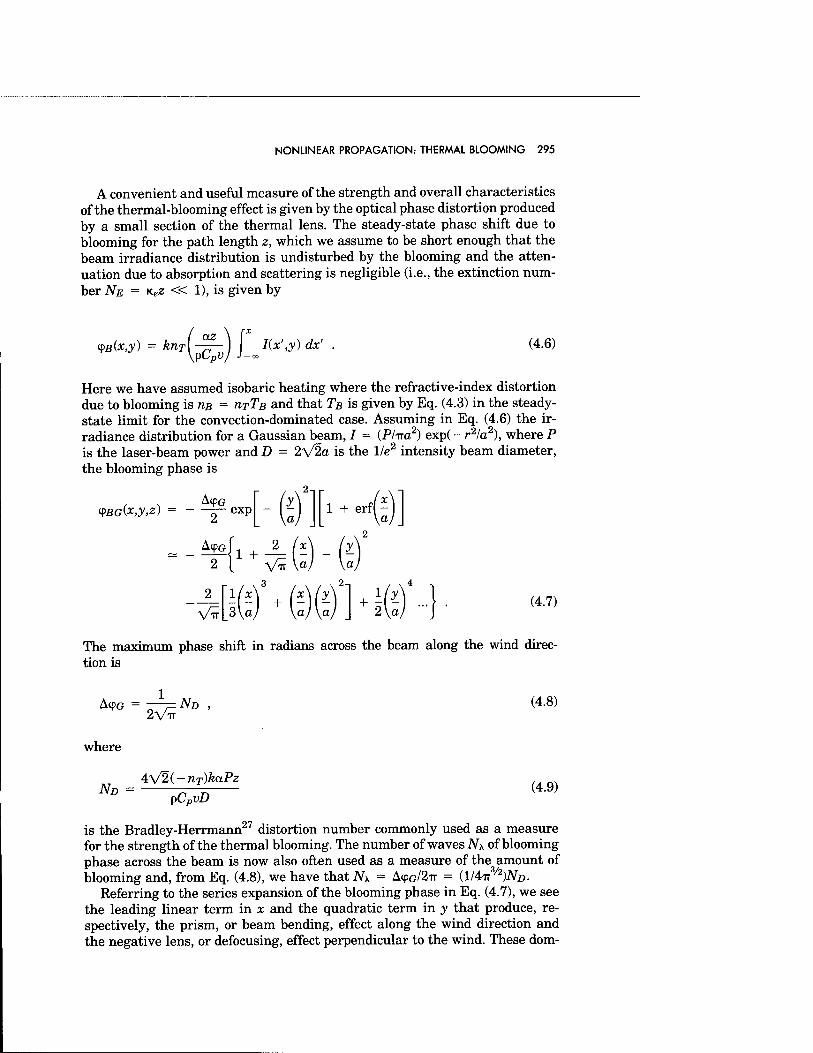
NONLINEAR PROPAGATION: THERMAL BLOOMING 295
A convenient and useful measure of the strength and overall characteristics of the thermal-blooming effect is given by the optical phase distortion produced by a small section of the thermal lens. The steady-state phase shift due to blooming for the path length z, which we assume to be short enough that the beam irradiance distribution is undisturbed by the blooming and the atten- uation due to absorption and scattering is negligible (i.e., the extinction num- ber NE = Kez « 1), is given by
VB(x,y) = ^f-^rj \_J{x',y)dx' (4.6)
Here we have assumed isobaric heating where the refractive-index distortion due to blooming is riß = UTTB and that TB is given by Eq. (4.3) in the steady- state limit for the convection-dominated case. Assuming in Eq. (4.6) the ir- radiance distribution for a Gaussian beam, / = (P/ira2) exp( - r2/a2), where P is the laser-beam power and D = 2V2a is the 1/e2 intensity beam diameter, the blooming phase is
<PBG(xj,z) = ~ AipG exp
+ 2 1 vir
3 2 ill' +
1 + erfF
2
♦§G (4.7)
The maximum phase shift in radians across the beam along the wind direc- tion is
A<PG 2VÜ
ND , (4.8)
where
ND = 4V2(-nT)kaPz
pCpvD (4.9)
is the Bradley-Herrmann27 distortion number commonly used as a measure for the strength of the thermal blooming. The number of waves N\ of blooming phase across the beam is now also often used as a measure of the amount of blooming and, from Eq. (4.8), we have thatiV\ = A(PG/2IT = (1/4TT
/2)ND-
Referring to the series expansion of the blooming phase in Eq. (4.7), we see the leading linear term in x and the quadratic term in y that produce, re- spectively, the prism, or beam bending, effect along the wind direction and the negative lens, or defocusing, effect perpendicular to the wind. These dom-
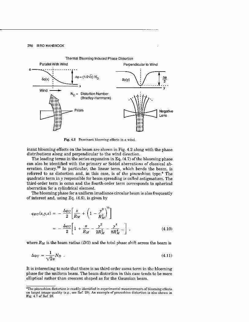
296 IR/EO HANDBOOK
Thermal Blooming Induced Phase Distortion
Parallel With Wind Perpendicular to Wind
A<|> = (1/2VTT) Nr
ND = Distortion Number (Bradley-Herrmann)
Prism Negative Lens
Fig. 4.2 Dominant blooming effects in a wind.
inant blooming effects on the beam are shown in Fig. 4.2 along with the phase distributions along and perpendicular to the wind direction.
The leading terms in the series expansion in Eq. (4.7) of the blooming phase can also be identified with the primary or Seidel aberrations of classical ab- erration theory.28 In particular, the linear term, which bends the beam, is referred to as distortion and, in this case, is of the pincushion type.a The quadratic term in y responsible for beam spreading is called astigmatism. The third-order term is coma and the fourth-order term corresponds to spherical aberration for a cylindrical element.
The blooming phase for a uniform irradiance circular beam is also frequently of interest and, using Eq. (4.6), is given by
q>Bu(x,y,z) A<p£/
RM +
A<pu 1 + RM
R2
2R2
Vs>-
Ml J
M 8R\, M J (4.10)
where RM is the beam radius (D/2) and the total phase shift across the beam is
Acptr = V2¥
ND (4.11)
It is interesting to note that there is no third-order coma term in the blooming phase for the uniform beam. The beam distortion in this case tends to be more elliptical rather than crescent shaped as for the Gaussian beam.
"The pincushion distortion is readily identified in experimental measurements of blooming effects on target image quality (e.g., see Ref. 29). An example of pincushion distortion is also shown in Fig. 4.7 of Ref. 28.
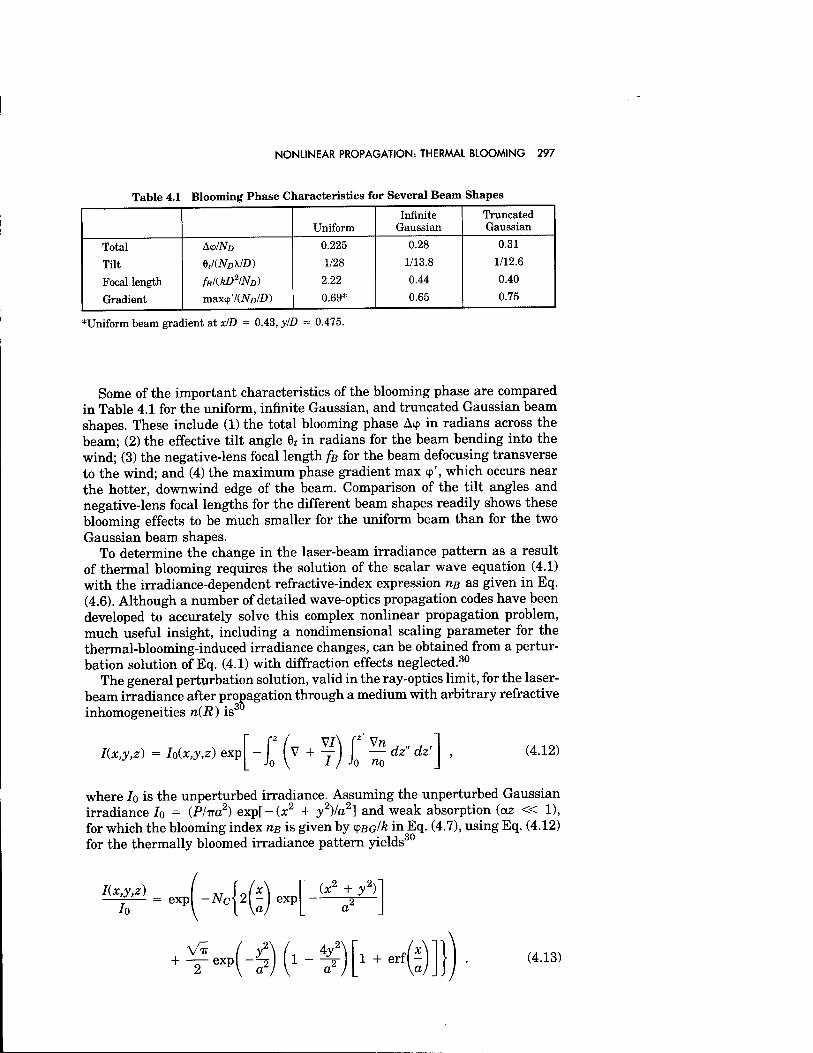
NONLINEAR PROPAGATION: THERMAL BLOOMING 297
Table 4.1 Blooming Phase Characteristics for Several Beam Shapes
Infinite Truncated Uniform Gaussian Gaussian
Total A<p/iVz) 0.225 0.28 0.31
Tilt Q,/(ND\ID) 1/28 1/13.8 1/12.6
Focal length fBl{kD2IND) 2.22 0.44 0.40
Gradient maxif'I(NDID) 0.69* 0.65 0.75
»Uniform beam gradient at xlD = 0.43, yID = 0.475.
Some of the important characteristics of the blooming phase are compared in Table 4.1 for the uniform, infinite Gaussian, and truncated Gaussian beam shapes. These include (1) the total blooming phase A<p in radians across the beam; (2) the effective tilt angle 8* in radians for the beam bending into the wind; (3) the negative-lens focal length /B for the beam defocusing transverse to the wind; and (4) the maximum phase gradient max cp', which occurs near the hotter, downwind edge of the beam. Comparison of the tilt angles and negative-lens focal lengths for the different beam shapes readily shows these blooming effects to be much smaller for the uniform beam than for the two Gaussian beam shapes.
To determine the change in the laser-beam irradiance pattern as a result of thermal blooming requires the solution of the scalar wave equation (4.1) with the irradiance-dependent refractive-index expression m as given in Eq. (4.6). Although a number of detailed wave-optics propagation codes have been developed to accurately solve this complex nonlinear propagation problem, much useful insight, including a nondimensional scaling parameter for the thermal-blooming-induced irradiance changes, can be obtained from a pertur- bation solution of Eq. (4.1) with diffraction effects neglected.30
The general perturbation solution, valid in the ray-optics limit, for the laser- beam irradiance after propagation through a medium with arbitrary refractive inhomogeneities n(R) is3
I(x,y,z) = Io(x,y,z) exp Jo V I / Jo no
(4.12)
where Jo is the unperturbed irradiance. Assuming the unperturbed Gaussian irradiance 70 = (P/na2) exp[-0e2 + y2)/a2] and weak absorption (<xz « 1), for which the blooming index nB is given by <pBG/k in Eq. (4.7), using Eq. (4.12) for the thermally bloomed irradiance pattern yields30
^ = -l-H2(>' te2+/>
♦£•*(-$) (-* 1 + erf I - a
(4.13)
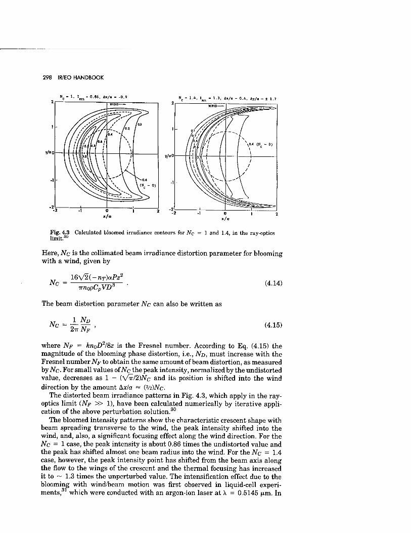
298 IR/EO HANDBOOK
Nc - >•*. !ML " 1-3. Ax/« - 0.4. Ay/« - ± 1.7
v/«o
Fig. 4.3 Calculated bloomed irradiance contours for Nc = 1 and 1.4, in the ray-optics limit.30
Here, Nc is the collimated beam irradiance distortion parameter for blooming with a wind, given by
Nc = 16V2(-nT)aPz2
■nnopCpVD3 (4.14)
The beam distortion parameter Nc can also be written as
N = — ^£ C 2iriV> (4.15)
where NF = knoD2/8z is the Fresnel number. According to Eq. (4.15) the magnitude of the blooming phase distortion, i.e., ND, must increase with the Fresnel number NF to obtain the same amount of beam distortion, as measured by Nc. For small values of Nc the peak intensity, normalized by the undistorted value, decreases as 1 - (\ZTT/2)NC and its position is shifted into the wind direction by the amount Ax/a = (3/2)Nc-
The distorted beam irradiance patterns in Fig. 4.3, which apply in the ray- optics limit (NF » 1), have been calculated numerically by iterative appli- cation of the above perturbation solution.30
The bloomed intensity patterns show the characteristic crescent shape with beam spreading transverse to the wind, the peak intensity shifted into the wind, and, also, a significant focusing effect along the wind direction. For the Nc = 1 case, the peak intensity is about 0.86 times the undistorted value and the peak has shifted almost one beam radius into the wind. For the Nc = 1.4 case, however, the peak intensity point has shifted from the beam axis along the flow to the wings of the crescent and the thermal focusing has increased it to ~ 1.3 times the unperturbed value. The intensification effect due to the blooming with wind/beam motion was first observed in liquid-cell experi- ments,31 which were conducted with an argon-ion laser at K = 0.5145 |j.m. In
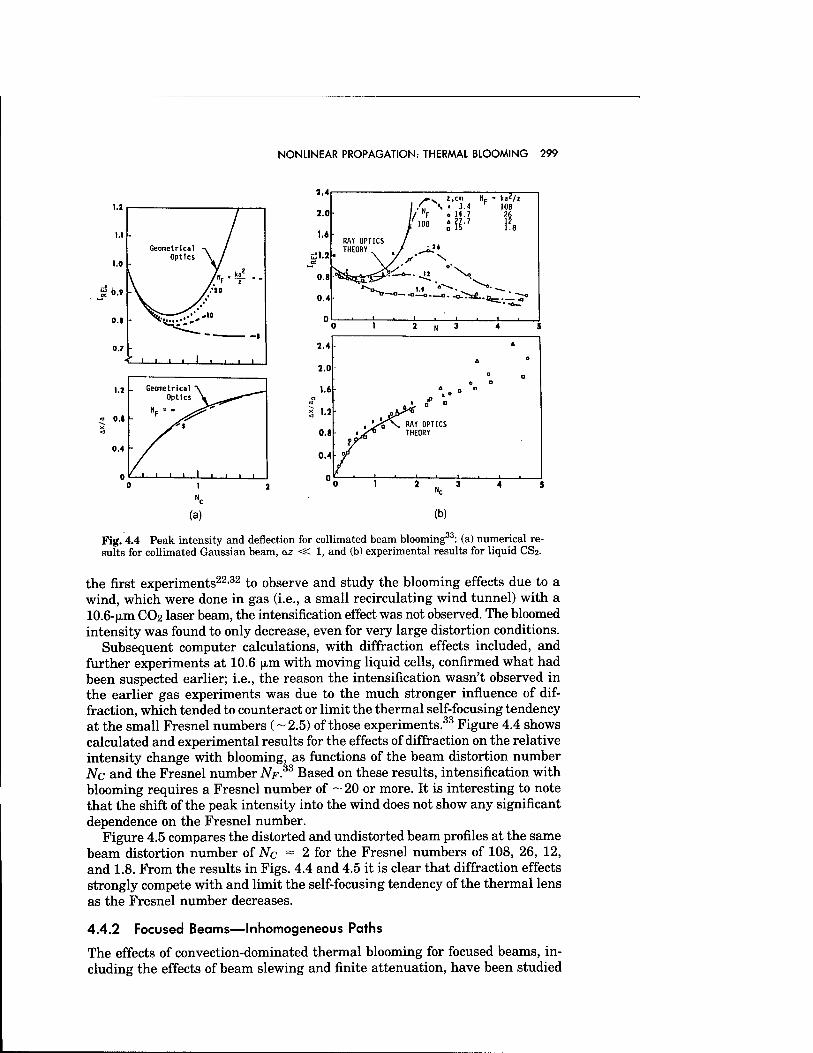
NONLINEAR PROPAGATION: THERMAL BLOOMING 299
3.4
2.0
1.4
0.8
0.4
0
| 4> . 3.4 // NF o H.7
/"» ill'
- kaz/j 108 26
1?8 MY OPTICS / THEORY „ . / ^."
^r"-°---<1--^--o^^i£..e_ V
■ 1 ■
1.2 Geometrical "\ Optics
0.1
^fi
0.4
0 1 l i i i 1 —l_..l i i
Fig. 4.4 suits for
I 2 Nc
(a)
Peak intensity and deflection for collimated beam blooming33: (a) numerical re- collimated Gaussian beam, az <sc 1, and (b) experimental results for liquid CS2.
the first experiments22,32 to observe and study the blooming effects due to a wind, which were done in gas (i.e., a small recirculating wind tunnel) with a 10.6-|xm CO2 laser beam, the intensification effect was not observed. The bloomed intensity was found to only decrease, even for very large distortion conditions.
Subsequent computer calculations, with diffraction effects included, and further experiments at 10.6 jx,m with moving liquid cells, confirmed what had been suspected earlier; i.e., the reason the intensification wasn't observed in the earlier gas experiments was due to the much stronger influence of dif- fraction, which tended to counteract or limit the thermal self-focusing tendency at the small Fresnel numbers (~2.5) of those experiments.33 Figure 4.4 shows calculated and experimental results for the effects of diffraction on the relative intensity change with blooming, as functions of the beam distortion number Nc and the Fresnel number iV>33 Based on these results, intensification with blooming requires a Fresnel number of ~ 20 or more. It is interesting to note that the shift of the peak intensity into the wind does not show any significant dependence on the Fresnel number.
Figure 4.5 compares the distorted and undistorted beam profiles at the same beam distortion number of Nc ~ 2 for the Fresnel numbers of 108, 26, 12, and 1.8. From the results in Figs. 4.4 and 4.5 it is clear that diffraction effects strongly compete with and limit the self-focusing tendency of the thermal lens as the Fresnel number decreases.
4.4.2 Focused Beams—Inhomogeneous Paths
The effects of convection-dominated thermal blooming for focused beams, in- cluding the effects of beam slewing and finite attenuation, have been studied
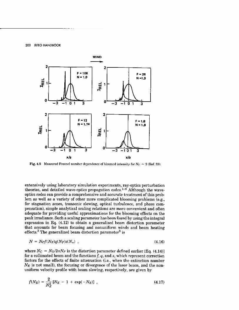
300 IR/EO HANDBOOK
WIND
m 1
*.J £ F-108 N-1.9
-3 -10 1
F-26 N-1.9
,x 1. -3 -10 1
-3-10 1 3 ~ -3-1013
x/a x/a
Fig. 4.5 Measured Fresnel number dependence of bloomed intensity for Nc ~ 2 (Ref. 33).
extensively using laboratory simulation experiments, ray-optics perturbation theories, and detailed wave-optics propagation codes.1-6 Although the wave- optics codes can provide a comprehensive and accurate treatment of this prob- lem as well as a variety of other more complicated blooming problems (e.g., for stagnation zones, transonic slewing, optical turbulence, and phase com- pensation), simple analytical scaling relations are more convenient and often adequate for providing useful approximations for the blooming effects on the peak irradiance. Such a scaling parameter has been found by using the integral expression in Eq. (4.12) to obtain a generalized beam distortion parameter that accounts for beam focusing and nonuniform winds and beam heating effects.3 The generalized beam distortion parameter3 is
N = Ncf(NE)q(NF)s(NJ (4.16)
where Nc = ND/2TTNF is the distortion parameter denned earlier [Eq. (4.14)] for a collimated beam and the functions /, q, and s, which represent correction factors for the effects of finite attenuation (i.e., when the extinction number NE is not small), the focusing or divergence of the laser beam, and the non- uniform velocity profile with beam slewing, respectively, are given by
f(NE) = -2 WE JSIE
1 + exp(-iV£)] (4.17)
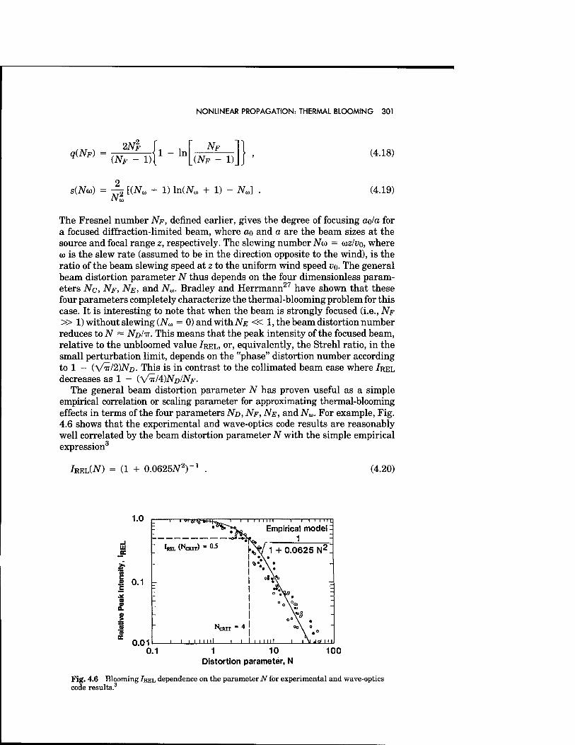
NONLINEAR PROPAGATION: THERMAL BLOOMING 301
q{NF) = m^n?1 ~ln NF
(NF - 1) (4.18)
s(iVo>) = -2 [(#„ _2_
+ 1) ln(iVw + 1) - 2VJ (4.19)
The Fresnel number NF, denned earlier, gives the degree of focusing ao/a for a focused diffraction-limited beam, where ao and a are the beam sizes at the source and focal range z, respectively. The slewing number Nu = <az/vo, where <i) is the slew rate (assumed to be in the direction opposite to the wind), is the ratio of the beam slewing speed at z to the uniform wind speed VQ. The general beam distortion parameter N thus depends on the four dimensionless param- eters Nc, NF, NE, and iVu. Bradley and Herrmann27 have shown that these four parameters completely characterize the thermal-blooming problem for this case. It is interesting to note that when the beam is strongly focused (i.e., NF » 1) without slewing (2VW = 0) and with NE « 1, the beam distortion number reduces to N ~ ND/TT. This means that the peak intensity of the focused beam, relative to the unbloomed value IREL, or, equivalently, the Strehl ratio, in the small perturbation limit, depends on the "phase" distortion number according to 1 — (\/TT/2)ND. This is in contrast to the collimated beam case where IREL
decreases as 1 - (\/TT/4)ND/NF. The general beam distortion parameter N has proven useful as a simple
empirical correlation or scaling parameter for approximating thermal-blooming effects in terms of the four parameters ND, NF, NE, and Nw. For example, Fig. 4.6 shows that the experimental and wave-optics code results are reasonably well correlated by the beam distortion parameter N with the simple empirical expression3
IREL(N) = (1 + 0.0625iV2r (4.20)
1 1—I I I I I II 1 1—I I MIL
Empirical model ■oS-SS*. 1
IREL (NCHII) = °-5 LW ., + 0 0625 N2
1 10 Distortion parameter, N
100
Fig. 4.6 Blooming /REL dependence on the parameter N for experimental and wave-optics code results.3
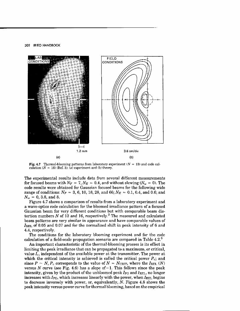
302 IR/EO HANDBOOK
1.2 mm
(a)
Fig. 4.7 Thermal-blooming patterns from laboratory experiment (N culation (N = 16) (Ref. 3): (a) experiment and (b) theory.
3.6 cm/div
(b)
13) and code cal-
The experimental results include data from several different measurements for focused beams with NF = 7, NE = 0.4, and without slewing (AL = 0). The code results were obtained for Gaussian focused beams for the following wide range of conditions: NF = 3, 6,10, 18, 28, and 66; NE = 0.1, 0.4, and 0.6; and Nw = 0, 3.8, and 8.
Figure 4.7 shows a comparison of results from a laboratory experiment and a wave-optics code calculation for the bloomed irradiance pattern of a focused Gaussian beam for very different conditions but with comparable beam dis- tortion numbers N of 13 and 16, respectively.3 The measured and calculated beam patterns are very similar in appearance and have comparable values of IREL of 0.05 and 0.07 and for the normalized shift in peak intensity of 6 and 4.4, respectively.
The conditions for the laboratory blooming experiment and for the code calculation of a field-scale propagation scenario are compared in Table 4.2.3
An important characteristic of the thermal-blooming process is its effect in limiting the peak irradiance that can be propagated to a maximum, or critical, value 7C, independent of the available power at the transmitter. The power at which the critical intensity is achieved is called the critical power Pc; and since P ~ N, Pc corresponds to the value of N = NCRIT, where the JREL (N) versus N curve (see Fig. 4.6) has a slope of-1. This follows since the peak intensity, given by the product of the unbloomed peak 7po and 7REL, no longer increases with IPO, which increases linearly with the power, when ZREL begins to decrease inversely with power, or, equivalently, N. Figure 4.8 shows the peak intensity versus power curve for thermal blooming, based on the empirical
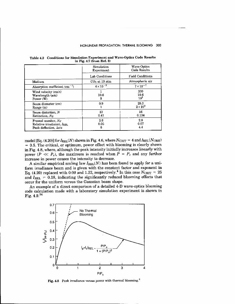
NONLINEAR PROPAGATION: THERMAL BLOOMING 303
Table 4.2 Conditions for Simulation Experiment and Wave-Optics Code Results in Fig. 4.7 (from Ref. 3)
Simulation Experiment
Wave-Optics Code Results
Lab Conditions Field Conditions
Medium C02 at 10 atm Atmospheric air
Absorption coefficient (cm-1) 4xl0-3 7xl0"7
Wind velocity (cm/s) Wavelength (n,m) Power (W)
1 10.6
9
200 10.6 105
Beam diameter (cm) Range(m)
0.9 1
28.3 2xl03
Beam distortion, N Extinction, NB
13 0.41
16 0.134
Fresnel number, iV> Relative irradiance, JREL Peak deflection, Ax/a
2.6 0.05
6
2.8 0.07 4.4
model [Eq. (4.20)] forlxEiiN) shown in Fig. 4.6, where NCBIT = 4 and/REL(iVcRiT) = 0.5. The critical, or optimum, power effect with blooming is clearly shown in Fig. 4.8, where, although the peak intensity initially increases linearly with power (P « Pc), the maximum is reached when P = Pc and any further increase in power causes the intensity to decrease.
A similar empirical scaling law IREL(N) has been found to apply for a uni- form irradiance beam and is given with the constant factor and exponent in Eq. (4.20) replaced with 0.09 and 1.22, respectively.4 In this case iVcRiT = 25 and ZREL = 0.18, indicating the significantly reduced blooming effects that occur for the uniform versus the Gaussian beam shape.
An example of a direct comparison of a detailed 4-D wave-optics blooming code calculation made with a laboratory simulation experiment is shown in Fig. 4.9.34
0.7
0.6 No Thermal Blooming
Fig. 4.8 Peak irradiance versus power with thermal blooming.'
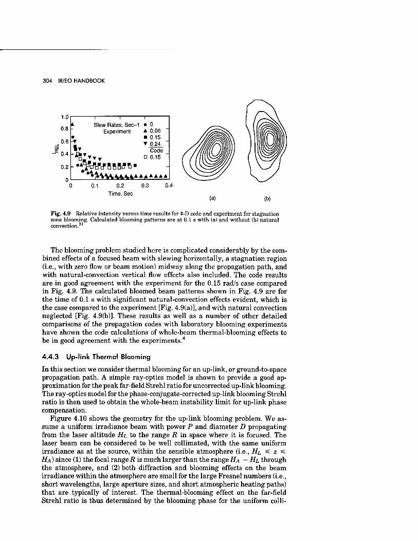
304 IR/EO HANDBOOK
1.0
0.8
0.6 -T
0.2
Slew Rates, Sec-1 Experiment
IT
•V.4,
I • 0 A 0.06 ■ 0.15 ▼ 0.24
Code D 0.15
'V.^AA.AAA.^AAAAAA
0.1 0.2
Time, Sec
0.3 0.4
(a) (b)
Fig. 4.9 Relative intensity versus time results for 4-D code and experiment for stagnation zone blooming. Calculated blooming patterns are at 0.1 s with (a) and without (b) natural convection.34
The blooming problem studied here is complicated considerably by the com- bined effects of a focused beam with slewing horizontally, a stagnation region (i.e., with zero flow or beam motion) midway along the propagation path, and with natural-convection vertical flow effects also included. The code results are in good agreement with the experiment for the 0.15 rad/s case compared in Fig. 4.9. The calculated bloomed beam patterns shown in Fig. 4.9 are for the time of 0.1 s with significant natural-convection effects evident, which is the case compared to the experiment [Fig. 4.9(a)], and with natural convection neglected [Fig. 4.9(b)]. These results as well as a number of other detailed comparisons of the propagation codes with laboratory blooming experiments have shown the code calculations of whole-beam thermal-blooming effects to be in good agreement with the experiments.4
4.4.3 Up-link Thermal Blooming
In this section we consider thermal blooming for an up-link, or ground-to-space propagation path. A simple ray-optics model is shown to provide a good ap- proximation for the peak far-field Strehl ratio for unconnected up-link blooming. The ray-optics model for the phase-conjugate-corrected up-link blooming Strehl ratio is then used to obtain the whole-beam instability limit for up-link phase compensation.
Figure 4.10 shows the geometry for the up-link blooming problem. We as- sume a uniform irradiance beam with power P and diameter D propagating from the laser altitude HL to the range R in space where it is focused. The laser beam can be considered to be well collimated, with the same uniform irradiance as at the source, within the sensible atmosphere (i.e., HL =£ z ^ HA) since (1) the focal range R is much larger than the range HA - HL through the atmosphere, and (2) both diffraction and blooming effects on the beam irradiance within the atmosphere are small for the large Fresnel numbers (i.e., short wavelengths, large aperture sizes, and short atmospheric heating paths) that are typically of interest. The thermal-blooming effect on the far-field Strehl ratio is thus determined by the blooming phase for the uniform colli-
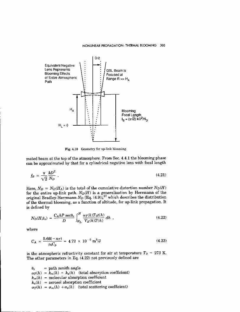
NONLINEAR PROPAGATION: THERMAL BLOOMING 305
Equivalent Negative Lens Represents Blooming Effects of Entire Atmospheric Path
HL = 0
GBL Beam is Focused at Range R » HA
Blooming Focal Length fB = (jn/jjj kD2/ND
Fig. 4.10 Geometry for up-link blooming.
mated beam at the top of the atmosphere. From Sec. 4.4.1 the blooming phase can be approximated by that for a cylindrical negative lens with focal length
fn = IT kD2
V2 ND (4.21)
Here, ND = ND(HA) is the total of the cumulative distortion number ND(H) for the entire up-link path. ND(H) is a generalization by Herrmann of the original Bradley-Herrmann ND [Eq. (4.9)],27 which describes the distribution of the thermal blooming, as a function of altitude, for up-link propagation. It is denned by
„,„A, CAkP sec6z [H aT(h)Ttit(h) JL ND(HA) = \HL yE{h)T{h) dh ,
where
CA = 5.66( — TIT)
poCp = 4.72 x 10 "9 m3/J
(4.22)
(4.23)
is the atmospheric refractivity constant for air at temperature To = 273 K. The other parameters in Eq. (4.22) not previously defined are
6Z = path zenith angle aT(h) = km(h) + ka(h) (total absorption coefficient) km(h) = molecular absorption coefficient ka(h) = aerosol absorption coefficient OT(/I) = Vmih) +(Ta(h) (total scattering coefficient)
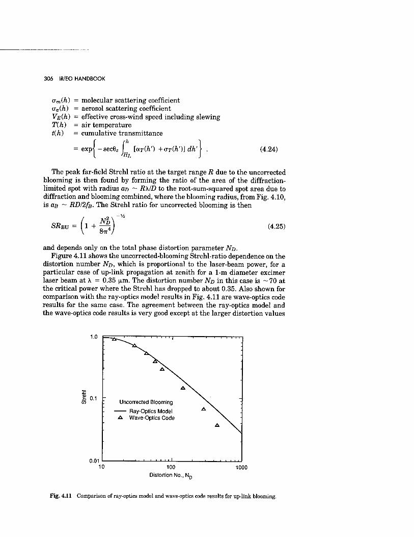
306 IR/EO HANDBOOK
(rm(h) = molecular scattering coefficient (Ta(h) = aerosol scattering coefficient Vß(A) = effective cross-wind speed including slewing T(h) = air temperature t(h) = cumulative transmittance
= expj -sec62 j [aT(h') +aT(h')] dh' (4.24)
The peak far-field Strehl ratio at the target range R due to the unconnected blooming is then found by forming the ratio of the area of the diffraction- limited spot with radius ao ~ RX/D to the root-sum-squared spot area due to diffraction and blooming combined, where the blooming radius, from Fig. 4.10, is as ~ RDI2fß. The Strehl ratio for unconnected blooming is then
SÄBU = 1 + ND
8TT4
-y2
(4.25)
and depends only on the total phase distortion parameter ND. Figure 4.11 shows the unconected-blooming Strehl-ratio dependence on the
distortion number ND, which is proportional to the laser-beam power, for a particular case of up-link propagation at zenith for a 1-m diameter excimer laser beam at \ = 0.35 fim. The distortion number ND in this case is ~ 70 at the critical power where the Strehl has dropped to about 0.35. Also shown for comparison with the ray-optics model results in Fig. 4.11 are wave-optics code results for the same case. The agreement between the ray-optics model and the wave-optics code results is very good except at the larger distortion values
1.0
£ o.i
0.01
Uncorrected Blooming
Ray-Optics Model A Wave-Optics Code
_l_ 10 100
Distortion No., Nr
1000
Fig. 4.11 Comparison of ray-optics model and wave-optics code results for up-link blooming.
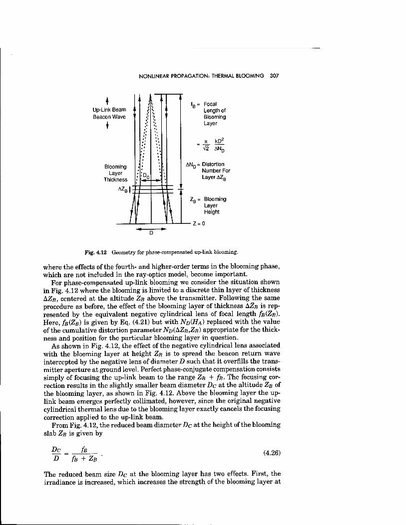
NONLINEAR PROPAGATION: THERAAAL BLOOMING 307
T Up-Link Beam Beacon Wave
t
Blooming Layer
Thickness
AZB1
■D,
fB= Focal Length of Blooming Layer
7i kD
V2 AN,
AND = Distortion Number For Layer AZB
ZB= Blooming Layer Height
Z = 0
Fig. 4.12 Geometry for phase-compensated up-link blooming.
where the effects of the fourth- and higher-order terms in the blooming phase, which are not included in the ray-optics model, become important.
For phase-compensated up-link blooming we consider the situation shown in Fig. 4.12 where the blooming is limited to a discrete thin layer of thickness AZB, centered at the altitude ZB above the transmitter. Following the same procedure as before, the effect of the blooming layer of thickness AZB is rep- resented by the equivalent negative cylindrical lens of focal length /B(ZB). Here, fßiZß) is given by Eq. (4.21) but with ND(HA) replaced with the value of the cumulative distortion parameter ND(&ZB,ZB) appropriate for the thick- ness and position for the particular blooming layer in question.
As shown in Fig. 4.12, the effect of the negative cylindrical lens associated with the blooming layer at height ZB is to spread the beacon return wave intercepted by the negative lens of diameter D such that it overfills the trans- mitter aperture at ground level. Perfect phase-conjugate compensation consists simply of focusing the up-link beam to the range ZB + fß. The focusing cor- rection results in the slightly smaller beam diameter Dc at the altitude ZB of the blooming layer, as shown in Fig. 4.12. Above the blooming layer the up- link beam emerges perfectly collimated, however, since the original negative cylindrical thermal lens due to the blooming layer exactly cancels the focusing correction applied to the up-link beam.
From Fig. 4.12, the reduced beam diameter Dc at the height of the blooming slab ZB is given by
Dc D
h fß + ZB
(4.26)
The reduced beam size Dc at the blooming layer has two effects. First, the irradiance is increased, which increases the strength of the blooming layer at
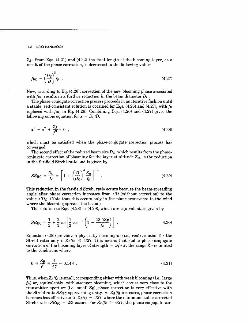
308 IR/EO HANDBOOK
ZB. From Eqs. (4.21) and (4.22) the focal length of the blooming layer, as a result of the phase correction, is decreased to the following value:
/Bc = (^j/b. (4.27)
Now, according to Eq. (4.26), correction of the new blooming phase associated with /BC results in a further reduction in the beam diameter Dc-
The phase-conjugate correction process proceeds in an iterative fashion until a stable, self-consistent solution is obtained for Eqs. (4.26) and (4.27), with fs replaced with /BC in Eq- (4.26). Combining Eqs. (4.26) and (4.27) gives the following cubic equation for x = Dc/D:
x3 - x2 + Z§-= 0 , (4.28)
which must be satisfied when the phase-conjugate correction process has converged.
The second effect of the reduced beam size Dc, which results from the phase- conjugate correction of blooming for the layer at altitude ZB, is the reduction in the far-field Strehl ratio and is given by
SRBC = -jr
3 D\ ZB
1 + \Dc) h (4.29)
This reduction in the far-field Strehl ratio occurs because the beam-spreading angle after phase correction increases from KID (without correction) to the value A7.Dc- (Note that this occurs only in the plane transverse to the wind where the blooming spreads the beam.)
The solution to Eqs. (4.28) or (4.29), which are equivalent, is given by
12 SRBC = ö + Ö cos 1 _! L 13.5ZB - cos 1 -
3 \ fa (4.30)
Equation (4.30) provides a physically meaningful (i.e., real) solution for the Strehl ratio only if Zßlfß =S 4/27. This means that stable phase-conjugate correction of the blooming layer of strength ~ 1/fß at the range ZB is limited to the conditions where
Zn 4 0 ^ -4 ^ — - 0.148 . (4.31)
T 27
Thus, when Zßlfß is small, corresponding either with weak blooming (i.e., large fß) or, equivalently, with stronger blooming, which occurs very close to the transmitter aperture (i.e., small ZB), phase correction is very effective with the Strehl ratio SRBC approaching unity. As Zß/fß increases, phase correction becomes less effective until Zßlfß = 4/27, where the minimum stable corrected Strehl ratio SRBC = 2/3 occurs. For Zßlfß > 4/27, the phase-conjugate cor-
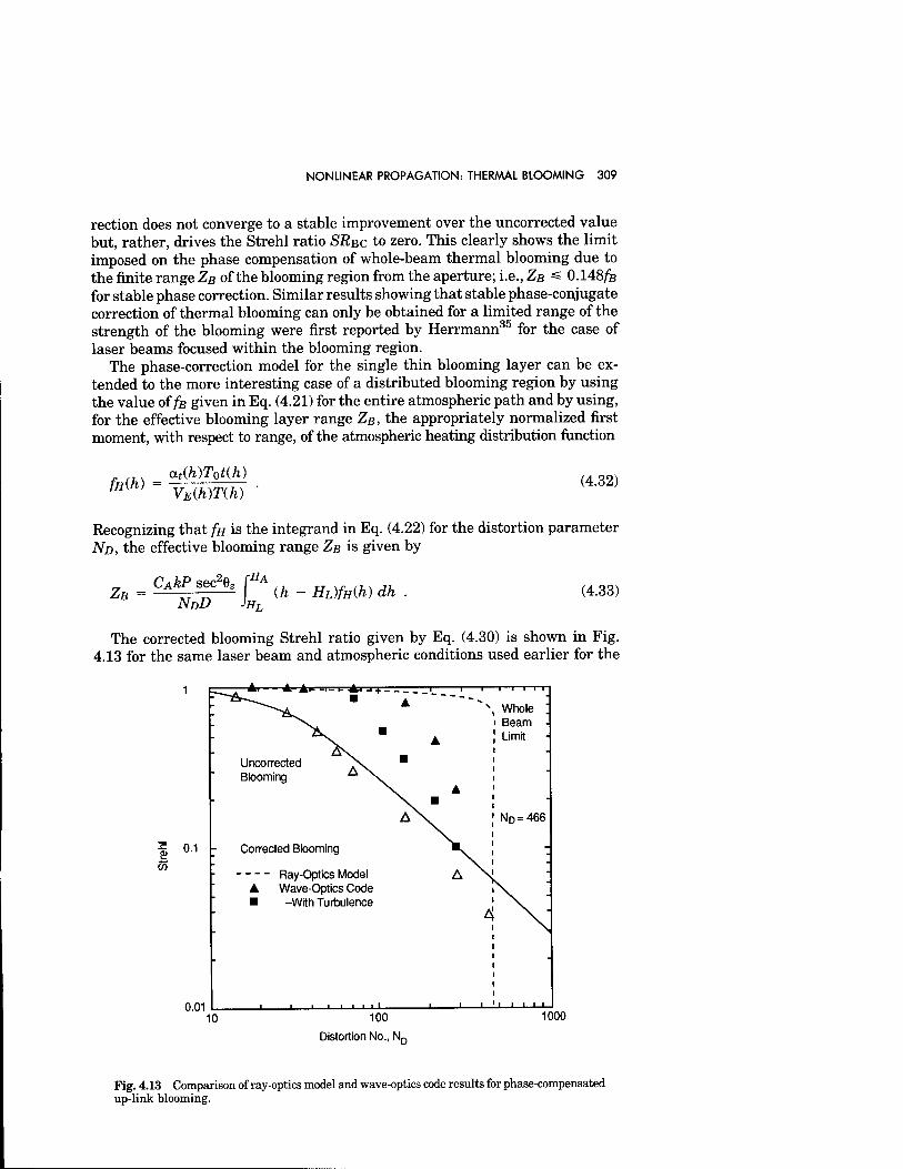
NONLINEAR PROPAGATION: THERAAAL BLOOMING 309
rection does not converge to a stable improvement over the uncorrected value but, rather, drives the Strehl ratio SRBC to zero. This clearly shows the limit imposed on the phase compensation of whole-beam thermal blooming due to the finite range ZB of the blooming region from the aperture; i.e., ZB =S 0.148/B for stable phase correction. Similar results showing that stable phase-conjugate correction of thermal blooming can only be obtained for a limited range of the strength of the blooming were first reported by Herrmann35 for the case of laser beams focused within the blooming region.
The phase-correction model for the single thin blooming layer can be ex- tended to the more interesting case of a distributed blooming region by using the value of /B given in Eq. (4.21) for the entire atmospheric path and by using, for the effective blooming layer range ZB, the appropriately normalized first moment, with respect to range, of the atmospheric heating distribution function
feih) = at(h)Tot(h) VE(h)T(h)
(4.32)
Recognizing that fa is the integrand in Eq. (4.22) for the distortion parameter ND, the effective blooming range ZB is given by
ZB = CAki *?*' \HA (h - HL)fH(h) dh NDD JHL
(4.33)
The corrected blooming Strehl ratio given by Eq. (4.30) is shown in Fig. 4.13 for the same laser beam and atmospheric conditions used earlier for the
2> 55
0.1 -
0.01
1 —Ai - A- Ar- H- i- -A* -I T"^
A "\ Whole ; ^*^ i Beam -
2K. " A J Limit
Uncorrected ^K
Blooming ^v
■
A ■ i
As J ND=466
; Corrected Blooming J -
Ray-Optics Model A Wave-Optics Code ■ -With Turbulence
A
III!
W
■ i i ■ i i i 11 ■ ■
|
10 100
Distortion No., Nn
1000
Fig. 4.13 Comparison of ray-optics model and wave-optics code results for phase-compensated up-link blooming.
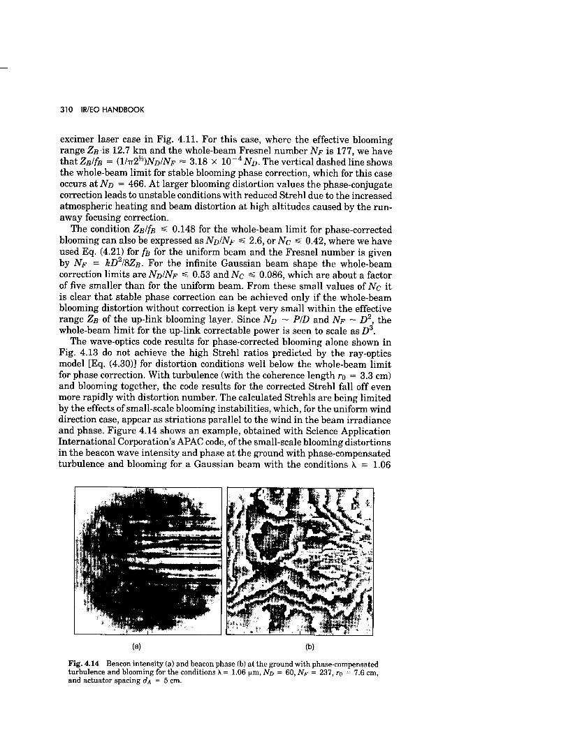
310 IR/EO HANDBOOK
excimer laser case in Fig. 4.11. For this case, where the effective blooming range ZB is 12.7 km and the whole-beam Fresnel number NF is 177, we have that ZB//5» = {V^NDINF = 3.18 x 10 ~4ND. The vertical dashed line shows the whole-beam limit for stable blooming phase correction, which for this case occurs at No = 466. At larger blooming distortion values the phase-conjugate correction leads to unstable conditions with reduced Strehl due to the increased atmospheric heating and beam distortion at high altitudes caused by the run- away focusing correction.
The condition Zß/fß *£ 0.148 for the whole-beam limit for phase-corrected blooming can also be expressed as ND/NF «S 2.6, or Nc =£ 0.42, where we have used Eq. (4.21) for /B for the uniform beam and the Fresnel number is given by NF = kD2/8Zß- For the infinite Gaussian beam shape the whole-beam correction limits are ND/NF =£ 0.53 and Nc =£ 0.086, which are about a factor of five smaller than for the uniform beam. From these small values of Nc it is clear that stable phase correction can be achieved only if the whole-beam blooming distortion without correction is kept very small within the effective range ZB of the up-link blooming layer. Since No ~ PID and NF ~ D2, the whole-beam limit for the up-link correctable power is seen to scale as D3.
The wave-optics code results for phase-corrected blooming alone shown in Fig. 4.13 do not achieve the high Strehl ratios predicted by the ray-optics model [Eq. (4.30)] for distortion conditions well below the whole-beam limit for phase correction. With turbulence (with the coherence length ro = 3.3 cm) and blooming together, the code results for the corrected Strehl fall off even more rapidly with distortion number. The calculated Strehls are being limited by the effects of small-scale blooming instabilities, which, for the uniform wind direction case, appear as striations parallel to the wind in the beam irradiance and phase. Figure 4.14 shows an example, obtained with Science Application International Corporation's APAC code, of the small-scale blooming distortions in the beacon wave intensity and phase at the ground with phase-compensated turbulence and blooming for a Gaussian beam with the conditions X = 1.06
(a) (b)
Fig. 4.14 Beacon intensity (a) and beacon phase (b) at the ground with phase-compensated turbulence and blooming for the conditions \ = 1.06 ^.m, No = 60, NF = 237, ro = 7.6 cm, and actuator spacing CLA = 5 cm.
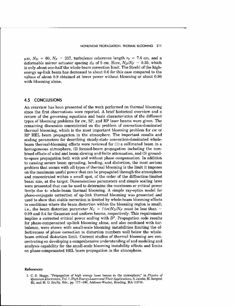
NONLINEAR PROPAGATION: THERMAL BLOOMING 311
(xm, ND = 60, NF = 237, turbulence coherence length ro = 7.6 cm, and a deformable mirror actuator spacing CLA of 5 cm. Here, ND/NF ~ 0.25, which is only about one-half the whole-beam correction limit. The Strehl of the high- energy up-link beam has decreased to about 0.6 for this case compared to the values of about 0.9 obtained at lower power without blooming or about 0.96 with blooming alone.
4.5 CONCLUSIONS
An overview has been presented of the work performed on thermal blooming since the first observations were reported. A brief historical overview and a review of the governing equations and basic characteristics of the different types of blooming problems for cw, SP, and RP laser beams were given. The remaining discussion concentrated on the problem of convection-dominated thermal blooming, which is the most important blooming problem for cw or RP HEL beam propagation in the atmosphere. The important results and scaling parameters for describing steady-state convection-dominated whole- beam thermal-blooming effects were reviewed for (1) a collimated beam in a homogeneous atmosphere, (2) focused-beam propagation including the com- bined effects of wind and beam slewing and finite attenuation, and (3) ground- to-space propagation both with and without phase compensation. In addition to causing severe beam spreading, bending, and distortion, the most serious problem that occurs with all types of thermal blooming is the limit it imposes on the maximum useful power that can be propagated through the atmosphere and concentrated within a small spot, of the order of the diffraction-limited beam size, at the target. Dimensionless parameters and simple scaling laws were presented that can be used to determine the maximum or critical power limits due to whole-beam thermal blooming. A simple ray-optics model for phase-conjugate correction of up-link thermal blooming was presented and used to show that stable correction is limited by whole-beam blooming effects to conditions where the beam distortion within the blooming region is small; i.e., the beam distortion parameter Nc = (V-mWo/iW must be less than ~ 0.09 and 0.4 for Gaussian and uniform beams, respectively. This requirement implies a corrected critical power scaling with Dz. Propagation code results for phase-compensated up-link blooming alone, and also combined with tur- bulence, were shown with small-scale blooming instabilities limiting the ef- fectiveness of phase correction to distortion numbers well below the whole- beam critical distortion limit. Current studies of thermal blooming are con- centrating on developing a comprehensive understanding of and modeling and analysis capability for the small-scale blooming instability effects and limits on phase-compensated HEL beam propagation in the atmosphere.
References
1. C. B. Hogge, "Propagation of high energy laser beams in the atmosphere," in Physics of Quantum Electronics, Vol. 1, High Energy Lasers and Their Applications, S. Jacobs, M. Sargent III, and M. O. Scully, Eds., pp. 177-246, Addison-Wesley, Reading, MA (1974).
312 IR/EO HANDBOOK
2. J. N. Hayes, "Propagation of high energy laser beams through the atmosphere: An overview," AGARD Conf. Proc. No. 183, Optical Propagation in the Atmosphere, Sec. 27 (May 1976).
3. F. G. Gebhardt, "High power laser propagation," Appl. Opt. 15(6), 1479-1493 (1976). 4. D. C. Smith, "High-power laser propagation: Thermal blooming," Proc. IEEE 65(12), 1679-1714
(1977). 5. J. L. Walsh and P. B. Ulrich, "Thermal blooming in the atmosphere," in Laser Beam Propa-
gation in the Atmosphere, J. W. Strohbehn, Ed., Springer-Verlag, New York (1978). 6. F. G. Gebhardt, "Overview of atmospheric effects on propagation of high energy laser radia-
tion," in Atmospheric Effects on Radiative Transfer, C. B. Ludwig, Ed., Proc. SPIE 195, 162-170 (1979).
7. T. J. Karr, "Thermal blooming compensation instabilities," J. Opt. Soc. Am. A 6(7), 1038-1048 (1989).
8. K. A. Breuckner and S. Jorna, "Linearized theory of laser induced instabilities in liquids and gases," Phys. Rev. 164, 182-193 (1967).
9. N. M. Kroll and P. L. Kelley, "Temporal and spatial gain in stimulated light scattering," Phys. Rev. A 4, 763-776 (1971).
10. J. P. Gordon, R. C. C. Leite, R. S. Moore, S. P. S. Porto, and J. R. Whinnery, Bull. Am. Phys. Soc. Ser. II 9, 501 (1964).
11. J. P. Gordon, R. C. C. Leite, R. S. Moore, S. P. S. Porto, and J. R. Whinnery, "Long transient effects in lasers with inserted liquid samples," J. Appl. Phys. 36, 3-7 (1965).
12. K. E. Rieckhoff, "Self-induced divergence of CW laser beams in liquids—A new nonlinear effect in the propagation of light," Appl. Phys. Lett. 9, 87 (1966).
13. W. R. Callen, B. G. Huth, and R. H. Pantell, "Optical patterns of thermally self-defocused light," Appl. Phys. Lett. 11, 103 (1967).
14. J. R. Whinnery, D. T. Miller, and F. Dabby, "Thermal convection and spherical aberration distortion of laser beams in low-loss liquids," IEEE J. Quantum Electron. QE-3, 382 (1967).
15. H. Inaba and H. Ito,"Observation of power-dependent distortion of an IR beam at 10.6 JJL from a C02 laser," IEEE J. Quantum Electron. QE-4, 45 (1968).
16. R. L. Carman and P. L. Kelley, "Time dependence in the thermal blooming of laser beams," Appl. Phys. Lett. 12, 241 (1968).
17. R. C. C. Leite, R. S. Moore, and J. R. Whinnery, "Low absorption measurements by means of the thermal lens effect using an He-Ne laser," Appl. Phys. Lett. 5, 141 (1964).
18. D. Solimini, "Loss measurements of organic materials at 6328 Ä," J. Appl. Phys. 37, 3314 (1966).
19. D. Solimini, "Accuracy and sensitivity of the thermal lens method for measuring absorption," Appl. Opt. 5, 1931 (1966).
20. R. C. C. Leite, S. P. S. Porto, and T. C. Damen, "The thermal lens effect as a power-limiting device," Appl. Phys. Lett. 10, 100 (1967).
21. S. A. Akhmanov, D. P. Krindach, A. V. Migulin, A. P. Sukhorukov, and R. V. Khokhlov, "Thermal self-actions of laser beams," IEEE J. Quantum Electron. QE-4U0), 568-575 (1968).
22. F. G. Gebhardt and D. C. Smith, "Effects of wind on thermal defocusing of CO2 laser radiation," Appl. Phys. Lett. 14(2), 52-54 (1969).
23. D. C. Smith, "Thermal defocusing of CO2 laser radiation in gases," IEEE J. Quantum Electron. QE-5, 600-607 (1969).
24. A. J. Glass, "Thermal blooming in gases," Opto-Electronics 1, 174-178 (1969). 25. D. M. Cordray and P. B. Ulrich, "Computer techniques for solution of the high-energy laser
propagation problem," in Atmospheric Effects on Radiative Transfer, C. B. Ludwig, Ed., Proc. SPIE 195, 182-191 (1979).
26. F. G. Gebhardt, D. C. Smith, R. G. Buser, and R. S. Rohde, "Turbulence effects on thermal blooming," Appl. Opt. 12(8), 1794-1805 (1973).
27. L. C. Bradley and J. Herrmann, "Phase compensation for thermal blooming," Appl. Opt. 13(2), 331-334 (1974).
28. E. L. O'Neill, Introduction to Statistical Optics, Chap. 4, Addison-Wesley, Reading, MA (1964). 29. F. G. Gebhardt, "Self-induced thermal distortion effects on target image quality," Appl. Opt.
11(6), 1419-1423 (1972).
NONLINEAR PROPAGATION: THERMAL BLOOMING 313
30. F. G. Gebhardt and D. C. Smith, "Self-induced thermal distortion in the near field for a laser beam in a moving medium," IEEE J. Quant. Electron. QE-7(2) 63-73 (1971).
31. R. J. Hull, P. L. Kelley, and R. L. Carman, "Self-induced thermal lens effect in CC14 in the presence of beam motion," Appl. Phys. Lett. 17, 539-541 (1970).
32. D. C. Smith and F. G. Gebhardt, "Saturation of the self-induced thermal distortion of laser radiation in a wind," Appl. Phys. Lett. 16(7), 275-278 (1970).
33. F. G. Gebhardt and D. C. Smith, "Effects of diffraction on the self-induced thermal distortion of a laser beam in a crosswind," Appl. Opt. 11(2), 244-248 (1972).
34. P. J. Berger, P. B. Ulrich, J. T. Ulrich, and F. G. Gebhardt, "Transient blooming of a slewed laser beam containing a region of stagnant absorber," Appl. Opt. 16(2), 345-354 (1977).
35. J. Herrmann, "Properties of phase conjugate adaptive optical systems," J. Opt. Soc. Am. 67(3), 290-295 (1977).
Index
1.7- to 1.5-um window water-vapor absorption in, 53
1976 U.S. Standard Atmosphere, 13 2.0- to 2.5-um window
water-vapor absorption in, 53 3- to 5-um window
water-vapor absorption in, 49-52 8- to 12-|im window
water vapor absorption in, 46-50
Aberrations, optical, 235-237, 246-284, 296 beam spread, 246, 248, 256 beam tilt, 246 boundary-layer aberrations, 264-269 heat-induced, 261-264 inviscid aberration field, 249 jitter, 248, 257 low-order aberrations, 249 open cavity optical degradation, 269-270 scaled to aperture diameter, 260 Strehl loss, 246, 248, 254-256 strong aberrations, 258-259 supersonic vehicle optical aberrations, 274—
278 look angle errors, 276 shock curvature effects, 276
from thermal blooming, 296 astigmatism, 296 coma, 296 pincushion distortion, 296 Seidel, 296 spherical, 296
total wave-front variance, 259 wave-front error, 254 weak aberrations, 254-258
Absolute humidity, 11 Absorbance, 69-71, 81-82
closed-form expressions for, 82 Absorber amount, 70 Absorptance, 6, 81 Absorption, atmospheric, 13-86, 291
aerosols, 130 carbon monoxide, 62-63 collision-induced, 9, 17, 36-38 continuum absorption, 17, 39-56, 58-59,130
1.7- to 1.5-um window, 53-54 2.0- to 2.5-um window, 53 3- to 5-um window, 49-52 8- to 12-um window, 46-50 effects of scattering on, 55-56 far-wing absorption, 54-56
millimeter-wave window, 44-47 models, 54-55 temperature dependence, 54-55 water-vapor dimers, 54
line-by-line models, 17 local-line absorption, 39-40, 42, 58,130 methane, 59-60 molecular, 13 nitrogen, 63-65 nitrous oxide, 60-61 oxygen, 60-65 ozone, 59-61 total absorption, 15 trace gases, 63 water vapor, 41-56
Absorption band models, 17, 69-87 absorbance, 69-71, 81-82 absorber amount, 70-71 absorptance, 81 Elsasser (regular) band model, 69, 71-75
nonoverlapping approximation, 74—75 strong-line approximation, 73-74 weak-line approximation, 71-73
quasi-random model, 69, 80-81 random-Elsasser model, 69, 80 statistical (random) band model, 69, 75-80
equal intensity lines, 76 exponential-tail S~' random-band model,
79-80 Goody band model, 77 line strength with exponential probability
distribution, 76-77 strong-line, weak-line, and
nonoverlapping line approximations, 77-79
strong-line absorption, 70, 77-79 temperature and frequency dependence, 81-
83 transmittance, 69, 75, 80 transmittance calculations, 83-87 weak-line absorption, 71, 77-79
Absorption coefficient collision-broadened absorption coefficient, 41 continuum absorption coefficient, 41, 50
of carbon dioxide, 59 dimensionless broadening coefficient, 41,
52 foreign broadening coefficient, 41 gas self-broadening coefficient, 41 of mixed gases, 86 nitrogen-broadening water-vapor
coefficient, 46, 48, 50 ofozone, 85
314
INDEX 315
of a spectral line, 14—15, 24 of water vapor, 41-56, 86 water-vapor self-broadening coefficient,
46-52 up-link propagation equation, 305
Acoustic sounders, 206 Acoustic transit time, 293 Actuators, 280, 311 Adaptive optics, 201, 279-284
actuators, 280 deformable mirrors, 279-280, 283 Guidestar technique, 280 wave-front sensors, 280, 283
Adaptive phase correction, 291, 307-308 Advection, 175,193 Aero-optical design examples, 264-284
aperture optimization, 271-272 boundary-layer aberrations, 264-269 IR window thermal noise, 272-274 open cavity, 269-270 optimal wavelength, 270-271 subsonic imaging platforms, 264-268 supersonic imaging platforms, 268-269 supersonic vehicle aberrations, 274-277 supersonic vehicle thermal radiation effects,
277-278 visible imagers, 270-271
Aero-optical design solutions, 278-284 adaptive optics, 279-284 atmospheric compensation, 279 deformable mirrors, 279-280, 283 flow removal, 278 four-wave mixing, 280-283 Guidestar technique, 280 holography, 280 nonlinear optics, 279-284 pulsed compensation systems, 279-280 spatial light modulators, 280 splitter plates, 278 supplemental flow, 278 wave-front sensors, 280, 283
Aerodynamic effects on optical systems, 235-285 flow-field-induced heating, 261-264 inviscid flows, 247-249 random flow fields, 253-264
infinite-aperture assumption, 254, 260 strong aberrations, 258-260 weak aberrations, 254-258
shock waves, 249-253 optical reflections, 252-253
Aerodynamic flow fields, 235, 237-246 boundary layers, 241-243, 247 compressibility effects, 240 free-stream velocity, 240 heating, 240-241 inviscid flows, 247 Mach number, 237-239 Newtonian flow, 237 open cavities, 243-246 plasmas, 241 Reynolds number, 237-238 shear layers, 243-247 stagnation temperature, 241
Aerodynamic lensing, 249
Aerodynamic parameters density fluctuations, 236, 254 correlation length, 236, 254 path length, 236, 254 symbols, nomenclature, and units, 239-240 wave-front variance, 236-237
Aeromechanical mechanical effects on optical systems, 235-285
Aerosol blooming, 290 Aerosol scatter, 12, 92-109, 123-127
mutual coherence function, 123-127 polydispersions, 99-100
particle size distribution function, 99 phase function, 99-101, 110
single scatter (Mie theory), 92-96 absorption efficiency, 98 backscatter cross section, 96 backscatter efficiency, 96, 98 backscatter intensity, 96 electric dipole scattering, 97 extinction cross section, 96, 99 extinction efficiency, 95-98 m-x domain, 97-99 polarization effects, 94—95 Rayleigh scattering, 97 scatter cross section, 96 scatter efficiency, 95-98 single-scatter albedo, 96, 99
Aerosols, 11-12 absorption, 130 aerosol size distribution models, 105-109
Junge (power law) model, 107-108 log-normal distribution, 108 modified gamma distribution, 105-108 zero-order logarithmic distribution, 108
obscurants, 109 permittivity, 104 refractive index of, 104—105 terrestrial aerosols, 100-109 vertical density variations, 102-104
AFGL. See Phillips Laboratory AFGL AMOS turbulence model, 218-219 Air density, 209, 247, 250, 254, 291, 293-294 Aircraft, 235-285 Airy pattern, 254 Ammonium sulfate refractive index, 104 Amplitude, 179-183 Angle of arrival, 194-195,197 Anisoplanatism, 201 Aperture diameter, 193-194,199 Aperture filter function, 195 Aperture plane, 190 Apertures, 191, 200-201
circular (Airy), 254, 259 finite, 260, 272 infinite-aperture limit, 254, 260 optimization of, 271-272 transmitter, 195, 307-308
Atmosphere, 7-13. See also Earth-atmosphere geometry
gas composition, 9-11 particle composition, 11-13 structure, 7-8
316 INDEX
Atmospheric boundary layer, 168, 201-206 interfacial layer, 202 inversion layer, 202-204 mixed layer, 202 surface layer, 202, 204
Atmospheric heating distribution function, 309 Atmospheric phenomena
absorption, 13-86 aerodynamic effects, 233-285 refraction, 86-91 scattering, 92-127 spectral characteristics, 13-39 thermal blooming, 287-313 transmission, 3-156 turbulence, 157-232
Atmospheric propagation. See Absorption; Atmospheric transmission; Laser beam propagation; Propagation; Scattering; Turbulence; Thermal blooming
Atmospheric refractivity constant, 305 Atmospheric spectroscopy. See Spectroscopy,
atmospheric Atmospheric transfer function, 190 Atmospheric transmission, 1-156. See also
Absorption; Atmosphere; Index of refraction; Propagation; Refraction, atmospheric; Scattering; Spectroscopy, atmospheric; Thermal blooming
symbols, nomenclature, and units, 4-5 Atmospheric transmission codes, 127-147. See
also FASCODE, HITRAN database; LOWTRAN; MODTRAN
Attenuation, 299
Backscattering, 92, 96, 98 Balloon-borne instruments, 207, 209-211 Beacon wave intensity, 310 Beam distortion parameter, 295-296, 299-302,
305-306, 309-311 Beam focus/defocus, 249 Beam jitter, 290. See also Jitter Beam profiles, 299 Beam radius, 196 Beam slewing, 290, 294, 299-300, 304
slewing number, 301 Beam spreading (broadening), 196-197, 227-
229, 235, 246, 248, 256, 290, 298, 308 Beam tilt, 182, 197, 246 Beam wander, 159, 182,196-197, 227-229, 235,
290 Beams. See also Laser beam propagation
coherence of, 200-201 collimated, 195,198-199 diverging, 195 focused 195—199 Gaussian, 196, 293-297, 299, 302, 305, 310-
311 BHMIE subroutine, 133,136-138 Blooming phase, 295-297, 305, 307-308. See
also Thermal blooming negative-lens focal length, 297 phase gradient, 297
tilt angle, 297 Blur angle, 256, 258-259 Blur spot, 258-259 Born approximation, 178-180 Bouguer's law (Beer-Lambert's law), 112 Boundary layers, 241-243. See also Random
flows laminar boundary layers, 241
inviscid lensing effects, 241 static pressure, 241
and optical aberrations, 264—268 turbulent boundary layers, 241-243, 247,
253-254, 265 free-stream density, 242 optical phase variance, 242 scale length, 242 scaling relations, 241-242 shock waves, 243, 247 turbules, 242
Boundary-layer turbulence models, 212-217 boundary-layer inversion, 215 convective boundary layer, 216 Kaimal model, 212-215 Kukharets-Tsvang model, 215-216 Kunkel-Walters model, 213-215 Monin-Obhukov length, 212-213 similarity theory, 212-214
Broadening coefficients, 41, 46-56 Brunt-Vaisala frequency, 170,173, 213, 223
C\ See Index of refraction structure parameter Carbon dioxide, 9
absorption, 32, 39, 44, 56-59 continuum absorption, 58-59 integrated intensities, 57 local-line absorption, 58 vibrational bands, 57
concentration of, 11 Carbon monoxide, absorption, 62-63 Cavities, open, 235-236, 243-246
acoustical effects, 243 aft ramp, 245-246 Airborne Optical Adjunct aircraft, 245 entrainment requirement, 244 porous fence, 244-245 resonance, 243-246 sound pressure level, 246
Cavity flow field, 236 Central limit theorem, 180 Chapman function, 113-115 CLEAR I turbulence model, 220, 228 Clouds, 108-109, 203 Coherence length, 191-193,197, 200, 210-211,
216, 219, 222, 228, 311 Computer codes for atmospheric propagation,
127-147 Computers, personal, 96 Contrast. See Image contrast Convection, 167, 203, 205, 210, 214-216, 289,
291-292, 304 Covariance, 180-181, 184-190,198 Covariance function, 161-167
INDEX 317
CT2 instruments, 202, 206
Cutoff frequency, 192
Deformable mirrors, 279-280, 283, 311 Density, air. See Air density Deserts, 205, 210-211, 220 Detectors, 187, 246. See also Imagers Detectors, airborne. See also Imaging systems,
airborne emissivity, 263 power, 261 spectral exitance, 261 spectral irradiance, 261-263 spectral radiance, 261 transmission, 262
Diffraction, 197,257, 259-260, 299, 306 Distortion, 195 Dust, 100
refractive index, 104
Earth-atmosphere geometry, 89-91 effects of refraction, 90 optical horizon, 89
Eddies, 193 Effective blooming range, 309 Electric field, 177 Electro-optic sensors, scattering effects, 111-112 Energy, conservation of, 200
Exosphere, 8 Extinctance, 6 Extinction coefficient, 3, 6-7,112, 292 Extinction cross section, 95 Extinction number, 295, 300
Far-infrared, 18 FASCODE, 25, 32, 55,128,133-135 Fata Morgana, 91 Figure of merit, 256 Filter functions, 181,183,188-189 Finite optical apertures, 260 Focal plane, 195 Focusing, beam, 300-301 Focusing correction, 307 Fog, 103,109 Free atmosphere, 206-209
stratification, 206-207, 212 stratosphere, 207, 209 tropopause, 207 troposphere, 206-207, 209
Free-stream density, 242, 244 Fresnel approximation, 179,185-186 Fresnel length, 187, 210 Fresnel number, 293,298-301, 304 Frozen turbulence hypothesis, 175-176,186,
206, 209 Fused quartz, 264 Fused silica optical mode constants, 106
Gases, atmospheric. See also Absorption; Carbon dioxide; Carbon monoxide; Methane; Nitrogen; Nitrous oxide; Oxygen; Ozone; Trace gases; Water vapor
absorption by, 39-65 amount in atmosphere, 9 density in atmosphere, 12-13 fundamental vibrational frequencies, 21 isotopic abundance, 67 mixing ratio, 10 rotational constants of, 19
Gaussian focal-plane spot, 256 Gaussian laser beams. See Laser beam
propagation Geometric-optics limit, 259 Geometrical optics, 299 Germanium, 262, 273 Gladstone-Dale parameter, 236, 247, 252-254 Green flash, 91 Green spot, 90 Greenhouse effect, 39, 57
Haze, 12, 100, 108 Heat transfer, 262, 289, 291-293 Heat-balance equation, 264 HITRAN database, 19, 21, 26, 35, 39, 42, 58, 65-
69,85 Holography, 237, 280 Homogeneous fluctuations, 165 Hufnagel turbulence model, 221-223 Hufhagel-Valley turbulence model, 222, 225 Humidity. See also Absolute humidity; Relative
humidity effects on C,2,172-173 specific, 170-171
Huygens-Fresnel theory, 179, 200 Hydrometers, 11-12 Hygroscopic particles, 100,102
Ideal gas law, 11,13 Image blurring, 190,193-195, 235 Image contrast, 123, 235, 246, 254-258 Image dancing, 182,190,193-195 Image displacement, 195 Image quality, 256-257. See also Aberrations,
optical; Aerodynamic effects on optical systems; Image contrast; Image resolution
Image resolution, 192-193, 226-227, 235, 246, 254-258
Imagers, visible, 269-271, 282-284 Imaging, effects of turbulence, 190-195, 226-
227 image blurring, 190, 193-195 image dancing, 190,193-195
Imaging systems, airborne, 236, 248-284. See also Detectors, airborne
aero-optical design considerations, 264-284 Imaging through a scattering medium, 123-127
contrast, 123 mutual coherence function, 123-127
318 INDEX
optical transfer function, 123-127 point spread function, 123, 127 polarization, 125 visibility range, 123
Index of extinction, 6-7 Index of refraction, 21, 86-89,159,169, 171-
174, 177,180, 247, 253, 291-294 aerosols, 104-105 Brunt-Vaisala frequency, 171,173 complex, 25, 93,104 ducting effects, 91 Fata Morgana, 91 green flash, 91 green spot effect, 90 inferior mirages, 91 at infrared wavelengths, 88 mirages, 91 potential refractivity, 173 at radar frequencies, 88 refraction correction angle, 89-91 Sellmeier model, 88-89 subrefractive conditions, 90-91 superior mirages, 91 superrefractive conditions, 90-91 water-vapor contribution, 88 '
Index of refraction structure parameter (C2), 159, 172-174, 185-186,189,191, 202-228
Inertial range, 167 Infrared windows, 235, 243, 262-263, 272-274 Intensification effect, 298 Intensity, 184,186-187, 200-201, 225-225 Intensity, far-field, 256-257 Intensity variance, 184, 225 Interferometric calorimeter measuring
technique, 53-54 Interferometry, 237 Interferometry, speckle, 195 INTRP subroutine, 139-142 Inviscid flows, 247-249 Ionization, 247, 250, 277 Ionosphere, 7-8 Irradiance distortion parameter, 298 Isobaric heating, 289, 292-293, 295
energy-balance equation, 292 Isoplanatic angle, 201, 210-211, 219, 222 Isoplanatism, 201
Jet stream, 207-209, 222 Jitter, 235, 248, 257, 279, 290
Kaimal turbulence model, 212-215 Kinetic cooling, 290 Kolmogorov theory, 161,167-169,175,180-181,
183,185, 209 Kukharets-Tsvang turbulence model, 215-216 Kunkel-Walters turbulence model, 213-215
Laboratory simulation experiments, 300, 302- 303
Laser beam power density, 292
Laser beam propagation, 157-232, 287-313. See also Aberrations, optical; Absorption; Scattering; Thermal blooming; Turbulence, optical
atmospheric scattering, 111 beam intensity, 292-293, 298-304 critical intensity, 302 critical power, 302-303 cw beams, 292-294 empirical scaling law, 303 Gaussian beams, 293-297, 299, 302, 305,
310-311 laboratory propagation simulation
experiments, 300-303 peak irradiance, 302-303, 307 ray-optics thermal propagation model, 300,
306, 309, 311 repetitively pulsed beams, 292-294 thermal blooming effects, 289-311 uniform beams, 297, 311 very-short-pulse HEL beams, 293-294 wave-optics propagation codes, 297, 301,
303-304, 306, 309-310 Lidar, 197, 206 Localized gradients, 291 Log amplitude, 182-190,198-199, 225 LOWTRAN, 25, 55, 83, 85-87,127-132
Mach number, 237-239, 266-267 Magnesium fluoride, 263 Maxwell's equations, 177 Mesosphere, 7 Meteorology, synoptic, 202, 207, 209 Methane, absorption, 59-60 Microwave spectral region
absorption bands, 39 Mid-infrared, 18 Mie scatter, 92-98. See also Aerosols, scatter MIEGEN subroutine, 143-147 Millimeter-wave spectral region
absorption bands, 39 propagation model, 32 water-vapor absorption in, 44-47
Mirages, 91 Modified von Karman spectrum, 174-175,182 MODTRAN, 25, 86, 128,132
Curtis-Godson approximation, 86 Modulation transfer function, 191-194, 200-201,
258, 260 Molecular Rayleigh scattering. See Rayleigh
scattering Molecule classification, 18 Moments, measurement of, 210-211 Monin-Obhukov length, 212-213 Mountains, 205, 210-211, 218-220 Mutual coherence function, 123-127,187-188,
190-191, 193 Mutual intensity function, 190
Navier-Stokes equations, 161 Near-infrared, 18
INDEX 319
Negative lens (defocusing) effect, 295, 305
Nitrogen, 9,17, 21, 32, 41 absorption continuum, 63-65 broadening, 43, 46, 48, 50, 52
Nitrous oxide, absorption, 60-61 NOAA (VanZandt) turbulence model, 223-224 Nonisobaric heating, 293-294 Nonlinear optics, 279-284
coherent beacon, 282-283 four-wave mixing, 279, 283 holography, 280 spatial light modulators, 280
Nonlinear propagation. See Thermal blooming Nonuniform velocity profile, 300 Number density, 3
Obscurants. See Aerosols; Dust; Haze Optical aberrations. See Aberrations, optical Optical depth, 6 Optical design. See Aero-optical design
examples; Aero-optical design solutions Optical mode constants, 105-107
a-Fe20? 107 fused silica, 106 quartz, 107 sodium chloride, 105
Optical phase, 247 Optical phase distortion, 295 Optical phase variance, 242 Optical transfer function, 123-127,181,191, 201 Optical turbulence. See Turbulence, optical Optical turbulence profiles, 217-221 Optimal wavelength, 257,270-271 Oxygen, 9,17, 21-22, 41
absorption, 32, 60-65 broadening, 48
Ozone, 7, 22 absorption, 59-61
Paraxial scalar wave equation, 291-292 Particle scattering. See Aerosol scatter Particles, atmospheric, 11-13
aerosols, 11-12 hydrometers, 11-12 radius range, 12
Permittivity, 104 Perturbation series, 177-178 Perturbations, 179, 293 Phase, 179-183,190 Phase compensation, 300, 304, 307-311 Phase covariance, 182 Phase distortions, 159,190, 195, 201 Phase function approximation, 121-22
Henyey-Greenstein phase functions, 121-122 Phase shift, 295-296 Phase-correlation function, 258 Phillips Laboratory (formerly AFGL), 19, 21, 25,
39, 66 Photoacoustic laser measurement, 44, 46, 49-50
Photon absorption, 14 Photon scattering, 254 Pixel field of view, 236 Plane waves, 181,183-185,188-192,195, 198-
200 Plasmas, 247,277 Point spread function, 123, 127, 190, 258 Polarization, 94-95,177 Polydispersions, 99-100. See also Aerosol scatter Power in the bucket, 246 Power spectrum, 162-163 Prandtl number, 171 Prism (beam-bending) effect, 295 Propagation, 115-147,157-232, 287-313. See
also Atmospheric transmission; Laser beam propagation; Scattering; Thermal blooming; Turbulence
computer codes, 127-147 far-field, 194 FASCODE examples, 134-135 LOWTRAN examples, 130-132 near-field, 194 optical, 7-8 phase function approximation, 121-122 pulse stretching, 122-123 radio-wave, 7-8 symbols, nomenclature, and units, 160 transport theory, 115-119 through turbulence, 176-201
amplitude and phase statistics, 179-183 beam effects, 195-201 imaging effects, 190-195 isoplanatism, 201 polarization effects, 177 scintillation, 184-190 wave equation solutions, 177-179
Pulse length, 293 Pulse stretching, 122-123
Quartz optical mode constants, 107 refractive index, 104
Radar, 177, 207, 223 Doppler, 210 Sousy, 208
Radiation slide rule, 261 Radiative transfer, atmospheric, 3-7 Radiative transfer equation, 6-7 Radiosonde, 223 Raman scattering, 17 Random flow fields, 253-264. See also
Aerodynamic effects on optical systems shear layers, 253-254 turbulent boundary layers, 253
Range gating, 253 Ray-optics model, 297-300, 304, 306, 309-311 Rayleigh (molecular) scattering, 12,17, 55-56,
97,109-110. See also Aerosol scatter Receivers, 185 Reflections, at shock-wave interface, 252-253
320 INDEX
Refraction, atmospheric, 86-91 Refractive index. See Index of refraction Relative humidity, 10,103, 203-205, 207 Resolution. See Image resolution Reynolds number, 237-238, 242, 253 Ricatti equation, 178 Rytov approximation, 178-180,184,186-187,
190, 199, 225
Sapphire, 263 Saturation vapor pressure of H20,10,12
Scatterance, 6 Scattering, 177-179
backscattering, 177 forward scattering, 177 laser, 195 multiple scattering, 177,186
Scattering angle, 254 Scattering, atmospheric, 92-127. See also
Aerosol scatter; Mie scatter; Rayleigh scattering; Propagation
aerosol scatter, 92-109,123-127 algorithms, 133,136-147
BHMIE subroutine, 133,136-138 INTRP subroutine, 139-142 MIEGEN subroutine, 143-147 SPHERE scattering program, 139
example applications, 110-115 molecular Rayleigh scattering, 12, 17, 55-56,
109-110 multiple scattering, 115-119 mutual coherence function, 123-127 by particles, 9,12 Raman scattering, 17
Scattering coefficient, 305 Scintillation, 159,183-195,198-200, 210, 224-
226, 291 Scintillometers, 186, 219
horizontal, 186 stellar, 186, 210, 224
Sea salt, 102 Sellmeier's equation, 25 Shear layers, 236, 243-247, 253-254
Bernoulli effect, 244 Shock waves, 243, 249-253 Signal-to-noise ratio, 237, 253, 273 Silicon, 262 Similarity theory, 212-214 Single scatter. See Mie scatter Single-scatter approximation, 7 SLC turbulence models, 217-219 Sodium chloride
optical mode constants, 105 refractive index, 104,106
Solar flux, 213 Source term for path emission or scattering, 3, 6 Spatial coherence, 191 Spatial frequency, 192 Specific intensity, 115-119 Speckle, 195
Speckle interferometry, 195 Spectral extinction cross section, 3 Spectral radiance, 3 Spectral scattering cross section, 3 Spectrometers, 43-44 Spectroscopy, atmospheric, 13-39
Birnbaum's line shape, 59 classical oscillator model, 22-25
absorption coefficient, 24 electric susceptibility, 23 free-space permittivity, 23-25 Lorentz line shape, 24, 30, 32, 36 relative permittivity, 23-25 Sellmeier's equation, 25 time harmonic behavior, 23 Van Vleck-Weisskopf line-shape function,
25 collision-broadened line shape, 30-38
autocorrelation function, 30-31, 33-34 collision-broadened half-width at half-
intensity, 31 exponential wing, 34 far-wing, 33-34 line-mixing effects, 32 self-broadening coefficient, 31-32
definitions, 14-15 absorption coefficient, 14-15 line-shape function, 14 spectral line half-width, 14 spectral line strength, 14
Doppler line shape, 35-36 Doppler equation, 35 Maxwell-Boltzmann distribution, 35
Doppler spectral density function, 36 dipole moments, 15-17, 23 electron polarizability, 17 electronic spectra, 18, 21-22 Heisenberg uncertainty principle, 29 homogeneous line shapes, 28-35 infrared-active rotational spectra, 16 inhomogeneous line shapes, 28, 35-37 intramolecular potentials, 15-17 light-matter interaction, 22-26 line position, 18, 66 line-shape profiles, 28-37 line strength, 26, 66 molecule classification, 18
asymmetric top, 18-19 linear, 18 spherical top, 18
natural line shapes, 30 Einstein spontaneous emission
coefficient, 30 half-width at half-intensity, 30 line-profile function, 30
nonpolar molecules, 16 partition functions, 26-28
for diatomic molecules, 27 Maxwell-Boltzmann distribution function,
26 for polyatomic molecules, 27-28
polar molecules, 16 quadrupole moments, 16 quantum mechanical model, 25-26
autocorrelation function, 25 dipole matrix element, 26
INDEX 321
line strength, 26 line-profile function, 25 partition function, 26 power spectral density function, 25
refractivity model, 37-39 anomalous dispersion, 38 Hilbert transform, 37-38 index of absorption, 37 index of refraction, 37-38 Sellmeier equation, 38
rotation bands, 20-21 rotational quantum numbers, 16 rotational selection rules, 16-17
anti-Stokes vibrational band, 17 O-branch, 17 P-branch, 17, 21 Q-branch, 17, 21 R-branch, 17, 21 S-branch, 17 Stokes vibrational band, 17
rotational spectra, 18-20 rotational constants, 18-19 rotational term values, 18-19
rotational-vibrational spectra, 21-22 vibration bands, 20-21
combination bands, 20 fundamental transitions, 20 hot bands, 20 overtone bands, 20 vibrational term value function, 20
vibrational frequencies of atmospheric molecules, 21
vibrational quantum numbers, 16 vibrational spectra, 16 Voigt line shape, 36-37
Spectrum, 180-181,185 SPHERE scattering program, 139 Spherical waves, 183-185,188-192,195,198-
200 Stagnation zones, 290, 300, 304 Stars
scintillation, 186, 224-225 Stimulated thermal Rayleigh scattering, 289 Stokes vector, 94 Stratification, 206-207, 212 Stratosphere, 7, 207, 209, 219, 221 Strehl ratio, 246, 248, 255-256,258-260, 301,
304, 306, 308-309, 311 Structure functions, 165-173,180-181,198
structure coefficient, 172 Surface boundary layers, 235 Symbols, nomenclature and units, 3-5,160,
239-240
Tatarski equation, 173 Temperature, 203-207
adiabatic wall, 262, 277 inversions, 174, 203-204 lapse rate, 209 potential temperature, 169-170, 223 relation to Cf, 209 temperature spectrum, 174
Thermal blooming, 287-313. See also Laser
beam propagation; Propagation blooming phase, 295-297 collimated beam—homogeneous path, 294-
299 convection-dominated blooming, 293, 299,
311 focused beams—inhomogeneous path, 299 isobaric heating, 292-293 nonisobaric heating, 293-294 paraxial scalar wave equation, 291-292, 297 pulse overlap blooming effects, 294 single-pulse thermal-blooming effects, 293-
294 small-scale thermal-blooming instabilities,
289-291, 310 stagnation zone blooming, 290, 304 steady-state blooming, 294-311 «-cubed blooming, 293 thermal blooming intensification effect, 298 thermal-blooming phase distortion, 296, 298 thermal-conduction-dominated blooming,
292-293 thermally bloomed irradiance pattern, 297-
298 up-link (ground-to-space) thermal blooming,
304-311 up-link thermal-blooming compensation, 289 wave-optics propagation codes, 297 whole-beam thermal blooming, 289-290
Thermal blooming phase distortion, 296, 298 Thermal conductivity, 292 Thermal diffusivity, 292 Thermal focusing, 298 Thermal lens, 289-290, 295 Thermal noise, 261-262, 272-274, 277 Thermal plumes, 173, 206 Thermo-optical aberrations, 253, 261-264, 274 Thermomechanical loads, 262 Thermosonde, 203-205, 207-208, 223 Thermosphere, 8 Trace gases, absorption, 63 Transmission. See Atmospheric transmission Transmission along a slant path, 112-115, 131 Transmittance, 6, 69, 75, 80, 83-87, 306
calculation methods, 83-87 aggregate method, 83-84 LOWTRAN method, 83, 85-87 MODTRAN method, 86
Transonic slewing, 290, 300 Transport theory, 115-119
discrete ordinates method, 120-121 four-flux theory, 120 transport equation parameters, 115-119
diffuse intensity, 120 field intensity, 116-117 flux density, 117 incident flux, 120 irradiance, 117 optical distance, 118 radiant emittance, 117 source function, 118 specific intensity, 116-119 surface intensity, 116
two-flux theory (Kubelka-Munk), 119-120
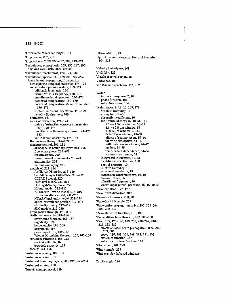
322 INDEX
Transverse coherence length, 191 Trope-pause, 207, 219 Troposphere, 7, 39, 206-207, 209, 219-221 Turbulence, atmospheric, 159, 235-237, 290,
310. See also Turbulence, optical Turbulence, mechanical, 173-174, 203 Turbulence, optical, 159-232, 300. See also
Laser beam propagation; Propagation atmospheric temporal statistics, 174-176 conservative passive scalars, 169-171
adiabatic lapse rate, 170 Brunt-Vaisala frequency, 170,173 one-dimensional spectrum, 170-172 potential temperature, 169-170 potential temperature structure constant,
170-171 three-dimensional spectrum, 170-172 velocity fluctuations, 169
definition, 161 index of refraction, 171-174
index of refraction structure parameter (C*), 172-174
modified von Karman spectrum, 174-175, 182
von Karman spectrum, 174,182 Kolmogorov theory, 167-169,175 measurement of, 201-211
atmospheric boundary layer, 201-206 free atmosphere, 206-209 intermittency, 209 measurement of moments, 210-211 stationarity, 209 volume averaging, 209
models of, 211-224 AFGL AMOS model, 218-219 boundary-layer turbulence, 212-217 CLEAR I model, 220 Hufnagel model, 221-223 Hufhagel-Valley model, 222 Kaimal model, 212-215 Kukharets-Tsvang model, 215-216 Kunkel-Walters model, 213-215 NOAA (VanZandt) model, 223-224 optical turbulence profiles, 217-221 similarity theory, 212-214 SLC models, 217-219
propagation through, 176-201 statistical concepts, 161-164
covariance function, 161-167 ergodicity, 162 homogeneity, 163,165 isotropism, 163 power spectrum, 162-163 Wiener-Khinchine theorem, 162,165-166
structure functions, 165-173 inverse relation, 166 isotropic property, 166
theory, 161-176 Turbulence, strong, 187,197 Turbulence, weak, 197 Turbulent boundary layers, 236, 247, 253-254 Turbulent mixing, 290 Turret, hemispherical, 249
Ultraviolet, 18, 21 Up-link (ground-to-space) thermal blooming,
304-311
Velocity turbulence, 161 Visibility, 123 Visible spectral region, 18 Volcanoes, 100 von Karman spectrum, 174,182
Water in the atmosphere, 7,10 phase function, 101 refractive index, 104
Water vapor, 9-12,16, 169,171 absolute humidity, 11 absorption, 39-56 absorption coefficient, 86 continuum absorption, 42-56, 130
1.7- to 1.5-nm window, 53-54 2.0- to 2.5-um window, 53 3- to 5-um window, 49-52 8- to 12-um window, 46-50 effects of scattering on, 55-56 far-wing absorption, 54-56 millimeter-wave window, 44—47 models, 54-55 temperature dependence, 54-55 water-vapor dimers, 54
integrated intensities, 41, 43 local-line absorption, 42, 130 partial pressure, 10 relative humidity, 10 rotational constants, 19 saturation vapor pressure, 10,12 transmittance, 85 vibrational frequency, 20 water-vapor partial pressure, 45-46, 49, 54
Wave equation, 177-179 Wave-front distortion, 247 Wave-front sensors, 280, 283 Wave-front tilt angle, 257 Wave-optics propagation codes, 297, 303-304,
306, 309-310 Wave-structure function, 181,190 Wiener-Khinchine theorem, 162,165-166 Wind, 165,175-176,186, 203, 206-207, 216-
217,222-223 effects on laser beam propagation, 289, 294-
299 301 speed, 186, 193, 203, 208, 213, 221, 306 structure function, 167 velocity structure function, 167
Wind shear, 167, 223 Wind tunnels, 237 Windows. See Infrared windows
Zenith angle, 190


