arX

iv:0

707.

4069

v2 [

quan

t-ph

] 1

9 O

ct 2

007

Atomic cluster state build up with macroscopic heralding

Jeremy Metz,1 Christian Schon,1 and Almut Beige 2

1Blackett Laboratory, Imperial College London, Prince Consort Road, London SW7 2BZ, United Kingdom2The School of Physics and Astronomy, University of Leeds, Leeds LS2 9JT, United Kingdom

(Dated: February 1, 2008)

We describe a measurement-based state preparation scheme for the efficient build up of clusterstates in atom-cavity systems. As in a recent proposal for the generation of maximally entangledatom pairs [Metz et al., Phys. Rev. Lett. 97, 040503 (2006)], we use an electron shelving techniqueto avoid the necessity for the detection of single photons. Instead, the successful fusion of smallerinto larger clusters is heralded by an easy-to-detect macroscopic fluorescence signal. High fidelitiesare achieved even in the vicinity of the bad cavity limit and are essentially independent of theconcrete size of the system parameters.

PACS numbers: 03.67.Mn, 03.67.Pp, 42.50.Lc

I. INTRODUCTION

In 2001 Raussendorf and Briegel pointed out that cer-tain highly entangled states present an innovative ap-proach to quantum computing [1]. The attractivenessof these so-called cluster states [2] arises from the factthat they can be grown off-line in a probabilistic fashion.Afterwards, a so-called one-way quantum computationcan be carried out without having to create additionalentanglement. Any quantum algorithm can then be per-formed using only single-qubit rotations and single-qubitmeasurements. Scalable fault-tolerant one-way compu-tation is possible, provided the noise in the implemen-tation is below a certain threshold [3, 4]. For exam-ple, Raussendorf et al. [5] recently introduced a fault-tolerant three dimensional cluster state quantum com-puter based on methods of topological quantum errorcorrection. Other authors identified highly efficient clus-ter state purification protocols [6, 7].

A very efficient way to create a cluster state of a verylarge number of atoms with very few steps is to employcold controlled collisions within optical lattices with oneatom on each site [8]. Using this approach, Mandel etal. [9] already created cluster state entanglement andreported the observation of coherence of an atom de-localised over many sites. Unfortunately, single-qubit ro-tations cannot be easily realised, since laser fields appliedto one atom generally affect also its neighbours. To fa-cilitate one-way quantum computing in optical latticesseveral schemes have been proposed for the realisationof single-qubit rotations without having to address theatoms individually [10, 11, 12].

However, higher fidelities can be obtained using ameasurement-based cluster state growth approach. Anexample is the linear optics proposal by Browne andRudolph [13]. Using linear optics, a four-photon clusterstate has already been generated in the laboratory [14].Currently, the scalability of this approach is hamperedby the lack of reliable photon storage. To overcome thisand the above mentioned addressability problem in opti-cal lattices, quantum computing architectures have beenproposed using hybrid systems based on atomic and pho-

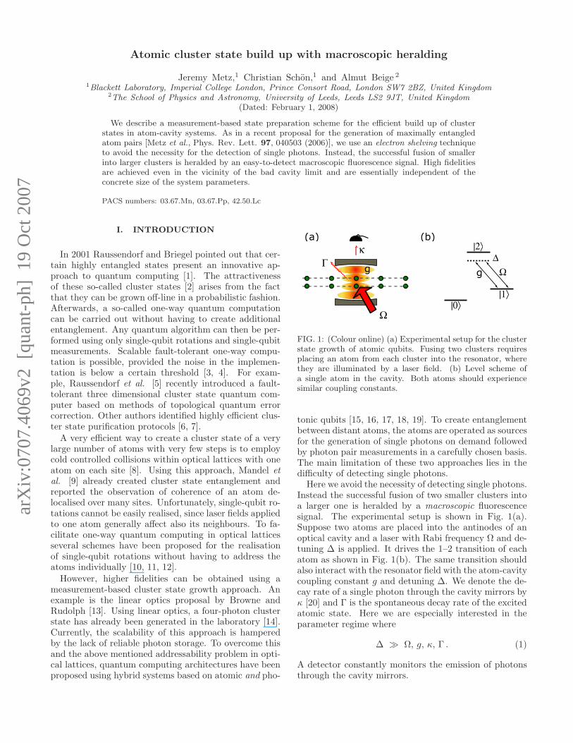
FIG. 1: (Colour online) (a) Experimental setup for the clusterstate growth of atomic qubits. Fusing two clusters requiresplacing an atom from each cluster into the resonator, wherethey are illuminated by a laser field. (b) Level scheme ofa single atom in the cavity. Both atoms should experiencesimilar coupling constants.

tonic qubits [15, 16, 17, 18, 19]. To create entanglementbetween distant atoms, the atoms are operated as sourcesfor the generation of single photons on demand followedby photon pair measurements in a carefully chosen basis.The main limitation of these two approaches lies in thedifficulty of detecting single photons.

Here we avoid the necessity of detecting single photons.Instead the successful fusion of two smaller clusters intoa larger one is heralded by a macroscopic fluorescencesignal. The experimental setup is shown in Fig. 1(a).Suppose two atoms are placed into the antinodes of anoptical cavity and a laser with Rabi frequency Ω and de-tuning ∆ is applied. It drives the 1–2 transition of eachatom as shown in Fig. 1(b). The same transition shouldalso interact with the resonator field with the atom-cavitycoupling constant g and detuning ∆. We denote the de-cay rate of a single photon through the cavity mirrors byκ [20] and Γ is the spontaneous decay rate of the excitedatomic state. Here we are especially interested in theparameter regime where

∆ ≫ Ω, g, κ, Γ . (1)

A detector constantly monitors the emission of photonsthrough the cavity mirrors.

2

As in Refs. [21, 22], we assume that both atoms expe-rience similar interactions. Here the state |0〉 is decou-pled from any dynamics of the system. As we see below,there are therefore three distinct fluorescence levels in theleakage of photons through the cavity mirrors. These aresimilar to the discrete fluorescence levels of two dipoleinteracting three-level atoms, which exhibit macroscopicquantum jumps [23, 24, 25]. The lack of cavity photonsindicates that both atoms are in |0〉. The emission ofcavity photons at a lower intensity level indicates thatone atom is in |0〉 and one atom is in |1〉 without reveal-ing which one, while cavity photons at a maximum rateindicate that the atoms are in |11〉. In fact, the observa-tion of the cavity fluorescence implements a probabilisticparity measurement with the projections

P00 ≡ |00〉〈00| ,P01 + P10 ≡ |01〉〈01|+ |10〉〈10| ,

P11 ≡ |11〉〈11| . (2)

The successful projection of the atoms onto the subspacespanned by the states |01〉 and |10〉 can be used to createentanglement [26, 27, 28]. For example,

(P01 + P10)[

12 (|0〉 + |1〉) ⊗ (|0〉 + |1〉)

]

= 12 (|01〉 + |10〉) . (3)

However, it can also be used to generate entanglementbetween atoms without destroying any previous entan-glement of these atoms with other atoms. For example,the projection P01 + P10 applied to atoms 2 and 3 ob-tained from two different Bell pairs,

(P01 + P10)(2,3)

[

12 (|01〉 + |10〉) ⊗ (|01〉 + |10〉)

]

= 12 (|0101〉+ |1010〉) , (4)

results in the generation of a four-atom GHZ state.Browne and Rudolph moreover showed that the measure-ment (2) enables the fusion of two smaller cluster statesinto one larger one with a success rate of 50 % [13]. Itcan therefore be used for the sequential build up of largecluster states. Detailed analyses on the scalability of re-lated probabilistic cluster state growth schemes can befound for example in Refs. [17, 19, 29, 30, 31].

Achieving high fidelities is possible, even when usingmoderate atom-cavity systems with relatively large spon-taneous decay rates. The reason is that the qubits areencoded in long-living atomic ground states. Moreover,as in Refs. [21, 22, 27, 28], we can allow for single atom-cooperativity parameters C,

C ≡ g2

κΓ, (5)

of the order of one and larger, as they are currently be-coming available in the laboratory [32, 33, 34, 35, 36, 37].For C = 1 and when using a perfect single photon detec-tor, we show that it is possible to achieve fidelities above0.88. Lower photon detector efficiencies η require larger

C’s. For example, if η = 0.2 the cooperativity parameterC should be 5 or larger.

The above described distinct fluorescence levels occurin the emission from the cavity mode for a very widerange of experimental parameters. The performance ofthe proposed state preparation scheme is therefore es-sentially independent of the concrete size of the systemparameters. To illustrate this we show that high fi-delity parity measurements are possible even when thetwo atoms experience coupling constants differ from eachother by up to 30 %. Once a cluster state has beenbuilt, performing a one-way quantum computation re-quires only single-qubit rotations and measurements asthey are routinely used in ion trap experiments [38, 39].More specifically, read out measurements are performedvia the creation of macroscopic fluorescence signals andtoo have a very high accuracy even when using finite ef-ficiency photon detectors [40].

It is experimentally feasible to trap two atoms fairly ac-curately in different antinodes of the cavity field. The ef-ficiency of cavity cooling has recently been demonstratedby Nußmann et al. [41]. Domokos and Ritsch showedthat it is possible to take advantage of cavity-mediatedforces to keep the atoms predominantly at positions withmaximum atom-cavity couplings [42]. A disadvantage ofthe proposed state preparation scheme lies in the neces-sity to move atoms in an out of an optical cavity. Theso-called shuttling of atoms [43] is relatively time con-suming and limits the efficiency with which one can buildlarge cluster states. However, its feasibility has alreadybeen demonstrated by several groups who combined forexample atom trapping [34, 37, 44, 45] or ion trapping[46, 47] technology with optical cavities. New perspec-tives arise from the development of atom-cavity systemsmounted on atom chips [36, 48].

There are six sections in this paper. In Section II wedescribe the setup shown in Fig. 1 and derive its effec-tive dynamics. In Section III we discuss the nature ofthe three distinct levels in the fluorescence through thecavity mirrors and describe how to exploit these for theimplementation of the probabilistic parity measurement(2). In Section IV we analyse the performance of theproposed protocol. In Section V we review the clusterstate build up with parity checks. Finally, we summariseour findings in Section VI. Some mathematical detailsare given in Appendix A.

II. THEORETICAL MODEL

In this section we use the quantum jump approach [49,50, 51] to obtain an effective theoretical model for thedescription of the atom-cavity system in Fig. 1.

3

A. The no-photon evolution

Proceeding as in Ref. [49], i.e. assuming rapidly re-peated environment-induced measurements and startingfrom the total Hamiltonian for the atom-cavity systemand the surrounding free radiation fields, one can showthat the (unnormalised) state of the system under thecondition of no photon emission within (0, t) can be writ-ten as

|ψ0(t)〉 = Ucond(t, 0) |ψ0〉 . (6)

Here |ψ0〉 is the state of the system at t = 0 andUcond(t, 0) is the no-photon evolution operator. The cor-responding conditional Hamiltonian equals, with respectto an appropriately chosen interaction picture,

Hcond =∑

i=1,2

12~Ω

[

|1〉ii〈2| + |2〉ii〈1|]

+∑

i=1,2

~g[

|1〉ii〈2| b† + |2〉ii〈1| b]

+∑

i=1,2

~

(

∆ − i2Γ

)

|2〉ii〈2| − i2~κ b†b . (7)

The non-Hermitian terms in the last line of this equationdamp away population in states that can cause an emis-sion. After renormalisation of the state vector |ψ0(t)〉,this results in a relative increase in population of stateswith a lower spontaneous decay rate. In this way, thequantum jump approach takes into account that the ob-servation of no photons reveals information about thesystem. It gradually reveals that the system is more likelyto be in a state where it cannot emit.

In the following, we decompose |ψ0〉 in Eq. (6) as

|ψ0〉 =

2∑

j,k=0

∞∑

n=0

cjk;n |jk;n〉 , (8)

where cjk;n is the amplitude of the state |jk;n〉 with thefirst atom in |j〉, the second atom in |k〉 and n photons inthe cavity mode. According to the Schrodinger equation,the evolution of these coefficients is given by

cjk;n = − i

~〈jk;n|Hcond|ψ0〉 . (9)

Writing out these equations and using Eq. (1) we findthat the coefficients of states with population in |2〉change on a much faster time scale than the coefficients ofatomic ground states. We can therefore eliminate themadiabatically from the system’s evolution. Doing so, andsetting their derivative equal to zero, we obtain

c02;n =i

4∆2

(

2i∆ − Γ − nκ)

×[

Ω c01;n + 2√n+ 1g c01;n+1

]

,

c20;n =i

4∆2

(

2i∆ − Γ − nκ)

×[

Ω c10;n + 2√n+ 1g c10;n+1

]

,

c12;n = c21;n =i

4∆2

(

2i∆ − Γ − nκ)

×[

Ω c11;n + 2√n+ 1g c11;n+1

]

,

c22;n =1

4∆2

[

Ω2 c11;n + 4√n+ 1Ωg c11;n+1

+4√

(n+ 1)(n+ 2)g2 c11;n+2

]

(10)

up to second order in 1/∆, given that most of the popu-lation remains in the atomic ground states. SubstitutingEq. (10) into the differential equation (9), we then findthat

c00;n = − 12nκ c00;n ,

c01;n =Ω

8∆2

(

2i∆ − Γ − nκ)[

Ω c01;n + 2√n+ 1g c01;n+1

]

+

√ng

4∆2

(

2i∆ − Γ − (n− 1)κ)[

Ω c01;n−1 + 2√ngc01;n

]

− 12nκ c01;n ,

c10;n =Ω

8∆2

(

2i∆ − Γ − nκ)[

Ω c10;n + 2√n+ 1g c10;n+1

]

+

√ng

4∆2

(

2i∆ − Γ − (n− 1)κ)[

Ω c10;n−1 + 2√ngc10;n

]

− 12nκ c10;n ,

c11;n =Ω

4∆2

(

2i∆ − Γ − nκ)[

Ω c11;n + 2√n+ 1g c11;n+1

]

+

√ng

2∆2

(

2i∆ − Γ − (n− 1)κ)[

Ω c11;n−1 + 2√ngc11;n

]

− 12nκ c11;n (11)

up to second order in 1/∆. Given the parameter regimein Eq. (1), these differential equations contain two very

different time scales. Since κ is much larger than all otherfrequencies that scale as 1/∆ or 1/∆2, the coefficients of

4

states with n ≥ 1 evolve much faster than the coefficientsof states with n = 0. This allows us to eliminate the cav-ity field adiabatically from the evolution of the system.Setting the derivative of the coefficients with n = 1 equalto zero, we find that

c00;1 = 0 ,

c01;1 =Ωg

2∆2κ2

(

2i∆κ− Ω2 − 4g2 − κΓ)

c01,0 ,

c10;1 =Ωg

2∆2κ2

(

2i∆κ− Ω2 − 4g2 − κΓ)

c10,0 ,

c11;1 =Ωg

∆2κ2

(

2i∆κ− 2Ω2 − 8g2 − κΓ)

c11,0 (12)

up to second order in 1/∆. On average there is much lessthan one photon in the cavity mode.

Finally we derive a set of differential equations for theground state coefficients of the atom-cavity system. In-troducing the effective parameters

∆eff ≡ Ω2

4∆, Γeff ≡ Ω2Γ

4∆2, κeff ≡ Ω2g2

∆2κ(13)

and substituting Eqs. (10) and (12) into Eq. (9), we ob-tain the effective differential equations

c00;0 = 0 ,

c01;0 =(

i∆eff − 12Γeff − 1

2κeff

)

c01;0 ,

c10;0 =(

i∆eff − 12Γeff − 1

2κeff

)

c10;0 ,

c11;0 =(

2i∆eff − Γeff − 2κeff

)

c11;0 . (14)

Here the spontaneous decay rates are correct up to secondorder in 1/∆, while level shifts small compared to ∆eff

have been neglected. Eq. (14) can be sumarised in theeffective Hamiltonian

Heff = −~(

∆eff + i2Γeff + i

2κeff

)[

|01〉〈01| + |10〉〈10|]

−~(

2∆eff + iΓeff + 2iκeff

)

|11〉〈11| , (15)

which acts only on the atomic ground states. The state|00〉 is effectively decoupled from the dynamics of thesystem, while the states |01〉 and |10〉 evolve in the sameway. Both cause an atomic emission with the effectivedecay rate Γeff or the leakage of a photon through thecavity mirrors with κeff . The state |11〉 causes an atomicemission with the decay rate 2Γeff and the emission of acavity photon with 4κeff .

B. The effect of a photon emission

The effect of a photon emission on the state of theatom-cavity system can be described with the help ofsupplementary jump or reset operators Rx. If |ψ〉 is thestate prior to a photon emission of type x, then Rx|ψ〉is the (unnormalised) state immediately afterwards. Forconvenience we define the reset operators Rx in the fol-lowing such that

wx(ψ) = ‖Rx|ψ〉 ‖2 , (16)

is the probability density for the corresponding emissionto take place.

According to the quantum jump approach [49], the re-set operator for the emission of a photon via the 2–jtransition of the atoms is given by

Rj =√

Γj

∑

i=1,2

|j〉ii〈2| , (17)

if the photons from the 2–0 and the 2–1 transition are dis-tinguishable. The discussion in the previous subsectionshows that the only states with population in the excitedatomic state are |02; 0〉, |20; 0〉, |12; 0〉, |21; 0〉, and |22; 0〉.From Eq. (10) we see that that coefficients of these statesdepend to first order in 1/∆ only on the coefficients c00;0,c01;0, c10;0 and c11;0. Combining Eqs. (10) and (17), wesee that the reset operators for the photon emission fromthe atoms are effectively and up to an overall phase factorgiven by

Reff;0 =√

Γeff;0

[

|00〉〈01|+ |00〉〈10|+ |01〉〈11|+|10〉〈11|

]

,

Reff;1 =√

Γeff;1

[

|01〉〈01|+ |10〉〈10|+ 2 |11〉〈11|]

(18)

with

Γeff;j ≡ ΓjΓeff

Γ, (19)

and Γeff;0 + Γeff;1 = Γeff . Again we find that the states|01〉 and |10〉 have the atomic decay rate Γeff , while |11〉has the atomic decay rate 2Γeff .

During the leakage of a photon through the cavity mir-rors with decay rate κ, one photon is removed from theresonator field. The corresponding reset operator is ther-fore given by

RC =√κ b . (20)

In the previous section we have seen that there is onaverage at most one photon in the cavity. Only the states|01; 1〉, |01; 1〉, and |11; 1〉 contribute to a cavity photonemission. We know that their coefficients depend only onc01;0, c10;0 and c11;0. Combining Eqs. (12) and (20) wefind that the cavity jump operator RC is to first order in1/∆ given by

Reff;C =√κeff

[

|01〉〈01|+ |10〉〈10|+ 2 |11〉〈11|]

. (21)

Again, we see that the states |01〉 and |10〉 can cause acavity photon emission with decay rate κeff , while |11〉has the collectively enhanced cavity decay rate 4κeff .

C. The master equation

It should also be noted that the quantum jump ap-proach above is consistent with the master equation,

5

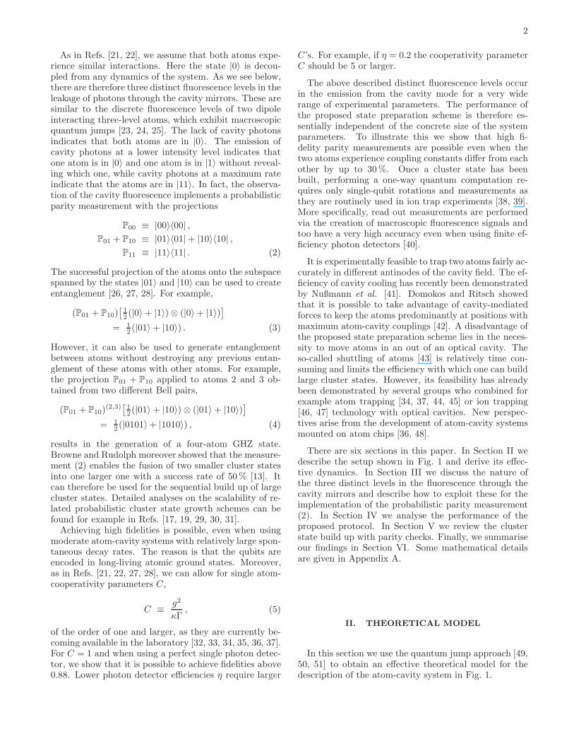
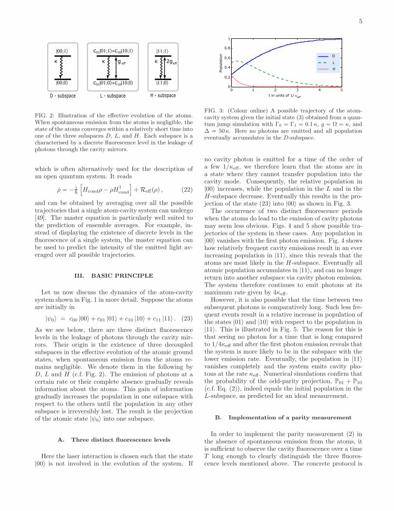
FIG. 2: Illustration of the effective evolution of the atoms.When spontaneous emission from the atoms is negligible, thestate of the atoms converges within a relatively short time intoone of the three subspaces D, L, and H . Each subspace is acharacterised by a discrete fluorescence level in the leakage ofphotons through the cavity mirrors.

which is often alternatively used for the description ofan open quantum system. It reads

ρ = − i~

[

Hcondρ− ρH†cond

]

+ Reff(ρ) , (22)

and can be obtained by averaging over all the possibletrajectories that a single atom-cavity system can undergo[49]. The master equation is particularly well suited tothe prediction of ensemble averages. For example, in-stead of displaying the existence of discrete levels in thefluorescence of a single system, the master equation canbe used to predict the intensity of the emitted light av-eraged over all possible trajectories.

III. BASIC PRINCIPLE

Let us now discuss the dynamics of the atom-cavitysystem shown in Fig. 1 in more detail. Suppose the atomsare initially in

|ψ0〉 = c00 |00〉+ c01 |01〉+ c10 |10〉 + c11 |11〉 . (23)

As we see below, there are three distinct fluorescencelevels in the leakage of photons through the cavity mir-rors. Their origin is the existence of three decoupledsubspaces in the effective evolution of the atomic groundstates, when spontaneous emission from the atoms re-mains negligible. We denote them in the following byD, L and H (c.f. Fig. 2). The emission of photons at acertain rate or their complete absence gradually revealsinformation about the atoms. This gain of informationgradually increases the population in one subspace withrespect to the others until the population in any othersubspace is irreversibly lost. The result is the projectionof the atomic state |ψ0〉 into one subspace.

A. Three distinct fluorescence levels

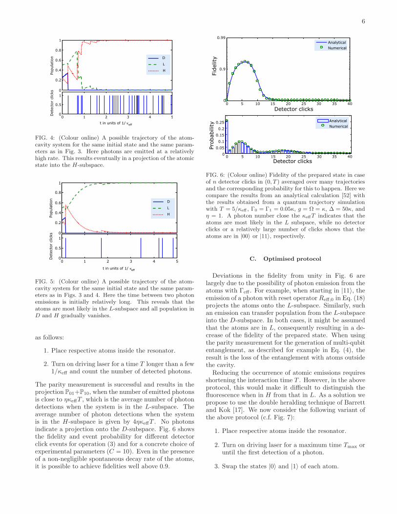
Here the laser interaction is chosen such that the state|00〉 is not involved in the evolution of the system. If

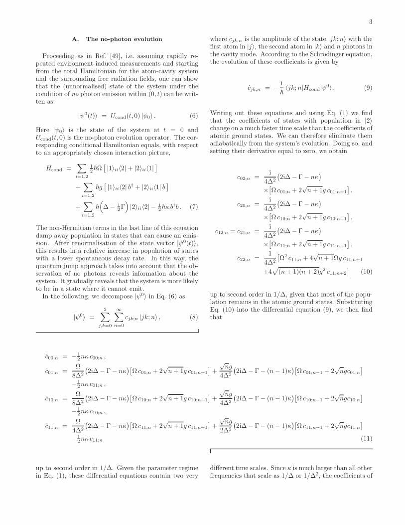
FIG. 3: (Colour online) A possible trajectory of the atom-cavity system given the initial state (3) obtained from a quan-tum jump simulation with Γ0 = Γ1 = 0.1 κ, g = Ω = κ, and∆ = 50 κ. Here no photons are emitted and all populationeventually accumulates in the D-subspace.

no cavity photon is emitted for a time of the order ofa few 1/κeff , we therefore learn that the atoms are ina state where they cannot transfer population into thecavity mode. Consequently, the relative population in|00〉 increases, while the population in the L and in theH-subspace decrease. Eventually this results in the pro-jection of the state (23) into |00〉 as shown in Fig. 3.

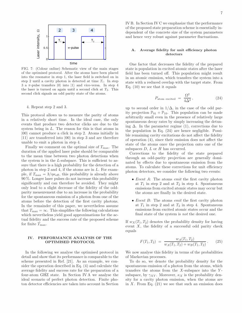
The occurrence of two distinct fluorescence periodswhen the atoms do lead to the emission of cavity photonsmay seem less obvious. Figs. 4 and 5 show possible tra-jectories of the system in these cases. Any population in|00〉 vanishes with the first photon emission. Fig. 4 showshow relatively frequent cavity emissions result in an everincreasing population in |11〉, since this reveals that theatoms are most likely in the H-subspace. Eventually allatomic population accumulates in |11〉, and can no longerreturn into another subspace via cavity photon emission.The system therefore continues to emit photons at itsmaximum rate given by 4κeff .

However, it is also possible that the time between twosubsequent photons is comparatively long. Such less fre-quent events result in a relative increase in population ofthe states |01〉 and |10〉 with respect to the population in|11〉. This is illustrated in Fig. 5. The reason for this isthat seeing no photon for a time that is long comparedto 1/4κeff and after the first photon emission reveals thatthe system is more likely to be in the subspace with thelower emission rate. Eventually, the population in |11〉vanishes completely and the system emits cavity pho-tons at the rate κeff . Numerical simulations confirm thatthe probability of the odd-parity projection, P01 + P10

(c.f. Eq. (2)), indeed equals the initial population in theL-subspace, as predicted for an ideal measurement.

B. Implementation of a parity measurement

In order to implement the parity measurement (2) inthe absence of spontaneous emission from the atoms, itis sufficient to observe the cavity fluorescence over a timeT long enough to clearly distinguish the three fluores-cence levels mentioned above. The concrete protocol is

6

FIG. 4: (Colour online) A possible trajectory of the atom-cavity system for the same initial state and the same param-eters as in Fig. 3. Here photons are emitted at a relativelyhigh rate. This results eventually in a projection of the atomicstate into the H-subspace.

FIG. 5: (Colour online) A possible trajectory of the atom-cavity system for the same initial state and the same param-eters as in Figs. 3 and 4. Here the time between two photonemissions is initially relatively long. This reveals that theatoms are most likely in the L-subspace and all population inD and H gradually vanishes.

as follows:

1. Place respective atoms inside the resonator.

2. Turn on driving laser for a time T longer than a few1/κeff and count the number of detected photons.

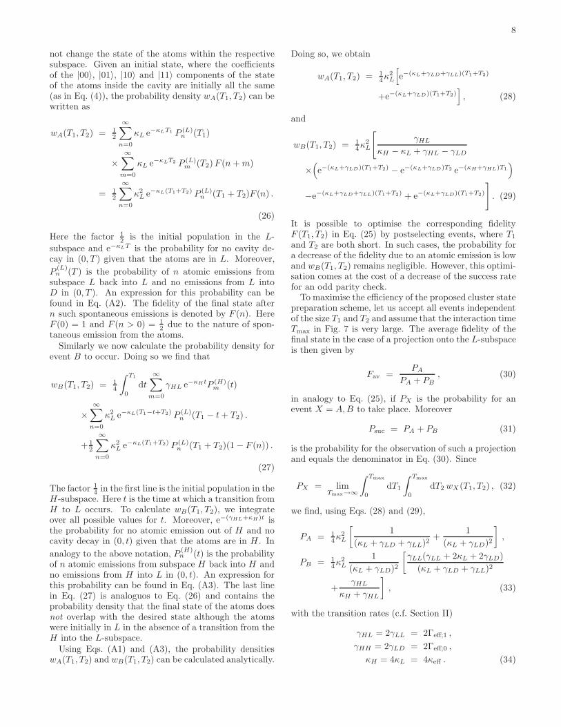
The parity measurement is successful and results in theprojection P01+P10, when the number of emitted photonsis close to ηκeffT , which is the average number of photondetections when the system is in the L-subspace. Theaverage number of photon detections when the systemis in the H-subspace is given by 4ηκeffT . No photonsindicate a projection onto the D-subspace. Fig. 6 showsthe fidelity and event probability for different detectorclick events for operation (3) and for a concrete choice ofexperimental parameters (C = 10). Even in the presenceof a non-negligible spontaneous decay rate of the atoms,it is possible to achieve fidelities well above 0.9.

FIG. 6: (Colour online) Fidelity of the prepared state in caseof n detector clicks in (0, T ) averaged over many trajectoriesand the corresponding probability for this to happen. Here wecompare the results from an analytical calculation [52] withthe results obtained from a quantum trajectory simulationwith T = 5/κeff , Γ0 = Γ1 = 0.05κ, g = Ω = κ, ∆ = 50κ, andη = 1. A photon number close the κeffT indicates that theatoms are most likely in the L subspace, while no detectorclicks or a relatively large number of clicks shows that theatoms are in |00〉 or |11〉, respectively.

C. Optimised protocol

Deviations in the fidelity from unity in Fig. 6 arelargely due to the possibility of photon emission from theatoms with Γeff . For example, when starting in |11〉, theemission of a photon with reset operator Reff;0 in Eq. (18)projects the atoms onto the L-subspace. Similarly, suchan emission can transfer population from the L-subspaceinto the D-subspace. In both cases, it might be assumedthat the atoms are in L, consequently resulting in a de-crease of the fidelity of the prepared state. When usingthe parity measurement for the generation of multi-qubitentanglement, as described for example in Eq. (4), theresult is the loss of the entanglement with atoms outsidethe cavity.

Reducing the occurrence of atomic emissions requiresshortening the interaction time T . However, in the aboveprotocol, this would make it difficult to distinguish thefluorescence when in H from that in L. As a solution wepropose to use the double heralding technique of Barrettand Kok [17]. We now consider the following variant ofthe above protocol (c.f. Fig. 7):

1. Place respective atoms inside the resonator.

2. Turn on driving laser for a maximum time Tmax oruntil the first detection of a photon.

3. Swap the states |0〉 and |1〉 of each atom.

7

FIG. 7: (Colour online) Schematic view of the main stagesof the optimised protocol. After the atoms have been placedinto the resonator in step 1, the laser field is switched on instep 2 until a cavity photon is detected at time T1. In step3 a π-pulse transfers |0〉 into |1〉 and vice-versa. In step 4the laser is turned on again until a second click at T2. Thissecond click signals an odd parity state of the atoms.

4. Repeat step 2 and 3.

This protocol allows us to measure the parity of atomsin a relatively short time. In the ideal case, the onlyevents that produce two detector clicks are due to thesystem being in L. The reason for this is that atoms in|00〉 cannot produce a click in step 2. Atoms initially in|11〉 are transferred into |00〉 in step 3 and are thereforeunable to emit a photon in step 4.

Finally we comment on the optimal size of Tmax. Theduration of the applied laser pulse should be comparableto the mean time between two photon detections whenthe system is in the L-subspace. This is sufficient to as-sure that there is a high probability for the detection of aphoton in step 2 and 4, if the atoms are in L. For exam-ple, if Tmax = 3/ηκeff , this probability is already above90 %. Longer laser pulses do not increase this probabilitysignificantly and can therefore be avoided. They mightonly lead to a slight decrease of the fidelity of the odd-parity measurement due to an increase in the probabilityfor the spontaneous emission of a photon from one of theatoms before the detection of the first cavity photons.In the remainder of this paper, we nevertheless assumethat Tmax = ∞. This simplifies the following calculationswhich nevertheless yield good approximations for the ac-tual fidelity and the success rate of the proposed schemefor finite Tmax.

IV. PERFORMANCE ANALYSIS OF THE

OPTIMISED PROTOCOL

In the following we analyse the optimised protocol indetail and show that its performance is comparable to thescheme presented in Ref. [21]. As an example, we con-sider the operation described in Eq. (4) and calculate theaverage fidelity and success rate for the preparation of afour-atom GHZ state. In Section IVA we analyse theideal scenario of perfect photon detection. Finite pho-ton detector efficiencies are taken into account in Section

IVB. In Section IVC we emphasize that the performanceof the proposed state preparation scheme is essentially in-dependent of the concrete size of the system parametersand hence very robust against parameter fluctuations.

A. Average fidelity for unit efficiency photon

detectors

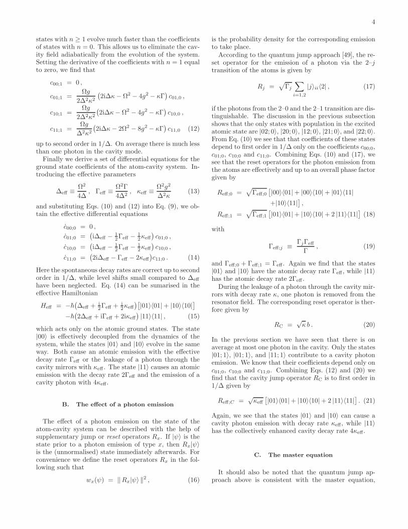
One factor that decreases the fidelity of the preparedstate is population in excited atomic states after the laserfield has been turned off. This population might resultin an atomic emission, which transfers the system into astate with a reduced overlap with the target state. FromEq. (10) we see that it equals

Patom excited =Ω2

4∆2, (24)

up to second order in 1/∆, in the case of the odd par-ity projection P01 + P10. This population can be madearbitrarily small even in the presence of relatively largespontaneous decay rates by simply increasing the detun-ing ∆. In the parameter regime (1), corrections due tothe population in Eq. (24) are hence negligible. Possi-ble remaining cavity excitations do not affect the fidelityof operation (4), since their emission does not affect thestate of the atoms once the projection onto one of thesubspaces D, L or H has occurred.

Corrections to the fidelity of the state preparedthrough an odd-parity projection are generally domi-nated by effects due to spontaneous emission from theatoms. To calculate these corrections for unit efficiencyphoton detectors, we consider the following two events:

• Event A: The atoms emit the first cavity photonat T1 in step 2 and at T2 in step 4. Spontaneousemissions from excited atomic states may occur butthe atoms are finally in the desired state.

• Event B: The atoms emit the first cavity photonat T1 in step 2 and at T2 in step 4. Spontaneousemissions from excited atomic states occur and thefinal state of the system is not the desired one.

If wX(T1, T2) denotes the probability density for havingevent X , the fidelity of a successful odd parity checkequals

F (T1, T2) =wA(T1, T2)

wA(T1, T2) + wB(T1, T2). (25)

We now analyse this fidelity in terms of the probabilitiesof Markovian processes.

To do so, we denote the probability density for thespontaneous emission of a photon from the atoms, whichtransfers the atoms from the X-subspace into the Y -subspace, by γXY . Moreover, κX is the probability den-sity for a cavity photon emission, when the atoms arein X . From Eq. (21) we see that such an emission does

8

not change the state of the atoms within the respectivesubspace. Given an initial state, where the coefficientsof the |00〉, |01〉, |10〉 and |11〉 components of the stateof the atoms inside the cavity are initially all the same(as in Eq. (4)), the probability density wA(T1, T2) can bewritten as

wA(T1, T2) = 12

∞∑

n=0

κL e−κLT1 P (L)n (T1)

×∞∑

m=0

κL e−κLT2 P (L)m (T2)F (n+m)

= 12

∞∑

n=0

κ2L e−κL(T1+T2) P (L)

n (T1 + T2)F (n) .

(26)

Here the factor 12 is the initial population in the L-

subspace and e−κLT is the probability for no cavity de-cay in (0, T ) given that the atoms are in L. Moreover,

P(L)n (T ) is the probability of n atomic emissions from

subspace L back into L and no emissions from L intoD in (0, T ). An expression for this probability can befound in Eq. (A2). The fidelity of the final state aftern such spontaneous emissions is denoted by F (n). HereF (0) = 1 and F (n > 0) = 1

2 due to the nature of spon-taneous emission from the atoms.

Similarly we now calculate the probability density forevent B to occur. Doing so we find that

wB(T1, T2) = 14

∫ T1

0

dt

∞∑

m=0

γHL e−κHtP (H)m (t)

×∞∑

n=0

κ2L e−κL(T1−t+T2) P (L)

n (T1 − t+ T2) .

+ 12

∞∑

n=0

κ2L e−κL(T1+T2) P (L)

n (T1 + T2)(1 − F (n)) .

(27)

The factor 14 in the first line is the initial population in the

H-subspace. Here t is the time at which a transition fromH to L occurs. To calculate wB(T1, T2), we integrateover all possible values for t. Moreover, e−(γHL+κH)t isthe probability for no atomic emission out of H and nocavity decay in (0, t) given that the atoms are in H . In

analogy to the above notation, P(H)n (t) is the probability

of n atomic emissions from subspace H back into H andno emissions from H into L in (0, t). An expression forthis probability can be found in Eq. (A3). The last linein Eq. (27) is analoguos to Eq. (26) and contains theprobability density that the final state of the atoms doesnot overlap with the desired state although the atomswere initially in L in the absence of a transition from theH into the L-subspace.

Using Eqs. (A1) and (A3), the probability densitieswA(T1, T2) and wB(T1, T2) can be calculated analytically.

Doing so, we obtain

wA(T1, T2) = 14κ

2L

[

e−(κL+γLD+γLL)(T1+T2)

+e−(κL+γLD)(T1+T2)]

, (28)

and

wB(T1, T2) = 14κ

2L

[

γHL

κH − κL + γHL − γLD

×(

e−(κL+γLD)(T1+T2) − e−(κL+γLD)T2 e−(κH+γHL)T1

)

−e−(κL+γLD+γLL)(T1+T2) + e−(κL+γLD)(T1+T2)

]

. (29)

It is possible to optimise the corresponding fidelityF (T1, T2) in Eq. (25) by postselecting events, where T1

and T2 are both short. In such cases, the probability fora decrease of the fidelity due to an atomic emission is lowand wB(T1, T2) remains negligible. However, this optimi-sation comes at the cost of a decrease of the success ratefor an odd parity check.

To maximise the efficiency of the proposed cluster statepreparation scheme, let us accept all events independentof the size T1 and T2 and assume that the interaction timeTmax in Fig. 7 is very large. The average fidelity of thefinal state in the case of a projection onto the L-subspaceis then given by

Fav =PA

PA + PB, (30)

in analogy to Eq. (25), if PX is the probability for anevent X = A,B to take place. Moreover

Psuc = PA + PB (31)

is the probability for the observation of such a projectionand equals the denominator in Eq. (30). Since

PX = limTmax→∞

∫ Tmax

0

dT1

∫ Tmax

0

dT2 wX(T1, T2) , (32)

we find, using Eqs. (28) and (29),

PA = 14κ

2L

[

1

(κL + γLD + γLL)2+

1

(κL + γLD)2

]

,

PB = 14κ

2L

1

(κL + γLD)2

[

γLL(γLL + 2κL + 2γLD)

(κL + γLD + γLL)2

+γHL

κH + γHL

]

, (33)

with the transition rates (c.f. Section II)

γHL = 2γLL = 2Γeff;1 ,

γHH = 2γLD = 2Γeff;0 ,

κH = 4κL = 4κeff . (34)

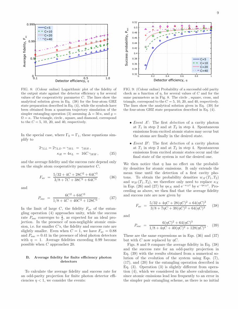
9

FIG. 8: (Colour online) Logarithmic plot of the fidelity ofthe output state against the detector efficiency η for severalvalues of the cooperativity parameter C. The lines show theanalytical solution given in Eq. (38) for the four-atom GHZstate preparation described in Eq. (4), while the symbols havebeen obtained from a quantum trajectory simulation of thesimpler entangling operation (3) assuming ∆ = 50 κ, and g =Ω = κ. The triangle, circle , square, and diamond, correspondto the C = 5, 10, 20, and 40, respectively.

In the special case, where Γ0 = Γ1, these equations sim-plify to

2γLL = 2γLD = γHL = γHH ,

κH = 4κL = 16C γHH , (35)

and the average fidelity and the success rate depend onlyon the single atom cooperativity parameter C,

Fav =5/32 + 4C + 28C2 + 64C3

3/8 + 7C + 38C2 + 64C3(36)

and

Psuc =6C2 + 64C3

1/8 + 4C + 40C2 + 128C3. (37)

In the limit of large C, the fidelity Fav of the entan-gling operation (4) approaches unity, while the successrate Psuc converges to 1

2 , as expected for an ideal pro-jection. In the presence of non-negligible atomic emis-sion, i.e. for smaller C’s, the fidelity and success rate areslightly smaller. Even when C = 1, we have Fav = 0.88and Psuc = 0.41 in the presence of ideal photon detectorswith η = 1. Average fidelities exceeding 0.99 becomepossible when C approaches 20.

B. Average fidelity for finite efficiency photon

detectors

To calculate the average fidelity and success rate foran odd-parity projection for finite photon detector effi-ciencies η < 1, we consider the events:

FIG. 9: (Colour online) Probability of a successful odd paritycheck as a function of η, for several values of C and for thesame parameters as in Fig. 8. The circle , square, cross, andtriangle, correspond to the C = 5, 10, 20, and 40, respectively.The lines show the analytical solution given in Eq. (39) forthe four-atom GHZ state preparation described in Eq. (4).

• Event A′: The first detection of a cavity photonat T1 in step 2 and at T2 in step 4. Spontaneousemissions from excited atomic states may occur butthe atoms are finally in the desired state.

• Event B′: The first detection of a cavity photonat T1 in step 2 and at T2 in step 4. Spontaneousemissions from excited atomic states occur and thefinal state of the system is not the desired one.

We then notice that η has no effect on the probabil-ity densities for atomic emissions. It only extends themean time until the detection of a first cavity pho-tons. To obtain the probability densities wA′(T1, T2)and wB′(T1, T2), we therefore only need to replace κX

in Eqs. (26) and (27) by ηκX and e−κXt by e−ηκX t. Pro-ceeding as above, we then find that the average fidelityand success rate are now given by

Fav =5/32 + 4ηC + 28(ηC)2 + 64(ηC)3

3/8 + 7ηC + 38(ηC)2 + 64(ηC)3(38)

and

Psuc =6(ηC)2 + 64(ηC)3

1/8 + 4ηC + 40(ηC)2 + 128(ηC)3. (39)

These are the same expressions as in Eqs. (36) and (37)but with C now replaced by ηC.

Figs. 8 and 9 compare the average fidelity in Eq. (38)and the success rate for an odd-parity projection inEq. (39) with the results obtained from a numerical so-lution of the evolution of the system using Eqs. (7),(17), and (20) for the entangling operation described inEq. (3). Operation (3) is slightly different from opera-tion (4), which we considered in the above calculations,since atomic emissions lead less frequently to an error inthe simpler pair entangling scheme, as there is no initial

10

entanglement that needs to be preserved. Nevertheless,there is relatively good agreement between both curves.Figs. 8 and 9 indeed confirm that reducing η has the sameeffect as replacing C by ηC.

C. Parameter dependence

Due to its postselective nature, the performance of theproposed state preparation scheme is essentially indepen-dent of the concrete system parameters. Fig. 8 shows thatfidelities well above 99 % are inevitably when ηC > 20.Whenever this condition is fulfilled, there are three dis-tinct fluorescence levels in the emission of cavity photons.The scheme is constructed such that the medium level al-ways indicates that one atom is in |0〉 and one atom isin |1〉 without revealing which one. Turning off the ap-plied laser field upon the detection of a photon in step 2and 4 is hence sufficient to realise the parity operation (2)with very high accuracy. The proposed state preparationscheme is therefore robust against a parameter fluctua-tions, like moderate fluctuations of cavity coupling con-stants and laser Rabi frequencies.

In the following, we show that high fidelities areachieved even when the atoms experience quite differ-ent coupling constants. As an example, we consider thecase where the cavity-coupling constant of atom 1 is g1and the cavity-coupling constant of atoms 2 is given byg2. For simplicity we neglect spontaneous emission fromthe atoms (Γ = 0) in the following. Proceeding as inSection II, we find that the conditional Hamiltonian (15)is now given by

Heff = −~(

∆eff + i2κeff;2

)

|01〉〈01|−~

(

∆eff + i2κeff;1

)

|10〉〈10|−~

[

2∆eff + i2 (√κeff;1 +

√κeff;2 )2

]

|11〉〈11| (40)

with

κeff;i ≡ Ω2g2i

∆2κ. (41)

At the same time, the reset operator in Eq. (21) becomes

Reff;C =√κeff;1

(

|10〉〈10|+ |11〉〈11|)

+√κeff;2

(

|01〉〈01|+ |11〉〈11|)

. (42)

These two equations can be used to simulate for exampleall the possible trajectories for the two-qubit entanglingoperation (3).

Let us first consider the case, where the atoms perma-

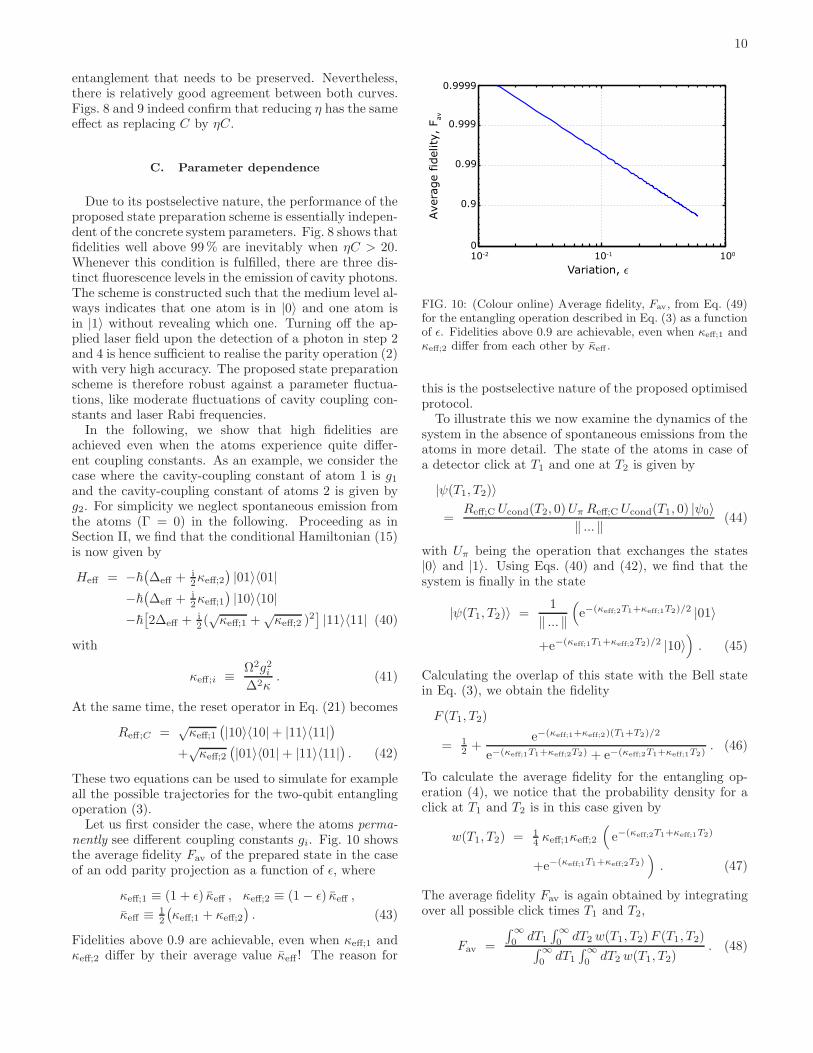
nently see different coupling constants gi. Fig. 10 showsthe average fidelity Fav of the prepared state in the caseof an odd parity projection as a function of ǫ, where

κeff;1 ≡ (1 + ǫ) κeff , κeff;2 ≡ (1 − ǫ) κeff ,

κeff ≡ 12

(

κeff;1 + κeff;2

)

. (43)

Fidelities above 0.9 are achievable, even when κeff;1 andκeff;2 differ by their average value κeff ! The reason for

FIG. 10: (Colour online) Average fidelity, Fav, from Eq. (49)for the entangling operation described in Eq. (3) as a functionof ǫ. Fidelities above 0.9 are achievable, even when κeff;1 andκeff;2 differ from each other by κeff .

this is the postselective nature of the proposed optimisedprotocol.

To illustrate this we now examine the dynamics of thesystem in the absence of spontaneous emissions from theatoms in more detail. The state of the atoms in case ofa detector click at T1 and one at T2 is given by

|ψ(T1, T2)〉

=Reff;C Ucond(T2, 0)Uπ Reff;C Ucond(T1, 0) |ψ0〉

‖ ... ‖ (44)

with Uπ being the operation that exchanges the states|0〉 and |1〉. Using Eqs. (40) and (42), we find that thesystem is finally in the state

|ψ(T1, T2)〉 =1

‖ ... ‖(

e−(κeff;2T1+κeff;1T2)/2 |01〉

+e−(κeff;1T1+κeff;2T2)/2 |10〉)

. (45)

Calculating the overlap of this state with the Bell statein Eq. (3), we obtain the fidelity

F (T1, T2)

= 12 +

e−(κeff;1+κeff;2)(T1+T2)/2

e−(κeff;1T1+κeff;2T2) + e−(κeff;2T1+κeff;1T2). (46)

To calculate the average fidelity for the entangling op-eration (4), we notice that the probability density for aclick at T1 and T2 is in this case given by

w(T1, T2) = 14 κeff;1κeff;2

(

e−(κeff;2T1+κeff;1T2)

+e−(κeff;1T1+κeff;2T2))

. (47)

The average fidelity Fav is again obtained by integratingover all possible click times T1 and T2,

Fav =

∫ ∞0 dT1

∫ ∞0 dT2 w(T1, T2)F (T1, T2)

∫ ∞0 dT1

∫ ∞0 dT2 w(T1, T2)

. (48)

11

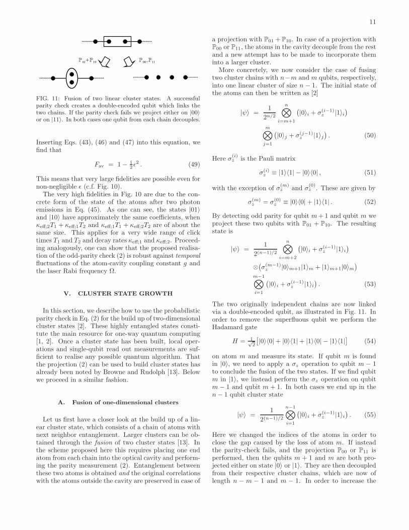
FIG. 11: Fusion of two linear cluster states. A successfulparity check creates a double-encoded qubit which links thetwo chains. If the parity check fails we project either on |00〉or on |11〉. In both cases one qubit from each chain decouples.

Inserting Eqs. (43), (46) and (47) into this equation, wefind that

Fav = 1 − 12ǫ

2 . (49)

This means that very large fidelities are possible even fornon-negligible ǫ (c.f. Fig. 10).

The very high fidelities in Fig. 10 are due to the con-crete form of the state of the atoms after two photonemissions in Eq. (45). As one can see, the states |01〉and |10〉 have approximately the same coefficients, whenκeff;2T1 + κeff;1T2 and κeff;1T1 + κeff;2T2 are of about thesame size. This applies for a very wide range of clicktimes T1 and T2 and decay rates κeff;1 and κeff;2. Proceed-ing analogously, one can show that the proposed realisa-tion of the odd-parity check (2) is robust against temporalfluctuations of the atom-cavity coupling constant g andthe laser Rabi frequency Ω.

V. CLUSTER STATE GROWTH

In this section, we describe how to use the probabilisticparity check in Eq. (2) for the build up of two-dimensionalcluster states [2]. These highly entangled states consti-tute the main resource for one-way quantum computing[1, 2]. Once a cluster state has been built, local oper-ations and single-qubit read out measurements are suf-ficient to realise any possible quantum algorithm. Thatthe projection (2) can be used to build cluster states hasalready been noted by Browne and Rudolph [13]. Belowwe proceed in a similar fashion.

A. Fusion of one-dimensional clusters

Let us first have a closer look at the build up of a lin-ear cluster state, which consists of a chain of atoms withnext neighbor entanglement. Larger clusters can be ob-tained through the fusion of two cluster states [13]. Inthe scheme proposed here this requires placing one endatom from each chain into the optical cavity and perform-ing the parity measurement (2). Entanglement betweenthese two atoms is obtained and the original correlationswith the atoms outside the cavity are preserved in case of

a projection with P01 + P10. In case of a projection withP00 or P11, the atoms in the cavity decouple from the restand a new attempt has to be made to incorporate theminto a larger cluster.

More concretely, we now consider the case of fusingtwo cluster chains with n−m and m qubits, respectively,into one linear cluster of size n − 1. The initial state ofthe atoms can then be written as [2]

|ψ〉 =1

2n/2

n⊗

i=m+1

(

|0〉i + σ(i−1)z |1〉i

)

m⊗

j=1

(

|0〉j + σ(j−1)z |1〉j

)

. (50)

Here σ(i)z is the Pauli matrix

σ(i)z ≡ |1〉〈1| − |0〉〈0| , (51)

with the exception of σ(m)z and σ

(0)z . These are given by

σ(m)z = σ(0)

z ≡ |0〉〈0| + |1〉〈1| . (52)

By detecting odd parity for qubit m+ 1 and qubit m weproject these two qubits with P01 + P10. The resultingstate is

|ψ〉 =1

2(n−1)/2

n⊗

i=m+2

(

|0〉i + σ(i−1)z |1〉i

)

⊗(

σ(m−1)z |0〉m+1|1〉m + |1〉m+1|0〉m

)

m−1⊗

i=1

(

|0〉i + σ(i−1)z |1〉i

)

. (53)

The two originally independent chains are now linkedvia a double-encoded qubit, as illustrated in Fig. 11. Inorder to remove the superfluous qubit we perform theHadamard gate

H = 1√2

[

|0〉〈0| + |0〉〈1| + |1〉〈0| − |1〉〈1|]

(54)

on atom m and measure its state. If qubit m is foundin |0〉, we need to apply a σz operation to qubit m − 1to conclude the fusion of the two states. If we find qubitm in |1〉, we instead perform the σz operation on qubitm− 1 and qubit m + 1. In both cases we end up in then− 1 qubit cluster state

|ψ〉 =1

2(n−1)/2

n−1⊗

i=1

(

|0〉i + σ(i−1)z |1〉i

)

. (55)

Here we changed the indices of the atoms in order toclose the gap caused by the loss of atom m. If insteadthe parity-check fails, and the projection P00 or P11 isperformed, then the qubits m + 1 and m are both pro-jected either on state |0〉 or |1〉. They are then decoupledfrom their respective cluster chains, which are now oflength n − m − 1 and m − 1. In order to increase the

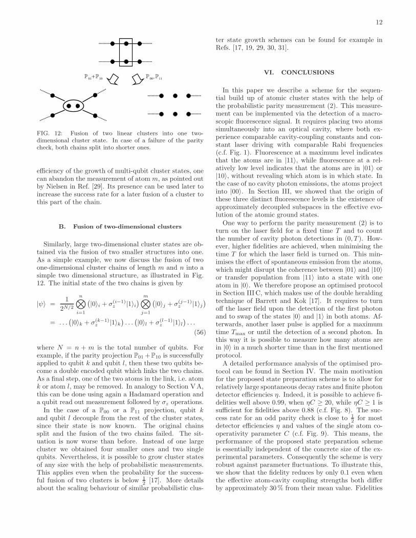
12

FIG. 12: Fusion of two linear clusters into one two-dimensional cluster state. In case of a failure of the paritycheck, both chains split into shorter ones.

efficiency of the growth of multi-qubit cluster states, onecan abandon the measurement of atom m, as pointed outby Nielsen in Ref. [29]. Its presence can be used later toincrease the success rate for a later fusion of a cluster tothis part of the chain.

B. Fusion of two-dimensional clusters

Similarly, large two-dimensional cluster states are ob-tained via the fusion of two smaller structures into one.As a simple example, we now discuss the fusion of twoone-dimensional cluster chains of length m and n into asimple two dimensional structure, as illustrated in Fig.12. The initial state of the two chains is given by

|ψ〉 =1

2N/2

n⊗

i=1

(

|0〉i + σ(i−1)z |1〉i

)

m⊗

j=1

(

|0〉j + σ(j−1)z |1〉j

)

= . . .(

|0〉k + σ(k−1)z |1〉k

)

. . .(

|0〉l + σ(l−1)z |1〉l

)

. . .

(56)

where N = n + m is the total number of qubits. Forexample, if the parity projection P01 +P10 is successfullyapplied to qubit k and qubit l, then these two qubits be-come a double encoded qubit which links the two chains.As a final step, one of the two atoms in the link, i.e. atomk or atom l, may be removed. In analogy to Section VA,this can be done using again a Hadamard operation anda qubit read out measurement followed by σz operations.

In the case of a P00 or a P11 projection, qubit kand qubit l decouple from the rest of the cluster states,since their state is now known. The original chainssplit and the fusion of the two chains failed. The sit-uation is now worse than before. Instead of one largecluster we obtained four smaller ones and two singlequbits. Nevertheless, it is possible to grow cluster statesof any size with the help of probabilistic measurements.This applies even when the probability for the success-ful fusion of two clusters is below 1

2 [17]. More detailsabout the scaling behaviour of similar probabilistic clus-

ter state growth schemes can be found for example inRefs. [17, 19, 29, 30, 31].

VI. CONCLUSIONS

In this paper we describe a scheme for the sequen-tial build up of atomic cluster states with the help ofthe probabilistic parity measurement (2). This measure-ment can be implemented via the detection of a macro-scopic fluorescence signal. It requires placing two atomssimultaneously into an optical cavity, where both ex-perience comparable cavity-coupling constants and con-stant laser driving with comparable Rabi frequencies(c.f. Fig. 1). Fluorescence at a maximum level indicatesthat the atoms are in |11〉, while fluorescence at a rel-atively low level indicates that the atoms are in |01〉 or|10〉, without revealing which atom is in which state. Inthe case of no cavity photon emissions, the atoms projectinto |00〉. In Section III, we showed that the origin ofthese three distinct fluorescence levels is the existence ofapproximately decoupled subspaces in the effective evo-lution of the atomic ground states.

One way to perform the parity measurement (2) is toturn on the laser field for a fixed time T and to countthe number of cavity photon detections in (0, T ). How-ever, higher fidelities are achieved, when minimising thetime T for which the laser field is turned on. This min-imises the effect of spontaneous emission from the atoms,which might disrupt the coherence between |01〉 and |10〉or transfer population from |11〉 into a state with oneatom in |0〉. We therefore propose an optimised protocolin Section III C, which makes use of the double heraldingtechnique of Barrett and Kok [17]. It requires to turnoff the laser field upon the detection of the first photonand to swap of the states |0〉 and |1〉 in both atoms. Af-terwards, another laser pulse is applied for a maximumtime Tmax or until the detection of a second photon. Inthis way it is possible to measure how many atoms arein |0〉 in a much shorter time than in the first mentionedprotocol.

A detailed performance analysis of the optimised pro-tocol can be found in Section IV. The main motivationfor the proposed state preparation scheme is to allow forrelatively large spontaneous decay rates and finite photondetector efficiencies η. Indeed, it is possible to achieve fi-delities well above 0.99, when ηC ≥ 20, while ηC ≥ 1 issufficient for fidelities above 0.88 (c.f. Fig. 8). The suc-cess rate for an odd parity check is close to 1

2 for mostdetector efficiencies η and values of the single atom co-operativity parameter C (c.f. Fig. 9). This means, theperformance of the proposed state preparation schemeis essentially independent of the concrete size of the ex-perimental parameters. Consequently the scheme is veryrobust against parameter fluctuations. To illustrate this,we show that the fidelity reduces by only 0.1 even whenthe effective atom-cavity coupling strengths both differby approximately 30 % from their mean value. Fidelities

13

in excess of 0.99 of the values calculated for equal cou-pling constants require that the atom-cavity couplingsdiffer by less than 10 % (c.f. Fig. 10).

In Section V, we show how the parity measure-ment (2) can be used to grow two-dimensional clusterstates. It has already been shown in the literature(c.f. e.g. Refs. [17, 19, 29, 30, 31]) that the build up oflarge cluster states is possible even when the probabilityfor the successful fusion of two clusters is below 1

2 . Herewe propose a scheme, in which the success rate for an oddparity check is close to 1

2 even in the presence of finite

efficiency photon detectors. Our cluster state growthscheme with macroscopic heralding is therefore expectedto be much more practical than recent schemes based onthe detection of single photons [15, 16, 17, 18, 19].

Acknowledgment. We thank S. D. Barrett and P. L.Knight for stimulating discussions. A. B. acknowledgessupport from the Royal Society and the GCHQ. Thiswork was supported in part by the EU Integrated ProjectSCALA, the EU Research and Training Network EMALIand the UK EPSRC through the QIP IRC.

[1] R. Raussendorf and H. J. Briegel, Phys. Rev. Lett. 86,5188 (2001).

[2] H. J. Briegel and R. Raussendorf, Phys. Rev. Lett. 86,910 (2001).

[3] M. A. Nielsen and C. M. Dawson, Phys. Rev. A 71,042323 (2005).

[4] C. M. Dawson, H. L. Haselgrove, and M. A. Nielsen,Phys. Rev. Lett. 96, 020501 (2006).

[5] R. Raussendorf, J. Harrington, and K. Goyal, Ann. ofPhys. 321, 2242 (2006).

[6] A. Kay and J. K. Pachos, Phys. Rev. A 75, 062307,(2007).

[7] K. Goyal, A. McCauley, and R. Raussendorf, Phys. Rev.A 74, 032318 (2006).

[8] D. Jaksch, H. J. Briegel, J. I. Cirac, C. W. Gardiner, andP. Zoller, Phys. Rev. Lett. 82, 1975 (1999).

[9] O. Mandel, M. Greiner, A. Widera, T. Rom, T. W.Hansch, and I. Bloch, Nature 425, 937 (2003).

[10] R. Scheunemann, F. S. Cataliotti, T. W. Hansch, and M.Weitz, Phys. Rev. A 62, 051801(R) (2000).

[11] T. Calarco, U. Dorner, P. S. Julienne, C. J. Williams,and P. Zoller, Phys. Rev. A 70, 012306 (2004).

[12] J. Joo, Y. L. Lim, A. Beige, and P. L. Knight, Phys. Rev.A 74, 042344 (2006).

[13] D. E. Browne and T. Rudolph, Phys. Rev. Lett. 95,010501 (2005).

[14] P. Walther, K. J. Resch, T. Rudolph, E. Schenck, H.Weinfurter, V. Vedral, M. Aspelmeyer, and A. Zeilinger,Nature 434, 169 (2005).

[15] C. Cabrillo, J. I. Cirac, P. Garcia-Fernandez, and P.Zoller, Phys. Rev. A 59, 1025 (1999).

[16] D. E. Browne, M. B. Plenio, and S. F. Huelga, Phys. Rev.Lett. 91, 067901 (2003).

[17] S. D. Barrett and P. Kok, Phys. Rev. A 71, 060310(R)(2005).

[18] Y. L. Lim, A. Beige, and L. C. Kwek, Phys. Rev. Lett.95, 030505 (2005).

[19] Y. L. Lim, S. D. Barrett, A. Beige, P. Kok, and L. C.Kwek, Phys. Rev. A 73, 012304 (2006).

[20] Note that many experimental papers use this notationfor the cavity field decay rate, which equals 1

2κ in our

notation.[21] J. Metz, M. Trupke, and A. Beige, Phys. Rev. Lett. 97,

040503 (2006).[22] J. Metz and A. Beige, Phys. Rev. A 76, 022331 (2007).[23] A. Beige and G. C. Hegerfeldt, Phys. Rev. A 59, 2385

(1999).

[24] S. U. Addicks, A. Beige, M. Dakna, and G. C. Hegerfeldt,Eur. J. Phys. D 15, 393 (2001).

[25] V. Hannstein and G. C. Hegerfeldt, Eur. Phys. J. D 38,415 (2006).

[26] T. B. Pittman, B. C. Jacobs, and J. D. Franson, Phys.Rev. A 64, 062311 (2001).

[27] A. S. Sørensen and K. Mølmer, Phys. Rev. Lett. 90,127903 (2003).

[28] A. S. Sørensen and K. Mølmer, Phys. Rev. Lett. 91,097905 (2003).

[29] M. A. Nielsen, Phys. Rev. Lett. 93, 040503 (2004).[30] D. Gross, K. Kieling, and J. Eisert, Phys. Rev. A 74,

042343 (2006).[31] E. T. Campbell, J. Fitzsimons, S. C. Benjamin, and P.

Kok, Phys. Rev. A 75, 042303 (2007).[32] J. Ye, D. W. Vernooy, and H. J.Kimble, Phys. Rev. Lett.

83, 4987 (1999).[33] A. Kuhn, M. Hennrich, and G. Rempe, Phys. Rev. Lett.

89, 067901 (2002).[34] J. McKeeve, A. Boca, A. D. Boozer, R. Miller, J. R.

Buck, A. Kuzmich, and H. J. Kimble, Science 303, 1992(2004).

[35] P. Maunz , T. Puppe, I. Schuster, N. Syassen, P. W.H. Pinkse, and G. Rempe, Phys. Rev. Lett. 94, 033002(2005).

[36] M. Trupke , E. A. Hinds, S. Eriksson, E. A. Curtis, Z.Moktadir, E. Kukharenka, and M. Kraft, Appl. Phys.Lett. 87, 211106 (2005).

[37] K. M. Fortier, S. Y. Kim, M. J. Gibbons, P. Ahmadi, andM. S. Chapman, Phys. Rev. Lett. 98, 233601 (2007).

[38] F. Schmidt-Kaler, H. Haffner, M. Riebe, S. Gulde, G.P. T. Lancaster, T. Deuschle, C. Becher, C. F. Roos, J.Eschner, and R. Blatt, Nature 422, 408 (2003).

[39] D. Leibfried, B. DeMarco, V. Meyer, D. Lucas, M. Bar-rett, J. Britton, W. M. Itano, B. Jelenkovic, C. Langer,T. Rosenband, and D. J. Wineland, Nature 422, 412(2003).

[40] A. Beige and G. C. Hegerfeldt, J. Mod. Opt. 44, 345(1997).

[41] S. Nußmann, K. Murr, M. Hijlkema, B. Weber, A. Kuhn,and G. Rempe, Nature Physics 1, 122 (2005).

[42] P. Domokos and H. Ritsch, Phys. Rev. Lett. 89, 253003(2002).

[43] D. Hucul, M. Yeo, W. K. Hensinger, J. Rabchuk, S. Olm-schenk, and C. Monroe, On the Transport of Atomic Ions

in Linear and Multidimensional Ion Trap Arrays, quant-ph/0702175.

14

[44] S. Nußmann, M. Hijlkema, B. Weber, F. Rohde, G.Rempe, and A. Kuhn, Phys. Rev. Lett. 95, 173602(2005).

[45] I. Dotsenko, W. Alt, M. Khudaverdyan, S. Kuhr, D.Meschede, Y. Miroshnychenko, D. Schrader, and A.Rauschenbeutel, Phys. Rev. Lett. 95, 033002 (2005).

[46] A. Kreuter, C. Becher, G. P. T. Lancaster, A. B. Mundt,C. Russo, H. Haffner, C. Roos, J. Eschner, F. Schmidt-Kaler, and R. Blatt, Phys. Rev. Lett. 92, 203002 (2004).

[47] G. R. Guthohrlein, M. Keller, K. Hayasaka, W. Lange,H. Walther, Nature 414, 49 (2001).

[48] T. Steinmetz, Y. Colombe, D. Hunger, T. W. Hansch, A.Balocchi, R. J. Warburton, and J. Reichel, Appl. Phys.Lett. 89, 111110 (2006).

[49] G. C. Hegerfeldt and T. S. Wilser, 104 Proc. 2nd Int.Wigner Symp. (1992); G. C. Hegerfeldt, Phys. Rev. A47, 449 (1993).

[50] J. Dalibard, Y. Castin, and K. Mølmer, Phys. Rev. Lett.68, 580 (1992).

[51] H. Carmichael, An Open Systems Approach to Quan-

tum Optics, Lecture Notes in Physics, Vol. 18 (Springer,Berlin, 1993).

[52] J. Metz, PhD Thesis, Imperial College London (in prepa-ration).

APPENDIX A: CALCULATION OF P(L)n (t) AND

P(H)n (t)

We now calculate the probability for n atomic emis-sions from the L to the L subspace, given that the system

is in this subspace at t = 0 and remains there throughout.It is given by

P (L)n (t) =

∫ t

0

dtn γLL e−(γLL+γLD)(t−tn)

×∫ tn

0

dtn−1 γLL e−(γLL+γLD)(t−tn−1) ...

×∫ t2

0

dt1 γLL e−(γLL+γLD)t1 , (A1)

if the ti denote the corresponding jump times. The evalu-ation of the above integrals is straightforward and yields

P (L)n (t) =

γnLLt

n

n!e−(γLL+γLD)t . (A2)

Similarly, the probability for n atomic emissions fromthe H to the H subspace, given that the system is in thissubspace at t = 0 and remains there throughout, is givenby

P (H)n (t) =

∫ t

0

dtn...

∫ t2

0

dt1 γnHH e−(γHH+γHL)t

=γn

HHtn

n!e−(γHH+γHL)t . (A3)