AUSTRALIA'S CARBON FOOTPRINT

AUSTRALIA’S CARBON FOOTPRINT

RICHARD WOODa,b� and CHRISTOPHER J. DEYa

aIntegrated Sustainability Analysis, School of Physics A28, The University of SydneyNSW 2006, Australia; bIndustrial Ecology Program, NTNU, Norway

(Received 21 April 2009; In final form 9 September 2009)

This paper gives an overview of the construction techniques and methods used to assign greenhouse gas accountsto industry sectors and of the use of input–output analysis to subsequently calculate the carbon footprint ofAustralia. The work is motivated by the introduction of an emissions-trading scheme in Australia, and by theneed for policy to be developed around the direct and indirect (life-cycle) greenhouse gas emissions ofindustries, especially with regards to the trade exposure of industries with large carbon footprints. Greenhousegas multipliers, which show the carbon footprint intensity of consumption items, are calculated to gain insightinto opportunities for ‘greening’ consumption. Key industries are identified in relation to both greenhouse gasemissions and economic importance. The effects of imports, exports and capital consumption are explored anda brief analysis of the change in greenhouse gas multipliers over time is given.

Keywords: Australia; Input–output analysis; Carbon footprint; Greenhouse gas emissions; Sectoral analysis

1 INTRODUCTION

In this paper we present an inventory of the carbon footprint of the Australian economy.

Our work goes beyond currently available emission inventories by using detailed econ-

omic and physical data to generate a higher level of detail in the emission inventory,

and by relating the responsibility of these emissions from producer to consumer by

means of input–output analysis.

The carbon footprint as used in this paper is defined as the total “basket of six”1 green-

house gas emissions (not just carbon dioxide emissions. cf. Wiedmann and Minx, 2008)

embodied in the goods and services required by current final demand. By using a footprint

methodology, we are, in essence, assigning all responsibility of greenhouse gas emissions

generation to consumers instead of producers (Peters, 2008). This is in line with traditional

economic thinking of demand-driven production.

The carbon footprint is also a popular tool for individuals, populations and other entities

to investigate their individual or collective consumption and to analyse which items of

consumption embody the most greenhouse gases (Weber and Matthews, 2008; Hertwich

and Peters, 2009; Minx et al., 2009). The publication of footprint results by type of good or

service is of value in helping consumers to ‘green’ their consumption – enabling shifts

from more to less greenhouse-gas-intensive products. Within a product carbon footprint,

Economic Systems Research, 2009, Vol. 21(3), September, pp. 243–266

�Corresponding author. E-mail: [email protected] Carbon dioxide, methane, nitrous oxide, hydrofluorocarbons, perfluorocarbons and sulphur hexafluoride.

Economic Systems Research, 2009, Vol. 21(3), September, pp. 243–266

ISSN 0953-5314 print; ISSN 1469-5758 online # 2009 The International Input–Output AssociationDOI: 10.1080/09535310903541397

a life-cycle approach (Finkbeiner, 2009; Weidema et al., 2008) is taken implicitly in the

calculation of the footprint for each item consumed by a population.

Measures of greenhouse gas emissions (in carbon dioxide equivalents, CO2-e) presented

in this study are:

. production approach – greenhouse gas emissions produced directly by industry (scope 1

under the Greenhouse Gas Protocol Corporate Standard – World Resources Institute

and World Business Council for Sustainable Development 2004); and. consumption approach – embodied greenhouse gas emissions by industry, i.e. the indirect

or life-cycle greenhouse gas emissions required in the production of goods and services.

Embodied emissions are expressed in relation to final demand as the functional unit.

Because of the importance of emissions from electricity production, these emissions

(known as scope 2 in the Greenhouse Gas Protocol) are handled explicitly, and calculated

separately:

. scope 2 greenhouse gas emissions by industry, i.e. emissions generated in the production

of electricity used by each industry; and. embodied electricity emissions by industry, i.e. the life-cycle greenhouse gas emissions

solely from electricity production, which are required in the production of goods and

services.

The objectives of this work require an approach that is consistent with national accounts

data for both the economy and greenhouse gas emissions, whilst being able to comprehen-

sively cover all processes that embody greenhouse gas emissions in final demand. In order

to accomplish this, the tool of input–output analysis has been employed. Australian

input–output tables are consistent with national accounts data, whilst allowing the track-

ing of greenhouse gas emissions from industry sources through the production system to

types of final demand. That is, input–output analysis allows a life-cycle approach to the

calculation of emissions embodied in the goods and services consumed by Australia’s

population.

Input–output analysis is a macroeconomic technique that uses data on inter-industrial

monetary transactions to account for the complex interdependencies of industries in

modern economies. Since its introduction by Leontief (1936, 1941), it has been applied

to numerous economic and environmental issues (Miller and Blair, 2009), and input–

output tables are now compiled on a regular basis for most industrialised, and also

many developing countries.

Greenhouse gas emissions in units of tonnes are allocated as exogenous inputs into

each industry, and subsequently allocated throughout the production system by means

of economic requirements – i.e. emissions are passed on from one industry to another

proportionally to the economic flows between industries. The advantage of this approach

is that price impacts associated with carbon cap and trade plans will likely be conveyed

throughout the economy in a way similar to the modelled allocation. That is, the addition

of a cost of emitting greenhouse gas emissions will likely be transferred to consumers as

an additional margin to current costs of production, not as a margin to the current

volumes of goods/services being used in production. Methods of allocation based on

physical data (e.g. through physical input–output analysis or material flow allocation:

244 R. WOOD and C.J. DEY

see Giljum and Hubacek, 2004 for an overview), whilst perhaps better at allocating

environmental pressures to material throughput, are not as closely aligned to the econ-

omic basis of decision making and policy development concerning carbon trading and

carbon taxation.

We briefly outline the required variables and calculations in Section 2, before describing

the methods and assumptions we made for constructing an integrated database. An exam-

ination of major trends is presented in Section 4 before conclusions are drawn in Section 5.

For background, basic input–output theory is provided in Appendix 1. Appendix 2

contains details of the allocation of greenhouse gas emissions to industry sectors.

2 CALCULATIONS OF EMISSIONS

2.1 Domestic Emissions

We focus on domestic emissions first and subsequently address emissions embodied in

imports and exports in the context of national carbon footprint accounting (see Sections

2.2 and 2.3). This is because domestic emissions are currently considered the basis for

policy development in Australia (Department of Climate Change, 2009). We therefore

align sector level emissions data with Australia’s National Greenhouse Gas Inventory

(NGGI) under the United Nations Framework Convention on Climate Change. Direct

(scope 1) emissions from all industrial sources are denoted Q1ind (see Appendix 1).

The direct emissions intensity of domestic production is then calculated to describe

emissions by industry sector per value of economic output of each industry sector. This

intensity represents only emissions produced directly in each industry, but not in upstream

supplying industries. A high emissions intensity shows that an industry directly produces

large quantities of greenhouse gas emissions per $ of its production value.

Total embodied emissions are then defined as all greenhouse emissions emitted in the

production of a particular good or service. They are the full life-cycle emissions for the

entire production chain and are referenced by the functional unit of final demand for

the good or service. Total embodied emissions by category of final demand are calculated

using the basic input–output relationship (see Appendix 1). Final demand is the end point

of all domestic production, thus no double counting of emissions occurs. If a functional

unit was chosen that is an intermediary stage of production (such as a factory or retailer)

either some form of subjective allocation (Gallego and Lenzen, 2005) of emissions must

occur, or emissions nationwide would be double counted. Final demand differs from

(current) private consumption in that allowance is made for public consumption, capital

formation, changes in stocks and goods and services going to export. The use of final

demand as a functional unit is convenient, as it represents a single point where products

are no longer processed domestically, thus avoiding double counting of embodied emis-

sions. The inclusion of exports in final demand is necessary (not only from a national

accounting point of view) but because there are no data available to separate production

processes for goods going to export compared with those going to other forms of final

demand.

Scope 2 emissions (Qelec) refer to emissions only from electricity supply. Electricity

supply is distinguished so that it can be treated as a direct flow, consistent with its

treatment under the NGGI. This increases the accuracy of emissions allocation, as

AUSTRALIA’S CARBON FOOTPRINT 245

electricity-related emissions allocated by physical usage rather than relying on distribution

by economic units within the input–output model.

In calculating embodied electricity emissions explicitly within the Scope 1 framework,

it is necessary to redistribute Q1ind of electricity using the physical allocation of emissions,

Qelec, across the economy. That is,

Qind ¼ Q1indi¼1:n;i=elec þQelec

The calculation of total embodied emissions including the direct allocation of electricity

emissions then proceeds as per standard input–output analysis (refer to Appendix 1).

2.2 Calculations of Emissions Embodied in Imports

The importance of imports in assessing the carbon footprint of a nation has been a recent

focus of research (Peters and Hertwich, 2006; Wiedmann et al., 2007, 2010; Hertwich and

Peters, 2009). For some countries, emissions embodied in imports are greater than dom-

estic emissions. Ideally, a model can be employed that explicitly accounts for production

processes in all trading partners of a country. The models most commonly used are multi-

regional input–output (MRIO) models. However, an approximation on emissions embo-

died in imports can be made by using a ‘domestic technology assumption’, which

assumes that imported goods are produced under the same technology as domestic goods.

Some criticism has been made of using the domestic technology assumption compared

with a full MRIO model. In Australia’s case, the import demand is much lower than for

other countries, which makes the effect of the assumption much smaller. The difference

in the aggregate national carbon footprint estimated in a 57-sector model (see Andrew

et al., 2009) was about 9% greater under the domestic technology assumption compared

with a full MRIO model. Further, the model we employ describes technology in signifi-

cantly more detail than any existing MRIO model (344 sectors here compared with 57

sectors in current MRIO models, for example: Andrew et al., 2009; Hertwich and

Peters, 2009). Hence the different technologies used by Australia’s trading partners

are already accounted for to some extent with the higher detail used within this study.

Using a more aggregated MRIO could just as easily give misleading results if emissions

intensive sectors are aggregated. The one sector that has a significantly different emis-

sions intensity globally is electricity supply, and we calculate these emissions separately

from other emissions so misleading results can be identified. The calculation of emis-

sions embodied in imports as per the domestic technology assumption is described in

Appendix 1.

2.3 Calculations of Emissions Embodied in Exports

As with imports, the knowledge of emissions going to export is essential for assigning a

carbon footprint to the population of Australia. Whilst the notion of a carbon footprint

includes responsibility for imported goods and services, it also implies that exported

goods and services are the responsibility of the importing country (i.e. of consumers

abroad), and hence should be subtracted from domestic footprints.


The estimation of emissions embodied in exports is straightforward due to the identifi-

cation of exports as a destination of final demand. It is noted that imported goods can also

be subsequently exported, and are also included here (see Appendix 1).

2.4 Calculations of the Carbon Footprint

The national carbon footprint of Australia is then simply domestic greenhouse gas

emissions plus greenhouse gas emissions embodied in imports and minus greenhouse

gas emissions embodied in exports. The carbon footprint is generally expressed as a

per-capita figure.

3 DATA SOURCES AND ALIGNMENT

A key issue in calculating a meaningful carbon footprint is the level of detail on sector

disaggregation. The more aggregated a dataset the less useful it is for policy formation,

and the less accurate it is for analysing specific goods and services. A reduction in

sector resolution can significantly limit the resulting model for impact analysis and

decision making, especially when investigating boundaries between economic and

non-economic indicators. It is generally desirable to use the maximum level of detail in

compiling the system, and aggregate results after impact analysis, if necessary.

The principal reason for working at a high level of detail is that physical data used for

allocating emissions is often available at varying levels of detail for different industry

sectors depending on the subject being investigated. Hence, in calculating footprints,

we are seeking ‘holistic accuracy’ – that is, the accuracy of the overall model and its

most influential components rather than precision of individual elements (Jensen and

West, 1980; Hewings et al., 1988; Gallego and Lenzen, 2008).

To highlight the issue of accuracy (compare Gallego and Lenzen, 2008), we note that

the greenhouse gas emissions allocated to beef cattle are considerably different from the

greenhouse gas emissions allocated to sheep farming. If, as is common in basic data, the

beef cattle industry is aggregated with sheep farming in a ‘livestock’ industry, it is not

possible to discern the difference in the greenhouse gas intensity of the two industries.

The consumption of livestock products will embody a large quantity of greenhouse

gases, even if, in reality, all consumption was from sheep products and none from beef

cattle. This is important in Australia’s situation, where large changes in sheep and

cattle farming are occurring in opposing directions (increase in beef production; decrease

in sheep production) and are often destined for different levels of demand, domestically

and for export. In an aggregated framework, the specific detail of the different practices is

not captured, whereas aggregation after analysis will include these differences. An

empirical study demonstrating this effect is found in Lenzen et al. (2004).

Thus, an important part of calculating carbon footprints is the allocation of emissions

data to end use categories. Various assumptions must be made to disaggregate emissions

data, and these must be done so as not to compromise the holistic accuracy of the analysis.

The importance of the work is twofold – first, economic data must be at sufficient detail in

order to distinguish economic flows with differing greenhouse gas intensities and, second,

greenhouse gas emissions data must be disaggregated to individual economic sectors.


The disaggregation of economic flows is described elsewhere (Wood, 2009). Here, we

describe the disaggregation and allocation of greenhouse gas emissions, particularly for

the Australian case.

3.1 Data Sources

Three main data sources have been used in this study. First, input–output data has been

generated as per Wood (2009). The input–output data was a combination of the published

input–output tables and more detailed product level data (Australian Bureau of Statistics,

2008). The product level data was integrated so as to give structural detail on emissions

intensive sectors such as aluminium. Secondly, the ABARE publication Australian

Energy Consumption and Production 1974–75 to 2004–05 (Australian Bureau of

Agricultural and Resource Economics, 2006) was used to delineate fuel combustion

energy emissions, by using higher levels of detail of energy data and by using industry-

specific equipment types, emission factors and fuel types. Third, the National Greenhouse

Gas Inventory (NGGI – Australian Greenhouse Office, 2008b) has been the key source of

data on greenhouse gas emissions. Additional data sources have been used in the disaggre-

gation of energy and emissions data in order to align them with the economic sector

classification, and these are described in detail in Appendix 2. A publicly available

database showing the end results of the transformations is available (Dey et al., 2008).

The NGGI database distinguishes six types of greenhouse gases (carbon dioxide,

methane, nitrous oxide, hydrofluorocarbons, perfluorocarbons and sulphur hexafluoride)

and six categories of emissions (fuel combustion, industrial processes, solvent and other

product use, agriculture, land use change and forestry, and waste). Within these six

categories, there are a varying number of sub-classifications, of which some conform

directly to input–output classifications, and some of which report on processes common

to a number of input–output classifications.

Fuel combustion emissions were allocated according to the specified industries.

Agricultural and land use change emissions were allocated mainly following the method-

ology employed by George Wilkenfeld & Associates Pty Ltd and Energy Strategies

(2002), but necessarily updated to more recent allocation factors due to the significant

changes in agricultural practices over time. In addition, the NGGI publishes a database

allocated to standard industry sectors, along with allocation factors. Where these data

were superior to other available data, these allocations were employed. Finally, where

disaggregated data were not available, it was necessary to use other proxies (such as pro-

duction value, employment, production volume, etc) in order to allocate emissions. These

assumptions are described in Appendix 2. Reference is made to the NGGI classification of

sectors as per UNFCCC accounting conventions.

For this work, 344 sectors were distinguished, representing one of the highest levels of

sector detail in environmental-economic modelling. However, this is not to say that all

results should be interpreted at the 344 level of detail. Utilising a model that crosses

economic and environmental disciplines means that some detailed data will be important

within one discipline whilst almost negligible in the other discipline. Hence, whilst

industries may be important economically, if they have small environmental consequences

they are likely to have very high uncertainty associated with their environmental data.

However, from a modelling point of view, they mean very little in the overall


interpretation of results. We concern ourselves with holistic accuracy by focusing on this

detail rather than by increasing precision on inconsequential flows. The specifics of how

the greenhouse gas data were allocated following this principle can be seen in Appendix 2.

4 RESULTS AND DISCUSSION

4.1 Summary

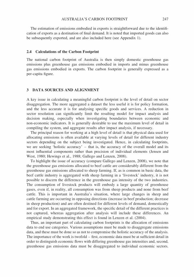
The top level results for Australia are presented in Table 1. In 2005, overall domestic emis-

sions were 581.9 Mt, with 194.1 Mt being from electricity supply (scope 2), equating to a

per-capita level of 28.6 Mt.2 Emissions embodied in imports are estimated at 142.7 Mt, of

which about 60 Mt came from electricity. These electricity emissions are probably over-

estimated, as Australian technology is assumed, and the Australian electricity supply is

predominantly coal fired (which has a higher emissions intensity than most other

foreign electricity producing technologies). Emissions embodied in exports are estimated

at 202.3 Mt, with 53.3 Mt being from the electricity supply. It is interesting to note that

whilst policy is generally focused on emissions-intensive, export-oriented industries

such as mining, of the order of 25% of Australia’s predominantly coal-fired electricity

will be embodied in goods and services consumed overseas. The estimated carbon foot-

print of demand in Australia is 522.4 Mt or 25.7 Mt/capita, slightly less than domestically

produced emissions (581.9 Mt or 28.6 Mt/capita).

4.2 Sector Emissions, 2005

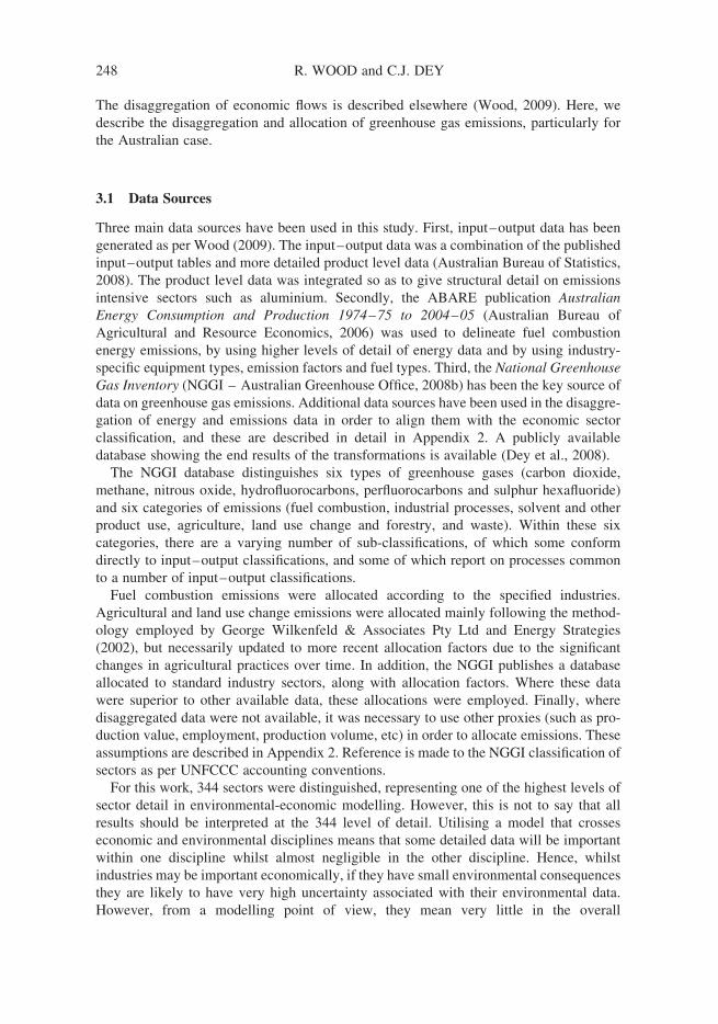
The direct emissions allocated to the producing sector are shown in Figure 1 for 2005.

These are the emissions as reported by Australia under the Kyoto Protocol (United

Nations, 1992), representing Qind. As expected, the importance of primary industries is

high, with over one-third of total emissions. Manufacturing and utilities make up an

additional third. Thus, even with the almost complete reliance on coal for electricity

generation in Australia, these emissions only make up less than 15% of the total. A signifi-

cant issue for Australia is the prominence of agricultural and mining emissions. These

emissions occur in non-urban areas and are caused by industry supporting rural

TABLE 1. Overall results for Australia, 2005. Scope 1 excludes emissions from electricity supplywhich are accounted for within Scope 2.

Emissions exclelectricity

Emissions fromelectricity Total

Totalper-capita

(Mt) (Mt) (Mt) (Mt/capita)

Total Domestic GHG emissions 387.7 194.1 581.9 28.6þ Emissions embodied in imports 79.6 63.1 142.7 7.02 Emissions embodied in exports 148.9 53.3 202.3 9.9¼ national carbon footprint 381.6 203.9 522.4 25.7

2 Consistent with the 2008 NGGI (Australian Greenhouse Office, 2008b).


communities. As these industries often have significant social and economic benefits, the

only politically palatable option to address these emissions is to seriously focus on effi-

ciency, management and technology improvements.

Applying the notion of the carbon footprint to the direct emissions means allocating

these emissions to the final commodities produced by industrial sectors. We observe a

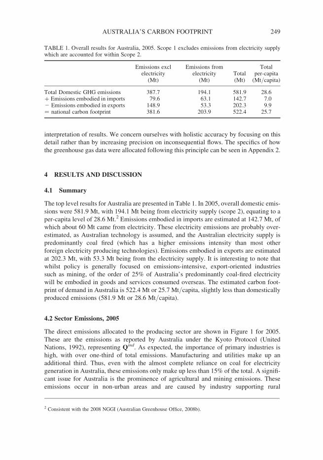
shift towards products from tertiary production. Figure 2 shows emissions embodied by

categories of final demand and include imports but exclude exports.

From a footprint or consumption perspective, manufacturing products contribute over

one-third of total emissions. Within manufacturing, the main emissions (cf. Table 2) are

from agriculture (primarily associated with beef cattle), embodied within the manufactur-

ing of food. Electricity emissions (going directly to final demand) contribute roughly 14%

of the total, whilst direct residential emissions (transport, cooking, etc) are around 9%.

Together, residential and electricity emissions are usually considered the main impact

FIGURE 2. Carbon footprint of final goods and services by industry, Australia, 2005.

FIGURE 1. Direct greenhouse gas emissions by industry, Australia 2005.


of the population, whilst, in this approach, we see they miss around three quarters of the

total impact.

Whilst some of these sectors contribute significantly to greenhouse gas emissions, they

also contribute significantly to the economic well being of Australia. If Australia is to

move to a lower carbon society, it would be the intention of good policy to support

production in sectors that have large social and economic contributions and small environ-

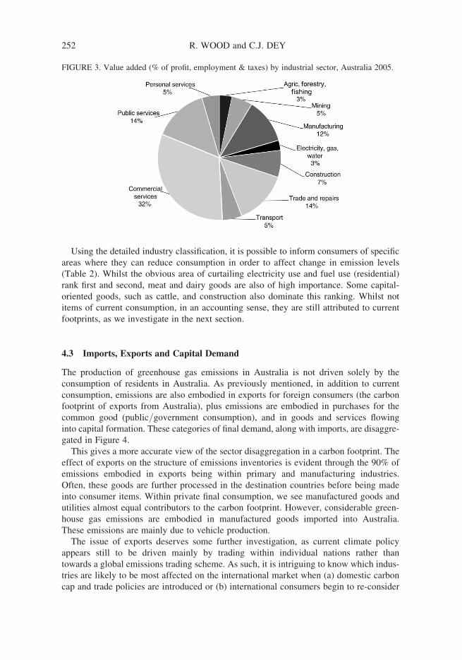
mental impacts. To investigate the social and economic contributions we use the income

approach to measuring GDP. Summing over value added (operating surplus, employment

& taxes), we compare the relative contribution of each sector to overall GDP in Australia

(Figure 3). By doing so, we see that Australia is a service-oriented society in economic

terms with roughly 50% of value added coming from the service sectors compared with

8% of emissions production (Figure 1) and 14% in terms of the carbon footprint

(Figure 2). In contrast, Manufacturing contributes only 12% to value added, whilst

producing 22% of Australia’s emissions, and has a carbon footprint of 28%.

The Australian Government is using Value Added as one proxy for determining permit

allocations and possible compensation under its forthcoming emissions trading scheme,

known as the Carbon Pollution Reduction Scheme (CPRS). Although there are thresholds

for the sizes of businesses included, under the draft CPRS, much of the manufacturing,

transport and primary industries will, as expected, require significant emissions permits.

In addition to the emissions calculations, the Australian Governments is currently

examining the level of trade exposure of Australian industries (Department of Climate

Change, 2009). As employing a carbon footprint measure assigns responsibility to the con-

sumer (within Australia in this case), it can be misleading to look only at the overall carbon

footprint results without looking at the effect of the emissions embodied in the trade flows.

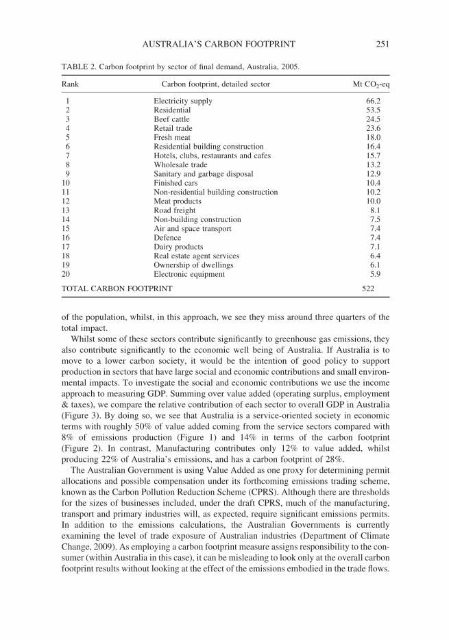
TABLE 2. Carbon footprint by sector of final demand, Australia, 2005.

Rank Carbon footprint, detailed sector Mt CO2-eq

1 Electricity supply 66.22 Residential 53.53 Beef cattle 24.54 Retail trade 23.65 Fresh meat 18.06 Residential building construction 16.47 Hotels, clubs, restaurants and cafes 15.78 Wholesale trade 13.29 Sanitary and garbage disposal 12.9

10 Finished cars 10.411 Non-residential building construction 10.212 Meat products 10.013 Road freight 8.114 Non-building construction 7.515 Air and space transport 7.416 Defence 7.417 Dairy products 7.118 Real estate agent services 6.419 Ownership of dwellings 6.120 Electronic equipment 5.9

TOTAL CARBON FOOTPRINT 522


Using the detailed industry classification, it is possible to inform consumers of specific

areas where they can reduce consumption in order to affect change in emission levels

(Table 2). Whilst the obvious area of curtailing electricity use and fuel use (residential)

rank first and second, meat and dairy goods are also of high importance. Some capital-

oriented goods, such as cattle, and construction also dominate this ranking. Whilst not

items of current consumption, in an accounting sense, they are still attributed to current

footprints, as we investigate in the next section.

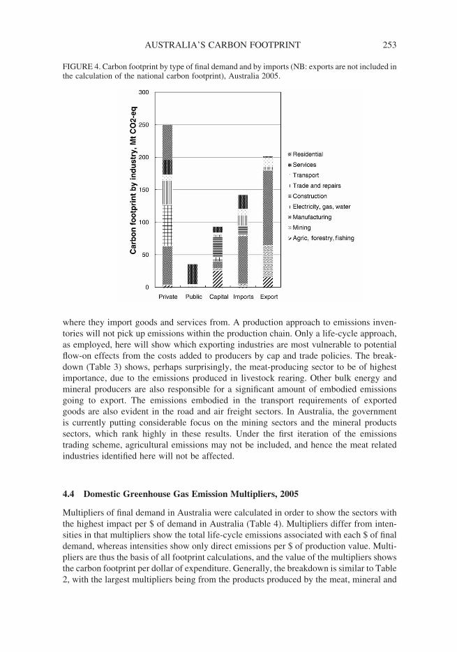
4.3 Imports, Exports and Capital Demand

The production of greenhouse gas emissions in Australia is not driven solely by the

consumption of residents in Australia. As previously mentioned, in addition to current

consumption, emissions are also embodied in exports for foreign consumers (the carbon

footprint of exports from Australia), plus emissions are embodied in purchases for the

common good (public/government consumption), and in goods and services flowing

into capital formation. These categories of final demand, along with imports, are disaggre-

gated in Figure 4.

This gives a more accurate view of the sector disaggregation in a carbon footprint. The

effect of exports on the structure of emissions inventories is evident through the 90% of

emissions embodied in exports being within primary and manufacturing industries.

Often, these goods are further processed in the destination countries before being made

into consumer items. Within private final consumption, we see manufactured goods and

utilities almost equal contributors to the carbon footprint. However, considerable green-

house gas emissions are embodied in manufactured goods imported into Australia.

These emissions are mainly due to vehicle production.

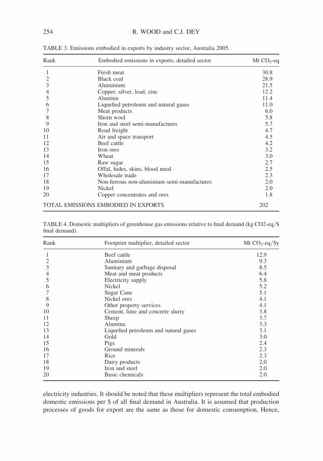
The issue of exports deserves some further investigation, as current climate policy

appears still to be driven mainly by trading within individual nations rather than

towards a global emissions trading scheme. As such, it is intriguing to know which indus-

tries are likely to be most affected on the international market when (a) domestic carbon

cap and trade policies are introduced or (b) international consumers begin to re-consider

FIGURE 3. Value added (% of profit, employment & taxes) by industrial sector, Australia 2005.


where they import goods and services from. A production approach to emissions inven-

tories will not pick up emissions within the production chain. Only a life-cycle approach,

as employed, here will show which exporting industries are most vulnerable to potential

flow-on effects from the costs added to producers by cap and trade policies. The break-

down (Table 3) shows, perhaps surprisingly, the meat-producing sector to be of highest

importance, due to the emissions produced in livestock rearing. Other bulk energy and

mineral producers are also responsible for a significant amount of embodied emissions

going to export. The emissions embodied in the transport requirements of exported

goods are also evident in the road and air freight sectors. In Australia, the government

is currently putting considerable focus on the mining sectors and the mineral products

sectors, which rank highly in these results. Under the first iteration of the emissions

trading scheme, agricultural emissions may not be included, and hence the meat related

industries identified here will not be affected.

4.4 Domestic Greenhouse Gas Emission Multipliers, 2005

Multipliers of final demand in Australia were calculated in order to show the sectors with

the highest impact per $ of demand in Australia (Table 4). Multipliers differ from inten-

sities in that multipliers show the total life-cycle emissions associated with each $ of final

demand, whereas intensities show only direct emissions per $ of production value. Multi-

pliers are thus the basis of all footprint calculations, and the value of the multipliers shows

the carbon footprint per dollar of expenditure. Generally, the breakdown is similar to Table

2, with the largest multipliers being from the products produced by the meat, mineral and

FIGURE 4. Carbon footprint by type of final demand and by imports (NB: exports are not included inthe calculation of the national carbon footprint), Australia 2005.


electricity industries. It should be noted that these multipliers represent the total embodied

domestic emissions per $ of all final demand in Australia. It is assumed that production

processes of goods for export are the same as those for domestic consumption. Hence,

TABLE 4. Domestic multipliers of greenhouse gas emissions relative to final demand (kg CO2-eq/$final demand).

Rank Footprint multiplier, detailed sector Mt CO2-eq/$y

1 Beef cattle 12.92 Aluminium 9.33 Sanitary and garbage disposal 8.54 Meat and meat products 6.45 Electricity supply 5.86 Nickel 5.27 Sugar Cane 5.18 Nickel ores 4.19 Other property services 4.1

10 Cement, lime and concrete slurry 3.811 Sheep 3.712 Alumina 3.313 Liquefied petroleum and natural gases 3.114 Gold 3.015 Pigs 2.416 Ground minerals 2.317 Rice 2.318 Dairy products 2.019 Iron and steel 2.020 Basic chemicals 2.0

TABLE 3. Emissions embodied in exports by industry sector, Australia 2005.

Rank Embodied emissions in exports, detailed sector Mt CO2-eq

1 Fresh meat 30.82 Black coal 28.93 Aluminium 21.54 Copper, silver, lead, zinc 12.25 Alumina 11.46 Liquefied petroleum and natural gases 11.07 Meat products 6.08 Shorn wool 5.89 Iron and steel semi-manufactures 5.7

10 Road freight 4.711 Air and space transport 4.512 Beef cattle 4.213 Iron ores 3.214 Wheat 3.015 Raw sugar 2.716 Offal, hides, skins, blood meal 2.517 Wholesale trade 2.318 Non-ferrous non-aluminium semi-manufactures 2.019 Nickel 2.020 Copper concentrates and ores 1.8

TOTAL EMISSIONS EMBODIED IN EXPORTS 202


the ranked list of multipliers includes a number of high ranking goods, such as aluminium,

that are more applicable to exported goods rather than domestic final consumption. These

data thus have two main purposes – first, for consumers seeking to reduce their consump-

tion, they should seek to avoid goods or services that rank highly in the multiplier ranking.

Secondly, export-oriented industries producing products with large multipliers will be

sensitive to competition from overseas under a domestic emissions trading scheme that

does not take into account carbon leakage (the potential off-shoring of polluting indus-

tries); and under an international emissions trading scheme, their costs of production

are likely to rise due to price increases associated with emissions being transferred to

their goods.

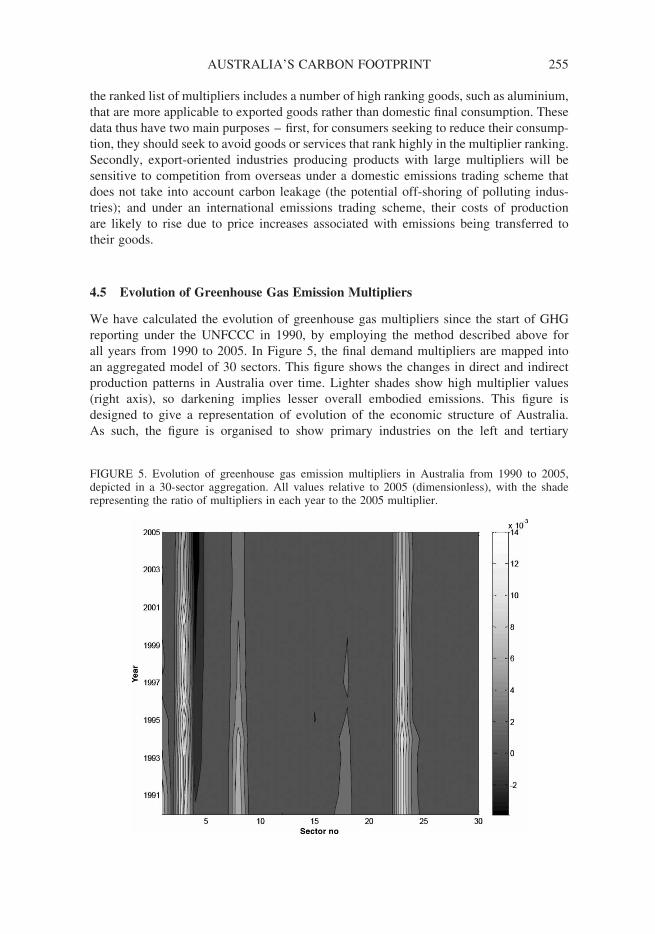
4.5 Evolution of Greenhouse Gas Emission Multipliers

We have calculated the evolution of greenhouse gas multipliers since the start of GHG

reporting under the UNFCCC in 1990, by employing the method described above for

all years from 1990 to 2005. In Figure 5, the final demand multipliers are mapped into

an aggregated model of 30 sectors. This figure shows the changes in direct and indirect

production patterns in Australia over time. Lighter shades show high multiplier values

(right axis), so darkening implies lesser overall embodied emissions. This figure is

designed to give a representation of evolution of the economic structure of Australia.

As such, the figure is organised to show primary industries on the left and tertiary

FIGURE 5. Evolution of greenhouse gas emission multipliers in Australia from 1990 to 2005,depicted in a 30-sector aggregation. All values relative to 2005 (dimensionless), with the shaderepresenting the ratio of multipliers in each year to the 2005 multiplier.


sectors on the right. All industries are represented but major change is only seen in rela-

tively few sectors of the economy – mostly sectors in primary industries, and utilities.

Beef cattle (leftmost) and electricity production (sector 23) are the two most important

sectors, with the changing land practices in beef cattle farming evident in the fluctuating

multiplier values (denoted by changing shade intensity). The liberalisation of the electri-

city markets in the mid 1990s is evident in the change in that multiplier (sector 23). The

mining sector (sectors 7–8) has also shown positive change, evolving slightly to be less

greenhouse gas intensive. And small improvement can also be seen in manufacturing

(sectors 17–18 showing mineral and metallic products).

5 CONCLUSIONS

This paper has presented the results of a national carbon footprint of Australia as well as

the methods used to estimate greenhouse gas emissions by industry category. The impor-

tance of addressing greenhouse gas emissions, the requirement for consistency from the

perspective of national accounting conventions, and the need for measures of emissions

embodied in import, export and various consumption categories drove this research. A

range of proxy data was used in order to break down aggregate emissions into categories

relevant to footprint analysis. Measures of greenhouse gas emissions were presented for

emissions due to domestic production, emissions embodied in imports and exports and

emissions embodied in capital formation. Emissions were calculated by industrial

sector, with 344 sectors used in the most disaggregated form of the model. A few key

sectors, particularly beef and electricity, produce the majority of Australia’s domestic

emissions, whereas emissions embodied in consumption (the carbon footprint) show the

higher importance of manufacturing and tertiary sectors. Apart from electricity and

direct residential emissions (which together account for about 25% of the total carbon

footprint), meat, trade and construction were other key sectors from a carbon footprint

perspective. Significant emissions are embodied in the export production of the mining

and manufacturing industries. Specific policy is being established within Australia to

try to prevent adverse effects of an emissions trading scheme on the competitiveness of

these industries in the international marketplace. Although very few of the emissions-

intensive industries contribute significantly to GDP, most are based in non-urban areas

whose socio-economic stability is highly dependent on these industries.

In terms of policy relevance, the contrasting viewpoints of emissions inventories

(production perspective) versus carbon footprints (consumption perspective) are useful

for examining the implications of any policy that places a cost on carbon. Although agri-

culture is likely not to be included in the Australian emissions trading scheme initially, the

high emissions intensity of the agricultural sectors is currently a major source of political

debate and unease in rural areas. A carbon footprint analysis, as presented here, can inform

more rational discussion about what proportions of emissions permit costs can realistically

be passed on to processors and ultimately to consumers, and the extent of any negative

trade implications. Past experience of the increasing cost and scarcity of water for agricul-

tural purposes, which has meant significant food price increases, represents a similar pre-

cedent to the effects of a price on carbon.

A carbon footprint broken down by different elements of final demand also gives

insights into some of the differences between Australia’s commodities bound for export


markets, often with less value adding, and the commodities that go through higher levels of

transformation for domestic use. One example of this is a comparison between direct live-

stock exports (live trade) and domestic consumption of meat products. Much greater econ-

omic benefits could be reaped at minimal additional environmental cost if greater levels of

transformation were applied prior to export.

Some other important policy considerations for new emissions trading schemes are the

amount and allocation method for emissions permits, and, related to this, the amount of

compensation paid by governments to industries predicted to have changes in the value

of their assets and/or profitability. Overly focusing on sources of direct emissions in

policy development, and downplaying the connectedness and dynamic nature of econom-

ies, may not lead to the optimum overall outcome that emissions trading schemes are

intended to achieve: significant and ongoing emissions reductions at lowest abatement

costs with minimum social and economic disruption.

References

Andrew, R., G. Peters and J. Lennox (2009) Approximation and Regional Aggregation in Multi-regional Input–

Output Analysis for National Carbon Footprint Accounting. Economic Systems Research, 21 (this issue).

Apelbaum Consulting Group Pty Ltd (2007) Australian Rail Transport Facts j 2007. Victoria, Australia,

Mulgrave.

Australian Bureau of Agricultural and Resource Economics (1997) Australian Energy Consumption and

Production, Table C1AUST 1973–74 to 1994–95.

Australian Bureau of Agricultural and Resource Economics (2006) Australian Energy Consumption and

Production, Statistical Tables: Historical.

Australian Bureau of Agricultural and Resource Economics (2007) Energy Update. http://www.abareconomics.

com/publications_html/data/data/data.html

Australian Bureau of Statistics (2003) Survey of Motor Vehicle Use 2002 - Data Cube; ABS Catalogue No.

9210.0.55.001 Canberra, Australia, Australian Bureau of Statistics.

Australian Bureau of Statistics (2008) Australian National Accounts, Input–Output Tables, 2004–05, Cat. no.

5209.0.55.001. 5209.0, Canberra, Australia, Australian Bureau of Statistics.

Australian Greenhouse Office (2008a) National Greenhouse Accounts (NGA) Factors. 2004, Canberra, Australia,

Australian Government.

Australian Greenhouse Office (2008b) National Greenhouse Gas Inventory, Canberra, Australia, Australian

Greenhouse Office.

Australian Taxi Industry Association (2001) Submission to the Fuel Tax Inquiry. http://fueltaxinquiry.treasury.

gov.au/content/Submissions/Industry/ATIA_222.asp

Danish Environment Ministry (DMU) (2004) Emission Factors, Stationary Combustion Main. http://www2.

dmu.dk/1_Viden/2_miljoe-tilstand/3_luft/4_adaei/Emission_factors_en.asp

Department of Climate Change, A.G (2009) Carbon Pollution Reduction Scheme: Emissions-Intensive Trade-

Exposed Industries. http://www.climatechange.gov.au/whitepaper/assistance/index.html.

Dey, C., R. Wood and M. Lenzen (2008) Production, Trade and Embodied Emissions Database. Report on Con-

sultancy Work for the Department of Climate Change, Australian Government. Canberra, Australia. http://www.climatechange.gov.au/emissionstrading/publications/pubs/isa-data.zip

Finkbeiner, M. (2009) Carbon Footprinting – Opportunities and Threats. The International Journal of Life Cycle

Assessment, 14, 91–94.

Gallego, B. and M. Lenzen (2005) A Consistent Input–Output Formulation of Shared Consumer and Producer

Responsibility. Economic Systems Research, 17, 365–391.

Gallego, B. and M. Lenzen (2008) Estimating Generalised Regional Input–Output Systems: A Case Study of

Australia. In: M. Ruth and B. Davidsdottir (eds), Dynamics of Industrial Ecosystems. Boston, MA, MIT

Press.

George Wilkenfeld & Associates Pty Ltd and Energy Strategies (2002) Australia’s National Greenhouse Gas

Inventory 1990, 1995 and 1999 – End Use Allocation of Emissions, Canberra, Australia, Australian

Greenhouse Office.


http://www.abareconomics.com/publications_html/data/data/data.html



http://fueltaxinquiry.treasury.gov.au/content/Submissions/Industry/ATIA_222.asp



http://www2.dmu.dk/1_Viden/2_miljoe-tilstand/3_luft/4_adaei/Emission_factors_en.asp



http://www.climatechange.gov.au/whitepaper/assistance/index.html

http://www.climatechange.gov.au/whitepaper/assistance/index.html

http://www.climatechange.gov.au/emissionstrading/publications/pubs/isa-data.zip



Giljum, S. and K. Hubacek (2004) Alternative Approaches of Physical Input–Output Analysis to Estimate

Primary Material Inputs of Production and Consumption Activities. Economic Systems Research, 16,

301–310.

Hertwich, E. and G. Peters (2009) Carbon Footprint of Nations: A Global, Trade-Linked Analysis. Environmental

Science & Technology.

Hewings, G.J.D., M. Sonis and R.C. Jensen (1988) Fields of Influence of Technological Change in Input–Output

Models. Papers of the Regional Science Association, 64, 25–36.

Jensen, R.C. and G.R. West (1980) The Effect of Relative Coefficient Size on Input–Output Multipliers.

Environment and Planning A, 12, 659–670.

Lenzen, M. (2001) A Generalised Input–Output Multiplier Calculus for Australia. Economic Systems Research,

13, 65–92.

Lenzen, M., L.-L. Pade and J. Munksgaard (2004) CO2 Multipliers in Multi-Region Input–Output Models.

Economic Systems Research, 16, 391–412.

Leontief, W. (1936) Quantitative Input and Output Relations in the Economic System of the United States.

Review of Economics and Statistics, 18, 105–125.

Leontief, W. (1941) The Structure of the American Economy, 1919–1939. Oxford, Oxford University Press:

Oxford University Press.

Miller, R.E. and P.D. Blair (2009) Input–Output Analysis: Foundations and Extensions, 2nd ed. Cambridge

University Press.

Minx, J., T. Wiedmann, R. Wood, G. Peters, M. Lenzen, A. Owen, K. Scott, J. Barrett, K. Hubacek, G. Baiocchi,

A. Paul, E. Dawkins, J. Briggs, D. Guan, S. Suh and F. Ackermann (2009) Input–Output Analysis and

Carbon Footprinting: an Overview of Regional and Corporate Applications. Input–Output Analysis and

Carbon Footprinting: an Overview of Regional and Corporate Applications. Economic Systems Research,

21 (this issue).

National Greenhouse Gas Inventory Committee (1994) Australian Methodology for the Estimation of Green-

house Gas Emissions and Sinks. 3.0, Canberra, Australia, Department of the Environment, Sport and

Territories.

National Greenhouse Gas Inventory Committee (1998a) Australian Methodology for the Estimation of Green-

house Gas Emissions and Sinks, Fuel Combustion Activities (Stationary Sources). 1.1, Canberra, Australia,

Australian Greenhouse Office.

National Greenhouse Gas Inventory Committee (1998b) Australian Methodology for the Estimation of Green-

house Gas Emissions and Sinks, Land Use Change and Forestry. 4.2, Canberra, Australia, Australian Green-

house Office.

National Greenhouse Gas Inventory Committee (1998c) Australian Methodology for the Estimation of Green-

house Gas Emissions and Sinks, Land Use Change and Forestry, Transport (Mobile Sources). 3.1, Canberra,

Australia, Australian Greenhouse Office.

National Greenhouse Gas Inventory Committee (1998d) Australian Methodology for the Estimation of Green-

house Gas Emissions and Sinks, Waste. 8.1, Canberra, Australia, Australian Greenhouse Office.

National Greenhouse Gas Inventory Committee (2008) Australian Methodology for the Estimation of Green-

house Gas Emissions and Sinks, Energy (Transport), Canberra, Australia, Australian Greenhouse Office.

Peters, G.P. (2008) From Production-Based to Consumption-Based National Emission Inventories. Ecological

Economics, 65, 13–23.

Peters, G.P. and E.G. Hertwich (2006) The Importance of Imports for Household Environmental Impacts. Journal

of Industrial Ecology, 10, 89–109.

United Nations (1992) Framework Convention on Climate Change. Rio de Janeiro, Brazil, United Nations.

Weber, C.L. and H.S. Matthews (2008) Quantifying the Global and Distributional Aspects of American House-

hold Carbon Footprint. Ecological Economics, 66, 379–391.

Weidema, B.P., M. Thrane, P. Christensen, J. Schmidt and S. Løkke (2008) Carbon Footprint. A Catalyst for

Life Cycle Assessment? Journal of Industrial Ecology, 12, 3–6.

Wiedmann, T. and J. Minx (2008) A Definition of ’carbon Footprint’. In: C.C. Pertsova (ed.), Ecological

Economics Research Trends. Hauppauge, NY, Nova Science Publishers.

Wiedmann, T., R. Wood, M. Lenzen, J. Minx, D. Guan and J. Barrett (2007) Development of an Embedded

Carbon Emissions Indicator – Producing a Time Series of Input–Output Tables for the UK by Using a

MRIO Data Optimisation System, Report to the UK Department for Environment, Food and Rural

Affairs by Stockholm Environment Institute at the University of York and Centre for Integrated Sustain-

ability Analysis at the University of Sydney, London, DEFRA.


Wiedmann, T., R. Wood, M. Lenzen, J. Minx, D. Guan and J. Barrett (2010) The Carbon Footprint of the

UK – Results from a Multi-Region Input–Output Model. Economic Systems Research, forthcoming.

Wood, R. (2009) Structural Evolution of Economy and Environment in Australia. Centre for Integrated Sustain-

ability Analysis, University of Sydney, Australia. Ph.D. thesis.

World Resources Institute and World Business Council for Sustainable Development (2004) The Greenhouse

Gas Protocol: A Corporate Accounting and Reporting Standard. Washington, DC, and Geneva,

Switzerland, WRI and WBCSD.

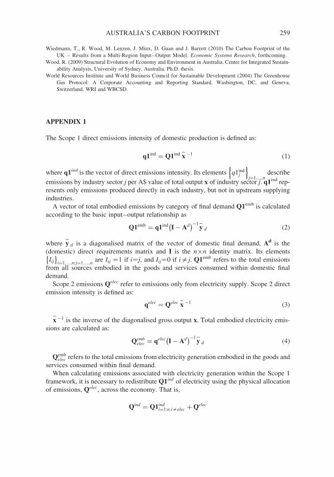
APPENDIX 1

The Scope 1 direct emissions intensity of domestic production is defined as:

q1ind ¼ Q1ind x_ �1 (1)

where q1ind is the vector of direct emissions intensity. Its elements q1indj

n oj¼1;...;n

describe

emissions by industry sector j per A$ value of total output x of industry sector j. q1ind rep-

resents only emissions produced directly in each industry, but not in upstream supplying

industries.

A vector of total embodied emissions by category of final demand Q1emb is calculated

according to the basic input–output relationship as

Q1emb ¼ q1ind I� Ad� ��1

y_

d (2)

where y_

d is a diagonalised matrix of the vector of domestic final demand, Ad is the

(domestic) direct requirements matrix and I is the n�n identity matrix. Its elements

Iij

� �i¼1;...;n;j¼1;...;n

are Iij ¼1 if i¼j, and Iij¼0 if i=j. Q1emb refers to the total emissions

from all sources embodied in the goods and services consumed within domestic final

demand.

Scope 2 emissions Qelec refer to emissions only from electricity supply. Scope 2 direct

emission intensity is defined as:

qelec ¼ Qelec x_ �1 (3)

x_ �1 is the inverse of the diagonalised gross output x. Total embodied electricity emis-

sions are calculated as:

Qembelec ¼ qelec I� Ad

� ��1y_

d (4)

Qembelec refers to the total emissions from electricity generation embodied in the goods and

services consumed within final demand.

When calculating emissions associated with electricity generation within the Scope 1

framework, it is necessary to redistribute Q1ind of electricity using the physical allocation

of emissions, Qelec, across the economy. That is,

Qind ¼ Q1indi¼1:n;i=elec þQelec


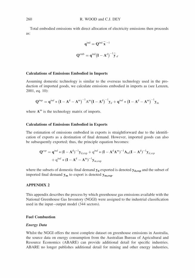
Total embodied emissions with direct allocation of electricity emissions then proceeds

as:

qind ¼ Qind x_ �1

Qemb ¼ qind I� Ad� ��1

y_

d

Calculations of Emissions Embodied in Imports

Assuming domestic technology is similar to the overseas technology used in the pro-

duction of imported goods, we calculate emissions embodied in imports as (see Lenzen,

2001, eq. 10):

Qimp ¼ qind � I� Ad � Am� ��1

Am I� Ad� ��1

yd þ qind � I� Ad � Am� ��1

ym

where Am is the technology matrix of imports.

Calculations of Emissions Embodied in Exports

The estimation of emissions embodied in exports is straightforward due to the identifi-

cation of exports as a destination of final demand. However, imported goods can also

be subsequently exported; thus, the principle equation becomes:

Qexp ¼ qind � ðI� AdÞ�1yd;exp þ qind � ðI� AdAmÞ

�1AmðI� AdÞ�1yd;exp

þ qind � ðI� Ad � AmÞ�1ym;exp

where the subsets of domestic final demand yd exported is denoted yd,exp and the subset of

imported final demand ym to export is denoted ym,exp.

APPENDIX 2

This appendix describes the process by which greenhouse gas emissions available with the

National Greenhouse Gas Inventory (NGGI) were assigned to the industrial classification

used in the input–output model (344 sectors).

Fuel Combustion

Energy Data

Whilst the NGGI offers the most complete dataset on greenhouse emissions in Australia,

the source data on energy consumption from the Australian Bureau of Agricultural and

Resource Economics (ABARE) can provide additional detail for specific industries.

ABARE no longer publishes additional detail for mining and other energy industries,


and no longer publishes fuel use by equipment type. Hence, data at this level of detail

come from the late 1990s. Therefore, the final data have the relative breakdown of this

highest level of detail whilst conforming in absolute terms to the level of detail of the

current year data.

We created an initial estimate of energy use by input–output category. This was then

optimised to account for additional data on equipment use by fuel and equipment use

by industry.

The sales breakdown of each of the 28 fuels in the ABARE energy statistics to all indus-

tries is used to create an initial estimate. The sales breakdown is taken directly from the

input–output tables, and where purchases of the product corresponding to each fuel are

shown for each industry. The input–output data are the best available detail on the use

of fuels by industry, but unlike the fuel data, are in monetary terms. The effect is that

there is an implicit assumption that within each category of the ABARE energy data,

all industries pay the same price for fuels. This assumption is expected to be valid for

most types of energy consumption. Where a significant difference in price is expected

within an ABARE category, such as for aluminium production within non-ferrous

metals, additional data are sourced and applied. Further, due to the nature of the

ABARE data, important energy flows were at a sufficient level of detail such that the

data could be allocated directly to input–output categories, whilst less energy intensive

sectors, particularly within the services sector, required more disaggregation. Thus, inac-

curacies caused by disaggregation are limited.

Unpublished data on mining of mineral sands, iron ore, gold, silver, etc, and briquette

manufacturing, as well as the separation of aluminium from other non-ferrous metals were

made available for the 1990s, and the relative values of this data were applied in the initial

estimate for subsequent years.

In addition to the direct energy consumption data, energy consumption was previously

available by equipment type (17 types) and fuel (27 fuels) (Australian Bureau of Agricul-

tural and Resource Economics, 1997) and shares of equipment type were available by

industry and fuel (National Greenhouse Gas Inventory Committee, 1994). The importance

of this data is highlighted for particular industries such as aluminium production, silver,

lead, zinc, coal and uranium mining, mineral sands mining, and others. As a result, emis-

sion factors by industry, equipment type and fuel type were used in the estimation of

greenhouse emissions by industrial sector, with the final form of the energy consumption

matrix showing input–output category by equipment type by fuel use.

Transport

The ABARE data set on energy consumption aggregates all forms of road transport into

the ‘road transport’ sector – hence the data set does not distinguish between private use

of automobiles, business use of automobiles and freight. Similarly, for military purposes,

all energy use within vehicular transport and air transport are aggregated into the road and

air transport sectors. In order to allocate transport energy use to the end use industry, mili-

tary use is first extracted (National Greenhouse Gas Inventory Committee, 2008), then the

remaining fuel use is apportioned between private and business fuel use for road transport

(Australian Bureau of Statistics, 2003), and directly to air transport and water transport for

these transport types.


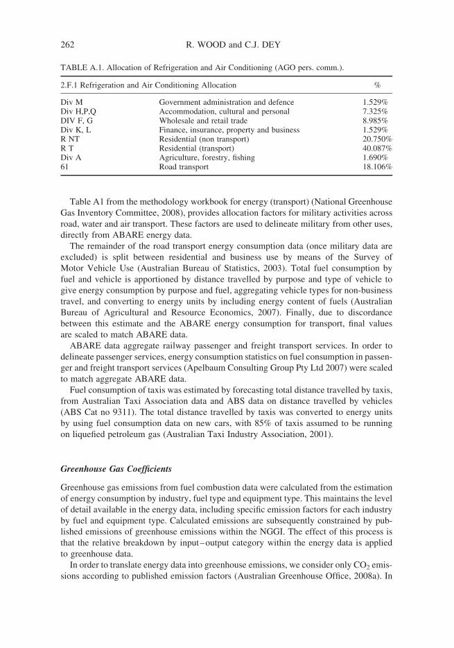
Table A1 from the methodology workbook for energy (transport) (National Greenhouse

Gas Inventory Committee, 2008), provides allocation factors for military activities across

road, water and air transport. These factors are used to delineate military from other uses,

directly from ABARE energy data.

The remainder of the road transport energy consumption data (once military data are

excluded) is split between residential and business use by means of the Survey of

Motor Vehicle Use (Australian Bureau of Statistics, 2003). Total fuel consumption by

fuel and vehicle is apportioned by distance travelled by purpose and type of vehicle to

give energy consumption by purpose and fuel, aggregating vehicle types for non-business

travel, and converting to energy units by including energy content of fuels (Australian

Bureau of Agricultural and Resource Economics, 2007). Finally, due to discordance

between this estimate and the ABARE energy consumption for transport, final values

are scaled to match ABARE data.

ABARE data aggregate railway passenger and freight transport services. In order to

delineate passenger services, energy consumption statistics on fuel consumption in passen-

ger and freight transport services (Apelbaum Consulting Group Pty Ltd 2007) were scaled

to match aggregate ABARE data.

Fuel consumption of taxis was estimated by forecasting total distance travelled by taxis,

from Australian Taxi Association data and ABS data on distance travelled by vehicles

(ABS Cat no 9311). The total distance travelled by taxis was converted to energy units

by using fuel consumption data on new cars, with 85% of taxis assumed to be running

on liquefied petroleum gas (Australian Taxi Industry Association, 2001).

Greenhouse Gas Coefficients

Greenhouse gas emissions from fuel combustion data were calculated from the estimation

of energy consumption by industry, fuel type and equipment type. This maintains the level

of detail available in the energy data, including specific emission factors for each industry

by fuel and equipment type. Calculated emissions are subsequently constrained by pub-

lished emissions of greenhouse emissions within the NGGI. The effect of this process is

that the relative breakdown by input–output category within the energy data is applied

to greenhouse data.

In order to translate energy data into greenhouse emissions, we consider only CO2 emis-

sions according to published emission factors (Australian Greenhouse Office, 2008a). In

TABLE A.1. Allocation of Refrigeration and Air Conditioning (AGO pers. comm.).

2.F.1 Refrigeration and Air Conditioning Allocation %

Div M Government administration and defence 1.529%Div H,P,Q Accommodation, cultural and personal 7.325%DIV F, G Wholesale and retail trade 8.985%Div K, L Finance, insurance, property and business 1.529%R NT Residential (non transport) 20.750%R T Residential (transport) 40.087%Div A Agriculture, forestry, fishing 1.690%61 Road transport 18.106%


order not to double count primary and secondary fuels, and to enable tractability of impor-

tant physical flows, within solid fuels only primary fuels were included. Only minor com-

bustion of solid secondary fuels occurs for such fuels as coke and briquettes. For liquid

fuels, only secondary fuels were included, such that no emissions are associated with

their raw feedstock. In this way, gross, rather than net, emissions are estimated without

double counting.

In addition, non-CO2 emissions are considered for the greenhouse gases CH4 and N2O.

Emission factors are calculated by sector, by fuel type and by equipment type (Danish

Environment Ministry, 2004) and (National Greenhouse Gas Inventory Committee,

1998a, 1998b, 1998c, 1998d). Other greenhouse gases are not directly considered due

to uncertainty in emission factors. They are, however, included indirectly when included

in the NGGI by the benchmarking of the greenhouse gases estimated from fuel combustion

with the CO2-equivalent greenhouse emissions of the NGGI. Non-CO2 transport emissions

are estimated from the energy data, with mobile sources of emissions from Australian

Greenhouse Office (AGO) Workbook 3.1 A.5.

Scope 2 Emissions

Scope 2 emissions (emissions from the generation of purchased electricity) are estimated

directly from ABARE energy consumption data, specifically for electricity use. The

process used in this estimation is identical to the general fuel consumption data (allocation

is undertaken per economic flows from the input–output table). Emissions are then con-

strained by the data on scope 2 emissions in the level of detail of the Australian New

Zealand Standard Industry Classification (ANSZIC). Scope 2 emissions by industry

then replace the aggregate electricity emissions.

Industrial Processes

For industrial processes, emissions from category 2.A Mineral Products of the NGGI are

allocated directly to the cement and lime input–output category and to Iron and Steel

semi-manufacturers for Limestone and Dolomite Use. Emissions from category 2.B

Chemical Industry and 2.D,F Production of Halocarbons and Sulphur Hexafluoride are

allocated to Basic Chemicals and Other Chemical Products by production value. Emis-

sions from 2.C Metal Production are allocated directly from the NGGI to the input–

output categories Iron and steel semi-manufactures, Alumina, and to the three aluminium

product sectors (Aluminium, Aluminium semi-manufactures, Aluminium foil – allocated

within these three sectors by production value). Emissions from 2.E,F Consumption of

Halocarbons and Sulphur Hexafluoride are principally due to Refrigeration and Air Con-

ditioning Equipment, and make up almost 3 kilotonnes of emissions. The use of refriger-

ation and air conditioning is common to many economic sectors, hence making allocation

difficult. The AGO provided allocation to ANZSIC divisions (Table A.1) which was used

as an initial breakdown to industry subgroups. Emissions were then allocated according to

employment for other industries, where it was assumed that air conditioning of employee

space was the major cause of emissions, and according to production value for Trade and

Road transport, as these sectors are margin industries with throughput assumed to reflect

the volume of refrigeration of goods driving these emissions.


Emissions from foam blowing were allocated to Other Chemical products, emissions

from fire extinguishers to Fire Brigade, emissions from Solvents to Machinery and Equip-

ment and Other Electrical to Electrical Equipment. Emissions from ‘2.G Other’ are

confidential emissions but stem from soda ash, ammonia and nitric acid production.

These chemicals are used within the sectors glass products, fertiliser and chemical

products, pulp and paper and water supply/sewerage. The emissions are allocated to

these sectors by production value in lieu of any other information.

Agriculture

For agriculture, a number of proxy variables are needed in order to allocate NGGI cat-

egories to input–output categories. The main proxies used are land use area, production

volume and heads of livestock. The principal source data is the ABARE Commodity Stat-

istics, along with ABS publication Agricultural Commodities, ABS Cat. No. 7121.0.

Whilst data are available on total pasture land area, and land area of crops, land area

data are not available for livestock. Hence, an estimation process is employed following

George Wilkenfeld & Associates Pty Ltd and Energy Strategies (2002) where total

natural and sown pasture area is allocated by head number, with a stocking ratio for

sheep to cattle of 14.3 used (Table A.2). In addition, dairy cattle are delineated, with a

stocking ratio for dairy to beef cattle of 2.

Other land area data (e.g. for crops) and production volume (tonnes) are taken direct

from ABARE Commodity Statistics and Agricultural Commodities, ABS Cat. No.

7121.0. In 7121.0, land area data are available by irrigated area as well as total area,

corresponding to NGGI classification by irrigated and non-irrigated emissions.

Emissions from NGGI category 4.A Enteric fermentation and 4.B Manure management

are provided within the NGGI by type of livestock. These emissions are hence allocated

directly. Emissions from 4.C Rice cultivation are also allocated directly. Within NGGI

category 4.D Agricultural Soils, Direct Soil Emissions; Synthetic fertilisers are allocated

directly to discrete categories and by shares in fertiliser use (see Table A.3) for non-

TABLE A.2. Estimation of land use data for principal livestock.

Equiv Heada

(’000)Hectareb

(’000 ha)

GrazingDensityc

(ha/head)Land Share

(%)

Sheep and lambs 106,166 103,691 1.0 22%Beef cattle 24,739 345,516 1 4.0 73%Dairy cattle 3,131 21,865 7.0 5%TOTAL 134,035 471,071Pastures and grasses 471,071Sownd 24,064Naturald 447,007

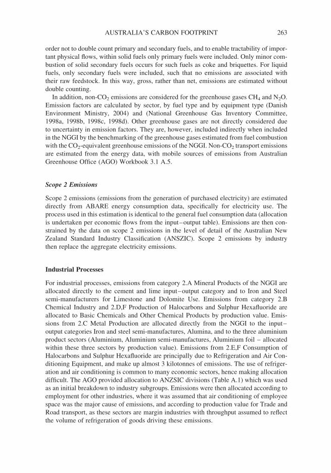
a ABARE Commodity Statistics 2007.b Estimated from Total Pastures and Head numbers.c Grazing density ratio of 14.3 used from Wilkenfield, 2002, Table 5.10.

Dairy assumed to have a grazing density twice that of beef.d ABS 7121.0; 2001-02.


discrete categories. The shares in fertiliser use is estimated as per George Wilkenfeld &

Associates Pty Ltd and Energy Strategies (2002) and updated to current year land area

data.

Emissions from Synthetic Fertilisers for Pasture are estimated solely by land area.

NGGI level 5 data, Animal Waste Applied to Soils, Nitrogen Fixing Crops, Cultivation

of Histosols, and Crop Residue are allocated directly to input output categories. Crop

residue data for Cereals was allocated to input–output sub-categories by production

volume (tonne).

Emissions from NGGI 4.D Agricultural Soils; Animal production are aggregated but are

due to nitrogen excretion via faeces and urine, and are hence allocated by animal pro-

duction volume (tonnes). Indirect emissions from Atmospheric deposition from fertilisers

are allocated as per Table A.3. Manure is allocated directly according to identified live-

stock types. Emissions from Field burning of agricultural residue are again allocated by

production volume (tonne) for Cereals, and directly for other categories. Prescribed

burning of Savannahs was fully allocated to beef cattle grazing, as per George Wilkenfeld

& Associates Pty Ltd and Energy Strategies (2002).

Indirect emissions from Nitrogen leaching and run-off were allocated per fertiliser use

(Table A.3) for crops and by land use area for pasture. Emissions associated with nitrogen

leaching from manure were allocated directly to respective livestock industries. Other

(Soil disturbance) emissions within Agricultural Soils were allocated by land use area

for crops and pasture respectively.

NGGI category 4.E Prescribed burning of savannahs was allocated fully to beef cattle,

as per George Wilkenfeld & Associates Pty Ltd and Energy Strategies (2002). Category

4.F emissions from field burning of agricultural residues were allocated by land use

area for cereals, and directly for pulses and sugar cane.

Land Use Change and Forestry

Land use change and forestry is broken down within the NGGI to Afforestation and refor-

estation and Land use change (cropland/grassland). Afforestation and reforestation emis-

sions were allocated according to number of seedlings planted. The ABS publication

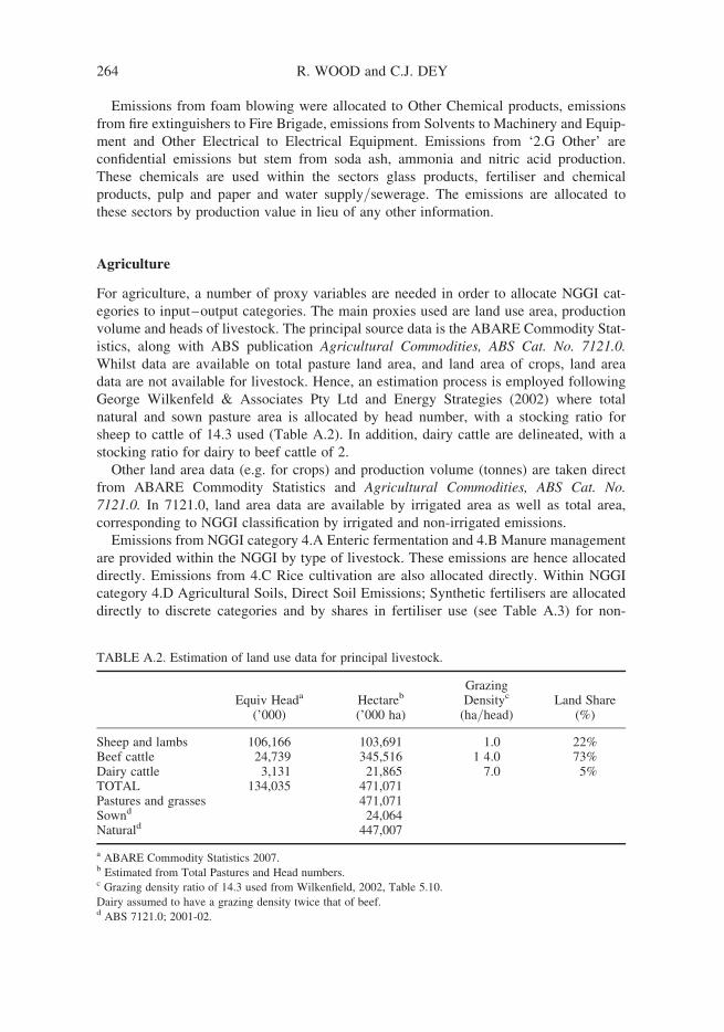
TABLE A.3. Allocation of emissions from synthetic fertilisers.

Synthetic fertiliserallocation

Application ratesa

(kg N20/ha)Land area(’000 ha)

Estimatedemissions

(’000 kg N20)

Fertiliseremissions share

(%)

Oats, sorghum andother cereal grainsb

0.72 2,099 1,511 10%

Wheatb 0.72 11,529 8,301 57%Barleyb 0.72 3,707 2,669 18%Rice 0.73 144 105 1%Oilseeds 0.62 1,881 1,166 8%Legumes 0.38 2,086 793 5%

a George Wilkenfield & Associates Pty Ltd and Energy Strategies (2002), Table 5.4, 1999 data.b Application rates of cereals used.


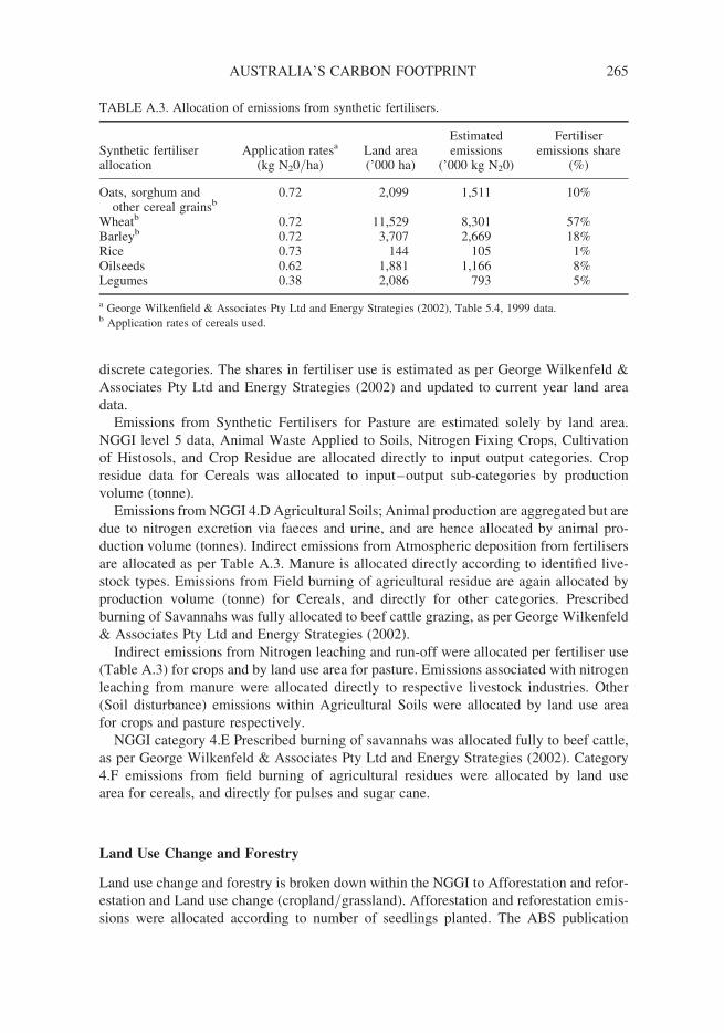
Agricultural Commodities ABS Cat. No. 7121.0 details forestry activities by purpose for

both number of seedlings planted and area (Table A.4). Number of seedlings planted

was used as the proxy to allocate emissions in order not to subject the allocation to differ-

ence within planting practices (intensive verses extensive planting). As a result, this does

not take into account differences in seedling mortality between purposes, and assumes

uniform carbon absorption by seedling. Timber or pulp planting was allocated between

softwoods and hardwoods by production volume (m3) of each. Proportion of seedlings

planted for nature conservation and protection of land and water were allocated directly

to Residents. Enhanced production and Fodder, plant products were allocated to agricul-

tural sectors by land use area.

Land use change emissions from deforestation (land converted to cropland) were allo-

cated to the various crops sectors by land use area. Emissions from land converted to grass-

land were allocated as per George Wilkenfeld & Associates Pty Ltd and Energy Strategies

(2002), which allocated 85% of total land use change emissions to beef, 4.5% to residen-

tial, and the remainder to crops – which are separately identified in the current NGGI.

Waste

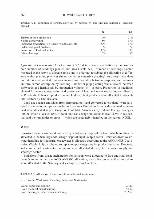
Emissions from waste are dominated by solid waste disposal on land, which are directly

allocated to the Sanitary and Garbage disposal input–output sector. Emissions from waste-

water handling for Industrial wastewater is allocated according to the AGO ANZSIC allo-

cation (Table A.5) distributed to input–output categories by production value. Domestic

and commercial wastewater emissions were allocated directly to the water supply and

sewerage sector.

Emissions from Waste incineration for solvents were allocated to Iron and steel semi-

manufacturers as per the AGO ANZSIC allocation, and other non-specified emissions

were allocated to the Sanitary and garbage disposal sectors.

TABLE A.4. Proportion of forestry activities by purpose by area (ha) and number of seedlingsplanted.

ha no

Timber or pulp production 9% 21%Nature conservation 15% 17%Enhanced production (e.g. shade, windbreaks, etc) 29% 17%Fodder and plant products 3% 7%Protection of land and water 39% 33%Other plantings 3% 5%

TABLE A.5. Allocation of emissions from industrial wastewater.

6.B.1 Waste, Wastewater Handling, Industrial Wastewater

Wood, paper and printing 19.92%Basic chemical manufacturing 6.43%Food, beverages, tobacco manufacturing 73.65%


Copyright of Economic Systems Research is the property of Routledge and its content may not be copied or

emailed to multiple sites or posted to a listserv without the copyright holder's express written permission.

However, users may print, download, or email articles for individual use.

Documents

AUSTRALIA'S CARBON FOOTPRINT