RESEARCH ARTICLE

Automated topology classification method for instantaneousvelocity fields

S. Depardon Æ J. J. Lasserre Æ L. E. Brizzi ÆJ. Boree

Received: 31 August 2006 / Revised: 31 January 2007 / Accepted: 2 February 2007 / Published online: 11 March 2007

� Springer-Verlag 2007

Abstract Topological concepts provide highly compre-

hensible representations of the main features of a flow with

a limited number of elements. This paper presents an

automated classification method of instantaneous velocity

fields based on the analysis of their critical points distri-

bution and feature flow fields. It uses the fact that topo-

logical changes of a velocity field are continuous in time to

extract large scale periodic phenomena from insufficiently

time-resolved datasets. This method is applied to two test-

cases : an analytical flow field and PIV planes acquired

downstream a wall-mounted cube.

1 Introduction

Unsteady separated flows such as those induced by bluff

bodies are characterized by coherent vortex sheddings,

with consequences in terms of aerodynamic forces on

the body itself and noise generation. Therefore, the

understanding of the flow dynamic behavior is of great

interest for many industrial applications. Its experimental

characterization requires both global and quantitative

measurement methods, for which particle image veloci-

metry (PIV) is particularly adequate. Not only does it

provide time averaged representations (streamlines topol-

ogy, mean and rms velocity components, vorticity) but it

also gives insights into instantaneous features of the flow.

Both the quantitative nature of PIV data, and its richness

must be taken advantage of, especially the instantaneous

velocity fields acquired for each configuration. Their

analysis has received great attention in terms of filtering

strategies, feature detection, and interpretation. Reviews of

these methods can be found in Bonnet et al. (1998),

Rockwell (2000) and Adrian et al. (2000).

In order to characterize the global dynamic behaviour of

the flow (its coherent, large scale energetic vortical struc-

tures), instantaneous velocity fields must be analyzed and

classified. Since they represent a great amount of data,

these processes should be automated as much as possible.

To the authors’ knowledge, there is a lack of efficient

methods for the rapid classification of instantaneous data-

sets acquired at different times.

Cipolla et al. (1998) and Rockwell (2000) show how a

combined approach of PIV, proper orthogonal decompo-

sition (POD) and topological concepts can yield significant

insights into the interpretation of instantaneous velocity

fields. This paper presents an extension of these concepts

by introducing an automated topological classification

method, based on feature extraction and tracking strategies.

Such a classification enables to extract the large scale dy-

namic behavior of the flow from insufficiently time-re-

solved data, using the topological continuity of a given

velocity field in time. The principle of this post-processing

strategy is described in Sect. 2, and applied to an analytical

case in Sect. 3. Section 4 presents an application to

experimental PIV data acquired downstream a wall-

mounted cube.

S. Depardon (&) � J. J. Lasserre

PSA Peugeot Citroen,

Direction de la Recherche et de l’Innovation Automobile,

Route de Gisy, 78943 Velizy-Villacoublay Cedex, France

e-mail: sebastien.depardon@mpsa.com

S. Depardon � L. E. Brizzi � J. Boree

Laboratoire d’Etudes Aerodynamiques,

Teleport 2, 1 Av. Clement Ader, BP 40109,

86961 Futuroscope Chasseneuil, France

123

Exp Fluids (2007) 42:697–710

DOI 10.1007/s00348-007-0277-3

2 Principle of the automated topology classification

method

2.1 Topological concepts

The use of topological concepts have been introduced by

Legendre (1956), who used part of the work by Poincare

(1928) to provide a theoretical framework for the analysis

of three-dimensional separated flows. They were initially

developed for the interpretation of oil-flow visualizations

(Hunt et al. 1978): to a given shear-stress pattern (type,

position, connectivity of critical points) corresponds a

specific 3-D separated flow topology. These concepts were

then extended to the analysis of in flow measurements

(Tobak and Peake 1982; Perry and Chong 1987), especially

velocity fields (acquired either with PIV techniques, or

phase averaged pointwise measurement systems). A great

advantage of topological concepts is the synthetic nature of

this information: given a distribution of critical points of a

velocity field, most of the remaining flow field can be

deduced (Foss 2004). They provide a clear representation

of the flow salient features.

Although topological concepts are clear when applied

to time-averaged skin friction patterns, they become

ambiguous when used for the interpretation of instanta-

neous velocity fields of plane cuts of a three-dimensional

flow: the topology of instantaneous streamlines corre-

sponds to the signature of vortical structures in a certain

frame of reference. The effect of its velocity on instan-

taneous turbulent velocity fields topology can be seen in

Adrian et al. (2000). If the frame of reference travels at

the convection velocity of the shed vortices, phenomena

such as entrainment and vortex pairing can be addressed.

If it is fixed to the body, the emphasis is laid on sepa-

ration and vortex formation processes (Dallmann and

Schewe 1987; Dallmann et al. 1991). Furthermore the

topological analysis of sectional-streamlines patterns of

three dimensional flows is open to misunderstanding.

Perry and Chong (1994) show with an analytical example

that the sectional-streamline pattern of a Burger vortex

strongly depends on the angle between this vortex and the

measurement plane.

Despite these limitations, of which one must be aware,

topological concepts are very powerful tools for the inter-

pretation of instantaneous velocity fields. They enable to

compress the information of large databases by restricting

the discussion to an analysis of topological changes, which

could be combined with other quantities such as vorticity

or Reynolds stress (Braza et al. 2006).

The aim of the classification method presented in this

paper is to extract large scale topological changes from

insufficiently time-resolved data. It is based on a three-step

analysis that is presented in the following subsections:

• Identification of each velocity field’s critical points

(i.e., their type and position).

• Determination of a ‘‘field-to-field distance’’ between

every pair of velocity fields (Ideally, this ‘‘distance’’ is

all the smaller as their critical point distribu-

tion—position, type and shape is similar).

• Adequate (i.e. easily understandable) representation of

the results for their interpretation.

2.2 Critical point identification

Given any set of instantaneous velocity fields, the first step

consists in identifying its critical points. If the data-sets are

taken from noisy experimental data, they can be filtered

prior to their analysis, using for example low-order

POD reconstruction methods (Cipolla et al. 1998; van

Oudheusden et al. 2005). This will however be addressed

in the next section, as the present section is focused on the

topological classification method itself.

The critical point identification method used in this work

is that presented in Depardon et al. (2006). Given any 2-D/

2-C velocity field, it provides the position, type and jaco-

bian matrix of its first-order non-degenerate critical points.1

Based on macroscopic properties such as the Poincare-

Bendixson index (Hunt et al. 1978) and other integrated

variables, it has proved to be sufficiently robust, fast and

efficient for the analysis of a large number of experimental

datasets. This process is run on every instantaneous

velocity field.

2.3 Concept of ‘‘field-to-field distance’’

In order to classify the velocity fields, the concept of

‘‘field-to-field distance’’ between each pair of them needs

to be introduced. The ‘‘field-to-field distance’’ between

two velocity fields (‘‘i’’ and ‘‘j’’) can be seen as the

‘‘work’’ needed to transform ‘‘i’’ into ‘‘j’’. In this appli-

cation, the definition of this ‘‘work’’ must be based on

topological properties. Ideally, it should be zero for iden-

tical critical point distributions (position, type and shape),

and increase all the more as their distribution differ. Initial

developments were based on their type and shape. A

topological distance was introduced to account for topo-

logical variations between velocity fields Lavin et al.

(1998). Our approach is mainly based on the critical points’

positions, as they can indicate large scale phenomena

within the flow.

1 Let O be a critical point of a 2-D/2-C velocity field (U(x,y), V(x,y)),

its jacobian matrix J is defined as

@U@x

@U@y

@V@x

@V@y

0@

1A

O

:

698 Exp Fluids (2007) 42:697–710

123

2.3.1 Initial developments

Such a concept has first been introduced by Lavin et al.

(1998), and extended in Batra et al. (1999) and Theisel

et al. (2002) for the analysis of large datasets produced by

computational fluid dynamics (CFD). Since typical exper-

imental databases tend to grow in size, due to the devel-

opment of non-intrusive, global and quantitative

measurement techniques such as PIV, adequate post-pro-

cessing strategies need to benefit from progresses achieved

in CFD.

The first strategies for the calculation of this topological

distance, Lavin et al. (1998) were only based on the

properties of critical points (i.e. their Jacobian matrix

coefficients), regardless of their positions. Although

improvements were provided in this area, Batra et al.

(1999), these methods had still an excessive computing

time, hence limited applicability.

2.3.2 Coupling strategy: feature flow fields (FFF)

Great improvements were achieved with the introduction

of a coupling strategy for critical points of two velocity

fields: feature flow fields. This approach has first been

introduced by Theisel et al. (2003) and Theisel and Seidel

(2003) for feature tracking purposes. Given a time depen-

dent 2-D velocity field:

uðx1; x2; tÞ ¼u1ðx1; x2; tÞu2ðx1; x2; tÞ

� �ð1Þ

A 3-D vector field f is constructed:

f ðx1; x2; tÞ ¼f1ðx1; x2; tÞf2ðx1; x2; tÞf3ðx1; x2; tÞ

0@

1A ð2Þ

¼detðux2

; utÞdetðut; ux1

Þdetðux1

; ux2Þ

0@

1A ð3Þ

¼ rðu1ðx1; x2; tÞÞ ^ rðu2ðx1; x2; tÞÞ ð4Þ

where the subscripts ux1; ux2

and ut denote the partial

derivatives of u(x1,x2,t). By definition, f is orthogonal to

the gradients of u(x1,x2,t). Therefore, f is such that its

streamlines are oriented along the smallest variation of

u(x1,x2,t), and define the behavior of its characteristic

features. Hence, a streamline of f integrated from a critical

point of u(x1,x2,t0) defines its behavior in time (Theisel

et al. 2003).

Velocity fields obtained by PIV are only available at

discrete time steps, and are either time resolved (such as

those obtained with high acquisition rate PIV systems), or

randomly sampled. When FFF are applied to track features

from time resolved datasets, streamlines of f between

successive time steps actually correspond to the true dis-

placement of critical points.

Indeed, let ua(x1,x2,ti) and ub(x1,x2,ti+1) be two succes-

sive time-steps. A linear interpolation is constructed as

follows:

uðx1; x2; tÞ ¼ ð1� fÞuaðx1; x2; tiÞ þ fubðx1; x2; tiþ1Þ ð5Þ

where f ¼ t�titiþ1�ti

; f 2 ½0; 1�: The corresponding feature flow

field f is constructed following Eq. (4). Streamlines of f are

generated from all critical points of both ua and ub,

yielding three possible configurations (provided

ua(x1,x2) „ 0 and ub(x1,x2) „ 0)2:

• A critical point from ua is paired with one from ub

(Fig. 1a)

• Two critical points from the same plane are paired

(either from ua as in Fig. 1b, or from ub)

• The streamline from a critical point (either from ua as

in Fig. 1b, or from ub) exits (or enters) the domain.

The same approach can be extended to insufficiently

time-resolved datasets. ua(x1,x2) and ub(x1,x2) are then two

independent instantaneous velocity fields. A linear inter-

polation can also be calculated (according to Eq. 5), as well

as the corresponding feature flow field. If ua(x1,x2) and

Fig. 1 Possible critical points pairings (Theisel et al. 2003)

2 Due to the linear interpolation, if any given velocity field ua is

compared to ub = 0, every streamline of f is aligned with f:

Exp Fluids (2007) 42:697–710 699

123

ub(x1,x2) are close time-steps, streamlines of f would again

actually correspond to the true displacement of critical

points between them. However, if it is not the case, these

streamlines would correspond to the most probable asso-

ciation determined from the linear interpolation. It is

important to note that FFF do not recreate missing infor-

mation; it reveals the features of the interpolated flow field.

2.3.3 Definition of the ‘‘field-to-field’’ distance

Theisel et al. (2003) defines a topological distance between

two velocity fields based on the modification of the paired

critical points features (Jacobian matrix coefficients). This

distance does not take into account the critical points’

displacement. Hence, the distance between a velocity field

and the same one convected downstream is zero. Further-

more, depending on the velocity fields’ quality (especially

for experimental results), the gradients can be noisy and

affect the quality of the results.

In the present application, a new ‘field-to-field’’ dis-

tance function (noted dist) is proposed, based on the critical

points’ positions.

Considering two velocity fields ua and ub. Nab is the

number of pairings between critical points (Fig. 1a, b) and

Mab the number of pairings between a critical point and a

point outside from the domain (Fig. 1c). With the notations

in Fig. 1, these points are noted (x0i ,y0

i ) and (xni ,yn

i )

(i 2[1,Nab + Mab]). dist(ua,ub) is defined as the summation

of the point-to-point distances between paired critical

points:

distðua; ubÞ ¼XNabþMab

i¼1

ffiffiffiffiffiffiffiffiffiffiffiffiffiffiffiffiffiffiffiffiffiffiffiffiffiffiffiffiffiffiffiffiffiffiffiffiffiffiffiffiffiffiffiffiffixi

0 � xin

� �2þ yi0 � yi

n

� �2q

ð6Þ

dist uses critical points as reference points to track the

velocity field variations. However, it is not rigorously a

‘‘topological distance’’ since it does not take into account

the variation of the critical points’ properties.

dist can define a metric on all vector field as long as it

verifies the following properties.

1. dist(ua,ub) ‡ 0

2. dist(ua, ua) = 0 (in fact 8k 2 <; distðua; kuaÞ ¼ 0Þ3. dist(ua,ub) = dist(ub,ua) (linearity of Eq. 4)

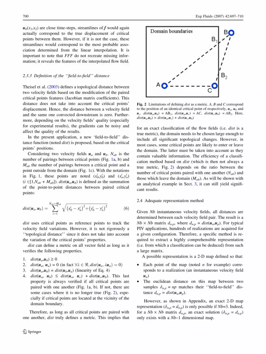
4. dist(ua, ub) £ dist(ua, uc) + dist(uc,ub). This last

property is always verified if all critical points are

paired with one another (Fig. 1a, b). If not, there are

some cases where it is no longer true (Fig. 2), espe-

cially if critical points are located at the vicinity of the

domain boundary.

Therefore, as long as all critical points are paired with

one another, dist truly defines a metric. This implies that

for an exact classification of the flow fields (i.e. dist is a

true metric), the domain needs to be chosen large enough to

include all significant topological changes. However, in

most cases, some critical points are likely to enter or leave

the domain. The latter must be taken into account as they

contain valuable information. The efficiency of a classifi-

cation method based on dist (which is then not always a

true metric, Fig. 2) depends on the ratio between the

number of critical points paired with one another (Nab) and

those which leave the domain (Mab). As will be shown with

an analytical example in Sect. 3, it can still yield signifi-

cant results.

2.4 Adequate representation method

Given Nb instantaneous velocity fields, all distances are

determined between each velocity field pair. The result is a

Nb · Nb matrix dn,p, where dn,p = dist(un,up). For typical

PIV applications, hundreds of realizations are acquired for

a given configuration. Therefore, a specific method is re-

quired to extract a highly comprehensible representation

(i.e. from which a classification can be deduced) from such

a large matrix.

A possible representation is a 2-D map defined so that:

• Each point of the map (noted n for example) corre-

sponds to a realization (an instantaneous velocity field

un)

• The euclidean distance on this map between two

samples dn,p = np matches their ‘‘field-to-field’’ dis-

tance dn,p = dist(un,up).

However, as shown in Appendix, an exact 2-D map

representation (dn,p = dn,p) is only possible if Nb=3. Indeed,

for a Nb · Nb matrix dn,p, an exact solution (dn,p = dn,p)

only exists with a Nb–1 dimensional map.

Fig. 2 Limitations of defining dist as a metric. A, B and C correspond

to the position of an identical critical point of respectively, ua, ub and

uc. dist(ua,ub) = AB1, dist(ua,uc) = AC, dist(uc,ub) = AB2. Here,

dist(ua,ub) > dist(ua,uc) + dist(uc,ub)

700 Exp Fluids (2007) 42:697–710

123

Otherwise, Multi dimensional scaling (MDS, Lavin

et al. (1998), Shepard (1962), see Appendix) is needed

to compute a 2-D representation that minimizes the

discrepancy between dn,p and dn,p i.e. minimizes

� ¼

ffiffiffiffiffiffiffiffiffiffiffiffiffiffiffiffiffiffiffiffiffiffiffiffiffiffiffiffiffiffiffiffiffiXn;p

dn;p � dn;p

� �2

Xn;p

d2n;p

vuuuuut :3

This topological classification method, based on the

analysis of the critical points distribution is now applied to

an analytical example.

3 Analytical example

The analytical case consists of 16 synthetic flow fields,

which reproduce the topology of an alternate vortex

shedding in a certain frame of reference over one period

(Fig. 3). It yields a distribution of foci and saddle points

convected from left to right.

Critical points are identified on each one and their

‘‘field-to-field’’ distance is computed using FFF and dist

presented in the previous section. Figure 4 shows specific

applications of FFF to pair up critical points of different

flow fields.

In Fig. 4a, FFF is applied to successive time steps

(No. 1, 3 and 5). In that case, the streamlines of f cor-

respond to the true displacement of the critical points.

Between No. 3 and 5, it reveals that two critical points

exit the domain downstream, while two new ones appear

upstream. In the present application, when two velocity

fields are selected independently, the only case where this

pairing does not correspond to the real one is presented in

Fig. 4b: when it is applied to two time steps in exact

opposition of phase. Indeed, FFF does not recreate

missing information. It is a mathematical construction

based on a linear interpolation which indicates the most

relevant pairing.

Figure 5 presents the dn,p matrix corresponding to the

distance between all pairs of velocity fields. It proves that

the choice of dist is relevant for this type of application,

since each time step is closest to its neighbors than all the

other ones. In this simple application, since only 16 time

steps are provided, this type of Figure may be sufficient to

yield some interpretations.

However, the representation provided by MDS, shown

in Fig. 6, is much clearer. It must be reminded that the

important parameter in such maps is the distance between

each point and the others, and not their coordinates or the

origin of the frame of reference. All points are equally

distributed, in order along a cycle that is nearly a ‘‘circle’’.

The fact that it is not truely a circle can be explained by the

impact of the domain boundary on the calculation of dist,

as shown in Fig. 2.

Nevertheless, this representation provides a simple

classification of all instantaneous velocity fields, and a

connection between them. For example, if they were ac-

quired in a random order, this method would enable to

rearrange them in order. The only uncertainties would be

the sense of rotation (clockwise or counterclockwise), and

the time between successive time steps (which is not nec-

essarily constant).

This analytical example shows the scopes and limita-

tions of this topological classification method. It is based

on the fact that topological changes are continuous in time.

Therefore, if datasets of a periodic movement are acquired

randomly, it is possible to rearrange them in order thanks to

their critical points distribution.

4 Experimental application

This section presents an application to real experimental

data : PIV measurements downstream from a wall mounted

cube. This geometry generates a quasi-periodic large scale

vortex shedding (Castro and Robins 1977; Hussein and

Martinuzzi 1996).

4.1 Experimental setup

The experiments are performed in a closed-circuit aca-

demic wind tunnel (test section size of 300 · 300 ·800 mm). The cube height is H = 60 mm. Incoming flow

velocity is set to Uo = 10 m/s (ReH = 40,000, as in

Martinuzzi and Tropea (1993)). Boundary layer is fully

turbulent and d99/H = 0.2 (see Fig. 7). The PIV system

consists of a Nd:YAG double cavity laser delivering

120 mJ light pulses (laser sheet thickness 1 mm). The

seeding particles are DEHS droplets. Images are acquired

with a Hisense 8bit 1,280 · 1,024 pixel camera fitted a

50 mm lens and a 532 nm narrow band optical filter.

Velocities are calculated with Dantec Dynamics Flow-

Manager software (Background image subtraction, four

step adaptive correlation and basic spurious vector detec-

tion). The classification method is tested on an iso-z=1 mm

plane (i.e 0.016 H), downstream from the cube, as shown

in Fig. 7. Its dimensions are 170 · 136 mm with a 1 mm

spatial resolution. For this configuration, 600 image pairs

(Nb = 600) were acquired at a frequency of 4.5 Hz (low

compared to the downstream vortex shedding frequency),

to ensure that the number of uncorrelated events was suf-

ficient to get good statistics. For additional details on the

experimental setup, the reader is referred to Depardon et al.

(2006).3 The Matlab cmdscale command is used.

Exp Fluids (2007) 42:697–710 701

123

4.2 POD low order reconstruction

The aim of this study is to extract the flow salient features

by analyzing critical points distribution of instantaneous

velocity fields. Instantaneous velocity fields contain lots of

critical points corresponding to the signatures of a large

variety of vortical structures, of different size and strength

(Fig. 8a). In order to focus on the topological signature of

large scale energetic structures, instantaneous flow fields

must be filtered. Snapshot POD can be used for this pur-

pose (Sirovich 1987; Huang 1994; Rockwell 2000). Each

instantaneous velocity field u(X,t) can be expanded as:

X

Y

X

Y

X

Y

X

Y

X

Y

X

Y

X

Y

X

Y

a b

dc

e f

hg

Fig. 3 Analytical example:

16 synthetic flow fields

reproducing an alternate vortex

shedding over one period

(Only one out of two is

represented—No. 1,

3,...,15—filled gray squareNode, filled circle Focus,

filled gray diamond Saddle)

702 Exp Fluids (2007) 42:697–710

123

Ui X; tð Þ ¼X

n

aðnÞðtÞUðnÞi Xð Þ ð7Þ

where the subscript i denotes the velocity field component

(i = 1, 2), (n) the decomposition order (n = 1,...,Nb), and

Nb the number of samples (i.e. image pairs). Fi(n) is an

orthonormal basis for the ith velocity field component. For

more information about POD, the reader is referred to

Berkooz et al. (1993) and Holmes et al. (1996).

The global dynamic behavior of the flow can be ana-

lyzed using low order POD reconstruction (Only a limited

number of the terms in Eq. 7 are retained). Indeed, in flows

dominated by large scale vortical structures, most of the

kinetic energy and coherent information are contained in

the first POD modes (Cipolla et al. 1998; Ben Chiekh et al.

2004; van Oudheusden et al. 2005). Figure 8 shows a

comparison between an instantaneous velocity field and

two low order reconstructions. The overall critical point

distribution naturally depends on the order of the recon-

struction. However, a few critical points are similar in all

figures (in type and position: two saddle points near the

cube, and two contra-rotating foci), which indicates that

they correspond to large scale energetic phenomena.

For applications to two dimensional mean flows, such as

the analysis of the vortex shedding generated by a flat

plate (Ben Chiekh et al. 2004) or square cylinder, (van

Fig. 4 Critical point pairing using FFF (filled gray square Node,

filled circle Focus, filled gray diamond Saddle). (a) FFF between

successive timesteps. (b) FFF between fields in opposition of phase

min

max2 4 6 8 10 12 14 16

2

4

6

8

10

12

14

16

Fig. 5 dn,p matrix for the analytical case

1

3 15

13

11

9

7

5

Fig. 6 Representation of the topological classification method results

provided by MDS

Exp Fluids (2007) 42:697–710 703

123

Oudheusden et al. 2005), the first two fluctuation modes

account for more than 80% of the averaged fluctuating

kinetic energy. In the present application they only account

for 27% of the averaged fluctuating kinetic energy (the first

three modes contain 81% of the total mean kinetic energy,

the first one corresponding to the time-averaged flow).

This is essentially due to important 3-D effects in this

area (the measurement plane being only 1mm above the

floor). Firstly, it is strongly affected by the main flow from

the top of the cube that reattaches downstream and im-

pinges on the floor in the X/H � 3 region. Secondly, there

is a strong interaction between the main vortex shedding

Uo

=0.2Hδ

4H 8.5H

H 5H

5HHRe = Uo.H/n

x

y

z

PIV plane99

Fig. 7 Experimental Setup

1 1.5 2 2.5 3−1.5

−1

−0.5

0

0.5

X/H

Y/H

1 1.5 2 2.5 3−1.5

−1

−0.5

0

0.5

X/H

Y/H

1 1.5 2 2.5 3−1.5

−1

−0.5

0

0.5

X/H

Y/H

a b

c

Fig. 8 Effect of POD low order

reconstruction on the flow field

topology. The most significant

critical points are represented

(circle focus, square node,

diamond saddle-point).

(a) Instantaneous velocity field.

(b) Reconstructed with 50

modes. (c) Reconstructed

with 3 modes

704 Exp Fluids (2007) 42:697–710

123

and the horseshoe vortex, generated upstream from the

cube, which extends on both sides of the cube (indicated in

Fig. 8 by the streamlines curvature in the Y/H � –1 re-

gion). As a result, there is no clear correlation between the

coefficients of the second and third POD modes (Fig. 9),

unlike 2-D applications, where this type of representa-

tion yields a true circle (Ben Chiekh et al. 2004; van

Oudheusden et al. 2005).

However, as shown in Fig. 10, the overall critical

point distribution determined from the 600 third order

reconstructed instantaneous velocity fields display a well

organized pattern. The longitudinal distribution of the

saddle-points and foci are consistent with the quasi-peri-

odic vortex shedding process generated by the wall-

mounted cube. Some nodes can also be noticed: they cor-

respond to a continuous transformation of foci as they

move downstream.4

Furthermore, all critical points are included within the

velocity field, which reduces the impact of the boundaries

on the calculation of the ‘‘field-to-field’’ distance.

4.3 Results and discussion

The topological classification method was applied to the

600 third order reconstructed velocity fields. Figure 11

shows two examples of critical points’ pairing using FFF

between two samples.5 All pairings are obvious in

Fig. 11a, as their phase in the shedding process is close.

Although this is not the case in Fig. 11b, some pairings are

also obvious, such as for the upstream saddle points, as

their position only slightly differs between both planes. In

Fig. 11b, the foci pairing highlights their longitudinal dis-

placement, which consists of the topological signature of

the vortex shedding process. The focus-saddle point gen-

eration between the two planes is linked to the generation

of a new wake vortex. In the present applications, these

pairings seem consistent with the temporal evolution of

these velocity fields.

The representation of the results obtained by MDS is

shown in Fig. 12. It displays a h-shaped distribution: most

of the datasets are distributed along a circle, suggesting a

cyclic behaviour.

As in Ben Chiekh et al. (2004) or van Oudheusden et al.

(2005) a phase ordering strategy can be introduced. All

datasets along the circle (red triangles) are sorted in 12

groups (A1,...,A12) according to their angular position.

Those along the diameter (blue circles) are divided into two

groups (B1 and B2). For each bin, an ensemble-average

flow field is computed (Fig. 13).

Provided the correct sense of rotation is chosen, the

sequence A1–A12 (Fig. 13a–l), which accounts for 90% of

the samples, defines a phase resolved period of an alternate

vortex shedding process (which is the coherent phenome-

non contained in the first three modes). However, unlike

phase averaging methods, or phase-sorting from the POD

modes coefficients, there is no temporal indication. The

cycle displayed in Fig. 12 is not traveled along at a con-

−1.5 −1 −0.5 0 0.5 1 1.5−1.5

−1

−0.5

0

0.5

1

1.5

a2 / (2 λ

2)1/2

a 3 / (2

λ3)1/

2

Fig. 9 Snapshot mode coefficient correlation

1 1.5 2 2.5 3−0.8

−0.6

−0.4

−0.2

0

0.2

0.4

0.6

0.8

X/H

Y/H

Fig. 10 Streamlines of the time-averaged velocity field (iso-

z=1 mm) and critical points determined from 600 POD-based third

order reconstructed instantaneous velocity fields (filled gray squarenode, filled circle focus, filled gray diamond saddle)

4 Let p = –trJ and q = detJ, where J is the jacobian matrix of the

velocity field taken at the critical point. p and q are continuous

functions as the critical point moves downstream. In some cases, this

leads to a configuration where we no longer have q > p2/4 (i.e. a

focus), but q < p2/4 instead (i.e. a node).5 With the notation defined in the next paragraph, Fig. 11a, b,

respectively, represent pairings between A2–A4 fields and A12–A4

fields.

Exp Fluids (2007) 42:697–710 705

123

stant speed, as proved by the number of realization in each

bin, which is not constant [ranging from 21 (A8) to 76

(A11)]. This is explained by the fact that their position on

the circle is determined by their critical point distribution.

Since the latter do not travel at a constant velocity, there is

no reason for the samples to be equally distributed along

the circle in Fig. 12. Further developments could take into

account this limitation by modifying the angular sectors

amplitude so that each bin contains an identical number of

realizations.

The last 10% of the samples (blue circles in Fig. 12),

devided in two groups (B1 and B2), do not seem consistent

with a simple vortex shedding process. As shown in

Fig. 13m, n, their ensemble average display a nearly sy-

metrical topology. In order to understand this feature, both

classifications (topological and POD mode correlation) are

compared in Fig. 14. B1 and B2 realizations are charac-

terized by low values of both second and third snapshot

mode coefficients. Therefore, the large scale phenomena

associated with these samples require more POD modes for

their analysis than the first three, which only contain the 2-

D alternate vortex shedding process. In such cases, where

both the second and third coefficients vanish, the impact of

the following modes must be reevaluated. For example, the

interaction with the upper flow or the horseshoe vortex may

induce coherence losses or intermittent phenomena such as

symetric vortex shedding from both sides of the cube.

Figure 14 also shows the strong link between the topo-

logical classification (A1–A12) and the second and third

snapshot mode coefficients. Although no coherent cycle

was identified from the latter, the velocity field topology

enables to extract the global behavior of the flow. This

robustness can be explained by the fact that topology is an

integrated variable of the velocity components.

This classification in 14 bins was chosen by interpreting

the MDS representation in Fig. 14a. As a comparison, the

dn,p matrix is represented in Fig. 15 (such as the one for the

analytical case in Fig. 5). In order to make it legible, the

entries are sorted by their angular position in Fig. 14a.

Indeed, without such a criterion, no interpretation would be

possible. The dark streak along the diagonal of the matrix

shows that the angular position is a relevant parameter for

the sorting. However, unlike for the analytical case, since

the datasets are not equally distributed along the circle, this

large diagonal streak has not a constant width. Finally, one

can notice thin vertical and horizontal lines, which do not

seem to match with the main trend. They correspond to the

datasets from both B1 and B2 bins.

The automated classification method presented in this

section enables to extract large scale features from insuf-

Fig. 11 Critical points pairing

between third order

reconstructed velocity fields

using feature flow fields

Fig. 12 Results of the topology classification method applied to the

third order reconstructed velocity fields (representation obtained by

MDS)

706 Exp Fluids (2007) 42:697–710

123

ficiently time resolved datasets. In this application, the

alternate vortex shedding was extracted from third order

reconstructed velocity fields. It also suggests that in some

cases, where both the second and third coefficients vanish,

the impact of the following modes must be reevaluated.

These phenomena could then be analyzed with a higher

order reconstruction, for which this method could still be

applied, unlike the analysis of the correlation between two

POD modes.

5 Conclusion and perspectives

Topological concepts are very powerful tools for the

analysis of instantaneous velocity fields: they provide

highly comprehensible representations of the main features

of a flow with a limited number of elements. Feature

detection and tracking can be used on time resolved data-

sets to extract the global dynamic behavior of a flow field.

However, even with low frequency PIV systems, topolog-

Fig. 13 Ensemble-average flow fields computed for each bin of the topology classification in Fig. 12 (a-l: A1 to A12, m: B1, n: B2)

Exp Fluids (2007) 42:697–710 707

123

ical concepts can also provide valuable insights into flow

structures.

The topological classification method presented in this

paper enables an automated analysis of instantaneous

velocity fields. Based on their critical point distribution, a

‘‘field-to-field’’ distance is computed between each pair of

velocity fields (This distance is all the smaller as their

critical point distribution is similar [in position]). This is

achieved by the use of feature flow fields and an appro-

priate metric. The latter is only based on the paired critical

points’ positions. Topological changes of a velocity field

being continuous in time, an appropriate representation of

Fig. 13 continued

−1.5 −1 −0.5 0 0.5 1 1.5−1.5

−1

−0.5

0

0.5

1

1.5a b

a2 / (2 λ

2)1/2

a 3 / (2

λ3)1/

2

Fig. 14 Link between the

snapshot mode coefficient

correlation (b) and the

topological classification (a)

708 Exp Fluids (2007) 42:697–710

123

the classification results can be used to extract large scale

periodic phenomena from insufficiently time-resolved

datasets.

For example, its application to experimental datasets

(low-order POD reconstructed velocity fields downstream a

wall-mounted cube) enabled to extract the large scale

periodic vortex shedding process contained in the first POD

modes and identify realizations where more POD modes

were required. Further developments could include the

application of this method to higher order reconstructed

datasets.

The efficiency of this method in both applications is

firstly due to the fact that topology is an integrated variable

of the velocity field, and therefore a robust parameter for

classification procedures. Furthermore, both examples in-

volve shedding processes, with large critical points dis-

placements. The metric dist was specifically developed for

this type of phenomenon. Further developments should be

considered for the definition of more complex ‘‘field-to-

field’’ distance metrics which could be efficient for all

types of flows. For example, the distance between paired

critical points could be weighted by the alteration of their

features (Jacobian matrix coefficients), or other quantita-

tive parameters.

Finally, this approach could also benefit from the

development of time-resolved PIV systems, although in

such applications the classification process would not be

used to put into order randomly acquired datasets. A per-

spective is the compression of the information by restrict-

ing the discussion to an analysis of topological changes.

Critical points would be automatically identified and

tracked. The analysis of the evolution of the ‘‘field-to-

field’’ distance between an instantaneous velocity field and

the next could enable to quickly extract extreme or inter-

mittent phenomena.

6 Appendix: Multi-dimensional scaling (MDS)

In this appendix is shown a basic application of multi

dimensional scaling [MDS, Lavin et al. (1998); Shepard

(1962)]. Let d be a 3 · 3 matrix corresponding to the

‘‘field-to-field’’ distance between three velocity fields:

d ¼0 4 9

4 0 6

9 6 0

0@

1A ð8Þ

For example, for Nb = 3:

The results can be represented on a 2-D map (Fig. 16a),

where:

• Each point corresponds to an instantaneous velocity

field

• The euclidean distance dn,p on this map matches their

‘‘field-to-field’’ distance dn,p. In this case dn,p = dn,p.

In such representations, the important parameter is the

distance between each point and the others, and not their

coordinates or the origin of the frame of reference.

−6 −4 −2 0 2 4 6−5

−4

−3

−2

−1

0

1

2

3

4

5a b

X

Y

4

9

6

No 1 No 3

No 2

−6 −3 0 3 6

X No 1 No 2 No 3

3.3 5.7

9

Fig. 16 MDS 2-D (a) and 1-D

(b) representation of d

Fig. 15 dn,p matrix for the experimental application (For sake of

clearness, the entries are sorted by their angular position in Fig. 14a)

Exp Fluids (2007) 42:697–710 709

123

The results can also be represented on a 1-D axis

(Fig. 16b). In that case, dij „ dij. Multi dimensional

scaling [MDS, Lavin et al. (1998); Shepard (1962)] is

needed to compute a configuration where the euclidean

distance between every pair of objects in this low order

representation matches their real ‘‘field-to-field’’ distance

i.e. to minimize � ¼

ffiffiffiffiffiffiffiffiffiffiffiffiffiffiffiffiffiffiffiffiffiffiffiffiffiffiPn;p

dn;p�dn;pð Þ2Pn;p

d2n;p

s: In this example, the

1-D representation yields e = 0.07 (Fig. 16b). For any Nb,

an exact representation requires a dimension of Nb–1,

which is not applicable for a few hundreds datasets.

Therefore, methods such as MDS is necessary to provide

understandable representation on 2-D or 3-D maps.

References

Adrian RJ, Christensen KT, Liu ZC (2000) Analysis and interpreta-

tion of instantaneous turbulent velocity fields. Exp Fluids

29:275–290

Batra R, Kling K, Hesselink L (1999) Topology based methods for

quantitative comparisons of vector fields. In: IIIE Visualization

’99, Late breaking hot topics, pp 25–28

Ben Chiekh M, Michard M, Grosjean N, Bera JC (2004) Recon-

struction temporelle d’un champ aerodynamique instationnaire a

partir de mesures PIV non resolues dans le temps. In: 9eme

Congres Francais de Velocimetrie Laser, Brussels, Belgium,

paper D.8.1

Berkooz G, Holmes P, Lumley JL (1993) The proper orthogonal

decomposition in the analysis of turbulent flows. Ann Rev Fluid

Mech 25:539–575

Bonnet JP, Delville J, Glauser MN, Antonia RA, Bisset DK, Cole DR,

Fiedler HE, Garem JH, Hilberg D, Jeong J, Kevlahan NKR,

Ukeiley LS, Vincendeau E (1998) Collaborative testing of eddy

structure identification methods in free turbulent shear flows.

Exp Fluids 25:197–225

Braza M, Perrin R, Hoarau Y (2006) Turbulence properties inthe

cylinder wake at high Reynolds number. In: Fourth symposium

on bluff body wakes and vortex induced vibrations (BBVIV4)

Castro IP, Robins AG (1977) The flow around a surface mounted

cube in uniform and turbulent flows. J Fluid Mech 79-2:307–335

Cipolla KM, Liakopoulos A, Rockwell D (1998) Quantitative

imaging in proper orthogonal decomposition of flow past a

delta wing. AIAA J 36(7):1247–1255

Dallmann U, Schewe G (1987) On topological changes of separating

flow structures at transition Reynolds numbers. In: AIAA-87-

1266, Honolulu

Dallmann U, Hilgenstock A, Riedelbauch S, Schulte-Werning B,

Vollmers H (1991) On the footprints of three-dimensional

separated vortex flows around blunt bodies. Tech Rep AGARD

Depardon S, Lasserre JJ, Brizzi LE, Boree J (2006) Instantaneous

skin-friction pattern analysis using automated critical point

detection on near-wall PIV data. Meas Sci Technol 17(7):1659–

1669

Foss JF (2004) Surface selections and topological constraint evalu-

ation for flow field analyses. Exp Fluids 37:883–898

Holmes P, Lumley JL, Berkooz G (1996) Turbulence, coherent

structures, dynamical system and symmetry. Cambridge

University Press

Huang H (1994) Limitations of and improvement to PIV and its

application to a backward-facing step flow. Ph.D. thesis,

Technical University of Berlin, Wissenschaftliche Schriftenreihe

Stroemungstechnik, band 1, D83, ISBN 3-929937-74-3

Hunt JCR, Abell CJ, Peterka J, Woo H (1978) Kinematical studies of

the flows around free or surface-mounted obstacles. J Fluid

Mech 86:179–200

Hussein HJ, Martinuzzi RJ (1996) Energy balance for turbulent flow

around a surface mounted cube placed in a channel. Phys Fluids

8(3):764–780

Lavin Y, Batra R, Hesselink L (1998) Feature comparisons of vector

fields using earth mover’s distance. In: Proceedings of the IEEE

Visualizations ’98, pp 103–109

Legendre R (1956) Separation de l’ecoulement laminaire tridimen-

sionnel. La Rech Aeronautique 54:3–8

Martinuzzi RJ, Tropea C (1993) The flow around surface-mounted,

prismatic obstacles placed in a fully developped channel flow.

J Fluid Eng 115:85–92

van Oudheusden BW, Scarano F, van Hinsberg NP, Watt DW (2005)

Phased-resolved characterization of vortex shedding in the near-

wake of a square-section cylinder at incidence. Exp Fluids

39:86–98

Perry AE, Chong MS (1987) A description of eddying motions and

flow patterns using critical-point concepts. Ann Rev Fluid Mech

19:125–155

Perry AE, Chong MS (1994) Topology of flow patterns in vortex

motions and turbulence. App Sci Research 53:357–374

Poincare H (1928) Oeuvres completes de Henri Poincare. Gaultier-

Villars, Paris

Rockwell D (2000) Imaging of unsteady separated flows: global

interpretation with particle image velocimetry. Exp Fluids

29(7):S255–S273

Shepard RN (1962) The analysis of proximities: Multidimensional

scaling with an unknown distance function I and II. Psychomet-

rika 27:125–140, 219–246

Sirovich L (1987) Turbulence and the dynamics of coherent

structures. Part I: coherent structures. Q J Appl Math 45:561–571

Theisel H, Seidel HP (2003) Feature flow fields. In: Proceedings of

the VisSym ’03

Theisel H, Rossl C, Seidel HP (2002) Vector field metrics based on

distance measures of first order critical points. J WSCG 10:121–

128

Theisel H, Rossl C, Seidel HP (2003a) Using feature flow fields for

topological comparison of vector fields. In: Proceedings of the

vision, modeling and visualization, Munich, Germany, pp 521–

528

Tobak M, Peake J (1982) Topology of three-dimensional separated

flows. Ann Rev Fluid Mech 14:61–85

710 Exp Fluids (2007) 42:697–710

123