Automatic parameter estimation for the

Discrete Algebraic Reconstruction Technique

(DART)Wim van Aarle, K. Joost Batenburg and Jan Sijbers

Abstract

Computed Tomography (CT) is a technique for non-invasive imaging of physical objects. In the Discrete Algebraic

Reconstruction Technique (DART), prior knowledge about the material’s densities is exploited to obtain high quality

reconstructed images from a limited number of its projections. In practice, this prior knowledge is typically not

readily available. Here, a fully automatic method, called Projection Distance Minimization DART (PDM-DART),

is proposed in which the optimal grey level parameters are adaptively estimated during the reconstruction process.

Simulation as well as real µCT experiments show that PDM-DART is capable of computing reconstructed images

of which the quality is equally high as that of the reconstructed images computed by conventional DART with exact

prior knowledge, thereby eliminating the need for tedious and error-prone user interaction.

Index Terms

computed tomography, segmentation, discrete tomography, automatic parameter optimization, DART, projection

distance minimization

Wim van Aarle, K. Joost Batenburg and Jan Sijbers are affiliated with IBBT-Vision Lab, University of Antwerp, Antwerp, Belgium;

K. Joost. Batenburg is also affiliated with Centrum Wiskunde & Informatica (CWI), Amsterdam, The Netherlands.

Corresponding author: Wim van Aarle, E-mail: wim.vanaarle@ua.ac.be.

November 29, 2011 DRAFT

1

Automatic parameter estimation for the

Discrete Algebraic Reconstruction Technique

(DART)

I. INTRODUCTION

Discrete tomography algorithms limit the set of possible reconstructions to those that contain only a small number

of grey levels. Compared to conventional reconstruction methods (e.g. FBP, SIRT), incorporating this constraint in

the reconstruction algorithm results in high quality reconstructions from substantially fewer projection angles, thus

reducing the radiation exposure to the scanned sample. In [1], the Discrete Algebraic Reconstruction Technique

(DART) was introduced. DART is an iterative technique that effectively combines reconstruction and segmentation

into a single algorithm. DART exploits prior knowledge about the grey levels of each of the scanned materials to

obtain accurate reconstructions even if the amount of projection data is limited (e.g. only a few projection angles

are measured, the angular range is limited or the projection data is truncated). DART has already been successfully

applied on electron tomography data [2], [3] and to reconstruct three-dimensional grain maps [4].

A key problem when applying DART to experimental datasets is its assumption that the set of grey levels in the

unknown reconstructed image is known a priori. While this is easy to satisfy in simulation experiments, obtaining

such knowledge in practice is non-trivial. Even if the attenuation value of each material is known in advance,

accurate hardware calibration is required to translate these values into grey levels for use in the reconstruction.

Such a calibration depends on various properties of the scanning system, which are typically not available to the

user. Furthermore, calibration parameters may change over time. In X-ray transmission tomography, for example,

the X-ray source constantly heats up during scanning, changing the spectrum of the emitted X-rays. While this may

have a negligible effect during a single scan, batch processing of scans is rendered impossible.

The knowledge of the reconstruction’s grey levels is of crucial importance to obtain high quality DART re-

constructions. In Fig. 1, DART reconstructions are shown of a binary phantom image. Each reconstruction was

performed adopting a different grey level for the foreground, ρ. Clearly, only with a correct estimation of ρ a

suficiently accurate reconstruction can be achieved. Note that the estimation of the threshold value, τ , used in the

segmentation phase of each DART iteration, also influences the reconstruction accuracy. The combination of grey

levels and threshold values will be referred to as the segmentation parameters of DART.

To estimate the grey levels of an image composed of only a few grey levels, the semi-automatic Discrete Grey

Level Selection (DGLS) method was introduced in [5] (Fig. 2b). For each grey level, the user selects an area in

the reconstruction volume that is assumed to be homogeneous. These user-selected parts are set to a candidate

grey level, after which their forward projection is subtracted from the measured projection data. The optimal grey

November 29, 2011 DRAFT

2

(a) ρ = 235, τ = 75

rNMP=0.024

(b) ρ = 235, τ = 125

rNMP=0.011

(c) ρ = 255, τ = 125

rNMP=0

(d) ρ = 275, τ = 125

rNMP=0.045

(e) ρ = 275, τ = 175

rNMP=0.078

Fig. 1. Parts of DART reconstructions of Fig. 3a for different values of ρ and τ (with 30 equiangular projections). For each (ρ,τ )

combination, the relative Number of Misclassified Pixels (rNMP) is given. The rNMP is defined by the number of erroneously

classified pixels divided by the amount of non-zero pixels in the phantom image.

user DART

(a) user expertise

DGLS

user

DART

(b) DGLS + DART

optimization

DART

(c) optimization of DART

DART

PDM

(d) PDM-DART

Fig. 2. Schematic overview of various methods to estimate the segmentation parameters of DART. (a) User expertise is used to set the correct

parameters. (b) The DGLS method is used prior to DART to semi-automatically estimate the correct grey levels. (c) An optimization strategy

is used to automatically minimize the projection difference between the DART reconstructed images and the measured projection data. (d) The

PDM segmentation strategy is used within each DART iteration to automatically estimate the optimal grey levels and threshold values.

levels are those for which this residual sinogram is the least inconsistent. With DGLS, the optimal threshold values

can not be estimated and still have to be set manually. Furthermore, it is not always possible to manually select a

homogeneous region. For example, in bone or foam-like objects, there are no sufficiently large homogeneous areas.

In [6], the projection difference was proposed as a cost function to optimize the segmentation parameters

of DART. Optimization strategies, such as the Nelder-Mead simplex search [7] or the more advanced adaptive

surrogate modelling optimization [8], can then be employed to obtain accurate values (Fig. 2c). Since such an

estimation approach requires a full DART reconstruction for each function evaluation in the optimization process,

it is computationally very inefficient.

In this work, the DART method is extended with an advanced segmentation algorithm. In the original DART

description [1], intermediate reconstructions are segmented using a global thresholding approach with fixed, a priori

specified, segmentation parameters. Here, a more advanced segmentation called Projection Distance Minimization

(PDM) [9] is applied in each iteration of DART. This method is hereafter referred to as PDM-DART. In PDM-

DART, the threshold values and grey levels are automatically optimised such that the Euclidean distance between

the projection of the intermediate segmented image and the measured projection data is minimal. By applying PDM-

DART results are obtained that are comparable to those obtained by conventional DART, without prior knowledge

November 29, 2011 DRAFT

3

about the segmentation parameters. This eliminates the need for labour intensive user interaction.

This paper is structured as follows. In Section II, notation for iterative and discrete tomography is presented.

Section III then gives a detailed description of PDM-DART. In the subsequent Section IV, the proposed method

is experimentally validated on simulated as well as experimental data. These results are discussed in Section V.

Finally, in Section VI, conclusions are drawn.

II. NOTATION

Let v = (vj) ∈ Rn denote the discretised square image of an object, with n the number of pixels. It is assumed

that the object is completely contained within this square.

In a parallel beam projection geometry, projection data is measured along lines lθ,t = {(x, y) ∈ R × R :

x cos θ + y sin θ = t}, where θ ∈ [0, π) represents the angle between the line and the y-axis and t represents the

coordinate along the projection axis. In practice, a projection is measured at a finite set of projection angles and at a

finite set of detector cells, each measuring the integral of the object density along a ray. Let p = (pi) ∈ Rm denote

the measured projection data, with m the total number of detector cells times the number of projection angles.

The Radon transform of the object for a finite set of projection directions can be modelled as a linear operator

W , called the projection operator, which maps the image v to the projection data q:

q := Wv. (1)

In Eq. (1), W = (wij) is an m×n matrix where wij represents the contribution of image pixel j to detector value

i. The vector q is called the forward projection or sinogram of v.

The tomographic reconstruction problem can be modelled by the recovery of v from a given vector of projection

data p by solving the following system of equations:

Wv = p. (2)

In the remainder of this work, the Simultaneous Iterative Reconstruction Technique (SIRT), as described in [10],

will be used to solve Eq. (2). SIRT is an iterative algorithm that finds a solution v such that the weighted squared

projection difference ||Wv − p||R = (Wv − p)TR(Wv − p) is minimal. R ∈ Rm×m is a diagonal matrix that

contains the inverse row sums of W : rii = 1/∑j wij . The update step of SIRT is given by:

v(k+1)j = v

(k)j + λ

1∑mi=1 wij

m∑i=1

wij

(pi −

∑nh=1 wihv

(k)h

)∑nh=1 wih

. (3)

In Eq. (3), λ is a relaxation parameter.

For the case v(0) = 0, the SIRT algorithm is a linear algorithm in the sense that a reconstructed image v ∈ Rn

is formed by applying a linear transformation to the input vector p ∈ Rm of projection data. Let S(t) : Rm → Rn

denote the linear operator that corresponds with t iterations of the SIRT algorithm, starting with v(0) = 0.

v = S(t)p, (4)

November 29, 2011 DRAFT

4

(a) phantom (b) SIRT (c) segmented SIRT (d) DART

Fig. 3. (a) A binary 512× 512 phantom image. (b) SIRT reconstruction from 5 equiangular parallel beam projection directions.

(c) Otsu’s segmentation of (b). (d) DART reconstruction from 5 equiangular parallel beam projection directions.

The SIRT algorithm can also be performed on a certain subset A ⊂ {1, . . . , n} of the reconstruction grid by

removing the columns of W that are not in A. Consider the case where A = {1, . . . , n} \ {j}, with j ∈ {1, . . . , n}.

Eq. (2) then becomes:

...

......

...

wi,1 . . . wi,j−1 wi,j+1 . . . wi,n...

......

...

v1

...

vj−1

vj+1

...

vn

=

p1

...

pm

. (5)

Let S(t)A : Rm → Rn denote the linear operator that corresponds with t iterations of the SIRT algorithm, restricted

to a set of pixels A ⊂ {1, . . . , n}, starting with v(0) = 0.

v = S(t)A p. (6)

Prior to analysis of the reconstructed images, they are often segmented using a simple global thresholding scheme.

The segmented image is then computed from the reconstructed image where each pixel is assigned one of the grey

levels in ρ ∈ Rl according to threshold values τ ∈ Rl−1. Let l denote the number of unique grey levels. Define

the threshold function Cτ ,ρ(v) : Rn → {ρ1, . . . , ρl}n as

Cτ ,ρ(vj) =

ρ1 vj < τ1

ρ2 τ1 ≤ vj < τ2...

ρl τl−1 ≤ vj

, j = 1, . . . , n. (7)

III. METHODS

Consider the case presented in Fig. 3, where a binary 512 × 512 phantom image (Fig. 3a) is reconstructed with

only 5 projection directions. The reconstruction problem is very ill-posed, leading to multiple solutions that adhere

November 29, 2011 DRAFT

5

to the projection data. In that case, the SIRT reconstruction (Fig. 3b) converges to the solution of which its weighted

Euclidean distance to the initial image (here a black image) is minimal [10].

To create a segmented image, a global thresholding scheme is typically applied to the reconstructed image.

Otsu’s clustering method [11] is commonly used. However, Otsu’s method determines its threshold values solely

on the basis of the reconstructed image and thus also on its reconstruction artefacts (shown in Fig. 3c). In [12],

an advanced tomographic segmentation technique, called Projection Distance Minimization (PDM) was proposed.

In PDM, thresholds values are selected such that the Euclidean distance between the forward projection of the

segmented image and the measured projection data is minimal. This method is further investigated in Section III-A.

Note that in Fig. 3c, most of the segmentation errors occur near the border of the object. This observation lies

at the core of the Discrete Algebraic Reconstruction Technique (DART), an iterative reconstruction technique that

combines conventional iterative reconstruction techniques and segmentation into a single algorithm [1]. In each

DART iteration, non-boundary pixels are assigned a given grey level in the known set ρ = (ρi) ∈ Rl. These pixels

are then kept fixed in the subsequent reconstruction step. This reduces the amount of unknowns in the reconstruction

equation Eq. (2) while keeping the amount of detector values stable, thus leading to improved reconstructions. Fig. 3d

shows a DART reconstruction of the phantom image in Fig. 3a from only 5 projections. DART is discussed in detail

in Section III-B.

Finally, in Section III-C, DART is extended with a novel approach to automatically estimate the set of discrete

grey levels.

A. Projection Distance Minimization (PDM)

The optimal tomographic image in which the possible grey levels are restricted to those in the set ρ ∈ Rl, is the

one for which the Euclidean distance between its forward projection and the measured projection data is minimal.

Let sopt ∈ {ρ1, . . . , ρl}n denote this image:

sopt = argmins∈{ρ1,...,ρl}n ||Ws− p||2. (8)

The search space of the optimization problem in Eq. (8) has a very high dimensionality, making it difficult to locate

the optimum. Therefore, segmented images are commonly obtained by application of a global thresholding scheme

on a certain, priorly reconstructed image v. The optimization problem of Eq. (8) can then be translated into

τopt,ρopt = argminτ∈Rl−1,ρ∈Rl ||W Cτ ,ρ(v)− p||2. (9)

The dimension of the search space of the optimization problem in Eq. (9) is only 2l − 1. To further increase the

computational efficiency of the optimization, it can be split into two smaller optimization problems:

• Inner optimization: Given certain threshold values τ , determine the optimal grey levels, ρopt, that minimize

Eq. (9):

ρopt = argminρ||W Cτ ,ρopt(v)− p||2. (10)

This optimization problem is discussed in Section III-A1.

November 29, 2011 DRAFT

6

• Outer optimization: Optimize τ by solving

τopt = argminτ ||W Cτ ,ρopt(v)− p||2. (11)

In each function evaluation, ρopt is given by the inner optimization. The outer optimization problem is discussed

in Section III-A2.

1) Grey level estimation: Given an image vector v and certain threshold values τ , for each t ∈ {1, . . . , l}, let

st ∈ {0, 1}n denote the partition mask of class t:

stj =

1 if Cτ ,{1,...,l}(vj) = t

0 otherwise, j = 1, . . . , n. (12)

Let A = (ait) denote an m × l matrix where column t contains the forward projection of st. The value ait is

defined by the total contribution to ray i of all pixels that belong to partition t.

ait =

n∑j=1

wij sti =∑

j:stj=1

wij (13)

For any set of grey levels ρ, the forward projection of Cτ ,ρ(v) can then be written as

W Cτ ,ρ(v) =

l∑t=1

Wstρt = Aρ. (14)

Let aj denote the jth row of A and let cj = −2pjaj , c =∑mj=1 cj , Qj = aja

Tj , Q =

∑mj=1Qj . The projection

difference then becomes:

||W Cτ ,ρ(v)− p||2 = ||Aρ− p||2 (15)

=

m∑j=1

(aTj ρ− pi

)2(16)

=

m∑j=1

(ρTQjρ− cTj ρ+ p2

i

)(17)

= ρT Qρ− cTρ+ |p|2 (18)

Given that the projection difference can not be negative, the optimal grey levels, ρ, can be computed by setting the

derivatives of Eq. (18) with respect to ρ1, . . . , ρl to zero, obtaining the easy to solve system:

2Qρopt = −c. (19)

2) Threshold value estimation: To optimize τ , Eq. (11) must be solved. Each evaluation in the search space

requires the computation of ρopt. Note that Eq. (11) is not differentiable. In [12], a strategy was proposed to

efficiently optimize Eq. (11). It made use of the fact that, if the threshold values are changed only by a small

amount, only a few pixels would fall into a different partition. The matrices c and Q could therefore be updated

very efficiently. However, such an approach is not optimally suited for optimization on modern GPU hardware and

its overall runtime depends greatly on the initial estimate. We have found that it is typically more computationally

efficient to compute GPU-accelerated forward projections of all pixels at each function evaluation. Experimental

November 29, 2011 DRAFT

7

findings have shown that the Nelder-Mead simplex search [7] offers accurate results with a sufficiently fast

convergence rate.

B. Discrete Algebraic Reconstruction Technique (DART)

Here, a concise summary of the iterative DART algorithm is given. Initially, an approximate reconstruction image,

v(0), is computed using SIRT with a certain number of iterations, t0:

v(0) = S(t0)p. (20)

Next, DART follows an iterative scheme with the following steps. Put k = 0, the iteration number of DART.

1) The current reconstructed image, v(k), is segmented to obtain an image that contains only grey levels from

the set ρ ∈ Rl. A simple global thresholding scheme with threshold values τ ∈ Rl−1 is used. Let s(k) ∈

{ρ1, . . . , ρl}n denote that segmented image:

s(k) = Cτ ,ρ(v(k)). (21)

2) The set U (k) ⊂ {1, . . . , n} of pixels to be updated is determined. This set contains pixels that are likely

to be misclassified in the current segmented image. The pixels in the complementary set of fixed pixels

F (k) = {1, . . . , n} \U (k) are those that will be removed from the reconstruction equation. U (k) contains two

types of pixels:

• As demonstrated in Fig. 3c, most errors occur near the edges of the object. All boundary pixels of the

current segmented image are thus added to U (k). A pixel is considered to be a boundary pixel if its value

is different from at least one of its neighbouring pixels:

U (k) ={j : ∃ h ∈ N(j) such that s(k)

j 6= s(k)h

}. (22)

In Eq. (22), N(j) ⊂ {1, . . . , n} denotes a certain neighbourhood window of pixel j. In [13], a variation

of DART, called Adaptive DART (ADART), was introduced. In ADART, the required number of pixels

from h ∈ N(j) for which s(k)j 6= s

(k)h is increased each time a certain convergence criterion is met. This

can lead to improved reconstruction quality.

• Each non-boundary pixel is added to U (k) with a certain probability 0 ≤ r ≤ 1. This increases the

accuracy of DART reconstruction in case of noisy projection data.

3) To reduce the set of unknowns in Eq. (2) to those in the set of free pixels, the forward projection of the

non-free pixels must first be subtracted from the measured projection data. Let f (k) ∈ Rn denote the current

segmented image in which all free pixels are set to zero, i.e.

f(k)j =

s(k)j j /∈ U (k)

0 j ∈ U (k). (23)

The residual sinogram, r(k) ∈ Rm, is then given by

r(k) = p−Wf (k). (24)

November 29, 2011 DRAFT

8

4) The current reconstructed image is then updated by the reconstruction of the residual sinogram, restricted to

the set of free pixels:

v(k+1) = f (k) + S(t)

U(k)r(k). (25)

In Eq. (25), t denotes the number of SIRT iterations that are performed to reconstruct the residual sinogram.

If certain pixels are misclassified in step 1, the residual sinogram is inconsistent. In that case, there does not

exist an exact solution to Eq. (25), leading to erroneous values in the updated reconstruction. To counter this,

a Gaussian smoothing filter is applied to v(k+1) as a means of regularization.

5) Increase k by 1 and return to step 1 until some termination criterion has been reached.

C. PDM-DART

residual sinogram

sinogram

reconstruction segmentation

reconstruction

sinogram p

v(0) s(k)

f (k)

U

Wf (k)

r (k)

r (k)S(t)U

W

S (t)U

S (t0)

-

+v(k+1)

blur

fixedpixels

optimize threshold

values

optimize grey

levels

(k)F

(k)

updatepixels

pixel mask

Fig. 4. Schematic overview of Projection Distance Minimization Discrete Algebraic Reconstruction Technique (PDM-DART).

In step 1 of each DART iteration a segmented image is computed from v(k) using a global thresholding scheme

with fixed, priorly specified, grey levels ρ and threshold values τ . Here, it is proposed to apply the PDM method,

November 29, 2011 DRAFT

9

v = S(t0)p ;

τ = initial threshold estimate ;

while stop criterion is not met

[τ ,ρ ] = est imate segmentat ion parameters (v, τ ) ;

s = Cτ ,ρ(v) ;

U = {} ;

for j = 1 :n

i f (∃h ∈ N(j) : sj 6= sh) | | rand ( ) < r

fj = 0 ;

U = U ∪ j ;

else

fj = sj ;

end

end

r = p−Wf ;

v = f + S(t)U r ;

v = v ∗ Gaussian smoothing filter ;

end

function [τopt,ρopt ] = est imate segmentat ion parameters (v, τinit )

[τopt,ρopt ] = simplex search of @compute project ion distance with τinit as initial estimate ;

end

function [ p r o j e c t i o n d i f f e r e n c e , ρopt ] = compute pro jec t ion d is tance (τ )

compute A ;

compute Q and c ;

ρopt = solution of 2Qρ = −c w.r.t ρ ;

p r o j e c t i o n d i f f e r e n c e = ||W Cτ ,ρopt (v)− p||2 ;

end

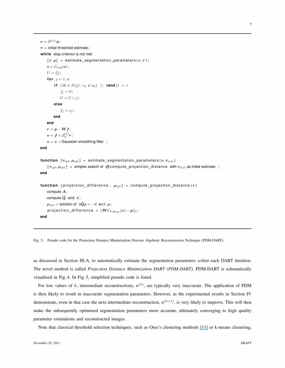
Fig. 5. Pseudo code for the Projection Distance Minimization Discrete Algebraic Reconstruction Technique (PDM-DART).

as discussed in Section III-A, to automatically estimate the segmentation parameters within each DART iteration.

The novel method is called Projection Distance Minimization DART (PDM-DART). PDM-DART is schematically

visualised in Fig. 4. In Fig. 5, simplified pseudo code is listed.

For low values of k, intermediate reconstructions, v(k), are typically very inaccurate. The application of PDM

is then likely to result in inaccurate segmentation parameters. However, as the experimental results in Section IV

demonstrate, even in that case the next intermediate reconstruction, v(k+1), is very likely to improve. This will then

make the subsequently optimised segmentation parameters more accurate, ultimately converging to high quality

parameter estimations and reconstructed images.

Note that classical threshold selection techniques, such as Otsu’s clustering methods [11] or k-means clustering,

November 29, 2011 DRAFT

10

are not suited for use within DART. Incorrect grey levels of an intermediate segmentation will negatively affect the

selection of new segmentation parameters in the subsequent iteration. In PDM, however, the optimal grey levels

are based on the measured projection data, not on the values obtained in the reconstructions.

The segmentation parameter estimation process does present an increased computational cost to each iteration of

the DART algorithm. To reduce this cost, one can opt to perform this optimization only once every few iterations.

The optimised segmentation parameters are then stored and reused until the next optimization takes place.

IV. EXPERIMENTS

(a) binary, grid-based (b) binary, grid-based (c) three grey levels, grid-based (d) three grey levels, analytical

Fig. 6. Simulated phantoms that are used to validate PDM-DART.

In this section, a series of experiments are described that were carried out to evaluate PDM-DART. Both simulation

data and experimental µCT data are included.

For all simulation experiments, four phantom images were considered (Fig. 6). Whereas Fig. 6a and Fig. 6b are

binary, Fig. 6c and Fig. 6d contain three grey levels. Fig. 6a-c were defined on a 512× 512 grid while Fig. 6d, and

its projection data, were analytically defined. All reconstructions were performed on a 512×512 grid. Only parallel

beam projection geometries with equiangular projection angles have been considered. However, the proposed method

can easily be applied on other projection geometries as well.

To validate the accuracy of the segmented images, the relative Number of Misclassified Pixels (rNMP) was

computed. This is the total number of erroneously classified pixels with respect to the phantom, divided by the

total number of non-zero pixels in the phantom image.

All experiments were performed on a single-core 2.4GHz system with 8GB memory. All tomographic operations,

such as DART, SIRT and the forward projection, were accelerated with NVIDIA CUDA and were run on an NVIDIA

GeForce GTX285.

A. Comparison of different estimation methods

In a first set of experiments, projection data was simulated of all phantom images depicted in Fig. 6. The number

of projection directions was varied. The following segmentation parameter estimation methods were applied.

November 29, 2011 DRAFT

11

(a) PDM-DART, 3 angles (b) PDM-DART, 4 angles (c) PDM-DART, 5 angles (d) PDM-DART, 6 angles

Fig. 7. PDM-DART reconstructions of Fig. 6a with an increasing number of projection directions.

angles search manual DGLS simplex PDM-DART

3 0.0947 0.1280 0.2068 0.1208 0.2117

4 0.0575 0.0798 0.1019 0.0911 0.1057

5 0.0007 0.0009 0.0022 0.0014 0.0008

6 0.0006 0.0009 0.0017 0.0009 0.0008

7 0.0004 0.0004 0.0009 0.0012 0.0004

8 0.0003 0.0004 0.0004 0.0003 0.0003

9 0.0002 0.0002 0.0003 0.0003 0.0002

10 0.0001 0.0001 0.0001 0.0001 0.0001

Fig. 8. This table lists, for phantom image Fig. 6a, the reconstruction accuracy in terms of rNMP for a variety of different segmentation

parameter estimation methods.

phantom rNMP goal search manual DGLS simplex PDM-DART

Fig. 6a 0.001 5 5 5 5 5

Fig. 6b 0.050 38 39 44 40 43

Fig. 6c 0.010 28 33 36 32 33

Fig. 6d 0.100 16 21 34 17 16

Fig. 9. This table lists, for each image of Fig. 6, the lowest number of projection directions with which it is possible to reach a certain rNMP

goal.

• Exhaustive parameter search: The parameters resulting in the most accurate reconstructions were found by

performing an exhaustive search. This method can only be applied for simulation experiments.

• Manual selection (Fig. 2a): The grey levels were measured in the phantom images. The threshold values were

set in the middle of each pair of consecutive grey levels.

• DGLS (Fig. 2b): The user-selected regions were manually chosen based on an initial SIRT reconstruction. The

threshold values were again set in the middle of each pair of consecutive grey levels. A positivity constraint

was included in the DGLS optimization process, as described in [5], as this was observed to result in more

November 29, 2011 DRAFT

12

accurate estimations.

• Optimization (Fig. 2c). The Nelder-Mead simplex search optimization strategy was performed on Eq. (9) to

estimate all grey levels and threshold values.

• PDM-DART (Fig. 2d). With PDM-DART, all grey levels and threshold values were estimated in each iteration

of DART.

In Fig. 7a-d, PDM-DART reconstructions are shown of phantom image Fig. 6a, for an increasing number of

projection directions. The rNMP values of these reconstructions, are listed in Fig. 8 for all previously mentioned

estimation methods. Both manual estimation and PDM-DART provided the best approximation of the optimal

values discovered by the exhaustive parameter search. Simplex search was slightly less accurate. This is likely due

to various local optima in the search space. The DGLS approach was also slightly less accurate, especially for very

low angle counts.

It can be clearly noted that, for phantom image Fig. 6a, there exists a certain lower bound to the number of

projection angles that is required to create highly accurate reconstructions (5 in this example). For all phantom

images and estimation methods, it was determined how many projection directions were needed in order to reach a

certain level of accuracy (in rNMP values). These results are shown in Fig. 9. Overall, PDM-DART did not require

substantially more projection directions to reach a certain accuracy than with the optimal segmentation parameters.

The same experiments were also performed with ADART [13] instead of DART, achieving similar results.

B. PDM-DART convergence

0 10 20 30 40 50200

250

300

iteration

ρ

manualt0=1

t0=10

t0=100

(a) grey level, Fig. 6b

0 10 20 30 40 500

0.5

1

iteration

rNM

P

manual , t 0 =100

PDM−DART, t0=1

PDM−DART, t0=10

PDM−DART, t0=100

(b) accuracy, Fig. 6b

Fig. 10. To study how PDM-DART performs when initial reconstructions do not allow for accurate tomographic segmentation, the algorithm

was run with different values for t0, the number of SIRT iterations to create v(0). (a) The estimated grey level of the foreground of phantom

image Fig. 6b as a function of the iteration number. (b) The corresponding accuracy in terms of rNMP.

It may be expected that, if the parameter estimation in PDM-DART is very inaccurate in one iteration, it can

still be improved in subsequent iterations.

To investigate the dependence of inaccurate parameter estimation in one iteration on the eventual result, projection

data of each phantom image was generated for 30 projections to which Poisson noise was applied. The intensity

November 29, 2011 DRAFT

13

0 20 40 60220

240

260

iteration

ρ manualPDM−DART(1)PDM−DART(5)PDM−DART(10)

(a) grey level convergence

0 10 20 30 40 500

0.1

0.2

iteration

rNM

P

manualPDM−DART(1)PDM−DART(5)PDM−DART(10)

(b) accuracy convergence

0 50 100 150 2000

0.1

0.2

time (s)

rNM

P

real ρPDM−DART(1)PDM−DART(5)PDM−DART(10)

(c) running time

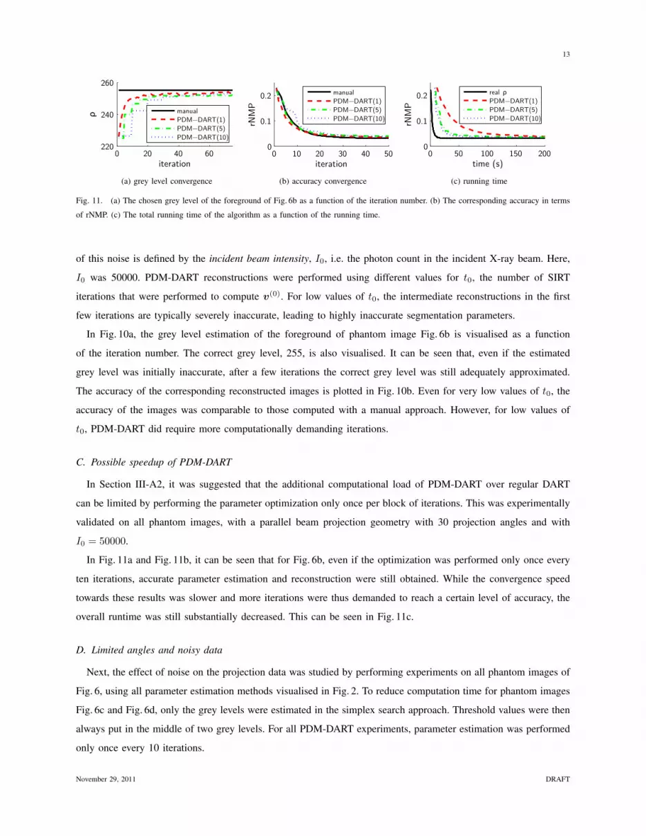
Fig. 11. (a) The chosen grey level of the foreground of Fig. 6b as a function of the iteration number. (b) The corresponding accuracy in terms

of rNMP. (c) The total running time of the algorithm as a function of the running time.

of this noise is defined by the incident beam intensity, I0, i.e. the photon count in the incident X-ray beam. Here,

I0 was 50000. PDM-DART reconstructions were performed using different values for t0, the number of SIRT

iterations that were performed to compute v(0). For low values of t0, the intermediate reconstructions in the first

few iterations are typically severely inaccurate, leading to highly inaccurate segmentation parameters.

In Fig. 10a, the grey level estimation of the foreground of phantom image Fig. 6b is visualised as a function

of the iteration number. The correct grey level, 255, is also visualised. It can be seen that, even if the estimated

grey level was initially inaccurate, after a few iterations the correct grey level was still adequately approximated.

The accuracy of the corresponding reconstructed images is plotted in Fig. 10b. Even for very low values of t0, the

accuracy of the images was comparable to those computed with a manual approach. However, for low values of

t0, PDM-DART did require more computationally demanding iterations.

C. Possible speedup of PDM-DART

In Section III-A2, it was suggested that the additional computational load of PDM-DART over regular DART

can be limited by performing the parameter optimization only once per block of iterations. This was experimentally

validated on all phantom images, with a parallel beam projection geometry with 30 projection angles and with

I0 = 50000.

In Fig. 11a and Fig. 11b, it can be seen that for Fig. 6b, even if the optimization was performed only once every

ten iterations, accurate parameter estimation and reconstruction were still obtained. While the convergence speed

towards these results was slower and more iterations were thus demanded to reach a certain level of accuracy, the

overall runtime was still substantially decreased. This can be seen in Fig. 11c.

D. Limited angles and noisy data

Next, the effect of noise on the projection data was studied by performing experiments on all phantom images of

Fig. 6, using all parameter estimation methods visualised in Fig. 2. To reduce computation time for phantom images

Fig. 6c and Fig. 6d, only the grey levels were estimated in the simplex search approach. Threshold values were then

always put in the middle of two grey levels. For all PDM-DART experiments, parameter estimation was performed

only once every 10 iterations.

November 29, 2011 DRAFT

14

10 20 30 400

0.01

0.02

0.03

angle count

rNM

PmanualDGLSsimplexPDM−DART(10)

(a) Fig. 6a

20 40 60 800

0.05

0.1

angle count

rNM

P

manualDGLSsimplexPDM−DART(10)

(b) Fig. 6b

20 40 60 800

0.05

0.1

0.15

0.2

angle count

rNM

P

manualDGLSsimplexPDM−DART(10)

(c) Fig. 6c

20 40 60 800

0.1

0.2

angle count

rNM

P

manualDGLSsimplexPDM−DART(10)

(d) Fig. 6d

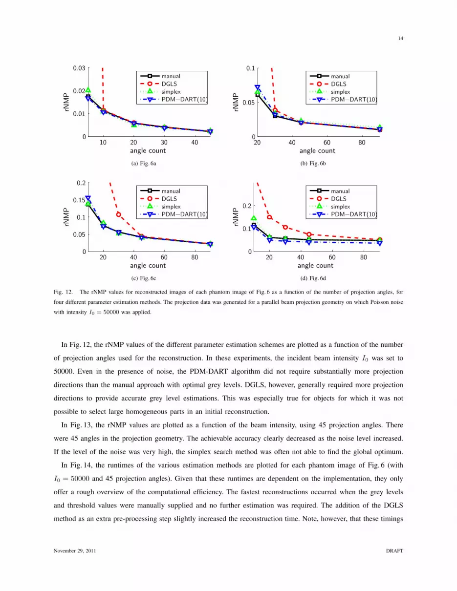
Fig. 12. The rNMP values for reconstructed images of each phantom image of Fig. 6 as a function of the number of projection angles, for

four different parameter estimation methods. The projection data was generated for a parallel beam projection geometry on which Poisson noise

with intensity I0 = 50000 was applied.

In Fig. 12, the rNMP values of the different parameter estimation schemes are plotted as a function of the number

of projection angles used for the reconstruction. In these experiments, the incident beam intensity I0 was set to

50000. Even in the presence of noise, the PDM-DART algorithm did not require substantially more projection

directions than the manual approach with optimal grey levels. DGLS, however, generally required more projection

directions to provide accurate grey level estimations. This was especially true for objects for which it was not

possible to select large homogeneous parts in an initial reconstruction.

In Fig. 13, the rNMP values are plotted as a function of the beam intensity, using 45 projection angles. There

were 45 angles in the projection geometry. The achievable accuracy clearly decreased as the noise level increased.

If the level of the noise was very high, the simplex search method was often not able to find the global optimum.

In Fig. 14, the runtimes of the various estimation methods are plotted for each phantom image of Fig. 6 (with

I0 = 50000 and 45 projection angles). Given that these runtimes are dependent on the implementation, they only

offer a rough overview of the computational efficiency. The fastest reconstructions occurred when the grey levels

and threshold values were manually supplied and no further estimation was required. The addition of the DGLS

method as an extra pre-processing step slightly increased the reconstruction time. Note, however, that these timings

November 29, 2011 DRAFT

15

0 2 4 6 8 10x 104

0

0.02

0.04

I0

rNM

PmanualDGLSsimplexPDM−DART(10)

(a) Fig. 6a

0 2 4 6 8 10x 104

0

0.05

0.1

I0

rNM

P

manualDGLSsimplexPDM−DART(10)

(b) Fig. 6b

0 2 4 6 8 10x 104

0

0.1

0.2

0.3

0.4

I0

rNM

P

manualDGLSsimplexPDM−DART(10)

(c) Fig. 6c

0 2 4 6 8 10x 104

0

0.05

0.1

0.15

0.2

I0

rNM

P

manualDGLSsimplexPDM−DART(10)

(d) Fig. 6d

Fig. 13. The rNMP values for reconstructed images of each phantom image of Fig. 6 as a function of the intensity of the applied Poisson noise,

for four different parameter estimation methods. The projection data was generated for a parallel beam projection geometry with 45 equiangular

projection angles.

Fig. 4a Fig. 4b Fig. 4c Fig. 4d0

1000

2000

3000

4000

5000

runt

ime

(s)

manualDGLS−PPDM−DART (10)PDM−DART (1)simplex

39 41 42 3749 52 56 6095 107 345 269527 442

2027 1794

36713189

3818

4428

Fig. 14. The runtimes of each estimation method for each of the phantom images of Fig. 6 with simulated parallel beam projection data with

45 angles and I0 = 50000.

do not take into account the extra time that it took to select the homogeneous part. The PDM-DART scheme

required more computation time than DGLS, especially for high-dimensional optimization problems (e.g. Fig. 6c

November 29, 2011 DRAFT

16

and Fig. 6d). However, the runtime was reduced by excluding the estimation of the segmentation parameters. The

simplex search scheme required by far the most computation time.

E. Experimental data

(a) FBP reconstruction (b) ground truth image (c) S-SIRT, 50 angles

rNMP=0.1293

(d) PDM-DART, 50 angles

rNMP=0.0619

100 200 300 4000.03

0.04

0.05

0.06

0.07

angle count

rNM

P

S−SIRTmanualDGLSsimplexPDM−DART(5)

(e)

0

2000

4000

6000ru

ntim

e (s

)S−SIRTmanualDGLSsimplexPDM−DART(5)

2 159 168535

5054

(f)

Fig. 15. Results of the experimental µCT dataset of an aluminium foam. (a) FBP reconstruction with 481 projection angles. (b)

The segmentation of (a) is used as the ground truth image. (c,d) Part of PDM-DART reconstructions with 481 and 50 projection

angles. The ground truth image is displayed in red and the reconstructions in green. Where both images overlap, i.e. where the

segmentation is correct, the corresponding pixel is yellow. (e) The rNMP w.r.t to (b) of various estimation methods, in function

of the number of projection directions.

The proposed method was also applied on experimental µCT data. Fig. 15a shows an FBP reconstruction of a

slice through an aluminium foam, which was recorded with a SkyScan 1172 µCT scanner with 481 equiangular

projection angles in the interval [0, π). The detector resolution was 9.7µm. Prior to reconstruction, the data was

corrected for ring artefacts and beam hardening with the standard SkyScan NRecon software package.

In Fig. 15b, the segmentation of Fig. 15a, performed with Otsu’s clustering method [11], is shown. This image

was used as the ground truth. Next, the number of projection angles in the sinogram was gradually reduced and

reconstructions were performed with five different techniques: (1) S-SIRT (a SIRT reconstruction segmented using

Otsu’s method); (2) a manual approach in which the median value of a user-selected part was used to estimate the

November 29, 2011 DRAFT

17

grey levels; (3) the DGLS approach; (4) the simplex search method; and (5) PDM-DART. Fig. 15c and Fig. 15d

show the S-SIRT and PDM-DART reconstructions from only 50 projection images respectively. In Fig. 15e, all

computed rNMP values are plotted in function of the angle count. In Fig. 15f, runtimes are shown. Note that, only

for a very small number of projections, the slow simplex search method slightly outperforms the PDM-DART

approach, which, in turn, slightly outperforms the fast DGLS approach.

V. DISCUSSION

In the previous section, a series of experiments was described in which the novel PDM-DART approach was

compared to other parameter estimation techniques. Each strategy has upsides as well as downsides:

• In simulation experiments, manual estimation (Fig. 2a) generally provides the highest quality reconstructed

images with the least amount of time. However, this method is often not feasible in practical applications as

various reconstruction artefacts can prevent accurate estimation.

• The DGLS technique (Fig. 2b) can generate accurate grey level estimations prior to the DART reconstruction

and does not present a significant computational overhead. However, it cannot be used to optimally select the

threshold values and it can only be applied if the user-based selection of homogeneous areas is easy. It also

tends to be inaccurate if the number of projection angles is very low. It is only semi-automatic.

• Optimization with the commonly used Nelder-Mead simplex search strategy (Fig. 2c) can approximate all

optimal segmentation parameters. Given that DART is an non-deterministic algorithm, a typical search space

contains many local optima. However, experiments have shown that very accurate estimations can still be made.

Furthermore, the method is fully automatic and can also be used to optimize other algorithm parameters such

as the number of additional random pixels in U (k) in step 2 of each DART iteration or the intensity of the

smoothing filter in step 4 of each DART iteration. Estimation with this method is computationally intensive.

• The fully automatic PDM-DART (Fig. 2d) generally results in accurate reconstructions even in cases where

the DGLS method typically fails. While its computational overhead is substantially lower than the simplex

estimation scheme, it is drastically larger than DGLS or manual estimation, especially for high dimensional

estimation problems, i.e. if there are many unique grey levels present in the image. This dimensionality can

be reduced by removing the grey level of the background, which should always be 0, or by excluding the

estimation of the threshold values, fixing them at the middle of two grey levels. With a minimal loss of

accuracy, a large speedup can also be achieved if the estimation of segmentation parameters is performed only

once per a certain number of DART iterations.

VI. CONCLUSIONS

In this work, a novel estimation method for use within DART was proposed. PDM-DART combines discrete

reconstruction with estimation of segmentation parameters. In contrast to classical DART, where these parameters

remain fixed throughout the entire reconstruction process, PDM-DART adaptively selects the optimal segmentation

parameters within each DART iteration.

November 29, 2011 DRAFT

18

Experiments have been performed on a range of different simulation images as well as on experiment µCT data.

They have confirmed that with the PDM-DART approach, high quality reconstructions can be made even for a low

number of projection angles. Furthermore, it was demonstrated that the use of PDM-DART does not require more

projection directions than other estimation methods. This paves the way for fully automatic discrete tomography in

a wide range of applications, (e.g. materials science, biomedical research, . . . ). Thus far, this was a highly labour

intensive procedure.

REFERENCES

[1] K. J. Batenburg and J. Sijbers, “DART: A practical reconstruction algorithm for discrete tomography,” IEEE Transactions on Image

Processing, vol. 20, no. 9, pp. 2542–2553, 2011.

[2] K. J. Batenburg, S. Bals, J. Sijbers, C. Kubel, P. A. Midgley, J. C. Hernandez, U. Kaiser, E. R. Encina, E. A. Coronado, and G. Van Tendeloo,

“3D imaging of nanomaterials by discrete tomography,” Ultramicroscopy, vol. 109, no. 6, pp. 730–740, 2009.

[3] S. Bals, K. J. Batenburg, D. Liang, O. Lebedev, G. Van Tendeloo, A. Aerts, J. A. Martens, and C. E. Kirschhock, “Quantitative three-

dimensional modeling of zeotile through discrete electron tomography,” Journal of the American Chemical Society, vol. 131, no. 13, pp.

4769–4773, 2009.

[4] K. J. Batenburg, J. Sijbers, H. F. Poulsen, and E. Knudsen, “DART: a robust algorithm for fast reconstruction of three-dimensional grain

maps,” Journal of Applied Crystalography, vol. 43, no. 6, pp. 1464–1473, 2010.

[5] K. J. Batenburg, W. van Aarle, and J. Sijbers, “A semi-automatic algorithm for grey level estimation in tomography,” Pattern Recognition

Letters, vol. 32, no. 9, pp. 1395–1405, 2011.

[6] W. van Aarle, K. Crombecq, I. Couckuyt, K. J. Batenburg, and J. Sijbers, “Efficient parameter estimation for discrete tomography using

adaptive modeling,” in Fully Three-Dimensional Image Reconstruction in Radiology and Nuclear Medicine, July 2011, pp. 229–232.

[7] J. C. Lagarias, J. A. Reeds, M. H. Wright, and P. E. Wright, “Convergence properties of the nelder-mead simplex method in low dimensions,”

SIAM Journal of Optimization, vol. 9, no. 1, pp. 112–147, 1998.

[8] D. Gorissen, K. Crombecq, I. Couckuyt, T. Dhaene, and P. Demeester, “A surrogate modeling and adaptive sampling toolbox for computer

based design,” Journal of Machine Learning Research, vol. 11, pp. 2051–2055, 2010.

[9] K. J. Batenburg and J. Sijbers, “Optimal threshold selection for tomogram segmentation by projection distance minimization,” IEEE

Transactions on Medical Imaging, vol. 28, no. 5, pp. 676–686, 2009.

[10] J. Gregor and T. Benson, “Computational analysis and improvement of SIRT,” IEEE Transactions on Medical Imaging, vol. 27, no. 7, pp.

918–924, 2008.

[11] N. Otsu, “A threshold selection method from gray level histograms,” IEEE Transactions on Systems, Man, and Cybernetics, vol. 9, no. 1,

pp. 62–66, March 1979.

[12] K. J. Batenburg and J. Sijbers, “Adaptive thresholding of tomograms by projection distance minimization,” Pattern Recognition, vol. 42,

no. 10, pp. 2297–2305, 2009.

[13] F. J. Maestre-Deusto, G. Scavello, J. Pizarro, and P. L. Galindo, “ADART: An adaptive algebraic reconstruction algorithm for discrete

tomography,” IEEE Transactions on Image Processing, vol. 20, no. 8, pp. 2146–2152, 2011.

November 29, 2011 DRAFT