Basis pursuit for geophysical inversion

Stanford Exploration Project, Report 114, October 14, 2003, pages 135–149

134

Stanford Exploration Project, Report 114, October 14, 2003, pages 135–149

Basis pursuit for geophysical inversion

Brad Artman and Mauricio Sacchi1

ABSTRACT

Accepting an inversion principle, it is possible to design an algorithm to meet any re-quirements or constraints. Given the context of representing a signal with an arbitraryovercomplete dictionary of waveforms within the signal, one can design an inversion al-gorithm that will focus energy into a small number of model space coefficients. With thisprinciple in mind, an analogy to linear programming is developed that results in an algo-rithm with: the properties of an l1 norm, a small and stable parameter space, definableconvergence, and impressive denoising capabilities. Linear programming methods solvea nonlinear problem in an interior/barrier loop method similar to iteratively reweightedleast squares (IRLS) algorithms, and are much slower than a least squares solution ob-tained with a conjugate gradient method. Velocity scanning with the hyperbolic radontransform is implemented as a test case for the methodology.

INTRODUCTION

Chen et al. (1999) introduces the idea of “basis pursuit” (BP) as a principle to aid in precisionanalysis of complex signals. The central tenet of the presentation lies in the assumption thata minimal number of constituent members of a model space dictionary are responsible for thesignal being analyzed. Therefore, the distribution of energy across the coefficients associatedwith dictionary atoms (be they sinusoids, wavelets, chirps, velocities, etc.) during the analysisof a signal should be uneven and sparse. This idea of a sparse model space is counter to asmoothly distributed l2 norm inversion, and thus a different algorithm needs development tosatisfy these requirements.

The development of this inversion principle into an algorithm can take any number offorms. Guitton and Symes (2003) choose the Huber norm to effect an l1-like measure ofthe inversion error. We will cast the problem through the primal-dual Linear Programming(LP) structure resulting in a methodology wherein the concept of convergence is central to thealgorithm. This fact has two important consequences. Firstly, the precision of the output modelspace is one of (the very few) input parameters. Secondly, the parameter space is insensitiveto manipulation as compared to ε in regularized least squares problems or the cutoff valueneeded for Huber norm approaches.

Conventionally, LP methods deal almost exclusively in a small world of conveniently short

1email: [email protected], [email protected]

135

136 Artman and Sacchi SEP–114

time signals such as bursts of speech. Application of these methods to geophysical problemsof much larger size may prove prohibitive. While at its best the complexity of this methodcan be comparable to IRLS, in practice the method is usually several times slower to produceoptimal solutions.

As an example of the method, the hyperbolic radon transforms are used as analysis opera-tors of seismic and synthetic seismic data. An exploration of the method comparable to Gui-tton and Symes (1999) will be used to highlight the strengths and weaknesses of the methodcompared to conventional least squares and Huber norm inversion for velocity from seismicdata.

DEVELOPMENT

The development of the BP principle begins with the assumption that the dictionary of indexedelementary waveform atoms, φi , used to analyze the signal is overcomplete. This means that asignal, s, is decomposed to the sum of all the atoms in the dictionary scaled by a scalar energycoefficient, αi where the last index number is much larger than the length of the input signalwith n points. Thus,

s =∑

i

αi φi (1)

has many possible configurations where the waveform atoms are linearly independent, thoughnot necessarily orthogonal. This differs from conventional Fourier analysis where a signal oflength n is decomposed into a list of n independent, orthogonal bases. There, the representa-tion of the signal through the waveform dictionary is unique if the dictionary is simply com-plete. Many such dictionaries exist including wavelets, cosines, chirps, etc. An overcompletedictionary can be devised through the combination of multiple dictionaries, or oversamplinga single choice. Using the Fourier example again, a four-fold overcomplete dictionary wouldbe defined as one where the indexed frequencies of sinusoidal waveforms sweep through thestandard frequency range definition, but at a four-fold finer sampling interval. 2

Given an overcomplete dictionary for analysis, BP simply states the goal of choosing theone representation of the signal whose coefficients, αi , have the smallest l1 norm. The pursuitthen is searching through the dictionary for a minimum number of atoms that will act as basesand represent the signal precisely. Mathematically, this takes the form

min||α||1 subject to 8α = s (2)

where 8 is the decomposition operator associated with the indexed waveforms φi above. Thisformulation, demanding an l1 minimization, has been investigated through IRLS by manyother authors in the geophysical literature (Nichols, 1994; Darche, 1989; Taylor et al., 1979).Endemic to this approach, however, are issues related to defining convergence and the difficul-ties in choosing appropriate values from the parameter space. Huber norm tactics also share

2Donoho and Huo (1999) prove for one dimensional time series, with a “highly sparse” model-spacerepresentation, that the proposed decomposition is unique. Also included are definitions of concepts such as“highly sparse”, and “sufficiently sparse”.

SEP–114 Inversion 137

similar issues. BP however has adopted the infrastructure of primal-dual Linear Programmingto solve the system.

Linear programming (LP) has a large literature and several techniques by which to solveproblems of the form

minxcT x subject to Ax = b, x ≥ 0 . (3)

This optimization problem minimizes an objective cost function, cT x, subject to two condi-tions: some data and an operator, and a positivity requirement. The underlying proposition ofChen et al. (1999) is the equivalence of the equations (2) and (3). If the analysis operator 8 isused as A, the cost function c is set to ones, and use the signal s as the forcing vector b, theBP principle falls neatly into the LP format.

Having recognized the format, one needs only choose among the available methods tosolve an LP problem. BP chooses an interior point (IP) method as opposed to the simplexmethod of Claerbout and Muir (1973) to solve the LP. IP introduces a two loop structure tothe solver: a barrier loop that calculates fabrication and direction variables, and an interiorsolver loop that uses a conjugate gradient minimization of the system derived from the cur-rent status of the solution and the derived directions. Heuristically, we begin with non-zerocoefficients across the dictionary, and iteratively modify them, while maintaining the feasibil-ity constraints, until energy begins to coalesce into the significant atoms of the sparse modelspace. Upon reaching this concentration, the method pushes small energy values to zero andcompletes the basis pursuit decomposition. For this reason, models where the answer has asparse representation converge much more rapidly. If the model space is not sparse, or cannotbe sparse, this is the wrong tool.

A particular benefit of adopting this structure to solve the decomposition problem lies inthe primal-dual nature of interior point (as opposed to simplex) LP methods. For any mini-mization problem, the primal, there is a equally valid maximization problem, its dual, that canbe simultaneously evaluated during the iterative solving process. It is known that at conver-gence, the primal and dual variables are the same. Thus, the separation between the primal anddual model space can be evaluated to provide a rigorous test for convergence. The two loopstructure then takes the form of setting up a least squares problem that solves for the updateto the dual variable, then evaluating the new solutions from this answer and testing the dual-ity gap. When the difference is less than the tolerance proscribed by the user, the algorithmterminates.

The interior loop that uses a CG solver solves a system that looks like

min∥

∥

∥

∥

(

D1/2AT

δ I

)

1y−

(

D1/2(t−X−1v)r/δ

)∥

∥

∥

∥

2(4)

where matrix D, and vectors t,v,r are calculated quantities from the IP method, X = diag(x),1y is the barrier step update for the dual variable, and δ is an input parameter that controlsthe regularization of the search direction for the IPLP solver. AT is the original operator fromequation (3), so we can see that during the inner loop we will be evaluating the operator andits adjoint many times. If there is not either a sparse matrix representation or a fast implicitalgorithm for this operator, this step makes using the method prohibitive. Importantly, because


the interior loop solves for model updates, it is not very important to produce precise results,and thus any relatively accurate solution will help the iterative improvement of the next barrierstep.

During this brief explanation of the concept, only two user defined parameters have beenmentioned. The first is the desired tolerance associated with the duality gap, and the second isδ. In a realistic implementation there are, of course, a few more parameters. They are largelyfunctions of these two mentioned, automatically updated in the IPLP algorithm, or constants.

δ has interesting properties to discuss. Saunders and Tomlin (1996) describes in detailthe mathematics associated with this approach. The regularization of the search directionintroduced with δ actually makes this one of a class of LP problems called perturbed, andintroduces a minor change to equation (3). Leaving those details to the reader, I will addressthe choice of the parameter. Thankfully, the BP will converge if δ is anywhere between 1and 4∗10−4. If the regularization parameter is small, the BP converges slowly, but to a moreprecise solution that honors the data exactly. As δ → 1, the central equations solved in the innerloop become highly damped resulting in three affects: 1) speedy convergence, 2) effectivedenoising, and 3) less rigor attached to the “subject to” condition in equation (3). The penaltyis that the result lacks some sparsity and precision compared to the result with a small value.

IMPLEMENTATION

The condition of using an overcomplete dictionary will hopefully be satisfied by choosing thenumber of model space variables to be roughly two times the number of data points. WhileChen et al. (1999) uses a minimum of four times oversampling for impressive super resolutionresults with the Fourier transform, their examples are normally of the order n = 1∗103. Largerdictionaries result in too slow processing for testing purposes.

Due to the fact that the LP infrastructure imposes a positivity constraint on the solution,we are forced to solve for a model space twice as large as we would choose with both nega-tivity and positivity constraints, and then combine the two. We will use the hyperbolic radontransform (HRT) as the analysis operator, 8 in equation (2) or A in equation (3). This operatoris normally approximately 1% full and, therefore, a tractable operator to use for this method.As such, the programming is implemented with a sparse matrix approach rather than operatorsas it is traditional at SEP.

EXPERIMENTS

Synthetic problems

We use the same data panels as Guitton and Symes (1999) to compare the results of BP toHuber norm results as they are both l1 minimization strategies. 3 Synthetic tests are designed

3Guitton and Symes (1999) include least squares inversion results with a CG method for each example aswell.


evaluate the method’s performance to invert the HRT under circumstances of missing data, aslow plane wave superimposed on hyperbolic events, and spiky data space noise. Two fieldCMP’s are also analyzed and compared to the Huber norm result. The dissimilarities in axesorigin and formating of the plots are unimportant. The spikes are at the correct values, andthe important thing to note in the plots is the distribution of energy around the model space.The HRT operator used for this implementation has no AVO qualities, although the syntheticswere modeled with a wavelet and amplitude variation.

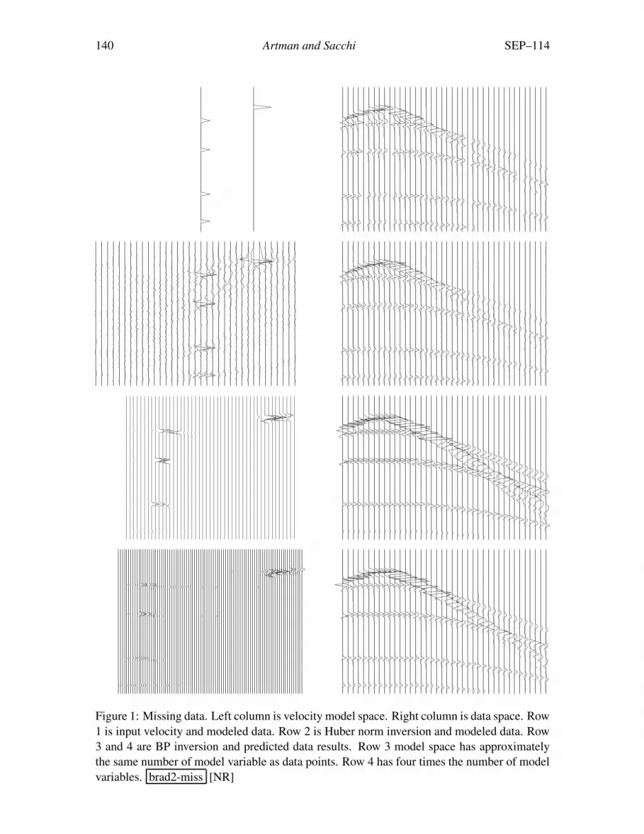
Figure 1 shows the results of the BP method when addressing the problem of missing data.We can see that the predicted data looks as accurate as the Huber norm result. The velocitymodel space, however, shows considerable difference. Notice the resolution increase over thesame range of velocities and the lack of appreciable chatter away from basis atoms. With thisfigure, and those to come dealing with the synthetic examples, the predicted data looses thewavelet character and the amplitude seems to diminish with depth.

Figure 2 shows the results of the BP method when a slow plane wave is superimposed onthe data. The overcomplete dictionary now shows significantly less chatter about the velocitypanel, and very distinguishable differences in the predicted data panel are emerging on theright side of the CMP where the events cross. Combination operators, linear and hyperbolichybrid operators (Trad et al., 2001), may be ideal for this situation, but have not been triedexhaustively yet.

Figure 3 shows the results of the BP method when randomly distributed spikes contaminatethe data. BP had significant trouble resolving this model. Unlike the Huber norm implemen-tations of Guitton and Symes (1999), the method has no capacity to utilize the properties ofthe l1 norm in the data space, and so cannot handle the large spikes. Manually limiting thenumber of outer loops to seven was the only way to avoid instability. However, this point iseasy to find as the duality gap begins increasing and the CG solver fails repeatedly to attain theinput tolerance. Regardless, the predicted data looks pretty bad, and while the model space issparse, the atoms that do have energy are inappropriate.

Real data

Two field data CMP’s are also analyzed with the BP algorithm. With an order of magnitudeincrease in size, as well as much energy in the data that leads to a more full model space,convergence does not seem as well behaved for real data. For the CMP with bad traces inFigure 4, we needed only 10 minutes of CPU time. Normally, this computation requires userintervention to stop the process as it looked to become unstable. The multiple ridden dataof Figure 7, however, required about 40 minutes to compute. The model space used in bothexamples was only approximately 2.5-fold overcomplete, and this fact may contribute to theproblems experienced. Interestingly, with the regularization parameter δ = 1, the algorithmhas a drastic denoising effect as well.

Figure 4 compares the predicted data from CG least squares inversion, the Huber norminversion, and the BP inversion. The noise reduction of the near traces is remarkable anddeserves further research. A very powerful linear noise train bounds the data to the right,


Figure 1: Missing data. Left column is velocity model space. Right column is data space. Row1 is input velocity and modeled data. Row 2 is Huber norm inversion and modeled data. Row3 and 4 are BP inversion and predicted data results. Row 3 model space has approximatelythe same number of model variable as data points. Row 4 has four times the number of modelvariables. brad2-miss [NR]


Figure 2: Slow plane wave superposition. Same format as explained in the caption of Figure1. brad2-surf [NR]


Figure 3: Randomly spiked data. Same format as explained in the caption of Figure 1.brad2-spike [NR]


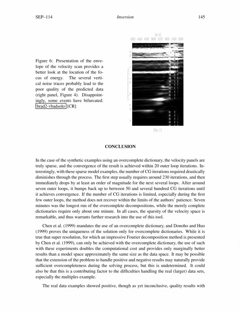
which we hypothesize is the result of the near offset noise in the raw data. Figure 6 containsfour powerful noisy traces between 2200 - 2700 m/s. Also noticeable is the tendency for theforward model to bifurcate real events into a correct and a fast event such as at 1.25 seconds.Replacing the high amplitude ringing trace with zeros did not fix the problem.

Figure 4: Modeled data after inversion compared to original a CMP that suffers from badtraces and substantial near offset noise. brad2-badtr [NR]

Figure 7 compares the predicted data from CG least squares inversion, the Huber norminversion, and the BP inversion. The BP solver had great difficulty with the multiples infestedCMP. The garbage in the low velocity range above 1.4 seconds is troublesome. This maycontribute to the problems analyzing this data, as I may not have made the model space largeenough to achieve the necessary overcompleteness, or the linear events are not well describedby the hyperbolic dictionary. This type of data is a good candidate to try the amalgamatedlinear/hyperbolic radon transform of Trad et al. (2001).


Figure 5: Velocity panel comparison. The different output of the different programs makes di-rect comparison impossible. The left panels scan to much higher velocity than was necessary.brad2-vel-badtr [NR]


Figure 6: Presentation of the enve-lope of the velocity scan provides abetter look at the location of the fo-cus of energy. The several verti-cal noise traces probably lead to thepoor quality of the predicted data(right panel, Figure 4). Disappoint-ingly, some events have bifurcated.brad2-vbadsolo [CR]

CONCLUSION

In the case of the synthetic examples using an overcomplete dictionary, the velocity panels aretruly sparse, and the convergence of the result is achieved within 20 outer loop iterations. In-terestingly, with these sparse model examples, the number of CG iterations required drasticallydiminishes through the process. The first step usually requires around 230 iterations, and thenimmediately drops by at least an order of magnitude for the next several loops. After aroundseven outer loops, it bumps back up to between 50 and several hundred CG iterations untilit achieves convergence. If the number of CG iterations is limited, especially during the firstfew outer loops, the method does not recover within the limits of the authors’ patience. Sevenminutes was the longest run of the overcomplete decompositions, while the merely completedictionaries require only about one minute. In all cases, the sparsity of the velocity space isremarkable, and thus warrants further research into the use of this tool.

Chen et al. (1999) mandates the use of an overcomplete dictionary, and Donoho and Huo(1999) proves the uniqueness of the solution only for overcomplete dictionaries. While it istrue that super resolution, for which an impressive Fourier decomposition method is presentedby Chen et al. (1999), can only be achieved with the overcomplete dictionary, the use of suchwith these experiments doubles the computational cost and provides only marginally betterresults than a model space approximately the same size as the data space. It may be possiblethat the extension of the problem to handle positive and negative results may naturally providesufficient overcompleteness during the solving process, but this is undetermined. It couldalso be that this is a contributing factor to the difficulties handling the real (larger) data sets,especially the multiples example.

The real data examples showed positive, though as yet inconclusive, quality results with


Figure 7: Modeled data after inversion compared to original a CMP that suffers from internalmultiples and strong ground roll. brad2-mult [NR]


Figure 8: Presentation of the enve-lope of the velocity scan provides abetter look at the location of the focusof energy. brad2-vmultsolo [CR]

this method. Usable, though not optimal, results can be achieved within a user terminateddozen loops of BP, though if allowed to run longer, a better product may result. The bifur-cation/event manufacturing in Figure 4 is unacceptable and needs serious attention in furtherinquiry to the usefulness of the technique. The multiple data of Figure 7 gives a reasonableresult, though not sufficiently better, to warrant the extra cost when compared to the CG ver-sion. These data exhibit a tendency to require several hundred CG iterations during the firstfew outer loops, and then drop to single digits for a dozen iterations before becoming unstable,after which the process is terminated.

A reason for the difficulty the algorithm has in convergence is its lack of understanding ofthe bandlimited nature of the data. This quality of the data makes the BP inversion unstableas it spends too much effort trying to solve for a sparse model of spikes that is inappropriate.A frequency domain Radon transform may well perform better with this thought in mind, as itwill not carry the infinite frequency assumption through the modeling operator. Alternatively,a second bandpass operator could be chained with an operator similar to the one used inthis example. In this manner, the composite operation could produce more stable and lessdemanding results from the IPLP algorithm.

A tangent concept that this work introduces evolves from the idea of the waveform dictio-naries used in any type of inversion. Rather than accepting the frequency, wavelet, or chirpdictionaries from mathematical context, it may be possible to compile “seismic waveform”dictionaries that have characteristics more directly suitable to the structures and features regu-larly exhibited in seismic data. This could include pinch-outs, lapping configurations, and/orvariations of simple hyperbolas. These could be useful for many other situations with differentalgorithms, and would not be restricted to this particular inversion implementation.


REFERENCES

Chen, S. S., Donoho, D. L., and Saunders, M. A., 1999, Atomic decomposition by basispursuit: SIAM Journal on Scientific Computing, 20, no. 1, 33–61.

Claerbout, J. F., and Muir, F., 1973, Robust modeling with erratic data: Geophysics, 38, no.05, 826–844.

Darche, G., 1989, Iterative l1 deconvolution: SEP–61, 281–302.

Donoho, D., and Huo, X. Uncertainty principles and ideal atomic decomposition:. WWW,citeseer.nj.nec.com/donoho99uncertainty.html, June 1999. NSF grants DMS 95-05151 andECS-97-07111.

Guitton, A., and Symes, W. W., 1999, Robust and stable velocity analysis using the Huberfunction: SEP–100, 293–314.

Guitton, A., and Symes, W. W., 2003, Robust inversion of seismic data using the huber norm:Geophyics, 68, no. 4, 1310–1319.

Nichols, D., 1994, Velocity-stack inversion using Lp norms: SEP–82, 1–16.

Saunders, M. A., and Tomlin, J. A. Solving regularized linear programs using barrier meth-ods and kkt systems:. IBM Research Report RJ 10064, and Stanford SOL Report 96-4,December 1996.

Taylor, H. L., Banks, S. C., and McCoy, J. F., 1979, Deconvolution with the L-one norm:Geophysics, 44, no. 01, 39–52.

Trad, D., Sacchi, M., and Ulrych, T. J., 2001, A hybrid linear-hyperbolic radon transform:Journal of Seismic Exploration, 9(4), 303–318.

280 SEP–114

Documents

Basis pursuit for geophysical inversion