Projection Pursuit for Discrete Data

Persi Diaconis

Deptartment of Mathematics and

Department of Statistics

Stanford University

Julia Salzman

Deptartment of Statistics

Stanford University

July 3, 2006

1 Introduction

Projection pursuit is an exploratory graphical tool for picturing high dimen-sional data through low dimensional projections. Introduced by Kruskal(1969), and developed by Friedman and Tukey (1974), the idea is to havethe computer select a small family of projections by numerically optimizingan index of “interest”. The original projection indices were ad hoc. In jointwork with David Freedman (1984), it was shown that for most data sets,most projections are about the same: approximately normal.

Therefore, interesting projections are those which are far from normal.Peter Huber (1985) found his own version of this: projections are uninfor-mative if they are unstructured or “random”. Thus projections with highentropy are uninformative. For a fixed scale, a distribution having high en-tropy or approximately normality are equivalent. Huber also showed thatthe Friedman-Tukey index is a measure of non-normality.

The purpose of the present paper is to give a parallel development fordata in discrete spaces: collections of binary vectors, rankings or phylo-genetic trees; or sets of graphs. We develop a notion of projection as apartition of the discrete data into blocks. We show that most for most datasets, most projections are close to uniformly partitioned. This suggests thatthe informative summaries are the ones with splits that are far from uniform.

The outline of the paper is as follows. Definitions and first examples aregiven in Section 2. The ideas lean on classical developments in block designsand give new applications for that theory. A discrete version of the Radontransform along with an inversion theory is presented, determining when acollection of projections loses information. Section 3 gives a data analytic

1

example in some detail. The data arises from the problem of putting someof Plato’s works in chronological order. Here, discrete projection pursuitleads to the discovery of a striking, easily interpretable structure that doesnot appear in other analyses of this data (eg. Ahn et al. (2003), Cox andBrandwood (1959), Holmes (2001), Wishart and Leach (1970)). Section4 proves that for most data sets, most partitions lead to approximatelyuniform projections. This leads directly to a usable criteria: a projectionis interesting if it is far from uniform. The distance to uniformity can bemeasured by any distance between probabilities, and we consider the well-known total variation, Hellinger and Vasserstein metrics.

The final section gives results for the least uniform projection. Theorem?? shows that if the class of projections is not too rich, for example, theaffine hyperplane in Zk, then for most data sets even the least uniformpartition is close to uniform. If the class of projections contains many sets,then least uniform projections are “structured”. The final theorem attacksthe problem of a data analyst finding “structure” in “noise”.

There has been extensive development of projection pursuit for den-sity estimation (Friedman et al. (1984)), regression (Friedman and Stuetzle(1981); Hall (1989)), applications to time series (Donoho (1981)), discrimi-nant analysis (Posse (1992); Polzehl (1995)) and standard multivariate prob-lems such as covariance estimation (Hwang et al. (1995)). This has led toa healthy development captured in the modern implementations (Xgobi,Ggobi). Online documentation for this software is an instructive catalog.We have not attempted to develop our ideas in these directions, but thebeginning steps of ridge functions will be found below.

This paper is written in tribute to David Freedman with thanks for hisintegrity and brilliance.

2 Projections and Radon Transforms

This section introduces our notation and set up for working with discretedata. It defines projection bases, the discrete Radon transform and gives ex-amples with binary data and permutation data. Analysis will be performedon binary n−tuple data from several works of Plato. Let X be a finite set.Let Y be a class of subsets of X . Let f : X → R be a function. The Radontransform of f at y ∈ Y is defined by

f̄(y) =∑

x∈Yf(x) (1)

2

The class Y is called a projection base if

|y| is constant for y ∈ Y (|y| denotes the cardinality of Y) (2)

There is a partition p1, . . . pj of Y s.t. each pi is a partition of X(3)

For a partition p, the numbers f̄(y)y∈p will be called the projection of fin direction p. The sets in Y may be thought of as “lines” in a geometry.If lines in the same partition are called parallel, then (??) corresponds tothe Euclidean axiom: for every point x ∈ X and every line y ∈ Y, thereis a unique line y∗ parallel to y such that x ∈ y∗. In the statistics litera-ture, designs with property (??) are called “resolvable” (See Hedayat et al.(1999) or Constantine (1987) for examples). Assumption (??) guaranteesthat projections are based on averages over comparable sets.

Consider the following examples:

Example 2.1. X = Zk2 the set of binary k−tuples. Here is a concrete exam-

ple of a data set with this structure; L. Brandwood classified each sentenceof Plato’s Republic according to its last five syllables. These can run fromall short (∪) through all long (-). Identifying ∪ with 1 and - with 0, eachsentence is associated with a binary 5−tuple. As x ranges over Z

52, let f(x)

denote the proportion of sentences with ending x. The values of f(x) aregiven in the first column of Table 1.

A second example of data with this structure is the result of gradingcorrect/incorrect in a test with k questions. There are several useful choicesof Y given next:

2.1 Projections for data in Zk2

2.1.1 Marginal projections in Zk2

For i = 1, 2, . . . k, let y0i = {x ∈ Z

k2 : xi = 0}, let y1

i = {x ∈ Zk2 : xi = 1}.

The sets Y = {yji }, 1 ≤ i ≤ k, j ∈ {0, 1} form a projection base. In the Plato

example, the projections have a simple interpretation as the proportion of

sentences with a specific ending in the ith place. Displaying projectionsoffers no problem here; a single number suffices.

A second natural choice of Y gives second order margins. This is basedon sets yab

ij = {x ∈ Zk2 : xi = a, xj = b}, 1 ≤ i < j ≤ k, a, b ∈ {0, 1}.

In this case, a projection consists of 4 numbers. In the Plato example, theprojection along coordinates i, j gives the proportion of sentences with each

3

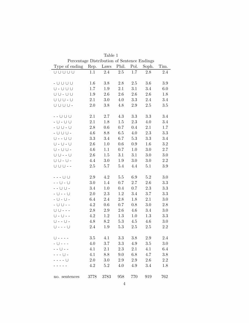
Table 1Percentage Distribution of Sentence Endings

Type of ending Rep. Laws Phil. Pol. Soph. Tim.

∪ ∪ ∪ ∪ ∪ 1.1 2.4 2.5 1.7 2.8 2.4

- ∪ ∪ ∪ ∪ 1.6 3.8 2.8 2.5 3.6 3.9∪ - ∪ ∪ ∪ 1.7 1.9 2.1 3.1 3.4 6.0∪ ∪ - ∪ ∪ 1.9 2.6 2.6 2.6 2.6 1.8∪ ∪ ∪ - ∪ 2.1 3.0 4.0 3.3 2.4 3.4∪ ∪ ∪ ∪ - 2.0 3.8 4.8 2.9 2.5 3.5

- - ∪ ∪ ∪ 2.1 2.7 4.3 3.3 3.3 3.4- ∪ - ∪ ∪ 2.1 1.8 1.5 2.3 4.0 3.4- ∪ ∪ - ∪ 2.8 0.6 0.7 0.4 2.1 1.7- ∪ ∪ ∪ - 4.6 8.8 6.5 4.0 2.3 3.3∪ - - ∪ ∪ 3.3 3.4 6.7 5.3 3.3 3.4∪ - ∪ - ∪ 2.6 1.0 0.6 0.9 1.6 3.2∪ - ∪ ∪ - 4.6 1.1 0.7 1.0 3.0 2.7∪ ∪ - - ∪ 2.6 1.5 3.1 3.1 3.0 3.0∪ ∪ - ∪ - 4.4 3.0 1.9 3.0 3.0 2.2∪ ∪ ∪ - - 2.5 5.7 5.4 4.4 5.1 3.9

- - - ∪ ∪ 2.9 4.2 5.5 6.9 5.2 3.0- - ∪ - ∪ 3.0 1.4 0.7 2.7 2.6 3.3- - ∪ ∪ - 3.4 1.0 0.4 0.7 2.3 3.3- ∪ - - ∪ 2.0 2.3 1.2 3.4 3.7 3.3- ∪ - ∪ - 6.4 2.4 2.8 1.8 2.1 3.0- ∪ ∪ - - 4.2 0.6 0.7 0.8 3.0 2.8∪ ∪ - - - 2.8 2.9 2.6 4.6 3.4 3.0∪ - ∪ - - 4.2 1.2 1.3 1.0 1.3 3.3∪ - - ∪ - 4.8 8.2 5.3 4.5 4.6 3.0∪ - - - ∪ 2.4 1.9 5.3 2.5 2.5 2.2

∪ - - - - 3.5 4.1 3.3 3.8 2.9 2.4- ∪ - - - 4.0 3.7 3.3 4.9 3.5 3.0- - ∪ - - 4.1 2.1 2.3 2.1 4.1 6.4- - - ∪ - 4.1 8.8 9.0 6.8 4.7 3.8- - - - ∪ 2.0 3.0 2.9 2.9 2.6 2.2- - - - - 4.2 5.2 4.0 4.9 3.4 1.8

no. sentences 3778 3783 958 770 919 762

4

of the 4 possibles patterns ∪ ∪, ∪ -, - ∪, - - in positions i, j. Table 3 inSection 3 is an example of one method displaying such projections. Section2 contains an analysis of the data in Table 1 based on these projections. Theanalysis gives a clear interpretation to a classical way of dating the booksof Plato. The analysis is independent of the other examples in this sectionand can be read at this time.

Here are some examples to show how the structure of f is reflected inf̄ . If f(x) = δx,x0 , f̄(y) = 1 if x0 ∈ y and zero otherwise. If f(x) = 1

2k ,

f̄(y) = |y|2k and hence is constant for all y. As a final example, consider a

fixed, non-zero vector y∗ ∈ Zk2. Let S be the hyperplane determined by

y∗ : S = {x ∈ Zk2 : x · y = 0 mod 2}. Let

f(x) =

{

12k if x ∈ S

0 otherwise

An easy computation shows

f̄(y0z) =

{

1 if z = y∗12 otherwise

f̄(y1z) =

{

0 if z = y∗12 otherwise

The hyperplane transform is essentially the same as the ordinary Fouriertransform on the group Z

k2. This is defined by

f̂(x) =∑

x

(−1)x·zf(x).

If f is a probability on Zk2 , f̂(z) = 2f̄(y0

z)−1. The transform f̂ has beenwidely used for data analysis of this type of data. See Solomon (1961) orDiaconis (1996 Chapter 11, 1997). The discrete Radon transform with pro-jections onto affine hyperplanes is also used by Ahn, Hofman Cook (2003).

2.1.2 Affine hyperplanes in Zk2

This is one natural way of “filling out” the marginal projections presentedabove. For z ∈ Z

k2 and a ∈ {0, 1}, let ya

z = {x ∈ Zk2 : x · z = a mod 2}.

The collection Y = {yaz}z∈Z

k2 , a∈{0,1} forms a projection base. Observe that

when z has a 1 in position i and zeros elsewhere, yaz equals the ya

i of theprevious example. The sets in Y are the affine hyperplanes in Z

k2 . Similarly,

the affine planes of any dimension form a projection base. An analysis ofthe Plao data using all affine hyperplanes is in Appendix A.3 below.

5

2.2 Projections for data in X = Sn, the sets of permutations

of n letters.

Permutation data arises in taste testing, ranking and elections; for example,in presidential elections of the American Psychological Association, membersare asked to rank order 5 candidates. Here, for a permutation π, f(π) istaken as the proportion of voters choosing the order π. For backgroundand many examples, see Critchlow (1988), Fligner and Verducci (1993) orMarden (1995).

2.2.1 Partitions based on marginal projections of permutations

in Sn.

Let yij = {π ∈ Sn : π(i) = j, 1 ≤ i, j ≤ n}. These sets form a projectionbase. For fixed i, the sets yi1, yi2, . . . yin form a partition p(i). The projectionin direction p(i) has a natural interpretation in the example: how did peoplerank candidate i? The projection can be displayed by making a histogram.

A second useful choice of Y is based on considering two positions: yklij =

{π ∈ Sn : π(i) = k, π(j) = l} i 6= j, k 6= l. This leads to projectionsgiving the joint rankings of a fixed pair of candidates in the example. Suchprojections can be displayed by making a 2-dimensional picture and grayscaling the (i, j) square to correspond to the proportion of voters ranking thepair of candidates in order (i, j). Similarly third and higher order projectionscan be defined.

2.2.2 Partitions based on subgroups of Sn.

When X is a group such as Sn, the following constructions for Y are avail-able. Let N be a subgroup of X . The orbits of N acting on X are the cosets{Ny}y∈X , and the distinct orbits partition X . Varying N by conjugation,{yNy−1}y∈X , gives a projection base for X .

When N is taken as Sn−1 = {π ∈ Sn : π(1) = 1} the projections arethe marginal projections defined above. Taking N as Sn−2 = {π ∈ Sn :π(1) = 1, π(2) = 2} gives the second order margins. An important classof subgroups are the so-called Young subgroups: let λ1 ≤ λ2 ≤ . . . λn bea partition of n so

∑

i λi = n. Let Sλ1 × Sλ2 × . . . × Sλnbe the permu-

tations that permute the first λ1 elements among themselves and the nextλ2 elements among themselves, etc. These include the previous examplesand provide enough transforms for an inversion theory, as will be shownbelow. Display of such projections is not a well studied problem. In thecase of a projection corresponding to a Young subgroup, one suggestion is a

6

1-dimensional histogram using one of the orderings suggested in Chapter 3of James (1978).

If X = G/H where G is a group and H is a subgroup and G ⊂ N ⊂ H,with N a subgroup, then the orbits of N in X are a partition and the orbitsof {gNg−1}g∈G form a partition base. One approach to the display of suchprojections is a 2-dimensional histogram using the ordering given by one ofthe metrics suggested in Chapter 7 of Diaconis (1986).

2.3 Projections for X = Rp: Euclidean data.

Consider data vectors x1, x2, . . . xn ∈ Rp. For γ in the p−dimensional unit

sphere, the projection in direction γ is just γ · x1, . . . , γ · xn. This is theclassical Radon transform, with Y consisting of the affine hyperplanes y t

γ =x ∈ R

p : x · γ = t. For fixed γ these partition the space Rp as t varies, and

the partitions vary as γ varies. In statistical applications, a histogram ismade of γ · xi and one varies γ, trying to understand the structure of thep−dimensional data from the varying histograms. This leads to the classicalversion of projection pursuit considered in the introduction.

2.4 Projections when X is a finite set with n elements, and

Y is the class of k− element subsets.

In this example, it is a non-trivial theorem of Baranyai that Y forms aprojections base. Details and discussion may be found in Cameron (1976).This example occurs naturally when considering extensions of a given class ofpartitions. For example, consider the marginal projections ya

i in Zk2 defined

above. These sets all have cardinality |ya1 | = 2k−1. It is natural to consider

the extension to projections based on the class of all subsets of cardinality2k−1.

2.5 Uniqueness of Radon Transforms:

We now consider the question: when is f → f̄ one to one? A convenientcriteria involves the notion of a block design. Let |X | = n. The class of setsY is a block design with parameters (n, c, k, l) provided

|y| = c for all y ∈ Y (4)

each x ∈ X is contained in k subsets y (5)

each pair x 6= x′

is contained in l subsets y (6)

7

Affine planes or Zk2 and k sets of an n set are block designs. A great many

other examples are discussed in the literature of combinatorial designs. Inthe statistics literature they are sometimes called balanced incomplete blockdesigns. In the combinatorial literature they are often called 2−designs, or2 − (n, c, l) designs. It is easy to see that the parameters n, c, k, l satisfy

|Y|c = nk (7)

(n − 1)l = k(c − 1) (8)

Dembroski (1968) and and Lander (1982) are useful references for blockdesigns.

The following result is well known in the theory of designs. We firstlearned it from Bolker (1987).

Theorem 2.2. If X is a finite set and Y is a block design with |Y| > 1,the the Radon transform f → f̄ is one to one, with an explicit inversionformula given by (??) below.

Proof. For any x,∑

y:x∈y

f̄(y) = kf(x) + l∑

s,s′∈X x6=x′

f(x′) (9)

= (k − l)f(x) + l∑

x∈Xf(x) (10)

If∑

x∈X f(x) = 1, this determines f as

f(x) =1

k − l

∑

y′x∈y

f̄(y) − l

k − l. (11)

Observe that k > l follows from the assumption that |Y| > 1. When∑

x∈X f(x) is not known, it can be recovered by summing both sides of(??) in x. This gives

∑

x∈Xf(x) =

c

k − l + nl

∑

y∈Yf̄(y)

and so the inversion formula

f(x) =1

k − l

∑

y:x∈y

f̄(y) +lc

(k − l)2 + nl(k − l)

∑

y∈Yf̄(y) (12)

8

Remarks:

• It is not necessary that Y be a block design for f → f̄ to be one to one.For example, Kung (1979) shows that the Radon transform is one toone when Y consists of the sets of rank i in a matroid. Diaconis andGraham (1985) give examples where the transform is one to one whenY consists of the nearest neighbors in a metric space. For example,when X = Z

2k2 and Y consists of the balls of Hamming distance less

than or equal to 1, the transform is one to one, and an explicit inversiontheorem is known. When X is Sn, the symmetric group, and Y is unitballs in the Cayley metric, the transform is one to one if and onlyif n is in {1, 2, 4, 5, 6, 8, 10, 12}. Further work on inversion formulasfor functions on finite symmetric spaces is found in Velasquez (1997)and for functions on the torus Z

kn in Dedeo and Velasquez (2004).

Fill (1989) discusses invertibility when the Radon transform of f atx averages over a set of translates of f(x) which has applications todirectional data and time series.

• The transform can still be useful and interesting if it is not one to one.For example, the marginal projections in the example above do notcapture all aspects of the data but are often the first things to be lookedat. In Z

k2, if high enough marginal distributions are considered, the

function f can be completely recovered. In the symmetric group, theprojections corresponding to all Young subgroups determine f becausethey determine it’s Fourier transform. See Diaconis (1986) for details.

3 Data analysis of syllable patterns in the works

of Plato

This section presents a new analysis of data arising from syllable patternsin the works of Plato. The data is given in Table 1. It records, for eachof 6 books, the pattern of long (-) and short (∪) syllables among the last 5syllables in each sentence. It is known that Plato wrote Republic early andLaws late. Plato also mentions that he changed his rhyming patterns overtime. This led Brandwood to collect the data in Table 1.

The other books were written between these but it is not known in whatorder. The goal of the analysis is to try to order the books. Our approachwill be to study the books one at a time, trying to find patterns.

9

Projection pursuit suggests looking at various partitions of the data,searching for structured partitions which are far from uniform. Using firstand second order margins as partitions, a reasonably striking difference be-tween Republic and Laws is observed. This suggests a simple, interpretableway of ordering the other books as Republic, Timaeus, Sophist, Politicus,Philebus, Laws.

This agrees with the standard ordering as discussed in Brandwood (1976,pg. XViii) and in Ahn et Al (2003). Other analyses of this data set are inCox and Brandwood (1959), Atchinson (1970), Wishart and Leach (1970)and Boneva (1971). The last reference contains a history and explanationfor the choice of data. The first three analyses all use statistical models.Boneva’s analysis uses a form of scaling. None of the previous analyses seemto have picked up the simple, striking pattern in the data that projectionpursuit leads to.

The analysis is presented below, in a somewhat discursive style, in theorder it was actually performed: first looking at the Republic, then Lawsand finally the other books. In the Appendix, we present a more automatedand formal version.

3.1 Republic

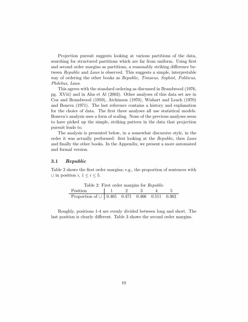
Table 2 shows the first order margins; e.g., the proportion of sentences with∪ in position i, 1 ≤ i ≤ 5.

Table 2: First order margins for RepublicPosition 1 2 3 4 5

Proportion of ∪ 0.465 0.471 0.466 0.511 0.362

Roughly, positions 1-4 are evenly divided between long and short. Thelast position is clearly different. Table 3 shows the second order margins.

10

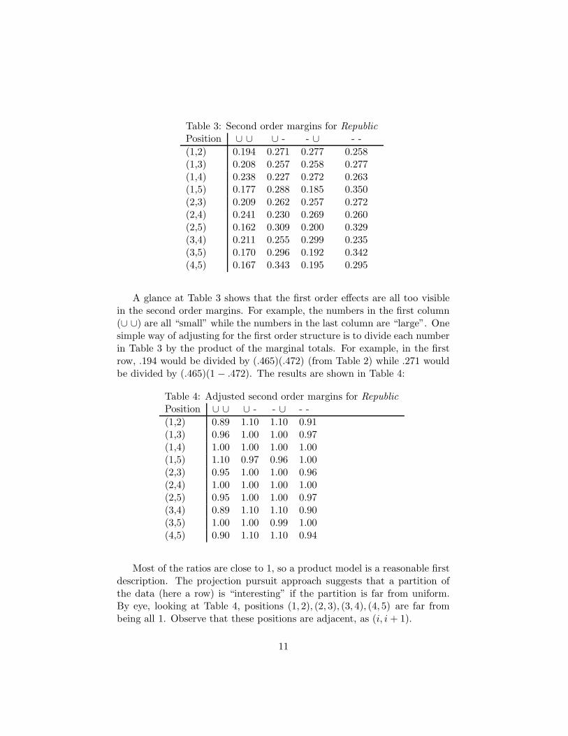
Table 3: Second order margins for RepublicPosition ∪ ∪ ∪ - - ∪ - -

(1,2) 0.194 0.271 0.277 0.258(1,3) 0.208 0.257 0.258 0.277(1,4) 0.238 0.227 0.272 0.263(1,5) 0.177 0.288 0.185 0.350(2,3) 0.209 0.262 0.257 0.272(2,4) 0.241 0.230 0.269 0.260(2,5) 0.162 0.309 0.200 0.329(3,4) 0.211 0.255 0.299 0.235(3,5) 0.170 0.296 0.192 0.342(4,5) 0.167 0.343 0.195 0.295

A glance at Table 3 shows that the first order effects are all too visiblein the second order margins. For example, the numbers in the first column(∪ ∪) are all “small” while the numbers in the last column are “large”. Onesimple way of adjusting for the first order structure is to divide each numberin Table 3 by the product of the marginal totals. For example, in the firstrow, .194 would be divided by (.465)(.472) (from Table 2) while .271 wouldbe divided by (.465)(1 − .472). The results are shown in Table 4:

Table 4: Adjusted second order margins for RepublicPosition ∪ ∪ ∪ - - ∪ - -

(1,2) 0.89 1.10 1.10 0.91(1,3) 0.96 1.00 1.00 0.97(1,4) 1.00 1.00 1.00 1.00(1,5) 1.10 0.97 0.96 1.00(2,3) 0.95 1.00 1.00 0.96(2,4) 1.00 1.00 1.00 1.00(2,5) 0.95 1.00 1.00 0.97(3,4) 0.89 1.10 1.10 0.90(3,5) 1.00 1.00 0.99 1.00(4,5) 0.90 1.10 1.10 0.94

Most of the ratios are close to 1, so a product model is a reasonable firstdescription. The projection pursuit approach suggests that a partition ofthe data (here a row) is “interesting” if the partition is far from uniform.By eye, looking at Table 4, positions (1, 2), (2, 3), (3, 4), (4, 5) are far frombeing all 1. Observe that these positions are adjacent, as (i, i + 1).

11

Next observe that each of the 4 designated rows has a common pattern:the first and last entries are small, the middle two entries are large. Goingback to the definitions, this pattern arises from a negative association ofadjacent syllables; in the Republic, adjacent syllables tend to alternate. Thepattern in positions (1, 3) shows that this cannot be a complete description;after all, if the symbols alternate, the positions two apart should be pos-itively associated, but (1, 3) displays negative association. Looking at theother rows of the table, we observe that the size goes big, small, small, bigor its opposite, small, big, big, small. This is an artifact. Consider the firstrow of Table 4. It was formed from 4 proportions that sum to 1: w, x, y, zsay. The 4 adjusted entries are

w

(w + x)(w + y)

x

(w + x)(x + z)

y

(y + z)(y + w)

z

(z + y)(z + x).

It is easy to show that the first entry is less than 1 if and only if thesecond is larger than 1, if and only if the third is larger than one if and onlyif the fourth is less than 1. This means that the first column in Table 4,together with the first order margins, determines the remaining entries. Thisartifact in no way reflects on the association pattern noted earlier– the moststructured rows correspond to adjacent syllables, and adjacent syllables arenegatively associated.

3.2 Laws and a comparison with Republic.

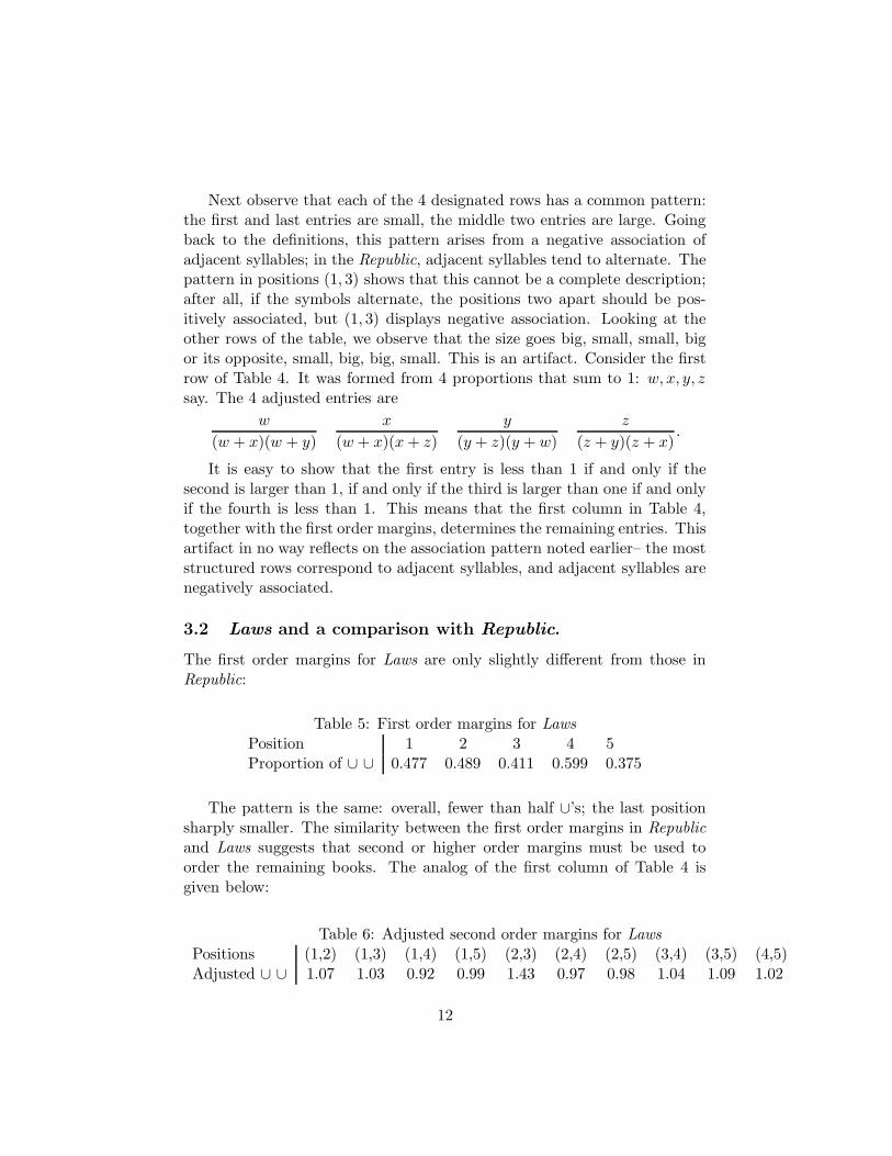
The first order margins for Laws are only slightly different from those inRepublic:

Table 5: First order margins for LawsPosition 1 2 3 4 5Proportion of ∪ ∪ 0.477 0.489 0.411 0.599 0.375

The pattern is the same: overall, fewer than half ∪’s; the last positionsharply smaller. The similarity between the first order margins in Republicand Laws suggests that second or higher order margins must be used toorder the remaining books. The analog of the first column of Table 4 isgiven below:

Table 6: Adjusted second order margins for LawsPositions (1,2) (1,3) (1,4) (1,5) (2,3) (2,4) (2,5) (3,4) (3,5) (4,5)Adjusted ∪ ∪ 1.07 1.03 0.92 0.99 1.43 0.97 0.98 1.04 1.09 1.02

12

The entries above are the proportion of sentences with ∪ ∪ in the (i, j)position divided by the product of the marginal proportions.

Again, pairwise adjacent positions are associated, all in the same way.Here, the association is positive, whereas for Republic, the association isnegative. This is the striking pattern referred to above. It suggests a methodof ranking the of the books: compare the sign pattern or actual ratios of theadjusted second order margins of other books with Republic and Laws.

For definiteness, the sum of absolute deviations between second ordermargins over all 10 positions will be used. This is carried out data analyti-cally in sections 2.3 − 2.5.

3.3 Analysis for Philebus and Politicus

These books are somewhat similar to each other. The first and second ordermargins for Philebus are as follows:

Table 7: First order margins for PhilebusPosition 1 2 3 4 5Proportion of ∪ 0.522 0.464 0.398 0.594 0.465

Table 8: Adjusted second order margins for PhilebusPositions (1,2) (1,3) (1,4) (1,5) (2,3) (2,4) (2,5) (3,4) (3,5) (4,5)Adjusted ∪ ∪ 1.11 1.03 0.85 1.11 1.48 0.92 0.85 1.02 0.95 1.01

Note the difference in first order margins: between Philebus and Republic(or Laws) position 1 is high, as are positions 4 and 5. For second ordermargins, the adjacent patterns are all positively associated ((2,3) beingtruly extreme). Comparing Table 8 with Table 6, the association patternmatches Laws in direction, except in position (1,5). The relevant averagesfor Politicus are:

Table 9: First order margins for PoliticusPosition 1 2 3 4 5Proportion of ∪ 0.477 0.457 0.348 0.524 0.469

Table 10: Adjusted second order margins for PoliticusPositions (1,2) (1,3) (1,4) (1,5) (2,3) (2,4) (2,5) (3,4) (3,5) (4,5)Adjusted ∪ ∪ 1.17 1.10 0.96 1.01 1.26 0.86 0.90 1.05 1.10 1.13

13

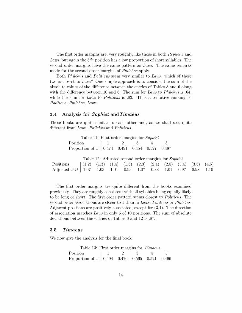
The first order margins are, very roughly, like those in both Republic and

Laws, but again the 3rd position has a low proportion of short syllables. Thesecond order margins have the same pattern as Laws. The same remarksmade for the second order margins of Philebus apply.

Both Philebus and Politicus seem very similar to Laws. which of thesetwo is closest to Laws? One simple approach is to consider the sum of theabsolute values of the difference between the entries of Tables 8 and 6 alongwith the difference between 10 and 6. The sum for Laws to Philebus is .64,while the sum for Laws to Politicus is .83. Thus a tentative ranking is:Politicus, Philebus, Laws

3.4 Analysis for Sophist andTimaeus

These books are quite similar to each other and, as we shall see, quitedifferent from Laws, Philebus and Politicus.

Table 11: First order margins for SophistPosition 1 2 3 4 5Proportion of ∪ 0.474 0.491 0.454 0.527 0.487

Table 12: Adjusted second order margins for SophistPositions (1,2) (1,3) (1,4) (1,5) (2,3) (2,4) (2,5) (3,4) (3,5) (4,5)Adjusted ∪ ∪ 1.07 1.03 1.01 0.93 1.07 0.88 1.01 0.97 0.98 1.10

The first order margins are quite different from the books examinedpreviously. They are roughly consistent with all syllables being equally likelyto be long or short. The first order pattern seems closest to Politicus. Thesecond order associations are closer to 1 than in Laws, Politicus or Philebus.Adjacent positions are positively associated, except for (3,4). The directionof association matches Laws in only 6 of 10 positions. The sum of absolutedeviations between the entries of Tables 6 and 12 is .87.

3.5 Timaeus

We now give the analysis for the final book.

Table 13: First order margins for TimaeusPosition 1 2 3 4 5Proportion of ∪ 0.494 0.476 0.565 0.521 0.496

14

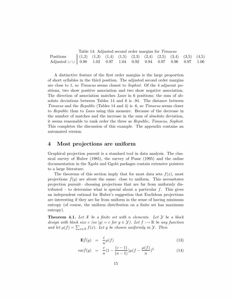
Table 14: Adjusted second order margins for TimaeusPositions (1,2) (1,3) (1,4) (1,5) (2,3) (2,4) (2,5) (3,4) (3,5) (4,5)Adjusted ∪ ∪ 0.98 1.02 0.97 1.04 0.92 0.94 0.97 0.96 0.97 1.06

A distinctive feature of the first order margins is the large proportionof short syllables in the third position. The adjusted second order marginsare close to 1, so Timaeus seems closest to Sophist. Of the 4 adjacent po-sitions, two show positive association and two show negative association.The direction of association matches Laws in 6 positions; the sum of ab-solute deviations between Tables 14 and 6 is .94. The distance betweenTimaeus and the Republic (Tables 14 and 4) is .6, so Timaeus seems closerto Republic than to Laws using this measure. Because of the decrease inthe number of matches and the increase in the sum of absolute deviation,it seems reasonable to rank order the three as Republic, Timaeus, Sophist.This completes the discussion of this example. The appendix contains anautomated version.

4 Most projections are uniform

Graphical projection pursuit is a standard tool in data analysis. The clas-sical survey of Huber (1985), the survey of Posse (1995) and the onlinedocumentation in the Xgobi and Ggobi packages contain extensive pointersto a large literature.

The theorems of this section imply that for most data sets f(x), mostprojections f̄(y) are about the same: close to uniform. This necessitatesprojection pursuit– choosing projections that are far from uniformly dis-tributed – to determine what is special about a particular f . This givesan independent rational for Huber’s suggestion that Euclidean projectionsare interesting if they are far from uniform in the sense of having minimumentropy (of course, the uniform distribution on a finite set has maximumentropy).

Theorem 4.1. Let X be a finite set with n elements. Let Y be a blockdesign with block size c (so |y| = c for y ∈ Y). Let f :→ R be any functionand let µ(f) =

∑

x∈X f(x). Let y be chosen uniformly in Y. Then

Ef̄(y) =c

nµ(f) (13)

varf̄(y) =c

n(1 − (c − 1)

(n − 1))µ(f − µ(f)

n)2 (14)

15

Proof. (??) follows from computing

Ef̄(y) =1

|Y|∑

y

f̄(y) =1

|Y|∑

x

f(x)|y : x ∈ y| =k

|Y|µ(f).

For (??), assume without loss of generality, that µ(f) = 0. Then

var(f̄(y)) =1

|Y|∑

y

f(y)2 =1

|Y|∑

y

∑

x∈y

f(x)2 + 2∑

x6=x′

x,x′∈y

f(x)f(x′)

=k

|Y|µ(f2) +2l

|Y|∑

x6=x′

f(x)f(x′) =k − l

|Y| µ(f2) +l

|Y|µ(f2)

=k − l

|Y| µ(f2)

From (??) and (??), k−l|Y| = c(n−c)

n(n−1) , giving the result.

Example 4.2. When Y is the j sets of an n set, |Y| =(n

j

)

, c = j, and theresult reduces to the usual mean and variance for a sample without replace-ment.

Example 4.3. Let X = Zk2 and Y be the j-dimensional affine planes. Then

n = 2k and c = 2k−j. If µ(f) = 1, the result becomes

E(f(y)) =1

2j, var(f(y)) =

2j

2k(1 − 2j − 1

2k − 1)µ(f − 1

2k)2.

For future use, observe that the cardinality of Y in this case is

2j(2k − 1)(2k − 1) . . . (2k − 2j−1)

(2j − 1) . . . (2j − 2j−1).

Returning to the situation in Theorem ??, Chebychev’s inequality im-plies:

Corollary 4.4. With notation as in Theorem ??, the proportion of y ∈ Ysuch that

|f̄(y) − c

nµ(f)| > ε

is smaller than1

ε2

c

n(1 − c − 1

n − 1)µ(f − µ(f)

n)2.

16

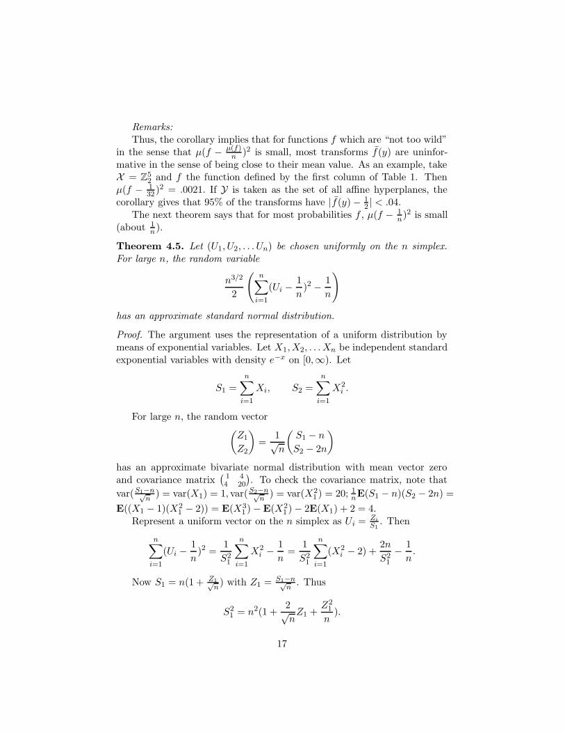
Remarks:Thus, the corollary implies that for functions f which are “not too wild”

in the sense that µ(f − µ(f)n )2 is small, most transforms f̄(y) are uninfor-

mative in the sense of being close to their mean value. As an example, takeX = Z

52 and f the function defined by the first column of Table 1. Then

µ(f − 132 )2 = .0021. If Y is taken as the set of all affine hyperplanes, the

corollary gives that 95% of the transforms have |f̄(y) − 12 | < .04.

The next theorem says that for most probabilities f , µ(f − 1n)2 is small

(about 1n).

Theorem 4.5. Let (U1, U2, . . . Un) be chosen uniformly on the n simplex.For large n, the random variable

n3/2

2

(

n∑

i=1

(Ui −1

n)2 − 1

n

)

has an approximate standard normal distribution.

Proof. The argument uses the representation of a uniform distribution bymeans of exponential variables. Let X1, X2, . . . Xn be independent standardexponential variables with density e−x on [0,∞). Let

S1 =

n∑

i=1

Xi, S2 =

n∑

i=1

X2i .

For large n, the random vector(

Z1

Z2

)

=1√n

(

S1 − n

S2 − 2n

)

has an approximate bivariate normal distribution with mean vector zeroand covariance matrix

( 1 44 20

)

. To check the covariance matrix, note that

var(S1−n√n

) = var(X1) = 1, var(S2−n√n

) = var(X21 ) = 20; 1

nE(S1 − n)(S2 − 2n) =

E((X1 − 1)(X21 − 2)) = E(X3

1 ) −E(X21 ) − 2E(X1) + 2 = 4.

Represent a uniform vector on the n simplex as Ui = Zi

S1. Then

n∑

i=1

(Ui −1

n)2 =

1

S21

n∑

i=1

X2i − 1

n=

1

S21

n∑

i=1

(X2i − 2) +

2n

S21

− 1

n.

Now S1 = n(1 + Z1√n) with Z1 = S1−n√

n. Thus

S21 = n2(1 +

2√n

Z1 +Z2

1

n).

17

Using the standard Op notation (see Pratt (1959)),

1

S21

=1

n2− 2Z1

n3/2+ Op(

1

n3).

Thus,

1

S21

n∑

i=1

(X2i − 2) =

1

n3/2

1√n

n∑

i=1

(X2i − 2) + Op(

1

n2),

2n

S21

=2

n− 4Z1

n3/2+ Op(

1

n2).

The bivariate limiting normality of(Z1

Z2

)

implies that Z2−4Z1 has an approx-imate normal distribution with mean 0 and variance var(Z2) + 16var(Z1) −8covar(Z1, Z2) = 4.

Corollary ?? and Theorem ?? imply that for most probabilities f , mosttransforms f̄(y) are close to uniform. The final result of this section dealswith the entire projection f̄(y)y∈p where p is a partition of X into blocks inY.

Let X be a finite set. Let Y be a block design on X with parameters(n, c, k, l). Suppose that Y is also a projection base for X with p1, p2, . . . pj

being a partition of Y, with each pi being a partition of X . Of course,j = |Y|c

n . The next theorem implies that for most functions, the projectiononto a randomly chosen partition is uniformly close to c

n .

Theorem 4.6. Let Y be a block design on X with parameters (n, c, k, l).Suppose that Y is a projection base. Let f be a fixed probability on X .Let the partition p be chosen uniformly at random over all partitions pi ofX ,pi ⊂ Y. For ε > 0,

∑

y∈p

|f̄(y) − c

n| ≤ ε. (15)

with probability at least

1 − 1

ε(n(n − c)

c(n + 1)µ(f − 1

n)2)

12 .

Proof. The probability model for choosing a random partition is based ona fixed enumeration p1, p2, . . . pj of the partitions that make up Y. Each

partition is assumed to be taken in a fixed order pi = {(y1i , . . . y

n/ci )}. The

18

random variable S(p) =∑

y∈p |f̄(y) − cn | is invariant under permuting the

y ∈ p among themselves. Thus a random variable with the same distributionof S(p) but exchangeable f̄(y)y∈p exists. For this realization, E(

∑

y∈p |f̄(y)−cn |) = n

c E|f̄(y∗)− cn | with y∗ chosen uniformly in Y. Using Cauchy-Schwartz

and Theorem ??, the expectation is bounded above by

n

c

√

c

n(1 − c − 1

n − 1)µ(f − 1

n)2.

Theorem ?? follows from this bound and Markov’s inequality applied tothe original random variable.

Remarks: From Theorem ??, µ(f − 1n)2

.= 1

n for most functions f . Forsuch f , the theorem implies that for large block size c, most partitions areclose to uniform in variation distance. This may be contrasted with Theo-rems ?? and ?? which imply that the components f̄(y) of most projectionsare close to c

n . When c is small, there are many terms in the sum (??). Asan example, consider the 2−sets of an n set where n = 2j. Let p be a ran-dom partition into 2−element sets. Let f be chosen at random from the nsimplex and p any fixed partition into two element sets. It is straightforwardto show that with probability tending to 1 as n tends to infinity,

∑

y∈p

|f̄(y) − 2

n| → 8e−2.

The analogous result holds with the same assumptions when p is anyfixed partition of fixed size c. Similarly, it is natural to ask for a centrallimit theorem in connection with Theorems ?? and ??. For j sets of an nset, such a theorem is available from the usual results on sampling withoutreplacement from a finite population. Most likely, there is a similar set ofresults for block designs with |Y| and c large. See Stein (1992) for resultsfor designs arising from subgroups of a finite group.

5 Least uniform partitions

The results of Section 4 imply that, under suitable conditions, for mostfunctions the projection along most partitions is close to uniform. Thissuggests that the special properties of particular functions are only seenin partitions that are far from uniform. In this section, properties of leastuniform partitions are examined. Theorem ?? shows that for most functions,

19

even the least uniform partitions will be close to uniform if the the numberof sets in Y is small in the sense that log |Y| is small compared both to nand the block size c. This is true, in particular, for affine hyperplanes in Z

k2.

Theorem 5.1. Let X be a set of n elements. Let Y be a class of subsetsin X of fixed cardinality c. Suppose that p1, . . . pj is a partition of Y intopartitions of X . Let f be chosen at random in the n simplex. Let p∗ be thepartition in pi that maximizes

∑

y∈p |f̄(y) − cn |. For any ε > 0,

∑

y∈p∗

|f̄(y) − c

n| < ε,

except for a set of f ′s of probability smaller than

(|Y| + 1)β

with β equal to 1 minus

1

β(c, n)

∫ cn

(1+ε)

cn

(1−ε)xc−1(1 − x)n−c−1dx (16)

where β(c, n) denotes the beta function.

Proof. Represent the ith component of a randomly chosen f as Xi

S where Xi

are independent standard exponentials and S =∑n

i=1 Xi. Let y∗ be the setin Y with the largest value of c

n(1 − ε). The argument begins by boundingthe probability that

|f̄(y∗) − c

n| < ε

c

n.

To begin with,

P(f̄(y∗) <c

n(1 − ε)) ≤ P(

X1 + . . . Xc

S<

c

n(1 − ε)).

Further,

P(f̄(y∗) >c

n(1+ε)) ≤

∑

y∈YP(f̄(y) >

c

n(1+ε)) = |Y|P(

X1 + . . . Xc

S>

c

n(1+ε)).

Next, let y∗ denote the set in Y with the smallest value of f̄(y). To boundthe probability that |f̄(y∗) − c

n | < ε cn , observe that f̄(y∗) = 1 − f̄(y∗∗) with

20

y∗∗ the union of sets in a partition omitting the one element that maximizesf̄ . Thus,

P(f̄(y∗) <c

n(1 − ε)) = P(f̄(y∗∗) > 1 − c

n(1 − ε))

≤ |Y|P(X1 + . . . + Xn−c

S> 1 − c

n(1 − ε))

= |Y|P(X1 + . . . + Xc

S<

c

n(1 − ε)).

Further,

P(f̄(y∗) >c

n(1 + ε)) = P(f̄(y∗∗) > 1 +

c

n(1 − ε))

≤ P(X1 + . . . + Xn−c

S< 1 − c

n(1 + ε))

= P(X1 + . . . + Xc

S>

c

n(1 + ε)).

Summing the four bounds thus obtained we see that both

|f̄(y∗) −c

n| < ε

c

n|f̄(y∗) − c

n| < ε

c

n(17)

except for a set of f ’s of probability smaller than (|Y| + 1)β as definedby (??). Now (??) implies that |f̄(y)− c

n | < ε cn for all y ∈ Y. Summing this

last inequality over the partition p∗ completes the proof of the theorem.

Remarks: The beta integral that appears in the bound is straightfor-ward to approximate numerically. A raft of techniques and approximationsappear in the first chapter of Pearson (1968). For example, consider caseswhere c

n = 12 . Then, using the Peister-Pratt approximation given in Pearson

(1968), and Mill’s ratio, the β in (??) is approximately

2√2π

e−x2

2

1 + xwith x =

√

2c log1

4(12 − ε)(1

2 + ε).

For this to be small when multiplied by |Y| + 1, it clearly suffices thatlog |Y| be small compared to c. This is the case for the affine subspaces ofdimension j in Z

k2 if j is bounded and k is large.

As a numerical example, consider the affine hyperplanes in Z102 . Then

|Y|+1 = 2049, c = 512, n = 1024. Taking ε = .1, (|Y|+1)|β .= 2.595×10−7 .

The next theorem shows that when there are many sets in Y, the leastuniform projection is typically far from uniform. The theorem deals with n

21

sets in a set of cardinality 2n. The variation distance of a typical probabilityprojected along the least uniform half split is shown to be about .3. Thismay be compared with Theorems ?? and ?? which show that for a typicalprobability f on 2n points, |f̄(y) − 1

2 | is close to zero for most sets y ofcardinality n.

Theorem 5.2. Let f be chosen at random on the 2n simplex. Let S− bethe sum of the n smallest f(x). Then for large n, the random variable

√2n(S− − (

1

2− log 2

2))

has an approximate normal distribution with mean 0 and variance 32−2 log 2.

Proof. Represent a randomly chosen f as Xi

S where Xi are independent

standard exponential random variables and S =∑2n

i=1 Xi. Denote the orderstatistics by round brackets:

X(1) ≤ X(2) ≤ . . . X(n).

Let L1 = X(1), L2 = X(2) − X(1), . . . , L2n = X(2n) − X(2n−1). Then theLi are independent, and Li+1 has the distribution of a standard exponentialtimes 1

(2n−1)– see Feller (1971, Section III.3). With this notation,

S =2n∑

i=1

Xi =2n−1∑

i=0

(2n − i)Li+1 (18)

S− =1

S

n∑

i=1

X(i) =1

S

n−1∑

i=0

(n − i)Li+1. (19)

The proof is completed by approximating the sums in this representationof S and S−. Let µi = n−i

2n−i , so (n − i)Li+1 has the same distribution as µi

times a standard exponential. Let

σ2 = 2

n−1∑

i=0

µ2i = 2

n−1∑

i=0

(1 − 2n

2n − i+

n2

(2n − i)2)

= 2(n − (2n log 2 + O(1)) +3

2+

n

2+ O(1))

= 2n(3

2− 2 log 2) + O(1).

22

Now, let Z1 = S−2n√2n

and Z2 =(Pn

i=1 X(i)−µ)√2n

. The vector (Z1, Z2) has

a limiting bivariate normal distribution, with mean (0, 0) and covariance

matrix(σ2

1 ρ

ρ σ22

)

with σ21 = 2, σ2

2 = 32 − 2 log 2, and ρ = 1

2(1− log 2). To check

the value of ρ, observe that the covariance of Z1 and Z2 is 12n times

n∑

i=0

E((2n−i)Li+1−1)((n−i)Li+1−n − i

2n − i)) =

n∑

i=0

n − i

2n − i= n−n log 2+O(1).

Using the standard Op calculus,

1

S=

1

2n

1

(1 + Z1√2n

)=

1

2n(1 − Z1√

2n) + Op(

1

n2).

In particular,1

S=

1

2n+ Op(

1

n32

).

The representation (??) for S− can be rewritten as

S− =√

2nZ2

X+

µ

S=

Z2√2n

+1 − log 2

2(1 − Z1√

2n) + Op(

1

n).

It follows that√

2n(S− − 1−log 22 ) has the same limiting distribution as

Z2 − (1−log 2)2 Z1. This is normal with mean 0 and variance

(3

2− 2 log 2) + 2(

1 − log 2

2) − 2(

1 − log 2

2) =

3

2− 2 log 2.

Corollary 5.3. Let f be chosen at random on the 2n simplex. Let (y, yc)be a partition of X into an n set and its complement which maximizes thevalue of

|f̄(y) − 1

2| + |f̄(yc) − 1

2|.

Then, as n tends to infinity, the maximum discrepancy tends to log 2.=

.301 with probability tending to 1.

Proof. For almost all f , the maximum is taken on uniquely at the partitionS−, (S−)c as defined in Theorem ??. The maximum discrepancy equals

2|S− − 1

2|,

and the result follows from Theorem ??.

23

Remark: The proof of Theorem ?? and its corollary can easily be ex-tended to cover the j sets of an n set. The argument shows that for mostprobabilities f , the variation distance between the least uniform projectionand the uniform distribution is bounded away from zero if j is an appreciablefraction of n.

For the final theorem, a different method of choosing a random probabil-ity is introduced. Let X be a set of cardinality 2n. Fix an integer b. Drop bballs into 2n boxes, and let f(x) be the proportion of balls in the box labeledx. Let Y be the subsets of X with cardinality n. Clearly, if b is large withrespect to n, f(x) is approximately 1

2n and so for any y ∈ Y, f̄(y).= 1

2 , evenfor the y∗ minimizing f̄(y). At the other extreme, if b is small with respectto n, f̄(y∗) will be close to zero. For example, if b = n f̄(y∗) = 0. It willfollow from Theorem ?? that f̄(y∗) is approximately zero for v ≤ 2n log 2.

This model for generating a random probability gives insight into thefollowing problem. If data is generated from a structureless model, randomfluctuations may produce structure that is picked up by a rich enough dataanalytic procedure. As b varies in the above model, the random probabilityconverges to a uniform distribution. The following theorem gives an indica-tion of how large b must be for all projections to be close to uniform. Somerequired notation: For λ < 0, let pλ(j) = e−λλj

j! denote the Poisson den-

sity. Let Pλ(j) =∑j

i=0 pλ(i). Let m be the largest integer with Pλ(m) ≤ 12 ,

Pλ(m + 1) > 12 . Define θ = θ(λ) by

Pλ(m) + θpλ(m + 1) =1

2, so 0 ≤ θ < 1.

When λ is an integer, Ramanujan showed that

θ =1

3+ O(

1

λ) as λ → ∞.

See Cheng (1949) for references and extensions of Ramanujan’s results.

Theorem 5.4. Suppose that n and b tend to infinity in such a way thatb

2n → λ. Let y∗ be the n set with smallest value of f̄(y∗). Then

|f̄(y∗) −1

2| + |f̄(yc

∗) −1

2| =

2e−λλm

m!(1 + θ(

λ

m + 1− 1)) + op(1).

Remarks: for λ ≤ log 2 and m = 0 , the variation distance can beshown to tend to one. For large λ, e−λλm

m! is roughly 1√2πλ

; thus for large λ,

24

the variation distance tends to zero like 1√λ. This is not very rapid as the

following table shows: (Note that for integer λ, m+1 = λ, so the asymptotic

value of the variation distance is 2 e−λλm

m! .)

λ 1 2 3 4 5 6 7 8 9 102e−λλm

m! .74 .54 .44 .40 .36 .32 .30 .28 .26 .24

Proof. The argument will only be sketched. For b and n large, the number

of balls in the ith box has a limiting Poisson distribution with parameterλ, and different boxes can be treated as independent. The arguments inDiaconis and Freedman (1982, Section 3) can be used to justify this step.

Thus let X1, X2, . . . be independent Poisson variables with mean λ. Withprobability 1, eventually the median of X1, X2, . . . X2n is m + 1 and theproportion of Xi, 1 ≤ i ≤ 2n equal to j is pλ(j) + o(1) uniformly for0 ≤ j ≤ m + 1. Let S− be the sum of the n smallest Xi, 1 ≤ i ≤ 2n. Itfollows that S−

2n equals

0pλ(0) + pλ(1) + . . . + mpλ(m) + θ(m + 1)pλ(m + 1) + o(1).

This sum equals

λ

2− e−λλm

m!(1 + θ(

λ

m + 1− 1)) + o(1).

The identity asserted in the theorem follows from noting that f̄(y∗) is

the limiting value of S−

2λn .

A Appendix: Automating the analysis

In Section 2, we used the adjusted second order margins in a graphical, dataanalytic fashion to seriate the books of Plato. For some purposes, it maybe desirable to have a more formal ranking procedure. We carry this outin Section A.1. The procedure is based on a collection of metrics betweenprobabilities. These are explained in Section A.2. Finally, in Section A.3,we carry out a fully automated analysis of the Plato data based on all affineprojections, not just first and second order statistics. We conclude that mostmethods agree, and suggest that the structures described in Section 3 arerobustly embedded in the Plato data.

25

A.1 A metric approach

In our data analysis, the adjusted second order statistics emerged as an infor-mative summary of the rhyming patterns in Plato’s Republic. As explainedin Section 2, this is a vector of ten numbers (one for each pair of the last fivesyllables, i.e.

(52

)

= 10). For the moment, call this vector pR = (pR1 , . . . pR

10)with “R” denoting Republic. A similar ten-vector can be computed for eachof the other books. We may then use the distance between these vectorsand pR to order the books. Books closest to pR are ranked earlier. We alsocompute a ranking based on the distance to pL, the adjusted second orderstatistics for Plato’s Laws. These two rankings generally agree, and agreewith the conclusions of Section 3.

To proceed, we need to choose a distance between vectors. We have ex-amined three standard distances between probability vectors: the HellingerDistance, H, the Total Variation distance, TV , and the Vasserstein distance-V . These are explained more carefully in Section A.2. The rankings aregiven in the table below: R denotes Republic, L denotes Laws, · denotes rowvariable.

Ranking of book in row based on distance in column.Book dH(R, ·) dTV (R, ·) dV (R, ·) dH(L, ·) dTV (L, ·) dV (L, ·)Tim. 2 2 2 5 5 5Soph. 1 1 1 4 4 4Pol. 6 5 6 1 1 1Crit. 3 3 3 3 3 3Phil. 4 4 4 2 2 2Laws. 5 6 5 - - -

Almost the same seriation is obtained when any of the three metrics areused to compute distances between Republic and the other books. Similarly,almost the same seriation is obtained when any of the three metrics areused to compute distances between Laws and the other books. Most clearly,Politicus is closest to Laws and furthest from the Republic. Timaeus andSophist, as a pair, are closest to Republic and furthest from Laws. However,Sophist is both closer to Laws and to Republic than Timaeus. From thesecalculations, aside from Politicus, Philebus is closest to Laws and furthestfrom Republic. This is then followed by Criticus. All of this points to the or-dering: Republic {Sophist, Timaeus},Criticus ,Philebus, {Politicus,Laws}.

This ordering is consistent with the ordering produced data analyticallyin Section 3 and with the ordering based on the exponential model of Coxand Brandwood (1959). In Ahn et al. (2003), a total of ten books were

26

used for analysis. They found “roughly three clusters” (618): {Tim., Soph,Crit., Pol. * } { Laws, Phil. }, { Rep, *,* }. Here ∗ denotes a book notanalyzed in our work. Their final ordering based on a cluster analysis usingthe Euclidean metric is Republic, Timaeusus, Criticus, Sophist, Politicus,Philebus, Laws.

A.2 Some metrics

Let p = (p1, . . . pn), q = (q1, . . . qn) be probability vectors. Thus p1 ≥ 0 andp1 + . . . pn = 1, and the same holds for q. Three widely used metrics are :

Total Variation: dtv(p, q) = 12

∑

i |pi − qi|Hellinger: dH(p, q) =

∑

i(√

pi −√

qi)2

Vassersetein: dV (p, q) = minX,Y E(d(X,Y ))

where the minimum is over all joint distributions of X and Y withmarginals p and q.

These metrics and their strengths, weaknesses and relations are discussedin Dudley (2002), Villani (2003), and Diaconis et al. (1995).

In Section A.1, we used these metrics between vectors of positive entrieswhich did not necessarily have sum one. This was done by forming p̄ =

∑

i pi,q̄ =

∑

i qi, p̃ = pi

p̄ , q̃ = qi

q̄ . We used the distance between p̃ and q̃ and addeda penalty term. For total variation, the penalty was |p̄ − q̄|. We computedand compared two penalty terms for Hellinger: both |p̄− q̄| and (

√p̄−√

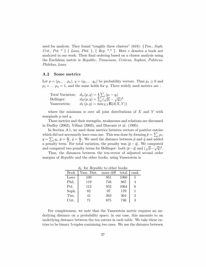
q̄)2.Thus, the distances between the ten-vector of adjusted second order

margins of Republic and the other books, using Vasserstein is

dV for Republic to other books

Book Vass. Dist. mass diff total rank

Laws 109 951 1060 5Phil. 119 748 867 4Pol. 112 952 1064 6Soph. 82 97 179 1Tim. 41 263 304 2Crit. 71 675 746 3

For completeness, we note that the Vasserstein metric requires an un-derlying distance on a probability space; in our case, this amounts to anunderlying distance between the ten entries in each table. We take these en-tries to be binary 5-tuples containing two ones. We use the distance between

27

two of these as the minimum number of pairwise adjacent switches requiredto bring one to the other. Thus the distance between 11000 and 00011 is6. Further background can be found in Diaconis et al. (1995) or Guo et al.(1992). With this choice specified, the minimization problem is equivalentto the Monge-Kantorovich Transshipment problem. We computed distancesusing the CS-2 code of Andrew Goldberg (www/avglab.org/andrew).

A.3 Using all Affine Projections

The data analysis of Section 2 used projections into first and second ordermargins. The general theory developed later points to all affine projectionsas a natural base for analysis. In this section, we complete our analysis ofthe Plato data by looking at all affine projections.

In the following, x and z range over all binary 5−tuples. If f(x) is theproportion of sentences in a fixed book (eg. Republic) with rhyming patternx, the projection of f in direction z is

∑

x·z=0

f(x),∑

x·z=1

f(x).

To use the information that Republic was written early and Laws waswritten late, we find 5−tuples, z, that maximize

(∑

x·z=0

f(x) −∑

x·z=1

f(x)) − (∑

x·z=0

g(x) −∑

x·z=1

g(x)).

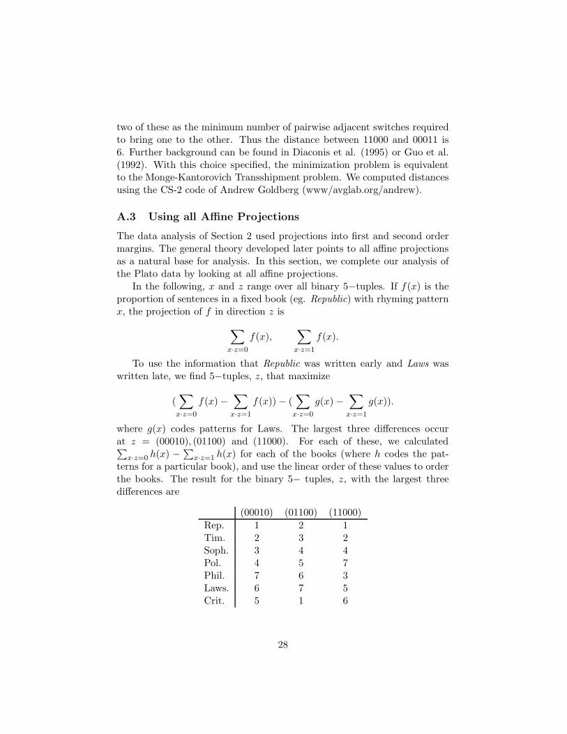
where g(x) codes patterns for Laws. The largest three differences occurat z = (00010), (01100) and (11000). For each of these, we calculated∑

x·z=0 h(x) −∑x·z=1 h(x) for each of the books (where h codes the pat-terns for a particular book), and use the linear order of these values to orderthe books. The result for the binary 5− tuples, z, with the largest threedifferences are

(00010) (01100) (11000)

Rep. 1 2 1Tim. 2 3 2Soph. 3 4 4Pol. 4 5 7Phil. 7 6 3Laws. 6 7 5Crit. 5 1 6

28

The first column thus gives the ranking : Rep., Tim. Soph., Pol., Crit.,Laws, Phil. This is based on the difference between a single syllable (secondfrom the end). It is close to, but not the same as the ranking based onadjusted second order margins found above. The other columns differ andshow that not ‘any old’ projection gives the same ranking.

References

[1] Ahn, J.S., Hofmann, H., and Cook, D.(2003). “A Projection Pursuit Methodon the multidimensional squared Contingency table”, Computational Statistics18, 605-626.

[2] Atkinson, A.C. (1970). “A method for discriminating between models”, Jour.Roy. Stat. Soc. B. 32, 323-353.

[3] Bolker, E. (1987). “The finite Radon transform”, Contemp. Math. Vol. 63,27-50.

[4] Boneva, L.I. (1971). “A new approach to a problem of chronological associ-ated with the works of Plato”. In Hodson, R.R., Kendall, D.G., Tautu, F.,eds. Mathematics in the Archaeological and Historical Sciences, EdinburghUniversity Press, Edinburgh.

[5] Brandwood, L. (1976). A Word Index to Plato. W.S. Maney, Leeds.

[6] Cameron, P. (1976). Parallelisms of Complete Designs. Cambridge UniversityPress, Cambridge.

[7] Charnomordic, B. and Holmes, S. (2001). “Correspondence Analysis with R”,Statistical Computing and Graphics. Vol. 12. No. 1, 19-25.

[8] Chvatal, V. (1983). Linear Programming. W.H. Freeman, New York.

[9] Cheng, T.T. (1949). The normal approximation to the Poisson distributionand a conjecture of Ramanujan. Bull. Americ. Math. Soc. 55, 396-401.

[10] Constantine, G. M. (1987). Combinatorial Theory and Statistical Designs. Wi-ley, NY.

[11] Cox, D.E. and Brandwood, L. (1959). “On a discriminatory problem connectedwith the works of Plato”, Jour. Roy. Stat. Soc. B 21, 195-200.

[12] Critchlow, D. (1988). Metric methods for analyzing partially ranked data. Lec-ture Notes in Statistics, No. 34. Springer-Verlag, Berlin.

[13] Dedeo, M. and Velasquez, E. (2003). “The Radon transform on Zkn”, Siam J.

Disc. Math. Vol. 18, No. 3, 472-478.

29

[14] Dembrowski, P. (1968). Finite Geometries Springer-Verlag. New York.

[15] Diaconis, P. and Freedman, D. (1982). “The mode of an empirical histogram”,Pacific Journal of Mathematics. 100. No 2, 359-385.

[16] Diaconis, P. and Freedman, D. (1982). “Asymptotics of graphical projectionpursuit”, Ann. Stat., vol. 12, 793-815.

[17] Diaconis, P. and Shahshahani, M., (1984). “On Nonlinear Functions of Lin-ear Combinations”, SIAM Journal of the Scientific and Statistical Computing5(1), 175-191.

[18] Diaconis, P. and Graham, R. (1985). “Finite Radon transforms on Zk2”, Pacific

J. Math, vol. 118, 323-345.

[19] Diaconis, P. (1986). Group Representations in Probability and Statistics. IMSLecture Notes - Monograph Series, vol. 11, S. S. Gupta (ed.), Institute ofMathematical Statistics, Hawyard CA.

[20] Diaconis, P. (1987). “Projection pursuit for discrete data”, Scand. J. Stat.

[21] Diaconis, P. (1987). “The 1987 Wald Memorial Lectures: A Generalizationof Spectral Analysis with Application to Ranked Data”, Annals of Statistics,September 1989, Vol. 17, No.3, 949-979.

[22] Diaconis, P., Holmes, S., Janson, S., Lalley, S. and Pemantle, R. (1995). “Met-rics on compositions and coincidences among renewal processes”, Random Dis-crete Structures, 81 - 101, IMA Vol. Math. Appl., 76,. Springer: New York.

[23] Dong, J. and Jiang, R. (1998). “Contingency Table Probability Estimation-Projection Pursuit Approach”, Computational Statistics 13, 425-445.

[24] Dudley, R.M. (2002). Real Analysis and Probability. Cambridge UniversityPress, Cambridge.

[25] Donoho, D. (1981). “On minimum entropy deconvolution”. In Applied TimeSeries Analysis II pp. 565-608, Academic Press, New York.

[26] Feller, W. (1971). An Introduction to Probability Theory and its ApplicationsVol. II 2nd edition. Wiley, New York.

[27] Fill, J.A. (1989). ”The Radon transform on Zn”, Siam. J. Disc. Math. Vol. 2,No. 2, 262-283.

[28] Fligner, M.A. and Verducci, J.S. (1993). Probability models and statisticalanalyses for ranking data. New York, Springer-Verlag.

[29] Friednman, J., Stuetzle, W. and Schroeder, A. (1984). “Projection PursuitDensity Estimation”, JASA 79, 599-608.

30

[30] Friedman, J. and Steuetzle, W. (1981). “Projection Pursuit Regression”, JASA76, 817-823.

[31] Friedman, J. and Tukey, J.W.T. (1974). “A projection pursuit algorithm forexploratory data analysis”, IEEE Transaactions on Computers 9, 881-890.

[32] CS-2 algorithm. www.avglab.org/andrew.

[33] Guo, S. W., Thompson, E. A.(1992). “Performing the exact test of Hardy-Weinberg proportion for multiple alleles”, Biometrics, 48, 361-372.

[34] Hall, P. (1989). “On Polynomial-based Projection Indices for Exploratory Pro-jection Pursuit”, Annals of Stat. 17. No.2, 589-605.

[35] Hedayat, A.S., Slaoane, N.J., Stufken, J. (1999). Orthogonal Arrays: Theoryand Applications. Springer, NY.

[36] Huber, P. (1985). “Projection Pursuit”, Ann. Stat.. Vol. 13. No. 2, 435-475.

[37] Hwang, J-N., Law, S-R, and Lippman, A. (1994). “Nonparametric Multivari-ate Density Estimation: A Comparative Study”, IEEE Transactions on SignalProcessing Vol. 42. No. 10, 2795-2810.

[38] James, G.D. (1978). The Representation Theory of the Symmetric Groups.Springer Lecture Notes in Mathematics, 682, Springer-Verlag, New York.

[39] Kruskal, J.B. (1969). “Toward a practical method which helps uncover thestucture of a set of multivariate observations by finding the linear transfor-mation that optimizes a new index of condensation”. In R.C. Milton and J.A.Nelder (eds.) Statistical Computation. Academic Press, New York.

[40] Kruskal, J.B. (1972). “Linear transformation of multivariate data to revealclustering”. In Multidimensional Scaling: Theory and Applications in the Be-havioral Sciences, Vol. 1, Theory. Seminar Press.

[41] Kung, J. (1979). “The Radon transform of a combinatorial geometry I”, Jour-nal of Combinatorial Theory A, 97-102.

[42] Lander, E. (1982). Symmetric Designs, an Algebraic Approach. CambridgeUniversity Press, Cambridge.

[43] Marden, J.I. (1995). Analyzing and Modeling Rank Data. Chapman and Hall,New York; print.google.com.

[44] Pearson, K. (1968). Tables of the Incomplete Beta-Function, 2nd edition. Cam-bridge University Press, England.

[45] Posse, C. (1995). “Tools for Two-dimensional Projection Pursuit”, Journal ofComputational and Graphical Statistics. 4(20), 83-100.

31

[46] Pratt. J. (1959). “On a general concept of “In probabilitiy””. Annals of Math.Stat. Vol. 30, No. 2, 549-558.

[47] Solomon, H. (1961). Studies in Item Analysis and Prediction. Stanford Uni-versity Press, Stanford, California.

[48] Stein, C. (1992). “A way of using auxiliary randomization”, Probability Theory.(Singapore, 1989), pages 159180. de Gruyter, Berlin, 1992.

[49] Sun, J. (1993). “Some Computational Aspects in Projection Pursuit”, SIAMJ. Sci. and Stat. Comp., Vol. 14, No. 1, pp. 68-80.

[50] Sun, J. (1991). “Significance Levels in Exploratory Projection Pursuit”,Biometrika, Vol. 78, pp. 759-769.

[51] Velasquez, E. (1997). ”The Radon transform on finite symmetric spaces”,Pacific J. Math. Vol. 177, No. 2, 369-376.

[52] Wishart, D. and Leach, S.V. (1970). “A multivariate analysis of Platonic proserhythm”, Computer Studies 3, No. 2, 90-99.

[53] Villani, C. (2003). Topics in Optimal Transportation. Graduate Studies inMathematics, Vol 58. AMS.

32