WP # 0095MSS-496-2009 Date June 24, 2009

THE UNIVERSITY OF TEXAS AT SAN ANTONIO, COLLEGE OF BUSINESS

Working Paper SERIES

October 2006

ONE UTSA CIRCLE SAN ANTONIO, TEXAS 78249-0631 210 458-4317 | BUSINESS.UTSA.EDU

Copyright © 2009, by the author(s). Please do not quote, cite, or reproduce without permission from the author(s).

Victor De Oliveira Department of Management Science and Statistics

University of Texas at San Antonio

BAYESIAN ANALYSIS OF CONDITIONAL AUTORIEGRESSIVE MODELS

BAYESIAN ANALYSIS OF CONDITIONAL AUTOREGRESSIVE

MODELS

Victor De Oliveira1

Department of Management Science and Statistics

The University of Texas at San Antonio

San Antonio, TX 78249, USA.

victor.deoliveira@utsa.edu

January 17, 2009

Abstract

Conditionally autoregressive (CAR) models have been extensively used for the analysis of spatial data

in diverse areas, such as demography, economy, epidemiology and geography, as models for both latent

and observed variables. In the latter case, the most common inferential method has been maximum

likelihood, and the Bayesian approach has not been used much. This work proposes default (automatic)

Bayesian analyses of CAR models. Two versions of Jeffreys prior, the independence Jeffreys and Jeffreys-

rule priors, are derived for the parameters of CAR models and properties of the priors and resulting

posterior distributions are obtained. The two priors and their respective posteriors are compared based

on simulated data. Also, frequentist properties of inferences based on maximum likelihood are compared

with those based on the Jeffreys priors and the uniform prior. Finally, the proposed Bayesian analysis

is illustraded by fitting a CAR model to a phosphate dataset from an archeological region.

Key words: CAR model; Eigenvalues and eigenvectors; Frequentist properties; Integrated likelihood;

Maximum likelihood; Spatial data; Weight matrix.

JEL Classifications: C11 and C31.

1This work was partially supported by National Science Foundation grant DMS-0719508, and a College of

Business (The University of Texas at San Antonio) summer research grant.

1

1 Introduction

Conditional autoregressive (CAR) models are used to describe the spatial variation of quantities

of interest in the form of summaries or aggregates over subregions. These models have been used

to analyze data in diverse areas such as demography, economy, epidemiology and geography.

The general goal of these spatial models is to unveil and quantify spatial relations present

among the data, in particular, to quantify how quantities of interest vary as a function of

explanatory variables and detect clusters of ‘hot spots’. General accounts of CAR models, a

class of Markov random fields, appear in Cressie (1993), Banerjee, Carlin and Gelfand (2004)

and Rue and Held (2005).

CAR models have been extensively used in spatial statistics to model observed data (Cressie

and Chan, 1989; Richardson, Guihenneuc and Lasserre, 1992; Bell and Broemeling, 2000;

Militino, Ugarte and Garcia-Reinaldos, 2004; Cressie, Perrin and Thomas-Agnan, 2005), as

well as (unobserved) latent variables and spatially varying random effects (Clayton and Kaldor,

1987; Sun, Tsutakawa and Speckman, 1999; Pettitt, Weir and Hart, 2002; see Banerjee, Carlin

and Gelfand, 2004 for further references). In this work I consider the former use of CAR models,

but note that the analysis proposed here may serve (or be the base) for the use of CAR models

in a default Bayesian analysis for hierarchical models.

The most commonly used method to fit CAR models has been maximum likelihood (Cressie

and Chan, 1989; Richardson et al. 1992; Cressie et al. 2005). Most results up to date on the

behavior of inferences based on maximum likelihood estimators are asymptotic in nature and

little is know about their behavior in small samples. The Bayesian approach, on the other

hand, allows ‘exact’ inference without the need for asymptotic approximations. Although

Bayesian analyses of CAR models have been extensively used to describe latent variables and

spatially varying random effects in the context of hierarchical models, not much has been done

on Bayesian analysis of CAR models to describe the observed data (with only rare exceptions,

e.g., Bell and Broemeling, 2000). This may be due to lack of familiarity about what could

be adequate priors for these models and lack of knowledge about frequentist properties of the

Bayesian procedures.

The goal main of this work is to propose default (automatic) Bayesian analyses for CAR

models and study some of their properties. Two versions of Jeffreys prior, called independence

Jeffreys and Jeffreys-rule priors, are derived for the parameters of CAR models and results on

propriety of the resulting posterior distributions and existence of posterior moments for the

covariance parameters are established. It is found that some properties of the posterior distri-

butions based on the proposed Jeffreys priors depend on a certain relation between the column

space of the regression design matrix and the extreme eigenspaces of the spatial design matrix.

2

Simple Monte Carlo algorithms are described for sampling from the appropriate posterior dis-

tributions for the cases when the data are complete and when there are missing observations.

Examples are presented based on simulated data to compare the two Jeffreys priors and their

corresponding posterior distributions.

A computational experiment is performed to compare frequentist properties of inferences

about the covariance parameters based on maximum likelihood with those based on the pro-

posed Jeffreys priors and the uniform prior. It is found that frequentist properties of all the

above procedures are adequate and similar to each other in most situations, except when the

spatial association is strong or the mean of the observations is not constant. In this case

inference about the ‘spatial parameter’ based on the independence Jeffreys prior has better

frequentist properties than the procedures based on the other priors or ML. Finally, it is found

that the independence Jeffreys prior is not very sensitive to some aspects of the design, such

as sample size and regression design matrix, while the Jeffreys-prior displays strong sensitivity

to the regression design matrix.

The organization of the paper is as follows. Section 2 describes the CAR model and the

behavior of an integrated likelihood. Section 3 derives two versions of Jeffreys prior and provides

properties of these priors and their corresponding posterior distributions in terms of propriety

and existence of posterior moments of the covariance parameters. Section 4 describes simple

Monte Carlo algorithms to sample from the appropriate posterior distributions, and provides

some comparisons based on simulated data between the two versions of Jeffreys priors. Section

5 presents a simulation experiment to compare frequentist properties of inferences based on

ML with those based on the two versions of Jeffreys priors and the uniform prior, and explores

sensitivity of Jeffreys priors to some aspects of the design. The proposed Bayesian methodology

is illustrated in Section 6 using a phosphate dataset from an archeological region in Greece.

Conclusions are given in Section 7.

2 CAR Models

2.1 Description

Consider a geographic region that is partitioned into subregions indexed by integers 1, 2, . . . , n.

This collection of subregions (or sites as they are also called) is assumed to be endowed with

a neighborhood system, Ni : i = 1, . . . , n, where Ni denotes the collection of subregions

that, in a well defined sense, are neighbors of subregion i. This neighborhood system, which

is key in determining the dependence structure of the CAR model, must satisfy that for any

i, j = 1, . . . , n, j ∈ Ni if and only if i ∈ Nj and i /∈ Ni. An emblematic example commonly

3

used in applications is the neighborhood system defined in terms of geographic adjacency

Ni = j : subregion j shares a boundary with subregion i, i = 1, . . . , n.

Other examples include neighborhood systems defined based on distance from the centroids of

subregions or similarity of an auxiliary variable; see Cressie (1993, p. 554) and Case, Rosen

and Hines (1993) for examples. This kind of specification is natural for modeling summary

or aggregate data where similarity between subregions often depends on similarity of shared

features.

For each subregion it is observed the variable of interest, Yi, and a set of p < n explanatory

variables, xi = (xi1, . . . , xip)′. The CAR model for the responses, Y = (Y1, . . . , Yn)′, is formu-

lated by specifying the set of full conditional distributions satisfying a form of auto-regression

given by

(Yi | Y(i)) ∼ N(

x′iβ +

n∑

j=1

cij(Yj − x′jβ), σ2

i

)

, i = 1, . . . , n, (1)

where Y(i) = Yj : j 6= i, β = (β1, . . . , βp)′ ∈ R

p are unknown regression parameters,

and σ2i > 0 and cij ≥ 0 are covariance parameters, with cii = 0 for all i. For the set of full

conditional distributions (1) to determine a well defined joint distribution for Y, the matrices

M = diag(σ21 , . . . , σ

2n) and C = (cij) must satisfy the conditions:

(a) M−1C is symmetric, which is equivalent to cijσ2j = cjiσ

2i for all i, j = 1, . . . , n;

(b) M−1(In − C) is positive definite;

see Cressie (1993) or Rue and Held (2005) for examples and further details. When (a) and (b)

hold, we would have that

Y ∼ Nn(Xβ, (In − C)−1M),

where X is the n × p matrix with ith row x′i, assumed to have full rank. This work considers

models in which (possibly after a transformation) the matrices M and C satisfy:

(i) M = σ2In, where σ2 > 0 is unknown;

(ii) C = φW , where φ is a ‘spatial parameter’ and W = (wij) is a known “weight” (“neighbor-

hood”) matrix that is nonnegative (wij ≥ 0), symmetric and satisfies that wij > 0 if and only

if sites i and j are neighbors (so wii = 0).

To guarantee that In − φW is positive definite φ is required to belong to (λ−1n , λ−1

1 ), where

λ1 ≥ λ2 ≥ . . . ≥ λn are the ordered eigenvalues of W , with λn < 0 < λ1 since tr(W ) = 0. It

immediately follows that (i) and (ii) imply that (a) and (b) hold. If η = (β ′, σ2, φ) denote the

model parameters, then the parameter space of this model, Ω = Rp × (0,∞) × (λ−1

n , λ−11 ), has

4

the distinctive feature that it depends on some aspects of the design (as it depends on W ).

Finally, the parameter value φ = 0 corresponds to the case when Yi − x′iβ

iid∼ N(0, σ2).

Many other CAR models that have been considered in the literature can be reduced to a

model where (i) and (ii) hold by the use of an appropriate scaling of the data and covariates

(Cressie et al., 2005). Suppose Y follows a CAR model with mean vector Xβ, with X of full

rank, and covariance matrix (In − C)−1M , where M = σ2G, G diagonal with known positive

diagonal elements, and C = φW with W as in (ii) except that it is not necessarily symmetric,

and M and C satisfy (a) and (b). Then, Y = G− 1

2 Y satisfies

Y ∼ Nn(Xβ, σ2(In − φW )−1),

where X = G− 1

2 X has full rank and W = G− 1

2 WG1

2 is nonnegative, symmetric and wij > 0 if

and only if sites i and j are neighbors; the symmetry of W follows from condition (a) above.

Hence, Y follows the CAR model satisfying (i) and (ii).

2.2 Integrated Likelihood

The likelihood function of η based on the observed data y is

L(η;y) ∝ (σ2)−n

2 |Σ−1φ |

1

2 exp−1

2σ2(y − Xβ)′Σ−1

φ (y − Xβ), (2)

where Σ−1φ = In −φW . Similarly to what is often done for Bayesian analysis of ordinary linear

models, a sensible class of prior distributions for η is given by the family

π(η) ∝π(φ)

(σ2)a, η ∈ Ω, (3)

where a ∈ R is a hyperparameter and π(φ) is the ‘marginal’ prior of φ with support (λ−1n , λ−1

1 ).

The relevance of this class of priors will be apparent when it is shown that the Jeffreys priors

derived here belong to this class. An obvious choice, used by Bell and Broemeling (2000), is

to set a = 1 and π(φ) = πU (φ) ∝ 1(λ−1n ,λ−1

1)(φ), which I call the uniform prior (1A(φ) denotes

the indicator function of the set A). Besides its lack of invariance, the uniform prior may not

(arguably) be quite appropriate in some cases. For many datasets found in practice there is

strong spatial correlation between observations measured at nearest neighbors, and such strong

correlation is reproduced in CAR models only when the spatial parameter φ is quite close to one

of the boundaries, λ−11 or λ−1

n (Besag and Kooperberg, 1995). The spatial information contained

in the uniform prior is somewhat in conflict with the aforementioned historical information

since it assigns too little mass to models with substantial spatial correlation and too much

mass to models with weak or no spatial correlation. In contrast, the Jeffreys priors derived

here do not have this unappealing feature since, as would be seen, they are unbounded around

5

λ−11 and λ−1

n , so they automatically assign substantial mass to spatial parameters near these

boundaries. Although using such priors may potentially yield improper posteriors, it would be

shown that the propriety of posterior distributions based on these Jeffreys priors depend on a

certain relation between the column space of X and the extreme eigenspaces of W (eigenspaces

associated with the largest and smallest eigenvalues) which is most likely satisfied in practice.

Another alternative, suggested by Banerjee et al. (2004, p. 164), is to use a beta-type prior

for φ that places substantial prior probability on large values of |φ|, but this would require

specifying two hyperparameters.

From Bayes theorem follows that the posterior distribution of η is proper if and only if

0 <∫

Ω L(η;y)π(η)dη < ∞. A standard calculation with the above likelihood and prior shows

that∫

Rp×(0,∞)L(η;y)π(η)dβdσ2 = LI(φ;y)π(φ),

with

LI(φ;y) ∝ |Σ−1φ |

1

2 |X ′Σ−1φ X|−

1

2 (S2φ)−( n−p

2+a−1), (4)

where

S2φ = (y − Xβφ)′Σ−1

φ (y − Xβφ),

and βφ = (X ′Σ−1φ X)−1X ′Σ−1

φ y; LI(φ;y) is called the integrated likelihood of φ. Then, the

posterior distribution of η is proper if and only if

0 <

∫ λ−1

1

λ−1n

LI(φ;y)π(φ)dφ < ∞, (5)

so to determine propriety of posterior distributions based on priors (3) it is necessary to de-

termine the behavior of both the integrated likelihood LI(φ;y) and marginal prior π(φ) in the

interval (λ−1n , λ−1

1 ).

Some notation is now introduced. Let C(X) denote the subspace of Rn spanned by the

columns of X, and u1, . . . ,un be the normalized eigenvectors of W corresponding, respectively,

to the eigenvalues λ1, . . . , λn, and recall that λn < 0 < λ1. Throughout this and the next

section φ → λ−11 (φ → λ−1

n ) is used to denote that φ approaches λ−11 (λ−1

n ) from the left

(right). Also, it is assumed throughout that λini=1 are not all equal.

Lemma 1 Consider the CAR model (2) with n ≥ p + 2, and suppose λ1 and λn are simple

eigenvalues. Then as φ → λ−11 we have

|X ′Σ−1φ X| =

O(1 − φλ1) if u1 ∈ C(X)

O(1) if u1 /∈ C(X), (6)

6

and for every η ∈ Ω

S2φ = O(1) with probability 1. (7)

The same results hold as φ → λ−1n when λ1 and u1 are replaced by, respectively, λn and un.

Proof. See the Appendix

Proposition 1 Consider the CAR model (2) and the prior distribution (3) with n ≥ p + 2,

and suppose λ1 and λn are simple eigenvalues. Then for every η ∈ Ω the integrated likelihood

LI(φ;y) in (4) is with probability 1 a continuous function on (λ−1n , λ−1

1 ) satisfying that as

φ → λ−11

LI(φ;y) =

O(1) if u1 ∈ C(X)

O((1 − φλ1)1

2 ) if u1 /∈ C(X).

The same result holds as φ → λ−1n when λ1 and u1 are replaced by, respectively, λn and un.

Proof. The continuity of LI(φ;y) on (λ−1n , λ−1

1 ) follows from the definitions of Σ−1φ , S2

φ and

the continuity of the determinant function. For any φ ∈ (0, λ−11 ) the eigenvalues of Σ−1

φ are

1 − φλ1 < 1 − φλ2 ≤ . . . ≤ 1 − φλn−1 < 1 − φλn, so

|Σ−1φ | = (1 − φλ1)

n∏

i=2

(1 − φλi),

and hence |Σ−1φ |

1

2 = O((1 − φλ1)1

2 ) as φ → λ−11 . Then the result follows from (6) and (7).

The proof on the behavior of LI(φ;y) as φ → λ−1n follows along the same lines.

Remark 1. Note that the limiting behaviors of LI(φ;y) as φ → λ−11 and φ → λ−1

n do not

depend on the hyperparameter a.

Remark 2. The neighborhood systems used for modeling most datasets are such that there is

a ‘path’ between any pair of sites. In this case the matrix W is irreducible, so λ1 is guaranteed

to be simple by the Perron-Frobenius theorem (Bapat and Raghavan, 1997 p. 17). For all the

simulated and real datasets I have looked at λn was also simple, but this is not guaranteed to

be so. For the case when each subregion is a neighbor of any other subregion, with wij = 1 for

all i 6= j, it holds that λn = −1 has multiplicity n − 1. But this kind of neighborhood system

is rarely considered in practice.

3 Jeffreys Priors

Default or automatic priors are useful in situations where it is difficult to elicit a prior, either

subjectively or from previous data. The most commonly used of such priors is the Jeffreys-rule

7

prior which is given by π(η) ∝ (det[I(η)])1

2 , where I(η) is the Fisher information matrix with

(i, j) entry

[I(η)]ij = Eη

(

∂

∂ηilog(L(η;Y))

)(

∂

∂ηjlog(L(η;Y))

)

∣

∣

∣η

.

The Jeffreys-rule prior has several attractive features, such as invariance to one-to-one reparame-

trizations and restrictions of the parameter space, but it also has some not so attractive features.

One of these is the poor frequentist properties that have been noticed for some multiparam-

eter models. This section derives two versions of Jeffreys prior, the Jeffreys-rule prior and

the independence Jeffreys prior, where the latter (intended to ameliorate the aforementioned

unattractive feature) is obtained by assuming that β and (σ2, φ) are ‘independent’ a priori and

computing each marginal prior using Jeffreys-rule when the other parameter is assumed known.

Since these Jeffreys priors are improper (as is usually the case) the propriety of the resulting

posteriors would need to be checked.

Theorem 1 Consider the CAR model (2). Then the independence Jeffreys prior and the

Jeffreys-rule prior of η, to be denoted by πJ1(η) and πJ2(η), are of the form (3) with, respec-

tively,

a = 1 and πJ1(φ) ∝

n∑

i=1

( λi

1 − φλi

)2−

1

n

[

n∑

i=1

λi

1 − φλi

]2

1

2

, (8)

and

a = 1 +p

2and πJ2(φ) ∝

(

p∏

j=1

(1 − φνj))

1

2

πJ1(φ),

where ν1 ≥ . . . ≥ νp are the ordered eigenvalues of X ′oWXo, and Xo is the matrix defined by

(18) in the Appendix.

Proof. From Theorem 5 in Berger et al. (2001) follows that for the spatial model Y ∼

Nn(Xβ, σ2Σφ), the independence Jeffreys prior and Jeffreys-rule prior are both of the form (3)

with, respectively,

a = 1 and πJ1(φ) ∝

tr[U2φ ] −

1

n(tr[Uφ])2

1

2

,

and

a = 1 +p

2and πJ2(φ) ∝ |X ′Σ−1

φ X|1

2 πJ1(φ),

where Uφ = ( ∂∂φΣφ)Σ−1

φ , and ∂∂φΣφ denotes the matrix obtained by differentiating Σφ element

by element. For the CAR model Σ−1φ = In − φW , so

Uφ = −Σφ

( ∂

∂φΣ−1

φ

)

= (In − φW )−1W.

8

Noting now that λi

1−φλin

i=1 are the eigenvalues of Uφ, it follows that

tr[U2φ ] −

1

n

(

tr[Uφ])2

=

n∑

i=1

( λi

1 − φλi

)2−

1

n

[

n∑

i=1

λi

1 − φλi

]2,

so the first result follows. The second result follows from the first and identity (19) in the

Appendix.

Lemma 2 Suppose λ1 and λn are simple eigenvalues. Then as φ → λ−11 it holds that

πJ1(φ) = O((1 − φλ1)−1),

and

πJ2(φ) =

O((1 − φλ1)− 1

2 ) if u1 ∈ C(X)

O((1 − φλ1)−1) if u1 /∈ C(X)

.

The same results hold as φ → λ−1n when λ1 and u1 are replaced by, respectively, λn and un.

Proof. From (8) and after some algebraic manipulation follow that

(

πJ1(φ))2

∝( λ1

1 − φλ1

)2+

n∑

i=2

( λi

1 − φλi

)2−

1

n

[ λ1

1 − φλ1+

n∑

i=2

λi

1 − φλi

]2

=( λ1

1 − φλ1

)2(

1 −1

n−

2(1 − φλ1)

nλ1

n∑

i=2

λi

1 − φλi

+(1 − φλ1

λ1

)2(n∑

i=2

( λi

1 − φλi

)2−

1

n

[

n∑

i=2

λi

1 − φλi

]2))

= O((1 − φλ1)−2) as φ → λ−1

1 ,

since λ1 > λi for i = 2, . . . , n. The behavior as φ → λ−1n is established in the same way, and

the second result follows from the first and (6).

Corollary 1 Consider the CAR model (2) and let k ∈ N. Then:

(i) The marginal independence Jeffreys prior πJ1(φ) is unbounded and not integrable.

(ii) The joint independence Jeffreys posterior πJ1(η | y) is proper when neither u1 nor un are

in C(X), while it is improper when either u1 or un are in C(X).

(iii) The marginal independence Jeffreys posterior πJ1(φ | y) has moments of any order k when

neither u1 nor un are in C(X).

(iv) The marginal independence Jeffreys posterior πJ1(σ2 | y) has a finite moment of order k

if n ≥ p + 2k + 1.

9

Proof. (i) From Lemma 2 follows that for i = 1 or n, limφ→λ−1

iπJ1(φ) = ∞. Also

∫ λ−1

1

0πJ1(φ)dφ ∝

∫ λ−1

1

0(1 − φλ1)

−1h(φ)dφ = λ−11

∫ 1

0t−1h(t)dt,

where the last identity is obtained by the change of variable t = 1−φλ1, h(φ) is an (unspecified)

function that is continuous on (0, λ−11 ) and O(1) as φ → λ−1

1 , and h(t) is an (unspecified) func-

tion that is continuous on (0, 1) and O(1) as t → 0; a similar identity holds for∫ 0λ−1

nπJ1(φ)dφ.

The result now follows since t−1 is not integrable around 0.

(ii) From Proposition 1 and Lemma 2, and noting that πJ1(φ | y) ∝ LI(φ;y)πJ1(φ)

∫ λ−1

1

0πJ1(φ | y)dφ ∝

∫ λ−1

1

0 (1 − φλ1)−1h(φ)dφ if u1 ∈ C(X)

∫ λ−1

1

0 (1 − φλ1)− 1

2 h(φ)dφ if u1 /∈ C(X)

=

λ−11

∫ 10 t−1h(t)dt if u1 ∈ C(X)

λ−11

∫ 10 t−

1

2 h(t)dt if u1 /∈ C(X), (9)

where h(φ) and h(t) are as in (i); a similar identity holds for∫ 0λ−1

nπJ1(φ | y)dφ with λ1 and u1

replaced by, respectively, λn and un. The result then follows by the same argument as in (i).

(iii) By a similar calculation as in (i) and (ii) and using the binomial expansion of (1 − t)k

∫ λ−1

1

0φkπJ1(φ | y)dφ ∝

λ−(k+1)1

∫ 10

(

t−1 +∑k−1

j=1(−1)k−j(k

j

)

tk−1−j)

h(t)dt if u1 ∈ C(X)

λ−(k+1)1

∫ 10

(

t−1

2 +∑k−1

j=1(−1)k−j(k

j

)

tk−1

2−j)

h(t)dt if u1 /∈ C(X),

where h(t) is as in (i); a similar identity holds for∫ 0λ−1

nφkπJ1(φ | y)dφ with λ1 and u1 replaced

by, respectively, λn and un. The result follows since t−1 is not integrable on (0, 1), while t−1

2 ,

tk−1+j and tk−1

2+j are, j = 0, 1, . . . , k − 1.

(iv) Note that E(σ2)k | y exists if E(σ2)k | φ,y exists and is integrable with respect to

πJ1(φ | y). A standard calculation shows that for any prior in (3) with a = 1, πJ1(σ2 | φ,y) =

IG(n−p

2 , 12S2

φ

)

, where IG(a, b) denotes the inverse gamma distribution with mean b/(a − 1).

Again by direct calculation, E(σ2)k | φ,y = c(S2φ)k < ∞, provided n ≥ p + 2k + 1, where

c > 0 does not depend on (φ,y). The result then follows from (7), (9) and the relation analogous

to (9) for∫ 0λ−1

nπJ1(φ | y)dφ.

Corollary 2 Consider the CAR model (2) and let k ∈ N. Then:

(i) The marginal Jeffreys-rule prior πJ2(φ) is unbounded. Also, it is integrable when both u1

and un are in C(X), while it is not integrable when either u1 or un is not in C(X).

(ii) The joint Jeffreys-rule posterior πJ2(η | y) is always proper.

10

(iii) The marginal Jeffreys-rule posterior πJ2(φ | y) has always moments of any order k.

(iv) The marginal Jeffreys posterior πJ2(σ2 | y) has a finite moment of order k if n ≥ p+2k+1.

Proof. These results are proved similarly as their counterparts in Corollary 1.

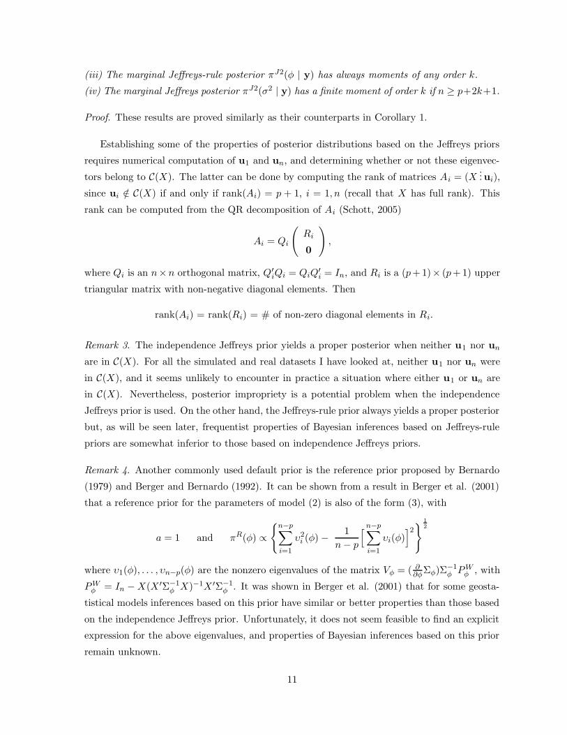
Establishing some of the properties of posterior distributions based on the Jeffreys priors

requires numerical computation of u1 and un, and determining whether or not these eigenvec-

tors belong to C(X). The latter can be done by computing the rank of matrices Ai = (X...ui),

since ui /∈ C(X) if and only if rank(Ai) = p + 1, i = 1, n (recall that X has full rank). This

rank can be computed from the QR decomposition of Ai (Schott, 2005)

Ai = Qi

(

Ri

0

)

,

where Qi is an n×n orthogonal matrix, Q′iQi = QiQ

′i = In, and Ri is a (p+1)× (p+1) upper

triangular matrix with non-negative diagonal elements. Then

rank(Ai) = rank(Ri) = # of non-zero diagonal elements in Ri.

Remark 3. The independence Jeffreys prior yields a proper posterior when neither u1 nor un

are in C(X). For all the simulated and real datasets I have looked at, neither u1 nor un were

in C(X), and it seems unlikely to encounter in practice a situation where either u1 or un are

in C(X). Nevertheless, posterior impropriety is a potential problem when the independence

Jeffreys prior is used. On the other hand, the Jeffreys-rule prior always yields a proper posterior

but, as will be seen later, frequentist properties of Bayesian inferences based on Jeffreys-rule

priors are somewhat inferior to those based on independence Jeffreys priors.

Remark 4. Another commonly used default prior is the reference prior proposed by Bernardo

(1979) and Berger and Bernardo (1992). It can be shown from a result in Berger et al. (2001)

that a reference prior for the parameters of model (2) is also of the form (3), with

a = 1 and πR(φ) ∝

n−p∑

i=1

υ2i (φ) −

1

n − p

[

n−p∑

i=1

υi(φ)]2

1

2

where υ1(φ), . . . , υn−p(φ) are the nonzero eigenvalues of the matrix Vφ = ( ∂∂φΣφ)Σ−1

φ PWφ , with

PWφ = In − X(X ′Σ−1

φ X)−1X ′Σ−1φ . It was shown in Berger et al. (2001) that for some geosta-

tistical models inferences based on this prior have similar or better properties than those based

on the independence Jeffreys prior. Unfortunately, it does not seem feasible to find an explicit

expression for the above eigenvalues, and properties of Bayesian inferences based on this prior

remain unknown.

11

4 Inference and Comparison

4.1 Inference

Posterior inference about the unknown quantities would be based on a sample from their

posterior distribution. When the observed data are complete, a sample from the posterior

distribution of the model parameters is simulated using a noniterative Monte Carlo algorithm

based on the factorization

π(β, σ2, φ | y) = π(β | σ2, φ,y)π(σ2 | φ,y)π(φ | y),

where from (2) and (3)

π(β | σ2, φ,y) = Np

(

βφ, σ2(X ′Σ−1φ X)−1

)

, (10)

π(σ2 | φ,y) = IG(n − p

2+ a − 1,

1

2S2

φ

)

, (11)

π(φ | y) ∝(

|Σφ||X′Σ−1

φ X|)− 1

2

(

S2φ

)−( n−p

2+a−1)

π(φ). (12)

Simulation from (10) and (11) is straightforward, while simulation from (12) would be accom-

plished using the adaptive rejection Metropolis sampling (ARMS) algorithm proposed by Gilks,

Best and Tan (1995). The ARMS algorithm requires no tuning and works very well for this

model. It was found that produces well mixed chains with very low autocorrelations, so long

runs are not required for precise inference.

The above algorithm cannot be easily modified to handle the case when there are missing

values at some of the sites. In this case, sampling from the posterior of the model parameters

and missing values is done using a Gibbs sampling algorithm. Let y = (yJ ,yI) be the “complete

data”, where J and I are the sites that correspond to, respectively, the observed and missing

values, and yJ = yj : j ∈ J are the observed values. Again from (2) and (3) follow that

the full conditional distribution of β is given by (10), while the full conditionals of the other

components of (yI ,β, σ2, φ) are given by

π(yi | y(i),β, σ2, φ) = N(

x′iβ + φ

n∑

j=1

wij(yj − x′jβ), σ2

)

, i ∈ I, (13)

π(σ2 | β, φ,y) = IG(n

2+ a − 1,

1

2(y − Xβ)′Σ−1

φ (y − Xβ))

, (14)

π(φ | β, σ2,y) ∝ |Σ−1φ |

1

2 exp

−1

2σ2(y − Xβ)′Σ−1

φ (y − Xβ)

π(φ). (15)

Simulation from (13) and (14) is straightforward, while simulation from (15) would be accom-

plished using the ARMS algorithm. This Gibbs sampling algorithm also works very well for

this model, as it was found that produces well mixed chains with low autocorrelations. Finally,

12

−0.2 −0.1 0.0 0.1 0.2

02

46

810

12

(a)

φ

π(φ

)

priorindep. JeffreysJeffreys−ruleuniform

−0.2 −0.1 0.0 0.1 0.20

24

68

10

12

(b)

φ

π(φ

)

priorindep. JeffreysJeffreys−ruleuniform

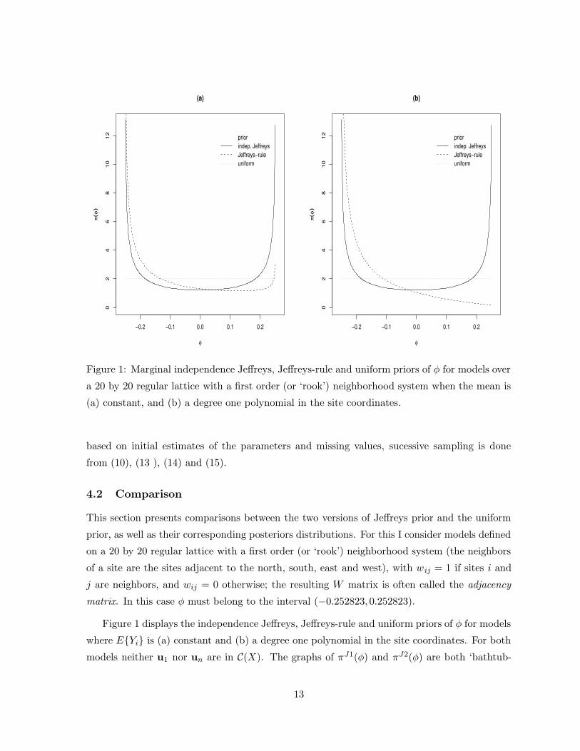
Figure 1: Marginal independence Jeffreys, Jeffreys-rule and uniform priors of φ for models over

a 20 by 20 regular lattice with a first order (or ‘rook’) neighborhood system when the mean is

(a) constant, and (b) a degree one polynomial in the site coordinates.

based on initial estimates of the parameters and missing values, sucessive sampling is done

from (10), (13 ), (14) and (15).

4.2 Comparison

This section presents comparisons between the two versions of Jeffreys prior and the uniform

prior, as well as their corresponding posteriors distributions. For this I consider models defined

on a 20 by 20 regular lattice with a first order (or ‘rook’) neighborhood system (the neighbors

of a site are the sites adjacent to the north, south, east and west), with wij = 1 if sites i and

j are neighbors, and wij = 0 otherwise; the resulting W matrix is often called the adjacency

matrix. In this case φ must belong to the interval (−0.252823, 0.252823).

Figure 1 displays the independence Jeffreys, Jeffreys-rule and uniform priors of φ for models

where EYi is (a) constant and (b) a degree one polynomial in the site coordinates. For both

models neither u1 nor un are in C(X). The graphs of πJ1(φ) and πJ2(φ) are both ‘bathtub-

13

−0.1 0.0 0.1 0.2

05

1015

2025

φ

π(φ | y

)

−0.1 0.0 0.1 0.2

05

1015

2025

φ

π(φ | y

)−0.1 0.0 0.1 0.2

05

1015

2025

3035

φ

π(φ | y

)

−0.1 0.0 0.1 0.2

05

1015

2025

φ

π(φ | y

)

−0.1 0.0 0.1 0.2

05

1015

2025

φ

π(φ | y

)

−0.1 0.0 0.1 0.2

05

1015

2025

3035

φ

π(φ | y

)

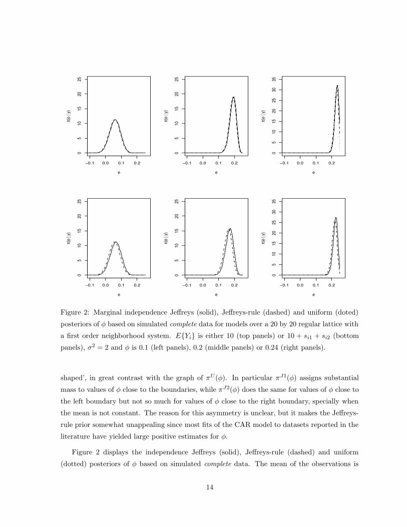
Figure 2: Marginal independence Jeffreys (solid), Jeffreys-rule (dashed) and uniform (doted)

posteriors of φ based on simulated complete data for models over a 20 by 20 regular lattice with

a first order neighborhood system. EYi is either 10 (top panels) or 10 + si1 + si2 (bottom

panels), σ2 = 2 and φ is 0.1 (left panels), 0.2 (middle panels) or 0.24 (right panels).

shaped’, in great contrast with the graph of πU (φ). In particular πJ1(φ) assigns substantial

mass to values of φ close to the boundaries, while πJ2(φ) does the same for values of φ close to

the left boundary but not so much for values of φ close to the right boundary, specially when

the mean is not constant. The reason for this asymmetry is unclear, but it makes the Jeffreys-

rule prior somewhat unappealing since most fits of the CAR model to datasets reported in the

literature have yielded large positive estimates for φ.

Figure 2 displays the independence Jeffreys (solid), Jeffreys-rule (dashed) and uniform

(dotted) posteriors of φ based on simulated complete data. The mean of the observations is

14

−0.1 0.0 0.1 0.2

05

1015

20

φ

π(φ

| yJ)

−0.1 0.0 0.1 0.20

510

1520

φ

π(φ

| yJ)

−0.1 0.0 0.1 0.2

010

2030

40

φ

π(φ

| yJ)

−0.1 0.0 0.1 0.2

05

1015

20

φ

π(φ

| yJ)

−0.1 0.0 0.1 0.2

05

1015

20

φ

π(φ

| yJ)

−0.1 0.0 0.1 0.2

010

2030

40

φ

π(φ

| yJ)

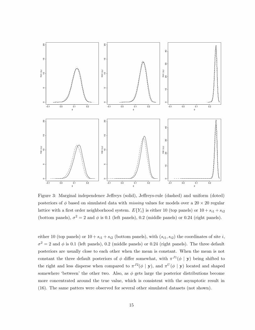
Figure 3: Marginal independence Jeffreys (solid), Jeffreys-rule (dashed) and uniform (doted)

posteriors of φ based on simulated data with missing values for models over a 20 × 20 regular

lattice with a first order neighborhood system. EYi is either 10 (top panels) or 10 + si1 + si2

(bottom panels), σ2 = 2 and φ is 0.1 (left panels), 0.2 (middle panels) or 0.24 (right panels).

either 10 (top panels) or 10 + si1 + si2 (bottom panels), with (si1, si2) the coordinates of site i,

σ2 = 2 and φ is 0.1 (left panels), 0.2 (middle panels) or 0.24 (right panels). The three default

posteriors are usually close to each other when the mean is constant. When the mean is not

constant the three default posteriors of φ differ somewhat, with πJ1(φ | y) being shifted to

the right and less disperse when compared to πJ2(φ | y), and πU (φ | y) located and shaped

somewhere ‘between’ the other two. Also, as φ gets large the posterior distributions become

more concentrated around the true value, which is consistent with the asymptotic result in

(16). The same patters were observed for several other simulated datasets (not shown).

15

Figure 3 displays the independence Jeffreys (solid), Jeffreys-rule (dashed) and uniform

(dotted) posteriors of φ based on simulated data with missing values (obtained by smoothing

the histogram of the posteriors). The data were simulated from the same models as in Figure

2 and later the observations from 40 sites (10%) selected at random were removed. The main

properties and comparative behavior of these posteriors are the same as for the case of complete

data.

5 Further Properties

5.1 Frequentist Properties

This section presents results of a simulation experiment to study some of the frequentist proper-

ties of Bayesian inferences based on the independence Jeffreys, Jeffreys-rule and uniform priors,

as well as those based on maximum likelihood (ML). These properties are often proposed as a

way to evaluate and compare default priors. The focus of interest is on the covariance param-

eters, and the frequentist properties to be considered are frequentist coverage of credible and

confidence intervals, and mean absolute error of estimators. For the Bayesian procedures I use

the 95% equal-tailed credible intervals for σ2 and φ, and the posterior medians as their esti-

mators, all of which are readily obtained from the Monte Carlo output. For the ML procedure

I use the large sample (approximate) 95% confidence intervals given by σ2 ± 1.96( ˆavar(σ2))1/2

and φ ± 1.96( ˆavar(φ))1/2, where σ2 and φ are the ML estimators of σ2 and φ, avar(·) denotes

asymptotic variance and ˆavar(·) indicates that avar(·) is evaluated at the ML estimators. Using

the result on the asymptotic distribution of ML estimators in Mardia and Marshall (1984) and

after some algebra, it follows that the above asymptotic variances are given by

avar(σ2) =2σ4

n(g(φ))2

n∑

i=1

( λi

1 − φλi

)2and avar(φ) =

2

(g(φ))2, (16)

where g(φ) is given by the right hand side of (8).

I consider models defined on a 10 by 10 regular lattice with first order neighborhood system,

and W the adjacency matrix. Then φ must belong to the interval (−0.260554, 0.260554). The

factors to be varied in the experiment are EYi, σ2 and φ. I consider EYi equal to 10 (p = 1)

or 10+si1+si2 (p = 3), σ2 equal to 0.1 or 2, and φ equal to 0.05, 0.12 or 0.25 (negative estimates

of the spatial parameter are rare in practice, if they appear at all, so only positive values of φ

are considered). This setup provides a range of different scenarios in terms of trend, variability

and spatial association. For each of the 12 (2 × 2 × 3) possible scenarios, 1500 datasets were

simulated and for each dataset a posterior sample of the model parameters of size m = 3000

was generated by the algorithm described in Section 4.

16

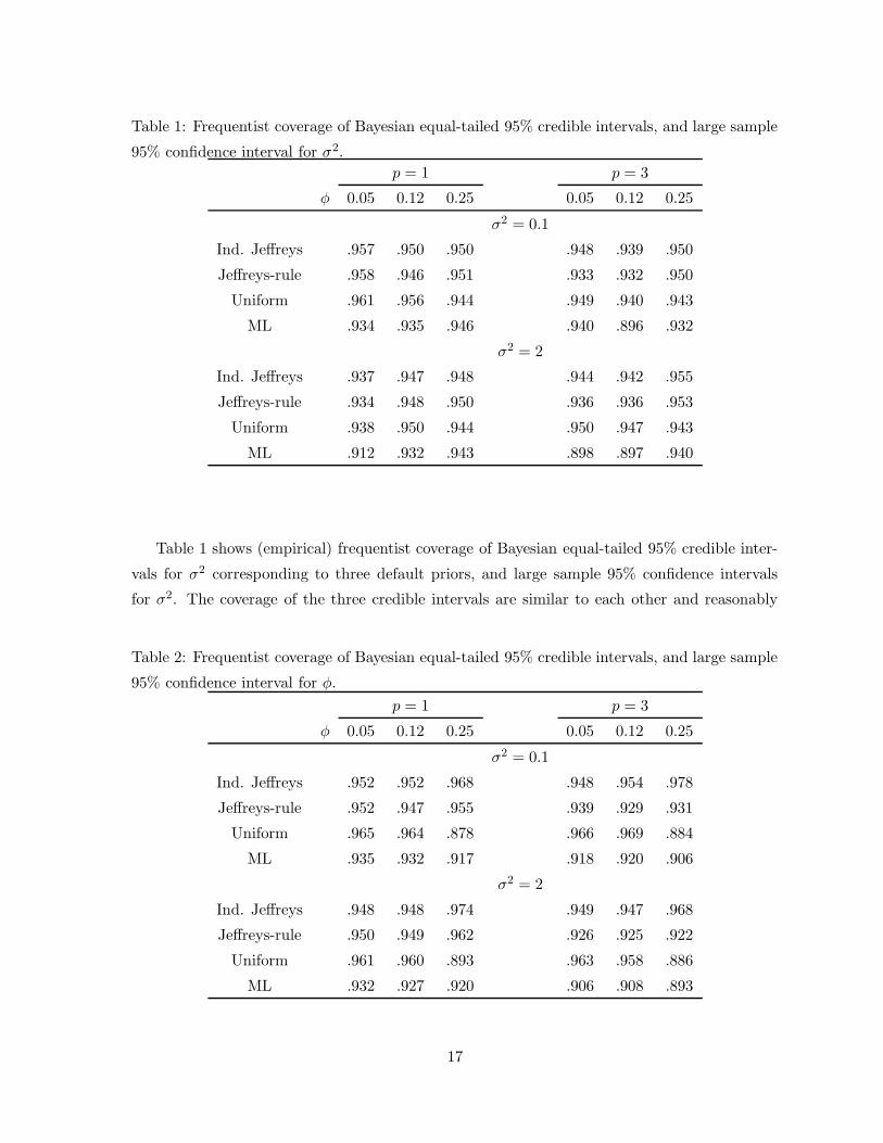
Table 1: Frequentist coverage of Bayesian equal-tailed 95% credible intervals, and large sample

95% confidence interval for σ2.

p = 1 p = 3

φ 0.05 0.12 0.25 0.05 0.12 0.25

σ2 = 0.1

Ind. Jeffreys .957 .950 .950 .948 .939 .950

Jeffreys-rule .958 .946 .951 .933 .932 .950

Uniform .961 .956 .944 .949 .940 .943

ML .934 .935 .946 .940 .896 .932

σ2 = 2

Ind. Jeffreys .937 .947 .948 .944 .942 .955

Jeffreys-rule .934 .948 .950 .936 .936 .953

Uniform .938 .950 .944 .950 .947 .943

ML .912 .932 .943 .898 .897 .940

Table 1 shows (empirical) frequentist coverage of Bayesian equal-tailed 95% credible inter-

vals for σ2 corresponding to three default priors, and large sample 95% confidence intervals

for σ2. The coverage of the three credible intervals are similar to each other and reasonably

Table 2: Frequentist coverage of Bayesian equal-tailed 95% credible intervals, and large sample

95% confidence interval for φ.

p = 1 p = 3

φ 0.05 0.12 0.25 0.05 0.12 0.25

σ2 = 0.1

Ind. Jeffreys .952 .952 .968 .948 .954 .978

Jeffreys-rule .952 .947 .955 .939 .929 .931

Uniform .965 .964 .878 .966 .969 .884

ML .935 .932 .917 .918 .920 .906

σ2 = 2

Ind. Jeffreys .948 .948 .974 .949 .947 .968

Jeffreys-rule .950 .949 .962 .926 .925 .922

Uniform .961 .960 .893 .963 .958 .886

ML .932 .927 .920 .906 .908 .893

17

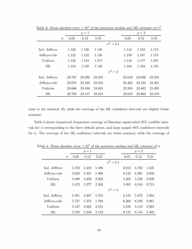
Table 3: Mean absolute error × 102 of the posterior median and ML estimate of σ2.

p = 1 p = 3

φ 0.05 0.12 0.25 0.05 0.12 0.25

σ2 = 0.1

Ind. Jeffreys 1.130 1.136 1.140 1.144 1.183 1.172

Jeffreys-rule 1.132 1.132 1.140 1.156 1.187 1.173

Uniform 1.126 1.134 1.217 1.140 1.177 1.237

ML 1.134 1.130 1.140 1.164 1.194 1.176

σ2 = 2

Ind. Jeffreys 23.737 23.292 23.282 23.043 23.636 23.524

Jeffreys-rule 23.678 23.160 23.310 23.404 23.520 23.461

Uniform 23.666 23.166 24.953 22.950 23.462 25.093

ML 23.702 23.147 23.234 23.610 23.602 23.570

close to the nominal .95, while the coverage of the ML confidence intervals are slightly below

nominal.

Table 2 shows (empirical) frequentist coverage of Bayesian equal-tailed 95% credible inter-

vals for φ corresponding to the three default priors, and large sample 95% confidence intervals

for φ. The coverage of the ML confidence intervals are below nominal, while the coverage of

Table 4: Mean absolute error × 102 of the posterior median and ML estimate of φ.

p = 1 p = 3

φ 0.05 0.12 0.25 0.05 0.12 0.25

σ2 = 0.1

Ind. Jeffreys 5.750 5.410 1.486 6.012 5.756 1.525

Jeffreys-rule 5.632 5.421 1.906 6.134 6.361 2.850

Uniform 5.090 4.856 2.562 5.205 5.120 2.930

ML 5.473 5.277 2.263 5.991 6.310 9.713

σ2 = 2

Ind. Jeffreys 5.761 5.307 1.375 6.125 5.872 1.604

Jeffreys-rule 5.727 5.372 1.760 6.268 6.232 2.961

Uniform 5.127 4.865 2.415 5.316 5.110 2.965

ML 5.570 5.246 2.110 6.127 6.144 3.462

18

the three credible intervals are similar to each other and reasonably close to the nominal .95

under most scenarios, except when φ is large. In this case the coverage of credible intervals

based on the uniform prior are well below nominal.

Tables 3 shows (empirical) mean absolute error (MAE) of the posterior median of σ2 cor-

responding to the three default priors and the MAE of the ML estimator of σ2. The MAEs of

the Bayesian estimators based on the three default priors and the ML estimator are close to

each other under all scenarios.

Tables 4 shows (empirical) MAE of the posterior median of φ corresponding to the three

default priors and the ML estimator of φ. For small or moderate values of φ the MAEs of

the three Bayesian estimators and the ML estimator are close to each other, with the MAE

of the Bayesian estimator based on the uniform prior being slightly smaller than the other

three. On the other hand, for large values of φ the MAE of the Bayesian estimator based

on the independence Jeffreys prior is substantially smaller than the MAEs of the other three

estimators. Also, when the the mean of the observations is not constant the MAE of the

estimator based on the independence Jeffreys prior is smaller than the MAE of the estimator

based on the Jeffreys-rule prior.

In summary, frequentist properties of ML estimators are inferior than those of Bayesian

inferences based on any of the three default priors. More notably, Bayesian inferences based

on the three default priors are reasonably good and similar to each other under most scenarios,

except when the spatial parameter φ is large or the mean of the observations is not constant.

In these cases frequentist properties of Bayesian inferences based on the independence Jeffreys

prior no worse or better than those based on any of the other two default priors in regard to

inference about φ.

5.2 Sensitivity to Design

The proposed Jeffreys priors depend on several features of the selected design, such as sample

size and regression matrix. This section explores how sensitive these default priors are to the

above features.

Sample Size. Consider the models defined over 10 by 10, 20 by 20 and 50 by 50 regular lattices

with first order neighborhood system and W the adjacency matrix. Figure 4(a) displays the

marginal independence Jeffreys priors πJ1(φ) corresponding to the three sample sizes, showing

that they are very close to each other. It should be noted that the domains of πJ1(φ) for the

above three models are not exactly the same, but are quite close. The priors were plotted over

the interval (−0.25, 0.25), the limit of (λ−1n , λ−1

1 ) as n → ∞. The same lack of sensitivity to

19

−0.2 −0.1 0.0 0.1 0.2

02

46

810

12

(a)

φ

π(φ

)

n1004002500

−0.2 −0.1 0.0 0.1 0.20

510

15

(b)

φ

π(φ

)

p136

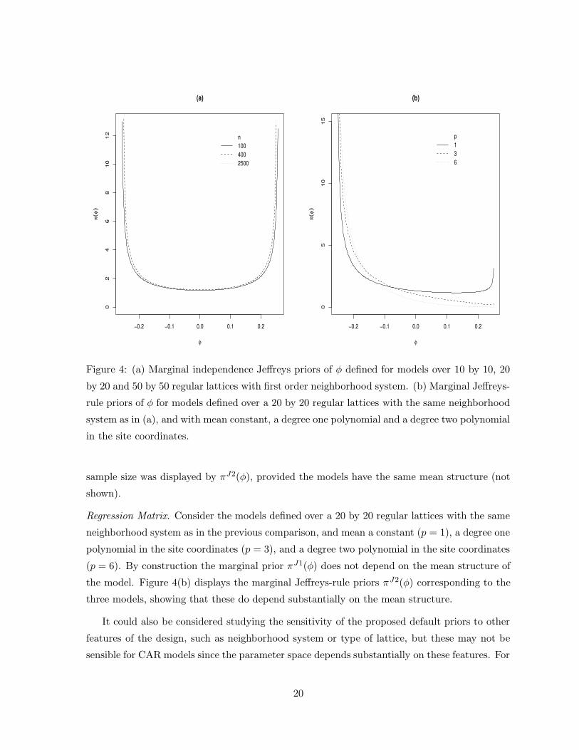
Figure 4: (a) Marginal independence Jeffreys priors of φ defined for models over 10 by 10, 20

by 20 and 50 by 50 regular lattices with first order neighborhood system. (b) Marginal Jeffreys-

rule priors of φ for models defined over a 20 by 20 regular lattices with the same neighborhood

system as in (a), and with mean constant, a degree one polynomial and a degree two polynomial

in the site coordinates.

sample size was displayed by πJ2(φ), provided the models have the same mean structure (not

shown).

Regression Matrix. Consider the models defined over a 20 by 20 regular lattices with the same

neighborhood system as in the previous comparison, and mean a constant (p = 1), a degree one

polynomial in the site coordinates (p = 3), and a degree two polynomial in the site coordinates

(p = 6). By construction the marginal prior πJ1(φ) does not depend on the mean structure of

the model. Figure 4(b) displays the marginal Jeffreys-rule priors πJ2(φ) corresponding to the

three models, showing that these do depend substantially on the mean structure.

It could also be considered studying the sensitivity of the proposed default priors to other

features of the design, such as neighborhood system or type of lattice, but these may not be

sensible for CAR models since the parameter space depends substantially on these features. For

20

0 5 10 15

05

10

15

s1 (meters)

s 2

(me

ters

)

121 112 108 91 68 59 294 50 101 27 71 48 36 71 66 83

108 101 75 83 52 55 50 41 30 47 47 55 75 108

62 80 50 88 77 77 73 50 50 59 57 55 57 38 71

17 52 60 91 166 68 60 32 47 45 34 57 60 64 68

32 48 27 88 116 66 34 62 77 41 23 38 68 68

73 33 60 66 62 143 60 62 80 59 75 57 27 57

55 53 80 80 62 91 71 68 77 104 75 41 33 131 41 37

64 45 62 21 60 38 47 77 73 62 27 44 53 53 52 36

64 28 44 45 60 62 34 47 75 83 71 77 83 73 77 59

59 38 32 55 60 30 41 59 57 71 66 83 85 85 77 83

45 47 48 68 80 44 64 64 68 68 88 116 108 85 91 73

37 41 38 36 19 57 47 131 80 83 80 88 73 73 97 62

31 45 34 66 71 85 80 121 91 136 108 108 80 80 73

55 34 62 41 80 75 101 50 71 91 94 94 91 75 68 59

57 55 66 40 57 68 73 80 71 125 83 66 77 71 47 55

77 59 45 55 59 60 48 68 71 57 60 55 53 57 62 64

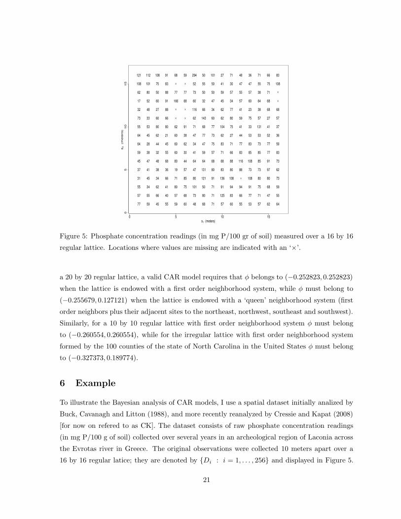
Figure 5: Phosphate concentration readings (in mg P/100 gr of soil) measured over a 16 by 16

regular lattice. Locations where values are missing are indicated with an ‘×’.

a 20 by 20 regular lattice, a valid CAR model requires that φ belongs to (−0.252823, 0.252823)

when the lattice is endowed with a first order neighborhood system, while φ must belong to

(−0.255679, 0.127121) when the lattice is endowed with a ‘queen’ neighborhood system (first

order neighbors plus their adjacent sites to the northeast, northwest, southeast and southwest).

Similarly, for a 10 by 10 regular lattice with first order neighborhood system φ must belong

to (−0.260554, 0.260554), while for the irregular lattice with first order neighborhood system

formed by the 100 counties of the state of North Carolina in the United States φ must belong

to (−0.327373, 0.189774).

6 Example

To illustrate the Bayesian analysis of CAR models, I use a spatial dataset initially analized by

Buck, Cavanagh and Litton (1988), and more recently reanalyzed by Cressie and Kapat (2008)

[for now on refered to as CK]. The dataset consists of raw phosphate concentration readings

(in mg P/100 g of soil) collected over several years in an archeological region of Laconia across

the Evrotas river in Greece. The original observations were collected 10 meters apart over a

16 by 16 regular latice; they are denoted by Di : i = 1, . . . , 256 and displayed in Figure 5.

21

5 10 15

2.02.5

3.03.5

4.0

s1 (meters)

transfo

rmed p

hospha

te

5 10 15

2.02.5

3.03.5

4.0

s2 (meters)

transfo

rmed p

hospha

te

Figure 6: Plots of phosphate concentration readings versus sites coordinates.

A particular feature of this dataset is that there are missing observations at nine sites (marked

with an ‘×’ in Figure 5). In their analysis, CK did not mention how these missing observations

were dealt with when fitting the model, although presumably they were inputed with the mean

(or median) of the observed values at the neighboring sites. The Bayesian analysis below fully

accounts for the uncertainty of the missing values.

CK built a model for this dataset based on exploratory data analysis and some numerical

and graphical diagnostics developed in that paper. I mostly use the model selected by these

authors, except for one difference. The original phosphate concentration readings were trans-

formed as Yi = D1

4

i , i = 1, . . . , 256, to obtain a reponse with distribution close to Gaussian. CK

assumed that EYi = β1 + β2si1 + β3si2, with (si1, si2) the coordinates of site i, but I find no

basis for this choice. There seems to be no apparent relation between the phosphate concen-

tration readings and the sites coordinates, as indicated in Figure 6, so I assume EY = β11

(1 is a vector of ones).

As for the spatial dependence structure, CK modeled these (transformed) data using a

second order neighborhood system, meaning that the neighbors of site i are its first order

neighbors and their first order neighbors (except for site i); the number of neighbors varies

between 5 and 12. Let aij = 1 if sites i and j are neighbors, and aij = 0 otherwise. For the

spatial dependence structure I use the model selected by CK, which they call the autocorrelation

(homogeneous) CAR model. It is assumed that varY = σ2(I256 − φW )−1G, with

G = diag(|N1|−1, . . . , |N256|

−1) and Wij = aij

(

|Nj |/|Ni|)

1

2 ,

where |Ni| the number of neighbors of site i. Finally following the discussion in Section 2.1, I

22

2.5 2.6 2.7 2.8 2.9 3.0 3.1

01

23

45

6

β1

0.4 0.5 0.6 0.7 0.8

02

46

8

σ2

0.060 0.065 0.070 0.075 0.080 0.085 0.090

050

100150

200

φ

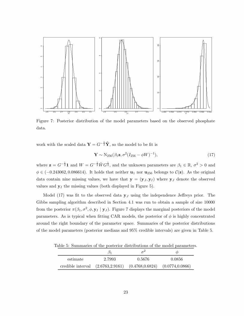
Figure 7: Posterior distribution of the model parameters based on the observed phosphate

data.

work with the scaled data Y = G− 1

2 Y, so the model to be fit is

Y ∼ N256(β1z, σ2(I256 − φW )−1), (17)

where z = G− 1

2 1 and W = G− 1

2 WG1

2 , and the unknown parameters are β1 ∈ R, σ2 > 0 and

φ ∈ (−0.243062, 0.086614). It holds that neither u1 nor u256 belongs to C(z). As the original

data contain nine missing values, we have that y = (yJ ,yI) where yJ denote the observed

values and yI the missing values (both displayed in Figure 5).

Model (17) was fit to the observed data yJ using the independence Jeffreys prior. The

Gibbs sampling algorithm described in Section 4.1 was run to obtain a sample of size 10000

from the posterior π(β1, σ2, φ,yI | yJ). Figure 7 displays the marginal posteriors of the model

parameters. As is typical when fitting CAR models, the posterior of φ is highly concentrated

around the right boundary of the parameter space. Summaries of the posterior distributions

of the model parameters (posterior medians and 95% credible intervals) are given in Table 5.

Table 5: Summaries of the posterior distributions of the model parameters.

β1 σ2 φ

estimate 2.7993 0.5676 0.0856

credible interval (2.6763,2.9161) (0.4768,0.6824) (0.0774,0.0866)

23

Remark 5. A possible caveat in the above analysis is in order. If model (17) is assumed for Y,

then the form of the joint distribution of YJ (the observed values) is unknown, and in particular

it does not follow a CAR model. As a result Proposition 1 and Corollary 1 do not apply in this

case and, strictly speaking, propriety of the posterior of the model parameters is not guaranteed.

Nevertheless, the Monte Carlo output of the above analysis based on the independence Jeffreys

prior was very close to that based on vague proper priors (normal–inverse gamma–uniform),

so the possibility of an improper posterior in the above analysis seems remote.

7 Conclusions

This work derives two versions of Jeffreys priors for CAR models, which provide default (auto-

matic) Bayesian analyses for these models, and obtains properties of Bayesian inferences based

on them. It was found that inferences based on the Jeffreys priors and the uniform prior have

similar frequentist properties under most scenarios, except when strong spatial association is

present. In this case the independence Jeffreys prior displayed a superior performance. So this

prior is the one I recommend, but note that the uniform prior is almost as good and may be

preferred by some due to its simplicity. It was also found that inferences based on ML have

inferior frequentist properties than inferences based on any of the three default priors.

Modeling of non-Gaussian (e.g. count) spatial data is often based on hierarchical models

where CAR models are used to describe (unobserved) latent processes or spatially varying ran-

dom effects. In this case choice of prior for the CAR model parameters has been done more or

less ad hoc, and problems have been reported for their estimation. A tentative possibility to

deal with this issue is to use one of the default priors proposed here, having in mind that this is

not a Jeffreys prior in the hierarchical model context but a reasonably proxy at best. For this

to be feasible, further research is needed to establish propriety of the relevant posterior distri-

bution in the hierarchical model context and to determine inferential properties of procedures

based on such default prior.

24

Appendix

Proof of Lemma 1.

Let X ′X = V TV ′ be the spectral decomposition of X ′X, with V orthogonal, V ′V = V V ′ = Ip,

and T diagonal with positive diagonal elements (since X ′X is positive definite). Then

T− 1

2 V ′(X ′Σ−1φ X)V T− 1

2 = X ′oΣ

−1φ Xo = Ip − φX ′

oWXo,

where

Xo = XV T− 1

2 . (18)

It then holds that X ′oXo = Ip,

|X ′oΣ

−1φ Xo| = |V T− 1

2 |2|X ′Σ−1φ X|, (19)

and rank(X ′oΣ

−1φ Xo) = rank(X ′Σ−1

φ X) since |V T− 1

2 | 6= 0. The cases when u1 ∈ C(X) and

when u1 /∈ C(X) are now considered separately.

Suppose u1 ∈ C(X). In this case u1 = Xoa for some a 6= 0 (since C(X) = C(Xo)), and then

(X ′oΣ

−1φ Xo)a = X ′

o(In − φW )u1 = (1 − φλ1)X′ou1 = (1 − φλn)a,

so (1−φλ1) is an eigenvalue of X ′oΣ

−1φ Xo. Now, for any c ∈ R

p, with ||c|| = 1, and φ ∈ (0, λ−11 )

c′X ′oΣ

−1φ Xoc = 1 − φc′oWco ≥ 1 − φλ1, with co = Xoc,

where the inequality holds by the extremal property of Rayleigh quotient (Schott, 2005 p. 105)

λ1 = max||c||=1

c′Wc = u′1Wu1.

Hence 1 − φλ1 is the smallest eigenvalue of X ′oΣ

−1φ Xo. In addition, 1 − φλ1 must be simple.

Otherwise there would exits at least two orthonormal eigenvectors associated to 1 − φλ1, say

c1 and c2, satisfying

1 − φλ1 = c′i(X′oΣ

−1φ Xo)ci = 1 − φc′oiWcoi, with coi = Xoci, i = 1, 2,

which implies that λ1 = c′oiWcoi, so co1 and co2 are two orthonormal eigenvectors of W

associated with λ1; but this contradicts the fact that λ1 is a simple eigenvalue of W . Finally,

if v1(φ) ≥ . . . ≥ vp−1(φ) > 1 − φλ1 > 0 are the eigenvalues of X ′oΣ

−1φ Xo, it follows from (19)

that for all φ ∈ (0, λ−11 )

|X ′Σ−1φ X| ∝ |X ′

oΣ−1φ Xo|

= (1 − φλ1)

p−1∏

i=1

vi(φ) = O(1 − φλ1) as φ → λ−11 . (20)

25

Suppose now u1 /∈ C(X). In this case it must holds that X ′oΣ

−1

λ−1

1

Xo is nonsingular. Other-

wise, if X ′oΣ

−1λ−1

1

Xo were singular, there is b 6= 0 with ||b|| = 1 for which X ′oWXob = λ1b, so

λ1 is an eigenvalue of X ′oWXo with b as its associated eigenvector. Then

λ1 = b′X ′oWXob = b′

oWbo, with bo = Xob.

By the extremal property of Rayleigh quotient bo is also an eigenvector of W associated with

the eigenvalue λ1. Since λ1 is simple, there is t 6= 0 for which u1 = tbo = X(tV T− 1

2 b), with

tV T− 1

2 b 6= 0, implying that u1 ∈ C(X); but this is a contradiction. From (19) it follows that

X ′Σ−1λ−1

1

X is non-singular and since |X ′Σ−1φ X| is a continuous function of φ, |X ′Σ−1

φ X|−1

2 =

O(1) as φ → λ−11 . This and (20) prove (6).

It is now shown that for every η ∈ Ω, S2λ−1

1

> 0 with probability 1. Let C(X,u1) denote the

subspace of Rn spanned by the columns of X and u1. If y ∈ C(X,u1), then y = Xa + tu1 for

some a ∈ Rp and t ∈ R, and hence X ′Σ−1

λ−1

1

Xa = X ′Σ−1λ−1

1

y. This means that a is a solution to

the (generalized) normal equations, so Xa = X βλ−1

1

and y−Xβλ−1

1

= tu1, which implies that

S2λ−1

1

= 0.

Suppose now that S2λ−1

1

= 0. Since 0 is the smallest eigenvalue of Σ−1λ−1

1

, and is simple with u1

as its associated eigenvector, it follows by the extremal property of the Rayleigh quotient that

y − Xβλ−1

1

= tu1 for some t ∈ R, which implies that y ∈ C(X,u1). Since n ≥ p + 2, C(X,u1)

is a proper subspace of Rn and because Y has an absolutely continuous distribution

P (S2λ−1

1

> 0 | η) = P (Y /∈ C(X,u1) | η) = 1 for every η ∈ Ω.

Since S2φ is a continuous function of φ, it holds with probability 1 that S2

φ = O(1) as φ → λ−11 .

The proofs of the results as φ → λ−1n follow along the same lines.

References

Banerjee, S., Carlin, B. and Gelfand, A. (2004). Hierarchical Modeling and Analysis for Spatial

Data. Chapman & Hall/CRC.

Bapat, R.B. and Raghavan, T.E.S. (1997). Nonnegative Matrices and Applications. Cam-

bridge University Press.

Bell, B.S. and Broemeling, L.D. (2000). A Bayesian Analysis of Spatial Processes With

Application to Disease Mapping. Statistics in Medicine, 19, 957-974.

Berger, J.O., De Oliveira, V. and Sanso, B. (2001). Objective Bayesian Analysis of Spatially

Correlated Data. Journal of the American Statistical Association, 96, 1361-1374.

26

Berger, J.O. and Bernardo, J.M. (1992). On the Development of the Reference Prior Method.

In Bayesian Statistics 4, eds. J.M. Bernardo, J.O. Berger, A.P. Dawid and A.F.M. Smith.

Oxford University Press, pp. 35-60.

Bernardo, J.M (1979). Reference Posterior Distributions for Bayes Inference (with discussion).

Journal of the Royal Statistical Society Ser. B, 41, 113-147.

Besag, J. and Kooperberg, C. (1995). On Conditional and Intrinsic Autoregressions. Biometrika,

82, 733-746.

Buck, C.E., Cavanagh, W.G. and Litton, C.D. (1988). The Spatial Analysis of Site Phosphate

Data. In Computer Applications and Quantitative Methods in Archeology, ed. S.P.Q.

Rahtz, British Archeological Reports, International Series, vol. 446, 151-160.

Case, A.C., Rosen, H.S. and Hines, J.R. (1993). Budget Spillovers and Fiscal Policy Interde-

pendence. Journal of Public Economics, 52, 285-307.

Clayton, D. and Kaldor, J. (1987). Empirical Bayes Estimates of Age-standardized Relative

Risks for use in Disease Mapping. Biometrics, 43, 671-681.

Cressie, N.A.C. (1993). Statistics for Spatial Data (rev. ed.). Wiley.

Cressie, N. and Kapat, P. (2008). Some Diagnostics for Markov Random Fields. Journal of

Computational and Graphical Statistics, 17, 726-749.

Cressie, N., Perrin, O. and Thomas-Agnan, C. (2005). Likelihood-based Estimation for Gaus-

sian MRFs. Statistical Methodology, 2, 1-16.

Cressie, N.A.C. and Chan, N.H. (1989). Spatial Modeling of Regional Variables. Journal of

the American Statistical Association, 84, 393-401.

Gilks, W.R., Best, N.G. and Tan, K.K.C. (1995). Adaptive Rejection Metropolis Sampling

Within Gibbs Sampling. Applied Statistics, 44, 455–472.

Mardia, K.V. and R.J. Marshall (1984). Maximum Likelihood Estimation of Models for

Residual Covariance in Spatial Regression. Biometrika, 71, 135-146.

Militino, A.F., Ugarte, M.D. and Garcia-Reinaldos, L. (2004). Alternative Models for Describ-

ing Spatial Dependence Among Dwelling Selling Prices. Journal of Real Estate Finance

and Economics, 29, 193-209.

27

Pettitt, A.N., Weir, I.S. and Hart, A.G. (2002). A Conditional Autoregressive Gaussian

Process for Irregularly Spaced Multivariate Data with Application to Modelling Large

Sets of Binary Data. Statistics and Computing, 12, 353-367.

Richardson, S., Guihenneuc, C. and Lasserre, V. (1992). Spatial Linear Models with Auto-

correlated Error Structure. The Statistician, 41, 539-557.

Rue, H. and Held, L. (2005). Gaussian Markov Random Fields: Theory and Applications.

Chapman & Hall/CRC.

Schott, J.R. (2005). Matrix Analysis for Statistics, 2nd. ed. Wiley.

Sun, D, Tsutakawa, R.K. and Speckman, P.L. (1999). Posterior Distribution of Hierarchical

Models Using CAR(1) Distributions. Biometrika, 86, 341-350.

28