Mobility Estimation Based on an Autoregressive

Model

Zainab R. Zaidi and Brian L. MarkDept. of Electrical and Computer Engineering

George Mason University

January 9, 2004

Regular paper submission to:IEEE Transactions on Vehicular Technology

∗Corresponding Author: Brian L. Mark

Author Contact Information:

Zainab R. Zaidi Brian L. MarkECE Dept., MS 1G5 ECE Dept., MS 1G5George Mason University George Mason University4400 University Drive 4400 University DriveFairfax, VA 22030 Fairfax, VA 22030tel: 703-993-1602 tel: 703-993-4069fax: 703-993-1601 fax: 703-993-1601e-mail: zzaidi@gmu.edu e-mail: bmark@gmu.edu

1

Abstract

We propose an integrated scheme for estimating the mobility state and model parameters of a user based

on a first-order autoregressive model of mobility that accurately captures the characteristics of realistic

user movements in wireless networks. Estimation of the mobility parameters is performed by applying

the Yule-Walker equations to the training data. Estimation of the mobility state, which consists of the

position, velocity, and acceleration of the mobile station is accomplished via an extended Kalman filter

using measurements from the wireless network. The integration of mobility state and model parameter

estimation results in an efficient and accurate real-time mobility tracking scheme that can be applied in a

variety of wireless networking applications. The mobility estimation scheme can also be used to generate

realistic mobility patterns to drive computer simulations of mobile networks. We validate the proposed

mobility estimation scheme using mobile trajectories collected from drive-test data obtained from a live

cellular network.

Keywords

Mobility model, Geolocation, Autoregressive model, Kalman filter, Yule-Walker equations

I. Introduction

User mobility is a fundamental characteristic of wireless mobile networks that profoundly

impacts network performance. To perform optimally, a wireless network should be designed

to take into account the mobility of the user. In this regard, two issues of fundamental

importance are: 1) the development of suitable models of user mobility to drive realistic

simulation studies of wireless networks and 2) efficient real-time tracking of user mobility to

enable seamless connectivity and quality-of-service in a wireless network. The two issues are

closely interrelated, since accurate real-time tracking of user mobility must be based on a

suitable mobility model that can be used to anticipate the future mobility state of the user.

Conversely, in order to generate realistic mobility patterns for the purpose of simulating

a wireless network, actual mobile trajectories from live networks should be fit to a model

that can capture the salient characteristics of user mobility. Furthermore, accurate mobility

tracking requires that the parameters of the mobility model be matched as closely as possible

to the available data.

2

Some of the more prominent mobility models (cf. [1], [2]) that have been proposed in the

literature include random walk models [3], the random waypoint model [4], Brownian models

[5], Gauss-Markov models [6], and Markov chain models [7]. Such models have the important

feature of simplicity, making them amenable for use in simulation and in some cases analytical

modeling of wireless network behavior. However, some recent work has shown that many of

them do not accurately represent actual user trajectories in real wireless networks [2], [8],

[9], [10]. Consequently, such models may result in misleading characterizations of network

performance. Moreover, such models are not sufficiently rich to enable accurate and precise

real-time mobility tracking.

A linear system model of mobility has been applied to real-time mobility tracking via

Kalman filters [11], [12]. Yang and Wang [13] proposed a joint mobility tracking and hard

handoff initiation scheme based on a similar linear system model. In this model, the mobility

state consists of position, velocity, and acceleration, in contrast to geolocation schemes that

estimate only the position of the mobile. The advantage of maintaining information about

velocity and acceleration is that the underlying model can provide predictive information

about the future location of the mobile. Such predictive mobility information can be crucial

in providing seamless connectivity and quality-of-service by anticipating handoffs or changes

in the mobile environment ahead of time.

The linear system model is capable of capturing realistic user mobility patterns, but speci-

fication of an optimal set of model parameters is not straightforward in general. The general

form of the linear system model does not lend itself to efficient estimation of an optimal

set of model parameters from real mobility data. Typically, the parameters are specified

in an ad hoc manner. Mobility tracking schemes derived from the linear dynamic system

model are accurate as long as the model parameters match the mobility characteristics of the

user. However, the mobility schemes described in [11], [12], [13] cannot adapt to significant

changes in the model parameters over time. Thus, there is a need for a systematic method

for real-time estimation of the mobility model parameters.

3

Autoregressive models are a type of linear system model that have been used to model

mobility in wireless networks. Recognizing the need for more realistic mobility models, a

Gauss-Markov model was presented in [6] for use in conjunction with mobility management

for PCS networks. A similar autoregressive model was used in [14] to perform location

tracking. These models capture correlation effects in the velocity of the mobile, but do

not model the acceleration component of mobility. The Global Position System (GPS) uses

a variety of autoregressive-based models, including one called the PVA (position, velocity,

and acceleration) model that incorporates acceleration [15]. However, the issue of how to

select the appropriate model parameters to represent realistic mobility patterns has not been

treated for these models, nor in the available literature on mobility modeling for wireless

networks (cf. [1], [2]).

We present a real-time mobility estimation scheme based on a first-order autoregressive

model, referred to as the AR-1 model. The AR-1 model is sufficiently simple to enable

real-time mobility tracking, but general enough to accurately capture the characteristics of

realistic mobility patterns in wireless networks. The AR-1 model is a variation of the linear

system model and is more general than the autoregressive models proposed earlier in [14],

[6]. An important feature of the AR-1 model is that the parameters of the model can be

determined in an optimal way (i.e., in the sense of minimum mean squared error) via the

Yule-Walker equations. This is not possible with the linear system model of mobility used

in [11], [12], [13].

Our mobility estimation scheme integrates optimal parameter estimation via the Yule-

Walker equations with mobility state estimation using Kalman filtering. The mobility track-

ing schemes proposed earlier do not incorporate a method to estimate the model parameters

based on training data. In such tracking schemes, the model parameters are typically de-

termined in an ad hoc manner. An improper choice of the model parameters can result in

suboptimal mobility tracking. Moreover, mobility tracking without parameter estimation

can be especially problematic if the mobility characteristics change over time, necessitating

4

a change in the model parameters. The integrated mobility estimation scheme can adapt to

changes in the mobility characteristics over time, since the model parameters are continu-

ously re-estimated using new observation data.

The mobility estimation scheme can be used to obtain mobility parameters from real

mobility data that can subsequently be used to generate representative mobility patterns

from the AR-1 model for simulation purposes. We applied the mobility estimation scheme

to obtain AR-1 model parameters from mobility data taken from a wireless network. The

importance of the mobility model in simulations of network performance has been pointed

out by a number of authors [1], [2]. Nevertheless, the existing works related to mobility

modeling have not considered the problem of matching the model parameters to actual

mobility data. Our numerical results using drive test data show that the AR-1 model can

accurately model realistic mobility patterns. Without a systematic approach to parameter

estimation, the existing mobility models cannot make a similar claim.

The present paper shows how to simultaneously estimate both the mobility model param-

eters and the mobility state of a mobile user based on a first-order autoregressive model.

The work contributes to the inter-related issues of realistic mobility modeling and real-time

mobility tracking for wireless networks. The remainder of the paper is organized as follows.

Section II motivates the AR-1 mobility model and specifies the model in detail. We point out

the differences between the AR-1 model and other autoregressive-type mobility models that

have appeared in the literature. A procedure for estimating the AR-1 model parameters via

the Yule-Walker equations is developed in section III. The parameter estimation procedure

is one component of an integrated scheme for real-time mobility estimation. Section IV dis-

cusses the second component of mobility state estimation via Kalman filtering using various

types of signal measurements as observation data. Section V presents a detailed validation

of the AR-1 mobility model using drive test data collected from the field. Finally, section VI

concludes the paper.

5

II. AR-1 Mobility Model

In the AR-1 model, the mobile unit’s state at time n is defined by a (column) vector1

sn = [xn, xn, xn, yn, yn, yn]′, (1)

where xn and yn specify the position, xn and yn specify the velocity, and xn and yn specify

the acceleration of a mobile node in the x and y directions in a two-dimensional grid. If

mobility state information is needed in three dimensions, the sn vector can be augmented

by [zn, zn, zn]′, where the vector elements represent position, velocity, and acceleration in the

z-dimension.

The AR-1 model for the mobility state sn is given as follows:

sn+1 = Asn + wn, (2)

where A is a 6× 6 transformation matrix, the vector wn is a 6× 1 discrete-time zero mean,

white Gaussian process with autocorrelation function Rw(k) = δkQ, where δ0 = 1 and δk = 0

when k 6= 0. The matrix Q is the covariance matrix of wn.

Comparing the state equation (2) with that of the linear system model discussed in [11],

[12], the linear system model includes an extra term Bun, where B is 6 × 2 matrix and

un is a vector of two independent semi-Markov discrete command processes that drive the

acceleration of the model in the two-dimensional plane. In the linear system model of [11],

[12], the matrices A and B have special forms that depend only on the sampling interval T

and a parameter α. The command process un must be specified by a set of discrete command

levels, a transition probability matrix, and probability distributions for the durations in each

command level. An outstanding issue is how to specify an appropriate set of parameters for

the linear system model.

In the AR-1 model, the matrix A and the covariance matrix Q are completely general.

In our approach, the appropriate values for the matrix A and the covariance matrix Q can

1The notation ′ indicates the matrix transpose operator.

6

be estimated based on training data using the Yule-Walker equations (see section III). This

allows the model to accurately characterize a wide class of mobility patterns. Our numerical

results show that the AR-1 model can accurately represent realistic mobile trajectories (see

section V).

The AR-1 model is more general than the Gauss-Markov model proposed in [6], which

is a type of autoregressive model. In the Gauss-Markov model of [6], the mobility state

consists of position, velocity, and direction, but does not explicitly represent acceleration.

A key feature of the Gauss-Markov model with respect to simpler mobility models is that

correlation between velocity states is explicitly modeled via a gain parameter α. A similar

model was used in [14] as the basis for a location tracking scheme. The AR-1 model captures

not only correlation between velocity states, but correlation between acceleration states.

Since no explicit form is assumed for the A matrix, correlations among position, velocity,

and acceleration can also be captured. The AR-1 model differs from the models of [14], [6]

in that acceleration is explicitly modeled for the purpose of mobility prediction.

The AR-1 model defined by (2) can also provide predictive information. If the state

information or estimate sn at any given time n is available, it is possible to predict the

mobility state at any time n+m in the future. The optimal predicted state sn+m of a mobile

node in the minimum mean-squared error (MMSE) sense, given the state estimate at time

n, is

sn+m = E[sn+m|sn] = Amsn. (3)

The covariance matrix for the predicted mobility state at time n+m, denoted Mn+m = Cov[sn+m],

is given by

Mn+m = AmMnA′m + Σm−1l=0 Am−1−lQA′m−1−l, (4)

where Mn = Cov[sn].

The predicted mobility state can be used to provide a “handoff pre-trigger” incorporated

in IP mobility protocols discussed in [16], [17] to provide transparent network layer mobility

7

management. In ad hoc networks, mobility prediction can be used in predicting link avail-

ability in future to improve routing performance by selecting stable routes. Such anticipatory

resource allocation schemes are not possible with existing geolocation systems, which track

only the current location of the mobile.

According to Bettstetter’s nomenclature for mobility models [1], the AR-1 model may be

classified as a microscopic mobility model. A microscopic model describes the movement, i.e.,

position, velocity etc., of an individual vehicle or person as opposed to a model describing

group behavior such as the fluid flow model, group mobility model [18], family of gravity

models [19], map or activity based models [20], [21], etc. Such composite mobility models

use microscopic models as basic building blocks (cf. [2]).

III. Mobility Parameter Estimation

The AR-1 mobility model is completely specified by the transition matrix A and the

covariance matrix Q of the noise. Using the Yule-Walker equations [22], an estimate of A,

denoted A(n), where n specifies the amount of training data available, can be found from the

mobility state data s1, · · · , sn as follows:

A(n) = R(n)s (1)R(n)

s (0)−1, (5)

where

R(n)s (1) =

1

n− 2

n−1∑i=1

sis′i+1, R(n)

s (0) =1

n− 1

n∑i=1

sis′i. (6)

The estimator A(n) is a Minimum Mean Squared Error (MMSE) estimator and can be directly

derived from the orthogonality principle as given below:

E[(sn − A(n)sn−1)sn−1] = 0. (7)

The noise covariance matrix Q(n) is estimated using the residual estimation error, ei ,

si − A(i)si−1, as follows:

Q(n) =1

n− 1

n∑i=1

eie′i. (8)

8

��������

������ ���

��������

��� ����

�� ���

����� ��������

Fig. 1. Integrated mobility state and parameter estimator.

An extended Kalman filter, described in section IV-B, is used to generate the mobility

state estimates sn from the wireless measurements on, which also are discussed in section

IV-A, at time n. The state estimates sn are used to re-estimate the model parameters at

time n. The recursive model parameter estimator is given below.

Recursive parameter estimation (time n):

1. R(n)s (0) = 1

n−1

((n− 2)R

(n−1)s (0) + sns′n

)

2. R(n)s (1) = 1

n−2

((n− 3)R

(n−1)s (1) + sn−1s

′n

)

3. A(n) = R(n)s (1)R

(n)s (0)−1

4. en = sn − A(n)sn−1

5. Q(n) = 1n−1

((n− 2)Q(n−1) + ene′n

)

We have assumed that a sufficient amount of training data is available to initialize R(0)s (0)

and R(0)s (1). In our numerical experiments, we have found that a training block containing

only a few data points is sufficient to initialize the estimator.

IV. Mobility State Estimation

The integrated mobility estimator, as shown in Fig. 1, consists of a mobility state estimator

and a model parameter estimator as described in section III. In this section, we discuss

the estimation of mobility state from signal measurements typically available in wireless

9

networks, i.e., received signal strength indicators (RSSI) or time of arrival (TOA). Three

independent signal measurements of either kind can be applied as observations to an extended

Kalman filter in order to estimate the mobility state of a user.

A. Observation Data in Wireless Networks

To perform mobility state estimation, we assume that either RSSI or TOA measurements

from at least three base stations are available. We remark that the angle of arrival (AOA) of

the mobile’s signal at multiple base stations is often used for location tracking [23], [24], [25],

[26]. The AOA is typically estimated using antenna arrays at the base station. However,

AOA information is not suitable for use in conjunction with an extended Kalman filter, since

the AOA measurements are non-continuous functions of mobility state that are generally not

differentiable. Another measurement used to locate the mobile callers is the time difference

of arrival (TDOA) of the signals from two base stations [23], [27], [28], [29], [30]. However,

calculation of the TDOA requires time synchronization of the base stations. Moreover, when

three base stations are used to provide TDOA measurements, there is often more than one

solution and, as observed in [23], [31], there is no way to determine the correct solution

without the help of additional information, e.g., additional TOA measurements as suggested

by [31].

A.1 Pilot Signal Strengths (RSSI)

In a wireless cellular network, the distance between the mobile and a reachable base station

can be inferred from the RSSI or signal strength of the pilot signal from the base station.

Pilot signal strengths are more readily available in wireless networks than TOA, TDOA, and

AOA measurements, for which extra infrastructure is needed to collect useful data. The

RSSI, measured in dB, received at the mobile unit from the base station with coordinates

(ai, bi) at time n can be modeled as follows [32]:

pn,i = κi − 10γ log(dn,i) + ψn,i, (9)

10

where κi is a constant determined by the transmitted power, antenna height, wavelength,

and gain of the base station i, γ is a slope index (typically γ is between 2− 5), ψn,i is a zero

mean, stationary Gaussian process with standard deviation σψ typically from 4− 8 dB, and

dn,i is the distance between the mobile node and base station i:

dn,i =√

(xn − ai)2 + (yn − bi)2. (10)

Distance measurements to three independent base stations are sufficient to locate the

mobile unit in the two-dimensional plane. For mobility estimation based on RSSI informa-

tion, we construct an observation vector consisting of the three largest RSSI measurements,

denoted by pn,1, pn,2, pn,3, as follows:

on = (pn,1, pn,2, pn,3)′ = h1(sn) + ψn, (11)

where ψn = (ψn,1, ψn,2, ψn,3)′ and

h1(sn) = κ− 10γ log(dn), (12)

where κ = (κ1, κ2, κ3)′ and dn = (dn,1, dn,2, dn,3)

′. The covariance matrix of ψn is given by

Rψ = σ2ψI3.

A.2 Time of Arrival (TOA)

Time-based methods of geolocation using TOA and TDOA measurements rely on accurate

estimates of the time of arrival of the signals received at several base stations from the mobile

station or at the mobile station from several base stations [23], [27]. Several approaches have

been developed for estimation of these parameters from received signals such as code tracking

and acquisition in spread spectrum systems using delay-locked loop (DLL) or tau-dither loop

as described in [23]. In the presence of measurement noise, the time delay estimate of the

signal τn,i, from base station i measured at the mobile station, at time instant n using DLL

is given by

τn,i = dn,i/c + ηn,i, (13)

11

where dn,i is given in (10), c is the speed of light, and ηn,i is the zero mean measurement

noise with typical variance of ση = 1 µs [33].

As in the case of pilot signal strengths, three TOA measurements to neighboring base

stations are sufficient for mobility state estimation. The observation vector for TOA-based

mobility estimation consists of the three TOAs, denoted by τn,1, τn,2, τn,3, is given as follows:

on = (τn,1, τn,2, τn,3)′ = h2(sn) + ηn, (14)

where ηn = (ηn,1, ηn,2, ηn,3)′ and

h2(sn) = dn/c, (15)

where dn = (dn,1, dn,2, dn,3)′. The covariance matrix of the measurement noise η is denoted

by Rη = σ2ηI3.

B. Mobility State Estimation

The general observation or measurement equation in a wireless environment is written as

follows, generalizing (11) and (14):

on = h(sn) + ρn, (16)

where

h(sn) =

h1(sn), for RSSI,

h2(sn), for TOA.

and

ρn =

ψn, for RSSI,

ηn, for TOA.

To apply the extended Kalman filter for state estimation the observations are linearized

as follows:

on = h(s∗n) + Hn∆sn + ρn,

12

where s∗n is the nominal or reference vector and ∆sn = sn− s∗n is the difference between the

true and nominal state vectors. In the extended Kalman filter (cf. [15]), the nominal vector

is obtained from the estimated state trajectory sn, i.e., s∗n = sn. The matrix Hn is given by

Hn =∂h

∂s|s=sn (17)

The matrix Hn for each type of measurement is given in the Appendix.

The steps in the extended Kalman filter are given as follows (cf. [15]):

Initialization:

1. s0|−1 = E(s0)

2. M0|−1 = Cov(s0)

Recursive estimation (time n):

1. Hn = ∂h∂s|s=sn

2. Kn = Mn|n−1H′n(HnMn|n−1H

′n + Rρ)

−1

3. sn|n = sn|n−1 + Kn(on − h(sn|n−1)) [Correction step]

4. sn+1|n = Asn|n [Prediction step]

5. Mn|n = (I −KnHn)Mn|n−1(I −KnHn)′ −KnRρK′n

6. Mn+1|n = AMn|nA′ + Q

Here, Mi|j = Cov(si|j), i = n, j ∈ {n, n− 1}, Kn is the Kalman gain matrix and Rρ is either

Rψ or Rη depending on the type of measurements used to perform the estimation.

V. Numerical Results

A. Data Collection

An Agilent drive test system E7473A was used to collect data over a CDMA air inter-

face. A typical data collection system includes a digital RF receiver, a CDMA phone, a

computer, a GPS receiver, and antennas [34]. The Agilent Technologies E7473A drive test

13

system was used to obtain RF coverage and service performance measurements for wireless

communications networks that use IS-95 and J-STD-008 technologies.

The data of interest, collected from the drive test, consisted of latitude and longitude values

at pre-defined measurement time intervals. The most commonly used coordinate system is

the latitude, longitude, and height system. The prime meridian and the equator are the

reference planes used to define latitude and longitude. The coordinates are designated in

the Degree-Minute-Second (DMS) format which can be converted into decimal format using

the following equation:

Decimal = Degrees +Minutes

60+

Seconds

3600. (18)

The geodetic latitude (there are many other defined latitudes) of a point is the angle from

the equatorial plane to the vertical direction of a line normal to the reference ellipsoid. The

geodetic longitude of a point is the angle between the reference plane and a plane passing

through the point, both planes being perpendicular to the equatorial plane.

TABLE I

Sample drive test data.

Longitude Latitude Pilot ID Time

-76.60 39.31 128 36:42.0

-76.60 39.31 108 36:42.0

-76.60 39.31 292 36:42.0

Sample data from the drive test is given in Table I. The GPS latitude and longitude

information of corresponding pilot signal identifiers was collected. The data collected from

the drive test can be converted from the decimal format (18) to two-dimensional cartesian

coordinates (x, y). The resultant coordinates correspond to a local coordinate system with

reference (Lat0, Long0) as the latitude and longitude, in decimal format, of the origin (0, 0)

14

of the local coordinate system. The x and y coordinates are given by

x = 6378137π cos Lat0

180(Long0 − Long) (19)

y = 6378137π

180(Lat− Lat0) (20)

where Lat and Long are the GPS latitude and longitude in decimal format, respectively,

calculated using (18).

B. Validation of AR-1 Model

Using the drive test method, we collected three sets of data containing more than 1200

sample points each. One set of data was collected from a sub-urban area while another test

was performed in a downtown city environment with an orthogonal street layout. The last

test was carried out by a walking subject in the Fairfax campus of George Mason University

(GMU). As given in the previous section, the drive test records the position of the mobile

user using GPS. However, velocity and acceleration can be computed using finite differences

of the position coordinates.

For each data set, training samples of the first 600 data points were used to estimate the

model parameters as given in section III. Figs. 2, 3, and 4 show the performance of the AR-1

model with respect to the real trajectories in suburban, urban, and campus environments,

respectively. The computations and plots were generated using MATLAB. Fig. 2 shows that

the AR-1 model performed very well in the suburban environment where the trajectory was

smoother. The model also did well in the city environment as shown in Fig. 3 even for the

trajectory data beyond the first 600 samples used for training. In both of these cases the

users were in cars driving at typical in-town speeds. Fig. 4 shows that the AR-1 model was

equally effective in modeling the movements of a pedestrian. Our results have validated

that the AR-1 model is capable of accurately representing a wide range of realistic mobile

trajectories.

To validate the adequacy of the AR-1 model in a more quantitative manner, we use the

15

−4000 −3000 −2000 −1000 0 1000 2000−3000

−2000

−1000

0

1000

2000

3000

x coordinate (m)

y co

ordi

nate

(m

)

Actual trajectory and model projection

actualmodel

Fig. 2. Actual and model trajectories for suburban area, driving scenario.

multiple coefficient of determination, denoted R2, and defined by (cf. [35], [36]):

R2 = 1− Σ(si − si)

Σ(si − s), (21)

where si is the actual ith data point (x and y), si is its estimated value from the model, and s

is the sample mean of the actual data. The value of R2 lies in the interval [0, 1]. A value of R2

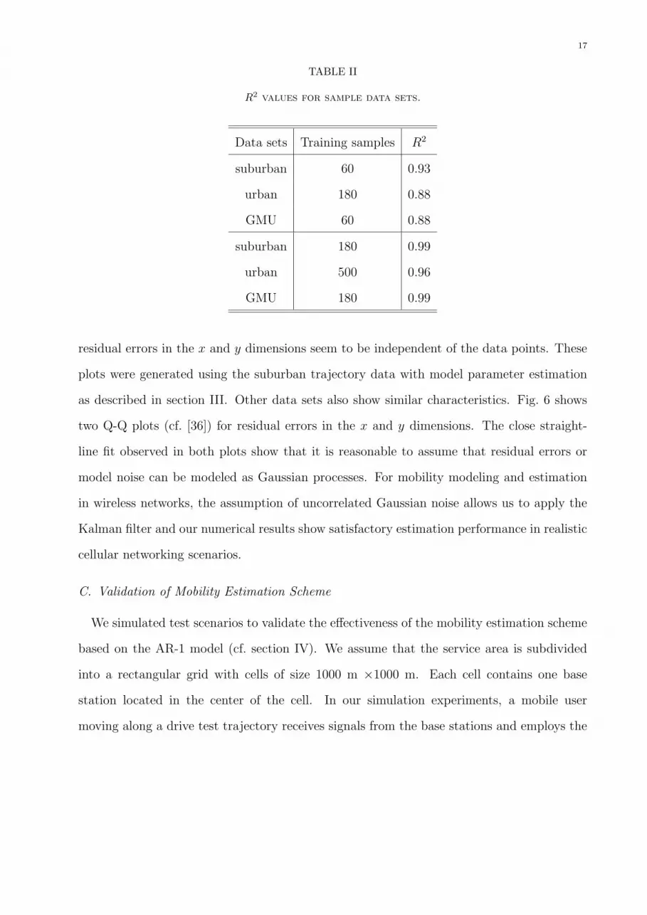
close to 1 indicates a strong model fit. Table II shows the R2 values for the two data sets for

different amounts of training data. Increasing the amount of training data results in better

R2 values. The table shows that AR-1 model captures real mobility scenarios accurately

given a reasonable number of training samples. We also found that using a second-order

autoregressive model did not improve the performance of the model.

The noise term in the AR-1 model is assumed to be zero mean uncorrelated Gaussian

noise. To check the validity of this assumption, we use residual error analysis (cf. [36]). The

residual error for a data point si is defined as ei = si− si. The plots in Fig. 5 show that the

16

1 1.1 1.2 1.3 1.4 1.5 1.6 1.7

x 104

0.95

1

1.05

1.1

1.15

1.2

1.25

1.3

1.35x 10

4

actualmodel

Fig. 3. Actual and model trajectories for urban area, driving scenario.

−100 0 100 200 300 400 500−200

−100

0

100

200

300

400

500

actualmodel

Fig. 4. Actual and model trajectories for GMU, walking scenario.

17

TABLE II

R2 values for sample data sets.

Data sets Training samples R2

suburban 60 0.93

urban 180 0.88

GMU 60 0.88

suburban 180 0.99

urban 500 0.96

GMU 180 0.99

residual errors in the x and y dimensions seem to be independent of the data points. These

plots were generated using the suburban trajectory data with model parameter estimation

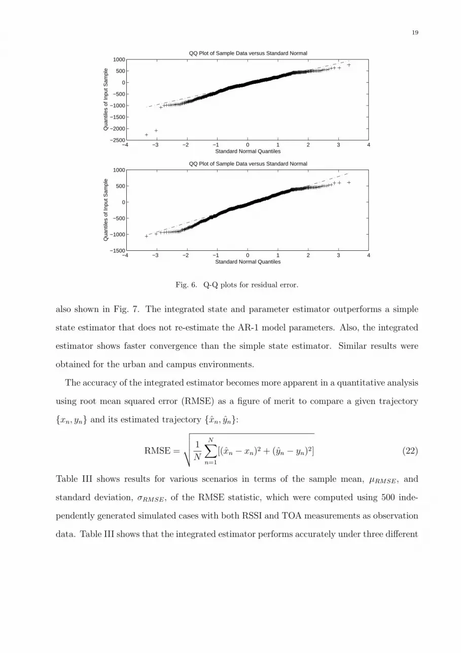
as described in section III. Other data sets also show similar characteristics. Fig. 6 shows

two Q-Q plots (cf. [36]) for residual errors in the x and y dimensions. The close straight-

line fit observed in both plots show that it is reasonable to assume that residual errors or

model noise can be modeled as Gaussian processes. For mobility modeling and estimation

in wireless networks, the assumption of uncorrelated Gaussian noise allows us to apply the

Kalman filter and our numerical results show satisfactory estimation performance in realistic

cellular networking scenarios.

C. Validation of Mobility Estimation Scheme

We simulated test scenarios to validate the effectiveness of the mobility estimation scheme

based on the AR-1 model (cf. section IV). We assume that the service area is subdivided

into a rectangular grid with cells of size 1000 m ×1000 m. Each cell contains one base

station located in the center of the cell. In our simulation experiments, a mobile user

moving along a drive test trajectory receives signals from the base stations and employs the

18

−4000 −3000 −2000 −1000 0 1000 2000−250

−200

−150

−100

−50

0

50

100Residual error vs. data points

x

resi

dual

err

or

−3000 −2000 −1000 0 1000 2000 3000−1000

−500

0

500

1000

y

resi

dual

err

or

Fig. 5. Independence of residual error.

integrated mobility estimator to determine the mobility state as well as the parameters of

the underlying AR-1 model.

The received signals provide two kinds of measurements, i.e., RSSI and TOA. Pilot signal

strengths are generated using (9) and TOA measurements are generated using (13). The

parameter κ is assumed to be zero for all base stations and γ is selected to be 5. Typical values

for the shadowing noise standard deviation, i.e., σφ, range from 4 − 8 dB. The shadowing

standard deviation is taken as 6 dB. The error noise in the TOA measurements is assumed

to be a white Gaussian processes with a standard deviation of ση ≈ 1 µs [33]. A training set

containing 300 data points is used to initialize the AR model.

A representative result from applying the mobility estimator in a suburban area simulation

environment is shown in Fig. 7. The figure shows that the integrated mobility estimator

efficiently computes the mobility model parameters and accurately tracks the mobile. The

estimation results from a simple estimator incorporating extended Kalman filter only are

19

−4 −3 −2 −1 0 1 2 3 4−2500

−2000

−1500

−1000

−500

0

500

1000

Standard Normal Quantiles

Qua

ntile

s of

Inpu

t Sam

ple

QQ Plot of Sample Data versus Standard Normal

−4 −3 −2 −1 0 1 2 3 4−1500

−1000

−500

0

500

1000

Standard Normal Quantiles

Qua

ntile

s of

Inpu

t Sam

ple

QQ Plot of Sample Data versus Standard Normal

Fig. 6. Q-Q plots for residual error.

also shown in Fig. 7. The integrated state and parameter estimator outperforms a simple

state estimator that does not re-estimate the AR-1 model parameters. Also, the integrated

estimator shows faster convergence than the simple state estimator. Similar results were

obtained for the urban and campus environments.

The accuracy of the integrated estimator becomes more apparent in a quantitative analysis

using root mean squared error (RMSE) as a figure of merit to compare a given trajectory

{xn, yn} and its estimated trajectory {xn, yn}:

RMSE =

√√√√ 1

N

N∑n=1

[(xn − xn)2 + (yn − yn)2] (22)

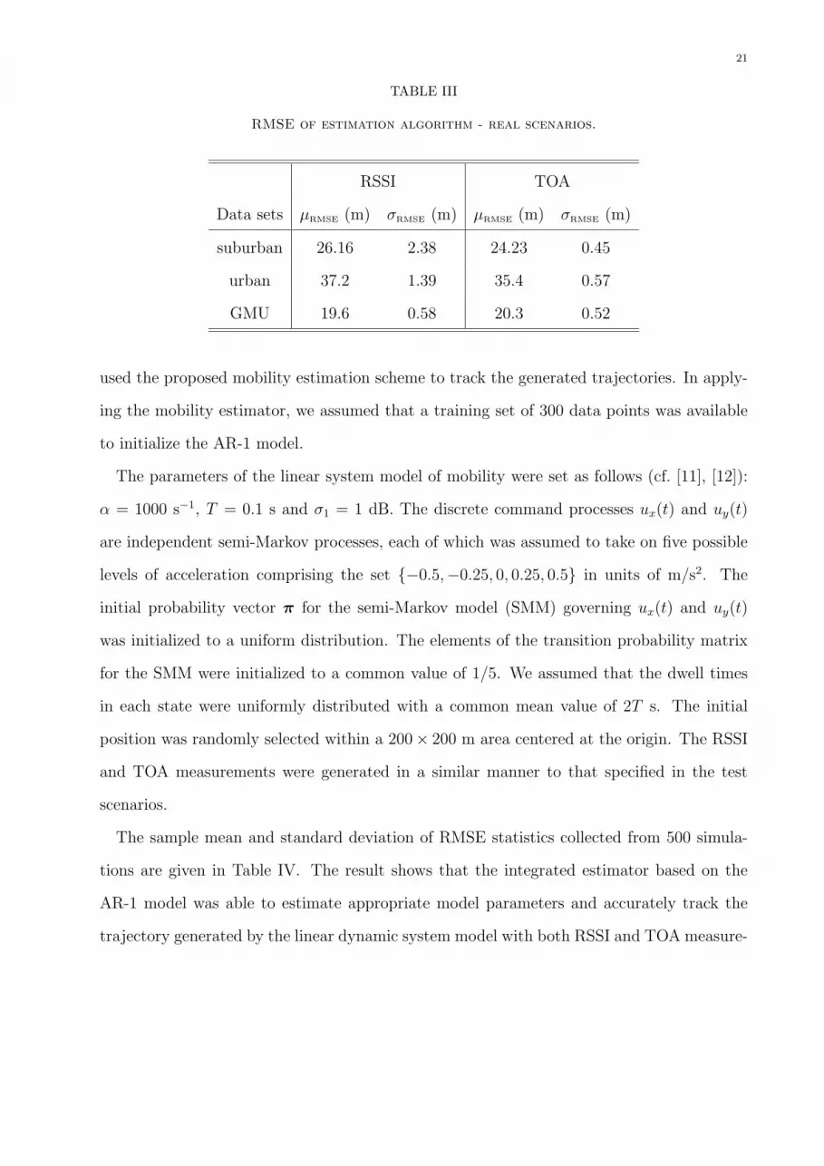
Table III shows results for various scenarios in terms of the sample mean, µRMSE, and

standard deviation, σRMSE, of the RMSE statistic, which were computed using 500 inde-

pendently generated simulated cases with both RSSI and TOA measurements as observation

data. Table III shows that the integrated estimator performs accurately under three different

20

−4000 −3000 −2000 −1000 0 1000 2000−3000

−2000

−1000

0

1000

2000

3000

x coordinate

y co

ordi

nate

Trajectory Estimation

Actualstate+parameter estimationstate estimation

Fig. 7. Comparative performance of integrated estimator for suburban environment.

mobility scenarios. The estimation error in an urban environment was mostly due to the

model parameter estimation. A larger training set yielded better parameter initialization

and hence better performance. Moreover, for lower values of the shadowing noise variance,

the estimation results were even better. It was observed that the use of RSSI and TOA

measurements have similar performance for the given observation parameters in all three

test environments. The difference in performance depends on the accuracy with which the

signal measurements are collected, especially in the case of TOA, and on the accuracy of the

assumed lognormal signal propagation model in the case of RSSI.

D. Comparison with Other Mobility Models

The AR-1 model can accurately represent trajectories generated by other stochastic mo-

bility models. We generated trajectories, containing more than 1000 data points, using the

linear dynamic system model [11], [12] and the random waypoint model [4], [37]. We then

21

TABLE III

RMSE of estimation algorithm - real scenarios.

RSSI TOA

Data sets µRMSE (m) σRMSE (m) µRMSE (m) σRMSE (m)

suburban 26.16 2.38 24.23 0.45

urban 37.2 1.39 35.4 0.57

GMU 19.6 0.58 20.3 0.52

used the proposed mobility estimation scheme to track the generated trajectories. In apply-

ing the mobility estimator, we assumed that a training set of 300 data points was available

to initialize the AR-1 model.

The parameters of the linear system model of mobility were set as follows (cf. [11], [12]):

α = 1000 s−1, T = 0.1 s and σ1 = 1 dB. The discrete command processes ux(t) and uy(t)

are independent semi-Markov processes, each of which was assumed to take on five possible

levels of acceleration comprising the set {−0.5,−0.25, 0, 0.25, 0.5} in units of m/s2. The

initial probability vector π for the semi-Markov model (SMM) governing ux(t) and uy(t)

was initialized to a uniform distribution. The elements of the transition probability matrix

for the SMM were initialized to a common value of 1/5. We assumed that the dwell times

in each state were uniformly distributed with a common mean value of 2T s. The initial

position was randomly selected within a 200× 200 m area centered at the origin. The RSSI

and TOA measurements were generated in a similar manner to that specified in the test

scenarios.

The sample mean and standard deviation of RMSE statistics collected from 500 simula-

tions are given in Table IV. The result shows that the integrated estimator based on the

AR-1 model was able to estimate appropriate model parameters and accurately track the

trajectory generated by the linear dynamic system model with both RSSI and TOA measure-

22

ments. The noise in the linear dynamic system model is correlated since it is a combination

of a semi-Markov process and a white Gaussian process. An interesting observation is that

the AR-1 model with the assumption of uncorrelated noise closely approximates the linear

system model.

We also generated trajectories using the random waypoint model and applied our pro-

posed integrated mobility estimator. The trajectories were generated within an area of

2000× 2000 m, which is centered at the origin. The speed of the mobile unit was uniformly

distributed in the interval [0 60] m/s2 and the mean pause time was assumed to be 1 s.

The random waypoint model tends to generate trajectories with sharp turns, quite different

from realistic mobility patterns. Nevertheless, the integrated mobility estimator was able

to accurately track the trajectory and compute the MMSE parameter values for the AR-1

model (see Table IV).

TABLE IV

RMSE of estimation algorithm - stochastic models.

RSSI TOA

Models µRMSE (m) σRMSE (m) µRMSE (m) σRMSE (m)

Linear system 10.2 7.77 9.86 4.7

Random waypoint 20.1 3.2 20.8 1.3

Our results confirm that the integrated mobility estimator based on the AR-1 model is

indeed a general, efficient and effective scheme to track mobile users in real-time and is also

a useful tool to generate realistic mobility patterns for simulation environments.

VI. Conclusion

We developed an integrated scheme for jointly estimating the mobility parameters and

state of a mobile user in real-time using RSSI or TOA measurements from a wireless network.

23

The mobility estimation scheme was based on a first-order autoregressive model, the AR-

1 model, that allows efficient estimation of the model parameters. The AR-1 model is

relatively simple, yet provides a more accurate representation of realistic mobility patterns

than existing mobility models. Simpler stochastic mobility models such as those based

on random walks or similar types of processes cannot faithfully represent the microscopic

movements of mobile user trajectories. The proposed mobility estimation scheme based on

the AR-1 model provides a viable solution to the two important issues of realistic mobility

modeling and real-time mobility tracking for wireless networks.

The AR-1 mobility model and estimation scheme were validated using three sets of real

data from a CDMA network in urban, suburban, and campus areas. A quantitative analysis

was provided to establish the adequacy of the AR-1 model for realistic networking environ-

ments. Numerical results showed that the integrated parameter and state estimation scheme

performed well using various types of measurement data obtained from typical wireless net-

working environments.

The mobility estimation scheme can be used to enable mobility-aware applications, which

can improve performance or provide new services in wireless networks. In cellular networks,

for example, the mobility estimation scheme could be used to predict cell crossings for

smoother handoffs and more efficient resource allocation [11]. The mobility tracking scheme

could also be adapted for mobile ad hoc networks along the lines of [38], which develops

a distributed mobility estimation algorithm based on the linear system model. Mobility

information provided by such a scheme could be used to improve the performance of mobility

management and routing protocols for ad hoc networks.

ACKNOWLEDGEMENTS

We wish to acknowledge Mohammed Benchaaboune for obtaining the drive test data, which

was used to validate the AR-1 mobility model. This work was supported in part by the

National Science Foundation under CAREER Award Grant ACI-0133390 and Grant CCR-

0209049.

24

Appendix

The matrix Hn in equation (17) is given by

Hn = (h′n,1, · · ·h′n,m)′, (23)

where hn,i is the ith row of Hn for i = 1, 2, 3.

1. For RSSI:

hn,i =−10γ

(dn,i)2(xn − ai, 0, 0, yn − bi, 0, 0) (24)

where i = 1, 2, 3.

2. For TOA:

hn,i =1

c(dn,i)(xn − ai, 0, 0, yn − bi, 0, 0) (25)

where i = 1, 2, 3.

References

[1] C. Bettstetter, “Smooth is better than sharp: A random mobility model for simulation of wireless networks,” in

Proc. of ACM MSWiM, pp. 19–27, July 2001.

[2] T. Camp, J. Boleng, and V. Davies, “Survey of mobility models for ad hoc network research,” Wireless Commu-

nication and Mobile Computing (WCMC), Special issue on Mobile Ad Hoc Networking, vol. 2, no. 5, pp. 483–502,

2002.

[3] I. F. Akyildiz, Y. B. Lin, W. R. Lai, and R. J. Chen, “A new random walk model for PCS networks,” IEEE

Journal of Selected Areas in Communications, vol. 18, no. 7, pp. 1254–1260, 2000.

[4] D. Johnson and D. Maltz, “Dynamic source routing in ad hoc wireless networks,” Mobile Computing, vol. 353,

1996.

[5] H. Stark and J. W. Woods, Probability and Random Processes with Applications to Signal Processing. Englewood

Cliffs, NJ 07632: Prentice Hall, 3rd ed., 2001.

[6] B. Liang and Z. J. Haas, “Predictive distance-based mobility management for multidimensional PCS networks,”

IEEE/ACM Trans. on Networking, vol. 11, no. 5, pp. 718–732, 2003.

[7] H. Kobayashi, S. Z. Yu, and B. L. Mark, “An integrated mobility and traffic model for resource allocation in

wireless networks,” in Proc. of 3rd ACM Int. Workshop on Wireless Mobile Multimedia, (Boston), pp. 39–47,

August 2000.

[8] J. Yoon, M. Liu, and B. Noble, “Random waypoint considered harmful,” in Proc. of IEEE INFOCOM ’03, vol. 2,

pp. 1312–1321, March 2003.

25

[9] J. Yoon, M. Liu, and B. Noble, “Sound mobility models,” in Proc. of ACM MOBICOM ’03, pp. 205–216,

September 2003.

[10] A. Jardosh, E. M. Belding-Royer, K. Almeroth, and S. Suri, “Towards realistic mobility models for mobile ad

hoc networks,” in Proc. of ACM MOBICOM ’03, pp. 217–229, September 2003.

[11] T. Liu, P. Bahl, and I. Chlamtac, “Mobility modeling, location tracking, and trajectory prediction in wireless

ATM networks,” IEEE J. Selected Areas in Comm., vol. 16, pp. 922–936, August 1998.

[12] B. L. Mark and Z. R. Zaidi, “Robust mobility tracking for cellular networks,” in Proc. of IEEE ICC ’02, vol. 1,

pp. 445–449, May 2002.

[13] Z. Yang and X. Wang, “Joint mobility tracking and hard handoff in cellular networks via sequential Monte Carlo

filtering,” in Proc. of IEEE INFOCOM ’02, vol. 2, pp. 968–975, June 2002.

[14] M. Hellebrandt and R. Mathar, “Location tracking of mobiles in cellular radio networks,” IEEE Trans. on

Vehicular Technology, vol. 48, pp. 1558–1562, Sept. 1999.

[15] R. G. Brown and P. Y. Hwang, Introduction to Random Signals and Applied Kalman Filtering. New York: John

Wiley & Sons, 3rd ed., 1997.

[16] J. Kempf, J. Wood, and G. Fu, “Fast mobile IPv6 handover packet loss performance,” in Proc. of IEEE Wireless

Networking and Communications Conference (WCNC ’03), (New Orleans, LA), March 2003.

[17] Y. Gwon, G. Fu, and R. Jain, “Fast Handoffs in Wireless LAN Networks Using Mobile Initiated Tunneling

Handoff Protocol for IPv4 (MITHv4),” in Proc. of IEEE WCNC 2003, (New Orleans), pp. 1248–1252, March

2003.

[18] X. Hong, M. Gerla, G. Pei, and C. C. Chiang, “A group mobility model for ad hoc wireless networks,” in Proc.

of ACM MSWiM, pp. 53–60, August 1999.

[19] D. Lam, D. C. Cox, and J. Widom, “Teletraffic modeling for personal communication services,” IEEE Commu-

nications Magazine, vol. 35, pp. 79–87, October 1997.

[20] T. Tugcu and C. Ersoy, “Application of a realistic mobility model to call admission in DS-CDMA cellular

systems,” in Proc. of IEEE VTC ’01, pp. 1047–1051, 2001.

[21] J. Scourias and T. Kunz, “An activity-based mobility model and location management simulation frameworks,”

in Proc. of ACM MSWiM, pp. 61–68, August 1999.

[22] J. S. Lim and A. V. Oppenheim, Advanced Topics in Signal Processing. Englewood Cliffs, NJ 07632: Prentice

Hall, 1987.

[23] J. J. Caffery Jr., Wireless Location in CDMA Cellular Radio Systems. Norwell, Massachusetts: Kluwer Academic

Publishers, 1999.

[24] P. Deng and P. Z. Fan, “An AOA assisted TOA positioning system,” in Proc. of WCC-ICCT ’00, vol. 2,

pp. 1501–1504, 2000.

[25] L. Cong and W. Zhuang, “Hybrid TDOA/AOA mobile user location for wideband CDMA cellular systems,”

IEEE Trans. on Wireless Communications, vol. 1, pp. 1439–1447, July 2002.

[26] N. J. Thomas, D. G. M. Cruickshank, and D. I. Laurenson, “Performance of a TDOA-AOA hybrid mobile

location system,” in Proc. of Second Int. Conf. on 3G Mobile Comm. Technologies, 2001, pp. 216 –220, 2001.

26

[27] Y. Jeong, H. You, W. C. Lee, D. Hong, D. H. Youn, and C. Lee, “A wireless position location system using

forward pilot signal,” in Proc. of IEEE VTC ’00, pp. 1354–1357, 2000.

[28] A. Abrardo, G. Benelli, C. Maraffon, and A. Toccafondi, “Performance of TDOA-based radiolocation techniques

in CDMA urban environments,” in Proc. of IEEE ICC ’02, pp. 431–435, May 2002.

[29] K. C. Ho and Y. T. Chan, “Solution and performance analysis of geolocation by TDOA,” IEEE Trans. on

Aerospace and Electronic Systems, pp. 1311–1322, October 1993.

[30] B. T. Fang, K. C. Ho, and Y. T. Chan, “Comments on ‘Analysis of geolocation by TDOA’ ,” IEEE Trans. on

Aerospace and Electronic Systems, vol. 31, pp. 510 –511, January 1995.

[31] G. Yost and S. Panchapakesan, “Automatic location identification using a hybrid technique,” in Proc. of IEEE

VTC ’98, pp. 264–267, 1998.

[32] G. L. Stuber, Principles of Mobile Communication. Massachusetts: Kluwer Academic Publishers, 2nd ed., 2001.

[33] H. C. So and E. M. K. Shiu, “Performance of TOA-AOA hybrid mobile location,” IEICE Trans. on Fundamentals,

vol. E86-A, pp. 2136–2138, August 2003.

[34] “E7473A Drive Test System, Data Sheet,” Agilent Technologies, February 2001.

[35] W. Mendenhall and T. Sincich, Statistics for the Engineering and Computer Sciences. San Francisco, CA 94133:

Dellen Publishing Co., Macmillan Inc., 1988.

[36] R. A. Johnson and D. W. Wichern, Applied Multivariate Statistical Analysis. Upper Saddle River, New Jersey:

Prentice Hall, 2002.

[37] J. Broch, D. A. Maltz, D. B. Johnson, Y. C. Hu, and J. Jetcheva, “A performance comparison of multi-hop

wireless ad hoc network routing protocols,” in Proc. of ACM Mobicom, pp. 85–97, October 1998.

[38] Z. R. Zaidi and B. L. Mark, “A mobility tracking model for wireless ad hoc networks,” in Proc. of IEEE WCNC

’03, vol. 3, pp. 1790–1795, March 2003.