Embed Size (px)
Citation preview
Bioinspired nanopatterned
surfaces via colloidal templating;
a pathway for tuning wetting
and adhesion
Sabine Akerboom
Thesis committee
Promotor
Prof. Dr F.A.M. Leermakers
Personal chair at Physical Chemistry and Soft Matter
Wageningen University
Co-promotor
Dr M.M.G. Kamperman
Associate professor, Physical Chemistry and Soft Matter
Wageningen University
Other members
Prof. Dr J.L. van Leeuwen, Wageningen University
Dr D. Dodou, Delft University of Technology
Dr S.J.A. de Beer, University of Twente, Enschede
Dr N.A.M. Besseling, Delft University of Technology
This research was conducted under the auspices of the Graduate School
VLAG (Advanced studies in Food Technology, Agrobiotechnology,
Nutrition and Health Sciences)

Bioinspired nanopatterned
surfaces via colloidal templating;
a pathway for tuning wetting
and adhesion
Sabine Akerboom
Thesis
submitted in fulfilment of the requirements for the degree of doctor
at Wageningen University
by the authority of the Rector Magnificus
Prof. Dr A.P.J. Mol,
in the presence of the
Thesis Committee appointed by the Academic Board
to be defended in public
on Wednesday, th of September
at p.m. in the Aula.

Sabine Akerboom
Bioinspired nanopatterned surfaces via colloidal templating; a pathway
for tuning wetting and adhesion,
pages.
PhD thesis, Wageningen University, Wageningen, NL ()
With references, with summary in English
ISBN
DOI:

To all those ‘sacrificed’ for science

Contents 1 Introduction ........................................................................ 1
2 Fabrication of nanopatterned elastomers using colloidal
lithography directly at the air/water interface ................................... 19
3 Adhesion enhancement of nanopatterned surfaces on two
different length scales ................................................................... 19
4 Controlled fabrication of polypyrrole surfaces with overhang
structures by colloidal templating ................................................... 75
5 Three-gradient regular solution model for simple liquids, wetting
complex surface topologies .......................................................... 111
6 General discussion ........................................................... 163
7 Summary ........................................................................ 187
8 Samenvatting .................................................................. 191
Acknowledgements ............................................................. 195
About the author ................................................................ 196
List of publications .............................................................. 197
Overview of completed training activities ............................... 198


1 Introduction
Chapter 1
2
Nature shows extraordinary examples of surfaces deriving functions using surface structures. Designing surface structures is therefore an interesting pathway to tune functions. In this thesis, we focus on two functions, namely adhesion and wetting. Although we understand adhesion and wetting of ideal surfaces (perfectly flat and homogeneous), our insights are less strong when switching to more complex systems by also including surface patterns. A systematic study on the influence of structure on function is needed. Such study should include a systematic way to fabricate surface structures, and test properties derived from the structure. This thesis is a step in that direction.
1.1 Functional surfaces in nature
The surface of a bacterium, fungus, plant, or animal is often complex. Living creatures must feed, move, breath, excrete, grow, sense and reproduce. Their surface is therefore not just a boundary between the inside and the outside, but entails essential properties and functions to survive.
It was not until the 20th century that these surfaces could be studied on scales smaller than the wavelength of visible light by the invention of techniques like the scanning electron microscope1 and atomic force microscope.2 These techniques can magnify surfaces to length scales previously unimaginable. And it is on these tiny scales that nature reveals one of its secrets to surfaces with special functions: surface structures.
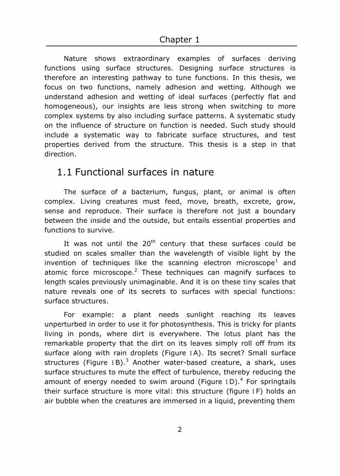
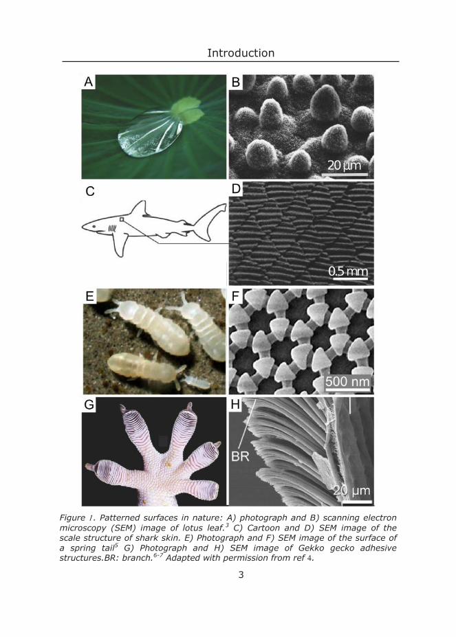
For example: a plant needs sunlight reaching its leaves unperturbed in order to use it for photosynthesis. This is tricky for plants living in ponds, where dirt is everywhere. The lotus plant has the remarkable property that the dirt on its leaves simply roll off from its surface along with rain droplets (Figure A). Its secret? Small surface structures (Figure B).3 Another water-based creature, a shark, uses surface structures to mute the effect of turbulence, thereby reducing the amount of energy needed to swim around (Figure D).4 For springtails their surface structure is more vital: this structure (figure F) holds an air bubble when the creatures are immersed in a liquid, preventing them
Introduction
3
Figure . Patterned surfaces in nature: A) photograph and B) scanning electron microscopy (SEM) image of lotus leaf.3 C) Cartoon and D) SEM image of the scale structure of shark skin. E) Photograph and F) SEM image of the surface of a spring tail5 G) Photograph and H) SEM image of Gekko gecko adhesive structures.BR: branch.6-7 Adapted with permission from ref .

Chapter 1
4
from suffocation.8 And without the surface structure on their feet (Figure H), geckos would not be able to climb and cling as well as they can.9
1.2 Bioinspiration
It is therefore instructive to look at nature for inspiration when you want to design a surface with functions of your choice. Unfortunately, we do not have the machinery to directly mimic nature. And, since surfaces in nature have often multiple functions and limitations and only have to function under ambient conditions, a structure that resembles nature’s examples may not always be the most optimal surface structure for our purpose.10
An example is the gecko toe pad as shown in Figure GH. This animal is the most prominent source of inspiration in the field of bioinspired, dry adhesion. The relatively large size of the animal and its ability to stick to almost any surface, has caught the attention of researchers since the 1900s.11 Scientific interest intensified from the start of this millennium, and the first bioinspired surfaces were developed mimicking the gecko’s toepad by making vertical pillars.12-14 This was not very successful: the adhesion of these mimics did not even come close to that of the gecko’s toepads. The gecko’s toepads namely consist of a hierarchical and highly branched structure, called setae, which are made of beta keratin. Beta keratin is a very stiff material, and this stiffness provides the strength, whereas the setae are compliant due to the structure. Therefore, the toe-pads can make contact with the surface, a property that is vital for good adhesion. The adhesive properties are lost when the structures of the toepads are simplified to pillars. However, fabricating a structure closer in design and material stiffness to that of a toepad, is difficult due to the scale of the structures (the smallest features at the end of the setae are on the nanometre scale) and the brittleness of small features made from stiff materials.
A more fruitful approach is trying to understand how the function is derived from the surface structure, and then design surface structures that achieve the same effect. To achieve this, the effect of surface structures on functions should be known. A first step in this approach is to focus on the properties of flat surfaces, and then study the effect of
Introduction
5
surface structuring. We will limit ourselves to the two properties that are the topics in this thesis: adhesion and wetting of surfaces.
1.3 Adhesion and wetting of flat surfaces
Let us consider perfectly flat surfaces as a first step. Wetting and adhesion of flat solid surfaces can be discussed in terms of surface free energy . Creating surfaces costs energy (even when done so in a reversible way). Since the energy is not dissipated (because it has been done reversibly), this means that the extra energy ended up at the freshly made surface, and this is .
A molecular picture behind the concept of surface free energy, is that within the bulk, a molecule is surrounded by the same molecules, allowing it to have favourable interactions in all directions. A molecule at the surface, on the other hand, only has half of the favourable interactions of neighbouring molecules, since the other half is occupied by air. This is unfavourable. Another contribution, that cannot be neglected when a liquid is considered, is of entropic origin: the density gradients at an air/liquid interface allow for more translational freedom of the molecules, and thus an increase in entropy.
Strictly speaking, is defined in vacuo, however, we will discuss it with vapour present.15 Both adhesion and wetting can be discussed in terms of the of all materials present. We will consider adhesion first.
1.3.1 Adhesion
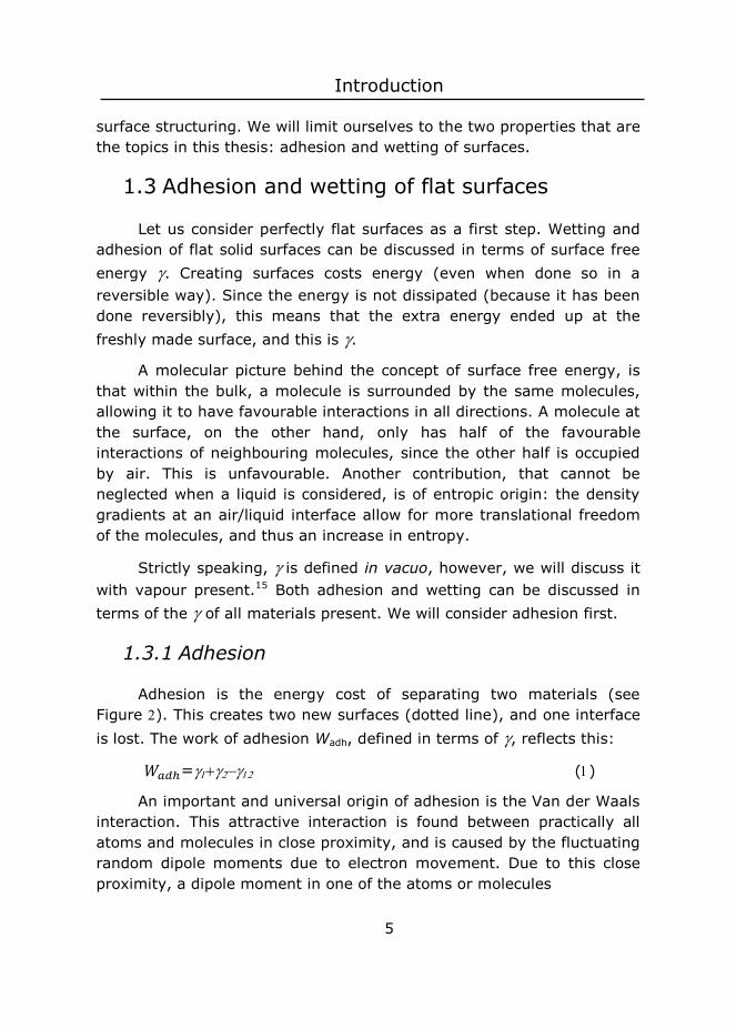
Adhesion is the energy cost of separating two materials (see Figure ). This creates two new surfaces (dotted line), and one interface is lost. The work of adhesion Wadh, defined in terms of , reflects this:
𝑊𝑊𝑎𝑎𝑎𝑎ℎ= ()
An important and universal origin of adhesion is the Van der Waals interaction. This attractive interaction is found between practically all atoms and molecules in close proximity, and is caused by the fluctuating random dipole moments due to electron movement. Due to this close proximity, a dipole moment in one of the atoms or molecules
Chapter 1
6
Figure : two materials that were attached, are separated, thereby creating additional surface (dotted line).
will induce a corresponding dipole moment in a neighbouring atom or molecule. The result is attraction between the two atoms or molecules. Therefore, materials tend to adhere to each other.
When one material is separated into two pieces, the term ‘cohesion’ is used, and Wcoh can be defined as:
𝑊𝑊𝑐𝑐𝑐𝑐ℎ= ()
Wcoh is equal to Van der Waals interaction in the absence of other contributions (e.g. hydrogen bonding).
In practice, other phenomena, besides the of both materials, contribute to the adhesion that is measured. Examples include chemical reactions, rearrangements of polymer chains, and surface structures.16
The measured work, or interface toughness Gc, is given by
𝐺𝐺𝑐𝑐 = 𝑊𝑊𝑎𝑎𝑎𝑎ℎ + 𝜓𝜓 ()
with ψ representing various energy dissipating mechanisms.17 The contribution of ψ on Gc is often much larger than that of Wadh.
1.3.2 Wetting
We shift from two materials on top of each other to a three-phase system, consisting of a solid (S), a liquid (L) and a vapour (V). We defined the surface free energy of the solid s and the liquidL with vapour present, so only one new term has to be introduced. This is the surface free energy between the solid and the liquid, SL. The forces
Introduction
7
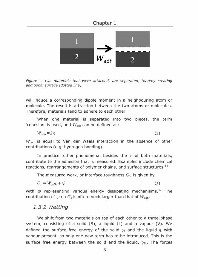
derived from these surface free energies on the contact line of a liquid on a solid are shown in Figure .18 In equilibrium, by definition, the three contributions add up to (the vertical component is hereby not taken into account because we assume that the solid is stiff). As a consequence, the liquid droplet wets the solid with a fixed contact angle , given by Young’s equation:17
𝛾𝛾𝑆𝑆 = 𝛾𝛾𝑆𝑆𝑆𝑆 + 𝛾𝛾𝑆𝑆 cos 𝜃𝜃 ()
Figure : The contact angle of a droplet on a flat surface is determined by the surface free energies of all three components.
1.4 Adhesion and wetting of structured surfaces
1.4.1 Adhesion
No general equations exist to describe the effect of structuring on adhesion. There are, however, guiding principles, some of which are listed here.
For two (effectively) stiff materials, structuring often reduces the true contact area: only the peaks of the two surfaces come in close contact, and therefore the Van der Waals interaction is limited. This reduces the overall adhesion.19-20
For a stiff and an soft material in contact, multiple effects play a role. Two adhesion enhancing effects are (i) increase in contact area because the soft material can conform to the surface of the stiff material, and (ii) energy dissipation due to unstable crack propagation during pull-off (see Chapter ). Two adhesion decreasing effects are (i)
Chapter 1
8
elastic penalty: the energy needed to deform an elastic surface during approach, facilitates detachment, and (ii) crack initiation at patches were the two surfaces are not in contact. Which of these effects dominates the others, depends on the exact surface topology, and whether the stiff or the elastic material is structured.
These effects are valid for all surface structures, whether it is random surface roughness or a carefully designed pattern. For some patterns, more specific effects come into play. A well-studied example is making long, fiber-like surface structures from stiff materials, mimicking the structures on the feet of the gecko. The geometry of this surface structure makes the stiff material compliant, allowing the structures to conform to the counter surface, thereby increasing contact area. The stiff material thus adopts some characteristics of a soft material due to the structure. We see here an example of a surface structure changing the properties in a dramatic way.
Also, detachment of one fiber-like pillar is in principle independent from the detachment of another pillar. Therefore, the energy required to remove one pillar, cannot be used to remove the next one. This results in more energy needed to pull the structured surface off, hence a higher adhesion. However, the overall contact area of an array of pillars is small, since the pillars should be spaced apart to prevent sticking to each other.
The detachment of one pillar depends on the geometry of the pillar.21 A simple pillar can more easily detach because the highest stress during pull-off is located at the edge of a pillar, which makes crack initiation and thus detachment, easy. If the pillar has a mushroom shape or a cap, the highest stress when the pillar is pulled, is not at the edge anymore, making detachment more difficult and therefore the adhesion better.22
These examples show that the effect of structuring on adhesion can be understood for some specific cases of different geometries. Unfortunately, our understanding is still too limited to be able to predict the final adhesion once the geometry and material properties of a new design are known.
Introduction
9
1.4.2 Wetting
The effect of surface structures on wetting is an classic field of research -Young worked on this problem at the start of the 19th century23- and hence more established. Two well-known models describe the deviation of due to the surface not being perfectly flat. The first model, developed by Wenzel, introduces the parameter r, which is the ratio between the true and the projected area. The apparent contact angle W is then given by:24
cos 𝜃𝜃𝑊𝑊 = 𝑟𝑟 cos 𝜃𝜃 ()
For a flat surface, r is equal to , and W is therefore simply . For
rough or structured surfaces, r >, and this results in W < for <
° (hydrophilic surfaces) and W > for > ° (hydrophobic surfaces). According to this model, hydrophilic surfaces become more hydrophilic, and hydrophobic surfaces become more hydrophobic.25
The second model, the Cassie-Baxter model, assumes that air is trapped between the (structured) surface and the droplet. This results in contact angles, θCB, given by26
cos 𝜃𝜃𝐶𝐶𝐶𝐶 = 𝜑𝜑𝑠𝑠 cos 𝜃𝜃 − (1 − 𝜑𝜑𝑠𝑠) ()
where S is the area under the droplet in contact with the solid, and
(S ) the area under the droplet in contact with the entrapped air. The air effectively lowers the average surface energy, leading to high apparent contact angles.27,28 Since air entrapment is energetically unfavourable for hydrophilic surfaces, this model only explains an increase in θCB for hydrophobic materials. However, the lotus leaf of Figure AB, is superhydrophobic ( > °), while the material itself is hydrophilic.29 Neither the equation of Wenzel nor the Cassie-Baxter model can explain this. These models only describe equilibrium wetting states, whereas a meta-stable Cassie-Baxter wetting state is the dominant wetting state of the lotus leaf.
Chapter 1
10
1.5 From nature to research
We have seen examples of nature assigning functions to surfaces by structuring them in Figure . The challenge is to close the gap between our theories and models describing the effect of structuring on function, and how surface structures influence a function in the real world. The most promising structures to start investigating, are those that resemble the structures found in nature in terms of dimensions and shape. The area over which these structures can be made, should be large enough for our measurements of adhesion and wetting. Two fabrication methods that are commonly used are soft lithography and wrinkling techniques, which will be presented next. We, however, use a different approach, which meets all the requirements regarding dimensions and shape of the surface structures, namely colloidal templating (Chapter and ).
1.6 Fabrication of patterned surfaces
Two methods commonly used to make patterned surfaces include soft lithography 14, 21, 30-34 and wrinkling techniques.35-39
1.6.1 Soft lithography
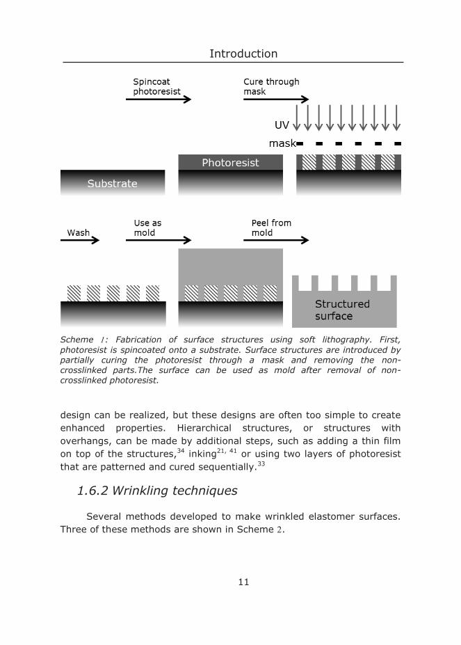
Soft lithography is a multistep process (see Scheme ). First, a photoresist layer is spincoated on a surface. The thickness of this photoresist determines the amplitude of the final structure. Next, a mask with the negative of the desired pattern is placed above the photoresist, and the uncovered areas are exposed to UV to crosslink the resin. The unexposed resin is subsequently removed, and this patterned surface is used as mold. The final patterned surface is obtained after peeling off from the mold.
The smallest features that can be made using soft lithography are several microns, the area is limited to the size of the mask40 and the features most often have straight walls. Within these limitations, every
Introduction
11
Scheme : Fabrication of surface structures using soft lithography. First, photoresist is spincoated onto a substrate. Surface structures are introduced by partially curing the photoresist through a mask and removing the non-crosslinked parts.The surface can be used as mold after removal of non-crosslinked photoresist.
design can be realized, but these designs are often too simple to create enhanced properties. Hierarchical structures, or structures with overhangs, can be made by additional steps, such as adding a thin film on top of the structures,34 inking21, 41 or using two layers of photoresist that are patterned and cured sequentially.33
1.6.2 Wrinkling techniques
Several methods developed to make wrinkled elastomer surfaces. Three of these methods are shown in Scheme .
Chapter 1
12
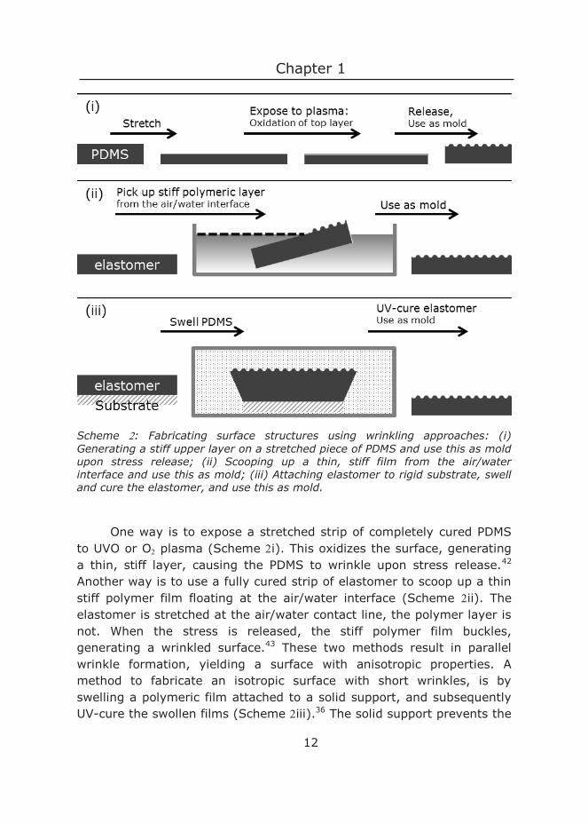
Scheme : Fabricating surface structures using wrinkling approaches: (i) Generating a stiff upper layer on a stretched piece of PDMS and use this as mold upon stress release; (ii) Scooping up a thin, stiff film from the air/water interface and use this as mold; (iii) Attaching elastomer to rigid substrate, swell and cure the elastomer, and use this as mold.
One way is to expose a stretched strip of completely cured PDMS to UVO or O plasma (Scheme i). This oxidizes the surface, generating a thin, stiff layer, causing the PDMS to wrinkle upon stress release.42 Another way is to use a fully cured strip of elastomer to scoop up a thin stiff polymer film floating at the air/water interface (Scheme ii). The elastomer is stretched at the air/water contact line, the polymer layer is not. When the stress is released, the stiff polymer film buckles, generating a wrinkled surface.43 These two methods result in parallel wrinkle formation, yielding a surface with anisotropic properties. A method to fabricate an isotropic surface with short wrinkles, is by swelling a polymeric film attached to a solid support, and subsequently UV-cure the swollen films (Scheme iii).36 The solid support prevents the
Introduction
13
polymeric film from swelling in every direction, resulting in non-aligned wrinkles.
The wrinkled surfaces can be used as mold to obtain the final nanopatterned surfaces. The adhesion of these surfaces have been investigated in depth, and we will show in Chapter that we can learn from these adhesion studies when discussing the adhesion of our surface structures.
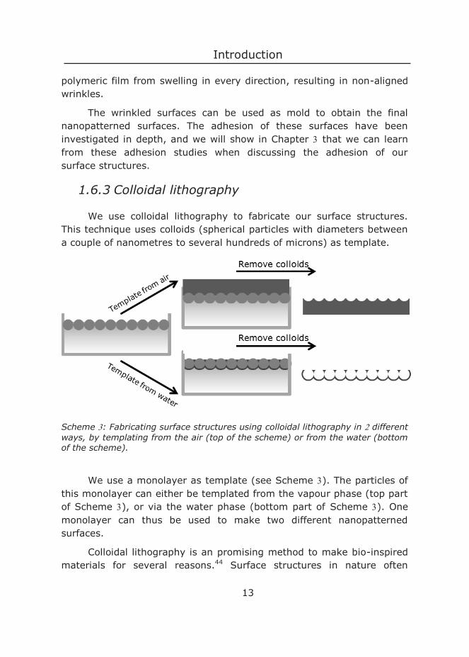
1.6.3 Colloidal lithography
We use colloidal lithography to fabricate our surface structures. This technique uses colloids (spherical particles with diameters between a couple of nanometres to several hundreds of microns) as template.
Scheme : Fabricating surface structures using colloidal lithography in different ways, by templating from the air (top of the scheme) or from the water (bottom of the scheme).
We use a monolayer as template (see Scheme ). The particles of this monolayer can either be templated from the vapour phase (top part of Scheme ), or via the water phase (bottom part of Scheme ). One monolayer can thus be used to make two different nanopatterned surfaces.
Colloidal lithography is an promising method to make bio-inspired materials for several reasons.44 Surface structures in nature often
Chapter 1
14
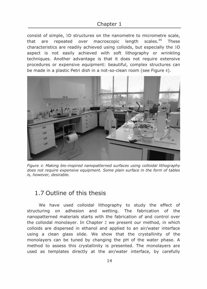
consist of simple, D structures on the nanometre to micrometre scale, that are repeated over macroscopic length scales.45 These characteristics are readily achieved using colloids, but especially the D aspect is not easily achieved with soft lithography or wrinkling techniques. Another advantage is that it does not require extensive procedures or expensive equipment: beautiful, complex structures can be made in a plastic Petri dish in a not-so-clean room (see Figure ).
Figure : Making bio-inspired nanopatterned surfaces using colloidal lithography does not require expensive equipment. Some plain surface in the form of tables is, however, desirable.
1.7 Outline of this thesis
We have used colloidal lithography to study the effect of structuring on adhesion and wetting. The fabrication of the nanopatterned materials starts with the fabrication of and control over the colloidal monolayer. In Chapter we present our method, in which colloids are dispersed in ethanol and applied to an air/water interface using a clean glass slide. We show that the crystallinity of the monolayers can be tuned by changing the pH of the water phase. A method to assess this crystallinity is presented. The monolayers are used as templates directly at the air/water interface, by carefully
Introduction
15
applying the elastomer PDMS on top. After crosslinking, the particles are easily removed, resulting in a nanopatterned elastomer surface.
A function of this nanopatterned surface, namely adhesion, is investigated in Chapter . Three different nanopatterned surfaces with varying dimple depth and dimple density are selected. Two spherical probes are used as counter surface: a macroscopic probe (diameter mm) and a microscopic probe (diameter m). In this way, adhesion is probed on two different length scales. The increase in adhesion is explained using an energy dissipating mechanism, and the influence of dimple depth and dimple density on adhesion, are discussed.
The same monolayer of Chapter is used in a completely different templating method in Chapter . In this case, the material is not deposited on top, but polymerized at the colloid/water interface. This is achieved by first swelling the particles with monomers, and subsequently adding an oxidant to the water, thereby starting polymerization. After removal of the colloids, a nanopatterned surface consisting of the stiff, highly-crosslinked polypyrrole, is obtained. Different surface structures can be fabricated by choosing the amount of monomer, the polymerization time and the monomer : oxidant ratio. These surface structures are used for wetting experiments.
The wetting experiments show that droplets of water on those surface structures, have contact angles °, whereas the contact angle is ° for water on non-structured polypyrrole surfaces. To understand this, we modelled the system in silico by extending the regular solution theory to three dimensions. This approach is presented in Chapter . Modelling allows us to systematically study the effect of particle diameter, immersion depth of the templated particles, and interparticle distance on the final droplet shape.
In the final chapter, number , we reflect on the previous chapters, and give suggestions for the next steps in research. We discuss the ideas we have of how the fabrication method can be improved and how other surface structures can be made using colloidal templating. The effect on adhesion of our structures are compared to other surface patterns and the influence of the important parameters on adhesion, is discussed. For our wetting experiments, we already performed modelling
Chapter 1
16
studies. The validity of our modelling studies is tested by additional experiments and results from literature. For example, we indeed find the contact angle hysteresis as predicted by our modelling studies. Finally, an outlook for this field of research is presented.
References 1. Ruska, E., The development of the electron microscope and of electron microscopy. Rev. Mod. Phys. 1987, 59 (3), 627. 2. Bennig, G. K., Atomic force microscope and method for imaging surfaces with atomic resolution. Google Patents: 1988. 3. Barthlott, W.; Neinhuis, C., Purity of the sacred lotus, or escape from contamination in biological surfaces. Planta 1997, 202 (1), 1-8. 4. Kamperman, M.; Kroner, E.; del Campo, A.; McMeeking, R. M.; Arzt, E., Functional adhesive surfaces with “gecko” effect: the concept of contact splitting. Advanced Engineering Materials 2010, 12 (5), 335-348. 5. Helbig, R.; Nickerl, J.; Neinhuis, C.; Werner, C., Smart skin patterns protect springtails. PloS one 2011, 6 (9), e25105-e25105. 6. Gao, H.; Wang, X.; Yao, H.; Gorb, S.; Arzt, E., Mechanics of hierarchical adhesion structures of geckos. Mechanics of Materials 2005, 37 (2), 275-285. 7. Autumn, K., How Gecko Toes Stick The powerful, fantastic adhesive used by geckos is made of nanoscale hairs that engage tiny forces, inspiring envy among human imitators. American scientist 2006, 94 (2). 8. Hensel, R.; Helbig, R.; Aland, S.; Braun, H.-G.; Voigt, A.; Neinhuis, C.; Werner, C., Wetting resistance at its topographical limit: the benefit of mushroom and serif T structures. Langmuir 2013, 29 (4), 1100-1112. 9. Autumn, K.; Liang, Y. A.; Hsieh, S. T.; Zesch, W.; Chan, W. P.; Kenny, T. W.; Fearing, R.; Full, R. J., Adhesive force of a single gecko foot-hair. Nature 2000, 405 (6787), 681-685. 10. Savage, N., Synthetic coatings: Super surfaces. Nature 2015, 519 (7544), S7-S9. 11. Autumn, K.; Peattie, A. M., Mechanisms of adhesion in geckos. Integrative and Comparative Biology 2002, 42 (6), 1081-1090. 12. Geim, A.; Grigorieva, S. D. I.; Novoselov, K.; Zhukov, A.; Shapoval, S. Y., Microfabricated adhesive mimicking gecko foot-hair. Nature materials 2003, 2 (7), 461-463. 13. Sitti, M.; Fearing, R. S., Synthetic gecko foot-hair micro/nano-structures as dry adhesives. Journal of Adhesion Science and Technology 2003, 17 (8), 1055-1073. 14. Greiner, C.; del Campo, A.; Arzt, E., Adhesion of bioinspired micropatterned surfaces: effects of pillar radius, aspect ratio, and preload. Langmuir 2007, 23 (7), 3495-3502. 15. Packham, D., Work of adhesion: contact angles and contact mechanics. International journal of adhesion and adhesives 1996, 16 (2), 121-128. 16. Toikka, G.; Spinks, G. M.; Brown, H. R., Interactions between micron-sized glass particles and poly (dimethyl siloxane) in the absence and presence of applied load. The Journal of Adhesion 2000, 74 (1-4), 317-340.
Introduction
17
17. Packham, D. E., Surface energy, surface topography and adhesion. International Journal of Adhesion and Adhesives 2003, 23 (6), 437-448. 18. De Gennes, P.-G.; Brochard-Wyart, F.; Quéré, D., Capillarity and wetting phenomena: drops, bubbles, pearls, waves. Springer: 2004; p 52. 19. Fuller, K.; Tabor, D., The effect of surface roughness on the adhesion of elastic solids. Proceedings of the Royal Society of London. A. Mathematical and Physical Sciences 1975, 345 (1642), 327-342. 20. Persson, B.; Tosatti, E., The effect of surface roughness on the adhesion of elastic solids. The Journal of Chemical Physics 2001, 115, 5597. 21. del Campo, A.; Greiner, C.; Arzt, E., Contact shape controls adhesion of bioinspired fibrillar surfaces. Langmuir 2007, 23 (20), 10235-10243. 22. Carbone, G.; Pierro, E.; Gorb, S. N., Origin of the superior adhesive performance of mushroom-shaped microstructured surfaces. Soft Matter 2011, 7 (12), 5545-5552. 23. Young, T., An essay on the cohesion of fluids. Philosophical Transactions of the Royal Society of London 1805, 95, 65-87. 24. Wenzel, R. N., Resistance of solid surfaces to wetting by water. Industrial & Engineering Chemistry 1936, 28 (8), 988-994. 25. Bormashenko, E.; Bormashenko, Y.; Whyman, G.; Pogreb, R.; Stanevsky, O., Micrometrically scaled textured metallic hydrophobic interfaces validate the Cassie–Baxter wetting hypothesis. Journal of colloid and interface science 2006, 302 (1), 308-311. 26. Cassie, A.; Baxter, S., Wettability of porous surfaces. Transactions of the Faraday Society 1944, 40, 546-551. 27. Choi, H.-J.; Choo, S.; Shin, J.-H.; Kim, K.-I.; Lee, H., Fabrication of Superhydrophobic and Oleophobic Surfaces with Overhang Structure by Reverse Nanoimprint Lithography. The Journal of Physical Chemistry C 2013, 117 (46), 24354-24359. 28. Bormashenko, E., Why does the Cassie–Baxter equation apply? Colloids and Surfaces A: Physicochemical and Engineering Aspects 2008, 324 (1), 47-50. 29. Cheng, Y.-T.; Rodak, D. E., Is the lotus leaf superhydrophobic? Applied physics letters 2005, 86 (14), 144101. 30. Crosby, A. J.; Hageman, M.; Duncan, A., Controlling polymer adhesion with “pancakes”. Langmuir 2005, 21 (25), 11738-11743. 31. Thomas, T.; Crosby, A. J., Controlling adhesion with surface hole patterns. The Journal of Adhesion 2006, 82 (3), 311-329. 32. Nanni, G.; Fragouli, D.; Ceseracciu, L.; Athanassiou, A., Adhesion of elastomeric surfaces structured with micro-dimples. Applied Surface Science 2015, 326, 145-150. 33. Sameoto, D.; Sharif, H.; Menon, C., Investigation of low-pressure adhesion performance of mushroom shaped biomimetic dry adhesives. Journal of Adhesion Science and Technology 2012, 26 (23), 2641-2652. 34. Glassmaker, N. J.; Jagota, A.; Hui, C.-Y.; Noderer, W. L.; Chaudhury, M. K., Biologically inspired crack trapping for enhanced adhesion. Proceedings of the National Academy of Sciences 2007, 104 (26), 10786-10791. 35. Lin, P.-C.; Vajpayee, S.; Jagota, A.; Hui, C.-Y.; Yang, S., Mechanically tunable dry adhesive from wrinkled elastomers. Soft Matter 2008, 4 (9), 1830-1835.
Chapter 1
18
36. Chan, E. P.; Smith, E. J.; Hayward, R. C.; Crosby, A. J., Surface wrinkles for smart adhesion. Advanced Materials 2008, 20 (4), 711-716. 37. Jin, C.; Khare, K.; Vajpayee, S.; Yang, S.; Jagota, A.; Hui, C.-Y., Adhesive contact between a rippled elastic surface and a rigid spherical indenter: from partial to full contact. Soft Matter 2011, 7 (22), 10728-10736. 38. Davis, C. S.; Crosby, A. J., Mechanics of wrinkled surface adhesion. Soft Matter 2011, 7 (11), 5373-5381. 39. Davis, C. S.; Martina, D.; Creton, C.; Lindner, A.; Crosby, A. J., Enhanced adhesion of elastic materials to small-scale wrinkles. Langmuir 2012, 28 (42), 14899-14908. 40. Whitesides, G. M.; Ostuni, E.; Takayama, S.; Jiang, X.; Ingber, D. E., Soft lithography in biology and biochemistry. Annual review of biomedical engineering 2001, 3 (1), 335-373. 41. Murphy, M. P.; Kim, S.; Sitti, M., Enhanced adhesion by gecko-inspired hierarchical fibrillar adhesives. ACS applied materials & interfaces 2009, 1 (4), 849-855. 42. Khare, K.; Zhou, J.; Yang, S., Tunable open-channel microfluidics on soft poly (dimethylsiloxane)(PDMS) substrates with sinusoidal grooves. Langmuir 2009, 25 (21), 12794-12799. 43. Miquelard-Garnier, G.; Croll, A. B.; Davis, C. S.; Crosby, A. J., Contact-line mechanics for pattern control. Soft Matter 2010, 6 (22), 5789-5794. 44. Kraus, T.; Brodoceanu, D.; Pazos‐Perez, N.; Fery, A., Colloidal Surface Assemblies: Nanotechnology Meets Bioinspiration. Advanced Functional Materials 2013, 23 (36), 4529-4541. 45. Vogel, N.; Retsch, M.; Fustin, C.-A.; del Campo, A.; Jonas, U., Advances in colloidal assembly: The design of structure and hierarchy in two and three dimensions. Chemical reviews 2015, 115 (13), 6265-6311.
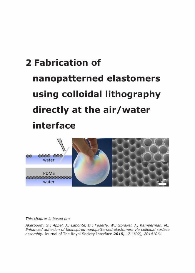
2 Fabrication of
nanopatterned elastomers
using colloidal lithography
directly at the air/water
interface
This chapter is based on:
Akerboom, S.; Appel, J.; Labonte, D.; Federle, W.; Sprakel, J.; Kamperman, M., Enhanced adhesion of bioinspired nanopatterned elastomers via colloidal surface assembly. Journal of The Royal Society Interface 2015, 12 (102), 20141061
Chapter
20
2.1 Abstract
We describe a fast and scalable method to fabricate nanopatterned polydimethylsiloxane (PDMS) using colloidal lithography directly at the air/water interface. Micron-sized polystyrene particles with parking areas of nm per –COOH group, are synthesized and applied to the air/water interface using ethanol as spreading agent. Close-packed monolayers are formed at the interface, on which PDMS is applied. PDMS completely wets the air water interface at first contact with water, thereby compressing the monolayer, similarly as is usually achieved using a Langmuir through. PDMS curing and particle extraction results in nanopatterned elastomers. Pattern disruption of the monolayer is minimized by omitting transfer and drying steps during the process. The order of the colloidal monolayer and the immersion depth of the particles are tuned by the pH of the subphase. This leads to direct control of the topography of PDMS surfaces. Crystallinity of the monolayer, which is quantified by counting the number of particles with six neighboring particles, shows a rapid increase when the pH of the subphase is higher than the first dissociation constant of the COOH-groups on the surface of the particles.
2.2 Introduction
Colloidal lithography is a technique that utilizes self-assembled colloidal monolayers for fabricating topologically-patterned surfaces with nanometer precision. This technique has proven to be a fast and cost-effective alternative to other nanofabrication processes such as electron beam lithography or focused ion beam lithography. Furthermore, nanopatterned surfaces are applied in a wide variety of technologically relevant areas including sensing, photonics, electronics, energy conversion and adhesion.1 Different methods have been developed to create colloidal monolayers directly on target solid substrates.2-3 A limitation to these methods is the low degree of lateral mobility of the particles upon contact with the substrate, which makes it difficult to prevent free void and multilayer formation.2 To overcome this limitation, gas/liquid interface deposition methods were developed, which provide enhanced particle mobility resulting in highly ordered monolayers.
Fabrication of nanopatterned elastomers
21
Recently, several groups have reported on methods to produce large-area, highly ordered, colloidal crystals For example, Pan et al. introduced a dynamic interface, by stirring the aqueous subphase, to facilitate colloidal crystal formation at the air/water interface4 Retsch et al. reported a two-step procedure in which colloids are applied to a glass slide by spin-coating.5 Subsequently, a colloidal monolayer was formed upon immersion of the glass slide in an aqueous surfactant solution. Assembly at the air/water interface was also successfully achieved by using interfacial deposition via a glass slide6 and a needle tip.7 In these examples the liquid interface acts as the assembly scaffold after which the monolayers are transferred to a solid substrate. Alternatively, material can be deposited via chemical reactions directly onto the colloidal monolayer at the air/liquid interface. This method was used to fabricate free-standing porous films8 and nanobowls9 by reacting monomers or inorganic precursors at the gas/liquid interface and at the liquid/solid interface, respectively. Ideally, however, deposition should not be limited to interfacial reactions and generalization towards other material systems would enable the fabrication of films with different property profiles. Yet, such approaches remain virtually unexplored.
In the study presented here, we describe a facile method to fabricate nanopatterned polydimethylsiloxane (PDMS) using colloidal lithography directly at the air/water interface. We show that close-packed monolayers at the air/water interface can be used as a template without the need to transfer the monolayer to a solid substrate. By omitting transfer and drying steps in the process, pattern disruption is minimized. Colloidal monolayers were obtained for a range of particle sizes. Moreover, the subphase is used to systematically tune the order of the colloidal monolayer and to control the immersion depth of the particles. This leads to direct control of the topography of PDMS surfaces.
2.3 Experimental
2.3.1 Materials
All materials were purchased from Sigma Aldrich and used as received. PDMS (Sylgard ) was mixed in a ratio of : of crosslinker
Chapter
22
: prepolymer by weight and degassed by centrifugation. Deionized water, from an Easypure-UV-system (Barnstead), was used in all experiments.
2.3.2 Particle synthesis
Carboxylated polystyrene particles were synthesized in a one-step synthesis according to ref . Briefly, for the biggest particles, water ( g), itaconic acid (g) and styrene (g) were heated to °C in a round bottom flask, and flushed with nitrogen for minutes. Meanwhile, ,′-Azobis(-cyanovaleric acid) (ACVA, mg) was dissolved in water (g) and 1M NaOH ( g). After adding this mixture to the round bottom flask, the solution reacted overnight under continuous stirring at rpm.
The smaller particles were synthesized usingmL water, or g styrene, and g (for g styrene) or g (for g styrene) itaconic acid, and a temperature of °C. The reaction was initiated with g ACVA (for g styrene) or g ACVA (for g styrene).
The product was filtered over glass wool to discard some coagulum that was formed during the reaction. The filtered particles were treated using two different protocols. Colloidal dispersion CP (‘Carboxylated Particles’) was directly exchanged to ethanol by three cycles of centrifugation at RPM for one hour followed by resuspension in ethanol. Colloidal dispersion CP-W (‘Carboxylated Particles- Washed’) was washed in water by three cycles of centrifugation at RPM for one hour followed by resuspension in Milli-Q water. After this washing step, CP-W was exchanged to ethanol, using the same procedure. The smaller particles were treated similar to CP-W.
2.3.3 Particle characterization
Static Light Scattering (SLS)
Light-scattering measurements were performed on an ALV instrument equipped with an ALV external correlator and a mW Cobolt Samba- DPSS laser operating at a wavelength of nm. The scattering intensity was recorded at ° ≤ θ ≤ ° in intervals of °, and

Fabrication of nanopatterned elastomers
23
the curve was fitted to a form factor of a solid sphere. From this measurement an average radius of nm and a polydispersity index (Rw/Rn) of (see Figure A) were obtained.
Figure : Characterization of the carboxylated particles, A) Size distribution as determined with SLS-measurements. B) Titration of ultrapure water, CP and CP-W with M NaOH.
Determination of surface charge density
The surface charge of the particles was determined by titration of mL colloidal dispersion in Milli-Q water ( g/L for CP and g/L for CP-W) with M NaOH and using the titration of mL Milli-Q water (brought to low pH with mL 1M HCl) as reference (see Figure B). The difference in NaOH added to reach a pH of (well above the pKa-values of itaconic acid, which are pKa= and pKa= 11), but below the plateau in the pH-curve) between the dispersion and the reference sample is taken as the number of itaconic acid groups in the sample. The weight per particle is calculated using the density of polystyrene. Since the weight of all particles in during titration is known, the number of charges per particle can be calculated. The parking area is then (particle area)/(number of charges per particle), and is nm- for both CP and CP-W.
A B
Chapter
24
2.3.4 Surface structure fabrication
Samples were prepared in polystyrene Petri dishes. This procedure is shown in Figure . The pH of the subphase was varied between and , keeping the ionic strength constant at either or M. A piranha-cleaned coverslip was placed diagonally against the side, and a suspension of particles in ethanol ( wt) was applied via this cover slip onto the water subphase using a pipette (Figure A (a)). The area covered by the particles at the air/water interface was well visible, and thus the amount of particles could be adjusted during preparation. The monolayer was left to equilibrate for at least one hour before further processing, to ensure evaporation of all ethanol from the air/water interface.
A syringe with a blunt tip needle was filled with PDMS and a small droplet was applied to the side of the Petri dish containing the monolayer of particles. Upon reaching the water surface, the droplet spread quickly (Figure A (b)). Next, PDMS was applied to the complete circumference of the Petri dish. This resulted in a ring of PDMS on water. By slowly adding more PDMS to this ring in a spiraling manner, PDMS eventually covered the whole interface. PDMS was allowed to crosslink at RT for days, resulting in PDMS layers of mm thickness (Figure A (c)).
To remove the template particles from the PDMS mold, we first applied Scotch Magic Tape, which removed the largest portion of templating particles. The remaining particles were removed by soaking the sample in N-methyl--pyrrolidone (NMP) for hour, followed by dipping the samples times in NMP in an ultrasonic bath (Figure A (d)). NMP was chosen as solvent because it dissolves polystyrene, yet does not swell PDMS.12 The samples were stored at RT.
Fabrication of nanopatterned elastomers
25
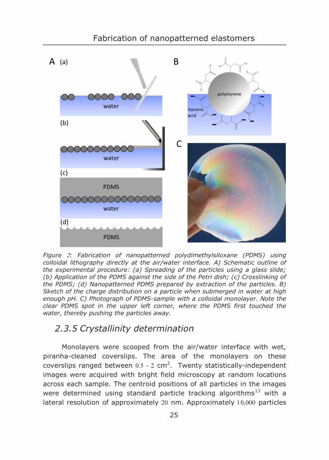
Figure : Fabrication of nanopatterned polydimethylsiloxane (PDMS) using colloidal lithography directly at the air/water interface. A) Schematic outline of the experimental procedure: (a) Spreading of the particles using a glass slide; (b) Application of the PDMS against the side of the Petri dish; (c) Crosslinking of the PDMS; (d) Nanopatterned PDMS prepared by extraction of the particles. B) Sketch of the charge distribution on a particle when submerged in water at high enough pH. C) Photograph of PDMS-sample with a colloidal monolayer. Note the clear PDMS spot in the upper left corner, where the PDMS first touched the water, thereby pushing the particles away.
2.3.5 Crystallinity determination
Monolayers were scooped from the air/water interface with wet, piranha-cleaned coverslips. The area of the monolayers on these coverslips ranged between cm2. Twenty statistically-independent images were acquired with bright field microscopy at random locations across each sample. The centroid positions of all particles in the images were determined using standard particle tracking algorithms13 with a lateral resolution of approximately nm. Approximately particles

Chapter
26
were found per image; per experiment we thus analyzed particles to assess the crystallinity of the monolayers. We then computed the number of nearest neighbours, using a cut-off distance of the particle diameter (for Matlab-code: see ref ). We considered a particle crystalline only when it had exactly nearest-neighbours in these hexagonal lattices. This method of assessing crystallinity is very strict: for example, all six particles surrounding vacancy are not regarded as crystalline, while in fact they are part of the crystal lattice. However, assessing the crystallinity by using the more elaborate Steinhardt orientational bond order parameter, Ψ,15 showed the same trends as simply counting the number of nearest neighbours.16 Therefore, the nearest neighbour method was used here.
Figure : The apparent radius Rh of the particles is related to the immersion depth as shown on the left. Rh can thus be used to calculate the immersion depth using Pythagorean theorem (see right).
2.3.6 Immersion depth determination
We put Petri dishes with monolayers in a desiccator, added some droplets of ethyl cyanoacrylate in a separate dish, and let the system react under reduced pressure for hours. Ethyl cyanoacrylate starts to polymerize when it comes in contact with water. The apparent radii of the particles embedded in poly(ethyl cyanoacrylate) was determined in SEM images ( to particles per image) in using the Analyze Particles function in ImageJ. See Figure for a definition of apparent radius. Six two-tailed t-tests were performed to test whether the differences in apparent radii were significant (with p) and the Bonferroni method
Fabrication of nanopatterned elastomers
27
was used to correct for multiple testing. This apparent radius was used to calculate the immersion depth, which is the height percentage of the particle that is immersed in the subphase, via (immersed height)/(diameter particle), using immersed height = 𝑅𝑅𝑝𝑝 + 𝑙𝑙 and
𝑙𝑙 = √𝑅𝑅𝑝𝑝2 − 𝑅𝑅ℎ2 (see Figure ).
2.3.7 Scanning Electron Microscopy (SEM)
Samples were sputtered with gold (mA, s) using a JEOL JFC- autofine coater, and imaged using a JEOL JAMP-F Field Emission Auger Microprobe. High magnification and tilt images were measured using a FEI Magellan FESEM.
2.3.8 Light Microscope
Images were made at a magnification of using a Zeiss Axiovert equipped with a Phantom V camera.
2.4 Results and discussion
2.4.1 Surface structure fabrication and
characterization
Monolayers were prepared according to Figure A. Upon applying ethanol on water, a surface tension gradient is generated that causes the dispersion to rapidly spread outwards and cover the interface with particles.7 Regions with distinct Bragg reflections formed spontaneously, which indicated the formation of close-packed and organized domains. The self-assembly of charged micrometre sized colloidal particles at an air-water interface is governed by a competition between attractive capillary forces and repulsive electrostatic dipolar forces.17 We observed the spontaneous formation of islands of close-packed particles, which suggests that attractive forces dominate. The charges on the particles originate from copolymerization with itaconic acid (see Figure B). The charge density increased with increasing pH as more itaconic acid groups got deprotonated. The parking area at pH was calculated to
Chapter
28
be nm per COOH group. This value is relatively small compared to values in literature,18 but the substantial ionic strength of the subphase screened the electrostatic repulsion between the particles, and thus attractive forces dominated nonetheless.
To use the monolayer of particles at the air-water interface as a template, the deposition material should (i) be immiscible and nonreactive with water, (ii) be able to crosslink in the presence of water, (iii) be able to replicate micron to nanoscale features and (iv) have a lower density than water. PDMS was selected because it fulfills these criteria and is a well-characterized material. PDMS completely wet the air-water interface19, and thus formed a homogeneous film at the interface. During spreading of the initial PDMS droplet, the particles are pushed together, similar to compression in a Langmuir through. This resulted in close-packed monolayers composed of the islands formed during deposition. A representative example of nanopatterned PDMS is shown in Figure C, in which the Bragg reflections can be clearly seen.
2.4.1 Determination of the monolayer crystallinity
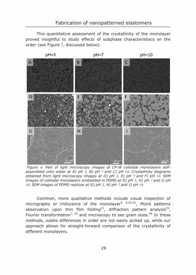
The order of the monolayer was assessed by scooping monolayers, which were not cast in PDMS and imaging them with brightfield microscopy (Figure A-C). We confirmed the presence of a monolayer, rather than multilayers, by changing the focus, and thus scanning through the sample. The positions of all particles in the images was found using a particle tracking algorithms and this spatial information was used to quantify the number of crystalline particles, i.e. particles with exactly 6 nearest-neighbours (see experimental section).
An exemplary result of this analysis is shown in Figure D-F, where crystalline particles are shown in light grey, and non-crystalline particles are shown in dark grey. The normalized crystallinity per image was then calculated using:
The normalized crystallinity per image was calculated using:
normalized crystallinity = crystalline particlestotal number of particles ()
Fabrication of nanopatterned elastomers
29
This quantitative assessment of the crystallinity of the monolayer proved insightful to study effects of subphase characteristiscs on the order (see Figure , discussed below).
Figure : Part of light microscopy images of CP-W colloidal monolayers self-assembled onto water at A) pH , B) pH and C) pH . Crystallinity diagrams obtained from light microscopy images at D) pH , E) pH and F) pH . SEM images of colloidal monolayers embedded in PDMS at G) pH , H) pH and I) pH . SEM images of PDMS replicas at G) pH , H) pH and I) pH
Common, more qualitative methods include visual inspection of micrographs or iridiscence of the monolayer5, 9,20-22, Moiré patterns observation upon thin film folding23, diffraction pattern analysis24, Fourier transformation7, 25 and microscopy to see grain sizes.26 In these methods, subtle differences in order are not easily picked up, while our approach allows for straight-forward comparison of the crystallinity of different monolayers.
Chapter
30
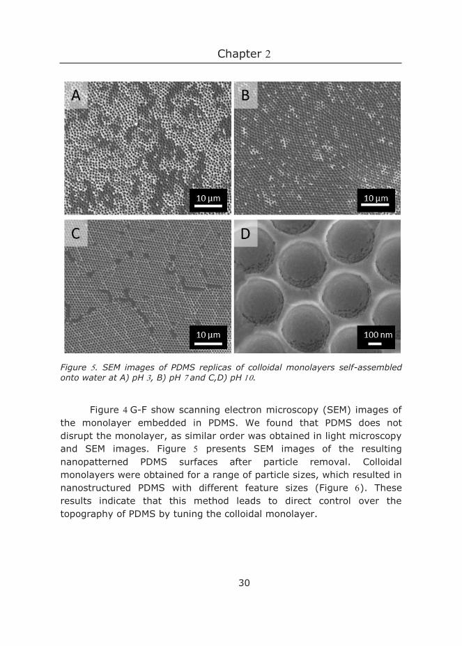
Figure . SEM images of PDMS replicas of colloidal monolayers self-assembled onto water at A) pH , B) pH and C,D) pH .
Figure G-F show scanning electron microscopy (SEM) images of the monolayer embedded in PDMS. We found that PDMS does not disrupt the monolayer, as similar order was obtained in light microscopy and SEM images. Figure presents SEM images of the resulting nanopatterned PDMS surfaces after particle removal. Colloidal monolayers were obtained for a range of particle sizes, which resulted in nanostructured PDMS with different feature sizes (Figure ). These results indicate that this method leads to direct control over the topography of PDMS by tuning the colloidal monolayer.
Fabrication of nanopatterned elastomers
31
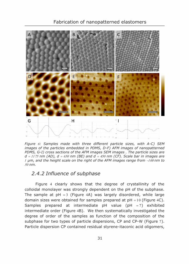
Figure : Samples made with three different particle sizes, with A-C) SEM images of the particles embedded in PDMS, D-F) AFM images of nanopatterned PDMS, G-I) cross sections of the AFM images SEM images . The particle sizes are d nm (AD), d nm (BE) and d nm (CF). Scale bar in images are µm, and the height scale on the right of the AFM images range from nm to nm.
2.4.2 Influence of subphase
Figure clearly shows that the degree of crystallinity of the colloidal monolayer was strongly dependent on the pH of the subphase. The sample at pH (Figure A) was largely disordered, while large domain sizes were obtained for samples prepared at pH (Figure C). Samples prepared at intermediate pH value (pH ) exhibited intermediate order (Figure B). We then systematically investigated the degree of order of the samples as function of the composition of the subphase for two types of particle dispersions, CP and CP-W (Figure ). Particle dispersion CP contained residual styrene-itaconic acid oligomers,
Chapter
32
whereas dispersion CP-W was thoroughly washed with ultrapure water to remove these oligomers to a great extent. To study the pH effect on monolayer formation, the pH was adjusted with HCl and NaOH, while keeping the ionic strength constant. The pH was calculated from the known composition of the subphase and not determined experimentally, but we expect no strong deviations between calculated and actual values due to the low particle concentration in the overall system. The crystallinity was again determined by scooping monolayers and subsequent light microscopy imaging.
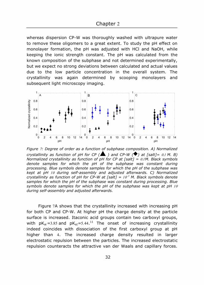
Figure : Degree of order as a function of subphase composition. A) Normalized crystallinity as function of pH for CP ( ) and CP-W ( ) at [salt]= M. B) Normalized crystallinity as function of pH for CP at [salt] = M. Black symbols denote samples for which the pH of the subphase was constant during processing. Blue symbols denote samples for which the pH of the subphase was kept at pH during self-assembly and adjusted afterwards. C) Normalized crystallinity as function of pH for CP-W at [salt] = M. Black symbols denote samples for which the pH of the subphase was constant during processing. Blue symbols denote samples for which the pH of the subphase was kept at pH during self-assembly and adjusted afterwards.
Figure A shows that the crystallinity increased with increasing pH for both CP and CP-W. At higher pH the charge density at the particle surface is increased. Itaconic acid groups contain two carboxyl groups, with pKa=and pKa=.11 The onset of increasing crystallinity indeed coincides with dissociation of the first carboxyl group at pH higher than . The increased charge density resulted in larger electrostatic repulsion between the particles. The increased electrostatic repulsion counteracts the attractive van der Waals and capillary forces.
0
0.2
0.4
0.6
0.8
1
0 2 4 6 8 10 12 14pH
A
Nor
mal
ized
cry
stal
linity
0
0.2
0.4
0.6
0.8
1
0 2 4 6 8 10 12 14pH
C
0
0.2
0.4
0.6
0.8
1
0 2 4 6 8 10 12 14pH
B
Fabrication of nanopatterned elastomers
33
Consequently, the particles remained more mobile at the interface resulting in more ordered monolayers.2 5-6 Thus, at pH 3, particles that approach each other closely (i.e., by capillary forces), immediately feel the attractive van der Waals forces that bring them in close contact. This process immobilizes the particles and results in monolayers with relatively low crystallinities. At pH 10, the electrostatic repulsion is greatly increased. This increases the energy barrier for a close contact between particles and the particles have sufficient time and mobility to crystallize in a low free energy position. Hence, monolayers with higher crystallinities are obtained.6
It was observed that monolayers made from CP were less mobile and more robust as compared to CP-W monolayers. More specifically, when part of the CP-monolayer was scooped with a coverslip, the hole left in the monolayer remained square, whereas for CP-W, the particles within the monolayer rearranged after scooping, leaving an irregular shaped hole in the monolayer. We speculate that the surface active styrene-itaconic acid oligomers left in the CP dispersions ‘glue’ the particles together, in a similar fashion as was observed by Ho et al. for polyethylene oxide polymers.27 To study the difference in robustness, CP and CP-W samples were prepared at high pH that resulted in well-ordered monolayers. HCl was added to the subphase to lower the pH while keeping the salt concentration constant. For CP monolayers order was maintained, even when the pH was as low as (Figure B). By contrast, lowering the pH of CP-W monolayers decreased the crystallinity significantly (Figure C). The cohesive layer between the CP particles thus plays an important role in preserving the order during further processing of the monolayer.
2.4.3 Immersion depth of the particles
We also altered the properties of the monolayer through changes in ionic strength of the subphase at constant pH. We determined the immersion depth of CP-W particles in subphases at different pH and ionic strength by fixing their position at the interface in a polymeric matrix (Figure ). The matrix was formed by interfacial polymerization of ethyl cyanoacrylate, which was introduced via the gas phase and started
Chapter
34
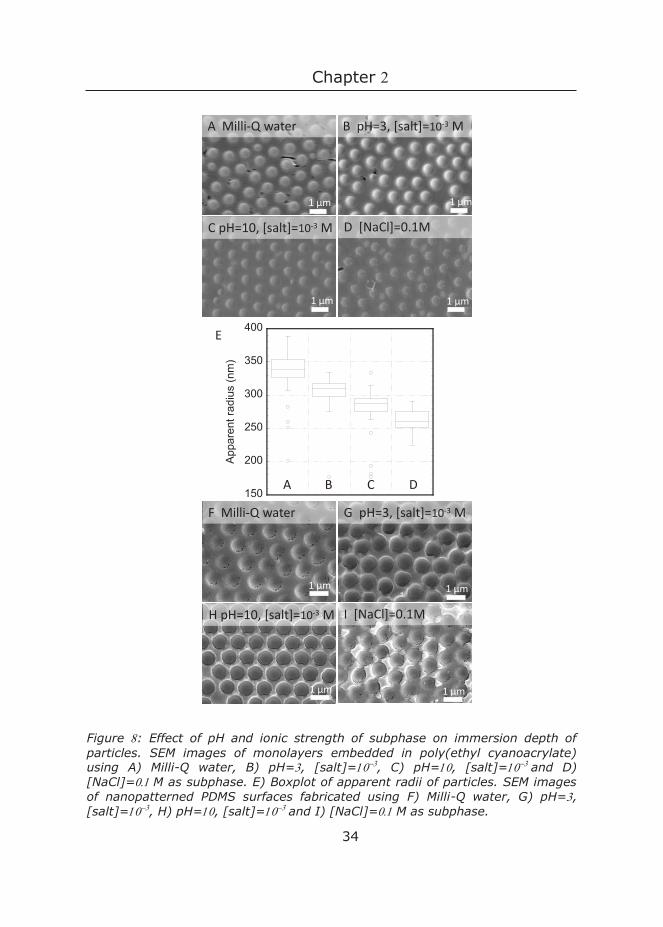
Figure : Effect of pH and ionic strength of subphase on immersion depth of particles. SEM images of monolayers embedded in poly(ethyl cyanoacrylate) using A) Milli-Q water, B) pH=, [salt]=, C) pH=, [salt]=and D) [NaCl]=M as subphase. E) Boxplot of apparent radii of particles. SEM images of nanopatterned PDMS surfaces fabricated using F) Milli-Q water, G) pH=, [salt]=, H) pH=, [salt]=and I) [NaCl]=M as subphase.
150
200
250
300
350
400
App
aren
t rad
ius
(nm
)
1 μm
A Milli-Q water B pH=3, [salt]=10-3 M
C pH=10, [salt]=10-3 M D [NaCl]=0.1M
1 μm
H pH=10, [salt]=10-3 M I [NaCl]=0.1M
G pH=3, [salt]=10-3 M
1 μm1 μm
F Milli-Q water
1 μm
1 μm
1 μm 1 μm
E
A B C D
Fabrication of nanopatterned elastomers
35
to polymerize when it came in contact with water. After drying, immersion depths were determined by imaging the poly(ethyl cyanoacrylate) layer with SEM.
Figure A-D show top-view images of monolayers embedded in the cyanoacrylate matrix, where deeper immersion of the particle resulted in a smaller spherical cap and thus a smaller apparent radius. The boxplots of the immersion depth of the particles in Figure E show that both salt concentration and pH influenced the immersion depth. Statistical analysis showed that the differences between the apparent radius of all four samples were significant (with p ). FigureB and C show that an increase in pH led to a deeper particle immersion. A and D also show that an increase in ionic strength (at pH , thus above the pKa-values of itaconic acid) resulted in a deeper immersion which illustrates that the influence of ionic strength on immersion depth can be more pronounced than that of pH. As discussed earlier, at higher pH, the charge density increases, making the particle more hydrophilic thus leading to deeper immersion into the water phase. Similarly, increasing the ionic strength, leads to screening of the densely-packed charges at the particle surface, and thus enhances deprotonation. This in turn also increases the surface charge density and increases the immersion depth in the aqueous subphase.28
CP-W monolayers using the same four subphases were prepared and used as templates for PDMS. Figure F-I show SEM images of the resulting nanopatterned PDMS surfaces. Subtle differences in dimple depth are observed, yet not as pronounced as observed with ethyl cyanoacrylate. Upon application of PDMS, the immersion depth of the particles may change because of PDMS-PS interactions, thereby reducing the effect of pH and ionic strength. Nevertheless, the results showed that ionic strength and pH of the subphase, as well as particle size can be used to tune the final topography of the PDMS surface.
2.5 Conclusion
In summary, we developed a fast, scalable method to pattern PDMS. Particles formed close-packed islands at the air/water interface that transitioned to well-ordered monolayers upon compression by adding PDMS. Colloidal monolayers at the air/water interface were used
Chapter
36
directly as template for PDMS. The composition of the subphase was altered to tune order and immersion depth of the monolayer, which was translated into the PDMS patterned surfaces. We anticipate this method to be advantageous in various fields including surface wetting, sensing and biomimetic fabrication.
References 1. Ye, X.; Qi, L., Two-dimensionally patterned nanostructures based on monolayer colloidal crystals: Controllable fabrication, assembly, and applications. Nano Today 2011, 6 (6), 608-631. 2. Vogel, N.; Weiss, C. K.; Landfester, K., From soft to hard: the generation of functional and complex colloidal monolayers for nanolithography. Soft Matter 2012, 8 (15), 4044-4061. 3. Jiang, P.; McFarland, M. J., Large-Scale Fabrication of Wafer-Size Colloidal Crystals, Macroporous Polymers and Nanocomposites by Spin-Coating. Journal of the American Chemical Society 2004, 126 (42), 13778-13786. 4. Pan, F.; Zhang, J.; Cai, C.; Wang, T., Rapid Fabrication of Large-Area Colloidal Crystal Monolayers by a Vortical Surface Method. Langmuir 2006, 22 (17), 7101-7104. 5. Retsch, M.; Zhou, Z.; Rivera, S.; Kappl, M.; Zhao, X. S.; Jonas, U.; Li, Q., Fabrication of Large-Area, Transferable Colloidal Monolayers Utilizing Self-Assembly at the Air/Water Interface. Macromolecular Chemistry and Physics 2009, 210 (3-4), 230-241. 6. Vogel, N.; Goerres, S.; Landfester, K.; Weiss, C. K., A Convenient Method to Produce Close- and Non-close-Packed Monolayers using Direct Assembly at the Air–Water Interface and Subsequent Plasma-Induced Size Reduction. Macromolecular Chemistry and Physics 2011, 212 (16), 1719-1734. 7. Zhang, J.-T.; Wang, L.; Lamont, D. N.; Velankar, S. S.; Asher, S. A., Fabrication of Large-Area Two-Dimensional Colloidal Crystals. Angewandte Chemie International Edition 2012, 51 (25), 6117-6120. 8. Xu, H.; Goedel, W. A., From Particle-Assisted Wetting to Thin Free-Standing Porous Membranes. Angewandte Chemie International Edition 2003, 42 (38), 4694-4696. 9. Chen, J.; Chao, D.; Lu, X.; Zhang, W.; Manohar, S. K., General Synthesis of Two-Dimensional Patterned Conducting Polymer-Nanobowl Sheet via Chemical Polymerization. Macromol. Rapid Commun. 2006, 27 (10), 771-775. 10. Appel, J.; Akerboom, S.; Fokkink, R. G.; Sprakel, J., Facile One‐Step Synthesis of Monodisperse Micron‐Sized Latex Particles with Highly Carboxylated Surfaces. Macromol. Rapid Commun. 2013, 34 (16), 1284-1288. 11. Taşdelen, B.; Kayaman-Apohan, N.; Güven, O.; Baysal, B. M., Preparation of poly (< i> N</i>-isopropylacrylamide/itaconic acid) copolymeric hydrogels and their drug release behavior. International journal of pharmaceutics 2004, 278 (2), 343-351.
Fabrication of nanopatterned elastomers
37
12. Lee, J. N.; Park, C.; Whitesides, G. M., Solvent compatibility of poly (dimethylsiloxane)-based microfluidic devices. Analytical chemistry 2003, 75 (23), 6544-6554. 13. Gao, Y.; Kilfoil, M. L., Accurate detection and complete tracking of large populations of features in three dimensions. Optics express 2009, 17 (6), 4685-4704. 14. Akerboom, S.; Appel, J.; Labonte, D.; Federle, W.; Sprakel, J.; Kamperman, M., Enhanced adhesion of bioinspired nanopatterned elastomers via colloidal surface assembly. Journal of The Royal Society Interface 2015, 12 (102), 20141061. 15. Higler, R.; Appel, J.; Sprakel, J., Substitutional impurity-induced vitrification in microgel crystals. Soft Matter 2013. 16. Steinhardt, P. J.; Nelson, D. R.; Ronchetti, M., Bond-orientational order in liquids and glasses. Physical Review B 1983, 28 (2), 784. 17. Sirotkin, E.; Apweiler, J. D.; Ogrin, F. Y., Macroscopic Ordering of Polystyrene Carboxylate-Modified Nanospheres Self-Assembled at the Water− Air Interface. Langmuir 2010, 26 (13), 10677-10683. 18. Weekes, S. M.; Ogrin, F. Y.; Murray, W. A.; Keatley, P. S., Macroscopic arrays of magnetic nanostructures from self-assembled nanosphere templates. Langmuir 2007, 23 (3), 1057-1060. 19. Mann, E.; Langevin, D., Poly (dimethylsiloxane) molecular layers at the surface of water and of aqueous surfactant solutions. Langmuir 1991, 7 (6), 1112-1117. 20. Moon, G. D.; Lee, T. I.; Kim, B.; Chae, G.; Kim, J.; Kim, S.; Myoung, J.-M.; Jeong, U., Assembled monolayers of hydrophilic particles on water surfaces. ACS nano 2011, 5 (11), 8600-8612. 21. Yu, J.; Yan, Q.; Shen, D., Co-Self-Assembly of Binary Colloidal Crystals at the Air− Water Interface. ACS Applied Materials & Interfaces 2010, 2 (7), 1922-1926. 22. Kim, M. H.; Im, S. H.; Park, O. O., Rapid Fabrication of Two‐and Three‐Dimensional Colloidal Crystal Films via Confined Convective Assembly. Advanced Functional Materials 2005, 15 (8), 1329-1335. 23. Fujii, S.; Kappl, M.; Butt, H.-J.; Sugimoto, T.; Nakamura, Y., Soft Janus Colloidal Crystal Film. Angewandte Chemie-International Edition 2012, 51 (39), 9809-9813. 24. Vlad, A.; Frölich, A.; Zebrowski, T.; Dutu, C. A.; Busch, K.; Melinte, S.; Wegener, M.; Huynen, I., Direct Transcription of Two‐Dimensional Colloidal Crystal Arrays into Three‐Dimensional Photonic Crystals. Advanced Functional Materials 2012. 25. Jiang, P.; Bertone, J.; Hwang, K.; Colvin, V., Single-crystal colloidal multilayers of controlled thickness. Chemistry of Materials 1999, 11 (8), 2132-2140. 26. Li, C.; Hong, G.; Yu, H.; Qi, L., Facile Fabrication of Honeycomb-Patterned Thin Films of Amorphous Calcium Carbonate and Mosaic Calcite. Chemistry of Materials 2010, 22 (10), 3206-3211. 27. Ho, C.-C.; Chen, P.-Y.; Lin, K.-H.; Juan, W.-T.; Lee, W.-L., Fabrication of Monolayer of Polymer/Nanospheres Hybrid at a Water-Air Interface. ACS Applied Materials & Interfaces 2011, 3 (2), 204-208.

Chapter
38
28. Lyklema, J.; van Leeuwen, H. P.; Vliet, M.; Cazabat, A.-M., Fundamentals of interface and colloid science. Academic Pr: 2005; Vol. 5.
3 Adhesion enhancement of
nanopatterned surfaces on
two different length scales
S. Akerboom, F.A.M. Leermakers and M. Kamperman
Chapter
40
3.1 Abstract
Adhesion and friction of nanopatterned surfaces with varying dimple depth and dimple density were studied. A macroscopic probe (diameter = mm) and a colloidal probe (diameter = µm) were used as counter surface. Compared to smooth surfaces, adhesion of nanopatterned surfaces was enhanced for both probe sizes. The relative increase in adhesion was similar for both probe sizes, and is attributed to an energy dissipating mechanism during pull-off. Every dimple acts hereby as a location for unstable crack propagation. The pull-off force is influenced by dimple depth and dimple density. For the macroscopic probe, deeper dimples result in more energy dissipation per dimple during pull-off. For the colloidal probe, the dimple density seems to dominate the effect on adhesion; a higher density resulted in a higher adhesion. All nanopatterned surfaces showed a significant decrease in friction compared to smooth surfaces for the macroscopic probe.
3.2 Introduction
Many animals have evolved adhesive organs on their feet enabling them to strongly attach to and quickly detach from nearly any kind of surface. These organs come in two basic designs: (i) pads densely covered with micro- or nanosized fibrils (“hairs”) with a wide variety of tip shapes observed in e.g. spiders, geckos, beetles, and flies, and (ii) pads with macroscopically smooth surface profiles, observed in e.g. tree frogs, ants and grasshoppers.1 Regardless of the design, both types use non-covalent surface forces to achieve adhesion, and research suggests that they rely primarily on van der Waals forces.2 The surface structure, not the chemistry, is therefore dominating the function of natural adhesive systems.
Over the last decade, synthetic patterned surfaces have been developed to mimic the geometry of natural attachment systems.3-4 Initial research focused on the development of vertical pillars with diameters in the micron range.5-7 To fabricate more complex structures, closer in design and performance to natural systems, relatively expensive semiconductor technologies and multi-step patterning techniques have been used.8-13 Alternatively, wrinkling techniques have
Adhesion of nanopatterned surfaces
41
been explored as a scalable, potentially cheaper production method. Wrinkled surfaces have been shown to increase or decrease adhesion depending on the testing geometry and wrinkle dimensions.14-18 Ideally, however, scalable methods should not be limited to two-dimensional patterns, as more complex, three-dimensional sub-micron structures would enable the fabrication of surfaces with different property profiles.19
In Chapter we presented a novel method to fabricate scalable nanopatterned surfaces. In this chapter, three structured surfaces are selected, and the adhesion of these surfaces, compared to a flat surface, is studied. The adhesion is determined on two different length scales, using counter surfaces of different size. For counter-surfaces of the same order of magnitude, the influence of a single or a few surface features on adhesion can be probed, whereas the average effect of structuring on adhesion is found for probe sizes which are orders of magnitude larger. Two different experimental set-ups are used to measure pull-off forces on both a macroscopic (mm) and a microscopic length scale (µm). The macroscopic probe (diameter = mm) is used in a force-controlled homebuilt adhesion tester. The microscopic probe (diameter = µm) is attached to an AFM cantilever and used in a (force-controlled) force robot.
3.3 Experimental
3.3.1 Samples
Nanopatterned PDMS surfaces were fabricated as described in Chapter . Three different nanopatterned PDMS surfaces and a flat control were selected for the adhesion measurements. The difference in fabrication between the structured samples is solely the pH of the subphase, which was for Sample , for Sample and for Sample .
AFM was used to visualize the surface structures. The PDMS samples were cut and glued with Norland Optical Adhesive on a silicon wafer. Samples were cleaned with Scotch Magic Tape and were imaged using a Nanoscope V in Scan Asyst imaging mode, using nonconductive silicon nitride probes (Veeco, NY, U.S.A.) with a spring constant of N/m.
Chapter
42
Images were recorded at Hz with a resolution of lines and further processed with NanoScope Analysis software. The software calculates the area per projected area by creating a D tessellation of the surface. More specifically, the actual area is defined as the sum of the areas of every triangle formed by three adjacent data points using the (x,y,z) position of each data point. Three independent AFM images were used to determine the actual area per sample. After this, the height with highest frequency was subtracted, such that the peak was positioned at zero, and all values were multiplied with -, so that negative values denote negative asperities and positive values denote positive asperities. The dimple depth was determined from the histogram at A.U.
3.3.2 Macroscopic probe
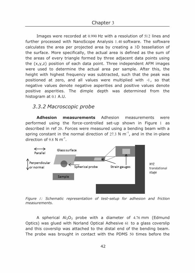
Adhesion measurements Adhesion measurements were performed using the force-controlled set-up shown in Figure as described in ref . Forces were measured using a bending beam with a spring constant in the normal direction of N m-1, and in the in-plane direction of N m-1.
Figure : Schematic representation of test-setup for adhesion and friction measurements.
A spherical Al2O3 probe with a diameter of mm (Edmund Optics) was glued with Norland Optical Adhesive to a glass coverslip and this coverslip was attached to the distal end of the bending beam. The probe was brought in contact with the PDMS times before the
Adhesion of nanopatterned surfaces
43
measurements started, and not cleaned in between measurements. This avoids variation in pull-off forces due to transfer of PDMS oligomers between the surfaces.21 For all measurements, the probe was moved against the sample until a predefined preload within s, and the time lag thus varies between and s. Pull-off forces were measured at different preloads, ranging between and mN, and using a motor velocity during pull-off of µm s-1, at the same spot.
Friction Friction was measured at least times per sample by applying a normal force of , and mN for s, followed by shearing the probe with a motor velocity of µm s-for s, while keeping the normal force constant via a Hz force feedback mechanism. For the friction measurements of flat PDMS, a stiffer bending beam (spring constant in in-plane direction: N/m) and a normal force of mN were used. However, the friction force required to initiate sliding was not met, and thus we can only say that the static friction force of smooth PDMS is > mN. The available beams were not suitable to measure the static friction of Sample at a preload of mN.
3.3.3 Colloidal probe
Cantilever preparation. A SiO particle of µm (Fiber Optic Center) was glued to a triangular silicon nitride cantilever with a spring constant of N/m (Veeco) using a micromanipulator. Norland Optical Adhesive was used as glue. The glue was cured under UV irradiation for s.
Adhesion measurements. The probe was first contaminated with PDMS by bringing it in contact with flat PDMS at least times. To calibrate the cantilever, a silicon wafer was used as hard counter surface.22 The wafer was cleaned with water and ethanol, then contaminated by pressing a piece of PDMS ~ times against it to reduce capillary condensation and hence adhesion between the probe and the wafer. The sensitivity was determined from the approach curve in the constant compliance regime and the spring constant was determined via the thermal tuning method.23
Force curves (~- per measurement) were recorded with the Force Robot (JPK), at an approach and retract velocity ofµm/s unless stated otherwise. The preload was nN.
Chapter
44
All curves were checked by eye, and curves with abnormalities were discarded. The curves were analyzed using the JPK data processing software.
3.4 Results & Discussion
3.4.1 Models for adhesion
Surface structures can significantly alter the adhesive properties of surfaces. To understand the effect of surface structures on adhesion, it is instructive to discuss models for adhesion between two spheres first.
Model of Hertz
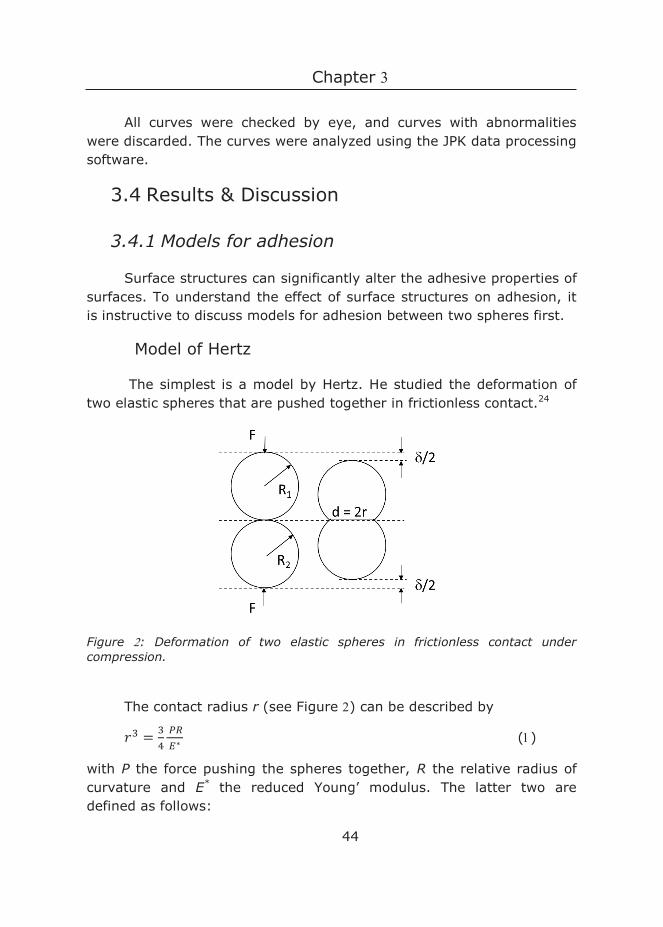
The simplest is a model by Hertz. He studied the deformation of two elastic spheres that are pushed together in frictionless contact.24
Figure : Deformation of two elastic spheres in frictionless contact under compression.
The contact radius r (see Figure ) can be described by
𝑟𝑟3 = 34
𝑃𝑃𝑃𝑃𝐸𝐸∗ ()
with P the force pushing the spheres together, R the relative radius of curvature and E* the reduced Young’ modulus. The latter two are defined as follows:
Adhesion of nanopatterned surfaces
45
1𝑅𝑅 = 1
𝑅𝑅1+ 1
𝑅𝑅2 ()
1𝐸𝐸∗ = 1−𝜈𝜈1
2
𝐸𝐸1+ 1−𝜈𝜈2
2
𝐸𝐸2 ()
with ν the Poisson’s ratio and E the elastic modulus.
The model of Hertz is only valid for spheres without adhesion which behave in a linear elastic way, and for r<<R.
The JKR model
Johnson, Kendall and Roberts extended the Hertz model to include adhesion. In this JKR-model, Van der Waals interactions inside the contact area are taken into account.25 The contact area in this model is
𝑟𝑟3 = 𝑃𝑃 𝑅𝑅𝐾𝐾 [1 + 3𝜋𝜋𝑊𝑊𝑎𝑎𝑎𝑎ℎ𝑅𝑅
𝑃𝑃 + √2 3𝜋𝜋𝑊𝑊𝑎𝑎𝑎𝑎ℎ𝑅𝑅𝑃𝑃 + (3𝜋𝜋𝑊𝑊𝑎𝑎𝑎𝑎ℎ𝑅𝑅
𝑃𝑃 )2
] ()
with Wadh the work of adhesion and K the reduced stiffness, which can be described by
𝑊𝑊𝑎𝑎𝑎𝑎ℎ= ()
with and the surface energies and the interfacial energy for the two contacting materials (see also Chapter , Figure ).
1𝐾𝐾 = 3
4 (1−𝜈𝜈12
𝐸𝐸1+ 1−𝜈𝜈2
2
𝐸𝐸2) ()
The contact area under the same compression is larger for the JKR-model than for the Hertz model.
Wadh has the same value for making contact (approach) as for breaking contact (retraction) when all interactions are derived solely from the contribution of surface energies. However, other contributions, such as chemical reactions, rearrangements of polymer chains, and surface structures often give rise to adhesion hysteresis. For clarity, the work done when breaking contact is often called Gc, the interface toughness.26 This includes the thermodynamic Wadh and energy dissipation.
In the JKR model, two spheres in contact can withstand a certain tensile load due to the attractive Van der Waals interaction. If the tensile
Chapter
46
load is bigger than a critical load, the two spheres separate. The force at which this occurs, is given by
𝑃𝑃𝑐𝑐 = − 32 𝜋𝜋𝑊𝑊𝑎𝑎𝑎𝑎ℎ𝑅𝑅 ()
The DMT model
The JKR model is suitable for large soft spheres with high surface energies. For small, hard spheres with low surface energies, the DMT theory has been developed by Derjaguin, Muller and Toporov.27 In this model, only Van der Waals interactions outside the contact area are taken into account, and the interactions within the contact area are neglected. This results in the following expressions for the contact radius and critical tensile load:
𝑟𝑟3 = 𝑅𝑅𝑅𝑅𝐾𝐾 + 2𝜋𝜋𝑊𝑊𝑎𝑎𝑎𝑎ℎ𝑅𝑅2
𝐾𝐾 ()
and
𝑃𝑃𝑐𝑐 = −2𝜋𝜋𝑊𝑊𝑎𝑎𝑎𝑎ℎ𝑅𝑅 ` (
The Tabor paramater
A continuous transition between the JKR model and DMT theory exists,28 and the Tabor parameter can be used to determine which model should be used.29 The Tabor parameter is given by
𝜇𝜇 = (𝑅𝑅𝑊𝑊𝑎𝑎𝑎𝑎ℎ2
𝐸𝐸∗2 𝑧𝑧𝑜𝑜3 )
1 3⁄ ()
with z0 the equilibrium separation of the two surfaces (usually - nm). The JKR model is suitable for µ > , and the DMT model for µ < .
The JKR and DMT models both describe adhesion between a spherical probe and a flat surface, and do not take the effect of surface structuring into account.
Adhesion of nanopatterned surfaces
47
Effect of structures on adhesion
Previous studies have shown that wrinkles and surface roughness typically decrease adhesive properties 17-18, 30-31, but in some studies adhesion enhancement was found.14, 32 Adhesion enhancement between compliant smooth surfaces and rigid rough surfaces is often attributed to an increase in true contact area.31 As long as the roughness of this rigid surface is small enough, the positive effect from the true contact area will outweigh the negative effect from the stored elastic energy, and adhesion will be enhanced. In this study, the maximum true contact area is defined by the smooth rigid probe, and hence does not change. Therefore, the increase in true contact area does not play a role in our system.
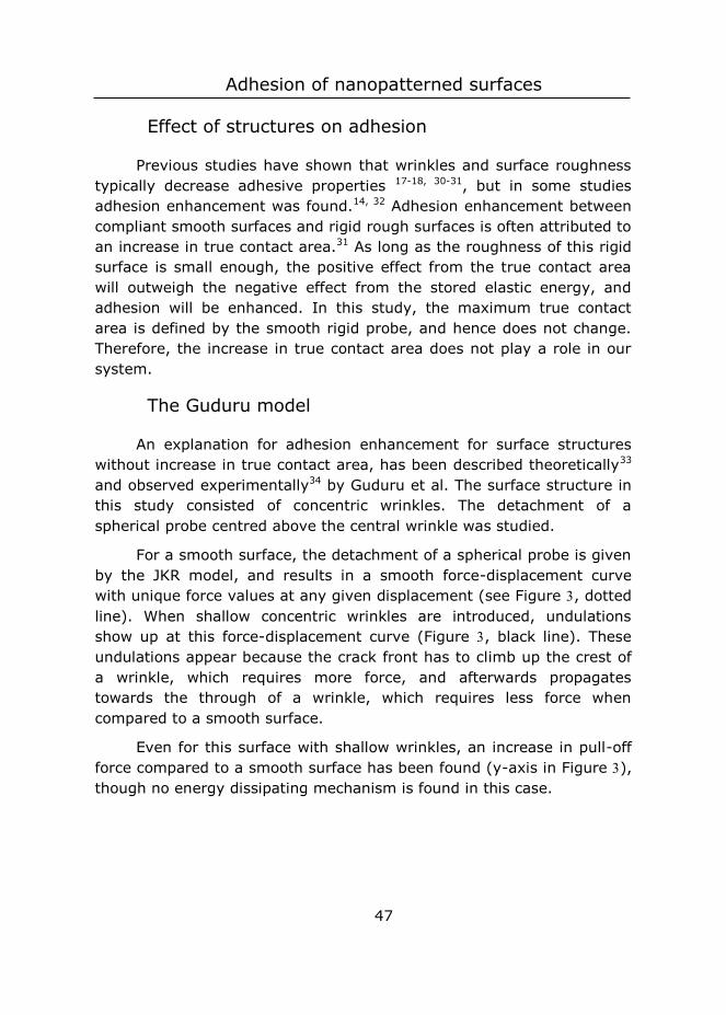
The Guduru model
An explanation for adhesion enhancement for surface structures without increase in true contact area, has been described theoretically33 and observed experimentally34 by Guduru et al. The surface structure in this study consisted of concentric wrinkles. The detachment of a spherical probe centred above the central wrinkle was studied.
For a smooth surface, the detachment of a spherical probe is given by the JKR model, and results in a smooth force-displacement curve with unique force values at any given displacement (see Figure , dotted line). When shallow concentric wrinkles are introduced, undulations show up at this force-displacement curve (Figure , black line). These undulations appear because the crack front has to climb up the crest of a wrinkle, which requires more force, and afterwards propagates towards the through of a wrinkle, which requires less force when compared to a smooth surface.
Even for this surface with shallow wrinkles, an increase in pull-off force compared to a smooth surface has been found (y-axis in Figure ), though no energy dissipating mechanism is found in this case.
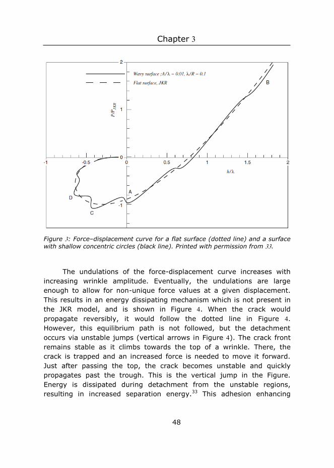
Chapter
48
Figure : Force–displacement curve for a flat surface (dotted line) and a surface with shallow concentric circles (black line). Printed with permission from .
The undulations of the force-displacement curve increases with increasing wrinkle amplitude. Eventually, the undulations are large enough to allow for non-unique force values at a given displacement. This results in an energy dissipating mechanism which is not present in the JKR model, and is shown in Figure . When the crack would propagate reversibly, it would follow the dotted line in Figure . However, this equilibrium path is not followed, but the detachment occurs via unstable jumps (vertical arrows in Figure ). The crack front remains stable as it climbs towards the top of a wrinkle. There, the crack is trapped and an increased force is needed to move it forward. Just after passing the top, the crack becomes unstable and quickly propagates past the trough. This is the vertical jump in the Figure. Energy is dissipated during detachment from the unstable regions, resulting in increased separation energy.33 This adhesion enhancing

Adhesion of nanopatterned surfaces
49
mechanism is only applicable in regimes where the JKR-model is valid, thus for µ > 35
This mechanism to enhance adhesion via surface patterns, functions only when the probe is directly centred above the central wrinkle. Ideally, adhesion enhancement should not depend on the exact position of the probe with respect to the surface structures. Therefore, a design of surface dimples has been chosen.
Figure : Dissipated energy due to unstable crack propagation for detachment of a spherical probe from a surface with concentric wrinkles. The dashed line shows the equilibrium path during detachment, the solid line shows the actual path. The vertical arrows indicate the (unstable) jump from one stable region to the next. The energy that is dissipated during this jump, is indicated as the hatched area. Printed with permission from
3.4.2 Sample characterization
Samples were prepared according to the fabrication process described in Chapter . Carboxylated polystyrene particles are hereby applied to the air/water interface to obtain a monolayer. The crystallinity
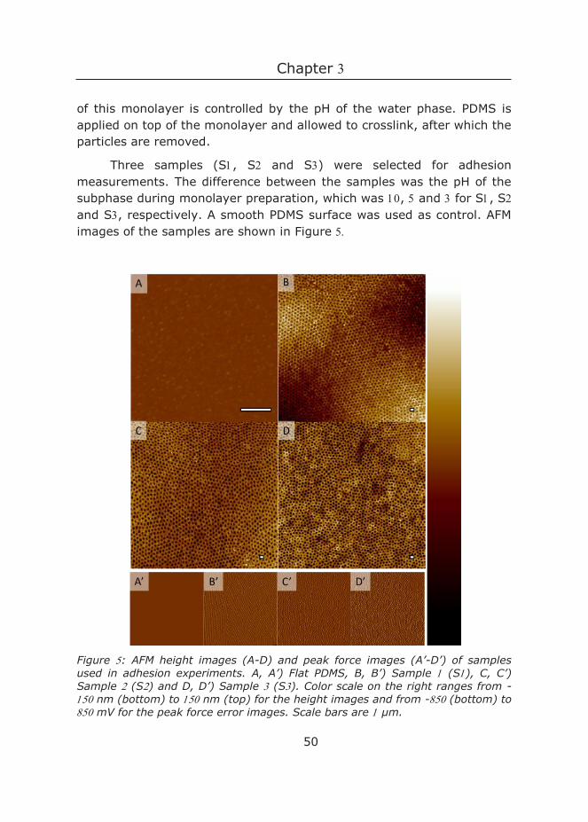
Chapter
50
of this monolayer is controlled by the pH of the water phase. PDMS is applied on top of the monolayer and allowed to crosslink, after which the particles are removed.
Three samples (S, S and S) were selected for adhesion measurements. The difference between the samples was the pH of the subphase during monolayer preparation, which was , and for S, S and S, respectively. A smooth PDMS surface was used as control. AFM images of the samples are shown in Figure
Figure : AFM height images (A-D) and peak force images (A’-D’) of samples used in adhesion experiments. A, A’) Flat PDMS, B, B’) Sample (S), C, C’) Sample (S) and D, D’) Sample (S). Color scale on the right ranges from - nm (bottom) to nm (top) for the height images and from - (bottom) to mV for the peak force error images. Scale bars are µm.
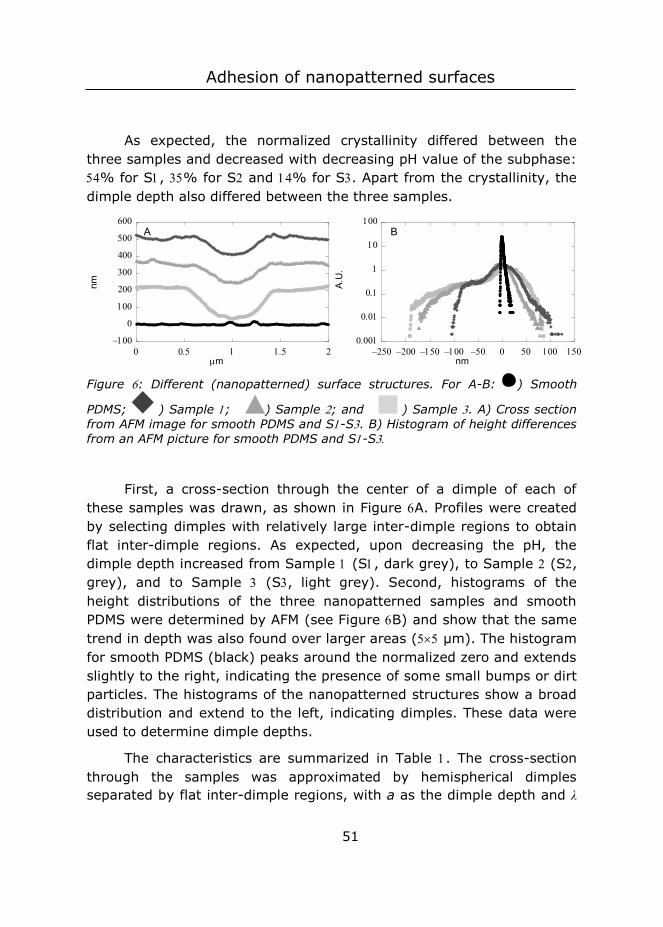
Adhesion of nanopatterned surfaces
51
As expected, the normalized crystallinity differed between the three samples and decreased with decreasing pH value of the subphase: % for S, % for S and % for S. Apart from the crystallinity, the dimple depth also differed between the three samples.
Figure : Different (nanopatterned) surface structures. For A-B: ) Smooth
PDMS; ) Sample ; ) Sample ; and ) Sample . A) Cross section from AFM image for smooth PDMS and S-S. B) Histogram of height differences from an AFM picture for smooth PDMS and S-S
First, a cross-section through the center of a dimple of each of these samples was drawn, as shown in Figure A. Profiles were created by selecting dimples with relatively large inter-dimple regions to obtain flat inter-dimple regions. As expected, upon decreasing the pH, the dimple depth increased from Sample (S, dark grey), to Sample (S, grey), and to Sample (S, light grey). Second, histograms of the height distributions of the three nanopatterned samples and smooth PDMS were determined by AFM (see Figure B) and show that the same trend in depth was also found over larger areas ( µm). The histogram for smooth PDMS (black) peaks around the normalized zero and extends slightly to the right, indicating the presence of some small bumps or dirt particles. The histograms of the nanopatterned structures show a broad distribution and extend to the left, indicating dimples. These data were used to determine dimple depths.
The characteristics are summarized in Table . The cross-section through the samples was approximated by hemispherical dimples separated by flat inter-dimple regions, with a as the dimple depth and λ
nm
A.U
.
m
nm
A B

Chapter
52
as the dimple wavelength. The wavelength λ is defined as the diameter of the particles for a cross-section through the center of the particles. Actual average wavelengths of the samples are a function of the degree of crystallinity and will deviate slightly from this value.
Table : Sample characteristics of samples S-S.
Sample Subphase Crystallinity a*
(nm)
(nm)
S pH=, [salt]=M
±
S pH=, [salt]=M
±
S pH=, [salt]=M
±
* determined by AFM.
3.4.3 Measuring adhesion: interpretation of a force-
distance curve
Adhesion can be studied by measuring force-distance curves. An example of such a curve is shown in Figure for a colloidal probe on a nanopatterned surface. The interpretation of these curves is discussed first.
Upon approach, the force-distance curve shows a jump-to-contact, which is caused by attractive surface forces.36 In the JKR-model, the surface itself bends towards the probe to achieve this contact.37 Then, the approach curve goes through zero. The deflection of the cantilever hereby has the same value as found when it is not in contact with the surface, and this baseline value is set to zerowhen analyzing the curve.
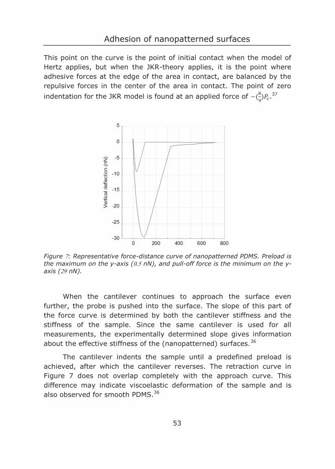
Adhesion of nanopatterned surfaces
53
This point on the curve is the point of initial contact when the model of Hertz applies, but when the JKR-theory applies, it is the point where adhesive forces at the edge of the area in contact, are balanced by the repulsive forces in the center of the area in contact. The point of zero indentation for the JKR model is found at an applied force of −(89)𝑃𝑃𝑐𝑐.
37
Figure : Representative force-distance curve of nanopatterned PDMS. Preload is the maximum on the y-axis ( nN), and pull-off force is the minimum on the y-axis ( nN).
When the cantilever continues to approach the surface even further, the probe is pushed into the surface. The slope of this part of the force curve is determined by both the cantilever stiffness and the stiffness of the sample. Since the same cantilever is used for all measurements, the experimentally determined slope gives information about the effective stiffness of the (nanopatterned) surfaces.36
The cantilever indents the sample until a predefined preload is achieved, after which the cantilever reverses. The retraction curve in Figure 7 does not overlap completely with the approach curve. This difference may indicate viscoelastic deformation of the sample and is also observed for smooth PDMS.36
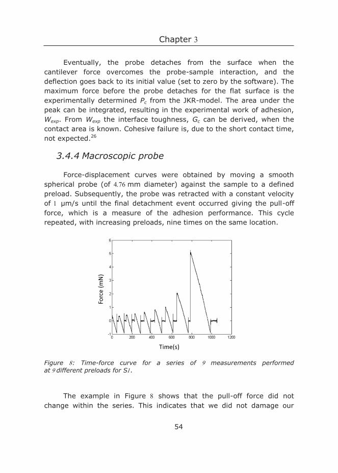
Chapter
54
Eventually, the probe detaches from the surface when the cantilever force overcomes the probe-sample interaction, and the deflection goes back to its initial value (set to zero by the software). The maximum force before the probe detaches for the flat surface is the experimentally determined Pc from the JKR-model. The area under the peak can be integrated, resulting in the experimental work of adhesion, Wexp. From Wexp the interface toughness, Gc can be derived, when the contact area is known. Cohesive failure is, due to the short contact time, not expected.26
3.4.4 Macroscopic probe
Force-displacement curves were obtained by moving a smooth spherical probe (of mm diameter) against the sample to a defined preload. Subsequently, the probe was retracted with a constant velocity of µm/s until the final detachment event occurred giving the pull-off force, which is a measure of the adhesion performance. This cycle repeated, with increasing preloads, nine times on the same location.
Figure : Time-force curve for a series of measurements performed atdifferent preloads for S.
The example in Figure shows that the pull-off force did not change within the series. This indicates that we did not damage our
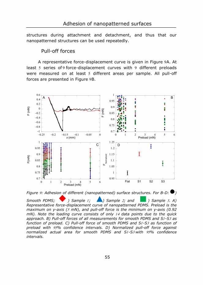
Adhesion of nanopatterned surfaces
55
structures during attachment and detachment, and thus that our nanopatterned structures can be used repeatedly.
Pull-off forces
A representative force-displacement curve is given in Figure A. At least series offorce-displacement curves with different preloads were measured on at least different areas per sample. All pull-off forces are presented in Figure B.
Figure : Adhesion of different (nanopatterned) surface structures. For B-D: )
Smooth PDMS; ) Sample ; ) Sample ; and ) Sample . A) Representative force-displacement curve of nanopatterned PDMS. Preload is the maximum on y-axis ( mN), and pull-off force is the minimum on y-axis (0.92 mN). Note the loading curve consists of only data points due to the quick approach. B) Pull-off forces of all measurements for smooth PDMS and S-S as function of preload. C) Pull-off force of smooth PDMS and S-S as function of preload with % confidence intervals. D) Normalized pull-off force against normalized actual area for smooth PDMS and S-Swith % confidence intervals.
x (mm)
F (m
N)
A
Preload (mN)
F (m
N)
B
Preload (mN)
F(m
N)
C
F Nor
mal
ized
Flat S1 S2 S3
D
Chapter
56
Figure C shows the average pull-off forces plotted against the applied preload for smooth PDMS and for patterned surfaces. The pull-off force values for patterned surfaces were higher compared to the smooth surface at almost any preload. Only S showed a preload dependency and exhibited a lower pull-off force than the smooth surface at the highest preload. Due to the relatively low preload forces used in this study, and the small dimple size this decreased pull-off force is unlikely due to mechanical damage. For all other samples, the pull-off force did not vary significantly with the preload. Normalized pull-off forces in the preload independent regime (i.e. < mN) are plotted in Figure D.
Contact between sample and probe
Full contact was likely always achieved for our structures. Although we did not observe the contact area directly due to the relatively small size of our surface structures, we conclude that full contact was achieved by comparing our surface feature dimensions and material properties to similar surface structures in previous reports.16, 38-39 For example, Jin et al. experimentally observed complete contact independent of preload for PDMS wrinkles with a wavelength of µm and amplitudes (analogous to dimple depth) smaller than µm, while wrinkles with amplitudes higher than µm showed partial contact. The sample with an amplitude of µm showed only complete contact upon applying preload.38 In addition, in a theoretical study by McMeeking et al. an approximate condition for complete contact of dimpled surfaces without the application of preload, i.e. spontaneous jump-to-contact, was derived. They showed that the depth of a dimple in a compliant material below which full contact occurs depended on dimple wavelength, , work of adhesion, Wad, and effective modulus, E*, as 40:
a < √𝜋𝜋𝑊𝑊𝑎𝑎𝑎𝑎𝐸𝐸∗ ()
Substituting parameter values as obtained by Jin et al.38 for PDMS with similar material properties, i.e. E*= MPa and Wad = J/m, we obtain a maximum dimple depth of µm, which is a larger value than the depths of our samples. Thus, the dimples in this study are most likely shallow enough to spontaneously jump-to-contact.
Adhesion of nanopatterned surfaces
57
Although theoretical considerations suggest that complete contact formation may occur for our dimple dimensions, in practice air can be trapped in the dimples and prevent complete contact from being achieved. A difference between our dimpled structures and wrinkles or an array of pillars, is that dimples are isolated and air can get locked in. However, PDMS is known to have good air permeability, and air will be removed through the material.41
Our results thus support complete contact formation. As stated above, for complete contact the true contact area is defined by the probe and, therefore, our results cannot be explained by a difference in contact area. Instead, the increase in adhesion of our materials may be attributed to a mechanical instability resulting from crack trapping as proposed by Guduru.33 A prerequisite for this explanation is that the Tabor parameter µ > 35, and filling in Equation , using Wadh = J m and E* = MPa 7, shows that for our system, µ >> .
Energy dissipation
The origin of this dissipation, namely the specific surface structure, is also present in our materials, and for both concentric wrinkles and dimples the crack can be trapped. Each dimple provides the possibility for the crack trapping and energy-dissipating mechanism. When the dimples are closely packed, the effect of structuring on adhesion is present over the whole area of the sample, and this eliminates the need to position the probe on a unique spot above the sample.
In contrast, for D wrinkled surfaces, it has been observed that the crack first moves parallel to the wrinkles after which it jumps in the direction perpendicular to the wrinkles.17 Therefore, for D wrinkles this crack trapping mechanism only applies to the last part of the detachment and may explain why no adhesion enhancement was found for D wrinkled surfaces with similar wrinkle dimensions to our dimple dimensions.17
An alternative energy dissipating mechanism may be provided by discrete crack initiation, which has been found for small wrinkle amplitudes of to µm and an aspect ratio of , but not for slightly bigger wrinkles (amplitude of µm with the same aspect ratio).17 For these small wrinkles, the individual wrinkles detach first, during pull-off.
Chapter
58
This discrete crack initiation throughout the surface dissipates energy. Additional energy could thus be dissipated ahead of the crack front. It should be pointed out that this crack initiation mechanism was found for a planar wrinkled surface in contact with a flat probe whereas in our case the probe is spherical. Therefore, in our case, the middle region will stay under compressive stress much longer during detachment compared to measurements with a flat probe. This means that energy dissipation due to discrete crack initiation can only occur in the vicinity of the crack front.
Effect of dimple depth and dimple density
The difference in adhesion enhancement for the three structured samples can be explained considering two parameters: (i) dimple depth and (ii) dimple density. The dimple depth determines both the magnitude of the crack trapping effect and the elastic penalty upon compression. These two effects counteract each other. A deeper dimple results in more energy dissipation.33 However, the larger the dimple depth, the more elastic energy is stored due to surface deformation to achieve complete contact. This stored elastic energy is (partly) recovered and may help to break interfacial bonds. Since all three structured samples show enhancement of adhesion compared to the flat control, the energy dissipation through unstable detachment outweighs the elastic penalty, and the net effect of one dimple, is an increase in adhesion.
In addition to the dimple depth, the dimple density will also affect the adhesion. More specifically, a higher density may have a larger influence on adhesion. For our samples the dimple density can be assessed by the crystallinity. A higher (normalized) crystallinity stems from a more efficient packing and thus a higher dimple density. Indeed, if we count all particles within the same area for all three monolayers and compare S (pH , normalized crystallinity ) and S (pH , normalized crystallinity ) a decrease in number of particles of % is found. Comparing S and S (pH , normalized crystallinity ) results in a decrease of %.
In our experiments, both the dimple depth and the dimple density are varied for each sample. We find that the largest increase in adhesion
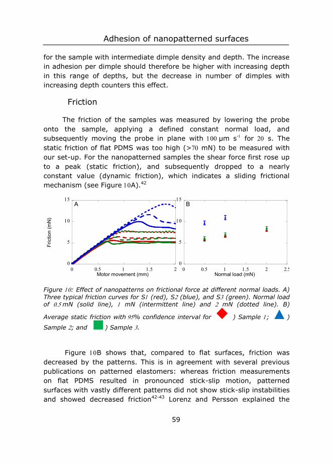
Adhesion of nanopatterned surfaces
59
for the sample with intermediate dimple density and depth. The increase in adhesion per dimple should therefore be higher with increasing depth in this range of depths, but the decrease in number of dimples with increasing depth counters this effect.
Friction
The friction of the samples was measured by lowering the probe onto the sample, applying a defined constant normal load, and subsequently moving the probe in plane with µm s- for s. The static friction of flat PDMS was too high (> mN) to be measured with our set-up. For the nanopatterned samples the shear force first rose up to a peak (static friction), and subsequently dropped to a nearly constant value (dynamic friction), which indicates a sliding frictional mechanism (see Figure A).42
Figure : Effect of nanopatterns on frictional force at different normal loads. A) Three typical friction curves for S (red), S (blue), and S (green). Normal load of mN (solid line), mN (intermittent line) and mN (dotted line). B)
Average static friction with% confidence interval for ) Sample ; )
Sample ; and ) Sample .
Figure B shows that, compared to flat surfaces, friction was decreased by the patterns. This is in agreement with several previous publications on patterned elastomers: whereas friction measurements on flat PDMS resulted in pronounced stick-slip motion, patterned surfaces with vastly different patterns did not show stick-slip instabilities and showed decreased friction42-43 Lorenz and Persson explained the
Motor movement (mm)
Fric
tion
(mN
)
A
Normal load (mN)
B
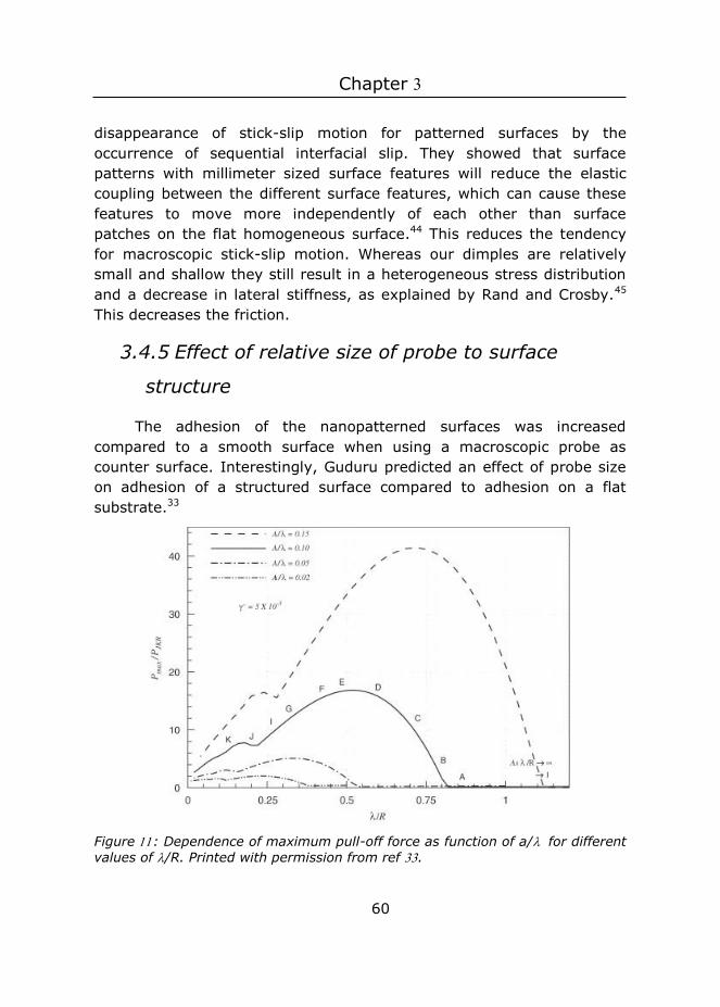
Chapter
60
disappearance of stick-slip motion for patterned surfaces by the occurrence of sequential interfacial slip. They showed that surface patterns with millimeter sized surface features will reduce the elastic coupling between the different surface features, which can cause these features to move more independently of each other than surface patches on the flat homogeneous surface.44 This reduces the tendency for macroscopic stick-slip motion. Whereas our dimples are relatively small and shallow they still result in a heterogeneous stress distribution and a decrease in lateral stiffness, as explained by Rand and Crosby.45 This decreases the friction.
3.4.5 Effect of relative size of probe to surface
structure
The adhesion of the nanopatterned surfaces was increased compared to a smooth surface when using a macroscopic probe as counter surface. Interestingly, Guduru predicted an effect of probe size on adhesion of a structured surface compared to adhesion on a flat substrate.33
Figure : Dependence of maximum pull-off force as function of a/ for different values of /R. Printed with permission from ref .
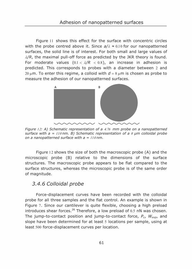
Adhesion of nanopatterned surfaces
61
Figure shows this effect for the surface with concentric circles with the probe centred above it. Since a/≈ for our nanopatterned surfaces, the solid line is of interest. For both small and large values of /R, the maximal pull-off force as predicted by the JKR theory is found. For moderate values (/R ), an increase in adhesion is predicted. This corresponds to probes with a diameter between and m. To enter this regime, a colloid with d m is chosen as probe to measure the adhesion of our nanopatterned surfaces.
Figure : A) Schematic representation of a mm probe on a nanopatterned surface with a = nm. B) Schematic representation of a µm colloidal probe on a nanopatterned surface with a = nm.
Figure shows the size of both the macroscopic probe (A) and the microscopic probe (B) relative to the dimensions of the surface structures. The macroscopic probe appears to be flat compared to the surface structures, whereas the microscopic probe is of the same order of magnitude.
3.4.6 Colloidal probe
Force-displacement curves have been recorded with the colloidal probe for all three samples and the flat control. An example is shown in Figure . Since our cantilever is quite flexible, choosing a high preload introduces shear forces.26 Therefore, a low preload of nN was chosen. The jump-to-contact position and jump-to-contact force, Pc, Wexp, and slope have been determined for at least locations per sample, using at least force-displacement curves per location.

Chapter
62
Work of adhesion and pull-off forces
Figure shows the work of adhesion and pull-off forces for all samples. The nanopatterned surfaces showed an increase in both Wexp and Pc. Both were highest for S (Figure BC), which is the sample with smallest dimple depth a and highest dimple density. The increase in Wexp for the patterned samples compared to the flat sample, shows that energy is indeed dissipated due to structuring during pull-off.
Figure Work of adhesion and pull-off force of nanopatterned surfaces for five
different locations per sample. For A-D: ) Smooth PDMS; ) Sample ; )
Sample ; and ) Sample . A) Work of adhesion as function of pull-off force. B) Average work of adhesion. C) Average pull-off force. D) Normalized pull-off force.
The relative increase in Pc as compared to the flat surface, was similar for both probe sizes (Figures D and D). However, Pc measured with the colloidal probe was two orders of magnitude smaller than the expected value of ~ mN, as calculated using Equation , the probe radius of µm and the literature value for Wadh for PDMS from ref ,
F (n
N)
Flat S1 S2 S3
C
Nor
mal
ized
pul
l-off
forc
e
Flat S1 S2 S3
D
Wor
k of
adh
esio
n (J
)
Flat S1 S2 S3
B
F (nN)
Wor
k (J
)
A
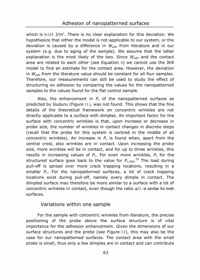
Adhesion of nanopatterned surfaces
63
which is J/m. There is no clear explanation for this deviation. We hypothesize that either the model is not applicable to our system, or the deviation is caused by a difference in Wadh from literature and in our system (e.g. due to aging of the sample). We assume that the latter explanation is the most likely of the two. Since Wadh and the contact area are related to each other (see Equation ) we cannot use the JKR model to find an estimate for the contact area. However, the deviation in Wadh from the literature value should be constant for all four samples. Therefore, our measurements can still be used to study the effect of structuring on adhesion by comparing the values for the nanopatterned samples to the values found for the flat control sample.
Also, the enhancement in Pc of the nanopatterned surfaces as predicted by Guduru (Figure , was not found. This shows that the fine details of the theoretical framework on concentric wrinkles are not directly applicable to a surface with dimples. An important factor for the surface with concentric wrinkles is that, upon increase or decrease in probe size, the number of wrinkles in contact changes in discrete steps (recall that the probe for this system is centred in the middle of all concentric wrinkles). An increase in Pc is found when, apart from the central crest, also wrinkles are in contact. Upon increasing the probe size, more wrinkles will be in contact, and for up to three wrinkles, this results in increasing values of Pc. For even more wrinkles, Pc for the structured surface goes back to the value for Pc,JKR.33 The load during pull-off is spread over more crack trapping locations, resulting in a smaller Pc. For the nanopatterned surfaces, a lot of crack trapping locations exist during pull-off, namely every dimple in contact. The dimpled surface may therefore be more similar to a surface with a lot of concentric wrinkles in contact, even though the ratio a/is similar for both surfaces.
Variations within one sample
For the sample with concentric wrinkles from literature, the precise positioning of the probe above the surface structure is of vital importance for the adhesion enhancement. Given the dimensions of our surface structures and the probe (see Figure ), this may also be the case for our nanopatterned surfaces. The contact area with the small probe is small, thus only a few dimples are in contact and can contribute

Chapter
64
to the energy dissipation. With decreasing dimple density for S S S, the number of dimples in contact may differ significantly between the samples; if the probe approaches the surface on a non-crystalline area (mostly found on S, less dimples are present in the contact area than when the probe is positioned above a crystalline area (mostly found on S. This effect is averaged out for the large contact areas when using a large probe, but a small probe can be positioned such that almost no dimples are in contact. The local dimple density is therefore expected to have an effect on the pull-off force for the small probe. And even within one sample, Pc may be different. The centre of the probe may be positioned directly above a dimple, or directly above an interdimple region. The area in contact may have dimples in a hexagonal packing, or the dimples are on a grain boundary. This all may influence the adhesion within one sample.46
To test this, Pc is measured times at five different locations per sample (Figure ).
Figure Peak force for series of force-displacement curves at five different locations for A) smooth PDMS, B) Sample , C) Sample , D) Sample
B
0 100 200 300 400 500
D
20
30
40
50
0 100 200 300 400 500
C
F (n
N)
20
30
40
50A
F (n
N)
F (n
N)
# #
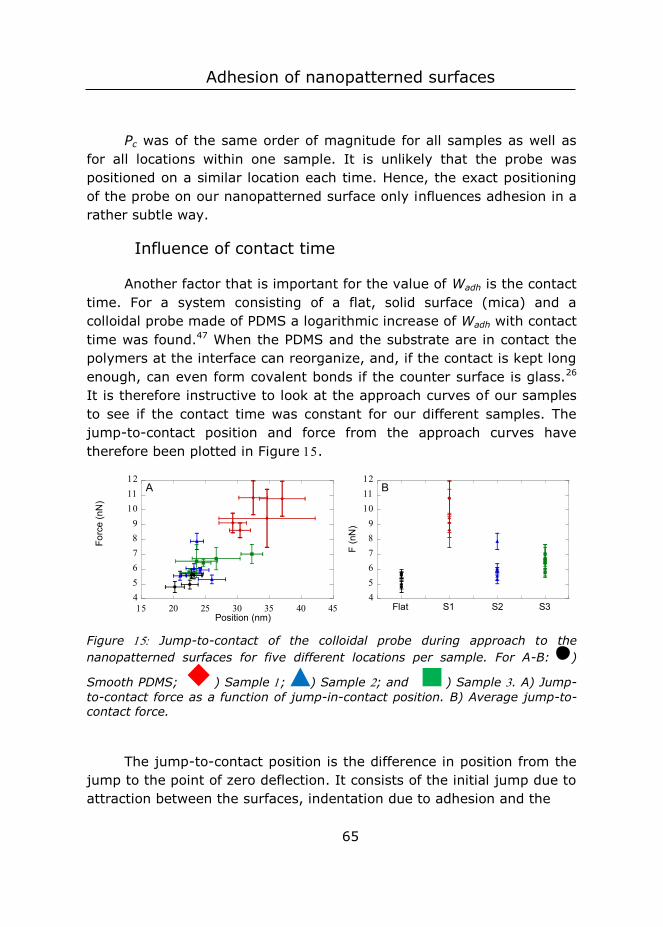
Adhesion of nanopatterned surfaces
65
Pc was of the same order of magnitude for all samples as well as for all locations within one sample. It is unlikely that the probe was positioned on a similar location each time. Hence, the exact positioning of the probe on our nanopatterned surface only influences adhesion in a rather subtle way.
Influence of contact time
Another factor that is important for the value of Wadh is the contact time. For a system consisting of a flat, solid surface (mica) and a colloidal probe made of PDMS a logarithmic increase of Wadh with contact time was found.47 When the PDMS and the substrate are in contact the polymers at the interface can reorganize, and, if the contact is kept long enough, can even form covalent bonds if the counter surface is glass.26 It is therefore instructive to look at the approach curves of our samples to see if the contact time was constant for our different samples. The jump-to-contact position and force from the approach curves have therefore been plotted in Figure .
Figure Jump-to-contact of the colloidal probe during approach to the nanopatterned surfaces for five different locations per sample. For A-B: )
Smooth PDMS; ) Sample ; ) Sample ; and ) Sample . A) Jump-to-contact force as a function of jump-in-contact position. B) Average jump-to-contact force.
The jump-to-contact position is the difference in position from the jump to the point of zero deflection. It consists of the initial jump due to attraction between the surfaces, indentation due to adhesion and the
F (n
N)
Flat S1 S2 S3
B
Position (nm)
Forc
e (n
N)
A
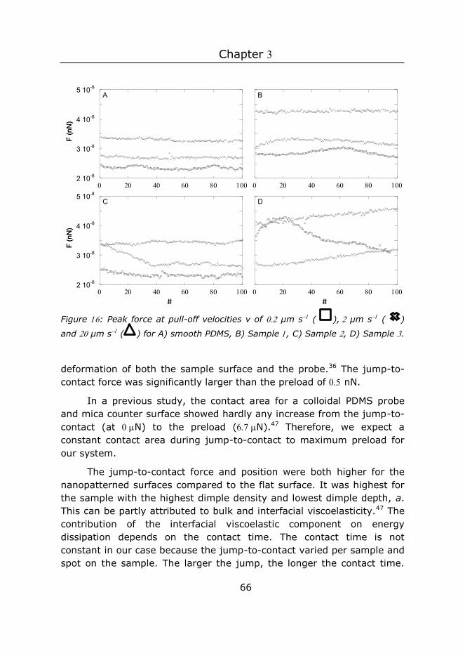
Chapter
66
Figure : Peak force at pull-off velocities v of µm s ( ), µm s ( )
and µm s ( ) for A) smooth PDMS, B) Sample , C) Sample , D) Sample .
deformation of both the sample surface and the probe.36 The jump-to-contact force was significantly larger than the preload of nN.
In a previous study, the contact area for a colloidal PDMS probe and mica counter surface showed hardly any increase from the jump-to-contact (at N) to the preload (N).47 Therefore, we expect a constant contact area during jump-to-contact to maximum preload for our system.
The jump-to-contact force and position were both higher for the nanopatterned surfaces compared to the flat surface. It was highest for the sample with the highest dimple density and lowest dimple depth, a. This can be partly attributed to bulk and interfacial viscoelasticity.47 The contribution of the interfacial viscoelastic component on energy dissipation depends on the contact time. The contact time is not constant in our case because the jump-to-contact varied per sample and spot on the sample. The larger the jump, the longer the contact time.
2 10-8
3 10-8
4 10-8
5 10-8
A
F (n
N)
F (n
N)
B
2 10-8
3 10-8
4 10-8
5 10-8
C
F (n
N)
F (n
N)
D
##
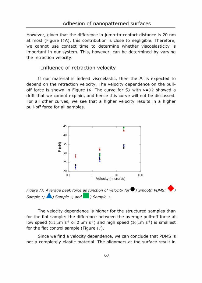
Adhesion of nanopatterned surfaces
67
However, given that the difference in jump-to-contact distance is 20 nm at most (Figure A), this contribution is close to negligible. Therefore, we cannot use contact time to determine whether viscoelasticity is important in our system. This, however, can be determined by varying the retraction velocity.
Influence of retraction velocity
If our material is indeed viscoelastic, then the Pc is expected to depend on the retraction velocity. The velocity dependence on the pull-off force is shown in Figure . The curve for S with v= showed a drift that we cannot explain, and hence this curve will not be discussed. For all other curves, we see that a higher velocity results in a higher pull-off force for all samples.
Figure : Average peak force as function of velocity for ) Smooth PDMS; )
Sample ; ) Sample ; and ) Sample .
The velocity dependence is higher for the structured samples than for the flat sample: the difference between the average pull-off force at low speed (m s or m s) and high speed (m s) is smallest for the flat control sample (Figure ).
Since we find a velocity dependence, we can conclude that PDMS is not a completely elastic material. The oligomers at the surface result in
Velocity (micron/s)
F (n
N)
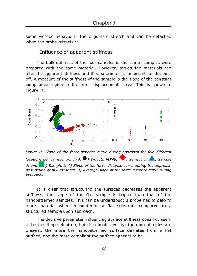
Chapter
68
some viscous behaviour. The oligomers stretch and can be detached when the probe retracts.22
Influence of apparent stiffness
The bulk stiffness of the four samples is the same: samples were prepared with the same material. However, structuring materials can alter the apparent stiffness and this parameter is important for the pull-off. A measure of the stiffness of the sample is the slope of the constant compliance region in the force-displacement curve. This is shown in Figure .
Figure Slope of the force-distance curve during approach for five different
locations per sample. For A-B: ) Smooth PDMS; ) Sample ; ) Sample
; and ) Sample . A) Slope of the force-distance curve during the approach as function of pull-off force. B) Average slope of the force-distance curve during approach.
It is clear that structuring the surfaces decreases the apparent stiffness; the slope of the flat sample is higher than that of the nanopatterned samples. This can be understood: a probe has to deform more material when encountering a flat substrate compared to a structured sample upon approach.
The decisive parameter influencing surface stiffness does not seem to be the dimple depth a, but the dimple density: the more dimples are present, the more the nanopatterned surface deviates from a flat surface, and the more compliant the surface appears to be.
F (nN)
Slo
pe (N
/m)
A
Flat S1 S2 S3
BB
Adhesion of nanopatterned surfaces
69
Influence of the elastic penalty
For the macroscopic probe, we observed that the higher the dimple depth a, the more energy is dissipated per dimple. The elastic penalty, which is higher for deeper dimples, does thus not overrule the increase in energy dissipation per dimple for deeper dimples. Since the sample with the deepest dimples (S) is also the sample with the smallest density, a trade-off between dimple density and dimple depth was found, in which the sample with medium dimple depth and density (S) showed the highest pull-off force.
For the small probe, this trade-off between dimple density and dimple depth is not found; not S but S shows the highest adhesion. The explanation may lie in the effect of probe size on the elastic penalty. The macroscopic probe is so large that it can be considered a flat surface on the scale of a dimple (see Figure ). For the smaller probe, the curvature of the probe itself is present on the scale of a dimple. The surface has to deform more in order to make full contact with the surface of the colloidal probe compared to that of the macroscopic probe. This deformation is more easily achieved for samples with a lower apparent stiffness, and thus with the higher dimple densities.
Due to these larger deformations that are required for a dimple to make contact, it is expected that the elastic penalty has a stronger effect on the final pull-off force. The deeper the dimple, the more deformation is needed, thus the higher is the elastic penalty. Using this line of reasoning, S shows the highest pull-off force for the colloidal probe because it has more and shallow dimples.
3.4.7 Conclusion
Nanopatterned surfaces have been made according to the method presented in Chapter . Three samples with varying dimple depth and dimple density were selected. The effect of the surface structures were investigated using two spherical probes with different size as counter surface, and the resulting force-displacement curves were analysed. The pull-off force was increased for all nanopatterned surfaces and for both probe sizes. The increase is attributed to energy dissipation during pull-off; the detachment process shows stable and unstable regions due to
Chapter
70
the surface structures. The two parameters controlling the final pull-off force are dimple density and dimple depth. Every dimple contributes to energy dissipation, thus the higher the dimple density, the more energy dissipation. The effect of dimple depth depends on the counter-surface used. For the large probe, the highest a gives the highest energy dissipation per dimple, but this trend is not found for the smaller probe. The scaling of pull-off force with probe size as described for a surface consisting of concentric wrinkles, has not been found for our nanopatterned surfaces. It is therefore suggested that not the ratio a/, but the number of crack trapping locations is important for the increase in Pc.
These results show that interfacial templating of colloidal particles provides a promising route for creating functional surfaces of which the three-dimensional topology can be tuned without elaborate and energy-consuming lithographic methods. With the emergence of a wide variety of new methods to tailor the size and shape of colloids, and their organisation at liquid interfaces, this opens a wealth of opportunities for lithography-free design of new adhesive and low-frictional materials.
References
1. Gorb, S., Attachment devices of insect cuticle. Springer: 2001.
2. Loskill, P.; Puthoff, J.; Wilkinson, M.; Mecke, K.; Jacobs, K.; Autumn, K., Macroscale adhesion of gecko setae reflects nanoscale differences in subsurface composition. Journal of The Royal Society Interface 2013, 10 (78).
3. Kamperman, M.; Kroner, E.; del Campo, A.; McMeeking, R. M.; Arzt, E., Functional adhesive surfaces with “gecko” effect: the concept of contact splitting. Advanced Engineering Materials 2010, 12 (5), 335-348.
4. Boesel, L. F.; Greiner, C.; Arzt, E.; del Campo, A., Gecko‐Inspired Surfaces: A Path to Strong and Reversible Dry Adhesives. Advanced Materials 2010, 22 (19), 2125-2137.
5. Geim, A.; Grigorieva, S. D. I.; Novoselov, K.; Zhukov, A.; Shapoval, S. Y., Microfabricated adhesive mimicking gecko foot-hair. Nature materials 2003, 2 (7), 461-463.
6. Sitti, M.; Fearing, R. S., Synthetic gecko foot-hair micro/nano-structures as dry adhesives. Journal of Adhesion Science and Technology 2003, 17 (8), 1055-1073.
Adhesion of nanopatterned surfaces
71
7. Greiner, C.; del Campo, A.; Arzt, E., Adhesion of bioinspired micropatterned surfaces: effects of pillar radius, aspect ratio, and preload. Langmuir 2007, 23 (7), 3495-3502.
8. del Campo, A.; Greiner, C.; Arzt, E., Contact shape controls adhesion of bioinspired fibrillar surfaces. Langmuir 2007, 23 (20), 10235-10243.
9. Murphy, M. P.; Aksak, B.; Sitti, M., Gecko‐Inspired Directional and Controllable Adhesion. Small 2009, 5 (2), 170-175.
10. Gorb, S.; Varenberg, M.; Peressadko, A.; Tuma, J., Biomimetic mushroom-shaped fibrillar adhesive microstructure. Journal of The Royal Society Interface 2007, 4 (13), 271-275.
11. Jeong, H. E.; Lee, J.-K.; Kim, H. N.; Moon, S. H.; Suh, K. Y., A nontransferring dry adhesive with hierarchical polymer nanohairs. Proceedings of the National Academy of Sciences 2009, 106 (14), 5639-5644.
12. Glassmaker, N. J.; Jagota, A.; Hui, C.-Y.; Noderer, W. L.; Chaudhury, M. K., Biologically inspired crack trapping for enhanced adhesion. Proceedings of the National Academy of Sciences 2007, 104 (26), 10786-10791.
13. Rong, Z.; Zhou, Y.; Chen, B.; Robertson, J.; Federle, W.; Hofmann, S.; Steiner, U.; Goldberg‐Oppenheimer, P., Bio‐Inspired Hierarchical Polymer Fiber‐Carbon Nanotube Adhesives. Advanced Materials 2013.
14. Chan, E. P.; Smith, E. J.; Hayward, R. C.; Crosby, A. J., Surface wrinkles for smart adhesion. Advanced Materials 2008, 20 (4), 711-716.
15. Kundu, S.; Davis, C. S.; Long, T.; Sharma, R.; Crosby, A. J., Adhesion of nonplanar wrinkled surfaces. Journal of Polymer Science Part B: Polymer Physics 2011, 49 (3), 179-185.
16. Davis, C. S.; Martina, D.; Creton, C.; Lindner, A.; Crosby, A. J., Enhanced adhesion of elastic materials to small-scale wrinkles. Langmuir 2012, 28 (42), 14899-14908.
17. Lin, P.-C.; Vajpayee, S.; Jagota, A.; Hui, C.-Y.; Yang, S., Mechanically tunable dry adhesive from wrinkled elastomers. Soft Matter 2008, 4 (9), 1830-1835.
18. Davis, C. S.; Crosby, A. J., Mechanics of wrinkled surface adhesion. Soft Matter 2011, 7 (11), 5373-5381.
19. Kraus, T.; Brodoceanu, D.; Pazos‐Perez, N.; Fery, A., Colloidal Surface Assemblies: Nanotechnology Meets Bioinspiration. Adv. Funct. Mater. 2013.
20. Drechsler, P.; Federle, W., Biomechanics of smooth adhesive pads in insects: influence of tarsal secretion on attachment performance. Journal of Comparative Physiology A 2006, 192 (11), 1213-1222.
Chapter
72
21. Kroner, E.; Maboudian, R.; Arzt, E., Adhesion Characteristics of PDMS Surfaces During Repeated Pull‐Off Force Measurements. Advanced Engineering Materials 2010, 12 (5), 398-404.
22. Gillies, G.; Prestidge, C. A.; Attard, P., An AFM study of the deformation and nanorheology of cross-linked PDMS droplets. Langmuir 2002, 18 (5), 1674-1679.
23. Hutter, J. L.; Bechhoefer, J., Calibration of atomic‐force microscope tips. Review of Scientific Instruments 1993, 64 (7), 1868-1873.
24. Hertz, H., Über die Berührung fester elastischer Körper. J. reine angew. Math. 1882, 92, 156-171.
25. Johnson, K.; Kendall, K.; Roberts, A. In Surface energy and the contact of elastic solids, Proceedings of the Royal Society of London A: Mathematical, Physical and Engineering Sciences, The Royal Society: 1971; pp 301-313.
26. Toikka, G.; Spinks, G. M.; Brown, H. R., Interactions between micron-sized glass particles and poly (dimethyl siloxane) in the absence and presence of applied load. The Journal of Adhesion 2000, 74 (1-4), 317-340.
27. Derjaguin, B. V.; Muller, V. M.; Toporov, Y. P., Effect of contact deformations on the adhesion of particles. Journal of Colloid and interface science 1975, 53 (2), 314-326.
28. Tabor, D., Surface forces and surface interactions. Journal of colloid and interface science 1977, 58 (1), 2-13.
29. Muller, V.; Yushchenko, V.; Derjaguin, B., On the influence of molecular forces on the deformation of an elastic sphere and its sticking to a rigid plane. Journal of Colloid and Interface Science 1980, 77 (1), 91-101.
30. Fuller, K.; Tabor, D., The effect of surface roughness on the adhesion of elastic solids. Proceedings of the Royal Society of London. A. Mathematical and Physical Sciences 1975, 345 (1642), 327-342.
31. Persson, B.; Tosatti, E., The effect of surface roughness on the adhesion of elastic solids. The Journal of Chemical Physics 2001, 115, 5597.
32. Briggs, G.; Briscoe, B., The effect of surface topography on the adhesion of elastic solids. Journal of Physics D: Applied Physics 1977, 10 (18), 2453.
33. Guduru, P., Detachment of a rigid solid from an elastic wavy surface: theory. Journal of the Mechanics and Physics of Solids 2007, 55 (3), 445-472.
34. Guduru, P.; Bull, C., Detachment of a rigid solid from an elastic wavy surface: Experiments. Journal of the Mechanics and Physics of Solids 2007, 55 (3), 473-488.
Adhesion of nanopatterned surfaces
73
35. Waters, J.; Lee, S.; Guduru, P., Mechanics of axisymmetric wavy surface adhesion: JKR–DMT transition solution. International Journal of Solids and Structures 2009, 46 (5), 1033-1042.
36. Butt, H.-J.; Cappella, B.; Kappl, M., Force measurements with the atomic force microscope: Technique, interpretation and applications. Surface science reports 2005, 59 (1), 1-152.
37. Lin, D. C.; Dimitriadis, E. K.; Horkay, F., Robust strategies for automated AFM force curve analysis—II: adhesion-influenced indentation of soft, elastic materials. Journal of biomechanical engineering 2007, 129 (6), 904-912.
38. Jin, C.; Khare, K.; Vajpayee, S.; Yang, S.; Jagota, A.; Hui, C.-Y., Adhesive contact between a rippled elastic surface and a rigid spherical indenter: from partial to full contact. Soft Matter 2011, 7 (22), 10728-10736.
39. Degrandi-Contraires, É.; Beaumont, A.; Restagno, F.; Weil, R.; Poulard, C.; Léger, L., Cassie-Wenzel–like transition in patterned soft elastomer adhesive contacts. EPL (Europhysics Letters) 2013, 101 (1), 14001.
40. McMeeking, R. M.; Ma, L.; Arzt, E., Bi‐Stable Adhesion of a Surface with a Dimple. Advanced Engineering Materials 2010, 12 (5), 389-397.
41. ChangáKim, Y., Analysis of pressure-driven air bubble elimination in a microfluidic device. Lab on a Chip 2008, 8 (1), 176-178.
42. Rand, C. J.; Crosby, A. J., Friction of soft elastomeric wrinkled surfaces. Journal of Applied Physics 2009, 106 (6), 064913-064913-4.
43. Varenberg, M.; Gorb, S. N., Hexagonal surface micropattern for dry and wet friction. Advanced Materials 2009, 21 (4), 483-486.
44. Lorenz, B.; Persson, B., On the origin of why static or breakloose friction is larger than kinetic friction, and how to reduce it: the role of aging, elasticity and sequential interfacial slip. Journal of Physics: Condensed Matter 2012, 24 (22), 225008.
45. Rand, C. J.; Crosby, A. J., Friction of soft elastomeric surfaces with a defect. Applied Physics Letters 2007, 91 (26), 261909-261909-3.
46. Nanni, G.; Fragouli, D.; Ceseracciu, L.; Athanassiou, A., Adhesion of elastomeric surfaces structured with micro-dimples. Applied Surface Science 2015, 326, 145-150.
47. Buzio, R.; Bosca, A.; Krol, S.; Marchetto, D.; Valeri, S.; Valbusa, U., Deformation and adhesion of elastomer poly (dimethylsiloxane) colloidal AFM probes. Langmuir 2007, 23 (18), 9293-9302.

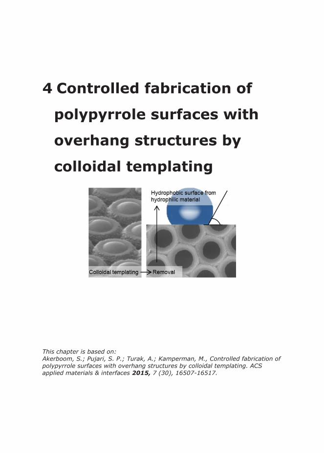
4 Controlled fabrication of
polypyrrole surfaces with
overhang structures by
colloidal templating
This chapter is based on: Akerboom, S.; Pujari, S. P.; Turak, A.; Kamperman, M., Controlled fabrication of polypyrrole surfaces with overhang structures by colloidal templating. ACS applied materials & interfaces 2015, 7 (30), 16507-16517.

Chapter
76
4.1 Abstract
Here we present the fabrication of polypyrrole (PPy) surfaces with a controlled overhang structure using a crystalline colloidal monolayer at the air/water interface as a template. With a scalable fabrication process, consisting of interfacial polymerization around sacrificial polystyrene particles, regularly structured PPy films were produced. The morphology of the final inverse colloidal PPy film is controlled by the amount of monomer, the monomer : oxidant ratio and polymerization time. The PPy films exhibit an overhang structure due to depth of particle immersion in the water phase. As a result of the overhang structure, the PPy films are made hydrophobic, although the material itself is hydrophilic. The apparent contact angle of water on the structured surfaces is °, which is in agreement with the predicted contact angle using the Cassie-Baxter equation for air-filled cavities. This fabrication technique can be readily extended to other systems where controlled wettability is required.
4.2 Introduction
Conducting polymers are an interesting class of materials due to the combination of traditional polymer properties with novel optical and electronic behaviour.1 They can be used in electronic nanodevices2-8, as chemical9-12 or optical sensors,13-14 in catalysis15, and energy storage.16-
17 A key parameter in many applications is the control of surface wetting. One common method to control wetting is to chemically change the surface energy. In the specific case of polypyrrole (PPy), chemical modification has been performed by copolymerizing pyrrole with a modified fluorinated pyrrole monomer18, adding different hydrophobic codopants19-22 or by silanization of PPy.23-24
Alternatively, wetting properties can be changed upon structuring the surface.25-27 In this way, the intrinsic electronic and optical properties of the PPy will be conserved. When pyrrole is polymerized, it usually grows in uncontrollable globules28 and becomes a highly crosslinked, insoluble powder. The crosslinked nature makes PPy difficult to process.29 One of the few reports on structuring PPy after synthesis
Polypyrrole surfaces by colloidal templating
77
uses laser patterning;30 however, complex D structures cannot be fabricated in this way. A bottom up approach with the desired surface structure fabricated in-situ during PPy synthesis is therefore highly desirable. This can be accomplished either by electrochemical or chemical synthesis. During electrochemical synthesis, pyrrole is polymerized to PPy at the anode. By changing the conditions, different structures can be fabricated9, 31, including hollow microhorn arrays32, butterfly scale-like ordered porous structures33, 2D honeycomb structures34, and nanopillars.35 Methods to chemically synthesize structured PPy films and coatings include interfacial synthesis at the water/organic solvent interface36-38, oxidant assisted synthesis39, and the use of templates. Both soft templates, consisting of surfactants40-42, and hard templates, consisting of colloids, have been employed to synthesize coated microspheres43-47 and nanocups.48
As PPy is a hydrophilic material, structuring the surface by simply increasing the roughness of the PPy surface is likely to result in complete contact between the water and the solid surface under the droplet, also called the Wenzel state. The apparent contact angle in the Wenzel state (θw) is related to the roughness r of the material as49
cos 𝜃𝜃𝑊𝑊 = 𝑟𝑟 cos 𝜃𝜃 ()
with θ the contact angle of the droplet on a perfectly flat substrate, and r the roughness of the surface (true contact area/projected area). The Wenzel state always magnifies the underlying wetting properties: the apparent contact angle for hydrophilic materials decreases, and the apparent contact angle for hydrophobic materials increases.50 As the Wenzel equation therefore cannot be used to predict an increase in contact angle due to structuring of a hydrophilic material, the Cassie-Baxter state is defined to describe this regime. In the Cassie-Baxter state, air is trapped underneath a droplet. The presence of air (which has a contact angle of ° with water) effectively lowers the average surface energy,51,52 which can yield hydrophobic apparent contact angles on intrinsically hydrophilic materials (θ < °). The apparent contact angle for a Cassie-Baxter state, θCB, is given by53
cos 𝜃𝜃𝐶𝐶𝐶𝐶 = 𝜑𝜑𝑠𝑠 cos 𝜃𝜃 − (1 − 𝜑𝜑𝑠𝑠) ()
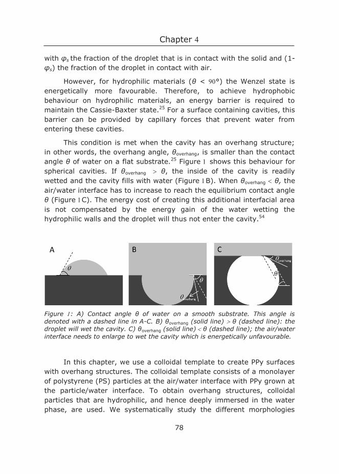
Chapter
78
with φs the fraction of the droplet that is in contact with the solid and (1- φs) the fraction of the droplet in contact with air.
However, for hydrophilic materials (θ < °) the Wenzel state is energetically more favourable. Therefore, to achieve hydrophobic behaviour on hydrophilic materials, an energy barrier is required to maintain the Cassie-Baxter state.25 For a surface containing cavities, this barrier can be provided by capillary forces that prevent water from entering these cavities.
This condition is met when the cavity has an overhang structure; in other words, the overhang angle, θoverhang, is smaller than the contact angle θ of water on a flat substrate.25 Figure shows this behaviour for spherical cavities. If θoverhang θ, the inside of the cavity is readily wetted and the cavity fills with water (Figure B). When θoverhang θ, the air/water interface has to increase to reach the equilibrium contact angle θ (Figure C). The energy cost of creating this additional interfacial area is not compensated by the energy gain of the water wetting the hydrophilic walls and the droplet will thus not enter the cavity.54
Figure : A) Contact angle θ of water on a smooth substrate. This angle is denoted with a dashed line in A-C. B) θoverhang (solid line) θ (dashed line): the droplet will wet the cavity. C) θoverhang (solid line) θ (dashed line); the air/water interface needs to enlarge to wet the cavity which is energetically unfavourable.
In this chapter, we use a colloidal template to create PPy surfaces with overhang structures. The colloidal template consists of a monolayer of polystyrene (PS) particles at the air/water interface with PPy grown at the particle/water interface. To obtain overhang structures, colloidal particles that are hydrophilic, and hence deeply immersed in the water phase, are used. We systematically study the different morphologies
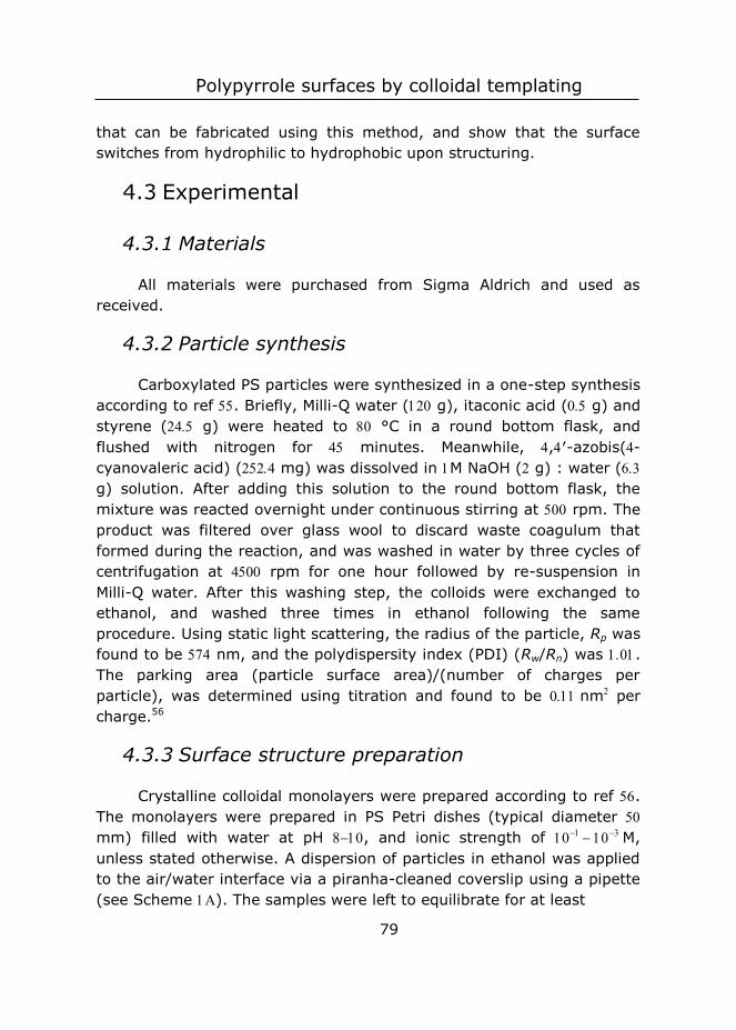
Polypyrrole surfaces by colloidal templating
79
that can be fabricated using this method, and show that the surface switches from hydrophilic to hydrophobic upon structuring.
4.3 Experimental
4.3.1 Materials
All materials were purchased from Sigma Aldrich and used as received.
4.3.2 Particle synthesis
Carboxylated PS particles were synthesized in a one-step synthesis according to ref . Briefly, Milli-Q water ( g), itaconic acid ( g) and styrene ( g) were heated to °C in a round bottom flask, and flushed with nitrogen for minutes. Meanwhile, ,′-azobis(-cyanovaleric acid) ( mg) was dissolved in M NaOH ( g) : water ( g) solution. After adding this solution to the round bottom flask, the mixture was reacted overnight under continuous stirring at rpm. The product was filtered over glass wool to discard waste coagulum that formed during the reaction, and was washed in water by three cycles of centrifugation at rpm for one hour followed by re-suspension in Milli-Q water. After this washing step, the colloids were exchanged to ethanol, and washed three times in ethanol following the same procedure. Using static light scattering, the radius of the particle, Rp was found to be nm, and the polydispersity index (PDI) (Rw/Rn) was . The parking area (particle surface area)/(number of charges per particle), was determined using titration and found to be nm per charge.56
4.3.3 Surface structure preparation
Crystalline colloidal monolayers were prepared according to ref . The monolayers were prepared in PS Petri dishes (typical diameter mm) filled with water at pH , and ionic strength of M, unless stated otherwise. A dispersion of particles in ethanol was applied to the air/water interface via a piranha-cleaned coverslip using a pipette (see Scheme ). The samples were left to equilibrate for at least
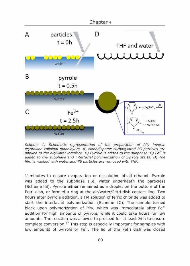
Chapter
80
Scheme 1: Schematic representation of the preparation of PPy inverse crystalline colloidal monolayers. A) Monodisperse carboxylated PS particles are applied to the air/water interface. B) Pyrrole is added to the subphase. C) Feis added to the subphase and interfacial polymerization of pyrrole starts. D) The film is washed with water and PS particles are removed with THF.
minutes to ensure evaporation or dissolution of all ethanol. Pyrrole was added to the subphase (i.e. water underneath the particles) (Scheme B). Pyrrole either remained as a droplet on the bottom of the Petri dish, or formed a ring at the air/water/Petri dish contact line. Two hours after pyrrole addition, a M solution of ferric chloride was added to start the interfacial polymerization (Scheme C). The sample turned black upon polymerization of PPy, which was immediately after Fe addition for high amounts of pyrrole, while it could take hours for low amounts. The reaction was allowed to proceed for at least h to ensure complete conversion.57 This step is especially important for samples with low amounts of pyrrole or Fe. The lid of the Petri dish was closed
Polypyrrole surfaces by colloidal templating
81
during this time, to prevent pyrrole evaporation.58 PPy crystalline colloidal monolayers (PPy-ccm) were washed by removing the subphase using a syringe and replacing it with ultrapure water (Scheme D). This washing step was repeated three times. The monolayers were subsequently transferred by immersing the Petri dish in a large clean water bath, containing at least mL water. As the monolayers float, they can be scooped up with another clean Petri dish. PS particles were removed by soaking cleaned PPy monolayers in THF for at least hours, resulting in PPy inverse crystalline colloidal monolayers (PPy-iccm) (Scheme D).
4.3.4 Flat PPy surfaces
Flat PPy surfaces were prepared according to ref . Briefly, microscope slides were submerged in KOH ( M) for minutes and thoroughly rinsed with water. Water (mL), ethanol ( mL) and (aminopropyl)triethoxysilane (APTES, µL) were mixed and stirred for h to hydrolyze the APTES. The microscope slides were subsequently submerged in hydrolyzed APTES solution for hours. After this, the microscope slides were rinsed with ultrapure water and put under vacuum at RT overnight. The contact angle changed from ° (after KOH treatment) to ° ° after APTES treatment, which is consistent with the initial contact angle found for APTES monolayers.60 The dried microscope slides were placed diagonally in a mL beaker, containing a mM aqueous solution of FeCl (mL). Pyrrole ( µL) was added and the reaction was allowed to proceed for hours under gentle stirring. PPy aggregates were removed from the surface with a tissue and by using excessive rinsing.
4.3.5 Characterization
Scanning Electron Microscopy (SEM)
Samples were prepared by scooping part of the floating monolayer from the air/water interface using cut silicon wafers as substrate. To prevent self-folding upon drying, Leitsilber Silver Paint (Ted Pella) was used to glue the films to the substrate. Samples were sputtered

Chapter
82
with gold (mA, s) using a JEOL JFC-0 autofine coater, and imaged using a JEOL JAMP-F Field Emission Auger Microprobe at kV.
X-ray photoelectron Spectroscopy (XPS)
XPS spectra were measured on a JPSX-ray photoelectron spectrometer (JEOL, Japan). High resolution spectra were obtained under UHV conditions using monochromatic Al Kα X-ray radiation at an angle of ° at kV and mA, using an analyzer pass energy of eV. Spectra were corrected with a standard background subtraction according to a linear procedure before fitting. The spectra were fitted using Casa XPS software (version ) and to compensate for the surface charging effects, the N s peak was calibrated at a binding energy of eV, in accordance with ref . Calculated atomic percentages were normalized by the corresponding atomic sensitivity factors.
Energy-dispersive spectroscopy (EDS)
Samples were first imaged at kV, pA, at room temperature, in a field emission scanning electron microscope (Magellan , FEI, Eindhoven, the Netherlands). EDS analyses were accomplished by an Oxford X-max detector and analysis software (Oxford Instruments Analytical, High Wycombe, England) at an acceleration voltage of kV, nA.
Contact angle measurements
Contact angles were determined using the Kruss Contact Angle measuring System G and using the “Drop Shape Analysis” software. Samples consisted of PPy films mounted on a cover slip using double sided tape and left to dry for at least a week at RT. Contact angles were measured on at least locations using droplets of µL.
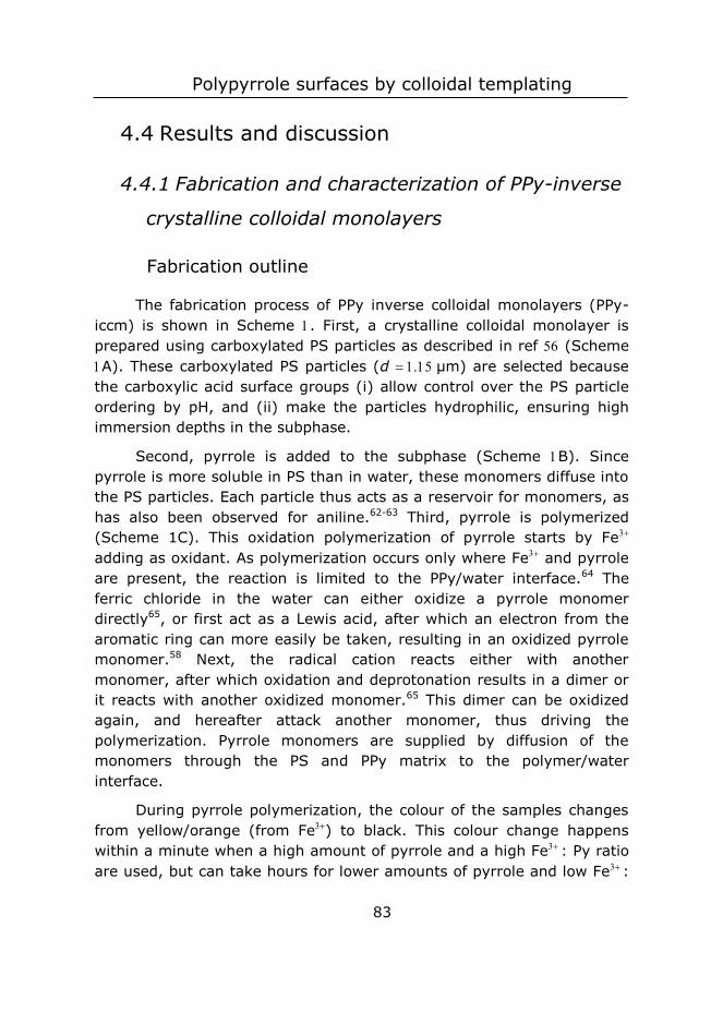
Polypyrrole surfaces by colloidal templating
83
4.4 Results and discussion
4.4.1 Fabrication and characterization of PPy-inverse
crystalline colloidal monolayers
Fabrication outline
The fabrication process of PPy inverse colloidal monolayers (PPy-iccm) is shown in Scheme . First, a crystalline colloidal monolayer is prepared using carboxylated PS particles as described in ref (Scheme A). These carboxylated PS particles (d µm) are selected because the carboxylic acid surface groups (i) allow control over the PS particle ordering by pH, and (ii) make the particles hydrophilic, ensuring high immersion depths in the subphase.
Second, pyrrole is added to the subphase (Scheme B). Since pyrrole is more soluble in PS than in water, these monomers diffuse into the PS particles. Each particle thus acts as a reservoir for monomers, as has also been observed for aniline.62-63 Third, pyrrole is polymerized (Scheme 1C). This oxidation polymerization of pyrrole starts by Fe adding as oxidant. As polymerization occurs only where Fe and pyrrole are present, the reaction is limited to the PPy/water interface.64 The ferric chloride in the water can either oxidize a pyrrole monomer directly65, or first act as a Lewis acid, after which an electron from the aromatic ring can more easily be taken, resulting in an oxidized pyrrole monomer.58 Next, the radical cation reacts either with another monomer, after which oxidation and deprotonation results in a dimer or it reacts with another oxidized monomer.65 This dimer can be oxidized again, and hereafter attack another monomer, thus driving the polymerization. Pyrrole monomers are supplied by diffusion of the monomers through the PS and PPy matrix to the polymer/water interface.
During pyrrole polymerization, the colour of the samples changes from yellow/orange (from Fe) to black. This colour change happens within a minute when a high amount of pyrrole and a high Fe: Py ratio are used, but can take hours for lower amounts of pyrrole and low Fe:
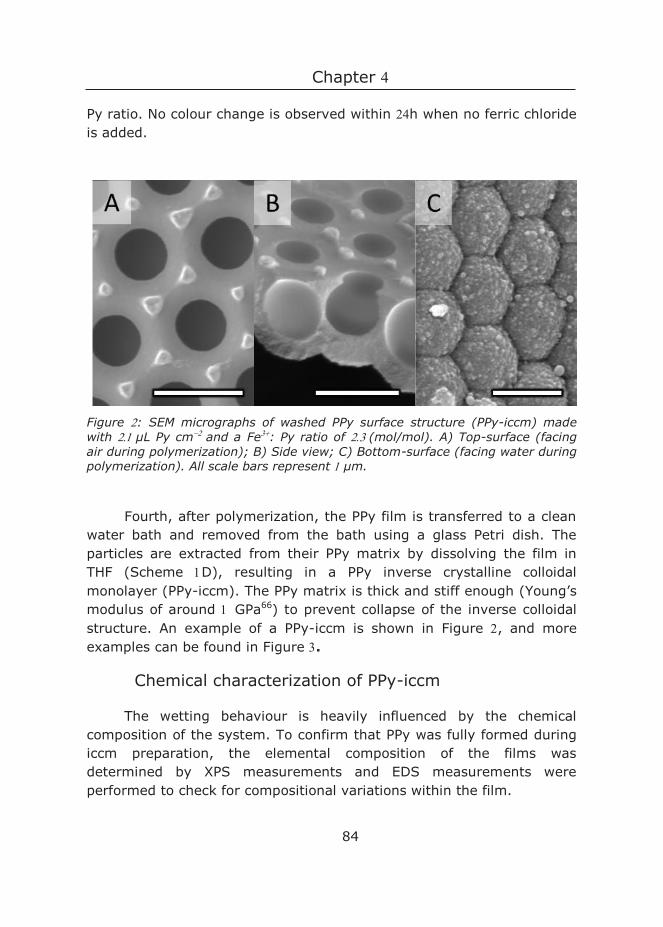
Chapter
84
Py ratio. No colour change is observed within h when no ferric chloride is added.
Figure : SEM micrographs of washed PPy surface structure (PPy-iccm) made with µL Py cm and a Fe: Py ratio of (mol/mol). A) Top-surface (facing air during polymerization); B) Side view; C) Bottom-surface (facing water during polymerization). All scale bars represent µm.
Fourth, after polymerization, the PPy film is transferred to a clean water bath and removed from the bath using a glass Petri dish. The particles are extracted from their PPy matrix by dissolving the film in THF (Scheme D), resulting in a PPy inverse crystalline colloidal monolayer (PPy-iccm). The PPy matrix is thick and stiff enough (Young’s modulus of around GPa66) to prevent collapse of the inverse colloidal structure. An example of a PPy-iccm is shown in Figure , and more examples can be found in Figure .
Chemical characterization of PPy-iccm
The wetting behaviour is heavily influenced by the chemical composition of the system. To confirm that PPy was fully formed during iccm preparation, the elemental composition of the films was determined by XPS measurements and EDS measurements were performed to check for compositional variations within the film.

Polypyrrole surfaces by colloidal templating
85
Figure : SEM micrographs of washed polypyrrole surface structures (PPy-iccm) A) µL Py cm and Fe: Py ratio of (left), µL Py cm and Fe: Py ratio of (right); B) µL Py cm and Fe: Py ratio of ; C) µL Py cm and Fe: Py ratio of ; D) µL Py cm and Fe: Py ratio of .
XPS measurements
Elemental composition was determined with XPS measurements on a PPy-iccm sample synthesized with µL Py cm and Fe: Py = , both at the top-surface of the sample (facing air during polymerization) and bottom-surface (facing water during polymerization). The XPS survey scan (Figure A-B) shows C and N as expected for pure PPy, as well as contaminants Cl, O and, at the bottom-surface, Fe. Core level peaks for C and N (see SI ) are fitted and assigned as described in ref . The assigned peaks are listed in Figure C. The fitting procedure for Ns and C s indicated that our iccm indeed consists of PPy (see SI ).
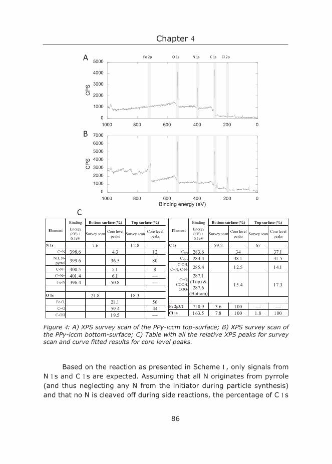
Chapter
86
Figure : A) XPS survey scan of the PPy-iccm top-surface; B) XPS survey scan of the PPy-iccm bottom-surface; C) Table with all the relative XPS peaks for survey scan and curve fitted results for core level peaks.
Based on the reaction as presented in Scheme , only signals from N s and C s are expected. Assuming that all N originates from pyrrole (and thus neglecting any N from the initiator during particle synthesis) and that no N is cleaved off during side reactions, the percentage of C s
0
1000
2000
3000
4000
5000
02004006008001000
CP
S
Binding energy (eV)
0
1000
2000
3000
4000
5000
6000
7000
02004006008001000
CP
S
Binding energy (eV)
Fe 2p O 1s N 1s C 1s Cl 2pA
B
C
Element
Binding Bottom surface (%) Top surface (%)Energy (eV) ±0.1eV
Survey scan Core level peaks Survey scan Core level
peaks
N 1s C=N
NH, N-pyrrol
C-N+ C=N+
Fe-N
O 1s Fe-O, C=O
C-OH
Element
Binding Bottom surface (%) Top surface (%)Energy (eV) ±0.1eV
Survey scan Core level peaks Survey scan Core level
peaks
C 1s Cbeta
Calpha C-OH,
C=N, C-N-
C=O, COOH,
COO-
(Top) &
(Bottom)
Fe 2p3/2 Cl 1s

Polypyrrole surfaces by colloidal templating
87
alpha and beta signal that can be attributed to polypyrrole (one N is attached to C, thus pure pyrrole is N s) can be determined. These calculations indicate a lower amount of pyrrole at the bottom surface ( vs for the top-surface). The rest of the Cs signal may be attributed to two additional processes: residue PS adsorption after particle dissolution and side reactions during pyrrole polymerization.
A common side reaction is overoxidation, which is the gradual oxidation of PPy by water in the presence of FeCl and results in O incorporation in the polymer matrix.44-45, 61, 67-68 Another common side reaction is the incorporation of dopants, such as chloride, that results in the Cl p signal from charge transfer interactions with the polymer backbone.45 Other dopant species, i.e. iron(III) chlorides (FeCl, FeCl) 57, can only be found at the bottom-surface, since the Fe p signal is absent at the top-surface. Part of this Fe is coordinated to N, as evidenced by the N s core level spectrum for the bottom-surface (see SI ). The pyrrole rings at the bottom-surface thus underwent further reactions while in contact with the FeCl solution. Additional evidence for further reactions at the bottom-surface can be determined from the (NH, N-pyrrole): N=C ratio. For the bottom-surface we find a high ratio of , while this ratio is only for the top-surface.
In addition to the presence of oxygen from overoxidation, O may stem from incomplete removal of the PS particles. The particles consist of copolymerized styrene (CH) and itaconic acid (CHO). The presence of polystyrene-co-poly(itaconic acid) residues is also indicated by the enrichment of the signal in C compared to N (N : C of for the top-surface, and N : C of for the bottom-surface).
EDS measurements
In SEM micrographs of PPy-iccm ( µL Py cm, Fe: Py ), triangular protrusions were observed at the top-surface that appear white in SEM (see Figure A and B). This contrast is either due to the surface topology or due to differences in chemical composition. EDS was performed to study compositional variations, and the maps can be found in Figure and the EDS spectra in Figure . C and O are evenly distributed over the sample (Figure A and C), and no differences are found between the protrusions and the rest of the sample. There is
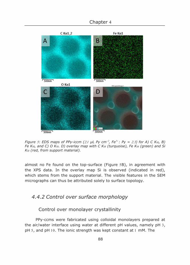
Chapter
88
Figure : EDS maps of PPy-iccm ( µL Py cm, Fe: Py = ) for A) C K, B) Fe K, and C) O K. D) overlay map with C K (turquoise), Fe K (green) and Si K (red, from support material).
almost no Fe found on the top-surface (Figure B), in agreement with the XPS data. In the overlay map Si is observed (indicated in red), which stems from the support material. The visible features in the SEM micrographs can thus be attributed solely to surface topology.
4.4.2 Control over surface morphology
Control over monolayer crystallinity
PPy-ccms were fabricated using colloidal monolayers prepared at the air/water interface using water at different pH values, namely pH , pH , and pH . The ionic strength was kept constant at mM. The
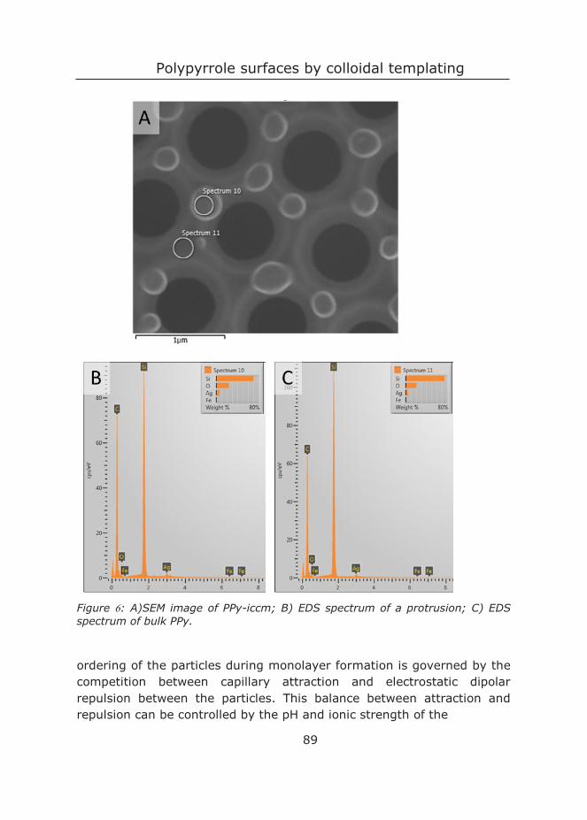
Polypyrrole surfaces by colloidal templating
89
Figure : A)SEM image of PPy-iccm; B) EDS spectrum of a protrusion; C) EDS spectrum of bulk PPy.
ordering of the particles during monolayer formation is governed by the competition between capillary attraction and electrostatic dipolar repulsion between the particles. This balance between attraction and repulsion can be controlled by the pH and ionic strength of the
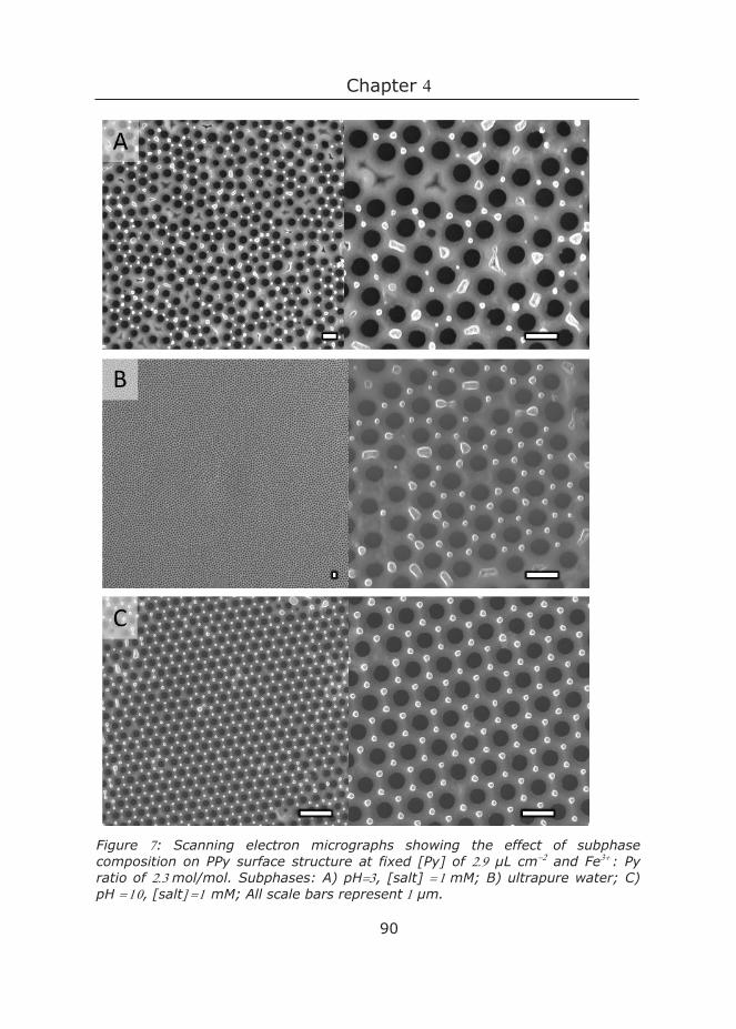
Chapter
90
Figure : Scanning electron micrographs showing the effect of subphase composition on PPy surface structure at fixed [Py] of µL cm and Fe: Py ratio of mol/mol. Subphases: A) pH, [salt] mM; B) ultrapure water; C) pH , [salt mM; All scale bars represent µm.
Polypyrrole surfaces by colloidal templating
91
subphase.56 At high pH, the carboxylic acid groups of the itaconic acid (with pKa and pKa
67) are deprotonated, giving rise to an asymmetric counter-ion distribution, resulting in a dipole moment. The dipole-dipole repulsion between the different particles counteracts the attractive van der Waals interactions. Consequently, the particles remain more mobile at the interface resulting in more ordered monolayers. This allows the particles to assemble in a hexagonal packing,68-69 thus resulting in crystalline monolayers. At low pH, the carboxylic acid groups on the surface of the monomers are protonated, and hence no electrostatic repulsion between the particles exists. Particles that approach each other closely thus immediately feel the attractive van der Waals forces that bring them in close contact. This process immobilizes the particles and results in close-packed monolayers with relatively low crystallinities.
The final PPy-ccm structure prepared at pH , though close-packed, shows low crystallinity (Figure A), which is consistent with the poor order in the monolayer. The crystallinity of the monolayers prepared at neutral and high pH increases with increasing pH and is preserved in the PPy-ccm (Figure B and C), although both the pH and the ionic strength of the subphase change during polymerization. The ionic strength increases dramatically upon addition of the Fe, and the pH drops during polymerization due to proton release (see Scheme B). Assuming complete conversion of pyrrole monomers, the theoretical pH value for this sample decreased to during polymerization. Conserving the crystallinity is therefore surprising, as it has previously been observed that changing the pH after the preparation of the monolayer decreases the particle order.56 The pyrrole here appears to act as a glue between the particles early in the polymerization process, preserving the crystallinity in the PPy-ccm layer.
Amount of pyrrole
The samples in Figure are made using µL pyrrole per cm of monolayer. The molar ratio Fe to pyrrole is chosen to be , which is the same value as used in ref . Keeping this ratio and the crystallinity of the monolayer fixed, samples were prepared using different amounts
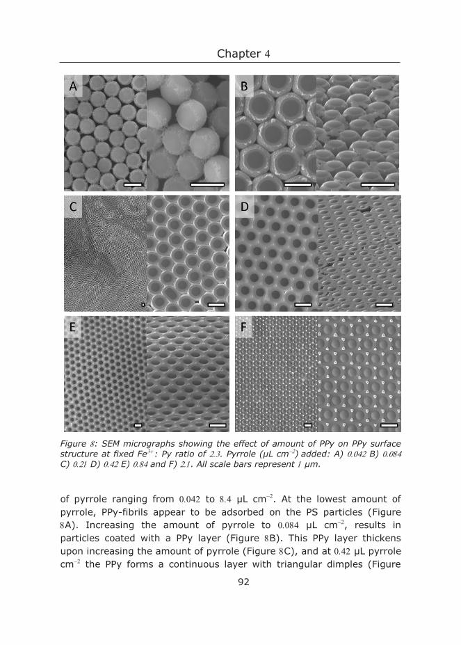
Chapter
92
Figure : SEM micrographs showing the effect of amount of PPy on PPy surface structure at fixed Fe: Py ratio of . Pyrrole (µL cm) added: A) B) C) D) E) and F) . All scale bars represent µm.
of pyrrole ranging from to µL cm. At the lowest amount of pyrrole, PPy-fibrils appear to be adsorbed on the PS particles (Figure A). Increasing the amount of pyrrole to µL cm, results in particles coated with a PPy layer (Figure B). This PPy layer thickens upon increasing the amount of pyrrole (Figure C), and at µL pyrrole cm the PPy forms a continuous layer with triangular dimples (Figure
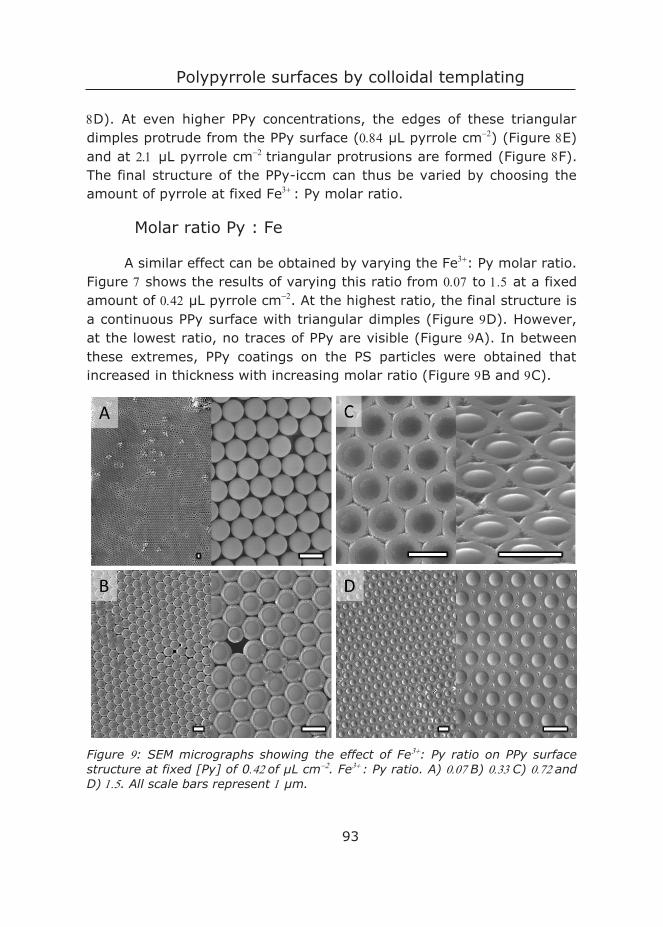
Polypyrrole surfaces by colloidal templating
93
D). At even higher PPy concentrations, the edges of these triangular dimples protrude from the PPy surface ( µL pyrrole cm) (Figure E) and at µL pyrrole cm triangular protrusions are formed (Figure F). The final structure of the PPy-iccm can thus be varied by choosing the amount of pyrrole at fixed Fe: Py molar ratio.
Molar ratio Py : Fe
A similar effect can be obtained by varying the Fe: Py molar ratio. Figure shows the results of varying this ratio from to at a fixed amount of µL pyrrole cm. At the highest ratio, the final structure is a continuous PPy surface with triangular dimples (Figure D). However, at the lowest ratio, no traces of PPy are visible (Figure A). In between these extremes, PPy coatings on the PS particles were obtained that increased in thickness with increasing molar ratio (Figure B and C).
Figure : SEM micrographs showing the effect of Fe: Py ratio on PPy surface structure at fixed [Py] of 0of µL cm. Fe: Py ratio. A) B) C) and D) . All scale bars represent µm.
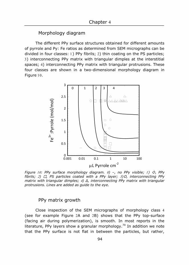
Chapter
94
Morphology diagram
The different PPy surface structures obtained for different amounts of pyrrole and Py: Fe ratios as determined from SEM micrographs can be divided in four classes: ) PPy fibrils; ) thin coating on the PS particles; ) interconnecting PPy matrix with triangular dimples at the interstitial spaces; ) interconnecting PPy matrix with triangular protrusions. These four classes are shown in a two-dimensional morphology diagram in Figure .
Figure : PPy surface morphology diagram. ) –, no PPy visible; ) , PPy fibrils; ) , PS particles coated with a PPy layer; ), interconnecting PPy matrix with triangular dimples; ) Δ, interconnecting PPy matrix with triangular protrusions. Lines are added as guide to the eye.
PPy matrix growth
Close inspection of the SEM micrographs of morphology class (see for example Figure A and B) shows that the PPy top-surface (facing air during polymerization), is smooth. In most reports in the literature, PPy layers show a granular morphology.70 In addition we note that the PPy surface is not flat in between the particles, but rather,
0
0.5
1
1.5
2
2.5
3
0.001 0.01 0.1 1 10 100
Fe3+
:Pyr
role
(mol
/mol
)
L Pyrrole cm-2
0 1 2 3 4

Polypyrrole surfaces by colloidal templating
95
follows a positive slope radiating from the particle (see for example Figure C). The SEM image in Figure C shows the bottom-surface of the PPy-iccm. The PPy coating around the particles follows the outline of the particles, and the surface is rough.
To study how these features arise during interfacial polymerization, colloidal monolayers were swollen with µL pyrrole cm and investigated at different incubation times after adding the ferric chloride. The molar ratio of Fe: Py was kept constant at . The first sample was taken immediately after ferric chloride addition (Scheme A)
Scheme : Growth of PPy in time (not to scale) and SEM micrographs. SEM micrographs taken at A) minute; B) minutes; C) minutes; and D) h minutes after Fe addition. The [Py] is µL cm and Fe: Py ratio is mol/mol. All scale bars represent µm.
and shows that a thin, rough PPy layer on the outside of the immersed parts of the particles is directly synthesized. The layer around the particle thickens after longer incubation times (Scheme B), resulting in an interconnecting PPy matrix. The water present in the interstitial space of the particles at the top-surface, may thereby be cut off from the bulk water below. The PPy keeps growing at the rough water/PPy interface

Chapter
96
and while doing so, it is pushed upwards, enabling the PPy to grow higher than the original water level (Scheme C). The smooth layer radiating from the particle is believed to originate from the air/water/PPy contact line, which slowly moves upward. Protrusions may arise due to polymer formation in the small remaining water droplet sitting at the interstitial sites (Scheme D).
Figure : Gradient of PPy surface structures within one sample with µL Py cm and a Fe: Py ratio of . A) Sample shortly after Fe addition. Pyrrole and Fe were added on the left hand side. B) Sample after h. C, D) Surface structures at different locations, as indicated in A) and B). All scale bars represent µm.
The variation in surface structure with time is used to produce a PPy-ccm with a surface structure gradient. To this end, a colloidal crystal monolayer was prepared in a Petri dish with a diameter of cm and µL pyrrole cm was added to the left side. Fe in a molar ratio Fe: Py of , was added after minutes at the same location as where the pyrrole was added. Figure A shows a picture taken almost immediately after Fe addition. The Fe solution spread quickly: the subphase was completely yellow. However, only on the left side rapid polymerization of
Polypyrrole surfaces by colloidal templating
97
the pyrrole was observed, as evidenced by the black colour. The picture in Figure B shows the sample after hours, and it can be seen that the complete Petri dish is covered with a PPy-ccm.
Four samples were scooped from left to right using silicon wafers of around cm. These PPy surface structures are shown in Figure C-F. The surface structure of the sample taken nearest to the location where pyrrole was added, location C, shows triangular protrusions (morphology class ), while triangular dimples (morphology class ) are found that grow in size as the sample is taken farther to the right.
4.4.3 Wetting of PPy
Wetting of flat and structured PPy
The contact angles, , of water on PPy-iccms with different morphologies (Class from morphology diagram) were measured and were all found to be very similar: ° for PPy-iccm with triangular protrusions (Class ), for PPy-iccm with triangular dimples (Class ) and ° for PPy-iccm with coated particles (Class ) (see Figure ). This similarity can be attributed to the similar overhang structure, as described in the next section, for the various morphologies. The of the bottom-surface of the sample was °. This shows that the film is hydrophobic on the top-surface and hydrophilic on the bottom-surface.
As a reference, of water on PPy grafted on a silicon wafer was measured. The average for this reference PPy is ° (Figure A). Unstructured PPy has been previously found to have between ° and °.20, 24, 30, 71 As our surface has micrometre-sized roughness, as is shown in the SEM image in Figure , the droplet is probably in a Wenzel state, and is therefore lower than of water on a perfectly flat PPy substrate.
Additionally, the excess C observed in the XPS measurements suggest that residual PS is left after etch removal of the template particles. As polymers tend to coat surfaces with a thin layer even at very low concentrations, and because PS has a higher with water of °,72 the effect of this residue layer on the of unstructured PPy was
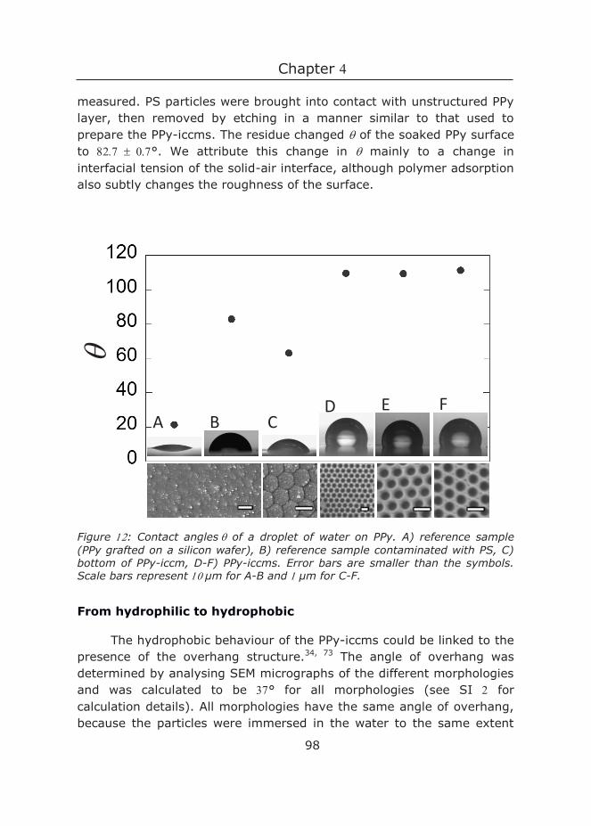
Chapter
98
measured. PS particles were brought into contact with unstructured PPy layer, then removed by etching in a manner similar to that used to prepare the PPy-iccms. The residue changed of the soaked PPy surface to °. We attribute this change in mainly to a change in interfacial tension of the solid-air interface, although polymer adsorption also subtly changes the roughness of the surface.
Figure : Contact angles of a droplet of water on PPy. A) reference sample (PPy grafted on a silicon wafer), B) reference sample contaminated with PS, C) bottom of PPy-iccm, D-F) PPy-iccms. Error bars are smaller than the symbols. Scale bars represent µm for A-B and µm for C-F.
From hydrophilic to hydrophobic
The hydrophobic behaviour of the PPy-iccms could be linked to the presence of the overhang structure.34, 73 The angle of overhang was determined by analysing SEM micrographs of the different morphologies and was calculated to be ° for all morphologies (see SI for calculation details). All morphologies have the same angle of overhang, because the particles were immersed in the water to the same extent
A B CD E F
Polypyrrole surfaces by colloidal templating
99
during polymerization. The immersion depth is mainly determined by the subphase, as the dissociation of –COOH groups on the surface of the particles and hence its hydrophilicity depends on the pH and ionic strength of the subphase. This also explains the fact that the contact angles for the three different morphologies of PPy-iccm are very similar.
The angle of overhang is well below of water on the PS-contaminated reference of °, and hence it is possible that capillary forces act as barrier preventing water to enter the cavity (see Figure ).
To compare the obtained results with theory, we use the Cassie-Baxter equation, where the water cannot enter the cavities (Equation ), to calculate of water on our structures. The fraction of solid, φs, can be calculated in two ways: either by adding the area of all holes in the SEM image, and dividing this by the total area of the SEM image, or by assuming hexagonal packing of the particles and using the radius of the particle, Rp and the radius of the opening of the cavities, Rh (see SI for further details). The first method underestimates φs due to the neglect of holes at the edge of the image and non-spherical holes, while the second method overestimates φs due to the assumption that the surface is covered with one perfect crystal lattice without defects or grain boundaries. The effective φs is therefore taken as the average of these two measurements. For our samples, the first method yields a φs of , and the second method yields a φs of . Therefore, an effective φs of is used for further calculations.
Using φs and 𝜃𝜃reference , we find a of °. As the is in good agreement with the observed contact angles on the different morphologies, which are all similar, the increase in to hydrophobic behaviour may be attributed to air entrapment in the cavities.
4.5 Conclusion
In summary, we introduced a scalable fabrication method to create PPy films with overhang structures yielding hydrophobic wetting behaviour on a hydrophilic material. Using carboxylated PS particles at the air/water interface as template enables control over the crystallinity by choosing the pH of the subphase. By varying the monomer and
Chapter
100
oxidant concentrations, different nanopatterned surface structures can be fabricated under mild conditions. Using this approach, synthesis of surface gradients is achieved by controlling the time between adding the monomer and the oxidant. The final inverse crystalline colloidal monolayer is obtained by soaking the PPy film in THF. The of water on top of the PPy-iccm is ° which indicates a switch from hydrophilic behaviour for the unstructured material to hydrophobic behaviour upon structuring. Comparing our experimentally determined with the prediction of the Cassie-Baxter model, we found that the increase in may be explained by air entrapment in the cavities. The presence of an overhang may prevent water from entering the cavities.
We have demonstrated that colloidal templating in combination with interfacial polymerization provides a promising approach to design surfaces with overhang structures. This approach is quite general and may be applied to manufacture different materials where controlled wetting behaviour is required.
References 1. Das, T. K.; Prusty, S., Review on Conducting Polymers and Their Applications. Polymer-Plastics Technology and Engineering 2012, 51 (14), 1487-1500. 2. Forrest, S. R., The path to ubiquitous and low-cost organic electronic appliances on plastic. Nature 2004, 428 (6986), 911-918. 3. Günes, S.; Neugebauer, H.; Sariciftci, N. S., Conjugated polymer-based organic solar cells. Chemical reviews 2007, 107 (4), 1324-1338. 4. Facchetti, A., Π-conjugated polymers for organic electronics and photovoltaic cell applications†. Chemistry of Materials 2010, 23 (3), 733-758. 5. Fabretto, M. V.; Evans, D. R.; Mueller, M.; Zuber, K.; Hojati-Talemi, P.; Short, R. D.; Wallace, G. G.; Murphy, P. J., Polymeric material with metal-like conductivity for next generation organic electronic devices. Chemistry of Materials 2012, 24 (20), 3998-4003. 6. Zhou, H.; Yang, L.; You, W., Rational design of high performance conjugated polymers for organic solar cells. Macromolecules 2012, 45 (2), 607-632. 7. Holliday, S.; Donaghey, J. E.; McCulloch, I., Advances in charge carrier mobilities of semiconducting polymers used in organic transistors. Chemistry of Materials 2013, 26 (1), 647-663. 8. Wudl, F., Spiers Memorial Lecture. Faraday Discuss. 2014, 174, 9-20. 9. Carquigny, S.; Sanchez, J.-B.; Berger, F.; Lakard, B.; Lallemand, F., Ammonia gas sensor based on electrosynthesized polypyrrole films. Talanta 2009, 78 (1), 199-206.
Polypyrrole surfaces by colloidal templating
101
10. Hamilton, A.; Breslin, C. B., The development of a novel urea sensor using polypyrrole. Electrochimica Acta 2014, 145, 19-26. 11. Safarnavadeh, V.; Zare, K.; Fakhari, A. R., Capability of parasulfonato calix[6]arene, as an anion dopant, and organic solvents in enhancing the sensitivity and loading of glucose oxidase (GOx) on polypyrrole film in a biosensor: A comparative study. Biosensors and Bioelectronics 2013, 49 (0), 159-163. 12. Apetrei, I. M.; Apetrei, C., Amperometric biosensor based on polypyrrole and tyrosinase for the detection of tyramine in food samples. Sensors and Actuators B: Chemical 2013, 178 (0), 40-46. 13. de Marcos, S.; Wolfbeis, O. S., Optical sensing of pH based on polypyrrole films. Analytica chimica acta 1996, 334 (1), 149-153. 14. Koncki, R.; Wolfbeis, O. S., Composite films of Prussian blue and N-substituted polypyrroles: fabrication and application to optical determination of pH. Analytical chemistry 1998, 70 (13), 2544-2550. 15. Esmaeili, C.; Ghasemi, M.; Heng, L. Y.; Hassan, S. H.; Abdi, M. M.; Daud, W. R. W.; Ilbeygi, H.; Ismail, A. F., Synthesis and application of polypyrrole/carrageenan nano-bio composite as a cathode catalyst in microbial fuel cells. Carbohydrate polymers 2014, 114, 253-259. 16. Nyström, G.; Strømme, M.; Sjödin, M.; Nyholm, L., Rapid potential step charging of paper-based polypyrrole energy storage devices. Electrochimica Acta 2012, 70 (0), 91-97. 17. Yuan, L.; Yao, B.; Hu, B.; Huo, K.; Chen, W.; Zhou, J., Polypyrrole-coated paper for flexible solid-state energy storage. Energy & Environmental Science 2013, 6 (2), 470-476. 18. Darmanin, T.; Nicolas, M.; Guittard, F., Synthesis and Properties of Perfluorinated Conjugated Polymers Based on Polyethylenedioxythiophene, Polypyrrole, and Polyfluorene. Toward Surfaces with Special Wettabilities. Langmuir 2008, 24 (17), 9739-9746. 19. Mecerreyes, D.; Alvaro, V.; Cantero, I.; Bengoetxea, M.; Calvo, P. A.; Grande, H.; Rodriguez, J.; Pomposo, J. A., Low surface energy conducting polypyrrole doped with a fluorinated counterion. Advanced Materials 2002, 14 (10), 749-752. 20. Azioune, A.; Chehimi, M. M.; Miksa, B.; Basinska, T.; Slomkowski, S., Hydrophobic Protein−Polypyrrole Interactions: The Role of van der Waals and Lewis Acid−Base Forces As Determined by Contact Angle Measurements. Langmuir 2002, 18 (4), 1150-1156. 21. Chang, J. H.; Hunter, I. W., A Superhydrophobic to Superhydrophilic In Situ Wettability Switch of Microstructured Polypyrrole Surfaces. Macromol. Rapid Commun. 2011, 32 (9-10), 718-723. 22. Xu, L.; Wang, J.; Song, Y.; Jiang, L., Electrically tunable polypyrrole inverse opals with switchable stopband, conductivity, and wettability. Chemistry of Materials 2008, 20 (11), 3554-3556. 23. Kim, P.; Wong, T.-S.; Alvarenga, J.; Kreder, M. J.; Adorno-Martinez, W. E.; Aizenberg, J., Liquid-infused nanostructured surfaces with extreme anti-ice and anti-frost performance. ACS nano 2012, 6 (8), 6569-6577.

Chapter
102
24. Zhu, H.; Hou, J.; Qiu, R.; Zhao, J.; Xu, J., Perfluorinated lubricant/ polypyrrole composite material: Preparation and corrosion inhibition application. Journal of applied polymer science 2014, 131 (9), n/a-n/a. 25. Cao, L.; Hu, H.-H.; Gao, D., Design and fabrication of micro-textures for inducing a superhydrophobic behavior on hydrophilic materials. Langmuir 2007, 23 (8), 4310-4314. 26. Bellanger, H.; Darmanin, T.; Taffin de Givenchy, E.; Guittard, F. d. r., Chemical and physical pathways for the preparation of superoleophobic surfaces and related wetting theories. Chemical reviews 2014, 114 (5), 2694-2716. 27. Feng, X.; Jiang, L., Design and creation of superwetting/antiwetting surfaces. Advanced Materials 2006, 18 (23), 3063-3078. 28. Silk, T.; Hong, Q.; Tamm, J.; Compton, R. G., AFM studies of polypyrrole film surface morphology I. The influence of film thickness and dopant nature. Synthetic metals 1998, 93 (1), 59-64. 29. Omastová, M.; Mičušík, M., Polypyrrole coating of inorganic and organic materials by chemical oxidative polymerisation. Chemical Papers 2012, 66 (5), 392-414. 30. Acevedo, D. F.; Frontera, E.; Broglia, M. F.; Mücklich, F.; Miras, M. C.; Barbero, C. A., One Step Lithography of Polypyrrole. Advanced Engineering Materials 2011, 13 (5), 405-410. 31. Wang, J.; Xu, Y.; Wang, J.; Du, X.; Xiao, F.; Li, J., High charge/discharge rate polypyrrole films prepared by pulse current polymerization. Synthetic metals 2010, 160 (17), 1826-1831. 32. Bai, Y.; Xu, Y.; Wang, J.; Gao, M.; Wang, J., Interface effect on the electropolymerized polypyrrole films with hollow micro/nanohorn arrays. ACS applied materials & interfaces 2014, 6 (7), 4693-4704. 33. Song, J.; Liu, H.; Wan, M.; Zhu, Y.; Jiang, L., Bio-inspired isotropic and anisotropic wettability on a Janus free-standing polypyrrole film fabricated by interfacial electro-polymerization. Journal of Materials Chemistry A 2013, 1 (5), 1740-1744. 34. Santos, L.; Martin, P.; Ghilane, J.; Lacaze, P. C.; Lacroix, J.-C., Micro/Nano-Structured Polypyrrole Surfaces on Oxidizable Metals as Smart Electroswitchable Coatings. ACS applied materials & interfaces 2013, 5 (20), 10159-10164. 35. Valsesia, A.; Lisboa, P.; Colpo, P.; Rossi, F., Fabrication of polypyrrole-based nanoelectrode arrays by colloidal lithography. Analytical chemistry 2006, 78 (21), 7588-7591. 36. Qi, G.; Huang, L.; Wang, H., Highly conductive free standing polypyrrole films prepared by freezing interfacial polymerization. Chemical Communications 2012, 48 (66), 8246-8248. 37. Qi, G.; Wu, Z.; Wang, H., Highly conductive and semitransparent free-standing polypyrrole films prepared by chemical interfacial polymerization. Journal of Materials Chemistry C 2013, 1 (42), 7102-7110. 38. Dallas, P.; Niarchos, D.; Vrbanic, D.; Boukos, N.; Pejovnik, S.; Trapalis, C.; Petridis, D., Interfacial polymerization of pyrrole and in situ synthesis of polypyrrole/silver nanocomposites. Polymer 2007, 48 (7), 2007-2013. 39. Shinde, S. S.; Gund, G. S.; Dubal, D. P.; Jambure, S. B.; Lokhande, C. D., Morphological modulation of polypyrrole thin films through oxidizing agents
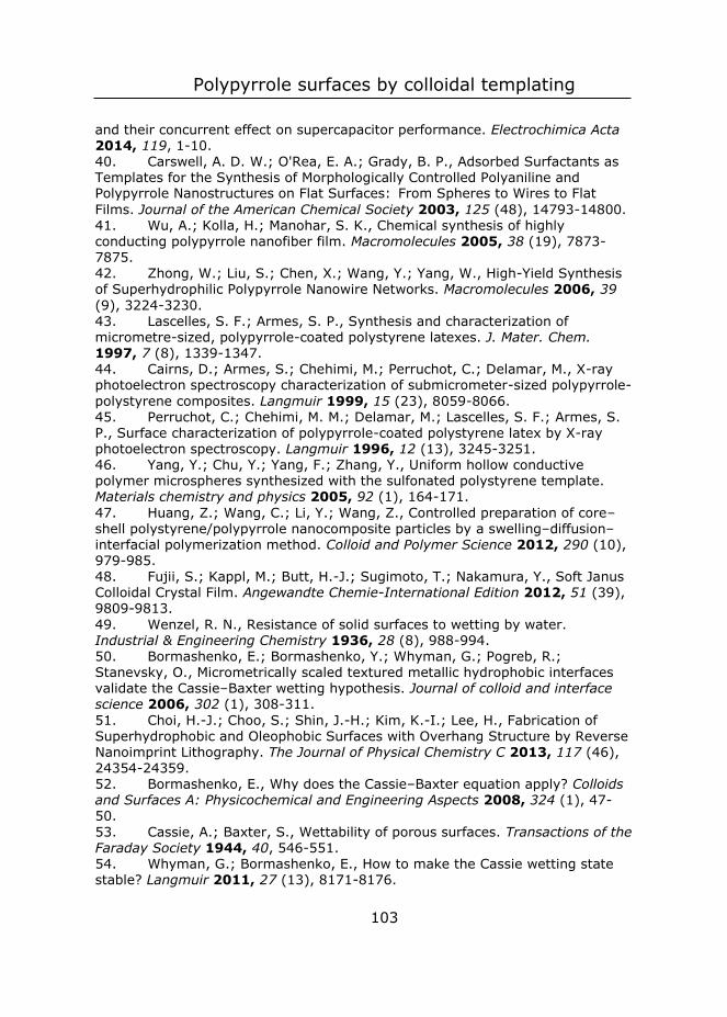
Polypyrrole surfaces by colloidal templating
103
and their concurrent effect on supercapacitor performance. Electrochimica Acta 2014, 119, 1-10. 40. Carswell, A. D. W.; O'Rea, E. A.; Grady, B. P., Adsorbed Surfactants as Templates for the Synthesis of Morphologically Controlled Polyaniline and Polypyrrole Nanostructures on Flat Surfaces: From Spheres to Wires to Flat Films. Journal of the American Chemical Society 2003, 125 (48), 14793-14800. 41. Wu, A.; Kolla, H.; Manohar, S. K., Chemical synthesis of highly conducting polypyrrole nanofiber film. Macromolecules 2005, 38 (19), 7873-7875. 42. Zhong, W.; Liu, S.; Chen, X.; Wang, Y.; Yang, W., High-Yield Synthesis of Superhydrophilic Polypyrrole Nanowire Networks. Macromolecules 2006, 39 (9), 3224-3230. 43. Lascelles, S. F.; Armes, S. P., Synthesis and characterization of micrometre-sized, polypyrrole-coated polystyrene latexes. J. Mater. Chem. 1997, 7 (8), 1339-1347. 44. Cairns, D.; Armes, S.; Chehimi, M.; Perruchot, C.; Delamar, M., X-ray photoelectron spectroscopy characterization of submicrometer-sized polypyrrole-polystyrene composites. Langmuir 1999, 15 (23), 8059-8066. 45. Perruchot, C.; Chehimi, M. M.; Delamar, M.; Lascelles, S. F.; Armes, S. P., Surface characterization of polypyrrole-coated polystyrene latex by X-ray photoelectron spectroscopy. Langmuir 1996, 12 (13), 3245-3251. 46. Yang, Y.; Chu, Y.; Yang, F.; Zhang, Y., Uniform hollow conductive polymer microspheres synthesized with the sulfonated polystyrene template. Materials chemistry and physics 2005, 92 (1), 164-171. 47. Huang, Z.; Wang, C.; Li, Y.; Wang, Z., Controlled preparation of core–shell polystyrene/polypyrrole nanocomposite particles by a swelling–diffusion–interfacial polymerization method. Colloid and Polymer Science 2012, 290 (10), 979-985. 48. Fujii, S.; Kappl, M.; Butt, H.-J.; Sugimoto, T.; Nakamura, Y., Soft Janus Colloidal Crystal Film. Angewandte Chemie-International Edition 2012, 51 (39), 9809-9813. 49. Wenzel, R. N., Resistance of solid surfaces to wetting by water. Industrial & Engineering Chemistry 1936, 28 (8), 988-994. 50. Bormashenko, E.; Bormashenko, Y.; Whyman, G.; Pogreb, R.; Stanevsky, O., Micrometrically scaled textured metallic hydrophobic interfaces validate the Cassie–Baxter wetting hypothesis. Journal of colloid and interface science 2006, 302 (1), 308-311. 51. Choi, H.-J.; Choo, S.; Shin, J.-H.; Kim, K.-I.; Lee, H., Fabrication of Superhydrophobic and Oleophobic Surfaces with Overhang Structure by Reverse Nanoimprint Lithography. The Journal of Physical Chemistry C 2013, 117 (46), 24354-24359. 52. Bormashenko, E., Why does the Cassie–Baxter equation apply? Colloids and Surfaces A: Physicochemical and Engineering Aspects 2008, 324 (1), 47-50. 53. Cassie, A.; Baxter, S., Wettability of porous surfaces. Transactions of the Faraday Society 1944, 40, 546-551. 54. Whyman, G.; Bormashenko, E., How to make the Cassie wetting state stable? Langmuir 2011, 27 (13), 8171-8176.
Chapter
104
55. Appel, J.; Akerboom, S.; Fokkink, R. G.; Sprakel, J., Facile One‐Step Synthesis of Monodisperse Micron‐Sized Latex Particles with Highly Carboxylated Surfaces. Macromol. Rapid Commun. 2013, 34 (16), 1284-1288. 56. Akerboom, S.; Appel, J.; Labonte, D.; Federle, W.; Sprakel, J.; Kamperman, M., Enhanced adhesion of bioinspired nanopatterned elastomers via colloidal surface assembly. Journal of The Royal Society Interface 2015, 12 (102), 20141061. 57. Armes, S. P., Optimum reaction conditions for the polymerization of pyrrole by iron (III) chloride in aqueous solution. Synthetic metals 1987, 20 (3), 365-371. 58. Planche, M.; Thieblemont, J.; Mazars, N.; Bidan, G., Kinetic study of pyrrole polymerization with iron (III) chloride in water. Journal of applied polymer science 1994, 52 (13), 1867-1877. 59. Perruchot, C.; Chehimi, M.; Delamar, M.; Cabet-Deliry, E.; Miksa, B.; Slomkowski, S.; Khan, M.; Armes, S., Chemical deposition and characterization of thin polypyrrole films on glass plates: role of organosilane treatment. Colloid and Polymer Science 2000, 278 (12), 1139-1154. 60. Zeng, X.; Xu, G.; Gao, Y.; An, Y., Surface wettability of (3-aminopropyl) triethoxysilane self-assembled monolayers. The Journal of Physical Chemistry B 2010, 115 (3), 450-454. 61. Malitesta, C.; Losito, I.; Sabbatini, L.; Zambonin, P. G., New findings on polypyrrole chemical structure by XPS coupled to chemical derivatization labelling. Journal of Electron Spectroscopy and Related Phenomena 1995, 76, 629-634. 62. Wu, Q.; Wang, Z.; Xue, G., Controlling the structure and morphology of monodisperse polystyrene/polyaniline composite particles. Advanced Functional Materials 2007, 17 (11), 1784-1789. 63. Yang, M.; Cao, L.; Tan, L., Synthesis of sea urchin-like polystyrene/polyaniline microspheres by seeded swelling polymerization and their catalytic application. Colloids and Surfaces A: Physicochemical and Engineering Aspects 2014, 441, 678-684. 64. Lee, J. M.; Lee, D. G.; Lee, S. J.; Kim, J. H.; Cheong, I. W., One-Step Synthetic Route for Conducting Core− Shell Poly (styrene/pyrrole) Nanoparticles. Macromolecules 2009, 42 (13), 4511-4519. 65. Tan, Y.; Ghandi, K., Kinetics and mechanism of pyrrole chemical polymerization. Synthetic metals 2013, 175, 183-191. 66. Satoh, M.; Kaneto, K.; Yoshino, K., Dependences of electrical and mechanical properties of conducting polypyrrole films on conditions of electrochemical polymerization in an aqueous medium. Synthetic metals 1986, 14 (4), 289-296. 67. Taşdelen, B.; Kayaman-Apohan, N.; Güven, O.; Baysal, B. M., Preparation of poly (< i> N</i>-isopropylacrylamide/itaconic acid) copolymeric hydrogels and their drug release behavior. International journal of pharmaceutics 2004, 278 (2), 343-351. 68. Vogel, N.; Weiss, C. K.; Landfester, K., From soft to hard: the generation of functional and complex colloidal monolayers for nanolithography. Soft Matter 2012, 8 (15), 4044-4061. 69. Retsch, M.; Zhou, Z.; Rivera, S.; Kappl, M.; Zhao, X. S.; Jonas, U.; Li, Q., Fabrication of Large‐Area, Transferable Colloidal Monolayers Utilizing Self‐
Polypyrrole surfaces by colloidal templating
105
Assembly at the Air/Water Interface. Macromolecular Chemistry and Physics 2009, 210 (3‐4), 230-241. 70. Chougule, M.; Pawar, S.; Godse, P.; Mulik, R.; Sen, S.; Pati, V., Synthesis and characterization of polypyrrole (PPy) thin films. Soft Nanoscience Letters 2011, 1 (1), 6-10. 71. Zhu, H.; Hou, J.; Qiu, R.; Zhao, J.; Xu, J., Perfluorinated lubricant/polypyrrole composite material: Preparation and corrosion inhibition application. Journal of Applied Polymer Science 2013. 72. Owens, D. K.; Wendt, R. C., Estimation of the surface free energy of polymers. Journal of applied polymer science 1969, 13 (8), 1741-1747. 73. Abdelsalam, M. E.; Bartlett, P. N.; Kelf, T.; Baumberg, J., Wetting of regularly structured gold surfaces. Langmuir 2005, 21 (5), 1753-1757. 74. Lim, V.; Kang, E.; Neoh, K.; Ma, Z.; Tan, K., Determination of pyrrole–aniline copolymer compositions by X-ray photoelectron spectroscopy. Applied Surface Science 2001, 181 (3), 317-326. 75. Kiyooka, H.; Matsumoto, O., Reaction scheme of ammonia synthesis in the ECR plasmas. Plasma chemistry and plasma processing 1996, 16 (4), 547-562. 76. Dhunna, R.; Lal, C.; Agarwal, G.; Jain, I., Ion-beam modifications in Fe-N thin films. OPTOELECTRONICS AND ADVANCED MATERIALS-RAPID COMMUNICATIONS 2010, 4 (10), 1489-1492. 77. Graat, P. C.; Somers, M. A.; Mittemeijer, E. J., The initial oxidation of ε-Fe 2 N 1− x: an XPS investigation. Applied surface science 1998, 136 (3), 238-259. 78. Zubir, N. A.; Yacou, C.; Motuzas, J.; Zhang, X.; da Costa, J. C. D., Structural and functional investigation of graphene oxide–Fe3O4 nanocomposites for the heterogeneous Fenton-like reaction. Scientific reports 2014, 4.
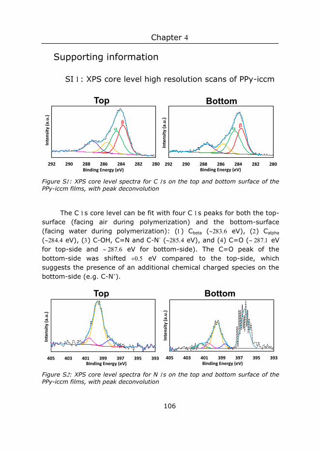
Chapter
106
Supporting information
SI : XPS core level high resolution scans of PPy-iccm
Figure S: XPS core level spectra for C s on the top and bottom surface of the PPy-iccm films, with peak deconvolution
The C s core level can be fit with four C s peaks for both the top-surface (facing air during polymerization) and the bottom-surface (facing water during polymerization): () Cbeta ( eV), () Calpha ( eV), () C-OH, C=N and C-N- ( eV), and () C=O ( eV for top-side and eV for bottom-side). The C=O peak of the bottom-side was shifted eV compared to the top-side, which suggests the presence of an additional chemical charged species on the bottom-side (e.g. C-N).
Figure S: XPS core level spectra for N s on the top and bottom surface of the PPy-iccm films, with peak deconvolution
280282284286288290292In
tens
ity (a
.u.)
Binding Energy (eV)280282284286288290292
Inte
nsity
(a.u
.)
Binding Energy (eV)
Top Bottom
Top Bottom
175
225
275
325
375
425
475
525
393395397399401403405
Inte
nsity
(a.u
.)
Binding Energy (eV)393395397399401403405
Inte
nsity
(a.u
.)
Binding Energy (eV)
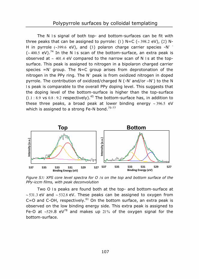
Polypyrrole surfaces by colloidal templating
107
The N s signal of both top- and bottom-surfaces can be fit with three peaks that can be assigned to pyrrole: () N=C ( eV), () N-H in pyrrole ( eV), and () polaron charge carrier species -N -
( eV).74 In the N s scan of the bottom-surface, an extra peak is observed at eV compared to the narrow scan of N s at the top-surface. This peak is assigned to nitrogen in a bipolaron charged carrier species =N group. The N=C group arises from deprotonation of the nitrogen in the PPy ring. The N peak is from oxidized nitrogen in doped pyrrole. The contribution of oxidized/charged N (-N and/or N) to the N s peak is comparable to the overall PPy doping level. This suggests that the doping level of the bottom-surface is higher than the top-surface ( vs respectively).45 The bottom-surface has, in addition to these three peaks, a broad peak at lower binding energy eV which is assigned to a strong Fe-N bond.75-77
Figure S: XPS core level spectra for O s on the top and bottom surface of the PPy-iccm films, with peak deconvolution
Two O s peaks are found both at the top- and bottom-surface at eV and eV. These peaks can be assigned to oxygen from C=O and C-OH, respectively.61 On the bottom surface, an extra peak is observed on the low binding energy side. This extra peak is assigned to Fe-O at .8 eV78 and makes up of the oxygen signal for the bottom-surface.
527529531533535537
Inte
nsity
(a.u
.)
Binding Energy (eV)527529531533535537
Inte
nsity
(a.u
.)
Binding Energy (eV)
Top Bottom
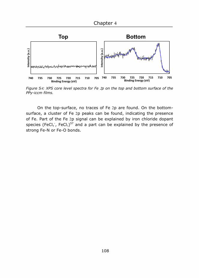
Chapter
108
Figure S: XPS core level spectra for Fe p on the top and bottom surface of the PPy-iccm films.
On the top-surface, no traces of Fe p are found. On the bottom-surface, a cluster of Fe p peaks can be found, indicating the presence of Fe. Part of the Fe p signal can be explained by iron chloride dopant species (FeCl-, FeCl)57 and a part can be explained by the presence of strong Fe-N or Fe-O bonds.
705710715720725730735740
Inte
nsity
(a.u
.)
Binding Energy (eV)705710715720725730735740
Inte
nsity
(a.u
.)
Binding Energy (eV)
Top Bottom
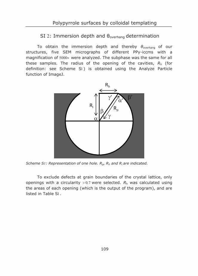
Polypyrrole surfaces by colloidal templating
109
SI : Immersion depth and θoverhang determination
To obtain the immersion depth and thereby θoverhang of our structures, five SEM micrographs of different PPy-iccms with a magnification of were analyzed. The subphase was the same for all these samples. The radius of the opening of the cavities, Rh (for definition: see Scheme S) is obtained using the Analyze Particle function of ImageJ.
Scheme S: Representation of one hole. Rp, Rh and Ri are indicated.
To exclude defects at grain boundaries of the crystal lattice, only openings with a circularity were selected. Rh was calculated using the areas of each opening (which is the output of the program), and are listed in Table S.
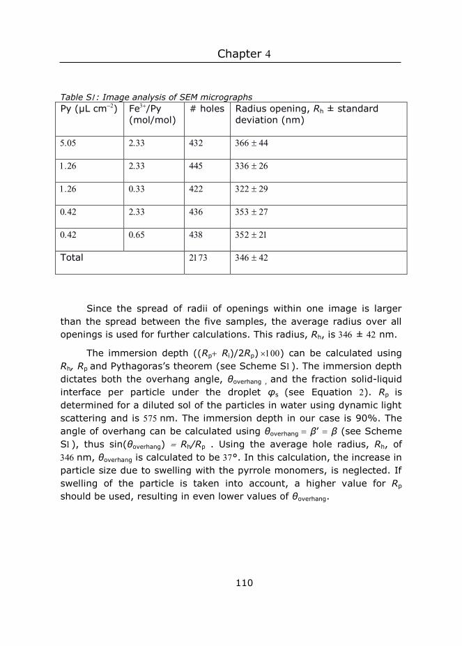
Chapter
110
Table S: Image analysis of SEM micrographs Py (µL cm) Fe/Py
(mol/mol) # holes Radius opening, Rh ± standard
deviation (nm)
Total
Since the spread of radii of openings within one image is larger than the spread between the five samples, the average radius over all openings is used for further calculations. This radius, Rh, is ± nm.
The immersion depth ((Rp Ri)/2Rp)) can be calculated using Rh, Rp and Pythagoras’s theorem (see Scheme S). The immersion depth dictates both the overhang angle, θoverhang , and the fraction solid-liquid interface per particle under the droplet φs (see Equation ). Rp is determined for a diluted sol of the particles in water using dynamic light scattering and is nm. The immersion depth in our case is 90%. The angle of overhang can be calculated using θoverhang β’ β (see Scheme S), thus sin(θoverhang) Rh/Rp . Using the average hole radius, Rh, of nm, θoverhang is calculated to be °. In this calculation, the increase in particle size due to swelling with the pyrrole monomers, is neglected. If swelling of the particle is taken into account, a higher value for Rp should be used, resulting in even lower values of θoverhang.
5 Three-gradient regular
solution model for simple
liquids, wetting complex
surface topologies
This chapter is based on: S. Akerboom, M. Kamperman, F.A.M. Leermakers, Three-gradient regular solution model for simple liquids, wetting complex surface topologies (submitted)
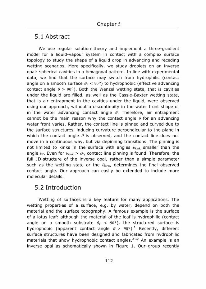
Chapter
112
5.1 Abstract
We use regular solution theory and implement a three-gradient model for a liquid-vapour system in contact with a complex surface topology to study the shape of a liquid drop in advancing and receding wetting scenarios. More specifically, we study droplets on an inverse opal: spherical cavities in a hexagonal pattern. In line with experimental data, we find that the surface may switch from hydrophilic (contact angle on a smooth surface Y < °) to hydrophobic (effective advancing contact angle > °). Both the Wenzel wetting state, that is cavities under the liquid are filled, as well as the Cassie-Baxter wetting state, that is air entrapment in the cavities under the liquid, were observed using our approach, without a discontinuity in the water front shape or in the water advancing contact angle . Therefore, air entrapment cannot be the main reason why the contact angle for an advancing water front varies. Rather, the contact line is pinned and curved due to the surface structures, inducing curvature perpendicular to the plane in which the contact angle is observed, and the contact line does not move in a continuous way, but via depinning transitions. The pinning is not limited to kinks in the surface with angles kink smaller than the angle Y. Even for kink > Y, contact line pinning is found. Therefore, the full D-structure of the inverse opal, rather than a simple parameter such as the wetting state or the kink, determines the final observed contact angle. Our approach can easily be extended to include more molecular details.
5.2 Introduction
Wetting of surfaces is a key feature for many applications. The wetting properties of a surface, e.g. by water, depend on both the material and the surface topography. A famous example is the surface of a lotus leaf: although the material of the leaf is hydrophilic (contact angle on a smooth substrate Y < °), the structured surface is hydrophobic (apparent contact angle > °).1 Recently, different surface structures have been designed and fabricated from hydrophilic materials that show hydrophobic contact angles.2-10 An example is an inverse opal as schematically shown in Figure 1. Our group recently
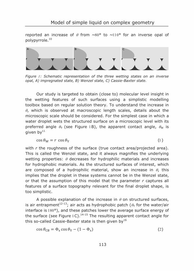
Model of simple liquid on complex geometry
113
reported an increase of from ~° to ~° for an inverse opal of polypyrrole.10
Figure : Schematic representation of the three wetting states on an inverse opal, A) impregnated state, B) Wenzel state, C) Cassie-Baxter state.
Our study is targeted to obtain (close to) molecular level insight in the wetting features of such surfaces using a simplistic modelling toolbox based on regular solution theory. To understand the increase in , which is observed at macroscopic length scales, details about the microscopic scale should be considered. For the simplest case in which a water droplet wets the structured surface on a microscopic level with its preferred angle Y (see Figure B), the apparent contact angle, W is given by11
cos 𝜃𝜃W = 𝑟𝑟 cos 𝜃𝜃Y ()
with r the roughness of the surface (true contact area/projected area). This is called the Wenzel state, and it always magnifies the underlying wetting properties: decreases for hydrophilic materials and increases for hydrophobic materials. As the structured surfaces of interest, which are composed of a hydrophilic material, show an increase in , this implies that the droplet in these systems cannot be in the Wenzel state, or that the assumption of this model that the parameter r captures all features of a surface topography relevant for the final droplet shape, is too simplistic.
A possible explanation of the increase in on structured surfaces, is air entrapment12-13; air acts as hydrophobic patch (Y for the water/air interface is °), and these patches lower the average surface energy of the surface (see Figure C).14-15 The resulting apparent contact angle for this so-called Cassie-Baxter state is then given by16
cos 𝜃𝜃CB = Φs cos 𝜃𝜃Y − (1 − Φs) ()
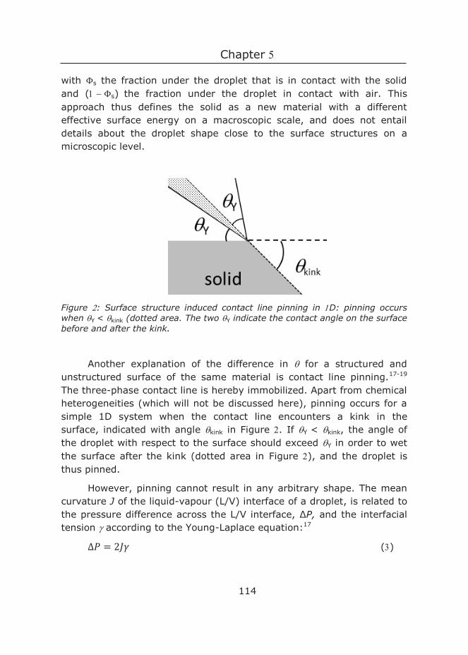
Chapter
114
with Φs the fraction under the droplet that is in contact with the solid and (Φs) the fraction under the droplet in contact with air. This approach thus defines the solid as a new material with a different effective surface energy on a macroscopic scale, and does not entail details about the droplet shape close to the surface structures on a microscopic level.
Figure : Surface structure induced contact line pinning in D: pinning occurs when Y < kink (dotted area. The two Y indicate the contact angle on the surface before and after the kink.
Another explanation of the difference in for a structured and unstructured surface of the same material is contact line pinning.17-19 The three-phase contact line is hereby immobilized. Apart from chemical heterogeneities (which will not be discussed here), pinning occurs for a simple 1D system when the contact line encounters a kink in the surface, indicated with angle kink in Figure . If Y < kink, the angle of the droplet with respect to the surface should exceed Y in order to wet the surface after the kink (dotted area in Figure ), and the droplet is thus pinned.
However, pinning cannot result in any arbitrary shape. The mean curvature J of the liquid-vapour (L/V) interface of a droplet, is related to the pressure difference across the L/V interface, ΔP, and the interfacial tension according to the Young-Laplace equation:17
∆𝑃𝑃 = 2𝐽𝐽𝐽𝐽 ()
Model of simple liquid on complex geometry
115
ΔP and can be considered constant for a droplet (neglecting small curvature corrections, the deformation due to gravity and the near surface contributions expressed in the disjoining pressure), thus J should also be constant.13 This implies that if the surface structure induces a curvature in one direction due to pinning, this should be compensated by the opposite curvature in the perpendicular direction. Hence, if structuring of a surface induces a noticeable curvature of the droplet parallel to the surface, this should lead to deformations of the droplet perpendicular to the surface. As the latter curvature is coupled to the apparent contact angle, which is commonly measured perpendicular to the surface, we notice contact angle variations.
The feature of hydrophilic surfaces showing hydrophobic contact angles is, for reasons mentioned above, often linked to re-entrant angles of the surface structures.20-21 An additional argument besides pinning, is that the liquid/air interfacial area should increase upon penetration of the liquid, creating more liquid/vapour interface.13 This may imply that air entrapment occurs, even for hydrophilic materials.12,
22
Common contact angle measurements typically do not have the correct resolution to see the local curvatures in both directions close to the surface. A better resolution can be achieved using AFM for non-volatile liquids,23 but this method is not suitable for droplets with >°. Recently droplet shapes have been studied using confocal microscopy with a resolution of hundreds of nanometres.18, 24 Although this is an improvement, the length scale may still be too high to observe curvature in the three phase contact line. Since it is difficult to reach these small length scales experimentally in the lab, we may find inspirations from the computational arena and therefore we turn to ‘experiments in silico’. The present study is targeted to obtain insight in the wetting features of surfaces of hydrophilic materials that show hydrophobic contact angles and to differentiate between air entrapment and contact line pinning using a modelling approach.
Using macroscopic approaches such as solving the Young-Laplace equation,25-26 minimizing the availability,27 or using geometry and energy12 to find the droplet shape do not take molecular details into account, and often require the contact angle as input parameter.
Chapter
116
Furthermore, air entrapment and coalescence28 cannot be obtained by solving the Young-Laplace equation, and surfaces with re-entrant curvatures give impossible solutions.28 Phase field methods,28 molecular dynamics (MD),22, 29-31 and mesoscopic lattice-Boltzmann (LB) models32-
36 are a viable option for this problem, but are challenging because wetting on complex structures involves multiple length scales37 and the time needed to converge to a solution can be long.30, 37
In this paper we focus on the very well-known regular solution theory, which is frequently used throughout the field of physical chemistry, but not so often applied for studying wetting on complex surface topologies in dimensions. Our models can be solved using a surprisingly simple algorithm (see Appendix) on a desktop PC in a few minutes CPU time. However, similarly to some of the theoretical approaches mentioned above, there are limitations with respect to the size of the systems that realistically can be considered, albeit that these limitations can easily be lifted with a factor of when the equations are solved using modern supercomputer facilities (which we here did not do). Here we focus on equilibrium and metastable states, which allows us to consider both advancing as well as receding contact angles. Even though the regular solution model is very well known, we will start by giving some backgrounds and highlights of the regular solution model. This gives us an opportunity to fix some of our parameters in the system. We then present the model and study the wetting of inverse opal structures.
5.3 Experimental
5.3.1 Regular solution theory
The start is a lattice model wherein the sites with linear length b are arranged in a cubic lattice geometry, that is, each cell has Z = neighbours. Let there be M sites in the system and thus the volume is given by V = Mb3. Sites are either filled by a solvent molecule, or the site is empty. The latter sites are said to be vacant and the number of vacant sites is NV. The remaining sites are filled by solvent and hence there are N = M NV sites filled. It is assumed that the solvent molecules only interact with each other when they occupy neighbouring
Model of simple liquid on complex geometry
117
sites and in this setting it is common to introduce the dimensionless Flory-Huggins interaction parameter, which is an Archimedes-like parameter needed for unlike-contacts:
𝜒𝜒 = 𝑍𝑍2𝑘𝑘B𝑇𝑇
(2𝑈𝑈LV − 𝑈𝑈LL − 𝑈𝑈VV) ()
A positive value means that LL contacts and VV ‘contacts’ are favoured over LV ones and this implies a tendency towards demixing. When we assume random mixing (mean-field approximation) we can evaluate the mixing interaction energy in the system by Umix = NV, where we ignored boundary effects and V = NV/M is the volume fraction of vacancies. The entropy of mixing can be evaluated when we assume once more that the sites are randomly filled by solvent. The total number of ways to arrange the fluid and the vacancies is given by
Ω = (𝑀𝑀𝑁𝑁) and the mixing entropy is found by 𝑆𝑆mix = −𝑘𝑘B lnΩ = −𝑘𝑘B (𝑁𝑁 ln𝜑𝜑 +𝑁𝑁𝑉𝑉 ln𝜑𝜑𝑉𝑉) with 𝜑𝜑= N/M and kB the Boltzmann constant. The free energy of mixing is given by Fmix = Umix TSmix. Introducing the dimensionless free energy density 𝑓𝑓 = 𝐹𝐹𝑚𝑚𝑚𝑚𝑚𝑚/(𝑀𝑀𝑏𝑏3𝑘𝑘B𝑇𝑇) wherein the thermal energy kBT and the volume V are used to reduce the free energy, we obtain the well-known regular solution free energy density:
𝑓𝑓 = 𝜑𝜑 ln𝜑𝜑 + 𝜑𝜑V ln𝜑𝜑V +𝜒𝜒𝜑𝜑𝜑𝜑V ()
with 𝜑𝜑 + 𝜑𝜑V = 1. The first two terms are negative and promote the mixing of the solvent and vapour. The last term drives the demixing. The critical conditions are found by setting the second and third derivatives of the free energy density Equation with respect to the volume fraction of liquid to zero. From such analysis it is found that there is a solubility gap as soon as > cr = . By symmetry the critical density cr = ½.
5.3.2 Liquid/vapour interface
Very famous is the extension of the regular solution theory to the description of the L/V interface. In the footsteps of Van der Waals38 we like to find the density profile across a L/V interface (z). Here z is a (lattice) coordinate running perpendicular to the interface. We set z = at the interface and consider a lattice model with layer numbers z = M, (M1), ⋯ , , , , ⋯, M, M. The boundary layers –M and M are taken
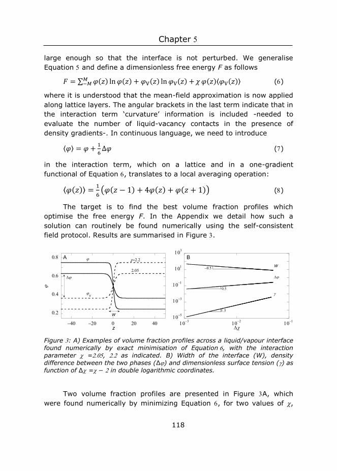
Chapter
118
large enough so that the interface is not perturbed. We generalise Equation and define a dimensionless free energy F as follows
𝐹𝐹 = ∑ 𝜑𝜑(𝑧𝑧) ln𝜑𝜑(𝑧𝑧) + 𝜑𝜑V(𝑧𝑧) ln𝜑𝜑V(𝑧𝑧) +𝜒𝜒𝜑𝜑(𝑧𝑧)⟨𝜑𝜑V(𝑧𝑧)⟩𝑀𝑀−𝑀𝑀 ()
where it is understood that the mean-field approximation is now applied along lattice layers. The angular brackets in the last term indicate that in the interaction term ‘curvature’ information is included -needed to evaluate the number of liquid-vacancy contacts in the presence of density gradients-. In continuous language, we need to introduce
⟨𝜑𝜑⟩ = 𝜑𝜑 + 16 Δ𝜑𝜑 ()
in the interaction term, which on a lattice and in a one-gradient functional of Equation , translates to a local averaging operation:
⟨𝜑𝜑(𝑧𝑧)⟩ = 16 (𝜑𝜑(𝑧𝑧 − 1) + 4𝜑𝜑(𝑧𝑧) + 𝜑𝜑(𝑧𝑧 + 1)) ()
The target is to find the best volume fraction profiles which optimise the free energy F. In the Appendix we detail how such a solution can routinely be found numerically using the self-consistent field protocol. Results are summarised in Figure .
Figure : A) Examples of volume fraction profiles across a liquid/vapour interface found numerically by exact minimisation of Equation, with the interaction parameter =, as indicated. B) Width of the interface (W), density difference between the two phases (Δ) and dimensionless surface tension () as function of Δ =− in double logarithmic coordinates.
Two volume fraction profiles are presented in Figure A, which were found numerically by minimizing Equation , for two values of ,
W
B
z
V
W
A
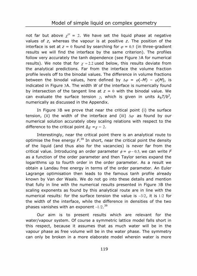
Model of simple liquid on complex geometry
119
not far but above cr = . We have set the liquid phase at negative values of z, whereas the vapour is at positive z. The position of the interface is set at z = found by searching for = (in three-gradient results we will find the interface by the same criterion). The profiles follow very accurately the tanh dependence (see Figure A for numerical results). We note that for used below, this results deviate from the analytical predictions. Far from the interface the volume fraction profile levels off to the binodal values. The difference in volume fractions between the binodal values, here defined by = (M) – (M), is indicated in Figure A. The width W of the interface is numerically found by intersection of the tangent line at z = with the binodal value. We can evaluate the surface tension , which is given in units kBT/b2, numerically as discussed in the Appendix.
In Figure B we prove that near the critical point (i) the surface tension, (ii) the width of the interface and (iii) as found by our numerical solution accurately obey scaling relations with respect to the difference to the critical point Δ =− .
Interestingly, near the critical point there is an analytical route to optimise the free energy F.39 In short, near the critical point the density of the liquid (and thus also for the vacancies) is never far from the critical value. Introducing an order parameter = we can write F as a function of the order parameter and then Taylor series expand the logarithms up to fourth order in the order parameter. As a result we obtain a Landau free energy in terms of the order parameter. An Euler Lagrange optimisation then leads to the famous tanh profile already known by Van der Waals. We do not go into these details and mention that fully in line with the numerical results presented in Figure B the scaling exponents as found by this analytical route are in line with the numerical results: for the surface tension the value is , it is for the width of the interface, while the difference in densities of the two phases vanishes with an exponent .39
Our aim is to present results which are relevant for the water/vapour system. Of course a symmetric lattice model falls short in this respect, because it assumes that as much water will be in the vapour phase as free volume will be in the water phase. The symmetry can only be broken in a more elaborate model wherein water is more
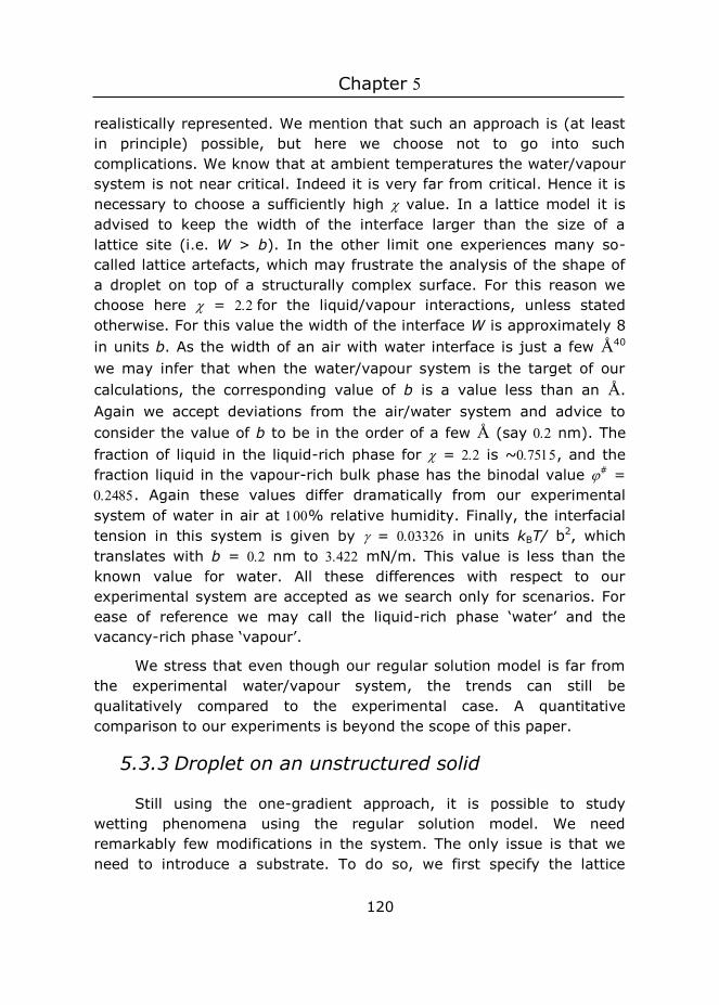
Chapter
120
realistically represented. We mention that such an approach is (at least in principle) possible, but here we choose not to go into such complications. We know that at ambient temperatures the water/vapour system is not near critical. Indeed it is very far from critical. Hence it is necessary to choose a sufficiently high value. In a lattice model it is advised to keep the width of the interface larger than the size of a lattice site (i.e. W > b). In the other limit one experiences many so-called lattice artefacts, which may frustrate the analysis of the shape of a droplet on top of a structurally complex surface. For this reason we choose here = for the liquid/vapour interactions, unless stated otherwise. For this value the width of the interface W is approximately 8 in units b. As the width of an air with water interface is just a few Å40 we may infer that when the water/vapour system is the target of our calculations, the corresponding value of b is a value less than an Å. Again we accept deviations from the air/water system and advice to consider the value of b to be in the order of a few Å (say nm). The fraction of liquid in the liquid-rich phase for = is ~, and the fraction liquid in the vapour-rich bulk phase has the binodal value # = . Again these values differ dramatically from our experimental system of water in air at % relative humidity. Finally, the interfacial tension in this system is given by = in units kBT/ b2, which translates with b = nm to mN/m. This value is less than the known value for water. All these differences with respect to our experimental system are accepted as we search only for scenarios. For ease of reference we may call the liquid-rich phase ‘water’ and the vacancy-rich phase ‘vapour’.
We stress that even though our regular solution model is far from the experimental water/vapour system, the trends can still be qualitatively compared to the experimental case. A quantitative comparison to our experiments is beyond the scope of this paper.
5.3.3 Droplet on an unstructured solid
Still using the one-gradient approach, it is possible to study wetting phenomena using the regular solution model. We need remarkably few modifications in the system. The only issue is that we need to introduce a substrate. To do so, we first specify the lattice
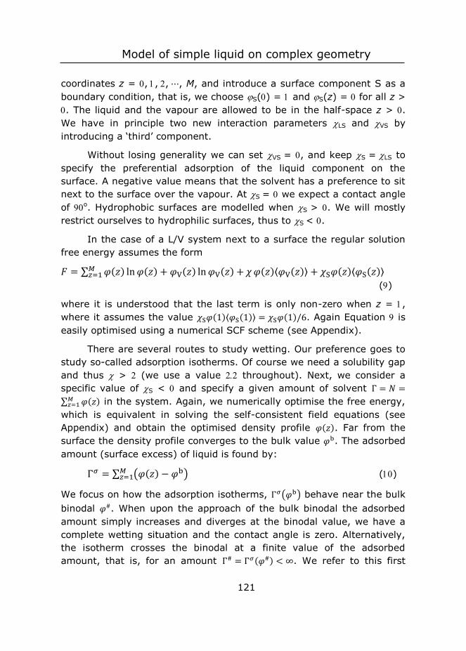
Model of simple liquid on complex geometry
121
coordinates z = ,,,⋯, M, and introduce a surface component S as a boundary condition, that is, we choose S() = and S(z) = for all z > . The liquid and the vapour are allowed to be in the half-space z > . We have in principle two new interaction parameters LS and VS by introducing a ‘third’ component.
Without losing generality we can set VS = , and keep S = LS to specify the preferential adsorption of the liquid component on the surface. A negative value means that the solvent has a preference to sit next to the surface over the vapour. At S = we expect a contact angle of o. Hydrophobic surfaces are modelled when S > . We will mostly restrict ourselves to hydrophilic surfaces, thus to S < .
In the case of a L/V system next to a surface the regular solution free energy assumes the form
𝐹𝐹 = ∑ 𝜑𝜑(𝑧𝑧) ln𝜑𝜑(𝑧𝑧) + 𝜑𝜑V(𝑧𝑧) ln𝜑𝜑V(𝑧𝑧) +𝜒𝜒𝜑𝜑(𝑧𝑧)⟨𝜑𝜑V(𝑧𝑧)⟩𝑀𝑀𝑧𝑧=1 + 𝜒𝜒S𝜑𝜑(𝑧𝑧)⟨𝜑𝜑S(𝑧𝑧)⟩
()
where it is understood that the last term is only non-zero when z = , where it assumes the value 𝜒𝜒S𝜑𝜑(1)⟨𝜑𝜑S(1)⟩ = 𝜒𝜒S𝜑𝜑(1)/6. Again Equation is easily optimised using a numerical SCF scheme (see Appendix).
There are several routes to study wetting. Our preference goes to study so-called adsorption isotherms. Of course we need a solubility gap and thus > (we use a value throughout). Next, we consider a specific value of S < and specify a given amount of solvent Γ = 𝑁𝑁 =∑ 𝜑𝜑(𝑧𝑧)𝑀𝑀𝑧𝑧=1 in the system. Again, we numerically optimise the free energy,
which is equivalent in solving the self-consistent field equations (see Appendix) and obtain the optimised density profile 𝜑𝜑(𝑧𝑧). Far from the surface the density profile converges to the bulk value 𝜑𝜑b. The adsorbed amount (surface excess) of liquid is found by:
Γ𝜎𝜎 = ∑ (𝜑𝜑(𝑧𝑧) − 𝜑𝜑b)𝑀𝑀𝑧𝑧=1 ()
We focus on how the adsorption isotherms, Γ𝜎𝜎(𝜑𝜑b) behave near the bulk binodal 𝜑𝜑#. When upon the approach of the bulk binodal the adsorbed amount simply increases and diverges at the binodal value, we have a complete wetting situation and the contact angle is zero. Alternatively, the isotherm crosses the binodal at a finite value of the adsorbed amount, that is, for an amount Γ# = Γ𝜎𝜎(𝜑𝜑#) < ∞. We refer to this first
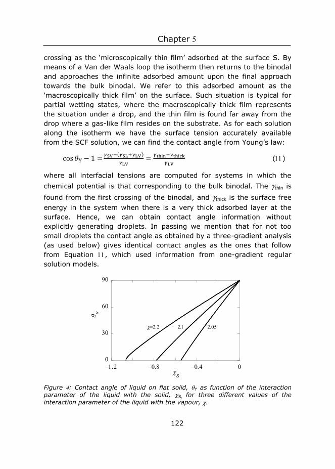
Chapter
122
crossing as the ‘microscopically thin film’ adsorbed at the surface S. By means of a Van der Waals loop the isotherm then returns to the binodal and approaches the infinite adsorbed amount upon the final approach towards the bulk binodal. We refer to this adsorbed amount as the ‘macroscopically thick film’ on the surface. Such situation is typical for partial wetting states, where the macroscopically thick film represents the situation under a drop, and the thin film is found far away from the drop where a gas-like film resides on the substrate. As for each solution along the isotherm we have the surface tension accurately available from the SCF solution, we can find the contact angle from Young’s law:
cos 𝜃𝜃Y − 1 = 𝛾𝛾SV−(𝛾𝛾SL+𝛾𝛾LV)𝛾𝛾LV
= 𝛾𝛾thin−𝛾𝛾thick𝛾𝛾LV
()
where all interfacial tensions are computed for systems in which the chemical potential is that corresponding to the bulk binodal. The thin is
found from the first crossing of the binodal, and thick is the surface free energy in the system when there is a very thick adsorbed layer at the surface. Hence, we can obtain contact angle information without explicitly generating droplets. In passing we mention that for not too small droplets the contact angle as obtained by a three-gradient analysis (as used below) gives identical contact angles as the ones that follow from Equation , which used information from one-gradient regular solution models.
Figure : Contact angle of liquid on flat solid, Y as function of the interaction parameter of the liquid with the solid, S, for three different values of the interaction parameter of the liquid with the vapour, .
S
Y

Model of simple liquid on complex geometry
123
The contact angle of a liquid droplet Y is calculated for various adsorption strengths S and for different strengths of interaction
between liquid and vapour (see Figure ). The more negative S, the more favourable the interaction between S and L, and the more the droplet spreads, resulting in smaller Y. Eventually, the liquid prefers to wet the solid completely, i.e. Y = °. At near the critical value of , the droplet enters the complete wetting regime (Y = °) already for very low values of the surface affinity S. For strong segregations the interfacial energies increase and we need larger adsorption energies to enforce wetting.
In this paper we aim to mimic a polypyrrole surface for which the water contact angle of a smooth surface is about Y = °. As we already selected = , we will be in the correct contact angle regime when we set the adsorption energies around S = . Below we will always mention the strength of adsorption.
5.3.4 Liquid condensation in parallel slit
The inverse opal surface structure consists of close to spherical cavities. In such structures we should anticipate the occurrence of capillary condensation or alternatively, capillary drying. For this reason we use the regular solution model to study classical capillary condensation. To this end we consider a system that contains two surfaces. One at z = and another one at z = D + . Hence 𝜑𝜑S(𝑧𝑧) = 0 for z = ,,⋯, D and unity elsewhere. Now our regular solution free energy is given by
𝐹𝐹 = ∑ 𝜑𝜑(𝑧𝑧) ln𝜑𝜑(𝑧𝑧) + 𝜑𝜑V(𝑧𝑧) ln𝜑𝜑V(𝑧𝑧) +𝜒𝜒𝜑𝜑(𝑧𝑧)⟨𝜑𝜑V(𝑧𝑧)⟩𝐷𝐷𝑧𝑧=1 + 𝜒𝜒S𝜑𝜑(𝑧𝑧)⟨𝜑𝜑S(𝑧𝑧)⟩
()
In this case the last term automatically accounts for the interactions with the surfaces, as it is nonzero for z = and z = D. More specifically, F has two surface contributions 𝜒𝜒S𝜑𝜑(1)/6 + 𝜒𝜒S𝜑𝜑(𝐷𝐷)/6.
As there are two interfaces, we anticipate the adsorption of the liquid onto both surfaces simultaneously. We want to record the adsorbed amount in the slit as a function of the (dimensionless)
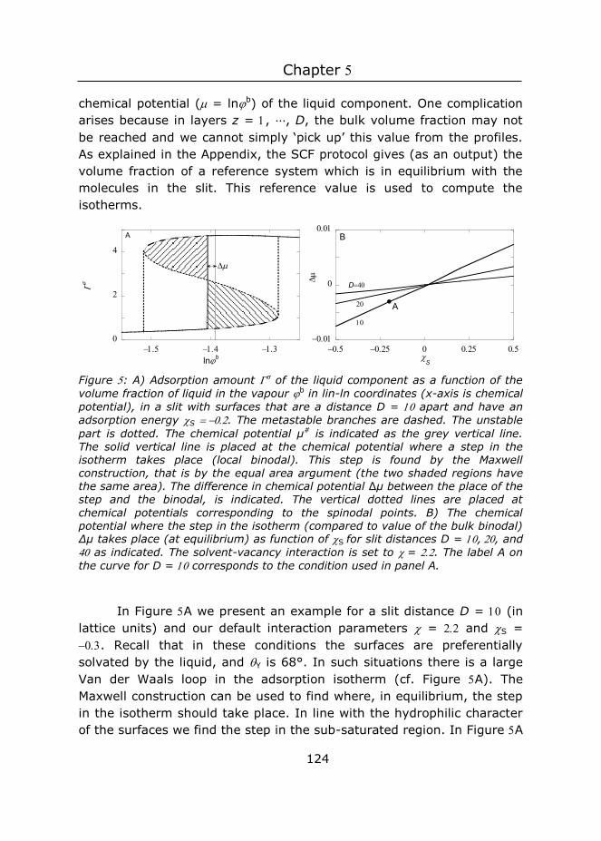
Chapter
124
chemical potential ( = lnb) of the liquid component. One complication arises because in layers z = , ⋯, D, the bulk volume fraction may not be reached and we cannot simply ‘pick up’ this value from the profiles. As explained in the Appendix, the SCF protocol gives (as an output) the volume fraction of a reference system which is in equilibrium with the molecules in the slit. This reference value is used to compute the isotherms.
Figure : A) Adsorption amount of the liquid component as a function of the volume fraction of liquid in the vapour b in lin-ln coordinates (x-axis is chemical potential), in a slit with surfaces that are a distance D = apart and have an adsorption energy S . The metastable branches are dashed. The unstable part is dotted. The chemical potential µ# is indicated as the grey vertical line. The solid vertical line is placed at the chemical potential where a step in the isotherm takes place (local binodal). This step is found by the Maxwell construction, that is by the equal area argument (the two shaded regions have the same area). The difference in chemical potential Δµ between the place of the step and the binodal, is indicated. The vertical dotted lines are placed at chemical potentials corresponding to the spinodal points. B) The chemical potential where the step in the isotherm (compared to value of the bulk binodal) Δµ takes place (at equilibrium) as function of S for slit distances D = ,, and as indicated. The solvent-vacancy interaction is set to = . The label A on the curve for D = corresponds to the condition used in panel A.
In Figure A we present an example for a slit distance D = (in lattice units) and our default interaction parameters = and S = . Recall that in these conditions the surfaces are preferentially solvated by the liquid, and Y is 68°. In such situations there is a large Van der Waals loop in the adsorption isotherm (cf. Figure A). The Maxwell construction can be used to find where, in equilibrium, the step in the isotherm should take place. In line with the hydrophilic character of the surfaces we find the step in the sub-saturated region. In Figure A
lnb
A
S
D
A
B
Model of simple liquid on complex geometry
125
the grey vertical line represents the bulk binodal value. The step takes place at a lower chemical potential (local binodal) than that corresponding to the bulk binodal. We define as the difference in lnb between the local and bulk binodals as indicated in Figure A.
It is important to consider the isotherm in slightly more detail. After the jump in the isotherm the adsorbed amount only marginally increases further: the isotherm continues into the supersaturated region and as the system increases the bulk volume fraction, in the limit of very high concentrations the excess should go down again to become zero in the limit of b to .
The most interesting feature of the isotherm the presence of a loop. Associated to the loop there are two spinodal points. These spinodal points are located at the turning points of the isotherm. There are two regions of metastability, namely between the local binodal and the first turning point. This spinodal point is found in supersaturated conditions. The other metastable region is found between the turning point in the sub-saturated region and the local binodal in the top region of the isotherm. In the isotherm the metastable branches are indicated by dashed line parts. When in the absence of strong fluctuations the bulk volume fraction is increased, the slit may not necessarily change its contents at the local binodal, but instead remains dry up to -in the extreme case- the spinodal point is reached, and the slit is filled with liquid following the dashed line. Inversely, when the slit is wet, and the bulk concentration is reduced, the drying does not necessarily take place at the local binodal, but enter the other metastable branch. Again the drying must take place before or at the lower spinodal point (following the other dashed line). Hence in dynamical situations a hysteresis loop may be followed where the steps at the spinodal are indicated by the vertical dotted lines. The spinodal points have important roles in the advancing or receding contact line calculations (see below). Even though the Van der Waals loop in the isotherm is due to the mean-field approximation, it is found that in real life experiments the system also may be trapped in metastable states very much alike those found in the mean-field model.
In Figure B we report that the difference between the local and the bulk binodal in confined spaces is a function of the affinity of the
Chapter
126
solvent for the substrate. When S is more negative the increases to
more negative values. Indeed when S > , that is for hydrophobic surfaces, the local binodal occurs at supersaturated solutions. With increasing D the local binodal shifts towards the bulk binodal.
5.3.5 Curved L/V interfaces; Kelvin & Laplace
Macroscopic droplets (with negligible curvature) cannot be generated using our method. As the system size is limited, our drops have L/V interfaces which are typically strongly curved. The thermodynamics of curved interfaces is well understood, but there are several complications. One of the issues is that the location of the interface is somewhat arbitrary. On top of this the interfacial tension in curved interfaces cannot uniquely be computed. It depends on the notion of the position of the interface. There exists a choice of the position of the interface, the so-called surface of tension, for which a small notional change of the radius does not influence the value of the surface tension. For this special case the Laplace equation simplifies to Equation , and the value of the interfacial tension does not deviate much from the planar value.
From the Laplace equation we know that in droplets with curved L/V interfaces there is a Laplace pressure. As a consequence the chemical potential of the liquid in a drop is at a higher chemical potential compared to systems with planar interfaces. The increased chemical potential is reflected in the oversaturation of water in the vapour phase; a phenomenon named after Kelvin. With oversaturation of the system, which necessarily occurs in our calculations due to the finite size of our droplets, one will invariably get closer to the spinodal point of the capillary condensation process. Hence, oversaturation may trigger the filling of confined regions by the liquid. Small droplets cause a stronger oversaturation than larger droplets and the presence of small droplets may result in a spontaneous filling of the voids by capillary condensation when this may not yet occur for larger drops.
The radius specified by the surface of tension RSOT coincides with the visual inspection of where the interface is for many systems. Below we therefore do not exactly determine the exact RSOT and use the Ansatz

Model of simple liquid on complex geometry
127
that the interface position is where the solvent volume fraction hits the value = .
5.3.6 Three-gradient regular solution model
Let us next extend the regular solution theory to model liquid drops at a complex surface topology. We consider a three-gradient coordinate system r = (x,y,z) with x = ,,⋯, Mx, y = ,,⋯, My and z = ,, ⋯, Mz. In contrast to the one-gradient systems where the surfaces were treated through the boundary conditions, in three gradient models it is more natural that the surface component S will occupy lattice sites within the specified volume. Hence, we will specify all the lattice sites within the system: the volume fraction of S is unity and the remainder of the lattice sites are filled by the liquid and vapour components in the usual way. The regular solution free energy is straightforwardly generalised and both interactions between L and V as well as with the surface component S are accounted for:
𝐹𝐹 = ∑ ∑ ∑ 𝜑𝜑(𝐫𝐫) ln𝜑𝜑(𝐫𝐫) + 𝜑𝜑V(𝐫𝐫) ln𝜑𝜑V(𝐫𝐫) +𝜒𝜒𝑀𝑀𝑧𝑧𝑧𝑧=1
𝑀𝑀𝑦𝑦𝑦𝑦=1
𝑀𝑀𝑥𝑥𝑥𝑥=1 𝜑𝜑(𝐫𝐫)⟨𝜑𝜑V(𝐫𝐫)⟩ +
𝜒𝜒S𝜑𝜑(𝐫𝐫)⟨𝜑𝜑S(𝐫𝐫)⟩ ()
wherein the angular brackets indicate that the free energy accounts for the ‘curvature’ information in three directions. The lattice implementa-tion is simply:
⟨𝜑𝜑(𝐫𝐫)⟩ = ⟨𝜑𝜑(𝑥𝑥, 𝑦𝑦, 𝑧𝑧)⟩ = 16 (𝜑𝜑(𝑥𝑥 − 1, 𝑦𝑦, 𝑧𝑧) + 𝜑𝜑(𝑥𝑥 + 1, 𝑦𝑦, 𝑧𝑧) + 𝜑𝜑(𝑥𝑥, 𝑦𝑦 −
1, 𝑧𝑧) + 𝜑𝜑(𝑥𝑥, 𝑦𝑦 + 1, 𝑧𝑧) + 𝜑𝜑(𝑥𝑥, 𝑦𝑦, 𝑧𝑧 − 1) + 𝜑𝜑(𝑥𝑥, 𝑦𝑦, 𝑧𝑧 + 1)) ()
Mirror-like, no-gradient boundary conditions are implemented in boundary layers in the system. This is implemented by setting 𝜑𝜑(0, 𝑦𝑦, 𝑧𝑧) =𝜑𝜑(1, 𝑦𝑦, 𝑧𝑧), 𝜑𝜑(𝑀𝑀𝑥𝑥 + 1, 𝑦𝑦, 𝑧𝑧) = 𝜑𝜑(𝑀𝑀𝑥𝑥, 𝑦𝑦, 𝑧𝑧), and similarly for the other boundaries in y- and z-directions. Using these boundary conditions it is possible to consider a representative part of the surface, while keeping the computation times and system volumes to a minimum.
Chapter
128
Table : Parameters that determine the structure of the inverse opal. Even and odd rows of cavities are displaced by half the distance between the cavities in a row, that is, by s/. All quantities are given in lattice units, that is in values of b. Below also the cut-off ratio c = h/d (to specify which part of the cavity is cut-off) and S (the fraction of the top of the surface that is solid) is used.
D diameter of a cavity (integer > )
S spacing between two cavities in a row (integer of order d)
T distance between the two rows (integer of order d)
N ‘number’ of cavities in a row (> ) may also be non-integer
m number of rows (integer > )
H cut-off height of the solid phase (integer > )
5.3.7 Specifying the inverse opal
The regular solution free energy of Equation still requires detailed information on the distribution of the solid material S in the inverse opal. The idea is to consider a representative piece of a substrate that contains spherical cavities in a specified arrangement (i.e. crystalline ordering with close to hexagonal or square packing symmetries). The cut-off height controls the opening of the cavities as shown in the example of Figure . The parameters that control the surface topology are listed in Table. Below we will use the parameter c = h/d, which is a fraction at which the cavities was cut and S is the fraction of the ‘top’ of the surface which is solid.
The parameters of Table completely specify how many cavities are present in the computation volume. Let the cavities be numbered by i = ,,, ⋯, Nc. In the example of Figure there are rows of cavities and thus we need i = , ⋯, cavity positions. The input parameters thus specify the coordinates of the cavities {𝐫𝐫1, 𝐫𝐫2,⋯ , 𝐫𝐫𝑖𝑖,⋯ , 𝐫𝐫𝑁𝑁𝑐𝑐}. The cavities in the inverse opal are placed in rows along the y-direction, the direction perpendicular to the rows is the x-direction and the cavities
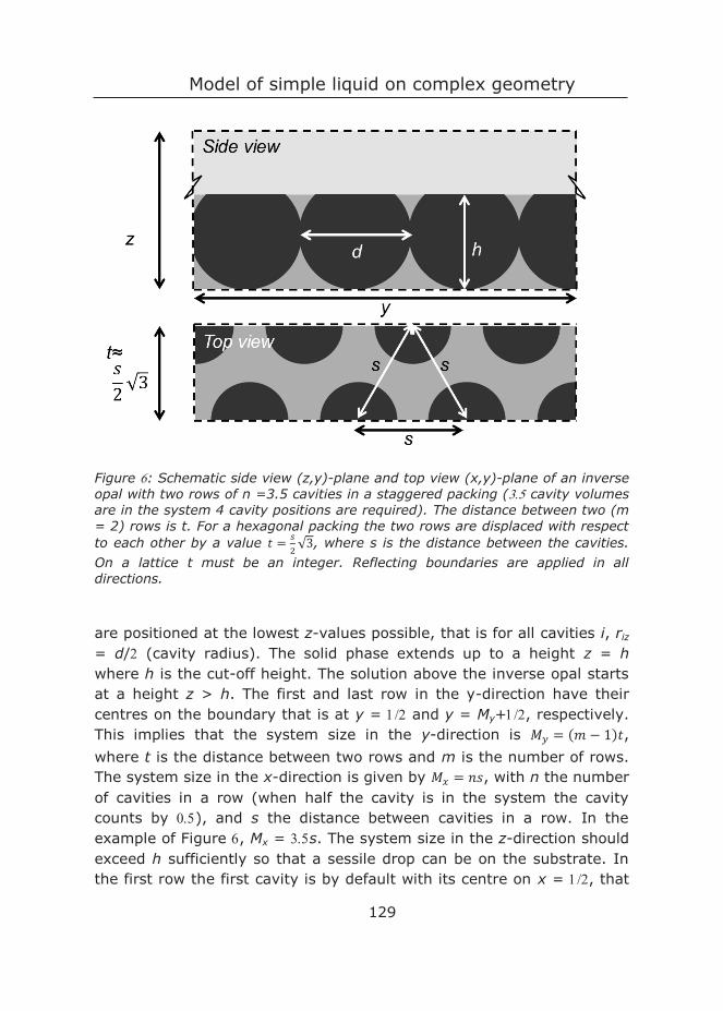
Model of simple liquid on complex geometry
129
Figure : Schematic side view (z,y)-plane and top view (x,y)-plane of an inverse opal with two rows of n =3.5 cavities in a staggered packing ( cavity volumes are in the system 4 cavity positions are required). The distance between two (m = 2) rows is t. For a hexagonal packing the two rows are displaced with respect to each other by a value 𝑡𝑡 = 𝑠𝑠
2 √3, where s is the distance between the cavities. On a lattice t must be an integer. Reflecting boundaries are applied in all directions.
are positioned at the lowest z-values possible, that is for all cavities i, riz = d/ (cavity radius). The solid phase extends up to a height z = h where h is the cut-off height. The solution above the inverse opal starts at a height z > h. The first and last row in the y-direction have their centres on the boundary that is at y = and y = My+, respectively. This implies that the system size in the y-direction is 𝑀𝑀𝑦𝑦 = (𝑚𝑚 − 1)𝑡𝑡, where t is the distance between two rows and m is the number of rows. The system size in the x-direction is given by 𝑀𝑀𝑥𝑥 = 𝑛𝑛𝑛𝑛, with n the number of cavities in a row (when half the cavity is in the system the cavity counts by ), and s the distance between cavities in a row. In the example of Figure , Mx = s. The system size in the z-direction should exceed h sufficiently so that a sessile drop can be on the substrate. In the first row the first cavity is by default with its centre on x = , that
Chapter
130
is, on the lower boundary. The first cavity in the second row is positioned at x = (s + )/, etcetera.
All nonzero surface densities can now be computed. When for a coordinate r’ the distance to all of the coordinates {𝐫𝐫1, 𝐫𝐫2, ⋯ , 𝐫𝐫𝑖𝑖, ⋯ , 𝐫𝐫𝑁𝑁𝑐𝑐} is larger than the radius of a cavity, i.e., d/ and when the z-value is less or equal to h, we set the 𝜑𝜑𝑆𝑆(𝐫𝐫′) = 1 and 𝜑𝜑𝑆𝑆(𝐫𝐫′) = 0 otherwise:
𝜑𝜑S(𝒓𝒓′) = {1 𝐫𝐫𝑧𝑧 ≤ ℎ & |𝐫𝐫𝑖𝑖 − 𝐫𝐫′| > 𝑑𝑑2 ∀𝑖𝑖
0 otherwise ()
This solid distribution is fixed during the free energy optimisation. Of course only the coordinates that are not taken up by the S can be filled with L or V. On the ‘top’ of the solid phase it is of interest to know the fraction of sites occupied by S. These are easily evaluated by
ΦS = 1𝑀𝑀𝑥𝑥𝑀𝑀𝑦𝑦
∑ ∑ 𝜑𝜑S(𝑥𝑥, 𝑦𝑦, ℎ)𝑀𝑀𝑦𝑦𝑦𝑦=1
𝑀𝑀𝑥𝑥𝑥𝑥=1 ()
Analytical estimates of Equation 16 are given in SI . The cut-off height h normalised by the particle diameter d will be referred to by c:
𝑐𝑐 = ℎ𝑑𝑑 ()
Below we will be interested in hexagonal ordered cavities. For an optimal hexagonal packing, the distance s between the particles along a row and the distance t between the rows, should obey 𝑡𝑡 = 𝑠𝑠
2 √3. However,
on the lattice only integer values are allowed. Rounding to closest integer values must be implemented. For some values of the particle distances s there is a reasonable value of t, for other distances the error is relatively large. Only values of s which required < rounding errors for the corresponding t value are used.
Parameters of Table can be used to generate a large variety of inverse opal structures. As long as s > d, we have the situation that the cavities are isolated. However, the cavities may become interconnected when s < d. In experimental situations such overlap of cavities may occur, and then there are usually small openings connecting the cavities. This is why this particular parameter setting is allowed.
Model of simple liquid on complex geometry
131
5.4 Results and discussion
5.4.1 Example 1. Liquid condensation in a weakly
hydrophilic face centred square inverse opal
We first consider a simple inverse opal structure which has cavities with a diameter d = . The distance s between the cavities is set to , and the distance between the rows t = . This implies a face centred square arrangement of the cavities. The number of cavities in a row is unity n = , whereas the number of rows is set to . As can be seen from Figure , this setting generates an equal box size in x and y directions. As the distance between the cavities exceeds the cavity diameter, we have isolated pockets. The surface interaction is set to a slightly hydrophilic value S = .
To compute the adsorption isotherm, we start with a low amount of liquid in the system and then increase this amount step by step. In the calculations the outcome of a given calculation serves as an initial guess for the subsequent calculation. This is why a system can be trapped in metastable states, similarly as in experimental counterparts.
In Figure A we present the adsorbed amount of the liquid component Γ𝜎𝜎 = Γ − 𝑉𝑉′𝜑𝜑𝑏𝑏, where V’ is the volume available for the L and V components, that is 𝑉𝑉′ = 𝑀𝑀𝑥𝑥𝑀𝑀𝑦𝑦𝑀𝑀𝑧𝑧 − ∑ 𝜑𝜑S(𝐫𝐫)r , as a function of the volume fraction of the liquid component in the bulk. Here we did not normalise with respect to the available surface area and thus this amount is proportional to the surface area. The bulk volume fraction is normalised by the bulk binodal value. The curve is plotted in linear-ln coordinates. Upon an increase in the amount of liquid component in the system , first the vapour phase is gradually saturated with liquid and the adsorbed excess remains modest: at the surface a gaseous adsorption layer develops. Then, upon further increase of the amount, the binodal value is crossed and the system enters the super-saturation regime. The liquid film remains homogeneous along the surface, until ~ , then a first-order jump in the isotherm takes place (cf Figure A dotted line). As can be seen in Figure B, at this stage a droplet formed in the confined space of the cavity and the curvature on the L/V interface in
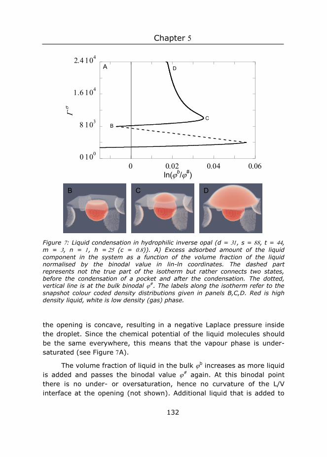
Chapter
132
Figure : Liquid condensation in hydrophilic inverse opal (d = , s = , t = , m = , n = , h = (c = )). A) Excess adsorbed amount of the liquid component in the system as a function of the volume fraction of the liquid normalised by the binodal value in lin-ln coordinates. The dashed part represents not the true part of the isotherm but rather connects two states, before the condensation of a pocket and after the condensation. The dotted, vertical line is at the bulk binodal #. The labels along the isotherm refer to the snapshot colour coded density distributions given in panels B,C,D. Red is high density liquid, white is low density (gas) phase.
the opening is concave, resulting in a negative Laplace pressure inside the droplet. Since the chemical potential of the liquid molecules should be the same everywhere, this means that the vapour phase is under-saturated (see Figure A).
The volume fraction of liquid in the bulk b increases as more liquid is added and passes the binodal value # again. At this binodal point there is no under- or oversaturation, hence no curvature of the L/V interface at the opening (not shown). Additional liquid that is added to
B C D
ln(b/#)
BC
A D

Model of simple liquid on complex geometry
133
the droplet induces a convex curvature on top of the droplet, and the bulk oversaturates up to C in Figure A. The at this point is approximately , and consists of a thin film (~ ) and the macroscopic droplet (~ ). The volume of a sphere with d = is about . Given that the density difference between the liquid-rich and vapour-rich phase is ~, and that part of the thin liquid film becomes part of the macroscopic droplet, the found at point C is in agreement with what is expected for a cavity with diameter d = .
Additional liquid is subsequently not used to fill the other cavities, but to increase the volume of the existing droplet (Figure D) and the droplet starts to spread on the substrate. Below we will follow this process in a slightly different geometry. The oversaturation needed for capillary condensation to occur for the other cavities is in this case not reached. This means that for this inverse opal, with d = , once condensation has taken place, a droplet grows on top of the filled cavity and the remaining cavities are not filled via capillary condensation, but typically rather fill once the central droplet spreads over and on top of the other cavities (not shown).
Most inverse opals in experiments, which are fabricated using sacrificial particles, have cavities of hundreds of nanometres or more (e.g. refs. ) These sizes are much larger than the cavities considered in the current calculations. Smaller cavities can fill more easily via capillary condensation (cf. Figure B). Since the impregnating wetting state is not observed even for such small cavity sizes as used in Figure , we conclude that the impregnating wetting state due to capillary condensation is not likely to develop for practical inverse opals which are marginally hydrophilic.
In this surface structure, the cavities are not connected, whereas for some experimentally fabricated inverse opals all cavities may be interconnected via a small opening. Since the curvature of the droplet should be constant, the curvature of the liquid-vapour interface at the small opening is the same as for the rest of the macroscopic droplet13, and hence the high curvature needed for the next cavity to be wetted via this opening, is not reached. Therefore, a cavity that is filled with liquid will wet the next cavity via the larger opening at the top, rather than through this small hole (not shown).
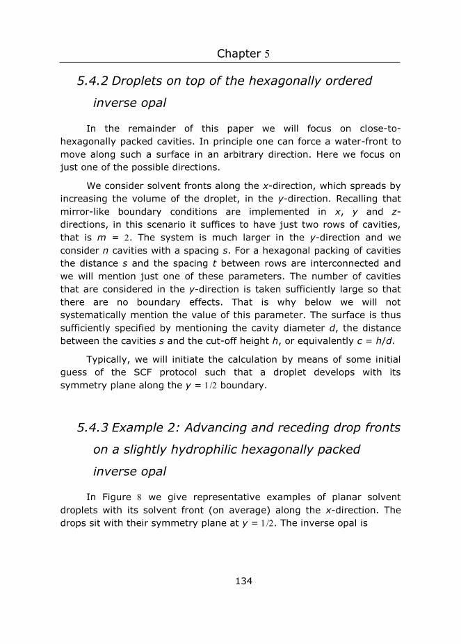
Chapter
134
5.4.2 Droplets on top of the hexagonally ordered
inverse opal
In the remainder of this paper we will focus on close-to-hexagonally packed cavities. In principle one can force a water-front to move along such a surface in an arbitrary direction. Here we focus on just one of the possible directions.
We consider solvent fronts along the x-direction, which spreads by increasing the volume of the droplet, in the y-direction. Recalling that mirror-like boundary conditions are implemented in x, y and z-directions, in this scenario it suffices to have just two rows of cavities, that is m = . The system is much larger in the y-direction and we consider n cavities with a spacing s. For a hexagonal packing of cavities the distance s and the spacing t between rows are interconnected and we will mention just one of these parameters. The number of cavities that are considered in the y-direction is taken sufficiently large so that there are no boundary effects. That is why below we will not systematically mention the value of this parameter. The surface is thus sufficiently specified by mentioning the cavity diameter d, the distance between the cavities s and the cut-off height h, or equivalently c = h/d.
Typically, we will initiate the calculation by means of some initial guess of the SCF protocol such that a droplet develops with its symmetry plane along the y = boundary.
5.4.3 Example 2: Advancing and receding drop fronts
on a slightly hydrophilic hexagonally packed
inverse opal
In Figure we give representative examples of planar solvent droplets with its solvent front (on average) along the x-direction. The drops sit with their symmetry plane at y = . The inverse opal is
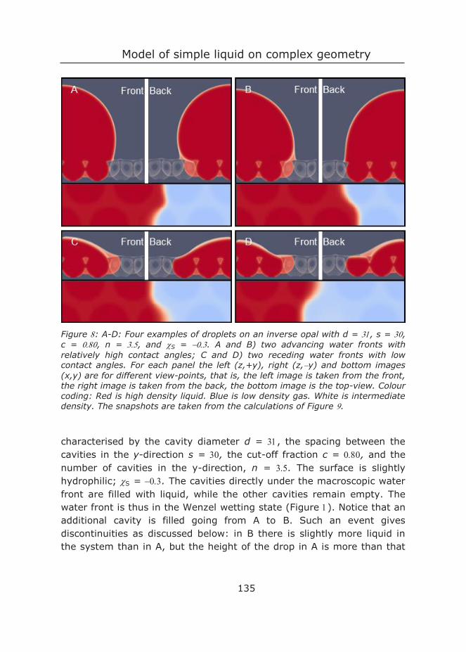
Model of simple liquid on complex geometry
135
Figure : A-D: Four examples of droplets on an inverse opal with d = , s = , c = , n = , and S = . A and B) two advancing water fronts with relatively high contact angles; C and D) two receding water fronts with low contact angles. For each panel the left (z,+y), right (z,y) and bottom images (x,y) are for different view-points, that is, the left image is taken from the front, the right image is taken from the back, the bottom image is the top-view. Colour coding: Red is high density liquid. Blue is low density gas. White is intermediate density. The snapshots are taken from the calculations of Figure .
characterised by the cavity diameter d = , the spacing between the cavities in the y-direction s = , the cut-off fraction c = , and the number of cavities in the y-direction, n = . The surface is slightly hydrophilic; S = . The cavities directly under the macroscopic water front are filled with liquid, while the other cavities remain empty. The water front is thus in the Wenzel wetting state (Figure ). Notice that an additional cavity is filled going from A to B. Such an event gives discontinuities as discussed below: in B there is slightly more liquid in the system than in A, but the height of the drop in A is more than that
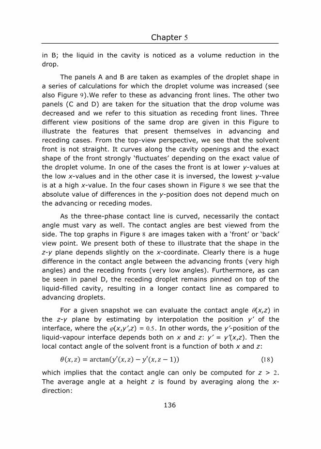
Chapter
136
in B; the liquid in the cavity is noticed as a volume reduction in the drop.
The panels A and B are taken as examples of the droplet shape in a series of calculations for which the droplet volume was increased (see also Figure ).We refer to these as advancing front lines. The other two panels (C and D) are taken for the situation that the drop volume was decreased and we refer to this situation as receding front lines. Three different view positions of the same drop are given in this Figure to illustrate the features that present themselves in advancing and receding cases. From the top-view perspective, we see that the solvent front is not straight. It curves along the cavity openings and the exact shape of the front strongly ‘fluctuates’ depending on the exact value of the droplet volume. In one of the cases the front is at lower y-values at the low x-values and in the other case it is inversed, the lowest y-value is at a high x-value. In the four cases shown in Figure we see that the absolute value of differences in the y-position does not depend much on the advancing or receding modes.
As the three-phase contact line is curved, necessarily the contact angle must vary as well. The contact angles are best viewed from the side. The top graphs in Figure are images taken with a ‘front’ or ‘back’ view point. We present both of these to illustrate that the shape in the z-y plane depends slightly on the x-coordinate. Clearly there is a huge difference in the contact angle between the advancing fronts (very high angles) and the receding fronts (very low angles). Furthermore, as can be seen in panel D, the receding droplet remains pinned on top of the liquid-filled cavity, resulting in a longer contact line as compared to advancing droplets.
For a given snapshot we can evaluate the contact angle (x,z) in the z-y plane by estimating by interpolation the position y’ of the interface, where the (x,y’,z) = . In other words, the y’-position of the liquid-vapour interface depends both on x and z: y’ = y’(x,z). Then the local contact angle of the solvent front is a function of both x and z:
𝜃𝜃(𝑥𝑥, 𝑧𝑧) = arctan(𝑦𝑦′(𝑥𝑥, 𝑧𝑧) − 𝑦𝑦′(𝑥𝑥, 𝑧𝑧 − 1)) ()
which implies that the contact angle can only be computed for z > . The average angle at a height z is found by averaging along the x-direction:
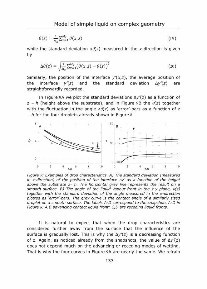
Model of simple liquid on complex geometry
137
𝜃𝜃(𝑧𝑧) = 1𝑀𝑀𝑥𝑥
∑ 𝜃𝜃(𝑥𝑥, 𝑧𝑧)𝑀𝑀𝑥𝑥𝑥𝑥=1 ()
while the standard deviation (z) measured in the x-direction is given by
∆𝜃𝜃(𝑧𝑧) = √ 1𝑀𝑀𝑥𝑥
∑ (𝜃𝜃(𝑥𝑥, 𝑧𝑧) − 𝜃𝜃(𝑧𝑧))2𝑀𝑀𝑥𝑥𝑥𝑥=1 ()
Similarly, the position of the interface y’(x,z), the average position of the interface y’(z) and the standard deviation Δy’(z) are straightforwardly recorded.
In Figure A we plot the standard deviations Δy’(z) as a function of z h (height above the substrate), and in Figure B the (z) together with the fluctuation in the angle (z) as ‘error’-bars as a function of z h for the four droplets already shown in Figure .
Figure : Examples of drop characteristics. A) The standard deviation (measured in x-direction) of the position of the interface y’ as a function of the height above the substrate z h. The horizontal grey line represents the result on a smooth surface. B) The angle of the liquid-vapour front in the z-y plane, (z) together with the standard deviation of the angle measured in the x-direction plotted as ‘error’-bars. The grey curve is the contact angle of a similarly sized droplet on a smooth surface. The labels A-D correspond to the snapshots A-D in Figure : A,B advancing contact liquid front; C,D are receding liquid fronts.
It is natural to expect that when the drop characteristics are considered further away from the surface that the influence of the surface is gradually lost. This is why the Δy’(z) is a decreasing function of z. Again, as noticed already from the snapshots, the value of Δy’(z) does not depend much on the advancing or receding modes of wetting. That is why the four curves in Figure A are nearly the same. We refrain
z-h
A
B
C D
B
z-h
y A BC D
A
Chapter
138
from trying to provide further comments about the differences. Similarly, far from the surface the angles become independent on x. That is why in Figure B the ‘error’ bars diminish in size when z h is increased. Indeed very close to the substrate z h < the fluctuations are very large, that is about % of its value.
We already noticed that the advancing contact angles are much larger than the receding ones. Figure B gives the numerics more accurately: the advancing angles are on average larger than °, whereas the receding angles are about °, very close to the angles found for the unstructured surface (grey line). Interestingly, the average contact angle in the advancing mode can go through a small local maximum at a height z h = . Such an effect hints to the presence of a foot on the droplets. However, at this height the fluctuations are large and we are hesitant not to over-interpret the results.
It is clear that, if we want to compare droplets and see trends, we need to reduce the outcome of the computations. That is why from hereon we will focus on the properties of the droplets on a height of z h = (as indicated by the arrow in Figure ). At this height above the substrate the ‘foot’ is not disturbing too much, while the structure of the surface is still well noticeable. We thus define (if not mentioned otherwise) the fluctuations of the liquid front measured as the standard deviation along the x-direction as ∆𝑦𝑦 = ∆𝑦𝑦′(ℎ + 3), and the average contact angle of the drop 𝜃𝜃 = 𝜃𝜃(ℎ + 3), as well as the fluctuations ∆𝜃𝜃 = ∆𝜃𝜃(ℎ + 3).
Calculations wherefrom the results of Figures and were taken were started with an initial amount of liquid = 3∙106. The more liquid is added to the system and these molecules are consumed by the drop. Hence the drop volume was increased. Typically we performed ten liquid addition steps and for each of these new profiles are calculated to obtain an advancing angle. The amount of the liquid is subsequently stepwise decreased to check for hysteresis and to obtain a receding angle. The structural properties of the drops are recorded during this cycle and the results were collected in Figure .

Model of simple liquid on complex geometry
139
Figure : Examples of structural features of advancing and receding drop fronts. A) The fluctuations of the position of the liquid front along the x-direction at a height z = h + as a function of the of the droplet component with an initial amount = ∙. B) The corresponding average contact angle (measured at a height z = h + ) and the standard deviation (plotted as error-bars).The advancing liquid front is given by the solid sphere data points, the receding ones in solid square data points. The lines are to guide the eye. A discontinuity in the line represents a jump-wise change of the drops on the substrate. The labels A-D correspond to the snapshots of Figure and the structural data of Figure . A and B are along the advancing branch, whereas C and D are taken from the receding drop fronts. Parameters are similar as in Figures and .
The starting point of the calculations is not extremely well defined in terms of advancing or receding states. The initial guess takes the system in this case close to an advancing situation: the contact angle is rather high. Typically this initial drop is disregarded from our averaging (see below). Upon stepwise increase of the drop volume (closed spheres) the y decreases from to while the contact angle increases gradually until point A is reached. The contact line did not move upon adding the liquid: the contact line is arrested as the contact line cannot be placed on top of a (water filled) cavity.44 Then with a small increase the system jumps from A to B. Above we saw that in this event one extra cavity is filled with liquid. At this event the contact line de-pins jump-like in an event that may be referred to as a de-pinning transition.19 In Figure AB we see that the three-phase contact line has the opposite curvature in the x-direction. At this de-pinning event the average contact angle jumps downward to ≈ ° (cf Figure B) and the y jump-like increases from to (cf Figure A). The contact angle close to the surface and directly in front of the cavity that fills up, switches thereby from > ° to ≈ ° (cf. Figure A,B). This
y
A
B
C
D
A
A
BCD
B Advancing
Receding
Chapter
140
increased contact angles with respect to Y (° for S = ) are hereby found for a hydrophilic surface without air entrapment. The system may suffer more of such events when more and more liquid is added. After another four additions of volume we were close to the initial condition and the advancing contact line calculations were stopped.
For receding water fronts (Figures CD), computed by taking liquid out of the system, the squares in Figure , we first retrace a part of the advancing curve, that is, the four latest volume additions were undone and the same results were recovered. However, as soon as the volume of the drop is decreased compared to point B we follow a different route. We do not jump to point A, but rather follow the trend downward for the average contact angle (cf Figure B) while also the fluctuations y decreases. Close to the initial volume the contact angle is found to be close to the value on the smooth surface = Y. At this point the curvature of dependence y() changes. Further reduction of the volume of the drop leads to a local minimum of y, while the contact angle drops significantly below the value of Y. Then point C is reached (cf. Figure C). Now the receding front is pinned on top of a liquid filled cavity. The low contact angle on top of the cavity, clearly visible for the right-hand site of droplet Figure C, is explained by the fact that the liquid wets a surface of the same material (namely the liquid in the cavity). During receding, the water front is thus pinned at the liquid/liquid surface with a local of °. The cavity remains filled after the droplet has retracted from the cavity (see cavity on the right-hand site of droplet D) which occurs once again step-wise. During this de-pinning step the three-phase contact line rearranges its curvature again (cf Figures C,D). At this de-pinning transition the value of y increases jump-like, while the average contact angle decreases somewhat. Upon further reduction of the drop volume the y increases further while the contact angles remain low.
The traces of Figure AB imply a hysteresis: the curves for adding and reducing volume only overlap when no de-pinning transition has occurred in between the addition or removal steps. The contact line of the advancing droplet experiences a surface consisting of solid and vapour, whereas the contact line of the receding angle experiences a surface consisting of solid and liquid. The true receding angle is only visible at Δ = ∙- ∙ (last data points) and is ~°. If the
Model of simple liquid on complex geometry
141
surface can be regarded as consisting of solid with a liquid, then the contact angle can be calculated using15
cos 𝜃𝜃water in cavity = 1 − Φ𝑆𝑆 + Φ𝑆𝑆 cos 𝜃𝜃Y (21)
with the fraction of solid on the top of the substrate S = (for c = . The contact angle according to this calculation (°) is in agreement with the contact angle we find here.
For these last droplets, high values of Δy are found. The contact line is in these cases pinned on the farther edge of a water-filled cavity (see Figure D).
5.4.4 Trends in the shape of advancing water fronts
In the remainder of this paper we will focus on advancing contact angles. Referring once again to the results of Figure B, we typically initiated calculations with the drop near the lower boundary on the y-axis in such a way that the resulting drop shape assumes properties of an advancing one. Then, as in Figure B ten subsequent increases of the amount of the liquid component were implemented. The average contact angle 𝜃𝜃 (along the x-direction and at z = h + ) were again averaged over these ten droplets to obtain ⟨𝜃𝜃⟩. Typically one or more de-pinning events were accepted in this averaging. Recall, that in the advancing branch the contact angle in a de-pinning event changes only slightly. The standard deviations were averaged similarly.
5.4.5 Effect of cavity size d
The size of the inverse opals in the calculations, which is linked to experimental sizes by the width of the interface, invariably is much smaller than the size of inverse opals used in experiments. To study the effect of size of the structures on the (double) averaged advancing contact angle ⟨𝜃𝜃⟩, droplets on inverse opals with cavity diameter ranging from to have been recorded. The trend observed for this series of sizes, can be extrapolated to even bigger sizes without the need to calculate those. In these calculations the spacing between the cavities was set to d, that is, the cavities were slightly overlapping so that a small hole connects the cavities. The cut-off fraction is kept at c = .
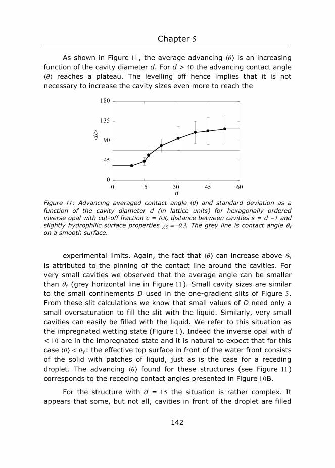
Chapter
142
As shown in Figure , the average advancing ⟨𝜃𝜃⟩ is an increasing function of the cavity diameter d. For d > the advancing contact angle ⟨𝜃𝜃⟩ reaches a plateau. The levelling off hence implies that it is not necessary to increase the cavity sizes even more to reach the
Figure : Advancing averaged contact angle ⟨𝜃𝜃⟩ and standard deviation as a function of the cavity diameter d (in lattice units) for hexagonally ordered inverse opal with cut-off fraction c = , distance between cavities s = d and slightly hydrophilic surface properties S . The grey line is contact angle Y on a smooth surface.
experimental limits. Again, the fact that ⟨𝜃𝜃⟩ can increase above Y is attributed to the pinning of the contact line around the cavities. For very small cavities we observed that the average angle can be smaller than Y (grey horizontal line in Figure ). Small cavity sizes are similar to the small confinements D used in the one-gradient slits of Figure . From these slit calculations we know that small values of D need only a small oversaturation to fill the slit with the liquid. Similarly, very small cavities can easily be filled with the liquid. We refer to this situation as the impregnated wetting state (Figure ). Indeed the inverse opal with d < are in the impregnated state and it is natural to expect that for this case ⟨𝜃𝜃⟩ < 𝜃𝜃Y: the effective top surface in front of the water front consists of the solid with patches of liquid, just as is the case for a receding droplet. The advancing ⟨𝜃𝜃⟩ found for these structures (see Figure ) corresponds to the receding contact angles presented in Figure B.
For the structure with d = the situation is rather complex. It appears that some, but not all, cavities in front of the droplet are filled
d
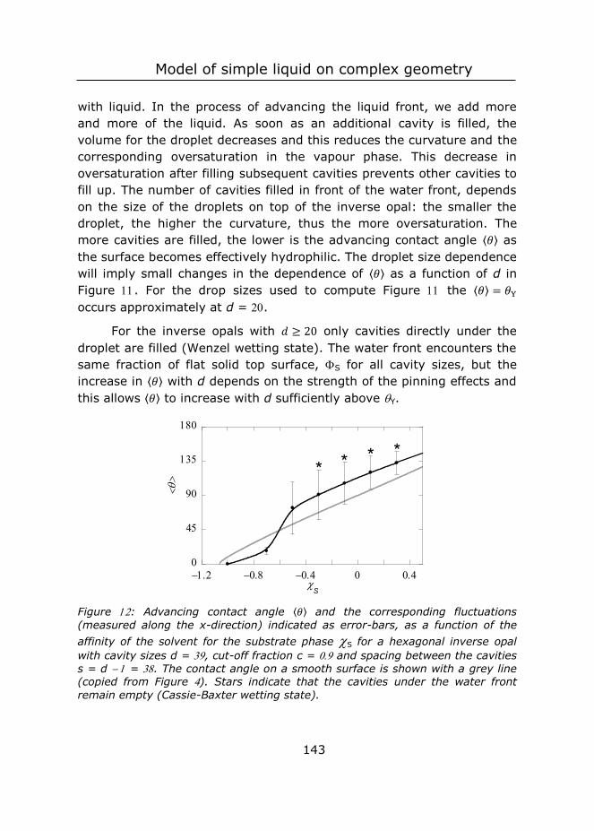
Model of simple liquid on complex geometry
143
with liquid. In the process of advancing the liquid front, we add more and more of the liquid. As soon as an additional cavity is filled, the volume for the droplet decreases and this reduces the curvature and the corresponding oversaturation in the vapour phase. This decrease in oversaturation after filling subsequent cavities prevents other cavities to fill up. The number of cavities filled in front of the water front, depends on the size of the droplets on top of the inverse opal: the smaller the droplet, the higher the curvature, thus the more oversaturation. The more cavities are filled, the lower is the advancing contact angle ⟨𝜃𝜃⟩ as the surface becomes effectively hydrophilic. The droplet size dependence will imply small changes in the dependence of ⟨𝜃𝜃⟩ as a function of d in Figure . For the drop sizes used to compute Figure the ⟨𝜃𝜃⟩ = 𝜃𝜃Y occurs approximately at d = .
For the inverse opals with 𝑑𝑑 ≥ 20 only cavities directly under the droplet are filled (Wenzel wetting state). The water front encounters the same fraction of flat solid top surface, S for all cavity sizes, but the increase in ⟨𝜃𝜃⟩ with d depends on the strength of the pinning effects and this allows ⟨𝜃𝜃⟩ to increase with d sufficiently above Y.
Figure : Advancing contact angle ⟨𝜃𝜃⟩ and the corresponding fluctuations (measured along the x-direction) indicated as error-bars, as a function of the affinity of the solvent for the substrate phase S for a hexagonal inverse opal with cavity sizes d = , cut-off fraction c = and spacing between the cavities s = d = . The contact angle on a smooth surface is shown with a grey line (copied from Figure ). Stars indicate that the cavities under the water front remain empty (Cassie-Baxter wetting state).
S
* * * *
Chapter
144
5.4.6 Effect of the S/L interaction parameter S
Let us next focus on the interaction of the liquid with the substrate via the S/L interaction parameter S. The more negative this parameter
the more hydrophilic (solvophilic) the surface is. When the S is positive we may refer to the surface as hydrophobic (solvophobic). We select for this study hexagonal ordered inverse opals with a cavity size d = . As shown in Figure such cavity sizes give wetting features in the plateau region where the size dependence was essentially lost. We consider here the case that the cut-off fraction c = This c-value is chosen to mimic the inverse opal in ref . The distance between the cavities was set to s = d as before: the cavities are connected to each other by small openings.
In Figure the grey curve represents the contact angle Y on the smooth surface as a function of S and this result is reproduced from Figure for ease of comparison. The average advancing contact angle ⟨𝜃𝜃⟩ follows the dependence Y: the advancing contact angle increases with decreasing hydrophilicity (solvophilicity) of the substrate. However, for S > the advancing contact angle is systematically above Y,
whereas it is systematically below Y when S <
The wetting transition, that is the point for which becomes 0, occurs at a S which is slightly less hydrophilic for the inverse opal as for the smooth surface. In the low contact angle cases all cavities under the droplets are filled (impregnating wetting state). The filled cavities render the surface slightly more hydrophilic than the smooth surface (see Equation ) and this caused the early wetting transition for the inverse opal as compared to the smooth surface.
The inverse opal remains in the impregnating wetting state for small but finite contact angles S = . In these cases the advancing contact angle is lower than the corresponding Y. The wetting switches to the Wenzel state by increasing the hydrophilicity further to S = . Now the advancing contact angle is larger than the Y. Eventually the wetting switches to a Cassie-Baxter wetting state for higher values of S. These cases are labelled by the asterisk in Figure . Again the
Model of simple liquid on complex geometry
145
advancing contact angle is larger than Y, and the difference ⟨𝜃𝜃⟩ − 𝜃𝜃Y is roughly constant, that is, it does not depend whether there is the Wenzel or the Cassie-Baxter state. This result suggests that for the advancing angle, it does not matter whether air is entrapped underneath
(observed for S ≥ ) the droplet or not (observed for S ≤ ). This implies that the increase in observed ⟨𝜃𝜃⟩ compared to Y cannot be explained in terms of wetting state. Rather, pinning of the contact line and the de-pinning transition should be considered. The immobilization of the contact line on the kinks in the surface (as explained in Figure ) on this hexagonally packed inverse opal induces the contact line to curve and extend (Δy > ), which is energetically unfavourable. The contact line is even further extended after a de-pinning transition (increase in Δy), indicating that in the stress perpendicular to the surface has increased. However, ⟨𝜃𝜃⟩ decreased locally to values close to on a smooth surface, showing that stress in the vertical direction is released after the transition. The average ⟨𝜃𝜃⟩ is still higher than Y surface directly after the de-pinning transition. This is caused by the build-up of stress at the other cavity (we consider two rows of cavities).
The interplay between curvature perpendicular to the surface (here discussed in terms of ⟨𝜃𝜃⟩) and parallel to the surface (here discussed in terms of Δy of the contact line) results in an overall high ⟨𝜃𝜃⟩. Whether the cavity under the moving water front fills with liquid or remains filled with air, depends on the S: air is entrapped for more hydrophobic materials, but the cavities fill for a more hydrophilic material.
The pinned water front on a surface with higher S can withstand higher ⟨𝜃𝜃⟩ before stress starts to build up and the de-pinning transition occurs.
5.4.7 Effect of cut-off height c at constant spacing s
Experimentally one can control the inverse opal structure by the cut-off height h, or equivalently to the cut-off fraction c. It is of interest to consider the effect of the cut-off height from a computation point of view. We can study this for a fixed spacing s between the cavities (in this paragraph) or with a fixed fraction of solid in the top of the substrate S (next paragraph). In both cases we choose slightly
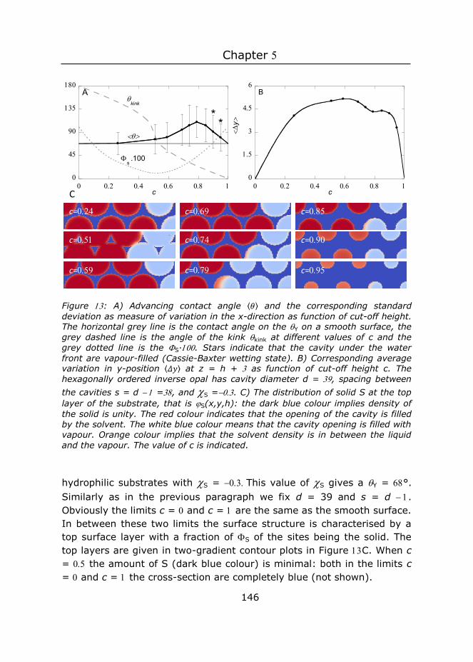
Chapter
146
Figure : A) Advancing contact angle ⟨𝜃𝜃⟩ and the corresponding standard deviation as measure of variation in the x-direction as function of cut-off height. The horizontal grey line is the contact angle on the Y on a smooth surface, the grey dashed line is the angle of the kink kink at different values of c and the grey dotted line is the S∙. Stars indicate that the cavity under the water front are vapour-filled (Cassie-Baxter wetting state). B) Corresponding average variation in y-position ⟨𝛥𝛥𝛥𝛥⟩ at z = h + as function of cut-off height c. The hexagonally ordered inverse opal has cavity diameter d = , spacing between the cavities s = d =, and S =. C) The distribution of solid S at the top layer of the substrate, that is S(x,y,h): the dark blue colour implies density of the solid is unity. The red colour indicates that the opening of the cavity is filled by the solvent. The white blue colour means that the cavity opening is filled with vapour. Orange colour implies that the solvent density is in between the liquid and the vapour. The value of c is indicated.
hydrophilic substrates with S = This value of S gives a Y = °. Similarly as in the previous paragraph we fix d = 39 and s = d . Obviously the limits c = and c = are the same as the smooth surface. In between these two limits the surface structure is characterised by a top surface layer with a fraction of S of the sites being the solid. The top layers are given in two-gradient contour plots in Figure C. When c = the amount of S (dark blue colour) is minimal: both in the limits c = and c = the cross-section are completely blue (not shown).
c=
c=
c=
c=
c=
c=
c=
c=
c=
C
c
**
A
kink
s .100
c
y
B
Model of simple liquid on complex geometry
147
Correspondingly, the contact line fluctuations, as monitored by y, are averaged over ten ‘snapshots’ while increasing the drop volume. The result is given by ⟨Δ𝑦𝑦⟩. In both limits c = and c = the surface is ideally smooth and the three-phase contact line will not fluctuate in the x-direction. In between these limits ⟨Δ𝑦𝑦⟩ > 0 because the contact line becomes pinned.
The advancing contact angle ⟨𝜃𝜃⟩ together with the standard deviation of this angle (measured in the x-direction) is presented in Figure A as a function of the parameter c = h/d. The corresponding fluctuations of the three-phase contact line ⟨Δ𝑦𝑦⟩ (measured in the x-direction at a height z = h + ) are given in Figure B.
Inspection of Figure A shows that by far the most interesting region is for < c < . For c < the average advancing contact ⟨𝜃𝜃⟩ hardly differs from Y. However, in small values of the cut-off fraction the contact line is already significantly curved (Figure B) and the surface structure alters the (x) locally to hydrophobic values > °. The average ⟨𝜃𝜃⟩ for < c < is higher than Y on a smooth surface, though locally, the (x) may be smaller; the variation in along the x-direction (depicted as vertical line) extends to values < ° for most values of c. A maximum in ⟨𝜃𝜃⟩ is found at c ~ , with ⟨𝜃𝜃⟩ = °. A local minimum in Δy at this c is found, which likely is coupled to the need to keep the overall curvature in the drop constant.
Two parameters of the surface structure that are important for contact line pinning are changed when c is varied: the fraction flat solid top surface S, which is the fraction of flat solid at the top of the surface (dark blue in Figure C) and the angle of the kink, kink (see SI for calculation of kink and SI and Equation for calculation of S). Both S∙ and kink are plotted in Figure A. The S∙equals 100 in both limits of c and has a minimum at c = . kink is o at c = , and decreases to at c = . The latter parameter is considered important for hydrophilic materials to obtain hydrophobic contact angles: it has been suggested that only for Y <kink pinning can occur, and a barrier for the water front to enter the cavities is obtained, resulting in air entrapment and hence the possibility of obtaining higher contact angles . However, in our case, kink is smaller than Y for most values of c, and no jump in
Chapter
148
⟨𝜃𝜃⟩ is observed between c = (kink >Y) and c = (kink < Y), and no air entrapment is found for < c < .
For c = , the kink is too large for pinning to occur according to the argument presented Figure . However, an advancing water front is immobilized at the front of a cavity, and moves in one step to a position in front of the next cavity. Hence, despite of the small kink in our calculations a true de-pinning transition is found.
In our case the pinning of the contact line is due to the complex D-structure of the surface: the cavities are placed close to each other, and the contact line thus encounters multiple cavities on a short distance. If the water front would not have been pinned at the front of a cavity, but rather partly fill the cavity, this result in more L-S interface and a longer contact line. This is apparently energetically more unfavourable than pinning the contact line in front of a cavity. Hence, the contact line pinning is governed by the D- structure, and not by the simple D-argument presented in Figure .
When looking at the top surface (Figure C) for c = , we see that some cavities on the left are filled (red), while the last cavities are not filled (light blue). The last upper cavity is just in front of the contact line. Some liquid (red colour) is present at this value of z. Moreover, the situation for c = , which has a similar top surface but a different kink, is comparable.
For c close to , the substrate is not a continuous structure, but consists of discrete triangular ‘pillars’ (see Figure C). Contact line pinning also occurs for discrete shapes.19, 45 Assuming that pinning is mainly found on the top surface in line with observations for c = , the length over which pinning can take place is limited. However, also in this case a de-pinning transition is observed for an advancing water front. Hence the pinning is not limited to the flat part of the top surface (the dark blue surfaces in Figure C) for all values of c, but pinning occurs over the D structure.
Decreasing or increasing c from c = results in a continuous top layer. The contact line can hereby be pinned on the front of every cavity. For higher values of S, the contact line is expected to be exclusively located on the top surface (and thus at constant z). Higher
Model of simple liquid on complex geometry
149
values of S (thus smaller cavities) also result in a surface that is more similar to a smooth surface.
In Figure C, the liquid-filled cavities are shown in red, whereas vapour-filled cavities are light blue. This is observed for all c up to c = . However, for c = andc = , we observe a colour in between red and white blue for cavities under the droplet (left hand side). This suggests that at that height, neither a liquid, nor a vapour phase is present, and thus that the interface is located at that value of z.
5.4.8 Effect of cut-off height c at constant S
One may argue that the true effect of the cut-off height is seen for cases where h (or equivalently c) is varied at a fixed amount of S in the top layer of the substrate, that is for fixed value of S. To do so, one has to vary the inter-cavity spacing s simultaneously when the cut-off height is changed. Note that the true limits c = and c = are hard to reach with fixed S as it requires odd distances between the cavities.
The dependence of the advancing contact angle as well as the contact line fluctuations are recorded for this scenario in Figure . Here we have chosen for a S = which is the value of S which corresponds to c = (near the maximum) of Figure . Note that all the top surfaces used in Figure are similar to the result shown in Figure C for c = .
It is natural to compare results between Figures and . For values of c < , the average contact angles differ very little. In Figure the average angle appears slightly larger. There is a dramatic difference between the cases of Figure and Compare, for example, the top surface for c = . While in the case of fixed distance between the cavities s there are individual posts with S ~ (Figure C), there is a continuous solid phase in Figure as S = . Nevertheless, the average contact angles were hardly affected.
At c > , ⟨𝜃𝜃⟩ at constant S (Figure ) keeps growing with increase in c, while with fixed s the contact angles decreased again. The decrease in ⟨𝜃𝜃⟩ for c > in the constant s case (Figure ) can thus be attributed to the top surface: higher c results in smaller cavities and thus in a surface that is more similar to a smooth surface. The increase
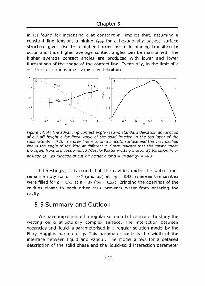
Chapter
150
in ⟨𝜃𝜃⟩ found for increasing c at constant S implies that, assuming a constant line tension, a higher kink for a hexagonally packed surface structure gives rise to a higher barrier for a de-pinning transition to occur and thus higher average contact angles can be maintained. The higher average contact angles are produced with lower and lower fluctuations of the shape of the contact line. Eventually, in the limit of c = the fluctuations must vanish by definition.
Figure : A) The advancing contact angle ⟨𝜃𝜃⟩ and standard deviation as function of cut-off height c for fixed value of the solid fraction in the top-layer of the substrate S = . The grey line is Y on a smooth surface and the grey dashed line is the angle of the kink at different c. Stars indicate that the cavity under the liquid front are vapour-filled (Cassie-Baxter wetting state). B) Variation in y-position ⟨𝛥𝛥𝛥𝛥⟩ as function of cut-off height c for d = and S = .
Interestingly, it is found that the cavities under the water front remain empty for c = (and up) at S = , whereas the cavities were filled for c = at s = (S = ). Bringing the openings of the cavities closer to each other thus prevents water from entering the cavity.
5.5 Summary and Outlook
We have implemented a regular solution lattice model to study the wetting on a structurally complex surface. The interaction between vacancies and liquid is parameterised in a regular solution model by the Flory Huggins parameter . This parameter controls the width of the interface between liquid and vapour. The model allows for a detailed description of the solid phase and the liquid-solid interaction parameter
c
A
* * *
kink
c
y
B
Model of simple liquid on complex geometry
151
S is the only parameter to control the hydrophilic/hydrophobic (solphophilic/solvophobic) character of the substrate. We find very complex and interesting wetting states when this model is applied to hexagonally ordered cavities in an inverse opal. It is found that the three-phase contact line is curved and becomes pinned at the cavity openings. Under the droplet the cavities can either be filled with water (impregnated; Wenzel) or filled with the vapour (Cassie-Baxter). No discontinuity in the contact angle is observed for water fronts that are either in the Wenzel state or Cassie-Baxter state, implying that the water front shape is not influenced by air entrapment under the water front, but is rather determined by the surface encountered by the contact line. The pinning of the contact line cannot solely be discussed in terms of the kink that a surface structure makes with respect to the top surface, kink: also for kink > Y, de-pinning transitions are found, and the spacing between the cavities influence whether a cavity under a water front is solvent-filled or vapour-filled. Hence, the full D-structure, rather than one parameter (kink) should be taken into account. We found a large difference between advancing and receding contact angles, which are also attributed to pinning of the three-phase contact line. More specifically, it was found that while the smooth surface has a contact angle much lower than ° the advancing contact angles in the inverse opal can be much larger than °. That is, slightly hydrophilic substrates can give hydrophobic contact angles.
Our method can readily be extended to mimic more closely experimental conditions. An interesting case is the wetting of an inverse opal of polypyrrole.10 The inverse opal of polypyrrole did not have a smooth top surface. Rather, the top surface showed a positive slope radiating from the position of the sacrificial particle. This more complex surface structure can be implemented easily by a more elaborated way to represent the substrate. Furthermore, polypyrrole is a hydrophilic material. The Y on a polypyrrole surface was measured to be ~°. However, the inverse opal was made using sacrificial polystyrene particles. The particles were removed by dissolving them. This removal was expected to be incomplete, and the contact angle changed to ~° for the polypyrrole surface. Polystyrene chains thus must have remained, e.g. in an adsorbed state onto the polypyrrole surface. These adsorbed polymers have a different hydrophilicity, but also changes the
Chapter
152
local roughness of the surface structures, resulting in both chemical and structural heterogeneities. These heterogeneities on molecular scale can be studied using the approach presented in this paper when the Scheutjens-Fleer machinery is more fully implemented. For example, we can easily consider polymer chains pinned at random locations along the surface of the inverse opal. It is even possible to consider polymer brushes on such substrates which may e.g. preferentially change wetting characteristics of the top surface or the insides of the cavities.46 Such decorated substrates may feature dramatic hysteresis effects in the contact angle, because the polymers can stabilize the three-phase contact line while the shape of the cavities induces pinning of the contact line. Hence polymers may introduce a second length scale in inverse opal surface structures.
In the current work we have solved the regular solution model using the self-consistent field machinery. There are low memory routes to find the SCF solution (see Appendix). This implies that the memory needed to find an SCF solution is linearly proportional to the volume, that is, the number of lattice sites in the system (𝑀𝑀𝑥𝑥, 𝑀𝑀𝑦𝑦, 𝑀𝑀𝑧𝑧). Also the CPU time scales only linearly with the volume. Here we focused on very small systems and used a desktop PC and found accurate results in a few minutes CPU time. Alternatively, the complete set of equations can be solved on a GPU and using CUDA technology the results may be generated to times faster.47 As a result systems which are times larger in each direction should still be feasible, while keeping the wall-time for the computations less than an hour. In this case the regular solution model captures the macroscopically relevant sizes and we do not need to rely on extrapolations.
5.6 Conclusions
Regular solution theory is used to study the wetting behaviour of a simplistic molecular model on a complex inverse opal surface topology. The model features molecular input parameters and gives interfacial energies, contact angles and three-phase contact line shapes. As a result, advancing as well as receding wetting front scenarios were considered. It was found that there is a large contact angle hysteresis in these systems, which was attributed to contact line pinning. We have seen that the cavities can be filled by the liquid or remain dry, that is

Model of simple liquid on complex geometry
153
filled by vapour. Cavities in front of the droplet may be filled by a capillary condensation effect, while receding contact angles typically do not empty the liquid filled cavities. Interestingly, when the substrate is slightly hydrophilic it is possible that advancing contact angles have contact angles larger than 90°. As calculation times are modest, it is possible, when detailed experimental evidence become available, to account for more complex molecular features on the inverse opal structures. For example we can envision a polymer brush as a means to modify either the top surface or the inside of the cavities to control the wetting characteristics to make truly responsive surfaces.
References 1. Cheng, Y.-T.; Rodak, D. E., Is the lotus leaf superhydrophobic? Applied physics letters 2005, 86 (14), 144101. 2. Guo, C.; Feng, L.; Zhai, J.; Wang, G.; Song, Y.; Jiang, L.; Zhu, D., Large-Area Fabrication of a Nanostructure-Induced Hydrophobic Surface from a Hydrophilic Polymer. ChemPhysChem 2004, 5 (5), 750-753. 3. Abdelsalam, M. E.; Bartlett, P. N.; Kelf, T.; Baumberg, J., Wetting of regularly structured gold surfaces. Langmuir 2005, 21 (5), 1753-1757. 4. Zhu, M.; Zuo, W.; Yu, H.; Yang, W.; Chen, Y., Superhydrophobic surface directly created by electrospinning based on hydrophilic material. Journal of materials science 2006, 41 (12), 3793-3797. 5. Cao, L.; Hu, H.-H.; Gao, D., Design and fabrication of micro-textures for inducing a superhydrophobic behavior on hydrophilic materials. Langmuir 2007, 23 (8), 4310-4314. 6. Ma, Y.; Cao, X.; Feng, X.; Ma, Y.; Zou, H., Fabrication of super-hydrophobic film from PMMA with intrinsic water contact angle below 90. Polymer 2007, 48 (26), 7455-7460. 7. Feng, L.; Song, Y.; Zhai, J.; Liu, B.; Xu, J.; Jiang, L.; Zhu, D., Creation of a superhydrophobic surface from an amphiphilic polymer. Angewandte Chemie 2003, 115 (7), 824-826. 8. Hosono, E.; Fujihara, S.; Honma, I.; Zhou, H., Superhydrophobic perpendicular nanopin film by the bottom-up process. Journal of the American Chemical Society 2005, 127 (39), 13458-13459. 9. Karlsson, M.; Forsberg, P.; Nikolajeff, F., From Hydrophilic to Superhydrophobic: Fabrication of Micrometer-Sized Nail-Head-Shaped Pillars in Diamond. Langmuir 2010, 26 (2), 889-893. 10. Akerboom, P., Turak, Kamperman, Controlled fabrication of polypyrrole surfaces with overhang structures by colloidal templating. 2015. 11. Wenzel, R. N., Resistance of solid surfaces to wetting by water. Industrial & Engineering Chemistry 1936, 28 (8), 988-994.

Chapter
154
12. Liu, J.-L.; Feng, X.-Q.; Wang, G.; Yu, S.-W., Mechanisms of superhydrophobicity on hydrophilic substrates. Journal of Physics: Condensed Matter 2007, 19 (35), 356002. 13. Marmur, A., From hygrophilic to superhygrophobic: theoretical conditions for making high-contact-angle surfaces from low-contact-angle materials. Langmuir 2008, 24 (14), 7573-7579. 14. Choi, H.-J.; Choo, S.; Shin, J.-H.; Kim, K.-I.; Lee, H., Fabrication of Superhydrophobic and Oleophobic Surfaces with Overhang Structure by Reverse Nanoimprint Lithography. The Journal of Physical Chemistry C 2013, 117 (46), 24354-24359. 15. Bormashenko, E.; Bormashenko, Y.; Whyman, G.; Pogreb, R.; Stanevsky, O., Micrometrically scaled textured metallic hydrophobic interfaces validate the Cassie–Baxter wetting hypothesis. Journal of colloid and interface science 2006, 302 (1), 308-311. 16. Cassie, A.; Baxter, S., Wettability of porous surfaces. Transactions of the Faraday Society 1944, 40, 546-551. 17. Herminghaus, S.; Brinkmann, M.; Seemann, R., Wetting and dewetting of complex surface geometries. Annu. Rev. Mater. Res. 2008, 38, 101-121. 18. Papadopoulos, P.; Deng, X.; Mammen, L.; Drotlef, D.-M.; Battagliarin, G.; Li, C.; Mu ̈llen, K.; Landfester, K.; del Campo, A.; Butt, H.-J. r., Wetting on the microscale: shape of a liquid drop on a microstructured surface at different length scales. Langmuir 2012, 28 (22), 8392-8398. 19. Forsberg, P. S. H.; Priest, C.; Brinkmann, M.; Sedev, R.; Ralston, J., Contact Line Pinning on Microstructured Surfaces for Liquids in the Wenzel State. Langmuir 2010, 26 (2), 860-865. 20. Tuteja, A.; Choi, W.; Ma, M.; Mabry, J. M.; Mazzella, S. A.; Rutledge, G. C.; McKinley, G. H.; Cohen, R. E., Designing superoleophobic surfaces. Science 2007, 318 (5856), 1618-1622. 21. Hensel, R.; Helbig, R.; Aland, S.; Braun, H.-G.; Voigt, A.; Neinhuis, C.; Werner, C., Wetting resistance at its topographical limit: the benefit of mushroom and serif T structures. Langmuir 2013, 29 (4), 1100-1112. 22. Savoy, E. S.; Escobedo, F. A., Simulation study of free-energy barriers in the wetting transition of an oily fluid on a rough surface with reentrant geometry. Langmuir 2012, 28 (46), 16080-16090. 23. Mugele, F.; Becker, T.; Nikopoulos, R.; Kohonen, M.; Herminghaus, S., Capillarity at the nanoscale: an AFM view. Journal of Adhesion Science and Technology 2002, 16 (7), 951-964. 24. Wu, J.; Zhang, M.; Wang, X.; Li, S.; Wen, W., A Simple Approach for Local Contact Angle Determination on a Heterogeneous Surface. Langmuir 2011, 27 (10), 5705-5708. 25. de Gennes, P. G., Wetting: statics and dynamics. Rev. Mod. Phys. 1985, 57 (3), 827-863. 26. Chamakos, N. T.; Kavousanakis, M. E.; Papathanasiou, A. G., Enabling efficient energy barrier computations of wetting transitions on geometrically patterned surfaces. Soft Matter 2013, 9 (40), 9624-9632. 27. Patankar, N. A., Hydrophobicity of Surfaces with Cavities: Making Hydrophobic Substrates from Hydrophilic Materials? Journal of Adhesion Science and Technology 2009, 23 (3), 413-433.
Model of simple liquid on complex geometry
155
28. Pashos, G.; Kokkoris, G.; Boudouvis, A. G., A modified phase-field method for the investigation of wetting transitions of droplets on patterned surfaces. Journal of Computational Physics 2015, 283 (0), 258-270. 29. Park, J.-Y.; Ha, M.-Y.; Choi, H.-J.; Hong, S.-D.; Yoon, H.-S., A study on the contact angles of a water droplet on smooth and rough solid surfaces. Journal of Mechanical Science and Technology 2011, 25 (2), 323-332. 30. Kumar, V.; Sridhar, S.; Errington, J. R., Monte Carlo simulation strategies for computing the wetting properties of fluids at geometrically rough surfaces. The Journal of chemical physics 2011, 135 (18), 184702. 31. Zhang, Z.; Kim, H.; Ha, M. Y.; Jang, J., Molecular dynamics study on the wettability of a hydrophobic surface textured with nanoscale pillars. Physical Chemistry Chemical Physics 2014, 16 (12), 5613-5621. 32. Dupuis, A.; Yeomans, J. M., Modeling Droplets on Superhydrophobic Surfaces: Equilibrium States and Transitions. Langmuir 2005, 21 (6), 2624-2629. 33. Pooley, C. M.; Kusumaatmaja, H.; Yeomans, J. M., Contact line dynamics in binary lattice Boltzmann simulations. Phys. Rev. E 2008, 78 (5), 056709. 34. Vrancken, R. J.; Kusumaatmaja, H.; Hermans, K.; Prenen, A. M.; Pierre-Louis, O.; Bastiaansen, C. W. M.; Broer, D. J., Fully Reversible Transition from Wenzel to Cassie−Baxter States on Corrugated Superhydrophobic Surfaces. Langmuir 2010, 26 (5), 3335-3341. 35. Kavousanakis, M. E.; Colosqui, C. E.; Kevrekidis, I. G.; Papathanasiou, A. G., Mechanisms of wetting transitions on patterned surfaces: Continuum and mesoscopic analysis. Soft Matter 2012, 8 (30), 7928-7936. 36. Blow, M.; Kusumaatmaja, H.; Yeomans, J., Imbibition through an array of triangular posts. Journal of Physics: Condensed Matter 2009, 21 (46), 464125. 37. De Coninck, J.; Blake, T., Wetting and molecular dynamics simulations of simple liquids. Annu. Rev. Mater. Res. 2008, 38, 1-22. 38. Van der Waals, J. D.; van der Waals, J. D., Over de Continuiteit van den Gas-en Vloeistoftoestand. AW Sijthoff: 1873. 39. Safran, S. A., Statistical thermodynamics of surfaces, interfaces, and membranes. Addison-Wesley Publishing Company: 1994; Vol. 90. 40. Stiopkin, I. V.; Weeraman, C.; Pieniazek, P. A.; Shalhout, F. Y.; Skinner, J. L.; Benderskii, A. V., Hydrogen bonding at the water surface revealed by isotopic dilution spectroscopy. 2011, 474 (7350), 192-195. 41. Lee, Y. J.; Braun, P. V., Tunable inverse opal hydrogel pH sensors. Advanced Materials 2003, 15 (7‐8), 563-566. 42. Li, H.; Vienneau, G.; Jones, M.; Subramanian, B.; Robichaud, J.; Djaoued, Y., Crack-free 2D-inverse opal anatase TiO 2 films on rigid and flexible transparent conducting substrates: low temperature large area fabrication and electrochromic properties. Journal of Materials Chemistry C 2014, 2 (37), 7804-7810. 43. Couturier, J. P.; Sütterlin, M.; Laschewsky, A.; Hettrich, C.; Wischerhoff, E., Responsive Inverse Opal Hydrogels for the Sensing of Macromolecules. Angewandte Chemie International Edition 2015.
Chapter
156
44. Bormashenko, E., Why does the Cassie–Baxter equation apply? Colloids and Surfaces A: Physicochemical and Engineering Aspects 2008, 324 (1), 47-50. 45. Gao, L.; McCarthy, T. J., The “Lotus Effect” Explained: Two Reasons Why Two Length Scales of Topography Are Important. Langmuir 2006, 22 (7), 2966-2967. 46. de Vos, W. M.; Leermakers, F. A., Modeling the structure of a polydisperse polymer brush. Polymer 2009, 50 (1), 305-316. 47. Harish, P.; Narayanan, P., Accelerating large graph algorithms on the GPU using CUDA. In High performance computing–HiPC 2007, Springer: 2007, pp 197-208.
Model of simple liquid on complex geometry
157
Appendix. Simple method to solve the regular
solution equations efficiently.
Here we consider the SCF route to optimise the regular solution free energy. We take the simplest one-gradient case without surfaces as an example and trust that the reader can generalise the protocol to include surfaces and to account for more than one dimension. The starting point is Eqn 6:
𝐹𝐹 = ∑ 𝜑𝜑(𝑧𝑧) ln 𝜑𝜑(𝑧𝑧) + 𝜑𝜑V(𝑧𝑧) ln 𝜑𝜑𝑉𝑉(𝑧𝑧) + 𝜒𝜒 𝜑𝜑(𝑧𝑧)⟨𝜑𝜑V(𝑧𝑧)⟩𝑀𝑀−𝑀𝑀 ()
where we notice that the free energy is a functional of the volume fraction distribution of the liquid and the vapour. We also recall that for each coordinate z we have a compressibility relation
𝜑𝜑(𝑧𝑧) + 𝜑𝜑V(𝑧𝑧) = 1 (A)
In the self-consistent field SCF theory the same free energy is expressed in terms of segment densities as well as segment potentials u(z) and uV(z). We take it that these potentials are dimensionless, that is they are already normalised by the thermal energy 𝑘𝑘B𝑇𝑇. The potentials are going to be used in Boltzmann equations:
𝐺𝐺(𝑧𝑧) = exp −𝑢𝑢(𝑧𝑧)𝐺𝐺V(𝑧𝑧) = exp −𝑢𝑢V(𝑧𝑧) (A)
In the self-consistent field theory the starting point of the approach is the mean-field free energy:
𝐹𝐹 =
− ln 𝑞𝑞𝑁𝑁
𝑁𝑁!𝑞𝑞V
𝑁𝑁 V
𝑁𝑁! − ∑ (𝑢𝑢(𝑧𝑧)𝜑𝜑(𝑧𝑧) + 𝑢𝑢V(𝑧𝑧)𝜑𝜑V(𝑧𝑧) )𝑀𝑀𝑧𝑧=1 + ∑ 𝜑𝜑(𝑧𝑧)𝜒𝜒⟨𝜑𝜑V(𝑧𝑧)⟩𝑀𝑀
𝑧𝑧=1 +∑ 𝛼𝛼(𝑧𝑧)[𝜑𝜑(𝑧𝑧) + 𝜑𝜑V(𝑧𝑧) − 1]𝑀𝑀
𝑧𝑧=1 (A)
It is relatively easy to show that Eqns A and A are the same (we will not prove this here). For this we need to know that the single molecule partition functions q are found by the summation over corresponding Boltzmann weights:
𝑞𝑞 = ∑ 𝐺𝐺(𝑧𝑧)𝑀𝑀𝑧𝑧=1
𝑞𝑞V = ∑ 𝐺𝐺V(𝑧𝑧)𝑀𝑀𝑧𝑧=1
(A)
Chapter
158
and the number of liquid and vapour sites is given by
𝑁𝑁 = ∑ 𝜑𝜑(𝑧𝑧)𝑀𝑀𝑧𝑧=1
𝑁𝑁V = ∑ 𝜑𝜑V(𝑧𝑧)𝑀𝑀𝑧𝑧=1
(A)
The optimisation of the Free energy A with respect to the segment potentials lead the rule how to compute the volume fractions:
𝜑𝜑(𝑧𝑧) = 𝑁𝑁
𝑞𝑞 𝐺𝐺(𝑧𝑧)
𝜑𝜑V(𝑧𝑧) =𝑁𝑁V𝑞𝑞V𝐺𝐺V(𝑧𝑧)
(A)
Optimisation of the free energy A with respect to the segment density leads to the rule to compute the segment potential:
𝑢𝑢(𝑧𝑧) = 𝛼𝛼(𝑧𝑧) + 𝐸𝐸(𝑧𝑧)𝑢𝑢V(𝑧𝑧) = 𝛼𝛼(𝑧𝑧) + 𝐸𝐸V(𝑧𝑧)
(A)
where the interaction contribution to the segment potentials are given by
𝐸𝐸(𝑧𝑧) = 𝜒𝜒⟨𝜑𝜑V(𝑧𝑧)⟩𝐸𝐸V(𝑧𝑧) = 𝜒𝜒⟨𝜑𝜑(𝑧𝑧)⟩
(A)
In summary we thus have the situation that
𝑢𝑢[𝜑𝜑]𝜑𝜑+𝜑𝜑V=1⇔ 𝜑𝜑[𝑢𝑢] (A)
In words the left hand side says that the segment potentials depend on the volume fractions (that is u given by Eqn A depends on E which is given in A to be a function of the ). The right hand side of Eqn A says that the volume fractions A can be computed from the segment potentials, by two routes, namely via the Boltzmann weights Eqn A and the partition functions A which are also traced to A. We need a numerical scheme to find the so-called SCF solution. We need a fixed point for which the segment potentials both follow from the volume fractions from which they are computed. Or inversely, we need the segment densities which determine the potentials on which they depend. Such a fixed point should obey to the compressibility relation of Eqn A.
Self-consistent field solutions must be generated numerically. Once such a solution is found we can compute the thermodynamic quantities. Of more than average interest there is the grand potential
Model of simple liquid on complex geometry
159
(sum of the surface tensions) S of the system. It can be shown that Ω𝑆𝑆 = ∑ 𝜔𝜔(𝑧𝑧)𝑀𝑀
𝑧𝑧=1 , where the grand potential density is given by
𝜔𝜔(𝑧𝑧) = −𝛼𝛼(𝑧𝑧) − 𝜒𝜒(𝜑𝜑(𝑧𝑧)⟨𝜑𝜑V(𝑧𝑧)⟩+𝜑𝜑V(𝑧𝑧)⟨𝜑𝜑(𝑧𝑧)⟩)2 + 𝜒𝜒𝜑𝜑𝑏𝑏𝜑𝜑V
𝑏𝑏 (A)
where the bulk volume fractions are found at large values of z or equivalently follow from
𝜑𝜑𝑏𝑏 = 𝑁𝑁𝑞𝑞
𝜑𝜑V𝑏𝑏 = 𝑁𝑁V
𝑞𝑞V
(A)
Consider the following pseudo code which makes use of a regularisation parameter (Pikar method). The code is safe but slow when this value is very small. When it is large (close to unity), the code is fast but the iterations may diverge. The suggested value will result in a solution in about iterations and then there will be seven significant digits.
Specify the lattice coordinates, e.g. z = ,,⋯,e.g. take M = .
Specify N = NV = 50 (half system filled by liquid other half by vapour; interface halfway system)
Specify the parameter, e.g. =
Set initial guesses:
𝜑𝜑(𝑧𝑧) = 1 for z = , ⋯, and zero otherwise.
𝜑𝜑𝑉𝑉(𝑧𝑧) = 1 − 𝜑𝜑(𝑧𝑧)
𝛼𝛼(𝑧𝑧) = 0
-Compute interactions using Eqn A
it =
error =
= (regularisation parameter)
tolerance =
Loop while error > tolerance, it <
Update it := it +
Store ‘old’ values of interactions: 𝐸𝐸𝑜𝑜(𝑧𝑧) = 𝐸𝐸(𝑧𝑧); 𝐸𝐸V𝑜𝑜(𝑧𝑧) = 𝐸𝐸V(𝑧𝑧)
Chapter
160
Compute potentials Eqn A
Compute Boltzmann weights Eqn A
Compute partition functions Eqn A
Compute volume fractions Eqn A
Compute interactions Eqn A
Update Lagrange field: 𝛼𝛼(𝑧𝑧) ∶= 𝛼𝛼(𝑧𝑧) + 𝛽𝛽(𝜑𝜑(𝑧𝑧) + 𝜑𝜑V(𝑧𝑧) − 1)
Update ‘interactions’: 𝐸𝐸(𝑧𝑧): = 𝛽𝛽(𝐸𝐸(𝑧𝑧)) + (1 − 𝛽𝛽)𝐸𝐸0(𝑧𝑧)
𝐸𝐸V(𝑧𝑧): = 𝛽𝛽(𝐸𝐸V(𝑧𝑧)) + (1 − 𝛽𝛽)𝐸𝐸V0(𝑧𝑧)
Compute error: error = |𝐸𝐸(𝑧𝑧) − 𝐸𝐸𝑜𝑜(𝑧𝑧)|+|𝐸𝐸V(𝑧𝑧) − 𝐸𝐸V𝑜𝑜(𝑧𝑧)|+| 𝜑𝜑(𝑧𝑧) + 𝜑𝜑V(𝑧𝑧) − 1|
Compute grand potential Eqn A and write results.
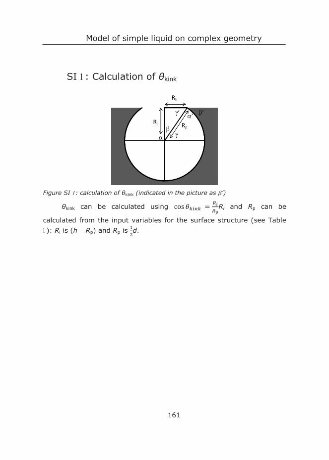
Model of simple liquid on complex geometry
161
SI : Calculation of θkink
Figure SI : calculation of θkink (indicated in the picture as ’)
θkink can be calculated using cos 𝜃𝜃𝑘𝑘𝑘𝑘𝑘𝑘𝑘𝑘 = 𝑅𝑅𝑖𝑖𝑅𝑅𝑝𝑝
Ri and Rp can be
calculated from the input variables for the surface structure (see Table ): Ri is (h Rp) and Rp is
12d.
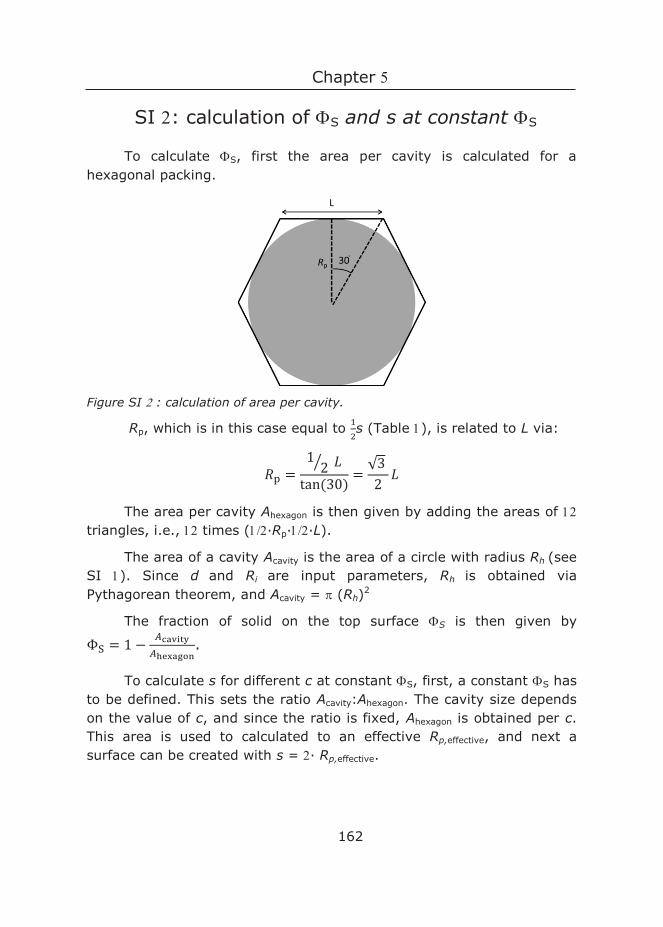
Chapter
162
SI : calculation of S and s at constant S
To calculate S, first the area per cavity is calculated for a hexagonal packing.
Figure SI : calculation of area per cavity.
Rp, which is in this case equal to 12s (Table ), is related to L via:
𝑅𝑅p =1 2 ⁄ 𝐿𝐿
tan (30) = √3 2 𝐿𝐿
The area per cavity Ahexagon is then given by adding the areas of triangles, i.e., times (∙Rp∙∙L).
The area of a cavity Acavity is the area of a circle with radius Rh (see SI ). Since d and Ri are input parameters, Rh is obtained via Pythagorean theorem, and Acavity = (Rh)2
The fraction of solid on the top surface S is then given by
ΦS = 1 − 𝐴𝐴cavity𝐴𝐴hexagon
.
To calculate s for different c at constant S, first, a constant S has to be defined. This sets the ratio Acavity:Ahexagon. The cavity size depends on the value of c, and since the ratio is fixed, Ahexagon is obtained per c. This area is used to calculated to an effective Rp,effective, and next a surface can be created with s = ∙ Rp,effective.

6 General discussion
Chapter
164
We can learn from nature that, next to chemistry, surface structures can be used for tuning different functions of surfaces. In this thesis we presented new approaches that we developed to make bioinspired nanopatterned surfaces. We use these surfaces to study the effect of structuring on two functions namely adhesion and wetting.
In Chapters and , we presented a novel fabrication method using colloidal templating. We described two distinct ways to obtain nanopatterned surfaces, namely (i) addition of PDMS on top of the colloidal monolayer and (ii) synthesis of polypyrrole around the particles of the monolayer, and we have shown the influence of these patterns on adhesion and wetting, respectively. In this chapter, we look back on what we have achieved and we put this in the broader context of research in the same area. We thus discuss some aspects of the fabrication of the nanopatterned surfaces, and the adhesion and wetting thereof.
6.1 Fabrication of nanopatterned surfaces
In this thesis, we chose colloidal templating to make nanopatterned surfaces. The use of colloidal assemblies to create surface patterns is an emerging research area and highly relevant. This is, for example, evidenced by a Feature Article entitled “Colloidal Surface Assemblies: Nanotechnology Meets Bioinspiration”.1 The authors state that:
“Colloidal lithography holds great promise for realization of powerful hierarchical templates in silicon for molding polymers (e.g., PDMS) that is expected to mimic the nanostructure found on Gecko toes.”
and
“Colloidal particles form an interesting basis for bioinspired processes and structures. Artificial particles are sufficiently well understood and robust to employ them in material synthesis. They are easier to observe and analyze than softer objects such as proteins. They are also more familiar to industry. Processes that employ particles are therefore realistic candidates for actual production processes.”
Colloidal templating allows us to fabricate complex, D structures. Our structures have the same dimensions as found in nature, and are
General Discussion
165
repeated over macroscopic length scales.1-2 Furthermore, this method is fast and cost-effective compared to other nanopatterning techniques.
6.1.1 Colloidal monolayer
Obtaining the colloidal monolayer
Highly charged, monodispersed particles are required for colloidal templating, and these were not commercially available. A robust synthesis method has been developed, and monolayers suitable for templating consisting of these particles, with sizes in the range nm < d < m, were readily obtained in a one-step synthesis.3
The fabrication of our nanopatterned materials started with a monolayer of colloids. Colloids are readily trapped at the air/water interface, but care must be taken to spread the particles homogeneously into a monolayer at the interface.4 To ensure monolayer formation, two methods are described in the literature: (i) application of particles at the air/water interface using a glass slide and using an alcohol as spreading agent5-6 and (ii) coating a surface with a sparse layer of (individual) particles, and dip this surface slowly in the water phase under an angle, so that the particles self-assemble at the air/water interface.7 The first method only requires transferring the particles to another solvent, whereas the second method contains multiple steps and is more time consuming. Therefore, the first method has been chosen.
Crystallinity of the monolayer
A high crystallinity is desirable because a crystalline, hexagonal packing is the packing with highest particle density, resulting in regular structures and the possibility to model the surface structures. We investigated two parameters to control crystallinity, namely pH and ionic strength, cs.
A high crystallinity is obtained when repulsion between the particles is combined with an external pressure pushing the particles together. This situation is difficult to achieve experimentally, since certain interactions are intrinsic to (charged) particles at interfaces. DLVO interactions, which include Born repulsion preventing two particles

Chapter
166
from overlapping, attractive Van der Waals interaction and electrostatic repulsion, are always found between two closely-spaced surfaces. Two additional forces that are found for particles at the interface are (i) attractive capillary interaction due to interface deformation, and (ii) repulsive dipole-dipole interactions.8 The first contribution is small in our case, since our particles are also small. The second contribution, however, is important. An assymetric charge distribution arises due to dissocation of the –COOH-groups in water phase, but not in the air. Therefore, the counter-ion distribution is also asymmetrical. This causes a dipole moment perpendicular to the air/water interface for each particle, and because the particles are pinned at the interface, the dipoles cannot align, resulting in repulsion.
To obtain closely packed crystalline monolayers at the air/water interface, a high charge density on the particle surface is needed. A higher charge density results in more repulsion and therefore a higher mobility of the particles. For our particles, which contain –COOH groups on their surface, the number of charges increases with pH. We indeed found an increase in crystallinity with increasing pH. The effect of cs on crystallinity however, has not yet been discussed.
cs is commonly used to control the interaction between charged objects in water. It sets the screening length between two charges: the higher the salt concentration, the shorter the Debye screening length .2 On the other hand, a higher cs enables dissociation of –COOH groups.9 The increase in charges with increasing ionic strength also results in more hydrophilic particles. The overall effect of changing the cs is hence not straightforward. Therefore, the effect of cs on crystallinity has been investigated for both CP and CP-W (Figure ). CP are particles that are transferred to ethanol directly after synthesis, whereas CP-W are washed three times in water before transfer to ethanol. CP-W thus contains less oligomers than CP. The normalized crystallinity is defined as the ratio between particles with six neighbouring particles over the total number of particles.10 This was determined by scooping the monolayers from the air/water interface using a coverslip and imaging them using a brighfield miscroscope.
Figure shows no effect of cs on crystallinity for both CP and CP-W. The trend that seems to be present for CP is mainly caused by the low crystallinity at an cs of M, but this is not conclusive, given the spread
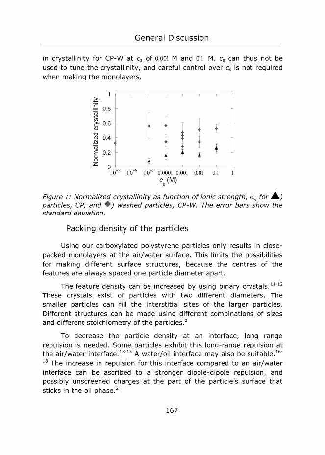
General Discussion
167
in crystallinity for CP-W at cs of M and M. cs can thus not be used to tune the crystallinity, and careful control over cs is not required when making the monolayers.
Figure : Normalized crystallinity as function of ionic strength, cs, for ) particles, CP, and ) washed particles, CP-W. The error bars show the standard deviation.
Packing density of the particles
Using our carboxylated polystyrene particles only results in close-packed monolayers at the air/water surface. This limits the possibilities for making different surface structures, because the centres of the features are always spaced one particle diameter apart.
The feature density can be increased by using binary crystals.11-12 These crystals exist of particles with two different diameters. The smaller particles can fill the interstitial sites of the larger particles. Different structures can be made using different combinations of sizes and different stoichiometry of the particles.2
To decrease the particle density at an interface, long range repulsion is needed. Some particles exhibit this long-range repulsion at the air/water interface.13-15 A water/oil interface may also be suitable.16-
18 The increase in repulsion for this interface compared to an air/water interface can be ascribed to a stronger dipole-dipole repulsion, and possibly unscreened charges at the part of the particle’s surface that sticks in the oil phase.2
0
0.2
0.4
0.6
0.8
1
cs (M)
Nor
mal
ized
cry
stal
linity
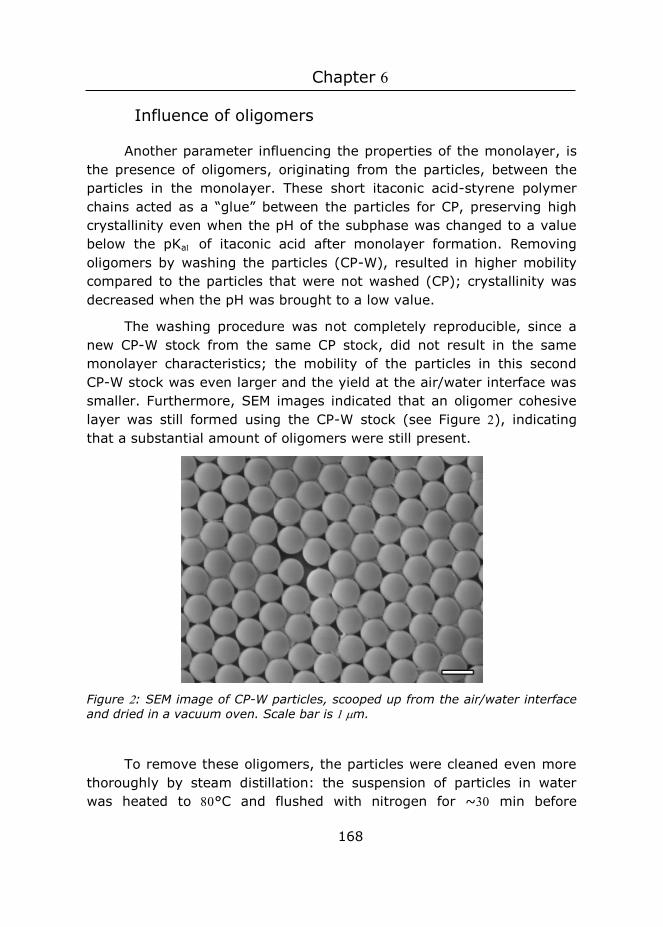
Chapter
168
Influence of oligomers
Another parameter influencing the properties of the monolayer, is the presence of oligomers, originating from the particles, between the particles in the monolayer. These short itaconic acid-styrene polymer chains acted as a “glue” between the particles for CP, preserving high crystallinity even when the pH of the subphase was changed to a value below the pKa of itaconic acid after monolayer formation. Removing oligomers by washing the particles (CP-W), resulted in higher mobility compared to the particles that were not washed (CP); crystallinity was decreased when the pH was brought to a low value.
The washing procedure was not completely reproducible, since a new CP-W stock from the same CP stock, did not result in the same monolayer characteristics; the mobility of the particles in this second CP-W stock was even larger and the yield at the air/water interface was smaller. Furthermore, SEM images indicated that an oligomer cohesive layer was still formed using the CP-W stock (see Figure ), indicating that a substantial amount of oligomers were still present.
Figure : SEM image of CP-W particles, scooped up from the air/water interface and dried in a vacuum oven. Scale bar is m.
To remove these oligomers, the particles were cleaned even more thoroughly by steam distillation: the suspension of particles in water was heated to °C and flushed with nitrogen for ~ min before
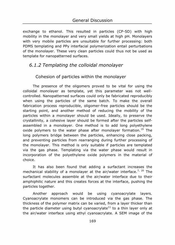
General Discussion
169
exchange to ethanol. This resulted in particles (CP-SD) with high mobility in the monolayer and very small yields at high pH. Monolayers with very mobile particles are unsuitable for further processing: both PDMS templating and PPy interfacial polymerization entail perturbations of the monolayer. These very clean particles could thus not be used as template for nanopatterned surfaces.
6.1.2 Templating the colloidal monolayer
Cohesion of particles within the monolayer
The presence of the oligomers proved to be vital for using the colloidal monolayer as template, yet this parameter was not well-controlled. Nanopatterned surfaces could only be fabricated reproducibly when using the particles of the same batch. To make the overall fabrication process reproducible, oligomer-free particles should be the starting point, and another method of reducing the mobility of the particles within a monolayer should be used. Ideally, to preserve the crystallinity, a cohesive layer should be formed after the particles self-assembled in a monolayer. One method is to add long polyethylene oxide polymers to the water phase after monolayer formation.19 The long polymers bridge between the particles, enhancing close packing, and preventing particles from rearranging during further processing of the monolayer. This method is only suitable if particles are templated via the gas phase. Templating via the water phase would result in incorporation of the polyethylene oxide polymers in the material of choice.
It has also been found that adding a surfactant increases the mechanical stability of a monolayer at the air/water interface.7, 20 The surfactant molecules assemble at the air/water interface due to their amphiphilic nature and this creates forces at the interface, pushing the particles together.
Another approach would be using cyanoacrylate layers. Cyanoacrylate monomers can be introduced via the gas phase. The thickness of the polymer matrix can be varied, from a layer thicker than the particle diameter using butyl cyanoacrylate11 to a thin layer only at the air/water interface using ethyl cyanoacrylate. A SEM image of the
Chapter
170
thin ethyl cyanoacrylate layer, made as described in Chapter , is shown in Figure .
Figure : SEM image of a colloidal monolayer embedded in ethyl cyanoacrylate. The contrast of this image is adjusted. Scale bar is m.
The cyanoacrylate layer can provide enough strength during further processing of the monolayer, and is readily removed by an organic solvent when dissolving the particles.
Gel trapping techniques, in which the liquid phase is turned into a hydrogel after monolayer formation, may also be a promising method to immobilize the particles at the air/water interface. This method has indeed been used to trap particles and replicate them with PDMS.21 However, most of these gelling agents are dissolved at elevated temperatures, and set at room temperature. The particles should therefore be applied at elevated temperatures ( > oC ), which we found to be disruptive for the formation of a close-packed crystalline monolayer.
Double molding
With one monolayer, two different surface structures can be fabricated, by either templating the air phase, or the water phase. However, the material of choice depends on the method of application: for example, PDMS cannot be applied via the water phase, and polypyrrole not via air. This limits the possible structures to be templated by PDMS to dimples and that of polypyrrole to a surface
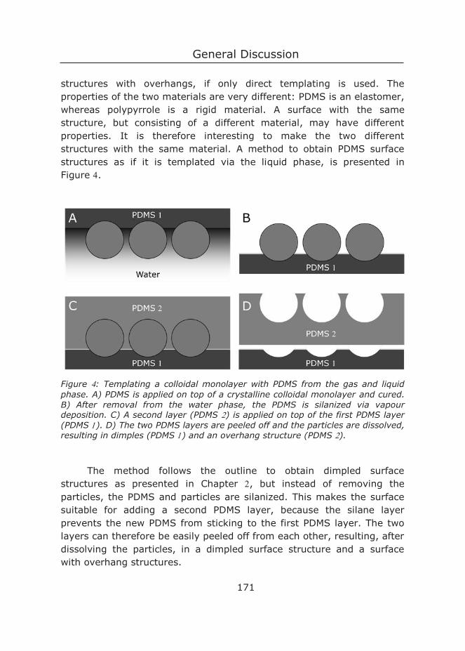
General Discussion
171
structures with overhangs, if only direct templating is used. The properties of the two materials are very different: PDMS is an elastomer, whereas polypyrrole is a rigid material. A surface with the same structure, but consisting of a different material, may have different properties. It is therefore interesting to make the two different structures with the same material. A method to obtain PDMS surface structures as if it is templated via the liquid phase, is presented in Figure .
Figure : Templating a colloidal monolayer with PDMS from the gas and liquid phase. A) PDMS is applied on top of a crystalline colloidal monolayer and cured. B) After removal from the water phase, the PDMS is silanized via vapour deposition. C) A second layer (PDMS ) is applied on top of the first PDMS layer (PDMS ). D) The two PDMS layers are peeled off and the particles are dissolved, resulting in dimples (PDMS ) and an overhang structure (PDMS ).
The method follows the outline to obtain dimpled surface structures as presented in Chapter , but instead of removing the particles, the PDMS and particles are silanized. This makes the surface suitable for adding a second PDMS layer, because the silane layer prevents the new PDMS from sticking to the first PDMS layer. The two layers can therefore be easily peeled off from each other, resulting, after dissolving the particles, in a dimpled surface structure and a surface with overhang structures.
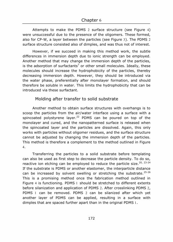
Chapter
172
Attempts to make the PDMS surface structure (see Figure ) were unsuccessful due to the presence of the oligomers. These formed, also for CP-W, a layer between the particles (see Figure ). The PDMS surface structure consisted also of dimples, and was thus not of interest.
However, if we succeed in making this method work, the subtle differences in immersion depth due to ionic strength can be employed. Another method that may change the immersion depth of the particles, is the adsorption of surfactants7 or other small molecules. Ideally, these molecules should increase the hydrophobicity of the particles, thereby decreasing immersion depth. However, they should be introduced via the water phase, preferentially after monolayer formation, and should therefore be soluble in water. This limits the hydrophobicity that can be introduced via these surfactant.
Molding after transfer to solid substrate
Another method to obtain surface structures with overhangs is to scoop the particles from the air/water interface using a surface with a spincoated polystyrene layer.22 PDMS can be poured on top of the monolayer and cured, and the nanopatterned surface is released when the spincoated layer and the particles are dissolved. Again, this only works with particles without oligomer residues, and the surface structure cannot be adjusted by changing the immersion depth of the particles. This method is therefore a complement to the method outlined in Figure .
Transferring the particles to a solid substrate before templating can also be used as first step to decrease the particle density. To do so, reactive ion etching can be employed to reduce the particle size.20, 23-24 If the substrate is PDMS or another elastomer, the interparticle distance can be increased by solvent swelling or stretching the substrate.25-26 This is a promising method once the fabrication method outlined in Figure is functioning. PDMS should be stretched to different extents before silanization and application of PDMS . After crosslinking PDMS , PDMS can be removed. PDMS can be silanized after which yet another layer of PDMS can be applied, resulting in a surface with dimples that are spaced further apart than in the original PDMS .
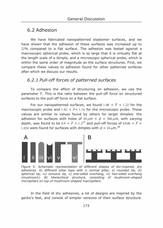
General Discussion
173
6.2 Adhesion
We have fabricated nanopatterned elastomer surfaces, and we have shown that the adhesion of these surfaces was increased up to % compared to a flat surface. The adhesion was tested against a macroscopic spherical probe, which is so large that it is virtually flat at the length scale of a dimple, and a microscopic spherical probe, which is within the same order of magnitude as the surface structures. First, we compare these values to adhesion found for other patterned surfaces after which we discuss our results.
6.2.1 Pull-off forces of patterned surfaces
To compare the effect of structuring on adhesion, we use the parameter �̅�𝐹. This is the ratio between the pull-off force on structured surfaces to the pull-off force on a flat surface.
For our nanopatterned surfaces, we found < �̅�𝐹 < for the macroscopic probe and < �̅�𝐹< for the microscopic probe. These values are similar to values found by others for larger dimples: the adhesion for surfaces with holes of m < d < m, with varying depth, was found to be < �̅�𝐹 < 27 and pull-off forces of < �̅�𝐹 < were found for surfaces with dimples with d = m.28
Figure 5: Schematic representation of different shapes of bio-inspired, dry adhesives. A) different pillar tops with i) normal pillar, ii) rounded tip, iii) spherical tip, iv) concave tip, v) one-sided overhang, vi) two-sided overhang (mushroom). B) Hierarchical structure, consisting of mushroom-shaped micropillars on top of mushroom-shaped macropillars.
In the field of dry adhesives, a lot of designs are inspired by the gecko’s feet, and consist of simpler versions of their surface structure.
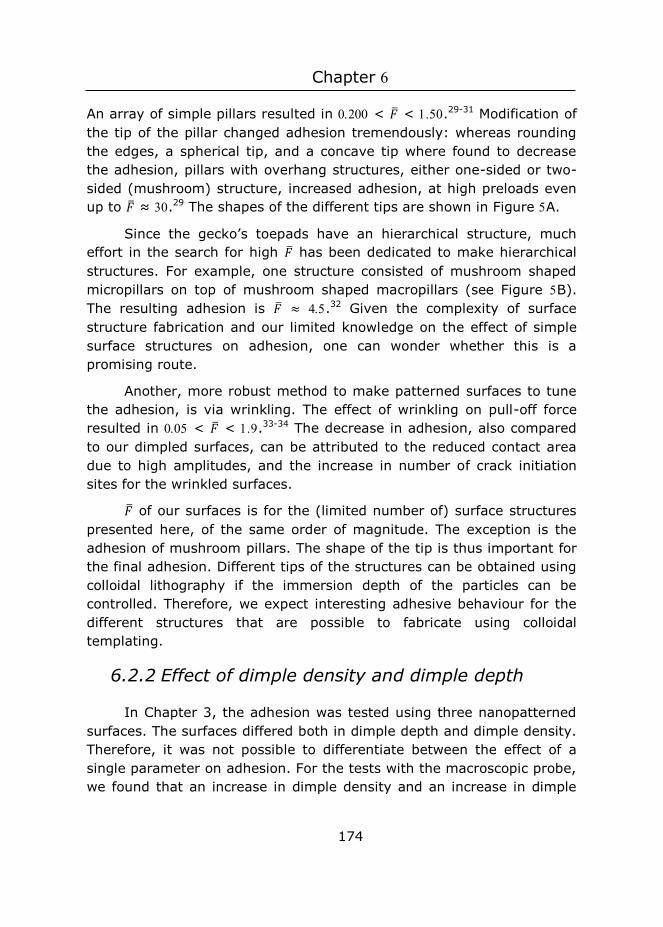
Chapter
174
An array of simple pillars resulted in < �̅�𝐹 < .29-31 Modification of the tip of the pillar changed adhesion tremendously: whereas rounding the edges, a spherical tip, and a concave tip where found to decrease the adhesion, pillars with overhang structures, either one-sided or two-sided (mushroom) structure, increased adhesion, at high preloads even up to �̅�𝐹 ≈ .29 The shapes of the different tips are shown in Figure A.
Since the gecko’s toepads have an hierarchical structure, much effort in the search for high �̅�𝐹 has been dedicated to make hierarchical structures. For example, one structure consisted of mushroom shaped micropillars on top of mushroom shaped macropillars (see Figure B). The resulting adhesion is �̅�𝐹 ≈ .32 Given the complexity of surface structure fabrication and our limited knowledge on the effect of simple surface structures on adhesion, one can wonder whether this is a promising route.
Another, more robust method to make patterned surfaces to tune the adhesion, is via wrinkling. The effect of wrinkling on pull-off force resulted in < �̅�𝐹 < .33-34 The decrease in adhesion, also compared to our dimpled surfaces, can be attributed to the reduced contact area due to high amplitudes, and the increase in number of crack initiation sites for the wrinkled surfaces.
�̅�𝐹 of our surfaces is for the (limited number of) surface structures presented here, of the same order of magnitude. The exception is the adhesion of mushroom pillars. The shape of the tip is thus important for the final adhesion. Different tips of the structures can be obtained using colloidal lithography if the immersion depth of the particles can be controlled. Therefore, we expect interesting adhesive behaviour for the different structures that are possible to fabricate using colloidal templating.
6.2.2 Effect of dimple density and dimple depth
In Chapter 3, the adhesion was tested using three nanopatterned surfaces. The surfaces differed both in dimple depth and dimple density. Therefore, it was not possible to differentiate between the effect of a single parameter on adhesion. For the tests with the macroscopic probe, we found that an increase in dimple density and an increase in dimple
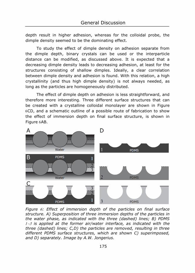
General Discussion
175
depth result in higher adhesion, whereas for the colloidal probe, the dimple density seemed to be the dominating effect.
To study the effect of dimple density on adhesion separate from the dimple depth, binary crystals can be used or the interparticle distance can be modified, as discussed above. It is expected that a decreasing dimple density leads to decreasing adhesion, at least for the structures consisting of shallow dimples. Ideally, a clear correlation between dimple density and adhesion is found. With this relation, a high crystallinity (and thus high dimple density) is not always needed, as long as the particles are homogeneously distributed.
The effect of dimple depth on adhesion is less straightforward, and therefore more interesting. Three different surface structures that can be created with a crystalline colloidal monolayer are shown in Figure CD, and a schematic outline of a possible route of fabrication to show the effect of immersion depth on final surface structure, is shown in Figure AB.
Figure : Effect of immersion depth of the particles on final surface structure. A) Superposition of three immersion depths of the particles in the water phase, as indicated with the three (dashed) lines; B) PDMS is applied at the former air/water interface, as indicated with the three (dashed) lines; C,D) the particles are removed, resulting in three different PDMS surface structures, which are shown C) superimposed, and D) separately. Image by A.W. Jongerius.
Chapter
176
In this thesis, the adhesion of Din Figure has been discussed, and it has been found that a higher dimple depth, thus lower immersion depth, resulted in an increase in adhesion for the macroscopic sphere as counter surface. This may be the case for dimple depths up to that of Figure D. A prerequisite for adhesion enhancement is that the surface is in full contact with the counter surface. In Chapter , equation we have seen that a spontaneous jump-to-contact is expected for dimples up to m. Since our particles have a radius m, full contact is expected, and hence adhesion enhancement for macroscopic counter surfaces.
The effect on adhesion of structure D is less easy to predict.
These structures have an overhang structure, similar to a mushroom shape. The stress distribution on these shapes are such that the highest stress is not located at the edge of a post.35 Therefore, crack initiation must start in the middle of the post which requires much more energy, and thus a higher pull-off force is expected.
A third important factor, is that these surface structures are quite fragile: the PDMS structures with overhang can be regarded as consisting of triangular pillars with touching overhang structures. These pillars are very narrow at the thinnest point. Adhesion could be so strong that detachment results in structure destruction due to cohesive failure. It could therefore become necessary to strengthen the structure. A method to accomplish this, is to fill the dimples with a viscous material. This may not interfere with the advantage of dry adhesives, namely its reusability; it has been found that a viscoelastic PDMS film shows interfacial failure, rather than cohesive failure, for small feature sizes.36
So far, we have seen that the shallow dimples that we have fabricated, showed a pronounced effect on adhesion. Other studies show that the shape of the tip influences the final adhesion significantly, and that mushroom shapes can increase adhesion tremendously. Fabricating this structure and measuring its adhesion is therefore the most interesting next step in this line of research.
General Discussion
177
6.3 Wetting
6.3.1 Wetting of PPy-iccms
We investigated the wetting of polypyrrole inverse crystalline colloidal monolayers (PPy-iccms). The hexagonal packing, the overhang structure and the length scale of these PPy-iccms reminded us of the surface structures of springtails. Springtails are able to entrap air in their (hierarchical) surface structure when immersed in liquids, allowing them to avoid suffocation.37-38 Air entrapment in any surface structure can lead to an increase in the contact angle . For hydrophilic surfaces, air entrapment is only possible if an energy barrier prevents the air bubble from escaping.39 A hypothesis is that the presence of re-entrant angles in the surface structure provides this barrier.39-48 Reason enough to expect interesting phenomena to arise when wetting of PPy-iccms is studied.
We have seen that of water droplets on our hydrophilic material was indeed o. It was not possible to conclude from our experiments directly whether air was entrapped in the PPy-iccms or not. To obtain more insight in the wetting at small length scales, modelling studies were carried out (Chapter ). In our models, depinning transitions were found, and these pinning effects are important for the final droplet shape, which is discussed in terms of . Whether cavities under the droplet were filled with liquid (Wenzel wetting state) or vapour (Cassie-Baxter wetting state) did not matter for . Furthermore, in the models we found that the complete D structure of a surface determines the , and this cannot be reduced to one parameter, such as the angle of a kink in the surface.
We thus showed that we could model droplets of liquid on structured surfaces, and that in this way we could indeed find o on hydrophilic materials. However, our model is a simple one, and does not capture every detail of the experimental system. We know, for example, that our model does not represent water molecules realistically. It is therefore the question how to interpret the outcomes. It would be an indication that our model captured all relevant parameters if we experimentally can find trends that were predicted using our model.
Chapter
178
Trends in contact angle have been predicted as function of (i) cavity diameter (ii) surface wettability, (iii) cavity cut-off height, (iv) spacing between the cavities, and high contact angle hysteresis was also found. This part of the General Discussion will be mainly dedicated to validate our modelling via (new) experimental results.
6.3.2 Effect of cavity diameter on wetting
The cavity diameter only influences the droplet shape if water condenses in the cavities, resulting in an impregnated wetting state. This only happens for very small cavities according to our models. To test this trend, very small particles ( nm) should be used for templating, which is with our fabrication method not possible.
6.3.3 Effect of surface wettability on wetting
The influence of the surface wettability on the final droplet shape was found to be twofold: the surface structures decreased for materials with θY < o, and increased for θY o. To test whether this could also be observed experimentally, PPy-iccms were modified in two ways: PPy-iccms were sputtered with gold to decrease θY
41, and silanized with trichloro (1H, 1H, 2H, 2H-perfluorooctyl)silane to increase the θY.49-
50 Water wets a clean gold surface completely (θY o), although in practice organic contaminations increase θY.51 The θY of the silane is
o.52 The apparent contact angles of water on the (treated) PPy-iccms are shown in Figure .
The θ of the silanized PPy-iccm is indeed higher ( ~ o ) than θ of the non-treated surface. However, coating the surface with gold does not result in a lower θ for the structured surface compared to a flat surface, although a decrease was predicted. The deviation can be explained in three ways: (i) our model is not valid; (ii) the gold layer was already contaminated and θY for this contaminated layer is larger than the θ we measured on the PPy-iccms; or (iii) the inhomogeneous distribution of gold on the PPy-iccms caused an increase in θ. Gold was deposited vertically on the surfaces. Only the top surface was thereby coated in a thin gold layer, leaving the cavities unaffected. This variation in surface chemistry may lead to air entrapment, rather than filling the
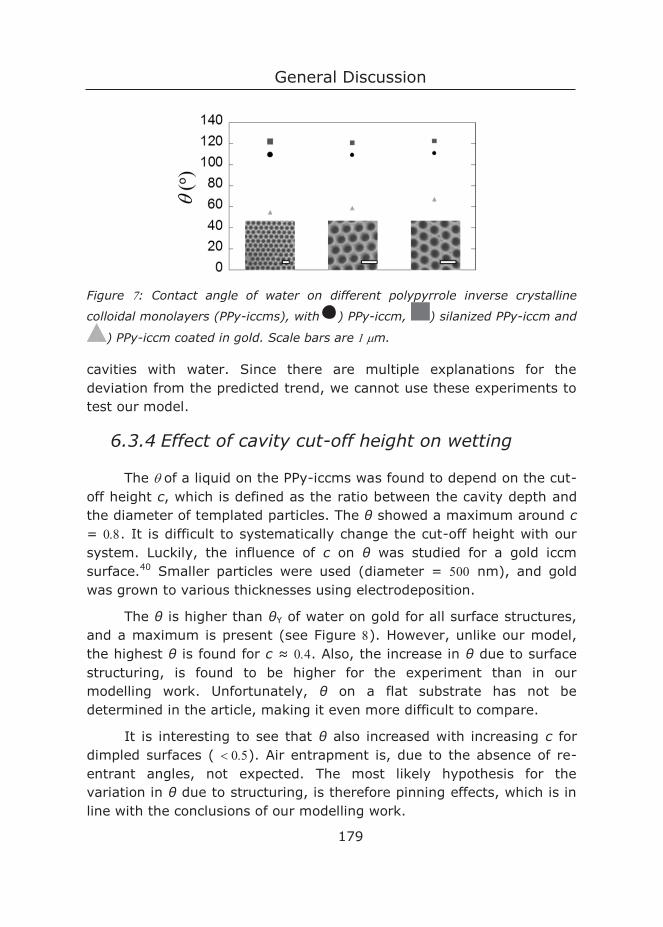
General Discussion
179
Figure : Contact angle of water on different polypyrrole inverse crystalline
colloidal monolayers (PPy-iccms), with ) PPy-iccm, ) silanized PPy-iccm and
) PPy-iccm coated in gold. Scale bars are m.
cavities with water. Since there are multiple explanations for the deviation from the predicted trend, we cannot use these experiments to test our model.
6.3.4 Effect of cavity cut-off height on wetting
The of a liquid on the PPy-iccms was found to depend on the cut-off height c, which is defined as the ratio between the cavity depth and the diameter of templated particles. The θ showed a maximum around c = . It is difficult to systematically change the cut-off height with our system. Luckily, the influence of c on θ was studied for a gold iccm surface.40 Smaller particles were used (diameter = nm), and gold was grown to various thicknesses using electrodeposition.
The θ is higher than θY of water on gold for all surface structures, and a maximum is present (see Figure ). However, unlike our model, the highest θ is found for c ≈ . Also, the increase in θ due to surface structuring, is found to be higher for the experiment than in our modelling work. Unfortunately, θ on a flat substrate has not be determined in the article, making it even more difficult to compare.
It is interesting to see that θ also increased with increasing c for dimpled surfaces ( ). Air entrapment is, due to the absence of re-entrant angles, not expected. The most likely hypothesis for the variation in θ due to structuring, is therefore pinning effects, which is in line with the conclusions of our modelling work.
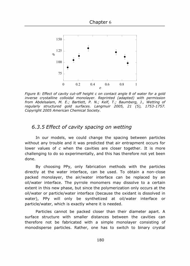
Chapter
180
Figure 8: Effect of cavity cut-off height c on contact angle θ of water for a gold inverse crystalline colloidal monolayer. Reprinted (adapted) with permission from Abdelsalam, M. E.; Bartlett, P. N.; Kelf, T.; Baumberg, J., Wetting of regularly structured gold surfaces. Langmuir 2005, 21 (5), 1753-1757. Copyright 2005 American Chemical Society.
6.3.5 Effect of cavity spacing on wetting
In our models, we could change the spacing between particles without any trouble and it was predicted that air entrapment occurs for lower values of c when the cavities are closer together. It is more challenging to do so experimentally, and this has therefore not yet been done.
By choosing PPy, only fabrication methods with the particles directly at the water interface, can be used. To obtain a non-close packed monolayer, the air/water interface can be replaced by an oil/water interface. The pyrrole monomers may dissolve to a certain extent in this new phase, but since the polymerization only occurs at the oil/water or particle/water interface (because the oxidant is dissolved in water), PPy will only be synthetized at oil/water interface or particle/water, which is exactly where it is needed.
Particles cannot be packed closer than their diameter apart. A surface structure with smaller distances between the cavities can therefore not be fabricated with a simple monolayer consisting of monodisperse particles. Rather, one has to switch to binary crystal
c
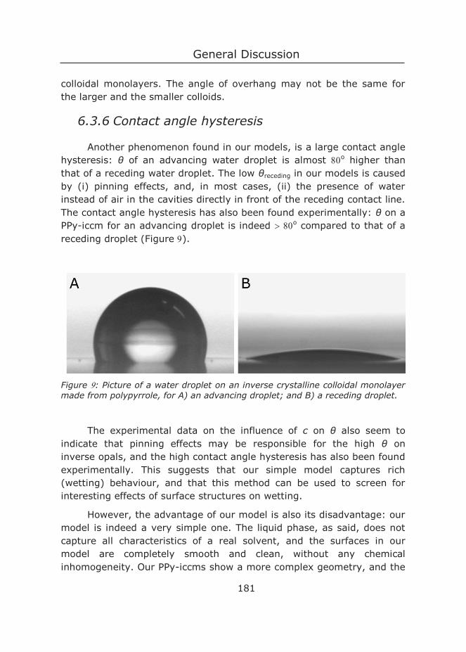
General Discussion
181
colloidal monolayers. The angle of overhang may not be the same for the larger and the smaller colloids.
6.3.6 Contact angle hysteresis
Another phenomenon found in our models, is a large contact angle hysteresis: θ of an advancing water droplet is almost o higher than that of a receding water droplet. The low θreceding in our models is caused by (i) pinning effects, and, in most cases, (ii) the presence of water instead of air in the cavities directly in front of the receding contact line. The contact angle hysteresis has also been found experimentally: θ on a PPy-iccm for an advancing droplet is indeed o compared to that of a receding droplet (Figure ).
Figure : Picture of a water droplet on an inverse crystalline colloidal monolayer made from polypyrrole, for A) an advancing droplet; and B) a receding droplet.
The experimental data on the influence of c on θ also seem to indicate that pinning effects may be responsible for the high θ on inverse opals, and the high contact angle hysteresis has also been found experimentally. This suggests that our simple model captures rich (wetting) behaviour, and that this method can be used to screen for interesting effects of surface structures on wetting.
However, the advantage of our model is also its disadvantage: our model is indeed a very simple one. The liquid phase, as said, does not capture all characteristics of a real solvent, and the surfaces in our model are completely smooth and clean, without any chemical inhomogeneity. Our PPy-iccms show a more complex geometry, and the
Chapter
182
particle residues, probably present as adsorbed polymers, are not taken into account. After these improvements are included in the model, even more interesting phenomena and insights are expected to be observed.
6.4 Outlook
Suggestions for research directions that directly follow from this thesis, have been presented in the previous paragraphs. As a closing remark, we would like to present the ultimate goal: the development of a comprehensive model that can predict the surface functions once the surface structure is given as input, and, conversely, can suggest a surface structure design based on the input of desired functions.
To do so, the effect of surface structuring should be understood for all functions. In this thesis, only two functions are discussed, and not even to their full extent. For example, for wetting one can also think of superhydrophobicity53 or non-wetting to prevent ice formation,54 selective wetting for water/oil separation,55 or directional wetting.56
Eventually, if our understanding of surface structuring on functions is sufficient, one can dream of one surface with different functions, just as is found in nature, and use the model to present the surface structure that should provide all desired characteristics. Hopefully the outcome is a design of a structure that can be fabricated experimentally, for example using a pipette, plastic Petri dish, some particles dispersed in ethanol and a not-so-clean room.
References 1. Kraus, T.; Brodoceanu, D.; Pazos‐Perez, N.; Fery, A., Colloidal Surface Assemblies: Nanotechnology Meets Bioinspiration. Advanced Functional Materials 2013, 23 (36), 4529-4541. 2. Vogel, N.; Retsch, M.; Fustin, C.-A.; del Campo, A.; Jonas, U., Advances in colloidal assembly: The design of structure and hierarchy in two and three dimensions. Chemical reviews 2015, 115 (13), 6265-6311. 3. Appel, J.; Akerboom, S.; Fokkink, R. G.; Sprakel, J., Facile One‐Step Synthesis of Monodisperse Micron‐Sized Latex Particles with Highly Carboxylated Surfaces. Macromol. Rapid Commun. 2013, 34 (16), 1284-1288. 4. Pieranski, P., Two-dimensional interfacial colloidal crystals. Physical Review Letters 1980, 45 (7), 569.
General Discussion
183
5. Moon, G. D.; Lee, T. I.; Kim, B.; Chae, G.; Kim, J.; Kim, S.; Myoung, J.-M.; Jeong, U., Assembled monolayers of hydrophilic particles on water surfaces. ACS nano 2011, 5 (11), 8600-8612. 6. Weekes, S. M.; Ogrin, F. Y.; Murray, W. A.; Keatley, P. S., Macroscopic Arrays of Magnetic Nanostructures from Self-Assembled Nanosphere Templates. Langmuir 2007, 23 (3), 1057-1060. 7. Retsch, M.; Zhou, Z.; Rivera, S.; Kappl, M.; Zhao, X. S.; Jonas, U.; Li, Q., Fabrication of Large‐Area, Transferable Colloidal Monolayers Utilizing Self‐Assembly at the Air/Water Interface. Macromolecular Chemistry and Physics 2009, 210 (3‐4), 230-241. 8. Vogel, N.; Weiss, C. K.; Landfester, K., From soft to hard: the generation of functional and complex colloidal monolayers for nanolithography. Soft Matter 2012, 8 (15), 4044-4061. 9. Lyklema, J.; van Leeuwen, H. P.; Vliet, M.; Cazabat, A.-M., Fundamentals of interface and colloid science. Academic Pr: 2005; Vol. 5. 10. Akerboom, S.; Appel, J.; Labonte, D.; Federle, W.; Sprakel, J.; Kamperman, M., Enhanced adhesion of bioinspired nanopatterned elastomers via colloidal surface assembly. Journal of The Royal Society Interface 2015, 12 (102), 20141061. 11. Vogel, N.; de Viguerie, L.; Jonas, U.; Weiss, C. K.; Landfester, K., Wafer‐Scale Fabrication of Ordered Binary Colloidal Monolayers with Adjustable Stoichiometries. Advanced functional materials 2011, 21 (16), 3064-3073. 12. Yu, J.; Yan, Q.; Shen, D., Co-Self-Assembly of Binary Colloidal Crystals at the Air− Water Interface. ACS Applied Materials & Interfaces 2010, 2 (7), 1922-1926. 13. Ray, M. A.; Jia, L., Micropatterning by Non‐Densely Packed Interfacial Colloidal Crystals. Advanced Materials 2007, 19 (15), 2020-2022. 14. Bhawalkar, S. P.; Qian, J.; Heiber, M. C.; Jia, L., Development of a colloidal lithography method for patterning nonplanar surfaces. Langmuir 2010, 26 (22), 16662-16666. 15. Qian, J.; Bhawalkar, S. P.; Xu, Y.; Jia, L., Novel use of polymer brushes in colloidal lithography to overcome lateral capillary force. ACS applied materials & interfaces 2010, 2 (11), 3111-3118. 16. Binks, B. P.; Horozov, T. S., Colloidal particles at liquid interfaces. Cambridge University Press: 2006. 17. Isa, L.; Kumar, K.; Muller, M.; Grolig, J.; Textor, M.; Reimhult, E., Particle lithography from colloidal self-assembly at liquid− liquid interfaces. ACS nano 2010, 4 (10), 5665-5670. 18. Horozov, T. S.; Aveyard, R.; Binks, B. P.; Clint, J. H., Structure and stability of silica particle monolayers at horizontal and vertical octane-water interfaces. Langmuir 2005, 21 (16), 7405-7412. 19. Ho, C.-C.; Chen, P.-Y.; Lin, K.-H.; Juan, W.-T.; Lee, W.-L., Fabrication of Monolayer of Polymer/Nanospheres Hybrid at a Water-Air Interface. ACS Applied Materials & Interfaces 2011, 3 (2), 204-208. 20. Vogel, N.; Goerres, S.; Landfester, K.; Weiss, C. K., A Convenient Method to Produce Close- and Non-close-Packed Monolayers using Direct Assembly at the Air–Water Interface and Subsequent Plasma-Induced Size Reduction. Macromolecular Chemistry and Physics 2011, 212 (16), 1719-1734.
Chapter
184
21. Paunov, V. N.; Cayre, O. J., Supraparticles and “Janus” particles fabricated by replication of particle monolayers at liquid surfaces using a gel trapping technique. Advanced Materials 2004, 16 (9‐10), 788-791. 22. Li, J.; Zhang, Y., Porous polymer films with size-tunable surface pores. Chemistry of Materials 2007, 19 (10), 2581-2584. 23. Haginoya, C.; Ishibashi, M.; Koike, K., Nanostructure array fabrication with a size-controllable natural lithography. Applied Physics Letters 1997, 71 (20), 2934-2936. 24. Choi, D.-G.; Yu, H. K.; Jang, S. G.; Yang, S.-M., Colloidal lithographic nanopatterning via reactive ion etching. Journal of the American Chemical Society 2004, 126 (22), 7019-7025. 25. Yan, X.; Yao, J.; Lu, G.; Li, X.; Zhang, J.; Han, K.; Yang, B., Fabrication of non-close-packed arrays of colloidal spheres by soft lithography. Journal of the American Chemical Society 2005, 127 (21), 7688-7689. 26. Li, X.; Wang, T.; Zhang, J.; Yan, X.; Zhang, X.; Zhu, D.; Li, W.; Zhang, X.; Yang, B., Modulating two-dimensional non-close-packed colloidal crystal arrays by deformable soft lithography. Langmuir 2009, 26 (4), 2930-2936. 27. Thomas, T.; Crosby, A. J., Controlling adhesion with surface hole patterns. The Journal of Adhesion 2006, 82 (3), 311-329. 28. Nanni, G.; Fragouli, D.; Ceseracciu, L.; Athanassiou, A., Adhesion of elastomeric surfaces structured with micro-dimples. Applied Surface Science 2015, 326, 145-150. 29. Greiner, C.; del Campo, A.; Arzt, E., Adhesion of bioinspired micropatterned surfaces: effects of pillar radius, aspect ratio, and preload. Langmuir 2007, 23 (7), 3495-3502. 30. Kroner, E.; Paretkar, D. R.; McMeeking, R. M.; Arzt, E., Adhesion of flat and structured PDMS samples to spherical and flat probes: a comparative study. The Journal of Adhesion 2011, 87 (5), 447-465. 31. O’Rorke, R.; Steele, T.; Taylor, H., Bioinspired fibrillar adhesives: a review of analytical models and experimental evidence for adhesion enhancement by surface patterns. Journal of Adhesion Science and Technology 2016, 30 (4), 362-391. 32. Murphy, M. P.; Kim, S.; Sitti, M., Enhanced adhesion by gecko-inspired hierarchical fibrillar adhesives. ACS applied materials & interfaces 2009, 1 (4), 849-855. 33. Davis, C. S.; Crosby, A. J., Mechanics of wrinkled surface adhesion. Soft Matter 2011, 7 (11), 5373-5381. 34. Davis, C. S.; Martina, D.; Creton, C.; Lindner, A.; Crosby, A. J., Enhanced adhesion of elastic materials to small-scale wrinkles. Langmuir 2012, 28 (42), 14899-14908. 35. Carbone, G.; Pierro, E.; Gorb, S. N., Origin of the superior adhesive performance of mushroom-shaped microstructured surfaces. Soft Matter 2011, 7 (12), 5545-5552. 36. Patil, S.; Mangal, R.; Malasi, A.; Sharma, A., Biomimetic Wet Adhesion of Viscoelastic Liquid Films Anchored on Micropatterned Elastic Substrates. Langmuir 2012, 28 (41), 14784-14791. 37. Helbig, R.; Nickerl, J.; Neinhuis, C.; Werner, C., Smart skin patterns protect springtails. PloS one 2011, 6 (9), e25105-e25105.
General Discussion
185
38. Hensel, R.; Helbig, R.; Aland, S.; Braun, H.-G.; Voigt, A.; Neinhuis, C.; Werner, C., Wetting resistance at its topographical limit: the benefit of mushroom and serif T structures. Langmuir 2013, 29 (4), 1100-1112. 39. Cao, L.; Hu, H.-H.; Gao, D., Design and fabrication of micro-textures for inducing a superhydrophobic behavior on hydrophilic materials. Langmuir 2007, 23 (8), 4310-4314. 40. Abdelsalam, M. E.; Bartlett, P. N.; Kelf, T.; Baumberg, J., Wetting of regularly structured gold surfaces. Langmuir 2005, 21 (5), 1753-1757. 41. Bormashenko, E.; Bormashenko, Y.; Whyman, G.; Pogreb, R.; Stanevsky, O., Micrometrically scaled textured metallic hydrophobic interfaces validate the Cassie–Baxter wetting hypothesis. Journal of colloid and interface science 2006, 302 (1), 308-311. 42. Martines, E.; Seunarine, K.; Morgan, H.; Gadegaard, N.; Wilkinson, C. D.; Riehle, M. O., Air-trapping on biocompatible nanopatterns. Langmuir 2006, 22 (26), 11230-11233. 43. Herminghaus, S.; Brinkmann, M.; Seemann, R., Wetting and dewetting of complex surface geometries. Annu. Rev. Mater. Res. 2008, 38, 101-121. 44. Whyman, G.; Bormashenko, E., How to make the Cassie wetting state stable? Langmuir 2011, 27 (13), 8171-8176. 45. Badge, I.; Bhawalkar, S. P.; Jia, L.; Dhinojwala, A., Tuning surface wettability using single layered and hierarchically ordered arrays of spherical colloidal particles. Soft Matter 2013, 9 (11), 3032-3040. 46. Choi, H.-J.; Choo, S.; Shin, J.-H.; Kim, K.-I.; Lee, H., Fabrication of Superhydrophobic and Oleophobic Surfaces with Overhang Structure by Reverse Nanoimprint Lithography. The Journal of Physical Chemistry C 2013, 117 (46), 24354-24359. 47. Bellanger, H.; Darmanin, T.; Taffin de Givenchy, E.; Guittard, F. d. r., Chemical and physical pathways for the preparation of superoleophobic surfaces and related wetting theories. Chemical reviews 2014, 114 (5), 2694-2716. 48. Kang, H.; Lee, J. S.; Chang, W. S.; Kim, S. H., Liquid‐Impermeable Inverse Opals with Invariant Photonic Bandgap. Advanced Materials 2015, 27 (7), 1282-1287. 49. Kim, P.; Wong, T.-S.; Alvarenga, J.; Kreder, M. J.; Adorno-Martinez, W. E.; Aizenberg, J., Liquid-infused nanostructured surfaces with extreme anti-ice and anti-frost performance. ACS nano 2012, 6 (8), 6569-6577. 50. Zhu, H.; Hou, J.; Qiu, R.; Zhao, J.; Xu, J., Perfluorinated lubricant/ polypyrrole composite material: Preparation and corrosion inhibition application. Journal of applied polymer science 2014, 131 (9), n/a-n/a. 51. Schrader, M. E., Ultrahigh-vacuum techniques in the measurement of contact angles. II. Water on gold. The Journal of Physical Chemistry 1970, 74 (11), 2313-2317. 52. Zhang, M.; Wu, J.; Wang, L.; Xiao, K.; Wen, W., A simple method for fabricating multi-layer PDMS structures for 3D microfluidic chips. Lab on a Chip 2010, 10 (9), 1199-1203. 53. Deng, X.; Mammen, L.; Butt, H.-J.; Vollmer, D., Candle soot as a template for a transparent robust superamphiphobic coating. Science 2012, 335 (6064), 67-70.

Chapter
186
54. Mishchenko, L.; Hatton, B.; Bahadur, V.; Taylor, J. A.; Krupenkin, T.; Aizenberg, J., Design of ice-free nanostructured surfaces based on repulsion of impacting water droplets. ACS nano 2010, 4 (12), 7699-7707. 55. Wang, C.; Yao, T.; Wu, J.; Ma, C.; Fan, Z.; Wang, Z.; Cheng, Y.; Lin, Q.; Yang, B., Facile approach in fabricating superhydrophobic and superoleophilic surface for water and oil mixture separation. ACS applied materials & interfaces 2009, 1 (11), 2613-2617. 56. Jokinen, V.; Leinikka, M.; Franssila, S., Microstructured surfaces for directional wetting. Advanced Materials 2009, 21 (47), 4835-4838.

7 Summary
Chapter 7
188
Nature shows remarkable examples of functions derived from surface structures. In this thesis, called “Bioinspired nanopatterned surfaces via colloidal templating; a pathway for tuning wetting and adhesion” we studied the effect of surface structuring on adhesion and wetting.Wetting and adhesion is largely understood for perfectly flat and clean surfaces, but switching to the real (and contaminated) world proves to be hard. Predicting the relationship between surface patterns and functions is therefore not yet possible for every surface structure design, but would be desirable.. Making nanopatterned surfaces in a controlled way is the first step towards systematically studying the effect of structuring on different functions.
In Chapter , we present our fabrication method, namely colloidal templating. We synthesized anionic colloidal particles ( diameter (nm) ), consisting of copolymers of styrene with itaconic acid, with parking areas of nm per –COOH group. These particles form a monolayer at the air/water interface. The crystallinity of these monolayers and the immersion depth of the particles can be controlled by the pH and ionic strength of the water phase. It is shown that the crystallinity increases with increasing dissociation of the –COOH groups on the particles, at pH > pKa of itaconic acid: the increased electrostatic repulsion overcomes the attractive Van der Waals interactions, resulting in higher particle mobility. It was found that a higher ionic strength leads to a higher particle immersion depth. The monolayer can be used without pattern disruption of the template by careful application of PDMS, showing that control over the monolayer leads to control over the final surface pattern. After crosslinking, the particles are easily removed, resulting in elastomeric surfaces with dimples.
The nanopatterned PDMS described in Chapter are used for adhesion experiments in Chapter . Three patterned surfaces, with varying dimple depth and dimple density, were selected. A macroscopic probe (diameter = mm) and a colloidal probe (diameter = µm) were used as counter surface to probe different length scales. Adhesion enhancement compared to a flat control was found for all three surfaces and both probe sizes. The origin of this increase in adhesion is attributed to energy dissipation whereby each dimple acts as an unstable crack propagation site.
Summary
189
In Chapter , another method to make nanopatterned surfaces using the same colloidal monolayer, is presented. Pyrrole is added to the water phase, and allowed to swell the particles in the monolayer. Subsequently, ferric chloride is added, and the presence of this oxidant starts the polymerization of pyrrole at the particle/water interface. The particles are dissolved afterwards, yielding a polypyrrole inverse crystalline colloidal monolayer (PPy-iccm). Different surface structures can be obtained by choosing the amount of pyrrole, the pyrrole: oxidant ratio and the polymerization time. The final PPy-iccms have cavities and a small angle of overhang because the particles were for immersed in the water phase. The contact angle of water on three different PPy-iccms is found to be similar with a value of o, whereas the on the control surface consisting of flat PPy with particle residues is found to be o. Due to the pattern, the surface thus appears to be hydrophobic, although the material is hydrophilic. This may indicate that air is entrapped in the cavities of the surface structures.
To understand this increase in and thereby the origin of observing a hydrophobic contact angle on a hydrophilic surface, we employed modelling. In Chapter , we present this work. The regular solutions theory is extended to dimensions, and this allows for finding droplet shapes on inverse opals in short computation time ( minutes). The effect of particle size d, surface wettability SL, immersion depth (using the cut-off height c), and particle spacing s was studied. Both scenarios with water-filled cavities and air-filled cavities have been found, but the trend in did not show a discontinuity upon switching from water-filled to air-filled. This suggests that air entrapment is not responsible for the increase in . Rather, the increase in is attributed to pinning effects, whereby the air/water/surface contact line is fixed at one position. Our model suggests that these pinning effects are not limited to small surface structure angles, since pinning was also found for obtuse angles. Pinning is furthermore influenced by the full D structure of a surface, not just to kinks in the surface.
The last chapter, Chapter , places our research in a broader context. Suggestions to improve control over the monolayer and to fabricate different nanopatterned elastomers are presented. Adhesion of our nanopatterned surfaces is compared to that of surfaces from literature, and we speculate on the effect of different surface structures

Chapter 7
190
on adhesion. Furthermore, extra experimental data is provided to test predictions concerning wetting from our modelling work. As final paragraph, our ultimate goal is revealed: improve our understanding of the effect of structuring on functions to such an extent, that a comprehensive model can be made, which can predict the functions based on the surface structure, and vice versa.

8 Samenvatting
Chapter 8
192
In de natuur zijn er opmerkelijke voorbeelden te vinden van functie door structuur. In dit proefschrift, genaamd “Bioinspired nanopatterned surfaces via colloidal templating; a pathway for tuning wetting and adhesion”, hebben we het effect van oppervlakstructuren op adhesie en bevochtiging bestudeerd. Adhesie en bevochtiging van perfect gladde en schone oppervlakken is grotendeels bekend, maar als we de overstap naar de echte wereld maken, wordt het lastiger. Het is daarom nog niet mogelijk om het verband tussen de oppervlaktestructuur en de functionaliteit te voorspellen voor elke oppervlaktestructuur, maar dit is wel wenselijk. Een systematische studie van het effect van oppervlaktestructuur op de functionaliteiten is daarom wenselijk. De eerste stap in deze studie is het maken van gestructureerde oppervlakten op de nanometer schaal op een gecontroleerde wijze.
In Hoofdstuk laten we onze aanpak zien, namelijk het gebruiken van kolloïden als mal. We hebben kolloïdale deeltjes ( diameter (nm) ) met negatieve lading gemaakt, die bestaan uit copolymeren van styreen met itaconzuur, met op gemiddeld elke nm een –COOH-groep. Deze deeltjes vormen een monolaag op het luch/water grensvlak. De kristalliniteit van deze monolagen en de inzinkdiepte van de deeltjes kunnen worden ingesteld met behulp van de pH en de zoutsterkte van de waterfase. We laten zien dat de kristalliniteit toeneemt met toegenomen dissociatie van de –COOH-groepen op het oppervlak van de deeltjes als de pH hoger ligt dan de pKa van itaconzuur: de toegenomen elektrostatische afstoting domineert de aantrekkingskracht van de Van der Waals-interactie, wat resulteert in een hogere mobiliteit van de deeltjes. Ook vonden we dat een hogere zoutsterkte resulteerde in een grotere inzinkdiepte van de deeltjes. De monolaag kan, zonder dat de ordening wordt verstoord, worden gebruikt als mal, door er voorzichtig PDMS op te gieten. Hierdoor leidt controle over de monolaag direct tot controle over de uiteindelijke structuur. Nadat het PDMS is gecrosslinked, kunnen de deeltjes makkelijk worden opgelost, wat resulteert in een rubberen oppervlak met kuiltjes.
De oppervlakten van PDMS met nanostructuren die zijn beschreven in Hoofdstuk , zijn gebruikt voor adhesiemetingen in Hoofdstuk . We hebben drie gepatroneerde oppervlakten, met variërende kuildiepten en kuildichtheden, geselecteerd. Een
Samenvatting
193
macroscopische bol (diameter = mm) en een microscopische bol (diameter = µm) zijn gebruikt om de adhesie op verschillende lengteschalen te meten. Een toename in adhesie in vergelijking met de adhesie op een glad oppervlak, is gevonden voor alle gepatroneerde monsters en beide bolgroottes. De verklaring voor deze toename is toegeschreven aan dissipatie van energie, waarbij elk kuiltje dient als locatie voor het instabiel loslaten van het rubberen oppervlak. In Hoofdstuk wordt een andere manier om nanogepatroneerde oppervlakten met dezelfde kolloïdale monolaag te maken. Pyrrool wordt aan de waterfase toegevoegd, en verzamelt zich in de deeltjes van de monolaag. Vervolgens wordt ijzerchloride toegevoegd, en de aanwezigheid van deze oxidant start de polymerisatie van pyrrool op het deeltje/water grensvlak. De deeltjes worden naderhand opgelost, wat resulteert in een geïnverteerd kristallijne kolloïdale monolaag van polypyrrool (polypyrrole inverse crystalline colloidal monolayer, PPy-iccm). Verschillende oppervlaktenstructuren kunnen worden verkregen door de hoeveelheden pyrrool, de verhouding pyrrool : oxidant of de polymerisatietijd te variëren. De uiteindelijke PPy-iccms hebben holtes en een scherpe hoek aan de bovenkant, omdat de deeltjes voor ongeveer in het water staken. De randhoek van water op drie verschillende PPy-iccms bleek in alle drie de gevallen ongeveer o te zijn, terwijl op het controleoppervlak, bestaande uit glad PPy met resten van de deeltjes, o bleek te zijn. De oppervlaktestructuur zorgt er dus voor dat het oppervlakte hydrofoob lijkt, terwijl het gemaakt is van een hydrofiel materiaal. Dit zou erop kunnen wijzen dat er lucht in de holtes achterblijft.
Om deze toename in randhoek te begrijpen, en daarmee een verklaring voor het vinden van een hydrofobe randhoek op een hydrofiel materiaal, hebben we gemodelleerd. We presenteren dit werk in Hoofdstuk . De regular solution theorie is uitgebreid naar drie dimensies, waardoor we de vorm van druppels op iccm’s kunnen vinden in korte rekentijd ( minuten). De invloed van deeltjesgrootte d, bevochtingingseigenschappen van het oppervlak SL, inzinkdiepte van de deeltjes c en afstand tussen de deeltjes s, is onderzocht. We hebben zowel scenario’s met lucht als met water in de holtes gevonden, maar we zagen geen discontinuïteit in het verband tussen de randhoek als de holtes van gevuld met water naar gevuld met lucht gingen. Dit suggereert dat het invangen van lucht niet de verklaring voor de
Chapter 8
194
toename van kan zijn. Een verklaring die we met modelleren gevonden hebben, is dat de toename van verklaart kan worden doordat de druppel pint op een oppervlaktestructuur. Hierbij verplaatst de lucht/water/oppervlakte-contactlijn niet. Ons model suggereert dat deze pinningseffecten zich niet beperken tot structuren met kleine hoeken, want we hebben het ook gevonden voor stompe hoeken. Ook bleek de gehele D-structuur van een oppervlak belangrijk te zijn voor het pinnen van een druppel, en niet alleen een hoek in het oppervlak.
Het laatste hoofdstuk, nummer , plaatst ons onderzoek in een bredere context. We presenteren mogelijkheden om de monolaag beter te controleren en om verschillende structuren van rubber te maken. De adhesie van onze oppervlaktestructuren wordt vergeleken met literatuurwaarden, en we denken na over het effect van andere oppervlaktestructuren op adhesie. Ook wordt nieuw experimenteel werk gepresenteerd waarin de voorspellingen van ons modelleerwerk over bevochtiging, wordt bekeken. De allerlaatste paragraaf bespreekt ons uiteindelijke doel: het dusdanig vergroten van ons begrip over het verband tussen oppervlaktenstructuren en functionaliteiten, dat we een alomvattend model kunnen maken dat functionaliteiten kan voorspellen op basis van oppervlaktestructuur, en omgekeerd.
Acknowledgements
Bedankt
Marleen ook voor de kinderwagen en de gouden Arneco-tip
Frans voor het beschikbaar stellen van je terp der wijsheid
Marcel voor je hulp met alle elektronenmicroscopen in Wageningen
David Labonte for your help, both during my stay in Cambridge and afterwards
Walter Federle for those days in your lab
Sidhu for your (quick) help with the Auger and XPS
Barend voor je hulp met de NMR en de glovebox tijdens die warme, plakkerige zomerdagen
Frank en Elbert voor jullie hulp met de GPC
Kirsty for our crap discussion
Groetjes aan
Fysko voor een memorabele tijd/for a memorable time
JeBó en JeBé kantoorgenoten van begin tot (bittere) eind
Frank zonder jou was dit boekje er niet gekomen
Daphne zonder jou was dit boekje er eerder gekomen
Pups en mums voor al het zilverwater, kurkuma en zuiveringszout
Bas dankzij jou had de rest nu aan een half woord genoeg
Koen en Eva drink er nog maar eentje voor me
Daaaaf Bankelaaaaaf!
Oma nu geen ruggen meer breken hoor
Kruidbosjes en de hele nichtjescollectie onmeunig mooi, onnieda?
Pieterke en Aniek Bsc. Msc. etc. de beste imaginaire pseudoparanimfen ooit. Het wachtwoord is ‘Hiyaaaa! Ik ben klaaaaar!’
Freunden uit Wagga stelletje taartenbakkende badjassen
CP-moekes van Groep F voor alle gesprekken waarvan je nooit had gedacht dat je ze ooit zelf zou voeren
196
About the author
Sabine Akerboom was born on January in The Hague, the Netherlands. She obtained her vwo diploma (secondary education) from the Fioretti College in and then moved to Wageningen to start her studies of Molecular Sciences. She obtained her Bsc in Molecular Science with a minor in Environmental chemistry and philosophy in September . As part of her Msc, she carried out two research projects; At the Laboratory of Physical Chemistry and Colloid Science (later: Physical Chemistry and Soft Matter) of the Wageningen University, she worked on composite materials of silica particles with ABA-triblock copolymers. She worked on the adsorption of core/shell thermoresponsive microgels at the Applied Physical Chemistry group of TU Berlin. In October she graduated with an Msc in Molecular Life Sciences, and started her PhD research soon after at Physical Chemistry and Soft Matter in Wageningen. This thesis is the result.
197
List of publications 1. Akerboom, S; Kamperman, M; Leermakers F.A.M., Three-gradient regular solution model for simple liquids, wetting complex surface topologies (submitted)
2. Akerboom, S.; Appel, J.; Labonte, D.; Federle, W.; Sprakel, J.; Kamperman, M., Enhanced adhesion of bioinspired nanopatterned elastomers via colloidal surface assembly. Journal of The Royal Society Interface 2015, 12 (102), 20141061.
3. Akerboom, P., Turak, Kamperman, Controlled fabrication of polypyrrole surfaces with overhang structures by colloidal templating. ACS applied materials & interfaces 2015, 7 (30), 16507-16517.
4. Appel, J.; Akerboom, S.; Fokkink, R. G.; Sprakel, J., Facile One‐Step Synthesis of Monodisperse Micron‐Sized Latex Particles with Highly Carboxylated Surfaces. Macromol. Rapid Commun. 2013, 34 (16), 1284-1288.
5. Lemmers, M.; Spruijt, E.; Akerboom, S.; Voets, I. K.; van Aelst, A. C.; Cohen Stuart, M. A.; van der Gucht, J., Physical gels based on charge-driven bridging of nanoparticles by triblock copolymers. Langmuir 2012, 28 (33), 12311-12318.

198
Overview of completed
training activities Discipline-specific activities
Han-sur-Lesse winterschool Han-sur-Lesse, Belgium, 2011&2012
Scattering summer school Leuven , Belgium 2011
Conference on Adhesion Lisbon, Portugal 2012
European Student Colloid Conference Potsdam, Germany 2013
GRC Science of Adhesion South Hadley, USA 2013
Dutch Polymer Days Lunteren, The Netherlands 2014
GRC Biointerface Science Barga, Italy 2014
Soft Matter Days The Netherlands, 2011-2013
General courses
PhD Assessment Wageningen 2011
Physics with Industry Leiden 2011
Scientific Publishing Wageningen 2012
Writing and presenting scientific research Wageningen 2012
Pump your career Amsterdam 2012
Share your results Wageningen 2013
Career Orientation Wageningen 2013
Career Assessment Wageningen 2015
Optionals
PCC Meetings Wageningen 2011-2015
Colloquia PCC Wageningen 2011-2015
Organization PhD trip Wageningen 2012-2013
PhD trip California, USA 2013


200