Embed Size (px)
Citation preview
Multibody System Dynamics 1: 65–84, 1997. 65c 1997 Kluwer Academic Publishers. Printed in the Netherlands.
Biomechanical Model with Joint Resistance forImpact Simulation
M.P.T. SILVA, J.A.C. AMBROSIO and M.S. PEREIRAIDMEC Polo IST, Avenida Rovisco Pais, 1096 Lisboa Codex, Portugal
(Received: 30 July 1996; accepted in revised form: 19 December 1996)
Abstract. Based on a general methodology using natural co-ordinates, a three-dimensional wholebody response model for the articulated human body is presented in this paper. The joints betweenbiomechanical segments are defined by forcing adjacent bodies to share common points and vectorsthat are used in their definition. A realistic relative range of motion for the body segments is obtainedintroducing a set of penalty forces in the model rather than setting up new unilateral constraintsbetween the system components. These forces, representing the reaction moments between segmentsof the human body model when the biomechanical joints reach the limit of their range of motion, pre-vent the biomechanical model from achieving physically unacceptable positions. Improved efficiencyin the integration process of the equations of motion is obtained using the augmented Lagrange for-mulation. The biomechanical model is finally applied in different situations of passive human motionsuch as that observed in vehicle occupants during a crash or in an athlete during impact.
Key words: biomechanics, occupant models, injury.
1. Introduction
The development of reliable mathematical models of the human body has been amajor challenge for the biomechanics community over the last twenty years [1].The interest in the simulation of different human actions stems from the need topredict with sufficient accuracy the mechanical behavior of the human body invarious conditions of its activity. In fact the simulation of these capabilities havebeen shown to be useful in different types of applications, including: athletic actionswith the aim to improve different sport performances and to optimize the design ofsports outfits and equipment; ergonomic studies to assess operating conditions forcomfort and efficiency purposes in different aspects of human body interactionswith the environment; orthopedics and prosthesis design studies; occupant dynamicanalysis for crashworthiness and vehicle safety related research and design.
The biofidelity of modern human body representations is very sensitive tothe type of mathematical formalisms used and their capability of supporting theefficient description of the biomechanical aspects of the human activities underanalysis. In many situations, such as the case of athletic motions and occupantsin vehicle crash design studies, “gross-motion” simulators [2] are preferred to themore expensive finite element based models. In the “gross-motion” simulatorsthe different segments of the human body are typically represented within the
66 M.P.T. SILVA ET AL.
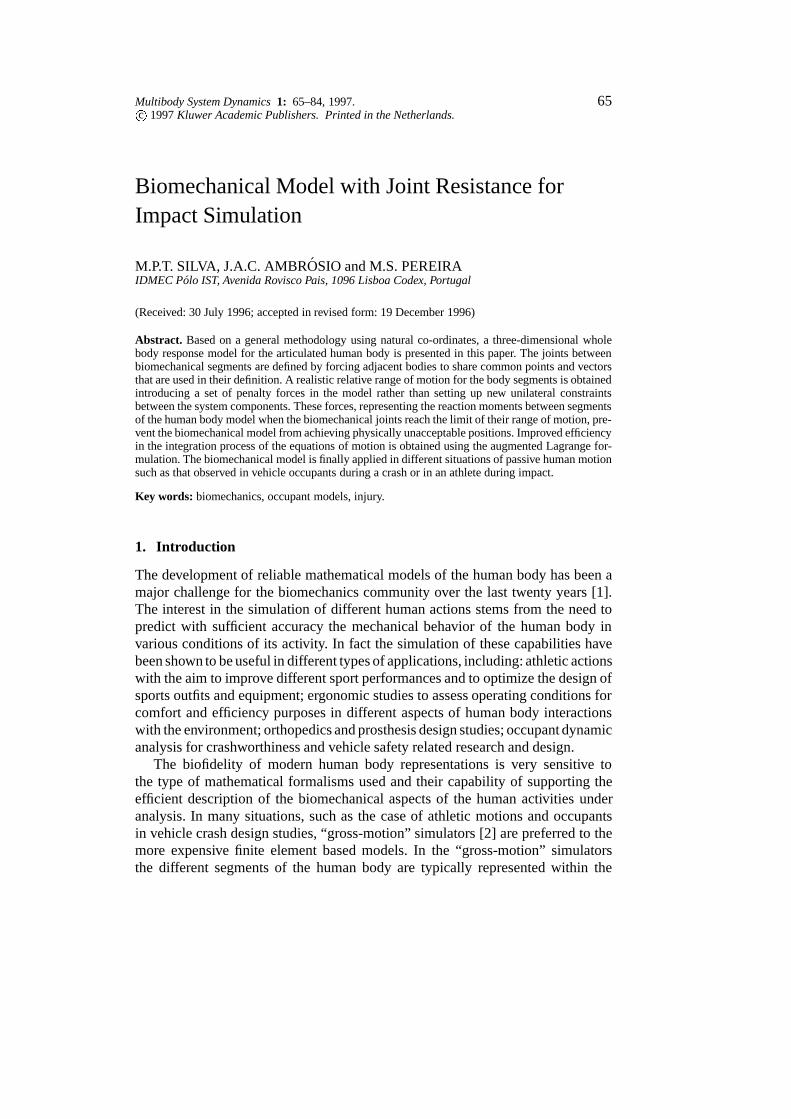
Figure 1. General multibody system.
framework of multibody systems by a set of rigid bodies connected by differenttypes of joints and actuators with a varying degree of complexity. Such detailedbiomechanic models are combined in a “gross-motion” simulation tool which canbe used with greater efficiency in different situations [3–6].
The multibody dynamics formulations used in this work are briefly introduced. Aset of natural co-ordinates are used in the description of the position of each body inthe system. The dynamic equations of motion are then obtained using the augmentedLagrangean formulation. The computer models of the human body include differentfeatures, namely: a complex system of generalized forcing functions representingadequate reactions between different segments of the human body; intrusion effectsand contact-impact capabilities.
Some applications of this complex model are presented in typical passive humanmotion cases such as the analysis of occupant motion in different vehicle crash sce-narios and the simulation of a side tackle of an athlete often observed in rugby andAmerican football. The biofidelity of such models is best illustrated in the computeranimation of the resulting gross motion events of the different simulations.
2. Multibody Equations of Motion with Natural Coordinates
2.1. GENERAL MULTIBODY SYSTEM
A multibody system is a collection of rigid and/or flexible bodies joined togetherby kinematic joints and acted by forces, as depicted by Figure 1. The forcesapplied over the system components may be the result of spring, dampers oractuators, devices or external applied forces describing, gravitational forces, seatbelts, contact-impact forces, or even complex biomechanical or mechanical joints.
Regardless of the system being modeled, it is necessary to describe systematical-ly and efficiently its equations of motion. Among the different sets of co-ordinates,
BIOMECHANICAL MODEL WITH JOINT RESISTANCE FOR IMPACT SIMULATION 67
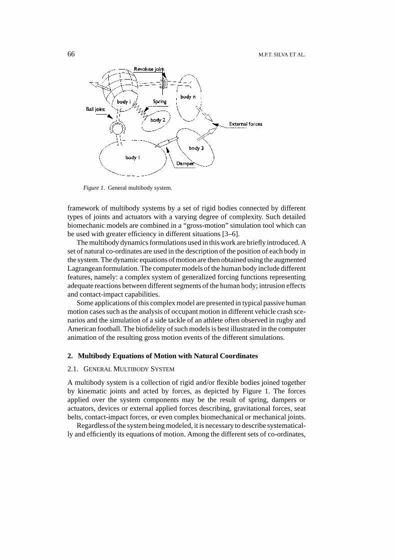
Figure 2. Inertial and local co-ordinate systems.
that can be chosen to describe the system, the natural co-ordinates provide a com-prehensive form of integrating efficiently different system features with generality[7–10].
2.2. EQUATIONS OF MOTION OF A RIGID BODY
With the use of natural co-ordinates a rigid body is described by a collection ofpoints and vectors. In Figure 2, a basic rigid body defined by two basic pointsand two non-coplanar unit vectors is represented. Other rigid bodies defined by anarbitrary large number of points and vectors may be obtained from this basic bodyby means of a co-ordinate transformation [7, 8].
Let the rigid body have a local reference frame (�; �; �) rigidly attached to it andwith an origin located in point o. Note that the origin of the body fixed referential isnot necessarily its center of mass. Let the principle of the virtual power be used toderive the equations of motion of the rigid body. The position vector r for a pointis described as a function of the co-ordinates of the basic points and vectors of therigid body
r = Cqe; (1)
where C is a transformation matrix independent of the motion of the body andtherefore constant in time
C = [(1� c1)I3 c1I3 c3I3 c3I3]; (2)
where c1, c2 and c3 are the components of (r� ri) described in the local referentialdefined by (rj�ri), u and v. I3 is a 3�3 identity matrix and qe = [rTi rTj uT vT ]T
is the vector of co-ordinates of the basic points and vectors with respect to the globalreference frame xyz. Differentiating Equation (1) with respect to time results inthe velocity and acceleration equations for point P :
_r = C _qe; (3)
68 M.P.T. SILVA ET AL.
�r = C�qe: (4)
The virtual power of the inertia forces for the rigid body is expressed as:
W � = � _q�Te
0@Z
�CTC d
1A �qe; (5)
where � is the mass density and the volume of the rigid body. It must be notedthat virtual velocity vector _q�e and the acceleration vector for the basic vectors andpoints �qe are independent of the body volume. The body mass matrix is
M =
Z
�CTC d: (6)
Integrating Equation (6) leads to the 12� 12 rigid body mass matrix
M =
2664(m� 2ma1 + z11)I3 (ma1 + z11)I3 (ma2 + z12)I3 (ma3 + z13)I3
(ma1 + z11)I3 z11I3 z12I3 z13I3
(ma2 + z21)I3 z21I3 z22I3 z23I3
(ma3 + z31)I3 z31I3 z32I3 z33I3
3775 ; (7)
where m is the rigid body mass, zij are coefficients related to the inertia tensor andai the components of the static moment of the rigid body [7]. This mass matrix isinvariant.
The mass matrix of bodies defined with different sets of basic points and vec-tors is obtained from this matrix after a proper co-ordinate transformation. Thistransformation corresponds to relate the position of the new points and vectors asa function of the points and vectors of the basic rigid body just described [7].
Concentrated forces can be applied in a generic point of the rigid body, otherthan a basic point, as described by Figure 3a. The case of an applied moment, asdepicted by Figure 3b, is described by a force binary where the two opposite forcesact in a plane perpendicular to the applied moment.
The concentrated force f applied on point P of a rigid body is described bya generalized force ge, applied to the basic points and vectors of that body. Therelation between these forces is obtained using the equivalence between their virtualwork
�W = �rTp f = �qTe ge: (8)
Vector rp, representing the position of pointP , is related with the basic co-ordinatesby Equation (1). Comparing the terms of the resulting equations, it is found that:
ge = CTp f: (9)
An applied moment is described here by a torque m given by two non-collinearand opposite forces f related by
m = ~umf; (10)
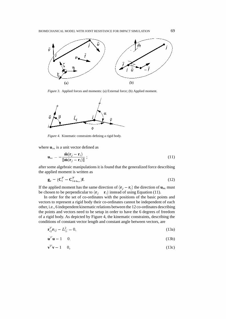
BIOMECHANICAL MODEL WITH JOINT RESISTANCE FOR IMPACT SIMULATION 69
Figure 3. Applied forces and moments: (a) External force; (b) Applied moment.
Figure 4. Kinematic constraints defining a rigid body.
where um is a unit vector defined as
um = �~m(rj � ri)k ~m(rj � ri)k
; (11)
after some algebraic manipulations it is found that the generalized force describingthe applied moment is written as
ge = (CTi + CT
i+um)f: (12)
If the applied moment has the same direction of (rj � ri) the direction of um mustbe chosen to be perpendicular to (rj � ri) instead of using Equation (11).
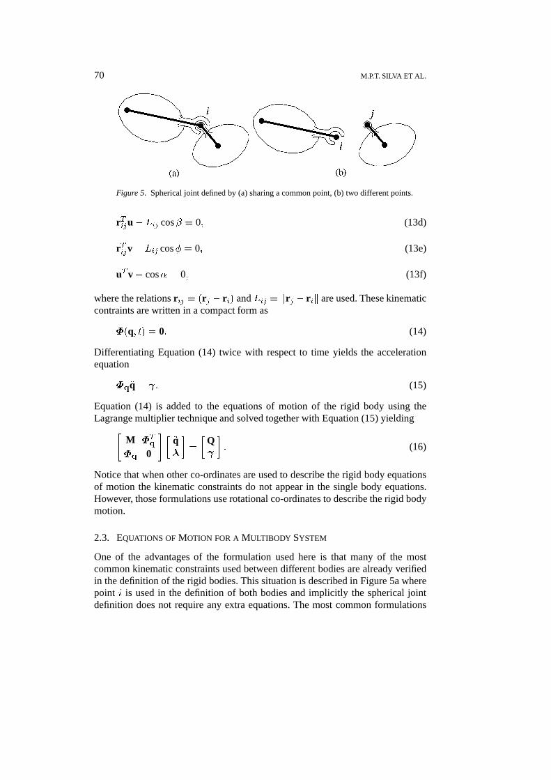
In order for the set of co-ordinates with the positions of the basic points andvectors to represent a rigid body their co-ordinates cannot be independent of eachother, i.e., 6 independent kinematic relations between the 12 co-ordinates describingthe points and vectors need to be setup in order to have the 6 degrees of freedomof a rigid body. As depicted by Figure 4, the kinematic constraints, describing theconditions of constant vector length and constant angle between vectors, are
rTijrij � L2ij = 0; (13a)
uTu� 1 = 0; (13b)
vT v� 1 = 0; (13c)
70 M.P.T. SILVA ET AL.
Figure 5. Spherical joint defined by (a) sharing a common point, (b) two different points.
rTiju� Lij cos� = 0; (13d)
rTijv� Lij cos� = 0; (13e)
uT v� cos� = 0; (13f)
where the relations rij = (rj � ri) and Lij = krj � rik are used. These kinematiccontraints are written in a compact form as
�(q; t) = 0: (14)
Differentiating Equation (14) twice with respect to time yields the accelerationequation
�q�q = : (15)
Equation (14) is added to the equations of motion of the rigid body using theLagrange multiplier technique and solved together with Equation (15) yielding"
M �Tq
�q 0
# ��q�
�=
�Q
�: (16)
Notice that when other co-ordinates are used to describe the rigid body equationsof motion the kinematic constraints do not appear in the single body equations.However, those formulations use rotational co-ordinates to describe the rigid bodymotion.
2.3. EQUATIONS OF MOTION FOR A MULTIBODY SYSTEM
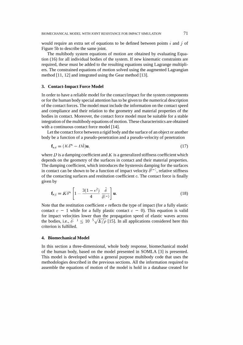
One of the advantages of the formulation used here is that many of the mostcommon kinematic constraints used between different bodies are already verifiedin the definition of the rigid bodies. This situation is described in Figure 5a wherepoint i is used in the definition of both bodies and implicitly the spherical jointdefinition does not require any extra equations. The most common formulations
BIOMECHANICAL MODEL WITH JOINT RESISTANCE FOR IMPACT SIMULATION 71
would require an extra set of equations to be defined between points i and j ofFigure 5b to describe the same joint.
The multibody system equations of motion are obtained by evaluating Equa-tion (16) for all individual bodies of the system. If new kinematic constraints arerequired, these must be added to the resulting equations using Lagrange multipli-ers. The constrained equations of motion solved using the augmented Lagrangianmethod [11, 12] and integrated using the Gear method [13].
3. Contact-Impact Force Model
In order to have a reliable model for the contact/impact for the system componentsor for the human body special attention has to be given to the numerical descriptionof the contact forces. The model must include the information on the contact speedand compliance and their relation to the geometry and material properties of thebodies in contact. Moreover, the contact force model must be suitable for a stableintegration of the multibody equations of motion. These characteristics are obtainedwith a continuous contact force model [14].
Let the contact force between a rigid body and the surface of an object or anotherbody be a function of a pseudo-penetration and a pseudo-velocity of penetration
fs;i = (K�n +D _�)u; (17)
whereD is a damping coefficient andK is a generalized stiffness coefficient whichdepends on the geometry of the surfaces in contact and their material properties.The damping coefficient, which introduces the hysteresis damping for the surfacesin contact can be shown to be a function of impact velocity _�(�), relative stiffnessof the contacting surfaces and restitution coefficient e. The contact force is finallygiven by
fs;i = K�n"
1 +3(1� e2)
4
_�
_�(�)
#u: (18)
Note that the restitution coefficient e reflects the type of impact (for a fully elasticcontact e = 1 while for a fully plastic contact e = 0). This equation is validfor impact velocities lower than the propagation speed of elastic waves acrossthe bodies, i.e., _�(�) � 10�5
pE=� [15]. In all applications considered here this
criterion is fulfilled.
4. Biomechanical Model
In this section a three-dimensional, whole body response, biomechanical modelof the human body, based on the model presented in SOMLA [3] is presented.This model is developed within a general purpose multibody code that uses themethodologies described in the previous sections. All the information required toassemble the equations of motion of the model is hold in a database created for
72 M.P.T. SILVA ET AL.
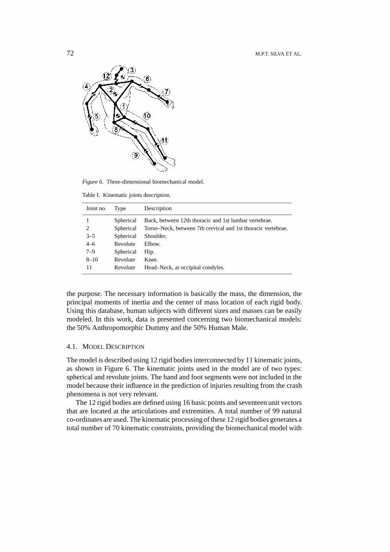
Figure 6. Three-dimensional biomechanical model.
Table I. Kinematic joints description.
Joint no. Type Description
1 Spherical Back, between 12th thoracic and 1st lumbar vertebrae.2 Spherical Torso–Neck, between 7th cervical and 1st thoracic vertebrae.3–5 Spherical Shoulder.4–6 Revolute Elbow.7–9 Spherical Hip.8–10 Revolute Knee.11 Revolute Head–Neck, at occipital condyles.
the purpose. The necessary information is basically the mass, the dimension, theprincipal moments of inertia and the center of mass location of each rigid body.Using this database, human subjects with different sizes and masses can be easilymodeled. In this work, data is presented concerning two biomechanical models:the 50% Anthropomorphic Dummy and the 50% Human Male.
4.1. MODEL DESCRIPTION
The model is described using 12 rigid bodies interconnected by 11 kinematic joints,as shown in Figure 6. The kinematic joints used in the model are of two types:spherical and revolute joints. The hand and foot segments were not included in themodel because their influence in the prediction of injuries resulting from the crashphenomena is not very relevant.
The 12 rigid bodies are defined using 16 basic points and seventeen unit vectorsthat are located at the articulations and extremities. A total number of 99 naturalco-ordinates are used. The kinematic processing of these 12 rigid bodies generates atotal number of 70 kinematic constraints, providing the biomechanical model with
BIOMECHANICAL MODEL WITH JOINT RESISTANCE FOR IMPACT SIMULATION 73
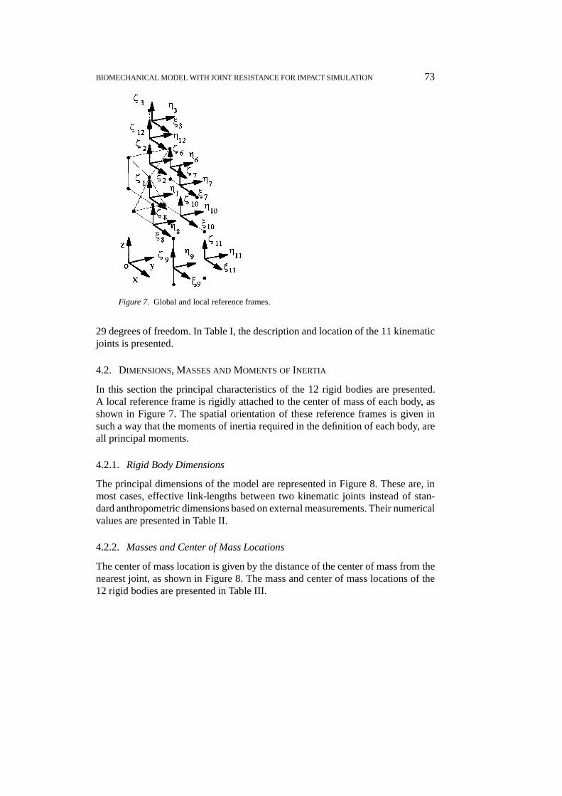
Figure 7. Global and local reference frames.
29 degrees of freedom. In Table I, the description and location of the 11 kinematicjoints is presented.
4.2. DIMENSIONS, MASSES AND MOMENTS OF INERTIA
In this section the principal characteristics of the 12 rigid bodies are presented.A local reference frame is rigidly attached to the center of mass of each body, asshown in Figure 7. The spatial orientation of these reference frames is given insuch a way that the moments of inertia required in the definition of each body, areall principal moments.
4.2.1. Rigid Body Dimensions
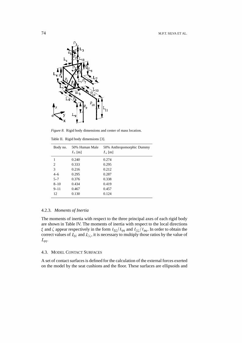
The principal dimensions of the model are represented in Figure 8. These are, inmost cases, effective link-lengths between two kinematic joints instead of stan-dard anthropometric dimensions based on external measurements. Their numericalvalues are presented in Table II.
4.2.2. Masses and Center of Mass Locations
The center of mass location is given by the distance of the center of mass from thenearest joint, as shown in Figure 8. The mass and center of mass locations of the12 rigid bodies are presented in Table III.
74 M.P.T. SILVA ET AL.
Figure 8. Rigid body dimensions and center of mass location.
Table II. Rigid body dimensions [3].
Body no. 50% Human Male 50% Anthropomorphic DummyLi [m] Li [m]
1 0.240 0.2742 0.333 0.2953 0.216 0.2124–6 0.295 0.2875–7 0.376 0.3388–10 0.434 0.4199–11 0.467 0.45712 0.130 0.124
4.2.3. Moments of Inertia
The moments of inertia with respect to the three principal axes of each rigid bodyare shown in Table IV. The moments of inertia with respect to the local directions� and � appear respectively in the form I��=I�� and I��=I�� . In order to obtain thecorrect values of I�� and I�� , it is necessary to multiply those ratios by the value ofI�� .
4.3. MODEL CONTACT SURFACES
A set of contact surfaces is defined for the calculation of the external forces exertedon the model by the seat cushions and the floor. These surfaces are ellipsoids and
BIOMECHANICAL MODEL WITH JOINT RESISTANCE FOR IMPACT SIMULATION 75
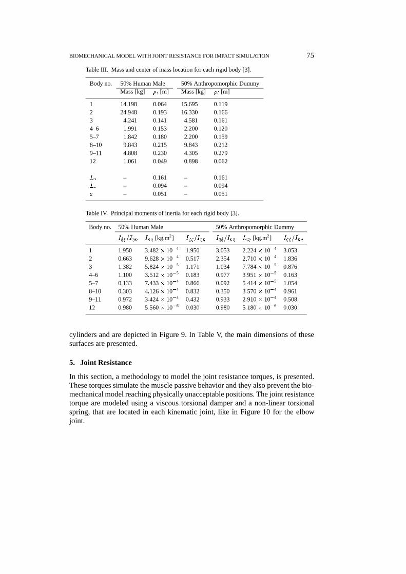
Table III. Mass and center of mass location for each rigid body [3].
Body no. 50% Human Male 50% Anthropomorphic DummyMass [kg] �i [m] Mass [kg] �i [m]
1 14.198 0.064 15.695 0.1192 24.948 0.193 16.330 0.1663 4.241 0.141 4.581 0.1614–6 1.991 0.153 2.200 0.1205–7 1.842 0.180 2.200 0.1598–10 9.843 0.215 9.843 0.2129–11 4.808 0.230 4.305 0.27912 1.061 0.049 0.898 0.062
Ls – 0.161 – 0.161Lh – 0.094 – 0.094e – 0.051 – 0.051
Table IV. Principal moments of inertia for each rigid body [3].
Body no. 50% Human Male 50% Anthropomorphic Dummy
I��=I�� I�� [kg.m2] I��=I�� I��=I�� I�� [kg.m2] I��=I��
1 1.950 3:482 � 10�4 1.950 3.053 2:224 � 10�4 3.0532 0.663 9:628 � 10�4 0.517 2.354 2:710 � 10�4 1.8363 1.382 5:824 � 10�5 1.171 1.034 7:784 � 10�5 0.8764–6 1.100 3:512 � 10�5 0.183 0.977 3:951 � 10�5 0.1635–7 0.133 7:433 � 10�4 0.866 0.092 5:414 � 10�5 1.0548–10 0.303 4:126 � 10�4 0.832 0.350 3:570 � 10�4 0.9619–11 0.972 3:424 � 10�4 0.432 0.933 2:910 � 10�4 0.50812 0.980 5:560 � 10�6 0.030 0.980 5:180 � 10�6 0.030
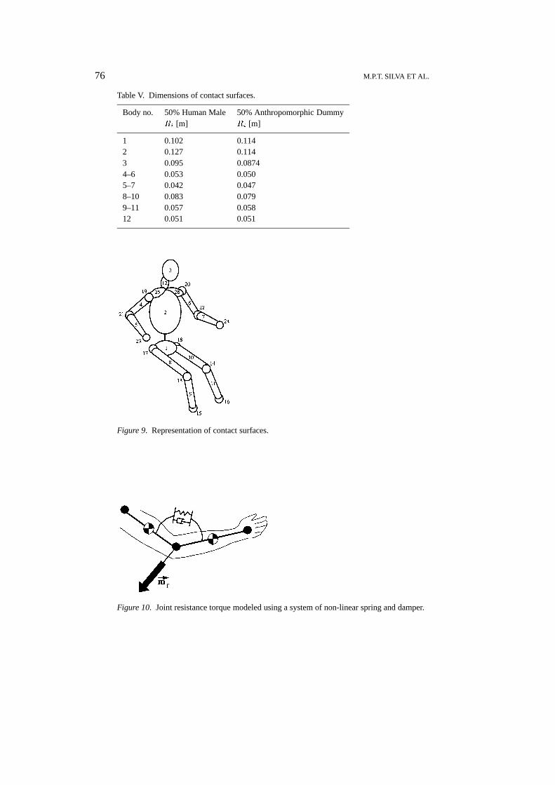
cylinders and are depicted in Figure 9. In Table V, the main dimensions of thesesurfaces are presented.
5. Joint Resistance
In this section, a methodology to model the joint resistance torques, is presented.These torques simulate the muscle passive behavior and they also prevent the bio-mechanical model reaching physically unacceptable positions. The joint resistancetorque are modeled using a viscous torsional damper and a non-linear torsionalspring, that are located in each kinematic joint, like in Figure 10 for the elbowjoint.
76 M.P.T. SILVA ET AL.
Table V. Dimensions of contact surfaces.
Body no. 50% Human Male 50% Anthropomorphic DummyRi [m] Ri [m]
1 0.102 0.1142 0.127 0.1143 0.095 0.08744–6 0.053 0.0505–7 0.042 0.0478–10 0.083 0.0799–11 0.057 0.05812 0.051 0.051
Figure 9. Representation of contact surfaces.
Figure 10. Joint resistance torque modeled using a system of non-linear spring and damper.
BIOMECHANICAL MODEL WITH JOINT RESISTANCE FOR IMPACT SIMULATION 77
5.1. VISCOUS TORSIONAL DAMPER
This element is included in order to permit some energy dissipation. The torsionaldamper has a small constant coefficient ji being the total damping torque at eachjoint given by the expression
mdi = �ji _�i; (19)
where _�i is the relative angular velocity vector between the two bodies intercon-nected by that joint and the index i denotes the joint number. As one can see fromEquation (19), the torque mdi and the vector _�i have opposite directions meaningthat this torque acts to resist the motion of the joint.
5.2. NON-LINEAR TORSIONAL SPRING
The contribution of the non-linear spring has two terms. The first one is a resistingtorque mri that acts to resist the motion of the joint. For the dummy joint, thistorque has a constant value and it is applied to the whole range of the joint motion.For the human joint this torque has an initial value which drops to zero after a smallangular displacement from the joint initial position [16]. In both cases, this torquehas a direction that is opposite to the direction of the relative angular velocity vectorbetween the two bodies interconnected by that joint, that is
mri = �mri_�ik
_�ik�1: (20)
The second term is a penalty resisting torque mpi . This torque is null duringthe normal joint rotation but it increases rapidly, from zero until a maximum value,when the two bodies interconnected by that joint, achieve physically unacceptablepositions. In the following section a methodology for the calculation of the valueof this torque is presented.
5.2.1. Calculation of the Penalty Resisting Torque
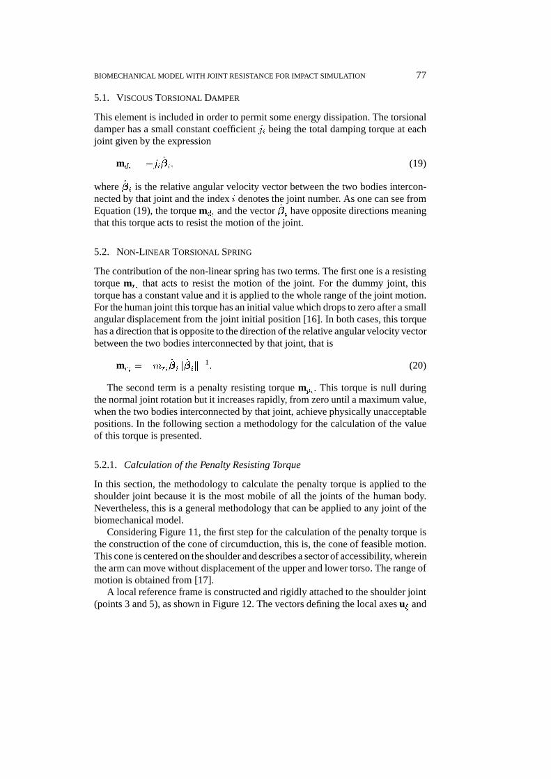
In this section, the methodology to calculate the penalty torque is applied to theshoulder joint because it is the most mobile of all the joints of the human body.Nevertheless, this is a general methodology that can be applied to any joint of thebiomechanical model.
Considering Figure 11, the first step for the calculation of the penalty torque isthe construction of the cone of circumduction, this is, the cone of feasible motion.This cone is centered on the shoulder and describes a sector of accessibility, whereinthe arm can move without displacement of the upper and lower torso. The range ofmotion is obtained from [17].
A local reference frame is constructed and rigidly attached to the shoulder joint(points 3 and 5), as shown in Figure 12. The vectors defining the local axes u� and
78 M.P.T. SILVA ET AL.
Figure 11. Cone of circumduction for the shoulder joint.
Figure 12. Local reference frame for the shoulder joint.
u� are built using basic points and unit vectors that were used in the definition ofthe upper torso rigid body, i.e.
u� = un (21)
and
u� =rj � rikrj � rik
: (22)
The third base vector is calculated as the result of the cross product of the first two:
u� = ~u�u�: (23)
BIOMECHANICAL MODEL WITH JOINT RESISTANCE FOR IMPACT SIMULATION 79
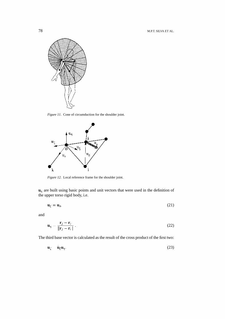
Figure 13. Longitude and latitude angles and interpolation curve for the shoulder joint.
After the construction of this reference frame, a fourth vector is introduced withthe same direction of the upper arm and is expressed using the two basic pointsbelonging to this body:
ur =rk � rokrk � rok
: (24)
With these vectors, the angles of longitude � and latitude � of the unit vector ur
in the local reference frame are calculated, as depicted in Figure 13a. The angleof maximum amplitude �max is also calculated for a specified longitude �, using acubic spline interpolation curve. This curve, uses the angles of maximum amplitudeat the four main quadrants (�I, �II, �III and �IV), to interpolate the angle of themaximum amplitude �max for a specified longitude �, as shown in Figure 13b.
If the effective latitude � exceeds the maximum allowable latitude �max, thena penetration on a zone of unacceptable position is occurring and the penaltyresisting torque is applied. The magnitude of this torque increases rapidly with thepenetration and the direction is the result of the cross-product between vector u�
and vector ur:
mpi = mpi
"3��i � �imax
��i
�2
� 2��i � �imax
��i
�3#~u�ur; (25)
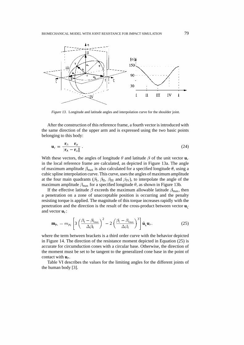
where the term between brackets is a third order curve with the behavior depictedin Figure 14. The direction of the resistance moment depicted in Equation (25) isaccurate for circumduction cones with a circular base. Otherwise, the direction ofthe moment must be set to be tangent to the generalized cone base in the point ofcontact with ur.
Table VI describes the values for the limiting angles for the different joints ofthe human body [3].
80 M.P.T. SILVA ET AL.
Figure 14. Third order curve.
Table VI. Joint resistance data.
Joint �iI [�] �iII [�] �iIII [�] �iIV [�] ��i [�] mi [g] mpi [Nm] ji [Nms]
1 40.0 35.0 30.0 35.0 11.5 2.0 226.0 16.9502 60.0 40.0 60.0 40.0 15.0 2.0 678.0 3.3903–5 140.0 90.0 30.0 90.0 11.5 1.0 226.0 3.7634–6 90.0 – 45.0 – 11.5 1.0 226.0 3.3907–9 10.0 120.0 50.0 45.0 11.5 2.0 452.0 5.6508–10 – 90.0 – 45.0 11.5 1.0 226.0 5.65011 19.0 – 2.0 – 15.0 2.0 452.0 16.950
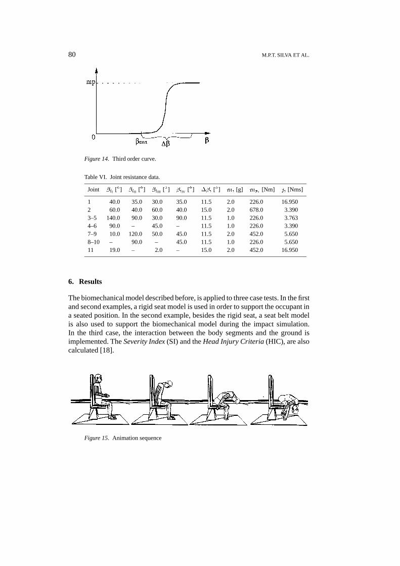
6. Results
The biomechanical model described before, is applied to three case tests. In the firstand second examples, a rigid seat model is used in order to support the occupant ina seated position. In the second example, besides the rigid seat, a seat belt modelis also used to support the biomechanical model during the impact simulation.In the third case, the interaction between the body segments and the ground isimplemented. The Severity Index (SI) and the Head Injury Criteria (HIC), are alsocalculated [18].
Figure 15. Animation sequence
BIOMECHANICAL MODEL WITH JOINT RESISTANCE FOR IMPACT SIMULATION 81
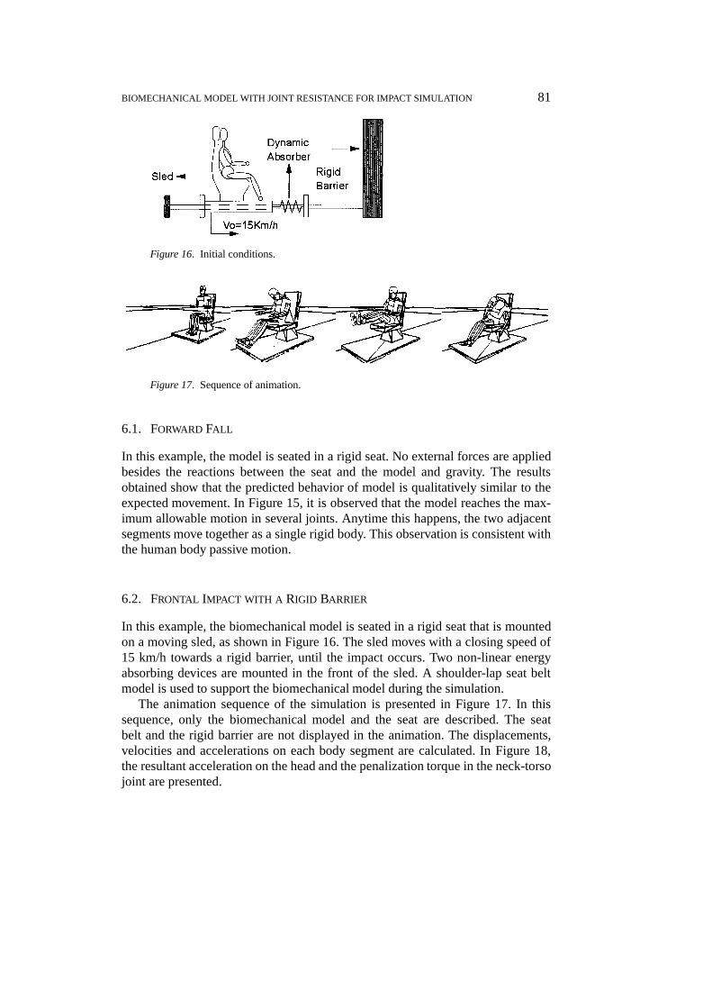
Figure 16. Initial conditions.
Figure 17. Sequence of animation.
6.1. FORWARD FALL
In this example, the model is seated in a rigid seat. No external forces are appliedbesides the reactions between the seat and the model and gravity. The resultsobtained show that the predicted behavior of model is qualitatively similar to theexpected movement. In Figure 15, it is observed that the model reaches the max-imum allowable motion in several joints. Anytime this happens, the two adjacentsegments move together as a single rigid body. This observation is consistent withthe human body passive motion.
6.2. FRONTAL IMPACT WITH A RIGID BARRIER
In this example, the biomechanical model is seated in a rigid seat that is mountedon a moving sled, as shown in Figure 16. The sled moves with a closing speed of15 km/h towards a rigid barrier, until the impact occurs. Two non-linear energyabsorbing devices are mounted in the front of the sled. A shoulder-lap seat beltmodel is used to support the biomechanical model during the simulation.
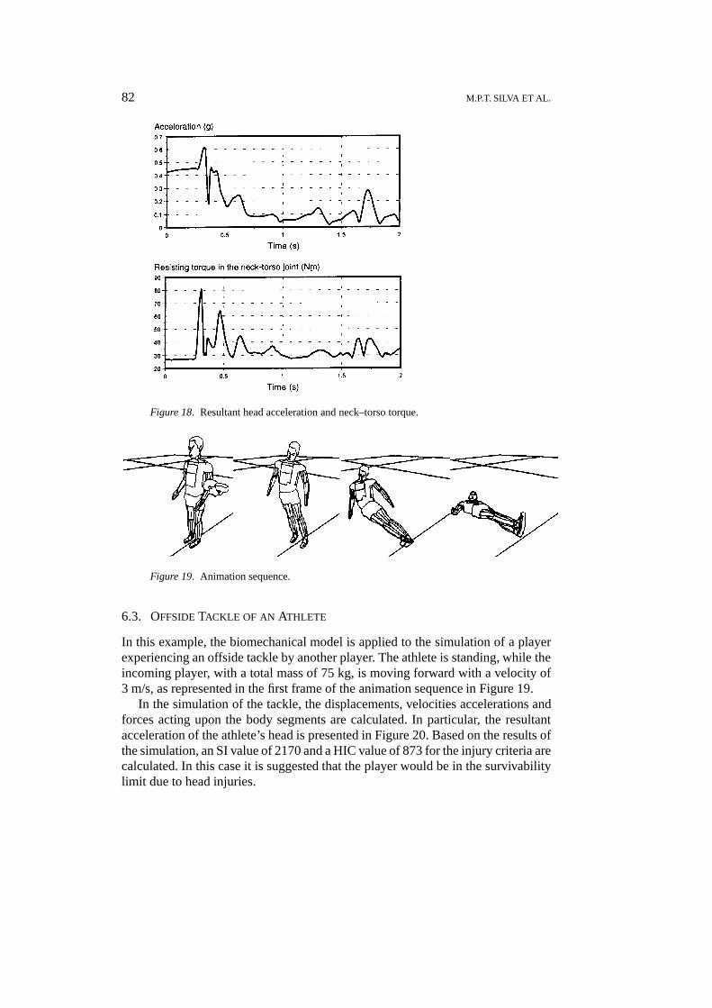
The animation sequence of the simulation is presented in Figure 17. In thissequence, only the biomechanical model and the seat are described. The seatbelt and the rigid barrier are not displayed in the animation. The displacements,velocities and accelerations on each body segment are calculated. In Figure 18,the resultant acceleration on the head and the penalization torque in the neck-torsojoint are presented.
82 M.P.T. SILVA ET AL.
Figure 18. Resultant head acceleration and neck–torso torque.
Figure 19. Animation sequence.
6.3. OFFSIDE TACKLE OF AN ATHLETE
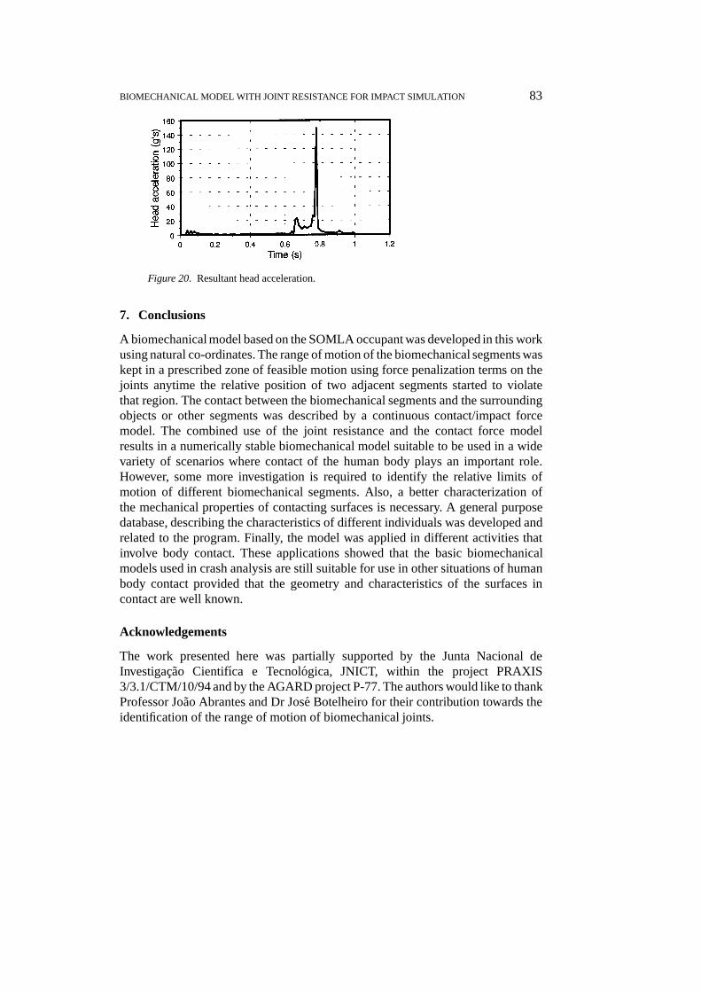
In this example, the biomechanical model is applied to the simulation of a playerexperiencing an offside tackle by another player. The athlete is standing, while theincoming player, with a total mass of 75 kg, is moving forward with a velocity of3 m/s, as represented in the first frame of the animation sequence in Figure 19.
In the simulation of the tackle, the displacements, velocities accelerations andforces acting upon the body segments are calculated. In particular, the resultantacceleration of the athlete’s head is presented in Figure 20. Based on the results ofthe simulation, an SI value of 2170 and a HIC value of 873 for the injury criteria arecalculated. In this case it is suggested that the player would be in the survivabilitylimit due to head injuries.
BIOMECHANICAL MODEL WITH JOINT RESISTANCE FOR IMPACT SIMULATION 83
Figure 20. Resultant head acceleration.
7. Conclusions
A biomechanical model based on the SOMLA occupant was developed in this workusing natural co-ordinates. The range of motion of the biomechanical segments waskept in a prescribed zone of feasible motion using force penalization terms on thejoints anytime the relative position of two adjacent segments started to violatethat region. The contact between the biomechanical segments and the surroundingobjects or other segments was described by a continuous contact/impact forcemodel. The combined use of the joint resistance and the contact force modelresults in a numerically stable biomechanical model suitable to be used in a widevariety of scenarios where contact of the human body plays an important role.However, some more investigation is required to identify the relative limits ofmotion of different biomechanical segments. Also, a better characterization ofthe mechanical properties of contacting surfaces is necessary. A general purposedatabase, describing the characteristics of different individuals was developed andrelated to the program. Finally, the model was applied in different activities thatinvolve body contact. These applications showed that the basic biomechanicalmodels used in crash analysis are still suitable for use in other situations of humanbody contact provided that the geometry and characteristics of the surfaces incontact are well known.
Acknowledgements
The work presented here was partially supported by the Junta Nacional deInvestigacao Cientifıca e Tecnologica, JNICT, within the project PRAXIS3/3.1/CTM/10/94 and by the AGARD project P-77. The authors would like to thankProfessor Joao Abrantes and Dr Jose Botelheiro for their contribution towards theidentification of the range of motion of biomechanical joints.
84 M.P.T. SILVA ET AL.
References
1. Nigg, B.M. and Herzog, W., Biomechanics of the Musculo-Skeletal System, John Wiley and Sons,Toronto, 1994.
2. Prasad, P., ‘An overview of major occupant simulation models’, in Mathematical Simulation ofOccupant and Vehicle Kinematics, SAE publication P-146, SAE paper No. 840855, 1984.
3. Laananen, D., Bolukbasi, A. and Coltman, J., ‘Computer simulation of an aircraft seat andoccupant in a crash environment – Volume 1: Technical report’, US Department of Transportation,Federal Aviation Administration, Report No. DOT/FAA/CT-82/33-I, 1993.
4. Laananen, D., ‘Computer simulation of an aircraft seat and occupant(s) in a crash environment –Program SOM-LA/SOM-TA User manual’, US Department of Transportation, Federal AviationAdministration, Report No. DOT/FAA/CT-90/4, 1991.
5. Obergefell, L.A., Gordon, T.R. and Fleck, J.I., ‘Articulated total body model enhancements,Vol. 2: User’s guide’, Report No. AAMRL-TR-88-043, Armstrong Aerospace Med. ResearchLab., Wright Patterson Airforce Base, Dayton, Ohio, 1988.
6. TNO,Madymo User’s Manual, Version 5.0, TNO, Delft, 1992.7. Jalon, J.G. and Bayo, E., Kinematic and Dynamic Simulation of Multibody Systems, Springer-
Verlag, Heidelberg, 1994.8. Nikravesh, P.E. and Affifi, H.A., ‘Construction of the equations of motion for multibody dynamics
using point and joint coordinates’, in Computer-Aided Analysis of Rigid and Flexible MechanicalSystems, M.S. Pereira and J.A.C. Ambrosio (eds), Kluwer Academic Publishers, Dordrecht, 1994,31–60.
9. Nikravesh, P.E., Computer-Aided Analysis of Mechanical Systems, Prentice-Hall, Englewood-Cliffs, NJ. 1988.
10. Haug, E.J., Computer Aided Kinematics and Dynamics of Mechanical Systems, Allyn and Bacon,Chicago, 1989.
11. Bayo, E. and Ledesma, R., ‘Augmented Lagrangian and mass-orthogonal projection methods forconstrained multibody dynamics’, Journal of Nonlinear Dynamics 9, 1996, 113–130.
12. Avello, A. and Bayo, E., ‘A singularity-free penalty formulation for the dynamics of constrainedmultibody systems’, Mechanical Design and Synthesis, ASME DE-Vol. 1, 1992, 643–649.
13. Gear, C.W., ‘Numerical solution of differential-algebraic equations’, IEE Transactions on CircuitTheory CT-18, 1981, 89–95.
14. Lankarani, H., Ma, D. and Menon, R., ‘Impact dynamics of multibody mechanical systems andapplication to crash responses of aircraft occupant/structure’, in Computational Dynamics inMultibody Systems, M.F.O.S. Pereira and J.A.C. Ambrosio (eds), Kluwer Academic Publishers,Dordrecht, 1995, 239–265.
15. Love, A.E.H., A Treatise on the Mathematical Theory of Elasticity, 4th edition, Dover Publica-tions, New York, 1944.
16. Silva, M.S.T and Ambrosio, J.A.C., ‘Modelo Biomecanico Para A Dinamica Computacional DoMovimento Humano Articulado’ (Biomechanical model for the computational dynamics of thehuman articulated motion), Technical Report IDMEC/CPM-96/003, IDMEC – Instituto SuperiorTecnico, 1996.
17. CIBA GEIGY, Folia Rheumatologica, Motilitat von Hufte, Schulter, Hand und Fuß, CIBA GEIGYGrubH Wehr/Baden, 1979.
18. Wismans, J.S., Janssen, E.G., Beusenberg, M., Koppens, W.P. and Lupker, H.A., ‘Injury bio-mechanics’, Third term W-3.3, WMT-3.3, code 4J610, Faculty of Mechanical Engineering,Eindhoven University of Technology, 1994.


![[Biomechanical aspects of revision components for knee arthroplasty]](https://img.pdfslide.net/doc/110x75/6343c4a09611753592094cac/biomechanical-aspects-of-revision-components-for-knee-arthroplasty.jpg)


