Can the universe be represented by a superposition of spacetime manifolds?

Available online at www.sciencedirect.com

Physics Procedia 20 (2011) 47–62

1875-3892 © 2011 Published by Elsevier B.V. Selection and/or peer-review under responsibility of Institute for Advanced studies in Space, Propulsion and Energy Sciencesdoi:10.1016/j.phpro.2011.08.004

Space, Propulsion & Energy Sciences International Forum - 2011

Can the universe be represented by a superposition of space-time manifolds?

R. Jensen*

Dept of Mathematics & Informatics, Trine University, Angola IN 46703 USA

Abstract

In this article it is argued, that the universe cannot be modeled as a space-time manifold. A theorem of geometry provides that null geodesics on a space-time manifold which begin at the same point with the same initial tangent vector are unique. But in reality, light originating from a single point with a given initial direction does not travel along a unique null geodesic path when a massive object attracts it, in particular when the massive object is in an indefinite location. Therefore, the universe cannot be described as a space-time manifold. It is then argued that the universe is a superposition of space-time manifolds, where the manifolds form a Hilbert space over the complex numbers.

© 2011 Published by Elsevier B.V. Selection and/or peer-review under responsibility of Institute for Advanced Studies in the Space, Propulsion and Energy Sciences

PACS: 04.50.Kd Keywords: Superposition; Space-Time; Manifold; Many Worlds; Geodesic Uniqueness

1. Introduction

In the last seventy or so years, much has been written on the subject of "unifying" gravity with electromagnetism and the other known forces, but little underlying philosophy seems to be at the heart of such unification schemes. Perhaps this is why these ideas have not born fruit. Most of the approaches take the route of "quantizing" gravity: since the remaining forces have been "quantized," so also gravity must be quantized. The problem is gravity seems not to want to be quantized. So a different tact must be taken, other than simply attempting to “quantize” gravity by brute force. Thus, we begin a new approach, by first appealing to the main problem between the relativity theory and quantum mechanics: the determinism of the former vs. the indeterminism of the latter. This important

* Corresponding author. Tel.: 260-665-4244; fax: +0-000-000-0000 . E-mail address: [email protected] .

© 2011 Published by Elsevier B.V. Selection and/or peer-review under responsibility of Institute for Advanced studies in Space, Propulsion and Energy Sciences

48 R. Jensen / Physics Procedia 20 (2011) 47–62

difference (determinism vs. indeterminism) between the two theories cannot be ignored. In the next section it is shown that because quantum mechanics predicts indeterminate paths for particles of light, our universe cannot possibly be a four-dimensional space-time manifold. Following that, it is proposed, what kind of structure the universe must have: i.e. a "superposition of space-times."

Nomenclature

C = set of complex numbers

DMC = vector space of manifolds M with boundary D over the complex numbers

1C = set of functions with continuous derivative

C = vector space of space time-manifolds over the complex numbers

C = completion of C

DM = set of manifolds M with boundary D

DM = manifold with boundary D

MZ = Mach-Zehnder interferometer

i = projection operator for projecting onto a vector i

R = set of real numbers

= set of space-time manifolds TQFT = topological quantum field theory X* = the dual of the set X

2. Why the Universe is Not Representable by a Space-Time Manifold

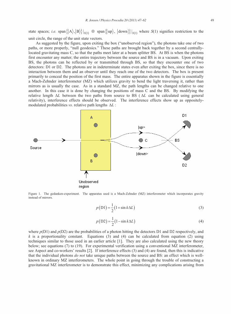
Consider the following gedanken-experiment: a box contains a small object with mass, and the box contains several holes, so that light may enter in and out of the box. See Figure 1. The object can take one of two positions: A or B. The probability that the object is in either position is assumed to be equivalent. If the observer is forbidden from observing the interior of the box and hence the position of the object, then the object will take on an indeterminate state. If we say that the state vector of the object is then

1

2A B (1)

is its representation in terms of positions A and B, where A , B is the basis, pertaining to the two

positions, respectively. Even if the object is microscopic, it nevertheless will have a gravitational field, and so light passing through the box will have its trajectory bent by it. If the object is in position A, then the light will be bent one way. If it is in position B, then the light will be bent another way, as illustrated in the figure. These two possible states for a single light particle can be designated as up and down

respectively, signifying the direction of bending. Thus, if a single light particle or photon is allowed to traverse the box, then the state of the combined system of photon plus object is given by the state

1A up B down

2. (2)

Equation (2) shows that since the object is in an indeterminate state, so will the photon be in an indeterminate state. This combined state (2) is an element of the tensor product of the two individual

R. Jensen / Physics Procedia 20 (2011) 47–62 49

state spaces; i.e. 1span A , B |S 1span up , down |S where S(1) signifies restriction to the

unit circle, the range of the unit state vectors. As suggested by the figure, upon exiting the box (“unobserved region”), the photons take one of two paths, or more properly, “null geodesics.” These paths are brought back together by a second centrally-located gravitating mass C, so that the paths meet later at a beam splitter BS. At BS is when the photons first encounter any matter; the entire trajectory between the source and BS is in a vacuum. Upon exiting BS, the photons can be reflected by or transmitted through BS, so that they encounter one of two detectors: D1 or D2. The photons are in indeterminate states even after exiting the box, since there is no interaction between them and an observer until they reach one of the two detectors. The box is present primarily to conceal the position of the first mass. The entire apparatus shown in the figure is essentially a Mach-Zehnder interferometer (MZ) which utilizes gravity to bend the light traversing it, rather than mirrors as is usually the case. As in a standard MZ, the path lengths can be changed relative to one another. In this case it is done by changing the positions of mass C and the BS. By modifying the relative length L between the two paths from source to BS ( L can be calculated using general relativity), interference effects should be observed. The interference effects show up as oppositely-modulated probabilities vs. relative path lengths L :

Figure 1. The gedanken-experiment. The apparatus used is a Mach-Zehnder (MZ) interferometer which incorporates gravity instead of mirrors.

1D1 1 sin

2p k L (3)

1D2 1 sin

2p k L (4)

where p(D1) and p(D2) are the probabilities of a photon hitting the detectors D1 and D2 respectively, and k is a proportionality constant. Equations (3) and (4) can be calculated from equation (2) using techniques similar to those used in an earlier article [1]. They are also calculated using the new theory below; see equations (7) to (19). For experimental verification using a conventional MZ interferometer, see Aspect and co-workers’ results [2]. If interference effects (3) and (4) are found, then this is indicative that the individual photons do not take unique paths between the source and BS: an effect which is well-known in ordinary MZ interferometers. The whole point in going through the trouble of constructing a gravitational MZ interferometer is to demonstrate this effect, minimizing any complications arising from


the light interacting with matter; i.e. mirrors. Thus we can consider the experiment within the context of general relativity theory. As to be demonstrated below, non-uniqueness of the geodesic will pose a problem for any theory claiming that the photons of light are propagating on something representable by a space-time manifold, or space-time for short. The following is a result from differential geometry: for a manifold M, a geodesic beginning at a point p in M with an initial tangent vector x must be unique for a non-zero length of time t: Theorem 1: Let M be a manifold with metric g. Let Mp and T Mpx = space of tangent vectors

of M at p. Let t I R be a parameter where I is an open interval containing 0. Then there exists

0 such that there exists geodesic : I M , 0 p and 0 x , where is unique for t .

Theorem 1 can be proved using techniques in differential equations; e.g. see Steiner’s online Fall2005 Graduate Differential Geometry Lecture Notes. Many texts on geometry do not include a proof of this important result; indeed many authors assume it to be true without comment. This is evident in texts where the exponential map is implied as well-defined, but not proven. In theorem 1, uniqueness is guaranteed only for t . Let us examine this restriction. Let M be a

space-time manifold. Suppose a unique null geodesic originates from 0 Mp for all 0 t but

then branches into two null geodesics at 1t t where 1t and 1t Mq . [See e.g. the text by

Beem, Ehrlich and Easley [3] for precise definitions of space-time and null geodesic.] According to the theorem, nothing is contradictory. However, if we reparametrize the geodesic using 1s t t so that now

q is the initial position (s = 0) of the geodesic, and say, T Mqy is its unique initial velocity there, then

there is now no such 0 so that the theorem holds, since the geodesic branches at s = 0. Thus to avoid a contradiction in theorem 1, one of two things must be true: (a) T Mqy is not unique; i.e. the two

branches begin at q with two different velocity vectors , ' , 'T Mqy y y y , or (b) any geodesic on M

never branches; i.e. the theorem holds not just for t but for all t I . If case (a) is true and M is a

space-time, then the null geodesics are not 1C everywhere since 'y y . Not only this, but ' cy y

, ' 0y y ; meaning that the initial tangents have different direction at s = 0 and so there is

definitely branching there (c is the speed of light.). Thus the null geodesic is not unique. Therefore: Theorem 2: Let Mp , where M is a space-time and T Mpx is the initial velocity of a null

geodesic. Then a null geodesic : I M originating at p 0 and x 0 is unique for all t I ,

provided that any such null geodesic originating from p and x is 1C on its domain I. In other words, there is no branching of null geodesics from a point anywhere provided that all null

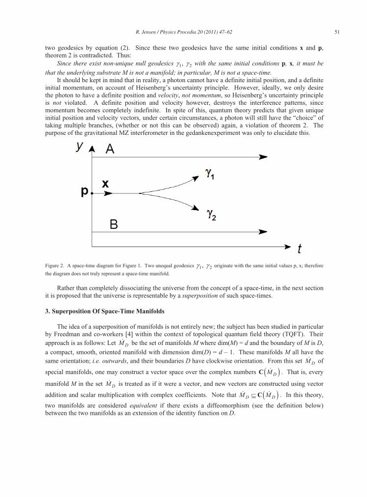
geodesics must have continuous derivatives. Here it will be assumed that the null geodesics are all 1C on a space-time manifold, provided there is no interaction with matter. On a space time, geodesics and null geodesics in particular should be at least C1, if there is no interaction with photons of light and matter. This was the reason a gravitational MZ interferometer was constructed in the gedankenexperiment—to sufficiently eliminate photon-matter interaction. Thus theorem 2 will be assumed to apply. With theorem 2 in mind, assume then that the universe can be represented by a space-time M. Mark the location of the source in Figure 1 by p, and the initial velocity of any photons leaving the source as x,the initial tangent vector. A space-time diagram of the situation in Figure 1 showing the time t axis and the space axis y perpendicular to x and in the plane of the null geodesics is given in Figure 2. Above and below the null geodesics are shown the world-lines of the mass in position A and in position B, respectively. The photon takes null geodesic 1 if the mass is in position A and 2 if in position B. But

the mass is in a superposition of the positions A and B, so the photon is likewise in a superposition of the


two geodesics by equation (2). Since these two geodesics have the same initial conditions x and p,theorem 2 is contradicted. Thus: Since there exist non-unique null geodesics 1 2, with the same initial conditions p, x, it must be

that the underlying substrate M is not a manifold; in particular, M is not a space-time. It should be kept in mind that in reality, a photon cannot have a definite initial position, and a definite initial momentum, on account of Heisenberg’s uncertainty principle. However, ideally, we only desire the photon to have a definite position and velocity, not momentum, so Heisenberg’s uncertainty principle is not violated. A definite position and velocity however, destroys the interference patterns, since momentum becomes completely indefinite. In spite of this, quantum theory predicts that given unique initial position and velocity vectors, under certain circumstances, a photon will still have the “choice” of taking multiple branches, (whether or not this can be observed) again, a violation of theorem 2. The purpose of the gravitational MZ interferometer in the gedankenexperiment was only to elucidate this.

Figure 2. A space-time diagram for Figure 1. Two unequal geodesics 1 2, originate with the same initial values p, x; therefore

the diagram does not truly represent a space-time manifold.

Rather than completely dissociating the universe from the concept of a space-time, in the next section it is proposed that the universe is representable by a superposition of such space-times.

3. Superposition Of Space-Time Manifolds

The idea of a superposition of manifolds is not entirely new; the subject has been studied in particular by Freedman and co-workers [4] within the context of topological quantum field theory (TQFT). Their approach is as follows: Let DM be the set of manifolds M where dim(M) = d and the boundary of M is D,

a compact, smooth, oriented manifold with dimension dim(D) = d – 1. These manifolds M all have the same orientation; i.e. outwards, and their boundaries D have clockwise orientation. From this set DM of

special manifolds, one may construct a vector space over the complex numbers DMC . That is, every

manifold M in the set DM is treated as if it were a vector, and new vectors are constructed using vector

addition and scalar multiplication with complex coefficients. Note that D DM MC . In this theory,

two manifolds are considered equivalent if there exists a diffeomorphism (see the definition below) between the two manifolds as an extension of the identity function on D.


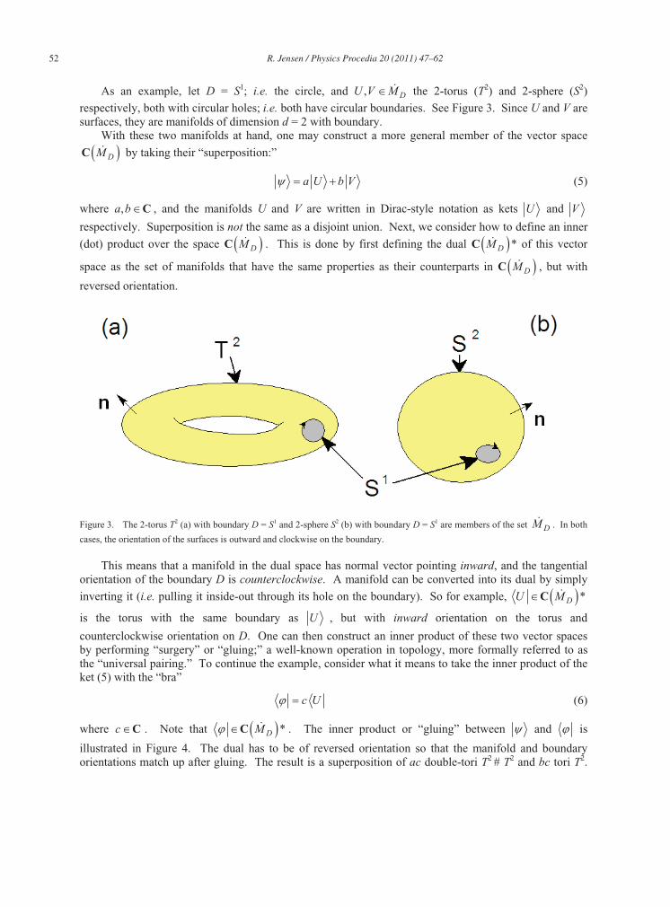
As an example, let D = S1; i.e. the circle, and , DU V M the 2-torus (T2) and 2-sphere (S2)respectively, both with circular holes; i.e. both have circular boundaries. See Figure 3. Since U and V are surfaces, they are manifolds of dimension d = 2 with boundary. With these two manifolds at hand, one may construct a more general member of the vector space

DMC by taking their “superposition:”

a U b V (5)

where ,a b C , and the manifolds U and V are written in Dirac-style notation as kets U and V

respectively. Superposition is not the same as a disjoint union. Next, we consider how to define an inner

(dot) product over the space DMC . This is done by first defining the dual *DMC of this vector

space as the set of manifolds that have the same properties as their counterparts in DMC , but with

reversed orientation.

Figure 3. The 2-torus T2 (a) with boundary D = S1 and 2-sphere S2 (b) with boundary D = S1 are members of the set DM . In both

cases, the orientation of the surfaces is outward and clockwise on the boundary.

This means that a manifold in the dual space has normal vector pointing inward, and the tangential orientation of the boundary D is counterclockwise. A manifold can be converted into its dual by simply

inverting it (i.e. pulling it inside-out through its hole on the boundary). So for example, *DU MC

is the torus with the same boundary as U , but with inward orientation on the torus and

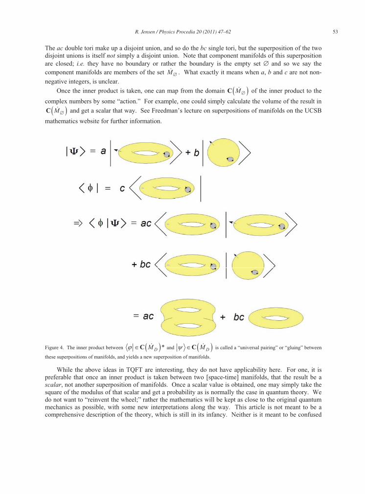
counterclockwise orientation on D. One can then construct an inner product of these two vector spaces by performing “surgery” or “gluing;” a well-known operation in topology, more formally referred to as the “universal pairing.” To continue the example, consider what it means to take the inner product of the ket (5) with the “bra”

c U (6)

where c C . Note that *DMC . The inner product or “gluing” between and is

illustrated in Figure 4. The dual has to be of reversed orientation so that the manifold and boundary orientations match up after gluing. The result is a superposition of ac double-tori T2 # T2 and bc tori T2.


The ac double tori make up a disjoint union, and so do the bc single tori, but the superposition of the two disjoint unions is itself not simply a disjoint union. Note that component manifolds of this superposition are closed; i.e. they have no boundary or rather the boundary is the empty set and so we say the component manifolds are members of the set M . What exactly it means when a, b and c are not non-

negative integers, is unclear.

Once the inner product is taken, one can map from the domain MC of the inner product to the

complex numbers by some “action.” For example, one could simply calculate the volume of the result in

MC and get a scalar that way. See Freedman’s lecture on superpositions of manifolds on the UCSB

mathematics website for further information.

Figure 4. The inner product between *DMC and DMC is called a “universal pairing” or “gluing” between

these superpositions of manifolds, and yields a new superposition of manifolds.

While the above ideas in TQFT are interesting, they do not have applicability here. For one, it is preferable that once an inner product is taken between two [space-time] manifolds, that the result be a scalar, not another superposition of manifolds. Once a scalar value is obtained, one may simply take the square of the modulus of that scalar and get a probability as is normally the case in quantum theory. We do not want to “reinvent the wheel;” rather the mathematics will be kept as close to the original quantum mechanics as possible, with some new interpretations along the way. This article is not meant to be a comprehensive description of the theory, which is still in its infancy. Neither is it meant to be confused


with Everett’s theory of the “universal wave function,” [5] commonly referred to as “many-worlds” or “relative states theory.” However, the wave functions here; i.e. superpositions of space-times, are meant to represent the universe as a whole, as in the case of Everett’s theory. But there is no assumption about the “universal” wave function branching into different “worlds.” We now begin presenting the basics of the theory. It is presented in discrete, non-degenerate form, but it should be possible to extend it, which will be the subject of later articles. First, we make the following postulate, which is analogous to the first postulate of quantum mechanics, as enumerated in Cohen-Tannoudji’s text [6]:

1. The universe can be represented as an element of the vector-space C , the completion of the

space of vectors C ; i.e. the completion of the vector space of space-times over the complex

numbers. Each vector in this vector space is a superposition of space-times which represents a “state” that the universe may possibly be represented by. By allowing the universe to be in a superposition of space-time manifold-states, one may overcome the contradiction of multiple vectors emanating from the same apparent initial conditions, which was the problem of the previous section. By extending to the

completion of the vector space C , we include the limit of every infinite Cauchy sequence in C ,

so that a Hilbert space C results, and thus countably infinite superpositions are included.

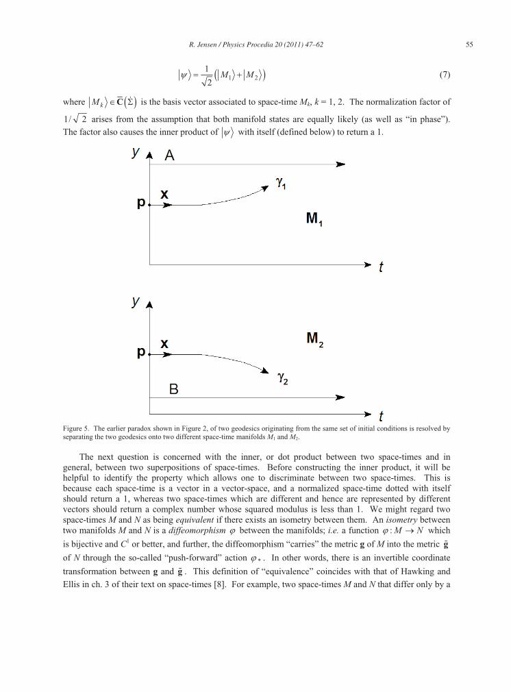
Suppose then that a photon emerges from a source located at p with a given initial direction x. At some point in time, as was previously, it may be the case that the photon takes an indeterminate path consisting of two branching geodesics with the same initial conditions p and x. To eliminate a contradiction, we regard the first branch to be a geodesic on one space-time manifold, and the other branch, on a separate space-time manifold. The overall physical situation is a superposition of these two space-times. That is, the photon and observer exist in a superposition of these two space-times. See Figure 5. Time is not explicitly mentioned in postulate 1 as it is usually, however it is possible that there is a parameter, call it t, which the wave function of the observer is dependent on. The space-times are

treated as basis vectors by the observer in the space C , and themselves are independent of t, although

as space-times, they have their “internal” time dimensions. Thus, only the coefficients of the basis vectors of can be dependent on t. The parameter t is discussed further below, under the sixth postulate.

Since space-times are basis vectors in the space C , space-times are also to be considered as

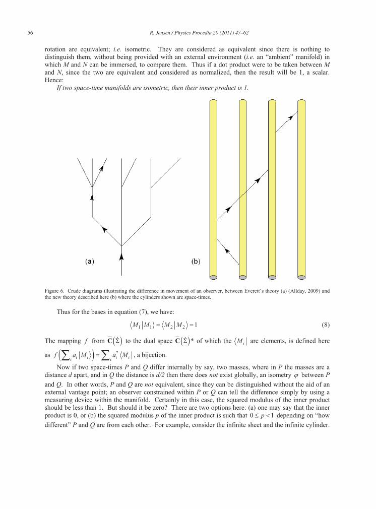
eigenvectors of observable operators. This idea will be examined more, when the second and third postulates of quantum mechanics are addressed. It should be noted once more that this theory is somewhat different from Everett’s, in that the latter considers reality according to an observer to be a branching tree where each possible outcome of a measurement is a branch (See ch. 25 of the text by Allday [7]). The observer travels up this tree, branch by branch, or more precisely, superpositions of branches. In the former, the observer is more like a traveler, jumping from space-time to space-time, or rather from a superposition of space-times to another superposition. See Figure 6. With the modified first postulate, the equation of state for the physical situation in the gedankenexperiment of the previous section is a superposition of two space-times: M1, where the mass is in position A and the photon takes geodesic 1 and M2, where the mass is in position B and the photon

takes geodesic 2 (again, see Figure 5). That is, the physical reality experienced by an observer is given

by the state


1 21

2M M (7)

where kM C is the basis vector associated to space-time Mk, k = 1, 2. The normalization factor of

1/ 2 arises from the assumption that both manifold states are equally likely (as well as “in phase”). The factor also causes the inner product of with itself (defined below) to return a 1.

Figure 5. The earlier paradox shown in Figure 2, of two geodesics originating from the same set of initial conditions is resolved by separating the two geodesics onto two different space-time manifolds M1 and M2.

The next question is concerned with the inner, or dot product between two space-times and in general, between two superpositions of space-times. Before constructing the inner product, it will be helpful to identify the property which allows one to discriminate between two space-times. This is because each space-time is a vector in a vector-space, and a normalized space-time dotted with itself should return a 1, whereas two space-times which are different and hence are represented by different vectors should return a complex number whose squared modulus is less than 1. We might regard two space-times M and N as being equivalent if there exists an isometry between them. An isometry between two manifolds M and N is a diffeomorphism between the manifolds; i.e. a function : M N which

is bijective and C1 or better, and further, the diffeomorphism “carries” the metric g of M into the metric g

of N through the so-called “push-forward” action * . In other words, there is an invertible coordinate

transformation between g and g . This definition of “equivalence” coincides with that of Hawking and

Ellis in ch. 3 of their text on space-times [8]. For example, two space-times M and N that differ only by a


rotation are equivalent; i.e. isometric. They are considered as equivalent since there is nothing to distinguish them, without being provided with an external environment (i.e. an “ambient” manifold) in which M and N can be immersed, to compare them. Thus if a dot product were to be taken between Mand N, since the two are equivalent and considered as normalized, then the result will be 1, a scalar. Hence: If two space-time manifolds are isometric, then their inner product is 1.

Figure 6. Crude diagrams illustrating the difference in movement of an observer, between Everett’s theory (a) (Allday, 2009) and the new theory described here (b) where the cylinders shown are space-times.

Thus for the bases in equation (7), we have:

1 1 2 2 1M M M M (8)

The mapping f from C to the dual space *C of which the iM are elements, is defined here

as *i i i ii i

f a M a M , a bijection.

Now if two space-times P and Q differ internally by say, two masses, where in P the masses are a distance d apart, and in Q the distance is d/2 then there does not exist globally, an isometry between P

and Q. In other words, P and Q are not equivalent, since they can be distinguished without the aid of an external vantage point; an observer constrained within P or Q can tell the difference simply by using a measuring device within the manifold. Certainly in this case, the squared modulus of the inner product should be less than 1. But should it be zero? There are two options here: (a) one may say that the inner product is 0, or (b) the squared modulus p of the inner product is such that 0 1p depending on “how

different” P and Q are from each other. For example, consider the infinite sheet and the infinite cylinder.


Both are 2-dimensional manifolds or surfaces, and both can be fitted with a Lorentzian metric and further, become a spacetime. Locally, both manifolds look the same, since the Gaussian curvature is zero for both. But globally, it is apparent that they are not the same and so are not isometric. They are however locally isometric, since locally, i.e. within a sufficiently small neighborhood there is no difference. So under option (b), the inner product of these two space-times could be made non-zero and less than 1. One could even consider further relaxing option (b) so that the only requirement for two space-times to have a non-zero squared modulus is that they for example, have the same number of holes; i.e. the same “Euler number.” Alternatively, it could be said that two space-times have an inner product different from zero if and only if it is possible that the first manifold can transition into the second. But since space-time are regarded as static, deterministic structures (again, from an external viewpoint), transitions from pure space-time manifolds can only occur between isometries. Therefore we settle on option (a); i.e. the inner product of two space-times U and V is

1 if

0 if

U VU V

U V (9)

where indicates isometry or equivalence. In particular, we have that

1 2 2 1 0M M M M . (10)

Hence 1 , from equations (7) (8) and (10) as was earlier claimed.

Recall that after the photon passes by the gravitating object, it enters the latter part of the gravitational MZ interferometer, and the outcome is registration of the photon at detector D1, or at detector D2. Now does space-time 1M contain the event of the photon registering at D1, or at D2? And

whither 2M ? The answer is actually “both,” for either space-time. Now a space-time was earlier said to

be a deterministic structure, and any deterministic theory will not allow mutually exclusive events to occur simultaneously. The way out of this dilemma is to admit to the fact that 1M and 2M are not truly

space-times; they themselves are each superpositions of two “space-times” 1iDM and 2iDM , which are

defined as those which contain events of the photon taking geodesic i (i = 1, 2) and registering at D1

and D2 respectively. See Figure 7. Further, the iDjM in turn are superpositions of space-times

themselves (hence the quotation marks), when one considers other events. Now since 1M and 2M are

not truly space-time manifolds, there is no guarantee anymore that equation (10) will hold. But if we do break down 1M and 2M completely into their basic component space-times, we will find that the basis

space-times for 1M and 2M are all orthogonal. Using property (9) on the basis space-time manifolds,

one can then show that (10) holds. We now continue with applying the theory to the gedankenexperiment presented earlier. Let and

be parameters. Then, due to normalization considerations, and the fact that

1 2 2 1 0iD iD iD iDM M M M , we have

1 1 1 1 2

2 2 1 2 2

cos sin

sin cos

D D

D D

M M M

M M M (11)

where, as explained previously, iDjM C is the space-time state in which the photon took path i

and reached detector j (i, j = 1, 2). Hence from equations (7) and (11), the following result is obtained:


1 1 1 2 2 1 2 21

cos sin sin cos2

D D D DM M M M . (12)

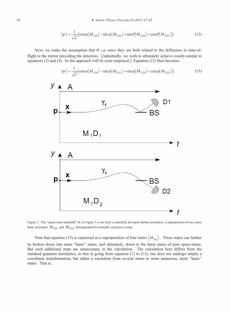
Next, we make the assumption that since they are both related to the difference in time-of-

flight to the mirror preceding the detectors. [Admittedly, we wish to ultimately achieve results similar to equations (3) and (4). So the approach will be semi-empirical.] Equation (12) then becomes

1 1 1 2 2 1 2 21

cos sin sin cos2

D D D DM M M M . (13)

Figure 7. The “space-time manifold” M1 in Figure 5 is not truly a manifold, but upon further resolution, a superposition of two more

basic structures 1 1DM and 1 2DM distinguished by mutually exclusive events.

Note that equation (13) is expressed as a superposition of four states iDjM . These states can further

be broken down into more “basic” states, and ultimately, down to the basis states of pure space-times. But such additional steps are unnecessary in the calculation. The calculation here differs from the standard quantum mechanics, in that in going from equation (7) to (13), one does not undergo simply a coordinate transformation, but rather a resolution from several states to more numerous, more “basic” states. That is,


equations (11) are not coordinate transformation equations as in the standard quantum theory, but

rather equations which express states iM in terms of “more basic” states iDjM ,

where “more basic” is defined as follows: if one has two superpositions of space-times, then the set of basis space-times making up the more basic superposition is a proper subset of the one which makes up

the less basic superposition. This definition provides a partial ordering on C .

In the end of the gedankenexperiment, the photon either reaches D1 or D2. The superposition of space-times containing the final events of photons hitting D1 or D2 are respectively, 1DM and 2DM .

Now either of these events can be expressed as the following superpositions respectively:

1 1 1 2 1

2 1 2 2 2

D D D

D D D

M a M b M

M c M d M (14)

where 2 2 2 2

1a b c d . Hence

11

cos sin2

DM a b . (15)

To go further, it will be necessary to define how the inner product (15) is related to the probability that one will jump from the superposition of space-times to the superposition 1DM . Before we try

to calculate this, it is necessary to define what the probability is when the final state is a single space-time manifold. This is given by the fourth postulate (we have skipped the second and third for now), which is exactly the same here as it is in ordinary quantum theory, except in interpretation: 4. The probability pk of an observer going from a superposition of space-times

i iia M C to a space-time kM is given by the squared-modulus of their inner

product: 2

k kp M .

This postulate tells us the probability in going from a superposition of space-times to a pure space-time, but not from one superposition to the next. In spite of this, we go ahead and take the squared-modulus between the two superpositions:

2 2 21

1cos 2 cos sin sin

2DM a ab b . (16)

Equation (16) becomes greatly simplified if we let 1/ 2a b c d . The interpretation of this is: given that a photon reaches detector Dj, it is equally probable that it has taken geodesic 1 or 2. This being the case, equation (16) simplifies to:

21

11 sin 2

4DM . (17)

Similarly, equations (13) and (14) give

22

11 sin 2

4DM . (18)

Adding equations (17) and (18), one obtains a normalization factor of 1/2. Equations (17) and (18) do not add to unity as postulate 4 demands because the transition is not to a pure state, but rather from one superposition to another. Dividing equations (17) and (18) by this normalization factor gives the correct probabilities:


21 1

22 2

1 1/ 1 sin 2

2 21 1

/ 1 sin 2 .2 2

D D

D D

p M

p M

(19)

Equations (19) are the same as equations (3) and (4) upon setting k L . For transitions to a

superposition of space-times such as (19), which is generally the case, we use (and have used) the following extension of postulate 4:

4b. The probability pk of an observer in going from a superposition of space-times C to a

superposition of space-times k C is given by the normalized squared-modulus of their inner

product: 2 2

/k k iip where the i C are all the possible superpositions which

may transition to.

This postulate is important in the new theory, since all transitions are essentially from superpositions to superpositions, not to pure states. Next, we consider the second and third postulates in terms of the new theory, which are the same as in the standard quantum theory: 2, 3. Every observable quantity a is an eigenvalue of an observable operator A acting on elements of

C .

Consider the matrix operator A defined by

1 0

0 1A . (20)

Note that A is the Pauli matrix x . The matrix A is Hermitian, and its eigenvalues are real; i.e. 1 ;

hence A is said to be an observable. The associated eigenvectors of A are 1 0 and 0 1

respectively, and these form two separate eigenspaces. In Dirac notation, these eigenvectors are 1M

and 2M respectively, the “basis” vectors in the representation (7). But earlier, it was found that these

“basis” vectors are not actually basis vectors, i.e. space-times, but can further be decomposed. The decomposition of 1M and 2M is given by equations (11). Likewise A must also be decomposed, into

a 4-by-4 matrix in order to act on them, e.g.:

2 0 0 0

0 1 0 0

0 0 1 0

0 0 0 2

A . (21)

A has eigenvectors 1 1DM , 1 2DM , 2 1DM and 2 2DM , the same basis in which equation (12) is

expressed. These eigenvectors may be decomposed further into more basic superpositions, and thus Amay be expanded further, and the process repeated as necessary. The reader is reminded that the new theory calls for an infinite vector space whose basis vectors are deterministic structures; i.e. space-times. However, in order to do calculations practically, one need not break everything down into an infinite number of individual basis vectors, but only resolve the situation to a finite number of vectors, which are not strictly basis vectors i.e. pure space-times. This is what was done earlier in obtaining equations (19). The fifth postulate states that


5. If the measurement of A on i iia M C yields the eigenvalue ak and eigenvector

kM , then the state immediately after measurement is

k

k

(22)

where k k kM M is the projection operator that projects onto the state kM .

The purpose of the denominator in (22) is for normalization. Again, in the new theory, the observer generally transitions from a superposition of space-times to another superposition . To this

process is associated a projection operator . Thus postulate 5 is extended as follows:

5b. If an observer transitions from a superposition of space-time manifolds to a superposition

,then the latter is given by

, (23)

where is the projection operator that projects onto the state .

Finally, the sixth postulate, which involves the Schrödinger equation, reads as follows, in the standard form:

The time evolution of the state vector t is governed by the Schrödinger equation

i t H t tt

(24)

where H(t) is the Hamiltonian operator. When an observer makes a measurement or transitions from one superposition to the next, the transition is governed by the modified fifth postulate given above. On the other hand, if the observer makes no such modification to his environment or state, it may be that the state of the observer “drifts” or changes deterministically according to equation (24) with respect to some parameter t which the observer may experience as “time.” Hence

6. The evolution of the superposition of space-time manifolds t with respect to t is given by the

Schrödinger equation (24), or its relativistic correction, where t is some time parameter experienced by the observer.

The individual basis vectors of t are space-time manifolds which all have a time component to

their metrics. But the overall 4-dimensional structures do not change with respect to an external time parameter; these are treated as static structures by the observer. Hence it is only the coefficients ak(t) of

that may change with respect to t. How this parameter t relates to the time dimensions of the space-

times is subject for future study. Although entire space-times are treated as static structures in the calculations, an observer admittedly does not experience the entire superposition of space-times at once, but rather experiences the space-times in the superposition locally. This must be kept in mind as calculations are done.


4. Some Final Notes

As an observer transitions from superposition to superposition, the observer observes the initial and final states again, locally, although in the calculation, the entire space-times are considered. It may therefore seem possible that, for example, an observer could transition from one superposition to the next and then back again, but upon returning to the original superposition, find himself in a “past” portion of the original superposition. In other words, he could time travel. The new theory should provide for some rules prohibiting such actions, or at least preventing paradoxes from arising. As stated earlier, the theory introduced here is by no means complete. Therefore the reader is invited to suggest additions or alterations. Nevertheless, the fundamental problem of geodesic non-uniqueness remains, and so does the necessity for a resolution of the contradiction.

5. Conclusion

It has been shown that single photons of light can travel along two distinguishable null geodesics with the same initial position and same initial velocity. In other words, in the universe, there are unequal null geodesics that arise from the same initial conditions; by theorem 2 this is something which is forbidden on a space-time manifold. Thus, it cannot be the case that the universe is representable by a single space-time manifold. We propose here instead that the universe be given by a superposition of space-time manifolds. The fundamentals of the theory are constructed in the second part of this article.

References

1. Jensen, R., On using Greenberger-Horne-Zeilinger three-particle states for superluminal communication, in the proceedings of Space Propulsion and Energy Sciences International Forum (SPESIF-2010), edited by G. A. Robertson, AIP CP1208, Melville, New York, 2010 p. 274-288.

2. Grangier, P., Roger, G. and Aspect, A., Experimental Evidence for a Photon Anticorrelation effect on a Beam Splitter: A New Light on Single-Photon Interferences, Europhysics Letters 1986 1(4):173.

3. Beem, J., Ehrlich, P. and Easley, K., Global Lorentzian Geometry, Marcel Dekker, New York, NY, 1996. 4. Freedman, M., Caligari, D. and Walker, K., Positivity of the universal pairing in 3 dimensions, J. Am. Math. Soc. 2010 23:107-

188. 5. Everett, H. ’Relative State’ Formulation of Quantum Mechanics, Rev. Mod. Phys. 1957 29(3):454-462. 6. Cohen-Tannoudji, C., Diu, B. and Laloë, F., Quantum Mechanics Volume I., Wiley, 1977. 7. Allday, J., Quantum Reality: Theory and Philosophy, CRC, Boca Raton, FL, 2009. 8. Hawking, S. and Ellis, G., The large scale structure of space-time, Cambridge, 1979.

Documents

Can the universe be represented by a superposition of spacetime manifolds?