Capital Structure Under Heterogeneous Beliefs

Electronic copy available at: http://ssrn.com/abstract=1596869

Capital Structure under Heterogeneous Beliefs�

Hae Won Jung

Department of Risk Management and Insurance

J. Mack Robinson College of Business

Georgia State University

[email protected]

Ajay Subramanian

Department of Risk Management and Insurance and Center for the Economic Analysis of Risk

J. Mack Robinson College of Business

Georgia State University

[email protected]

September 21, 2010

Abstract

We develop a dynamic structural model to examine the e¤ects of di¤ering beliefs of themanager and outsider investors regarding the pro�tability of a �rm�s projects and manager-shareholder agency con�icts on its capital structure. The manager receives dynamic incentivesthrough explicit contracts with shareholders. The implementation of the contracts through �-nancial securities leads to a dynamic capital structure consisting of inside equity, outside equity,long-term debt, and short-term debt. The analysis of the model generates novel testable impli-cations for the e¤ects of project characteristics on di¤erent components of capital structure: (i)Long-term debt declines with managerial optimism, while the manager�s inside equity stake andshort-term debt increase. (ii) Long-term debt and the manager�s inside equity stake decline withthe �rm�s transient risk, that is, the degree of uncertainty about the pro�tability of the �rm�sprojects. (iii) Long-term debt increases with the �rm�s intrinsic risk� the component of the�rm�s risk that is invariant through time� while short-term debt and the manager�s inside equitystake decline. (iv) Long-term and short-term debt increase with the �rm�s expected pro�tability.We calibrate our structural model to a sample of general �rms as well as a sample of IPO �rms,and show the quantitative impact of asymmetric beliefs on capital structure. The calibratedparameter values corresponding to the two sets of �rms suggest that managers/entrepreneursof IPO �rms are, indeed, signi�cantly more optimistic than general managers, and the degreeof uncertainty about the pro�tability of IPO �rms is substantially higher. Overall, our �ndingsshow that imperfect information and asymmetric beliefs are important determinants of �rms��nancial policies.

�We thank Thomas Chemmanur and seminar participants at the 2010 Western Finance Association Meetings(Victoria, BC) and Georgia State University for valuable comments. The usual disclaimers apply.

Electronic copy available at: http://ssrn.com/abstract=1596869

There is growing evidence to suggest that managers and outside investors often have di¤ering

beliefs about the pro�tabilities of projects in addition to asymmetric attitudes towards their risks

(Malmendier and Tate (2005), Baker et al. (2007), Ben-David et al. (2007)). While a growing

literature in dynamic corporate �nance provides quantitative guidance into the e¤ects of agency

con�icts among a �rm�s stakeholders on its capital structure, the quantitative e¤ects of asymmetric

beliefs are relatively unexplored, especially in structural frameworks. We contribute to the literature

by developing a dynamic, structural model to show how asymmetric beliefs and agency con�icts

interact to a¤ect capital structure.

We calibrate the model to aggregate data and derive novel, testable implications that link

characteristics of a �rm�s projects� the degree of asymmetry in beliefs, permanent and transient

components of risk, and expected pro�tability� to di¤erent components of its capital structure:

long-term debt, short-term debt, inside equity, and outside equity. (i) Long-term debt declines

with the degree of managerial optimism, while the manager�s inside equity stake and short-term

debt increase. (ii) Long-term debt and the manager�s inside equity stake decline with the transient

risk of a �rm�s earnings� the degree of uncertainty in agents�priors about the pro�tability of a

�rm�s projects� while short-term debt increases. (iii) Long-term debt increases with the intrinsic

risk of a �rm�s earnings� the component of risk that is invariant through time� while short-term

debt and the manager�s inside equity stake decline. (iv) Long-term and short-term debt increase

with the �rm�s expected pro�tability.

In our discrete-time, �nite horizon framework, the manager of an all-equity �rm raises �nancing

for a positive NPV project through outside equity and long-term debt that is non-callable and

completely amortized. The manager has an initial ownership stake and receives a proportion of

the net payo¤ from external �nancing (the total proceeds from �nancing net of the required initial

investment outlay). In addition to equity and long-term debt, the �rm�s capital structure also

consists of non-discretionary short-term (single-period) debt �nancing of the �rm�s working capital

requirements. The �rm�s earnings in each period are distributed among its stakeholders� the

manager, shareholders, bondholders, and the government (through corporate taxes). We abstract

1

away from personal taxes for simplicity.

We model the �rm�s total earnings gross of long-term debt interest payments, short-term debt

payments associated with working capital, corporate taxes, and the manager�s compensation. As

in Giat et al. (2010), the �rm�s total earnings in each period consist of two components: the

normally distributed base earnings, and the discretionary earnings that are generated by share-

holders�incremental capital investments and the manager�s e¤ort. The true mean of the project�s

base earnings (the mean under the beliefs of the hypothetical omniscient agent) is its intrinsic

quality or pro�tability. Outside investors and the manager have imperfect information and possibly

di¤ering priors about the project�s pro�tability. They �agree to disagree� about their respective

mean assessments. The di¤erence of their mean assessments is the degree of managerial optimism.

The true variance of the project�s earnings in each period is its intrinsic risk, which is invariant

through time. The project�s discretionary earnings are deterministic and determined by a Cobb-

Douglas production function. The common variance of outside investors�and the manager�s prior

assessments of the project�s pro�tability is its transient risk. In contrast with the intrinsic risk, the

transient risk is resolved over time as the players learn about the project�s pro�tability through

observations of the project�s earnings.

Outside investors are risk-neutral and capital markets are competitive (see Chapters 3 and 4 of

Tirole (2006)). The undiversi�ed manager has multiplicatively separable CARA preferences. We

consider an incomplete contracting environment in which the manager receives dynamic incentives

through a sequence of explicit contracts contingent on the �rm�s earnings. The contracts must be

incentive compatible for the manager. The contracts must also guarantee that shareholder value

under the contracts is at least as great as the shareholder value in the hypothetical absence of the

manager�s human capital inputs, that is, the net present value of the �rm�s base earnings. As the

manager has multiplicatively separable CARA preferences, and the �rm�s earnings are normally

distributed, we follow Gibbons and Murphy (1992) in restricting consideration to contracts that

are a¢ ne in the �rm�s earnings.

As in Leland (1994), debt is serviced entirely in �nancial distress by the additional issuance of

2

equity, and bankruptcy occurs endogenously when the equity value falls to zero. For simplicity, we

assume that the �rm is liquidated at bankruptcy and the absolute priority of debt is enforced. The

�bankruptcy payo¤�to debtholders is equal to a portion of the �rm�s asset value at bankruptcy,

which is the present value of the �rm�s base earnings �ow less bankruptcy costs.

We characterize the equilibrium in which the �rm�s capital structure and the manager�s contracts

are endogenously determined. Because the manager has an equity stake in the initial all-equity �rm,

she receives a portion of the net proceeds from external �nancing. The manager chooses the �rm�s

capital structure to maximize the total expected utility she derives from her initial payo¤ from

external �nancing and her stream of future contractual compensation payments.

We implement the risky component of the manager�s compensation in each period through an

inside equity stake in the �rm, and the performance-invariant or �cash�component through a cash

reserve. The cash reserve o¤sets the short-term debt �nancing of the �rm�s working capital. In our

implementation of the manager�s contracts, therefore, the �rm�s capital structure consists of inside

equity, outside equity, long-term debt, and short-term debt, where short-term debt incorporates

the �nancing of working capital and the manager�s cash compensation.1

The manager�s equilibrium inside equity stake is a deterministic function of time, but her cash

compensation depends on the project�s earnings history through its e¤ect on the players�posterior

assessments of the project�s pro�tability. The manager�s inside equity stake in each period increases

with the initial degree of managerial optimism. When the manager is optimistic, she overvalues the

project�s future earnings relative to outside investors. The optimal contract exploits the manager�s

optimism by providing the manager with more powerful incentives, that is, by increasing her equity

compensation relative to her cash compensation.

The manager�s �nancing choice at date zero re�ects its e¤ects on her initial payo¤ from external

�nancing and her expected utility from her future contractual compensation payments� hereafter,

her continuation utility. The manager�s initial payo¤ is proportional to the total proceeds from

external �nancing net of the initial required investment. Under rational expectations, the proceeds

1The incorporation of the short-term debt �nancing of working capital is necessary for the calibration of the modelbecause it is a signi�cant component of a �rm�s short-term debt in the data.

3

from external �nancing� the market value of debt plus the market value of outside equity� equal

the market value of the �rm�s after-tax earnings net of the manager�s stake. Because capital

markets are competitive, the manager captures the surplus she generates from her human capital.

Consequently, the manager�s beliefs and actions a¤ect her continuation utility, but do not a¤ect

the proceeds from external �nancing at date zero.

Long-term debt has con�icting e¤ects on the manager�s total expected utility. On the positive

side, because debt interest payments are shielded from corporate taxes, the manager can poten-

tially increase the proceeds from external �nancing at date zero (therefore, her initial payo¤) by

choosing greater long-term debt. Choosing greater long-term debt, however, increases the expected

bankruptcy costs for the �rm and personal bankruptcy costs for the manager, which negatively

a¤ect her continuation utility.

We show that long-term debt declines with the degree of managerial optimism. As discussed

earlier, an increase in the manager�s optimism increases the manager�s inside equity stake in each

period and, therefore, the output she generates. Consequently, the manager�s expected contractual

compensation in each period and continuation utility increase with her degree of optimism, while

her initial payo¤ is una¤ected as discussed earlier. At the margin, therefore, the manager gives

relatively more weight to her continuation utility than her initial payo¤ in choosing the �rm�s long-

term debt. Because long-term debt lowers the manager�s continuation utility through the likelihood

of bankruptcy, the manager chooses lower long-term debt to lower the probability of bankruptcy.

We derive quantitative implications of the model by calibrating it to aggregate data to obtain a

reasonable set of baseline parameter values. In particular, we indirectly infer the �deep�structural

parameters of the model that relate to agents�beliefs and preferences� outside investors�and the

manager�s mean assessments of the �rm�s pro�tability, the transient risk, the manager�s risk aver-

sion, and her disutility of e¤ort� so that key statistics predicted by the model match their median

values in the data. In our �rst calibration exercise, we use a sample of general �rms (excluding

�nancial �rms and regulated utilities) from Compustat. Our calibration shows that managers are,

indeed, signi�cantly optimistic relative to outside investors. Relative to outside investors, the av-

4

erage manager in the sample of general �rms overestimates the market to book ratio (the ratio

of �rm value to book value according to the manager�s beliefs) by 62%. Further, the ratio of the

project�s transient risk to its intrinsic risk is 2.4, which suggests that the degree of uncertainty

about pro�tability� the transient risk� is signi�cant relative to the intrinsic risk.

We derive additional testable implications of the model by varying parameters about their

baseline values. Long-term debt declines with the project�s transient risk, but increases with its

intrinsic risk. An increase in the transient risk increases the project�s �signal to noise ratio,�

that is, intermediate observations of the project�s earnings are more informative about its intrinsic

quality. Consequently, the standard deviation of the evolution of posterior assessments of the

project�s quality increases. As a result, the �option value�of continuing to service long-term debt

interest payments increases, which delays bankruptcy. Consequently, the marginal impact of the

manager�s continuation utility on her long-term debt choice increases relative to her initial payo¤.

The manager, therefore, chooses lower long-term debt to increase her continuation utility. An

increase in the intrinsic risk, however, decreases the signal to noise ratio and the option value of

delaying bankruptcy. Further, an increase in the intrinsic risk increases the costs of risk-sharing

between the manager and outside investors, which weakens the manager�s incentives and the output

she generates in each period. As a result, an increase in the intrinsic risk lowers the marginal impact

of the manager�s continuation utility on her long-term debt choice. The manager, therefore, chooses

greater long-term debt to increase her initial payo¤.

Next, we explore the e¤ects of project characteristics on short-term debt. As the manager�s

degree of optimism increases, she receives more powerful incentives so that her cash compensation

declines relative to her equity compensation. Because cash is e¤ectively negative short-term debt

(see DeMarzo and Fishman (2007)), the �rm�s short-term debt increases with managerial optimism.

Short-term debt increases with the project�s transient risk because an increase in the transient risk

delays bankruptcy and, therefore, increases the value of the �rm�s short-term debt. An increase in

the intrinsic risk, however, hastens bankruptcy and increases the costs of risk-sharing and, therefore,

the manager�s cash compensation relative to her equity compensation. Consequently, short-term

5

debt declines with the intrinsic risk.

Our main results are robust to two extensions of the model. First, we allow for di¤ering

allocations of bargaining power between the manager and shareholders so that shareholders capture

a portion of the surplus the manager generates in each period. In the extended model, the manager�s

actions a¤ect both the initial proceeds from �nancing and her continuation utility. Our main

predictions continue to hold as long as shareholders� bargaining power vis-a-vis the manager is

below a threshold (in our simulations, the threshold is close to 50%). Second, our results are also

robust to an extension of the model in which the manager continues to service long-term debt even

after the outside equity value falls to zero, that is, the �rm e¤ectively becomes privately held. The

manager declares bankruptcy when it is no longer optimal for her to service debt interest payments.

Finally, to provide further validation for the model, we calibrate its parameters to a sample of

IPO �rms for which uncertainty about pro�tability and asymmetric beliefs are likely to be more

important. Consistent with this intuition, we �nd that managerial optimism and transient risk

are, indeed, much more quantitatively signi�cant relative to their calibrated values for the sample

of general �rms. Relative to outside investors, the average manager in the sample of IPO �rms

overestimates the market to book ratio by 129%. The ratio of the project�s transient risk to its

intrinsic risk for the sample of IPO �rms is 4.4. In other words, without any a priori assumptions on

their relative magnitudes, the indirectly inferred values of managerial optimism and transient risk

are much higher for the sample of IPO �rms compared with the sample of general �rms. Consistent

with the notion that entrepreneurs are likely to be less diversi�ed than general �rm managers, the

risk aversion of managers of IPO/entrepreneurial �rms is, indeed, higher. Moreover, in conformity

with the fact that young �rms are likely to have greater growth opportunities on average, the

total factor productivity is signi�cantly higher for the IPO sample. Overall, our �ndings provide

additional support for the model as a viable (albeit stylized) descriptor of �rms��nancing decisions.

In particular, our results highlight the importance of imperfect information and asymmetric beliefs

as determinants of capital structure, especially for entrepreneurial �rms.

6

1 Related Literature

We contribute to the literatures in dynamic corporate �nance and behavioral �nance by developing

a structural model to examine the quantitative e¤ects of heterogeneous beliefs and agency con�icts

on di¤erent components of capital structure. Landier and Thesmar (2009) present a two-period

framework in which contracts are exogenously restricted to be debt contracts. They show that op-

timistic managers choose short-term debt, whereas realists opt for long-term debt. We complement

their analysis by examining the e¤ects of asymmetric beliefs on long-term debt, short-term debt,

inside equity, and outside equity in a dynamic principal-agent framework with general contractual

structures. Dittmar and Thakor (2007) develop a three-period model and show that a manager

chooses equity �nancing if there is greater agreement between the manager and investors. Chem-

manur et al. (2007) show that, if outside investors are more optimistic or more heterogenous in

their beliefs, the �rm is more likely to issue equity rather than debt. Hackbarth (2008) incorpo-

rates managerial traits, such as growth and risk perception biases, into a dynamic tradeo¤ model

of capital structure and shows that a biased manager chooses a higher debt level.

Our study complements these analyses in several aspects. First, we quantitatively examine

the e¤ects of asymmetric beliefs on capital structure in a structural model. The calibration of

the model leads to an indirect inference of the level of managerial optimism implied by the data.

Second, we consider a dynamic principal-agent framework in which the manager�s optimal dynamic

contract is derived and implemented through �nancial securities, which leads to a dynamic capital

structure. Third, we derive new implications for the e¤ects of optimism, permanent and transitory

components of risk, and expected pro�tability on di¤erent components of capital structure.

Adrian and Wester�eld (2009) and Giat et al. (2010) develop general dynamic, principal-

agent models to study the impact of asymmetric beliefs and agency con�icts on optimal dynamic

contracts. They abstract away from capital structure choices. Gervais et al. (2007) study the

e¤ects of manager overcon�dence on investment, but also abstract away from capital structure.

Our model builds on that of Giat et al. (2010) by incorporating an additional capital structure

choice problem. We show how the dynamic tradeo¤ between debt tax shields and bankruptcy costs,

7

https://www.researchgate.net/publication/46513197_Investment_under_Uncertainty_Heterogeneous_Beliefs_and_Agency_Conflicts?el=1_x_8&enrichId=rgreq-3ef27c307ee0d60a2ad3a3a79ac9ff4a-XXX&enrichSource=Y292ZXJQYWdlOzIyODI1Mjc3MDtBUzoxNjYzOTk3MjUwMjMyMzRAMTQxNjY4NDE5NDQ5MQ==


asymmetric beliefs, Bayesian learning, and agency con�icts interact to a¤ect capital structure.

Our study is also related to the literature on dynamic tradeo¤ models of capital structure (e.g.

Fischer et al. (1989), Leland and Toft (1996), Goldstein et al. (2001), Hennessy and Whited

(2005), Strebulaev (2007)). In these studies, the manager is assumed to behave in the interests of

shareholders, and agents have perfect information about project characteristics. Another group of

studies analyzes �nancial contracting in dynamic principal-agent frameworks in which all agents

are risk-neutral and beliefs are symmetric (e.g. DeMarzo and Sannikov (2006), DeMarzo and

Fishman (2007)). Berk et al. (2010) show that human capital costs of bankruptcy could explain

observed leverage levels in a framework with competitive capital and labor markets, no moral

hazard, and perfect information about project characteristics. Bhagat et al. (2010) examine the

e¤ects of manager-speci�c characteristics such as ability and risk aversion on capital structure in a

dynamic principal-agent model. They too assume all agents have perfect information about project

characteristics.

2 Model

We consider a �nite horizon framework with equally spaced dates, 0; 1; : : : ; T . At date 0; the

manager of an all-equity �rm, who has an initial ownership stake, ginitial 2 (0; 1); considers a

positive net present value project that requires an initial investment outlay, I. She raises �nancing

for the project from competitive public debt and equity markets. The total earnings from the

project are distributed among all the �rm�s claimants - the manager, shareholders, debt-holders,

and the government (through taxes). We ignore personal taxes for simplicity and assume that the

corporate tax rate is a constant, � 2 (0; 1). Security issuance costs are negligible, and the risk-free

interest rate, r, is a constant and the same for all market participants. All agents are fully rational,

but (as we describe shortly) could have di¤ering beliefs about the project�s payo¤ distribution.

8

https://www.researchgate.net/publication/4992198_Dynamic_Capital_Structure_Choice_Theory_and_Tests?el=1_x_8&enrichId=rgreq-3ef27c307ee0d60a2ad3a3a79ac9ff4a-XXX&enrichSource=Y292ZXJQYWdlOzIyODI1Mjc3MDtBUzoxNjYzOTk3MjUwMjMyMzRAMTQxNjY4NDE5NDQ5MQ==

https://www.researchgate.net/publication/24103344_An_Ebit-Based_Model_of_Dynamic_Capital_Structure?el=1_x_8&enrichId=rgreq-3ef27c307ee0d60a2ad3a3a79ac9ff4a-XXX&enrichSource=Y292ZXJQYWdlOzIyODI1Mjc3MDtBUzoxNjYzOTk3MjUwMjMyMzRAMTQxNjY4NDE5NDQ5MQ==

2.1 Total Earnings Flow

We follow Giat et al. (2010) in modeling the �rm�s total earnings in each period. In any period [i; i+

1] ; the earnings from the project are a¤ected by shareholders�capital investments and the manager�s

e¤ort. The total earnings �ow in any period has two components: the base earnings� a stochastic

component that is una¤ected by the capital investment and e¤ort, and the discretionary earnings�

a deterministic component that depends on the incremental capital investment by shareholders and

the manager�s e¤ort. Speci�cally, if the capital investment and e¤ort over period [i; i + 1] are ki

and �i; respectively, the total earnings �ow is

Ei+1 =

Base Earningsz }| {�+Ni+1 +

Discretionary Earningsz }| {Ak�i �

�i : (1)

The �rst component of the base earnings, �; represents the project�s intrinsic quality or core

pro�tability. The manager and outside investors� shareholders and debtholders� have imperfect

information and possibly asymmetric beliefs about �. Their respective beliefs are, however, com-

mon knowledge, that is, they agree to disagree (see Morris (1995), Allen and Gale (1999)). Their

respective priors on � at date zero are normally distributed as follows:

� � N��S0 ; �

20

�; Shareholders�Prior; (2)

� � N��M0 ; �

20

�; Manager�s Prior:

The equilibrium only depends on how the manager�s and outside investors�assessments of project

quality relate to each other, and not on the true project quality distribution. We, therefore, make

no assumptions on the true project quality distribution. Although we could consider the general

scenario in which the manager is optimistic or pessimistic relative to outside investors, we simplify

the exposition by considering the (empirically relevant) scenario in which the manager is optimistic.

It is important to mention here that, when we calibrate the model to data in Section 5, we do not

assume a priori that the manager is optimistic, and indirectly infer the average level of managerial

9


https://www.researchgate.net/publication/4789213_Diversity_of_Opinion_and_Financing_of_New_Technologies?el=1_x_8&enrichId=rgreq-3ef27c307ee0d60a2ad3a3a79ac9ff4a-XXX&enrichSource=Y292ZXJQYWdlOzIyODI1Mjc3MDtBUzoxNjYzOTk3MjUwMjMyMzRAMTQxNjY4NDE5NDQ5MQ==

optimism (or pessimism) implied by the data. De�ne

�0 := �M0 � �S0 ; (3)

which is the degree of managerial optimism at date zero.

The second component of the base earnings, Ni+1, is a normal random variable with mean 0

and variance s2. The random variables fNi+1; i � 0g are independent of each other, and are also

independent of �. The parameter s2 is the intrinsic risk of the �rm�s earnings because it is present

even when there is perfect information about �, and is invariant through time.

The discretionary earnings are described by a Cobb-Douglas production function, in which

the total factor productivity, A, and the parameters, �; � 2 (0; 1); are known constants. The

discretionary earnings are observable but non-veri�able, and, therefore, non-contractible.

All agents� the manager and outside investors� update their prior beliefs of the project�s core

pro�tability (hereafter, pro�tability)� over time based on intermediate observations of the project�s

earnings. De�ne the random variable

�i+1 := Ei+1 �Ak�i ��i = �+Ni+1; i = 0; 1; : : : ; T � 1: (4)

The posterior distribution on � for each date i � 1 is normally distributed under the beliefs of the

manager (denoted by N(�Mi ; �2i )) and outside investors (denoted by N(�

Si ; �

2i )), where

�2i =s2�2i�1s2 + �2i�1

=s2�20

s2 + i�20; (5)

�`i =s2�`i�1 + �

2i�1�i

s2 + �2i�1=s2�`0 + �

20(Pit=1 �t)

s2 + i�20; ` =M; S: (6)

Note that �i tends to zero as i!1. The parameter, �2i , is the project�s transient risk because it

represents the degree of uncertainty about the project�s quality that is resolved through time due

to Bayesian learning.

10

De�ne

�i := �Mi � �Si =s2�0

s2 + i�20=�2i�20�0; i = 0; 1; : : : ; T � 1: (7)

We refer to �i as the degree of managerial optimism at date i. By (7), the degree of managerial

optimism declines deterministically over time as the manager and outside investors update their

priors on � in a Bayesian manner based on observations of the project�s earnings.

2.2 Debt Structure

All long-term debt issued at date zero matures at date T and is non-callable. Further, if the

time horizon T is su¢ ciently long (we set it to 30 years in the calibration of the model), we can

follow Leland (1998) by assuming that long-term debt is completely amortized so that long-term

debtholders (hereafter, bondholders) receive a constant coupon payment, d, in each period as long

as the �rm remains solvent. The debt coupon payment d, which determines the �rm�s long-term

debt structure, is later determined endogenously.

In addition to long-term debt, the �rm also has non-discretionary working capital requirements

such as inventories, accounts payable and receivable, employee wages, etc. that are �nanced through

single-period, risk-free short-term debt. The incorporation of the short-term debt �nancing of

working capital is necessary for the subsequent calibration of the model because it is an important

component of a �rm�s short-term debt in the data. Consistent with empirical evidence (e.g. Fazzari

and Petersen (1993)), working capital requirements increase with the �rm�s total earnings. For

simplicity, we assume that working capital requirements are a constant proportion � of the �rm�s

total earnings �ow, where � is observable. Hence the �rm�s total earnings net of working capital

requirements in period [i; i+ 1] is

Qi+1 = (1� �)Ei+1: (8)

We hereafter refer to the process Qi+1 as the EBITM (earnings before interest, taxes, and the man-

ager�s compensation) because it will be distributed among bondholders, the government (through

taxes), the manager, and shareholders.

11

https://www.researchgate.net/publication/24048817_Working_Capital_and_Fixed_Investment_New_Evidence_on_Financing_Constraints_RAND_Journal_of_Economics_Vol_24_No_3_pp_328-342?el=1_x_8&enrichId=rgreq-3ef27c307ee0d60a2ad3a3a79ac9ff4a-XXX&enrichSource=Y292ZXJQYWdlOzIyODI1Mjc3MDtBUzoxNjYzOTk3MjUwMjMyMzRAMTQxNjY4NDE5NDQ5MQ==


For now, the �rm�s capital structure consists of equity, long-term debt, and short-term debt

�nancing of working capital. In Section 3.4, we implement the manager�s optimal contract through

an inside equity stake and a cash reserve. Since cash is e¤ectively negative short-term debt (see

DeMarzo and Fishman (2007)), it o¤sets the short-term debt �nancing of the �rm�s working capital.

In the calibrated model, therefore, the �rm�s capital structure consists of inside equity, outside

equity, long-term debt, and short-term debt, where short-term debt incorporates the �nancing of

working capital and the manager�s cash compensation.

2.3 Contracting and Bankruptcy

Outside investors are risk-neutral, while the manager is risk-averse with inter-temporal CARA

preferences. If the manager�s compensation is cmj and her e¤ort is �j in period [j; j + 1]; and

bankruptcy does not occur prior to date T , the expected utility at date i < T she derives from her

contractual compensation payments is

U(c; �) = EMi

�� exp

��

� T�1Xj=i

e�r(j�i)(cmj � �� j )��

: (9)

In the above, r is the risk-free interest rate, � is the manager�s absolute risk aversion, and �� j

(� > 0 is a constant) is the manager�s disutility of e¤ort in period [j; j + 1].

The manager receives dynamic incentives through contracts that could be explicitly contingent

on the EBITM process Qi+1 de�ned in (8). We consider an �incomplete contracting�environment

in which only single-period contracts are enforceable. As in Chapters 3 and 4 of Tirole (2006)

and Berk et al. (2010), capital markets are competitive. The manager o¤ers a contract to the

�rm�s competitive shareholders in each period, which speci�es the division of the �rm�s earnings

(net of corporate taxes and interest payments) between the manager and shareholders. In our

subsequent implementation of the manager�s contracts in Section 3.4, this is equivalent to the

manager dynamically issuing (or buying back) �nancial securities in competitive capital markets.

Following Leland (1994, 1998), debt payments are serviced entirely as long as the �rm is solvent.

In �nancial distress when the �rm�s earnings are insu¢ cient to meet its debt interest payments,

12

https://www.researchgate.net/publication/5217147_Optimal_Long-Term_Financial_Contracting?el=1_x_8&enrichId=rgreq-3ef27c307ee0d60a2ad3a3a79ac9ff4a-XXX&enrichSource=Y292ZXJQYWdlOzIyODI1Mjc3MDtBUzoxNjYzOTk3MjUwMjMyMzRAMTQxNjY4NDE5NDQ5MQ==

https://www.researchgate.net/publication/4992469_Agency_Costs_Risk_Management_and_Capital_Structure?el=1_x_8&enrichId=rgreq-3ef27c307ee0d60a2ad3a3a79ac9ff4a-XXX&enrichSource=Y292ZXJQYWdlOzIyODI1Mjc3MDtBUzoxNjYzOTk3MjUwMjMyMzRAMTQxNjY4NDE5NDQ5MQ==

https://www.researchgate.net/publication/46538159_Human_Capital_Bankruptcy_and_Capital_Structure?el=1_x_8&enrichId=rgreq-3ef27c307ee0d60a2ad3a3a79ac9ff4a-XXX&enrichSource=Y292ZXJQYWdlOzIyODI1Mjc3MDtBUzoxNjYzOTk3MjUwMjMyMzRAMTQxNjY4NDE5NDQ5MQ==

https://www.researchgate.net/publication/24139419_Long-Term_Debt_Value_Bond_Covenants_and_Optimal_Capital_Structure?el=1_x_8&enrichId=rgreq-3ef27c307ee0d60a2ad3a3a79ac9ff4a-XXX&enrichSource=Y292ZXJQYWdlOzIyODI1Mjc3MDtBUzoxNjYzOTk3MjUwMjMyMzRAMTQxNjY4NDE5NDQ5MQ==

they are serviced through an additional issuance of outside equity. Bankruptcy, therefore, occurs

endogenously when the equity value falls to zero. Note that, because the manager�s contracts

determine the payout �ows to outside equity, they also e¤ectively determine the bankruptcy time.

We can extend the model to allow for the manager to continue servicing debt after the equity value

falls to zero, which is e¤ectively equivalent to the scenario in which the �rm becomes privately

held. The manager declares bankruptcy when it is no longer optimal for her to service debt. The

implications of the extended model do not di¤er from those of the simpler model presented here in

which bankruptcy occurs when the equity value falls to zero.

For simplicity and concreteness, we assume that the manager leaves the �rm upon bankruptcy

and the �rm is liquidated. The absolute priority of debt is enforced at bankruptcy. The total payo¤

to bondholders upon bankruptcy is

Bondholders�Bankruptcy Payo¤ = LD(Tb)

= ESTb

24T�1Xi=Tb

e�r(i�Tb)(1� �)(1� �)(� +Ni+1)

35 ; (10)

where the expectation is with respect to outside investors� beliefs at the bankruptcy time, Tb:

Because the manager leaves the �rm at bankruptcy, its �asset value� or �liquidation value� is

determined by the net present value of its base earnings �ow, that is, the earnings �ow in the

absence of the manager�s human capital inputs (see (1)). As in Leland (1998), the �rm incurs

bankruptcy costs so that the payo¤ to bondholders upon bankruptcy is the net present value of

the base earnings �ow, � + Ni+1; net of corporate taxes and bankruptcy costs. The parameter

� 2 (0; 1) in (10) represents the �rm�s (proportional) bankruptcy costs.

As in traditional principal-agent models with moral hazard (see Bolton and Dewatripont (2005)),

it is convenient to augment the de�nition of the manager�s contracts to also include her e¤ort choices

and the incremental capital investments. We then require that the manager�s contract be incentive

compatible or implementable with respect to her e¤ort. Further, without loss of generality, we can

view the sequence of single-period contracts for the manager as a single long-term contract that is

13

implemented by the sequence.

Formally, a contract � � [cm(�); �; k] is a stochastic process describing the manager�s compen-

sation payment cmi (�), her e¤ort choice �i, and the capital investment ki in each period [i; i + 1].

If Fi denotes the information �ltration generated by the history of the �rm�s base earnings and

discretionary earnings, the process � is Fi-adapted. The bankruptcy time Tb is an Fi-stopping time

(recall that the bankruptcy time is determined by the contract).

Consistent with Holmström and Milgrom (1987) and Gibbons and Murphy (1992), the manager

has multiplicatively separable CARA preferences, as speci�ed in (9), and the �rm�s earnings �ow

evolves as a Gaussian process, as speci�ed in (1). Following these studies, therefore, we restrict

consideration to contracts in which the manager�s compensation in each period has the a¢ ne form

cmi =

cash compensationz}|{ai +

equity compensationz }| {bi(1� �)(Qi+1 � d); i < Tb: (11)

The component ai of the manager�s compensation is determined at the beginning of period [i; i+1]

and could, therefore, be interpreted as her cash compensation for the period. The second component

bi(1��)(Qi+1�d) of the manager�s compensation is contingent on the �rm�s earnings Qi+1 that are

realized at the end of the period and could, therefore, be interpreted as her equity compensation. We

express the manager�s compensation in terms of the earnings net of interest payments and taxes

because it clari�es our subsequent implementation of the manager�s contract through �nancial

securities.

By (11), a feasible contract for the manager can be described by the quadruple (a; b; �; k) where

a is the manager�s cash compensation process, b determines her equity compensation over time, �

is her e¤ort process, and k is the capital investment process.

2.4 Feasible Contracts

In any period [i; i+ 1] for i < Tb; the after-tax earnings �ow is

cai = (1� �)Qi+1 + �d: (12)

14

Next, the payo¤ to bondholders during the period is the long-term debt coupon payment

cdi = d: (13)

Finally, the payo¤ to outside shareholders is the after-tax earnings net of payments to the manager

as well as bondholders.

csi = cai � cmi � cdi : (14)

We now describe the constraints that must be satis�ed by feasible contracts. At any date i < Tb,

the manager�s conditional expected utility from a contract � = (a; b; �; k) is

M(i) := EMi

�� exp

��

� Tb�1Xj=i

e�r(j�i)(cmj � k� j )��

; (15)

where EMi denotes the expectation with respect to the manager�s beliefs at date i. A feasible

contract must be incentive compatible for the manager, that is, it must be optimal for the manager

to exert the e¤ort � speci�ed by the contract given her compensation structure. Therefore,

� = argmax�0

EMi

�� exp

��

� Tb�1Xj=i

e�r(j�i)(cmj � ��0j

)��

: (16)

By (1), the �rm�s total earnings �ow in the absence of any actions by the manager is simply

the base earnings. By (8) and (12), therefore, the after-tax payout �ow to the �rm without any

actions by the manager over period [i; i+ 1] is (1� �)(1� �)(� +Ni+1) + �d: After the long-term

debt coupon payment is made, the after-tax payout �ow to shareholders without any actions by the

manager is (1 � �)�(1 � �)(� + Ni+1) � d

�. Because shareholders competitively allocate capital,

they accept a contract if and only if the net present value of their payout �ows under the contract

at each date is at least as great as the net present value of their payout �ows without any actions

by the manager, that is, the following dynamic constraints must be satis�ed for a contract to be

15

feasible:

ESi

24Tb�1Xj=i

e�r(j�i)(csj � kj)

35 � ESi

24Tb�1Xj=i

e�r(j�i)(1� �)�(1� �)(� +Nj+1)� d

�35 ; for all i < Tb:

(17)

In Section 5.3, we show that our main implications are robust to an extended model in which

outside shareholders have nonzero bargaining power vis-a-vis the manager. In this extended model,

shareholders appropriate a portion of the surplus the manager generates in each period. Conse-

quently, the constraints (17) are modi�ed so that the right hand side includes an additional term

that represents a portion of discretionary earnings in each period.

2.5 Financing and Manager�s Contract

As in Bhagat et al. (2010), the level of long-term debt �nancing at date zero and the manager�s

subsequent contract maximize the total expected utility she derives due to her payo¤ at date zero

from �nancing the �rm�s initial investment outlay and her future payo¤s from operating the �rm.

In a rational expectations equilibrium, the proceeds from debt and equity issuance at date zero to

�nance the project are equal to their respective market values. For a given long-term debt coupon

d and contract � � (a; b; �; k) ; cdi and csi are the corresponding payout �ows to bondholders and

shareholders in period [i; i + 1] for i < Tb as described in (13) and (14). The market values of

long-term debt LD(0) and equity S(0) are given by

LD(0) = ES0

"h Tb�1Xi=0

e�ricdi

i+ e�rTbLD(Tb)

#; (18)

S(0) = ES0

"Tb�1Xi=0

e�ri(csi � ki)#: (19)

Note that the long-term debt and equity values depend on the long-term debt structure and

the manager�s contract; we avoid explicitly indicating this dependence for simplicity. The net

payo¤ generated from external �nancing at date zero is [LD(0) + S(0)� I]. Because the manager

holds a stake ginitial in the initial all-equity �rm, her initial payo¤ is a proportion ginitial of the net

16

https://www.researchgate.net/publication/228252536_Manager_Characteristics_and_Capital_Structure_Theory_and_Evidence?el=1_x_8&enrichId=rgreq-3ef27c307ee0d60a2ad3a3a79ac9ff4a-XXX&enrichSource=Y292ZXJQYWdlOzIyODI1Mjc3MDtBUzoxNjYzOTk3MjUwMjMyMzRAMTQxNjY4NDE5NDQ5MQ==

payo¤ from external �nancing.2 The manager�s valuation of her future contractual compensation

payments or continuation expected utility is

M(0) = EM0

�� exp

��

� Tb�1Xi=0

e�ri(cmi � �� i )��

: (20)

The optimal long-term debt coupon d� and the manager�s optimal contract ��, therefore, solve

the following optimization problem:

(d�;��) = argmax(d;�)

Initial Utility Payo¤z }| {exp

��

�ginitial[LD(0) + S(0)� I]

�� Continuation Expected Utilityz }| {[M(0)] : (21)

Note that the two components of the manager�s total expected utility are multiplied because the

manager has multiplicatively separable CARA preferences.

3 Equilibrium

We derive the equilibrium in two steps. In step one, for a given long-term debt structure d, we

derive the manager�s optimal contract, which speci�es the manager�s e¤ort choices, the incremental

capital investments by shareholders, payo¤s to both parties, and the bankruptcy time. In step two,

we derive the manager�s optimal choice of long-term debt, d�.

3.1 Optimal Contract for a Given Long-Term Debt Structure

The following theorem characterizes the manager�s optimal contract for a given long-term debt

structure d: The structure of the optimal contract is similar to that of the optimal contract in the

2We can show that it is optimal for the manager to sell her initial equity stake ginitial at date zero. To avoidcomplicating the analysis, we assume this result in the subsequent discussion (the proof is available upon request).The intuition for the result hinges on the fact that the only potential bene�t from retaining an equity stake is theprovision of appropriate e¤ort incentives for the manager. However, these incentives are already provided by her expost contract with shareholders. More precisely, if the manager were to retain any equity stake after date zero, her expost contract with shareholders would rationally �adjust� for her existing exposure to �rm-speci�c risk through herequity stake so that her �total incentives,�which determine her e¤ort in each period, would be unaltered. Further,as we show in Section 3.4, the manager�s compensation contract can be implemented by requiring the manager tohold an inside equity stake that provides her with the appropriate incentives.

17

general dynamic, principal�agent framework of Giat et al. (2010). The actual contractual terms

are, however, di¤erent because of the presence of taxes and a non-trivial capital structure in our

framework.

Theorem 1 (Manager�s Optimal Contract)

In any period [i; i+1] for i < Tb; the manager�s optimal contract for a given long-term debt structure

d is characterized as follows:

(a) The manager�s pay-performance sensitivity, b�i ; solves

maxbi�0

Fi(bi); (22)

where

Fi(bi)= (1� �)(1� �)�ibi � 0:5�(1� �)2(1� �)2(�2i + s2)b2i +(1� �) � �

� k(bi) (23)

(b) The incremental capital investment is

k�i = k(b�i ) =

��

� � (b�i )

� ��(1��) ��

; (24)

where

(b�i )=�A(1� �)(1� �)

� ��1�

� � ��b�i

� � ��1� �b�i

�

(c) The manager�s e¤ort is

��i = �(b�i ; k�i ) =

hA(1� �)(1� �)�k�i �b�i �

i 1 ��

(25)

(d) The manager�s cash compensation is

a�i = a(b�i ; k�i ) = (1� �)

�d� (1� �)�Si

�b�i + (1� �)(1� �)Ak�i

��i�(1� b�i )� k�i (26)

18


(e) The endogenous bankruptcy time solves the following optimal stopping problem:

Tb = argmaxt�T

ESi

� t�1Xj=i

e�r(j�i)(1� �)�(1� �)(� +Nj+1)� d

��; (27)

where the maximization is over all fFig-stopping times t � T .

(f) The manager�s continuation expected utility is given by

M(0) = EM0

�� exp

��

� Tb�1Xi=0

e�riFi(b�i )��

: (28)

Proof. See Appendix A

Given the manager�s and outside investors�beliefs about pro�tability, N(�Mi ; �2i ) and N(�

Si ; �

2i );

respectively, and conditional upon the �rm�s solvency at the beginning of period [i; i + 1], the

optimal contractual parameters for this period, (a�i ; b�i ; �

�i ; k

�i ), are described in Theorem 1. The

equilibrium values for the pay-performance sensitivity, e¤ort, and investment at each point in time

are deterministic. The cash component of the manager�s compensation a�i is, however, stochastic

and depends on the �rm�s earnings history through its e¤ect on shareholders� posterior mean

assessment �Si of the project�s pro�tability.

In (22) and (23), the optimal pay-performance sensitivity in each period maximizes an objective

function that has three components; the rents from managerial optimism, the costs of risk-sharing,

and the return on investment (see also Giat et al. (2010)):

b�i = argmaxbi�0

Fi(bi) =

rents from managerial optimismz }| {(1� �)(1� �)�ibi �

costs of risk-sharingz }| {0:5�(1� �)2(1� �)2(�2i + s2)b2i +

return on investmentz }| {(1� �) � �

� k(bi):

(29)

The following proposition, which is adapted from Giat et al. (2010), describes the e¤ects of optimism

and risk on the manager�s optimal pay-performance sensitivity at any date.

Proposition 1 (Optimism, Risk, and Incentives)

(a) The manager�s optimal pay-performance sensitivity b�i at each date i < Tb increases with the

initial degree of managerial optimism �0.

19



(b) The manager�s optimal pay-performance sensitivity b�i at each date i < Tb declines with the

initial transient risk �20.

(c) The manager�s optimal pay-performance sensitivity also declines with the intrinsic risk s2,

provided that �0 � 2�(1 � �)(1 � �)(�20 + s2): Otherwise, the manager�s optimal pay-performance

sensitivity could vary non-monotonically with the intrinsic risk.

Proof. See Theorems 4.2 and 4.3 in Giat et al. (2010).

The intuition for the above proposition is discussed in detail in Giat et al. (2010). We brie�y

repeat the main elements here for the reader�s convenience. Because the manager is optimistic, she

overvalues the �rm�s future earnings relative to shareholders. As the degree of managerial optimism

increases, therefore, the extent to which she overvalues the performance-sensitive component of her

compensation increases. The optimal contract exploits this by increasing the performance-sensitive

component of the manager�s compensation, that is, her pay-performance sensitivity.

An increase in the initial transient risk or the intrinsic risk increases the costs of risk-sharing;

the second component of the objective function in (29). It follows from (7), however, that the

intrinsic and transient risks also a¤ect the degree of managerial optimism, �i, at each date i and,

thereby, the rents from managerial optimism; the �rst component of the objective function in (29).

By (7), an increase in the initial transient risk lowers the degree of managerial optimism because

it increases the �signal to noise ratio�so that the manager learns more quickly. The decline in the

degree of managerial optimism, and the increase in the costs of risk-sharing, with the initial transient

risk combine to lower the manager�s pay-performance sensitivity. An increase in the intrinsic risk,

however, increases the degree of managerial optimism at each date because it decreases the signal

to noise ratio so that the manager learns more slowly. If the degree of managerial optimism is

below a threshold, the increase in the costs of risk-sharing with the intrinsic risk dominates so that

the manager�s pay-performance sensitivity declines. If the degree of managerial optimism is above

the threshold, however, the interplay between the rents from managerial optimism and the costs of

risk-sharing causes the pay-performance sensitivity to vary in a complex, non-monotonic manner

with the intrinsic risk. In our calibration of the model in Section 5, the baseline level of managerial

20

optimism is below the threshold so that the manager�s pay-performance sensitivity also declines

with the intrinsic risk.

3.2 Bankruptcy Time

The following theorem shows that bankruptcy occurs in any period if and only if shareholders�

mean posterior assessment of the project�s intrinsic quality falls below an endogenous trigger.

Theorem 2 (Bankruptcy Time)

There exists a trigger ��i for i = 0; :::; T � 1 such that bankruptcy occurs at date i if and only if

�Si � ��i :

Proof. See Appendix A.

As in Leland (1994, 1998), bankruptcy occurs when the �rm�s equity value falls to zero. As one

would intuitively expect, the equity value increases with shareholders�mean posterior assessment of

the project�s quality. Consequently, bankruptcy occurs if and only if shareholders�mean posterior

assessment is su¢ ciently low.

The following theorem describes the e¤ects of project characteristics� shareholders�initial mean

assessment of project quality or the project�s expected pro�tability, the intrinsic risk, and the

transient risk� on the bankruptcy time.

Theorem 3 (Project Characteristics and Bankruptcy)

The bankruptcy time Tb increases with shareholders�initial mean assessment of the project�s in-

trinsic quality �S0 ; increases with the initial transient risk �20, and decreases with the intrinsic risk

s2:


The �rm�s equity value at each date, which is given by the right hand side of (27), is the

net present value of the future payout �ows to shareholders under their beliefs. An increase in

shareholders�initial mean assessment of the project�s intrinsic quality also increases their posterior

assessment in each subsequent period and, therefore, the equity value at each date. Accordingly,

an increase in shareholders�initial mean assessment reduces the likelihood of bankruptcy.

21



The project�s transient and intrinsic risks have opposite e¤ects on the evolution of shareholders�

mean assessments of the project�s pro�tability, and, therefore, the bankruptcy time. More precisely,

by (5) and (6), the variance of the evolution of shareholders�mean assessments over period [i; i+1]

is

(��i )2 := V ari[�

Si+1 � �Si ] =

s2

[(s=�0)2 + i+ 1][(s=�0)2 + i]: (30)

By (30), we see that an increase in the initial transient risk increases the variance of the evolution

of the mean assessments of the project�s pro�tability. Roughly, as mentioned earlier, an increase

in the initial transient risk increases the �signal to noise ratio� so that intermediate signals are

more informative about the project�s pro�tability. Since the equity value is convex in shareholders�

mean assessments of the project�s pro�tability, an increase in the initial transient risk increases the

�option value�of continuing to service debt payments and delaying bankruptcy.

On the other hand, we also see by (30) that the intrinsic risk decreases the variance of the

evolution of mean assessments of project quality because it decreases the signal to noise ratio so

that intermediate signals are less informative. Hence an increase in the intrinsic risk decreases the

option value of postponing bankruptcy, that is, it decreases the bankruptcy time.

3.3 Optimal Long-Term Debt Structure

The optimal long-term debt structure d� solves (21), where the manager�s contractual parameters

for a given debt structure are described by Theorem 1. Because an analytical characterization of

the optimal long-term debt structure is not available, we numerically derive it in Section 5.

As shown by (21), the optimal long-term debt structure maximizes the manager�s total expected

utility derived from her initial payo¤and contractual compensation payments. For a given long-term

debt coupon payment d, her initial payo¤ is proportional to the surplus generated from external

�nancing. As we show in the proof of Theorem 1, the dynamic participation constraints (17) are

satis�ed with equality at each date. The expectation on the right hand side of (17) is under the

beliefs of outside investors and is also not a¤ected by the manager�s actions. It follows that the

market value of equity at date zero does not depend on the manager�s beliefs or her future actions.

22

The market value of debt at date zero� the net present value of coupon payments to debtholders

plus the bankruptcy payo¤� is also una¤ected by the manager�s beliefs or actions because the

bankruptcy time and bondholders�bankruptcy payo¤ only depend on the �rm�s base earnings �ow

and the beliefs of outside investors (see (10) and Theorem 2). In other words, the competitive

market for capital provision by outside shareholders ensures that the manager captures the surplus

she generates from her human capital. Consequently, the surplus from external �nancing at date

zero is not a¤ected by the manager�s beliefs or actions. The manager�s beliefs and actions only

a¤ect her continuation expected utility M(0):

In Section 5.3, we extend the model to allow for di¤ering allocations of bargaining power between

the manager and outside shareholders. In the extended model, shareholders extract a portion of

the surplus generated by the manager�s human capital in each period. Consequently, the equity

value, the bankruptcy time, and the debt value at date zero are a¤ected by the manager�s future

actions. We show that our main testable implications are robust to the incorporation of moderate

levels of bargaining power of outside shareholders.

3.4 Implementation of Manager�s Contract and Dynamic Capital Structure

We now implement the manager�s contract through �nancial securities. By (8), (13), and Theorem

1, we can rewrite the manager�s compensation payment in any pre-bankruptcy period [i; i+1], (11),

as

cmi = b�i [ctoti � cdi � csdi ]; (31)

where

ctoti = (1� �)Ei+1 + �d�; cdi = d�;

csdi = (1� �)�Ei+1 � �ai; and �ai = a�i =b�i ; (32)

where Ei+1 is the �rm�s total earnings �ow over the period described by (1). In (31), ctoti is the

�rm�s total after-tax earnings from the project, cdi is the long-term debt coupon payment, and

23

csdi represents the �rm�s total short-term debt payments over the period. Note that, by (32), the

total payout �ow to short-term debt csdi re�ects the �nancing of the �rm�s working capital and the

manager�s cash compensation. In other words, consistent with what we observe in reality, short-

term debt re�ects the �nancing of working capital requirements (inventories, accounts receivable

and payable, employee wages, etc.) and the cash compensation of the manager (more generally,

insiders).

By the above discussion, the expression ctoti � cdi � csdi in (31) represents the total payout �ow

to all equity holders� inside and outside� over the period. Since the manager�s compensation is a

proportion b�i of the total payout �ow to equity in (31), her compensation contract is implemented

through an inside equity stake, b�i (that evolves over time), and dynamic short-term lending or

borrowing. In this implementation, the market values of long-term debt, short-term debt, and

outside equity at any date i < Tb are as follows:

Long-Term Debt Value;LD(i) = ESi

24h Tb�1Xj=i

e�r(j�i)cdj

i+ e�rTbLD(Tb)

35 ;Short-Term Debt Value;SD(i) = ESi

24Tb�1Xj=i

e�r(j�i)csdj

35 ;Outside Equity Value;S(i) = ESi

24Tb�1Xj=i

e�r(j�i)(1� b�j )hctotj � cdj � csdj

i35 : (33)

The above-described implementation of the manager�s contract through �nancial securities leads

to a dynamic capital structure for the �rm that comprise of inside equity, outside equity, long-term

debt, and dynamic short-term (risk-free) debt that re�ects the �nancing of the �rm�s working

capital and the manager�s cash compensation.

4 Asymmetric Beliefs, Risk-Sharing, and Capital Structure

In this section, we analytically explore some properties of the �rm�s capital structure that is de-

scribed in Section 3.4. Given that the focus of this paper is on the e¤ects of asymmetric beliefs

24

on capital structure, the e¤ects of key underlying parameters� the degree of managerial optimism,

intrinsic risk, and transient risk� on the manager�s cash and equity compensation are especially

pertinent to our analysis. By (31), the manager�s inside equity stake at any date is her pay-

performance sensitivity. Proposition 1, therefore, describes the e¤ects of optimism and project

risks on the equity component of the manager�s compensation. The manager�s cash compensation

(and, therefore, the �rm�s short-term debt) described in (26) cannot be unambiguously character-

ized analytically, because it is a¤ected by con�icting forces whose relative magnitudes are di¢ cult

to pin down analytically. We calibrate the model to data in Section 5 to obtain quantitative as-

sessments of these potentially con�icting forces. Our numerical analysis of the calibrated model

yields clear predictions for the variations of the manager�s cash compensation with the underlying

parameters.

The following theorem analytically describes the e¤ects of the degree of managerial optimism

on long-term debt.

Theorem 4 (Optimism and Long-Term Debt)

Long-term debt declines with the initial degree of managerial optimism �0.


As discussed in Section 3.3, the net proceeds from external �nancing do not depend on the

manager�s beliefs or future actions, which only a¤ect her continuation expected utility. An increase

in the initial degree of managerial optimism increases her expectation of the �rm�s future earnings.

Further, by Proposition 1, the manager can be provided with more powerful incentives so that

she exerts greater e¤ort and generates greater output. Consequently, the manager�s continuation

expected utility increases, but her initial utility payo¤ from external �nancing is una¤ected. As a

result, at the margin, the manager cares more about her continuation expected utility relative to

her initial utility payo¤. Hence she chooses lower long-term debt, which lowers the likelihood of

bankruptcy and increases her continuation utility.

The e¤ects of intrinsic and transient risks on long-term debt are ambiguous for general para-

meter values. As shown in Theorem 3, both of these risks have opposing e¤ects on the option

25

value of continuing to service long-term debt coupon payments and, therefore, the bankruptcy

time. Moreover, these risks also a¤ect the manager�s compensation in each period. Because the

interactions between these forces are complex, an analytical characterization of their net e¤ects for

general parameter values cannot be obtained. We numerically explore the e¤ects of the intrinsic

and transient risks after calibrating the model to data in the next section.

5 Numerical Analysis

We �rst calibrate the structural parameters of the model using a sample of general �rms (excluding

�nancial and regulated �rms) from Compustat. We then perform a sensitivity analysis using the

baseline parameters to investigate how the �rm�s capital structure variables vary with the key

parameters of the model. Finally, we calibrate the model to a sub-sample of IPO �rms where

asymmetric beliefs are likely to play a more important role in in�uencing �nancing decisions. A

comparison of the calibrated models corresponding to the two samples allows us to quantitatively

investigate the impact of asymmetric beliefs on capital structure.

5.1 Model Calibration

Basic Economic Parameter Values: We set the risk-free rate r to 4.65%, which is equal to

the median rate of 3 month Treasury bills over our sample period, 1993 � 2003, as reported in

FRED (Federal Reserve Economic Data). We set the corporate tax rate � to 0.15 that is consistent

with the estimates of Graham (2000).3 The time horizon T is set to 30 years and the length of

each period is one year. The exponent � in the Cobb-Douglas production function is the capital

share of the discretionary earnings in each period (see (1)). We set it to 0:3, which is consistent

with U.S. macroeconomic data on the capital share of output. (Our implications are robust to

varying choices of �:) We set the bankruptcy cost parameter � to 0.15, which is the midpoint of

the estimates reported in Andrade and Kaplan (1998).

3An �e¤ective� corporate tax rate of 0.15 also incorporates the e¤ects of personal taxes that are not explicitlymodeled in our framework.

26

De�nitions of the Statistics: We calibrate the parameters of the model by matching key relevant

moments in the data. Our proxy for the asset value is the value of the hypothetically un-levered

(all-equity) �rm in the absence of the manager�s human capital inputs. Consequently, the asset

value at any date i; AV(i), is the present value (with respect to shareholders�beliefs) of the stream

of the �rm�s base earnings net of corporate taxes, that is,

AV(i) = ESi

24T�1Xj=i

e�r(j�i)(1� �)(� +Nj+1)

35 : (34)

We set the initial investment outlay I to the asset value at date zero. Similarly, the �rm value or

project value at any date i < Tb; FV(i); is measured as the sum of the present value of the stream

of the total after-tax earnings from the project ctoti , which is speci�ed in (32), and the present value

of the bankruptcy payo¤ to bondholders, that is,

FV(i) = ESi

24h Tb�1Xj=i

e�r(j�i)ctotj

i+ e�rTbLD(Tb)

35 : (35)

By (10), the total payo¤ to bondholders upon bankruptcy LD(Tb) is equal to a fraction (1� �) of

the asset value at that date, AV(Tb).

In the calibration of the model, we match the following moments to their median values in the

data: (i) the ratio of long-term debt value to asset value, LD(0)=AV(0) (ii) the ratio of short-term

debt to asset value, SD(0)=AV(0) (iii) the ratio of �rm value to asset value, FV(0)=AV(0) (iv)

the ratio of incremental capital investment to asset value, k�0=AV(0) (v) the ratio of total earnings

to asset value, ES0 [E1]=AV(0) (vi) the ratio of net income to asset value, ES0 [c

s0 � k�0]=AV(0); and,

�nally, (vii) the manager�s initial inside equity stake, b�0 (the inside equity stake after the �nancing

of the initial investment outlay I).

Data Description: To obtain the observed values of the statistics, we use a set of �rm-year

observations over the period of 1993-2003, which are reported in Standard and Poor�s Compustat

industrial �les. We �rst delete observations with missing variables or with total assets (Compustat

item #6) or investment (item #30) that is either zero or negative. We also omit regulated and

27

�nancial �rms.

The long-term debt is obtained from item #9, while short-term debt is measured as debt in

current liabilities (item #34) minus debt due in one year (item #44) minus cash (item #1). The

�rm value is measured by the sum of equity value, which is the closing stock price (item #199)

multiplied by the number of common shares outstanding (item #25), and the total value of debt,

which is long-term debt (item #9) plus short-term debt (item #34) minus cash (item #1). The

total project earnings of the model is measured by operating income (item #13). We use investment

(item #30) and net income (item #172) to compute the incremental investment and net income

ratios, respectively. These variables are all divided by asset value (item #6), and we use the median

values of the ratios in our calibration. Because ownership information corresponding to our sample

is not available, we set the initial inside equity stake of the manager, b�0, to 14.4%, which is the

median percentage ownership of insiders (o¢ cers and directors) that Holderness, Kroszner, and

Sheehan (1999) estimate for exchange-listed �rms in 1995 from Compact Disclosure. We also set

the manager�s ownership stake in the initial all-equity �rm ginitial to 14.4%.

The parameters � and cannot be separately identi�ed because all economic variables in the

model only depend on their ratio, =�. Consequently, the set of the remaining parameters to be

calibrated is

� = (A; s; �; �S0 ;�0; �0; �; �; =�):

Since at least the same number of statistics as the number of unknown parameter values are

required for model identi�cation, we directly estimate the intrinsic earnings risk parameter s and

the sensitivity of working capital requirements � from the data. First, in the sense that the intrinsic

risk is the pure stochastic part in the �rm�s total earnings, we proxy s by the median value of the

three-year standard deviation of operating income per share in the data. Next, we set � to the

slope coe¢ cient from a simple regression of working capital on operating income. Following Rayburn

(1986), working capital is computed as current assets net of cash and short-term investments (item

#4 - item #1) minus current liabilities net of the current portion of long-term liabilities (item #5

- item #44).

28

https://www.researchgate.net/publication/248881125_The_Assocation_of_Operating_Cash_Flow_and_Accruals_with_Security_Returns?el=1_x_8&enrichId=rgreq-3ef27c307ee0d60a2ad3a3a79ac9ff4a-XXX&enrichSource=Y292ZXJQYWdlOzIyODI1Mjc3MDtBUzoxNjYzOTk3MjUwMjMyMzRAMTQxNjY4NDE5NDQ5MQ==


We determine the baseline values of the remaining seven parameters by matching the model-

predicted statistics with their observed values. More precisely, their baseline values minimize the

distance between the predicted and observed values of the statistics. We describe the numerical

implementation of the model in Appendix B.

Baseline Parameter Values: Table I compares the observed values with the predicted values of

the statistics. The model reasonably matches all of the statistics except investment and net income

ratios, which are relatively di¢ cult to match because the observed ratios depend on several other

factors that are not captured in our stylized model. The baseline values of the parameters are

reported in Table II, where the parameters of the model are grouped into �technology,��belief,�

and �preference�categories.

The results show that managers are signi�cantly optimistic relative to outside investors. Note

that we do not assume that managers are optimistic at the outset; we indirectly infer this from

the calibration of the model. To further highlight the quantitative impact of managerial optimism,

we compute the �market to book ratio�under the manager�s beliefs and under outside investors�

beliefs, respectively. More precisely, we compute the value of the �rm at date zero, as speci�ed in

(35), under the manager�s and investors�beliefs, respectively. We then divide each by the initial

investment outlay to compute the market to book ratios under the manager�s and investors�beliefs.

The market to book ratio according to the beliefs of the average manager in the sample is 62%

higher than the market to book ratio according to the beliefs of outside investors. We also �nd

that the ratio of the baseline value of the initial transient risk to that of the intrinsic risk is 2.4,

which suggests that there is signi�cant uncertainty about project quality.

5.2 Sensitivity Analysis

We now explore the e¤ects of managerial optimism �0, the transient risk �20, the intrinsic risk s2,

and outside investors�initial mean assessments �S0 (or the expected pro�tability of the project) on

capital structure by varying these parameters about their baseline values.

29

5.2.1 E¤ects of Managerial Optimism

Figure 1 displays the variations of various components of capital structure� the long-term debt

ratio, the short-term debt ratio, and the inside equity stake� with the initial degree of managerial

optimism �0. Consistent with Theorem 4, long-term debt declines with the degree of optimism. By

contrast, the short-term debt ratio increases with managerial optimism. Furthermore, the �gure

shows that managerial optimism has a much more signi�cant quantitative impact on short-term

debt than it does on long-term debt.

To understand the e¤ects of optimism on short-term debt, consider the de�nition of short-

term debt in (32) and (33). By Proposition 1, an increase in managerial optimism increases the

manager�s inside equity stake in each period that, in turn, lowers her cash compensation relative

to her equity compensation. Second, because the manager receives more powerful incentives and

thus exerts greater e¤ort, the �rm�s discretionary earnings increase so that the short-term debt

payments associated with its working capital requirements increase. Consequently, short-term debt

increases with managerial optimism. In unreported results, we also �nd that outside equity declines

with the degree of managerial optimism, while the leverage ratio increases.

Our results are broadly consistent with empirical evidence. Landier and Thesmar (2009) com-

pare long-term debt and short-term debt �nancing, and empirically show that optimists prefer

short-term debt over long-term debt. Using various measures of agreement about project payo¤s

between managers and investors, Dittmar and Thakor (2007) �nd that managers tend to use debt

rather than equity in the presence of disagreement. Our results suggest �ner predictions about the

relative e¤ects of asymmetric beliefs on di¤erent components of capital structure� inside equity,

outside equity, long-term debt, and short-term debt.

5.2.2 E¤ects of Transient Risk and Intrinsic Risk

Figures 2 and 3 show the e¤ects of the initial transient risk and the intrinsic risk on capital structure.

The �gures show that the two risks have opposing e¤ects on the long-term debt and short-term

debt ratios. On the one hand, an increase in the transient risk and/or the intrinsic risk increases

30

the costs of providing incentives (or the costs of risk-sharing) to the manager, which lowers her

inside equity stake. The decline in the power of incentives to the manager lowers her e¤ort and

the output she generates in each period. This has the e¤ect of lowering the manager�s continuation

utility relative to her initial payo¤. On the other hand, for a given long-term debt structure, the

two types of risk have opposite e¤ects on the bankruptcy time as described in Theorem 3.

Long-term debt declines with the initial transient risk because the �bankruptcy e¤ect� dom-

inates the �risk-sharing� e¤ect in the calibrated model. In other words, an increase in the ini-

tial transient risk increases the manager�s continuation utility because bankruptcy is delayed by

Theorem 3. As discussed in the intuition for Theorem 4, the marginal impact of the manager�s

continuation utility on her long-term debt choice increases. She, therefore, chooses lower long-term

debt to increase her continuation utility relative to her initial payo¤.

An increase in the intrinsic risk, however, increases the costs of risk-sharing and also hastens

bankruptcy by Theorem 3. Both of these e¤ects work in the same direction to lower the man-

ager�s continuation utility relative to her initial payo¤. Consequently, the marginal impact of the

manager�s continuation utility on her long-term choice is lowered. She, therefore, chooses greater

long-term debt to increase her initial payo¤ from external �nancing through the exploitation of ex

post debt tax shields.

The �gures show that the short-term debt ratio declines with the intrinsic risk, but increases

with the initial transient risk. An increase in the intrinsic and/or the initial transient risks increases

the costs of risk-sharing and, therefore, increases the manager�s cash compensation relative to her

equity compensation. By (32), this has the e¤ect of lowering the �rm�s short-term debt. An increase

in the intrinsic risk lowers the bankruptcy time, which also has a negative e¤ect on the �rm�s short-

term debt. Consequently, the short-term debt ratio declines with the intrinsic risk. An increase

in the initial transient risk, however, increases the bankruptcy time. As discussed above, in the

calibrated model, the �bankruptcy e¤ect�of the initial transient risk dominates the �risk-sharing�

e¤ect. Consequently, the short-term debt ratio increases with the initial transient risk.

31

5.2.3 E¤ects of Expected Pro�tability

Figure 4 shows the e¤ects of outside investors�initial mean assessment of the project�s pro�tability

�S0 on the �rm�s capital structure. Long-term debt and short-term debt both increase with the

expected pro�tability.

The e¤ects of the expected pro�tability on the manager�s long-term debt choice are subtle

because they a¤ect both components of the manager�s objective function in (21). An increase

in the expected pro�tability increases the market value of outside equity so that the manager�s

initial payo¤ from external �nancing increases. However, an increase in the expected pro�tability

also delays bankruptcy by Theorem 3 and, therefore, increases the manager�s continuation utility.

For the calibrated model, the former e¤ect dominates the latter. The manager, therefore, chooses

greater long-term debt to increase her initial payo¤.

By (26), an increase in the expected pro�tability lowers the manager�s cash compensation. The

intuition is that an increase in �S0 tightens shareholders�dynamic participation constraints (17)

and, therefore, lowers the manager�s �guaranteed�cash compensation in each period. By (32) and

(33), the �rm�s short-term debt value increases.

5.3 Bargaining Power

In the basic model, outside investors are competitive so that the manager captures the surplus

she generates from her human capital. We now examine the robustness of the implications of our

theory by extending the model to allow for di¤ering allocations of bargaining power between the

manager and shareholders.

In the basic model, the discretionary earnings accrue to the manager because she has all the

bargaining power. If shareholders have some bargaining power, however, they are able to extract

a portion of the discretionary earnings. Let � 2 (0; 1) denote the bargaining power of sharehold-

ers. The manager�s contract must now satisfy the following dynamic participation constraints for

32

shareholders for all i < Tb(�) :

ESi

24Tb(�)�1Xj=i

e�r(j�i)(csj � kj)

35 � ESi

24Tb(�)�1Xj=i

e�r(j�i)(1� �)�(1� �)(� +Nj+1 + �Aek�j e��j )� d�

35 :(36)

In the above, A~k�j ~��j is the equilibrium discretionary surplus the manager generates that is rationally

anticipated by all agents. Tb(�) is the endogenous bankruptcy time where the argument indicates

its dependence on shareholders� bargaining power. Comparing (17) with (36), we see that the

right hand side includes the additional term �Aek�j e��j . The manager�s contract must, therefore,

guarantee shareholders the net present value of the base earnings �ow plus a proportion � of the

discretionary earnings �ow generated by the manager. The following proposition shows the e¤ects of

shareholders�bargaining power on the manager�s optimal contract and the market value of outside

equity.

Proposition 2 (Bargaining Power of Shareholders)

Given the bargaining power � of shareholders, the manager�s cash compensation for any period

[i; i+ 1] and the market value of outside equity at date i (i < Tb) are given by

eai(�) = (1� �)�d� (1� �)�Si �ebi + (1� �)(1� �)Aek�i e��i (1�ebi � �)�eki; (37)

S(i) = ESi

24Tb(�)�1Xj=i

e�r(j�i)(1� �)�(1� �)(� +Nj+1 + �Aek�j e��j )� d�

35 : (38)

In the above,�ebi;eki;e�i� � (b�i ; k

�i ; �

�i ) where b

�i solves (22) and (23), and k

�i and �

�i are given by

(24) and (25), respectively.


Proposition 2 shows that, while the manager�s cash compensation is a¤ected by shareholders�

bargaining power, the manager�s pay-performance sensitivity, the incremental capital investment

by shareholders, and the manager�s e¤ort are not. This is actually a direct consequence of the fact

that the allocation of bargaining power does not a¤ect the incentive e¢ ciency of the contract in

each period and, therefore, the total surplus that the manager generates. Bargaining power only

33

a¤ects the allocation of the surplus between the manager and the shareholders by changing the

manager�s cash compensation.

The optimal long-term debt structure d�(�) solves the problem in (21). In contrast with the

basic model, however, (38) shows that the initial equity value depends on the manager�s human

capital inputs because the manager cedes a proportion of the discretionary earnings she generates

in each period. We numerically analyze the e¤ects of shareholders�bargaining power � on capital

structure using the baseline parameter values in Table II.

Figures 5, 6, 7, and 8 display the variations of long-term debt and short-term debt with key

underlying parameters for varying values of �. First, notice that long-term debt and short-term

debt increase with the bargaining power of shareholders. As shareholders�bargaining power in-

creases, the manager�s initial payo¤ increases relative to her continuation utility. Consequently, the

importance of the manager�s initial payo¤ in driving her long-term debt choice increases relative

to her continuation utility. Therefore, the manager chooses greater long-term debt. Short-term

debt also increases with shareholders�bargaining power because the manager�s cash compensation

declines as shown in (37).

Second, the �gures show that the main testable implications of the theory are robust to di¤ering

levels of shareholders�bargaining power as long as the level is less than a threshold that is approxi-

mately 50%. Our empirical implications, therefore, hold for di¤ering allocations of bargaining power

between the manager and shareholders if shareholders�bargaining power is moderate. We believe

that the assumption of moderate levels of bargaining power is reasonable in well-developed capital

markets (such as the U.S. market) in which �rms typically have widely dispersed shareholders.

5.4 Analysis of IPO Firms

It is likely that �new�or �young��rms are more likely to be characterized by asymmetric beliefs

about their prospects than older, more mature �rms. To examine this hypothesis, and to further

explore the key underlying mechanisms that drive our results, we calibrate the model to a sample

of �rms that go public. We select a sub-sample of 3,308 �rms that undertake initial public o¤erings

34

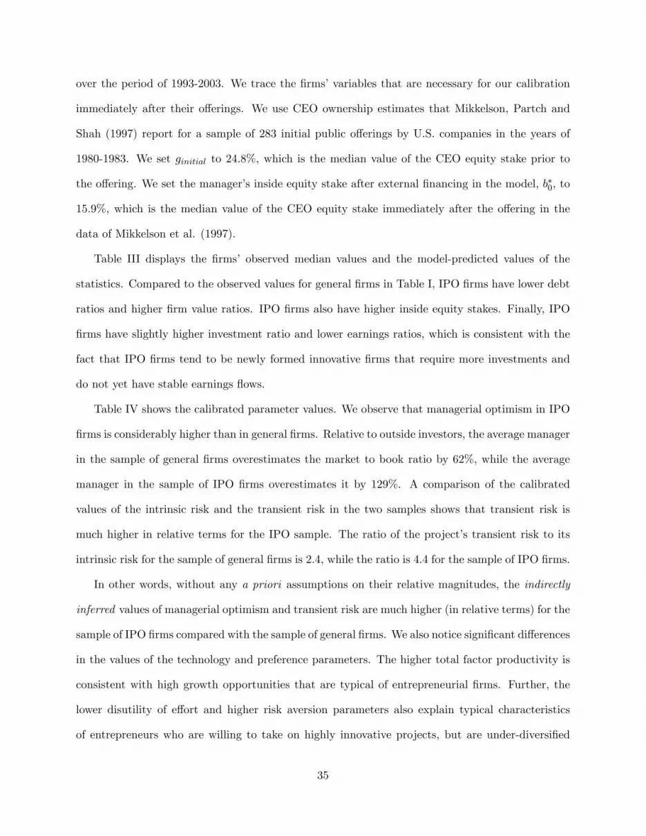
over the period of 1993-2003. We trace the �rms�variables that are necessary for our calibration

immediately after their o¤erings. We use CEO ownership estimates that Mikkelson, Partch and

Shah (1997) report for a sample of 283 initial public o¤erings by U.S. companies in the years of

1980-1983. We set ginitial to 24.8%, which is the median value of the CEO equity stake prior to

the o¤ering. We set the manager�s inside equity stake after external �nancing in the model, b�0, to

15.9%, which is the median value of the CEO equity stake immediately after the o¤ering in the

data of Mikkelson et al. (1997).

Table III displays the �rms� observed median values and the model-predicted values of the

statistics. Compared to the observed values for general �rms in Table I, IPO �rms have lower debt

ratios and higher �rm value ratios. IPO �rms also have higher inside equity stakes. Finally, IPO

�rms have slightly higher investment ratio and lower earnings ratios, which is consistent with the

fact that IPO �rms tend to be newly formed innovative �rms that require more investments and

do not yet have stable earnings �ows.

Table IV shows the calibrated parameter values. We observe that managerial optimism in IPO

�rms is considerably higher than in general �rms. Relative to outside investors, the average manager

in the sample of general �rms overestimates the market to book ratio by 62%, while the average

manager in the sample of IPO �rms overestimates it by 129%. A comparison of the calibrated

values of the intrinsic risk and the transient risk in the two samples shows that transient risk is

much higher in relative terms for the IPO sample. The ratio of the project�s transient risk to its

intrinsic risk for the sample of general �rms is 2.4, while the ratio is 4.4 for the sample of IPO �rms.

In other words, without any a priori assumptions on their relative magnitudes, the indirectly

inferred values of managerial optimism and transient risk are much higher (in relative terms) for the

sample of IPO �rms compared with the sample of general �rms. We also notice signi�cant di¤erences

in the values of the technology and preference parameters. The higher total factor productivity is

consistent with high growth opportunities that are typical of entrepreneurial �rms. Further, the

lower disutility of e¤ort and higher risk aversion parameters also explain typical characteristics

of entrepreneurs who are willing to take on highly innovative projects, but are under-diversi�ed

35

relative to managers of general �rms.

It is worth emphasizing here that the implications of the calibrations of the model to the two

di¤erent samples are not a priori obvious. We calibrate the model to a range of statistics and the

calibrated parameter set includes a number of parameters other than those that directly pertain to

the beliefs of managers and outside investors. Overall, our �ndings provide further support for the

quantitative importance of asymmetric beliefs as a determinant of capital structure (especially for

nascent �rms).

6 Conclusions

We develop a dynamic structural model to examine the e¤ects of heterogeneous beliefs and

agency con�icts on capital structure. In our dynamic agency model, the manager of a �rm has

discretion in �nancing and e¤ort and receives dynamic incentives through explicit contracts with

shareholders. Managers and outside investors have imperfect information and di¤ering beliefs about

the project�s intrinsic quality. We implement the manager�s optimal contract through �nancial se-

curities, which leads to a dynamic capital structure that re�ects the e¤ects of external imperfections

arising from taxes and bankruptcy costs as well as internal imperfections arising from asymmetric

beliefs and agency con�icts. The theoretical and numerical analyses of the model generate novel

testable implications that link project characteristics� the degree of managerial optimism, intrinsic

risk, transient risk, and expected pro�tability� to di¤erent components of capital structure.

We calibrate the model parameters to a sample of general and IPO �rms. We �nd that manager-

ial optimism and uncertainty about project quality are much more signi�cant (in relative terms) for

the IPO sample. Our calibrations also show that IPO �rms have higher growth opportunities and

the managers/entrepreneurs of IPO �rms are less diversi�ed than general �rm managers. Broadly,

our study shows that asymmetric beliefs and agency con�icts are important determinants of �rms�

�nancial policies.

36

Appendix A: Proofs

Proof of Theorem 1

As in the proof of Theorem 3.1 in Giat et al. (2010), we use backward induction to solve the

manager�s optimal contracting problem for a given long-term debt structure d. We normalize the

interest rate to zero to simplify notation in this proof as well as subsequent proofs.

We �rst derive the optimal contractual parameters in period [T � 1; T ]. Suppose that the �rmis solvent as of date i = T � 1. The manager�s conditional expected utility derived from her

compensation including her disutility of e¤ort over this period is

M(i) := EMi

�� exp

��

�cmi � ��

i

��= � exp

�� (ai; bi; ki; �i)

�; where (39)

�(ai; bi; ki; �i) = ai+(1��)(1��)��Mi +Ak�i �

�i

�bi�� i �(1��)dbi�0:5�(1��)

2(1��)2(�2i+s2)b2i :(40)

Equations (39) and (40) follow from (1), (8), (11), and the fact that � + Ni+1 � N(�Mi ; �2i + s2)

under the manager�s beliefs. Note that maximizing the manager�s conditional expected utility is

equivalent to maximizing �(ai; bi; ki; �i).

A feasible contract must be incentive compatible, that is, it is optimal for the manager to exert

the speci�ed e¤ort in the contract given the other contractual variables (ai; bi; ki). We assume that

(1� �) =� > 2, which guarantees a unique optimal e¤ort choice. The manager�s optimal e¤ort �ias a function of the other variables is given by

�i = �(bi; ki) =hA(1� �)(1� �)�k�i bi

�

i 1 ��

: (41)

In addition, shareholders�participation constraint (17) must be satis�ed by the remaining contrac-

tual variables (ai; bi; ki):

CVi := ESi

hcsi � ki

i� ESi

�(1� �)

�(1� �)(� +Ni+1)� d

��: (42)

It is evident that the participation constraint must be satis�ed with equality to maximize the

manager�s objective function. Consequently, the contractual parameter ai is derived as a function

of the other two variables:

ai = a(bi; ki) = (1� �)�d� (1� �)�Si

�bi + (1� �)(1� �)Ak�i �(bi; ki)�(1� bi)� ki: (43)

By substituting the manager�s e¤ort function (41) and cash compensation function (43) into her

objective function �(ai; bi; ki; �i), it simpli�es to

�(bi; ki) = (1� �)(1� �)�ibi + (bi)k� ��i � ki � 0:5�(1� �)2(1� �)2(�2i + s2)b2i ; where (44)

37


(bi) :=�A(1� �)(1� �)

� ��1�

� � ��bi

� � ��1� �bi

�: (45)

It now remains to determine the incremental capital investment and the manager�s pay-performance

sensitivity that maximize (44). For bi � =�, it follows from (44) that the optimal investment

is zero. For bi 2 [0; =�), the optimal capital investment as a function of the manager�s pay-

performance sensitivity is

k(bi) =

��

� � (bi)� ��(1��) ��

: (46)

By (46), the optimal contract choice problem reduces to the optimal choice of the manager�s pay-

performance sensitivity

b�i = argmaxbi�0

�(bi; k(bi)) = Fi(bi); (47)

where

Fi(bi) = (1� �)(1� �)�ibi +Bk(bi)� 0:5�(1� �)2(1� �)2(�2i + s2)b2i (48)

and B = (1��) �� .

In sum, the manager�s optimal contracting problem for period [T � 1; T ], conditional on the�rm�s solvency at the beginning of this period, is completely speci�ed by b�i . The optimal capital

investment of shareholders, k�i ; is k(b�i ), the manager�s optimal e¤ort, �

�i ; is �(b

�i ; k

�i ), and her

optimal cash compensation, a�i ; is a(b�i ; k

�i ). Note that the contract exists in period [T � 1; T ] if

and only if the �rm is solvent at date i = T � 1. If shareholders�continuation value based on theirbeliefs at this date is non-positive, bankruptcy is declared and the relationship is terminated, that

is, Tb = T � 1.We now set i = T �2 and consider the optimal contracting problem for period [i; i+1]. Suppose

that the �rm is still solvent at date i. By the law of iterated expectations, the manager�s conditional

expected utility can be written as

M(i) = EMi

�� exp

��

� Tb�1Xj=i

(cmj � �� j )��

= � exp�� (ai; bi; ki; �i)

�� cM�(i+ 1)

�; (49)

where � (ai; bi; ki; �i) is given by (40). The last term �cM�(i+ 1) equals one if bankruptcy occurs

at date i+1 because the manager�s future payo¤s will be zero, which is the payo¤ from her outside

opportunity. If bankruptcy is not declared at date i + 1, the term is the maximized conditional

expected utility at date i+1, which was determined in the contracting problem for period [T �1; T ]above. In either case, the term is una¤ected by the contractual variables for the current period.

Consequently, as in the analysis of period [T�1; T ], the contractual variables maximize the objective

38

function � (ai; bi; ki; �i) : Moreover, the participation constraint for shareholders is now given by

CVi = ESi

�csi � ki +max

nCVi+1; 0

o�� ESi

24Tb�1Xj=i

(1� �)�(1� �)(� +Nj+1)� d

�35 : (50)

If CVi+1 > 0 so that Tb > i+ 1, then it follows from the analysis of period [T � 1; T ] that

CVi+1 = ESi+1

24 Tb�1Xj=i+1

(1� �)�(1� �)(� +Nj+1)� d

�35 :It immediately follows from the above that, regardless of whether bankruptcy is declared at date

i+ 1, shareholders�participation constraint (50) is equivalent to the following:

ESi

hcsi � ki

i� ESi

�(1� �)

�(1� �)(� +Ni+1)� d

��;

which is identical in form to (42). Consequently, the optimization problem is identical to the one

for period [T � 1; T ]: Hence optimal contractual variables for period [T � 2; T � 1] are determinedin the same manner as in the contracting problem for period [T � 1; T ]. This argument can clearlybe extended by backward induction to any period [i; i+ 1] for i < T � 2. Q.E.D.

Proof of Theorem 2

As mentioned earlier, the bankruptcy time is endogenously determined by the optimal stopping

problem (27). The continuation value of shareholders at date i � T � 1 is given by (50), whichmust be satis�ed with equality. We denote the continuation value as CVi(�Si ) to make explicit its

dependence on shareholders�mean posterior assessment of project quality at each date i. Let Z

denote a standard normal random variable. By (4), (5), and (6), the continuation value is

CVi(�Si ) = (1� �)

�(1� �)�Si � d

�+ ESi

�max

nCVi+1(�

Si + �

�i Z); 0

o�; (51)

where we replace �Si+1 with �Si + ��i Z, and �

�i is de�ned in (30). We �rst need to show that the

continuation value CVi(�) is a continuous, non-decreasing function of �Si for 0 � i � T � 1. To doso, we use backward induction. For the proof of its continuity, we show that there exist positive

constants �1i , �2i such that

CVi(�Si ) � �1i + �

2i maxf�Si ; 0g: (52)

The assertions of monotonicity and continuity for date T�1 immediately follow because CVT�1(�ST�1)= (1 � �)

�(1 � �)�ST�1 � d

�. Suppose the assertions are true for dates i + 1; : : : ; T � 2. Then we

only need to demonstrate that the assertions also hold for date i.

The monotonicity of CVi(�) is a direct consequence on the fact that the expectation on the

39

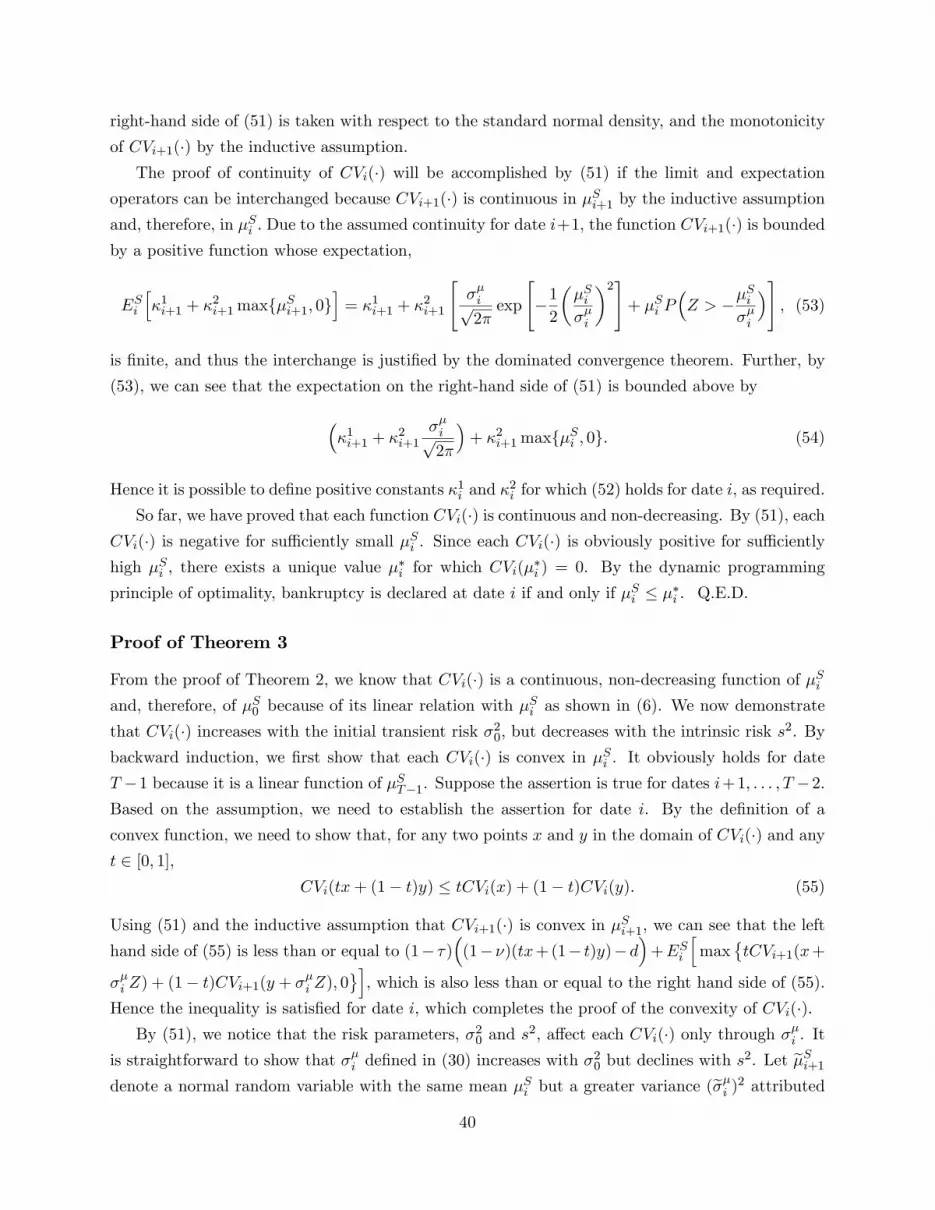
right-hand side of (51) is taken with respect to the standard normal density, and the monotonicity

of CVi+1(�) by the inductive assumption.The proof of continuity of CVi(�) will be accomplished by (51) if the limit and expectation

operators can be interchanged because CVi+1(�) is continuous in �Si+1 by the inductive assumptionand, therefore, in �Si : Due to the assumed continuity for date i+1, the function CVi+1(�) is boundedby a positive function whose expectation,

ESi

h�1i+1 + �

2i+1maxf�Si+1; 0g

i= �1i+1 + �

2i+1

"��ip2�exp

"�12

��Si��i

�2#+ �Si P

�Z > ��

Si

��i

�#; (53)

is �nite, and thus the interchange is justi�ed by the dominated convergence theorem. Further, by

(53), we can see that the expectation on the right-hand side of (51) is bounded above by

��1i+1 + �

2i+1

��ip2�

�+ �2i+1maxf�Si ; 0g: (54)

Hence it is possible to de�ne positive constants �1i and �2i for which (52) holds for date i, as required.

So far, we have proved that each function CVi(�) is continuous and non-decreasing. By (51), eachCVi(�) is negative for su¢ ciently small �Si . Since each CVi(�) is obviously positive for su¢ cientlyhigh �Si , there exists a unique value �

�i for which CVi(�

�i ) = 0. By the dynamic programming

principle of optimality, bankruptcy is declared at date i if and only if �Si � ��i . Q.E.D.

Proof of Theorem 3

From the proof of Theorem 2, we know that CVi(�) is a continuous, non-decreasing function of �Siand, therefore, of �S0 because of its linear relation with �

Si as shown in (6). We now demonstrate

that CVi(�) increases with the initial transient risk �20, but decreases with the intrinsic risk s2. Bybackward induction, we �rst show that each CVi(�) is convex in �Si . It obviously holds for dateT �1 because it is a linear function of �ST�1. Suppose the assertion is true for dates i+1; : : : ; T �2.Based on the assumption, we need to establish the assertion for date i. By the de�nition of a

convex function, we need to show that, for any two points x and y in the domain of CVi(�) and anyt 2 [0; 1],

CVi(tx+ (1� t)y) � tCVi(x) + (1� t)CVi(y): (55)

Using (51) and the inductive assumption that CVi+1(�) is convex in �Si+1, we can see that the lefthand side of (55) is less than or equal to (1� �)

�(1� �)(tx+(1� t)y)�d

�+ESi

hmax

�tCVi+1(x+

��i Z) + (1� t)CVi+1(y + ��i Z); 0

i, which is also less than or equal to the right hand side of (55).

Hence the inequality is satis�ed for date i, which completes the proof of the convexity of CVi(�).By (51), we notice that the risk parameters, �20 and s

2, a¤ect each CVi(�) only through ��i . Itis straightforward to show that ��i de�ned in (30) increases with �

20 but declines with s

2. Let e�Si+1denote a normal random variable with the same mean �Si but a greater variance (e��i )2 attributed

40

to an increase in �20 or a decrease in s2. Then the distribution of �Si+1 second-order stochastically

dominates that of e�Si+1. By the convexity of maxfCV Si+1(�); 0g, it follows thatESi

hmax

�CV Si+1(e�Si+1); 0i � ESi

hmax

�CV Si+1(�

Si+1); 0

i; (56)

which implies that each CVi(�) increases with �20, but declines with s2.As shown by Theorem 2, the optimal bankruptcy trigger ��i is uniquely determined by the

condition CVi(��i ) = 0. Since CVi(�) increases with �S0 by (51), increases with �20, and decreaseswith s2, the bankruptcy time increases with �S0 , increases with �

20, and decreases with s

2. Q.E.D.

Proof of Theorem 4

Taking the logarithm of the negative of the manager�s objective function speci�ed in (21), the

optimization program for the determination of the long-term debt coupon payment is

G(d�(�0);�0) := mind��

hginitial

hLD(0) + S(0)� I

ii+ log(�M(0)); (57)

where M(0) is given by (28). We denote the indirect objective function by G and indicate the

dependence of G on the degree of managerial optimism �0. By the implicit function theorem,

@d�

@�0= �@

2G=@d@�0@2G=@d2

jd=d� : (58)

Note that @2G=@d2jd=d� � 0 by the second order condition for d�. Consequently, the sign of @d�

@�0is

the negative of that of @2G=@d@�0. Moreover, the manager�s initial payo¤� her share of the �rm�s

net proceeds from external �nancing� does not depend on beliefs, which in turn implies that

@2G=@d@�0 =@2 log(�M(0))

@d@�0: (59)

We now show that @2G=@d@�0 � 0, which implies that @d�

@�0� 0 by (58). First, by (47), (48), and

(28), the continuation expected utilityM(0) depends on d only through the bankruptcy time Tb. As

shown in (51), each CVi(�) decreases with d so that the bankruptcy time Tb decreases monotonicallywith d. Second, by (48), Fi(b�i ) increases with �i for each i and, therefore, with �0 because an

increase in the initial degree of optimism increases the degree of optimism at each subsequent period

by (7): Third, one can use arguments similar to those used in the proof of Theorem 3 to show that,

under the manager�s beliefs, the shareholders�continuation value increases with the manager�s initial

mean assessment of project quality, �M0 (keeping shareholders�initial mean assessment, �S0 �xed)

and, therefore, with �0. It follows that, under the manager�s beliefs, the bankruptcy time increases

almost surely with �0. It follows that log(�M(0)) increases monotonically with an increase inthe debt coupon d and the degree of managerial optimism, �0: Consequently, the sign of (59) is

non-negative. By (58), @d�

@�0� 0; that is, long-term debt decreases monotonically with the initial

41

degree of managerial optimism. Q.E.D.

Proof of Proposition 2

In what follows, we solve the manager�s optimal contracting problem when shareholders have bar-

gaining power of �. The procedure is similar to the proof of Theorem 1; we only focus on the

contracting problem for period [i; i + 1] for i = T � 1 here because the same arguments apply tothe earlier dates.

Suppose that the �rm is solvent at date i and has a long-term debt structure d. The manager�s

objective function from her conditional expected utility is given by �(ai; bi; ki; �i) in (40), and,

therefore, her optimal e¤ort function is also determined by �(bi; ki) in (41). As mentioned in the

text, however, we have the modi�ed participation constraint for shareholders that additionally

requires a portion of the equilibrium discretionary earnings at the level rationally anticipated by

shareholders (recall that the discretionary earnings are observable but non-veri�able), which is

denoted by A~k�i ~��i :

ESi

hcsi � ki

i� ESi

h(1� �)

�(1� �)(� +Ni+1 + �A~k�i ~�

�i )� d

�i: (60)

This constraint must be satis�ed with equality, which derives the manager�s cash compensation

function as follows:

ai = a(bi; ki) = (1��)�d�(1��)�Si

�bi+(1��)(1��)Ak�i �(bi; ki)�(1�bi)�ki�(1��)(1��)�A~k�i ~�

�i :

(61)

After some algebra; we can rewrite the objective function as

�(bi; ki) = (1��)(1��)�ibi+ (bi)k� ��i �ki�0:5�(1��)2(1��)2(�2i+s2)b2i�(1��)(1��)�A~k�i ~�

�i ;

(62)

where (bi) is given by (45). As in the proof of Theorem 1, the equilibrium pay-performance

sensitivity and the capital investment must maximize �(bi; ki): Compared with (44), there is an

additional term regarding the rationally anticipated equilibrium discretionary surplus A~k�i ~��i , but

this term does not in�uence the manager�s optimization problem. Consequently, the optimal pay-

performance sensitivity, e¤ort, and investment are given by their values (b�i ; ��i ; k

�i ) in Theorem 1,

that is, they are una¤ected by the bargaining power parameter �.

In a rational expectations equilibrium, all agents correctly anticipate the optimal contractual

parameters. Consequently, we must have

e�i = ��i ;eki = k�i :

42

The allocation of bargaining power, however, a¤ects the manager�s cash compensation as follows.

ai(�) = (1� �)�d� (1� �)�Si

�b�i + (1� �)(1� �)Ak�i

��i�(1� b�i � �)� k�i : (63)

Finally, notice that the market value of outside equity when shareholders have nonzero bargaining

power is

S(i) = ESi

24Tb(�)�1Xj=i

(1� �)�(1� �)(� +Nj+1 + �Ak�j

��j�)� d

�35 : (64)

Appendix B: Numerical Implementation and Calibration

In this section, we describe our numerical implementation of the model. We calibrate the baseline

values of the following key parameters of the model: � = (A;�S0 ;�0; �0; �; �; =�): For a given

candidate parameter vector � and a given long-term debt structure d; we �rst compute the de-

terministic optimal contractual variables. We then discretize the state space and simulate the

stochastic process of the shareholders�mean posterior assessment of project pro�tability, �S : We

determine the states where bankruptcy is declared by the condition in Theorem 2. We then solve

for the optimal choice of long-term debt coupon payment d� as speci�ed in (57). Given d�; we

compute the vector of model-predicted values of the statistics listed in Section 5.1. The baseline

parameter values are those that minimize the sum of squared di¤erences between model-predicted

and observed values of the statistics. We use the Nelder-Meade optimization routine in MATLAB

to perform the minimization. To avoid a local minimum solution, we repeat the optimization

routine multiple times by randomizing the initial seed. We now describe the various steps of the

implementation in more detail.

Computation of non-stochastic variables: For a given parameter vector � and a long-term debt

structure d; the deterministic optimal contractual variables (b�i ; ��i ; k

�i ) and the resulting objective

function Fi(b�i ) for all i < T are determined by Theorem 1. We also compute other deterministic

variables (�i;�i; ��i ) for all i < T as de�ned in (5), (7), and (30).

Construction of discrete-state stochastic process: Because the key variables for our calibra-

tion are de�ned under the shareholders�beliefs, we directly model the evolution of shareholders�

mean posterior assessments of the project�s pro�tability �S . At date 0, shareholders�mean assess-

ment of the core output is �S0 . Let n(i) denote the number of states at date i > 0, which linearly

increases from period to period, that is, n(i) =Mi with M = 20; and let �Si;j denote shareholders�

mean assessment at the jth state at date i where j = 1; : : : ; n(i). The lattice is designed such that

the minimal and maximal states at date i, �Si;1 and �Si;n(i), respectively, are 2:5 standard deviations

below and above the minimal and maximal states at date i � 1. The values for the remainingn(i)� 2 states are equally spaced between the minimum and maximum states.

Determination of bankruptcy time: Once the discrete lattice of �S is set up, we need to

compute the continuation value of shareholders, which is denoted by CVi;j at each state j and date

43

i: As a terminal condition for dynamic programming, we assume that the continuation value at

date T is as follows:

CVT;j =(1� �)(1� �)�ST;j

(1� e�r) ; if �ST;j > 0;

CVT;j = 0; otherwise:

The two terminal conditions above specify that the shareholders�continuation value at the terminal

date is the net present value of future base earnings if shareholders�mean posterior assessment of

pro�tability is positive, and is zero otherwise.

For earlier dates i < T; the continuation values are computed as described in (51), that is,

CVi;j = (1� �)�(1� �)�Si;j � d

�+ e�r

n(i+1)Xk=1

pi+1;ki;j maxfCVi+1;k; 0g ;

where pi+1;ki;j is the transition probability that shareholders�mean assessment will transition from

state �Si;j at date i to state �Si+1;k at date i + 1: Using the normality of the stochastic component

of the model, we set

pi+1;ki;j = �

��12(�Si+1;k + �

Si+1;k+1)� �Si;j

� 1��i

��

��12(�Si+1;k + �

Si+1;k�1)� �Si;j

� 1��i

�; (65)

if �Si+1;k is within �2:5��i from �Si;j : In the above, �(�) denotes the cdf of the standard normal

distribution. Otherwise (if �Si+1;k appears away from �Si;j), the transition probability is zero.

Starting from i = T � 1 and working backwards through time, we compute the continuationvalues for all states and dates. Since the true continuation value function is continuous and non-

decreasing as shown in the proof of Theorem 2, we complete the approximation to CVi(�) by linearinterpolation. We then determine the optimal trigger ��i that solves CVi(�

�i ) = 0: By comparing

each state variable �Si;j with the trigger ��i ; we identify the states at which bankruptcy occurs for

each date i:

Optimal long-term debt structure choice: Next, we determine the manager�s objective func-

tion in (57) for a given long-term debt structure d: More speci�cally, we need to compute each

component in the objective function, LD(0) + S(0); I(= AV(0)); and M(0); by backward induc-

tion. The termination conditions at date T are given by:

AVT;j = MVT;j =(1� �)�ST;j(1� e�r) ; if �

ST;j > 0;

AVT;j = MVT;j = 0; otherwise;

where MV =LD + S; the market value of debt plus the market value of outside equity, which is

equivalent to the market value of the �rm�s after-tax earnings stream net of the manager�s stake.

44

For earlier dates i < T; each of these values is computed by backward induction. First, the

asset value is determined by

AVi;j = (1� �)�Si;j + e�rn(i+1)Xk=1

pi+1;ki;j AVi+1;k:

Second, the market value of long-term debt plus outside equity at each date i depends on

whether bankruptcy occurs at that date:

MVi;j = (1� �)AVi;j if �Si;j � ��i ;

MVi;j = (1� �)(1� �)�Si;j + �d+ e�rn(i+1)Xk=1

pi+1;ki;j MVi+1;k; otherwise.

Third, we compute the manager�s continuation expected utilityM(0). By (28), this is given by

M(0) = EM0

�� exp

��

� Tb�1Xi=0

e�riFi(b�i )��

: (66)

Since Fi(b�i ) is given by (22) and (23), we only need to determine the distribution of the bankruptcy

time Tb under the manager�s beliefs. To compute this, we simulate the evolution of the process

�S under the manager�s beliefs. We do this by simulating the evolution of the manager�s posterior

mean assessment �M : We set up a discrete lattice for �M similar to the discrete lattice for �S

described earlier. We then use the fact that �Si;j = �Mi;j � �i by (7). Analogous to (65), the

transition probabilities for the process �M are as follows:

epi+1;ki;j = �

��12(�Mi+1;k + �

Mi+1;k+1)� �Mi;j

� 1��i

��

��12(�Mi+1;k + �

Mi+1;k�1)� �Mi;j

� 1��i

�; (67)

We then follow the procedure outlined to determine the distribution of the bankruptcy time under

the shareholders�beliefs to determine its distribution under the manager�s beliefs.

Finally, we determine the optimal long-term coupon payment d� using the Nelder-Meade opti-

mization method. The optimization method evaluates the objective function at di¤ering values of

long-term coupon payment as illustrated above and then determines the best solution.

Determination of the model-predicted values: Once the optimal solution d� is obtained, we

compute in a similar manner long-term debt and short-term debt values and �rm (or project) value

at date zero, which are de�ned in (33) and in (35), respectively. Then the model-predicted values

of the statistics for the given parameter vector � are derived.

45

References

[1] Adrian, T., and M. Wester�eld. 2009. Disagreement and Learning in a Dynamic ContractingModel. Review of Financial Studies 22:3873-3906.

[2] Allen, F., and D. Gale. 1999. Diversity of Opinion and the Financing of New Technologies.Journal of Financial Intermediation 8:68-89.

[3] Andrade, G., and S. Kaplan. 1998. How Costly is Financial (Not Economic) Distress? Evidencefrom Highly Leveraged Transactions that Became Distressed. Journal of Finance 53:1443-1493.

[4] Baker, M., R. Ruback, and J. Wurgler. 2007. Behavioral Corporate Finance: A Survey. In E.Eckbo (ed.), Handbook of Corporate Finance: Empirical Corporate Finance. Amsterdam, TheNetherlands: Elsevier/North-Holland.

[5] Ben-David, I., J. Graham, and C. Harvey. 2007. Managerial Overcon�dence and CorporatePolicies. Working Paper, Duke University.

[6] Berk, J., R. Stanton, and J. Zechner. 2010. Human Capital, Bankruptcy, and Capital Structure.Journal of Finance 65: 891�926.

[7] Bhagat, S., B. Bolton, and A. Subramanian. 2010. Manager Characteristics and Capital Struc-ture: Theory and Evidence. Forthcoming in the Journal of Financial and Quantitative Analysis.

[8] Bolton, P. and M. Dewatripont. 2005. Contract Theory. MIT Press

[9] Chemmanur, T., D. Nandy, and A. Yan. 2008. Capital Strucuture and Security Issuance underHeterogeneous Beliefs. Working Paper, Boston College.

[10] DeMarzo, P., and M. Fishman. 2007. Optimal Long-Term Financial Contracting. Review ofFinancial Studies 20:2079-2128.

[11] DeMarzo, P., and Y. Sannikov. 2006. Optimal Security Design and Dynamic Capital Structurein a Continuous-Time Agency Model. Journal of Finance 61:2681-2724.

[12] Dittmar, A., and A. Thakor. 2007. Why Do Firms Issue Equity?. Journal of Finance 62:1-54.

[13] Fazzari, S. M., and B. C. Petersen. 1993. Working Capital and Fixed Investment: New Evidenceon Financing Constraints. Rand Journal of Economics 24:328-342.

[14] Fischer, E., R. Heinkel, and J. Zechner. 1989. Dynamic Capital Structure Choice: Theory andTests. Journal of Finance 44:19-40.

[15] Gervais, S., J. Heaton, and T. Odean. 2007. Overcon�dence, Investment Policy and ManagerWelfare. Working Paper, Duke University.

[16] Giat, Y., S. T. Hackman, and A. Subramanian. 2010. Investment under Uncertainty, Hetero-geneous Beliefs and Agency Con�icts. Review of Financial Studies. 23:1360-1404

[17] Gibbons, R., and K. J. Murphy. 1992. Optimal Incentive Contracts in the Presence of CareerConcerns: Theory and Evidence. Journal of Political Economy 100:468-505.

[18] Goldstein, R., N. Ju, and H. Leland. 2001. An EBIT Based Model of Dynamic Capital Struc-ture. Journal of Business 74:483-512.

46

https://www.researchgate.net/publication/4769631_Why_Do_Firms_Issue_Equity?el=1_x_8&enrichId=rgreq-3ef27c307ee0d60a2ad3a3a79ac9ff4a-XXX&enrichSource=Y292ZXJQYWdlOzIyODI1Mjc3MDtBUzoxNjYzOTk3MjUwMjMyMzRAMTQxNjY4NDE5NDQ5MQ==









https://www.researchgate.net/publication/24103723_Optimal_Incentive_Contracts_in_the_Presence_of_Career_Concerns_Theory_and_Evidence?el=1_x_8&enrichId=rgreq-3ef27c307ee0d60a2ad3a3a79ac9ff4a-XXX&enrichSource=Y292ZXJQYWdlOzIyODI1Mjc3MDtBUzoxNjYzOTk3MjUwMjMyMzRAMTQxNjY4NDE5NDQ5MQ==

https://www.researchgate.net/publication/24103723_Optimal_Incentive_Contracts_in_the_Presence_of_Career_Concerns_Theory_and_Evidence?el=1_x_8&enrichId=rgreq-3ef27c307ee0d60a2ad3a3a79ac9ff4a-XXX&enrichSource=Y292ZXJQYWdlOzIyODI1Mjc3MDtBUzoxNjYzOTk3MjUwMjMyMzRAMTQxNjY4NDE5NDQ5MQ==

https://www.researchgate.net/publication/5185539_Behavioral_Corporate_Finance_A_Survey?el=1_x_8&enrichId=rgreq-3ef27c307ee0d60a2ad3a3a79ac9ff4a-XXX&enrichSource=Y292ZXJQYWdlOzIyODI1Mjc3MDtBUzoxNjYzOTk3MjUwMjMyMzRAMTQxNjY4NDE5NDQ5MQ==



https://www.researchgate.net/publication/4736394_How_Costly_Is_Financial_Not_Economic_Distress_Evidence_From_Highly_Leveraged_Transactions_That_Became_Distressed?el=1_x_8&enrichId=rgreq-3ef27c307ee0d60a2ad3a3a79ac9ff4a-XXX&enrichSource=Y292ZXJQYWdlOzIyODI1Mjc3MDtBUzoxNjYzOTk3MjUwMjMyMzRAMTQxNjY4NDE5NDQ5MQ==

https://www.researchgate.net/publication/4736394_How_Costly_Is_Financial_Not_Economic_Distress_Evidence_From_Highly_Leveraged_Transactions_That_Became_Distressed?el=1_x_8&enrichId=rgreq-3ef27c307ee0d60a2ad3a3a79ac9ff4a-XXX&enrichSource=Y292ZXJQYWdlOzIyODI1Mjc3MDtBUzoxNjYzOTk3MjUwMjMyMzRAMTQxNjY4NDE5NDQ5MQ==



https://www.researchgate.net/publication/4769613_Optimal_Security_Design_and_Dynamic_Capital_Structure_in_a_Continuous-Time_Agency_Model?el=1_x_8&enrichId=rgreq-3ef27c307ee0d60a2ad3a3a79ac9ff4a-XXX&enrichSource=Y292ZXJQYWdlOzIyODI1Mjc3MDtBUzoxNjYzOTk3MjUwMjMyMzRAMTQxNjY4NDE5NDQ5MQ==

https://www.researchgate.net/publication/4769613_Optimal_Security_Design_and_Dynamic_Capital_Structure_in_a_Continuous-Time_Agency_Model?el=1_x_8&enrichId=rgreq-3ef27c307ee0d60a2ad3a3a79ac9ff4a-XXX&enrichSource=Y292ZXJQYWdlOzIyODI1Mjc3MDtBUzoxNjYzOTk3MjUwMjMyMzRAMTQxNjY4NDE5NDQ5MQ==







[19] Graham, J. 2000. How Big are the Tax Bene�ts of Debt. Journal of Finance 55:1901-1941.

[20] Hackbarth, D. 2008. Managerial Traits and Capital Structure Decisions. Journal of Financialand Quantitative Analysis 43:843-882.

[21] Hennessy, C., and T. Whited. 2005. Debt Dynamics. Journal of Finance 60:1129-1165.

[22] Holderness, C., R. Kroszner, D. Sheehan. 1999. Were the Good Old Days that Good? Changesin Managerial Stock Ownership since the Great Depression. Journal of Finance 54:435-469.

[23] Landier, A., and D. Thesmar. 2009. Financial Contracting with Optimistic Entrepreneurs.Review of Financial Studies 22:117-150.

[24] Leland, H. 1994. Corporate Debt Value, Bond Covenants, and Optimal Capital Structure.Journal of Finance 49:1213-1252.

[25] Leland, H. 1998. Agency Costs, Risk Management, and Capital Structure. Journal of Finance53:1213-1243.

[26] Leland, H., and K. Toft. 1996. Optimal Capital Structure, Endogenous Bankruptcy and theTerm Structure of Credit Spreads. Journal of Finance 51:987-1019.

[27] Mikkelson, W. H., M. M. Partch, and K. Shah. 1997. Ownership and Operating Performanceof Companies That Go Public. Journal of Financial Economics 44:281-307.

[28] Malmendier, U., and G. A. Tate. 2005. CEO Overcon�dence and Corporate Investment. Jour-nal of Finance 60:2660-2700.

[29] Morris, S. 1995. The Common Prior Assumption in Economic Theory. Economics and Philos-ophy 11:227-253.

[30] Rayburn, J. 1986. The Association of Operating Cash Flow and Accruals with Security Re-turns. Journal of Accounting Research 24: 112-133.

[31] Strebulaev, I. 2007. Do Tests of Capital Structure Theory Mean What they Say? Journal ofFinance 62:1747-1787.

[32] Tirole, J. 2006. The Theory of Corporate Finance. Princeton University Press.

47



https://www.researchgate.net/publication/4992767_Do_Tests_of_Capital_Structure_Theory_Mean_What_They_Say?el=1_x_8&enrichId=rgreq-3ef27c307ee0d60a2ad3a3a79ac9ff4a-XXX&enrichSource=Y292ZXJQYWdlOzIyODI1Mjc3MDtBUzoxNjYzOTk3MjUwMjMyMzRAMTQxNjY4NDE5NDQ5MQ==

https://www.researchgate.net/publication/4992767_Do_Tests_of_Capital_Structure_Theory_Mean_What_They_Say?el=1_x_8&enrichId=rgreq-3ef27c307ee0d60a2ad3a3a79ac9ff4a-XXX&enrichSource=Y292ZXJQYWdlOzIyODI1Mjc3MDtBUzoxNjYzOTk3MjUwMjMyMzRAMTQxNjY4NDE5NDQ5MQ==

https://www.researchgate.net/publication/222463471_Ownership_and_Operating_Performance_of_Companies_That_Go_Public?el=1_x_8&enrichId=rgreq-3ef27c307ee0d60a2ad3a3a79ac9ff4a-XXX&enrichSource=Y292ZXJQYWdlOzIyODI1Mjc3MDtBUzoxNjYzOTk3MjUwMjMyMzRAMTQxNjY4NDE5NDQ5MQ==

https://www.researchgate.net/publication/222463471_Ownership_and_Operating_Performance_of_Companies_That_Go_Public?el=1_x_8&enrichId=rgreq-3ef27c307ee0d60a2ad3a3a79ac9ff4a-XXX&enrichSource=Y292ZXJQYWdlOzIyODI1Mjc3MDtBUzoxNjYzOTk3MjUwMjMyMzRAMTQxNjY4NDE5NDQ5MQ==

https://www.researchgate.net/publication/5085772_The_Theory_Of_Corporate_Finance?el=1_x_8&enrichId=rgreq-3ef27c307ee0d60a2ad3a3a79ac9ff4a-XXX&enrichSource=Y292ZXJQYWdlOzIyODI1Mjc3MDtBUzoxNjYzOTk3MjUwMjMyMzRAMTQxNjY4NDE5NDQ5MQ==

https://www.researchgate.net/publication/227406452_Managerial_Traits_and_Capital_Structure_Decisions?el=1_x_8&enrichId=rgreq-3ef27c307ee0d60a2ad3a3a79ac9ff4a-XXX&enrichSource=Y292ZXJQYWdlOzIyODI1Mjc3MDtBUzoxNjYzOTk3MjUwMjMyMzRAMTQxNjY4NDE5NDQ5MQ==

https://www.researchgate.net/publication/227406452_Managerial_Traits_and_Capital_Structure_Decisions?el=1_x_8&enrichId=rgreq-3ef27c307ee0d60a2ad3a3a79ac9ff4a-XXX&enrichSource=Y292ZXJQYWdlOzIyODI1Mjc3MDtBUzoxNjYzOTk3MjUwMjMyMzRAMTQxNjY4NDE5NDQ5MQ==

https://www.researchgate.net/publication/227348441_The_Common_Prior_Assumption_in_Economic_Theory?el=1_x_8&enrichId=rgreq-3ef27c307ee0d60a2ad3a3a79ac9ff4a-XXX&enrichSource=Y292ZXJQYWdlOzIyODI1Mjc3MDtBUzoxNjYzOTk3MjUwMjMyMzRAMTQxNjY4NDE5NDQ5MQ==

https://www.researchgate.net/publication/227348441_The_Common_Prior_Assumption_in_Economic_Theory?el=1_x_8&enrichId=rgreq-3ef27c307ee0d60a2ad3a3a79ac9ff4a-XXX&enrichSource=Y292ZXJQYWdlOzIyODI1Mjc3MDtBUzoxNjYzOTk3MjUwMjMyMzRAMTQxNjY4NDE5NDQ5MQ==



https://www.researchgate.net/publication/4992404_Optimal_Capital_Structure_Endogenous_Bankruptcy_and_the_Term_Structure_of_Credit_Spreads?el=1_x_8&enrichId=rgreq-3ef27c307ee0d60a2ad3a3a79ac9ff4a-XXX&enrichSource=Y292ZXJQYWdlOzIyODI1Mjc3MDtBUzoxNjYzOTk3MjUwMjMyMzRAMTQxNjY4NDE5NDQ5MQ==

https://www.researchgate.net/publication/4992404_Optimal_Capital_Structure_Endogenous_Bankruptcy_and_the_Term_Structure_of_Credit_Spreads?el=1_x_8&enrichId=rgreq-3ef27c307ee0d60a2ad3a3a79ac9ff4a-XXX&enrichSource=Y292ZXJQYWdlOzIyODI1Mjc3MDtBUzoxNjYzOTk3MjUwMjMyMzRAMTQxNjY4NDE5NDQ5MQ==

https://www.researchgate.net/publication/278415648_How_Big_are_the_Tax_Benefits_of_Debt?el=1_x_8&enrichId=rgreq-3ef27c307ee0d60a2ad3a3a79ac9ff4a-XXX&enrichSource=Y292ZXJQYWdlOzIyODI1Mjc3MDtBUzoxNjYzOTk3MjUwMjMyMzRAMTQxNjY4NDE5NDQ5MQ==



https://www.researchgate.net/publication/288440518_Financial_Contracting_with_Optimistic_Entrepreneurs?el=1_x_8&enrichId=rgreq-3ef27c307ee0d60a2ad3a3a79ac9ff4a-XXX&enrichSource=Y292ZXJQYWdlOzIyODI1Mjc3MDtBUzoxNjYzOTk3MjUwMjMyMzRAMTQxNjY4NDE5NDQ5MQ==

https://www.researchgate.net/publication/288440518_Financial_Contracting_with_Optimistic_Entrepreneurs?el=1_x_8&enrichId=rgreq-3ef27c307ee0d60a2ad3a3a79ac9ff4a-XXX&enrichSource=Y292ZXJQYWdlOzIyODI1Mjc3MDtBUzoxNjYzOTk3MjUwMjMyMzRAMTQxNjY4NDE5NDQ5MQ==

https://www.researchgate.net/publication/280901299_Were_the_good_old_days_that_good_Changes_in_managerial_stock_ownership_since_the_great_depression?el=1_x_8&enrichId=rgreq-3ef27c307ee0d60a2ad3a3a79ac9ff4a-XXX&enrichSource=Y292ZXJQYWdlOzIyODI1Mjc3MDtBUzoxNjYzOTk3MjUwMjMyMzRAMTQxNjY4NDE5NDQ5MQ==

https://www.researchgate.net/publication/280901299_Were_the_good_old_days_that_good_Changes_in_managerial_stock_ownership_since_the_great_depression?el=1_x_8&enrichId=rgreq-3ef27c307ee0d60a2ad3a3a79ac9ff4a-XXX&enrichSource=Y292ZXJQYWdlOzIyODI1Mjc3MDtBUzoxNjYzOTk3MjUwMjMyMzRAMTQxNjY4NDE5NDQ5MQ==

Table I: Observed and Predicted Statistics for General Firms. The table displays the observed

values of the statistics that are used to calibrate the model and their predicted values from the model. We scale all

variables, except for the inside equity stake, by the asset value. The observed statistics are obtained from a sample

of general �rms (excluding �nancial and regulated �rms) from the annual Compustat industrial �les over the period

of 1993-2003.Observed Predicted

Long-term Debt Ratio 0.0943 0.0963Short-term Debt Ratio -0.0754 -0.0753Firm Value Ratio 1.1306 1.1443Inside Equity Stake 0.1440 0.1438Investment Ratio 0.0441 0.0034EBITM Ratio 0.0966 0.0782

Net Income Ratio 0.0189 0.0460

Table II: Baseline Parameter Values for General Firms. The table reports the baseline parametervalues obtained from the model calibration for general �rms. The parameters are classi�ed into three categories:

Technology parameters (the total-factor productivity A, the intrinsic risk s, and the sensitivity of working capital �);

Belief parameters (the initial mean assessment of project quality by shareholders �S0 , the degree of heterogeneous

beliefs �0, and the initial transient risk �0); and Preference parameters (the manager�s risk aversion �, and disutility

of e¤ort parameters � and =�).

Technology Parameters Belief Parameters Preference ParametersA s � �S0 �0 �0 � � =�

20.48 39.36 0.06 80.45 134.60 60.80 0.24 75.48 8.51

Table III: Observed and Predicted Statistics for Firms that Go Public. The table shows

the observed values and model-predicted values of the statistics for IPO �rms. The observed statistics are obtained

from a sample of the �rms that go public over the period of 1993-2003 from the annual Compustat industrial �les.Observed Predicted

Long-term Debt Ratio 0.0161 0.0188Short-term Debt Ratio -0.3348 -0.3347Firm Value Ratio 1.9926 1.9883Inside Equity Stake 0.1590 0.1610Investment Ratio 0.0471 0.0193EBITM Ratio 0.0718 0.1418

Net Income Ratio 0.0113 0.0428

Table IV: Baseline Parameter Values for Firms that Go Public. The table displays the baselineparameter values obtained from the model calibration for IPO �rms.

Technology Parameters Belief Parameters Preference Parameters

A s � �S0 �0 �0 � � =�

75:66 42:83 0:20 106 253:98 89:49 0:41 32:80 4:42

48

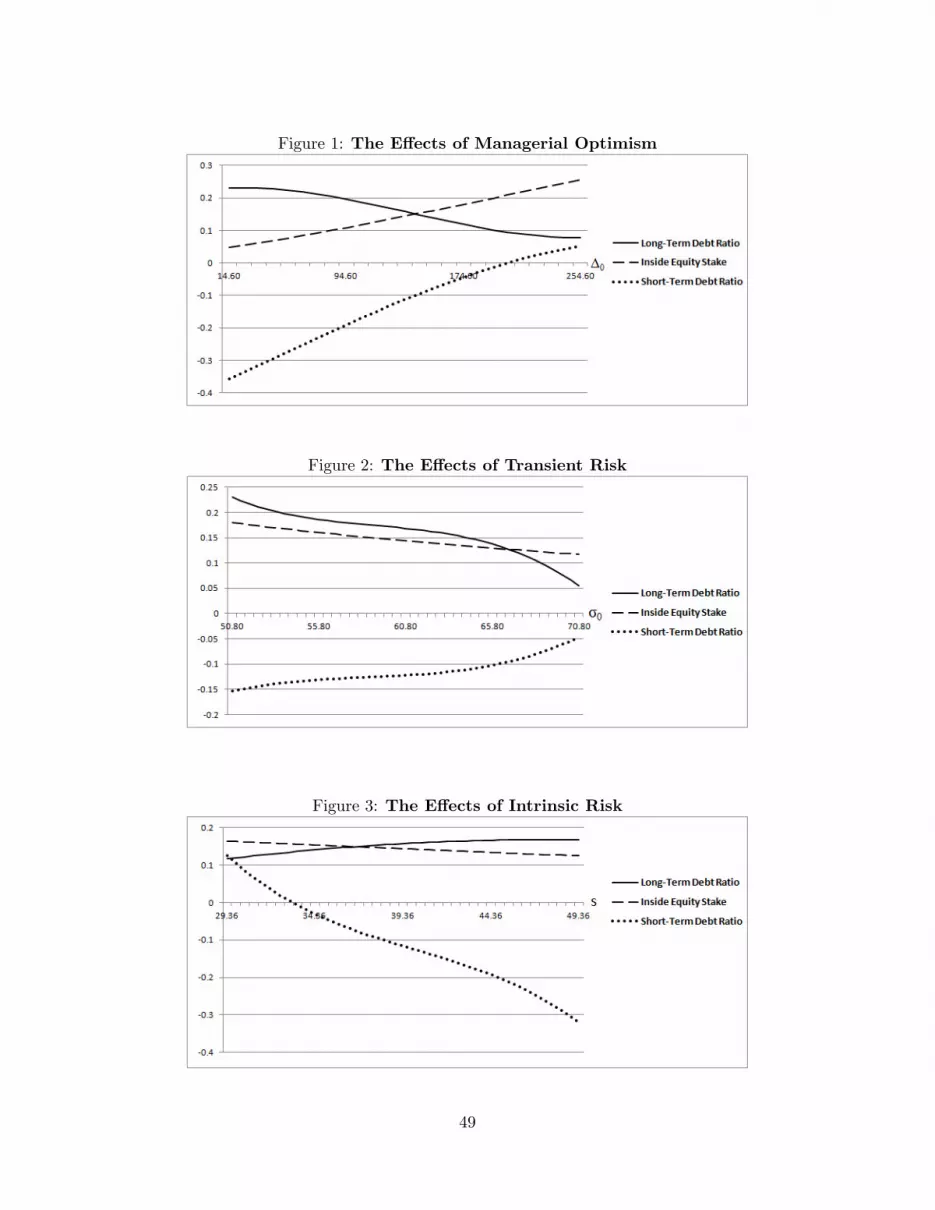
Figure 1: The E¤ects of Managerial Optimism

Figure 2: The E¤ects of Transient Risk

Figure 3: The E¤ects of Intrinsic Risk

49

Figure 4: The E¤ects of Expected Pro�tability

Figure 5: The E¤ects of Managerial Optimism for Varying Levels of Shareholders�Bargaining Power

Figure 6: The E¤ects of Transient Risk for Varying Levels of Shareholders�BargainingPower

50

Figure 7: The E¤ects of Intrinsic Risk for Varying Levels of Shareholders�BargainingPower

Figure 8: The E¤ects of Expected Pro�tability for Varying Levels of Shareholders�Bargaining Power

51

Documents

Capital Structure Under Heterogeneous Beliefs