Embed Size (px)
Citation preview
C0NF-79p518O United States Department of Energy
Assistant Secretary for EnvironmentOffice of Health and Environmental Research
December 1980
hi
012 Carbon Dioxide EffectsResearch ani AssessmentProgram
Proceedings of theInternational Meet" g onStable Isotopes in Tree-RingResearchNew Paltz, New YorkMay 22-25, 1979
United States Department of Energy
Assistant Secretary for EnvironmentOffice of Health and Environmental ResearchWashington, D.C. 20545
December 1980CONF-7905180
UC-11
012 Carbon Dioxide EffectsResearch and AssessmentProgram
Proceedings of theInternational Meeting onStable Isotopes in Tree-RingResearchNew Paltz, New YorkMay 22-25. 1979
Edited byGordon Jacoby
Work Suppored byU.S. Department of EnergyOffice of EnvironmentUnder Contract No. 79EV10037.000
Prepared byLamont-Doherty Geological ObservatoryColumbia University
DISCLAIMED
I book was prepared as an account of work sponsored by an agency of ihe United States Government.| Neither ihe United States Government no' any agency thereof, nor any ot their employees, makes any
ranty, express or implied, or assumes any legal liability ot responsibility 'or the iccuraty,| completeness, or usefulness ol any information, apparatus, product, or process disclosed, or
ewnts thai its use would not infringe privately owned rjgnis. Reference herein 10 any specilircommercial product, process, or service by trade name, trademark, manufacturer, or Otherwise, does |rwt necessarily constitute or imply its endorsement, • ecommendation, or favoring by irn. UniStates Government or any agency thereof. The views and opinions o< authors expressed herein do inecessarily state or reflect those of the United States Government or any agency Ihereof.
ACKNOWLEDGEMENTS
Many thanks are due to those attendees who submitted and revisedtheir papers for this volume. Also thanks go to those who aided in thepreparation of joint papers although they were unable to attend the meet-ing. The editor greatly appreciates the efforts and assistance of KateJennings in the early stages of organizing and editing these papers.
Ann Stern and Paula Lazov of the Tree-Ring Laboratory at Lamont-Doherty Geological Observatory were very helpful in the meeting arrange-ments. Special thanks go to Evelyn Maher and Jill Duncanson for typingof the final copy; and to Linda Ulan, James R. Lawrence and James W.C.White who assisted in the assembling of this volume.
Gordon JacobyLamont-Doherty Geological ObservatoryColumbia University
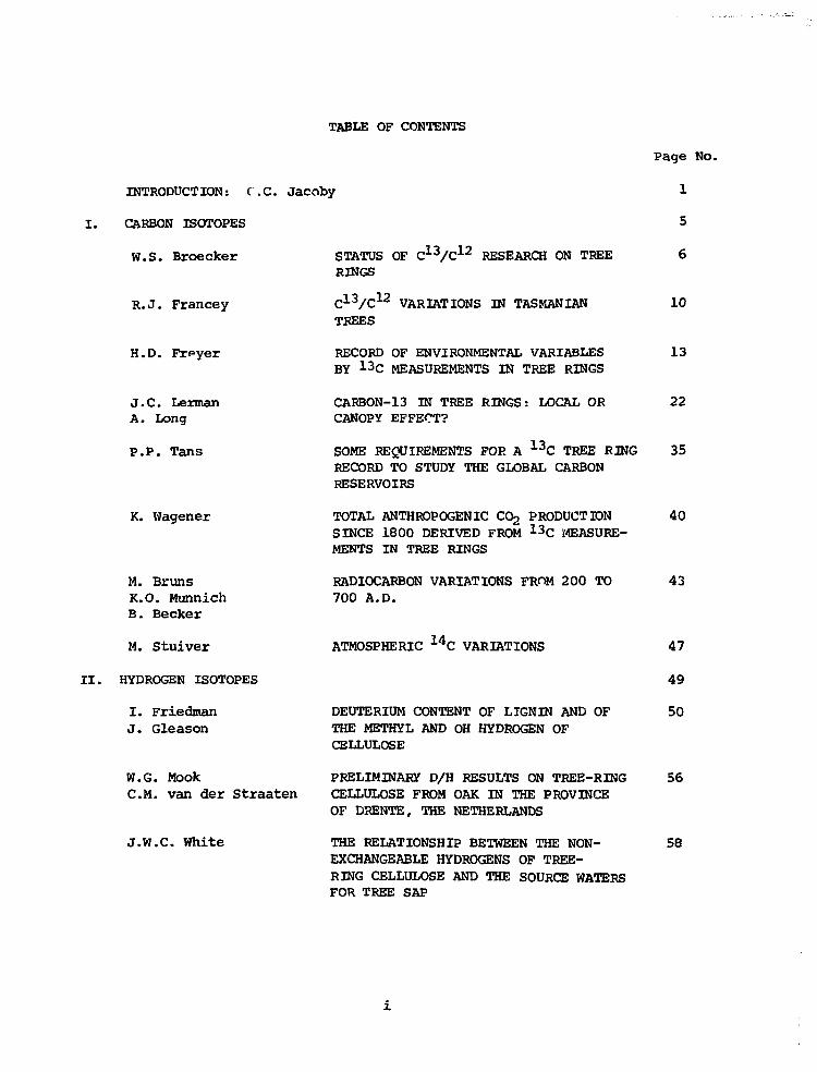
TABLE OF CONTENTS
INTRODUCTION: C.C. Jacoby
I . CARBON ISOTOPES
W.S. B r o e c k e r
R.J. Francey
H.D. Frpyer
J.C. LermanA. Long
P.P. Tans
K. Wagener
M. BrimsK.O. MunnichB. Becker
M. Stuiver
II. HYDROGEN ISOTOPES
I. FriedmanJ. Gleason
W.G. MookCM. van der Straaten
J .W.C. White
STATUS OF C 1 3 / C 1 2 RESEARCH ON TREERINGS
C 1 3 / C 1 2
TREESVARIATIONS IN TASMANIAN
RECORD OF ENVIRONMENTAL VARIABLESBY 1 3 C MEASUREMENTS IN TREE RINGS
CARBON-13 IN TREE RINGS: LOCAL ORCANOPY EFFECT?
SOME REQUIREMENTS FOR A 1 3 C TREE RINGRECORD TO STUDY THE GLOBAL CARBONRESERVOIRS
TOTAL ANTHROPOGENIC CO2 PRODUCTIONSINCE 1800 DERIVED FROM 1 3 C MEASURE-MENTS IN TREE RINGS
RADIOCARBON VARIATIONS FROM 2 0 0 TO700 A.D.
ATMOSPHERIC 1 4 C VARIATIONS
DEUTERIUM CONTENT OF LTGNIN AND OFTHE METHYL AND OH HYDROGEN OFCELLULOSE
PRELIMINARY D/H RESULTS ON TREE-RINGCELLULOSE FROM OAK IN THE PROVINCEOF DRENTE, THE NETHERLANDS
THE RELATIONSHIP BETWEEN THE NON-EXCHANGEABLE HYDROGENS OF TREE-RING CELLULOSE AND THE SOURCE WATERSFOR TREE SAP
Page No.
1
5
6
10
13
22
35
40
43
47
49
50
56
58
Ill- OXYGEN ISOTOPES
R.L. BurkM. Stuiver
A. FerhiR. LetolleA. LongJ.C. Lerman
J. GrayP. Thompson
IV: COMBINATIONS OF ISOTOPES
P. AharonJ. ChappellW. Campston
B.B. HdnshawI.J. WinogradF.J. Pearson, Jr.
A. LongA. FerhiR. LdtolleJ.C. Lerman
A.T. Wilson
V. GENERAL TOPICS
J.R. Lawrence
L. Machta
A. deL. Rebel loK. Wagener
R.H. Waring
VI. ISOTOPIC METHODS
R.L. BurkM. Stuiver
TABLE OF CONTENTS (cont.)
FACTORS AFFECTING 180/160 RATIOSIN CELLULOSE
FACTORS CONTROLLING THE VARIATIONSOF OXYGEN-18 IN PLANT CELLULOSE
NATURAL VARIATIONS IN THE 180CONTENT OF CELLULOSE
LATE PLEISTOCENE CLIMATIC CHANGESREGISTERED BY 618O AND 613C INTHE GIANT CLAM, TRIDACNA GIGAS, OFTHE NEW GUINEA CORAL REEFS
STABLE ISOTOPE STUDIES OFSUBGLACIALLY PRECIPITATEDCARBONATES AND OF ANCIENT GROUND-WATER: PALEOCLIMATIC IMPLICATIONS
POTENTIAL USE OF 618O AND 6DTOGETHER IN PLANT CELLULOSE AS APALEOENVIRONMENT INDICATOR
ISOTOPIC WORK ON TREE RINGS
D/H and 18O/16O RATIOS INPRECIPITATION
OXYGEN DEPLETION
GROWTH TREND IN RECENT TREE RINGS
FOREST AND TREE WATER-BUDGETS
CELLULOSE PREPARATION AND 18OANALYSIS
Page No.
67
68
71
84
93
94
102
105
116
121
122
125
128
133
135
136
ii
W. CompstonP. AharonT. McGee
P. ThompsonJ. GrayS.J. Song
VII. LIST OF ATTENDEES
TABLE OF CONTENTS (cont.)
ISOTOPIC ANALYSIS FOR <513C AND618O USING A SINGLE COLLECTOR ANDMATCHED MOLECULAR FLOW LEAKS
A PRELIMINARY REPORT ON THESIMULTANEOUS EXTRACTION OF HYDRO-GEN AND OXYGEN FROM ORGANICMATERIALS
Page No.
138
142
147
INTRODUCTION
Information about the past and present concentrations of CO2 in the
atmosphere and variations in climate can be obtained from measurements of
stable isotopes in tree rings; specifically carbon-13, oxygen-18 and
deuterium. The analysis of these stable isotopes in tree rings is a
relatively new and rapidly developing field.
In any new field of research there are often widely varying approaches,
philosophies, interpretations and methods of analysis. Research progress
can be aided by increased exchange of ideas from various researchers.
This meeting was convened in order to accelerate the flow of information
between scientists in this field. The costs of the meeting were under-
written by the U.S. Department of Energy.
The meeting was held on 22 through 25 May, 1979 at Mohonk Mountain
House in New Paltz, New York. The sessions covered latest research find-
ings, wood chemistry, tree physiology and new methods of isotopic analysis.
The various researchers attending represented most of the active research
groups throughout the world. The participants at the meeting were mainly
from the fields of geochemistry and biochemistry. Interdisciplinary per-
spectives were greatly enhanced by verbal contributions of Professors
H.C. Fritts and V.C. LaMarche from the Laboratory of Tree-Ring Research in
Tucson, Arizona, R.H. Waring from the Forestry Research Laboratory at
Oregon State University and E.R. Cook from the Tree-Ring Laboratory at
Lamont-Doherty Geological Observatory.
This proceedings volume contains most of the papers presented at the
meeting. There have been a few stylistic modifications in the manuscripts
but no changes in the scientific content or interpretations. Conclusions,
nomenclature, notation and interpretations are those of the individual
authors. The papers in each group and subgroup are in alphabetical order
by first author.
The analysis of carbon-13 in tree rings for climatic or global
carbon-budget information is one of the more important as well as complex
areas of stable isotope analysis. In the first paper Prof. W.S. Broecker
gives an overview of the status of carbon-13 research. Papers relating to
carbon-13 are in section I and grouped separately from the contributions
on carbon-14. Although the meeting was primarily concerned with stable
isotopes, all carbon isotopic analysis may be helpful in understanding the
carbon-13 record in tree rings.
The papers on hydrogen and oxygen isotope studies are in sections
II and III respectively. The remaining sections contain papers that con-
sider more than one isotope at a time, general topics related to isotopes,
atmospheric changes and tree growth, and methods of isotopic analysis.
In the analysis of stable isotopes in tree rings for atmospheric infor-
mation, there was initial success in empirical studies of some large-scale
changes. Subsequent research has shown the relationships between atmospheric
phenomena and isotopic ratios in tree rings to be more complex than at first
believed. These complexities require that specific interactions between
the atmosphere, isotopes and trees be studied as well as analysis of long
time-series of isotopic ratios. These types of detailed analyses must be
continued if the long-term, precisely-dated atmospheric histories recorded
in tree rings are to be fully understood. As Prof. Minze Stuiver noted at
this meeting, stable-isotope analysis of tree-ring material is in a state
similar to carbon-14 studies decades ago. It is a challenge to the re-
searchers and those who support research to see if this field of stable-
isotope analysis can make the progress that has bean achieved in carbon-14
research.
It is hoped that this volume will serve as a resource for researchers
interested in the field of stable isotope changes as recorded in tree rings.
Gordon C. JacobyTree-Ring LaboratoryLamont-Doherty Geological ObservatoryPalisades, New York 10964

I
CARBON ISOTOPES
STATUS OF C13/C12 RESEARCH ON TREE RINGS
W. S. Broecker Lamont-Doherty GeologicalObservatory of Columbia UniversityPalisades, New York
Fossil fuel carbon has a 6C13 value close to -25°/ and carries nooo
radiocarbon. Terrestrial biosphere carbon also has a 6C13 value close
to -25°/oo but carries an atmospheric C14/C ratio. Tree rings provide
a record of changes in the C14/C ratio in atmospheric CO2 and possibly
of the record of C13/C12 in atmospheric C02. These facts gave rise to
the idea that taken together the temporal changes in C13/C12 and C14/C12
as recorded in tree rings might allow one to estimate the ratio of addi-
tions of fossil fuel CO2 to net forest and soil CO2 to the atmosphere
over the last hundred years.
Since the initial euphoria concerning this idea, several sobering
realities have emerged. Two of these cast doubt on the C14/C12 normali-
zation procedure.
1) Cosmic-ray production changes as well as fossil fuel burning
have influenced the C14/C12 ratio in the atmosphere over the last hundred
years. Hence the C14/C12 ratio cannot be reliably used for normaliza-
tion. While sunspot and/or magnetic data might be used to estimate the
influence of cosmic ray changes, this approach will always be subject to
debate.
;) The period of greatest interest is that over which the CO2 con-
tent oi the atmosphere was monitored (i.e., 1958 to present). Because
of the overwhelming effect of the C14 produced during nuclear tests the
C14 normalization procedure is not applicable.
Because of the above we will likely have to treat the C13/C12 record
in tree rings directly using the known fossil fuel CO2 input rate and a
global carbon model to extract the forest effect. This approach opens up
several new problems.
1) The result obtained is quite sensitive to the mixing model
adopted.
2) The result obtained is sensitive to the time history of the
forest input (including the period preceding that modeled).
Taken together these problems will prevent a unique deconvolution
of the C13 data set.
The situation would at first glance be improved if the model were
«.o be required to fit the atmospheric CO2 trend (1958 to present) as
established by Keeling and his coworkers. Again there are difficulties.
1) While narrowing the limits on models and time histories, as shown
by the Bern group, the solution will not be unique.
2) Keeling, Bacasto and Tans have pointed out that if as most people
suspect there is a fractionation of C1302 and C1202 during the uptake of
excess CO2 by the ocean, then this fractionation must be taken into account.
Further, if it is comparable in magnitude to the photosynthetic fractiona-
tion, the C13 approach loses sensitivity.
Finally, the tree ring C13 data in hand thus far do not give a con-
cordant picture of the change in atmospheric C13/C12 ratio over the past
100 years. Causal suspects are as follows:
1. Local fossil fuel CO2 effects.
2. Canopy effects.
3. Temperature effects.
4. Effects of other environmental stresses.
At this point one might conclude that further work on the C13/C12
record in treas is not warranted. This is not true. Two facts must be
kept in mind.
1) Trees must carry the record of C13/C12 variations in atmospheric
CC>2- Granted it may be confounded in any given tree by other variations
but if care is taken in the selection of trees to minimize these other
effects and if enough trees are analyzed, the probability is large that
the atmospheric C13/C12 record can be recovered.
2) While the C13/C12 record alone will not permit the temporal his-
tory of forest and soil biomass to be reconstructed, this record will pro-
vide a much needed additional constraint on global carbon models.
If we are to take advantage of the information carried by the stable
carbon isotopes in trees, we must do the following research.
1) Wood must be grown under controlled environmental conditions in
order to determine the causes of C13/C12 variations (temperature, water
stress, wind speed...).
2) Trees free of canopy effects, local fossil fuel CO2 effects...
must be analyzed from a large number of areas - preferably areas with good
meteorological data.
3) A direct record of atmospheric C13/C12 change must be kept so
that the tree record may eventually be compared to an absolute standard.
4) The isotope fractionation accompanying th? uptake of (X>2 by sea
water must be determined as a function of environmental conditions (tem-
perature, wind velocity...).
5) The 0 2 method proposed by Hachta (see Machta, this volume) must
also be pursued as a crosscheck on the C13/C12 method.
6) As much as possible must be learned about the time history of
forest biomass. If the C13/C12 deconvolutions are required to be consis-
tent with this information, the range of possibilities will be correspond-
ingly reduced. This data will be especially valuable in reckoning with
the long term tail of the so-called Pioneer effect (i.e., the change in
atmospheric CO2 content and C13/C12 ratio resulting from the great defores-
tation of the areas colonized during the 1800s and early 1900s.).
With effort in these research areas, the initial promise of C13 analysis
of tree-ring material could be realized.
1 3C/ 1 2C VARIATIONS IN TASMANIAN TREES
R.J. Francey CSIRO Division of AtmosphericPhysics, Mordialloc, Victoria
The Tasmanian west coast has several features which make it
attractive as a source of timber for tree-ring isotope studies of global
carbon dioxide exchange:
(a) remoteness from local and global industry,
(b) a variety of easily dated softwoods with a range of habitat,
(c) trees of great age,
(d) supporting direct atmospheric carbon dioxide measurements.
On the debit side is the sparsity of historical weather records.
Cores from 6 trees have been analyzed involving Athrotaxis
selaginoides Don (King Billy Pine) from both rain-forest and moor-land
situations, and Phyllocladus asplenifolius (Labill.) Hook. (Celery Top
Pine) from a small coastal island. The latter has three radii from the
one tree.
Results of a systematic study of error introduced by various stages
in the analysis - cellulose extraction, combustion and trapping, and mass
spectrometer technique - are first discussed. The tree results are then
presented as the 513C of cellulose and/or wood, representing 5 or 10
year blocks, along with ring widths. Qualitative comparisons are made
with results of Stuiver (1978) post 1900, and Grinsted el: aT. (1979)
prior to 1900, both of which have been interpreted as representing global
atmospheric behavior.
10
Three main observations are made:
(1) In those trees in which both cellulose and whole wood analyses
are conducted the results are highly correlated. This may be signifi-
cant if it is necessary to conduct a large number of analyses, as the
cellulose extraction is time consuming.
(2) The differences in 6 records measured to date, particularly
prior to 1900, require explanation before any one record can be inter-
preted in terms of an atmospheric 613 trend.
(3) Notwithstanding a lack of knowledge on factors which influence the
6^3 trends in these trees, all complete records f rom 1900 to the present
show a depletion of 1 3 C / ^ C which, if present at all, is much smaller
than previously reported trends by Stuiver (1978), Freyer (1979), for
example. The present results are more in accord with the results of Tans
(1978), with some evidence in the Swift Creek trees for a similar 1940
dip.
In speculating on reasons for not seeing evidence of anthropogenic
effects in the Tasmanian trees, which are present in Northern Hemisphere
trees, three possibilities emerge:
(1) The number of Tasmanian samples to data is insufficient for a
genuine mean trend to emerge. The present agreement between trees
is anomalous.
13 12(2) Global atmospheric C/ C trends have been almost exactly offset by
regional influences on the biospheric fractionation process.
11
(3) The exchange processes for carbon dioxide are such that the
total amount of CO2 involved is far greater than the net exchanges.
Thus, while partial pressures of total CO2 are evenly distributed
over the globe the "partial pressures" of the individual isotopes
are much more a function of proximity to a source.
REFERENCES
Freyer, H.D. (1979a). On the 13C record in tree rings. I. 13Cvariations in northern hemispheric trees during the last 150 years,Tellus , 31, 124-138.
Freyer, H.D. (1979b). On the 13C record in tree rings. II. Regis-tration of microenvironmental CO2 and anomalous pollution effect,Tellus . 31, 308-312.
Grinsted, M.J., Wilson, A.T., and Ferguson, C.W. (1979). 13C/12Cratio variation in Pinus Longaeva (Bristlecone Pine) cellulose duringthe last millenium, Earth Planet Sci. Letters, 42, 251-253.
Stuiver, M. (1978). Atmospheric carbon dioxide and carbon reservoirchanges. Science, 199, 253-258.
Tans, P.P. (.1.978). Carbon 13 and carbon 14 in trees and the atmos-pheric CO2 increase. Ph.D Thesis, State University of Groeningen, TheNetherlands. 99 pp.
12
RECORD OF ENVIRONMENTAL VARIABLES13C MEASUREMENTS IN TREE RINGS
H.D. Preyer Institute of Chemistry 3(Atmospheric Chemistry),Nuclear Research Center, Jiilich, F.R.G.
CO2 emitted from combustion of fossil fuels as well as CO2 released
by man's modifications of land biota and soils (respiration CO2) are marked
by a <S13C deficit of about -18°/oo with respect to atmospheric background
CO2. Thus parallel to the long term increase of atmospheric CO2/ its car-
bon isotope ratio decreases with time, a fact which can be studied in the
record of carbon fixed in tree rings.
It is apparent from former measurements (Freyer and Wiesbe'-g, 1974)
that the relative ^3C isotope data obtained from individual trees differ
from one another by an amount which is, by far, larger than the reproduci-
bility of individual measurements or the natural variations within one tree
ring. Therefore, a relatively large number of trees have to be analyzed
to get a representative record. Data of ^C tree-ri g measurements averaged
over 26 trees from different northern hemispheric locations show an almost
linear decrease during the 1850-1920, 1920-1940, and 1960-1975 time inter-
vals, while the data in the 1940-1960 time interval show an increase (Freyer,
1979a). The total 613C shift from 1850 to 1975 amounts to nearly -2°/oo
whereas 3C tree-ring data in the preindustrial period from 1800 to 1850
seem to be relatively constant (measurements on only 2 trees; Wilson, 1978;
Freyer, 1979a). All mean data correspond within the given error-proba-
bility (Freyer, 1979a) to those from additional 12 trees measured by other
authors (Farmer and Baxter, 1974; Pearman et^al., 1976; Rebello and Wagener,
1976; Tans, 1978; Stuiver, 1978; Wilson, 1978) with the exception of the
13
data for the 1920-1940 time interval. The total 13C decrease, both in
magnitude and form, is not consistent with exponentially increasing atmos-
pheric CO2 levels, as would be expected from the fossil CO2 input alone.
An additional biospheric CO2 input is required, which has been estimated
from ^3C data in preliminary studies (Freyer, 1978; Stuiver, 1378; Wilson,
1978).
It has been pointed out that the expected *3C decrease caused by
increasing atmospheric CO- concentrations may be superimposed by other
effects, possibly by environmental and climatic influences. Increasing
C values during the youth stage of forest trees, which have been explained
as due to the uptake of ^3C depleted respiration CO2 in a forest stand
(Freyer, 1979a, b), have been omitted for calculation of the mean 13C record,
but other effects (pollution and climatic effects) are still included. Tree-
ring studies and laboratory experiments have demonstrated that heavy air
pollution lowers the photosynthetic fractionation factor of carbon isotopes
between atmospheric CO2 and plant material (Freyer, 1979b), whereas the frac-
tionation factor is enlarged by increasing CO2 concentrations (Park and
Epstein, 1960). As yet, both opposing effects cannot be quantified; the
effects may influence the present 13C tree-ring data, but by only an insigni-
ficant amount. Nevertheless, the measured decrease in 13C in late nineteenth-
and early twentieth-century trees has been shown to be nearly the same, while
the C record among individual twentieth-century trees exhibits larger varia-
tions (Freyer, 1979a). This greater recent fluctuation may reflect, at least
partly, increasing ambient pollution levels and more acid rain, as well, on
the one hand and increasing atmospheric CO2 concentrations in this century on
the other.
14
Furthermore, climatic fluctuations may disturb the C tree-ring
record for increasing atmospheric CO2 concentrations especially within
the 1920-1960 time interval. A maximum of mean annual temperatures in
both hemispheres existed in 1940 of about 0.5°C above the 1920 tempera-
ture levels (See Wilson and Matthews, 1971; Lamb, 1973). Such temperature
fluctuations will have a direct effect on the carbon isotope fractionation
during photosynthesis and an indirect effect on the mass and isotope ex-
change of atmospheric C02 between ocean and biosphere. Laboratory experi-
ments on non-arboreal species generally show a non-linear enlargement of
the photosynthetic carbon isotope fractionation with temperature. The
temperature coefficients obtained over the range 14° - 40°C are low and
vary between -0.01 and - 0.13 °/oo/°C (Smith ejt al ., 1973; Freyer and
Wiesberg, 1975; Troughton and Card, 1975). Similar effects between -0.11
and -0.33°/oo/°C have been observed for the enzymatic CO, fixation by ribu-
lose-diphosphate carboxylase in vitro over the same temperature range
(Christeller et al_., 1976; Estep et a^., 1978), which are opposite to the
large positive temperature response of +1.2°/oo/ °C reported by Whelan ejt al_.
(1973).
Tree-ring C data have been correlated oppositely with a positive
temperature coefficient of + 0.24 and + 0.48 o/oo/oC for summer (February)
maximum temperatures on southern hemisphere trees (Pearman et al., 1976)
and +0.39 °/oo/°C for summer mean and + 0.27 °/oo/°C for all year mean
temperatures (Tans, 1978). Libby and Pandolfi (1974) seem to have observed
in tree rings a temperature coefficient of as high as + 2.4 °/oo/°C corre-
lated with winter mean temperatures. On the other hand, Lerman (1974) has
derived from 13C tree-ring data of Farmer and Baxter (1974) a negative
15
correlation with spring temperatures of the order of - 0.1 °/oo/°C.
From other recently published data (Fanner, 1979; Grinsted e_t al., 1979)
higher negative coefficients of -0.7°/oo/oc and mOre have been evaluated.
Yapp and Epstein (1977), in addition, have observed that 6 C values of
glacial and postglacial wood cellulose differ by about -1.4°/oo, which
would result a negative temperature coefficient of at least -0.3°/oo/°C,
under the assumption that 613C values of atmospheric C02 have remained
unchanged.
Our own findings on the direct temperature ^C response in tree
rings are only briefly summarized here and will be reported elsewhere
(Freyer and de Silva, 1979). S^C values of wood cellulose seem to
decrease with increasing mean annual temperatures ranging from 6° to
18°C with a negative coefficient of the order of - 0.14 to
-0.28°/oo/°C depending on the species and region. Studies on about
50 individual tree-rings show that early wood in the mean exhibit lower
6 C values than late wood in opposition to measurements of Wilson and
Grinsted (1977). It has been observed in a few trees the 5lj'C values
of early and late wood are negatively correlated with summer temperatures
of the previous and spring temperatures of the current year, respectively,
whereas 6"C values in wood of other tree species of the same location
gave no correlation. Multiple linear regression analysis of five-year
blocks of the mean *-3C record during the 1920-1960 time interval with
temperature and precipitation during the growing season gave coefficients
of - 0.30 °/Oo/°c f°r mean spring + summer (April-September) temperatures
and of - 0.10 °/oo/10 mm mean monthly precipitation during summer
16
(July-September), which are the same for two locations - French Atlantic
coast (8 trees) and North Carolina, U.S.A. (6 trees). However, only
55% (R2) of the total variation in 613C can be explained by use of this
regression. This percentage still declines if c data for the 1960-
1975 time interval are considered additionally, possibly due to the strong
*3C decrease during this time interval because of increasing CO2 levels.
For combinations of climatic variables within other intervals of the
growing season the coefficients differ for both locations, but no evi-
dence for a positive temperature effect on 5 C has been found.
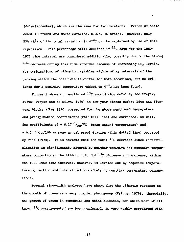
Figure 1 shows our unaltered *3C record (for details, see Freyer,
1979a; Freyer and de Silva, 1979) in ten-year blocks before 1890 and five-
year blocks after 1890, corrected for the above mentioned temperature
and precipitation coefficients (thin full line) and corrected, as well,
for coefficients of + 0.27 °/oo/°C (mean annual temperature) and
- 0.24 °/oo/l°0 rom mean annual precipitation (thin dotted line) observed
by Tans (1978). It is obvious that the total 13C decrease since industri-
alization is significantly altered by neither positive nor negative temper-
ature corrections; the effect, i.e. the 13C decrease and increase, within
the 1930-1960 time interval, however, is leveled out by negative tempera-
ture correction and intensified oppositely by positive temperature correc-
tions .
Several ring-width analyses have shown that the climatic response on
the growth of trees is a very complex phenomenon (Fritts, 1976). Especially,
the growth of trees in temperate and moist climates, for which most of all
known 13C measurements have been performed, is very weakly correlated with
17
1840 60 80 1900 20 40 60tear AD
Figure 1: Mean C record since industrialization from tree-ringmeasurements corrected for climatic variables (thin full anddotted lines = negative and positive corrections, respectively,with temperature).
{Species: 1840-1935, Pinus sylvestris L., Black Forest,Germany, weather station (w.s.) Schomberg, Black Forest.Pseudotsuga menziesii (Mirb.) Franco, Eifel, Germany (w.s.),Schneifelforsthaus, Eifel. 1920-1975, 8 trees, French Atlanticcoast, (w.s.) Nantes, France. 6 trees, North Carolina, USA, (w.s.)Reidsville, Waynesville, Wilmington, North Carolina}.
18
climatic factors. This may be true even for the 13C photosynthetic
fractionation factor because temperature effects opposite in sign, or
no correlation at all, have been observed. A postulate therefore, to
use the 13C record in tree rings for paleoclimatic studies on trees of
temperate regions of the midlatitudes seems to be far off common validity.
It has to be concluded from our results that the observed total *3C decrease
in tree rings since industrialization is altered only insignificantly by
climatic corrections; it has to be due, accordingly, mainly to increasing
atmospheric CO2 levels.
REFERENCES
Christeller, J.T., Lair.g, W.A. and Troughton, J.H. (1976). Isotopediscrimination by ribulose-l,5-diphosphate carboxylase. Plant Physiol.,57, 580-582.
Estep, M.F., Tabita, F.R., Parker, P.L. and Van Baalen, C. (1978).Carbon isotope fractionation by ribulose-l,5-bisphosphate carboxylasefrom various organisms, Plant Physiol., 61, 680-687.
Farmer, J.G. (1979). Problems in interpreting tree-ring 613C records,Nature, 279, 229-231.
Farmer, J.G. and Baxter, M.S. (1974). Atmospheric carbon dioxidelevels as indicated by the stable isotope record inwood, Nature, 247,273-275.
Freyer, H.D. (1978). Preliminary evaluation of past CO2 increase asderived from 13C measurements in tree rings, In Williams, J. (Ed.)Carbon dioxide, climate and society 69-77, Pergamon Press, Oxford.
Freyer, H.D. (1979a). On the 13C record in tree rings. I. 13cvariations in northern hemispheric trees during the last 150 years,Tellus, 31, 124-138.
Freyer, H.D. (1979b). On the 13C record in tree rings. II. Regis-tration of microenvironmental CO2 and anomalous pollution effect, Tellus,31, 308-312
19
Freyer, H.D. and de Silva, M.P. ^1979). On the 13C record intree rings, III. Climatic implications. Unpublished manuscript, tobe submitted to Tellus.
Freyer, H.D. and Wiesberg, L. (1974). Anthropogenic carbon-13decrease in atmospheric carbon dioxide as recorded in modern wood, InIsotope Ratios as Pollutant Source and Behavior Indicators, 49-62, Proc.FAO/IAEA Symp. Vienna IAEA.
Freyer, H.D. and Wiesberg, L. (1975). Review on different attemptsof tracing back the increasing atmospheric C02 level to preindustrialtimes, In E.R. Klein and P.D. Klein (Eds.) Proc. Second Internat. Conf.Stable Isotopes. USERDA CONF 751027, 611-620. Oak Brook, Illinois.
Fritts, U.C. (1976). Tree Rings and Climate. Academic Press,London. 567 pp.
Grinsted, M.J., Wilson, A.T. and Ferguson, C.W. (1979). 13C/12Cratio variations in Pinus longeieva (bristle-cone pine) cellulose duringthe last millennium, Earth Planet. Sci. Lett., 42, 251-253.
Lamb, H.H. (1973). Whither climate now? Nature, 244, 395-397.
Lerman, J.C. (1974). Isotope paleothermometers on continental matter:assessment. In Colloq. Internat. du C.N.R.S. No. 219. Les methodesquantitatives d'etude des variations du climat au cours du Pleistocene,163-181. Paris: Editions du Centre National de la Recherche Scientifique.
Libby, L.M. and Pandolfi, L.J. (1974). Temperature dependence ofisotope ratios in tree rings, Proc. Nat. Acad. Sci. U.S.A., 71, 2482-2486.
Park, R. and Epstein, S. (1960). Carbon isotope fractionation duringphotosynthesis, Geochim. Cosmochim. Acta. 21, 110-126.
Pearman, G.I., Francey, R.J. and Fraser, P.J.B. (1976). Climaticimplications of stable carbon isotopes in tree rings, Nature, 260, 771-773.
Rebello, A. and Wagener, K. (1976). Evaluation of 12C and 13C data onatmospheric C02 on the basis of a diffusion model for oceanic mixing. InJ.O. Nriagu (Ed.) Environmental Biogeochemistry, Vol. 1, 13-23. AnnArbor Science Publishers, Inc., Ann Arbor, Michigan.
Smith, B.N., Herath, H.M.W. and Chase, J.B. (1973). Effect of growthtemperature on carbon isotopic ratios in barley, pea and rape, Plant CellPhysiol., 14, 177-182.
Stuiver, M. (1978). Atmospheric carbon dioxide and carbon reservoirchanges, Science, 199, 253-258.
20
Tans, P.P. (1978). Carbon-13 and carbon-14 in trees and theatmospheric C02 increase, Ph.D Thesis, State University of Groningen,Netherlands. 99 pp.
Troughton, J.H. and Card, K.A. (1975). Temperature effects on thecarbon-isotope ratio of C3, C4 and Crassulacean-acid-metabolism (CAM)plants, Planta, 123, 185-190.
Whelan, T., Sackett, W.M. and Benedict, C.R. (1973). Enzymaticfractionation of carbon isotopes by phosphoenolpyruvate carboxylasefrom C4 plants, Plant Physiol., 51, 1051-1054.
Wilson, A.T. (1978). Pioneer agriculture explosion and CO, levelsin the atmosphere. Nature, 273, 40-41
Wilson, C.L. and Grinsted, M.J. (1977). 12C/12C in cellulose andlignin as palaeothermometers, Nature, 265, 133-135.
Wilson, C.L. and Matthews, W.H. (Eds.) (1971) Inadvertent Climate
Modification (SMIC), Cambridge, MIT press, Massachusetts-
Yapp, C.J. and Epstein, S. (1977). Climatic implications of D/H
ratios of meteoric water over North America (9500-22000 B.P.) as inferred
from ancient wood cellulose C-H hydrogen, Earth Planet, Sci. Letters, 34,
333-350.
21
CARBON-13 IN TREE-RINGS: LOCAL OR CANOPY EFFECT?
Juan Carlos Lerman Laboratory of Isotope GeochemistryAustin Long Department of Geosciences
University of Arizona, Tucson
INTRODUCTION
We are interested in the use of stable isotopes in trees as proxy
indicators of climate. Within this framework our research group has been
measuring the abundance of carbon-13 in trees in s "sries of experiments
done on two types of samples: leaves and tree-rings.
We will here first discuss our results as case-histories, and then
will attempt to elaborate on our model of the local or 'canopy1 effect.
The cases are:
1. Archaeological tree-rings of ponderosa pine and white firtrees from Chaco Canyon, New Mexico.
2. Recent leaves from juniper trees in Arizona.
3. Several centuries long time-series of ponderosa pine tree-rings from Flagstaff, Arizona.
4. Recent leaves and tree-rings of bristlecone pine trees fromthe White Mountains of California.
Cases 1 and 2 have been studied and discussed by two of our co-workers
who have published preliminary accounts on the research (Arnold, 1978;
Mazany, 1978; Mazany t jil., 1978). More complete communication of Case 1
is in press (Mazany_et_al., 1980), while Case 2 has b *n the subject of a
recent dissertation by Arnold (1979). (Incidentally, these two cases also
signal the possible importance of the applications of the isotope method
to archaeology and to isotope-dendrochronology in arid localities of the
U.S. Southwest.)
22
Cases 3 and 4 refer to experiments designed to obtain more infor-
mation to complement that acquired in the first two cases. All these case
histories contributed to our understanding of the isotope record, which
proved not to be the expected pure paleotemperature record often suggested
in the literature.
Case 1
Mazany's investigation of the wood in the archaeologic site of Chetro
Ketl was done on dated tree sections of a Pinus ponderosa (ponderosa pine)
and an Abies concolor (white fir). For this area, it has been shown that
the regional tree-ring indices can be interpreted as follows: narrow
rings indicate a warm and dry climate while wide rings indicate a wet
and cool climate (Fritts, 1976; LaMarche, 1974). The results (Mazany e_t
al., 1980) show a significant correlation between the 6-values and the
tree ring indices, thus indicating a valid correlation between climate
(as expressed in tree-ring widths) and carbon-13 abundances in cellulose.
That this is not an artifact of tree-growth has been clearly demonstrated
by the comparison of a) the correlation coefficients between the 6-values
and the regional tree-ring indices, with b) the correlation coefficient
between the 6-values and the indices of the particular specimens (Table 1).
It is clearly seen that the isotope response is specimen independent.
The general pattern observed is that during a cool-wet climate the
6-values are low while during a warm-dry climate the 6-values are high.
Case 2
Arnold's research on the leaves of juniper trees grown in a wide
range of localities in Arizona waj done on leaves estimated to be 10 years
old on the average. Carbon isotope analyses of these leaves, obtained
23
from trees growing through the whole range of juniper habitats, were
correlated against the temperature and precipitation records of meteoro-
logic stations situated in the proximity of the trees.
Calculation of the correlation coefficients of 6 C (leaves) vs.
temperature and vs. precipitation during the photosynthetically active
months showed, respectively, positive and negative correlation coefficients
of some significance. However/ when correlated with a combined variable
chosen to fa's the ratio T/P (temperature( C)/precipitation(mm)), the
correlation coefficients increased to a very significant value: e.g.,
'adjusted R1 = 0.985 (Arnold, 1979). The regression equation obtained
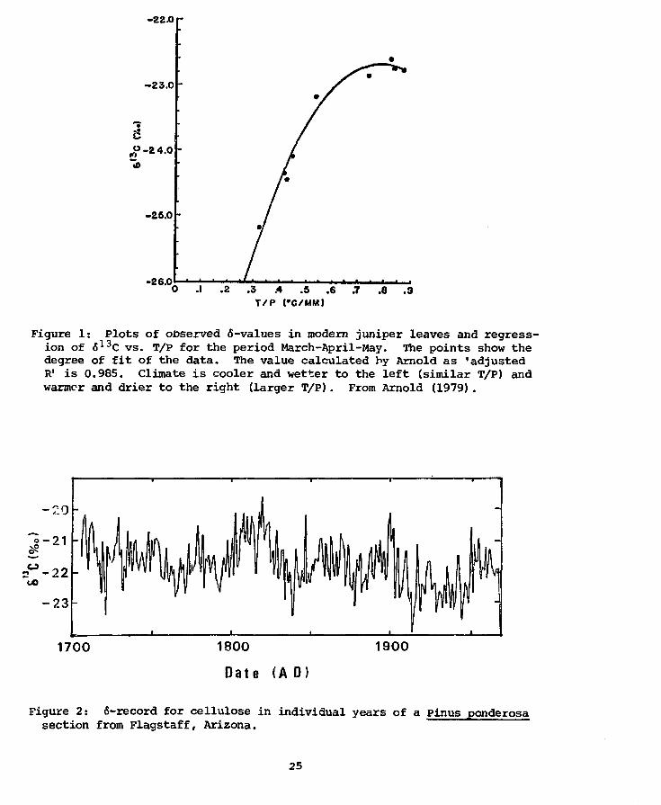
by Arnold (1979) is (Fig. 1):
<S13C = _30.19 + 19.04 (T/P)-12.08 (T/P)2.
The general pattern of the variations is, as for Case 1, that for a
cool-wet climate the 6-values are low while for a warm-dry climate the
6-values are high.
Case 3
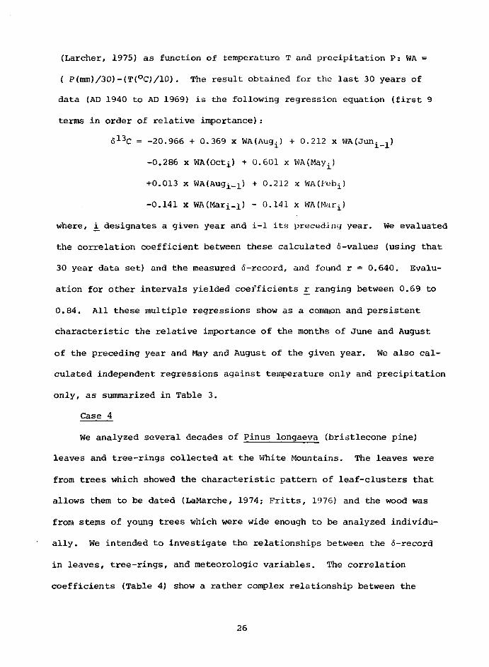
We analyzed 266 individual tree-r^ngs (Pig. 2) from a ponderosa pine
grown in Flagstaff, close to the meteorologic station. Our purpose was
to investigate whether the good correlation between the 6-values and the
tree-ring indices observed for Case 1 would also be verified for this
specimen and site. Linear regressions of the 6-values against four dif-
ferent series of tree-ring indices for the region were calculated. Table 2
lists these correlation coefficients, which are significantly lower than
those obtained for Case 1 (Table 1). We also performed a stepwise mul-
tiple regression of the 6-values against the water availability at the
site. Water availability (WA) was defined according to Walter and Lieth
24
-22.0
-23.0
C
la
-25.0
-26.0.1 .2 .3 .4 .5 .6 .7
T/P (#C/MM).8 .9
Figure 1: Plots of observed 6-values in modem juniper leaves and regress-ion of 613C vs. T/P for the period March-April-May. The points show thedegree of fit of the data. The value calculated by Arnold as 'adjustedR1 is 0.985. Climate is cooler and wetter to the left (similar T/P) andwarmer and drier to the right (larger T/P). From Arnold (1979).
1700 1800
Date (A 0)
1900
Figure 2: 6-record for cellulose in individual years of a Pinus ponderosasection from Flagstaff, Arizona.
25
(Larcher, 1975) as function of temperature T and precipitation P: WA =
( P(mm)/30)-(T(°C)/10). The result obtained for the last 30 years of
data (AD 1940 to AD 1969) is the following regression equation (first 9
terms in order of relative importance):
613C = -20.966 + 0.369 x WA(Augi) + 0.212 x WA(Juni_1)
-0.286 x WA(Octi) + 0.601 x WA(Mayi)
+0.013 x WAlAugj^) + 0.212 x WACFebjJ
-0.141 x WA(Mari-i) ~ 0.141 x WA(Mari)
where, i designates a given year and i-1 its preceding year. We evaluated
the correlation coefficient between these calculated <5-values (using that
30 year data set) and the measured 6-record, and found r = 0.640. Evalu-
ation for other intervals yielded coefficients £ ranging between 0.69 to
0.84. All these multiple regressions show as a common and persistent
characteristic the relative importance of the months of June and August
of the preceding year and May and August of the given year. We also cal-
culated independent regressions against temperature only and precipitation
only, as summarized in Table 3.
Case 4
We analyzed several decades of Pinus longaeva (bristlecone pine)
leaves and tree-rings collected at the White Mountains. The leaves were
from trees which showed the characteristic pattern of leaf-clusters that
allows them to be dated (LaMarche, 1974; Fritts, 1976) and the wood was
from stems of young trees which were wide enough to be analyzed individu-
ally. We intended to investigate the relationships between the 6-record
in leaves, tree-rings, and meteorologic variables. The correlation
coefficients (Table 4) show a rather complex relationship between the
26
different localities and types of samples (leaves or tree-rings). In
general, samples which are geographically related like EVB and SCG
correlate better than samples from more distant localities. We did some
preliminary exploratory data analysis on these series of measurements and
found that the 6-values have a greater dependence on precipitation than
on temperature (we used the climatic data collected by the University of
California station in the White Mountains and the U.S. Weather Bureau
station at Bishop, California). We then selected the series from Cold
Water Spring, which was the one that showed more variability in the
6-values, and performed a stepwise multiple correlation between the water
availability (as defined in Case 3) and the 6-values. We found a nega-
tive correlation between the water availability and the 6-values for
the early months of the year (March to May) just prior to the bristlecone
pine growth season and a positive correlation with the water availability
during the previous winter. We then performed a stepwise multiple re-
gression of the 6-values in the tree-rings and the water availability for
the months considered important for tree-ring growth (Fritts, 1976): from
June of the previous year to July of the given year. The three major
components resulted to be:
613 = -24.38 - (0.23 ± 0.19) WA March + (0.37 ± 0.17) WA December.
This means that rings grown during years which had dry Marches and were
preceded by wet Decembers are enriched in carbon-13.
DISCUSSION
The carbon isotope abundance as preserved in tree-rings appears to
be a record related to environmental-climatic variables such as water
availability, with some superimposed noise. We have attempted to explain
27
the variations observed in the different cases above described with the
same general hypothesis: that most of the variability in the 6-value of
cellulose in tree-rings is due to variations in the isotope compositic.n
of the local atmospheric C02 (Lerman, 1974, 1975; Lennan and Long, 1978).
If we can explain these changes in the local composition of CO2 with re-
lation to changes in climate, we can then establish the relationship be-
tween climate and the 6-record in tree-rings. That the 6-values of the
atmosphere are directly related to the regional plant activity was shown
by Keeling (1961). The mechanism is the following: an increase in
photosynthetic activity produces a depletion in the amount of carbon-13
in the atmosphere. This depletion is due to the increased contribution
of C02 respired by the plants, which is added to and mixed with the
local atmosphere. The 5-values of the atmospheric C02 become more nega-
tive in direct proportion to the amount of respired C02 that remains in
the enrivonment because the respired C02 has an isotope composition
similar to the composition of plant tissue (Park and Epstein, 1960),
which is more depleted in carbon-13 than the atmosphere. The link between
plant activity and the 6-values of the atmosphere appears to be the water
availability in areas where plant growth is limited by precipitation.
In those cases, climates that favor plant activity are those in which
evapotranspiration is low, i.e., when the water availability is high.
During these times the 6-record would be more depleted than in times of
reduced plant activity when the 6-value of the atmospheric C02 would
approach the value of the free atmosphere.
The 6-record of tree-rings would be affected by any other factor
that influences the degree of confinement of the local atmosphere or the
28
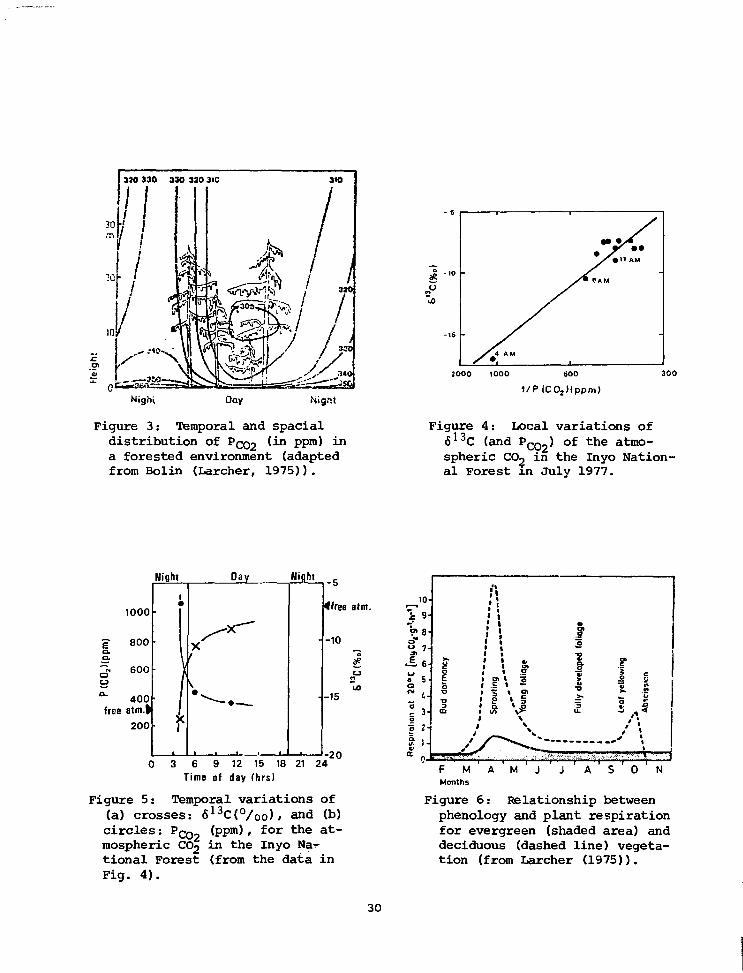
release of C02 from plants or soil, reinforced by the density of the
vegetation in the area. Fig. 3 shows a characteristic profile of PCC>2*
To verify the extent of such an effect in a well ventilated forest, such
as the Inyo National Forest (Keeling, 1961), we analyzed some spot samples
taken in July 1977 (Figs. 4 and 5). From them we conclude that the trees
are effectively immersed in a local atmosphere, well confined during
night. Consequently, when photosynthesis begins in the early morning
the trees would fix CO, which is very depleted in carbon-13. This effect
can be very local, as discussed by Mazany ejt al_. (1980).
This local effect would be more intense in times of the year when
plant activity produced more respiration. The importance of the early
months of the growing season (Cases 2, 3, and 4) can be explained by
Fig. 6. Also the importance (with opposite sign) given to the winter
months by the regression of Case 3 might well be related to the snow CO2-
barrier mentioned elsewhere (Lerman and Long, 1978).
CONCLUSIONS
We are confident that with additional field and growth chamber ex-
periments and modeling of trees and their environments, we would better
understand the relative magnitude of each one of the effects which con-
tribute to the 'local' or 'canopy' atmosphere as expressed in the 6-record
of tree-rings.
ACKNOWLEDGMENTS
This work has been possible thanks to the collaboration of T. Harlan,
B. Bannister, C.W. Ferguson and H. Fritts from the Laboratory of Tree-
Ring Research of the University of Arizona, and T. Mazany, L.D. Arnold,
29
Nignt
Figure 3: Temporal and spacialdistribution of Pco2 '^n PPm^ -n
a forested environment (adaptedfrom Bolin (Larcher, 1975)).
lC02)(ppm)
Figure 4: Local variations of613C (and PC02) of the atmo-spheric CO^ in the Inyo Nation-al Forest in July 1977.
1000
= 800a.
"i 600
400free atm.|
200
Wight
1
f
Oay
Xf
* - —
Wight
•
-
0 3 6 9 12 15 18 21 24
Time of day (hrs)
Figure 5: Temporal variations of(a) crosses: 613C(°/oo), and (b)circles: PQQ0 (ppm), for the at-mospheric CO2 in the Inyo Na-rtional Forest (from the data inFig. 4).
- 5
(free aim.
-10
e
O
-15
-20I.
en
0a*
«0rv
aEO
Odin«>
a.
9-
8-
7-
6
5
t -
3-
2'
1-
Bud
do
rman
cy
/
F M
Months
!".
;
• I• !1 :• 1
1 1 t>
; •. f; r \ s; i \ I• a. to1 1/) \>-1 \
/ ^ ^ \
A M J
1"O
Fu
lly d
evet
oped
J A
Leaf
yel
low
ing
t/
: L - . . X . •>• • • • * : ; •
s '
c
t/tu
\
1
' • • • • ; • 1 ' • • '
0 ' N
Figure 6: Relationship betweenphenology and plant respirationfor evergreen (shaded area) anddeciduous (dashed line) vegeta-tion (from Larcher (1975)).
30
J. LoFaro, G. Hennington, s. Wallin and P.E. Damon from our Laboratory.
This research was funded by NSF Grant Ho. ATM77-06790 and the State of
Arizona.
REFERENCES
Arnold, L.D., 1978. The climatic response in the 613C value of junipertrees from the american southwest, In: R.E. Zart-jnan, ed. ShortPapers 4th, Int'l. Conf. Geochronol., Cosmochronol., IsotopeGeology, Snowmass-at-Aspen 20-25 August 1978 (U.S.G.S. Open-FileReport 78-701), p. 15-17.
Arnold, L.D., 1979. The Climatic Response in the Partitioning of theStable Isotopes of Carbon in Juniper Trees frm Arizona, Unpubl.Ph.D. Diss., Univ. of Arizona, Tuscon, AZ.
Fritts, H.C., 1976. Tree Rings and Climate, Academic Press, New York,567 p.
Keeling, CD., 1961. The concentration and isotopic abundance of carbondioxide in rural and marine air, Geochim. Cosmochim. Acta, 24:277-298.
LaMarche, V.C., Jr., 1974. Paleoclimatic inferences from long tree-ring records, Science, v. 183, p. 1043-1048.
Larcher, W., 1975. Physiological Plant Ecology, Springer Verlag, NewYork, 252 p.
Lerman, J.C., 1974. Isotope "paleothermometers" on^continental matter:Assessment, In: Les Methodes Quantitatives d'Etude des Variationsdu Climat au Cours du Pleistocene. Coll. Int. CNRS. no. 219(CNRS, Paris) p. 163-181.
Lerman, J.C., 1975. How to interpret variations in the carbon isotoperatio of plants: Biologic and environmental effects, In: Environ-mental and Biological Control of Photosynthesis, R. Marcelle, ed.(W. Junk, The Hague, The Netherlands) p. 1267-1276.
Lerman, J.C. and A. Long, 1978. Carbon-13 as climate indicator; factorscontrolling stable carbon isotope ratios in tree rings. In: R.E.Zartman, ed. Short Papers 4th, Int'l. Conf. Geochronol., Cosmo-chronol., Isotope Geology, Snowmass-at-Aspen 20-25 August 1978(U.S.G.S. Open-File Report 78-701), p. 248-250.
Mazany, T., 1978. Isotope dendroclimatology: natural stable carbonisotope analysis of tree rings from an archaeological site, In:R.E. Zartman, ed. Short Papers 4th, Int'l. Conf. Geochronol., Cos-
31
mochronol.. Isotope Geology, Snowroass-at-Aspen 20-25 August 1978(U.S.G.S. Open-Pile Report 78-701}, p. 280-282.
Mazany, T., J.C. Lerman, and A. Long, 1970. Climatic sensitivity in13c/^«c values in tree rings from Chaco Caryon, In: A. Herschman,ed. Abstracts of Papers of the 144th National Meeting, 12-17 Feb-ruary 1978, Washington, D.C. (AAAS-Amer. Assoc. Adv. of Sci.,Washington, D.C.), p. 620.
Mazany, T., J.C. Lerman, and A. Long, 1980. Carbon-13 in tree-ringcellulose as indicator of past climates. Nature, in the press.
Park, R., and S. Epstein, 1960. Carbon isotope fractionation duringphotosynthesis, Geoohim. Cosmochim. Acta, 21:110-126.
32
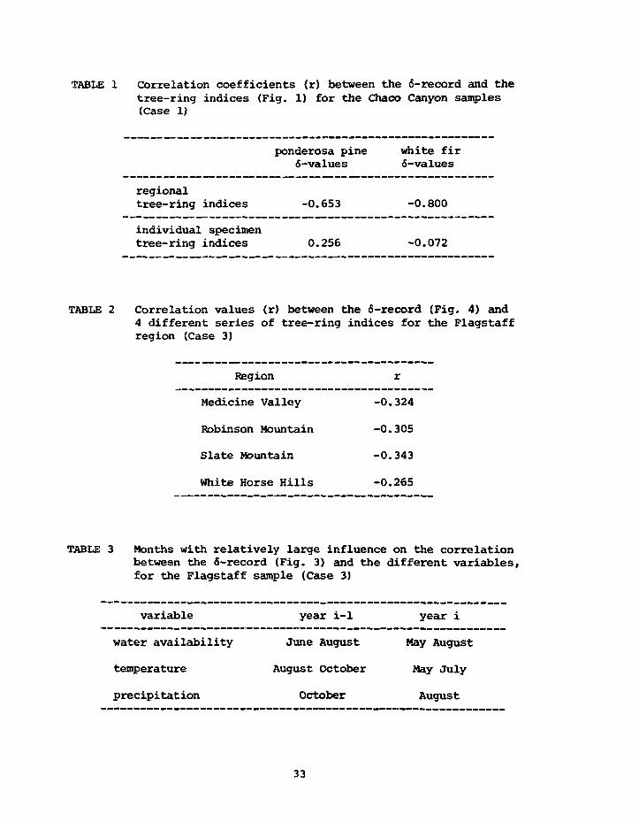
TABLE 1 Correlation coefficients (r) between the 5-record and thetree-ring indices (Fig. 1) for the Chaco Canyon samples(Case 1)
regionaltree-ring
individualtree-ring
indices
specimenindices
ponderosa pine6-values
-0.653
0.256
white fir6-values
-0.800
-0.072
TABLE 2 Correlation values (r) between the 6-record (Fig. 4) and4 different series of tree-ring indices for the Flagstaffregion (Case 3)
Region
Medicine Valley
Robinson Mountain
Slate Mountain
White Horse Hills
r
-0.324
-0.305
-0.343
-0.265
TABLE 3 Months with relatively large influence on the correlationbetween the 6-record (Fig. 3} and the different variables,for the Flagstaff sample (Case 3)
variable
water availability
temperature
precipitation
year i-1
June August
August October
October
year i
May August
May July
August
33
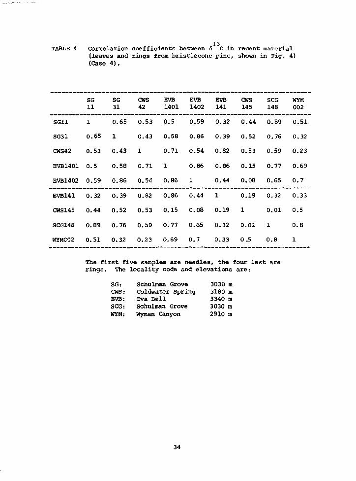
131 OTABLE 4 Correlation coefficients between 6 C in recent material
(leaves and rings from bristlecone pine, shown in Fig. 4)(Case 4).
SG11
SG31
CWS42
EVB1401
EVB1402
EVB141
CWS145
SCG148
WYM002
SG11 1 0.65 0.53 0.5 0.59 0.32 0.44 0.89 0.51
SG31 0.65 1 0.43 0.58 0.86 0.39 0.52 0.76 0.32
CWS42 0.53 0.43 1 0.71 0.54 0.82 0.53 0.59 0.23
EVB1401 0.5 0.58 0.71 1 0.86 0.86 0.15 0.77 0.69
EVB1402 0.59 0.86 0.54 0.86 1 0.44 0.08 0.65 0.7
EVB141 0.32 0.39 0.82 0.86 0.44 1 0.19 0.32 0.33
CWS145 0.44 0.52 0.53 0.15 0.08 0.19 1 0.01 0.5
SCG148 0.89 0.76 0.59 0.77 0.65 0.32 0.01 1 0.8
WYMC02 0.51 0.32 0.23 0.69 0.7 0.33 0.5 0.8 1
The first five samples are needles, the four last arerings. The locality code and elevations are:
SG: Schulman Grove 3030 mCHS: Coldwater Spring 3180 raEVB: Eva Bell 3340 mSCG: Schulman Grove 3030 mWYM: Wyman Canyon 2910 m
34
SOME REQUIREMENTS FOR A 13C TREE RIKG RECORDTO STUDY THE GLOBAL CARBON RESERVOIRS
Pieter Tans Scripps Institution ofOceanography,La Jolla, California
Model calculations indicate that we can infer the atmospheric CO2
level from C tree ring records in terms of historic changes in net
growth or shrinkage of the biota and humus reservoir. From the outset
we assume that 6 - c trends as obtained from tree rings reflect changes
in the 13C/12C ratio of atmospheric C02-
We have to keep in mind the fact that the precise link between a
613C time series and one for carbon-total (12C + 13C) depends on how the
carbon exchange takes place in the real world, and therefore, on how we
model the carbon reservoirs. The model used here is a 3*s box perturba-
tion model which comprises a biosphere, atmosphere, ocean mixed layer,
and a one-way transport of perturbations from the mixed layer to the
deep seas.
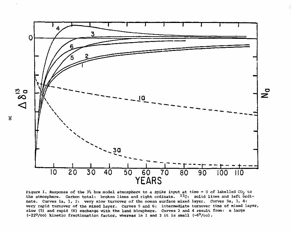
Application of a spike input shows that due to the oceanic buffer
factor, uptake of an atmospheric 6 - C spike takes place an order of mag-
nitude more rapidly than uptake of the associated CO2 spike (fig. 1).
The uptake of an atmospheric <5-"C perturbation is sensitive to the air-
sea gas exchange. On the other hand, the disappearing of a CO2 pertur-
bation from the atmosphere depends more on the turnover time of the mixed
layer, because the sea surface is already in equilibrium with the atmos-
phere after uptake of only a small fraction of the perturbation. This
also is the basic reason why a reconstruction of historic C02 levels is
35
1 1 \ +
10 20 30 40 50 60 70 80 90 100 110YEARS
Figure 1. Response of the 3h box model atmosphere to a spike input at time = 0 of labelled CO2 tothe atmosphere. Carbon total: brokan lines and right ordinate. 1 3C: solid lines and left ordi-nate. Curves la, 1, 2: very slow turnover of the ocean surface mixed layer. Curves 3a, 3, 4:very rapid turnover of the mixed layer. Curves 5 and 6: intermediate turnover time of mixed layer,slow (5) and rapid (6) exchange with the land biosphere. Curves 2 and 4 result from: a large(_22°/oo) kinetic fractionation factor, whereas in 1 and 3 it is small (-6°/oo).
very sensitive to the long term stability of the isotopic signal. There
are two more differences between 613C and C-total that are important for
the atmosphere. The exchange with the biosphere dilutes all isotopic
signals while the net effect of this exchange on CO2 may be zero, and also
the magnitude of the kinetic isotope fractionation factor of air-sea
exchange influences 613C.
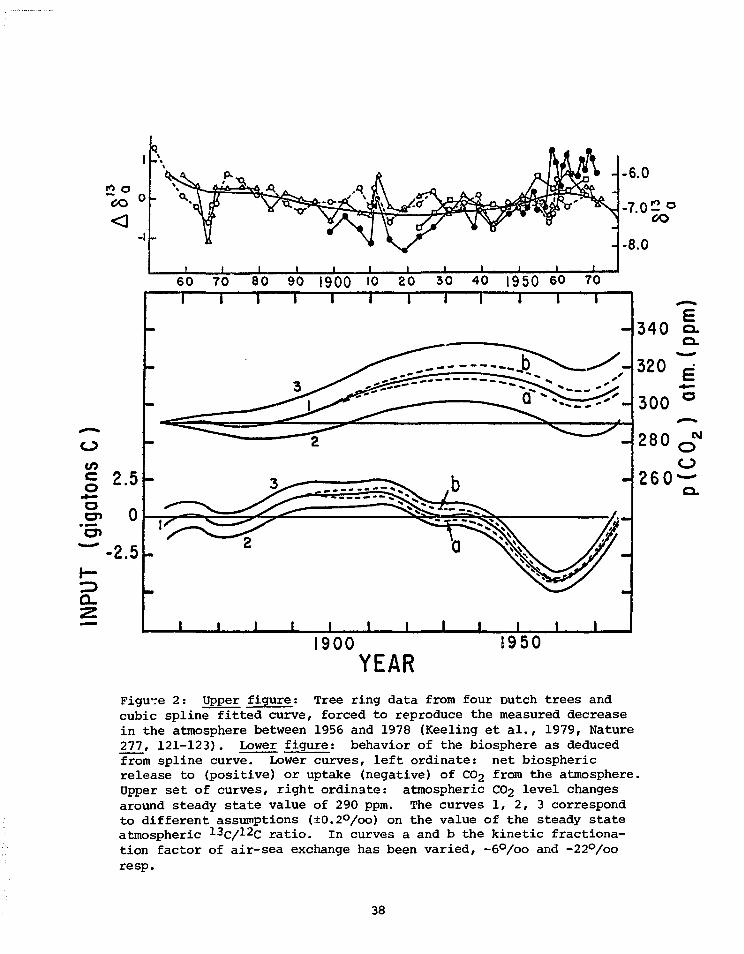
Having chosen a global carbon model and a 13C curve from tree rings
we still find that very different curves of atmospheric CO2 are compatible
with exactly the same 613C curve. They depend on our choice of initial
conditions (the CO2 inventories and isotopic ratios of the reservoirs
when the tree-ring data start) and on what value we assign to the steady
state "c/12^ ratio of the atmosphere (fig. 2). In steady state, there is
no net flow of CO2 to or from the atmosphere. We don't know which isotopic
xacio corresponds to that situation. If the biota are losing carbon at a
constant rate, the atmospheric 13C/12C will also be constant, but below
its steady state value. Another problem is that during times of rapid
change of atmospheric 6 -3C, like the present time, our prediction of net
biota CO2 release or uptake is also sensitive to addition to the model of
a reservoir that exchanges rapidly with the atmosphere ("short-lived biota"
reservoir). While not affecting the total CO2 balance, such a reservoir
can considerably reduce isotopic signals.
In conclusion, in order to use information from ^3C in tree, rings
to reconstruct past CO2 levels quantitatively we need, after we have sepa-
rated out the atmospheric signal from the tree rings:
37
*<5O
-I
-6.0
-7.0 2 o
-8.0
60 70 80 90 1900 10 20 30 40 1950 60 70
o
JO"o
2 .5
0o»
-2.5 -
Q_
1900YEAR
1950
Figu-re 2: Upper figure; Tree ring data from four Dutch trees andcubic spline fitted curve, forced to reproduce the measured decreasein the atmosphere between 1956 and 1978 (Keeling et al., 1979, Nature277, 121-123). Lower figure: behavior of the biosphere as deducedfrom spline curve. Lower curves, left ordinate: net biosphericrelease to (positive) or uptake (negative) of CO2 from the atmosphere.Upper set of curves, right ordinate: atmospheric CO2 level changesaround steady state value of 290 ppm. The curves 1, 2, 3 correspondto different assumptions (±0.2°/oo) on the value of the steady stateatmospheric 13c/^2c ratio. In curves a and b the kinetic fractiona-tion factor of air-sea exchange has been varied, -6°/oo and -22°/ooresp.
38
1. A proven model of the real world carbon exchange.
2. A 13C record starting at least a century before the period of
interest - to reduce the impact of the unknown initial condi-
tions and to narrow the possible range of atmospheric steady
state &^c values.
3. A tree ring record as precise (^0.1°/oo) and homogeneous as
possible - we cannot allow small (tenth of a part per mil) but
slow shifts of the "calibration" of the trees, either in the
trees themselves or by matching overlapping trees, due to the
insensitivity of the isotopic signal to low frequency phenomena.
REFERENCES
Tans, P.P. and Mook, W.G. (1979). Past atmospheric CO2 levels andthe *-*c/ C ratios in tree rings, Tellus (in press).
39
TOTAL ANTHROPOGENIC CO2 PRODUCTION SINCE 1800DERIVED FROM 13c MEASUREMENTS IN TREE RINGS
K. Wagener Department of Biophysics,Technical University of Aachen,Aachen, Federal Republic of Germany
The l^C records in tree-ring cellulose have been evaluated in
terms of CO2 production rates. For this purpose records from Europe,
North America, Brazil, and Australia were grouped together with the
idea that the interesting information is only contained in the slope
of the records. The absolute 1^Q/12 C values found in individual trees
depend on the species of tree and local environmental conditions. (For
details see Wagener, 1978). In general it turns out that during the
periods 1800 - 1935 and after 1960 there are worldwide, parallel
decreasing trends, while during 1936 - 1960 the records are more con-
troversial. According to Freyer (1980) there was, on the average, a
slight increase of the 13C record during 1936 - 1960.
An evaluation of this average 13c record in terms of CO2 production
rates exceeding the steady state turnover was done firstly by Wagener
(1978) based on a two-box model of atmosphere and ocean. For the period
1800 - 1935, a total production of about 100 ppm = 212 • 10$ tons of
carbon (t C) results, therefore after subtraction of the fossil produc-
tion a net production from the biosphere of 80 ppm = 170 • 109 t C is
obtained. This would correspond to a reduction of 10 to 15 ' 10**
of standing biomass.
40
Recently a more detailed evaluation of the same ^C record (somewhat
augmented by new data) was carried out by Wagener and Offermann based on
a four-box model of atmosphere, biosphere, mixad layer and deep sea. The
evaluation was extended up to 1975. The results can be summarized in
this way:
(1) The record C versus time gives information about the total net
input of CO2 into the atmosphere. (Note: Fossil carbon as well as car-
bon derived from the living or dead biosphere has the same isotopic com-
position.)
(2) The fraction of total excess CO2 taken up by the oceans depends only
on the parameters used there (sizes of reservoirs, mean residence times,
buffer factor). Any chosen data set does not influence the behavior of
the biosphere that results.
(3) The net reduction of the biosphere during 1800 - 1935 is 68 ppm =
145 • 10 9 t C. This is 15% less than derived from the two-box model.
(4) An open point is the possibly enhanced turnover through the biosphere.
The model is unsensitive to variations of the biological growth factor, $.
For 6 = 0 the additional (anthropogenic) CO2 production of the biosphere
is 68 ppm. For B = 0.2 the total biospheric production would have been
107 ppm, but 39 ppm would have been immediately recycled via a stimulated
rate of photosynthesis. In this way even still higher turnover rates
through the biosphere would be in agreement with the ^C record. This
leads to the conclusion that it is most desirable to have additional and
41
independent information about the role of the biosphere in a disturbed
carbon cycle. Being a source and a sink of carbon at the same time may
have essentially cancelled out the net carbon budget of the biosphere
during the past. This, however, could change in the future.
REFERENCES
Freyer, H.D. (1980). See contribution in this publication.
Wagener, K. (1978). Total anthropogenic CO2 production during theperiod 1800 - 1935 from carbon-13 measurements in tree rings, Rad. andEnvironm. Biophys., 15, 101-111.
Wagener, K. and Offermann, P. (In preparation)
42
RADIOCARBON VARIATIONS FROM 200 TO 700 A.D.
M. Bruns Heidelberg Academy of SciencesInstitute of Environmental Physics,Federal Republic of Germany
K.O. Munnich Institute of Environmental PhysicsUniversity of Heidelberg,Federal Republic of Germany
B. Becker Institute for BotanyUniversity of Hohenheim, Stuttgart-Hohenheim, Federal Republic of Germany
In 1970, when H.E. Suess presented his preliminary Bristlecone Pine
Calibration Curve, it caused a lot of discussion and the significance of
some of the short term variations in it was largely questioned.
However, carbon-14, unlike other parameters such as stable isotopes
in tree rings, reliably represents a global effect. This is due to fast
atmospheric mixing following from the spread of artificial nuclear-weapon-
test carbon-2 4, and to the fact that in C-14 the tree ring is simply a
sampling device, the intrinsic variations in efficiency of the tree ring
is eliminated by C-13 correction. Moreover, the worldwide correlation
of C-14 in tree rings has been shown experimentally by direct sample com-
parison of trees from Europe and America.
Approximately 60 tree-ring samples have now been measured at the
Heidelberg Laboratory, using an absolutely-dated oak chronology of oaks
from gravel beds of the river Danube. The time scale covered is about
200 to 700 A.D., a period rather ill-defined by Bristlecone Pine measure-
ments. Contrary to former measurements, only samples covering 1 to 3 years
have been used, to provide a maximum of resolution. (Oak shows broad rings,
43
which can be separated year by year). The measurement precision was
2.5°/o , STD corresponding to a C-14 age error of ± 20 years.
RESULTS
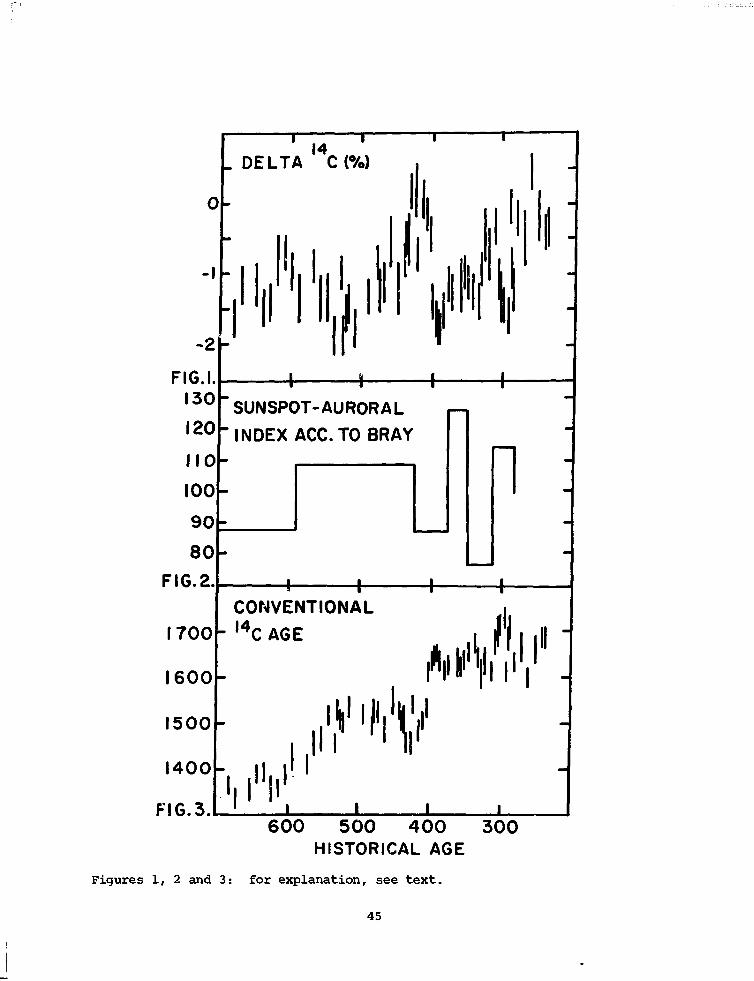
Fig. 1 indicates the existence of pronounced "wriggles" between 250
and 600 A.D. of up to 2°/Q difference in atmospheric C-14 content. Due
to the non-uniqueness of the relation C-14 age versus historical age of
the samples (fig. 3), C-14 dating of samples of short atmospheric sampling
time (grains, twigs, etcetera) may cause an uncertainty of up to 200 years.
C-14 variations of that size have been well established for the so-called
"little ice age" during the sixteenth and eighteenth centuries. For this
period a positive correlation of sunspot activity and climate, and an
anti-correlation between sunspot activity and C-14 are well documented.
A direct proof of this relationship is nearly impossible in the
present set of samples due to the absence of detailed and continuous cli-
matic and astronomical records. Nevertheless, some attempts have been
made to recalculate the sunspot activity of ancient epochs.
Fig. 2 indicates that C-14 activity (fig.l) seems to follow the sun-
spot activity, showing high C-14 for low sunspot numbers, and vice versa.
A global climatic response cannot be proven, although some regional trends
in climate seem to have occurred around that time, they do not, however,
lead to a comprehensive global picture.
FURTHER STUDIES
We recently started measurements of oak material from two "floating"
44
-I
-2
FIG.I130
120
110
100
90
80
FIG. 2.
1700
1600
1500
1400
. DELTA C(%)
!
FIG.3.
4-SUNSPOT-AURORAL
INDEX ACC.TOBRAY nCONVENTIONALI4C AGE f\
I. I"HI
600 500 400 300HISTORICAL AGE
Figures 1, 2 and 3: for explanation, see text.
45
chronologies covering 7300 to 8700 B.P. In addition to possible short
time variations to be found, the results will give information about the
general trend of C-14. This is important since Bristlecone Pine Calibra-
tion ends around 8000 B.P.
ACKNOWLEDGEMENT
We wish to thank the Heidelberg Academy of Sciences for funding.
REFERENCES
Bray, J.R. (1967). Variation in atmospheric C-14 activity relativeto a sunspot auroral solar index, Science, 156, 640-642.
Clark, R.M. (1975). A calibration curve for radiocarbon dates.Antiquity, 28, 387-410.
Clark, D.H. and Stephenson, F.R. (1978). An interpretation of pre-telescopic sun-spot records from the orient, Q. J.R. Astr. Soc, 387-410.
Eddy, J.A. (1976). The maunder minimum, Science, 192, No. 4245,1189-1902.
Mitchell, J.M. (1977). The changing climate, in Energy and Climate,National Academy of science, Washington, 51-59.
Pearson, G.W., Pilcher, J.R., Baillie, M.G. and Hillam, J., (1977).An absolute radiocarbon dating using a low altitude European tree ringcalibration, Nature, 270, 25-28.
Stuiver, M. (1961). Variation in Radiocarbon concentration and sun-spot activity, Geophy. Res., 166, 273.
Suess, H.E. and Becker, B. (1977). Der Radiocarbongehalt vonJahresrLngenproben aus postglazialen Eichenstammen Mitteleuropas,Erdwissenschaftliche Forschung, Vol. XII, p. 173.
Suess, H.E. (1968). Climatic changes, solar activity and the cosmicray production rate of natural radiocarbon, Meteorol. Monographs, 8,146-150 .
Suess, H.E. (1978). La Jolla measurements of radiocarbon in treerings, Radiocarbon, 20, 1-18.
46
ATMOSPHERIC 14C VARIATIONS
M. Stuiver Quaternary Isotope Laboratory,University of WashingtonSeattle, Washington
Sunspot numbers, as well as cosmic ray fluxes, reflect solar
variability. Because the atmospheric *4C levels recorded in tree rings
depend on the magnitude of the cosmic ray flux, it is possible to derive;
a detailed record of solar variability from the ^ C records.
The post 1645 A.D. history of 14C production rates correlates well
with the basic features of the historical record of sunspot numbers. A
900 year 14C production record, calculated from the atmospheric 14C
changes, can be used to identify four episodes where sunspotj were absent,
namely at 1654-1714 (Maunder minimum), at 1416-1534 (Sporer minimum), at
1282-1342 (Wolf minimum), and at 1010-1050 (Oort minimum). Each of these
intervals of minimum solar activity was preceded by a 60 to 80 year period
of similar 14C production rate increases.
The magnitude of the calculated 14C production rates points to a
further increase in cosmic ray flux when sunspots are absent. This resi-
dual modulation was greatest during the Sporer minimum.
The geomagnetic record present in Aa indices indicates a long term
modulation of the cosmic ray flux that is not apparent in the sunspot
record alone.
Editor's Note: This research is described in detail in Stuiver, M. andQuay, P. (1980) "Changes in atmospheric carbon-14 attributed to a variablesun," Science, 207, 4426, 11-19; and Stuiver, M. (1980) "Solar variabilityand climatic change during the current millennium" Nature, (in press).
47
DEUTERIUM CONTENT OF LIGNIN AND OF THEMETHYL AND OH HYDROGEN OF CELLULOSE
Irving Friedman U.S. Geological SurveyDenver,
Jim Gleason Colorado
We have measured the deuterium content of various organic components
of tree rings from five Engelmann Spruce (Picea engelmanni, Parry) trees
growing at 9,000 to 12,000 feet in the Rocky Mountains of Colorado. Four
of the trees grew in a cirque at elevations from 10,800 to 12,000 feet,
and one tree grew at 9,000 feet along the stream draining the basin. The
trees were chosen at places where for the past eight years we have been
monitoring the deuterium concentration of snow as well as of the stream
draining the basin.
•i"ha vood representing the past seven years of growth was selected
from 1-inch diameter cores. The samples were ground, extracted with
benzene-alcohol to remove resins, and then divided into aliquots. One
aliquot called "extracted wood" was equilibrated with water of known deu-
terium concentration, dried in vacuo, and then combusted in pure oxygen.
The resulting water was analyzed for its deuterium content by conven-
tional mass-spectrometric methods. Another aliquot was treated with
sodium chlorite to separate cellulose. The cellulose was separated into
two aliquots. One was equilibrated with water of known <5D, dried, and
combusted. The other was converted to cellulose nitrate and then com-
busted. Sap was expressed from cores taken in the late summer, and also
was analyzed for deuterium. The proportion of exchangeable water in
50
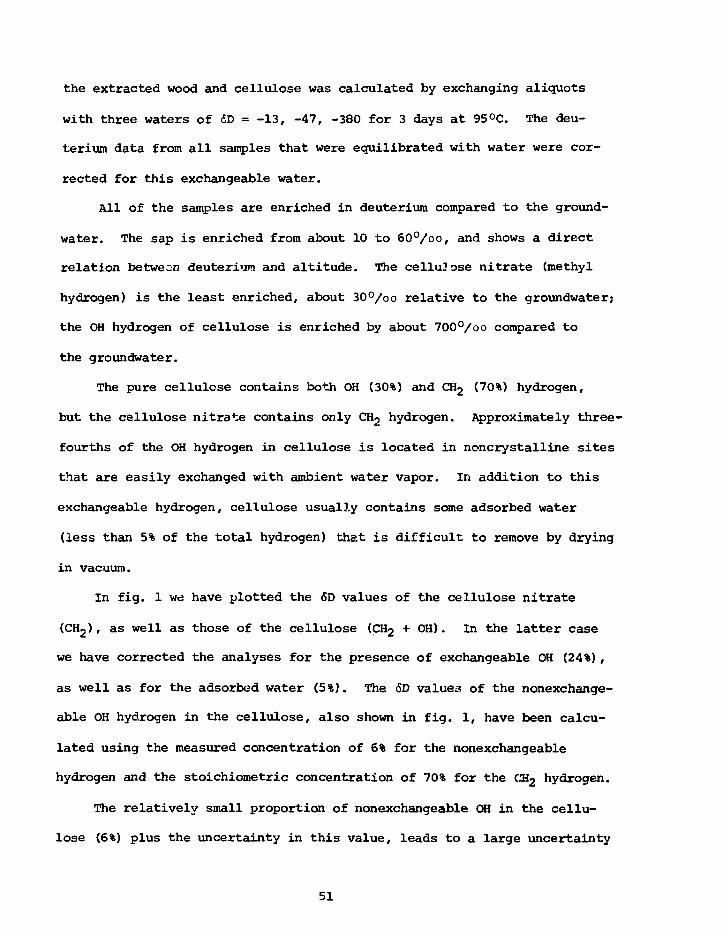
the extracted wood and cellulose was calculated by exchanging aliquots
with three waters of <SD = -13, -47, -380 for 3 days at 95°C. The deu-
terium data from all samples that were equilibrated with water were cor-
rected for this exchangeable water.
All of the samples are enriched in deuterium compared to the ground-
water. The sap is enriched from about 10 to 60°/oo, and shows a direct
relation between deuterium and altitude. The cellulose nitrate (methyl
hydrogen) is the least enriched, about 30°/oo relative to the groundwater;
the OH hydrogen of cellulose is enriched by about 700°/oo compared to
the groundwater.
The pure cellulose contains both OH (30%) and CH2 (70%) hydrogen,
but the cellulose nitrate contains only CH2 hydrogen. Approximately three-
fourths of the OH hydrogen in cellulose is located in noncrystalline sites
that are easily exchanged with ambient water vapor. In addition to this
exchangeable hydrogen, cellulose usually contains some adsorbed water
(less than 5% of the total hydrogen) that is difficult to remove by drying
in vacuum.
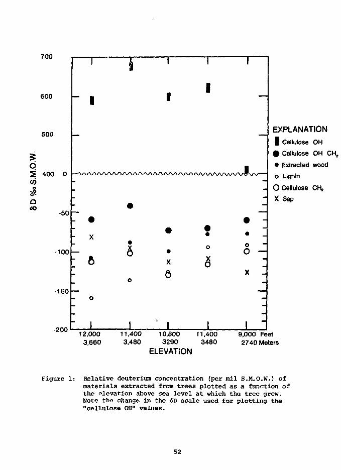
In fig. 1 we have plotted the 6D values of the cellulose nitrate
(CH2), as well as those of the cellulose (CH2 + OH). In the latter case
we have corrected the analyses for the presence of exchangeable OH (24%),
as well as for the adsorbed water (5%). The <SD values of the nonexchange-
able OH hydrogen in the cellulose, also shown in fig. 1, have been calcu-
lated using the measured concentration of 6% for the nonexchangeable
hydrogen and the stoichiometric concentration of 70% for the CH2 hydrogen.
The relatively small proportion of nonexchangeable OH in the cellu-
lose (6%) plus the uncertainty in this value, leads to a large uncertainty
51
700
600 —
500 —
400 0(0
o
Q
to-50
-100 —
•150 —
-200
I
- 1
—W\AAA/\
X
: o
-o
" 1
s
lAA/WVNA;
#
s0
1
1
1
WWVW\
•
•
X
6
1
1
1
•/V\A/\/\A/\/\
•
o
6
i
i
• -•oO —
X I--
1 "
EXPLANATION
I Cellulose OH
# Cellulose OH CH,
• Extracted wood
o Lignin
O Cellulose CH,
X Sap
12,000 11,400 10,800 11.400 9,000 Feet3,660 3,480 3290 3480 2740 Meters
ELEVATJON
Figure 1: Relative deuterium concentration (per mil S.M.O.W.) ofmaterials extracted from trees plotted as a function ofthe elevation above sea level at which the tree grew.Note the change in the 6D scale used for plotting the"cellulose OH" values.
52
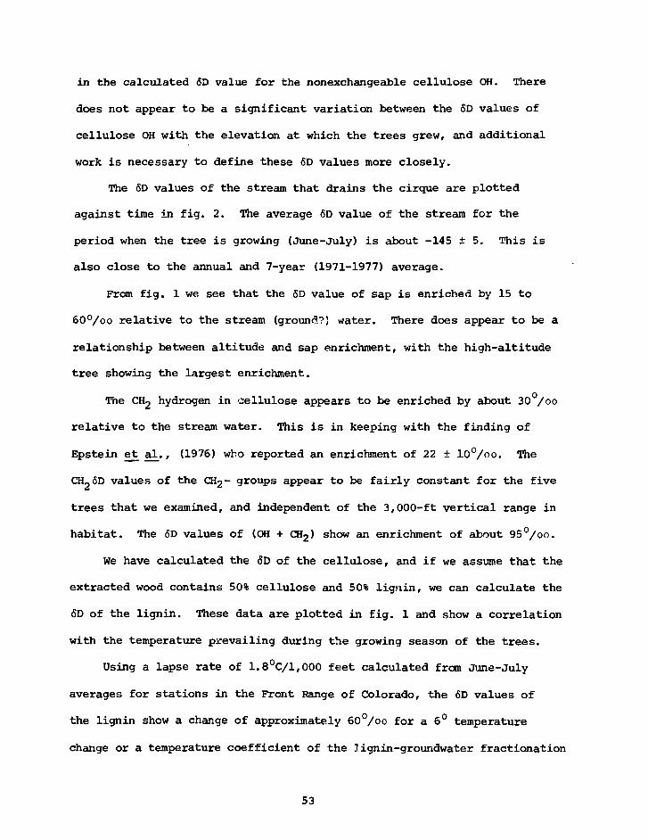
in the calculated <5D value for the nonexchangeable cellulose OH. There
does not appear to be a significant variation between the 6D values of
cellulose OH with the elevation at which the trees grew, and additional
work is necessary to define these £D values more closely.
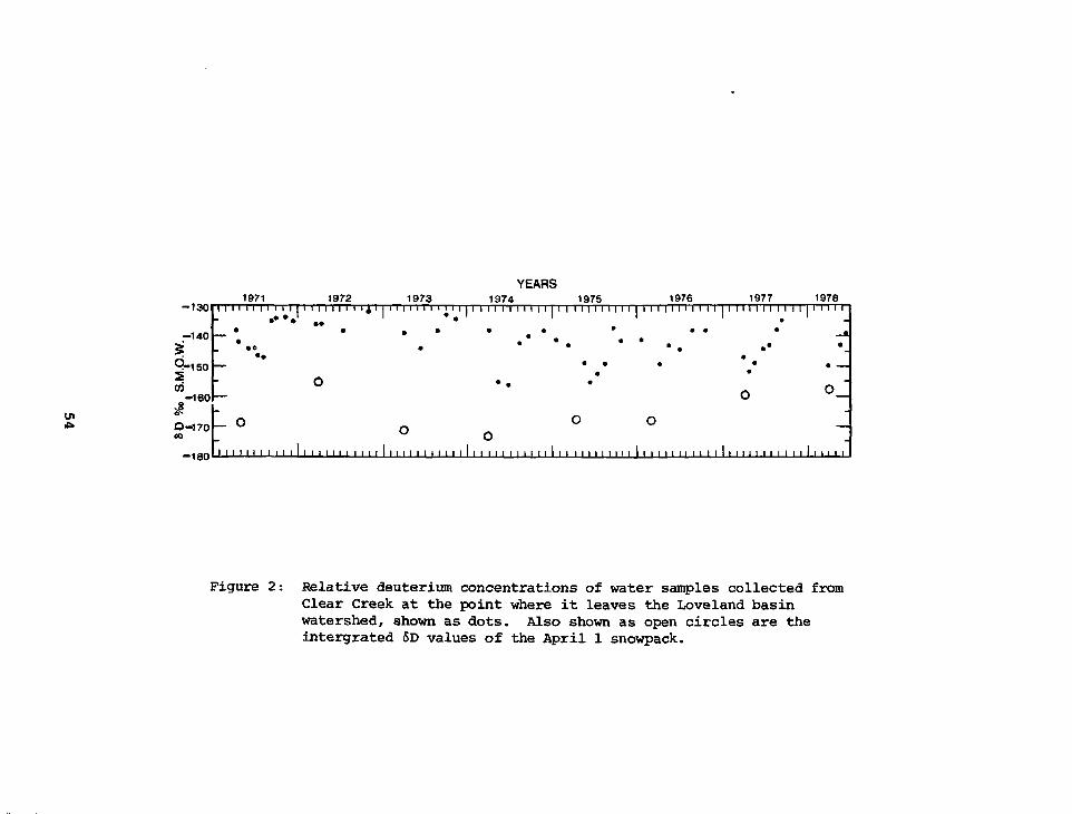
The 6D values of the stream that drains the cirque are plotted
against time in fig. 2. The average 6D value of the stream for the
period when the tree is growing (June-July) is about -145 ± 5. This is
also close to the annual and 7-year (1971-1977) average.
From fig. 1 we see that the 6D value of sap is enriched by 15 to
60°/oo relative to the stream (ground?) water. There does appear to be a
relationship between altitude and sap enrichment, with the high-altitude
tree showing the largest enrichment.
The CH2 hydrogen in cellulose appears to be enriched by about 30 /oo
relative to the stream water. This is in keeping with the finding of
Epstein et al ., (1976) who reported an enrichment of 22 ± 10°/°o. The
CH26D values of the CH2- groups appear to be fairly constant for the five
trees that we examined, and independent of the 3,000-ft vertical range in
habitat. The 6D values of (OH + CH2) show an enrichment of about 95°/oo.
We have calculated the 6D of the cellulose, and if we assume that the
extracted wood contains 50% cellulose and 50% lignin, we can calculate the
6D of the lignin. These data are plotted in fig. 1 and show a correlation
with the temperature prevailing during the growing season of the trees.
Using a lapse rate of 1.8°C/l,000 feet calculated from June-July
averages for stations in the Front Range of Colorado, the 6D values of
the lignin show a change of approximately 60°/oo for a 6° temperature
change or a temperature coefficient of the lignin-groundwater fractionation
53
in
-130
-140
siQ-150CO. - 1 6 0
O-170
- 1 8 0
1971 1972 1973
YEARS1974 1975 1976 1977
.:'.'.! " j . 1 1 * 1 1 r.-rrjrrj, rrrrTT1 t M M I I M l I I | M I M V\ I M I M M I M I M
I M I M I I I I I I I I M M I I M I I M I I I M 1 I I 1 I 1 1 M I I M 1 I I I I I I I I I I I I I II I I I I I 1 I I 1 I I I 1 I I 1
197811 " " I " "
I I M I I I 1 1 I
Figure 2: Relative deuterium concentrations of water samples collected fromClear Creek at the point where it leaves the Loveland basinwatershed, shown as dots. Also shown as open circles are theintergrated 6D values of the April 1 snowpack.
of about -10°/oo per degree.
The uncertainty in the lignin-cellulose ratio in the extracted wood,
plus uncertainty in the amount of hydration water left in the cellulose
before combustion ( 5% of the total H), results in a large uncertainty in
the slope of the lignin versus temperature curve. We intend to reduce
this uncertainty by additional experiments.
From the data presented in this paper, it would appear that any of
the three samples (exchanged extracted wood, exchanged cellulose, cellu-
lose nitrate) can be used to derive the &D value of the water utilized by
the tree.
It is also clear that 6D of the sap of the trees sampled is a func-
tion of the elevation at which the tree grows.
REFERENCES
Epstein, S., Yapp, C.J. and Hall, J.H. (1976). The determination ofthe D/H ratio of non-exchangeable hydrogen in cellulose extracted fromaquatic and land plants, Earth & Planet. Sci. Lett., 30, 241-251.
55
PRELIMINARY D/H RESULTS ON TREE-RING CELLULOSE FROMOAK IN THE PROVINCE OF DRENTE, THE NETHERLANDS
W.G. Mook State University,CM. van der Straaten Groningen, Netherlands
Some D/H analyses were performed on a-cellulose prepared from single
average tree rings of one of the oak trees used by Tans for c/ C and C
measurements (Tans, 1978; Tans e_t al_., 1979). Prior to combustion of the
a-cellulose samples were nitrated to remove the exchangeable hydrogen.
The results are shown in fig. 1.
13At first glance there is no correlation between SD and 6 C, whereas
the correlation between 6D and ring width is surprisingly obvious, especially
where each consecutive year was analyzed (since 1959): high 6D correlates
with small ring width and conversely. Possible other correlations, for
instance with 6D of precipitation and temperature, have to be unraveled
before any more definite conclusions can be drawn.
REFERENCES
Tans, P.P. (1978). Carbon-13 and carbon-14 in trees and the atmos-pheric C02 increase, Thesis (Univ. of Groningen), 99 pp.
Tans, P.P., de Jong, A.F.M., and Mook, W.A. (1979). Natural atmospheric•^C variation and the Suess effect, Nature, 280, 826-828.
56
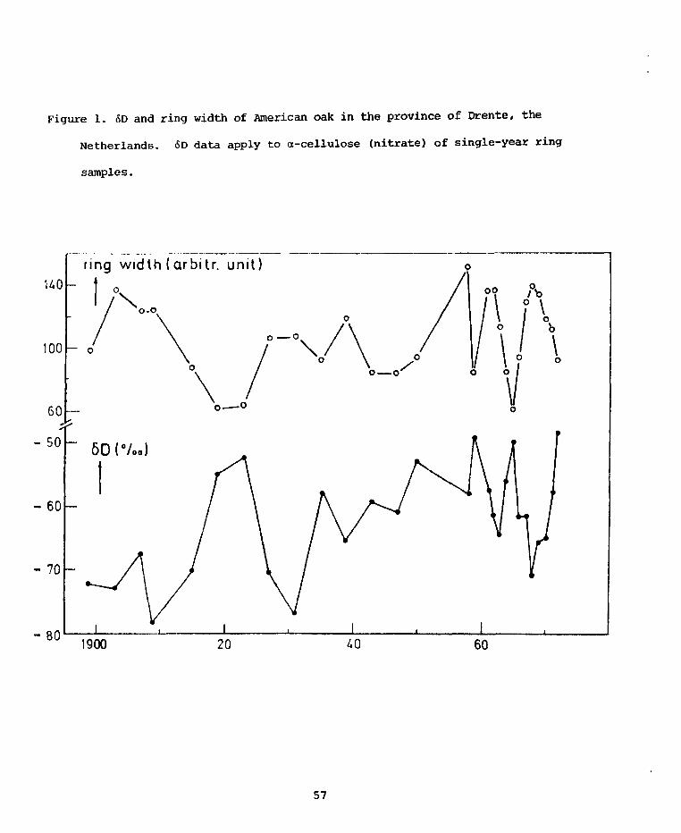
Figure 1. &D and ring width of American oak in the province of Drente, the
Netherlands. 6D data apply to a-cellulose (nitrate) of single-year ring
samples.
HO
100
60
- 50
- 60
- 70h
- 80
ring w id th ( arbitr . unit)
o-o.
1900 20 60
57
THE RELATIONSHIP BETWEEN THE NON-EXCHANGEABLE HYDROGENSOF TREE-RING CELLULOSE AND THE SOURCE WATERS FOR TREE SAP
J. W. C. White Lamont-Doherty Geological ObservatoryJ. R. Lawrence of Columbia University
Palisades, New York
A linear relationship has been found between the D/H ratio in the
non-exchangeable (carbon bound) hydrogens of tree cellulose, and the
growing season D/H ratio in tree sap for eastern white pine (Pinus
Strobus L.). The slope of the line is 1.0 and the intercept is -21°/oo
(sap heavier) for eleven intra-ring comparisons at two sites. The D/H
ratio of tree sap for the entire growing season (early May through mid-
August, 1977) was modeled using D/H ratios of growing season rain and
groundwater to define a mixing relationship of rain and groundwater to
form tree sap.
Two sites on the Mohonk Trust Properties near New Paltz, New York,
were used. The sites were chosen to study the relative importance of
groundwater versus rainfall input to tree sap. The first is a site
located in a depression at the base of a large talus area and has abundant
groundwater near the soil surface as evidenced by ubiquitous pools of
standing water and a perennial spring. The second site has no nearby sur-
face water, but the soil is saturated at a depth of approximately one meter.
Rain, which in this area has an average SD value of -30°/oo for the
period May through August, blends with groundwater, which has a constant
6D value of -56°/oo, to form tree sap. This blending is probably due to
deeper roots absorbing primarily groundwater while shallower roots absorb
58
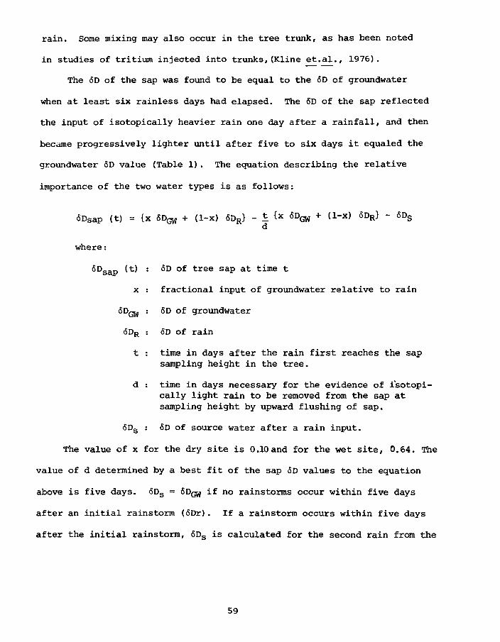
rain. Some mixing may also occur in the tree trunk, as has been noted
in studies of tritium injected into trunks,(Kline et.al., 1976).
The 6D of the sap was found to be equal to the 6D of groundwater
when at least six rainless days had elapsed. The 6D of the sap reflected
the input of isotopically heavier rain one day after a rainfall, and then
became progressively lighter until after five to six days it equaled the
groundwater 6D value (Table 1). The equation describing the relative
importance of the two water types is as follows:
•SDsap (t) = {x SDGW + (1-x) 6DR} - t {X SD^ + (1-x) <SDR} - SDSd
where:
6Dsap (t) : 6D of tree sap at time t
x : fractional input of groundwater relative to rain
SDQ^ : 6D of groundwater
<5DR : SD of rain
t : time in days after the rain first reaches the sapsampling height in the tree.
d -. time in days necessary for the evidence of isotopi-cally light rain to be removed from the sap atsampling height by upward flushing of sap.
5DS : 6D of source water after a rain input.
The value of x for the dry site is 0.10 and for the wet site, 0.64. The
value of d determined by a best fit of the sap 6D values to the equation
above is five days. 6DS = SDQJ if no rainstorms occur within five days
after an initial rainstorm (6Dr). If a rainstorm occurs within five days
after the initial rainstorm, &DS is calculated for the second rain from the
59
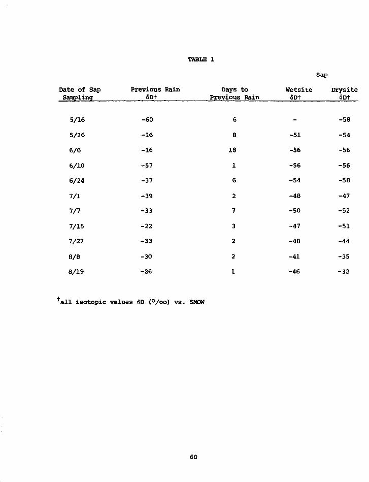
Date of SapSampling
5/16
5/26
6/6
6/10
6/24
7/1
m7/15
7/27
8/8
8/19
Previous Rain6Dt
-60
-16
-16
-57
-37
-39
-33
-22
-33
-30
-26
TABLE 1
Days toPrevious Rain
6
8
18
1
6
2
7
3
2
2
1
Wetsite6Dt
_
-51
-56
-56
-54
-48
-50
-47
-48
-41
-46
Sap
Drysite<SDt
-58
-54
-56
-56
-58
-47
-52
-51
-44
-35
-32
+all isotopic values <SD (°/oo) vs. SMOW
60
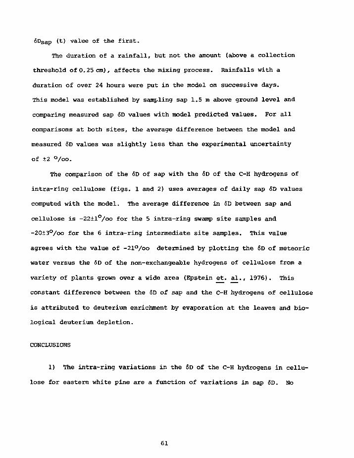
6Dsap (t) value of the first.
The duration of a rainfall, but not the amount (above a collection
threshold of 0.25 cm), affects the mixing process. Rainfalls with a
duration of over 24 hours were put in the model on successive days.
This model was established by sampling sap 1.5 m above ground level and
comparing measured sap 6D values with model predicted values. For all
comparisons at both sites, the average difference between the model and
measured 6D values was slightly less than the experimental uncertainty
of ±2 °/oo.
The comparison of the 6D of sap with the 6D of the C-H hydrogens of
intra-ring cellulose (figs. 1 and 2) uses averages of daily sap <SD values
computed with the model. The average difference in 6D between sap and
cellulose is -22±l°/oo for the 5 intra-ring swamp site samples and
-20±3°/oo for the 6 intra-ring intermediate site samples. This value
agrees with the value of -21°/oo determined by plotting the 6D of meteoric
water versus the 6D of the non-exchangeable hydrogens of cellulose from a
variety of plants grown over a wide area (Epstein et. al., 1976). This
constant difference between the 6D of sap and the C-H hydrogens of cellulose
is attributed to deuterium enrichment by evaporation at the leaves and bio-
logical deuterium depletion.
CONCLUSIONS
1) The intra-ring variations in the 6D of the C-H hydrogens in cellu-
lose for eastern white pine are a function of variations in sap SD. No
61
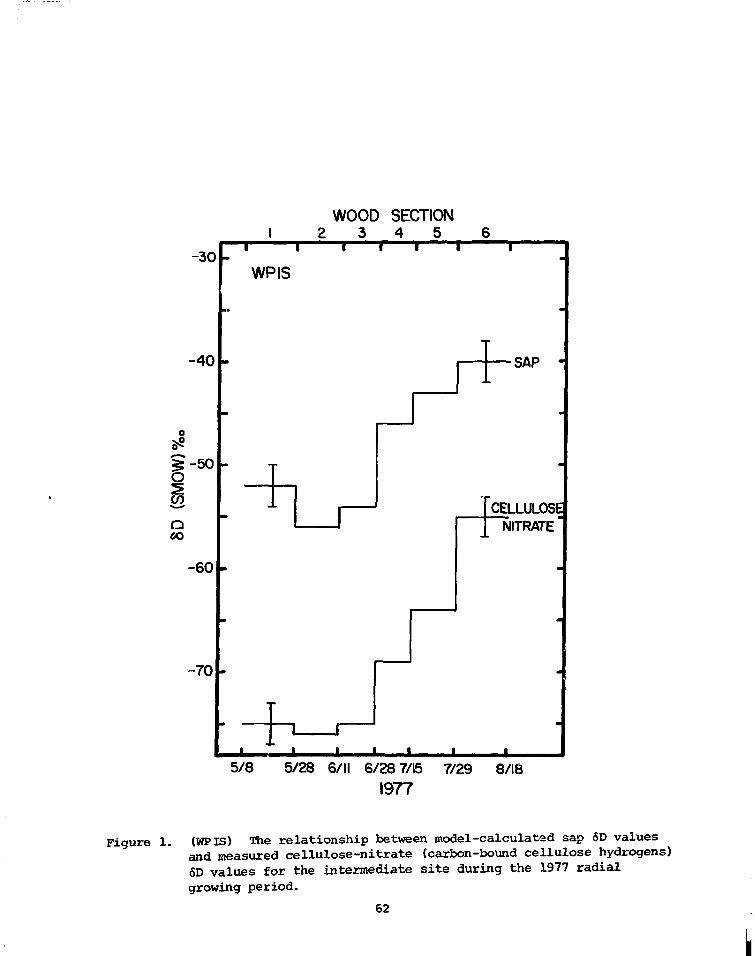
WOOD SECTION2 3 4 5
-30
-40
§-50O
QCO
-60
•70
I t
WPIS
i SAP -
i
CELLULOSENITRATE
5/8 5/28 6/11 6/28 7/151977
7/29 8/18
Figure 1. (WPIS) The relationship between model-calculated sap 6D values
and measured cellulose-nitrate (carbon-bound cellulose hydrogens)6D values for the intermediate site during the 1977 radialgrowing period.
62
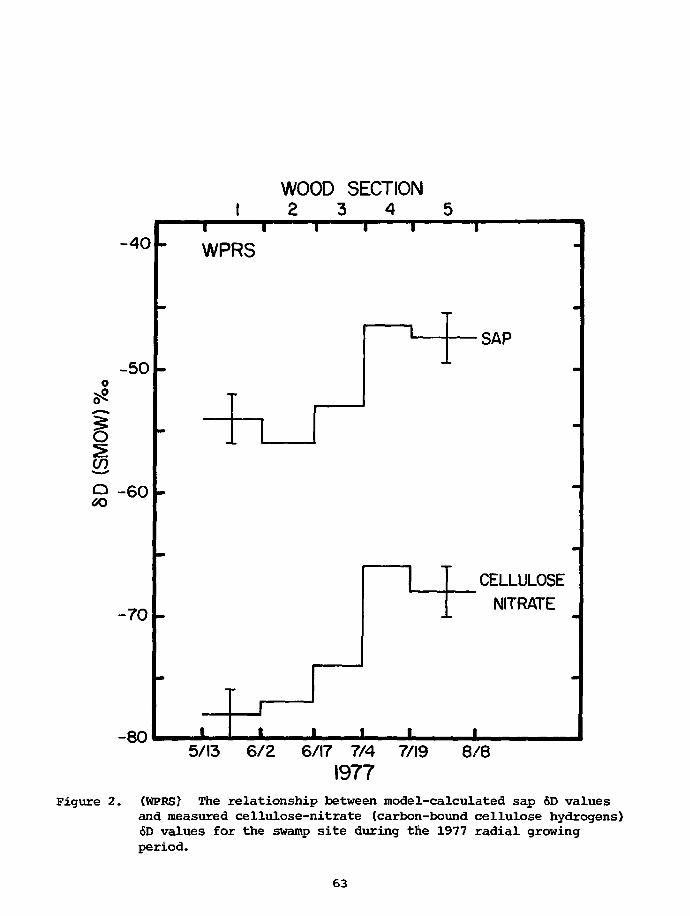
WOOD SECTION2 3 4 5
-40 -
-50 -
O
Q-60
-70
- 80
1 1 1 1 1
- WPRS
-
MB
I
I
1
OADoAr
-
CELLULOSE
NITRATE
-
t i l l i
5/13 6/2 6/17 7/41977
7/19 8/8
Figure 2. (WPRS? The relationship between model-calculated sap 6D valuesand measured cellulose-nitrate (carbon-bound cellulose hydrogens)6D values for the swamp site during the 1977 radial growingperiod.
63

effect of temperature, such as has been suggested by Wilson and Grinsted
(1975) was found. Relative humidity, an important variable in modeling
isotope fractionation by evapotranspiration (e.g., Dongmann et. al. 1974),
also appears to have no effect.
2) Bain and groundwater blend in the tree trunk and soil to form
sap. The mixing can be quantified using D/H ratios to define precisely
the source waters for tree sap.
3) Groundwater contributes more to tree sap at sites where ground-
water is plentiful in the root zone.
4) Trees will rely completely on groundwater, if available, during
dry periods.
5) Based on our findings, we predict that the variations in the
tree ring 6D record in the northeastern U.S. are primarily a function of
(a) variations in the average 6D of growing season rain, (b) changes in
the relative inputs of rain and groundwater caused by short-term drought,
and (c) changes in site conditions reflecting a change in groundwater
level caused by long-term drought. These last two effects will conflict
as short-term drought causes a negative change in the <SD record in tree
rings (more reliance on groundwater) whereas long-term drought causes a
positive change in the record (water table lowered, less reliance on ground-
water) . Analyses of wood are necessary to clarify this contradiction.
ACKNOWLEDGEMENT
This research was supported by grant no. ATM-77-19217 from the Climate
Dynamics Program of the National Science Foundation.
Iamont-Doherty Geological Observatory contribution number 3064.
64
REFERENCES
Dongmann, G., Nurnberg, H.W., Forstel, H. and Wagener, K. (1974).On the enrichment of H2
180 in the leaves of transpiring plants,Rad. Environ. Biophys., 11, 41-52.
Epstein, S., Yapp, C.J. and Hall, J.H. (1976). The determination ofthe D/H ratio of non-exchangeable hydrogen in cellulose extracted fromaquatic and land plants, Earth Planet. Sci. Lett., 30, 241-251.
Kline, J.R., Reed, K.L., Waring, R.H. and Stewart, M.L. (1976).Field measurement of transpiration in Douglas - Fir, J. App. Ecol., 13273-283.
Wilson, A.T. and Grinsted, N.J.(1975). Paleotemperatures from treerings and the D/H ratio of cellulose as a biochemical thermometer,Nature, 257, 387-388.
65
FACTORS AFFECTING 18O/16O RATIOS IN CELLULOSE
R.L. Burk Quaternary Isotope LaboratoryM. Stuiver University of Washington, Seattle
Measurements of 618O in cellulose from trees at selected sites in
Alaska, Washington, and California show latitudinal and altitudinal corre-
lations with environmental water and mean annual temperature. Experimental
work in controlled environment chambers has delineated leaf water as an
important variable in determining oxygen isotope ratios in cellulose.
Coastal stations plus the inland station at Fairbanks show changes in
6*8O of tree cellulose of approximately 0.27°/oo per degree of latitude.
This amounts to a 0.41°/oo per degree Celsius shift with respect to mean
annual temperature. Interrational Atomic Energy Agency (IAEA) data for
Santa Maria, California, Destruction Island, Washington, Bethel, Alaska and
Barrow, Alaska, show similar relationships for 618O in precipitation versus
latitude and mean annual temperature.
An altitude effect for 6^8O in precipitation and cellulose is demon-
strated for Mount Rainier, Washington. Assuming an annual lapse rate of
5°C per 1000 meters, the 0.41°/oo per °C from latitude information fits the
observed changes in 6*8O of cellulose at different elevations.
A 59 year record of 618O in cellulose for single rings from a tree
growing near Quillayute, Washington, shows no correlation with mean annual
temperature. If variations in 6^8O in precipitation are determined by
factors which relate to surface temperature, and cellulose variations relate
to temperature via precipitation, then this lack of correlation is expected.
68
The 618o in precipitation for approximately two week sampling periods
during 1976-1978 correlates poorly (R=.3O) with temperature during the
sampling period.
while the data collected on latitude and altitude effects are simply
correlations, they do suggest 6*8O in cellulose is related to 6^8O in pre-
cipitation. However, water available to a tree during photosynthesis is
modified isotopically by evaporation at the leaf-air interface. Because
humidity and wind are major factors controlling evaporation, we measured
needle water in Douglas Fir (Pseudotsuga menziesii (Mirb.) Franco.) and
Ponderosa Pine (Pinus ponderosa Laws.) trees at 30%, 50%, and 70% relative
humidity using wind speeds of .09 m/sec and .9 m/sec. Temperature was held
constant at 25°C and input water had a 618O value of -10.9°/oo 6l8O.
Values for needle water at a wind speed of .9 m/sec agree with values
calculated from equation 2 (below) using an eR (21 /oo) consistent with
laminar air flow.
A central question is whether carbon dioxide is used directly in photo-
synthesis or whether it equilibrates with needle water. We assume that both
assimilated and respired CO2 must pass through the same liquid boundary in
the leaf. Our measurements of needle water and respired CO2 suggest that
equilibration between CO2 and water is complete. Because the kinetics and
site of this exchange are not entirely understood, the best current evidence
for CO- - H2O equilibration is presented in DeNiro and Epstein,(1979).
We are left with leaf water as the only variable determining the 618O
composition of cellulose. Until further work is completed, k is an empiri-
cal constant:
69
6180 cellulose = k (40.73)+(l+.04073k) (<SLW) . (1)
18Leaf water <5 O can be calculated using an equation for leaf water
enrichment from Dongmann et al. (1974):
60O=e*+eK+(6A-eK)h , (2)
where 6^0 of leaf water is approximately equal to 6,+ input water (<SW) .
Using k = 2/3 from Epstein (1977) in equation (1) and e*= 9°/oo,
EK = 16°/oo and 6fl = -9°/oo in equation (2) we compare actual versus cal-
culated 6^0 cellulose values for our West Coast stations plus Fairbanks
and find relatively good agreement.
Our primary results suggest that S*-8o in cellulose from coastal trees
is a useful indicator of temperature on a latitudinal basis and that leaf
water isotopic composition and equilibrated CO2 are major factors in deter-
mining the oxygen isotope composition of this cellulose.
REFERENCES
DeNiro, M. and Epstein, S. (1979). Relationship between the oxygenisotope ratio of terrestrial plant cellulose, carbon dioxide, and water,Science, 204, 51-53.
Dongman, G., Nurnberg, H.W., Forster, H. and Wagner, K. (1974). Onthe enrichment of H2*8O in the leaves of transpiring plants, Rad. andEnvironm. Biophys., 11, 41-52.
Epstein, S., Thompson, P. and Yapp, C.J. (1977). Oxygen and hydro-gen isotopic ratios in plant cellulose, Science, 198, 1209-1216.
70
FACTORS CONTROLLING THE VARIATIONS OFOXYGEN-18 IN PLANT CELLULOSE
Andre Ferhi U.E.R. Sciences De La TerreRene Letolle Universite Paris VI, France
and
Austin Long Laboratory of Isotope GeochemistryJuan Carlos Lerman Department of Geosciences,
University of Arizona, Tucson.
The present communication forms part of a more general series by
A. Ferhi and co-workers which relates to an investigation of the oxygen-
isotope composition of cellulose of plants grown in natural environments
and in the laboratory (Ferhi and Letolle, 1977a, 1977b, 1978; Ferhi et al.,
1975, 1977; Long et al., 1978). Both field and laboratory experiments
were conducted to unravel the origin of the oxygen fixed by cellulose and
the variables which affect the isotope ratio.
Work along these lines began in 1974 in Paris with the installation of
an extraction line (Ferhi et al ., 1975) according to the description by
Hardcastle and Friedman (1974). Further experimental work and modeling
continued in Paris while activities in Tucson consisted of readying several
extraction lines and performing some of the modeling discussed by Long,
et al. (this volume),
While other authors reported a correlation of the 6^°0 (6) values in a
series of tree rings with the mean annual temperature for the regions where
the trees grew (Libby and Pandolfi, 1974; Libby et_a^., 1976; Gray and
Thompson, 1976), we investigated the origin of the oxygen fixed in cellu-
lose. The origin may be atmospheric oxygen, or carbon dioxide, or soil water.
71
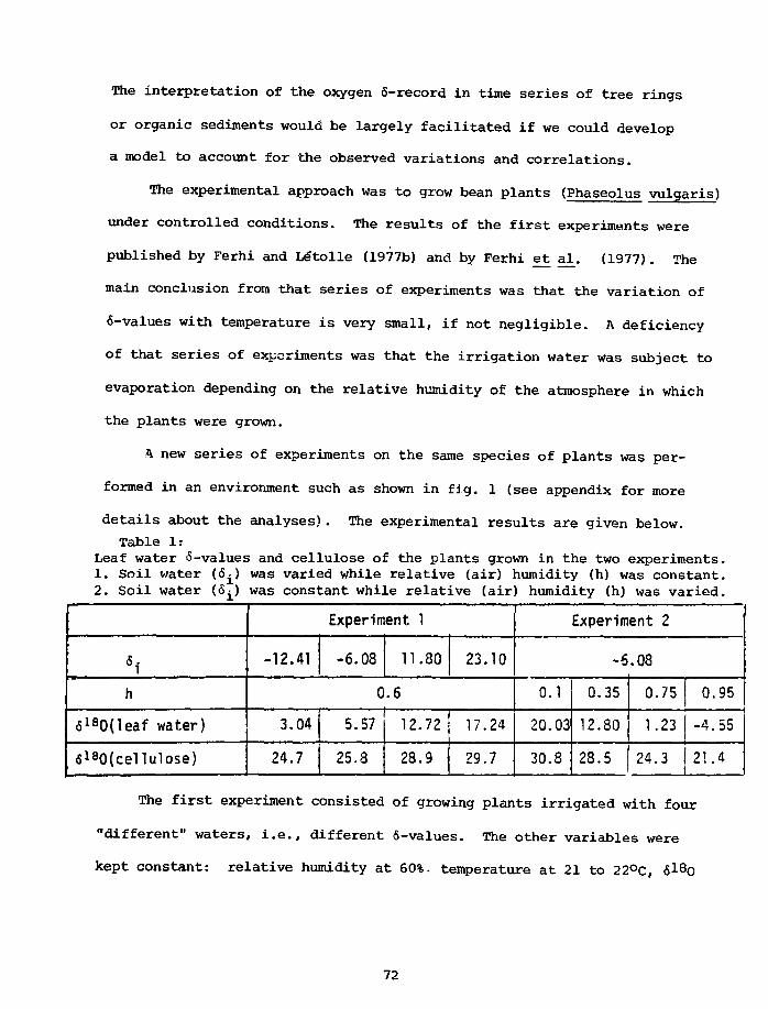
The interpretation of the oxygen 6-record in time series of tree rings
or organic sediments would be largely facilitated if we could develop
a model to account for the observed variations and correlations.
The experimental approach was to grow bean plants (Phaseolus vulgaris)
under controlled conditions. The results of the first experiments were
published by Ferhi and Le"tolle (1977b) and by Ferhi et al. (1977) . The
main conclusion from that series of experiments was that the variation of
6-values with temperature is very small, if not negligible. A deficiency
of that series of experiments was that the irrigation water was subject to
evaporation depending on the relative humidity of the atmosphere in which
the plants were grown.
ft new series of experiments on the same species of plants was per-
formed in an environment such as shown in fig. 1 (see appendix for more
details about the analyses). The experimental results are given below.
Table 1:Leaf water 6-values and cellulose of the plants grown in the two experiments.1. Soil water (6^) was varied while relative (air) humidity (h) was constant.2. Soil water (6^) was constant while relative (air) humidity (h) was varied.
h
6 l80(leaf water)
<S180(cellulose)
- 12 .
3.
24.
41
04
7
Experiment
-6
5
25
08
0
57
8
11
.6
12
28
1
.80
.72
.9
23.
17.
29.
10
24
7
0.
20.
30.
1
03
8
Experiment
0
12
28
-6
35
80
5
.08
0.
1.
24.
2
75
23
3
0.
-4.
21.
95
55
4
The first experiment consisted of growing plants irrigated with four
"different" waters, i.e., different 6-values. The other variables were
kept constant: relative humidity at 60%. temperature at 21 to 22°C,
72
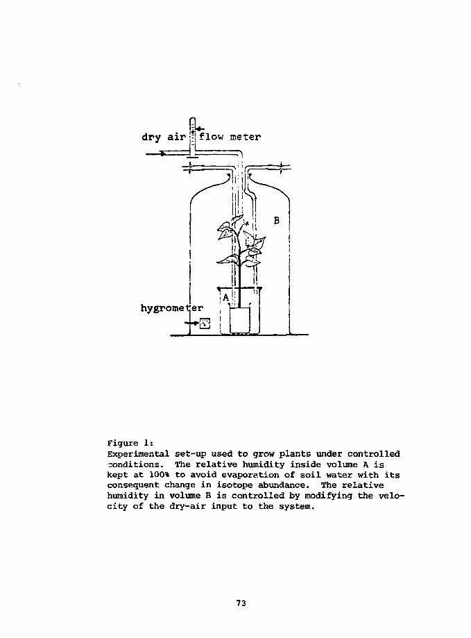
0*dry air -A flow meter
hygromet
Figure 1:Experimental set-up used to grow plants under controlledconditions. The relative humidity inside volume A iskept at 100% to avoid evaporation of soil water with itsconsequent change in isotope abundance. The relativehumidity in volume B is controlled by modifying the velo-city of the dry-air input to the system.
73
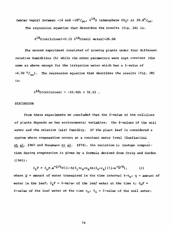
(water vapor) between -14 and -16,°/^, 618O (atmosphere C02) at 39.4°/oo-
The regression equation that describes the results (fig. 2A) is:
618O(cellulose) =0.15 <5180(soil water)+26.68
The second experiment consisted of growing plants under four different
relative humidities (h) while the other parameters were kept constant (the
same as above except for the irrigation water which has a 6-value of
-6.08 °/ o o)• The regression equation that describes the results (fig. 2B)
IS:
618O(cellulose) = -10.92h + 32.12 .
DISCUSSION
From these experiments we concluded that the 6-value of the cellulose
of plants depends on two environmental variables: the (5-values of the soil
water and the relative (air) humidity. If the plant leaf is considered a
system where evaporation occurs at a constant water level (Gonfiar.tini
et al. 1965 and Dongmann e_t al. 1974), the variation in isotope composi-
tion during evaporation is given by a formula derived from Craig and Gordon
(1965) .-
6tP = 6oF.e"2/(3+{(l-h)6i+ee+ek+h(5v-
ek)Hl-e~Q/9}' (1>
where Q = amount of water transpired in the time interval t-to; g = amount of
water in the leaf; 6tF = 6-value of the leaf water at the time t; 6OF =
6-value of the leaf water at the time to; 6^ = 6-value of the soil water;
74
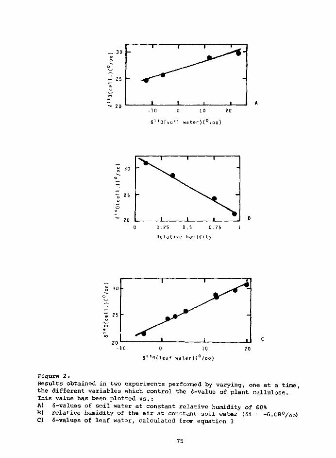
„ 3D -
-10 0 10 20
{''Ofsoil water)(°/oo)
2 30 -
T, 25 -
0.25 0.5 0.75
Relative humidity
-10 0 106Ie0(leaf water)(°/oo)
Figure 2:Results obtained in two experiments performed by varying, one at a time,the different variables which control the 6-value of plant cellulose.This value has been plotted vs.:A) 6-values of soil water at constant relative humidity of 60%B) relative humidity of the air at constant soil water (Si = -6.08°/oo)C) 6-values of leaf water, calculated from equation 3
75
ee = equilibrium enrichment factor between liquid and vapor; ek = kinetic
enrichment factor; 6V = 6-value of the atmospheric water vapor; h = relative
(air) humidity.
For given h and 6^, the 6-value of leaf water attains a limit with
increasing Q. At the isotopic equilibrium point, the 6-value of the leaf
water is:
618O(eq) = (l-h)6i+ee+ek+h(6v-ek) (2)
From this equation we can calculate the 6-values for the conditions of both
experiments described above. We need to know the values of eo, e., and 6 .
The first (ee) was evaluated by Baertschi and Thurkauf (1969). At 21°C it
is approximately 9°/oo« The kinetic factor ek is more difficult to esti-
mate. From measurements by Forstel ejt al_. (1975) one concludes that e^
is about 20°/ . Using these values and considering a mean 6y of -15°/oo,
the equation for the 6-value of leaf water is:
618O(leaf water) = (1-h)6i+29-35h (3)
Using this equation we calculate the 6-value of leaf-water for the plants
in both experiments described above, and we obtain the line in fig. 2C:
618O(cellulose) = 0.376 518o(lec.: water) + 23.56 (4)
Thus we see that the 6-value of leaf tissue depends both on the 6-value
of the soil water and on the relative humidity of the environment where the
76
plant grew. In other words, the 6-values of leaf tissue depend on the
6-values of leaf water because this isotope composition depends on the
isotope composition of soil water and on the relative humidity.
In equation 4 we see that about 38% of the variation of the 6-values
of leaf cellulose can be explained by its provenance from the leaf water.
We are interested in investigating where the other 62% originates. If we
assume that it is atmospheric CC>2» we can write an equation like this:
618O(cellulose) = a(<S(leaf water)+e1) + (a-1) (6 (CO2)+e2), (5)
where a is about 0.38 and £^ and e- are the corresponding isotope enrich-
ment factors. As <5(CC>2) of the laboratory air was measured (39.4O/QO), we
can introduce its value in equation 5 which then becomes:
S180(cellulose) = 0.38618O(leaf water) + 24.43+0.38E2+0.6262 (6)
The three last terms of this equation must equal the last term of equation 4.
Henco,
0.38(^+0.62e2 = -0.87 (7)
Although the experiments were not designed to distinguish between the
possibilities of complete exchange or no exchange of the oxygen in the car-
bon dioxide with the oxygen in the leaf water, the range of variability of
equation 7 between these two extreme possibilities is very small. From the
temperature dependence observed in previous experiments (0.04°/oo /°C), we
can already prove that there is not a complete exchange of CCU with leaf
77
water because the calculated temperature effect (0.22 x 0.62 = 0.14°/oo/oc)
would be observable in the S-values of cellulose. (These results appear
to be at odds with DeNiro and Epstein (1979) who report complete exchange
of the CO2 with the water in the wheat plants of their experiment.)
From equations 2, 4, and 5, we can write general equations for the
isotope composition of the cellulose of terrestrial plants:
6180(cellulose) = 0.376 {(1-h) e^c^e^n^-Ek) }+23.56, (8)
and
618O(cellulose) = 0.38{(l-h) 6i+ee+Ek+h(6v-e]t)} +0.62618o(CO2) . (9)
The significance of these relationships is that once the steady state is
attained (which occurs rather quickly according to Dongmann et al_. (1974)
and Farris and Strain (1978)), the 6-value of the leaf water is controlled
not only by the isotope ratio in tht soil water but also by the relative
humidity, and by the 6-value of the atmospheric water vapor. The higher
the humidity is, the greater the contribution of the 6-value of the water
vapor compared with the effect by the 6-value of the soil water.
The general validity of these expressions has been qualitatively
tested by measuring plants naturally grown in different climates and lati-
tudes. Climates of very diverse humidities were selected, whereas the
latitude transect provides for a wide range in the 6-values of the soil
water due to the known latitudinal effect in the isotope composition of
precipitations (Forstel et al., 1975). In fig. 3 we observe that for regions
like the north of Europe, where the 6-value of the soil water would be very
78
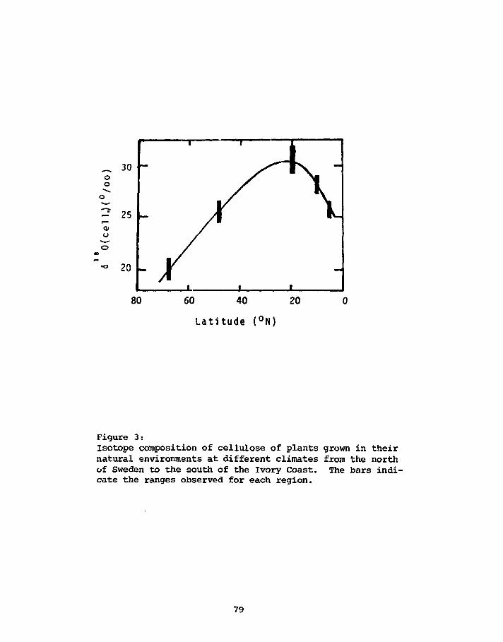
60 40 20
L a t i t u d e ( ° N )
Figure 3:Isotope composition of cellulose of plants grown in theirnatural environments at different climates from the northof Sweden to the south of the Ivory Coast. The bars indi-cate the ranges observed for each region.
79
negative and ~\e humidity high, cellulose has a 6-value of about 20°/oo.
For desert regions like the Sahara, where h is low and 6(soil water) is
high, the cellulose has values of about 30°/ . Finally, for tropical
wet regions where both h and 6(soil water) are high, both effects compen-
sate each other and the observed 6(cellulose) is intermediate in isotope
composition.
CONCLUSIONS
The <518O values of plant cellulose are not a significant function of
lfitemperature, but rather of the 6 0 values of water absorbed in the roots
and of the d o and vapor pressure deficit of atmospheric water vapor
during photosynthesis.
The <$180 in plant cellulose can be a paleoclimatological indicator,
but its interpretation is more complex than first anticipated.
These studies illustrate the value of controlled growth-chamber
exp triments in addition to empirical field studies.
RE* SRENCES
Baertschi, P. and Thurkauf, M. (1969). Isotopische Effekt bei derTrennung der Sauerstoff-Iaotopen 160 und -80 bei der Rektiffikation vonleichten und schweren Wasser, (Isotope effect during separation of oxygenisotopes l^o and ^0 through rectification of light and heavy water.)Helv. Chim. Acta, 43, 80-89.
Craig, H. and Gordon, L.I. (1965). Deuterium and oxygen-16 variationsin the ocean and the marine atmosphere, in Stable Isotopes rn OceanographicStudies and Paleotemperatures, Spoleto, July 26 - 30, 1965: 9-130.
80
DeNiro, M.J. and Epstein, S. (1979). Relationship between theoxygen isotope ratios of terrestrial plant cellulose, carbon dioxide,and water, Science, 204, 51-53.
Dongmann, G., Nurnberg, H.W., Forstel, H. and Wagener, K. (197«*) .On the enrichment of H2 -80 in the leaves of transpiring plants, Rad.Environm. Biophys., 11, 41-52.
Farris, F. and Strain, B.R. (1978). The effects of water-stresson leaf H218O enrichment, Pad, and Environm. Biophys., 15, 167-202.
Ferhi, A. and Letolle, R. (1977a). Variation de la compositionisctopigue de l'oxygene organigue de guelgues plantes en fonction deleur milieu de vie, (Variations of the isotopic composition of organicoxygen from some plants with their environment.) C.R. Acad. S c ,284, D: 1,887-1,889.
Ferhi, A. and Letolle, R. <1977b). Transpiration and evaporationas the principal factors in oxygen isotope variations of organic matterin land plants, Physiol. Veg., 15, 363-370.
Ferhi, A. and Letolle, R. (1978). Relation entre le milieu clima-tigue et les teneurs en oxygene-18 de la cellulose des plantes terrestres,(Relation between climatic environment and oxygen-18 content of celluloseof aerial plants.) Physiol. Veg., 17, 107-117.
Ferhi, A.M., Letolle, R. and Lerman, J.C. (1975). Oxygen isotoperatios of organic matter; analyses of natural compositions, Proc. 2ndInt'l Conf. on Stable Isotopes. Oak Brook, Illinois, October 1975.ERDA CONF 751027:716-724.
Ferhi, A.M., Long, A. and Lerman, J.C. (1977). Stable isotopes ofoxygen in plants: a possible paleohygrometer, Hydrol. Water Resourc.Arizona and Southwest, 7, 191-198.
Forstel, H., Putral, A., Schleser, G. and Lieth, H. (1975). Theworld pattern of oxygen-18 in rainwater and its importance in under-standing the biogeochemical oxygen cycle, in Isotope ratios as pollutantsource and behavior indicators. Proc. Sympos. Vienna, November 18-22,1974, IAEA, Vienna: 3-20.
Gonfiantini, R., Gratziu, S. and Tongiorgi, E. (1965). Oxygen iso-tope composition of water in leaves, in Isotopes and Rad. in Soil plantnutrition studies, IAEA, Vienna: 405-410.
Gray, J. and Thompson, P. (1976) Climatic information from 180/160ratios of cellulose in tree rings, Nature, 262, 481-482.
81
Hardcastle, K.G. and Friedman, I. (1974). A method for oxygenisotope analysis of organic material, Geophys. Res. Lett., 1, 165-167.
Libby, L.M. and Pandolfi, L.J, (1974). Temperature dependence ofisotope ratios in tree rings, Proc. Natl. Acad. Sci., 71, 2482-2486.
Libby, L.M., Pandolfi, L.J., Payton, P.H., Marshall III, J.,Becker, B. and Giertz-Siebenlist, V. (1976). Isotopic tree thermometers,Nature, 261, 284-288.
Long, A., Lerman, J.C. and Ferhi, A. (1978). Oxygen-18 in tree rings:paleothermometers or paleohygrometers? In Zartman, R.E. (Ed.), ShortPapers 4th, Int'l. Conf. Geochronol., Cosmochronol., Isotope Geology,Snowmass-at-Aspen, August 20-25, 1978, (USGS Open-File Report 78-701):253-254.
82
APPENDIX
SAMPLE ANALYSES
All oxygen in the samples was converted to C02 and analyzed in an
isotope mass spectrometer. All 6*°0 values are expressed with references
to SMOW. The different procedures used to prepare the samples are sum-
marized as follows:
Cellulose: The 6-values of total tissue and of cellulose were compared and
proved to be, in general, different. This difference was small for the bean
plants (0.6°/oo) but rather large for Nerium oleander from the Sahara (about
3°/ o o). Thus all analyses for the present article were done on cellulose
which was prepared according to current techniques (summarized by Ferhi
and Letolle, 1978). This cellulose was then pyrolized and converted to
CO as described as elsewhere (Ferhi et al ., 1975) .
Atmospheric C02: The 6-value of the atmospheric carbon dioxide was measured
after separating this compound from the air (2-liter samples) with liquid
nitrogen, and further dried by distillation at the dry-ice-agetone tempera-
ture.
Atmospheric water vapor: The 6-value of the atmospheric water vapor was
measured after the wacer vapor was collected (mentioned in the previous
paragraph as a remainder of the carbon dioxide separation). It was then
passed through a diamonds column at 1200°C which results in its reduction
to a mixture of CO and H2. After the hydrogen was pumped away, the CO
was oxidized to C02 as described by Hardcastle and Friedman (1974) and
Ferhi et aJU_ (1975).
83
1 Q
NATURAL VARIATIONS IN THE O CONTENT OF CELLULOSE
J. Gray Department of PhysicsP. Thompson University of Alberta,
Edmonton, Alberta
INTRODUCTION
Results of recent field experiments and controlled laboratory
I Q
experiments suggest that natural variations in 0 content of cellulose
produced in plant materials may be useful as indicators of climate vari-
ables.
While it is apparent that eventually a detailed understanding of all
the isotopic fractionation processes involved in the production of cellu-
lose in a natural system must be obtained, the ultimate usefulness of the
method as a climate indicator must lie in an ability to interpret the iso-
tope measurements in terms of a small number of meaningful climate variables.
Results are presented of 0/ 0 measurements on tree rings and peat-
producing plants from areas in North America representing a diversity of
climate regions. The isotope results are compared empirically with climate
records obtained from appropriate meteorological stations to determine
correlations, if any, between S^&O results and climate variables.
RESULTS
Fig. 1 shows the isotope curves for 5-year groups of tree rings plotted
against time for each site. In general the trends of the curves do not
correlate closely although there are points of similarity such as maxima
84
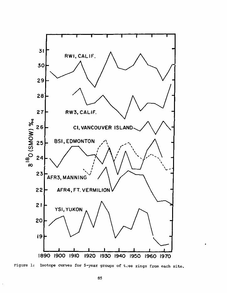
31
30
29
28
27o
! ! 26
OCO
25
co° 24CO
23
22
21
20
19
I I
RWI,CALIF
RW3, CALIF.
Cl,VANCOUVER ISLAND
. BSI, EDMONTON / \
AFR4, FT. VERMILION
j i i I
1890 1900 1910 1920 1930 1940 1950 I960 1970
Figure 1: Isotope curves for 5-year groups of t -ee rings from each site.
85
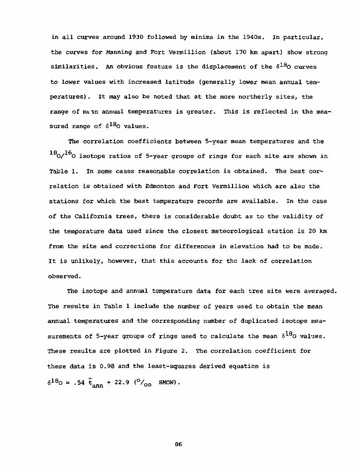
in all curves around 1930 followed by minima in the 1940s. In particular,
the curves for Manning and Fort Vermillion (about 170 km apart) show strong
similarities. An obvious feature is the displacement of the 618o curves
to lower values with increased latitude (generally lower mean annual tem-
peratures) . It may also be noted that at the more northerly sites, the
range of mtin annual temperatures is greater. This is reflected in the mea-
sured range of 6 -®0 values.
The correlation coefficients between 5-year mean temperatures and the
1 ft 16
0/ 0 isotope ratios of 5-year groups of rings for each site are shown in
Table 1. In some cases reasonable correlation is obtained. The best cor-
relation is obtained with Edmonton and Fort Vermillion which are also the
stations for which the best temperature records are available. In the case
of the California trees, there is considerable doubt as to the validity of
the temperature data used since the closest meteorological station is 20 km
from the site and corrections for differences in elevation had to be made.
It is unlikely, however, that this accounts for the lack of correlation
observed.
The isotope and annual temperature data for each tree site were averaged.
The results in Table 1 include the number of years used to obtain the mean
annual temperatures and the corresponding number of duplicated isotope mea-
surements of 5-year groups of rings used to calculate the mean 8^°0 values.
These results are plotted in Figure 2. The correlation coefficient for
these data is 0.98 and the least-squares derived equation is
618O = .54 t ^ + 22.9 (°/oo SM0W).
86
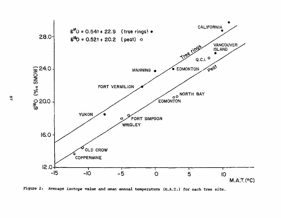
CO
28.0-
J24.0-o
o
o 20.0 -To
16.0-
12.0-
Sm0 = 0.54t4 22.S
S' O = 0.52t + 20.2
(tree rings) •
(peat) o
MANNING • y /
FORT VERMILION y (
yS
Y U K O N / *
/^"^OLD CROW
y S COPPERMINE
•
/ / -
'•EDMONTON y^Z^
.NORTH BAY
' /^EDMONTON
0 / FORT SIMPSON
'WRIGLEY
1 1' 1 1
-15 -10 -5 0 10M.A.T.(°C)
Figure 2: Average isotope value and mean annual temperature (M.A.T.) for each tree site.
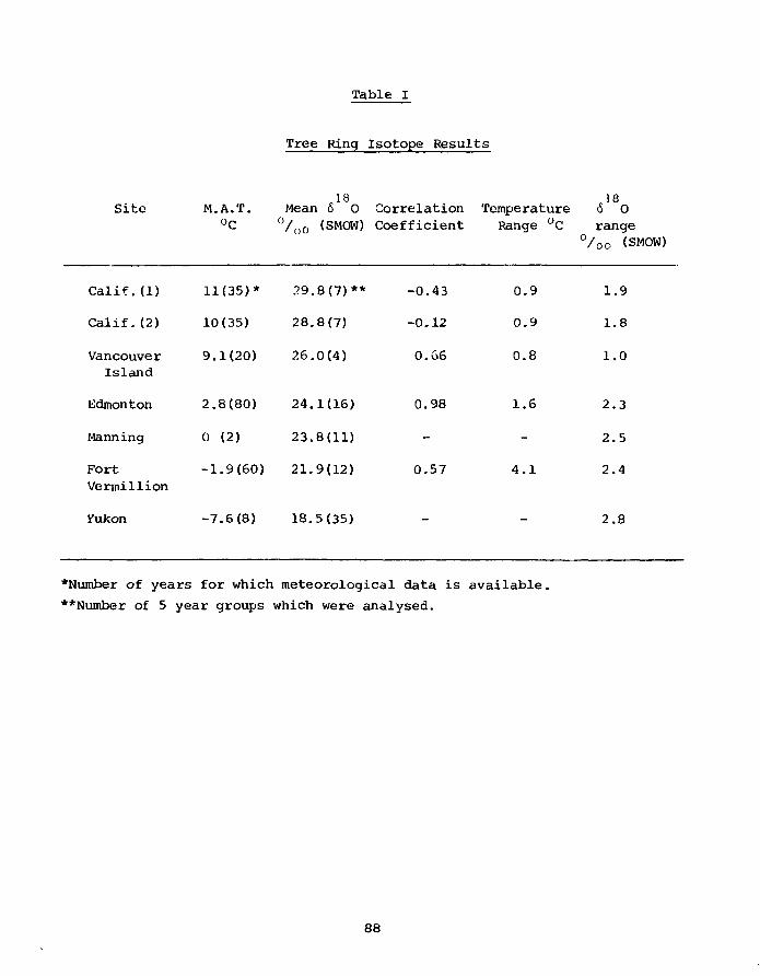
Table I
Site
Calif. (1)
Calif.(2)
VancouverIsland
Edmonton
Manning
FortVe million
M.A.T.°C
11(35)*
10(35)
9.1(20)
2.8(80)
0 (2)
-1.9(60)
Tree Ring
Mean 6 0°/o0 (SMOW)
29.8(7)**
28.8(7)
26.0(4)
24.1(16)
23.8(11)
21.9(12)
Isotope Results
CorrelationCoefficient
-0.43
-0.12
0.66
0.98
-
0.57
TemperatureRange °C
0.9
0.9
0.8
1.6
-
4.1
186 0range
°/oo (SMOW)
1.9
1.8
1.0
2.3
2.5
2.4
Yukon -7.6(8) 18.5(35) 2.8
*Number of years for which meteorological data is available.
**Number of 5 year groups which were analysed.
88
Samples of sphagnum moss were collected from sites across Canada
and the isotopic composition of the cellulose determined. Measurements
of 6*8Q carried out at a single site on cellulose from living plants
representing all the major peat-producing species showed them to be the
same within experimental error (18.5±0.2°/oo). The <5 O of the cellulose
from the sphagnum moss samples is plotted as a function of temperature in
Fig. 2 to allow comparison with the tree-ring data. The equation defining
these data is 618O = 0.52 t___ + 20.2 (correlation coefficient = 0.98).aim
The slopes of these two lines are the same within experimental error while
the intercept of the peat 6 0 values is approximately 2.7 °/oo lower than
for the tree rings.
DISCUSSION
The linear relation between 618O of cellulose from the tree rings and
the peat-producing plants and mean annual temperature suggests that it is
the isotopic composition of the meteoric (ground) water feeding the tree
which plays a domi lant role in determining the O content of the cellulose.
While it is not always true that the isotopic composition of meteoric
water is determines by local environmental temperatures, it often is the
case. Records for E&nonton, for instance, show a correlation between mean
annual surface temperature and mean annual 6 0 of precipitation of 0.9.
However, this does not explain the different slopes found for 6^8O
versus MAT at different sites and the possibility of a temperature-dependent
fractionation step during metabolism still exists.
89
Furthermore, these data, particularly the parallel behavior of the
two curves, do not give any insight into the role played by evapotranspira-
tion at the leaf surface. The sphagnum moss samples were collected from
peat bogs where humidity is generally high and Gvapotranspiration minimized.
It is possible, therefore, that the 2.7°/oo upward displacement of the tree
ring 6l8O curve may reflect evapotranspiiation effects. Given the relatively
constant enrichment of the tree ring 6^0 values relative to the sphagnum
moss it appears unlikely that the effects of variation of relative humidity
on evapotranspiration will be detectable. It is also feasible that the
displacement between the two curves represents a real temperature difference
associated with microclimatic temperature difference between ground-level
and tree-crown elevation.
A simple model of equilibration between atmospheric carbon dioxide
with water in the leaf (whether or not enriched by evapotranspiration rela-te
tive to the water drawn up by the tree) yields CO2 of higher 0 content than
1 ftthe measured 0 content of cellulose when the temperature dependence of the
fractionation factor for CO2 = H2O equilibration is taken into account. This
means that either further oxygen exchange occurs in the subsequent photo-
synthetic metabolism or that one or more fractionation steps occur during the
subsequent production of cellulose resulting in a depletion of -^O in the
cellulose relative to the CO2 precursor. This fractionation step may well
be temperature dependent. The data shown here do not show a strong correla-
tion between measured 6^°0 values of cellulose and growth season temperature,
but this does not preclude the possibility of a temperature-dependent
fractionation step.
90
SUMMARY
The correlation between 0 content of cellulose and mean annual
temperature at a number of widely separated sites suggests that the prin-
cipal determining factor of the cellulose °0 composition is the 0 com-
position of the groundwater used by the plant. In a region where the
l ftgroundwater-meteoric water 0 composition is closely tied to mean annual
temperature and where large variations in relative humidity do not occur,
the 6 0 cellulose curve can be interpreted as a mean annual temperature
curve. Also in these regions, it appears that the oxygen isotopic compo-
sition of cellulose is somewhat insensitive to small relative-humidity
changes making it unlikely that relative-humidity information can be
extracted from the isotope data.
Finally, the data presented here do not preclude the possibility
of a temperature dependent biological fractionation occurring during the
production of cellulose from C02 after photosynthesis.
ACKNOWLEDGEMENTS
The work on peat samples was initiated and carried out by S.C. Chatwin
of the Geology Department of the University of Alberta. Analyses were
carried out in the Physics Department, University of Alberta. This work
was supported in part by grants from NRC Canada, Alberta Forestry Research
and Atmospheric Environment Service, Alberta.
91
REFERENCES
DeNiro, M.J. and Epstein, S. (1979). Mechanisms of carbon isotopefractionation associated with lipid synthesis. Science, 197, 261-263.
Epstein, S., Thompson, P. and Yapp, C.J. (1977). Oxygen and hydro-gen isotopic ratios in plant cellulose, Science, 198, 4323: 1209-1215.
Gray, J. and Thompson, P. (1976). Climatic information from 18O/16Oratios of cellulose in tree-rings. Nature, 276, 281-262.
Gray, J. and Thompson, P. (1977). Climatic information from 18O/16Oanalysis of cellulose, lignin and whole wood from tree rings, Nature, 270,708-709.
Hage, K.D., Gray, J. and Linton, J.C. (1975). Isotopes in precipita-tion in northwestern North America, Monthly Weather Review, 103, 958-966.
92
IV
COMBINATIONS OF ISOTOPES
93
LATE PLEISTOCENE CLIMATIC CHANGES REGISTERED BY 518O and 613C inTHE GIANT CLAM, TRIDACNA GIGAS, OF THE NEW GUINEA CORAL REEFS
P. Aharon Australian NationalJ. Chappell University,W. Compston Canberra, A.C.T.
18 13This report describes variation in 6 0 and 6 C for the giant clam,
Tridacna gigas, sampled over the time-period zero to 150,000 years B.P.,
which reflect past changes in sea level and in ocean temperature. The
clams also have potential for tracing the input of industrial CO_ to sur-
face ocean water, as they contain well-defined annual growth bands and
live for up to 80 years.
In the Huon Peninsula, New Guinea, Tridacna is found in clear water
between 5 to 20 m deep. It deposits a dense cross-lamellar shell aragonite
which despite the association of Tridacna with symbiotic algae, is
apparently in i.sotopic equilibrium with seawater. Present-day Tridacna
give an oxygen isotope temperature of 27°C, exactly matching the mean sea-
water temperature observed for the region, and they also exhibit small <S 0
fluctuations within the annual growth bands that correspond well with the
observed seasonal temperature range.
Fossil Tridacnas occur in a sequence of raised coral reefs on the tectoni-
cally rising Huon Peninsula. The reefs represent interglacial and inter-
stadial peaks of sea level generated by past fluctuations in the global mass
of glacial ice. Their ages have been measured by C14 and uranium series
disequilibrium methods, and correlations have been made with similar reefs
elsewhere and with the 618O stratigraphy of deep-sea cores (Bloom et a_l, 1974;
94
Chappell, 1974). Fiq. 1 gives the relative sea level curve represented
by the reef sequence. The detailed stratigraphy of each reef complex
gives a higher time-resolution than most deep-sea core rerords, o-*t this
advantage is offset by the discontinuous occurrence of the reefs.
The data (Fig. 2) show a distinct variation in 6 0 and <5 C between
reefs. Kight modern Tridacnas define the variability for the present-day
population which is 0.14°/ in <5 0 (o) per individual, and of this,OO
0.10°/^ is contributed by the total experimental procedure. Tridacna
is thus substantially more uniform than molluscs from the Barbados reefs
for example, which showed 0.4°/OQ variation pir individual (Shackleton
and Matthews, 1977). Fossil Tridacnas were slabbed, inspected for infillings
of secondary calcite, and X-rayed to confirm 100% aragonite. Assuming that
fossil populations have the same dispersion as modern Tridacnas, some reefs
such as Complex III apparently contain more than one population. We con-
sider this is due mainly to the sampling of each reef spanning an inter-
val of several thousand years within the culmination periods of reef growth.
Variability in (S13C between individuals is slightly greater than 618O, as
expected from the much smaller mass of the seawater carbon reservoir. The
<S13C range in a given Tridacna is substantially smaller, however, than the
diurnal range of up to 2°/QO monitored in Huon Peninsula F.eawater, which
reflects mirine plant photosynthesis.
Most of the change in 618O between reefs must be attributed to the
changing mass of global ice, as shown for pelagic foraminifera by shackleton
and Opdyke (1973). The lower the sea level, the greater the mass of glacial
95
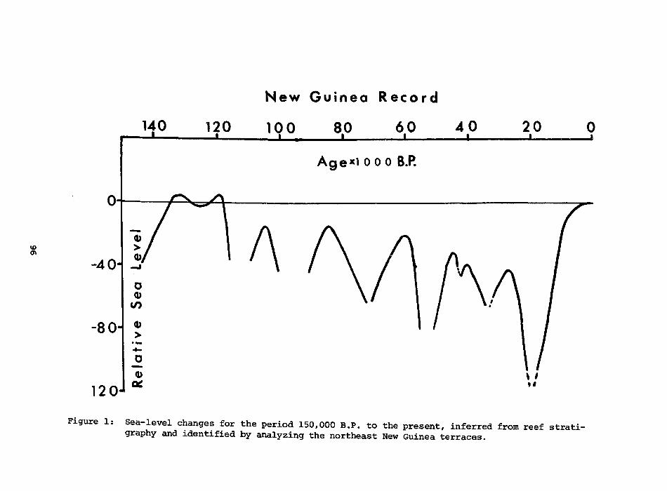
New Guinea Record
a
140
120
120 100 80 60 4 0
Age"i ooo 6.P.
20 0
Figure 1: Sea-level changes for the period 150,000 B.P. to the present, inferred from reef strati-graphy and identified by analyzing the northeast New Guinea terraces.
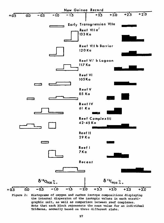
New Guinea Record
+0.5 "oS" -0.5 -1.0 -1.5 3.5 + 3.0 +2.5 2.0
Early Transgression Vila
Reef V i la '133 Ka
Reef VII b Barrier120Ka
Reef V!! b Lagoon117Ka
|Reef VI105Ka
Reef V85 Ka
Reef IV61 Ka
Reef ComplexlJI42-45Ka
Reef II29Ka
Reef I7Ka
Recent
613cPDB /o
+ 0.5 0.0 -0.5 -1.0 -1.5 - 2 0 +3.5 +3.0 +2.5 +2.0Figure 2: Histograms of oxygen and carbon isotope compositions displaying
the internal dispersion of the isotopic values in each strati-graphic unit, as well as comparison between reef complexes.Note that each block represents the mean value for an individualTridacna, normally based on three different slabs.
97
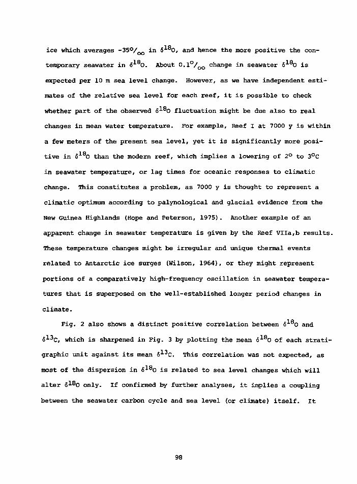
ice which averages ~3 5°/ o o in 6*8O, and hence the more positive the con-
temporary seawater in 6 0. About 0.1°/oo change in seawater 6 80 is
expected per 10 m sea level change. However, as we have independent esti-
mates of the relative sea level for each reef, it is possible to check
whether part of the observed 6^8O fluctuation might be due also to real
changes in mean water temperature. For example, Reef I at 7000 y is within
a few meters of the present sea level, yet it is significantly more posi-
tive in 6 0 than the modern reef, which implies a lowering of 2° to 3°C
in seawater temperature, or lag times for oceanic responses to climatic
change. This constitutes a problem, as 7000 y is thought to represent a
climatic optimum according to palynological and glacial evidence from the
New Guinea Highlands (Hope and Peterson, 1975). Another example of an
apparent change in seawater temperature is given by the Reef VIIa,b results.
These temperature changes might be irregular and unique thermal events
related to Antarctic ice surges (Wilson, 1964), or they might represent
portions of a comparatively high-frequency oscillation in seawater tempera-
tures that is superposed on the well-established longer period changes in
climate.
Fig. 2 also shows a distinct positive correlation between 618O and
6-^C, which is sharpened in Fig. 3 by plotting the mean 6*8O of each strati-
graphic unit against its mean 613C. This correlation was not expected, as
most of the dispersion in <S180 is related to sea level changes which will
alter 6 -8O only. If confirmed by further analyses, it implies a coupling
between the seawater carbon cycle and sea level (or climate) itself. It
98
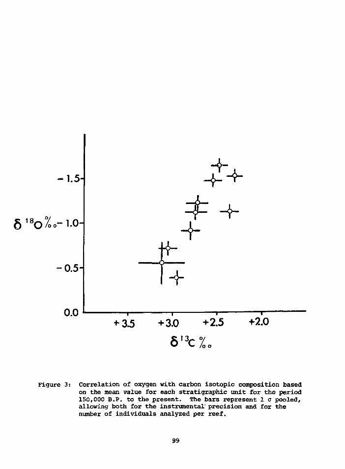
1.5-
1.0-
0.5-
-1-i ( ) i
1 +3.5 +3.0 +2.5
813c7+2.0
Figure 3: Correlation of oxygen with carbon isotopic composition basedon the mean value for each stratigraphic unit for the period150,000 B.P. to the present. The bars represent 1 a pooled,allowing both for the instrumental' precision and for thenumber of individuals analyzed per reef.
99
would require an increase in stored organic carbon at times of increased
glacier mass, perhaps by a decrease in the rate of oxidation of oceanic
organic debris which currently maintains the deep ocean water some 2°/
lighter in 6^-^C than the surface. Alternatively, lowered sea level might
be accompanied by increased dissolution of (heavy) calcareous oozes. We
have not yet assessed the fractional changes in the mass of the various
carbon reservoirs required to induce such effects.
Future work on Tridacna will include the following:
(1) The securing and analysis of well-dated Tridacnas from other regions
to ensure that any local effects (water changes due to evaporation or to
runoff) are identified.
(2) Analysis of seasonal bands from fossil Tridacnas to see whether the
seasonal contrast in sea water temperature in various interstadial periods
match the changing pattern of solar radiation as predicted by the
Milankovitch astronomical model (Berger, 1978; Chappell, 1978).
(3) Analysis of seasonal bands in modern Tridacnas to search for the
fossil fuel effect in/surface ocean water.
REFERENCES
Berger, A.L. (1978). Long-term variations of caloric insolationresulting from the Earth's Orbital Elements, Quat. Res., 9, 139-167.
Bloom, A.L., Broecker, W.S., Chappell, J.M.A., Matthews, R.K. andMesolella, K.J. (1974). Quaternary sea-level fluctuations on a tectoniccoast: new 230Tn/234u aates from the Huon Peninsula, New Guinea,Quat. Res., 4, 185-205.
Chappell, J. (1974). Geology of coral terraces, Huon Peninsula,New Guinea: a study of Quaternary tectonic movements and sea-levelchanges, Geol. Soc. Am. Bull., 85, 553-570.
100
Chappell, J. (1978). Theories of upper Quaternary ice ages, inPittcock, A.B., Frakes, L.A., Jenssen, D-, Petersen, J.A. and Zillman, J.(Eds.) Climatic Change and Variability - A Southern Perspective.Cambridge University Press: 211-225. Cambridge.
Hope, G.S. and Peterson, J.A. (1975). Glaciation and vegetationin the high New Guinea mountains, In Suggate, R.P. and Cresswell, M.M.(Eds.) Quaternary Studies. The Royal Society of New Zealand: Wellington155-162.
Shackleton, N.J. and Opdyke, N.D. (1973). Oxygen isotope and paleo-magnetic stratigraphy of equatorial Pacific core V28-238: oxygen isotopetemperatures and ice volumes on a 105 year and 106 year scale, Quat. Res.,3, 39-55.
Shackleton, N.J. and Matthews, R.K. (1977). Oxygen isotope strati-graphy of late Pleistocene coral terraces in Barbados, Nature, 268, 618-619.
Wilson, A.T. (1964). Origin of ice ages: an ice shelf theory forPleistocene glaciation. Nature, 201, 147-149.
101
STABLE ISOTOPE STUDIES OF SUBGLACIALLY PRECIPITATED CARBONATESAND OF ANCIENT GROUND WATER: PALEOCLIMATIC IMPLICATIONS
B.B. Hanshaw U.S. Geological SurveyI.J. Winograd Reston,F.J. Pearson, Jr. Virginia
Isotopic analyses of subglacially-precipitated calcite from near a
modern temperate glacier show that the 6 0 ( O / O relative to standard
18mean ocean water) of the calcite records the 6 0 of the ice from that
glacier (Hanshaw and Hallet, 1978). It may, therefore, be possible to
determine the &*-°0 of Pleistocene ice sheets on the basis of isotopic
analyses of calcite formed under that ancient ice. This, in turn, would
allow estimation of the S o of Pleistocene oceans and correction of the
paleotemperature scale based on foraminiferal oxygen isotopic analyses.
We have recently analyzed a sample of ancient, subglacially-precipitated
calcite from central Ohio which was overlain by a till estimated by
R. Goldthwaite (oral communication, 1977) to be > 13,500 YBP. The pre-
cipitate has glacial striae across it and parallel to those on the bed-
rock, supporting its subglacial origins. Based upon preliminary analysis
18
of the 5 0 of the precipitate, the ice from which it formed had an iso-
topic composition similar to that of locaJ modern mean-annual precipita-
tion. This could imply an absence of isotopic shift during the last glacial
maximum although this interpretation is highly speculative, being based on
only one analysis.
The isotopic composition of groundwater recharged during late
Wisconsin time indicates no glacial/interglacial isotopic shift. Water from
102
shallow wells containing modern precipitation reflects the isotopic com-
position of mean annual recharge. Samples of groundwater with carbon-14
and/or hydrologically estimated ages provide isotopic data of much older
recharge, back at least 30,000 years B.P. Studies of regional aquifer
systems in Texas, Florida, Nevada, California, the Atlantic Coastal Plain,
and the Northern Great Plains indicate that the 6D and 6*°0 content of
groundwater samples that span the last 30,000 years do not deviate signi-
ficantly from that of modern recharge. For any one aquifer system, uncer-
tainties in flow-system definition, varying depths of sampling points in
the aquifer, and differences in elevation of recharge areas mandate a
conservative interpretation of isotopic data. However, the apparent absence
of any temporal differences in the large number of regional aquifer systems
investigated lends credence to our conclusion of lack of isotopic shift in
recharge water. Because groundwater recharge typically occurs chiefly
during spring months, our conclusion will generally apply only to the iso-
topic composition of winter and spring precipitation.
The absence of a shift in conterminous U.S. ground waters may imply
(a) That the mean continental winter and spring temperatures were not much
different from today, even during the late Wisconsin glacial maximum;
(b) that oceanic shifts of 6 0 and temperature were minimal and were off-
set by a shift in temperature at each site of precipitation; (c) that the
winter and spring storm tracks remained generally similar over this time;
and (d) some combination of the above.
We note in closing that our conclusions differ from those of Harmon,
et al. (1979) and Yapp and Epstein (1977). Harmon et al. (1979) report a
103
-12% ir.terglacial/glacial shift in deuterium composition of precipitation
as recorded in speleothem-fluid inclusions in ice—free areas of east-
central North America. Yapp and Epstein (1977), in contrast, report an
average +19% shift in deuterium in North American wood during the inter-
val 14,000 - 22,0CC Y.B.P. We are surprised by the discrepancy between
Harmon et al. (1979) and our work. Furthermore, we believe that ground-
water should be a better, and more easily interpreted, intergrator of
the isotopic composition of winter and spring precipitation than cellulose.
Nevertheless, it is encouraging that these various approaches to unraveling
the continental paleoclimatic record differ so little.
REFERENCES
Hanshaw, 3.B. and Ballet, Bernard (1978). Oxygen isotope compositionof subglacially precipitated calcite: paleoclimatic implications. Science,200, 1267-1270.
Harmon, R.S., Schwarcz, H.P., and O'Neil, J.R. (1979). D/H ratios inspeleothem fluid inclusions: a guide to variations in the isotopic composi-tion of mateoric precipitation?: Earth Planet. Sci. Lett., 42, (2)254-266.
Yapp, C.J. and Epstein, Samuel (1977). Climatic implications of D/Hratios of meteoric water over North America (9500-22,000 B.P.) as inferredfrom ancient wood cellulose C-H hydrogen. Earth Planet Sci. Lett., 34,333-350.
104
POTENTIAL USE OF 618O AND 6D TOGETHER IN PLANTCELLULOSE AS A PALEQENVTFONMENT INDICATOR
A. Long Laboratory of Isotope GeochemistryDepartment of Geosciences,University of Arizona, Tucson
A. Ferhi U.E.R. des Sciences de la Terre,R. Lfitolle Universite Pierre-et-Marie-Curie,
Paris, France
J.C. Lerman Laboratory of Isotope Geochemistry,Department of Geosciences,University of Arizona, Tucson
We wondered if the humidity effect on 618O (Ferhi e_t al., this volume)
observed in bean plants in a growth chamber and also implied from a lati-
tude transect on natural trees, could be quantified in terms of measur-
able environmental conditions on natural trees. If so, this would be a
major step toward climatic inference from tree-ring isotope studies. Our
conclusions from Ferhi et al. (this volvme) are as follows:
(a) Temperature alone has insignificant effect on the 618O in bean-
plant cellulose.
18
(b) The 6 0 in bean-plant cellulose responds to only about 15% of
the variability of 618o in irrigation water at a humidity of 60%
and constant 618O in atmospheric vapor.is
(c) The 5 0 in bean-plant cellulose is inversely proportional to
relative humidity.
(d) These responses are explainable in terms of a model which con-
siders both leaf water and CO2 contributing oxygen to the plant
cellulose. In the model C0 2 is invariant in <518O and leaf H2O
105
behaves isotopically like an evaporating basin in a steady state.
(e) The variability of 618O in cellulose from natural plants of many
species throughout a wide latitude transect is qualitatively
consistent with the above model.
l ft
In this paper we have modified the model to use 5 o values of precipi-
tation only and to accommodate DeNiro and Epstein's (1979) conclusions on
the isotopic equilibration of CO2 and leaf H20. We have also included 6D
in the model and have carefully evaluated the kinetic enrichment factors
for the isotopic molecules of water.
Firstly, we shall consider the factors controlling 6-values for leaf
water. Our modification of the Craig and Gordon (1965) equation for evapo-
rating basins was simple. We assume that the precipitation in a tree's
locality is in isotopic equilibrium with the atmospheric water vapor,
i.e., 6(precip) = <S (vap) + ee. The Craig and Gordon equation then simplifies
to
6(steady state)= 6(input) + (1-h) (eeq + e K). (1)
This equation, now expressed in terms of precipitation 6's and humidity,
represents the isotopic value of leaf water at a steady state if (precipita-
tion) = (input to leaf). Note that if the water drawn in by the roots is
not local seasonal precipitation but groundwater from winter snowmelt,
leaf water 6's will be lower than predicted by this equation. We recall that
from the original equation the higher the humidity, the less effect ground-
water has. At 100% humidity, atmospheric water vapor alone controls the
106
isotopic composition of leaf water. Thus, the effect of exotic or non-
seasonal irrigation water is minimal in high-humidity growth areas.
Note also that equation 1 now contains a precipitation term (essen-
tially) which is more or lc:^ modified depending on humidity.
The selection of £„ values was not straightforward. We assumed that
HDO molecules obey equation 1 but with different constants. For evapo-
rating water, kinetic enrichment factors are sensitive to the boundary
conditions at the liquid surface. Experimental measurements (Table 1)
are only in fair agreement on values for these enrichment factors.
Table 1: KINETIC ENRICHMENT FACTORS FOR HDO AND H 21 8O MERLIVAT, 1978
(EHHALT AND KNOTT, 1965)
Boundary Layer Conditions: Static Laminar Turbulent Average
e k(H 21 8O) in °/ o o 28 (30) 19 (20) 14 (15) 16 (17)
ek(HDO) in °/OQ 25 (15) 17 (10) 12 (8) 14 (8)
For leaf water, HDO molecules should obey the same equation as H2^8O;
thus, the slope of the le^f water in D : 1&O coordinates should be calcul-
able from the modified basin equation below.
A &D SD(leaf water) -- 6D(utem water)
618O(leaf water) - 618O(stem water)
,. , . , D D, D D(1-h) (ee + e.k) _ ee + ee (2)
107
Depending on one's choice of experimental values, boundary con-
ditions, and temperature, a range exists of predicted leaf-water slopes
from 2.5 to over 4.5 (see Pig. 1),
When one searches the literature for experimental determinations of
this leaf-water isotope slope from naturally grown trees, the results
are not bountiful. These are only two values: 2.9 from France (Bricout,
1973), and 2.5 from southern California (Epstein et al., 1977). if these
values are representative, they imply static boundary conditions for trans-
piration. If this situation is universal, paleoclimatology would be made
easier, but it does not seem to be reasonable hydrodynamically. The usual
image of a leaf cross section shows substomatal cavities simply as holes,
whereas in fact many are interconnected galleries, within the leaf. With
this in mind, it is easiest to imagine an exchange with atmospheric water
vapor and a static boundary layer.
Our task now is to attempt to infer from isotope measurements of
plant cellulose what could amount to a mean growing-season leaf-water iso-
tope composition. Its composition in SD : 618O coordinates could possibly
give us mean photoperiod humidity as well as precipitation 6-values
(assuming a slope to the meteoric line) — see Fig. 2. From the work of
Andre Ferhi it seems that leaf water, perhaps through C02, influences the
isotope composition of oxygen in cellulose. In the present model we assume
that the same water in the same locale as the leaf also influences the cellu-
lose C-H hydrogen-isotope composition.
108
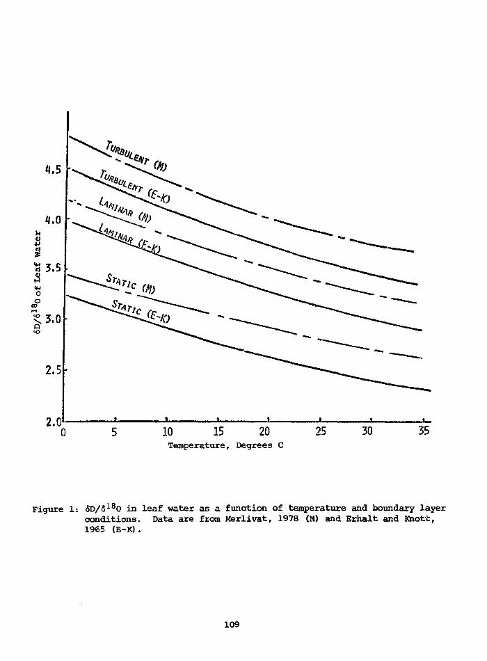
10 15 20Temperature, Degrees C
25 30
Figure 1: 6D/6I8O in leaf water as a function of temperature and boundary layerconditions. Data are from Merlivat, 1978 (M) and Erhalt and Khott,1965 (E-K).
109
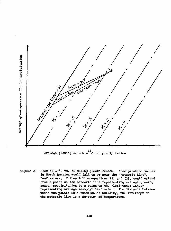
3•H
U
Q
id
I1
18Average growxng-season S 0, in precipitation
Figure 2: Plot of 6180 vs. 6D during growth season. Precipitation valuesin North America would fall on or near the "Meteoric Line".Leaf waters, if they follow equations (2) and (3), would extendfrom a point on the meteoric line representing average growingseason precipitation to a point on the "leaf water lines"representing average mesophyl leaf water. The distance betweenthese two points is a function of humidity; the intercept onthe meteoric line is a function of temperature.
110
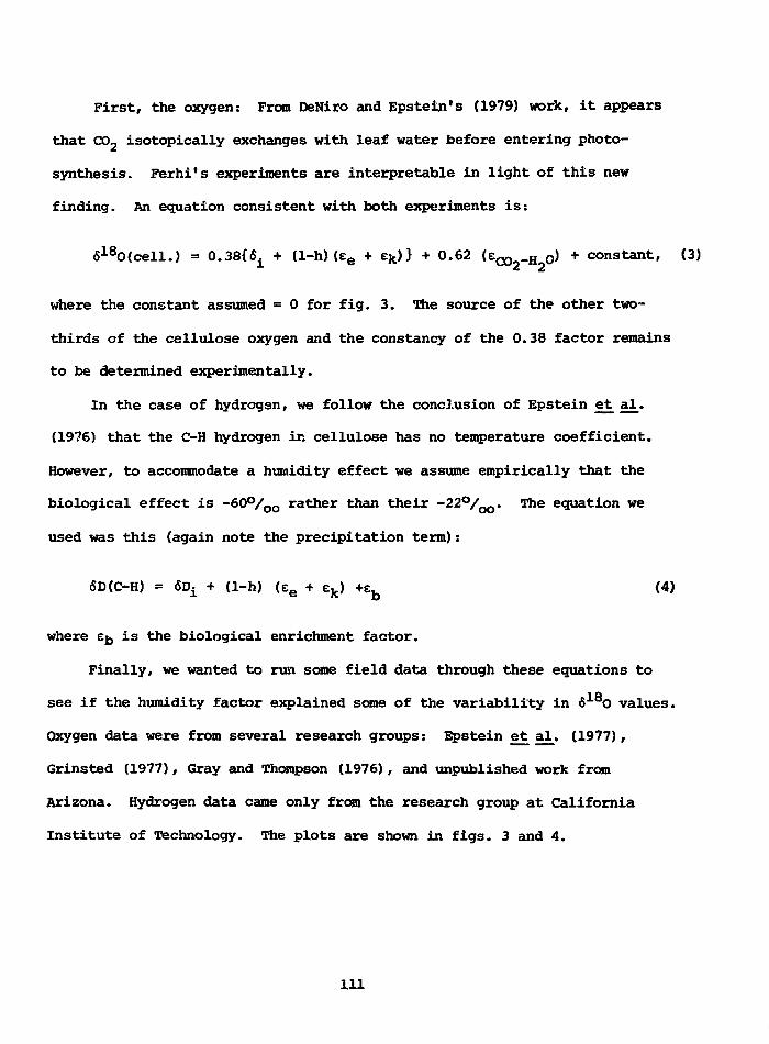
First, the oxygen: Prom DeNiro and Epstein's (1979) work, it appears
that C02 isotopically exchanges with leaf water before entering photo-
synthesis. Ferhi's experiments are interpretable in light of this new
finding. An equation consistent with both experiments is:
<S18O(cell.) = 0.38^ + (1-h) (ee + ek)} + 0.62 (e^ H 0) + constant, (3)
where the constant assumed = 0 for fig. 3. The source of the other two-
thirds of the cellulose oxygen and the constancy of the 0.38 factor remains
to be determined experimentally.
In the case of hydrogen, we follow the conclusion of Epstein e_t al.
(1976) that the C-H hydrogen in cellulose has no temperature coefficient.
However, to accommodate a humidity effect we assume empirically that the
biological effect is -60°/Oo rather than their -22°/QO. The equation we
used was this (again note the precipitation term):
6D(C-H) = 6DL + (1-h) (ee + ek) +eb (4)
where eb is the biological enrichment factor.
Finally, we wanted to run some field data through these equations to
see if the humidity factor explained some of the variability in 618O values.
Oxygen data were from several research groups: Epstein et al. (1977),
Grinsted (1977), Gray and Thompson (1976), and unpublished work from
Arizona. Hydrogen data came only from the research group at California
Institute of Technology. The plots are shown in figs. 3 and 4.
Ill
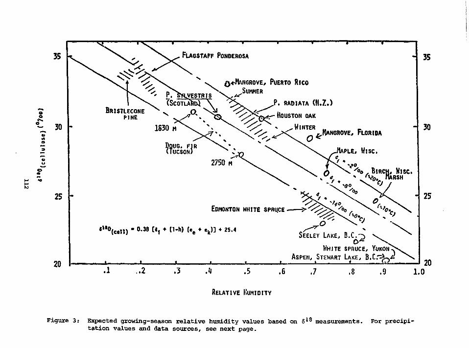
35
°- 30
25
20
FLAGSTAFF PONDEROSA
0<-MANGROVE, PUERTO RICO
BRISTLECONEPINE
.1
vTSC0TLA7»D)
O
1S30M
DOUG, FIR(TUCSON)
,P. RADIATA (N.Z.)
HOUSTON OAK
.WINTERMANGROVE, FLORIDA
MAPLE, MISC.
'oo , BIRCH, HISC.CH,HA RSH
EDMONTON WHITE SPRUCE
0.38 [«f • (l-h) (ee + ck)] + 25.4SEELEY LAKE, B.C.-)
WHITE SPRUCE, I U M J ^
ASPEH, STEWART LAKE, B.C."
35
30
25
20.,2 .3 .5
RELATIVE HUMIDITY
.6 .7 .8 .9 1.0
Figure 3: Expected growing-season relative humidity values based on 618 measurements. For precipi-tation values and data sources, see next page.
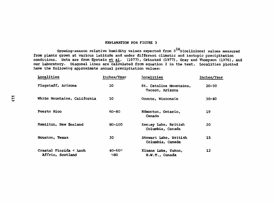
EXPLANATION FOR FIGUKE 3
18Growing-season relative humidity values expected from 6 O(cellulose) values measured
from plants grown at various latitude and under different climatic and isotopic precipitationconditions. Data are from Epstein et al. (1977), Grinsted (1977), Gray and Thompson (1976), andour laboratory. Diagonal lines are calculated from equation 2 in the text. Localities plottedhave the following approximate annual precipitation values:
Localities Inches/Year
Flagstaff, Arizona 20
White Mountains, California 10
Localities
St. Catalina Mountains,Tucson, Arizona
Oconto, Wisconsin
Inches/Year
20-30
30-40
Puerto Rico
Hamilton, New Zealand
Houston, Texas
Coastal Florida < LochAffric, Scotland
60-80
80-100
30
40-60<-\,80
Edmonton, Ontario,Canada
Seeiey Lake, BritishColumbia, Canada
Stewart Lake, BritishColumbia, Canada
Kluane Lake, Yukon,N.W.T., Canada
19
20
15
12
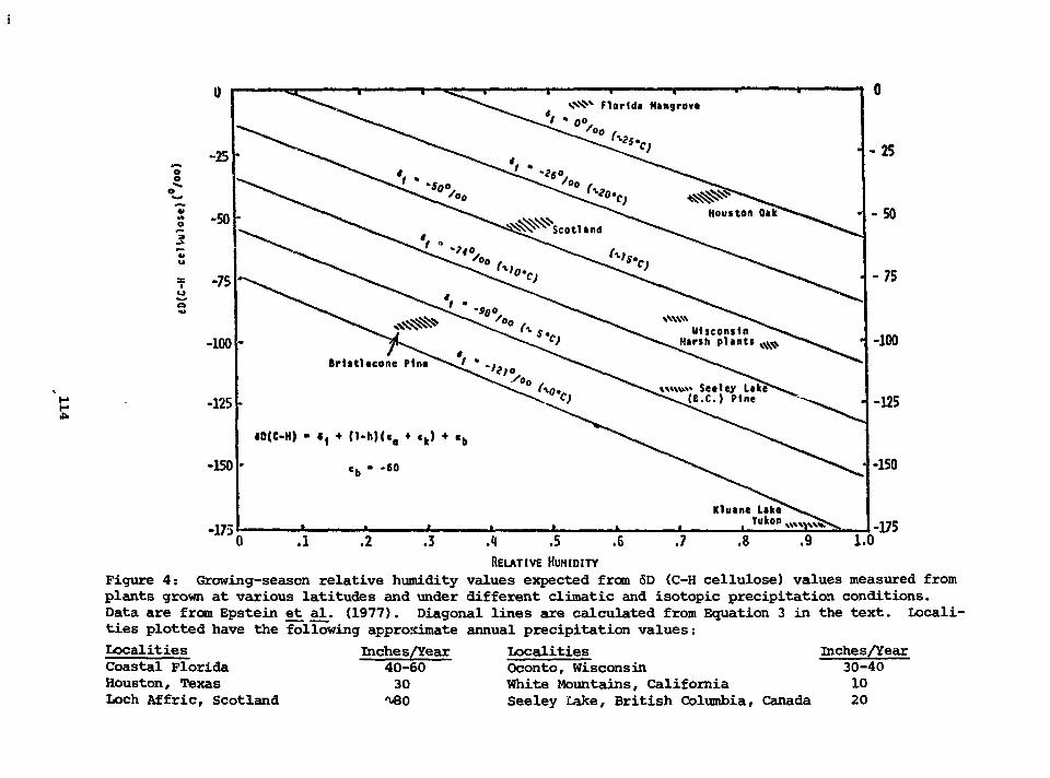
oo
os
-100
-125
-150
-1750 .1 .2 .3
-25
-50
-75
-100
-125
-150
-175.4 .5 .6RELATIVE HUMIDITY
Figure 4: Growing-season relative humidity values expected from 6D (C-H cellulose) values measured fromplants grown at various latitudes and under different climatic and isotopic precipitation conditions.Data are from Epstein et_ al^ (1977). Diagonal lines are calculated from Equation 3 in the text. locali-ties plotted have the following approximate annual precipitation values:
Localities Inches/Year Localities Inches/Year40-60 Oconto, Wisconsin 30-4030 White Mountains, California 10
Seeley lake, British Columbia, Canada 20
Coastal FloridaHouston, TexasLoch Affric, Scotland
We conclude from this that the humidity factor does indeed help to
explain some of the data, but not all. Some variance is undoubtedly due
to an inherent lack of complete environmental information at field loca-
tions, and to a multiplicity of variables as compared with growth-chamber
conditions. Additional factors influencing the <S-values in cellulose
certainly exist and will only be quantified with further planned experi-
mentation .
REFERENCES
Bricout, J. (1973). Control of authenticity of fruit juices byisotopic analysis, J.Assoc. Off. Anal. Chem., 57, 739.
Craig, H. and Gordon, L.I. (1965). Deuterium and oxygen-18 varia-tions in the ocean and marine atmosphere, In Stable Isotopes in Oceano-graphic Studies and Paleotemperatures, Sp.leto, July 26-30, 1965: 9-130.
DeNiro, M.Y. and Epstein, S. (1979). Relationship between the oxygenisotope ratios of terrestrial plant cellulose, carbon dioxide and water,Science, 204, 51-53.
Ehhalt, D. and Knott, K. (1965). Kinetische Isotopentrennung beider Verdampfung von Wasser, Tellus, 17, 389-397.
Epstein, S., Yapp, C.J. and Hall, J.H. (1976). The determinationof the D/H ratio of nonexchangeable hydrogen in cellulose extracted fromaquatic and land plants. Earth Planet. Sci. Lett., 30, 241.
Epstein, S., Thomas, P. and Yapp, C.J. (1977). Oxygen and hydrogenisotopic ratios in plant cellulose, Science, 198: 4323, 1209-1215.
Ferhi, A., Letolle, R., Long, A. and Lerman, J.c. (1980). See contri-bution to this publication.
Gray, J. and Thompson, P. (1976). Climatic information from ^ 0 / ^ 0ratios of cellulose in tree rings. Nature, 262, 481-482.
Grinsted, J.M. (1977). A study of the relationships between cli-mate and stable isotope ratios in tree rings. Unpubl. PhD dissertation,Univ. of Waikato, N.Z., 237 pp.
Merlivat, L. (1978). Molecular diffusivities of H216O, HD16O andH2
18O in gases, J. Chem. Phys., 69 (6), 2864-2871.
115
ISOTOPIC WORK ON TREE RINGS
A.T. Wilson 4715 E. Fort LowellTucson, Arizona
The isotopic work on tree rings carried out by the group at Waikato
University was reviewed. The initial approach was to study how the car-
bon, oxygen, and hydrogen isotopes changed as one sampled across an
annual growth ring of Pinus radiata (D.Don). The sample of Pinus radiata
was chosen from a growth site where wood is laid down throughout the whole
yearo Such a procedure enables one to sample wood laid down over a 10°C
temperature range and one can readily see how the isotopes in the various
compounds in wood respond to changing temperatures.
613C
Evidence was presented to suggest that the 6 3C values in both cellu-
lose and lignin reflect temperature but that other factors such as water
stress can have an important influence on the isotope ratios deposited in
the compounds in the wood of tree rings. The approach used by the author
has been to measure the 613c value of cellulose back in time on trees as
complacent as possible growing in regions of adequate water supply and
high' relative humidity. This work has been compared with parallel work
on calcite samples from stalagmites where the chemistry is simple but the
time base is less certain. Using data from both sources the author has
produced temperature versus time curves for New Zealand over the last
millennia.
116
The author's work on the modification of the Rittenberg and Ponticorvo
method to convert the oxygen in organic material to carbon dioxide suitable
for measurement in an isotope-ratio mass spectrometer was described. This
work was carried out initially in the Geoscience Department of the Univer-
sity of Arizona. The basic advance was the discovery that both CO and C02
are produced by the oxidation of an organic compound with the chlorine
liberated on heating HgCl2. The CO is separated and converted to CO2 using
an electrical discharge. The purification of the CO2 is most important for
accurate determination of 618O. The method has been tested on a wide variety
of organic materials and appears to be of .general applicability. Experiments
to determine the isotopic biochemistry of oxygen in a living system were
described. These have been carried out by John Dunbar, a gr duate student
at the University of Waikato. Basically, the carbohydrate formed from the
photosynthesis reaction is very enriched in 18o (M%) with respect to the
water in the cell. This is probably due to the CO2/H2O fractionation. As*
the carbon fixed by the photosynthesis moves through the biochemical network,
the oxygen associated with it is progressively diluted by the addition of and
exchange with cell water. The range in the compounds measured is very large,
from primary products of photosynthesis such as carbohydrate ('w10o/oo) to the
end products of metabolism such as caffeine t^O 0/^). It was suggested that
such techniques could be used to determine the source of organic natural pro-
ducts. Caffeine from tea from different regions was presented as an example.
Determining the source of narcotics such as heroin should be feasible.
117
6D
The author, with Irving Friedman, developed an isotopic method for
measuring the nonexchangeable hydrogens in cellulose. This technique was
extended by Martin Grinsted and the author in Waikato and applied to the
Pinus radiata system. Measurements were made of cellulose taken across
annual rings of Pinus radiata. The results show that over the winter-to-
suiraner temperature range (10°C) the nor.exchangeable hydrogens in the cellu-
lose have an apparent temperature coefficient of -5°/oo/°C. The negative
temperature coefficient was unexpected as thermodynamics would have pre-
dicted a positive value. These results at the time were attributed to the
effect of temperature on the rather complex biochemical pathways leading to
cellulose. The 6D values of the cellulose are less depleted in deuterium
that the water on which the tree grew. While their work was taking place,
Epstein and Yapp independently developed a method for determining the D/H
ratio in the C-H hydrogens of cellulose. They kindly measured some samples
of Pinus radiata and found that the C-H hydrogen of the cellulose was
70°/ o o more depleted in deuterium than the water on which the tree grew and
that the temperature coefficient was of the opposite sign to that measured
by Wilson and Grinsted. Epstein and Yapp's measurements on the C-H hydrogens
of cellulose showed that they appeared to reflect atmospheric precipitation
rather than temperature. In our v;ork we had assumed that the fractionation
between the hydrogen of the water and the -OH hydrogen of the cellulose was
small. Clearly this is not so. In fact, it is very large. This is perhaps
due to the extensive hydrogen bonding in the cellulose. The fractionation
must be of the order of 200 c/ o o such that the -OH hydrogen is enriched in
118
deuterium. Furthermore, to explain the results, this fractionation must
be temperature dependent of the order of 10°/oo/°C. Thus,the -OH hydrogens
in the nonexchangeable "crystalline" regions of the cellulose provide a
very sensitive paleothermometer which would be independent of the cell-
water composition. The isotope ratio of these hydrogens could be deter-
mined by finding the 6D of the C-H hydrogen on a sample of wood using the
nitration method of Epstein and Yapp and the nonexchangeable hydrogen
determined by Grinsted and Wilson. Such a technique would provide a means
of determining past temperatures without the need to estimate the &D value
of the plant sap water which has been shown by ourselves and others to be
very susceptible to evapotranspiration changes.
119
D/H AND 18O/16O RATIOS IN PRECIPITATION
J.R. Lawrence Lamont-Doherty Geological Observatoryof Columbia University,Palisades, New York.
Isotopic and climatic data from 80 International Atomic Energy
Agency (IAEA) hydrologic stations, excluding the USSR and China, were
examined using simple statistical methods. The parameters studied
1ft 1 6included the D/H and 0/ 0 isotopic composition of a monthly sample
of precipitation, the amount of monthly precipitation, and mean monthly
temperature and vapor pressure. The number of data points statistically
analyzed varied from as few as 20 to as many as 180. Most stations had
data sets in yearly blocks.
The mean and standard deviation of the monthly temperatures, precipi-
tation amounts and 6D values were plotted on world maps. Linear regression
18analysis was done on four parameter pairs: 6D-6 O, 6D-Temperature, 6D-
Precipitation Amount and 6D-Vapor Pressure. The slopes and coefficients of
determination were also plotted on world maps. Areas of the world were
divided into climatic regimes from examination of the statistical data
plotted on world maps (see Table 1).
Whether correlations determined from the examination of monthly data
points are related to general longer-term changes in climate is open to
question. If they are - perhaps when the climate in an area is simple
(i.e., sources of precipitable water are limited to one or two areas and
storm patterns are simple) - the monthly data may be of use in suggesting
possible areas for selecting trees for isotopic studies. Under these
122
tenuous assumptions correlations between temperature and 6D in tree rings
might be best found in North America and Europe. Correlations between
precipitation amounts and 6D in tree rings might best be found in equa-
torial regions. Positive correlations of vapor pressure and 6D might
best be found in North America and Europe, whereas negative correlations
might be best found in equatorial regions.
In a separate study of the 6D of individual storms causing precipi-
tation in the New York area, it. was found that two major winter storm
tracks gave markedly different 6D ranges. The study period was July 1977
to July 1978. One pattern of winter storm tracks is movement from south-
eastern U.S. west of the Appalachian Mountains and moving north-northeast
up the St. Lawrence valley. The other pattern is movement from the coastal
southeastern U.S. east of the Appalachians and moving northeast along the
U.S. east coast. The mean and standard deviation in 6D of the first pattern
was -55±32°/oo, whereas for the second it was -94±ll°/oo. The first pattern
provided 54% of the year's precipitation, the second, 19%. The remainder
came from summer storms without well-defined tracks. If it can be deter-
mined that a change in climate changes the percentages of the types of winter
storms, it is conceivable that the 6D of precipitation as recorded in tree
rings could record a change in the climate for northeastern U.S.
123
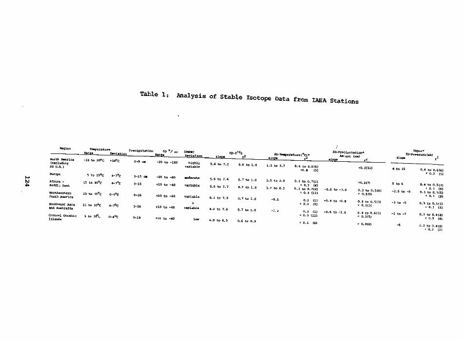
Table I, toalysis o f s t a b l e
RegionPrecipitation «D °/ o o (SICK)
North Africa -10 to 20°c >lo°o-20 to -ISO ^i£lv 5. 4 t o 7., 0. 6 t o l_ 0 ^ ^ ^ o _ 4 t o ^
Africa -Middle East
NortheasternSouth America
5 to 15°c 4-7°c
15 to 30°C 4-7°c
20 to 30°C 0-4°c
Southeast Asia VJ to 30°c 4-7°cand Australia
Central Oceanic 5 to 30°c 0-4°cIslands
3-15 o -20 to -SO aoderate
3-155.6 to 7.4 0.7 to 1.0 1.5 to 3.0 0.3 to 0.7(3)
< 0.3 (4)+10 to -40 variable 5.a to 7.7 0.7 to 1.0 1.7 to 6.3 0.3 to 0.7(4) -0.8 to -3.0
+10 to -60 variable
+10 to -60 variable
•10 to -40 low
6.1 to 7.9 0.7 to 1.0
4.2 to 7.6 0.7 to 1.0
4.0 to 6.S 0.6 to 0.9
<0.3(7)
„ . , 0.3 to 0.5(6)< 0.3 (11) < 0 - 3 ( 9 )
0.3 (1) -0.4 to -0.9: 0.3 (5)
0.3 (1) -0.6 to -1.1< 0.3 (11)
0.3 to 0.5(3)< 0.3(3)
0.3 to 0.6(3)< 0.3(9)
slope
Vapor*6D-Pressure(nb)
5 to 6
-2.5 to -8
-3 to -5
-2 to -7
0.4 to 0.6(6)< 0.3 (5)
0.4 to 0.5(3)
< 0.3 (9,
0.3 to 0.5(3)< 0.3 (3)
0.3 to 0.4(4)< 0.3 (6)
0.3 to 0.4(1)< 0.3 (51
OXYGEN DEPLETION
L. Machta Air Resources Laboratories,NOAA,Silver Spring, Maryland
The combustion of fossil fuels and biospheric oxidation remove
oxygen from the atmosphere. If the observed oxygen depletion were mea-
sured in the atmosphere and the fossil-fuel-combustion oxygen-removal were
subtracted from it, the residual would reflect biospheric oxidation. This
would provide net global biospheric oxidation due to all sources (soil
disturbance, deforestation, etc.).
As background, it may be noted that in 1967-70, the oxygen concentra-
tion was 20.946% by volume (mole fraction) by Machta and Hughes (1970).
They estimated an accuracy of 0.006% (one standard deviation) due to an
uncertain standard gas. The geographic and temporal variation was neg-
libible (± 0.0005%). On the other hand, in 1911 Benedict found the same
20.946% (when corrections were made) but with a variability among samples
taken at different geographical locations of 0.007%. Other errors are un-
known. The change in atmospheric oxygen concentration between 1911 and
1968 might be 0 ± 0.01%. The expected depletion due solely to the known
combustion of fossil fuel was 0.005%. This is half the error (one standard
deviation of the difference) and may account for the failure to detect any
oxygen depletion in that time interval. At one standard deviation, the
biospheric oxidation could be equal to the fossil fuel oxygen reduction
and the sum of the two sources of oxygen depletion would still equal only
one standard deviation of the oxygen change.
125
In the near future, the annual combustion of fossil fuels will
deplete oxygen concentration by 0.0003 or 0.0004%. This is at least an
order of magnitude beyond the precision of the presently demonstrated
measurement techniques (the paramagnetic devices). However, a proposed
Raman method suggested by Schwiesow and Derr (1970) has a precision of
0.00003% which is, in fact, ten times more precise than needed to detect
the annual fossil fuel combustion oxygen depletion. Thus, in principle,
in one year one could detect biospheric oxidation (from all sources)
amounting to 10% of current fossil fuel combustion in one year. Fossil
fuel consumption is known to about 10% (or perhaps a little better).
The uncertainties in this proposed "technique are:
1. Oxygen concentration changes of 0.0003% may compete with significant
geographical and seasonal variability making for a difficult sampling
problem. Even in the southern hemisphere (South Pole) the C02 shows a
seasonal variability of about 0.0001% (by volume) hence one would expect
a seasonal variability of oxygen concentration of about 0.0001%.
2. There may be natural sources and s^nks not necessarily in steady state
which can swamp the small oxygen changes attributed to biospheric oxida-
tion. The literature estimates by Garrels, Lerman, and MacKenzie (1976)
suggest that this is not important.
3. Achieving a precision of three (3) parts in 107 and standards or sample
stability are very difficult.
4. Finally, one may ask whether the oxygen depletion truly measures the
formation of biospheric C02. We assume this to be the case.
126
REFERENCES
Garrels, R.M., Lerman, A., and MacKenzie, F.T. (1976). Controlsof atmospheric 02 «nd CO2: past, present and future, Amer. Scientist,64, 306-315.
Machta, L. and Hughes, E. (1970). Atmospheric oxygen in 1967 to1970. Science, 168, 1582-1584.
S-hwiesow, R.L. and Derr, V.E. (1970). A Raman scattering methoafor precise measurement of atmospheric oxygen balance, Journ. Geophys.Res., 75, 1629-1632.
127
GROWTH TREND IN RECENT TREE RINGS
Angela de Luca Rebello
Klaus Wagener
Department of Chemistry,Pontificia University, Rio de Janeiro
Department of Biophysics,Technical University of Aachen,Federal Republic of Germany
The role of the biosphere in the disturbed carbon cycle is not clear.
It is considered partly as a sink for excess CO2 present in the atmosphere,
and partly as an additional source of man-made carbon dioxide. The
recently available C record from tree rings gives the total net input
of carbon into the atmosphere, but a higher turnover through the biosphere
is still possible. Therefore, independent information directly derived
from the biosphere would be useful. Changes in the soil's organic matter
pool are certainly hard to detect. However, as far as standing biomass
is concerned, tree-ring analyses could provide some information. The
response of standing biomass to any known environmental changes would be
an important factor to know. This was the reason why we started to search
for growth trends in tree rings.
Most important is a reference which is not subject :o a growth trend.
We used the ring data of E. Hollstein who analyzed about 3000 oak trees
from central Europe. Out of these trees a random selection of 376 trees
was made covering the last 2700 years. From this group the average ring
width of central European oak trees was derived as a function of the ring
number, N. This gave the standard tree where all short term variations
due to climate variations as well as the various local environmental con-
ditions should be cancelled out.
128
When talking about stimulation of the fixation rate, we should con-
sider the annual increase in total biomass of the tree. Most available
data, however, give only the ring width so that we have to take the annual
increase in cross section, AA, as a relative measure for the productivity:
AA(N) = 2TT r(N) • w(N) (1)
with r = radius of the ring, number N, and w = ring width. In case there
is any stimulation, then we expect
(favorable conditions)
= 1 + e . (2)
(regular conditions)
The regular conditions ° are those of the standard tree. The stimulation
factor is 1 + e. The question: whether for recent trees e is significantly
different from zero?
In order to get rid of individual data and find a normal, we define
the specific productivity (SP):
annual increase in cross section of stemSP (N) =
cm of cambium perimeter
2TT • r(N) • w (N)(3)
2ir • r(N)
= w(N).
From equation 2 and 3 follows:
SP (N) = l + e . (4)SP°(N)
Collecting data according to equation 4 includes the assumption that
the recent oak trees analyzed are a sample of trees which is representative
for recent European oak trees. Such a claim is cez"tainly hard to prove.
129
In spite of this difficulty, we tried as a first approach to select trees
from various locations in Argonner Forest (Germany), Rhine River Valley,
Saarland (Germany) and others. Up to now 20 trees have been analyzed
according to equation 4. For practical reasons, 10 rings were always
lumped together, i.e. ring numbers 1 - 10, 11 - 20, 21 - 30, etcetera,
giving a total of about 200 ratios of 4 with an average of
1 + e = 1.20 ± 0.18 . (5)
The ages of these trees were between 60 and 150 years, with an aver-
age of 115 years. Assuming that this sample has any significance for
present European oak trees, equation 5 jneans that the average ring width
of the last 115 years increased by (20 ± 18)% compared with the long-term
average.
In order to overcome the principal difficulty of needing a representa-
tive sample, we tried to refer the absolute SP values to the actual size
of the tree. As shown later, such a procedure reduces the size of the.
stimulation signal (if there is any at all), but a positive proof of exis-
tence (in case it turns up) is then independent of having a representative
sample or not. The question is how to find a proper reduction procedure.
For this purpose two series of trees of same species and same age
but grown under different local conditions and thus having different radii
were considered. The factors creating the abiotic environments of the two
series are variations around the contemporary average, while a secular
trend of any of these factors of continental, hemispheric, or global
dimension should influence both series in the same way or, more precisely,
130
in the same qualitative way. This is trua for the following reason:
the productivity response of a tree to any change of one of the abiotic
factors depends largely on the importance that this factor has in the
context of the local environment. In case it is the limiting factor,
then the response will be pronounced; otherwise it will be moderate or
even zero.
The following reduction procedure cancels out the absolute size
of the productivity change, arid gives a reduced figure. Therefore, any
significant stimulation factor eventually obtained in this way will turn
out smaller than equation 5.
The reduction procedure is based on equation 6 which holds for the
average of the two series of trees for any N:
wN(big trees) rN(big trees)
^T (6)WN(small trees) rN(small trees)
From equation 6 follows that, on the average, w(N)/r(N) should be constant
for contemporary trees of same species, so that we define the reduced
specific productivity (RSP) as follows:
RSP (N) »r(N)
Consequently,
RSP°(N)(N) = 1 + e* (8)
An evaluation of the same 20 trees mentioned before and based on equation 8
gave the following:
131
1 + e* = 1.073 ± 0.070 (9)
It is most important to check through all available data of big
series of trees for recent growth trends. Special emphasis should be
given to southern trees, in order to find out if there is any global
trend. An analysis of Brazilian araucarias is presently underway.
There are certainly several possibilities that could create a stimu-
lation of plant growth:
1. The temperature increase on the northern hemisphere of 0.8°C
during 1860 - 1940 could have enhanced the rate of soil respiration
and thus giving the higher CO2 excess present, especially in forests;
2. Human activities grew exponentially during the last 150 years,
including most certainly the production of man-made nitrate which
comes down with the rain;
3. The C02 increase in the atmosphere could also contribute to a
world-wide stimulation.
Independent of the actual reason that may have caused a growth trend
is the importance that any enhanced fixation of carbon over 100 or 150
years would have in the context of our carbon cycle models. Further investi-
gations are most desirable.
REFERENCES
Hollstein, E.: private communication. A publication on the averagedata of European oak trees is in preparation. A more detailed paper byKlaus Wagener and E. Hollstein on the present analysis is underway.
Wagener, Klaus: See contribution in this volume.
132
FOREST AND TREE HATER-BUDGETS
R. H. Waring Forest Research LaboratoryOregon State UniversityCorvallis, Oregon
Water transpired by a tree may originate in the snows of last winter.
Following snowmelt, water stored in the soil approaches the average age
of the snow pack. Tree roots extract water, if available, from the upper
soil horizons first. As water enters the stem it exchanges with all free
water in the cells of conducting wood.
The conducting wood of diffuse porous hardwoods and conifers repre-
sents a major water reservoir. Even after a forest canopy fully develops,
the reservoir continues to increase as the trees increase in volume. Water
may be withdrawn from the conducting tissue to meet up to half of the daily
transpiration, e.g. more than 20 m of water per hectare a day. Removal
of this water from the conducting tissue greatly decreases wood permeability.
Wood permeability may also be decreased by cold temperatures, slow tree
growth, or an inadequate supply of water at the root tips. To compensate for
the additional resistance to flow, the water potential gradient that drives
water movement through trees increases. At a critical point where the water
potential gradient equals the solute potential in leaves, cell turgor drops
to zero and stomata are forced to close.
Leaves also offer a small, easily tapped reservoir that may be partly
recharged by absorption of water from the leaf surfaces. Atmospheric con-
centrations of water vapor, often low, may cause stomata to close independent
of general state of leaf hydration. Inadequate light, freezing temperatures,
133
low potassium concentrations and high levels of abscisic acid may also
cause stomatal closure.
The most important physiological variables controlling transpiration
are equilibrium leaf water potential (measured at night without transpira-
tion) , sapwood relative water content, leaf area, and leaf geometry. The
most important atmospheric variables controlling transpiration are atmos-
pheric humidity, adsorbed radiation and wind speed. Together these and
other factors interact to limit the daily water loss from forest canopies
to about 50 m3 of water per hectare (5 mm day ~ 1 ) .
REFERENCES
Black, T.A. (1979). Evapotranspiration from Douglas-fir stands exposedto soil water deficits, Water Resources Research: 15:164-170
Jarvis, P.T. (1975). Water transfer in plants, In Heat and MassTransfer in the Environment of Vegetation, 369-394. 1974 Seminar of theInternational Centre for Heat and Mass Transfer, Dubrovnik. Scripta BookCo., Washington, D.C.
Jarvis, P.G., James, G.B. and Landsberg, J.J. (1976). Coniferousforest, In Monteith, J.L. (Ed.) Vegetation and the Atmosphere, Vol. 2.,Academic Press, New York. p. 171-240.
Lange, O.L., Kappen, L. and Schulze, E-D. (1976). Water and plant life,Ecological studies: Analysis and Synthesis, Vol. 19. Springer-Verlag,New York, New York. 536 pp.
Linder, S. (1979). Photosynthesis and respiration in conifers.A classified reference list 1891 - 1977, Studia Forestalia Suecica, 149.Swedish University of Agricultural Science, Uppsala, Sweden. 71 pp.
Tan, C.S., Black, T.A. and Nnyaman, J.U. (1978). A simple diffusionmodel of transpiration applied to a thinned Douglas-fir stand, Ecology, 59;1221-1229.
Waring, R.H. and Franklin, J.F. (1979). Evergreen coniferous forestsof the Pacific Northwest, Science, 204; 1380-1386.
Waring, R.H. and Running, S.W. (1976). Water uptake, storage andtranspiration by conifers: A physiological model, In Ecological Studies:Analysis and Synthesis, Vol. 19, Lange, O.L., Kappen, L., and Schulze, E-D.,(Eds.) Springer-Verlag, New York. pp. 189-202.
134

VI
ISOTOPIC METHODS
135
CELLULOSE PREPARATION AND 18O ANALYSIS
R.L. Burk Quaternary Isotope LaboratoryM. Stuiver University of Washington, Seattle
After being counted and split into appropriate sections, tree rings
are ground in a Wiley mill to minus 60 mesh. The ground wood is then
placed in fritted vessels and extractiver are removed with petroleum ether
(4 hours) and then ethanol (4 hours) in a Soxhlet extractor. Lignin is
removed by two bleaching steps and two sodium sulfite steps, followed by
alternating solutions of bleach mixed with sulfuric acid and sodium sul-
fite. This alternation allows a Maule color reaction (Sarkanen and Ludwig,
1971) to take place if lignin is present. Hemicellulose is removed by
treatment with sodium hydroxide. Saturated sodium chloride is used to help
remove the sodium hydroxide. The samples are then treated with dilute hydro-
chloric acid and washed with water overnight in a Soxhlet extractor. All
treatments are at room temperature, except for the sodium sulfite step,
which is performed at approximately 100°C.
After thorough drying in a 60°C oven, the samples are then placed in
Vycor break-seal tubes with mercuric chloride and pumped down for at least
12 hours in a vacuum better than O.lp. The tubes are initially surrounded
with boiling water. These break-seal tubes are then sealed and heated to
550°C for six hours. After cooling, the tubes are placed on a vacuum line
inside another tube containing triple-distilled quinoline. Phosphorus pent-
oxide is placed both in the quinoline and along the side of the containment
vessel to remove water. After the break-seal tube is broken, carbon monoxide
is converted to carbon dioxide with a 15,000 volt discharge between parallel
136
platinum plates (Aggett e_t al_., 1965) . After one more quinoline treat-
ment, the sample gas is passed through two liquid nitrogen/ethanol traps
and collected in a sample bottle. This method is modified from a method
first described by Rittenberg and Pontecorvo (1956).
We analyzed 10 samples of a cellulose from the Sigma Chemical Co.
(provided by S. Epstein) prior to beginning our research and found a
standard deviation of ±.20°/oo. During data collection we ran 17 more
samples of Sigma a cellulose at r'.ntervals of approximately one month and
found a standard deviation of ±.26°/ . Maximum deviation from the mean
was ±.52°/oo.
REFERENCES
Aggett, J., Bunton, C.A., Lewis, T.A., Llewellyn, D.R., O'Connor, C.,and Odell, A.L. (1965). The isotopic analysis of oxygen in organic com-pounds containing organic ligands, Inter. J. App. Rad. and Isotopes, 16,165-170.
Rittenberg, D. and Pontecorvo, L. (1956). A method for determinrtionof the l°0 concentration of the oxygen compounds, Inter J. App. Rad. jidIsotopes, 1, 208-214.
Sarkenen, K.V. and Ludwig, C.H. (Eds.) (1971). Lignins: Occurrence,Formation, Structure and Reactions, Wiley Interscience, New York. 916 pages.
137
ISOTOPIC ANALYSIS FOR 613C and 618O USING A SINGLECOLLECTOR AND MATCHED MOLECULAR FLOW LEAKS
W. Compston Australian NationalP. Aharon University,T. McGee Canberra, A.C.T.
A modest program in oxygen isotope palaeothermometry was instituted
at the Australian National University by adapting an Associated Electrical
Industries MS12 mass spectrometer. It has a single collector and a 1951
vintage Metropolitan-Vickers gas handling plant for precise measurements
of 613C and 518O using C02- A precision of 0.06°/oo (standard error for
a single analysis) was routinely achieved for both 6 c and 618O, which is
comparable or better than many orthodox machines although not as good as
the best. This report describes the modified instrument and indicates its
advantages and disadvantages.
The MSI2 had been set up previously for mass analysis of Pb using
Pbl2 evaporated into the electron beam (Oversby eit al., 1970). It had been
equipped with (hardwired) programmable magnetic field stations and automatic
switching between any two selected fields, and the electrometer output was
digitized through a voltage-to-frequency converter and counter. Data were
reduced by an on-line computer. This measurement system was modified to
incorporate automatic selection of the electrometer input resistor, so that
mass 44 (12C16O2> was measured using a 109 ohm resistor and mass 45 and
46 using 10 ohms. In addition, the electrometer was adjusted for maximum
speed of response by careful selection of trimming capacitors across each
input resistor, so that full response was attained within 1 second for all
138
resistors. Ratios were measured by the following repeated cycle: 1-second
integration on mass 44, 1-second delay for switching the magnetic field
and amplifier response, 1-second integration on mass 45 or mass 46,
1-second delay to switch back to mass 44 and 1-second repeat integration
of the mass 44 voltage. The aim was to offset any fluctuations in beam
intensity by employing the fastest possible measurement cycle. A single
ratio observation constituted the mass 45 or 46 voltage divided by the mean
of the two observations of the 44 voltage. The average of 12 such cycles
constituted one ratio measurement of either the reference or the sample gas,
after which the gases were interchanged. The coefficient of variation for
a single cycle was usually between 0.1 and 0.2°/oo a n d f o r t h e m e a n o f 1 2
cycles lower by Jl2 at M).04°/oo. Fig. 1 illustrates 7 comparisons of
2 gases, in which the means of successive sample ratios are divided by the
intervening reference ratios to obtain individual observations for the o
values. The precision observed for the mean 6^3C in fig. 1 (0.02°/oo) is
approximately the value expected from the internal precision for each ratio
Cv>0.15o/oo) I but that of the 618O is somewhat larger probably owing to beam-
intensity fluctuations.
The molecular flow leaks are sintered tungsten carbide plugs which
have nearly equal flow-rates of 0.033 std. cc CO2 per hour, matched to better
than 3%. Dual mercury "dosers" deliver approximately equal masses of gas
( 0.8 std. ccs. at V5 cms. pressure), to 2 matched 2-liter reservoirs, from
which the gases can be admitted to the leaks and the interchange valves
which follow. Interchange is effected by 4 stainless steel valves which
139
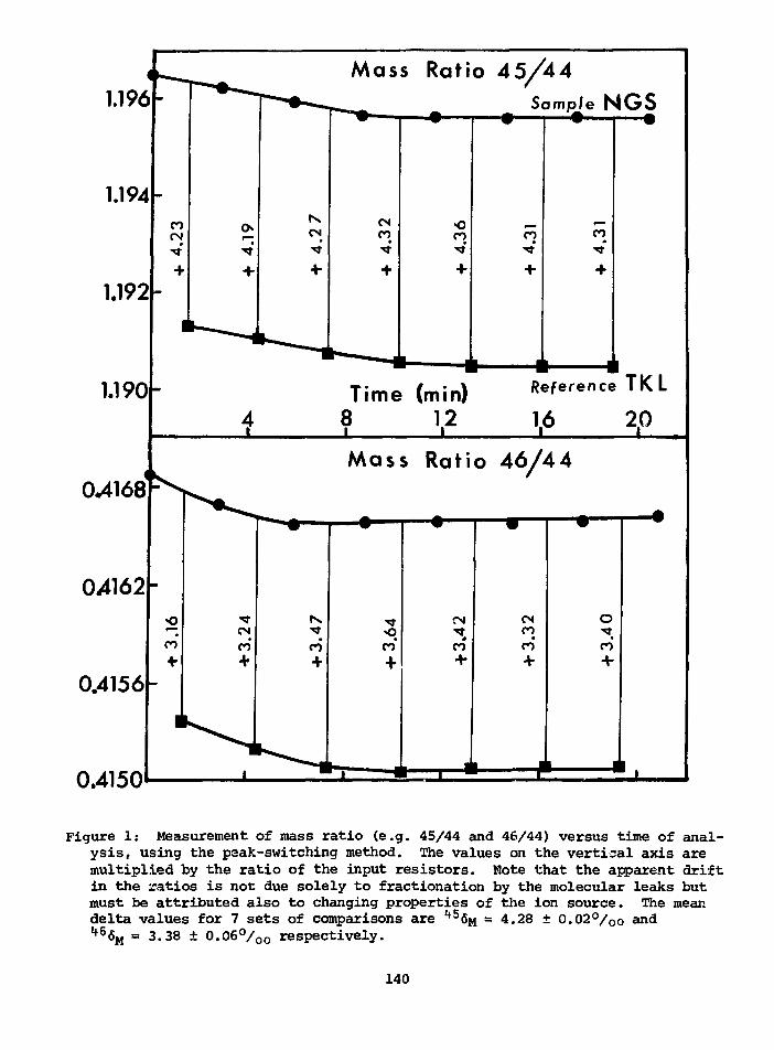
1.194
1.192
1.190
CU168
04162
0.4156
0.4150
CO
(N CN
Mass Ratio 45/44Sample N G S
CNCO
oCO• * *
CO CO
Time (min) Reference TK L
8 12 20
Mass Ratio 46/44
COCN
CO* co
r—
CO*
—#—
CN
CO
CNCO
CO*
— • —
o
co'
Figure 1: Measurement of mass ratio (e.g. 45/44 and 46/44) versus time of anal-ysis, using the peak-switching method. The values on the vertical axis aremultiplied by the ratio of the input resistors. Note that the apparent driftin the ratios is not due solely to fractionation by the molecular leaks butmust be attributed also to changing properties of the ion source. The meandelta values for 7 sets of comparisons are 1*56M = 4.28 ± 0.02°/oo andIf65M = 3.38 ± 0.06°/oo respectively.
140
do not permit any detectable gas mixing. Mass 44 beam-intensities are
equalized by prior adjustment of the dosers such that the faster leak
has a slightly smaller gas pressure in the 2-liter reservoir. The slow
changes in reservoir isotopic compositions that accompany molecular flow
are equalized by opening both reservoirs to the leaks at the same instant.
A fresh (unfractionated) dose of the working standard gas is used with
each sample.
The single advantage of the peak-switching, single collector method
is the versatility it provides for different gases and isotopes. The same
machine can be used without change for D/H, C02 or SFg analyses which would
ordinarily require a special tube and special collector spacings for the
double-collection method. Disadvantages are that each beam is measured
only 25% of the time, and that there is no automatic compensation for beam-
intensity fluctuations.
REFERENCES
Oversby, V.M., Compston, W. and Penikis, E. (1970). Isotopic analysisof microgram quantities of lead iodide using an electron-bombardment sourcemass spectrometer, Earth Planet. Sci. Letters, 10, 121-128.
141
A PRELIMINARY REPORT ON THE SIMULTANEOUS EXTRACTIONOF HYDROGEN AND OXYGEN FROM ORGANIC MATERIALS
Peter Thompson Department of PhysicsJohn Gray University of Alberta,Se Jong Song Edmonton, Alberta
A method of obtaining hydrogen and oxygen for isotopic analysis from
organic matter is described. The principle of the extraction method is
similar to that previously described by Thompson and Gray (1977) and by
Epstein et al., (1977) in which the sample is combusted in a nickel reaction
vessel at l,150°C. The reaction products from a C,H,0 compound are CO2r CO
and K2« Hydrogen rapidly diffuses through the walls of the reaction vessel
(1.5 mm) where it is contained by a quartz tube surrounding the vessel.
From here the hydrogen is collected in a liquid nitrogen cooled charcoal
trap. CO2 and CO remain in the vessel and are collected on a liquid nitro-
gen cooled silica gel trap after the combustion is completed. CO is con-
verted to CO2 in a discharge and then combined with the CO2 from the re-
action vessel. The reaction vessel is shown in fig. 1.
To check reproducibility and accuracy of the method, water samples were
placed in glass capillaries and introduced into the reaction vessel along
with carbon. The products of the combustion were predominantly CO and H2-
Because of possible oxygen exchange with silicate oxygen, only the hydrogen
was collected and analyzed. Results published previously (Thompson and Gray,
1977) on oxygen in which the water was transferred into the vessel by
freezing are shown in Table 1. Table 2 shows a comparison of D/H ratios
obtained with water samples using the method described and the conventional
142
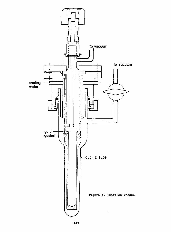
to vacuum
coolingwater
gold —gasket
\
quartz tube
Figure 1: Reaction Vessel
143
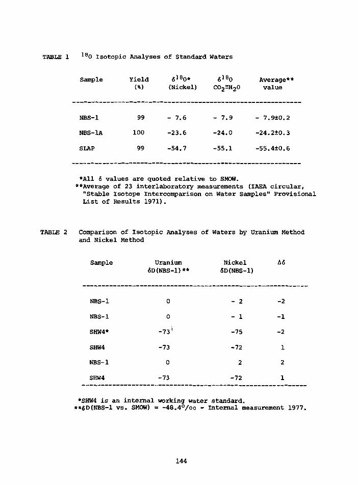
TABLE 1 180 Isotopic Analyses of Standard Waters
Sample Yield 618O* 6180 Average**(%) (Nickel) CO2HH20 value
NBS-1
NBS-lA
SLAP
99
100
99
- 7.
-23.
-54.
6
6
7
- 7.
-24.
-55.
9
0
1
- 7.
-24.
-55.
9±0.
2±0.
4±0.
2
3
6
*A11 6 values are quoted relative to SMOW.**Average of 23 interlaboratory measurements (IAEA circular,"Stable Isotope Intercomparison on Water Samples" ProvisionalList of Results 1971).
TABLE 2 Comparison of Isotopic Analyses of Waters by Uranium Methodand Nickel Method
Sample Uranium Nickel A6«D(NBS-1)** 6D(NBS-1)
NBS-1
NBS-1
SHW4*
SHW4
NBS-1
SHW4
0
0
-73'
-73
0
-73
- 2
- 1
-75
-72
2
-72
-2
-1
-2
1
2
1
*SHW4 is an internal working water standard.**6D(NBS-1 vs. SMOW) = -48.4°/oo - Internal measurement 1977.
144
Uranium furnace method. The results are the same within experimental
error.
£/extrose was analyzed to check the reproducibility of the method.
Initially, incomplete combustion occurred resulting in the formation of
tars on the upper parts of the vessel. This was found to have a marked
effect on the D/H composition of the hydrogen collected. Replicate
analyses yielded D/H ratios of 48±3% (NBS-1) with an average yield of
102% and 18O/16O ratios of 28.7±0.3°/oo with an average yield of 98%.
When ZnCl2 was added to the reaction as a catalyst the amount of tar for-
mation was markedly reduced resulting in higher yields of oxygen and hydro-
l ft l figen. 0/ 0 ratios were the same, whereas the 6D values increased by
(on average) llo/oo.
Samples of cellulose from filter paper were analyzed with and without
ZnCl2 present. Reproducibility of the D/H ratios measured was poorer than
with dextrose. There also may have been impurities in the filter paper.
The D/H ratios with ZnCl2 present were 26°/oo higher than without ZnC^
although the yield increased by only 2%. &^0 values of cellulose were
unaffected.
Memory tests were carried out using two cellulose samples differing
in D/H ratios by 170°/oo. When the vessels were cleaned between analyses
with a rotary wire brush, no significant memory effects were observed.
These preliminary results suggest the method may be useful for simul-
taneous analysis of hydrogen and oxygen from organic compounds provided
problems associated with tar formation can be eliminated.
145
ACKNOWLEDGEMENTS
We thank N. Riebeek for help in the design and construction of the
reaction vessel.
This work was supported in part by grants from the National Research
Council of Canada.
REFERENCES
Epstein, S., Thompson, P. and Ya p, C.J. (1977). Oxygen and hydrogenisotopic ratios in plant cellulose, fjience, 198, 1209.
Thompson, P. and Gray, J. (1977). Determination of 180/160 ratios incompounds containing C, H and 0, Int. J. Rad. Isotopes, 28, 411.
146


